Estimates of the Trade and Welfare Effects of NAFTA
75
Estimates of the Trade and Welfare Effects of NAFTA Lorenzo Caliendo & Fernando Parro (2015 RES) Presenter: Shu Wang March 11, 2020 Caliendo & Parro (2015 RES) Estimate: Trade and Welfare Effects of NAFTA March 11, 2020 1 / 75
Transcript of Estimates of the Trade and Welfare Effects of NAFTA

Estimates of the Trade and Welfare Effects of NAFTA
Lorenzo Caliendo & Fernando Parro (2015 RES)
Presenter: Shu Wang
March 11, 2020
Caliendo & Parro (2015 RES) Estimate: Trade and Welfare Effects of NAFTA March 11, 2020 1 / 75

Outline
1 Introduction
2 Tariffs, intermediate goods and sectoral linkages
3 A quantitative model for trade policy evaluation
4 A new method to estimate trade elasticities
5 Quatifying the trade and welfare effets of NAFTA
6 Conclusion
Caliendo & Parro (2015 RES) Estimate: Trade and Welfare Effects of NAFTA March 11, 2020 2 / 75

Abstract
In this paper, They build into a Richardian model sectoral linkage, tradein intermediate goods, and sectoral heterogeneity in production toquantify the trade and welfare effects from tariff changes.
They propose a new method to estimate sectoral trade elasticities.
They apply the model and use their estimated elasticities to identify theimpact of NAFTA’s tariff reductions.
Caliendo & Parro (2015 RES) Estimate: Trade and Welfare Effects of NAFTA March 11, 2020 3 / 75

Findings
Mexico’s welfare increases by 1.31%, U.S.’s welfare increases by 0.08%, andCanada’s welfare declinces by 0.06%.
Intra-bloc trade increases by 118% for Mexico, 11% for Canada, and 41% forthe U.S.
Welfare effects from tariff reductions are reduced when the structure ofproduction does not take into account intermediate goods or input-outputlinkages.
Caliendo & Parro (2015 RES) Estimate: Trade and Welfare Effects of NAFTA March 11, 2020 4 / 75

Introduction
When the U.S. reduce tariffs applied to Mexico in a given sector, it not onlyaffects prices in that industry but also in sectors that purchase materials fromthat country.
Moreover, a tariff reduction affects prices in non-tradable sectors that areusing inputs from tradable sectors.
If non-tradable goods are used as inputs in the production of other goods, oras final goods in consumption, then the benefits spread to the rest of theeconomy.
Caliendo & Parro (2015 RES) Estimate: Trade and Welfare Effects of NAFTA March 11, 2020 5 / 75
Methodology
A multi-country, multi-sector Ricardian model which describe the interactionacross tradable and non-tradable sectors observed in the input-output tables.Based on EK(2002) to develop a tractable and simple model for tariff policyevaluation.The model can be reduced to a system of one equation per country, and thesolution depends on estimates of one set of parameters, the dispersion ofproductivity across sectors (trade elasticities).There are many impact of NAFTA including tariff, technology, trade cost etc.But they hold other factors fixed to focus on the direct effect of tariffchanges over the allocation of resources.
Caliendo & Parro (2015 RES) Estimate: Trade and Welfare Effects of NAFTA March 11, 2020 6 / 75

Related Literature
Anderson and van Wincoop(2002): A one good gravity model to evaluate thegains from NAFTA.
Our model: multiple sectors, intermediate goods trade, a production economy,non-tradable sectors, and builds on Ricardian motives of trade instead of lovefrom variety.
Caliendo and Parro(2010), Costinot et al.(2012), Arkolakis et al.(2012) etc.Our model: Sectoral linkages between tradable and non-tradable sectors.The importance of accounting for intermediate goods in production andsectoral linkages.Extending the Ricardian model to perform a thoroughly quantitativeevaluation of trade and welfare effects from changes in trade policies.Performing counterfactuals without relying on estimates of unobservedstructural parameters, like fundamental productivity.
Caliendo & Parro (2015 RES) Estimate: Trade and Welfare Effects of NAFTA March 11, 2020 7 / 75

Outline
1 Introduction
2 Tariffs, intermediate goods and sectoral linkages
3 A quantitative model for trade policy evaluation
4 A new method to estimate trade elasticities
5 Quatifying the trade and welfare effets of NAFTA
6 Conclusion
Caliendo & Parro (2015 RES) Estimate: Trade and Welfare Effects of NAFTA March 11, 2020 8 / 75

Data
Year: 1993,the year before NAFTA went into effect
Inudstry: 2-digit ISIC Rev.3, added up to 40 sectors
Bilateral trade flows: United Nations Statistical Division (UNSD) CommodityTrade (COMTRADE) database
Tariff: Year 1993/2005; United Nations Statistical Division-Trade Analysisand Information System (UNCTAD-TRAINS)
Value added and Gross production: OECD STAN database; IndustrialStatistics Database INDSTAT2; OECD InputOutput database.
IO tables and intermediate consumption: WIOD and the OECD Input-OutputDatabase
Estimation of dispersion of productivity: Trade flows and tariff rates for 16economies
Caliendo & Parro (2015 RES) Estimate: Trade and Welfare Effects of NAFTA March 11, 2020 9 / 75

Data
[14:25 16/12/2014 rdu035.tex] RESTUD: The Review of Economic Studies Page: 34 1–44
34 REVIEW OF ECONOMIC STUDIES
E. DATA SOURCES AND DESCRIPTION
This appendix describes the data sources and data construction we use in the article. The list of countries included in ourdatabase is: Argentina, Australia, Austria, Brazil, Canada, Chile, China, Denmark, Finland, France, Germany, Greece,Hungary, India, Indonesia, Ireland, Italy, Japan, Korea, Mexico, Netherlands, New Zealand, Norway, Portugal, SouthAfrica, Spain, Sweden, Turkey, U.K., U.S., and a constructed rest of the world. The list of sectors is reported in Table A1.All the data and programs used are included in the online Supplementary data.
Bilateral trade flows. We use bilateral trade flows for the 20 tradable sectors described in Table A1 and oursample of 31 countries for the year 1993. Bilateral trade data come from the United Nations Statistical Division (UNSD)Commodity Trade (COMTRADE) database. Values are reported in thousands of U.S. dollars at current prices and includecost, insurance and freight (CIF). Commodities are defined using the Harmonized Commodity Description and CodingSystem (HS)1988/1992 at the 6-digit level of aggregation and were concorded to 2-digit ISIC Rev. 3 using the UnitedNations concordance table. To construct imports from the rest of the world, we use data on imports of each country nin our sample from the world and subtract total imports of that country n from the rest of the countries included in oursample. Analogously, to construct exports to the rest of the world, we use data on exports of each country n in our sampleto the world and subtract total imports of the rest of the countries included in our sample from that country n.
TABLE A1Tradable and non-tradable sectors
Product Classification System: International Standard Industrial Classification (ISIC) Revision 3.
Number Industry Description ISIC Rev.31 Agriculture Agriculture forestry and fishing 1 – 52 Mining Mining and quarrying 10 – 143 Food Food products, beverages and tobacco 15–164 Textile Textiles, textile products, leather and footwear 17–195 Wood Wood and products of wood and cork 206 Paper Pulp, paper, paper products, printing and publishing 21–227 Petroleum Coke refined petroleum and nuclear fuel 238 Chemicals Chemicals 249 Plastic Rubber and plastics products 2510 Minerals Other nonmetallic mineral products 2611 Basic metals Basic metals 2712 Metal products Fabricated metal products, except machinery and equipment 2813 Machinery n.e.c Machinery and equipment n.e.c 2914 Office Office, accounting and computing machinery 3015 Electrical Electrical machinery and apparatus, n.e.c. 3116 Communication Radio, television and communication equipment 3217 Medical Medical, precision and optical instruments, watches and clocks 3318 Auto Motor vehicles trailers and semi-trailers 3419 Other Transport Other transport equipment 351 – 35920 Other Manufacturing n.e.c and recycling 36 –3721 Electricity Electricity Gas and Water Supply 40 – 4122 Construction Construction 4523 Retail Wholesale and retail trade repairs 50 – 5224 Hotels Hotels and restaurants 5525 Land Transport Land transport transport via pipelines 6026 Water Transport Water transport 6127 Air Transport Air transport 6228 Aux Transport Support. & aux. transport act. travel agencies activ. 6329 Post Post and telecommunications 6430 Finance Financial intermediation 65 – 6731 Real State Real estate activities 7032 Renting Mach Renting of machinery and equipment 7133 Computer Computer and related activities 7234 R&D Research and development 7335 Other Business Other business activities 7436 Public Public admin. and defense compulsory social security 7537 Education Education 8038 Health Health and social work 8539 Other services Other community social and personal services 90 – 9340 Private Private households with employed persons 95
at Singapore Managem
ent University on July 5, 2015
http://restud.oxfordjournals.org/D
ownloaded from
Caliendo & Parro (2015 RES) Estimate: Trade and Welfare Effects of NAFTA March 11, 2020 10 / 75

Data
[14:25 16/12/2014 rdu035.tex] RESTUD: The Review of Economic Studies Page: 35 1–44
CALIENDO & PARRO TRADE AND WELFARE EFFECTS OF NAFTA 35
0
5
10
15
20
%
Applied tariff rates Mexico to U.S. (1993)
0
5
10
15
20
%
Applied tariff rates Canada to U.S. (1993)
0
5
10
15
20
%
Applied tariff rates Canada to Mexico (1993)
0
5
10
15
20
%
Applied tariff rates U.S. to Canada (1993)
0
5
10
15
20%
Applied tariff rates U.S. to Mexico (1993)
0
5
10
15
20
%
Applied tariff rates Mexico to Canada (1993)
Source: UNCTAD-TRAINS)
Figure A1
Effective applied tariff rates before NAFTA
Tariffs. Bilateral tariffs data at the sectoral level for the years 1993 and 2005 are obtained from the United NationsStatistical Division-Trade Analysis and Information System (UNCTAD-TRAINS). The tariff measures are tariff lines andare reported in two ways; simple and weighted average effective applied rates at 2-digit ISIC Rev. 3 industries. Effectiveapplied rates refers to the actual tariff applied, taking into account whether there is any trade agreement between thecountries. We also downloaded the most-favoured-nation (MFN) tariffs for each country. Under the rules of the WorldTrade Organization (WTO), members cannot discriminate between their trading partners; therefore, they need to grantall countries the same favourable treatment as all other WTO members. The tariff that considers this rule is the MFNtariff. If countries sign bilateral and multilateral trade agreements, then they are exempt from this rule. We compared bothmeasures to see if they were consistent, that is, if the effective applied rates are lower or equal than the MFN tariffs. Wedecided to use weighted average rates in the counterfactual exercises, although we checked that the results are robust byalso using the simple averages. When tariff data for the year 1993 was not available, we input this value with the closestvalue available, searching for the four previous years. When tariff data were not available in 2005, we input the valueof 2006 or 2004. When the effective applied tariff was not available in all these years, which occurs in about 2% of allthe observations, we input the most-favoured-nation (MFN) tariff rate for each country. Figure A1 presents the effectivetariffs rates across NAFTA members for the year 1993.
Value added and gross production. We obtained data on gross output and value added at the sectoral level for theyear 1993 from three different sources. First, we collected data from OECD STAN database for industrial analysis thatcontains gross output and value added data for OECD countries at the sectoral level based on ISIC Rev. 3 at current pricesand in national currency. We use data from OECD STAN exchange rates to covert values into U.S. dollars. Secondly, valueadded and gross output data for the remaining countries are sourced from the Industrial Statistics Database INDSTAT2.This database contains data at current prices in U.S. dollars for 23 ISIC Rev. 3 manufacturing sectors at 2-digit levelof aggregation. These two databases allow us to complete gross output and value added for about two-third of the totalnumber of countries and sectors in our sample, and nearly all the observations in the manufacturing sectors.
at Singapore Managem
ent University on July 5, 2015
http://restud.oxfordjournals.org/D
ownloaded from
Caliendo & Parro (2015 RES) Estimate: Trade and Welfare Effects of NAFTA March 11, 2020 11 / 75

Facts
The importance of intermediate goods.imports from NAFTA members: Mexico, 82.1%; Canada, 72.3%; the U.S.,72.8%
Tradable and non-tradable sectors are interconnected. I-O table
The diagonal expenditure share is far from 100%.(For the U.S. mean:16%,sd:14%; for Mexico mean:13%, sd:14%)Average share of tradable sectors in the production of non-tradable sectors is23% for the U.S. and 32% for Mexico.Avarage share of non-tradable sectors in the production of tradable sectors is34% for the U.S. and 26% for Mexico.
Caliendo & Parro (2015 RES) Estimate: Trade and Welfare Effects of NAFTA March 11, 2020 12 / 75
Outline
1 Introduction
2 Tariffs, intermediate goods and sectoral linkages
3 A quantitative model for trade policy evaluation
4 A new method to estimate trade elasticities
5 Quatifying the trade and welfare effets of NAFTA
6 Conclusion
Caliendo & Parro (2015 RES) Estimate: Trade and Welfare Effects of NAFTA March 11, 2020 13 / 75

Basic setup
A quatitative general equlibrium model with trade in intermediate goods,sectoral heterogenity, and I-O linkages.N countries, J sectors.Denote countries by i and n; sectors by j and k.Only one factor of production, labor.All market are perfectly competitive and labour is mobile across sectors andnot mobile across countries.
Caliendo & Parro (2015 RES) Estimate: Trade and Welfare Effects of NAFTA March 11, 2020 14 / 75

Households
There are a measure of Ln representative households that maximize utility byconsuming final goods C j
n.
u(Cn) =J∏
j=1C j
nαj
n , whereJ∑
j=1αj
n = 1 (1)
Denote by In household’s income. It has two sources: households supplylabour Ln at a wage wn and receive transfers on a lump-sum basis (tariffrevenues and transfers from the rest of the world)
Equation5
Caliendo & Parro (2015 RES) Estimate: Trade and Welfare Effects of NAFTA March 11, 2020 15 / 75

Intermediate goods
A continuum of intermediate goods w j ∈[0,1] is produced in each sector j .Two type of inputs, labour and composite intermediate goods (materials)from all sectors, are used for the production of each w j
Denote by z jn(w j) the effciency of producing intermediate good w j in country
n.
qjn(w j) = z j
n(w j)[l jn(w j)
]γ jn
J∏k=1
[mk,j
n (w j)]γk,j
n
Where l jn(w j) is labour and mk,j
n (w j) are the composite intermediate goods.The parameter γk,j
n ≥ 0 is the share of materials from sector k used in theproduction of intermediate good w j ,with
∑Jk=1 γk,j
n = 1 − γjn, and the
parameter γj ≥ 0 is the share of value added.
Caliendo & Parro (2015 RES) Estimate: Trade and Welfare Effects of NAFTA March 11, 2020 16 / 75

Intermediate goods
Production of intermediate good is at constant return of scale; Markets areperfectly competitive.So firms price are unit cost, c j
n/z jn(w j), where c j
n denotes the cost of an inputbundle.
c jn = Υj
nwγ jnn
J∏k=1
pkn
γk,jn (2)
Where pkn is the price of a composite intermediate good from sector k, and
Υjn is a constant.
A change in policy that affects the price in any single sector will affectindirectly all the sectors in the economy via the input bundle.
Equation6
Caliendo & Parro (2015 RES) Estimate: Trade and Welfare Effects of NAFTA March 11, 2020 17 / 75

Composite intermediate goods
Producers of composite intermediate goods in sector j and country n, supplyQj
n at minimunm cost by purchasing intermediate goods w j from the lowestsuppliers across countries.
Qjn =
[∫r jn(w j)1−1/σj
dw j]σj /σj −1
Where σj > 0 is the elasticity of substitution across intermediate goodswithin sector j , and r j
n(w j) is the demand of intermediate goods w j from thelowest cost supplier.
Caliendo & Parro (2015 RES) Estimate: Trade and Welfare Effects of NAFTA March 11, 2020 18 / 75

Composite intermediate goods
The solution:
r jn(w j) =
(pj
n(w j)P j
n
)−σj
Qjn
Where P jn is the unit price of the composite intermediate good
P jn =
[∫pj
n(w j)1−σjdw j
] 11−σj
pjn(w j) denotes the lowest price of intermediate good w j across all locations
n.
Qjn = C j
n +J∑
k=1
∫mj,k(wk)dwk
Caliendo & Parro (2015 RES) Estimate: Trade and Welfare Effects of NAFTA March 11, 2020 19 / 75
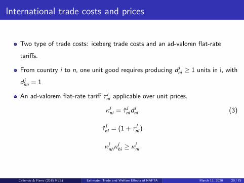
International trade costs and prices
Two type of trade costs: iceberg trade costs and an ad-valoren flat-rate
tariffs.
From country i to n, one unit good requires producing d jni ≥ 1 units in i, with
d jnn = 1
An ad-valorem flat-rate tariff τ jni applicable over unit prices.
κjni = τ j
nidjni (3)
τ jni = (1 + τ j
ni)
κjnhκj
hi ≥ κjni
Caliendo & Parro (2015 RES) Estimate: Trade and Welfare Effects of NAFTA March 11, 2020 20 / 75

International trade costs and prices
The price of intermediate good w j in country n is given by:
pjn(w j) = min
i
{c j
i κjni
z ji (w j)
}
For non-tradable sectors, κjni = ∞
As a result, pjn(w j) = c j
n/z ji (w j)
EK(2002): Motives to trade are introduced by probabilistic representation oftechnologies allowing productivities to differ by country and also by sectors.
Fi(z) = e−λjnz−θj
λjn: absolute advantage; θj : comparative advantage
Fréchet
Caliendo & Parro (2015 RES) Estimate: Trade and Welfare Effects of NAFTA March 11, 2020 21 / 75

International trade costs and prices
The price of the composite intermediate good followed EK(2002) is given by:
P jn = Aj
[ N∑i=1
λji (c
ji κ
jni)−θj
]−1/θj
(4)
Aj is a constant including a Gamma function.
With Cobb-Douglas preferences (equation 1), the consumption price index isgiven by:
Pn =J∏
j=1(P j
n/θjn)αj
n (5)
Caliendo & Parro (2015 RES) Estimate: Trade and Welfare Effects of NAFTA March 11, 2020 22 / 75

Expenditure shares
Total expenditure on sector j goods in country n is given by X jn = P j
nQjn.
Denote by X jni to the expenditure in country n of sector j goods from
country i .Country n’s share of expenditure of goods from i are given by πj
ni = X jni/X j
n
Using the properities of the Fréchet distribution, it can be described by:
πjni =
λji
[c j
i κjni
]−θj
∑Nh=1 λj
h
[c j
hκjnh
]−θj (6)
Changes in tariffs have a direct effect in trade shares via κjni , also from
equation (2) note that it also have an indirect effect through the inputbundle c j
i .
Caliendo & Parro (2015 RES) Estimate: Trade and Welfare Effects of NAFTA March 11, 2020 23 / 75

Total expenditure and trade balance
Total expenditure on goods j is the sum of the expenditure on the compositeintermediate goods by firms and the expenditure by households.
X jn =
J∑k=1
γj,kn
N∑i=1
X ki
πjin
1 + τ jin
+ αjnIn (7)
whereIn = wnLn + Rn + Dn (8)
In denotes the final absorption.
Rn =∑J
j=1∑N
i=1 τ jniM
jni , where M j
ni = X jn
πjni
1+τ jin
, are country n’s imports ofsector j goods from country i .
Caliendo & Parro (2015 RES) Estimate: Trade and Welfare Effects of NAFTA March 11, 2020 24 / 75

Total expenditure and trade balance
∑Nn=1 Dn = 0 and Dn =
∑Jk=1 Dk
n
Djn =
∑Ni=1 M j
ni −∑N
i=1 E jni , where E j
ni = X ji
πjin
1+τ jin
are country n’s export ofsector j goods to country i .Aggregate trade deficits in each country are exogenous, an sectoral tradedeficits are endogenously determinded.
J∑j=1
N∑i=1
X jn
πjni
1 + τ jni
− Dn =J∑
j=1
N∑i=1
X ji
πjin
1 + τ jin
(9)
Add equation (7) across sectors and substitute into equation (9) to obtain:
wnLn =J∑
j=1γj
n
N∑i=1
X ji
πjin
1 + τ jin
Caliendo & Parro (2015 RES) Estimate: Trade and Welfare Effects of NAFTA March 11, 2020 25 / 75
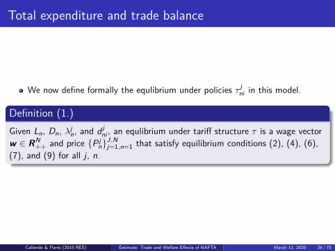
Total expenditure and trade balance
We now define formally the equlibrium under policies τ jni in this model.
Definition (1.)Given Ln, Dn, λj
n, and d jni , an equlibrium under tariff structure τ is a wage vector
w ∈ RN++ and price {P j
n}J,Nj=1,n=1 that satisfy equilibrium conditions (2), (4), (6),
(7), and (9) for all j , n.
Caliendo & Parro (2015 RES) Estimate: Trade and Welfare Effects of NAFTA March 11, 2020 26 / 75

Equilibrium in relative changes
Instead of solving for an equlibrium under policy τ , they solve for changes inprices and wages after changing from policy τ to τ
′ , which they define as anequlibrium in relative changes.
It can match exactly the model to the data in a base year.They can identify the effect on equlibrium outcomes from a pure change intariffs.They can solve for the equlibrium without needing to estimate parameterswhich are difficult to identify in the data, as productivities λj
n, and icebergtrade costs d j
ni .
Definition (2.)Let (w, P) be an equilibrium under tariff structure τ and let (w ′
, P′) be an
equilibrium under tariff structure τ′ . Define (w , P) as an equlibrium under τ
′
relative to τ , where a variable with a hat ”x” represents the relative change of thevariable, namely x = x ′
/x . Using equations (2), (4), (6), (7) and (9) to constructthe equlibrium.
Caliendo & Parro (2015 RES) Estimate: Trade and Welfare Effects of NAFTA March 11, 2020 27 / 75
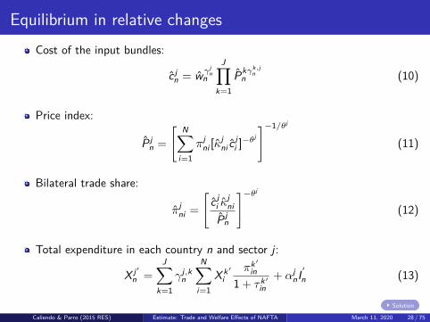
Equilibrium in relative changesCost of the input bundles:
c jn = wγ j
nn
J∏k=1
Pkγk,jnn (10)
Price index:
P jn =
[ N∑i=1
πjni [κ
jni c
ji ]−θj
]−1/θj
(11)
Bilateral trade share:
πjni =
[c j
i κjni
P jn
]−θj
(12)
Total expenditure in each country n and sector j :
X j′
n =J∑
k=1γj,k
n
N∑i=1
X k′
iπk′
in1 + τ k′
in+ αj
nI′
n (13)
Solution
Caliendo & Parro (2015 RES) Estimate: Trade and Welfare Effects of NAFTA March 11, 2020 28 / 75

Equilibrium in relative changes
Total balance:J∑
j=1
N∑i=1
X j′
nπj′
ni
1 + τ j′
ni− Dn =
J∑j=1
N∑i=1
X j′
iπj′
in
1 + τ j′
in(14)
Where κjni
1+τ j′in
1+τ jin
and I ′
n = wnwnLn +∑J
j=1∑N
i=1 τ j′
inπj′
ni
1+τ j′in
x j′
n + Dn
In order to solve the problem, we only need two sets of tariff structures (τand τ
′), data on the bilateral trade shares (πjni), the share of value added in
production (γk,jn ), and the sectoral dispersion of productivity (θj).
The only set of parameter to estimate is the sectoral dispersion ofproductivity θj .
Caliendo & Parro (2015 RES) Estimate: Trade and Welfare Effects of NAFTA March 11, 2020 29 / 75

Relative change in real wages
Using equations (10) and (12), they solve for the counterfactual changes inreal wages wn/P j
n.They aggregate across sectors using consumption expenditure shares andobtain the following expression for the logarithm change in real wags:
ln wn
Pn=
J∑j=1
αjn
θj ln πjnn︸ ︷︷ ︸
Final goods
−J∑
j=1
αjn
θj1 − γj
n
γjn
ln πjnn︸ ︷︷ ︸
Intermediate goods
−J∑
j=1
αjn
γjn
lnJ∏
k=1(Pk
n /P jn)γk,j
n
︸ ︷︷ ︸Sectoral linkages
(15)
Consider the case where γjn = 1 for all j and n, then:
ln(wn/P jn) = −(αj
n/θj) ln πjnn
Caliendo & Parro (2015 RES) Estimate: Trade and Welfare Effects of NAFTA March 11, 2020 30 / 75

Relative change in real wages
Consider the general model. The materials price index∏J
k=1(Pkn /P j
n)γk,jn
captures the effect of a change in the price of composite intermediates fromsector k on real wages in sector j .
The larger is γk,jn for sectors in which prices decline, the larger is the
reduction in the cost of material inputs used in production.
In other words, it captures the importance of the I-O structure of theeconomy.
Caliendo & Parro (2015 RES) Estimate: Trade and Welfare Effects of NAFTA March 11, 2020 31 / 75

Welfare effects from tariff changes
We decompose the welfare effects from tariff changes into terms of tradeeffects and volumn of trade effects.They denote welfare of the representative consumer in country n byWn = In/Pn. Then we can get the equation (16).
d ln Wn = 1In
J∑j=1
N∑i=1
(E jnid ln c j
n − M jnid ln c j
i )︸ ︷︷ ︸Terms of trade
+ 1In
J∑j=1
N∑i=1
τ jniM
jni(d ln M j
ni − d ln c ji )︸ ︷︷ ︸
Volumn of trade(16)
TOT effects: A multi-lateral weighted change in export and import prices atthe sectoral level, where the weights are given by bilateral exports andimports respectively.VOT effects: Import values deflated by import prices, the initial tariffs andimport volumes weight how important this effect is across sectors andcountries.
Details
Caliendo & Parro (2015 RES) Estimate: Trade and Welfare Effects of NAFTA March 11, 2020 32 / 75

Welfare effects from tariff changesThe change in bilateral terms of trade:
d ln totni =J∑
j=1(E j
nid ln c jn − M j
nid ln c ji ) (17)
The change in bilateral volumn of trade:
d ln votni =J∑
j=1τ j
niMjni(d ln M j
ni − d ln c ji ) (18)
The change in sectoral terms of trade:
d ln tot jn =
N∑i=1
(E jnid ln c j
n − M jnid ln c j
i ) (19)
The change in sectoral volumn of trade:
d ln vot jn =
N∑i=1
τ jniM
jni(d ln M j
ni − d ln c ji ) (20)
Caliendo & Parro (2015 RES) Estimate: Trade and Welfare Effects of NAFTA March 11, 2020 33 / 75

Taking the model to the data
The data needed are bilateral trade flow (M jni), value added (V j
n), grossproduction (Y j
n), and I-O tables. Then they can calculate the datacounterparts of πj
ni , γjn, γj,k
n , and αjn.
Domestic sale: M jnn = Y j
n −∑N
i=1,i =n M jin
Expenditure: X jni = M j
ni(1 + τ jni)
Expenditure share: πjni = X j
ni/∑N
i=1 X jni
Value added share: γjn = V j
n/Y jn
Sectoral linkage: γj,kn , the share of intermediate consumption of sector j in
sector k over the toal intermediate consumption of sector k, times (1 − γjn)
Final consumption share, αjn = (Y j
n + Djn −
∑Jk=1 γj,k
n Y kn )/In
The only parameter missing are the sectoral dispersion of productivity, θj
Caliendo & Parro (2015 RES) Estimate: Trade and Welfare Effects of NAFTA March 11, 2020 34 / 75
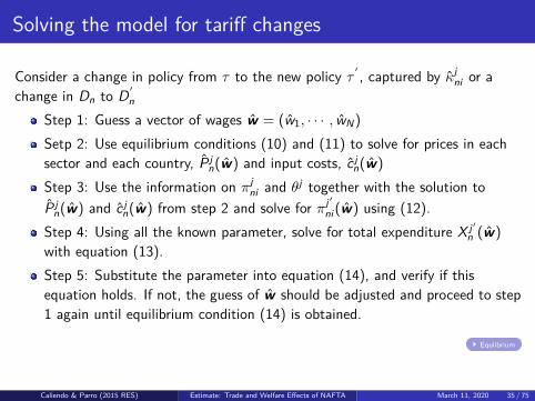
Solving the model for tariff changes
Consider a change in policy from τ to the new policy τ′ , captured by κj
ni or achange in Dn to D′
n
Step 1: Guess a vector of wages w = (w1, · · · , wN)Setp 2: Use equilibrium conditions (10) and (11) to solve for prices in eachsector and each country, P j
n(w) and input costs, c jn(w)
Step 3: Use the information on πjni and θj together with the solution to
P jn(w) and c j
n(w) from step 2 and solve for πj′
ni(w) using (12).Step 4: Using all the known parameter, solve for total expenditure X j′
n (w)with equation (13).Step 5: Substitute the parameter into equation (14), and verify if thisequation holds. If not, the guess of w should be adjusted and proceed to step1 again until equilibrium condition (14) is obtained.
Equlibrium
Caliendo & Parro (2015 RES) Estimate: Trade and Welfare Effects of NAFTA March 11, 2020 35 / 75
Outline
1 Introduction
2 Tariffs, intermediate goods and sectoral linkages
3 A quantitative model for trade policy evaluation
4 A new method to estimate trade elasticities
5 Quatifying the trade and welfare effets of NAFTA
6 Conclusion
Caliendo & Parro (2015 RES) Estimate: Trade and Welfare Effects of NAFTA March 11, 2020 36 / 75

A new method to estimate trade elasticities
The relation between dispersion of productivity and trade elasticities:If productivity is less dispersed (a larger value of θj), for the reason that goodsare less substitutable, the change of tariffs will not change the share of tradedgoods in a substaintial way.Equation (6) can explain it formally:
πjni =
λji
[c j
i κjni
]−θj
∑Nh=1 λj
h
[c j
hκjnh
]−θj
Caliendo & Parro (2015 RES) Estimate: Trade and Welfare Effects of NAFTA March 11, 2020 37 / 75

A new method to estimate trade elasticities
Consider three countries indexed by n, i , and h.Take the goods from sector j shipped in two different directions.Eg: i ⇒ n ⇒ h ⇒ i and i ⇒ h ⇒ n ⇒ i (the second one is the same ash ⇒ n ⇒ i ⇒ h)Then, using equation (6), they can calculate each expression and then takethe ratio:
X jniX
jihX j
hn
X jnhX j
hiXjin
=(
κjni
κjin
κjih
κjhi
κjhn
κjnh
)(21)
Each set of three countries can be used as an observations in equation (21),so the total observations can be calculated by C3
N , where N is the number ofcountries in the sample. (The expression shown in the paper is∑N−2
n=1 n(n + 1)/2, there is no difference between the two).
Caliendo & Parro (2015 RES) Estimate: Trade and Welfare Effects of NAFTA March 11, 2020 38 / 75

A new method to estimate trade elasticities
Consider the following model of asymmetric trade costs (which is differentfrom the method before).Trade costs are composed of tariffs (non-symmetric) and iceberg (alsonon-symmetric) trade costs, namely ln κj
ni = ln τ jni + ln d j
ni .Iceberg trade costs ln d j
ni , can be modelled quite generally as linear functionsof cross-country characteristics.
ln κjni = ln τ j
ni + ln d jni = ln τ j
ni + v jni + µj
n + δji + ϵj
ni (22)
Where v jni = v j
in captures symmetric bilateral trade costs like distance,language, common border, and belonging to FTA or not.The parameter µj
n and δji capture the importer sectoral and exporter sectoral
fixed effect respectively.(Which is common to all the trade partners)
Caliendo & Parro (2015 RES) Estimate: Trade and Welfare Effects of NAFTA March 11, 2020 39 / 75

A new method to estimate trade elasticities
Substituting equation (22) into equation (21), they get:
ln(
X jniX
jihX j
hn
X jinX j
hiXjnh
)= −θj ln
(τ j
ni
τ jin
τ jih
τ jhi
τ jhn
τ jnh
)+ ϵj (23)
Note that all the symmetric and asymmetric components of the iceberg tradecosts cancel out.They estimate the parameter sector by sector using the data for 1993, theyear before NAFTA was active.The estimate gives an equal weight to all countries; thus, as a robustnesscheck, they dropped observations with small trade flows.In each sector, they rank the countries according to the share of trade theycontribute in that particular sector.
Caliendo & Parro (2015 RES) Estimate: Trade and Welfare Effects of NAFTA March 11, 2020 40 / 75

A new method to estimate trade elasticities
[14:25 16/12/2014 rdu035.tex] RESTUD: The Review of Economic Studies Page: 18 1–44
18 REVIEW OF ECONOMIC STUDIES
TABLE 1Dispersion-of-productivity estimates
Full sample 99% sample 97.5% sample
Sector θ j s.e. N θ j s.e. N θ j s.e. N
Agriculture 8.11 (1.86) 496 9.11 (2.01) 430 16.88 (2.36) 364Mining 15.72 (2.76) 296 13.53 (3.67) 178 17.39 (4.06) 152Manufacturing
Food 2.55 (0.61) 495 2.62 (0.61) 429 2.46 (0.70) 352Textile 5.56 (1.14) 437 8.10 (1.28) 314 1.74 (1.73) 186Wood 10.83 (2.53) 315 11.50 (2.87) 191 11.22 (3.11) 148Paper 9.07 (1.69) 507 16.52 (2.65) 352 2.57 (2.88) 220Petroleum 51.08 (18.05) 91 64.85 (15.61) 86 61.25 (15.90) 80Chemicals 4.75 (1.77) 430 3.13 (1.78) 341 2.94 (2.34) 220Plastic 1.66 (1.41) 376 1.67 (2.23) 272 0.60 (2.11) 180Minerals 2.76 (1.44) 342 2.41 (1.60) 263 2.99 (1.88) 186Basic metals 7.99 (2.53) 388 3.28 (2.51) 288 −0.05 (2.82) 235Metal products 4.30 (2.15) 404 6.99 (2.12) 314 0.52 (3.02) 186Machinery n.e.c. 1.52 (1.81) 397 1.45 (2.80) 290 −2.82 (4.33) 186Office 12.79 (2.14) 306 12.95 (4.53) 126 11.47 (5.14) 62Electrical 10.60 (1.38) 343 12.91 (1.64) 269 3.37 (2.63) 177Communication 7.07 (1.72) 312 3.95 (1.77) 143 4.82 (1.83) 93Medical 8.98 (1.25) 383 8.71 (1.56) 237 1.97 (1.36) 94Auto 1.01 (0.80) 237 1.84 (0.92) 126 −3.06 (0.86) 59Other Transport 0.37 (1.08) 245 0.39 (1.08) 226 0.53 (1.15) 167Other 5.00 (0.92) 412 3.98 (1.08) 227 3.06 (0.83) 135
Test equal parameters F(17, 7294) = 7.52 Prob>F=0.00
Aggregate elasticity 4.55 (0.35) 7212 4.49 (0.39) 5102 3.29 (0.47) 3482
robust since they changed sign as we restricted the sample.42 These sectors are Basic metals,Machinery n.e.c., and Auto.43
Our estimates are in the range of the trade elasticities estimated in the literature.44 Ourbenchmark estimates are the estimates presented in Table 1 for the 99% sample, since theycontrol for outliers. For the sectors Basic metals, Machinery n.e.c., and Auto, we replace them bythe mean estimate for the manufacturing sector. We also re-estimated the dispersion parametersincluding importer and exporters fixed effects as an additional robustness check. The resultsappear in Table A2, Appendix “Additional Results.”
42. For the case of Chemicals China was an outlier. The estimates including China were 1.39 for the full sample,−0.64 for the 99% sample and −0.93 for the 97.5% sample. The numbers without China are presented in the table. Chinarepresented 5% of the share of trade in that sector.
43. Machinery n.e.c. corresponds to manufacture of electrical machinery and apparatus not elsewhere classified.44. The magnitudes of the sectoral trade elasticities are within the range of the coefficient estimated by
Eaton and Kortum, (2002) for the manufacturing sector as a whole using data from 1990. Their estimate ranged between3.60 and 12.86, and their preferred estimate is 8.28. Other studies, e.g.: Anderson et al. (2005) document that the averageelasticity is 17. Broda and Weinstein (2006) find that the simple average of the elasticities is 17 at the seven-digit (TSUSA),7 at the three-digit (TSUSA), 12 at the ten-digit (HTS), and 4 at the three-digit (HTS) goods disaggregation. Clausing(2001) and Head and Ries (2001) find values between 7 and 11.4, Romalis (2007) finds values between 4 and 13. Bishop(2006) estimates the trade elasticity for the steel industry and finds values between 3 and 5. Yi (2003) compares severalmodels and finds that to match the bilateral trade flows in the data, the Armington-type models need a value of elasticityof 15. Imbs and Méjean (2011) make the point that the “true” elasticity of substitution is more than twice the elasticityimplied by the aggregate data. Hertel et al. (2003) estimate sectoral trade elasticities between 3 and 30.
at Singapore Managem
ent University on July 5, 2015
http://restud.oxfordjournals.org/D
ownloaded from
Caliendo & Parro (2015 RES) Estimate: Trade and Welfare Effects of NAFTA March 11, 2020 41 / 75

Outline
1 Introduction
2 Tariffs, intermediate goods and sectoral linkages
3 A quantitative model for trade policy evaluation
4 A new method to estimate trade elasticities
5 Quatifying the trade and welfare effets of NAFTA
6 Conclusion
Caliendo & Parro (2015 RES) Estimate: Trade and Welfare Effects of NAFTA March 11, 2020 42 / 75

Quatifying the trade and welfare effets of NAFTA
Two different but equally informative counterfactual exercises.Exercise one: Introduce the change in the tariff from 1993 to 2005 betweenNAFTA members and fix the tariff of others to the levels in 1993.Exercise two: Measure the effects of NAFTA by quatifying the gains fromNAFTA’s tariff reductions given observed world tariff changes.
Step 1: Introduce the change in world tariff structure (also including NAFTA)from 1993 to 2005.Step 2: Recalibrate the model to the year 1993 and introduce the observedworld tariff change from 1993 to 2005 holding NAFTA tariffs fixed to the year1993.Compare the gains between the two, namely the gains from world tariffreduction with and without NAFTA.
Caliendo & Parro (2015 RES) Estimate: Trade and Welfare Effects of NAFTA March 11, 2020 43 / 75

Quatifying the trade and welfare effets of NAFTA
Counterfactual changes are not going to adjust the aggregate exogenoustrade deficit.
They use two ways to deal with it.
Firstly, they calibrate the model with trade deficits and solve the modelimposing zero aggregate deficit, D′ = 0. (Benchmark)
Secondly, they calibrate the model with aggregate deficits to the year 1993and then calculate all counterfactuals holding the countries aggregate tradedeficits constant, as a share of world GDP. (Robustness check)
Caliendo & Parro (2015 RES) Estimate: Trade and Welfare Effects of NAFTA March 11, 2020 44 / 75

Counterfactual I
[14:25 16/12/2014 rdu035.tex] RESTUD: The Review of Economic Studies Page: 20 1–44
20 REVIEW OF ECONOMIC STUDIES
TABLE 2Welfare effects from NAFTA’s tariff reductions
Welfare
Country Total Terms of trade Volume of Trade Real wages
Mexico 1.31% −0.41% 1.72% 1.72%Canada −0.06% −0.11% 0.04% 0.32%U.S. 0.08% 0.04% 0.04% 0.11%
we eliminate all aggregate deficits by first calibrating the model with trade deficits and thensolving the model imposing zero aggregate deficit, D′
n =0. We then use the implied no-deficitworld economy as our base year. Secondly, we calibrate the model with aggregate deficits tothe year 1993 and then calculate all counterfactuals holding the countries aggregate trade deficitsconstant, as a share of world GDP. We compute all the counterfactual exercises using both solutionstrategies but present in the main text only the results with no aggregate deficit in the base year.The Appendix “Additional Results” shows a variety of additional results including the case whereaggregate trade deficits remain fixed as a share of world GDP.
5.1. Trade and welfare effects from NAFTA’s tariff reductions
We now quantify the trade and welfare effects of NAFTA. Table 2 presents the welfare effectsfrom NAFTA’s tariff reductions while fixing the tariff to and from the rest of the world to theyear 1993. Welfare effects are calculated using equation (16), and changes in real wages usingequation (15). As we can see, Mexico’s welfare increases by 1.31%. The effects for Canada andthe U.S. are smaller. Canada loses 0.06% whereas the U.S. gains 0.08%. Still, we find that realwages increase for all NAFTA members and Mexico gains the most, followed by Canada and theU.S.47
Decomposing the welfare effects into terms of trade and volume of trade underscores thesources of these gains. The third column in Table 2 shows that the major source of gains areincreases in volume of trade. The welfare gains from trade creation for Mexico, Canada, and theU.S. are 1.72%, 0.04% and 0.04%, respectively. We can look deeper and measure the extent towhich the welfare effects are a result of trade creation with NAFTA members vis-a-vis the rest ofthe world. This is done by applying the bilateral volume of trade measures equation (18) definedbefore.
Column 3 in Table 3 shows that the trade created with NAFTA members is the single mostimportant contributor to the positive welfare effects. The figures are 1.80%, 0.08%, and 0.04%for Mexico, Canada, and the U.S., respectively. This result unmasks an important channel bywhich NAFTA generated positive welfare effects to all of its members, by creating more tradewithin the bloc. On the other hand, column 4 from Table 3 shows that the reduction in volumeof trade with the rest of the world has a negative welfare effect. This negative welfare effect,which we discuss further below, arises from NAFTA diverting trade from countries outside ofthe agreement.
Another source of welfare effects are changes in terms of trade. From column 2 of Table 2,we can see that Mexico and Canada’s terms of trade deteriorate whereas the U.S. terms of trade
47. The welfare effects results in the model with trade deficits are very similar, 1.17%, −0.04%, and 0.09% forMexico, Canada, and the U.S., respectively. Appendix “Additional Results”, Tables A4–A7, includes this and additionalresults with trade deficits and it shows that all the results in this section are robust to include trade deficits or not.
at Singapore Managem
ent University on July 5, 2015
http://restud.oxfordjournals.org/D
ownloaded from
[14:25 16/12/2014 rdu035.tex] RESTUD: The Review of Economic Studies Page: 21 1–44
CALIENDO & PARRO TRADE AND WELFARE EFFECTS OF NAFTA 21
TABLE 3Bilateral welfare effects from NAFTA’s tariff reductions
Terms of trade Volume of Trade
Country NAFTA Rest of the world NAFTA Rest of the world
Mexico −0.39% −0.02% 1.80% −0.08%Canada −0.09% −0.02% 0.08% −0.04%U.S. 0.03% 0.01% 0.04% 0.00%
improve. One way to understand this differential effect is by looking at how export prices changein each country. From equation (10), notice that the change in unit costs, or the change in exportprices, are an increasing function of input prices; namely wages and the price of materials. Thelast column of Table 2 shows that real wages increase for all NAFTA members but relatively morefor Mexico and Canada compared to the U.S. So, all else equal, the increase in wages increaseexport prices. However, from equation (11) note that, all else equal, the price of materials fallwith reductions in import tariffs. Therefore, export prices change according to how large is theincrease in wages relative to the fall in the price of materials. It turns out that the average exportprices across sectors fall by 2% and 0.6% for Mexico and Canada and increase by 0.1% forthe U.S. If we now factor in that most trade between NAFTA members is with other NAFTAmembers, then this explains why terms of trade deteriorate for Mexico and Canada and increasefor the U.S.
Table 3, columns 2 and 3, present the bilateral terms of trade changes with respect to NAFTAmembers and the rest of the world using equation (17). As we can see, Mexico and Canada’sterms of trade deteriorate against both group of countries, but mostly with NAFTA countries. Forthe U.S. the story is different. Terms of trade improve with respect to all countries. However, theterms of trade improve relatively more against NAFTA members since the U.S. mostly sourcesintermediate goods from Mexico and Canada, countries that experience a reduction in exportprices.
Table 4 presents the sectoral contribution to the aggregate terms of trade and volumeof trade effects for each NAFTA member. These figures are calculated for each sectorj as d lntotj
n/∑J
j=1d lntotjn and d lnvotj
n/∑J
j=1d lnvotjn using the sectoral measures defined in
equations (19) and (20). As we can see, there is considerable variation in the sectoral contributionto the aggregate effects. Still, the aggregate change in terms of trade in each country is explainedby a handful of sectors. The three sectors that contribute the most to Mexico’s terms oftrade deterioration account for 76% of the reduction. These sectors are Electrical Machinery,Communication Equipment, and Auto (Motor Vehicles). These same three sectors are also thesectors that contribute the most to U.S.’s terms of trade change accounting for 51% of the increase.In the case of Canada, the three sectors that contribute the most to the change in terms of tradeaccount for 52.5% of the reduction. These sectors are, Auto, Other Transport, and Basic Metals.The main explanations why certain sectors have a large aggregate effect compared to othersare the magnitude of the reduction in import tariffs, how large is the share of materials used inproduction, and how important are sectoral linkages.
To see this, consider the case of Mexico and U.S. From the previous discussion we knowthat Mexico’s terms of trade deteriorate mainly as a consequence of the reduction in exportprices and that most trade is with NAFTA, in particular with the U.S. Similarly, since the U.S.mostly imports goods from Mexico, and Mexican export prices fall, this is the first order effectwhy the U.S. aggregate terms of trade improve. So to understand why certain sectors contributemore to the aggregate terms of trade changes in Mexico and the U.S. we need to understand
at Singapore Managem
ent University on July 5, 2015
http://restud.oxfordjournals.org/D
ownloaded from
Caliendo & Parro (2015 RES) Estimate: Trade and Welfare Effects of NAFTA March 11, 2020 45 / 75

Counterfactual I
[14:25 16/12/2014 rdu035.tex] RESTUD: The Review of Economic Studies Page: 22 1–44
22 REVIEW OF ECONOMIC STUDIES
TABLE 4Sectoral contribution to welfare effects from NAFTA’s tariff reductions
Mexico Canada United States
Sector Terms Volume Terms Volume Terms Volumeof of of of of of
trade trade trade trade trade trade
Agriculture −0.13% 2.87% 3.41% −0.01% 3.41% 0.65%Mining −3.01% 0.25% 4.04% −0.20% 1.54% 0.04%Manufacturing
Food 0.45% 1.17% 3.56% 2.37% 3.16% 1.04%Textile 3.30% 12.00% 1.15% 16.20% 4.32% 22.20%Wood 0.30% 2.26% 4.17% 0.24% 1.31% 0.41%Paper 0.39% 3.82% 5.86% 0.49% 2.83% 0.33%Petroleum −0.09% 14.60% 0.60% 30.40% 1.85% 11.40%Chemicals 0.57% 2.15% 5.74% 0.08% 5.60% 1.11%Plastic 0.62% 4.21% 2.53% 7.56% 1.61% 0.32%Minerals 0.05% 0.73% 0.93% 0.47% 0.70% 0.57%Basic metals 1.07% 3.02% 10.10% 1.48% 3.40% 1.05%Metal products 0.90% 5.56% 2.22% 7.99% 1.61% 1.06%Machinery n.e.c. 3.68% 4.32% 5.16% −0.02% 5.63% 0.65%Office 8.37% 4.72% 2.32% −0.83% 3.50% 1.43%Electrical 41.20% 25.80% 1.37% 7.18% 24.20% 42.20%Communication 21.00% 3.64% 2.67% 0.15% 11.60% 4.58%Medical 4.72% 1.34% 0.94% −0.23% 3.48% 4.46%Auto 13.80% 4.78% 29.50% 27.80% 15.80% 4.47%Other Transport 0.21% 0.82% 12.90% −0.97% 1.51% 0.32%Other 2.63% 1.92% 0.81% −0.11% 2.90% 1.69%
why export prices in these sectors fall so much as a consequence of NAFTA.48 There are threereasons for this. First, the average tariffs applied by Mexico to imports from Canada and the U.S.on Electrical Machinery, Communication Equipment, and Autos in the year 1993 were 13.4%,14.9%, and 15.5%, respectively. These sectors were not the sectors with the largest import tariffsbut still larger than the average (12.4%), and the median (13.2%), import tariff applied acrossall sectors. Secondly, the share of materials used in production is 82% for the case of ElectricalMachinery and Communication Equipment, and 73% for Autos. These figures are considerablylarger than the average (49%), and the median (48.3%), share of material use in productionfor the rest of the sectors in the Mexican economy. Finally, these sectors are very interrelated.The shares of Electrical Machinery and Communication Equipment used for the production ofElectrical Machinery are 37% and 3%, whereas for the production of Communication Equipmentthe shares are 53% and 7%. Therefore, the reduction in import tariffs in these sectors explainpart of the effect on prices. The rest is explained by the fact that a reduction in the unit cost ofproduction in any of these sectors has a multiplicative effect because of the strong I–O feedbackthat these sectors present. Also, a large share of material use in production makes, other thingsequal, reductions in import tariffs across sectors to have a larger impact in export prices in thesesectors compared to the rest.
From Table 4 we can also learn how the sectoral contribution to the aggregate change in volumeof trade varies across NAFTAmembers. The first thing to note is that for the case of Mexico and theU.S., every sector has a positive contribution to the welfare increase from volume of trade. Threesectors account for more than 50% of the sectoral contribution of Mexico’s and U.S.’s volume of
48. In fact, trade weighted export prices of Electrical Machinery, Communication Equipment, and Autos fall by6.6%, 3.5%, and 5.6% in Mexico; the largest reductions across all sectors.
at Singapore Managem
ent University on July 5, 2015
http://restud.oxfordjournals.org/D
ownloaded from
Caliendo & Parro (2015 RES) Estimate: Trade and Welfare Effects of NAFTA March 11, 2020 46 / 75
Counterfactual I
[14:25 16/12/2014 rdu035.tex] RESTUD: The Review of Economic Studies Page: 23 1–44
CALIENDO & PARRO TRADE AND WELFARE EFFECTS OF NAFTA 23
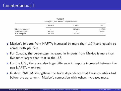
TABLE 5Trade effects from NAFTA’s tariff reductions
Mexico Canada U.S.
Mexico’s imports - 116.60% 118.31%Canada’s imports 58.57% - 9.49%U.S.’s imports 109.54% 6.57% -
trade. These are Textiles, Petroleum, and Electrical Machinery. For the case of Canada, the sectorsthat contribute the most are Textiles, Petroleum, and Auto. In general, volume of trade effectsdepend on the magnitude of the tariff reduction, the trade elasticity, and the share of materialsused in production and these factors weight differently for each of these sectors. Textiles wasthe most protected sector by Mexico in the year 1993. Applied import tariffs were on average18%. So the large reduction in tariffs facilitates trade between members of NAFTA and resultsin a significant contribution to the increase in volume of trade. Petroleum is a homogenous goodsector. As a consequence, small changes in import tariffs can have large trade effects since it isrelatively easy to substitute suppliers, as documented by its high import tariff trade elasticity (seeTable 1). The average import tariffs in Petroleum in the year 1993 across NAFTA members was7%. Finally, NAFTA’s tariffs reductions has important effects over the price of intermediate goodstraded in some sectors compared to others. This is particularly important for the sectors ElectricalMachinery and Autos for reasons we discussed in the previous paragraph. The reduction in tradeprices in these sectors explains the increase in the volume of trade effect.
Table 5 presents aggregate trade effects from NAFTA. As we can see, NAFTA generated largeaggregate trade effects for all members. Mexico’s imports from NAFTA increased by more than110% and equally so across both partners. For the case of Canada, we find that the percentageincrease in imports from Mexico is more than five times larger than the percentage increase inimports from the U.S. This results reflect that Mexico’s role as a supplier of intermediate goodsto NAFTA members increased as a consequence of NAFTA. In fact, this is even more evidentwhen we look at the case of the U.S. imports. Imports from Mexico increase more than 100%whereas from Canada only 6.57%. These figures reflect how interdependent these economiesbecome after the tariff reductions imposed by the agreement. In short, NAFTA strengthened thetrade dependence that these countries had before the agreement, and as a consequence Canadaand the U.S. source more goods from Mexico, whereas Mexico sources more goods from Canadaand the U.S.
NAFTA also had an effect on sectoral specialization. Table 6 presents export shares byindustry before and after reducing NAFTA’s tariffs. First, note that sectoral concentration variesconsiderably across sectors and countries. Consider the case of Mexico before NAFTA, the year1993. Three sectors account for 52.75% of total exports. These sectors are Electrical Machinery,Autos, and Mining. For the case of Canada, the three sectors with the largest shares are Autos,Basic Metals, and Mining, and account for 43.7% of total exports. Whereas for the U.S. the threelargest sectors are Machinery, Chemicals, and Autos, and account for 28.57% of total exports.These figures reflect that Mexico was the country with the highest degree of sectoral specializationwhereas the U.S. the most diversified. In fact, the last row of the table presents the normalizedHerfindahl index (henceforth, HHI) and we make use of it as a measure of sectoral specialization.As we can see, the HHI for Mexico was the largest and twice as large as the U.S. HHI, the smallestamong all NAFTA members. After NAFTA’s tariffs reductions we find that Mexico became morespecialized whereas Canada and the U.S. more diversified. In fact, Mexico’s share of exportsfrom Electrical Machinery increase to 34.07% and the three largest sectors account for 54.95%
at Singapore Managem
ent University on July 5, 2015
http://restud.oxfordjournals.org/D
ownloaded from
Mexico’s imports from NAFTA increased by more than 110% and equally soacross both partners.For Canada, the percentage increased in imports from Mexico is more thanfive times larger than that in the U.S.For the U.S., there are also huge difference in imports increased between thetwo NAFTA members.In short, NAFTA strengthens the trade dependence that these countries hadbefore the agreement. Mexico’s connection with others increases most.
Caliendo & Parro (2015 RES) Estimate: Trade and Welfare Effects of NAFTA March 11, 2020 47 / 75

Counterfactual I
[14:25 16/12/2014 rdu035.tex] RESTUD: The Review of Economic Studies Page: 24 1–44
24 REVIEW OF ECONOMIC STUDIES
TABLE 6Export shares by sector before and after NAFTA’s tariff reductions
Mexico Canada U.S.
Sector Before After Before After Before After
Agriculture 4.72% 3.03% 4.99% 5.04% 6.91% 6.35%Mining 15.53% 7.85% 8.99% 8.96% 1.72% 1.52%Manufacturing
Food 2.33% 1.48% 4.82% 4.68% 5.09% 4.73%Textile 4.42% 6.92% 1.05% 1.49% 2.68% 3.49%Wood 0.59% 0.52% 8.12% 8.05% 2.02% 1.98%Paper 0.62% 0.51% 8.34% 8.44% 4.99% 4.89%Petroleum 1.62% 5.28% 0.59% 0.78% 4.30% 5.71%Chemicals 4.40% 2.53% 5.58% 5.40% 10.00% 9.25%Plastic 0.80% 0.48% 2.06% 2.06% 2.28% 2.43%Minerals 1.32% 0.84% 0.81% 0.78% 0.94% 0.92%Basic metals 3.24% 2.00% 10.29% 10.19% 3.05% 3.11%Metal products 1.22% 1.03% 1.47% 1.53% 2.23% 2.59%Machinery n.e.c. 4.30% 2.53% 4.69% 4.49% 10.37% 9.70%Office 3.34% 5.07% 2.44% 2.54% 7.70% 7.29%Electrical 20.79% 34.07% 2.50% 2.35% 6.07% 7.97%Communication 8.57% 7.08% 3.11% 3.02% 7.19% 6.81%Medical 2.48% 3.28% 0.98% 1.03% 5.16% 4.79%Auto 16.43% 13.05% 24.42% 24.07% 8.20% 8.09%Other Transport 0.28% 0.26% 3.21% 3.58% 7.32% 6.65%Other 3.02% 2.20% 1.55% 1.52% 1.77% 1.74%
Normalized Herfindahl 0.092 0.138 0.083 0.081 0.042 0.040
of total exports after NAFTA. This sectoral concentration is reflected in Mexico’s HHI whichincreases to 0.138. On the other hand, the HHI indices of Canada and the U.S. decrease.49
The rest of the world was hardly affected by NAFTA’s tariff reductions. Table A3 in Appendix“Additional Results”, which we do not include in the main text for brevity, presents the change inwelfare, terms of trade and volume of trade effects for the rest of the 28 countries in our sample.The effects are small. The two countries most impacted are China and Korea and in both caseswelfare falls by 0.03%. This is mostly due to a reduction in the volume of trade for the case ofChina, and an equal reduction in the terms of trade and volume of trade for the case of Korea.Looking at other countries we find that volumes of trade decreased for most cases. These resultsare suggestive of countries having a negative impact from NAFTA mainly due to trade diversiontowards NAFTA members. Still, the impact is small.
We now turn to the analysis of the effects of NAFTA given world tariff changes.
5.2. The effects of NAFTA given world tariff changes
From 1993 to 2005 more than 100 regional trade agreements entered into force.50 Of theseagreements, several involved NAFTA members. Since NAFTA was active during this process
49. Many factors, besides NAFTA, could have influenced the pattern of sectoral specialization in the data. Still, thepattern of sectoral specialization implied by the model from NAFTA’s tariff reductions for NAFTA members is in linewith the observed pattern in the year 2005. In fact, the correlations are 0.59, 0.86, and 0.83 for Mexico, Canada, and theU.S., respectively.
50. This figure was computed using the list of agreements in force from 1993 to 2005 from the WTO-RTA Database,(http://rtais.wto.org/).
at Singapore Managem
ent University on July 5, 2015
http://restud.oxfordjournals.org/D
ownloaded from
Caliendo & Parro (2015 RES) Estimate: Trade and Welfare Effects of NAFTA March 11, 2020 48 / 75

Counterfactual I
NAFTA has a effect on sectoral specialization.(Two ways to obtain thisconclusion)For the three most concentrated sectors, in Mexico, 52.75% to54.95%(electrical 20.79% to 34.07%); In Canada, 43.7% to 43,22%; In theU.S., 28.57% to 27.04%.The result is the same as HHI.
For the case of the rest of the 28 countries, two countriesc most impacted areChina and Korea and in both cases welfare falls by 0.03% .A reduction in VOT for China and an equal reduction in TOT and VOT forKorea.The VOT decreased for most cases, because of the trade diversion towardsNAFTA members.
Caliendo & Parro (2015 RES) Estimate: Trade and Welfare Effects of NAFTA March 11, 2020 49 / 75

Counterfactual I
[14:25 16/12/2014 rdu035.tex] RESTUD: The Review of Economic Studies Page: 37 1–44
CALIENDO & PARRO TRADE AND WELFARE EFFECTS OF NAFTA 37
F. ADDITIONAL RESULTS
TABLE A2Dispersion-of-productivity estimates (with importer and exporter fixed effects)
Full sample 99% sample 97.5% sample
Sector θ j s.e. N θ j s.e. N θ j s.e. N
Agriculture 8.59 (2.00) 496 9.54 (2.11) 430 16.97 (2.48) 364Mining 14.83 (2.87) 296 11.96 (3.84) 178 14.84 (4.38) 152Manufacturing
Food 2.84 (0.57) 495 3.02 (0.57) 429 2.89 (0.65) 352Textile 5.99 (1.24) 437 8.55 (1.38) 314 0.61 (1.89) 186Wood 10.19 (2.24) 315 10.72 (2.63) 191 9.30 (2.82) 148Paper 8.32 (1.66) 507 15.20 (2.69) 352 0.51 (2.86) 220Petroleum 69.31 (19.32) 91 68.47 (19.08) 86 65.92 (19.51) 80Chemicals 3.64 (1.75) 430 3.23 (1.76) 341 −0.02 (2.07) 220Plastic 0.88 (1.57) 376 3.10 (2.24) 272 1.95 (2.22) 180Minerals 3.38 (1.54) 342 3.03 (1.73) 263 3.85 (2.07) 186Basic metals 6.58 (2.28) 388 0.88 (2.58) 288 −1.31 (2.77) 235Metal products 5.03 (1.93) 404 7.30 (2.01) 314 0.82 (2.83) 186Machinery n.e.c. 2.87 (1.85) 397 3.88 (3.14) 290 0.70 (4.24) 186Office 13.88 (2.21) 306 9.85 (5.60) 126 21.57 (5.78) 62Electrical 11.02 (1.46) 343 13.95 (1.66) 269 4.66 (2.82) 177Communication 4.86 (1.69) 312 3.27 (2.07) 143 3.33 (2.19) 93Medical 7.63 (1.22) 383 7.49 (1.48) 237 2.45 (1.25) 94Auto 0.49 (0.91) 237 1.59 (1.04) 126 −2.13 (1.34) 59Other Transport 0.90 (1.16) 245 0.91 (1.15) 226 1.05 (1.22) 167Other 4.95 (0.92) 412 3.52 (1.04) 227 2.61 (0.81) 135
TABLE A3Welfare effects from NAFTA’s tariff reductions
Terms Volume Terms VolumeCountry Welfare of of Country Welfare of of
trade trade trade trade
Argentina 0.001% 0.000% 0.001% Ireland −0.018% −0.012% −0.006%Australia 0.000% 0.000% −0.000% Italy −0.004% −0.003% −0.001%Austria −0.004% −0.002% −0.002% Japan −0.007% −0.005% −0.002%Brazil −0.002% −0.002% 0.000% Korea −0.029% −0.018% −0.011%Chile 0.010% 0.009% 0.001% Netherlands −0.005% −0.003% −0.002%China −0.028% −0.006% −0.022% New Zealand 0.002% 0.002% −0.000%Denmark −0.002% −0.001% −0.001% Norway 0.003% 0.004% −0.001%Finland −0.001% 0.000% −0.001% Portugal −0.003% −0.002% −0.001%France −0.004% −0.003% −0.001% South Africa 0.003% 0.002% 0.002%Germany −0.005% −0.003% −0.001% Spain −0.008% −0.004% −0.001%Greece 0.000% 0.001% −0.000% Sweden −0.009% −0.006% −0.002%Hungary −0.003% −0.002% −0.002% Turkey −0.001% −0.001% −0.001%India −0.005% −0.002% −0.003% U.K. −0.005% −0.003% −0.002%Indonesia −0.001% 0.000% −0.001% ROW −0.003% −0.001% −0.002%
at Singapore Managem
ent University on July 5, 2015
http://restud.oxfordjournals.org/D
ownloaded from
Caliendo & Parro (2015 RES) Estimate: Trade and Welfare Effects of NAFTA March 11, 2020 50 / 75
Counterfactual II
Exercise two, step 1.
[14:25 16/12/2014 rdu035.tex] RESTUD: The Review of Economic Studies Page: 25 1–44
CALIENDO & PARRO TRADE AND WELFARE EFFECTS OF NAFTA 25
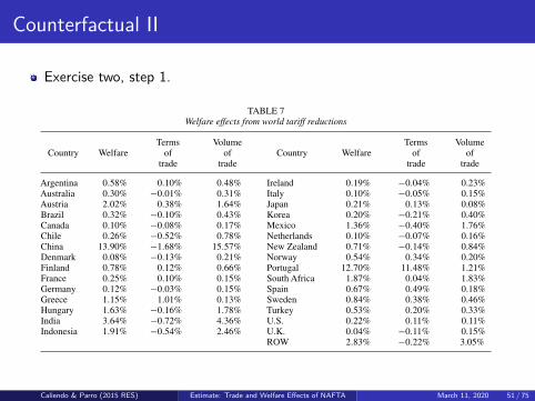
TABLE 7Welfare effects from world tariff reductions
Terms Volume Terms VolumeCountry Welfare of of Country Welfare of of
trade trade trade trade
Argentina 0.58% 0.10% 0.48% Ireland 0.19% −0.04% 0.23%Australia 0.30% −0.01% 0.31% Italy 0.10% −0.05% 0.15%Austria 2.02% 0.38% 1.64% Japan 0.21% 0.13% 0.08%Brazil 0.32% −0.10% 0.43% Korea 0.20% −0.21% 0.40%Canada 0.10% −0.08% 0.17% Mexico 1.36% −0.40% 1.76%Chile 0.26% −0.52% 0.78% Netherlands 0.10% −0.07% 0.16%China 13.90% −1.68% 15.57% New Zealand 0.71% −0.14% 0.84%Denmark 0.08% −0.13% 0.21% Norway 0.54% 0.34% 0.20%Finland 0.78% 0.12% 0.66% Portugal 12.70% 11.48% 1.21%France 0.25% 0.10% 0.15% South Africa 1.87% 0.04% 1.83%Germany 0.12% −0.03% 0.15% Spain 0.67% 0.49% 0.18%Greece 1.15% 1.01% 0.13% Sweden 0.84% 0.38% 0.46%Hungary 1.63% −0.16% 1.78% Turkey 0.53% 0.20% 0.33%India 3.64% −0.72% 4.36% U.S. 0.22% 0.11% 0.11%Indonesia 1.91% −0.54% 2.46% U.K. 0.04% −0.11% 0.15%
ROW 2.83% −0.22% 3.05%
of trade liberalization, we can evaluate to what extent the economic effects of NAFTA’s tariffreductions were influenced by world tariff changes. To that end, we first use observable changesin tariffs and quantify the global effects from world tariff reductions, including the change inNAFTA’s tariffs.
Table 7 presents the welfare effects for the 31 countries in our sample. As we can see, everysingle country gained from world tariff reductions. The largest winner was China, with a welfaregain of 13.9%.51 The most important source of these gains for China are the increased volumeof trade. This is also the case for most countries in the sample. Focusing on NAFTA members,all countries gained more compared to the case where only NAFTA tariff change. In the caseof Canada, the gains are 0.10% and most of the gains arise from an increase in trade volumes.For the case of Mexico, the gains are similar, 1.36% compared to 1.31%, but the source isslightly different. Terms of trade deteriorate less, -0.40% compared to -0.41%, and volume oftrade increase more, 1.76% instead of 1.72%. For the case of the U.S., the gains are considerablylarger, 0.22% compared to 0.08%.
We also decompose the welfare effects into bilateral measures of terms of trade and volumeof trade with respect to NAFTA members and the rest of the world. Table 8 shows the results forMexico, Canada, and the U.S. We find that volume of trade effects with respect to the rest of theworld increase. This is a key difference relative to the case where only NAFTA tariffs changed;compare the last columns from Tables 3 and 8. In fact, this reflects that trade was created withthe rest of the world after NAFTA was in force, due in part to the reduction of world tariffs.
Focusing on other outcomes, Table 8 also shows that the terms of trade improvements for theU.S. are now mostly with countries outside NAFTA. In the case of Canada, the terms of tradeeffects are still negative with respect to NAFTA members, but now switched to positive withrespect to other countries. These figures explain why Canada and the U.S. gained more from
51. The welfare gains in Table 7 are calculated using equation (16). We can use the model to understand more thesource of the welfare gains for each country. For the case of China, we find that the gains due to the reduction in importtariffs that the rest of the world applied to China, are 13.4%. The gains from the reduction of China’s import tariffs are0.08%. Whereas if China’s import and export tariffs did not changed it would have lost -0.16%.
at Singapore Managem
ent University on July 5, 2015
http://restud.oxfordjournals.org/D
ownloaded from
Caliendo & Parro (2015 RES) Estimate: Trade and Welfare Effects of NAFTA March 11, 2020 51 / 75

Counterfactual II
Every single country gained from world tariff reduction.The most important source of these gains for China are the increased VOT,which is the case for most countries.Compared with the first counterfactual, the gains of Mexico, from 1.31% to1.36%; for Canada, from -0.06% to 0.10%; for the U.S., from 0.08% to0.22%.
Caliendo & Parro (2015 RES) Estimate: Trade and Welfare Effects of NAFTA March 11, 2020 52 / 75

Counterfactual II
[14:25 16/12/2014 rdu035.tex] RESTUD: The Review of Economic Studies Page: 26 1–44
26 REVIEW OF ECONOMIC STUDIES
TABLE 8Bilateral welfare effects from world’s tariff reductions
Terms of trade Volume of Trade
Country NAFTA Rest of the world NAFTA Rest of the world
Mexico −0.39% −0.01% 1.64% 0.13%Canada −0.10% 0.02% 0.05% 0.12%U.S. 0.03% 0.08% 0.04% 0.08%
TABLE 9Welfare effects from NAFTA given world tariff changes
Welfare
Country Total Terms of trade Volume of trade Real wages
Mexico 1.17% −0.38% 1.55% 1.63%Canada −0.06% −0.09% 0.03% 0.31%U.S. 0.08% 0.04% 0.04% 0.11%
global tariff reductions relative to only NAFTA tariff reductions. The results on terms of tradeeffects for Mexico are similar than before.
We also measured the sectoral contribution to the aggregate terms of trade and volume of tradeeffects for NAFTA members.52 The salient difference, compared to the case where only NAFTAtariffs changed, is that for Canada the volume of trade effects are positive in almost all sectors,and that Textiles is the sector that contribute the most to welfare for Canada and the U.S. The mainreason for this result is their bilateral volume of trade effect with respect to China. Regarding thesectoral specialization of export shares, qualitatively we find similar results as before. Namely,that Mexico became more specialized, whereas Canada and the U.S. more diversified. However,quantitatively we find that Mexico’s HHI increased less, to 0.133, whereas the HHI of Canadaand U.S. decreased more, to 0.079 and 0.04, respectively. These results reflect once again howsectoral variations in tariffs can have important effects for sectoral specialization.
We now recalibrate the model to the year 1993 and introduce the observed change in worldtariff structure from 1993 to the year 2005 holding NAFTA tariffs fixed. In this way, we measurethe economic effects of all observed world tariff changes excluding the reduction in NAFTA’stariffs. After this, we compare the gains from world tariff reductions with and without NAFTA.In other words, the effects of NAFTA given world tariff changes. Table 9 presents the welfareeffects.As we can see, welfare and real wage changes for Canada and the U.S. are almost identicalto the ones we find in the previous subsection, Table 2. For the case of Mexico, the welfare effectsand real wage effects are somehow smaller. The main reason for this lower gains is that volumeof trade effects are lower, 1.55% instead of 1.80%.
As we did before, we can make use of the bilateral measure of terms of trade to identifythe reason why Mexico’s volume of trade effects fall. We find that this is a consequence of thereduction in volume of trade effects with respect to the rest of the world, not with respect toNAFTA members. Table 10 presents these results. As we can see, Mexico’s volume of trade
52. Table A8 in Appendix “Additional Results” presents these results. Table A9 reports the trade effects for NAFTAmembers from world tariff reductions. It shows that intra-bloc import growth are lower compared to the case when onlyNAFTA tariffs changed. We omit both tables from the main text for brevity.
at Singapore Managem
ent University on July 5, 2015
http://restud.oxfordjournals.org/D
ownloaded from
The VOT with respect to the rest of the world increase, which is a keydifference relative to the before case.TOT improvements for the U.S. are mostly with countries outside NAFTA,which is also true of Canada.TOT effects explain why Canada and the U.S. gained more from global tariffreductions relative to only NAFTA tariff reductions.
Caliendo & Parro (2015 RES) Estimate: Trade and Welfare Effects of NAFTA March 11, 2020 53 / 75

Counterfactual II
Exercise two, step 2.
They introduce the observed change in world tariff from 1993 to 2005 holding
NAFTA tariffs fixed.
Then they measure the economic effects of all observed world tariff reduction
with and without NAFTA. In other word, the effects of NAFTA given world
tariff changes.
Illustration
Caliendo & Parro (2015 RES) Estimate: Trade and Welfare Effects of NAFTA March 11, 2020 54 / 75

Counterfactual II
[14:25 16/12/2014 rdu035.tex] RESTUD: The Review of Economic Studies Page: 20 1–44
20 REVIEW OF ECONOMIC STUDIES
TABLE 2Welfare effects from NAFTA’s tariff reductions
Welfare
Country Total Terms of trade Volume of Trade Real wages
Mexico 1.31% −0.41% 1.72% 1.72%Canada −0.06% −0.11% 0.04% 0.32%U.S. 0.08% 0.04% 0.04% 0.11%
we eliminate all aggregate deficits by first calibrating the model with trade deficits and thensolving the model imposing zero aggregate deficit, D′
n =0. We then use the implied no-deficitworld economy as our base year. Secondly, we calibrate the model with aggregate deficits tothe year 1993 and then calculate all counterfactuals holding the countries aggregate trade deficitsconstant, as a share of world GDP. We compute all the counterfactual exercises using both solutionstrategies but present in the main text only the results with no aggregate deficit in the base year.The Appendix “Additional Results” shows a variety of additional results including the case whereaggregate trade deficits remain fixed as a share of world GDP.
5.1. Trade and welfare effects from NAFTA’s tariff reductions
We now quantify the trade and welfare effects of NAFTA. Table 2 presents the welfare effectsfrom NAFTA’s tariff reductions while fixing the tariff to and from the rest of the world to theyear 1993. Welfare effects are calculated using equation (16), and changes in real wages usingequation (15). As we can see, Mexico’s welfare increases by 1.31%. The effects for Canada andthe U.S. are smaller. Canada loses 0.06% whereas the U.S. gains 0.08%. Still, we find that realwages increase for all NAFTA members and Mexico gains the most, followed by Canada and theU.S.47
Decomposing the welfare effects into terms of trade and volume of trade underscores thesources of these gains. The third column in Table 2 shows that the major source of gains areincreases in volume of trade. The welfare gains from trade creation for Mexico, Canada, and theU.S. are 1.72%, 0.04% and 0.04%, respectively. We can look deeper and measure the extent towhich the welfare effects are a result of trade creation with NAFTA members vis-a-vis the rest ofthe world. This is done by applying the bilateral volume of trade measures equation (18) definedbefore.
Column 3 in Table 3 shows that the trade created with NAFTA members is the single mostimportant contributor to the positive welfare effects. The figures are 1.80%, 0.08%, and 0.04%for Mexico, Canada, and the U.S., respectively. This result unmasks an important channel bywhich NAFTA generated positive welfare effects to all of its members, by creating more tradewithin the bloc. On the other hand, column 4 from Table 3 shows that the reduction in volumeof trade with the rest of the world has a negative welfare effect. This negative welfare effect,which we discuss further below, arises from NAFTA diverting trade from countries outside ofthe agreement.
Another source of welfare effects are changes in terms of trade. From column 2 of Table 2,we can see that Mexico and Canada’s terms of trade deteriorate whereas the U.S. terms of trade
47. The welfare effects results in the model with trade deficits are very similar, 1.17%, −0.04%, and 0.09% forMexico, Canada, and the U.S., respectively. Appendix “Additional Results”, Tables A4–A7, includes this and additionalresults with trade deficits and it shows that all the results in this section are robust to include trade deficits or not.
at Singapore Managem
ent University on July 5, 2015
http://restud.oxfordjournals.org/D
ownloaded from
[14:25 16/12/2014 rdu035.tex] RESTUD: The Review of Economic Studies Page: 26 1–44
26 REVIEW OF ECONOMIC STUDIES
TABLE 8Bilateral welfare effects from world’s tariff reductions
Terms of trade Volume of Trade
Country NAFTA Rest of the world NAFTA Rest of the world
Mexico −0.39% −0.01% 1.64% 0.13%Canada −0.10% 0.02% 0.05% 0.12%U.S. 0.03% 0.08% 0.04% 0.08%
TABLE 9Welfare effects from NAFTA given world tariff changes
Welfare
Country Total Terms of trade Volume of trade Real wages
Mexico 1.17% −0.38% 1.55% 1.63%Canada −0.06% −0.09% 0.03% 0.31%U.S. 0.08% 0.04% 0.04% 0.11%
global tariff reductions relative to only NAFTA tariff reductions. The results on terms of tradeeffects for Mexico are similar than before.
We also measured the sectoral contribution to the aggregate terms of trade and volume of tradeeffects for NAFTA members.52 The salient difference, compared to the case where only NAFTAtariffs changed, is that for Canada the volume of trade effects are positive in almost all sectors,and that Textiles is the sector that contribute the most to welfare for Canada and the U.S. The mainreason for this result is their bilateral volume of trade effect with respect to China. Regarding thesectoral specialization of export shares, qualitatively we find similar results as before. Namely,that Mexico became more specialized, whereas Canada and the U.S. more diversified. However,quantitatively we find that Mexico’s HHI increased less, to 0.133, whereas the HHI of Canadaand U.S. decreased more, to 0.079 and 0.04, respectively. These results reflect once again howsectoral variations in tariffs can have important effects for sectoral specialization.
We now recalibrate the model to the year 1993 and introduce the observed change in worldtariff structure from 1993 to the year 2005 holding NAFTA tariffs fixed. In this way, we measurethe economic effects of all observed world tariff changes excluding the reduction in NAFTA’stariffs. After this, we compare the gains from world tariff reductions with and without NAFTA.In other words, the effects of NAFTA given world tariff changes. Table 9 presents the welfareeffects.As we can see, welfare and real wage changes for Canada and the U.S. are almost identicalto the ones we find in the previous subsection, Table 2. For the case of Mexico, the welfare effectsand real wage effects are somehow smaller. The main reason for this lower gains is that volumeof trade effects are lower, 1.55% instead of 1.80%.
As we did before, we can make use of the bilateral measure of terms of trade to identifythe reason why Mexico’s volume of trade effects fall. We find that this is a consequence of thereduction in volume of trade effects with respect to the rest of the world, not with respect toNAFTA members. Table 10 presents these results. As we can see, Mexico’s volume of trade
52. Table A8 in Appendix “Additional Results” presents these results. Table A9 reports the trade effects for NAFTAmembers from world tariff reductions. It shows that intra-bloc import growth are lower compared to the case when onlyNAFTA tariffs changed. We omit both tables from the main text for brevity.
at Singapore Managem
ent University on July 5, 2015
http://restud.oxfordjournals.org/D
ownloaded from
For the case of Mexico, the welfare and real wage become smaller, and themain reason for this lower gains is that VOT effects are lower.As for Canada and U.S., there are little changes.
Caliendo & Parro (2015 RES) Estimate: Trade and Welfare Effects of NAFTA March 11, 2020 55 / 75

Counterfactual II
[14:25 16/12/2014 rdu035.tex] RESTUD: The Review of Economic Studies Page: 21 1–44
CALIENDO & PARRO TRADE AND WELFARE EFFECTS OF NAFTA 21
TABLE 3Bilateral welfare effects from NAFTA’s tariff reductions
Terms of trade Volume of Trade
Country NAFTA Rest of the world NAFTA Rest of the world
Mexico −0.39% −0.02% 1.80% −0.08%Canada −0.09% −0.02% 0.08% −0.04%U.S. 0.03% 0.01% 0.04% 0.00%
improve. One way to understand this differential effect is by looking at how export prices changein each country. From equation (10), notice that the change in unit costs, or the change in exportprices, are an increasing function of input prices; namely wages and the price of materials. Thelast column of Table 2 shows that real wages increase for all NAFTA members but relatively morefor Mexico and Canada compared to the U.S. So, all else equal, the increase in wages increaseexport prices. However, from equation (11) note that, all else equal, the price of materials fallwith reductions in import tariffs. Therefore, export prices change according to how large is theincrease in wages relative to the fall in the price of materials. It turns out that the average exportprices across sectors fall by 2% and 0.6% for Mexico and Canada and increase by 0.1% forthe U.S. If we now factor in that most trade between NAFTA members is with other NAFTAmembers, then this explains why terms of trade deteriorate for Mexico and Canada and increasefor the U.S.
Table 3, columns 2 and 3, present the bilateral terms of trade changes with respect to NAFTAmembers and the rest of the world using equation (17). As we can see, Mexico and Canada’sterms of trade deteriorate against both group of countries, but mostly with NAFTA countries. Forthe U.S. the story is different. Terms of trade improve with respect to all countries. However, theterms of trade improve relatively more against NAFTA members since the U.S. mostly sourcesintermediate goods from Mexico and Canada, countries that experience a reduction in exportprices.
Table 4 presents the sectoral contribution to the aggregate terms of trade and volumeof trade effects for each NAFTA member. These figures are calculated for each sectorj as d lntotj
n/∑J
j=1d lntotjn and d lnvotj
n/∑J
j=1d lnvotjn using the sectoral measures defined in
equations (19) and (20). As we can see, there is considerable variation in the sectoral contributionto the aggregate effects. Still, the aggregate change in terms of trade in each country is explainedby a handful of sectors. The three sectors that contribute the most to Mexico’s terms oftrade deterioration account for 76% of the reduction. These sectors are Electrical Machinery,Communication Equipment, and Auto (Motor Vehicles). These same three sectors are also thesectors that contribute the most to U.S.’s terms of trade change accounting for 51% of the increase.In the case of Canada, the three sectors that contribute the most to the change in terms of tradeaccount for 52.5% of the reduction. These sectors are, Auto, Other Transport, and Basic Metals.The main explanations why certain sectors have a large aggregate effect compared to othersare the magnitude of the reduction in import tariffs, how large is the share of materials used inproduction, and how important are sectoral linkages.
To see this, consider the case of Mexico and U.S. From the previous discussion we knowthat Mexico’s terms of trade deteriorate mainly as a consequence of the reduction in exportprices and that most trade is with NAFTA, in particular with the U.S. Similarly, since the U.S.mostly imports goods from Mexico, and Mexican export prices fall, this is the first order effectwhy the U.S. aggregate terms of trade improve. So to understand why certain sectors contributemore to the aggregate terms of trade changes in Mexico and the U.S. we need to understand
at Singapore Managem
ent University on July 5, 2015
http://restud.oxfordjournals.org/D
ownloaded from
[14:25 16/12/2014 rdu035.tex] RESTUD: The Review of Economic Studies Page: 27 1–44
CALIENDO & PARRO TRADE AND WELFARE EFFECTS OF NAFTA 27
TABLE 10Bilateral welfare effects from NAFTA given world tariff changes
Terms of trade Volume of Trade
Country NAFTA Rest of the world NAFTA Rest of the world
Mexico −0.37% −0.01% 1.78% −0.23%Canada −0.08% −0.01% 0.08% −0.05%U.S. 0.03% 0.01% 0.04% 0.00%
effects fall by 0.23% with the rest of the world. Therefore, we find a larger negative effect dueto trade diversion compared to the case when only NAFTA’s tariff changed, last column of Table3. The logic of this result is as follows. When we evaluate the effects of NAFTA holding worldtariffs fixed, trade is diverted from the lowest cost supplier outside NAFTA to a new lower costsupplier inside the bloc, because of the lower tariffs. Now, as we also allow tariffs with respectto the rest of the world to change, there is a larger pool of lowest cost suppliers in the world thatMexico is not getting access to, because of low NAFTA tariffs. In this sense, what the modelis measuring is the implied trade diversion from NAFTA. Said differently, the change in worldtariffs has raised the opportunity cost, measured by the volume of trade effect, of belonging toNAFTA.53
5.3. The effects of NAFTA across different models
We now quantify the role that different mechanisms in our model have at explaining the results.We compare the results from our model (Benchmark) to a one-sector model (One sector), a multi-sector model with no materials used in production (No materials), and with no I–O connections(No I–O).54 We calibrate each of these models to the year 1993 and compute the welfare andtrade responses from NAFTA’s tariff reductions. Table 11 presents the simulated trade and welfareeffects implied by the different models. The first column shows the welfare effect from the one-sector model. The second column presents the welfare result for the no materials model, and thethird column presents the welfare result for the no I–O model.
We find that for all models the welfare effects are smaller compared to the benchmark model.Still, in all cases Mexico gains the most followed by the U.S. then Canada. The results one-sectormodel reflect the importance of accounting for sectoral heterogeneity. In fact, recent studieshave emphasized that the sectoral variation in trade elasticities is particularly important for the
53. Tables A10–A13 in Appendix “Additional Results” presents additional welfare and trade effects at the aggregateand sectoral level. Overall, we find that the results are similar to the case when only NAFTA’s tariff change, Section 5.1.We also performed an additional counterfactual exercise to quantify how the welfare gains from NAFTA compare to aunilateral tariff elimination by each member. We do this exercise calibrating the model to the year 1993 and then, for eachNAFTA member independently, we reduce their import tariffs to zero with respect to every country in the world. As aresult, we find a welfare increase of 0.54% for Mexico and a welfare loss of 0.03% and 0.02% for Canada and the U.S.,respectively. Real wage increase by 1.53%, 0.60%, and 0.19%, for Mexico, Canada, and the U.S. These welfare effectsare due to the standard optimal tariff reasons.
54. The one-sector model has one tradable sector and one non-tradable sector. Production uses materials from bothsectors, (I-O). We agregate all sectoral data to calibrate the parameters and use the median tariff across sectors. We useour specification (23) to estimate an aggregate elasticity, the value is θ =4.5. In the multi-sector model “No materials”there are no materials used in production, γ
jn =1, and as a result value added is equal to gross output. In the multi-sector
model “No I-O”, materials are used in production, γjn <1, but we zero out the off-diagonal elements of the I–O matrix.
Firms can only use materials sourced from the same sector they operate, γ j,jn =1−γ
jn. We use I–O tables for each country
to calibrate γj,jn . For all cases, we first calibrate the model and then eliminate the observed aggregate trade deficits.
at Singapore Managem
ent University on July 5, 2015
http://restud.oxfordjournals.org/D
ownloaded from
Caliendo & Parro (2015 RES) Estimate: Trade and Welfare Effects of NAFTA March 11, 2020 56 / 75

Counterfactual II
In Mexico, the reduction in VOT effects result from the VOT with respect tothe rest of world, not with respect to NAFTA members.
They find a larger negative effect due to trade diversion compared to the casewhen only NAFTA’s tariff changes.
The change in world tariffs has raise the opportunity cost, measured by theVOT effects, of belonging to NAFTA.
Caliendo & Parro (2015 RES) Estimate: Trade and Welfare Effects of NAFTA March 11, 2020 57 / 75

The effect of NAFTA across different models
They compare the results from their model (Benchmark) to a one-sectormodel (One sector), a multi-sector model with no matreials used inproduction (No materials), and with no I-O connections (No I-O).The one-sector model has one tradable sector and one non-tradable sector.Production uses material from both sectors (I-O). They agregate all sectoraldata to calibrate the parameters and use the median tariff across sectors.In the multi-sector model "No materials", there are no materials used inproduction, γj
n = 1, and as a result value added is equal to gross output.In the multi-sector model "No I-O", materials are used in production, γj
n < 1,but they zero out the off-diagonal elements of the I-O matrix.
Caliendo & Parro (2015 RES) Estimate: Trade and Welfare Effects of NAFTA March 11, 2020 58 / 75

The effect of NAFTA across different models
[14:25 16/12/2014 rdu035.tex] RESTUD: The Review of Economic Studies Page: 28 1–44
28 REVIEW OF ECONOMIC STUDIES
TABLE 11Trade and welfare effects from NAFTA across different models
Welfare Imports growth from NAFTA members
Multi-sector Multi-sector
Country One sector No materials No I–O One sector No materials No I–O Benchmark
Mexico 0.41% 0.50% 0.66% 60.99% 88.08% 98.96% 118.28%Canada −0.08% −0.03% −0.04% 5.98% 9.95% 10.14% 11.11%U.S. 0.05% 0.03% 0.04% 17.34% 26.91% 30.70% 40.52%
quantification of the welfare gains.55 The calculations also show that intermediate goods amplifythe welfare effects from tariff reductions. Mexico’s figure increase from 0.50% to 0.66%, Canada’sdeteriorate more from −0.03% to −0.04% and the U.S. increase from 0.03% to 0.04% as wemove from a model with no materials to a model with materials. We also find that the modelwith I–O linkages amplifies the effects as well. If we compare the third column on Table 11 tothe results from the benchmark model, Table 2, we can clearly see that the welfare effects aresubstantially larger for the countries that win and lower for the countries that loose.
Trade effects are also smaller across these models compared to the benchmark case. The lastfour columns of Table 11 presents, for the case of Mexico, Canada, and the U.S., the changein imports from NAFTA members implied by the different models. As we can see, the tradeeffects are reduced substantially compared to the benchmark case. In the one-sector model, thetrade responses are almost reduced by half. The intuition for this result relates to the result onwelfare. By averaging out the effects, a one-sector model fails to capture the large increase intrade flows from certain sectors. In fact, we know from Tables 4 and 6 that NAFTA generated veryheterogenous responses across sectors. If we compare the results from column five to column sixwe can see that adding intermediate goods increases the trade effects. The intuition for this resultis as follows. In the model with no materials, goods are only traded to produce final goods forconsumption and not for the production of intermediate goods. However, in the no I–O model,materials are also used for the production of intermediate goods. Therefore, a tariff reductiondelivers a larger trade effect due to the increase in demand of tradable goods for the production ofintermediates. Finally, we can also compare the implied changes in trade flows from a model withintermediate goods in production but no sectoral linkages, the no I–O model, to the benchmarkcase. The trade effects from tariff reductions are lower in the no I–O model than in the model withsectoral interrelations (Benchmark). The reason is that since producers are only using inputs fromone sector they are not exploiting the benefits of having access to cheaper materials from othersectors. This in turn delivers a smaller trade effect from tariff changes. In short, the results fromthis subsection unmask the importance of accounting for sectoral heterogeneity, intermediategoods in production and I–O linkages to evaluate the trade and welfare gains from tariff changes,in general, and in particular for the case of NAFTA.
6. CONCLUSION
This study develops a general equilibrium model to quantify the trade and welfare effects of tariffchanges. The model is able to perform complex trade policy evaluations for an arbitrary number of
55. In a recent study, Ossa (2012) shows that the heterogeneity in trade elasticities per se has an important effecton the quantification of the welfare gains from trade. He shows this for the case of iceberg trade costs and by calculatingwelfare losses from reverting to autarky.
at Singapore Managem
ent University on July 5, 2015
http://restud.oxfordjournals.org/D
ownloaded from
For all models, the welfare effects are smaller compared to the benchmarkmodel.Still, in all cases Mexico gains the most followed by the U.S. then Canada.The results of one-sector model reflect the importance of accounting forsectoral heterogenity.They find that it is important to take intermediate goods in to account.(fromNo materials to No I-O).
Caliendo & Parro (2015 RES) Estimate: Trade and Welfare Effects of NAFTA March 11, 2020 59 / 75
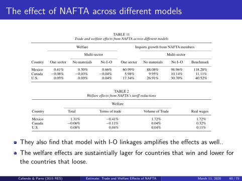
The effect of NAFTA across different models
[14:25 16/12/2014 rdu035.tex] RESTUD: The Review of Economic Studies Page: 28 1–44
28 REVIEW OF ECONOMIC STUDIES
TABLE 11Trade and welfare effects from NAFTA across different models
Welfare Imports growth from NAFTA members
Multi-sector Multi-sector
Country One sector No materials No I–O One sector No materials No I–O Benchmark
Mexico 0.41% 0.50% 0.66% 60.99% 88.08% 98.96% 118.28%Canada −0.08% −0.03% −0.04% 5.98% 9.95% 10.14% 11.11%U.S. 0.05% 0.03% 0.04% 17.34% 26.91% 30.70% 40.52%
quantification of the welfare gains.55 The calculations also show that intermediate goods amplifythe welfare effects from tariff reductions. Mexico’s figure increase from 0.50% to 0.66%, Canada’sdeteriorate more from −0.03% to −0.04% and the U.S. increase from 0.03% to 0.04% as wemove from a model with no materials to a model with materials. We also find that the modelwith I–O linkages amplifies the effects as well. If we compare the third column on Table 11 tothe results from the benchmark model, Table 2, we can clearly see that the welfare effects aresubstantially larger for the countries that win and lower for the countries that loose.
Trade effects are also smaller across these models compared to the benchmark case. The lastfour columns of Table 11 presents, for the case of Mexico, Canada, and the U.S., the changein imports from NAFTA members implied by the different models. As we can see, the tradeeffects are reduced substantially compared to the benchmark case. In the one-sector model, thetrade responses are almost reduced by half. The intuition for this result relates to the result onwelfare. By averaging out the effects, a one-sector model fails to capture the large increase intrade flows from certain sectors. In fact, we know from Tables 4 and 6 that NAFTA generated veryheterogenous responses across sectors. If we compare the results from column five to column sixwe can see that adding intermediate goods increases the trade effects. The intuition for this resultis as follows. In the model with no materials, goods are only traded to produce final goods forconsumption and not for the production of intermediate goods. However, in the no I–O model,materials are also used for the production of intermediate goods. Therefore, a tariff reductiondelivers a larger trade effect due to the increase in demand of tradable goods for the production ofintermediates. Finally, we can also compare the implied changes in trade flows from a model withintermediate goods in production but no sectoral linkages, the no I–O model, to the benchmarkcase. The trade effects from tariff reductions are lower in the no I–O model than in the model withsectoral interrelations (Benchmark). The reason is that since producers are only using inputs fromone sector they are not exploiting the benefits of having access to cheaper materials from othersectors. This in turn delivers a smaller trade effect from tariff changes. In short, the results fromthis subsection unmask the importance of accounting for sectoral heterogeneity, intermediategoods in production and I–O linkages to evaluate the trade and welfare gains from tariff changes,in general, and in particular for the case of NAFTA.
6. CONCLUSION
This study develops a general equilibrium model to quantify the trade and welfare effects of tariffchanges. The model is able to perform complex trade policy evaluations for an arbitrary number of
55. In a recent study, Ossa (2012) shows that the heterogeneity in trade elasticities per se has an important effecton the quantification of the welfare gains from trade. He shows this for the case of iceberg trade costs and by calculatingwelfare losses from reverting to autarky.
at Singapore Managem
ent University on July 5, 2015
http://restud.oxfordjournals.org/D
ownloaded from
[14:25 16/12/2014 rdu035.tex] RESTUD: The Review of Economic Studies Page: 20 1–44
20 REVIEW OF ECONOMIC STUDIES
TABLE 2Welfare effects from NAFTA’s tariff reductions
Welfare
Country Total Terms of trade Volume of Trade Real wages
Mexico 1.31% −0.41% 1.72% 1.72%Canada −0.06% −0.11% 0.04% 0.32%U.S. 0.08% 0.04% 0.04% 0.11%
we eliminate all aggregate deficits by first calibrating the model with trade deficits and thensolving the model imposing zero aggregate deficit, D′
n =0. We then use the implied no-deficitworld economy as our base year. Secondly, we calibrate the model with aggregate deficits tothe year 1993 and then calculate all counterfactuals holding the countries aggregate trade deficitsconstant, as a share of world GDP. We compute all the counterfactual exercises using both solutionstrategies but present in the main text only the results with no aggregate deficit in the base year.The Appendix “Additional Results” shows a variety of additional results including the case whereaggregate trade deficits remain fixed as a share of world GDP.
5.1. Trade and welfare effects from NAFTA’s tariff reductions
We now quantify the trade and welfare effects of NAFTA. Table 2 presents the welfare effectsfrom NAFTA’s tariff reductions while fixing the tariff to and from the rest of the world to theyear 1993. Welfare effects are calculated using equation (16), and changes in real wages usingequation (15). As we can see, Mexico’s welfare increases by 1.31%. The effects for Canada andthe U.S. are smaller. Canada loses 0.06% whereas the U.S. gains 0.08%. Still, we find that realwages increase for all NAFTA members and Mexico gains the most, followed by Canada and theU.S.47
Decomposing the welfare effects into terms of trade and volume of trade underscores thesources of these gains. The third column in Table 2 shows that the major source of gains areincreases in volume of trade. The welfare gains from trade creation for Mexico, Canada, and theU.S. are 1.72%, 0.04% and 0.04%, respectively. We can look deeper and measure the extent towhich the welfare effects are a result of trade creation with NAFTA members vis-a-vis the rest ofthe world. This is done by applying the bilateral volume of trade measures equation (18) definedbefore.
Column 3 in Table 3 shows that the trade created with NAFTA members is the single mostimportant contributor to the positive welfare effects. The figures are 1.80%, 0.08%, and 0.04%for Mexico, Canada, and the U.S., respectively. This result unmasks an important channel bywhich NAFTA generated positive welfare effects to all of its members, by creating more tradewithin the bloc. On the other hand, column 4 from Table 3 shows that the reduction in volumeof trade with the rest of the world has a negative welfare effect. This negative welfare effect,which we discuss further below, arises from NAFTA diverting trade from countries outside ofthe agreement.
Another source of welfare effects are changes in terms of trade. From column 2 of Table 2,we can see that Mexico and Canada’s terms of trade deteriorate whereas the U.S. terms of trade
47. The welfare effects results in the model with trade deficits are very similar, 1.17%, −0.04%, and 0.09% forMexico, Canada, and the U.S., respectively. Appendix “Additional Results”, Tables A4–A7, includes this and additionalresults with trade deficits and it shows that all the results in this section are robust to include trade deficits or not.
at Singapore Managem
ent University on July 5, 2015
http://restud.oxfordjournals.org/D
ownloaded from
They also find that model with I-O linkages amplifies the effects as well..The welfare effects are sustaintially lager for countries that win and lower forthe countries that loose.
Caliendo & Parro (2015 RES) Estimate: Trade and Welfare Effects of NAFTA March 11, 2020 60 / 75

The effect of NAFTA across different models
[14:25 16/12/2014 rdu035.tex] RESTUD: The Review of Economic Studies Page: 28 1–44
28 REVIEW OF ECONOMIC STUDIES
TABLE 11Trade and welfare effects from NAFTA across different models
Welfare Imports growth from NAFTA members
Multi-sector Multi-sector
Country One sector No materials No I–O One sector No materials No I–O Benchmark
Mexico 0.41% 0.50% 0.66% 60.99% 88.08% 98.96% 118.28%Canada −0.08% −0.03% −0.04% 5.98% 9.95% 10.14% 11.11%U.S. 0.05% 0.03% 0.04% 17.34% 26.91% 30.70% 40.52%
quantification of the welfare gains.55 The calculations also show that intermediate goods amplifythe welfare effects from tariff reductions. Mexico’s figure increase from 0.50% to 0.66%, Canada’sdeteriorate more from −0.03% to −0.04% and the U.S. increase from 0.03% to 0.04% as wemove from a model with no materials to a model with materials. We also find that the modelwith I–O linkages amplifies the effects as well. If we compare the third column on Table 11 tothe results from the benchmark model, Table 2, we can clearly see that the welfare effects aresubstantially larger for the countries that win and lower for the countries that loose.
Trade effects are also smaller across these models compared to the benchmark case. The lastfour columns of Table 11 presents, for the case of Mexico, Canada, and the U.S., the changein imports from NAFTA members implied by the different models. As we can see, the tradeeffects are reduced substantially compared to the benchmark case. In the one-sector model, thetrade responses are almost reduced by half. The intuition for this result relates to the result onwelfare. By averaging out the effects, a one-sector model fails to capture the large increase intrade flows from certain sectors. In fact, we know from Tables 4 and 6 that NAFTA generated veryheterogenous responses across sectors. If we compare the results from column five to column sixwe can see that adding intermediate goods increases the trade effects. The intuition for this resultis as follows. In the model with no materials, goods are only traded to produce final goods forconsumption and not for the production of intermediate goods. However, in the no I–O model,materials are also used for the production of intermediate goods. Therefore, a tariff reductiondelivers a larger trade effect due to the increase in demand of tradable goods for the production ofintermediates. Finally, we can also compare the implied changes in trade flows from a model withintermediate goods in production but no sectoral linkages, the no I–O model, to the benchmarkcase. The trade effects from tariff reductions are lower in the no I–O model than in the model withsectoral interrelations (Benchmark). The reason is that since producers are only using inputs fromone sector they are not exploiting the benefits of having access to cheaper materials from othersectors. This in turn delivers a smaller trade effect from tariff changes. In short, the results fromthis subsection unmask the importance of accounting for sectoral heterogeneity, intermediategoods in production and I–O linkages to evaluate the trade and welfare gains from tariff changes,in general, and in particular for the case of NAFTA.
6. CONCLUSION
This study develops a general equilibrium model to quantify the trade and welfare effects of tariffchanges. The model is able to perform complex trade policy evaluations for an arbitrary number of
55. In a recent study, Ossa (2012) shows that the heterogeneity in trade elasticities per se has an important effecton the quantification of the welfare gains from trade. He shows this for the case of iceberg trade costs and by calculatingwelfare losses from reverting to autarky.
at Singapore Managem
ent University on July 5, 2015
http://restud.oxfordjournals.org/D
ownloaded from
Trade effects are also smaller acorss these models compared to thebenchmark case.In the one-sector model, the trade responses are almost reduced by half. Byaveraging out the effect, a one-sector model fails to capture the largeincrease in trade flow from certain sectors (sector heterogenity).As for "No materials" model, goods are only traded to produce final goodsfor consumption and not for the production of intermediate goods.
Caliendo & Parro (2015 RES) Estimate: Trade and Welfare Effects of NAFTA March 11, 2020 61 / 75

The effect of NAFTA across different models
[14:25 16/12/2014 rdu035.tex] RESTUD: The Review of Economic Studies Page: 28 1–44
28 REVIEW OF ECONOMIC STUDIES
TABLE 11Trade and welfare effects from NAFTA across different models
Welfare Imports growth from NAFTA members
Multi-sector Multi-sector
Country One sector No materials No I–O One sector No materials No I–O Benchmark
Mexico 0.41% 0.50% 0.66% 60.99% 88.08% 98.96% 118.28%Canada −0.08% −0.03% −0.04% 5.98% 9.95% 10.14% 11.11%U.S. 0.05% 0.03% 0.04% 17.34% 26.91% 30.70% 40.52%
quantification of the welfare gains.55 The calculations also show that intermediate goods amplifythe welfare effects from tariff reductions. Mexico’s figure increase from 0.50% to 0.66%, Canada’sdeteriorate more from −0.03% to −0.04% and the U.S. increase from 0.03% to 0.04% as wemove from a model with no materials to a model with materials. We also find that the modelwith I–O linkages amplifies the effects as well. If we compare the third column on Table 11 tothe results from the benchmark model, Table 2, we can clearly see that the welfare effects aresubstantially larger for the countries that win and lower for the countries that loose.
Trade effects are also smaller across these models compared to the benchmark case. The lastfour columns of Table 11 presents, for the case of Mexico, Canada, and the U.S., the changein imports from NAFTA members implied by the different models. As we can see, the tradeeffects are reduced substantially compared to the benchmark case. In the one-sector model, thetrade responses are almost reduced by half. The intuition for this result relates to the result onwelfare. By averaging out the effects, a one-sector model fails to capture the large increase intrade flows from certain sectors. In fact, we know from Tables 4 and 6 that NAFTA generated veryheterogenous responses across sectors. If we compare the results from column five to column sixwe can see that adding intermediate goods increases the trade effects. The intuition for this resultis as follows. In the model with no materials, goods are only traded to produce final goods forconsumption and not for the production of intermediate goods. However, in the no I–O model,materials are also used for the production of intermediate goods. Therefore, a tariff reductiondelivers a larger trade effect due to the increase in demand of tradable goods for the production ofintermediates. Finally, we can also compare the implied changes in trade flows from a model withintermediate goods in production but no sectoral linkages, the no I–O model, to the benchmarkcase. The trade effects from tariff reductions are lower in the no I–O model than in the model withsectoral interrelations (Benchmark). The reason is that since producers are only using inputs fromone sector they are not exploiting the benefits of having access to cheaper materials from othersectors. This in turn delivers a smaller trade effect from tariff changes. In short, the results fromthis subsection unmask the importance of accounting for sectoral heterogeneity, intermediategoods in production and I–O linkages to evaluate the trade and welfare gains from tariff changes,in general, and in particular for the case of NAFTA.
6. CONCLUSION
This study develops a general equilibrium model to quantify the trade and welfare effects of tariffchanges. The model is able to perform complex trade policy evaluations for an arbitrary number of
55. In a recent study, Ossa (2012) shows that the heterogeneity in trade elasticities per se has an important effecton the quantification of the welfare gains from trade. He shows this for the case of iceberg trade costs and by calculatingwelfare losses from reverting to autarky.
at Singapore Managem
ent University on July 5, 2015
http://restud.oxfordjournals.org/D
ownloaded from
In the "No I-O" model, materials are also used for the production ofintermediate goods, so imports growth more.Finally, we compare benchmark model with "No I-O" model, trade effectincrease as well.Since producers are only using inputs from one sector , they are notexploiting the benefits of having access to cheaper materials from othersectors in "No I-O" model.In short, the results from this subsection unmask the importance ofaccounting for sectoral heterogeneity, intermediate goods in production andI-O linkages to evaluate the trade and welfare gains from tariff changes.
Caliendo & Parro (2015 RES) Estimate: Trade and Welfare Effects of NAFTA March 11, 2020 62 / 75

Outline
1 Introduction
2 Tariffs, intermediate goods and sectoral linkages
3 A quantitative model for trade policy evaluation
4 A new method to estimate trade elasticities
5 Quatifying the trade and welfare effets of NAFTA
6 Conclusion
Caliendo & Parro (2015 RES) Estimate: Trade and Welfare Effects of NAFTA March 11, 2020 63 / 75

Conclusion
This study develops a general equilibrium model to quantify the trade andwelfare effects of tariff changes.
Require few data and parameters.Decompose the different channel including TOT and VOT effects.Intermediate goods and sectoral linkages is quantitatively and economicallymeaningful.
It is important to clarify how their results about NAFTA should beinterpreted.
By no means their results should be interpreted as the trade and welfareeffects of the entire agreement.NAFTA may influence the non-tariff barriers or unobservable trade costs, therate of technological change and many other factors.
Caliendo & Parro (2015 RES) Estimate: Trade and Welfare Effects of NAFTA March 11, 2020 64 / 75

The end
Thanks for your listening!
Caliendo & Parro (2015 RES) Estimate: Trade and Welfare Effects of NAFTA March 11, 2020 65 / 75

Fréchet distribution
Features of Fréchet distributionFi(z) = e−Ti z−θ
0.5
11.
52
0 1 2 3 4 5x
T=1, θ=5 T=5, θ=5
01
23
0 1 2 3 4 5x
T=5, θ=5 T=5, θ=10
Technology
Caliendo & Parro (2015 RES) Estimate: Trade and Welfare Effects of NAFTA March 11, 2020 66 / 75

I-O table
剥削程度与身体健康水平
6
1
( )n
d m
i i
i
Q F F
Ⅱ (2)
iQ q Q Ⅰ Ⅱ (3)
Table X Input-Output Table
Intermediate Product Final product Total
production
1 2 …n Expenditure Investment Net export
Domestic
intermediate input
1
2
…
N
d
ijc d
iF d
iG d
iex d
iq
Imported
intermediate input
1
2
…
N
m
ijc m
iF m
iG m
iex m
iq
Value added
Payment of
labor jv
Social net
income jk
Total Inpot jq
而后分别计算第二部类的不变资本,可变资本及剩余价值。(4)式中,我们将全部中间
品投入占总投入的比重作为不变资本的权重,然后乘以第二部类总产出,即可得到第二部类
不变资本。(5)式中,将劳动报酬投入占总投入的比重作为可变资本的权重,而后乘以第二
部类总产出,得到第二部类可变资本。但是需要注意的是,在投入产出表中没有直接给出有
关于劳动报酬的数据。因此我们选择从 SEA 中对增加值进行分解(Cockshott and Cottrell,
2003),提取出其中的劳动报酬,并按照汇率换算至不变价格美元1。而对于(6)式,我们使
用增加值减去劳动报酬,即社会纯收入占总投入的比重作为剩余价值的权重,乘以第二部类
总产出后得到第二部类剩余价值。
1 1
[ ( ) / ( )]n n
d m d m
i i j j j
j i
C c j c j q F F
Ⅱ
(4)
1
[ ( )]
j
nj d m
j j
j
vV F F
q
Ⅱ
(5)
1
[ ( )]
j
nj d m
j j
j
kM F F
q
Ⅱ
(6)
(7)到(9)式分别计算了第一部类的不变资本、可变资本和剩余价值。计算方法为使
用不变资本、可变资本及剩余价值总量分别减去各自第二部类的数量值,即可得到第一部类
的相应数值。而后用第一部类、第二部类及总体的剩余价值除以各自的可变资本,即可得到
剥削率水平。
1 需要说明的是,SEA 中数据均为本国货币,为了保持单位的统一,本文使用联合国的公布的当年数据进
行换算。官方网站:https://unctad.org/en/Pages/statistics.aspx
Facts
Caliendo & Parro (2015 RES) Estimate: Trade and Welfare Effects of NAFTA March 11, 2020 67 / 75

Derivation
Welfare is given by Wn = wnLn+Rn+DnPn
.They assume that exogenous trade deficits remain constant, dDn = 0.Holding iceberg trade costs fixed, namely d ln κj
ni = d ln τ jni .
ln Wn = ln(wnLn + Rn + Dn) − ln Pn
d ln Wn = LnwnLn + Rn + Dn
dwn + 1wnLn + Rn + Dn
dRn − d ln Pn
d ln Wn = wnLnIn
d ln wn + 1In
dRn − d ln Pn (24)
Caliendo & Parro (2015 RES) Estimate: Trade and Welfare Effects of NAFTA March 11, 2020 68 / 75

Derivation
Recall that Rn =∑J
j=1∑N
i=1 τ jniM
jni
dRn =J∑
j=1
N∑i=1
τ jnidM j
nid ln M jni +
J∑j=1
N∑i=1
M jnidτ j
ni
Recall that M jni = E j
in and dτ jni = d τ j
ni , then M jnidτ j
ni = E jind τ j
ni .
And you also need to recall that E jin = X j
nπj
ni1+τ j
ni. Besides, 1
1+τ jni
d τ jni = d ln τ j
ni .In this way, they can get:
M jnidτ j
ni = E jind τ j
ni = X jn
πjni
1 + τ jni
dτ jni = X j
nπjnid ln τ j
ni
dRn =J∑
j=1
N∑i=1
τ jnidM j
nid ln M jni +
J∑j=1
X jn
N∑i=1
πjnid ln τ j
ni (25)
Caliendo & Parro (2015 RES) Estimate: Trade and Welfare Effects of NAFTA March 11, 2020 69 / 75
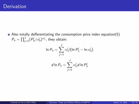
Derivation
Also totally defferentiating the consumption price index equation(5)Pn =
∏Jj=1(P j
n/αjn)αj
n , they obtain:
ln Pn =J∑
j=1αj
nl(ln P jn − ln αj
n)
d ln Pn =J∑
j=1αj
nd ln P jn
Caliendo & Parro (2015 RES) Estimate: Trade and Welfare Effects of NAFTA March 11, 2020 70 / 75

Derivation
Then they use the definition of of sectoral prices (equation 4) together withequation (6):
P jn = Aj
[ N∑i=1
λji (c
ji κ
jni)−θj
]−1/θj
πjni =
λji
[c j
i κjni
]−θj
∑Nh=1 λj
h
[c j
hκjnh
]−θj
Then, they can get:
ln P jn = ln Aj − (1/θj) ln
[ N∑i=1
λji (c
ji κ
jni)−θj
]
d ln P jn =
N∑i=1
πjni [d ln c j
i + d ln τ jni ]
Caliendo & Parro (2015 RES) Estimate: Trade and Welfare Effects of NAFTA March 11, 2020 71 / 75

Derivation
Substituting d ln P jn into d ln Pn, they can get:
d ln Pn =J∑
j=1αj
nd ln P jn =
J∑j=1
αjn
N∑i=1
πjni [d ln c j
i + d ln τ jni ] (26)
Finally, from the definition of the input bundle (equation 2)c j
n = Υjnwγ j
nn∏J
k=1 pkn
γk,jn , they get:
d ln wn = 1γj
nd ln c j
n −∑k=1
γk,jn
γjn
d ln pkn (27)
Caliendo & Parro (2015 RES) Estimate: Trade and Welfare Effects of NAFTA March 11, 2020 72 / 75

Derivation
Substituting (25) and (26) into (24), they get:
d ln Wn =wnLnIn
d ln wn + 1In
J∑j=1
N∑i=1
τ jniM
jnid ln M j
ni
+ 1In
J∑j=1
X jn
N∑i=1
πjnid ln τni
−J∑
j=1αj
n
N∑i=1
πjni(d ln c j
i + d ln τ jni)
(28)
Then using equation (7): X jn =
∑Jk=1 γj,k
n∑N
i=1 X ki
πjin
1+τ jin
+ αjnIn to solve for
αjn, together with adding and substracing 1
In∑J
j=1∑N
i=1 E jnid ln c j
n.
Caliendo & Parro (2015 RES) Estimate: Trade and Welfare Effects of NAFTA March 11, 2020 73 / 75

Derivation
d ln Wn =wnLnIn
d ln wn + 1In
J∑j=1
N∑i=1
τ jniM
jni(d ln M j
ni − d ln c ji )
− 1In
J∑j=1
N∑i=1
E jni
(d ln c j
n −∑k=1
γk,jn d ln pk
n
)
+ 1In
J∑j=1
N∑i=1
(E jnid ln c j
n − M jnid ln c j
i )
(29)
Finally, they use equation(27) to obtain equation(16)
Caliendo & Parro (2015 RES) Estimate: Trade and Welfare Effects of NAFTA March 11, 2020 74 / 75

Illustrition
NAFTA ROW
NAFTA ROW
NAFTA ROW
Exercise one:
Exercise two: Step 1
Exercise two: Step 2
1993 to 2005 1993
1993
1993 to 2005 1993 to 2005
1993 to 2005
Minus
Back
Caliendo & Parro (2015 RES) Estimate: Trade and Welfare Effects of NAFTA March 11, 2020 75 / 75


![INDIRECT EXPROPRIATION UNDER NAFTA AND DR-CAFTA: … · 2006] INDIRECT EXPROPRIATION UNDER NAFTA AND DR-CAFTA 933 NAFTA and DR-CAFTA. Part II explains how three earlier NAFTA tribunals](https://static.fdocuments.us/doc/165x107/5ec6d30ffb2475648e7b2fba/indirect-expropriation-under-nafta-and-dr-cafta-2006-indirect-expropriation-under.jpg)