Essays on Supply Chain Contracting and RetailPricing

by

Thunyarat Amornpetchkul

A dissertation submitted in partial fulfillmentof the requirements for the degree of

Doctor of Philosophy(Business Administration)

in The University of Michigan2014

Doctoral Committee:

Associate Professor Hyun-Soo Ahn, ChairProfessor Izak DuenyasAssistant Professor Ozge SahinAssociate Professor Mark P. Van OyenAssistant Professor Xun Wu

c© Thunyarat (Bam) Amornpetchkul 2014

All Rights Reserved

To my parents and all of my teachers

ii

ACKNOWLEDGEMENTS

To me, this dissertation is not only part of the requirements for graduation, but it

is also a keepsake that will always remind me of all the things I learned, all the work

I did, and all the support I received during my years as a PhD student.

My special thanks and appreciation go to the two advisors, Professor Hyun-Soo

Ahn and Professor Ozge Sahin. Our student-advisors relationship may have started

from mutual research interests. But as it developed, I think the three of us formed

a unique combination of researchers who can be both productive and fun. The main

products coming out of our research meetings are research papers, included in this

dissertation. But if we were to record all of the other discussions that have taken

place during those meetings, I think we would have had a byproduct as a fashion or

lifestyle book. Thank you for your guidance, which helped me start my PhD journey.

Thank you for your kindness and patience, which gave me enough room to learn

along the way. Thank you for your trust and encouragement, which pushed me to go

further. Thank you for everything you did for me, which landed me at the finish line.

I also would like to thank the other committee members: Professor Izak Duenyas,

Professor Xun (Brian) Wu, and Professor Mark Van Oyen. I truly appreciate their

time and valuable suggestions which helped improve various aspects of this disser-

tation. I am especially grateful to Professor Izak Duenyas for his contribution and

advice on the first essay, as well as his support as the department chair.

In addition to the dissertation committee, I would like to extend my gratitude

towards the faculty of the Department of Operations and Management Science (now

iii

Technology and Operations) as a whole. Thank you for believing in me that I could

meet the department’s high expectations, and for giving me all the support I needed to

thrive here. In particular, I would like to thank the PhD program coordinators during

the past five years: Professor Roman Kapuscinski, Professor Hyun-Soo Ahn, Professor

Damian Beil, and Professor Amitabh Sinha, for helping guide me through different

phases in the program. Outside of the department, I also received wonderful support

on administrative matters from the Doctoral Studies Program staff: Brian Jones,

Roberta Perry, and Kelsey Zill. They have always been very kind and responsive in

addressing my questions and needs.

Another group of people who made my PhD experience unexpectedly enjoyable

is the “OMS family,” as we PhD students like to call ourselves. They are indeed

like a second family to me. Although the members have changed over time, as we

had graduated and newly admitted students, one thing that never changes is that we

always hope for the best for one another. One person to whom I would like to express

my deep gratitude for our friendship is Anyan Qi, who joined the PhD program in

the same year as me. His outstanding intelligence helped me learn and inspired me

to set higher goals for myself. His affability and optimism created our pleasant work

environment and kept me sane during difficult times. I cannot imagine having a

better person to go through these challenging years with – thank you, Anyan.

Last but not least, I am always thankful to my family and loved ones. Their love

and heartfelt encouragement helped build the confidence that carried me through the

PhD journey. My achievement today owes much to their continuous support that I

will never forget.

iv

TABLE OF CONTENTS

DEDICATION . . . . . . . . . . . . . . . . . . . . . . . . . . . . . . . . . . ii

ACKNOWLEDGEMENTS . . . . . . . . . . . . . . . . . . . . . . . . . . iii

LIST OF FIGURES . . . . . . . . . . . . . . . . . . . . . . . . . . . . . . . vii

LIST OF TABLES . . . . . . . . . . . . . . . . . . . . . . . . . . . . . . . . viii

LIST OF APPENDICES . . . . . . . . . . . . . . . . . . . . . . . . . . . . ix

ABSTRACT . . . . . . . . . . . . . . . . . . . . . . . . . . . . . . . . . . . x

CHAPTER

1. Introduction . . . . . . . . . . . . . . . . . . . . . . . . . . . . . . 1

2. Mechanisms to Induce Buyer Forecasting: Do Suppliers Al-ways Benefit from Better Forecasting? . . . . . . . . . . . . . . 5

2.1 Introduction . . . . . . . . . . . . . . . . . . . . . . . . . . . 52.2 Literature Review . . . . . . . . . . . . . . . . . . . . . . . . 112.3 Model and Preliminary Results . . . . . . . . . . . . . . . . . 15

2.3.1 Model . . . . . . . . . . . . . . . . . . . . . . . . . 152.3.2 Preliminary Results . . . . . . . . . . . . . . . . . . 23

2.4 Contract Preferences and Effects of Forecast Accuracy . . . . 262.5 Capable Buyer and Bayesian Updating Supplier . . . . . . . . 322.6 Screening the Forecasting Capability . . . . . . . . . . . . . . 342.7 Conclusion . . . . . . . . . . . . . . . . . . . . . . . . . . . . 39

3. Conditional Promotions and Consumer Overspending . . . . 42

3.1 Introduction . . . . . . . . . . . . . . . . . . . . . . . . . . . 423.2 Literature Review . . . . . . . . . . . . . . . . . . . . . . . . 463.3 Model . . . . . . . . . . . . . . . . . . . . . . . . . . . . . . . 49

v

3.3.1 Types of Conditional Promotions . . . . . . . . . . 503.3.2 Consumer’s Types and Utility . . . . . . . . . . . . 51

3.4 Consumer’s Problem . . . . . . . . . . . . . . . . . . . . . . . 553.4.1 All-Unit Discount . . . . . . . . . . . . . . . . . . . 563.4.2 Fixed-Amount Discount . . . . . . . . . . . . . . . . 56

3.5 Seller’s Problem . . . . . . . . . . . . . . . . . . . . . . . . . 623.5.1 Deal-Prone Market with Heterogeneous Valuation . 663.5.2 Homogeneous Valuation with Heterogeneous Deal-

Proneness . . . . . . . . . . . . . . . . . . . . . . . 693.6 Numerical Study . . . . . . . . . . . . . . . . . . . . . . . . . 73

3.6.1 Profit Improvement . . . . . . . . . . . . . . . . . . 733.6.2 Effects of Problem Parameters . . . . . . . . . . . . 75

3.7 Extension . . . . . . . . . . . . . . . . . . . . . . . . . . . . . 773.7.1 Positive Unit Cost . . . . . . . . . . . . . . . . . . . 773.7.2 Concave Consumer Valuation . . . . . . . . . . . . . 783.7.3 Endogenous Price . . . . . . . . . . . . . . . . . . . 79

3.8 Conclusion . . . . . . . . . . . . . . . . . . . . . . . . . . . . 80

4. Dynamic Pricing or Dynamic Logistics? . . . . . . . . . . . . . 83

4.1 Introduction . . . . . . . . . . . . . . . . . . . . . . . . . . . 834.2 Literature Review . . . . . . . . . . . . . . . . . . . . . . . . 874.3 Model . . . . . . . . . . . . . . . . . . . . . . . . . . . . . . . 92

4.3.1 Customer Choice Model . . . . . . . . . . . . . . . . 934.3.2 Retailer’s Problem . . . . . . . . . . . . . . . . . . . 94

4.4 Optimal Pricing and Transshipping Policies . . . . . . . . . . 964.4.1 Base Model: Uniform Pricing and No Transshipment 974.4.2 Price Differentiation and No Transshipment . . . . . 994.4.3 Uniform Pricing with Transshipment . . . . . . . . 1024.4.4 Price Differentiation with Transshipment . . . . . . 107

4.5 Numerical Study . . . . . . . . . . . . . . . . . . . . . . . . . 1124.6 Extension . . . . . . . . . . . . . . . . . . . . . . . . . . . . . 118

4.6.1 Ex-post Transshipment . . . . . . . . . . . . . . . . 1184.7 Conclusion . . . . . . . . . . . . . . . . . . . . . . . . . . . . 120

5. Conclusion . . . . . . . . . . . . . . . . . . . . . . . . . . . . . . . 123

APPENDICES . . . . . . . . . . . . . . . . . . . . . . . . . . . . . . . . . . 126

BIBLIOGRAPHY . . . . . . . . . . . . . . . . . . . . . . . . . . . . . . . . 185

vi

LIST OF FIGURES

Figure

2.1 Sequence of events: Dynamic Contract . . . . . . . . . . . . . . . . 202.2 Sequence of events: Early Static Contract . . . . . . . . . . . . . . . 222.3 Sequence of events: Late Static Contract . . . . . . . . . . . . . . . 222.4 Preferences of the high-type buyer, supplier, and supply chain . . . 292.5 High-type buyer’s and supplier’s profits . . . . . . . . . . . . . . . . 393.1 Consumer’s valuation function . . . . . . . . . . . . . . . . . . . . . 533.2 Value-conscious purchase quantity under a conditional discount . . . 583.3 Cognitive overspending under a conditional discount . . . . . . . . . 583.4 Seller’s optimal discount schemes . . . . . . . . . . . . . . . . . . . 653.5 Switching curve ΓA(t) . . . . . . . . . . . . . . . . . . . . . . . . . . 693.6 Optimal purchase quantity under a conditional discount with a con-

cave valuation . . . . . . . . . . . . . . . . . . . . . . . . . . . . . . 794.1 Benefit from transshipment in the current period vs. the customer

arrival rate . . . . . . . . . . . . . . . . . . . . . . . . . . . . . . . . 1074.2 Benefit from price differentiation vs. transshipment cost . . . . . . . 1104.3 Optimal prices vs. inventory level and remaining time . . . . . . . . 111

vii

LIST OF TABLES

Table

2.1 Notation used in Chapter 2 . . . . . . . . . . . . . . . . . . . . . . . 173.1 Problem parameters for the numerical study of profit improvement . 733.2 Statistics for the seller’s profit improvement when using conditional

discounts over no discount . . . . . . . . . . . . . . . . . . . . . . . 743.3 Profit difference between all-unit and fixed-amount discounts . . . . 753.4 Problem parameters for the numerical study of effects of parameters

on the profit improvement . . . . . . . . . . . . . . . . . . . . . . . 753.5 Statistics for profit improvement with respect to changes in problem

parameters . . . . . . . . . . . . . . . . . . . . . . . . . . . . . . . . 754.1 Possible pricing and transshipping policies . . . . . . . . . . . . . . 974.2 Statistics for the optimal prices in the current period . . . . . . . . 1134.3 Benefit of price differentiation and transshipment . . . . . . . . . . 114B.1 Consumer’s utility from purchasing q = θi and K . . . . . . . . . . 149B.2 Seller’s profit from offering no discount and DA when β > 0 . . . . . 151B.3 Possible outcomes under a price markdown . . . . . . . . . . . . . . 156B.4 Possible outcomes under an optimal all-unit discount . . . . . . . . 159B.5 Closed-form expressions of tAi (R) and ΓAi (t, R) for all-unit discount

when sh < p . . . . . . . . . . . . . . . . . . . . . . . . . . . . . . . 171B.6 Closed-form expressions of tFi (R) and ΓFi (t, R) for fixed-amount dis-

count when sl < p ≤ sh . . . . . . . . . . . . . . . . . . . . . . . . . 172

viii

LIST OF APPENDICES

Appendix

A. Additional Results and Proofs for Chapter 2 . . . . . . . . . . . . . . 127

B. Additional Results and Proofs for Chapter 3 . . . . . . . . . . . . . . 148

C. Proofs for Chapter 4 . . . . . . . . . . . . . . . . . . . . . . . . . . . . 173

ix

ABSTRACT

Essays on Supply Chain Contracting and Retail Pricing

by

Thunyarat (Bam) Amornpetchkul

An important operational decision that a seller has to make is how to price his

product under different situations. This dissertation addresses three unique pricing

problems, commonly faced by a seller in a supply chain, in a series of three essays.

The first essay considers a supplier’s problem of choosing which type of contracts to

offer to a retailer whose demand forecasts can be improved over time. It is shown that

there exist mechanisms which enable the supplier to always benefit from the retailer’s

improved demand forecasts. Such a mechanism consists of an initial contract, offered

to the retailer before she obtains improved forecasts, and a later contract (contingent

on the initial contract), offered to the retailer after she obtains improved forecasts.

The second essay investigates a retailer’s problem of choosing which form of price

promotions to offer to consumers, some of which are more inclined to increase spend-

ing when satisfied with the value of the deals. Two types of promotions are consid-

ered: i) all-unit discount, where a price reduction applies to every unit of a purchase

that meets the minimum requirement, and ii) fixed-amount discount, where the final

amount that a consumer has to pay is reduced by a predetermined discount amount if

the purchase meets the minimum requirement. It is shown that both discount schemes

x

can induce consumers to overspend. However, depending on consumer valuation of

the product, one scheme can be more profitable to the retailer than the other.

The third essay discusses a dual-channel retailer’s problem of choosing a price

differentiating policy (charging different prices for the same product sold at different

channels) and/or inventory transshipping policy (transferring inventory between the

channels) to balance available inventory and demand arriving at each channel. It is

shown that the two mechanisms have different implications on sales volume. Which

mechanism is more effective depends on the retailer’s initial inventory position. Fur-

thermore, when implemented concurrently, the benefit from price differentiation and

inventory transshipment mechanisms may either substitute or complement each other.

xi

CHAPTER 1

Introduction

A fundamental question for any sellers in a supply chain is what pricing mecha-

nism to use to generate most profits from selling their products. The answer to this

question heavily depends on the nature of the businesses as well as the characteristics

of the buyers. For example, a supplier selling to a retailer who has superior informa-

tion about the end demand would benefit from a mechanism that promotes demand

information sharing. A retailer selling to customers who enjoy receiving discounts

would find it profitable to offer a price promotion that induces larger purchases. For

a retailer who operates in more than one channel, it is important to use a pricing

mechanism that helps balance available inventory and demand at each channel in

order to maximize the overall profit.

This dissertation explores seller’s problems across two different areas of a supply

chain: upstream (a supplier selling to a retailer) and downstream (a retailer selling to

customers). More precisely, the dissertation consists of three essays; one on Supply

Chain Contracting, and the other two on Retail Pricing. Each essay investigates

operational problems arising from interactions between the respective supply chain

parties as a seller or a buyer. Despite different focuses, all essays consider realistic

business situations where the seller and the buyer make decisions based on their own

benefits, and the buyer’s behavior may be influenced by her perspectives towards the

1

pricing mechanism offered by the seller.

The first essay titled “Mechanisms to Induce Buyer Forecasting: Do Suppliers

Always Benefit from Better Forecasting?” explores the effects of improved demand

information on the supplier’s and the retailer’s profitability under different types of

supply chain contracts. More specifically, three types of contracts that a supplier

(seller) can offer to a retailer (buyer) are considered: 1) a contract that is offered

before the buyer can obtain improved forecasts, 2) a contract that is offered after

the buyer has obtained improved forecasts, and 3) a contingent (dynamic) contract

where an initial contract is offered to the buyer before she obtains improved forecasts,

followed by a later contract (contingent on the initial contract) offered after improved

forecasts have been obtained. In a scenario where the supplier is certain that the

buyer can obtain more accurate forecasts over time, the contingent contract is shown

to be the most profitable mechanism for the supplier. The contingent contract also

guarantees the supplier an increasingly larger profit as the buyer’s forecast accuracy

increases. In a different scenario where the supplier is uncertain whether the buyer

can improve forecasts over time, the essay discusses how the supplier can modify

the contingent contract to screen the buyer on both her demand and forecasting

capability information. Under such a contract, the supplier’s profit increases with

the probability that the buyer is capable of improving forecast accuracy. In contrast

to the existing literature, the results from this essay show that there exist mechanisms

which enable the supplier to always benefit from better demand information.

The second essay, “Conditional Promotions and Consumer Overspending,” dis-

cusses the implications of sales promotions on consumer spending. In particular,

when a deal comes with an eligibility requirement in the form of a minimum purchase

quantity or a minimum spending, it may lead some consumers to end up buying more

than what they need just to qualify for the discount offer. This essay investigates

the effects of conditional promotions (e.g., buy 2 or more get 30% off, spend $50 or

2

more get $15 off) on consumer purchase decisions and the retailer’s profitability. Two

popular types of conditional promotions are considered: i) all-unit discount, where

a price reduction applies to every unit of a purchase that meets the minimum re-

quirement, and ii) fixed-amount discount, where the final amount that a consumer

has to pay is reduced by a predetermined discount amount if the consumer’s purchase

meets the minimum requirement. The results from this essay show that both discount

schemes can induce consumers to overspend. However, consumer overspending bene-

fits the retailer only when there is a sufficiently large proportion of highly deal-prone

or high-valuation consumers in the market. Additionally, depending on the nature

of products, one discount scheme can be more profitable to the retailer than the

other. The all-unit discount outperforms the fixed-amount discount when consumers

are not willing to pay the regular price for the product; while, the fixed-amount dis-

count is more profitable than the all-unit discount when there exist consumers who

would make a purchase even without a discount. These findings suggest that adopt-

ing an appropriate type of conditional discounts can effectively improve the retailer’s

profit over what obtained through selling at the regular price or a conventional price

markdown.

The third essay, “Dynamic Pricing or Dynamic Logistics?” aims to understand

how the pricing mechanism and inventory transshipping mechanism can help improve

the retailer’s profit in a dual-channel environment. This study considers a dynamic

pricing problem of a retailer who sells a product through two channels (e.g., online and

physical store), where inventory is kept at two separate locations, dedicated for de-

mand arriving at each channel. To balance inventory and demand at each channel, the

retailer may employ a price differentiation policy and/or an inventory transshipment

policy. A price differentiation policy helps manage demand by allowing the retailer to

charge different prices for the same product sold at different channels in each period.

On the other hand, an inventory transshipment policy acts on the inventory side by

3

allowing the retailer to transfer inventory between the channels when needed. This es-

say characterizes the retailer’s optimal pricing and transshipping policy, and compares

the effectiveness of the two mechanisms in improving profits. The findings show that

the optimal price differentiation policy in the current period always results in a larger

expected sales volume, compared to the optimal uniform pricing policy. On the other

hand, the optimal transshipment decision may result in a larger or smaller expected

sales. While price differentiation provides a larger profit improvement than trans-

shipment does in many situations, transshipment is shown more effective when the

retailer holds significantly less inventory at the high-margin channel. Furthermore,

when implemented concurrently, the benefit from price differentiation and inventory

transshipment mechanisms may either substitute or complement each other. The two

mechanisms can substitute each other when the retailer’s objective is to correct his

inventory position. However, when the retailer prefers to maintain the same balance

of inventory at the channels, the two mechanisms work together, complementarily.

The rest of this dissertation is organized as follows. Chapter 2, 3, and 4 discuss the

first, second, and third essay, respectively. An overall conclusion of the dissertation

is provided in Chapter 5.

4

CHAPTER 2

Mechanisms to Induce Buyer Forecasting: Do

Suppliers Always Benefit from Better Forecasting?

2.1 Introduction

In this chapter, we consider a supplier selling goods to a buyer under information

asymmetry and multiple forecast updates before the selling season. We assume that

the buyer, due to her proximity to the markets in which she is selling, may have more

information about demand than the supplier. Furthermore, as the selling period

approaches, the buyer may have the capability to obtain even better (more accurate)

forecasts. We focus on investigating when the buyer would have the incentive to

obtain better forecasts, and what kinds of contract offerings would allow the supplier

to benefit from the better information obtained by the buyer over the procurement

season. We are interested in how temporal changes in forecast accuracy affect whether

the supplier benefits from the buyer obtaining improved forecasts. Previous literature

has obtained contradictory results, showing that it is possible for the supplier’s profits

to decrease when buyers obtain improved demand forecasts. We note however that

these results were obtained under the assumption that the supplier and the buyer

utilize static contracts, where contract ordering takes place only once. In this essay,

we consider another type of contract which allows multiple ordering opportunities,

5

and show that such mechanism can guarantee the supplier’s benefit from the buyer’s

improved demand information. More specifically, three unique contributions of this

essay are: 1) we consider dynamic (contingent) contracts and show how they can

be utilized in conjunction with forecast updates in favor of the supplier. We show

that if dynamic contracts are used effectively, then the supplier can in fact always

benefit from temporal improvements in the buyer’s forecast accuracy (in contrast to

the static case) so long as the buyer is capable of obtaining forecast updates. We

also show how dynamic contracts can be easily adapted to benefit the supplier even

when the buyer may refuse to obtain forecast updates. 2) We derive results that are

robust under many possible business situations (e.g., endogenous/exogenous retail

price with/without salvage values). And, 3) we provide analytical results regarding

the effects of the supplier’s uncertainty about the buyer’s forecasting capability on

the supplier’s and the buyer’s profit. In particular, we show that even in presence

of such uncertainty, the supplier can design a sophisticated screening contract which

allows him to benefit from more accurate demand information.

The value of a buyer’s demand forecast on supply chain profits has drawn a lot of

attention recently. It is intuitive to expect that both supplier and buyer benefit from

better demand information. However, under information asymmetry, and certain type

of contract structures, it may not be true that both parties benefit from improved

demand information. For example, Taylor (2006) showed that the supplier may prefer

to contract with the buyer before more accurate demand information is received. Most

of the other OM papers on this topic to date have focused on static contracts and single

forecast update scenarios. However, in this essay, we model an evolving information

asymmetry between a buyer and a supplier due to a second forecast update by the

buyer and introduce dynamic or contingent contracts. We show that if the supplier

has enough power to offer take-it-or-leave-it contingent contracts, and if the buyer has

capability to obtain better forecasts, then contingent contracts would always result in

6

higher profits for the supplier than static contracts. Furthermore, utilizing dynamic

contracts, the supplier can always take advantage of the buyer’s improved demand

forecasting to increase his profits. We consider a simple two-period model similar

to those considered in other papers (e.g. Taylor 2006). We assume that in period

1, the buyer and the supplier have some priors on demand. We capture the initial

information asymmetry between the two parties by assuming that the buyer may have

more detailed prior information due to her proximity to the market, previous selling

experience, etc. Furthermore, the buyer may or may not have the capability to obtain

a better second forecast of demand in period 2. The supplier can produce in both

periods, but faces a higher production cost if producing in period 2 (This reflects the

higher capacity cost due to expedited production or transportation costs.). In such

situations, most of the contracts that have been considered in the literature are either

“early contracting,” where the buyer and supplier sign a contract in period 1, or “late

contracting,” where the contract takes place only after the buyer has obtained the

more refined forecast. If we limit ourselves to only these kinds of contracts, then

consistent with previous literature, there exist situations where both parties prefer to

contract with less accurate demand information. However, we show that the supplier

can offer a contingent contract, where he offers the buyer a menu of choices in period

1, and also a menu of choices in period 2 (which is a function of what was chosen

in period 1). In this case, we show that this contract always provides the supplier

with higher profits than either type of static contracts; hence, the supplier always

benefits from the forecast refinement. Although the contingent contract is not always

the most profitable for the buyer, there exist situations where the buyer also prefers

it and the contingent contract is a win-win solution for the supply chain.

As a simple example that describes the setting of this chapter, consider the fa-

mous Sport Obermeyer Ltd case (Hammond and Raman, 1994) taught in most MBA

programs. In the case, Sport Obermeyer first has an initial forecast, then has most

7

of its demand uncertainty resolved at the Las Vegas trade show where it displays its

ski jackets for the new season and receives orders. However, to obtain better fore-

casts, Sport Obermeyer institutes an early-write program where it invites some of its

largest and most representative buyers to an all-expenses paid ski vacation in Aspen

a few months before the Las Vegas trade show and gauges the buyer’s reaction to

the products, receives some early orders, and uses the reactions and the early orders

to update its forecasts for the different ski jacket models. A key take-away of this

case study, as it is taught in many business schools, is to show the importance of

obtaining better demand forecasts before the final demand is revealed. Realizing the

importance of more accurate demand information, many manufacturers and retailers

update their demand forecasts multiple times in a procurement season as in the Sport

Obermeyer case. However, today many companies selling goods in the U.S. use fairly

large contract manufacturers or supply chain integrators in Asia to get their prod-

ucts manufactured. Increasingly, these suppliers have become much larger and more

powerful in their respective supply chains. Therefore, in certain product categories,

especially if the product requires advanced know-how, it is very difficult for a small

manufacturer to produce its products without using one of these large contract man-

ufacturers. As these contract manufacturers become larger and more powerful, they

are able to offer take-it-or-leave-it contracts to relatively smaller buyers. In an article

on aligning incentives in supply chains, Narayanan and Raman (2004) write “Com-

panies should explore contract-based solutions before they turn to other approaches,

because contracts are quick and easy to implement.” As the contract manufacturer

increasingly gets more power to set contractual terms, a reasonable question to ask

is whether a buyer would be willing to obtain better forecasts and share these with

the contract manufacturer. Consider a small start-up high tech company who would

probably have to contract with much more powerful contract manufacturers or supply

chain integrators or a small start-up apparel manufacturer who would have to con-

8

tract with Li&Fung to get its products manufactured. Is it still true that obtaining

more detailed forecasts will benefit such a manufacturer facing a much more powerful

supplier as was the case 20 years ago?

A novel aspect of our research is that we also consider the situation where the

buyer’s capability to obtain more detailed forecasts may be unknown to the supplier.

Thus, our analysis is divided into two cases: 1) where all parties know that the buyer

is capable of obtaining more accurate forecasts, and 2) where the supplier is uncertain

of the buyer’s capability. Even a very powerful supplier that can offer take-it-or-leave-

it contracts may not be able to force all buyers to obtain more accurate forecasts. For

example, a buyer may claim that her staff does not have the technical sophistication,

the resources, or the market leads necessary to obtain more accurate forecasts than

what is available in period 1. If the supplier knows that the buyer in fact does have

such capabilities, then any refusal to obtain more accurate forecasts will lead the

supplier to update his beliefs about the demand that the buyer is facing. However,

the supplier may be truly uncertain about the buyer’s forecasting capabilities. For

example, even though Wal-Mart is very well regarded for its precision in matching

supply to demand, it struggled in estimating demand when entering the markets

in China, Brazil, and Indonesia. When even Wal-Mart struggles in forecasting in

these countries, a supplier facing a buyer that claims obtaining better forecasts is

not possible may have some uncertainty about the buyer’s forecasting capability.

Therefore, it is interesting to explore how such a supplier can offer contracts to a

buyer by screening them both for forecasting capability as well as demand type.

Our study aims to answer the following research questions:

1. Which type of contracts is most profitable for the buyer and supplier?

2. How does the buyer decide (if she is capable) whether or not to obtain more

accurate forecasts? How do the types of contracts offered by the supplier affect

this decision?

9

3. How does the supplier’s knowledge of whether the buyer is capable of obtaining

better forecasts affect the kind of contracts he offers to the buyer?

These questions differentiate our work from most of the supply chain coordination

literature in that our emphasis is not on coordinating contracts, but rather, which

contract is most profitable to which party, and whether (and when) multiple forecasts

benefit the buyer or supplier. We note that the answer to question 2, which asks if

a buyer would ever suffer (or benefit) from a more accurate forecast, also depends

greatly on the supplier’s knowledge of the buyer’s capability. If the supplier knows

that the buyer is capable of obtaining more accurate forecasts, an announcement that

the buyer chooses not to obtain forecasts can lead the supplier to update his beliefs

about the buyer’s demand expectation. We take this into account and address whether

a buyer can ever decide not to obtain forecasts (because obtaining forecasts can result

in profit reduction) so long as the supplier knows the buyer has the capability to

obtain forecasts. Additionally, since the supplier may not be certain whether the

buyer indeed has the capability to obtain more detailed forecasts, we also address

how the supplier should revise his contract offerings taking into account his priors

on the buyer’s forecast capability. Thus, our main research focus is not only to see

whether the supplier and the buyer can benefit from contracting dynamically, but

also (and more importantly) to determine “when” or under “which circumstances”

the dynamic contract is implementable (both parties agree to contract), and when it

is not. This is why we analyze the buyer’s preferences for contracts which leads to

the question of whether the buyer can refuse to obtain more accurate forecasts. This

in turn leads us to analyze how the supplier would interpret this refusal when he is

sure the supplier is capable of obtaining forecast updates and when he is not.

The rest of the chapter is organized as follows. In Section 2, we review the lit-

erature on contracting with information asymmetry and forecast updating. Section

3 introduces the model framework, and discusses the three contract choices we an-

10

alyze. In Section 4, we study which of the three contract types (early static, late

static, or dynamic) the buyer and supplier prefer. We also address the question of

whether a buyer can refuse to obtain better forecasts if this refusal has signal value

to the supplier in Section 5. In Section 6, we address the case where the supplier is

uncertain about the buyer’s accurate forecast capability (or cost) and show how the

supplier can write a two-dimensional screening contract (on buyer’s second forecast

capability and demand type) to screen the buyer. We conclude with discussion and

future research directions.

2.2 Literature Review

In this essay, we study the nonlinear optimal static and contingent contracts that

can be signed before or after the buyer obtains more accurate demand forecast when

the information is asymmetric in the supply chain. We review three areas of research

that are related to the present work. Methodologically, this essay draws results from

Incentive Theory, a branch of Economics studying strategic interaction between two

parties under asymmetric information. Incentive Theory deals with both static and

dynamic screening problems. Its focus has mainly been on deriving the optimal static

screening contract for a principal who wants to optimally elicit information from a

privately informed agent, also known as an adverse selection problem. For more in-

formation on static adverse selection problems see Laffont and Martimort (2002).

Multi-period models with dynamic information structures are less understood. Fu-

denberg et al. (1990) is one of the first papers to study a dynamic principal-agent

model with an underlying stochastic process. Bolton and Dewatripont (2005) pro-

vides a good summary of the literature on dynamic principal agent models. In this

essay, we consider both static and dynamic (contingent) contracts in a single procure-

ment season. There are a number of papers in the operations management literature

that study the dynamic procurement contracts in a principal agent framework. Plam-

11

beck and Zenios (2000) and Zhang and Zenios (2008) study dynamic principal agent

models and show that the models can be solved using dynamic programming. Lobel

and Xiao (2013) study the manufacturer’s problem of designing a long-term dynamic

supply contract, and show that the optimal contract takes a simple form: a menu of

wholesale prices and associated upfront payments. While these papers assume that

the principal and the agent contract repeatedly over multiple procurement seasons,

we assume that they contract only once but the contract terms may require repeated

(dynamic) interaction in a single procurement season. We are interested in modeling

the multiple forecast updates in a procurement season and identify situations where

the dynamic contracts are implementable.

The second related area is on the effect of the accuracy of the demand forecasts

on supply chain, supplier, and buyer profits. The issue of buyer’s demand forecast

accuracy on supply chain profits has drawn increasing attention. It is natural to

think that both supplier and buyer benefit from better forecasts. However, recently,

Taylor (2006), Taylor and Xiao (2010), and Miyaoka and Hausman (2008) show

that more accurate or precise forecasts are not always profitable to the supplier and

the retailer. Taylor (2006) examines the impact of information asymmetry, forecast

accuracy, and retailer sales effort on the manufacturer’s sale timing decision. He

characterizes the sales timing preference as a function of the production cost. Miyaoka

and Hausman (2008) consider the effects of having the wholesale price determined

by different parties and at different times. They present scenarios where the supplier

and the retailer are hurt or rewarded by the improved forecasts. One fundamental

difference between the present work and the earlier literature is that we investigate

when it benefits the supplier for the buyer to obtain multiple forecast updates in a

procurement season; while, the existing literature mostly focuses on the refinement of

a single demand forecast, and whether increased accuracy of this one demand forecast

benefits the supplier or the supply chain under almost exclusively static contracts.

12

Additionally, we investigate the contract structures that promote or inhibit such

forecast updates such as dynamic (contingent) contracts that allows the supplier to

screen the buyer multiple times as she updates her forecast. This allows us to provide

managerial insights, which are different from what have been shown in the literature,

that temporal increases in forecast accuracy in fact can always benefit the supplier if

an appropriate mechanism is utilized.

Others who examine different aspects of information asymmetry and forecast shar-

ing in supply chains are Cachon and Lariviere (2001), Ozer and Wei (2006), and

Taylor and Xiao (2009). Cachon and Lariviere (2001) focus on information asym-

metry and study forecast sharing between a manufacturer and a supplier. In their

model, the retailer offers the contract and channel coordination is achievable only

if she dictates the capacity decision. Similarly, Ozer and Wei (2006) study forecast

sharing but assume that the supplier offers the contract. They consider capacity

reservation and advance purchase contracts to assure credible forecast sharing. Tay-

lor and Xiao (2009) study incentives to induce buyer forecasting with rebates and

returns contracts if the forecast update is costly. They design contracts that induce

the buyer to forecast and compare these with the contracts that do not induce fore-

casting. These papers assume a single forecast update and no uncertainty on the

buyer’s forecasting capability. Another relevant work to ours is Lariviere (2002). He

considers a supplier selling to a retailer who may be capable (incur a cheap forecast-

ing cost) or incapable (incur an expensive forecasting cost) of forecasting demand,

similar to our model in Section 6. To induce the capable retailer to forecast and

share improved demand information, the supplier employs either price-based returns

mechanisms (buy backs) or quantity-based returns mechanisms (quantity flexibility

contracts). His paper considers a single-period and single-forecast model, and focuses

on comparing the performance of the two restricted return mechanisms mostly rely-

ing on a numerical study. On the other hand, we focus on investigating the effects

13

of uncertainty in the buyer’s forecasting capability and the buyer’s forecast accuracy

on the supplier’s and the buyer’s profit using a general non-linear contract. Solving

a two-dimensional screening problem, we analytically show that the supplier benefits

from the increased forecast accuracy and increased probability of facing a capable

buyer while the buyer’s profit decreases as the supplier’s prior about the capability

probability increases. Interestingly, when the capability of the buyer is uncertain and

the supplier screens both dimensions, as the forecast accuracy in period 2 improves,

buyer’s profit stays constant. For a general multidimensional screening problem, see

Rochet and Chone (1998). While the contract constraints in their multidimensional

screening problem are similar to what we consider in Section 6, they only consider a

single-period problem and their model does not involve demand forecasts.

The third related area is the optimal contract structure and timing of orders

when the demand information evolves over time. Ferguson (2003), and Ferguson

et al. (2005), study a buyer that produces and assembles components using parts

procured from the supplier. Similar to our model Ferguson et al. (2005) assumes that

the demand uncertainty is partially resolved before the buyer makes its production

decision. The buyer can commit early (before the forecast update) or later (after

the forecast update). They consider a wholesale price contract with a single type

of buyer and single production opportunity. Iyer and Bergen (1997) study how the

retailer’s and the manufacturer’s profits change when the retailer orders before or

after a demand forecast update. Gurnani and Tang (1999) study a two-period model

where the buyer updates his demand forecast in period 2 and can place orders in both

periods. Assuming the unit cost in the second period is uncertain and could be higher

or lower than the unit cost in the first period, they provide conditions under which

the buyer may prefer to delay her order. Similar to these papers, Brown and Lee

(1997), Donohue (2000), Huang et al. (2005), Barnes-Schuster et al. (2002), Seifert

et al. (2004), and Erhun et al. (2008) study multiple ordering opportunities where a

14

delayed commitment can be either purchased upfront as an option or purchased later

at a higher per-unit cost for symmetric information scenarios. A common modeling

assumption of all of these papers is that the supplier fully knows the buyer’s demand

information and therefore he does not act strategically. Courty and Hao (2000) study

a screening contract where consumers know at the time of contracting only the distri-

bution of their valuations, but subsequently learn their actual valuations. The seller

offers a menu of refund contracts, specifying an advanced payment and a refund that

can be claimed after the consumer’s valuation is realized. Under such a contract, the

consumer is sequentially screened, as in our contingent contract. However, the con-

text and the model of their paper are significantly different as they focus on valuation

uncertainty with a single update while we consider demand forecast accuracy in a

supply chain management problem. Finally Oh and Ozer (2012) consider a problem

of a supplier selling to a manufacturer when both parties can obtain asymmetric de-

mand forecast for the same product. The supplier decides when to build capacity,

how much capacity to build, whether to offer a menu of contracts to elicit private

forecast information from the manufacturer, and if so, what contract to offer. They

provide a capacity reservation contract which can be close to optimal. While they

study how the contract terms are affected by demand forecast and costs, while we

focus on comparing the performance of different types of contracts, mechanisms to

induce retailer to obtain higher forecasts accuracy and investigating the effects of

increased forecast accuracy on the supplier’s and the buyer’s profit.

2.3 Model and Preliminary Results

2.3.1 Model

We consider a supply chain composed of a single supplier (he) and a single buyer

(she). At the beginning of the season, both the supplier and the buyer have priors

15

on the buyer’s demand distribution but do not know the realization. For simplicity,

we will restrict our analysis to the case where the buyer is expected to have either

high (H) or low (L) demand, with priors pH and pL respectively. We model the

information asymmetry by assuming that based on experience with the market, past

sales, etc., the buyer can privately observe information about her demand type (high

or low) in period 1. The buyer who receives a high (low) demand signal is called high

(low) type buyer. In period 2, the buyer can update her demand forecast to be more

accurate. The supplier, on the other hand, only has priors on the buyer’s demand

type at all times.

Below, we provide further details of the buyer’s demand forecast evolution, the

buyer’s revenue, and the supplier’s choices of contract types to offer to the buyer.

Demand Forecast Evolution

In period 1, the buyer observes a demand signal S1, which is type i ∈ {L,H} with

probability p1i . The accuracy of the period 1 signal is denoted by θ1, such that the

buyer’s actual demand type coincides with the signal of S1 with probability θ1. We

assume θ1 ∈ [max(pL, pH), 1) so that the observed signals provide additional infor-

mation regarding the buyer’s demand type. In period 2, the buyer observes another

demand signal S2, which is of type j ∈ {L,H} with probability pij. The period 2

signal is accurate with probability θ2, where θ2 ≥ θ1 to reflect the improvement of

demand forecast accuracy over time. We assume that the more accurate informa-

tion overwrites the less accurate one. That is, after the buyer observes the period

2 signal, her actual demand type will match the period 2 signal with probability θ2,

and the period 1 signal becomes irrelevant.1 Finally, at the end of the second period,

the buyer will observe her actual demand type ξ ∈ {L,H}, and realize the actual

demand. If ξ = k, then her demand realization will be Dk = µk + ε, k ∈ {L,H},1 We note that our model is similar to that adopted by Taylor (2006) except for the fact that in

the current model, the buyer can obtain a second signal which is more accurate, whereas in Taylor’smodel, there is only one signal before demand is realized.

16

where µk is the mean of actual demand type k, and ε is a zero-mean random variable,

whose cumulative distribution function (cdf) F is continuous and differentiable over

[−δ, δ]. This variable ε represents the idiosyncratic risk that affects both demand

types, referred to as “market uncertainty.”

Table 1 summarizes the notation used in this chapter.

Table 2.1: Notation used in Chapter 2

Notation Math. Definition Value when i = L DescriptionS1 S1 L if S1 = i Period 1 signal of demand typeS2 S2 L if S2 = i Period 2 signal of demand typeξ ξ L if ξ = i Actual demand typeDi Di DL Demand of type iµi µi µL Mean of demand type iθ1 P (ξ = i|S1 = i) θ1 Accuracy of period 1 forecastθ2 P (ξ = i|S2 = i) θ2 Accuracy of period 2 forecastε ε ε Market uncertaintyδ δ δ Parameter controlling the support

of the market uncertaintypi P (ξ = i) pL Unconditional probability of

having demand type i

p1i P (S1 = i) θ1+pL−12θ1−1 Probability of observing signal of

demand type i in period 1

p2i P (S2 = i) θ2+pL−12θ2−1 Probability of observing signal of

demand type i in period 2

pij P (S2 = j|S1 = i) pLL = pHH = θ1+θ2−12θ2−1 , Probability of observing signal

pLH = pHL = 1− pLL type j in period 2, given thatthe signal observed in period 1 is type i

p1ij P (ξ = j|S1 = i) p1LL = p1HH = θ1, Probability of having demandp1LH = p1HL = 1− θ1 type j, given that the signal observed

in period 1 is type ip2ij P (ξ = j|S2 = i) p2LL = p2HH = θ2, Probability of having demand

p2LH = p2HL = 1− θ2 type j, given that the signal observedin period 2 is type i

Buyer’s Revenue

We define Γ(D, q) as the buyer’s revenue from selling q units in a market with

demand D ∈ {DL, DH}. Let Γ′(D, q) := dΓ(D,q)dq

and Γ′′(D, q) = d2Γ(D,q)dq2

.

Assumption 2.1. : Γ(D, q) satisfies the following properties.

1. Γ(Di, q) ≥ Γ(Dj, q) if Di < Dj (where < indicates stochastic ordering).

17

2. Γ(D, q1) ≥ Γ(D, q2) if q1 ≥ q2.

3. Γ(Di, q1)− Γ(Di, q2) ≥ Γ(Dj, q1)− Γ(Dj, q2) if Di < Dj and q1 ≥ q2.

4. Γ′′(Di, q) ≤ 0 and −Γ′′(Di, q) is unimodal in q for all i.

These four properties are satisfied by many revenue functions commonly used in

the contracting literature. Property 1 to 3 characterize natural behavior that the

revenue should increase in demand and the quantity that the buyer has available for

sales. Property 4 helps guarantee the unimodality of the supplier’s profit in contract

quantities. We will discuss two of the most standard revenue models that satisfy

these properties.

Exogenous price with salvage value: If the market is highly competitive and

the buyer has limited pricing power, the retail price r is exogenous to the system.

Let s, 0 ≤ s < r, be the salvage value that the buyer can obtain for each unsold

unit. Then, the buyer’s revenue Γ(D, q) is given by rEmin(D, q) + sE(q−D)+. This

revenue satisfies Properties 1-3. As long as the density of the market uncertainty

ε is unimodal (e.g., Normal, Uniform, Exponential), Property 4 is satisfied as well.

In this model, the retail price and salvage value are public information, known to

both the supplier and the buyer prior to their contracting. The buyer observes her

demand signals, then chooses a contract providing a quantity q and charging a transfer

payment t, which maximizes her expected profit of rEmin(D, q) + sE(q −D)+ − t.

Endogenous price: If the buyer has pricing power, then we need to define a

demand response function. Suppose the demand curve of type ξ ∈ {L,H} is linear in

retail price r, and is given by D(r, ξ) = a+ µξ + ε− br, similar to Taylor (2006). We

assume µL < µH , and hence, D(r, L) 4 D(r,H). The buyer sets the optimal retail

price. Without loss of generality, we assume a = 0, and normalize b to 1. Then, for

a buyer type ξ with q units for sale, the optimal retail price is min(q,µξ+ε

2), and the

resulting revenue is given by Γ(Dξ, q) := (µξ +ε−min(q,µξ+ε

2)) min(q,

µξ+ε

2). It is easy

18

to check that Γ(Dξ, q) satisfies all four properties. In this model, prior to contracting,

the buyer’s demand curve as a function of demand type is known to both the supplier

and the buyer, and the supplier knows that the buyer will set the retail price that

maximizes her revenue. The buyer chooses a contract from the menu based on her

observed demand signals. After the total order quantity q is delivered and the actual

demand type ξ and market uncertainty ε are realized at the end of period 2, the buyer

sets the corresponding optimal retail price min(q,µξ+ε

2).

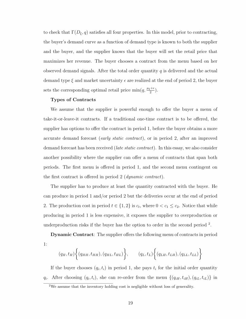
Types of Contracts

We assume that the supplier is powerful enough to offer the buyer a menu of

take-it-or-leave-it contracts. If a traditional one-time contract is to be offered, the

supplier has options to offer the contract in period 1, before the buyer obtains a more

accurate demand forecast (early static contract), or in period 2, after an improved

demand forecast has been received (late static contract). In this essay, we also consider

another possibility where the supplier can offer a menu of contracts that span both

periods. The first menu is offered in period 1, and the second menu contingent on

the first contract is offered in period 2 (dynamic contract).

The supplier has to produce at least the quantity contracted with the buyer. He

can produce in period 1 and/or period 2 but the deliveries occur at the end of period

2. The production cost in period t ∈ {1, 2} is ct, where 0 < c1 ≤ c2. Notice that while

producing in period 1 is less expensive, it exposes the supplier to overproduction or

underproduction risks if the buyer has the option to order in the second period 2.

Dynamic Contract: The supplier offers the following menu of contracts in period

1:

(qH , tH)

{(qHH , tHH), (qHL, tHL)

}, (qL, tL)

{(qLH , tLH), (qLL, tLL)

}If the buyer chooses (qi, ti) in period 1, she pays ti for the initial order quantity

qi. After choosing (qi, ti), she can re-order from the menu {(qiH , tiH), (qiL, tiL)} in

2We assume that the inventory holding cost is negligible without loss of generality.

19

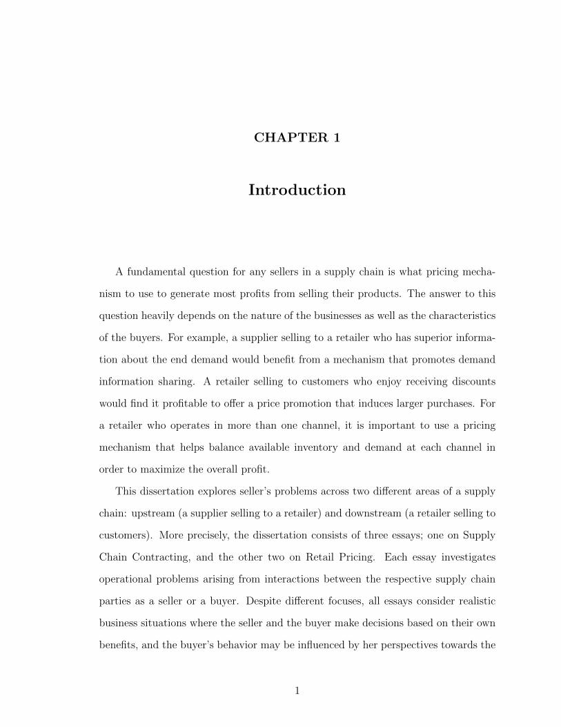
Buyer conducts initial forecast, obtains first signal type i {L, H}

Supplier announces dynamic contract menu

Buyer selects contract type i

Supplier produces 𝜌𝑖 at cost 𝑐1

Period 1 Buyer updates her forecast, obtains second signal type j {L, H}

Buyer selects contract ij contingent on period 1 contract choice i

Supplier produces (𝑞𝑖 + 𝑞𝑖𝑗 − 𝜌𝑖)+ at cost 𝑐2

and delivers 𝑞𝑖 + 𝑞𝑖𝑗

Buyer realizes and satisfies her actual demand

Period 2

Figure 2.1: Sequence of events: Dynamic Contract

period 2. She pays tij for the additional order quantity qij. The total order qi + qij

is delivered at the end of period 2. Notice that the contract (qi, ti) is meant for the

buyer who observes a signal i in period 1, and the contingent contract (qij, tij) is

meant for the buyer who subsequently observes a signal j in period 2.

The supplier decides how much to produce upfront in period 1 after the buyer

makes the initial selection from the period 1 menu of contracts. We define ρi as the

supplier’s decision variable of the production quantity in period 1, given that the

buyer chooses the type i contract from the period 1 menu. The benefit of producing

in period 1 is the cheaper unit production cost. However, delaying part of production

to period 2 allows the supplier to produce after learning exactly how much the buyer

will order in total, and hence, reduces the risk of over- or underproduction. The

sequence of events with dynamic contract is displayed in Figure 1.

20

The supplier’s optimization problem under the dynamic contract is given by:

maxq,t,ρ

∑i∈{L,H}

p1i (−c1ρi + ti) +

∑i∈{L,H}

p1i

∑j∈{L,H}

pij[tij − c2(qi + qij − ρi)+]

(2.1)

s.t. Period 1 Participation Constraints∑j∈{L,H}

pij∑

k∈{L,H}

p2jk[Γ(Dk, qi + qij)− tij] ≥ ti, i ∈ {L,H}

Period 1 Incentive Constraints∑j∈{L,H}

pij∑

k∈{L,H}

p2jk[Γ(Dk, qi + qij)− tij]− ti ≥∑

j∈{L,H}

pij∑

k∈{L,H}

p2jk[Γ(Dk, q−i + q(−i)l)− t(−i)l]− t−i, i ∈ {L,H}, l ∈ {L,H}

Period 2 Participation Constraints∑k∈{L,H}

p2jk[Γ(Dk, qi + qij)− tij] ≥

∑k∈{L,H}

p2jkΓ(Dk, qi), i ∈ {L,H}, j ∈ {L,H}

Period 2 Incentive Constraints∑k∈{L,H}

p2jk[Γ(Dk, qi + qij)− tij] ≥

∑k∈{L,H}

p2jk[Γ(Dk, qi + qi(−j))− ti(−j)],

i ∈ {L,H}, j ∈ {L,H}

Nonnegativity Constraints

ρi, qi, qij, ti, tij ≥ 0 i ∈ {L,H}, j ∈ {L,H}

The first term in the objective function includes the initial payment and period

1 production cost c1ρi. The second term accounts for the period 2 payment and the

remaining production cost c2(qi + qij − ρi)+ for the total quantity ordered by the

buyer. The first constraint is the participation constraint that guarantees the type-

i buyer’s expected profit from the whole horizon is non-negative in period 1. The

second constraint is the incentive compatibility constraint, which ensures that the

type-i buyer selects the contract designed for her type in period 1. Similarly, the third

and fourth constraints are the participation and incentive compatibility constraints

in period 2. They guarantee non-negative expected profits from participating in the

21

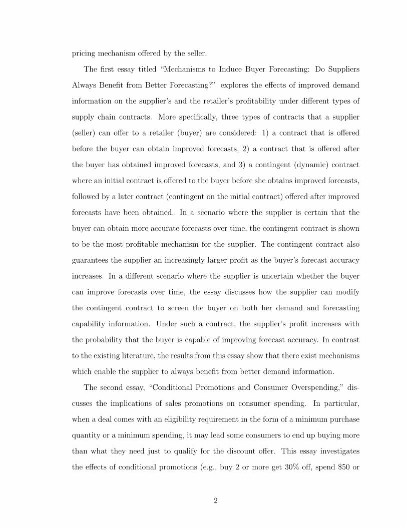
Buyer conducts initial forecast, obtains first signal type i {L, H}

Supplier announces early static contract menu (𝑞𝑖 , 𝑡𝑖), i {L, H}

Buyer selects contract type i

Supplier produces 𝑞𝑖 at cost 𝑐1

Period 1

Supplier delivers 𝑞𝑖

Buyer realizes and satisfies her actual demand

Period 2

Figure 2.2: Sequence of events: Early Static Contract

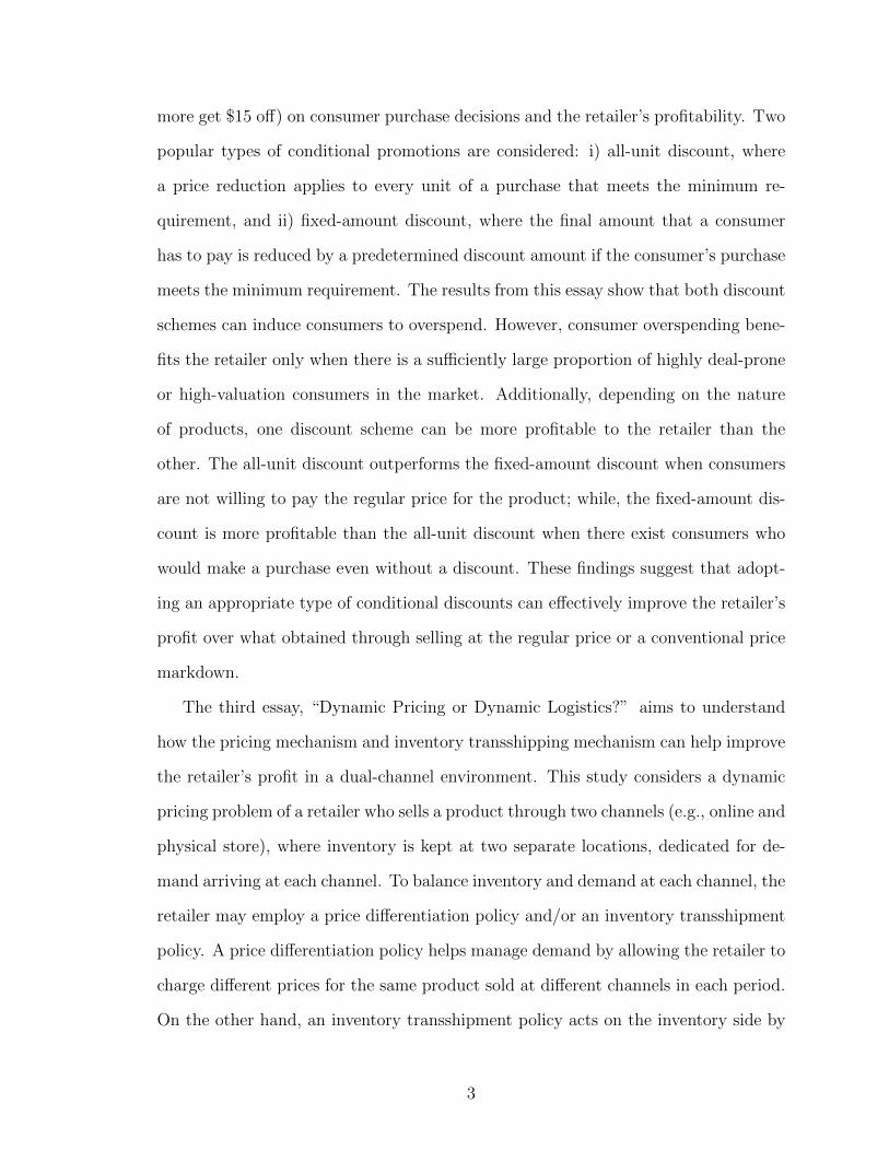
Buyer conducts initial forecast, obtains first signal type i {L, H}

Supplier produces 𝜌 at cost 𝑐1

Period 1 Buyer updates her forecast, obtains second signal type j {L, H}

Buyer selects contract j

Supplier produces (𝑞𝑖 −𝜌)+ at cost 𝑐2 and delivers 𝑞𝑖

Buyer realizes and satisfies her actual demand

Period 2

Supplier announces late static contract menu (𝑞𝑖 , 𝑡𝑖), i {L, H}

Figure 2.3: Sequence of events: Late Static Contract

period 2 contracts, and maximum expected profits from committing to the contract

corresponding to the buyer’s second demand signal type.

Static Contracts: The early static and late static contracts are special cases

of dynamic contract. More precisely, under an early static contract, the supplier

announces a menu of contracts {(qH , tH), (qL, tL)} in period 1 to screen the buyer’s

period 1 signal type. Hence, it can be viewed as a dynamic contract with constraints

qij = 0 and tij = 0, i, j ∈ {L,H} in period 2. Under a late static contract, the supplier

offers a menu of contracts {(qH , tH), (qL, tL)} in period 2 to screen the buyer’s period

2 signal type. Hence, it is equivalent to a dynamic contract with constraints qi = 0

and ti = 0, i ∈ {L,H} in period 1. The sequence of events with early and late

static contract are given in Figure 2 and 3, respectively. In Appendix A, we provide

the supplier’s optimization problems and solutions of the early static and late static

contracts.

22

2.3.2 Preliminary Results

Propositions 2.1 through 2.3 characterize the structure of an optimal dynamic

contract (The proofs are provided in Appendix A). We will use these properties in

the next section when we discuss which contract structure (dynamic, early static or

late static) is most beneficial for the buyer or seller under different conditions.

There are multiple contracts that result in the same expected profit for the buyer

and the supplier. Proposition 2.1 shows that in one form of the optimal dynamic

contracts, all contract quantities are deferred to the second period contracts (qi =

0, i ∈ {L,H} in period 1). In this contract, the supplier charges ti in period 1 as an

option price, which gives the buyer the right to order qi + qiH or qi + qiL in period

2, and pay the additional fee tij if necessary. The buyer will have the total order,

qi + qij, delivered by the end of period 2. This contract structure is similar to that of

a capacity reservation contract commonly used in practice.

Proposition 2.1. For an optimal dynamic contract with contract quantities {qi, qij},

i, j ∈ {L,H}, there exists an equivalent dynamic contract with q′i = 0 and q′ij =

qi + qij, i, j ∈ {L,H}.

Similarly, we can show that the supplier can transfer the payments of the period

2 low-type contracts to period 1 (tiL = 0, i ∈ {L,H} in period 2) without losing

optimality. Proposition 2.2 states that there exists an optimal dynamic contract such

that if the second forecast indicates the demand is low (i.e. the buyer observes HL

or LL), then the buyer is not charged another fee in the second period. Only when

the buyer needs additional units to meet expected high demand, she has to pay an

extra fee in the second period.

Proposition 2.2. For an optimal dynamic contract with transfer payments {ti, tij},

i, j ∈ {L,H}, there exists an equivalent dynamic contract with t′i = ti + tiL, t′iH =

tiH − tiL, and t′iL = 0, i ∈ {L,H}.

23

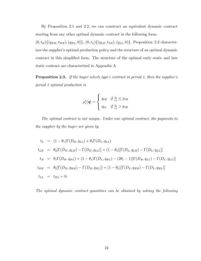
By Proposition 2.1 and 2.2, we can construct an equivalent dynamic contract

starting from any other optimal dynamic contract in the following form:

(0, tH){(qHH , tHH), (qHL, 0)}, (0, tL){(qLH , tLH), (qLL, 0)}. Proposition 2.3 character-

izes the supplier’s optimal production policy and the structure of an optimal dynamic

contract in this simplified form. The structure of the optimal early static and late

static contract are characterized in Appendix A.

Proposition 2.3. If the buyer selects type i contract in period 1, then the supplier’s

period 1 optimal production is

ρ∗i (q) =

qiH if c1c2≤ piH

qiL if c1c2> piH

The optimal contract is not unique. Under one optimal contract, the payments to

the supplier by the buyer are given by

tL = (1− θ1)Γ(DH , qLL) + θ1Γ(DL, qLL)

tLH = θ2[Γ(DH , qLH)− Γ(DH , qLL)] + (1− θ2)[Γ(DL, qLH)− Γ(DL, qLL)]

tH = θ1Γ(DH , qHL) + (1− θ1)Γ(DL, qHL)− (2θ1 − 1)[Γ(DH , qLL)− Γ(DL, qLL)]

tHH = θ2[Γ(DH , qHH)− Γ(DH , qHL)] + (1− θ2)[Γ(DL, qHH)− Γ(DL, qHL)]

tLL = tHL = 0.

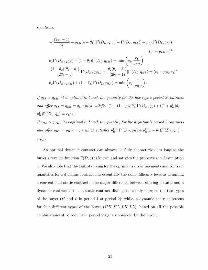
The optimal dynamic contract quantities can be obtained by solving the following

24

equations:

−[(2θ1 − 1)

p1L

+ pLHθ2 − θ1][Γ′(DH , qLL)− Γ′(DL, qLL)] + pLLΓ′(DL, qLL)

= (c1 − pLHc2)+

θ2Γ′(DH , qLH) + (1− θ2)Γ′(DL, qLH) = min

(c2,

c1

pLH

)[(1− θ2)(θ2 − θ1)

(2θ2 − 1)]Γ′(DH , qHL) + [

θ2(θ2 − θ1)

(2θ2 − 1)]Γ′(DL, qHL) = (c1 − pHHc2)+

θ2Γ′(DH , qHH) + (1− θ2)Γ′(DL, qHH) = min

(c2,

c1

pHH

).

If qLL > qLH , it is optimal to bunch the quantity for the low-type’s period 2 contracts

and offer qLL = qLH = qL which satisfies (1− (1 + p1H)θ1)Γ′(DH , qL) + ((1 + p1

H)θ1 −

p1H)Γ′(DL, qL) = c1p

1L.

If qHL > qHH , it is optimal to bunch the quantity for the high-type’s period 2 contracts

and offer qHL = qHH = qH which satisfies p1Hθ1Γ′(DH , qH) + p1

H(1− θ1)Γ′(DL, qH) =

c1p1H .

An optimal dynamic contract can always be fully characterized as long as the

buyer’s revenue function Γ(D, q) is known and satisfies the properties in Assumption

1. We also note that the task of solving for the optimal transfer payments and contract

quantities for a dynamic contract has essentially the same difficulty level as designing

a conventional static contract. The major difference between offering a static and a

dynamic contract is that a static contract distinguishes only between the two types

of the buyer (H and L in period 1 or period 2); while, a dynamic contract screens

for four different types of the buyer (HH,HL,LH,LL), based on all the possible

combinations of period 1 and period 2 signals observed by the buyer.

25

2.4 Contract Preferences and Effects of Forecast Accuracy

We now address the question of which contracts are most profitable for the sup-

plier or the buyer under which conditions. First, we assume that the buyer will always

obtain a more accurate forecast in period 2. As noted earlier, early static and late

static contract are special cases of dynamic contract. Hence, it is straightforward to

see that from the supplier’s point of view, dynamic contract weakly dominates early

static and late static contracts. The advantage of dynamic contract over early static

contract comes from the supplier’s ability to screen not only the initial demand esti-

mate, but also the improved demand information, under the dynamic contract. This

allows the supplier to potentially sell more to the buyer who observes the high-type

signal in the second period. In comparison with late static contract, the superiority

of dynamic contract comes from its structure that enables the supplier to screen the

initial demand forecast. By learning about the buyer’s type upfront in period 1, the

supplier can make a better production decision, resulting in cheaper production costs

under a dynamic contract.

Given that the supplier would always prefer to use the dynamic contract (com-

pared to early static or late static contracts), an interesting question is whether the

buyer’s receiving better forecasts over time is beneficial to the supplier. There are two

ways to address this question. First, we note that the buyer receives a second signal

with accuracy θ2 > θ1 in period 2. It is straightforward to see that the supplier would

always prefer that the buyer receive this second signal. That is, if the buyer did not

receive this second (more accurate signal) or if the buyer received a second signal but

the accuracy of this second signal was identical to the first period, the supplier would

definitely be worse off. Indeed, the better the accuracy of the signal that the buyer

receives in period 2, the higher profits the supplier can receive so long as he uses the

dynamic contract.

26

Theorem 2.1. The supplier’s profit under an optimal dynamic contract monotoni-

cally increases with the buyer’s second-period forecast accuracy, θ2.

We would like to point out how Theorem 2.1 complements the analysis of Taylor

(2006). In that paper, Taylor (using a model similar to ours but with a single period

analysis) analyzed a situation where the buyer received only one signal and showed

that increasing the accuracy of that signal does not necessarily increase the profits

of the supplier. In our setting, if the supplier used a late static contract, increasing

the accuracy of θ2 would not always increase the profits of the supplier, similar to

Taylor’s result. Likewise, if the buyer uses an early static contract, the only relevant

forecast signal is the first one and an increase in the accuracy of this signal does

not always increase the profits of the supplier either. However, a contrasting and

interesting result we show here is that as long as the supplier uses the dynamic

contract we specify above, a second (improved) forecast always benefits the supplier,

and the more improved the forecast is, the greater the benefit to the supplier. This

is because with a dynamic contract, the supplier screens both the initial and more

accurate demand signals, allowing him to effectively extract most of the potential

gain from the reduction in the mismatch between the buyer’s ordered quantity and

actual demand without having to pay high rents to the buyer. An example of the

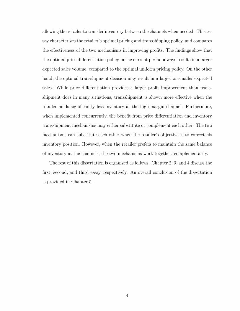
supplier’s profit under the three contract types as the forecast accuracy improves is

shown in Figure 4.

It is also worth pointing out that the dynamic contract can be more profitable to

the supplier than the early static contract even when the buyer contracting under the

early static contract has an initial forecast that is more accurate than the improved

forecast of the buyer contracting under the dynamic contract. That is, even when the

demand information the supplier obtains from a dynamic contract is inferior to that

obtained from an early static contract, the supplier’s profit can still be higher under

the dynamic contract. Proposition 2.4 provides sufficient conditions for this scenario.

27

When the demand is more likely to be low (pL ≥ 0.5), if the buyer does not learn

additional information from a demand forecast (θ1 = max{pL, pH} = pL), then the

buyer will always buy the low-type contract under the early static contract (p1L = 1).

If the buyer obtains a more informative demand forecast (θ1 > pL), then with a

positive probability, the buyer will observe a high signal and select the high-type

contract. However, when the additional cost to sell to the high-type buyer (production

cost c1(qH − qL) and high-type rent (2pL − 1)[Γ(DH , qL) − Γ(DL, qL)]) is greater

than the expected gain from having a high demand (pL[Γ(DH , qH) − Γ(DH , qL)] +

pH [Γ(DL, qH) − Γ(DL, qL)]), the supplier finds it less profitable to sell to the high-

type. In this case, the supplier’s profit under an early static contract is decreasing in

the forecast accuracy θ1 when the accuracy is small.3 Hence, the supplier can earn

larger profits from a dynamic contract even when the buyer’s accuracy is lower.

Proposition 2.4. If demand is more likely to be low (pL ≥ 0.5) and if the optimal

early static contract when θ1 = pL is such that c1(qH − qL) + (2pL − 1)[Γ(DH , qL) −

Γ(DL, qL)] > pL[Γ(DH , qH)−Γ(DH , qL)]+pH [Γ(DL, qH)−Γ(DL, qL)], then there exists

θ ∈ (0, 1] such that the supplier’s profit under the optimal early static contract with

a buyer whose period 1 accuracy is θ < θ is less than the supplier’s profit under an

optimal dynamic contract with a buyer whose period 2 accuracy is θ2 < θ.

While the supplier can always benefit from more accurate forecasts with a dynamic

contract, it is required that the buyer obtains a more accurate forecast in the second

period for a dynamic contract to be viable. This actually raises two interesting

questions: 1) Is the buyer willing to obtain better forecasts?; i.e., do better forecasts

also always benefit the buyer assuming the buyer has the capability to obtain them?,

and 2) What if the supplier is uncertain about the buyer’s capability to obtain more

accurate forecasts in the first place? To address these two questions, we first develop

an understanding of which contracts are most profitable for each type of the buyer.

3Notice that this result is analogous to Taylor and Xiao (2010).

28

0.65 0.7 0.75 0.8 0.85 0.9 0.95 12

3

4

5

6

7

8

9

10

θ2

Exp

ecte

d P

rofit

Buyer’s Profit Vs. θ2

Early StaticLate StaticDynamic

0.65 0.7 0.75 0.8 0.85 0.9 0.95 1510

520

530

540

550

560

570

580

θ2

Exp

ecte

d P

rofit

Supplier’s Profit Vs. θ2

Early StaticLate StaticDynamic

0.65 0.7 0.75 0.8 0.85 0.9 0.95 1520

530

540

550

560

570

580

590

θ2

Exp

ecte

d P

rofit

Supply Chain Profit Vs. θ2

Early StaticLate StaticDynamic

Figure 2.4: Preferences of the high-type buyer, supplier, and supply chain: r =1, c1/c2 = 0.67, c1 = 0.1, pL = 0.46, µH = 900, µL = 400, δ = 50, θ1 = 0.6)

Proposition 2.5 presents the contract preferences of the low-type buyer (who ob-

serves a low demand signal in period 1).

Proposition 2.5. The low-type buyer always prefers late static contract to early

static and dynamic contract. She is indifferent between early static and dynamic

contracts.

Under early static and dynamic contract, the low-type buyer commits to the

low-type contract in period 1, before she obtains a more accurate demand forecast.

Hence, she is screened as the lowest type, and is awarded zero expected profits since

the low-type participation constraints in period 1 under both early static and dynamic

contract are binding at optimality. The supplier sets the quantity and transfer pay-

ment such that the low-type buyer makes a positive profit only if her actual demand

turns out to be high-type; she loses money ex-post otherwise. If a late static contract

is offered, however, the low-type buyer has a chance to observe an improved demand

signal in period 2, before she commits to a contract. With a positive probability, her

second signal can be high-type and she can receive a positive expected profit from

the high-type contract. Otherwise, if her second signal is low-type, she receives a

zero expected profit. Thus, her ex-ante expected profit is positive under a late static

contract. Since the low-type buyer prefers to contract late and is indifferent between

early static and dynamic contract, she would always agree to update her forecasts

29

even when the supplier offers her a dynamic contract.

The situation for the high-type buyer is different. In a screening contract, the

profit to the high-type buyer comes from the information rent that the supplier has

to offer in order to prevent the high-type from deviating to lower type contracts.

Hence, the high-type buyer always makes positive profits under all three types of

contracts. However, it is not immediate under which situations, the high-type buyer

will prefer which contract type to the others. Proposition 2.6 shows that the high-

type buyer always prefers to contract early rather than dynamically. Furthermore,

under the dynamic contract, the high-type buyer’s expected profit is hurt even more

as her second period information accuracy improves. This is because under early

static contract, the buyer only reveals her less accurate demand information, leaving

sufficient amount of uncertainty which results in higher rents. On the other hand,

the buyer reveals both her initial and improved demand information under dynamic

contract, leaving little rents to her. The additional demand information revealed

in the second period always benefits the supplier rather than the buyer because it

decreases the uncertainty about the buyer’s type.

Proposition 2.6.

1. The high-type buyer’s profit under the early static contract is at least as high as

her profit under the dynamic contract.

2. The high-type buyer’s profit under the dynamic contract monotonically decreases

with the second-period forecast accuracy.

Since the early static contract is more profitable to the high-type buyer than the

dynamic contract, if the buyer expects the supplier to offer her a dynamic contract,

she would opt out from conducting a more accurate forecast in order to be offered

an early static contract instead. However, if both the supplier’s and the buyer’s

profit are higher with the late static than with the early static contract, then the

30

supplier can benefit from offering the late static contract upfront (in a sense, take

the dynamic contract off the table), so that the buyer would agree to obtain a more

accurate forecast. In this case, both parties can still benefit from more accurate

demand information. An example of such situation where the late static contract is

more preferable to both parties than the early static contract is shown in Figure 4,

when the period 2 accuracy, θ2, is between 0.78 and 0.83. Notice that the supplier

prefers the late static contract only when the forecast accuracy is sufficiently increased

in period 2 (θ2 > 0.78). This is because the significant improvement in the accuracy

of demand forecasts makes it worth waiting to contract late even though the supplier

has to incur higher production costs. For the high-type buyer, she prefers late static

to early static contract when the period 2 accuracy is sufficiently low (θ2 < 0.83).

This is because a moderate accuracy of her signal leaves enough uncertainty about

her demand type, and the supplier, after waiting to contract in period 2, would be

willing to offer her a higher rent in exchange for the more accurate and only demand

information. This situation is particularly prevalent when the period 2 production

cost is not much more expensive than the period 1 production cost (signified by

a large c1c2

). It is worth noting that the supply chain can also benefit from more

accurate demand forecast through dynamic and late static contract, especially when

the increase in accuracy is substantial. This is because when the period 2 accuracy

is high, the value of more accurate demand information outweighs the increase in

production costs in the later period.

This section has shown that while the supplier always benefits most from, and

therefore, favors the dynamic contracts, the buyer may actually prefer the early static

contract and may claim that she will not obtain a more accurate forecast as the high

type buyer’s profit is monotonically decreasing in period 2 accuracy. But if the

supplier knows that the buyer is capable of obtaining a more accurate forecast, how

does the supplier interpret this refusal to obtain a better forecast? We answer this

31

question in the next section.

2.5 Capable Buyer and Bayesian Updating Supplier

In the previous section, we showed that although there are some situations where

both parties benefit from more accurate forecasts, there are others where the buyer

does not. Since the buyer is the one obtaining the better forecast, the question is

whether the buyer can simply announce that she is not obtaining a second forecast,

when she knows that having the better forecast will put her under a less profitable

contract type. The problem is that if the supplier knows that the buyer is capable

of obtaining improved forecasts, then a decision by the buyer not to obtain them can

lead the supplier to update his beliefs about the buyer’s demand type, which will

affect the type of contracts he will offer to the buyer.

We study the Perfect Bayesian Equilibrium (PBE) of the two-stage game played by

the supplier and the buyer. In period 1, the buyer observes her own period 1 demand

signal, and then announces whether she intends to obtain the second demand signal

or not. If she does, the supplier offers a dynamic contract menu (since it is always

most profitable for him). If the buyer does not update, the supplier offers an early

static contract menu. Note that if the Bayesian updating leads the supplier to be

certain about the buyer’s type, then the supplier can offer a first-best contract for

the buyer’s type.

In this Bayesian game, the supplier has an initial belief about the buyer’s period 1

signal type described by the probabilities p1i , i ∈ {L,H}. Let {U,N} be the set of the

buyer’s possible strategies where U is to update, and N is to not update. The buyer

with signal type i chooses U with probability σUi , and N with probability σNi = 1−σUi .

After the buyer announces her strategy S ∈ {U,N}, the supplier updates his belief

about the type distribution to τi(S), i ∈ {L,H} as follows: τi(S) =p1i σ

Si∑

k∈{L,H} p1kσSi.

The standard result for this Bayesian game is that there is no separating PBE.

32

There are two pure strategy pooling PBE: one where both types of buyers announce

they will obtain better demand forecasts, and the other where both types of buyers

announce they will not obtain better demand forecasts 4. This result is driven by the

fact that the lowest type buyer is indifferent between obtaining and not obtaining a

more accurate forecast. If one assumes that the lowest type buyer will obtain a better

forecast when she is indifferent, then the equilibrium is the one where all types of the

buyer obtain more accurate forecasts. However, if one assumes that when indifferent,

the lowest type buyer will actually not obtain better forecasts, then the equilibrium

is the one where all types of the buyer choose not to obtain better forecasts, which

makes the supplier unable to benefit from more accurate demand information.

To rule out the no-updating PBE, the supplier can in fact utilize a side payment to

induce the lowest type buyer to update demand forecasts. More precisely, the supplier

can announce upfront that all buyers who obtain a better forecast will be given a small

side payment. In this case, the lowest type buyer will have an incentive to obtain a

more accurate forecast, leading to a unique all-update equilibrium. This shows that

even when the buyer has a bargaining power to refuse updating her demand forecasts,

the supplier can offer a dynamic contract with a side payment to guarantee the buyer’s

willingness to obtain improved forecasts. The only exception where such a dynamic

contract may not be preferable to the supplier is when there is a cost involved with

updating the forecasts. In this case, the supplier’s optimal strategy depends on the

update cost, as discussed in Theorem 2.2.

Theorem 2.2. There exists a threshold K such that if the forecast update costs K ≤

K, the unique PBE with a side payment is where both types of the buyer obtain more

accurate demand forecasts. If K > K, the supplier offers an early static contract.

The cost of obtaining better demand forecast has essentially no impact on the

4This result extends naturally to the case where there are n > 2 types of buyers, where the typesare ordered according to the period 1 demand signal.

33

buyer’s behavior since the cost is transferred to the supplier through the optimal

contract design. It is profitable for the supplier to offer a side payment to incentivize

both types of the buyer to obtain more accurate demand information at the equilib-

rium as long as the update cost is reasonable. If the forecast update is so costly that

the benefit to the supplier is less than the cost of obtaining better forecasts, then

the supplier chooses to offer an early static contract that does not require a second

forecast.

An important managerial implication here is that while the buyer may not always

benefit from more accurate forecasts, so long as the supplier offers even a small side

payment for obtaining better forecasts, he can induce the Bayesian equilibrium where

all types of the buyer agree to obtain more accurate forecasts. This is, of course, only

possible when the supplier is certain about the buyer’s capability of conducting more

accurate forecasts in the second period, which may not always be the case in practice.

Hence, we discuss the supplier’s best contract options in presence of an uncertainty

about the buyer’s forecasting capability in the next section.

2.6 Screening the Forecasting Capability

When the supplier is truly uncertain as to how accurate of a demand forecast the

buyer can obtain, we propose that the supplier can improve the screening nature of

his contracts by screening the buyer not only on demand level, but also on forecasting

capability. Suppose that the supplier has a prior on the capability of the buyer to

obtain improved forecasts. The supplier can design a capability and type screening

menu of contracts such that the capable (high accuracy θ2) buyer prefers dynamic

contract, and the incapable (low accuracy θ1) buyer prefers early static contract.

The model in this section also applies to a situation where the forecast updates are

costly, but the supplier is uncertain about the buyer’s forecasting costs, as modeled

by Lariviere (2002). That is, the buyer may incur a small update cost KL or a large

34

update cost KH . If the buyer’s update cost is small (KL ≤ K), then it is worthwhile

for the supplier to induce the buyer to obtain improved forecasts using a dynamic

contract. On the other hand, if the buyer’s update cost is large (KH > K), then

the supplier prefers to contract with the buyer under an early static contract. In

this case, the large update cost will never be incurred (since the buyer is offered an

early static contract). Then, the buyer with a small update cost is equivalent to the

capable buyer, and the buyer with a large update cost is equivalent to the incapable

buyer in this model.

The capability to obtain a better demand forecast is private information to the

buyer. However, we assume the supplier estimates that with probability φ, the buyer

is capable of obtaining a more accurate demand forecast, and with probability 1− φ,

she is not capable. The capable buyer is simply the buyer described in previous

sections, who receives a better forecast in period 2. On the other hand, the incapable

buyer observes a signal whether she is low-type or high-type in period 1, but is

incapable of making that forecast more accurate in period 2. Since the incapable

buyer does not receive a second signal, if she purchases a dynamic contract, she uses

a strategy such that with probability υiH , she chooses the iH contract in period 2,

and with probability υiL = 1− υiH , she chooses the iL contract, where i ∈ {L,H} is

her signal type in period 1. Notice that if a buyer chooses the early static contract,

then she will always receive the same expected profit, whether she is capable or not,

since the contract decision is only made in period 1 and the more accurate forecasting

is irrelevant.

The supplier offers a menu of contracts that screens both the type and forecasting

capability of the buyer. He offers a menu of the early static contract, (qi, ti), i ∈

{L,H}, and the dynamic contract, (qDi , tDi ),

((qiH , tiH), (qiL, tiL)

), i ∈ {L,H}. The

35

supplier’s optimization problem is as follows

maxq,t,ρ

{(1− φ)

∑i∈{L,H}

p1i (−c1qi + ti) + φ

[ ∑i∈{L,H}

p1i (−c1ρi + tDi ) +

∑i∈{L,H}

p1i∑

j∈{L,H}

pij [tij − c2(qDi + qij − ρi)+]

]}s.t. Period 1 Participation Constraints∑

j∈{L,H}

p1ij [Γ(Dj , qi)− ti] ≥ 0, i ∈ {L,H}

∑j∈{L,H}

pij∑

k∈{L,H}

p2jk[Γ(Dk, qDi + qij)− tij ] ≥ tDi , i ∈ {L,H}

Period 1 Incentive Constraints∑j∈{L,H}

p1ij [Γ(Dj , qi)− ti] ≥∑

j∈{L,H}

p1ij [Γ(Dj , q−i)− t−i], i ∈ {L,H}

∑j∈{L,H}

pij∑

k∈{L,H}

p2jk[Γ(Dk, qDi + qij)− tij ]− tDi ≥∑

j∈{L,H}

pij∑

k∈{L,H}

p2jk[Γ(Dk, qD−i + q(−i)l)− t(−i)l]− tD−i, i ∈ {L,H}, l ∈ {L,H}

Period 2 Participation Constraints∑k∈{L,H}

p2jk[Γ(Dk, qDi + qij)− tij ] ≥

∑k∈{L,H}

p2jkΓ(Dk, qDi ), i ∈ {L,H}, j ∈ {L,H}

Period 2 Incentive Constraints∑k∈{L,H}

p2jk[Γ(Dk, qDi + qij)− tij ] ≥

∑k∈{L,H}

p2jk[Γ(Dk, qDi + qi(−j))− ti(−j)],

Forecasting Capability Incentive Constraints∑j∈{L,H}

p1ij [Γ(Dj , qi)− ti] ≥∑

l∈{L,H}

∑j∈{L,H}

υilpij∑

k∈{L,H}

p2jk[Γ(Dk, qDi + qil)− til]− tDi , i ∈ {L,H}∑

j∈{L,H}

pij∑

k∈{L,H}

p2jk[Γ(Dk, qDi + qij)− tij ]− tDi ≥

∑j∈{L,H}

p1ij [Γ(Dj , qi)− ti], i ∈ {L,H}

Nonnegativity Constraints

qi, ti, ρi, qDi , qij , t

Di , tij ≥ 0 i ∈ {L,H}, j ∈ {L,H}

The optimization problem includes the participation and incentive compatibility

constraints for both the early static and dynamic contract. The participation and

incentive compatibility constraints of the early static contract ensures that the type

i ∈ {L,H} buyer who does not have the forecasting capability picks the early static

contract meant for her type. Similarly, dynamic contract constraints ensures that type

36

i ∈ {L,H} buyer who has the forecasting capability picks the dynamic contract meant

for her type. The forecasting capability incentive constraints prevent the incapable

buyer from deviating to the dynamic contract by ensuring that, regardless of the

mixed strategy chosen by the buyer (any value of vik), the incapable buyer will do

worse by choosing a dynamic contract. Similarly, the second forecasting capability

incentive constraint ensures that the capable buyer will prefer to obtain a revised

forecast and will not deviate to the early static contract.

In this setting, we have the following results regarding the supplier’s and the

buyer’s optimal strategies and profit.

Theorem 2.3. Under an optimal two-dimensional screening contract:

1. The optimal strategy for the incapable type i buyer if she were to contract

dynamically is to choose the iL contract in period 2 with probability 1, i.e.

υiL = 1, i ∈ {L,H}.

2. Both capable and incapable buyer of the same type receive the same expected

profit, where the profit is zero for the low-type buyer and is positive for the

high-type buyer.

3. The supplier’s profit monotonically increases with the capability probability φ

and the period 2 forecast accuracy θ2.

4. The high-type buyer’s profit is monotonically decreasing in the capability proba-

bility φ and is independent of period 2 forecast accuracy θ2.

Part 1 and 2 of the theorem are driven by the binding constraints in an optimal

two-dimensional screening contract. More precisely, when the buyer is incapable

of obtaining a more accurate demand signal to help her make decision on which

contract to choose in the second period, she minimizes her risk of losing money

from ordering too much by always relying on the low-type contract. This is because

37

an optimal screening contract is designed such that the high-type buyer’s expected

profit from deviating to the low-type contract is the same as the expected profit from

choosing the high-type contract; however, the low-type buyer could lose money from

deviating to the high-type contract. The forecasting capability incentive constraints

are also binding at optimality, resulting in the same expected profit to the capable

and incapable buyer of the same type. Like under other screening contracts, the low-

type expected profit is zero while the high-type expected profit is positive due to the

information rents.

Part 3 and 4 of the theorem describe the effects of the capability probability

as well as the second forecast accuracy on the supplier’s and the high-type buyer’s

expected profit. In Section 4, it has been shown that the supplier always prefers

dynamic contract; while, the high-type buyer always prefers early static contract

to dynamic contract. Hence, as the capability probability increases, implying it is

more likely that dynamic contract will take place, the high-type buyer’s expected

profit is reduced but the supplier’s profit is increased. Figure 5a and b display the

expected profits of the high-type buyer and supplier for different values of capability

probability. (Note also that an increase in the market uncertainty δ benefits the buyer

and hurts the supplier as expected.) If instead the capability probability is fixed, but

the capable buyer’s second forecast accuracy is improved, we show that the supplier

can continue to take advantage of the buyer’s better demand information. This result

is consistent with Theorem 2.1, where we show the supplier is better off contracting

with a more accurate buyer using a dynamic contract. What is less expected here is

that a change in the capable buyer’s improved forecast accuracy has no effect on the

buyer’s expected profit. This is because the second forecast accuracy only influences

the performance of the capable buyer, but not the incapable buyer. Since the supplier

holds the same belief about the buyer’s forecasting capability and since it is optimal

to offer both capable and incapable buyer the same profit, the supplier gives the same

38

optimal level of rent to the buyer, and keeps the remaining increase in supply chain

profit due to better forecast accuracy to himself.

The results in this section show that even in the presence of the uncertainty about

the buyer’s forecast capability, there still exist a mechanism which allows the supplier

to always benefit from more accurate demand information. An implication here is

that more accurate information is always potentially beneficial to the supplier as long

as he designs a contract wisely.

a.0 50 100 150 200 250

0

5

10

15

20

25

30

35

40

45

δ

Buy

er’s

Pro

fit

High−Type Buyer’s Expected Profit over δ

Early Static (φ = 0)φ = 0.2φ = 0.5φ = 0.7Dynamic (φ = 1)

b.0 50 100 150 200 250

540

545

550

555

560

565

570

575

580

δ

Sup

plie

r’s P

rofit

Supplier’s Expected Profit over δ

Early Static (φ = 0)φ = 0.2φ = 0.5φ = 0.7Dynamic (φ = 1)

Figure 2.5: High-type buyer’s and supplier’s profits: r = 1, c1c2

= 0.4, c1 = 0.2, pL =0.5, µH = 1000, µL = 600, θ1 = 0.6, θ2 = 0.8

2.7 Conclusion

In this chapter, we consider a stylized model of a multi-period procurement game

between a powerful supplier and a buyer under demand information asymmetry. We

investigate whether and when the parties benefit from more accurate demand forecasts

obtained by the buyer under different contract structures. A key finding of our study

is that a supplier who knows that a buyer is capable and is going to obtain more

accurate forecasts will always benefit from offering a dynamic contract, which screens

both the buyer’s initial and improved forecasts. We show however that there are

39

cases where the buyer prefers the early static contract the most, and therefore, is

disincentivized to obtain more accurate forecasts in the second period. But if the

supplier knows the buyer is capable of obtaining a forecast update, we argue that

the buyer can not simply refuse to obtain better forecasts as this would lead the

supplier to update his beliefs about the buyer’s demand type and end up offering a

first-best contract to extract even more profit from the buyer. In fact, we show that

as long as the supplier is certain that the buyer is capable of obtaining more accurate

demand forecasts, he can always induce the buyer to update her demand forecasts

by offering a small side payment. An interesting situation is when the supplier may

be uncertain about the buyer’s capability to obtain more accurate forecasts. In this

case, the buyer may claim an inability to obtain more accurate forecasts especially

when better forecasts are likely to hurt her profits. But in response, we show that

the supplier can offer a more sophisticated contract to screen the buyer both on her

forecast updating capability and demand type.

An important conclusion of this chapter is that suppliers can always benefit from

demand forecasts obtained by buyers that become more accurate over time. How-

ever, to achieve this benefit, the supplier may sometimes be required to design more

sophisticated contracts than what are common in practice. Our findings complement

what has been found in the existing contract literature which considers mostly sim-

ple static contracts and reports that the supplier’s profit can be hurt by improved

demand forecasts from the buyer. This essay indicates a need for more sophisticated

dynamic contracts. We note that similar contracts with contingent clauses have re-

cently been observed in practice. However, the standard dynamic contracts may not

be enough when the supplier is facing a buyer who can claim an inability to obtain

more accurate forecasts. In this case, the supplier may have to develop dual-screening

contracts, which have been much less common in practice. Our finding may indicate

that there is a certain point in the supply chain contract’s complexity level where the

40

benefit obtained by the contract is outweighed by its complexity. Further research is

needed on simpler mechanisms that achieve most if not all of the more sophisticated

mechanisms developed here.

41

CHAPTER 3

Conditional Promotions and Consumer

Overspending

3.1 Introduction

Price promotion is a key component in today’s retailing. In 2010, the total promo-

tion spending in the United States reached $337 billions, out of which 85% was spent

on price discounts (Borrell Associates , 2010). Retailers employ price promotions to

stimulate sales in their stores, which not only generate larger revenues, but also re-

duce costs by accelerating the disposal of excess inventory (Blattberg et al., 1981).

The most common forms of price promotions include price markdowns (e.g., 20% off

from regular price), bundling (e.g., buy shirt and pants together and save $20), and

conditional discounts (e.g., buy 2 or more and get 20% off).

Among these, conditional discounts are increasingly more popular in practice.

Their use in consumer packaged goods increased by 10.3% in 2010 from 2009. They

accounted for 26% of total coupon distribution, and was as high as 33% among gro-

cery products (NCH Marketing Services , 2011). Retailers typically offer conditional

discounts in the form of either percent-off or dollars-off. For example, Travelodge

offered 15% off its regular room rate if customers stayed 2 nights or longer. Bath

& Body Works offered $10 off a purchase of $30 or more as a Mother’s Day sale.

42

A distinct feature of conditional discounts is that the deal is always coupled with

an eligibility requirement, mostly in the form of a minimum purchase quantity or a

minimum spending, that customers need to fulfill in order to receive the discount.

This strategy can benefit retailers in several ways: it allows finer price discrimination

contingent on purchase quantity or spending, and potentially induces buyers with

higher consumption level or reservation price to consume more than what they would

without a discount offer.

Most existing literature on price promotions identifies price elasticity as the main

reason driving buyers to increase purchase quantity in response to a price reduction

(Jeuland and Narasimhan, 1985; Bell et al., 1999). However, this argument falls short

of explaining why some consumers go the extra mile and buy a significantly larger

quantity than what they actually need just to qualify for the deals. In fact, stories

about impulsive, deal-driven shopping behavior regularly appear in news articles,

popular press magazines, and personal blogs (Klaft , Sep. 3, 2011; Tuttle, Jul. 23,

2010; Sherman, Feb. 5, 2009; Fontinelle, Aug. 17, 2011; Tsai , 2007).

Such shopping behavior is referred to in the literature as “deal-proneness,” which

is the propensity to purchase products when they are offered on a “deal” basis (Hack-

leman and Duker , 1980). Existing studies on this subject explain that deal-proneness

arises as consumers gain psychological benefits from paying a lower-than-expected

price for a product (Schindler , 1989, 1998; Laroche et al., 2001; DelVecchio, 2005).

This enhanced positive feeling associated with the transaction is referred to as “trans-

action utility” (Thaler , 1985). Consumers who receive transaction utility when com-

pleting a deal are labeled “deal-prone.” Consumers who are not sensitive to such

cognitive benefits, and value a discount offer based solely on its monetary value, are

called “value-conscious.” (Lichtenstein et al., 1990) In order to investigate how deal-

proneness influences purchase decisions, we define overspending as a situation where

a deal-prone consumer increases her purchase quantity purely due to the transaction

43

utility received from completing a deal.

The heterogeneity in consumer deal-proneness together with the heterogeneity in

consumer willingness to pay result in multiple consumer segments who make differ-

ent purchase decisions when facing a discount offer. Thus, when designing a price

promotion, retailers must account for the impact of the deal on different groups of

consumers. This is a challenging problem as it is not clear how terms of promotional

offers influence purchase decisions of heterogeneous consumers, and which discount

policy should be adopted for a given set of market parameters. This chapter aims to

study the effects of conditional discounts on consumer behavior and seller’s profitabil-

ity, focusing on two most common forms of conditional discounts: i) all-unit discount,

where the price reduction (in percentage or dollars off) applies to every unit if the

eligibility condition is met, and ii) fixed-amount discount, in which a fixed discount

(e.g., $10 off) is applied to the total expense that satisfies the condition. Note that

price markdown is a special case of the all-unit discount with no minimum purchase

requirement, and mixed bundling with a limit of one deal per transaction is a special

case of the fixed-amount discount.

Our main research questions are: 1) How do different types of consumers respond

to conditional discounts? Do conditional discounts induce consumers to overspend?

2) When should a retailer offer conditional discounts?, and 3) What are the market

conditions that favor a fixed-amount discount to an all-unit discount or vice versa?

To answer these questions, we consider a model of a single seller facing heteroge-

neous consumers whose marginal consumption surplus decreases in the quantity they

consume. Consumers are heterogeneous in two dimensions: their cognitive attitude

towards a deal (deal-prone or value-conscious) and valuation (how much they value

consumption of the product). Facing these consumers, the seller’s problem is to decide

whether to offer a discount, and if so, which discount type (all-unit or fixed-amount)

and what specific terms of discount to offer in order to maximize his expected profit.

44

To our knowledge, this essay is the first to analytically investigate consumers’

heterogeneity in deal-proneness and their response towards conditional discounts.

We show that a conditional discount can induce deal-prone consumers to overspend.

Furthermore, we derive the seller’s optimal discount strategies and show that a condi-

tional discount is strictly more profitable than selling at the regular price when either

consumer willingness to pay for the product is low, or there exist deal-prone con-

sumers in the market. If a sufficiently large proportion of consumers are deal-prone,

we show that a conditional discount also dominates a conventional price markdown.

Hence, conditional discount is an effective tool to increase the seller’s profitability. In-

terestingly, we find that the optimal terms of discounts (discount depth and minimum

purchase requirement) and consumer purchase quantities induced by the optimal dis-

counts are not always monotone in the magnitude of transaction utility. Finally, we

identify market conditions under which the all-unit or the fixed-amount discount is

more profitable than the other. We show however that regardless of the type of dis-

counts used, it is not always optimal to induce consumers to overspend. Consumer

overspending benefits the seller only when there is a sufficient proportion of highly

deal-prone consumers in the market.

The rest of the chapter is organized as follows. In Section 3.2, we review relevant

literature on sales promotion and consumer deal-proneness. In Section 3.3, we de-

scribe the framework, introduce the model, and define the two types of conditional

discounts considered in this chapter. Section 3.4 provides analyses of the consumer’s

problem and discusses consumer purchase behavior under different types of discounts.

Section 3.5 addresses the seller’s problem and discusses optimal discount policies that

maximize the seller’s profits. To gain more insights about the effects of each dimen-

sion of consumer heterogeneity, we also derive the structure of the optimal discount

policies and the induced outcomes under two special cases. Section 3.6 presents nu-

merical study showing that the profit improvement the seller can achieve with the use

45

of conditional discounts is significant. Finally, we discuss extensions of the original

model in Section 3.7 and conclude the chapter with discussion of the main results and

future research directions in Section 3.8.

3.2 Literature Review

We will review three major streams of literature on sales promotion and consumer

deal-proneness. The first stream of work relevant to ours is on price promotions. One

of the most common forms of price promotion is a simple price markdown. Early

studies on this subject explained sales as a mechanism that increases seller’s profit

from certain groups of buyers (e.g., informed buyers in Varian 1980; low-demand and

low-holding cost buyers in Jeuland and Narasimhan 1985; brand switchers in Bell

et al. 1999). Other works analyzed the profitability of periodic price reduction poli-

cies and proposed optimization models, taking into account consumer’s promotion

response and retailer’s inventory level (Lazear , 1986; Achabal et al., 1990; Smith and

Achabal , 1998). Under these price markdown mechanisms, the deal is not contingent

on the purchase quantity. On the other hand, the current essay considers condi-

tional discounts, where the deal is realized only when buyers purchase at least the

minimum required quantity. This fundamental difference in pricing schemes allows

us to investigate another potential benefit of promotions in enticing consumers to

increase their purchase quantity to complete the deal, which is not observable under

price markdowns. A more characteristically similar price promotion mechanism to

conditional discount is quantity discount. A number of papers on quantity discount

analyzed a cost-minimizing or profit-maximizing problem of a supplier selling to a

buyer, where price discounts are given on large order sizes (Monahan, 1984; Lee and

Rosenblatt , 1986; Dada and Srikanth, 1987; Corbett and de Groote, 2000). Another

group of quantity discount literature compared different types of quantity discounts

(e.g., all-unit vs. package pricing in Wilcox et al. 1987; all-unit vs. incremental dis-

46

count in Weng 1995, and Munson and Rosenblatt 1998). However, the comparison

between all-unit and fixed-amount discount has not been addressed. Furthermore,

the quantity discount literature has been largely focusing on the upstream supply

chain parties, rather than a retailer selling to end consumers like in the current essay.

The closest price promotion mechanisms to the conditional discounts, both in

terms of structure and usage, are certain forms of bundling. The bundling literature

traditionally considered only pure bundling, pure unbundling, and mixed bundling

(Schmalensee, 1984; Chuang and Sirbu, 1999; Herrmann et al., 1997). Other papers

broadened their scope to consider bundling schemes where many more combinations

of products are offered to consumers (Hanson and Martin, 1990; Venkatesh and Maha-

jan, 1993; Armstrong , 1996). However, the challenges in pricing all different bundles

reduce the attractiveness of bundling when selling a large number of products. This

gave rise to the study of customized bundling, where bundles are priced based on

quantity rather than specific components, the closest mechanism to conditional dis-

counts. Hitt and Chen (2005) and Wu et al. (2008) analyzed customized bundling

problems and compared the profitability of customized bundling, pure bundling, and

individual selling. Hui et al. (2008) studied the problem of choosing the optimal

number of sizes of bundles to offer under a customized bundling scheme. They con-

cluded that, due to the cognitive cost consumers experience when evaluating many

bundle options, a small number of versions are sufficient to capture the majority of

the potential profit from versioning. An important difference between customized

bundling and conditional discount is that under customized bundling, there are often

more than one price breakpoints and discount rates. That is, consumers may receive

a deeper discount if they purchase an even larger quantity. On the other hand, under

a conditional discount, the discount rate or the discount amount is unified as long

as the purchase quantity meets the single minimum requirement. This makes con-

ditional discount simpler to implement and more straightforward to communicate to

47

consumers, which explains why conditional discounts are widely used in retailing.

The second stream of literature is on consumer response to price promotions. A

handful of papers in the framing literature compared consumer response to price

promotions framed in percentage terms and in dollar terms. For example, Bitta

et al. (1981), Chen et al. (1998), Hardesty and Bearden (2003), and Gendall et al.

(2006) compared the consumer perception of the value of price discounts presented in

percentages and dollars. Their experimental results showed that discounts on high-

priced items framed in dollars were perceived more significant than the same discounts

framed in percentage. These papers have different focus and methodology from ours.

They experimentally studied consumer response to different presentations of the exact

same price promotion; while, in the current essay, we analytically compare between

structurally different price discount policies. Other papers in this stream studied the

effects of promotions which require a minimum spending or multiple-unit purchases

on consumer purchase behavior (Wansink et al., 1998; Lee and Ariely , 2006; Kivetz

et al., 2006; Foubert and Gijsbrechts , 2007). However, they did not compare the two

types of conditional discounts considered in the current essay, and did not study the

seller’s profit-maximizing promotional strategies.

Finally, the third stream of relevant literature is on consumer deal-proneness. The

existence and characteristics of deal-prone consumers have been extensively stud-

ied over the past few decades (Hackleman and Duker , 1980; Schindler , 1989, 1998;

DelVecchio, 2005; Kukar-Kinney et al., 2012). On a related subject, Thaler (1985,

1999), and Lichtenstein et al. (1990) employed the theory of mental accounting and

reference price to explain the consumer propensity to purchase products when they

are offered on a “deal” basis as driven by transaction utility, which depends on the

perceived value of the deals. Schindler (1992) and Heath et al. (1995) provided ex-

perimental results supporting that consumers are more likely to purchase at a deal

when they are informed that the price reduction is significantly lower than the regular

48

price. These studies, however, did not analytically model consumer deal-proneness

when multiple units are purchased, and did not investigate how deal-prone consumers

respond to different types of deals. There are a limited number of papers which stud-

ied the purchase behavior of deal-prone consumers under different promotion types.

Lichtenstein et al. (1997) identified a consumer segment that is deal-prone across

various types of promotions. Laroche et al. (2003) studied deal-prone consumer per-

ception and purchase intention when offered coupons and two-for-one promotions.

However, similar to the second stream of literature, the papers in this area are mostly

empirical and experimental, aiming to understand consumer behavior rather than the

seller’s profitability. which is contrastingly different from our analytical approach.

Overall, the main difference that distinguishes our work from the existing litera-

ture is that we are the first to compare the profitability and the impact on consumer

purchase behavior of all-unit and fixed-amount discount, two of the most commonly

used price promotions in retailing. Furthermore, we analytically model consumer

deal-proneness and investigate its implications on consumer spending under condi-

tional discounts.

3.3 Model

We consider a seller of one product facing heterogeneous consumers. If the seller

does not offer a discount, the product is sold at a retail price of p per unit. To reflect

a retail price regulation commonly imposed by a manufacturer, we assume that the

retail price p is exogenous to the seller, as is the case for a manufacturer’s suggested

retail price (MSRP) in practice. However, the seller can adjust the price at which the

product is sold using a price promotion (discount).

While there are many different forms of discounts used in retailing, this essay

focuses on conditional discount, which refers to a discount that is applied only when a

consumer satisfies the purchase condition (e.g. minimum purchase quantity, minimum

49

spending). In particular, we examine two widely used forms of conditional discounts:

all-unit discount (A) and fixed-amount discount (F). These two forms of discounts

capture all types of the price promotions identified as most commonly employed

according to Lichtenstein et al. (1997) (e.g. buy-one-get-one-free, sales, coupons,

cents-off).1

3.3.1 Types of Conditional Promotions

All-Unit Discount (A)

In an all-unit discount, a discount is applied to all purchased units if a customer’s

purchase meets a minimum eligibility requirement (e.g. buy 2 or more and get 25%

off). To represent the terms of an all-unit discount, let r ∈ [0, 1) denote the promotion

depth, or the “percent-off,” and let K denote the minimum purchase quantity required

to obtain the discount.2 For tractability purpose, we assume that K is a continuous

parameter. We acknowledge that in practice, all-unit discounts are generally offered

for products sold in discrete quantities. However, our use of continuous quantity

provides a good approximation of the discrete quantity model without sacrificing the

insights.

Let DA = (r,K) represent an all-unit discount. Then, the purchase price for q

units of product under an all-unit discount DA is given by

P (q,DA) =

pq if 0 ≤ q < K

p(1− r)q if q ≥ K

Notice that a standard price markdown is a special case of all-unit discounts with

K equals to the smallest sellable unit of the product (e.g. 1 shirt, half-order, 1 oz.),

1Incremental discount is another well-known form of conditional discounts, primarily used bysuppliers or manufacturers. However, given its small presence in retailing, it is not considered inLichtenstein et al. (1997). Hence, we do not consider incremental discount in this chapter.

2Notice that an all-unit discount with an eligibility requirement in a form of a minimum spendingcan be represented in the same way since the retail price is fixed. For example, a promotion “spend$50 or more and get 25% off” for a product priced at $25 each has K = 2.

50

so that any purchase is qualified for the discount.

Fixed-Amount Discount (F)

In a fixed-amount discount, the final amount that a consumer has to pay is reduced

by a predetermined discount amount if the consumer’s purchase meets a minimum

eligibility requirement (e.g. buy 2 or more get $25 off). To represent the terms of a

fixed-amount discount, let m ≥ 0 be the “dollars-off,” which is the dollar discount

amount to be subtracted from the total price of an eligible purchase; let K be the

minimum purchase quantity to qualify for the discount.

Let DF = (m,K) denote a fixed-amount discount. Then, the purchase price for q

units of product under a fixed-amount discount DF is given by

P (q,DF ) =

pq if 0 ≤ q < K

pq −m if q ≥ K

Notice that under a fixed-amount discount, the discount amount that a customer

receives for an eligible purchase does not go up with the total purchase quantity. On

the other hand, under an all-unit discount, the dollar discount amount is larger for

an eligible purchase of a larger quantity since the discount is applied to all purchased

units. Note also that no discount is a special case of conditional discounts when the

discount is zero (r = 0 for an all-unit discount, or m = 0 for a fixed-amount discount).

Next, we discuss different types of consumers and their corresponding utility when

purchasing the product under a conditional discount.

3.3.2 Consumer’s Types and Utility

We assume that consumers are heterogenous in two dimensions: valuation of the

product, and deal-proneness. A consumer may have a high (“high-type” h) or low

valuation (“low-type” l). A high-type consumer is willing to pay a higher price and

consume a larger quantity of the product, compared to a low-type consumer. We

51

denote the proportion of high-type consumers in the market by γ. Consumers may

also differ in their responses to deals. That is, some consumers are more inclined to

purchase when a deal is present. To reflect this, we assume that there are two types

of consumers based on their cognitive behavior towards deals: value-conscious (v)

and deal-prone (d). A value-conscious consumer only draws utility from purchasing

and consuming the product (acquisition utility). On the other hand, a deal-prone

consumer draws additional utility when purchasing the product at a sufficiently large

discount (transaction utility). The proportion of deal-prone consumers in the market

is denoted by β.

Notice that the two attributes of consumers: valuation and deal-proneness, are

assessed based on different aspects of consumer purchase behavior. That is, a con-

sumer’s valuation is based solely on her liking of the product; whereas, the consumer’s

deal-proneness is based on her cognitive response towards a pricing scheme. Hence,

we assume that the two attributes are independent. This gives rise to four differ-

ent consumer segments: high-type deal-prone (hd), high-type value-conscious (hv),

low-type deal-prone (ld), and low-type value-conscious (lv), with a proportion of γβ,

γ(1− β), (1− γ)β, and (1− γ)(1− β), respectively.

A consumer’s net utility from making a purchase under a conditional discount

is a sum of the acquisition utility and transaction utility, based on the acquisition-

transaction utility theory proposed by Thaler (1985). We define acquisition and

transaction utility below.

Acquisition Utility

Following the standard practice, we define acquisition utility as a consumer’s val-

uation less the purchase price. Let Vi(q), i ∈ {h, l} denotes a type-i consumer’s

valuation (willingness to pay) for q units of the product. We assume that a type-i

consumer receives a utility of si from consuming each additional unit of the product.

However, there is a limit, θi, above which consuming additional units will not increase

52

the consumer’s utility. This reflects the fact that after a certain quantity, the con-

sumer gains no additional surplus from consuming more. That is, a type-i consumer

accrues utility from the first θi units at the rate of si per unit. Beyond this limit, the

marginal utility gained from consuming an additional unit becomes zero. We assume

sl < sh and θl ≤ θh to represent that a high-type consumer has a higher willingness to

pay and a larger demand for the product, compared to a low-type consumer. Thus,

Vi(q) is given by the following equation and illustrated in Figure 3.1.3

Vi(q) =

siq if 0 ≤ q ≤ θi

siθi if q > θi

𝑙 ℎ

𝑠𝑙

𝑠ℎ

𝑉𝑖(𝑞)

𝑉ℎ(𝑞)

𝑉𝑙(𝑞)

𝑞

Figure 3.1: Consumer’s valuation functionLet P (q,Dk) denotes the purchase price of q units of the product under a con-

ditional discount Dk, k ∈ {A,F}, as defined previously. Then, a type-i consumer’s

acquisition utility from purchasing q units under a conditional discount Dk is given

by

Ai(q,Dk) := Vi(q)− P (q,Dk).

Transaction Utility

In addition to acquisition utility, deal-prone consumers may draw transaction

utility from buying the product at a discount. Following empirical evidence that

consumers judge the merits of a deal by its promotion depth and dollar savings

(DelVecchio, 2005; DelVecchio et al., 2007), we assume that deal-prone consumers

3We also consider a model with linearly decreasing marginal valuation, which results in a concaveutility function, in Section 3.7.2.

53

draw transaction utility whenever they make a purchase at what they perceive as a

“good deal” (measured by a promotion depth or dollar savings). More specifically,

for a deal-prone consumer to receive transaction utility, the value of the savings must

be greater than a threshold. In an all-unit discount, we assume that a deal-prone

consumer receives transaction utility of t if the promotion depth (r) is greater than or

equal to a threshold R. If she does not buy enough to qualify for the discount or if the

discount does not meet the threshold, she receives zero transaction utility. Likewise,

in a fixed-amount discount, a deal-prone consumer receives transaction utility of t if

and only if the dollars-off (m) is at least as large as a threshold M . Note however

that if a consumer is value-conscious, she does not draw transaction utility from any

discount.

Let Tj(q,Dk), j ∈ {v, d}, k ∈ {A,F} denote the transaction utility of a type-j

consumer (d for deal-prone and v for value-conscious) when she purchases q units of

the product at a conditional discount Dk. Then, the transaction utility Tj(q,DA) for

an all-unit discount DA = (r,K) is given by:

Td(q,DA) =

0 if q < K or r < R

t if q ≥ K and r ≥ R

Tv(q,DA) = 0 (3.1)

Similarly, the transaction utility Tj(q,DF ) for a fixed-amount discount DF =

(m,K) is given by equation (3.1) with r and R replaced by m and M , respectively.

We will sometimes refer to t as “cognitive surplus,” and R and M as “deal-prone

threshold.” A large value of t reflects that the deal-prone consumer receives a large

additional cognitive gain when completing a good deal. A small value of R and M

represents when the deal-prone consumer perceives almost every deal as worthy, and

is therefore easily induced to commit to a deal. The value of t, R, and M are product-

specific, and may depend on several factors. For example, a deal-prone consumer may

have a small t, R, and M for a low price tag product (e.g., bags of chips, yogurt cups)

54

but a larger t, R, and M for a high price tag product (e.g., shoes, shirts, hotel rooms).

Based on the definition of acquisition utility and transaction utility given above,

the net utility of a type-ij consumer, i ∈ {l, h}, j ∈ {v, d}, who purchases q units of

the product at a conditional discount Dk, k ∈ {A,F}, is as follows:

Uiv(q,Dk) = Ai(q,D

k) (3.2)

Uid(q,Dk) = Ai(q,D

k) + Td(q,Dk)

In the next section, we will analyze how different types of consumers respond

to deals in the form of all-unit and fixed-amount discounts. In particular, we are

interested in comparing the effectiveness of these two types of discounts in boosting

the consumer’s purchase quantity.

3.4 Consumer’s Problem

We first examine how each type of consumers behaves when a conditional discount

is offered. More specifically, we are interested in characterizing how the valuation and

deal-proneness of a given consumer (defined by type ij) influence her purchase decision

whether to buy the product, and if so, how much.

We consider a type-ij consumer’s problem of choosing the purchase quantity (q ≥

0) that maximizes her utility.4 When facing a conditional discount Dk, k ∈ {A,F},

the consumer’s utility from purchasing a quantity q is given by Uij(q,Dk), as in

equation (3.2). Notice that acquisition utility Ai(q,Dk) depends on the consumer’s

valuation type i ∈ {l, h}; transaction utility Tj(q,Dk) depends on the consumer’s deal-

prone type j ∈ {v, d}. Both acquisition utility and transaction utility also depend on

the discount type k ∈ {A,F}. Below, we discuss the consumer’s problem of choosing

an optimal purchase quantity under an all-unit discount and a fixed-amount discount.

4We assume that if the utility from purchasing two different quantities are the same, the consumeralways chooses to purchase the larger quantity due to the lower perceived per-unit price.

55

3.4.1 All-Unit Discount

In an all-unit discount DA = (r,K), the utility that a type-ij consumer draws

when purchasing q units of the product is given by:

Uij(q,DA) =

siq − pq if 0 ≤ q < min{θi, K}

siθi − pq if θi ≤ q < K

siq − p(1− r)q + Tj(q,DA) if K ≤ q < θi

siθi − p(1− r)q + Tj(q,DA) if q ≥ max{θi, K}

The first two expressions correspond to the consumer’s utility when she buys fewer

than the minimum requirement of K units and receives no discount. Notice that

when q ≥ θi, the consumer obtains the maximum valuation of siθi. Analogously, the

third and the fourth expressions correspond to the consumer’s utility when she buys

at least the minimum required quantity and receives the discount. Note also that,

depending on the relative size of K to θi, the second or the third interval of q may

be empty.

3.4.2 Fixed-Amount Discount

In a fixed-amount discount DF = (m,K), the utility that a type-ij consumer

draws when purchasing q units of the product is given by:

Uij(q,DF ) =

siq − pq if 0 ≤ q < min{θi, K}

siθi − pq if θi ≤ q < K

siq − pq +m+ Tj(q,DF ) if K ≤ q < θi

siθi − pq +m+ Tj(q,DF ) if q ≥ max{θi, K}

Notice that the only difference between the utility under a fixed-amount discount

56

and that under an all-unit discount is the discount amount. That is, the fixed-amount

discount m is independent of q as long as q ≥ K, but the discount amount received

under the all-unit scheme, prq, increases with q.

The optimal purchase decision of a consumer is characterized in Proposition 3.1.

Proposition 3.1. For a given conditional discount Dk, k ∈ {A,F}, with a minimum

purchase requirement of K, the optimal purchase decision of a type-ij consumer,

i ∈ {l, h}, j ∈ {v, d}, is characterized by two switching curves: σj(θi, Dk) and θj(D

k),

as follows:

i) If si < σj(θi, Dk), no purchase is optimal.

ii) If si ≥ σj(θi, Dk) and θi < θj(D

k), it is optimal to buy quantity θi < K at the

full price.

iii) If si ≥ σj(θi, Dk) and θi ≥ θj(D

k), it is optimal to buy either K or θi at the

discount.

The switching curves σj(θi, Dk) and θj(D

k) are increasing in p and K, and de-

creasing in the depth of the discount. Furthermore, θd(Dk) ≤ θv(D

k) ≤ K and

σd(θi, Dk) ≤ σv(θi, D

k) ≤ p.

Proposition 3.1 states that a type-ij consumer’s optimal purchase quantity under

a conditional discount depends on her marginal valuation of the product (si) and her

maximum consumption (θi). If the consumer has low marginal valuation compared

to the price, then she will not buy the product (part i) of the proposition). If her

marginal valuation is sufficiently high, even when her consumption level is low, she

will still buy the product at the full price (part ii) of the proposition). When both

her valuation and maximum consumption level are high, she will buy at least the

required quantity K and receive the discount. If the terms of a discount become more

57

attractive (smaller K or larger r or m), the consumer’s purchase quantity increases

as the switching curves decrease.

Figure 3.2 and 3.3 together show how deal-prone consumers behave differently

from value-conscious consumers for a given conditional discount Dk.5 Since deal-

prone consumers draw additional utility when they buy at a discount, they are more

likely than value-conscious consumers to increase their purchase quantity to meet the

requirement for the discount. Consequently, the deal-prone switching curves lie below

the value-conscious switching curves, as stated in Proposition 3.1 and illustrated in

Figure 3.3. This implies that deal-prone consumers always buy no less than value-

conscious consumers who have the same valuation and consumption level.

𝑠

𝑣𝑘()

𝐾

𝑝

𝑝 1 − 𝑟

or 𝑝 − 𝑚

𝐾

𝑞𝑣𝐴∗ = , 𝑞𝑣

𝐹∗ = K

Not buy

Buy at full price Buy K at

discount

Buy at discount

𝜃 𝑣𝑘

Value-Conscious

Figure 3.2: Value-conscious purchasequantity under a conditional discount

𝑠

𝑣𝑘()

𝐾

𝑝

𝑝 1 − 𝑟

or 𝑝 − 𝑚

𝐾

𝑞𝑣𝐴∗ = , 𝑞𝑣

𝐹∗ = K

Not buy

Buy at full price Buy K at

discount

Buy at discount

𝜃 𝑣𝑘

Value-Conscious

Figure 3.3: Cognitive overspending undera conditional discount

Figure 3.3 highlights the regions (A and B, shaded) where a deal-prone consumer

purchases a strictly greater quantity than a value-conscious consumer does. Notice

that these regions are bounded by the value-conscious and the deal-prone switching

curves. If the consumer valuation falls in Region A (high marginal valuation, low

consumption), the value-conscious consumer buys θ at no discount since her maximum

consumption level is too far from the minimum requirement K (θ is below the value-

5For notational simplicity, we drop the valuation type i and discount Dk from the expressionsdisplayed in the figures.

58

conscious switching curve). On the other hand, the deal-prone consumer is willing to

increase her purchase quantity to K in order to qualify for the discount (θ is above the

deal-prone switching curve). In this case, the deal-prone consumer ends up buying

much more than what she could consume just to receive the satisfaction (transaction

utility) from completing the deal. If the consumer valuation falls in Region B (low

marginal valuation, high consumption), the value-conscious consumer does not buy

the product since her valuation is too low (s is below the value-conscious switching

curve). However, the deal-prone consumer still buys K units to receive the discount

(s is above the deal-prone switching curve). In this case, although the deal-prone

consumer does not highly value the consumption of the product, she ends up making

a purchase anyway due to the transaction utility she receives from the discount.

We can see that when the consumer valuation is confined by the value-conscious

and deal-prone switching curves, only deal-prone consumers, not value-conscious con-

sumers, are enticed to purchase more in order to qualify for the conditional discount.

This is because in that situation, the acquisition utility from buying at discount is

marginally lower than that from buying at no discount (or not buying). Deal-prone

consumers are actually better off purchasing a larger quantity to receive the discount

since the transaction utility they obtain with the discount is sufficient to increase their

overall utility. We define such a situation where the purchase quantity of a deal-prone

consumer is strictly greater than the purchase quantity of a value-conscious consumer

with the same valuation as “cognitive overspending.”

Note that in the other regions outside of Region A and B, both value-conscious

and deal-prone consumer behave the same. In the region above the value-conscious

switching curves (to the right of Region A and B), both value-conscious and deal-

prone consumers purchase at the discount because their valuation falls above their

respective switching curves. Likewise, in the region below the deal-prone switching

curves (to the left of Region A and B), both value-conscious and deal-prone consumers

59

do not buy at the discount because their valuation falls below their switching curves.

These comparisons between the purchase behavior of value-conscious and deal-

prone consumers are summarized in Proposition 3.2.

Proposition 3.2. For a consumer valuation (θ, s) and a conditional discount Dk, k ∈

{A,F}, with a minimum purchase requirement K:

i) If (θ, s) falls between the value-conscious and deal-prone switching curves (Region

A and B in Figure 3.3), a deal-prone consumer buys K units, which is strictly

more than what a value-conscious consumer buys (i.e., cognitive overspending).

ii) In all other cases, both deal-prone and value-conscious consumer behave identi-

cally.

Next, we investigate differences between consumer behavior under the all-unit and

fixed-amount discount. To rule out the framing effects (e.g. percent-off vs. dollars-off)

and make the comparison fair, we compare the all-unit and fixed-amount discount that

require the same minimum purchase quantity and offer the same amount of savings

when a consumer buys exactly K units, i.e., DA = (r,K) and DF = (m = prK,K).

When facing these discounts, a consumer who buys K units pays the same amount

of p(1 − r)K after receiving the same discount of prK, which triggers the same

transaction utility.6

Proposition 3.3 discusses the conditions under which the consumer’s optimal pur-

chase quantity is the same or different under the all-unit and fixed-amount discount.

Proposition 3.3. For any consumer’s valuation (θ, s), an all-unit discount DA =

(r,K), and a fixed-amount discount DF = (m = prK,K):

i) The all-unit and fixed-amount switching curves are identical. That is, σj(θ,DA) =

σj(θ,DF ) and θj(D

A) = θj(DF ), for j ∈ {v, d}.

6For this, we establish the relationship between the all-unit and fixed-amount deal-prone thresh-olds, R and M , that M = pKR. Hence, m ≥M is equivalent to r ≥ R.

60

ii) If θ > K and p(1 − r) ≤ s < p, then the consumer purchases θ units under

the all-unit discount, but K units under the fixed-amount discount. In all other

cases, the consumer purchases the same quantity under both discount schemes.

Part i) of the proposition shows that the forms of discounts do not change the

region in which a consumer buys at the discount or not. This is because the two

discounts set the same condition for the minimum purchase quantity, and the offered

discounts trigger the same transaction utility. However, part ii) of the proposition

points out that a consumer may in fact purchase different quantities under the two

types of discounts in certain situations. More precisely, when a consumer has a high

consumption level (θ > K) but moderate willingness to pay (p(1 − r) ≤ s < p), she

will buy θ under the all-unit discount, but will buy a smaller quantity of K under the

fixed-amount discount. This is because the consumer is willing to pay for the product

only at the discounted price, but not the regular price. Under the all-unit discount,

she pays the discounted price for every unit. Hence, she is willing to buy as much

as her maximum consumption level. On the other hand, under the fixed-amount

discount, the consumer essentially has to pay the full price for any units beyond K.

Since the full price is too high, the consumer has no incentive to purchase more than

what she needs to qualify for the discount.

Proposition 3.1, Proposition 3.2, and Proposition 3.3 altogether fully characterize

and compare the consumer purchase behavior under all-unit and fixed-amount dis-

counts. It is worth noting that the effects of deal-proneness on consumer purchase

behavior may be either stronger or weaker than the effects of valuation. That is, a

deal-prone consumer with a lower valuation may buy a larger or a smaller quantity,

compared to what a value-conscious consumer with a higher valuation buys.

61

3.5 Seller’s Problem

We now examine the seller’s expected profit when offering a conditional discount

Dk, denoted by Π(Dk), k ∈ {A,F}. Let Πij(Dk) be the seller’s expected profit from

selling to a type-ij consumer. For instance, Πhd(Dk) represents the seller’s profit from

a high-type deal-prone consumer; likewise, Πlv(Dk) represents the seller’s profit from

a low-type value-conscious consumer. Then, the seller’s total expected profit is

Π(Dk) =∑

i∈{l,h},j∈{v,d}

Pr(i, j)Πij(Dk) (3.3)

= βγΠhd(Dk) + β(1− γ)Πld(D

k) + (1− β)γΠhv(Dk) + (1− β)(1− γ)Πlv(D

k).

To simplify our analysis, we assume in the base model that the seller’s unit cost

is normalized to 0 (e.g., the procurement/production cost is sunk, and the seller’s

objective is to maximize revenues from sales.). But later in Section 3.7.1, we will

discuss how to modify our model to reflect when the unit cost is c > 0, and show

that the presence of a positive unit cost does not change the main insights obtained

in this chapter.

For each type of conditional discounts, the seller’s problem is to choose the terms

of a discount – minimum purchase quantity K, and the discount rate r (all-unit) or

m (fixed-amount) – that maximize his expected profit. The seller may also choose to

offer no discount by setting r = 0 or m = 0. While offering a discount can boost the

sales volume, the benefit does not come for free. The seller needs to forgo the margin

in exchange for the increased sales. This intuition suggests that a conditional discount

may not provide additional profits to the seller under all circumstances. Proposition

3.4 identifies exactly when the seller should employ conditional discounts.

Proposition 3.4. [When is it optimal to offer a discount or not?] 7

i) If there exist deal-prone consumers (β > 0), no discount is never optimal.

7The results in part i) and iia) continue to hold when there are N > 2 types of consumer valuation.

62

ii) If all consumers are value-conscious (β = 0), then no discount is optimal if and

only if a) all consumers are willing to buy the product at the regular price (i.e.

sl ≥ p) or b) only high-type consumers are willing to buy the product at the

regular price and γ ≥ slp

.

Part i) of the proposition states that no discount can never be optimal as long as

there exist deal-prone consumers in the market. This is because the seller can always

set the terms of a discount to offer just enough discount to trigger transaction utility

of deal-prone consumers while requiring them to purchase a sufficiently large quan-

tity for the discount to be profitable. Even when all consumers are value-conscious,

conditional discounts increase the seller’s profit in all cases except when there exist

enough consumers in the market who are willing to buy the product at the regular

price (part ii)). This is because in that situation, the demand for the product is

already high without a discount offer. Hence, it is not worth increasing sales volume

by discounting the price.

Proposition 3.4 implies that there are many circumstances where the seller can

utilize a conditional discount to extract more profits. The next result discusses which

type of discounts the seller should use.

Proposition 3.5. [All-unit discount, fixed-amount discount, and price mark-

down] 8

i) When no consumers are willing to buy at the regular price (i.e., sh < p), all-unit

discount weakly dominates fixed-amount discount. Furthermore, price markdown

is an optimal all-unit discount when β ≤ β, for some β ∈ [0, 1].

ii) In all other cases, fixed-amount discount weakly dominates all-unit discount.

8When there are N > 2 types of consumer valuation, it continues to hold that all-unit discountweakly dominates fixed-amount discount when no consumers are willing to buy at the regular price,and fixed-amount discount weakly dominates all-unit discount when all consumers are willing to buyat the regular price.

63

All-unit discount outperforms fixed-amount discount when consumer willingness

to pay for the product is sufficiently low that no consumers are willing to buy at

the regular price. In this case, only the all-unit discount can induce consumers to

buy a quantity strictly greater than the minimum requirement because the price

reduction applies to all units purchased. The fixed-amount discount can at most

attract consumers to buy exactly the minimum quantity required for the discount

because consumers are not willing to pay the full price for any units beyond that.

On the other hand, if there exist some consumers in the market who are already

willing to pay for the product at the regular price, then fixed-amount discount is

more profitable than all-unit discount. If only the high-type consumers are willing to

pay the regular price, the seller’s main objective of offering a discount is to attract

low-valuation consumers, who originally are not willing to pay the regular price, to

buy the product. However, since a discount is offered to all consumers, the high-

valuation consumers, who otherwise would buy up to their maximum consumption

level at the full price, can also take advantage of the lowered price. Under the all-unit

discount, the high-valuation consumers can “free ride” on the discount for every unit

they purchase. But under the fixed-amount discount, the maximum discount amount

the high-valuation consumers can be awarded is capped. Thus, the seller’s margin and

total profit are greater with a fixed-amount discount. If all consumers are willing to

pay the regular price, notice from Proposition 3.3 part ii) that each type of consumers

always purchase the same quantity, either K or θ, under all-unit and fixed-amount

discount. If all consumers buy K, then they all receive the same discount of m = prK

under both all-unit and fixed-amount discount, and the two discounts result in the

same profit to the seller. However, if some consumers buy θ, which is strictly greater

than K (This happens when the seller intends to offer the discount to increase the

purchase quantity of the low-type only, so θl < K < θh.), then the seller has to award

them a larger amount of discount under the all-unit scheme. Hence, the fixed-amount

64

scheme is more profitable.

Proposition 3.5 also shows that price markdown is optimal when most consumers

in the market are value-conscious. This is because the benefit from inducing deal-

prone consumers to overspend is not significant enough to boost the seller’s profit

when there are not enough deal-prone consumers in the market. In this case, it suffices

to use a stand price markdown to increase profits from both value-conscious and deal-

prone consumers. The seller’s optimal discount schemes discussed in Proposition 3.4

and Proposition 3.5 are summarized in Figure 3.4a to c.

Fixed-Amount

No Discount

𝑠𝑙𝑝

𝑠𝑙 ≥ p

𝑠ℎ < p

𝑠𝑙 < p ≤ 𝑠ℎ

Price Markdown

a. β = 0

𝑠𝑙 ≥ p

𝑠ℎ < p

𝑠𝑙 < p ≤ 𝑠ℎ

Fixed-Amount

Price Markdown

b. 0 < β ≤ β

𝑠𝑙 ≥ p

𝑠ℎ < p

𝑠𝑙 < p ≤ 𝑠ℎ

Fixed-Amount

All-Unit

c. β > β

Figure 3.4: Seller’s optimal discount schemes

In addition to identifying the seller’s optimal discount scheme, we discuss when

a conditional discount is increasingly more profitable than no discount and price

markdown in Proposition 3.6.

Proposition 3.6. An optimal conditional discount is increasingly more profitable

than no discount and price markdown when either more consumers are deal-prone (β

increases), or deal-prone consumers have a larger cognitive surplus (t increases).

A conditional discount is especially beneficial when the market is more deal-prone,

signified by either a larger proportion of deal-prone consumers, or a larger degree of

responsiveness to deals of deal-prone consumers. This is because conditional discounts

can effectively induce deal-prone consumers to overspend.

So far, we have characterized the seller’s optimal discount policies when selling to

65

consumers who are heterogenous in both valuation and deal-proneness. To understand

how each dimension of consumer heterogeneity affects the seller’s discount policies, we

analyze two special cases where consumer valuation and deal-proneness are considered

in isolation.

3.5.1 Deal-Prone Market with Heterogeneous Valuation

In order to isolate the effects of the heterogeneity in consumer valuation, we

consider a special case where all consumers are deal-prone (β = 1) but they are

heterogeneous in valuation. That is, the market consists of two types of consumers:

high-valuation deal-prone, and low-valuation deal-prone.9 Hence, the seller’s profit

in (3.3) reduces to

Π(Dk) = γΠhd(Dk) + (1− γ)Πld(D

k).

When choosing the optimal discount terms, the seller needs to decide either to

offer a conservative discount, to increase purchase quantity of only the high-type

consumers, or to offer a more aggressive discount to increase purchase quantity of

the low-type consumers. Lemma 3.1 describes that it is optimal to offer a more

generous discount (larger r and/or smaller K) to generate more sales from the low-

type consumers only when there is a sufficiently large proportion of them.

Lemma 3.1. For a conditional discount of type k ∈ {A,F}, there exists a threshold

Γk ∈ [0, 1] such that offering a discount targeted to only high-type consumers is optimal

for γ > Γk. Otherwise, offering a deeper discount targeted to low-type consumers is

optimal.

We now examine how the threshold Γk changes with respect to the magnitude

of transaction utility, t. Let Γk(t) denote the switching curve that characterizes,

9The situation where all consumers are value-conscious is a special case of a deal-prone marketwith t = 0.

66

for a given t, at which γ the seller should target the discount at which segment of

consumers. An example of Γk(t) is shown in Figure 3.5, where the shaded region

denotes when the proportion of the high-type consumers is small (γ ≤ Γ(t)) and

hence it is optimal to target the discount at the low-type segment. Notice that since

all consumers are deal-prone, the seller should always offer some form of discounts

to increase the purchase quantity of at least one type of consumers, as previously

discussed in Proposition 3.4 part i). However, this does not mean that at least one

type of consumers should always be induced to overspend (i.e., enticed by transaction

utility to purchase more than what a value-conscious consumer would do). To induce

cognitive overspending, the seller needs to offer a deep enough discount and set a

sufficiently large minimum purchase quantity, which may or may not improve the

overall profit. Our next result identifies when cognitive overspending is indeed optimal

for the seller.

Proposition 3.7. When consumers are deal-prone but different in valuation, there

exists a continuous switching curve ΓA(t) such that for a given t:

i) If γ > ΓA(t), then r∗ ≥ R and K∗ ≥ θh (only high-type consumers overspend).

ii) If γ ≤ ΓA(t), then there exists a threshold t such that r∗ ≥ R and K∗ ≥ θl (at

least low-type consumers overspend) for t > t.

The same results hold for the optimal fixed-amount discount DF∗ = (m∗, K∗) when

replacing ΓA(t) with ΓF (t), and r∗ ≥ R with m∗ ≥M .

Proposition 3.7 implies that it is optimal for the seller to trigger transaction utility

and induce cognitive overspending (evident by r∗ ≥ R or m∗ ≥ M) when either a)

there is a sufficiently large proportion of consumers with high valuation (large γ),

or b) the magnitude of transaction utility is sufficiently large (large t). Under these

conditions, there exist enough consumers who can be induced by transaction utility

to significantly increase their purchase quantity due to either a large consumption

67

level (condition a)) or large transaction utility (condition b)). Hence, the seller can

improve profit by offering a deep discount while requiring a large minimum purchase

quantity to induce cognitive overspending.

We note, however, that when t and γ are both small, it is not always optimal to

induce cognitive overspending (i.e., it is possible to have r∗ < R or m∗ < M). Such

a situation where cognitive overspending is not optimal is illustrated by the darker

region in Figure 3.5. When the cognitive surplus is too small, the consumers are not

willing to overspend by much when they receive transaction utility. Hence, it may not

be profitable for the seller to offer a deep discount that triggers transaction utility in

exchange for a small increase in sales. In particular, when the proportion of neither

type of consumers is sufficiently large (moderate γ), it is not profitable for the seller

to induce either type of consumers to overspend since they do not have enough mass

to generate much larger sales. Notice however that as the cognitive surplus increases,

both types of consumers are willing to overspend more when their transaction utility

is triggered, making cognitive overspending more profitable for the seller. Hence, the

no-overspending region shrinks, and finally disappears.

The exact behavior of the switching curve with respect to t is rather complicated

as revealed in Figure 3.5. (The closed-form expressions of the switching curve under

each type of conditional discounts are provided in Appendix B.) As a result, for a

given γ, the terms of the optimal discount may not be monotone in t. For example,

consider γ = 0.55 in Figure 3.5. Notice that in this example, both types of consumers

do not buy at no discount since sl < sh < p. When t is small (point A), it is not

optimal to induce the consumers to overspend. Instead, it is most profitable for

the seller to offer a modest discount (r∗ = 0.4 < R) and require a small purchase

quantity (K∗ ≤ 2), just enough to get both the low-type and high-type consumers

to purchase their corresponding maximum consumption level. As t increases to a

medium value (point B), it becomes profitable to induce the high-type consumers to

68

overspend since they are willing to increase their purchase quantity far beyond their

maximum consumption level (K∗ = 7, θh = 4) when receiving transaction utility

(r∗ = 0.5 = R). It is however still not profitable to induce the low-type consumers to

overspend since their consumption level is much lower (θl = 2). When t is sufficiently

large (point C), even the low-type consumers are willing to increase their purchase

quantity by a lot due to large transaction utility. Given a significant presence of the

low-type consumers in the market, it is optimal for the seller to set a smaller minimum

purchase quantity (K∗ = 4.65) for the discount, so that the low-type consumers will

also overspend.

Increase low-type purchases

Increase only high-type purchases

No Overspending

𝒌(𝒕) A

B

C

Figure 3.5: Switching curve ΓA(t): sl = 2.4, sh = 3, θl = 2, θh = 4, p = 4, R = 0.5

Our results for this special case show that it is not always optimal for the seller to

induce deal-prone consumers to overspend even when all consumers are deal-prone.

Next, we investigate the effects of consumer heterogeneity in deal-proneness on the

optimal discount policies.

3.5.2 Homogeneous Valuation with Heterogeneous Deal-Proneness

To isolate the effects of the heterogeneity in consumers’ attitude towards a deal,

we consider a special case where all consumers have the same valuation, characterized

69

by the same s and θ, but they are either deal-prone or value-conscious. For a given

proportion of deal-prone consumers β, the seller’s profit in (3.3) can be expressed by

Π(Dk) = βΠd(Dk) + (1− β)Πv(D

k).

The seller’s optimal strategy in targeting the discount at either the deal-prone or

value-conscious segment of the market is characterized in Lemma 3.2.

Lemma 3.2. For a conditional discount of type k ∈ {A,F}:

i) There exists a threshold βk ∈ [0, 1) such that offering a discount to increase

the purchase quantity of only deal-prone consumers (cognitive overspending) is

optimal for β > βk. Otherwise, offering a discount to increase the purchase

quantity of all consumers is optimal.

ii) If consumers are willing to buy at the regular price (s ≥ p), then βk = 0. Other-

wise, βk = sθt+sθ

.

Lemma 3.2 part i) implies that it is optimal to induce cognitive overspending only

when there are enough deal-prone consumers in the market. Notice that in order to

induce cognitive overspending, the seller needs to offer a sufficiently deep discount

to trigger transaction utility. In exchange, the seller will set a large minimum pur-

chase quantity so that the deal-prone consumers end up purchasing a larger quantity

than the value-conscious consumers do. Such a discount does not attract the value-

conscious consumers to buy more. Hence, cognitive overspending is not profitable

when the proportion of deal-prone consumers is small.

Part ii) of the lemma reveals that if the consumers are willing to buy at the

regular price, then cognitive overspending is always optimal (evident by βk = 0). In

this case, since the value-conscious consumers are already willing to buy up to their

maximum consumption at the full price, it is in fact optimal to not offer them any

discount. If the consumers are not willing to pay the regular price, the threshold βk is

70

given by a function that is decreasing in t. This implies that as deal-prone consumers

receive larger transaction utility from a deep discount, the proportion of deal-prone

consumers that is required for cognitive overspending to be profitable for the seller

gets smaller because they are willing to overspend by a larger amount.

Next, we investigate whether the all-unit discount or fixed-amount discount is

more profitable. Interestingly, as Proposition 3.8 reveals, the optimal all-unit and

fixed-amount discount always induce the same consumer purchase behavior and yield

the same profit to the seller.

Proposition 3.8. When consumers have the same valuation but are different in their

deal-proneness, the optimal all-unit discount and fixed-amount discount always result

in the same consumer purchase quantities and the same seller’s profit.10

To understand this result, consider the following two cases of a conditional dis-

count: a) cognitive overspending is optimal, and b) cognitive overspending is not

optimal. In case a), we learn from Proposition 3.2 that the deal-prone consumers buy

K while the value-conscious consumers buy less than K. Since no consumers buy

more than K, the optimal all-unit and fixed-amount discounts (DA = (r,K), DF =

(m = prK,K)) always induce the same purchase quantity, give the same discounts to

the consumers, and yield the same seller’s profit. In case b), we know from Lemma

3.2 part ii) that it is only possible when s < p. Hence, from Proposition 3.5, the

all-unit discount weakly dominates the fixed-amount discount. Notice that the only

situation where the all-unit discount DA = (r,K) can be strictly more profitable than

the fixed-amount discount is when both types of consumers buy θ > K. However, in

this case, there is always a fixed-amount discount DF = (m = prθ, θ) which induces

both types of consumers to buy the same quantity θ, and results in the same profit

of p(1− r)θ.10This result continues to hold when t is a random variable, uniformly distributed over a finite

interval, e.g., t ∼ U [0, t].

71

The results from the two special cases (Section 3.5.1 and 3.5.2) show that it is not

always optimal for the seller to induce deal-prone consumers to overspend. In a market

where all consumers are deal-prone, cognitive overspending can be optimal when the

magnitude of transaction utility (t) is large or the proportion of the high-type (γ)

is large. In a market where consumers have the same valuation for the product,

cognitive overspending can be optimal when the consumers have high valuation (s)

or the proportion of the deal-prone consumers (β) is large. While it is intuitive to

find that cognitive overspending is likely to be profitable when the market is highly

deal-prone (large t or large β), it is quite surprising to find that the seller is also likely

to benefit from cognitive overspending when the market has high valuation (large s

or large γ). Naturally, one would think that offering a discount to increase consumer

purchase quantities is only beneficial when the consumers have low valuation. We

show, however, that when some consumers are deal-prone, the seller can extract even

more profit when the consumers have high valuation by using a conditional discount

to induce the deal-prone consumers to overspend.

Regarding the types of discounts, we find that the all-unit and fixed-amount dis-

count may perform differently only in presence of heterogeneity in consumer valu-

ation. If consumers have the same valuation, even when they are heterogenous in

deal-proneness, both all-unit and fixed-amount discount are equally profitable. This

implies that the fundamental differences between the two mechanisms of conditional

discounts are the different effects they have on consumers with different valuations of

the product.

Our next interest is to get a sense of how much profit improvement can be gen-

erated by implementing conditional discounts under different retailing scenarios. We

employ numerical study to address this in the next section.

72

3.6 Numerical Study

We conduct two sets of numerical experiments to address a few important manage-

rial questions regarding the use of conditional discounts in practice. More specifically,

we are interested in answering the following questions: 1) By how much can a seller

improve profits with a conditional discount? 2) What is the profit difference between

using all-unit and fixed-amount discounts? and 3) What factors affect the magnitude

of profit improvement from offering a conditional discount?

3.6.1 Profit Improvement

In the first numerical study, we compare the performance of different types of

discounts under a large number of different retailing scenarios. We generate 1,296

different problem instances by varying each parameter, as summarized in Table 3.1.11

θl θh sl sh p t R γ β

1 {2, 3, 4} 1 2 {0.5, 1.5, 2.5} {0.1, 0.3,0.5, 0.75}

{0, 0.25,0.5, 0.75}

{0.2, 0.5,0.8}

{0.2, 0.5,0.8}

Table 3.1: Problem parameters for the numerical study of profit improvement

For each problem instance, we solve for the optimal price markdown, all-unit,

and fixed-amount discount, and compare the seller’s profit under different discount

schemes. Table 3.2 summarizes how much profit (in percentage) the seller can gain

by offering an optimal price markdown, all-unit, and fixed-amount discount, over no

discount. We note however that the instances where the no-discount profit is zero (p =

2.5) are excluded from the statistics presented in the table as the profit improvement

in those cases is infinite. Since only the instances where at least some consumers are

willing to pay the regular price are considered, we observe that the profit improvement

from offering the fixed-amount discount is greater than that from offering the all-unit

discount, supporting the result in Proposition 3.5. Overall, Table 3.2 provides some

11We normalize θl and sl to 1, and sh to 2 since similar effects of changing these parameters canbe observed by changing θh and p.

73

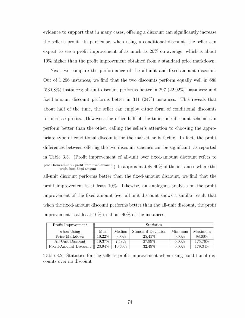
evidence to support that in many cases, offering a discount can significantly increase

the seller’s profit. In particular, when using a conditional discount, the seller can

expect to see a profit improvement of as much as 20% on average, which is about

10% higher than the profit improvement obtained from a standard price markdown.

Next, we compare the performance of the all-unit and fixed-amount discount.

Out of 1,296 instances, we find that the two discounts perform equally well in 688

(53.08%) instances; all-unit discount performs better in 297 (22.92%) instances; and

fixed-amount discount performs better in 311 (24%) instances. This reveals that

about half of the time, the seller can employ either form of conditional discounts

to increase profits. However, the other half of the time, one discount scheme can

perform better than the other, calling the seller’s attention to choosing the appro-

priate type of conditional discounts for the market he is facing. In fact, the profit

differences between offering the two discount schemes can be significant, as reported

in Table 3.3. (Profit improvement of all-unit over fixed-amount discount refers to

profit from all-unit - profit from fixed-amountprofit from fixed-amount

.) In approximately 40% of the instances where the

all-unit discount performs better than the fixed-amount discount, we find that the

profit improvement is at least 10%. Likewise, an analogous analysis on the profit

improvement of the fixed-amount over all-unit discount shows a similar result that

when the fixed-amount discount performs better than the all-unit discount, the profit

improvement is at least 10% in about 40% of the instances.

Profit Improvement Statistics

when Using Mean Median Standard Deviation Minimum MaximumPrice Markdown 10.22% 0.00% 25.45% 0.00% 98.00%

All-Unit Discount 19.37% 7.48% 27.99% 0.00% 175.76%Fixed-Amount Discount 23.94% 10.66% 32.49% 0.00% 179.34%

Table 3.2: Statistics for the seller’s profit improvement when using conditional dis-counts over no discount

74

Profit improvement of All-unit over Fixed-amount Discounts

< −10% −10− 0% 0− 10% 10− 20% 20− 30% 30− 40% 40− 50% > 50%106 893 177 53 49 9 7 2

Table 3.3: Profit difference between all-unit and fixed-amount discounts

3.6.2 Effects of Problem Parameters

In the second numerical study, we investigate how each parameter affects the

performance of conditional discounts, compared to other discount schemes. We sys-

tematically increase the value of each parameter at steps of 0.01, one at a time, from

the three base cases (p > sh, sl < p ≤ sh, and p ≤ sl). This results in a total of

1,400 problem instances, as summarized in Table 3.4. In each problem, we solve for

the optimal discount policies and compare the seller’s profits. Table 3.5 presents the

results.

Scenario θl θh sl sh p t R γ β

Base cases 1 2 1 2 {0.5, 1.5, 2.5} 0.2 0.2 0.2 0.2

Increase θh 1 [2.01, 3] 1 2 {0.5, 1.5, 2.5} 0.2 0.2 0.2 0.2

Increase t 1 2 1 2 {0.5, 1.5, 2.5} [0.21, 1] 0.2 0.2 0.2

Increase R 1 2 1 2 {0.5, 1.5, 2.5} 0.2 [0.21, 0.8] 0.2 0.2

Increase γ 1 2 1 2 {0.5, 1.5, 2.5} 0.2 0.2 [0.21, 1] 0.2

Increase β 1 2 1 2 {0.5, 1.5, 2.5} 0.2 0.2 2 [0.21, 1]

Increase p 1 2 1 2 [0.51, 2.5] 0.2 0.2 2 0.2

Table 3.4: Problem parameters for the numerical study of effects of parameters onthe profit improvement

ScenarioOptimal Policy Vs. Optimal Policy Vs. All-unit Vs.

No Discount a Price Markdown Fixed-AmountMean Median Std. Dev. Mean Median Std. Dev. Mean Median Std. Dev.

Base cases 58.74% 58.74% 81.19% 3.50% 1.33% 4.95% 9.26% 7.79% 10.08%Increase θh 47.38% 1.33% 47.14% 4.53% 1.23% 5.66% 11.43% 10.50% 10.08%Increase t 65.96% 73.08% 50.76% 8.31% 9.17% 8.33% 9.26% 7.79% 8.25%Increase R 58.57% 57.77% 57.48% 3.44% 1.33% 3.98% 9.27% 7.79% 7.79%Increase γ 4.17% 3.01% 11.66% 3.52% 1.72% 4.43% 2.97% 0.07% 5.28%Increase β 65.46% 68.45% 55.81% 8.33% 9.17% 6.57% 9.36% 7.79% 8.42%Increase p 81.52% 91.70% 63.87% 4.74% 1.27% 5.38% 8.67% 7.85% 7.50%

Table 3.5: Statistics for profit improvement with respect to changes in problem pa-rameters

aThe statistics for the comparisons with no discount does not include the case of p > sh since nodiscount profit is zero.

As in Table 3.2, the profit improvement of the optimal policy vs. no discount

and the profit improvement of the optimal policy vs. price markdown in Table 3.5

75

measure the gains in profits from using the better one of the all-unit and fixed-amount

discount. The profit improvement of the all-unit vs. fixed-amount discount measures

the profit difference between using the two types of conditional discounts. From the

table, we observe that an increase in θh, γ, and R lead to a smaller profit improvement;

while, an increase in p, t, and β lead to a larger profit improvement of the optimal

conditional discount over no discount and price markdown. This is because as θh and

γ increase, consumers have larger consumption and higher willingness to pay for the

product. These characteristics of consumers contribute to a larger sales volume in

the market, making it less necessary for the seller to employ a conditional discount to

boost sales. Analogously, when the regular price of the product increases, the sales

volume decreases. In this case, offering a discount is needed in order to generate more

sales, and requiring a minimum purchase quantity for the discount helps improve sales

even further. The profit improvement obtained from the use of conditional discounts

is also strengthened when the market is more deal-prone, caused by a decrease in

R, an increase in t, or an increase in β, following the results we have discussed in

Proposition 3.6.

The profit difference between all-unit and fixed-amount discount is shown to be

most affected by a change in θh and γ. More precisely, the profit difference increases

with θh but decreases with γ. To understand this result, recall from the discussion

of Proposition 3.5 that the all-unit discount is more profitable than the fixed-amount

discount when consumers buy strictly more under the all-unit discount (θ) than un-

der the fixed-amount discount (K, where K < θ). Hence, as θh increases, the profit

difference becomes larger. On the other hand, the fixed-amount discount is more prof-

itable than the all-unit discount when the high-type consumer buys their maximum

consumption level (θh, where θh > K) but receives a larger discount amount under

the all-unit discount (prθh under all-unit; m = prK under fixed-amount). In this

case, the profit difference becomes larger when the discount rate and θh are larger.

76

Notice that the seller is likely to offer a larger discount rate when there are more

low-type consumers in the market (γ small). This explains why the profit difference

decreases with γ.

3.7 Extension

3.7.1 Positive Unit Cost

In our base model, we assume that the unit cost is normalized to 0. Here, we

modify the model to reflect when the seller incurs a unit cost of c for each unit sold,

where 0 < c < p. Notice that a positive unit cost has no effects on the consumer’s

problem since consumers do not observe the cost. Hence, all results regarding the

consumer purchase behavior (Section 3.4) continue to hold.

For the seller’s problem, the presence of a positive unit cost affects the seller’s

profit as follows. The seller’s profit from selling q units under an all-unit discount

DA = (r,K) is given by (p(1 − r) − c)q if q ≥ K, and (p − c)q if q < K. Likewise,

the seller’s profit from selling q units under a fixed-amount discount DF = (m,K) is

given by (p − c)q −m if q ≥ K, and (p − c)q if q < K. Hence, with a positive unit

cost, we find that the region where no discount is optimal becomes larger, and the

region where cognitive overspending is optimal becomes smaller. Consequently, the

following results need to be modified to reflect a positive unit cost. Proposition 3.4

part i), which states that no discount is not optimal as long as there exist deal-prone

consumers, will hold only when the unit cost is not too large. (We can prove that

there exists a threshold c such that the result holds as long as c < c.) Condition b)

of Proposition 3.4 part ii) will be changed from sl < p ≤ sh and γ ≥ slp

to sl < p ≤ sh

and γ ≥ sl−cp−c . Notice that the threshold on γ is smaller with a positive unit cost than

with no unit cost ( sl−cp−c <

slp

), implying that the region where no discount is optimal is

larger. Likewise, the results for the two special cases (Section 3.5.1 and 3.5.2) will be

77

affected in the same way that no discount is more likely to be optimal and cognitive

overspending is less likely to be optimal. Other than these, all other results continue

to hold in presence of a positive unit cost.

3.7.2 Concave Consumer Valuation

In our base model, we assume that a consumer type i ∈ {l, h} has a constant

marginal valuation of si for the first θi units of consumption. Here, we consider an

alternate form of the consumer valuation in which the marginal valuation is linearly

decreasing in the units consumed, as adopted in Chuang and Sirbu (1999). More

precisely, let v0 be the marginal valuation of the first unit of goods. Then, for a

consumer type i, the marginal valuation of the qth unit of goods is given by

vi(q) =

v0(1− qθi

) if 0 ≤ q ≤ θi

0 if q > θi

This implies that a consumer valuation is a concave increasing function of q:

Vi(q) =

q∫0

vi(x)dx =

v0q(1− q2θi

) if 0 ≤ q ≤ θi

v0θi2

if q > θi

Solving the consumer’s problem with this acquisition utility, we obtain similar results

as in Proposition 3.1. That is, the consumer’s optimal purchase quantity under

a conditional discount DA = (r,KA) and DF = (m,KF ) is characterized by two

thresholds: θj(v0, Dk) and θj(v0, D

k), k ∈ {A,F}, such that a type-ij consumer buys

a quantity smaller than Kk at no discount if θi < θj(v0, Dk), buys exactly Kk at

discount if θj(v0, Dk) ≤ θi < θj(v0, D

k), and buys more than Kk at discount if

θi ≥ θj(v0, Dk), i ∈ {l, h}, j ∈ {v, d}. Furthermore, if KA = KF and m = prK,

then θj(v0, DA) = θj(v0, D

F ) and θj(v0, DA) ≤ θj(v0, D

F ). Figure 3.6a and 3.6b

graphically illustrate the consumer’s optimal purchase quantity, qj(θi), under the all-

78

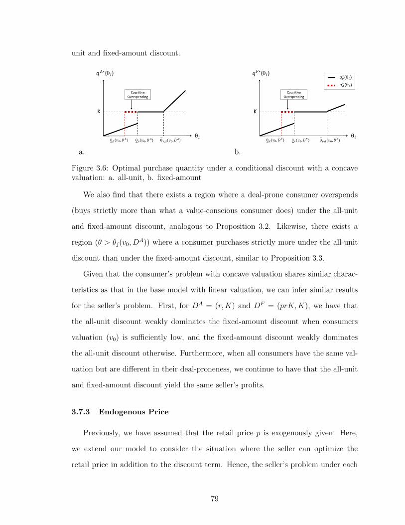
unit and fixed-amount discount.

a.

𝑞𝐴∗(𝑖)

𝑖

K

𝑣(𝑣0, 𝐷𝐴) 𝑣,𝑑(𝑣0, 𝐷

𝐴) 𝑑(𝑣0, 𝐷𝐴)

Cognitive Overspending

b.

𝑞𝐹∗(𝑖)

𝑖

K

𝑣(𝑣0, 𝐷𝐹)

𝑞𝑣∗(𝑖)

𝑞𝑑∗ (𝑖)

𝑣,𝑑(𝑣0, 𝐷𝐹) 𝑑(𝑣0, 𝐷

𝐹)

Cognitive Overspending

Figure 3.6: Optimal purchase quantity under a conditional discount with a concavevaluation: a. all-unit, b. fixed-amount

We also find that there exists a region where a deal-prone consumer overspends

(buys strictly more than what a value-conscious consumer does) under the all-unit

and fixed-amount discount, analogous to Proposition 3.2. Likewise, there exists a

region (θ > θj(v0, DA)) where a consumer purchases strictly more under the all-unit

discount than under the fixed-amount discount, similar to Proposition 3.3.

Given that the consumer’s problem with concave valuation shares similar charac-

teristics as that in the base model with linear valuation, we can infer similar results

for the seller’s problem. First, for DA = (r,K) and DF = (prK,K), we have that

the all-unit discount weakly dominates the fixed-amount discount when consumers

valuation (v0) is sufficiently low, and the fixed-amount discount weakly dominates

the all-unit discount otherwise. Furthermore, when all consumers have the same val-

uation but are different in their deal-proneness, we continue to have that the all-unit

and fixed-amount discount yield the same seller’s profits.

3.7.3 Endogenous Price

Previously, we have assumed that the retail price p is exogenously given. Here,

we extend our model to consider the situation where the seller can optimize the

retail price in addition to the discount term. Hence, the seller’s problem under each

79

discount scheme involves three decision variables: the regular price p, the discount

rate r for all-unit or discount amount m for fixed-amount discount, and the minimum

purchase quantity K. Given large degrees of freedom in the discount terms, there

can be multiple optimal prices for a given problem. However, we can show for each

discount scheme that an optimal price is either p = sl (all consumers are willing to

pay the regular price), p = sh (only high-type consumers are willing to pay the regular

price), or p = shθh+tθh(1−R)

(no consumers are willing to pay the regular price).12

Let pA and pF denote the optimal price under the all-unit and fixed-amount dis-

count, respectively. If pA = pF , then all results in the base model with exogenous

price follow immediately. Otherwise, Proposition 3.5 implies that the all-unit discount

can be better than the fixed-amount discount only when pA = shθh+tθh(1−R)

. Likewise, the

fixed-amount discount can be better than the all-unit discount only when pF is sl

or sh. Furthermore, we can show that the result in Proposition 3.5 part i), which

states that price markdown is an optimal all-unit discount for β < β still holds, and

we continue to have that the optimal all-unit and fixed-amount discount result in

identical outcome when consumers have homogeneous valuation but different levels

of deal-proneness, as in Proposition 3.8.

3.8 Conclusion

Motivated by consumer behavior in retailing, this chapter discusses how price

promotions influence purchase decisions of different types of consumers, and which

type of promotions is most profitable to the seller under which market situations.

We consider a market where consumers can be heterogeneous in two dimensions:

willingness to pay for the product and the deal-proneness to a discount offer, and focus

on two popular types of conditional promotions: all-unit discount and fixed-amount

discount. Our study shows that deal-prone consumers may be induced to overspend

12See Appendix B for the proof.

80

when offered a conditional discount. As a result, retailers can employ conditional

discounts to effectively improve their profitability, especially when facing a market of

consumers with low willingness to pay and high deal-proneness. We find, however,

that it is not always optimal for the seller to induce consumer overspending. Only

when there is a sufficiently large proportion of highly deal-prone or high-valuation

consumers in the market that inducing overspending can be profitable.

Another key finding is that, depending on the market, one conditional discount

scheme can perform better than the other. We show that when consumers are not

willing to pay the regular price for the product, the all-unit discount outperforms

the fixed-amount discount because only the all-unit discount can induce consumers

to buy strictly more than the minimum quantity required for the discount. On the

other hand, when some consumers are already willing to pay the regular price, the

fixed-amount discount is more profitable than the all-unit discount. In this case, the

fixed-amount discount awards only a limited discount amount, less than that awarded

under the all-unit scheme, to the consumers who otherwise would voluntarily pay the

regular price. Hence, it allows the seller to maintain a greater profit margin. Based

on these findings, an important implication is that an all-unit discount should be

adopted to stimulate sales of a high price tag product or a newly-launched item;

while, a fixed-amount discount is more effective as a frequent promotion of a low

price tag or established brand-named product. Our key results are shown robust

to changes in modeling assumptions, suggesting that the insights from this chapter

apply to a broad range of realistic retailing situations.

There are a few aspects of price promotions and consumer psychology relevant to

our problem that are not included in the current study, but can serve as interesting fu-

ture research directions. We will discuss two major areas here. The first area involves

post-promotion effects. As reported in several studies, price promotions may lead

consumers to experience sticker shock due to the downward price expectation they

81

develop after seeing the product sold at a cheaper price during the promotion period

(DelVecchio et al., 2007). Such effect may be more or less intense under different dis-

count schemes, and may pose a limitation on the discount rate that should be offered.

These factors could affect the profitability of conditional discounts, which may lead

to different results from this essay. The second area is framing and promotional vehi-

cles. When consumers make a purchase decision in an actual shopping scenarios, they

are sometimes influenced by how a promotion is framed (e.g., dollars-off, percent-off,

Buy-X-Get-Y-Free, Buy-X-for-Y) and how it is awarded (e.g., coupons, straight off

the shelf) in addition to the discount term. For example, Chen et al. (1998) reported

that for high-price products, a price reduction framed in dollar terms was perceived

more significant than the same price reduction framed in percentage terms. Dhar

and Hoch (1996) found that coupons lead to higher sales compared to straight-off-

the-shelf price discounts. Taking consumer psychological response to different forms

of promotions into account, the seller’s joint decision on the discount term and its

vehicle can be complicated, yet meaningful to study.

82

CHAPTER 4

Dynamic Pricing or Dynamic Logistics?

4.1 Introduction

An important operational problem faced by retailers is how to most effectively

match inventory to customer demand over a selling horizon. This problem becomes

especially challenging for retailers who sell their products through multiple channels

or stores. While multi-channel retailing is found to be associated with enhanced

customer loyalty and sales growth, it requires extra efforts in coordinating channel

strategies to efficiently serve customers across channels (Neslin et al., 2006). If not

managed well, a multi-channel environment could result in a supply-demand mis-

match, and hurt the retailer. For example, Best Buy reported that 2 to 4 percent of

its online traffic did not result in a purchase because the inventory was out of stock

at distribution centers, and hence, was shown on the website as unavailable. The

company estimated, however, that in 80 percent of those cases, the products were in

fact available at one of its stores. The Best Buy CEO Hubert Joly admitted that

this lost sales due to the stockouts at their online channel represented a very large

number (Schinkel , Jun. 25, 2013; Blair , Jul. 1, 2013).

To efficiently balance inventory and demand in a multi-channel environment, re-

tailers may deploy various tools from marketing and supply chain management. The

most common marketing tools involve some form of pricing and promotions, aiming

83

to shape demand to match with available inventory at each channel. These are often

implemented through channel-specific discounts or promotions such as online-only

sale events at Forever21, and in-store-only coupons at Staples. In fact, a number

of major retailers like JC Penney, Kohl’s, and Walmart, explicitly state under their

pricing policies that they do not match the prices of an item sold in-store and online

(DeNicola, May 13, 2013). JC Penney explains that it may offer a clearance discount

on an online item if it does not sell as quickly as it does it store (Brownell , May 31,

2013); whereas, Walmart attributes this pricing policy to differences in distribution,

regional competition and other factors (Walmart.com).

Alternatively, retailers can better manage and allocate their inventory across mul-

tiple channels in pace of sales. For example, retailers like Macy’s, Nordstrom, and

Toys ‘R’ Us leverage their store inventory to fulfill online orders through the practice

known as “ship-from-store distribution” (Lynch, Jul. 18, 2013). A Canadian clothing

company, Roots, utilizes inventory for online orders to fulfill an in-store purchase by

offering to ship items, which are out of stock in stores, to an in-store customer’s house

(Financial-Post , Sep. 24, 2013).

Although both pricing and inventory strategies are intended to serve the same

purpose of reducing supply-demand mismatch and increasing the firm’s profit, many

retailers choose to adopt both of these strategies, sometimes in an uncoordinated

way. This raises an important research question as to whether managing the supply-

demand balance in a multi-channel environment using a pricing tool or an inventory

tool is more effective under which situations. Furthermore, if a retailer uses both

tools, how do they interact with each other?

In this chapter, we consider a dual-channel retailer selling over a finite horizon.

The retailers in this category include many of the major department stores, electron-

ics stores, and fashion retailers, who offer short life-cycle products both online and

in physical stores (“brick-and-click” retailers). Facing uncertain and price-sensitive

84

demand at each channel, the retailer may use a pricing strategy (charging different

prices at different channels), or a transshipment strategy (transferring inventory be-

tween store and distribution center) 1 to maximize total profits from sales. We are

interested in answering the following research questions:

1. What is the optimal dynamic pricing and transshipment strategy?

2. What factors affect the benefit of price differentiation and transshipment?

3. Is transshipping inventory more or less effective than differentiating prices under

which situations?

4. If the retailer adopts both price-differentiating and transshipment strategies,

how is the optimal pricing decision influenced by the transshipping decision,

and vice versa?

We model a joint dynamic pricing and transshipping problem, where the retailer

incurs a unit transaction cost when selling the product at each channel, and a unit

transshipping cost when making a transshipment of inventory between the channels.

An arriving customer decides whether to purchase the product from one of the avail-

able channels, based on her valuations and the observed prices at the channels. In

this setting, although both channels sell the same product, the customer may de-

rive different utilities when purchasing from different channels due to the nature of

transactions (e.g. ability to try on) and associated costs (e.g. shipping fee) involved.

Hence, the product sold at one channel can be perceived as a different product from

the product sold at the other channel. This justifies the assumption that the customer

choice model follows the multinomial logit (MNL) model, which is widely used in the

multi-product literature.

1This is an instance of lateral transshipments (stock movements between locations of the sameechelon (Paterson et al., 2011))

85

To answer the research questions, we first consider the situation where the re-

tailer can adopt either a price differentiation policy or an inventory transshipment

policy in the current period, but not both. We characterize the retailer’s optimal

dynamic pricing and transshipping policies. Our findings show that the optimal price

differentiation policy always results in a larger probability of making a sale in the

current period, compared to what would happen under the optimal uniform pricing

policy. On the other hand, a transshipment in the current period may or may not

be profitable, and an optimal transshipment decision may result in either a larger or

a smaller probability of making a sale in the current period. We also investigate the

factors that affect the benefit from adopting a price differentiation policy or a trans-

shipment policy. Next, we consider the situation where the retailer can utilize both

price differentiation and inventory transshipment. We show that transshipment can

increase the value of the remaining inventory at the channel from which the trans-

shipment is made, allowing the retailer to charge a higher price for the product at

the channel. Transshipment can also be used to replenish stock at the channel that

stocks out. This makes it possible for the retailer to continue selling the product at

both channels and benefit from price differentiation.

To further investigate the benefit of price differentiation and transshipment, we

conduct a numerical study. Our results show that the benefit of price differentiation

is generally larger than the benefit of transshipment. However, when the retailer’s

inventory position is significantly out of balance (e.g. very low inventory at the

channel with high customer valuation), transshipment can be more effective than

price differentiation. We also find that the benefit of price differentiation and the

benefit of transshipment may either substitute or complement each other. When the

retailer’s inventory position is unfavorable (low inventory at the high-margin channel),

the two mechanisms substitute each other since the retailer can use either mechanism

to try to adjust his inventory position in the intended direction. On the other hand,

86

when the retailer’s inventory position is already favorable (high inventory at the

high-margin channel), the same balance of the inventory levels at the channels should

be maintained. In this case, the two mechanisms are complementarily employed to

influence the inventory position in the opposite direction, so that the balance is kept.

4.2 Literature Review

Our research problem lies in the area of both dynamic pricing and transship-

ment decisions for multi-channel retailers. These two topics have been studied in the

Operations Management as well as the Marketing literature. We will review three

main streams of relevant work: dynamic pricing, transshipment for multi-location or

multi-channel retailers, and joint dynamic pricing and inventory policies.

Dynamic pricing problems have received much attention from the academia due to

its popularity and practicality in many industries. One of the most influential works

in this field is Gallego and van Ryzin (1994), who consider a dynamic pricing problem

of a single product over a finite horizon, and show that the optimal price is strictly

decreasing in the stock level but increasing in the length of the selling horizon. A

similar problem is considered in Bitran and Mondschein (1997), with extensions to

periodic-review pricing and pricing policies with announced discounts. Their compu-

tational experiments reveal that loss of profits when using periodic review instead of

continuous review is small. With announced discounts, the resulting optimal prices

allow the store to sell most of the merchandise during the first periods and avoid

offering large discounts toward the end of the horizon. A natural extension of these

works is to consider a dynamic pricing problem for multiple products. When a firm

sells multiple products, the demand for each product may be influenced by the avail-

ability and price of the other products that the customers consider as substitutes.

This gives rise to research problems on dynamic pricing of substitutable products.

A similarity between the setting where a retailer sells substitutable products and

87

our setting where the retailer sells an identical product through multiple channels is

that a customer’s decision on which product to buy or where to buy it from depends

on her valuations and prices of all the possible choices. Hence, we assume our cus-

tomer choice model is characterized by the MNL model, which is widely used among

the substitutable products literature. Dong et al. (2009) study a dynamic pricing

problem of multiple substitutable products, where the customer’s choice is explained

by the MNL model. They show that dynamic pricing converges to static pricing as

inventory levels of all products approach the number of remaining selling periods.

Furthermore, their numerical findings, considering only two substitutable products,

suggest that the performance of unified dynamic pricing (charging the same price for

all products) is closest to that of the full-scale dynamic pricing especially when the

quality difference among the products decreases. Suh and Aydin (2011) considers a

dynamic pricing problem of two substitutable products; they also adopts the MNL

model to describe the customer’s choice. They provide analytical results showing that

the marginal value of an item is increasing in the remaining time and decreasing in

the stock level of either product; however, the optimal prices of an item do not always

behave in the same direction as the marginal value. Another multi-product pricing

paper using logit models is Li and Huh (2011). They consider the nested logit model

and show the concavity of the seller’s profit function with respect to market shares

in a single-period setting. This result can be applied to other settings, including the

joint inventory and dynamic pricing problem, to find optimal policies. While these

papers consider similar customer choice model and seller’s dynamic pricing problem

to ours, they do not consider inventory transshipments since the substitutable prod-

ucts in their settings are not identical. Additionally, no analytical results regarding

the benefits of price differentiation are provided.

Another group of pricing papers which are relevant to our work is in the area of

multi-channel pricing. According to some earlier studies and practitioners’ beliefs,

88

retailers generally keep consistent prices across distribution channels to maintain a

strong brand and to avoid customers’ irritation due to the perception of price unfair-

ness (Neslin et al., 2006; Campbell , 1999). However, other studies argue that channel-

based price differentiation could be justified by differences in channel characteristics

and the fact that consumers derive different utility from various distribution channels

(Chu et al., 2007; Kacen et al., 2003). Hence, options to differentiate price levels

among channels can in fact create opportunities for firms to improve their pricing

strategies (Sotgiu and Ancarani , 2004). Based on data collected from multi-channel

retailers, Wolk and Ebling (2010) find that many multi-channel retailers do engage in

channel-based price differentiation, with some indication that this tendency increases

over time. Analytical works on multi-channel pricing mostly consider a dual-channel

seller selling a product through a physical store and an online store. Yan (2008) as-

sumes that customers value a purchase from the physical store more than that from

the online store. It is shown that the optimal online price is higher than the physical

store price if and only if the marginal cost to sell the product online is far larger

than the marginal cost to sell through the physical channel. Shen and Zhang (2012)

consider a market with two groups of customers: fashion customers who value an

online purchase more, and traditional customers who value a physical-store purchase

more. They show that when there exist enough fashion customers and the unit cost

for the online channel is low, it is profitable for the seller to offer the product through

the online channel in addition to the traditional store, and charge a higher price.

These papers consider a pricing problem of a dual-channel retailer similar to our es-

say. However, they study a single-period problem with different customer’s choice

models from ours, and without inventory or transshipment consideration.

The second stream of relevant literature is on inventory transshipments in a multi-

location system. Rudi et al. (2001) study a problem of two retail firms at distinct

locations selling the same product; the firm who runs out of stock may receive a

89

transshipment from the other firm with surplus inventory at a cost. Under central

coordination, this problem is similar to our transshipment problem in the sense that

the system’s objective is to make transshipment decisions which maximize the total

profits. However, they consider a single-period model, where demand at the two loca-

tions are independent and retail prices are exogenously given. A multi-period setting

is considered in Hu et al. (2005), where a centralized-ordering system of N stores

periodically decides on order sizes, allocation quantities, and if necessary, emergency

transshipments among the stores, in order to minimize the total expected cost until

the end of the horizon. Since they focus on inventory problems and the systems’s

objective is to minimize costs rather than maximize profits, dynamic pricing is not

addressed. For additional review of inventory transshipment literature, please see

Paterson et al. (2011).

The closest literature to the current essay is in the area of joint dynamic pricing

and inventory policies. A joint dynamic pricing and inventory problem of a distri-

bution system consisting of multiple geographically dispersed retailers is considered

in Federgruen and Heching (2002). In each period, the system decides on size of a

replenishment, the price to be charged, and the allocation of any arriving order to

the retailers. They provide an approximate model where a base-stock/list-price pol-

icy is optimal. The optimal price is shown to be nonincreasing in the system-wide

inventory position. What differentiates our work form their work is that we allow

prices at different locations to differ; whereas, in their model, the price in each period

is applied to all stores. Moon et al. (2010) study a joint dynamic pricing and inven-

tory problem in a dual-channel supply chain system. A customer chooses to buy the

product from the channel where she receives a larger surplus. Under the vertical in-

tegration setting, the manufacturer decides on the production quantity as well as the

price for each channel. Their inventory problem is rather different from ours because

they assume that production can occur at any time. Hence, there are no stockouts,

90

and no need for transshipments in their model. Another relevant work in this area

is Ceryan et al. (2013), who study a joint dynamic pricing and capacity allocation

problem for two substitutable products sharing a flexible resource. Their results sug-

gest that the availability of a flexible resource helps maintain stable price differences

across products over time even though the price of each product may fluctuate. The

allocation of a flexible resource among substitutable products is similar to the option

to transship inventory among the channels in our model. However, in their setting,

the products can be replenished in each period; while, in our setting, the inventory

is not replenishable. This difference can lead to different implications of inventory

decisions on the system’s performance. The closest work to ours in terms of inventory

model is Bitran et al. (1998), considering a dynamic pricing problem of a retail chain

of multiple stores, who has an option to transfer merchandise among stores at a cost.

They propose a heuristic and numerically show that it performs better than the cur-

rent practice in a fashion retail chain in Chile. While the transshipment problem in

their paper is similar to the transshipment problem that we consider, there are some

notable differences in other dimensions. Their paper considers coordinated prices and

independent demand among stores. On the other hand, we allow different stores to

charge different prices and let a customer’s purchase decision depend on her valua-

tions and prices of all stores. Furthermore, we analytically characterize the optimal

pricing and transshipping policies, and investigate their benefits to the retailer.

To our best knowledge, we are the first to consider a joint dynamic price differ-

entiating and inventory transshipping policy for a dual-channel retailer. This model

enables us to answer important questions regarding best practices in pricing and

transshipping strategies, which have not been addressed by existing literature, for

instance: How do transshipping policies affect pricing policies, and vice versa? Is

transshipping more or less effective than pricing, under what situations? We address

these questions in subsequent sections.

91

4.3 Model

We consider a retailer who sells a seasonal product through two channels (e.g.

“brick-and-click” retailer who sells products both online and at a physical store,

retailer who has two physical stores at different locations) over a finite horizon of

length T . Since the selling horizon is short, we assume no replenishment can take

place during the horizon. No salvage value is obtained for unsold units at the end

of the horizon. Stocks of the product are kept at two separate locations, dedicated

for demand arriving at each channel. At the beginning of period t = 1, ..., T , the

inventory level is denoted by It = (I t1, It2), where I ti ≥ 0 is the level of inventory to

satisfy demand at channel i ∈ {1, 2}. The retailer decides on i) whether to transship

any stock from one channel to the other2, and ii) how much to charge for the product

sold at each channel.

The retailer’s transshipment decision is characterized by st = (st12, st21), where stij

is the amount of inventory being transshipped from channel i to channel j, i 6= j.

For simplicity, any transshipment is assumed to occur instantaneously and before a

customer arrival in each period.3 Let Yt = (Y t1 , Y

t2 ), where Y t

i = I ti + stji − stij, i, j ∈

{1, 2} denote the inventory level at channel i after a transshipment is made in period

t. Notice that a transaction can occur at channel i only when Y ti > 0. We let

A(Yt) = {i : Y ti > 0} denote the set of channels with the product available in stock.

The retailer’s pricing decision is characterized by pt = (pt1, pt2), where pti is the

price of a unit of product sold at channel i in period t. In each period, a pricing

policy pt is made based on the updated inventory level Yt, and is announced before

a customer arrival.

2A transshipment in our setting refers to the practice where inventory dedicated for a channel isused to satisfy demand at the other channel with or without the actual transfer of inventory betweentwo warehouses.

3Transshipment lead times can be incorporated with slight modifications.

92

4.3.1 Customer Choice Model

We assume that each period is short enough that at most one customer arrives,

and each customer buys at most one unit of the product. The probability that a

customer arrives and demands the product in a single period t is λt ∈ [0, 1]. Due to

easy access to price and availability information nowadays, we assume that an arriv-

ing customer can observe the product price and availability at both channels before

making a purchase decision. Hence, pt1, pt2, and A(Yt) are known to the customer.4

The customer only considers purchasing the product from one of the channels with

product availability (i ∈ A(Yt)). We adopt a multinomial logit model (MNL), which

has been extensively used in the marketing and operations management literature,

to describe the choice of an arriving customer to make a purchase from one of the

available channels, or neither. The MNL model nicely captures both the known and

random factors that influence the purchase decision of a utility-maximizing customer

in a dual-channel setting while still providing desirable properties, which make the

analyses tractable.

Let Ui = vi − pi + ζi be a customer’s net utility from purchasing a unit of the

product from channel i ∈ A(Yt) at price pi, where vi denotes the customer’s net

valuation from the purchase, and ζi is a Gumbel error term with mean 0 and shape

parameter 1. The customer’s net valuation vi represents the product valuation ad-

justed for channel-specific (dis)utilities. These include, for instance, the ability to try

on the product, traveling time, customer service, time until the product arrives, etc.

Although the customer’s valuation of the product itself should generally be the same

for both channels, the customer may have shopping preferences for a channel over

the other, resulting in different net valuation of the purchase at each channel. The

random variable ζi represents the utility influenced by unobservable characteristics.

4Customers do not need to know the exact inventory level at each channel, but they can observewhether the product is in stock or out of stock at each channel.

93

We assume that ζ1 and ζ2 are independent and identically distributed.

Let µi be the probability that an arriving customer purchases from channel i ∈

{1, 2}, and µ0 be the probability that the customer does not purchase. Then, we have

the following well-known results from the MNL model (Luce, 1959; McFadden, 1974),

adjusted for the condition for the product availability (Suh and Aydin, 2011):

µi(pt, A(Yt)) =

exp(vi−pti)

1+∑j∈A(Yt) exp(vi−pti)

if i ∈ A(Yt)

0 if i /∈ A(Yt)(4.1)

µ0(pt, A(Yt)) =1

1 +∑

j∈A(Yt) exp(vi − pti)

For notational simplicity, we will sometimes write µi(pt, A(Yt)) as µi when pt

and A(Yt) are clearly stated in the context.

4.3.2 Retailer’s Problem

In a period t = 1, ..., T , the retailer’s problem is to decide whether to make a

transshipment from one channel to the other: st = (st12, st21), and what price to

charge for the product sold at each channel: pt = (pt1, pt2). Notice that if the product

is out of stock at channel i (Y ti = 0), then pti becomes irrelevant since a customer will

never consider buying the product from channel i. We let pti →∞ for i /∈ A(Yt).

The unit transshipment cost from channel i to channel j is mij ≥ 0. To avoid un-

necessary transshipments, we assume that st12 · st21 = 0. Since a transshipment occurs

instantaneously, we can innocuously restrict the retailer’s transshipment decision to

be such that a positive transshipment may be made only when the current inventory

at the destination channel is zero.5 Furthermore, since the retailer can sell at most

one unit in each period, there is no need to transship more than one unit at a time.

As a result, the transshipment decisions in our model can be simplified to stij ∈ {0, 1}5This practice corresponds to “reactive transshipment,” as opposed to “proactive transshipment”,

in Paterson et al. (2011).

94

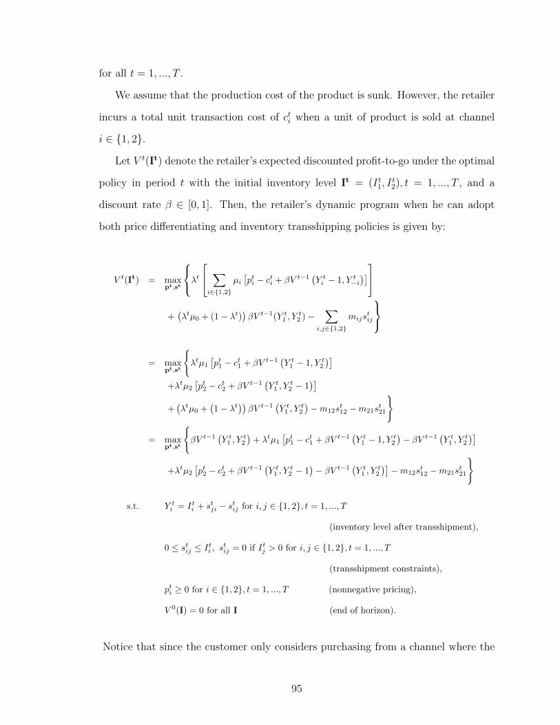
for all t = 1, ..., T .

We assume that the production cost of the product is sunk. However, the retailer

incurs a total unit transaction cost of cti when a unit of product is sold at channel

i ∈ {1, 2}.

Let V t(It) denote the retailer’s expected discounted profit-to-go under the optimal

policy in period t with the initial inventory level It = (I t1, It2), t = 1, ..., T , and a

discount rate β ∈ [0, 1]. Then, the retailer’s dynamic program when he can adopt

both price differentiating and inventory transshipping policies is given by:

V t(It) = maxpt,st

λt ∑i∈{1,2}

µi[pti − cti + βV t−1

(Y ti − 1, Y t−i

)]+(λtµ0 + (1− λt)

)βV t−1(Y t1 , Y

t2 )−

∑i,j∈{1,2}

mijstij

= max

pt,st

{λtµ1

[pt1 − ct1 + βV t−1

(Y t1 − 1, Y t2

)]+λtµ2

[pt2 − ct2 + βV t−1

(Y t1 , Y

t2 − 1

)]+(λtµ0 +

(1− λt

))βV t−1

(Y t1 , Y

t2

)−m12s

t12 −m21s

t21

}

= maxpt,st

{βV t−1

(Y t1 , Y

t2

)+ λtµ1

[pt1 − ct1 + βV t−1

(Y t1 − 1, Y t2

)− βV t−1

(Y t1 , Y

t2

)]+λtµ2

[pt2 − ct2 + βV t−1

(Y t1 , Y

t2 − 1

)− βV t−1

(Y t1 , Y

t2

)]−m12s

t12 −m21s

t21

}

s.t. Y ti = Iti + stji − stij for i, j ∈ {1, 2}, t = 1, ..., T

(inventory level after transshipment),

0 ≤ stij ≤ Iti , stij = 0 if Itj > 0 for i, j ∈ {1, 2}, t = 1, ..., T

(transshipment constraints),

pti ≥ 0 for i ∈ {1, 2}, t = 1, ..., T (nonnegative pricing),

V 0(I) = 0 for all I (end of horizon).

Notice that since the customer only considers purchasing from a channel where the

95

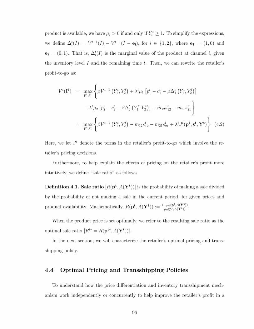
product is available, we have µi > 0 if and only if Y ti ≥ 1. To simplify the expressions,

we define ∆ti(I) = V t−1(I) − V t−1(I − ei), for i ∈ {1, 2}, where e1 = (1, 0) and

e2 = (0, 1). That is, ∆ti(I) is the marginal value of the product at channel i, given

the inventory level I and the remaining time t. Then, we can rewrite the retailer’s

profit-to-go as:

V t(It) = maxpt,st

{βV t−1

(Y t

1 , Yt

2

)+ λtµ1

[pt1 − ct1 − β∆t

1

(Y t

1 , Yt

2

)]+λtµ2

[pt2 − ct2 − β∆t

2

(Y t

1 , Yt

2

)]−m12s

t12 −m21s

t21

}

= maxpt,st

{βV t−1

(Y t

1 , Yt

2

)−m12s

t12 −m21s

t21 + λtJ t(pt, st,Yt)

}(4.2)

Here, we let J t denote the terms in the retailer’s profit-to-go which involve the re-

tailer’s pricing decisions.

Furthermore, to help explain the effects of pricing on the retailer’s profit more

intuitively, we define “sale ratio” as follows.

Definition 4.1. Sale ratio [R(pt, A(Yt))] is the probability of making a sale divided

by the probability of not making a sale in the current period, for given prices and

product availability. Mathematically, R(pt, A(Yt)) := 1−µ0(pt,A(Yt))µ0(pt,A(Yt))

.

When the product price is set optimally, we refer to the resulting sale ratio as the

optimal sale ratio [Rt∗ = R(pt∗, A(Yt))].

In the next section, we will characterize the retailer’s optimal pricing and trans-

shipping policy.

4.4 Optimal Pricing and Transshipping Policies

To understand how the price differentiation and inventory transshipment mech-

anism work independently or concurrently to help improve the retailer’s profit in a

96

dual-channel environment, we consider situations where the retailer implements each

mechanism alone, and when he can implement both mechanisms together. To rep-

resent different policy options, we will denote a joint pricing-transshipping policy

with AB, where A ∈ {u, d} denotes the pricing option (u for uniform pricing, d for

differentiated pricing), and B ∈ {n, t} denotes the transshipment option (n for no

transshipment, t for transshipment). For example, if the retailer adopts a policy of

type dt, he can set different prices at the two channels, and make an inventory trans-

shipment from the non-empty location to the empty location. On the other hand,

under a policy of type un, the retailer always sets the same price at both channels,

and cannot transfer any inventory between the channels. Table 4.1 summarizes the

four types of policies we consider in this essay.

Price Differentiation No Transshipment With TransshipmentYes dn dtNo un ut

Table 4.1: Possible pricing and transshipping policies

As a benchmark, we first study the base model where the retailer adopts a uniform

pricing policy without transshipment.

4.4.1 Base Model: Uniform Pricing and No Transshipment

When the retailer charges the same price for the product sold at both channels

and when transshipment is not an option, the retailer’s only decision is the optimal

uniform price for each period. In this case, the retailer’s dynamic program is given

by equation (4.2), with the following constraints:

Y ti = I ti for i, j ∈ {1, 2}, t = 1, ..., T ,

stij = 0 for i, j ∈ {1, 2}, t = 1, ..., T (no transshipment),

pt1 = pt2 = pt ≥ 0 for t = 1, ..., T (uniform pricing),

V 0(I) = 0 for all I.

97

Let V tun denote the retailer’s optimal profit-to-go under uniform pricing and no trans-

shipment. Then,

V tun(It) = max

pt

{βV t−1

un

(I t1, I

t2

)+ λtJ t(pt, It)

}. (4.3)

We derive the retailer’s optimal uniform dynamic pricing policy under two sce-

narios: i) when inventory is in stock at both channels, and ii) when inventory runs

out at one channel. (If inventory runs out at both channels, the selling horizon ends

immediately.) In the first scenario, the retailer can expect to make a sale at each

channel with a positive probability. However, in the second scenario, the retailer can

never make a sale at the channel where the stockout occurs, regardless of the price.

Without loss of generality, when analyzing the stockout scenario, we assume that the

inventory runs out at channel 1. The results for the case when the inventory runs out

at channel 2 is analogous. Proposition 4.1 characterizes the optimal uniform dynamic

pricing and the optimal profit.

Proposition 4.1. For any remaining time t = 1, ..., T and inventory level It, the

optimal uniform pricing policy without transshipment is as follows:

1. If I t1 > 0 and I t2 > 0, the optimal uniform price pt∗un is unique and it satisfies

pt∗un =exp(v1)(ct1+β∆t

1(It))+exp(v2)(ct2+β∆t2(It))

exp(v1)+exp(v2)+ 1

µ0(pt∗un). The retailer’s expected dis-

counted profit-to-go under the optimal policy is given by V tun(It) = [exp(v1 −

pt∗un) + exp(v2 − pt∗un)]λt + βV t−1un (It) = Rt∗

unλt + βV t−1

un (It).

2. If I t1 = 0 and I t2 > 0, the optimal uniform price pt∗un is unique and it satisfies

pt∗un = ct2 + β∆t2(It) + 1

µ0(pt∗un). The retailer’s expected discounted profit-to-go

under the optimal policy is given by V tun(It) = exp(v2 − pt∗un)λt + βV t−1

un (It) =

Rt∗unλ

t + βV t−1un (It).

When there is no stockout, the optimal uniform price consists of two components.

The first component is a weighted average of the sum of the marginal value and

98

the unit transaction cost associated with each channel. This quantity depends on

how likely a customer will buy from each channel. Since the price is uniform, what

determines the purchase decision is simply the net valuation of the purchase, v1 and

v2. The optimal price is more influenced by the marginal value and transaction cost

of the channel from which a customer is more likely to make a purchase. The other

component of the optimal price is a base premium, 1µ0(pt∗un)

, which goes up with the

probability that the customer makes a purchase from one of the channels.

When there is a stockout at a channel, the optimal uniform price has similar

characteristics as in the no stockout case. That is, it includes a base premium on top

of the marginal value and the unit transaction cost of the product. The only difference

is that the optimal price in the stockout case involves only the marginal value and the

unit transaction cost of the product at the channel with available inventory. This is

because the product can never be sold from the stockout channel. The base premium

remains the same as that under the no stockout case.

Next, we investigate the retailer’s optimal pricing policy when the price at the

two channels can be differentiated.

4.4.2 Price Differentiation and No Transshipment

Suppose the retailer can charge different prices for the product sold at different

channels, but cannot transfer inventory between channels. Then, the retailer’s pricing

problem becomes similar to a standard dynamic pricing problem of two substitutable

products (e.g., Suh and Aydin 2011). The retailer’s dynamic program in this case is

similar to (4.3) except that pt1 and pt2 in each period can be different, and hence, ∆ti

under this pn policy can be different from that under the un policy. Let V tdn denote

the retailer’s optimal profit-to-go under price differentiation and no transshipment.

99

Then,

V tdn(It) = max

pt

{βV t−1

dn

(I t1, I

t2

)+ λtJ t(pt, It)

}, pt = (pt1, p

t2). (4.4)

Under this pricing policy, only the prices at the channels where the product is available

are relevant. Hence, when there is a stockout at channel 1, the retailer essentially sets

only one price at channel 2. This optimal price corresponds to the optimal uniform

price in the stockout case, as characterized by Proposition 4.1 part 2. The retailer

can take advantage of price differentiation only when the product is available at both

channels. We characterize the optimal dynamic pricing policy in Proposition 4.2.

Proposition 4.2. For any remaining time t = 1, ..., T and inventory level It, the

optimal dynamic pricing policy without transshipment is as follows:

1. If I t1 > 0 and I t2 > 0, the optimal price pair (pt∗1 , pt∗2 ) is unique and it satisfies

pt∗i = cti + 1µ0(pt∗1 ,p

t∗2 )

+ β∆ti(I

t). The retailer’s expected discounted profit-to-go

under the optimal price differentiation policy is given by V tdn(It) = [exp(v1 −

pt∗1 ) + exp(v2 − pt∗2 )]λt + βV t−1dn (It) = Rt∗

dnλt + βV t−1

dn (It).

2. If I t1 = 0 and I t2 > 0, the optimal price at channel 2, pt∗2 , is the same as the

optimal uniform price for the same inventory level.

Under the price differentiation policy, when there is no stockout, we see that the

optimal price for each channel has a similar structure as the optimal uniform price

discussed in Proposition 4.1 part 1. That is, the optimal channel price consists of the

marginal value and unit transaction cost, specific to the channel, as well as the base

premium, which is the same for both channel. Alternatively, we can view this result

as the optimal margin pt∗i − cti for each channel is the sum of the marginal value of

the product in the channel and a base premium, which is channel-independent.

Now that we have characterized the retailer’s optimal pricing policies, we can

compare the retailer’s profit under the price differentiation and uniform pricing policy

100

to see the benefit of price differentiation for a dual-channel retailer. Since many

problem variables are time-dependent, we focus our comparisons on the retailer’s

profit under different pricing policies in a single period in order to provide clean

results that highlight the benefit of the price differentiation strategy. For this, we

consider the benefit from price differentiation as how much profit the retailer can

gain if he is allowed to price differentiate in period t only, as supposed to using a pure

uniform pricing policy.6

Corollary 4.1 shows that the optimal sale ratio under price differentiation is always

greater than or equal to the optimal sale ratio under uniform pricing. This implies

that the retailer’s ability to price discriminate between the two channels allows him

to strategically convert more of the customer traffic into sales. In fact, as shown in

Proposition 4.3, the larger the sale ratio he can induce using price differentiation, the

more profit he can generate.

Corollary 4.1. For any remaining time t = 1, ..., T and inventory level It, the optimal

sale ratio under price differentiation is greater than or equal to the optimal sale ratio

under uniform pricing: Rt∗dn ≥ Rt∗

un.

Proposition 4.3. For any remaining time t = 1, ..., T and inventory level I t where

I t1 > 0 and I t2 > 0, the benefit from using price differentiation in the current period is

monotonically increasing with the sale ratio difference, Rt∗dn −Rt∗

un.

Due to differences in customer preferences and nature of the transactions taken

place at different channels, the customer willingness to pay and the costs incurred

by the retailer when selling the product at each channel generally differ across the

channels. Price differentiation allows the retailer to reflect such differences on the

product prices. That is, the retailer can charge a high price at the channel where

the customer has high willingness to pay and/or the transaction cost is high in order

6Alternatively, we can consider how much the retailer will lose if constrained to offer a uniformprice in period t only. The same results hold.

101

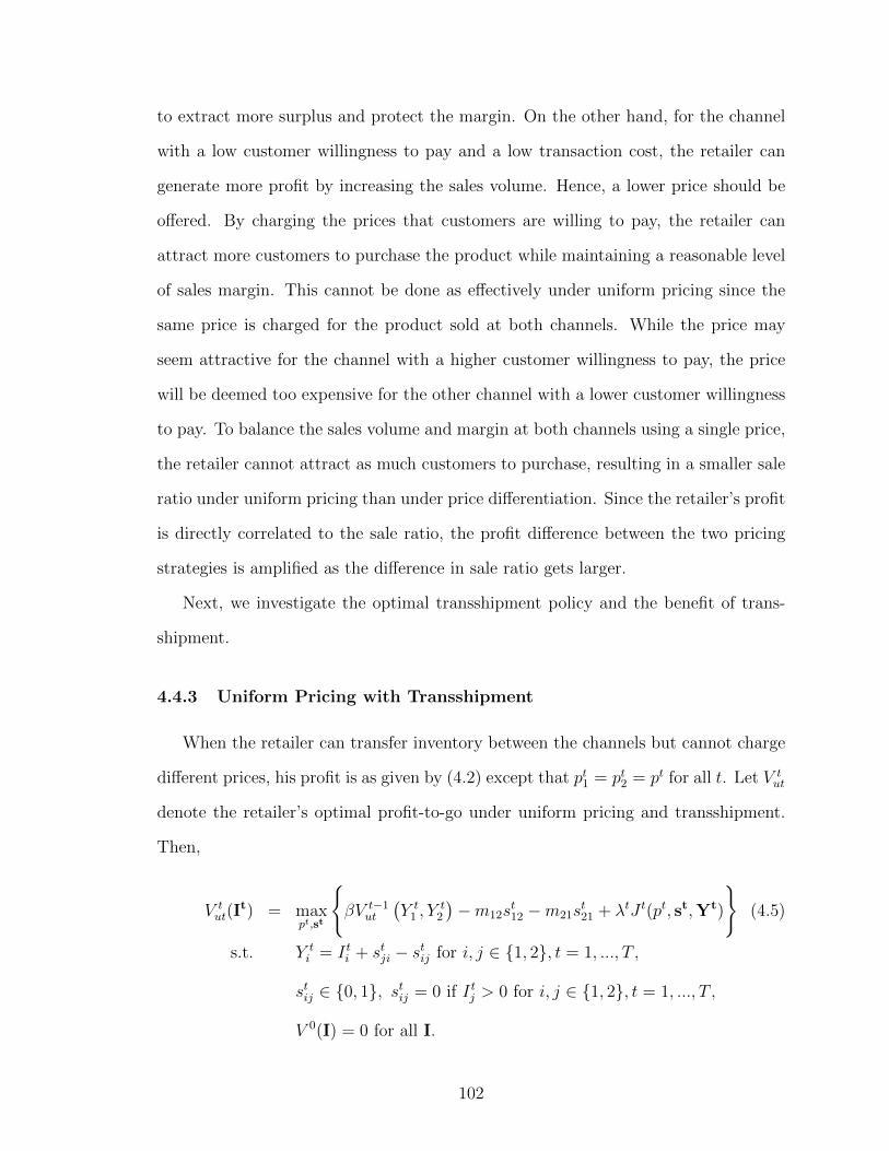
to extract more surplus and protect the margin. On the other hand, for the channel

with a low customer willingness to pay and a low transaction cost, the retailer can

generate more profit by increasing the sales volume. Hence, a lower price should be

offered. By charging the prices that customers are willing to pay, the retailer can

attract more customers to purchase the product while maintaining a reasonable level

of sales margin. This cannot be done as effectively under uniform pricing since the

same price is charged for the product sold at both channels. While the price may

seem attractive for the channel with a higher customer willingness to pay, the price

will be deemed too expensive for the other channel with a lower customer willingness

to pay. To balance the sales volume and margin at both channels using a single price,

the retailer cannot attract as much customers to purchase, resulting in a smaller sale

ratio under uniform pricing than under price differentiation. Since the retailer’s profit

is directly correlated to the sale ratio, the profit difference between the two pricing

strategies is amplified as the difference in sale ratio gets larger.

Next, we investigate the optimal transshipment policy and the benefit of trans-

shipment.

4.4.3 Uniform Pricing with Transshipment

When the retailer can transfer inventory between the channels but cannot charge

different prices, his profit is as given by (4.2) except that pt1 = pt2 = pt for all t. Let V tut

denote the retailer’s optimal profit-to-go under uniform pricing and transshipment.

Then,

V tut(I

t) = maxpt,st

{βV t−1

ut

(Y t

1 , Yt

2

)−m12s

t12 −m21s

t21 + λtJ t(pt, st,Yt)

}(4.5)

s.t. Y ti = I ti + stji − stij for i, j ∈ {1, 2}, t = 1, ..., T ,

stij ∈ {0, 1}, stij = 0 if I tj > 0 for i, j ∈ {1, 2}, t = 1, ..., T ,

V 0(I) = 0 for all I.

102

Under the assumption that a transshipment occurs instantaneously and the trans-

shipment costs and discount rate are time-independent, it is easy to see that the

retailer’s optimal strategy in the current period is to not make any transshipment as

long as there is some inventory at both channels. Thus, st∗ij = 0, i, j ∈ {1, 2} whenever

I t1 > 0 and I t2 > 0. We will consider a transshipment decision only when there is a

stockout. As before, we assume that the stockout occurs at channel 1: I t1 = 0 and

I t2 > 0. When there is a stockout at channel 1, a transshipment in the current period

may or may not be profitable. Since the retailer can sell at most one unit in each

period (λt ≤ 1), he only needs to transfer at most one unit of inventory from channel

2 to channel 1. Hence, the retailer’s transshipment decision in period t is essentially

to decide whether to transfer a unit of inventory from channel 2 to channel 1 or not.

That is, the optimal transshipment decision in period t is st∗ = (st∗12 = 0, st∗21 ∈ {0, 1}).

Since a transshipment results in a change in the inventory level at both channels,

there is a tradeoff between the marginal value of a unit of inventory before and after

the transshipment. We define the quantity “transshipment marginal value” to capture

this tradeoff, which plays an important role in determining optimal transshipment

strategies.

Definition 4.2. Transshipment marginal value (∆t12(It)) is the difference be-

tween the marginal value of the inventory at channel 1 after the transshipment is

made, and the marginal value of the inventory at channel 2 before the transshipment

is made. Mathematically, ∆t12(It) := ∆t

1(1, I t2 − 1)−∆t2(0, I t2).

The retailer’s optimal transshipment strategy and the benefit of transshipment

under uniform pricing are characterized in Proposition 4.4. Again, to highlight the

effect of transshipment on the retailer’s profit, we consider the benefit from transship-

ment as the profit gain when the retailer is allowed to transship a unit of inventory

to the stockout channel in a single period. To exclude the effect from pricing policies,

we assume the retailer uses the optimal uniform pricing policy in all periods.

103

Proposition 4.4. For any remaining time t = 1, ..., T and inventory level It such

that I t1 = 0 and I t2 > 0, let Rt∗un(Rt∗

ut) be the optimal sale ratio before (after) the

transshipment; pt∗un(pt∗ut) be the optimal uniform price before (after) the transshipment.

1. It is optimal for the retailer to transship a unit from channel 2 to channel 1

(st∗21 = 1) in period t if and only if m21 ≤ (Rt∗ut −Rt∗

un)λt + β∆t12(It).

2. Suppose a transshipment is made from channel 2 to channel 1 in period t. Then,

pt∗ut ≥ pt∗un if β∆t12(It) ≥ ct2 − ct1 and a) I t2 > 1 and ∆t

2(1, I t2 − 1) ≥ ∆t2(0, I t2), or

b) I t2 = 1 and v1 ≥ v2.

3. The benefit from making a transshipment in period t is monotonically decreasing

in m21 and ct1, but is monotonically increasing in the sale ratio difference Rt∗ut−

Rt∗un.

When a transshipment is made, the retailer’s inventory position is changed. This

in turn influences the retailer’s pricing decisions both in the current period and the

future periods. Hence, the overall effects of a transshipment on the retailer’s profit

can be viewed as coming from two parts: the effects in the current period, and the

effects in the future periods. After a transshipment takes place in the current period,

the retailer charges an optimal price corresponding to the updated inventory position.

This price may be different from what he would have charged if the transshipment

was not made. The difference in prices leads to different customer purchase decisions,

which subsequently result in the difference in the retailer’s current period profit. This

profit difference is therefore captured by the difference in the sale ratio before and

after the transshipment, multiplied by the customer arrival rate: (Rt∗ut − Rt∗

un)λt. For

future periods, the effects of transshipment essentially come from the tradeoff between

the marginal value of a unit of inventory before and after the transshipment. Hence,

the expected profit difference before and after the transshipment coming from the

future periods is given by the discounted transshipment marginal value, β∆t12(It). To

104

decide whether a transshipment in the current period is profitable or not, the retailer

needs to compare the overall potential gain in profit with a transshipment to the

transshipment cost he has to incur. As characterized in Proposition 4.4 part 1, it is

optimal for the retailer to make a transshipment if the expected gain in profit is large

enough to cover the transshipment cost.

Part 2 of the proposition discusses an implication of the transshipment marginal

value on the optimal uniform price before and after the transshipment. Recall from

Proposition 4.1 that the optimal uniform price is larger the larger the unit transaction

cost and the marginal value of the product. Without a transshipment, the optimal

price depends on the transaction cost and the marginal value at channel 2 only since

channel 1 stocks out. If a transshipment is made, then the optimal price will also

depend on the transaction cost and the marginal value at channel 1. Hence, if the

transshipment results in a significant increase in the marginal value of inventory, or

if the transaction cost at channel 1 is large relative to the transaction cost at channel

2, then the retailer should charge a higher price after the transshipment. The same

insight holds for a special case where there is only one unit of inventory left (I t1 = 0

and I t2 = 1). However, in this case, the optimal price after the transshipment is

essentially the price at channel 1 alone since channel 2 stocks out. Hence, for the

retailer to charge a higher price after the transshipment, the customer valuation at

channel 1 should also be greater than the customer valuation at channel 2.

The benefit of transshipment depends on several factors as discussed in part 3 of

the proposition. Intuitively, we see that the transshipment cost negatively affects the

benefit because it is an additional cost that the retailer has to incur when making a

transshipment. The benefit also goes down with the transaction cost at channel 1.

This is because the main purpose of transshipping a unit of inventory from channel 2

to channel 1 is to trade the potential loss in profit from not selling the unit at channel

2 with the potential gain from selling the unit at channel 1. A higher transaction cost

105

at channel 1 translates to a lower potential gain of selling a unit at channel 1, and

subsequently, a smaller benefit from making a transshipment to channel 1.

A quantity that positively affects the benefit of transshipment is the sale ratio

difference. As pointed out earlier, the sale ratio difference is directly linked to the

current period gain in profit from the transshipment. Hence, the larger sale ratio

generated by the transshipment, the larger benefit to the retailer. This result is

similar to what we have seen from Proposition 4.3 that the benefit from price differ-

entiation monotonically increases with the sale ratio difference. There is however a

notable difference between the benefit from price differentiation and the benefit from

transshipment. Recall from Corollary 4.1 that the optimal sale ratio under price dif-

ferentiation is always greater than that under uniform pricing, implying the sale ratio

difference between the two pricing policies is always positive. This is not the case

when we consider the sale ratio difference between uniform pricing with transship-

ment and uniform pricing without transshipment. When the stockout channel does

not have a significantly higher customer willingness to pay or a much lower transac-

tion cost, the optimal price after the transshipment may result in a smaller sale ratio,

signifying that the retailer does not benefit from the transshipment in the current

period. Figure 4.1 illustrates a scenario when the optimal sale ratio after a transship-

ment is smaller than the optimal sale ratio before a transshipment (Rt∗ut − Rt∗

un < 0).

Since the retailer’s current period profit is smaller with the transshipment, the bene-

fit from transshipment monotonically decreases with the customer arrival rate in the

current period. Notice however that in this example, the benefit of transshipment

from future periods is still positive (∆t12(It) > 0). Hence, when the customer arrival

rate in the current period is sufficiently small, the overall benefit of transshipment is

still positive.

So far, we have considered the retailer’s optimal decisions and benefit from im-

plementing price differentiation and inventory transshipment policies independently.

106

0.1 0.2 0.3 0.4 0.5 0.6 0.7 0.8 0.9−0.035

−0.03

−0.025

−0.02

−0.015

−0.01

−0.005

0

0.005

0.01

0.015

Benefit of Current−Period Transshipment under Uniform Pricing vs. Customer Arrival Rate

Customer Arrival Rate in Current Period (λT)

Ben

efit

of T

rans

ship

men

t

Figure 4.1: Benefit from transshipment in the current period vs. the customer arrivalrate: T = 5, I5

1 = 0, I52 = 2, β = 0.95, v1 = 8.5, v2 = 10, ct1 = 1, ct2 = 2,m12 =

0.2,m21 = 0.05, λt = 0.3 for t = 4, 3, 2, 1

In the next section, we investigate the scenario where the retailer adopts both price

differentiating and inventory transshipping policies together, and discuss how the two

mechanisms interact with each other.

4.4.4 Price Differentiation with Transshipment

When evaluating the benefit of price differentiation and transshipment separately

in a single period, we know that price differentiation is beneficial only when both

channels hold some inventory. On the other hand, for a transshipment decision to be

relevant in the current period, there must be a stockout at a channel. These different

requirements prevent us from conducting a fair comparison of the two mechanisms

when implemented in a single period. However, we are able to provide results in

Theorem 4.1 which describe how a price differentiating decision as well as its benefit

are influenced by a transshipment decision when the retailer adopts a joint price

differentiating-inventory transshipping policy.

Theorem 4.1. For any remaining time t = 1, ..., T and inventory level I t such that

I t1 = 0 and I t2 > 0:

107

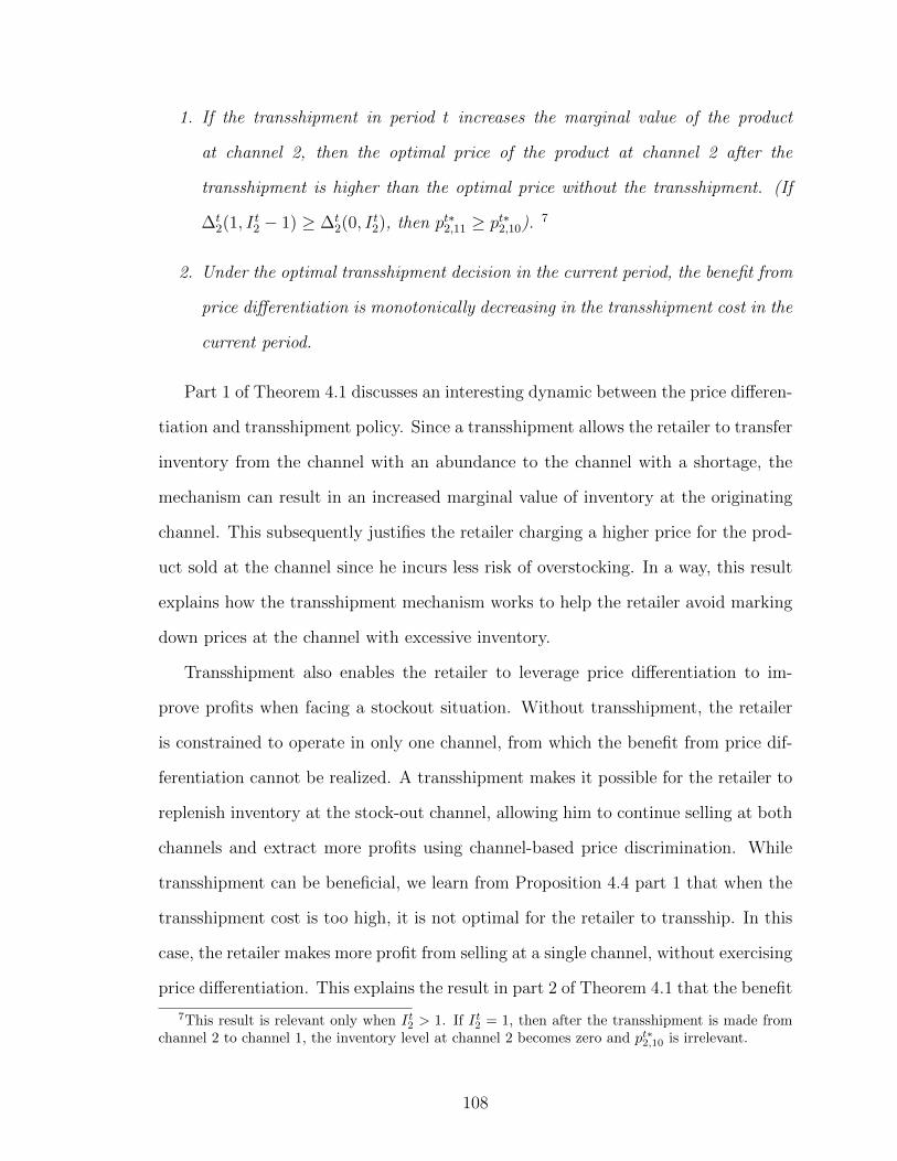
1. If the transshipment in period t increases the marginal value of the product

at channel 2, then the optimal price of the product at channel 2 after the

transshipment is higher than the optimal price without the transshipment. (If

∆t2(1, I t2 − 1) ≥ ∆t

2(0, I t2), then pt∗2,11 ≥ pt∗2,10). 7

2. Under the optimal transshipment decision in the current period, the benefit from

price differentiation is monotonically decreasing in the transshipment cost in the

current period.

Part 1 of Theorem 4.1 discusses an interesting dynamic between the price differen-

tiation and transshipment policy. Since a transshipment allows the retailer to transfer

inventory from the channel with an abundance to the channel with a shortage, the

mechanism can result in an increased marginal value of inventory at the originating

channel. This subsequently justifies the retailer charging a higher price for the prod-

uct sold at the channel since he incurs less risk of overstocking. In a way, this result

explains how the transshipment mechanism works to help the retailer avoid marking

down prices at the channel with excessive inventory.

Transshipment also enables the retailer to leverage price differentiation to im-

prove profits when facing a stockout situation. Without transshipment, the retailer

is constrained to operate in only one channel, from which the benefit from price dif-

ferentiation cannot be realized. A transshipment makes it possible for the retailer to

replenish inventory at the stock-out channel, allowing him to continue selling at both

channels and extract more profits using channel-based price discrimination. While

transshipment can be beneficial, we learn from Proposition 4.4 part 1 that when the

transshipment cost is too high, it is not optimal for the retailer to transship. In this

case, the retailer makes more profit from selling at a single channel, without exercising

price differentiation. This explains the result in part 2 of Theorem 4.1 that the benefit

7This result is relevant only when It2 > 1. If It2 = 1, then after the transshipment is made fromchannel 2 to channel 1, the inventory level at channel 2 becomes zero and pt∗2,10 is irrelevant.

108

of price differentiation decreases as the transshipment cost increases. Notice however

that this result applies to the situation where the retailer has only one opportunity

(in the current period) to transship and/or price differentiate the product. If the

retailer is allowed to implement both mechanisms over a longer period of time, the

result may be different, as shown in Figure 4.2. In this example, we observe that the

benefit from price differentiation (V Tdn − V T

un) increases with the transshipment cost

when the cost is not too high. This is because for this particular setting, the retailer

can employ either the price differentiation or the transshipment mechanism to balance

inventory and demand at each channel over the selling horizon. In other words, the

two mechanisms can substitute each other. (We will discuss more in the next section

when the benefit from the two mechanisms may substitute or compliment each other.)

Hence, when the transshipment cost is larger, the retailer increasingly prefers to use

price differentiation rather than transshipment, resulting in larger benefits from price

differentiation. When the transshipment cost is too large, however, the retailer finds

it not profitable to transship even in a stockout situation, which could occur in future

periods. Hence, the benefit from price differentiation is less likely to be realized in

future periods, following the same insight from Theorem 4.1 part 2.

When considering the benefit of transshipment, many retailers may only think

about the ability to use inventory at one channel to cover the possible loss in demand

arriving at the other channel. The less visible, but potentially more substantial

benefit of transshipment in enabling the retailer to realize the benefit from pricing

to a larger extent is often understated or overlooked. Hence, our results in Theorem

4.1 as well as Proposition 4.4 part 2 provide important managerial insights to help

retailers understand the transshipment and pricing mechanisms better.

Although transshipment can affect the optimal price levels, we note that the overall

behavior of optimal prices with respect to inventory level and remaining time is not

significantly changed by the transshipment option. As illustrated in Figure 4.3 a. and

109

0 0.2 0.4 0.6 0.8 16

7

8

9

10

11

12

Benefit of Price Differentiation under Transshipment Option vs. Transshipment Cost

Transshipment Cost from Channel 2 to Channel 1

Ben

efit

of P

rice

Diff

eren

tiatio

n (%

)

Figure 4.2: Benefit from price differentiation vs. transshipment cost: T = 5, I51 =

1, I52 = 2, β = 0.95, v1 = 4, v2 = 2, ct1 = 2, ct2 = 0.5,m12 = 0.1, λt = 0.8 for t =

5, 4, ..., 1

b., the optimal prices with and without transshipment options share similar trends

with respect to the inventory level at channel 1. Likewise, Figure 4.3 c. and d. show

that the optimal prices with and without transshipment options behave similarly with

respect to the remaining time. Notice also that, unlike the case of a single channel

(e.g. Gallego and van Ryzin (1994)), the optimal prices in our dual-channel setting

are not necessarily monotone in either the inventory level or the remaining time. For

example, as the inventory level at channel 1 increases, the optimal price at channel

2 may either decrease or increase. This is because an increase in stock at channel

1 requires the retailer to lower the price at channel 1 to reduce the risk of having

unsold inventory at the end of the selling horizon. The lower price at channel 1

draws some customers away from channel 2. Hence, the retailer may need to lower

the price at channel 2 as well in order to avoid overstocking at channel 2 due to the

substitution effect. On the other hand, if the inventory level at channel 1 becomes

a lot higher, the potential loss from overstocking at channel 1 is significantly larger

than that from overstocking at channel 2. In this case, it may be optimal for the

retailer to increase the price at channel 2, in addition to lowering the price at channel

110

1, to send even more customers from channel 2 to buy from channel 1. We note that

similar non-monotonicity results have been observed in Suh and Aydin (2011) for the

optimal prices of two substitutable products without transshipment options, where

the customer choice also follows a MNL model.

0 1 2 3 4 56

6.5

7

7.5

8

8.5

9

9.5

10

Inventory Level at Channel 1 (It1)

Opt

imal

Pric

es

Optimal Prices vs. Inventory Level at Channel 1 under Transshipment Option

pt*1

pt*2

pt*

(a) Prices vs. inventory, with transshipment

0 1 2 3 4 55.5

6

6.5

7

7.5

8

8.5

9

9.5

10

Optimal Prices vs. Inventory Level at Channel 1 under No Transshipment

Inventory Level at Channel 1 (It1)

Opt

imal

Pric

es

pt*1

pt*2

pt*

(b) Prices vs. inventory, no transshipment

1 2 3 4 5 6 7 8 9 102.5

3

3.5

4

4.5

5Optimal Prices vs. Remaining Time under Transshipment Option

Remaining Time (t)

Opt

imal

Pric

es

pt*1

pt*2

pt*

(c) Prices vs. remaining time, with transship-ment

10 9 8 7 6 5 4 3 2 12.5

3

3.5

4

4.5

5

5.5Optimal Prices vs. Remaining Time under No Transshipment

Remaining Time (t)

Opt

imal

Pric

es

pt*1

pt*2

pt*

(d) Prices vs. remaining time, no transshipment

Figure 4.3: Optimal prices vs. inventory level and remaining time: IT2 = 2, λt =0.8, β = 0.95. In Figure a-b, T = 5, v1 = 10, v2 = 6, ct1 = 3, ct2 = 1,m12 = 0.5,m21 =0.5. In Figure c-d, IT1 = 1, v1 = 4, v2 = 2, ct1 = 2, ct2 = 0.5,m12 = 0.1,m21 = 0.2.

We have discussed how the transshipment and pricing mechanisms work together

to most effectively balance inventory and demand in a dual-channel setting. Our next

interest is to compare the effectiveness of the transshipment and price differentiation

111

policies in improving the retailer’s profit. To get a sense of how much benefit the

retailer can gain from each policy, we employ numerical study to determine the re-

tailer’s optimal profits under different scenarios. The results are presented in the next

section.

4.5 Numerical Study

We conduct three sets of numerical examples, 200 instances each. Each set is given

a different initial inventory level, but the problem parameters are either the same,

or randomly chosen based on the same distributions for all three sets. The problem

parameters are summarized below.

Set 1: IT1 = 2, IT2 = 3

Set 2: IT1 = 1, IT2 = 4

Set 3: IT1 = 4, IT2 = 1

For all three sets, T = 5, β = 0.95, v1 ∼ U [1, 4), v2 ∼ U [1, 2),m12 = 0.1,m21 =

0.2, ct1 ∼ U [0.5, 2.5), ct2 ∼ U [0.5, 1.5), λt ∼ U [0, 1) for t = 5, 4, ..., 1.

Notice that the problem parameters are chosen to simulate a situation where chan-

nel 1 is a premium channel (higher customer valuation and higher transaction cost,

on average). Hence, for a brick-and-click retailer, channel 1 in our model represents

the physical store whereas channel 2 represents the online store. Note also that we

keep the total initial inventory the same across the three sets of experiments, and

only vary the inventory distribution between the two channels.

Our program randomly generates 200 problem instances for each set, and solves

for optimal solutions under the four types of pricing and transshipping policies, listed

in Table 4.1. The statistics of the optimal prices in the current period and the

profit improvement from using price differentiation and/or transshipment policies are

summarized in Table 4.2 and Table 4.5, respectively.

112

Table 4.2: Statistics for the optimal prices in the current periodNo Transshipment With Transshipment

Mean Standard Deviation Mean Standard Deviation

Price DifferentiationpT∗1 3.47 0.54 3.42 0.53

pT∗2 2.77 0.32 2.80 0.35

Uniform Pricing pT∗ 3.24 0.45 3.21 0.42

Table 4.2a: Optimal prices under Set 1No Transshipment With Transshipment

Mean Standard Deviation Mean Standard Deviation

Price DifferentiationpT∗1 3.69 0.54 3.42 0.47

pT∗2 2.69 0.30 2.80 0.39

Uniform Pricing pT∗ 3.34 0.48 3.19 0.38

Table 4.2b: Optimal prices under Set 2No Transshipment With Transshipment

Mean Standard Deviation Mean Standard Deviation

Price DifferentiationpT∗1 3.29 0.50 3.33 0.51

pT∗2 3.09 0.35 2.92 0.39

Uniform Pricing pT∗ 3.23 0.37 3.18 0.39

Table 4.2c: Optimal prices under Set 3

First, we discuss the optimal prices in Table 4.2. We observe that in Set 1 and Set

2, the average optimal price at channel 1 under transshipment options is lower than

that under no transshipment; while, the average optimal price at channel 2 under

transshipment options is higher than that under no transshipment. This is due to

the fact that the initial inventory level in Set 1 and Set 2 are such that there is less

inventory at channel 1, which is the premium channel. Hence, if the retailer has an

option to transship, it is likely that most of the transshipments will be made from

channel 2 to channel 1. In response to a higher expected stock level at channel 1

and a lower expected stock level at channel 2 as a result of future transshipments,

it is optimal for the retailer to charge a lower price at channel 1 and a higher price

at channel 2 in the current period. Furthermore, notice that the gaps between the

average optimal prices with and without transshipment options are larger in Set 2

than in Set 1. This is because the initial inventory level at channel 1 in Set 2 is less

113

Set 1 Set 2 Set 3Mean Std. Dev. Mean Std. Dev. Mean Std. Dev.

Benefit of Price Diff. under5.18% 5.44% 5.27% 5.11% 2.97% 3.86%

No Transshipment

(V T10−V

T00

V T00

)Benefit of Price Diff. under

5.04% 5.55% 4.71% 5.56% 3.93% 5.40%

Transshipment

(V T11−V

T01

V T01

)Benefit of Transshipment

1.35% 2.64% 8.39% 12.12% 2.27% 3.53%

under Uniform Pricing

(V T01−V

T00

V T00

)Benefit of Transshipment

1.20% 2.33% 7.69% 10.97% 3.21% 4.88%

under Price Diff.

(V T11−V

T10

V T10

)Joint Benefit of Price Diff.

6.41% 5.38% 13.20% 11.01% 6.34% 7.48%

and Transshipment

(V T11−V

T00

V T00

)

Table 4.3: Benefit of price differentiation and transshipment

than that in Set 1. Hence, transshipments are likely to take place more often in Set

2, resulting in larger effects of future transshipments on the current prices.

Now, consider the optimal prices in Set 3. We find that under transshipment

options, the average optimal price at channel 1 is higher while the average optimal

price at channel 2 is lower, compared to the optimal prices without transshipment.

These results are in contrast with what we observe from Set 1 and Set 2. This

is because, unlike Set 1 and Set 2, Set 3 is given an initial inventory level with

significantly more inventory at channel 1. In this case, it is much more likely that

channel 2 will stock out in the future periods. Hence, if the retailer has an option to

transship, most of the transshipments are likely to be made from channel 1 to channel

2. Since the expected stock level at channel 1 is lower whereas the expected stock

level at channel 2 is higher under transshipment options, it is optimal for the retailer

to charge a higher price at channel 1 and a lower price at channel 2 in the current

period.

It is interesting to see that in all three sets of experiments, the average optimal

uniform price in the current period is lower with transshipment options than without

transshipment. This is mainly driven by the fact that under transshipment options,

the retailer can always make a transshipment to the stockout channel when needed

114

in a future period, and still be able to charge a reasonable price for the product, as

we have learned from Proposition 4.4 part 2. Since stocking out at a channel in the

future periods is not a huge concern, the opportunity cost of selling a unit in the

current period (marginal value of a unit of inventory) is lower, compared to under

no transshipment. Hence, it is optimal for the retailer to charge a lower price in

the current period, when a transshipment is not needed (since the initial inventory

level in all three sets are such that both channels carry some inventory), in order to

generate more sales earlier on and reduce the risk of overstocking at the end of the

selling horizon.

Next, we discuss the profit improvements from using price differentiation and

inventory transshipment. From Table 4.5, we see that the benefits of price differenti-

ation in Set 1 and Set 2 are higher than that in Set 3 on average. This is because the

initial inventory level in Set 3 is already quite in balance with the arriving demand.

Since the customer valuation is generally higher at channel 1, even when a uniform

price is offered, more customers are likely to buy from channel 1, where there is more

inventory to serve. Hence, there is only a small room for profit improvement using

price differentiation. On the other hand, in Set 1 and Set 2, the retailer starts with

less inventory at channel 1. If a uniform price is offered, the retailer will quickly run

out of inventory at channel 1. Therefore, charging different prices at the two channels

(specifically, higher prices at channel 1) has a high potential in helping the retailer

more efficiently balance inventory with demand.

The benefit from transshipment is also largely influenced by the initial inventory

level. Notice from Table 4.5 that transshipment improves the retailer’s profit the

most in Set 2, and the least in Set 1. This is because in Set 2, the initial inventory

level is notably out of balance as there is a lot less inventory at channel 1, which is

the premium channel. In this case, the retailer is in critical need of more inventory

at channel 1. Hence, the ability to transfer inventory between the channels greatly

115

improves profits. In Set 3, the initial inventory level is preferable to the retailer as

there is a lot more inventory at channel 1. However, since channel 2 has very little

inventory, the chance of stocking out is high. Hence, transshipment is still very much

necessary in this setting. On the other hand, Set 1 is given an initial inventory level

where both channels have almost equal amount of inventory in stock. Since the chance

of stocking out is not particularly high at either channel, inventory transfers are not

required very often, resulting in small benefits of transshipment.

While both price differentiation and inventory transshipment can significantly im-

prove the retailer’s profit, the performance of the two mechanisms can vary, depending

on the problem parameters. We note that in the majority of the problem instances

(70% in Set 1, 54.5% in Set 2, and 62% in Set 3, out of 200 instances conducted in each

set), the benefit of price differentiation is larger than the benefit of transshipment.

This is likely to be due to the fact we pointed out earlier that price differentiation is

always profitable whereas transshipment may or may not be profitable. Furthermore,

we notice that transshipment is especially beneficial when the initial inventory level is

such that there is a lot more inventory at channel 2, and channel 1 has high customer

valuation but low transaction cost, relative to channel 2. When these conditions do

not hold, the benefit of transshipment is generally smaller than the benefit of price dif-

ferentiation. This is because, when the inventory level is substantially uneven (large

difference between the inventory levels at the two channels) in a way that there is

less inventory at the high-margin channel, the retailer can resolve the situation more

effectively by correcting his inventory position. If he only price differentiates between

the channels, he could prevent stocking out at the high-margin channel by charging a

high price. However, doing so results in less sales at the high-margin channel and less

profits overall. Based on this reason, it is not surprising to observe that the benefit

of transshipment is larger than the benefit of price differentiation in more problem

instances in Set 2.

116

Finally, it is worth noting that the benefit from price differentiation and the benefit

from transshipment may either substitute or complement each other. To see this,

notice from Table 4.5 that in Set 1 and Set 2, the benefit of price differentiation is

larger when the retailer does not have an option to transship. Likewise, in Set 1 and

Set 2, the benefit of transshipment is larger under uniform pricing than under price

differentiation. This implies that the benefit of price differentiation and the benefit

of transshipment generally substitute each other under the settings of Set 1 and Set

2. The main driver of this result is the fact that Set 1 and Set 2 are given an initial

inventory level that is unfavorable to the retailer (less inventory at the high-margin

channel). In such a situation, the retailer would want to rebalance his inventory

position by trying to reduce the inventory at channel 2 and maintain or increase the

inventory at channel 1. Both price differentiation and transshipment mechanisms

can be employed for this same purpose. Hence, the benefit of the two mechanisms

substitute each other. However, the opposite result is observed in Set 3, where the

benefit of price differentiation is larger when the retailer can transship, and the benefit

of transshipment is larger when the retailer can price differentiate. This is because in

Set 3, the initial inventory level is favorable for the retailer as there is more inventory

at the high-margin channel. In this case, it is in the retailer’s best interest to try to

maintain the same balance in his inventory position. To most effectively achieve this,

the retailer needs to employ both price differentiation and transshipment mechanisms

to complement each other’s effect. More precisely, the retailer would maintain a high

price at channel 1 to extract most surplus. However, doing so increases the chance

of having a stock out at channel 2 and a leftover at channel 1 in the future periods.

Hence, transshipments will be needed to replenish the stock at channel 2, allowing

the retailer to continue to benefit from price differentiation.

117

4.6 Extension

4.6.1 Ex-post Transshipment

So far, we have assumed that if the retailer decides to make a transshipment in

the current period, the transshipment then takes place before a customer arrival,

and an arriving customer observes the actual product availability at the channels. In

practice, some retailers may have more flexibility in the timing of a transshipment, and

hence, are able to delay the transshipment until after the customer makes a decision

to purchase. In this case, even when the product is out of stock at a channel, the

retailer can announce the product availability at both channels, but only transship the

product to the stock-out channel when a customer decides to buy from that channel.

If an arriving customer does not buy or buys from the in-stock channel, then the

retailer does not need to make a transshipment in that period. For example, if the

product is out of stock at the distribution center, used to fulfill demand at the online

store, the retailer may continue to display the product as available online, and ship

the product from the physical store only after a customer places an online order. We

refer to this transshipment policy as “ex-post transshipment,” and use x to denote

the policy.

To see how the results regarding transshipment (Proposition 4.4 and Theorem

4.1) are affected by the ex-post transshipment policy, we consider an inventory level

It = (0, I t2), where I t2 > 0, and assume as before that the retailer may transship the

product from channel 2 to channel 1 only in the current period. Under the ex-post

transshipment policy, if the retailer decides to continue selling at both channels, he

makes a unit transshipment from channel 2 to channel 1 only when the customer

chooses to buy from channel 1. Hence, the retailer’s pricing problem under price

118

differentiation in period t is given by:

V tdx(I

t) = maxpt

{λtµ1

[pt1 − ct1 + βV t−1

un

(0, I t2 − 1

)−m21

]+λtµ2

[pt2 − ct2 + βV t−1

un

(0, I t2 − 1

)]+(λtµ0 +

(1− λt

))βV t−1

un

(0, I t2

)}

= maxpt

{βV t−1

un

(0, I t2

)+ λtµ1

[pt1 − ct1 − β∆t

2

(0, I t2

)−m21

]+λtµ2

[pt2 − ct2 − β∆t

2

(0, I t2

)]}

= maxpt

{βV t−1

un

(0, I t2

)+ λtJ tdx(p

t, It)

}(4.6)

s.t. pti ≥ 0 for i ∈ {1, 2}, t = 1, ..., T ,

V 0dx(I) = 0 for all I.

The retailer’s uniform pricing problem is given by (4.6) with pt1 = pt2 = pt.

Comparing V tdx to the retailer’s pricing problem with ex-ante transshipment in

period t, given by (4.2) with st21 = 1, st12 = 0,Yt = (1, I t2 − 1), and V t−1 = V t−1un , we

see that the terms that depend on prices (J t) under the ex-post transshipment are

the same as those under the ex-ante transshipment with β∆t1(1, I t2 − 1) replaced by

β∆t2(0, I t2) + m21, and ∆t

2(1, I t2 − 1) replaced by ∆t2(0, I t2). With these two modifi-

cations, the optimal prices under ex-post transshipment can be characterized in the

same way as under ex-ante transshipment. Notice also that by replacing β∆t1(1, I t2−1)

with β∆t2(0, I t2) + m21, the transshipment marginal value ∆t

12(It) is modified to m21

β

under the ex-post transshipment.

The results in Proposition 4.4 and Theorem 4.1 continue to hold under ex-post

transshipment with the two term modifications discussed above. For example, the

condition when it is optimal to make a transshipment (in this case, to offer the

product at both channels) in the current period, given in Proposition 4.4 part 1., is

119

modified from m21 ≤ (Rt∗ut − Rt∗

un)λt + β∆t12(It) to (Rt∗

ux − Rt∗un)λt ≥ 0, which reduces

to Rt∗ux − Rt∗

un ≥ 0 since λt ≥ 0. In Theorem 4.1 part 1., the sufficient condition

for the optimal price at channel 2 after the transshipment to be higher than the

optimal price without transshipment is modified from ∆t2(1, I t2 − 1) ≥ ∆t

2(0, I t2) to

∆t2(0, I t2) ≥ ∆t

2(0, I t2), which is always true. Hence, with ex-post transshipment, the

optimal price at channel 2 with the transshipment is always higher than the optimal

price without the transshipment.

4.7 Conclusion

Channel-based price differentiation and inventory transshipment are two of the

most common mechanisms used by multi-channel retailers to balance inventory and

demand arriving at each channel. Price differentiation can be employed to shift the

demand from the channel with low inventory to the channel with more inventory

in order to prevent overstocking or understocking. On the other hand, inventory

transshipment does not affect the demand, but it allows the retailer to directly correct

his inventory position by transferring inventory from the channel with more inventory

to the channel with less inventory. Since both mechanisms can be implemented to

serve the same purpose of balancing the inventory and demand across the channels,

we are interested in investigating what factors affect the benefit from each mechanism,

when one mechanism is likely to be more effective than the other, and how the two

mechanisms influence each other if they are adopted concurrently.

We model a dual-channel retailer’s joint dynamic pricing and transshipping prob-

lem over a finite horizon. In each period, the retailer decides how much to charge for

the product sold at each channel, and whether to make any inventory transshipment

between the channels. An arriving customer decides whether to purchase the product

from one of the available channels, based on her valuations and the observed prices

at the channels. Her purchase decision follows the multinomial logit model.

120

We characterize the retailer’s optimal dynamic pricing and transshipping policies.

We find that price differentiation and transshipment policies have different implica-

tions on the product sales. The optimal price differentiation policy always results in

a larger probability of making a sale in the current period, compared to the optimal

uniform pricing policy. On the other hand, the optimal transshipment decision may

result in a larger or smaller probability of making a sale in the current period. When

price differentiation and inventory transshipment policies are implemented together,

we show that transshipment can increase the value of the remaining inventory, and

subsequently the price, at the channel from which the transshipment is made. Ad-

ditionally, since a transshipment is required in a stock-out situation for the benefit

of price differentiation to be realized, we find that the benefit of price differentiation

may decrease in the transshipment cost when the cost is large.

Our numerical study helps compare the benefit of price differentiation and in-

ventory transshipment under various scenarios. The results show that the benefit of

price differentiation is generally larger than the benefit of transshipment. However,

transshipment can be more effective than price differentiation when the retailer holds

significantly less inventory at the high-margin channel. When adopted together, the

price differentiation and inventory transshipment mechanisms may either substitute

or complement each other. When the retailer’s inventory position requires some cor-

rection, either price differentiation or inventory transshipment can be used. Hence,

the two mechanisms substitute each other in this case. On the other hand, when the

current inventory balance at the channels should be maintained in the same propor-

tion, the two mechanisms work together complementarily to improve the retailer’s

profit.

This study considers a joint dynamic pricing and inventory problem in a setting

and context that are different from existing literature. In particular, we focus on

the price differentiation and inventory transhipment mechanisms in a dual-channel

121

retailing, which are widely observed in practice, but not well studied in the literature.

Our results help explain how each mechanism works in a dual-channel environment,

how the two mechanisms are similar or different, and when one should be chosen

over the other, or both are required. Although our current model assumes a specific

customer choice model and a simple retailer’s cost structure, we believe that the

managerial insights obtained from this study can be applied to many realistic dual-

channel situations to help make appropriate pricing and inventory decisions.

There are several directions for future research on this topic that would further

provide valuable contribution to the literature. A natural extension of the current

model is to consider a multi-channel setting (more than two channels/stores). Hav-

ing multiple channels is likely to result in a significantly higher complexity level of

the problem, especially on the transshipment decisions. However, certain modeling

assumptions may help reduce the decision space and make it possible to achieve some

interesting results. One could also extend the model to consider a different customer

choice model. For example, the heterogeneity in customer valuation for the product

sold at each channel may be distributed over a general distribution; different cus-

tomers may react differently when they find that their preferred channel stocks out;

observing different prices at the channels may have certain effects on how customers

evaluate their purchases. Lastly, the model can be extended to incorporate additional

costs and operational constraints that could affect the retailer’s pricing and transship-

ping decisions. These include, for instance, costs associated with managing different

prices at the channels, fixed transshipment costs, inventory holding costs, inventory

holding capacity, transshipment lead times.

122

CHAPTER 5

Conclusion

While there are many pricing mechanisms used in practice, different mechanisms

may not deliver the same benefits to sellers under different business situations. Hence,

choosing an appropriate mechanism can be a challenging problem for a seller. This

dissertation aims to provide insights into how different pricing mechanisms affect the

buyer’s behavior and the seller’s profitability to ultimately help business managers

make effective operational decisions.

To address various types of pricing problems commonly occurring in a supply

chain, this dissertation considers three different seller’s problems in a series of three

essays.

The first essay (Chapter 2) examines whether and when the supplier benefits from

more accurate demand forecasts obtained by the buyer under different contract struc-

tures. An important finding of the essay is that there indeed exist contracts under

which the supplier can always benefit from the buyer’s more accurate demand fore-

casts. However, depending on how certain the supplier is about the buyer’s forecasting

capability, the contract structure may be more sophisticated than what is common

in practice. This finding complements the existing supply chain contract literature

which has considered simpler forms of contracts and reported that the supplier’s profit

can be hurt by the buyer’s improved demand forecasts.

123

The second essay (Chapter 3) discusses how price promotions influence purchase

decisions of different types of consumers, and which type of promotions is most prof-

itable to the seller under which market situations. Two forms of conditional discounts,

all-unit and fixed-amount discount, are considered. This study shows that both all-

unit and fixed-amount discount are equally effective in inducing deal-prone consumers

to overspend. However, when consumers are heterogenous in their willingness to pay

for the product, one form of discounts may outperform the other. Hence, the seller’s

choice of discount types can significantly determine how much profit he obtains. The

findings from this essay provide guidance on when it is optimal to offer a conditional

discount, and which form of discounts to offer to maximize profits.

The third essay (Chapter 4) considers a dual-channel retailer who can employ

either price differentiation or inventory transshipment to balance inventory and de-

mand at each channel. This study investigates what factors affect the benefit from

each mechanism, when one mechanism is likely to be more effective than the other,

and how the two mechanisms influence each other if they are implemented concur-

rently. It is shown that while price differentiation always increases sales volume,

inventory transshipment may sometimes result in a smaller sales volume in the cur-

rent period. In terms of benefits to the retailer, whether the mechanism of price

differentiation or inventory transshipment results in a larger profit improvement, and

whether the benefit of the two mechanisms, when adopted together, substitute or

complement each other primarily depend on the retailer’s initial inventory position.

The results obtained from this study can help retailers make good judgement when

implementing joint pricing and inventory policies in a dual-channel environment.

On the academic side, this dissertation studies new research problems and provides

original results that contribute to the existing Operations Management literature as

well as other related fields such as Marketing and Economics. On the practical side,

the insights discussed in this work can help managers craft their strategies to achieve

124

successful operations in many realistic business situations.

125

APPENDICES

126

APPENDIX A

Additional Results and Proofs for Chapter 2

A.1 Characterization of Optimal Contracts

A.1.1 Early Static Contract

The supplier’s optimization problem with early static contract is given by

maxq,t

∑i∈{L,H}

p1i (−c1qi + ti)

s.t.∑

j∈{L,H}

p1ij[Γ(Dj, qi)− ti] ≥ 0, i = {L,H}

∑j∈{L,H}

p1ij[Γ(Dj, qi)− ti] ≥

∑j∈{L,H}

p1ij[Γ(Dj, q−i)− t−i], i = {L,H}

qi, ti ≥ 0 i = {L,H}

One can show that the supplier’s problem is equivalent to the following reduced

problem. (We provide the detailed discussion of how to obtain this reduced form

when we study the supplier’s problem with dynamic contract, the derivation for early

127

and late static contracts are similar.)

maxq,t

∑i∈{L,H}

p1i (−c1qi + ti) (A.1)

s.t.∑

j∈{L,H}

p1Lj [Γ(Dj , qL)− tL] ≥ 0,

∑j∈{L,H}

p1Hj [Γ(Dj , qH)− tH ] ≥∑

j∈{L,H}

p1Hj [Γ(Dj , qL)− tL], i = {L,H}

qH ≥ qL

From this, we can characterize the optimal early static contract, which is presented

in Proposition A.1.

Proposition A.1. The optimal early static contract quantities can be obtained by

solving the following equations.

(1− (1 + p1H)θ1)Γ′(DH , qL) + ((1 + p1H)θ1 − p1H)Γ′(DL, qL)− c1p1L = 0

θ1Γ′(DH , qH) + (1− θ1)Γ′(DL, qH)− c1 = 0

The supplier charges the retailer tL = (1− θ1)Γ(DH , qL) + θ1Γ(DL, qL),

tH = θ1Γ(DH , qH)− (2θ1 − 1)Γ(DH , qL) + (1− θ1)Γ(DL, qH) + (2θ1 − 1)Γ(DL, qL).

The supplier always produces exactly the quantity selected by the buyer.

Proof of Proposition A.1: Consider the reduced early static optimization prob-

lem given by (A.1). The optimal contract quantities can be obtained from solving

the first-order conditions because Γ(D, q) satisfies Property 4 in Assumption 1, which

implies the unimodality of the supplier’s profit in contract quantities. If Γ(D, q) also

satisfies Γ′(Di, q) ≥ Γ′(Dj, q) for any Di < Dj, as is the case for the buyer’s revenue

in both exogenous price and endogenous price models, the solution of qL and qH that

satisfy the first-order conditions always satisfy the monotonicity constraint qL ≤ qH .

To see this, let ΠES be the objective function of this optimization problem. From the

128

first-order conditions given in the proposition, we have,

∂ΠES

∂qL|qH = (1− θ1)Γ′(DH , qH) + θ1Γ′(DL, qH)− c1

≤ θ1Γ′(DH , qH) + (1− θ1)Γ′(DL, qH)− c1 = 0

where the inequality is due to θ1 ≥ max{pL, pH} ≥ 12

and Γ′(DH , qH) ≥ Γ′(DL, qH),

and the last equality follows from the first-order condition with respect to qH . Since

the objective function is unimodal in qL, ∂ΠES∂qL|qH ≤ 0 implies qH ≥ qL.

The supplier produces the exact quantity selected by the buyer in period 1 because

the production is made after the screening.

A.1.2 Late Static Contract

The supplier’s optimization problem with late static contract is given by

maxq,t,ρ

−c1ρ +∑

i∈{L,H}

p1i

∑j∈{L,H}

pij(tj − c2(qj − ρ)+)

s.t.∑

k∈{L,H}

p2jkΓ(Dk, qj) ≥ tj∑

k∈{L,H}

p2jkΓ(Dk, qj)− tj ≥

∑k∈{L,H}

p2jkΓ(Dk, q−j)− t−j

ρ, qj, tj ≥ 0, j = {L,H}

The reduced optimization problem under late static contract is given by

maxq, t,ρ

−c1ρ +∑

i∈{L,H}

p2i (ti − c2(qi − ρ)+) (A.2)

s.t.∑

j∈{L,H}

p2Lj[Γ(Dj, qL)− tL] ≥ 0,

∑j∈{L,H}

p2Hj[Γ(Dj, qH)− tH ] ≥

∑j∈{L,H}

p2Hj[Γ(Dj, qL)− tL],

qH ≥ qL

129

The optimal late static contract is characterized in Proposition A.2.

Proposition A.2. The supplier’s period 1 optimal production under late static con-

tract is

ρ∗(q) =

qH if c1c2 ≤ p2H

qL if c1c2 > p2H

The optimal late static contract quantities can be obtained by solving the following

equations:

(1− (1 + p2H)θ2)Γ′(DH , qL) + ((1 + p2H)θ2 − p2H)Γ′(DL, qL) = (c1 − p2Hc2)+

p2H [θ2Γ′(DH , qH) + (1− θ2)Γ′(DL, qH)] = min{c1, p2Hc2}

If qL > qH , it is optimal to bunch the low- and high-type quantity and offer qL =

qH = q which satisfies (1− θ2)Γ′(DH , q) + θ2Γ′(DL, q)− c1 = 0.

The supplier charges the buyer tL = (1− θ2)Γ(DH , qL) + θ2Γ(DL, qL),

tH = θ2Γ(DH , qH)− (2θ2 − 1)Γ(DH , qL) + (1− θ2)Γ(DL, qH) + (2θ2 − 1)Γ(DL, qL).

Proof of Proposition A.2: We know from (A.2) that qH ≥ qL holds at the

optimal solution. If the expected saving is greater than the loss, p2Hc2 ≥ c1, the

supplier improves his expected profit by producing the larger quantity of qH in period

1.

The transfer payments are derived from the binding constraints stated above. The

unimodality of −Γ′′(D, q) implies the concavity of the supplier’s profit function in the

contract quantities. Plugging in the expressions of the optimal transfer payments

into the objective function, we can use first-order conditions to derive the optimal

contract quantities. First, we solve the first-order conditions ignoring the constraints

qH ≥ qL. However, if the inequality qH ≥ qL is violated, then we know that bunching

is optimal for the two quantities. Hence, we replace qL and qH by q in the supplier’s

profit, and solve the first-order condition with respect to q to obtain the optimal

solution of qL = qH = q.

130

A.1.3 Dynamic Contract

We will first show that the supplier’s optimization problem for dynamic contract

can be reduced to the following problem.

maxq,t,ρ

∑i={L,H}

p1i (−c1ρi + ti) +∑

i∈{L,H}

p1i∑

j∈{L,H}

pij [tij − c2(qi + qij − ρi)+]

(A.3)

s.t.∑

j∈{L,H}

pLj∑

k∈{L,H}

p2jk[Γ(Dk, qL + qLj)− tLj ] ≥ tL (Period 1 Participation Constraints)

∑j∈{L,H}

pHj∑

k∈{L,H}

p2jk[Γ(Dk, qH + qHj)− tHj ]− tH ≥ (Period 1 Incentive Constraint)

pHH∑

k∈{L,H}

p2Hk[Γ(Dk, qL + qLH)− tLH ] + pHL∑

k∈{L,H}

p2Lk[Γ(Dk, qL + qLL)− tLL]− tL

∑k∈{L,H}

p2Lk[Γ(Dk, qi + qiL)− tiL] ≥∑

k∈{L,H}

p2LkΓ(Dk, qi), i = {L,H}

(Period 2 Participation Constraints)∑k∈{L,H}

p2Hk[Γ(Dk, qi + qiH)− tiH ] ≥∑

k∈{L,H}

p2Hk[Γ(Dk, qi + qiL)− tiL], i = {L,H}

(Period 2 Incentive Constraints)

ρi, qi, qij , ti, tij ≥ 0 i = {L,H}, j = {L,H} (Nonnegativity Constraints)

qHH ≥ qHL, qLH ≥ qLL

Let PCi and PCij i, j ∈ {L,H} be the participation constraints of buyer type i and

type ij in period 1 and 2, respectively. Let ICij, i(−j)/(−i)k,(−i)l i, j, k, l ∈ {L,H} be

the period 1 incentive constraint of the type i buyer not to deviate to contract (−i)k

in period 2 when she observes ij, and not to deviate to (−i)l when she observes i(−j).

Let ICij be the period 2 incentive constraint for the buyer observing ij not to deviate

to i(−j).

Period 1 PCH is implied by period 1 PCL, period 1 ICHH,HL/LH,LL, and pe-

riod 2 ICLH as follows:∑

j∈{L,H} pHj∑

k∈{L,H} p2jk[Γ(Dk, qH + qHj) − tHj] − tH ≥

pHH∑

k∈{L,H} p2Hk[Γ(Dk, qL+ qLH)− tLH ]+pHL

∑k∈{L,H} p

2Lk[Γ(Dk, qL+ qLL)− tLL]−

tL ≥ pLH∑

k∈{L,H} p2Hk[Γ(Dk, qL + qLH)− tLH ] + pLL

∑k∈{L,H} p

2Lk[Γ(Dk, qL + qLL)−

tLL] − tL ≥ 0. The first inequality is period 1 ICHH,HL/LH,LL. The second in-

equality follows from period 2 ICLH and the fact that pHH ≥ pLH . The third

131

inequality is period 1 PCL. Next, period 1 ICHH,HL/LL,LL is implied by period 1

ICHH,HL/LH,LL and period 2 ICLH since pHH∑

k∈{L,H} p2Hk[Γ(Dk, qL + qLH)− tLH ] +

pHL∑

k∈{L,H} p2Lk[Γ(Dk, qL + qLL)− tLL]− tL ≥ pHH

∑k∈{L,H} p

2Hk[Γ(Dk, qL + qLL)−

tLL] + pHL∑

k∈{L,H} p2Lk[Γ(Dk, qL + qLL)− tLL]− tL.

Similarly, period 1 ICHH,HL/LH,LH is implied by period 1 ICHH,HL/LH,LL and

period 2 ICLL; period 1 ICHH,HL/LL,LH is implied by period 1 ICHH,HL/LH,LL and

period 2 ICLH and ICLL.

For the low-type period 1 incentive constraints, similar to high type period 1

incentive constraints, we can show that ICLH,LL/HH,HH is implied by ICLH,LL/HH,HL

and period 2 ICHL; ICLH,LL/HL,HL is implied by ICLH,LL/HH,HL and period 2 ICHH ;

and ICLH,LL/HL,HH is implied by period 2 ICHL and ICHH .

Period 2 constraints can be reduced as follows. PCHH is implied by PCHL, ICHH ,

and p2HH ≥ p2

LH . PCLH is implied by PCLL, ICLH , and p2HH ≥ p2

LH . Adding ICHH

and ICHL, we see that ICHL is implied by ICHH and qHH ≥ qHL. Similarly, adding

ICLH and ICLL, we see that ICLL is implied by ICLH and qLH ≥ qLL.

Finally, note that at the optimal solution, period 1 PCL, period 1 ICHH,HL/LH,LL,

period 2 ICHH , and period 2 ICLH must be binding, or else the supplier can profitably

increase tL, tH , tHH , and tLH , correspondingly. Notice that the binding period 1 PCL

together with pLH ≤ pHH and qHH ≥ qHL implies ICLH,LL/HH,HL. Hence, all four

period 1 low-type incentive constraints can be removed.

Proof of Proposition 2.1: Suppose an optimal dynamic contract is given by

DC := (qi, ti){(qiH , tiH), (qiL, tiL)}, i = L,H. Now, consider another contract, DC ′ :=

(0, ti){(qi+qiH , tiH), (qi+qiL, tiL)}, i = L,H. Since the total quantities and payments

at both DC and DC ′ are the same for all types, the two contracts result in the same

profits to the supplier and the buyer if the buyer chooses the contract meant for

her type. We will show that DC ′ satisfies all the constraints, so that it is also

an optimal contract. To see this, observe from the supplier’s reduced optimization

132

problem given by (A.3) that all constraints of DC and DC ′ are the same except

for period 2 participation constraints. Notice however that the period 2 participation

constraints of DC ′ are implied by the constraints of DC since∑

k∈{L,H} p2Lk[Γ(Dk, qi+

qiL)− tiL] ≥∑

k∈{L,H} p2LkΓ(Dk, qi) ≥

∑k∈{L,H} p

2LkΓ(Dk, 0), i = {L,H} by Property

2 in Assumption 1. Hence, DC ′ satisfies all the constraints and it is equivalent to

DC.

Proof of Proposition 2.2: By Proposition 2.1, there exists an optimal dynamic

contract in the following form DC := (0, ti){(qiH , tiH), (qiL, tiL)}, i = L,H. Now, con-

sider the following dynamic contract, DC ′ := (0, ti+ tiL){(qiH , tiH− tiL), (qiL, 0)}, i =

L,H.

Since the total quantities and payments in both DC and DC ′ are the same for

all types, the two contracts result in the same profits to the supplier and the buyer if

the buyer chooses the contract meant for her type. We will show that period 1 and

period 2 constraints hold under DC ′. Period 1 participation and incentive constraints

of DC ′ are the same as those of DC because the total transfers ti+ tij from the buyer

to the supplier are the same under both contracts. Since period 2 transfer payments

of DC ′ are smaller than those of DC, period 2 participation constraints of DC ′ are

implied by period 2 participation constraints of DC. Period 2 incentive constraints

of DC ′ are equivalent to those of DC. Therefore, DC ′ is a feasible contract and it is

equivalent to the optimal dynamic contract DC.

Proof of Proposition 2.3: Suppose that in period 1 the buyer chooses type i

contract. Then, the supplier produces at least qiL units in period 1. We know that

qiH ≥ qiL, i = L,H in a dynamic contract from (A.3). Therefore, if the cost of

producing an additional unit at c1 is less than the expected saving, piHc2, then the

supplier produces exactly qiH in period 1. The optimal transfer payments are obtained

from the binding constraints. Since Γ(D, q) satisfies Property 4 in Assumption 1, the

supplier’s profit is unimodal in the contract quantities. Hence, the optimal contract

133

quantities can be derived from solving the first-order conditions, provided in the

proposition. If any of the two monotonicity constraints of the contract quantities

qiH ≥ qiL is violated, we replace the two quantities with the same variable (qi =

qiH = qiL) and resolve the first-order condition. This case corresponds to bunching

of contract quantities.

A.2 Contract Preferences

Proof of Theorem 2.1: We consider the reduced problem for the dynamic con-

tract given in (A.3). Let S∗(θ2) := {q∗i (θ2), q∗ij(θ2), ρ∗i (θ2), t∗i (θ2), t∗ij(θ2)}, i, j ∈ {L,H}

denote an optimal solution to the supplier’s optimization problem under dynamic

contract when the buyer’s second period information accuracy is θ2, with q∗i = 0

and t∗iL = 0, i ∈ {L,H}. Let Π∗DC(θ2) := ΠDC(S∗(θ2), θ2) denote the corresponding

supplier’s optimal profit. We will show that there exists a solution S(θ′′2) such that

Π∗DC(θ′′2) ≥ ΠDC(S(θ′′2), θ′′2) ≥ Π∗DC(θ′2), for θ′′2 > θ′2.

Suppose an optimal solution at θ2 = θ′2 is given by S∗(θ′2) = {q∗ij(θ′2), ρ∗i (θ′2),

t∗i (θ′2), t∗iH(θ′2)}, i, j ∈ {L,H}. We construct a solution S(θ′′2) = {q∗ij(θ′2), ρ∗i (θ

′2), t∗i (θ

′2),

tiH(θ′′2)}, i, j ∈ {L,H} with

tLH(θ′′2) = θ′′2 [Γ(DH , q∗LH(θ′2))− Γ(DH , q

∗LL(θ′2))]

+(1− θ′′2)[Γ(DL, q∗LH(θ′2))− Γ(DL, q

∗LL(θ′2))] (A.4)

tHH(θ′′2) = θ′′2 [Γ(DH , q∗HH(θ′2))− Γ(DH , q

∗HL(θ′2))]

+(1− θ′′2)[Γ(DL, q∗HH(θ′2))− Γ(DL, q

∗HL(θ′2))]

Notice that we adopt the same contract quantities, period 1 production, and transfer

payments from the optimal contract for θ2 = θ′2 except for the period 2 transfer

payments tLH(θ′′2) and tHH(θ′′2). We will first show that this solution is feasible for

the problem with θ2 = θ′′2 .

134

Since t∗L(θ′2) and t∗H(θ′2) are optimal for θ′2, by Proposition 2.3 they must satisfy

t∗L(θ′2) = (1− θ1)Γ(DH , q∗LL(θ′2)) + θ1Γ(DL, q

∗LL(θ′2))

t∗H(θ′2) = θ1Γ(DH , q∗HL(θ′2)) + (1− θ1)Γ(DL, q

∗HL(θ′2))

−(2θ1 − 1)[Γ(DH , q∗LL(θ′2))− Γ(DL, q

∗LL(θ′2))]

Both the period 1 low-type participation constraint and the period 1 high-type in-

centive constraint ICHH,HL/LH,LL are reduced to 0 ≥ 0. Hence, it follows immedi-

ately that these constraints are satisfied when θ2 = θ′′2 . The period 2 participation

constraints are satisfied since q∗i = 0. Additionally, the period 2 ICHH and ICLH

constraints are satisfied by our choice of tHH(θ′′2) and tLH(θ′′2) as provided above.

Therefore, S(θ′′2) is a feasible solution.

Next, we will show ΠDC(S(θ′′2), θ′′2) ≥ Π∗DC(θ′2). Since the contract quantities,

period 1 production, and period 1 transfer payments in S(θ′′2) are chosen to be identical

to those in S∗(θ′2), and hence are independent of θ2, we will drop the script θ2 from

these quantities for notational simplicity. We will write only tHH and tLH , which

are given by (A.4), as functions of θ2. Then, the supplier’s profit function with

S(θ2) = {q∗ij(θ′2), ρ∗i (θ′2), t∗i (θ

′2), tiH(θ2)}, i, j ∈ {L,H} with tiH given by (A.4) can be

written as ΠDC(θ2) = p1H [pHH(tHH(θ2)−c2(qHH−ρH)+)+tH−c1ρH ]+p1

L[pLH(tLH(θ2)−

c2(qLH − ρL)+) + tL − c1ρL]. Notice that ΠDC(θ′′2) = ΠDC(S(θ′′2), θ′′2) and ΠDC(θ′2) =

Π∗DC(θ′2). Hence, we can show ΠDC(S(θ′′2), θ′′2) ≥ Π∗DC(θ′2) by showing dΠDC(θ2)dθ2

≥

0 for any θ2 ∈ (θ′2, 1], where dΠDC(θ2)dθ2

= p1H [−(2θ1−1)

(2θ2−1)2(tHH(θ2) − c2(qHH − ρH)+) +

(θ1+θ2−1)(2θ2−1)

(Γ(DH , qHH)−Γ(DH , qHL)−Γ(DL, qHH)+Γ(DL, qHL))]+p1L[ (2θ1−1)

(2θ2−1)2(tLH(θ2)−

c2(qLH − ρL)+) + (θ2−θ1)(2θ2−1)

(Γ(DH , qLH)− Γ(DH , qLL)− Γ(DL, qLH) + Γ(DL, qLL))].

Notice that by Property 3 in Assumption 1, the term (Γ(DH , qHH)−Γ(DH , qHL)−

Γ(DL, qHH) + Γ(DL, qHL)) is nonnegative because qHH ≥ qHL and DH < DL. Simi-

larly, (Γ(DH , qLH)− Γ(DH , qLL)− Γ(DL, qLH) + Γ(DL, qLL)) ≥ 0 because qLH ≥ qLL

135

and DH < DL. The term tHH(θ2) − c2(qHH − ρH)+ and tLH(θ2) − c2(qLH − ρL)+

are also nonnegative because tHH(θ2) and tLH(θ2) are increasing in θ2, implying

tiH(θ2) > t∗iH(θ′2) ≥ c2(qiH − ρL)+, i ∈ {L,H}, where the second inequality follows

from the fact that t∗iH(θ′2) is optimal for qiH and ρi, and hence, must be profitable for

the supplier to sell the iH contract in period 2. Given that θ2 ≥ θ1 ≥ max{pL, 1−pL},

θ2 ≥ θ1 ≥ 12. Hence, all of the following terms 2θ1− 1, 2θ2− 1, θ1 + θ2− 1, and θ2− θ1

are nonnegative. Then, the only possibly negative term in dΠDC(θ2)dθ2

is the first term.

Observe from Proposition 2.3 that if c1c2≤ pHH , then ρH = qHH and the optimal

qHL is the solution of [ (1−θ2)(θ2−θ1)(2θ2−1)

]Γ′(DH , qHL) + [ θ2(θ2−θ1)(2θ2−1)

]Γ′(DL, qHL) = 0. Since

the left hand side of the equation is always nonnegative, in this case it is optimal to

offer the maximum possible quantity for qHL, which is qHL = qHH = qH . In other

words, whenever c1c2≤ pHH , bunching is optimal for the high-type contract, leading

to tHH(θ2)− c2(qHH − ρH)+ = 0. Then, it follows that dΠDC(θ2)dθ2

≥ 0.

When c1c2> pHH , ρH = qHL. This also implies ρL = qLL since pLH ≤ pHH < c1

c2; the

first inequality follows from θ1 ≥ 12. We will prove by contradiction that dΠDC(θ2)

dθ2≥ 0.

d2ΠDC(θ2)

dθ22is given by d2ΠDC(θ2)

dθ22= ( −4

2θ2−1)dΠDC(θ2)

dθ2+ 4θ2

(2θ2−1)2[Γ(DH , qHH)−Γ(DH , qHL)−

Γ(DL, qHH) + Γ(DL, qHL) + Γ(DH , qLH) − Γ(DH , qLL) − Γ(DL, qLH) + Γ(DL, qLL)].

Suppose dΠDC(θ2)dθ2

< 0 for some θ2. Then, from d2ΠDC(θ2)

dθ22, we must have that d2ΠDC(θ2)

dθ22>

0 at θ2 since the first term is positive and the second term is nonnegative. Given this,

whenever dΠDC(θ2)dθ2

< 0, we must have d2ΠDC(θ2)

dθ22> 0, which implies that dΠDC(θ2)

dθ2is

minimized at the minimum θ2 ≤ θ2. Since we are considering the case of c1c2> pHH =

θ1+θ2−12θ2−1

, and since pHH is monotonically decreasing in θ2, the minimum θ2 corresponds

to the maximum pHH , which is pHH = c1c2

. But we have seen earlier that at this point

it is optimal to bunch the high-type contracts, resulting in dΠDC(θ2)dθ2

≥ 0, which is a

contradiction. Thus, there exists no such θ2 where dΠDC(θ2)dθ2

∣∣θ2< 0. The supplier’s

profit monotonically increases in the buyer’s second period information accuracy.

Proof of Proposition 2.4: We will first show that under the conditions stated

136

in the proposition, the supplier’s profit under the optimal early static contract is

decreasing in θ1 at θ1 = pL (i.e., ∂ΠES∂θ1|θ1=pL < 0). From equation (A.1) and the

results in Proposition A.1, we can derive:

∂ΠES

∂θ1= Γ(DH , qL)

[−θ1

dp1Hdθ1− 1− p1H

]+ Γ(DL, qL)

[−(1− θ1)

dp1Hdθ1

+ 1 + p1H

](A.5)

+Γ(DH , qH)

[θ1dp1Hdθ1

+ p1H

]+ Γ(DL, qH)

[(1− θ1)

dp1Hdθ1− p1H

]−dp

1H

dθ1c1(qH − qL)

Notice that when θ1 = pL, we have p1H = 0 and

dp1Hdθ1

= 12pL−1

. Plugging these into

(A.5), we obtain

∂ΠES

∂θ1|θ1=pL =

1

(2pL − 1)[(1− 3pL)Γ(DH , qL) + (3pL − 2)Γ(DL, qL) +

pLΓ(DH , qH) + (1− pL)Γ(DL, qH)− c1(qH − qL)]

Then, it follows immediately that whenever c1(qH − qL) + (2pL − 1)[Γ(DH , qL) −

Γ(DL, qL)] > pL[Γ(DH , qH)−Γ(DH , qL)]+pH [Γ(DL, qH)−Γ(DL, qL)], ∂ΠES∂θ1|θ1=pL < 0.

This implies that there exists θ > pL such that the supplier’s profit under the optimal

early static contract is decreasing in θ1 for θ1 ≤ θ. Hence, for a θ ≤ θ, we have that

ΠES|θ1=θ < ΠES|θ1=pL . Now, consider the supplier’s profit under an optimal dynamic

contract when the buyer’s first-period accuracy is θ1 = pL and the buyer’s second-

period accuracy is a θ2 ∈ (pL, θ). Notice that ΠDC in this case cannot be smaller than

ΠES|θ1=pL since the early static contract is a special case of the dynamic contract.

Hence, we have ΠDC |θ1=pL,θ2<θ ≥ ΠES|θ1=pL > ΠES|θ1=θ.

Proof of Proposition 2.5: The low-type buyer is the lowest type under early

static and dynamic contract, and hence, makes zero expected profit under those two

contract types in period 1. However, if offered a late static contract and if she observes

a high demand signal in period 2, the low-type buyer can make a non-zero profit

because (qH , tH) is not the lowest-type contract. More precisely, the expected profit

of the buyer observing LH demand signal is given by∑

j∈{L,H} p2Hj(Γ(Dj, qH)− tH),

137

which is positive by the incentive compatibility constraint of the high-type. This

occurs with positive probability, pLH . Therefore, the expected profit of a low-type

buyer under late static contract may be strictly more than that from early static and

dynamic contracts.

Proof of Proposition 2.6: 1. Given the expression of optimal transfer payments

for early static contract in Proposition A.1, we can derive the high-type buyer’s

expected profit from early static contract as πES := (2θ1− 1)[Γ(DH , qL)−Γ(DL, qL)].

Likewise, from the result in Proposition 2.3, we can derive the high-type buyer’s

expected profit from dynamic contract as πDC := (2θ1− 1)[Γ(DH , qLL)−Γ(DL, qLL)].

Hence, the profit difference is

πES − πDC = (2θ1 − 1)[Γ(DH , qL)− Γ(DH , qLL) + Γ(DL, qL)− Γ(DL, qLL)].

Notice that to show πES − πDC ≥ 0, it suffices to show that qL ≥ qLL. Under

an optimal dynamic contract characterized in Proposition 2.3, qL is the solution to

the sum of the equations for qLL and qLH . Note however that the equation that

characterizes qL is identical to the equation that characterizes the optimal qL in early

static contract. Hence, qL = q. Let qLj be the solution to the first-order condition of

the dynamic contract: yLj(q) = 0, j ∈ {L,H} (i.e., yLL(q) = 0 is equal to the equation

for qLL in Proposition 2.3). Then, qL and qL is the solution to yLL(q) + yLH(q) = 0.

Notice that yLH(qLL) ≥ 0 by the unimodality of the supplier’s profit in the contract

quantity, and the fact that qLL ≤ qLH . This implies yLL(qLL)+yLH(qLL) = yLH(qLL) ≥

0. Hence, it follows that qLL ≤ qL = qL, which in turn implies that πES − πDC ≥ 0.

2. From part 1., we have πDC := (2θ1−1)[Γ(DH , qLL)−Γ(DL, qLL)]. By Property

3 in Assumption 1, πDC increases with qLL since DH < DL. We will show the

result by showing ∂qLL∂θ2≤ 0. By the implicit function theorem, ∂qLL

∂θ2= −∂yLL/∂θ2

∂yLL/∂qLL,

where yLL(θ2, qLL) = 0 denotes the first-order condition with respect to qLL given in

138

Proposition 2.3. We will show the result for the two cases of i) c1c2≤ pLH , and ii)

c1c2> pLH .

i) c1c2≤ pLH : In this case, we have ∂yLL

∂θ2= (2θ2(1−θ2)−θ1)

(2θ2−1)2[Γ′(DH , qLL)−Γ′(DL, qLL)]−

(2θ1−1)(2θ2−1)2

Γ′(DL, qLL). First, we will show that A := (2θ2(1− θ2)− θ1) ≤ 0. To see

this, notice that dAdθ2

= −2(2θ2−1) ≤ 0 since θ2 ≥ θ1 ≥ max{pL, pH} ≥ 12. Hence,

A is maximized at θ2 = θ1. Note that A|θ2=θ1 = −θ1(2θ1−1) ≤ 0, implying A ≤

0 for any θ1 and θ2. Next, notice from ∂yLL∂θ2

that Γ′(DH , qLL)−Γ′(DL, qLL) ≥ 0 by

Property 3 in Assumption 1, and Γ′(DL, qLL) ≥ 0 by Property 2 in Assumption

1. Thus, we can conclude that ∂yLL∂θ2

≤ 0. Now, consider ∂yLL∂qLL

. Let ΠDC

denote the supplier’s profit under the dynamic contract. Then, by definition

yLL = ∂ΠDC∂qLL

, and ∂yLL∂qLL

= ∂2ΠDC∂q2LL

. Since the supplier’s profit is unimodal in qLL

by Property 4 in Assumption 1, it follows that ∂2ΠDCq2LL

≤ 0 at an optimal qLL.

Hence, ∂yLL∂qLL

≤ 0. Together with ∂yLL∂θ2≤ 0 that we have shown earlier, we have

that ∂qLL(θ2)∂θ2

≤ 0.

ii) c1c2> pLH : In this case, we have ∂yLL

∂θ2= (2θ2(1−θ2)−θ1)

(2θ2−1)2[Γ′(DH , qLL)−Γ′(DL, qLL)]−

(2θ1−1)(2θ2−1)2

[Γ′(DL, qLL) − c2]. Since c1c2

> pLH , ρ∗L = qLL by Proposition 2.3.

Hence, if the buyer orders the LH contract in the second period, the sup-

plier needs to produce qLH − qLL at the cost of c2, and will receive a trans-

fer payment of tLH . For the LH contract to be profitable to the supplier,

the production cost must be no greater than the transfer payment. That

is, c2(qLH − qLL) ≤ tLH . From the expression of tLH in Proposition 2.3, it

is implied that c2 ≤ θ2[Γ(DH ,qLH)−Γ(DH ,qLL)qLH−qLL

] + (1 − θ2)[Γ(DL,qLH)−Γ(DL,qLL)qLH−qLL

] ≤

θ2Γ′(DH , qLL) + (1 − θ2)Γ′(DL, qLL), where the second inequality follows from

Property 4 in Assumption 1. Applying this to the expression of ∂yLL∂θ2

derived

above, we have ∂yLL∂θ2≤ [ (2θ2(1−θ2)−θ1+θ2(2θ1−1))

(2θ2−1)2][Γ′(DH , qLL) − Γ′(DL, qLL)]. Let

B := (2θ2(1− θ2)− θ1 + θ2(2θ1 − 1)). Notice that dBdθ1

= 2θ2 − 1 ≥ 0. Hence, B

is maximized at θ1 = θ2, where B|θ1=θ2 = 0. This implies B ≤ 0 for any θ1 and

139

θ2. Note also that Γ′(DH , qLL)− Γ′(DL, qLL) ≥ 0 by Property 3 in Assumption

1. Hence, ∂yLL∂θ2≤ 0. Next, consider ∂yLL

∂qLL, which is identical to that in i) since

c1 − pLHc2 is independent of qLL. We have shown in i) that ∂yLL∂qLL

≤ 0. Thus,

∂qLL(θ2)∂θ2

≤ 0.

Proof of Theorem 2.2: We will first show that the supplier’s optimal strategy

when K ≤ K is to announce upfront that a side payment will be given to any

buyer who updates forecast, and the optimal strategy when K > K is to offer an

early static contract. Let ΠES and ΠDC be the supplier’s expected profits from an

optimal early static and dynamic contract, respectively. We denote the supplier’s

profit when the update is free by Πfx, x ∈ {ES,DC}, and when the update is costly

by Πcx, x ∈ {ES,DC}. Since an early static contract is a special case of dynamic

contract, we have ΠfDC ≥ Πf

ES. Let K = ΠfDC − Πf

ES ≥ 0. If the update cost is K,

and the supplier pays the update cost, it is easy to see that the supplier’s profit from

dynamic contract is reduced by K. If the buyer pays the update cost, the supplier’s

profit from dynamic contract is reduced by K since the supplier has to reduce the

transfers to tij − K, to ensure the buyer’s participation. The supplier’s profit from

early static contract remains the same because there is no update cost involved. Thus,

ΠcDC = Πf

DC −K, and ΠcES = Πf

ES. Consequently, ΠcDC − Πc

ES = K −K. If K ≥ K,

early static contract is more profitable to the supplier than dynamic contract. Hence,

the supplier always offers an early static contract without a side payment. If K < K,

then the supplier offers a dynamic contract with a side payment of S < K−K to any

buyer who is willing to obtain a forecast update. Notice that under such contract,

the low-type buyer strictly prefers to obtain a forecast update. The high-type buyer

does not have an incentive to deviate from updating, which can be supported by an

off-the-path equilibrium belief such that if the supplier observes no-update, then he

believes the buyer is high-type with probability one, and will offer the first-best high-

type early static contract, resulting in zero profit to the deviating high-type. Hence,

140

the pooling equilibrium where both types update is a PBE.

Next, we will show that if K ≤ K, separating equilibrium does not exist when the

supplier announces upfront that a side payment will be given if the buyer updates

forecast. Suppose there exists a separating equilibrium where the low-type announces

an update while the high-type announces no update. Then, the supplier’s optimal

contract for the high-type is the first-best early static contract. For the low-type, the

optimal contract is the first-best dynamic contract with a side payment. In this case,

the high-type has an incentive to mimic the low-type since the low-type’s contract

gives the high-type positive profits. Therefore, such an equilibrium does not exist.

Now consider the opposite separating equilibrium where the low-type buyer announces

to not update; the high-type announces to update. In this equilibrium, the low-type

buyer is offered the first-best early static contract; the high-type buyer is offered the

first-best dynamic contract with a side payment. Let the high-type profit from taking

the low-type’s first-best early static contract be M . Notice that it is optimal for the

supplier to offer a side payment smaller than M to maximize his expected profit. In

this case, it is profitable for the high-type buyer to deviate to the no-update strategy.

Hence, this separating equilibrium does not exist.

We can show there is no separating equilibrium for the case of K > K in the same

way.

Proof of Theorem 2.3: 1. Observe that the constraints for the two-dimensional

screening contract in the supplier’s problem include all the constraints of both early

static and dynamic contract. Hence, the set of constraints that are implied and re-

moved from the problem is the same as what we have shown in Appendix A.1. Based

on the resulting reduced problem, we can show that the period 2 incentive compati-

bility constraints ICHH and ICLH are binding at optimality. Otherwise, the supplier

can increase tHH and tLH , respectively, without violating any other constraints. The

binding ICiH implies that the type iH buyer’s expected profit from choosing the

141

contract type iH and iL in period 2 are the same, i ∈ {L,H}.

Now, consider the incapable type i buyer’s expected profit from the dynamic

contract, given by

υiH

∑j∈{L,H}

∑k∈{L,H}

pijp2jkΓ(Dk, q

Di + qiH)− tiH

+

υiL

∑j∈{L,H}

∑k∈{L,H}

pijp2jkΓ(Dk, q

Di + qiL)− tiL

− tDi .We can see that the difference in the expected profit to the capable buyer and the inca-

pable buyer essentially comes from the mismatch of the chosen contract quantity and

the demand type predicted by the improved forecast: υiH∑

k∈{L,H} piLp2LkΓ(Dk, q

Di +

qiH) and υiL∑

k∈{L,H} piHp2HkΓ(Dk, q

Di + qiL). That is, with probability υiHpiL, the

incapable buyer chooses the iH contract but would have observed signal L in period

2 if she were capable. With probability υiLpiH , the buyer chooses the iL contract but

would have observed signal H in period 2 if she were capable. Given what we showed

earlier that the period 2 constraint ICiL can be removed and ICiH is binding, we

know that the low-subtype (iL) deviation to the high-subtype (iH) contract is not

profitable; while, the high-subtype deviation to the low-subtype contract yields the

same expected profit as that from the high-subtype contract. This implies with prob-

ability υiHpiL, the incapable buyer may end up losing money. The optimal strategy

for the incapable buyer is to always choose the low-subtype contract, iL, in period 2;

υiL = 1.

2. From υiL = 1 in part 1., we have that∑

l∈{L,H}∑

j∈{L,H} υilpij∑

k∈{L,H} p2jk[

Γ(Dk, qDi +qil)− til]− tDi =

∑j∈{L,H} pij

∑k∈{L,H} p

2jk[Γ(Dk, q

Di +qiL)− tiL]− tDi . Since

the period 2 constraints ICiH are binding at optimality, it follows that∑

j∈{L,H} pij∑k∈{L,H} p

2jk[Γ(Dk, q

Di + qiL)− tiL]− tDi =

∑j∈{L,H} pij

∑k∈{L,H} p

2jk[Γ(Dk, q

Di + qij)−

tij] − tDi . That is, the RHS of the first forecasting capability incentive constraint is

142

equal to the LHS of the second forecasting capability constraint, i ∈ {L,H}. This

shows that both forecasting capability incentive constraints are binding at optimality

since the LHS of the first constraint is the same as the RHS of the second constraint.

Therefore, the equality of the capable and incapable expected profit for each buyer

type i is shown.

Now, consider the low-type buyer. Given the remaining constraints in the reduced

problem, we can check that the period 1 participation constraints for both incapable

and capable low-type buyer must be binding at optimality. Otherwise, the supplier

can profitably and feasibly increase tL and tDL accordingly. This implies that the low-

type expected profit is zero for both capable and incapable buyer. For the high-type

buyer, the period 1 participation constraints are not binding, implying the high-type

expected profit is positive for both capable and incapable buyer.

3. We will first show that the supplier’s profit monotonically increases with the

capability probability φ. The supplier’s profit for a given capability probability φ ∈

[0, 1] is Π(φ) = φΠC(φ) + (1 − φ)ΠI(φ) where ΠC(φ) is the expected profit from

contracting with a capable buyer and ΠI(φ) is the expected profit from contracting

with an incapable buyer. Notice that ΠC(φ) ≥ ΠI(φ) for any φ ∈ [0, 1]. Otherwise, the

supplier can increase his profit by offering the same early static contract to the capable

buyer while satisfying all constraints because the early static contract is a special case

of the dynamic contract. Next, we show that Π(φ′) ≥ Π(φ) for any φ′ > φ. Notice

that if φ′ > φ, then we have φ′ΠC(φ)+(1−φ′)ΠI(φ) ≥ φΠC(φ)+(1−φ)ΠI(φ) = Π(φ)

because ΠC(φ) ≥ ΠI(φ). This implies that at probability φ′, the supplier can at least

offer the same optimal contract for φ to receive at least as much profit as Π(φ). Note

that all constraints will be satisfied since the forecasting capability probability does

not affect the buyer’s profit as long as the same contract is offered. Hence, it follows

that Π(φ′) ≥ Π(φ).

Next, we will show that the supplier’s profit monotonically increases with the

143

buyer’s period 2 forecast accuracy θ2. It is easy to see that the results in Proposition

2.1 and Proposition 2.2 for the dynamic contract continue to hold in this model.

Hence, we will consider the two-dimensional screening contract where the dynamic

contract is in this simplified form with qDi , tiL = 0.

Let S∗(θ2) denote an optimal contract when the buyer’s second-period informa-

tion accuracy is θ2. Let Π∗(θ2) := Π(S∗(θ2), θ2) denote the corresponding supplier’s

optimal profit. We will show that when the buyer’s second-period accuracy is θ′′2 > θ′2,

there exists a solution S(θ′′2) such that Π∗(θ′′2) ≥ Π(S(θ′′2), θ′′2) ≥ Π∗(θ′2).

Suppose an optimal solution at θ′2 is given by S∗(θ′2) = {q∗i (θ′2), t∗i (θ′2), q∗ij(θ

′2),

tD∗i (θ′2), t∗iH(θ′2), ρ∗i (θ′2)}, i, j ∈ {L,H}. We construct a solution S(θ′′2) = {q∗i (θ′2), t∗i (θ

′2),

q∗ij(θ′2), tD∗i (θ′2), tiH(θ′′2), ρ∗i (θ

′2)}, i, j ∈ {L,H} where

tLH(θ′′2 ) = θ′′2 [Γ(DH , q∗LH(θ′2))− Γ(DH , q

∗LL(θ′2))] + (1− θ′′2 )[Γ(DL, q

∗LH(θ′2))− Γ(DL, q

∗LL(θ′2))]

tHH(θ′′2 ) = θ′′2 [Γ(DH , q∗HH(θ′2))− Γ(DH , q

∗HL(θ′2))] + (1− θ′′2 )[Γ(DL, q

∗HH(θ′2))− Γ(DL, q

∗HL(θ′2))]

Notice that we adopt the same early static contract and dynamic contract as the

optimal contract for θ′2 except that we modify the period 2 transfer payments tLH(θ′′2)

and tHH(θ′′2) for the dynamic contract. This construction technique is the same as

what we have done in the proof of Theorem 2.1, allowing us to employ the results we

have shown there.

We will first show that this solution is feasible for the supplier’s problem with θ2 =

θ′′2 . From the proof of Theorem 2.1, it follows immediately that this contract satisfies

all the constraints in the original early static and dynamic contract. It remains to

show that the contract satisfies the forecasting capability incentive constraints. By

construction of tiH(θ′2′) and given that the period 2 ICiH constraints are binding for

i ∈ {L,H}, we have that the forecasting capability incentive constraints under S(θ′′2)

are the same as those under S∗(θ′2). Hence, S(θ′′2) is a feasible contract.

Next, we will show Π(S(θ′′2), θ′′2) ≥ Π∗(θ′2). Since the early static contract in S(θ′′2)

144

is the same as that in S∗(θ′2), we have that the supplier’s profit from the early static

contract under S(θ′′2) is the same as that under S∗(θ′2). Hence, it suffices to show

that the supplier’s profit from the dynamic contract under S(θ′′2) is no less than that

under S∗(θ′2). Let ΠDC denote the supplier’s profit from the dynamic contract. We

will show ΠDC(S(θ′′2), θ′′2) ≥ Π∗DC(θ′2).

As in the proof of Theorem 2.1, since the differences between S(θ′′2) and S∗(θ′2)

only arise from tiH , i ∈ {L,H}, we define ΠDC(θ2) as the supplier’s profit from the

dynamic contract where only tiH are functions of θ2, and the rest of the quantities

and transfer payments are given. We will show dΠDC(θ2)dθ2

≥ 0 for any θ′′2 ∈ (θ′2, 1]. Since

we construct S(θ′′2) in the same way as in the proof of Theorem 2.1, we have the same

expression of dΠDC(θ2)dθ2

. Furthermore, notice that the characterization of the optimal

period 1 production is the same as presented in Proposition 2.3 since the tradeoff

between producing a unit in period 1 and in period 2 remains the same. Then, for

the case of c1c2> pHH , the arguments in the proof of Theorem 2.1 also apply to this

model since they are independent of the contract structure. It remains to show that

the arguments in the case of c1c2≤ pHH also apply. For this, it suffices to show that the

equation that characterizes qHL in the optimal two-dimensional screening contract is

the same as that in the original dynamic contract.

First, we will argue that in an optimal two-dimensional screening contract, the

period 1 incentive constraint for the incapable high-type (early static) must be bind-

ing. To see this, observe that at least one of the two period 1 incentive constraints

for the high-type must be binding. Otherwise, the supplier can increase profit by

increasing both tH and tDH proportionally without violating other constraints. Let

ICESH denote the early static constraint, and ICDC

H denote the dynamic constraint.

Notice that the LHS of both ICESH and ICDC

H are equal due to the fact that the

forecasting capability incentive constraints of the high-type are binding. The RHS

of ICESH is given by (2θ1 − 1)[Γ(DH , qL)− Γ(DL, qL)] and the RHS of ICDC

H is given

145

by (2θ1 − 1)[Γ(DH , qLL) − Γ(DL, qLL)], following from the binding PCL, ICLH , and

ICHH . Hence, we can show that ICESH is binding by showing qL ≥ qLL. Suppose the

contrary that qL < qLL so that it is ICDCH that is binding. Then, tDH is derived from

the binding ICDCH , and tH is derived from the binding high-type forecasting capability

incentive constraints. However, this results in the following first-order conditions:

yL(qL) := (1− (1 + p1H)θ1)Γ′(DH , qL) + ((1 + p1

H)θ1 − p1H)Γ′(DL, qL)− c1p

1L

+p1H(2θ1 − 1)[Γ′(DH , qL)− Γ′(DL, qL)] = 0

yL(qL) := φ[(1− (1 + p1H)θ1)Γ′(DH , qL) + ((1 + p1

H)θ1 − p1H)Γ′(DL, qL)− c1p

1L]

−(1− φ)p1H(2θ1 − 1)[Γ′(DH , qL)− Γ′(DL, qL)] = 0,

where qL is the optimal low-type quantity for the dynamic contract when bunch-

ing is optimal for the low-type. Notice that yL(qL) = −p1H(2θ1 − 1)[Γ′(DH , qL) −

Γ′(DL, qL)] ≤ 0. Given the unimodality of the supplier’s profit in qL, this implies

qL ≥ qL. By the same argument as in the proof of Proposition 2.6 part 1, we can

show that qL ≥ qLL. Hence, qL ≥ qLL, which is a contradiction. This shows that

ICESH is binding at optimality. Then, it follows that tH is derived from the binding

ICESH , and tDH is derived from the binding high-type forecasting capability incentive

constraints. More precisely, tH is as given in Proposition A.1, which is independent of

qHL, and tDH = θ1Γ(DH , qHL) + (1− θ1)Γ(DL, qHL)− (2θ1− 1)[Γ(DH , qL)−Γ(DL, qL)].

Notice thatdtDHdqHL

is the same as in the original dynamic contract.

Finally, consider the rest of the transfer payments in the two-dimensional screening

contract. It is easy to see that tL, tDL , and tLH are independent of qHL. The expression

of tHH is given by the binding ICHH , which is the same as in the original dynamic

contract. Hence, the first-order condition which characterizes qHL is the same as given

in Proposition 2.3. Then, the result that dΠDC(θ2)dθ2

≥ 0 for the case of c1c2≤ pHH also

applies to this model.

146

4. We will first show that the high-type buyer’s profit is monotonically decreasing

in the capability probability φ. From part 2., we know that both incapable and

capable high-type buyer receive the same expected profit. From the proof of part 3.,

we have shown that under an optimal contract, the period 1 incentive constraint for

the incapable high-type, ICESH , is binding. Hence, the high-type buyer’s profit is given

by the RHS of ICESH , which is (2θ1 − 1)[Γ(DH , qL) − Γ(DL, qL)]. We will show the

result by showing ∂qL∂φ≤ 0. By the implicit function theorem, ∂qL

∂φ= −∂yL/∂φ

∂yL/∂qL, where

yL(φ, qL) = 0 denotes the first-order condition with respect to qL. We have shown in

part 3. that the transfer payments tH , tL, and tDH are functions of qL. Plugging in the

expression of the transfer payments in the supplier’s profit, we can derive yL(φ, qL)

as

yL(φ, qL) := (1− φ)[(1− (1 + p1H)θ1)Γ′(DH , qL) + ((1 + p1

H)θ1 − p1H) (A.6)

Γ′(DL, qL)− c1p1L]− φp1

H(2θ1 − 1)[Γ′(DH , qL)− Γ′(DL, qL)] = 0

=: (1− φ)A(qL)− φp1H(2θ1 − 1)B(qL).

Notice that B(qL) ≥ 0 by Property 3 in Assumption 1. Since yL(φ, qL) = 0 at

optimality, this implies A(qL) ≥ 0. Hence, it follows that ∂yL∂φ

= −A(qL) − p1H(2θ1 −

1)B(qL) ≤ 0. Now, consider ∂yL∂qL

. Let Π denote the supplier’s profit under an optimal

two-dimensional contract. Then, by definition, yL = ∂Π∂qL

, and ∂yL∂qL

= ∂2Π∂q2L

. Since the

supplier’s profit is unimodal in qL by Property 4 in Assumption 1, it follows that

∂2Π∂q2L≤ 0 at an optimal qL. Hence, ∂yL

∂qL≤ 0. Together with what we have shown earlier

that ∂yL∂φ≤ 0, we have that ∂qL

∂φ≤ 0.

Next, we will show that the high-type buyer’s profit is independent of the second

forecast accuracy, θ2. Given the expression for the high-type profit above, we can

show the result by showing ∂qL∂θ2

= 0. It is easy to see from equation (A.6), which

characterizes the optimal qL, that qL is independent of θ2. Hence, the result follows

immediately.

147

APPENDIX B

Additional Results and Proofs for Chapter 3

B.1 Proofs for Chapter 3

Proof of Proposition 3.1: We will first show the results for an all-unit discount

DA = (r,K). Given the utility function in (3.3), we solve the consumer’s maximiza-

tion problem. Notice that Uij(q,DA) is linear in q within each of the four intervals,

implying that the optimal purchase quantity is a boundary solution, which is either

0, K, or θi. After applying some algebra, we derive the closed-form expression of

σj(θi, DA) and θj(D

A) as follow.

σj(θi, DA) :=

p if θi < θj(D

A)

p(1−r)K−Tj(DA)

θiif θj(D

A) ≤ θi < K

p(1− r)− Tj(DA)

Kif θi ≥ K

(B.1)

and θj(DA) := K(1− r)− Tj(D

A)

p

148

where Tj(DA) :=

0 if j = v or r < R

t if j = d and r ≥ R

It is immediate to see that σj(θi, DA) and θj(D

A) increase in p and K, and decrease

in r. Additionally, it follows directly from (B.1) that θd(Dk) ≤ θv(D

k) ≤ K and

σd(θi, Dk) ≤ σv(θi, D

k) ≤ p.

To show part i) to iii) of the proposition, we will consider the three cases of i)

s < σj(θi, DA), ii) s ≥ σj(θi, D

A) and θi < θj(DA), and iii) s ≥ σj(θi, D

A) and

θi ≥ θj(DA), respectively. To determine the optimal purchase quantity in each case,

we compare the utility at q = 0, θi, and K. Note that the utility at q = 0 is always 0.

The utility at q = θ and K are summarized in Table B.1.

θi σj(θi, DA)

Utility when q = θi Utility when q = KUij(θi, D

A) Uij(K,DA)

θi < θj(DA) p (si − p)θi

siθi − p(1− r)K + Tj(DA)

= siθi − pθj(DA)

θj(DA) ≤ θi < K p(1−r)K−Tj(D

A)

θi(si − p)θi

siθi − p(1− r)K + Tj(DA)

= (si − σj(θi, DA))θi

θi ≥ K p(1− r)− Tj(DA)

K

(si − p(1− r))θi + Tj(DA) = siK − p(1− r)K + Tj(D

A)

(si − σj(θi, DA))θi − ( θi−KK

)Tj(DA) = (si − σj(θi, DA))K

Table B.1: Consumer’s utility from purchasing q = θi and K

i) si < σj(θi, DA)

It is straightforward to see from Table B.1 that the utility from purchasing θi

and K are negative in all three intervals of θi because si < σj(θi, DA) ≤ p. Thus,

no purchase is optimal.

ii) si ≥ σj(θi, DA) and θi < θj(D

A)

From Table B.1, Uij(θi, DA) ≥ 0 since s ≥ σj(θi, D

A) = p. Notice also that

Uij(θi, DA) − Uij(K,D

A) = p(θj(DA) − θi) > 0 since θi < θj(D

A). Thus, it is

optimal to buy θi at the full price.

iii) si ≥ σj(θi, DA) and θi ≥ θj(D

A)

From Table B.1, if θj(DA) ≤ θi < K, we have Uij(K,D

A) ≥ 0 and Uij(K,DA)−

Uij(θi, DA) = p(θi − θj(DA)) ≥ 0 from si ≥ σj(θi, D

A) and θi ≥ θj(DA). Thus,

149

it is optimal to buy K to receive the discount. If θi ≥ K, we have Uij(θi, DA)−

Uij(K,DA) = (si − p(1 − r))(θi − K). This implies it is better to buy θi if

si ≥ p(1 − r), and it is better to buy K if si < p(1 − r). Note also that

Uij(θi, DA) ≥ 0 if si ≥ p(1 − r), and Uij(K,D

A) ≥ 0 because si ≥ σj(θi, DA).

Thus, it is optimal to buy either K or θi > K and receive the discount if θi ≥ K.

The results for a fixed-amount discount DF = (m,K) can be shown in an anal-

ogous manner, where σj(θi, DF ) and θj(D

F ) are constructed by replacing r with mpK

in the expressions of σj(θi, DF ) and θj(D

F ), respectively.

Proof of Proposition 3.2: The results follow directly from Proposition 3.1.

Proof of Proposition 3.3: i) This result is implicitly shown in the proof of

Proposition 3.1.

ii) Part i) and Proposition 3.1 immediately imply that the optimal purchase quan-

tity under the fixed-amount discount is identical to that under the all-unit discount

when i) s < σj(θ,DF ), and ii) s ≥ σj(θ,D

F ) and θ < θj(DF ). Now, consider the

remaining case where s ≥ σj(θ,DF ) and θ ≥ θj(D

F ). If θj(DF ) ≤ θ < K, we have

Uij(K,DF ) = Uij(K,D

A) and Uij(θ,DF ) = Uij(θ,D

A). Hence, the optimal purchase

quantity is the same under the two discount schemes. If θ ≥ K, we have Uij(θ,DF ) =

sθ− pθ+m+Tj(DF ) and Uij(K,D

F ) = sK − pK +m+Tj(DF ) = (s− σj(θ,DF ))K

under the fixed-amount discount, so Uij(θ,DF )−Uij(K,DF ) = (s−p)(θ−K). Notice

that since s ≥ σj(θ,DF ), Uij(K,D

F ) ≥ 0. Note also that Uij(θ,DF ) ≥ 0 if and only

if s ≥ p. Thus, the optimal purchase quantity under the fixed-amount discount is θ

if s ≥ p or K if s < p. But on the other hand, for any s ≥ σj(θ,DA) and θ ≥ K,

the optimal purchase quantity under the all-unit discount is θ if s ≥ p(1− r) or K if

s < p(1− r). The result follows from comparing the optimal purchase quantity under

the two discount schemes.

Proof of Proposition 3.4: i) Suppose β > 0. We consider three cases: 1)

sh < p, 2) sl < p ≤ sh, and 3) sl ≥ p. In each case, we prove the result by providing

150

an all-unit discount DA = (r,K), r > 0, K > 0, which yields a strictly higher profit

than the profit from selling at no discount. Let Π(0) be the seller’s profit from offering

no discount. We summarize Π(0) and Π(DA) for each case in Table B.2.

Case DA = (r,K) θj(DA) σj(θh, D

A) Π(DA) Π(0)

sh < p (1− shp, θh) θhsh−Tj(D

A)

p≤ θh sh −

Tj(DA)

θh≤ sh

γshθh+0

(1− γ)βΠld(DA)

sl < p ≤ sh (R, t+pθhp(1−R)

)t+pθh−Tj(D

A)

p≥ θh p γpθh + βγt γpθh

sl ≥ p (R, t+pθhp(1−R)

) t+pθh−Tj(DA)

p≥ θh p

γpθh + γβt γpθh++(1− γ)pθl (1− γ)pθl

Table B.2: Seller’s profit from offering no discount and DA when β > 0

The seller’s profits Π(DA) are derived using the result from Proposition 3.1 and

equation (3.3). It is straightforward to see that Π(DA) > Π(0) for all three cases.

ii) Suppose β = 0. We will first show that no discount is optimal when condition

a) or b) holds. Notice that sh ≥ p in both condition a) and b). From Proposition

3.5, we know that when sh ≥ p, fixed-amount discount is the most profitable type of

discounts. Hence, to show that no discount is optimal, it suffices to show that the

optimal fixed-amount discount cannot yield a strictly greater profit than no discount.

a) Suppose sl ≥ p. From Figure 3.2, a type-i consumer buys either θi or K > θi.

Notice that it is not optimal to offer a discount and induce the consumer to

buy θi since the consumer is already willing to buy θi at the full price. Suppose

it is optimal to offer a fixed-amount discount DF = (m,K) to induce a type-

i consumer to buy K. Then, from Proposition 3.1 and equation (B.1), the

discount needs to satisfy θi ≥ θv(DF ) = pK−m

p. This implies that the seller’s

profit from selling to the type-i consumer is pK−m ≤ pθi. Notice however that

the profit from selling to the type-i consumer under no discount is pθi. Hence,

no discount is optimal.

b) Suppose sh ≥ p > sl and γ ≥ slp

. Under no discount, the seller’s profit is

γpθh. If a fixed-amount discount DF = (m,K) is offered, the following out-

comes of (ql, qh) can be induced: (0, 0), (0, θh), (0, K), (K,K), and (K, θh). It

151

is immediate to see that (0, 0) and (0, θh) cannot be more profitable than no

discount. Now, consider (0, K). To induce the high-type to buy K, the discount

needs to satisfy θh ≥ θv(DF ) = pK−m

pfrom Proposition 3.1 and equation (B.1(.

This implies that the seller’s profit from inducing (0, K) is γ(pK −m) ≤ γpθh,

which cannot be strictly greater than the no-discount profit. Next, consider

(K,K). To induce the low-type consumer to buy K, the discount needs to sat-

isfy sl ≥ σv(θl, DF ), which from equation (B.1) implies that the seller’s profit

from inducing (K,K) is pK −m ≤ slθl. Notice that slθl ≤ γpθh since γ ≥ slp

and θh ≥ θl. Hence, the outcome (K,K) cannot be optimal. Finally, consider

(K, θh), where the seller’s profit is given by γ(pθh − m) + (1 − γ)(pK − m).

Solving the seller’s problem, we obtain that the seller’s profit from inducing

(K, θh) is maximized at K = 0 if γ ≥ slp

, and is maximized at K = θl otherwise.

Since γ ≥ slp

in this case, we have that the seller’s profit is maximized at K = 0

and m = 0, which is equivalent to offering no discount.

To complete the proof, we will show that no discount is not optimal in the other

cases outside of condition a) and b). That is, we will show there exists a discount

which yields a strictly greater profit than offering no discount when c) sh < p, or d)

sl < p ≤ sh and γ < slp

.

c) Suppose sh < p. In this case, the no-discount profit is zero. The seller can do

better by offering a price markdown with a discount r = p−slp

. Under this price

markdown, the high-type consumer buys θh and the low-type consumer buys

θl. The seller receives a profit of γslθh + (1− γ)slθl > 0. Hence, no discount is

not optimal.

d) Suppose sl < p ≤ sh and γ < slp

. The seller can offer a fixed-amount discount

with K = θl and m = (p − sl)θl. Under this discount, the high-type consumer

buys θh and the low-type consumer buys K = θl. The seller’s profit is γp(θh −

152

θl) + slθl, which is greater than the no-discount profit of γpθh since γ < slp

.

Proof of Proposition 3.5: i) We first show that the optimal all-unit discount

dominates the optimal fixed-amount discount when sh < p. For this, we prove that

for an optimal fixed-amount discount DF∗ = (m∗, K), there exists an all-unit discount

that results in at least as much profit for the seller. Consider an all-unit discount

DA = (r = m∗

pK, KA = K). We compare the profit that the seller obtains from a

consumer type ij, i ∈ {l, h}, j ∈ {v, d}, under DA and DF∗. From Proposition 3.3, if

K ≥ θi or si < p(1− r), the consumer will buy the same quantity under both the all-

unit and fixed-amount discount. Notice that under this situation, the consumer will

never buy more than K since sh < p. Hence, the seller’s profits under the two discount

schemes are the same. Now, consider the case where K < θi and si ≥ p(1− r). From

Proposition 3.3, the consumer will buy exactly K under the fixed-amount discount,

but will buy θi > K under the all-unit discount. Hence, the seller earns pK−m∗ under

the fixed-amount discount, but earns p(1− r)θi = p(1− m∗

pK)θi > pK −m∗ under the

all-unit discount. Thus, the all-unit discount weakly outperforms the fixed-amount

discount.

Next, we will show the existence of β ∈ [0, 1] by contradiction. To represent a

price markdown, we let ε > 0 denote the smallest sellable unit of the product, where

ε is arbitrarily small. Then, a price markdown is given by DM = (r,K = ε). Suppose

that there exist β1 < β2 such that when the proportion of deal-prone consumers is

β1, price markdown is not an optimal all-unit discount; but at β2, price markdown

is an optimal all-unit discount. We will show that there exists an all-unit discount

with K > ε which is strictly more profitable than the optimal price markdown at

β2. Let DA = (r1, K1 > ε) be an optimal all-unit discount at β1, and DM = (r2, ε)

be the optimal price markdown at β2. Also, let Π(β,D) be the seller’s profit from

offering an all-unit discount D at β. Then, Π(β1, DA) > Π(β1, D

M) and Π(β2, DM) ≥

Π(β2, DA). Since β2 > β1, Π(β2, D

A) ≥ Π(β1, DA) from Proposition 3.2. Hence,

153

it follows that Π(β2, DM) > Π(β1, D

M), which implies the seller’s profit from the

deal-prone consumer is strictly greater than that from the value-conscious consumer

with DM (i.e., DM results in an overspending). From Proposition 3.2, overspending

under DM occurs when qdi = K = ε > qvi = 0 for some i ∈ {l, h}, resulting in

the seller’s expected profit from the type-i consumer of β2(p(1− r2))ε. Now, consider

another all-unit discount DA′ = (r2, K = min{ tp(1−r∗(β2))−si , θi}). Under this discount,

σd(θi, DA′(β2)) = p(1 − r∗(β2)) − Td(DA∗(β2))

K≤ si. Hence, from Proposition 3.1, the

type-i deal-prone consumer buys K; other types buy the same quantity as under

DM . The seller’s expected profit from the type-i consumer is β2(p(1− r2))K, which

is strictly greater than that under DM since K > ε. Thus, DA′ is more profitable

than DM at β2, which contradicts the optimality of price markdown at β2.

ii) There are two cases to consider here: iia) sl ≥ p, and iib) sl < p. We will show

in each case that for any optimal all-unit discount DA∗ = (r∗, K), there exists a fixed-

amount discount DF = (m,KF ) which yields at least as much profit to the seller. For

this, we will compare the seller’s profit from a consumer type ij, i ∈ {l, h}, j ∈ {v, d},

under DF and DA∗.

iia) Suppose sl ≥ p. Consider a fixed-amount discount DF = (m = pr∗K,KF = K).

From Proposition 3.3, since si ≥ p, the consumer always purchases the same quantity

q under the two discount policies, which is either θi < K,K, or θi > K . If q ≤ K,

the seller’s profit under both discount policies are the same. However, if q = θi > K,

the seller earns p(1− r∗)θi under the all-unit discount, but p(θi− r∗K) > p(1− r∗)θi

under the fixed-amount discount. Thus, the seller’s profit from any consumer type ij

under the fixed-amount discount weakly dominates that under the optimal all-unit

discount.

iib) Suppose sl < p. Consider a fixed-amount discount DF = (m = pr∗K,KF = K).

From Proposition 3.3, if sl < p(1− r∗) or θl ≤ K, the consumer purchases the same

quantity under DF and DA∗. By the same argument as in iia), we can show that

154

the seller’s profit under DF is greater than or equal to that under DA∗. Now, for

the remaining case where sl ≥ p(1− r∗) and θl > K, consider another fixed-amount

discount DF ′ = (m′ = pr∗K,KF ′ = θl). From Proposition 3.3, under DA∗, the low-

type consumer buys θl and the high-type consumer buys θh; under DF ′ , the low-type

consumer buys KF ′ = θl and the high-type consumer buys θh as well. The seller’s

profits from selling to the low-type consumer under both discount policies are the

same at p(1− r∗)θl. However, the seller’s profit from the high-type consumer under

the optimal all-unit discount is p(1− r∗)θh, which is less than that under the fixed

amount discount of pθh−pr∗K. Hence, the fixed-amount discount weakly dominates

the all-unit discount.

The results from iia) and iib) together complete the proof of ii).

Proof of Proposition 3.6: First, we consider the seller’s profit difference be-

tween no discount and an optimal conditional discount. Under no discount, deal-

prone consumers never receive transaction utility. Hence, the purchase quantity of

deal-prone and value-conscious consumers are always the same, implying the seller’s

profit under no discount is independent of β and t. On the other hand, the seller’s

profit under an optimal conditional discount weakly increases in β because the profit

from selling to deal-prone consumers is always greater than or equal to the profit

from selling to value-conscious consumers under any conditional discount. The profit

under an optimal conditional discount also weakly increases in t because an increase

in t weakly increases the transaction utility realized by deal-prone consumers under

any given conditional discount, resulting in a weak increase in the purchase quantity

of deal-prone consumers, and subsequently, in the seller’s profit at optimality.

Next, we consider the seller’s profit differences between price markdown and con-

ditional discount. To represent a price markdown, we let ε > 0 denote the smallest

sellable unit of the product, where ε is arbitrarily small. Then, a price markdown is

given by DM = (r,K = ε). We will show the result for the three cases: i) sl ≥ p, ii)

155

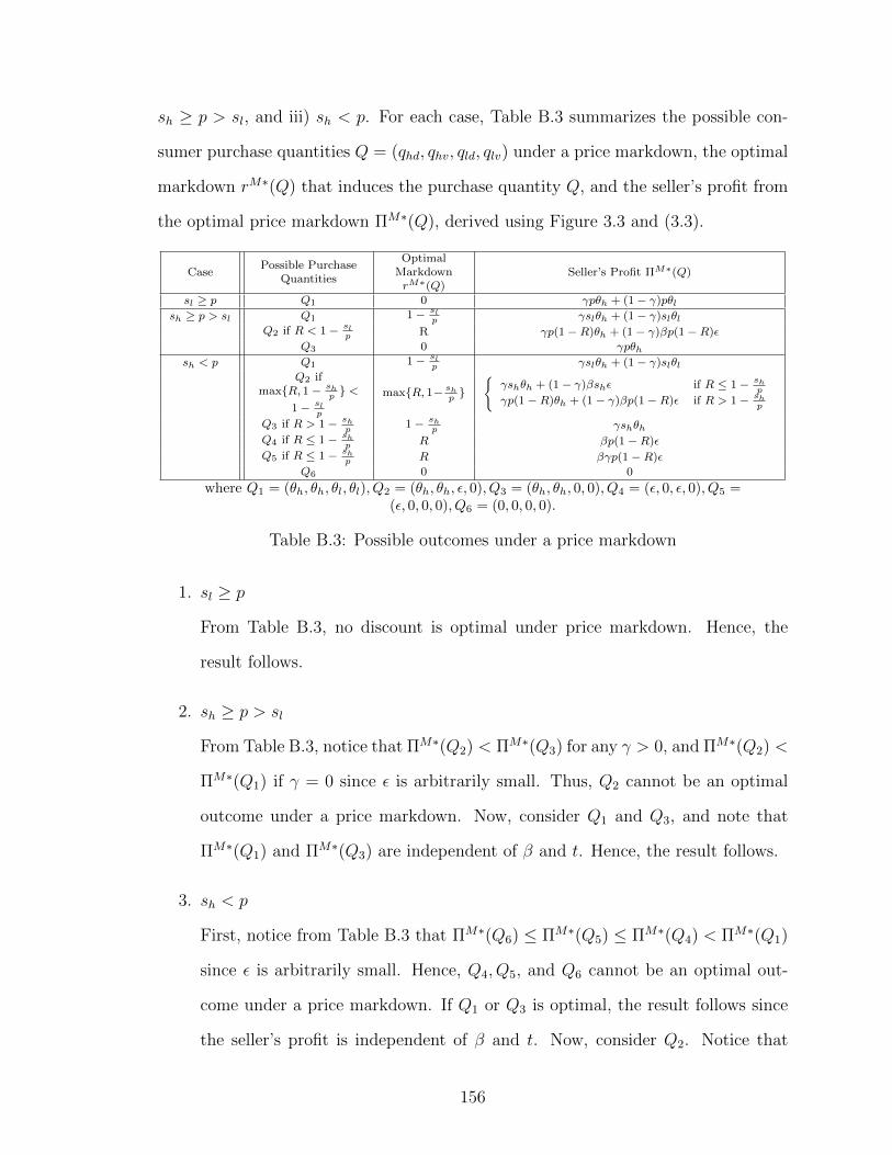
sh ≥ p > sl, and iii) sh < p. For each case, Table B.3 summarizes the possible con-

sumer purchase quantities Q = (qhd, qhv, qld, qlv) under a price markdown, the optimal

markdown rM∗(Q) that induces the purchase quantity Q, and the seller’s profit from

the optimal price markdown ΠM∗(Q), derived using Figure 3.3 and (3.3).

CasePossible Purchase

Quantities

OptimalMarkdownrM∗(Q)

Seller’s Profit ΠM∗(Q)

sl ≥ p Q1 0 γpθh + (1− γ)pθlsh ≥ p > sl Q1 1− sl

p γslθh + (1− γ)slθlQ2 if R < 1− sl

p R γp(1−R)θh + (1− γ)βp(1−R)ε

Q3 0 γpθhsh < p Q1 1− sl

p γslθh + (1− γ)slθlQ2 if

max{R, 1− shp} <

1− slp

max{R, 1− shp}

{γshθh + (1− γ)βshε if R ≤ 1− sh

p

γp(1−R)θh + (1− γ)βp(1−R)ε if R > 1− shp

Q3 if R > 1− shp

1− shp γshθh

Q4 if R ≤ 1− shp R βp(1−R)ε

Q5 if R ≤ 1− shp R βγp(1−R)ε

Q6 0 0

where Q1 = (θh, θh, θl, θl), Q2 = (θh, θh, ε, 0), Q3 = (θh, θh, 0, 0), Q4 = (ε, 0, ε, 0), Q5 =(ε, 0, 0, 0), Q6 = (0, 0, 0, 0).

Table B.3: Possible outcomes under a price markdown

1. sl ≥ p

From Table B.3, no discount is optimal under price markdown. Hence, the

result follows.

2. sh ≥ p > sl

From Table B.3, notice that ΠM∗(Q2) < ΠM∗(Q3) for any γ > 0, and ΠM∗(Q2) <

ΠM∗(Q1) if γ = 0 since ε is arbitrarily small. Thus, Q2 cannot be an optimal

outcome under a price markdown. Now, consider Q1 and Q3, and note that

ΠM∗(Q1) and ΠM∗(Q3) are independent of β and t. Hence, the result follows.

3. sh < p

First, notice from Table B.3 that ΠM∗(Q6) ≤ ΠM∗(Q5) ≤ ΠM∗(Q4) < ΠM∗(Q1)

since ε is arbitrarily small. Hence, Q4, Q5, and Q6 cannot be an optimal out-

come under a price markdown. If Q1 or Q3 is optimal, the result follows since

the seller’s profit is independent of β and t. Now, consider Q2. Notice that

156

ΠM∗(Q2) is independent of t. Hence, the result regarding an increase in t fol-

lows immediately. It remains to show the result regarding an increase in β

when Q2 is optimal. If R > 1 − shp

, then ΠM∗(Q2) < ΠM∗(Q3) for any γ > 0,

and ΠM∗(Q2) < ΠM∗(Q1) if γ = 0 since ε is arbitrarily small. Hence, Q2

cannot be optimal. If R ≤ 1 − shp

, Q2 is optimal if ΠM∗(Q2) > ΠM∗(Q1),

which requires γ > slθlshθh−slθh+slθl

. However, in this situation, the optimal con-

ditional discount, derived from solving the seller’s problem, is an all-unit dis-

count which induces at least one type of deal-prone consumers to overspend

by K > ε. Thus, ΠA∗ = βPr(i)p(1 − rA∗)K + (1 − Pr(i))p(1 − rA∗)q−i,

where i ∈ {l, h} is the type of deal-prone consumers who overspends. Then,

d[ΠA∗−ΠM∗(Q2)]dβ

= Pr(i)p(1− rA∗)K − (1− γ)shε > 0 since ε is arbitrarily small.

Hence, the result follows.

Proof of Lemma 3.1: We will first show the result for the all-unit discount.

Notice from Proposition 3.4 part i) that since β > 0, no discount cannot be optimal.

Thus, an optimal discount must increase purchase quantity of at least one type of

consumers. Let DA∗(γ) = (r∗(γ), K∗(γ)) be the terms of the optimal all-unit discount

when the proportion of high-type consumers is γ. Let ΠH(Dk∗(γ)) and ΠL(Dk∗(γ))

be the seller’s profits earned from the high-type and the low-type consumers under

the optimal discount, respectively.

We will show the result by contradiction. Suppose at γ = γ1, the optimal discount

DA∗(γ1) induces only the high-type consumers to increase their purchase quantity.

Suppose also that there exists γ2 > γ1 such that the optimal discount DA∗(γ2) induces

the low-type consumers to increase their purchase quantity. From the optimality of

DA∗(γ1) at γ = γ1, and DA∗(γ2) at γ = γ2, we have

γ1ΠH(DA∗(γ1)) + (1− γ1)ΠL(DA∗(γ1)) > γ1ΠH(DA∗(γ2)) + (1− γ1)ΠL(DA∗(γ2)), and (B.2)

157

γ2ΠH(DA∗(γ2)) + (1− γ2)ΠL(DA∗(γ2)) ≥ γ2ΠH(DA∗(γ1)) + (1− γ2)ΠL(DA∗(γ1)). (B.3)

We will now show that ΠH(DA∗(γ1)) ≥ ΠH(DA∗(γ2)). To see this, suppose

ΠH(DA∗(γ2)) > ΠH(DA∗(γ1)). Since sh > sl and θh > θl, the high-type purchase

quantity is always no less than the low-type purchase quantity. Given the fact

that the low-type consumer increases purchase quantity under DA∗(γ2), we must

have qh(DA∗(γ2)) ≥ ql(D

A∗(γ2)) > 0. Then, using the results from Proposition

3.1 and equation (B.1), we can construct an all-unit discount DA′ = (r′, K∗(γ2)),

with r′ < r∗(γ2), such that ql(DA′) = ql(r = 0) and qh(D

A′) = qh(DA∗(γ2)). Since

r′ < r∗(γ2) and qh(DA′) = qh(D

A∗(γ2)), it follows that ΠH(DA′) ≥ ΠH(DA∗(γ2)) >

ΠH(DA∗(γ1)). Notice also that under the discount DA′, the low-type does not in-

crease purchase quantity. Hence, the low-type purchases the same quantity at no

discount under both DA′ and DA∗(γ1), implying ΠL(DA′) = ΠL(DA∗(γ1)). Hence,

when γ = γ1, we must have Π(DA′, γ1) > Π(DA∗(γ1), γ1). But this contradicts the

optimality of DA∗(γ1). Thus, it must be that ΠH(DA∗(γ1)) ≥ ΠH(DA∗(γ2)). Ap-

plying this inequality to (B.3), we have ΠL(DA∗(γ2)) ≥ ΠL(DA∗(γ1)). Now, since

ΠH(DA∗(γ1)) ≥ ΠH(DA∗(γ2)),ΠL(DA∗(γ2)) ≥ ΠL(DA∗(γ1)), and γ1 < γ2, it follows

that

γ2[ΠH(DA∗(γ1))− ΠH(DA∗(γ2))]− (1− γ2)[ΠL(DA∗(γ2))− ΠL(DA∗(γ1))] ≥

γ1[ΠH(DA∗(γ1))− ΠH(DA∗(γ2))]− (1− γ1)[ΠL(DA∗(γ2))− ΠL(DA∗(γ1))].

Then, from (B.2), we must have γ2ΠH(DA∗(γ1)) + (1− γ2)ΠL(DA∗(γ1)) >

γ2ΠH(DA∗(γ2)) + (1 − γ2)ΠL(DA∗(γ2)), which contradicts the optimality of DA∗(γ2)

at γ2.

The result for the fixed-amount discount can be shown in the same way.

158

Proof of Proposition 3.7: We will first show the results for the all-unit discount.

In preparation, we employ the results from Proposition 3.1 and enumerate possible

purchase quantities for three cases: no discount, discount increases the high-type

purchase quantity, and discount increases the low-type purchase quantity. Table B.4

summarizes these results.

CaseNo

DiscountOnly High-type Increases

Purchase QuantityLow-type Increases Purchase

Quantity

(ql, qh) (ql, qh)DA∗ = (r,K)

satisfies(ql, qh) DA∗ = (r,K) satisfies

sh < p (0, 0)

(0, θh)K ≤ θh;

(θl, θh) K ≤ θl; sl ≥ p(1− r)sh ≥ p(1− r)

(0,K)(K, θh)

K ≤ θh; θl ≥ θd(DA);θh ≥ θd(DA); sl ≥ σd(θl, DA)sh ≥ σd(θh, DA)

(K,K)θl ≥ θd(DA);sl ≥ σd(θl, DA)

sl < p ≤ sh (0, θh) (0,K) K > θh ≥ θd(DA)

(θl, θh) K ≤ θl; sl ≥ p(1− r)

(K, θh)K ≤ θh; θl ≥ θd(DA);

sl ≥ σd(θl, DA)

(K,K)K ≥ θh; θl ≥ θd(DA);

sl ≥ σd(θl, DA)

sl ≥ p (θl, θh) (θl,K) K > θh ≥ θd(DA)(K, θh) θd(D

A) ≤ θl < K ≤ θh(K,K) K > θl ≥ θd(DA)

Table B.4: Possible outcomes under an optimal all-unit discount

i) Suppose γ > ΓA(t). From Lemma 3.1, the optimal all-unit discount increases

the purchase quantity of only the high-type consumer.

ia) We will show that KA∗ ≥ θh. Notice from Table B.4 that if sh ≥ p, the optimal

discount must satisfy K > θh ≥ θd(DA); thus, the result holds. Now consider

the case of sh < p. From Table B.4, the possible outcomes in this case are (0, θh)

and (0, K). Suppose that K < θh under the optimal discount DA = (r,K). We

will show that there exists another all-unit discount which yields a greater profit

than DA.

a.1) (0, K): From the proof of Proposition 3.1 part iii), when K < θh, the

high-type consumer buys K if σd(θh, DA) ≤ sh < p(1 − r). Applying the

definition of σd(θh, DA) given in equation (B.1), we have p(1−r)− Td(DA)

K≤

159

sh < p(1− r). This implies Td(DA) = t > 0. Thus, p(1− r)K ≤ shK + t,

implying Π(DA) = γp(1− r)K ≤ γ(shK + t).

Now, consider another all-unit discountDA′ = (r′ = max{pK′−shθh−tpK′

, R}, K ′ =

max{θh, t+shθhp(1−R)}). This discount has K ′ ≥ θh. Applying the definitions

from (B.1), we have θd(DA′) = shθh

p< θh ≤ K ′ and sh = σd(θh, D

A′) for

the high-type consumer. Hence, from Proposition 3.1, the high-type pur-

chases K ′. For the low-type consumer, we have sl < σd(θl, DA′), implying

the low-type does not purchase. Applying the expressions of r′ and K ′, we

have Π(DA′) = γp(1− r′)K ′ = γ(shθh + t) > Π(DA) since θh > K.

a.2) (0, θh): From the proof of Proposition 3.1 part iii), when K < θh, the

high-type consumer buys θh if sh ≥ p(1 − r). This implies Π(DA) =

γp(1 − r)θh ≤ γshθh. Notice that this profit is less than the profit from

offering DA′ given in a.1). since t > 0.

Hence, when γ > ΓA(t), an optimal all-unit discount has KA∗ ≥ θh.

ib) We will show that r∗ ≥ R. From ia), KA∗ ≥ θh. This implies the optimal

discount must induce either (ql, qh) = (0, K) when sl < p, or (θl, K) when

sl ≥ p. Suppose the optimal all-unit discount is DA = (r,K), with K ≥ θh

and r < R. Hence, the deal-prone consumers do not receive transaction utility;

i.e., Td(DA) = 0. From equation (B.1), this results in σd(θ,D

A) = σv(θ,DA)

and θd(DA) = θv(D

A). We will show that there exists another all-unit discount

which yields a greater profit than DA.

b.1) (0, K): First, consider the case of sh ≥ p. From Proposition 3.1 and

equation (B.1), since the high-type buys K, we must have θh ≥ θd(DA) =

K(1 − r). This implies Π(DA) = γp(1 − r)K ≤ γpθh. Notice that DA′

with r′ ≥ R given in a.1) results in Π(DA′) = γ(shθh + t) > Π(DA) since

sh ≥ p and t > 0. Now, consider the case of sh < p. From Proposition 3.1,

160

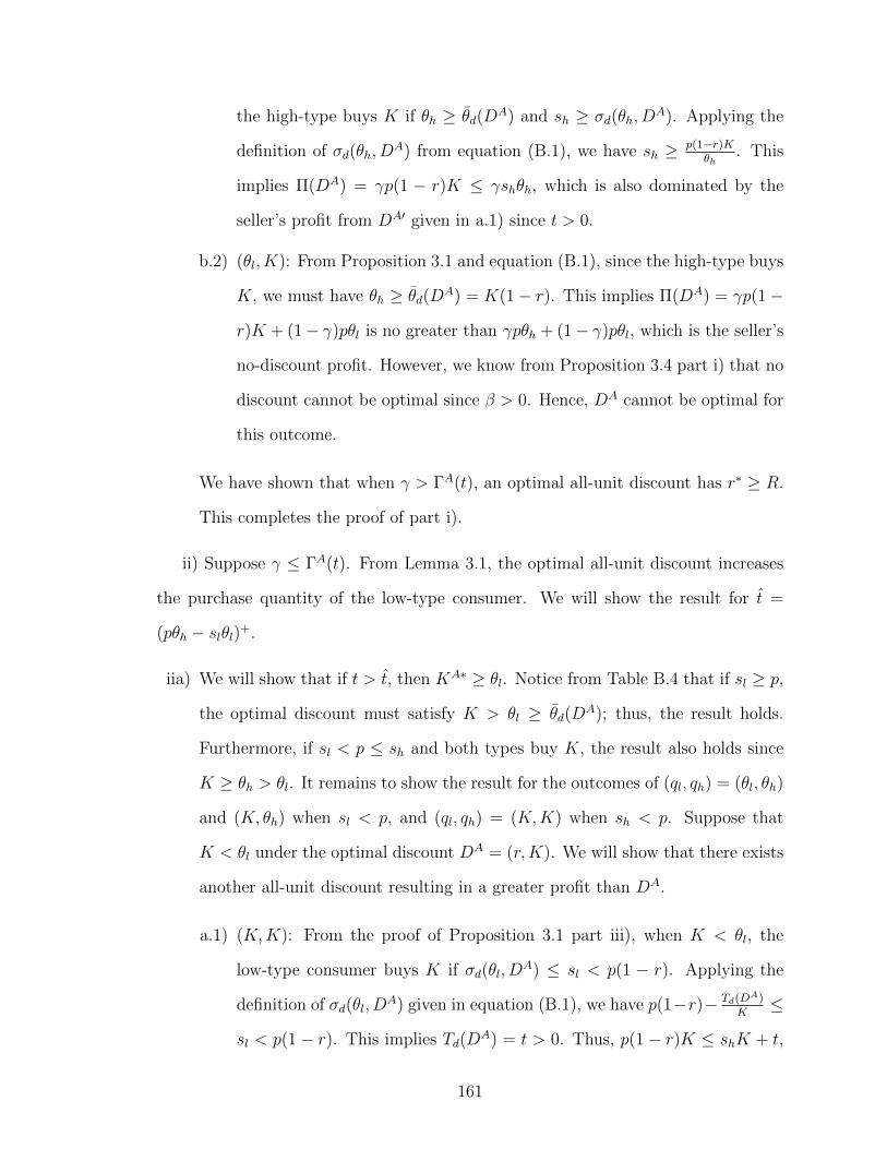
the high-type buys K if θh ≥ θd(DA) and sh ≥ σd(θh, D

A). Applying the

definition of σd(θh, DA) from equation (B.1), we have sh ≥ p(1−r)K

θh. This

implies Π(DA) = γp(1 − r)K ≤ γshθh, which is also dominated by the

seller’s profit from DA′ given in a.1) since t > 0.

b.2) (θl, K): From Proposition 3.1 and equation (B.1), since the high-type buys

K, we must have θh ≥ θd(DA) = K(1− r). This implies Π(DA) = γp(1−

r)K + (1− γ)pθl is no greater than γpθh + (1− γ)pθl, which is the seller’s

no-discount profit. However, we know from Proposition 3.4 part i) that no

discount cannot be optimal since β > 0. Hence, DA cannot be optimal for

this outcome.

We have shown that when γ > ΓA(t), an optimal all-unit discount has r∗ ≥ R.

This completes the proof of part i).

ii) Suppose γ ≤ ΓA(t). From Lemma 3.1, the optimal all-unit discount increases

the purchase quantity of the low-type consumer. We will show the result for t =

(pθh − slθl)+.

iia) We will show that if t > t, then KA∗ ≥ θl. Notice from Table B.4 that if sl ≥ p,

the optimal discount must satisfy K > θl ≥ θd(DA); thus, the result holds.

Furthermore, if sl < p ≤ sh and both types buy K, the result also holds since

K ≥ θh > θl. It remains to show the result for the outcomes of (ql, qh) = (θl, θh)

and (K, θh) when sl < p, and (ql, qh) = (K,K) when sh < p. Suppose that

K < θl under the optimal discount DA = (r,K). We will show that there exists

another all-unit discount resulting in a greater profit than DA.

a.1) (K,K): From the proof of Proposition 3.1 part iii), when K < θl, the

low-type consumer buys K if σd(θl, DA) ≤ sl < p(1 − r). Applying the

definition of σd(θl, DA) given in equation (B.1), we have p(1−r)− Td(DA)

K≤

sl < p(1− r). This implies Td(DA) = t > 0. Thus, p(1− r)K ≤ shK + t,

161

implying Π(DA) = p(1 − r)K ≤ slK + t. Now, consider another all-

unit discount DA′ = (r′ = max{pK′−slθl−tpK′

, R}, K ′ = t+slθlp(1−R)

). Notice that

since t > t = (pθh − slθl)+, this discount has K ′ > θh > θl. Applying

the definition from equation (B.1), we have θd(DA′) = slθl

p< θl < K ′

and σd(θl, DA′) = sl for the low-type consumer. Hence, from Proposition

3.1, the low-type purchases K ′. For the high-type consumer, we have

θd(DA′) < θh < K ′ and σd(θh, D

A′) = slθlθh

< sh. Hence, the high-type also

purchases K ′. Applying the expressions of r′ and K ′, we have Π(DA′) =

p(1 − r′)K ′ = slθl + t. Notice that Π(DA′) > Π(DA) since K < θl. Thus,

DA cannot be optimal.

a.2) (K, θh): Similar to a.1), for the low-type consumer to buyK < θl, DA needs

to trigger transaction utility, i.e., Td(DA) = t > 0. This implies r ≥ R.

Hence, Π(DA) = p(1−r)(γθh+(1−γ)K) ≤ p(1−R)(γθh+(1−γ)K) < pθh,

where the last inequality comes from K < θl < θh, and R > 0. Notice

that Π(DA) is less than the profit from DA′ given in a.1) since Π(DA′) =

slθl + t > pθh from t > t = (pθh − slθl)+.

a.3) (θl, θh): From the proof of Proposition 3.1 part iii), when K < θl, the

low-type buys θl if sl ≥ p(1−r). This implies Π(DA) = p(1−r)(γθh+(1−

γ)θl) ≤ sl(γθh + (1 − γ)θl). Notice that this is less than pθh since sl < p

and θl < θh. Hence, it is also dominated by Π(DA′) as shown in a.2).

We have shown that when γ ≤ ΓA(t) and t > t, an optimal all-unit discount

has KA∗ ≥ θl.

iib) We will show that if t > t, then r∗ ≥ R. From iia), KA∗ ≥ θl. Hence, from

Table B.4, the optimal discount must induce either (ql, qh) = (K,K) or (K, θh).

Suppose that the optimal all-unit discount is DA = (r,K) with K ≥ θl and

r < R. Hence, the deal-prone consumers do not receive transaction utility, i.e.,

162

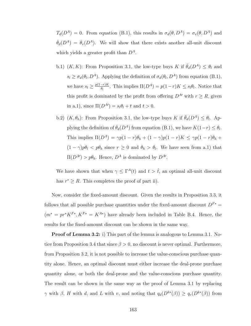
Td(DA) = 0. From equation (B.1), this results in σd(θ,D

A) = σv(θ,DA) and

θd(DA) = θv(D

A). We will show that there exists another all-unit discount

which yields a greater profit than DA.

b.1) (K,K): From Proposition 3.1, the low-type buys K if θd(DA) ≤ θl and

sl ≥ σd(θl, DA). Applying the definition of σd(θl, D

A) from equation (B.1),

we have sl ≥ p(1−r)Kθl

. This implies Π(DA) = p(1− r)K ≤ slθl. Notice that

this profit is dominated by the profit from offering DA′ with r ≥ R, given

in a.1), since Π(DA′) = slθl + t and t > 0.

b.2) (K, θh): From Proposition 3.1, the low-type buys K if θd(DA) ≤ θl. Ap-

plying the definition of θd(DA) from equation (B.1), we have K(1−r) ≤ θl.

This implies Π(DA) = γp(1 − r)θh + (1 − γ)p(1 − r)K ≤ γp(1 − r)θh +

(1 − γ)pθl < pθh since r ≥ 0 and θh > θl. We have seen from a.1) that

Π(DA′) > pθh. Hence, DA is dominated by DA′.

We have shown that when γ ≤ ΓA(t) and t > t, an optimal all-unit discount

has r∗ ≥ R. This completes the proof of part ii).

Now, consider the fixed-amount discount. Given the results in Proposition 3.3, it

follows that all possible purchase quantities under the fixed-amount discount DF∗ =

(m∗ = pr∗KF∗, KF∗ = KA∗) have already been included in Table B.4. Hence, the

results for the fixed-amount discount can be shown in the same way.

Proof of Lemma 3.2: i) This part of the lemma is analogous to Lemma 3.1. No-

tice from Proposition 3.4 that since β > 0, no discount is never optimal. Furthermore,

from Proposition 3.2, it is not possible to increase the value-conscious purchase quan-

tity alone. Hence, an optimal discount must either increase the deal-prone purchase

quantity alone, or both the deal-prone and the value-conscious purchase quantity.

The result can be shown in the same way as the proof of Lemma 3.1 by replacing

γ with β, H with d, and L with v, and noting that qd(Dk∗(β)) ≥ qv(D

k∗(β)) from

163

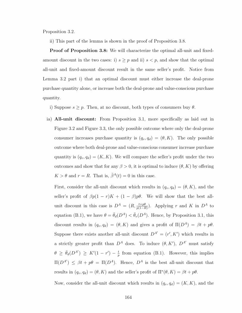
Proposition 3.2.

ii) This part of the lemma is shown in the proof of Proposition 3.8.

Proof of Proposition 3.8: We will characterize the optimal all-unit and fixed-

amount discount in the two cases: i) s ≥ p and ii) s < p, and show that the optimal

all-unit and fixed-amount discount result in the same seller’s profit. Notice from

Lemma 3.2 part i) that an optimal discount must either increase the deal-prone

purchase quantity alone, or increase both the deal-prone and value-conscious purchase

quantity.

i) Suppose s ≥ p. Then, at no discount, both types of consumers buy θ.

ia) All-unit discount: From Proposition 3.1, more specifically as laid out in

Figure 3.2 and Figure 3.3, the only possible outcome where only the deal-prone

consumer increases purchase quantity is (qv, qd) = (θ,K). The only possible

outcome where both deal-prone and value-conscious consumer increase purchase

quantity is (qv, qd) = (K,K). We will compare the seller’s profit under the two

outcomes and show that for any β > 0, it is optimal to induce (θ,K) by offering

K > θ and r = R. That is, βA(t) = 0 in this case.

First, consider the all-unit discount which results in (qv, qd) = (θ,K), and the

seller’s profit of βp(1 − r)K + (1 − β)pθ. We will show that the best all-

unit discount in this case is DA = (R, t+pθp(1−R)

). Applying r and K in DA to

equation (B.1), we have θ = θd(DA) < θv(D

A). Hence, by Proposition 3.1, this

discount results in (qv, qd) = (θ,K) and gives a profit of Π(DA) = βt + pθ.

Suppose there exists another all-unit discount DA′ = (r′, K ′) which results in

a strictly greater profit than DA does. To induce (θ,K ′), DA′ must satisfy

θ ≥ θd(DA′) ≥ K ′(1 − r′) − t

pfrom equation (B.1). However, this implies

Π(DA′) ≤ βt + pθ = Π(DA). Hence, DA is the best all-unit discount that

results in (qv, qd) = (θ,K) and the seller’s profit of Π∗(θ,K) = βt+ pθ.

Now, consider the all-unit discount which results in (qv, qd) = (K,K), and the

164

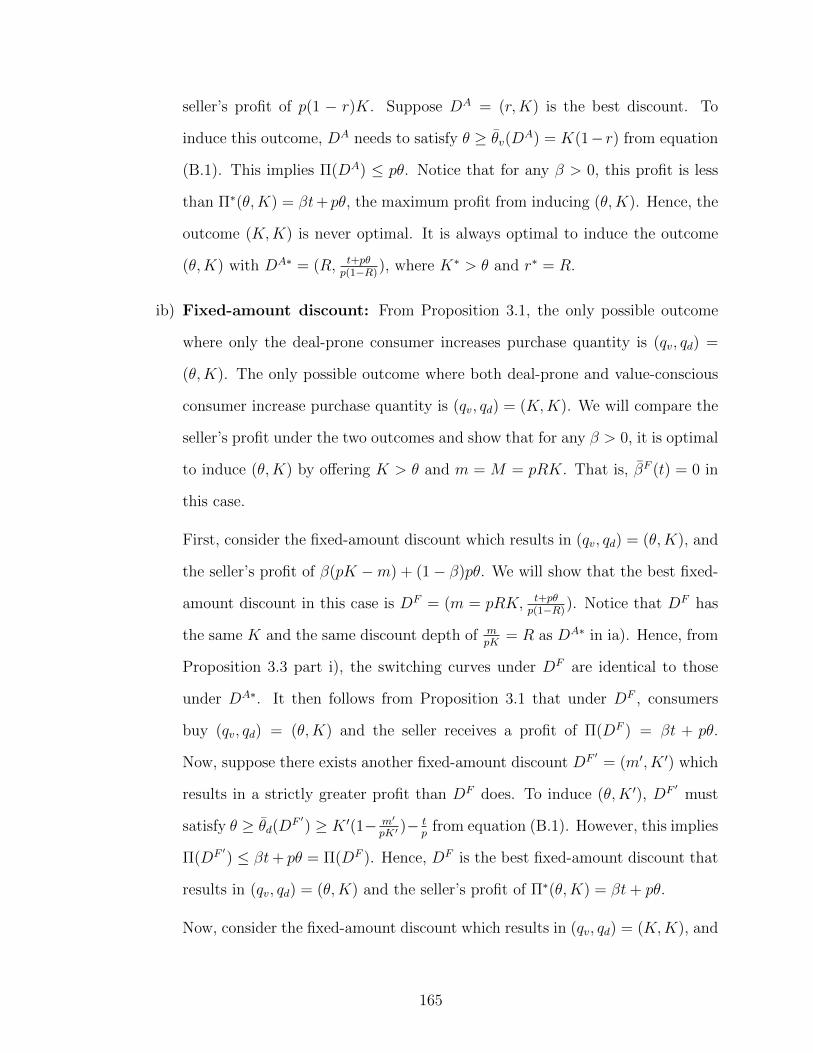
seller’s profit of p(1 − r)K. Suppose DA = (r,K) is the best discount. To

induce this outcome, DA needs to satisfy θ ≥ θv(DA) = K(1− r) from equation

(B.1). This implies Π(DA) ≤ pθ. Notice that for any β > 0, this profit is less

than Π∗(θ,K) = βt+ pθ, the maximum profit from inducing (θ,K). Hence, the

outcome (K,K) is never optimal. It is always optimal to induce the outcome

(θ,K) with DA∗ = (R, t+pθp(1−R)

), where K∗ > θ and r∗ = R.

ib) Fixed-amount discount: From Proposition 3.1, the only possible outcome

where only the deal-prone consumer increases purchase quantity is (qv, qd) =

(θ,K). The only possible outcome where both deal-prone and value-conscious

consumer increase purchase quantity is (qv, qd) = (K,K). We will compare the

seller’s profit under the two outcomes and show that for any β > 0, it is optimal

to induce (θ,K) by offering K > θ and m = M = pRK. That is, βF (t) = 0 in

this case.

First, consider the fixed-amount discount which results in (qv, qd) = (θ,K), and

the seller’s profit of β(pK −m) + (1− β)pθ. We will show that the best fixed-

amount discount in this case is DF = (m = pRK, t+pθp(1−R)

). Notice that DF has

the same K and the same discount depth of mpK

= R as DA∗ in ia). Hence, from

Proposition 3.3 part i), the switching curves under DF are identical to those

under DA∗. It then follows from Proposition 3.1 that under DF , consumers

buy (qv, qd) = (θ,K) and the seller receives a profit of Π(DF ) = βt + pθ.

Now, suppose there exists another fixed-amount discount DF ′ = (m′, K ′) which

results in a strictly greater profit than DF does. To induce (θ,K ′), DF ′ must

satisfy θ ≥ θd(DF ′) ≥ K ′(1− m′

pK′)− t

pfrom equation (B.1). However, this implies

Π(DF ′) ≤ βt+ pθ = Π(DF ). Hence, DF is the best fixed-amount discount that

results in (qv, qd) = (θ,K) and the seller’s profit of Π∗(θ,K) = βt+ pθ.

Now, consider the fixed-amount discount which results in (qv, qd) = (K,K), and

165

the seller’s profit of pK −m. Suppose DF = (m,K) is the best discount. To

induce this outcome, DF needs to satisfy θ ≥ θv(DF ) = K(1− m

pK) from equation

(B.1). This implies Π(DF ) ≤ pθ. Notice that for any β > 0, this profit is less

than Π∗(θ,K) = βt+ pθ, the maximum profit from inducing (θ,K). Hence, the

outcome (K,K) is never optimal. It is always optimal to induce the outcome

(θ,K) with DF∗ = (m = pRK, t+pθp(1−R)

).

From ia) and ib), we have that the optimal all-unit and fixed-amount discount

have the same K and the same discount depth, and result in the same seller’s profit.

ii) Suppose s < p. Then, at no discount, both types of consumers do not buy.

iia) All-unit discount: From Proposition 3.1, the only possible outcome where

only the deal-prone consumer increases purchase quantity is (qv, qd) = (0, K).

There are two possible outcomes where both deal-prone and value-conscious

consumer increase purchase quantity: (qv, qd) = (K,K) and (qv, qd) = (θ, θ).

Following the same procedure as in part i), we can characterize the best all-unit

discount which increases only the deal-prone purchase quantity, and the best

discount which increases both deal-prone and value-conscious purchase quantity.

The best all-unit discount in each case is provided below.

If only the deal-prone purchase quantity is increased, it is most profitable to

offer

DA = (r,K) =

( θ(p−s)−tpθ

, θ) if θ(p−s)−tpθ

≥ R

(R, θs+tp(1−R)

) if θ(p−s)−tpθ

< R

Notice that r ≥ R and K ≥ θ. The resulting outcome is (qv, qd) = (0, K), and

the seller’s profit is Π∗(0, K) = β(t+ sθ).

If both the deal-prone and value-conscious purchase quantity are increased, it

is most profitable to offer DA = (1− sp, θ). The resulting outcome is (qv, qd) =

166

(θ, θ), and the seller’s profit is Π∗(θ, θ) = sθ.

Now, notice that Π∗(0, K) > Π∗(θ, θ) if and only if β > sθt+sθ

. Hence, it is

optimal to increase only the deal-prone purchase quantity if β > sθt+sθ

, and it

is optimal to increase both deal-prone and value-conscious purchase quantity if

β ≤ sθt+sθ

. This shows that βA(t) = sθt+sθ

from Lemma 3.2 part i).

iib) Fixed-amount discount: We know from Proposition 3.5 that when s < p,

the all-unit discount weakly dominates the fixed-amount discount. Hence, to

show that the optimal fixed-amount discount results in the same profit as the

optimal all-unit discount does, it suffices to show that there exists a fixed-

amount discount which yields the same seller’s profit as DA∗ = (r∗, K∗) does.

For this, consider DF = (m = pr∗K∗, K∗). It is easy to check that DF results

in the same outcomes and the same seller’s profit as DA∗, characterized above.

Then, it also follows that βF (t) = βA(t) = sθt+sθ

.

iia) and iib) complete the proof of part ii).

Proof for Optimal Endogenous Prices

We will first show the result for the all-unit discount by showing that the seller’s

profit from setting p = sl, sh, or shθh+tθh(1−R)

weakly dominates the seller’s profit obtained

from all other prices.

i) p < sl is dominated by p = sl

Suppose DA = (p, r,K) is optimal for some p < sl. Now, consider DA′ = (p′ =

sl, r′ = sl−p(1−r)

sl, K ′ = K). Since p′(1 − r′) = p(1 − r), K ′ = K, and r′ > r,

from equation (B.1) and Proposition 3.1, we have that a consumer purchases at

least as much under DA′ as under DA. Notice that if the consumer purchases

at discount, the seller’s margin is the same at p(1− r) under both DA and DA′ .

However, if the consumer purchases at no discount, the seller’s margin is greater

(p′ = sl > p) under DA′ . Hence, DA′ weakly dominates DA.

167

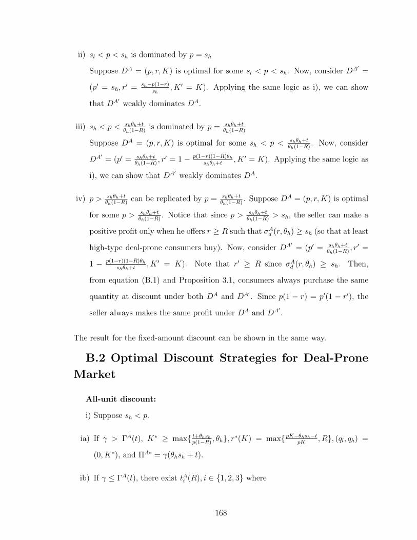
ii) sl < p < sh is dominated by p = sh

Suppose DA = (p, r,K) is optimal for some sl < p < sh. Now, consider DA′ =

(p′ = sh, r′ = sh−p(1−r)

sh, K ′ = K). Applying the same logic as i), we can show

that DA′ weakly dominates DA.

iii) sh < p < shθh+tθh(1−R)

is dominated by p = shθh+tθh(1−R)

Suppose DA = (p, r,K) is optimal for some sh < p < shθh+tθh(1−R)

. Now, consider

DA′ = (p′ = shθh+tθh(1−R)

, r′ = 1− p(1−r)(1−R)θhshθh+t

, K ′ = K). Applying the same logic as

i), we can show that DA′ weakly dominates DA.

iv) p > shθh+tθh(1−R)

can be replicated by p = shθh+tθh(1−R)

. Suppose DA = (p, r,K) is optimal

for some p > shθh+tθh(1−R)

. Notice that since p > shθh+tθh(1−R)

> sh, the seller can make a

positive profit only when he offers r ≥ R such that σAd (r, θh) ≥ sh (so that at least

high-type deal-prone consumers buy). Now, consider DA′ = (p′ = shθh+tθh(1−R)

, r′ =

1 − p(1−r)(1−R)θhshθh+t

, K ′ = K). Note that r′ ≥ R since σAd (r, θh) ≥ sh. Then,

from equation (B.1) and Proposition 3.1, consumers always purchase the same

quantity at discount under both DA and DA′ . Since p(1 − r) = p′(1 − r′), the

seller always makes the same profit under DA and DA′ .

The result for the fixed-amount discount can be shown in the same way.

B.2 Optimal Discount Strategies for Deal-Prone

Market

All-unit discount:

i) Suppose sh < p.

ia) If γ > ΓA(t), K∗ ≥ max{ t+θhshp(1−R)

, θh}, r∗(K) = max{pK−θhsh−tpK

, R}, (ql, qh) =

(0, K∗), and ΠA∗ = γ(θhsh + t).

ib) If γ ≤ ΓA(t), there exist tAi (R), i ∈ {1, 2, 3} where

168

• For t ≤ tA1 (R), ΓA(t) = ΓA1 (t, R), K∗ ≤ θl and (ql, qh) = (θl, θh).

• For tA1 (R) < t ≤ tA2 (R), ΓA(t) = ΓA2 (t, R), (ql, qh) = (θl, θh) or (K∗, θh).

• For tA2 (R) < t ≤ tA3 (R), ΓA(t) = ΓA3 (t, R), K∗ ≥ θl and (ql, qh) = (θl, θh) or

(K∗, θh) or (K∗, K∗).

• For t > tA3 (R), ΓA(t) = ΓA4 (t, R), K∗ ≥ θl and (ql, qh) = (K∗, K∗).

The closed-form expressions of tAi (R) and ΓAi (t, R) are summarized in Table B.5.

ii) Suppose sl < p ≤ sh. In this case, ΓA(t) and the optimal all-unit discount in

this case are as characterized in i) by replacing sh with p.

iii) Suppose sl ≥ p.

iiia) If γ > ΓA(t), K∗ = t+pθhp(1−R)

, r∗ = R, (ql, qh) = (θl, K∗), and Π∗ = γ(t + p(θh −

θl)) + pθl.

iiib) If γ ≤ ΓA(t):

• For t ≤ θhp(1 − R) − pθl, ΓA(t) = t2t+pRθh

, K∗ = t+pθlp(1−R)

, r∗ = R, (ql, qh) =

(K∗, θh), and Π∗ = (1− γ)t+ p(θl + γ(θh(1−R)− θl).

• For t > θhp(1−R)− pθl, ΓA(t) = tt+p(θh−θl)

, K∗ = t+pθlp(1−R)

, r∗ = R, (ql, qh) =

(K∗, K∗), and Π∗ = pθl + t.

Fixed-amount discount:

i) sh < p

For all t ≥ 0, ΓF (t) = t+slθlt+shθh

.

ia) If γ > ΓF (t), K∗ ≥ max{θh, t+θhshp(1−R)},m∗ ≥ max{θh(p − sh) − t,M}, (ql, qh) =

(0, K∗) and Π∗ = γ(shθh + t).

ib) If γ ≤ ΓF (t), K∗ ≥ max{θh, θlsl+tp(1−R)

},m∗ ≥ max{pθh − θlsl − t,M}, (ql, qh) =

(K∗, K∗), and Π∗ = slθl + t.

ii) sl < p ≤ sh

169

iia) If γ > ΓF (t), K∗ = pθh+tp(1−R)

,m∗ = R(pθh+t)1−R , (ql, qh) = (0, K∗), and Π∗ = γ(pθh+t).

iib) If γ < ΓF (t), there exist tFi (R), i ∈ {1, 2, 3} where

• For t ≤ tF1 (R), ΓF (t) = ΓF1 (t, R), K∗ ≤ θl and (ql, qh) = (θl, θh).

• For tF1 (R) < t ≤ tF2 (R), ΓF (t) = ΓF2 (t, R), (ql, qh) = (θl, θh) or (K∗, θh).

• For tF2 (R) < t ≤ tF3 (R), ΓF (t) = ΓF3 (t, R), K∗ ≥ θl and (ql, qh) = (θl, θh) or

(K∗, θh) or (K∗, K∗).

• For t > tF3 (R), ΓF (t) = ΓF4 (t, R), K∗ ≥ θh and (ql, qh) = (K∗, K∗).

The closed-form expressions of tFi (R) and ΓFi (t, R) are summarized in Table B.6.

iii) sl ≥ p

iiia) If γ > ΓF (t), K∗ = t+pθhp(1−R)

,m∗ = R(pθh+t)1−R , (ql, qh) = (θl, K

∗), and Π∗ = γ(t +

p(θh − θl)) + pθl.

iiib) If γ ≤ ΓF (t):

• For t ≤ θhp(1−R)− pθl, ΓF (t) = t(1−R)2t−Rt+pRθl

, K∗ = t+pθlp(1−R)

,m∗ = R(pθl+t)p(1−R)

,

(ql, qh) = (K∗, θh), and Π∗ = γpθh + (1−γ−R)(pθl+t)1−R .

• For t > θhp(1−R)− pθl, ΓF (t) = tt+p(θh−θl)

, K∗ = t+pθlp(1−R)

,m∗ = R(pθl+t)1−R ,

(ql, qh) = (K∗, K∗), and Π∗ = pθl + t.

170

itA i

(R)

ΓA i

(t,R

)

1{ 0

ifR<R

(sh

)orR≥R

(sl)

slθhθl(s

h−p(1−R))

p(1−R)θ

h−slθl

ifR

(sh

)≤R<R

(sl)

{slθl

shθh−sl(θ

h−θl)

ifR<R

(sh

)orR≥R

(sl)

θl(t+slθl)

θl(s

hθh−sl(θ

h−θl))−t(θh−2θl)

ifR

(sh

)≤R<R

(sl)

2

θ l(p

(1−r)−s l

)ifR<R

(sl)

1 2[√ θ h

(θh

(sh−s l

)2+

4s lθ l

(sl−p(1−R

)))−θ h

(sh−s l

)]ifR

(sl)≤R<R

(sA

)

θ hp(1−R

)−s lθ l

ifR≥R

(sA

)

{p(1−r)t

(2p(1−r)−sl)t+θh(s

h−p(1−r))(p

(1−r)−sl)

ifR<R

(sl)

slθl

t+shθh−sl(θ

h−θl)

ifR≥R

(sl)

3

{ θhp(1−r)−s lθ l

ifR<R

(sA

)θ hsA−s lθ l

ifR≥R

(sA

)

{t+slθl

2t+θh(s

h−p(1−r))+slθl

ifR<R

(sA

)

ΓA 2

(t,R

)ifR≥R

(sA

)

4N/A

t+s lθ l

t+s hθ h

Tab

leB

.5:

Clo

sed-f

orm

expre

ssio

ns

oftA i

(R)

and

ΓA i

(t,R

)fo

ral

l-unit

dis

count

when

s h<p

wher

eR

(x)

:=p−x

p

sA:=

1 2θh

[√ 4s2 lθ l

(θh−θ l

)+

(shθ h−s l

(θh−θ l

))2−s hθ h

+s l

(θh

+θ l

)]

r:=

max{1−s h p,R}

sF:=

1 2θh

[√ pθl(

4sl(θ h−θ l

)+pθ

l)+θ l

(2s l−p)

]

171

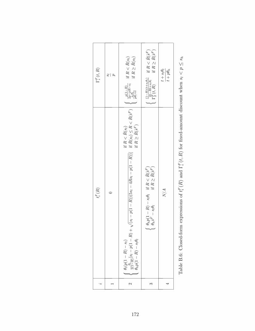
itF i

(R)

ΓF i

(t,R

)

10

s l p

2

θ l(p

(1−R

)−s l

)ifR<R

(sl)

θl

2(1−R)[sl−p(1−R

)+√ (s

l−p(1−R

))(5s l−

4Rs l−p(1−R

))]

ifR

(sl)≤R<R

(sF

)

θ hp(1−R

)−s lθ l

ifR≥R

(sF

)

{p(1−R)

2p−pR−sl

ifR<R

(sl)

slθl

pθl+t

ifR≥R

(sl)

3

{ θ hp(1−R

)−s lθ l

ifR<R

(sF

)θ hsF−s lθ l

ifR≥R

(sF

)

{ (1−R)(t+slθl)

2t−Rt+slθl

ifR<R

(sF

)

ΓF 2

(t,R

)ifR≥R

(sF

)

4N/A

t+s lθ l

t+pθ h

Tab

leB

.6:

Clo

sed-f

orm

expre

ssio

ns

oftF i

(R)

and

ΓF i

(t,R

)fo

rfixed

-am

ount

dis

count

when

s l<p≤s h

172

APPENDIX C

Proofs for Chapter 4

Proof of Proposition 4.1: 1. Suppose I t1 > 0 and I t2 > 0, so A(It) = {1, 2}.

We will first show that the retailer’s profit-to-go in period t is strictly unimodal in

the uniform price pt. Notice from equation (4.3) that only J t(pt, It) depends on pt,

where J t(pt, It) = µ1 [pt − ct1 − β∆t1(It)] + µ2 [pt − ct2 − β∆t

2(It)]. Hence, to show the

unimodality of the profit function in pt, it suffices to show that ∂2Jt(pt,It)∂(pt)2

< 0 whenever

∂Jt(pt,It)∂pt

= 0. We derive the first- and second-order derivative of J t(pt, It) with respect

to pt as follows:

∂J t(pt,Yt)

∂pt=

∂µ1

∂pt[pt − ct1 − β∆t

1(Y t1 , Y

t2 )] + µ1 + (C.1)

∂µ2

∂pt[pt − ct2 − β∆t

2(Y t1 , Y

t2 )] + µ2

∂2J t(pt,Yt)

∂(pt)2=

∂2µ1

∂(pt)2[pt − ct1 − β∆t

1(Y t1 , Y

t2 )] + 2

∂µ1

∂pt+

∂2µ2

∂(pt)2[pt − ct2 − β∆t

2(Y t1 , Y

t2 )] + 2

∂µ2

∂pt,

173

where

∂µi∂pt

= −µiµ0 (C.2)

∂2µi∂(pt)2

= µiµ0(2µ0 − 1), i ∈ A(It).

From equation (C.1), if ∂Jt(pt,It)∂pt

= 0, then

pt − ct1 − β∆t1(It) =

(−∂µ2

∂pt[pt − ct2 − β∆t

2(It)]− µ1 − µ2

)∂µ1∂pt

(C.3)

Substituting equations (C.3) and (C.2) into (??), we obtain

∂2J t(pt, It)

∂(pt)2| ∂Jt(pt,It)

∂pt=0

= −µ1 − µ2 < 0.

This shows that the retailer’s profit-to-go in period t is strictly unimodal in the uni-

form price pt, so the optimal pt is unique. Notice from equation (C.2) that ∂µi∂pt

< 0, i ∈

A(It). Hence, it is easy to see from equation (C.1) that ∂Jt(pt,It)∂pt

> 0 for sufficiently

small pt, and ∂Jt(pt,It)∂pt

< 0 for sufficiently large pt. This implies that the optimal

uniform price pt∗un is an interior solution, characterized by the first-order condition,

∂Jt(pt,It)∂pt

= 0. We can rearrange the first-order condition and apply the definition of

µi, i ∈ {0, 1, 2}, from equation (4.1) to obtain: pt∗un =exp(v1)(ct1+β∆t

1(It))+exp(v2)(ct2+β∆t2(It))

exp(v1)+exp(v2)+

1µ0(pt∗un)

. Applying this to the definition of J t, we have J t(pt∗un, It) = exp(v1 − pt∗un) +

exp(v2−pt∗un) = R(pt∗un, A(It)). Hence, from (4.3), the retailer’s profit-to-go is V tun(It) =

Rt∗unλ

t + βV t−1un (It).

2. Suppose I t1 = 0 and I t2 > 0, so At(It) = {2}. Then, µ1 = 0, and J t(pt, It) =

µ2[pt−ct2−β∆t2(0, I t2)]. Following the same procedure as part 1., we will show that the

optimal uniform price is unique and is characterized by the first-order condition by

showing ∂2Jt(pt,It)∂(pt)2

< 0 whenever ∂Jt(pt,It)∂pt

= 0. The first- and second-order derivative

174

are given by:

∂J t(pt, It)

∂pt=

∂µ2

∂pt[pt − ct2 − β∆t

2(It)] + µ2 (C.4)

∂2J t(pt, It)

∂(pt)2=

∂2µ2

∂(pt)2[pt − ct2 − β∆t

2(It)] + 2∂µ2

∂pt, (C.5)

where

∂µ2

∂pt= −µ2µ0 (C.6)

∂2µ2

∂(pt)2= µ2µ0(2µ0 − 1)

From equation (C.4), if ∂Jt(pt,It)∂pt

= 0, then

pt − ct2 − β∆t2(It) =

−µ2

∂µ2∂pt

(C.7)

Substituting equations (C.7) and (C.6) into (C.5), we obtain: ∂2Jt(pt,It)∂(pt)2

| ∂Jt(pt,It)∂pt

=0=

−µ2 < 0. Hence, the optimal uniform price pt∗un is characterized by the first-order

condition, ∂Jt(pt,It)∂pt

= 0. Rearranging the condition, we obtain: pt∗un = ct2 + β∆t2(It) +

1µ0(pt∗un)

. Applying this to equation (4.3) results in J t(pt∗un, It) = exp(v2 − pt∗un) =

R(pt∗un, A(It)), and the retailer’s profit-to-go of V tun(It) = Rt∗

unλt + βV t−1

un (It).

Proof of Proposition 4.2: 1. Suppose I t1 > 0 and I t2 > 0, so At(It) = {1, 2}.

We will show that the retailer’s profit-to-go in period t is strictly unimodal in the

price vector pt = (pt1, pt2). Notice from equation (4.4) that only J t(pt, It) depends

on pt, where J t(pt, It) = µ1 [pt1 − ct1 − β∆t1(It)] + µ2 [pt2 − ct2 − β∆t

2(It)]. Hence, we

will show the result by showing that J t is unimodal in pt. We derive the first-order

derivative of J t(pt, It) with respect to pti, i ∈ {1, 2}, as follows:

∂J t(pt, It)

∂pti=

∂µ1

∂pti[pt1 − ct1 − β∆t

1(It)] +∂µ2

∂pti[pt2 − ct2 − β∆t

2(It)] + µi (C.8)

175

where

∂µi∂pti

= −µi(1− µi) (C.9)

∂µj∂pti

= µjµi, i, j ∈ A(It), i 6= j.

Notice from equation (C.8) that ∂Jt(pt,It)∂pti

> 0 for sufficiently small pti since ∂µi∂pti

< 0.

Likewise, ∂Jt(pt,It)∂pti

< 0 for sufficiently large pti. This implies that an optimal solution

must be an interior solution and satisfy the first-order conditions with respect to pti:

∂Jt(pt,It)∂pti

= 0, i ∈ A(It).

Substituting (C.9) into (C.8), we obtain the first-order conditions:

∂J t(pt, It)

∂pti= µi

[−(1− µi)

(pti − cti − β∆t

i(It))

+ µj(ptj − ctj − β∆t

j(It))

+ 1]

= µi[J t(pt, It) + 1−

(pti − cti − β∆t

i(It))]

= 0, i, j ∈ At(It), i 6= j.

Since µi > 0, a pti which satisfies the first-order conditions must be such that pti −

cti − β∆ti(I

t) = J t(pt, It) + 1 for i ∈ At(It). Hence, an optimal pt = (pt1, pt2) must

satisfy pt1 − ct1 − β∆t1(It) = pt2 − ct2 − β∆t

2(It). Let m := pti − cti − β∆ti(I

t). Then,

substituting m in the definition of J t, we have J t(pt, It) = (µ1 + µ2)m. From the

first-order conditions, J t(pt, It) = m − 1. Hence, we have J t(pt, It) = m − 1 =

(µ1 + µ2)m. Solving this yields m = 11−µ1−µ2 = 1

µ0. Thus, an optimal solution must

satisfy pt∗i = m+ cti + β∆ti(I

t) = 1µ0(pt∗1 ,p

t∗2 )

+ cti + β∆ti(I

t), i ∈ At(It).

Next, we will show that the optimal price pt is unique. For notational simplicity,

we will drop It from the expressions below. Since pt1− ct1−β∆t1 = pt2− ct2−β∆t

2 = m,

J t can be written as a function of m as follows:

J t(m) = [µ1(pt(m)) + µ2(pt(m))]m = [1− µ0(pt(m))]m (C.10)

where pt(m) = (m+ ct1 + β∆t1,m+ ct2 + β∆t

2), and

176

µ0(pt(m)) = 11+exp(v1−m−ct1−β∆t

1)+exp(v2−m−ct2−β∆t2)

.

The first-order derivative of J t is given by ∂Jt(m)∂m

= 1− µ0(pt(m))−m∂µ0(pt(m))∂m

.

Notice that

∂µ0(pt(m))

∂m=

exp(v1 −m− ct1 − β∆t1) + exp(v2 −m− ct2 − β∆t

2)

(1 + exp(v1 −m− ct1 − β∆t1) + exp(v2 −m− ct2 − β∆t

2))2(C.11)

= µ0(pt(m))[1− µ0(pt(m))]

Applying (C.11) and (C.10) to ∂Jt(m)∂m

, we obtain

∂J t(m)

∂m= 1− µ0(pt(m))[1 + J t(m)] (C.12)

Then, we can derive the second-order derivative of J t as:

∂2J t(m)

∂m2= −∂µ0(pt(m))

∂m[1 + J t(m)]− µ0(pt(m))

∂J t(m)

∂m(C.13)

Notice from (C.12) and (C.13) that whenever ∂Jt(m)∂m

= 0, ∂2Jt(m)∂m2 = −∂µ0(pt(m))

∂m[1 +

J t(m)] = −µ0(pt(m))(1−µ0(pt(m)))[1+J t(m)] < 0. This implies the unimodality of

J t with respect to m, which in turn implies the uniqueness of the optimal solution pt.

Hence, the unique optimal prices are characterized by: pt∗i = cti + 1µ0(pt∗1 ,p

t∗2 )

+ β∆ti(I

t).

Applying this to equation (4.4), we have J t(pt∗, It) = exp(v1− pt∗1 ) + exp(v2− pt∗2 ) =

R(pt∗, A(It)), resulting in the retailer’s profit-to-go of V tdn(It) = Rt∗

utλt + βV t−1

dn (It).

2. Suppose I t1 = 0 and I t2 > 0, so At(It) = {2}. Since transshipment is not

allowed, we have I t1 = 0 and µ1 = 0 for t, t + 1, ..., T . Then, the retailer’s pricing

problem in period t and on is the same as that under the uniform pricing policy

without transshipment. It follows immediately that pt∗2 is the same as pt∗un and the

retailer receives the same profit as characterized in Proposition 4.1 part 2.

Proof of Corollary 4.1: First, notice from Proposition 4.2 part 2 that if I t1 = 0

and I t2 > 0, then the optimal price under both pricing policies are the same, resulting

in the same sale ratio. Hence, the result trivially holds for this case. Next, we

177

will show the result for I t1 > 0 and I t2 > 0. From Proposition 4.1 and 4.2, we show

that the retailer’s expected profit under the optimal uniform pricing policy is given by

V tun(It) = Rt∗

unλt+βV t−1

un (It), and the retailer’s expected profit under the optimal price

differentiating policy is given by V tdn(It) = Rt∗

dnλt + βV t−1

dn (It). If the retailer adopts

the optimal price differentiating policy in period t only, then V t−1dn (It) = V t−1

un (It).

Let V tdn denote the retailer’s expected profit under the optimal price differentiating

policy in period t only. Then, we have V tdn(It) = Rt∗

dnλt+βV t−1

un (It). Since the uniform

pricing policy is a special case of the price differentiating policy, the retailer’s expected

profit under the optimal price differentiating policy in period t must weakly dominate

the profit under the optimal uniform pricing policy. That is, the profit difference is

nonnegative: V tdn − V t

un = Rt∗dnλ

t −Rt∗unλ

t ≥ 0. Since λt ≥ 0, this implies Rt∗dn ≥ Rt∗

un.

Proof of Proposition 4.3: From the proof of Corollary 4.1, we have shown that

the benefit of adopting the optimal price differentiation policy in period t only is given

by V tdn − V t

un = (Rt∗dn − Rt∗

un)λt. Since λt ≥ 0, it follows immediately that the benefit

from price differentiation is monotonically increasing with the sale ratio difference:

Rt∗dn −Rt∗

un.

Proof of Proposition 4.4: 1. We will consider the two cases of i) I t1 = 0 and

I t2 > 1, and ii) I t1 = 0 and I t2 = 1.

i) Suppose I t1 = 0 and I t2 > 1. To show when a transshipment from channel 2 to 1

in period t is optimal or not, we compare the retailer’s profit with and without

such a transshipment. If the retailer does not make a transshipment, then his

profit under the optimal uniform pricing strategy is as given in Proposition

4.1 part 2: V tun(It) = Rt∗

unλt + βV t−1

un (It), where It = (0, I t2). If he makes a

transshipment in period t, the resulting inventory level is Yt = (Y t1 = 1, Y t

2 =

I t2 − 1), and he incurs a transshipment cost of m21. Notice that since Y t1 > 0

and Y t2 > 0, the optimal uniform price after the transshipment, pt∗ut, can be

characterized by Proposition 4.1 part 1 by replacing It with Yt. Hence, the

178

retailer’s profit with the transshipment in period t only is given by V tut(I

t) =

Rt∗utλ

t + βV t−1un (Yt) − m21, where Yt = (1, I t2 − 1). The profit difference is

V tut(I

t)−V tun(It) = (Rt∗

ut−Rt∗un)λt+β [V t−1

un (1, I t2 − 1)− V t−1un (0, I t2)]−m21. Notice

that V t−1un (1, I t2−1)−V t−1

un (0, I t2) = V t−1un (1, I t2−1)−V t−1

un (0, I t2−1)−V t−1un (0, I t2)+

V t−1un (0, I t2 − 1) = ∆t

1(1, I t2 − 1)−∆t2(0, I t2) = ∆t

12(It), by definition. Hence, it is

optimal to make the transshipment if and only if m21 ≤ (Rt∗ut−Rt∗

un)λt+β∆t12(It).

ii) Suppose I t1 = 0 and I t2 = 1. The only difference in this case from i) is that after

the transshipment is made from channel 2 to 1, the inventory level at channel

2 becomes 0. Since Yt = (1, 0), the optimal uniform price after transshipment,

pt∗ut, is characterized by Proposition 4.1 part 2 by replacing It with Yt, ct2 with

ct1, and v2 with v1. Hence, the retailer’s profit after the transshipment is made

in period t only is given by V tut(I

t) = exp(v1 − pt∗ut)λt + βV t−1

un (Yt) − m21 =

Rt∗utλ

t+βV t−1un (Yt)−m21, where Yt = (1, 0). This results in the profit difference

of V tut(I

t)−V tun(It) = (Rt∗

ut−Rt∗un)λt+β [V t−1

un (1, 0)− V t−1un (0, 1)]−m21 = (Rt∗

ut−

Rt∗un)λt + β [V t−1

un (1, I t2 − 1)− V t−1un (0, I t2)] −m21. Notice that V t−1

un (1, I t2 − 1) −

V t−1un (0, I t2) = ∆t

12(It) as shown in part i). Hence, the result follows.

2. We will show pt∗ut ≥ pt∗un for the two sets of conditions, stated in the proposition:

a) I t2 > 1, β∆t12(It) ≥ ct2 − ct1, and ∆t

2(1, I t2 − 1) ≥ ∆t2(0, I t2), and b) I t2 = 1, v1 ≥ v2,

and β∆t12(It) ≥ ct2 − ct1.

a) Suppose I t2 > 1, β∆t12(It) ≥ ct2 − ct1, and ∆t

2(1, I t2 − 1) ≥ ∆t2(0, I t2). First,

recall from the proof of Proposition 4.1 part 2 that under the uniform pricing

policy without transshipment, and for I t1 = 0 and I t2 > 0, we have J tun(pt, It) is

unimodal in pt, and pt∗un is such that ∂Jtun(pt,It)∂pt

|pt=pt∗un = 0. Hence, to show pt∗ut ≥pt∗un, it suffices to show ∂Jtun(pt,It)

∂pt|pt=pt∗ut ≤ 0. From equation (C.4) and (C.6),

we obtain ∂Jtun(pt,It)∂pt

= µ2(pt, A(Yt)) [−µ0(pt, A(Yt)) (pt − ct2 − β∆t2(It)) + 1] =

exp(v2+pt)[ct2+β∆t2(It)+1+exp(v2−pt)−pt]

(exp(pt)+exp(v2))2since A(Yt) = {2}. Let C(pt) denote

exp(v2+pt)(exp(pt)+exp(v2))2

, which is positive for any pt. Now, consider pt∗ut. Since I t2 > 1, we

have Y t1 = 1 and Y t

2 > 0 after the transshipment is made. Hence, pt∗ut satisfies

179

the condition in Proposition 4.1 part 1 for It = Yt = (1, I t2 − 1), which is

pt∗ut =exp(v1)(ct1+β∆t

1(Yt))+exp(v2)(ct2+β∆t2(Yt))

exp(v1)+exp(v2)+ 1

µ0(pt∗ut), where 1

µ0(pt∗ut)= 1 + exp(v1 −

pt∗ut) + exp(v2− pt∗ut) since A(Yt) = {1, 2}. Applying this to ∂Jtun(pt,It)∂pt

, we obtain

∂J tun(pt, It)

∂pt|pt=pt∗ut

= C(pt∗ut)[ct2 + β∆t

2(0, It2)− exp(v1 − pt∗ut)−[exp(v1)(ct1 + β∆t

1(1, It2 − 1)) + exp(v2)(ct2 + β∆t2(1, It2 − 1))

exp(v1) + exp(v2)

]].

Given that β∆t12 ≥ ct2−ct1 and ∆t

2(1, I t2−1) ≥ ∆t2(0, I t2), we have ct1+β∆t

1(1, I t2−

1) ≥ ct2 + β∆t2(0, I t2). Hence,

[exp(v1)(ct1+β∆t

1(1,It2−1))+exp(v2)(ct2+β∆t2(1,It2−1))

exp(v1)+exp(v2)

]≥ ct2 +

β∆t2(0, I t2). Note also that exp(v1−pt∗ut) ≥ 0. Thus, it follows that∂J

tun(pt,It)∂pt

|pt=pt∗ut ≤

0, which implies pt∗ut ≥ pt∗un.

b) Suppose I t2 = 1, v1 ≥ v2, and β∆t12(It) ≥ ct2 − ct1. Following the same

procedure as in a), we will show pt∗ut ≥ pt∗un by showing ∂Jtun(pt,It)∂pt

|pt=pt∗ut ≤

0. Notice that the only difference in this case from a) is that since I t2 =

1, after the transshipment is made from channel 2 to channel 1, the inven-

tory level at channel 2 becomes zero. Hence, pt∗ut in this case is character-

ized by Proposition 4.1 part 2, with It replaced by Yt = (1, 0), ct2 replaced

by ct1, v2 replaced by v1, and ∆t2(It) replaced by ∆t

1(Yt). That is, pt∗ut =

ct1 + β∆t1(Yt) + 1

µ0(pt∗ut). Applying this to ∂Jtun(pt,It)

∂pt, we obtain ∂Jtun(pt,It)

∂pt|pt=pt∗ut =

C(pt∗ut) [ct2 + β∆t2(0, I t2) + exp(v2 − pt∗ut)− ct1 − β∆t

1(1, I t2 − 1)− exp(v1 − pt∗ut)] =

C(pt∗ut) [ct2 − ct1 − β∆t12 + exp(v2 − pt∗ut)− exp(v1 − pt∗ut)]. Given that β∆t

12(It) ≥

ct2 − ct1, we have ct2 − ct1 − β∆t12 ≤ 0. From v1 ≥ v2, we have exp(v2 − pt∗ut) −

exp(v1 − pt∗ut) ≤ 0. Hence, it follows that ∂Jtun(pt,It)∂pt

|pt=pt∗ut ≤ 0, which implies

pt∗ut ≥ pt∗un.

3. From part 1, we have shown that the retailer’s benefit from transshipment in

period t is given by V tut(I

t)−V tun(It) = (Rt∗

ut−Rt∗un)λt +β∆t

12(It)−m21. Since λt ≥ 0,

it is immediate to see that the benefit of transshipment is monotonically increasing in

180

the sale ratio Rt∗ut−Rt∗

un. For m21, notice that pt∗un, pt∗ut, and ∆t

12(It) are independent of

the transshipment cost m21. Hence, Rt∗ut and Rt∗

un are also independent of m21. Then,

it is easy to see that the benefit of transshipment is monotonically decreasing in m21.

Now, consider the effect of ct1 on the benefit of transshipment. Let ∆Πtut =

V tut(I

t)− V tun(It) denote the benefit of transshipment. Then, by total differentiation,

we haved∆Πtutdct1

=∂∆Πtut∂ct1

+∂∆Πtut∂pt∗un

∂pt∗un∂ct1

+∂∆Πtut∂pt∗ut

∂pt∗ut∂ct1

. Notice that pt∗un is independent

of ct1 since without a transshipment, the customer can never buy from channel 1

in period t. Hence, ∂pt∗un∂ct1

= 0. On the other hand, we have seen from part 2 that

pt∗ut is a function of ct1. By the implicit function theorem,∂pt∗ut∂ct1

= −(∂Gut∂ct1

)/(∂Gut∂pt∗ut

),

where Gut is the first-order condition for pt∗ut. Applying these tod∆Πtutdct1

, we obtain

d∆Πtutdct1

= − exp(v1)λt

exp(pt∗ut)+exp(v1)+exp(v2)≤ 0 if I t2 > 1; and

d∆Πtutdct1

= − exp(v1)λt

exp(pt∗ut)+exp(v1)≤ 0 if I t2 = 1.

Hence, the benefit from the transshipment from channel 2 to channel 1 in period t is

monotonically decreasing in the unit transaction cost ct1.

Proof of Theorem 4.1: 1. Suppose ∆t2(1, I t2 − 1) ≥ ∆t

2(0, I t2). Since I t1 = 0

and I t2 > 0, we know from Proposition 4.2 part 2 that without transshipment, the

optimal price at channel 2, pt∗2,10, is the same as the optimal uniform price without

transshipment. Hence, the retailer’s profit is unimodal in pt2, and pt∗2,10 satisfies the

first-order condition∂Jtdn(pt2,I

t)

∂pt2|pt2=pt∗2,10

= 0. Let pt∗2,11 denote the optimal price at

channel 2 after a transshipment is made from channel 2 to channel 1. We will show

pt∗2,11 ≥ pt∗2,10 by showing∂Jtdn(pt2,I

t)

∂pt2|pt2=pt∗2,11

≤ 0. From equation (C.4) and (C.6), we

derive:

∂J tdn(pt2, It)

∂pt2=

exp(v2 + pt2) [ct2 + β∆t2(It) + 1 + exp(v2 − pt2)− pt2]

(exp(pt2) + exp(v2))2. (C.14)

Let C(pt2) denoteexp(v2+pt2)

(exp(pt2)+exp(v2))2, which is positive for any pt2. Now, consider pt∗2,11. Af-

ter a transshipment is made, Y t1 = 1 and Y t

2 = I t2−1 > 0. Hence, we have that pt∗2,11 is

as characterized in Proposition 4.2 part 1 by replacing It with Yt = (1, I t2−1): pt∗2,11 =

181

ct2+1+exp(v1−pt∗1,11)+exp(v2−pt∗2,11)+β∆t2(1, I t2−1). Applying this to (C.14), we ob-

tain∂Jtdn(pt2,I

t)

∂pt2|pt2=pt∗2,11

= C(pt∗2,11)[− exp(v1 − pt∗1,11)− β(∆t

2(1, I t2 − 1)−∆t2(0, I t2))

]≤

0 since ∆t2(1, I t2 − 1) ≥ ∆t

2(0, I t2).

2. Let mt21 denote the transshipment cost from channel 2 to channel 1 in period

t. We will first characterize the optimal transshipment decision in period t under the

uniform pricing and price differentiating policies by showing that there exist mL and

mH , mL ≤ mH , such that:

i) If mt21 ≤ mL, it is optimal to transship a unit from channel 2 to channel 1 under

both uniform pricing and price differentiating policies.

ii) If mL < mt21 ≤ mH , it is optimal to transship a unit from channel 2 to channel

1 under the price differentiating policy, but it is optimal to not transship under

the uniform pricing policy.

iii) If mt21 > mH , it is optimal to not transship under both uniform pricing and

price differentiating policies.

First, consider the transshipment decision under the uniform pricing policy. From

Proposition 4.4 part 1 and 3, it is implied that there exists mut such that it is optimal

to transship a unit from channel 2 to channel 1 in period t if mt21 ≤ mut, and it

is optimal not to transship if mt21 > mut. That is, V t

ut(It) ≥ V t

un(It) if and only

if mt21 ≤ mut, where V t

ut(It) denotes the retailer’s expected profit when making a

transshipment from channel 2 to channel 1 and charge the optimal uniform price in

period t. Now, consider the transshipment decision under the price differentiating

policy. Let V tdt(I

t) denote the retailer’s expected profit when making a transshipment

from channel 2 to channel 1 and charge the optimal differentiating prices in period

t. Notice that V tdt(I

t) is monotonically decreasing in mt21 since the retailer needs to

pay a fixed cost of mt21 when making the transshipment. On the other hand, if the

retailer does not make a transshipment, he can only sell through channel 2 and will

182

receive the profit of V tun(It), independent of mt

21, which is the same as that under the

uniform pricing without transshipment. Hence, the profit difference under the price

differentiating policy, V tdt(I

t)− V tun(It), is monotonically decreasing in mt

21, implying

the existence of mdt such that V tdt(I

t) ≥ V tun(It) if and only if mt

21 ≤ mdt. Since the

uniform pricing policy is a special case of the price differentiating policy, we must have

V tdt(I

t) ≥ V tut(I

t). This implies whenever it is optimal to transship under the uniform

pricing policy, it must also be optimal to transship under the price differentiating

policy, which in turn implies mdt ≥ mut. Now, let mL = mut and mH = mdt. It is

easy to check that they satisfy the properties stated above.

Next, we will show that when the transshipment decision is made optimally, the

benefit from price differentiation monotonically decreases in mt21. Let V t

dt(It) denote

the retailer’s expected profit under the optimal transshipment and price differentiation

policy in period t. Likewise, let V tut(I

t) denote the retailer’s expected profit under

the optimal transshipment and uniform pricing policy in period t. Let ∆V tdt :=

V tdt(I

t) − V tut(I

t) denote the benefit from price differentiation. We will consider the

three cases of optimal transshipment decisions stated above.

i) Suppose mt21 ≤ mL. Then, V t

dt(It) = V t

dt(It) and V t

ut(It) = V t

ut(It). The benefit

from price differentiation is given by ∆V tdt = V t

dt(It) − V t

ut(It). Notice that

whether the retailer uses the uniform pricing or price differentiating policy,

he incurs the same transshipment cost of mt21. Furthermore, since mt

21 is a

fixed cost, it does not affect the retailer’s pricing decisions. Hence, ∆V tdt is

independent of mt21.

ii) Suppose mL < mt21 ≤ mH . Then, V t

dt(It) = V t

dt(It) and V t

ut(It) = V t

un(It). The

benefit from price differentiation is given by ∆V tdt = V t

dt(It) − V t

un(It). Since

V tdt(I

t) is monotonically decreasing in mt21 while V t

un(It) is independent of mt21,

we have that ∆V tdt monotonically decreases in mt

21.

183

iii) Suppose mt21 > mH . Then, V t

dt(It) = V t

un(It) and V tut(I

t) = V tun(It). The benefit

from price differentiation is given by ∆V tdt = V t

un(It)−V tun(It) = 0. Hence, ∆V t

dt

is independent of mt21.

We have shown that in each interval of mt21, the benefit from price differentiation

is (weakly) monotonically decreasing in mt21. To complete the proof, it suffices to

show that ∆V tdt is continuous at mt

21 = mL and mt21 = mH . To see this, notice that

at mt21 = mL, V t

ut(It) = V t

un(It), and at mt21 = mH , V t

dt(It) = V t

un(It). Then, the

continuity follows immediately from the monotonically of V tut(I

t) and V tdt(I

t) in mt21.

184

BIBLIOGRAPHY

185

BIBLIOGRAPHY

Achabal, D. D., S. McIntyre, and S. A. Smith (1990), Maximizing profits from periodicdepartment store promotions, J. Retailing, 66 (4), 383–407.

Armstrong, M. (1996), Multiproduct nonlinear pricing, Econometrica, 64 (1), 51–75.

Barnes-Schuster, D., Y. Bassok, and R. Anupindi (2002), Coordination and flexibilityin supply contracts with options, Manufacturing Service Oper. Management, 4 (3),171–207.

Bell, D. R., J. Chiang, and V. Padmanabhan (1999), The decomposition of promo-tional response: An empirical generalization, Marketing Sci., 18 (4), 504–526.

Bitran, G., R. Caldentey, and S. Mondschein (1998), Coordinating clearance mark-down sales of seasonal products in retail chains, Oper. Res., 46 (5), 609–624.

Bitran, G. R., and S. V. Mondschein (1997), Periodic pricing of seasonal products inretailing, Management Sci., 43 (1), 64–79.

Bitta, A. J. D., K. B. Monroe, and J. M. McGinnis (1981), Consumer perceptions ofcomparative price advertisements, J. Marketing Res., 18 (4), 416–427.

Blair, A. (Jul. 1, 2013), Best buy enables online fulfillment from all dcs, pilots ship-from-store, Retail Info Systems News.

Blattberg, R. C., G. D. Eppen, and J. Lieberman (1981), A theoretical and empiricalevaluation of price deals for consumer nondurables, J. Marketing, 45 (1), 116–129.

Bolton, P., and M. Dewatripont (2005), Contract theory, MIT Press.

Borrell Associates, I. (2010), Proximity-based marketing: Mobile devices untetheradvertising from media.

Brown, A., and H. Lee (1997), Optimal pay-to-delay capacity reservation with appli-cation to the semiconductor industry, Working paper, Stanford University.

Brownell, M. (May 31, 2013), Which stores price-match their own websites - andwhich ones won’t, Daily Finance.

Cachon, G., and M. Lariviere (2001), Contracting to assure supply: How to sharedemand forecasts in a supply chain, Management Sci., 47 (5), 629–646.

186

Campbell, M. C. (1999), Perceptions of price unfairness: Antecedents and conse-quences, J. Marketing Res., 36 (2), 187–199.

Ceryan, O., O. Sahin, and I. Duenyas (2013), Dynamic pricing of substitutable prod-ucts in the presence of capacity flexibility, Manufacturing Service Oper. Manage-ment, 15 (1), 86–101.

Chen, S. S., K. B. Monroe, and Y. Lou (1998), The effects of framing price promotionmessages on consumers’ perceptions and purchase intentions, J. Retailing, 74 (3),353–372.

Chu, J., P. K. Chintagunta, and N. J. Vilcassim (2007), Assessing the economicvalue of distribution channels: An application to the personal computer industry,J. Marketing Res., 44 (1), 29–41.

Chuang, J. C., and M. A. Sirbu (1999), Optimal bundling strategy for digital infor-mation goods: network delivery of articles and subscriptions, Inf. Econ. Policy, 11,147–176.

Corbett, C. J., and X. de Groote (2000), A supplier’s optimal quantity discount policyunder asymmetric information, Management Sci., 46 (3), 444–450.

Courty, P., and L. Hao (2000), Sequential screening, Rev. Econ. Stud., 67 (4), 697–717.

Dada, M., and K. N. Srikanth (1987), Pricing policies for quantity discounts, Man-agement Sci., 33 (10), 1247–1252.

DelVecchio, D. (2005), Deal-prone consumers’ response to promotion: The effects ofrelative and absolute promotion value, Psychol. Market., 22 (5), 373–391.

DelVecchio, D., H. S. Krishnan, and D. C. Smith (2007), Cents or percent? theeffects of promotion framing on price expectations and choice, J. Marketing, 71 (3),158–170.

DeNicola, L. (May 13, 2013), Best price-matching policies, Cheapism.com.

Dhar, S. K., and S. J. Hoch (1996), Price discrimination using in-store merchandising,J. Marketing, 60 (1), 17–30.

Dong, L., P. Kouvelis, and Z. Tian (2009), Dynamic pricing and inventory control ofsubstitute products, Manufacturing Service Oper. Management, 11 (2), 317–339.

Donohue, K. (2000), Efficient supply contracts for fashion goods with forecast updat-ing and two production modes, Management Sci., 46 (11), 1397–1411.

Erhun, F., P. Keskinocak, and S. Tayur (2008), Dynamic procurement, quantitydiscounts, and supply chain efficiency, Prod. Oper. Manag., 17 (5), 543–550.

Federgruen, A., and A. Heching (2002), Multilocation combined pricing and inventorycontrol, Manufacturing Service Oper. Management, 4 (4), 275–295.

187

Ferguson, M. (2003), When to commit in a serial supply chain with forecast updating,Nav. Res. Log., 50 (8), 917–936.

Ferguson, M., G. Decroix, and P. Zipkin (2005), Commitment decisions with partialinformation updating, Nav. Res. Log., 52 (8), 780–795.

Financial-Post (Sep. 24, 2013), Retailers creating a seamless shopping experience,Financial Post.

Fontinelle, A. (Aug. 17, 2011), 6 sneaky ways coupons make you spend more, Investo-pedia.

Foubert, B., and E. Gijsbrechts (2007), Shopper response to bundle promotions forpackaged goods, J. Marketing Res., 44 (4), 647–662.

Fudenberg, D., B. Holmstrom, and P. Milgrom (1990), Short-term contracts andlong-term agency relationships, J. Econ. Theory, 51, 1–31.

Gallego, G., and G. van Ryzin (1994), Optimal dynamic pricing of inventories withstochastic demand over finite horizons, Management Sci., 40 (8), 999–1020.

Gendall, P., J. Hoek, T. Pope, and K. Young (2006), Message framing effects on pricediscounting, J. of Product & Brand Management, 15 (7), 458–465.

Gurnani, H., and C. Tang (1999), Optimal ordering decisions with uncertain cost anddemand forecast updating, Management Sci., 45 (10), 1456–1462.

Hackleman, E. C., and J. M. Duker (1980), Deal proneness and heavy usage: Mergingtwo market segmentation criteria, J. Acad. Market. Sci., 8 (4), 332–344.

Hammond, J. H., and A. Raman (1994), Sport obermeyer, ltd.

Hanson, W., and R. K. Martin (1990), Optimal bundle pricing, Management Sci.,36 (2), 155–174.

Hardesty, D. M., and W. O. Bearden (2003), Consumer evaluations of different pro-motion types and price presentations: the moderating role of promotional benefitlevel, J. Retailing, 79 (1), 17–25.

Heath, T. B., S. Chatterjee, and K. R. France (1995), Mental accounting and changesin price: The frame dependence of reference dependence, J. Consum. Res., 22 (1),90–97.

Herrmann, A., F. Huber, and R. H. Coulter (1997), Product and service bundlingdecisions and their effects on purchase intention, Pricing Strategy and Practice,5 (3), 99–107.

Hitt, L. M., and P. Chen (2005), Bundling with customer self-selection: A simpleapproach to bundling low-marginal-cost goods, Management Sci., 51 (10), 1481–1493.

188

Hu, J., E. Watson, and H. Schneider (2005), Approximate solutions for multi-locationinventory systems with transshipments, Int. J. Prod. Econ., 97 (1), 31–43.

Huang, H., S. Sethi, and H. Yan (2005), Purchase contract management with demandforecast updates, IIE Trans., 37 (8), 775–785.

Hui, W., B. Yoo, and K. Y. Tam (2008), The optimal number of versions: Why doesgoldilocks pricing work for information goods?, J. Manage. Inform. Syst., 24 (3),167–191.

Iyer, A., and M. Bergen (1997), Quick response in manufacturer-retailer channels,Management Sci., 43 (4), 559–570.

Jeuland, A. P., and C. Narasimhan (1985), Dealing-temporary price cuts-by seller asa buyer discrimination mechanism, J. Bus., 58 (3), 295–308.

Kacen, J. J., J. D. Hess, and W. K. Chiang (2003), Bricks or clicks? consumerattitudes toward traditional stores and online stores, Working paper.

Kivetz, R., O. Urminsky, and Y. Zheng (2006), The goal-gradient hypothesis resur-rected: Purchase acceleration, illusionary goal progress, and customer retention, J.Marketing Res., 43 (1), 39–58.

Klaft, H. (Sep. 3, 2011), Coupon fever: Using deals to save on groceries a way of lifefor local woman, Jackson Citizen Patriot.

Kukar-Kinney, M., N. M. Ridgway, and K. B. Monroe (2012), The role of price in thebehavior and purchase decisions of compulsive buyers, J. Retailing, 88 (1), 63–71.

Laffont, J. J., and D. Martimort (2002), The theory of incentives: The principal-agentmodel, Princeton University Press.

Lariviere, M. A. (2002), Inducing forecast revelation through restricted returns, Work-ing paper, Northwestern University.

Laroche, M., F. Pons, N. Zgolli, and C. Kim (2001), Consumers use of price pro-motions: a model and its potential moderators, J. Retailing Consum. Services, 8,251–260.

Laroche, M., F. Pons, N. Zgolli, M. Cervellon, and C. Kim (2003), A model of con-sumer response to two retail sales promotion techniques, J. Bus. Res., 56, 513–522.

Lazear, E. P. (1986), Retail pricing and clearance sales, Am. Econ. Rev., 76 (1), 14–32.

Lee, H. L., and M. J. Rosenblatt (1986), A generalized quantity discount pricingmodel to increase supplier’s profits, Management Sci., 32 (9), 1177–1185.

Lee, L., and D. Ariely (2006), Shopping goals, goal concreteness, and conditionalpromotions, J. Consum. Res., 33 (1), 60–70.

189

Li, H., and W. T. Huh (2011), Pricing multiple products with the multinomial logitand nested logit models: Concavity and implications, Manufacturing Service Oper.Management, 13 (4), 549–563.

Lichtenstein, D. R., R. G. Netemeyer, and S. Burton (1990), Distinguishing couponproneness from value consciousness: An acquisition-transaction utility theory per-spective, J. Marketing, 54 (3), 54–67.

Lichtenstein, D. R., S. Burton, and R. G. Netemeyer (1997), An examination of dealproneness across sales promotion types: A consumer segmentation perspective, J.Retailing, 73 (2), 283–297.

Lobel, I., and W. Xiao (2013), Optimal long-term supply contracts with asymmetricdemand information, Working paper, New York University.

Luce, R. D. (1959), Individual Choice Behavior: A Theoretical Analysis, Wiley, NewYork.

Lynch, E. (Jul. 18, 2013), Why omnichannel fulfillment matters, Multichannel Mer-chant.

McFadden, D. L. (1974), Conditional logit analysis of qualitative choice behavior,105-142 pp., Academic Press, New York.

Miyaoka, J., and W. Hausman (2008), How improved forecasts can degrade decen-tralized supply chains, Manufacturing Service Oper. Management, 10 (3), 547–562.

Monahan, J. P. (1984), A quantity discount pricing model to increase vendor profits,Management Sci., 30 (6), 720–726.

Moon, Y., T. Yao, and T. L. Friesz (2010), Dynamic pricing and inventory policies:A strategic analysis of dual channel supply chain design, Service Science, 2 (3),196–215.

Munson, C. L., and M. J. Rosenblatt (1998), Theories and realities of quantity dis-counts: An exploratory study, Prod. Oper. Manag., 7 (4), 352–369.

Narayanan, V. G., and A. Raman (2004), Aligning incentives in supply chains, Har-vard Bus. Rev., 82 (11), 94–102.

NCH Marketing Services, I. (2011), Coupon facts report.

Neslin, S. A., D. Grewal, R. Leghorn, V. Shankar, M. L. Teerling, J. S. Thomas,and P. C. Verhoef (2006), Challenges and opportunities in multichannel customermanagement, J. Serv. Res., 9 (2), 95–112.

Oh, S., and O. Ozer (2012), Mechanism design for capacity planning under dynamicevolutions of asymmetric demand forecasts, Management Sci., 59 (4), 987–1007.

190

Ozer, O., and W. Wei (2006), Strategic commitment for optimal capacity decisionunder asymmetric forecast information, Management Sci., 52 (8), 1238–1257.

Paterson, C., G. Kiesmller, R. Teunter, and K. Glazebrook (2011), Inventory modelswith lateral transshipments: A review, Eur. J. Oper. Res., 210 (2), 125–136.

Plambeck, E., and S. Zenios (2000), Performance-based incentives in a dynamicprincipal-agent model, Manufacturing Service Oper. Management, 2 (3), 240–263.

Rochet, J. C., and P. Chone (1998), Ironing, sweeping, and multidimensional screen-ing, Econometrica, 66 (4), 783–826.

Rudi, N., S. Kapur, and D. F. Pyke (2001), A two-location inventory model withtransshipment and local decision making, Management Sci., 47 (12), 1668–1680.

Schindler, R. M. (1989), The excitement of getting a bargain: Some hypotheses con-cerning the origins and effects of smart-shopper feelings, Adv. Consum. Res., 16,447–453.

Schindler, R. M. (1992), A coupon is more than a low price: Evidence from a shopping-simulation study, Psychol. Market., 9 (6), 431–451.

Schindler, R. M. (1998), Consequences of perceiving oneself as responsible for obtain-ing a discount: Evidence for smart-shopper feelings, J. Consum. Psychol., 7 (4),371–392.

Schinkel, M. (Jun. 25, 2013), Out of stock online while best buys are on the shelf!,Wall St. Cheat Sheet, pp. –.

Schmalensee, R. (1984), Gaussian demand and commodity bundling, J. Bus., 57 (1),S211–S230.

Seifert, R. W., U. W. Thonemann, and W. H. Hausman (2004), Optimal procurementstrategies for online spot markets, Eur. J. Oper. Res., 152 (3), 781–799.

Shen, C., and X. Zhang (2012), Retailer’s pricing and channel selection under e-commerce environment, Soft Computing in Information Communication Technol-ogy, 161, 355–363.

Sherman, L. (Feb. 5, 2009), Eight reasons why we overspend, Forbes.

Smith, S. A., and D. D. Achabal (1998), Clearance pricing and inventory policies forretail chains, Management Sci., 44 (3), 285–300.

Sotgiu, F., and F. Ancarani (2004), Exploiting the opportunities of internet and multi-channel pricing: an exploratory research, J. of Product & Brand Management,13 (2), 125–136.

Suh, M., and G. Aydin (2011), Dynamic pricing of substitutable products with limitedinventories under logit demand, IIE Trans., 43 (5), 323–331.

191

Taylor, T., and W. Xiao (2009), Incentives for retailer forecasting: Rebates versusreturns, Management Sci., 55 (10), 1654–1669.

Taylor, T., and W. Xiao (2010), Does a manufacturer benefit from selling to a better-forecasting retailer?, Management Sci., 56 (9), 1584–1598.

Taylor, T. A. (2006), Sale timing in a supply chain: When to sell to the retailer,Manufacturing Service Oper. Management, 8 (1), 23–42.

Thaler, R. (1985), Mental accounting and consumer choice, Marketing Sci., 4 (3),199–214.

Thaler, R. H. (1999), Mental accounting matters, J. Behav. Decis. Making, 12 (3),183–206.

Tsai, D. (2007), Cash rewards effect on unplanned buying behaviors–watch yourwallet carefully!, Consumer Interests Annual, Nbr. 53.

Tuttle, B. (Jul. 23, 2010), Bound to buy: The 10 types of consumers who inevitablyoverspend, Time Magazine.

Varian, H. R. (1980), A model of sales, Am. Econ. Rev., 70 (4), 651–659.

Venkatesh, R., and V. Mahajan (1993), A probabilistic approach to pricing a bundleof products or services, J. Marketing Res., 30 (4), 494–508.

Wansink, B., R. J. Kent, and S. J. Hoch (1998), An anchoring and adjustment modelof purchase quantity decisions, J. Marketing Res., 35 (1), 71–81.

Weng, Z. K. (1995), Modeling quantity discounts under general price-sensitive de-mand functions: Optimal policies and relationships, Eur. J. Oper. Res., 86, 300–314.

Wilcox, J. B., R. D. Howell, P. Kuzdrall, and R. Britney (1987), Price quantitydiscounts: Some implications for buyers and sellers, J. Marketing, 51 (3), 60–70.

Wolk, A., and C. Ebling (2010), Multi-channel price differentiation: An empiricalinvestigation of existence and causes, Int. J. Res. Mark., 27 (2), 142–150.

Wu, S., L. M. Hitt, P. Chen, and G. Anandalingam (2008), Customized bundle pricingfor information goods: A nonlinear mixed-integer programming approach, Manage-ment Sci., 54 (3), 608–622.

Yan, R. (2008), Pricing strategy for companies with mixed online and traditionalretailing distribution markets, J. of Product & Brand Management, 17 (1), 48–56.

Zhang, H., and S. Zenios (2008), A dynamic principal-agent model with hidden infor-mation: Sequential optimality through truthful state revelation, Oper. Res., 56 (3),681–696.

192