Essays on Stock Investing and Investor Behavior The - DASH

Essays on Stock Investingand Investor Behavior

The Harvard community has made thisarticle openly available. Please share howthis access benefits you. Your story matters

Citation Ranish, Benjamin Michael. 2013. Essays on Stock Investing andInvestor Behavior. Doctoral dissertation, Harvard University.

Citable link http://nrs.harvard.edu/urn-3:HUL.InstRepos:11129149

Terms of Use This article was downloaded from Harvard University’s DASHrepository, and is made available under the terms and conditionsapplicable to Other Posted Material, as set forth at http://nrs.harvard.edu/urn-3:HUL.InstRepos:dash.current.terms-of-use#LAA

http://osc.hul.harvard.edu/dash/open-access-feedback?handle=&title=Essays%20on%20Stock%20Investing%20and%20Investor%20Behavior&community=1/1&collection=1/4927603&owningCollection1/4927603&harvardAuthors=8ae9afaac978379cb156d1c7c9f27216&departmentEconomics

http://nrs.harvard.edu/urn-3:HUL.InstRepos:11129149

http://nrs.harvard.edu/urn-3:HUL.InstRepos:dash.current.terms-of-use#LAA



Essays on Stock Investing and Investor Behavior

A dissertation presented

by

Benjamin Michael Ranish

to

The Department of Economics

in partial fulfillment of the requirements

for the degree of

Doctor of Philosophy

in the subject of

Economics

Harvard University

Cambridge, Massachusetts

May 2013

Dissertation Advisor:Professor John Y. Campbell

Author:Benjamin Michael Ranish

Essays on Stock Investing and Investor Behavior

Abstract

Chapter one shows that US households with high unconditional and cyclical labor income

risk are more leveraged and allocate a greater share of their financial assets to stocks. I

use self-reported risk preferences to show that rational sorting of risk tolerant workers into

risky employment is responsible for this otherwise puzzling result. With risk preferences

accounted for, I find evidence that households with greater permanent income variance

reduce leverage and stock allocations to an extent consistent with theory. However, house-

hold portfolios and employment selection do not respond significantly to any of the other

three forms of labor income risk I measure: disaster risk, permanent income cyclicality, and

permanent income variance cyclicality.

Chapter two reports evidence that individual investors in Indian equities hold better

performing portfolios as they become more experienced in the equity market. Experienced

investors tilt their portfolios profitably towards value stocks and stocks with low turnover,

but these tilts do not fully explain their performance. Experienced investors also tend to

have lower turnover and disposition bias. These behaviors, as well as underdiversification,

diminish when investors experience poor returns resulting from them, consistent with

models of reinforcement learning. Furthermore, Indian stocks held by experienced, well

diversified, low-turnover and low-disposition-bias investors deliver higher average returns

even controlling for a standard set of stock-level characteristics.

Chapter three shows that news reflected by industry stock returns is only gradually

incorporated into stock prices in other countries. Information links between cross-border

portfolios play a significant role in explaining variation in the speed of this incorporation;

iii

responses to industry news are rapid across borders where portfolios share more cross-

listings, equity analyst coverage, and a greater common equity investor base. The drift in

returns following cross-border industry news has halved in the past 25 years. About half of

this change relates to a growth in information links and reductions in expropriations risks

facing foreign investors. A simple long-short trading strategy designed to exploit gradual

diffusion of industry news across borders appears profitable, but is unlikely to yield returns

as high as the 8 to 9 percent annual rate the strategy has returned historically.

iv

Contents

Abstract . . . . . . . . . . . . . . . . . . . . . . . . . . . . . . . . . . . . . . . . . . . . iiiAcknowledgments . . . . . . . . . . . . . . . . . . . . . . . . . . . . . . . . . . . . . vii

1 Why do Households with Risky Labor Income Take Greater Financial Risks? 11.1 Introduction . . . . . . . . . . . . . . . . . . . . . . . . . . . . . . . . . . . . . . 11.2 Modeling Labor Income Risks . . . . . . . . . . . . . . . . . . . . . . . . . . . . 6

1.2.1 Model of Labor Income Dynamics . . . . . . . . . . . . . . . . . . . . . 61.2.2 Estimation of Labor Income Risks from the Model . . . . . . . . . . . 11

1.3 The Relationship of Labor Income Risks, Household Portfolios, and RiskPreferences . . . . . . . . . . . . . . . . . . . . . . . . . . . . . . . . . . . . . . . 231.3.1 How Financial and Labor Income Risks are Distributed . . . . . . . . 231.3.2 How Risk Preferences Relate to the Distribution of Financial and Labor

Income Risks . . . . . . . . . . . . . . . . . . . . . . . . . . . . . . . . . 321.4 Conclusion . . . . . . . . . . . . . . . . . . . . . . . . . . . . . . . . . . . . . . . 48

2 Getting Better: Learning to Invest in an Emerging Stock Market 492.1 Introduction . . . . . . . . . . . . . . . . . . . . . . . . . . . . . . . . . . . . . . 49

2.1.1 Related Literature . . . . . . . . . . . . . . . . . . . . . . . . . . . . . . 522.2 Data and Summary Statistics . . . . . . . . . . . . . . . . . . . . . . . . . . . . 56

2.2.1 Electronic stock ownership records . . . . . . . . . . . . . . . . . . . . 562.2.2 Characteristics of individual accounts . . . . . . . . . . . . . . . . . . . 61

2.3 Account Age Effects on Performance and Behavior . . . . . . . . . . . . . . . 702.3.1 Regression specifications . . . . . . . . . . . . . . . . . . . . . . . . . . 702.3.2 How performance improves with age . . . . . . . . . . . . . . . . . . . 742.3.3 How behavior changes with age . . . . . . . . . . . . . . . . . . . . . . 81

2.4 Investment Experience and Behavior . . . . . . . . . . . . . . . . . . . . . . . . 842.5 Stock Returns and the Investor Base . . . . . . . . . . . . . . . . . . . . . . . . 872.6 Conclusion . . . . . . . . . . . . . . . . . . . . . . . . . . . . . . . . . . . . . . . 91

3 The Flow of Global Industry News 933.1 Introduction . . . . . . . . . . . . . . . . . . . . . . . . . . . . . . . . . . . . . . 93

v

3.1.1 Related Literature . . . . . . . . . . . . . . . . . . . . . . . . . . . . . . 973.2 Construction of Industry Portfolios, Returns, and News . . . . . . . . . . . . 100

3.2.1 Construction of Industry Portfolios and Excess Returns . . . . . . . . 1003.2.2 Construction of Industry News . . . . . . . . . . . . . . . . . . . . . . . 102

3.3 Impact of Cross-Border Industry News . . . . . . . . . . . . . . . . . . . . . . 1123.4 Responsiveness of Stock Returns to Cross-Border Industry News . . . . . . . 118

3.4.1 What Speeds up Diffusion Across Borders? . . . . . . . . . . . . . . . . 1203.4.2 Multivariate Model . . . . . . . . . . . . . . . . . . . . . . . . . . . . . . 128

3.5 Changes in Responsiveness to Cross-Border Industry News over Time andTrading Strategy Profitability . . . . . . . . . . . . . . . . . . . . . . . . . . . . 1373.5.1 Trading Strategy . . . . . . . . . . . . . . . . . . . . . . . . . . . . . . . 140

3.6 Conclusion . . . . . . . . . . . . . . . . . . . . . . . . . . . . . . . . . . . . . . . 146

References 148

Appendix A Appendix to Chapter 1 159A.1 PSID Data Screens . . . . . . . . . . . . . . . . . . . . . . . . . . . . . . . . . . 159A.2 Construction of Employment Characteristics in CHAR . . . . . . . . . . . . . 160A.3 Data Screens and Construction of Variables from SCF Data . . . . . . . . . . 161A.4 Construction of Human Wealth Estimates for Workers in the SCF . . . . . . . 163A.5 SCF Versus PSID Self-Reported Risk Tolerance Measures . . . . . . . . . . . . 164A.6 Endogeneity Bias Analysis . . . . . . . . . . . . . . . . . . . . . . . . . . . . . . 165

Appendix B Appendix to Chapter 2 169B.1 Classification of Investor Account Geography (Urban/Rural/Semi-Urban) . 169B.2 Stock Data . . . . . . . . . . . . . . . . . . . . . . . . . . . . . . . . . . . . . . . 169

Appendix C Appendix to Chapter 3 171C.1 Daily Frequency Stock Data . . . . . . . . . . . . . . . . . . . . . . . . . . . . . 171C.2 Construction of Variables Measuring Attributes of Portfolios and Portfolio Pairs174C.3 Industry News Construction Across Markets with Asynchronous Trading

Hours . . . . . . . . . . . . . . . . . . . . . . . . . . . . . . . . . . . . . . . . . . 180C.4 Responses to Within Country Industry News . . . . . . . . . . . . . . . . . . . 181C.5 Rationally Allocated Attention as an Explanation for the Impact of Common

Analyst Coverage and Cross-Listings on Stock Return Response Speed . . . . 183C.6 Supplementary Tables and Figures . . . . . . . . . . . . . . . . . . . . . . . . . 184

vi

Acknowledgments

I owe much to the friendly and expert guidance received by my advisors, John Campbell,

Robin Greenwood, and Amanda Pallais. I would also like to acknowledge the helpful

feedback received from Luis Viceira, Jeremy Stein, Joseph Altonji, Lauren Cohen, Tarun

Ramadorai, Sebastien Betermier, numerous participants of the Harvard Finance Lunch

seminars, and my job market seminars.

I owe much to my co-authors, John Campbell and Tarun Ramadorai, from whom I

have learned a great deal about the research process. For co-authored chapter two of

the dissertation, I also acknowledge the National Securities Depository Limited and the

Securities and Exchange Board of India for providing access to this wonderful Indian equity

holdings data, and to Vimal Balasubramaniam and Sushant Vale for excellent and dedicated

research assistance. I am also grateful for the advice and useful discussions we have received

on this paper from Samar Banwat, Chandrashekhar Bhave, Gavin Boyle, Stefano Della Vigna,

Luigi Guiso, Michael Haliassos, Matti Keloharju, Ralph Koijen, Nagendar Parakh, Prabhakar

Patil, Gagan Rai, Renuka Sane, Manoj Sathe, Ajay Shah, U.K. Sinha, Jayesh Sule, and seminar

participants at NSDL, SEBI, NIPFP, NSE, the Einaudi Institute of Economics and Finance,

EDHEC, the Oxford-Man Institute of Quantitative Finance, the IGIDR Emerging Markets

Finance Conference, and the Sloan-Russell Sage Working Group on Behavioral Economics

and Consumer Finance.

I also gratefully acknowledge my parents, Ann and Joseph Ranish, relatives, and friends

both local and distant for providing support and perspective during volatility in the research

process. Finally, thanks go to my local aunt, uncle, and cousin, who from the beginning

helped me think of Boston as a new home, and to the MIT Strategic Game Society for

serving as my weekly mind-cleansing ritual.

vii

Chapter 1

Why do Households with Risky Labor

Income Take Greater Financial Risks?

1.1 Introduction

For most households, labor income is the greatest source of wealth, and a major source of

risk. Does this labor income risk affect the financial risks that households take as theory

suggests? The theoretical impact of labor income risk on household financial risks is not

immediately apparent in US households. I show that employment characteristics associated

with greater labor income risk are found among households that take greater leverage and

allocate a greater share of financial assets to stocks. To understand this puzzle, I investigate

how four forms of labor income risk are distributed across households, paying particular

attention to the role of risk preferences.

First, I model labor income dynamics to identify these four forms of labor income risk

and relate these risks to worker demographics and employment characteristics. I estimate

this model using four decades of data from the Panel Study of Income Dynamics (PSID). In

the second stage of my analysis, I use the Survey of Consumer Finances (SCF) to study how

these demographics and employment characteristics further relate to financial risks and risk

preferences. The labor income risks I study include the unconditional variance of permanent

1

labor income (permanent income variance), the probability of becoming unemployed (as a

proxy for disaster risk), the comovement of permanent labor income level and unexpected

stock returns (permanent income cyclicality), and the comovement of permanent labor

income variance and unexpected stock returns (variance cyclicality). I find economically

and statistically significant variation across workers in each of these risks.

According to theory, exposure to these four labor income risks should affect the financial

risks that households take. For example, Viceira (2001) shows that optimal stock allocations

for workers with power utility fall in response to greater permanent income variance and

permanent income cyclicality. Jacobson et al (1993) study the economic costliness of job

loss, the likelihood of which can produce large changes in optimal portfolio allocations to

risky assets (Bremis and Kuzin 2011). Mankiw (1986) and Constantinides and Duffie (1996)

demonstrate the importance of variance cyclicality in asset pricing, with Lynch and Tan

(2011) demonstrating implications for life-cycle variation in portfolio choice.

Labor income risks impact the optimal choice of household financial risks through two

channels. These channels create the distinction between unconditional and cyclical risks.

The first channel by which labor income risk operates is through the effective risk

tolerance of the household. Effective risk tolerance is the willingness of the household to

take an additional risk, such as an investment in a volatile unhedged asset or by increasing

leverage. Theory suggests that an investor’s effective risk tolerance declines as the amount

of uninsurable risk they face increases; the marginal costs of taking a risk increases with

the total amount of risk.1 I refer to labor income risks that decrease household effective

risk tolerance by increasing background risk as unconditional labor income risks. The two

unconditional labor income risks I measure are permanent (labor) income variance and the

probability of becoming unemployed, which is a feasible measure of disaster risk.

The second channel by which labor income risk operates on optimal household stock

allocations is through the desirability of stocks as a hedge; the covariance of the marginal

1Economic theory establishes that uncompensated background wealth risks decrease the willingness toaccept independent gambles in conventional specifications of utility functions. For rigorous discussions of thegenerality and desirability of this, see Pratt and Zeckhauser (1987), Kimball (1993), and Gollier and Pratt (1996).

2

utility of wealth and stock returns. Risk averse households generally have greater marginal

utility of wealth when wealth is low or highly uncertain.2 Therefore, I measure two forms

of cyclical income risk. Permanent income cyclicality measures the desirability of stocks due

to covariation in permanent labor income level and unexpected stock returns. Permanent

labor income variance cyclicality measures the desirability of stocks due to covariation in

permanent labor income variance and unexpected stock returns.

My first main finding is that these unconditional and cyclical labor income risks are

positively related with financial risks for households in the SCF. Controlling for household

demographics and other sources of household wealth, such as home or private business

ownership, does not explain this puzzle. Risk preferences remain the most promising

explanation for the seemingly counter-theoretical relationships of labor income and financial

risks.

The SCF provides a self-reported measure of willingness to accept financial risks, a proxy

for risk tolerance. I use this measure to shed light on the relationship of labor income and

financial risks. Past researchers have shown that this risk preference measure in the SCF is

related to household stock investment.3 I show that the SCF risk preference measure is also

related to labor income risk.4 For example, I show that households with greater permanent

income variance, such as workers in business services industries or the self-employed, report

significantly greater willingness to accept financial risks.

I investigate whether the relationships between labor income risks and risk preferences

are coincidental or evidence of self-selection. I find that the positive relationship between

permanent income variance and self-reported risk preferences relates to employment char-

2The marginal utility of wealth is also higher when disaster risk is greater, but it is very difficult to preciselyestimate the heterogeneity in the covariance of workers’ disaster risk and stock returns.

3For example, Bertaut and Starr-McCluer (2000), Vissing-Jorgenson (2002), and Curcuru et al (2010) relate theSCF risk preference measure to stock allocations. Brown, Garino, and Taylor (2012) link the PSID’s self-reportedrisk preferences to debt accumulation.

4Guiso and Paiella (2005) and Bonin et al (2007) relate self-reported risk preferences in other datasets (theItalian Survey of Household Income and Wealth and German Socio-Economic Panel respectively) to incomevolatility and the variability of career outcomes. Saks and Shore (2005) relate background wealth to unexplainedcross-sectional variation and volatility in occupational wages.

3

acteristics over which the household has significant control. In contrast, the relationship

of the other three risks to self-reported risk preferences occurs primarily through worker

demographics which are largely outside the household’s control. This leaves doubt that

aspects of labor income risk beyond permanent labor income variance enter meaningfully

into employment decisions.

How does the endogenous distribution of risks affect conclusions about how households

respond to labor income risks? To fully account for the role of risk preferences, I must

deal with the measurement error in self-reported preferences. I use characteristics of the

households, workers, and employment as instruments for the self-reported risk preferences.

The instrumentation strategy assumes that employment characteristics (industry, occupation,

and unionization and self-employment status) affect household stock allocations and lever-

age only indirectly through observed worker and household characteristics, labor income

risks, and risk preferences.5

Once I account for household risk preferences, the puzzling relationships between

labor income and financial risks disappear. Tobit regressions predict that a one-standard

deviation increase in permanent income variance leads to an increase of 3.35% in household

stock allocation when risk preferences are ignored. This changes to a 3.16% decrease once

instrumented risk preferences are included as controls; a sign and magnitude consistent

with theory. The impact of a one standard-deviation increase in permanent income variance

on household leverage (debt-equity ratio) changes from 0.02 to -0.13 when controls for risk

preferences are added, implying a 28% debt reduction for the typical household in the data.6

While I find evidence that households do respond to permanent income variance, I find

no evidence that households adjust their stock allocations significantly in response to the

other three labor income risks. I also find no evidence that the disaster risk (probability of

5I run a supplementary analysis motivated by Altonji, Elder, and Taber (2005) which suggests that the mainresults I obtain with this instrumentation strategy are robust to further omitted household characteristics.

6The full negative response of leverage and stock allocations to unconditional labor income risks is actuallyeven larger to the extent that self-reported risk preferences already internalize household unconditional laborincome risks. I discuss this issue further in Section 1.3.

4

job loss) affects household leverage. The lack of significant response of either financial risks

or career choice to disaster risk may suggest that individuals are uncertain or unaware of

their unemployment risk. The lack of portfolio response to the hedge-able cyclical labor

income risks may additionally relate to narrow framing of risks. In order for households to

respond optimally to their cyclical labor income risks, they must recognize and consider the

statistical relationships between their labor income and stock returns. Such broad framing

seems unlikely given that workers appear to miss out on substantial benefits of hedging

labor income risks within their stock portfolios.7

This paper builds on previous research on how households adjust stock holdings

in response to labor income risks.8 Apart from demonstrating the importance of risk

preference heterogeneity, I make three other contributions to the literature.9 First, the set of

unconditional and cyclical labor income risks I measure provides a more comprehensive

description of the relevant aspects of labor income risk. Household responses to labor

income disaster risk and variance cyclicality have not previously been studied. Secondly,

I use a four decade time series and allow labor income to respond to unexpected stock

returns with a lag. Both features are necessary to find the economically and statistically

significant relationships between labor income and stock returns that might be expected.10

Finally, I extend the analysis of household financial risks to consider leverage.

Section 1.2 of the paper describes the modeling, estimation, and distribution of the four

labor income risks. Section 1.2 investigates the relationships between labor income risks,

household financial risks, and self-reported risk preferences. Section 1.4 concludes.

7See Davis and Willen (2000) and Massa and Simonov (2006).

8A few examples are Guiso et al (1996), Heaton and Lucas (2000), and Angerer and Lam (2009). Two otherpapers look at shifts in household savings or portfolios around plausibly exogenous changes in labor incomevolatility to avoid bias due to endogenous distribution of labor income risks (e.g. Betermier et al (2012), orFuchs-Schundeln and Schundeln (2005) for the role of precautionary savings).

9Schulhofer-Wohl (2011) demonstrates the importance of accounting for risk preferences in tests of risksharing using consumption data.

10Most of the literature looks at the (weak) contemporaneous covariances between labor income growth, anduses short time windows to measure covariances. For example, see Vissing Jorgenson (2002) and Angerer andLam (2009).

5

1.2 Modeling Labor Income Risks

1.2.1 Model of Labor Income Dynamics

This section provides a framework for estimating unconditional and cyclical labor income

risks for households in the Survey of Consumer Finances (SCF). The SCF is an excellent

dataset for measuring household financial risks, but it lacks the panel structure required

to estimate labor income risk. Conversely, the PSID has a smaller cross-section and only

rudimentary data on household financial risks, but it provides a four-decade panel data

series on labor income and employment data. To use the strengths of both datasets, I

develop a model which instruments the components of labor income risk using a set of

worker demographics and employment characteristics, CHAR, which are found in both the

SCF and the PSID. I then use the PSID to calibrate the model. This model is used in turn to

estimate labor income risk for workers in the SCF as a function of their CHAR.

I start with a simple model of labor income dynamics described in Meghir and Pistaferri

(2011). In this model, observed log labor income is characterized by a deterministic compo-

nent, homoskedastic permanent shocks, temporary shocks which follow an MA(1) process,

and measurement error. This is the simplest model which is able to adequately describe the

variance of log labor income over both short and longer horizons. Permanent shocks are a

useful feature as they are more easily interpreted in terms of their impact on welfare.

Equation (1.1) below is the adapted specification I use, expressed in terms of the observed

labor income growth of worker i in year t + 1, gi,t+1.

gi,t+1︸︷︷︸observed growth

= f (i, t)︸︷︷︸deterministic growth

+ βtemp(L)(i, t)(rt+1 − rt) + βperm(i, t)rt+1︸︷︷︸cyclical labor income

+ ∆[ ei,t+1 + αei,t︸︷︷︸transitory shock

+ mi,t+1︸︷︷︸measurement error

] + ζi,t+1︸︷︷︸permanent shock

(1.1)

I add “cyclical labor income”to the basic specification that make the level of permanent

labor income dependent on unexpected stock returns, rt. These terms allow me to estimate

permanent income cyclicality, the comovement of stock returns and the permanent part of

6

log labor income. I now describe the terms in Equation (1.1) in more detail.

The first component, f (i, t), represents expected changes in income that do not depend

on stock returns. Individual variation in this deterministic labor income growth is fit by the

vector of worker demographics and employment characteristics CHARi,t as in Equation (1.2).

f (i, t) = θCHARi,t (1.2)

CHARi,t = [Educi Educi ×Agei,t Other Demographicsi,t︸︷︷︸Worker Demographics

Employment Characteristicsi,t]

Worker demographics in CHAR include age interacted with educational background at

age 25 (high school dropout, graduate, or four-year college graduate), gender, race, marital

status, and presence of children. Employment characteristics include occupation, industry,

job tenure, and self-employment and unionization status. Deterministic labor income, f (i, t),

follows a quadratic hump-shaped pattern over the life-cycle, which is captured by the

interacted age and education terms. Other terms in CHARi,t are less important predictors

of deterministic labor income growth.

Consider next the cyclical labor income terms from Equation (1.1). These terms are

described by Equation (1.3) below. Variation in both terms is allowed through variation in

CHAR.

βtemp(L)(i, t)(rt+1 − rt) = ωtemp0 CHARi,t(rt+1 − rt) + ω

temp1 CHARi,t(rt − rt−1)

βperm(i, t)rt+1 = ωpermCHARi,t︸︷︷︸permanent income cyclicality

rt+1 (1.3)

The combination of βtemp and βperm terms allow unexpected stock returns, rt, to have

distinct temporary and permanent impacts on the level of log labor income. I model the

temporary impact βtemp as an MA(1) for consistency with the MA(1) process assumed for

the temporary shocks, e.11 Since I work in terms of log labor income growth, the βtemp term

appears in Equation (1.3) as an MA(1) in the change in unexpected stock returns.

11An MA(1) process is chosen to match the empirical autocorrelations of log labor income. For furtherdiscussion, see Meghir and Pistaferri (2011).

7

The permanent impact of stock returns on labor income βperm = ωpermCHAR is the

measure of permanent income cyclicality I use. The term βperm can also be thought of as the

stock market beta of permanent log labor income, which is an approximation of the stock

market beta of human wealth (present value of future labor income).12 Stocks will tend to

be especially unattractive investments for workers with high βperm, whose lifetime earnings

tend to fall at the same time as stocks do poorly.

Although βperm is the risk measure of interest, βtemp terms are included in the model to

allow log labor income to respond to unexpected stock returns differently in the short and

long-run. This is quite important in practice, as the empirical relationship between labor

income growth and stock returns appears much stronger when labor income is allowed to

respond with a one year lag.13

The remaining three components of Equation (1.1) represent variation in log labor

income growth not explained by deterministic growth rates or unexpected stock returns. The

components mi,t+1 and ei,t+1 + αei,t represent i.i.d. measurement error of log labor income

and the MA(1) temporary shocks to log labor income. These terms are first differenced in

Equation (1.1), which is stated in terms of log labor income growth rates rather than levels.

The third component is a serially uncorrelated term, ζi,t+1, which represents shocks to

permanent log labor income that are not explained by stock returns and therefore cannot be

hedged with stock investment. The variance of this component, σ2(ζi,t+1), is modeled in

12Discrepancies between the stock market beta of permanent log labor inomce and human wealth are likelyto be modest and arise from (1) the fact that human wealth is also affected by temporary fluctuations in laborincome and (2) changes in the discount rate (due to changes in relative wealth and background risk) which alsoaffect the individual’s human wealth. For a detailed discussion of the discount rate on worker-specific humanwealth, see Huggett and Kaplan (2012).

13In the PSID, the correlation of aggregate labor income growth and contemporaneous unexpected stockreturns is only 0.08, but the correlation of aggregate labor income growth and the past year’s unexpected stockreturns is 0.53. The lagged response of labor income is also pointed out by Campbell et al (1999) and Campbelland Viceira (2002).

8

Equation (1.4) below.14

Et[σ2(ζi,t+1)] = φCHARi,t︸︷︷︸

permanent income variance

+ ψCHARi,t︸︷︷︸variance cyclicality

rt (1.4)

The variance of ζ is decomposed into unconditional permanent income variance and

variance cyclicality, with both parts instrumented by CHAR as usual. Variance cyclicality is

defined as the change in the cyclical part of permanent income variance predicted by the

past year’s unexpected stock returns.15 Negative variance cyclicality (i.e. variance counter-

cyclicality) makes stocks a less attractive investment, as poor stock returns predict greater

uncertainty in permanent income, increasing precautionary savings and the marginal utility

of wealth. High unconditional permanent income variance should make extra financial risk,

in the form of stocks or greater leverage, less attractive.

The permanent shocks ζ are not observed, but they can be identified. Since the temporary

part of labor income growth, ∆[ei,t+1 + αei,t +mi,t+1], has two lags, the temporary component

of labor income growth over the period t − 1 through t + 3 is uncorrelated with ζt+1.

As a result, permanent income variance and variance cyclicality can be identified using

Equation (1.5).

E[ζ2i,t+1] =E[g̃i,t+1

3

∑k=−1

g̃i,t+k] (1.5)

where g̃i,t+1 = gi,t+1 −(

f (i, t) + βtemp(L)(i, t)(rt+1 − rt) + βperm(i, t)rt+1)

The probability of disaster outcomes is an important aspect of labor income risk to

capture, as it can have a drastic impact on effective risk tolerance.16 There is no reason to

expect that permanent income variance is a good proxy for the cross-sectional variation

14I do not model the variance of temporary shocks for two reasons. First, temporary shocks to labor income,which last only a year or two, should be less economically important than permanent shocks to labor incomeare. Second, identifying the variance of temporary labor income shocks in the presence of measurement errorrequires further assumptions.

15A one-year lag of returns is used since stock returns primarily impact log labor income with a one-year lag;the change in permanent income variance associated with rt is likely realized by the worker in t though it onlyappears to the econometrician in t + 1.

16See, for example, Cocco, Gomes, and Maenhout (2005).

9

in the left tail of permanent labor income shocks (i.e. disasters), so a separate measure is

required. In principle, I could estimate higher moments of ζ, such as skewness. However,

cross-sectional variation in higher moments cannot be estimated precisely unless the data

have a very large cross-sectional dimension.17 As a viable alternative disaster risk measure,

I estimate the probability that a worker becomes unemployed using the specification given

by Equation (1.6) below.

Pr[Becomes Unemployed in t + 1] = zt (µCHAR′i,t)︸︷︷︸disaster risk

(1.6)

The zt in Equation (1.6) reflects annual macroeconomic shocks, which I assume affect each

worker’s probability of job loss proportionally. Variation in the unconditional probability of

job loss is modeled by CHAR′, which is equal to CHAR with the self-employment dummy

removed. It is difficult to interpret job loss for the self-employed, so I exclude them from

the estimation of Equation (1.6).

Comments on the Model

Although the model I adapt is standard, it is worth considering how the modeling

assumptions shape estimates of the labor income risks. One of the most actively debated

areas in modeling labor income dynamics is whether or not (log) labor income has a unit root.

Evidence in favor of a unit root is generally quite strong unless individual-specific variation

in income growth is allowed for, in which case results are mixed.18 If the permanent income

shocks, ζ, are replaced by a persistent autoregressive process, this persistent process adopts

the cyclical growth and variance otherwise attributed to permanent income shocks. While

comparably sized shocks to a autoregressive process are less economically important (and

17One such cross-sectional investigation is by Guvenen et al 2012, who explore the distribution of incomechanges over economic upturns and downturns using a very large administrative database.

18See Meghir and Pistaferri (2011) for further discussion. To allow greater heterogeneity in income growthrates, I have experimented with expanding the set of PSID variables used to fit deterministic labor incomegrowth rates, such as self-reported employment problems the worker has had or is likely to experience, housingcost-income ratios, and survey measures of workers’ aspirations and ambitions. Adding these variables haslittle effect on the estimated labor income risks.

10

harder to interpret) than comparably sized permanent shocks, relative comparisons of risks

between workers remain largely unchanged.

However, even if the dynamics of the true labor income process do have a unit root,

the permanent labor income variance I estimate should be interpreted with caution.19 The

worker may have information that allows them to forecast their future labor income better

than the econometrician so that the variance of ζ I estimate is too large.20 However, as with

the issue of shock persistence, if workers have superior information, the “permanent”income

shocks are less economically important than they appear, but comparisons of permanent

income variance across workers should still be valid.

1.2.2 Estimation of Labor Income Risks from the Model

I use panel data from the “Core Sample”of the PSID to estimate the labor income models in

the last section.21 These data cover labor income growth g, and worker demographics and

employment characteristics CHAR of household heads over the period 1968 through 2008.

I cannot use spousal labor income to fit the model since the PSID contains less complete

data on the characteristics of spousal employment. I include workers in the analysis only

if they are in the labor force and between the ages of 25 and 60. This minimizes the role

of transitions around education and retirement decisions. I detail further data screens

and discuss how labor force status (employed, unemployed, or not in the labor force) is

determined in Appendix A.1. The resulting cross-sectional dimension of the data used

varies from 2,032 to 4,082 workers.

19The worker’s superior information set does not bias the estimates of permanent income cyclicality orvariance cyclicality, since the worker’s information would need to also predict future unexpected stock returns.

20Evidence of this superior information is suggested by the lower levels of variance in consumption growthdata and self-reported income uncertainty measures (e.g. Italian SHIW data), and predictability of incomegrowth from the household choices of consumption commitments such as housing. See also Guvenen andSmith (2010), who use household consumption-savings data to argue that lifetime labor income appears far lessrisky to workers than it does to the econometrician.

21The Core Sample consists of a representative sample (Survey Research Center Sample) and a supplementaloversampling of lower income and minority households (Survey of Economic Opportunity Sample). The PSID’scomposition changes in 1997 when coverage of about half of the SEO sample is discontinued and a relativelysmall supplement of immigrant households is introduced.

11

I include unemployment insurance and workers’ compensation payments in labor

income. Income and all other monetary amounts throughout the paper are expressed in

constant 2009 US Dollars using the “all items, all urban consumers”price index from the

Bureau of Labor Statistics.

Table 1.1 provides summary statistics for most recent wave of the PSID that I use. The

set of household heads from which labor income risks can be estimated has a similar

distribution of age, job tenure, income, and educational background as the greater universe

of household heads.

Table 1.2 provides the joint distribution of workers across industry and occupation

categories. The particular classification of industries and occupations I use matches the

classification in the Survey of Consumer Finances (SCF) so that the instrumented labor

income risks can be fit to workers in the SCF. The “agriculture and forestry”industry and

“farmer, forester, and animal related”occupation category are extremely similar so I reclassify

a few workers to make the categories equivalent. Otherwise, workers in each industry have

representation across all occupations.

To measure cyclical risks, I construct a measure of unexpected stock returns, rt. I start

with the value-weighted US excess stock return from Ken French’s website. To remove

the expected part of the excess stock return, I take the residual from a regression of the

excess return over the period 1927 through 2011 on one-year lagged excess stock returns and

Robert Shiller’s cyclically-adjusted price-earnings ratio. Annual unexpected stock returns

over the period 1968 through 2008 vary between -44.2% in 1974 and 32.5% in 2003.

The PSID has been conducted biennially since 1997. To make use of the entire time-series,

I modify Equations (1.1), (1.4), and (1.5) slightly to make use of observations of log labor

income growth over two-year periods. Specifically, I use Equations (1.7) and (1.8) below

to estimate three of the four labor income risks. These equations result from combining

Equations (1.1), (1.2), and (1.3) and Equations (1.4) and (1.5) respectively, and then summing

12

Tabl

e1.

1:Su

mm

ary

Stat

istic

s:W

orki

ngH

eads

inth

ePS

ID(2

009

Wav

e)

PSID

sam

plin

gw

eigh

tsar

eus

edto

prod

uce

stat

istic

sin

this

tabl

e.La

bor

inco

me

isex

pres

sed

inC

PIad

just

ed20

09do

llars

and

isco

mpu

ted

only

for

the

subs

etof

wor

kers

who

are

curr

entl

yem

ploy

ed.

All

Wor

king

Hea

ds,A

ge25

to60

Hea

dsU

sed

inR

isk

Esti

mat

ion

Num

ber

ofH

ouse

hold

s5,

181

3,89

8

Perc

enti

les

Perc

enti

les

Mea

n10

th50

th90

thM

ean

10th

50th

90th

Age

42.7

28.0

43.0

57.0

44.6

31.0

45.0

57.0

Hea

dis

Mal

e81

.7%

76.9

%

Whi

te74

.0%

83.7

%

Hig

hSc

hool

Dro

pout

7.8%

7.2%

Hig

hSc

hool

Gra

duat

e59

.1%

59.9

%

BAD

egre

eor

Abo

ve33

.1%

32.9

%

Mar

ried

50.4

%56

.2%

Has

Dep

ende

ntC

hild

40.2

%41

.0%

Hea

dLa

bor

Inco

me

(in

2008

)$6

6,01

7$1

9,10

7$4

7,83

1$1

19,5

76$6

9,77

7$2

0,55

1$4

9,82

4$1

21,5

69

Job

Tenu

re(Y

ears

)8.

00.

54.

522

.08.

80.

55.

023

.5

13

Tabl

e1.

2:D

istr

ibut

ion

ofW

orke

rsA

cros

sIn

dust

ryan

dO

ccup

atio

nG

roup

s

The

dis

trib

uti

onof

wor

kers

acro

ssin

du

stry

and

occu

pat

ion

grou

ps

isco

mp

ute

dfo

rea

chw

ave

ofth

eP

SID

usi

ngsa

mp

ling

wei

ghts

.T

hed

istr

ibu

tion

abov

eis

the

aver

age

ofth

ese

year

lyes

tim

ates

.I

omit

3.1%

ofw

orke

rsw

hoar

ecl

assi

fied

inth

e“a

gric

ultu

reor

fore

stry

”ind

ustr

y.D

ueto

the

alm

ostp

erfe

ctov

erla

pof

this

indu

stry

cate

gory

with

the

“far

mer

,for

este

r,or

anim

alre

late

d”oc

cupa

tion

cate

gory

,Ire

clas

sify

afe

ww

orke

rsso

that

the

two

are

equi

vale

nt.

Occ

upat

ions

Cle

rica

l,Sa

les,

Serv

ice

Mai

nten

ance

Equi

pmen

t

Indu

stri

esPr

ofes

sion

als

Tech

nici

ans

Wor

kers

and

Ass

embl

yO

pera

tors

Min

ing

and

Con

stru

ctio

n2.

8%0.

5%0.

2%5.

7%0.

8%

Man

ufac

turi

ng4.

7%2.

0%0.

5%4.

6%5.

7%

Trad

e7.

0%5.

8%1.

5%2.

6%4.

0%

Busi

ness

Serv

ices

5.1%

3.2%

0.5%

1.3%

0.3%

Uti

litie

s,Pe

rson

alSe

rvic

es15

.0%

4.9%

5.0%

3.0%

2.5%

Publ

icA

dmin

istr

atio

n2.

7%1.

7%2.

4%0.

5%0.

7%

14

over two consecutive years.

E[gi,t+2 + gi,t+1] =θ(CHARi,t+1 + CHARi,t) + ωtemp0 [CHARi,t+1(rt+2 − rt+1) + CHARi,t(rt+1 − rt)]

+ ωtemp1 [CHARi,t+1(rt+1 − rt) + CHARi,t(rt − rt−1)]

+ ωperm(CHARi,t+1rt+2 + CHARi,trt+1) (1.7)

E[(g̃i,t+2 + g̃i,t+1)[4

∑k=−1

g̃i,t+k]] = φ(CHARi,t+1 + CHARi,t) + ψ(CHARi,t+1rt+1 + CHARi,trt) (1.8)

where g̃i,t+1 = gi,t+1 −(

f (i, t) + βtemp(L)(i, t)(rt+1 − rt) + βperm(i, t)rt+1)

Given worker demographics and employment characteristics CHAR, the estimated coef-

ficients φ (Equation (1.8)), µ (Equation (1.6)), ωperm (Equation (1.7)), and ψ (Equation (1.8))

determine a worker’s permanent income variance, disaster risk, permanent income cycli-

cality, and variance cyclicality respectively. Equations (1.7) and (1.8) are estimated by least

squares with each cross-section (year) weighted so that it receives equal weight in the

estimation.22 Equation (1.6) is first estimated cross-sectionally. As a second step, classical

minimum distance estimation is used to estimate coefficients µ and the macroeconomic

scaling factors zt. All estimates make use of PSID sampling weights in the cross-section.23

Table 1.3 provides summary statistics describing cross-sectional variation in each of

the four labor income risks across workers in the PSID. Time-series variation in the risk

measures is suppressed by setting rt and zt equal to their time-series averages. The last two

columns of Table 1.3 provide the labor income risks for two hypothetical demographically

identical workers, one with high risk employment as a self-employed general building

contractor (worker A) and the other with low risk employment as a unionized postal worker

(worker B).

The building contractor has 70% greater permanent income variance and significantly

22Years where the survey is annual (through 1996) are assigned half as much weight since these observationsare otherwise double-counted when using two-year periods as the basis for estimates.

23The PSID sampling weights result from (1) variations in PSID response rates and (2) oversampling of lowincome households in the Survey of Economic Opportunity part of the sample.

15

Table 1.3: Summary Statistics - Labor Income Risks

Statistics are produced for the set of worker-years used for the risk estimation. Weightsare set within each year so as to be representative of the broader population of householdheads, and set across years to equalize the total weight received by each two-year period.Permanent income variance (counter) cyclicality is measured here as 100 times the changein variance per negative one standard deviation of unexpected stock returns. I remove thetime-series variation in permanent income variance and disaster risk due to rt and zt byreplacing these values with their time-series averages. Workers (A) and (B) are both 40-yearold married white male high-school graduates with two children and 10 years job tenure.Worker (A) is a self-employed general building contractor. Worker (B) is a unionized postalworker. Worker (A)’s self-employment status does not affect the estimate of A’s disaster risksince disaster risk (probability of job loss) is estimated on data that excludes self-employedworkers.

Worker-Year Observations Mean Median Std Dev Worker (A) Worker (B)

100 X Permanent Income Variance (σ2(ζ))

62,009 2.25 2.26 1.11 2.35 1.38

Disaster Risk (Job Loss)

71,991 2.77% 2.58% 2.18% 3.41% 0.66%

Permanent Income Cyclicality (Stock Market Beta βperm)

103,810 0.115 0.114 0.066 0.243 0.085

Permanent Income Variance (Counter) Cyclicality

62,009 0.13 0.06 0.73 1.58 0.16

16

greater disaster risk as compared to the postal worker.24 The contractor’s permanent income

level moves three times as strongly with the stock market, equating to $160,000 of extra stock

market exposure if the value of the contractor’s future labor income, i.e. human wealth,

is $1 million. Finally, only the building contractor faces much higher permanent income

variance following poor stock returns.

To show how this variation is spread across workers more generally, Figure 1.1 plots

the average of each type of labor income risk for workers sorted by demographic and

employment characteristics. The two unconditional risks are shown in the part (a) plots and

the two cyclical risks in the part (b) plots. Colored bars and bold type distinguish where

the sorts produce statistically significant variation based on a block bootstrap (Hall and

Horowitz 1996).

The last two sorts in Figure 1.1 compare the labor income risks with two measures of

income cyclicality. Occupation and industry wage betas are the coefficients from regressions

of occupation and industry-specific wage growth on aggregate wage growth. Employment

industry stock beta is the stock market beta of the portfolio which holds stocks from the

worker’s industry of employment. The construction of these characteristics is detailed

further in Appendix A.2.

Table 1.3 shows that unconditional permanent log labor income variance averages around

0.02 and generally varies between about 0.008 and 0.04, corresponding to a range of standard

deviations of 9 to 20 percent. In contrast, the standard deviation of annual aggregate real

log labor income growth is less than three percent. However, the worker’s own permanent

labor income variance is lower than my estimate to the extent that the worker is able to

produce a superior forecast of their own labor income.

Figure 1.1 shows that very little of the cross-sectional variation in permanent income

variance is related to worker demographics, but employment characteristics are quite

important. Permanent income variance is larger for recently hired employees and the

24Disaster risk (probability of becoming unemployed) is not computed for self-employed workers, so workerA’s estimated disaster risk is not conditional on his self-employment status (estimated using CHAR′, notCHAR).

17

Figure 1.1: Labor Income Risks

(a) Unconditional Risks

HS

Dro

po

ut

Fem

ale

No

n-W

hit

e

Und

er 3

5

Un

ion

ized

Les

s th

an

2.5

Yea

rs

Bo

tto

m D

ecil

e

Bo

tto

m D

ecil

e

Bo

tto

m D

ecil

e

HS

Gra

duat

e

Ma

le

Wh

ite

Over

50

Mo

re t

ha

n 1

0 Y

ears

To

p D

ecil

e

To

p D

ecil

e

To

p D

ecil

e

BA

Deg

ree

No

t U

nii

on

ized

0.00%

1.00%

2.00%

3.00%

4.00%

5.00%

6.00% ii) Disaster Risk (Job Loss)

HS

Dro

po

ut

Fem

ale

No

n-W

hit

e

Und

er 3

5

Un

ion

ized

Les

s th

an

2.5

Yea

rs

Bo

tto

m D

ecil

e

Bo

tto

m D

ecil

e

Bo

tto

m D

ecil

e

HS

Gra

duat

e

Mal

e

Whit

e

Over

50 S

elf-

Em

plo

yed

Mo

re t

ha

n 1

0 Y

ears

To

p D

ecil

e

To

p D

ecil

e

To

p D

ecil

e

BA

Deg

ree

Nei

ther

0

0.005

0.01

0.015

0.02

0.025

0.03

0.035

0.04

0.045

i) Permanent Income Variance (σ2(ϚϚϚϚ))

The labor income risks are computed as the average (using sampling weights) by group, where the groupsare formed by sorts on worker demographics and employment characteristics. Time-series variation due to rtand zt is removed by replacing these values with their time-series averages when constructing the fitted values.Continued on next page.

18

Figure 1.1: (Continued) Labor Income Risks

(b) Cyclical Risks

HS

Dro

po

ut F

ema

le

No

n-W

hit

e

Und

er 3

5

Unio

niz

ed

Les

s th

an 2

.5 Y

ears

Bo

tto

m D

ecil

e

Bo

tto

m D

ecil

e

Bo

tto

m D

ecil

e

HS

Gra

duat

e

Ma

le

Whit

e

Over

50 Sel

f-E

mp

loyed

Mo

re t

han

10

Yea

rs

To

p D

ecil

e

To

p D

ecil

e

To

p D

ecil

e

BA

Deg

ree

Nei

ther

0

0.2

0.4

0.6

0.8

1

1.2

1.4

1.6

1.8

2

ii) Permanent Income Variance Cyclicality - Ratio of Permanent Income Variance

following -1 SD versus +1 SD Unexpected Stock Returns

HS

Dro

po

ut

Fem

ale

No

n-W

hit

e

Un

der

35

Un

ion

ized

Les

s th

an

2.5

Yea

rs

Bo

tto

m D

ecil

e

Bo

tto

m D

ecil

e

Bo

tto

m D

ecil

e

HS

Gra

duat

e

Ma

le

Whit

e

Ov

er 5

0 Sel

f-E

mp

loy

ed

Mo

re t

ha

n 1

0 Y

ears

To

p D

ecil

e

To

p D

ecil

e

To

p D

ecil

e

BA

Deg

ree

Nei

ther

0

0.02

0.04

0.06

0.08

0.1

0.12

0.14

0.16

0.18

0.2

i) Permanent Income Cyclicality

i.e. Stock Market Beta (βperm)

Continued. For interpretive ease, the permanent income variance cyclicality is given here as the ratio of theestimated permanent log labor income variance following a negative one-standard deviation unexpected stockmarket return to the variance of the same following a positive one-standard deviation unexpected stock marketreturn. Statistically significant differences (two-sided 10% level or better) are indicated by shaded bars and boldtype, and is determined by bootstrap of disjoint three-year blocks of data.

19

self-employed, who have permanent log labor income variance about three times as great as

that of employees with long job tenure or who are unionized. Permanent income variance is

also positively related to wage and industry stock betas.

Labor income disaster risk, the probability of becoming unemployed, typically varies

from about one to four percent in the cross-section. The mean is just below three percent.

These numbers are lower than unemployment rates since it sometimes takes more than one

year to retain employment once unemployed.25 As with permanent income variance, the risk

of job loss is greater for less tenured, non-unionized workers, and workers in cyclical (high

stock beta) industries. However, demographics also predict the probability of becoming

unemployed. Less educated workers and workers who are in low wage occupations or are

racial minorities, face a greater likelihood of becoming unemployed.

The average permanent income cyclicality, or permanent income stock beta, is about

0.115. This implies that log labor income typically increases permanently by about two

percent for each standard deviation of annual unexpected stock returns. Figure 1.2 uses the

fitted temporary (driven by βtemp) and permanent (driven by βperm) parts of the log labor

income response to show that the majority of the response does not appear until after a one

year lag.26 Allowing further lags in the temporary response of labor income to stock returns

does not significantly change the magnitude of the estimated permanent response.

Most workers have permanent income stock betas between about 0.03 and 0.20, which is

a large enough range to make a significant difference in the composition of optimal financial

portfolios, as the example of workers (A) and (B) illustrates. Part (b) of Figure 1.1 shows

that younger (0.14) and male (0.13) household heads have significantly higher labor income

stock betas than older (0.10) and female (0.07) household heads. Self-employed workers

have much higher labor income stock betas (0.19). Labor income betas are almost twice

as high for workers with little job tenure as for those with a decade or more job tenure

25Cross-sectional variation in estimates of the probability of being unemployed is very similar to thecross-sectional variation in the estimates of the (smaller) probability of becoming unemployed that I use.

26This is similar to the finding in Campbell and Viceira (2002).

20

Figure 1.2: Average Response of Log Labor Income to a Positive One-Standard Deviation Unexpected StockMarket Return in Year t

0.00%

0.50%

1.00%

1.50%

2.00%

2.50%

t-1 t t+1 t+2 t+3

The plotted series is the population average fitted response of log labor income to a positive one standarddeviation (16.63%) unexpected stock market return. The coefficients used to generate the plot are the averagefitted βtemp and βperm from Equation (1.1).

(0.14 versus 0.08). Wage beta and employment industry stock beta predict economically

significant variation in betas, though this difference is not highly statistically significant.

The fourth risk in Table 1.3 is variance (counter) cyclicality, the change in permanent

log labor income variance predicted by a negative one-standard deviation unexpected stock

return in the prior year. Permanent income variance is typically only modestly counter-

cyclical, increasing only a few percent following the negative one standard-deviation return.

However, permanent income variance appears to be far more counter cyclical for a few

workers, such as the self-employed building contractor.

The final plot of Figure 1.1 presents the cross-sectional variation in variance cyclicality by

dividing each group’s average permanent income variance following bad unexpected stock

returns by the average such variance for the group following good unexpected stock returns.

The most robust result is that permanent income variance is counter-cyclical primarily for

more educated workers. The cyclicality of variance is hard to estimate, and results based on

21

Table 1.4: Cross-Sectional Correlation of Labor Income Risks

Notes to Table 1.3 describe the labor income risks used and weighting scheme. Thecorrelations are computed in a weighted pairwise manner using all worker-years used inthe estimation.

[1] [2] [3] [4]

Permanent Income Variance (σ2(ζ)) [1] 1.000 0.424 0.479 0.186

Disaster Risk (Job Loss) [2] 1.000 0.459 0.190

Permanent Income Cyclicality (Stock Market Beta βperm) [3] 1.000 0.187

Permanent Income Variance (Counter) Cyclicality [4] 1.000

the other sorts show low statistical significance levels as a result.27

Table 1.4 provides a cross-sectional correlation of the four labor income risks. The

correlations between permanent income variance, labor income disaster risk, and permanent

income cyclicality (stock beta) are all substantial, between 0.42 and 0.48. This is not

surprising given that all three point towards greater risks for workers with short job tenure,

self-employment, high wage beta, and high stock beta in the industry of employment. The

lower correlations of the cyclicality of the variance with the other labor income risks is due

in part to the difficulty in precisely measuring this risk.

Use of a long time-series is necessary to estimate cyclical labor income risks; four decades

of data still only represent a handful of business cycles. However, four decades may be

long enough for the distribution of labor income risks across the population to change.

To investigate this possibility, I re-estimate unconditional labor income risks using only

the last decade of data. Overall, the distribution of risks looks reassuringly similar, with

the relative riskiness of industries and occupations unchanged. The largest discrepancy is

that self-employed workers appear to have modest permanent income variance in the past

27Storesletten, Telmer, and Yaron (2004) use cross-sectional wage dispersion within cohorts to identifyvariance cyclicality with out of sample data (past business cycles). However, I cannot use this technique to gainstatistical power since I model variance as dependent on time-varying employment characteristics (which arenot observed prior to the start of the PSID).

22

decade, though there is not enough data to say that this recent difference is statistically

significant.

1.3 The Relationship of Labor Income Risks, Household Portfo-

lios, and Risk Preferences

1.3.1 How Financial and Labor Income Risks are Distributed

Variation in labor income risks should predict variation in household financial portfolios,

provided that households are aware of these risks and respond as theory suggests. Per-

manent income variance and disaster risk represent major background risks to household

budgets. Greater levels of these unconditional risks should decrease the household’s effec-

tive risk tolerance, discouraging leverage or holdings of volatile, non-hedged assets. The

two cyclical labor income risks relate to the covariance of marginal utility of wealth and

stock returns; payoffs on stock are more valuable when labor income declines or its variance

increases. For most workers, permanent labor income falls and its variance rises following

unexpected declines in the stock market. This statistical relationship makes stocks less at-

tractive than they would be if stock returns and labor income were independent.28 However,

stocks exacerbate risks to wealth even more for workers who are younger, self-employed,

and in cyclical industries.

I use data on household financial portfolios from the Survey of Consumer Finances (SCF)

to investigate how labor income risks relate to actual household portfolios. I use the 2004,

2007, and 2010 waves of the SCF, as these most recent waves of the survey provide specific

accounting for the share of mutual funds and retirement plan assets invested in stocks.29 As

28I treat stocks as a diversified investment in the US stock market, but households may be able to form betterhedges against their labor income fluctuations using individual stocks. This discrepancy is not a concern aslong as the household’s permanent labor income stock market beta is a good proxy for the household’s abilityto hedge with an optimal stock portfolio. Furthermore, it seems unlikely that many households would have thefinancial sophistication or will to spend the effort to form such “hedge”portfolios from individual stocks. Massaand Simonov (2006) suggest they do not.

29Earlier waves of the SCF indicate only if a retirement plan or mutual fund was fully, partially, or not at allinvested in stocks.

23

with the PSID dataset, I restrict analysis to households whose employed head and spouse

have an average age between 25 and 60.30 Self-reported expectations of years to retirement

are reported in the SCF, so I also exclude households where the average time to retirement

is less than two years. Further data screens and the construction of variables from SCF data

are discussed in Appendix A.3.

Although the SCF does not provide data on the dynamics of household labor income,

it does provide demographic and employment characteristic data CHAR for working

household heads and spouses. To estimate labor income risks for workers in the SCF, I fit

the CHAR of workers in the SCF to the instrumented labor income risks estimated using

PSID panel data in the last section.

In SCF households where only the head or spouse is part of the labor force, I equate

household level labor income risks with the worker specific labor income risks. However,

both the head and spouse are in the labor force in about 50% of SCF households, with

the secondary income earner accounting for an average of 32% of household human

wealth. Where head and spouse both work, I construct the household level disaster

risk and permanent income cyclicality as the weighted average of these risks for the

head and spouse, using each worker’s share of household human wealth as weights.31 I

approximate the variance of household-level permanent log labor income as σ2(ζhhold) =

w2headσ2(ζhead) + w2

spouseσ2(ζspouse), where the whead and wspouse are the head and spouse

share of household human wealth. This is only an approximation as it assumes that

ζhhold = wheadζhead + wspouseζspouse and that ζhead and ζspouse are uncorrelated.32 Similarly, I

estimate the response of household-level permanent log labor income variance to stock

returns as w2headψ̂headCHARhead +w2

spouseψ̂spouseCHARspouse, where ψ̂headCHARhead represents

30In all instances of averaging demographic attributes across the (possibly) two working members of ahousehold, the attributes of household workers are weighted by the worker’s share of household human wealth.The estimation of human wealth is discussed in Appendix A.4.

31Admittedly, job loss is less of a disaster where another worker in the household remains unemployed. Tohelp deal with this, I include a control for the concentration of household labor income in subsequent analysis.

32Household level permanent log labor income shocks only approximately equal the given weighted sum ofhead and spouse permanent log labor income shocks. Head and spouse permanent labor income shocks ζ havea small positive correlation (0.06) in the PSID.

24

the response of the head’s permanent log labor income variance to stock returns.

Many households have extremely limited financial assets.33 Even modest participation

or attention costs would be sufficient to keep such households from investing in stocks

or optimizing portfolio allocations. I restrict attention to households for which financial

portfolio adjustments could significantly respond to labor income risks and have non-trivial

welfare implications. To do this, I exclude households with financial assets worth less than

one tenth of their human wealth, the present discounted value of future labor income.34

Estimating human wealth is a non-trivial task involving estimates of income trajectories,

self-reported retirement expectations, and selection of a discount rate that appropriately

accounts for the uninsurable risk that labor income represents.35 Details of the human

wealth estimation are covered in Appendix A.4. After excluding households with relatively

modest financial assets, very few households where the head or spouse are high-school

dropouts remain, so I exclude these potentially aberrant households from the sample.

Relatively few young households have accumulated sufficient financial assets relative

to their human wealth to be included in the sample. To deal with concerns that these

households may be atypical in other ways, I include controls for age and financial assets

relative to human wealth in the following analysis. Furthermore, the relationships that I

will show exist between labor income risks, stock allocations, and leverage weaken a bit

but remain sizable when households with limited financial assets relative to human wealth

are not excluded from analysis.36 Some attenuation of results should be expected. For

33According to the 2010 SCF, 37% of US households have less than $10,000 in financial assets, includingemployer and individual retirement plans. Financial assets exclude property and owned private businesses.

34This has a similar impact to excluding households with less than around $80,000 in financial assets, but afixed amount of financial assets may provide ample hedging opportunity for a low income household whilebeing economically unimportant and insufficient to hedge labor income risks for a high income household.

35I use real discount rates between four and nine percent motivated by the work of Huggett and Kaplan(2012).

36For example, the estimated response of stock allocation to a one standard-deviation increase in permanentincome variance in specification [4] in Table 1.6A shrinks from a decline of 3.16 percent to a decline of 2.30percent when households with relatively limited financial assets are returned to the sample. The response ofscaled stock allocations in Table 1.6B and leverage in Table 1.7, and responses to the other labor income risksalso reduce by about 30 percent.

25

households with few financial assets, asset allocations should be relatively arbitrary as

portfolio allocation has little welfare consequence.

Table 1.5 provides summary statistics for the 2010 wave of the SCF sample both before

and after removing the excluded households. Patterns are broadly similar for the 2004

and 2007 waves. The households that remain after exclusions have median financial assets

varying from $254,000 in 2004 to $296,000 in 2007. Of these households, between 86.0% (in

2010) and 88.5% (in 2004 and 2007) own stocks in some form. The remaining households

represent about 40% of the population of workers between the ages of 25 and 60, and

about 54% of the population of workers between age 40 and 60. Excluded households are

disproportionately younger, less educated, and lower income. The excluded households

have median financial assets varying from $6,000 in 2010 to $8,000 in 2007, with only about

half owning stocks in some form, typically in retirement accounts.

Figure 1.3 compares the average labor income risks and stock allocations across groups of

households sorted by industry, occupation, and unionization and self-employment status.37

The size of the plotted bubbles reflect the fraction of the population represented by each

group.

In Figure 1.3, the relationship between each of the four labor income risks and stock

allocations is positive. The weighted least squares line in plot (a) shows that the relationship

between the variance of permanent log labor income and stock allocations is particularly

strong, with a t-statistic over 3. For example, workers in business service industries have

education-adjusted stock allocations about 5% higher than average despite facing permanent

labor income variance about 40% higher than average, above-average probability of job loss,

and above-average permanent income cyclicality.

One concern is whether these results are driven by holdings of financial assets over

which workers have little control given their employment, such as defined benefit pensions.

If financial assets over which workers have no control are excluded from the computation of

37Where only one of two workers in a household belongs to a group, that household’s contribution towardsthe group’s average labor income risk and stock allocation is weighted by the share of household human wealthrepresented by the worker belonging to the group. Group averages also account for SCF sampling weights.

26

Tabl

e1.

5:Su

mm

ary

Stat

istic

s:W

orki

ngH

eads

inth

eSC

F(2

010

Wav

e)

SCF

sam

plin

gw

eigh

tsar

eus

edto

prod

uce

stat

isti

csin

this

tabl

e,an

dm

onet

ary

amou

nts

are

give

nin

CPI

adju

sted

2009

dolla

rs.

The

dem

ogra

phic

com

posi

tion

ofw

orke

rsin

the

2004

and

2007

wav

esof

the

SCF

are

sim

ilar,

thou

ghw

ealt

hle

vels

and

the

valu

eof

stoc

kho

ldin

gsin

part

icul

arar

elo

wes

tin

2010

and

high

est

in20

07.

Fina

ncia

lAss

ets>

Hum

anW

ealt

h/10

Full

Sam

ple

wit

hW

orki

ngH

ead

and

No

Hig

h-Sc

hool

Dro

pout

sN

umbe

rof

Hou

seho

lds

3,24

81,

298

Perc

enti

les

Perc

enti

les

Mea

n10

th50

th90

thM

ean

10th

50th

90th

Age

42.8

29.0

43.0

56.0

48.9

38.0

50.0

58.0

Expe

cted

Futu

reYe

ars

ofEm

ploy

men

t23

.47.

022

.041

.015

.55.

014

.028

.0H

ead

isM

ale

49.4

%55

.6%

Whi

te66

.1%

78.6

%H

igh

Scho

olD

ropo

ut7.

9%0.

0%H

igh

Scho

olG

radu

ate

53.7

%46

.1%

BAD

egre

eor

Abo

ve38

.4%

53.9

%M

arri

ed55

.8%

66.9

%H

asD

epen

dent

Chi

ld58

.1%

52.8

%H

ead

Labo

rIn

com

e(0

00s)

$70.

8$1

6.8

$45.

0$1

20.0

$105

.8$2

2.0

$65.

0$1

90.0

Hea

dpl

usSp

ouse

Labo

rIn

com

e(0

00s)

$91.

1$2

0.8

$61.

0$1

60.0

$134

.9$2

9.6

$90.

0$2

50.0

Job

Tenu

re(Y

ears

)9.

21.

06.

022

.013

.71.

012

.029

.0To

talF

inan

cial

Ass

ets

(000

s)$2

40.5

$0.2

$32.

5$5

36.6

$636

.3$5

9.0

$285

.2$1

,429

.5St

ock

Shar

eof

Fina

ncia

lAss

ets

18.4

%0.

0%11

.5%

67.6

%27

.1%

0.0%

23.2

%60

.1%

Tota

lPri

vate

Busi

ness

Wea

lth

(000

s)$6

3.8

$0.0

$0.0

$11.

9$1

37.2

$0.0

$0.0

$116

.1To

talP

rope

rty

Wea

lth

(000

s)$2

73.0

$4.5

$148

.3$5

48.1

$504

.4$4

5.3

$286

.7$1

,073

.0To

talD

ebt

(000

s)$1

43.1

$0.0

$78.

0$3

22.5

$214

.6$0

.0$1

16.3

$497

.0

27

Figure 1.3: Stock Share of Financial Assets and Labor Income Risks of Industry and Occupation SortedGroups

Professionals

(Broadly Defined)

Clerical, Sales,

and Technicians

Service Workers

Maintenance and

Assembly

Equipment

Operators

Agriculture or

Forestry

Mining and

Construction

Manufacturing

Trade

Business Services

Utilities and

Personal Services

Public

Administration

Self Employed

Union Employees

20%

25%

30%

35%

40%

0 0.005 0.01 0.015 0.02 0.025 0.03

(a) Permanent Income Variance - σ2(Ϛ)

Occupations Industries

Professionals

(Broadly Defined)

Clerical, Sales,

and Technicians

Service Workers

Maintenance and

Assembly

Equipment

Operators

Agriculture or

Forestry

Mining and

Construction

Manufacturing

Trade

Business Services

Utilities and

Personal Services

Public

Administration

Union Employees

20%

25%

30%

35%

40%

0 0.01 0.02 0.03 0.04 0.05

(b) Disaster Risk (Job Loss)

Professionals

(Broadly Defined)

Clerical, Sales,

and Technicians

Service Workers

Maintenance and

Assembly

Equipment

Operators

Agriculture or

Forestry

Mining and

Construction

Manufacturing Trade

Business Services

Utilities and

Personal Services

Public

Administration

Self Employed

Union Employees

20%

25%

30%

35%

40%

0 0.05 0.1 0.15

(c) Permanent Income Cyclicality - (Stock

Market Beta βperm)

Stock allocations

hedging cyclical

fluctuations in

permanent labor

income

Professionals

(Broadly Defined)

Clerical, Sales,

and Technicians

Service Workers

Maintenance and

Assembly

Equipment

Operators

Agriculture or

Forestry

Mining and

Construction

Manufacturing

Trade

Business Services

Utilities and

Personal Services

Public

Administration

Self Employed

Union Employees

20%

25%

30%

35%

40%

0 0.005 0.01 0.015

(d) Permanent Income Variance (Counter) Cyclicality - Increase

in Variance per -1 SD Unexpected Stock Returns

Equations (1.6), (1.7), and (1.8) are estimated using PSID data and then used to fit risks to households in the2004, 2007, and 2010 SCF using CHAR, the set of worker demographics and employment characteristics. Thehouseholds included for analysis are those where either the head or spouse works, is age 25 to 60, plans towork for at least two more years, has at least a high-school equivalent education, and household financial assets(excludes real property, private businesses, and human wealth) are at least one tenth that of estimated householdhuman wealth (see Appendix A.4). Household risks and stock share are averaged by industry and occupationsorted groups for each wave of the SCF, and then averaged across the three SCF waves. Households weightswithin each group are proportional to the SCF sampling weights multiplied by the share of the household’shuman wealth represented by workers (head or spouse) that are part of the group. The size of the bubbles inthe plots reflect the fraction of the included population falling into each group. The solid lines are least squaresregression lines. The dashed line in the “permanent income cyclicality”plot indicates stock allocation levelswhich offset the variation in implicit stock market exposure assuming the average ratio of human to financialwealth in the represented population.

28

Figure 1.4: Leverage (Household Debt/Equity) and Labor Income Risks of Industry and Occupation SortedGroups

Professionals

(Broadly Defined)

Clerical, Sales,

and Technicians

Service WorkersMaintenance and

Assembly

Equipment

Operators

Agriculture or

Forestry

Mining and

Construction

Manufacturing

Trade

Business Services

Utilities and

Personal Services

Public

Administration

Self Employed

Union Employees

0.30

0.35

0.40

0.45

0.50

0.55

0.60

0 0.005 0.01 0.015 0.02 0.025 0.03

(a) Permanent Income Variance - σ2(Ϛ)


Professionals

(Broadly Defined)

Clerical, Sales,

and Technicians

Service Workers

Maintenance and

Assembly

Equipment

Operators

Agriculture or

Forestry

Mining and

Construction

Manufacturing

Trade

Business Services

Utilities and

Personal ServicesPublic

AdministrationUnion Employees

0.30

0.35

0.40

0.45

0.50

0.55

0.60

0 0.01 0.02 0.03 0.04 0.05

(b) Disaster Risk (Job Loss)

Household leverage is computed as total household debt divided by household equity (financial assets plusproperty). Leverage is winsorized above at two, and set equal to two for a few households with negative equity.See the notes to Figure 1.3 for further reference, as construction is analogous.

stock allocation, the positive relationship between labor income risks and stock allocations

only weakens by about 20%, mostly due a disproportionate increase in the stock shares of

unionized workers, who are most likely to have significant defined benefit pensions.38

Figure 1.4 performs an analysis similar to Figure 1.3 using household leverage instead

of stock allocations. I define household leverage as a debt to equity ratio. Debt includes all

forms of household debt, most commonly, mortgages, student loans, auto loans, and credit

card debt. Equity equals the value of household financial assets plus property. I do not

compare leverage to the cyclical labor income risks, as these risks have no clear theoretical

relationship with the attractiveness of leverage. Figure 1.4 shows that households with large

unconditional labor income risks also take greater leverage, exacerbating differences in the

magnitude of total wealth risks across households.

To build on the simple analysis in Figures 1.3 and 1.4, I turn to multivariate regressions

of financial risk measures in Tables 1.6 and 1.7. Tobit is used to deal with censoring of stock

allocations at zero. However, least squares regressions yield very similar results in all cases

38Households in the SCF are asked if they have control over the asset allocation in their employer pensionplans.

29

as relatively few observations of zero debt or zero stock holdings exist in the sample I use.

In Panel A of Table 1.6, just as in Figure 1.3, the dependent variable is the value of stock

owned as a fraction of total financial assets. In Panel B of Table 1.6, stock holdings are scaled

by the sum of financial assets and human wealth, and labor income risks are scaled by the

ratio of human wealth to financial assets plus human wealth.39 This scaling is done to reflect

the fact that portfolio adjustments motivated by labor income risk should take into account

the relative value of financial assets and human wealth. In all specifications, the reported

bootstrap standard errors account for the fact that the household labor income risks are

estimated from the PSID panel data and adjust for multiple imputation used in the SCF.

Specification [1] in Panel A of Table 1.6 predicts household stock allocations using the

four types of household labor income risk and year dummies (2004, 2007, and 2010). The

primary differences between this analysis and Figures 1.3 and 1.4 are that (1) the regression

considers variation in risks at the household level rather than the industry or occupation

level, and (2) the analysis now conditions the relationships between labor income and

financial risks on the level of the other labor income risks. The relationship of permanent

income variance and stock allocations remains significantly positive. The relationship of

disaster risk and stock allocations turns negative primarily because of change (1). Household

level variation in disaster risk is strongly related to demographics, such as lower education

levels, which predict reduced stock holdings.40 Results are similar in Panel B.

In specification [2] of Table 1.6, I add controls for the composition of household wealth to

account for potentially rational adjustments to stock allocations resulting from the ownership

of real estate, private businesses, and other valuable property. Demographic variables and

log household wealth are included to test the possibility that they are the cause of the positive

relationship between labor income risk and stock allocations. The included demographic

39The specifications in Panel B all also include the ratio of financial assets to financial assets plus humanwealth as a control.

40If Figures 1.3 and 1.4 were reproduced using demographic-based sorts (i.e. worker age, education, gender,race, and marital status), the relationships between labor income risks and stock allocations would be closeto zero for all but the probability of becoming employed, where worker demographics associated with highprobability of job loss are associated with lower stock allocations.

30

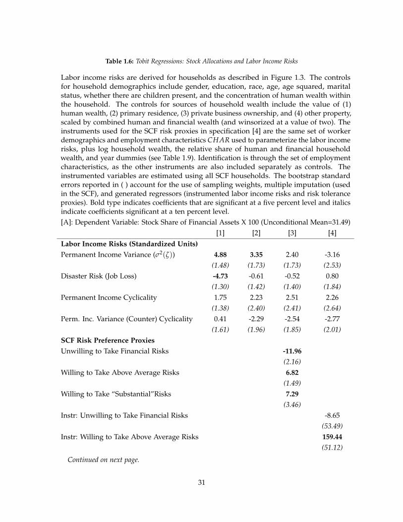
Table 1.6: Tobit Regressions: Stock Allocations and Labor Income Risks

Labor income risks are derived for households as described in Figure 1.3. The controlsfor household demographics include gender, education, race, age, age squared, maritalstatus, whether there are children present, and the concentration of human wealth withinthe household. The controls for sources of household wealth include the value of (1)human wealth, (2) primary residence, (3) private business ownership, and (4) other property,scaled by combined human and financial wealth (and winsorized at a value of two). Theinstruments used for the SCF risk proxies in specification [4] are the same set of workerdemographics and employment characteristics CHAR used to parameterize the labor incomerisks, plus log household wealth, the relative share of human and financial householdwealth, and year dummies (see Table 1.9). Identification is through the set of employmentcharacteristics, as the other instruments are also included separately as controls. Theinstrumented variables are estimated using all SCF households. The bootstrap standarderrors reported in ( ) account for the use of sampling weights, multiple imputation (usedin the SCF), and generated regressors (instrumented labor income risks and risk toleranceproxies). Bold type indicates coefficients that are significant at a five percent level and italicsindicate coefficients significant at a ten percent level.[A]: Dependent Variable: Stock Share of Financial Assets X 100 (Unconditional Mean=31.49)

[1] [2] [3] [4]Labor Income Risks (Standardized Units)Permanent Income Variance (σ2(ζ)) 4.88 3.35 2.40 -3.16

(1.48) (1.73) (1.73) (2.53)Disaster Risk (Job Loss) -4.73 -0.61 -0.52 0.80

(1.30) (1.42) (1.40) (1.84)Permanent Income Cyclicality 1.75 2.23 2.51 2.26

(1.38) (2.40) (2.41) (2.64)Perm. Inc. Variance (Counter) Cyclicality 0.41 -2.29 -2.54 -2.77

(1.61) (1.96) (1.85) (2.01)SCF Risk Preference ProxiesUnwilling to Take Financial Risks -11.96

(2.16)Willing to Take Above Average Risks 6.82

(1.49)Willing to Take “Substantial”Risks 7.29

(3.46)Instr: Unwilling to Take Financial Risks -8.65

(53.49)Instr: Willing to Take Above Average Risks 159.44

(51.12)

Continued on next page.

31

Table 1.6: (Continued) Tobit Regressions: Stock Allocations and Labor Income Risks

[A]: Dependent Variable: Stock Share of Financial Assets X 100 (Unconditional Mean=31.49)[1] [2] [3] [4]

Instr: Willing to Take “Substantial”Risks 46.63(157.99)

Other ControlsYear Dummies (2004, 2007, 2010) Y Y Y YControls for Household Demographics N Y Y YControls for Sources of Household Wealth and N Y Y YLog Household WealthObservations (Households) 3,542 3,542 3,542 3,542R-Squared (from Least Squares Regression) 0.045 0.102 0.139 0.121

Continued on Panel B.

controls cover gender, education, race, age, marital status, the presence of children, and the

concentration of human wealth across the household.

Household demographics and wealth composition explain only part of the positive

relationship between permanent income variance and stock allocations. A similar set of

controls also fails to reverse the positive conditional relationship of permanent income

variance and leverage seen in Table 1.7. In the next section, I show that heterogeneity in

household risk preferences explains why households with volatile income hold more stock

and take greater leverage.

1.3.2 How Risk Preferences Relate to the Distribution of Financial and Labor

Income Risks

Households with greater risk tolerance require less compensation for bearing unconditional

labor income risk. As a result, the most risk tolerant should tend to select employment with

greater unconditional labor income risk. Table 1.4 shows that unconditional and cyclical

labor income risks are correlated, so the risk tolerant should have greater cyclical labor

income risks as well. The positive relationships seen earlier between labor income risks,

stock allocations, and household leverage might be rational if the role of risk preferences in

32

Table 1.6: (Continued) Tobit Regressions: Stock Allocations and Labor Income Risks

Addition to notes from Panel [A]: The four labor income risks in this panel scaled by theratio of household human wealth to combined household financial assets and human wealth,and are then standardized.[B] Dependent Variable: Stock Share of Financial Assets Plus Human Wealth X 100 (Uncon-ditional Mean=10.24)

[1] [2] [3] [4]Scaled Labor Income Risks (Standardized Units)Permanent Income Variance (σ2(ζ)) 2.05 0.74 0.18 -3.38

(0.59) (0.85) (0.86) (1.36)Disaster Risk (Job Loss) -1.40 0.50 0.53 1.18

(0.36) (0.49) (0.49) (0.72)Permanent Income Cyclicality 0.19 0.71 0.84 1.25

(0.49) (0.89) (0.89) (1.09)Perm. Inc. Variance (Counter) Cyclicality 0.34 -1.16 -1.25 -1.41

(0.52) (0.63) (0.62) (0.92)SCF Risk Preference ProxiesUnwilling to Take Financial Risks -4.56




(23.21)Instr: Willing to Take Above Average Risks 64.31

(22.79)Instr: Willing to Take “Substantial”Risks 8.93

(68.29)Other ControlsYear Dummies (2004, 2007, 2010) Y Y Y YFinancial Assets as a Fraction of Financial Plus Y Y Y YHuman Wealth X Year DummiesControls for Household Demographics N Y Y YControls for Sources of Household Wealth and N Y Y YLog Household WealthObservations (Households) 3,542 3,542 3,542 3,542R-Squared (from Least Squares Regression) 0.292 0.334 0.352 0.357

33

Table 1.7: Tobit Regressions: Household Leverage and Labor Income Risks

Household equity is the sum of household financial assets and property (primarily realestate). Household debt includes mortgages, short term debt (e.g. credit cards), and otherconsumer loans. See notes to Table 1.6A for further details on the estimation procedure.Standard errors are indicated in ( ). Bold type indicates coefficients that are significant at afive percent level and italics indicate coefficients significant at a ten percent level.Dependent Variable: Household Leverage - Debt to Equity Ratio X 100, Winsorized at 200(Unconditional Mean=42.28)

[1] [2] [3] [4]Labor Income Risks (Standardized Units)

Permanent Income Variance (σ2(ζ)) 3.79 2.14 1.33 -12.67(3.13) (2.18) (2.15) (4.91)

Disaster Risk (Job Loss) 0.57 -3.56 -3.36 5.03(2.30) (1.72) (1.68) (3.42)

SCF Risk Preference ProxiesUnwilling to Take Financial Risks -10.21




(85.98)Instr: Willing to Take Above Average Risks -28.61

(112.28)Instr: Willing to Take “Substantial”Risks -528.64

(301.14)Other ControlsYear Dummies (2004, 2007, 2010) Y Y Y YControls for Household Demographics N Y Y YControls for Sources of Household Wealth and N Y Y YLog Household EquityObservations (Households) 3,542 3,542 3,542 3,542R-Squared (from Least Squares Regression) 0.016 0.428 0.437 0.494

34

the selection of labor income risks is strong enough.

In the SCF, attitudes towards financial risk are revealed by the question, “Which...comes

closest to the amount of financial risk that [your household is] willing to take when you

save or make investments?”Interviewees are allowed responses of the form, “Take XXX

risks, expecting XXX returns”and “Not willing to take any financial risks,”where XXX is

either “substantial,”“above average,”or “average.”This is a coarse, self-reported measure,

with responses that can be interpreted somewhat subjectively, but it still proves quite useful

in explaining how risks are distributed across households. The 1996 wave of the PSID also

includes a question about risk preferences. In Appendix A.5, I discuss the similarity of

the SCF and PSID measures and the practical reasons why I proceed using the SCF risk

tolerance proxy. The SCF measure is available for larger cross-section of households, which

allows for significantly improved precision of estimates.

Self-reported willingness to take financial risk may reflect more than just the household’s

innate risk tolerance. First, responses may be affected by household labor income risks. If so,

they partially reflect effective risk tolerance; the household’s willingness to take additional

risk. The distinction between effective and innate risk tolerance is important because the

difference between the two serves as the channel by which unconditional labor income risks

should cause households to reduce their financial risks. Rather than taking a stand on the

extent to which the self-reported measure is a proxy for innate or effective risk preferences,

I proceed with a more general interpretation. I point out where distinction between the two

is important to interpretation of results.

Self-reported preferences over financial risks also appear to reflect the household’s

experience, outlook, and familiarity with financial risk. The top plots of Figure 1.5 show

that households indicate greater willingness to accept financial risk when they feel that they

have been financially fortunate and have more optimistic forecasts about economic growth

and their own longevity. Similarly, Malmendier and Nagel (2011) show that willingness

to accept financial risk is related to the stock market returns investors have lived through.

The lower plots of Figure 1.5 suggest that households that have greater interest in financial

35

matters are more willing to accept financial risk, though the causality in the relationship is

unclear. Interest in and greater understanding of financial matters may reduce the unknowns

(Knightian uncertainty) or distrust of financial markets that discourage households from

taking financial risks. Alternatively, there may be greater return to paying attention to a

range of investment options if you have greater innate willingness to accept financial risks.

Figure 1.5: Relationship of Self-Reported Risk Preferences with Luck, Optimism, and Financial Preparedness

26.2%

11.4%

37.7%

57.3%

31.7%

48.8%

0%

10%

20%

30%

40%

50%

60%

70%

% Feel Financially Lucky vs Peers - % Feel

Financially Unlucky vs Peers

% Expecting Economy to Fare Better in Next 5

Years - % Expecting Economy to Fare Worse in

Next 5 Years

% Expecting to Live to Age 85+

Luck and Optimism

Unwilling to Take Financial Risks Average Above Average Substantial

-12.5%

10.1%

35.8%

19.2%

36.3%

61.7%

-20%

-10%

0%

10%

20%

30%

40%

50%

60%

70%

% Spending High Effort Shopping for Best

Investments - % Spending Low Effort Shopping

for Best Investments

% That Make Use of Financial Planning Software % With a High Level of Interest in SCF Interview

- % With a Low Level of Interest in SCF

Interview

Financial Preparedness

Responses above are the average across SCF waves (2004, 2007, and 2010), where the average for each wave isconstructed using sampling weights.

Figure 1.6 confirms that self-reported preferences for financial risk do correspond to

the financial risks which households actually take. The high leverage (debt-to-equity) of

the most risk averse college educated group is largely explained by the relatively limited

36

Figure 1.6: Share of Financial Assets in Stocks and Leverage by Education and Self-Reported Risk Preferences

No Risk

AverageAbove Average

"Substantial"

No Risk

Average

Above Average

"Substantial"

0.35

0.40

0.45

0.50

0.55

0.60

0.65

0.70

15% 20% 25% 30% 35% 40% 45%

House

hold

Lev

erag

e (D

ebt/

Equit

y)

Share of Financial Assets Invested in Stocks

BA Degree or Above High School Graduate

The categories plotted respond to education levels and responses to the SCF question, “Which...comes closest tothe amount of financial risk that [your household is] willing to take when you save or make investments?”Thepopulation and computation of group averages is analogous to that in Figures 1.3 and 1.4. The size of thebubbles in the plots reflect the fraction of the included population falling into each group.

household equity of representatives of this group.41 Barsky et al (1997) shows that a self-

reported measure of risk tolerance found in the Health and Retirement Study and PSID also

behaves as a proxy for preferences over risks to human health as well; with risk tolerant

individuals reporting higher rates of smoking, drinking, and lower levels of health and life

insurance. The SCF has less data on non-financial risk taking behavior, but individuals

in the SCF reporting greater willingness to accept financial risk are more likely to own

motorcycles relative to cars, and are more likely to respond that the reason they do not have

health insurance is that they do not need it or believe in it.

Risk preferences are a source of endogeneity bias in the regressions of financial risks on

labor income risks only if the risk preferences also have a role to play in the selection of

labor income risks. To see if this is likely, I first define a variable called “pref”that equals one

if the SCF household indicated willingness to take “above average”or “substantial”financial

risks, negative one if the household indicated it was “unwilling”to take financial risks, and

41Household equity is a strong predictor of the debt-equity ratio as relatively low equity households mustnecessarily take considerable leverage to buy homes.

37

Figure 1.7: Self-Reported Risk Preference and Permanent Income Variance of Industry and Occupation SortedGroups

Professionals

(Broadly Defined)

Clerical, Sales,

and Technicians

Service Workers

Maintenance and

Assembly

Equipment

Operators

Agriculture or

Forestry

Mining and

Construction

Manufacturing

Trade

Business Services

Utilities and

Personal Services

Public

Administration

Self Employed

Union Employees

-0.10

0.00

0.10

0.20

0.30

0.40

0 0.005 0.01 0.015 0.02 0.025 0.03

pre

f

Permanent Income Variance - σ2(Ϛ)


The plot above represents the average household permanent income variance and “pref”for households sortedinto industry and occupation groups. The risk preference measure “pref”equals 1 if the SCF householdindicated willingness to take “above average”or “substantial”financial risks, -1 if the household indicated it was“unwilling”to take financial risks, and 0 otherwise. See the notes to Figure 1.3 for further details, as constructionis analogous.

zero if the household was willing to accept “average”financial risks. Figure 1.7 plots the

average value of “pref”against the average permanent income variance of each industry

and occupation group seen in the earlier plots. The strong positive relationship in the plot

suggests risk preferences are an important determinant of labor income risk.

As an extension of this simple analysis, Panel A of Table 1.8 runs regressions of standard-

ized labor income risks on the variable “pref”and year dummies. Consistent with Figure 1.7,

risk tolerant workers have higher permanent income variance. Cyclical risks are also higher

for risk tolerant workers. However, disaster risk, the probability of becoming unemployed,

is greater for workers reporting less willingness to accept financial risk. The concentration

of disaster risk in the least risk tolerant may seem odd, but disaster risk may be largely

coincidental and unavoidable.42

42Alternatively, the distribution of disaster risk could be rationalized if it has a very large negative effect onthe risk tolerance that households report. This alternative is less plausible given the strong positive relationshipbetween permanent income variance and “pref.”

38

Table 1.8: Least Squares Regressions: The Relationship of Self-Reported Risk Tolerance to Components ofLabor Income Risk

The risk tolerance proxy (“pref”) used in these regressions equals 1 if the SCF householdindicated willingness to take “above average”or “substantial”financial risks, -1 if the house-hold indicated it was “unwilling”to take financial risks, and 0 otherwise. The dependentvariables in Panel A are decomposed into components fit separately to the sets of instru-ments from CHAR reflecting (1) quasi-exogenous worker demographics other than jobtenure (education, age, gender, race, marital status, children), (2) endogenous employmentcharacteristics (industry, occupation, self-employment, unionization), and (3) job tenure.Components (1) and (2) are used as the dependent variables in Panels B1 and B2 respectively.The risks used in this analysis pertain only to the household head (if in the labor force) tosimplify the decomposition. The bootstrap standard errors reported in ( ) adjust for multipleimputation used in the SCF and generated regressors (the labor income risks). Bold typeindicates coefficients that are significant at a five percent level and italics indicate coefficientssignificant at a ten percent level.

Number of Household Head Observations Used: 3,448

Perm. Income Disaster Risk Perm. Income Variance Counter-

Labor Income Risk: Variance (Job Loss) Cyclicality Cyclicality

[1] [2] [3] [4]

[A] Dep. Variable: Standardized Household Head Labor Income Risk

Risk Tolerance Proxy 0.225 -0.133 0.175 0.043

“pref” (0.041) (0.042) (0.091) (0.084)

Year Dummies Y Y Y Y

R-squared 0.028 0.008 0.016 0.003

[B1] Dep. Variable: Standardized Head Labor Income Risk Fit to Worker Demographics

Risk Tolerance Proxy 0.022 -0.124 0.164 0.071

“pref” (0.039) (0.035) (0.091) (0.055)


R-squared 0.005 0.021 0.032 0.006


39

Table 1.8: (Continued) Least Squares Regressions: The Relationship of Self-Reported Risk Tolerance toComponents of Labor Income Risk

Perm. Income Disaster Risk Perm. Income Variance Counter-

Labor Income Risk: Variance (Job Loss) Cyclicality Cyclicality

[1] [2] [3] [4]

[B2] Dep. Variable: Standardized Head Labor Income Risk Fit to Employment Characteristics

Risk Tolerance Proxy 0.143 -0.058 -0.014 -0.017

“pref” (0.036) (0.030) (0.044) (0.075)


R-squared 0.031 0.005 0.001 0.004

[C] Dep. Variable: The Set of Fit Risks in [B2] Orthogonalized w.r.t. Each Other

Risk Tolerance Proxy 0.128 0.020 -0.024 -0.038

“pref” (0.043) (0.037) (0.037) (0.045)


R-squared 0.036 0.001 0.002 0.005

40

Is the relationship of labor income risks to risk preferences coincidental (and unfortunate

in the case of disaster risk) or does it result from employment decisions over which the

worker has control? To investigate, I decompose labor income risks into separate components

attributed to worker demographics and employment characteristics. Demographics are

largely outside the worker’s control, while the worker’s risk preferences likely play a

more active role in the choice of employment characteristics. The worker demographic

components of the labor income risks are constructed by fitting the instrumentation of

labor income risks to only the demographic related components of CHAR; worker age,

education, race, gender, marital status, and whether there are children in the household.

Similarly, the components attributed to employment characteristics are constructed by fitting

only the worker’s industry of employment, occupation, self-employment, and unionization.

For comparability, these components are scaled by the same standard deviation as is used

to scale the labor income risks in Panel A. The worker demographics and employment

characteristic components form a mostly complete decomposition of the labor income risks.

Job tenure seems conceptually less endogenous than the other employment characteristics,

so I leave it out of this analysis.

In Panels B1 and B2 of Table 1.8, I separately regress the demographic and employment

related components of labor income risks on “pref.”The regression in column [1] of Panel B2

shows that the permanent income variance associated with workers’ choice of employment

characteristics, industry, occupation, self-employment, and unionization, is significantly

positively related to the workers’ self-reported risk tolerance. Panel B1 shows that worker

demographics explain little of the positive relationship of permanent income variance and

“pref.”

In contrast, the coefficients in specifications [2] through [4] are much more significant in

Panel B1 than B2. Demographics are the primary explanation for why workers with high

disaster risk report lower risk tolerance and workers with greater cyclical labor income risks

report higher risk tolerance. Certain household demographics, such as less education and

minority status, are associated with both higher probability of job loss and lower levels of

41

self-reported risk tolerance.

In Panel C, the employment related components of labor income risks from B2 are

orthogonalized with respect to each other. This is done to confirm that omitted variable bias

due to considering the risks one at a time is not distorting the implications drawn from

Panel B2. Panel C suggests that permanent income variance is the only of the four labor

income risks which is considered in workers’ selection of occupation, industry, and whether

to self-employ or opt for union employment.

So far, the discussion of Table 1.8 has treated “pref”as a measure of innate preferences. If

self-reported preferences partly reflect effective risk tolerance, the evidence that high levels

of permanent labor income variance is self-selected by the risk tolerant is even stronger.

For example, workers with high permanent labor income variance may have reported even

greater willingness to accept financial risk if it were not for their volatile incomes.

The analysis so far demonstrates that risk tolerant households simultaneously take

greater financial risk and accept employment with characteristics associated with higher

permanent income variance. This makes the positive unconditional relationship between

household labor income risks and financial risks less surprising. To investigate the rela-

tionship conditional on risk preferences, Specification [3] in Tables 1.6 and 1.7 introduces

dummies for the self-reported risk preference responses. As a result, the “puzzling”evidence

suggesting households increase financial risk in response to greater permanent income

variance weakens, but the impact is not very large.

Error in the measurement of risk tolerance is responsible for the modest impact of

adding SCF risk preference dummies. The respondent’s concept of risks when “savi[ing]

and investing”may vary, the four possible responses have partly subjective interpretations

(e.g. what is an “average”level of risk), and the response given may be colored by the

way the question is asked or the respondent’s frame of mind. This measurement error,

the difference between the respondent’s true and self-reported risk preferences, is almost

certainly correlated with household labor income risks. For example, a household that has

high permanent income variance but reports only “average”willingness to accept financial

42

risks is probably truly more risk tolerant than average. Therefore, the regression coefficients

on the four labor income risks are biased when the measurement error is ignored.

To address measurement error, I use a set of instrumental variables for self-reported

risk preferences.43 The instruments include worker demographics and employment charac-

teristics found in CHAR, log household wealth, the relative share of human and financial

household wealth, and year dummies.

The “stage-one”regression for this instrumentation is given by Equation (1.9) and the

regression coefficients, λ, are given in Table 1.9.44 The sizable F-statistics suggest the

instruments are highly relevant in predicting self-reported effective risk tolerance.

Dummy[Willing to accept...risks]i,t =λ0 [1 Demographicsi,t Employment Characteristicsi,t]︸︷︷︸CHARi,t

+ λ1Total Wealth and Wealth Sharesi,t + λt (1.9)

I include household demographics, wealth and wealth composition, year dummies,

and the instrumented labor income risks as control variables along with the instrumented

risk preferences. Household demographics are included in the set of control variables as

demographics may predict financial risks even conditional on labor income risks and risk

preferences.45 Therefore, validity of the instrumentation in Equation (1.9) requires that

employment characteristics (industry, occupation, self-employment and unionization) affect

financial risks only through risk preferences and the set of control variables. If this is not

true, the specification has further omitted variable bias. Of course, omitted variable bias

may also exist even if the instruments for risk preferences are valid.

43Kimball et al (2008) show how, with some assumptions, repeated responses can be used to account formeasurement error in self-reported risk preferences. However, the SCF (and PSID) have only one observedresponse to the risk preference question per household.

44I use all 8,315 SCF households (i.e. including those not meeting the wealth or age criteria) to estimatethe instrumented risk preferences. The instrumented variables and resulting coefficient estimates are similarto those produced using only the wealthier, age-restricted subsample focused on elsewhere, but including allobservations strengthens the instruments, improving statistical power.

45For example, more educated households may buy more stocks due to greater familiarity with financialmarkets or greater awareness of the equity premium.

43

Table 1.9: Least Squares Regressions: Instrumentation of Self-Reported Risk Preference Responses in the SCF

“Willing to Take Average Financial Risks”is the fourth (excluded) possible response to thesurvey question. Total wealth includes financial assets, human wealth, private businessownership, and property minus total household debt. The bootstrap standard errorsreported in ( ) account for the use of sampling weights and multiple imputation. Bold typeindicates coefficients that are significant at a five percent level and italics indicate coefficientssignificant at a ten percent level.Dependent Variables (Dummies): Unwilling to Willing to Take Willing to Take

Take Financial “Above Average” “Substantial”Risk Financial Risks Financial Risks

Unconditional Means: 0.335 0.206 0.040Demographics:High School Dropout 0.322 -0.156 -0.015

(0.027) (0.019) (0.010)High School Graduate, No BA Degree 0.114 -0.095 0.000

(0.015) (0.014) (0.007)Worker Age / 10 -0.083 0.160 -0.022

(0.057) (0.047) (0.025)Worker Age Squared / 100 0.014 -0.022 0.001

(0.007) (0.006) (0.003)Race is White -0.101 0.037 -0.001

(0.013) (0.011) (0.006)Male -0.076 0.070 0.019

(0.015) (0.013) (0.007)Married Couple 0.002 -0.026 -0.004

(0.013) (0.012) (0.006)Dependent Children in Household 0.025 -0.013 -0.004

(0.013) (0.011) (0.006)Employment Characteristics:Self-Employed -0.086 0.037 0.031

(0.017) (0.017) (0.009)Unionized 0.003 -0.029 0.010

(0.019) (0.018) (0.008)Industry: Utilities and Personal Services - Omitted DummyMining and Construction 0.045 -0.013 0.010

(0.029) (0.022) (0.011)Manufacturing -0.029 0.033 0.007

(0.020) (0.019) (0.009)


44

Table 1.9: (Continued) Least Squares Regressions: Instrumentation of Self-Reported Risk Preference Responsesin the SCF

Dependent Variables (Dummies): Unwilling to Willing to Take Willing to TakeTake Financial “Above Average” “Substantial”

Risk Financial Risks Financial RisksTrade -0.010 0.024 0.008

(0.020) (0.018) (0.009)Business Services -0.046 0.073 0.009

(0.020) (0.022) (0.010)Public Administration -0.040 -0.021 0.007

(0.026) (0.024) (0.012)Occupation: Professionals - Omitted DummyClerical, Sales, and Technicians 0.032 -0.027 -0.001

(0.019) (0.017) (0.009)Service Workers 0.089 -0.018 -0.014

(0.025) (0.021) (0.010)Maintenance and Assembly 0.055 -0.043 -0.006

(0.025) (0.022) (0.010)Equipment Operators 0.050 -0.035 -0.015

(0.025) (0.021) (0.010)Agriculture, Forestry, and Animal Trades 0.123 -0.017 -0.013

(0.042) (0.034) (0.016)Other ControlsEmployment Tenure / 10 0.019 -0.006 -0.006

(0.009) (0.008) (0.003)Fin. Wealth/(Fin.+Human Wealth) -0.310 0.154 0.008

(0.032) (0.032) (0.015)Log Total Wealth -0.077 0.033 0.001

(0.006) (0.006) (0.003)Year Dummies (2004, 2007, 2010) Y Y YObservations (Households) 8,320 8,320 8,320R-Squared 0.476 0.263 0.049F-value 196.7 67.6 11.1

45

To test the likely significance of remaining omitted variable bias, I run an analysis in

Appendix A.6 motivated by the work of Altonji, Elder, and Taber (2005). This analysis uses

the endogeneity of financial and labor income risks with respect to observed demographics

as an estimate of the endogeneity of these risks with respect to unobserved demographic

variation. Since the endogeneity of risks with respect to a wide selection of observed

household demographics is quite limited, I argue that unobserved variation in household

demographics is unlikely to significantly impact the results that I discuss below.46

Specification [4] in Tables 1.6 and 1.7 adds the instrumented risk preferences to stock

allocation and household leverage regressions.

The predicted change in stock allocation resulting from a one-standard deviation increase

in the unconditional variance of permanent labor income moves from positive 3.35% to

negative 3.16% once risk preferences are accounted for. The corresponding predicted change

in stock holdings as a percent of total financial assets plus human wealth (Panel B of

Table 1.6) moves from positive 2.05% to negative 3.38%. These regressions imply that the

typical household in the sample would invest between $20,000 and $80,000 more in stocks

if they were at the 10th percentile of household permanent income variance instead of the

90th percentile of household permanent income variance. The magnitudes of these portfolio

shifts are consistent with middle-aged power utility investors that have constant relative risk

aversion of roughly γ = 8 (in Panel A) and γ = 2 (in Panel B) respectively (Viceira 2001).47

The estimated impact of a one standard deviation increase in unconditional labor

income variance on household leverage moves from positive 0.02 to negative 0.13 when

risk preferences are accounted for. Based on the median household equity (assets minus

46Specifically, unobserved demographics need to be about ten times as important as the observed demo-graphics in explaining stock allocations and leverage in order to neutralize the negative responses to permanentincome variance that I find. An informal way of showing that unobserved variation is likely to have limitedimpact is to note that when I include 34 more household characteristics in the SCF as additional controls, thecoefficients on labor income risks change very little despite significant gains in R-squared.

47Viceira (2001) shows that risk tolerant households’ stock allocations should be more sensitive to permanentincome variance. For example, a highly risk averse household holds little stock regardless of the level ofpermanent income variance (except in the unlikely event that stock returns hedge the household’s backgroundrisk). The declining sensitivity of stock allocations to permanent labor income variance (as risk aversion rises) isan additional testable hypothesis, but the cross-section I work with is not large enough to test this conclusively.

46

debt) in the sample, this implies a reduction in debt of nearly $50,000, or nearly 25% of the

average total debt, per each standard deviation increase in unconditional permanent income

variance. While this effect is economically large, a comparison with optimal household

behavior needs to take into account the risk characteristics of the assets (typically real estate)

acquired through leverage.

The impact of permanent income variance on the financial risks households take is

consistent with the finding in Table 1.8 that risk tolerant households select employment

with greater permanent income variance. Households are not oblivious of their permanent

labor income variance. Furthermore, these results are actually stronger to the extent that

the self-reported risk preferences reflect effective risk tolerance, as opposed to innate risk

tolerance.48

Household stock allocations and leverage are not significantly affected by disaster risk;

the probability of becoming unemployed. Similarly, careers bearing a high probability of

unemployment do not appear to be allocated towards risk tolerant households as high

permanent income variance careers are. One possibility is that households have difficulty

estimating how the probability of job loss varies across careers. Alternatively, the probability

of job loss may be a weak measure of disaster risk if there is substantial predictable

heterogeneity in the costliness of job loss.49

Table 1.6 also shows that cyclical risks do not have significant impact on stock allocations.

The absence of a significant response does provide evidence that households are not hedging

their cyclical labor income risks as theory predicts. For example, in Panels A and B of

Table 1.6 the coefficients on permanent income cyclicality should be approximately -0.20

and -0.05 respectively in order for the reduction in stock holdings to offset the exposure

of permanent labor income to stock returns. Such values are over five standard errors

below the actual coefficients, which are a statistically insignificant 0.02 and 0.01. In order

48The understatement is probably not too large given that estimated magnitude of the response of stockallocations to permanent income variance is already roughly at a level consistent with theory. This is indirectevidence that self-reported risk preferences are probably a better measure of innate than effective risk tolerance.

49The measure I currently use (see Equation (1.6)) treats all job loss as equally undesirable.

47

to hedge cyclical labor income risks, households must recognize the statistical relationship

between their labor income and stock returns and then broadly frame the set of economic

risks that they face when making investing and borrowing decisions. The data suggest few

households have this ability.

1.4 Conclusion

Households with employment in industries and occupations with greater unconditional and

cyclical labor income risks hold more stock and have greater leverage. These relationships

appear to contradict established theory on how portfolios should respond to labor income

risks. This puzzle is explained by the fact that risk tolerant households select employment

with greater risk, and especially employment with greater permanent income variance.

Conditional on risk preferences, households decrease stock allocations and leverage in

response to higher permanent income variance by about as much as theory suggests.

However, I find no evidence suggesting that disaster risk, modeled by the probability of job

loss, affects the financial risks that households take.

I find heterogeneity in permanent income cyclicality that should lead to substantial

variation in stock allocations, yet I do not find evidence that stock allocations are affected

by it. As a result, households employed in procyclical industries and occupations appear

to face higher marginal costs of investing in stock than households employed in acyclical

industries.

One direction to take this work is to estimate the magnitude and distribution of the costs

of ignoring the cyclicality of labor income and its variance. This would provide an interesting

comparison with the costs of other common household investment mistakes, such as under-

diversification of risky assets, non-participation in equity markets, and extrapolation of asset

returns. Several aspects of investor education may prove beneficial in reducing the costs of

ignoring the relationship of labor income and stock returns: building awareness about the

relationship between stock returns and labor income, ensuring diversification is understood,

and encouraging investors to broadly frame their risks.

48

Chapter 2

Getting Better: Learning to Invest in

an Emerging Stock Market1

2.1 Introduction

It’s a little better all the time. (It can’t get no worse.)

Lennon and McCartney, “Getting Better,”1967.

Equities play an important role in normative theories of household investment. Because

stocks have historically offered a risk premium, households with no initial exposure to the

asset class can benefit from holding at least some stocks. The optimal equity allocation

depends on market conditions, the equity premium, and many details of the household’s

financial situation, including the household’s risk aversion and other risk exposures, but

typical calibrations suggest it is substantial—at least for households with sufficient wealth

to justify paying the fixed cost of equity market participation (Campbell and Viceira 2002,

Campbell 2006, Siegel 2007).

Direct investment in stocks is not straightforward, however, and households can lose

much of the benefit of stock market participation if they engage in certain widely-studied

investment behaviors. Three such investment behaviors can be costly even in a market where

1Co-authored with John Y. Campbell and Tarun Ramadorai

49

all individual stocks have the same risk and the same expected return. First, underdiversifica-

tion increases portfolio risk without increasing return (Blume and Friend 1975, Kelly 1995,

Calvet et al. 2007). Second, high turnover of an equity portfolio leads to high trading costs

(Odean 1999, Barber and Odean 2000). Third, selling stocks that have appreciated while

holding those that have depreciated—a tendency known as the disposition effect—increases

the present value of tax obligations by accelerating the realization of capital gains and

deferring the realization of offsetting losses (Shefrin and Statman 1985, Odean 1998).

In a market where expected returns differ across stocks, it is also possible for households

to lose by picking underperforming stocks. They may do this by taking risk exposures that are

negatively compensated, for example by holding growth stocks in a market with a value

premium, or by adopting a short-term contrarian investment strategy (perhaps driven by

the disposition effect) in a market with momentum where outperforming stocks continue to

outperform for a period of time. If these style tilts do not offset other risks of the household,

they are welfare reducing.2 Alternatively, households may lose by trading with informed

counterparties in a market that is not strong-form efficient, and thus rewards investors who

possess private information (Grossman and Stiglitz 1980, O’Hara 2003).

Households can control suboptimal investment behaviors in several ways. They can hold

mutual funds as a way to gain equity exposure without trading stocks directly. This, however,

may result in trade-offs between households’ tendencies to engage in these behaviors, the

level of fees charged by intermediaries, and the possibility that mutual fund managers may

themselves be susceptible to these behaviors. Households can also learn from observing

overall patterns in the market, or from their own investment experience (Nicolosi et al.

2009, Seru et al. 2010, Malmendier and Nagel 2011, 2012). In this paper we report evidence

that learning from experience is important. Importantly, however, we do not claim that

such learning is rational. Instead, it may reflect reinforcement learning, in which personal

2This is true whether risk prices are driven by fundamentals or by investor sentiment (the preferences ofunsophisticated investors for certain types of stocks). In a model with fundamental risks it may be more likelythat households’ non-equity risk exposures justify equity positions with low expected returns, but if this is notthe case such positions still reduce household welfare just as they would in a sentiment-driven model.

50

experiences are overweighted relative to broader patterns of evidence in historical data.

Our study uses data from the Indian equity market. For several reasons this is an ideal

laboratory for studying learning among equity investors. First, India is an emerging market

whose capitalization and investor base have been growing rapidly. In such a population

of relatively inexperienced investors, learning may be faster and easier to detect than in

better established equity markets. Second, as discussed more fully below, mutual funds

account for a relatively small value share of Indian individuals’ equity exposure, so it is

meaningful to measure the diversification of directly held stock portfolios. The prevalence

of direct equity ownership also implies that it is more important for Indian investors to

develop the skills necessary to own stocks directly than it is in a mature market with a large

mutual fund share. Third, India has electronic registration of equity ownership, allowing us

to track the complete ownership history of listed Indian stocks over a decade. The relatively

long time dimension of our panel allows us to measure investors’ performance using their

realized returns, a method that is vulnerable to common shocks when applied to a short

panel. Moreover, our data are monthly, and this relatively high frequency allows us to more

accurately measure important determinants of performance such as momentum investing

and turnover.

A limitation of our Indian data is that we have almost no information about the de-

mographic characteristics of investors. Thus we cannot follow the strategies, common in

household finance, of proxying financial sophistication using information about investors’

age, education, and occupation (Calvet et al. 2007, 2009a), their IQ test scores (Grinblatt and

Keloharju 2011), or survey evidence about their financial literacy (Lusardi and Mitchell 2007).

Instead, we study learning by relating account age (the length of time since an account was

opened) and summary statistics about past portfolio behavior and investment performance

to the future behavior and performance of each account.

We have four main results. First, investment performance improves with account age.

Second, older accounts have several profitable tilts in their portfolio weights, particularly

towards value stocks and stocks with low turnover. However, these style tilts leave much

51

of the outperformance of older accounts unexplained. Third, two of the three potentially

harmful investment behaviors that we focus on, namely high turnover and the disposition

effect, are less prevalent among older accounts. Fourth, all three investment behaviors

diminish in response to painful experiences, including account underperformance, large

losses in a single month, and poor returns from past trading and sales of gains. Putting

these results together, investors appear to learn from stock market participation, at a rate

that is influenced by their investment experiences.

2.1.1 Related Literature

The behavior of individual investors in equity markets has been of interest to financial

economists studying market efficiency ever since the efficient markets hypothesis was first

formulated. Shleifer (2000) succinctly summarizes the importance of this line of inquiry for

the study of market efficiency, outlining that theoretical defenses of the efficient markets

hypothesis rest on three pillars, the first of which is rational decision making and securities

valuation by individuals, the second, the absence of correlated deviations from rationality

even if some investors deviate from rational decision making, and the third, limits to

arbitrage.

Understanding the behavior of individual investors is also important for the field of

household finance (see Campbell 2006, for example). There has been much work on

theoretically optimal investment in risky assets, and deviations from such idealized behavior

by households have important implications for the evolution of the wealth distribution in

the economy.

While the theoretical motivation for the study of individual investors has been clear for

some time, empirical work in this area has been hampered by the difficulty of obtaining

detailed data on individual investors’ portfolios as well as by the large computational

burden imposed by the study of such large datasets. These constraints have gradually been

surmounted, and this field of study has increasingly become one of the most active areas of

empirical research in financial economics.

52

Early work in the area (Cohn et al. 1975, Schlarbaum et al. 1978, Badrinath and Lewellen

1991) utilized relatively small samples of trader accounts from retail or discount brokerages

to shed light on the stocks held by individual investors, the returns they earned, and

the practice of tax-loss selling. The first set of empirical studies with a primary focus on

questions related to rationality and market efficiency followed in the late 1990s, also using

data sourced from discount brokerages, identifying that individual investors exhibit the

disposition effect (Odean 1998), and trade excessively in the sense that their transactions

costs outweigh any stock-picking ability they may possess (Odean 1999, Barber and Odean

2000). These tendencies were found to vary with the demographic characteristics and

trading technologies of investors such as gender, marital status, and access to online trading

(Barber and Odean 2001, 2002).

A characteristic of this early literature, and continuing to the present day, is the focus on

trading rather than investment decisions of individual investors. While many questions in

household finance are about the performance and risk properties of the entire risky asset

portfolio of individual households, much of the literature has concentrated on performance

evaluation of individual investors’ purchases and sales at different post-trade horizons (see,

for example, Coval et al. 2005, Barber et al. 2008, Seru et al. 2010), and on contrasting

individual returns with those achieved by domestic and foreign institutional investors

(Grinblatt and Keloharju 2000, Kaniel et al. 2008). A related focus has been on characterizing

the trading strategies of individual investors through the lens of various behavioral biases

such as the disposition effect, overconfidence, or inattention (see, for example, Barber and

Odean 2008 and references above), and demonstrating the types of stocks (large, hard-

to-value) in which these biases are most likely to manifest themselves (Ranguelova 2001,

Kumar 2009).

This focus on trades rather than on investment arises quite naturally from the limitations

of the data used to study investor behavior. In the US, discount brokerage accounts from a

single service provider may not be truly representative of the entire portfolio of an individual

investor, a problem made significantly worse when investors also have untracked mutual

53

fund or 401(k) investments.3 And some international datasets, such as the Taiwanese stock

exchange data used by Barber et al. (2008), track all individual investor transactions but

have little detail on holdings.

Our use of Indian data on direct equity holdings and trades helps us to partially sur-

mount this obstacle. We have a relatively high-quality proxy for total household investment

in risky assets, because equity mutual fund ownership by individual investors in India

is very much smaller than direct equity ownership. As explained in the next section, we

estimate that Indian households’ equity mutual fund holdings are between 8% and 16% of

their direct equity holdings over our sample period.

There are some other countries, such as Sweden and Finland, in which both direct

equity ownership and mutual fund holdings are tracked. In principle this allows for a fuller

characterization of household investment, but most previous studies using data from these

countries have pursued different objectives than our focus on learning to invest. For example,

Grinblatt et al. (2011) show that IQ affects stock market participation using data from the

Finnish registry which provides detailed information on direct equity portfolios combined

with an indicator for whether the household invested in mutual funds in the year 2000.

Grinblatt et al. (2012) highlight the impacts of IQ on mutual fund choice by Finnish investors

using detailed data on mutual fund choices alongside less detailed information on direct

equity investment. Calvet et. al (2007, 2009) use comprehensive data on Swedish investors’

total wealth to shed light on stock-market participation and portfolio rebalancing, but the

annual frequency of their data makes it difficult for them to evaluate higher-frequency

phenomena such as momentum investing and turnover.

Several papers, including those referenced in the previous section, share our focus on

learning by individual investors, but emphasize different facets of this important issue.

Feng and Seasholes (2005) use data on over 1500 individual accounts from China over the

1999 to 2000 period, and find that both experience (measured by the number of positions

3Calvet et al. (2007), show that mutual fund investments are an important source of diversification forSwedish investors.

54

taken) and sophistication (measured by variables that include the idiosyncratic variance

share) attenuate the disposition effect. Our analysis differs from theirs in our use of a

more comprehensive set of portfolio characteristics, including the idiosyncratic variance

share, and our exploration of feedback effects on future investing behavior. Linnainmaa

(2010) estimates a structural model of learning and trading by investors in Finland, focusing

on high-frequency traders, who make at least one round-trip trade in a given day. He

finds, intriguingly, that traders appear to experiment with high-frequency trading to better

understand their levels of skill, and cease trading if they experience poor returns. Our

estimated feedback effects on underdiversification suggest that households also experiment

with the composition of their equity portfolios, choosing to underdiversify more aggressively

if they beat the market. This finding of experimentation is also consistent with Seru et.

al. (2010), who carefully study the trading behavior of Finnish investors, focusing on the

disposition effect. Seru et al. find that investors stop trading (“exit”) after inferring that their

ability is poor, and that trading experience weakens the disposition effect.4 Our work is

distinguished from this literature by our focus on investments rather than trades; to provide

an instructive example, “exit”in our setting is the relatively uncommon exit of an investor

from all equity positions, whereas Seru et al. use this term to refer to a period of time

during which no trading occurs.5

Other authors have demonstrated the impacts of learning, including reinforcement

learning, in other settings, such as trend following by mutual fund managers during the

technology boom (Greenwood and Nagel 2009), individual investment in IPOs (Kaustia

and Knüpfer 2008, Chiang et al. 2011) and household choice of credit cards (Agarwal et al.,

2006, 2008). Agarwal et al. (2008) find that households learn how best to reduce fees on

their credit card bills, and estimate that knowledge depreciates by roughly 10% per month,

4Related work on the positive effect of trader experimentation and trader experience on returns and biasattenuation includes Dhar and Zhu (2006), Mahani and Bernhardt (2007), and Nicolosi et al. (2009). Korniotisand Kumar (2011), in contrast, find that the adverse effects of aging dominate the positive effects of experience.

5While the frequency of exits is relatively low in our data, we estimate two alternative specifications toaccount for any potential biases caused by exits that are driven either by skill or luck.

55

i.e., they find evidence that households learn and subsequently forget. While our current

specifications do not explore this possibility, this is an important avenue that we intend to

pursue in future work.

Finally, while we explore the role of personal feedback and investment experience in

households’ learning about investment, we do not currently consider the important topic

of how social interaction or local networks affect learning (Hong et al., 2004, Ivkovic and

Weisbenner, 2005, 2007).

The organization of the remainder of the paper is as follows. Section 2.2 describes

our data, defines the empirical proxies we use for investment mistakes and style tilts, and

presents some summary statistics. Section 2.3 relates account age to investment performance

and behaviors. Section 2.4 shows that past performance predicts account behavior, while

Section 2.5 shows that the behavior of the investor base predicts the returns on Indian stocks.

Section 2.6 concludes.

2.2 Data and Summary Statistics

2.2.1 Electronic stock ownership records

Our data come from India’s National Securities Depository Limited (NSDL), with the

approval of the Securities and Exchange Board of India (SEBI), the apex capital markets

regulator in India. NSDL was established in 1996 to promote dematerialization, that is,

the transition of equity ownership from physical stock certificates to electronic records of

ownership. It is the older of the two depositories in India, and has a significantly larger

market share (in terms of total assets tracked, roughly 80%, and in terms of the number

of accounts, roughly 60%) than the other depository, namely, Central Depository Services

Limited (CDSL).

While equity securities in India can be held in both dematerialized and physical form,

settlement of all market trades in listed securities in dematerialized form is compulsory.

To facilitate the transition from the physical holding of securities, the stock exchanges do

56

provide an additional trading window, which gives a one time facility for small investors to

sell up to 500 physical shares; however the buyer of these shares has to dematerialize such

shares before selling them again, thus ensuring their eventual dematerialization. Statistics

from the Bombay Stock Exchange (BSE) and the National Stock Exchange (NSE) highlight

that virtually all stock transactions take place in dematerialized form.

The sensitive nature of these data mean that there are certain limitations on the demo-

graphic information provided to us. While we are able to identify monthly stock holdings

and transactions records at the account level in all equity securities on the Indian markets,

we have sparse demographic information on the account holders. The information we do

have includes the state in which the investor is located, whether the investor is located in

an urban, rural, or semi-urban part of the state, and the type of investor. We use investor

type to classify accounts as beneficial owners, domestic financial institutions, domestic

non-financial institutions, foreign institutions, foreign nationals, government, and individual

accounts.6 This paper studies only the last category of individual accounts.

A single investor can hold multiple accounts on NSDL; however, a requirement for

account opening is that the investor provides a Permanent Account Number (PAN) with

each account. The PAN is a unique identifier issued to all taxpayers by the Income Tax

Department of India. NSDL provided us with a mapping from PANs to accounts, so in our

empirical work, we aggregate all individual accounts associated with a single PAN. PAN

aggregation reduces the total number of individual accounts in our database from about

13.7 million to 11.6 million. It is worth noting here that PAN aggregation may not always

correspond to household aggregation if a household has several PAN numbers, for example,

if children or spouses have separate PANs.

Table 2.1 summarizes the coverage of the NSDL dataset. The first two columns report

the total number of securities (unique International Securities Identification Numbers or

6We classify any account which holds greater than 5% of an stock with market capitalization above 500million Rs (approximately $10 million) as a beneficial owner account if that account is a trust or “bodycorporate”account, or would otherwise be classified as an individual account. This separates accounts withsignificant control rights from standard investment accounts. Otherwise our account classifications are many-to-one mappings based on the detailed investor types we observe.

57

ISIN) and the total number of Indian equities reported in each year. Securities coverage

grows considerably over time from just over 12,200 in 2004 to almost 23,000 in 2012, as does

the number of unique Indian equities covered. Starting at 4,510 in 2004, the number of

equities reaches a peak of 7,721 in 2012. When we match these data to price, returns, and

corporate finance information from various datasets, we are able to match between 95%

and 98% of the market capitalization of these equities, and roughly the same fraction of the

individual investor ownership share each year.

The third column shows the market capitalization of the BSE at the end of each year.

The dramatic variation in the series reflects both an Indian boom in the mid-2000s, and the

impact of the global financial crisis in 2008.

The fourth column of Table 2.1 shows the fraction of Indian equity market capitalization

that is held in NSDL accounts. The NSDL share grows from about 50% at the beginning

of our sample period to about 70% at the end. The fifth column reports the fraction of

NSDL market capitalization that is held in individual accounts. The individual share starts

at about 18% in 2004, but declines to just below 10% in 2012, reflecting changes in NSDL

coverage of institutions, as well as an increase in institutional investment over our sample

period.

The sixth column shows the mutual fund share of total equities, which accounts for a

little over 3.5% of total assets in the NSDL data in 2004, growing to a maximum of 4.72%

in 2006, and declining to 3.97% by 2012. While comparing the fifth and sixth columns

of Table 2.1 demonstrates the magnitude of direct household equity ownership relative

to mutual funds, this simple comparison would lead to an overestimate of mutual fund

ownership by households. SEBI data in 2010 show that roughly 60% of mutual funds in

India are held by corporations.7 Assuming that this share has been static over our sample

period, and that corporations and individuals hold roughly the same fraction of equity

and bond mutual funds, this leads us to estimate that mutual fund holdings were between

8% and 16% of household direct equity holdings over the sample period. We note also

7See SEBI website, http://www.sebi.gov.in/mf/unithold.html.

58

Tabl

e2.

1:N

SDL

Dat

abas

eSu

mm

ary

Stat

istic

s

The

perc

enta

ges

belo

war

eco

mpu

ted

for

each

mon

thly

cros

s-se

ctio

n,an

dth

eav

erag

eof

thes

em

onth

lype

rcen

tage

sw

ithi

nea

chye

arap

pear

inth

eta

ble.

The

num

ber

ofu

niqu

ese

curi

ties

and

equ

itie

sar

ed

eter

min

edby

the

aver

age

num

ber

ofu

niqu

eIS

INap

pear

ing

inth

eN

SDL

dat

abas

ein

each

mon

thin

the

give

nye

ar.

Ind

ivid

ual

acco

unt

sex

clu

de

bene

fici

alow

ners

.B

SEm

arke

tca

pita

lizat

ion

(fro

mth

eW

orld

Fede

rati

onof

Exch

ange

s),i

sfr

omth

een

dof

each

year

(exc

ept

2012

,whe

reda

tais

from

Oct

ober

),an

dre

pres

ents

the

mar

ket

capi

taliz

atio

nof

alle

quit

ies

liste

don

the

BSE,

repr

esen

ting

the

vast

maj

orit

yof

Indi

aneq

uiti

es.

Mar

ket

Cap

ital

izat

ion

%of

Indi

anEq

uity

%of

NSD

LEq

uity

Uni

que

Uni

que

ofBS

E(B

illio

nsof

Cap

ital

izat

ion

Val

uein

Indi

vidu

al%

ofN

SDL

Equi

ty

Secu

riti

es(I

ndia

n)Eq

uiti

esU

S$)

inN

SDL

Acc

ount

sA

ccou

nts

inM

utua

lFun

ds

2004

12,2

644,

510

$386

.351

.24%

17.5

9%3.

51%

2005

13,4

874,

818

$553

.158

.04%

15.8

6%3.

73%

2006

15,2

795,

126

$818

.963

.74%

15.0

4%4.

72%

2007

17,0

915,

479

$1,8

19.1

66.7

2%12

.87%

4.55

%

2008

17,5

115,

949

$647

.265

.26%

11.9

4%4.

46%

2009

17,4

586,

367

$1,3

06.5

64.7

3%11

.29%

4.56

%

2010

19,4

586,

846

$1,6

31.8

67.6

9%10

.84%

4.35

%

2011

22,6

637,

448

$1,0

07.2

69.6

7%10

.16%

4.00

%

2012

22,6

967,

721

$1,2

02.9

70.2

2%9.

90%

3.97

%

59

Figure 2.1: Individual Equity Investors and Cumulative Excess Indian Equity Returns

0.1

1.0

10.0

0

1,000,000

2,000,000

3,000,000

4,000,000

5,000,000

6,000,000

7,000,000Ja

n-0

4

Apr-

04

Jul-

04

Oct

-04

Jan-0

5

Apr-

05

Jul-

05

Oct

-05

Jan-0

6

Apr-

06

Jul-

06

Oct

-06

Jan-0

7

Apr-

07

Jul-

07

Oct

-07

Jan-0

8

Apr-

08

Jul-

08

Oct

-08

Jan-0

9

Apr-

09

Jul-

09

Oct

-09

Jan-1

0

Apr-

10

Jul-

10

Oct

-10

Jan-1

1

Apr-

11

Jul-

11

Oct

-11

Jan-1

2

Figure 1: Individual Equity Investors and Cumulative Excess Indian Equity Returns

NSDL Individual Equity Investors Holding Stock in Given Month Cumulative Excess Indian Equity Returns

Equity investors are defined by the aggregation of accounts by Permanent Account Number (PAN) which uniquely identify individuals. Excess Indian equity returns are computed using

the yield on three-month Indian Treasury bills, and total returns and market capitalization of all Indian stocks for which we have such information.

Equity investors are defined by the aggregation of accounts by Permanent Account Number (PAN) whichuniquely identify individuals. Excess Indian equity returns are computed using the yield on three-monthIndian Treasury bills, and total returns and market capitalization of all Indian stocks for which we have suchinformation.

that a 2009 SEBI survey of Indian equity-owning households found that about 65% of such

households did not own any bonds or mutual funds.

Figure 2.1 illustrates the expansion of equity ownership in India by plotting the number

of individual accounts active at each point in time. From the beginning to the end of our

sample period, this number grew from 2.7 million to roughly 6.1 million, that is, by 125%.

Equity ownership expanded throughout the decade, but the rate of growth is correlated

with the return on the aggregate Indian market (illustrated by the dashed line in the figure).

Growth was particularly rapid in 2004 and 2007, and much slower in the period since the

onset of the global financial crisis.

60

2.2.2 Characteristics of individual accounts

Table 2.2 describes some basic characteristics of the individual accounts in our dataset.

Because this dataset is an unbalanced panel, with accounts entering and exiting over time,

we summarize it in two ways. The first set of three columns reports time-series moments of

cross-sectional means. The first column is the time-series mean of the cross-sectional means,

which gives equal weight to each month regardless of the number of accounts active in

that month. The second and third columns are the time-series maximum and minimum of

the cross-sectional mean, showing the extreme extent of time-variation in cross-sectional

average account behavior.

The second set of three columns reports cross-sectional moments of time-series means

calculated for each account over its active life, giving equal weight to each account which

is active for at least twelve months. Since the cross-sectional dimension of the dataset is

much larger than the time-series dimension, we report the 10th percentile, median, and 90th

percentile of the cross-sectional distribution.

For this table and all subsequent analysis, the data used represents a stratified random

sample of our full dataset, an approach we also use (and describe more fully) in the

regression analysis of the next section.

Account size, number of stocks held, and location

In the first panel of Table 2.2, we begin by reporting account sizes both in rupees (using

Indian conventions for comma placement), and in US dollars, both corrected for inflation to

a January 2012 basis. The cross-sectional average account size varies across months from

under $4,000 in 2004 to about $68,000 in June 2008, with a time-series mean of $24,760.

The median account size is however much smaller at $1,330, and even the 90th percentile

account size is only $10,494, reflecting positive skewness in the distribution of account sizes.

This positive skewness also explains the time-series variability of cross-sectional average

account size, which is strongly influenced by the entry and exit of very large accounts. The

large difference between mean and median account sizes implies that the weighting scheme

used in summary statistics and regressions will have an important influence on the results.

61

Tabl

e2.

2:Su

mm

ary

Stat

istic

sfo

rIn

divi

dual

s’N

SDL

Acc

ount

s

Stat

istic

sar

eco

mpu

ted

onth

eba

sis

ofal

lind

ivid

uals

’acc

ount

mon

ths

used

inth

ere

gres

sion

mod

els.

Sam

plin

gw

eigh

tsar

eus

edto

refle

ctth

est

ratifi

edm

anne

rin

whi

chth

era

ndom

sam

ple

was

draw

n.Ti

me-

seri

esav

erag

esof

thes

eac

coun

t-le

velv

aria

bles

are

com

pute

don

lyfo

rac

coun

tsw

hich

the

give

nda

taap

pear

for

atle

ast

12m

onth

s.Ti

me

Var

iati

onin

Cro

ss-S

ecti

onal

Mea

nsC

ross

-Sec

tion

alV

aria

tion

inTi

me-

Seri

esM

eans

Mea

nM

inM

ax10

th50

th90

thA

ccou

ntV

alue

,Jan

2012

Rs

Rs

12,6

2,75

7R

s2,

00,1

60R

s34

,66,

283

Rs

7,40

3R

s67

,833

Rs

5,35

,213

Acc

ount

Val

ue,J

an20

12U

S$$2

4,76

0$3

,925

$67,

966

$145

$1,3

30$1

0,49

4N

umbe

rof

Equi

tyPo

siti

ons

6.81

4.73

8.38

1.00

3.43

14.1

8U

rban

Acc

ount

s55

.66%

54.5

4%57

.31%

01

1Se

mi-

Urb

anA

ccou

nts

12.2

5%11

.76%

12.7

7%0

01

Rur

alA

ccou

nts

32.0

9%30

.39%

33.1

5%0

01

Mon

thly

Acc

ount

Stoc

kR

etur

n-0

.06%

-7.7

7%9.

71%

-1.8

9%-0

.19%

1.56

%M

inus

Mar

ket

Idio

sync

rati

cSh

are

ofPo

rtfo

lio0.

450.

230.

540.

230.

450.

67V

aria

nce

Mon

thly

Turn

over

5.59

%1.

93%

12.3

6%0.

00%

2.26

%15

.76%

Dis

posi

tion

Effe

ct-

ln(P

GR

/PLR

)1.

24-1

.26

2.42

0.26

1.37

2.42

Stoc

kPo

rtfo

lioBe

ta1.

020.

941.

080.

951.

021.

12Si

zePe

rcen

tile

ofSt

ocks

Hel

d-4

.60

-6.1

0-3

.08

-18.

24-1

.58

3.27

Rel

ativ

eto

Mar

ket

Port

folio

Book

-Mar

ket

Perc

enti

leof

Stoc

ks3.

22-5

.96

17.5

4-9

.71

1.89

22.0

2H

eld

Rel

ativ

eto

Mar

ket

Port

folio

Mom

entu

mPe

rcen

tile

ofSt

ocks

-5.4

3-1

7.18

6.05

-21.

35-5

.59

4.60

Hel

dR

elat

ive

toM

arke

tPo

rtfo

lio

62

Given our focus on household finance questions, as opposed to the determination of Indian

asset prices, we equally weight accounts in most of our empirical analysis as advocated by

Campbell (2006).

The number of stocks held in each account is also positively skewed. The average

number of stocks held across all accounts and time periods is almost 7, but the median

account holds only 3.4 stocks on average over its life. The 10th percentile account holds 1

stock, while the 90th percentile account holds 14.2 stocks.

The next row shows that around 56% of individual accounts are associated with urban

account addresses, 32% with rural addresses, and 12% with semi-urban addresses. These

relative shares do change somewhat over time.8

Account performance

The second panel of Table 2.2 looks at monthly account returns, calculated from

beginning-of-month stock positions and monthly returns on Indian stocks.9 These re-

turns are those that an account will experience if it does not trade during a given month; in

the language of Calvet et al. (2009a), it is a “passive return”. It captures the properties of

stocks held, but will not be a perfectly accurate measure of return for an account that trades

within a month.

The table shows that on average, individual accounts have slightly underperformed

the Indian market (proxied by a value-weighted index that we have calculated ourselves).

There is considerable variation over time in the cross-sectional average, with individual

accounts underperforming in their worst months by as much as 7.8% or overperforming

in their best months by as much as 9.7%. This variation is consistent with the literature

on institutional and individual performance in US data (e.g. Grinblatt and Titman 1993,

Kovtunenko and Sosner 2004, Kaniel et al. 2008), and can be explained in part by style

preferences of individual investors. There is also dramatic variation across investors in

8See the Appendix B.1 for a description of the method used to classify accounts into location-basedcategories.

9Appendix B.2 provides details on our procedures for calculating Indian stock returns.

63

their time-series average performance, with the 10th percentile account underperforming by

1.89% per month and the 90th percentile account overperforming by 1.56% per month.

Underdiversification

The next set of three rows examines account-level statistics that proxy for the investment

mistakes described in the introduction. The idiosyncratic share of portfolio variance is

calculated from estimates of each stock’s beta and idiosyncratic risk, using a market model

with the value-weighted universe of Indian stocks as the market portfolio, using a procedure

very similar to that employed in Calvet et al. (2007). In order to reduce noise in estimated

stock-level betas, however, we do not use past stock-level betas but instead use fitted values

from a panel regression whose explanatory variables include stock-level realized betas (in

monthly data over the past two years), the realized betas of stocks in the same size, value,

and momentum quintiles, industry dummies, and a dummy for stocks that are less than two

years from their initial listing. To reduce noise in estimated idiosyncratic risk, we estimate

idiosyncratic variance from a GARCH(1,1) model.10

The average idiosyncratic share is 45% in both the time-series and cross-sectional mo-

ments, which is slightly lower than the median idiosyncratic share of 55% reported by Calvet

et al. (2007), the difference probably resulting from our use of an Indian rather than a global

market index. Once again there is considerable variation over time (from 23% to 54%) and

across accounts (from 23% at the 10th percentile to 67% at the 90th percentile). However, the

idiosyncratic variance share is not skewed to the same degree as the number of stocks held

(reported in the top panel of the table), reflecting the convex declining relation between the

number of stocks held in a portfolio and the portfolio’s idiosyncratic risk.

Turnover

Turnover is estimated by averaging sales turnover (the fraction of the value of last

month’s holdings, at last month’s prices, that was sold in the current month) and purchase

turnover (the fraction of the value of this month’s holdings, using this month’s prices, that

10The GARCH model is first estimated for each stock, then is re-estimated with the GARCH coefficientsconstrained to equal the median such coefficient estimated across stocks. This approach deals with stocks forwhich the GARCH model does not converge or yields unstable out of sample estimates.

64

was purchased in the current month). This measure of turnover is not particularly high on

average for Indian individual accounts. The time-series mean of the cross-sectional mean is

5.6% per month (or about 67% per year), and the cross-sectional median turnover is only

2.3% (or 28% per year). Turnover this low should not create large differences between the

passive return we calculate for accounts and the true return that takes account of intra-month

trading.

Once again, however, there is important variation over time and particularly across

accounts. The 10th percentile account has no turnover at all (holding the same stocks

throughout its active life), while the 90th percentile account has a turnover of 15.8% per

month (190% per year).

Following Odean (1999), we have compared the returns on stocks sold by individual

Indian investors to the returns on stocks bought by the same group of investors over the

four months following the purchase or sale. In India, the former exceeds the latter by 2.78%,

which makes it more difficult to argue that trading by individuals is not economically

harmful. By comparison, the difference Odean finds in US discount brokerage data is a

much smaller 1.36%. At a one year horizon following the purchase or sale, we find that

stocks sold outperform stocks bought by 5.25% compared to 3.31% in Odean’s data.

The disposition effect

We calculate the disposition effect using the log ratio of the proportion of gains realized

(PGR) to the proportion of losses realized (PLR). This is a modification of the previous

literature which often looks at the simple difference between PGR and PLR. PGR and PLR

are measured within each month where the account executes a sale as follows: Gains and

losses on each stock are determined relative to the cost basis of the position if the position

was established after account registry with NSDL (i.e. if the cost basis is known). Otherwise,

we use the median month-end price over the 12 months prior to NSDL registry as the

reference point for determining gains and losses (we do this in roughly 30% of cases). Sales

are counted only if a position is fully sold, although this convention makes little difference

to the properties of the measure. When computing the measure, we winsorize PGR and

65

PLR below at 0.01.

The disposition effect is important for Indian individual accounts. On average across

months, the cross-sectional mean proportion of gains realized is 1.24 log points or 245%

larger than the proportion of losses realized, while the median account has a PGR that

is 1.37 log points or 293% larger than its PLR. While both time-series and cross-sectional

variation in the disposition effect are substantial, it is worth noting that over 90% of accounts

in the sample with 12 or more months with sales exhibit this effect.

Figure 2.2 compares the disposition effect in our Indian data with US results reported by

Odean (1998). The figure plots the log mean ratio of PGR to PLR by calendar month, a series

that can be compared with Odean’s numbers. The Indian disposition effect is considerably

stronger on average than the US effect. In both India and the US, the disposition effect is

weaker towards the end of the tax year (calendar Q4 in the US, and calendar Q1 in India).

Style tilts

Table 2.2 also reports several measures of individual accounts’ style tilts. We construct

account-level betas with the Indian market by estimating stock-level betas as described

earlier, and then value-weighting them within each account. The average beta is very

slightly greater than one at 1.02 in both the time-series and cross-sectional moments. The

cross-sectional mean betas have modest variation over time from 0.94 to 1.08, and the

cross-sectional variation in the time-series average beta is also small.

In US data, individual investors overweight small stocks, which of course implies that

institutional investors overweight large stocks (Falkenstein 1996, Gompers and Metrick

2001, Kovtunenko and Sosner 2004). We measure this tendency in our Indian dataset by

calculating the value-weighted average market-capitalization percentile of stocks held in

individual accounts, relative to the value-weighted average market-capitalization percentile

of stocks in the market index. We find a modest individual-investor tilt towards small stocks:

the time-series mean percentile of market cap held by individual investors is 4.6% lower

than the market index. This tilt varies modestly over time, but never switches sign. The

small-cap tilt is skewed across accounts: the 10th percentile account has an 18% small-cap

66

Figure 2.2: Disposition Bias of Individual NSDL Accounts vs US Discount Brokerage Accounts (Odean 98,99)

0.5

0.75

1

1.25

1.5

1.75

2

2.25

2.5

January February March April May June July August September October November December

Dis

po

siti

on

Bia

s: E

(PG

R)/

E(P

LR

)

Figure 2: Disposition Bias of Individual NSDL Accounts vs US Discount Brokerage Accounts (Odean

98, 99)

India (NSDL) US

PGR/PLR is computed for each month, aggregating across accounts and years as in Odean (1998), which is the source for the US brokerage based statistics plotted.

PGR/PLR is computed for each month, aggregating across accounts and years as in Odean (1998), which is thesource for the US brokerage based statistics plotted.

67

tilt while the 90th percentile account has a 3% large-cap tilt.

Individual Indian investors have a very small tilt on average towards value stocks.

Ranking stocks by their book-market ratio and calculating percentiles in the same manner

that we did for market capitalization, we find that the time-series mean percentile of value

held by individual investors is only 3.2% greater than the market index. This value tilt

varies over time and does switch sign, reaching almost -6% in the month that is most tilted

towards growth. There are also very large differences across accounts in their orientation

towards growth or value, with a spread of over 30% between the 10th and 90th percentiles

of accounts.

Finally, individual investors have a strong contrarian, or anti-momentum tilt. Ranking

stocks by momentum and calculating the momentum tilt using our standard methodology,

we find that both the time-series mean and cross-sectional median momentum tilts are about

-5%. This pattern is consistent with results reported for US data by Cohen et al. (2002), and

with short-term effects (but not longer-term effects) of past returns on institutional equity

purchases estimated by Campbell et al. (2009).

Cross-sectional correlations of characteristics

Table 2.3 asks how the account characteristics described in Table 2.2 are correlated across

accounts. We calculate cross-sectional correlations of account characteristics for each month,

and then report the time-series mean of these correlations. To limit the influence of outliers,

we winsorize account-level stock returns at the 1st and 99th percentiles, and winsorize

account value below at 10,000 rupees (approximately $200).

There are a number of intriguing patterns in Table 2.3. Older accounts tend to be larger,

and account age is negatively correlated with all three of our investment behavior proxies

– an effect we explore in detail in the next section. Among the proxies, turnover also has

a 0.34 correlation with the idiosyncratic share of variance, implying that underdiversified

accounts tend to trade more. All the investment behavior proxies are positively correlated

with accounts’ market betas and negatively correlated with their size tilts, implying that

accounts holding high-beta and small-cap stocks tend to be less diversified, trade more,

68

Tabl

e2.

3:C

ross

-Sec

tiona

lCor

rela

tions

ofA

ccou

ntLe

velV

aria

bles

Stat

istic

sar

eco

mpu

ted

onth

eba

sis

ofin

divi

dual

s’ac

coun

tmon

ths

used

inth

ere

gres

sion

mod

els.

Sam

plin

gw

eigh

tsar

eus

edto

refle

ctth

est

ratifi

edm

anne

rin

whi

chth

era

ndom

sam

ple

was

draw

n.C

ross

-sec

tiona

lcor

rela

tions

are

com

pute

dfo

rea

chm

onth

,an

dth

eav

erag

ecr

oss-

sect

iona

lcor

rela

tion

isre

port

edbe

low

.Acc

ount

stoc

kre

turn

sar

ew

inso

rize

dat

the

1sta

nd99

thpe

rcen

tiles

,an

dlo

gac

coun

tva

lue

isw

inso

rize

dbe

low

atap

prox

imat

ely

10,0

00R

s(a

ppro

xim

atel

y$2

00).

[1]

[2]

[3]

[4]

[5]

[6]

[7]

[8]

[9]

[10]

Acc

ount

Age

[1]

1.00

Log

Acc

ount

Val

ue[2

]0.

321.

00

Acc

ount

Stoc

kR

etur

nO

ver

the

Past

Year

[3]

0.03

0.08

1.00

Idio

sync

rati

cSh

are

ofPo

rtfo

lioV

aria

nce

[4]

-0.1

7-0

.46

0.03

1.00

Turn

over

Ove

rth

ePa

stYe

ar[5

]-0

.40

-0.3

10.

020.

341.

00

Dis

posi

tion

Effe

ctO

ver

the

Past

Year

[6]

-0.1

2-0

.15

0.01

0.03

0.00

1.00

Stoc

kPo

rtfo

lioBe

ta[7

]-0

.10

-0.1

4-0

.01

0.16

0.17

0.04

1.00

Size

Perc

enti

leof

Stoc

ksH

eld

[8]

0.02

0.14

0.02

-0.3

0-0

.13

-0.0

5-0

.33

1.00

Book

-Mar

ket

Perc

enti

leof

Stoc

ksH

eld

[9]

-0.0

1-0

.11

-0.0

90.

150.

060.

050.

12-0

.46

1.00

Mom

entu

mPe

rcen

tile

ofSt

ocks

Hel

d[1

0]0.

050.

180.

27-0

.06

0.02

-0.1

50.

000.

15-0

.26

1.00

Urb

anA

ccou

nt[1

1]0.

050.

070.

01-0

.03

-0.0

2-0

.02

-0.0

10.

01-0

.01

0.02

Sem

i-U

rban

Acc

ount

[12]

0.00

-0.0

20.

010.

010.

000.

010.

02-0

.02

0.02

0.00

Rur

alA

ccou

nt[1

3]-0

.05

-0.0

6-0

.01

0.03

0.02

0.02

-0.0

10.

000.

00-0

.02

69

and have a stronger disposition effect. The log of account value correlates negatively with

beta and value, and positively with size and momentum tilts. This implies that larger

individual accounts look more like institutional accounts in that they prefer lower-beta

stocks, growth stocks, large stocks, and recent strong performers. Finally, there is a strong

negative correlation of -0.46 between the size tilt and the value tilt, implying that individuals

who hold value stocks also tend to hold small stocks. This effect is somewhat mechanical

given the correlation of these characteristics in the Indian universe.

2.3 Account Age Effects on Performance and Behavior

2.3.1 Regression specifications

In this section we explore the relation between the age of an account—our measure of overall

investor experience and sophistication—and the account’s performance and behavioral

biases. In order to do this, we work with two alternative regression specifications. Defining

an outcome (account return or behavior) for investor i at time t as Yit, and the cross-sectional

average of Yit at time t as Yt, we first estimate:

Yit −Yt = β(Ait − At) + si + ε it (2.1)

where Ait is a measure of the age of account i at time t, At is the cross-sectional average

age measure for all accounts at time t, and si is an investor fixed effect that captures the

inherent sophistication of investor i. We include the investor fixed effect to address the

concern that more sophisticated investors may enter the market earlier and exit the market

later than unsophisticated investors, which would make older accounts disproportionately

sophisticated and would bias the estimation of a pure age effect. Equation (2.1) is our

baseline specification.

A potential weakness in this approach is that the disposition effect – the tendency of

investors to sell gains rather than losses – could lead to the disproportionate exit of investors

who have earned high returns, presumably largely due to luck (Calvet et al. 2009a). As a

70

consequence, older accounts may disproportionately be held by investors who had poor

returns when their accounts were newer. In the presence of investor fixed effects, this biases

upwards the estimated effect of account age on portfolio returns. To deal with this potential

source of bias, we also estimate an alternative specification:

Yi,t = δt + βAit + θCi + ε it (2.2)

where δt represents an unobserved time fixed effect. The vector Ci contains measured

attributes of investor i which proxy for sophistication. The Ci include initial account value,

initial number of stocks held, investor location type (urban or rural), and the income and

literacy levels of the Indian state in which the investor resides at the time that the account

was opened. In addition we include cohort-level means of these characteristics to capture

the idea that accounts opened at a time when most other accounts are sophisticated are

more likely to be sophisticated themselves.

In specification (2.2), account exits driven by lucky returns have no effect on the estimated

age effect, but early entry and late exit by sophisticated, skilled investors does bias upward

the age effect to the extent that the variables in Ci do not fully capture investor sophistication.

For these reasons, we estimate both specifications to check the robustness of our results to

these two potential sources of bias. As we continue this research we plan to estimate an

auxiliary model of exit in order to estimate the possible size of exit-related bias.

Other explanatory variables can be added to these regressions. One natural choice

is account size, which we know from Table 2.3 is correlated with both account age and

investment behaviors. We note however that account size is mechanically correlated with

past returns. In the presence of an investor fixed effect, as in specification (2.1), this can lead

to a spurious negative effect of size on returns along with a spuriously positive fixed effect

for accounts that experience high early returns. Accordingly we exclude account size from

our regressions predicting returns, although we have confirmed that the inclusion of size in

specification (2.2) has little impact on the reported results. Investment behaviors can also be

added as regressors in both specifications (2.1) and (2.2).

71

In both regression specifications we consider several possible forms for the account age

effect. First and most simply, we consider linear age effects: Ait = Ageit. Since there is

no particular reason why an investor’s expected returns or behavior should be a linear

function of account age, we also model account age effects as a piecewise linear form of

account age. The curvature of the piecewise linear age effects suggests age effects of the

form Ait = Age0.5it , which we adopt as our benchmark for the non-linear functional form of

account age effects.

These regressions are estimated on a stratified random sample, drawing 5,000 individual

accounts from each Indian state with more than 5,000 accounts, and all accounts from states

with fewer than 5,000 accounts. Figure 2.3 shows the distribution of NSDL accounts from

various states. The size of the bubbles in the plot are proportional to the population of each

state. The Y-axis shows the number of people in each state per NSDL account, and the

X-axis plots the per-capita income of the state in 2011. For example, in Bihar, a poor state

with a per-capita annual income of roughly $350 per annum, 1 in 1400 people invest in the

stock market and are captured in NSDL data, whereas the small, relatively wealthy state

of Delhi, with per-capita annual income of roughly $2600, has 1 in 33 people participating

and captured in NSDL. Given that the NSDL share of total equity capitalization is around

70% in 2012, these fractions are relatively accurate representations of total participation

(without accounting for pure indirect equity ownership) by individual households in the

stock market.

Our return regressions are estimated using 4 million account months of data spanning

January 2004 through January 2012, and our regressions of account behaviors use somewhat

fewer observations, as these measures cannot be defined for as many account months. We

estimate panel regressions applying equal weight to each cross-section, and within each

cross-section, we use weights to account for the sampling strategy. Standard errors are

computed by bootstrapping months of data, to account for any possible contemporaneous

correlation of the residuals.

72

Figure 2.3: State Population per Individual NSDL Account by Per Capita State Income (2011)

Andhra Pradesh

Assam Bihar

Delhi

Goa Gujarat

Maharashtra

Punjab

Tamil Nadu

Uttar Pradesh

West Bengal

10

100

1,000

10,000

100,000

$0 $500 $1,000 $1,500 $2,000 $2,500 $3,000 $3,500

Annual Per Capita State Income (US$)

Figure 3: State Population per Individual NSDL Account by Per Capita State Income

(2011)

Bubble size is proportional to state population in 2011 (Indian Census). State per capita income data is as ofMarch 2011 from the Reserve Bank of India.

73

2.3.2 How performance improves with age

Table 2.4 reports four variants of our basic regression approach and documents the rela-

tionship of our behavior measures to returns at the account level. The first three columns

predict account returns relative to the cross-sectional average of all account returns (specifi-

cation 2.1), while the next three columns (specification 2.2) allow for a time effect. The effect

of age is estimated either to be linear (columns [a] and [c]) or square-root (columns [b]),

where the coefficients reported give the expected performance of a one-year-old account

relative to a brand new account. The linear age effect is estimated to be about 14 basis

points per month in specification 2.1, and 11 basis points per month in specification 2.2,

and both effects are statistically significant at the 5% level. The square-root age effect is

greater for a one-year-old account (39 basis points in specification 2.1 and 30 basis points in

specification 2.2), but of course it dies off more rapidly and the coefficient is only statistically

significant at the 10% level for specification 2.2.

Columns [c] of Table 2.4 show that the age effect in returns barely changes once we

control for lagged investor behaviors. The superior performance of older accounts cannot

be purely attributed to any propensity of older accounts to better diversify, trade less, or

show less disposition bias.

Figure 2.4 illustrates the choice between a linear and a square-root functional form, with

results for account returns shown in the top left panel of the figure. The solid line shows

the estimates from a more general piecewise linear function of age, while the dashed lines

illustrate three parametric models, linear, square-root, and cube-root. The piecewise linear

function is upward-sloping but somewhat jagged, and evidence for concavity is quite weak.

An important question is how more experienced investors achieve higher average returns.

In Table 2.5 we attempt to answer this question by forming a zero-cost portfolio that goes

long stocks held by a representative experienced investor (a stratified-sample-weighted

average of the portfolio weights of accounts in the oldest quintile), and goes short stocks held

by a representative novice investor (a stratified-sample-weighted average of the portfolio

weights of accounts in the youngest quintile). Figure 2.5 illustrates the cumulative excess

74

Table 2.4: Account Age Effects in Equity Portfolio Returns

A bit over 4 million account months from our stratified random sample spanning January2004 through January 2012 are used in the regressions. Specification 2.1 is (Rit − Rt) =β(Ait − At) + κ(Bit − Bt) + si + ε it, and specification 2.2 is Rit = δt + βAit + κBit + θCi + ε it,where Rit represents the returns of investor i in month t, A represents the account age (incolumns [a] and [c]) or its square root (in column [b]), B are the lagged account behaviorsappearing in columns [c], and δ and s are time and individual fixed effects. Lagged behaviorsare averages over the past 12 months, with values winsorized at the 1st and 99th percentileof accounts for which at least five observations of the given behavior are available over thepast year. Where missing, the (de-meaned) values of lagged behaviors are imputed as zeros.The account characteristics Ci include initial log account value, initial log number of equitypositions, rural/urban account address dummies, and the time-series average income andrecent literacy rate of the state in which the account is from, as well as the cohort levelmeans of each of these account-level characteristics. Several variables in Ci are unavailablefor pre-2002 cohorts, so these cohorts are excluded. Panel regressions are run using weightsthat account for sampling probability and further apply equal weight to each cross-section(month). Standard errors in ( ) are computed from bootstraps of monthly data. Coefficientsthat are significant at a five percent level are in bold type, and coefficients that are significantat a ten percent level are in italics. Incremental R-squared is the ratio of the variance of thefitted age effects to the variance of the dependent variable.

Dependent Variable: Account Monthly Return Minus Risk-Free Rate (bp) (Mean: 110.2bp)

Specification 2.1 Specification 2.2

[a] [b] [c] [a] [b] [c]

Account Age14.34 13.00 11.02 11.32

(7.11) (7.27) (4.77) (5.06)

Account Age1/238.73 29.71

(24.62) (16.37)

InvestorBehavior

Lagged Idio.Share of PortfolioVar.

54.73 102.02

(82.98) (83.62)

Lagged PortfolioTurnover

-159.34 -110.75

(73.69) (75.21)

LaggedDisposition Bias

-2.45 -0.45

(2.02) (1.97)

Incremental R2 0.00040 0.00031 0.00033 0.00023 0.00018 0.00025

75

Figure 2.4: Account Age Effects in Equity Portfolio Returns and Investing Behavior

0

20

40

60

80

100

120

140

160

180

0 0.5 1 1.5 2 2.5 3 3.5 4 4.5 5

Ret

urn

s (b

p/m

o)

Account Age (Years)

Specification [2.1], Piecewise-Linear Specification [2.1], age^(1/2)

Specification [2.1], age^(1/3) Specification [2.1], age (Linear)

-16%

-11%

-6%

-1%

4%

9%

14%

0 0.5 1 1.5 2 2.5 3 3.5 4 4.5 5

Idio

syn

crati

c S

har

of

Port

foli

o

Vari

an

ce (

%)

Account Age (Years)

-13%

-11%

-9%

-7%

-5%

-3%

-1%

0 0.5 1 1.5 2 2.5 3 3.5 4 4.5 5

Mon

thly

Tu

rnover

(%

)

Account Age (Years)

-1.30

-1.10

-0.90

-0.70

-0.50

-0.30

-0.10

0 0.5 1 1.5 2 2.5 3 3.5 4 4.5 5

Dis

posi

tion

Bia

s, l

n(P

GR

/PL

R)

Account Age (Years)

The blue and red dashed curves represent the age effects estimated in Tables 2.4 and 2.7 under Specification 2.1(individual fixed effects). The purple dashed curve represents estimated age effects when the impact of age onthe given behavior is a function of age1/3. Similarly, the solid black line is produced by specifying age effectsas a piecewise-linear function with breakpoints every year (out to five years). The vertical axis in each plot isscaled to a range equal to twice the cross-sectional standard deviation of the measured behavior.

76

Figure 2.5: Cumulative Indian Excess Equity Return Received by Oldest and Newest Quintile of Accounts

0.00

0.50

1.00

1.50

2.00

2.50

3.00

3.50

4.00

Jan

-04

Ap

r-0

4

Jul-

04

Oct

-04

Jan

-05

Ap

r-0

5

Jul-

05

Oct

-05

Jan

-06

Ap

r-0

6

Jul-

06

Oct

-06

Jan

-07

Ap

r-0

7

Jul-

07

Oct

-07

Jan

-08

Ap

r-0

8

Jul-

08

Oct

-08

Jan

-09

Ap

r-0

9

Jul-

09

Oct

-09

Jan

-10

Ap

r-1

0

Jul-

10

Oct

-10

Jan

-11

Ap

r-1

1

Jul-

11

Oct

-11

Jan

-12

Figure 5: Cumulative Indian Excess Equity Return Received by Oldest and Newest Quintile of

Accounts

Cumulative Excess Indian Equity Returns Cumulative Excess Equity Returns, Newest Quintile of Accounts

Cumulative Excess Equity Returns, Oldest Quintile of Accounts

Each month, individual investors are sorted into quintiles based on their account age, and a representative portfolio of holdings of oldest and newest quintile accounts is formed by equally

weighting across the actual portfolio weights of accounts in that age quintile. The plot above subtracts the yield on three-month Indian Treasury bills from returns on the portfolios formed

from the oldest and newest account quintiles as well as the market portfolio.

Each month, representative portfolios are formed using the average portfolio weights across accounts in theoldest and newest quintile of individual investor accounts. This plot subtracts the yield on three-month IndianTreasury bills from returns on these portfolios, as well as from the market portfolio.

returns to the long and short legs of this portfolio relative to the Indian short rate, along with

the overall excess return of the Indian equity market, over the period January 2004-January

2012. By the end of this period the cumulative excess return on the experienced-investor

portfolio was 122%, while the cumulative excess return on the Indian market index was

87%, and the cumulative excess return on the novice-investor portfolio was only 29%.

In the first column of Table 2.5, we regress the portfolio weights in the zero-cost portfolio

onto a vector of stock characteristics, to see what characteristics are preferred or avoided by

experienced investors relative to novice investors. In the second column, we decompose

the returns on the zero-cost portfolio into unconditional and timing effects related to either

stock characteristic tilts or a residual that we call “selectivity”following Wermers (2000). The

top half of this column reports the unconditional contribution of each stock characteristic

77

Table 2.5: Decomposition of the Difference in Returns on Old and New Accounts

For the period January 2004 through January 2012, a zero-cost portfolio is formed whichbuys the each stock in proportion to its average weight in the oldest quintile of accountsand sells each stock in proportion to its average weight in the newest quintile of accounts.Stocks with market capitalization below 500 million Rs (approximately $10 million) areexcluded during formation of the portfolio, leaving 2,677 stocks j in the sample. Columns [1]and [3] report the time-series average of coefficients, φ̄, from the Fama MacBeth regressionWjt = φtXjt + ε jt of portfolio weights W on the set X of cross-sectionally de-meaned stockcharacteristics below. Normalized rank transforms are used to measure market capitaliza-tion, book-market, prior returns (momentum), turnover, and beneficial and institutionalownership shares. In columns [2] and [4], we decompose the returns in the zero-cost port-folio. Total returns (ΣjWjtRjt) on the zero-cost portfolio are first broken into timing effects(ΣjWjtRjt − ΣjW̄jR̄j) and selection effects (ΣjW̄jR̄j). To decompose timing and selection ef-fects, we run Fama MacBeth regressions of returns on stock characteristics (Rjt = ψtXjt + ηjt).Selection effects are decomposed into “stock characteristic selection”(Σj(φ̄X̄j)

′(ψ̄X̄j)) and“additional stock selection”(Σj ε̄ jη̄j) effects. We further decompose the “stock characteristicselection”effect into components attributed to marginal returns associated with each stockcharacteristic c (Σjψ̄c ¯xc,j(φ̄X̄j)). Timing effects are decomposed into “stock characteristictiming”(Σj[(φtXjt)

′(ψtXjt)− (φ̄X̄j)′(ψ̄X̄j)]) and “additional stock timing”(Σj(ε jtηjt − ε̄ jη̄j)),

where the t-subscriped coefficients are from the cross-sectional regressions run in FamaMacBeth estimation. Standard errors given in ( ) are computed by bootstrap, with standarderrors in the top half of columns [2] and [4] accounting for the uncertainty in coefficientsin columns [1] and [3]. Bold type indicates coefficients that are significant at a five percentlevel and italics indicate coefficients significant at a ten percent level.

1000 xPortfolio

Weight (Oldminus New)

Contributionto Difference

in Returns(bp/mo)

1000 xPortfolio



in Returns(bp/mo)

[1] [2] [3] [4]

Market beta-0.603 0.79 -0.656 0.78

(0.420) (1.99) (0.420) (2.04)

Marketcapitalization

-0.555 -0.14 -0.230 -2.60

(0.274) (2.22) (0.223) (2.33)

Book-market0.337 3.92 0.238 3.24

(0.100) (1.65) (0.113) (1.57)

Momentum(t-2:t-12 returns)

0.077 2.24 0.046 1.62

(0.170) (1.00) (0.158) (0.92)


78

Table 2.5: (Continued) Decomposition of the Difference in Returns on Old and New Accounts

1000 xPortfolio



in Returns(bp/mo)

1000 xPortfolio



in Returns(bp/mo)

[1] [2] [3] [4]

Stock turnover-0.972 10.29 -0.988 8.19

(0.186) (2.30) (0.186) (1.99)

Beneficialownership

-0.673 1.33 -0.639 1.17

(0.248) (3.79) (0.218) (3.66)

Institutionalownership

0.769 2.01 0.770 2.05

(0.228) (3.45) (0.226) (3.47)

Ln(1+stock age)0.493 1.77 -0.114 2.24

(0.121) (4.53) (0.080) (3.16)Large IPOs(market cap ifage<1 year)

-12.690 -0.53

(3.108) (1.95)Stockcharacteristicselection

22.20 16.17

(6.78) (6.70)

Additional stockselection

6.78 6.57

(13.04) (14.11)Stockcharacteristictiming

-1.82 -1.80

(11.72) (16.50)

Additional stocktiming

11.52 17.74

(18.37) (19.72)Total differencein old and newaccount returns

38.67 38.67

(26.94) (26.94)

79

tilt to returns, reporting standard errors that take into account the sampling error in returns

to characteristics as well as uncertainty in the characteristic tilt itself. The lower part of this

column reports the overall performance contribution of all unconditional characteristic tilts,

together with the contributions of unconditional stock selectivity, and stock characteristic

and other stock timing effects. The third and fourth columns of the table repeat this exercise

adding a variable for large, attention-grabbing initial public offerings, to capture the idea

that such events might be important contributors to the performance of novice investors.

Table 2.5 shows that relative to novice investors, experienced Indian investors tilt their

portfolios towards low-beta stocks; this has a minimal effect on return while reducing risk.

Experienced investors also have little systematic preference for momentum. However, they

do have a number of other important characteristic tilts. They favor small stocks, value

stocks, stocks with low turnover, stocks without large beneficial ownership, stocks held by

institutions, and older stocks. All of these tilts except for the size tilt, which contributes

negligibly, are return-enhancing. In particular, more experienced investors enjoy higher

returns from their tilts towards value stocks and low turnover stocks.

Taken together, the stock characteristics explain 22 basis points per month out of a total

excess return of 39 basis points. The remainder is not explained by characteristic timing,

which makes an insignificant negative contribution of -2 basis points. The remaining 19

basis points of performance are split between non-characteristic related stock selection (7

basis points) and stock timing effects (12 basis points). Results are generally similar when

we add in a dummy for large IPOs, though the apparent preference of older accounts for

older stocks appears to be entirely due to their avoidance of large IPOs.

The characteristic tilts documented in Table 5 suggest that performance evaluation of

experienced investors relative to novice investors may need to correct for exposures to

systematic risk factors. Table 2.6 compares raw excess returns to CAPM and multi-factor

alphas for the long-short portfolio constructed in Table 2.5. The first column of the table

reports a raw excess return of 39 basis points per month, which is statistically significant

only at the 10% level because of noise created by market movements. The second column

80

shows that this corresponds to a CAPM alpha of 54 basis points per month—significant at

the 5% level—and a negative market beta of -0.15, reflecting the fact that older accounts

tend to hold somewhat lower-beta stocks even while delivering a higher return. The third

and fourth columns show that the alpha increases to 64 basis points per month in a Fama-

French-Carhart four-factor model including momentum, and 93 basis points per month in a

six-factor model that includes factors for short-term reversals and illiquidity (proxied by a

long-short portfolio constructed by sorting the universe of stocks on turnover). Interestingly,

the long-short portfolio has negative loadings on an Indian version of the Fama-French

HML factor and our illiquidity factor, despite the preference of experienced investors for

stocks with high book-market ratios and lower turnover documented in Table 2.5.

2.3.3 How behavior changes with age

We now ask whether our three proxies for investment behaviors change with the age of

the account. Table 2.7 predicts the idiosyncratic variance share, turnover, and disposition

bias measured by the log ratio of PGR to PLR, again using our two specifications (2.1) and

(2.2) and allowing for either a linear or square-root age effect. While a positive linear age

effect fit performance better, turnover is better captured by a negative square-root function

of age. This is shown by the incremental R2 statistics reported in the table, which measure

the contribution of the age variable to the overall fit of the regression, and are markedly

higher for the square-root specification. The piecewise linear regressions shown in the lower

left panel of Figure 2.4 is also clearly declining and convex.

The age effects documented in Table 2.7 are not only statistically significant, but large in

economic magnitude. To see this, the vertical axes on the plots in Figure 2.4 are scaled to have

a range equal to twice the cross-sectional standard deviation in returns or behavior. Over

the course of five years, monthly turnover declines by 11 percentage points and disposition

bias declines by 56 log percentage points, both of which are on par with or greater than the

cross-sectional standard deviation. In contrast, the portfolio share of idiosyncratic variance

changes little with age. This may not be surprising when considering the results of Ivkovic

81

Table 2.6: Performance Evaluation of the Difference in Returns on Old and Young Account Quintiles

The zero-cost portfolio evaluated below is the difference in the representative portfolio heldby the oldest quintile of accounts and the representative portfolio held by the youngestquintile of accounts (as in Table 2.5). Portfolio returns are adjusted using unconditionalCAPM, four, or six factor models, where the factor returns (except Illiq) are constructed inan analogous way to the factor returns from Ken French’s website. The yield on three-monthIndian Treasury bills is used as the risk free rate. The illiquidity factor is constructed froman independent double sort on size and turnover over the past 12 months: Illiq=0.5 x (Small,Low Turnover-Small, High Turnover)+0.5 x (Large, Low Turnover-Large, High Turnover).All standard errors are computed using a Newey West adjustment for serial correlation(with three lags). Bold type indicates coefficients that are significant at a five percent leveland italics indicate coefficients significant at a ten percent level.

Raw Returns CAPM Four Factor Six Factor

[1] [2] [3] [4]

Monthly alpha0.39% 0.54% 0.64% 0.93%

(0.21%) (0.22%) (0.19%) (0.27%)

Factor Loadings

Market beta-0.15 -0.11 -0.11

(0.04) (0.06) (0.06)

SMB0.01 0.03

(0.03) (0.03)

HML-0.08 -0.14

(0.08) (0.08)

UMD0.05 0.06

(0.05) (0.05)

Short TermReversals

-0.12

(0.07)

Illiquidity-0.09

(0.09)

82

Table 2.7: Account Age Effects in Individuals’ Equity Investing Behavior

Results are constructed from the subsample of data used in Table 2.4 where lagged equityinvesting behaviors are measurable. About 3.3 million account-months are used in theidiosyncratic variance share and turnover regressions, and about 400 thousand in thedisposition bias regressions (disposition bias is only defined for account months in whichthere are both gains and losses, and trading occurs). Specification 2.1 is (Yit − Yt) =β(Ait − At) + λ(Vit −Vt) + si + ε it, and specification 2.2 is Yit = δt + βAit + λVit + θCi + ε it,where Yit represents the indicated behavior of investor i in month t and V is log accountvalue from the end of the previous month (winsorized below at 10,000Rs or about $200).See Table 2.4 for definitions of other terms. Panel regressions are run using weights thataccount for sampling probability and further apply equal weight to each cross-section(month). Standard errors in ( ) are computed from bootstraps of monthly data. Bold typeindicates coefficients that are significant at a five percent level and italics indicate coefficientssignificant at a ten percent level. Incremental R-squared is the ratio of the variance of thefitted age effects to the variance of the dependent variable.

IdiosyncraticShare of Portfolio

Variance (%)

MonthlyTurnover (%)

Disposition Bias -ln(PGR/PLR) x

100

Mean: 44.72% 5.06% 124.18

Specification: [2.1] [2.2] [2.1] [2.2] [2.1] [2.2]

[A] Linear Age Effect

Account Age0.57 -0.08 -1.31 -1.39 -9.33 -6.05

(0.08) (0.05) (0.09) (0.09) (1.07) (0.68)

Log(Account Value)-5.58 -6.18 0.80 0.60 -1.48 -4.42

(0.09) (0.08) (0.07) (0.04) (1.52) (1.27)

Incremental R2 0.0027 0.0001 0.0250 0.0282 0.0051 0.0021

[B] Age Effect=√

Account Age

√Account Age

0.36 -1.09 -5.59 -5.21 -29.94 -19.05

(0.22) (0.18) (0.27) (0.24) (2.97) (2.17)

Log(Account Value)-5.40 -6.12 1.08 0.69 -0.76 -4.14

(0.10) (0.08) (0.07) (0.04) (1.52) (1.26)

Incremental R2 0.0001 0.0011 0.0349 0.0346 0.0056 0.0023

83

et al (2008), who suggest that underdiversification may also represent extreme sophistication

– they find that individual trader performance improves as the number of stock holdings

decrease, holding other determinants of performance constant. In addition, Table 2.5 showed

that experienced Indian investors have a preference for small value stocks, which have

unusually high idiosyncratic volatility.

2.4 Investment Experience and Behavior

Since behavior changes dramatically with account age, it is plausible that it may also be

affected not only by the fact of investing, but also by the experiences that investors have in

the market. We explore this possibility in Table 2.8, which uses fixed-effect regressions (2.1)

to predict our three proxies for investment mistakes. All regressions include square-root

age effects and account size controls as in the previous section.

Panel A of Table 2.8 predicts the idiosyncratic share of portfolio variance. The predictor

variables are two summaries of past investment success: the cumulative outperformance of

the account relative to the market, and the worst monthly return experienced by each account.

Cumulative account outperformance may lead investors to assess their investing skills more

optimistically, encouraging them to make larger idiosyncratic bets. Large negative returns

may remind investors of the risks of stock market investing in general, and undiversified

investing in particular. Both variables enter strongly, with positive and negative signs

respectively. However, this result must be interpreted with some caution because the effect

of cumulative outperformance may result in part from inertia. If an account has a diversified

component and an undiversified bet, the weight of the undiversified bet increases with its

return if the account is not rebalanced, and this will mechanically increase the idiosyncratic

share of variance.

In panel B of Table 2.8 we predict turnover from the cumulative increase in returns due

to trades, a measure of an account’s past trading success. For each month, the return to

trades is calculated as the difference between actual returns in the current month and the

returns that would have been experienced if the account had stopped trading three months

84

Table 2.8: Response of Individual Investor Behavior to Feedback

The same sample is used as in Table 2.7. The regression is a variation on specification 2.1:(Yit −Yt) = β(Ait − At) + λ(Vit −Vt) + η(Fit − Ft) + si + ε it. The si are account fixed effectsand the terms Y, A, V, and F are cross-sectionally de-meaned account behavior, square rootof account age, (winsorized) log account value, and the feedback measures used below. Theincrease in returns due to trades for a given month is computed as the difference betweenactual returns in the current month and the returns that would have obtained if no tradeshad been made in the past three months. The cumulative value of this measure is usedbelow. The cumulative increase in returns due to selling off gains versus losses is computedby comparing the three-month returns following past sales with market returns over thatperiod, with each gain and loss weighted in proportion to the value of the sale relative tothe investor’s stock portfolio and the outperformance of gains counting negatively in themeasure. Panel regressions use weights that account for sampling probability and furtherapply equal weight to each cross-section (month). Standard errors in ( ) are computed frombootstraps of monthly data. Bold type indicates coefficients that are significant at a fivepercent level and italics indicate coefficients significant at a ten percent level.

[A] Dependent Variable: Idiosyncratic Share of Portfolio Variance (Mean=44.72%)

[1] [2]

FeedbackMeasures

Cumulative outperformancerelative to the market

4.15 3.92

(0.32) (0.32)

Size of worst monthly stockportfolio return experienced

-13.23

(1.55)

Age Effects:√

Account Age Y Y

Log(Account Value) Y Y

[B] Dependent Variable: Monthly Turnover (Mean=5.06%)

[1] [2]

FeedbackMeasures

Cumulative increase in returns dueto trades

3.81 3.20

(0.39) (0.37)


0.75

(0.11)


-14.41

(1.20)

Age Effects:√

Account Age Y Y



85

Table 2.8: (Continued) Response of Individual Investor Behavior to Feedback

[C] Dependent Variable: Disposition Bias - ln(PGR/PLR) x 100 (Mean=124.18)

[1] [2]

FeedbackMeasures

Cumulative increase in returns dueto selling off gains versus losses

6.46 8.45

(6.46) (6.56)


14.21

(3.44)


-17.63

(17.57)

Age Effects:√

Account Age Y Y


earlier. This return to trades is then cumulated over the life of the account. This variable

strongly predicts turnover, implying that trading profits strengthen the tendency to trade

stocks frequently. This result is consistent with the findings of Linnainmaa (2011), who

employs information on a set of high-frequency traders from Finland. The two variables

from panel A also enter the turnover regression significantly.

It should be noted that the effect of recent trading profits on turnover may result in part

from the disposition effect. If recent trading is profitable, then an account has tended to

purchase winners which are more likely to be sold if the investor has disposition bias. Such

sales, and subsequent purchases of replacement stocks, increase turnover.

Finally, in panel C we predict disposition bias using the returns to past sales of winners

and losers. We calculate excess returns relative to the market index on stocks that each

account sold, during the three month period following each sale, and compare the excess

returns to losers sold relative to winners sold, weighting by the value of each sale and finally

cumulating this measure over the life of the account. The idea of this measure is that if an

account holds mean-reverting stocks, disposition bias tends to be profitable because winners

sold underperform losers sold after the sale date, encouraging further disposition bias. If an

account holds stocks that display short-term momentum, however, disposition bias tends to

86

be unprofitable and may be discouraged by experience. This variable enters the regression

with the expected sign, but is not statistically significant.

Figure 2.6 illustrates the relative importance of account age and investment experience in

predicting each of our three investment behaviors. For all accounts that opened in December

2003, the figure shows the predicted behaviors from January 2004 through the end of the

sample, using the all predictor variables except account value from the specification in

column [2] of Table 2.8. The figure illustrates the median and the 10th and 90th percentiles

of predicted behaviors. In both the disposition effect and turnover plots, the dominant

influence of the age effect is clearly visible in the figure, but the spread in predicted behaviors

across accounts is meaningful in the case of all investment behavior proxies. Declines in

predicted behaviors occur rapidly at the beginning of the period, because of a strong early

age effect and a market downturn in the spring of 2004. There is also a marked decline in

the fall of 2008, again resulting from poor stock returns.

The empirical results of this section provide suggestive evidence of reinforcement

learning among Indian equity investors. Our interpretation might be challenged if there

is reverse causality, for example if skilled traders generate trading profits and continue to

trade frequently in the future, or if certain investors specialize in holding mean-reverting

stocks for which realizing gains and holding losses is a systematically profitable strategy.

The presence of account level fixed effects in our specifications should significantly reduce

concerns on this score, as the investor’s average skill at trading should be absorbed by these

account level effects. In addition, our regressions in Table 2.4 showed that turnover and

disposition bias are associated with lower account returns, not higher returns as reverse

causality would require.

2.5 Stock Returns and the Investor Base

In this section we change our focus from the performance of individual accounts to the

performance of the stocks they hold, as predicted by the investor base of those stocks. This

is somewhat analogous to the recent literature on the performance of mutual funds’ stock

87

Figure 2.6: Simulated Cumulative Change in Investor Behaviors from Age Effects and Feedback

-6%

-4%

-2%

0%

2%

4%

6%

Jan

-04

Ap

r-0

4

Jul-

04

Oct

-04

Jan

-05

Ap

r-0

5

Jul-

05

Oct

-05

Jan

-06

Apr-

06

Jul-

06

Oct

-06

Jan

-07

Ap

r-0

7

Jul-

07

Oct

-07

Jan

-08

Ap

r-0

8

Jul-

08

Oct

-08

Jan

-09

Ap

r-0

9

Jul-

09

Oct

-09

Jan

-10

Ap

r-1

0

Jul-

10

Oct

-10

Jan

-11

Ap

r-1

1

Jul-

11

Cum

ula

tive

Chan

ge

in I

dio

syncr

atic

Shar

e o

f P

ort

foli

o V

aria

nce

Figure 6: Simulated Cumulative Change in Investor Behaviors from Age

Effects and Feedback 10th, Median, and 90th Percentile of Accounts Opened Dec. 2003

-18%

-16%

-14%

-12%

-10%

-8%

-6%

-4%

-2%

0%

Jan

-04

Ap

r-0

4

Jul-

04

Oct

-04

Jan

-05

Ap

r-0

5

Jul-

05

Oct

-05

Jan

-06

Apr-

06

Jul-

06

Oct

-06

Jan

-07

Ap

r-0

7

Jul-

07

Oct

-07

Jan

-08

Ap

r-0

8

Jul-

08

Oct

-08

Jan

-09

Ap

r-0

9

Jul-

09

Oct

-09

Jan

-10

Ap

r-1

0

Jul-

10

Oct

-10

Jan

-11

Ap

r-1

1

Jul-

11

Cum

ula

tive

Chan

ge

in M

onth

ly T

urn

over

-0.90

-0.80

-0.70

-0.60

-0.50

-0.40

-0.30

-0.20

-0.10

0.00

Jan

-04

Ap

r-0

4

Jul-

04

Oct

-04

Jan

-05

Ap

r-0

5

Jul-

05

Oct

-05

Jan

-06

Ap

r-0

6

Jul-

06

Oct

-06

Jan

-07

Ap

r-0

7

Jul-

07

Oct

-07

Jan

-08

Ap

r-0

8

Jul-

08

Oct

-08

Jan

-09

Ap

r-0

9

Jul-

09

Oct

-09

Jan

-10

Ap

r-1

0

Jul-

10

Oct

-10

Jan

-11

Ap

r-1

1

Jul-

11

Oct

-11

Jan

-12

Cum

ula

tive

Chan

ge

in D

isp

osi

tio

n B

ias

These figures are produced using age and feedback coefficients in specifications [b] of Table 8 combined with the actual age and feedback

received by individual investor accounts opened in December 2003. This feedack consists of cumulative market outperformance and worst

monthly return experienced, return improvement due to trading (turnover plot), and return improvement due to selling gains versus losses

(disposition bias plot). These figures are produced using age and feedback coefficients in the second column of Table 2.8 combined withthe actual age and feedback received by individual investor accounts opened in December 2003. This feedackconsists of cumulative market outperformance and worst monthly return experienced, return improvement dueto trading (turnover plot), and return improvement due to selling gains versus losses (disposition bias plot).

88

picks, as opposed to the overall performance of the funds themselves (Wermers 2000, Cohen

et al. 2010).

Table 2.9 uses Fama-MacBeth regressions to predict the returns of Indian stocks with at

least 10 individual investors in our sample of individual accounts. Column 1 shows that the

average age of the accounts that hold a stock predicts the return to that stock, consistent

with the account-level results reported in Table 2.4. Column 2 adds information on the

behavior of the investor base: the average share of idiosyncratic variance in the portfolios of

the stock’s investors, the turnover of these portfolios, and the disposition bias of the stock’s

investors. A high turnover investor base in particular predicts lower returns. The age effect,

though somewhat diminished, remains significant.

Column 3 adds a standard set of stock characteristics to the regression. The book-market

ratio and momentum enter positively, and stock turnover enters negatively, consistent with

evidence from developed markets. The effect of account age in the investor base is now

much weaker, but stocks with undiversified investors have lower average returns (significant

at the 5% level), and stocks with disposition-biased investors have lower average returns.

The effect of a high-turnover investor base remains negative, but it is smaller in magnitude

because it is correlated with turnover in the stock itself.

The institutional ownership of stocks is included in Table 2.9 to addresses one possible

concern about our finding of a positive age effect. Since institutional investors have gained

market share over our sample period, stocks favored by such investors may rise in price just

because they control more capital over time (Gompers and Metrick 2001). If older individual

accounts are more like institutions, and hold similar stocks, this transitional effect may

benefit long-established individual investors as well as institutions. However, this story

is contradicted by the fact that in Table 2.9, the coefficient on institutional ownership is

negative rather than positive.

89

Table 2.9: Predicting Indian Stock Returns Using Characteristics of Investors

The dependent variable is monthly stock returns from January 2004 through September 2011for each of 3,614 stocks with at least 10 individual investors from our sample individualaccounts. Stockholder account age is the average account age of investors in the stockin the given month. For behavioral characteristics of stockholders, we similarly use theaverage behavior across individual investors, where the behavior from a given individualinvestor is taken as the cumulative average of a cross-sectionally de-meaned measure ofthe behavior (idiosyncratic share of portfolio variance, monthly turnover, or ln(PGR/PLR)).Average investor account age and behavior measures, as well as market capitalization, book-market, momentum, turnover, and beneficial and institutional ownership share measuresare converted to normalized rank form. The regressions below are carried out by the FamaMacBeth procedure, and a serial correlation adjustment (Newey West, 3 monthly lags) isapplied. All coefficients are multiplied by 100 for readability, and statistical significance atthe five and ten percent level are indicated by bold and italicized type respectively.

[1] [2] [3]

InvestorCharacteristics

Account age1.85 1.21 0.13

(0.55) (0.57) (0.26)

Idiosyncratic share ofportfolio variance

0.93 -0.63(0.82) (0.29)

Portfolio turnover-1.75 -0.89(0.51) (0.32)

Disposition bias-0.11 -0.26(0.48) (0.32)

StockCharacteristics

Market beta0.22

(1.22)

Market capitalization-1.51(1.56)

Book-market3.84

(0.64)

Momentum3.20

(0.63)

Stock turnover-1.52(0.39)

Beneficial ownership-0.67(0.42)

Institutional ownership-0.75(0.63)

Ln(1+stock age)0.06

(0.11)

90

2.6 Conclusion

In this paper we have studied the investment strategies and performance of individual

investors in Indian equities over the period from 2004 to 2012. We find strong effects of

account age, the number of years since a particular account begins holding Indian stocks

and appears in our dataset. Older accounts outperform younger ones, in part by tilting

profitably towards value stocks and stocks of longer-established companies, but also by

picking stocks that perform well after controlling for their characteristics. Older accounts

also have lower turnover and a smaller disposition effect.

Our evidence also suggests that learning is important among Indian individual investors.

Accounts that have experienced low returns relative to the market, and low returns in a

single month, increase their diversification and reduce their turnover and disposition bias.

Moreover, accounts that have experienced low returns from their trading decisions tend

to reduce their turnover in the future, while poor returns associated with the disposition

effect have an imprecisely estimated negative effect on future disposition bias. These results

suggest that Indian individual investors learn, not only from the experience of stock market

participation itself, but also from the returns generated by their investment behaviors.

If investment behaviors are related to investor financial sophistication, and if sophisti-

cated investors are able to pick stocks with high expected returns, then the characteristics of

a stock’s investor base can be used to predict the stock’s returns. We present evidence that

this is the case, even controlling for the stock’s own characteristics.

There are several interesting questions we have not yet explored, but plan to examine

in the next version of this paper. We can ask whether the effect of experience on behavior

is permanent, as implicitly assumed by our specification that predicts behavior using

cumulative past returns, or whether the effect of experience decays over time as suggested

by Agarwal et al. (2006, 2008). Second, we can explore whether the effect of experience on

behavior varies with age, as might be the case if investors update priors about their skill

or about the merits of selling winning positions, and gradually become more confident in

their beliefs. Finally, we can ask whether all three of the behaviors studied in this paper can

91

be aggregated into a single index of financial sophistication, as suggested by Calvet et al.

(2009b).

92

Chapter 3

The Flow of Global Industry News

3.1 Introduction

Industry stock returns in a given country reflect news about demand, supply, and techno-

logical change which is often globally relevant. For example, high stock returns due to an

unexpected increase in demand reflects good news for firms that sell their products in the

same markets. Stock returns also signal of globally relevant information where it reflects

changes in preferences and technology that are common across markets. A substantial

literature shows that news reflected in stock returns is gradually incorporated in the prices of

other stocks. Does the additional complexity of interpreting news from foreign markets and

limited overlap of active investors across stock markets mean that news spreads even more

gradually across borders than within borders? What properties of pairs of country-industry

portfolios promote rapid incorporation of this cross-border news into prices? What do these

findings suggest about trends in the relationship of industry returns in different markets?

In the next section, I review the literatures on gradual incorporation of news across

stock prices and segmentation of equity markets. What follows is an endeavor to answer

the questions above. The focus on industry level news is helpful as it allows usage of the

significant variation in industry level cross-border linkages.

Figure 3.1 provides two examples of responses to cross-border industry news. These

93

Figure 3.1: Responses to Industry News Between Two Selected Country-Industry Pairs

0 10 20 30 40 50 600

0.2

0.4

0.6

0.8

1

Solid Line: German response to US steel industryDashed Line: Argentine response to Japanese business supply industry

Fra

ctio

n o

f 6

0-D

ay R

esp

on

se

0 10 20 30 40 50 600

5

10

15

20

Ab

no

rma

l R

etu

rn (

bp

)

Trading Days Following News

The top plot scales responses by the magnitude of the 60 trading day response, while the bottom plot providesthe response per standard deviation of industry news. Results are based on regression Equation 3.7.

estimates are produced from Equation 3.7, which is discussed in Section 3.4.

The dashed line in Figure 3.1 represents the estimated response of stock returns in the

Argentine business supplies industry to one standard deviation of news in the Japanese

business supplies industry. The Argentine response is very gradual. This inefficiency

is not surprising given the limited means for industry information to flow between the

Argentine and Japanese business supply industry portfolios. The two portfolios have no

equity analysts in common or cross-listings with each other. Neither Argentines nor the

Japanese hold significant equity stakes in each other’s markets, and language may be a

94

barrier to interpreting news. Furthermore, trading in the Argentine business supplies

industry portfolio is a relatively unattractive proposition for international arbitrageurs, both

due to the small size and liquidity of the Argentine business supplies industry and the

expropriations risk inherent in investing in Argentina.

In other cases, responses to cross-border industry news are quite rapid. The solid lines

in Figure 3.1 show that about 83% of the total response of German steel industry stocks to

US steel industry stock return based news occurs within two trading days. Industry news

travels between the two markets through the pricing of cross-listings such as Alcoa and the

reports of several sell side equity analysts that cover both US and German steel industry

stocks. The US and German stock markets also have a large base of investors in common.

These examples and other insights proceed from a methodical analysis of industry

returns and the links between fundamentals and investors’ likely information sets across

country-industry pairs.

As a first step in the analysis, I construct daily excess industry returns spanning 47

industries in up to 55 countries over a period of 25 years. I define excess industry returns as

the sum of responses to industry news generated across countries. Positive correlations of

excess industry returns across countries show that industry news is typically relevant in

several countries.

In Section 3.2, I detail the process by which the unobserved industry news is extracted

from the set of excess industry returns. Conclusions in this paper rely on estimates of how

the magnitude and speed of responses to industry news relate to a set of variables X, where

these variables represent properties of the links between portfolios. It is important that the

estimated relationships are not driven by arbitrary econometric assumptions. The procedure

I use to extract industry news is designed to maintain a relationship between the news and

X which is consistent with the observed covariances of excess industry stock returns.

In Section 3.3, I detail the global significance of industry news. Industry news generated

by US markets triggers the largest stock return responses in foreign markets by a significant

margin. More generally, I show news from major industry constituents and consumer

95

markets generates greater responses. Responses to news are also greater between industry-

country pairs that have historically had greater comovement in profitability. As a result,

industry news has the greatest global impact in relatively homogeneous industries and

industries with heavily traded products, such as computer software, steel, and various

mining industries. There is little evidence that cross-border industry news is relevant in

some local service industries, such as entertainment and health care.

In Section 3.4, I assess the speed with which markets respond to industry news from

other countries. To do this, I regress excess industry returns over a range of horizons on

industry news. Responses to cross-border industry news are gradual. On average, roughly

half of the total response accumulates after the market has had a few trading days to

incorporate the foreign news into prices. This drift accumulates primarily over a period

of one to two months. Furthermore, the size of the drift relative to initial response is far

greater when the industry news travels across borders than it is when the industry news

originates within the same country.

I turn next to explanations for the significant variation across countries, industries, and

time in the speed with which industry news is incorporated into prices. I measure this

speed by the ratio of short-term to long-term response to news. To explain variation, I

use the previously mentioned variables X. These variables capture three aspects relevant

to the size and efficiency of responses: (i) the extent to which industry fundamentals are

shared between countries, (ii) channels for and hindrances to information flows between the

representative investors in industry portfolios, and (iii) the costliness of deploying arbitrage

capital to correct underreaction in the responding portfolio.

Industry news generates stronger responses abroad when the news is from a large

country or between countries and industries sharing strong fundamental connections such

as trade. However, I find that strong fundamental links are not necessarily associated

with more rapid responses; rational allocation of attention towards the most significant

sources of news appears to play a limited role in explaining variation in response speed.

In contrast, extensive information links, such as cross-listings, overlap in analyst coverage,

96

and cross-border equity ownership are associated with more rapid cross-border responses.

Responses of an industry portfolio are also faster where trading is relatively easy for large

foreign investors, such as when the stocks are large and liquid, and where the country’s

institutions pose less risk to foreign investment. Results are robust to variation in the

controls, fixed effects, and other methodological variations.

Section 3.5 studies how responses to cross-border industry news have changed over the

years. While the long-run response to cross-border industry news has not changed much

over time, the speed with which markets respond has increased dramatically. Emerging

markets today respond to cross-border news about as rapidly as did developed markets in

the early 1990s, and the magnitude of delayed response (drift) from developed markets is

less than half of what it used to be. About half of this trend of improving efficiency is related

to the growth of information links between stock markets and reduction of risks facing

foreign investors over the past 25 years. Gains in response speed have disproportionately

gone to countries which have improved the most along these lines.

Finally, I show that gradual responses to cross-border industry news has historically

led to profitable trading strategies. An investor who buys stock in the industries in each

country that have outperformed the most in other countries over the past month (a global

industry momentum strategy) would have earned excess profits of about 8 percent per year.

Profits remain a significant 4.5 percent per year after controlling for similarities between this

strategy and the (within country) industry momentum strategy of Grinblatt and Moskowitz

(1999). However, the profitability of the global industry momentum strategy has declined as

the response speed to cross-border industry news has increased.

3.1.1 Related Literature

A broad literature in finance documents situations in which relevant information is only

slowly reflected in stock prices. Stock prices, particularly of small stocks, underreact to

earnings news (Bernard and Thomas 1989) and the information contained in accruals (Sloan

1996). Stocks all around the world exhibit momentum in performance over moderate

97

horizons of a few months to a year (e.g. Jegadeesh and Titman 1993, Rouwenhorst 1998),

which Hong, Lim, and Stein 2000 attribute to gradual diffusion of (firm-specific) information.

Momentum of a similar magnitude also exists in returns of portfolios sorted by style, size,

and industry (e.g. Moskowitz and Grinblatt 1999 and Lewellen 2000).

If stocks underreact to information reflected in their own returns, it is not surprising that

they also underreact to information reflected in the returns of related assets. For example,

returns on large and heavily traded stocks predict returns on small and thinly traded stocks

(Lo and MacKinlay 1990 and Chordia and Swaminathan 2000), stock returns on customers

predict stock returns of suppliers (Cohen and Frazzini 2008 and Menzly and Ozbas 2010),

returns on stocks with lots of analyst coverage lead returns on stocks with less analyst

coverage (Brennan, Jegadeesh, and Swaminathan 1993), returns on stocks with direct and

simple relationships with news lead returns on stocks with complex relationships to the

news (Cohen and Lou 2011), and stocks in some industries tend to lead the market (Hong,

Torous, and Valkanov 2007). These findings are difficult to justify by means of rational

risk-based models.

The same cognitive limitations and limits on arbitrage that lead to gradual diffusion

of information within markets should also create gradual diffusion between markets. If

anything, diffusion of information should be slower across borders. Investors are generally

better informed about local investments than they are about distant or foreign investments

(e.g. Coval and Moskowitz 2001 and Sonney 2009), and cross-border arbitrage may entail

additional costs and complexity.

The literature on the speed and efficiency of responses to cross-border news (or returns)

is less developed. Early papers tended to focus on the transmission of market returns across

countries over short horizons and tended to conclude that responses were fairly efficient

based on the observation that international responses taper off significantly after a few days

(e.g. Eun and Shim 1989 and Copeland and Copeland 1998).1 However, Rizova (2010) finds

1However, Becker, Finnerty, and Gupta 1990 show that Japan open-to-close returns are significantly correlatedwith the preceding US open-to-close returns.

98

that aggregate returns are predictable (over several months) by the lagged stock returns

of trading partners, suggesting that investors pay insufficient attention to foreign country

fundamentals. Albuquerque, Ramadorai, and Watugala 2011 build on this idea and suggest

that trade credit is an important part of the mechanism generating cross-serial predictability

of index returns. Unlike these papers, I study the pricing of industry-specific news. Industry

level heterogeneity allows a more detailed analysis of the drivers of predictability across

borders than is possible in previous research.

A much more developed literature studies market segmentation; the extent to which

global stock markets do not appear to function as one large stock market with risk prices that

are consistent across borders. Market segmentation is a clearly established fact. For example,

studies have shown that “twin”stocks which share cash flows but have separate primary

trading venues often trade at different prices (violating the law of one price) and co-move

more strongly with returns in the market in which they are listed (Rosenthal and Young

1990 and Froot and Dabora 1999). A few of the ways segmentation has been measured

include factor prices from a single factor (e.g. Errunza and Losq 1985 and Carrieri, Chaieb,

and Errunza 2010) or multifactor/arbitrage pricing model (e.g. Cho, Eun, and Senbet 1986,

Gultekin, Gultekin, and Penalti 1989, and Pukthuanthong and Roll 2009), the likelihood

country risk is priced (Bekaert and Harvey 1995), comparing equity premium forecasts (e.g.

Campbell and Hamao 1992), examining closed-end country fund premiums (Bonser-Neal et

al 1990), or using industry valuation levels (Bekaert et al 2011). This project can be viewed

as measuring segmentation in an alternative way. If two markets are integrated and behave

as two halves of a single larger market, then industry news from either market should be

incorporated equally rapidly.

99

3.2 Construction of Industry Portfolios, Returns, and News

3.2.1 Construction of Industry Portfolios and Excess Returns

The industries studied are from the SIC-based Fama French 49 industry classification. I use

47 of the 49 industries. The defence industry is omitted as it exists in too few countries for

the news identification method used in this paper to work. The 49th industry is not used as

it is a miscellaneous industry category which contains diversified conglomerates.

Use of this classification reflects a compromise. A more specialized classification poten-

tially increases within industry similarities across countries and expands the cross-sectional

variation in the data. However, greater specialization also results in smaller industry portfo-

lios that have returns reflecting relatively more company specific information, contributing

noise to the analysis. The Fama French classification system is commonly used, and pro-

vides strong within-industry return and fundamentals co-movement for a given number

of industry portfolios (e.g. see Bhojraj, Lee, and Oler 2003 and Chan, Lakonishok, and

Swaminathan 2007).

Stock returns data for the US are provided by the Center for Research in Security

Prices (CRSP), while returns in other countries are from Compustat.2 SIC codes from

Compustat are used to sort the stocks into the Fama French industry portfolios. All foreign

currencies are converted to US Dollars using historical exchange rates from Global Financial

Database. I screen the securities, keeping only common share classes of equity that are the

primary listings for a company. As a result, each company’s stock is included in only one

country’s portfolio at a given point in time. I exclude the relatively few companies which

are headquartered in a different country than the country in which their primary listing

trades. Further data screens and adjustments are detailed in Appendix C.1. The data that

remains for use after applying screens generally represents the majority of each country’s

market capitalization. Table C.1 lists the market capitalization covered by the equity data

2For a set of major stocks, I have verified that the data from Compustat Global and Datastream are virtuallyidentical. Datastream generally has better coverage of the smallest securities, but these are all but irrelevant invalue weight based analysis.

100

used for each of the markets at three points in time both in US dollars and as a percentage

of the market’s total capitalization according to the World Federation of Exchanges.3

I subtract a local return benchmark for each country from value-weighted industry

returns to produce excess industry returns.4 These returns reflect changing prospects for

an industry relative to the broader economy. An advantage of removing a local return

benchmark is that exchange rates enter benchmark and industry returns in much the same

way, so my results cannot be attributed to features of or inefficiencies in the foreign exchange

market. There is also no need for intra-day foreign exchange rate data.

A simple choice of benchmark is value-weighted market returns for each of the 55

markets. However, in smaller economies, market returns disproportionately reflect returns

on certain industries. For example, high returns in the Finnish telecommunications industry

around year 1999 result in high returns in the value-weighted Finnish stock market as a

result of the disproportionately large telecommunications industry weighting. To address

this, I construct industry-weight-adjusted market returns by weighting each (value-weighted)

industry portfolio within a country in proportion to that industry’s share of the global

equity market. The resulting adjusted market returns are generally very similar to value-

weighted market returns, with correlations averaging 0.96 across the 55 markets. I have also

investigated using characteristic benchmarks instead (as in Daniel, Grinblatt, Titman, and

Wermers 1997), but results are similar, and construction of reasonable benchmark portfolio

returns in all but the largest markets faces challenges.

3Coverage is lower in countries where many non-common equity listings (such as REITs) were removed,and where many of the listed companies are headquartered abroad (e.g. companies headquartered in Chinaand trading in Hong Kong). Coverage levels are a bit lower on average in the early years. A comparison ofreconstructed market returns with broader indices suggest this does not reflect survivorship, which would haveonly limited impact on the analysis I perform anyway. The daily frequency value-weighted returns that I useare unlikely to meaningfully correlate with firm survival, and if they do relate, it is more likely in a directionthat biases towards findings of efficiency of response (i.e. fewer stocks survive following bad foreign returns).

4Use of equal weighted returns would be problematic since coverage of small stocks varies across countriesin the data. Equal weighted returns are also significantly more volatile and less correlated across countries.

101

3.2.2 Construction of Industry News

One way to start is to define industry news using directly observed, relevant, and easily

placed events, such as earnings surprises. Unfortunately, such events explain relatively

little of the variation in excess industry returns. As a result, such analysis lacks sufficient

power to identify causes of variation in the speed of responses to cross-border industry

news. Instead, I associate the vector of daily industry i news from all countries c, Z(i), with

daily excess industry i stock returns, Rex(i), as in Equation (3.1) below. Defined this way,

industry news reflects all information that appears in industry stock returns somewhere

around the globe. This can be interpreted as a strength; results are more general than if

industry news were associated with a set of easily identified events.

Rex(i)t = Φ(0, i, t)Z(i)t + Φ(−1, i, t)Z(i)t−1 + . . . , where zc1(i) ⊥ zc2(i)∀c1, c2 (3.1)

The matrices Φ in Equation (3.1) determine how responsive excess industry returns in

day t are to industry news generated in each market, with off-diagonal elements reflecting

news’ impact on stock returns abroad. The elements of Z are orthogonal; industry news

is defined to be uncorrelated across countries. This can be interpreted as saying that each

bit of information is priced first in a specific market, even if that information is ultimately

reflected in the returns across many markets.

Figure 3.2 shows that cross-country correlations of quarterly excess industry returns are

significant across a wide range of industries. This suggests that the global impact of industry

news is economically important. Correlations are highest in natural resource industries (coal,

oil, precious metals, non-metallic minerals). These industries are relatively homogeneous

across countries and their output is heavily exported, so news generated in the natural

resource industries has greater relevance across a range of countries. Correlations tend to

be higher for goods than for services, with the lowest correlations found in services that

cater primarily to customers within local markets, such as healthcare and recreation.

The difficulty in using Equation (3.1) is that only the excess industry returns, Rex, are

102

Figure 3.2: Cross-Country Correlations of Quarterly Excess Industry Returns for Five Large DevelopedMarkets (the US, Japan, the UK, Germany, and France), by Industry over Three Time Periods

-0.2

-0.1

0

0.1

0.2

0.3

0.4

0.5

0.6

0.7

Average Pairwise C

orrelations

1986-1994 1995-2002 2003-2010

Natural Resources Other Goods Services

The plotted correlations represent the average for a given industry and time-period across all pairs of the fivemarkets and years for which industry portfolios exist.

103

observed. An infinite number of matrices Φ and vectors Z can fit. The remainder of this

section describes an identification strategy designed so as not to bias the type of inferences

made subsequently with the derived news terms.

To see why careful derivation of news is important, consider a simple two country

example. Suppose Mexico (M) and the US (U) are the only two countries with steel industry

portfolios, so that Z(steel) =

[zM(steel) zU(steel)

]. A simple decomposition of returns

into industry news is given below. This news is denoted by Z̃ to distinguish it from the better

justified news that will ultimately be constructed. The expression E∗[rexU (steel)t|rex

M(steel)t]

represents the least squares best fit of US excess steel industry returns on Mexican steel

industry returns, so z̃U(steel)t is a regression residual.

z̃M(steel)t = rexM(steel)t

z̃U(steel)t = rexU (steel)t − E∗[rex

U (steel)t|rexM(steel)t]

With this construction, a regression yields the decomposition below.

rexM(steel)t = 1.00z̃M(steel)t + 0.00z̃U(steel)t

rexU (steel)t = 0.06z̃M(steel)t + 1.00z̃U(steel)t

According to this decomposition, while Mexican news generates a response from US

steel industry stocks (coefficient equals 0.06), US steel industry news causes no response

in the Mexican stock market. This is an odd result. The US steel industry, both in terms

of listed market capitalization and output, is about five times the size of the Mexican steel

industry. Furthermore, while the exports to Mexico account for only 3% of US steel industry

production, exports to the US account for about 20% of Mexican steel industry production.

Suppose I use this decomposition to estimate the relationship of exports to the magnitude

of cross-border responses to news. Intuitively, cross-border responses should increase with

the value of exports to the news generating country; news is more informative about

demand facing an industry portfolio when it is generated in a larger consumer market for

104

that industry. However, this example supports the presumably faulty conclusion that news

from major export consuming countries is less important.

More generally, counterfactual conclusions can be obtained if the econometrician is

free to create arbitrary relationships between variables (such as export share) and news.

Ideally, conclusions about how variables relate to responses to industry news should only

be driven by the structure of the stock returns data. I use covariances of excess industry

returns to estimate how initial responses to industry news should relate to variables X

used in subsequent analyses. I then construct industry news in a way that preserves these

relationships.

The variables used later on in the paper and included in X are measures of fundamental

and information links between industry portfolios, as well as measures of the obstacles

facing arbitrageurs in each portfolio. Measures of fundamental links include: 1) the size of

the industry portfolio generating the news, 2) the share of a country’s industry exports sent

to the country where the industry news originates, and 3) an estimate of the correlation in

return on equity between portfolios. Measures of information links include: 1) the fraction

of the portfolio’s capitalization covered by sell-side equity analysts that provide coverage of

stocks from both countries, 2) a (scaled) measure of cross-border equity holdings within

each pair of countries, 3) the fraction of the portfolio’s capitalization that is cross-listed in

the other country, and 4) a dummy indicating whether the two countries share a primary

language. Obstacles to arbitrage in the country responding to the news are measured by

the 1) size of stocks in and 2) turnover of the responding portfolio, and 3) a professional

assessment of the risks (such as expropriation) faced in particular by foreign investors in

the responding country. In addition to these variables, X includes: 1) a constant term, 2)

a measure of the extent to which trading hours overlap in the countries generating and

responding to news, 3) an adjacent country dummy, 4) a measure of cultural distance, 5) the

excess return volatility of the country responding to the news, and 6) the volatility of the

news itself. The construction of these variables is detailed in Appendix C.2. A correlation

matrix for the variables in X is given in Table 3.1.

105

Table 3.1: Correlation Matrix and Standard Deviations of Attributes of Industry Portfolio Pairs

Standard deviations of each variable are given along the diagonal of the table, and below diagonal elements give pairwisecorrelations between the variables across pairs of country-industry portfolios and years.

Variable [sz] [vol] [trade] [roe] [lang] [xanalyst] [xhold] [xlist]Attributes of Portfolio Where the Industry News is From (p f (c))

Size of p f (c) [sz] 1.00Log(σ(z(i, c))) [vol] -0.35 0.45

Attributes Related to Fundamental Ties between Industry PortfoliosExports from c1 to c [trade] 0.32 -0.18 1.00(Return on Equity) [roe] 0.06 0.01 0.04 1.00

Attributes Related to Information Channels between Industry PortfoliosCommon Language [lang] 0.08 -0.05 0.13 0.02 0.49Analyst Overlap [xanalyst]Between Portfolios -0.03 -0.01 0.33 0.08 0.14 0.22Cross-Border Equity [xhold]Holdings Within Pair 0.17 -0.08 0.41 0.11 0.34 0.51 1.00Industry Cross-Listings [xlist]Between Pair 0.15 -0.07 0.14 0.09 0.15 0.18 0.25 0.09

Attributes of the Portfolio Responding to the News (p f (c1)) Related to Arbitrage CostsSize of Stocks in p f (c1) [sz_resp] -0.05 -0.11 -0.01 0.15 0.06 0.23 0.25 0.26Log(σ(Rex(i, c1))) [v_resp] 0.04 0.30 0.01 -0.06 -0.07 -0.08 -0.16 -0.14Turnover of p f (c1) [turn] 0.01 0.01 0.09 0.01 -0.04 0.03 0.16 0.08Investment Risk [risk] 0.06 -0.07 -0.04 -0.06 -0.08 -0.25 -0.51 -0.04

Other Country Pair AttributesOverlap in Trading Hours [hrs] -0.12 0.04 0.35 0.03 0.08 0.56 0.29 0.10Adjacent Country [adj] -0.04 0.01 0.31 0.02 0.08 0.39 0.21 0.14Cultural Distance [cult] 0.03 0.01 -0.09 -0.05 -0.14 -0.22 -0.18 -0.11

Variable [sz_resp] [v_resp] [turn] [risk] [hrs] [adj] [cult]Attributes of the Portfolio Responding to the News (p f (c1)) Related to Arbitrage Costs

Size of Stocks in p f (c1) [sz_resp] 1.00Log(σ(Rex(i, c1))) [v_resp] -0.51 0.52Turnover of p f (c1) [turn] 0.16 -0.20 0.11Investment Risk [risk] -0.23 0.10 0.01 1.00

Other Country Pair AttributesOverlap in Trading Hours [hrs] 0.03 0.00 -0.04 -0.09 0.42Adjacent Country [adj] 0.05 -0.04 0.02 -0.02 0.40 0.28Cultural Distance [cult] -0.10 0.09 0.02 0.08 -0.20 -0.19 1.00

106

Now, let us return to the US-Mexico steel industry example. This example has the advan-

tage that the American and Mexican stock markets are open at the same time. Appendix C.3

discusses how the method developed here is generalized to apply to markets that trade

asynchronously.

The relationship of returns and news in this example is taken from Equation (3.1) and

given as Equation 3.2 below.

rexM(steel)t

rexU (steel)t

=

φM,M(0, steel, t) φM,U(0, steel, t)

φU,M(0, steel, t) φU,U(0, steel, t)

zM(steel)t

zU(steel)t

(3.2)

+

φM,M(−1, steel, t) φM,U(−1, steel, t)

φU,M(−1, steel, t) φU,U(−1, steel, t)

zM(steel)t−1

zU(steel)t−1

+ . . .

Next, I use X to estimate initial response coefficients as in Equation (3.3) below. I also

scale news and coefficients so that the loading of a portfolio’s response to its own news

equals one.

φM,U(0, steel, t) = β(steel, y(t))X(steel, M, U, y(t)) + ε(0, steel, M, U)t (3.3)

φU,M(0, steel, t) = β(steel, y(t))X(steel, U, M, y(t)) + ε(0, steel, U, M)t

φM,M(0, steel, t) = φU,U(0, steel, t) = 1

The coefficients β(steel, y(t)) give the extent to which X predicts day t responses to news

in the steel industry in year y(t). The ε terms are assumed to be idiosyncratic. I also assume

here that responses to old news are zero; Φ(τ, steel, t) = 0 for τ < 0. This simplifying

assumption has an immaterial impact on the estimation of β; delayed responses to older

news play a negligible role in the covariances of day t stock returns.

With these assumptions about the structure of stock return responses to industry news

and recalling that zM(steel) and zU(steel) are uncorrelated, the expected covariance of

Mexican and US excess steel industry is given by Equation (3.4) below.

107

E[rexM(steel)trex

U (steel)t|X] =β(steel, y(t))X(steel, M, U, y(t))σ2zU(steel)t

(3.4)

+ β(steel, y(t))X(steel, U, M, y(t))σ2zM(steel)t

In the simple example there are only two countries used, but in actuality I use all

countries for which the industry portfolio comprises at least one percent of the global

market capitalization for that industry in the given year. Ignoring small portfolios in the

derivation of industry news has minimal impact. Subsequent results suggest that the impact

of industry news on stock prices in other countries is strongly predicted by the size of the

portfolio producing the news.

Suppose Nc countries are included for a given industry and year. There are Nc(Nc− 1)/2

excess industry return covariances which can estimated.5 Variance terms add another N

equations. The unknowns consist of the 16 elements of β(i, y) and N variances of industry

i news zc(i). When Nc is large enough for the given industry and year to provide at least

10 over-identifying equations, then I estimate β(i, y) separately by year and industry. This

condition, which is usually met where Nc ≥ 6, is provided to minimize the risk of extreme

over-fitting. If the cross-section is smaller, I add adjacent years of data for the industry,

allowing only the intercept term in β and volatility of industry news to vary across years,

until there are at least 10 over-identifying equations.

Allowing β to vary across industries and years allows greater flexibility in the way

in which the structure of responses to industry news relates to X, reducing the role of

econometric assumptions. As a result, β is usually estimated quite imprecisely for a given

industry and year. However, the mean β has several statistically significant elements as

shown in Table C.2. I do not detail the estimates of β further here, as they are by construction

reflected in the subsequent analysis of short run responses to cross-border news. However,

the typical estimate of β suggests that responses of Mexican steel industry stock returns to

5Due to asynchronous trading (discussed in Appendix C.3), I obtain a further Nc(Nc − 1)/2 equations fromcovariances of day t and t− 1 returns.

108

US steel industry news should be significantly larger than the responses of US steel industry

stock returns to Mexican steel industry news.

Once β is estimated, providing an estimate of Φ, I derive industry news according to

Equation (3.5) below. The set Φ̂−1Rex is nearly orthogonal, and by construction preserves

the relationships given by β̂. Equation (3.5) uses a singular value decomposition to define

industry news as the orthogonal set which is closest to Φ̂−1Rex in a Euclidean sense.6

Z(steel) =argminZ∗(steel) ||Z

∗(steel)− Φ̂−1(0, steel, t)Rex(steel)|| s.t. zM(steel) ⊥ zU(steel)

(3.5)

Φ̂−1(0, steel, t) =

1 β̂(steel, y(t))X(steel, M, U, y(t))

β̂(steel, y(t))X(steel, U, M, y(t)) 1

−1

Figure 3.3 provides a first look at how excess industry stock returns compare with the

constructed industry news, taking the US steel industry as an example. The difference

between US returns and US news primarily reflects the response of US steel industry stock

returns to steel industry news from other countries. In general, the local industry news

is the primary driver of excess industry returns, but foreign industry news generates a

noticeable response in mid-2009.

Table 3.2 generalizes this comparison of industry news and excess industry returns.

Correlations between excess industry returns and industry news are typically close to one.

This results primarily from low cross-country correlations in daily excess industry returns.

The table also shows that industry news and excess industry stock returns are most volatile

around the “Dot-Com Bubble”and the Financial Crisis.

Table 3.2 shows that the correlation of industry news varies over time. It also varies

significantly across countries and industries. This variation is driven by cross-sectional and

6In a large sample, if the structure imposed by Equation (3.3) were exactly true, then Φ̂−1Rex would be anorthogonal set. As is, X explains much of the contemporaneous covariation in excess industry stock returns, sothe mean correlation between Φ̂−1Rex and the resulting Z exceeds 0.995.

109

Figure 3.3: Excess US Steel Industry Stock Returns and US Steel Industry News, January 2009 throughNovember 2010

-15.0%

-10.0%

-5.0%

0.0%

5.0%

10.0%

15.0%

Ja

n-0

9

Ju

l-0

9

Ja

n-1

0

Ju

l-1

0

Mo

nth

ly R

etu

rns o

r N

ew

s

Excess US Steel Industry Returns US Steel Industry News Difference (Response to Foreign News)

110

Table 3.2: Industry News Volatility and Correlations with Excess Industry Returns

Distributions are measured across all industry portfolios which represent at least one percentof the global market capitalization for the given industry in the given year.

σ(z) ρ(Rex, z)Year 10th Median 90th 10th Median 90th1986 0.60% 1.25% 2.02% 0.968 0.994 0.9991987 0.73% 1.27% 2.25% 0.971 0.993 0.9991988 0.53% 0.97% 1.84% 0.971 0.994 0.9991989 0.51% 0.93% 1.64% 0.977 0.993 0.9981990 0.62% 1.04% 2.06% 0.972 0.992 0.9981991 0.55% 0.96% 1.69% 0.971 0.992 0.9981992 0.57% 1.03% 1.94% 0.979 0.992 0.9981993 0.56% 0.99% 1.85% 0.972 0.992 0.9981994 0.51% 0.97% 1.72% 0.977 0.990 0.9971995 0.57% 0.95% 1.83% 0.978 0.992 0.9971996 0.56% 0.96% 1.70% 0.971 0.991 0.9971997 0.76% 1.23% 2.18% 0.972 0.989 0.9961998 0.95% 1.56% 2.59% 0.959 0.987 0.9951999 1.07% 1.58% 2.55% 0.960 0.987 0.9952000 1.30% 1.92% 2.92% 0.896 0.976 0.9942001 1.03% 1.58% 2.53% 0.898 0.979 0.9952002 0.87% 1.46% 2.27% 0.913 0.980 0.9942003 0.75% 1.23% 1.90% 0.937 0.984 0.9952004 0.59% 0.97% 1.66% 0.942 0.985 0.9952005 0.55% 0.88% 1.49% 0.957 0.988 0.9952006 0.59% 0.98% 1.69% 0.936 0.985 0.9952007 0.66% 1.10% 1.87% 0.931 0.983 0.9942008 1.15% 1.66% 2.87% 0.898 0.973 0.9902009 0.95% 1.42% 2.33% 0.907 0.977 0.9932010 0.64% 1.01% 1.63% 0.937 0.982 0.993

111

time-series differences in the way industry stock returns respond to cross-border industry

news. In the rest of the paper, I investigate how these differences relate both to links in

industry fundamentals and investor information across countries.

3.3 Impact of Cross-Border Industry News

To gauge the impact of industry news across borders, I run regressions of cumulative

excess industry returns on industry news from other countries. These regressions, given

by Equation 3.6 below, are run over the set of all country pairs, industries, and years y.7

In Equation 3.6, rexc1(i)t:t+τ represents excess returns from industry i country c1 over days t

through t + τ, and zc2(i)t∗ is industry i news from country c2 on day t∗. Day t∗ is the most

recent trading day in c2 which ended before the close of day t trading in c1.

rexc1(i)t:t+τ = b(i, c1, c2, y, τ)zc2(i)t∗ + ε(i, c1, c2, τ)t (3.6)

I set τ = 1 or τ = 30. By the end of t + 1, all industry news from c2 on day t∗ should be

incorporated into prices if markets are efficient with respect to cross-border industry news.8

If markets respond slowly, measuring returns through day t + 30 provides a more complete

and less downwards biased, but less precisely estimated measure of the impact of industry

news.

In Table 3.3, I use Equation (3.6) to list the industries from which industry news has

the greatest impact on industry stock returns in other countries. I report the average

coefficient b by industry, applying equal weight to each year worth of observations and

weighting coefficients within each year in proportion to the responding (c1) country’s market

7Adding a constant term to Equation 3.6 has minimal impact.

8A more stringent measurement would be to measure only the impact on opening prices on day t for caseswhere the foreign market closes before the local market opens (or opening prices on day t + 1 where the foreignmarket opens after the local market closes), or the closing prices on day t where the foreign market closes whilethe local market is open. However, opening price data is of limited availability, and microstructure issues (suchas differences in how opening prices are determined) complicate interpretation.

112

capitalization.9 In the third column, I average coefficients scaled by the standard deviation

of the industry news to provide a sense of the economic magnitude of the responses.

The industries where news has greatest impact in other countries are where output is

heavily exported (such as control equipment and computers) or relatively homogeneous

(such as oil, gold, and utilities). In these industries, news for companies of one country is

more informative about consumer demand and changes in technology that affect companies

in other countries. The 30 day response coefficients for the top 10 industries are quite sizable,

ranging from approximately 0.10 to 0.18, though true response coefficients for the top 10 are

likely a bit lower as coefficients are estimated. In contrast, industries that generate news of

minimal impact abroad, such as the personal services industry, are relatively heterogeneous

across countries. I do not provide an analogous list of the bottom 10 industries as the

estimated coefficients are statistically indistinguishable.

In Table 3.4, I instead average the b across news originating countries c2. This table

shows that large markets and economies generate industry news with the greatest impact

on excess industry stock returns abroad. News from large industry portfolios reflects

relatively less company specific news and relatively more news of industry-wide relevance.

News from (large) countries with greater demand for industry output is more relevant to

exporting companies. Industry news from the United States has about the same impact on

excess industry stock returns in other countries as does news from the next four countries

combined (United Kingdom, Japan, Germany, and China), which is consistent with the

much larger size of the United States economy and stock market throughout most of the

time series. I do not provide a longer list of rankings of countries by impact of industry

news, as the standard error of the coefficient estimates is large relative to the magnitude of

the estimated response coefficients, and the ranking becomes meaningless.

Figure 3.4 generalizes the observations of Tables 3.3 and 3.4 by plotting average response

coefficients b to cross-border industry news for groups defined by attributes of the country

9The averages are taken across only the largest five news producing portfolios for the given industry andyear. This is done to improve comparability across industries; some industries are present in many minormarkets while others are not.

113

Table 3.3: Ten Industries with News Generating the Greatest 30 Day Responses in Other Countries’ StockMarkets

Response coefficients above are the average b (from Equation (3.6): rexc1(i)t:t+τ =

b(i, c1, c2, y, τ)zc2(i)t∗ + ε(i, c1, c2, τ)t) for the given industry across the largest five newsproducing portfolios for the industry in the given year. In the computation, equal weight isapplied to each year worth of observations and coefficients within each year are weightedin proportion to the responding (c1) country’s market capitalization. The third columninstead takes averages of coefficients scaled by the standard deviation of the industry news.Standard errors are provided in parentheses.

Response Coefficient 30 Day Response (bp)Industry Name 30 Day (τ = 30) 1 Day (τ = 1) per +1 S.D.

Gold/Precious Metals 0.179 0.201 42.6(0.050) (0.024) (9.6)

Utilities 0.177 0.063 12.5(0.066) (0.009) (3.7)

Measuring & Control Eq. 0.163 0.021 13.7(0.041) (0.009) (3.7)

Machinery 0.141 0.037 10.0(0.032) (0.009) (2.2)

Petroleum & Nat. Gas 0.134 0.144 14.2(0.027) (0.014) (2.8)

Pharmaceuticals 0.129 0.092 12.3(0.028) (0.014) (2.5)

Non-Metallic Indus. Metals 0.122 0.117 15.4(0.029) (0.014) (3.7)

Chemicals 0.110 0.040 8.8(0.023) (0.006) (1.9)

Food Products 0.101 0.079 9.9(0.027) (0.012) (2.4)

Computer Hardware 0.096 0.057 10.0(0.036) (0.011) (4.1)

114

Table 3.4: Five Countries with Industry News Generating the Greatest 30 Day Responses in Other Countries’Stock Markets

Response coefficients above are the average b (from Equation (3.6): rexc1(i)t:t+τ =

b(i, c1, c2, y, τ)zc2(i)t∗ + ε(i, c1, c2, τ)t) for the given news originating country (c2). In thecomputation, equal weight is applied to each year worth of observations and coefficientswithin each year are weighted in proportion to the responding (c1) country’s market capi-talization. The third column instead takes averages of coefficients scaled by the standarddeviation of the industry news. Standard errors are provided in parentheses.

Response Coefficient 30 Day Response (bp)

Industry Name 30 Day (τ = 30) 1 Day (τ = 1) per +1 S.D.

United States 0.159 0.081 15.8

(0.012) (0.004) (1.0)

United Kingdom 0.037 0.020 5.0

(0.012) (0.004) (1.6)

Japan 0.037 0.021 4.4

(0.014) (0.004) (1.5)

Germany 0.027 0.011 3.1

(0.011) (0.003) (1.3)

China 0.021 0.007 2.8

(0.012) (0.004) (1.6)

115

pairs and industries. The solid blue part of each bar represents the response coefficient

corresponding to returns from day t through day t + 1, while the entire bar represents the

response coefficient through day t + 30. Across groups, the initial response to industry news

(the blue part of the bars) accounts for only about half of the 30 day response. Given that

this proportion is similar across most of the groups plotted in Figure 3.4, other variables

need to be considered to provide an explanation for delay in stock price responses. This is

the focus of the next section.

A number of sensible patterns emerge in Figure 3.4. The first two bars show that industry

portfolios in the top quintile by market capitalization produce news with more than three

times the impact on stock returns abroad as portfolios in the bottom quintile, with 30 day

response coefficients averaging larger than 0.10 versus about 0.03 for news from the smallest

portfolios.10 The second two bars show a similar sized difference between country pairs

sorted based on the fraction of the responding country’s industry output imported by the

country generating the news. The third pair of bars demonstrate that industry news has

much greater impact where industry fundamentals have comoved more strongly across

borders as measured by estimates of correlations in industry return on equity. The remaining

three pairs of bars show that industry news impact is on average greater from adjacent

countries, between countries that have less “cultural distance”as measured by the World

Values Survey, and between countries in the Euro zone.

The strength of the conclusions drawn from Figure 3.4 are limited by confounding

correlations in the chosen attributes. For example, large portfolios tend to be found in large

countries that are major end markets for exporters. I disentangle competing explanations

for the impact of industry news across borders in a multivariate analysis in the next section.

However, it remains the case that each of the variables in Figure 3.4 is shown to have

incremental explanatory power for the impact of industry news on stock prices across

borders.11

10The smallest industry portfolios included in the bottom quintile represent at least one percent of the globalmarket capitalization for the given industry in the given year.

11However, the incremental role of cultural distance and the Euro zone and adjacent country dummies on

116

Figure 3.4: Average One and 30 Day Response of Excess Industry Stock Returns to Industry News fromAcross Country Borders

Responses are averaged across groups sorted by attributes of the portfolio where the news is from and thepair of portfolios between which the news is flowing. Results are based on the estimated coefficients b fromEquation 3.6: rex

c1(i)t:t+τ = b(i, c1, c2, y, τ)zc2(i)t∗ + ε(i, c1, c2, τ)t. The solid blue portion of each bar representsthe response coefficient from regressions of excess industry returns from trading days t through t + 1 (i.e. τ = 1)on day t∗ industry news, where t∗ is the most recent trading day in c2 which ended before the close of day ttrading in c1. The total height of each bar represents the response coefficient from regressions of excess industryreturns from trading days t through t + 30 (i.e. τ = 30) on day t industry news. The largest portfolios (bymarket capitalization), major importers, highest estimated return on equity correlations, and greatest culturaldistance categories reflect the average responses from country-pair-industry years in the top quintile under thegiven measure and vice versa. Construction of these measures is detailed in Appendix C.2.

117

Figure 3.5: Average Response of Excess Industry Stock Returns to Industry News Across Country Borders,by Time Period

0 20 40 600

0.02

0.04

0.06

0.08

0.1


Response C

oeffic

ient

0 20 40 600

0.2

0.4

0.6

0.8

1

1.2


Fra

ction o

f 60 D

ay R

esponse

2003-2010

1995-2002

1986-1994

Results are based on estimated response coefficients b from regression Equation 3.6: rexc1(i)t:t+τ =

b(i, c1, c2, y, τ)zc2(i)t∗ + ε(i, c1, c2, τ)t. Regressions are run over time horizons extending from day t out toup to 60 trading days following the news (τ = 1 to 60), where t∗ is the most recent trading day in c2 whichcloses prior to the end of day t trading in c1. Left plot: The average of b is across all country pairs, industries,and years within each of three time periods. Right Plot: Equal to the left plot scaled by the average responsecoefficient over 60 trading days (τ = 60).

3.4 Responsiveness of Stock Returns to Cross-Border Industry News

Figure 3.5 plots the average (excess industry stock return) response coefficients over three

periods of time to industry news from across country borders. These coefficients are the b

in regression Equation 3.6 used in the last section. The curves correspond to regressions of

excess industry stock returns on industry news where the returns are accumulated from

day t through various horizons out to day t + 60 (τ = 1 to 60). The left plot in the figure

shows the average response coefficients. The right plot of the figure scales these coefficients

by the average response coefficient at τ = 60 so that the speed at which markets incorporate

industry news can be easily compared across time periods.

determining response magnitudes is modest.

118

The dashed line near the vertical axis reflects responses as of the end of day t + 1, the

measure of initial response. If markets are efficient with respect to cross-border industry

news, day t industry news should be incorporated into prices by the end of day t + 1; the

curves should not be below this dashed line after this date.

The typical response to industry news from other countries is quite inefficient over the

three month horizon plotted. The delayed part of the response (occurring after t + 1) is

typically of the same order of magnitude as the the initial response. As can be seen from

the figure, this conclusion is unchanged if the initial response were redefined to include an

extra day or two of trading; the response on day t is the strongest by a large margin.

The response gradually tapers off. After 60 trading days, there is no evidence of

significant continuing response to the news.12 Going forward, I use responses at a horizon

of 30 trading days as a proxy for the total response. This reduces measurement error, and

most (generally at least 80%) of the response is completed within 30 trading days.13

Table 3.5 reports statistics corresponding to Figure 3.5, along with standard errors.

The inefficiency and the improvement in response speed over time are statistically and

economically significant. Over time, the delayed portion of the response has fallen by

half from about 76% to 38%. The improvement would be even more stark if the changing

composition of markets in the dataset were taken account of at this stage; data from more

recent years have a higher proportion of smaller developing markets which I show respond

less efficiently. I discuss how responses to industry news from other countries have changed

over time in more detail in Section 3.5.

Given the abundance of research on gradual diffusion of information within a market, a

12This drift horizon is comparable to that found from the lag effect of returns on the smallest quintile of stocksto market returns (documented by Lo and MacKinlay 1990), “complicated trades”(Cohen and Lou 2011), andthe between industry lead-lag effects documented by Hong, Torous, and Valkanov (2007). Industry momentumdocumented by Moskowitz and Grinblatt 1999 has similar duration when formed on only one month’s laggedindustry returns. Trade related momentum documented by Rizova 2010 appears to last somewhere betweentwo and eight months, but this effect represents purely mispricing across (not within) markets.

13There is greater evidence of drift in the 30 to 60 day horizon in earlier time periods (see the right hand sideplot of Figure 3.5, and for smaller, less developed industries. When the response cutoff is moved further out,results tend to suggest these factors predict slightly larger variation.

119

Table 3.5: Average Response of Excess Industry Stock Returns to Industry News Across Country Borders, byHorizon and Time Period

Results are based on estimated response coefficients (b) from regression Equation 3.6:rex

c1(i)t:t+τ = b(i, c1, c2, y, τ)zc2(i)t∗ + ε(i, c1, c2, τ)t. Standard errors for the ratio of delayedto total response are computed by applying the delta method to a covariance matrix derivedusing simultaneous estimation of initial and delayed responses with heteroskedastic-robustclustering on responding and origination countries, industry, and year (c1, c2, i, y).

Initial Delayed Total Delayed/Total

Years Observations (τ = 1) (Total minus Initial) (τ = 30) Ratio SE

1986-1994 34,239 0.013 0.041 0.054 0.76 0.14

1995-2002 88,994 0.030 0.039 0.069 0.56 0.10

2003-2010 116,899 0.030 0.019 0.049 0.38 0.08

finding of underreaction to industry news from other countries should come as no surprise.

Could it be the case that the inefficiency found is unrelated to borders and is merely the

result of a more general gradual diffusion of information between stock prices regardless of

where the companies are located and traded? I address this concern in an analysis described

in Appendix C.4; a simulation where industry portfolios in each country are split into two

separate portfolios. I find that the response speed to industry news generated within the

same country’s stock markets is generally much more rapid than the response speed to

industry news generated in other countries. However, the two are significantly correlated

across countries, which suggests there are some common drivers of both inefficiencies.

3.4.1 What Speeds up Diffusion Across Borders?

Significant differences may exist between pairs of portfolios in the both the size and speed

of responses to industry news that flows across country borders. In the remainder of this

section, I investigate how these cross-sectional differences in the speed of response relate to

the relevance of the industry news in foreign markets, features of the pairs of portfolios that

facilitate information flow across borders (information links), and the ability of arbitrageurs

120

to moderate short-run mispricing.

In addition to news from larger industry constituents, news has greater impact on prices

across borders where fundamental ties are stronger. This is seen in Figure 3.4. For example,

industry news is more informative about consumer demand when it comes from a country

that imports a large fraction the industry output from a given country.14 I obtain estimates of

industry trade between country pairs in each year through a combination of databases from

the UN and IMF. The correlation in the industry component of return on equity provides

another measure of where news flow has greater impact. When this correlation is high, it is

more likely that companies face similar risks across portfolios. I estimate these correlations

by regression using Compustat Global data.

While the strength of fundamental ties should primarily predict the magnitude of the

response of excess industry stock returns, there may also be some implications for the speed

of the response. If investors are rationally inattentive, it may be that they choose to receive

more information about and pay more attention to the most relevant foreign signals, namely

where fundamental links are stronger. However, the top two panels of Figure 3.6 show only

weak evidence in favor of a rational attention based explanation for variation in response

speed. Similarly, Table 3.6 shows that while the largest quintile of portfolios generate news

with more than three times the impact of the smallest quintile (30-day response coefficients

of 0.104 and 0.031), the fraction of those responses that occur in the first day are comparable.

Another set of variables describe features of the information environment between

portfolios that facilitate flow of industry news across borders. These include common

analyst coverage across portfolios, cross-border equity holdings within the given pair of

countries, and cross-listings between portfolios. I also consider the possibility that language

barriers slow information flow.

The opinions of sell-side equity analysts play a role in cross-sectional pricing, so the

overlap of equity analyst coverage across markets provides another channel for industry

14Rizova (2010) (also Albuquerque, Ramadorai, and Watagula (2011)) use trade as a link between stockmarket fundamentals.

121

Figure 3.6: Average Response of Excess Industry Stock Returns to Industry News Across Country Borders

Results are based on estimated response coefficients b from regression Equation 3.6: rexc1(i)t:t+τ =

b(i, c1, c2, y, τ)zc2(i)t∗ + ε(i, c1, c2, τ)t. Regressions are run over time horizons extending from day t out to30 trading days following the news (τ = 1 to 30), where t∗ is the most recent trading day in c2 which closesprior to the end of day t trading in c1. In the plots above, coefficients are scaled to set the 30-Day response equalto one and are averaged across groups sorted by attributes of the portfolio where the news is from and the pairof portfolios between which the news is spreading.

122

Tabl

e3.

6:A

vera

geR

espo

nse

ofEx

cess

Indu

stry

Stoc

kR

etur

nsto

Indu

stry

New

sA

cros

sC

ount

ryBo

rder

s,by

Hor

izon

and

Att

ribu

tes

ofC

ount

ry-P

airs

and

Port

folio

s

The

attr

ibu

tes

use

din

the

tabl

ear

ed

etai

led

inA

pp

end

ixC

.2.

Res

ult

sar

eba

sed

ones

tim

ated

resp

onse

coef

fici

ents

(b)

from

regr

essi

onEq

uatio

n3.

6:rex c1

(i) t

:t+

τ=

b(i,

c1,c

2,y,

τ)z

c2(i) t∗+

ε(i ,

c1,c

2)t.

Day

t∗is

the

mos

tre

cent

trad

ing

day

inc2

whi

chcl

oses

prio

rto

the

end

ofda

yt

trad

ing

inc1

.Sta

ndar

der

rors

are

com

pute

dby

appl

ying

the

delta

met

hod

toa

cova

rian

cem

atri

xde

rive

du

sing

sim

ult

aneo

us

esti

mat

ion

ofin

itia

land

dri

ftre

spon

ses

wit

hhe

tero

sced

asti

c-ro

bust

clu

ster

ing

onre

spon

din

gan

dso

urc

eco

untr

ies,

indu

stry

,and

year

.The

sest

anda

rder

rors

are

used

toco

mpu

teth

etw

o-si

ded

p-va

lues

give

nab

ove.

Mag

nitu

deof

Res

pons

eR

espo

nse

Effic

ienc

yO

bser

vati

ons

Init

ial

Del

ayed

(t+2

:t+30

)30

Day

Del

ayed

/30

Day

SED

iffer

ence

p-va

lue

Size

ofPo

rtfo

liow

here

Indu

stry

New

sis

From

Top

Qui

ntile

48,0

390.

050

0.05

50.

104

0.52

0.11

0.00

0.98

Bott

omQ

uint

ile48

,003

0.01

50.

016

0.03

10.

530.

08A

ttri

bute

sR

elat

edto

Fund

amen

talT

ies

betw

een

Indu

stry

Port

folio

sEx

port

sto

Cou

ntry

whe

reIn

dust

ryN

ews

isFr

omTo

pQ

uint

ile48

,027

0.05

00.

048

0.09

80.

490.

08-0

.10

0.20

Bott

omQ

uint

ile48

,010

0.01

20.

017

0.02

90.

590.

10R

etur

non

Equi

tyC

orre

lati

ons

Betw

een

Port

folio

sTo

pQ

uint

ile48

,026

0.04

30.

034

0.07

70.

440.

09-0

.14

0.07

Bott

omQ

uint

ile48

,025

0.01

70.

023

0.04

00.

580.

08A

ttri

bute

sof

the

Port

folio

Res

pond

ing

toth

eN

ews

Rel

ated

toA

rbit

rage

Cos

tsSi

zeof

Stoc

ksin

the

Res

pond

ing

Port

folio

Top

Qui

ntile

48,0

350.

048

0.02

30.

071

0.33

0.08

-0.3

20.

00Bo

ttom

Qui

ntile

48,0

250.

019

0.03

40.

053

0.65

0.08

Vola

tilit

yof

Res

pond

ing

Port

folio

Ret

urns

Bott

omQ

uint

ile47

,902

0.02

40.

019

0.04

30.

450.

09-0

.16

0.05

Top

Qui

ntile

47,9

200.

027

0.04

10.

068

0.61

0.10

PRS

Gro

upIn

vest

men

tR

isk

Mea

sure

Bott

omQ

uint

ile46

,485

0.04

30.

018

0.06

10.

290.

08-0

.47

0.00

Top

Qui

ntile

53,6

100.

014

0.04

40.

058

0.76

0.05

Con

tinue

don

next

page

.

123

Tabl

e3.

6:(C

onti

nued

)A

vera

geR

espo

nse

ofE

xces

sIn

dust

rySt

ock

Ret

urns

toIn

dust

ryN

ews

Acr

oss

Cou

ntry

Bor

ders

,by

Hor

izon

and

Att

ribu

tes

ofC

ount

ry-P

airs

and

Port

folio

s

Mag

nitu

deof

Res

pons

eR

espo

nse

Effic

ienc

yO

bser

vati

ons

Init

ial

Del

ayed

(t+2

:t+30

)30

Day

Del

ayed

/30

Day

SED

iffer

ence

p-va

lue

Att

ribu

tes

Rel

ated

toIn

form

atio

nLi

nks

betw

een

Indu

stry

Port

folio

sC

omm

onLa

ngua

gew

ithi

nC

ount

ryPa

irYe

s93

,873

0.03

70.

035

0.07

20.

490.

07-0

.05

0.11

No

146,

259

0.02

10.

025

0.04

70.

540.

08A

naly

stC

over

age

Ove

rlap

Betw

een

Port

folio

s(1

990-

2010

)>2

5+%

Cap

ital

izat

ion

34,3

530.

072

0.03

30.

105

0.32

0.07

-0.2

70.

00O

ther

s19

8,21

50.

020

0.02

80.

049

0.58

0.08

Cro

ss-B

orde

rEq

uity

Hol

ding

sw

ithi

nPa

ir(2

001-

2009

)To

pQ

uint

ile26

,002

0.06

60.

015

0.08

20.

190.

08-0

.30

0.01

Bott

omQ

uint

ile25

,972

0.01

60.

015

0.03

10.

490.

11In

dust

ryC

ross

-Lis

ting

sBe

twee

nPa

ir>2

5+%

Cap

ital

izat

ion

9,20

90.

088

0.03

30.

121

0.27

0.06

-0.2

70.

00O

ther

s23

0,92

30.

025

0.02

90.

054

0.54

0.07

124

relevant information to travel across markets.15 When portfolios are covered by analysts that

also research stocks in a foreign country, the professional opinion reflected in stock prices

should be better informed by news from both countries. Cross-border industry responses to

industry news should then be more efficient. I measure the overlap in analyst coverage as

the share of market capitalization in the industry portfolio of the responding country that

has coverage by an equity analyst in IBES who also covers stocks primarily traded in the

country where the news is from.

The amount of interest investors in one country have in news from another country’s

equity markets should relate to the amount that is invested in that equity market. Alterna-

tively, viewing cross-border holdings as endogenous, if investors are viewed as endowed

with certain attention or information regarding another country, this endowment might

be directly reflected in the amount of equity holdings they choose to have. Either way,

cross-border information flow should be greater and incorporation of cross-border news

more rapid across borders between countries where investors in each country own substan-

tial equity in the other country.16 To measure holdings overlap, I use data from the IMF’s

Coordinated Portfolio Investment Survey to produce a measure of holdings for each country

pair. The measure is scaled by GDP in each country so that it would be equal across country

pairs if all countries were equally well capitalized and held identically composed foreign

equity portfolios. The resulting measure is scaled to a standard deviation of one.

Cross-listings should facilitate transfer of news across borders. Suppose a company

has a secondary stock listing in the foreign market where industry news originates.17 The

industry news should be incorporated relatively rapidly into the price of the secondary

listing, as this news does not need to travel across borders. Arbitrageurs then ensure that

15Other papers that relate the speed of information diffusion to analyst coverage include Hong, Lim, andStein 2000 and Menzly and Ozbas 2010. However, note that I measure common analyst coverage, not just thelevel of analyst coverage in the country responding to the news.

16Cohen and Frazzini 2008 use common holdings as a proxy for attention paid to customer-supplierrelationships, and find a positive relationship between common holdings and efficiency.

17Eun and Sabherwal 2003 and Gagnon and Karolyi 2010 provide evidence that price discovery for cross-listedsecurities takes place in both markets where the shares are listed.

125

prices between domestic and foreign listed stocks stay quite close. Through this process,

industry news is transferred across borders into the price of the primary listing. The primary

listing serves as a benchmark (or anchor) for the returns to other local industry stocks that

are not cross-listed, so the foreign industry news may be incorporated more rapidly in their

prices as well. A similar scenario plays out when the news originates in the market where

the stock has its primary listing. To measure the intensity of cross-listings for each pair

of portfolios, I compute the fraction of the market capitalization of each portfolio that is

cross-listed in the other country of the pair, and combine these two values into the measure

I use. Note that cross-listed companies are included in only in a single portfolio in my data.

The mere fact that a company is cross-listed in two markets does not mechanically increase

the return correlation of the two portfolios.

The middle plots of Figure 3.6 and second page of Table 3.6 show that responses between

country pairs are much more rapid where there is substantial overlap in analyst coverage,

large cross-border equity holdings within the pair, and substantial cross-listings within the

pair. The delayed part of the response to industry news (day t + 2 through t + 30) is less

than half as large for industry pairs with the strongest information linkages as it is for the

average industry pair. Table 3.6 shows that each of these measures is also related to much

larger total response sizes between country industry pairs.18 However, it seems unlikely

that rational allocation attention could alone account for the extreme differences in response

speed found here given the apparently limited effect of the strength of fundamental ties on

response speed.

Information may not flow as smoothly between countries that do not share a common

language. Foreign investors who are unfamiliar with the language predominantly used

by the media and/or businesses in a country may find themselves at at informational

disadvantage, and are thereby discouraged from actively investing. Similarly, many local

investors might find it too costly to pay attention to news coming from a country where

18International coverage by equity analysts and cross-listings are more common in industries that are moreglobal in their operations. Analyst coverage, cross-border equity holdings, and cross-listings all occur morefrequently across pairs of countries that are similar.

126

much of the information is in a foreign language. To gauge the impact of language as a

barrier, I produce a dummy variable equal to one whenever a significant fraction of the

population in the responding country understands at least one of the primary languages in

the country where the signal originates.

Figure 3.6 and Table 3.6 show only modest evidence (p-value of 0.11) in favor of a

language barrier affecting the response speed to cross-border industry news. This finding

might relate to the dominance of the English language in the professional investing commu-

nity across most of the world; my measures of language understanding are based on the

fluency of the general population in each country. Measures of cultural distance (from the

World Values Survey) between country pairs yield similarly weak results for their impact on

response speed.

The third set of variables relate primarily to the costs facing arbitrageurs who might wish

to act upon and correct the mispricing. The size of the stocks in the responding industry

portfolio is a clear candidate. Price impact in the smallest stocks would significantly reduce

the profitability of trading. I measure portfolio size as the log value-weighted average

market capitalization of stocks in the portfolio. The result is scaled to a standard deviation

of one. The volatility of the industry returns in the portfolio responding to the news is a cost

to be borne by arbitrageurs as well. I measure this volatility as one-year moving average

realized volatility. Finally, institutional risks discourage arbitrageurs from operating in some

countries. As a proxy for the these risks to investment, such as expropriations or taxation

and limits on repatriations and investments, I use the Investment Profile index produced by

the PRS Group, multiply it by negative one (so it relates positively to the level of risk) and

scale the index to a standard deviation of one.19

Figure 3.6 and Table 3.6 show that differences in the size of the stocks responding to

the cross-border industry news and the institutional investment risks faced by arbitrageurs

in different countries are associated with drastic differences in the speed of cross-border

19Erb, Harvey, and Viskanta 1996 relate PRS Group indices to priced country specific risk. Carrieri, Chaieb,and Errunza 2010 have used the Political Risk series as a proxy for implicit barriers to international investment.

127

news incorporation. The lowest risk quintile of portfolios under the PRS Investment Profile

measure incorporate more than three-quarters of the impact of foreign industry news in the

first day whereas the most risky incorporate only 29 percent by that time. These differences

are even larger (though less precisely estimated) if responses are measured out through day

t + 60.

3.4.2 Multivariate Model

While several of the proposed explanations meet with success in finding differences in the

speed of information flow between markets, relationships between the explanatory variables

(see correlations in Table 3.1) could confound conclusions drawn from the univariate analysis.

To address this, I fit a multivariate model of responses to industry news from other countries.

This model is used to assess explanations for cross-sectional variation in diffusion speed of

industry news across borders.

The analyses so far have used direct estimates of response coefficients b from Equation 3.6.

For the multivariate model, b is replaced by θX as in Equation 3.7 below, where X is the

usual set of variables representing properties of links between portfolios. Also, Equation 3.7

includes news from all foreign countries on the right hand side of the regression, though

this is unimportant since the industry news is orthogonal across countries by construction.

rexc1(i)t:t+τ = ∑

c 6=c1θ(τ)X(i, c1, c, t)zc(i)t∗ + ε(i, c1)t (3.7)

The coefficients θ describe how the variables X relates to the way excess industry stock

returns respond to industry news. For example, θ(30) is large if X predicts larger total

(30-day) responses to industry news, and θ(1) is large if X predicts larger initial responses

to industry news. If X increases the drift following cross-border industry news then

θ(30) > θ(1).

Equation 3.7 is estimated in yearly cross-sections for initial (τ = 1) and total 30-day

(τ = 30) responses to industry news. This means that coefficients are identified from

cross-sectional and not time-series, variation in the explanatory variables. Some variables

128

are not available for the entire data series spanning 1986 through 2010, so these are included

in the cross-sectional regressions when available.20

Table 3.7 provides estimates of θ for initial, total, and delayed responses of excess

industry stock returns to industry news. Initial responses are measured from the first day

news can be responded to through the end of the following trading day (τ = 1). Delayed

responses accumulate thereafter through t + 30. The coefficients reported in Table 3.7 are the

average of the available yearly cross-sectional estimates of θ. Standard errors are estimated

under the assumption that errors are independent across years. This usual Fama MacBeth

assumption appears approximately true in this application.

Table 3.7 does not provide a direct measure of the impact of the X on response speed. It

does present the impact of X on the total magnitude of delayed response of stock returns

(i.e. drift). An arbitrageur may find the absolute rather than relative size of drift to be more

interesting; a relatively small underreaction to major news is more useful to know about

than news of minor importance that is almost completely ignored. Table 3.7 shows that the

largest drift is found in small developing countries (i.e. high investment risk) in response

to news from major markets with strong fundamental ties to the responding market. For

example, drift increases by about 41 percent (equals 1.20/2.93) for a one standard deviation

increase in the size of the portfolio the news is from, and increases 26 percent for each one

standard deviation increase in the responding country’s investment risk as determined by

the PRS Investment Profile index.

In order to assess the marginal impact of each variable X on the response speed of stock

prices to cross-border news, a few more equations are required. Given Equation 3.7, the

predicted ratio of delayed to total 30-day response of industry i stock returns in country c1

to industry news from country c2, DELAY, is given by Equation 3.8 below.

DELAY(i, c1, c2, t) = (θ(30)− θ(1))X(i, c1, c2, t)/θ(30)X(i, c1, c2, t) (3.8)

20These variables are analyst coverage overlap (1990-2010), cross-border equity holdings (2001-2009), andportfolio turnover (1995-2010).

129

Table 3.7: Explanations for Variation in the Speed and Size of the Response of Excess Industry Stock Returnsto Industry News from Other Countries

The coefficients below are the θ from regression Equation 3.7: rexc1(i)t:t+τ =

∑c 6=c1 θ(τ)X(i, c1, c, t)zc(i)t∗ + ε(i, c1)t. X denotes the set of variables used to explain themagnitude or speed of country c1 industry i responses to day t news zt from country c.Controls included in X but not detailed in the table below include a constant term, monthlyturnover of the portfolio responding to the industry news, a measure of cultural distance,a measure of overlap in stock market trading hours, and dummy variables for adjacentcountry pairs. The coefficients in this table reflect the average across years of regressioncoefficients that are estimated separately in yearly cross-sectional regressions. Day t∗ is themost recent trading day in c2 which ends before the close of day t trading in c1. Standarderrors in ( ) are estimated under the assumption of independence of residuals across years,allowing for arbitrary residual correlations within each year. Bold type indicates coefficientsthat are significant at a five percent level and italics indicate coefficients significant at a tenpercent level.

Impact on Response (x 100)Variable X σ(X) Initial: θ(1) 30 Day: θ(30) Delayed: θ(30)− θ(1)

Full Sample Mean 2.75 5.68 2.93Attributes of Portfolio Where the Industry News is From (p f (c))

Size of p f (c) 1.00 1.12 2.33 1.20(0.10) (0.21) (0.16)

Log(σ(z(i, c))) 0.45 -0.34 -1.77 -1.42(0.15) (0.56) (0.55)

Attributes Related to Fundamental Ties between Industry PortfoliosExports from c1 to c 1.00 0.18 0.70 0.52

(0.09) (0.21) (0.18)ρ(Return on Equity) 1.00 0.47 0.82 0.35

(0.09) (0.25) (0.20)Attributes of the Portfolio Responding to the News (p f (c1)) Related to Arbitrage Costs

Size of Stocks in p f (c1) 1.00 0.35 0.04 -0.31(0.13) (0.35) (0.29)

Log(σ(Rex(i, c1))) 0.52 0.35 0.86 0.50(0.12) (0.41) (0.37)

Investment Risk 1.00 -0.11 0.66 0.77(0.11) (0.57) (0.54)


130

Table 3.7: (Continued) Explanations for Variation in the Speed and Size of the Response of Excess IndustryStock Returns to Industry News from Other Countries

Impact on Response (x 100)Variable X σ(X) Initial: θ(1) 30 Day: θ(30) Delayed: θ(30)− θ(1)

Attributes Related to Information Links between Industry PortfoliosCommon Language 0.49 0.57 1.13 0.56

(0.15) (0.52) (0.47)Analyst Coverage OverlapBetween Portfolios 0.22 5.08 6.18 1.10(1990-2010) (0.65) (1.76) (1.64)Cross-Border EquityHoldings Within Pair 1.00 0.10 -0.24 -0.35(2001-2009) (0.11) (0.19) (0.17)Industry Cross-Listings 0.09 6.92 4.81 -2.11Between Pair (0.76) (1.56) (1.43)

I denote the impact of Xj (the j-th explanatory variable in X) on response delay as

∆DELAYj. This ∆DELAYj is the derivative of DELAY with respect to Xj evaluated at

the sample average across all portfolio pairs and years, DELAY. This measure, given by

Equation 3.9, is scaled by the cross-sectional standard deviation of Xj. That way it can be

interpreted as the estimated change in the delayed part of the response (to cross-border

industry news) given a one-standard deviation increase in Xj from the mean.

∆DELAYj = σ(Xj)× DELAY× (θj(30)− θj(1)

(θ(30)− θ(1))X̄−

θj(30)θ(30)X̄

) (3.9)

Table 3.8 provides estimates of ∆DELAY using the same set of explanatory variables

X as in Table 3.7, as well as estimates based on variations of this baseline specification as

a robustness check. Results show the importance of information links such as common

analyst coverage and cross-listings in generating spread in response speed. A one standard

deviation (i.e. 22 percent) increase in the fraction of portfolio capitalization covered by

analysts that provide coverage of both countries in the pair is associated with a decrease

of about 0.08 in the ratio of delayed to total response to industry news. This is equivalent

to a roughly 15 percent decrease in the size of the average drift. A one standard deviation

131

(i.e. nine percent) increase in the fraction of the portfolio capitalization cross-listed in both

countries in the pair predicts a similar size decrease in the drift.

In contrast to the univariate plots, there is no evidence that strong fundamental ties

lead to more rapid responses to industry news from other countries. Earlier results (e.g.

Figure 3.6) finding a modest relationship between fundamental ties and response speed

were driven by the generally positive correlations between fundamental ties and information

links (see Table 3.1).

Arbitrage costs remain important. Each standard deviation increase in the average

size of the responding stocks decreases the delayed to total response ratio by about 0.06,

reducing the drift by over 10 percent. The PRS investment risk measure has a very large

but imprecisely estimated impact on response speed, with greater risks facing foreign

investors associated with slower responses. The lack of precision relates to the fact that this

risk measure is a country level variable, and does not exploit variation across industries

or different pairs of countries. Coefficient estimates are similar, but a bit more precisely

estimated when they are taken as a precision instead of equal weighted averages across

years; coefficient estimates θ from earlier years are significantly less precise.

Some stock markets are much larger, considered less risky, and are more connected with

other markets via analyst coverage or cross-listing. As a result, Equation 3.7 estimates a

large spread across countries in the ratio of delayed to 30-day responses to cross-border

industry news. This spread in estimates is illustrated in Table 3.9. Cross-border industry

news is incorporated into prices most rapidly in larger developed markets with ample

international analyst coverage and cross-listings (US, UK, France, Germany, Finland) and

least rapidly in small relatively isolated emerging markets (Sri Lanka, Pakistan, Argentina,

Turkey, Thailand). Table 3.9 also provides estimates of the delayed-total response from the

direct (non-parameterized) regressions on industry news from Equation 3.6. The two sets of

estimates are highly correlated; the variables used in X fit a great deal of the variation in

average response speed across countries.

These conclusions about the drivers of variation in response speed are robust to exclusion

132

Tabl

e3.

8:Es

timat

esof

∆D

EL

AY

:Bas

elin

eSp

ecifi

catio

nfr

omTa

ble

3.7

and

Var

iatio

ns

∆D

EL

AY

isth

ees

tim

ated

imp

act

onth

ed

elay

edto

tota

lre

spon

sera

tio

(of

exce

ssin

du

stry

stoc

kre

turn

sto

ind

ust

ryne

ws

from

othe

rco

unt

ries

)d

ue

toa

one

stan

dar

dd

evia

tion

incr

ease

inX

.T

his

isco

mp

ute

din

each

year

asth

ed

eriv

ativ

eof

the

esti

mat

edra

tio

ofd

elay

ed(d

ays

t+2

thro

ugh

t+30

)to

tota

l30

-day

exce

ssin

du

stry

stoc

kre

turn

resp

onse

eval

uat

edat

mea

nd

elay

edan

d30

-day

resp

onse

s.V

aria

bles

Xar

esc

aled

soth

atth

ed

eriv

ativ

eco

rres

pon

ds

toth

ees

tim

ated

chan

gep

eron

est

and

ard

dev

iati

onin

crea

sein

X.

Est

imat

esof

resp

onse

sto

ind

ust

ryne

ws

are

give

nby

regr

essi

onE

quat

ion

3.7:

rex c1(i) t

:t+

τ=

∑c6=

c1θ(

τ)X

(i,c

1,c,

t)z c(i) t∗+

ε(i,

c1) t

.T

hesp

ecifi

cati

onin

colu

mn

[A]

isth

eba

selin

em

odel

from

Tabl

e3.

7.T

hed

epen

den

tva

riab

le(s

tock

retu

rns)

inco

lum

n[B

]is

win

sori

zed

atth

e1s

tan

d99

thp

erce

ntile

s.C

olu

mn

[C]

isth

esa

me

asth

eba

selin

em

odel

exce

ptw

ithou

tth

ead

ditio

nalc

ontr

ols

from

[A]

that

are

omitt

edfr

omTa

ble

3.7

and

belo

w.C

olum

ns[D

]th

roug

h[G

]pr

ovid

ere

sult

sun

der

ava

riet

yof

fixed

effe

cts

wit

hal

lcon

trol

sfr

omth

eba

selin

em

odel

[A]

incl

uded

exce

ptfo

rth

ose

that

are

not

iden

tifie

dun

der

the

ind

icat

edfix

edef

fect

s.St

and

ard

erro

rsin

()

are

esti

mat

edun

der

the

assu

mpt

ion

ofin

dep

end

ence

ofre

sid

uals

acro

ssye

ars,

allo

win

gfo

rar

bitr

ary

resi

dua

lcor

rela

tion

sw

ithi

nea

chye

ar.

Bol

dty

pein

dic

ates

coef

fici

ents

that

are

sign

ifica

ntat

afiv

epe

rcen

tle

vela

ndit

alic

sin

dica

teco

effic

ient

ssi

gnifi

cant

ata

ten

perc

ent

leve

l.Fi

xed

Effe

cts

Var

iabl

eX

Base

line

Win

sori

zed

No

Add

tlC

ontr

ols

Cou

ntry

c1In

dust

ryi

c1X

ic1

Xc

[A]

[B]

[C]

[D]

[E]

[F]

[G]

Att

ribu

tes

ofPo

rtfo

lioW

here

the

Indu

stry

New

sis

From

(pf(

c))

Size

ofp

f(c)

0.00

1-0

.001

-0.0

03-0

.006

0.03

60.

029

0.03

2(0

.015

)(0

.011

)(0

.001

5)(0

.017

)(0

.017

)(0

.020

)(0

.024

)Lo

g(σ(z(i

,c))

)-0

.041

-0.0

34-0

.040

-0.0

36-0

.024

-0.0

48-0

.040

(0.0

25)

(0.0

21)

(0.0

25)

(0.0

25)

(0.0

26)

(0.0

24)

(0.0

26)

Att

ribu

tes

Rel

ated

toFu

ndam

enta

lTie

sbe

twee

nIn

dust

ryPo

rtfo

lios

Expo

rts

from

c1to

c0.

027

0.01

70.

026

0.03

60.

001

0.00

30.

037

(0.0

16)

(0.0

15)

(0.0

15)

(0.0

24)

(0.0

16)

(0.0

23)

(0.0

25)

ρ(R

etur

non

Equi

ty)

-0.0

13-0

.012

-0.0

17-0

.001

-0.0

33-0

.003

-0.0

11(0

.016

)(0

.016

)(0

.016

)(0

.020

)(0

.026

)(0

.022

)(0

.023

)

Con

tinue

don

next

page

.

133

Tabl

e3.

8:(C

ontin

ued)

Estim

ates

of∆

DE

LA

Y:B

asel

ine

Spec

ifica

tion

from

Tabl

e3.

7an

dV

aria

tions

Fixe

dEf

fect

sV

aria

ble

XBa

selin

eW

inso

rize

dN

oA

ddtl

Con

trol

sC

ount

ryc1

Indu

stry

ic1

Xi

c1X

c[A

][B

][C

][D

][E

][F

][G

]A

ttri

bute

sR

elat

edto

Info

rmat

ion

Link

sbe

twee

nIn

dust

ryPo

rtfo

lios

Com

mon

Lang

uage

-0.0

020.

004

0.00

50.

005

-0.0

020.

007

(0.0

20)

(0.0

18)

(0.0

21)

(0.0

27)

(0.0

19)

(0.0

27)

Ana

lyst

Cov

erag

eO

verl

ap-0

.081

-0.0

82-0

.073

-0.0

71-0

.080

-0.0

63-0

.082

(0.0

33)

(0.0

30)

(0.0

34)

(0.0

31)

(0.0

32)

(0.0

32)

(0.0

33)

XBo

rder

Equi

tyH

oldi

ngs

-0.0

39-0

.024

-0.0

41-0

.020

-0.0

41-0

.016

(0.0

31)

(0.0

29)

(0.0

31)

(0.0

31)

(0.0

28)

(0.0

29)

Cro

ss-L

isti

ngs

-0.0

73-0

.066

-0.0

75-0

.068

-0.0

61-0

.039

-0.0

56(0

.013

)(0

.012

)(0

.014

)(0

.013

)(0

.014

)(0

.013

)(0

.012

)A

ttri

bute

sof

the

Port

folio

Res

pond

ing

toth

eN

ews

(pf(

c1))

Rel

ated

toA

rbit

rage

Cos

tsSi

zeof

Stoc

ksin

pf(

c1)

-0.0

59-0

.052

-0.0

58-0

.066

-0.0

40-0

.065

(0.0

25)

(0.0

20)

(0.0

25)

(0.0

32)

(0.0

25)

(0.0

33)

Log(

σ(R

ex(i

,c1)))

0.00

60.

003

0.00

9-0

.012

0.01

4-0

.016

(0.0

16)

(0.0

12)

(0.0

16)

(0.0

20)

(0.0

18)

(0.0

20)

Inve

stm

ent

Ris

k0.

075

0.06

20.

072

0.09

8(0

.053

)(0

.040

)(0

.051

)(0

.059

)

134

Table 3.9: Delay in Response to Cross-Border Industry News, by Country Responding to the News

The delay in response is computed as the ratio of the average delayed (day t + 2through t + 30) response to the 30-day (day t through t + 30) response, with eachobservation weighted by the industry’s share of the given country’s capitalization inthe year. Responses are the estimated coefficients on industry news from regressionEquations 3.6: rex

c1(i)t:t+τ = b(i, c1, c2, y, τ)zc2(i)t∗ + ε(i, c1, c2)t and 3.7: rexc1(i)t:t+τ =

∑c 6=c1 θ(τ)X(i, c1, c, t)zc(i)t∗ + ε(i, c1)t.From Equation 3.7 From Equation 3.6

Country Based on θX Based on bTen Largest Markets in Dataset (as of Dec 2010)

United States 0.19 0.04Japan 0.36 0.44China 0.57 0.63United Kingdom 0.30 0.41France 0.32 0.41India 0.59 0.72Germany 0.33 0.46Australia 0.31 0.38Switzerland 0.34 0.48

Five Most Efficient Markets in Dataset as Predicted by Equation 3.7United States 0.19 0.04United Kingdom 0.30 0.41France 0.32 0.41Germany 0.33 0.46Finland 0.33 0.40

Five Least Efficient Markets in Dataset as Predicted by Equation 3.7Thailand 0.67 0.52Turkey 0.68 0.71Argentina 0.70 0.78Pakistan 0.70 0.84Sri Lanka 0.80 1.11 [1]1 In regressions based on Equation 3.6, the average estimated initial response of Sri Lankan

industry portfolios is slightly negative, which explains why this figure is greater than one.

135

of outliers, changes in controls, and various fixed effects represented by the results in

columns [B] through [F] of Table 3.8. Column [B] shows that the same conclusions hold

when the dependent variable (excess industry stock returns) are winsorized at the 1st and

99th percentiles. Column [C] drops the controls in the baseline specification that do not

appear in the results tables. These dropped controls do not predict substantial variation

in response speed and size, and their removal has minimal effect on conclusions about the

remaining variables. Fixed effects implemented in columns [D] through [G] address the

concern that conclusions may be driven by unobserved variables that are functions of a

given country, portfolio, industry, or pair of countries. For example, portfolios with many

large overlaps in analyst coverage with other portfolios might be those that receive more

attention from professional investors in general. This attention is not directly measured and

could generate unobserved variable bias, but is controlled for by imposing portfolio fixed

effects in each year, which is done in column [F]. Not all variables continue to appear when

fixed effects are applied; variables that vary only along the same dimensions as the fixed

effects within each year cannot be identified.

However, it seems plausible that responses are more efficient where news is more

important simply because investors may rationally pay more attention to more important

sources of news and use more capital to correct mispricings resulting from underreaction to

this news. Since expected total response varies over years, industries, and country pairs, it

is not controlled for by the fixed effects in the robustness analysis represented in Table 3.8.

In Appendix C.5, I consider the possibility that apparent increases in response speed due

to equity analysts and cross-listings are significantly driven by a relationship with overall

response size. In short, this appears unlikely given that several variables (e.g. size of the

portfolio the industry news is from) that predict even more substantial increases in total

response size have minimal impact on the speed of response. The impact of these other

fundamental links on response speed should be significant if rational allocation of attention

is a major driver of variation in response speed.

136

3.5 Changes in Responsiveness to Cross-Border Industry News

over Time and Trading Strategy Profitability

Figure 3.7 plots the average coefficient b from yearly cross-sectional regressions of Equa-

tion 3.6. The total height of each bar reflects the average 30-day response of excess industry

stock returns to industry news. This response is split into portions attributed to initial (black)

and delayed (white) response. The magnitude of the 30-day response is fairly similar across

years, with 1999 as a noticeable exception.21 In 1999, stocks in technology related industries

outperformed other industries substantially in many countries, but these gains typically

spread across borders with a lag. While 30-day responses have been fairly consistent, initial

responses have grown over time, corresponding to the increase in response speed noted

in Figure 3.5. One possibility that Figure 3.7 suggests is that substantial and inefficient

transmission of industry news in 1999 woke investors up to the importance of information

contained in foreign industry returns. Prior to 1999 drift typically exceeded initial response

while the reverse is true afterwards.

Improvement in response speed is predicted by some of the same variables that predict

substantial cross-sectional variation in response speed. The top plot of Figure 3.8 shows

the ratio of initial to total (30-day) response by year (along with a five year average) from

Equation 3.6 against a yearly average of fitted values from Equation 3.7.22 These fitted

values are computed using the time-series mean of θ, so variation in the fitted time-series

comes from changes over time in the means of the explanatory variables X.23 About half of

the trend in response speed is explained by this variation, with the remaining unexplained

21If the set of countries included in the figure were held constant over the years, a slight upwards trend in30-day response would emerge. Countries for which data is added later in the time series tend to be smallerand produce industry news with less impact in other countries.

22Since a few of the variables X are unavailable for part of the time series, their values are imputed by linearregression using the remaining variables when necessary. The trends in fitted values in Figure 3.8 are affectedvery little by this imputation; results are similar when using time-series means for the missing variables insteadof imputed values.

23The downtrend in efficiency seen in the early 1990s is mostly due to the incremental addition of smallemerging markets to the dataset. Future drafts of this paper will control for country composition.

137

Figure 3.7: Responses of Excess Industry Stock Returns to Industry News from Other Countries, Averagesby Year

1985 1990 1995 2000 2005 2010

0

0.02

0.04

0.06

0.08

0.1

0.12

0.14

0.16

0.18

0.2

Year

Through Day t+1Day t+2 Through t+30

Results are based on the average (across country pairs and industries) stock return response coefficientsb estimated from yearly cross-sectional regressions of Equation 3.6: rex

c1(i)t:t+τ = b(i, c1, c2, y, τ)zc2(i)t∗ +ε(i, c1, c2, τ)t. The full bar comes from regressions of returns through day t + 30 (τ = 30), while the solid blackpart of the bar uses returns through day t + 1.

138

half attributed to either imperfections in the model or investors learning over time.

Figure 3.8: Trends in the Ratio of Initial to 30-Day Stock Price Responses (Efficiency) to Industry News fromOther Countries

1990 1995 2000 2005 20100

0.2

0.4

0.6

0.8

1

Efficiency

1990 1995 2000 2005 2010-0.1

-0.05

0

0.05

0.1

Deviation from Mean Efficiency

5-Year Average

Fitted Value (All Covariates)

Fitted Value (Inf. Linkages)

Fitted Value (Inv. Risk)

Fitted Value (Other Cov.)

Top Plot: The x represent estimates of efficiency based on average response coefficients b from Equation 3.6across all country pairs and industries in the given year. The dashed line gives a five year average of these x. Thesolid black line represents estimates of efficiency based on fitted response coefficients from Equation 3.7 acrossall country pairs and industries in the given year. The coefficients θ predicting the impact of X on responses areheld constant across years. Bottom Plot: Each bar represents the deviation of fitted values of efficiency from thetime-series average attributed to variables in each of three categories: 1) investment safety (PRS InvestmentProfile), 2) information links (shared analyst coverage, common equity holdings within the country pair, andcross-listings), and 3) the remaining 13 variables in X.

The bottom panel of Figure 3.8 decomposes time-series deviations from response speed,

the ratio of initial to 30-day response, into portions attributed to investment risk, information

links, and all other variables. Investment risk (PRS Investment Profile) emerges as the single

most important predictor of improving efficiency, but information links (overlap in analyst

coverage, common equity holdings, and cross-listings) remain significant as well.

139

Figure 3.9 provides some justification for the notion that the same variables predict

cross-sectional and time-series variation in response speed. For each country, I compute the

changes in average common analyst coverage, cross-listings, and investment risk between

the pre-1995 time period and the post-2002 time period.24 I take the principal component

of these three series, and sort countries by this principal component measure. Responses

to cross-border industry news are plotted for countries that have shown the greatest

improvement under this measure on the left hand side, and least improvement on the

right hand side. Countries that have shown the greatest improvement under the principal

component measure have shown the most gain in response speed, and vice versa.

3.5.1 Trading Strategy

Interpreting the myriad foreign returns is a nontrivial task. Trading hours are generally

asynchonous, and the extent to which returns reflect news that is relevant in other countries

is almost never clear ex-ante. Rather than inducing a forward looking bias by relying on the

multivariate model to identify portfolios pairs susceptible to large drift, I construct a simple

cross-sectional trading strategy that buys industries that have just been exposed to good

news (proxied here by high industry returns) in foreign markets, and vice versa.

The “global momentum”strategy constructed in this test buys industry portfolios in each

country in proportion to the amount by which the industry has recently outperformed in

foreign markets, and vice versa for sales. The performance of foreign industry portfolios

is measured by comparing the cumulative industry return over days t− 1− N through

t− 1 (where N reflects the portfolio formation and holding period) with the cumulative

industry weight adjusted return for that market over the corresponding period.25 Excess

industry returns are then aggregated across foreign markets using market capitalization of

the industry in each country (from the past month) as weights.

24Only the 39 (out of 55) countries that are present in the data prior to 1995 are included in this analysis.

25As with earlier analysis, the use of industry weight adjusted market returns does not result in significantlydifferent results from the use of value weighted market returns or characteristic benchmark returns, but is usedas it is a more industry neutral measure of returns than value weighted returns in many smaller stock markets.

140

Figure 3.9: Average Response of Excess Industry Stock Returns to Industry News from Other Countries, byTime Period and Changes in Analyst Coverage Overlap, Cross-Listings, and Investment Risk

0 10 20 300

0.2

0.4

0.6

0.8

1

Fra

ctio

n of

30-

Day

Res

pons

e


Most Improved Third

1986-19941995-20022003-2010

0 10 20 300

0.2

0.4

0.6

0.8

1


Fra

ctio

n of

30-

Day

Res

pons

e

Least Improved Third

1986-19941995-20022003-2010

Responses to news are based on estimated response coefficients b from regression Equation 3.6. Regressions onday t industry news from other countries are run over time horizons extending from day t out to t + 30. The leftplot is average b across all country pairs and industries where the country responding to the news is in the topthird of countries in terms of increases in the principal component of analyst coverage overlap, cross-listings,and investment risk (PRS Investment Profile) between the 1986 to 1994 and 2003-2010 time periods. The righthand side plot similarly averages across groups where the country responding to the industry news ranks inthe bottom third in terms of these efficiency related improvements.

141

Domestic industry portfolios are bought at the closing prices on day t, which allows the

domestic market at least one full trading day to price the foreign news. Since most drift

occurs within the first month, I focus on a monthly holding period (N = 20). The specific

dates on which portfolios are formed are arbitrary, so the strategy invests 1/N in each of

the N possible sets of formation dates.

Table 3.10 provides the mean monthly returns to global momentum (long $1, short

$1) across each of three time periods.26 Returns are given separately for strategies that

set up equally sized long-short portfolios in each country as well as for strategies that set

up long-short strategies in each country in proportion to the market capitalization of that

country’s stock markets. Smaller markets generally respond more slowly to cross-border

industry news, so the strategy that invests equal (as opposed to value weighted) amounts in

each market is a bit more profitable, with raw returns averaging 72 versus 63bp per month

across the time series. Table 3.10 does not break out returns on the global momentum

strategy separately by country, but the level of profitability in each country is significantly

correlated with the estimated country-level ratio of delayed to 30-day responses (as in

Table 3.9).27

Figure 3.10 plots cumulative returns to the global momentum trading strategy. With the

exception of 1999, raw trading strategy returns are quite consistent. The large returns in

1999 correspond to large estimated drift for the year in Figure 3.7.

Despite being based on the same underlying mechanism (news travels slowly across

borders) the time series of returns is quite distinctive from the returns on the international

trade momentum strategy documented by Rizova (2010) and elaborated upon by the trade

credit strategy of Albuquerque, Ramadorai, and Watagula (2011). In Rizova’s strategy, most

returns accumulate during the late 1980s and during the Asian Financial Crisis in 1997-1999.

A key difference is that Rizova’s strategy trades market portfolios across countries whereas

26As usual with a long-short strategy, the returns assume there is also $1 of non interest bearing capital heldas collateral.

27The global momentum trading strategy is economically and statistically significantly profitable in all butfew markets.

142

Table 3.10: Global Industry Momentum Trading Strategy Monthly Returns, Alphas, and Sharpe Ratios

The global industry momentum trading strategy buys stock in each country in industrieswhose stock portfolios have outperformed in other countries over the past month, and viceversa for sales. The local industry momentum portfolio is the trading strategy of Grinblattand Moskowitz (1999) which buys stock portfolios in industries that have outperformedlocally over the past month. Risk factor adjustments are carried out using twelve monthrolling windows to estimate risk factor loadings. Risk factors are constructed by the methodof Fama and French. Sharpe ratios are monthly. Bold type indicates coefficients that aresignificant at a five percent level and italics indicate coefficients significant at a ten percentlevel.

Three Factor Alpha Three Factor PlusRaw Returns SMB, HML, UMD Local Industry Momentum

Strategy Invests Equally Across Countries1986-1994 Returns 0.51% 0.50% 0.39%

S.E. (0.09%) (0.09%) (0.08%)Sharpe [2] 0.54 0.54 0.46

1995-2002 Returns 0.99% 0.97% 0.48%S.E. (0.21%) (0.18%) (0.11%)Sharpe 0.48 0.55 0.44



Strategy Invests Across Countries in Proportion to Their Capitalization1986-1994 Returns 0.42% 0.23% 0.19%

S.E. (0.14%) (0.13%) (0.11%)Sharpe 0.29 0.18 0.16




143

Figure 3.10: Cumulative Log Return to Trading Strategies, March 1986 through November 2010

Mar

19

86

Mar

19

89

Mar

19

92

Mar

19

95

Mar

19

98

Mar

20

01

Mar

20

04

Mar

20

07

Mar

20

10

0.5

5

Raw Returns

Adjusted for Conditional 3

Factor (HML, SMB, UMD)

ExposuresAdjusted for Conditional 3

Factor and Local Industry

Momentum ExposuresM

ar 1

98

6

Mar

19

89

Mar

19

92

Mar

19

95

Mar

19

98

Mar

20

01

Mar

20

04

Mar

20

07

Mar

20

10

0.5

5

Raw Returns

Raw Returns (Strategy Value

Weights Across Countries)

Local Industry Momentum

Strategy Raw Returns

The global industry momentum trading strategy buys stock in each country in industries whose stock portfolioshave outperformed in other countries over the past month, and vice versa for sales. The local industrymomentum portfolio the trading strategy of Grinblatt and Moskowitz (1999) which buys stock portfolios inindustries that have outperformed locally over the past month. On the left hand side plot, returns on a globalindustry momentum strategy that invests equal amounts in each market are compared to returns on the samestrategy after an adjustment for Fama French market, size, and value risk factors, and after an additionaladjustment for loadings on the local industry momentum strategy. On the right hand side plot, returns areshown for a global industry momentum strategy that invests equally across markets as well as for a strategythat invests across markets in proportion to their capitalization. Raw returns to the local industry momentumstrategy are also shown on the right hand side plot.

144

the global industry momentum strategy trades industries within each country, with minimal

exposure to market returns in any country. These strategies can be combined for significant

improvement in Sharpe ratios over either strategy individually.

In addition to raw returns, I report trading strategy returns under two sets of risk

adjustments (alphas). Risk factor loadings for each set of adjustments are computed using

twelve-month rolling windows. The first set of reported alphas are based on adjustments

for exposure to Fama-French risk factors (market, size, and value). The second adjustment

controls for the similarity between the global industry momentum strategy and a monthly

local industry momentum strategy as advocated by Moskowitz and Grinblatt (1999).28

Monthly industry returns are correlated across countries, so an industry that outperforms

in other countries is likely to outperform at home. As a result, the global and local industry

momentum strategies often yield similar portfolios and have an average return correlation

of 0.59.

Controlling for local industry momentum in addition to Fama-French factors significantly

reduces the profitability of the global industry momentum trading strategy, especially in

1999. After both sets of adjustments are applied, the strategy’s average monthly alpha

declines to 36bp per month (either value or equal weighted positions across countries),

but remains highly significant and has a low monthly standard deviation of just over one

percent. However, local and global industry momentum have grown more similar in the

past decade, reducing the incremental value of employing a global momentum trading

strategy (as seen by the thick dashed line in the left hand plot of Figure 3.10). Since 2003,

the global momentum trading strategy has yielded returns of only about 2.5 percent per

year after controlling for local industry momentum and Fama French factors.

28The most profitable local industry momentum strategy published by Moskowitz and Grinblatt was astrategy that forms portfolios monthly based on the past month’s performance.

145

3.6 Conclusion

Industry returns bear relevant industry news for countries around the globe. This news

is incorporated into stock prices at such a gradual rate that national borders appear to

be a barrier to information flow. However, just as some market pairs appear segmented

and others integrated with respect to risk prices, industry news spreads quickly between

some pairs of industry portfolios and slowly between others. I use a multivariate model to

disentangle explanations for this variation.

Overlap in equity analyst coverage and cross-listings between two industry stock port-

folios are important links by which relevant industry news can be transmitted between

portfolios. I show that drift relative to total response to industry news is reduced by about

0.08 for each one standard deviation increase in cross-listings or overlap in equity analyst

coverage with the country where the news is from. In contrast I find limited connection

between the strength of fundamental ties and response speed. For example, news from

large industry portfolios or consumer markets has a much larger impact on stock prices in

other countries, but this news appears in stock prices about as gradually as news from small

portfolios or consumer markets. Of course, response speed is also related to the difficulty of

arbitrage. Industry news is incorporated much more slowly in portfolios of small stocks

and in developing markets.

Although responses to industry news across borders have historically been quite in-

efficient, responses have sped up drastically over the past 25 years. While drift used to

account for the majority of cross-border responses, this fraction has halved, and many

emerging markets today respond about as quickly as did developed markets 20 years ago.

About half of this improvement relates to substantial reductions in institutional risk (such

as expropriation) facing foreign investors in many of the countries and improvements in

the extent of information links between portfolios in different countries such as shared

analyst coverage and cross-listings. The other half of this improvement may reflect investor

learning.

Trading on underreaction to foreign industry returns has been profitable historically,

146

earning average excess returns of 8 to 9 percent a year over the past 25 years. However, as

correlations in monthly industry returns have increased across countries, this strategy has

become less distinct from a local industry momentum strategy. As a result, the profitability

offered beyond local industry momentum has eroded to below three percent per year.

If information links across markets continue to improve and investors continue to learn

about the importance of signals from foreign markets, the processing and incorporation of

information across markets into prices will continue to speed up and profitability of the

trading strategies will decline further.

147

References

[1] John Abowd and David Card. On the covariance structure of earnings and hourschange. Econometrica, 57:411–445, 1989.

[2] Sumit Agarwal, Souphala Chomsisengphet, Chunlin Liu, and Nicholas Souleles. Doconsumers choose the right credit contracts? Working Paper, 2006.

[3] Sumit Agarwal, John Driscoll, Xavier Gabaix, and David Laibson. Learning in thecredit card market. NBER Working Paper 13822, 2008.

[4] Rui Albuquerque, Tarun Ramadorai, and Sumudu Watugala. Trade credit and inter-national return comovement. Working Paper, 2011.

[5] Joseph Altonji, Todd Elder, and Christopher Taber. Selection on observed and unob-served variables: Assessing the effectiveness of catholic schools. Journal of PoliticalEconomy, 113:151–184, 2005.

[6] Xiaohong Angerer and Pok-Sang Lam. Income risk and portfolio choice: An empiricalstudy. Journal of Finance, 64:1037–1055, 2009.

[7] S.G. Badrinath and Wilbur Lewellen. Evidence on tax-motivated securities tradingbehavior. Journal of Finance, 46:369–382, 1991.

[8] Brad Barber, Yi-Tsung Lee, Yu-Jane Liu, and Terrance Odean. Just how much doindividual investors lose by trading? Review of Financial Studies, 22:609–632, 2009.

[9] Brad Barber and Terrance Odean. Trading is hazardous to your wealth: The commonstock investment performance of individual investors. Journal of Finance, 55:773–806,2000.

[10] Brad Barber and Terrance Odean. Boys will be boys: Gender, overconfidence, andcommon stock investment. Quarterly Journal of Economics, 116:261–292, 2001.

[11] Brad Barber and Terrance Odean. Online investors: Do the slow die first? Review ofFinancial Studies, 15:455–487, 2002.

[12] Brad Barber and Terrance Odean. All that glitters: The effect of attention and newson the buying behavior of individual and institutional investors. Review of FinancialStudies, 21:785–818, 2008.

148

[13] Robert Barsky, Thomas Juster, Miles Kimball, and Matthew Shapiro. Preferenceparameters and behavioral heterogeneity: An experimental approach in the healthand retirement study. Quarterly Journal of Economics, 112:537–579, 1997.

[14] Sohnke Bartram, John Griffin, and David Ng. How important is foreign ownershipfor international stock co-movement? Working Paper, 2010.

[15] Kent Becker, Joseph Finnerty, and Manoj Gupta. The intertemporal relation betweenthe u.s. and japanese stock markets. Journal of Finance, 45:1297–1306, 1990.

[16] Geert Bekaert. Market integration and investment barriers in emerging equity markets.World Bank Economic Review, 9:75–107, 1995.

[17] Geert Bekaert and Campbell Harvey. Time-varying world market integration. Journalof Finance, 50:403–443, 1995.

[18] Geert Bekaert, Campbell Harvey, Christian Lundblad, and Stephan Siegel. Whatsegments equity markets? Working Paper, 2011.

[19] Geert Bekaert, Robert Hodrick, and Xiaoyan Zhang. International stock return co-movements. ECB Working Paper 931, 2008.

[20] Itzhak Ben-David and David Hirshleifer. Are investors really reluctant to realize theirlosses? trading responses to past returns and the disposition effect. Review of FinancialStudies, 25:2485–2532, 2012.

[21] Victor Bernard and Jacob Thomas. Post-earnings-announcement drift: Delayed priceresponse or risk premium? Journal of Accounting Research, 27:1–36, 1989.

[22] Carol Bertaut and Michael Haliassos. Precautionary portfolio behavior from a life-cycleperspective. Journal of Economic Dynamics and Control, 21:1511–1542, 1997.

[23] Carol Bertaut and Martha Starr-McCluer. Household portfolios in the united states.Working Paper, 2000.

[24] Sebastien Betermier, Thomas Jansson, Christine Parlour, and Johan Walden. Hedginglabor income risk. Journal of Financial Economics, 105:622–639, 2012.

[25] Sanjeev Bhojraj, Charles Lee, and Derek Oler. What’s my line? a comparison ofindustry classification schemes for capital market research. Journal of AccountingResearch, 41:745–774, 2003.

[26] Marshall Blume and Irwin Friend. The asset structure of individual portfolios andsome implications for utility functions. Journal of Finance, 30:585–603, 1975.

[27] Zvi Bodie, Robert Merton, and William Samuelson. Labor supply flexibility andportfolio choice in a life cycle model. Journal of Economic Dynamics and Control, 16:427–449, 1992.

[28] Holger Bonin, Thomas Dohmen, Armin Falk, David Huffman, and Uwe Sunde. Cross-sectional earnings risk and occupational sorting: The role of risk attitudes. LabourEconomics, 14:926–937, 2007.

149

[29] Catherine Bonser-Neal, Greggory Brauer, Robert Neal, and Simon Wheatley. Interna-tional investment restrictions and closed-end country fund prices. Journal of Finance,45:523–547, 1990.

[30] Franziska Bremus and Vladimir Kuzin. Unemployment and portfolio choice: Doespersistence matter? IAW Working Paper, 2011.

[31] Michael Brennan, Narasimhan Jegadeesh, and Bhaskaran Swaminathan. Investmentanalysis and the adjustment of stock prices to common information. Review of FinancialStudies, 6:799–824, 1993.

[32] Sarah Brown, Gaia Garino, and Karl Taylor. Household debt and attitudes towardrisk. Review of Income and Wealth, pages 1–22, 2012.

[33] Markus Brunnermeier and Stefan Nagel. Do wealth fluctuations generate time-varyingrisk aversion? micro-evidence on individuals’asset allocation. American EconomicReview, 98:713–736, 2008.

[34] Laurent Calvet, John Campbell, and Paolo Sodini. Assessing the welfare costs ofhousehold investment mistakes. Journal of Political Economy, 115:707–747, 2007.

[35] Laurent Calvet, John Campbell, and Paolo Sodini. Fight or flight? portfolio rebalancingby individual investors. Quarterly Journal of Economics, 124:301–348, 2009.

[36] Laurent Calvet, John Campbell, and Paolo Sodini. Measuring the financial sophisti-cation of households. American Economic Review Papers and Proceedings, 99:393–398,2009.

[37] Laurent Calvet and Paolo Sodini. Twin picks. NBER Working Paper 15859, 2010.

[38] Colin Cameron, Jonah Gelbach, and Douglas Miller. Robust inference with multi-wayclustering. Journal of Business and Economic Statistics, 29:238–249, 2011.

[39] John Campbell. Household finance. Journal of Finance, 61:1553–1604, 2006.

[40] John Campbell, Joao Cocco, Francisco Gomes, and Pascal Maenhout. Investingretirement wealth: A life-cycle model. NBER Working Paper 7029, 1999.

[41] John Campbell and Yasushi Hamao. Predictable stock returns in the united states andjapan: A study of long-term capital market integration. Journal of Finance, 47:43–69,1992.

[42] John Campbell, Tarun Ramadorai, and Allie Schwartz. Caught on tape: Institutionaltrading, stock returns, and earnings announcements. Journal of Financial Economics,92:66–91, 2009.

[43] John Campbell and Luis Viceira. Strategic Asset Allocation: Portfolio Choice for Long-TermInvestors. Oxford University Press, Oxford, UK, 2002.

[44] Christopher Carroll and Andrew Samwick. The nature of precautionary wealth.Journal of Monetary Economics, 40:41–71, 1997.

150

[45] Ines Chaieb, Francesca Carrieri, and Vihang Errunza. Do implicit barriers matter forglobalization? Working Paper, 2010.

[46] Yao-Min Chiang, David Hirshleifer, Yiming Qian, and Ann Sherman. Do investorslearn from experience? evidence from frequent ipo investors. Review of FinancialStudies, 24:1560–1589, 2011.

[47] D. Chinhyung Cho, Cheol Eun, and Lemma Senbet. International arbitrage pricingtheory: An empirical investigation. Journal of Finance, 41:313–329, 1986.

[48] Tarun Chordia and Bhaskaran Swaminathan. Trading volume and cross-autocorrelations in stock returns. Journal of Finance, 55:913–935, 2000.

[49] Joao Cocco, Francisco Gomes, and Pascal Maenhout. Consumption and portfoliochoice over the life cycle. Review of Financial Studies, 18:491–533, 2005.

[50] Lauren Cohen and Andrea Frazzini. Economic links and predictable returns. Journalof Finance, 63:1977–2011, 2008.

[51] Lauren Cohen and Dong Lou. Complicated firms. Working Paper, 2011.

[52] Randolph Cohen, Paul Gompers, and Tuomo Vuolteenaho. Who underreacts to cash-flow news? evidence from trading between individuals and institutions. Journal ofFinancial Economics, 66:409–462, 2002.

[53] Randolph Cohen, Christopher Polk, and Bernard Silli. Best ideas. Working Paper,2010.

[54] Richard Cohn, Wilbur Lewellen, Ronald Lease, and Gary Schlarbaum. Individualinvestor risk aversion and investment portfolio composition. Journal of Finance, 30:605–620, 1975.

[55] George Constantinides and Darrell Duffie. Asset pricing with heterogeneous con-sumers. Journal of Political Economy, 104:219–240, 1996.

[56] Maggie Copeland and Tom Copeland. Leads, lags, and trading in global markets.Financial Analysts Journal, 54:70–80, 1998.

[57] Joshua Coval, David Hirshleifer, and Tyler Shumway. Can individual investors beatthe market? Working Paper, 2005.

[58] Joshua Coval and Tobias Moskowitz. The geography of investment: Informed tradingand asset prices. Journal of Political Economy, 109:811–841, 2001.

[59] Martijn Cremers and Antti Petajisto. How active is your fund manager? a newmeasure that predicts performance. Review of Financial Studies, 22:3329–3365, 2009.

[60] Stephanie Curcuru, John Heaton, Deborah Lucas, and Damien Moore. Heterogeneityand portfolio choice: Theory and evidence. Handbook of Financial Econometrics, pages337–382, 2010.

151

[61] Kent Daniel, Mark Grinblatt, Sheridan Titman, and Russ Wermers. Measuring mutualfund performance with characteristic-based benchmarks. Journal of Finance, 52:1035–1058, 1997.

[62] Steven Davis and Paul Willen. Occupation-level income shocks and asset returns:Their covariance and implications for portfolio choice. NBER Working Paper 7905,2000.

[63] Sankar De, Naveen Gondhi, and Bhimasankaram Pochiraju. Does sign matter morethan size? an investigation into the source of investor overconfidence. Working Paper,2010.

[64] Sankar De and Saptarshi Mukherjee. Are investors ever rational? Working Paper,2012.

[65] Ravi Dhar and Ning Zhu. Up close and personal: An individual level analysis of thedisposition effect. Management Science, 52:726–740, 2006.

[66] Simeon Djankov, Rafael La Porta, Florencio Lopez de Silanes, and Andrei Shliefer.The law and economics of self-dealing. Journal of Financial Economics, 88:430–465, 2008.

[67] Hali Edison and Francis Warnock. A simple measure of the intensity of capital controls.Journal of Empirical Finance, 10:81–103, 2003.

[68] Claude Erb, Campbell Harvey, and Tadas Viskanta. Political risk, economic risk, andfinancial risk. Financial Analysts Journal, 52:29–46, 1996.

[69] Vihang Errunza and Etienne Losq. International asset pricing under mild segmenta-tion: Theory and test. Journal of Finance, 40:105–124, 1985.

[70] Cheol Eun and Sanjiv Sabherwal. Cross-border listings and price discovery: Evidencefrom u.s.-listed canadian stocks. Journal of Finance, 58:549–575, 2003.

[71] Cheol Eun and Sangdal Shim. International transmission of stock market movements.Journal of Financial and Quantitative Analysis, 24:241–256, 1989.

[72] Eric Falkenstein. Preferences for stock characteristics as revealed by mutual fundportfolio holdings. Journal of Finance, 51:111–135, 1996.

[73] Eugene Fama and Kenneth French. Common risk factors in the returns on stocks andbonds. Journal of Financial Economics, 33:3–56, 1993.

[74] Eugene Fama and James MacBeth. Risk, return, and equilibrium: Empirical tests.Journal of Political Economy, 81:607–636, 1973.

[75] Lei Feng and Mark Seasholes. Do investor sophistication and trading experienceeliminate behavioral biases in financial markets? Review of Finance, 9:305–351, 2005.

[76] Kenneth Froot and Emil Dabora. How are stock prices affected by the location oftrade? Journal of Financial Economics, 53:189–216, 1999.

152

[77] Nicola Fuchs-Schundeln and Matthias Schundeln. Precautionary savings and self-selection: Evidence from the german reunification “experiment". Quarterly Journal ofEconomics, 120:1085–1120, 2005.

[78] Louis Gagnon and G. Andrew Karolyi. Do international cross-listings still matter?Working Paper, 2010.

[79] Christian Gollier and John Pratt. Risk vulnerability and the tempering effect ofbackground risk. Econometrica, 64:1109–1123, 1996.

[80] Paul Gompers and Andrew Metrick. Institutional ownership and equity prices.Quarterly Journal of Economics, 116:229–260, 2001.

[81] Robin Greenwood and Stefan Nagel. Inexperienced investors and bubbles. Journal ofFinancial Economics, 93:239–258, 2009.

[82] John Griffin, Patrick Kelly, and Federico Nardari. Are emerging markets moreprofitable? implications for comparing weak and semi-strong form efficiency. WorkingPaper, 2009.

[83] Mark Grinblatt, Seppo Ikaheimo, Matti Keloharju, and Samuli Knüpfer. Iq and mutualfund choice. Working Paper, 2012.

[84] Mark Grinblatt and Matti Keloharju. The investment behavior and performanceof various investor types: a study of finland’s unique data set. Journal of FinancialEconomics, 55:43–67, 2000.

[85] Mark Grinblatt, Matti Keloharju, and Juhani Linnainmaa. Iq and stock marketparticipation. Journal of Finance, 66:2121–2164, 2011.

[86] Mark Grinblatt and Sheridan Titman. Performance measurement without benchmarks:An examination of mutual fund returns. Journal of Business, 66:47–66, 1993.

[87] Sanford Grossman and Joseph Stiglitz. On the impossibility of informationally efficientmarkets. American Economic Review, 70:393–408, 1980.

[88] Luigi Guiso, Tullio Jappelli, and Daniele Terilizzesse. Income risk, borrowing con-straints, and portfolio choice. American Economic Review, 86:158–172, 1996.

[89] Luigi Guiso and Monica Paiella. The role of risk aversion in predicting individualbehavior. Bank of Italy Working Paper, 2005.

[90] Mustafa Gultekin, N. Bulent Gultekin, and Alessandro Penalti. Capital controlsand international capital market segmentation: The evidence from the japanese andamerican stock markets. Journal of Finance, 44:849–869, 1989.

[91] Fatih Guvenen, Serdar Ozkan, and Jae Song. The nature of countercyclical incomerisk. NBER Working Paper 18035, 2012.

[92] Peter Hall and Joel Horowitz. Bootstrap critical values for tests based on generalized-method-of-moments estimators. Econometrica, 64:891–916, 1996.

153

[93] John Heaton and Deborah Lucas. Portfolio choice and asset prices: The importance ofentrepreneurial risk. Journal of Finance, 55:1163–1198, 2000.

[94] John Heaton and Deborah Lucas. Portfolio choice in the presence of background risk.The Economic Journal, 110:1–26, 2000.

[95] Steven Heston and K. Geert Rouwenhorst. Does industrial structure explain thebenefits of international diversification? Journal of Financial Economics, 36:3–27, 1994.

[96] Harrison Hong, Jeffrey Kubik, and Jeremy Stein. Social interaction and stock-marketparticipation. Journal of Finance, 59:137–163, 2004.

[97] Harrison Hong, Terence Lim, and Jeremy Stein. Bad news travels slowly: Size, analystcoverage, and the profitability of momentum strategies. Journal of Finance, 55:265–295,2000.

[98] Harrison Hong and Jeremy Stein. A unified theory of underreaction, momentumtrading, and overreaction in asset markets. Journal of Finance, 54:2143–2184, 1999.

[99] Harrison Hong, Walter Torous, and Rossen Valkanov. Do industries lead the stockmarket? Journal of Financial Economics, 83:367–396, 2007.

[100] Mark Huggett and Greg Kaplan. The money value of a man. Working Paper, 2012.

[101] Rustam Ibragimov and Ulrich Muller. t -statistic based correlation and heterogeneityrobust inference. Journal of Business and Economic Statistics, 28:453–468, 2010.

[102] Ann Arbor Institute for Social Research, University of Michigan. Panel study ofincome dynamics, public use dataset, 2012.

[103] Gultekin Isiklar. Structural var identification in asset markets using short-run marketinefficiencies. Unpublished Paper, 2005.

[104] Zoran Ivkovic, Clemens Sialm, and Scott Weisbenner. Portfolio concentration andthe performance of individual investors. Journal of Financial and Quantitative Analysis,43:613–655, 2008.

[105] Zoran Ivkovic and Scott Weisbenner. Local does as local is: Information content ofthe geography of individual investors common stock investments. Journal of Finance,60:267–306, 2005.

[106] Zoran Ivkovic and Scott Weisbenner. Information diffusion effects in individualinvestors’ common stock purchases: Covet thy neighbors’ investment choices. Reviewof Financial Studies, 20:1327–1357, 2007.

[107] Louis Jacobson, Robert LaLonde, and Daniel Sullivan. Earnings losses of displacedworkers. American Economic Review, 83:685–709, 1993.

[108] Narasimhan Jegadeesh and Sheridan Titman. Returns to buying winners and sellinglosers: Implications for stock market efficiency. Journal of Finance, 48:65–91, 1993.

154

[109] Bernd Kaltenhouser. Country and sector-specific spillover effects in the euro area, theunited states and japan. European Central Bank Working Paper, 2003.

[110] Ron Kaniel, Gideon Saar, and Sheridan Titman. Individual investor trading and stockreturns. Journal of Finance, 63:273–310, 2008.

[111] Arie Kapteyn and Federica Teppa. Subjective measures of risk aversion, fixed costs,and portfolio choice. Journal of Economic Psychology, 32:564–580, 2011.

[112] Markku Kaustia and Samuli Knüpfer. Do investors overweight personal experience?evidence from ipo subscriptions. Journal of Finance, 63:2679–2702, 2008.

[113] Morgan Kelly. All their eggs in one basket: Portfolio diversification of u.s. households.Journal of Economic Behavior and Organization, 27:87–96, 1995.

[114] Miles Kimball. Standard risk aversion. Econometrica, 61:589–611, 1993.

[115] Miles Kimball, Claudia Sahm, and Matthew Shapiro. Imputing risk tolerance fromsurvey responses. Journal of the American Statistical Association, 103:1028–1038, 2008.

[116] Boris Kovtunenko and Nathan Sosner. Avoidance of small stocks and institutionalperformance. Working Paper, 2004.

[117] Alok Kumar. Hard-to-value stocks, behavioral biases, and informed trading. Journalof Financial and Quantitative Analysis, 44:1375–1401, 2009.

[118] Alok Kumar and George Korniotis. Do older investors make better investmentdecisions? Review of Economics and Statistics, 93:244–265, 2011.

[119] Ronald Lease, Wilbur Lewellen, and Gary Schlarbaum. Realized returns on commonstock investments: The experience of individual investors. Journal of Business, 51:299–325, 1978.

[120] Jonathan Lewellen. Momentum and autocorrelation in stock returns. Review ofFinancial Studies, 15:533–563, 2000.

[121] Juhani Linnainmaa. Why do (some) households trade so much? Review of FinancialStudies, 24:1630–1666, 2011.

[122] Andrew Lo and A. Craig MacKinlay. When are contrarian profits due to stock marketoverreaction? Review of Financial Studies, 3:175–206, 1990.

[123] Hamish Low, Costas Meghir, and Luigi Pistaferri. Wage risk and employment riskover the life cycle. American Economic Review, 100:1432–1467, 2010.

[124] Annamaria Lusardi and Olivia Mitchell. Baby boomer retirement security: The rolesof planning, financial literacy, and household wealth. Journal of Monetary Economics,54:205–224, 2007.

[125] Anthony Lynch and Sinan Tan. Labor income dynamics at business-cycle frequencies:Implications for portfolio choice. Journal of Financial Economics, 101:333–359, 2011.

155

[126] Thomas MaCurdy. The use of time series processes to model the error structure ofearnings in longitudinal data analysis. Journal of Econometrics, 18:83–114, 1982.

[127] Reza Mahani and Dan Bernhardt. Financial speculators’ underperformance: Learning,self-selection, and endogenous liquidity. Journal of Finance, 62:1313–1340, 2007.

[128] Ulrike Malmendier and Stefan Nagel. Learning from inflation experiences. WorkingPaper, 2012.

[129] Ulrike Malmendier and Stephan Nagel. Depression babies: Do macroeconomicexperiences affect risk-taking? Quarterly Journal of Economics, 126:373–416, 2011.

[130] N Gregory Mankiw. The equity premium and the concentration of aggregate shocks.Journal of Financial Economics, 17:211–219, 1986.

[131] Massimo Massa and Andrei Simonov. Hedging, familiarity, and portfolio choice.Review of Financial Studies, 19:633–685, 2006.

[132] Costas Meghir and Luigi Pistaferri. Earnings, consumption and life cycle choices.Handbook of Labor Economics, 4:773–854, 2011.

[133] Lior Menzly and Oguzhan Ozbas. Market segmentation and cross-predictability ofreturns. Journal of Finance, 65:1555–1580, 2010.

[134] Tobias Moskowitz and Mark Grinblatt. Do industries explain momentum? Journal ofFinance, 54:1249–1290, 1999.

[135] Gina Nicolosi, Liang Peng, and Ning Zhu. Do individual investors learn from theirtrading experience? Journal of Financial Markets, 12:317–366, 2009.

[136] Helena Nielsen and Annette Vissing-Jorgensen. The impact of labor income risk oneducational choices: Estimates and implied risk aversion. Working Paper, 2006.

[137] Terrance Odean. Are investors reluctant to realize their losses? Journal of Finance,53:1775–1798, 1998.

[138] Terrance Odean. Do investors trade too much? American Economic Review, 89:1279–1298, 1999.

[139] Maureen O’Hara. Presidential address: Liquidity and price discovery. Journal ofFinance, 58:1335–1354, 2003.

[140] Darius Palia, Yaxuan Qi, and Yangru Wu. Heterogeneous background risks, portfoliochoice, and asset returns: Evidence from micro-level data. Working Paper, 2009.

[141] Lubos Pastor and Pietro Veronesi. Learning in financial markets. Annual Review ofFinancial Economics, 1:361–381, 2009.

[142] John Pratt and Richard Zeckhauser. Proper risk aversion. Econometrica, 55:143–154,1987.

156

[143] Kuntara Pukthuanthong and Richard Roll. Global market integration: An alternativemeasure and its application. Journal of Financial Economics, 94:214–232, 2009.

[144] Dennis Quinn and Hans-Joachim Voth. Free flows, limited diversification: Opennessand the fall and rise of stock market correlations, 1890-2001. NBER InternationalSeminar on Macroeconomics, 2010.

[145] Elena Ranguelova. Disposition effect and firm size: New evidence on individualinvestor trading activity. Working Paper, 2001.

[146] Savina Rizova. Predictable trade flows and returns of trade-linked countries. WorkingPaper, 2010.

[147] Richard Roll. Industrial structure and the comparative behavior of international stockmarket indices. Journal of Finance, 47:3–41, 1992.

[148] Leonard Rosenthal and Colin Young. The seemingly anomalous price behavior ofroyal dutch/shell and unilever n.v./plc. Journal of Financial Economics, 26:123–141,1990.

[149] Geert Rouwenhorst. International momentum strategies. Journal of Finance, 53:267–284,1998.

[150] Raven Saks and Stephen Shore. Risk and career choice. Advances in Economic Analysisand Policy, 5:1–43, 2005.

[151] Sergei Sarkissian and Michael Schill. The overseas listing decision: New evidence ofproximity preference. Review of Financial Studies, 17:769–810, 2004.

[152] Sergei Sarkissian and Michael Schill. Are there permanent valuation gains to overseaslisting? Review of Financial Studies, 22:371–412, 2009.

[153] Diane Schooley and Debra Worden. Risk aversion measures: Comparing attitudesand asset allocation. Financial Services Review, 5:87–99, 1996.

[154] Sam Schulhofer-Wohl. Heterogeneity and tests of risk sharing. Journal of PoliticalEconomy, 119:925–958, 2011.

[155] Amit Seru, Tyler Shumway, and Noah Stoffman. Learning by trading. Review ofFinancial Studies, 23:705–739, 2010.

[156] Hersh Shefrin and Meir Statman. The disposition to sell winners too early and ridelosers too long: Theory and evidence. Journal of Finance, 40:777–790, 1985.

[157] Jeremy Siegel. Stocks for the Long Run. McGraw-Hill, New York, 4th edition, 2007.

[158] Richard Sloan. Do stock prices fully reflect information in accruals and cash flowsabout future earnings? Accounting Review, 71:289–315, 1996.

[159] Frederic Sonney. Sector versus country specialization and financial analysts perfor-mance. Review of Financial Studies, 22:2087–2131, 2009.

157

[160] Nicholas Souleles. Household portfolio choice, transaction costs, and hedging motives.Working Paper, 2003.

[161] Kjetil Storesletten, Chris Telmer, and Amir Yaron. Cyclical dynamics in idiosyncraticlabor market risk. Journal of Political Economy, 112:695–717, 2004.

[162] Luis Viceira. Optimal portfolio choice for long-horizon investors with nontradeablelabor income risk. Journal of Finance, 56:433–470, 2001.

[163] Annette Vissing-Jorgensen. Towards and explanation of household portfolio choiceheterogeneity: Nonfinancial income and participation cost structures. NBER WorkingPaper 8884, 2002.

[164] Russ Wermers. Mutual fund performance: An empirical decomposition into stock-picking talent, style, transaction costs, and expenses. Journal of Finance, 55:1655–1695,2000.

[165] Russ Wermers. Is money really “smart"? new evidence on the relation between mutualfund flows, manager behavior, and performance persistence. Working Paper, 2003.

158

Appendix A

Appendix to Chapter 1

A.1 PSID Data Screens

Household heads are considered “out of the labor force" if they indicate that they are a

student, homemaker, permanently disabled, or retired. If labor status is unavailable for a

given year, the worker is considered to be in the labor force only if they are classified as in

the labor force in both surrounding years.

I change a worker’s self-reported employment status from unemployed to employed

in worker-years where the worker was employed for over 1,500 hours and this represents

at least 80% of the worker’s lagged average employment hours. This change affects about

10% of all self-reported unemployment years. I change the self-reported status for about as

many worker-years to unemployed from employed in years where the worker was employed

for fewer than 1,000 hours and later reports that they were unemployed for more than

one-quarter of the year.

I winsorize inflation-adjusted income below at $7,000, which is roughly half the full-time

federal minimum-wage income. This accounts for incomplete reporting of transfer income

such as unemployment benefits. Winsorization of very low incomes is necessary when

working with log labor income. I drop a few workers whose income is winsorized in at

least half of all observations. I further exclude workers where (i) negative labor income is

159

reported in at least one year (ii) at least 25 percent of (year) observations of labor income are

imputed in the PSID or (iii) the average number of hours worked per year when employed

is less than 500. Worker-years are excluded where labor income is unavailable or unreliable.

Labor income is considered unreliable where (i) it is imputed with a note indicating that

the imputation error likely exceeds ten percent of total income or (ii) the reported full-time

labor income for the worker in exactly one year lies outside of a range of 20 to 500 percent

the median full-time income for the given occupation and is less than half or more than

double the worker’s median full-time income in other years.

A.2 Construction of Employment Characteristics in CHAR

I use sampling weights throughout the construction of the following characteristics so that

they best represent the distribution that would result when using the entire population.

• (Relative) Occupational Wage - For each occupation code and year in the PSID, I

compute the mean hourly wage using workers who report working in that occupation

for at least 1,500 hours in the given year. This wage rate is normalized by the mean

wage rate for the year (across all occupations). The relative wage for each occupational

code is taken as the median normalized occupational wage rate across the years for

which the given occupational code is used.

• Occupation and Industry Based Wage Beta - Workers are sorted into groups separately

by occupation and industry of employment, and the average growth in log labor

income is computed for each group. These occupation and industry-based log labor

income growth rates are regressed upon the aggregate growth in log labor income

and a constant term. The coefficient on the aggregate growth rate in log labor income

is the “wage beta" for the given occupation or industry. I use only six occupational

categories and seven industry categories (matching those found in the SCF) to keep

group sizes large enough for wage betas to be estimated accurately.

• Employment Industry Stock Beta - I construct CRSP portfolios for each worker’s

160

industry of employment by mapping the two- and three-digit Census industry codes

used in the PSID to corresponding SIC code ranges. In cases where Census industry

codes map to CRSP portfolios with a median of less than 50 stocks per year, I instead

use the next broader SIC category (i.e. one less digit) to construct the portfolio. The

employment industry (stock portfolio) beta is estimated by regression of the equity

premium of the industry portfolios on the CRSP value weighted equity premium over

the period 1968 to present, with equity premia computed from returns by subtracting

the three-month US Treasury Bill rate.

A.3 Data Screens and Construction of Variables from SCF Data

I focus on households with reliance on human wealth for which current employment

characteristics are available, so I remove households where (1) either the head or spouse is

currently unemployed, (2) either the head or spouse is already receiving income from social

security or is planning to retire within two years, and (3) the weighted average age of the

head and spouse is not between 25 and 60 (using the share of household human wealth as

weights). I remove a few further households with difficult to interpret financial situations;

where (1) the head and spouse are financially independent, (2) either the head or spouse

receives income from secondary employment that exceeds 50% of their income from primary

employment, or (3) income in the given year is non-positive and/or less than 10% or more

than 1000% of what the interviewee reports as the household’s typical annual income. In

most analysis, I further restrict attention to those households for which adjusting portfolios

for labor income risks could have non-trivial welfare implications. Specifically I exclude

households for which financial assets (including individual and employer retirement plans

but excluding owned private businesses) are less than one-tenth of human wealth. The SCF

data is provided in a multiple imputation form, so if at least one imputed version of the

household is excluded by the screens above, I exclude all imputations of that household (so

as not to bias the multiple imputation procedure).

In this paper I construct and use the following household level variables for each imputed

161

SCF household.

• Financial Assets - This the total value of all checking, savings, money market accounts,

certificates of deposit, brokerage accounts, bonds, stocks, mutual funds, hedge funds,

money owed by others (including businesses), the value of whole life insurance

policies, cash value of annuities, trusts, individual retirement accounts, college savings

accounts, and employer pension plans (e.g. 401k, 403b, Keogh accounts, defined

benefit plans). In some cases, the cash value of annuities, trusts, or other defined

benefit plans is unknown. In these instances I use the starting date for the payments

(if payments are not already being received), the expected duration of the payments

(most commonly using self-reported life expectancy, winsorized at 95), and a constant

discount rate. The discount rate is chosen to imply the same yield as is found in other

accounts where both the cash value of the plan and cash flows are available. This

discount rate ends up being between 4 and 6 percent.

• Stock Holdings - This is the total value of common stock, equity mutual funds, and 80

percent of the value of hedge funds held by the household. I include stock holdings in

retirement accounts, which are generally significant. The most recent SCF waves ask

respondents what fraction of a given account (e.g. spouse’s Roth IRA) is invested in

stocks, so I do not have to make assumptions about allocations. However, allocations

sometimes vary across imputations, indicating that some respondents were uncertain

of their holdings. The standard errors I use account for this source of uncertainty.

• Debt - The total value of mortgages on residential and investment property, auto loans,

home equity loans, other consumer loans, credit card debt, loans against retirement

plans or insurance policies, and money owed to others, including businesses.

• Private Business - The self-reported value of the respondent’s ownership of privately

owned businesses.

• Real Estate and Investment Property - The total value of the household’s share of

residential and commercial buildings and land owned.

162

• Other Property - The self-reported value of other significant non-financial, non-real

estate household property. Most commonly this includes vehicles, art, jewelry, and

precious metals.

• Equity - This is computed as the sum of financial assets, real estate and investment

property, and other property minus debt. In regressions I winsorize the value below at

$10,000. This affects very few observations given the screen on financial assets relative

to human wealth.

A.4 Construction of Human Wealth Estimates for Workers in the

SCF

Estimating the value of human wealth is quite complicated. The appropriate discount rate

for future labor income depends on dynamics of the labor income process and relative

importance of human wealth in maintaining consumption. Huggett and Kaplan (2012)

derive discount rates for representative constant relative risk aversion workers from three

different education level cohorts. Theoretically, discount rates should also account for

the substantial heterogeneity in unconditional labor income risks I document, as well as

variations in risk preferences, and background wealth. The appropriate discount rates may

be lower or higher for “high risk" careers depending on the extent to which the greater risk

tolerance of individuals with such careers offsets the higher risk level of the employment.

However, I primarily use human wealth in this paper as a way of improving the

comparability of cross-sectional comparisons. Such analysis is not very sensitive to bias

that affects the valuation of all workers’ human wealth. Furthermore, complicated sources

of variation in the cross-sectional discounting of labor income are realistically a much less

important cause of cross-sectional variation in human wealth than is the variation in size

and duration of workers’ projected income streams. As a compromise, I use real discount

rates that are representative of the calibration by Huggett and Kaplan. These rates start at

9.25% for workers at age 25 and decline by a constant 0.15% per year, reflecting declining

163

sensitivity to labor income risk as human wealth loses importance over the life cycle. As

a robustness check, I find that coefficients from the analysis in Tables 1.6 and 1.7 change

by one tenth of a standard error or less when I instead use a constant 4% discount rate to

compute human wealth for all workers.

To estimate the income stream to be discounted for each worker, I use the average real

income growth by age and educational attainment (high school graduate, BA degree) from

the PSID, which produces hump shaped profiles of projected real lifetime earnings. I apply

this growth path to the income earned in the present year (which includes self-employment

income), unless this income level is reported to be abnormal, in which case I use a self-

reported “normal" level of income instead. If the worker is currently employed part time,

but reports that they expect to be employed full-time in the future, I multiply income in

the expected future full-time employment years by two. Similarly, I halve income in future

years where the worker expects to only work part-time, and terminate labor income at the

workers self-reported expected retirement age, which is limited by the workers self-reported

life expectancy (winsorized at 95).

A.5 SCF Versus PSID Self-Reported Risk Tolerance Measures

In the 1996 PSID, the interviewed family member is asked a series of questions of the

form “Suppose that the chances were 50-50 that a new job would double [your/your

family] income, and 50-50 that it would cut it by X percent. Then, would you take the

new job?," where X is 10, 20, 33, 50, and finally 75. With power utility, this measure has a

straightforward theoretical relationship to the risk tolerance parameter, at least when labor

income risk is ignored.1 It has also been shown to explain a wide variety of risky behavior

(see Barsky 1997).

I find that the PSID and SCF risk tolerance measures relate similarly to worker demo-

graphics and employment characteristics. Specifically, I create a risk tolerance proxy from

1With parametric assumptions about the form of the measurement error and a way to estimate it (e.g.repeated observations), an estimate of the actual risk tolerance parameter can be obtained (see Kimball 2008).

164

the PSID responses that is similar to the SCF-based proxy I use in Table 1.8. The proxy

equals -1 if the interviewee refuses an offer of X equals 10 percent, 1 if the interviewee

accepts an offer of X equals 33 percent, and 0 otherwise. I then instrument both this PSID

proxy and the SCF-based proxy from Table 1.8 using the set of worker demographics and

employment characteristics CHAR, and compare the two instrumented risk preference

proxies using the distribution of CHAR across PSID and SCF households. The correlation

of the instrumented proxies across households is about 0.6.

I proceed in the text using the SCF measure as this measure is available for a substantially

larger cross-section of usable households (8,315 versus 2,352). As a result, my analysis has

much greater statistical power when using the SCF measure, and there is little power to

spare. I do confirm that using an instrumented PSID measure also results in (1) a switch

in sign from positive to negative for the coefficient on permanent income variance in stock

allocation and leverage regressions and (2) statistically insignificant coefficients on the

other three labor income risks. However, standard errors are large, so little can be said

conclusively.

A.6 Endogeneity Bias Analysis

Suppose the correct equation to estimate household financial risk is given by Equation (A.1),

where the impact of labor income risk on financial risk, α0, is the coefficient of interest.

Demographic controls are decomposed into observed demographics, Dem, and unobserved

demographic variation, UnobsDem, that predicts financial risks and is orthogonal to Dem

by construction. Additional control variables, such as year dummies, are included in

OtherControls.

FinRisk = α0LabRisk + α1Dem + α2OtherControls + UnobsDem + ε (A.1)

However, I can only estimate Equation (A.2) since UnobsDem is unobserved.

FinRisk = α̂0LabRisk + α̂1Dem + α̂2OtherControls + ε̂ (A.2)

165

If UnobsDem is correlated with either OtherControls or LabRisk, then α̂0 is a biased

estimate of α0. This bias is given by the standard formula in Equation (A.3). ˜LabRisk is the

residual of LabRisk from the regression LabRisk = β̂0Dem + β̂1OtherControls.2

α̂0 − α0 →σ( ˜LabRisk, UnobsDem)

σ2( ˜LabRisk)(A.3)

Following Altonji, Elder, and Taber (2005), I assume that the endogeneity of labor income

and financial risks with respect to observed demographics is comparable to the endogeneity

of labor income and financial risks with respect to unobserved demographics. Specifically, I

make the assumption in Equation (A.4) below: the coefficient from a univariate regression

of labor income risk (or other demographic controls) is the same when UnobsDem is the

right hand side variable as it is when the right hand side variable is the part of observed

demographic controls which predict financial risks, α̂1Dem.

σ(X, UnobsDem)

σ2(UnobsDem)=

σ(X, α̂1Dem)

σ2(α̂1Dem)where X is LabRisk, OtherControls (A.4)

With this assumption, the estimated bias can be rewritten as Equation (A.5) below. The

first term in parenthesis can be estimated, and is large when observed variables are an

important source of endogeneity. To estimate the endogeneity of observed demographics

more precisely, I add 34 new household variables to the existing baseline variables in Dem.3

However, adding these variables and/or using a randomly selected half of the variables

now in Dem makes relatively little difference to the estimate of the first term. The second

term represents the relative importance of unobserved demographics in explaining financial

risks. This term is unknown, but presumably is not too large given that the demographic

2These formulas in this appendix apply to least squares regressions whereas I run tobit regressions. However,in the data I use, censored values are uncommon, so least squares and tobit regressions yield very similarresults. Therefore I view the formulas in this appendix as approximately true for the regressions I run.

3Examples of these variables include whether the head is divorced, latino, asian, holds an advanced degree,measures of household mobility and health, the use of financial planning software, and controls for reasons forsaving.

166

variables of most obvious importance, such as education level, are included in Dem.

E[α̂0 − α0] =

(σ(LabRisk− β̂1OtherControls, α̂1Dem)

σ2( ˜LabRisk)

)(σ2(UnobsDem)

σ2(α̂1Dem)

)(A.5)

In Table A.1, I report the coefficients α̂0 estimated in Tables 1.6 and 1.7 along with

the estimated bias that results when unobserved UnobsDem is as important in predicting

financial risks as is the observed Dem. Bold type indicates coefficients previously identified

as statistically significant. The estimated impact of permanent income variance is largely

unaffected by the observed demographics (including the 34 new variables), and as a result

the estimated bias is quite modest. Unobserved variation in demographics would need

to be roughly ten times (e.g. -3.38/-0.38=8.89) as important as variation due to observed

demographics in order to explain the magnitude of the statistically significant coefficients.

167

Table A.1: Estimate of Omitted Variable Bias in Regressions with Full Set of Controls (Specifications [4])

Bias (E[α̂0 − α0]) per

Dependent Variable α̂0 σ(UnobsDem) = σ(α̂1Demog)

Stock Share of Financial Assets X 100, Table 1.6A

Permanent Income Variance (σ2(ζ)) -3.16 0.07

Disaster Risk (Job Loss) 0.80 1.40

Permanent Income Cyclicality 2.26 -1.22

Permanent Income Variance (Counter) Cyclicality -2.77 1.42

Stock Share of Financial Plus Human Wealth X 100, Table 1.6B

Permanent Income Variance (σ2(ζ)) -3.38 -0.38


Permanent Income Cyclicality 1.25 -0.49

Permanent Income Variance (Counter) Cyclicality -1.41 0.34

Household Leverage X 100, Table 1.7

Permanent Income Variance (σ2(ζ)) -12.67 -1.24


168

Appendix B


B.1 Classification of Investor Account Geography (Urban/Rural/Semi-

Urban)

We provided NSDL with a mapping of PIN codes (Indian equivalent of ZIP codes) to an

indicator of whether the PIN is a rural, urban, or semi-urban geography. To make this

determination, PIN codes were matched to state and district in an urbanization classification

scheme provided by Indicus. In cases where urbanization at the district level is ambiguous,

we use use postal data, noting that the distribution of number of large postal branches and

small sub-branches in a PIN is markedly different in urban and rural geographies.

B.2 Stock Data

We collect stock-level data on monthly total returns, market capitalization, and book value

from three sources: Compustat Global, Datastream, and Prowess. Prowess further reports

data sourced from both of India’s major stock exchanges, the BSE and NSE. In addition,

price returns can be inferred from the month-end holding values and quantities in the NSDL

database. We link the datasets by ISIN.1

1Around dematerialisation, securities’ ISINs change, with some data linked to pre-dematerialisation ISINsand other data linked to post-dematerialisation ISINs. We use a matching routine and manual inspection to

169

To verify reliability of total returns, we compare total returns from the (up to three)

data sources, computing the absolute differences in returns series across sources. For each

stock-month, we use returns from one of the datasets for which the absolute difference in

returns with another dataset is smallest, where the exact source is selected in the following

order of priority: Compustat Global, Prowess NSE, then Prowess BSE. If returns are available

from only one source, or the difference(s) between the multiple sources all exceed 5% then

we compare price returns from each source with price returns from NSDL, We then use total

returns from the source for which price returns most closely match NSDL price returns,

provided the discrepancy is less than 5%.

After selecting total returns, we drop extended zero-return periods which appear for

non-traded securities. We also drop first (partial) month returns on IPOs and re-listings,

which are reported inconsistently. For the 25 highest and lowest remaining total monthly

returns, we use internet sources such as Moneycontrol and Economic Times to confirm that

the returns are indeed valid. The resulting data coverage is spotty for the very smallest

equity issues, which could lead to survivorship issues. Therefore, in computing account

returns we stock-months where the aggregate holdings of that stock across all account types

in NSDL is less than 500 million Rs (approximately $10 million) at the end of the prior

month.

We follow a similar verification routine for market capitalization and book value, con-

firming that the values used are within 5% of that reported by another source. Where market

capitalization cannot be determined for a given month, we extrapolate it from the previous

month using price returns. Where book value is unknown, we extrapolate it forward using

the most recent observation over the past year.

match multiple ISINs for the same security.

170

Appendix C


C.1 Daily Frequency Stock Data

Data for stocks with primary listing and company headquarters in the US are from the

Center for Research in Security Prices (CRSP).

I exclude all non-common stocks and securities not traded on one of the three major

exchanges (NYSE, AMEX, and NASDAQ). I then link the CRSP dataset to Compustat, and

use the Compustat historical SIC codes to map stocks to industries. When not available, I

use SIC codes provided by CRSP. I exclude shares of companies that are headquartered in

locations other than their primary trading venue using the primary issue and headquarters

location tags from Compustat. I also exclude all issues that are indicated as other than

primary issues in the Compustat database. I further exclude stocks classified in the industries

that are removed from the international (Compustat) dataset (SIC codes starting 672, 673, or

679), as most securities matching these SIC codes are not common stock. Stocks are adjusted

for delisting returns, assuming returns of -40 percent or 0 percent where the delisting

is missing, depending upon whether the delisting was performance related. However,

including delisting returns has no meaningful impact on any of the results or conclusions.

Data on securities with primary listings outside the US are from Compustat Global.

In this data, I associate a security with a country when that security trades in that

171

country’s markets, is priced in the common currency(s) used in the country’s local equity

markets, and is headquartered in the country. This means that a relatively small number

of companies that have primary listing and headquarters in different countries will be

excluded from all portfolios. I then remove all securities that Compustat indicates do

not participate in the parent company’s earnings, as well as securities that are mutual

funds, trusts, multi-sector holding companies, or fixed income. For this latter exclusion, I

rely on Compustat’s issue type code (excluding all but common equity when indicated),

industry classifications, and security names. I exclude SIC codes beginning 672, 673, and

679 (investment offices, trusts, and miscellaneous investing activities). I screen names using

a substantial list of terms (e.g. “FND" and “YIELD") obtained by inspection of random

samples of the remaining names until the remaining sample contains no securities with

suspect names.1 The vast majority of securities excluded on the basis of name fall within

one of the excluded industry categories. I also remove cross-listed stocks that primarily

trade on another country’s stock exchanges, as well as secondary issues trading in the same

country as a more primary issue.2 I then convert all financial figures to US dollars using

historical exchange rate series obtained from Global Financial Database.

I next employ a series of fixes and further exclusions to remove suspect data. I remove a

few securities with prices, returns, or shares outstanding that do not appear to be adjusted

at the proper time for currency splits (in Argentina, Mexico, Poland, Peru, Russia, and

Turkey) or currency conversions (Euro area countries).3 I adjust prices and returns for share

splits in a few instances where they appear to be unadjusted.4 I adjust shares outstanding

where Compustat indicates that a significant split or share adjustment has occurred but

1I use the name based screens suggested by Griffin, Kelly, and Nardari 2009 as a starting point.

2Primary issues are identified using the Compustat “PRIROW" tag.

3I drop Brazilian data available prior to 1996 as handling of several currency splits makes fixing the dataquite complicated.

4I adjust based on the change in outstanding shares where the absolute log changes in shares outstandingand allegedly split adjusted prices both exceed 0.67 and where the sum of the two is less than 0.2. Also, in a fewinstances some, but not all, share classes of an issue appear to be properly split adjusted, so these adjustmentsare carried over to the primary share class (if applicable).

172

shares outstanding are not adjusted.5 I remove remaining large returns that occur at the

same time as large changes in shares outstanding, suggesting a share adjustment may not

have been accounted for properly.6 Similarly, I exclude cases where returns are large, but

the price change is not, suggesting a faulty share adjustment factor.7 I use more recent share

counts in cases where shares outstanding decline drastically without accompanying changes

in price.8 I remove observations of very large returns that reverse to previous prices on the

following day, suggesting either data error or extreme bid-ask bounce.9 Finally, I correct

prices (and returns) in cases where both shift by almost exactly a multiple of 10, suggesting

a change in quotation or shifted decimal.10

I then take the repaired data and define market days as those for which the number of

stocks with current transaction prices available is at least 50 percent of the monthly moving

average. I then exclude observations on other days. Out of concern about using infrequently

traded issues, I remove a stock from the dataset if more than half of the sequential price

pairs available are not on adjacent market days, or if more than 10 percent of the sequential

price pairs are more than one week apart.11 I also exclude all stocks that indicate at least one

daily return exceeding either -95 percent or 400 percent. A manual check of 100 randomly

drawn extreme returns from the remaining distribution suggests that the fixes detailed

5I only make this change where the adjustment is to reduce shares outstanding, so as to avoid potentiallyoverweighting issues with this data adjustment.

6Specifically, where absolute changes in both log shares and log returns exceed 0.67.

7I search for cases where the log adjusted price moves by more than 0.4, but the log price moves by lessthan 0.1.

8I find cases where the log share count and market capitalization both change by more than -1.5, and logreturns are less than 0.3. I do not backwards adjust case where share counts increase drastically without changesin price, as this may lead to erroneously overweighting very small stocks.

9I search for absolute log returns exceeding 0.67 with two-day returns less than 25 percent of that amount.

10Specifically, I look for cases where the ratio of subsequent adjusted price is between 0.9 and 1.1 timesa non-zero power of 10 and correct by that power of ten. The exception is returns of -90 percent, which areconceivably not data errors. In this case I only correct returns of exactly -90 percent.

11Throughout the paper, calculations of portfolio returns are based on only those observations of prices onadjacent market days, but I do track the fraction of the capitalization of the total portfolio that the includedreturns reflect.

173

above are successful in removing erroneous extreme returns.

C.2 Construction of Variables Measuring Attributes of Portfolios

and Portfolio Pairs

Size of Industry Portfolio where News is From

I first compute the market capitalization of each industry within each market for each

year and month as the sum of the median market capitalization (over the course of the year

or month) of the stocks in that market and industry. The size of the industry is taken as a

fraction of the total size of the industry summed across the 55 markets. I use the natural log

of this value and then scale the result so that the cross-sectional standard deviation equals

one. There are no negative outliers (very small portfolios) as all portfolios generating news

represent at least one percent of the global industry market capitalization

(Log) Volatility of Excess Industry Returns and News

Volatility is measured using moving average standard deviations over the most recent 60

trading days. These standard deviations are estimated assuming mean daily excess returns

or news of zero (i.e. using squared news terms rather than squared deviations of news

terms about the mean). I use natural logs of these estimates in regressions.

Exports to Market where Industry News is From

Data on the annual value of exports by ISIC code is from the United Nations Comtrade

database. Data on production by ISIC code is from the United Nations INDSTAT3 database.

All data are in terms of constant (2000) US dollars, and span 1986 through 2009. I merge

these databases and then use concordances from Statistics Canada to map ISIC codes to

the SIC codes on which Fama-French industries are based. Some ISIC codes are mapped

to multiple SIC codes. In these cases, I allocate the exports and production across such

SIC codes in proportion to the market capitalization by SIC code in the given country. For

174

each pair of countries, industry, and year, I compute the fraction of the industry’s output

exported to each given foreign country in each year.

Unfortunately, the UN databases only cover manufacturing industries, and do not have

coverage for some industries across some country pairs and years. To supplement this data,

I obtain data on the annual value of exports (in constant, year 2000 US dollars) by origin

and destination from the International Monetary Fund’s Direction of Trade database.12 I

also obtain GDP data from the World Bank. For country pairs, industries, and years where

UN data is unavailable I compute an alternative figure as total exports to a given country

divided by the GDP of the exporting country. If UN data is available for the given industry,

just not the given country pair and year as well, I apply an industry and year specific

modifier this ratio; multiplying by the fraction of the industries production exported, and

dividing by the fraction of all industry’s production exported.

To reduce the role of outliers, I winsorize the resulting export-output ratios at the 5th

and 95th percentiles, and then take natural logs. The measure is then scaled to a standard

deviation of one. Regression coefficients based on UN data derived measures are similar to

regression coefficients based on measures based on IMF data, so mixing the measures does

not significantly affect results.

Correlations of Return on Equity (Industry Fundamentals)

I first use accounting data from Compustat to calculate industry return on equity for

each country and year as industry level income divided by industry level shareholder equity.

In the calculation I exclude firms with negative shareholder equity as well as firms with

return on equity exceeding positive or negative 100 percent. To convert industry level return

on equity to industry-specific return on equity, I subtract out the industry-weight adjusted

12This data is missing export statistics for Taiwan. The missing Taiwan data is provided beginning in 1995from the Statistical Yearbook of China, and covers most trading partners. Trading partner data missing from theStatistical Yearbook of China (used for Taiwan data) is extrapolated as the average of the export share of GDPfrom two other small Asian exporting entities, Singapore and Hong Kong, which generally have similar exportshares to Taiwan where data on both is available.

175

market return on equity.13

An alternative at this point is to compute a moving average comovement or correlation

of the returns on equity by country-pair and industry. However, these measures are

very noisy due to outliers produced by small industry portfolios, and there is a tradeoff

between estimating the comovement more precisely using a longer time series and capturing

potential dynamics in the strength of the fundamental connections. Furthermore, some

smaller country-industry pairs do not have sufficient accounting data in Compustat, both of

which would necessitate some extrapolation.

Instead, I predict correlations. To do this, I normalize the industry-specific return on

equity measures by country and industry and compute the product of these normalized

measures for each industry and year across country pairs. This country-pair, industry,

year product is then predicted in a linear regression by industry, year, and country pair

dummy variables. I produce fitted values from the country pair and industry dummies, and

then scale these to a standard deviation of one for use as a measure of cross-border ties in

industry fundamentals.

Common Language

Using Google searches and websites including Paul Lewis’ Ethnologue and the CIA

World Factbook, I determine the primary languages spoken in each country. I also determine

the languages which are fluently understood by at least one quarter of the population, which

I classify as secondary languages if they are not primary. I construct a dummy variable

equal to one where at least one of the primary language(s) of the country producing the

signal is a primary or secondary language in the responding country. Regression results

are similar when the foreign and local country are required to share at least one primary

language.

Analyst Coverage Overlap

13Industry-weight adjusted return on equity is a weighted average return on equity across industries inwhich the weights for each industry are in proportion to the industry’s share of the global market capitalization.As with construction of industry-adjusted abnormal returns, I do not allow the weight on a given industry toincrease by more than five times to avoid producing excess noise from large weights to very small industries.

176

The statistic I produce is the fraction of the capitalization of the given country and

industry portfolio which is covered by at least one equity analyst who simultaneously covers

equities in the country from where the industry news is from.14 An analyst is defined as

covering a stock if he has produced an earnings estimate or recommendation on the stock at

some point in the past year. Analyst coverage data is from IBES, and is matched to stocks in

Compustat and CRSP by ISIN/SEDOL and CUSIP respectively. Where matches to the CRSP

and Compustat data are not found, the country of the rated issue is identified by IBES ticker,

ISIN header, and the IBES “usfirm" flag. Analysts are found following stocks in all countries

used in the analysis except Bangladesh. I do not compute analyst coverage overlap prior to

1990 as the IBES coverage level appears to drop off sharply prior to that date.

Cross-Border Equity Holdings

I obtain data on cross-country equity holdings from the International Monetary Fund’s

Coordinated Portfolio Investment Survey (CPIS). For each country pair (countries A and B),

I compute the scaled measure of holdings below.15

Holdings Overlap =Country A holdings of Country B equity × Country B holdings of Country A equity

(Country A GDP × Country B GDP)2

The motivation for the scaling is that simple economic models would generally suggest

that the value of holdings of one country in another country in equilibrium should be

proportional to the economies of both countries. CPIS data is only available back to 2001

(through 2009).

This measure contains large outliers where small countries have substantial cross-

holdings (e.g. Portugal and Ireland, Kuwait and Jordan, and Hong Kong and Singapore) or

where cross-holdings are approximately zero. I therefore winsorize each part of this ratio

14Only about 15 percent of analysts in IBES cover issues in multiple countries for at least one year.

15The foreign holdings of thirteen of the countries, all among the smallest except for China and Taiwan areunavailable. For these countries, I excluded the missing observation from the numerator of the computed ratio,do not square the denominator, and multiply the result by the square root of the sample mean.

177

(i.e. scaled holdings of A in B, and scaled holdings of B in A) at 0.01 and 5. I then take the

log of the result and scale to a standard deviation of one.

Cross-Listings

I define a measure (given by XlistA,B) which incorporates both the extent to which

country A’s stocks are listed on a major exchange in foreign country B as well as the extent

to which companies headquartered in A choose to make their primary stock listing in a

country B. The variable I use in the analysis for country pair A-B, is equal to the average of

XlistA,B and XlistB,A, which are computed separately for each calendar year, industry, and

country pair. This variable is bounded by zero and one.

XlistA,B =(Capitalization of Country A Companies Cross-Listed in B + Capitalization of Companies HQ in A, Primarily Listed in B)

(Capitalization of Country A Companies + Capitalization of Companies HQ in A, Primarily Listed in B)

Headquarters location and primary issue trading location are determined from Compus-

tat. Note that companies with different headquarters and trading locations do not appear

in any of the industry portfolios. Such cases are far less common than cross-listings, but

there are a few country pairs, most notably Hong Kong and China, for which a significant

number of companies are headquartered in one and trade primarily in the other.

I use two sources of data to determine where cross-listings exist. The first is Compustat

Global, which indicates multiple trading venues for many major issues. This data is linked

with CRSP, which contains pricing data for cross-listings on the major US exchanges. I also

use a dataset of global cross-listings constructed by Sergei Sarkissian and available from his

website. These listings were matched to Compustat and CRSP data by company name, with

substantial manual matching employed.

Size of Stocks in Portfolio Responding to the News

The size of stocks in each industry portfolio is computed as the value weighted average

market capitalization of stocks in the portfolio. I take the natural log of this measure and

scale it so that the standard deviation is equal to one.

178

PRS Risk Index for Responding Market

The Political Risk Services (PRS) Group publishes several indices measuring country-

specific risks that might concern foreign investors. I use the PRS Investment Profile index,

which measures risk to operations, taxation, repatriation, and labor costs that face foreign

investors. I multiply the index by negative one (so that higher levels correspond to greater

risk) and scale the index to have a standard deviation of one prior to its use in the regressions.

Trading Hours Overlap

Historical trading hours for each market are determined by a combination of searches in

both Google and Factiva. For each date and market pair I compute the number of hours for

which trading in the two markets overlaps.16 This statistic is divided by the lesser of the

number of hours traded in the pair of markets, resulting in a number ranging between zero

(when there is no overlap in trading hours) to one (when one market’s hours are a subset

of the other’s). Adding a dummy variable for where the overlap is positive has negligible

incremental explanatory power for responses, so it is not included.

Turnover

Share turnover is computed from Compustat and CRSP data as the market value of

shares (at the current price per share) traded over the past year divided by the current

market capitalization of the portfolio. This statistic is divided by 12 to represent monthly

turnover. Turnover for about 0.1% of observations (which are disproportionately extreme

outliers) is truncated at 100% per month. Due to availability, I compute portfolio turnover

beginning in 1995.

Cultural Distance

16I also track whether, and for which years, the country adheres to daylight savings time. A few countriesthat do not adhere to daylight savings time nonetheless adjust their market trading hours to correspond todaylight savings time.

179

I obtain an index of each country’s traditional or secular-rational values and an index of

survival or self-expression values from the World Values Surveys (conducted 1981 to present

and available at www.worldvaluessurvey.org). The survey designers conclude that these

two cultural dimensions capture a great deal of the cross-country variation in a range of

cultural measures. These values indices are scaled to a standard deviation of one. Cultural

distance between two countries is measured as the sum of squared differences in the two

indices (where the most recent survey as of the given year for each country is used), which

is then scaled to a standard deviation of one.

Adjacent Country Dummy

The adjacent country dummy is set equal to one iff the countries in a given pair border

each other directly on land, or directly across a relatively narrow (less than 500 mile) stretch

of water (e.g. the United Kingdom and France).

C.3 Industry News Construction Across Markets with Asynchronous

Trading Hours

Most stock markets are not open at the same time, with trading hours with overlap some

or not at all. To make this determination, I collected the time-series of each of the 55 stock

market’s hours of operation (1986-2010) from a variety of sources through web searches on

Google and Factiva.

With asynchronous trading, I do not assume that all elements of Φ(−1, i, t) are zero

when setting up equations to estimate β (e.g. Equation (3.3)). Specifically, the only elements

of Φ(−1, i, t) which are set equal to zero are those corresponding to news generated in a

market that closes no later than the responding country’s market (i.e. where the news could

have been responded to on day t− 1). Also, I set elements of Φ(0, i, t) equal to zero where

they correspond to news generated in a market which opens after the responding country’s

market on day t (i.e. where the news cannot be responded to until trading day t + 1). In

some cases where trading hours overlap, the country pair may correspond to non-zero

180

elements in both Φ(0, i, t) and Φ(−1, i, t). To account for this, the controls in X include a

measure of the extent to which trading hours overlap on the given day in the countries

generating and responding to news. A final tweak to the assumption used to identify β in

this setting is that industry news is now assumed to also be orthogonal to a one-day lag of

news in countries with markets which close earlier in the day.

Once the β are estimated, the fact that Φ(−1, i, t) is non-zero means that Equation (3.5)

for industry i is adjusted to Equation (C.1) below.

Z(i) =argminZ∗(i) ||Z

∗(i)− [Φ̂(0, i, t) + Φ̂(−1, i, t)(L)]−1Rex(i)|| s.t. zc1(i) ⊥ zc2(i) (C.1)

s.t zc1(i) ⊥ zc2(i) (and zc1(i)t ⊥ zc2(i)t−1 if markets in c1 close after those in c2)

C.4 Responses to Within Country Industry News

I split each country’s portfolios randomly in two, forming two fictitious markets where there

really is one.17 Stocks are assigned to one portfolio or the other in a random way stratified

by size to ensure that the market capitalizations of the two portfolios are comparable. I

then compute excess industry returns to both portfolios, using the same industry adjusted

market benchmark used elsewhere for adjusting stock returns in the country. Next, I define

news from each half of the portfolio by singular value decomposition; setting industry news

as the set of orthogonal vectors closest to the excess industry returns.

For each of the two halves of the original industry portfolio for each country, I regress

excess industry returns from day t through day t + 1 or t + 30 on the day t industry news

from the other half of the country’s industry portfolio. These coefficients are averaged

across both halves of each country, and are defined as the initial and total response to

within country industry news. The difference between the two sets of coefficients defines

the delayed response to within country industry news.

Figure C.1 plots the ratio of delayed to total (30-day) response from these within-country

17I thank Jeremy Stein for suggesting this.

181

Figure C.1: Cross-Country Comparison of Ratios of Delayed to Total Response to Industry News: News fromWithin the Same Country versus News from Other Countries

-0.5 0 0.5 1-0.5

0

0.5

1

News from Within Country

New

s fr

om O

ther

Cou

ntrie

s

Delayed response is given by the difference between initial (day t through t + 1) and total (days t through t + 30)responses of excess industry stock returns to industry news derived from regression Equation 3.6. Results areonly shown for the larger half of the 55 countries, as estimates are considerably less precise for the smallestmarkets.

regressions against the same ratio derived from responses to industry news from other

countries. The fact that most points lie well below the diagonal shows that a significantly

greater fraction of the response to cross-border news comes in the form of drift.

While this procedure does not explicitly test the possibility that inefficiency is driven by

distance, (which is typically greater across than within borders) distance based inefficiency

is unlikely to be the driver. First, in the multivariate analysis, adjacency of countries has

fairly limited marginal explanatory power for response size and appears unrelated to the

response speed of stock returns to industry news. Second, there is a negative correlation

between a country’s geographical size and its inefficiency with respect to within-country

signals (i.e. the output of this test).

182

C.5 Rationally Allocated Attention as an Explanation for the Im-

pact of Common Analyst Coverage and Cross-Listings on Stock

Return Response Speed

Suppose that the delayed response (previously θ(2, 30)X = (θ(30) − θ(1))X) can be ex-

pressed in two parts. The first part, f (θ(30)X)θ(30)X is due solely to the importance (total

response) of the news, and the second part θ̃(2, 30)X is unrelated to the news importance

and is explained by other features of X that enhance information flow or affect the cost of

arbitrage. With this in mind, I rewrite the delayed to initial response ratio as Equation C.2

below.

DELAY(i, c1, c2, t) = f (θ(30)X(i, c1, c2, t)) +θ̃(2, 30)X(i, c1, c2, t)θ(0, 30)X(i, c1, c2, t)

(C.2)

If the mere importance of news generates significant investor attention and increases

the trading activity of arbitrageurs, then f () should be a decreasing function of the news

size. Now, consider a variable Xj that affects the delay-initial response ratio only through

the “rational attention" channel f () so that θ̃(2, 30)j = 0, and ∆DELAYj = f ′()θ(0, 30)j. A

few candidates for such an Xj are the size of the portfolio the news is from and the two

measures of fundamental ties: exports to the country the news is from, the estimated return

on equity correlation of portfolios.18

Figure C.2 plots the impact of variables on the delayed-total response ratio (vertical

axis) against the impact of those variables on the total response size (horizontal axis). The

variables (relating to fundamental ties) that are proposed to affect the response ratio only

through f are indicated by triangular icons. For these variables, there is little relationship

between the impact of variables on the total response size and the impact on the ratio of

delayed to total response as indicated by the slight slope of the line in Figure C.2. This weak

relationship suggests that f ′ is small and rational attention is not a likely explanation for the

18These variables can also be pre-orthogonalized with respect to measures of information links acrossborders.

183

Figure C.2: ∆DELAY and Impact on 30-Day Response Sizes (θ(0, 30)) Estimated from Equation 3.7

-0.01 0 0.01 0.02 0.03 0.04 0.05 0.06-0.1

-0.08

-0.06

-0.04

-0.02

0

0.02

0.04

Size of Portfolio Where News is From

Exports to Country Where News is From

ROE Correlation Between Portfolios

Common Language

Analyst Coverage Overlap Between Portfolios

Cross-Border Equity Holdings Within Pair

Industry Cross-Listings Between Pair

Size of Responding Stocks

Turnover of Responding Portfolio

PRS Group Investment Risk Measure

Impa

ct o

f X o

n R

atio

of D

elay

ed to

Tot

al (

30-D

ay)

Res

pons

e

Impact of X on Total (30-Day) Response

∆DELAY is the impact of a one standard deviation change in variables X on the estimated ratio of delayed(days t + 2 through t + 30) to total 30-day (days t through t + 30) excess industry stock return responses. Returnresponses (and the impact of X on return responses) are estimated using Equation 3.7; regressions of excessindustry stock returns on preceding news from other countries.

results. In contrast, the variables measuring information links between portfolios (indicated

by diamond icons), such as common analyst coverage, require a strong rational attention

effect (i.e. a steeply downward sloped f ) in order to be satisfactorily explained.

C.6 Supplementary Tables and Figures

184

Tabl

eC

.1:M

arke

tCov

erag

eby

Cou

ntry

Icom

pute

aggr

egat

em

arke

tcap

ital

izat

ion

asth

esu

mof

the

mar

ketc

apit

aliz

atio

nsof

the

incl

uded

stoc

ks,w

hich

are

com

pute

din

turn

asth

em

edia

nm

arke

tcap

ital

izat

ion

give

nby

clos

ing

(or

last

avai

labl

e)pr

ices

inth

egi

ven

mon

th.

This

resu

lts

insl

ight

lydi

ffer

ent

esti

mat

esas

com

pare

dw

ith

com

puti

ngth

eag

greg

ate

mar

ket

capi

taliz

atio

nfo

rea

chda

yan

dta

king

the

med

ian,

but

the

latt

erm

etho

dis

com

plic

ated

byth

efa

ctth

atca

pita

lizat

ion

isno

tca

lcul

able

for

asu

bset

ofth

est

ocks

onan

ygi

ven

day.

His

tori

calm

arke

tca

pita

lizat

ion

figur

esar

efr

omth

eW

orld

Fede

rati

onof

Exch

ange

s(h

ttp:

//w

ww

.wor

ld-e

xcha

nges

.org

/sta

tist

ics)

.The

sefig

ures

dono

tcon

sist

entl

yin

clud

eth

eca

pita

lizat

ion

ofst

ocks

liste

don

smal

ler

stoc

km

arke

ts.

Ther

efor

e,th

eca

pita

lizat

ion

rati

ois

unav

aila

ble

for

seve

ralc

ount

ries

,and

ther

ear

ea

few

inst

ance

sw

here

the

mar

ket

capi

taliz

atio

nof

the

stoc

ksus

edex

ceed

sth

atac

coun

ted

for

byth

eW

FE.F

orex

ampl

e,W

FEca

pita

lizat

ion

for

Japa

nin

1990

and

2000

does

not

incl

ude

the

Osa

kaex

chan

geor

JASD

AQ

.In

dust

ries

Rep

rese

nted

Mar

ket

Cap

ital

izat

ion

Cov

ered

(Bill

ions

USD

)C

apit

aliz

atio

nC

over

ed/

Cap

ital

izat

ion

per

WFE

Cou

ntry

Year

sU

sed

Fam

aFr

ench

49[3

]N

ov20

10D

ec20

00D

ec19

90N

ov20

10D

ec20

00D

ec19

90U

nite

dSt

ates

1986

-201

047

13,4

9514

,122

2,70

20.

810.

930.

87Ja

pan

1986

-201

046

3,61

33,

485

2,83

50.

951.

100.

97C

hina

1994

-201

046

3,03

759

0.77

Uni

ted

Kin

gdom

1986

-201

047

2,54

52,

406

741

0.76

0.92

0.87

Fran

ce19

86-2

010

461,

716

1,26

927

4In

dia

1989

-201

047

1,63

613

217

[1]

Hon

gK

ong

1986

-201

046

1,49

543

955

0.55

0.70

0.65

Ger

man

y19

86-2

010

441,

356

1,11

232

91.

030.

880.

93A

ustr

alia

1986

-201

047

1,17

530

688

0.90

0.82

0.82

Swit

zerl

and

1986

-201

039

1,02

166

776

0.91

0.84

0.48

Sout

hK

orea

1989

-201

046

1,00

215

745

1.01

1.06

0.41

Braz

il19

96-2

010

4388

411

50.

610.

51Ta

iwan

1988

-201

043

797

266

941.

101.

080.

96R

ussi

a19

96-2

010

2569

837

0.85

Spai

n19

86-2

010

4163

136

292

0.59

0.72

0.83

Ital

y19

86-2

010

4356

064

313

00.

840.

87So

uth

Afr

ica

1986

-201

040

462

112

650.

560.

850.

48Sw

eden

1986

-201

045

454

279

270.

850.

29Si

ngap

ore

1986

-201

046

420

137

270.

690.

880.

79M

exic

o19

91-2

010

2738

998

0.90

0.78

Mal

aysi

a19

87-2

010

4537

411

439

0.97

1.00

0.81

Net

herl

ands

1986

-201

039

345

576

109

Indo

nesi

a19

90-2

010

3933

919

61.

000.

690.

76Tu

rkey

1990

-201

037

320

6010

1.05

0.86

0.55

Saud

iAra

bia

2002

-201

025

319

0.94

Thai

land

1988

-201

043

268

2722

0.99

0.91

1.04

Chi

le19

93-2

010

2724

343

0.74

0.72

Nor

way

1989

-201

036

241

5618

0.98

0.85

0.67

Belg

ium

1986

-201

039

220

133

34D

enm

ark

1986

-201

031

196

9023

0.83

0.60

1M

any

ofth

ela

rges

tco

mpa

nies

inIn

dia

are

liste

don

both

the

Bom

bay

and

Nat

iona

lSt

ock

Exch

ange

,ea

chof

whi

chis

abi

tsm

alle

rth

anth

eca

pita

lizat

ion

ofIn

dian

stoc

ksco

vere

dhe

re.

Con

tinue

don

next

page

.

185

Tabl

eC

.1:(

Con

tinue

d)M

arke

tCov

erag

eby

Cou

ntry

Indu

stri

esR

epre

sent

edM

arke

tC

apit

aliz

atio

nC

over

ed(B

illio

nsU

SD)

Cap

ital

izat

ion

Cov

ered

/C

apit

aliz

atio

npe

rW

FEC

ount

ryYe

ars

Use

dFa

ma

Fren

ch49

[3]

Nov

2010

Dec

2000

Dec

1990

Nov

2010

Dec

2000

Dec

1990

Finl

and

1987

-201

037

194

287

100.

980.

45Is

rael

1995

-201

038

189

470.

910.

72Po

land

1994

-201

042

177

281.

020.

88A

ustr

ia19

89-2

010

3310

723

220.

980.

770.

84K

uwai

t20

04-2

010

2110

6Ph

ilipp

ines

1993

-201

034

103

130.

730.

50Po

rtug

al19

92-2

010

2684

66U

nite

dA

rab

Emir

ates

2005

-201

016

83G

reec

e19

89-2

010

3969

938

1.05

0.87

0.55

Egyp

t19

98-2

010

2564

120.

78M

oroc

co20

01-2

010

2262

Irel

and

1991

-201

024

6168

1.13

0.83

Peru

1997

-201

014

513

0.55

0.31

Nig

eria

2001

-201

024

48Ba

ngla

desh

2003

-201

030

47A

rgen

tina

1989

-201

022

4637

40.

810.

801.

02Pa

kist

an19

94-2

010

3034

4Jo

rdan

1999

-201

029

274

0.89

New

Zea

land

1991

-201

037

2711

0.62

Vie

tnam

2007

-201

038

26C

roat

ia20

05-2

010

2518

SriL

anka

1990

-201

031

161

00.

820.

510.

43O

man

2004

-201

015

15C

ypre

ss19

99-2

010

167

90.

99Bu

lgar

ia20

07-2

010

233

186

Table C.2: Mean Coefficients β on Variables X Used to Estimate Response Coefficients (φ) in the Derivationof Industry News, φ = βX

Mean β is estimated by weighting equally across yearly cross-sectional means of β, wherethe yearly cross-sectional means are taken across all industries and markets present forthe year. Standard errors are taken by bootstrapping years of data. ∗∗ denotes two-sidedsignificance at the five percent level.

Variable σ(X) β

Size of Portfolio where News is From 1.00 1.31∗∗

(0.13)Volatility of News Generating Portfolio 0.45 0.27

(0.17)Industry Exports to Country where News is From 1.00 0.03

(0.12)Est. Corr. of Portfolio Ret. on Equity 1.00 0.10∗∗

(0.04)Common Language Dummy 0.49 -0.12

(0.11)Analyst Coverage Overlap Between Portfolios 0.22 5.24∗∗

(0.40)Cross-Border Equity Holdings Within Pair 1.00 0.81∗∗

(0.15)Industry Cross-Listings Within Pair 0.09 4.14∗∗

(0.62)Size of Responding Stocks 1.00 0.45∗∗

(0.15)Volatility of Responding Portfolio 0.52 3.46∗∗

(0.30)PRS Group Investment Risk Measure 1.00 0.03

(0.11)Adjacent Country Dummy 0.29 0.25

(0.16)Cultural Distance 1.00 -0.47∗∗

(0.06)Turnover of Responding Portfolio 1.00 -0.76∗∗

(0.23)Trading Hour Overlap 1.00 0.06

(0.09)

187

Essays on Stock Investing and Investor Behavior The - DASH

Documents

Transcript of Essays on Stock Investing and Investor Behavior The - DASH