Kennesaw State UniversityDigitalCommons@Kennesaw State University

Dissertations, Theses and Capstone Projects

4-2014

Essays on Motivating InvestmentJ. Reid CummingsKennesaw State University, jrc@cummingsal.com

Follow this and additional works at: http://digitalcommons.kennesaw.edu/etdPart of the Accounting Commons, Business Administration, Management, and Operations

Commons, and the Finance and Financial Management Commons

This Dissertation is brought to you for free and open access by DigitalCommons@Kennesaw State University. It has been accepted for inclusion inDissertations, Theses and Capstone Projects by an authorized administrator of DigitalCommons@Kennesaw State University.

Recommended CitationCummings, J. Reid, "Essays on Motivating Investment" (2014). Dissertations, Theses and Capstone Projects. Paper 628.

ESSAYS ON MOTIVATING INVESTMENT

By

J. Reid Cummings

A Dissertation

Presented in Partial Fulfillment of the Requirements

For the

Degree of

Doctorate of Business Administration

In the

Coles College of Business

Kennesaw State University

Kennesaw, Georgia

April 1, 2014

Copyright by

J. Reid Cummings

2014

iv

ACKNOWLEDGEMENTS

“A worthy woman who can find? For her price is far above rubies. The heart of her

husband trusteth in her. And he shall have no lack of gain. She doeth him good and not

evil all the days of her life.”

Proverbs 31: 10-12, KJV

Many years ago, I was set to embark upon a journey much like the one I have just

completed. God had other plans for me; plans that of course, only He knew. Shortly

before I was to begin my doctoral journey, He changed my life‘s course. My life to that

point had been full of heartache. Maybe He saw the heartache and decided to change it,

or maybe its purpose was to make me appreciate what was to come. Only God knows.

Either way, God was gracious to me, and sent me a Godly woman to quickly turn my life

into one filled with enduring, pure, sweet love, and ever-present joy. I thank God for

giving me His eternal Grace through His son Jesus Christ, and for bestowing upon me in

this earthly life, a righteous beauty, whose love for me has been as constant and

unwavering as her support of me and everything I have pursued. Only God knew what

my journey would be, and what would happen along the way. Because only He knew the

failures, triumphs, and all things in between to come, only He knew the helpmate I most

needed to see me through it all. And so, He sent Rebecca to me all those years ago, and

while she has seen me through all that God knew was to come, there she was again, ready

to stand by me as I began this doctoral journey a little more than three years ago. I thank

God for my beautiful, loving, Godly wife, Rebecca. Without God‘s Grace or the Godly

v

wife He sent me, this journey would not have been possible. Thank you Rebecca for

taking this journey with me. I expect we will have many more. I love you.

“Even a child maketh himself known by his doings, whether his work be pure, and

whether it be right.”

Proverbs 20: 11, KJV

During my journey with Rebecca, God again showed His graciousness by giving

us our beautiful daughter, Mary Chamberlin. She has been a blessing each and every day

she has been in our lives. We know that Mary Chamberlin is truly a child of God, for she

is pure of heart, and kind in spirit. I hope she will remember my doctoral journey, and all

those many nights when she came to my study to kiss me goodnight, only to find me

sitting in the same place early the next morning; and that she will take away the lesson

and understanding that doing anything takes much effort, but doing anything well takes

steadfast, resolute commitment. I expect she will do many things in her life, and I have

great confidence that with God‘s help, she will do all of them well. I thank God for the

gift of Mary Chamberlin, and my hope is that I was able to use the opportunities God

gave me to teach His child well. Thank you Mary Chamberlin for understanding why

what I was doing was so important. I love you.

Two others among my family also deserve special thanks. The first is my father,

Jack Cummings, whom I have always tried to make proud, yet at times, I am sure my

efforts have fallen short. From the moment I first told him I was considering embarking

upon this doctoral journey, he never doubted my abilities. His unconditional love and

resounding confidence gave me great strength along the way to work hard, and to make

him proud. Daddy, I hope I did. Thank you and I love you.

vi

I also owe many thanks to my brother, Kelly Cummings. Surely he was surprised

the day I told him my plan to pursue a doctorate. No doubt as my journey unfolded, he

wondered more than once, what my plans were when my journey was completed. I am

grateful for his willingness to keep things running smoothly at the office while I diverted

increasing amounts of attention away from our business, even though all the while he

must have wondered what was to come. Thank you Kelly and I love you.

Were it not for my friend, and mentor, Dr. Don Epley, I would never have set foot

in the Mitchell College of Business as anything other than a visitor. Don recognized

something in me that I only saw in time. Since the day we met, and during the many

hours we have spent together since, his encouragement, guidance, inspiration, leadership,

and friendship have been very dear to me, and have had everything to do with the success

of not only this journey, but my next one as well. I thank God for seeing to it that my

path crossed with Don‘s. Thank you Don, you are truly my friend.

From the beginning of my journey, in many ways I was probably not the best fit

for Kennesaw‘s DBA program. I will never forget that moment after spending nearly a

year getting through the various stages of the application process, I sat in the interview

room knowing I needed to really close the deal if I ever stood a chance at admission. Dr.

Gabriel Ramirez looked at me and said that my research interest overview was about real

estate, and that the faculty in the DBA program did not know much about real estate. I

looked right at him and deadpanned that I did not know much about finance; I quickly

added that maybe I could teach them something about real estate while they could teach

me something about finance. It was the worst close of my life, and I knew that my

attempt at humor was a disaster when no one cracked a smile. I drove back to Mobile

vii

convinced I was dead in the water. Yet somehow, even though I was somewhat of an

outlier, they saw fit to make an exception in my case, and I am forever grateful for the

opportunity they gave me. Once they did, I vowed to make the most of it. Thank you to

those whose input tipped the decision in my favor.

The beginning of this journey was a little bumpy at first, and there were some

who caused me to doubt if I had even made the right choice. Dr. Torsten Pieper spent

well over an hour on the telephone with me one September afternoon urging me on. As

soon as the conversation was over, all doubts vanished. He probably never fully realized

the profound effect that telephone conversation had on me. I can only express my

sincerest thanks to him, and assure him that had we not spoken, quite likely I would not

be writing his name at this moment, as my journey would have ended far too soon.

Thank you Torsten, I will never forget what you did for me.

Two others, who knew early on that I doubted neither my abilities, nor my will,

but my presence and fit for the program, are Dr. Joe Hair and Dr. Neal Mero. Both men,

wise, learned men, are committed to the excellence of their craft, and both seek to inspire

their students to make similar commitments in pursuit of their passion. For that, they

both have my utmost respect. On more than one occasion, their quiet assurances that I

was in the right place kept me from falling off of my journey‘s path, and continually

inspired me to always keep moving forward. Thank you both Joe and Neal. You both

have been tremendous influences in my life, and have both been integral to any success I

have achieved.

It seemed that beginning with our very first class, Dr. Gabriel Ramirez, no doubt

recalling the fantastic impression I had made months earlier, eyed me somewhat warily.

viii

In time though, I began to sense that he understood me as one who truly wanted to be

here, and who would never quit until the work was complete, even if I did not always

seem to get it right the first time around. He was always willing to answer every question

nearly as quickly as we asked, and though we surely frustrated him more than once, he

always encouraged me and my finance and accounting classmates, Lisa, Tonya and

Robert, to exceed all expectations, even our own. His guidance not only in class, but also

in advice on the things we should do to prepare for success in academia, have for me,

proved invaluable. From the beginning, he insisted we go to conferences to present

papers, to learn new ideas, and build a network of colleagues and potential coauthors. I

followed his advice and from those experiences came the ideas for both of the essays in

this dissertation, entrée into leadership in one of the most prestigious academic real estate

societies in the world, and development of a group of fellow researchers with whom I

expect to work in the future. I garnered so much respect for Dr. Ramirez during our year

of classes, that when it came time to pick a Chair for my dissertation committee, he was

the obvious best choice. Gabriel, I know you spoiled me. I also know that I could have

never completed this journey if not for your unceasing commitment to my success.

Nights, weekends, holidays, day after day, month after month, you were always available,

and were always quick to respond. Our work styles fit together like a hand in a glove, for

me anyway. I probably drove you crazy sometimes, and I am grateful you never kicked

me to the curb even though you should have more than once. You were the perfect

choice for my Chair. I will never forget what you have done for me, and can only hope

that somehow, someday, that you will be as glad as I am that you were such a vital part of

my journey. You are a scholar‘s scholar, with ethics above reproach. I have valued all of

ix

the time you have given me. More importantly, I have come to value your friendship as

well. I vow never to tarnish your reputation. Gabriel, there are simply no words that can

adequately express my gratitude for what you have done for me, so I will not attempt to

write any at all.

As I stood at the front of the room, for well over two hours presenting my final

paper, each of the questions Dr. Divesh Sharma asked me seemed increasingly

penetrating, painful even; yet at the same time they were all insightfully revealing and

remarkably thought-provoking. When it was over, my head ached, my body drained. As

I walked with him to lunch, I asked him if he really thought my paper had any upside.

He assured me it was worthy of a dissertation. Not until that very moment had I given

any serious thought to what my dissertation topic or topics might be. As I settled in over

the weeks ahead, not only did the topic keep coming back to me as a possibility, but so

did the selection of Divesh as the Second Chair on my Committee. Divesh, although you

jokingly told us that day in class that your nickname was ‗Dissertations R Us,‘ it turns out

those words were more prophetic than comical. Thank you Divesh for your keen

insights, motivation, and guidance, as well as for the opportunity to study under and work

with a true scholar.

The funny thing about taking a journey is that one always expects to do really fun

things and visit incredibly beautiful places. What inevitably is the most surprising though

are the people one meets along the way. So it was with this doctoral journey. I thank

each of my classmates—Christine, Chuck, Donna, Frank, George, Hank, Lee, Lisa, Kelli,

Morten, Robert, Scott, Shalonda, and Tonya—for the unique privilege I had to take this

journey with you. As we have all done our best to keep calm and carry on, each of you

x

have touched my life in so many different, remarkable ways. I cherish the time we spent

together, the meals we enjoyed as we ate our way through some of Atlanta‘s finest

restaurants, everyone‘s passion for learning that inspired me to always want more, and

the comfort of knowing that when I was down, all I needed to do was reach out, and you

all would lift me up. Only those who have experienced what we have can truly

understand and appreciate how unbelievably difficult this kind of journey really is. For

me, the journey was that much more special because I took it with each of you.

Finally, I must say that although my Mama died a year before my journey began,

I know she would have been proud of my endeavor. She always aspired to learn and

grow and experience new things, and I respect all of her efforts, many of which were

incredibly difficult. She fought many battles in her own journey. She never ceased to

amaze me by her many successes. Mama, I love you, and I miss you terribly.

Oh what a journey it has been. What a journey, indeed!

xi

TABLE OF CONTENTS

Title Page ............................................................................................................................. i

Copyright Page.................................................................................................................... ii

Signature Page ................................................................................................................... iii

Acknowledgements ............................................................................................................ iv

Table of Contents ............................................................................................................... xi

List of Tables .................................................................................................................... xv

List of Charts.................................................................................................................. xviii

Chapter 1.

Research Overview ................................................................................................. 1

References - Chapter 1 ............................................................................................ 4

Chapter 2: Essay 1. Motivating Capital Investment: REITs, Transparency, and the Audit

Construct ................................................................................................................. 5

Section I: Introduction. .......................................................................................... 6

Section II: Literature Review…… ....................................................................... 11

Theories of Capital Structure .................................................................... 11

Signaling Theory ....................................................................................... 14

REIT History and Structure ...................................................................... 15

REITs and Agency Problems .................................................................... 17

The Audit Process, Transparency Signaling, and REITs .......................... 19

xii

REIT Liquidity and Information Transparency Mechanisms ................... 22

REIT Complexity and Information Transparency Mechanisms ............... 23

REITs' Auditor Relationships and Financial Transparency ...................... 26

Research Implications and Contributions ................................................. 29

Section III: Hypotheses Development ................................................................. 32

Hypothesis 1.............................................................................................. 33

Hypothesis 2.............................................................................................. 33

Hypothesis 3.............................................................................................. 33

Hypothesis 4.............................................................................................. 33

Hypothesis 5.............................................................................................. 33

Hypothesis 6.............................................................................................. 33

Section IV: Data Selection and Sample Construction ......................................... 34

Section V: Research Design and Methodology ................................................... 37

Empirical Model - Part 1........................................................................... 37

Transparency Vector ................................................................................. 37

Firm Characteristics Vector ...................................................................... 39

Auditor Relationship Vector ..................................................................... 40

REIT Complexity Vector .......................................................................... 41

Testable Equation...................................................................................... 41

Empirical Model - Part 2........................................................................... 42

Financial Crisis Vector ............................................................................. 43

Testable Equation...................................................................................... 43

Section VI: Results and Analysis ......................................................................... 44

xiii

Descriptive Statistics ................................................................................. 44

Correlations ............................................................................................... 46

Results of Hypothesis Testing .................................................................. 48

Hypotheses 1 - 3 Results ........................................................................... 48

Hypotheses 4 - 6 Results ........................................................................... 55

Limitations ................................................................................................ 63

Section VII: Concluding Remarks ....................................................................... 63

References ............................................................................................................. 65

Chapter 3: Essay 2. Motivating Real Estate Investment: Buyer and Agent Sales

Incentives .............................................................................................................. 76

Section I: Introduction. ........................................................................................ 77

Section II: Literature Review…… ....................................................................... 84

Liquidity and Illiquidity ............................................................................ 84

Capital Markets, Financial Intermediaries, and Analysts' Coverage ........ 86

Real Estate Markets, Real Estate Intermediaries, and Agents' Coverage . 87

Sales Incentives ......................................................................................... 90

Research Importance and Contributions ................................................... 91

Section III: Hypotheses Development ................................................................. 91

Hypothesis 1.............................................................................................. 91

Hypothesis 2.............................................................................................. 94

Hypothesis 3.............................................................................................. 96

Hypothesis 4.............................................................................................. 96

Section IV: Data Selection and Variable Selection ............................................. 97

xiv

MLS Data .................................................................................................. 97

Variable Selection ..................................................................................... 98

Sales Incentives Variables ........................................................................ 99

Section V: Research Design and Methodology ................................................. 103

Empirical Analysis - Hypothesis 1 ......................................................... 103

Empirical Analysis - Hypothesis 2 ......................................................... 107

Empirical Analysis - Hypothesis 3 ......................................................... 108

Empirical Analysis - Hypothesis 4 ......................................................... 108

Robustness Checks.................................................................................. 115

Section VI: Results and Analysis ....................................................................... 116

Descriptive Statistics and Correlations ................................................... 116

Hypothesis 1 ........................................................................................... 126

Hypothesis 2............................................................................................ 126

Hypothesis 3............................................................................................ 129

Hypothesis 4............................................................................................ 129

Robustness Tests ..................................................................................... 136

Limitations .............................................................................................. 149

Section VII: Concluding Remarks ..................................................................... 150

References ........................................................................................................... 154

xv

LIST OF TABLES

Chapter 2 - Essay 1

Table 1: Long-term historical investment performance comparison of REITs

versus other major indices. ..................................................................................... 7

Table 2. Sample period historical investment performance comparison. ............ 7

Table 3. Major legal differences between a REIT and a corporation. ............... 16

Table 4. Publicly-traded REIT equity and debt issues from 2002-2011............ 30

Table 5. Description of variables. ...................................................................... 35

Table 6: REIT-type distributions.. ..................................................................... 36

Table 7. Summary statistics – REIT firm financial information. ...................... 36

Table 8. REIT auditors. ...................................................................................... 39

Table 9. Descriptive statistics – dependent and independent variables. ............ 46

Table 10. Correlations .......................................................................................... 47

Table 11. Results of OLS Regression testing the expectation of a positive

association between the Audit Construct and equity investment in REITs.. ........ 49

Table 12. Results of OLS Regression testing the expectation of a positive

association between the Audit Construct and debt investment in REITs.. ........... 52

Table 13. Results of OLS Regression testing the expectation of a positive

association between the Audit Construct and combined equity and debt

investment in REITs.. ........................................................................................... 53

xvi

Table 14. Results of OLS Regression testing the expectation that the financial

crisis of 2007-2008 positively influenced the relationship between the Audit

Construct and equity investment in REITs... ........................................................ 56

Table 15. Results of OLS Regression testing the expectation that the financial

crisis of 2007-2008 positively influenced the relationship between the Audit

Construct and debt investment in REITs... ........................................................... 59

Table 16. Results of OLS Regression testing the expectation that the financial

crisis of 2007-2008 positively influenced the relationship between the Audit

Construct and combined equity and debt investment in REITs... ......................... 60

Chapter 3 - Essay 2

Table 1: Description of variables ..................................................................... 100

Table 2. Types and distributions of seller-paid sales incentives ...................... 102

Table 3. Two-sample t-Tests of select Mobile and Montgomery variables .... 117

Table 4. Descriptive statistics .......................................................................... 118

Table 5. Variable correlations .......................................................................... 120

Table 6: Results of logit regression testing the hypothesis that there is a positive

relationship between a seller offering buyer incentives and real estate asset bid-

ask spread ............................................................................................................ 127

Table 7. Results of logit regression testing the hypothesis that offering sales

incentives to buyers‘ agents is positively associated with a seller being highly

motivated to sell .................................................................................................. 128

Table 8. Results of 2SLS regression testing the hypothesis that offering sales

incentives is positively associated with sale price .............................................. 131

xvii

Table 9. Results of 2SLS regression testing the hypothesis that offering sales

incentives is negatively associated with marketing duration .............................. 134

Table 10. Description of additional incentives variables ................................... 138

Table 11. Results of additional robustness testing using logit regression to test

the hypothesis that there is a positive relationship between seller-paid incentives

offered to buyers and real estate asset bid-ask spread ........................................ 139

Table 12. Results of additional robustness testing using logit regression to test the

hypothesis that offering sales incentives to buyers‘ agents is positively associated

with a seller being highly motivated to sell ........................................................ 142

Table 13. Results of additional robustness testing of 2SLS regression testing the

hypothesis that offering sales incentives is positively associated with sale price

............................................................................................................................. 145

Table 14. Results of additional robustness 2SLS Regression testing the

hypothesis that offering sales incentives is negatively associated with marketing

duration ............................................................................................................... 148

xviii

LIST OF CHARTS

Chapter 2 - Essay 1

Chart 1: Mean annual capital investment for all REITs in sample from 2002-

2011....................................................................................................................... 45

1

CHAPTER 1

RESEARCH OVERVIEW

Economic equilibrium is the point at which the supply and demand curves

intersect, remaining unchanged until affected by some exogenous force (Samuelson &

Nordhaus, 2004); one such exogenous force is information. Economic equilibrium per

se, does not depend upon the presence of information, much less, perfect information.

However, economic actors can manipulate and affect equilibrium outcomes by either

providing sufficient, too much, or even misleading information (Dixit & Skeath, 1995).

Information is therefore a powerful force that can disrupt equilibrium, create

inefficiencies, and deter economic actors from either taking action, or taking less than

desirable action.

When markets are efficient, market participants have near perfect information,

and economic exchanges have the highest probability of transacting efficiently, smoothly,

and without friction. Hence, it is reasonable to consider that in markets with greatly

reduced information asymmetries, efficient, frictionless economic exchanges are more

likely to occur. However, when one party knows more than a potential transacting party,

information asymmetry occurs. To mitigate this situation, more informed parties often

signal less informed parties in order to prompt a desired response. Using signaling in this

2

way to reduce information asymmetries works to help pave the way for efficient,

frictionless exchanges.

Information asymmetries can take the simplest form, such as when only a baby

knows how hungry he/she is, or when only a farmer knows how fresh his tomatoes are.

Information asymmetries can also be more complex, such as when only a mortgage loan

applicant knows the likelihood of his continued employment, and thus his future ability to

repay his debt. Conceptually, sending signals to overcome these information deficiencies

seems quite simple, logical even. In the cradle, the hungry baby signals his/her mother

by crying softly to prompt feeding. At the market, the clever farmer signals shoppers by

displaying juicy tomato slices to entice purchases. At the bank, the eager mortgagor

signals the lender by expounding his job fondness to underscore his creditworthiness.

Yet, no one had theoretically explained the concept of signaling until Michael

Spence (1973), in his groundbreaking doctoral dissertation, first proposed signaling

theory. Signaling theory suggests that firms and individuals who are able to reduce or

even eliminate information asymmetries within their respective markets will motivate

greater investment successes than their competition. If it is true that markets and their

participant‘s value information, and more importantly, highly accurate, credible

information, then it is important to understand how to use signaling to reduce information

asymmetry, and provide incentives designed to improve the probabilities of motivating

economic exchanges.

Because of the U.S. financial crisis of 2007-2008, the nation‘s capital and real

estate markets contracted, making raising capital and selling real estate difficult.

Economic conditions changed quickly, and accurate, reliable information was in short

3

supply. As market frictions spurred higher levels of information asymmetries between

participants in the capital and real estate markets, those firms and individuals taking steps

to reduce or eliminate information asymmetries stood the best chances of motivating

investments.

This research is comprised of two essays that explore strategies implemented by

firms and individuals to reduce information asymmetries, and prompt favorable responses

from less informed parties within the capital and real estate markets; in essence, to

motivate investment. In Essay 1, ―Motivating Capital Investment: REITs, Transparency,

and the Audit Construct,‖ I examine the question in the context of Real Estate Investment

Trusts‘ pursuits of capital. In Essay 2, ―Motivating Real Estate Investment: Buyer and

Agent Sales Incentives,‖ I examine the question in the context of residential real estate

sellers‘ pursuits of real estate sales. Although both essays use different datasets and

methodologies, the goals of each essay are the same: to examine ways in which market

participants take actions to reduce information asymmetries, in order to motivate

investment.

4

REFERENCES

Dixit, A. K., & Skeath, S. (1995). Games of strategy, 2nd

Ed. New York: W.W. Norton &

Company, Inc.

Samuelson, P. A., & Nordhaus, W. D. (2004). Microeconomics. Columbus, OH:

Irwin/McGraw-Hill.

Spence, A. M. (1973). Job market signaling. Quarterly Journal of Economics, 87(3),

355-374.

5

CHAPTER 2

ESSAY 1

MOTIVATING CAPITAL INVESTMENT:

REITS, TRANSPARENCY, AND THE AUDIT CONSTRUCT

ABSTRACT

This research examines the relationship between Real Estate Investment Trusts‘ uses of

the audit process to increase financial transparency, and their ability to attract and/or

maintain reasonable access to capital investment. I find that capital investment is

positively and significantly associated with three commonly used audit-related attributes:

auditor quality (captured by higher audit fees), auditor specialization (captured by

industry-audit specialization), and auditor reputation (captured by the audit firm being a

Big 4 auditor). Moreover, I find the positive relationship between capital issuance and

auditor fees remains after controlling for the financial crisis of 2007-2008. This positive

association between the use of audit fees as a means of signaling transparency and capital

investment after the crisis offers a possible strategy for firms seeking capital investment

during periods of high capital market illiquidity resulting from a severe external shock to

the financial markets.

Keywords: Real Estate Investment Trusts; financial transparency; REIT transparency;

audit process; capital investment.

6

MOTIVATING CAPITAL INVESTMENT:

REITS, TRANSPARENCY, AND THE AUDIT CONSTRUCT

Real Estate Investment Trusts (REITs) are corporations that invest in income-

producing real estate, mortgages collateralized by real estate, and real estate-related

securities. United States federal law requires REITs to distribute at least 90% of their net

income to shareholders as dividends (Scherrer, 2004). Because of this de minimus

requirement, REITs must frequently turn to the debt and equity capital markets to raise

the funds necessary to finance their investments and operations. Historically, this has not

been a challenge as investors have viewed REITs as an attractive and relatively safe way

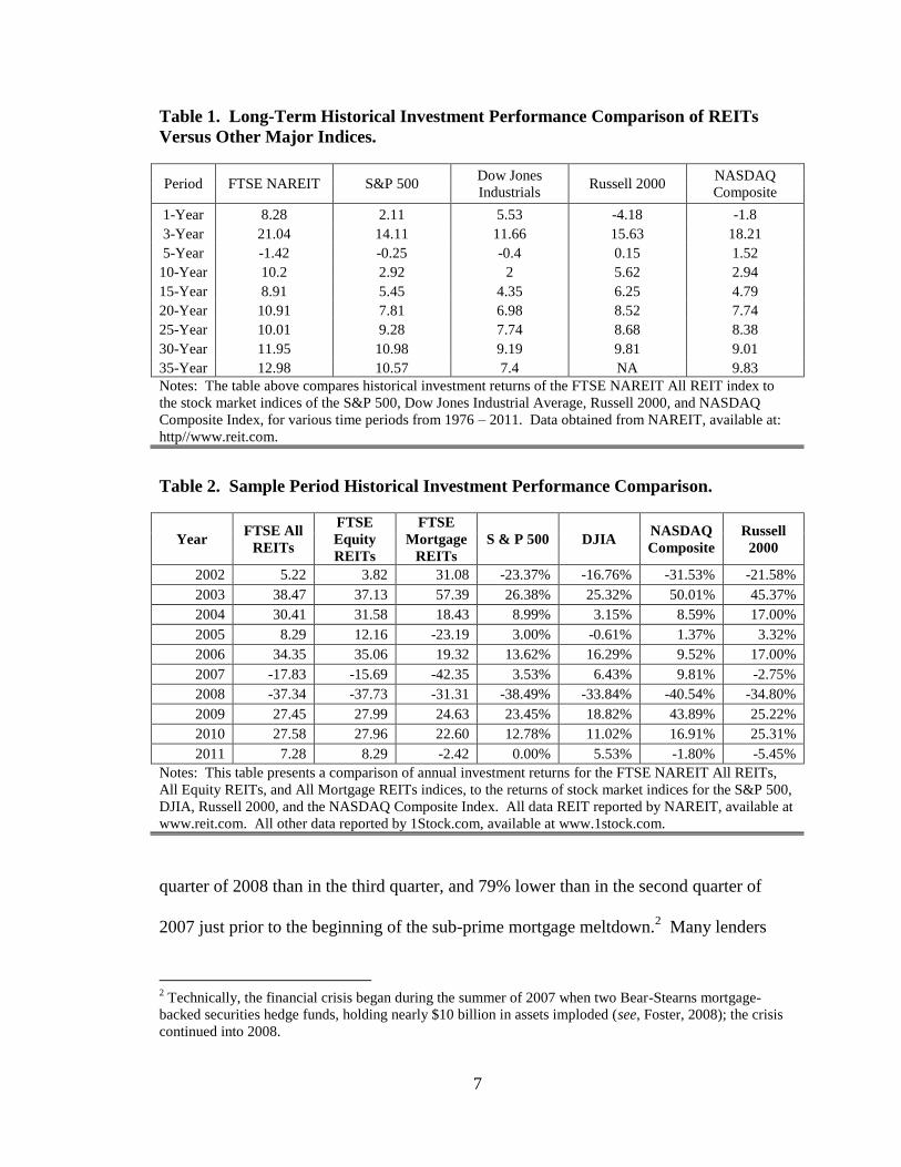
to invest in real estate (Goebel & Kim, 1989; Goodman, 2000, 2003). Indeed, Table 1

shows that over a 35-year period, as an asset class, REITs outperformed many major

stock market indices.1 Even after the financial crisis of 2007-2008, in most cases, REITs

outperformed major stock market indices annually as shown in Table 2.

The financial crisis triggered restricted debt financing and increased equity

investor wariness, creating difficulties for many participants in the highly illiquid capital

(Brunnermeier, 2008). Beginning in mid-2007, and continuing through the end of 2008,

declines in bank loans for acquisitions, investment, and revolving credit facilities were

universal (Ivashina & Scharfstein, 2010). Lending volume was 47% lower in the fourth

1 Data obtained from NAREIT, available at www.reit.com.

7

Table 1. Long-Term Historical Investment Performance Comparison of REITs

Versus Other Major Indices.

Period FTSE NAREIT S&P 500 Dow Jones

Industrials Russell 2000

NASDAQ

Composite

1-Year 8.28 2.11 5.53 -4.18 -1.8

3-Year 21.04 14.11 11.66 15.63 18.21

5-Year -1.42 -0.25 -0.4 0.15 1.52

10-Year 10.2 2.92 2 5.62 2.94

15-Year 8.91 5.45 4.35 6.25 4.79

20-Year 10.91 7.81 6.98 8.52 7.74

25-Year 10.01 9.28 7.74 8.68 8.38

30-Year 11.95 10.98 9.19 9.81 9.01

35-Year 12.98 10.57 7.4 NA 9.83

Notes: The table above compares historical investment returns of the FTSE NAREIT All REIT index to

the stock market indices of the S&P 500, Dow Jones Industrial Average, Russell 2000, and NASDAQ

Composite Index, for various time periods from 1976 – 2011. Data obtained from NAREIT, available at:

http//www.reit.com.

Table 2. Sample Period Historical Investment Performance Comparison.

Year FTSE All

REITs

FTSE

Equity

REITs

FTSE

Mortgage

REITs

S & P 500 DJIA NASDAQ

Composite

Russell

2000

2002 5.22 3.82 31.08 -23.37% -16.76% -31.53% -21.58%

2003 38.47 37.13 57.39 26.38% 25.32% 50.01% 45.37%

2004 30.41 31.58 18.43 8.99% 3.15% 8.59% 17.00%

2005 8.29 12.16 -23.19 3.00% -0.61% 1.37% 3.32%

2006 34.35 35.06 19.32 13.62% 16.29% 9.52% 17.00%

2007 -17.83 -15.69 -42.35 3.53% 6.43% 9.81% -2.75%

2008 -37.34 -37.73 -31.31 -38.49% -33.84% -40.54% -34.80%

2009 27.45 27.99 24.63 23.45% 18.82% 43.89% 25.22%

2010 27.58 27.96 22.60 12.78% 11.02% 16.91% 25.31%

2011 7.28 8.29 -2.42 0.00% 5.53% -1.80% -5.45%

Notes: This table presents a comparison of annual investment returns for the FTSE NAREIT All REITs,

All Equity REITs, and All Mortgage REITs indices, to the returns of stock market indices for the S&P 500,

DJIA, Russell 2000, and the NASDAQ Composite Index. All data REIT reported by NAREIT, available at

www.reit.com. All other data reported by 1Stock.com, available at www.1stock.com.

quarter of 2008 than in the third quarter, and 79% lower than in the second quarter of

2007 just prior to the beginning of the sub-prime mortgage meltdown.2 Many lenders

2 Technically, the financial crisis began during the summer of 2007 when two Bear-Stearns mortgage-

backed securities hedge funds, holding nearly $10 billion in assets imploded (see, Foster, 2008); the crisis

continued into 2008.

8

struggled to maintain adequate capital reserves, and those banks that were able to shore

up their reserves through customer deposits reduced lending far less than banks without

such access (Ivashina & Scharfstein, 2010). Bond debt was difficult to place because of

yield curve uncertainties (Adrian & Shin, 2010), and equity issues were equally

challenging in the face of tumbling stock markets (Block & Sandner, 2009).

Because of their structure, REITs have to raise external capital. After the crisis,

as economic uncertainties tightened credit markets and increased information

asymmetries among financial market participants, it was important for REITs to

implement strategies designed to reduce information asymmetries as much as possible so

that they could continue to access needed capital. Doing so, however, was difficult

because many real estate markets were in decline, and convincing investors to invest in

REITs—firms in the business of investing in real estate—was challenging (Basse,

Friedrich, & Bea, 2009).

The decisions a firm makes about the formation of its capital structure are critical

to its opportunities for growth and profitability (Myers, 1984; Titman & Wessels, 1988).

Capital structure decisions are complex, and often become more complicated because of

information asymmetries between firm managers and potential investors. If investors or

lenders are reluctant to invest because of information asymmetries, capital markets

function inefficiently (Healy & Palepu, 2001; Merton, 1987). As in Akerlof‘s (1970)

lemons problem, if investors cannot distinguish between the ‗good‘ and ‗bad‘

investments because of information asymmetries, they will either not invest at all, or will

price all investments as if they are ‗bad‘ ones. Thus, it is important that firms resolve the

9

‗lemons problem‘ by reducing information asymmetries that contribute to investors‘

reluctance to invest (Healy & Palepu, 2001).

Whether seeking equity or debt, the more effective firms are at conveying

information about themselves to potential investors and lenders, the more they can

decrease information asymmetries and motivate capital investment (Beatty, 1989; Carter

& Manaster, 1990). One study in particular investigates using some aspects of the audit

process to reduce information asymmetries (Titman & Trueman, 1986). However, as of

yet, no study has examined how using the audit-related attributes of auditor quality

(captured by higher audit fees), auditor specialization (captured by industry-audit

specialization), and auditor reputation (captured by the audit firm being a Big 4 auditor)

as mechanisms to increase transparency, impact access to capital investment. In this

paper, I explore these relationships, and collectively refer to these three audit-related

attributes as the Audit Construct.

Firms that raise capital either through initial public offerings (IPOs), seasoned

equity offerings (SEOs), or by issuing different types of debt financing provide a

prospectus to investors containing detailed information about their business structure,

management team, operations, investments, and performance. At a minimum, disclosure

regulations dictate that a prospectus contains certain elements of information, which

prudent investors carefully scrutinize when considering investing. Even so, firms

frequently include information in the prospectus that exceeds that which is required by

regulators. In doing so, their intent is often to provide additional signals to investors

about the firm‘s value, investment grade, and future prospects (Deeds, Decarolis, and

Coombs, 1997).

10

The prospectus also includes extensive, detailed information about the firm‘s

auditor and the audit process. Research shows that firms hire higher quality auditors, and

often pay much higher audit fees to signal to investors that their financial information is

highly credible (Datar, Feltham, & Hughes, 1991; Titman & Trueman, 1986). Investors

interpret such signals to mean the auditor will be less likely to succumb to pressures by

the firm‘s management to paint a rosier picture than actually exists. Because investors

view the information presented as being more transparent, in a sense, the firm is relying

on the reputational capital of the higher quality, more expensive audit firm to signal to

investors that they are more financially transparent (Feltham, Hughes, & Simunic, 1991).

It seems reasonable then to expect that by using the audit process to convey

increased transparency to investors, firms can also increase the likelihood of attracting or

increasing capital investment. In this study, I take a different approach by examining the

connection between REITs‘ uses of the Audit Construct as a means of signaling increased

financial transparency, in order to motivate capital investment. This is an important issue

because, just as other highly regulated, complexly structured firms that access capital

markets frequently must do, REITs continually need strategies supportive of their efforts

to motivate investment, especially when market conditions make accessing capital

difficult. In the next section, I present existing research supporting using the audit

process and audit-related attributes to convey increased financial transparency to

investors. In the following sections, I present and discuss the results of the empirical

analyses that test my expectation that there is a positive association between using the

Audit Construct as a means to signal increased transparency and increased capital

investment.

11

Section II. Literature Review

When a corporation‘s management makes the decision to become a real estate

investment trust (REIT), inherent in that decision is awareness that due to the dividend

distribution requirements required by federal law, the nature of its capital structure will

be irrevocably different after obtaining REIT status. Understanding the unique capital

structure of REITs is therefore essential to appreciating the significance of their

successfully conveying financial transparency to capital markets. I begin by reviewing

some of the most widely researched areas of capital structure, and continue with a

discussion of the history and structure of REITs, with particular focus on the significant

differences between the capital structure of typical corporations and those of REITs. I

follow with an assessment of general agency problems, paying specific attention to those

agency problems most important to REITs. I then discuss using the audit process as a

means of reducing information asymmetry and increasing financial transparency. In the

last section, I identify gaps in the literature, and discuss the importance of addressing

them in this study.

Theories of Capital Structure

Current capital structure theories stem from the Modigliani-Miller Theorem,

which states that in a perfect market a firm‘s financing decisions are irrelevant with

respect to its value (Modigliani & Miller, 1958). As seminal a work as it is, it disregards

the realities of taxes, bankruptcy, agency costs, asymmetric information, adverse

selection, and the ebb and flow of capital market inefficiencies. This oversight leads

12

modern capital structure researchers to focus instead on the trade-off theory, the pecking

order theory, and the market timing theory.

The essence of the trade-off theory is that when pursuing leverage, firms strive for

optimal balance between the benefits and costs of leverage. Under static trade-off theory,

firms ideally balance their capital structures using a mix of debt and equity (Altman,

1968). While there are associated benefits, such as the use of debt as a tax shield, there

are risks as well, such as the increased risks of financial distress and bankruptcy from

higher debt levels. Also important are agency costs associated with the use of debt and

equity that result from conflicts of interest between management and owners due to

asymmetric information (Jensen & Meckling, 1976; Jensen, 1986). Dynamic trade-off

theory considers the interaction between financing decisions made by a firm in one

period, and the prospects of where a firm will be in another period (Baker & Wurgler,

2002); variations through time due to changes in operations or investments affect the

firm‘s demand for capital, and therefore, influence its financing decisions.

The essence of the pecking order theory is that firms prefer internal financing to

external financing. Because investors tend to discount a firm‘s value when management

opts to issue equity over debt, firms will issue equity only if internal funds or debt

financing are not available (Myers & Majluf, 1984; Myers, 1984). However, in both

cases, adverse selection occurs because of information asymmetry (Bharath, Pasquariello,

& Wu, 2009). Investors often counter information asymmetry by exerting influence on

management through block voting or control by directors, while lenders often do so by

using varying credit terms to differentiate between good and bad borrowers. This is why

13

established banking relationships are so important to firms such as REITs, which must

borrow frequently (Hardin & Wu, 2010).

An important research conclusion regarding the pecking order theory is that while

Myers and Majluf (1984) indicate that informational asymmetry and leverage move in the

same direction, Ross (1977), Leland and Pyle (1977), Downes and Heinkel (1982),

Blazenko (1987), John (1987), Poitevin (1989), and Ravid and Sarig (1989) show no

correlations between leverage and a firm‘s value. However, these findings seem

intuitively at odds with each other. Consider that reductions in information asymmetry

lead to reduced leverage, yet leverage is a means by which firms use to maximize value.

Leary and Roberts (2010) indicate that although strict interpretation of the pecking order

leads to poorer firm performance, when firms modify, or more loosely apply their

adherence to the pecking order hypothesis, the theory‘s predictive power improves. This

finding is consistent with Fama and French (2002) who find strong links between the

trade-off theory and the pecking order theory, and each theory‘s respective abilities to

predict financing decisions.

The essence of the market timing theory is that firms are generally indifferent

over using debt or equity to finance their investments, but rather time their decisions

based on existing market conditions that place the highest value on one choice over the

other (Baker & Wurgler, 2002). Thus, when market valuations are high, we expect firms

to issue equity, but when they are low, we expect firms to issue debt. It follows then that

as a firm‘s stock prices rise and fall, the effects of this movement directly influence its

capital structure. Huang and Ritter (2009) test the market-timing theory by examining

14

how quickly firms adjust their capital structure, and find that the market timing theory

becomes less important the faster firms adjust toward their target leverage.

Signaling Theory

Signaling theory springs from the seminal proposition that an informed party will

convey information to influence a particular desired response by an uninformed party

(Spence, 1973). The ‗signaled‘ information effectively reduces information asymmetry

between the parties, and works to persuade the uninformed party to act in a way they

otherwise would not. Senders design signals to motivate a particular response; signals

must be costly to lend to credibility, and be difficult to mimic. Receivers of signals make

decisions about the intended purpose of the signal, the credibility of the sender, and the

accuracy, and reliability of the information received (Spence, 1973).

A major empirical implication of signaling is how a news event affects a firm‘s

stock price. For example, when firms announce intentions to issue debt, Myers and

Majluf (1984) and Krasker (1986) find no price effects when the debt has little risk, but

Noe (1988) and Narayanan (1988) show that prices decrease when firms issue more risky

debt. When firms announce plans to issue equity, studies show that stock prices

decrease, and that price changes are proportional to the amount of information

asymmetry, and the size of the equity offering (Krasker, 1986; Korajczyk, Lucas &

McDonald, 1992; Myers & Majluf, 1984; Noe, 1988).

15

REIT History and Structure

In 1960, the United States Congress passed legislation authorizing the formation

of REITs to provide average investors access to different types of income-producing real

estate, and the benefits of diversification and liquidity (Scherrer, 2004). While REITs

enjoy certain tax advantages that other corporations do not, they are also subject to

certain unique ownership structure and tax treatment requirements. Table 3 illustrates the

primary differences between REITs and corporations. REITs must annually elect to

maintain REIT status, and if they fail to comply with the law, they lose their REIT status.

The most significant difference between REITs and non-REITs is the requirement that

REITs distribute a minimum of 90% of net taxable income to shareholders as dividends.

Doing so leaves REITs with little free cash flow for operations or new investments.

Because dividends are deductible from corporate taxable income, many REITs

pay out all of their taxable income as dividends, and pay no corporate income taxes

(Edgerton, 2010). Shareholders pay taxes on dividends and any capital gains at the

individual level. Most states honor this federal tax treatment, and do not require REITs

to pay state income tax. Like other businesses, but unlike partnerships, REITs cannot

pass any tax losses through to its investors (Howe & Shilling, 1988).

Equity REITs focus primarily on owning and operating income-producing real

estate. They also participate in other real estate related activities such as leasing,

maintenance, tenant representation, and development of real property. Mortgage REITs

focus on lending money directly to real estate owners and operators, but only on existing

properties (Ambrose & Linneman, 2001). REITs do not provide construction or

development financing. However, they do apply their management expertise to

16

Table 3. Major Legal Differences Between a REIT and a Corporation.

REIT CORPORATION

A REIT may deduct dividends from its taxable

annual income. Dividends only taxed at the

individual shareholder level when dividends issued

annually and not at the corporate level.

A corporation (C-Corp) is subject to so-called

―double taxation‖ meaning taxable annual income

taxed at both the corporate level, and then again, at

the individual level if/when dividends declared and

issued.

A REIT must distribute a minimum of 90% of its

annual taxable income as dividends to shareholders.

A corporation is free to choose if/when it will

declare and issue dividends to shareholders.

A REIT must invest a minimum of 75% of its assets

in cash, government securities, real estate property,

real estate mortgage loans, and shares in other

REITs.

A corporation is free to invest its assets in any way

they see fit.

A minimum of 75% of a REIT‘s gross annual

income must come from rents from real estate

holdings, interest from real estate mortgages, or

capital gains from the sale of real estate assets.

A corporation‘s gross annual income may come

from any source; no minimums or maximums

required of any particular source of gross annual

income.

A minimum of 95% of a REIT‘s gross annual

income must come from rents from real estate

holdings, interest from real estate mortgages, capital

gains from the sale of real estate assets, dividends,

interest, and capital gains from the sale of securities.

A corporation‘s gross annual income may come

from any source and there are no minimums or

maximums required of any particular source of

gross annual income.

A REIT may not be a financial institution. A corporation may be a financial institution.

A REIT must have a minimum of 100 shareholders. A corporation may have only 1 shareholder.

No more than 50% of the outstanding shares of a

REIT owned by 5 or fewer investors during the last

half of each year.

There are no minimums or maximums applicable to

the percentages of ownership of a corporation‘s

outstanding shares.

Notes: The table above contrasts the major differences as defined by federal law between REITs and non-

REITs. Data obtained from NAREIT. Data obtained from NAREIT, available at: http//www.reit.com.

manage their interest rate risks using various hedging strategies, derivative investments,

and securitized mortgage instruments (Ambrose & Linneman, 2001).

Most REITs specialize in one property type or geographic location. Investment

opportunities in the REIT industry are diverse, as REITs invest in various types of

income-producing real estate including shopping centers, regional malls, office buildings,

industrial properties, self-storage facilities, multi-family properties, manufactured homes,

hotels and resorts, health care facilities, and even timberland (Beals & Singh, 2002). A

few REITs invest in a diversified portfolio of property types, but REITs that do so tend to

17

be larger and well established, and are the exception, not the norm (Capozza & Korean,

1995).

My earlier review of capital structure research was to set the stage for

highlighting and contrasting the significant differences in capital structure policies

between REITs and corporations. REIT capital structure literature differs from that of

other corporations by recognizing that regardless of their choice to issue equity or debt,

neither action has much impact on a REIT‘s stock price (Danielsen, Harrison, Van Ness,

& Warr, 2009). This is because REIT investors understand the implications of the

federally mandated dividend distribution requirement, and therefore, REITs needs to raise

capital frequently. However, because they must turn to the capital markets more

frequently than other types of corporations, it is also critical that REITs present a

compelling case to the capital markets to motivate investment. Increasing transparency is

one way of doing so.

REITs and Agency Problems

Examinations of agency problems in the literature are numerous. Jensen and

Meckling (1976) and Myers and Majluf (1984) address means to reduce asymmetric

information between a firm‘s managers and its investors. Houston and Ryngaert (1997),

Lewis, Rogalski, and Seward (1998), and Van Ness, Van Ness, and Warr (2001)

investigate the role that stock pricing plays in the reduction of concerns about asset

substitution and adverse selection. Diamond (1984, 1991), Ooi, Ong, and Li (2010), and

Williamson (1987) study the role of the use of debt as a monitoring function to reduce

moral hazard and frictions between firms and investors. Another well-documented

18

monitoring mechanism is the effective use of the audit process to reduce agency

concerns, and send strong, positive signals about a firm‘s corporate governance efficacy

to the capital markets (Cohen, Krishnamoorthy, & Wright, 2002; Danielsen, Harrison,

Van Ness, & Warr, 2010; Karamanou & Vafeas, 2005).

Understanding that REITs are very different from other types of corporations,

investors believe REITs have less severe agency problems (Bauer, Eichholtz, & Kok,

2010). For example, moral hazard is not as concerning, as there is little money available

for managers to waste. Adverse selection is less of a concern, as failure to comply with

required investment thresholds subjects REITs to losing their REIT status (Danielsen et

al., 2009); hence, investors are generally less apprehensive that REIT managers will

reject investment opportunities in order to hoard cash.

Chen, Chung, Lee, and Liao (2007) indicate that firms can reduce information

asymmetry and increase their financial transparency through better corporate focus and

governance. Capozza and Seguin (1999) affirm that REITs‘ corporate focus is clear due

to tax codes mandating investment of substantially all of their assets in income-producing

real estate. Anglin, Edelstein, Gao, and Tsang (2011) find correlations between reduced

levels of information asymmetry and better REIT corporate governance. Compared to

other types of firms that have more free-cash flow available for significant, new

investments, because REITs must distribute substantial portions of their net income, they

are much more dependent on new capital. As REIT investors understand this, typically,

asymmetric information is less problematic (Gentry & Mayer, 2003). Even so, because

higher levels of information asymmetries after the 2007-2008 crisis led to more

challenging capital market conditions in general, it was important that REIT managers

19

work to minimize any potential information asymmetries to strengthen their abilities to

continue to attract new capital investment. One way firms can lower information

asymmetries is by sending clear financial transparency signals to investors (Brau &

Holmes, 2006). Indeed, Danielsen et al. (2009) conclude that successful financial

transparency signaling is an effective means of attracting capital investment.

The Audit Process, Financial Transparency Signaling, and REITs

The audit process is a well-documented monitoring mechanism effective in

reducing agency conflicts. Firms use it to send financial transparency signals to

investors—signals intended to reduce information asymmetries—when they engage

financial intermediaries to represent their efforts to raise capital (Healy & Palepu, 2001).

In receiving signals, investors make decisions about the intended purpose of the signal,

the credibility of the sender, and the accuracy of the information received. In using the

audit process as a transparency signaling mechanism, certain audit attributes such as audit

quality, fee structure, and auditor reputation become factors that investors use to evaluate

a firm‘s financial transparency (Datar, et al., 1991; Titman & Trueman, 1986). Because

REITs can benefit from sending strong signals to investors designed to convey their

financial transparency, the audit process, including hiring high quality auditors and

paying higher audit fees—presumably to secure higher quality audits—is a means of

transparency signaling that is a critical aspect of REIT capital structure mechanisms

(Danielson, et al., 2009).3

3 Demsetz (1968) and Bagehot (1971) were the first researchers to study the link between asymmetric

information and the firm‘s financial market liquidity. They show a relationship exists between the bid-ask

spread in the stock price for a particular firm, and the trading characteristics of its securities. Glosten and

20

The studies of Titman and Trueman (1986) and Feltham et al. (1991) support the

idea that firms wishing to convey positive signals to investors will hire auditors with

higher quality reputations. An interesting aspect of the auditing process is the

motivations of the firms that hire the auditors. In game, finance, and behavioral theories,

the possibility exists that low quality entities would mimic actions (signals) employed by

high quality firms to reap the benefits of the signal. Thus, to be credible, the signal must

be costly and difficult to replicate in order for investors to perceive the signal as a

separating equilibrium (Spence, 1973). Hiring auditors with higher quality reputations is

costly; firms often do so as a way of signaling increased transparency to investors.

Danielsen, Van Ness, and Warr (2007) suggest that when firms pay higher audit

fees to auditors with higher quality reputations, they benefit from the reputational quality

of the audit firm. Investors‘ perceptions of higher auditor quality reputation add

credibility to the audit process and financial information transparency. Hence, investors

will more likely favorably view firms that hire auditors with higher quality reputations

over those that do not. Balvers, McDonald, and Miller (1988) posit that auditor

reputation sends an important signal when firms issue new securities. They indicate the

intention of selecting a highly reputable auditor is to signal greater audit credibility.

Their findings suggest that appointing a highly reputable auditor tends to lower earnings

variability, reflecting favorably on the investment banker selecting the auditor. A

Milgrom (1985) and Kyle (1985) find trading differences between informed and uninformed traders result

from the presence of asymmetric information. Glosten and Milgrom (1985) demonstrate that spreads

between a security‘s bid and ask prices result from the level of an informed trader‘s private information.

Amihud and Mendelson (1986, 2000) find a positive correlation between information asymmetry and

capital costs. Danielsen et al. (2010) suggest that bid-ask spreads partly reflect the significance of

information asymmetries affecting investors.

21

somewhat related finding by Datar et al. (1991) reveals firms that choose higher quality

auditors do so to convey private information to investors.

Daily, Certo, Dalton, and Roengpitya (2003) find that in firms pursuing equity

offerings, if managers are aware of negative information, it is unlikely they will hire high

quality auditors. Because audit firms that fail to reveal negative information that they

uncover may face possible criminal prosecution, such a possibility acts as a deterrent to

non-disclosure. This also relates to the reputation of the audit firm, as not revealing

negative information and facing criminal charges later, or the possibility that the market

eventually finds out about the negative information can be very damaging to a firm‘s

reputation. These two consequences provide compelling motivations for most auditors to

be very diligent and careful in the course of an audit. It makes sense then that if a firm‘s

management is aware of potential negative information, it will be less likely to hire the

highest quality auditor. This is not to say or suggest that only the highest quality auditors

will find and reveal negative information. Rather, it is to say that there is a higher

probability that lower quality audit firms may not have the resources to provide higher

quality audits. Thus, by not hiring a high quality auditor, firms potentially signal to

investors that the firm poses higher investment risks.

There are numerous studies using audit fee structure to signal transparency.

Francis, Lys, and Vincent (2004) find that REITs typically experience more favorable

investor reaction than other types of firms when issuing securities, and that signaling

plays a significant role in the way investors react to such offerings. As it is highly

probable that audit quality and auditor reputation will influence their efforts to raise

capital, assuming that costly audits translate into greater transparency, Danielsen et al.

22

(2009) examine which firms are most likely to benefit from a higher priced audit. They

posit that REITs that undertake expensive audits increase their liquidity. They also

reason that it is likely that non-REITs are willing to absorb higher audit fees to signal

greater transparency, and hence, attract investors. Danielsen et al. (2009) find firms

signal greater financial transparency through heavier investment in audit services, and

reduce their capital costs when issuing SEOs. Beatty (1989) finds that firms who pay a

premium for audit services have lower initial returns after going public. This suggests

that firms willing to pay more for audit services do so to signal increased financial

transparency to investors. Higgs and Skantz (2006) conclude that investors interpret high

audit fees as signals of a firm‘s commitment to high earnings quality. In their

examination of voluntary auditor choice, Hay and Davis (2002) find that firms seeking

higher quality audits (again, knowingly make a choice to pay higher audit fees) do so for

signaling reasons. Similarly, in their examination of small auditees, Peel and Roberts

(2003) find that small firms willingly hire higher priced audit firms in order to send

signals of operations and earnings quality to investors. Signaling is important to firms

seeking to reduce information asymmetries, and increase financial transparency because

doing so enhances abilities to attract investment. For firms such as REITs that must

access capital often, it is especially important.

REIT Liquidity and Information Transparency Mechanisms

Providing timely financial information reduces information asymmetry (Bushman

& Smith, 2001, 2003; Diamond & Verrecchia, 1991; Fama & Jensen, 1983). However,

in order to be effective, the financial information must be transparent. Just as important,

23

in order for the receiver to view the information as transparent, the receiver must also

view both the information received and the sender as being credible. Firms can signal

their credibility and financial transparency by providing highly accurate and reliable

audited financial statements (Hope, Thomas, & Vyas, 2009). Because investors tend to

favor firms that are more transparent, greater transparency helps firms attract investment,

and therefore, increase their liquidity (Cohen, Krishnamoorthy, & Wright, 2002;

Danielsen, et al., 2010; Karamanou & Vafeas, 2005). Hence, it seems logical that if

using vigorous audit services ―can improve liquidity for any firm, it seems especially

likely to do so for REITs‖ (Danielsen et al., 2009, p. 517).

REIT Complexity and Information Transparency Mechanisms

Highly regulated firms or those holding multifarious, wide-ranging assets

typically require complex, expensive audits (Chersan, Robu, Carp, & Mironiuc, 2012).

For example, banks and other types of financial institutions, which quite often own and

operate their businesses through a labyrinth of holding companies, subsidiaries, and

controlling interest positions, are subject to a high threshold of regulatory compliance

(Boo & Sharma, 2008). Auditors examining their books must employ a high degree of

scrutiny to limit their potential liability associated with audit results. REITs are also

highly regulated and many are extremely complex, owning and operating their assets

through a vast network of subsidiaries, partnerships, and joint venture arrangements.

Because of their multifaceted nature, REITs face a persistent challenge to minimize

information asymmetries between themselves and investors; the financial crisis only

exacerbated this task (Hardin & Wu, 2010). Therefore, due to their frequent need for

24

capital investment, after the crisis, it was critical for REITs to find ways to meet this

challenge. By hiring higher quality auditors, audit specialists, or auditors with a higher

quality reputation (such as a Big 4 audit firm), REITs could take steps not only to reduce

information asymmetries, but more importantly, they could send clear transparency

signals to investors to motivate capital investment.

Audits of REITs are complex, partly because they operate in a highly regulated

environment, and partly because the majority of their assets are valuation driven. Unlike

a typical corporation, federal laws dictate not only how and to what extent REITs must

distribute their income, but also how and to what extent they must invest their assets. As

shown in Table 3, in addition to the dividend distribution requirement, REITs must invest

a minimum of 75% of their assets in cash, government securities, real estate property,

real estate mortgage loans, and shares in other REITs. Hence, REIT audits are often

complex because of the diversity of their assets, and market effects on their underlying

values.

With regard to equity REITs, individual, property level real estate assets are

essentially independent, self-contained investments, each with their own sources and uses

of revenues and expenses, and each with their own degrees of risk that vary from

property to property. These may be difficult for the auditor to understand or value

(Danielsen et al., 2009; Friday & Sirmans, 1998). This is because the values of income-

producing real estate assets are determined at the individual property level based on the

cash flows produced by each property within a portfolio (Epley, Rabianski, & Haney,

2002); evaluating these types of assets may be difficult for many auditors because they

lack professional real estate appraisal expertise. Similarly, auditing mortgage REITs is

25

difficult because within their portfolio, they hold myriad commercial mortgage-backed

securities, real estate mortgage notes, and other types of real estate credit facilities.

Without a thorough understanding of the specific risks associated with each instrument

within the portfolio, providing a detailed audit of a mortgage REIT could be very

difficult. In either event, auditing an equity or mortgage REIT can potentially be

extremely complex and costly. Therefore, it is necessary to control for REITs‘

complexity when analyzing REITs in the context of the audit process.

The financial crisis compounded the REIT audit-complexity problem in several

ways. Income-producing properties in a portfolio, or more accurately, the cash flows

derived therefrom, are highly dependent on the credit risk of the tenants providing the

income (Epley, et al., 2002). During the crisis, the financial health of many tenants,

especially those that were not public companies, may have been difficult, if not altogether

impossible to ascertain. The risks associated with possible disruptions in future cash

flows from each of the properties within a REIT portfolio would have also been difficult

to quantify and evaluate. Additionally, carefully managing operating expenses of

income-producing real estate is essential to producing and protecting investment returns

(Epley, et al., 2002). A significant portion of operating expenses stems from the costs of

property and casualty insurance. If an insurer‘s business suffered during the crisis as a

result of deterioration of its own operations or investments, or worse, failed, the impact

on properties within a REIT‘s portfolio could be significant as well (Monroe, 2009).

Finally, financing related to an income-producing property is critical to the stability of its

cash flows (Epley, et al., 2002). As banks struggled during the crisis, the risks and

uncertainties related to poor bank performance, or even failure, potentially posed

26

problems for REITs. This is because it may have been difficult to reposition debt on

portfolio properties facing financing resets or looming balloon payments after the crisis.

Any of these market condition difficulties may have added to the complexity of auditing

REITs, especially ones with very diverse property portfolios, or high-credit-risk tenant

mixes.

REITs‘ Auditor Relationships and Financial Transparency

Hardin and Wu (2010) show that REITs with strong banking relationships tend to

obtain public debt-ratings, enabling them to go to the public debt markets more often.

These REITs typically use less bank financing secured or collateralized by their

underlying real estate assets. They conclude that establishing banking relationships

enable REITs to lower their leverage. This is important because investors tend to favor

firms with lower leverage because reduced capital costs decrease financial risk (Baxter,

1967). Just as the existence of banking relationships and rating agency status convey

information to the market as to the prospects of the firm, auditors‘ relationships with their

client firms likely have an impact on the transparency of firms‘ financial information and

access to capital markets.

Investors understand that, over time, auditors gain significant understanding about

the nature of their clients‘ business operations (AICPA, 1978; Bells, Marrs, Solomon, &

Thomas, 1997), and numerous researchers find a positive association between auditor

tenure and audit quality (Geiger & Raghunanandan, 2002; Johnson, Khurana &

Reynolds, 2002; Myers, Myers, & Omer, 2003; Mansi, Maxwell, & Miller, 2004).

Similarly, Ghosh and Moon (2005) find empirical support for a positive relationship

27

between auditor tenure and investors‘ beliefs about the firm‘s earnings quality. In

addition, longer auditor tenure may improve investors‘ perceptions of the quality of a

firm‘s financial transparency because of learning curve effects associated with new

auditors. Although the Sarbanes-Oxley Act of 2002 (SOX) mandates individual auditor

rotation within an audit firm, hiring a new audit firm does necessitate a certain ‗learning

curve‘ for the new audit firm; not surprisingly, audit failures are higher in the early years

of an auditor‘s engagement (Geiger & Raghunandan, 2002). Based on these studies, a

reasonable inference is that the longer an auditor provides services for a firm, the more its

reputation is at stake. It is reasonable then that after a long record of consistent quality

service, the market expects a continuation of that service. Therefore, the market likely

perceives a mistake by the audit firm after a long record of good service with suspicion,

and as potential deterioration of service.

On the other hand, investors may also view extended auditor tenure as somewhat

problematic. Although engaged by the auditee, an essential duty of the auditor is to

remain independent in the conduct of its audit to safeguard the interests of other

interested parties such as investors, lenders, and employees (Lavin, 1976; Schleifer &

Shockley, 2011). So it seems plausible that after years of engagement—years spent

developing a sound sense of the nature of its client‘s business—mistakes or errors made

by a long-term auditor might lead some to question the auditor‘s independence (Carcello

& Nagy, 2004; Chang & Monroe, 1994; Goldman & Barlev, 1974; Johnson, Khurana, &

Reynolds, 2002), or whether the auditor capitulated to client demands rather than risk

future revenues (Basiousis, Gul, & Ng, 2012; Hoyle, 1978; Windsor & Cavanaugh,

28

2012). Still, an auditor might simply fail to remain diligent in pursuit of its audit

responsibilities (Braswell, Daniels, Landis, & Chang, 2012; Mautz & Sharaf, 1961).

Similarly, hiring an auditor with industry specialization is likely to play an

important role in conveying financial transparency to the markets, especially when the

auditee presents a complex audit (Abdolmohammadi, Searfoss, & Shanteau, 2004).

Choosing to specialize in a particular industry is not a decision that audit firms take

lightly, as doing so requires committing substantial amounts of time and money to train

audit personnel on the workings of a particular industry (Lim & Tan, 2010). Because of

the auditor‘s advanced knowledge about the specific nature of an auditee‘s industry, the

likelihood is lower that the firm‘s management will deceive or mislead the auditor

(Solomon, Shields, & Whittington, 1999). Equally important is that precisely because of

the audit firm‘s industry specialization, safeguarding its reputational capital is also an

important incentive to perform quality audits (Watts & Zimmerman, 1983). This is

because, as an industry specialist, the audit firm is at greater risk of losing other clients in

the same industry, should it make a mistake auditing one. In other words, by becoming

an industry audit specialist, in a sense by proverbially ‗putting its eggs in one basket,‘ the

audit firm has much more to lose. Investors understand the significance of an audit

firm‘s commitment to becoming an industry specialist, and realize firms often hire audit

specialists to improve their disclosures (Dunn & Mayhew, 2004), thereby enhancing their

transparency. As discussed earlier, many REITs are complex firms with diverse, wide-

ranging assets. Hence, hiring an auditor recognized as a REIT audit specialist can be an

important mechanism through which REITs can signal increased transparency to

investors.

29

Audit firm size and reputation is also likely to convey information about the

financial transparency of the auditee. Auditor quality is often associated with auditor size

because larger audit firms have more resources and provide higher quality audits

(DeAngelo, 1981). When information asymmetry is high, such as when a firm is

preparing to issue equity for the first time, firms are more likely to engage a larger, higher

quality auditor (e.g. Big 4 auditor) for signaling purposes. The studies of Balvers et al.

(1988), and Firth and Smith (1992) provide evidence to support this argument. They find

that firms experience less IPO underpricing when they hire larger audit firms.

Willenborg (1999) finds support for signaling in his study of the demand for pre-IPO

audit services by showing a Big-5 audit is more valuable. Firth and Liau-Tan (2003) find

a correlation between investor perceptions of high risk IPOs, and audits performed by

high quality auditors. Similarly, Simunic and Stein (1987), Beatty (1989), and Chan,

Ezzamel, and Gwilliam (1993) show that large audit firms charge higher audit fees than

their smaller competitors because of the demand for their higher quality services,

generally driven by their higher audit quality reputation.

Research Implications and Contributions

Historically, REITs have largely been successful in raising both equity and debt

capital. Table 4 shows the number of equity and debt issues, and the commensurate

amounts of money raised by REITs through such offerings from 2002-2011. Generally,

the number of issues and the amounts of capital raised increased each year prior to the

2007-2008 crisis, but not surprisingly, the numbers fell precipitously afterwards. This

evidence suggests one of two things: either (1) REITs did not seek increasing amounts of

30

Table 4. Publicly-Traded REIT Equity and Debt Issues from 2002-2011.

Year

Issued

Equity Issues Debt Issues Total Equity &

Debt

# $ % of

Total # $

% of

Total # $

2002 113 $8,384 42.41% 74 $11,383 57.58% 187 $19,768

2003 154 $13,309 52.07% 74 $12,252 47.93% 228 $25,562

2004 169 $21,176 55.03% 97 $17,306 44.97% 266 $38,482

2005 118 $15,405 41.09% 141 $22,088 58.91% 259 $37,492

2006 119 $22,205 45.30% 85 $26,812 54.70% 204 $49,018

2007 86 $17,876 49.61% 43 $18,155 50.39% 129 $36,031

2008 71 $12,818 71.25% 11 $5,173 28.75% 82 $17,991

2009 96 $24,234 69.93% 34 $10,422 30.07% 130 $34,656

2010 117 $28,221 59.48% 56 $19,230 40.53% 173 $47,450

2011 131 $37,490 73.11% 33 $13,790 26.89% 164 $51,280

Notes: The table above reports equity, debt, and combined equity and debt capital investment made in all

publicly-traded REITs as reported by NAREIT. All data reported in millions of dollars, available at

www.reit.com

capital after the financial crisis, which is inconsistent with REITs‘ well-established need

to raise capital frequently, or, most likely, (2) generally, the financial crisis severely

constrained REITs‘ access to capital markets.

Whether the capital outlet is the equity or debt market, when investors have a

better understanding of the financial condition of the firm, the higher the likelihood they

will invest. Therefore, engaging in actions that reduce or eliminate information

asymmetry and thus signaling increased transparency, is one logical strategy for firms to

pursue when attempting to raise capital. After the crisis, facing a new, very uncertain

financial environment, all firms seeking new capital had to find ways to reduce or

eliminate information asymmetries. Because of REITs‘ dependence on new capital, the

question then becomes: How do REITs reduce information asymmetries and increase

their abilities to motivate capital investment?

31

Collectively, the extant research underscores the importance of using the audit

process as a mechanism for reducing information asymmetries to signal increased

transparency. The literature also connects increased transparency to increased capital

investment. Thus, the expectation is that the financial crisis increased the prevalence of

information asymmetries within the financial markets, leading to higher levels of

illiquidity and investor conservatism, and increasing the difficulties of raising new

capital. If using the audit process to signal transparency is important for all firms seeking

to increase capital investment, clearly it must be as important, if not more so, for capital-

dependent REITs.

To date, there has been no examination of whether increased transparency via the

auditing process leads to better access to capital markets, and more importantly, during

periods of high capital market illiquidity caused by a major shock to the financial system.

This study contributes to the literature by examining how highly regulated, complexly

structured firms that raise capital frequently use the audit process to signal transparency

to attract new investment. Although the outcomes pertain specifically to REITs, the

results are important in many other respects. All firms that rely heavily on capital

markets can gain from this study‘s insight into using the audit process to signal increased

transparency as a means of attracting capital investment. Investors choosing among

investment alternatives will benefit through a better understanding of how firms use the

audit process to signal transparency. Finally, the results will give researchers a deeper

understanding of how increased transparency, resulting from using the audit process, can

maintain indispensable access to capital markets.

32

Section III. Hypotheses Development

Exogenous events can shock and disrupt capital markets, and create pressures on

market equilibrium. As many investors respond by moving money from equities and

corporate debt into safer investments such as government debt and cash, often the result

is substantially increased capital market illiquidity. Any type of shock that creates

volatile, unstable market conditions, combined with swift investor reactions that work to

reduce liquidity, can make raising capital difficult. The severity of the shocks to the

financial system, and the ensuing post-crisis market conditions caused major problems

for many firms needing to raise new capital. Even though REITs faced the same situation

as all capital market participants seeking new investment, for them it was likely more

challenging. As cash flows fell due to required dividend payouts, and in some instances,

reduced rent flows from struggling real estate portfolios, REITs had no choice but to seek

new capital investment. Still, they had to do so at the very time when real estate markets,

experiencing significant value declines throughout the country, were generally out of

favor with investors (DeLisle, 2007, 2008).

As discussed earlier, Table 4 shows that the number of equity and debt issues, and

the total amounts of capital raised by all publicly traded REITs fell dramatically after the

onset of the financial crisis. Although the numbers gradually began to improve in 2009,

and continued to do so thereafter, not until 2011 did total investment eclipse the high set

in 2006. Therefore, a reasonable question to consider is: What steps REITs took to

attract investment from wary investors, nervous about highly illiquid, unstable financial

market conditions? In the literature review, I highlight several studies that examine

33

different ways that firms signal financial transparency to investors to attract new capital

investment. One of them, using the audit process, is the focus of this research.

Using a two-part approach, I examine the relationship between REITs using the

Audit Construct to increase transparency and accessing new capital. In the first part of

the analysis, I examine the relationship between the Audit Construct and equity, debt, and

combined equity and debt investment, posited by the following hypotheses:

Hypothesis 1: There is a positive association between the Audit Construct and

equity investment in REITs.

Hypothesis 2: There is a positive association between the Audit Construct and

debt investment in REITs.

Hypothesis 3: There is a positive association between the Audit Construct and

combined equity and debt investment in REITs.

In the second part of the analysis, I examine the relationship between REITs‘ use of the

Audit Construct and access to new capital, accounting for possible mediating effects of

the financial crisis, posited by the following hypotheses:

Hypothesis 4: The financial crisis of 2007-2008 positively influenced the

relationship between the Audit Construct and equity investment in

REITs.

Hypothesis 5: The financial crisis of 2007-2008 positively influenced the

relationship between the Audit Construct and debt investment in

REITs.

Hypothesis 6: The financial crisis of 2007-2008 positively influenced the

relationship between the Audit Construct and combined equity and

debt investment in REITs.

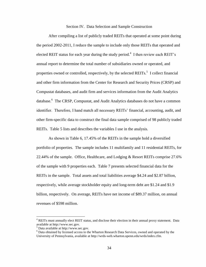
34

Section IV. Data Selection and Sample Construction

After compiling a list of publicly traded REITs that operated at some point during

the period 2002-2011, I reduce the sample to include only those REITs that operated and

elected REIT status for each year during the study period.4 I then review each REIT‘s

annual report to determine the total number of subsidiaries owned or operated, and

properties owned or controlled, respectively, by the selected REITs.5 I collect financial

and other firm information from the Center for Research and Security Prices (CRSP) and

Compustat databases, and audit firm and services information from the Audit Analytics

database.6 The CRSP, Compustat, and Audit Analytics databases do not have a common

identifier. Therefore, I hand match all necessary REITs‘ financial, accounting, audit, and

other firm-specific data to construct the final data sample comprised of 98 publicly traded

REITs. Table 5 lists and describes the variables I use in the analysis.

As shown in Table 6, 17.45% of the REITs in the sample hold a diversified

portfolio of properties. The sample includes 11 multifamily and 11 residential REITs, for

22.44% of the sample. Office, Healthcare, and Lodging & Resort REITs comprise 27.6%

of the sample with 9 properties each. Table 7 presents selected financial data for the

REITs in the sample. Total assets and total liabilities average $4.24 and $2.87 billion,

respectively, while average stockholder equity and long-term debt are $1.24 and $1.9

billion, respectively. On average, REITs have net income of $89.37 million, on annual

revenues of $598 million.

4 REITs must annually elect REIT status, and disclose their election in their annual proxy statement. Data

available at http://www.sec.gov. 5 Data available at http://www.sec.gov.

6 Data obtained by licensed access to the Wharton Research Data Services, owned and operated by the

University of Pennsylvania, available at http://wrds-web.wharton.upenn.edu/wrds/index.cfm.

35

Table 5. Description of Variables.

Variable Variable Description

ln(Equity Investment) Natural log of proceeds from common and preferred stock issuance1

ln(Debt Investment) Natural log of proceeds from debt issuance1

ln(Equity & Debt Investment) Total value of ln(Equity Investment) and ln(Debt Investment) as defined

above

ln(Audit Fees) Natural log of total audit fees2

Specialist

A dummy variable taking the value of 1 if the auditor employed by an

individual REIT performs more than 30% of all REIT audits in the sample,

and 0 otherwise3

Big 4 Auditor A dummy variable taking the value of 1 if the auditor ranks as a Big 4

audit firm, and 0 otherwise4

Bid-Ask Spread The standard deviation of the mean annual bid-ask spread

Intangible Assets The total value of intangible assets1

Book/Market Computed as book value1 divided by market value

1

ROA Net annual income1 divided by total assets

1

Leverage Total assets1 divided by total liabilities

1

Initial A dummy variable taking the value of 1 if an individual REIT's audit firm

is in either the first or second year of engagement, and 0 otherwise3

ln(Other Fees)

Natural log of all non-audit fees including income tax preparation services,

information systems consulting, benefits administration and other non-

audit fees2

ln(Properties)

The natural log of the number of properties owned or controlled by the

individual REITs or their respective subsidiaries as reported in their annual

10-k report5

ln(Subsidiaries)

The natural log of the number of subsidiaries owned or controlled by the

individual REITs or their respective subsidiaries as reported in their annual

10-k report5

Foreign

A dummy variable taking the value of 1 if an individual REIT has

operations outside of the United States as reported in CRSP/Compustat

database, and 0 otherwise1

Extra/Disc

A dummy variable taking the value of 1 if an individual REIT has

extraordinary items and/or discontinued operations as reported in the

CRSP/Compustat database, and 0 otherwise1

REIT Type A dummy variable taking the value of 1 if an individual REIT is Y-type,

and 0 otherwise6

Notes: 1Log values computed on values reported in the Compustat database.

2Log values computed on

values reported in the Audit Analytics database. 3Specific REIT audit and auditor information reported in

the Audit Analytics database. 4The group of audit firms currently known as the ―Big 4‖ includes

PriceWaterhouseCoopers, Deloitte & Touche, Ernst & Young, and KPMG, ranked "1" through "4" based

on annual revenues, respectively, as reported at http://www.big4.com. 5Specific, individual REIT 10-k

annual reports accessed at http://www.sec.gov. 6Property Y-type indicates type of REIT industry

classification including Multifamily, Manufacturing, Healthcare, Shopping Center, Freestanding, Regional

Mall, Lodging/Resort, Diversified, Office, Industrial, Office/Industrial Mixed, Self-Storage, Commercial

Mortgage, and Residential Mortgage.

36

Table 6. REIT-Type Distributions.

REIT Specialization REIT Type # of REITs in

Sample

% of REITs in

Sample

Diversified Portfolio of Properties

Equity 17 17.35%

Multifamily Residential Properties

Equity 11 11.22%

Retail Shopping Center Properties

Equity 11 11.22%

Office Properties

Equity 9 9.18%

Healthcare Properties

Equity 9 9.18%

Lodging & Resort Properties

Equity 9 9.18%

Retail Regional Mall Properties

Equity 6 6.12%

Residential Mortgage Investments

Mortgage 6 6.12%

Office & Industrial Properties

Equity 5 5.10%

Freestanding Single-Tenant Properties

Equity 4 4.08%

Industrial Properties

Equity 4 4.08%

Residential Manufactured Home Properties

Equity 3 3.06%

Commercial Mortgage Investments

Mortgage 3 3.06%

Self-Storage & Mini-Warehouse Properties

Equity 1 1.02%

Notes: A total of 98 REITs maintained REIT status during the entire sample period of 2002-2011 as

confirmed in specific, individual REIT 10-k annual reports.

Table 7. Summary Statistics - REIT Firm Financial Information ($,000,000s).

Variable N Mean Std. Dev. 25th Median 75th

Total Assets 980 4241.69 6914.66 1013.14 2356.18 4970.25

Intangible Assets 980 51.97 242.16 0.00 0.00 12.65

Total Liabilities 980 2874.69 5675.55 530.19 1428.67 3078.19

Long Term Debt 980 1903.69 2582.56 336.67 1072.03 2292.27

Annual Revenues 980 598.63 900.21 138.63 303.06 674.72

Earnings Before Interest & Taxes 980 191.39 312.20 46.18 106.89 233.34

Net Income 980 89.37 217.02 12.05 45.87 128.93

Stockholder Equity 980 1246.49 1603.97 295.73 763.73 1539.79

Notes: Data are for the entire sample period of 2002-2011 as reported in the Compustat database.

37

Section V. Research Design and Methodology

In this study, the outcome of interest is Capital Investment, which I proxy for by

using the three measures of equity investment, debt investment, and combined equity and

debt investment. I use the metrics in Danielson et al. (2009), along with a third

dimension, auditor specialization, to compose the Audit Construct. As done in the

literature, I use these three audit-related variables in particular to capture Transparency.

In the first part of the analysis, the study period is much broader, covering the years of

2002-2011. In the second part of the analysis, I analyze the impact of the financial crisis

on this expected relationship.

Empirical Model – Part 1

In addition to the main independent variables I use to capture Transparency, I

include three additional vectors of variables to capture the dimensions of Firm

Characteristics, Auditor Relationship, and REIT Complexity. I also use a number of

dummy variables to control for effects related to specific REIT-types and/or changes

across time. The empirical model for the first part of the analysis takes the following

form:

Capital Investment = ᶂ {Transparency, Firm Characteristics, Auditor

Relationship, REIT Complexity}. (1)

Transparency Vector

Earlier, I mentioned research findings that firms often pay higher audit fees to hire

higher quality auditors to signal to investors that their financial information is highly

38

credible (Datar, Feltham, & Hughes, 1991; Titman & Trueman, 1986). Therefore, the

central piece of the investigation centers on Transparency. To proxy for auditor quality, I

use the variable ln(Audit Fees),7 which is the natural log of audit fees. To capture auditor

specialization, I use the variable Specialist,8 a dummy variable that takes the value of one

if the auditing firm has performed audits on more than 30% of the audits in the entire

sample in each year, and zero otherwise. Finally, to proxy for auditor reputation, I use

the variable Big 4 Auditor,9 a dummy variable that takes the value of one if the auditor

ranks as one of the Big 4 audit firms, and zero otherwise.

Earlier, I also discuss the association between information asymmetry, financial

information transparency, and the bid-ask spread, a widely used measure of transparency.

Intangible assets are difficult to define or value, aggravated by the fact that firms often

choose not to reveal certain information that they view as proprietary. Researchers

commonly use intangible assets to proxy for information asymmetry. I include two

additional variables within the Transparency vector: Bid-Ask Spread, which I construct

using the standard deviation of the mean annual bid-ask spread of each REIT‘s stock

price; and Intangible Assets, which is the total value of each REIT‘s intangible assets.

7 Audit fee information comes from the Audit Analytics database.

8 For the purposes of this research, auditor specialization includes auditors that performed 30% or more of

all REIT audits in the sample. Table 8 groups all REIT audits by audit firm, total audit fees, and average

audit fees. Of the 980 total REIT audits performed in the sample, Ernst & Young, LLP, performed 327, or

33.37%. All other auditors each performed less than 18% of the total number of REIT audits in the sample.

Auditor rank order is by percentage of REIT audits performed. 9 The group of audit firms currently known as the ―Big 4‖ includes PriceWaterhouseCoopers, LLP,

Deloitte & Touche, LLP, Ernst & Young, LLP, and KPMG, LLP, ranked 1 through 4 based on annual

revenues, respectively (www.Big4.com, 2012).

39

Table 8. REIT Auditors

REIT Auditor Name

REIT

Auditor

Rank

# REIT

Audits

% of

REIT

Audits

Total REIT

Audit Fees

($,000s)

Average Per-

Audit Fees

($,000s)

Ernst & Young 1 327 33.37% 367,564 1,124

KPMG 2 175 17.86% 140,926 805

PricewaterhouseCoopers 3 167 17.04% 146,222 876

Deloitte & Touche 4 118 12.04% 128,541 1,089

BDO USA 5 69 7.04% 42,508 616

Grant Thornton 6 49 5.00% 48,530 990

PKF O‘Connor Davies 7 14 1.43% 3,077 220

Reznick Group 8 14 1.43% 1,736 124

Berenfeld Spritzer Shechter & Sheer 9 8 0.82% 667 83

Swalm & Associates 10 8 0.82% 451 56

McGladrey & Pullen 11 7 0.71% 1,662 237

Burr Pilger Mayer 12 6 0.61% 1,690 282

Calvetti Ferguson & Wagner 13 5 0.51% 7,286 1,457

Moss Adams 14 5 0.51% 653 131

Donaldson Holman & West 15 2 0.20% 1,402 701

Epstein Weber & Conover 16 2 0.20% 154 77

Moore Stephens 17 1 0.10% 79 79

Cherry Bekaert & Holland 18 1 0.10% 77 77

Brady Martz & Associates 19 1 0.10% 51 51

Farmer Fuqua & Huff 20 1 0.10% 10 10

Totals 980 100.00% 893,285 912

Notes: REIT Auditor Rank ranked first by the number of REIT audits performed and then by the total audit

fees for REIT audits. Audits by Big 4 audits shown in bold print in the table above as reported in Audit

Analytics database.

Firm Characteristics Vector

Within the sample, REITs vary by type, size, and industry focus. To capture and

control for the differences between them, I use variables within the Firm Characteristics

vector. First in the group is Book-Market, which I calculate by dividing book value (total

assets minus total liabilities and total intangible assets) by market value (common shares

outstanding at year‘s end multiplied by share price at year‘s end). The second variable is

ROA, the result of dividing net income by total assets. Rounding out the Firm

40

Characteristics vector is Leverage, which I compute by dividing total liabilities by total

assets.

Auditor Relationship Vector

In addition to the three primary components of the Audit Construct, I also use a

vector of two additional observable variables to control for other aspects of the

relationship between the audit firm and its client. The first variable in the Auditor

Relationship vector is Initial, a dummy variable taking the value of one if the current

auditor is in either the first or second year of engagement, and zero otherwise. Audit

firms commonly provide clients with non-audit services such as tax preparation, risk

management, and pension plan administration consulting services. Fees for these types

of services can often exceed those paid for audits. Some researchers theorize that audit

firms price audit services somewhat as a ‗loss-leader‘ in order to gain a foothold in to a

firm, thus paving the way for the provision of more profitable ‗non-audit‘ services (Antle,

Gordon, Narayanamoorthy, & Zhou, 2006; Knechel & Sharma 2012). Even so,

regulators have long had concerns about the relationship between an auditor and its

client, and its impact on firm transparency. In 2001, even before the passage of SOX, the

U.S. Securities and Exchange Commission began requiring full disclosure of audit and

non-audit fees amidst concerns over firm transparency, audit and non-audit fees, and

auditor independence (Danielson, et al., 2009). Less than two years later, SOX went

even further by establishing stringent new standards designed to enhance auditor

independence and limit conflicts of interest (Naiker, Sharma, & Sharma, 2013). Because

the rationale is that high non-audit fees weaken auditor independence, and hence, by

41

extension, reduce audit quality, non-audit fees can influence investors‘ perceptions of

firm transparency. Although the research in this paper does not specifically explore the

impact of non-audit fees, I include the variable ln(Non-Audit Fees), the natural log of

non-audit fees, to control for the impact of non-audit fees.

REIT Complexity Vector

As earlier discussed, auditing REITs is often a complex process, partly because

REITs operate in a highly regulated environment, and partly because of the means used

to value investments within their portfolios. I include a number of observable variables

within the REIT Complexity vector to capture the complex asset types and/or corporate

structures associated with the REITs within the sample. The variables I use include

ln(Subsidiaries), the natural log of the total number of subsidiaries owned or controlled

by the REIT; ln(Properties), the natural log of the total number of properties owned or

controlled by the REIT or one of its subsidiaries; Foreign, a dummy variable taking the

value of one if the REIT conducts business outside of the United States, and zero

otherwise; and Extra/Disc., a dummy variable taking the value of one if the REIT has

extraordinary items or discontinued operations, and zero otherwise. Within the sample,

there are 12 different equity REIT types and 2 different mortgage REIT types, so for

robustness, I also use dummy variables to control for each of the different REIT-types.

Testable Equation

To test each of Hypotheses 1-3, I conduct four separate estimations. In the first

three estimations, I individually test each of the Audit Construct components. In the

42

fourth estimation, I combine all components together. I do this to account for any

potential collinearity problems that may occur from grouping all variables within the

same model. Again, using data from all REITs during the entire sample period, the

outcome of interest is Capital Investment, which I capture using equity, debt, and

combined equity and debt investment, using the testable form of Equation (1) as follows:

Capital Investment = β0 + β1∙ln(Audit Fees) + β2∙Specialist

+ β3∙Big 4 Auditor +β4∙Bid-Ask Spread

+ β5∙Intangible Assets + β6∙Book/Market

+ β7∙ROA + β8∙Leverage + β9∙Initial

+ β10∙ln(Non-Audit Fees) + β11∙ln(Properties)

+ β12∙ln(Subsidiaries) + β13∙Foreign

+ β14∙Extra/Disc. + β15-26∙REIT Type + ε. (2)

Empirical Model – Part 2

Thus far, the research question examines the relationship between REITs‘ use of

the Audit Construct as a means to convey increased financial information transparency

and capital investment. In the second part of the analysis, I analyze the impact of the

2007-2008 financial crisis on the relationship between the Audit Construct and capital

investment. After adding a fifth vector, Financial Crisis, the extended empirical model

takes the following form:

Capital Investment = ᶂ {Transparency, Firm Characteristics, Auditor

Relationship, REIT Complexity, Financial Crisis}. (3)

43

Financial Crisis Vector

Using the model shown in the form of Equation (2), I add additional variables

within the Financial Crisis vector to investigate the interactive effects between the crisis

and each of the Audit Construct components. The first variable added is Crisis, a dummy

variable that takes the value of one for the period 2008-2011, and zero for the period

2002-2007. I also add three interaction terms, the first of which is Crisis*ln(Audit Fees),

which captures the interaction between Crisis and ln(Audit Fees); it is designed to

measure whether or not the relationship between audit fees and capital investment is

affected by the financial crisis. The second interaction term is Crisis*Specialist, which

captures the interaction between Crisis and Specialist; it is designed to measure whether

or not the relationship between audit specialist and capital investment is affected by the

financial crisis. The third interaction term is Crisis*Big 4 Auditor, which captures the

interaction between Crisis and Big 4 Auditor; it is designed to measure whether or not the

relationship between Big 4 auditor and capital investment is affected by the financial

crisis.

Testable Equation

The testable form of Equation (3) is as follows:

Capital Investment = β0 + β1∙Crisis + β2∙ln(Audit Fees)

+ β3∙Crisis*ln(Audit Fees) + β4∙Specialist

+ β5∙Crisis*Specialist + β6∙Big 4 Auditor

+ β7∙Crisis*Big 4 Auditor + β8∙Bid-Ask Spread

+ β9∙Intangible Assets + β10∙Book/Market

44

+ β11∙ROA + β12∙Leverage + β13∙Initial

+ β14∙ln(Non-Audit Fees) + β15∙ln(Properties)

+ β16∙ln(Subsidiaries) + β17∙Foreign

+ β18∙Extra/Disc. + β19-30∙REIT Type + ε. (4)

I test each hypothesis using robust regression estimations. I also account for the

possibility of any firm-related or time-related invariant characteristics affecting the

REITs within the sample. For example, a diversified REIT that invests in different types

of properties, such as regional shopping malls, office properties, or timberland, may have

entirely different factors affecting their abilities to raise capital, than a REIT that only

invests in one type of property. Likewise, as business cycles change over time, it is

possible that a REIT that invests strictly in one property type, for example retail

properties, may experience different investor responses when seeking equity as opposed

to another type of REIT. This may be due to one particular property sector falling out of

favor as an investment, or having trouble at one point in time versus other types of REITs

in the same period. Therefore, in addition to using dummy variables for each firm year to

account for changes over time, I also use dummies to control for the different types of

REITs within the sample.

Section VI. Results and Analysis

Descriptive Statistics

Other than year-specific and REIT-type variables, Table 9 presents descriptive

statistics for all variables that I use in the analysis. On average, REITs in the sample

have $132.9 million in total equity investment. Given that most of the REITs in the

45

sample are Equity REITs investing in real estate properties, it is understandable that as

illustrated in Chart 1, debt constitutes a substantial portion of their overall capital,

totaling over $2.5 billion. However, leverage ratios average only 60%. Annual audit fees

are a substantial expense, averaging $911,515. More than a third of the firms in the

sample use a REIT audit specialist, nearly all use a Big 4 auditor, and close to 20% of

auditors are in their first or second year of engagement. Statistics for several variables

confirm the existence of REIT complexity within those REITs in the sample. The

average number of properties owned is 245, with a median number of 112. In addition,

most REITs tend to have a substantial number of subsidiaries, averaging 135.7. Only a

fraction of REITs conduct foreign operations. Slightly more than half of the audits report

either an extraordinary item (a net income adjustment made due to an unusual or

infrequent occurrence, such as a loss due to a hurricane), or a discontinued operation (a

net income adjustment made because a portion of a company‘s operation is discontinued,

such as due to the sale of an asset).

Correlations

Table 10 presents correlations of the variables I use in the analysis. As indicated,

although ln(Equity) is not strongly correlated with ln(Audit Fees) (0.30), ln(Debt) does

have a strong correlation with ln(Audit Fees) (0.68), as does ln(Equity & Debt) (0.70).

Although the correlation between ln(Audit Fees) and Specialist is not strong (0.15), the

expectation that a Big 4 Auditor charges higher fees does show up somewhat in the

correlation between ln(Audit Fees) and Big 4 Auditor (0.40). Finally, again providing

support for the discussion centered around REIT complexity, ln(Audit Fees) are

significantly correlated with ln(Properties) and ln(Subsidiaries) at (0.51 and 0.55,

46

Table 9. Descriptive Statistics - Dependent & Independent Variables.

Variable N Mean Std. Dev. 25th Median 75th

Equity Investment ($,000,000s) 980 132.923 311.653 1.139 31.645 158.333

ln(Equity Investment) 840 3.399 2.395 1.878 4.058 5.246

Debt Investment ($,000,000s) 973 2513.338 4960.427 468.072 1286.987 2650.700

ln(Debt Investment) 969 6.882 1.584 6.161 7.171 7.886

Equity & Debt Investment ($,000,000s) 973 2647.033 5155.188 507.282 1390.827 2816.782

ln(Equity & Debt Investment) 969 6.970 1.553 6.252 7.239 7.945

Audit Fees ($,000s) 980 911.516 986.854 342.591 673.500 1072.150

ln(Audit Fees) 980 13.290 0.961 12.744 13.420 13.885

Specialist 980 0.334 0.472 0.000 0.000 1.000

Big 4 Auditor 980 0.924 0.264 1.000 1.000 1.000

Bid-Ask Spread 953 0.004 0.006 0.001 0.003 0.005

Intangible Assets ($,000,000s) 932 54.647 248.033 0.000 0.000 15.721

ln(Intangible Assets) 409 3.123 1.926 1.906 3.121 4.478

Book-Market 980 0.577 2.154 0.349 0.516 0.732

ROA 980 0.026 0.056 0.011 0.025 0.045

Leverage 980 0.605 0.193 0.502 0.595 0.707

Initial 980 0.190 0.392 0.000 0.000 0.000

Other Fees ($,000s) 980 430.075 885.781 47.815 159.997 392.591

ln(Other Fees) 980 11.932 1.538 11.135 11.983 12.881

Properties 980 245.363 364.864 33.000 112.500 273.000

ln(Properties) 860 4.863 1.360 4.078 4.931 5.740

Subsidiaries 980 135.695 281.810 14.000 45.000 146.000

ln(Subsidiaries) 945 3.886 1.525 2.773 3.871 5.004

Foreign 980 0.020 0.141 0.000 0.000 0.000

Extra/Disc 980 0.532 0.499 0.000 1.000 1.000

Notes: The table above presents descriptive statistics for the variables used in the analysis (except for

REIT-type and Year Dummies). REIT-type distributions and selected financial data for the REITs in the

sample presented in Tables 5 and 6, respectively.

Chart 1. Mean Annual Capital Investment for all REITs in Sample from 2002 –

2011.

FY02 FY03 FY04 FY05 FY06 FY07 FY08 FY09 FY10 FY11

Debt 396 460 630 666 883 1875 1331 1034 1039 1242

Equity 56 99 119 63 136 132 117 173 178 256

0

500

1000

1500

2000

2500

Mil

lio

ns

of

Do

lla

rs Mean Annual Capital Investment 2002 - 2011

47

Table 10. Correlations.

# Variable Name 1 2 3 4 5 6 7 8 9 10 11 12 13 14 15 16 17

1 ln(Equity) 1.00

2 ln(Debt) 0.42* 1.00

3 ln(Equity&Debt) 0.48* 0.99* 1.00

4 ln(Audit Fees) 0.30* 0.68* 0.70* 1.00

5 Specialist 0.18* 0.19* 0.20* 0.15* 1.00

6 Big 4 Auditor 0.10* 0.40* 0.40* 0.40* 0.20* 1.00

7 Bid-Ask Spread -0.23* -0.38* -0.40* -0.43* -0.11* -0.40* 1.00

8 Intangible Assets 0.07* -0.02 -0.02 0.16* 0.04 -0.11* 0.07* 1.00

9 Book/Market -0.03 -0.11* 0.11* 0.11* -0.09* -0.11* 0.10* 0.05 1.00

10 ROA -0.04 -0.06 -0.07 -0.08 -0.02 -0.05 0.05 0.05 0.01 1.00

11 Leverage -0.04 0.53* 0.49* 0.20* 0.01 0.07 0.06 0.01 0.26* -0.13 1.00

12 Initial -0.04 -0.13* -0.14* 0.20* -0.07 -0.19* 0.11* 0.03 0.01 0.03 0.01 1.00

13 ln(Other Fees) 0.13* 0.40* 0.40* 0.48* -0.00 0.25* -0.16* 0.11 -0.05 0.01 0.11* -0.07* 1.00

14 ln(Properties) 0.29* 0.59* 0.60* 0.51* 0.28* 0.39* -0.43* 0.04 0.18* 0.06 -0.79* -0.19* 0.27* 1.00

15 ln(Subsidiaries) 0.26* 0.45* 0.46* 0.55* 0.00 0.25* 0.23* 0.18* -0.03 0.04 0.06 -0.18* 0.34* 0.42* 1.00

16 Foreign 0.69 0.10 0.10 0.25* 0.05 0.04 -0.07 0.51* -0.01 -0.04 0.01 0.04 0.14* 0.09* 0.15* 1.00

17 Extra/Disc 0.04 0.15* 0.15* 0.20* -0.03 0.17* -0.15* 0.00 0.03 0.01 -0.15* -0.04 0.18* 0.30 0.20 -0.02 1.00

Notes: The table above presents correlations between all with variables. Statistical significance indicated as * p < 0.05, ** p < 0.01, *** p < 0.001, respectively.

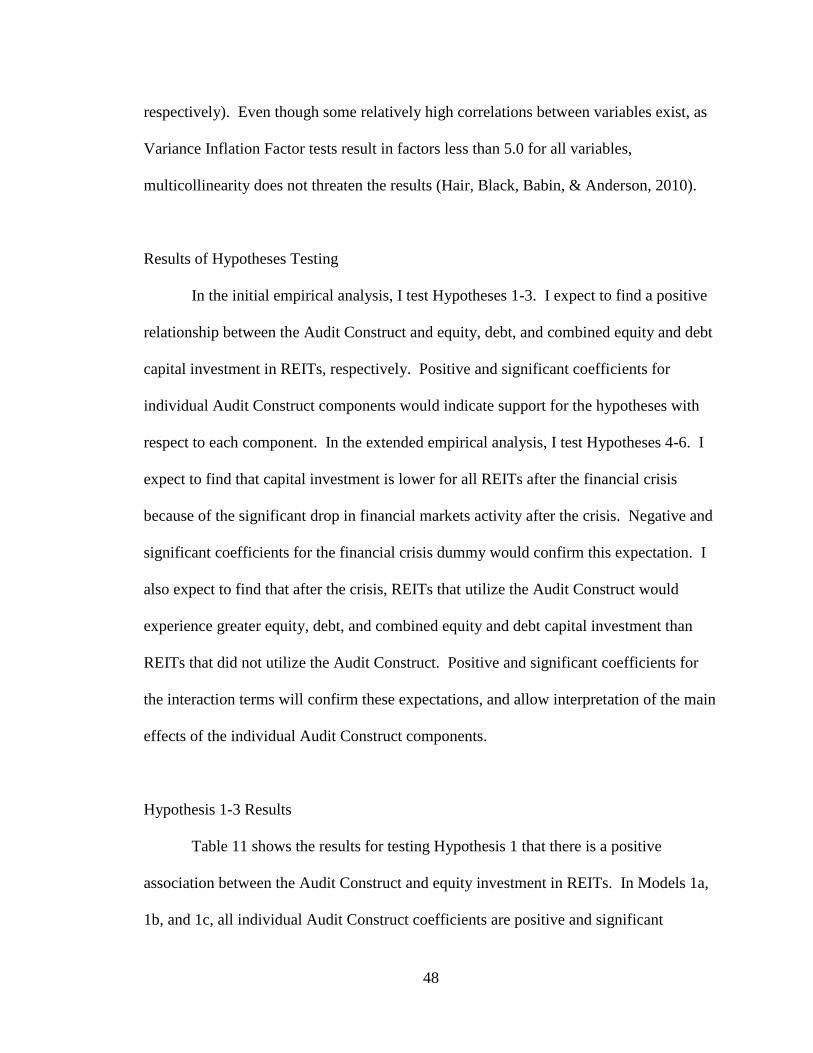
48

respectively). Even though some relatively high correlations between variables exist, as

Variance Inflation Factor tests result in factors less than 5.0 for all variables,

multicollinearity does not threaten the results (Hair, Black, Babin, & Anderson, 2010).

Results of Hypotheses Testing

In the initial empirical analysis, I test Hypotheses 1-3. I expect to find a positive

relationship between the Audit Construct and equity, debt, and combined equity and debt

capital investment in REITs, respectively. Positive and significant coefficients for

individual Audit Construct components would indicate support for the hypotheses with

respect to each component. In the extended empirical analysis, I test Hypotheses 4-6. I

expect to find that capital investment is lower for all REITs after the financial crisis

because of the significant drop in financial markets activity after the crisis. Negative and

significant coefficients for the financial crisis dummy would confirm this expectation. I

also expect to find that after the crisis, REITs that utilize the Audit Construct would

experience greater equity, debt, and combined equity and debt capital investment than

REITs that did not utilize the Audit Construct. Positive and significant coefficients for

the interaction terms will confirm these expectations, and allow interpretation of the main

effects of the individual Audit Construct components.

Hypothesis 1-3 Results

Table 11 shows the results for testing Hypothesis 1 that there is a positive

association between the Audit Construct and equity investment in REITs. In Models 1a,

1b, and 1c, all individual Audit Construct coefficients are positive and significant

49

Table 11. Results of OLS Regression testing the expectation of a positive association between the Audit Construct and equity

investment in REITs.

Model 1a Model 1b Model 1c Model 1d

Coefficient St. Error Coefficient St. Error Coefficient St. Error Coefficient St. Error

ln(Audit Fees) 0.569*** 0.152 0.442*** 0.159

Specialist 0.752*** 0.180 0.624*** 0.185

Big 4 Auditor 0.803* 0.480 0.399 0.506

Bid-Ask Spread -115.050*** 41.102 -120.156*** 40.466 -118.873*** 42.257 -116.644*** 39.896

Intangible-Assets -6.537* 3.607 -6.903* 3.658 -6.323* 3.643 -7.039* 3.602

Book-Market Ratio -0.297 0.283 -0.347 0.276 -0.376 0.278 -0.244 0.278

ROA -0.467 1.216 -0.778 1.242 -0.718 1.189 -0.459 1.238

Leverage -1.247* 0.725 -1.043 0.719 -1.229* 0.745 -1.280* 0.719

Initial 0.026 0.243 -0.012 0.240 0.056 0.243 -0.004 0.241

ln(Non-Audit Fees) -0.016 0.059 0.044 0.057 0.048 0.058 -0.006 0.058

ln(Properties) 0.367*** 0.085 0.404*** 0.084 0.463*** 0.084 0.324*** 0.086

ln(Subsidiaries) 0.121 0.079 0.234*** 0.075 0.188** 0.074 0.173** 0.080

Foreign -0.047 0.405 0.266 0.392 0.418 0.384 -0.042 0.402

Extra/Disc 0.144 0.180 0.199 0.179 0.154 0.180 0.176 0.178

Multifamily 0.064 0.610 0.900 0.611 0.661 0.614 0.435 0.617

Manufacturing -0.837 0.675 -0.333 0.695 -0.464 0.738 -0.325 0.714

Healthcare 0.594 0.607 1.115* 0.612 0.997 0.622 0.777 0.606

Shopping Center -0.004 0.603 0.952 0.618 0.549 0.613 0.565 0.618

Freestanding -1.007 0.718 -0.186 0.730 -0.812 0.742 -0.438 0.722

Regional Mall 0.196 0.727 1.378* 0.737 0.883 0.730 0.795 0.747

Lodging/Resort 1.013 0.635 1.994*** 0.648 1.571** 0.648 1.491** 0.648

Diversified 0.100 0.625 1.092* 0.632 0.666 0.627 0.597 0.644

Office 0.599 0.623 1.580** 0.629 1.250** 0.626 1.023 0.638

Industrial 0.047 0.662 1.310* 0.684 0.618 0.670 0.763 0.691

Office/Indust -0.528 0.676 0.513 0.686 0.038 0.679 0.041 0.683

Constant -4.545*** 1.742 -0.036 1.045 -0.245 1.097 -4.140** 1.748

Number of Obs. 661 661 661 661

50

F 9.863 9.507 9.357 9.460

Adjusted R2 0.245 0.247 0.233 0.256

Notes: In each of the four models presented, the dependent variable is equity investment, with the model variation being the respective inclusion or exclusion of

ln(Audit Fees), Specialist, and Big 4 Auditor, as indicated in bold-faced type in the table. ln(Audit Fees), Specialist, and Big 4 Auditor are variables comprising

the Audit Construct. Bid-Ask Spread is an often used measure to capture transparency. Intangible Assets is used to capture firm's level of information asymmetry

or opacity. Book/Market, ROA, and Leverage are used to capture individual REIT firm characteristics. Initial and ln(Other Fees) are used to capture individual

REIT-auditor relationships. ln(Properties), ln(Subsidiaries), Foreign, and Extra/Disc are used to capture firm complexity. Year dummies are used but are not

reported. All regressions use robust estimations. Statistical significance indicated as: * p < 0.05, ** p < 0.01, *** p < 0.001, respectively.

51

(ln(Audit Fees), β = 0.569; Specialist, β = 0.752; and, Big 4 Auditor, β = 0.803,

respectively), while in Model 1d, the coefficients for ln(Audit Fees) and Specialist are

positive and significant (β = 0.442 and β = 0.624, respectively). These results provide

partial support for the hypothesis, suggesting that investors view REITs that either pay

higher audit fees or engage audit specialists, as more transparent, and are willing to

provide equity investment.

Table 12 shows the results for testing Hypothesis 2 that there is a positive

association between the Audit Construct and debt investment in REITs. Results mirror

those from Hypothesis 1 testing showing partial support for the hypothesis. In Models

2a, 2b, and 2c, the coefficients for the Audit Construct components are positive and

significant (ln(Audit Fees), β = 0.564; Specialist, β = 0.344; and, Big 4 Auditor, β =

0.466, respectively), while in Model 2d, only the coefficients for ln(Audit Fees) and

Specialist are positive and significant (β = 0.519 and β = 0.199, respectively). As in

Hypothesis 1 testing, these results suggest that investors are willing to invest in REIT

debt when REITs increase their transparency as captured by higher audit fees or hiring

audit specialists.

Table 13 shows the results of testing Hypothesis 3 that there exists a positive

association between the Audit Construct and combined equity and debt investment in

REITs. In Models 3a, 3b, and 3c, the coefficients for ln(Audit Fees), Specialist, and Big

4 Auditor are all positive and significant (β = 0.571, β = 0.368, and β = 0.581,

respectively); likewise, in Model 3d, all Audit Construct component coefficients are

positive and significant (β = 0.513, β = 0.217, and β = 0.237, respectively). These results

suggest that investors view REITs that pay higher audit fees to obtain higher quality

52

Table 12. Results of OLS Regression testing the expectation of a positive association between the Audit Construct and debt

investment in REITs.

Model 2a Model 2b Model 2c Model 2d

Coefficient St. Error Coefficient St. Error Coefficient St. Error Coefficient St. Error

ln(Audit Fees) 0.564*** 0.048 0.519*** 0.049

Specialist 0.344*** 0.066 0.199*** 0.061

Big 4 Auditor 0.466*** 0.104 0.123 0.106

Bid-Ask Spread -39.507*** 6.993 -52.014*** 7.591 -44.725*** 7.692 -37.868*** 7.098

Intangible-Assets -6.672*** 0.731 -7.202*** 0.867 -6.536*** 0.838 -6.711*** 0.763

Book-Market Ratio 0.147*** 0.051 0.107** 0.043 0.111*** 0.042 0.153*** 0.049

ROA 0.691* 0.382 0.326 0.438 0.410 0.391 0.681* 0.394

Leverage 3.227*** 0.273 3.478*** 0.292 3.359*** 0.303 3.211*** 0.283

Initial 0.077 0.066 0.045 0.068 0.077 0.067 0.076 0.065

ln(Non-Audit Fees) 0.058*** 0.016 0.133*** 0.018 0.132*** 0.017 0.060*** 0.016

ln(Properties) 0.334*** 0.032 0.409*** 0.034 0.433*** 0.033 0.318*** 0.032

ln(Subsidiaries) 0.110*** 0.021 0.201*** 0.023 0.173*** 0.022 0.128*** 0.023

Foreign 0.455*** 0.139 0.922*** 0.178 0.967*** 0.166 0.451*** 0.145

Extra/Disc 0.186*** 0.055 0.247*** 0.058 0.205*** 0.059 0.201*** 0.055

Multifamily 0.216 0.134 0.891*** 0.120 0.804*** 0.124 0.344*** 0.133

Manufacturing -0.304** 0.144 0.009 0.160 -0.064 0.170 -0.146 0.146

Healthcare 0.093 0.131 0.539*** 0.119 0.497*** 0.119 0.142 0.129

Shopping Center 0.154 0.119 0.813*** 0.107 0.662*** 0.108 0.325*** 0.122

Freestanding -0.174 0.216 0.353* 0.210 0.073 0.221 0.006 0.208

Regional Mall 0.598*** 0.172 1.459*** 0.165 1.276*** 0.175 0.772*** 0.168

Lodging/Resort 0.088 0.161 0.816*** 0.151 0.638*** 0.161 0.237 0.154

Diversified 0.228* 0.138 0.905*** 0.131 0.743*** 0.134 0.379*** 0.139

Office 0.658*** 0.130 1.428*** 0.119 1.282*** 0.122 0.793*** 0.127

Industrial 0.166 0.142 1.006*** 0.144 0.706*** 0.139 0.399*** 0.146

Office/Indust 0.368*** 0.122 1.118*** 0.130 0.924*** 0.115 0.558*** 0.138

Constant -5.286*** 0.501 -0.686** 0.287 -0.878*** 0.289 -5.091*** 0.501

Number of Obs. 761 761 761 761

53

F 104.621 93.544 104.057 106.361

Adjusted R2 0.816 0.785 0.781 0.818

Notes: In each of the four models presented, the dependent variable is debt investment, with the model variation being the respective inclusion or exclusion of

ln(Audit Fees), Specialist, and Big 4 Auditor, as indicated in bold-faced type in the table. ln(Audit Fees), Specialist, and Big 4 Auditor are variables comprising

the Audit Construct. Bid-Ask Spread is an often used measure to capture transparency. Intangible Assets is used to capture firm's level of information asymmetry

or opacity. Book/Market, ROA, and Leverage are used to capture individual REIT firm characteristics. Initial and ln(Other Fees) are used to capture individual

REIT-auditor relationships. ln(Properties), ln(Subsidiaries), Foreign, and Extra/Disc are used to capture firm complexity. Year dummies are used but are not

reported. All regressions use robust estimations. Statistical significance indicated as: * p < 0.05, ** p < 0.01, *** p < 0.001, respectively.

Table 13. Results of OLS Regression testing the expectation of a positive association between the Audit Construct and

combined equity and debt investment in REITs.

Model 3a Model 3b Model 3c Model 3d

Coefficient St. Error Coefficient St. Error Coefficient St. Error Coefficient St. Error

ln(Audit Fees) 0.571*** 0.047 0.513*** 0.048

Specialist 0.368*** 0.066 0.217*** 0.061

Big 4 Auditor 0.581*** 0.102 0.237** 0.103

Bid-Ask Spread -41.043*** 6.843 -53.648*** 7.495 -44.390*** 7.460 -37.658*** 6.822

Intangible-Assets -6.507*** 0.703 -7.055*** 0.855 -6.265*** 0.807 -6.456*** 0.723

Book-Market Ratio 0.112** 0.046 0.072* 0.041 0.079** 0.040 0.121*** 0.043

ROA 0.360 0.406 -0.009 0.476 0.095 0.403 0.362 0.422

Leverage 2.612*** 0.260 2.865*** 0.279 2.717*** 0.290 2.572*** 0.268

Initial 0.051 0.066 0.018 0.068 0.055 0.067 0.053 0.065

ln(Non-Audit Fees) 0.062*** 0.016 0.138*** 0.017 0.136*** 0.017 0.065*** 0.016

ln(Properties) 0.316*** 0.031 0.389*** 0.034 0.413*** 0.033 0.298*** 0.032

ln(Subsidiaries) 0.119*** 0.021 0.213*** 0.023 0.181*** 0.022 0.138*** 0.023

Foreign 0.354*** 0.130 0.823*** 0.167 0.867*** 0.154 0.354*** 0.135

Extra/Disc 0.155*** 0.053 0.217*** 0.057 0.171*** 0.058 0.168*** 0.054

Multifamily 0.243* 0.136 0.933*** 0.128 0.848*** 0.131 0.400*** 0.135

Manufacturing -0.208 0.146 0.119 0.168 0.065 0.174 -0.006 0.146

Healthcare 0.131 0.139 0.584*** 0.132 0.537*** 0.133 0.189 0.137

Shopping Center 0.182 0.123 0.861*** 0.117 0.709*** 0.117 0.389*** 0.125

54

Freestanding -0.108 0.223 0.441** 0.220 0.141 0.231 0.091 0.215

Regional Mall 0.667*** 0.174 1.550*** 0.169 1.358*** 0.179 0.872*** 0.169

Lodging/Resort 0.159 0.159 0.907*** 0.154 0.717*** 0.163 0.332** 0.153

Diversified 0.243* 0.139 0.938*** 0.137 0.769*** 0.139 0.420*** 0.141

Office 0.680*** 0.133 1.467*** 0.126 1.312*** 0.128 0.838*** 0.130

Industrial 0.209 0.140 1.077*** 0.146 0.760*** 0.140 0.475*** 0.144

Office/Indust 0.493*** 0.112 1.266*** 0.125 1.066*** 0.106 0.718*** 0.127

Constant -4.921*** 0.500 -0.274 0.286 -0.541* 0.287 -4.704*** 0.497

Number of Obs. 761 761 761 761

F 103.133 87.458 105.158 108.215

Adjusted R2 0.813 0.782 0.778 0.818

Notes: In each of the four models presented, the dependent variable is combined equity and debt investment, with the model variation being the respective

inclusion or exclusion of ln(Audit Fees), Specialist, and Big 4 Auditor, as indicated in bold-faced type in the table. ln(Audit Fees), Specialist, and Big 4 Auditor

are variables comprising the Audit Construct. Bid-Ask Spread is an often used measure to capture transparency. Intangible Assets is used to capture firm's level of

information asymmetry or opacity. Book/Market, ROA, and Leverage are used to capture individual REIT firm characteristics. Initial and ln(Other Fees) are used

to capture individual REIT-auditor relationships. ln(Properties), ln(Subsidiaries), Foreign, and Extra/Disc are used to capture firm complexity. Year dummies

are used but are not reported. All regressions use robust estimations. Statisitical significance indicated as: * p < 0.05, ** p < 0.01, *** p < 0.001, respectively.

55

audits, hire REIT industry-audit specialists, and/or hire auditors with a higher quality

reputation, as more transparent, and are thus willing to invest in their equity and debt

offerings.

Hypotheses 4-6 Results

As I state earlier, the financial crisis caused major disruptions in the capital

markets, resulting in capital flight, and conditions of severe illiquidity. Therefore, I

expect there was less equity investment for all REITs. However, more importantly then

is: How did REITs that needed to raise capital differentiate themselves from others

seeking capital under such restricted market conditions? Table 14 shows the results for

testing Hypothesis 4. As shown in Model 4a, the Crisis dummy coefficient is negative

and significant (β = -5.978), confirming the expectation that equity capital investment

was less for all REITs after the crisis. However, the interaction term Crisis*ln(Audit

Fees) coefficient is positive and significant (β = 0.405). This suggests that audit fees had

a larger impact on equity investment in REITs in the post-crisis period than before the

financial crisis.10

There is no statistical significance for the interactive terms for

Crisis*Specialist and Crisis*Big. These results suggest that after accounting for the

effects of the downturn in the financial markets caused by severe exogenous shocks, there

is partial support for Hypothesis 4 with respect to the auditor quality component of the

Audit Construct.

10

After controlling for the interactive effect of the financial crisis, the slope parameter for ln(Audit Fees) is

0.856 (derived from the addition of the coefficients for ln(Audit Fees) (β = 0.451) and Crisis*ln(Audit

Fees) (β = 0.405).

56

Table 14. Results of OLS Regression testing the expectation that the financial crisis of 2007-2008 positively influenced the

relationship between the Audit Construct and equity investment in REITs.

Model 4a Model 4b Model 4c Model 4d

Coefficient St. Error Coefficient St. Error Coefficient St. Error Coefficient St. Error

Crisis -5.978** 3.021 0.047 0.489 -0.753 0.923 -5.755* 3.036

Crisis*ln(Audit Fees) 0.405* 0.220 0.348 0.234

ln(Audit Fees) 0.451*** 0.162 0.355** 0.171

Crisis*Specialist -0.064 0.322 -0.220 0.320

Specialist 0.779*** 0.218 0.713*** 0.224

Crisis*Big 4 Auditor 0.877 0.823 0.730 0.923

Big 4 Auditor 0.306 0.555 -0.056 0.603

Bid-Ask Spread -116.057*** 40.583 -120.441*** 40.547 -119.410*** 42.417 -118.842*** 39.657

Intangible-Assets -6.749* 3.754 -6.839* 3.642 -6.396* 3.652 -7.064* 3.697

Book-Market Ratio -0.297 0.278 -0.351 0.277 -0.380 0.278 -0.259 0.274

ROA -0.667 1.212 -0.767 1.243 -0.721 1.187 -0.590 1.234

Leverage -1.250* 0.720 -1.053 0.721 -1.237* 0.747 -1.320* 0.718

Initial 0.025 0.242 -0.015 0.240 0.057 0.244 -0.015 0.240

ln(Non-Audit Fees) -0.018 0.059 0.044 0.057 0.052 0.059 -0.008 0.058

ln(Properties) 0.368*** 0.085 0.403*** 0.084 0.465*** 0.084 0.320*** 0.086

ln(Subsidiaries) 0.117 0.078 0.234*** 0.075 0.188** 0.074 0.170** 0.079

Foreign -0.115 0.418 0.265 0.392 0.429 0.385 -0.107 0.415

Extra/Disc 0.134 0.179 0.200 0.180 0.147 0.180 0.165 0.178

Multifamily 0.031 0.576 0.899 0.608 0.659 0.617 0.384 0.580

Manufacturing -0.841 0.651 -0.333 0.693 -0.455 0.740 -0.341 0.689

Healthcare 0.533 0.574 1.111* 0.608 1.003 0.625 0.706 0.568

Shopping Center -0.032 0.569 0.950 0.616 0.571 0.617 0.534 0.583

Freestanding -1.054 0.694 -0.183 0.729 -0.807 0.745 -0.475 0.695

Regional Mall 0.172 0.700 1.376* 0.734 0.886 0.733 0.750 0.718

Lodging/Resort 0.951 0.602 1.989*** 0.645 1.564** 0.651 1.399** 0.613

Diversified 0.065 0.592 1.090* 0.629 0.664 0.631 0.542 0.608

Office 0.558 0.590 1.580** 0.626 1.259** 0.629 0.975 0.603

57

Industrial 0.021 0.631 1.309* 0.682 0.620 0.673 0.723 0.658

Office/Indust -0.564 0.642 0.512 0.683 0.053 0.681 0.000 0.646

Constant -2.979 1.891 -0.020 1.040 0.185 1.123 -2.474 1.870

Number of Obs. 661 661 661 661

F 9.753 9.216 9.138 8.887

Adjusted R2 0.247 0.246 0.233 0.257

Notes: In Model 1, Crisis and Crisis*ln(Audit Fees) are added to examine the impact of audit fees on post-crisis equity investment. In Model 2, Crisis and

Crisis*Specialist are added to examine the impact of auditor specialization on post-crisis equity investment. In Model 3, Crisis and Crisis*Big 4 Auditor are

added to examine the impact of auditor reputation on post-crisis equity investment. In Model 4, Crisis and all three interaction terms are included to examine the

impact of the Audit Construct on post-crisis equity investment. Bid-Ask Spread is an often used measure to capture transparency. Intangible Assets is used to

capture firm's level of information asymmetry or opacity. Book/Market, ROA, and Leverage are used to capture individual REIT firm characteristics. Initial and

ln(Non-Audit Fees) are used to capture individual REIT-auditor relationships. ln(Properties), ln(Subsidiaries), Foreign, and Extra/Disc are used to capture firm

complexity. Year dummies are used but are not reported. All regressions use robust estimations. Statistical significance indicated as: * p < 0.05, ** p < 0.01, ***

p < 0.001, respectively.

58

Table 15 shows the results for testing Hypothesis 5. As shown in Model 5a, the

Crisis dummy coefficient is negative and significant (β = -1.709); however, the Crisis

dummy coefficients are positive and significant in Models 5b and 5c, yet insignificant in

Model 5d. The interaction terms are insignificant in all models. Although a definitive

conclusion is not possible, conceivably it is possible that REITs that could not raise

equity capital after the crisis, and were able to shift to debt, were those that could not pay

higher fees to obtain higher quality audits. However, they could still engage an industry-

audit specialist and/or a Big 4 auditor (the other two attributes used to signal

transparency). If so, perhaps the debt was more in the form of collateralized bank loans;

transparency would therefore be less important as banks would most likely rely more

heavily on the values of underlying REIT assets. This may suggest that the type of

security issue (debt, in this case) in combination with certain audit attributes jointly serve

to signal financial transparency.

Table 16 shows the results for testing Hypothesis 6. As shown in Model 6a, the

Crisis dummy coefficient is negative and significant (β = -1.709), again providing

confirmation that, as expected, there was less overall capital investment for all REITs

after the crisis. The Crisis*ln(Audit Fees) interaction term coefficient is positive and

significant (β = 0.113). Similar to the results from testing Hypothesis 4, this suggests that

audit fees had a larger impact on combined equity and debt investment in REITs after the

crisis than before it.11

There is no statistical significance for the interactive terms for

Crisis*Specialist and Crisis*Big. Therefore, the conclusion is that there is partial support

for Hypothesis 6 with respect to the auditor quality component of the Audit Construct.

11

After controlling for the interactive effect of the financial crisis, the slope parameter for ln(Audit Fees) is

0.657 (derived from the addition of the coefficients for ln(Audit Fees) (β = 0.544) and Crisis*ln(Audit

Fees) (β = 0.113).

59

Table 15. Results of OLS Regression testing the expectation that the financial crisis of 2007-2008 positively influenced the

relationship between the Audit Construct and debt investment in REITs.

Model 5a Model 5b Model 5c Model 5d

Coefficient St. Error Coefficient St. Error Coefficient St. Error Coefficient St. Error

Crisis -1.533* 0.905 0.288** 0.136 0.542** 0.212 -1.535 0.987

Crisis*ln(Audit Fees) 0.099 0.065 0.112 0.078

ln(Audit Fees) 0.540*** 0.048 0.491*** 0.051

Crisis*Specialist 0.065 0.109 0.036 0.101

Specialist 0.317*** 0.074 0.185*** 0.070

Crisis*Big 4 Auditor -0.140 0.168 -0.133 0.206

Big 4 Auditor 0.535*** 0.125 0.172 0.140

Bid-Ask Spread -38.132*** 6.909 -51.883*** 7.594 -45.004*** 7.509 -36.847*** 7.014

Intangible-Assets -6.658*** 0.748 -7.226*** 0.868 -6.507*** 0.833 -6.699*** 0.779

Book-Market Ratio 0.157*** 0.052 0.109** 0.044 0.106** 0.044 0.160*** 0.051

ROA 0.629* 0.379 0.312 0.438 0.418 0.393 0.607 0.391

Leverage 3.218*** 0.274 3.486*** 0.291 3.363*** 0.304 3.215*** 0.285

Initial 0.068 0.067 0.048 0.068 0.082 0.067 0.071 0.066

ln(Non-Audit Fees) 0.057*** 0.016 0.133*** 0.018 0.131*** 0.017 0.058*** 0.017

ln(Properties) 0.332*** 0.032 0.409*** 0.034 0.433*** 0.033 0.317*** 0.033

ln(Subsidiaries) 0.109*** 0.021 0.201*** 0.023 0.173*** 0.022 0.127*** 0.023

Foreign 0.448*** 0.138 0.922*** 0.180 0.957*** 0.167 0.438*** 0.144

Extra/Disc 0.186*** 0.054 0.246*** 0.058 0.206*** 0.059 0.202*** 0.055

Multifamily 0.204 0.129 0.891*** 0.123 0.802*** 0.124 0.329** 0.128

Manufacturing -0.303** 0.138 0.008 0.162 -0.071 0.171 -0.155 0.141

Healthcare 0.074 0.128 0.542*** 0.123 0.494*** 0.118 0.122 0.127

Shopping Center 0.141 0.114 0.814*** 0.110 0.656*** 0.108 0.307*** 0.118

Freestanding -0.180 0.213 0.352* 0.212 0.071 0.221 -0.001 0.206

Regional Mall 0.582*** 0.168 1.458*** 0.167 1.272*** 0.175 0.753*** 0.164

Lodging/Resort 0.063 0.158 0.818*** 0.154 0.641*** 0.160 0.216 0.152

Diversified 0.211 0.134 0.905*** 0.134 0.743*** 0.133 0.362*** 0.135

Office 0.639*** 0.126 1.427*** 0.122 1.280*** 0.121 0.772*** 0.123

60

Industrial 0.154 0.138 1.006*** 0.147 0.705*** 0.138 0.386*** 0.142

Office/Indust 0.356*** 0.117 1.120*** 0.133 0.919*** 0.115 0.541*** 0.133

Constant -4.960*** 0.541 -0.695** 0.288 -0.928*** 0.295 -4.745*** 0.543

Number of Obs. 761 761 761 761

F 103.098 90.004 113.609 104.346

Adjusted R2 0.816 0.785 0.780 0.819

Notes: In Model 1, Crisis and Crisis*ln(Audit Fees) are added to examine the impact of audit fees on post-crisis equity investment. In Model 2, Crisis and

Crisis*Specialist are added to examine the impact of auditor specialization on post-crisis equity investment. In Model 3, Crisis and Crisis*Big 4 Auditor are

added to examine the impact of auditor reputation on post-crisis equity investment. In Model 4, Crisis and all three interaction terms are included to examine the

impact of the Audit Construct on post-crisis debt investment. Bid-Ask Spread is an often used measure to capture transparency. Intangible Assets is used to

capture firm's level of information asymmetry or opacity. Book/Market, ROA, and Leverage are used to capture individual REIT firm characteristics. Initial and

ln(Non-Audit Fees) are used to capture individual REIT-auditor relationships. ln(Properties), ln(Subsidiaries), Foreign, and Extra/Disc are used to capture firm

complexity. Year dummies are used but are not reported. All regressions use robust estimations. Statistical significance indicated as: * p < 0.05, ** p < 0.01, ***

p < 0.001, respectively.

Table 16. Results of OLS Regression testing the expectation that the financial crisis of 2007-2008 positively influenced the

relationship between the Audit Construct and combined equity and debt investment in REITs.

Model 6a Model 6b Model 6c Model 6d

Coefficient St. Error Coefficient St. Error Coefficient St. Error Coefficient St. Error

Crisis -1.709* 0.886 0.312** 0.132 0.570*** 0.203 -1.678* 0.970

Crisis * ln(Audit Fees) 0.113* 0.064 0.127 0.077

ln(Audit Fees) 0.544*** 0.048 0.480*** 0.050

Crisis * Specialist 0.026 0.107 -0.013 0.099

Specialist 0.357*** 0.073 0.224*** 0.069

Crisis * Big 4 Auditor -0.131 0.160 -0.132 0.198

Big 4 Auditor 0.646*** 0.123 0.287** 0.139

Bid-Ask Spread -39.477*** 6.773 -53.596*** 7.487 -44.651*** 7.292 -36.519*** 6.734

Intangible-Assets -6.491*** 0.730 -7.065*** 0.854 -6.238*** 0.802 -6.424*** 0.742

Book-Market Ratio 0.123*** 0.047 0.073* 0.041 0.074* 0.041 0.128*** 0.045

ROA 0.290 0.401 -0.015 0.477 0.103 0.404 0.288 0.418

Leverage 2.602*** 0.260 2.869*** 0.279 2.720*** 0.290 2.568*** 0.269

61

Initial 0.040 0.067 0.019 0.069 0.060 0.067 0.045 0.066

ln(Non-Audit Fees) 0.061*** 0.016 0.138*** 0.017 0.135*** 0.017 0.063*** 0.016

ln(Properties) 0.314*** 0.032 0.390*** 0.034 0.413*** 0.033 0.296*** 0.032

ln(Subsidiaries) 0.118*** 0.021 0.213*** 0.023 0.182*** 0.022 0.137*** 0.022

Foreign 0.347*** 0.129 0.823*** 0.167 0.858*** 0.155 0.340** 0.134

Extra/Disc 0.155*** 0.053 0.217*** 0.057 0.171*** 0.058 0.170*** 0.054

Multifamily 0.229* 0.130 0.933*** 0.129 0.846*** 0.130 0.384*** 0.128

Manufacturing -0.207 0.140 0.119 0.168 0.058 0.175 -0.015 0.140

Healthcare 0.109 0.135 0.585*** 0.134 0.534*** 0.132 0.164 0.133

Shopping Center 0.167 0.117 0.861*** 0.118 0.704*** 0.117 0.367*** 0.119

Freestanding -0.115 0.220 0.440** 0.221 0.139 0.231 0.085 0.211

Regional Mall 0.649*** 0.169 1.549*** 0.170 1.355*** 0.179 0.851*** 0.164

Lodging/Resort 0.131 0.156 0.907*** 0.155 0.720*** 0.163 0.306** 0.149

Diversified 0.224* 0.134 0.938*** 0.138 0.770*** 0.138 0.401*** 0.135

Office 0.658*** 0.128 1.467*** 0.128 1.310*** 0.128 0.814*** 0.124

Industrial 0.194 0.135 1.077*** 0.148 0.759*** 0.139 0.461*** 0.138

Office/Indust 0.479*** 0.105 1.266*** 0.126 1.061*** 0.105 0.699*** 0.120

Constant -4.550*** 0.540 -0.278 0.287 -0.587** 0.291 -4.302*** 0.536

Number of observations 761 761 761 761

F 100.962 84.951 115.914 105.920

Adjusted R2 0.814 0.782 0.778 0.818

Notes: In Model 1, Crisis and Crisis*ln(Audit Fees) are added to examine the impact of audit fees on post-crisis equity investment. In Model 2, Crisis and

Crisis*Specialist are added to examine the impact of auditor specialization on post-crisis equity investment. In Model 3, Crisis and Crisis*Big 4 Auditor are

added to examine the impact of auditor reputation on post-crisis equity investment. In Model 4, Crisis and all three interaction terms are included to examine the

impact of the Audit Construct on post-crisis combined equity and debt investment. Bid-Ask Spread is an often used measure to capture transparency. Intangible

Assets is used to capture firm's level of information asymmetry or opacity. Book/Market, ROA, and Leverage are used to capture individual REIT firm

characteristics. Initial and ln(Non-Audit Fees) are used to capture individual REIT-auditor relationships. ln(Properties), ln(Subsidiaries), Foreign, and Extra/Disc

are used to capture firm complexity. Year dummies are used but are not reported. All regressions use robust estimations. Statistical significance indicated as: * p

< 0.05, ** p < 0.01, *** p < 0.001, respectively.

62

Many of the control variables provide interesting results. For example, Bid-Ask

Spread, one of the variables used to capture transparency, is also negative and significant

in all models. Similarly, Intangible Assets, used to control for information

asymmetry/opacity, is negative and significant in all models. This suggests that when

REIT investors view REITs as less transparent (higher bid-ask spreads), or when they

perceive higher levels of information asymmetry (higher levels of intangible assets), they

are less inclined to invest in REITs. The number of properties owned by REITs and/or

their subsidiaries contributes to their demand for capital investment. To control for this, I

use the variable ln(Properties). In all models, the coefficients for ln(Properties) are

positive and significant, revealing a positive relationship between the number of

properties owned and REIT capital investment. This finding is not altogether surprising.

REITs have to distribute the bulk of their available cash as dividends. This means that to

acquire additional properties, they need new capital. The more properties REITs acquire,

the more they need additional capital, magnifying the importance of lowering information

asymmetries and increasing transparency. Therefore, finding means of doing so takes on

added importance.

The literature indicates that when firms signal investors about their increased

financial information transparency, they increase their chances of motivating capital

investment. Results from the initial empirical analysis show a positive association

between the Audit Construct components and increased capital investment. In the

extended empirical analysis, after controlling for the effects of the financial crisis, the

results support the auditor quality component of the Audit Construct by showing that

63

firms that pay higher audit fees to increase transparency are able to increase capital

investment.

Limitations

Part of the analysis in this study is the comparison of relationships between using

the Audit Construct to increase transparency, and REITs‘ access to capital in the post-

crisis period to the pre-crisis period. Since the authorization of REITs in 1960, there

have been six economic recessions in the United States prior to the financial crisis of

2007-2008.12

To the extent that data are available, as this study includes data from a

single post-recession period, it may be of interest to include other such recessionary

periods in future tests of the Audit Construct in relation to increasing transparency as a

means to motivate capital investment to see if the outcomes are similar.

Section VII. Concluding Remarks

Because REITs must distribute a minimum of 90% of their net income as

dividends, they frequently access capital markets to raise cash necessary for operations or

new investments. Existing research indicates that firms use aspects of the audit process

as a means of conveying information to investors, often in attempts to signal their

increased financial information transparency. In this paper, I examine how REITs use the

audit-related attributes of auditor quality, specialization, and reputation to signal or

convey financial information transparency to potential investors in order to motivate

capital investment. I first analyze the relation between audit attributes and REIT equity,

12

Data obtained from ECR Research available at http://www.ecrresearch.com/world-economy/table-us-

recessions.

64

debt, and combined equity and debt capital investment. I further analyze this relationship

by taking into account the 2007-2008 financial crisis to investigate whether the use of

these attributes has a stronger impact on capital issuance after the crisis.

Extant research shows that when firms signal their increased financial information

transparency to investors, they improve their abilities to attract new capital investment.

Results from this study show a positive relationship between audit attributes as a means

of increasing transparency, and capital investment in REITs. Using auditing fees, and

controlling for the effects of the financial crisis, the results suggest that transparency

related to auditor quality is more important after the financial crisis than before it.

However, there was no support for the use of the other two audit attributes of auditor

specialization or auditor reputation as means to increase transparency, and the reader

should therefore use caution with respect to this interpretation. A possible explanation

for the lack of support for the other two auditing attributes may be that REITs in the

sample most likely already have a specialized auditor or one from the Big 4. As such, it

is unlikely that the status of either auditor specialization or auditor reputation would

change significantly after the financial crisis. Therefore, any substantial impact on

capital investment during the post-crisis period is due primarily to the auditor quality

changes as captured by audit fees.

65

REFERENCES

Abdolmohammadi, M. J., Searfoss, D. G., & Shanteau, J. (2004). An investigation of the

attributes of top industry audit specialists. Behavioral Research in Accounting,

16(1), 1-17.

Adrian, T., & Shin, H. S. (2010). The changing nature of financial intermediation and

the financial crisis of 2007-09. (Federal Reserve Bank of New York, Working

Paper Number 439). Retrieved on January 7, 2013, from

http://www.econstor.eu/bitstream/10419/60810/1/622939211.pdf.

Altman, E. I. (1968). Financial ratios discriminant analysis and the prediction of

corporate bankruptcy. The Journal of Finance, 23(4), 589-609.

Ambrose, B. W., & Linneman, P. (2001). REIT organizational structure and operating

characteristics. Journal of Real Estate Research, 21(3), 141-162.

American Institute of Certified Public Accountants (AICPA). (1978). The commission

on auditors‘ responsibilities: Report, conclusions and recommendations. The

Cohen Commission. New York: AICPA.

Amihud, Y., & Mendelson, H. (1986). Asset pricing and the bid-ask spread. Journal of

Financial Economics, 17(2), 223-249.

Amihud, Y., & Mendelson, H. (2000). The liquidity route to a lower cost of capital.

Journal of Applied Corporate Finance, 12(4), 8-25.

Anglin, P., Edelstein, R., Gao, Y., & Tsang, D. (2011). How does corporate governance

affect the quality of investor information? The curious case of REITs. Journal of

Real Estate Research, 33(1), 1-23.

Antle, R., Gordon, E., Narayanamoorthy, G., & Zhou, L. (2006). The joint determination

of audit fees, non-audit fees, and abnormal accruals. Review of Quantitative

Finance and Accounting, 27(3), 235-266.

Bagehot, W. (1971). The only game in town. Financial Analysts Journal, 51(1), 12-14.

Baker, M., & Wurgler, J. (2002). Market timing and capital structure. The Journal of

Finance, 57(1), 1-32.

66

Balvers, R. J., McDonald, B., & Miller, R. E. (1988). Underpricing of new issues and the

choice of auditor as a signal of investment banker reputation. The Accounting

Review, 63(4), 605-622.

Basiousis, I., Gul, F., & Ng, A. (2012). Non-audit fees, auditor tenure, and auditor

independence. Available at SSRN 2043311.

Basse, T., Friedrich, M., & Bea, E. V. (2009). REITs and the financial crisis: Empirical

evidence from the U.S. International Journal of Business and Management,

4(11), 1-10.

Bauer, R., Eichholtz, P., & Kok, N. (2010). Corporate governance and performance: The

REIT effect. Real Estate Economics, 38(1), 1-29.

Baxter, N. D. (1967). Leverage, risk of ruin, and the cost of capital. The Journal of

Finance, 22(3), 395-403.

Beals, P., & Singh, A. J. (2002). The evolution and development of equity REITs: The

securitization of equity structures for financing the U.S. lodging industry. Journal

of Hospitality Financial Management, 10(1), 15-33.

Beatty, R. P. (1989). Auditor reputation and the pricing of initial public offerings. The

Accounting Review, 64(4), 693–709.

Bell, T., Marrs, F., Solomon, I., & Thomas, H. (1997). Auditing organizations through a

strategic lens, the KPMG business measurement process. Montvale, NJ: Peat

Marwick LLP.

Bharath, S. T., Pasquariello, P., & Wu, G. (2009). Does asymmetric information drive

capital structure decisions? The Review of Financial Studies, 22(8), 3211-3243.

Blazenko, G. W. (1987). Managerial preference, asymmetric information, and financial

structure. The Journal of Finance, 42(4), 839-862.

Block, J., & Sandner, P. (2009). What is the effect of the financial crisis on venture

capital financing? Empirical evidence from U.S. internet start-ups. Venture

Capital: An International Journal of Entrepreneurial Finance, 11(4), 1-22.

Boo, E., & Sharma, D. (2008). Effect of regulatory oversight on the association between

internal governance characteristics and audit fees. Accounting and Finance,

48(1), 51-71.

Braswell, M., Daniels, R. B., Landis, M., & Chang, C. C. A. (2012). Characteristics of

diligent audit committees. Journal of Business & Economics Research, 10(4),

191-206.

67

Brau, J. C., & Holmes, A. (2006). Why do REITs repurchase stock? Extricating the

effect of managerial signaling in open market share repurchase announcements.

Journal of Real Estate Research, 28(1), 1-24.

Brunnermeier, M. K. (2008). Deciphering the liquidity and credit crunch 2007-08. (The

National Bureau of Economic Research, Working Paper). Retrieved on January

7, 2013, from http://www.nber.org/papers/w14612.ack.

Bushman, R. M., & Smith, A. J. (2001). Financial accounting information and corporate

governance. Journal of Accounting and Economics, 32(1-3), 237-333.

Bushman R. M., & Smith, A. J. (2003). Transparency, financial accounting information

and corporate governance. Federal Reserve Bank of New York‟s Economic Policy

Review, 9(1), 65-87.

Capozza, D. R., & Korean, S. L. (1995). Property type, size, and REIT value. Journal of

Real Estate Research, 10(4), 363-379.

Capozza, D. R., & Seguin, P. J. (1999). Focus, transparency, and value: The REIT

evidence. Real Estate Economics, 27(4), 587-619.

Carcello, J., & Nagy, A. (2004). Audit firm tenure and fraudulent financial reporting.

AUDITING: A Journal of Theory and Practice, 23(1), 55-69.

Carter, R. B., & Manaster, S. (1990). Initial public offerings and underwriter reputation.

The Journal of Finance, 45(4), 1045–1067.

Chan, P., Ezzamel, M., & Gwilliam, D. (1993). Determinants of audit fees for quoted

U.K. companies. Journal of Business, Finance and Accounting, 20(6), 765-786.

Chang, M., & Monroe, G. S. (1994). The impact of reputation, audit contract type,

tenure, audit fees and other services on auditors‟ perceptions of audit quality.

(Working paper). Department of Accounting and Finance, University of Western

Australia.

Chen, W. P., Chung, H., Lee, C., & Liao, W. L. (2007). Corporate governance and equity

liquidity: Analysis of S&P transparency and disclosure rankings. Corporate

Governance: An International Journal, 15(4), 644-660.

Chow, C. W., & Rice, S. J. (1982). Qualified audit opinions and auditor switching. The

Accounting Review, 57(2), 326-335.

Cohen, J., Krishnamoorthy, G., & Wright, A. M. (2002). Corporate governance and audit

process. Contemporary Accounting Research, 19(4), 573-594.

68

Daily, C. M., Certo, S. T, Dalton, D. R., & Roengpitya, R. (2003). IPO underpricing: A

meta-analysis and research synthesis. Entrepreneurship Theory and Practice,

27(3), 271-295.

Danielsen, B. R., Harrison, D. M., Van Ness, R. A., & Warr, R. S. (2009). REIT auditor

fees and financial market transparency. Real Estate Economics, 37(3), 515-557.

Danielsen, B. R., Harrison, D. M., Van Ness, R. A., & Warr, R. S. (2010). Investment in

audit services and the external financing needs of the firm. (Working Paper).

North Carolina State University, Texas Tech University, and University of

Southern Mississippi. Retrieved on May 10, 2012, from

http://www4.ncsu.edu/~rswarr/auditfees_and_seos_1.1.pdf.

Danielsen, B. R., Van Ness, R. A., & Warr, R. S. (2007). Auditor fees, market

microstructure, and firm transparency. Journal of Business Finance &

Accounting, 34(1-2), 202-221.

Datar, S., Feltham, G., & Hughes, J. (1991). The role of audits and audit quality in

valuing new issues. Journal of Accounting and Economics 14(1), 3-49.

Davidson, W. N., Jiraporn, P. & DaDalt, P. (2006). Causes and consequences of audit

shopping: An analysis of auditor opinions, earnings management, and auditor

changes. Quarterly Journal of Business and Economics, 45(1/2), 69-87.

DeAngelo, L. E. (1981). Auditor size and quality. Journal of Accounting and

Economics, 3(3), 183-199.

Deeds, D. L., Decarolis, D., & Coombs, J. E. (1997). The impact of firm-specific

capabilities on the amount of capital raised in an initial public offering: Evidence

from the biotechnology industry. Journal of Business Venturing, 12(1), 31–46.

DeLisle, J. R. (2007). At the crossroads of expansion and recession. The Appraisal

Journal, 75(4), 314-322.

DeLisle, J. R. (2008). The perfect storm rippling over to real estate. The Appraisal

Journal, 76(3), 200-210.

Demsetz, H. (1968). The cost of transacting. Quarterly Journal of Economics, 82(1), 33-

53.

Diamond, D. W. (1984). Financial intermediation and delegated monitoring. Review of

Economic Studies, 51(3), 393-414.

69

Diamond, D. W. (1989). Reputation acquisition in debt markets. Journal of Political

Economy, 97(4), 828-862.

Diamond, D. W. (1991). Monitoring and reputation: The choice between bank loans and

directly placed debt. Journal of Political Economy, 99(4), 689-721.

Diamond, D. W., & Verrecchia, R. E. (1991). Disclosure, liquidity, and the cost of

capital. The Journal of Finance, 46(4), 1325-1359.

Downes, D. H., & Heinkel, R. (1982). Signaling and the valuation of unseasoned new

issues. The Journal of Finance, 37(1), 1-10.

Edgerton, J. (2010). Investment incentives and corporate tax asymmetries. Journal of

Public Economics, 94(11-12), 936-952.

Epley, D. R., Rabianski, J. S., & Haney, Jr., R. L. (2002). Real estate decisions. Mason,

Ohio: Southwestern Publishing.

Fama, E. F., & French, K. R. (2002). Testing trade-off and pecking order predictions

about dividends and debt. Review of Financial Studies, 15(1), 1-33.

Fama, E. F., & French, K. R. (2005). Financing decisions: Who issues stock? Journal of

Financial Economics, 76(3), 549-582.

Fama, E. F., & Jensen, M. C. (1983). Separation of ownership and control. Journal of

Law and Economics, 26(June), 301-325.

Feltham, G. A., Hughes, J. S., & Simunic, D. A. (1991). Empirical assessment of the

impact of auditor quality on the valuation of new issues. Journal of Accounting

and Economics, 14(4), 375–399.

Firth, M., & Liau-Tan, C. K. (2003). Auditor quality, signaling, and the valuation of

initial public offerings. Journal of Business and Financial Accounting, 25(1-2),

145-165.

Firth, M., & Smith, A. (1992). Selection of auditor firms by companies in the new issue

market. Applied Economics, 24(2), 247-255.

Foster, J. B. (2008). The financialization of capital and the crisis. Monthly Review,

59(11), 1-19.

Francis, J., Lys, T., & Vincent, L. (2004). Valuation effects of debt and equity offerings

by real estate investment trusts. (Working Paper). Duke University and

Northwestern University. Retrieved on April 23, 2012, from

http://www.kellogg.northwestern.edu/faculty/vincentl/htm/offerings.pdf.

70

Friday, S. W., & Sirmans, S. G. (1998). Board of director monitoring and firm value in

REITs. Journal of Real Estate Research, 16(3): 411-428.

Geiger, M. A., & Raghunandan, K. (2002). Auditor tenure and audit reporting failures.

AUDITING: A Journal of Practice and Theory, 21(1), 67-78.

Gentry, W. M., & Mayer, C. J. (2003). The effects of share prices relative to

„fundamental‟ value on stock issuances and repurchases. (Working Paper).

University of Chicago, National Bureau of Economic Research, and University of

Pennsylvania. Retrieved on April 26, 2012, from

http://web.williams.edu/Economics/gentry/REIT-Repurchase-Issuance-04-09-

03.pdf.

Ghosh, A., & Moon, D. (2005). Auditor tenure and perceptions of audit quality. The

Accounting Review, 80(2), 585-612.

Glosten, L. R., & Milgrom, P. R. (1985). Bid, ask, and transaction prices in a specialist

market with heterogeneously informed traders. Journal of Financial Economics,

14(1), 71-100.

Goebel, P. R., & Kim, K. S. (1989). Performance evaluation of finite-life real estate

investment trusts. Journal of Real Estate Research, 4(2), 57-69.

Goldman, A., & Barlev, B. (1974). The auditor-firm conflict of interests: Its implications

for independence. The Accounting Review, 49(4), 707-718.

Goodman, G. A. (2000). German investment in U.S. real estate: The acceleration

continues. Real Estate Review, 30(1), 1-20.

Goodman, G. A. (2003). Homeownership and investment in real estate stocks. Journal

of Real Estate Portfolio Management, 9(2), 93-105.

Hair, J. F., Jr., Black, W. C., Babin, B. J., & Anderson, R. E. (2002). Multivariate data

analysis (7th

Ed)., Upper Saddle River, NJ: Prentice-Hall.

Hardin, W. G., & Wu, Z. (2010). Banking relationships and REIT capital structure.

Real Estate Economics, 38(2), 257-284.

Hay, D., & Davis, D. (2004). The voluntary choice of an audit of any level of quality.

AUDITING: A Journal of Practice & Theory, 23(2), 37-53.

Healy, P. M., & Palepu, K. G. (2001). Information asymmetry, corporate disclosure, and

the capital markets: A review of the empirical disclosure literature. Journal of

Accounting and Economics, 31(1-3), 405-440.

71

Higgs, J. L., & Skantz, T. R. (2006). Audit and nonaudit fees and the market‘s reaction

to earnings announcements. AUDITING: A Journal of Practice Theory, 25(1), 1-

26.

Hope, O. K., Thomas, W. B., & Vyas, D. (2009). Transparency, ownership, and

financing constraints in private firms. (Working Paper). Canada: University of

Toronto. Retrieved on October 30, 2012, from

http://www2.accountancy.smu.edu.sg/research/seminar/pdf/OleKristianHOPE_pa

per.pdf.

Houston, J. F., & Ryngaert, M. D. (1997). Equity issuance and adverse selection: A

direct test using conditional stock offers. The Journal of Finance, 53(1), 197-219.

Howe, J. S., & Shilling, J. D. (1988). Capital structure theory and REIT offerings. The

Journal of Finance, 43(4), 983-993.

Hoyle, J. (1978). Mandatory auditor rotation: The arguments and an alternative. Journal

of Accountancy, 145(5), 69-78.

Huang, R., & Ritter, J. R. (2009). Testing theories of capital structure and estimating the

speed of adjustment. Journal of Financial and Quantitative Analysis, 44(2), 237-

271.

Ivashina, V., & Scharfstein, D. (2010). Bank lending during the financial crisis of 2008.

Journal of Financial Economics, 97(3), 319-338.

Jensen, M. C. (1986). Agency cost of free cash flow, corporate finance, and takeovers.

The American Economic Review, 76(2), 323-329.

Jensen, M. C., & Meckling, W. H. (1976). Theory of the firm: Managerial behavior,

agency costs, and ownership structure. Journal of Financial Economics, 3(4),

305-360.

John, K. (1987). Risk-shifting incentives and signaling through corporate capital

structure. The Journal of Finance, 42(3), 623-641.

Johnson, V. E., Khurana, I. K., & Reynolds, J. K. (2002). Audit-firm tenure and the

quality of financial reports. Contemporary Accounting Research, 19(4), 637-660.

Karamanou, I., & Vafeas, N. (2005). The association between corporate boards, audit

committees, and management earnings forecasts: An empirical analysis. Journal

of Accounting Research, 43(3), 453-486.

72

Knechel, W. R., & Sharma, D. S. (2012). Auditor-provided nonaudit services and audit

effectiveness and efficiency: Evidence from pre-and post-SOX audit report logs.

Auditing: A Journal of Practice & Theory, 31(4), 85-114.

Korajczyk, R. A., Lucas, D., & McDonald, R. (1992). Equity issues with time-varying

asymmetric information. Journal of Financial and Quantitative Analysis, 27(3),

393-417.

Krasker, W. (1986). Stock price movements in response to stock issues under

asymmetric information. The Journal of Finance, 41(4), 93-105.

Kyle, A. (1985). Continuous auctions and insider trading. Econometrica, 53(6), 1315-

1336.

Lavin, D. (1976). Perceptions of the independence of the auditor. The Accounting

Review, 51(1), 41-50.

Leary, M. T., & Roberts, M. R. (2010). The pecking order, debt capacity, and

information asymmetry. Journal of Financial Economics, 95(3), 332-355.

Leland, H. E., & Pyle, D. H. (1977). Informational asymmetries, financial structure, and

financial intermediation. The Journal of Finance, 32(2), 371-387.

Lewis, C. M., Rogalski, R. J., & Seward, J. K. (1998). Agency problems, information

asymmetries, and convertible debt security design. Journal of Financial

Intermediation, 7(1), 32-59.

Mansi, S. A., Maxwell, W. F., & Miller, D. P. (2004). Does auditor quality and tenure

matter to investors? Evidence from the bond market. Journal of Accounting

Research, 42(4), 755-793.

Mautz, R. K., & Sharaf, H. A. (1961). The philosophy of auditing. American Accounting

Association Monograph, No. 6. Sarasota, FL, American Accounting Association.

Merton, R. C. (1987). A simple model of capital market equilibrium with incomplete

information. The Journal of Finance, 42(3), 483-510.

Mishkin, F. S. (2009). Is monetary policy effective during financial crises? The

American Economic Review, 99(2), 573-577.

Modigliani, F., & Miller, M. (1958). The cost of capital, corporation finance and the

theory of investment. The American Economic Review, 48(3), 261-297.

73

Monroe, P. (2009). REITs amidst the current real estate crisis: An analysis of the REITs

investment diversification and empowerment act. Journal of Business and

Securities Law, 6(1), 29-55.

Myers, S. C. (1984). The capital structure puzzle. The Journal of Finance, 39(3), 574-

592.

Myers, S. C., & Majluf, N. (1984). Corporate financing and investment decisions when

firms have information that investors do not have. Journal of Financial

Economics, 13(2), 187-221.

Myers, J. N., Myers, L. A., & Omer, T. C. (2003). Exploring the term of the auditor-

client relationship and the quality of earnings, a case for mandatory auditor

rotation. The Accounting Review, 78(3), 779-799.

Naiker, V., Sharma, D. S., & Sharma, V. D. (2013). Do former audit firm partners on

audit committees procure greater nonaudit services from the auditor? The

Accounting Review, 88(1), 297-326.

Narayanan, M. P. (1988). Debt versus equity under asymmetric information, Journal of

Financial and Quantitative Analysis, 23(1), 39-51.

National Association of Real Estate Investment Trusts. (2012). Retrieved on May 4,

2012, from: http:www/reit.com.

Noe, T. H. (1988). Capital structure and signaling game equilibria. Review of Financial

Studies, 1(4), 331-356.

Ooi, J. S., Ong, S. & Li., L. (2010). An analysis of the financing decisions of REITs: The

role of market timing and target leverage. The Journal of Real Estate Finance

and Economics, 40(2), 130-160.

Peel, M. J., & Roberts, R. (2003). Audit fee determinants and auditor premiums:

Evidence from the micro-firm sub-market. Accounting and Business Research,

33(3), 207-233.

Poitevin, M. (1989). Financial signaling and the ―deep-pocket‖ argument. The RAND

Journal of Economics, 20(1), 26-40.

Ravid, S. A., & Sarig, O. H. (1989). Financial signaling by committing to cash outflows.

Journal of Financial and Quantitative Analysis, 26(2), 165-180.

Ross, S. (1977). The determination of financial structure: The incentive-signaling

approach. The Bell Journal of Economics, 8(1), 23-40.

74

Sarig, O. H. (1988). Bargaining with a corporation and the capital structure of the

bargaining firm. (Working Paper). Israel: Tel Aviv University. Retrieved on

February 16, 2012, from

http://econ.tau.ac.il/research/search_workingPapers.asp_research=sarig_o_h.pdf.

Scherrer, P. S. (2004). Financing and investing considerations for REITs. Corporate

Governance, 4(4), 78-82.

Schleifer, L. L., & Shockley, R. A. (2011). Policies to promote auditor independence:

More evidence on the perception gap. Journal of Applied Business Research,

7(2), 10-17.

Schwartz, K. B., and Menon, K. (1985). Auditor switches by failing firms. The

Accounting Review, 60(2), 248-261.

Simunic, D., & Stein, M. (1987). Production differentiation in auditing: A study of

auditor choice in the market for new issues. (Canadian Certified General

Accountant‘s Research Foundation, Research Report). Retrieved on May 8, 2012,

from

http://scholar.google.com/scholar?cites=6579729753907499239&as_sdt=205&sci

odt=0,1&hl=en.

Solomon, I., Shields, M., & Whittington, R. (1999). What do industry-specialist auditors

know? Journal of Accounting Research, 37(1), 191-208.

Spence, M. (1973). Job market signaling. Quarterly Journal of Economics, 87(3), 355-

374.

Titman, S., & Trueman, B. (1986). Information quality and the valuation of new issues.

Journal of Accounting and Economics, 8(2), 159–172.

Titman. S., & Wessels, R. (1988). The determinants of capital structure. The Journal of

Finance, 43(1), 1-19.

Van Ness, B. F., Van Ness, R. A., & Warr, R. S. (2001). How well do adverse selection

components measure adverse selection? Financial Management, 30(3), 77-98.

Watts, R. L., & Zimmerman, J. L. (1983). Agency problems, auditing, and the theory of

the firm: Some evidence. Journal of Law and Economics, 26(3), 613-633.

Willenborg, M. (1999). Empirical analysis of the economic demand for auditing in the

initial public offerings market. Journal of Accounting Research, 37(1), 225-238.

Williamson, O. (1987). Transaction cost economics: The comparative contracting

perspective. Journal of Economic Behavior and Organization, 8(4), 617-625.

75

Windsor, C., & Kavanagh, M. (2012). Auditor independence and client economic power:

Qualitative evidence and propositions involving auditors' emotions and moral

reasoning. In Proceedings of the 2012 AFAANZ Conference (pp. 1-39).

Accounting & Finance Association of Australia and New Zealand.

76

CHAPTER 3

ESSAY 2

MOTIVATING REAL ESTATE INVESTMENT:

BUYER AND AGENT SALES INCENTIVES

Abstract

Challenging real estate market conditions present highly motivated sellers with a difficult

trade-off between lowering list price, and offering sales incentives to attract buyers.

Research suggests that under-pricing may not prove effective, while empirical

investigations of seller-paid sales incentives have yielded mixed results. This study

extends the literature by investigating seller-paid incentives offered to buyers, buyers‘

agents, and/or both. I find a positive association between: (1) the likelihood of sellers

offering buyer sales incentives and higher real estate asset bid-ask spread; (2) the

likelihood of sellers offering agent sales incentives and highly motivated sellers; (3)

offering sales incentives and sales price; and (4) offering sales incentives and market

duration.

Keywords: Residential real estate sales; sales incentives; bid-ask spread; coverage; sales

prices; marketing duration.

77

MOTIVATING REAL ESTATE INVESTMENT:

BUYER AND AGENT SALES INCENTIVES

In the aftermath of the 2007-2008 financial crisis,13

millions of Americans faced

a new, unfamiliar reality: homeowners, who prior to the crisis had enjoyed a strong

seller‘s market characterized by rising property values and a robust mortgage-lending

environment, faced a different post-crisis market characterized by falling property values

and a weak mortgage-lending environment (Baker, 2008). Many sellers, buyers, and

agents, accustomed to continuously rising home prices before the crisis, struggled

afterward to determine fair market values14

as sales prices plummeted nationwide.

Federally-mandated, tightened underwriting requirements added to the market confusion

(Samuel, 2009), restricting credit and effectively eliminating thousands of potential

borrowers who most likely would have qualified for a loan prior to the crisis (Udell,

2009). To make matters worse, many sellers discovered that because they owed more on

their mortgages than their homes were worth, selling without incurring a loss was

unlikely (Cunningham & Reed, 2012). All of these conditions worked to reduce sales

prices and increased marketing durations (Lutz, Molloy, & Shan, 2011).

Under any market condition, a seller‘s property pricing and listing decisions are

critical to a successful sales outcome. Fundamental to the pricing decision is how to best

position a property‘s list price relative to its fair market value. Also important is whether

13

The financial crisis began during the summer of 2007 with the implosion of two Bear-Stearns mortgage

backed securities hedge funds holding nearly $10 billion in assets (Foster, 2008). 14

―Fair market value is the market price established in a market that is characterized by several necessary

conditions, such as rational, well-informed, and typically motivated buyers and sellers; reasonable time of

exposure of the product on the market; normal circumstances surrounding financing of the purchase; and

freedom from undue bargaining power by one of the parties in the transaction‖ (Epley, Rabianski, &

Haney, 2002, p. 520).

78

to hire a real estate agent to market the property for sale, or to go it alone as a FSBO—for

sale by owner. In a cold market, information asymmetries and rapidly falling sales prices

can make fair market value determinations difficult. Moreover, as real estate agents

scramble for the few qualified buyers that do exist, sellers who try the FSBO route can

find it difficult to compete with the many organized marketing and sales resources

available only to licensed real estate professionals. The focus of this study is on sellers,

who during cold market conditions, list their property for sale with real estate agents and

offer sales incentives to buyers, buyers‘ agents, and/or both to motivate property sales.15

It seems intuitive that the easiest way for a motivated seller to attract buyers is to

price her/his property well below comparable ones in the hopes that buyers will consider

it a bargain. Yet, existing research shows that setting the initial list price too low impacts

marketing success as buyers have difficulty interpreting the seller‘s motivations (Anglin,

Rutherford, & Springer, 2003). Additionally, buyers often avoid underpriced homes

because they believe there may be unobservable problems associated with a house that is

highly underpriced relative to similar available properties (Anglin, et al., 2003).

The motivated seller can offer sales incentives (often referred to hereafter as

―incentives‖) to the buyer or the selling agent as a way of sweetening the deal, but

research in this area is limited. Studies on buyer incentives focus primarily on seller-

provided closing costs assistance, yet the results are somewhat mixed.16

Another study of

15

This study does not examine incentives offered by listing agents to sellers. 16

For example, Johnson, Anderson, & Webb (2000) find full capitalization of closing costs into the sales

price, yet Asabere & Huffman (1997), Smith & Sirmans (1984), and Zerbst & Brueggeman (1977) find

only partial capitalization of closing costs when the seller also provides mortgage financing.

79

agent incentives finds that selling agent bonuses do not consistently produce higher sales

prices or shorter marketing durations (Johnson, Anderson, & Benefield, 2004).

Not all sellers are alike, as each has different levels of selling motivation. Highly

motivated sellers face a trade-off: lowering the price versus offering incentives as a

means to attract buyers. It is an especially important question for highly motivated

sellers trying to sell under any market condition, but even more so when conditions are

challenging. Using residential sales transactions data that occurred during the volatile

post-financial-crisis market, this study seeks to expand three areas that so far have

received little attention from researchers. The first examines whether there is a positive

association between real estate asset bid-ask spreads, and the likelihood of sellers

offering incentives to buyers. The second looks at whether highly motivated sellers are

more likely to offer incentives to buyers‘ agents. The third investigates whether offering

incentives to buyers, buyers‘ agents, and/or both is associated with sales prices and/or

lower marketing durations.

Capital market illiquidity is often due to information asymmetry (Healy & Palepu,

2001; Welker, 1995). For real estate market participants, information asymmetry also

contributes significantly to illiquidity (Goetzmann & Spiegel, 1995; Schill, 1991).

Consider that in capital markets, there is a high degree of standardization among financial

assets. Unlike capital market assets, however, all real estate assets are uniquely different

from every other, partly due to differences among each real estate asset‘s individual

attributes—age, size, number of rooms, type of construction—and partly due to

differences between parcels of land—no parcel of land is the same as another. Precisely

because each real estate asset is different from all others, and because only sellers know

80

what their true motivations are for selling, it is not only critical for sellers to reduce

property information asymmetries, but in many ways, they must also undertake actions

that reduce information asymmetries about their individual motivations as well (Springer,

1996).

Typically, information asymmetry is a firm level concept. For example, a firm‘s

management knows more than the market does about the firm‘s prospects for growth, and

continued abilities to meet its financial obligations (Healy & Palepu, 2001). However,

there are also many examples or areas in finance in which information asymmetry is

found at the individual level. For example, a health insurer has no idea if an applicant

will start smoking after purchasing a policy (Browne, 1992), and a lender cannot be

certain if a loan applicant intends to repay a loan after borrowing money (Gardner &

Mills, 1989).

Information asymmetry is also applicable at the individual level in a real estate

transaction between a seller and a buyer. In a declining capital market, investors can

liquidate their investment positions relatively easily, albeit at a loss; however, the same

does not hold in declining real estate markets. In the post-crisis real estate environment,

the presence of severe information asymmetries made a typically illiquid asset even more

difficult to sell. Therefore, finding ways to reduce illiquidity, and thereby increase sale

probability is crucial for sellers under such market conditions. One strategy for sellers to

consider, and one of the propositions investigated in this study, is offering incentives

directly to buyers.

Wimmer, Townsend, and Chezum (2000) find that, historically, intermediaries in

market-based economies have played a crucial role in the function of commerce by

81

matching sellers and buyers with similar risk profiles; indeed, sharing information and

providing market exposure on behalf of their clients are key aspects of an intermediary‘s

function. In capital markets, intermediaries perform multiple services for their clients,

including collecting and analyzing data, providing strategic guidance and advice,

analyzing and underwriting investment risk, identifying sources of debt financing or

directly providing it, and insuring against financial risk (Allen & Gale, 2004). While the

obvious role of financial intermediaries is to assist their clients in the pursuit of their

business, financial intermediaries also help shape and drive the market by sharing

information, effectively mitigating substantial portions of their clients‘ risks by exposing

their assets to the broader market (Adrian & Shin, 2010).

In real estate markets, intermediaries, commonly referred to as real estate agents,

also perform myriad functions for their clients. Services include data collection and

analysis, strategic advice and guidance, risk analysis, valuation, assessment, and

identification of sources of mortgage financing and insurance (Zumpano, Elder, &

Baryla, 1996). Thus, as with their capital market counterparts, real estate market

intermediaries assist their clients in the pursuit of their business. They also help shape

and drive the market through their direct involvement and participation in exposing their

clients‘ properties to buyers and buyers‘ agents.

When considering issuing securities, particularly equity, a critical decision facing

a firm‘s managers is how to best position its stock, in order to maximally expose it to the

market, and enhance the likelihood of attracting investment. Because investors know less

about a firm than its managers do, it can be difficult for them to evaluate the firm

thoroughly or accurately. Often, a firm‘s managers will hire an agent, such as an

82

investment banker who employs financial analysts, to assist in overcoming this problem

(Healy & Palepu, 2001). After assessing the firm‘s current financial condition, analysts

formulate sentiments about its future prospects, and issue investment advice expressed in

terms of recommendations to buy or sell its stock. This process is also known as

providing analysts‘ coverage of the firm. As firms become better known, it is common

for other analysts to initiate coverage, and provide investment recommendations.

Increasing coverage reduces information asymmetry (Chang, Dasgupta, & Hilary, 2006),

and increases the likelihood of investment in the firm.

Likewise, when considering selling property, a seller faces a critical decision

about how to best position her/his property for maximum market exposure. Because the

property listing process can be complex, many sellers may not be well-equipped to

initiate or manage the process by themselves. Hence, just as when a firm hires an

investment banker to act as her/his intermediary to assist in overcoming the information

asymmetry problem and increasing market exposure, a property seller can turn to a real

estate agent to act as its intermediary to do likewise. In doing so, sellers not only enlist

the services of a single agent, but also in effect, hire an entire network of agents due to

agents‘ participation in wide-ranging, electronic Multiple Listing Services (MLS). Yet,

when market conditions are difficult, or when sellers are highly motivated to sell their

properties within a short timeframe, simply listing and exposing their properties through

an MLS system may not be enough. Under such circumstances, sellers may need to do

something more to interest and motivate other agents to present their homes when

showing properties to prospective buyers. If a seller can successfully increase the

number of buyers‘ agents who are aware of her/his property, and who are willing to show

83

it to their clients, chances of a sale will likely increase. One way a seller may increase

buyers‘ agent coverage is to offer incentives directly to agents. Increased buyers‘ agent

coverage will most likely lead to increased showing activity, and eventually a sale.

Although a seller cannot hire all buyers‘ agents in a market, she/he can make

her/his property more financially attractive to buyers‘ agents, and thereby, effectively

increase buyers‘ agent coverage. Even though the data I use in this study do not permit

direct testing of increased buyers‘ agent coverage—the number of buyers‘ agents

showing a seller‘s property—I can observe and quantify what sellers explicitly indicate to

their agents regarding their high level of motivation to sell their property. I argue that

because they are highly motivated to sell, to increase agent coverage, these sellers will be

more willing to offer incentives to buyers‘ agents. Therefore, I expect to observe a strong

relationship between a seller‘s statement that indicates high selling motivation and

increased buyers‘ agent coverage.

In sum, selling a typically illiquid asset is difficult under any market condition,

and increased information asymmetries most likely added to the difficulties after the

financial crisis. Devising means to reduce illiquidity, despite the turmoil in the market,

such as by offering incentives to buyers, was most likely critical to many sellers‘

achieving successful sales outcomes. After the financial crisis, the role of real estate

agents as intermediaries was likely more vital as they assisted many sellers, irregular

market participants to begin with, who were at a distinct disadvantage grappling with

market conditions not seen in many years. Devising means to engage the coverage and

support of additional agents, such as by offering incentives to buyers‘ agents, is one

strategy that may have worked for motivated sellers. Finally, as difficult as market

84

conditions were for sellers after the crisis, even though many considered it a strong

buyer‘s market, still, buyers had to find some way to make sense of the market confusion.

Offering incentives might mitigate this problem, and result in higher sales prices and

shorter marketing durations.

Section II. Literature Review

Liquidity and Illiquidity

Liquidity is the ability to convert an asset to cash, with little or no real loss in

value, to make funds immediately available to satisfy obligations (Mises, 1912). In

capital markets, one way that researchers measure a security‘s liquidity is through its bid-

ask spread—the degree to which its ‗bid‘ price differs from its ‗ask‘ price (Chordia, Roll,

& Subrahmanyan, 2000; Chordia, Sarkar, & Subrahmanyan, 2005; Holmstrom & Tirole,

1993; Kluger & Stephan, 1997). Securities with low trading volume, frequently referred

to as ‗thinly traded‘ assets, with only a few trades in a given trading day, generally have

higher bid-ask spreads than securities with heavy daily trading volume (Ibbotson, 1975).

Thus, the higher the bid-ask spread of a security, the higher the degree of illiquidity

associated with it (Amihud & Mendelson, 1986; Demsetz, 1968). While illiquidity is

applicable to financial assets, it can also occur in other types of markets, involving other

types of non-financial assets such as art, antiques, collectibles, jewelry, and of course,

real estate.

Residential properties are characteristically highly illiquid assets (Goetzmann &

Spiegel, 1995; Schill, 1991); but the illiquidity associated with residential real estate is

different from that of thinly traded securities (Lin & Vandell, 2007). Although

85

occasionally, home sales do occur simultaneously with the time of listing, such

transactions are rare, primarily due to the illiquid nature of real estate assets (Kluger &

Miller, 1990). Real estate assets vary not only from market to market, but also on a more

basic level, from property to property. Typically, homeowners hold their properties for

long periods. Trading in residential properties is thin, and does not occur using a

simultaneous, real time bid-type auction process. Instead, residential real estate trades

occur through a negotiation process that is essentially a no-recall, sequential bid

mechanism, and search and discovery costs are high. A significant difference is that

while in capital markets all participants are aware of all bid and ask prices, in real estate

markets, only the final bid price (sales price) is made public; all other bid prices (offers)

are known only to the seller and the buyer(s) making the offer(s). Thus, only the seller

knows the price below which he/she will not sell (reserve price), and only the seller can

initiate actions to reduce the difference between his list price and his reserve price (the

bid-ask spread).

Real estate markets are not static. Unique, heterogeneous assets, differing

motivations of the market players, fluid financing environments, and various economic

forces all contribute to the dynamism that characterizes individual real estate markets.

Such characteristics work to create an endogenous relationship between trading time,

trading volume, and trading price in residential real estate markets (Lin & Vandell, 2007).

Real estate agents, participants, and other market observers describe real estate markets

as being ‗hot,‘ or ‗cold,‘ and ‗up,‘ or ‗down.‘ In a ‗hot‘ or ‗up‘ market, there are many

bidders, trades occur frequently, marketing durations are shorter, and the increased

number of buyers tends to force the distribution of seller reservation prices upward.

86

Hence, when markets are ‗hot‘ or ‗up,‘ real estate asset bid-ask spreads increase (Krainer,

2001). Conversely, in a ‗cold‘ or ‗down‘ market, such as in the post-crisis period, there

are few bidders, trades occur infrequently, marketing durations are longer, and the

decreased number of buyers tends to force the distribution of seller reservation prices

downward. Hence, when markets are ‗cold‘ or ‗down,‘ real estate asset bid-ask spreads

decrease (Krainer, 2001).

Capital Markets, Financial Intermediaries, and Analysts‘ Coverage

Financial intermediaries work to mitigate their clients‘ risks (Adrian & Shin,

2010) through such functions as data gathering and analysis, developing and

implementing investment and capital acquisition strategies, operations and investment

risk analysis, loan underwriting, and assistance in securing or even providing equity and

debt capital (Allen & Gale, 2004). In essence, financial intermediaries have a significant

impact on modern capital markets due to their specialized abilities to expose their clients‘

assets to a broader investment base. In doing so, they match their clients with buyers

having similar risk and investment objectives (Wimmer, Townsend, & Chezum, 2000).

Because an absence or shortage of information works to inhibit efficient capital

market functions (Healy & Palepu, 2001), it is crucial for firms to provide myriad types

of information to market participants. While federal and state laws mandate certain

disclosures such as financial statements and earnings reports, other information

disclosures such as earnings forecasts and press releases about firm actions or operations

are strictly voluntary. Firms use disclosures as the primary means of delivering such

information, and doing so helps pave the way for investment in the firm. Quite often,

87

they hire financial intermediaries, such as investment bankers, and the financial analysts

whom they employ, to provide many of these voluntary disclosures (Healy & Palepu,

2001).

The role of the financial analyst is to provide investment analysis and

recommendations to the market—also known as providing coverage—about their client

firms. They do so by gathering and analyzing data, formulating opinions and forecasts

about the firm‘s future performance prospects, and issuing investment advice and

recommendations to investors about the firm‘s stock. Research suggests that financial

analysts add value to the capital markets (Healy & Palepu, 2001), their forecasts are

highly accurate (Givoly, 1982), and investment recommendations based on their coverage

tend to affect stock prices (Francis & Soffer, 1997; Lys & Sohn, 1990). Indeed, Barth

and Hutton (2004) indicate that financial analysts play a key role in the efficient

functioning of capital markets, and the study of Elgers, Lo, and Pfeiffer (2001) confirms

the value that financial analysts provide through their coverage as purveyors of

information. As firms become better known when analysts provide coverage, other

analysts are more likely to follow suit and initiate coverage. This increased coverage

works to reduce information asymmetry (Chang, Dasgupta, & Hilary, 2006), with the

most likely outcome being increased investment in the firm.

Real Estate Markets, Real Estate Intermediaries, and Agents‘ Coverage

The preamble to the Code of Ethics of the National Association of Realtors©

begins with the following sentence: ―Under all is the land.‖17

This statement underscores

17

The Code of Ethics is available at http://www.realtor.org/mempolweb.nsf/pages/code.

88

the heterogeneous nature of real estate assets. Just as every real estate asset is different,

so too is every real estate owner. Both the heterogeneity of real estate assets and their

owners contribute to the complexity of real estate markets. At the core of this complexity

is information, and by extension, varying levels of information asymmetry.

Consider that securities transactions involving publicly traded companies take

place on organized exchanges, and are subject to myriad regulations dictating extensive,

complex information disclosures. In contrast, real estate sales transactions occur in

small, local markets, and are subject to minimal information disclosure regulations.

Because of the complexity of real estate as an asset class, as well as the real estate sales

transaction process itself, disseminating information as accurately and thoroughly as

possible is critical to successful outcomes (Garmaise & Moskowitz, 2004).

Detailed information about listed properties can be difficult and costly to obtain,

and search times can be extensive (Zumpano, Elder, & Baryla, 1996). Buyers can

thoroughly examine surveys, appraisals, title abstracts, ad valorem tax assessments,

public records, and sellers‘ disclosure statements. Buyers can also contract with various

service professionals to perform professional inspections and offer property condition

evaluations. All such efforts work to reduce information asymmetries related to

individual properties (Knight, Lizieri, & Satchell, 2005). Quite often though, the most

difficult type of information asymmetry for many buyers to overcome is the true extent of

a seller‘s motivation for selling. Real estate intermediaries can assist sellers in conveying

this type of information to the market.

Just as firms in capital markets hire financial intermediaries to assist them in

exposing their assets to a broader market, real estate owners do likewise by hiring real

89

estate intermediaries (Jud, 1983; Zumpano et al., 1996). These intermediaries, or real

estate agents, participate in MLS systems to gather, organize, track, and disseminate

information about properties that are for sale, or that have previously sold. Listing

agents, who work for sellers, gather and analyze data on comparable properties, advise

their clients as to their property‘s optimum list price, and effectively provide coverage for

their client‘s property by exposing it to the broader market by listing it on MLS systems

and other types of electronic property listing platforms18

(Crowston, Sawyer, & Wigand,

2001). Because inherent within MLS systems is an agreement between participating

agents to share information, cooperate in transactions, and split commissions in the event

of a sale, selling agents, who work for buyers, also participate by providing additional

coverage. Indeed, research suggests that buyers who hire an agent to represent them

improve their search efficiency, primarily because of their agent‘s access to multiple

listing services (Baryla & Zumpano, 1995).19

18

Other internet-based platforms exist, such as Trulia, Redfin, and Zillow, but these are more marketing

oriented. Because MLS systems are local-market oriented and invite cooperation between participating

agents, it is the listing platform preferred by most agents. 19

In a typical real estate transaction, there are two sides of a deal. The listing side involves the listing agent

(the seller‘s agent) who lists the seller‘s property for sale. The selling side involves the selling agent (the

buyer‘s agent) who brings the buyer to the table. In most transactions, there are two agents involved, and

each agent receives a portion of the sales commission for their efforts. However, when a single agent

handles both sides of the sales transaction, she/he receives the entire sales commission—the listing side and

the selling side, as well as any incentives offered to the selling agent. Additionally, although many buyers

choose agent representation in purchase transactions, there is no federal law in the United States requiring

that buyers do so. In Alabama, the state in which the sales transactions in this study‘s data sample occur,

the Real Estate Consumers Agency and Disclosure Act (RECAD) provides that an agent may act: (1) as a

single agent representing only one party; (2) as a sub-agent representing only one party; (3) as a dual agent

representing both parties with mutual consent; or (4) as a transaction broker providing assistance, but not

representation to one or more parties. For more information on RECAD, go to

http://acre.cba.ua.edu/license_index/License%20Law/code/34-27-81.htm.

90

Sales Incentives

Sales incentives can be cash,20

non-cash,21

and/or both, and sellers can offer them

to the buyer, the agent, and/or both. However, existing research is limited to studying

cash incentives offered to buyers, and cash and non-cash incentives offered to agents;

moreover, these studies provide mixed results. To the best of my knowledge, only seven

studies investigate specific examples of buyer cash incentives, and none that examine to

non-cash buyer incentives. Rutherford, Springer, and Yavas (2001), and Yavas and Yang

(1995), show that sellers use buyer cash incentives to signal increased selling motivation,

and Johnson, Anderson, and Webb (2000) show that list prices reflect full capitalization

of closing costs when buyers use lender-funded mortgage financing. However, Asabere

and Huffman (1997), Smith and Sirmans (1984), and Zerbst and Bruggeman (1977) find

that such capitalization is only partial when owners offer mortgage financing.

In terms of existing research of agent incentives, only one study investigates cash

incentives, and the few studies on non-cash incentives are very limited in scope. The

study examining agent cash incentives shows that when sellers offer selling agent

bonuses, they do not consistently experience either higher sales prices or shorter

marketing durations (Johnson, Anderson, & Benefield, 2004). The primary focus of

agent non-cash incentives is on the use of imputed non-cash incentives derived from

finite duration listing contracts (Brastow, Springer, & Waller, 2011; Geltner, Kluger, &

20

Examples of buyer cash incentives include offering to pay for closing costs, appraisal, survey, home

warranty, and allowances for repairs or redecorating. Examples of agent cash incentives include higher

selling agent commission splits and/or selling bonuses. 21

Examples of buyer non-cash incentives include offering to include removable items such as refrigerators,

washers and dryers, televisions and surround sound systems, art, furniture, and automobiles with the

property, and gifts or prizes such as airline tickets, cruises, club memberships, jewelry, and even fur coats.

Examples of agent non-cash incentives can also take the form of various prizes or gifts.

91

Miller, 1991; Miceli, 1989; Waller, Brastow, & Johnson, 2010). Soyeh, Wiley, and

Johnson (2012) find no selling price capitalization of closing costs in cold markets, and

that closings costs are the only incentives type to reduce marketing duration.

Research Importance and Contribution

To date, no one has studied sales incentives paid to the buyer, the buyer‘s agent,

and/or both in the course of residential real estate sales transactions. This study seeks to

fill that gap by focusing on the role such seller-paid incentives play in increasing real

estate asset liquidity bid-ask spreads, and reflecting the degree to which sellers are

motivated to sell. Doing so will contribute to our understanding of what strategies are

available to address and overcome the adverse effects of financial crisis shocks on real

estate market functions. In addition, this study will clear new ground in an area that, thus

far, has received little attention: the use of seller-paid incentives as a means to reveal a

seller‘s level of selling motivation to the marketplace. Moreover, examining the impact

of the use of several types of incentives on sales price and marketing duration will add to

the literature, and offer valuable information to many real estate market researchers and

participants, such as if, to what extent, and what forms or types of incentives work best to

increase sales price, and/or reduce marketing duration.

Section III. Hypotheses Development

Hypothesis 1

Researchers show a connection between real estate market information

asymmetries and real estate asset liquidity; higher information asymmetries cause larger

92

bid-ask spreads, while lower information asymmetries cause smaller bid-ask spreads

(Krainer, 1999; Lippman & McCall, 1986). Demsetz (1968) and Bagehot (1971) were

the first economics and finance researchers, respectively, to suggest a relationship

between the bid-ask spread in a firm‘s stock price, and the trading characteristics of the

firm‘s securities. Since these early studies, researchers now commonly use bid-ask

spread as a proxy for the liquidity associated with the firm‘s stock; the smaller the bid-

ask spread, the greater the liquidity (e.g., Amihud & Mendelson, 1986, 2000; Glosten &

Milgrom, 1985; Kyle, 1985). Housing market researchers commonly account for market

liquidity in terms of measures of marketing duration, which they define in the context of

various property and market characteristics (e.g., Asabere, Huffman, & Mehdian, 1993;

Belkin, Hempel, & McLeavey, 1976; Haurin, 1988; Kalra & Chan, 1993; Kluger &

Miller, 1990; Miller, 1978).

Jud, Winkler, and Kissling (1995) are the first to develop a model for housing

market liquidity based on bid-ask spread: the difference between the averages of the sale

and list prices of all observations. However, in their model, they use the average of list

prices, at the time of contract, which does not take into account changes in individual

property list prices over time.

In practice, over the duration of the listing period, it is common for a seller to

reduce the list price, sometimes more than once. If the property remains unsold at the

termination of the listing period and the seller still desires to sell, she/he re-lists the

property at the then current list price, or at another, presumably lower price, and

continues to reduce the price until it either sells or reaches the seller‘s reservation price. I

argue that a better measure of the real estate asset‘s liquidity should reflect the difference

93

between the original list price established on the first listing day and the ultimate sales

price. To the best of my knowledge, this is the first study to use the difference between

the average market sales price, and a property‘s original list price in the computation of

the bid-ask spread to capture real estate asset liquidity.

Using the original list price is likely to capture more realistically the level of the

real estate assets‘ liquidity for the following reason. Prior to finalizing a listing contract,

the listing agent gathers information about the seller‘s property, and compares it to other

similar properties that have recently sold, and that are currently for sale in the market

area. In a process similar to that used by the real estate appraiser establishing a fair

market value,22

the listing agent prepares a Comparative Market Analysis (CMA) for the

seller‘s property. Using MLS data, the listing agent evaluates the seller‘s property in

terms of recent sales and current listings of properties that are comparable and within

close proximity. After adjusting for property features differences, the listing agent is then

able to approximate an initial list price that is optimal relative to the selected comparable

properties. Thus, I argue that computing a bid-ask spread using the original price is more

representative of the underlying unobserved liquidity of the real estate asset.

It is typical that in cold markets, the CMA will reveal larger differences between

sales and list prices (larger bid-ask spreads), underscoring increased market illiquidity

problems. As these market conditions increase selling difficulties, it is critical that sellers

implement strategies enabling them to overcome market illiquidity problems, and make

22

When performing a real estate appraisal, the appraiser compares the subject property against comparable

properties, and makes certain adjustments in terms of size, land area, property features, and location

between the properties compared. After doing so, the appraiser is able to derive a fair market value for the

subject property based on adjusted equivalent sales of other similar properties recently sold in the market

(Epley et al, 2002).

94

their properties more financially attractive. One such strategy is to offer sales incentives

directly to buyers. Buyer sales incentives work to reduce buyer costs, and likely increase

the probability of a sale. Therefore, I argue that when real estate market conditions are

highly illiquid—when bid-ask spreads are larger—the probability that sellers will offer

buyer sales incentives increases. Hence, the following hypothesis posits:

H1: There is a positive association between seller-paid sales incentives offered to

buyers and real estate asset bid-ask spread.

Hypothesis 2

In financial markets, firms increase their exposure to investors and others in the

market by hiring financial analysts to provide coverage of the firm (D‘Mello & Ferris,

2000). Similarly, real estate sellers can increase their property‘s exposure to the market

by engaging as many buyers‘ agents as possible to show their property to prospective

buyers. While a seller cannot hire all buyers‘ agents in a market, she/he can make her/his

property more financially attractive to buyers‘ agents, and thereby, effectively increase

buyers‘ agent coverage. A likely outcome of increased buyer‘s agent coverage is an

increased probability of sale. In a cold market, it is important for motivated sellers to

consider taking action designed to appeal to the agents who represent the few qualified

buyers who are active in the market.

The process of selling a house is generally time-consuming, and for many sellers,

it is a very stressful, emotional experience (Meyer, 1987). Therefore, it is logical to

assume that all sellers have some basic degree of selling motivation; otherwise, they

would not even begin the selling process. However, the level of selling motivation varies

from seller to seller. For example, a seller who is simply interested in selling, and is

95

under no particular pressure or other outside influence requiring or forcing him to sell,

may have a very low level of selling motivation. For this seller, achieving a particular

sales price is most likely more important than how long it takes to sell the property.

However, other sellers may be more motivated to sell due to their own actions. For

example, a seller who accepts a job in another city and must sell her/his home in order to

free up the equity and debt resources that she/he needs to purchase another home in

her/his new location. Although not financially desperate, compared to the seller in the

first example, this type of seller is more motivated to sell. Still, there exists a most highly

motivated seller, one who is under financial duress due to circumstances over which

she/he has no control, such as job loss or health issues, and who must therefore sell

her/his home to reduce the risk of foreclosure, or even bankruptcy.

It is possible that all three types of sellers can simply say they are ‗motivated to

sell‘ as a ploy to attract potential buyers. However, it is logical to assume that sellers

who are under pressure to sell will do more than just say they are motivated; it is highly

likely that they will actually act on their motivation. One such available action is to offer

incentives to increase the probability of a sale.

To the extent that the inability to determine a seller‘s level of selling motivation

acts to impede a buyer‘s decision to buy a property, it becomes important for a seller,

especially a highly motivated one, to find ways to reveal her/his selling motivation to

buyers in the market. One of the most important marketing mechanisms the listing agent

typically has at her/his disposal is the MLS. An interesting facet of how MLS systems

work is their multi-tiered information structures. The first information tier contains two

types of information: property specific information (e.g. number of rooms, square

96

footage, price, etc.), and descriptive information (e.g. setting, location, aesthetics, etc.).

The first tier is viewable by all market participants, as well as anyone capable of viewing

the MLS‘s public website. The second tier also contains two types of information: listing

information (e.g. listing date, type of agency, commission split offered to the selling

agent, etc.), and an Agent‘s Remarks section that contains subjective information

provided by the listing agent. However, as the second tier is only viewable by other

agents, listing agents often use the second tier‘s Agent‘s Remarks section to reveal

information about her/his client‘s selling motivation to other agents in the market by

using such phrases as ‗seller extremely motivated,‘ ‗seller transferred, make offer,‘ or

even more telling, ‗seller desperate‘ (referred to hereafter as ―Motivated Phrases‖).

Typically, this section will also provide selling motivation clues as evidenced by a

seller‘s willingness to offer sales incentives. I argue that because these types of sellers

are highly motivated to sell, they will be willing to offer incentives to buyers‘ agents as a

means of increasing buyer‘s agent coverage of their property, and motivating a sale.

Therefore, I expect to observe a positive association between a seller‘s statements

indicating she/he is highly motivated to sell and her/his desire for increased buyers‘ agent

coverage. Hence, the following hypothesis posits:

H2: There is a positive association between seller-paid sales incentives offered to

agents and a seller being highly motivated to sell.

Hypotheses 3 and 4

In a cold market, when sellers far outnumber buyers, implementing strategies that

attract buyers and buyers‘ agents to a seller‘s property can ultimately be the difference

between a seller successfully selling her/his property, or continuing to own it. Because

97

the dataset used in the proposed study reveals that some sellers did in fact offer incentives

to buyers and buyers‘ agents, a possible inference is that sellers did so in an effort to

market their properties differently, perhaps even more aggressively, than sellers of

properties who did not offer incentives. Hence, the following two hypotheses refer to the

expected positive association between offering seller-paid incentives and sales prices, and

the expected negative association between offering seller-paid sales incentives and

marketing duration:

H3: Offering seller-paid sales incentives is positively associated with sales

prices.

H4: Offering seller-paid sales incentives is negatively associated with

marketing durations.

Section IV. Data and Variable Selection

MLS Data

The data used in this study includes Mobile and Montgomery, Alabama

residential property sales that occurred during the ‗cold market‘ conditions experienced

from 2008 to 2011.23

The Mobile market area, in the southwest part of the state, is

approximately the same size as the Montgomery market area, in the central part of the

state. Each area has active, diverse economies, significant manufacturing bases,

innovative healthcare systems, established higher education systems, and strategically

located, well-developed waterway and rail transportation networks.

23

All Mobile, Alabama market sales activity as reported by the Gulf Coast Multiple Listing Service, Inc., a

subsidiary of the Mobile Area Association of Realtors, Inc. All Montgomery, Alabama market sales

activity as reported by the Alabama Multiple Listing Service, Inc., a subsidiary of the Montgomery Area

Association of Realtors, Inc.

98

The same vendor operates both MLS systems. However, there are certain

structural differences between each of the MLS databases. Some differences are minor

such as in the naming conventions used. For example, Mobile‘s MLS system uses the

term ―#Stories‖ to refer to the number of stories in listed properties, while Montgomery‘s

MLS system uses the term ―Design.‖ Similarly, the Montgomery MLS system simply

indicates whether a fireplace is present, whereas Mobile‘s system actually provides the

number of fireplaces that are present. A more complicated example is while Mobile‘s

MLS system lists one variable for the presence of a garage, and another variable for the

number of parking spaces, Montgomery‘s MLS system utilizes an additional descriptive

category that uses words such as one, two, or three to indicate the number of garage

parking spaces. To enable a precise database merging, I thoroughly review raw data from

each MLS system, and clean as necessary to correct errors, align conventions, match

descriptions, and remove duplications.

Variable Selection

Prior to beginning the empirical analysis, to control for the unique qualities of

each individual real estate asset, I construct a number of variables following hedonic

models typically used in the real estate literature to estimate sales price. Sirmans,

Macpherson, and Zietz (2005) conduct an extensive review of the history of the use of

hedonic price modeling to estimate real estate sales prices and related marketing

durations. In their review of over 125 studies dating back to 1922, they group the

variables typically used into eight general categories as follows: (1) Construction and

Structure; (2) House Internal Features; (3) House External Features; (4) Environmental:

99

Natural; (5) Environmental: Neighborhood and Location; (6) Environmental: Public

Service; (7) Marketing, Occupancy, and Selling Factors; and, (8) Financial Issues. In this

study, I replicate as much as possible a number of the variable controls and modeling

structures of Sirmans et al. (2005). Table 1 lists and defines all variables I use in the

initial analysis.

Sales Incentives Variables

I use different sales incentive types and forms to test the hypotheses. I capture the

presence of any type of incentive using a dummy variable, Incentives, that takes the value

of one if the seller offers incentives, and zero otherwise. I capture the presence of buyer

incentives using a dummy variable, Buyer Incentives, that takes the value of one if the

seller offers incentives only to the buyer, and zero otherwise. I capture the presence of

agent incentives using a dummy variable, Agent Incentives, that takes the value of one if

the seller offers incentives only to the agent, and zero otherwise. I capture the presence

of incentives to both the buyer and the agent using a dummy variable, Both Incentives,

that takes the value of one if the seller offers incentives to both the buyer and the agent,

and zero otherwise. Table 2, Panel A, lists the distributions of sales incentives offered to

buyers, buyers‘ agents, and/or both. Of the 32,128 sold property observations in the

dataset, 20,789 included some type of seller-paid sales incentive. There are 9,809

observations of buyer only incentives, 4,843 observations of agent only incentives, and

6,137 observations of incentives offered to both the buyer and the agent.24

24

Although logically it seems likely that a highly motivated seller will offer sales incentives, it is not

possible to account for such sellers who do not. Likewise, although logically it seems unlikely that a seller

who is not highly motivated to sell will offer incentives, it is not possible to account for such sellers who

100

Table 1. Description of Variables.

List List price at time of sale

Reduced Percentage difference between original property list price and contract sales price

Motivated 1 if Motivated Phrases appear in MLS Agent Remarks section; 0 otherwisea

Sale Property contract sales price

TOM Total number of days between current property list date and sale date

IMR Inverse Mills Ratio produced in first stage of 2SLS estimation

Incentives 1 if incentives are offered; 0 otherwise

Age Property age in years

SqFeet Total number of heated and cooled square feet within property

Storynum Total number of stories within property

New 1 if property is either new construction or never previously occupied; 0 otherwiseb

Brick 1 if property exterior is brick, cement block, or cement board; 0 otherwise

Bedroom Total number of bedrooms within property

Bathnum Total number of bathrooms within property

Fire Total number of fireplaces within property

Central 1 if property has central heating and cooling; 0 otherwise

Parknum Total number of garage parking spaces (default value is zero if no garage is present)

Pool 1 if property has a swimming pool, hot tub, and/or spa; 0 otherwise

Water 1 if property is situated on or has a view of a body of water; 0 otherwise

Urban 1 if property is located within city or municipal jurisdictional limits; 0 otherwise

Golf 1 if property I situated on or has a view of a golf course; 0 otherwise

Subd-PUD 1 if property is subject to subdivision or planned unit development covenants; 0 otherwise

Pubwater 1 if property has access to public water service; 0 otherwise

Pubsewer 1 if property has access to public sewer service; 0 otherwise

DOP Degree-of- Over-Pricing measurec

Vacant 1 if property is vacant; 0 otherwise

Inven Total number of active listings in property listing month

SL-Ratio Ratio of property sales to property listings in property listing month

Exclusive 1 if property listing type is an exclusive-right-to-sell agency; 0 otherwised

Listrank 1 if listing firm is ranked in the top five of all listing firms in the market; 0 otherwise

Salerank 1 if selling firm is ranked in the top five of all selling firms in the market; 0 otherwise

Agentsame 1 if selling agent is also listing agent; 0 otherwisee

Corporate 1 if property seller is not an individual; 0 otherwise

Zip-Md Median income by Zip Code

Unemp Unemployment rate for location of property listing

Interest Prevailing national 30-year conventional interest rate in month of property listingf

Foreclosed 1 if property has been foreclosed; 0 otherwise

Financing 1 = None; 2 = Conventional; 3 = FHA; 4 = VA; 5 = USDA; 6 = Owner; 7 = Other

Mobsold 1 if property observation is from Mobile MLS database; 0 otherwise

Spring 1 if property is listed in March, April or May; 0 otherwise

Summer 1 if property is listed in June, July, or August; 0 otherwise

Fall 1 if property is listed in September, October, or November; 0 otherwise

do. The dataset‘s richness permits testing using more specific incentive types (cash or noncash),

combinations (cash and noncash), and forms (home warranty or agent bonus). The Robustness Testing

Results section contains explanations of the remainder of the data presented in Table 2, and the outcomes

of a series of additional robustness tests utilizing dummy variables constructed from these data.

101

Winter 1 if property is listed in December, January, or February; 0 otherwise

Year2008 1 if property is listed in 2008; 0 otherwise

Year2009 1 if property is listed in 2009; 0 otherwise

Year2010 1 if property is listed in 2010; 0 otherwise

Year2011 1 if property is listed in 2011; 0 otherwise a First, I examine the Multiple Listing Services‘ Agent Remarks sections of 2,500 randomly drawn listing

observations, and compile a list of over 500 Motivated Phrases, that directly indicate, or I that interpret to

suggest the seller is highly motivated to sell. I then develop a macro within an Excel® (Microsoft, 2010)

spreadsheet, and use it to scan the Agent Remarks section of each property listing to identify listings with

any of the Motivated Phrases. b New refers to houses that have never been occupied since being built, regardless of age.

c ―The degree of above-market pricing, as measured by the difference between the natural logarithm of the

list price and the natural logarithm of the predicted price from a hedonic price equation‖ (Jud, Seaks, and

Winkler, 1996, p. 450). In a footnote to this quote, the authors state, ―The hedonic price equation used in

this study is the same as that reported in the appendix to Jud and Winkler (1994)‖ (Jud, Seaks and Winkler,

1996, p. 456). Referring to that article, Jud and Winkler (1994) use a hedonic price equation to estimate

predicted residential prices using a vector of housing physical characteristics. In the spirit of Jud and

Winkler (1994), the calculation necessary to form the DOP variable for use in the proposed study adapts

similar variables including age, bedrooms, bathrooms, square feet, garage, fireplace, central air

conditioning, and swimming pool. d Under an exclusive-right-to-sell agency, the listing agent receives a sales commission regardless of who

sells the property, even if sold by the seller (Epley et al., 2002). e In some instances, the listing agent is also the selling agent, and therefore receives any buyer‘s agent

incentives. f Mortgage interest rate data obtained from FreddieMac available at

http://www.freddiemac.com/pmms/pmms30.htm

102

Table 2. Types & Distributions of Seller-Paid Sales Incentives.

Panel A

Total Buyer

Only % Of Total

Agent

Only % Of Total

Both Buyer

& Agent % Of Total

Seller-Paid Incentives 20,789 9,809 47.18% 4,843 23.30% 6,137 29.52%

Buyer

Only

% Of Buyer

Total

Agent

Only

% Of Agent

Total

Both Buyer

& Agent

% Of Both

Total Cash Only 16,056 7,405 75.49% 4,797 99.05% 3,854 62.80%

Noncash Only 2,483 1,489 15.18% 36 0.74% 958 15.61%

Both Cash & Noncash 3,647 915 9.33% 10 0.21% 2,722 44.35%

Panel B

Total Cash

Type % Of Total % Of Type

Noncash

Type % Of Total % Of Type

Incentives to Buyers: 13,762 10,019 72.80%

3,743 27.20%

Warranty

9,211

91.94%

Closing Costs Allowance

724

7.23%

Repair/Redecorating Allowance

84

0.84%

Owner Finance/Lease Purchase1/Trade

2,083

55.65%

Appliances/Fixtures

1,477

39.46%

Prize or Gift

183

4.89%

Incentives to Agents: 8,893 6,532 73.45%

2,361 26.55%

Higher Commission Split

5,098

78.05%

Selling Agent Bonus

1,434

21.95%

Prize or Gift

2,361

100.00%

Notes: The table above presents the distribution of seller-paid sales incentives offered to buyers, buyers' agents, or both. 1

Lease-purchase means the seller is willing to lease the property for a time while providing the tenant the right to acquire the property at a set price within a

set period of time, and in some instances, the seller may also agree to apply a portion of the rent to the purchase price in the event the tenant purchases the

property.

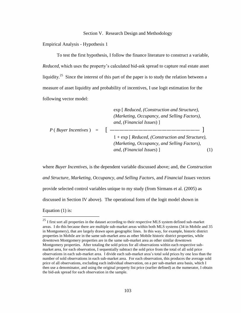
103

Section V. Research Design and Methodology

Empirical Analysis - Hypothesis 1

To test the first hypothesis, I follow the finance literature to construct a variable,

Reduced, which uses the property‘s calculated bid-ask spread to capture real estate asset

liquidity.25

Since the interest of this part of the paper is to study the relation between a

measure of asset liquidity and probability of incentives, I use logit estimation for the

following vector model:

exp [ Reduced, (Construction and Structure),

(Marketing, Occupancy, and Selling Factors),

and, (Financial Issues) ]

P ( Buyer Incentives ) = [ ――――――――――――――――――― ]

1 + exp [ Reduced, (Construction and Structure),

(Marketing, Occupancy, and Selling Factors),

and, (Financial Issues) ] (1)

where Buyer Incentives, is the dependent variable discussed above; and, the Construction

and Structure, Marketing, Occupancy, and Selling Factors, and Financial Issues vectors

provide selected control variables unique to my study (from Sirmans et al. (2005) as

discussed in Section IV above). The operational form of the logit model shown in

Equation (1) is:

25

I first sort all properties in the dataset according to their respective MLS system defined sub-market

areas. I do this because there are multiple sub-market areas within both MLS systems (34 in Mobile and 35

in Montgomery), that are largely drawn upon geographic lines. In this way, for example, historic district

properties in Mobile are in the same sub-market area as other Mobile historic district properties, while

downtown Montgomery properties are in the same sub-market area as other similar downtown

Montgomery properties. After totaling the sold prices for all observations within each respective sub-

market area, for each observation, I sequentially subtract the sold price from the total of all sold price

observations in each sub-market area. I divide each sub-market area‘s total sold prices by one less than the

number of sold observations in each sub-market area. For each observation, this produces the average sold

price of all observations, excluding each individual observation, on a per sub-market area basis, which I

then use a denominator, and using the original property list price (earlier defined) as the numerator, I obtain

the bid-ask spread for each observation in the sample.

104

P ( Buyer Incentives ) ( β0 + β

1∙Reduced + β

2Ln(Age)

ln ――――――――――――― =

1 - P ( Buyer Incentives ) + β3∙Vacant + β

4Ln(Inven)

+ β5∙SL-Ratio + β

6∙Exclusive

+ β7∙Listrank + β

8∙Salerank

+ β9

∙Agentsame + β10

Corporate

+ β11

Spring +β12

Summer + β13

Fall

+ β14

Winter + β15

Year2008 + β16

Year2009

+ β17

Year2010 + β18

Year2011

+ β19

∙Year2010 + β20

∙Year2011

+ β21

∙Ln(Zip-Md) + β22

∙Unemp

+ β23

∙Interest + β24

∙Foreclosed

+ β25

∙Financing + β26

∙Mobsold ) (2)

where the Construction and Structure vector includes Ln(Age), the natural logarithm of

the age of the property in years;26

the Marketing, Occupancy, and Selling Factors vector

26

According to the American Society of Home Inspectors (ASHI), 39 states now require a professional

home inspection as part of a purchase contract, and 29 states require that professional home inspectors

obtain licensure; Alabama requires a license (Information obtained from ASHI available at:

www.ashi.org.). The purpose of a professional home inspection is to provide buyers with comprehensive

information on the age, condition, and performance of all property components, including exterior systems,

structural systems, roofing systems, electrical systems, heating and cooling systems, insulating and

ventilating systems, plumbing systems, interior systems, and fireplace and chimney systems. In addition, it

is customary for the seller to provide a comprehensive seller‘s property disclosure to the buyer that either

affirms or denies the existence of a multitude of conditions possibly considered problematic (Epley et al.,

2002). The seller‘s property disclosure is the foundation upon which any future legal action by the buyer

against the seller rests, and prior to signing the seller‘s disclosure, listing agents advise their clients to be

both careful and thorough when completing it. Therefore, while it is possible that older properties will

present higher levels of information asymmetries, it is most likely that the home inspection process and

seller‘s disclosure either greatly reduces or eliminates them.

105

includes Vacant, a dummy variable that takes the value of one if no one occupies the

property, and zero otherwise; Ln(Inven), the natural logarithm of the total number of

active listings in the property listing month; SL- Ratio, the ratio of property sales to

property listings in the property listing month; Exclusive, a dummy variable that takes the

value of one if the listing contract type is an exclusive-right-to-sell listing, and zero

otherwise;27

Listrank, a dummy variable that takes the value of one if the listing

brokerage firm is ranked in the top five of all listing firms in the market, and zero

otherwise; Salerank, a dummy variable that takes the value of one if the selling brokerage

firm is ranked in the top five of all selling firms in the market, and zero otherwise;

Agentsame, a dummy variable that takes the value of one if the selling agent is also the

listing agent, and zero otherwise; Corporate, a dummy variable that takes the value of

one if the property is not owned by an individual, and zero otherwise; Spring,28

a dummy

variable that takes the value of one if the property is listed in March, April, or May, and

zero otherwise; Summer, a dummy variable that takes the value of one if the property is

listed in June, July, or August, and zero otherwise; Fall, a dummy variable that takes the

value of one if the property is listed in September, October or November, and zero

otherwise; Winter, a dummy variable that takes the value of one if the property is listed in

December, January, or February, and zero otherwise; Year2008, a dummy variable that

takes the value of one if the property is listed in 2008, and zero otherwise;29

Year2009, a

dummy variable that takes the value of one if the property is listed in 2009, and zero

27

Under an exclusive-right-to-sell agency, the listing agent receives a sales commission regardless of who

sells the property, even if sold by the seller within a specified period of time (Epley et al., 2002). 28

Forgey et al. (1996), and Springer (1996) reveal that season of the year of the property listing affects the

likelihood of sale in terms of both sales price and marketing duration. 29

Properties sold in 2008 or later but listed prior to 2008 are included in the sample.

106

otherwise; Year2010, a dummy variable that takes the value of one if the property is

listed in 2010, and zero otherwise; Year2011, a dummy variable that takes the value of

one if the property is listed in 2011, and zero otherwise; Ln(Zip-Md), the median income

per Zip Code;30

and Unemp, either the Mobile or Montgomery market unemployment

rate by county in the month of property listing; and, the Financing Issues vector includes

Interest, the prevailing national average interest rate for a 30-year conventional

residential mortgage in the month of the property listing;31

Foreclosed, a dummy variable

that takes the value of one if the property is marketed as a foreclosed property sale, and

zero otherwise; Financing, a variable drawn from the MLS‘ reporting of buyer financing

taking the value of one if the buyer used no financing, two if the buyer used conventional

financing, three if the buyer used financing insured by the U.S. Federal Housing

Administration, four if the buyer used financing insured by the Veteran‘s Administration,

five if the buyer used financing insured by the U.S. Department of Agriculture or

underwritten by some type of housing bond, six if the buyer used financing provided by

the owner, and seven if the buyer used some other type of financing such as a lease-

purchase option arrangement;32

and, Mobsold, a dummy variable that takes the value of

one if the observation is from the Mobile, AL MLS system.

30

Per capita income per zip code is based on the 2007-2011 American Community Survey 5-Year

Estimates, as reported by the U.S. Census Bureau available at

http://factfinder2.census.gov/faces/nav/jsf/pages/community_facts.xhtml#none. 31

Mortgage interest rate data obtained from FreddieMac available at:

http://www.freddiemac.com/pmms/pmms30.htm. 32

Buyer‘s type of financing not reported in all cases.

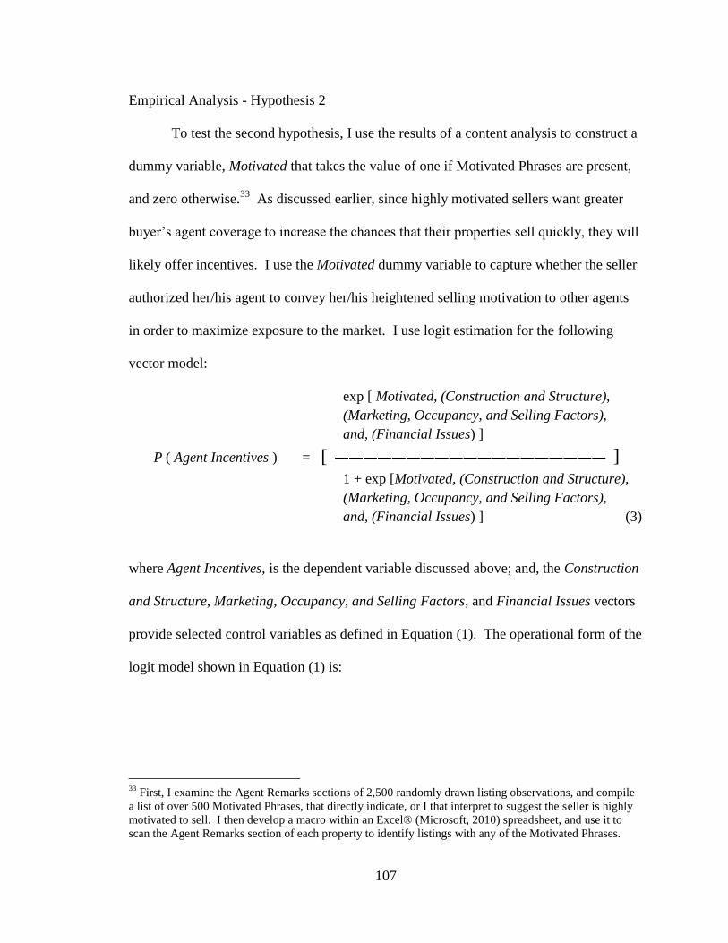
107

Empirical Analysis - Hypothesis 2

To test the second hypothesis, I use the results of a content analysis to construct a

dummy variable, Motivated that takes the value of one if Motivated Phrases are present,

and zero otherwise.33

As discussed earlier, since highly motivated sellers want greater

buyer‘s agent coverage to increase the chances that their properties sell quickly, they will

likely offer incentives. I use the Motivated dummy variable to capture whether the seller

authorized her/his agent to convey her/his heightened selling motivation to other agents

in order to maximize exposure to the market. I use logit estimation for the following

vector model:

exp [ Motivated, (Construction and Structure),

(Marketing, Occupancy, and Selling Factors),

and, (Financial Issues) ]

P ( Agent Incentives ) = [ ――――――――――――――――――― ]

1 + exp [Motivated, (Construction and Structure),

(Marketing, Occupancy, and Selling Factors),

and, (Financial Issues) ] (3)

where Agent Incentives, is the dependent variable discussed above; and, the Construction

and Structure, Marketing, Occupancy, and Selling Factors, and Financial Issues vectors

provide selected control variables as defined in Equation (1). The operational form of the

logit model shown in Equation (1) is:

33

First, I examine the Agent Remarks sections of 2,500 randomly drawn listing observations, and compile

a list of over 500 Motivated Phrases, that directly indicate, or I that interpret to suggest the seller is highly

motivated to sell. I then develop a macro within an Excel® (Microsoft, 2010) spreadsheet, and use it to

scan the Agent Remarks section of each property to identify listings with any of the Motivated Phrases.

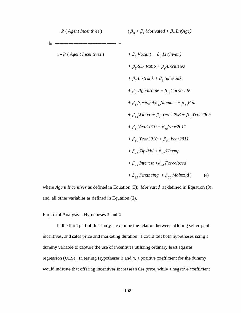
108

P ( Agent Incentives ) ( β0 + β

1∙Motivated + β

2∙Ln(Age)

ln ――――――――――――― =

1 - P ( Agent Incentives ) + β3∙Vacant + β

4∙Ln(Inven)

+ β5∙SL- Ratio + β

6∙Exclusive

+ β7∙Listrank + β

8∙Salerank

+ β9

∙Agentsame + β10

Corporate

+ β11

Spring +β12

Summer + β13

Fall

+ β14

Winter + β15

Year2008 + β16

Year2009

+ β17

Year2010 + β18

Year2011

+ β19

∙Year2010 + β20

∙Year2011

+ β21

∙Zip-Md + β22

∙Unemp

+ β23

∙Interest +β24

∙Foreclosed

+ β25

∙Financing + β26

∙Mobsold ) (4)

where Agent Incentives as defined in Equation (3); Motivated as defined in Equation (3);

and, all other variables as defined in Equation (2).

Empirical Analysis – Hypotheses 3 and 4

In the third part of this study, I examine the relation between offering seller-paid

incentives, and sales price and marketing duration. I could test both hypotheses using a

dummy variable to capture the use of incentives utilizing ordinary least squares

regression (OLS). In testing Hypotheses 3 and 4, a positive coefficient for the dummy

would indicate that offering incentives increases sales price, while a negative coefficient

109

for the dummy would indicate that offering incentives decreases marketing duration. If it

were certain that the data were normally distributed, OLS would be a logical choice.

However, with respect to the research question, therein lays the problem: that there is no

certainty that all sellers choose to offer incentives. Hence, precisely because of this

uncertainty, sample selection bias is a potential concern.

Within the real estate literature, two-stage least squared estimation (2SLS) is a

well-established method for addressing sample selection bias issues (Elder, Zumpano, &

Baryla, 2000; Knight, 2002; Munneke & Slade, 2000; Waller et al., 2010). Therefore, in

this study, I utilize 2SLS estimation to test Hypotheses 3 and 4. The first stage uses a

probit regression to capture the choice of using incentives. In the second stage, the

Inverse Mills Ratio (IMR)34

from the first stage becomes an independent variable in the

(OLS) estimation of the equations for sales price and marketing duration. The decision to

use incentives represents a binary outcome, and is therefore an index function of the

following form:

Incentives Used: Ii = 1 if Zi'γ ≥ i

Incentives Not Used: Ii = 0 otherwise

where Zi = 'Xi; Xi is a vector of independent, observable variables, are the estimators,

and i is normally distributed with a mean zero and standard deviation of one (i.e.

NID(0,1)), for a probit model. Thus, I denote the likelihood of using a sales incentive

considering observable vectors as:

34

Due to the possibility that some sellers will not offer sales incentives, effectively, some incentives values

may be missing. The 2SLS regression corrects for any potential bias resulting from missing values. In the

first stage, a probit estimation produces the Inverse Mills Ratio (IMR), which essentially is a prediction of

missing ‗incentives‘ variable values based on estimates of ‗incentives‘ variable values that are present.

110

p (Incentives) = Φ [ ln(List)

+ ∑ (Construction and Structure)

+ ∑ (Marketing, Occupancy, and Selling Factors)

+ ∑(Financial Issues) ] (5)

where Incentives is the dependent variable discussed at the beginning of this section;

Ln(List) is the natural logarithm of the property list price on the date of sale; and, the

Construction and Structure, Marketing, Occupancy, and Selling Factors, and Financial

Issues vectors as defined in Equation (1). In the first stage, I derive the Inverse Mills

Ratio (IMR) using the Incentives dummy variable as the dependent variable. The

following operational form of Equation (5) is:

P (Incentives = 1 | x) = Φ ( β0 + β

1∙Ln(List) + β

2Ln(Age) + β

3∙Vacant

+ β4∙Ln(Inven) + β

5∙SL-Ratio + β

6∙Exclusive

+ β7∙Listrank + β

8∙Salerank + β

9 ∙Agentsame

+ β10

Corporate + β11

Spring +β12

Summer

+ β13

Fall + β14

Winter + β15

Year2008

+ β16

Year2009 + β17

Year2010 + β18

Year2011

+ β19

∙Year2010 + β20

∙Year2011 + β21

∙Ln(Zip-Md)

+ β22

∙Unemp + β23

∙Interest +β24

∙Foreclosed

+ β25

∙Financing + β26

∙Mobsold ) + ε. (6)

111

where Incentives and Ln(List) as defined in Equation (5), and all other variables as

defined in Equation (2). The second stage of the empirical model takes the following

form:

Ln(Sale) = ᶂ {IMR + ∑(Incentives)

+ ∑(Construction and Structure)

+ ∑(House Internal Features)

+ ∑(House External Features)

+ ∑(Environmental - Natural)

+ ∑(Environmental – Neighborhood and Location)

+ ∑(Environmental – Public Service)

+ ∑(Marketing, Occupancy, and Selling Factors)

+ ∑(Financing Issues)} (7)

where Ln(Sale) is the natural logarithm of the property sales price; IMR and Incentives as

defined in Equation (5); and, selected vectors of control variables as discussed in Section

IV above. The operational form of Equation (7) is:

Ln(Sale) = β0 + β

1∙IMR + β

2∙Incentives + β

3Ln(Age)

+ β4∙Ln(Sqfeet) + β

5∙Storynum + β

6∙New

+ β7∙Brick + β

8∙Bednum + β

9∙Bathnum

+ β10

∙Fire + β11

∙Central + β12

∙Parknum

+ β13

∙Pool + β14

∙Water + β15

∙Urban

+ β16

∙Golf + β17

∙Subdpud + β18

∙Pubwater

112

+ β19

∙Pubsewer + β20

∙DOP + β21

∙Vacant

+ β22

Ln(Inven) + β23

∙SL-Ratio + β24

∙Exclusive

+ β25

∙Listrank + β26

∙Salerank

+ β27

∙Agentsame + β28

∙Corporate + β29

∙Spring

+ β30

∙Summer + β31

∙Fall + β32

∙Winter

+ β33

∙Year2008 + β34

∙Year2009 + β35

∙Year2010

+ β36

∙Year2011 + β37

∙Zip-Md + β38

∙Unemp

+ β39

∙Interest +β40

∙Foreclosed

+ β41

∙Financing + β42

∙Mobsold + ε. (8)

where Ln(Sale) as defined above; and IMR and Incentives as defined in Equation (5). As

controls, the Construction and Structure vector includes: Ln(Age), as defined in Equation

(2); Ln(SqFeet), the natural logarithm of the total number of heated and cooled square

feet in the property; Storynum, the total number of stories in the property; New, a dummy

variable taking the value of one if the property is new construction and has never been

occupied, and zero otherwise; and, Brick, a dummy variable that takes the value of one if

the property exterior is brick, cement block, or cement board, and zero otherwise; the

House Internal Features vector includes Bednum, the total number of bedrooms;

Bathnum, the total number of bathrooms; Fire, a dummy variable that takes the value of

one if the property has a fireplace, and zero otherwise; and Central, a dummy variable

that takes the value of one if the property has central heating and air-conditioning, and

zero otherwise; the House External Features vector includes Parknum, the total number

of garage parking spaces (the default is zero if there is no garage); and Pool, a dummy

113

variable that takes the value of one if the property has a swimming pool, hot tub, or spa,

and zero otherwise; the Environmental – Natural vector includes Water, a dummy

variable that takes the value of one if the property is situated on or has a view of a body

of water such as a lake, river, or bay, and zero otherwise; the Environmental –

Neighborhood and Location vector includes Urban, a dummy variable that takes the

value of one if the property is located within an incorporated municipal jurisdiction, and

zero otherwise; and, Golf, a dummy variable that takes the value of one if the property is

situated on a golf course, and zero otherwise; the Environmental - Public Service vector

includes Subd-PUD, a dummy variable that takes the value of one if the property is in a

subdivision or planned unit development, and zero otherwise; Pubwater, a dummy

variable that takes the value of one if public water service is available to the property, and

zero otherwise; Pubsewer, a dummy variable that takes the value of one if public sewer

service is available to the property, and zero otherwise; DOP is the degree of overpricing

of the listed property;35

the Marketing, Occupancy, and Selling Factors and Financing

Issues vectors are the same as in Equation (2).

As with the sales price estimation, the second stage of the empirical model to

estimate marketing duration takes the following form:

35

―The degree of above-market pricing, as measured by the difference between the natural logarithm of the

list price and the natural logarithm of the predicted price from a hedonic price equation‖ (Jud, Seaks, &

Winkler, 1996, p. 450). In a footnote to this quote, the authors state, ―The hedonic price equation used in

this study is the same as that reported in the appendix to Jud and Winkler (1994)‖ (Jud, Seaks & Winkler,

1996, p. 456). Referring to that article, Jud and Winkler (1994) use a hedonic price equation to estimate

predicted residential prices using a vector of housing physical characteristics. In the spirit of Jud and

Winkler (1994), the calculation necessary to form the DOP variable for use in the proposed study adapts

similar variables including age, bedrooms, bathrooms, square feet, garage, fireplace, central air

conditioning, and swimming pool.

114

TOM = ᶂ {IMR + ∑(Incentives)

+ ∑(Construction and Structure)

+ ∑(House Internal Features)

+ ∑(House External Features)

+ ∑(Environmental - Natural)

+ ∑(Environmental – Neighborhood and Location)

+ ∑(Environmental – Public Service)

+ ∑(Marketing, Occupancy, and Selling Factors)

+ ∑(Financing Issues)} (9)

where TOM, is the marketing duration calculated as the total number of days between the

property‘s original listing date and the property sales date; IMR and Incentives as defined

in Equation (5); and, selected vectors of control variables as discussed in Section IV

above.

The operational form of the second stage of the empirical model to estimate

marketing duration shown in Equation (9) is:

TOM = β0 + β

1∙IMR + β

2∙Incentives + β

3∙Ln(Sale)

+ β4∙Ln(Age) + β

5∙Ln(Sqfeet) + β

6∙Storynum +

+ β7∙New + β

8∙Brick + β

9∙Bednum + β

10∙Bathnum

+ β11

∙Fire + β12

∙Central + β13

∙Parknum

+ β14

∙Pool + β15

∙Water + β16

∙Urban

+ β17

∙Golf + β18

∙Subdpud + β19

∙Pubwater

115

+ β20

∙Pubsewer + β21

∙DOP + β22

∙Vacant

+ β23

Ln(Inven) + β24

∙SL-Ratio + β25

∙Exclusive

+ β26

∙Listrank + β27

∙Salerank + β28

∙Agentsame

+ β29

∙Corporate + β30

∙Spring + β31

∙Summer

+ β32

∙Fall + β33

∙Winter + β34

∙Year2008

+ β35

∙Year2009 + β36

∙Year2010

+ β37

∙Year2011 + β38

∙Zip-Md + β39

∙Unemp

+ β40

∙Interest +β41

∙Foreclosed

+ β42

∙Financing + β43

∙Mobsold + ε. (10)

where TOM as defined above; IMR and Incentives as defined in Equation (5); Ln(Sale) as

defined in Equation (10); and, all other vectors and variables are the same as used in

Equation (9). All estimations are robust (White, 1980).

Robustness Checks

In general, robustness testing is necessary to attain reasonable degrees of quality

assurance, not only with respect to the predictive power of the critical core variables,36

but also with respect to the soundness of the empirical design (White & Lu, 2010). The

purpose of robustness testing is to determine if the addition, removal, or substitution of

variables changes the significance of the most important independent variables. Because

36

Critical core variables are of primary interest as plausible drivers or determinants of the dependent

variable. While only critical core variables should be subject to robustness testing, other core and non-core

variables are necessary (White & Lu, 2010). For detailed discussion of the process for selecting critical

core covariates, core covariates, and non-core covariates, as well as the relationships and importance of

exogeneity among covariates, see White and Lu (2010).

116

―robustness is necessary for valid causal inference‖ (White & Lu, 2010, p. 3), a failure to

implement effective robustness testing methods may lead readers to consider the

possibility that inferences drawn from the coefficient results are not robust. This may

then lead readers to question the structural validity of the empirical models. Therefore, I

conduct a battery of robustness tests to diminish such possibilities.

Sellers can offer sales incentives that are cash, non-cash, or both, and can offer

them to buyers, buyers‘ agents, or both. In some cases, the incentive may be only one

type offered to only one party, such as a buyer cash incentive. Other cases may include

multiple incentive types offered to multiple parties, such as buyer cash incentives and

agent non-cash incentives. I first disaggregate the data into specific incentive subsets. I

then retest each hypothesis to conclude if the results of using particular incentive types,

forms, or combinations are similar to those from the initial hypotheses testing. As a final

robustness test, I also estimate Equations (8) and (10) using OLS.

Section VI. Results of Empirical Analysis

Descriptive Statistics and Correlations

Table 3 presents t-test results comparing means of selected variables, and Table 4

presents descriptive statistics for the variables used in the primary analysis. The dataset

includes 32,128 residential properties sold in the Mobile and Montgomery, Alabama

markets from 2008 to 2011. Properties average 1,891 square feet, 3.3 bedrooms, 2.3

bathrooms, 1.15 stories, and 0.82 garage parking spaces. Properties sell for an average

$153,139, in an average of 142.5 days. Of the approximately 89% of property

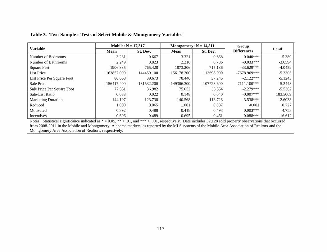
117

Table 3. Two-Sample t-Tests of Select Mobile & Montgomery Variables.

Variable Mobile: N = 17,317 Montgomery: N = 14,811 Group

Differences t-stat

Mean St. Dev. Mean St. Dev.

Number of Bedrooms 3.281 0.667 3.321 0.668 0.040*** 5.389

Number of Bathrooms 2.249 0.823 2.216 0.786 -0.033*** -3.6594

Square Feet 1906.835 765.428 1873.206 715.136 -33.629*** -4.0459

List Price 163857.000 144459.100 156178.200 113698.000 -7678.969*** -5.2303

List Price Per Square Foot 80.658 39.673 78.446 37.245 -2.122*** -5.1243

Sale Price 156417.400 131532.200 149306.300 107728.600 -7111.100*** -5.2448

Sale Price Per Square Foot 77.331 36.982 75.052 36.554 -2.279*** -5.5362

Sale-List Ratio 0.083 0.022 0.148 0.040 -0.007*** 183.5009

Marketing Duration 144.107 123.738 140.568 118.728 -3.538*** -2.6033

Reduced 1.000 0.065 1.001 0.087 -0.001 0.727

Motivated 0.392 0.488 0.418 0.493 0.003*** 4.753

Incentives 0.606 0.489 0.695 0.461 0.088*** 16.612

Notes: Statistical significance indicated as * < 0.05, ** < .01, and *** < .001, respectively. Data includes 32,128 sold property observations that occurred

from 2008-2011 in the Mobile and Montgomery, Alabama markets, as reported by the MLS systems of the Mobile Area Association of Realtors and the

Montgomery Area Association of Realtors, respectively.

118

Table 4. Descriptive Statistics.

Variable Obs. Mean Std. Dev. Min. Max.

Reduced 32,128 1.001 0.076 0.573 1.302

Motivated 32,128 0.404 0.491 0.00 1.00

Sale 32,128 153,139.200 121,190.900 1000.00 3562500.00

TOM 32,128 142.476 121.465 1.00 1910.00

Incentives 32,128 0.647 0.478 0.00 1.00

List 32,128 160,317.200 131,231.400 2,000.00 3,750,000.00

Age 28,427 23.620 22.115 1.00 186.00

SqFeet 32,127 1,891.331 742.843 440.00 17,655.00

Storynum 27,774 1.149 0.339 1.00 3.00

New 28,548 0.168 0.374 0.00 1.00

Brick 32,023 0.596 0.491 0.00 1.00

Bednum 32,128 3.299 0.671 0.00 8.00

Bathnum 32,128 2.233 0.806 0.00 12.00

Fire 32,128 0.645 0.479 0.00 1.00

Central 32,128 0.901 0.299 0.00 1.00

Parknum 32,128 0.827 0.999 0.00 5.00

Pool 32,128 0.086 0.281 0.00 1.00

Water 32,128 0.072 0.258 0.00 1.00

Urban 32,128 0.543 0.498 0.00 1.00

Golf 32,128 0.022 0.147 0.00 1.00

Subd-PUD 32,128 0.795 0.404 0.00 1.00

Pubwater 28,279 0.960 0.196 0.00 1.00

Pubsewer 28,198 0.775 0.418 0.00 1.00

DOP 28,427 0.000 0.450 -4.81 3.28

Vacant 31,976 0.646 0.478 0.00 1.00

Invent 32,128 3,137.541 1,072.319 1,293.00 4,691.00

SL-Ratio 32,128 0.113 0.045 0.04 0.41

Exclusive 32,089 0.970 0.170 0.00 1.00

Listrank 32,128 0.209 0.407 0.00 1.00

Salerank 32,128 0.191 0.393 0.00 1.00

Agentsame 32,128 0.025 0.156 0.00 1.00

Corporate 31,241 0.352 0.478 0.00 1.00

Zip-Md 32,128 51,458.290 12,785.870 18,190.38 85,103.67

Unemp 32,128 0.076 0.026 0.02 0.20

Interest 32,128 0.052 0.007 0.04 0.07

Foreclosed 32,126 0.317 0.466 0.00 1.00

Mobsold 32,128 0.539 0.498 0.00 1.00

Financing 23,809 2.450 1.273 1.00 7.00

Spring 32,128 0.272 0.445 0.00 1.00

Summer 32,128 0.256 0.436 0.00 1.00

Fall 32,128 0.238 0.426 0.00 1.00

Winter 32,128 0.235 0.424 0.00 1.00

Year2008 32,128 0.253 0.435 0.00 1.00

Year2009 32,128 0.234 0.424 0.00 1.00

Year2010 32,128 0.219 0.413 0.00 1.00

Year2011 32,128 0.207 0.405 0.00 1.00

Notes: The table above provides descriptive statistics for dependent, main independent, and

control variables.

119

observations with age information, the average is 23.6 years. On average, 64.5% of sold

properties have a fireplace, 90.1% have central heating and cooling, and 8.6% have a

pool or spa. Nearly all properties use public water services, and a significant number of

homes use public sewer services (96.0% and 77.5%, respectively). Most properties‘

exteriors are brick, block, or cement board (59.6%), and nearly all have central heating

and cooling (90.1%). Approximately 7.2% of the properties are on or have view of a

body of water, while a mere 2.2% are on or have a view of a golf course. Slightly more

than half of the properties are located in an incorporated city or municipality, but more

than 78% are subject to subdivision or planned unit development covenants.37

Table 5

shows correlations between all variables. I ran Variance Inflation Factor (VIF) tests to

detect if there are issues with multicollinearity. Testing reveals VIF factors greater than

10.0 for Ln(Age) and Ln(SqFeet) with respect to Ln(Sale) and TOM. To determine if

these collinear relationships threaten any of the estimation results, I re-estimate all

equations excluding the Ln(Age) and Ln(SqFeet) variables. Although the coefficient

values vary slightly as expected, the signs and significance levels remain the same for the

main independent variables. Therefore, multicollinearity is not problematic in my

estimations (Hair, Black, Babin, & Anderson, 2010).

37

As shown in Table 3, the t-test results show that all of the means of the select variables are statistically

different from each other (p < .001), with the exception of the Reduced variable. This is not surprising

given the Reduced variable mean and standard deviation for the entire sample are 1.006 and 0.076,

respectively. I use a dummy variable in all regressions to account for the differences between Mobile and

Montgomery, AL data.

120

Table 5. Variable Correlations.

# Variables 1 2 3 4 5 6 7 8

1 Reduced 1.0000

2 Motivated -0.1801* 1.0000

3 Ln(Sale) 0.9524* -0.1908* 1.0000

4 Ln(TOM) 0.0663* 0.0653* 0.0773* 1.0000

5 Incentives 0.0688* 0.2884* 0.0666* 0.0181 1.0000

6 Buyer Only 0.2291* -0.1286* 0.2094* 0.0083 0.4896* 1.0000

7 Agent Only -0.2660* 0.2688* -0.2706* -0.0271* 0.3111* -0.2793* 1.0000

8 Both 0.0575* 0.2566* 0.0819* 0.0369* 0.3589* -0.3221* -0.2047* 1.0000

9 Ln(Age) -0.4682* 0.0399* -0.5020* -0.0223* -0.2587* -0.1313* 0.1700* -0.3073*

10 Ln(SqFeet) 0.6521* -0.0690* 0.6851* 0.1128* 0.0257* 0.0653* -0.1148* 0.0592*

11 Storynum 0.3039* -0.0228* 0.3242* 0.0617* -0.0020 -0.0007 -0.0158 0.0122

12 New 0.2600* -0.0244* 0.2836* 0.0100 0.3209* 0.1718* -0.1844* 0.3459*

13 Brick 0.1514* -0.0113 0.1644* -0.0068 0.0785* 0.0806* -0.0727* 0.0672*

14 Bednum 0.4341* -0.0187* 0.4402* 0.0623* 0.0627* 0.0664* -0.0733* 0.0652*

15 Bathnum 0.5905* -0.0595* 0.6222* 0.0888* 0.0354* 0.0683* -0.0945* 0.0490*

16 Fire 0.4563* -0.0583* 0.4679* 0.0546* 0.0406* 0.1426* -0.1280* -0.0012

17 Central 0.4150* -0.0745* 0.4295* 0.0574* 0.0514* 0.1538* -0.1707* 0.0376*

18 Parknum 0.4753* -0.0589* 0.5163* 0.0669* 0.0704* 0.0547* -0.1182* 0.1291*

19 Pool 0.1805* -0.0172 0.1853* 0.0380* -0.0222* -0.0031 -0.0219* -0.0035

20 Water 0.0584* -0.0102 0.0803* 0.0318* -0.0168 -0.0566* -0.0129 0.0575*

21 Urban -0.1721* 0.0146 -0.1950* -0.0325* -0.0418* 0.0026 0.0122 -0.0649*

22 Golf 0.0774* -0.0301* 0.0858* 0.0291* -0.0171 0.0038 -0.0187* -0.0081

23 Subd-PUD 0.0582* -0.0355* 0.0573* -0.0004 0.0313* 0.1570* -0.1380* -0.0202*

24 Pubwater -0.0208* 0.0041 -0.0043 -0.0135 0.0174 0.0092 -0.0023 0.0123

25 Pubsewer -0.1258* 0.0057 -0.1026* -0.0392* 0.0174 0.0285* -0.0044 -0.0093

26 DOP 0.5467* -0.2116* 0.5715* 0.0223* -0.0002 0.1771* -0.2177* -0.0169

27 Vacant -0.1530* 0.1054* -0.1693* -0.0204* 0.0410* -0.0077 0.0879* -0.0213*

28 Ln(Inven) -0.0070 -0.0171 0.0573* -0.0003 -0.0885* -0.3670* 0.1345* 0.2000*

29 SL-Ratio 0.0453* -0.0320* 0.0033 0.0544* 0.0579* 0.3046* -0.1359* -0.1627*

30 Exclusive -0.0182 0.0065 -0.0084 0.0105 -0.0197* -0.0362* 0.0114 0.0082

31 Listrank 0.1055* -0.1480* 0.0959* 0.0219* -0.1520* 0.0154 -0.1184* -0.0951*

32 Salerank 0.0319* -0.0382* 0.0232* -0.0146 -0.0014 0.0723* -0.0591* -0.0325*

33 Agentsame -0.0466* -0.0714* -0.0415* -0.1539* -0.0464* -0.0718* 0.0206* 0.0090

34 Corporate -0.1728* 0.3043* -0.1782* -0.0193* 0.2286* -0.0782* 0.1820* 0.2046*

35 Ln(ZipMd) 0.5212* -0.0458* 0.5262* 0.0172 0.1038* 0.2036* -0.1458* 0.0203*

36 Unemp -0.1171* 0.1064* -0.1219* -0.0533* 0.0345* -0.1123* 0.0960* 0.0861*

37 Interest 0.0980* -0.1137* 0.1006* 0.0504* -0.0455* 0.0889* -0.0974* -0.0708*

38 Foreclosed -0.4340* 0.3620* -0.4397* -0.0696* 0.0405* -0.3050* 0.4194* 0.0248*

39 Mobsold -0.0041 -0.0265* 0.0628* 0.0101 -0.0923* -0.3665* 0.1312* 0.1978*

40 Financing 0.2581* -0.0604* 0.2596* 0.0410* 0.0829* 0.1570* -0.1162* 0.0148

41 Spring 0.0342* -0.0112 0.0346* -0.0311* -0.0053 0.0092 -0.0172 -0.0016

42 Summer -0.0086 0.0055 -0.0095 0.0046 0.0150 -0.0007 0.0030 0.0162

43 Fall -0.0220* 0.0023 -0.0225* 0.0423* 0.0043 0.0038 0.0047 -0.0035

44 Winter -0.0050 0.0038 -0.0040 -0.0147 -0.0142 -0.0128 0.0102 -0.0114

45 Year2008 0.0468* -0.0838* 0.0449* -0.1007* -0.0446* 0.0443* -0.0579* -0.0534*

46 Year2009 0.0185* -0.0017 0.0209* -0.0167 -0.0077 0.0205* -0.0018 -0.0318*

47 Year2010 -0.0320* 0.0613* -0.0338* 0.0127 0.0195* -0.0389* 0.0287* 0.0432*

48 Year2011 -0.0794* 0.0674* -0.0809* -0.0277* 0.0427* -0.0684* 0.0714* 0.0670*

Notes: The table above presents the correlations between all variables. Statistical significance indicated as: * p < 0.05,

** p < 0.01, *** p < 0.001, respectively.

121

Table 5. Variable Correlations (Continued).

# Variables 9 10 11 12 13 14 15 16

1 Reduced

2 Motivated

3 Ln(Sale)

4 Ln(TOM)

5 Incentives

6 Buyer Only

7 Agent Only

8 Both

9 Ln(Age) 1.0000

10 Ln(SqFeet) -0.2473* 1.0000

11 Storynum -0.0859* 0.5052* 1.0000

12 New -0.7857* 0.1232* 0.0485* 1.0000

13 Brick -0.2124* 0.1030* -0.1079* 0.1511* 1.0000

14 Bednum -0.2450* 0.6690* 0.3656* 0.1530* 0.1235* 1.0000

15 Bathnum -0.2651* 0.7857* 0.5709* 0.1229* 0.0668* 0.5906* 1.0000

16 Fire -0.2097* 0.4638* 0.1827* 0.0789* 0.0716* 0.2654* 0.3536* 1.0000

17 Central -0.1948* 0.2083* 0.0507* 0.1057* 0.1055* 0.1456* 0.2075* 0.2182*

18 Parknum -0.4904* 0.5017* 0.2257* 0.3038* 0.1521* 0.3475* 0.4112* 0.3196*

19 Pool 0.0206* 0.2225* 0.1247* -0.0663* -0.0056 0.1385* 0.1962* 0.1222*

20 Water -0.0328* 0.0528* 0.0621* 0.0022 -0.0445* 0.0060 0.0518* 0.0003

21 Urban 0.2915* -0.0885* -0.0415* -0.1422* 0.0125 -0.0711* -0.0918* -0.0317*

22 Golf -0.0313* 0.0815* 0.0548* -0.0006 -0.0049 0.0412* 0.0840* 0.0529*

23 Subd-PUD -0.0462* 0.0289* -0.0153 0.0653* 0.0876* 0.0495* 0.0368* 0.1102*

24 Pubwater -0.0013 -0.0150 -0.0103 0.0175 0.0295* -0.0053 -0.0099 -0.0090

25 Pubsewer 0.0934* -0.0679* -0.0366* -0.0053 0.0780* -0.0340* -0.0496* -0.0350*

26 DOP -0.0677* 0.0562* -0.0209* 0.0710* 0.0350* 0.0000 0.0000 0.0000

27 Vacant 0.0052 -0.0777* -0.0307* 0.0876* 0.0114 -0.0347* -0.0782* -0.0434*

28 Ln(Inven) -0.1137* 0.0194* 0.0520* 0.0520* -0.1015* -0.0263* 0.0203* -0.1594*

29 SL-Ratio 0.0341* -0.0148 -0.0376* 0.0031 0.0635* 0.0149 -0.0170 0.1281*

30 Exclusive 0.0015 0.0006 0.0073 -0.0172 -0.0303* -0.0075 -0.0004 -0.0191*

31 Listrank 0.0595* 0.0384* 0.0258* -0.0902* -0.0430* 0.0002 0.0292* 0.0071

32 Salerank -0.0026 0.0107 -0.0120 -0.0049 0.0385* 0.0111 0.0063 0.0371*

33 Agentsame -0.0369* -0.0396* -0.0132 0.0520* -0.0401* -0.0429* -0.0441* -0.0525*

34 Corporate -0.3263* -0.0478* -0.0107 0.4682* 0.0806* 0.0374* -0.0303* -0.0417*

35 Ln(ZipMd) -0.3468* 0.3224* 0.1219* 0.1876* 0.1601* 0.2627* 0.3155* 0.3503*

36 Unemp 0.0776* -0.0130 -0.0018 -0.0640* 0.0250* -0.0088 -0.0092 -0.0554*

37 Interest -0.0692* -0.0241* -0.0256* 0.0680* -0.0283* -0.0260* -0.0291* 0.0172

38 Foreclosed 0.2457* -0.1613* -0.0446* -0.2374* -0.0820* -0.0966* -0.1375* -0.1864*

39 Mobsold -0.1176* 0.0171 0.0501* 0.0534* -0.1067* -0.0301* 0.0204* -0.1627*

40 Financing -0.1496* 0.0693* -0.0063 0.0875* 0.0644* 0.0698* 0.0638* 0.1233*

41 Spring 0.0079 0.0157 0.0073 -0.0207* 0.0000 0.0122 0.0126 0.0140

42 Summer -0.0239* -0.0095 -0.0091 0.0233* 0.0014 -0.0058 -0.0136 -0.0018

43 Fall 0.0015 -0.0053 0.0095 0.0092 -0.0020 -0.0101 -0.0010 -0.0113

44 Winter 0.0148 -0.0013 -0.0079 -0.0115 0.0005 0.0032 0.0017 -0.0015

45 Year2008 -0.0159 -0.0353* -0.0252* 0.0138 -0.0231* -0.0296* -0.0398* 0.0038

46 Year2009 0.0120 -0.0160 -0.0162 -0.0235* -0.0001 -0.0149 -0.0039 -0.0026

47 Year2010 0.0217* 0.0108 -0.0003 -0.0364* 0.0076 0.0115 0.0094 -0.0087

48 Year2011 0.0321* 0.0311* 0.0369* -0.0104 0.0242* 0.0301* 0.0265* -0.0052

Notes: The table above presents the correlations between all variables. Statistical significance indicated as: * p < 0.05,

** p < 0.01, *** p < 0.001, respectively.

122

Table 5. Variable Correlations (Continued).

# Variables 17 18 19 20 21 22 23 24

1 Reduced

2 Motivated

3 Ln(Sale)

4 Ln(TOM)

5 Incentives

6 Buyer Only

7 Agent Only

8 Both

9 Ln(Age)

10 Ln(SqFeet)

11 Storynum

12 New

13 Brick

14 Bednum

15 Bathnum

16 Fire

17 Central 1.0000

18 Parknum 0.1692* 1.0000

19 Pool 0.0712* 0.1064* 1.0000

20 Water 0.0306* 0.0558* 0.0212* 1.0000

21 Urban -0.0502* -0.1696* -0.0116 -0.0567* 1.0000

22 Golf 0.0348* 0.0848* 0.0173 0.0281* -0.0687* 1.0000

23 Subd-PUD 0.1345* 0.0466* -0.0094 -0.0767* 0.1011* 0.0037 1.0000

24 Pubwater 0.0253* 0.0036 -0.0007 -0.0369* 0.0901* 0.0010 0.1377* 1.0000

25 Pubsewer -0.0190 -0.0438* -0.0221* -0.0710* 0.2837* -0.0013 0.2586* 0.3112*

26 DOP 0.0000 0.0000 0.0000 0.0541* -0.0948* 0.0172 -0.0327* -0.0013

27 Vacant -0.1003* -0.0555* -0.0630* -0.1182* 0.0285* -0.0310* 0.0061 0.0005

28 Ln(Inven) -0.0609* 0.0840* 0.0630* 0.1882* -0.0783* 0.0077 -0.3194* 0.0441*

29 SL-Ratio 0.0520* -0.0502* -0.0464* -0.1369* 0.0653* -0.0100 0.2405* -0.0303*

30 Exclusive -0.0213* 0.0034 0.0076 0.0225* -0.0148 0.0075 -0.0395* 0.0035

31 Listrank 0.0690* 0.0026 0.0642* 0.0452* 0.1441* -0.0130 -0.0325* -0.0013

32 Salerank 0.0113 0.0033 0.0033 -0.0599* 0.0568* -0.0350* 0.0429* 0.0012

33 Agentsame -0.0550* -0.0092 -0.0149 -0.0181 -0.0037 -0.0116 -0.0726* 0.0099

34 Corporate -0.1410* 0.0466* -0.1024* -0.0463* -0.0267* -0.0375* 0.0220* 0.0022

35 Ln(ZipMd) 0.2639* 0.3221* 0.0894* -0.0258* -0.1440* 0.0587* 0.1271* -0.0011

36 Unemp -0.0384* -0.0375* 0.0014 0.0057 0.0715* -0.0055 -0.0673* -0.0008

37 Interest 0.0174 0.0008 -0.0034 0.0060 0.0483* -0.0113 0.0370* 0.0008

38 Foreclosed -0.2671* -0.1772* -0.0547* -0.0172 0.0300* -0.0344* -0.1515* -0.0150

39 Mobsold -0.0626* 0.0845* 0.0647* 0.1926* -0.0772* 0.0089 -0.3215* 0.0463*

40 Financing 0.1791* 0.0615* 0.0198 -0.0266* -0.1029* 0.0094 0.0999* -0.0023

41 Spring 0.0176 0.0064 0.0047 -0.0109 -0.0019 -0.0047 0.0002 -0.0087

42 Summer -0.0073 0.0007 -0.0033 0.0035 -0.0017 0.0070 -0.0088 0.0020

43 Fall -0.0059 -0.0094 -0.0031 0.0017 0.0036 0.0023 -0.0008 -0.0015

44 Winter -0.0050 0.0021 0.0015 0.0061 0.0002 -0.0045 0.0096 0.0085

45 Year2008 0.0037 -0.0119 -0.0058 0.0001 0.0419* -0.0180 0.0217* 0.0025

46 Year2009 -0.0016 -0.0261* -0.0008 0.0007 0.0145 0.0126 0.0099 -0.0023

47 Year2010 -0.0017 0.0075 0.0036 -0.0054 -0.0182 -0.0019 -0.0217* -0.0102

48 Year2011 -0.0141 0.0197* -0.0008 -0.0009 -0.0477* 0.0065 -0.0282* 0.0071

Notes: The table above presents the correlations between all variables. Statistical significance indicated as: * p < 0.05,

** p < 0.01, *** p < 0.001, respectively.

123

Table 5. Variable Correlations (Continued).

# Variables 25 26 27 28 29 30 31 32

1 Reduced

2 Motivated

3 Ln(Sale)

4 Ln(TOM)

5 Incentives

6 Buyer Only

7 Agent Only

8 Both

9 Ln(Age)

10 Ln(SqFeet)

11 Storynum

12 New

13 Brick

14 Bednum

15 Bathnum

16 Fire

17 Central

18 Parknum

19 Pool

20 Water

21 Urban

22 Golf

23 Subd-PUD

24 Pubwater

25 Pubsewer 1.0000

26 DOP -0.0615* 1.0000

27 Vacant 0.0792* -0.1456* 1.0000

28 Ln(Inven) -0.0399* 0.0828* -0.1554* 1.0000

29 SL-Ratio 0.0212* -0.0018 0.1004* -0.7619* 1.0000

30 Exclusive -0.0274* -0.0048 0.0012 0.0956* -0.0548* 1.0000

31 Listrank -0.0012 0.1089* -0.1080* 0.1604* -0.0870* 0.0280* 1.0000

32 Salerank 0.0335* 0.0246* 0.0339* -0.1148* 0.0930* 0.0029 0.2902* 1.0000

33 Agentsame 0.0101 -0.0016 0.0193* 0.1440* -0.1016* 0.0103 0.0114 0.0123

34 Corporate 0.0374* -0.2717* 0.2699* -0.1107* 0.0680* -0.0217* -0.2289* -0.0356*

35 Ln(ZipMd) -0.0399* 0.2405* -0.0279* -0.1915* 0.1272* -0.0422* -0.0527* 0.0263*

36 Unemp 0.0135 -0.1337* 0.0102 0.1468* -0.4242* 0.0123 -0.0451* -0.0065

37 Interest 0.0034 0.1552* -0.0348* -0.0803* 0.4258* 0.0092 0.1073* 0.0183

38 Foreclosed 0.0146 -0.3786* 0.2527* 0.1200* -0.1502* 0.0310* -0.1496* -0.0561*

39 Mobsold -0.0396* 0.0958* -0.1620* 0.9782* -0.7154* 0.1014* 0.1738* -0.1049*

40 Financing -0.0775* 0.2172* -0.0754* -0.0900* 0.0603* -0.0084 0.0241* 0.0230*

41 Spring -0.0098 0.0372* -0.0338* 0.0112 0.1616* 0.0118 0.0021 0.0083

42 Summer -0.0064 -0.0159 0.0276* 0.0407* 0.1454* -0.0076 -0.0067 -0.0011

43 Fall 0.0161 -0.0233* 0.0037 0.0121 -0.0857* -0.0005 0.0061 -0.0066

44 Winter 0.0007 0.0006 0.0033 -0.0657* -0.2332* -0.0040 -0.0015 -0.0011

45 Year2008 0.0102 0.0926* -0.0221* -0.0355* 0.1923* 0.0127 0.0750* 0.0151

46 Year2009 0.0042 0.0455* -0.0243* -0.0393* -0.0399* 0.0093 0.0645* -0.0080

47 Year2010 -0.0260* -0.0519* 0.0169 0.0489* -0.1620* -0.0034 -0.0732* 0.0352*

48 Year2011 0.0121 -0.1428* 0.0342* 0.0683* -0.2200* -0.0142 -0.0975* -0.0396*

Notes: The table above presents the correlations between all variables. Statistical significance indicated as: * p < 0.05,

** p < 0.01, *** p < 0.001, respectively.

124

Table 5. Variable Correlations (Continued).

# Variables 33 34 35 36 37 38 39 40

1 Reduced

2 Motivated

3 Ln(Sale)

4 Ln(TOM)

5 Incentives

6 Buyer Only

7 Agent Only

8 Both

9 Ln(Age)

10 Ln(SqFeet)

11 Storynum

12 New

13 Brick

14 Bednum

15 Bathnum

16 Fire

17 Central

18 Parknum

19 Pool

20 Water

21 Urban

22 Golf

23 Subd-PUD

24 Pubwater

25 Pubsewer

26 DOP

27 Vacant

28 Ln(Inven)

29 SL-Ratio

30 Exclusive

31 Listrank

32 Salerank

33 Agentsame 1.0000

34 Corporate -0.0304* 1.0000

35 Ln(ZipMd) -0.0701* 0.0026 1.0000

36 Unemp -0.0071 0.0303* -0.0602* 1.0000

37 Interest 0.0225* -0.0458* -0.0274* -0.7624* 1.0000

38 Foreclosed -0.0370* 0.3702* -0.2213* 0.1658* -0.1783* 1.0000

39 Mobsold 0.1475* -0.1190* -0.2008* 0.1100* -0.0363* 0.1128* 1.0000

40 Financing -0.0271* -0.1094* 0.1538* -0.0202 0.0013 -0.2426* -0.0903* 1.0000

41 Spring 0.0025 -0.0358* 0.0112 -0.0576* -0.0055 -0.0254* -0.0047 0.0030

42 Summer -0.0072 0.0224* -0.0028 0.0845* 0.0885* 0.0153 -0.0058 -0.0005

43 Fall 0.0039 0.0277* -0.0041 -0.0549* -0.0533* 0.0135 0.0029 0.0026

44 Winter 0.0009 -0.0132 -0.0048 0.0287* -0.0318* -0.0026 0.0080 -0.0053

45 Year2008 0.0296* -0.0431* -0.0243* -0.6529* 0.6586* -0.1008* -0.0244* -0.0056

46 Year2009 0.0052 -0.0331* 0.0024 0.3873* -0.1399* -0.0406* -0.0003 0.0286*

47 Year2010 -0.0176 0.0233* -0.0019 0.3537* -0.3607* 0.0952* 0.0025 -0.0147

48 Year2011 -0.0169 0.0510* 0.0287* 0.2881* -0.5204* 0.1226* 0.0309* -0.0071

Notes: The table above presents the correlations between all variables. Statistical significance indicated as: * p < 0.05,

** p < 0.01, *** p < 0.001, respectively.

125

Table 5. Variable Correlations (Continued).

# Variables 41 42 43 44 45 46 47 48

1 Reduced

2 Motivated

3 Ln(Sale)

4 Ln(TOM)

5 Incentives

6 Buyer Only

7 Agent Only

8 Both

9 Ln(Age)

10 Ln(SqFeet)

11 Storynum

12 New

13 Brick

14 Bednum

15 Bathnum

16 Fire

17 Central

18 Parknum

19 Pool

20 Water

21 Urban

22 Golf

23 Subd-PUD

24 Pubwater

25 Pubsewer

26 DOP

27 Vacant

28 Ln(Inven)

29 SL-Ratio

30 Exclusive

31 Listrank

32 Salerank

33 Agentsame

34 Corporate

35 Ln(ZipMd)

36 Unemp

37 Interest

38 Foreclosed

39 Mobsold

40 Financing 1.0000

41 Spring 1.0000

42 Summer -0.3577* 1.0000

43 Fall -0.3412* -0.3275* 1.0000

44 Winter -0.3382* -0.3246* -0.3097* 1.0000

45 Year2008 0.0312* -0.0010 -0.0454* 0.0140 1.0000

46 Year2009 -0.0026 0.0086 0.0092 -0.0155 -0.3221* 1.0000

47 Year2010 0.0389* -0.0077 -0.0525* 0.0199* -0.3080* -0.2929* 1.0000

48 Year2011 0.0205* 0.0109 -0.0292* -0.0034 -0.2977* -0.2831* -0.2707* 1.0000

Notes: The table above presents the correlations between all variables. Statistical significance indicated as: * p < 0.05,

** p < 0.01, *** p < 0.001, respectively.

126

Hypothesis 1

Table 6 shows the results for testing Hypothesis 1. The coefficient for the

Reduced dummy variable is positive and significant (β = 2.663). This means that as the

property bid-ask spread increases in the context of a cold market, there is a higher

probability that the seller will offer incentives to the buyer. The marginal effects value of

the Reduced variable is 0.505, which means that sellers of properties with higher bid-ask

spreads are 50.5% more likely to offer buyer sales incentives compared to sellers of

properties with lower bid-ask spreads. This finding provides support for Hypothesis 1.

Many of the control variable coefficients are also significant. For example, the

coefficient for Ln(Age) is negative and significant (β = -3.99), indicating that sellers of

older properties are less likely to offer incentives to buyers. The negative and significant

coefficient for the Foreclosed dummy (β = -1.271) suggests that sellers have little room

for price negotiation, and therefore are less likely to incur the additional expense of

offering incentives. A possible explanation for the positive and significant coefficient for

the Vacant dummy (β = 0.162) is that sellers of empty properties may benefit from

offering buyer incentives. The negative and significant coefficients for Agentsame and

Listrank dummies (β = -0.673 and β = -0.125, respectively) may indicate that when the

listing agent is also the selling agent, or when the listing company is one of the top-

ranked listing companies in the market, sellers are less likely to offer incentives.

Hypothesis 2

Table 7 shows the results for testing Hypothesis 2. The coefficient for the

Motivated dummy variable is positive and significant (β = 2.165). This suggests that

127

Table 6. Results of Logit Regression testing the hypothesis that there is a positive

relationship between a seller offering buyer incentives and real estate asset bid-ask

spread.

Variable Coefficient St. Error Marginal Effects St. Error

Reduced 2.663*** 0.351 0.505*** 0.066

Ln(Age) -0.399*** 0.020 -0.076*** 0.004

Vacant 0.162*** 0.044 0.031*** 0.008

Ln(Inven) 0.246 0.414 0.047 0.079

SL-Ratio 0.151 1.063 0.029 0.202

Exclusive -0.039 0.097 -0.007 0.018

Listrank -0.125** 0.059 -0.024** 0.011

Salerank 0.055 0.052 0.010 0.010

Agentsame -0.673*** 0.148 -0.128*** 0.028

Corporate 0.069 0.060 0.013 0.011

Spring 0.016 0.079 0.003 0.015

Summer 0.019 0.083 0.004 0.016

Fall 0.011 0.066 0.002 0.012

Ln(Zip-Md) 0.2005** 0.090 0.038 0.017

Unemp 3.606 2.286 0.684 0.434

Interest 6.847 8.700 1.300 1.651

Foreclosed -1.271*** 0.067 -0.241*** 0.012

Financing 0.104*** 0.017 0.020 0.003

Mobsold -1.544*** 0.269 -0.293*** 0.051

Year2008 -0.114 0.095 -0.022 0.018

Year2009 -0.130 0.221 -0.025 0.042

Year2010 -0.153 0.240 -0.029 0.046

Year2011 -0.237 0.258 -0.045 0.049

Constant -5.769* 3.384 - -

Number of Obs. 14,280

Wald Chi2 2,636.604

Pseudo R2 0.186

Notes: Logit Regression Empirical Model: P ( Buyer Incentives ) = exp [ Reduced, (Construction and

Structure), (Marketing, Occupancy, and Selling Factors), and, (Financial Issues) ] / 1 + exp [ Reduced,

(Construction and Structure), (Marketing, Occupancy, and Selling Factors), and, (Financial Issues) ]. The

Incentives dependent variable is Buyer Incentives Only, defined as Buyer Incentives = 1 when all other

incentives = 0. The main independent variable is Ln(Reduced), calculated by sorting all properties

according to their respective MLS system defined sub-markets areas; totaling the sold prices for all

observations within each respective sub-market area; subtracting the sold price for each observation from

the total of all sold price observations in each sub-market area; calculating the average sold price of all

observations per sub-market area by dividing each sub-market area‘s total sold prices by one less than the

number of sold observations in each sub-market area; and, dividing the original list price established on the

first day of the property listing by the average sold price of all observations per sub-market area (excluding

each individual observation) (shown in bold-faced type). Control variables as follows: Construction &

Structure vector: Ln(Age); Marketing, Occupancy, and Selling Factors vector: include Vacant, Ln(Inven),

SL-Ratio, Exclusive, Listrank, Salerank, Agentsame, Corporate, Spring, Summer, Fall, Winter (omitted),

Year2008, Year2009, Year2010, Year2011, Ln(Zip-Md), and Unemp; Financing Issues vector: Interest,

Foreclosed, and Financing; and Mobsold is the Mobile dummy. The results in the table reflect a total of

14,280 observations because the control variables Ln(Age), Vacant, Exclus, Corporate, and Financing have

128

missing values. Estimation of the equation without these five control variables produces different

coefficient values; however, the result is the same, as the Reduced variable remains positive and

significant. All regressions use robust estimations. Marginal effects reported are average marginal effects.

Statistical significance indicated as: * p < 0.05, ** p < 0.01, *** p < 0.001, respectively.

Table 7. Results of Logit Regression testing the hypothesis that offering sales

incentives to buyers' agents is positively associated with a seller being highly

motivated to sell.

Variable Coefficient St. Error Marginal Effects St. Error

Motivated 2.165*** 0.066 0.267*** 0.007

Ln(Age) -0.017 0.039 -0.002 0.005

Vacant 0.016 0.097 0.002 0.012

Ln(Inven) -0.673 0.588 -0.083 0.072

SL-Ratio -0.640 1.781 -0.079 0.219

Exclusive -0.061 0.174 -0.008 0.021

Listrank -0.864*** 0.108 -0.106*** 0.013

Salerank -0.267*** 0.083 -0.033*** 0.010

Agentsame 0.610*** 0.168 0.075*** 0.021

Corporate 0.731*** 0.090 0.090*** 0.011

Spring -0.032 0.122 -0.004 0.015

Summer 0.004 0.124 0.001 0.015

Fall -0.106 0.100 -0.013 0.012

Ln(Zip-Md) -0.306** 0.120 -0.038** 0.015

Unemp -0.575 3.091 -0.071 0.380

Interest 2.076 12.762 0.256 1.571

Foreclosed 1.217*** 0.085 0.150*** 0.010

Financing 0.033 0.022 0.004 0.003

Mobsold 2.140*** 0.372 0.263*** 0.045

Year2008 0.137 0.157 0.017 0.019

Year2009 0.081 0.324 0.010 0.040

Year2010 -0.004 0.357 -0.001 0.044

Year2011 0.316 0.375 0.039 0.046

Constant 4.667 4.822 - -

Number of Obs. 9,332

Wald Chi2 2,213.868

Pseudo R2 0.365

Notes: Logit Regression Empirical Model: P ( Agent Incentives ) = exp [ Motivated, (Construction and

Structure), (Marketing, Occupancy, and Selling Factors), and, (Financial Issues) ] / 1 + exp [ Reduced,

(Construction and Structure), (Marketing, Occupancy, and Selling Factors), and, (Financial Issues) ]. The

Incentives dependent variable is Agent Incentives Only, defined as Agent Incentives = 1 when all other

incentives = 0. The main independent variable is Motivated, representing property listings sold by highly

motivated sellers as determined by content analysis of MLS agent remarks section searching for phrases

indicative of seller motivation (shown in bold-faced type). Control variables as follows: from the

Construction & Structure vector: Ln(Age); from the Marketing, Occupancy, and Selling Factors vector:

Vacant, Ln(Inven), SL-Ratio, Exclusive, Listrank, Salerank, Agentsame, Corporate, Spring, Summer, Fall,

Winter (omitted), Year2008 (omitted in Model 4), Year2009, Year2010, Year2011, Ln(Zip-Md), and

Unemp; from the Financing Issues vector: Interest, Foreclosed, and Financing; and Mobsold is the Mobile

129

dummy. The results in the table reflect a total of 9,332 observations because the control variables Ln(Age),

Vacant, Exclus, Corporate, and Financing have missing values. Estimation of the equation without these

five control variables produces different coefficient values; however, the result is the same, as the

Motivated variable remains positive and significant. All regressions use robust estimations. Marginal

effects reported are average marginal effects. Statistical significance indicated as: * p < 0.05, ** p < 0.01,

*** p < 0.001, respectively.

motivated sellers are more likely to offer incentives to agents, providing support for the

hypothesis.38

The marginal effects value of the Motivated variable is 0.267, which means

that highly motivated sellers are 26.7% more likely to offer agent sales incentives

compared to sellers who are not highly motivated. The Corporate and Foreclosed

dummy coefficients (β = 0.731 and β = 1.217, respectively) suggest that sellers of

corporately owned, as well as foreclosed properties are more likely to offer agent

incentives. The coefficient for the Agentsame dummy is positive and significant (β =

0.610). This perhaps implies that listing agents are motivated to sell their own listings

first, thereby earning both the listing and selling sides of the sales commission.

Additionally, the significant, yet negative coefficients for the Listrank and Salerank

dummies (β = -0.864 and β = -0.267, respectively) possibly indicate that motivated sellers

believe a top-ranked company will perform better, and if this is so, they may be less

likely to offer incentives.

Hypotheses 3 and 4

In testing Hypotheses 3 and 4, my interest is in finding out whether offering sales

incentives helps sellers achieve a higher price and a shorter marketing duration. I test

Hypotheses 3 and 4 using the Incentives dummy variable. Significant coefficients for the

38

This result extends the findings of Rutherford, Springer and Yavas (2001) and Yavas and Yang (1995)

that motivated sellers may offer varying types of buyer cash incentives to convey their heightened selling

motivation to the market.

130

IMR will indicate whether the model corrected for self-selection. In testing Hypothesis 3,

a positive and significant coefficient for the Incentives dummy will confirm whether

sellers achieve higher prices by offering incentives. In testing Hypothesis 4, a negative

and significant coefficient for the Incentives dummy will confirm whether sellers realize

shorter marketing durations by offering incentives.

Table 8 shows the results for testing Hypothesis 3. The coefficient for the

Incentives dummy is positive and significant (β = 0.018), which suggests that sellers can

achieve a higher sales price by offering incentives.39

This finding provides support for

Hypothesis 3. As an example of the economic impact that offering an incentive has on

sales price, consider three houses, each sold without incentives at prices of $100,000,

$250,000, and $500,000, respectively. The estimation results suggest that had the sellers

offered incentives, sales prices would have been $101,800, $254,500, and $509,000,

respectively.40

The coefficient for Ln(Age)is negative and significant (β = -0.047), which

indicates that property age tends to decrease sales price. The coefficient for the New

dummy variable is also negative and significant (β = -0.164), which at first glance seems

at odds with the coefficient results for Ln(Age). This may be because as the New dummy

variable captures newly constructed, never occupied properties, regardless of age,

builders may be more willing to reduce a property‘s price rather than hold it in inventory

for an extended time.

39

Effectively, the seller lowers the bid-ask spread by offering incentives. 40

As the data do not contain specific incentive values, it is not possible to determine if a higher- or lower-

valued incentive is more or less effective in increasing sales price.

131

Table 8. Results of 2SLS Regression testing the hypothesis that offering sales

incentives is positively associated with sale price.

Variable Coefficient St. Error

IMR -1.133*** 0.044

Incentives 0.018*** 0.003

Ln(Age) -0.047*** 0.006

Ln(SqFeet) 0.680*** 0.008

Storynum 0.010 0.007

New -0.164*** 0.007

Brick 0.011*** 0.003

Bednum -0.051*** 0.003

Bathnum 0.200*** 0.007

Fire 0.195*** 0.003

Central 0.670*** 0.010

Parknum 0.078*** 0.001

Pool 0.104*** 0.004

Water 0.015*** 0.005

Urban -0.001 0.003

Golf -0.000 0.007

Subd-PUD 0.003 0.004

Pubwater -0.005 0.006

Pubsewer -0.006** 0.003

DOP 0.938*** 0.009

Vacant -0.013*** 0.003

Ln(Inven) 0.038 0.024

SL-Ratio -0.136** 0.062

Exclusive 0.029*** 0.006

Listrank 0.200*** 0.008

Salerank -0.048*** 0.003

Agentsame 0.163*** 0.011

Corporate -0.227*** 0.007

Ln(Zip-Md) 0.093*** 0.007

Unemp -2.095*** 0.184

Interest -1.938*** 0.506

Foreclosed 0.048*** 0.005

Financing -0.019*** 0.002

Mobsold 0.079*** 0.016

Spring -0.003 0.004

Summer 0.004 0.005

Fall -0.002 0.004

Year2008 0.023*** 0.006

Year2009 0.062*** 0.015

Year2010 0.049*** 0.016

Year2011 0.017 0.017

Constant 5.190*** 0.198

Number of Obs. 17,322

F 7,440.726

132

Adjusted R2 0.970

Notes: 2SLS Regression Empirical Model: P (Incentives) = Φ [ ln(List) + ∑ (Construction and Structure)

+ ∑ (Marketing, Occupancy, and Selling Factors) + ∑ (Financial Issues) ]. In each of the four models

presented, the first stage dependent variable is Incentives. The main independent variable is Ln(List).

Control variables are: from the Construction & Structure vector: Ln(Age); from the Marketing, Occupancy,

and Selling Factors vector: Vacant, Ln(Inven), SL-Ratio, Exclusive, Listrank, Salerank, Agentsame,

Corporate, Spring, Summer, Fall, Winter (omitted), Year2008, Year2009, Year2010, Year2011, Ln(Zip-

Md), and Unemp; from the Financing Issues vector: Interest, Foreclosed, and Financing. In the second

stage, the dependent variable is Ln(Sale). The IMR of Any Incentives from the first stage is included as an

independent variable, and the main independent variable is Incentives. Control variables are: from the

Construction & Structure vector: Ln(Age), Ln(SqFeet), Storynum, New, and Brick; from the House

Internal Features vector: Bednum, Bathnum, Fire, and Central; from the House External Features vector:

Parknum and Pool; from the Environmental-Natural vector: Water; from the Environmental-Neighborhood

& Location vector: Urban and Golf; from the Environmental-Public Service vector: Subdpud, Pubwater,

Pubsewer; from the Marketing, Occupancy, and Selling Factors vector: Vacant, Ln(Inven), SL-Ratio,

Exclusive, Listrank, Salerank, Agentsame, Corporate, Spring, Summer, Fall, Winter (omitted), Year2008,

Year2009, Year2010, Year2011, Ln(Zip-Md), and Unemp; from the Financing Issues vector: Interest,

Foreclosed, and Financing; Mobsold is the Mobile dummy; and DOP is the degree of over-pricing. All

regressions use robust estimations. Statistical significance indicated as: * p < 0.05, ** p < 0.01, *** p <

0.001, respectively.

The coefficient for Vacant is negative and significant (β = -0.013), which suggests

that empty homes sell for less money than occupied homes. The positive and significant

coefficients for Brick, Fire, Central, Pool, and Water dummies (β = 0.011, β = 0.195, β =

0.670, β = 0.104, and β = 0.015, respectively), and Bathnum and Parknum (β = 0.200 and

β = 0.078, respectively) suggest that these property features have a positive impact on

sales prices. The positive and significant coefficient for the DOP variable (β = 0.938)

suggests that homes that are not initially overpriced sell for higher prices than homes that

are over-priced. The positive and significant coefficients for Listrank and Agentsame (β

= 0.200 and β = 0.163, respectively) suggest that listing properties with an agent at a top-

ranked listing company, or when the listing agent sells his/her own listing both work to

increase sales price. However, the negative and significant coefficient for Salerank (β = -

0.048) indicates homes sold by agents of top-ranked selling companies sell for less,

possibly because sellers might perceive that an agent at such a firm is more likely to work

133

with a near certain buyer, and therefore they may be more willing to lower the price so as

not to risk losing a deal.

Table 9 shows the results for testing Hypothesis 4. The Incentives dummy

coefficient is positive and significant (β = 0.068), which is an unexpected result that does

not provide support for Hypothesis 4. Instead, it suggests an association between sales

incentives and increased market duration. To quantify the impact of sales incentives on

marketing duration in terms of the estimation results, a property that sells in 180 days

with no sales incentive would require 6.8% more time, or an additional 12 days to sell if

the seller offered a sales incentive. A possible explanation for this unexpected finding

may draw from the basic tenets of economics: there are fewer people willing to pay a

higher price than a lower one. With respect to property sales, this would indicate that a

greater number of potential buyers must view and consider a property in order to produce

one that is willing and able to pay a higher price. As incentives effectively increase

selling expenses and decrease net profit, if sellers feel they have little room for price

negotiation, finding a buyer willing to pay more may extend marketing duration.

Consider a second, somewhat related possible explanation. If buyers‘ agents

understand their clients‘ needs and wants, then they would also have a clear

understanding of their limitations, especially in terms of price. If buyers‘ agents think

sellers will only accept a higher price because of the lower expected net profit due to a

sales incentive, then they may only show properties offering agent incentives to those

buyers whom they believe will pay a higher price. Again, because there are fewer such

potential buyers, this possibility would also likely increase marketing duration.

A third explanation for longer marketing durations in the presence of incentives

134

Table 9. Results of 2SLS Regression testing the hypothesis that offering sales

incentives is negatively associated with marketing duration.

Variable Coefficient St. Error

IMR -2.618*** 0.326

Any Incentives 0.068*** 0.014

Ln(Sale Price) -0.720*** 0.054

Ln(Age) 0.207*** 0.043

Ln(SqFeet) 0.786*** 0.052

Storynum 0.02 0.028

New -0.091* 0.049

Brick -0.043*** 0.014

Bednum -0.058*** 0.015

Bathnum 0.119*** 0.019

Fire 0.152*** 0.022

Central 0.497*** 0.049

Parknum 0.060*** 0.01

Pool 0.112*** 0.025

Water 0.145*** 0.033

Urban 0.005 0.018

Golf 0.114*** 0.04

Subd-PUD 0.03 0.023

Pubwater -0.013 0.034

Pubsewer -0.094*** 0.019

DOP 0.614*** 0.058

Vacant 0.041*** 0.015

Ln(Inventory) -0.389*** 0.144

SL-Ratio -0.538 0.379

Exclusive 0.166*** 0.038

Listrank 0.421*** 0.061

Salerank -0.106*** 0.023

Agentsame -0.393*** 0.09

Corporate -0.428*** 0.06

Ln(Zip-Median) -0.132*** 0.036

Unemployment -5.787*** 1.068

Interest 3.45 3.183

Foreclosed -0.024 0.025

Financing -0.047*** 0.012

Mobsold 0.555*** 0.092

Spring 0.001 0.028

Summer 0.122*** 0.029

Fall 0.069*** 0.024

Year2008 -0.642*** 0.033

Year2009 -0.351*** 0.086

Year2010 -0.295*** 0.093

Year2011 -0.337*** 0.097

Constant 12.351*** 1.297

Number of Obs. 12,949

135

F 60.541

Adjusted R2 0.098

Notes: 2SLS Regression Empirical Model: P (Incentives) = Φ [ ln(List) + ∑ (Construction and Structure)

+ ∑ (Marketing, Occupancy, and Selling Factors) + ∑ (Financial Issues) ]. In each of the four models

presented, the first stage dependent variable is Incentives. The main independent variable is Ln(List).

Control variables are: from the Construction & Structure vector: Ln(Age); from the Marketing, Occupancy,

and Selling Factors vector: Vacant, Ln(Inven), SL-Ratio, Exclusive, Listrank, Salerank, Agentsame,

Corporate, Spring, Summer, Fall, Winter (omitted), Year2008, Year2009, Year2010, Year2011, Ln(Zip-

Md), and Unemp; from the Financing Issues vector: Interest, Foreclosed, and Financing. In the second

stage, the dependent variable is Ln(Sale). The IMR of Any Incentives from the first stage is included as an

independent variable, as is Ln(Sale). The main independent variable is Incentives. Control variables are:

from the Construction & Structure vector: Ln(Age), Ln(SqFeet), Storynum, New, and Brick; from the

House Internal Features vector: Bednum, Bathnum, Fire, and Central; from the House External Features

vector: Parknum and Pool; from the Environmental-Natural vector: Water; from the Environmental-

Neighborhood & Location vector: Urban and Golf; from the Environmental-Public Service vector:

Subdpud, Pubwater, Pubsewer; from the Marketing, Occupancy, and Selling Factors vector: Vacant,

Ln(Inven), SL-Ratio, Exclusive, Listrank, Salerank, Agentsame, Corporate, Spring, Summer, Fall, Winter

(omitted), Year2008, Year2009, Year2010, Year2011, Ln(Zip-Md), and Unemp; from the Financing Issues

vector: Interest, Foreclosed, and Financing; Mobsold is the Mobile dummy; and DOP is the degree of over-

pricing. All regressions use robust estimations. Statistical significance indicated as: * p < 0.05, ** p < 0.01,

*** p < 0.001, respectively.

may be due to buyers simply taking longer to evaluate and compare the economic values

of incentives offered before making a purchase decision. Certainly, agents may do

likewise, yet the buyer is the ultimate driver of the transaction. The additional marketing

durations in this case are most likely due to buyer comparisons rather than agent

comparisons.

The coefficients for Ln(Age) and the Vacant dummy are positive and significant

(β = 0.207 and β = 0.041, respectively) which indicate that it takes more time to sell older

homes, and homes that are vacant. The negative and significant coefficient for the New

dummy variable (β = -0.091) suggests that new homes sell more quickly than existing

homes, and as discussed above, one reason may be that builders want to turn their

inventory over as quickly as possible. The negative and significant coefficient for the

Brick dummy variable (β = -0.043) suggests that homes with brick, block, or cement-

board exteriors sell faster than homes with other types of exteriors such as wood or

136

stucco. Likewise, the negative and significant coefficient for the Bednum dummy

variable (β = -0.058) indicates that the more bedrooms a home has the faster it will sell.

However, the positive and significant coefficients for the Fire, Pool, and Water dummy

variables (β = 0.152, β = 0.112, and β = 0.145, respectively) suggest that properties with

these features take longer to sell. The positive and significant coefficient for the DOP

variable (β = 0.614) indicates that initially overpriced properties take longer to sell than

ones that are not. Interestingly, the positive and significant Listrank dummy variable

coefficient (β = 0.421) may suggest that listing a property for sale with a top-ranked

listing company may actually increase the time it takes for a property to sell. This may

be because top-ranked listing agents, who because of their market activity help make

their company rank high in terms of listing firms, focus more so on listing properties

rather than selling them. However, the negative and significant coefficients for the

Agentsame and Salerank dummies (β = -0.393 and β = -0.106, respectively) may suggest

that agents working for top-ranked selling companies sell homes faster than agents at

other companies, and that listing agents sell their own listings faster than they sell other

agents‘ listings.

Robustness Tests

Hypotheses 1-4 test results confirm that sellers are more likely to offer buyer

incentives to reduce bid-ask spreads; highly motivated sellers are more likely to offer

agent incentives; and seller-paid sales incentives increase sales prices. These results may

lead to other interesting questions. For example, whether one form of incentive (such as

cash or non-cash) or type of incentive (such as a bonus or a prize) is more effective than

137

another is. Another set of questions might consider whether buyer incentives work the

same as agent incentives do, or perhaps whether the results are the same when sellers

offer incentives to both buyers and agents. Therefore, for added robustness, I explore

these questions by testing each hypothesis using a number of different dummy variables

constructed to include different incentive forms, types, and combinations. I list the

dummy variables I construct for the additional testing on Table 10 and provide detailed

explanations below.

Although the primary focus of Hypothesis 1 is the use of seller-paid buyer

incentives to reduce bid-ask spreads, it is possible that cash incentives will be more

effective than non-cash incentives at doing so, or vice-versa. To test this, I construct the

dummy variables Buyer Only Cash that takes the value of one if the seller offers only

cash incentives only to the buyer, and zero otherwise, and Buyer Only Noncash that takes

the value of one if the seller offers only non-cash incentives only to the buyer, and zero

otherwise. As shown in Table 2, Panel A, of the 9,809 buyer only incentives, there are

7,405 (75.49%) cash and 1,489 (15.18%) non-cash incentives.

Table 11 shows the results for additional Hypothesis 1 testing. In Models 1 and 2,

the dependent variables are Buyer Only Cash, and Buyer Only Noncash, respectively.

The Reduced variable is positive and significant in both models (β = 2.491 and β = 1.882,

respectively), which suggests that sellers are likely to offer cash or non-cash incentives to

reduce the bid-ask spread. To find out if cash incentives are more effective than noncash

incentives, or vice-versa, after condensing the sample to include only buyer incentives, I

construct a dummy variable Buyer-Compare that takes the value of one if buyer

incentives are cash, and zero otherwise. I use the Buyer-Compare dummy variable to test

138

Table 10. Description of Additional Incentives Variables.

Panel A

Buyer Incentives Only 1 if incentives are offered only to the buyer; 0 otherwise

Agent Incentives Only 1 if incentives are offered only to the agent; 0 otherwise

Both Incentives 1 if incentives are offered to both the buyer and the agent; 0 otherwise

Buyer Only Cash 1 if the only incentives offered are buyer cash incentives; 0 otherwise

Agent Only Cash 1 if the only incentives offered are agent cash incentives; 0 otherwise

Both Cash 1 if the only incentives offered are both buyer and agent cash incentives;

0 otherwise

Buyer Only Noncash 1 if the only incentives offered are buyer noncash incentives; 0

otherwise

Agent Only Noncash 1 if the only incentives offered are agent noncash incentives; 0 otherwise

Both Noncash 1 if the only incentives offered are both buyer and agent noncash

incentives; 0 otherwise

Buyer Only Cash & Noncash 1 if the only incentives offered are buyer cash and noncash incentives; 0

otherwise

Agent Only Cash & Noncash 1 if the only incentives offered are agent cash and noncash incentives; 0

otherwise

Both Cash & Noncash 1 if the only incentives offered are both buyer and agent cash and

noncash incentives; 0 otherwise

Both Cash & Noncash 1 if the only incentives offered are both buyer and agent cash and

noncash incentives; 0 otherwise

Buyer-Compare From the buyer incentives only sub-group, 1 if the only incentives

offered are buyer cash incentives and zero if the only incentives offered

are buyer noncash incentives

Agent-Compare From the agent incentives only sub-group, 1 if the only incentives

offered are agent cash incentives and zero if the only incentives offered

are agent noncash incentives

Buyer-CNC1 From the buyer incentives only sub-group, 1 if the only incentives

offered are buyer cash and noncash incentives or no incentives are

offered at all (incentives = 0)

Buyer-CNC2 From the buyer incentives only sub-group, 1 if the only incentives

offered are buyer cash and noncash incentives and zero if the only

incentives offered are buyer cash incentives

Buyer-CNC3 From the buyer incentives only sub-group, 1 if the only incentives

offered are buyer cash incentives, zero if the only incentives offered are

buyer noncash incentives, and zero if the only incentives offered are

buyer cash and noncash incentives

Agent-CNC1 From the agent incentives only sub-group, 1 if the only incentives

offered are agent cash and noncash incentives or no incentives are

offered at all (incentives = 0)

Agent-CNC2 From the agent incentives only sub-group, 1 if the only incentives

offered are agent cash and noncash incentives and zero if the only

incentives offered are agent cash incentives

Agent-CNC3 From the agent incentives only sub-group, 1 if the only incentives

offered are agent cash incentives, zero if the only incentives offered are

agent noncash incentives, and zero if the only incentives offered are

agent cash and noncash incentives

Panel B

Warranty 1 if the seller or builder offer the buyer a home warranty; 0 otherwise

Closing Costs Allowance 1 if the seller offers the buyer a closing costs allowance; 0 otherwise

139

Repair/Redecorating Allowance 1 if the sellers the buyer a repair or redecorating allowance; 0 otherwise

Finance/Lease Purchase/Trade 1 if the seller offers the buyer to finance, lease purchase, or trade; 0

otherwise

Appliances/Fixtures 1 if the seller offers the buyer to include unattached appliances or

fixtures; 0 otherwise

Buyer Prize or Gift 1 if the sellers offers the buyer a prize or gift; 0 otherwise

Higher Commission Split 1 if the seller offers the buyers' agent a higher commission split; 0

otherwise

Selling Agent Bonus 1 if the seller offers the buyers' agent a selling bonus; 0 otherwise

Agent Prize or Gift 1 if the sellers offers the buyers' agent a prize or gift; 0 otherwise

Notes: The table above presents the dummy variables used to depict the different forms and types of seller-

paid incentives.

Table 11. Results of additional robustness testing using Logit Regression to test the

hypothesis that there is a positive relationship between sellers offering incentives to

buyers and real estate asset bid-ask spread.

Variable Model 1 Model 2 Model 3

Coefficient St. Error Coefficient St. Error Coefficient St. Error

Reduced 2.491*** 0.383 1.882*** 0.588 1.884* 0.989

Ln(Age) -0.474*** 0.023 0.060 0.046 -0.564*** 0.045

Vacant 0.177*** 0.048 0.044 0.089 0.161* 0.096

Ln(Inven) 0.092 0.462 -0.209 0.746 -0.243 0.895

SL-Ratio -0.204 1.161 0.771 2.194 -2.655 2.343

Exclusive -0.109 0.105 0.240 0.245 -0.407 0.265

Listrank -0.059 0.067 -0.238** 0.103 0.269** 0.118

Salerank -0.029 0.059 0.205** 0.094 -0.239** 0.108

Agentsame -0.356** 0.160 -1.474*** 0.392 0.810** 0.401

Corporate 0.157** 0.069 -0.096 0.119 -0.174 0.125

Spring 0.047 0.087 -0.065 0.158 0.197 0.176

Summer 0.029 0.093 -0.030 0.162 0.249 0.181

Fall 0.003 0.073 0.039 0.130 0.032 0.149

Ln(Zip-Md) 0.274*** 0.099 -0.042 0.176 0.139 0.191

Unemp 3.983 2.481 -1.722 3.828 11.066* 6.301

Interest 0.109 9.559 43.058** 17.077 -63.153*** 20.834

Foreclosed -1.682*** 0.084 -0.050 0.111 -1.091*** 0.121

Financing 0.110*** 0.019 0.072** 0.030 0.007 0.040

Mobsold -1.934*** 0.301 0.422 0.475 -2.273*** 0.586

Year2008 -0.163 0.103 0.213 0.190 -0.645*** 0.223

Year2009 -0.300 0.241 0.792* 0.408 -1.859*** 0.593

Year2010 -0.311 0.261 0.929** 0.447 -2.059*** 0.635

Year2011 -0.405 0.282 0.823* 0.482 -2.064*** 0.675

Constant -4.637 3.771 -5.451 6.173 7.243 7.344

Number of Obs. 12,798 7,312 7,036

Wald Chi2 2,852.398 75.392 738.788

Pseudo R2 0.244 0.016 0.205

Notes: Logit Regression Empirical Model: P ( Buyer Incentives ) = exp [ Reduced, (Construction and

140

Structure), (Marketing, Occupancy, and Selling Factors), and, (Financial Issues) ] / 1 + exp [ Reduced,

(Construction and Structure), (Marketing, Occupancy, and Selling Factors), and, (Financial Issues) ]. The

Incentives dependent variable differs among the three models using dummy variables as follows: for Model

1, the dummy variable includes observations when Buyer Only Cash = 1 (any observation with any other

type of incentive is excluded), and the default value of zero is for cases where an incentive is not offered;

for Model 2, the dummy variable includes observations when Buyer Only Noncash = 1 (any observation

with any other type of incentive is excluded), and the default value of zero is for cases where an incentive is

not offered; Model 3 compares Buyer Only Cash versus Buyer Only Noncash incentives when all other

incentives = 0 (any observation with any other type of incentive is excluded). The main independent

variable is Ln(Reduced), calculated by sorting all properties according to their respective MLS system

defined sub-markets areas; totaling the sold prices for all observations within each respective sub-market

area; subtracting the sold price for each observation from the total of all sold price observations in each

sub-market area; calculating the average sold price of all observations per sub-market area by dividing each

sub-market area‘s total sold prices by one less than the number of sold observations in each sub-market

area; and, dividing the original list price established on the first day of the property listing by the average

sold price of all observations per sub-market area (excluding each individual observation) (shown in bold-

faced type). Control variables as follows: Construction & Structure vector: Ln(Age); Marketing,

Occupancy, and Selling Factors vector: include Vacant, Ln(Inven), SL-Ratio, Exclusive, Listrank,

Salerank, Agentsame, Corporate, Spring, Summer, Fall, Winter (omitted), Year2008, Year2009, Year2010,

Year2011, Ln(Zip-Md), and Unemp; Financing Issues vector: Interest, Foreclosed, and Financing; and

Mobsold is the Mobile dummy. The results in the table reflect a total of 12,798 observations in Model 2,

7,312 observations in Model 3, and 7,036 observations in Model 3 because the control variables Ln(Age),

Vacant, Exclus, Corporate, and Financing have missing values. Estimation of the equation without these

five control variables produces different coefficient values; however, the result is the same, as the Reduced

variable remains positive and significant. All regressions use robust estimations. Statistical significance

indicated as: * p < 0.05, ** p < 0.01, *** p < 0.001, respectively.

Equation (2), comparing the use of buyer cash incentives to buyer non-cash incentives;

the purpose is to determine if it makes a difference whether the incentive is cash or

noncash as captured by the dummy variable. As shown in Table 11, in Model 3 the

Reduced variable coefficient is positive and significant (β = 1.884), which means that to

reduce the bid-ask spread, sellers are more likely to offer buyer cash incentives compared

to buyer noncash incentives.41

41 I also conduct three additional series of robustness tests using additional dummy variables as defined in

Table 10 (results not reported). First, I test Equation (2) three separate ways using Buyer-CNC1, Buyer-

CNC2, and Buyer-CNC3, respectively, instead of the incentives dummy. All estimations produce positive,

significant coefficients for the Reduced variable, which again, suggests that sellers are more likely to offer

incentives to buyers to reduce the bid-ask spread. Second, I test Equation (2) six different ways using the

individual buyer incentive types shown in Table 3, Panel B, to determine if a seller is more or less likely to

offer a specific type of buyer cash or non-cash incentive. The Reduced dummy coefficient is positive and

significant for buyer cash incentives of Warranty and Repair/Redecorating Allowance, and the buyer non-

cash incentives of Appliances/Fixtures and Owner Finance/Lease Purchase/Trade. Lastly, I test Equation

(2) four different ways using various forms of agent incentives dummies in place of the buyer dummies as

141

To test Hypothesis 2, I examine whether there is a positive association between

highly motivated sellers and the presence of agent incentives. In the initial testing, I

simply look at the presence of agent incentives but do not dissect the sample into specific

subsets of cash or noncash incentives. However, it may be that sellers are more likely to

offer one type of incentive than another is. To test this, I construct the dummy variables

Agent Only Cash that takes the value of one if the seller offers only cash incentives only

to the agent, and zero otherwise, and Agent Only Noncash that takes the value of one if

the seller offers only noncash incentives only to the agent, and zero otherwise. As shown

in Table 2, Panel A, of the 4,843 agent only incentives, there are 4,797 (99.05%) cash and

36 (0.74%) noncash incentives.

Table 12 shows the results for additional Hypothesis 2 testing. In Models 1 and 2,

the dependent variables are Agent Only Cash, and Agent Only Noncash, respectively.

The Motivated variable is positive and significant in both models (β = 2.161 and β =

3.000, respectively), which suggests that highly motivated sellers are likely to offer cash

or noncash incentives to agents to increase buyers‘ agent coverage. To find out if cash

incentives are more effective than noncash incentives, or vice-versa, after condensing the

sample to include only agent incentives, I construct a dummy variable Agent-Compare

that takes the value of one if agent incentives are cash, and zero if noncash. I use the

Agent-Compare dummy variable to test Equation (4) to compare the use of agent cash to

agent noncash incentives; the purpose is to determine if it makes a difference whether the

incentive is cash or noncash as captured by the dummy variable. As shown in Table 12,

follows: Agent Incentives, Agent Cash, Agent Noncash, and Agent-Compare. The Reduced coefficients are

negative and significant when using Agent Incentives and Agent Noncash, suggesting sellers are less likely

to offer agent incentives to reduce the bid-ask spread. There are no significant results in the other two

estimations.

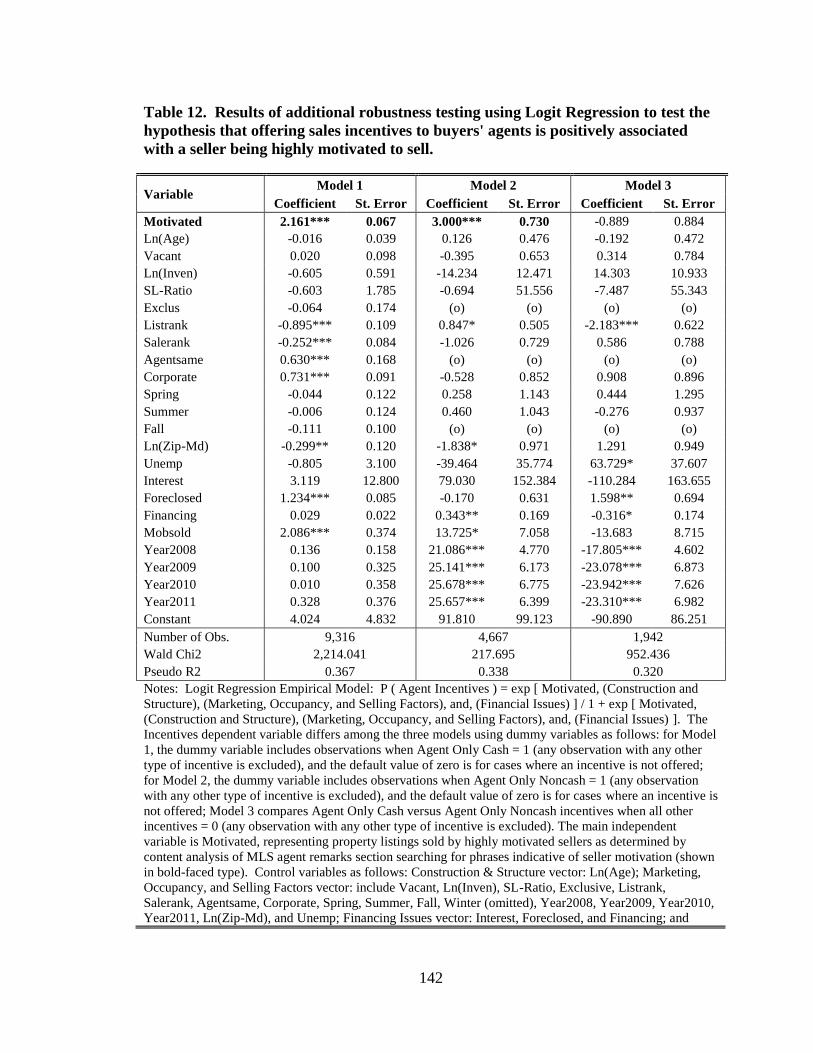
142

Table 12. Results of additional robustness testing using Logit Regression to test the

hypothesis that offering sales incentives to buyers' agents is positively associated

with a seller being highly motivated to sell.

Variable Model 1 Model 2 Model 3

Coefficient St. Error Coefficient St. Error Coefficient St. Error

Motivated 2.161*** 0.067 3.000*** 0.730 -0.889 0.884

Ln(Age) -0.016 0.039 0.126 0.476 -0.192 0.472

Vacant 0.020 0.098 -0.395 0.653 0.314 0.784

Ln(Inven) -0.605 0.591 -14.234 12.471 14.303 10.933

SL-Ratio -0.603 1.785 -0.694 51.556 -7.487 55.343

Exclus -0.064 0.174 (o) (o) (o) (o)

Listrank -0.895*** 0.109 0.847* 0.505 -2.183*** 0.622

Salerank -0.252*** 0.084 -1.026 0.729 0.586 0.788

Agentsame 0.630*** 0.168 (o) (o) (o) (o)

Corporate 0.731*** 0.091 -0.528 0.852 0.908 0.896

Spring -0.044 0.122 0.258 1.143 0.444 1.295

Summer -0.006 0.124 0.460 1.043 -0.276 0.937

Fall -0.111 0.100 (o) (o) (o) (o)

Ln(Zip-Md) -0.299** 0.120 -1.838* 0.971 1.291 0.949

Unemp -0.805 3.100 -39.464 35.774 63.729* 37.607

Interest 3.119 12.800 79.030 152.384 -110.284 163.655

Foreclosed 1.234*** 0.085 -0.170 0.631 1.598** 0.694

Financing 0.029 0.022 0.343** 0.169 -0.316* 0.174

Mobsold 2.086*** 0.374 13.725* 7.058 -13.683 8.715

Year2008 0.136 0.158 21.086*** 4.770 -17.805*** 4.602

Year2009 0.100 0.325 25.141*** 6.173 -23.078*** 6.873

Year2010 0.010 0.358 25.678*** 6.775 -23.942*** 7.626

Year2011 0.328 0.376 25.657*** 6.399 -23.310*** 6.982

Constant 4.024 4.832 91.810 99.123 -90.890 86.251

Number of Obs. 9,316 4,667 1,942

Wald Chi2 2,214.041 217.695 952.436

Pseudo R2 0.367 0.338 0.320

Notes: Logit Regression Empirical Model: P ( Agent Incentives ) = exp [ Motivated, (Construction and

Structure), (Marketing, Occupancy, and Selling Factors), and, (Financial Issues) ] / 1 + exp [ Motivated,

(Construction and Structure), (Marketing, Occupancy, and Selling Factors), and, (Financial Issues) ]. The

Incentives dependent variable differs among the three models using dummy variables as follows: for Model

1, the dummy variable includes observations when Agent Only Cash = 1 (any observation with any other

type of incentive is excluded), and the default value of zero is for cases where an incentive is not offered;

for Model 2, the dummy variable includes observations when Agent Only Noncash = 1 (any observation

with any other type of incentive is excluded), and the default value of zero is for cases where an incentive is

not offered; Model 3 compares Agent Only Cash versus Agent Only Noncash incentives when all other

incentives = 0 (any observation with any other type of incentive is excluded). The main independent

variable is Motivated, representing property listings sold by highly motivated sellers as determined by

content analysis of MLS agent remarks section searching for phrases indicative of seller motivation (shown

in bold-faced type). Control variables as follows: Construction & Structure vector: Ln(Age); Marketing,

Occupancy, and Selling Factors vector: include Vacant, Ln(Inven), SL-Ratio, Exclusive, Listrank,

Salerank, Agentsame, Corporate, Spring, Summer, Fall, Winter (omitted), Year2008, Year2009, Year2010,

Year2011, Ln(Zip-Md), and Unemp; Financing Issues vector: Interest, Foreclosed, and Financing; and

143

Mobsold is the Mobile dummy. The results in the table reflect a total of 9,316 observations in Model 1,

4,667 observations in Model 2, and 1,942 observations in Model 3 because the control variables Ln(Age),

Vacant, Exclus, Corporate, and Financing have missing values. Estimation of the equation without these

five control variables produces different coefficient values; however, the result is the same, as the

Motivated variable remains positive and significant. All regressions use robust estimations. Statistical

significance indicated as: * p < 0.05, ** p < 0.01, *** p < 0.001, respectively.

in Model 3 the Motivated variable coefficient is insignificant. This means there is no

statistical difference between using agent cash incentives versus agent noncash

incentives. Therefore, all that matters is the presence of incentives offered to the agent,

not whether it is a cash or noncash incentive. The results of these additional tests provide

further support for Hypothesis 2, confirming that highly motivated sellers are likely to

offer incentives to agents.42

In my initial testing of Hypotheses 3 and 4, I include just the Incentives dummy

variable to test how seller-paid sales incentives affect sales price and marketing duration.

However, I did not analyze the effects of any specific incentive types or forms.

Therefore, for robustness, using a 2SLS estimation, I test Hypotheses 3 and 4 using a

number of incentives dummy variables constructed to include different incentive forms,

42

I also conduct three additional series of robustness tests using additional dummy variables as defined in

Table 10 (results not reported). First, I test Equation (4) three separate ways using Agent-CNC1, Agent-

CNC2, and Agent-CNC3, respectively, instead of the incentives dummy. When Agent-CNC1 is the

dependent variable, the Motivated dummy variable coefficient is positive and significant, which again

suggests that highly motivated sellers are likely to offer sales incentives to agents, regardless of whether

they are cash or noncash. The Motivated dummy coefficients are insignificant when Agent-CNC2 and

Agent-CNC3 are the dependent variables, respectively. Second, I test Equation (4) three different ways

using the individual agent incentive types shown in Table 2, Panel B, to determine if a highly motivated

seller is more or less likely to offer a specific type of agent cash or noncash incentive. The Motivated

dummy coefficient is positive and significant in all estimations, suggesting that highly motivated sellers are

just as likely to offer one type of agent incentive as another type. Lastly, I test Equation (4) four different

ways using various forms of buyer incentives dummies in place of the agent incentives dummies as

follows: Buyer Incentives, Buyer Cash, Buyer Noncash, and Buyer-Compare. The Motivated dummy

coefficients are positive and significant in the first three estimations, suggesting that highly motivated

sellers are likely to offer buyer incentives that are either cash, noncash, or both. However, in the fourth

estimation, the Motivated coefficient is negative and significant, suggesting that when comparing cash

incentives to noncash incentives, highly motivated sellers are less likely to offer cash incentives than

noncash incentives.

144

types, and combinations, to test Equations (8) and (10).43

I use two models to test

separately each of the hypotheses. In Model 1, I include the dummy variables Buyer

Incentives Only that takes the value of one if the seller offers incentives only to the buyer,

and zero otherwise; Agent Incentives Only that takes the value of one if the seller offers

incentives only to the agent, and zero otherwise; and, Both Incentives that takes the value

of one if the seller offers incentives to both the buyer and the agent, and zero otherwise.

In Model 2, I include dummies for Buyer Only Cash that takes the value of one if the

seller offers only cash incentives only to the buyer, and zero otherwise; Buyer Only

Noncash that takes the value of one if the seller offers only noncash incentives only to the

buyer, and zero otherwise; Agent Only Cash that takes the value of one if the seller offers

only cash incentives only to the agent, and zero otherwise; Agent Only Noncash that takes

the value of one if the seller offers only noncash incentives only to the agent, and zero

otherwise; Both Cash that takes the value of one if the seller offers only cash incentives

to both the buyer and the agent, and zero otherwise; and, Both Noncash that takes the

value of one if the seller offers only noncash incentives to both the buyer and the agent.

Table 13 shows the results for the additional Hypothesis 3 testing. In Model 1,

the Buyer Incentives Only and Both Incentives dummy variable coefficients are positive

and significant (β = 0.023 and β = 0.013, respectively), yet there is no significance for the

Agent Incentives Only dummy coefficient. In Model 2, the dummy variable coefficients

for Buyer Only Cash, Buyer Only Noncash, and Both Noncash are positive and

significant (β = 0.015, β = 0.017, and β = 0.025, respectively), but in this model too, there

is no significance for the agent incentives dummies. These results provide additional

43

The second stage includes the IMR as an independent variable (produced in testing Equation (7)).

145

Table 13. Results of 2SLS Regression testing the hypothesis that offering sales

incentives is positively associated with sale price.

Variable Model 1 Model 2

Coefficient St. Error Coefficient St. Error

IMR -1.134*** 0.044 -1.148*** 0.044

Buyer Incentives Only 0.023*** 0.003

Agent Incentives Only 0.008 0.006

Both Incentives 0.013*** 0.004

Buyer Only Cash 0.015*** 0.003

Buyer Only Noncash 0.017*** 0.006

Agent Only Cash 0.006 0.006

Agent Only Noncash -0.112 0.077

Both Cash -0.005 0.004

Both Noncash 0.025*** 0.009

Ln(Age) -0.047*** 0.006 -0.045*** 0.006

Ln(SqFeet) 0.680*** 0.008 0.680*** 0.008

Storynum 0.010 0.007 0.010 0.007

New -0.166*** 0.007 -0.158*** 0.007

Brick 0.011*** 0.003 0.011*** 0.003

Bednum -0.051*** 0.003 -0.051*** 0.003

Bathnum 0.200*** 0.007 0.200*** 0.007

Fire 0.195*** 0.003 0.195*** 0.003

Central 0.670*** 0.010 0.671*** 0.010

Parknum 0.078*** 0.001 0.078*** 0.001

Pool 0.104*** 0.004 0.105*** 0.004

Water 0.015*** 0.005 0.016*** 0.005

Urban -0.001 0.003 -0.001 0.003

Golf -0.000 0.007 -0.001 0.007

Subd-PUD 0.003 0.004 0.003 0.004

Pubwater -0.005 0.006 -0.005 0.006

Pubsewer -0.006** 0.003 -0.006** 0.003

DOP 0.936*** 0.009 0.937*** 0.009

Vacant -0.013*** 0.003 -0.014*** 0.003

Ln(Inven) 0.038 0.024 0.040* 0.024

SL-Ratio -0.137** 0.062 -0.140** 0.062

Exclusive 0.029*** 0.006 0.030*** 0.006

Listrank 0.199*** 0.008 0.200*** 0.008

Salerank -0.048*** 0.003 -0.048*** 0.003

Agentsame 0.163*** 0.011 0.164*** 0.011

Corporate -0.225*** 0.007 -0.228*** 0.007

Ln(Zip-Md) 0.093*** 0.007 0.092*** 0.007

Unemp -2.090*** 0.184 -2.105*** 0.184

Interest -1.940*** 0.506 -1.932*** 0.506

Foreclosed 0.050*** 0.005 0.049*** 0.005

Financing -0.019*** 0.002 -0.019*** 0.002

Mobsold 0.082*** 0.017 0.081*** 0.017

Spring -0.003 0.004 -0.003 0.004

146

Summer 0.004 0.005 0.004 0.005

Fall -0.002 0.004 -0.002 0.004

Year2008 0.023*** 0.006 0.023*** 0.006

Year2009 0.061*** 0.015 0.062*** 0.015

Year2010 0.049*** 0.016 0.050*** 0.016

Year2011 0.017 0.017 0.018 0.017

Constant 5.192*** 0.198 5.191*** 0.199

Number of Obs. 17,322 17,322

F 7,108.402 6,644.945

Adjusted R2 0.970 0.970

Notes: 2SLS Regression Empirical Model: P (Incentives) = Φ [ ln(List) + ∑ (Construction and Structure)

+ ∑ (Marketing, Occupancy, and Selling Factors) + ∑ (Financial Issues) ]. In each of the four models

presented, the first stage dependent variable is Any Incentives. The main independent variable is Ln(List).

Control variables are: from the Construction & Structure vector: Ln(Age); from the Marketing, Occupancy,

and Selling Factors vector: Vacant, Ln(Inven), SL-Ratio, Exclusive (omitted in Model 5b), Listrank,

Salerank (omitted in Model 5b), Agentsame, Corporate, Spring, Summer, Fall, Winter (omitted), Year2008,

Year2009, Year2010, Year2011, Ln(Zip-Md), and Unemp; from the Financing Issues vector: Interest,

Foreclosed, and Financing. In the second stage, the dependent variable is Ln(Sale). The IMR of Any

Incentives from the first stage is included as an independent variable, and the main independent variables

are drawn from the Incentives vector as follows: (1) Model 1 uses Buyer Incentives Only, defined as Buyer

Incentives = 1 and all other incentives = 0 , Agent Incentives Only, defined as Agent Incentives = 1 and all

other incentives = 0, and Both Buyer & Agent Incentives, defined as Buyer & Agent Incentives = 1; Model

2 uses Buyer Only Cash, defined as Buyer Only Cash = 1 when all other incentives = 0, Buyer Only

Noncash, defined as Buyer Only Noncash = 1 when all other incentives = 0, Agent Only Cash, defined as

Agent Only Cash = 1 when all other incentives = 0, Agent Only Noncash, defined as Agent Only Noncash

= 1 when all other incentives = 0, Buyer Only Cash & Noncash, defined as Buyer Only Cash & Noncash

incentives = 1 when all other incentives = 0, Agent Only Cash & Noncash, defined as Agent Only Cash &

Noncash incentives = 1 when all other incentives = 0, and Both Buyer & Agent Cash & Noncash, defined

as Buyer & Agent Cash & Noncash incentives = 1 when all other incentives = 0 (statistically significant

IMR and main independent variables shown in bold-faced type). Control variables are: from the

Construction & Structure vector: Ln(Age), Ln(SqFeet), Storynum, New, and Brick; from the House

Internal Features vector: Bednum, Bathnum, Fire, and Central; from the House External Features vector:

Parknum and Pool; from the Environmental-Natural vector: Water; from the Environmental-Neighborhood

& Location vector: Urban and Golf; from the Environmental-Public Service vector: Subdpud, Pubwater,

Pubsewer; from the Marketing, Occupancy, and Selling Factors vector: Vacant, Ln(Inven), SL-Ratio,

Exclusive, Listrank, Salerank, Agentsame, Corporate, Spring, Summer, Fall, Winter (omitted), Year2008,

Year2009, Year2010, Year2011, Ln(Zip-Md), and Unemp; from the Financing Issues vector: Interest,

Foreclosed, and Financing; Mobsold is the Mobile dummy; and DOP is the degree of over-pricing. All

regressions use robust estimations. Statistical significance indicated as: * p < 0.05, ** p < 0.01, *** p <

0.001, respectively.

support for Hypothesis 3, but also show that buyer sales incentives positively affect sales

price, while agent sales incentives do not.44

44

This finding concurs with the findings of Johnson, Anderson, and Benefield (2004) that selling agent

bonuses do not consistently produce higher sales prices.

147

Table 14 shows the results for the additional testing of Hypothesis 4. In Model 1,

the Agent Incentives Only and Both Incentives dummy variable coefficients are positive

and significant (β = 0.119 and β = 0.022, respectively), yet there is no significance for the

Buyer Incentives Only dummy coefficient. In Model 2, the dummy variable coefficient

for Buyer Only Cash is negative and significant (β = -0.033), while the coefficients for

the Agent Only Cash and Both Cash dummies are positive and significant (β = 0.092 and

β = 0.151, respectively). In my initial tests of Hypothesis 4, contrary to my expectation, I

find that incentives do not decrease marketing duration, but rather increase it. The results

of these additional tests underscore the influence of agent incentives in the initial test

results, while they also indicate that buyer cash incentives, by themselves, may reduce

marketing duration. The significance of this particular result may be because of the

actual type of buyer cash incentive itself. Consider that a home warranty that insures

against property component failures, or allowances for either closing costs or repairs

essentially put cash in a buyer‘s pocket. As these types of incentives actually reduce a

buyer‘s purchase costs, buyers may react to properties offering these types of buyer cash

incentives faster than they react to properties without them.45

45

I use the individual types of incentives as shown on Table 2, Panel B, to test whether the type of

incentive a seller offers a buyer or an agent (such as a warranty or prize) makes a difference in achieving

the goal of higher price or shorter time on market (results not reported). The coefficients for the

Seller/Builder Warranty and Allowance for Repair/Redecorating dummies, both buyer cash incentives, and

the Agent Prize or Gift dummy, an agent noncash incentive, are positive and significant, which suggests

that offering these particular types of incentives may positively influence sales price. The coefficients for

Closings Costs Allowance, a buyer cash incentive, and Selling Agent Bonus and Selling Agent Prize or Gift,

agent cash and non-cash incentives, dummies, respectively, are positive and significant, which suggests an

association between these types of individual incentives and longer marketing duration. As a final

robustness test, I use OLS to alternatively test Hypotheses 3 and 4. The results are strikingly similar to the

results using a 2SLS estimation (results not reported). The lone exception is that the results for tests for

Hypothesis 3 also show a positive and significant coefficient for Both Noncash.

148

Table 14. Results of 2SLS Regression testing the hypothesis that offering sales

incentives is negatively associated with marketing duration.

Variable Model 1 Model 2

Coefficient St. Error Coefficient St. Error

IMR -2.572*** 0.326 -2.621*** 0.327

Buyer Incentives Only 0.010 0.016

Agent Incentives Only 0.119*** 0.022

Both Incentives 0.179*** 0.022

Buyer Only Cash -0.033** 0.016

Buyer Only Noncash 0.015 0.032

Agent Only Cash 0.092*** 0.022

Agent Only Noncash 0.266 0.244

Both Cash 0.151*** 0.029

Both Noncash 0.019 0.039

Ln(Sale) -0.711*** 0.055 -0.701*** 0.055

Ln(Age) 0.206*** 0.043 0.214*** 0.043

Ln(SqFeet) 0.775*** 0.052 0.768*** 0.052

Storynum 0.018 0.028 0.014 0.028

New -0.087* 0.050 -0.059 0.050

Brick -0.044*** 0.014 -0.044*** 0.014

Bednum -0.058*** 0.014 -0.057*** 0.014

Bathnum 0.121*** 0.019 0.119*** 0.019

Fire 0.154*** 0.022 0.155*** 0.022

Central 0.492*** 0.050 0.496*** 0.050

Parknum 0.061*** 0.010 0.059*** 0.010

Pool 0.110*** 0.025 0.111*** 0.025

Water 0.141*** 0.033 0.141*** 0.033

Urban 0.004 0.018 0.003 0.018

Golf 0.115*** 0.040 0.112*** 0.040

Subd-PUD 0.031 0.023 0.032 0.023

Pubwater -0.010 0.034 -0.011 0.034

Pubsewer -0.092*** 0.019 -0.092*** 0.019

DOP 0.616*** 0.059 0.609*** 0.059

Vacant 0.045*** 0.015 0.042*** 0.015

Ln(Inven) -0.397*** 0.144 -0.395*** 0.144

SL-Ratio -0.505 0.378 -0.540 0.378

Exclusive 0.168*** 0.038 0.171*** 0.038

Listrank 0.424*** 0.061 0.431*** 0.061

Salerank -0.105*** 0.023 -0.108*** 0.023

Agentsame -0.398*** 0.090 -0.394*** 0.090

Corporate -0.441*** 0.060 -0.449*** 0.060

Ln(Zip-Md) -0.126*** 0.036 -0.133*** 0.036

Unemp -5.876*** 1.065 -5.907*** 1.065

Interest 3.407 3.178 3.341 3.178

Foreclosed -0.045* 0.026 -0.041 0.026

Financing -0.046*** 0.012 -0.047*** 0.012

Mobsold 0.515*** 0.092 0.513*** 0.092

149

Spring 0.000 0.027 0.001 0.027

Summer 0.121*** 0.029 0.123*** 0.029

Fall 0.071*** 0.024 0.071*** 0.024

Year2008 -0.641*** 0.033 -0.641*** 0.033

Year2009 -0.345*** 0.086 -0.345*** 0.086

Year2010 -0.292*** 0.093 -0.291*** 0.093

Year2011 -0.334*** 0.097 -0.335*** 0.097

Constant 12.316*** 1.294 12.371*** 1.296

Number of Obs. 17,322 17,322

F 58.784 54.543

Adjusted R2 0.101 0.100

Notes: 2SLS Regression Empirical Model: P (Incentives) = Φ [ ln(List) + ∑ (Construction and

Structure) + ∑ (Marketing, Occupancy, and Selling Factors) + ∑ (Financial Issues) ]. In each of the

four models presented, the first stage dependent variable is Incentives. The main independent

variable is Ln(List). Control variables are: from the Construction & Structure vector: Ln(Age); from

the Marketing, Occupancy, and Selling Factors vector: Vacant, Ln(Inven), SL-Ratio, Exclusive,

Listrank, Salerank, Agentsame, Corporate, Spring, Summer, Fall, Winter (omitted), Year2008,

Year2009, Year2010, Year2011, Ln(Zip-Md), and Unemp; from the Financing Issues vector:

Interest, Foreclosed, and Financing. In the second stage, the dependent variable is TOM. The IMR

of Any Incentives from the first stage is included as an independent variable, as is Ln(Sale). The

main independent variables are drawn from the Incentives vector as follows: (1) Model 1 uses

Buyer Incentives Only, defined as Buyer Incentives = 1 and all other incentives = 0 , Agent

Incentives Only, defined as Agent Incentives = 1 and all other incentives = 0, and Both Buyer &

Agent Incentives, defined as Buyer & Agent Incentives = 1; Model 2 uses Buyer Only Cash,

defined as Buyer Only Cash = 1 when all other incentives = 0, Buyer Only Noncash, defined as

Buyer Only Noncash = 1 when all other incentives = 0, Agent Only Cash, defined as Agent Only

Cash = 1 when all other incentives = 0, Agent Only Noncash, defined as Agent Only Noncash = 1

when all other incentives = 0, Buyer Only Cash & Noncash, defined as Buyer Only Cash &

Noncash incentives = 1 when all other incentives = 0, Agent Only Cash & Noncash, defined as

Agent Only Cash & Noncash incentives = 1 when all other incentives = 0, and Both Buyer & Agent

Cash & Noncash, defined as Buyer & Agent Cash & Noncash incentives = 1 when all other

incentives = 0 (statistically significant IMR and main independent variables shown in bold-faced

type). Control variables are: from the Construction & Structure vector: Ln(Age), Ln(SqFeet),

Storynum, New, and Brick; from the House Internal Features vector: Bednum, Bathnum, Fire, and

Central; from the House External Features vector: Parknum and Pool; from the Environmental-

Natural vector: Water; from the Environmental-Neighborhood & Location vector: Urban and Golf;

from the Environmental-Public Service vector: Subdpud, Pubwater, Pubsewer; from the Marketing,

Occupancy, and Selling Factors vector: Vacant, Ln(Inven), SL-Ratio, Exclusive, Listrank, Salerank,

Agentsame, Corporate, Spring, Summer, Fall, Winter (omitted), Year2008, Year2009, Year2010,

Year2011, Ln(Zip-Md), and Unemp; from the Financing Issues vector: Interest, Foreclosed, and

Financing; Mobsold is the Mobile dummy; and DOP is the degree of over-pricing. All regressions

use robust estimations. Statistical significance indicated as: * p < 0.05, ** p < 0.01, *** p < 0.001,

respectively.

Limitations

Many real estate markets across the country, even though in different locations,

share certain similarities including various demographic factors such as population size,

150

ethnicity makeup, education profiles, workforce characteristics, and income levels. Many

markets are also similar in terms of geography or climate patterns. Thus, to the extent

that other markets in the U.S. share such similarities with this study‘s samples, the results

of the use of seller-paid incentives in this study should be generalizable to property sales

in other, similar markets. Nonetheless, the reader should exercise caution in interpolating

the results of this study.

An agent may possibly offer incentives to a seller (i.e. reduced sales commission)

to secure a property listing. However, the MLS systems do not report these data.

Therefore, I do not examine any incentives that listing agents may offer to sellers.

Individual seller and buyer characteristics, such as age, gender, occupation,

wealth, income, tolerance for risk, and tastes and preferences for different types of

properties are likely to influence sales outcomes. However, because of privacy laws,

MLS systems typically restrict the reporting of these data. Therefore, such information is

not included in the empirical analysis, providing opportunities for future research using

field-based studies such as surveys and interviews to obtain the necessary data.

VII. Concluding Remarks

This study examines sellers who offer sales incentives to motivate residential

property sales. The dataset includes sales transactions occurring in the Mobile and

Montgomery, Alabama market areas during the 2008-2011 cold market conditions. I

include a variety of cash and/or noncash seller-paid sales incentives offered to buyers,

buyers‘ agents, and/or both. Four areas are of primary interest.

151

First, just as the issue of financial asset liquidity is important to stockholders, it is

equally important to owners of real estate assets. Indeed, because stockholders may

easily buy and sell their positions, yet owners of real estate generally cannot; therefore,

liquidity may be an even more important issue to real estate owners. Second, some

sellers are highly motivated to sell for extreme reasons, such as financial problems, job

loss, health problems, or even possible foreclosure. These sellers not only want to sell,

they have to sell. Therefore, discovering ways to signal selling motivation to produce

desired outcomes may be an important issue to property sellers. Third, this study extends

the work of previous studies that investigate the use of buyer incentives to increase sales

price by also including agent incentives, and combinations of buyer and agent incentives.

I do this to determine if, and to what extent offering incentives to the buyer, the agent, or

both; or even if, and to what extent a particular type or form of incentive influences sales

price. Fourth, within the real estate literature, studies of the factors influencing sales

price generally include a parallel examination of the length of time necessary to sell a

property given certain conditions. Accordingly, I also investigate if, and to what extent

sales incentives affect marketing duration.

I start by examining the use of buyer incentives as a means of adjusting a

property‘s price downward relative to comparable properties in the market. By offering

incentives to buyers, things such as closing cost allowances, or a willingness to provide

mortgage financing, effectively the seller attempts to reduce the difference between the

list and sales prices, and as a result, works to motivate investment by pricing his/her

property more competitively than similar properties. I do find a positive relationship

between the bid-ask spread and the likelihood that sellers will offer buyer incentives.

152

This suggests that by offering sales incentives to buyers, sellers can effectively increase

the liquidity of their properties. Of course, this also would seem to imply that by doing

so, sellers should be able to sell in less time as well.

I then explore the use of agent incentives as a means of attracting as many buyers‘

agents as possible. By offering incentives to agents, things such as a higher selling agent

commission split or selling bonus, or some type of prize or reward, in essence, the highly

motivated seller effectively increases the economic utility available to agents for selling

his/her property. In doing so, the seller is in essence working to motivate investment by

attempting to increase his/her property‘s awareness amongst the agents at work in the

market. I do find a positive relationship between a seller being highly motivated to sell,

and the likelihood that sellers will offer agent incentives. By successfully increasing

agent coverage, a likely outcome is that not only will the chances of a sale increase, but

also that it will happen in less time.

Next, I investigate whether the use of incentives results in higher sales prices. I

test this in general at first, and find that offering incentives, regardless of recipient, or

mode, does produce higher sales prices. I further find that buyer incentives, and buyer

incentives offered in combination with agent incentives have a positive impact on sales

price, but that agent incentives, when tested in isolation, do not. Moreover, I find no

differentiation in the outcomes between the uses of buyer cash versus non-cash

incentives. Thus, the conclusion from this analysis is that it is possible for sellers to

achieve higher sales prices by utilizing a sales incentives strategy.

Finally, I assess how incentives influence marketing duration. As in the

examination of incentives‘ impacts on sales price, I start by testing the use of incentives

153

generally. In this case, I find that incentives tend to increase marketing duration, and that

specifically, buyer incentives as a whole have no statistically significant affect, but that

agent incentives do. The lone exception is buyer cash incentives, which according to the

analysis, do seem to decrease the time it takes to sell a property. Overall, though, these

results seem at odds with the earlier findings that suggest that sellers are more likely to

use incentives to reduce the bid-ask spread and increase buyers‘ agent coverage, both for

the apparent purpose of obtaining the highest possible price in the shortest possible time.

Collectively, the results of my study are consistent with a number of findings.

Sellers offer sales incentives to buyers to reduce the bid-ask spread. Sellers offer sales

incentives to agents to increase buyers‘ agents‘ coverage. Sellers offer sales incentives to

increase their sales price. However, when offering sales incentives, the seller must also

be willing to wait longer in order to realize a higher price.

154

REFERENCES

Adrian, T., & Shin, H. (2010). Financial intermediaries and monetary economics. FRB of

New York Staff Report No. 398. Retrieved on June 3, 2013 from:

http://ssrn.com/abstract=1491603 or http://dx.doi.org/10.2139/ssrn.1491603.

Allen, F., & Gale, D. (2004). Financial intermediaries and markets. Econometrica, 72(4),

1023-1061.

Amihud, Y., & Mendelson, H. (1986). Asset pricing and the bid-ask spread. Journal of

Financial Economics, 17(2), 223-249.

Amihud, Y., & Mendelson, H. (2000). The liquidity route to a lower cost of capital.

Journal of Applied Corporate Finance, 12(4), 8-25.

Anglin, P. M., Rutherford, R., Springer, T. M. (2003). The trade-off between the selling

price of residential properties and time-on-the-market: The impact of selling

price. Journal of Real Estate Finance and Economics, 26(1), 95-111.

Asabere, P. K., & Huffman, F. E. (1997). Discount point concessions and the value of

homes with conventional versus nonconventional mortgage financing. Journal of

Real Estate Finance and Economics, 15(3), 261–270.

Asabere, P. K., Huffman, F. E., & Mehdian, S. (1993). Mispricing and optimal time on

the Market. Journal of Real Estate Research, 8(1), 149-155.

Bagehot, W. (1971). The only game in town. Financial Analysts Journal, 27(2), 12-14.

Baker, D. (2008). The housing bubble and the financial crisis. Center for Economic and

Policy Research, Real-World Economics Review. Retrieved on August 3, 2012,

from http://faculty.unlv.edu/msullivan/Housing%20Bubble.pdf.

Barth, M. E., & Hutton, A. P. (2004). Analyst earnings forecast revisions and the pricing

of accruals. Review of Financial Studies, 9(1), 59-96.

Baryla, E. A., & Zumpano, L. V. (1995). Buyer search duration in the residential real

estate market: The role of the real estate agent. Journal of Real Estate Research,

10(1), 1-13.

155

Belkin, J., Hempel, D. J., & McLeavy, D. W. (1976). An empirical study of time on

market using multidimensional segmentation of housing markets. Real Estate

Economics, 4(2), 57-75.

Brastow, R. T., Springer, T. M., & Waller, B. D. (2011). Efficiency and incentives in

residential brokerage. Journal of Real Estate Finance and Economics, 45(4),

1041-1061.

Browne, M. J. (1992). Evidence of adverse selection in the individual health insurance

market. Journal of Risk and Insurance, 59(1), 13-33.

Chang, X., Dasgupta, S., & Hilary, G. (2006). Analyst coverage and financing decisions.

The Journal of Finance, 61(6), 3009-3048.

Chordia, T., Roll, R., & Subrahmanyam, A. (2000). Commonality in liquidity. Journal

of Financial Economics, 56(1), 3-28.

Chordia, T., Sarkar, A., & Subrahmanyam, A. (2005). An empirical analysis of stock

and bond market liquidity. Review of Financial Studies, 18(1), 85-129.

Crowston, K. Sawyer, S. & Wigand, R. (2001). Investigating the interplay between

structure and information and communications technology in the real estate

industry. Information Technology & People, 14(2), 163-183.

Cunningham, C., & Reed, R. R. (2012). The role of housing equity for labor market

activity. Mimeo, University of Alabama. Retrieved on April 28, 2013, from

http://old.cba.ua.edu/~rreed/NegativeEquityLaborMarketsShortVersionJuly92012

.pdf.

D'Mello, R., & Ferris, S. P. (2000). The information effects of analyst activity at the

announcement of new equity issues. Financial Management, 29(1), 78-95.

Demsetz, H., (1968). The cost of transacting. Quarterly Journal of Economics, 82(1),

33–53.

Elder, H. W., Zumpano, L. V., & Baryla, E. A. (2000). Buyer brokers: do they make a

difference? Their influence on selling price and search duration. Real Estate

Economics, 28(2), 337-362.

Elgers, P. T., Lo, M. H., & Pfeiffer, R. J. (2001). Delayed security price adjustments to

financial analysts‘ forecasts of annual earnings. The Accounting Review, 76(4),

613-632.

Epley, D. R., Rabianski, J. S., & Haney, R. L., Jr. (2002). Real estate decisions, Mason,

Ohio: Southwestern Publishing.

156

Forgey, F. A, Rutherford, R. C., & Springer, T. M. (1996). Search and liquidity in single

family housing. Real Estate Economics, 24(3), 273–292.

Foster, J. B. (2008). The financialization of capital and the crisis. Monthly Review,

59(11), 1-19.

Francis, J., & Soffer, L. (1997). The relative informativeness of analysts‘ stock

recommendations and earnings forecast revisions. Journal of Accounting

Research, 35(2), 193–212.

Gardner, M. J., & Mills, D. L. (1989). Evaluating the likelihood of default on delinquent

loans. Financial Management, 18(4), 55-63.

Garmaise, M. J., & Moskowitz, T. J. (2004). Confronting information asymmetries:

Evidence from real estate markets. Review of Financial Studies, 17(2), 405-437.

Geltner, D., Kluger, B. D., & Miller, N. G. (1991). Optimal price and selling effort from

the perspectives of the broker and seller. Real Estate Economics, 19(1), 1–24.

Givoly, D. (1982). Financial analysts‘ forecasts of earnings: A better surrogate for

market expectations. Journal of Accounting and Economics, 4(2), 85–108.

Glosten, L. R., & Milgrom, P. R. (1985). Bid, ask, and transaction prices in a specialist

market with heterogeneously informed traders. Journal of Financial Economics,

14(1), 71-100.

Goetzmann, W. N., & Spiegel, M. (1995). Non-temporal components of residential real

estate appreciation. Review of Economics and Statistics, 77(1), 199-206.

Hair, J. F., Jr., Black, W. C., Babin, B. J., & Anderson, R. E. (2002). Multivariate data

analysis.(7th

Ed.). Upper Saddle River, NJ: Prentice-Hall.

Haurin, D. (1988). The duration of marketing time of residential housing. Real Estate

Economics, 16(4), 396-410.

Healy, P. M., & Palepu, K. G. (2001). Information asymmetry, corporate disclosure, and

the capital markets: A review of the empirical disclosure literature. Journal of

Accounting and Economics, 31(1), 405-440.

Heckman, J. (1979). Sample selection bias as a specification error. Econometrica, 47(1),

153–61.

Holmström, B., & Tirole, J. (1993). Market liquidity and performance monitoring.

Journal of Political Economy, 101(4), 678-709.

157

Ibbotson, R. G. (1975). Price performance of common stock new issues. Journal of

Financial Economics, 2(3), 235-272.

Johnson, K. H., Anderson, R. I., & Benefield, J. D. (2004). Salesperson bonuses and

their impact on residential property price and duration. Journal of Real Estate

Practice and Education, 7(1), 1–14.

Johnson, K. H., Anderson, R. I., & Webb, J. R. (2000). The capitalization of seller paid

concessions. Journal of Real Estate Research, 19(3), 287-300.

Jud, G. D. (1983). Real estate brokers and the market for residential housing. Real

Estate Economics, 11(1), 69-82.

Jud, G., Seeks, T., & Winkler, D. (1996). Time on market: The impact of residential

brokerage. Journal of Real Estate Research, 12(2), 447-458.

Jud, G., & Winkler, D. (1994). What do real estate brokers do: An examination of

excess returns in the housing market. Journal of Housing Economics, 3(4), 283-

295.

Jud, G. D., Winkler, D. T., & Kissling, G. E. (1995). Price spreads and residential

housing market liquidity. Journal of Real Estate Finance and Economics, 11(3),

251-260.

Kalra, R., & Chan, K.C. (1994). Censored sample bias, macroeconomic factors, and

time on market of residential housing. Journal of Real Estate Research, 9(2),

253-262.

Kluger, B. D, & Miller, N. G. (1990). Measuring real estate liquidity. Real Estate

Economics, 18(2), 145-159.

Kluger, B. D., & Stephan, J. (1997). Alternative liquidity measures and stock returns.

Review of Quantitative Finance and Accounting, 8(1), 19-36.

Knight, J. R. (2002). Listing price, time on market, and ultimate selling price: Causes and

effects of listing price changes. Real Estate Economics, 30(2), 213-237.

Knight, J. R., Lizieri, C., & Satchell, S. (2005). Diversification when it hurts? The joint

distributions of real estate and equity markets. Journal of Property Research,

22(4), 309-323.

Krainer, J. (2001). A theory of liquidity in residential real estate markets. Journal of

Urban Economics, 49(1), 32-53.

158

Kyle, A. (1985). Continuous auctions and insider trading. Econometrica, 53(6), 1315-

1336.

Lippman, S. & McCall, J. (1986). An operational measure of liquidity. The American

Economic Review, 76(1), 43-55.

Lutz, B., Molloy, R., & Shan, H. (2011). The housing crisis and state and local

government tax revenue: Five channels. Regional Science and Urban Economics,

41(4), 306-319.

Lys, T., & Sohn, S., (1990). The association between revisions of financial analysts‘

earnings forecasts and security price changes. Journal of Accounting and

Economics, 13(4), 341–364.

Meyer, C. J. (1987). Stress: There‘s no place like a first home. Family Relations, 36(2),

198-203.

Miceli, T. J. (1989). The optimal duration of real estate listing contracts. Journal of

American Real Estate and Urban Economics Association, 17(3), 267-277.

Microsoft. (2010). Microsoft Excel [computer software]. Redmond, Washington:

Microsoft Corporation.

Miller, N. G. (1978). Time on market and selling price. Real Estate Economics, 6(2),

164-174.

Mises, L. V. (1912). The theory of money and credit. H. E. Baston, translator.

Indianapolis, Indiana: Liberty Classics.

Munneke, H. J., & Slade, B. A. (2000). An empirical study of sample-selection bias in

indices of commercial real estate. The Journal of Real Estate Finance and

Economics, 21(1), 45-64.

Rutherford, R. C., Springer, T. M., & Yavas, A. (2001). The impacts of contract type on

broker performance. Real Estate Economics, 29(3), 389-401.

Samuel, D. (2009). Subprime mortgage crisis: Will new regulations help avoid future

financial debacles? The Albany Governmental Law Review, 2(1), 217-258.

Schill, M. H. (1991). Uniformity or diversity: Residential real estate finance law in the

1990s and the implications of changing financial markets. University of Southern

California Law Review, 64(July), 1261-1283.

Sirmans, S. G., Macpherson, D. A., & Zietz, E. N. (2005). The composition of hedonic

pricing models. Journal of Real Estate Literature, 13(1), 1-44.

159

Smith, S. D., & Sirmans, G. S. (1984). The shifting of FHA discount points: Actual vs.

expected. Journal of American Real Estate and Urban Economics, 12(2), 153–

61.

Soyeh, K.W., Wiley, J. A., & Johnson, K. H. (2012). Do buyer incentives work for

houses? Presented at the 2012 American Real Estate Society Annual Conference,

St. Petersburg, Florida.

Springer, T. M. (1996). Single-family housing transactions: Seller motivations, price,

and marketing time. Journal of Real Estate Finance and Economics, 13(3), 237-

254.

Udell, G. F. (2009). Wall street, main street, and a credit crunch: Thoughts on the current

financial crisis. Business Horizons, 52(2), 117.

Waller, B., Brastow, R., & Johnson, K. H. (2010). Listing contract length and marketing

duration. Journal of Real Estate Research, 32(3), 271–288.

Welker, M. (1995). Disclosure policy, information asymmetry, and liquidity in equity

markets. Contemporary Accounting Research, 11(2), 801-827.

White, H. (1980). A heteroskedasticity-consistent covariance matrix estimator and a

direct test for heteroskedasticity. Econometrica, 48(4), 817-838.

White, H., & Lu, X. (2010). Robustness checks and robustness tests in applied

economics. University of California, San Diego, Department of Economics

Discussion Paper, retrieved on August 25, 2013 from

http://www.socsci.uci.edu/files/economics/docs/micro/s11/white.pdf.

Wimmer, B. S., Townsend, A. M., & Chezum, B. E. (2000). Information technologies

and the changing workplace. Journal of Labor Research, 21(3), 407-418.

Yavas, A., & Yang, S. (1995). The strategic role of listing price in marketing real estate:

Theory and evidence. Real Estate Economics, 23(3), 347-368.

Zerbst, R. H., & Bruggeman, W. B. (1977). FHA and VA mortgage discount points and

housing prices. The Journal of Finance, 32(5), 1766–1773.

Zumpano, L. V., Elder, H. W., & Baryla, E. A. (1996). Buying a house and the decision

to use a real estate broker. Journal of Real Estate Finance and Economics, 13(2),

169-181.