Essays in Infrastructure Investment - uni-regensburg.de · Essays in Infrastructure Investment...
159
Essays in Infrastructure Investment DISSERTATION by Diplom-Kaufmann, Master of Science Konrad Finkenzeller Submitted to the Faculty of Business Administration at the University of Regensburg in partial fulfillment of the requirements for the degree of Doctor rerum politicarum Dr. rer. pol. Regensburg, January 2012
Transcript of Essays in Infrastructure Investment - uni-regensburg.de · Essays in Infrastructure Investment...

Essays in Infrastructure Investment
DISSERTATION
by
Diplom-Kaufmann, Master of Science Konrad Finkenzeller
Submitted to the Faculty of Business Administration
at the University of Regensburg
in partial fulfillment of the requirements
for the degree of
Doctor rerum politicarum
Dr. rer. pol.
Regensburg, January 2012

Introduction
2
Table of Contents
1. Introduction ....................................................................................................................................................... 4
1.1 General Motivation ........................................................................................................................................... 4
1.2 Research Question ............................................................................................................................................. 6
1.3 Course of Analysis ............................................................................................................................................ 9
2. The Interactions Between Direct and Securitized Infrastructure and its Relationship to Real Estate ... 11
2.1 Introduction ..................................................................................................................................................... 12
2.2 Data ................................................................................................................................................................. 15
2.2.1 Correlations ........................................................................................................................................ 18
2.3 Methodology ................................................................................................................................................... 19
2.4 Results ............................................................................................................................................................. 21
2.4.1 Long-Run Dynamics........................................................................................................................... 21
2.4.2 Short-Run Dynamics .......................................................................................................................... 25
2.5 Summary and Conclusions .............................................................................................................................. 26
2.6 Appendix ......................................................................................................................................................... 27
2.5 Literature ......................................................................................................................................................... 28
3. Infrastructure - A New Dimension of Real Estate? An Asset Allocation Analysis .................................... 31
3.1 Introduction ..................................................................................................................................................... 32
3.2 Applied Data ................................................................................................................................................... 33
3.3 Why Infrastructure is not Real Estate ............................................................................................................. 34
3.4 Infrastructure Asset Allocation ....................................................................................................................... 37
3.4.1 Modern Portfolio Theory (MPT) ........................................................................................................ 37
3.4.2 Mean Semivariance Optimization ...................................................................................................... 38
3.4.3 Research Design ................................................................................................................................. 40
3.4.4 Asset Allocations ................................................................................................................................ 40
3.5 Concluding Remarks ....................................................................................................................................... 43
3.7 References ....................................................................................................................................................... 45
4. Real Estate: A Victim of Infrastructure? Evidence from Conditional Asset Allocation .......................... 47
4.1 Introduction ..................................................................................................................................................... 48
4.2 Literature Review ............................................................................................................................................ 51
4.3 The Concept of Downside Risk ...................................................................................................................... 53
4.4 Data ................................................................................................................................................................. 55
4.5 Descriptive Statistics and Downside Risk ....................................................................................................... 60
4.5 Downside Correlations .................................................................................................................................... 62
4.6 Asset Allocations ............................................................................................................................................ 65
4.6.1 Unconditional Portfolios ..................................................................................................................... 65
4.6.2 Bull Market Portfolios ........................................................................................................................ 66
4.6.3 Bear Market Portfolios ....................................................................................................................... 67
4.6.4 Constrained Asset Allocations ............................................................................................................ 70
4.7 The Effects of Infrastructure on Asset Weights .............................................................................................. 73
Introduction
3
4.7.1 Unconditional Portfolios ..................................................................................................................... 73
4.7.2 Bull Market Portfolios ........................................................................................................................ 74
4.7.3 Bear Market Portfolios ....................................................................................................................... 75
4.8 Conclusion ...................................................................................................................................................... 78
4.9 References ....................................................................................................................................................... 81
5. How much into Infrastructure? Evidence from Dynamic Asset Allocation ............................................... 85
5.1 Introduction ..................................................................................................................................................... 86
5.2 Literature Review ............................................................................................................................................ 87
5.3 Data ................................................................................................................................................................. 89
5.4 Methodology ................................................................................................................................................... 91
5.5 Descriptive Statistics ....................................................................................................................................... 95
5.6 Results ............................................................................................................................................................. 97
5.6.1 Mean-Variance Optimization ............................................................................................................. 97
5.6.2 Mean-Downside Risk Optimization ................................................................................................... 99
5.6.3 The Effects of Infrastructure on Portfolio Performance ................................................................... 101
5.6.4 The Role of the Investment Horizon................................................................................................. 103
5.6.5 Nominal vs. Real Returns ................................................................................................................. 106
3.6.6 Infrastructure and Real Estate ........................................................................................................... 107
5.7 Conclusion .................................................................................................................................................... 110
5.8 References ..................................................................................................................................................... 112
6. Direct Infrastructure Investment and its Role in Drawdown-Efficient Portfolios .................................. 114
6.1 Introduction ................................................................................................................................................... 115
6.2 Data and Descriptive Statistics ...................................................................................................................... 117
6.3 Methodology ................................................................................................................................................. 120
6.4 Results ........................................................................................................................................................... 125
6.4.1 The Role of Infrastructure in Drawdown Efficient Portfolios .......................................................... 125
6.4.2 Infrastructure, Pension Liabilities and Target Rate Relative Drawdown Risk ................................. 130
6.4.3 Downside Beta Hedged Portfolios .................................................................................................... 137
6.5 Conclusion .................................................................................................................................................... 142
6.6 Appendix ....................................................................................................................................................... 144
6.7 References ..................................................................................................................................................... 150
7. Conclusion ..................................................................................................................................................... 153
7.1 Executive Summary ...................................................................................................................................... 153
7.2 Final Remarks and Further Research ............................................................................................................ 158

Introduction
4
1. Introduction
1.1 General Motivation
The importance of asset allocation is widely discussed in the academic literature and free of
any controversy. It constitutes the essential foundation of investment decisions and is the
main determinant of portfolio performance. However, there is no consensus on how much
wealth should be allocated on a given asset class, as this depends on numerous variables such
as return expectations, risk aversion, macroeconomic circumstances, illiquidity and the specif-
ic investment horizon. The original basis for asset allocation has been eroded during the last
decade, as the traditionally main assets such as bonds, stocks and real estate have been affect-
ed by significant losses and are subject to considerable uncertainty. This makes it even more
difficult for fund managers to decide how much wealth should be allocated to the various po-
tential assets. Stock markets have suffered substantially through macroeconomic distortions
reflected in high volatility and poor average performance. Bonds, which constitute a major
share of institutional investment portfolios, are currently heavily influenced by growing gov-
ernmental debt obligations. The former “save haven” of real estate was the main activator of
the recent financial crisis and property markets lost substantially in value.
These impacts on investment portfolios have substantially altered investor perceptions and
attitudes towards their original asset allocation strategy. In order to avoid further substantial
losses as experienced during recent years, investors are now seeking sources of diversification
to supplement core assets like stocks, bonds and real estate. In this context, private invest-
ments in infrastructure have been identified by many institutional investors as a viable alter-
native. The infrastructure asset universe can be divided into two main categories: economic
and social infrastructure. Economic infrastructure includes long-lasting, large-scale physical
structures like transportation and communication infrastructure, as well as energy and utility
facilities. Social infrastructure, on the other hand, includes education, healthcare, waste dis-
posal and judicial facilities. Despite this diversity and heterogeneity, infrastructure assets are
considered to have attractive investment characteristics. The nature of infrastructure as a con-
servative, tangible and real asset seems to constitute a viable alternative to synthetic and com-
plex financial products. Furthermore, due to their monopolistic nature, infrastructure invest-
ments are expected to provide stable and predictable long-term cash flows, which may enable
investors to match their long-term liabilities. This monopolistic character and the provision of
basic services, might induce cash flows which are less vulnerable to economic downturns than

Introduction
5
those from other, more cyclical assets. In consequence, infrastructure might be able to stabi-
lize portfolio returns and reduce volatility. The private involvement in the infrastructure sec-
tor is driven by financial strains on governments, which render the public sector unable to
guarantee adequate infrastructure provision. However, this imbalance between infrastructure
provision and demand is expected to gain further momentum and increase privatization pres-
sure over the long run. Nevertheless, despite the promising future infrastructure’s track record
and its investment history are still young, raising the question of whether infrastructure will
really be able to meet optimistic investor expectations.
The infrastructure sector still lacks of professional structures and standardization at different
levels and additionally faces a classification problem within the portfolio. Accordingly, infra-
structure assets are often managed together with (seemingly) related assets like real estate.
Short histories and a lack of good quality direct performance data still impede independent
(academic) research and render infrastructure investment in-transparent, which in turn hinders
investment. The objective of this dissertation is to deal with some of these shortcomings and
to coherently analyze the role of direct infrastructure in a diversified portfolio, by using a
novel set of direct infrastructure performance data. In order to provide robust and meaningful
results, the dissertation deals with a number of different aspects which are important to the
asset allocation management process. In particular, the investigation accounts for different
markets, empirical models, expected returns, target rates, market phases, nominal and real
returns, hedging abilities in the context of liabilities and systematic market risk. Furthermore,
there is a specific and detailed focus on the relationship between real estate and infrastructure
and on the relationship between direct and indirect infrastructure returns.

Introduction
6
1.2 Research Question
The section provides a basic framework for this dissertation and the five articles, dealing with
the related research questions for each.
The Interactions Between Direct and Securitized Infrastructure and its Relationship to
Real Estate
What are the contemporaneous correlations between direct and indirect infrastructure and
other asset returns?
What is the long-run relationship between direct and indirect real infrastructure i.e. are
investors able to achieve long-term portfolio diversification benefits by allocating funds to
both direct and securitized infrastructure?
Are indirect and direct infrastructure assets driven in the long run by the same underlying
business factor - namely infrastructure?
Are there similarities regarding the long-run relationship between direct and indirect real
estate and direct and indirect infrastructure and are there any links between infrastructure
and real estate returns over the long run?
What are the adjustment speeds between direct and indirect infrastructure and the long-run
equilibrium?
What are the short-run dynamics between direct and indirect infrastructure and what are
the theoretical and empirical implementations?
Does indirect infrastructure reflect stock market or infrastructure performance in the short
run?
Infrastructure - A New Dimension of Real Estate? An Asset Allocation Analysis
What is an appropriate definition of infrastructure and what is the present status of research
on infrastructure investment research and what is the future potential in an asset allocation
context?
What mechanisms and frameworks are necessary to further develop the infrastructure in-
vestment market?
What data are currently available and to what extent do they limit infrastructure investment
research?

Introduction
7
What are the risk, return and diversification characteristics of direct and indirect infrastruc-
ture assets compared to other main assets?
What are the theoretical similarities and differences between real estate and infrastructure
assets?
What are the empirical similarities and differences between infrastructure and real estate
and should both be regarded as unique and separate asset classes?
Which role do direct and indirect infrastructure play in a multi-asset portfolio using a semi-
variance optimization (Estrada, 2007) and different investor specific target rates of return?
Real Estate: A Victim of Infrastructure? Evidence from Conditional Asset Allocation
What is the present state and scope of the literature in this relatively new field of invest-
ment research?
What role does infrastructure play in a multi-asset portfolio when using a downside risk
optimization (Bawa and Lindenberg, 1977) and a broad set of assets including traditional
assets like stocks bonds and real estate as well as alternatives like private equity and com-
modities?
What are the downside diversification benefits of infrastructure compared to other assets
when a distinction is made between different market phases?
What performance characteristics does infrastructure delivers during different phases of the
general equity market and what are the effects on specific portfolio allocations?
How does a situation of constrained asset weights affect the role of infrastructure in the
portfolio?
How does the allocation to infrastructure change under the assumption of different investor
specific target rates?
Infrastructure and real estate share some similar underlying characteristics, but is infra-
structure able to replace real estate in the portfolio by delivering performance characteris-
tics which are superior to those of real estate?

Introduction
8
How much into Infrastructure? Evidence from Dynamic Asset Allocation
What are the time-varying asset weights of infrastructure, when using an extending as well
as a rolling optimization approach, which accounts for semi-variance as well as downside-
risk?
To what extent do these results differ from static optimization procedures?
What are the long-term asset characteristics and diversification benefits of infrastructure
compared to other assets?
How does changing the investment horizon affect infrastructure allocations?
How does the inclusion of infrastructure affect the risk (mean-variance and mean-
downside risk) and return characteristics of a multi-asset portfolio over time?
Is there a difference in portfolio weights if real as opposed to nominal asset returns are
used for optimization?
Does changing the target returns affect the allocation to infrastructure over the observation
horizon?
Does the inclusion of infrastructure specifically affect the allocation to real estate and is the
allocation pattern of both assets similar over time?
Direct Infrastructure Investment and its Role in Drawdown-Efficient Portfolios
To what extent is infrastructure allocated to the portfolio when the data frequency is on a
monthly basis and the applied measure of risk is Conditional Drawdown at Risk (CDaR)
according to Checkolov et al. (2000, 2003, 2005)
What are the drawdown characteristics of infrastructure compared to other assets over
time?
What is the allocation to infrastructure if a dynamic optimization process is applied in this
context?
How does changing the confidence intervals affect allocations?
Is Infrastructure a hedge against pension liabilities?
How does the allocation towards infrastructure change if different investor specific target
rates of return are applied?
Can infrastructure hedge against downside systematic risk?

Introduction
9
1.3 Course of Analysis
The following overview presents the chronology of the five articles, with regard to the authors
(alphabetical), the publication history as well as the current publication status.
The Interactions Between Direct and Securitized Infrastructure and its Relationship to
Real Estate
Authors: Konrad Finkenzeller, Benedikt Fleischmann
Submission to: Review of Quantitative Finance and Accounting
First Submission: 16/09/2011
Current Status: Under review
Infrastructure – A New Dimension of Real Estate? An Asset Allocation Analysis
Authors: Tobias Dechant, Konrad Finkenzeller, Wolfgang Schaefers
Submission to: Journal of Property Investment and Finance
First Submission: 16/12/2009
Acceptance for Publication: 30/03/2010
Current Status: Published Volume 28, Number 4, 2010
Real Estate: A Victim of Infrastructure? Evidence from Conditional Asset Allocation
Authors: Tobias Dechant, Konrad Finkenzeller, Wolfgang Schaefers
Submission to: Journal of Real Estate Portfolio Management
First Submission: 21/09/2011
Current Status: Under review
How much into Infrastructure? Evidence from Dynamic Asset Allocation
Authors: Tobias Dechant, Konrad Finkenzeller
Submission to: Journal of Property Research
First Submission: 02/08/2011
Revised Submission: 18/10/2011
Revised Submission: 09/01/2012
Current Status: Under review

Introduction
10
Direct Infrastructure Investment and its Role in Drawdown-Efficient Portfolios
Authors: Tobias Dechant, Konrad Finkenzeller
Submission to: Journal of Banking and Finance
First Submission: 16/12/2011
Current Status: Under Review/with editor

2. The Interactions Between Direct and Securitized Infrastructure and its Relationship to Real Estate
11
2. The Interactions Between Direct and Securitized Infrastructure and its Relationship
to Real Estate
Konrad Finkenzeller Benedikt Fleischmann
Abstract
The importance of infrastructure as an alternative asset has emerged significantly in recent
years. Based on a novel dataset, this paper investigates the long-run relationships and short-
run dynamics between direct and securitized infrastructure returns and the relationsship to the
relevant real estate indices. Based on a cointegration analysis, we are able to detect the exist-
ence of a long-run relationship between direct and securitized infrastructure driven by a com-
mon underlying infrastructure business factor. This result implies that investors are not able to
realize long-term portfolio diversification benefits by allocating funds to both direct and secu-
ritized infrastructure, since they are substitutable over the long run. However, in the short run
indirect infrastructure is driven by the general stock market and follows the direct infrastruc-
ture market - a status (similar in particular to the “pre-Reit era”), which might reflect the lack
of segmentation and focus of listed infrastructure companies. Furthermore, we are unable to
investigate the relationship between direct infrastructure and direct real estate returns, either
in the short run or long run - a result which contradicts to the assumption of infrastructure as
being a subset of or substitute for real estate.
2. The Interactions Between Direct and Securitized Infrastructure and its Relationship to Real Estate
12
2.1 Introduction
During recent years, infrastructure investments1 have become increasingly appealing for insti-
tutional investors such as pension funds and insurance companies.2 Especially factors like
infrastructures conservative nature, as a tangible and real asset, along with distinctive risk
return characteristics (compared to conventional assets) account for it being classified as a
viable alternative investment opportunity. However, despite the diversity in the infrastructure
asset universe, investors have been attracted by the asset class for three main reasons. Firstly,
institutional investors are seeking new sources of diversification to supplement core assets
like stocks, bonds and real estate in order to avoid substantial losses as experienced during
market downturns. Earlier studies measuring the diversification benefits of infrastructure,
such as Newell and Peng (2009), Finkenzeller et al. (2010), Dechant et al. (2010) have pro-
vided evidence of such benefits. Secondly, the inelastic demand for and consequently stable
and predictable cash flows of infrastructure investments match investors’ future liabilities
(Inderst 2010). Thirdly, infrastructure investments are considered as providing an (at least
partial) hedge against inflation. However, this depends on the specific design of the asset, as
well as the degree of regulation and pricing power (Bitsch et al. 2010).
Private investment opportunities in this sector are driven predominantly by a major imbalance
between demand and supply. By 2030, global infrastructure requirements are estimated at
being around US$ 3 trillion per annum, while financially constrained governments will only
be able to provide about US$ 1 trillion (OECD 2006). The economic impact of this imbalance
will be significant and further promote private involvement, along with private investment
opportunities. The link between infrastructure investment, economic productivity and growth
is well established in the macroeconomic literature (Röller and Waverman, 2001; Esfahani
and Ramirez, 2003) and is generally accepted. The World Economic Forum recently high-
lighted underinvestment in infrastructure as one of three main global risks in the future (WEF
2010).
Private investment in infrastructure can be made either directly (unsecuritized) by acquiring
the physical asset /the specific user rights3 or via several forms of indirect (securitized) infra-
structure, such as closed-ended funds (for example private equity funds, Axelson et al. 2007)
1 Infrastructure assets can be divided into two main categories: economic and social infrastructure. Economic infrastructure includes long lasting, large-scale physical structures like transportation and communication infrastructure, as well as energy and utility facilities. Social infrastructure, on the other hand, includes education, healthcare, waste disposal as well as judicial facilities (Wagenvoort et al.2010) 2 The US pension fund CalPERS, for example, intends to increase its infrastructure allocation from 0.5% to 1.5% within the next two years. Some Australian and Canadian pension funds already have an infrastructure share of over 10% (Inderst, 2009). 3 Specific infrastructure sectors/projects are subject to specific pre-defined user rights with the government i.e. the private investors are not able to gain freehold interests on the assets. User rights entail private investors’ duties and rights for a specific contract period, after which the user right returns to the government.representing the owner of the freehold right.
2. The Interactions Between Direct and Securitized Infrastructure and its Relationship to Real Estate
13
and listed infrastructure companies. Intuition suggests that the same fundamental market fac-
tors influence both securitized and unsecuritized infrastructure assets, although some major
differences remain. Unsecuritized infrastructure assets face lot-size and illiquidity issues, im-
mature market structures and lack effective secondary asset markets. Additionally, direct in-
frastructure markets are characterized by low information efficiency along with intransparent
structures which in turn yields in (comparatively) high information and due-diligence costs,
which significantly affect direct investment returns. Especially listed infrastructure can miti-
gate the specific disadvantages of direct infrastructure assets and has thus experienced a sig-
nificant rise during the last few decades. Listed infrastructure shares/assets offer a high level
of liquidity and transparency, also reducing the minimum required investment i.e. the market
entrance barriers for potential investors. However, infrastructure share prices are only reflect
the underlying fundamental (the infrastructure business) value, but also depended on factors
like the state of the overall capital market, stock market sentiment as well as liquidity.
Both direct and securitized infrastructure assets are influenced by and represent the same un-
derlying business, namely infrastructure. The relationship between the two is of considerable
importance for asset allocation decisions and subsequently, the first focus of the paper is on
providing an understanding of dynamic interactions and linkages between direct and listed
infrastructure assets. The question of whether listed infrastructure actually provides exposure
to direct infrastructure or merely represents additional exposure to common stocks, is funda-
mental to the analysis, with respect to both the short and long-run dynamics. Although the
contemporaneous correlation between indirect and direct infrastructure returns is estimated as
low (Dechant et al. 2010) and suggests potential gains from diversification, the existence of a
long-run relationship between both assets may limit such diversification benefits, especially
for long investment horizons. If listed and direct infrastructure are cointegrated with each oth-
er, both assets would be substitutable within a portfolio i.e. the long run diversification bene-
fits of adding infrastructure to the portfolio would be similar for both indirect and direct infra-
structure assets. This information is crucial for long-term buy and hold investors such as pen-
sion funds and contributes significantly to their long-term asset allocation decisions with re-
gard to infrastructure. Furthermore, we also consider the effect of cointegration on the short-
run dynamics between indirect and direct infrastructure and analyze whether one asset has
predictive power for the other.
The second focus of the paper is on the relationship between infrastructure and the related real
estate sector. Due to their apparently underlying similarities with similar investment vehicles,
investors indentify with infrastructure mainly as assets that are related to/ or are a subset of

2. The Interactions Between Direct and Securitized Infrastructure and its Relationship to Real Estate
14
commercial real estate and therefore often replace real estate with infrastructure assets in their
portfolios. This study analyzes the rationality of such behavior and investigates the short-run
dynamics and long-term interrelations between real estate and infrastructure assets. Indeed,
despite the diversity of infrastructure assets, the similarities in underlying infrastructure asset
characteristics and real estate assets are obvious. Among others, both asset classes share a
physical and real-asset character, large investment lot sizes4 which create high entry barriers,
long-term investment horizons, stable and predictable cash-flow patterns during operating
phases, income and capital-return components, a dependency of asset pricing on valuations,
expected inflation-hedging characteristics and diversification potential with respect to tradi-
tional assets.5
Due to the underlying asset similarities, along with the existence of direct and securitized in-
vestment opportunities for both assets -infrastructure and real estate- the literature related to
our research questions is sourced from the real estate sector. The interrelation and dynamics
between direct and securitized real estate is a core question in real estate research and has
been discussed in various academic studies. Research shows that the long–term linkages be-
tween indirect and direct real estate assets are indeed substantially stronger than assumed by
the simple correlation figures (Oikarinen et al. 2011, Kluger 1998, Giliberto 1990). Indirect
returns are estimated to lead direct real estate returns (Geltner and Kluger 1998, Pagliari et al.
2005), a result which is evident from the early 1990s6 onwards. During this period, an infor-
mationally maturing REITs market began to reflect the true underlying real estate value more
accurately, so that the differences between indirect and direct real estate returns began to di-
minish over time (Clayton MacKinnon 2001, Pagliari et al 2005). However, in the short run
REITs are influenced by general stock market behavior and sentiment (Hoesli and Serrano
2007). These questions are similar to those associated with listed and direct infrastructure
assets. Therefore, we adopt objects of study from the field of real estate research and apply
them to infrastructure.
4 Private infrastructure project finance (Esty, 2004, Gatti et al. 2007) is usually operated through a special purpose vehicle (SPV). Dependent on the maturity stage and/or the type and size of the infrastructure project, various different equity investors and debt lenders are involved. Although individual projects can be extremely large, the involvement of a variety of equity investors, along with high gearing ratios, could reduce the lot-size problem from an equity investor perspective. The median project deal size (debt plus equity) is estimated at about $200-300 million (Araujo 2010). 5 However, despite the obvious similarities, the differences between both assets are striking. Whereas property markets can be described as relatively competitive, infrastructure markets often reveal oligopolistic or even monopolistic structures. A further issue is the limited poten-tial to acquire ownership of direct infrastructure assets, due to regulatory constraints, which often only allow user rights. Moreover, real estate, in general, may lend itself to appropriate alternative uses, whereas infrastructure assets are limited to very specific and restricted uses. Furthermore, there is a greater degree of transparency in the real estate market, than in the infrastructure market. 6 The so called “new REIT era“ in the early 1990’s is regarded as a point of segmentation and maturitisation of REITs and goes along with the tax reform act in 1993. An increasing number of institutional participants was able to facilitate information demand and flows in public markets (see, for example, Bradrinath 1995, Chiang, 2009, Glascock et. al. 2000).
2. The Interactions Between Direct and Securitized Infrastructure and its Relationship to Real Estate
15
We are able to detect a long-run relationship between direct and securitized infrastructure
driven by an unquantifiable underlying infrastructure factor which stems from a common
business model of both indices. Additionally, we find that in the short run, the direct infra-
structure market leads the indirect market, a situation which is comparable with the pre-REIT
era in the US (Meyer and Webb, 1994) and may reflect the immature and inefficient state of
the infrastructure market. With regard to the related real estate sector, we are not able to de-
tect short-run dynamics or long-term interactions between both asset classes.
The reminder of the paper is structured as follows. Section 2 describes the data and the meth-
odology which is based on Johannsen and Engle Granger cointegration tests. The results are
presented in Section 3. The final section draws conclusions and suggests areas for further re-
search.
2.2 Data
The investigation employs US total return index data covering the period from Q2 1990 to Q2
2010. In particular, we consider direct and listed infrastructure, direct and listed real estate,
stocks and bonds. Infrastructure and real estate data are selected in accordance with our re-
search questions, whereas stocks and bonds represent the main assets classes.
The general stock market is represented by the S&P 500 Composite series. The bond market
is represented by the Barclays US Treasury Bond 104 Index. Listed infrastructure is repre-
sented by the UBS US Infrastructure and utilities index, which is sourced from Bloomberg. At
Q2 2010, the index consists of 88 infrastructure and utility companies listed in the US and has
a total market capitalization of US$ 574 billion.
The direct infrastructure performance index is provided by the Center of Private Equity Re-
search (CEPRES) and is a sub-index of a more general CEPRES dataset of private equity in-
vestments and which has been used by former studies including Franzoni et al. (2011),
Krohmer et al. (2009), Füss and Schweizer (2011). The infrastructure index covers a 930 in-
dividual operating infrastructure project in the US and is based on a broad reporting sample of
135 global infrastructure equity investors. The index methodology is in accordance with Peng
(2001) and is based on the Method of Moment Repeat Sales Regression (MM-RSR). In
Peng’s original approach to determining a venture capital index, his dataset is based on fi-
nancing rounds of various venture capital firms7. The initial financing round at time is em-
ployed to determine the actual price of the investment project. With the next financing
round at , the new value of the investment is established. This process continues through
7 Financial rounds could refer to the initial financial rounds, follow-on investments, IPOs, amortization or write- offs.

2. The Interactions Between Direct and Securitized Infrastructure and its Relationship to Real Estate
16
each financing round. An issue with the CEPRES data is that the base data does not consist of
financing rounds, but is derived from cash flows, and the matching financing rounds are un-
known. Therefore, prices are estimated by using the cash flows (net) themselves. With these
estimated prices, one can proceed with the methodology proposed by Peng (2001). In order to
estimate the prices of investments using cash-flows, the IRR from each cash flow is deter-
mined. The initial cash flow in constitutes . By using the IRR of the cash flow series,
is compounded until the next cash flow. This results in an estimation of the value , which
corresponds to the interest gained at time . Adding the costs (or subtracting the gains) for
the interests acquired (or sold) at time .to the actual value acquired at , yields in the total
worth of the interests held. 8 For a more formal illustration of this process, refer to Schmidt
and Ott (2006).
To aid comparison with unlevered real estate data and to demonstrate unbiased direct infra-
structure performance, the index is corrected for gearing. The capitalization of the index adds
up to around $27.2 billion of invested equity and only includes sectors in accordance with the
definition of infrastructure from Kaserer et al. (2009). The relatively high weights of health
care, energy and telecom assets are in accordance with the investment objectives of various
types of investors and reflect the weights of institutional infrastructure investments. Together
with a sufficient number of transactions and a high market capitalization, the index constitutes
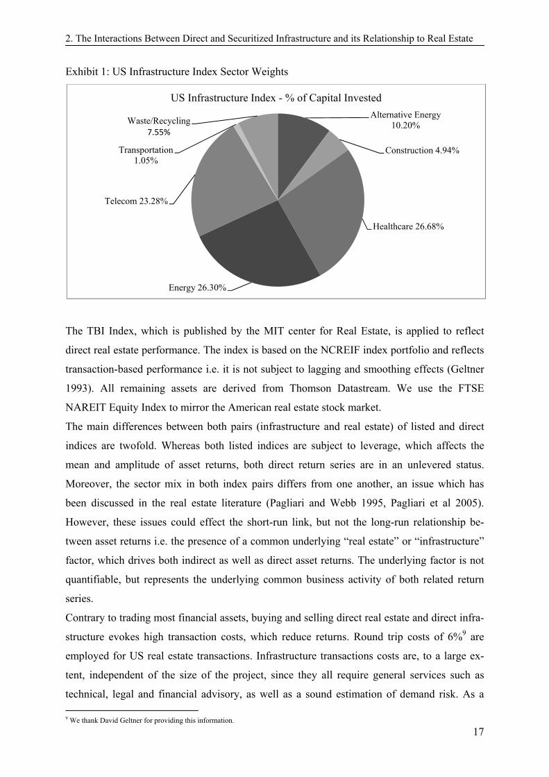
an appropriate tool for benchmarking direct infrastructure performance in the US. Exhibit 1
shows the average sector weights, which are calculated according to capital invested over the
entire sample period. The average index shares are 34% for social (health care,
waste/recycling) and 66% for economic (transportation, telecom, energy, alternative energy,
construction) infrastructure.
8 When the subsequent values of the initial cash are not all positive, the original cash flow series is divided into smaller series.
2. The Interactions Between Direct and Securitized Infrastructure and its Relationship to Real Estate
17
Exhibit 1: US Infrastructure Index Sector Weights
The TBI Index, which is published by the MIT center for Real Estate, is applied to reflect
direct real estate performance. The index is based on the NCREIF index portfolio and reflects
transaction-based performance i.e. it is not subject to lagging and smoothing effects (Geltner
1993). All remaining assets are derived from Thomson Datastream. We use the FTSE
NAREIT Equity Index to mirror the American real estate stock market.
The main differences between both pairs (infrastructure and real estate) of listed and direct
indices are twofold. Whereas both listed indices are subject to leverage, which affects the
mean and amplitude of asset returns, both direct return series are in an unlevered status.
Moreover, the sector mix in both index pairs differs from one another, an issue which has
been discussed in the real estate literature (Pagliari and Webb 1995, Pagliari et al 2005).
However, these issues could effect the short-run link, but not the long-run relationship be-
tween asset returns i.e. the presence of a common underlying “real estate” or “infrastructure”
factor, which drives both indirect as well as direct asset returns. The underlying factor is not
quantifiable, but represents the underlying common business activity of both related return
series.
Contrary to trading most financial assets, buying and selling direct real estate and direct infra-
structure evokes high transaction costs, which reduce returns. Round trip costs of 6%9 are
employed for US real estate transactions. Infrastructure transactions costs are, to a large ex-
tent, independent of the size of the project, since they all require general services such as
technical, legal and financial advisory, as well as a sound estimation of demand risk. As a
9 We thank David Geltner for providing this information.
Alternative Energy 10.20%
Construction 4.94%
Healthcare 26.68%
Energy 26.30%
Telecom 23.28%
Transportation 1.05%
Waste/Recycling7.55%
US Infrastructure Index - % of Capital Invested
2. The Interactions Between Direct and Securitized Infrastructure and its Relationship to Real Estate
18
result, the cost can amount to a maximum of 10% of total project cost. Average infrastructure
projects evoke round trip costs of about 7.5%10 (for road projects, see for example Dudkin
and Välilä, 2005, Salino and de Santos, 2008). However, actual transaction costs depend on
the holding period of assets. Based on the findings of Fisher and Young (2000) and Geltner
and Pollakowski (2007), the average institutional holding period of direct real estate is rough-
ly ten years. According to Kaserer et al. (2009), the average duration of infrastructure invest-
ments is four years, which seems very short. However, there is a huge difference between the
average concession period which is agreed between the government and the SPV, and the
holding period of an individual equity investor. While concession periods agreed between the
regulator and the SPV are around 30 years across all sectors, on average, an individual inves-
tor might have shorter holding periods, depending on strategic issues, such as the stage of the
infrastructure project (OECD, 2010). Due to the growing maturity of the market and the in-
creasing involvement of long-term investors, the average holding is likely to rise over the next
few years. We use this information from Geltner and Pollakowski (2007) and from Kaserer
(2009) to adjust direct real estate and direct infrastructure returns.
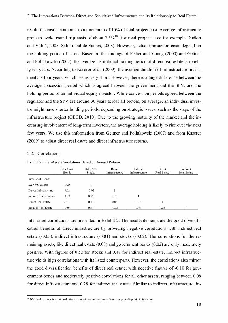
2.2.1 Correlations
Exhibit 2: Inter-Asset Correlations Based on Annual Returns
Inter Govt.
Bonds S&P 500 Stocks
Direct Infrastructure
Indirect Infrastructure
Direct Real Estate
Indirect Real Estate
Inter Govt. Bonds 1
S&P 500 Stocks -0.23 1
Direct Infrastructure 0.02 -0.02 1
Indirect Infrastructure 0.08 0.52 -0.01 1
Direct Real Estate -0.10 0.17 0.08 0.18 1
Indirect Real Estate -0.08 0.61 -0.03 0.48 0.28 1
Inter-asset correlations are presented in Exhibit 2. The results demonstrate the good diversifi-
cation benefits of direct infrastructure by providing negative correlations with indirect real
estate (-0.03), indirect infrastructure (-0.01) and stocks (-0.02). The correlations for the re-
maining assets, like direct real estate (0.08) and government bonds (0.02) are only moderately
positive. With figures of 0.52 for stocks and 0.48 for indirect real estate, indirect infrastruc-
ture yields high correlations with its listed counterparts. However, the correlations also mirror
the good diversification benefits of direct real estate, with negative figures of -0.10 for gov-
ernment bonds and moderately positive correlations for all other assets, ranging between 0.08
for direct infrastructure and 0.28 for indirect real estate. Similar to indirect infrastructure, in-
10 We thank various institutional infrastructure investors and consultants for providing this information.

2. The Interactions Between Direct and Securitized Infrastructure and its Relationship to Real Estate
19
direct real estate is correlated with stocks (0.61) and indirect infrastructure (0.28), but exhib-
its, in contrast to indirect infrastructure, a positive correlation with its underlying direct real
estate performance (0.28).
2.3 Methodology
In order to determine the role and relationship of infrastructure investments, we test for long-
run co-movements, as well as short-run dynamics with respect to other time series, because
simple correlations on quarterly frequency can lead to misleading interpretations of portfolio
diversification effects. Although the time series of returns can be zero (highly) correlated in
the short run, they can exhibit strong (weak) long-term relationship(s) and this in turn, should
lead to diminishing (increasing) diversification effect between assets (Pengpis and Swanson
2010).
Our first step is to perform a battery of unit roots tests to reach the prerequisite of cointegra-
tion, i.e. the time series contain a unit root and are integrated of the same order. We perform
the three different unit root tests with various benefits. The Dickey-Fuller Generalized Least
Squares (DF-GLS) test (Elliot et al. 1996), the Zivot-Andrews (ZA) test (Zivot and Andrews
1992) and the Kwaitkowski, Phillips, Schmidt and Shin (KPSS) test (Kwaitkowski et al.
1992). The DF-GLS test dominates the ordinary Dickey-Fuller, in terms of small-sample size
and power (Maddala and Kim 1998). The ZA test allows for a structural break at an unknown
time. While DF-GLS and ZA test have the null hypothesis of non-stationary the KPSS test
controls for the converse. Thus, the latter test is for robustness, since it investigates whether
the time series is fractionally integrated (that is neither )0(I nor )1(I ). All unit root tests are
performed including a constant and thus allowing for a break in the intercept for the ZA test.
Exhibit 3 shows that the null hypothesis of a unit root is not rejected for levels, and clearly
rejected for the first differences at a 1 percent significance level for the DF-GLS and ZA
tests. The KPSS test rejects the stationarity of the levels and indicates the stationarity of the
first differences (except the direct real estate returns at a 10 percent level). Hence, all exam-
ined time series should be )1(I .

2. The Interactions Between Direct and Securitized Infrastructure and its Relationship to Real Estate
20
Exhibit 3. Unit Root Test Log Levels Log First Differences
ADF DF-GLS ZA KPSS ADF DF-GLS ZA KPSS
Direct Infrastructure -2.077 0.58 -3.174 1.553***
-8.062*** -2.214** -10.904*** 0.028
Indirect Infrastructure -1.499 0.124 -3.344 0.444***
-5.058*** -2.628*** -7.897*** 0.049
Direct Real Estate -0.395 0.471 -3.664 0.444***
-4.202*** -2.606*** -9.27*** 0.201*
Indirect Real Estate -1.189 0.226 -4.214 0.309***
-5.991*** -2.886*** -8.251*** 0.054
S&P 500 Stocks -1.817 -0.046 -2.701 1.449***
-5.119*** -3.089*** -8.623*** 0.078
In the second step, we test the pair-wise co-movement of two time series by using the Engle
and Granger (1987) procedure and the Johansen (1988) / Johansen and Juselius (1990) meth-
odology, and test for the null hypothesis of no co-integration. According to Engle and
Granger, two non-stationary time series are regressed on each other by simple OLS:
ttjti XX ,, (1)
and the residuals t are tested for stationarity by ADF and by using the MacKinnon (1991)
critical values. The two time series are co-integrated, if they are both )1(I , which we tested
above and their residuals from (1) are stationary. The results are summarized in Exhibit 3.
The procedure of Johansen and Juselius links vector auto regression (VAR) with cointegration.
A VAR(k), which is defined as:
tktkttt XAXAXAX 2211 iA (2)
where k is the lag length, iA are the coefficient matrices, tX is the n-dimensional vector of
price levels or the levels of the state variables respectively at time t , and is a vector of
constants. If two or more time series are cointegrated (share a long-run relationship), the VAR
(k) can be written as a vector error correction model (VECM):
t
k
iititt XXX
11 (3)
where tX is the vector of first differences respectively the asset returns as above. The matri-
ces i represent short-term dynamics, whereas represents long-run relationships. If has
a full rank n , no cointegration relationship is present. If has a rank nr 0 then r coin-
tegration relations do exist. Here, can be decomposed into:

2. The Interactions Between Direct and Securitized Infrastructure and its Relationship to Real Estate
21
βα
where α is the matrix with the adjustment speeds towards the long-run equilibrium and β
describes the r cointegrating relationships. To determine the number r of cointegration rela-
tionships, we rely on the maximum-eigenvalue and the trace test with the test statistics:
k
riitrace Tr
1
)1ln()(
)1ln(max ieigen T
where i are the estimated eigenvalues of matrix . The test starts at 0r and investigates
the number of eigenvalues significantly different from zero i.e. the number of cointegration
relationships which could not be rejected.
In order to measure the short run dynamics, Granger Causality tests (1969a see lütkepohl) are
applied. The test is based on the described VAR system. The approach tests whether the in-
formation of a lagged variable 1tX has no information content to describe another variable
tY . The causality is tested with a simple F -test and can provide some information with re-
spect to lead-lag structures among the assets.
2.4 Results
2.4.1 Long-Run Dynamics
The diversification potential of assets generally entails two aspects, short-term correlation
structures and long term co-movement. Correlation analysis is based a on specific frequency
of observations (for example quarterly or annually) and may lead to miss-specified long term
investment allocations. For this reason, we use cointegration technique to analyze long-term
asset co-movements.
The findings of the Engel and Granger and Johansen cointegration tests for long run relation-
ships are presented in Exhibits 4 and 5.
2. The Interactions Between Direct and Securitized Infrastructure and its Relationship to Real Estate
22
Exhibit 4: Engle-Granger Test
Indices
Unit Root Test in Residuals Endogenous Exogenous Variable Variable ADF lag length Direct Infrastructure Indirect Infrastructure -2.907** 1
Indirect Infrastructure Direct Infrastructure -2.609* 1
Direct Real Estate Indirect Real Estate -3.126** 1
Indirect Real Estate Direct Real Estate -2.884* 1
Direct Infrastructure Direct Real Estate -2.292 1
Direct Real Estate Direct Infrastructure -2.423 1
Indirect Infrastructure Indirect Real Estate -2.042 1
Indirect Real Estate Indirect Infrastructure -2.175 1
Indirect Infrastructure S&P 500 Stocks -1.961 1
S&P 500 Stocks Indirect Infrastructure -1.916 1
Indirect Real Estate S&P 500 Stocks -1.461 1
S&P 500 Stocks Indirect Real Estate -1.183 1 Note. The ADF test is employed with the MacKinnon (1991) ciritical values, lag length is selected with the AIC. ***,** and * indicate the rejection of the null hypothesis at a 1%, 5% and 10% significance level.
Exhibit 5: Johansen and Juselius Test for Cointegration Rank
Trace Test Statistic
Maximum Eigenvalue Test Statistic
Eigen- value Tested Pairs 0H
Direct Infrastructure r=0 0.185 17.836** 17.602**
Indirect Infrastructure r>=1 0.003 0.234 0.234
Direct Real Estate r=0 0.204 18.947** 18.207**
Indirect Real Estate r>=1 0.009 0.740 0.740
Direct Infrastructure r=0 0.098 9.692 8.259
Direct Real Estate r>=1 0.018 1.433 1.433
Indirect Infrastructure r=0 0.099 10.839 8.347
Indirect Real Estate r>=1 0.031 2.493 2.493
Indirect Infrastructure r=0 0.067 8.618 5.607
S&P 500 Stocks r>=1 0.036 3.011 3.011
Indirect Real Estate r=0 0.044 5.278 3.601
S&P 500 Stocks r>=1 0.021 1.677 1.677
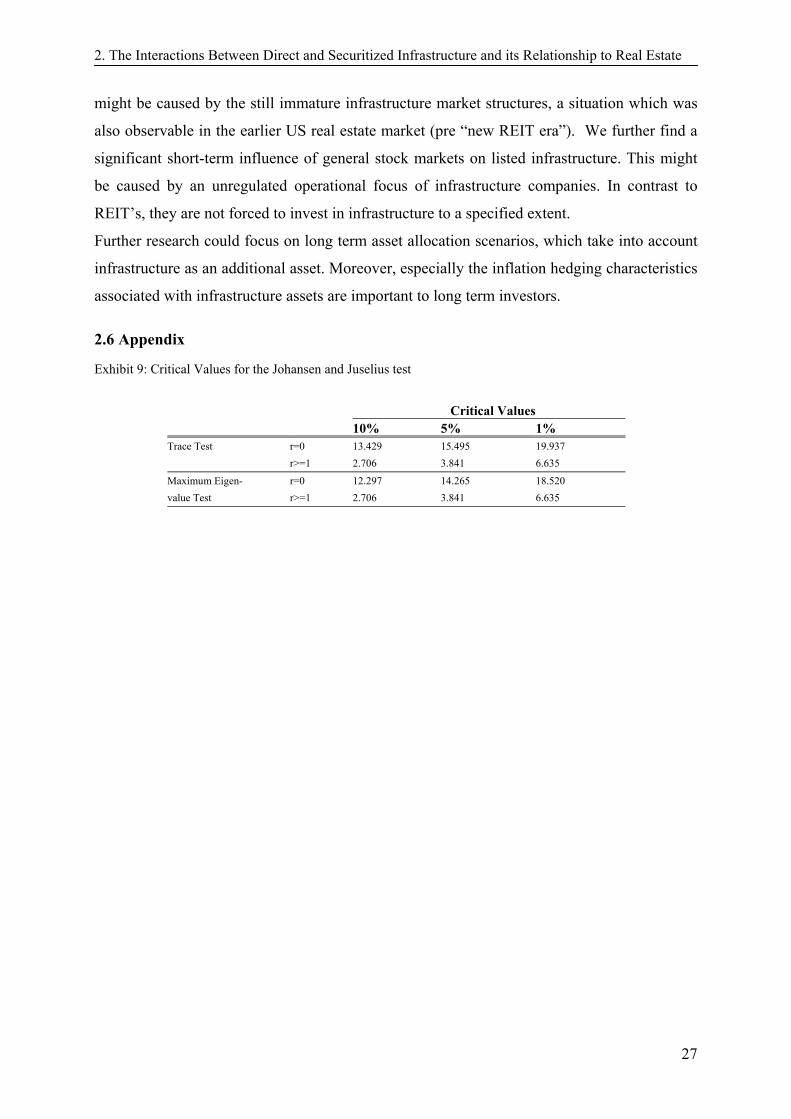
Note. ***,** and * indicate the rejection of the null hypothesis at 1%, 5% and 10% significance levels. The critical values are reported in Table 9.
Exhibit 6: Normalized Cointegration Vectors
Direct Infrastructure Constant Indirect Infrastructure
1 0.365 -1.261***
(-0.135)
Direct Real Estate Constant Indirect Real Estate
1 0.219 -0.847***
(-0.049)
Note. ***,** and * indicate the rejection of the null hypothesis at 1%, 5% and 10% significance levels.
2. The Interactions Between Direct and Securitized Infrastructure and its Relationship to Real Estate
23
We provide new findings about infrastructure assets and are furthermore able to support and
confirm some previous findings in the literature. Infrastructure and real estate exhibit similar
behavior in terms of long-term relationships between their listed performance and their direct
counterpart. Both pairs (real estate and infrastructure) reveal a significant link over the long-
run at a 5 percent level for the Engel Granger test. The Johansen test rejects the hypothesis
r=0 for both assets at a five percent level, so that the hypothesis r>=1 cannot be rejected. The
used critical values can be found in Exhibit 9 in the appendix. The Johannsen procedure sup-
ports the results from the Engle Granger tests i.e. proves a cointegration relation between di-
rect and indirect assets in each case. However, it is important to note that REITs are forced by
law to remain within the core real estate business11, but the listed infrastructure index is only a
specialized sector-specific stock index with no binding investment rules and limitations, and
is limited only with respect to the definition of infrastructure or to the index classification.
Nevertheless, infrastructure characteristics seem to be present in the listed infrastructure index
for the long run i.e. a common underlying, but not quantifiable infrastructure factor seems to
influence both indices. This underlying factor can be explained theoretically by a common
business activity of both infrastructure series (indices) and therefore, an exposure to similar
cash-flow and risk patterns. The argument holds, despite the fact that the infrastructure mix of
the UBS index differs from that of the CEPRES Index. This result corresponds with the find-
ings from the real estate literature, namely the existence of a common long-term “real estate”
factor in both indices (listed and direct), which is independent of the sector-specific break-
down of the index (see Oikarinen et al.2010, Pagliari et al. 2005).
The real estate findings are in accordance with the literature, whereas direct real estate per-
formance is mostly represented by the NCREIF index, instead of the transaction-based TBI.
However, the difference between the lagged appraisal-based NCREIF and the TBI should not
matter for long-run cointegration relations (see Oikarinen et al. 2011).12 Both results under-
pin the theory that indirect assets are driven by sentiment and noise in the short run, but in the
long run, the prices of indirect assets float around their fundamental values. These fundamen-
tal values are based on current and future cash flows of the underlying business models i.e.
infrastructure and real estate.
A relationship between real estate and infrastructure may be indicative of the fact that both
assets share similar underlying characteristics (see Dechant et al. 2010). However, both coin-
tegration tests reject this theoretical hypothesis, by yielding insignificant values for the listed
11 US Internal Revenue Code:Sec. 856. 12 For reasons of robustness, we also performed the analysis by using the NCREIF direct real estate index. The results obtained are similar to those of the TBI index in terms of estimated parameters and significance.
2. The Interactions Between Direct and Securitized Infrastructure and its Relationship to Real Estate
24
assets as well as for their direct counterparts. Since, in consequence, an interrelationship be-
tween both assets cannot be confirmed in the long run, it is rational to include both assets in a
portfolio aiming at long-term investment horizons.
As indicated in Exhibit 1, all listed assets exhibit high positive correlations with the main
stock market (0.49 for infrastructure and 0.65 for real estate) and are caused by short-term
stock market sentiment. However, our cointegration tests do not support a significant long-run
interrelationship between our listed real assets and the main stock market.
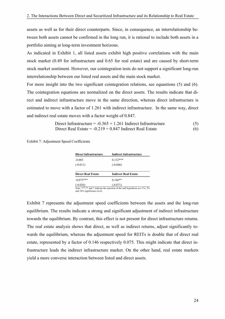
For more insight into the two significant cointegration relations, see equastions (5) and (6).
The cointegration equations are normalized on the direct assets. The results indicate that di-
rect and indirect infrastructure move in the same direction, whereas direct infrastructure is
estimated to move with a factor of 1.261 with indirect infrastructure. In the same way, direct
and indirect real estate moves with a factor weight of 0.847.
Direct Infrastructure = -0.365 + 1.261 Indirect Infrastructure (5) Direct Real Estate = -0.219 + 0.847 Indirect Real Estate (6)
Exhibit 7: Adjustment Speed Coefficients
Direct Infrastructure Indirect Infrastructure
-0.003 0.132***
(-0.011) (-0.046)
Direct Real Estate Indirect Real Estate
-0.075*** 0.146**
(-0.026) (-0.071) Note. ***,** and * indicate the rejection of the null hypothesis at a 1%, 5% and 10% significance level.
Exhibit 7 represents the adjustment speed coefficients between the assets and the long-run
equilibrium. The results indicate a strong and significant adjustment of indirect infrastructure
towards the equilibrium. By contrast, this effect is not present for direct infrastructure returns.
The real estate analysis shows that direct, as well as indirect returns, adjust significantly to-
wards the equilibrium, whereas the adjustment speed for REITs is double that of direct real
estate, represented by a factor of 0.146 respectively 0.075. This might indicate that direct in-
frastructure leads the indirect infrastructure market. On the other hand, real estate markets
yield a more converse interaction between listed and direct assets.
2. The Interactions Between Direct and Securitized Infrastructure and its Relationship to Real Estate
25
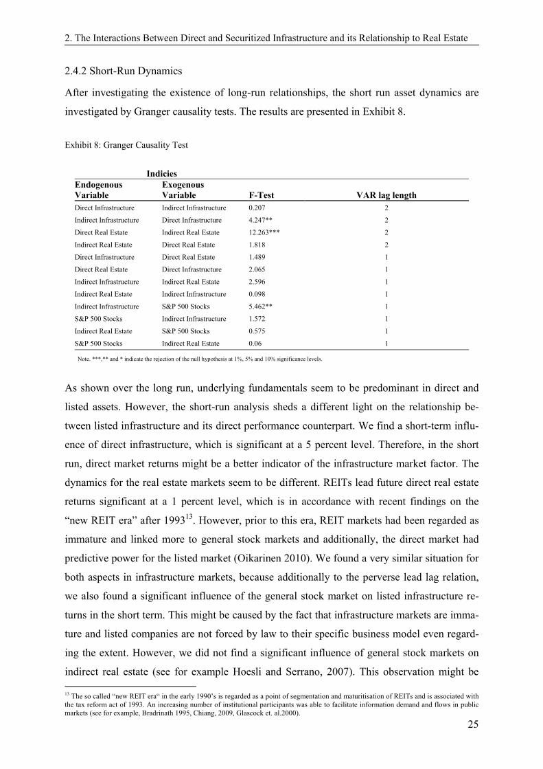
2.4.2 Short-Run Dynamics
After investigating the existence of long-run relationships, the short run asset dynamics are
investigated by Granger causality tests. The results are presented in Exhibit 8.
Exhibit 8: Granger Causality Test
Indicies Endogenous Variable
Exogenous Variable F-Test VAR lag length
Direct Infrastructure Indirect Infrastructure 0.207 2
Indirect Infrastructure Direct Infrastructure 4.247** 2
Direct Real Estate Indirect Real Estate 12.263*** 2
Indirect Real Estate Direct Real Estate 1.818 2
Direct Infrastructure Direct Real Estate 1.489 1
Direct Real Estate Direct Infrastructure 2.065 1
Indirect Infrastructure Indirect Real Estate 2.596 1
Indirect Real Estate Indirect Infrastructure 0.098 1
Indirect Infrastructure S&P 500 Stocks 5.462** 1
S&P 500 Stocks Indirect Infrastructure 1.572 1
Indirect Real Estate S&P 500 Stocks 0.575 1
S&P 500 Stocks Indirect Real Estate 0.06 1
Note. ***,** and * indicate the rejection of the null hypothesis at 1%, 5% and 10% significance levels.
As shown over the long run, underlying fundamentals seem to be predominant in direct and
listed assets. However, the short-run analysis sheds a different light on the relationship be-
tween listed infrastructure and its direct performance counterpart. We find a short-term influ-
ence of direct infrastructure, which is significant at a 5 percent level. Therefore, in the short
run, direct market returns might be a better indicator of the infrastructure market factor. The
dynamics for the real estate markets seem to be different. REITs lead future direct real estate
returns significant at a 1 percent level, which is in accordance with recent findings on the
“new REIT era” after 199313. However, prior to this era, REIT markets had been regarded as
immature and linked more to general stock markets and additionally, the direct market had
predictive power for the listed market (Oikarinen 2010). We found a very similar situation for
both aspects in infrastructure markets, because additionally to the perverse lead lag relation,
we also found a significant influence of the general stock market on listed infrastructure re-
turns in the short term. This might be caused by the fact that infrastructure markets are imma-
ture and listed companies are not forced by law to their specific business model even regard-
ing the extent. However, we did not find a significant influence of general stock markets on
indirect real estate (see for example Hoesli and Serrano, 2007). This observation might be 13 The so called “new REIT era“ in the early 1990’s is regarded as a point of segmentation and maturitisation of REITs and is associated with the tax reform act of 1993. An increasing number of institutional participants was able to facilitate information demand and flows in public markets (see for example, Bradrinath 1995, Chiang, 2009, Glascock et. al.2000).

2. The Interactions Between Direct and Securitized Infrastructure and its Relationship to Real Estate
26
caused by the quarterly data frequency, which ignores the more rapid inter-quarterly effects
between stocks and REITs. High correlations between both assets (0.61) support this argu-
ment. Furthermore, we are not able to support significant influences between direct real estate
and direct infrastructure, which indicates the independency of both assets even in the short
run.
2.5 Summary and Conclusions
Instigated by the attractive investment characteristics associated with infrastructure assets,
institutional investor interest in and demand for private infrastructure investments has risen
significantly during recent years. However, due to a lack of (direct) infrastructure perfor-
mance data, academic research lags behind this development. Using a unique infrastructure
dataset, we extend the existing literature on infrastructures portfolio benefits, by examining
the short-run and long-run dynamic relationships and interactions between securitized and
direct infrastructure returns, as well as their relation to the associated real estate sector. Our
results contribute to the general understanding of direct and listed infrastructure asset returns
and their relation to each other and in consequence, yield some important insights for actual
asset allocation decisions.
Our results support a long run cointegration relationship between direct and indirect infra-
structure return indices. Consequently, we detect similar behavior for infrastructure assets to
that between direct and indirect real estate assets. This contradicts the intuition based on the
short term inter-asset correlation between direct and indirect infrastructure returns which indi-
cates no link between both assets. Thus, indirect infrastructure seems to reflect direct infra-
structure performance in the long run i.e. a common unobservable underlying “infrastructure
factor” seems to drive both indices. More precisely, indirect and direct infrastructure assets
would be substitutes in an asset allocation context, if an investor’s investment horizon is long.
Therefore, asset allocation models which are based on correlations and extended to long hori-
zons, could imply diversification benefits which are not present. Driven by similar underlying
asset characteristics, practically-oriented investors often do not distinguish meaningfully be-
tween infrastructure and real estate investments in their portfolio. However, we are not able to
support long-term relationships between infrastructure and real estate assets, whereas the indi-
rect assets do reveal a high correlation. As a result, the two asset classes are not substitutable,
have diversification benefits to each other in the long run and could, therefore, theoretically
coexist in the same portfolio.
Our results for short run dynamics reveal an influence of direct on indirect infrastructure re-
turns, a result which is not intuitive from an efficient market perspective. However, this result
2. The Interactions Between Direct and Securitized Infrastructure and its Relationship to Real Estate
27
might be caused by the still immature infrastructure market structures, a situation which was
also observable in the earlier US real estate market (pre “new REIT era”). We further find a
significant short-term influence of general stock markets on listed infrastructure. This might
be caused by an unregulated operational focus of infrastructure companies. In contrast to
REIT’s, they are not forced to invest in infrastructure to a specified extent.
Further research could focus on long term asset allocation scenarios, which take into account
infrastructure as an additional asset. Moreover, especially the inflation hedging characteristics
associated with infrastructure assets are important to long term investors.
2.6 Appendix
Exhibit 9: Critical Values for the Johansen and Juselius test
Critical Values 10% 5% 1% Trace Test r=0 13.429 15.495 19.937
r>=1 2.706 3.841 6.635
Maximum Eigen- r=0 12.297 14.265 18.520
value Test r>=1 2.706 3.841 6.635

2. The Interactions Between Direct and Securitized Infrastructure and its Relationship to Real Estate
28
2.5 Literature
Araujo, S.; Sutherland, D. (2010): Public-Private Partnerships and Investment in Infrastruc-ture. OECD Economics Department; Working Papers, No. 803.
Axelson, U.; Stromberg, P.; Weisbach, M. (2007): Why are buyouts levered: The financial structure of private equity funds. National Bureau of Economic Research, NBER Working papers, No.12826.
Bitsch, F.; Buchner, A.; Kaserer, C. (2010): Risk, return and cash flow characteristics of infrastructure fund investments, Euroepan Investment Bank (EIB); EIB-Papers, Vol. 15, p.106–136.
Bradrinath, S.; Kale, J.; Noe, T. (1995): Of shepherds, sheep, and the cross-autocorrelations in equity returns, Review of Financial Studies, Vol.8, p. 401-430.
Chiang, K. (2010): On the Comovement of REIT Prices, Journal of Real Estate Research, Vol. 32 No. 2, p. 187-200.
Clayton, J.; MacKinnon, G. (2001): The Time-Varying Nature of the Link Between REIT, Real Estate and Financial Asset Returns, Journal of Real Estate Portfolio Management, Vol. 7, p. 43-54.
Dechant, T.; Finkenzeller, K.; Schäfers, W. (2010): Real Estate: A Victim of Infrastruc-ture? Evidence from Conditional Asset Allocation, IREBS Infrastructure Working Paper Se-ries, Vol. 2.
Dudkin, G.; Välilä, T. (2006): Transaction costs in Public-Private Partnership: A first look at the evidence. Competition and regulation in network industries, Mortsel, Intersentia, Vol. 1, p.307-330.
Elliott, G.; Rothenberg, T.; Stock, J. (1996): Efficient tests for an autoregressive unit root, Econometrica, Vol. 64, p. 813–36.
Engle, R.; Granger, C. (1987): Co-integration and error correction: Representation, estima-tion and testing. Econometrica, Vol. 55, p. 251–276.
Esfahani, H.; Ramirez, M. (2003): Institutions, infrastructure and economic growth. Journal of Development Economics, Vol. 70, p.443-477.
Esty, B. (2004): Why Study Large Projects? An Introduction to Research on Project Finance, European Financial Management, Vol. 10, p.213-224.
Franzoni F.; Nowak E.; Phalippou L. (2011): Private equity performance and liquidity risk, Journal of Finance, (Forthcoming).
Finkenzeller, K.; Dechant, T.; Schaefers, W. (2010): Infrastructure: a new dimension of real estate? An asset allocation analysis, Journal of Property Investment and Finance, Vol. 28, No. 4, p. 263-274.

2. The Interactions Between Direct and Securitized Infrastructure and its Relationship to Real Estate
29
Fuess, R.; Schweizer, D. (2011): Dynamic Interactions between Venture Capital Returns and the Macroeconomy: Theoretical and Empirical Evidence from the United States, Review of Quantitative Finance and Accounting, (Forthcoming).
Gatti, S.; Rigamonti, A.; Saita, F.; Senati, M. (2007): Measuring value-at-risk in project finance transactions, European Financial Management, Vol. 13, No. 1, p. 135-158.
Giliberto, S. (1990): Equity Real Estate Investment Trusts and Real Estate Returns. Journal of Real Estate Research, Vol. 5, p. 259-263.
Glascock, J.; Lu, C.; So, R. (2010): Further evidence on the integration of REIT, bond, and stock returns, Journal of Real Estate Finance and Economics, Vol. 20, p.177–194.
Geltner, D.; Kluger B. (1998): REIT-Based Pure-Play Portfolios: The Case of Property Types, Real Estate Economics, Vol. 26, p.581-612.
Geltner, D.; Pollakowski H. (2007): A Set of Indexes for Trading Commercial Real Estate Based on the Real Capital Analytics Transaction Prices Database, MIT Center for Real Estate Commercial Real Estate Data Laboratory – CREDL.
Hoesli, M.; Serrano, C. (2007): Securitized Real Estate and Its Link with Financial Assets and Real Estate: An International Analysis, Journal of Real Estate Literature, Vol.15, p. 59-84.
Inderst, G. (2010): Infrastructure as an Asset Class, European Investment Bank (EIB); EIB Research Papers, Vol.15.
Johansen, S. (1988): Statistical Analysis of Cointegration Vectors, Journal of Economic Dy-namics and Control, Vol. 12, p. 231-254.
Johansen, S.; and Juselius, K. (1990): Maximum Likelihood Estimation and Inference on Cointegration – with Applications to the Demand for Money, Oxford Bulletin of Economics and Statistics, Vol. 52, p. 169-210.
Kaserer, C.; Buchner, A.; Schmidt, D.; Krohmer, P. (2010): Infrastructure Private Equity, Center of Private Equity Research.
Krohmer, P.; Lauterbach, R.; Calanog, V. (2009): The bright and dark side of staging: In-vestment performance and the varying motivations of private equity, Journal of Banking and Finance, Vol. 33, p.1597-1609.
Kwiatkowski, D.; Phillips, B.; Schmidt, P.; Shin, Y. (1992): Testing the null hypothesis of stationarity against the alternative of a unit root, Journal of Econometrics, Vol. 54, p. 91–115.
Maddala G.; Kim I. (1998): Unit roots, cointegration, and structural change, Cambridge University Press, Cambridge.

2. The Interactions Between Direct and Securitized Infrastructure and its Relationship to Real Estate
30
MacKinnon, J. (1998): Critical values for cointegration tests. Long-Run Economic Relation-ships; Readings in Cointegration, Oxford University Press, Oxford.
Myer, F.; Webb J. (1994): Retail Stocks, Retail REITs and Retail Real Estate. Journal of Real Estate Research, Vol. 9, p. 65-84.
Newell, G.; Peng; H. (2008): The Role of U.S. Infrastructure in Investment Portfolios. Jour-nal of Real Estate Portfolio Management, Vol.14, No. 1, p. 21-33.
Oikarinen, E.; Hoesli, M.; Serrano, C. (2011): The Long-Run Dynamics Between Direct and Securitized Real Estate, Journal of Real Estate Research, Vol. 33, p. 73-104.
Pagliari J.; Scherer K.; Monopoli T. (2005): Public versus Private Real Estate Equities: A More Refined, Long-Term Comparison, Journal of Real Estate Economics, Vol. 33, p. 147-187.
Peng, L. (2001): Building a Venture Capital Index, Yale ICF; Working Paper, Vol. 00-5.
Schmitt, D.; Ott, T. (2006): Modelling a Performance Index for Non-traded Private Equity Transactions: Methodology and Practical Application, Center of Private Equity Research (CEPRES), Research Paper.
Wagenvoort, R.; de Nicola, C.; and Kappler A. (2010): Infrastructure Finance in Europe: Composition, evaluation and crisis impact, European Investment Bank Papers, Vol. 15, No. 1, p. 16-39.
WEF, World Economic Forum (2010): Global Risks 2010, A Global Risk Network Report.
Zivot, E.; Andrews, D. (1992): Further Evidence on the Great Crash, the Oil-Price Shock, and the Unit-Root Hypothesis, Journal of Business & Economic Statistics, Vol. 10, No. 3, p. 251-270.
3. Infrastructure – A New Dimension of Real Estate? An Asset Allocation Analysis
31
3. Infrastructure - A New Dimension of Real Estate? An Asset Allocation Analysis
Konrad Finkenzeller Tobias Dechant Wolfgang Schäfers
Abstract
Purpose: The purpose of this paper is to provide conclusive evidence that infrastructure con-
stitutes a separate asset class and cannot be classified as real estate from an investment point
of view. Furthermore, we determine optimal allocations for direct and indirect infrastructure
within a multi-asset portfolio.
Design/Methodology/Approach: We optimize portfolio allocations by using an algorithm
which accounts for downside risk rather than variance. This approach is more in accordance
with the actual investor behaviour and might meet their investment objectives more effective-
ly. An Australian dataset comprising stocks, bonds, direct real estate, direct infrastructure and
indirect infrastructure is applied for portfolio construction.
Findings: Although infrastructure and real estate have common characteristics, we arrive at
the conclusion that they constitute two different asset classes. Furthermore, we highlight the
diversification benefits of direct and indirect infrastructure within multi-asset portfolios and
determine efficient allocations up to 78% for target rates of 0.0%, 1.5% and 3.0% quarterly.
Practical Implications:The results will help investors and portfolio managers to efficiently
allocate funds to various asset classes. Most institutional investors are not familiar with in-
vestments in infrastructure. This study facilitates a better understanding of the asset class in-
frastructure and yields some important implications for the optimal allocation of infrastruc-
ture within institutional investment portfolios.
Originality/Value:This is the first study to examine the role of direct and indirect infrastruc-
ture within a multi-asset portfolio by applying a downside-risk approach.

3. Infrastructure – A New Dimension of Real Estate? An Asset Allocation Analysis
32
3.1 Introduction
The economic importance of infrastructure has been the subject of extensive research since
the late 1980s and is free of controversy. The World Economic Forum (2008) lists infrastruc-
ture as one of the most crucial elements to a country’s productivity and competitiveness.
Aschauer (1989) provides evidence of significant links between investment in infrastructure
and a country’s economic development and wealth. Yeaple and Golub (2004) suggest that
infrastructure is one of the key determinants of a region’s comparative advantage. Though
infrastructure is recognized as a crucial input for economic productivity, there is no clear and
unanimous definition of the term. An early definition is given by Stohler (1964), who charac-
terizes infrastructure as the substructure or the “skeleton” assets of an economy that are essen-
tial for the production of goods and services. Later approaches have subdivided infrastructure
into social and economic subgroups. Economic infrastructure (including transport, ener-
gy/utilities and communication facilities) provides key services to business and industry and
enhances productivity and innovation. Social infrastructure, on the other hand, is seen as a
medium for supplying basic services to households (healthcare, education and judicial facili-
ties) (ING, 2006). In recent years, private investments in infrastructure have increased signifi-
cantly and investors have begun to perceive infrastructure as an attractive asset class enhanc-
ing the efficiency of their investment portfolios. Financial strain on governments, making
them unable to provide adequate infrastructure provision in times of increasing global com-
petitiveness has contributed to the emergence of private investment opportunities in recent
years (RREEF, 2006). A shortage of good quality commercial real estate, along with declin-
ing yields, has intensified this development and amplified the capital flow into seemingly re-
lated sectors (Newell and Peng 2008). Although many investors are restraining their invest-
ments due to the current financial crisis, infrastructure still seems to be very attractive, a fact
which is underpinned by the INREV14 Investment Intentions Survey 2009: According to this
study, more than 60% of all institutional real estate investors considered allocating funds to
the infrastructure sector in 2009.
Since infrastructure and real estate exhibit many common characteristics, this paper aims at
contributing to the debate on whether infrastructure can be regarded as real estate or consti-
tutes a separate asset class. Furthermore, we provide an asset allocation model which deter-
mines optimal infrastructure asset allocations for a downside risk (DR) – averse investor. This
optimization technique is based on Estrada (2008) and considers target semivariance instead 14 European Association for Investors in Non-listed Real Estate Vehicles.

3. Infrastructure – A New Dimension of Real Estate? An Asset Allocation Analysis
33
of variance as measure of risk. This might more effectively meet the investment objectives of
rational investors and result in more realistic asset allocations for a set of Australian data. The
remainder of this paper is structured as follows. Part two presents the applied data, and sec-
tion three analyses the differences between infrastructure and real estate. This is followed by a
review of the downside risk concept and its application to portfolio structuring. The study is
completed with some conclusions and an outlook for future research.
3.2 Applied Data
The Australian infrastructure market is relatively mature and time series data on infrastructure
returns (direct and indirect) are available. For that reason, this market is in the focus of this
analysis.
During the past decade, definitions of infrastructure have broadened and sometimes encom-
pass categories that can barely be linked to one another (Beeferman, 2008): There are oppos-
ing views on the issue of whether utilities can be regarded as infrastructure or not (Inderst
2009). Researchers and practitioners generally do not draw any accurate distinction between
them, but use the term “infrastructure” interchangeably. Estimating the correlations between
quarterly (1994:4 to 2009:1) indirect infrastructure (UBS Australia Infrastructure Index) and
indirect utilities (UBS Australia Utilities Index) returns, reveals a coefficient of correlation of
0.35 which is significant at a 5%-level. As a result, we adhere to this common definition and
use the UBS Australia Infrastructure and Utilities Index to mirror the performance of indirect
infrastructure.15
Time series total return data on direct and indirect infrastructure performance are provided by
Bloomberg and Colonial First State, respectively. Return data on equities, bonds and direct
property are from Thomson Datastream and IPD (Investment Property Databank). All time
series range from Q4 1994 to Q1 2009, which is sufficient to cover at least one entire market
cycle. The UBS Australia Infrastructure & Utility Index depicts the performance of indirect
infrastructure. An index constructed by Colonial First State measures direct infrastructure
performance. This index is an equally weighted total return index comprising five Australian
infrastructure funds, and is based on valuations and therefore subject to smoothing. This im-
plies a downward bias in the second central moment of the return distribution, since apprais-
ers take into account current as well as historic information to perform valuations. In order to
15 Although this index covers infrastructure and utility performance, we refer to the expression “infrastructure” in the course of this paper
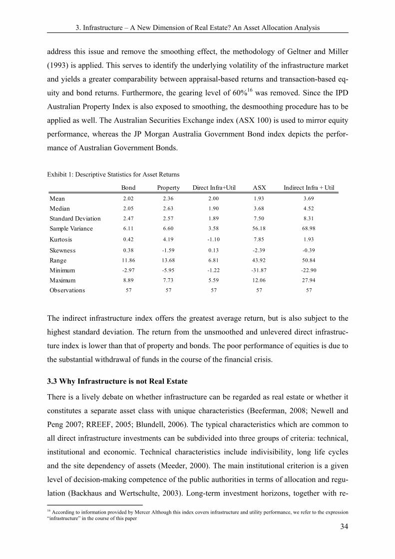
3. Infrastructure – A New Dimension of Real Estate? An Asset Allocation Analysis
34
address this issue and remove the smoothing effect, the methodology of Geltner and Miller
(1993) is applied. This serves to identify the underlying volatility of the infrastructure market
and yields a greater comparability between appraisal-based returns and transaction-based eq-
uity and bond returns. Furthermore, the gearing level of 60%16 was removed. Since the IPD
Australian Property Index is also exposed to smoothing, the desmoothing procedure has to be
applied as well. The Australian Securities Exchange index (ASX 100) is used to mirror equity
performance, whereas the JP Morgan Australia Government Bond index depicts the perfor-
mance of Australian Government Bonds.
Exhibit 1: Descriptive Statistics for Asset Returns
The indirect infrastructure index offers the greatest average return, but is also subject to the
highest standard deviation. The return from the unsmoothed and unlevered direct infrastruc-
ture index is lower than that of property and bonds. The poor performance of equities is due to
the substantial withdrawal of funds in the course of the financial crisis.
3.3 Why Infrastructure is not Real Estate
There is a lively debate on whether infrastructure can be regarded as real estate or whether it
constitutes a separate asset class with unique characteristics (Beeferman, 2008; Newell and
Peng 2007; RREEF, 2005; Blundell, 2006). The typical characteristics which are common to
all direct infrastructure investments can be subdivided into three groups of criteria: technical,
institutional and economic. Technical characteristics include indivisibility, long life cycles
and the site dependency of assets (Meeder, 2000). The main institutional criterion is a given
level of decision-making competence of the public authorities in terms of allocation and regu-
lation (Backhaus and Wertschulte, 2003). Long-term investment horizons, together with re-
16 According to information provided by Mercer Although this index covers infrastructure and utility performance, we refer to the expression “infrastructure” in the course of this paper
Bond Property Direct Infra+Util ASX Indirect Infra + Util
Mean 2.02 2.36 2.00 1.93 3.69
Median 2.05 2.63 1.90 3.68 4.52
Standard Deviation 2.47 2.57 1.89 7.50 8.31
Sample Variance 6.11 6.60 3.58 56.18 68.98
Kurtosis 0.42 4.19 -1.10 7.85 1.93
Skewness 0.38 -1.59 0.13 -2.39 -0.39
Range 11.86 13.68 6.81 43.92 50.84
Minimum -2.97 -5.95 -1.22 -31.87 -22.90
Maximum 8.89 7.73 5.59 12.06 27.94
Observations 57 57 57 57 57

3. Infrastructure – A New Dimension of Real Estate? An Asset Allocation Analysis
35
stricted liquidity due to a very limited secondary market, can be classified as two of the main
economic criteria (RREEF, 2007; Erlendson, 2006). Furthermore, infrastructure has inherent
monopoly characteristics and provides essential economic and social services (Mercer, 2005;
Erlendson, 2006). Stable, and therefore, predictable cash flows associated with potential capi-
tal gains allow for high levels of financial leverage (compared to other asset classes) (Befer-
man, 2008; Colonial First State, 2009; RREEF, 2005). Furthermore, large investment lot sizes
create high barriers of entry. This, in turn, yields a market environment with professional ac-
tors who have high levels of market expertise (RREEF, 2007). Moreover, compared to other
markets, the infrastructure market can be described as intransparent, due to a shortage of qual-
ity data and research (Inderst, 2009). The pricing of direct infrastructure projects is based on
valuations (Newell and Peng, 2008), and underlying cash flows are intended to provide a
hedge against inflation (ING, 2006). Due to its monopolistic character, there may be a lack of
market prices (Backhaus and Werschulte, 2003). Erlendson (2006,) further states that infra-
structure has (at least in the short run) a low elasticity of demand, since the construction of
new assets requires a considerable amount of time. A high level of individual expertise in
legal and regulatory regimes is necessary to provide efficient asset management.
Although direct infrastructure and direct property have some characteristics in common (indi-
visibility, long life cycles and site dependency), long-term investment horizons, restricted
liquidity, valuation-based performance, supposed inflation hedge, capital gains), there are also
substantial differences. Whereas property markets can be described as relatively competitive,
infrastructure markets, as mentioned, often have oligopolistic or even monopolistic structures.
Moreover, there is a greater degree of transparency in the real estate market than in the infra-
structure market. A further issue is the limited potential to obtain ownership of direct infra-
structure assets, due to regulatory constraints, which often only allow user rights (Newell and
Peng, 2008). Even though an investment in direct real estate is inhibited by large investment
scales, this problem becomes even more serious when an investment in direct infrastructure is
considered. This, in turn, decreases the diversification benefit when infrastructure is allocated
to a(n) (multi) asset portfolio. Moreover, real estate, in general, may provide alternative ap-
propriate uses, whereas infrastructure assets are limited to very specific and restricted uses.
Institutional investors also face this classification problem when allocating infrastructure to
their portfolios. Therefore, infrastructure is often placed in existing allocations, namely pri-
vate equity, real estate or fixed income, although the risk-return characteristics do not match

3. Infrastructure – A New Dimension of Real Estate? An Asset Allocation Analysis
36
(PFG, 2007). However, especially over the last few years, infrastructure has begun to emerge
as an independent asset class (Inderst, 2009; Newell and Peng, 2008) as confirmed by a num-
ber of investor surveys. According to Preqin and Inderst (2008), 47% of active investors have
a separate infrastructure allocation, whereas 43% include it in their private equity portfolio
and 10% in their real estate allocation. PFG's investor survey reveals figures of 47% for a
separate infrastructure asset allocation, 37% for an allocation within the private equity portfo-
lio and 15% for a real estate allocation. (PFG, 2007).
According to Newell and Peng (2008), Colonial First State (2006) and RREEF (2007), infra-
structure is appropriate for portfolio diversification, since it delivers a moderate to low corre-
lation with traditional asset classes. We find similar results for the Australian data which, in
turn, yield further indications for the separation of real estate from infrastructure.
As Exhibit 2 shows, there is positive but insignificant (5%) correlation (0.20) between direct
property and direct infrastructure returns from Q4 1994 to Q1 2009, which contradicts the
claim that infrastructure can be regarded as a subclass of real estate. Moreover, the correlation
is even lower (0.04), when the effects of the financial crisis (Q3 2007 to Q1 2009) are extract-
ed. This indicates that the higher correlation in the period from Q4 1994 to Q1 2009 is due to
extreme market downturns from which neither asset class could withdraw. There is a strong
and significant relationship between the indirect infrastructure and the NAREIT index (0.54),
which might be due to the fact that both indices contain listed companies affected by move-
ments in the equity market. However, before the crisis, this correlation was lower (0.27) and
significant at only a 10%-level. This indicates that both investments were perceived as only
weakly related before the financial crisis. According to these results, one might expect a di-
vergence in return behavior when the world economy recovers.

3. Infrastructure – A New Dimension of Real Estate? An Asset Allocation Analysis
37
Exhibit 2: Correlations
These findings, as well as the different risk-return characteristics, constitute an indicator for
distinguishing explicitly between infrastructure and real estate, although many physical char-
acteristics are common to both.
3.4 Infrastructure Asset Allocation
3.4.1 Modern Portfolio Theory (MPT)
Modern portfolio theory still constitutes an important tool for ascertaining the optimal propor-
tion of an asset within a mixed-asset portfolio and for determining "efficient" portfolios out of
a set of possible and permitted ones. According to Markowitz (1952), a portfolio is efficient
when it either delivers the minimum risk for a given level of expected return or achieves the
highest level of return for a given amount of risk. Efficient portfolios are considered as domi-
nant, implying that a rational investor would prefer an efficient portfolio to one that is not
efficient. The set of these efficient portfolios form the efficient frontier and can be determined
by a mean-variance analysis. However, modern portfolio theory is constrained by some seri-
ous theoretical weaknesses and practical complications:
MPT is not consistent with the concept of a minimum required return or target return, which,
however, is usually applied by institutional investors (Sivitanides, 1998, Mao, 1970). This
concept describes an investor's concern with failing to meet a minimum required level of re-
turn. A rational investor would only be apprehensive of returns below this aspiration level,
Bond Property Direct Infra+Util ASX Indirect Infra + Util NAREIT
Bond 1.00 -0.21 -0.02 -0.39 0.27 -0.09
Property 1.00 0.20 0.64 0.38 0.70
Direct Infra+Util 1.00 0.27 0.29 0.17
ASX 1.00 0.36 0.54
Indirect Infra + Util 1.00 0.54
NAREIT 1.00
Bond Property Direct Infra+Util ASX Indirect Infra + Util NAREIT
Bond 1.00 -0.03 0.09 -0.18 0.45 0.11
Property 1.00 0.04 0.16 -0.03 0.07
Direct Infra+Util 1.00 0.05 0.22 -0.08
ASX 1.00 0.12 0.21
Indirect Infra + Util 1.00 0.27
NAREIT 1.00
1995 Q1 - 2007 Q2
1995 Q1 - 2009 Q1
3. Infrastructure – A New Dimension of Real Estate? An Asset Allocation Analysis
38
whereas returns exceeding this target rate cannot be considered as risk, but rather as a riskless
chance of obtaining unanticipated high returns (Sing and Ling, 2003). The mean-variance
approach does not allow for a certain, investor-specific, target rate, but has an implicitly de-
fined reference point, namely the mean. This number, however, might not be suitable for all
investors and could contribute to portfolio allocations which are not appropriate for a particu-
lar investor. Moreover, the mean-variance model treats deviations from the mean – irrespec-
tive of whether they are above or below – in the same way, and both kinds of deviations are
incorporated into the risk assessment of a certain asset (Sing and Ong, 2000). However, this
theory does not adequately mirror the risk perceptions of rational investors and therefore
simply ignores their investment objectives. Consequently, the application of MPT could result
in flawed asset allocations. Furthermore, due to assumptions of normally and independently
distributed returns, the application of the mean-variance methodology is limited when asset
returns are skewed. In terms of utility theory, the underlying utility function is unable to take
into account varying degrees of risk aversion. To overcome these drawbacks and to derive
asset allocations which are more in accordance with the actual behaviour and preferences of
investors, a portfolio optimization technique based on a downside risk measure is taken into
account.
3.4.2 Mean Semivariance Optimization
According to Estrada (2007), the downside risk of an asset i can be described by its semivari-
ance with respect to a benchmark B )( 2iB and is given by:
22 )0;()( BRMinE tiiB (1)
With:
:itR Return on asset j during period t
:B Investor specific benchmark return
The semivariances of the considered assets with respect to different targets are given in Ex-
hibit 3:

3. Infrastructure – A New Dimension of Real Estate? An Asset Allocation Analysis
39
Exhibit 3: Target Semivariances
The square root of (1) describes the semideviation of asset i with regard to a benchmark B , a
common measure of downside risk. The complement to the covariance in the MPT optimiza-
tion is depicted by the semicovariance )( ij between asset i and j with respect to a bench-
mark B . This is defined as follows:
)0,(*)0,( BRMinBRMinE jiij (2)
The fact that this definition can be customized to any desired B and generates a symmetric
semicovariance matrix
jiij
constitutes an advantage towards the traditional Hogan and Warren (1974) measure.
In order to derive the optimal asset allocation, the risk measure of a portfolio, defined as the
semivariance, is minimized:
Minimize: ijB
n
i
n
jjipB xx
1 1
2
Subject to:
N
i
pii RRx1
N
iix
1
1
Nixi ......,,2,1,0 (3)
Target Rate Bond IPD Direct Infra+Util ASX Indirect Infra + Util
0.0% 0.49 2.00 0.09 33.21 20.10
1.5% 1.88 3.37 0.99 39.65 25.74
3.0% 5.20 5.65 3.87 47.63 33.13

3. Infrastructure – A New Dimension of Real Estate? An Asset Allocation Analysis
40
With:
iR : Expected return on asset i
pR : Expected portfolio return
3.4.3 Research Design
This study constructs mean-downside risk-efficient mixed-asset portfolios, including. stocks,
government bonds, treasury bills and commercial real estate. The expected portfolio returns
range from the return on a minimum-risk portfolio of up to 3.4% quarterly. The maximum
achievable return is 3.69%, which, however, can only be gained when all funds are invested
in indirect infrastructure. The benchmark returns within the downside risk optimization algo-
rithms are 0%, 1.5%, and 3%. The first target level indicates that an investor is concerned
mainly with the nominal preservation of capital. A target rate of 1.5% quarterly mirrors the
Australian inflation rate in 2008, reflecting an investor whose main priority is the real preser-
vation of capital. It is not a contradiction to consider an expected return which is above the
target return. The implication is that, although the investor aims at achieving the expected
return, only outcomes below the benchmark constitute a risk to him. The third target rate is set
arbitrarily and is appropriate for investors who require higher benchmark returns. Although
this number does not necessarily constitute a reasonable value – it is not practical to set a
benchmark of 3% per quarter and to assess assets with a maximum expected return below that
number – this benchmark is examined, so as to determine how allocations tend towards a rela-
tively high target level. The parameter of risk aversion is set to “2”, which implies that the
risk measured at the asset level is the target semivariance.
3.4.4 Asset Allocations
When the target rate of return is set to 0.0%, the allocation to indirect infrastructure increases,
the higher the expected portfolio return is set, and the theoretical weights range between 0%
and 78%. This is due to the fact that indirect infrastructure has proved to deliver the highest
return of all considered assets, but is also inherent subject to downside risk. Therefore, indi-
rect infrastructure is only allocated to the portfolio when relatively high returns must be
achieved. For a return of 3.4%, the proportion of infrastructure in the portfolio amounts theo-
retically to 78%. Although this number is derived by the optimization algorithm, it must be
interpreted with care, since it does not seem to be rational to have an exposure of 78% at-
tributable to diversification issues. This high allocation is also due to the fact that no equities

3. Infrastructure – A New Dimension of Real Estate? An Asset Allocation Analysis
41
are incorporated into the mixed asset portfolio which, in turn, is caused by significant losses
during the financial crisis.
Due to diverse risk-return characteristics, the case with direct infrastructure is different. The
minimum semivariance portfolio has an exposure to direct infrastructure of 85%. The low
level of downside risk, especially for a target of 0%, leads to this high proportion. Up to a
quarterly portfolio return of 3.00%, the allocation to direct infrastructure diminishes to zero
percent, since direct property, bonds and indirect infrastructure are incorporated. Therefore,
the allocation to direct infrastructure is suggested to be situated within a range of 0% to 85%.
However, in contrast to indirect infrastructure, direct infrastructure allocations are highest
when a relatively safe portfolio has to be composed. But, as stated above, due to diversifica-
tion issues, the overwhelming allocation to direct infrastructure has to be considered from a
theoretical point of view.
These results demonstrate the role of infrastructure – direct as well as indirect – for invest-
ment portfolios when investors are downside risk averse: An allocation to infrastructure with-
in a range of 0% up to 85% is suggested by the above optimization algorithm when stocks,
bonds, property and direct as well as indirect infrastructure are considered. Taking into ac-
count lower expected returns, an exposure to direct infrastructure is preferable, whereby, for
higher expected portfolio returns, the portfolio should be heavily weighted towards indirect
infrastructure. This model obviously reveals the role and importance of infrastructure for asset
allocation and demonstrates that infrastructure could play an important role in institutional
investment portfolios.
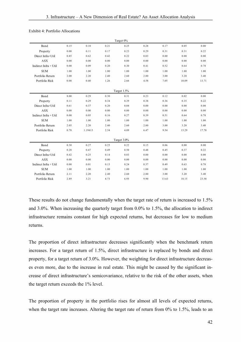
3. Infrastructure – A New Dimension of Real Estate? An Asset Allocation Analysis
42
Exhibit 4: Portfolio Allocations
These results do not change fundamentally when the target rate of return is increased to 1.5%
and 3.0%. When increasing the quarterly target from 0.0% to 1.5%, the allocation to indirect
infrastructure remains constant for high expected returns, but decreases for low to medium
returns.
The proportion of direct infrastructure decreases significantly when the benchmark return
increases. For a target return of 1.5%, direct infrastructure is replaced by bonds and direct
property, for a target return of 3.0%. However, the weighting for direct infrastructure decreas-
es even more, due to the increase in real estate. This might be caused by the significant in-
crease of direct infrastructure’s semicovariance, relative to the risk of the other assets, when
the target return exceeds the 1% level.
The proportion of property in the portfolio rises for almost all levels of expected returns,
when the target rate increases. Altering the target rate of return from 0% to 1.5%, leads to an
Bond 0.15 0.18 0.21 0.25 0.28 0.17 0.05 0.00
Property 0.00 0.11 0.17 0.23 0.29 0.31 0.31 0.22
Direct Infra+Util 0.85 0.62 0.42 0.22 0.03 0.00 0.00 0.00
ASX 0.00 0.00 0.00 0.00 0.00 0.00 0.00 0.00
Indirect Infra + Util 0.00 0.09 0.20 0.30 0.41 0.52 0.64 0.78
SUM 1.00 1.00 1.00 1.00 1.00 1.00 1.00 1.00
Portfolio Return 2.00 2.20 2.40 2.60 2.80 3.00 3.20 3.40
Portfolio Risk 0.08 0.40 1.26 2.66 4.58 7.05 10.09 13.71
Bond 8.00 0.29 0.30 0.31 0.23 0.12 0.02 0.00
Property 0.11 0.29 0.34 0.39 0.38 0.36 0.35 0.22
Direct Infra+Util 0.61 0.37 0.20 0.04 0.00 0.00 0.00 0.00
ASX 0.00 0.00 0.00 0.00 0.00 0.00 0.00 0.00
Indirect Infra + Util 0.00 0.05 0.16 0.27 0.39 0.51 0.64 0.78
SUM 1.00 1.00 1.00 1.00 1.00 1.00 1.00 1.00
Portfolio Return 2.05 2.20 2.40 2.60 2.80 3.00 3.20 3.40
Portfolio Risk 0.78 1.19413 2.34 4.09 6.47 9.54 13.29 17.78
Bond 0.30 0.27 0.25 0.22 0.15 0.06 0.00 0.00
Property 0.28 0.47 0.49 0.50 0.48 0.45 0.37 0.22
Direct Infra+Util 0.42 0.25 0.14 0.03 0.00 0.00 0.00 0.00
ASX 0.00 0.00 0.00 0.00 0.00 0.00 0.00 0.00
Indirect Infra + Util 0.00 0.01 0.13 0.24 0.37 0.49 0.63 0.78
SUM 1.00 1.00 1.00 1.00 1.00 1.00 1.00 1.00
Portfolio Return 2.11 2.20 2.40 2.60 2.80 3.00 3.20 3.40
Portfolio Risk 2.89 3.21 4.73 6.95 9.90 13.63 18.15 23.58
Target 0%
Target 1.5%
Target 3.0%

3. Infrastructure – A New Dimension of Real Estate? An Asset Allocation Analysis
43
increase in the allocation to bonds for low-to-medium expected levels of returns, but to a de-
crease for higher expected return levels. Altering the target rate to 3.0% diminishes the pro-
portion of bonds in the portfolio for each level of expected return.
3.5 Concluding Remarks
This paper, on the one hand, contributes to the debate on whether or not infrastructure can be
classified as real estate. The discussion, as well as the empirical investigation, yields at the
conclusion that two distinct asset classes are present, even though infrastructure and real es-
tate have some common characteristics. Especially the evaluation of correlation figures pro-
vides conclusive evidence of the different performance characteristics of infrastructure and
real estate.
The portfolio allocation model as well, reveals some interesting results and suggests the bene-
fit of substantial allocations to direct and indirect infrastructure ranging from 0% to 85%.
However, the results obtained from this study must be interpreted with caution. The optimiza-
tion algorithm does not include equities, due to their very poor performance during the finan-
cial crisis. However, due to diversification benefits, a rational investor will always include
stocks in his portfolio. Since stocks are usually perceived as high risk – high return assets
their inclusion is likely to reduce the allocation to indirect infrastructure at the upper end of
the expected returns. Moreover, the portfolio model is not able to take into account some ma-
jor characteristics of investing in direct infrastructure. Acquiring or selling a direct infrastruc-
ture project requires a considerable amount of transaction time, which, in turn, reduces the
potential to react immediately to prevailing market trends. In addition, when investing in in-
frastructure, long-term contracts are imposed on investors by public agencies, considerably
restricting flexibility. The very large lot size and indivisibility, especially impedes smaller
investment funds in allocating a small proportion of infrastructure to their portfolios, which in
turn constrains diversification. Furthermore, infrastructure is a relatively young, immature and
illiquid asset class which lacks a secondary market, thus constituting a risk for an investor
who intends to allocate funds to this market. According to these facts, it would be rational for
investors to impose a risk premium when investing in direct infrastructure, something which
should also be considered in an asset allocation framework. Furthermore, depending on the
holding period of infrastructure assets, the incorporation of transaction costs might diminish
the return on investment and therefore influence portfolio weights.
If the number of investors in the infrastructure market increases and the secondary market
grows, these elements of uncertainty may decline, which, in turn, may induce a reduction in

3. Infrastructure – A New Dimension of Real Estate? An Asset Allocation Analysis
44
the required risk premium. Accordingly, it is possible that infrastructure returns will change
fundamentally when the market becomes more sophisticated. This, of course, does not ex-
clude the possibility that infrastructure and real estate return characteristics converge in the
future. Nevertheless, a current view of real estate and infrastructure yields a picture of two
different asset classes with the associated need to draw an explicit distinction between the
two.
We conclude that infrastructure represents an attractive asset class, which can enhance the
benefits of diversification and, therefore, the performance of institutional investment portfoli-
os. Further research could usefully consider the pricing of infrastructure firms’ securities.
Thus, the question arises as to what constitutes the main factors driving infrastructure returns
and whether infrastructure returns can be explained by conventional asset pricing models.
Moreover, transaction costs as well as liquidity risk premia should be on the agenda, when an
infrastructure asset allocation model is considered.

3. Infrastructure – A New Dimension of Real Estate? An Asset Allocation Analysis
45
3.7 References
Aschauer, D. (1989): Is public expenditure productive? Journal of Monetary Economics, Vol. 23, No. 2, p. 177-200.
Backhaus, K.; Wertschulte, H. (2003): Projektfinanzierung – Wirtschaftliche und rechtliche Aspekte einer Finanzierungsmethode für Großprojekte, Stuttgart.
Beeferman, L. (2008): Pension Fund Investment in Infrastructure: A Resource Paper, Occa-sional Paper Series No. 3.
Citigroup Global Markets (2008): Global Infrastructure Digest, Citigroup Equity Research publication.
Colonial First State (2009): A review of the Australian infrastructure investment market, Infrastructure Research Paper Series.
Colonial First State (2009): Constructing an investment return series for the UK unlisted infrastructure market: estimation and application, Infrastructure Research Paper Series.
Colonial First State (2006): Investing in infrastructure – the Australian experience, Infra-structure Research Paper Series.
Engineers Australia (2008): Australia´s Infrastructure Requirements, Engineers Australia publication.
Erlendson, P. (2006): Infrastructure: The Investment that saves the World?, Callan Associ-ates Inc. publication.
Estrada, J. (2006): Downside Risk in Practice, Journal of Applied Corporate Finance, Vol. 18, p. 117-25.
Estrada, J. (2008): Mean-Semivariance Optimization: A Heuristic Approach, Journal of Ap-plied Finance Spring/Summer, p. 57-72.
Geltner, D. (1993): Estimating market values form appraised values without assuming an efficient market. Journal of Real Estate Research, Vol. 8, No.3, p.325-346.
Hall, P. (2007): Trackling the global infrastructure market, The Royal Bank of Scotland pub-lication.
Harlow, W. (1991): Asset Allocation in a Downside Risk Framework, Financial Analysts Journal, p. 28-40.
Hogan, W.; James, W. (1972): Toward the Equilibrium Capital-Market Model Based on Semivariance. Journal of Financial and Quantitive Analysis, Vol. 9, p. 1-11.
Inderst, G. (2009): Pension Fund Investment in Infrastructure, OECD Economic Depart-ments Department, Working Paper on Infrastructure and Private Pensions No.32.
ING Real Estate (2006): An Introduction to Infrastructure Investment, ING Real Estate pub-lication.
INREV (2009): Investment Intentions Survey 2009, INREV.
Koutsoftas, N. (2008): The Growing Trend Toward Commodities Exposure, General Electric publication.
Löwik, L.; Hobbs, P. (2007): Asian Infrastructure Markets, RREEF Research publication.

3. Infrastructure – A New Dimension of Real Estate? An Asset Allocation Analysis
46
Mansour, A.; Nadji, H. (2007): Performance Characteristics of Infrastructure Investments, RREEF Research publication.
Mansour, A.; Patel, J. (2007): Infrastructure Goes Global, RREEF Research publication.
Markowitz H. (1952): Portfolio Selection. Journal of Finance, Vol.7, 1952, p. 77-91.
Meeder, S. (2000): Public Private Partnership zur Finanzierung von Flughafen-projekten, Frankfurt am Main.
Newell, G.; Peng, H. (2008): The Role of U.S. Infrastructure in Investment Portfolios, Jour-nal of Real Estate Management, Vol.14, No.1, p. 21-33.
Newell, G.; Peng, H. (2006): The Significance of Emerging Property Sectors in Property Portfolios. Pacific Rim Property Research Journal, Vol. 12, No. 2, p. 177-96.
Probitas Partners (2007): Investing in Infrastructure Funds, Probitas Partners publication.
Rintala, K. (2008): Global Infrastructure: Trend Monitor, KPMG International publication.
Sing, T.; Ling, S. (2003): The role of Singapore REITs in a downside risk asset allocation framework. Journal of Real Estate Portfolio Management, Vol. 9 No. 3, p. 219-35.
Sing, T.; Ong, S. (2000): Asset Allocation in a Downside Risk Framework. Journal of Real Estate Portfolio Management, Vol. 6 No.3, p. 213-24.
Stohler, J. (1964): Zur rationale Planung der Infrastruktur, Konjunkturpolitik, Vol. 11 No, 5.
Yeaple, S.; Golub, S. (2004): International differences, infrastructure and comparative ad-vantage. Review of International Economics, Vol. 15, No.2, p.223-242.
WEF, World Economic Forum (2008): The Global Competitiveness Report, World Eco-nomic Forum publication.

4. Real Estate. A Victim of Infrastructure? Evidence from Conditional Asset Allocation
4. Real Estate: A Victim of Infrastructure? Evidence from Conditional Asset Allocation
Tobias Dechant Konrad Finkenzeller Wolfgang Schäfers
Abstract
The emergence and increasing importance of the asset class “infrastructure” requires a reas-
sessment of traditional portfolio strategies. Due to their underlying similarities, the inclusion
of infrastructure might, in particular, affect the allocation to real estate. This study investi-
gates the role of real estate in a multi-asset portfolio, when infrastructure and further (alterna-
tive) assets are considered. We use a novel dataset which allows, for the first time, the exact
evaluation of direct infrastructure returns and its role in well diversified institutional invest-
ment portfolios. We assume correlations to be varying and investors to be downside risk
averse. Our results underpin the significance of direct infrastructure for portfolio diversifica-
tion and show that theoretical allocations to direct real estate are likely to be overestimated
when direct infrastructure is not considered. Moreover, direct real estate and direct infrastruc-
ture constitute attractive investments for downside risk-averse investors, especially during
bear market states. The results also indicate that allocations differ significantly with changes
in investor-specific target rates.

4. Real Estate. A Victim of Infrastructure? Evidence from Conditional Asset Allocation
48
4.1 Introduction
The emergence of a new asset class always raises the issue of the extent to which it should be
included in institutional investment portfolios and which asset should be replaced. Private
infrastructure investments17 have received considerable attention during recent years and large
institutional investors began to include or even increase the infrastructure allocations in their
investment portfolios18.
According to Mansour and Patel (2008), the entire global infrastructure universe is estimated
to be worth $20.5 trillion (real estate: $11 trillion). The total global infrastructure project fi-
nance volume involving private participation was estimated to be at around US$ 242 billion in
2010 (Kjorstad 2011). The macroeconomic impacts and the importance of adequate infra-
structure provision are significant (Röller and Wavermann, 2001) and the World Economic
Forum recently highlighted underinvestment in infrastructure as one of three key global risks
(WEF 2010). However, at the center of the need for private participation in infrastructure fi-
nancing is a major imbalance of demand and supply. Up to 2030, global infrastructure re-
quirements are estimated at about US$ 3 trillion per annum, while governments can only pro-
vide about US$ 1 trillion (OECD 2006). This development will further create diverse private
investment opportunities in future years. The American Society of Civil Engineers (2009)
estimates the need for infrastructure investments in the US alone to be at 2.2 trillion for the
next five-year period.
The motivation of (institutional) investors to undertake infrastructure investments is straight-
forward. They are seeking for conservative, liability-matching, less complex and tangible as-
sets which provide new sources of stable, attractive and risk-adjusted returns, as well as com-
prehensive diversification benefits – being a rationale alternative to real estate Due to their
apparently underlying similarities, investors identify with infrastructure mainly assets that are
related to real estate. Additionally, the fund structures are similar for both assets: That is un-
listed private equity fund structures have a long track record for real estate investments and
are now also used for infrastructure investments.19 Both aspects of similar underlying charac-
teristics and similar investment fund structures make infrastructure assets familiar to real es-
tate investments, certainly at first glance.
17 The infrastructure investment universe is highly diverse, but in general terms, infrastructure assets can be divided into two main categories: economic and social infrastructure. Economic infrastructure includes long lasting, large-scale physical structures like transportation and communication infrastructure, as well as energy and utility facilities and its main use is for essential economic services that enter many industries directly as common inputs. Social infrastructure, on the other hand, includes education, healthcare, waste disposal as well as judicial facilities and provides social benefits to the economy (Wagenvoort et al.2010). 18 The US pension fund CalPERS, for example, intends to increase its infrastructure allocation from 0.5% to 1.5% within the next two years. Some Australian and Canadian pension funds already have an infrastructure share of over 10% (Inderst, 2009). 19 Similar to real estate investments, private infrastructure investments (equity) can be subdivided into three different categories: Listed infrastructure investments (stocks, listed funds), unlisted infrastructure investments (unlisted funds) as well as direct investments.

4. Real Estate. A Victim of Infrastructure? Evidence from Conditional Asset Allocation
49
Indeed, despite the diversity of infrastructure assets, the similarities in underlying infrastruc-
ture asset characteristics and real estate assets are obvious. Both asset classes most important-
ly have a physical and real-asset character, large investment lot sizes20 which create high bar-
riers of entry, long-term investment horizons, stable and predictable cash flow patterns during
operating phases, income and capital return components, a dependency of asset pricing on
valuations, expected inflation-hedging characteristics and diversification potential with re-
spect to traditional assets.
In contrast to the obvious similarities, the differences between both assets are striking.
Whereas property markets can be described as relatively competitive, infrastructure markets
often reveal oligopolistic or even monopolistic structures. A further issue is the limited poten-
tial to acquire ownership of direct infrastructure assets, due to regulatory constraints, which
often only allow user rights. Moreover, real estate, in general, may lend itself to appropriate
alternative uses, whereas infrastructure assets are limited to very specific and restricted uses.
Furthermore, there is a greater degree of transparency in the real estate market, than in the
infrastructure market. Although the relationship between infrastructure and real estate has
been documented theoretically, the research on infrastructure asset allocation and its relation
to real estate in institutional investment portfolios, has received little attention in the academic
literature, primarily as a result of the lack of comprehensive data on infrastructure transac-
tions. According to Inderst (2010), this lack of a performance benchmark also prevents inves-
tors from allocating funds to infrastructure assets. Although there are remarkable differences
between infrastructure and real estate, their abovementioned similar underlying characteristics
might result in identical diversification benefits, inducing investors to face a trade-off be-
tween both assets. However, this observation is based only on theoretical considerations, ra-
ther than on fundamental empirical evidence.
In this paper, we aim to close this research gap and account for the role of real estate and in-
frastructure in investment portfolios, by employing a novel data set of returns on individual
US infrastructure transactions. In contrast to other infrastructure return indices, this index
series is not constructed synthetically from a listed series, but based on direct infrastructure
cash flows. This innovation enables, for the first time, the measurement of actual direct infra-
structure performance.
20 Private infrastructure project finance is usually operated through a special purpose vehicle (SPV). Dependent on the maturity stage and/or the type and size of the infrastructure project, various different equity investors and debt lenders are involved. Although individual projects can be extremely large, the involvement of a variety of equity investors, along with high gearing ratios could reduce the lot size problem from an equity investor point of view. The median project deal size (debt plus equity) is estimated to be about $200-300 million (Araujo 2010).

4. Real Estate. A Victim of Infrastructure? Evidence from Conditional Asset Allocation
50
The aim of this paper is twofold. Firstly, we determine theoretical asset weights for invest-
ment portfolios that contain real estate and infrastructure. Secondly, we assess the extent to
which the inclusion of infrastructure assets affects the allocation to real estate and other asset
classes.
We allow for the fact that unconditional asset allocations reflect a simple buy and hold strate-
gy, but disregard time varying correlations across different market states. The asymmetric
return relationship between the returns on various assets and those of the general market is
well documented and provides a rationale for assessing a dynamic asset allocation strategy.
Moreover, we account for the asymmetric return distributions21 of different assets. The tradi-
tional mean variance (MV) framework introduced by Markowitz (1959) in modern portfolio
theory (MPT) is typically applied to determine efficient allocations and investment strategies
for portfolio managers. However, this methodology is based on the strict assumption that as-
set returns follow a symmetric bell-shaped distribution. Therefore, its application is limited
when asset returns are skewed (and exhibit excess kurtosis). To account for non-normal return
distributions, the present study determines mean-downside risk (DR) efficient portfolios. In
contrast to the variance, downside risk measures do not treat up and down movements from
the mean as equally undesirable, but account only for returns below a pre-specified target rate
of return. This is more intuitive and more accurately reflects a rational investor’s objectives22.
Our analysis spans the period from Q2 1990 to Q1 2009. The results show that infrastructure
is an important asset for portfolio diversification and that theoretical allocations to direct real
estate are likely to be overestimated when direct infrastructure is not considered. Moreover,
compared to direct real estate, direct infrastructure asset weights are very sensitive towards
changes in investor-specific target returns. We also find that direct real estate and direct infra-
structure constitute attractive investments for downside risk-averse investors, especially dur-
ing equity market downturns. The remainder of the paper is structured as follows. The next
section reviews the literature on infrastructure and real estate asset allocation. Sections three
and four present the concept of downside risk and the applied data. The paper continues with
a discussion of downside correlations and efficient portfolio sets. We close with some conclu-
sions.
21 Myer and Webb (1993, 1994), Young and Graf (1995), Lizieri and Satchell (1997), Liu and Mei (1998), Bond and Patel (2003), Liow and Sim (2004) and Lee, Robinson and Reed (2008) provide evidence that real estate returns are not normally distributed. 22 An ample body of empirical literature shows that a downside move in return is far more detrimental to an investor than the same amount of upside gain. Ang et al. (2006) examine US data and show that investors demand a downside risk premium of approximately 6% per annum for stocks, which covary strongly with the market during market downturns.
4. Real Estate. A Victim of Infrastructure? Evidence from Conditional Asset Allocation
51
4.2 Literature Review
The literature review is divided into two subsections. The first reviews the literature on inter-
national infrastructure performance, as well as on its theoretical importance to asset alloca-
tion. The second subsection reviews the relevant body of real-estate asset-allocation literature.
Despite the increasing importance of infrastructure as an asset class, the academic literature
on the diversification benefits of infrastructure and its role in institutional investment portfoli-
os is limited. The existing literature is based predominantly on listed infrastructure assets.
This is caused by a lack of good quality direct performance data that would allow for a com-
prehensive analysis of underlying asset performance.23
Bond, Hwang, Mitchell, and Satchell (2007) employ the Macquarie Global Infrastructure In-
dex and demonstrate that no alternative asset class, such as commodities, hedge funds or indi-
rect infrastructure, provides the same level of risk reduction as property, when allocated to a
portfolio of UK core assets. Peng and Newell (2007) investigate the risk adjusted performance
and portfolio diversification benefits of Australian listed infrastructure funds, listed infrastruc-
ture companies and unlisted infrastructure funds over the eleven year period from 1995 to
2006. They show that infrastructure contributes to investment portfolios by generating the
highest return, but that it also exhibits high volatility. They further present evidence of in-
creasing correlations of unlisted infrastructure and property returns over time. Portfolio diver-
sification benefits from the infrastructure sectors however, were limited, particularly with
unlisted infrastructure. Newell and Peng (2008) further analyze the risk adjusted performance
and portfolio diversification benefits of listed infrastructure in the US over the 2000 to 2006
period, and highlight the outstanding performance and significant diversification benefits
from 2003 onwards. Newell et al. (2008) conducted the first academic work on infrastructure
performance in China, by constructing a listed infrastructure time-series for Hong Kong and
China between 1995 and 2006. They find that infrastructure delivers improved risk-adjusted
returns over time, but they also mention a decreasing diversification effect. They also find
strong linkages between listed infrastructure and listed commercial property markets in China.
Finkenzeller, Dechant and Schaefers (2010) employ a sample of unlisted Australian infra-
structure funds from Q4 1994 to Q1 2009 to proxy for direct infrastructure performance.
Their results confirm the diversification benefits of direct infrastructure and reveal heavy
portfolio weights for low-to-medium expected returns. When expected returns increase, indi-
rect infrastructure is given a greater allocation. By using a similar Australian dataset for the
Q3 1995 to Q2 2009 period, Newell et al. (2011) underpin the significant diversification bene- 23 Due to the increasing importance of the asset for institutional investors, there already exists a rich body of industry research (see for exam-ple Goldman Sachs (2008), RREEF (2007), Idzorek, Armstrong (2009).
4. Real Estate. A Victim of Infrastructure? Evidence from Conditional Asset Allocation
52
fits of unlisted infrastructure in a multi asset portfolio and furthermore report robust risk-
adjusted unlisted infrastructure returns during the financial crisis. For the Indian market,
Singhal et al. (2011) use some fundamental key data and show that listed Indian infrastructure
stocks deliver strong risk-adjusted returns, compared with other infrastructure stocks in the
Asia-Pacific region, globally as well as compared to general Indian and international equity
markets. In order to overcome the data limitations regarding unlisted infrastructure perfor-
mance data, Hartigan et al. (2011) synthetically construct an unlisted UK infrastructure series
for the Q3 1998 to Q3 2008 period. The application of the series in the multi- asset portfolio
context suggests allocations of up to 80 percent of total wealth to unlisted infrastructure and
up to 20 percent to listed infrastructure.
In contrast to the diversification benefits of infrastructure, real estate and its role in institu-
tional investment portfolios is well documented. Lee (2005) argues that the rationale for in-
cluding direct real estate in a multi-asset portfolio is its diversification benefits, rather than its
contribution to portfolio returns. He considers the return due to diversification (RDD) and
justifies allocations of up to 20% to real estate for US mixed asset portfolios. Terhaar, Straub
and Singer (2003) employ a broad range of alternative investment opportunities, including
private equity, hedge funds and commodities, and simulate asset returns after identifying
common factors in the data. They recommend a weighting of around 10% to real estate, 10%
to alternative assets, roughly 50% to equities and 30% to bonds, when the investor has mod-
erate liquidity needs and a moderately long investment horizon. However, the work of Hung,
Onayev and Tu (2008) is closest to our analysis. They examine the role of direct and indirect
US real estate and the benefits of a dynamic asset allocation strategy, which arises from time
varying correlations. They consider a broad range of assets and derive an optimal proportion
of direct real estate between 3% and 26%, when asset weights are constrained.
Although the concept of DR is intuitively more appealing than that MPT, there is only limited
research employing an optimization algorithm based on DR, in order to determine efficient
portfolios containing real estate. Sing and Ong (2000) estimate allocations for a quarterly set
of Singaporean direct property, stock and bond returns from Q2 1983 to Q2 1997. Depending
on the expected return, the proportion of property ranges from 3% to 90%. Cheng (2001) ap-
plies a bootstrap procedure to annual US data on stocks, bonds, T-bills and direct real estate
from 1970 to 1998. He finds that the DR model produces allocations which are in accordance
with actual practice in institutional investment portfolios. Depending on the target rate of re-
turn, allocations to direct real estate range from 0% to 14%. Sing and Ling (2003) use ex post
Australian market parameters to construct a hypothetical property trust (HPT) return series
4. Real Estate. A Victim of Infrastructure? Evidence from Conditional Asset Allocation
53
and to examine the role of Singaporean REITs together with stocks and bonds. Their results
reveal a large proportion of HPTs in the portfolio, which increases up to a maximum of 80%
for high expected returns. From the perspective of a German and a US-based investor, Maurer
and Reiner (2002) find real estate securities to be a good portfolio diversifier, when added to
international stocks/bonds portfolios. Examining an ex post and an ex ante analysis, the au-
thors find the reduction in downside risk to be the main source of diversification. Kroencke
and Schindler (2010) examine efficient portfolios of real estate securities from eight countries
over the 1990 to 2009 period. They find that MV optimization yields inherently misleading
results and DR optimized portfolios show stronger out-of-sample performance – at least dur-
ing time periods characterized by high market volatility.
4.3 The Concept of Downside Risk
The concept of downside risk dates back to Roy (1952) who addresses the concern of falling
short of a certain target return by means of a “safety first” rule. Bawa and Lindenberg (1977)
develop a Capital Asset Pricing Model in a mean lower partial moment (LPM) framework,
generalizing the semicovariance measure of Hogan and Warren (1974) into an -degree LPM
structure.
Following Fishburn (1977), an -degree Lower Partial Moment is defined as
(1)
where represents the target rate of return, is the return on asset , characterizes the
probability density function of the return on asset and is the parameter of risk aversion.
Bawa (1975) and Fishburn (1977) derive the relationship between LPM and stochastic domi-
nance, and prove that decisions taken on the basis of LPM (n = 0, 1, 2) are consistent with the
stochastically dominant decisions (1st, 2nd, 3rd degree).
Consistent with Bernoulli’s expected utility criterion, Fishburn (1977) proposes a utility func-
tion given by
(2)
(3)

4. Real Estate. A Victim of Infrastructure? Evidence from Conditional Asset Allocation
54
With 1
(4)
The part of the utility function below the target return can express various risk preferences,
such as risk aversion for n > 1, neutrality for n = 1, and risk seeking for 0 < n < 1. Depending
on the parameter of risk aversion, the utility function is convex (n > 1), concave (0 < n < 1) or
linear (n = 1). Given that returns above the benchmark are captured in the expected return,
risk neutrality is assumed to imply linearity in this part of the utility function.
Nantell and Price (1979) and Harlow and Rao (1989) generalize the models of Hogan and
Warren (1974) and Bawa and Lindenberg (1977), by specifying risk as deviations below any
arbitrarily chosen target rate of return that does not need to be equal to the risk free rate of
return. The Co-Lower Partial Moment (CLPM) of order between the returns on asset
and on asset is, therefore, given by:
(5)
(6)
(7)
This measure of return dependence between asset i and j expresses the extent to which the risk
of underperformance of asset i is diversified away by asset j. However, one should note that
this is not equal to the diversification of a shortfall of asset j by asset i, which leads to an
asymmetric CLPM matrix. Efficient portfolios are determined by constructing a convex com-
bination of risky assets , which is stochastically dominant, by providing the minimum risk
for all levels of expected return to a downside risk-averse investor. The algorithm is based on
Harlow and Rao’s (1989) unrestricted version of Bawa’s and Lindenberg’s (1977) gerneral-
ized CLPM, which can be presented formally as:
Minimize:
(8)
Subject to:
(9)
4. Real Estate. A Victim of Infrastructure? Evidence from Conditional Asset Allocation
55
(10)
(11)
With:
: Proportion of an investor’s funds allocated to asset
: Expected return on asset
: Expected portfolio return
The DR methodology prefers positively skewed assets. This contradicts Cheng (2001), who
proposes the DR algorithm to include assets with negative skewness, as fewer returns are sit-
uated below a certain target return. Even if a positive skewness describes a return distribution
with more values situated to the left of the mean, a positively skewed investment tends to
generate lower losses than assets with negative skewness. Therefore, when losses occur, they
are smaller and gains are larger, compared to a negatively skewed investment. Beyond that, an
asset’s DR is not only characterized by its skewness, but also by its kurtosis. DR-averse in-
vestors prefer a lower kurtosis, due to the less frequent occurrence of extremely negative re-
turns. Consequently, both measures have to be examined simultaneously. An asset whose
return distribution is characterised by negative skewness and positive (excess) kurtosis in its
return distribution is inherent to an increased probability of producing significant negative
returns. An asset whose return distribution is characterised by positive skewness and positive
(excess) kurtosis is inherent to an increased probability of producing significant positive re-
turns.
4.4 Data
We employ quarterly US total return data from ten different asset classes, which are deflated
by the consumer price index. In particular, we consider direct real estate, direct infrastructure,
large cap stocks, small cap stocks, commodities, REITs, government bonds, cash, indirect
infrastructure and private equity. The optimization is performed both unconditionally and
conditionally. The unconditional optimization considers the entire return sample from Q2
1990 to Q1 2009, whereas the conditional optimization draws a distinction between up mar-
kets and down markets. An up market is classified as a situation in which the quarterly real
4. Real Estate. A Victim of Infrastructure? Evidence from Conditional Asset Allocation
56
market return – illustrated by the real return on the S&P 500 total return index – is above the
quarterly median real market return. The opposite holds for down markets. According to this
classification, 38 up and 38 down market states are identified. This approach is in accordance
with Hung et al. (2008).
The TBI Index, which is published by the MIT center for Real Estate is applied to illustrate
direct real estate performance. The index is based on the NCREIF index portfolio and is not
subject to lagging and smoothing effects. The direct infrastructure performance index is pro-
vided by the Center of Private Equity Research (CEPRES) and is a sub-index of a more gen-
eral CEPRES dataset of private equity investments which has been used in former studies
including Krohmer et al. (2009), Franzoni et al. (2011) and Füss and Schweizer (2011). The
infrastructure index covers a sample of 788 individual operating infrastructure projects in the
US and is based on a broad reporting sample of 135 global infrastructure equity investors. The
index methodology is in accordance with Peng (2001) and is based on the Method of Moment
Repeat Sales Regression (MM-RSR). In Peng’s original approach to determining a venture
capital index, his dataset is based on financing rounds of various venture capital firms24. The
initial financing round at time is employed to determine the actual price of the invest-
ment project. With the next financing round at , the new value of the investment is estab-
lished. This process continues through each financing round. An issue with the data of
CEPRES is that the base data does not consist of financing rounds, but is derived from cash
flows, and the matching financing rounds are unknown. Therefore, prices are estimated by
using the cash flows (net) themselves. With these estimated prices, one can proceed with the
methodology proposed by Peng (2001). In order to estimate prices of investments using cash
flows, the IRR from each cash flow is determined. The initial cash flow in constitutes .
By using the IRR of the cash flow series, is compounded until the next subsequent cash
flow. This results in an estimation of the value which corresponds to the interest gained at
time . Adding the costs (or subtracting the gains) for the interests acquired (or sold) at time
.to the actual value that was acquired at , results in the total worth of the held interests. 25
For a more formal illustration of this process, refer to Schmidt and Ott (2006).
To aid comparison with unlevered real estate data and to demonstrate unbiased direct infra-
structure performance, the index is corrected for gearing. The capitalization of the index adds
up to around $24.3 billion of invested equity and only includes sectors which are in accord-
ance with the definition of infrastructure from Kaserer et al. (2009). The relative high weights
of health care, energy and telecom assets are in accordance with the investment objectives of 24 Financial rounds could refer to first financial rounds, follow-on investments, IPOs, amortization or write offs. 25 When the subsequent values of the initial cash are not all positive, the original cash flow series is divided into smaller series.
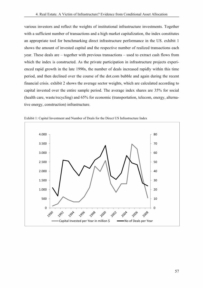
4. Real Estate. A Victim of Infrastructure? Evidence from Conditional Asset Allocation
57
various investors and reflect the weights of institutional infrastructure investments. Together
with a sufficient number of transactions and a high market capitalization, the index constitutes
an appropriate tool for benchmarking direct infrastructure performance in the US. exhibit 1
shows the amount of invested capital and the respective number of realized transactions each
year. These deals are – together with previous transactions – used to extract cash flows from
which the index is constructed. As the private participation in infrastructure projects experi-
enced rapid growth in the late 1990s, the number of deals increased rapidly within this time
period, and then declined over the course of the dot.com bubble and again during the recent
financial crisis. exhibit 2 shows the average sector weights, which are calculated according to
capital invested over the entire sample period. The average index shares are 35% for social
(health care, waste/recycling) and 65% for economic (transportation, telecom, energy, alterna-
tive energy, construction) infrastructure.
Exhibit 1: Capital Investment and Number of Deals for the Direct US Infrastructure Index
0
10
20
30
40
50
60
70
80
0
500
1.000
1.500
2.000
2.500
3.000
3.500
4.000
Capital Invested per Year in million $ No of Deals per Year
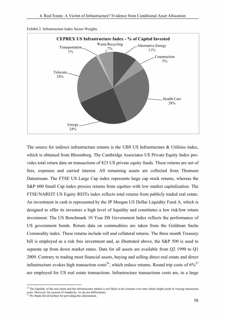
4. Real Estate. A Victim of Infrastructure? Evidence from Conditional Asset Allocation
58
Exhibit 2: Infrastructure Index Sector Weights
The source for indirect infrastructure returns is the UBS US Infrastructure & Utilities index,
which is obtained from Bloomberg. The Cambridge Associates US Private Equity Index pro-
vides total return data on transactions of 823 US private equity funds. These returns are net of
fees, expenses and carried interest. All remaining assets are collected from Thomson
Datastream. The FTSE US Large Cap index represents large cap stock returns, whereas the
S&P 600 Small Cap index proxies returns from equities with low market capitalization. The
FTSE/NAREIT US Equity REITs index reflects total returns from publicly traded real estate.
An investment in cash is represented by the JP Morgan US Dollar Liquidity Fund A, which is
designed to offer its investors a high level of liquidity and constitutes a low risk/low return
investment. The US Benchmark 10 Year DS Government Index reflects the performance of
US government bonds. Return data on commodities are taken from the Goldman Sachs
Commodity index. These returns include roll and collateral returns. The three month Treasury
bill is employed as a risk free investment and, as illustrated above, the S&P 500 is used to
separate up from down market states. Data for all assets are available from Q2 1990 to Q1
2009. Contrary to trading most financial assets, buying and selling direct real estate and direct
infrastructure evokes high transaction costs26, which reduce returns. Round trip costs of 6%27
are employed for US real estate transactions. Infrastructure transactions costs are, to a large
26 The liquidity of the real estate and the infrastructure market is not likely to be constant over time which might result in varying transaction costs. However, for reasons of simplicity, we do not differentiate. 27 We thank David Geltner for providing this information.
Alternative Energy11%
Construction5%
Health Care 28%
Energy 24%
Telecom 24%
Transportation1%
Waste/Recycling7%
CEPREX US Infrastructure Index - % of Capital Invested

4. Real Estate. A Victim of Infrastructure? Evidence from Conditional Asset Allocation
59
extent, independent of the size of the project, since they all require general services like tech-
nical, legal and financial advisory, as well as a sound estimation of demand risk. As a result,
the cost can amount to a maximum of 10% of total project cost. Average infrastructure pro-
jects evoke round trip costs of about 5.5%28. However, actual transaction costs depend on the
holding period of assets. Based on the findings of Fisher and Young (2000) and Geltner and
Pollakowski (2007), the average institutional holding period of direct real estate is roughly ten
years. According to the findings of Kaserer et al. (2009), the average duration of infrastructure
investments is four years. This average holding period seems to be very short for direct infra-
structure investments. However, one has to consider that there is a huge difference between
the average concession period which is agreed between the government and the SPV and the
holding period of an individual equity investor. While concession periods agreed between the
regulator and the SPV, is around 30 years across all sectors, on average, an individual investor
might have shorter holding periods, depending on strategic issues, such as the stage of the
infrastructure project (OECD, 2010). Due to the growing maturity of the market and the in-
creasing involvement of long-term investors, the average holding is likely to rise over the next
years. We use this information from Geltner and Pollakowski (2007) and from Kaserer (2009)
to adjust direct real estate and direct infrastructure returns.
Since investors are not homogenous, but have different investment objectives, different
benchmark returns are considered. These are 0.0%, 0.5%, 1.0%, and 2.0% real return quarter-
ly. The first target level indicates that an investor is mostly concerned with the real preserva-
tion of capital. A target rate of 0.5% reflects the objective of a conservative investor attempt-
ing to achieve a surplus over the capital preservation level which meets certain liabilities
(pension fund etc.). The 1.0% target rate reflects a core plus investor aiming to raise his capi-
tal stock in a risk-sensitive manner. The last target rate represents an opportunistic investor,
who is already concerned when returns fall below a relatively high benchmark. It is not a con-
tradiction to consider an expected return which exceeds the target return. The implication is
that, although the investor aims to achieve the expected return, only outcomes below the
benchmark constitute a risk to him.
28 We thank various institutional infrastructure investors and consultants for providing this information.

4. Real Estate. A Victim of Infrastructure? Evidence from Conditional Asset Allocation
60
4.5 Descriptive Statistics and Downside Risk
The descriptive statistics for unconditional asset returns are summarized in exhibit 3. The re-
quirement for an approach which allows for asymmetric return distributions is evident, as
most assets exhibit significant skewness and/or kurtosis. Jarque Bera tests indicate non-
normal return distributions for all assets, apart from infrastructure stocks. Private equity pro-
vides the highest return over the entire period whereas cash performs worst, but is also ex-
posed to the smallest downside risk. Direct real estate outperforms direct infrastructure but
entails a higher level of downside risk. exhibit 4 and exhibit 5 present descriptive statistics for
conditional returns. The non normal distribution of the majority of asset returns is still evident
when the sample is split into up- and down markets. Equities, commodities and private equity
outperform in up markets, direct real estate, direct infrastructure and private equity yield at-
tractive returns in down markets.
We employ Sortino-ratios to determine downside risk adjusted excess target returns. These
are given by:
(12)
Due to the small downside risk of cash, this asset class provides an attractive risk-return
tradeoff for a benchmark of 0.0%. For higher target returns, private equity yields the highest
risk adjusted returns. Direct infrastructure and direct real estate returns are not as prone to
falling short of a certain target rate as returns from stocks, commodities and REITs. There-
fore, these assets provide higher risk adjusted returns for three out of four target rates. In up
markets, depending on the target rate, cash, large caps or small caps prove to be superior in
terms of risk-adjusted returns. In down markets, the same holds for cash, bonds and private
equity.
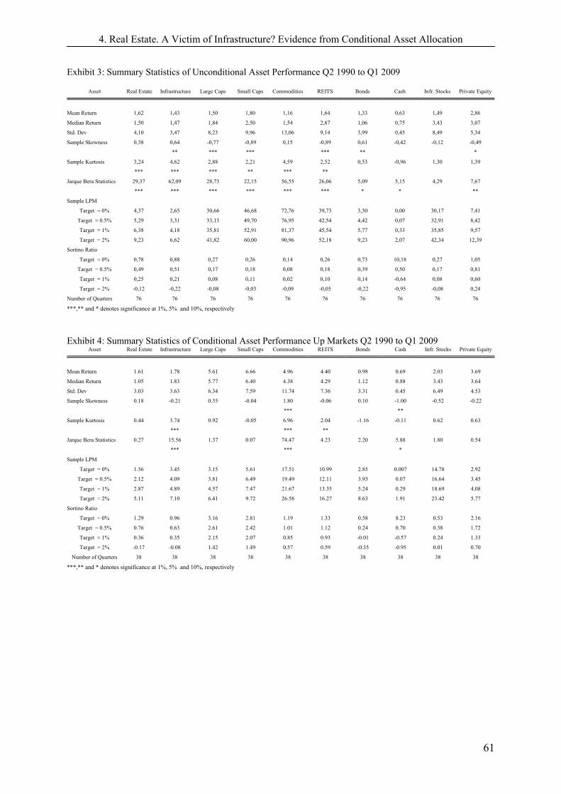
4. Real Estate. A Victim of Infrastructure? Evidence from Conditional Asset Allocation
61
Exhibit 3: Summary Statistics of Unconditional Asset Performance Q2 1990 to Q1 2009
Asset Real Estate Infrastructure Large Caps Small Caps Commodities REITS Bonds Cash Infr. Stocks Private Equity
Mean Return 1,62 1,43 1,50 1,80 1,16 1,64 1,33 0,63 1,49 2,86
Median Return 1,50 1,47 1,84 2,50 1,54 2,87 1,06 0,75 3,43 3,07
Std. Dev 4,10 3,47 8,23 9,96 13,06 9,14 3,99 0,45 8,49 5,34
Sample Skewness 0,38 0,64 -0,77 -0,89 0,15 -0,89 0,61 -0,42 -0,12 -0,49
** *** *** *** ** *
Sample Kurtosis 3,24 4,62 2,88 2,21 4,59 2,52 0,53 -0,96 1,30 1,39
*** *** *** ** *** **
Jarque Bera Statistics 29,37 62,09 28,73 22,15 56,55 26,06 5,09 5,15 4,29 7,67
*** *** *** *** *** *** * * **
Sample LPM
Target = 0% 4,37 2,65 30,66 46,68 72,76 39,73 3,30 0,00 30,17 7,41
Target = 0.5% 5,29 3,31 33,13 49,70 76,95 42,54 4,42 0,07 32,91 8,42
Target = 1% 6,38 4,18 35,81 52,91 81,37 45,54 5,77 0,33 35,85 9,57
Target = 2% 9,23 6,62 41,82 60,00 90,96 52,18 9,23 2,07 42,34 12,39
Sortino Ratio
Target = 0% 0,78 0,88 0,27 0,26 0,14 0,26 0,73 10,18 0,27 1,05
Target = 0.5% 0,49 0,51 0,17 0,18 0,08 0,18 0,39 0,50 0,17 0,81
Target = 1% 0,25 0,21 0,08 0,11 0,02 0,10 0,14 -0,64 0,08 0,60
Target = 2% -0,12 -0,22 -0,08 -0,03 -0,09 -0,05 -0,22 -0,95 -0,08 0,24
Number of Quarters 76 76 76 76 76 76 76 76 76 76
***,** and * denotes significance at 1%, 5% and 10%, respectively
Exhibit 4: Summary Statistics of Conditional Asset Performance Up Markets Q2 1990 to Q1 2009 Asset Real Estate Infrastructure Large Caps Small Caps Commodities REITS Bonds Cash Infr. Stocks Private Equity
Mean Return 1.61 1.78 5.61 6.66 4.96 4.40 0.98 0.69 2.03 3.69
Median Return 1.05 1.83 5.77 6.40 4.38 4.29 1.12 0.88 3.43 3.64
Std. Dev 3.03 3.63 6.34 7.59 11.74 7.36 3.31 0.45 6.49 4.53
Sample Skewness 0.18 -0.21 0.35 -0.04 1.80 -0.06 0.10 -1.00 -0.52 -0.22
*** **
Sample Kurtosis 0.44 3.74 0.92 -0.05 6.96 2.04 -1.16 -0.11 0.62 0.63
*** *** **
Jarque Bera Statistics 0.27 15.56 1.37 0.07 74.47 4.23 2.20 5.88 1.80 0.54
*** *** *
Sample LPM
Target = 0% 1.56 3.45 3.15 5.61 17.51 10.99 2.85 0.007 14.78 2.92
Target = 0.5% 2.12 4.09 3.81 6.49 19.49 12.11 3.93 0.07 16.64 3.45
Target = 1% 2.87 4.89 4.57 7.47 21.67 13.35 5.24 0.29 18.69 4.08
Target = 2% 5.11 7.10 6.41 9.72 26.58 16.27 8.63 1.91 23.42 5.77
Sortino Ratio
Target = 0% 1.29 0.96 3.16 2.81 1.19 1.33 0.58 8.23 0.53 2.16
Target = 0.5% 0.76 0.63 2.61 2.42 1.01 1.12 0.24 0.70 0.38 1.72
Target = 1% 0.36 0.35 2.15 2.07 0.85 0.93 -0.01 -0.57 0.24 1.33
Target = 2% -0.17 -0.08 1.42 1.49 0.57 0.59 -0.35 -0.95 0.01 0.70
Number of Quarters 38 38 38 38 38 38 38 38 38 38
***,** and * denotes significance at 1%, 5% and 10%, respectively
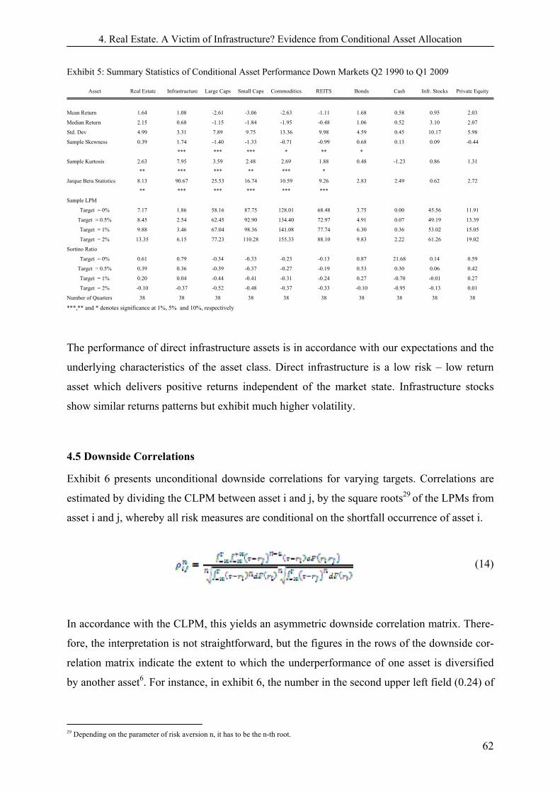
4. Real Estate. A Victim of Infrastructure? Evidence from Conditional Asset Allocation
62
Exhibit 5: Summary Statistics of Conditional Asset Performance Down Markets Q2 1990 to Q1 2009
Asset Real Estate Infrastructure Large Caps Small Caps Commodities REITS Bonds Cash Infr. Stocks Private Equity
Mean Return 1.64 1.08 -2.61 -3.06 -2.63 -1.11 1.68 0.58 0.95 2.03
Median Return 2.15 0.68 -1.15 -1.84 -1.95 -0.48 1.06 0.52 3.10 2.07
Std. Dev 4.99 3.31 7.89 9.75 13.36 9.98 4.59 0.45 10.17 5.98
Sample Skewness 0.39 1.74 -1.40 -1.33 -0.71 -0.99 0.68 0.13 0.09 -0.44
*** *** *** * ** *
Sample Kurtosis 2.63 7.95 3.59 2.48 2.69 1.88 0.48 -1.23 0.86 1.31
** *** *** ** *** *
Jarque Bera Statistics 8.13 90.67 25.53 16.74 10.59 9.26 2.83 2.49 0.62 2.72
** *** *** *** *** ***
Sample LPM
Target = 0% 7.17 1.86 58.16 87.75 128.01 68.48 3.75 0.00 45.56 11.91
Target = 0.5% 8.45 2.54 62.45 92.90 134.40 72.97 4.91 0.07 49.19 13.39
Target = 1% 9.88 3.46 67.04 98.36 141.08 77.74 6.30 0.36 53.02 15.05
Target = 2% 13.35 6.15 77.23 110.28 155.33 88.10 9.83 2.22 61.26 19.02
Sortino Ratio
Target = 0% 0.61 0.79 -0.34 -0.33 -0.23 -0.13 0.87 21.68 0.14 0.59
Target = 0.5% 0.39 0.36 -0.39 -0.37 -0.27 -0.19 0.53 0.30 0.06 0.42
Target = 1% 0.20 0.04 -0.44 -0.41 -0.31 -0.24 0.27 -0.70 -0.01 0.27
Target = 2% -0.10 -0.37 -0.52 -0.48 -0.37 -0.33 -0.10 -0.95 -0.13 0.01
Number of Quarters 38 38 38 38 38 38 38 38 38 38
***,** and * denotes significance at 1%, 5% and 10%, respectively
The performance of direct infrastructure assets is in accordance with our expectations and the
underlying characteristics of the asset class. Direct infrastructure is a low risk – low return
asset which delivers positive returns independent of the market state. Infrastructure stocks
show similar returns patterns but exhibit much higher volatility.
4.5 Downside Correlations
Exhibit 6 presents unconditional downside correlations for varying targets. Correlations are
estimated by dividing the CLPM between asset i and j, by the square roots29 of the LPMs from
asset i and j, whereby all risk measures are conditional on the shortfall occurrence of asset i.
(14)
In accordance with the CLPM, this yields an asymmetric downside correlation matrix. There-
fore, the interpretation is not straightforward, but the figures in the rows of the downside cor-
relation matrix indicate the extent to which the underperformance of one asset is diversified
by another asset6. For instance, in exhibit 6, the number in the second upper left field (0.24) of
29 Depending on the parameter of risk aversion n, it has to be the n-th root.
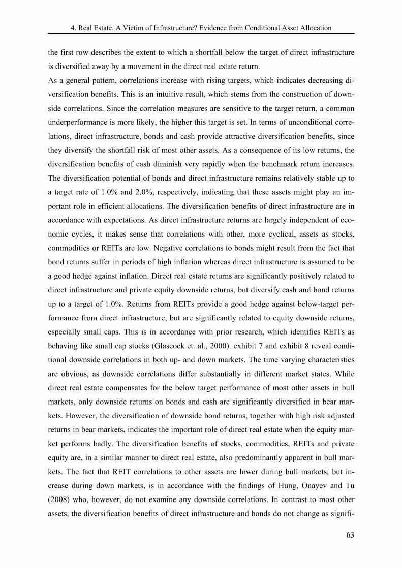
4. Real Estate. A Victim of Infrastructure? Evidence from Conditional Asset Allocation
63
the first row describes the extent to which a shortfall below the target of direct infrastructure
is diversified away by a movement in the direct real estate return.
As a general pattern, correlations increase with rising targets, which indicates decreasing di-
versification benefits. This is an intuitive result, which stems from the construction of down-
side correlations. Since the correlation measures are sensitive to the target return, a common
underperformance is more likely, the higher this target is set. In terms of unconditional corre-
lations, direct infrastructure, bonds and cash provide attractive diversification benefits, since
they diversify the shortfall risk of most other assets. As a consequence of its low returns, the
diversification benefits of cash diminish very rapidly when the benchmark return increases.
The diversification potential of bonds and direct infrastructure remains relatively stable up to
a target rate of 1.0% and 2.0%, respectively, indicating that these assets might play an im-
portant role in efficient allocations. The diversification benefits of direct infrastructure are in
accordance with expectations. As direct infrastructure returns are largely independent of eco-
nomic cycles, it makes sense that correlations with other, more cyclical, assets as stocks,
commodities or REITs are low. Negative correlations to bonds might result from the fact that
bond returns suffer in periods of high inflation whereas direct infrastructure is assumed to be
a good hedge against inflation. Direct real estate returns are significantly positively related to
direct infrastructure and private equity downside returns, but diversify cash and bond returns
up to a target of 1.0%. Returns from REITs provide a good hedge against below-target per-
formance from direct infrastructure, but are significantly related to equity downside returns,
especially small caps. This is in accordance with prior research, which identifies REITs as
behaving like small cap stocks (Glascock et. al., 2000). exhibit 7 and exhibit 8 reveal condi-
tional downside correlations in both up- and down markets. The time varying characteristics
are obvious, as downside correlations differ substantially in different market states. While
direct real estate compensates for the below target performance of most other assets in bull
markets, only downside returns on bonds and cash are significantly diversified in bear mar-
kets. However, the diversification of downside bond returns, together with high risk adjusted
returns in bear markets, indicates the important role of direct real estate when the equity mar-
ket performs badly. The diversification benefits of stocks, commodities, REITs and private
equity are, in a similar manner to direct real estate, also predominantly apparent in bull mar-
kets. The fact that REIT correlations to other assets are lower during bull markets, but in-
crease during down markets, is in accordance with the findings of Hung, Onayev and Tu
(2008) who, however, do not examine any downside correlations. In contrast to most other
assets, the diversification benefits of direct infrastructure and bonds do not change as signifi-
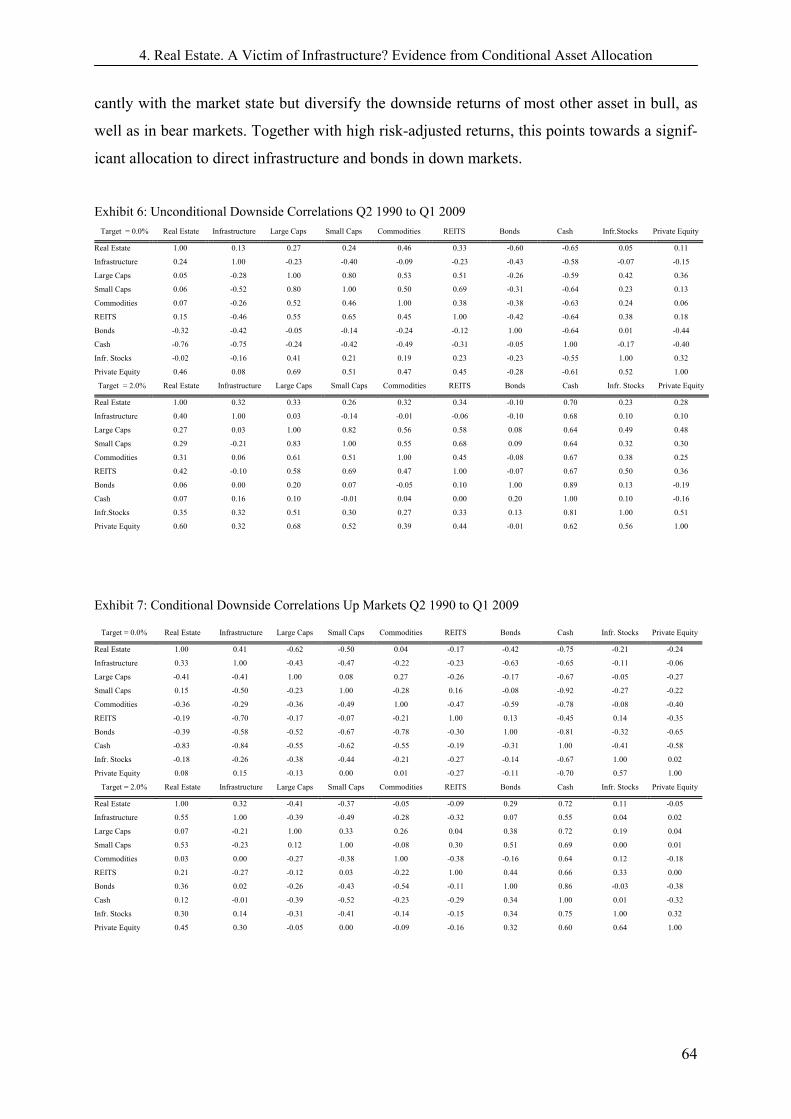
4. Real Estate. A Victim of Infrastructure? Evidence from Conditional Asset Allocation
64
cantly with the market state but diversify the downside returns of most other asset in bull, as
well as in bear markets. Together with high risk-adjusted returns, this points towards a signif-
icant allocation to direct infrastructure and bonds in down markets.
Exhibit 6: Unconditional Downside Correlations Q2 1990 to Q1 2009 Target = 0.0% Real Estate Infrastructure Large Caps Small Caps Commodities REITS Bonds Cash Infr.Stocks Private Equity
Real Estate 1.00 0.13 0.27 0.24 0.46 0.33 -0.60 -0.65 0.05 0.11
Infrastructure 0.24 1.00 -0.23 -0.40 -0.09 -0.23 -0.43 -0.58 -0.07 -0.15
Large Caps 0.05 -0.28 1.00 0.80 0.53 0.51 -0.26 -0.59 0.42 0.36
Small Caps 0.06 -0.52 0.80 1.00 0.50 0.69 -0.31 -0.64 0.23 0.13
Commodities 0.07 -0.26 0.52 0.46 1.00 0.38 -0.38 -0.63 0.24 0.06
REITS 0.15 -0.46 0.55 0.65 0.45 1.00 -0.42 -0.64 0.38 0.18
Bonds -0.32 -0.42 -0.05 -0.14 -0.24 -0.12 1.00 -0.64 0.01 -0.44
Cash -0.76 -0.75 -0.24 -0.42 -0.49 -0.31 -0.05 1.00 -0.17 -0.40
Infr. Stocks -0.02 -0.16 0.41 0.21 0.19 0.23 -0.23 -0.55 1.00 0.32
Private Equity 0.46 0.08 0.69 0.51 0.47 0.45 -0.28 -0.61 0.52 1.00
Target = 2.0% Real Estate Infrastructure Large Caps Small Caps Commodities REITS Bonds Cash Infr. Stocks Private Equity
Real Estate 1.00 0.32 0.33 0.26 0.32 0.34 -0.10 0.70 0.23 0.28
Infrastructure 0.40 1.00 0.03 -0.14 -0.01 -0.06 -0.10 0.68 0.10 0.10
Large Caps 0.27 0.03 1.00 0.82 0.56 0.58 0.08 0.64 0.49 0.48
Small Caps 0.29 -0.21 0.83 1.00 0.55 0.68 0.09 0.64 0.32 0.30
Commodities 0.31 0.06 0.61 0.51 1.00 0.45 -0.08 0.67 0.38 0.25
REITS 0.42 -0.10 0.58 0.69 0.47 1.00 -0.07 0.67 0.50 0.36
Bonds 0.06 0.00 0.20 0.07 -0.05 0.10 1.00 0.89 0.13 -0.19
Cash 0.07 0.16 0.10 -0.01 0.04 0.00 0.20 1.00 0.10 -0.16
Infr.Stocks 0.35 0.32 0.51 0.30 0.27 0.33 0.13 0.81 1.00 0.51
Private Equity 0.60 0.32 0.68 0.52 0.39 0.44 -0.01 0.62 0.56 1.00
Exhibit 7: Conditional Downside Correlations Up Markets Q2 1990 to Q1 2009
Target = 0.0% Real Estate Infrastructure Large Caps Small Caps Commodities REITS Bonds Cash Infr. Stocks Private Equity
Real Estate 1.00 0.41 -0.62 -0.50 0.04 -0.17 -0.42 -0.75 -0.21 -0.24
Infrastructure 0.33 1.00 -0.43 -0.47 -0.22 -0.23 -0.63 -0.65 -0.11 -0.06
Large Caps -0.41 -0.41 1.00 0.08 0.27 -0.26 -0.17 -0.67 -0.05 -0.27
Small Caps 0.15 -0.50 -0.23 1.00 -0.28 0.16 -0.08 -0.92 -0.27 -0.22
Commodities -0.36 -0.29 -0.36 -0.49 1.00 -0.47 -0.59 -0.78 -0.08 -0.40
REITS -0.19 -0.70 -0.17 -0.07 -0.21 1.00 0.13 -0.45 0.14 -0.35
Bonds -0.39 -0.58 -0.52 -0.67 -0.78 -0.30 1.00 -0.81 -0.32 -0.65
Cash -0.83 -0.84 -0.55 -0.62 -0.55 -0.19 -0.31 1.00 -0.41 -0.58
Infr. Stocks -0.18 -0.26 -0.38 -0.44 -0.21 -0.27 -0.14 -0.67 1.00 0.02
Private Equity 0.08 0.15 -0.13 0.00 0.01 -0.27 -0.11 -0.70 0.57 1.00
Target = 2.0% Real Estate Infrastructure Large Caps Small Caps Commodities REITS Bonds Cash Infr. Stocks Private Equity
Real Estate 1.00 0.32 -0.41 -0.37 -0.05 -0.09 0.29 0.72 0.11 -0.05
Infrastructure 0.55 1.00 -0.39 -0.49 -0.28 -0.32 0.07 0.55 0.04 0.02
Large Caps 0.07 -0.21 1.00 0.33 0.26 0.04 0.38 0.72 0.19 0.04
Small Caps 0.53 -0.23 0.12 1.00 -0.08 0.30 0.51 0.69 0.00 0.01
Commodities 0.03 0.00 -0.27 -0.38 1.00 -0.38 -0.16 0.64 0.12 -0.18
REITS 0.21 -0.27 -0.12 0.03 -0.22 1.00 0.44 0.66 0.33 0.00
Bonds 0.36 0.02 -0.26 -0.43 -0.54 -0.11 1.00 0.86 -0.03 -0.38
Cash 0.12 -0.01 -0.39 -0.52 -0.23 -0.29 0.34 1.00 0.01 -0.32
Infr. Stocks 0.30 0.14 -0.31 -0.41 -0.14 -0.15 0.34 0.75 1.00 0.32
Private Equity 0.45 0.30 -0.05 0.00 -0.09 -0.16 0.32 0.60 0.64 1.00

4. Real Estate. A Victim of Infrastructure? Evidence from Conditional Asset Allocation
65
Exhibit 8: Conditional Downside Correlations Down Markets Q2 1990 to Q1 2009
Target = 0.0% Real Estate Infrastructure Large Caps Small Caps Commodities REITS Bonds Cash Infr. Stocks Private Equity
Real Estate 1.00 0.04 0.55 0.51 0.52 0.52 -0.64 -0.68 0.15 0.28
Infrastructure 0.21 1.00 0.07 -0.28 0.12 -0.24 -0.41 -0.48 -0.05 -0.26
Large Caps 0.09 -0.29 1.00 0.84 0.55 0.60 -0.26 -0.61 0.48 0.45
Small Caps 0.05 -0.57 0.86 1.00 0.55 0.75 -0.33 -0.62 0.26 0.17
Commodities 0.16 -0.29 0.77 0.72 1.00 0.63 -0.34 -0.65 0.33 0.19
REITS 0.21 -0.41 0.72 0.76 0.72 1.00 -0.49 -0.72 0.42 0.26
Bonds -0.33 -0.34 0.52 0.32 0.15 0.06 1.00 -0.49 0.25 -0.24
Cash -0.71 -0.63 0.19 -0.08 -0.47 -0.87 0.40 1.00 -0.20 -0.31
Infr.Stocks 0.05 -0.11 0.78 0.52 0.42 0.46 -0.26 -0.53 1.00 0.43
Private Equity 0.52 0.07 0.85 0.59 0.72 0.61 -0.31 -0.59 0.52 1.00
Target = 2.0% Real Estate Infrastructure Large Caps Small Caps Commodities REITS Bonds Cash Infr. Stocks Private Equity
Real Estate 1.00 0.33 0.61 0.54 0.53 0.54 -0.28 0.73 0.28 0.43
Infrastructure 0.35 1.00 0.37 0.16 0.23 0.13 -0.23 0.81 0.14 0.16
Large Caps 0.29 0.08 1.00 0.86 0.60 0.65 0.04 0.65 0.53 0.54
Small Caps 0.26 -0.22 0.89 1.00 0.60 0.73 0.05 0.65 0.35 0.36
Commodities 0.38 0.09 0.83 0.78 1.00 0.70 -0.07 0.71 0.48 0.37
REITS 0.49 -0.03 0.74 0.80 0.75 1.00 -0.19 0.71 0.53 0.43
Bonds -0.10 -0.01 0.64 0.55 0.35 0.32 1.00 0.93 0.23 -0.01
Cash 0.05 0.33 0.46 0.38 0.26 0.20 0.09 1.00 0.15 -0.04
Infr. Stocks 0.36 0.42 0.82 0.61 0.51 0.57 0.06 0.87 1.00 0.57
Private Equity 0.65 0.36 0.85 0.66 0.63 0.66 -0.09 0.65 0.54 1.00
4.6 Asset Allocations
4.6.1 Unconditional Portfolios
Unconditional DR portfolios30 are presented in exhibits 9A and 9B. One striking result is the
sensitivity of asset weights to changes in the target rate. This underpins the need for an ap-
proach that allows for varying benchmark returns. Direct infrastructure and bond allocations
are significantly affected, as their allocations apparently decrease with rising targets. This is
due to a strong increase in downside correlations when the target rate increases. However,
both assets are significantly weighted in unconditional portfolios, which is not attributable to
their performance but a result of low exposure to downside risk and good diversification ben-
efits. This is in accordance with the distributional characteristics of direct infrastructure re-
turns as they exhibit significant positive skewness and kurtosis – which is preferred by the
optimization algorithm. Private equity and cash allocations tend to rise with higher target lev-
els. A high exposure to cash does not seem to be intuitively correct, when the target return is
high. However, even for high targets, cash is not exposed to high downside risk and is there-
fore allocated to low and medium expected return portfolios. Direct real estate allocations
range from 0% to 7% of an investor’s total wealth and are highest in medium-expected-return
portfolios. These weights tend to rise to a benchmark return of 1.0% and then decrease for the
highest target returns. Direct real estate allocations are lower than in most other studies and
30 The Exhibits on target returns 0.5 and 1.0 percent for all scenarios are available from the authors upon request

4. Real Estate. A Victim of Infrastructure? Evidence from Conditional Asset Allocation
66
more in accordance with actual weights in institutional investment portfolios. This result
could be caused by the inclusion of direct infrastructure. Both, direct real and direct infra-
structure returns are positively correlated to each other and both diversify bond returns. How-
ever, as direct infrastructure exhibits considerably lower levels of downside risk, it is more
heavily weighted than direct real estate. Moreover, the diversification benefits between direct
infrastructure and private equity are much more distinctive than those between direct real es-
tate and private equity. Therefore, direct infrastructure seems to partially replace direct real
estate in unconditional portfolios. This issue is discussed further in Section VIII. When the
target return is low, stocks, commodities and REITs are represented only marginally and dis-
appear from efficient portfolios when the target is set to the highest level. One might argue
that the low proportion of stocks stems from their poor performance during the recent finan-
cial crisis. However, the allocation to stocks is even smaller when we control for the effects of
the crisis and run the optimization from Q2 1990 to Q2 2007.31
4.6.2 Bull Market Portfolios
While hardly any equities are present in unconditional portfolios, their importance is apparent
in up markets as shown in exhibits 10A and 10B. Due to outstanding performance, high allo-
cations to small caps of between 21% and 54% of total wealth are recommended. They are
not only heavy in high return portfolios, but appear across all levels of expected returns. Sur-
prisingly, large caps do not move together with small caps, but even diversify their shortfalls
for lower targets. Together with high returns, this induces allocations within a range from 6%
to 26%. Although direct real estate returns are negatively correlated with shortfalls of some
assets, at least for the first and the second target, it is not accounted for within any efficient
bull-market portfolio. This is, on the one hand, due to its low returns, but is also caused by the
fact, that other assets feature even better diversification benefits. Direct infrastructure, which
yields lower risk-adjusted returns than direct real estate, for three out of four targets, exhibits
better diversification benefits with important up-market assets like small caps or commodities.
These diversification effects are apparent even for high target rates. As a result, infrastructure
increases with rising targets and mounts to a maximum of 28% and constitutes an important
asset for low-to-medium-return portfolios across all benchmark returns. Despite its low re-
turns, bonds are allocated to low-return portfolios, as they offer good diversification benefits,
in particular with respect to downside returns of small caps, direct infrastructure and com-
modities. The allocation to commodities is relatively stable across all expected returns, which
31 The results are available from the authors upon request.
4. Real Estate. A Victim of Infrastructure? Evidence from Conditional Asset Allocation
67
reflects a mix of good performance and diversification effects. Although REITs deliver higher
returns, by simultaneously being exposed to lower downside risk than indirect infrastructure,
both assets are weighted to a similar extent for targets of 0.0% and 0.5%. This is due to the
diversification properties of infrastructure stocks, especially towards small caps. When higher
targets have to be achieved, REITs are allocated more heavily.
4.6.3 Bear Market Portfolios
Sortino ratios and downside correlations reveal that an investment in direct real estate yields
attractive risk-adjusted returns, along with significant diversification benefits towards bonds
and cash in down markets. Therefore, direct real estate contributes essentially to portfolio
performance and plays a major role in asset allocation. As exhibits 11A and 11B indicate,
relatively high allocations of between 0% and 27%, which clearly exceed the numbers in un-
conditional models and those in most institutional investment portfolios, are recommended.
These high proportions of direct real estate are robust towards a change in the target rate,
which indicates that direct real estate is included in the portfolio mainly because of its rela-
tively high returns. Although direct real estate has higher risk-adjusted returns than direct in-
frastructure, direct infrastructure accounts for a significant proportion, predominantly in low
and medium- expected-return portfolios and amounts to a maximum of 52% of total wealth.
Together with direct real estate, it exhibits low correlations to bonds, but is more effective in
diversifying private equity downside returns. The higher allocation to direct infrastructure is,
however, not mainly attributable to better diversification benefits, but rather to the fact that it
exhibits much lower downside risk than direct real estate. The distributional characteristics,
i.e. positive skewness and kurtosis, contribute to these results and indicate a preference for
direct infrastructure in a downside risk framework. Bonds diversify direct real estate, as well
as direct infrastructure downside returns across all benchmarks. Together with high risk-
adjusted returns, this provides a strong rationale for including a large proportion of bonds in
down- market states. The theoretical allocations amount to a maximum of 54%. In contrast to
direct real estate and infrastructure allocations, bonds are also included in higher-expected-
return portfolios, as they exhibit negative correlations with shortfalls of private equity, which
is allocated for higher return levels. Stocks, indirect infrastructure and commodities only play
a minor role, due to their weak performance and common downward bias in bear markets.
Only REITs are included up to a small proportion of 6% for low expected returns and target
rates.
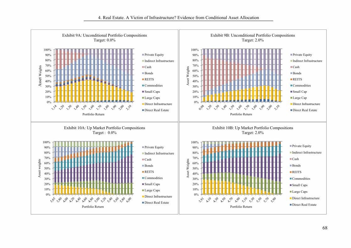
0%
10%
20%
30%
40%
50%
60%
70%
80%
90%
100%
Ass
et W
eigh
tsE
0%
10%
20%
30%
40%
50%
60%
70%
80%
90%
100%
Ass
et w
eigh
ts
Portfolio
Exhibit 9A: UncondT
Portfolio R
Exhibit 10A: Up MT
4. Real Estate. A
Return
ditional Portfolio CoTarget: 0.0%
Return
Market Portfolio Comarget : 0.0%
A Victim of Infras
ompositions
Private Equ
Indirect In
Cash
Bonds
REITS
Commodit
Small Cap
Large Cap
Direct Infr
Direct Rea
mpositions
Private Equ
Indirect In
Cash
Bonds
REITS
Commodit
Small Cap
Large Cap
Direct Infr
Direct Rea
structure? Eviden
uity
frastructure
ties
s
s
rastructure
al Estate
Ass
et W
eigh
ts
uity
frastructure
ties
s
s
rastructure
al Estate
Ass
et W
eigh
ts
ce from Condition
0%
10%
20%
30%
40%
50%
60%
70%
80%
90%
100%
Exhibit
0%
10%
20%
30%
40%
50%
60%
70%
80%
90%
100%
Exhib
nal Asset Allocati
Portfolio Return
t 9B: UnconditionalTarget:
Portfolio Return
it 10B: Up Market Target:
ion
l Portfolio Compos2.0%
Portfolio Composit2.0%
itions
Private Equity
Indirect Infrastruct
Cash
Bonds
REITS
Commodities
Small Cap
Large Cap
Direct Infrastructu
Direct Real Estate
tions
Private Equity
Indirect Infrastructu
Cash
Bonds
REITS
Commodities
Small Caps
Large Caps
Direct Infrastructur
Direct Real Estate
68
ture
ure
ure
re
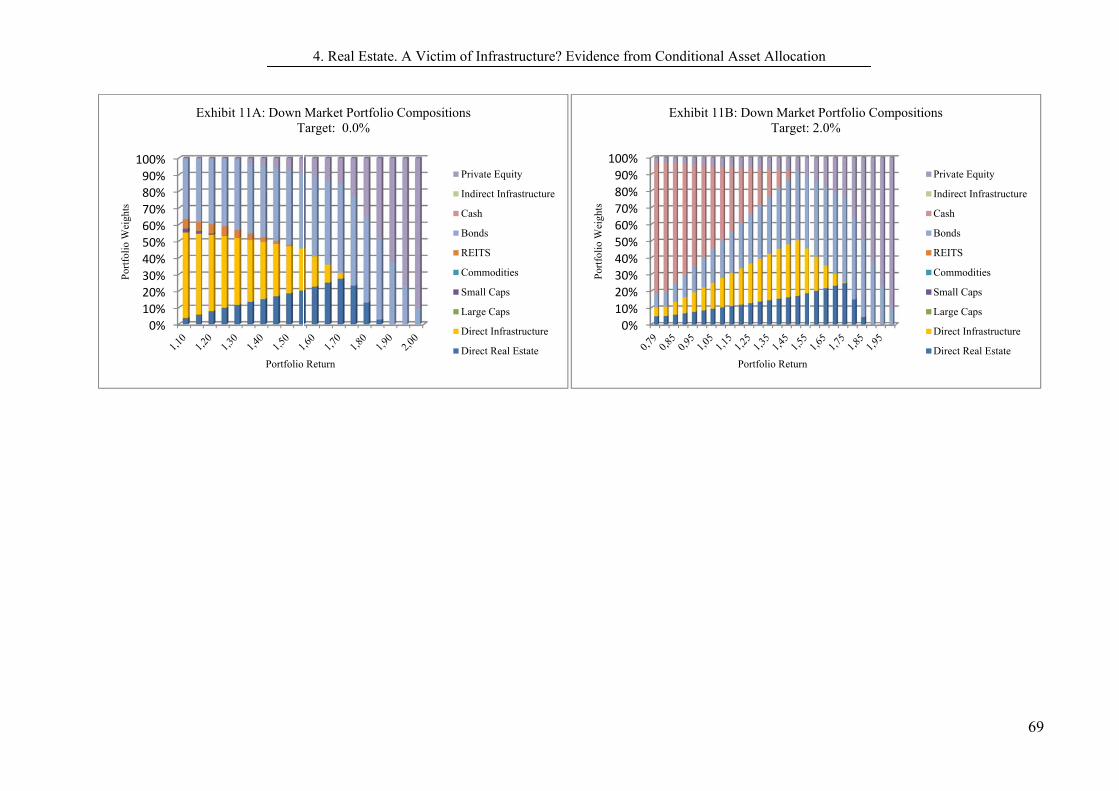
0%10%20%30%
40%50%60%70%80%90%100%
Por
tfol
io W
eigh
tsE
Portfolio
Exhibit 11A: Down T
4. Real Estate. A
Return
Market Portfolio CTarget: 0.0%
A Victim of Infras
Compositions
Private Equ
Indirect In
Cash
Bonds
REITS
Commodit
Small Cap
Large Cap
Direct Infr
Direct Rea
structure? Eviden
uity
frastructure
ties
s
s
rastructure
al Estate
Por
tfol
io W
eigh
ts
ce from Condition
0%
10%
20%
30%
40%
50%
60%
70%
80%
90%
100%
Exhibit
nal Asset Allocati
Portfolio Return
11B: Down MarkeTarget:
ion
et Portfolio Compos2.0%
sitions
Private Equity
Indirect Infrastruct
Cash
Bonds
REITS
Commodities
Small Caps
Large Caps
Direct Infrastructu
Direct Real Estate
69
ture
ure

4. Real Estate. A Victim of Infrastructure? Evidence from Conditional Asset Allocation
70
4.6.4 Constrained Asset Allocations
The previous results were determined without any restrictions on portfolio weights and consti-
tute theoretical asset weights. In statistical terms, these allocations are corner solutions. How-
ever, in practice, many institutional investors like pension funds are – due to regulatory con-
straints or strategic issues – restricted in terms of their asset allocations and often heavily in-
vested in large cap stocks and bonds. In order to examine the effect and role of direct real es-
tate and direct infrastructure in constrained portfolios, we impose restrictions on the efficient
frontiers. The combined allocation to bonds and large cap stocks must sum up to at least 60%
with at least 20% of the total wealth being allocated to one of these assets. To be responsive
to changing market conditions, many investors hold a proportion of their total wealth in liquid
assets which, however, should not exceed a certain percentage. Therefore, we specify the
weighting to cash at a minimum of 5% and a maximum 10%.
Exhibits 12A to 14B present constrained portfolio weights in three different market states. As
the diversification benefits of direct real estate to large cap stocks are not very distinctive
across the whole sample, real estate is removed from the portfolio. Since large caps enter the
portfolio, the allocation to direct infrastructure declines for the first and the second target re-
turn. However, the allocation remains relatively high with weights up to 35%. For the two
higher target returns, the allocation to direct infrastructure increases, due to its diversification
benefits with large caps and bonds, as well as from removing cash. While real estate loses its
position in unconditional portfolios, infrastructure remains an important asset when asset
weights are constrained. Although the inclusion of large cap stocks and bonds induces a re-
duction of direct infrastructure weights in up markets, infrastructure is still included in the
portfolio and allocations amount to a maximum of 15% - again a result of its diversification
benefits with bond and stock returns. In down market portfolios, both assets – direct infra-
structure and direct real estate – are still heavily weighted and contribute to portfolio diversi-
fication as well as to stable returns.
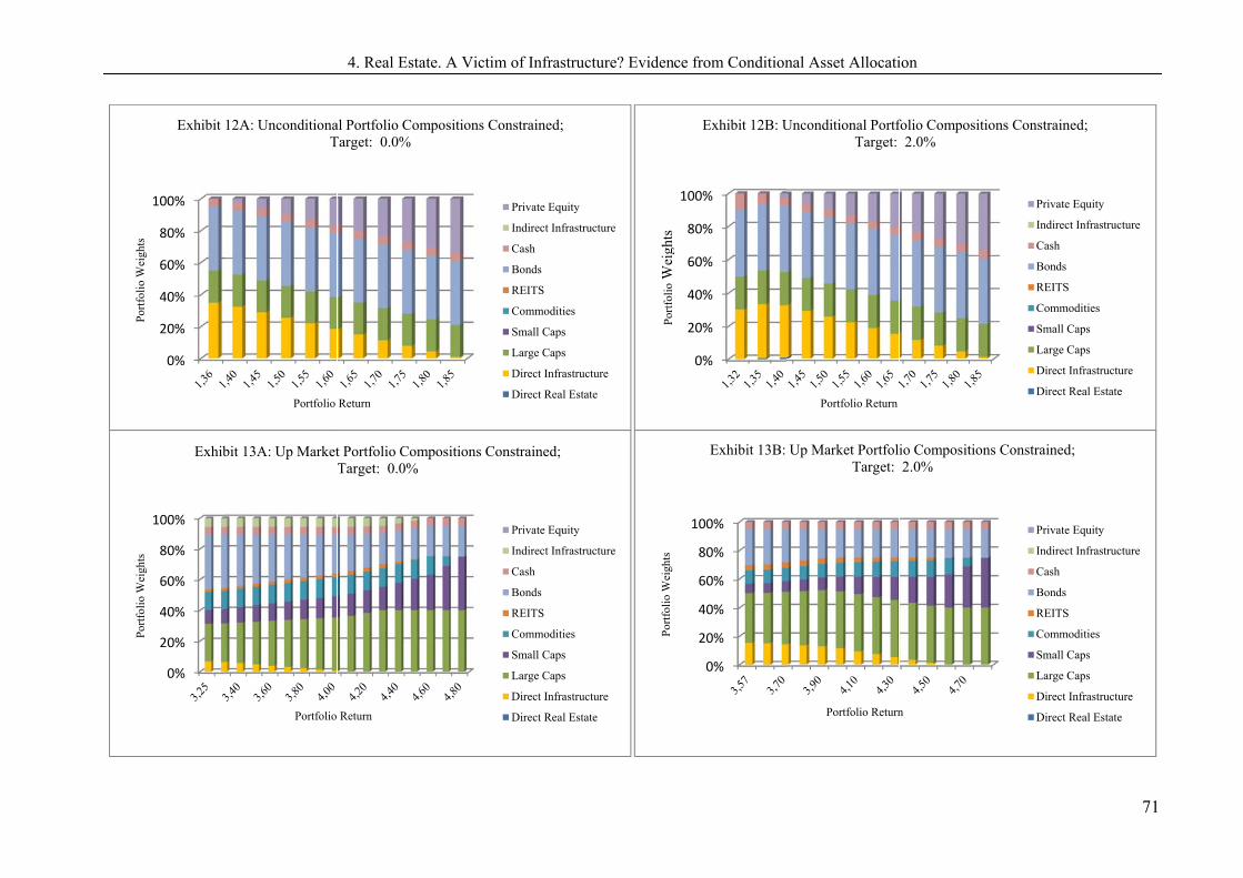
0%
20%
40%
60%
80%
100%
Por
tfol
io W
eigh
ts
Exhibit
0%
20%
40%
60%
80%
100%
Por
tfol
io W
eigh
ts
Exhib
Portfolio
12A: UnconditionaT
Portfolio
bit 13A: Up Market
4. Real Estate. A
Return
al Portfolio ComposTarget: 0.0%
Return
t Portfolio ComposiTarget: 0.0%
A Victim of Infras
sitions Constrained;
Private Equ
Indirect Inf
Cash
Bonds
REITS
Commodit
Small Caps
Large Caps
Direct Infra
Direct Rea
itions Constrained;
Private Equ
Indirect Inf
Cash
Bonds
REITS
Commodit
Small Caps
Large Caps
Direct Infra
Direct Rea
structure? Eviden
;
uity
frastructure
ties
s
s
astructure
al Estate
Por
tfol
ioW
eigh
ts
uity
frastructure
ties
s
s
astructure
al Estate
Por
tfol
io W
eigh
ts
ce from Condition
0%
20%
40%
60%
80%
100%
g
Exhibit 12B: U
0%
20%
40%
60%
80%
100%
Exhibit 13B:
nal Asset Allocati
Portfolio Return
Unconditional PortfTarget:
Portfolio Return
Up Market PortfoliTarget:
ion
folio Compositions 2.0%
n
io Compositions Co2.0%
Constrained;
Private Equity
Indirect Infrastruct
Cash
Bonds
REITS
Commodities
Small Caps
Large Caps
Direct Infrastructur
Direct Real Estate
onstrained;
Private Equity
Indirect Infrastruct
Cash
Bonds
REITS
Commodities
Small Caps
Large Caps
Direct Infrastructur
Direct Real Estate
71
ture
re
ture
re
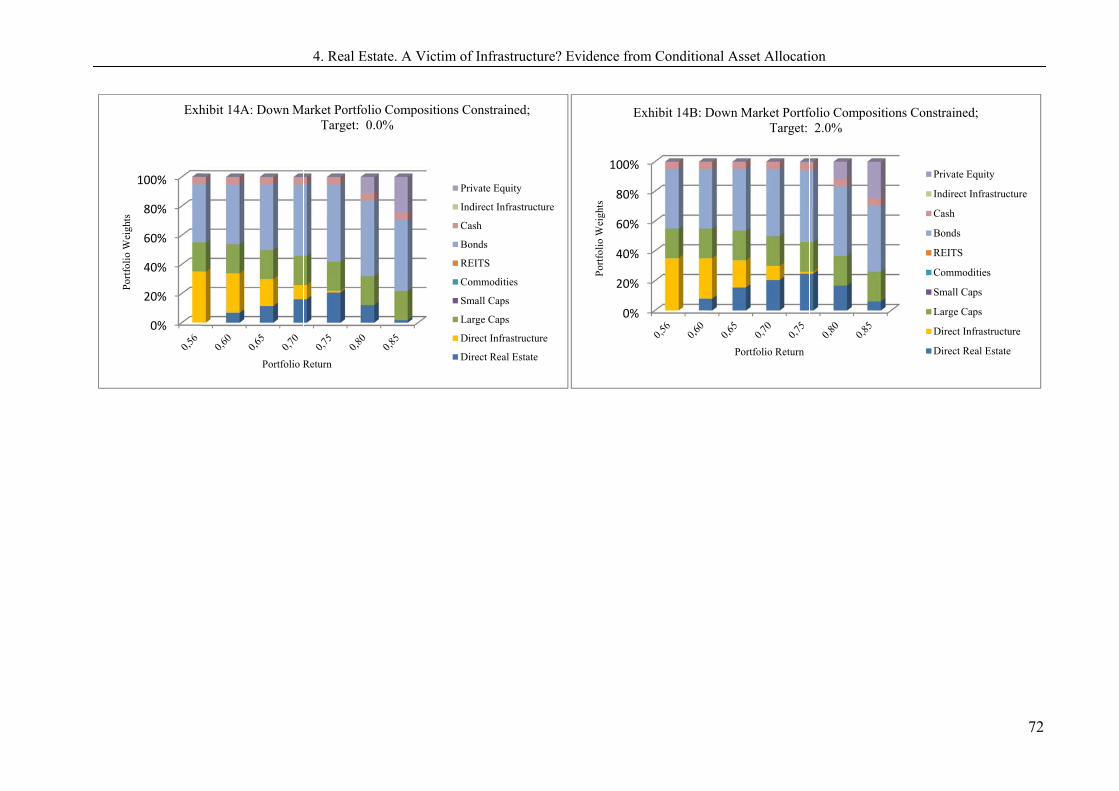
0%
20%
40%
60%
80%
100%
Por
tfol
io W
eigh
ts
Exh
Portfolio R
hibit 14A: Down M
4. Real Estate. A
Return
Market Portfolio ComTarget: 0.0%
A Victim of Infras
mpositions Constrai
Private Equ
Indirect Inf
Cash
Bonds
REITS
Commodit
Small Caps
Large Caps
Direct Infra
Direct Rea
structure? Eviden
ined;
uity
frastructure
ties
s
s
astructure
al Estate
Por
tfol
io W
eigh
ts
ce from Condition
0%
20%
40%
60%
80%
100%
Exhibit 14B: D
nal Asset Allocati
Portfolio Return
Down Market PortfoTarget:
ion
folio Compositions 2.0%
Constrained;
Private Equity
Indirect Infrastruct
Cash
Bonds
REITS
Commodities
Small Caps
Large Caps
Direct Infrastructu
Direct Real Estate
72
ture
ure

4. Real Estate. A Victim of Infrastructure? Evidence from Conditional Asset Allocation
73
4.7 The Effects of Infrastructure on Asset Weights
4.7.1 Unconditional Portfolios
In order to gain an impression of the extent to which the inclusion of direct and indirect infra-
structure8 affects the allocation to other assets, in particular real estate, unconditional and
conditional efficient portfolios are estimated with and without infrastructure assets. As exhib-
its 15A and 15B reveal, the inclusion of direct infrastructure to unconditional multi-asset port-
folios significantly impacts on the allocations to direct real estate, cash and private equity, by
inducing a reduction in the proportion of these assets. As direct infrastructure is, similar to
cash, perceived as a low-risk, low-return asset, and exhibits characteristics common to direct
real estate, these changes in asset allocations make sense intuitively. Portfolios without infra-
structure comprise direct real estate up to a maximum of 25%. This allocation, however, de-
creases down to a maximum of 7%. The effect that direct real is replaced by direct infrastruc-
ture is consistent across all examined target returns. Although direct real estate outperforms
direct infrastructure in unconditional market states, there are several reasons why the alloca-
tion to direct real estate diminishes when infrastructure is added to the portfolio. One reason is
that direct infrastructure investments exhibit lower levels of downside risk. Furthermore, as a
consequence of its positively skewed returns, direct infrastructure more effectively diversifies
downside returns from other assets. Moreover, downside returns from infrastructure can more
easily be diversified than those from real estate. As the downside returns of both assets are,
moreover, positively correlated, direct infrastructure usurps the position that real estate occu-
pied before the inclusion of infrastructure. While other studies find no asset that provides such
unique diversification benefits as direct real estate, direct infrastructure does indeed seem to
do so and additionally provides attractive risk-adjusted returns. Although our results suggest a
need to remove funds from direct real estate and allocate them to direct infrastructure, one has
to bear in mind that actual direct real estate allocations are not as high as suggested by the
model, but significantly lower. Therefore, these results do not automatically imply that inves-
tors should replace real estate with infrastructure, but investors might reconsider their portfo-
lio allocations, so as to obtain a better risk return tradeoff through the inclusion of infrastruc-
ture. In terms of theoretical portfolio allocations, these results imply that the allocation to di-
rect real estate and cash might be overstated, when direct infrastructure is not considered in an
asset allocation framework. As a further result, one can easily see that direct infrastructure
removes a significant proportion of cash from the portfolio. This occurs, as infrastructure sig-
nificantly outperforms cash by contemporaneously offering relatively low levels of downside

4. Real Estate. A Victim of Infrastructure? Evidence from Conditional Asset Allocation
74
risk. However, cash returns are negatively correlated to most other assets and cash, further-
more, exhibits the lowest downside risk of all analyzed investment opportunities. Therefore,
allocations to this asset class remain fairly high, especially for low-to-medium-expected-
return portfolios. For higher expected returns, cash is replaced almost entirely by direct infra-
structure. Private equity is replaced by direct infrastructure in low-return portfolios, which
stems from direct infrastructure’s diversification effects with bonds. This does not hold for
higher expected-return portfolios, as private equity returns are required to achieve these re-
turns. In contrast to the common belief that infrastructure assets show some bond-type charac-
teristics, as stable and predictable cash flows, the allocation to bonds is not very heavily af-
fected by the inclusion of direct infrastructure. As a result of higher average infrastructure
returns, bonds lose weight for higher-expected-return portfolios. However, since bonds and
direct infrastructure diversify each other for lower target returns, the allocation to bonds even
increases in low-return portfolios when direct infrastructure is allowed to enter the portfolio.
A similar argumentation applies to REITs, whose allocations increase slightly with the inclu-
sion of infrastructure. Their downside returns are also negatively correlated to indirect infra-
structure performance.
4.7.2 Bull Market Portfolios
Although infrastructure is regarded as a low-risk, low return investment, it is present in up-
market portfolios and predominantly replaces bonds, which lose weight for each target rate
(see Exhibit 16A and 16B). Furthermore, one can observe that private equity investments are
eliminated from the portfolio. As direct real estate is not present in up-market portfolios, the
inclusion of infrastructure cannot affect its allocation. However, REITs lose weight when di-
rect and indirect infrastructure enters the portfolio. This is mostly due to the inclusion of indi-
rect rather than direct infrastructure and mostly happens for smaller targets. At a first glance,
there seems to be no reason why infrastructure should replace private equity. Private equity
exhibits higher average returns and lower downside risk than direct and indirect infrastructure
investments. Moreover, neither direct nor indirect infrastructure diversifies downside returns
on most other assets more effectively than private equity. However, the ability of other assets
to diversify direct and indirect infrastructure downside returns is much more distinctive than
diversifying downside returns on private equity. The loss in return which results from the ex-
clusion of private equity is offset by the inclusion of small caps, which exhibit the best per-
formance in up markets. The higher downside risk of small caps is tolerated, as small caps
exhibit more attractive diversification properties with (direct) infrastructure than with private
equity. This explains the switch in allocations from private equity to infrastructure assets and

4. Real Estate. A Victim of Infrastructure? Evidence from Conditional Asset Allocation
75
to small caps in up markets. As infrastructure assets have higher risk-adjusted returns than
bonds and also offer attractive diversification benefits with stocks, the explanation of the de-
crease in bond weights is straightforward. The reason for the exclusion of private equity and
bonds is due mainly to the inclusion of direct infrastructure rather than indirect infrastructure
assets.
4.7.3 Bear Market Portfolios
Although, the inclusion of direct infrastructure also leads to a decrease in direct real estate
weights in down markets, these effects are not as distinctive as those found for unconditional
portfolios (see Exhibit 17A and 17B). Although direct infrastructure is more effective in terms
of diversification, it offers a lower level of downside risk and is positively related to downside
real estate returns across all target rates. Direct real estate is still heavily weighted and its al-
location is above those in most institutional investment portfolios. This stems mostly from the
superior performance of direct real estate in down markets, which is significantly above that
of infrastructure. The negative correlation with bonds, which is the dominant asset in down
markets, is a further reason for the relatively high direct real estate weights.
Contrary to intuition, the inclusion of direct infrastructure enhances the proportion of bonds in
the portfolio for the two lower-benchmark returns and for low expected returns. Due to the
negative correlations between both assets, this comes as no surprise.
For lower target rates and lower expected returns, the inclusion of infrastructure raises the
proportion of REITs in the portfolio. Although this also sounds somewhat counterintuitive,
this stems from the fact that direct infrastructure investments diversify down movements in
REIT returns and vice versa. Similar to unconditional portfolios, cash is removed from the
portfolio.
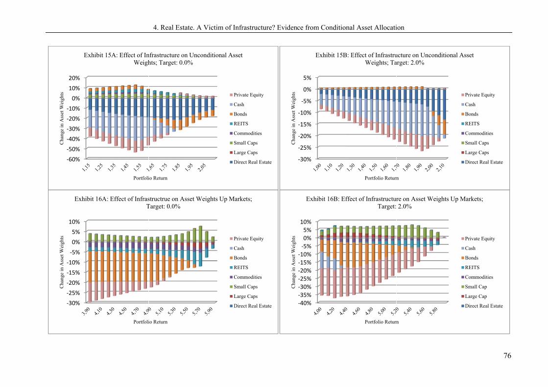
‐60%
‐50%
‐40%
‐30%
‐20%
‐10%
0%
10%
20%
Cha
nge
in A
sset
Wei
ghts
Exhib
‐30%
‐25%
‐20%
‐15%
‐10%
‐5%
0%
5%
10%
Cha
nge
in A
sset
Wei
ghts
Exhibit 16
Portfoli
bit 15A: Effect of InWeigh
Portfoli
6A: Effect of InfrasT
4. Real Estate. A
io Return
nfrastructure on Unchts; Target: 0.0%
io Return
structrue on Asset WTarget: 0.0%
A Victim of Infras
conditional Asset
Private
Cash
Bonds
REITS
Comm
Small C
Large C
Direct
Weights Up Market
Private
Cash
Bonds
REITS
Comm
Small C
Large C
Direct
structure? Eviden
e Equity
S
modities
Caps
Caps
Real Estate
Cha
nge
in A
sset
Wei
ghts
s;
e Equity
S
modities
Caps
Caps
Real Estate
Cha
nge
in A
sset
Wei
ghts
ce from Condition
‐30%
‐25%
‐20%
‐15%
‐10%
‐5%
0%
5%
Exhibit 15B
‐40%‐35%‐30%‐25%‐20%‐15%‐10%‐5%0%5%10%
Exhibit 16B: Ef
nal Asset Allocati
Portfolio Return
: Effect of InfrastruWeights; Ta
Portfolio Return
ffect of InfrastructurTarget:
ion
n
ucture on Unconditiarget: 2.0%
n
re on Asset Weight2.0%
ional Asset
Private Equity
Cash
Bonds
REITS
Commodities
Small Caps
Large Caps
Direct Real Est
ts Up Markets;
Private Equity
Cash
Bonds
REITS
Commodities
Small Cap
Large Cap
Direct Real Est
76
tate
tate
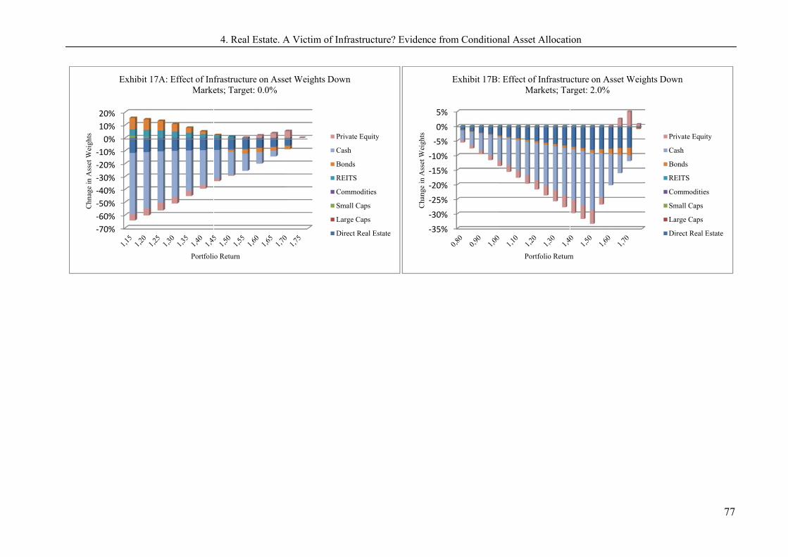
‐70%
‐60%
‐50%
‐40%
‐30%
‐20%
‐10%
0%
10%
20%
Chn
age
in A
sset
Wei
ghts
Exhibi
Portfoli
it 17A: Effect of InfMarke
4. Real Estate. A
o Return
frastructure on Asseets; Target: 0.0%
A Victim of Infras
et Weights Down
Private
Cash
Bonds
REITS
Comm
Small C
Large C
Direct
structure? Eviden
e Equity
S
modities
Caps
Caps
Real Estate
Cha
nge
in A
sset
Wei
ghts
ce from Condition
‐35%
‐30%
‐25%
‐20%
‐15%
‐10%
‐5%
0%
5%
Exhibit 17B:
nal Asset Allocati
Portfolio Return
: Effect of InfrastruMarkets; Ta
ion
n
ucture on Asset Weiarget: 2.0%
ights Down
Private Equity
Cash
Bonds
REITS
Commodities
Small Caps
Large Caps
Direct Real Est
77
tate

4. Real Estate. A Victim of Infrastructure? Evidence from Conditional Asset Allocation
78
4.8 Conclusion
The emergence of infrastructure as an asset class requires a reassessment of traditional portfo-
lio strategies, which are based mainly on assets like stocks, bonds and real estate. This study
addresses the issue by using a novel data set on individual infrastructure cash flows which
facilitates – for the first time – building a direct infrastructure total return index. We deter-
mine efficient portfolio weights when infrastructure and real estate are allocated simultane-
ously to a multi-asset portfolio that contains a range of further assets. We focus in particular,
on the relationship between real estate and infrastructure as these assets are often assumed to
exhibit similar underlying characteristics and similar diversification benefits.
Since the role of downside risk is intuitive and evident in the pricing of risky assets, we apply
an optimization algorithm which accounts for a measure of downside risk, rather than of vari-
ance. This approach is likely to conform more closely to rational investor behavior and is ca-
pable of reflecting different target returns. In order to account for time-varying asset behavior,
we draw a distinction between up and down markets and determine dynamic portfolio
weights.
Two general results can be summarized as follows. Firstly, attributable to the time-varying
return characteristics of various assets, the composition of efficient portfolios is heavily de-
pendent on the state of the market. Secondly, asset allocations differ significantly with a
change in investor-specific target return. Ignoring these issues may lead to results of only lim-
ited significance.
In terms of direct real estate portfolio weights, the unconditional models produce allocations
which are more in accordance with the practice of institutional investment portfolios, but be-
low the allocations in most other asset allocation studies. This result is caused mainly by two
factors. Firstly, employing downside risk instead of variance is more appropriate when asset
returns are not normally distributed. As direct real estate returns are characterized by high
kurtosis, this is accounted for in the downside-risk approach. Furthermore, the inclusion of a
broad range of investment opportunities is likely to avoid allocations which are too heavy in
one asset. Unconditional results in particular, reveal the importance of direct infrastructure for
portfolio diversification and show that theoretical allocations to direct real estate are likely to
be overestimated when direct infrastructure is not considered. The allocation to real estate is
significantly higher when infrastructure assets are not accounted for. This effect is mostly
evident in unconditional portfolios and a result of similar returns and infrastructure’s diversi-
fication benefits as well as its lower downside risk.
4. Real Estate. A Victim of Infrastructure? Evidence from Conditional Asset Allocation
79
The important role of direct real estate is apparent in a conditional allocation framework.
While equities – including infrastructure stocks – commodities, REITs and direct infrastruc-
ture are the predominant assets in up markets, direct real estate performs well in bear markets
and is helpful in diversifying downside returns from other assets. As a result, the recommend-
ed allocations rise to a maximum of 27%. These high proportions hold across all target rates.
Although the allocation to direct real estate also suffers in down markets when infrastructure
is included, this effect is not as distinctive as in unconditional market states. This is caused
mainly by relatively high direct real-estate returns in down markets, which significantly ex-
ceed those from direct infrastructure. Nevertheless, direct infrastructure is weighted more
heavily than direct real estate, as it also provides diversification benefits and exhibits a low
level of downside risk when stock markets perform badly. However, it is more sensitive to-
wards changes in the benchmark return than direct real estate. According to these findings,
both assets, direct real estate and direct infrastructure add substantial value to portfolios in
bear markets. Real estate does so mainly due to its high returns and infrastructure due to its
diversification benefits. These results throw new light on the role of real estate in the asset
allocation process and highlight the importance of the market state for portfolio compositions.
Efficient allocations are dependent on numerous parameters and no strict proportion of assets
proves to be consistently superior. However, as transferring direct real estate and direct infra-
structure assets evokes significant transaction costs and is associated with a high expenditure
of time, the adjustment of portfolio weights creates enormous difficulties. Therefore, when
direct assets are considered within a time-varying allocation framework, the results must be
interpreted with caution. It makes no sense for investors to change their allocation in accord-
ance with their expectation1 of market moves, but direct real estate, as well as direct infra-
structure, constitute important assets when the main concern is to protect the portfolio in
downside markets and when investors are prepared to relinquish some return in order to
achieve this aim. An investor who is interested mainly in participating in market upswings is
recommended to invest in equities and indirect, rather than direct real estate. As direct infra-
structure also constitutes an important component in bull markets, our results point to a signif-
icant allocation to direct infrastructure investments. However, one has to consider that, the
allocation to direct infrastructure in particular is highly sensitive to a change in the target rate,
as it is included in the portfolio mainly due to its diversification benefits, rather than to its
outstanding returns. Considering the fact that infrastructure accounts for a significant propor-
tion of GDP and considerating our results, an investor is exposed to non-systematic risk, if
1 Moreover, the investor has to anticipate the state of the market ex ante.

4. Real Estate. A Victim of Infrastructure? Evidence from Conditional Asset Allocation
80
direct infrastructure is not included in the investment portfolio. However, neither infrastruc-
ture nor any other alternative asset is able to replace real estate in institutional investment
portfolios as a whole. Although the allocation to direct real estate is below the findings in oth-
er asset allocation studies, the importance of direct real estate is evident. Especially in down
markets, there is no other asset which delivers such high returns, while providing similar di-
versification benefits.

4. Real Estate. A Victim of Infrastructure? Evidence from Conditional Asset Allocation
81
4.9 References
Ang, A.; Chen, J.; Xing, Y. (2006): Downside Risk, Review of Financial Studies, Vol. 19, No. 4, p. 1191-1239.
Araujo S.; Sutherland D. (2010): Public-Private Partnerships and Investment in Infrastruc-ture, OECD Economics Department Working Papers, No. 803.
Bawa, V. (1975): Optimal Rules for Ordering Uncertain Prospects, Journal of Financial Eco-nomics, Vol. 2, No. 1, p. 95-121.
Bawa, V.; E. Lindenberg, E. (1977): Capital Market Equilibrium in a mean-lower partial moment framework. Journal of Financial Economics, Vol. 5, No. 2, p. 189-200.
Bond, S.; Patel, K. (2003): The Conditional Distribution of Real Estate Returns: Are Higher Moments Time Varying?, Journal of Real Estate Finance and Economics, Vol. 26, No. 2, p. 319-339.
Bond, S.; Hwang, S.; Mitchell P.; Satchell, S. (2007): Will Private Equity and Hedge Funds Replace Real Estate in Mixed-Asset Portfolios?, Journal of Portfolio Management, Vol. 33, p. 74-84.
Cheng, P. (2001): Comparing Downside-Risk and Mean-Variance Analysis Using Bootstrap Simulation, Journal of Real Estate Portfolio Management, Vol. 7, No. 3, p. 225-238.
Finkenzeller, K.; Dechant T.; Schaefers W. (2010): Infrastructure: a new dimension of real estate? An asset allocation analysis, Journal of Property Investment and Finance, Vol. 28, No. 4, p. 263-274.
Fishburn, P. (1977): Mean-Risk Analysis with Risk Associated with Below-Target Returns, The American Economic Review, Vol. 67, No. 2, p. 116-126.
Fisher, J.; Young M. (2000): Holding Periods for Institutional Real Estate in the NCREIF Database, Journal of Real Estate Finance, Vol. 17, No. 3, p. 27-34.
Franzoni F.; Nowak, E.; Phalippou, L. (2011): Private equity performance and liquidity risk, Journal of Finance, (Forthcoming).
Fuess, R.; Schweizer, D. (2011): Dynamic Interactions between Venture Capital Returns and the Macroeconomy: Theoretical and Empirical Evidence from the United States, Review of Quantitative Finance and Accounting, (Forthcoming).
Geltner, D.; Pollakowski, H. (2007): A Set of Indexes for Trading Commercial Real Estate Based on the Real Capital Analytics Transaction Prices Database, MIT Center for Real Estate Commercial Real Estate Data Laboratory – CREDL.
Glascock, J.; Lu, C.; So, R. (2000): Further Evidence on the Integration of REIT, Bond, and Stock Returns, Journal of Real Estate Finance and Economics, Vol. 20, No. 2, p. 177-194.

4. Real Estate. A Victim of Infrastructure? Evidence from Conditional Asset Allocation
82
Haran, M.; Newell, G.; Adair, A.; McGreal, S.; Berry, J. (2011): The Performance of UK Regeneration Property within a Mixed Asset Portfolio, Journal of Property Research, Vol. 28, No. 1, p. 75-95.
Harlow, W.; Rao, R. (1989): Asset Pricing in a Generalized Mean-Lower Partial Moment Framework: Theory and Evidence, Journal of Financial and Quantitative Analysis, Vol. 24, No. 3, p. 285-311.
Hogan, W.; Warren, J. (1974): Toward the development of an equilibrium capital-market model based on semivariance, Journal of Financial and Quantitative Analysis, Vol. 9, No. 1, p. 1-11.
Hung, K.; Onayev, Z.; Tu, C. (2008): Time-Varying Diversification Effect of Real Estate in Institutional Portfolios: When Alternative Assets Are Considered, Journal of Real Estate Portfolio Management, Vol. 14, No. 4, p. 241-262.
Idzorek, T; Armstrong, C. (2009): Infrastructure and Strategic Asset Allocation: Is Infra-structure an Asset Class?, Ibbotson Associates publication.
Inderst, G. (2009): Pension Fund Investment in Infrastructure, OECD Economics Depart-ment Working Papers on Insurance and Private Pensions, No. 32.
Inderst, G. (2010): Infrastructure as an asset class. European Investment Bank Papers, Vol. 15, No. 1, p. 70-106.
Kaserer, C.; Buchner, A.; Schmidt, D.; Krohmer, P. (2009): Infrastructure Private Equity, Center of Private Equity Research.
Krohmer, P.; Lauterbach, R.; Calanog, V. (2009): The bright and dark side of staging: In-vestment performance and the varying motivations of private equity, Journal of Banking and Finance, Vol. 33, p. 1597-1609.
Kjorstad, J. (2011): Global Infrastructure Finance Review 2010, Infrastructure Journal, online publication.
Kroenecke, T.; Schindler, F. (2010): Downside risk optimization in securitized real estate markets, Journal of Property Investment and Finance, Vol. 28, No. 6, p. 434-453.
Lawson, S.; Dragu, R. (2008): Building the World: Mapping Infrastructure Demand, Gold-man Sachs Global Economics Paper No: 166.
Lee, S. (2005): The Return Due to Diversification of Real Estate to the U.S. Mixed-Asset Portfolio, Journal of Real Estate Portfolio Management, Vol. 11, No. 1, p. 19-28.
Liow, K.; Sim, M. (2004): Risk and Return of Asian Property Stocks, Department of Real Estate, National University of Singapore; Working paper.

4. Real Estate. A Victim of Infrastructure? Evidence from Conditional Asset Allocation
83
Liu, C.; Mei, J. (1998): The Predictability of International Real Estate Markets, Exchange Rate Risks and Diversification Consequences, Real Estate Economics, Vol. 26, No. 1, p. 3-39.
Lizieri, C.; Satchell, S. (1972 – 1992): Interactions Between Property and Equity Markets: An Investigation of Linkages in the United Kingdom, Journal of Real Estate Finance and Economics, Vol. 15, No. 1, p. 11-26.
Mansour, A.; Nadji, H. (2007): Performance Characteristics of Infrastructure Investments. RREEF Research.
Mansour, A.; Patel, J. (2008): Infrastructure Goes Global, RREEF Research.
Markowitz, H. (1959): Portfolio Selection, New York, NY. Markowitz, H. (Ed.): John Wiley and Sons, New York, NY.
Maurer, R.; Reiner, F. (2002): International Asset Allocation with Real Estate Securities in a Shortfall Risk Framework: The Viewpoint of German and U.S. Investors, Journal of Real Estate Portfolio Management, Vol. 8, No. 1, p. 27-43.
Myer, F.; Webb, J. (1994): Return Statistical Properties of Returns: Financial Assets versus Commercial Real Estate, Journal of Real Estate Finance and Economics, Vol. 8, No. 3, p. 267-282.
Nantell, T.; Price, B. (1979): An Analytical Comparison of Variance and Semivariance Capi-tal Market Theories, Journal of Financial and Quantitative Analysis, Vol. 14, No. 2, p. 221-242.
Newell, G.; Peng, H. (2008): The Role of U.S. Infrastructure in Investment Portfolios, Jour-nal of Real Estate Portfolio Management, Vol. 14, No.1, p. 21-33.
Newell, G.; Chau, K.; Wong, S. (2008): The Significance and Performance of Infrastructure in China, Journal of Property Investment & Finance, Vol. 27, No. 2, p. 180-202.
Newell, G.; Peng, H.; De Francesco, A. (2011): The Performance of Unlisted Infrastructure in Investment Portfolios, Journal of Property Research, Vol. 28, No. 1, p. 59-74.
OECD, Organisation for Economic Co-Operation and Development (2007): Infrastruc-ture to 2030: Mapping Policy for Electricity, Water and Transport, Vol. 2.
Peng, L. (2001): Building a Venture Capital Index, Yale ICF; Working Paper 00-51.
Peng, H.; Newell, G. (2007): The Significance of Infrastructure in Australian Investment Portfolios, Pacific Rim Property Research Journal, Vol. 13, No. 4, p. 423-450.
Roy, A. (1952): Safety First and the Holding of Assets, Econometrica, Vol. 20, No. 3, p. 431-448.

4. Real Estate. A Victim of Infrastructure? Evidence from Conditional Asset Allocation
84
Röller, L.; Waverman, L. (2001): Telecommunications Infrastructure and Economic Devel-opment: A Simultaneous Approach, American Economic Review, Vol. 91, No. 4, p. 909-923.
Schmitt, D.; Ott, T. (2006): Modelling a Performance Index for Non-traded Private Equity Transactions: Methodology and Practical Application, Center of Private Equity Research; Research Paper.
Sing, T.; Ling, S. (2003): The Role of Singapore REITs in a Downside Risk Asset Allocation Framework, Journal of Real Estate Portfolio Management, Vol. 9, No. 3, p. 219-235.
Sing, T.; Ong, S. (2000): Asset Allocation in a Downside Risk Framework, Journal of Real Estate Portfolio Management, Vol. 6, No. 3, p. 213-223.
Singhal, S.; Newell, G.; Nguyen, T. (2011): The Significance and Performance of Infrastruc-ture in India, Journal of Property Research, Vol. 28, No. 1, p. 15-34.
Terhaar, K.; Staub, R.; Singer, B. (2003): Appropriate Policy Allocation for Alternative Investments, The Journal of Portfolio Management, Vol. 29, No. 3, p. 101-110.
Wagenvoort, R.; de Nicola, C.; Kappler, A. (2010): Infrastructure Finance in Europe: Composition, evaluation and crisis impact. European Investment Bank Papers, Vol. 15, No. 1, p. 16-39.
WEF, World Economic Forum (2010): Global Risks 2010, A Global Risk Network Report.

5. How much into Infrastructure? Evidence from Dynamic Asset Allocation
85
5. How much into Infrastructure? Evidence from Dynamic Asset Allocation
Tobias Dechant Konrad Finkenzeller
Abstract
This paper investigates the role of direct infrastructure investments in a multi-asset portfolio,
by employing a US transaction-based index which covers the period Q2 1990 to Q2 2010. We
determine time-varying asset allocations using a mean-variance, as well as a mean-downside
risk optimization algorithm and show that infrastructure plays an important role in both mod-
els. It is allocated predominantly to portfolios that exhibit low-to-medium risk with maximum
allocations of 32% and 28%, respectively. With increasing investment horizons, infrastructure
is also attractive to investors who aim at earning higher returns, and especially to those who
wish to protect low - expected - return portfolios from downside risk. As infrastructure and
large cap stocks are highly correlated over longer investment horizons, the allocation to infra-
structure is sensitive to whether large cap stocks are allocated to the portfolio. Furthermore,
we find that infrastructure is not a substitute for real estate.

5. How much into Infrastructure? Evidence from Dynamic Asset Allocation
86
5.1 Introduction
Direct Infrastructure1 investments have become increasingly important for investors in recent
years and private transaction volumes are estimated to be about $250 billion globally in 2010
(Mahmudova et. al., 2011). Australian and Canadian pension schemes, in particular, constitute
pioneers in this sector and already hold infrastructure shares of up to 15 percent of total
wealth in their portfolios (Inderst, 2009).
There is general consensus on the economic significance of infrastructure as a driver of eco-
nomic growth, productivity and competitiveness and this is well documented in the macroe-
conomic literature (Röller and Wavermann, 2001). However, the provision of adequate infra-
structure facilities throughout the world is currently jeopardized by financial strains on gov-
ernments, causing underinvestment, inadequate replacement and poor maintenance. Emerging
markets, on the other hand, are forced to synchronize infrastructure provision in tandem with
their high economic growth rates in order to foster sustainable growth and global competi-
tiveness. This situation creates an imbalance between the demand and supply for infrastruc-
ture assets. According to the OECD (2006, 2007), global infrastructure requirements are esti-
mated at about US$ 3 trillion p.a., while governments are only able to cover US$ 1 trillion – a
situation which could induce the rapid growth of private investment opportunities in the ensu-
ing years.
Investor demand for infrastructure assets is driven primarily by certain main attributes which
are in accordance with the requirements of many (institutional) investors. The long investment
horizons match their long-term liabilities and the inelastic demand for infrastructure services
implies steady and inflation-hedged cash flows. Most importantly, the unique risk-return
characteristics of infrastructure assets are intended to supplement new sources of diversifica-
tion towards traditional assets like stocks, bonds and real estate. Therefore, investors are be-
ginning to perceive infrastructure as a separate asset class, thus establishing specific infra-
structure allocation targets and concomitantly removing infrastructure from their private equi-
ty or real estate portfolios.
However, the underlying market for direct infrastructure investments is rather opaque and
inefficient, and still lacks professional structures such as efficient secondary markets and ex-
perienced market participants. A further issue with infrastructure investments is the limited
1 Infrastructure assets can be divided into two main categories: economic and social infrastructure. Economic infrastructure includes long-lasting, large-scale physical structures like transportation and communication infrastructure, as well as energy and utility facilities. Social infrastructure, on the other hand, includes education, healthcare, waste disposal as well as judicial facilities (Wagenvoort et al.2010). The infrastructure investment universe is accessible via direct physical acquisitions of the asset/ the user rights or via several forms of securitized infrastructure, such as closed-ended private equity funds, as well as listed infrastructure companies.

5. How much into Infrastructure? Evidence from Dynamic Asset Allocation
87
availability of direct performance data, which also impedes academic research. Consequently,
only a few studies investigate the role of infrastructure in investment portfolios and the related
academic literature is dominated by research dealing with listed infrastructure data. This paper
contributes to the existing literature by investigating whether direct infrastructure can contrib-
ute to portfolio performance and diversification, and how much infrastructure should be allo-
cated to investment portfolios. Employing a transaction-based infrastructure index, we esti-
mate time-varying allocations to infrastructure, using two different optimization algorithms.
We first employ a simple mean-variance (MV) procedure. Secondly, to account for the non-
normal distribution of various asset returns, we employ a mean-downside risk (MDR) algo-
rithm. Downside risk (DR) is a more intuitive measure of risk, as it only accounts for short-
falls below a pre-defined target rate of return. The dynamic optimization procedure enables
accounting for time-varying asset characteristics and therefore delivers more robust alloca-
tions than a static optimization procedure, which yields only one value for each asset in an
efficient portfolio.
Our results indicate that infrastructure plays an important role in both mean-variance and in
mean-downside risk efficient portfolios. Infrastructure is allocated predominantly to portfolios
that exhibit low-to-medium risk with maximum allocations of 32% and 28%, respectively.
With increasing investment horizons, infrastructure is also attractive to investors who aim at
higher returns, and especially to those who wish to protect low-expected-return portfolios
from downside risk. Due to the similar underlying characteristics of large cap stocks and in-
frastructure, both assets exhibit significant positive correlations over longer investment hori-
zons. If the share of large cap stocks is fixed and sufficiently high, this induces a significant
decrease in the proportion of infrastructure. Furthermore, we present evidence that infrastruc-
ture is no substitute for real estate.
The remainder of this paper is structured as follows. The next section reviews the literature on
infrastructure asset allocation. Section 3 introduces the employed data. The applied methodol-
ogy is explained in detail in part 4, and some descriptive statistics are presented in part 5. The
paper continues with a description and discussion of the results. The final section concludes.
5.2 Literature Review
Research on infrastructure asset allocation is mainly industry driven (see for example
Mansour and Nadji (2007) as well as, Idzorek and Armstrong (2009)). Due to a lack of direct
performance data, academic research is still in its infancy and mostly based on listed asset
performance.

5. How much into Infrastructure? Evidence from Dynamic Asset Allocation
88
Bond, Hwang, Mitchell, and Satchell (2007) employ the Macquarie Global Infrastructure In-
dex over the period 1997 to 2006 and show that no alternative asset class, such as commodi-
ties, hedge funds or indirect infrastructure, provides a significant level of risk reduction, when
allocated to a portfolio of UK core assets. Newell and Peng (2008) use the entire UBS US-
Infrastructure and utility index series, including different infrastructure sub-sectors, to further
analyze the risk adjusted performance and portfolio diversification benefits of listed infra-
structure in the US over the period 2000 to 2006. They highlight the outstanding performance
and significant diversification benefits from 2003 onwards. Newell, Chau and Wong (2008)
conduct the first academic work on infrastructure performance in China, by constructing a
listed infrastructure series for Hong Kong and China which covers the period from 1995 to
2006. They find that infrastructure delivers attractive risk-adjusted returns, but they also men-
tion decreasing diversification benefits over time. They further find strong and effective link-
ages between listed infrastructure and listed commercial property markets. For the Indian
market, Singhal, Newell and Nguyen (2011) show that listed Indian infrastructure has high
risk-adjusted returns, compared to other infrastructure sectors in the Asia-Pacific region, and
compared to general Indian and global stock markets.
The second group of literature enlarges the focus on listed infrastructure by incorporating di-
rect historical performance data. Peng and Newell (2007) investigate the risk adjusted perfor-
mance and portfolio-diversification benefits of Australian listed infrastructure funds, listed
infrastructure companies and unlisted infrastructure funds over the eleven year period from
1995 to 2006. They show that infrastructure contributes to investment portfolios by generating
the highest return, but also exhibits high volatility. They additionally present evidence of in-
creasing correlations between unlisted infrastructure and property returns over time. Portfolio
diversification benefits from the infrastructure sector however, were confined, particularly
with unlisted infrastructure. Finkenzeller, Dechant and Schäfers (2010) employ a sample of
major unlisted Australian infrastructure funds to mirror direct infrastructure performance over
the Q4 1990 to Q1 2009 horizon. By using a downside risk approach, their results confirm the
diversification benefits of direct infrastructure and reveal heavy theoretical portfolio weights
for low to medium expected returns. When expected returns increase, indirect infrastructure is
allocated to a greater extent to the portfolio. The equal infrastructure dataset is used by New-
ell, Peng and DeFrancesco (2011) over the period Q3 1995 to Q2 2009. They apply a simple
risk/return and correlation analysis and provide some additional insights in regards to the per-
formance of direct and indirect infrastructure during the financial crisis. They report direct
infrastructure to be a strongly performing asset on a risk adjusted basis as well as providing
5. How much into Infrastructure? Evidence from Dynamic Asset Allocation
89
significant diversification benefits towards major asset classes both also holding for the recent
financial crisis. Based on a US dataset including a broad set of alternatives, Dechant, Finken-
zeller and Schäfers (2010) investigate the role of direct infrastructure in a multi asset portfolio
by using a professionally constructed US-transaction based infrastructure index. Their analy-
sis underpins the significance of direct infrastructure for portfolio diversification in a down-
side risk framework and accounts for different states of the market. The findings show that
direct infrastructure exhibits a unique asset behavior and optimal allocations are estimated to
be between 0% and 27% dependent on return expectations and different market states. More-
over, the authors underline the importance and attractive performance of infrastructure in bear
markets.
5.3 Data
We employ quarterly US total return data from nine different asset classes, which are deflated
by the consumer price index. In particular, we consider direct real estate, direct infrastructure,
large cap stocks, small cap stocks, cash, long-term government bonds, long-term corporate
bonds, as well as short-term government bonds and short term corporate bonds. The index
history covers the period from Q2 1990 to Q2 2010.
The TBI Index, which is published by the MIT center for Real Estate is applied to illustrate
direct real estate performance. The direct infrastructure performance index is provided by the
Center of Private Equity Research (CEPRES) and is a sub-index of a more general CEPRES
dataset of private equity investments, which is used in studies including Krohmer, Lauterbach
and Calanog (2009), Franzoni, Nowak and Phalippou (2011) and Füss and Schweizer (2011).
The specific infrastructure data/data series is employed by Bitsch, Buchner and Kaserer
(2010), Dechant et al. (2011) and Finkenzeller and Fleischmann (2011).The infrastructure
index covers a sample of 930 individual operating infrastructure projects in the US and is
based on a broad reporting sample of 135 global infrastructure equity investors. The index
methodology is in accordance with Peng (2001) and is based on the Method of Moment Re-
peat Sales Regression (MM-RSR). For a more formal illustration of this process, refer to
Schmidt and Ott (2006).
In order to obtain unbiased direct infrastructure performance, the index is corrected for gear-
ing. The capitalization of the index adds up to around $27.2 billion of invested equity and
only includes sectors which correspond with the definition of infrastructure from Kaserer et
al. (2009). Figure 1 shows the average sector weights, which are calculated according to capi-
tal invested over the entire sample period. The relatively high weights of health care, energy
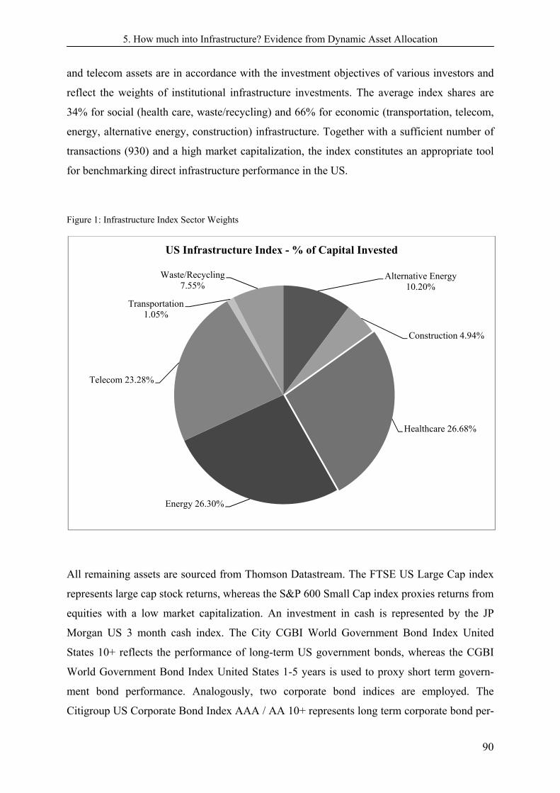
5. How much into Infrastructure? Evidence from Dynamic Asset Allocation
90
and telecom assets are in accordance with the investment objectives of various investors and
reflect the weights of institutional infrastructure investments. The average index shares are
34% for social (health care, waste/recycling) and 66% for economic (transportation, telecom,
energy, alternative energy, construction) infrastructure. Together with a sufficient number of
transactions (930) and a high market capitalization, the index constitutes an appropriate tool
for benchmarking direct infrastructure performance in the US.
Figure 1: Infrastructure Index Sector Weights
All remaining assets are sourced from Thomson Datastream. The FTSE US Large Cap index
represents large cap stock returns, whereas the S&P 600 Small Cap index proxies returns from
equities with a low market capitalization. An investment in cash is represented by the JP
Morgan US 3 month cash index. The City CGBI World Government Bond Index United
States 10+ reflects the performance of long-term US government bonds, whereas the CGBI
World Government Bond Index United States 1-5 years is used to proxy short term govern-
ment bond performance. Analogously, two corporate bond indices are employed. The
Citigroup US Corporate Bond Index AAA / AA 10+ represents long term corporate bond per-
Alternative Energy 10.20%
Construction 4.94%
Healthcare 26.68%
Energy 26.30%
Telecom 23.28%
Transportation 1.05%
Waste/Recycling 7.55%
US Infrastructure Index - % of Capital Invested

5. How much into Infrastructure? Evidence from Dynamic Asset Allocation
91
formance and the Citigroup US Corporate Bond Index AAA / AA 1-5 Years represents re-
turns on short term corporate bonds.
Contrary to trading most financial assets, buying and selling direct real estate and direct infra-
structure evokes high transaction costs, which reduces return. Round trip costs of 6%2 are
employed for US real estate transactions. Infrastructure transaction costs are, to a large extent,
independent of the size of the project, since they all require general services like technical,
legal and financial advisory, as well as a sound estimation of demand risk. Moreover, opaque
market structures, along with low levels of information efficiency result in high information
and due-diligence costs. Therefore, gross transaction costs for all initial project participants
can amount to more than 10% of total project value (Dudkin and Välilä (2005), Salino and de
Santos (2008)). From a private investor’s point of view, average direct infrastructure invest-
ments evoke round trip costs of about 7.5%3. However, actual transaction costs depend on the
holding period of assets. Based on the findings of Kaserer, Buchner, Schmidt and Krohmer
(2009), the average duration of infrastructure investments is four years, which seems very
short for direct infrastructure investments. However, one has to consider that there is a huge
difference between the average concession period which is agreed between the government
and the SPV (special purpose vehicle) and the holding period of an individual equity investor.
While the concession period agreed between the regulator and the SPV is around 30 years
across all sectors, on average, an individual investor might have shorter holding periods, de-
pending on strategic issues, such as the stage of the infrastructure project (Araújo and Suther-
land, 2010). Due to the growing maturity of the market and the increasing involvement of
long-term investors, the average investment period is likely to rise over the next years. We use
the information from Kaserer et al. (2009) to adjust infrastructure returns and to compare real
estate returns for a holding period of four years.
5.4 Methodology
We employ two different algorithms for portfolio construction. Firstly, we conduct a mean-
variance optimization which is based on the portfolio theory of Markowitz (1952). Secondly,
we employ a mean-downside risk optimization which is based on Estrada (2008). Downside
risk is a more intuitive measure of risk than variance, as it accounts only for return deviations
below a pre-specified target rate and considers the non-normal distribution of asset returns.
Using the Estrada methodology has the advantage that it creates a symmetrical and exogenous
co-lower partial moment (CLPM) matrix.
2 We thank David Geltner for providing this information. 3 We thank various institutional infrastructure investors and consultants for providing this information.

5. How much into Infrastructure? Evidence from Dynamic Asset Allocation
92
Formally, the Markowitz-optimization can be written as follows:
Minimize
(1)
Subject to
Where
= the proportion of the portfolio allocated to asset
= the expected portfolio return
= the expected return on asset
= the covariance between asset and asset

5. How much into Infrastructure? Evidence from Dynamic Asset Allocation
93
We employ the lower partial moment (LPM) as a measure of downside risk. This is defined as
follows:
(2)
Where is an investor-specific target rate of return, is the parameter of risk-aversion and
is the return on asset which follows the distribution .
Downside risk optimization is given by:
Minimize
(3)
Subject to

5. How much into Infrastructure? Evidence from Dynamic Asset Allocation
94
Where
= the CLPM between asset and asset which is given by
(4)
To account for time variation in the covariance and in the CLPM, we employ a dynamic asset
allocation procedure. This means that we form ten efficient portfolios at each point in time
(each quarter), by using observations from the past 48 quarters. The ten estimated portfolios
comprise the minimum-risk4 portfolio (portfolio 1) and the maximum return portfolio (portfo-
lio 10), as well as the eight portfolios in between. The distance between the expected portfolio
return on the ten portfolios is equal for each separate point in time. In order to match our
model with the actual holding period of infrastructure assets in the market, we assume a hold-
ing period of four years and calculate transactions costs correspondingly. As a result of the
investment period and the 48 period rolling window, we obtain the initial efficient portfolios
in Q1 2006. After each optimization, we roll forward one quarter and again perform the opti-
mization. This results in a time series of portfolio allocations for each of the ten portfolios.
The rolling optimization procedure enables accounting for changing asset characteristics over
time and delivers more meaningful results than a static optimization procedure, which yields
only one value for each asset in the portfolio. In the downside risk optimization, we employ a
target of 6% real return5 per annum, which implies that only outcomes below this target rate
constitute a risk to an investor, and only these outcomes are employed to calculate the LPM
and the CLPM. Although this number seems to be very high in comparison to other asset allo-
cation studies, one has to bear in mind that we assume a holding period of four years, which
makes it more realistic that a certain target rate is met, on average. In summary, our base-
model employs 48 quarters of data for optimization and assumes a holding period of four
years. Furthermore, the downside-risk approach is conducted with an annual target return of
6% real return.
4 This is the minimum variance portfolios (MVP) and minimum downside risk portfolio (MDP). 5 Many asset allocation studies employ the risk-free rate of return or zero as a benchmark return. However, this definition only makes sense for shorter investment horizons, because it is clear that assets which are riskier than the risk-free rate are likely to produce higher returns over greater investment horizons. Because we employ an investment horizon of four years, only a very few return are situated below that of the risk-free rate. This results in a reduced number of data for the calculation of the CLPM, which makes the results less reliable and dependent on extreme outliers. For this reason, the risk-free rate is not employed as a benchmark return. A target return of zero tightens this problem and does not even allow for calculating the portfolio LPM.

5. How much into Infrastructure? Evidence from Dynamic Asset Allocation
95
In reality, the characteristics of infrastructure and real estate assets entail a construction and/or
an implementation lag. However, our infrastructure and real estate data are based on con-
servative brownfield/core assets, which deliver available operating cash-flows and do not in-
volve planning and/or construction periods. One might argue that the implementation of infra-
structure/real estate assets demands a time-intensive due diligence process which depends on
such parameters as project type, size, etc. However, the quarterly observation frequency of
our analysis should, on average, be able to cover this phase for the majority of projects. Fur-
thermore, we assume a holding period of four years so that implementation is a minor prob-
lem. Moreover, the main focus of the study is not on comparing different portfolio strategies
in terms of the risk, return and timing of implementation, but to construct efficient combina-
tions of assets, based on the information available at each point in time. Furthermore, il-
liquidity is (at least partially) accounted for by transaction costs.
5.5 Descriptive Statistics
Table 1 shows the descriptive statistics from different asset classes when a holding period of
four years6 is assumed. In accordance with our base model, we use a target rate of 6% real
return p. a. to calculate the LPM. Figure 2 shows total return indices of the different assets.
Table 1: Descriptive Statistics for Real Asset Returns (Holding Period: 4 Years) Q2 1994 – Q2 2010
LTGovBonds SMTGovBonds Large Caps Small Caps Cash LTCorpBonds SMTCorpBonds Real Estate Infrastructure
Mean 23.87 15.32 38.11 33.99 7.80 21.59 14.63 26.55 20.11
6.07 4.14 6.86 6.16 1.91 5.86 3.86 4.72 4.18
Median 24.85 17.20 29.93 35.51 7.97 20.87 16.19 27.19 22.04
6.07 4.23 8.10 8.52 2.58 5.49 4.26 4.60 4.76
Sample Deviation 10.70 8.06 62.82 29.13 5.51 12.91 8.00 24.22 8.76
7.89 4.61 18.72 17.59 1.84 8.65 3.94 11.25 3.70
Sample Variance 114.59 64.95 3946.98 848.80 30.40 166.74 63.99 586.53 76.79
62.31 21.24 350.43 309.50 3.40 74.74 15.50 126.66 13.68
LPM (Target = 6%) 74.13 183.24 952.31 311.46 370.36 144.67 198.02 304.88 107.59
31.99 20.44 189.84 139.33 20.10 38.19 17.39 92.47 14.71
Min 2.68 -3.32 -44.40 -41.66 -3.30 -12.60 -4.25 -25.24 -0.96
-13.38 -5.11 -36.96 -44.77 -1.96 -14.60 -5.33 -29.89 -6.25
Max 57.62 28.60 176.90 105.04 15.49 47.64 26.71 71.44 37.32
26.18 12.45 40.17 60.47 4.57 32.01 13.84 32.73 12.62
6 The returns for different holding periods are constructed by employing overlapping returns on a quarterly basis. This means that a return for an investment period of z years could be calculated from Q1 of year t to Q1 of year t + z, another from Q2 of year t to Q2 of year t + z, and so on.

5. How much into Infrastructure? Evidence from Dynamic Asset Allocation
96
Figure 2: Total Return of Assets
Infrastructure assets do not yield very high returns, but are not exposed to high risk, irrespec-
tive of whether measured by variance or the LPM. This indicates that infrastructure might
predominantly be allocated to low-risk low-return portfolios.
The correlation coefficients in Table 2 reveal a strong relationship between the returns on
infrastructure and those on large cap stocks. Where does this high correlation come from?
One argument could be that, in the long term, both assets exhibit the same underlying charac-
teristics. Large cap stocks are mostly stocks of companies which exhibit high market power,
pay stable dividends to their shareholders, but do not have high growth rates. Conservative
infrastructure projects exhibit similar characteristics. They provide fundamental services to
the economy, often have little growth potential and their main source of income is from the
generated cash flow, rather than appreciation returns. In the short term, stock returns are high-
ly volatile and driven by the equity market; their underlying large cap characteristics become
apparent with medium- to long-term investment horizons. This could explain why both assets
are correlated over longer investment horizons. The observation, that the correlation between
infrastructure and large cap stocks rises when the holding period increases, supports this ar-
gument.
In order to further investigate the relationship between the returns on direct infrastructure and
large cap stocks, we determine the extent to which the companies in the FTSE Large Cap In-
0
50
100
150
200
250
300
350
400
450
Tot
al R
etur
n In
dex
Q2
1990
= 1
00
LTGovBonds
SMTGovBonds
Large Caps
Small Caps
Cash
LTCorpBonds
SMTCorpBonds
Real Estate
Infrastructure

5. How much into Infrastructure? Evidence from Dynamic Asset Allocation
97
dex do infrastructure business. We do so by filtering the companies in the FTSE Large Cap
Index in terms of their sector code. According to the classification of infrastructure by the
CEPRES index, we define a company as an infrastructure company if it operates telecommu-
nication, utilities, waste, transportation or healthcare businesses. After filtering these compa-
nies out, we determine the share of infrastructure company market capitalization of the total
market capitalization of the FTSE Large Cap Index at the end of the years 2004, 2006, 2008,
20107. We find that the proportion of infrastructure companies’ market capitalization to total
market capitalization of the FTSE Large Cap Index is 18%, 23%, 26% and 25% in 2004,
2006, 2008 and 2010. Although we cannot calculate this number across the entire sample pe-
riod, it indicates that a significant share of the performance of the total index stems directly
from the performance of infrastructure companies. This further explains why returns from
both index series are highly correlated over longer investment horizons.
Table 2: Correlations (Holding Period: 4 Years) Q2 1994 – Q2 2010
LTGovBonds SMTGovBonds Large Caps Small Caps Cash LTCorpBonds SMTCorpBonds Real Estate Infrastructure
LTGovBonds 1.00 0.80 0.27 0.08 0.42 0.79 0.75 -0.20 0.10
SMTGovBonds 1.00 0.00 -0.32 0.59 0.65 0.92 -0.60 -0.14
Large Caps 1.00 0.43 0.58 0.06 0.06 0.38 0.80
Small Caps 1.00 -0.24 0.23 -0.15 0.50 0.34
Cash 1.00 0.13 0.60 -0.25 0.50
LTCorpBonds 1.00 0.76 -0.10 -0.22
SMTCorpBonds 1.00 -0.44 -0.14
Real Estate 1.00 0.22
Infrastructure 1.00
5.6 Results
5.6.1 Mean-Variance Optimization
In the base MV-model, we find time-varying allocations with a maximum of more than 30%
of total wealth allocated to infrastructure. Because infrastructure exhibits low expected returns
and a low variance, it is allocated mostly to portfolios designed to have similar characteristics.
Consequently, infrastructure plays an important role in the MVP with an average/maximum8
proportion of 9%/26%. Furthermore, there is a significant proportion of infrastructure in port-
7 Unfortunately, the index constituents of the FTSE Large Cap Index are only available from 2004 onwards. We thank FTSE for providing the index constituents. 8 The average allocation in the base model is the average proportion of infrastructure from Q3 2006 to Q2 2010. The maximum allocation is the highest weight of infrastructure during this time period.
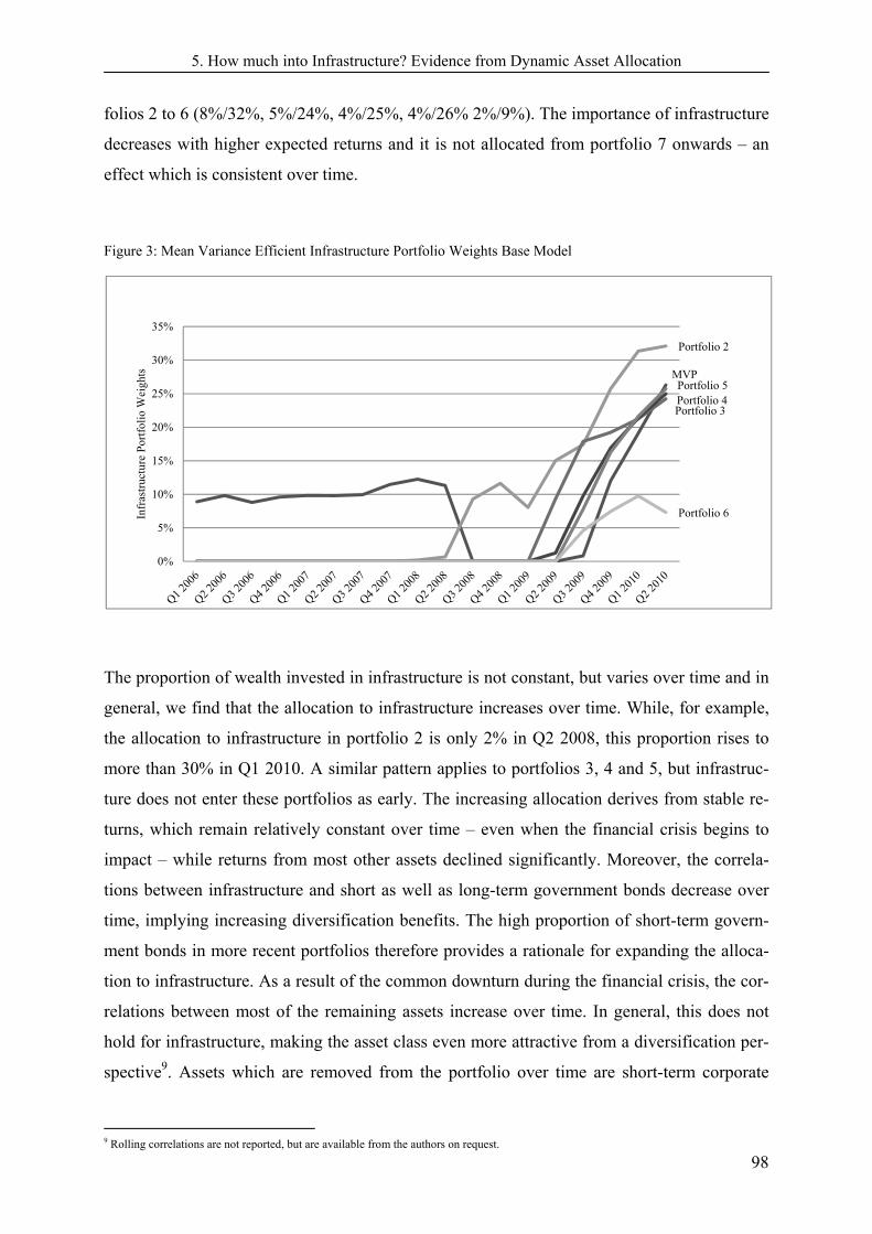
5. How much into Infrastructure? Evidence from Dynamic Asset Allocation
98
folios 2 to 6 (8%/32%, 5%/24%, 4%/25%, 4%/26% 2%/9%). The importance of infrastructure
decreases with higher expected returns and it is not allocated from portfolio 7 onwards – an
effect which is consistent over time.
Figure 3: Mean Variance Efficient Infrastructure Portfolio Weights Base Model
The proportion of wealth invested in infrastructure is not constant, but varies over time and in
general, we find that the allocation to infrastructure increases over time. While, for example,
the allocation to infrastructure in portfolio 2 is only 2% in Q2 2008, this proportion rises to
more than 30% in Q1 2010. A similar pattern applies to portfolios 3, 4 and 5, but infrastruc-
ture does not enter these portfolios as early. The increasing allocation derives from stable re-
turns, which remain relatively constant over time – even when the financial crisis begins to
impact – while returns from most other assets declined significantly. Moreover, the correla-
tions between infrastructure and short as well as long-term government bonds decrease over
time, implying increasing diversification benefits. The high proportion of short-term govern-
ment bonds in more recent portfolios therefore provides a rationale for expanding the alloca-
tion to infrastructure. As a result of the common downturn during the financial crisis, the cor-
relations between most of the remaining assets increase over time. In general, this does not
hold for infrastructure, making the asset class even more attractive from a diversification per-
spective9. Assets which are removed from the portfolio over time are short-term corporate
9 Rolling correlations are not reported, but are available from the authors on request.
MVP
Portfolio 2
Portfolio 3Portfolio 4Portfolio 5
Portfolio 6
0%
5%
10%
15%
20%
25%
30%
35%
Infr
astr
uctu
re P
ortf
olio
Wei
ghts

5. How much into Infrastructure? Evidence from Dynamic Asset Allocation
99
bonds and small cap stocks. Their real returns decrease significantly over time and their diver-
sification benefits suffer as the analyzed time period increases.
It should be noted that the presented allocations are extreme outcomes and constitute corner
solutions. In reality, fund managers are restricted, either by institutional or regulatory issues,
in allocating wealth to various assets. To reflect this situation, we impose restrictions on port-
folio weights. We assume that a representative fund manager has to allocate at least 20%, but
not more than 40%, to long-term government bonds and large cap stocks, respectively. Fur-
thermore, the proportion of real estate is restricted to a minimum of 2% and a maximum of
10%. Small cap stocks are subject to a maximum of 10%. At least 5% of all funds must be
allocated to cash, with a maximum allocation of 20%. As a result of the high correlation be-
tween infrastructure and large cap stocks, we find that the allocation to infrastructure is heavi-
ly dependent on the proportion of large caps in the portfolio. If a restriction is imposed on
large cap stocks, infrastructure is removed from the portfolio. The high correlation between
both assets and the high variance of large cap stocks creates a high covariance term, which is
punished in the optimization. We test whether a change in the restriction of another asset
evokes a similar effect. We cannot find any evidence of this, but demonstrate that removing
infrastructure from the efficient portfolios is caused mainly by the inclusion of large cap
stocks.
5.6.2 Mean-Downside Risk Optimization
In accordance with the results from the MV-optimization, we obtain time-varying allocations
in which infrastructure is allocated predominantly to low-risk and low-expected-return portfo-
lios mainly from Q1 2009 onwards. However, one main difference occurs when absolute in-
frastructure weights are compared; allocations to infrastructure are higher when risk is meas-
ured by variance, rather than by LPM. This holds across almost all portfolios and across time
– only in some late MDPs, infrastructure is allocated to a greater extent than in MVPs. The
portfolio with the lowest LPM contains an average/maximum proportion of infrastructure of
more than 6%/28%, which then decreases in portfolios 2, 3 and 4 (4/20%, 2%/13%, 1%/5%).
These results imply that infrastructure is a more attractive asset class for investors who are
averse towards variance, rather than to downside risk1011
10 When “optimal” solutions from different optimization algorithms are compared, one has to consider that it does not make sense to draw a conclusion as to which optimization algorithm performs “better”. Each one, by definition, minimizes a different measure of risk and each approach is inferior from the perspective of the other. Therefore, a comparison is only appropriate when based on a common measure of risk. Hence, mean-variance optimization is appropriate for an investor who is averse towards deviations around the mean, while mean-downside risk optimization should be the favorable approach when an investor is averse towards failing to achieve a pre-defined target rate. Ultimately, which measure of risk is perceived as more appropriate by a given investor, is fundamental.
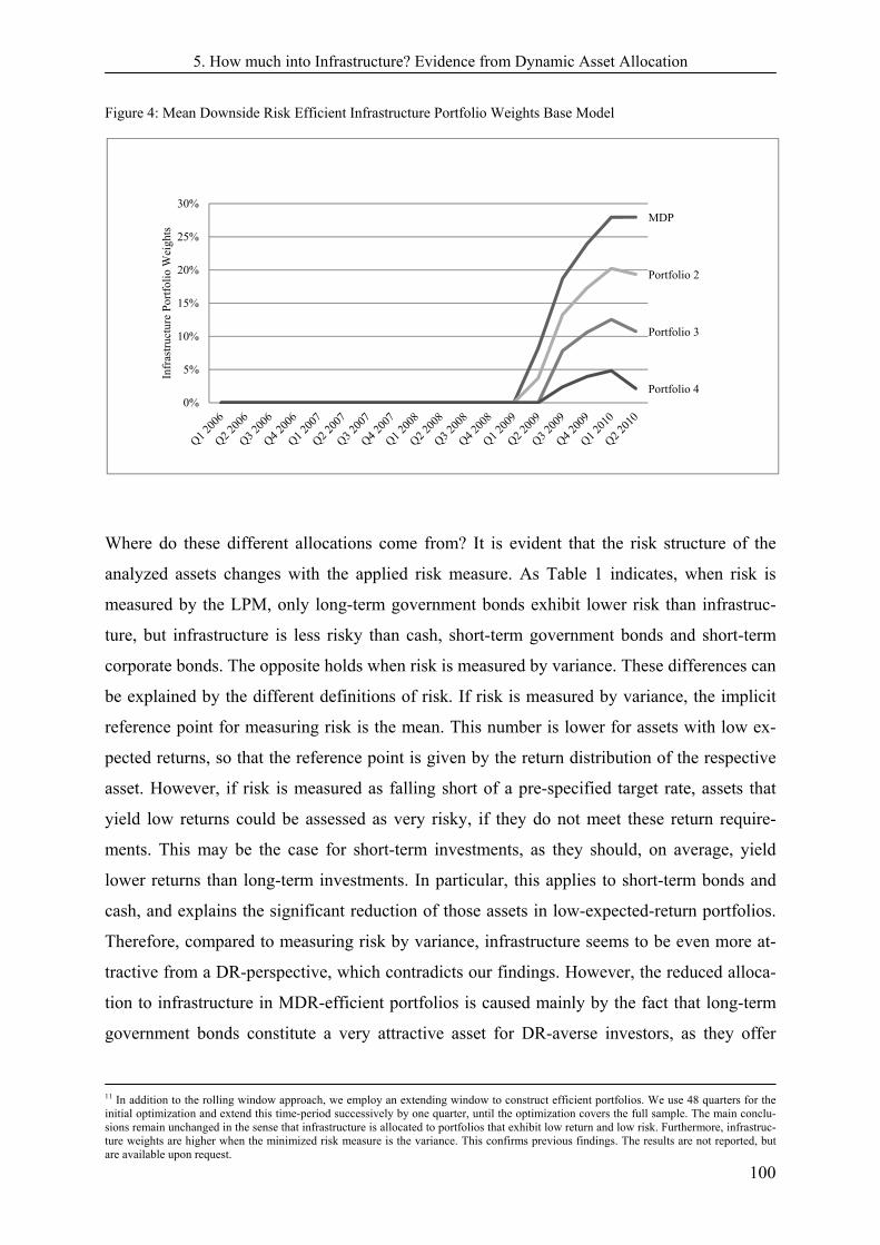
5. How much into Infrastructure? Evidence from Dynamic Asset Allocation
100
Figure 4: Mean Downside Risk Efficient Infrastructure Portfolio Weights Base Model
Where do these different allocations come from? It is evident that the risk structure of the
analyzed assets changes with the applied risk measure. As Table 1 indicates, when risk is
measured by the LPM, only long-term government bonds exhibit lower risk than infrastruc-
ture, but infrastructure is less risky than cash, short-term government bonds and short-term
corporate bonds. The opposite holds when risk is measured by variance. These differences can
be explained by the different definitions of risk. If risk is measured by variance, the implicit
reference point for measuring risk is the mean. This number is lower for assets with low ex-
pected returns, so that the reference point is given by the return distribution of the respective
asset. However, if risk is measured as falling short of a pre-specified target rate, assets that
yield low returns could be assessed as very risky, if they do not meet these return require-
ments. This may be the case for short-term investments, as they should, on average, yield
lower returns than long-term investments. In particular, this applies to short-term bonds and
cash, and explains the significant reduction of those assets in low-expected-return portfolios.
Therefore, compared to measuring risk by variance, infrastructure seems to be even more at-
tractive from a DR-perspective, which contradicts our findings. However, the reduced alloca-
tion to infrastructure in MDR-efficient portfolios is caused mainly by the fact that long-term
government bonds constitute a very attractive asset for DR-averse investors, as they offer
11 In addition to the rolling window approach, we employ an extending window to construct efficient portfolios. We use 48 quarters for the initial optimization and extend this time-period successively by one quarter, until the optimization covers the full sample. The main conclu-sions remain unchanged in the sense that infrastructure is allocated to portfolios that exhibit low return and low risk. Furthermore, infrastruc-ture weights are higher when the minimized risk measure is the variance. This confirms previous findings. The results are not reported, but are available upon request.
MDP
Portfolio 2
Portfolio 3
Portfolio 40%
5%
10%
15%
20%
25%
30%
Infr
astr
uctu
re P
ortf
olio
Wei
ghts
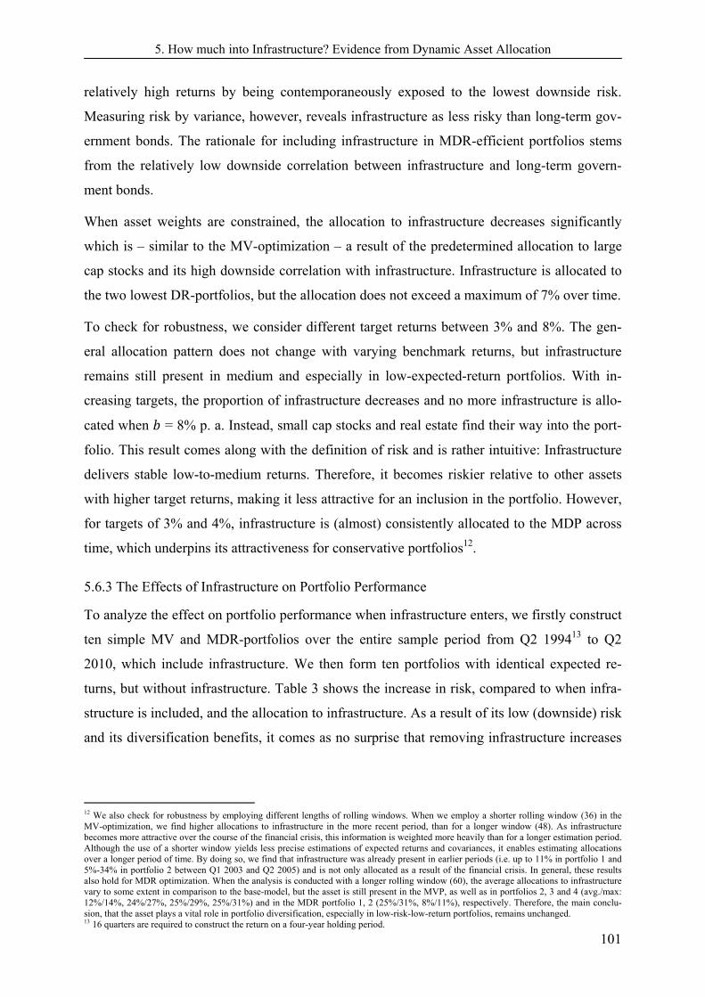
5. How much into Infrastructure? Evidence from Dynamic Asset Allocation
101
relatively high returns by being contemporaneously exposed to the lowest downside risk.
Measuring risk by variance, however, reveals infrastructure as less risky than long-term gov-
ernment bonds. The rationale for including infrastructure in MDR-efficient portfolios stems
from the relatively low downside correlation between infrastructure and long-term govern-
ment bonds.
When asset weights are constrained, the allocation to infrastructure decreases significantly
which is – similar to the MV-optimization – a result of the predetermined allocation to large
cap stocks and its high downside correlation with infrastructure. Infrastructure is allocated to
the two lowest DR-portfolios, but the allocation does not exceed a maximum of 7% over time.
To check for robustness, we consider different target returns between 3% and 8%. The gen-
eral allocation pattern does not change with varying benchmark returns, but infrastructure
remains still present in medium and especially in low-expected-return portfolios. With in-
creasing targets, the proportion of infrastructure decreases and no more infrastructure is allo-
cated when = 8% p. a. Instead, small cap stocks and real estate find their way into the port-
folio. This result comes along with the definition of risk and is rather intuitive: Infrastructure
delivers stable low-to-medium returns. Therefore, it becomes riskier relative to other assets
with higher target returns, making it less attractive for an inclusion in the portfolio. However,
for targets of 3% and 4%, infrastructure is (almost) consistently allocated to the MDP across
time, which underpins its attractiveness for conservative portfolios12.
5.6.3 The Effects of Infrastructure on Portfolio Performance
To analyze the effect on portfolio performance when infrastructure enters, we firstly construct
ten simple MV and MDR-portfolios over the entire sample period from Q2 199413 to Q2
2010, which include infrastructure. We then form ten portfolios with identical expected re-
turns, but without infrastructure. Table 3 shows the increase in risk, compared to when infra-
structure is included, and the allocation to infrastructure. As a result of its low (downside) risk
and its diversification benefits, it comes as no surprise that removing infrastructure increases
12 We also check for robustness by employing different lengths of rolling windows. When we employ a shorter rolling window (36) in the MV-optimization, we find higher allocations to infrastructure in the more recent period, than for a longer window (48). As infrastructure becomes more attractive over the course of the financial crisis, this information is weighted more heavily than for a longer estimation period. Although the use of a shorter window yields less precise estimations of expected returns and covariances, it enables estimating allocations over a longer period of time. By doing so, we find that infrastructure was already present in earlier periods (i.e. up to 11% in portfolio 1 and 5%-34% in portfolio 2 between Q1 2003 and Q2 2005) and is not only allocated as a result of the financial crisis. In general, these results also hold for MDR optimization. When the analysis is conducted with a longer rolling window (60), the average allocations to infrastructure vary to some extent in comparison to the base-model, but the asset is still present in the MVP, as well as in portfolios 2, 3 and 4 (avg./max: 12%/14%, 24%/27%, 25%/29%, 25%/31%) and in the MDR portfolio 1, 2 (25%/31%, 8%/11%), respectively. Therefore, the main conclu-sion, that the asset plays a vital role in portfolio diversification, especially in low-risk-low-return portfolios, remains unchanged. 13 16 quarters are required to construct the return on a four-year holding period.

5. How much into Infrastructure? Evidence from Dynamic Asset Allocation
102
portfolio risk. Removing infrastructure leads, for example, to an increase in portfolio risk by
up to almost 24% in MV-portfolio 2, and by 31% in the MDP.
Table 3: Portfolio Risk and Return Characteristics with and without Infrastructure
Portfolio 1 2 3 4 5 6
Allocation to Infrastructure 0.12 0.25 0.29 0.31 0.06 0.00
Portfolio Return
with Infrastructure 14.79 17.38 19.97 22.56 25.15 27.75
Portfolio Variance
with Infrastructure 19.50 20.09 29.74 49.52 85.20 176.69
without Infrastructure 20.61 25.05 36.67 57.66 86.37 176.69
Increase in Portfolio Variance 5.68% 24.68% 23.33% 16.46% 1.38% 0.00%
Allocation to Infrastructure 0.31 0.14 0.01 0.00 0.00 0.00
Portfolio Return
with Infrastructure 22.48 24.22 25.96 27.69 29.43 31.17
Portfolio LPM
with Infrastructure 62.63 68.28 80.82 103.26 140.14 191.36
without Infrastructure 82.40 71.52 80.82 103.26 140.14 191.36
Increase in Portfolio LPM 31.57% 4.75% 0.01% 0.00% 0.00% 0.00%
This table shows portfolio risk for both risk measures when portfolios are constructed with and without infrastructure, and when the expected portfolio return is constant. Reported infrastructure allocations are estimated over the full sample period.
Figure 5 shows the time-varying risk-reducing characteristics of infrastructure for a typical
institutional investor who invests 10% of total wealth to long and short-term government and
corporate bonds. The allocation to large cap and small cap stocks is 25% and 20% respective-
ly. The proportion of cash is 5% and real estate is weighted at 10%. We then reduce the allo-
cation to each asset by 10% of its percentage allocation - except for cash – and allocate infra-
structure instead, which results in a 9.5% proportion of infrastructure. When we compare the
risk and return from these different portfolios over time, the impact of infrastructure is quite
clear. The portfolio risk is reduced consistently over time (the decrease in variance ranges
between 12.2% and 14.2%), while the reduction in return is only between 2.6% and 4.1%,
measured on a relative basis. This indicates that the inclusion of infrastructure mainly con-
tributes to reducing portfolio risk, while only marginally affecting the return. Similar results
are obtained for the DR- approach.
5. How much into Infrastructure? Evidence from Dynamic Asset Allocation
103
Figure 5: Effect of Infrastructure on Portfolio Return and Risk Base Model
5.6.4 The Role of the Investment Horizon
As described in the data-section, infrastructure and real estate assets are subject to high trans-
action costs. The impact of transaction costs on returns becomes more accentuated with de-
creasing holding periods and risk, as well as return characteristics vary with the investment
horizon. Therefore, the role of infrastructure might change along with the investment horizon.
When a holding period of one year is assumed, buying and selling costs significantly reduce
the return on infrastructure and the average expected return is negative. Nevertheless, the as-
set is still allocated to low-return portfolios – a result of its low variance and its diversification
benefits. As the negative expected return is not accounted for when the MVP is formed, the
highest proportion of infrastructure is allocated to the first portfolio and ranges between 11%
and 38% over time. This is somewhat counter-intuitive and reveals one major shortcoming of
the second central moment around the mean as a measure of risk. While a rational investor is
unlikely to invest in an asset which has a negative expected return, but is likely to consider the
asset as very risky, this is not accounted for by the variance. Variance only accounts for the
average deviation around the mean, irrespective of whether the mean is positive or negative.
Therefore, we do not consider the variance as an appropriate measure of risk when the in-
vestment horizon is relatively short, as the resulting allocations might yield a flawed picture
of the role of infrastructure in the portfolio. An increase in the holding period induces a shift
of infrastructure from low-expected return portfolios to those portfolios which aim at yielding
a higher expected return. For example, when the investment horizon is extended to 6 (7)
Portfolio Return
Portfolio Variance
Portfolio Downside-Risk
-16%
-14%
-12%
-10%
-8%
-6%
-4%
-2%
0%
Cha
nge
in P
ortf
olio
Ret
urn
and
Ris
k

5. How much into Infrastructure? Evidence from Dynamic Asset Allocation
104
years, infrastructure is allocated even to portfolio 9 with maximum weights of more than 19%
(24%) and is, furthermore, almost consistently present in medium-expected-return portfolios
over time. In addition to a decrease in transaction costs, there is one major reason why infra-
structure becomes more important for portfolios that are constructed to yield higher expected
returns. Mature infrastructure investments, as mirrored by the index at hand, do not generally
yield very high returns, but exhibit a low probability of yielding losses. This return behavior is
advantageous in the long run when compounded returns are employed to measure the ex-
pected return on an investment. Consequently, in comparison to returns on other assets, the
return on infrastructure increases disproportionately when the holding period increases. This
is illustrated in Table 4.
Table 4: Asset Returns Dependent on Holding Period
Holding Period in Years LTGovBonds SMTGovBonds Large Caps Small Caps Cash LTCorpBonds SMTCorpBonds Real Estate Infrastructure
2 12.18 8.24 14.32 14.66 3.83 10.80 7.38 5.33 2.92
3 18.28 11.95 25.36 24.35 5.76 16.04 10.96 15.38 11.29
4 23.87 15.32 38.11 33.99 7.80 21.59 14.63 26.55 20.11
5 31.25 19.45 51.67 45.51 9.87 28.39 18.79 38.47 29.26
6 38.75 23.92 63.03 55.29 12.04 35.36 23.26 50.52 38.75
7 46.97 29.12 73.57 66.15 14.45 43.22 28.48 62.93 48.69
This table shows the compounded returns on the different assets for different holding periods.
When the LPM is the relevant measure of risk, the results differ to a certain degree. Because
transaction costs significantly reduce the return on infrastructure for short holding periods, it
makes the asset very risky from a DR-perspective. This makes sense, as the reference point
for measuring risk is the target return, instead of the mean, so that negative returns are pun-
ished more severely than by the variance. As a result, no infrastructure is allocated to any
portfolio for a holding period of one year, and only marginal allocations appear for a two-year
investment horizon. This result seems to be more intuitive from a rational investor’s point of
view.
However, infrastructure becomes more attractive for low-return portfolios, the longer the
holding period. While the proportion of infrastructure in MDR-portfolios is below that of
MV-portfolios in the base-model, this reverses with increasing investment horizons, but infra-
structure becomes an important asset to protect an investor from downside risk. If the invest-
ment horizon is set to 6 (7) years, average/maximum allocations in portfolio 1, 2 and 3 are
13%/40% (21%/38%), 11%/36% (16%/33%) and 9%/31% (13%/29%), respectively. The in-

5. How much into Infrastructure? Evidence from Dynamic Asset Allocation
105
creasing importance of infrastructure is based on the fact, that, due to stable long-term returns,
the downside risk decreases with increasing investment horizons. This is illustrated in Table
5. For an investment horizon of 6 and 7 years, infrastructure has the lowest downside risk of
all considered assets. Because the downside risk of long-term government bonds increases
over longer time horizons, they are replaced by infrastructure. These results show that if in-
vestment horizons are sufficiently long, infrastructure becomes very attractive in terms of DR-
protection and accounts for a substantial part of overall wealth – especially in low-expected-
return portfolios.
Table 5: Lower Partial Moments
Holding Period in Years LTGovBonds SMTGovBonds Large Caps Small Caps Cash LTCorpBonds SMTCorpBonds Real Estate Infrastructure
1 31.99 20.44 189.84 139.33 20.10 38.19 17.39 172.32 126.66
2 34.97 56.21 461.15 229.99 82.24 63.97 54.32 293.75 125.33
3 53.72 110.52 698.46 296.91 196.81 104.64 113.60 331.24 120.61
4 74.13 183.24 952.31 311.46 370.36 144.67 198.02 304.88 116.03
5 99.15 276.88 1228.57 355.79 616.11 171.43 306.29 227.57 113.86
6 122.11 398.33 1430.03 211.78 943.18 202.36 440.94 177.30 111.23
7 158.69 552.14 1812.26 270.12 1354.12 223.80 588.97 130.27 111.62
This table shows the LPMs for different holding periods and for different assets. The underlying target return is 6%p.a. and it is compounded according to the holding period.
In accordance with the results from the MV-optimization, the allocation to infrastructure in-
creases with longer investment horizons in portfolios that have medium and high-expected-
returns. However, compared to MV-efficient portfolios, the allocation to infrastructure is not
as high, but real estate is allocated instead. This results from real estate’s low downside risk,
compared to variance, for longer investment horizons. Figure 6 and 7 show infrastructure al-
locations for an investment horizon of 6 years.
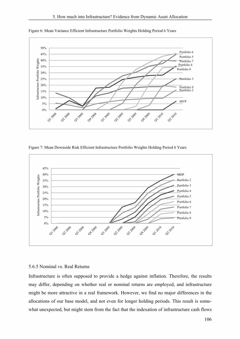
5. How much into Infrastructure? Evidence from Dynamic Asset Allocation
106
Figure 6: Mean Variance Efficient Infrastructure Portfolio Weights Holding Period 6 Years
Figure 7: Mean Downside Risk Efficient Infrastructure Portfolio Weights Holding Period 6 Years
5.6.5 Nominal vs. Real Returns
Infrastructure is often supposed to provide a hedge against inflation. Therefore, the results
may differ, depending on whether real or nominal returns are employed, and infrastructure
might be more attractive in a real framework. However, we find no major differences in the
allocations of our base model, and not even for longer holding periods. This result is some-
what unexpected, but might stem from the fact that the indexation of infrastructure cash flows
MVP
Portfolio 2
Portfolio 3
Portfolio 4
Portfolio 5
Portfolio 6
Portfolio 7
Portfolio 8
Portfolio 9
0%
5%
10%
15%
20%
25%
30%
35%
40%
45%
50%
Infr
astr
uctu
re P
ortf
olio
Wei
ghts
MDP
Portfolio 2
Portfolio 3
Portfolio 4
Portfolio 5
Portfolio 6
Portfolio 7
Portfolio 8
Portfolio 9
0%
5%
10%
15%
20%
25%
30%
35%
40%
45%
Infr
astr
uctu
re P
ortf
olio
Wei
ghts

5. How much into Infrastructure? Evidence from Dynamic Asset Allocation
107
is dependent on the specific project. Due to the fact that we employ a diversified index, not all
projects are hedged against inflation. Roedel and Rothballer (2011), for example, show that
only infrastructure firms with high pricing power can improve inflation hedging. Moreover,
one further possibility might be to distinguish between expected and unexpected inflation.
Although we cannot find any evidence that infrastructure assets are more attractive in a real
framework, this topic might be suitable for future research.
3.6.6 Infrastructure and Real Estate
Many institutional investors do not have a separate target allocation for infrastructure invest-
ments, but these are rather part of their alternative assets or real estate allocation. Although
there are theoretical differences between real estate and infrastructure, both assets exhibit
some common characteristics and are often mentioned “in one breath”14. For that reason, we
test whether the inclusion of infrastructure in particular affects the allocation to real estate.
We do so by forming time-varying portfolios in which infrastructure weights are set to zero.
Then, we compare these allocations to the portfolio weights from our base model. The de-
scriptive statistics of infrastructure and real estate returns do not indicate a high degree of sim-
ilarity, as real estate exhibits higher risk and a higher expected return than infrastructure and
both assets are not very highly correlated. This also holds over time. Therefore, it is no sur-
prise that the availability of infrastructure for portfolio selection does, on average, not affect
the weightings to real estate very extensively. Nevertheless, real estate is partially removed
from the latest MV-portfolios when infrastructure is included. As illustrated in Figure 8, the
removed share ranges from 0% to a maximum of 9%. Although the proportion of real estate
decreases, it is still a viable asset with allocations between 5% and more than 40%. This un-
derpins recent results, as in Finkenzeller et al. (2010), who find that infrastructure and real
estate constitute two distinct asset classes. However, when infrastructure enters the portfolio,
we observe a switch in portfolio weights from cash (and to a much lesser extent, from real
estate) to short-term government bonds and to infrastructure in low-return portfolios. This is
caused by the low correlation between infrastructure and short-term government bonds, mak-
ing infrastructure attractive from a diversification perspective. For low-to-medium-return
portfolios, the inclusion of infrastructure decreases the allocation to short-term government
bonds (and to a lesser extent, the allocation to real estate), but increases the proportion of
long-term government bonds. This result derives from the low correlation of infrastructure
14 For example illiquidity, large lot sizes, stable cash-flows and potential inflation hedging characteristics are supposed to be common to infrastructure and real estate. However, infrastructure assets are often inherently monopolistic and provide essential services. Moreover, the infrastructure market is often characterized by the decision making competency of public authorities in terms of regulation. Beyond that, the infrastructure market is, due to a shortage of research and high quality data, even less transparent than the real estate market.
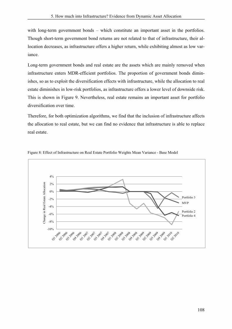
5. How much into Infrastructure? Evidence from Dynamic Asset Allocation
108
with long-term government bonds – which constitute an important asset in the portfolios.
Though short-term government bond returns are not related to that of infrastructure, their al-
location decreases, as infrastructure offers a higher return, while exhibiting almost as low var-
iance.
Long-term government bonds and real estate are the assets which are mainly removed when
infrastructure enters MDR-efficient portfolios. The proportion of government bonds dimin-
ishes, so as to exploit the diversification effects with infrastructure, while the allocation to real
estate diminishes in low-risk portfolios, as infrastructure offers a lower level of downside risk.
This is shown in Figure 9. Nevertheless, real estate remains an important asset for portfolio
diversification over time.
Therefore, for both optimization algorithms, we find that the inclusion of infrastructure affects
the allocation to real estate, but we can find no evidence that infrastructure is able to replace
real estate.
Figure 8: Effect of Infrastructure on Real Estate Portfolio Weights Mean Variance - Base Model
MVP
Portfolio 2
Portfolio 3
Portfolio 4
-10%
-8%
-6%
-4%
-2%
0%
2%
4%
Cha
nge
in R
eal E
stat
e A
lloc
atio
n

5. How much into Infrastructure? Evidence from Dynamic Asset Allocation
109
Figure 9: Effect of Infrastructure on Real Estate Portfolio Weights Mean Variance - Base Model
MDP
Portfolio 1
Portfolio 2
Portfolio 3Portfolio 4
-18%
-16%
-14%
-12%
-10%
-8%
-6%
-4%
-2%
0%
Cha
nge
in R
eal E
stat
e A
lloc
atio
n

5. How much into Infrastructure? Evidence from Dynamic Asset Allocation
110
5.7 Conclusion
Infrastructure has emerged as a separate asset class, but research on its role in mixed asset
portfolios is scarce. This study contributes to filling this research gap and sheds light on the
issue of whether and to what extent direct infrastructure should be allocated to a multi-asset
portfolio. To do so, we construct time-varying multi-asset portfolios using two different opti-
mization algorithms – a standard mean-variance approach as well as a mean-downside risk
methodology. Our results show that infrastructure is an important asset for portfolio diversifi-
cation and is, in particular, allocated to low and medium-risk portfolios with maximum alloca-
tions of 32% and 28%, respectively. With increasing investment horizons, infrastructure is
also allocated to portfolios which aim at yielding higher expected returns – a result which
stems from stable returns and a low probability of yielding losses. Moreover, infrastructure
proves to be a particularly attractive investment for long-term downside risk-averse investors
who aim at earning low returns.
Infrastructure and real estate have similar underlying characteristics and are often perceived
as related assets. However, we cannot find strong evidence that the inclusion of infrastructure
significantly affects the weightings to real estate, as it is not able to replace property in the
portfolio. Different risk and return characteristics, along with diverging asset allocation pat-
terns, speak in favor of two separate asset classes.
Infrastructure exhibits a high positive correlation with large cap stocks, which makes an in-
vestment less attractive when a certain proportion of total wealth has already been allocated to
large cap stocks. This result is obtained, independent of the optimization algorithm. If inves-
tors were aware of this fact, it could explain why there is a lower allocation to infrastructure
in institutional investment portfolios than suggested by theoretical models.
There is no simple answer to the question of how much infrastructure is “optimal” for a multi-
asset portfolio, as this depends on various parameters, such as the holding period of the assets,
the investor’s expected return, perception of risk, target return, as well as the market phase.
However, we obtain stable and conclusive evidence that the inclusion of infrastructure is ben-
eficial, especially in low to medium-return portfolios and for investors who exhibit longer
investment horizons. We do not know exactly how much infrastructure is on average allocat-
ed to investment portfolios, as no reliable data are available. However, there is some indica-
tion that it is less than suggested by our empirical model. Our results do not necessarily sug-
gest that it is beneficial for all investors to reallocate their portfolios and to increase their allo-
cation to infrastructure, but we provide some evidence that the inclusion of infrastructure

5. How much into Infrastructure? Evidence from Dynamic Asset Allocation
111
might deliver a better risk-return tradeoff than conventional portfolio allocations, which com-
prise mainly stocks, bonds and real estate. This insight might be especially useful for inves-
tors whose aim is not to earn superior returns, but to protect their portfolios from extreme
shortfalls and/or who have longer investment horizons.

5. How much into Infrastructure? Evidence from Dynamic Asset Allocation
112
5.8 References
Araujo, S.; Sutherland, D. (2010): Public-Private Partnerships and Investment in Infrastruc-ture, OECD Economics Department; Working Papers, No. 803.
Bawa, V. (1975): Optimal Rules for Ordering Uncertain Prospects, Journal of Financial Eco-nomics, Vol. 2, No. 1, p. 95-121.
Bawa, V.; Lindenberg, E. (1977): Capital Market Equilibrium in a mean-lower partial mo-ment framework, Journal of Financial Economics, Vol. 5, No. 2, p. 189-200.
Bond, S.; Hwang, S.; Mitchell, P.; Satchell, S. (2007): Will Private Equity and Hedge Funds Replace Real Estate in Mixed-Asset Portfolios?, Journal of Portfolio Management, Vol. 33, No. 5, p. 74-84.
Bond, S.; Patel, K. (2003): The Conditional Distribution of Real Estate Returns: Are Higher Moments Time Varying?, Journal of Real Estate Finance and Economics, Vol. 26, No.2-3, p. 319-339.
Bitsch, F.; Buchner, A.; Kaserer, K. (2010): Risk, Return and Cash Flow Characteristics of Infrastructure Fund Investments, EIB Papers, Vol. 15, No. 1.
Dechant, T.; Finkenzeller, K.; Schäfers, W. (2010): Real Estate: A Victim of Infrastruc-ture? Evidence from Conditional Asset Allocation, IREBS Infrastructure Research Working Paper Series 2.
Estrada, J. (2008): Mean-semivariance optimization: a heuristic approach, Journal of Ap-plied Finance, Spring/Summer, 57-72.
Finkenzeller, K.; Fleischmann, B. (2011): Real Estate: The interactions Between Direct and Securitized Real Estate and its Relationship to Real Estate, IREBS Infrastructure Research Working Paper Series 4.
Finkenzeller, K.; Dechant, T.; Schaefers, W. (2010): Infrastructure: a new dimension of real estate? An asset allocation analysis, Journal of Property Investment and Finance, Vol. 28, No. 4, p. 263-274.
Franzoni, F.; Nowak E.; Phalippou, L. (2011): Private equity performance and liquidity risk, Journal of Finance, (Forthcoming).
Harlow, W.; Rao, R. (1989): Asset Pricing in a Generalized Mean-Lower Partial Moment Framework: Theory and Evidence, Journal of Financial and Quantitative Analysis, Vol. 24, No. 3, p. 285-311.
Idzorek, T.; Armstrong, C. ( 2009): Infrastructure and Strategic Asset Allocation: Is Infra-structure an Asset Class?, Ibbotson (January).
Inderst, G. (2009): Pension Fund Investment in Infrastructure, OECD Economics Depart-ment Working Papers on Insurance and Private Pensions, No. 32.
Jain, S. (2008): Investing in Developed Country Private Infrastructure Funds, Citi Alternative Investments Research Paper Series.
Kaserer, C.; Buchner, A.; Schmidt, D.; Krohmer, P. (2009): Infrastructure Private Equity, Center of Private Equity Research.
Krohmer, P.; Lauterbach, L.; Calanog, V. (2009): The bright and dark side of staging: In-vestment performance and the varying motivations of private equity, Journal of Banking and Finance, Vol. 33, p. 1597-1609.

5. How much into Infrastructure? Evidence from Dynamic Asset Allocation
113
Mahmudova, M.; Sharma, G.; Rey, Y. (2011): Global Infrastructure Finance Review, In-frastructure Journal.
Mansour, A.; Nadji, H. ( 2007): Performance Characteristics of Infrastructure Investments, RREEF Research p. 1-19.
Markowitz, H. (1959): Portfolio Selection, New York, NY. Markowitz, H. (Ed.): John Wiley and Sons, New York, NY.
Newell, G.; Chau K.; Wong, S. (2008): The Significance and Performance of Infrastructure in China, Journal of Property Investment & Finance, Vol. 27, No. 2, p. 180-202.
Newell, G.; Peng, H. (2008): The Role of U.S. Infrastructure in Investment Portfolios. Jour-nal of Real Estate Portfolio Management, Vol. 14, No. 1, p. 21-33.
Newell, G.; Peng, H.; De Francesco, A. (2011): The performance of unlisted infrastructure in investment portfolios, Journal of Property Research, Vol. 28, No. 1, p. 59-74.
Araujo, S.; Sutherland, D. (2010): Public-Private Partnerships and Investment in Infrastruc-ture, OECD Economics Department; Working Papers, No. 803.
OECD, Organisation for Economic Co-Operation and Development (2007): Infrastruc-ture to 2030, Mapping Policy for Electricity.Water and Transport, Vol.2.
Peng, L. (2001): Building a Venture Capital Index, Yale ICF Working Paper 00-5.
Peng, H.; Newell, G. (2007): The Significance of Infrastructure in Australian Investment Portfolios, Pacific Rim Property Research Journal, Vol. 13, No. 4, p. 423-450.
Röller, L.; Waverman, L. (2001): Telecommunications Infrastructure and Economic Devel-opment: A Simultaneous Approach, American Economic Review, Vol. 91, No. 4, p. 909-923.
Schmitt, D.; Ott, T. (2006): Modelling a Performance Index for Non-traded Private Equity Transactions: Methodology and Practical Application, Center of Private Equity Research, Research Paper.
Singhal, S.; Newell, G.; Nguyen, T. (2011): The Significance and Performance of Infrastruc-ture in India, Journal of Property Research, Vol. 28, No. 1, p. 15-34.
Röller, L.H.; Waverman, L. (2001): Telecommunications Infrastructure and Economic De-velopment: A Simultaneous Approach, American Economic Review, Vol. 91, No. 4, p. 909-923.
Wagenvoort, R.; de Nicola, C.; Kappler, A. (2010): Infrastructure Finance in Europe: Composition, evaluation and crisis impact, European Investment Bank Papers, Vol. 15, No. 1, p. 16-39

6. Direct Infrastructure Investment and its Role in Drawdown- Efficient Portfolios
114
6. Direct Infrastructure Investment and its Role in Drawdown-Efficient Portfolios
Tobias Dechant Konrad Finkenzeller
Abstract
This paper investigates the role of direct infrastructure in a multi-asset portfolio, by employ-
ing a US transaction-based index which covers the period Q2 1990 to Q2 2010. We use an
algorithm which minimizes Conditional Drawdown at Risk (CDaR) to determine time-
varying asset allocations. In addition to infrastructure, the asset menu comprises large and
small cap stocks, bonds of different maturities and cash. Our results show that infrastructure
plays an important role and is allocated predominantly to portfolios that exhibit low-to-
medium risk exposure. We cannot find any evidence that infrastructure provides a hedge
against pension liabilities, but it is a viable asset when various predefined target returns are
the reference point for evaluating portfolio risk and performance. We also find that infrastruc-
ture is a hedge against systematic equity-market downside risk and contributes to a portfolio
which is designed to protect an investor against a decline in portfolio value when the equity
market drops.

6. Direct Infrastructure Investment and its Role in Drawdown- Efficient Portfolios
115
6.1 Introduction
During the last few years, direct infrastructure investments have moved into the focus of
many institutional investors1. This private involvement is driven by financial strains on gov-
ernments, which render the public sector unable to guarantee adequate infrastructure provi-
sion2. The imbalance between infrastructure provision and demand is expected to gain further
momentum and increase privatization pressure over the long run. According to the OECD
(2006, 2007), cumulative global infrastructure needs are estimated to rise to US$ 71 trillion
by 2030, this is about four times the value of the current global infrastructure stock and in-
cludes the enormous requirements of developing countries.
Despite the heterogeneity of the infrastructure universe, investors are attracted by several ma-
jor characteristics associated with the asset class. Firstly, due to their monopolistic nature,
infrastructure investments are expected to provide stable and predictable cash flows which
may enable investors to match their long-term liabilities. As a result of this monopolistic
character and the provision of basic services, cash flows from infrastructure investments are
also assumed to be less vulnerable to economic downturns than other more cyclical assets.
This could make them attractive to investors seeking new sources of diversification, in order
to hedge their portfolios against downturns of traditional assets such as stocks and bonds.
Studies from Newell and Peng (2008) as well as Dechant, Finkenzeller and Schaefers (2010)
provide some empirical evidence of the benefits of including infrastructure in an investment
portfolio. Thirdly, some specific infrastructure investments, such as alternative energies, are
associated with the increasing significance of socially responsible investment strategies and
the need for an enhanced public image.
The increasing attraction of infrastructure investments, along with its unique asset characteris-
tics, have confirmed the role of infrastructure as separate asset class and large institutional
investors have begun to establish specific allocation targets. Although the average allocation
to infrastructure is not expected to exceed 2% on average globally (Croce, 2011; Inderst,
2010), large North American and Australian pension schemes already hold up to 15% of their
total wealth in infrastructure .
However, the market for direct infrastructure assets is still young and opaque, and specific
barriers have to be considered. Political structures and regulations with respect to privatizing 1 Infrastructure assets can be divided into two main categories of economic and social infrastructure. Economic infrastructure includes long-lasting, large-scale physical structures like transportation and communication infrastructure, as well as energy and utility facilities. Social infrastructure, on the other hand, includes education, healthcare, waste disposal, as well as judicial facilities (see, for example, Kaserer, Buchner, Schmidt and Krohmer, 2009). According to Mansour and Patel (2008), the entire global infrastructure universe is estimated to be worth $20.5 trillion. 2 The relationship between infrastructure provision and economic growth is well established in the macroeconomic literature (Röller and Waverman 2011, WEF 2010).
6. Direct Infrastructure Investment and its Role in Drawdown- Efficient Portfolios
116
are significantly different, immature or absent across the globe. Large investment lot sizes3,
along with an immature secondary market make direct infrastructure an illiquid asset. Fur-
thermore, the specific design and unique characteristics requires specialized knowledge and
dedicated resources, so as to provide adequate due diligence and a sufficient risk monitoring
process. To generate scale effects in managing infrastructure assets, a sufficient allocation
should be made. Although a range of different listed performance benchmarks does exist, the
market remains subject to a shortage of data on direct infrastructure performance, and lacks
sufficient academic research to understand the general behavior of the asset (Croce, 2011;
Inderst, 2010).
The research stream which deals with direct infrastructure asset allocation basically covers
two markets, Australia, the pioneer of privatization and private infrastructure investment, and
the United States. Finkenzeller, Dechant and Schäfers (2010) use a sample of major unlisted
Australian infrastructure funds to depict direct infrastructure performance over the Q4 1990 to
Q1 2009 horizon. The authors construct efficient portfolios for downside risk-averse investors
and provide evidence of the diversification benefits of direct infrastructure. The constructed
portfolios contain a significant proportion of direct infrastructure, when the expected return is
not particularly high. Newell, Peng and DeFrancesco (2011) employ a similar data set over
the period Q3 1995 to Q2 2009. Their analysis is based on variance, return and correlation
characteristics. They show that direct infrastructure has attractive risk adjusted returns and
offers significant diversification benefits against equities and bonds. These results also apply
when the impact of the financial crisis is accounted for. Based on a set of different US asset
returns and a transaction-based direct infrastructure series, Dechant et al. (2010) analyze the
role of direct infrastructure in a conditional shortfall risk framework. They find that infra-
structure exhibits unique asset characteristics and they underpin the significance of direct in-
frastructure for portfolio diversification. Efficient portfolios contain a significant proportion
of infrastructure which, however, depends on the expected return and state of the equity mar-
ket. Moreover, the authors highlight the importance of infrastructure for portfolio diversifica-
tion in bear markets.
This paper contributes to the existing literature by investigating the role of direct infrastruc-
ture in a multi-asset portfolio over time, considering different investment scenarios. To con-
struct efficient portfolios, we use a horizon-dynamic algorithm which minimizes Conditional
Drawdown at Risk (CDaR), for a given level of expected return. Chekhlov, Uryasev and Za-
barankin (2000, 2003, 2005) define a portfolio’s drawdown on a sample path as the drop in 3 According to Prequin (2011), an average infrastructure deal size is estimated to be at around US$ 400 million.

6. Direct Infrastructure Investment and its Role in Drawdown- Efficient Portfolios
117
the uncompounded portfolio value, compared to the maximum value attained in the previous
moments on that sample path. This approach is appropriate for investors who define their al-
lowed losses as a percentage of initial wealth. The CDaR approach is based on stochastic pro-
gramming and has proven its efficiency in various portfolio management applications, includ-
ing Rockafellar and Uryasev (2002), Krokhmal, Uryasev and Zrazhevsky (2002), Cheklov et
al. (2005) as well as Berkelaar and Kouwenberg (2010). In particular, we firstly construct
unconstrained and constrained investment portfolios. Secondly, we introduce the assumption
that an investor is averse to falling short of the return on pension liabilities or some predefined
target return. Thirdly, we investigate the role of infrastructure when the investor’s main aim is
to hedge against downside systematic equity market risk.
The article is organized as follows. The next section introduces the data and presents some
descriptive statistics. We continue with a description of the methodology. The results of dif-
ferent models are given in Section 4 and the final section concludes.
6.2 Data and Descriptive Statistics
We employ US total return data from ten different asset classes, which are deflated by the
consumer price index. Observations have a monthly frequency and cover the period from Q2
1990 to Q2 2010. The asset selection focuses on a menu of investment opportunities which
are typically preferred by institutional investors. In particular, we consider direct infrastruc-
ture, large cap stocks, small cap stocks, cash, short, medium, and long-term government and
corporate bonds.
The direct infrastructure performance index is based on transactions and is provided by the
Center of Private Equity Research (CEPRES). It is a sub-index of a more general CEPRES
dataset of private equity investments, which is employed in studies such as Krohmer, Lauter-
bach and Calanog (2009), Franzoni, Nowak and Phalippou (2011) and Füss and Schweizer
(2011). The specific infrastructure data is applied in studies such as Kaserer, Buchner and
Schmidt (2009), Dechant et al. (2010), Bitsch, Buchner and Kaserer (2011), as well as Fin-
kenzeller and Fleischmann (2011). The infrastructure index covers a sample of 930 individual
operating infrastructure projects in the US and is based on a broad reporting sample of 135
global infrastructure equity investors. The index construction methodology corresponds with
Peng (2001) and is based on the Method of Moment Repeat Sales Regression (MM-RSR). A
more formal and detailed illustration of the applied procedure and the data implementation
process is provided by Schmidt and Ott (2006).

6. Direct Infrastructure Investment and its Role in Drawdown- Efficient Portfolios
118
To reflect unbiased direct infrastructure performance, the index is free of survivorship bias,
and corrected for gearing, carried interest, management fees and transaction costs, which re-
flect the illiquidity of the underlying asset. The capitalization of the index adds up to around
$27.2 billion of invested equity and only includes sectors which are in accordance with the
definition of infrastructure from Kaserer et al. (2009). Figure 1 shows the average sector
weights, which are calculated according to capital invested over the entire sample period. The
average index shares are 34% for social infrastructure (health care, waste/recycling) and 66%
for economic infrastructure (transportation, telecom, (alternative) energy, construction). The
relatively high weights for health care, energy and telecom assets are in line with the invest-
ment objectives of various types of investors (Probitas, 2011) and reflect direct investment
opportunities in the market. Together with a sufficient number of transactions and a high mar-
ket capitalization, the index constitutes an appropriate tool for benchmarking direct infrastruc-
ture performance in the US.
Figure 1: Infrastructure Index Sector Weights
The remaining assets are collected from Thomson Reuters DataStream. The general stock
market is represented by the S&P 500 Composite series, whereas the S&P 600 small cap se-
Alternative Energy 10.20%
Construction 4.94%
Healthcare 26.68%
Energy 26.30%
Telecom 23.28%
Transportation 1.05%
Waste/Recycling 7.55%
US Infrastructure Index - % of Capital Invested

6. Direct Infrastructure Investment and its Role in Drawdown- Efficient Portfolios
119
ries represents the performance of small cap stocks. The Cash index is the JP Morgan JP US
Cash 1 month series. To mirror corporate as well as government bond performance, we use
the Citigroup US Broad Investment-Grade (USBIG) index series. We choose a duration of 1-5
years for short-term bond performance (US Citigroup USBIG Government 1-5Y and US
Citigroup USBIG Corporate AAA/AA 1-5Y), a duration of 3-7 years for medium-term bond
performance (US Citigroup USBIG Government 3-7Y and US Citigroup USBIG Corporate
AAA/AA 3-7Y) and a duration of 10 or more years (US Citigroup USBIG Government 10+Y
and US Citigroup USBIG Corporate AAA/AA 10+Y) to represent long-term bond perfor-
mance.
Table 1: Descriptive Statistics for Monthly Asset Returns May 1990 – July 2010
STGovBonds MTGovBonds LTGovBonds STCorpBonds MTCorpBonds LTCorpBonds Cash Small Caps Large Caps Infrastructure
Mean 0.29% 0.37% 0.51% 0.32% 0.36% 0.47% 0.13% 0.46% 0.38% 0.27%
Max 3.05% 5.01% 10.75% 3.46% 4.65% 14.18% 2.34% 17.24% 14.47% 4.21%
Min -1.95% -3.97% -12.13% -3.96% -5.26% -10.38% -1.06% -23.52% -15.86% -4.69%
St. Deviation 0.72% 1.10% 2.74% 0.84% 1.21% 2.55% 0.31% 5.68% 4.53% 1.20%
Skewness 0.05 -0.09 -0.35 -0.43 -0.39 0.22 1.28 -0.78 -0.61 -0.79
Kurtosis 3.96 4.87 5.61 6.07 5.64 9.34 13.94 5.32 4.62 9.94
Table 1 presents the descriptive statistics for various asset classes. The infrastructure index
does not yield high returns, but is, on the other hand, also not exposed to high levels of stand-
ard deviation. Contrary to intuition, small and large cap stocks are not the assets with the
highest level of expected return. The returns from both assets are influenced by almost a dec-
ade of extreme impacts on the stock market, thus resulting in the presented numbers. Long-
term government bonds yield the highest average return over the sample period. This is likely
to have been driven by a favorable interest policy in recent years and a capital flow away from
the equity into the government bond market.
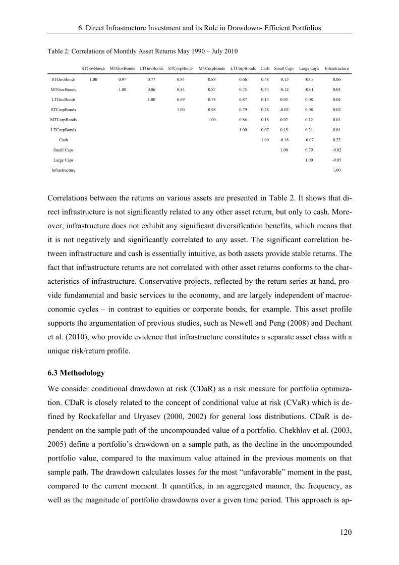
6. Direct Infrastructure Investment and its Role in Drawdown- Efficient Portfolios
120
Table 2: Correlations of Monthly Asset Returns May 1990 – July 2010
STGovBonds MTGovBonds LTGovBonds STCorpBonds MTCorpBonds LTCorpBonds Cash Small Caps Large Caps Infrastructure
STGovBonds 1.00 0.97 0.77 0.84 0.83 0.66 0.48 -0.15 -0.03 0.06
MTGovBonds 1.00 0.86 0.84 0.87 0.75 0.34 -0.12 -0.01 0.04
LTGovBonds 1.00 0.69 0.78 0.87 0.13 0.03 0.08 0.04
STCorpBonds 1.00 0.98 0.79 0.28 -0.02 0.08 0.02
MTCorpBonds 1.00 0.86 0.18 0.02 0.12 0.01
LTCorpBonds 1.00 0.07 0.15 0.21 0.01
Cash 1.00 -0.18 -0.07 0.22
Small Caps 1.00 0.79 -0.02
Large Caps 1.00 -0.05
Infrastructure 1.00
Correlations between the returns on various assets are presented in Table 2. It shows that di-
rect infrastructure is not significantly related to any other asset return, but only to cash. More-
over, infrastructure does not exhibit any significant diversification benefits, which means that
it is not negatively and significantly correlated to any asset. The significant correlation be-
tween infrastructure and cash is essentially intuitive, as both assets provide stable returns. The
fact that infrastructure returns are not correlated with other asset returns conforms to the char-
acteristics of infrastructure. Conservative projects, reflected by the return series at hand, pro-
vide fundamental and basic services to the economy, and are largely independent of macroe-
conomic cycles – in contrast to equities or corporate bonds, for example. This asset profile
supports the argumentation of previous studies, such as Newell and Peng (2008) and Dechant
et al. (2010), who provide evidence that infrastructure constitutes a separate asset class with a
unique risk/return profile.
6.3 Methodology
We consider conditional drawdown at risk (CDaR) as a risk measure for portfolio optimiza-
tion. CDaR is closely related to the concept of conditional value at risk (CVaR) which is de-
fined by Rockafellar and Uryasev (2000, 2002) for general loss distributions. CDaR is de-
pendent on the sample path of the uncompounded value of a portfolio. Chekhlov et al. (2003,
2005) define a portfolio’s drawdown on a sample path, as the decline in the uncompounded
portfolio value, compared to the maximum value attained in the previous moments on that
sample path. The drawdown calculates losses for the most “unfavorable” moment in the past,
compared to the current moment. It quantifies, in an aggregated manner, the frequency, as
well as the magnitude of portfolio drawdowns over a given time period. This approach is ap-

6. Direct Infrastructure Investment and its Role in Drawdown- Efficient Portfolios
121
propriate for investors who define their allowed losses as a percentage of initial wealth. The
theoretical concept of drawdown risk is given as follows.
Suppose that the initial portfolio value is equal to 1. The uncompounded portfolio value at
time j then equals
(1)
where ijr is the return on asset i in time period j , with Jj ,...,1 . Asset weights in the port-
folio are denoted by ix , ni ,...,1 .
The drawdown function ),( jx for a portfolio at time j is defined as the decline in portfolio
value, compared to the highest portfolio value achieved before that time moment j .
(2)
This means that, for a specified sample path, the drawdown function is defined at each point
in time. In order to aggregate all drawdown information over a certain time period, and to
evaluate portfolio performance across the entire sample path, one can, for example, choose
the Maximum Drawdown (MaxDD)
(3)
or the Average Drawdown (AvDD)
(4)
as a measure of portfolio risk.
A disadvantage of the Maximum Drawdown is that it focuses only on one single event, the
worst case in the sample path. This outcome might be very specific, and risk management
n
i
j
siisj xrxv
1 1
)1()(
i
n
i
j
sisi
n
i
k
sis
jkxrxrjx
1 11 11max),(
i
n
i
j
sisi
n
i
k
sis
jkJtxrxrMaxDD
1 11 111maxmax
djjxJ
AvDDJ
0
),(1

6. Direct Infrastructure Investment and its Role in Drawdown- Efficient Portfolios
122
based only on this event may be too restrictive. A further extreme is the average drawdown,
which accounts for all drawdowns in the sample path. The shortcoming of this measure is that
it treats even relatively small deviations as risky outcomes and is prone to averaging out large
drawdowns. The Conditional Drawdown at Risk, as demonstrated by Chekhlov et al. (2003,
2005), combines both the drawdown approach and the concept of conditional value at risk.
For a given value of the tolerance parameter α, the α-CDaR is defined as the mean of the
highest (1-α)*100% of all drawdowns over an analyzed period of time.
If the product J)1( is an integer, the CDaR function )(x is defined as
(5)
represents the threshold which is exceeded by J)1( drawdowns. Therefore,
)(x is the average of the J)1( highest drawdowns in the analyzed sample path.
If J)1( is not an integer, the CDaR )(x is the solution of
(6)
Table 3 shows conditional drawdowns of different assets calculated over the full sample peri-
od and for various levels of α.
Table 3: Conditional Drawdowns of Asset Returns Full Sample
alpha STGovBonds MTGovBonds LTGovBonds STCorpBonds MTCorpBonds LTCorpBonds Cash Small Caps Large Caps Infrastructure
0.00 1.00% 1.43% 4.44% 1.03% 1.59% 3.75% 0.66% 10.57% 24.25% 0.97%
0.80 3.39% 4.31% 11.34% 3.39% 4.76% 10.88% 2.69% 33.90% 62.75% 3.12%
0.90 4.19% 5.12% 12.69% 4.29% 5.57% 12.65% 3.37% 44.06% 71.56% 3.70%
0.95 4.93% 5.67% 13.87% 4.99% 6.41% 14.11% 3.67% 54.76% 77.96% 4.23%
0.99 5.41% 6.64% 15.61% 6.11% 8.65% 19.86% 4.50% 74.61% 89.56% 5.30%
It can easily be seen that, independent of the confidence parameter, infrastructure is likely to
be an attractive asset when an investor’s main aim is to protect her portfolio from drawdown
i
n
i
j
sisi
n
i
k
sis
jk
J
j
xrxrJ
x1 11 1
11
max,0max)1(
1)(
i
n
i
j
sisi
n
i
k
sis
jk
J
j
xrxrJ
x1 11 1
11
max,0max*)1(
1min)(
)(x

6. Direct Infrastructure Investment and its Role in Drawdown- Efficient Portfolios
123
risk; only cash is exposed to less drawdown risk, but contemporaneously offers a significantly
lower average return. This conforms to the perception of infrastructure as a low-risk, low-
return asset and speaks in favor of including infrastructure in portfolios designed to have these
properties. It is necessary to bear in mind that these values are calculated over the entire sam-
ple period. This does not, of course, exclude the possibility that some changes in these num-
bers within the considered sample path, may affect time-varying allocations.
Chekhlov et al. (2000) show that CDaR has appealing properties, such as convexity, with re-
spect to portfolio positions, so that linear optimization algorithms can be applied to treat
CDaR efficiently. Based on the sample path of the available assets, the optimization problem
is formulated as minimizing portfolio drawdown risk, subject to constraints on the expected
rate of return. Formally, this is given by
Subject to
(I)
(II)
(III)
Where ir is the expected return on asset .
Constraint (I) ensures that some predetermined expected portfolio return is met. Condition
(II) imposes restrictions on the amount of wealth invested in one single asset (no short sales),
and condition (III) guarantees that 100% of the available capital is invested. The reduction of
the CDaR optimization problem to a linear programming problem is shown by Chekhlov et al.
(2003) and is given in the appendix.
To account for time variation in asset behavior, we employ a dynamic asset allocation proce-
dure. This means that we operate the optimization at each point in time (each month), starting
in April 1996. Therefore, the first optimization covers the time frame from May 1990 to April
1996, a sample of 72 observations which is sufficient to obtain meaningful portfolio composi-
),...,(min 1 nx
xx
nixi ,...,1,10
n
iix
1
1
n
iii xr
1

6. Direct Infrastructure Investment and its Role in Drawdown- Efficient Portfolios
124
tions. We then expand the time frame over which the optimization is performed by one month
successively, until our analysis spans the entire time frame from May 1990 to July 2010, with
efficient portfolio compositions from April 1996 to July 2010. This expanding window ap-
proach yields a time series of allocations for each asset. The optimization procedure thus ac-
counts for changing asset characteristics over time and delivers more meaningful results than
a static optimization procedure, which yields only one “optimal” value for each instrument in
the portfolio.
At each point in time, we estimate ten efficient portfolios. These ten portfolios comprise the
minimum CDaR portfolio (portfolio 1) and the maximum return portfolio (portfolio 10), as
well as eight portfolios in between. We refer to portfolio 1-3 as low-return portfolios, portfo-
lios 4-7 as medium return portfolios, and portfolios 8-10 as high-return. At each point in time,
the return distance between two successive portfolios is equal (e.g. the difference in expected
return between portfolios 2 and 1 is equal to the difference in expected return between portfo-
lios 3 and 2, and so on). To check for robustness of our results, we perform the optimization
in Section 4.1 with different specifications of the confidence parameter α. These are 0.99,
0.95, 0.90, 0.80 and 0.00. A confidence parameter of zero constitutes a limiting case of the
CDaR risk function, which is the average drawdown. When α approaches one, the drawdown
function accounts for one single event – the maximum portfolio loss compared to its previous
value. For reasons of clarity, we mostly refer to the results for α = 0.95 which constitutes a
form of base case.
Although it is intrinsic to the CDaR concept to structure the optimization problem so that the
return is maximized for a certain level of portfolio drawdown (because it is convenient for an
investor to define the amount of wealth she is willing to risk), we fix an expected return and
minimize the respective risk measure. This methodology has the advantage that, at each point
in time, we cover the range of possible portfolio compositions from the MinCDaR portfolio to
the maximum return portfolio. However, this means that the expected portfolio returns do not
exactly match for the different models and for different points in time, which might impede
comparability. Nevertheless, this methodology ensures that, for example, a MinCDaR portfo-
lio is always compared to another MinCDaR portfolio. It would make no sense to compare
portfolios which have identical levels of absolute return, because expected returns change
over time. Furthermore, comparing portfolios with identical returns also creates the problem
that one might choose a portfolio with an expected return below that of the MinCDaR portfo-
lio. No rational investor would choose such a portfolio structure. Therefore, our approach

6. Direct Infrastructure Investment and its Role in Drawdown- Efficient Portfolios
125
guarantees that we always compare a low (medium, high) return portfolio to another low (me-
dium, high) return portfolio and that we choose from a set of efficient portfolios.
6.4 Results
6.4.1 The Role of Infrastructure in Drawdown Efficient Portfolios
The allocations from different CDaR optimizations exhibit two general results. Firstly, as Ta-
ble 4 indicates, infrastructure is on average mainly allocated to low and medium-expected
return portfolios, and, secondly, as shown in Figure 24, infrastructure allocations vary signifi-
cantly over time.
4 The graphs for other confidence levels than 0.95 are provided in the appendix (Figures 3-6).

6. Direct Infrastructure Investment and its Role in Drawdown- Efficient Portfolios
126
Figure 2: Time-Varying Infrastructure Allocations (α = 0.95)
Time
Per
cent
age
Allo
catio
n
1996 2000 2004 2008
00.
10.
2
Time
Per
cent
age
Allo
catio
n
1996 2000 2004 20080.
10.
2
Time
Per
cent
age
Allo
catio
n
1996 2000 2004 2008
0.2
0.3
Time
Per
cent
age
Allo
catio
n
1996 2000 2004 2008
0.3
0.4
Time
Per
cent
age
Allo
catio
n
1996 2000 2004 2008
0.3
0.4
0.5
Time
Per
cent
age
Allo
catio
n
1996 2000 2004 2008
0.1
0.2
0.3
0.4
0.5
Time
Per
cent
age
Allo
catio
n
1996 2000 2004 2008
00.
10.
20.
30.
4
Time
Per
cent
age
Allo
catio
n
1996 2000 2004 2008
00.
10.
20.
3
Time
Per
cent
age
Allo
catio
n
1996 2000 2004 2008
00.
1

6. Direct Infrastructure Investment and its Role in Drawdown- Efficient Portfolios
127
Table 4: Average Infrastructure Allocations April 1996 – July 2010
alpha MinCDaR Portfolio 2 Portfolio 3 Portfolio 4 Portfolio 5 Portfolio 6 Portfolio 7 Portfolio 8 Portfolio 9 Portfolio 10
0.00 10% 21% 33% 42% 40% 34% 23% 13% 5% 0%
0.80 9% 20% 30% 37% 40% 34% 22% 12% 5% 0%
0.90 8% 17% 27% 35% 40% 34% 23% 12% 4% 0%
0.95 9% 18% 29% 37% 39% 27% 13% 4% 1% 0%
0.99 10% 20% 28% 32% 31% 21% 12% 6% 2% 0%
This table shows average infrastructure weights of the constructed portfolios from April 1996 – July 2010.
The upper left graph in Figure 2 depicts the allocation to infrastructure in portfolio 1, the
graph to the right is the allocation to portfolio 2, and so on. The last graph shows infrastruc-
ture weights in portfolio 9. The allocation to portfolio 10 is not reported, as infrastructure
plays almost no role.
The fact that infrastructure is, on average, primarily placed in low and medium-expected re-
turn portfolios derives from the simple fact that infrastructure investments exhibit moderate
returns and low drawdown risk. This result applies independently of the chosen confidence
parameter, as the absolute levels of average allocations do not vary much for a different α.
Only for a confidence level of α = 0.99, one can observe a decrease in infrastructure weights
in portfolios 3 to 8 compared to portfolios based on lower confidence levels. In this respect,
the algorithm replaces infrastructure mainly by short and mid-term bonds, since these assets
exhibit lower conditional drawdown risk in previous time periods.
When we analyze time-varying infrastructure allocations, we focus on portfolios 1 to 5. This
is because we find a relatively clear distribution of infrastructure across time in these portfoli-
os and the asset seems to play a major role. Let us, for example, have a closer look at draw-
down-efficient portfolios when α is set to 0.95. Theoretical infrastructure weights rise to a
maximum of 43% and the asset is – except for MinCDaR portfolios – consistently allocated
over time. This implies that infrastructure plays an important role when the aim of an investor
is to preserve his real capital, i.e. when reducing drawdown risk is at the center of his invest-
ment objectives. Not considering infrastructure therefore implies portfolio compositions
which either have a higher drawdown risk for an identical return, or a lower expected return
for the same level of drawdown risk5.
However, we observe some inconsistency in allocations, which means that efficient infra-
structure weights vary over time. From Figure 2, it is evident that infrastructure comprises
5 The effect of the inclusion of infrastructure, i.e. the reduction in portfolio drawdown risk for various confidence levels is shown in the appendix in Table 10.
6. Direct Infrastructure Investment and its Role in Drawdown- Efficient Portfolios
128
more than 40% (33%, 17%) of total wealth in portfolio 4 (3, 2) in March 2000. This allocation
decreases rapidly to below 25% (17%, 8%) in August 2002, and recovers to almost 45%
(37%, 26%) again throughout 2007. Since then, it remains quite stable. A similar allocation
pattern holds for portfolio 5, although infrastructure weights recover faster during the impact
of the dot.com crisis, and they are, on average, higher. The question rises, as to why the allo-
cation to infrastructure decreases with the dot.com bubble in March 2000 and is followed by a
sharp increase some years later. The fact that the allocation to infrastructure decreases along
with the decline in the equity market seems to be rather counterintuitive, as one assumes that
losses in the equity market (the average monthly loss of the S&P 500 is 1.64% between
March 2000 and August 2002) induce an increase in the attractiveness of relatively conserva-
tive assets like infrastructure. However, instead of infrastructure, the algorithm allocates
short-term corporate bonds and cash. The reason is simple; the average drawdown risk of in-
frastructure increases as a result of relatively low returns, while the opposite applies to short
term corporate bonds and cash. This example shows that a bear market for equities does not
necessarily advocate the inclusion of infrastructure, but short-term assets, such as AAA-rated
corporate bonds and money market instruments, are rather preferred. A period of rising infra-
structure weights again begins in Q4 2003. This is especially evident in the MinCDaR portfo-
lio, where infrastructure is included, although this portfolio had previously been dominated by
cash. The inclusion of infrastructure, at the cost of cash, is a general result in low-return port-
folios and explains rising infrastructure weights. From Q3 2003 onwards, the average draw-
down risk of cash increases6, while that of infrastructure decreases contemporaneously. The
levels of drawdown risk persist to the end of the period under examination and explain the
stable proportion of infrastructure up to July 2010. Although, there are some differences in
absolute infrastructure weights when the confidence parameter is changed to 0.00, 0.80 or
0.90, the results remain qualitatively unchanged and the conclusion that infrastructure consti-
tutes a viable asset for low to medium-return portfolios – in which it is consistently allocated
– persists. Only for an extreme value of α = 0.99, can one observe a substitution of infrastruc-
ture by short-term government bonds and cash over the course of the Lehman collapse.
Allocations in portfolios 6 and 7 are highly volatile and strongly reliant on whether mid/long-
term bonds or equities are allocated. Depending on the return information available at a given
point in time, either infrastructure or mid/long-term bonds or equities are placed in the portfo-
lio. For example, after September 2008, infrastructure weights decrease remarkably, but mid- 6 The increase in the drawdown risk of cash is might come from the increase in unexpected inflation. We employ the approach of Fama and Schwert (1977), to proxy for unexpected inflation, and find that unexpected inflation is negatively related to the returns on cash, and that unexpected inflation increases from 2002 to 2004. This induces a contemporaneous decrease in the return on cash and an increase in draw-down risk.

6. Direct Infrastructure Investment and its Role in Drawdown- Efficient Portfolios
129
term government bonds enter the portfolio. Especially the volatility of equity returns entails
volatile portfolio compositions with no such consistent allocation patterns, as in lower-return
portfolios. It is therefore difficult to make a general statement on the role of infrastructure.
Although its average allocation is not particularly low, the asset is, as a logical consequence
of moderate returns, not as heavily allocated as in lower-return portfolios. Contrary to the
findings for lower-return portfolios, the allocation to infrastructure is sensitive to the confi-
dence level, when the expected return increases. When α is set to lower values, such as 0.00,
0.80 or 0.90, infrastructure is allocated consistently to portfolios 6 to 9 before 2001, while it
(almost) disappears, when α is set to 0.95 and 0.99. As already stated, there is a tendency to
average out extreme drawdowns for lower levels of α, while a higher confidence parameter, in
contrast, tends to account only for very extreme outcomes. This leads to the exclusion of in-
frastructure before 2001, and to the inclusion of mid-term government bonds, as their 0.99-
CDaRs are smaller than those of infrastructure. However, this tendency reverses when α is set
to 0.00. These inconsistent results make it impractical to make a general recommendation on
the role of infrastructure in portfolios which aim at yield high expected returns, but efficient
weights largely depend on the perception of risk.
It should be noted that the presented allocations are extreme outcomes and constitute corner
solutions. In reality, fund managers are restricted, either institutionally or through regulatory
issues, in allocating wealth to various assets. To reflect this situation, we impose restrictions
on portfolio weights. We assume that a representative fund manager has to allocate at least
20%, but not more than 40%, to long-term government bonds and large cap stocks, respec-
tively. Furthermore, in the interest of diversification, no asset, apart from long-term govern-
ment bonds and large cap stocks, is allowed to exceed a proportion of more than 20% of total
wealth. At least 5% of all funds must be allocated to cash, with a maximum allocation of
15%. The average portfolio weights for various levels of α are given in Table 5 and show that
infrastructure is a viable asset for portfolio performance, especially in low and medium- re-
turn portfolios, but decreases with rising expected returns.
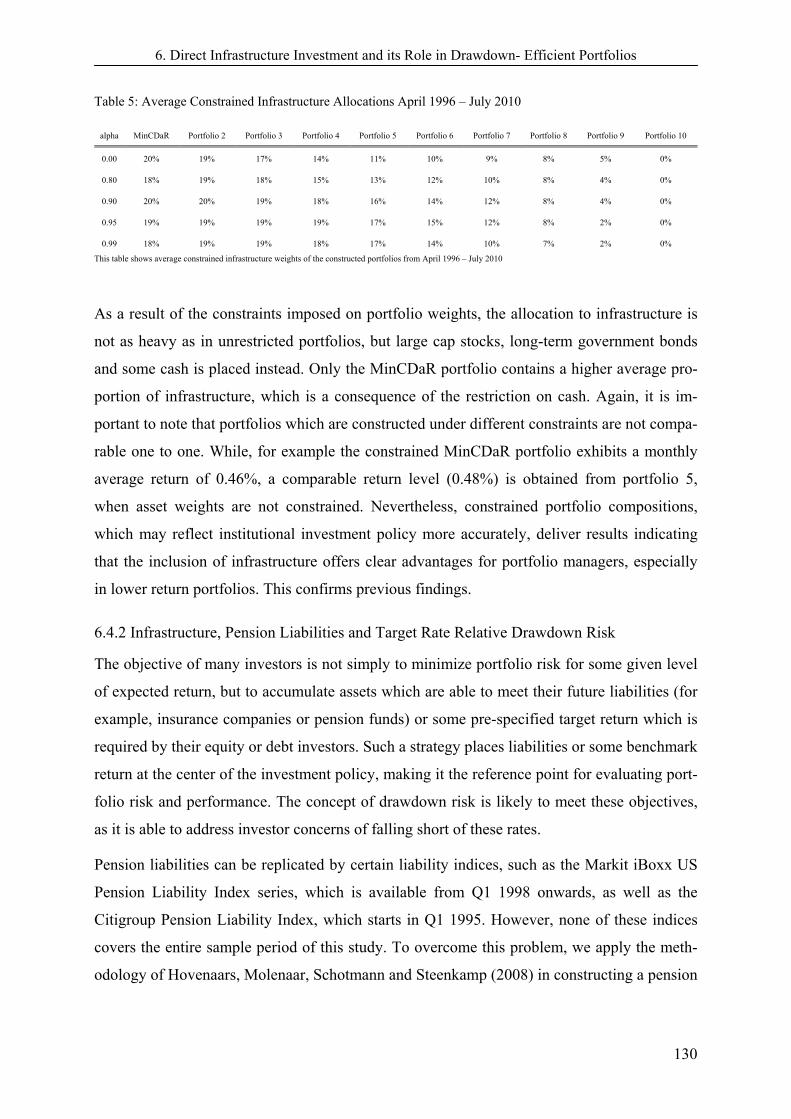
6. Direct Infrastructure Investment and its Role in Drawdown- Efficient Portfolios
130
Table 5: Average Constrained Infrastructure Allocations April 1996 – July 2010
alpha MinCDaR Portfolio 2 Portfolio 3 Portfolio 4 Portfolio 5 Portfolio 6 Portfolio 7 Portfolio 8 Portfolio 9 Portfolio 10
0.00 20% 19% 17% 14% 11% 10% 9% 8% 5% 0%
0.80 18% 19% 18% 15% 13% 12% 10% 8% 4% 0%
0.90 20% 20% 19% 18% 16% 14% 12% 8% 4% 0%
0.95 19% 19% 19% 19% 17% 15% 12% 8% 2% 0%
0.99 18% 19% 19% 18% 17% 14% 10% 7% 2% 0%
This table shows average constrained infrastructure weights of the constructed portfolios from April 1996 – July 2010
As a result of the constraints imposed on portfolio weights, the allocation to infrastructure is
not as heavy as in unrestricted portfolios, but large cap stocks, long-term government bonds
and some cash is placed instead. Only the MinCDaR portfolio contains a higher average pro-
portion of infrastructure, which is a consequence of the restriction on cash. Again, it is im-
portant to note that portfolios which are constructed under different constraints are not compa-
rable one to one. While, for example the constrained MinCDaR portfolio exhibits a monthly
average return of 0.46%, a comparable return level (0.48%) is obtained from portfolio 5,
when asset weights are not constrained. Nevertheless, constrained portfolio compositions,
which may reflect institutional investment policy more accurately, deliver results indicating
that the inclusion of infrastructure offers clear advantages for portfolio managers, especially
in lower return portfolios. This confirms previous findings.
6.4.2 Infrastructure, Pension Liabilities and Target Rate Relative Drawdown Risk
The objective of many investors is not simply to minimize portfolio risk for some given level
of expected return, but to accumulate assets which are able to meet their future liabilities (for
example, insurance companies or pension funds) or some pre-specified target return which is
required by their equity or debt investors. Such a strategy places liabilities or some benchmark
return at the center of the investment policy, making it the reference point for evaluating port-
folio risk and performance. The concept of drawdown risk is likely to meet these objectives,
as it is able to address investor concerns of falling short of these rates.
Pension liabilities can be replicated by certain liability indices, such as the Markit iBoxx US
Pension Liability Index series, which is available from Q1 1998 onwards, as well as the
Citigroup Pension Liability Index, which starts in Q1 1995. However, none of these indices
covers the entire sample period of this study. To overcome this problem, we apply the meth-
odology of Hovenaars, Molenaar, Schotmann and Steenkamp (2008) in constructing a pension
6. Direct Infrastructure Investment and its Role in Drawdown- Efficient Portfolios
131
liability index. Their approach is based on a log-linear transformation process, and the con-
struction of liability returns 1, tLr is given as follows
(7)
where trr is the 10 Year Treasury Yield adjusted to constant maturity and LD the duration of
pension fund liabilities. As in Hoevenaars et al. (2008)7, an average duration of 17 years is
assumed8. This self-constructed series is significantly related to the Markit, as well as the
Citigroup series, with statistically significant (1%) correlations of 0.65 and 0.44, respectively.
This makes it an appropriate tool for depicting liability performance, which is used in the fur-
ther course of our analysis. To construct liability efficient portfolios, we employ the same
methodology as before and now minimize liability relative drawdown risk (α = 0.95)9, while
achieving some excess return over liabilities.
The constructed portfolios are dominated by long-term government bonds in low and medi-
um-return portfolios. When higher returns have to be achieved, large cap stocks are allocated
at earlier time moments and are, from 2001 onwards, mainly replaced by better performing
small cap stocks. In terms of infrastructure weights, we obtain a rather unexpected result. In
contrast to the findings in Section 4.1, infrastructure is not included in any efficient portfolio,
regardless of the expected portfolio return, the confidence level and the time moment. Where
does this result come from? The valuation of pension liabilities is at the very core of this out-
come. Pension liabilities are valued simply by discounting the cash flow of future pension
payments via daily available government bond spot curves or swap quotations. As liabilities
are usually retained for a long time before they are distributed to the beneficiaries, this places
them at the long end of the yield curve and renders their values sensitive to changes in interest
rates and other changes in the yield curve. This inherently links the return on pension liabili-
ties to the returns on long term (government) bonds. A significant fall in interest rates, such as
during the recession in 2008, therefore has a dramatic impact on the value of pension liabili-
ties, with an increases of almost 20% in value. No other asset apart from long term (govern-
7 The data/methodology used is subject to the condition of constant age groups and pension rights accrued per group over time. The assump-tion that the pension fund is in a stationary state allows us to describe liabilities as a constant maturity index-linked bond. We further assume that the inflow from pension contributions is equal to the NPV of new liabilities and the current payments of the fund, and additionally ignore taxation issues, demographics and longevity risk. In consequence, interest rate and inflation risk are the only factors which are rele-vant to the pension scheme. 8 To check for robustness, we apply different durations to construct liabilities, namely 15, 16, 18 and 19 years. The results, however, do not change fundamentally and are available from the authors upon request. 9 We checked for robustness by employing confidence levels of 0.99, 0.95, 0.80 and 0.00.
)(12
1111, ttLttL rrrrDrrr

6. Direct Infrastructure Investment and its Role in Drawdown- Efficient Portfolios
132
ment) bonds can match such an increase in value and makes other assets less attractive from a
liability point of view.
Table 6: Relation of Monthly Asset Returns with Liabilities May 1990 – July 2010
STGovBonds MTGovBonds LTGovBonds STCorpBonds MTCorpBonds LTCorpBonds Cash Small Caps Large Caps Infrastructure
Correlation 0.56 0.58 0.58 0.49 0.52 0.52 0.25 -0.29 -0.18 0.00
Beta 0.11 0.17 0.42 0.11 0.17 0.35 0.02 -0.44 -0.21 0.00
The correlations and betas of liabilities10 with other assets, as shown in Figure 6, underpin this
finding and provide – together with the high expected return on long term government bonds
– a rationale for significant long term government bond allocations in liability-efficient port-
folios. If the return on an asset is sufficiently high, and moves together with the return on lia-
bilities, it is a viable asset for minimizing liability-relative drawdown risk. Equities are, on
average, included, as they offer high expected returns, especially in former years. The reason,
why drawdown-efficient portfolios do not contain any infrastructure is straightforward. First-
ly, infrastructure returns are lower than those of small caps, large caps and long term govern-
ment bonds and, secondly, infrastructure does not move together with liabilities, which is also
not favorable from a drawdown perspective. This contradicts the reputation of infrastructure
as an appropriate asset for pension plan liability matching.
In addition to the liability-driven approach, we benchmark each asset against a fixed target
return. Since investors are not homogenous, but have different investment objectives, we con-
sider three different real target returns. These are 2.0%, 3.0% and 4.0% annually. One has to
bear in mind that the applied target rates should not be confused with expected returns. While
the expected return reflects the return an investor aims to achieve, the target rate is essential
for the definition of risk and reflects some level of return, to which the investor is averse to
falling short. Therefore, it is not a contradiction to assume an expected return which exceeds
the target rate.
10 The monthly real average return on the liabilities is 0.61%, and the standard deviation is 3.79%. We compare the return and the standard deviation of our self constructed liability series to the Citigroup and the Markit series over matching intervals and find quite similar numbers. While, for example, our series exhibits a nominal return and a standard deviation of 0.71% and 3.77% over the January 1995 to July 2010 period, the corresponding values for the Citigroup series are 0.87% and 3.95%.

6. Direct Infrastructure Investment and its Role in Drawdown- Efficient Portfolios
133
Table 7: Average Infrastructure Allocations (α = 0.95) April 1996 - July 2010
Target p. a. MinCDaR Portfolio 2 Portfolio 3 Portfolio 4 Portfolio 5 Portfolio 6 Portfolio 7 Portfolio 8 Portfolio 9 Portfolio 10
2.00% 30% 37% 42% 43% 33% 20% 9% 3% 1% 0%
3.00% 44% 45% 46% 40% 28% 16% 8% 2% 0% 0%
4.00% 49% 49% 43% 33% 23% 13% 5% 1% 0% 0%
This table shows average infrastructure weights of the constructed portfolios from April 1996 – July 2010 for different target rates.
The average portfolio compositions for different targets are presented in Table 7. In accord-
ance with the results from Section 4.1, we find that infrastructure is, on average, present in
low and medium-return portfolios across all target returns. The allocation to infrastructure is
higher than in the base model in Section 4.1 and increases with rising target rates in low-
return portfolios, a result which contradicts intuition. However, this outcome can easily be
explained by the fact that infrastructure replaces cash. This effect becomes more pronounced
the higher the target return is set. The fact that the allocation towards cash diminishes with
rising target rates is intuitive. An increase in the target return raises the drawdown risk of cash
as a result of relatively low returns, and provides momentum for including an asset which
exhibits higher returns, but moderate drawdown risk – a role played by infrastructure. When
the expected return increases, infrastructure is removed more from the portfolio than in our
base case; as a logical consequence of relatively low infrastructure returns, this pattern is
more conspicuous, the higher the target rate is set. These findings confirm the results from
Section 4.1 and accentuate the role of infrastructure as a viable asset for low-risk portfolios,
when investors exhibit different target rates of return.
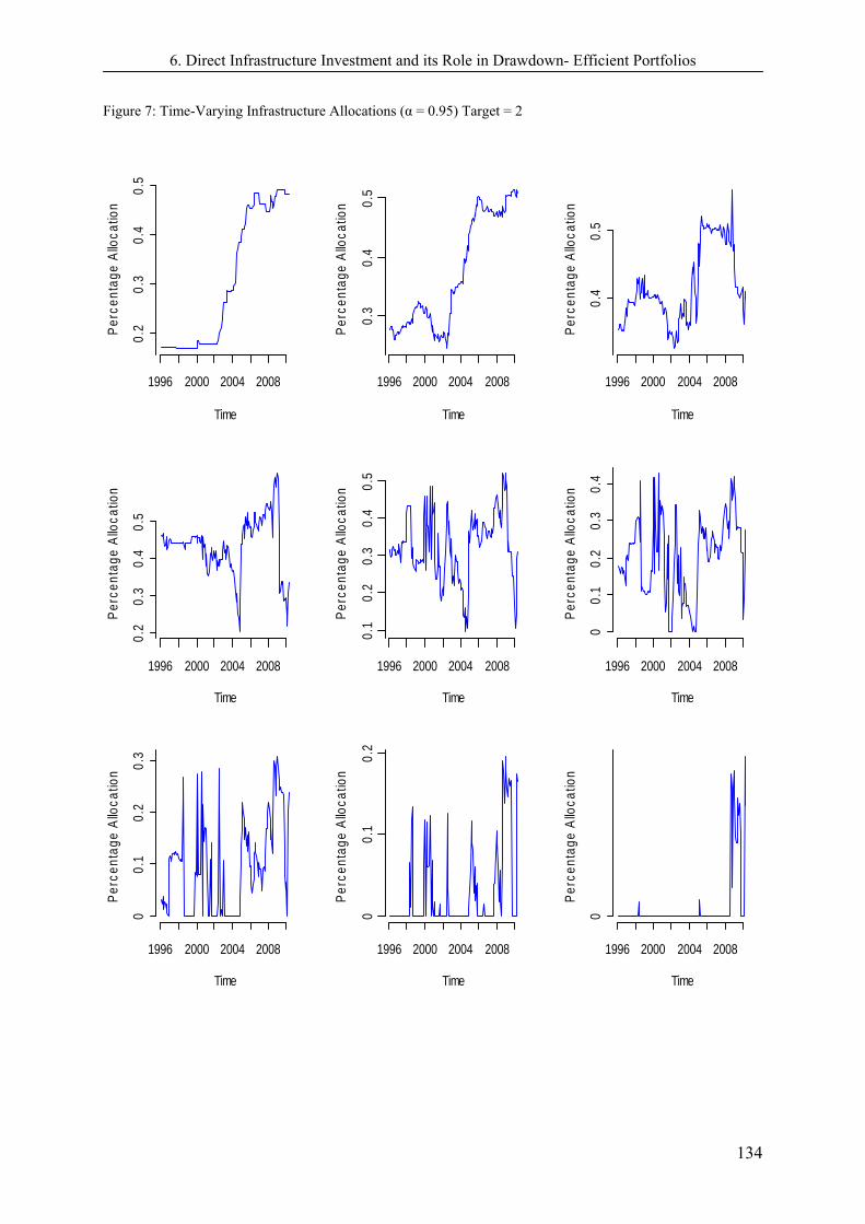
6. Direct Infrastructure Investment and its Role in Drawdown- Efficient Portfolios
134
Figure 7: Time-Varying Infrastructure Allocations (α = 0.95) Target = 2
Time
Per
cent
age
Allo
catio
n
1996 2000 2004 2008
0.2
0.3
0.4
0.5
Time
Per
cent
age
Allo
catio
n
1996 2000 2004 20080.
30.
40.
5
Time
Per
cent
age
Allo
catio
n
1996 2000 2004 2008
0.4
0.5
Time
Per
cent
age
Allo
catio
n
1996 2000 2004 2008
0.2
0.3
0.4
0.5
Time
Per
cent
age
Allo
catio
n
1996 2000 2004 2008
0.1
0.2
0.3
0.4
0.5
Time
Per
cent
age
Allo
catio
n
1996 2000 2004 2008
00.
10.
20.
30.
4
Time
Per
cent
age
Allo
catio
n
1996 2000 2004 2008
00.
10.
20.
3
Time
Per
cent
age
Allo
catio
n
1996 2000 2004 2008
00.
10.
2
Time
Per
cent
age
Allo
catio
n
1996 2000 2004 2008
0
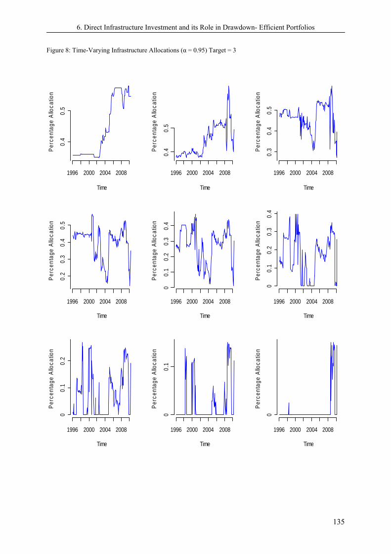
6. Direct Infrastructure Investment and its Role in Drawdown- Efficient Portfolios
135
Figure 8: Time-Varying Infrastructure Allocations (α = 0.95) Target = 3
Time
Per
cent
age
Allo
catio
n
1996 2000 2004 2008
0.4
0.5
Time
Per
cent
age
Allo
catio
n
1996 2000 2004 20080.
40.
5
Time
Per
cent
age
Allo
catio
n
1996 2000 2004 2008
0.3
0.4
0.5
Time
Per
cent
age
Allo
catio
n
1996 2000 2004 2008
0.2
0.3
0.4
0.5
Time
Per
cent
age
Allo
catio
n
1996 2000 2004 2008
00.
10.
20.
30.
4
Time
Per
cent
age
Allo
catio
n
1996 2000 2004 2008
00.
10.
20.
30.
4
Time
Per
cent
age
Allo
catio
n
1996 2000 2004 2008
00.
10.
2
Time
Per
cent
age
Allo
catio
n
1996 2000 2004 2008
00.
1
Time
Per
cent
age
Allo
catio
n
1996 2000 2004 2008
0

6. Direct Infrastructure Investment and its Role in Drawdown- Efficient Portfolios
136
Figure 8: Time-Varying Infrastructure Allocations (α = 0.95) Target = 4
Time
Per
cent
age
Allo
catio
n
1996 2000 2004 2008
0.4
0.5
Time
Per
cent
age
Allo
catio
n
1996 2000 2004 2008
0.4
0.5
Time
Per
cent
age
Allo
catio
n
1996 2000 2004 2008
0.3
0.4
0.5
Time
Per
cent
age
Allo
catio
n
1996 2000 2004 2008
0.1
0.2
0.3
0.4
0.5
Time
Per
cent
age
Allo
catio
n
1996 2000 2004 2008
00.
10.
20.
30.
4
Time
Per
cent
age
Allo
catio
n
1996 2000 2004 2008
00.
10.
20.
3
Time
Per
cent
age
Allo
catio
n
1996 2000 2004 2008
00.
10.
2
Time
Per
cent
age
Allo
catio
n
1996 2000 2004 2008
00.
1
Time
Per
cent
age
Allo
catio
n
1996 2000 2004 2008
0

6. Direct Infrastructure Investment and its Role in Drawdown- Efficient Portfolios
137
In accordance with our previous findings, infrastructure allocations vary over the time hori-
zon, as shown in Figure 7 to 9. The volatility of infrastructure weights increases with an in-
crease in the expected return and in the target rate. As a result of implementing the target re-
turn, infrastructure allocations are not as sensitive to short-term bonds, but rather to mid-term
(corporate and government) bonds. This result makes sense, as short-term investments be-
come – due to their low expected returns – more unattractive from a target-rate perspective.
This sensitivity can be observed over the course of the dot.com and the recent financial crisis,
with infrastructure being replaced by mid-term bonds, especially for medium and some higher
-return portfolios. Nevertheless, the picture of infrastructure as an asset which is able to con-
tribute mainly to the performance of low-risk and low-return portfolios is clearly evident, as
the asset is stable and persistently allocated to those portfolios. Since it tends to replace cash,
infrastructure is now allocated to the MinCDaR portfolio across the entire time horizon. Fur-
thermore, infrastructure weights are more stable in low-return portfolios when a benchmark is
implemented.
6.4.3 Downside Beta Hedged Portfolios
Ang, Chen and Xing (2006) show that investors demand a premium on equities which move
together with the market when it drops. To incorporate this aversion to (equity) market down-
side risk, we construct portfolios which do not follow the equity market when it is in a poor
state – expressed simply, a restriction on portfolio downside beta. We define portfolio down-
side beta as the weighted sum of individual assets’ downside betas. Accordingly, this is given
by
(9)
Following Ang et al. (2006), we define individual asset downside beta as
(10)
i
n
iip x
1
)0|var(
)0|,cov(
mm
mmii rr
rrr
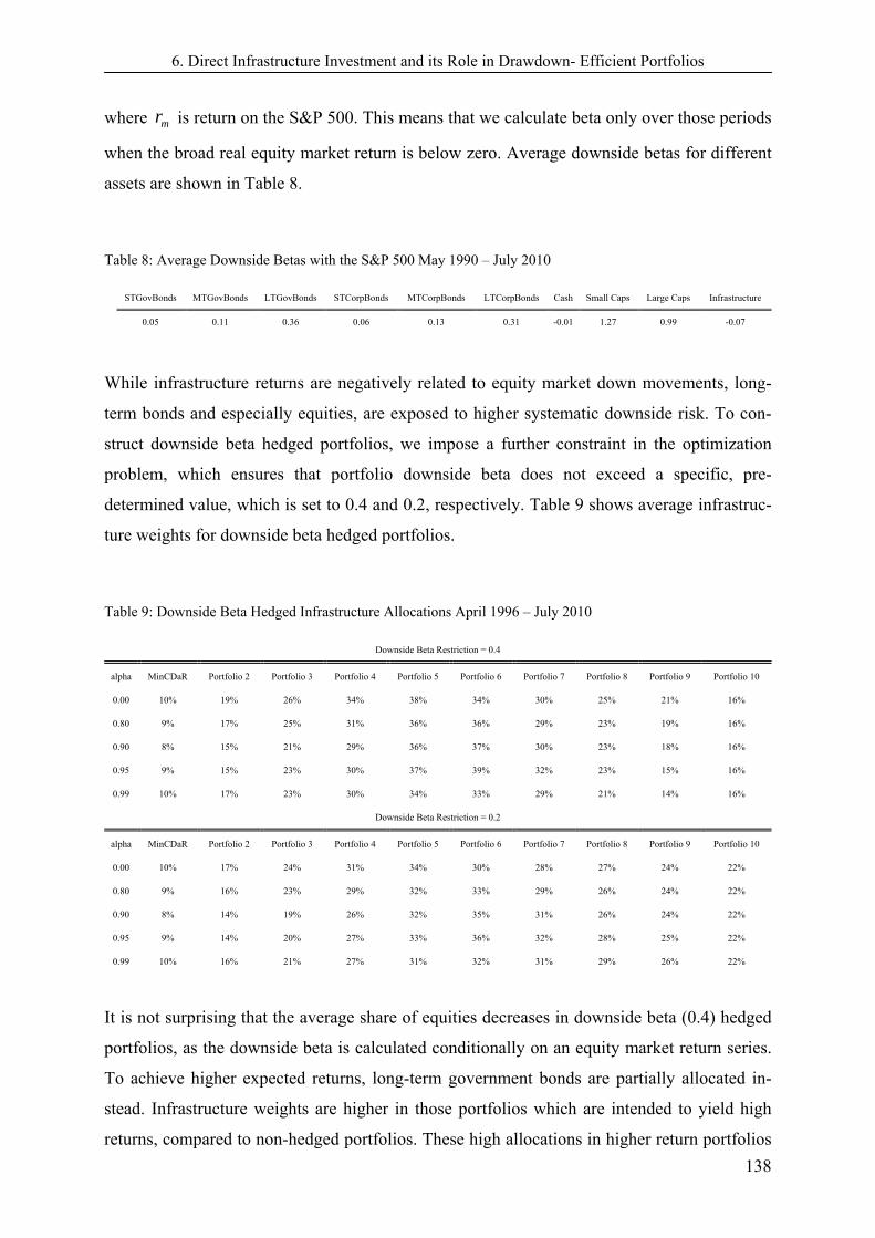
6. Direct Infrastructure Investment and its Role in Drawdown- Efficient Portfolios
138
where mr is return on the S&P 500. This means that we calculate beta only over those periods
when the broad real equity market return is below zero. Average downside betas for different
assets are shown in Table 8.
Table 8: Average Downside Betas with the S&P 500 May 1990 – July 2010
STGovBonds MTGovBonds LTGovBonds STCorpBonds MTCorpBonds LTCorpBonds Cash Small Caps Large Caps Infrastructure
0.05 0.11 0.36 0.06 0.13 0.31 -0.01 1.27 0.99 -0.07
While infrastructure returns are negatively related to equity market down movements, long-
term bonds and especially equities, are exposed to higher systematic downside risk. To con-
struct downside beta hedged portfolios, we impose a further constraint in the optimization
problem, which ensures that portfolio downside beta does not exceed a specific, pre-
determined value, which is set to 0.4 and 0.2, respectively. Table 9 shows average infrastruc-
ture weights for downside beta hedged portfolios.
Table 9: Downside Beta Hedged Infrastructure Allocations April 1996 – July 2010
Downside Beta Restriction = 0.4
alpha MinCDaR Portfolio 2 Portfolio 3 Portfolio 4 Portfolio 5 Portfolio 6 Portfolio 7 Portfolio 8 Portfolio 9 Portfolio 10
0.00 10% 19% 26% 34% 38% 34% 30% 25% 21% 16%
0.80 9% 17% 25% 31% 36% 36% 29% 23% 19% 16%
0.90 8% 15% 21% 29% 36% 37% 30% 23% 18% 16%
0.95 9% 15% 23% 30% 37% 39% 32% 23% 15% 16%
0.99 10% 17% 23% 30% 34% 33% 29% 21% 14% 16%
Downside Beta Restriction = 0.2
alpha MinCDaR Portfolio 2 Portfolio 3 Portfolio 4 Portfolio 5 Portfolio 6 Portfolio 7 Portfolio 8 Portfolio 9 Portfolio 10
0.00 10% 17% 24% 31% 34% 30% 28% 27% 24% 22%
0.80 9% 16% 23% 29% 32% 33% 29% 26% 24% 22%
0.90 8% 14% 19% 26% 32% 35% 31% 26% 24% 22%
0.95 9% 14% 20% 27% 33% 36% 32% 28% 25% 22%
0.99 10% 16% 21% 27% 31% 32% 31% 29% 26% 22%
It is not surprising that the average share of equities decreases in downside beta (0.4) hedged
portfolios, as the downside beta is calculated conditionally on an equity market return series.
To achieve higher expected returns, long-term government bonds are partially allocated in-
stead. Infrastructure weights are higher in those portfolios which are intended to yield high
returns, compared to non-hedged portfolios. These high allocations in higher return portfolios

6. Direct Infrastructure Investment and its Role in Drawdown- Efficient Portfolios
139
are associated with the ability of infrastructure to diversify systematic equity risk. When, for
example, the proportion of small caps rises in mid 2005, the allocation to infrastructure rises
simultaneously. Therefore, if investors wish to earn relatively high returns, but have an aver-
sion towards systematic equity downside risk, they would be well advised to allocate some of
their capital to infrastructure, along with equities. However, when long-term government
bond returns increase over the course of the financial crisis and begin to enter high-return
portfolios in place of equities, the importance of infrastructure for diversifying systematic
equity risk decreases, as bonds themselves do not exhibit as high a downside beta as equities.
Therefore, the weight of infrastructure, especially in high-return portfolios, depends on the
relative weights of bonds and equities. If an investor intends to invest in equities, she is ad-
vised to devote some capital to infrastructure for diversification reasons, although this does
not apply when the main investment asset is fixed income. In contrast to high-return portfoli-
os, the average proportion of infrastructure decreases in low-return and some medium-return
portfolios, but cash and some short-term corporate bonds are used instead.
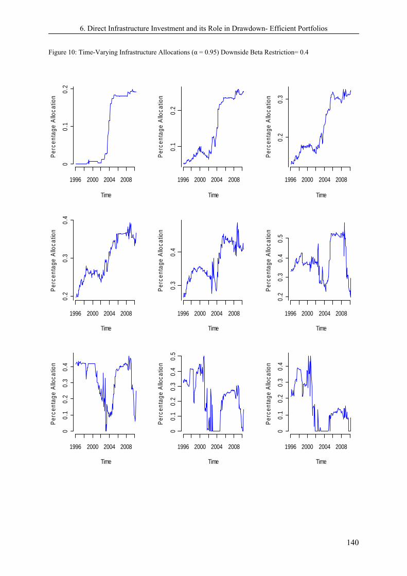
6. Direct Infrastructure Investment and its Role in Drawdown- Efficient Portfolios
140
Figure 10: Time-Varying Infrastructure Allocations (α = 0.95) Downside Beta Restriction= 0.4
Time
Per
cent
age
Allo
catio
n
1996 2000 2004 2008
00.
10.
2
Time
Per
cent
age
Allo
catio
n
1996 2000 2004 20080.
10.
2
Time
Per
cent
age
Allo
catio
n
1996 2000 2004 2008
0.2
0.3
Time
Per
cent
age
Allo
catio
n
1996 2000 2004 2008
0.2
0.3
0.4
Time
Per
cent
age
Allo
catio
n
1996 2000 2004 2008
0.3
0.4
Time
Per
cent
age
Allo
catio
n
1996 2000 2004 2008
0.2
0.3
0.4
0.5
Time
Per
cent
age
Allo
catio
n
1996 2000 2004 2008
00.
10.
20.
30.
4
Time
Per
cent
age
Allo
catio
n
1996 2000 2004 2008
00.
10.
20.
30.
40.
5
Time
Per
cent
age
Allo
catio
n
1996 2000 2004 2008
00.
10.
20.
30.
4
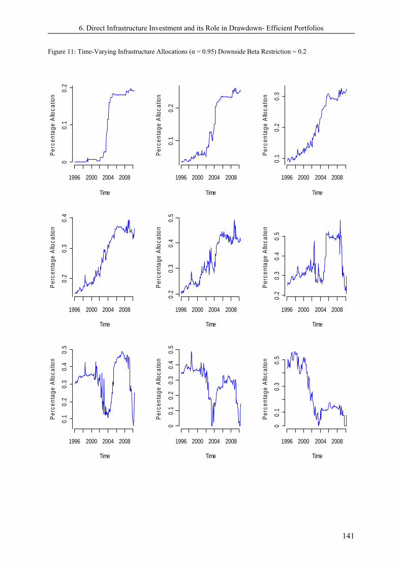
6. Direct Infrastructure Investment and its Role in Drawdown- Efficient Portfolios
141
Figure 11: Time-Varying Infrastructure Allocations (α = 0.95) Downside Beta Restriction = 0.2
Time
Per
cent
age
Allo
catio
n
1996 2000 2004 2008
00.
10.
2
Time
Per
cent
age
Allo
catio
n
1996 2000 2004 20080.
10.
2
Time
Per
cent
age
Allo
catio
n
1996 2000 2004 2008
0.1
0.2
0.3
Time
Per
cent
age
Allo
catio
n
1996 2000 2004 2008
0.2
0.3
0.4
Time
Per
cent
age
Allo
catio
n
1996 2000 2004 2008
0.2
0.3
0.4
0.5
Time
Per
cent
age
Allo
catio
n
1996 2000 2004 2008
0.2
0.3
0.4
0.5
Time
Per
cent
age
Allo
catio
n
1996 2000 2004 2008
0.1
0.2
0.3
0.4
0.5
Time
Per
cent
age
Allo
catio
n
1996 2000 2004 2008
00.
10.
20.
30.
40.
5
Time
Per
cent
age
Allo
catio
n
1996 2000 2004 2008
00.
10.
30.
5
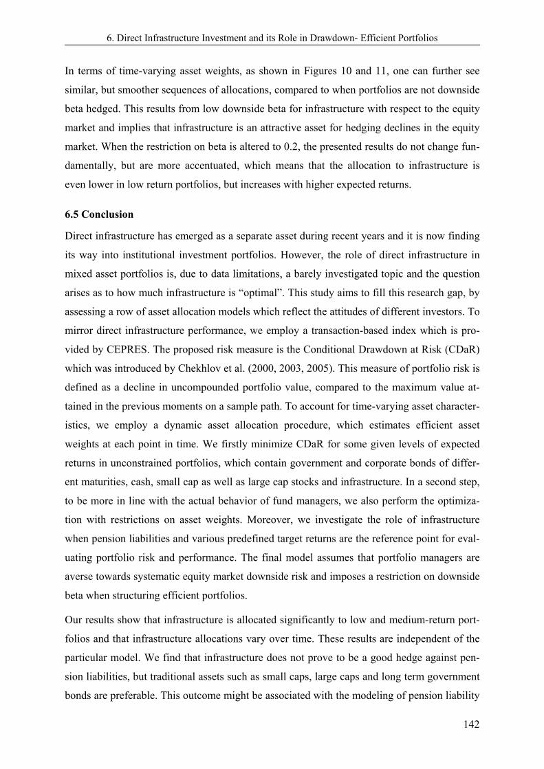
6. Direct Infrastructure Investment and its Role in Drawdown- Efficient Portfolios
142
In terms of time-varying asset weights, as shown in Figures 10 and 11, one can further see
similar, but smoother sequences of allocations, compared to when portfolios are not downside
beta hedged. This results from low downside beta for infrastructure with respect to the equity
market and implies that infrastructure is an attractive asset for hedging declines in the equity
market. When the restriction on beta is altered to 0.2, the presented results do not change fun-
damentally, but are more accentuated, which means that the allocation to infrastructure is
even lower in low return portfolios, but increases with higher expected returns.
6.5 Conclusion
Direct infrastructure has emerged as a separate asset during recent years and it is now finding
its way into institutional investment portfolios. However, the role of direct infrastructure in
mixed asset portfolios is, due to data limitations, a barely investigated topic and the question
arises as to how much infrastructure is “optimal”. This study aims to fill this research gap, by
assessing a row of asset allocation models which reflect the attitudes of different investors. To
mirror direct infrastructure performance, we employ a transaction-based index which is pro-
vided by CEPRES. The proposed risk measure is the Conditional Drawdown at Risk (CDaR)
which was introduced by Chekhlov et al. (2000, 2003, 2005). This measure of portfolio risk is
defined as a decline in uncompounded portfolio value, compared to the maximum value at-
tained in the previous moments on a sample path. To account for time-varying asset character-
istics, we employ a dynamic asset allocation procedure, which estimates efficient asset
weights at each point in time. We firstly minimize CDaR for some given levels of expected
returns in unconstrained portfolios, which contain government and corporate bonds of differ-
ent maturities, cash, small cap as well as large cap stocks and infrastructure. In a second step,
to be more in line with the actual behavior of fund managers, we also perform the optimiza-
tion with restrictions on asset weights. Moreover, we investigate the role of infrastructure
when pension liabilities and various predefined target returns are the reference point for eval-
uating portfolio risk and performance. The final model assumes that portfolio managers are
averse towards systematic equity market downside risk and imposes a restriction on downside
beta when structuring efficient portfolios.
Our results show that infrastructure is allocated significantly to low and medium-return port-
folios and that infrastructure allocations vary over time. These results are independent of the
particular model. We find that infrastructure does not prove to be a good hedge against pen-
sion liabilities, but traditional assets such as small caps, large caps and long term government
bonds are preferable. This outcome might be associated with the modeling of pension liability

6. Direct Infrastructure Investment and its Role in Drawdown- Efficient Portfolios
143
returns, which are strongly related with the returns on long-term bonds. The role of infrastruc-
ture in a liability framework, especially in consideration of longer holding periods, may con-
stitute a promising topic for further research.
When asset returns are targeted against some predetermined benchmark to mirror capital cost,
the role of infrastructure in low-risk portfolios is even more accentuated. Due to the inability
of cash to achieve higher return targets, infrastructure is weighted more heavily.
As infrastructure does not correlate with equity returns in down markets, it proves to be a val-
uable hedge against downside systematic risk which also results in portfolio compositions that
exceed those in current investment portfolios.
The proposed models do not demonstrate exactly how much infrastructure should be allocated
to a multi-asset portfolio, as this depends on various parameters, such as the investor’s ex-
pected return, her perception of risk, some target return or the market phase. Furthermore, our
results do, not necessarily suggest that investors should reallocate their portfolios and increase
their allocation to infrastructure, as we also do not know exactly how much infrastructure is
already allocated. However, there are many indications that the actual proportion of infra-
structure is, on average, below that suggested by our models.
In summary, we find stable and conclusive evidence that infrastructure can contribute to port-
folio performance, especially in low and medium-return portfolios, and that the inclusion of
infrastructure may deliver a better risk-return tradeoff than conventional portfolio allocations,
which comprise mainly stocks and bonds. This insight should be especially useful for inves-
tors whose aim is not to earn superior returns, but to protect their portfolios from extreme de-
clines in value.

6. Direct Infrastructure Investment and its Role in Drawdown- Efficient Portfolios
144
6.6 Appendix
The optimization problem in which drawdown risk is minimized for a certain level of ex-
pected return at each point in time is reduced to the following linear programming problem.
,1
10
)(
0
1
1*
10
1*
)1(
1
..
),,,(
1
0
1
1
n
ii
i
kk
kk
k
kkk
J
kk
x
x
xR
u
Jkuu
Jkxyu
Jkz
Jkxyuz
zzJ
ts
zzuxinMinimize
where ky is a vector of cumulative asset returns up to the time moment k , x is a vector of
portfolio weights, and kz as well as Jkuk 1, are auxiliary variables. is a predeter-
mined value for the return on the portfolio )(xR .

6. Direct Infrastructure Investment and its Role in Drawdown- Efficient Portfolios
145
Figure 3: Time-Varying Infrastructure Allocations (α = 0.00)
Time
Per
cent
age
Allo
catio
n
1996 2000 2004 2008
00.
10.
2
Time
Per
cent
age
Allo
catio
n
1996 2000 2004 20080.
10.
20.
3
Time
Per
cent
age
Allo
catio
n
1996 2000 2004 2008
0.2
0.3
0.4
Time
Per
cent
age
Allo
catio
n
1996 2000 2004 2008
0.3
0.4
Time
Per
cent
age
Allo
catio
n
1996 2000 2004 2008
0.3
0.4
0.5
Time
Per
cent
age
Allo
catio
n
1996 2000 2004 2008
00.
10.
30.
5
Time
Per
cent
age
Allo
catio
n
1996 2000 2004 2008
00.
10.
20.
30.
4
Time
Per
cent
age
Allo
catio
n
1996 2000 2004 2008
00.
10.
20.
3
Time
Per
cent
age
Allo
catio
n
1996 2000 2004 2008
00.
1
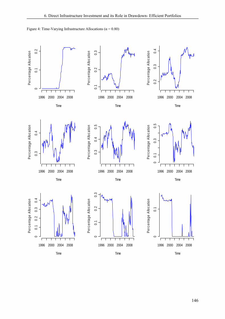
6. Direct Infrastructure Investment and its Role in Drawdown- Efficient Portfolios
146
Figure 4: Time-Varying Infrastructure Allocations (α = 0.80)
Time
Per
cent
age
Allo
catio
n
1996 2000 2004 2008
00.
10.
2
Time
Per
cent
age
Allo
catio
n
1996 2000 2004 20080.
10.
20.
3
Time
Per
cent
age
Allo
catio
n
1996 2000 2004 2008
0.2
0.3
0.4
Time
Per
cent
age
Allo
catio
n
1996 2000 2004 2008
0.3
0.4
Time
Per
cent
age
Allo
catio
n
1996 2000 2004 2008
0.3
0.4
0.5
Time
Per
cent
age
Allo
catio
n
1996 2000 2004 2008
00.
10.
30.
5
Time
Per
cent
age
Allo
catio
n
1996 2000 2004 2008
00.
10.
20.
30.
4
Time
Per
cent
age
Allo
catio
n
1996 2000 2004 2008
00.
10.
20.
3
Time
Per
cent
age
Allo
catio
n
1996 2000 2004 2008
00.
1
6. Direct Infrastructure Investment and its Role in Drawdown- Efficient Portfolios
147
Figure 5: Time-Varying Infrastructure Allocations (α = 0.90)
Time
Per
cent
age
Allo
catio
n
1996 2000 2004 2008
00.
10.
2
Time
Per
cent
age
Allo
catio
n
1996 2000 2004 20080.
10.
2
Time
Per
cent
age
Allo
catio
n
1996 2000 2004 2008
0.2
0.3
Time
Per
cent
age
Allo
catio
n
1996 2000 2004 2008
0.3
0.4
Time
Per
cent
age
Allo
catio
n
1996 2000 2004 2008
0.3
0.4
0.5
Time
Per
cent
age
Allo
catio
n
1996 2000 2004 2008
0.1
0.2
0.3
0.4
0.5
Time
Per
cent
age
Allo
catio
n
1996 2000 2004 2008
00.
10.
20.
30.
4
Time
Per
cent
age
Allo
catio
n
1996 2000 2004 2008
00.
10.
20.
3
Time
Per
cent
age
Allo
catio
n
1996 2000 2004 2008
00.
1

6. Direct Infrastructure Investment and its Role in Drawdown- Efficient Portfolios
148
Figure 6: Time-Varying Infrastructure Allocations (α = 0.99)
Time
Per
cent
age
Allo
catio
n
1996 2000 2004 2008
00.
10.
2
Time
Per
cent
age
Allo
catio
n
1996 2000 2004 20080.
10.
20.
3
Time
Per
cent
age
Allo
catio
n
1996 2000 2004 2008
0.2
0.3
Time
Per
cent
age
Allo
catio
n
1996 2000 2004 2008
0.2
0.3
0.4
Time
Per
cent
age
Allo
catio
n
1996 2000 2004 2008
0.2
0.3
0.4
Time
Per
cent
age
Allo
catio
n
1996 2000 2004 2008
00.
10.
20.
30.
4
Time
Per
cent
age
Allo
catio
n
1996 2000 2004 2008
00.
10.
20.
30.
4
Time
Per
cent
age
Allo
catio
n
1996 2000 2004 2008
00.
10.
20.
3
Time
Per
cent
age
Allo
catio
n
1996 2000 2004 2008
00.
1
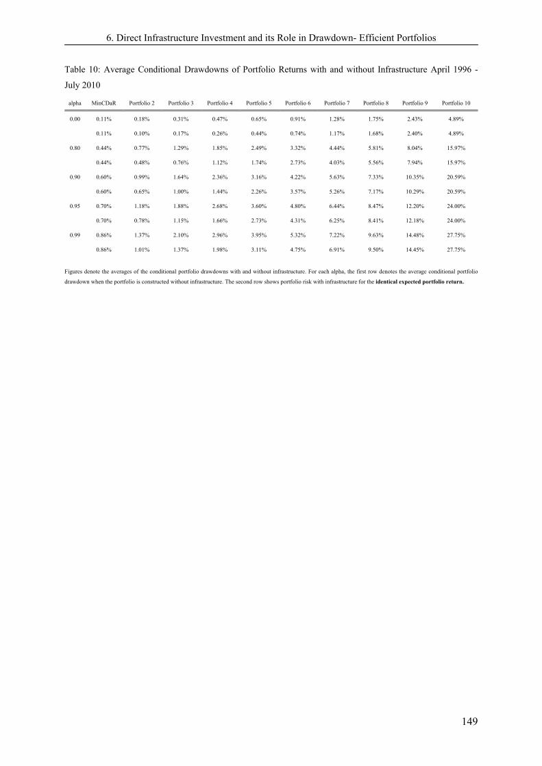
6. Direct Infrastructure Investment and its Role in Drawdown- Efficient Portfolios
149
Table 10: Average Conditional Drawdowns of Portfolio Returns with and without Infrastructure April 1996 -
July 2010
alpha MinCDaR Portfolio 2 Portfolio 3 Portfolio 4 Portfolio 5 Portfolio 6 Portfolio 7 Portfolio 8 Portfolio 9 Portfolio 10
0.00 0.11% 0.18% 0.31% 0.47% 0.65% 0.91% 1.28% 1.75% 2.43% 4.89%
0.11% 0.10% 0.17% 0.26% 0.44% 0.74% 1.17% 1.68% 2.40% 4.89%
0.80 0.44% 0.77% 1.29% 1.85% 2.49% 3.32% 4.44% 5.81% 8.04% 15.97%
0.44% 0.48% 0.76% 1.12% 1.74% 2.73% 4.03% 5.56% 7.94% 15.97%
0.90 0.60% 0.99% 1.64% 2.36% 3.16% 4.22% 5.63% 7.33% 10.35% 20.59%
0.60% 0.65% 1.00% 1.44% 2.26% 3.57% 5.26% 7.17% 10.29% 20.59%
0.95 0.70% 1.18% 1.88% 2.68% 3.60% 4.80% 6.44% 8.47% 12.20% 24.00%
0.70% 0.78% 1.15% 1.66% 2.73% 4.31% 6.25% 8.41% 12.18% 24.00%
0.99 0.86% 1.37% 2.10% 2.96% 3.95% 5.32% 7.22% 9.63% 14.48% 27.75%
0.86% 1.01% 1.37% 1.98% 3.11% 4.75% 6.91% 9.50% 14.45% 27.75%
Figures denote the averages of the conditional portfolio drawdowns with and without infrastructure. For each alpha, the first row denotes the average conditional portfolio
drawdown when the portfolio is constructed without infrastructure. The second row shows portfolio risk with infrastructure for the identical expected portfolio return.

6. Direct Infrastructure Investment and its Role in Drawdown- Efficient Portfolios
150
6.7 References
Ang, A.; Chen, J.; Xing, Y. (2006): Downside Risk, Review of Financial Studies, Vol. 19, No. 4, p. 1191-1239.
Araujo, S.; Sutherland, D. (2010): Public-Private Partnerships and Investment in Infrastruc-ture, OECD Economics Department; Working Papers, No. 803.
Berkelaar A.; Kouwenberg, R. (2010): A Liability-Relative Drawdown Approach to Pen-sion Asset Liability Management, Journal of Asset Management, Vol. 11, No. 22, p. 194-217.
Bitsch, F.; Buchner, A.; Kaserer, C. (2010): Risk, return and cash flow characteristics of infrastructure fund investments, European Investment Bank (EIB); EIB – Papers, No. 15, p. 106-136.
Chekhlov, A.; Uryasev, S.; Zabarankin, M. (2000): Portfolio Optimization with Drawdown Constraints, Research Report, No. 2000-5, University of Florida.
Chekhlov, A.; Uryasev, S.; Zabarankin, M. (2003): Portfolio Optimization with Drawdown Constraints, Asset and Liability Management Tools, Chekhlov, A.; Uryasev, S.; Zabarankin, M. (Eds.): Risk Books, London.
Chekhlov, A.; Uryasev, S.; Zabarankin, M. (2005): Drawdown Measure in Portfolio Opti-mization, International Journal of Theoretical and Applied Finance, Vol. 8, No. 1, p. 1–46.
Dechant, T.; Finkenzeller, K.; Schäfers, W. (2010): Real Estate: A Victim of Infrastruc-ture? Evidence from Conditional Asset Allocation, IREBS University of Regensburg; Working paper.
Fama, E.; Schwert, G. (1977): Asset returns and inflation, Journal of Financial Economics, Vol. 5, p. 115–146.
Finkenzeller, K.; Dechant, T.; Schaefers, W. (2010): Infrastructure: a new dimension of real estate? An asset allocation analysis, Journal of Property Investment and Finance, Vol. 28, No. 4, p. 263-274.
Finkenzeller, K.; Fleischmann, B. (2011): The interactions Between Direct and Securitized Infrastructure and its Relationship to Real Estate, IREBS University of Regensburg; Working paper.
Franzoni F.; Nowak, E.; Phalippou, L. (2011): Private equity performance and liquidity risk, Journal of Finance, (forthcoming).
Fuess, R.; Schweizer, D. (2011): Dynamic Interactions between Venture Capital Returns and the Macroeconomy: Theoretical and Empirical Evidence from the United States, Review of Quantitative Finance and Accounting, (forthcoming).

6. Direct Infrastructure Investment and its Role in Drawdown- Efficient Portfolios
151
Hoevenaars, R.; Molenaar, R.; Schotman, P.; Steenkamp T. (2008): Strategic Asset Allo-cation with Liabilities: Beyond Stocks and Bonds, Journal of Economic Dynamics and Con-trol, Vol. 32, No. 9, p. 2939-2970.
Inderst, G. (2010): Infrastructure as an asset class. European Investment Bank Papers (EIB), EIB-Papers, Vol. 15, No. 1, p. 70-106.
Kaserer, C.; Buchner, A.; Schmidt, D.; Krohmer, P. (2009): Infrastructure Private Equity, Center of Private Equity Research (CEPRES), Munich.
Krohmer, P.; Lauterbach, R.; Calanog, V. (2009): The bright and dark side of staging: In-vestment performance and the varying motivations of private equity. Journal of Banking and Finance, Vol. 33, No. 9, p. 1597-1609.
Krokhmal, P.; Uryasev, S.; Zrazhevsky, G. (2002): Risk management for hedge fund port-folios: A comparative analysis of linear portfolio rebalancing strategies, Journal of Alterna-tive Investments, Vol. 5, No. 1, p. 10–29.
Mansour, A.; Patel, J. (2008): Infrastructure Goes Global, RREEF Research Report.
Newell, G.; Peng, H. (2008): The Role of U.S. Infrastructure in Investment Portfolios. Jour-nal of Real Estate Portfolio Management, Vol. 14, No. 1, p. 21-33.
Newell, G.; Peng, H.; De Francesco, A. (2011): The performance of unlisted infrastructure in investment portfolios. Journal of Property Research, Vol. 28, No. 1, p. 59-74.
Organisation for Economic Co-operation and Development (2006): Infrastructure to 2030. Telecom, Land Transport, Water and Electricity, Paris.
Peng, L. (2001): Building a Venture Capital Index, Yale University, Working paper 00-5.
Preqin (2011): The Preqin Quarterly Infrastructure Q3 2011.
Probitas Partner (2011): Infrastructure Market Review and Institutional Investor Trends Survey for 2011.
Röller, L.H.; Waverman, L. (2001): Telecommunications Infrastructure and Economic De-velopment: A Simultaneous Approach, American Economic Review, Vol. 91, No. 4, p. 909-923.
Rothballer, C.; Kaserer C. (2011): Is Infrastructure Really Low Risk? An Empirical Analy-sis of Listed Infrastructure Firms, Technical University of Munich (TUM), Working paper.
Rockafellar R.; Uryasev, S. (2002): Conditional Value-at-Risk for General Loss Distribu-tions, Journal of Banking and Finance, Vol. 26, No. 7, p. 1443-1471.
Rockafellar, R.; Uryasev, S. (2000): Optimization of Conditional Value-At-Risk, The Jour-nal of Risk, Vol. 2, No. 3, p. 21-41.

6. Direct Infrastructure Investment and its Role in Drawdown- Efficient Portfolios
152
Schmitt, D.; Ott, T. (2006): Modelling a Performance Index for Non-traded Private Equity Transactions: Methodology and Practical Application, Center of Private Equity Research (CEPRES), Research paper.
WEF, World Economic Forum (2010): Global Risks 2010. A Global Risk Network Report.
Conclusion
153
7. Conclusion
The following section provides an overview of the five papers comprising the main body of
this dissertation. This sheds a light on the motivation and role of each individual paper within
the general structure, explains the infrastructure data and methodology used and presents the
main findings of each article. The work closes with some more general remarks and offers an
overview of some potential fields of research on infrastructure investment.
7.1 Executive Summary
The Interactions Between Direct and Securitized Infrastructure and its Relationship to
Real Estate
The first publication investigates, for the first time, the long-run relationships and short-run
dynamics between direct and securitized infrastructure returns, as well as the relationship be-
tween infrastructure and real estate returns. These questions are of fundamental importance
for potential infrastructure investors in terms of diversification issues and contribute to the
understanding of infrastructure as an asset within an (institutional) investment portfolio. Due
to their apparently underlying similarities with similar investment vehicles, investors indentify
with infrastructure mainly as assets that are related to/ or are a subset of commercial real es-
tate and therefore often replace real estate with infrastructure assets in their portfolios. The
paper analyzes the rationality and financial viability of such behavior and investigates the
short-run dynamics and long-term interrelations between real estate and infrastructure assets.
The direct infrastructure performance index is provided by the Center of Private Equity Re-
search (CEPRES) and covers a unique dataset of 930 individual operating infrastructure pro-
jects in the US. The time series analysis is based on a Q2 1990 to Q2 2010 sample with a
quarterly frequency and further includes indirect infrastructure, direct and indirect real estate
as well as stock returns. The analysis is based on the Engel and Granger and Johansen cointe-
gration tests (long-run relationships), as well as the Granger Causality test (short-run dynam-
ics).The most relevant findings are as follows. The analysis reveals the existence of a long-run
relationship between direct and securitized infrastructure which is driven by a common under-
lying infrastructure business factor. This result implies that investors are not able to achieve
long-term portfolio diversification benefits by allocating funds to both direct and securitized
infrastructure, since they are substitutable over the long run. Therefore, asset allocation mod-
els which are based on correlations and extended to long horizons could imply diversification
benefits which are not in fact present. However, in the short run indirect infrastructure is driv-
en by the general stock market and follows the direct infrastructure market - a status (similar

Conclusion
154
in particular to the “pre-Reit era”), which might reflect the current lack of segmentation and
focus of listed infrastructure companies. Furthermore, the investigation is not able to find a
relationship between direct infrastructure and direct real estate returns, either in the short run
or long run - a result which contradicts to the assumption of infrastructure as being a subset of
or substitute for real estate.
Infrastructure: A new dimension of real estate? An asset allocation analysis
The emergence and increasing importance of the asset class “infrastructure” requires a reas-
sessment of traditional portfolio strategies. This paper contributes to this debate, and analyses
for the first time the behavior of indirect and direct infrastructure assets within a multi-asset
portfolio, by specifically taking into account the theoretical and empirical similarities towards
the related real estate sector. Due to the maturity of its infrastructure market and the availabil-
ity of direct and indirect performance data, the analysis focuses on the Australian market. The
dataset includes direct and indirect infrastructure, direct real estate as well as stocks and bonds
and spans the Q4 1994 to Q1 2009 period on a quarterly observation bias. In order to isolate
the effects of the financial crisis, a second sample explicitly excludes the period between Q3
2007 and Q1 2009. The direct infrastructure index is an equally weighted total return index
comprising five Australian infrastructure funds and is corrected for smoothing effects. Portfo-
lio allocations are calculated according to the methodology proposed by Estrada (2006). The
static algorithm accounts for downside risk, rather than variance - an approach which is more
in accordance with the actual behavior of institutional investors.
The first part of this paper is intended to improve the basic understanding of infrastructure as
an asset. Basic theoretical terms relating to infrastructure, as well as similarities and basic
differences (especially with regard to related assets like real estate) are defined, in order to
gain a better understanding and a more accurate classification of the asset. The theoretical
discussion, as well as the empirical investigation, yields the conclusion that two distinct asset
classes are present, even though infrastructure and real estate have some common characteris-
tics. In particular, the evaluation of correlation figures provides conclusive evidence of the
different performance characteristics of infrastructure and real estate. The portfolio allocation
model also reveals some interesting results and suggests the theoretical benefit of substantial
allocations to direct and indirect infrastructure. Nevertheless, the last section underlines the
hypothetical nature of the results. Nonetheless, the work provides an overview of influence
factors and barriers to infrastructure investments, such as immature investment market struc-
tures, a lack of secondary markets, large lot sizes as well as long transaction periods.

Conclusion
155
Real Estate: A Victim of Infrastructure? Evidence from Conditional Asset Allocation
Due to their underlying similarities, the inclusion of infrastructure might, in particular, affect
the allocation to real estate and consequently, the question arises of whether it is rational from
an investors point of view to substitute (at least partially) real estate with infrastructure assets
in the portfolio. The analysis specifically accounts for different target allocations, up and
down phases of the general investment market and also sheds light on the role of infrastruc-
tures in constrained asset portfolios. The analysis is based on US data with a quarterly fre-
quency and spans the horizon Q2 1990 to Q1 2009. In order to obtain robust results, the study
applies a broad set of assets including direct and indirect infrastructure, direct and indirect real
estate, cash, bonds, small and large cap stocks, private equity and commodities. The optimiza-
tion technique accounts for downside risk and is based on Bawa and Lindeberg (1977) and
also includes correlation measures in accordance with this definition of risk.
The results show that infrastructure is an important asset for portfolio diversification and that
theoretical allocations to direct real estate are likely to be overestimated when direct infra-
structure is not considered. Although the allocation to direct real estate also suffers in down
markets when infrastructure is included, this effect is not as distinctive as in unconditional
market states. This is caused mainly by relatively high direct real-estate returns in down mar-
kets, which significantly exceed those from direct infrastructure. However, analysis also
shows find that direct real estate and direct infrastructure constitute attractive investments for
downside risk-averse investors, especially during equity market downturns but direct infra-
structure is weighted more heavily than direct real estate, as it also provides diversification
benefits and exhibits a low level of downside risk when stock markets perform badly. Moreo-
ver, compared to direct real estate, direct infrastructure asset weights are very sensitive to-
wards changes in investor-specific target returns. Nevertheless, neither infrastructure nor any
other alternative asset is able to replace real estate in institutional investment portfolios as a
whole. Although the allocation to direct real estate is below the findings in other asset alloca-
tion studies, the importance of direct real estate is evident. Especially in down markets, there
is no other asset which delivers such high returns, while providing similar diversification ben-
efits.
How much into Infrastructure? Evidence from Dynamic Asset Allocation
Paper four uses a dynamic optimization process to investigate the role of infrastructure in a
multi-asset portfolio context. The dynamic optimization analysis focuses on a rolling, as well
as an extending window approach, and also takes into account constrained and unconstrained
Conclusion
156
portfolio observations. The paper considers in detail how the inclusion of infrastructure af-
fects the risk and return characteristics of the portfolio. A further focus is on the effect of the
specific investment horizon on infrastructure allocations and the difference between an obser-
vation in real as opposed to nominal returns. An additional element of the research concerns
the relationship between infrastructure and real estate. The analysis is conducted on a quarter-
ly frequency, deals with US data and ranges from Q2 1990 to Q2 2010. The dataset includes
direct infrastructure (CEPRES US infrastructure index), direct real estate, cash, small and
large cap stocks, as well as corporate and government bonds of different maturities. The anal-
ysis was conducted using a dynamic mean-semivariance and a mean-downside risk measure
in accordance with Estrada (2008). The results demonstrate that infrastructure constitutes an
important asset for portfolio diversification and is allocated particularly to low and medium-
risk portfolios with maximum allocations of 32% and 28%, respectively. With increasing in-
vestment horizons, infrastructure is also allocated to portfolios which aim at yielding higher
expected returns – a result which stems from stable returns and a low probability of yielding
losses. Moreover, infrastructure proves to be a particularly attractive investment for long-term
downside risk-averse investors. The analysis does not reveal strong evidence that the inclu-
sion of infrastructure significantly affects the weightings to real estate and it is not able to
replace property in the portfolio. Different risk and return characteristics, along with diverg-
ing asset allocation patterns, speak in favor of two separate asset classes. Infrastructure exhib-
its a high positive correlation with large cap stocks, which makes an investment less attractive
when a certain proportion of total wealth has already been allocated to large cap stocks. This
result is independent of the optimization algorithm. Investors being aware of this fact could
explain why there is a lower allocation to infrastructure in institutional investment portfolios
than suggested by theoretical models.
Direct Infrastructure Investment and its Role in Drawdown-Efficient Portfolios
The final publication further contributes to the debate on how much infrastructure is “opti-
mal” and applies a series of asset allocation models which reflect the requirements of different
types of investors. More precisely, the analysis focuses on unconstrained portfolios, con-
strained portfolios, the ability of infrastructure to hedge pension liabilities, as well as prede-
fined target rates of return and also sheds a light on the ability of infrastructure to protect the
portfolio against systematic equity market downside risk. In order to obtain results which are
more robust, a monthly data frequency from Q2 1990 to Q2 2010 has been applied. Besides
the CEPRES US infrastructure index (direct infrastructure), the dataset comprises large and

Conclusion
157
small cap stocks, bonds of different maturities as well as cash. The applied risk measure is the
Conditional Drawdown at Risk (CDAR) which was introduced by Chekholov et al. (2000,
2003, 2005). In order to account for time varying asset characteristics, we employ a dynamic
asset allocation procedure, which estimates efficient asset weights at each point in time. The
results show – independent of the particular model - that infrastructure is allocated significant-
ly to low and medium-return portfolios and that infrastructure allocations vary over time. Ad-
ditionally, infrastructure does not prove to be a good hedge against pension liabilities, but
traditional assets such as small caps, large caps and long-term government bonds are prefera-
ble. This outcome might be associated with the modeling of pension liability returns, which
are strongly related to the returns on long-term bonds. When asset returns are targeted against
some predetermined benchmark so as to reflect capital cost, the role of infrastructure in low-
risk portfolios is even more accentuated. Due to the inability of cash to achieve higher return
targets, infrastructure is weighted more heavily than in the first model. As infrastructure does
not correlate with equity returns in down markets, it proves to be a valuable hedge against
downside systematic risk and also results in portfolio compositions which exceed those in
current investment portfolios

Conclusion
158
7.2 Final Remarks and Further Research
By using a unique dataset, for the first time, this dissertation enables a detailed analysis of the
role of direct infrastructure investments in a portfolio context. The results indicate that infra-
structure has the potential to play a crucial role in institutional investment portfolios in the
ensuing years, especially for investors with moderate return expectations. Moreover, the
unique asset characteristics support the argumentation that infrastructure should be regarded
as a separate asset class.
Infrastructure allocations and investment strategies depend largely on investor-specific re-
quirements like the market phase, liquidity, return expectations, risk aversion, investment
horizon, target rates of return or the desire to hedge the portfolio against liabilities or equity
market downturns. However, infrastructure allocations seem to be clearly advantageous, espe-
cially in low-to-medium expected return portfolios. This result is consistent over all applied
models and markets and reflects the nature of infrastructure as a conservative asset, which
predominantly yields only modest returns, but also limits the volatility and risk exposure of a
portfolio. Infrastructure offers substantial diversification benefits with respect to conventional
assets like stocks, bonds and real estate and protects a portfolio against extreme downturns in
value.
However, although infrastructure in theory offers some attractive investment characteristics,
the development and success of the asset class depends largely on various different factors.
The market structures are still immature and in-transparent, and lack professional structures
and efficient secondary asset markets. Although they are under pressure to privatize infra-
structure assets and could have learned their lessons from countries like Australia and Canada,
most governments failed to develop a professional framework to effectively structure, imple-
ment and control these relevant processes in a standardized manner. However, the demand
side of private infrastructure investment opportunities is also still in its infancy. Most invest-
ment professionals, in the form of institutional investors and investment analysts, for example,
are still inexperienced with regard to infrastructure investments and are thus unable to ade-
quately value these investments. Instead of taking into account its attractive and unique char-
acteristics and distinct role within the portfolio, infrastructure investments are still often man-
aged and valued from a related-sector perspective (like real estate). A lack of data and of
benchmarks and thus of independent (academic) research, significantly contributes to the
problems. Along with a maturing infrastructure market, new data could further contribute to
research by considering different markets and specific infrastructure sub-sectors in financial
models. A comprehensive dataset of single-asset deals could further facilitate a sector specific

Conclusion
159
analysis, which sheds some light on this heterogeneous asset class. Since many investors ad-
just their strategy along with their liabilities, one could further investigate this issue and ana-
lyze the specific role of infrastructure over long term horizons. A further research stream
should focus associated on the relationship between indirect and direct infrastructure and its
long-term diversification benefits. Additionally, infrastructure assets are often regarded as
hedging inflation. This claim is unlikely to hold for the asset class in general, being largely
dependent on the specific asset design. Therefore, this might be an useful topic for future re-
search, especially considering the question which type of infrastructure project indeed provide
a hedge against inflation.