Eric Rosen Machine Learning Reading Group, UBC, August 22 ... · was opened. If Bastet had not gone...

Counterfactuals

Eric Rosen

Machine Learning Reading Group, UBC, August 22, 2017

1 / 52

What are counterfactuals and how do we calculate counterfactualprobabilities?

1. An example from Pearl’s Causality book, chapter 7, with thecharacters changed.

2. An example from Balke and Pearl (1994) Probabilistic evaluation ofcounterfactual queries (characters changed again)

3. Johansson et al (2016) Learning representations for counterfactualinference

2 / 52

Example from Pearl’s bookSuppose that we have:

◮ a cat, Oscar

◮ another cat: Bastet

◮ a bird feeder outside that we assume is always populatedwith birds unless at least one cat is outside

◮ and a window.

3 / 52

If the door is open the cats will always go outside. The door is normallyclosed but if the temperature outside goes above 20C, someone will openit. There are always birds at the feeder unless there is at least one catoutside in which case they will all leave the feeder. We have the followingpropositions:

◮ T = The temperature is above 20C.

◮ D = Someone opens the door.

◮ O = Oscar goes outside.

◮ B = Bastet goes outside.

◮ L = All the birds leave the feeding station.

4 / 52

Some sentences:

1. Prediction If Bastet did not go outside then there are birds at thefeeding station.

¬B ⇒ ¬L.

2. Abduction If there are birds at the feeder then no one opened the door.

¬L ⇒ ¬D. (Given D ⇒ O ∧ B, and B ∨ O ⇒ L, then D ⇒ L, so itscontrapositive is true.)

3. Transduction If Oscar went outside then so did Bastet.

O ⇒ B (Given D ⇔ B and D ⇔ O, then O ⇒ D. So O ⇒ B.)

4. Action If no one opened the door and Bastet snuck outside through a windowthen all the birds will leave the feeder and Oscar will remain inside.

¬D ⇒ LB & ¬OB

5. Counterfactual If the birds have left the feeder then they still would have left thefeeder even if Bastet had not gone outside.

L ⇒ L¬B

5 / 52

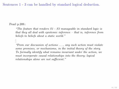
Sentences 1 - 3 can be handled by standard logical deduction.

Pearl p.209.:

“The feature that renders S1 - S3 manageable in standard logic isthat they all deal with epistemic inference – that is, inference frombeliefs to beliefs about a static world.”...

“From our discussion of actions . . . , any such action must violatesome premises, or mechanisms, in the initial theory of the story.To formally identify what remains invariant under the action, wemust incorporate causal relationships into the theory; logicalrelationships alone are not sufficient.”

6 / 52

Equality to show two-way inference

Pearl uses equality rather than implication in order to permit two-wayinference. The independent variable is given in brackets in the secondcolumn below, to demonstrate the causal asymmetry.

Here is the causal model so far:

Model M

(T )D = T (D) (Door opens iff temp > 20C.)

O = D (O) (Oscar goes out iff door opens.)

B = D (B) (Bastet goes out iff door opens.)

L = O ∨B (L) (Birds leave iff Oscar or Bastet goes out)

7 / 52

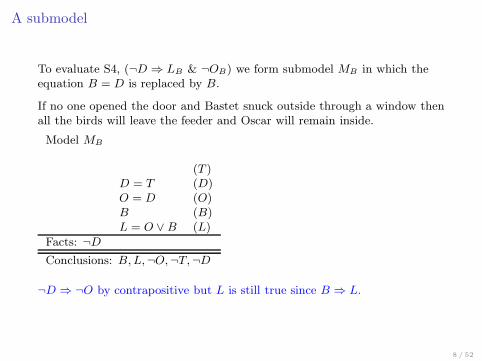
A submodel

To evaluate S4, (¬D ⇒ LB & ¬OB) we form submodel MB in which theequation B = D is replaced by B.

If no one opened the door and Bastet snuck outside through a window thenall the birds will leave the feeder and Oscar will remain inside.

Model MB

(T )D = T (D)O = D (O)B (B)L = O ∨ B (L)

Facts: ¬D

Conclusions: B,L,¬O,¬T,¬D

¬D ⇒ ¬O by contrapositive but L is still true since B ⇒ L.

8 / 52

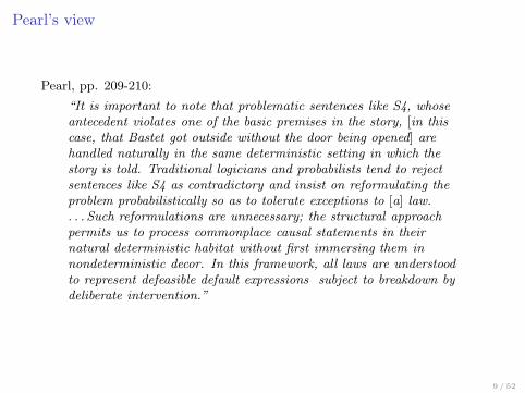
Pearl’s view

Pearl, pp. 209-210:

“It is important to note that problematic sentences like S4, whoseantecedent violates one of the basic premises in the story, [in thiscase, that Bastet got outside without the door being opened] arehandled naturally in the same deterministic setting in which thestory is told. Traditional logicians and probabilists tend to rejectsentences like S4 as contradictory and insist on reformulating theproblem probabilistically so as to tolerate exceptions to [a] law.. . . Such reformulations are unnecessary; the structural approachpermits us to process commonplace causal statements in theirnatural deterministic habitat without first immersing them innondeterministic decor. In this framework, all laws are understoodto represent defeasible default expressions subject to breakdown bydeliberate intervention.”

9 / 52

Evaluating counterfactuals: step 1If the birds have left the feeder then they still would have left the feedereven if Bastet had not gone outside.

The counterfactual L¬B stands for the value of L in submodel M¬B below.The value L depends on the value of T , which is not specified in M¬B Theobservation L removes the ambiguity: if we see the birds have left thefeeder, we can infer that the temperature rose above 20C and thus the doorwas opened. If Bastet had not gone outside then Oscar would have, scaringthe birds away from the feeder. We can derive L¬B as follows.

We add the fact L to the original model and evaluate T . Then we formsubmodel M¬B and reevaluate L in M¬B using the value of T found in thefirst step.

Model M (Step 1)


O = D (B) (Oscar goes out iff door opens.)

B = D (O) (Bastet goes out iff door opens.)

L = O ∨B (L) (Birds leave iff Oscar or Bastet go out)

Facts: L (Birds leave the feeder.)

Conclusions: T,B,O,D, L

10 / 52

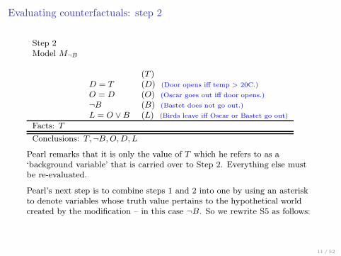
Evaluating counterfactuals: step 2

Step 2Model M¬B


O = D (O) (Oscar goes out iff door opens.)

¬B (B) (Bastet does not go out.)

L = O ∨B (L) (Birds leave iff Oscar or Bastet go out)

Facts: T

Conclusions: T,¬B,O,D, L

Pearl remarks that it is only the value of T which he refers to as a‘background variable’ that is carried over to Step 2. Everything else mustbe re-evaluated.

Pearl’s next step is to combine steps 1 and 2 into one by using an asteriskto denote variables whose truth value pertains to the hypothetical worldcreated by the modification – in this case ¬B. So we rewrite S5 as follows:

11 / 52

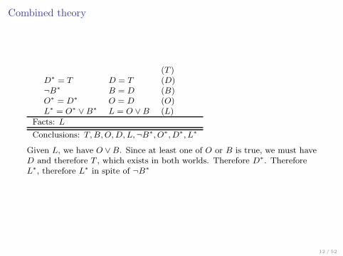
Combined theory

(T )D∗ = T D = T (D)¬B∗ B = D (B)O∗ = D∗ O = D (O)L∗ = O∗ ∨B∗ L = O ∨B (L)

Facts: L

Conclusions: T,B,O,D, L,¬B∗, O∗, D∗, L∗

Given L, we have O ∨B. Since at least one of O or B is true, we must haveD and therefore T , which exists in both worlds. Therefore D∗. ThereforeL∗, therefore L∗ in spite of ¬B∗

12 / 52

Why is S4 ‘action’ and S5 ‘counterfactual’?

◮ In S4, the fact given (no one opened the door) is not affected by theantecedent (Bastet snuck outside through a window.)

◮ In S5 we were asking if changing B to ¬B would affect the outcome L

vs. ¬L. To determine this we had to calculate the potential impact of¬B on L and route the impact of ¬B through T .

13 / 52

Probabilistic evaluation of counterfactuals

Suppose that . . .

1. There is a probability P (T ) = p that the temperature goes above 20C.

2. Bastet has a probability q of sneaking out through a window.

3. Bastet’s inclination to sneak out a window is independent of T .

We want to compute the probability P (¬L¬B|L), the probability that thebirds would not have left the feeder if Bastet had not gone outside, giventhat the birds have in fact left the feeder.

14 / 52

Intuitive calculation

◮ Intuitively, ¬L¬B is true, given ¬B iff the temperature did not goabove 20C. So we want to compute P (¬T |L) = P (¬T∧L)

P (L)

15 / 52



P (L)

◮ This comes to the probability that the birds all left under thecircumstances that the temperature did not rise above 20C divided bythe probability that the birds all left.

15 / 52



P (L)


◮ The only way that the birds would have all left if the temperature hadnot gone above 20C is that Bastet snuck out a window. (We areassuming that Oscar is not capable of doing so.)

15 / 52



P (L)



◮ So the numerator is the probability that Bastet snuck out a windowtimes the probability that the temperature did not rise above 20C (thetwo events independent) which is q(1− p).

15 / 52



P (L)




◮ The denominator is 1 minus the probability that the birds are stillthere, the latter only being possible if the temperature did not riseabove 20C and Bastet did not sneak out a window – i.e.1− (1− p)(1− q)

15 / 52



P (L)




◮ The denominator is 1 minus the probability that the birds are stillthere, the latter only being possible if the temperature did not riseabove 20C and Bastet did not sneak out a window – i.e.1− (1− p)(1− q)

◮ So P (¬L¬B |L) = q(1−p)1−(1−p)(1−q)

.

15 / 52

A probabilistic causal model

Pearl comments that we can calculate this using a probabilistic causalmodel using two background variables T (temperature rises above 20C) andW (Bastet decides to go out through a window.)

P (t, w) =

pq ⇐⇒t = 1, w = 1,p(1− q) ⇐⇒t = 1, w = 0,(1− p)q ⇐⇒t = 0, w = 1,(1− p)(1− q) ⇐⇒t = 0, w = 0

We need to first compute the posterior probability P (t, w|L). This canbecome a problem computationally to compute and store if there are a lotof background variables. And conditioning on some variable e normallydestroys the mutual independence of the background variables so that wehave to maintain the joint distribution of all the background variables.

16 / 52

Solution: Balke and Pearl 1994: Twin network graphical model

Two networks: one to represent the actual world and one to represent thehypothetical world.

TW

D D∗

B O B∗ O∗

L L∗

Since we are conditioning on Bastet not going outside, there is no pathfrom D∗ to B∗.

17 / 52

A different example

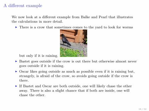
We now look at a different example from Balke and Pearl that illustratesthe calculations in more detail.

◮ There is a crow that sometimes comes to the yard to look for worms

but only if it is raining.

◮ Bastet goes outside if the crow is out there but otherwise almost nevergoes outside if it is raining.

◮ Oscar likes going outside as much as possible even if it is raining but,strangely, is afraid of the crow, so avoids going outside if the crow isthere.

◮ If Bastet and Oscar are both outside, one will likely chase the otheraway. There is also a slight chance that if both are inside, one willchase the other.

18 / 52

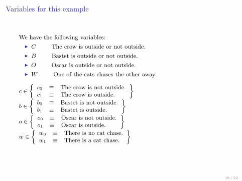
Variables for this example

We have the following variables:

◮ C The crow is outside or not outside.

◮ B Bastet is outside or not outside.

◮ O Oscar is outside or not outside.

◮ W One of the cats chases the other away.

c ∈

{

c0 ≡ The crow is not outside.c1 ≡ The crow is outside.

}

b ∈

{

b0 ≡ Bastet is not outside.b1 ≡ Bastet is outside.

}

o ∈

{

o0 ≡ Oscar is not outside.o1 ≡ Oscar is outside.

}

w ∈

{

w0 ≡ There is no cat chase.w1 ≡ There is a cat chase.

}

19 / 52

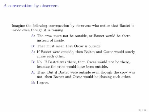
A conversation by observers

Imagine the following conversation by observers who notice that Bastet isinside even though it is raining.

A: The crow must not be outside, or Bastet would be thereinstead of inside.

B: That must mean that Oscar is outside!

A: If Bastet were outside, then Bastet and Oscar would surelychase each other.

B: No. If Bastet was there, then Oscar would not be there,because the crow would have been outside.

A: True. But if Bastet were outside even though the crow wasnot, then Bastet and Oscar would be chasing each other.

B: I agree.

20 / 52

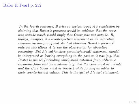
Balke & Pearl p. 232

‘In the fourth sentence, B tries to explain away A’s conclusion byclaiming that Bastet’s presence would be evidence that the crowwas outside which would imply that Oscar was not outside. B,though, analyzes A’s counterfactual statement as an indicativesentence by imagining that she had observed Bastet’s presenceoutside; this allows A to use the observation for abductivereasoning. But A’s subjunctive (counterfactual) statement shouldbe interpreted as leaving everything in the past as it was [e.g. thatBastet is inside] (including conclusions obtained from abductivereasoning from real observations [e.g. that the crow must be outsideand therefore Oscar must be inside]) while forcing variables totheir counterfactual values. This is the gist of A’s last statement.

21 / 52

Unknown factors

Suppose that we have the following probabilities:

p(b1|c1) = 0.9

p(b0|c0) = 0.9

We observe that neither Bastet nor the crow is outside and ask whetherBastet would be there if the crow were there: p(b∗1|c

∗1, c0, b0). The answer

depends on what causes Bastet not to go outside even when the crow isthere.

We model the influence of A on B by a function: b = Fb(a, ǫb) where ǫ

represents all the unknown factors that could influence B as quantified bythe prior distribution P (ǫb). For example, possible components of ǫb couldbe Bastet being sick or Bastet being sulky about never being able to catchthe crow.

22 / 52

Response function variables

Each value in ǫb’s domain specifies a response function that maps eachvalue of A to some value in B’s domain.

rb : domain(ǫb) → N:

rb(ǫb) =

0 if Fb(a0, ǫb) = 0 & Fb(a1, ǫb) = 0 (b = b0 regardless of a)1 if Fb(a0, ǫb) = 0 & Fb(a1, ǫb) = 1 (b = b1⇐⇒ a = a1)2 if Fb(a0, ǫb) = 1 & Fb(a1, ǫb) = 0 (b has opposite value of a)3 if Fb(a0, ǫb) = 1 & Fb(a1, ǫb) = 1 (b = b1 regardless of a)

rb is a random variable that can take on as many values as there arefunctions between a and b. Balke and Pearl call this a response functionvariable.

23 / 52

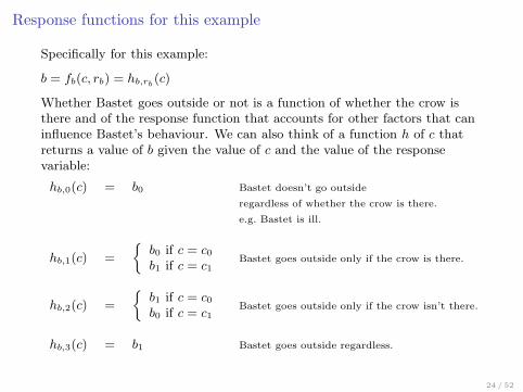
Response functions for this example

Specifically for this example:

b = fb(c, rb) = hb,rb(c)

Whether Bastet goes outside or not is a function of whether the crow isthere and of the response function that accounts for other factors that caninfluence Bastet’s behaviour. We can also think of a function h of c thatreturns a value of b given the value of c and the value of the responsevariable:

hb,0(c) = b0 Bastet doesn’t go outside

regardless of whether the crow is there.

e.g. Bastet is ill.

hb,1(c) =

{

b0 if c = c0b1 if c = c1

Bastet goes outside only if the crow is there.

hb,2(c) =

{

b1 if c = c0b0 if c = c1

Bastet goes outside only if the crow isn’t there.

hb,3(c) = b1 Bastet goes outside regardless.

24 / 52

An example counterfactualIf we have the prior probability P (rb) we can calculate P (b∗1|c

∗1, c0, b0): i.e.

‘Given that the crow is not outside and Bastet is not outside, if the crowwere outside, what is the probability that Bastet would be outside?’

We crucially assume that:

‘. . . the disturbance ǫb, and hence the response-function rb, isunaffected by the actions that force the counterfactual values;therefore, what we learn about the response-function from theobserved evidence is applicable to the evaluation of belief in thecounterfactual consequent.’

If we observe (c0, b0) (neither Bastet nor the crow is outside), then it mustbe that rb ∈ {0, 1}, an event with prior probability P (rb = 0) + P (rb = 1).This updates the posterior probability of rb as follows, letting→

P (rb) = 〈P (rb = 0), P (rb = 1), P (rb = 2), P (rb = 3)〉:

→

P (rb) =→

P (rb|c0, b0)

=

⟨

P (rb = 0)

P (rb = 0) + P (rb) = 1,

P (rb = 1)

P (rb = 0) + P (rb) = 1, 0, 0

⟩

25 / 52

Calculating this counterfactual

From the definition of rb(ǫb) above, if C were forced to c1 (the crow isoutside), then B would have been b1 (Bastet would have also been outsideiff rb ∈ {1, 3}, whose probability is P ′(rb = 1) + P ′(rb = 3) = P ′(rb = 1).(P ′(rb = 3) must be zero since we have determined that rb ∈ {0, 1}.) Thisgives the solution to the counterfactual query:

P (b∗1|c∗1, c0, b0) = P ′(rb = 1) = P (rb=1)

P (rb=0)+P (rb=1)

The probability of external influence 1 that causes Bastet to go outside ifthe crow is there divided by the probability of external influence 1 plusexernal influence 0, the latter causing Bastet to stay inside regardless.

26 / 52

Representation with a DAG

We can represent the causal influences over a set of variables in thisexample through a DAG. If the set of variables is {X1, X2, . . . Xn}, for eachxi there is a functional mapping xi = fi(pa(xi), ǫi), where pa(xi) is thevalue of Xi’s parents in the graph and there is a prior probabilitydistribution P (ǫi) for each ‘disturbance’ ǫi.

A counterfactual query will be of the form: ‘What is P (c∗|a∗, obs), where c∗

is a set of counterfactual values for C ⊂ X, a∗ is a set of forced values inthe counterfactual antecedent and obs represents observed evidence.

For our example, we assume that Bastet is not outside (b = b0) and want toask ‘what is P (c∗1 |b

∗1 , b0)?’ Or further, what is the probability that the cats

will chase each other under those conditions?

27 / 52

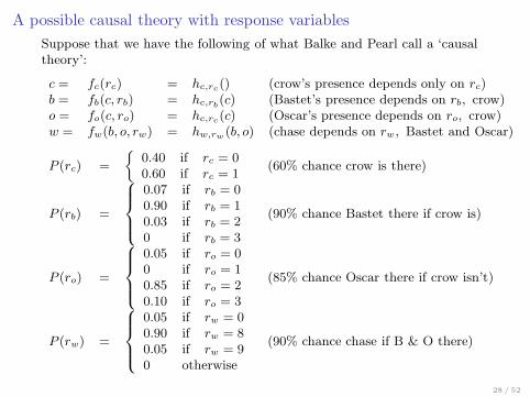
A possible causal theory with response variables

Suppose that we have the following of what Balke and Pearl call a ‘causaltheory’:

c = fc(rc) = hc,rc() (crow’s presence depends only on rc)b = fb(c, rb) = hc,rb(c) (Bastet’s presence depends on rb, crow)o = fo(c, ro) = hc,rc(c) (Oscar’s presence depends on ro, crow)w = fw(b, o, rw) = hw,rw (b, o) (chase depends on rw, Bastet and Oscar)

P (rc) =

{

0.40 if rc = 00.60 if rc = 1

(60% chance crow is there)

P (rb) =

0.07 if rb = 00.90 if rb = 10.03 if rb = 20 if rb = 3

(90% chance Bastet there if crow is)

P (ro) =

0.05 if ro = 00 if ro = 10.85 if ro = 20.10 if ro = 3

(85% chance Oscar there if crow isn’t)

P (rw) =

0.05 if rw = 00.90 if rw = 80.05 if rw = 90 otherwise

(90% chance chase if B & O there)

28 / 52

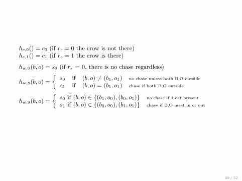
hc,0() = c0 (if rc = 0 the crow is not there)hc,1() = c1 (if rc = 1 the crow is there)

hw,0(b, o) = s0 (if rs = 0, there is no chase regardless)

hw,8(b, o) =

{

s0 if (b, o) 6= (b1, o1) no chase unless both B,O outside

s1 if (b, o) = (b1, o1) chase if both B,O outside

hw,9(b, o) =

{

s0 if (b, o) ∈ {(b1, o0), (b0, o1)} no chase if 1 cat present

s1 if (b, o) ∈ {(b0, o0), (b1, o1)} chase if B,O meet in or out

29 / 52

DAG

rc

C C∗

rb ro

B OB∗ O∗

WW ∗

rw

Variables marked with ∗ indicate the counterfactual world and thosewithout the factual world. The r variables are response functions.

30 / 52

DAG for counterfactual evaluation

rc

C C∗

rb ro

b0 O b∗1 O∗

WW ∗

rw

To evaluate P (w∗1 |b

∗1, b0), instantiate B as b0 and B∗ as b∗1. Sever links

pointing to b∗1

31 / 52

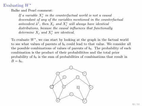
Evaluating W∗

Balke and Pearl comment:

If a variable X∗

j in the counterfactual world is not a causaldescendant of any of the variables mentioned in the counterfactualantecedent a∗, then Xj and X∗

j will always have identicaldistributions, because the causal influences that functionallydetermine Xj and X∗

j are identical.

To evaluate W ∗, we can start by looking at the graph in the factual worldto see what values of parents of b0 could lead to that value. We consider allthe possible combinations of values of parents of b0. The probability of eachcombination is the product of their probabilitites and the total priorprobability of b0 is the sum of probabilities of combinations that result inB = b0.

rc

C C∗

rb ro

b0 O b∗1 O∗

WW ∗

rw

32 / 52

Evaluating W∗

◮ rc = 0 (0.4) and rb = 0 (0.07) → C = c0 and B = b0 (0.028)

◮ rc = 0 (0.4) and rb = 1 (0.90) → C = c0 and B = b0 (0.36)

◮ rc = 0 (0.4) and rb = 2 (0.03) → C = c0 and B = b1 (0.012)

◮ rc = 1 (0.6) and rb = 0 (0.07) → C = c1 and B = b0 (0.042)

◮ rc = 1 (0.6) and rb = 1 (0.90) → C = c1 and B = b1 (0.54)

◮ rc = 1 (0.6) and rb = 2 (0.03) → C = c1 and B = b0 (0.018)

The prior probability P (B = b0) = 0.028 + 0.36 + 0.042 + 0.018 = 0.448. Sop(C = c0|B = b0) =

0.028+0.360.448

= 0.86607

rc

C C∗

rb ro

b0 O b∗1 O∗

WW ∗

rw

33 / 52

Evaluating W∗

Given that C∗ is not a causal descendant of any B variables, we can givecounterfactual C∗ the same probability as C. We can now work down onthe counterfactual side of the DAG and calculate O∗. We calculate theprobability of each possible combination of values of ro and C∗ anddetermine for each the value of O∗ that results. We add to get the totalprobability of o∗1 .

rc

C C∗

rb ro

b0 O b∗1 O∗

WW ∗

rw

34 / 52

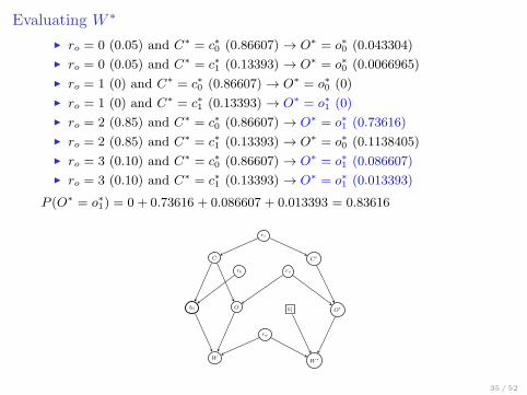
Evaluating W∗

◮ ro = 0 (0.05) and C∗ = c∗0 (0.86607) → O∗ = o∗0 (0.043304)

◮ ro = 0 (0.05) and C∗ = c∗1 (0.13393) → O∗ = o∗0 (0.0066965)

◮ ro = 1 (0) and C∗ = c∗0 (0.86607) → O∗ = o∗0 (0)

◮ ro = 1 (0) and C∗ = c∗1 (0.13393) → O∗ = o∗1 (0)

◮ ro = 2 (0.85) and C∗ = c∗0 (0.86607) → O∗ = o∗1 (0.73616)

◮ ro = 2 (0.85) and C∗ = c∗1 (0.13393) → O∗ = o∗0 (0.1138405)

◮ ro = 3 (0.10) and C∗ = c∗0 (0.86607) → O∗ = o∗1 (0.086607)

◮ ro = 3 (0.10) and C∗ = c∗1 (0.13393) → O∗ = o∗1 (0.013393)

P (O∗ = o∗1) = 0 + 0.73616 + 0.086607 + 0.013393 = 0.83616

rc

C C∗

rb ro

b0 O b∗1 O∗

WW ∗

rw

35 / 52

Evaluating W∗

Given that P (b∗0) = 1, we can now calculate P (W ∗ = 1|b∗0 , O∗), moving

further down the graph. We look at all the possible combinations ofpossible values of parents of W ∗. Since B∗ is set at b∗1, we need not includeit in the set of combinations.

rc

C C∗

rb ro

b0 O b∗1 O∗

WW ∗

rw

36 / 52

Evaluating W∗

◮ rw = 0 (0.05) and O∗ = o∗0 (0.16184) → W ∗ = w∗0 (0.008092)

◮ rw = 0 (0.05) and O∗ = o∗1 (0.83616) → W ∗ = w∗0 (0.041808)

◮ rw = 8 (0.90) and O∗ = o∗0 (0.16184) → W ∗ = w∗0 (0.145656)

◮ rw = 8 (0.90) and O∗ = o∗1 (0.83616) → W ∗ = w∗1 (0.752544)

◮ rw = 9 (0.05) and O∗ = o∗0 (0.16184) → W ∗ = w∗0 (0.008092)

◮ rw = 9 (0.05) and O∗ = o∗1 (0.83616) → W ∗ = w∗1 (0.041808)

So P (W ∗ = 1|b∗0 , O∗) = 0.75254 + 0.041808 = 0.79435, which to two decimal

places is the value given by Balke and Pearl.

rc

C C∗

rb ro

b0 O b∗1 O∗

WW ∗

rw

37 / 52

References

Pearl, Judea. 2000. Causality Chapter 7: The logic of structure-basedcounterfactuals. Cambridge University Press.

Balke, Alexander and Judea Pearl. 1994. Probabilistic evaluation ofcounterfactual queries. In proceedings of AAAI.

38 / 52

Johansson et al (2016) Learning representations for counterfactual

inference

Suppose that we have data on 1000 patients who either did or did notreceive some medical treatment and we know some quantity that representsthe results of the treatment such as blood sugar level or blood pressure. Foreach patient we know whether or not they received the treatment and whatthe result was.

What we do not know is what the characteristics were for each patient onwhich the decision to give the treatment or not was based. We also do notknow what the results would have been if the opposite course of action hadbeen taken for each patient – no treatment for those who received it andvice versa.

39 / 52

◮ For each patient x, Y1(x) is the measurable result of x receiving thetreatment and Y0(x) the result of x not receiving the treatment.

◮ For each x we know only one of the two.

◮ For each x the individualized treatment effect ITE = Y1(x)− Y0(x) is aquantity that would enable us to choose the best choice for eachpatient, but we do not know this quantity.

◮ If p(x) is the distribution under which x values occur, the averagetreatment effect ATE is defined as ATE=Ex∼p(x)[ITE(x)].

◮ We also define the factual and counterfactual outcomes of thetreatment given to individual x as yF (x) and yCF (x) respectively.

40 / 52

What they call direct modeling for estimating ITE, works as follows.

◮ We have n samples: {(xi, ti, yFi )}ni=1,

◮ where xi is the individual,

◮ ti is the binary value for treatment (1) or no treatment (1)

◮ and yFi is the factual outcome.

41 / 52

◮ We can see that yFi = ti · Y1(xi) + (1− ti) · Y0(xi) where Y0 is the

function applied to x of not giving the treatment and Y1 is giving thetreatment.

◮ Either ti or 1− ti must be zero, so one of the above two terms will bezero.

◮ If the treatment was given, ti = 1 and the second term drops out;

◮ if not, ti = 0 and the first term drops out.

◮ We want to learn a function h that maps an individual xi paired witha treatment ti to an outcome yF

i :

h : X × T → Y such that h(xi, ti) ≈ yFi

42 / 52

We can then use h to represent the half of the ITE that we don’t know.If the treatment was given, ti = 1 and ˆITE(x) = yF

i − h(xi, 1− ti). If not,ti = 0 and ˆITE(x) = h(xi, 1− ti)− yF

i .

43 / 52

The observed sample is PF = {(xi, ti)}ni=1: ‘the factual distribution’.

The counterfactual distribution is PCF = {(xi, 1− ti)}ni=1.

Crucially, the two distributions may be different – i.e. if the decision how totreat a given patient was not random, but based on some characteristics ofthat patient, t and x will not be independent. And we don’t have theinformation about how decisions about treatment assignment were made.

44 / 52

We have:PF (x, t) = P (x) · P (t|x)PCF (x, t) = P (x) · P (¬t|x)

We assume that we have some information about the patients so that wecan given them relevant features, even though we don’t know if these werethe same features that were used to decide on the treatment nor how thefeatures might have been taken into account.

We want to learn two things:

A representation Φ that maps each patient onto a feature set and afunction h that gives a numerical outcome for each patient feature setpaired with a treatment.

45 / 52

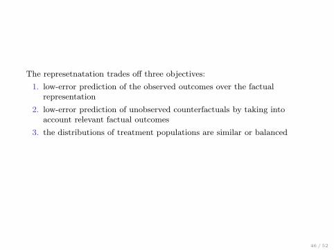
The represetnatation trades off three objectives:

1. low-error prediction of the observed outcomes over the factualrepresentation

2. low-error prediction of unobserved counterfactuals by taking intoaccount relevant factual outcomes

3. the distributions of treatment populations are similar or balanced

46 / 52

How do we accomplish each?

1. error-minimization over a training set using regularization to avoidoverfitting

2. assign a penalty that encourages counterfactual predictions to be closeto the nearest observed outcome from the respective treated or controlset

3. minimize the discrepancy distance between treated and controlpopulations

47 / 52

Patients: X = {xi}ni=1

Treatments: T = {ti}ni==1

Factual outcomes: Y F = {yFi }ni=1

We define the nearest oppositely-treated neighbour of patient xi, xj , wherej ∈ {1, . . . b} and tj = 1− ti such that j = argmin d(xi, xj) where d(a, b) isthe distance from a to b in the metric space X .

48 / 52

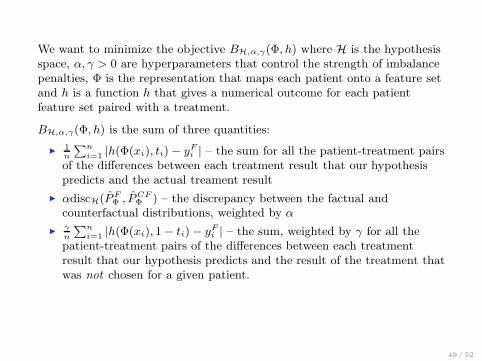
We want to minimize the objective BH,α,γ(Φ, h) where H is the hypothesisspace, α, γ > 0 are hyperparameters that control the strength of imbalancepenalties, Φ is the representation that maps each patient onto a feature setand h is a function h that gives a numerical outcome for each patientfeature set paired with a treatment.

BH,α,γ(Φ, h) is the sum of three quantities:

◮1n

∑n

i=1 |h(Φ(xi), ti)− yFi | – the sum for all the patient-treatment pairs

of the differences between each treatment result that our hypothesispredicts and the actual treament result

◮ αdiscH(PFΦ , PCF

Φ ) – the discrepancy between the factual andcounterfactual distributions, weighted by α

◮γ

n

∑n

i=1 |h(Φ(xi), 1− ti)− yFi | – the sum, weighted by γ for all the

patient-treatment pairs of the differences between each treatmentresult that our hypothesis predicts and the result of the treatment thatwas not chosen for a given patient.

49 / 52

Once again:

◮ Φ is a representation of X that maps each patient onto a vector offeatures

◮ and H represents the set of possible hypothesis functions h each ofwhich maps each feature vector and treatment choice for a patient ontoa real number that represents the hypothesized results of thattreatment for that patient.

◮ The paper states that if the hypothesis class H is the set of linearfunctions, the term discH(PF

Φ , PCFΦ ) has closed form ||µ2(P )− µ2(Q)||2

where ||A||2 is the spectral norm of A and µ2(P ) = Ex∼P [xxT ] is the

variance of the distribution P .

◮ If x is a binary-valued matrix whose rows are patients and columns arefeatures we have assigned to each patient,then xxT will represent thedegree to which each pair of patients differs with respect to the binaryvalues we have assigned to them. The more they differ, the lower thevalue in the cell of xxT

i,j for patients i and j.

50 / 52

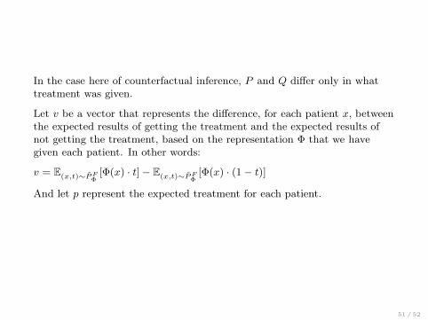
In the case here of counterfactual inference, P and Q differ only in whattreatment was given.

Let v be a vector that represents the difference, for each patient x, betweenthe expected results of getting the treatment and the expected results ofnot getting the treatment, based on the representation Φ that we havegiven each patient. In other words:

v = E(x,t)∼PF

Φ[Φ(x) · t]− E(x,t)∼PF

Φ[Φ(x) · (1− t)]

And let p represent the expected treatment for each patient.

51 / 52

So discH(PFΦ , PCF

Φ ) is the spectral norm of Ex∼PF

Φ[xxT ]− Ex∼PCF

Φ[xxT ],

that difference being the difference between the expected amount by whicheach pair of patients differs under the factual distribution and the expectedamount by which each pair of patients differs under the counterfactualdistribution.

52 / 52

Eric Rosen Machine Learning Reading Group, UBC, August 22 ... · was opened. If Bastet had not gone...

Documents

Transcript of Eric Rosen Machine Learning Reading Group, UBC, August 22 ... · was opened. If Bastet had not gone...