Mathematical Modeling Lecture

Equilibrium : Jacobian Matrix– ODE of the Dynamical System and its stability

2009. 10. 15

Sang-Gu Lee, Duk-Sun KimSungkyunkwan University

sglee@skku.edu

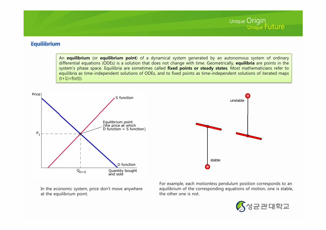
An equilibrium (or equilibrium point) of a dynamical system generated by an autonomous system of ordinarydifferential equations (ODEs) is a solution that does not change with time. Geometrically, equilibria are points in thesystem's phase space. Equilibria are sometimes called fixed points or steady states. Most mathematicians refer toequilibria as time-independent solutions of ODEs, and to fixed points as time-independent solutions of iterated maps(t+1)=f(x(t)).

In the economic system, price don’t move anywhere at the equilibrium point.

For example, each motionless pendulum position corresponds to an equilibrium of the corresponding equations of motion, one is stable, the other one is not.

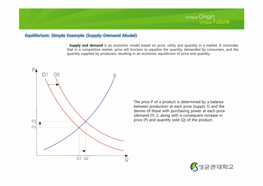
Supply and demand is an economic model based on price, utility and quantity in a market. It concludesthat in a competitive market, price will function to equalize the quantity demanded by consumers, and thequantity supplied by producers, resulting in an economic equilibrium of price and quantity.

The price P of a product is determined by a balance between production at each price (supply S) and the desires of those with purchasing power at each price (demand D). 2, along with a consequent increase in price (P) and quantity sold (Q) of the product.

How we can find equilibrium points from the supply-demand model?

Demand : 1

2)(+

=x

xf

=2/(A3+1)

Supply : 4.05.0)( 2 += xxg

=0.5*A3^2+0.4

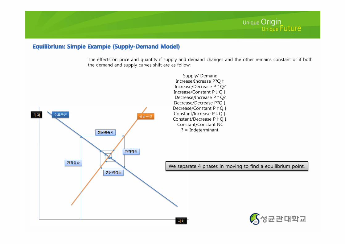
The effects on price and quantity if supply and demand changes and the other remains constant or if boththe demand and supply curves shift are as follow:

Supply/ DemandIncrease/Increase P?Q↑Increase/Decrease P↑Q?Increase/Constant P↓Q↑Decrease/Increase P↑Q?Decrease/Decrease P?Q↓Decrease/Constant P↑Q↑Constant/Increase P↓Q↓Constant/Decrease P↑Q↓Constant/Constant NCConstant/Constant NC? = Indeterminant.

We separate 4 phases in moving to find a equilibrium point.

How we can find equilibrium points from the supply-demand model?

Demand : 1

2)(+

=x

xf

=2/(A3+1)

Phases

Cobweb points

Supply : 4.05.0)( 2 += xxg

=0.5*A3^2+0.4

How we can find equilibrium points from the supply-demand model?

Demand : 1

2)(+

=x

xf

=2/(A3+1)

Supply : 4.05.0)( 2 += xxg

=0.5*A3^2+0.4

Phases

Cobweb points

Fail scenario: Don’t approach the equilibrium point.In this case, first supply was determined by its prices and demands in the market and we must consider itseffect in the real-market.

Fail to approach the equilibriumpoint.

In logistic growth model, we add the harvesting process from the growth objects.

가축, 농작물등수확가능한 개체

수확된 개체(농장의 수익 또는기타 수치로

해당 수확물을 수확년간 수확량(Harvest)

수확가능한 개체

자체적으로 성장: 생성비율(Growth Rate)수용용량을 가짐: Capacity

기타 수치로산출됨)

수확가능한개체수의 변화량 : HS

dt

dS−−= )1( θα capacity

S=θ

In logistic growth model, we add the harvesting process from the growth objects.

수확가능한개체수의 변화량 : HS

dt

dS−−= )1( θα

capacity

S=θ

=(1-B5/$B$2)*$B$1 =$E$1

Equilibrium point: To make a balance between the growth and the harvest of the objects.Using the cobweb, we can find an equilibrium point.

Identity Function G1 :

Farm Function G2 :

xxg =)(1

bxL

rxrxg −−+= 2

2 )1()(

개체 증가율수용한계

L2수확량

The stability of typical equilibria of smooth ODEs is determined by the sign of real part of eigenvaluesof the Jacobian matrix. These eigenvalues are often referred to as the 'eigenvalues of the equilibrium'. TheJacobian Matrix of a system of smooth ODEs is the matrix of the partial derivatives of the right-hand sidewith respect to state variables

∂∂∂∂∂

∂∂

∂∂

∂n

fffx

f

x

f

x

f

f L

L

222

1

2

1

1

1

∂∂

∂∂

∂∂

∂∂

∂∂

∂∂

=

∂∂===

n

nnn

nj

ixx

x

f

x

f

x

f

x

f

x

f

x

f

x

fffDJ

L

MOMM

L

21

2

2

2

1

2

where all derivatives are evaluated at the equilibrium point. Its eigenvalues determine linear stabilityproperties of the equilibrium.An equilibrium is asymptotically stable if all eigenvalues have negative real parts; it is unstable if at leastone eigenvalue has positive real part.

In mathematics, in the study of dynamical systems, the Hartman-Grobman theorem or linearizationtheorem is an important theorem about the local behavior of dynamical systems in the neighborhood of ahyperbolic fixed point.Basically the theorem states that the behavior of a dynamical system near a hyperbolic fixed point isqualitatively the same as the behavior of its linearization near the origin. Therefore when dealing with suchfixed points we can use the simpler linearization of the system to analyze its behavior.

Let be a smooth map with a hyperbolic fixed point p.Let A denote the linearization of f at point p. Then there exist a neighborhood U of p and a homeomorphism such that

nnf ℜ→ℜ:nUh ℜ→:Then there exist a neighborhood U of p and a homeomorphism such that

that is in a neighborhood U of p, f is topologically conjugate to its linearization. In general, even for infinitely differentiable maps f, the homomorphism h need not to be smooth, nor even locally Lipschitz. However, it turns out to be Hölder continuous, with an exponent depending on the constant of hyperbolicity of A.

Uh ℜ→:

Ahhfu1−

=

Hartman, Philip (August 1960). "A lemma in the theory of structural stability of differential equations". Proc. A.M.S. 11 (4): 610–620. doi:10.2307/2034720.

local phase portrait of a hyperbolic equilibrium of a non-linear system is equivalent to that of itslinearization. This statement has a mathematically precise form known as the Hartman-Grobman Theorem.It says that solutions of

)(' xfx =

in a small neighborhood of a hyperbolic equilibrium can be mapped with a homeomorphism (i.e.,continuous map with a continuous inverse) onto solutions of the linear system

Jyy =' Jyy ='

where is the Jacobian matrix at the equilibrium. One says that these systems are locally topologicallyconjugate (equivalent). That is, adding nonlinear terms to a linear system at a hyperbolic equilibrium maydistort but does not change qualitatively the phase portrait near the equilibrium.If at least one eigenvalue of the Jacobian matrix is zero or has zero real part, then the equilibrium is saidto be non-hyperbolic. Non-hyperbolic equilibria are not robust (i.e., the system is not structurallystable): Small perturbations can result in a local bifurcation of a non-hyperbolic equilibrium, i.e., it canchange stability, disappear, or split into many equilibria. Some refer to such an equilibrium by the name ofthe bifurcation, e.g., saddle-node equilibrium.In practice, one often has to consider non-hyperbolic equilibria with all eigenvalues having negative orzero real parts. These equilibria are sometimes referred to as being critical. Their stability cannot bedetermined from the signs of the eigenvalues of the Jacobian matrix; it depends on the nonlinear terms of f.

Consider a one-dimensional (scalar) dynamical system1 ),(' ℜ∈= xxfx

)(' xfJ =

Equilibria of a one-dimensional system

Its equilibria are the zeros of the function f(x). An equilibrium is asymptotically stable when f’(x)<0. that is,the slope of f is negative. It is unstable when f’(x)>0. The left two equilibria in the figure are hyperbolic(f’(x)=0), the others are non-hyperbolic because the slope (eigenvalue) is zero. Nevertheless, a non-hyperbolic equilibrium of a one-dimensional system is stable if the function changes the sign from positiveto negative at the equilibrium.

Consider a two-dimensional (planar) system with smooth right-hand side

),(

),(

212'2

211'1

xxfx

xxfx

=

=

∂∂ 11 ff

The Jacobian matrix has the form

TraceDeterminant

∂∂

∂∂

∂∂=2

2

1

2

2

1

1

1

x

f

x

fxx

J

It has two eigenvalues, which are either both real or complex-conjugate. A hyperbolic equilibrium can be a� Node when both eigenvalues are real and of the same sign. The node is stable when the eigenvaluesare negative and unstable when they are positive. For the stable node, the eigenvalue(s) with minimalabsolute value of the real part is called principle or leading; when the eigenvalues are different, all orbitsbut two tend to the node along the leading eigenvector (the picture is reversed for the unstable node);� Saddle when eigenvalues are real and of opposite signs. The saddle is always unstable;� Focus (sometimes called spiral point) when eigenvalues are complex-conjugate; The focus is stablewhen the eigenvalues have negative real part and unstable when they have positive real part.

The Jacobian matrix of a three-dimensional system has 3 eigenvalues,one of which must be real and the other two can be either both real orcomplex-conjugate. A hyperbolic equilibrium can be� Node when all eigenvalues are real and have the same sign; Thenode is stable (unstable) when the eigenvalues are negative (positive);� Saddle when all eigenvalues are real and at least one of them ispositive and at least one is negative; Saddles are always unstable;� Focus-Node when it has one real eigenvalue and a pair of complex-conjugate eigenvalues, and all eigenvalues have real parts of thesame sign; The equilibrium is stable (unstable) when the sign isnegative (positive);� Saddle-Focus when it has one real eigenvalue with the sign opposite� Saddle-Focus when it has one real eigenvalue with the sign oppositeto the sign of the real part of a pair of complex-conjugateeigenvalues; This type of equilibrium is always unstable.

Examples of equilibria in R^3

There are many more types of non-hyperbolic equilibria, i.e., those that have at least one eigenvaluewith zero real part, since the phase portrait in a small neighborhood of such equilibria also dependson the nonlinear terms of f(x). Most of these equilibria do not have names or are named after thetype of the bifurcation in which they play a role.The center equilibrium occurs when a system has only two eigenvalues on the imaginary axis,namely, one pair of pure-imaginary eigenvalues. Centers in linear systems have families of concentricperiodic orbits around them, as in the figure. Many refer to centers only in the context of two-dimensional systems or Hamiltonian systems. If all other eigenvalues have negative real parts, centersare neutrally stable but not asymptotically stable. A pair of pure-imaginary eigenvalues also occurs inAndronov-Hopf bifurcation, however due to the nonlinear terms, the neighborhood of such anequilibrium looks like a focus; it could be asymptotically stable (supercritical Andronov-Hopfbifurcation) or unstable (subcritical Andronov-Hopf bifurcation) even if the other eigenvalues havebifurcation) or unstable (subcritical Andronov-Hopf bifurcation) even if the other eigenvalues havenegative real parts.The saddle-node equilibrium occurs in nonlinear systems with one zero eigenvalue when the systemundergoes the saddle-node bifurcation, where a saddle and a node approach each other, coalesceinto a single equilibrium (depicted in the figure), and then disappear. Saddle-nodes are alwaysunstable.The Bogdanov-Takens equilibrium occurs in nonlinear systems with 2 zero eigenvalues, typicallywhen the system undergoes the Bogdanov-Takens bifurcation. It is also an unstable equilibrium.

Examples of non-hyperbolic equilibria in R^2

• Guckenheimer J. and Holmes P. (1983) Nonlinear Oscillations, Dynamical systems and Bifurcations of Vector Fields. Springer• Izhikevich E.M. (2007) Dynamical Systems in Neuroscience: The Geometry of Excitability and Bursting. The MIT Press, Cambridge,MA.

• D.K. Arrowsmith and C.M. Place, Dynamical Systems, Section 3.3, Chapman & Hall, London, 1992. ISBN 0-412-39080-9.• Kuznetsov Yu.A. (2004) Elements of Applied Bifurcation Theory, Springer, 3rd edition

• Steven H. Strogatz, (1994) Nonlinear Dynamics and Chaos, Addison-Wesley Publishing Company

• Hartman, Philip (August 1960). "A lemma in the theory of structural stability of differential equations". Proc. A.M.S. 11 (4): 610–620. doi:10.2307/2034720.

• Grobman, D.M. (1959). "Homeomorphisms of systems of differential equations". Dokl. Akad. Nauk SSSR 128: 880–881.• Hartman, Philip (1960). "On local homeomorphisms of Euclidean spaces". Bol. Soc. Math. Mexicana 5: 220–241.