Rethinking Low Genus Hyperelliptic Jacobian Arithmetic...

Rethinking Low Genus Hyperelliptic JacobianArithmetic over Binary Fields: Interplay of Field

Arithmetic and Explicit Formulæ

R. Avanzi1, N. Theriault2, and Z. Wang2

1 Faculty of Mathematics and Horst Gortz Institute for IT-SecurityRuhr University Bochum, Germany

[email protected] University of Waterloo, Department of Combinatorics and Optimization, Canada

[email protected] and [email protected]

Abstract. This paper is an extensive study of the issues of efficient softwareimplementation of low genus hyperelliptic Jacobians over binary fields.We first give a detailed description of the methods by which one obtains explicitformulæ from Cantor’s algorithm. We then present improvements on the bestknown explicit formulæ for curves of genus three and four. Special routines formultiplying vectors of field elements by a fixed quantity (which are much fasterthan performing the multiplications separately) are also deployed, and the explicitformulæ for all genera are redesigned or re-implemented accordingly.To allow a fair comparison of the curves of different genera, we use a highlyoptimized software library for arithmetic in binary fields. Our goals in its devel-opment were to minimize the overheads and performance penalties associatedto granularity problems, which have a larger impact as the genus of the curvesincreases. The current state of the art in attacks against the discrete logarithmproblem is taken into account for the choice of the field and group sizes andperformance tests are done on a personal computer.Our results can be shortly summarized as follows: Curves of genus three provideperformance similar, or better, to that of curves of genus two, and these two typesof curves perform consistently around 50% faster than elliptic curves; Curves ofgenus four attain a performance level comparable to, and more often than not,better than, elliptic curves. A large choice of curves is therefore available for thedeployment of curve based cryptography, with curves of genus three and fourproviding their own advantages as larger cofactors can be allowed for the grouporder.

Keywords. Elliptic and hyperelliptic curves, cryptography, efficient implementa-tion, binary field arithmetic, explicit formulæ

1 Introduction

The discrete logarithm problem (DLP) is a quite popular primitive in the design of cryp-tosystems. It can be formulated as follows: Given a group G generated by an element g,and a second element h ∈G, find some t ∈ Z with t ·g = h (this integer is called the dis-crete logarithm of h with respect to g). The computation of scalar multiples of elements

of a group (i.e. given an integer t and an element g, compute t · g) is the fundamentaloperation of a DLP-based cryptosystem.

Systems based on the DLP in the Jacobian of curves over finite fields were con-sidered as early as 1985, when Miller [44] and Koblitz [27] independently proposedto use elliptic curves (EC). Shortly thereafter Koblitz [29] suggested the Jacobians ofhyperelliptic curves (HEC) of higher genus (EC are HEC of genus one).

After a slow start, the use of EC in cryptography has now gained momentum andthere are several books covering the subject (for example [6, 23, 7, 1]). HEC have beenenjoying increasing attention in recent years. They have long been considered as notcompetitive with EC because of construction and performance issues, but the situationhas changed in the last few years. It is now possible to efficiently construct HEC whoseJacobian has cryptographically good order (for an overview see [36]), and the perfor-mance has been considerably improved. For curves of genus two over binary fields, thefastest explicit formulæ are given in [34], and active research has also been done forother genera. A recent summary can be found in [9, 10], but of course research has notstopped: Recent improvements for genus three can be found in [13], and further resultsfor genus three and four are the main subject of the present paper.

No subexponential algorithm is known for solving the DLP on elliptic and hyper-elliptic curves of genus at most four (cfr. [3–5] for an overview of the techniques in-volved). For curves of genus one and two, the index calculus method is not faster thanPollard’s methods, therefore the security level of these curves is assessed by the numberof operations required to solve the DLP with Pollard’s Rho algorithm.

For curves defined over a fixed field and increasing genus the complexity of com-putinging the discrete logarithm becomes subexponential in the group order [12] byusing index calculus methods (see also [4]), but for “small”, fixed genus the complex-ity of the methods remains exponential. Starting with genus three, one has to take intoaccount a loss of security by a constant factor, and therefore one has to increase thefield size because the index calculus techniques start to become faster than Pollard’smethods.

On the other hand, the best algorithms for solving the factorization problem and theDLP in finite fields are subexponential. Therefore, to achieve a security increase equiv-alent to doubling the RSA key size, one needs to add only a few bits to an EC group.For example, according to [35] the security of 1323 bit RSA (or of a 137 bits subgroupof a 1024 bit finite field) is attained by an EC over a 157 bit field and with a groupof prime order (of 157 bits). For that same level of security, the field would have 79bits for a HEC of genus two, 59 bits for genus three and 53 bits for genus four (for allthree, the curve must have a prime subgroup of order at least 157 bits); In comparison,the security of 2048 bits RSA is (roughly) achieved by 200-bits curve groups, and thatof 3072 bits RSA by 240-bits curve groups [11]. NIST [49] suggests to use 224 and256 bit groups in place of the values 200 and 240. There are obvious bandwidth andperformance advantages in using curve based systems, in particular when the securityrequirements increase: Curves of genus up to three are now heavily investigated alter-natives. One of the purposes of this paper will be to show that systems based on curvesof genus four may also prove interesting.

2

In this paper we reconsider the issue of efficient implementation of low genus hy-perelliptic Jacobians. Our focus is on curves over fields of characteristic two. We brieflyrecall the state of the art of implementation of HEC arithmetic in low genus: This willmotivate our investigations.

Explicit formulæ for curves of genus two have been studied extensively [24, 40, 31,51, 34, 33], both in the odd and even characteristic cases. An overview of the differentresults can be found in [10]. In particular, the fastest known algorithm for curves overbinary fields makes use of the doubling formula by Lange and Stevens [34]: In thatpaper, the authors use Shoup’s NTL software library [57] for the arithmetic in the basefield, and obtain that the best case for curves of genus two can perform about 10% betterthan elliptic curves.

There are also a number of papers on explicit formulæ for curves of genus three [47,31, 21, 13] in both odd and even characteristic, with a very complete description of allcases in [21]. A detailed comparisons between the performances of curves of genus one,two, and three in odd characteristic can be found in [2] and for characteristic two somecomparisons are found in [59].

The literature is much more restricted when it comes to curves of genus four, withonly the formulæ of Pelzl, Wollinger and Paar for characteristic two [51], and no de-tailed comparison with the performance of other genera that includes a security analysisand a careful choice of fields.

This paper reconsiders the issue of implementing low genus hyperelliptic Jacobianarithmetic over finite fields of even characteristic. A difference with respect to existingliterature is that we simultaneously address field arithmetic enhancements, the deriva-tion of the explicit formulæ and the impact of recent attacks, and consider the interplayof these factors. This produces surprising implementation results, which can be listedin the following two groupings:

1. A thorough approach to finite field implementation can be used to deliver perfor-mance essentially independent of the granularity of the computing architecture em-ployed. In other words, the timings of the multiplication in the field is a close ap-proximation of the quadratic bit complexity of (small) multiplication. Special finitefield functions can be used to speed up explicit formulæ by up to 20% and theimpact of such functions increases with the genus.

2. The genus two formulæ by Lange and Stevens in even characteristic can be usedto beat EC performance by as much as 50% but curves of genus three deliver sim-ilar performance while using even smaller fields. Moreover, curves of genus fourperform in fact quite well, often matching or improving EC performance.

Section 2 gives a detailed overview the general technique used to derive explicitformulæ. In Section 3 we describe our approach to implementation of the underly-ing field arithmetic: The technique of sequential multiplications is introduced. Our im-provements to the explicit formulæ are presented in Section 4. Security considerationsare the subject of Section 5, where key and field size equivalence issues are addressed.A description of our experiments and the corresponding results are given in Section 6.Finally, in Section 7 we draw conclusions.

3

2 From Cantor’s algorithm to explicit formulæ

An excellent, low brow, introduction to hyperelliptic curves is [43], including elemen-tary proofs of many facts used implicitly below. A more geometric presentation of thetheoretical background is given in [1].

Let Fq be a finite field of characteristic two. Let us consider a hyperelliptic curve ofgenus g explicitly given by an equation of the form

C : y2 +h(x)y = f (x)

over the field Fq, with deg( f ) = 2g+1 and deg(h)≤ g.Let ∞ be the point at infinity on the curve. In general, the points on a hyperelliptic

curve do not form a group (the notable exception being represented by the hyperellipticcurves of genus one, i.e. the elliptic curves). Instead, the divisor class group of C isused: We briefly recall its main properties. The divisor class group is isomorphic to,and sometimes identified with, the algebraic variety called the Jacobian of C , which wedo not define nor study here.

A divisor D is a formal sum of points on the curve, considered with multiplicities,or, in other words, any element of the free Abelian group Z[C (F q)]. Its degree is thesum of those multiplicities, and its support the set of points with nonzero multiplicity.We are interested in the divisors of degree zero given by sums of the form

k

∑i=1

miPi−m∞ : Pi ∈ C \ {∞} (1)

where m = ∑ki=1 mi. The degree of the associated effective divisor ∑k

i=1 miPi is the inte-ger m. The points Pi form the finite support of D. The principal divisors are the divisorsof functions, i. e. those whose points are the poles and zeros of a rational function onthe curve, the multiplicity of each point being the order of the zero or minus the orderof the pole at that point. The divisor class group is the quotient group of the degree zerodivisors modulo the principal divisors. In each divisor class there exists a unique ele-ment of the form (1) with (effective) degree m≤ g. Such an element is called a reduceddivisor.

The group elements are these reduced divisors and they can be represented as pairsof polynomials [u(x),v(x)] satisfying:

1. deg(u) ≤ g (i.e. the roots of u(x) are the x–coordinates of the points belonging tothe finite support of the divisor);

2. deg(v) < deg(u);3. v(xPi) = yPi for all 1≤ i≤ m (i.e. the polynomial v(t) interpolates these points);4. u(x) divides v(x)2 + v(x)h(x)− f (x).

This representation is usually attributed to Mumford [46]. If the first degree conditionis not satisfied, the divisor is called semi-reduced.

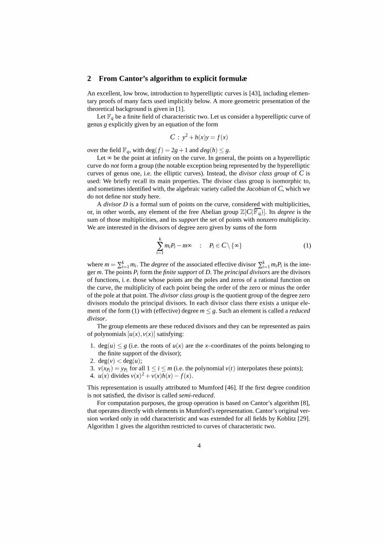
For computation purposes, the group operation is based on Cantor’s algorithm [8],that operates directly with elements in Mumford’s representation. Cantor’s original ver-sion worked only in odd characteristic and was extended for all fields by Koblitz [29].Algorithm 1 gives the algorithm restricted to curves of characteristic two.

4

Algorithm 1. Group operation for hyperelliptic Jacobians in characteristic two

INPUT: Reduced divisors D1 = [u1(x),v1(x)] and D2 = [u2(x),v2(x)]OUTPUT: Reduced divisor D3 = [u3(x),v3(x)], D3 = D1 +D2

1. Composition: [uC ,vC] = D1 +D2 (semi-reduced)

2. d1← gcd(u1,u2)where d1 = s1u1 + s2u2 [Extended Euclidean Algorithm]

3. d(x)← gcd(d1,v1 +v2 +h2)where d = t1d1 + t2(v1 +v2 +h) [Extended Euclidean Algorithm]

4. r1← s1t1, r2← s2t1 and r3← t2

5. uC← u1u2/d2

6. vC← v2 + u2d r2(v1 +v2)+ r3

v22+hv2+ f

d

7. Reduction: D3 = [u3,v3] (reduced)

8. u0← uC, v0← vC

9. for i = 0 while deg(ui) > g do

10. ui+1←Monic(

v2i +hvi+ f

ui

)11. vi+1← vi +h mod ui+1

12. i← i+1

13. u3← ui, v3← vi

Note that at step 6 we are simply computing vC(x) to be congruent to v1(x) modulou1(x)/d(x) and congruent to v2(x) modulo u2(x)/d(x).

The idea behind explicit formulæ is to replace the polynomial-based form of Can-tor’s algorithm by a coefficient-based approach. These formulæ are case-specific, i.e.they depend on whether the divisors are distinct (addition) or equal (doubling), on thedegrees of the polynomials involved, etc. (For a detailed case consideration in genus twosee three see for example [33]; for genus three see [21].) This approach has a numberof advantages which result in a significant speed-up in the computations:

– Conditional statements can be reduced to a minimum. Polynomial arithmetic isinherently dependent on conditional loops (mainly on the degree of the polyno-mial), which cannot be avoided in a general setting. Although checking a condi-tional statement (for example “is k < deg(u)?”) is not very expensive on its own,the cumulative impact over the whole algorithm should not be ignored.

– Coefficients which have no impact on the final result are no longer computed. Thisis quite evident in step 10 where we do not compute the coefficients of x of degree

less than deg(ui) in v2i +hvi + f , since we know that the division v2

i +hvi+ fui

is exactand thus has no fractional part.

– In Cantor’s algorithm, some of the partial computations may be done twice, withonly the variable names being different. These duplications are avoided in the ex-plicit formulæ – by keeping those values in memory.

5

– Parts of the algorithm can be replaced by more efficient techniques that cannot beused in a general setting. Sections 4.1 and 4.2 are good examples of these situations.

We also take advantage of the following observations:

– For almost all reduced divisors D = [u(x),v(x)], u(x) has degree g.– For almost all pairs of polynomials u and v such that u divides v 2 +hv+ f , v mod u

has degree deg(u)−1.– Almost all randomly chosen polynomials are relatively coprime.

(These are standard assumptions which are made by nearly every author in the devel-opment of explicit formulæ, beginning with Harley [24]). In all three of these cases,“almost-all” can be interpreted as “all but a proportion of size O(g/q)”. This meansthat if we concentrate on developing additions formulæ which apply to the most generalcase (i.e. assuming that all polynomials have maximal degree and non-related polyno-mials are coprime) then only a negligible proportion of all group operations requires adifferent implementation. From the point of view of efficiency, we can handle all othercases with the general Cantor algorithm without having a noticeable impact on the com-putation of [e]D (via a double-and-add approach), so only the general case is discussedhere.

To reduce computational cost (mostly for the doublings), we restrict ourselves tocurves of the form

y2 + y = x7 + f5x5 + f3x3 + f1x+ f0 (2)

for genus three and of the form

y2 + y = x9 + f7x7 + f5x5 + f3x3 + f1x+ f0 (3)

for genus four (the security of curves of these special forms is discussed in Section 5).As already mentioned, we consider only the most common case of the addition anddoubling formulæ, i.e. when the degrees are maximal, and (for the addition formula)when u1 and u2 are coprime.

The form of the most common case for the addition and doubling formulæ are verysimilar for genus three and four (except for the degrees of the polynomials, obviously)since we need to go through the reduction loop twice to obtain a reduced divisor. The

only major difference is thatv21+hv1+ f

u1is already monic in the genus three formulæ

(since the leading coefficient in the denominator comes from f (x)) but must be mademonic for the genus four formulæ.

Since the formulæ are in terms of the coefficients instead of polynomials, we willdenote pi the coefficient of xi in p(x). As there could easily be confusions with thepolynomials u1(x), u2(x) and u3(x), as well as v1(x), v2(x) and v3(x), we will denotetheir coefficients differently:

– u1(x) = a0 +a1x+a2x2 + x3 (genus g = 3) oru1(x) = a0 +a1x+a2x2 +a3x3 + x4 (genus g = 4);

– u2(x) = b0 +b1x+b2x2 +x3 (g = 3) or u2(x) = b0 +b1x+b2x2 +b3x3 +x4 (g = 4);– v1(x) = c0 + c1x+ c2x2 (g = 3) or v1(x) = c0 + c1x+ c2x2 + c3x3 (g = 4);– v2(x) = d0 +d1x+d2x2 (g = 3) or v2(x) = d0 +d1x+d2x2 +d3x3 (g = 4);

6

– u3(x) = e0 + e1x+ e2x2 + x3 (g = 3) or u3(x) = e0 + e1x+ e2x2 + e3x3 + x4 (g = 4);– v3(x) = ε0 + ε1x+ ε2x2 (g = 3) or v3(x) = ε0 + ε1x+ ε2x2 + ε3x3 (g = 4).

We also replace u1(x) and v1(x) from steps 10 and 11 by uT (x) and vT (x).

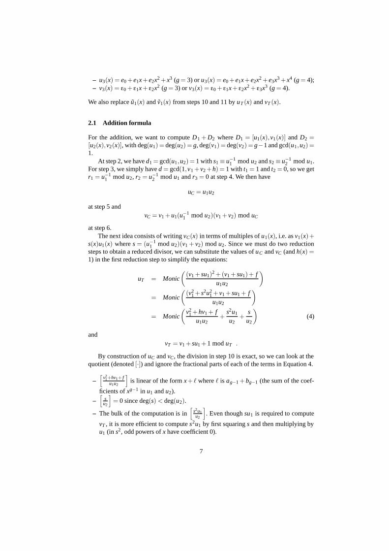
2.1 Addition formula

For the addition, we want to compute D1 + D2 where D1 = [u1(x),v1(x)] and D2 =[u2(x),v2(x)], with deg(u1) = deg(u2) = g, deg(v1) = deg(v2) = g−1 and gcd(u1,u2) =1.

At step 2, we have d1 = gcd(u1,u2) = 1 with s1≡ u−11 mod u2 and s2 ≡ u−1

2 mod u1.For step 3, we simply have d = gcd(1,v1 +v2 +h) = 1 with t1 = 1 and t2 = 0, so we getr1 = u−1

1 mod u2, r2 = u−12 mod u1 and r3 = 0 at step 4. We then have

uC = u1u2

at step 5 andvC = v1 +u1(u−1

1 mod u2)(v1 + v2) mod uC

at step 6.The next idea consists of writing vC(x) in terms of multiples of u1(x), i.e. as v1(x)+

s(x)u1(x) where s = (u−11 mod u2)(v1 + v2) mod u2. Since we must do two reduction

steps to obtain a reduced divisor, we can substitute the values of uC and vC (and h(x) =1) in the first reduction step to simplify the equations:

uT = Monic

((v1 + su1)2 +(v1 + su1)+ f

u1u2

)

= Monic

((v2

1 + s2u21 + v1 + su1 + fu1u2

)

= Monic

(v2

1 +hv1 + fu1u2

+s2u1

u2+

su2

)(4)

andvT = v1 + su1 +1 mod uT .

By construction of uC and vC, the division in step 10 is exact, so we can look at thequotient (denoted [·]) and ignore the fractional parts of each of the terms in Equation 4.

–[

v21+hv1+ f

u1u2

]is linear of the form x+ � where � is ag−1 +bg−1 (the sum of the coef-

ficients of xg−1 in u1 and u2).

–[

su2

]= 0 since deg(s) < deg(u2).

– The bulk of the computation is in[

s2u1u2

]. Even though su1 is required to compute

vT , it is more efficient to compute s2u1 by first squaring s and then multiplying byu1 (in s2, odd powers of x have coefficient 0).

7

We now observe that the leading term in[

s2u1u2

](and therefore of

v2C+hvC+ f

uCas well)

is the square of the leading term of s. An easy way of making u T monic is then to firstmake s monic and use this new polynomial (we call it s) in the computation of u T .

In terms of the number of operations, it is less expensive to compute s and[

s2u1u2

]and

multiply[

v21+hv1+ f

u1u2

]by the corresponding factor than to compute the whole polynomial

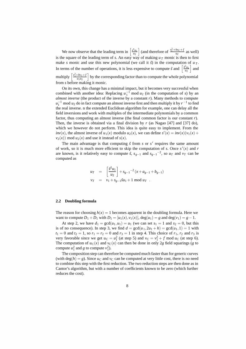
from s before making it monic.On its own, this change has a minimal impact, but it becomes very successful when

combined with another idea: Replacing u−11 mod u2 (in the computation of s) by an

almost inverse (the product of the inverse by a constant r). Many methods to computeu−1

1 mod u2 do in fact compute an almost inverse first and then multiply it by r−1 to findthe real inverse. n the extended Euclidean algorithm for example, one can delay all thefield inversions and work with multiples of the intermediate polynomials by a commonfactor, thus computing an almost inverse (the final common factor is our constant r).Then, the inverse is obtained via a final division by r (as Nagao [47] and [37] do),which we however do not perform. This idea is quite easy to implement. From theinv(x), the almost inverse of u1(x) modulo u2(x), we can define s′(x) = inv(x)(v1(x)+v2(x)) mod u2(x) and use it instead of s(x).

The main advantage is that computing s from s or s ′ requires the same amountof work, so it is much more efficient to skip the computation of s. Once s ′(x) and rare known, is it relatively easy to compute s, sg−1 and sg−1

−2, so uT and vT can becomputed as

uT =[

s2u1

u2

]+ sg−1

−2 (x+ag−1 +bg−1)

vT = v1 + sg−1su1 +1 mod uT .

2.2 Doubling formula

The reason for choosing h(x) = 1 becomes apparent in the doubling formula. Here wewant to compute D1 +D1 with D1 = [u1(x),v1(x)], deg(u1) = g and deg(v1) = g−1.

At step 2, we have d1 = gcd(u1,u1) = u1 (we can set s1 = 1 and s2 = 0, but thisis of no consequence). In step 3, we find d = gcd(u 1,2u1 + h) = gcd(u1,1) = 1 witht1 = 0 and t2 = 1, so r1 = r2 = 0 and r3 = 1 in step 4. This choice of r1, r2 and r3 isvery favorable since we get uC = u2

1 (at step 5) and vC = v21 + f mod uC (at step 6).

The computation of uC(x) and vC(x) can then be done in only 2g field squarings (g tocompute u2

1 and g to compute v21).

The composition step can therefore be computed much faster than for generic curves(with deg(h) = g). Since uC and vC can be computed at very little cost, there is no needto combine this step with the first reduction. The two reduction steps are then done as inCantor’s algorithm, but with a number of coefficients known to be zero (which furtherreduces the cost).

8

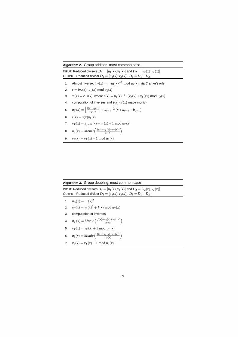
Algorithm 2. Group addition, most common case


1. Almost inverse, inv(x) = r ·u1(x)−1 mod u2(x), via Cramer’s rule

2. r = inv(x) ·u1(x) mod u2(x)

3. s′(x) = r · s(x), where s(x) = u1(x)−1 · (v2(x)+v1(x)) mod u2(x)

4. computation of inverses and s(x) (s′(x) made monic)

5. uT (x) =[

s(x)2u1(x)u2(x)

]+ sg−1

−2(x+ag−1 +bg−1

)6. z(x) = s(x)u1(x)

7. vT (x) = sg−1z(x)+v1(x)+1 mod uT (x)

8. u3(x) = Monic(

f (x)+vT (x)+vT (x)2

uT (x)

)9. v3(x) = vT (x)+1 mod u3(x)

Algorithm 3. Group doubling, most common case


1. uC(x) = u1(x)2

2. vC(x) = v1(x)2 + f (x) mod uC(x)

3. computation of inverses

4. uT (x) = Monic(

f (x)+vC(x)+vC(x)2

uC(x)

)5. vT (x) = vC(x)+1 mod uT (x)

6. u3(x) = Monic(


uT (x)

)7. v3(x) = vT (x)+1 mod u3(x)

9

3 Field Arithmetic

Field arithmetic efficiency is crucial to the speed of the implementation of curve arith-metic. Its realization is often the Achilles’ heel of HEC implementations. In [2] it isshown that HEC in odd characteristic are heavily penalized in most comparisons to EC,because of many types of overheads in the field arithmetic whose impact increases asfield sizes get smaller. This is also the case in characteristic 2, but the nature of the worstoverheads and the techniques used to address them differ.

1. Using loops to process operands produces expensive branch mispredictions, whosecost is heavier for shorter loops.Smaller fields are thus more penalized. This issue is addressed by full loop unrollingfor all input sizes, for example in the implementation of the schoolbook multipli-cation used to implement the underlying integer arithmetic. This is a very commonimplementation practice. Loop unrolling is also useful in even characteristic, butthe way it is used is different: For details see Subsection 3.1.

2. Inlining can often be used to reduce function call overheads.For prime field of small sizes, inlining multiplications makes a big difference. How-ever, the binary field multiplication code is much larger than the code for a multi-precision integer multiplication of the same size. Therefore inlining would result incode size explosion causing big performance drops. In the even characteristic case,all multiplications, squarings and inversions are done using function calls, and onlyadditions and comparisons are inlined.

3. The cost of a modular reduction relative to the multiprecision multiplication in-creases as operands size decreases.Therefore in odd characteristic HEC implementations more time is spent doingmodular reductions than in EC implementations. This issue was addressed in [2]by delaying modular reductions for sums of products of two operands.In even characteristic, the reduction modulo the irreducible polynomial definingthe field extension is much cheaper, and the advantages of delaying modular re-ductions is debatable: The additional memory traffic involved can lead to reducedperformance. After doing some atomic operation counts and some testing, we optednot to implement it.

4. Architecture granularity also induces irregular performance penalties.A 32-bits CPU usually processes 32-bits operands, and we say that the architec-ture has a granularity of 32 bits. Similarly, Granularity issues may affect curves ofhigher genus more than elliptic curves: An elliptic curve over a 223-bits field uses7 words operands, but a curve of genus two offering similar security needs a fieldof approximately 112 bits, i.e. 4 words operands. The number of field multiplica-tions for a group operation increases roughly quadratically with the genus, but inthis scenario the cost of a field multiplication in the smaller field is about 33% ofthe cost of a multiplication in the larger field. As a result the HEC of genus two ispenalized by a factor of 1.32by granularity alone.Not much can be done to defeat granularity problems in the large prime field case. Apartial solution [2] applies when operand sizes are between 32n−31 and 32n−16bits. It consists of using half-word operands for the most significant bits, reducing

10

memory accesses, and speeding up modular reduction. The savings are howeverlimited and are more noticeable for n = 2 (i.e. in the 33 to 48 bits range) than forlarger values of n. The technique can also be used in even characteristic, however,the problem of granularity in even characteristic can be addressed more thoroughlyas we show in Subsection 3.1.

5. In the explicit formulæ, sometimes several different field elements are multiplied bythe same field element.This situation is similar to the multiplication of vector by a scalar, and it is pos-sible to speed up these multiplications appreciably. The technique for doing thisis described in Subsection 3.2. Similar optimization techniques do not seem to bepossible in the prime field case.

The next two Subsections look at the implementation of field multiplication (Sub-section 3.1) and at the technique of sequential multiplications (Subsection 3.2). Squar-ing are described in Subsection 3.3, modular inversion in Subsection 3.4, and modularreduction in Subsection 3.5. We conclude the section with the performance results forfield arithmetic (Subsection 3.6).

A field F2n is represented using a polynomial basis as the quotient ring F 2[t]/(p(t)),where p(t) is an irreducible polynomial of degree n. Elements of the field are rep-resented by binary polynomials of degree less than n. To perform multiplication (resp.squaring) in F2n , the polynomial(s) representing the input(s) are first multiplied together(resp. squared), and the result is then reduced modulo p(t).

3.1 Field multiplication and architecture granularity

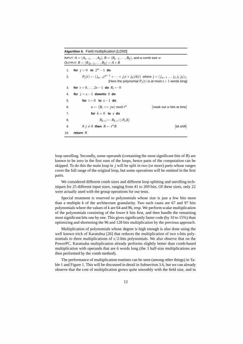
The starting point for our implementation of field multiplication is the algorithm byLopez and Dahab [39], which is based on the comb exponentiation method by Lim andLee [38]. ([23, Subsection 2.3] also describes this method.) It is given as Algorithm 4.

Note that if u = 0 in Step 6, then Steps 7–8 may be skipped. However, insertingan “if u �= 0” statement before Step 7 slows down the algorithm in practice, becausethe implied branch cannot successfully be predicted by the CPU, and frequent pipelineflushes cannot be avoided.

There are a few obvious optimizations of Algorithm 4. The first one applies if theoperands are at most sγ−w+1 bits long. In this case the polynomials P j(t) fit in swords, and the loop beginning at Step 7 requires k to go from 0 to s−1 only.

The second optimization applies if operands are between sγ−w+2 and sγ bits long.We proceed as follows: First, zero the w− 1 most significant bits of A for the compu-tations in Steps 2 and 3, thus obtaining the polynomials P j(t) that fit in s words; Then,perform the computation as in the case of shorter operands, thus in Step 7 the upperbound for k is s−1; Finally, add the multiples of B(t) corresponding to the most w−1most significant bits of A to R before returning the result. This leads to a much fasterimplementation since a lot of memory writes in Step 2 and memory reads in Step 8 aretraded for a minimal amount of memory operations later. This approach is commonlyused for generic implementations of binary polynomial multiplication.

More optimizations can be applied if the field size is known in advance. Firstly,as the lengths of all the loops are known in advance it is possible to do partial or full

11

Algorithm 4. Field multiplication [LD00]

INPUT: A = (As−1, . . . ,A0), B = (Bs−1, . . . ,B0), and a comb size wOUTPUT: R = (R2s−1, . . . ,R0) = A×B

1. for j = 0 to 2w−1 do

2. Pj(t)← ( jw−1tw−1 + · · ·+ j1t + j0)A(t) where j = ( jw−1 . . . j2 j1 j0)2.[Here the polynomial Pj(t) is at most s+1 words long]

3. for i = 0, . . . ,2s−1 do Ri← 0

4. for j = s−1 downto 0 do

5. for i = 0 to s−1 do

6. u← (Bi >> jw) mod tw [mask out w bits at time]

7. for k = 0 to s do

8. Rk+i← Rk+i⊕Pu[k]

9. If j �= 0 then R← twR [bit shift]

10. return R

loop unrolling. Secondly, some operands (containing the most significant bits of R) areknown to be zero in the first runs of the loops, hence parts of the computation can beskipped. To do this the main loop in j will be split in two (or more) parts whose rangescover the full range of the original loop, but some operations will be omitted in the firstparts.

We considered different comb sizes and different loop splitting and unrolling tech-niques for 25 different input sizes, ranging from 41 to 269 bits. Of these sizes, only 22were actually used with the group operations for our tests.

Special treatment is reserved to polynomials whose size is just a few bits morethan a multiple k of the architecture granularity. Two such cases are 67 and 97 bitspolynomials where the values of k are 64 and 96, resp. We perform scalar multiplicationof the polynomials consisting of the lower k bits first, and then handle the remainingmost significant bits one by one. This gives significantly faster code (by 10 to 15%) thanoptimizing and shortening the 96 and 128 bits multiplication by the previous approach.

Multiplication of polynomials whose degree is high enough is also done using thewell known trick of Karatubsa [26] that reduces the multiplication of two s-bits poly-nomials to three multiplications of s/2-bits polynomials. We also observe that on thePowerPC, Karatsuba multiplication already performs slightly better than comb-basedmultiplication with operands that are 6 words long (the 3 half-size multiplications arethen performed by the comb method).

The performance of multiplication routines can be seen (among other things) in Ta-ble 1 and Figure 1. This will be discussed in detail in Subsection 3.6, but we can alreadyobserve that the cost of multiplication grows quite smoothly with the field size, and in

12

fact approaches the curve of the quadratic theoretical bit complexity of multiplicationmuch better than a simpler approach that works at the word level.

3.2 Sequential multiplications

In the explicit formulæ for the curves of genus two to four, we can find several setsof multiplications with one of terms in common. At this point it is natural to decideto preserve the precomputations (Steps 1 and 2 of Algorithm 4) associated to one fieldelement and to re-use them in the next multiplications. However, this would require alot of extra variables in the implementation of the explicit formulæ and memory man-agement techniques. We therefore opted for a simpler approach: We wrote routines thatperform the precomputations once and then repeat the Steps 3 to 10 of Algorithm 4for each multiplication. We call this type of operation sequential multiplication (scalarmultiplication would be more correct, but in our context this terminology is alreadyused...).

It turns out that the optimal comb size for a single multiplication (on a given archi-tecture) may not be optimal for 2, 3, or more multiplications, so we adapt the comb sizeto the number of multiplications that are performed together. For example, for the 73bits field on the PowerPC, a comb of size 3 is optimal for the single multiplication andfor pairs of multiplications (sequences of 2 multiplications), but for 3 to 5 multiplica-tions the optimal comb of size is 4. For 89 bits fields, the optimal comb size for singlemultiplications is still 3, but it is 4 already for the double multiplication.

If a comb method is used for 6-word fields on our target architecture, then 4 isthe optimal size for single multiplications and 5 is the optimal size for groups of atleast 3 multiplications. As we mentioned in Subsection 3.1, Karatsuba performs slightlybetter for the single multiplications and the same method is also used in the sequentialmultiplications, where a sequential multiplication of s-word operands is turned intothree sequential multiplications of s/2-word operands.

In order to keep function call overheads low and to avoid the use of virtual param-eter lists in C, the sequential multiplication procedures for at least 3 multiplicationsrequire the input and output vectors to consist of elements which are adjacent in mem-ory. This can also speed up memory accesses, since successive parameters are stored inconsecutive memory locations, better exploiting the structure of modern caches.

For historical reasons, we need to mention that using static precomputations has al-ready been done for multiplications by a constant parameter (coming from the curve orthe field) – this is for example suggested in the context of square root extraction in [14].We found no references on adapting the comb size to the number of multiplications bythe same value.

3.3 Polynomial squaring

Squaring is a linear operation in even characteristic: If p(t) = ∑ni=0 eiti where ei ∈ F2,

then(p(t)

)2 = ∑ni=0 eit2 i. In other words, the result is obtained by inserting a zero bit

between each two adjacent bits of the polynomial to be squared. To efficiently imple-ment this process, a 512-byte table is precomputed for converting 8-bits polynomialsinto their expanded 16-bits counterparts [56].

13

3.4 Modular inversion

There are several different algorithms for computing the inverse of a polynomial a(t)modulo another polynomial p(t), where both polynomials are defined over the field F 2.

In [22] three different methods are described (see also [23, Subsection 2.3]):

– The Extended Euclidean Algorithm (EEA), where the partial quotients are approx-imated by powers of t, hence no polynomial division is required, but only a com-parison of degrees.

– The Almost Inverse Algorithm (AIA), which is a variant of the binary extendedGCD algorithm where the final result is given as a polynomial b(t) together with aninteger k such that b(t)a(t)≡ t k (mod p(t)). The final result must then be adjusted.

– The Modified Almost Inverse Algorithm (MAIA), which is a variant of the binaryextended GCD algorithm which returns the correct inverse as a result.

We refer to [22] for details.Depending on the nature of the different parameters, it can be assumed that each

algorithm can be faster than the other two. However our experiments agree with theresults in [22] and we find that EEA performs consistently better than the other twomethods.

In our implementations with inputs of up to 8 words we always keep all words(limbs) of all multiprecision operands in separate integer variables explicitly, not inindexed arrays. This allows the compiler to reserve a register for each of these inte-ger variables if enough registers are provided by the architecture (such as on RISCprocessors). Furthermore, it does not penalize register-starved CISC architectures: thecontents of many registers containing individual words are spilled on the stack, but thisdata would be stored in memory anyway if we used arrays.

Another advantage of the EEA is that we have good control on the bit lengths of theintermediate variables. We can therefore split the main loop in several copies dependingon the sizes of the operands, with n sections of code for inputs of n words. Thesesections are written to avoid operations between registers which are known to be zero(for example, with the most significant words of some variables). At the same time wecan reduce the local usage of registers, allowing an increase in the size of the inputsbefore the compiler has to produce code that spills some information to memory. GCC4.0 has decent register coloring algorithms and analysis of the code showed very goodreuse of registers across different blocks of code. See Subsection 3.6 for the impact ofthis approach on performance on RISC architectures.

A limited number of registers disadvantages inversion, but a slow memory bus isnot a big problem on RISC architectures: since all the inputs can be stored in internalregisters, most of the computations take place without memory accesses. In comparison,a slow memory bus penalizes the multiplication much more than register paucity. Thesefacts are reflected in the low inversion to multiplication (I/M) ratio (often between 4and 6) on the Powerpc G4 (slow memory interface), with an increase of this ratio toabout 10 on Powerpc G5 (many registers, but also a fast bus, which advantages themultiplication) or even 12 on a Pentium 3 or Athlon k6 CPU (very few registers, slowbus). On the Pentium 4 because of a slower shift operation the inversion tends to be lessefficient (the I/M ratio can in some cases exceed 20).

14

3.5 Modular reduction

For modular reduction we implemented two sets of routines.The generic routine reduces arbitrary polynomials over F 2 modulo arbitrary poly-

nomials over F2. This code is in fact rather efficient, and a reduction by means of thisroutine can often take less than 20% of the time of a multiplication. The approach issimilar to the one taken in SUN’s contributions to OpenSSL or in NTL’s code base, andexploits a compact representation of the reduction polynomial. The reduction polyno-mial is given as a decreasing sequence of integers (n0,n1,n2, ...,nk−1) and it is equalto ∑k−1

i=0 tni . Whenever possible we use a trinomial (k = 3), otherwise we use a pen-tanomial (k = 5). Only in very few cases an eptanomial is used when its reduction ismore efficient than that of the most efficient pentanomial.

The second set of routines uses fixed reduction polynomials, and is therefore spe-cific for each polynomial degree. The code is very compact and streamlined. In thissituation we sometimes prefer reduction eptanomials to pentanomials when the re-duction code is shorter due to the form of the polynomial. For example, for degree59 we have two good irreducible polynomials: f 1(t) = t59 + (t + 1)(t5 + t3 + 1) andf2(t) = t59 + t7 + t4 + t2 +1.

The C code takes a polynomial of degree up to 116 (= 2 ·58) stored in variables r3(most significant word), r2, r1 and r0 (least significant word), and reduces it modulof1(t), leaving the result in r1 and r0

#define bf_mod_59_6_5_4_3_1_0(r3,r2,r1,r0) do { \r3 = ((r3) << 5) ^ ((r3) << 6); r1 ^= (r3) ^ ((r3) << 3) ^ ((r3) << 5); \r3 = ((r2) << 5) ^ ((r2) << 6); r0 ^= (r3) ^ ((r3) << 3) ^ ((r3) << 5); \r3 = ((r2) >> 22) ^ ((r2) >> 21); r1 ^= (r3) ^ ((r3) >> 2) ^ ((r3) >> 5); \r2 = (r1) >> 27; r2 ^= (r2) << 1; \r1 &= 0x07ffffff; r0 ^= (r2) ^ ((r2) << 3) ^ ((r2) << 5); \} while (0)

and the C code to reduce the same input modulo f 2(t) is

#define bf_mod_59_7_4_2_0(r3,r2,r1,r0) do { \r1 ^= ((r3) << 5) ^ ((r3) << 7) ^ ((r3) << 9) ^ ((r3) << 12); \r2 ^= ((r3) >> 25) ^ ((r3) >> 23) ^ ((r3) >> 20); \r0 ^= ((r2) << 5) ^ ((r2) << 7) ^ ((r2) << 9) ^ ((r2) << 12); \r1 ^= ((r2) >> 27) ^ ((r2) >> 25) ^ ((r2) >> 23) ^ ((r2) >> 20); \r2 = (r1) >> 27; r1 &= 0x07ffffff; \r0 ^= (r2) ^ ((r2) << 2) ^ ((r2) << 4) ^ ((r2) << 7); \} while (0)

Comparing the two codes, we find that the first one is slightly more efficient. Asimilar choice occurs at degree 107 (the irreducible polynomial is t 107 +(t6 +t2 +1)(t +1)), and the idea of factoring the “lower degree part” of the reduction polynomial is alsoused for degree 109 (the polynomial is t 109 +(t6 +1)(t +1)).

These considerations have been applied to degrees 43, 53, 59, 67, 71, 73, 79, 83, 89,101, 107, 109, 127, 137, 139, 157, 179, 199, 211, 239, 251, and 269 (which are used inthe tests) as well as the intermediate values 97, 131, and 149.

By doing this, we can keep the time for the modular reduction between 3 and 5% ofthe time required for a multiplication in the case the reduction polynomial is a trinomial,and between 6 and 10% in the other cases. Reduction modulo a trinomial is about as

15

twice fast as polynomial squaring (Subsection 3.3), because in the latter there are morememory accesses.

For degrees 47, 71, 79, 89, 97, 127, 137, 159, 199, and 239 we used a trinomial. Fordegrees 43, 53, 67, 73, 83, 101, 109, 131, 139, 149, 179, 211, 251, and 269 we used apentanomial. For degrees 59, 107, and 219 we opted for eptanomials, when they werereducible and had a sedimentary part of lower degree than the optimal pentanomial (seeremarks above).

As operand sizes increase, the relative cost of modular reduction decreases consid-erably and becomes in practice negligible.

3.6 Field arithmetic and its performance

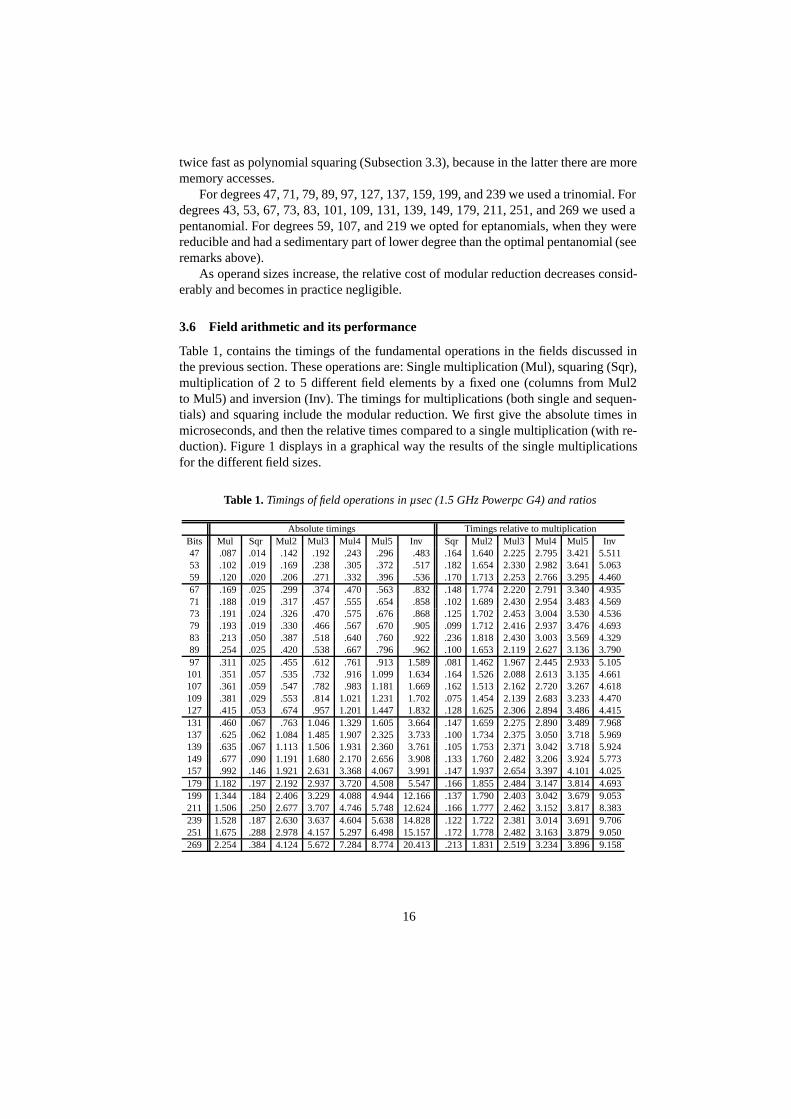
Table 1, contains the timings of the fundamental operations in the fields discussed inthe previous section. These operations are: Single multiplication (Mul), squaring (Sqr),multiplication of 2 to 5 different field elements by a fixed one (columns from Mul2to Mul5) and inversion (Inv). The timings for multiplications (both single and sequen-tials) and squaring include the modular reduction. We first give the absolute times inmicroseconds, and then the relative times compared to a single multiplication (with re-duction). Figure 1 displays in a graphical way the results of the single multiplicationsfor the different field sizes.

Table 1. Timings of field operations in µsec (1.5 GHz Powerpc G4) and ratios

Absolute timings Timings relative to multiplicationBits Mul Sqr Mul2 Mul3 Mul4 Mul5 Inv Sqr Mul2 Mul3 Mul4 Mul5 Inv47 .087 .014 .142 .192 .243 .296 .483 .164 1.640 2.225 2.795 3.421 5.51153 .102 .019 .169 .238 .305 .372 .517 .182 1.654 2.330 2.982 3.641 5.06359 .120 .020 .206 .271 .332 .396 .536 .170 1.713 2.253 2.766 3.295 4.46067 .169 .025 .299 .374 .470 .563 .832 .148 1.774 2.220 2.791 3.340 4.93571 .188 .019 .317 .457 .555 .654 .858 .102 1.689 2.430 2.954 3.483 4.56973 .191 .024 .326 .470 .575 .676 .868 .125 1.702 2.453 3.004 3.530 4.53679 .193 .019 .330 .466 .567 .670 .905 .099 1.712 2.416 2.937 3.476 4.69383 .213 .050 .387 .518 .640 .760 .922 .236 1.818 2.430 3.003 3.569 4.32989 .254 .025 .420 .538 .667 .796 .962 .100 1.653 2.119 2.627 3.136 3.79097 .311 .025 .455 .612 .761 .913 1.589 .081 1.462 1.967 2.445 2.933 5.105101 .351 .057 .535 .732 .916 1.099 1.634 .164 1.526 2.088 2.613 3.135 4.661107 .361 .059 .547 .782 .983 1.181 1.669 .162 1.513 2.162 2.720 3.267 4.618109 .381 .029 .553 .814 1.021 1.231 1.702 .075 1.454 2.139 2.683 3.233 4.470127 .415 .053 .674 .957 1.201 1.447 1.832 .128 1.625 2.306 2.894 3.486 4.415131 .460 .067 .763 1.046 1.329 1.605 3.664 .147 1.659 2.275 2.890 3.489 7.968137 .625 .062 1.084 1.485 1.907 2.325 3.733 .100 1.734 2.375 3.050 3.718 5.969139 .635 .067 1.113 1.506 1.931 2.360 3.761 .105 1.753 2.371 3.042 3.718 5.924149 .677 .090 1.191 1.680 2.170 2.656 3.908 .133 1.760 2.482 3.206 3.924 5.773157 .992 .146 1.921 2.631 3.368 4.067 3.991 .147 1.937 2.654 3.397 4.101 4.025179 1.182 .197 2.192 2.937 3.720 4.508 5.547 .166 1.855 2.484 3.147 3.814 4.693199 1.344 .184 2.406 3.229 4.088 4.944 12.166 .137 1.790 2.403 3.042 3.679 9.053211 1.506 .250 2.677 3.707 4.746 5.748 12.624 .166 1.777 2.462 3.152 3.817 8.383239 1.528 .187 2.630 3.637 4.604 5.638 14.828 .122 1.722 2.381 3.014 3.691 9.706251 1.675 .288 2.978 4.157 5.297 6.498 15.157 .172 1.778 2.482 3.163 3.879 9.050269 2.254 .384 4.124 5.672 7.284 8.774 20.413 .213 1.831 2.519 3.234 3.896 9.158

16

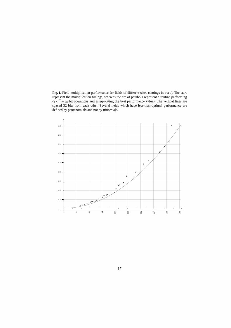
Fig. 1. Field multiplication performance for fields of different sizes (timings in µsec). The starsrepresent the multiplication timings, whereas the arc of parabola represent a routine performingc1 · n2 + c0 bit operations and interpolating the best performance values. The vertical lines arespaced 32 bits from each other. Several fields which have less-than-optimal performance aredefined by pentanomials and not by trinomials.

32 64 96 128

160

192

224

256

288

** * **** ** *

** **

*

***

*

**

**

*

*

*

0.25

0.50

0.75

1.00

1.25

1.50

1.75

2.00

2.25

17

The timings were obtained on a 1.5 Ghz PowerPC G4 (Motorola 7447) CPU, a 32-bits RISC architecture with 32 general purpose integer registers. This means that wecan put several intermediate operands in the registers. Note that we do not use specificcompiler directives, but we simply declare all limbs of all intermediate operands assingle word variables, and operate on them with the usual C language logic and shiftoperations. The code in fact compiles correctly on any 32-bits architecture supportedby the gnu compiler collection (we used gcc 4.0.1 under Mac OS X 10.4.3).

The register abundance easily explains not only the very good performance (multi-plications are often 30% faster than on a 2.8 Ghz Pentium 4 processor), but also the lowtimings for the inversion. If the operands of the EEA all fit in the registers (which wasthe case for elements of up to 6 words), then the whole inversion is performed exclu-sively in the registers, without accessing external memory except to load the inputs andto store the final result. The “bump” in inversion performance occurs when the registersare no longer sufficient, and the compiler must store some partial data in main memory(as confirmed by analysis of the disassembly of the compiled code).

Note that the usage of trinomials and pentanomials or eptanomials is reflected inthe timings. The ratio Sqr/Mul is higher if a pentanomial is used because the reductionis slower than it would have been if a trinomial of the same degree had existed. Thereduction has a small relative impact on the field multiplication, but it makes a biggerdifference for the field squaring (since polynomial squaring is very inexpensive).

4 Improvements in the formulæ

In this section, we describe the algorithmic methods used to improve the formulæ ofGuyot, Kaveh and Patankar (for genus three, [21]) and of Pelzl, Wollinger and Paar (forgenus four, [52, 59]). We follow three main approaches:

1. Reduce the number of inversions. As inversions are usually much more costly thanother operations, it is often a good idea to combine as many of them together,even if this means increasing the number of multiplications. This was common forgenus two and three, but it can be pushed further for genus four as is described inSection 4.1.

2. Reduce the number of multiplications. It goes without saying that if the numberof multiplications in the explicit formulæ can be reduced, the overall performancewill improve. Most explicit formulædo this by introducing Karatsuba multiplicationto compute the product of polynomials. We obtain further improvements by select-ing faster algorithms (Section 4.2), combining multiplications using Karatsuba-liketricks (Section 4.3) and keeping products in memory if they are used again later inthe formula.

3. Combine multiplications with a repeated operand. The goal here is to make useof the sequential multiplications. Although this does not affect the total operationcount, this approach reduced the effective cost of some (but not all) steps by morethan 30%.

Note that approaches 2 and 3 are not always compatible. In most cases, reducing thenumber of multiplications using Karatsuba-like tricks will hinder the use of sequential

18

multiplications. For example, the computation of inv(x) · (v 2(x)+ v1(x)) in the genusfour addition formula takes 16 multiplications using classical methods. With sequen-tial multiplications, we still have the same number of multiplications, but the effectivecost is close to that of 11.4 normal multiplications (using estimates for sequential mul-tiplications extrapolated from Table 1 – see subsection 4.5 for the exact equivalencesadopted). With two layers of Karatsuba multiplications, we can do this in 9 multiplica-tions, but then no operand is used in more than one product so we cannot use sequentialmultiplications to get any further savings.

In this example it is clear that a Karatsuba-like approach is a better choice. In manycases however, the choice is not always so clear as the savings obtained by giving prece-dence to Karatsuba-like tricks or to sequential multiplications may be very close andwill vary depending on the processor and the field size. To avoid writing a different for-mula for each field size, the formulæ described in this paper assume the average case.For some field sizes, the formula may not be completely optimal, although the savingthat could be obtained by using a field-specific formula would be marginal at best.

4.1 Inversions

As for curves of genus three, the common case of group addition for curves of genus

four requires two reduction steps. However, f+vt+v2T

uTin the second reduction step (Step

8 of Algorithm 2) for genus four is not automatically monic since the leading term inf + vt + v2

T is vT,52x10. For these curves, we must therefore compute the inverses of s 3

(to make uT monic), r (to get s3, for the computation of vT ), s′3 (to make s′ monic) andvT,5 (to make u3 monic).

The inverses of s3, r and s′3 can be combined in the same way it is done for curvesof genus three, but this still leaves us with two inversion to be performed. At the timethe inverses of s′3 and s3 are obtained, only inv(x), r and s ′(x) have been computed.To minimize the number of inversions, one has to express v T,5 in terms of r and thecoefficients s′(x) and u2(x).

To improve readability, we use the coefficients of the polynomials u T (x), z(x) =s(x)u1(x), s(x) = 1

r s′(x) and s(x) = 1s′3

s′(x), even though those polynomials are not com-

puted before the inverses. Since vT (x) = s3z(x)+ v1(x)+1 mod uT (x), we have

vT,5 = s3 (z5 +uT,4 +uT,5(z6 +uT,5)) .

Furthermore, replacing s(x)2u1(x) by s(x)z(x) in the equation for uT (x), we have

uT (x) =[

s(x)z(x)u2(x)

]+ s−2

3 (x+a3 +b3) ,

so uT,5 = z6 + s2 +b3 and uT,4 = z5 + s2z6 + s1 +b2 +uT,5b3. Substituting back into theequation of vT,5, we get

vT,5 = s3 (s2z6 + s1 +b2 +uT,5b3 +uT,5(z6 +uT,5))= s3 (s2z6 + s1 +b2 +uT,5s2)= s3 (s2z6 + s1 +b2 +(z6 + s2 +b3)s2)= s3

(s1 +b2 + s2

2 +b3s2)

.

19

Using the definitions of s(x) and s(x), we get

vT,5 =s′3r

(s′1s′3

+b2 +(

s′2s′3

)2

+b3s′2s′3

)=

1rs′3

(s′2

2 + s′3(s′1 +b3s

′2 +b2s

′3))

.

Since 1/rs′3 is not yet known, we replace the computation of vT,5 by the computation of

rs′3vT,5 = s′22 + s′3(s

′1 +b3s′2 +b2s′3) .

To obtain the inverses of s3, r, s′3 and vT,5, we first compute rs′3 and rs′3vT,5, and let

t =1

(rs′3) · (rs′3vT,5).

Then, the inverses of vT,5 and rs′3 are obtained as

t · (rs′3)2 =1

vT,5and t · (rs′3vT,5) =

1rs′3

.

The inverses of s3, r and s′3 are then obtained as before. In this manner, it is possibleto combine the final inversion with the previous ones, at the cost of an extra five mul-tiplications and two squarings. Note that the computation of v T,5 (which is needed forthe final step) can then be done in one multiplication instead of two and that we nolonger need to compute z5 (which saves one more multiplication). This approach re-duces computation time if an inversion costs more than three multiplications and twosquarings.

For the doubling formula, the approach must be modified slightly since in this caseuC(x) and vC(x) are computed directly. This time, we need the inverses of vC,7 and vT,5

and we havevC,7vT,5 = vC,6

2 + vC,5vC,7 +uC,6(vC,72) .

We then compute

t =1

vC,7(vC,7vT,5)

and the inverses of vT,5 and vC,7 are found as

t · (vC,72) =

1vT,5

and t · (vC,7vT,5) =1

vC,7.

The second inverse is then replaced by five multiplications and two squarings, of whichone (vC,6

2) is used again at a later step. Since two of these multiplications can be com-bined, the exchange is advantageous if one inversion cost more than (roughly) 4.7 mul-tiplications and one squaring. This trade-off is slightly to our disadvantage on the Pow-erPC G4 (by about 0.2 multiplications on average for the fields used for genus fourtesting), but we still opted to implement it as it always produces significant savings inother processors.

20

4.2 Almost inverse

One of the most costly step of explicit formulæ is the computation of the almost inverse.Most of the explicit formulæ published so far [24, 47, 40, 31, 51, 50, 52, 21, 34, 33] findthe almost inverse via the computation of a resultant, however this approach is notoptimal. For every genus bigger than two, the almost inverse can be computed withfewer field multiplications using Cramer’s rule (for genus two, the cost are the same ifboth methods are implemented carefully). This approach has the added bonus of takingfull advantage of sequential multiplications, making it even more efficient.

Cramer’s rule computes a solution v to the system Mv = w where M is an n× nmatrix. The solution is

v =1|M|

|Sub0(M,w)||Sub1(M,w)|

...|Subn−1(M,w)|

where Subi(M,w) is matrix M with the ith column replaced by w.To apply this method to computing the inverse of polynomials, we need a map

between polynomials (of degree smaller then n) and vectors. To the coefficient of x i inthe polynomial p(x), we associate the i th coordinate of the vector p (and vice versa).

To compute the inverse of a(x) modulo b(x), we use the matrix M where the i th rowcorresponds to xia(x) mod b(x). We then solve for the vector w = 1 = (1,0,0, . . . ,0) t

(the constant polynomial 1). Since the matrices have many coefficients in common,most of the computations can be combined using a bottom-to-top approach (see Ap-pendix A for details).

As we do not require the inverse, but rather an almost inverse (the product of theinverse by a constant multiple r), we compute all the determinants used in Cramer’srule, but we avoid the division by |M|. We obtain:

inv =

|Sub0(M,1)||Sub1(M,1)|

...|Subn−1(M,1)|

and r = |M|=

n−1

∑i=0

M0,i|Subi(M,1)| .

Note that in the formulæ, the computation of r is done with some of the computationsfor s′(x) in order to combine some of the multiplications into pairs (and use sequentialmultiplications).

4.3 Polynomial divisions

Although Karatsuba-like multiplications are most commonly applied to polynomialmultiplication, they can also be used when dealing with polynomial divisions (bothfor the quotient and the remainder). We consider three main cases: The reduction ofinv(x)(v2(x)+v1(x)) modulo u2(x) (computation of s′(x)), the division on (s(x)2)·u1(x)by u2(x) (computation of uT (x)), and the reduction of vT (x)+h(x) modulo u3(x) (com-putation of v3(x)).

21

For the computation of s′(x), let us assume that the product inv(x) ·(v2(x)+v1(x)) isalready computed (even though the product is intermingled with the reduction modulou2(x) in practice) and let us call it

p(x) = p6x6 + p5x5 + p4x4 + p3x3 + p2x2 + p1x+ p0 .

We want to reduce p(x) modulo u2(x), i.e. we want to write p(x) = λ(x)u2(x)+ s′(x)with λ(x) = λ2x2 +λ1x +λ0. Note that although we do not really want λ(x), its com-putation is necessary to the efficient computation of s ′(x). The computations take theform:

λ2 = p6

λ1 = p5 +b3λ2

λ0 = p4 +b3λ1 +b2λ2

s′3 = p3 +b3λ0 +b2λ1 +b1λ2

s′2 = p2 +b2λ0 +b1λ1 +b0λ2

s′1 = p1 +b1λ0 +b0λ1

s′0 = p0 +b0λ0 .

One important thing to notice is that although the coefficients of s ′(x) cannot be com-puted before λ0, there is no problem (other than memory requirements) with computingsome of the products containing λ1 or λ2 before computing λ0. The maximum num-ber of multiplications that can be saved using a Karatsuba-like approach is three. Onecan combine the pairs of multiplications in the sums b3λ1 + b2λ2, b3λ0 + b1λ2 andb2λ0 +b1λ1 (where λ0 is obtained before the last two pairs are handled). The result is 6products with no terms in common and 3 multiplications by b 0 (handled sequentially),for an effective cost of around 8.3 multiplications. Note that in this case, using 3 se-quential multiplications (by λ2, λ1 and λ0) on the original set of operations would havehad an effective cost of around 8.45 multiplications. (Again, see subsection 4.5 for theequivalences.)

For the computation of uT (x), most of the work involves computing the quotient of(s(x)2 ·u1(x)) divided by u2(x). Since u2(x) has degree 4, the coefficients of xi for i < 4in s(x)2 · u1(x) do not have to be computed as they have no impact on the result. Thistime, we assume that we have already computed

p(x) = s(x)2 ·u1(x) = x10 + p9x9 + p8x8 + p7x7 + p6x

6 + p5x5 + p4x4 + . . .

(with p9 = a3) and we see that the coefficients of uT (x) are:

uT,5 = a3 +b3

uT,4 = p8 +b2 +b3uT,5

uT,3 = p7 +b1 +b3uT,4 +b2uT,5

uT,2 = p6 +b0 +b3uT,3 +b2uT,4 +b1uT,5

uT,1 = p5 +b3uT,2 +b2uT,3 +b1uT,4 +b0uT,5

uT,0 = p4 +b3uT,1 +b2uT,2 +b1uT,3 +b0uT,4 .

22

However, the products of b3, b2, b1 and b0 by uT,5 = (a3 +b3) are already known fromthe computation of the almost inverse (using Cramer’s rule), so we only need to computeproducts of the form

uT,3 = sum3 +b3uT,4

uT,2 = sum2 +b3uT,3 +b2uT,4

uT,1 = sum1 +b3uT,2 +b2uT,3 +b1uT,4

uT,0 = sum0 +b3uT,1 +b2uT,2 +b1uT,3 +b0uT,4 .

After a few checks, one might be tempted to conclude that the most that can be savedusing Karatsuba-like tricks in this situation is one multiplication, but in fact it is not thecase. Although only three combinations (b3uT,3 +b2uT,4, b3uT,2 +b2uT,3 and b2uT,3 +b1uT,4) could be used without requiring extra products (and no two of these can be usedsuccessfully at the same time), it is possible to reduce the operation count by addingone new product. If one also computes b1uT,2, then it becomes possible to add two morecombinations (b3uT,2 +b1uT,4 and b2uT,2 +b1uT,3) to b3uT,3 +b2uT,4, in effect reducingthe number of multiplication by two instead of one. Once again, it is slightly moreefficient to use sequential multiplications after reducing the number of multiplicationsas much as possible than using them on the original equations.

Let us now consider the final step of the the genus four formulæ (that step is es-sentially identical for both the addition and the doubling) where we compute v 3(x) =vT (x)+1 mod u3(x). We have

t = vT,4 + e3vT,5

ε3 = vT,3 + e2vT,5 + e3t

ε2 = vT,2 + e1vT,5 + e2t

ε1 = vT,1 + e0vT,5 + e1t

ε0 = vT,0 +1+ e0t

which, at first glance, requires 8 multiplications. Although the use of Karatsuba multi-plications (combining e2vT,5 + e3t and e0vT,5 + e1t) reduces the number of multiplica-tions by 2 whereas the use of sequential multiplications reduces the cost to around 5.7multiplications, the Karatsuba approach is in fact better. The idea here is to reorder the6 products into three pairs:

– e3vT,5 and e1vT,5 (done first, so t can be computed)– e2t and e0t– (e3 + e2)(vT,5 + t) and (e1 + e0)(vT,5 + t) to obtain the two sets of combined prod-

ucts).

By computing these pairs as sequential multiplications, we can get the effective costdown to around 5.1 multiplications.

For the genus four addition, there are three remaining cases that we do not discusswhere a Karatsuba-like approach can be considered:

– The computation of z(x) = s(x) ·u1(x). The pattern of multiplications encounteredare the same as for the reduction of inv(x)(v2(x)+v1(x)) modulo u2(x), but viewedupside down since z5 is not required (see Section 4.1).

23

– The computation of (s(x)2) · u1(x) (before the division by u2(x)). Since only thecoefficients of powers of x greater than 4 are needed and s(x) 2 only contains evenpowers of x, it is not possible to obtain any saving from this approach.

– The computation of u3(x). Here we have only one possible way of reducing multi-plications, by combining the products in e3uT,4 + e2uT,5.

4.4 Variables

A very serious issue with the genus four formulæ (and, to a lesser extent, the genus threeformulæ as well), is the number of variables involved. An implementation of the addi-tion operation for genus four that does not worry about memory requirements woulduse 234 variables (240 to take into account the “sequential” form of our implementa-tion of sequential multiplications). This number of variables is obviously too large forconstrained environments, and even with two or three words per field elements (as isthe case for the security levels considered in this paper), this would mean a storage inthe order of one kilobyte for the variables alone. At this point, the memory allocationmight affect the performance of the computations also for high-end processors: even ifthis memory is allocated statically, its use may still take up a non-negligible part of thelevel 1 cache of the processor.

The natural solution is to use the same variables multiple times. We decided tominimize the number of variables as much as possible without losing any (significant)efficiency in exchange. The result is a more compact and portable code which can beused even in constrained environments. To minimize memory allocations as much aspossible, we chose to define an array of field elements, whose address is passed as partof the function calls for the addition and doubling and where all the intermediate resultsof the group operations are stored.

To improve readability, the formulæ in the appendix are given in terms of distinctvariables and they are accompanied by an allocation schedule for the variable array.In a few cases, a variable is copied into a different location in the array to obtain anadjacent sequence that can be used for the sequential multiplications (this is due to ourchoice for the function call), or a long sum is broken into two shorter sums to free someof the variables. The final values are kept with the other variables until the last minute(at which point they are copied into the space allocated to a divisor) so the function’soutput can replace one of its inputs if desired.

The resulting formulæ require 14 variables for the genus three addition and dou-bling, 19 for the genus four doubling and 23 for the addition. In all cases, these numbersare minimal with the present formulæ as there are “bottlenecks” where all the variablesare either in use for the current operation or contain values that were computed earlierand will be used later.

4.5 Operation counts

The addition and doubling formulæ for genus three, with the tables of variable alloca-tion, are in Appendix B, and those for genus four are in Appendix C. Tables 2 and 3compare the operation counts of our formulæ with previous works (note that for the

24

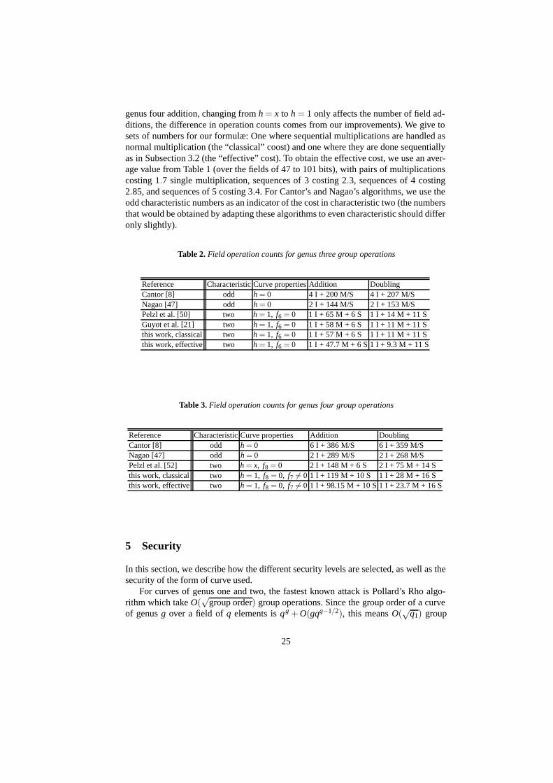
genus four addition, changing from h = x to h = 1 only affects the number of field ad-ditions, the difference in operation counts comes from our improvements). We give tosets of numbers for our formulæ: One where sequential multiplications are handled asnormal multiplication (the “classical” coost) and one where they are done sequentiallyas in Subsection 3.2 (the “effective” cost). To obtain the effective cost, we use an aver-age value from Table 1 (over the fields of 47 to 101 bits), with pairs of multiplicationscosting 1.7 single multiplication, sequences of 3 costing 2.3, sequences of 4 costing2.85, and sequences of 5 costing 3.4. For Cantor’s and Nagao’s algorithms, we use theodd characteristic numbers as an indicator of the cost in characteristic two (the numbersthat would be obtained by adapting these algorithms to even characteristic should differonly slightly).

Table 2. Field operation counts for genus three group operations

Reference Characteristic Curve properties Addition DoublingCantor [8] odd h = 0 4 I + 200 M/S 4 I + 207 M/SNagao [47] odd h = 0 2 I + 144 M/S 2 I + 153 M/SPelzl et al. [50] two h = 1, f6 = 0 1 I + 65 M + 6 S 1 I + 14 M + 11 SGuyot et al. [21] two h = 1, f6 = 0 1 I + 58 M + 6 S 1 I + 11 M + 11 Sthis work, classical two h = 1, f6 = 0 1 I + 57 M + 6 S 1 I + 11 M + 11 Sthis work, effective two h = 1, f6 = 0 1 I + 47.7 M + 6 S 1 I + 9.3 M + 11 S

Table 3. Field operation counts for genus four group operations

Reference Characteristic Curve properties Addition DoublingCantor [8] odd h = 0 6 I + 386 M/S 6 I + 359 M/SNagao [47] odd h = 0 2 I + 289 M/S 2 I + 268 M/SPelzl et al. [52] two h = x, f8 = 0 2 I + 148 M + 6 S 2 I + 75 M + 14 Sthis work, classical two h = 1, f8 = 0, f7 �= 0 1 I + 119 M + 10 S 1 I + 28 M + 16 Sthis work, effective two h = 1, f8 = 0, f7 �= 0 1 I + 98.15 M + 10 S 1 I + 23.7 M + 16 S

5 Security

In this section, we describe how the different security levels are selected, as well as thesecurity of the form of curve used.

For curves of genus one and two, the fastest known attack is Pollard’s Rho algo-rithm which take O(

√group order) group operations. Since the group order of a curve

of genus g over a field of q elements is qg + O(gqg−1/2), this means O(√

q1) group

25

operations for elliptic curves over the field Fq1 and O(q2) group operations for curvesof genus two over the field Fq2 .

For curves of genus three and four, the fastest known attack is the index calcu-lus algorithm. Using the double large prime variations of Gaudry, Thome, Theriaultand Diem [20] and Nagao [48], and ignoring logarithmic terms, this attack requiresO(q2−2/g) group operations for a genus g over of field of q elements. For a curve ofgenus three over Fq3 , this means O(q3

4/3) group operations, and for a curve of genusfour over Fq4 , this means O(q4

3/2) group operations.To obtain a precise comparison of the security levels, we would need to take into

account any logarithmic term present in the index calculus running time, as well asthe underlying constants in both algorithms. To simplify the analysis, we assume nologarithmic term and identical constants. This assumption should in fact disadvantageslightly the curves of genus three and four: The constants are most likely of similarsize, while proven results on the double large prime index calculus contain an extralogarithmic factor, so we are underestimating the cost for genus three and four.

For the discrete log to require the same amount on each curve, we need

12

log(q1)≈ log(q2)≈ 43

log(q3)≈ 32

log(q4) ,

where qg is the order of the field of definition for the curve of genus g. To compare withan EC over a field of n bits, we need a field of n/2 bits for genus two, 3n/8 bits forgenus three and n/3 bits for genus four.

Since Pollard Rho can be adapted to take advantage of the existence of subgroupsor knowledge of the key size, curves of genus one and two are assumed to groups oforder twice a prime (the form of the curves forces the group order to be even) with keysof n bits.

For genus three and four, the situation is different since the index calculus algorithmworks on the algebraic group as a whole, so it cannot take advantage of the existenceof subgroups or any information on the key (including the bit size). On the other hand,Pollard Rho could still be used if the subgroups were small enough or if the keys wereshort enough, so to have an equivalent security the curves must have a prime-orderedsubgroup of at least n bits. Similarly, the keys used must also be at least n bits long, butkeys of more than n bits do not give any added security since they are attacked usingindex calculus.

The last remark is very important from an efficiency point of view, since it meansthat the same key (scalar) can be used for all four genera instead of having to increasethe key length for genus three and four. The (sub)group sizes are also of interest, sincecurves of genus three could allow a cofactor of up to n/8 bits and curves of genus fourcould have a cofactor of n/4 bits (the group orders have 9n/8 and 4n/3 bits respec-tively), which could make the search for a “good” curve much easier.

A final concern in the choice of the field is the Weil descent attack, which is arisk for some field extensions (see [19] for EC, [58] for HEC). Although these attacksmay not always be a risk for every curve over a given field extension, recent develop-ments [25, 42] show that for some extension degrees a large proportion of curves are atrisk. Gaudry [18] also showed that small factors in the extension degree can expose all

26

curves defined over that field to a Weil descent-like attack. However, no known varia-tion exists for prime extensions, so we avoid the issue of “how likely is a Weil descentto work on a given field?”, by choosing all fields of the form F 2p , where p is a prime.

The only security aspect that remains to be discussed is the form of the definingequation of the curves. For genus one and two, curves of the form y 2 + y = f (x) aresupersingular and are exposed to the MOV [41] or Frey-Ruck [16] attack and theirhyperelliptic variant [17] (all of which can be subsumed under the treatment of Tate-Lichtenbaum pairings) and, hence, they should be avoided for designing DL systems.Hence we selected curves of the form y2 + xy = f (x) for security and efficiency. As wechoose curves of the form y2 + y = f (x) for genus three and four, it is natural to askwhether they are supersingular or not. Using results of Scholten and Zhu [55], we knowthat none of the curves of genus three over binary fields are supersingular, while theonly supersingular curves of genus four over binary fields are of the (simplified) formy2 + y = x9 + f5x5 + f3x3 + f1x+ f0. We can then safely use the special form for curvesof genus three, and the only condition required for genus four is to insure that f 7 �= 0,which is easily verified.

6 Timings and comparisons

In Table 4 we show the timings of our implementation of EC and of HEC jacobians ofgenus up to four. Since our goal is to make a comparison between the performance ofcurves of different genera offering the same security level, we attempted to find quadru-plets of degrees of field extensions (p1, p2, p3, p4) where p2 ≈ p1/2, p3 ≈ 3 p1/8, andp4 ≈ p1/3 (see Section 5), and used randomly chosen curves of genus i over F pi fori = 1,2,3, and 4. We admitted tolerances of at most 2% (in bits) of security level be-tween the “most” and the “least” secure curves in each quadruplet. Due to the highlyirregular distribution of primes, we could not find neat matches for all security levels,but we could find 9 good sets, from low-cost security (roughly 140 bits), to high secu-rity (270 bits). In four of these sets some curves are missing, but we included them tooffer a broad range of cases.

For each curve and security level we report the timings for doubling of a point(DBL) and addition of two different points on the curve (ADD), then scalar multiplica-tion timings using the non-adjacent form (NAF) and a signed windowing method basedon the NAFw. We also compare the timings of our implementations using sequentialmultiplications (cfr. Section 3.2) and without using sequential multiplications (i.e. eachsequential multiplication is replaced by several multiplication).

We did not devise and implement projective coordinates for curves of genus greaterthan one. We either looked at the formulæ currently available in literature, or estimatedthe number of multiplications that such formulæ would require, and verified that in oursituation (with relatively low inversion to multiplication ratios) projective coordinateswould not give a performance gain. For EC the situation is slightly different. We showtimings for both operations in affine coordinates and mixed affine/Lopez-Dahab coor-dinates (also using a mixed coordinate approach to reduce some of the precomputationcosts of the NAFw scalar multiplication).

27

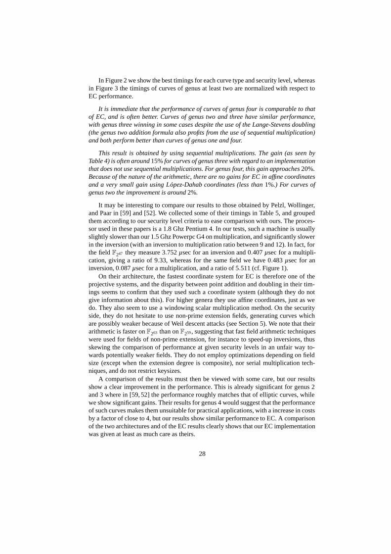
In Figure 2 we show the best timings for each curve type and security level, whereasin Figure 3 the timings of curves of genus at least two are normalized with respect toEC performance.

It is immediate that the performance of curves of genus four is comparable to thatof EC, and is often better. Curves of genus two and three have similar performance,with genus three winning in some cases despite the use of the Lange-Stevens doubling(the genus two addition formula also profits from the use of sequential multiplication)and both perform better than curves of genus one and four.

This result is obtained by using sequential multiplications. The gain (as seen byTable 4) is often around 15% for curves of genus three with regard to an implementationthat does not use sequential multiplications. For genus four, this gain approaches 20%.Because of the nature of the arithmetic, there are no gains for EC in affine coordinatesand a very small gain using Lopez-Dahab coordinates (less than 1%.) For curves ofgenus two the improvement is around 2%.

It may be interesting to compare our results to those obtained by Pelzl, Wollinger,and Paar in [59] and [52]. We collected some of their timings in Table 5, and groupedthem according to our security level criteria to ease comparison with ours. The proces-sor used in these papers is a 1.8 Ghz Pentium 4. In our tests, such a machine is usuallyslightly slower than our 1.5 Ghz Powerpc G4 on multiplication, and significantly slowerin the inversion (with an inversion to multiplication ratio between 9 and 12). In fact, forthe field F247 they measure 3.752 µsec for an inversion and 0.407 µsec for a multipli-cation, giving a ratio of 9.33, whereas for the same field we have 0.483 µsec for aninversion, 0.087 µsec for a multiplication, and a ratio of 5.511 (cf. Figure 1).

On their architecture, the fastest coordinate system for EC is therefore one of theprojective systems, and the disparity between point addition and doubling in their tim-ings seems to confirm that they used such a coordinate system (although they do notgive information about this). For higher genera they use affine coordinates, just as wedo. They also seem to use a windowing scalar multiplication method. On the securityside, they do not hesitate to use non-prime extension fields, generating curves whichare possibly weaker because of Weil descent attacks (see Section 5). We note that theirarithmetic is faster on F263 than on F259 , suggesting that fast field arithmetic techniqueswere used for fields of non-prime extension, for instance to speed-up inversions, thusskewing the comparison of performance at given security levels in an unfair way to-wards potentially weaker fields. They do not employ optimizations depending on fieldsize (except when the extension degree is composite), nor serial multiplication tech-niques, and do not restrict keysizes.

A comparison of the results must then be viewed with some care, but our resultsshow a clear improvement in the performance. This is already significant for genus 2and 3 where in [59, 52] the performance roughly matches that of elliptic curves, whilewe show significant gains. Their results for genus 4 would suggest that the performanceof such curves makes them unsuitable for practical applications, with a increase in costsby a factor of close to 4, but our results show similar performance to EC. A comparisonof the two architectures and of the EC results clearly shows that our EC implementationwas given at least as much care as theirs.

28

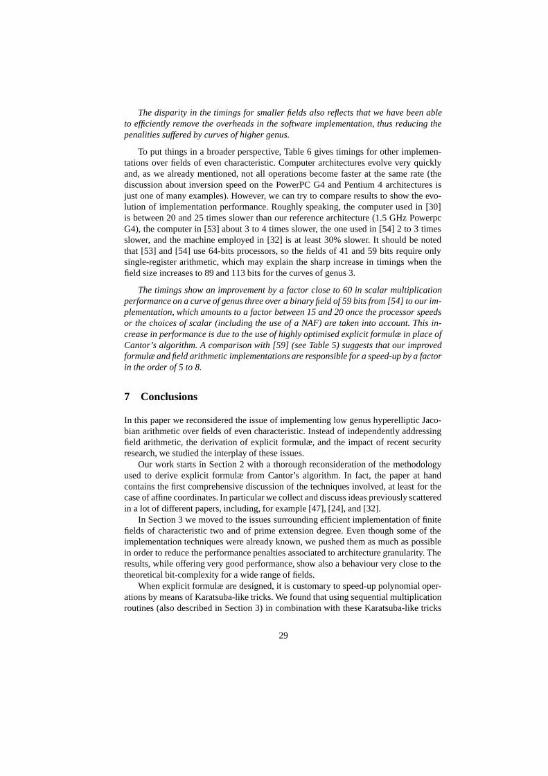
The disparity in the timings for smaller fields also reflects that we have been ableto efficiently remove the overheads in the software implementation, thus reducing thepenalities suffered by curves of higher genus.

To put things in a broader perspective, Table 6 gives timings for other implemen-tations over fields of even characteristic. Computer architectures evolve very quicklyand, as we already mentioned, not all operations become faster at the same rate (thediscussion about inversion speed on the PowerPC G4 and Pentium 4 architectures isjust one of many examples). However, we can try to compare results to show the evo-lution of implementation performance. Roughly speaking, the computer used in [30]is between 20 and 25 times slower than our reference architecture (1.5 GHz PowerpcG4), the computer in [53] about 3 to 4 times slower, the one used in [54] 2 to 3 timesslower, and the machine employed in [32] is at least 30% slower. It should be notedthat [53] and [54] use 64-bits processors, so the fields of 41 and 59 bits require onlysingle-register arithmetic, which may explain the sharp increase in timings when thefield size increases to 89 and 113 bits for the curves of genus 3.

The timings show an improvement by a factor close to 60 in scalar multiplicationperformance on a curve of genus three over a binary field of 59 bits from [54] to our im-plementation, which amounts to a factor between 15 and 20 once the processor speedsor the choices of scalar (including the use of a NAF) are taken into account. This in-crease in performance is due to the use of highly optimised explicit formulæ in place ofCantor’s algorithm. A comparison with [59] (see Table 5) suggests that our improvedformulæ and field arithmetic implementations are responsible for a speed-up by a factorin the order of 5 to 8.

7 Conclusions

In this paper we reconsidered the issue of implementing low genus hyperelliptic Jaco-bian arithmetic over fields of even characteristic. Instead of independently addressingfield arithmetic, the derivation of explicit formulæ, and the impact of recent securityresearch, we studied the interplay of these issues.

Our work starts in Section 2 with a thorough reconsideration of the methodologyused to derive explicit formulæ from Cantor’s algorithm. In fact, the paper at handcontains the first comprehensive discussion of the techniques involved, at least for thecase of affine coordinates. In particular we collect and discuss ideas previously scatteredin a lot of different papers, including, for example [47], [24], and [32].

In Section 3 we moved to the issues surrounding efficient implementation of finitefields of characteristic two and of prime extension degree. Even though some of theimplementation techniques were already known, we pushed them as much as possiblein order to reduce the performance penalties associated to architecture granularity. Theresults, while offering very good performance, show also a behaviour very close to thetheoretical bit-complexity for a wide range of fields.

When explicit formulæ are designed, it is customary to speed-up polynomial oper-ations by means of Karatsuba-like tricks. We found that using sequential multiplicationroutines (also described in Section 3) in combination with these Karatsuba-like tricks

29

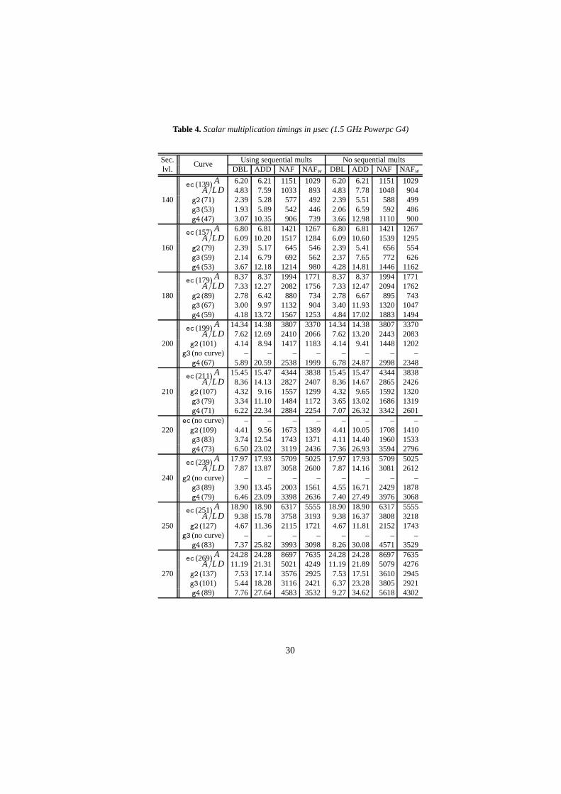
Table 4. Scalar multiplication timings in µsec (1.5 GHz Powerpc G4)

Sec. Using sequential mults No sequential multslvl.

CurveDBL ADD NAF NAFw DBL ADD NAF NAFw

ec (139) A 6.20 6.21 1151 1029 6.20 6.21 1151 1029A/LD 4.83 7.59 1033 893 4.83 7.78 1048 904

140 g2 (71) 2.39 5.28 577 492 2.39 5.51 588 499g3 (53) 1.93 5.89 542 446 2.06 6.59 592 486g4 (47) 3.07 10.35 906 739 3.66 12.98 1110 900

ec (157) A 6.80 6.81 1421 1267 6.80 6.81 1421 1267A/LD 6.09 10.20 1517 1284 6.09 10.60 1539 1295

160 g2 (79) 2.39 5.17 645 546 2.39 5.41 656 554g3 (59) 2.14 6.79 692 562 2.37 7.65 772 626g4 (53) 3.67 12.18 1214 980 4.28 14.81 1446 1162

ec (179) A 8.37 8.37 1994 1771 8.37 8.37 1994 1771A/LD 7.33 12.27 2082 1756 7.33 12.47 2094 1762

180 g2 (89) 2.78 6.42 880 734 2.78 6.67 895 743g3 (67) 3.00 9.97 1132 904 3.40 11.93 1320 1047g4 (59) 4.18 13.72 1567 1253 4.84 17.02 1883 1494

ec (199) A 14.34 14.38 3807 3370 14.34 14.38 3807 3370A/LD 7.62 12.69 2410 2066 7.62 13.20 2443 2083

200 g2 (101) 4.14 8.94 1417 1183 4.14 9.41 1448 1202g3 (no curve) – – – – – – – –

g4 (67) 5.89 20.59 2538 1999 6.78 24.87 2998 2348

ec (211) A 15.45 15.47 4344 3838 15.45 15.47 4344 3838A/LD 8.36 14.13 2827 2407 8.36 14.67 2865 2426

210 g2 (107) 4.32 9.16 1557 1299 4.32 9.65 1592 1320g3 (79) 3.34 11.10 1484 1172 3.65 13.02 1686 1319g4 (71) 6.22 22.34 2884 2254 7.07 26.32 3342 2601

ec (no curve) – – – – – – – –220 g2 (109) 4.41 9.56 1673 1389 4.41 10.05 1708 1410

g3 (83) 3.74 12.54 1743 1371 4.11 14.40 1960 1533g4 (73) 6.50 23.02 3119 2436 7.36 26.93 3594 2796

ec (239) A 17.97 17.93 5709 5025 17.97 17.93 5709 5025A/LD 7.87 13.87 3058 2600 7.87 14.16 3081 2612

240 g2 (no curve) – – – – – – – –g3 (89) 3.90 13.45 2003 1561 4.55 16.71 2429 1878g4 (79) 6.46 23.09 3398 2636 7.40 27.49 3976 3068

ec (251) A 18.90 18.90 6317 5555 18.90 18.90 6317 5555A/LD 9.38 15.78 3758 3193 9.38 16.37 3808 3218

250 g2 (127) 4.67 11.36 2115 1721 4.67 11.81 2152 1743g3 (no curve) – – – – – – – –

g4 (83) 7.37 25.82 3993 3098 8.26 30.08 4571 3529

ec (269) A 24.28 24.28 8697 7635 24.28 24.28 8697 7635A/LD 11.19 21.31 5021 4249 11.19 21.89 5079 4276

270 g2 (137) 7.53 17.14 3576 2925 7.53 17.51 3610 2945g3 (101) 5.44 18.28 3116 2421 6.37 23.28 3805 2921g4 (89) 7.76 27.64 4583 3532 9.27 34.62 5618 4302

30

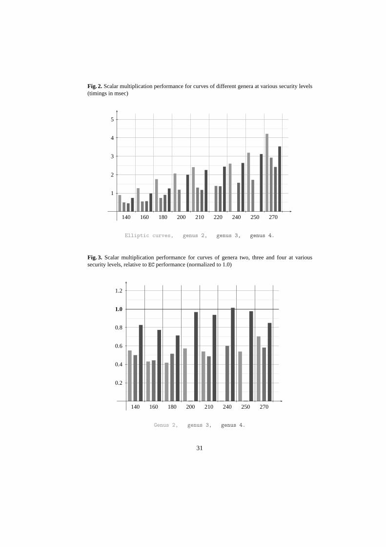
Fig. 2. Scalar multiplication performance for curves of different genera at various security levels(timings in msec)

140 160 180 200 210 220 240 250 270

1

2

3

4

5

Elliptic curves, genus 2, genus 3, genus 4.

Fig. 3. Scalar multiplication performance for curves of genera two, three and four at varioussecurity levels, relative to EC performance (normalized to 1.0)

140 160 180 200 210 240 250 270

0.2

0.4

0.6

0.8

1.0

1.2

Genus 2, genus 3, genus 4.

31

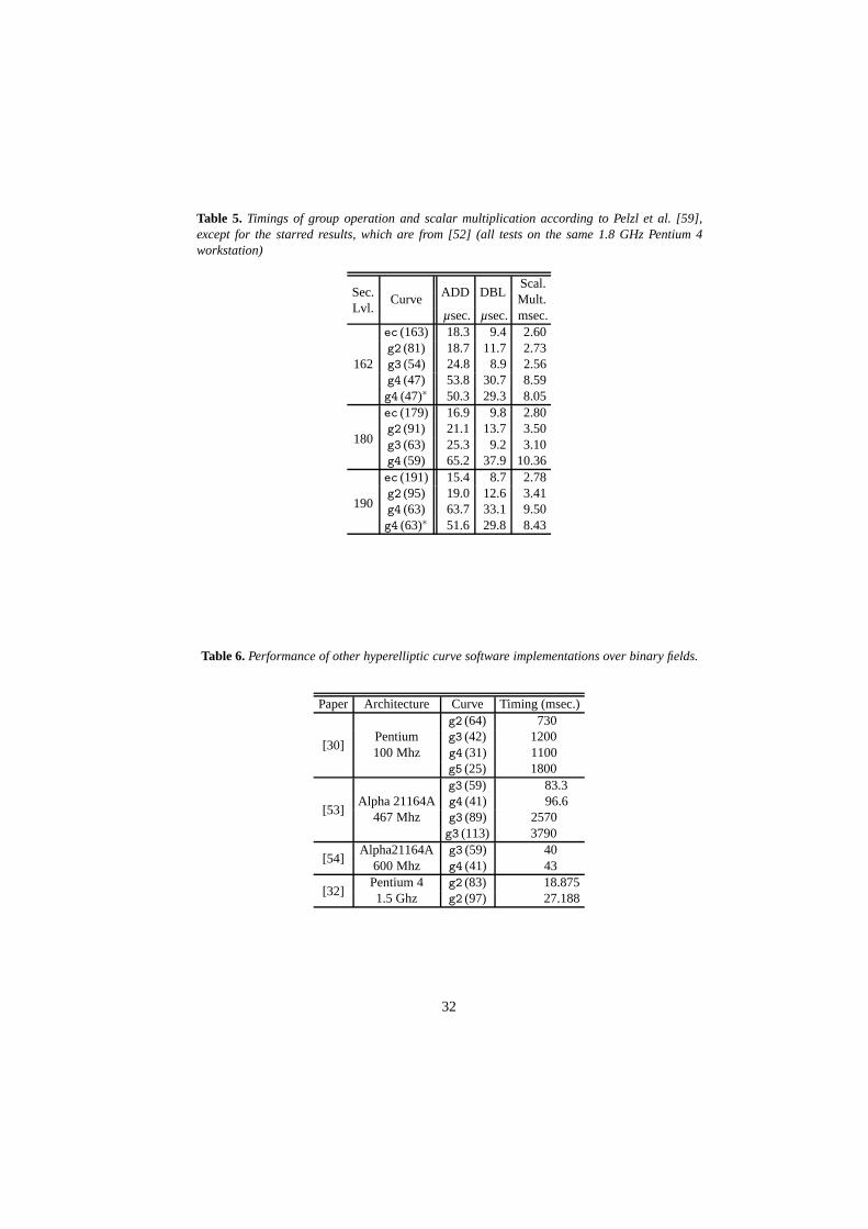
Table 5. Timings of group operation and scalar multiplication according to Pelzl et al. [59],except for the starred results, which are from [52] (all tests on the same 1.8 GHz Pentium 4workstation)

Sec. ADD DBLScal.

Lvl.Curve Mult.

µsec. µsec. msec.ec (163) 18.3 9.4 2.60g2 (81) 18.7 11.7 2.73

162 g3 (54) 24.8 8.9 2.56g4 (47) 53.8 30.7 8.59g4 (47)∗ 50.3 29.3 8.05ec (179) 16.9 9.8 2.80g2 (91) 21.1 13.7 3.50

180 g3 (63) 25.3 9.2 3.10g4 (59) 65.2 37.9 10.36ec (191) 15.4 8.7 2.78g2 (95) 19.0 12.6 3.41

190 g4 (63) 63.7 33.1 9.50g4 (63)∗ 51.6 29.8 8.43

Table 6. Performance of other hyperelliptic curve software implementations over binary fields.

Paper Architecture Curve Timing (msec.)g2 (64) 730

[30]Pentium g3 (42) 1200100 Mhz g4 (31) 1100

g5 (25) 1800g3 (59) 83.3

[53]Alpha 21164A g4 (41) 96.6

467 Mhz g3 (89) 2570g3 (113) 3790

[54]Alpha21164A g3 (59) 40

600 Mhz g4 (41) 43

[32]Pentium 4 g2 (83) 18.8751.5 Ghz g2 (97) 27.188

32

brings substantial performance gains, especially as the genus increases. This is one ofthe key observations in Section 4, and these are reflected in the real world results re-ported in Section 6. For genera three, resp. four, the gains are often close to 15%, resp.20%. Smaller gains can be obtained even when using Lopez-Dahab coordinates for el-liptic curves as well as in the affine genus two formulæ: this has been taken into accountin our comparisons. Our genus four formulæ are much better than the best ones previ-ously published (for example, doublings costs decrease from 2I+75M+14S in [52] to1I+28M+16S in this paper) and are further improved by the use of sequential multipli-cations

Moreover, we restrict the computations to specific subgroups or subsets of the con-sidered algebraic groups to speed up scalar multiplication provided there is no reductionin security (Section 5) by doing so. This is due to the fact that index calculus methodsattack the DLP in the whole algebraic group and do not consider subgroups or key sizes- whereas square root methods (such as Pollard’s methods) can be restricted to searchin subgroups or among keys of a certain size.

Some interesting results and observations stemming from the benchmarks (Sec-tion 6) are:

– Curves of genus three provide similar performance to curves of genus two, andperform even better in some circumstances.If sequential multiplications can successfully be implemented in hardware, thesecurves could be very interesting for hardware implementors since smaller multi-plying units are required for genus three than for genus two.

– Cryptographically secure curves of genus three and four may be easier to find sincewe can allow larger cofactors than in the genus one and two cases.

– Genus four is still interesting, when used wisely, as its performance is comparableto that of elliptic curves.

References

1. R. Avanzi, H. Cohen, C. Doche, G. Frey, T. Lange, K. Nguyen, and F. Vercauteren. TheHandbook of Elliptic and Hyperelliptic Curve Cryptography. CRC Press, 2005.

2. R. Avanzi. Aspects of hyperelliptic curves over large prime fields in software implemen-tations. In Cryptographic Hardware and Embedded Systems – CHES 2004, LNCS 3156,148–162, Springer-Verlag, 2004.

3. R. Avanzi. Generic Algorithms for Computing Discrete Logarithms. In [1], chapter 19,477–494.

4. R. Avanzi and N. Theriault. Index Calculus. In [1], chapter 20, 495–509.5. R. Avanzi and N. Theriault. Index Calculus for Hyperelliptic Curves. In [1], chapter 21,

511–527.6. I. F. Blake, G. Seroussi, and N. P. Smart. Elliptic curves in cryptography. London Math-

ematical Society Lecture Note Series, vol. 265. Cambridge University Press, Cambridge,1999.

7. I. F. Blake, G. Seroussi, and N. P. Smart. Advances in Elliptic Curve Cryptography. LondonMathematical Society Lecture Note Series, vol. 317. Cambridge University Press, Cam-bridge, 2005.

8. D. G. Cantor. Computing in the Jacobian of hyperelliptic curves. Mathematics of Computa-tion, 48 (177), 95–101, 1987.

33

9. C. Doche and T. Lange. Arithmetic of Elliptic Curves. In [1], chapter 13, 267–302.10. S. Duquesne and T. Lange. Arithmetic of Hyperelliptic Curves. In [1], chapter 14, 303–353.11. ECRYPT. Ecrypt yearly report on algorithms and keysizes. Technical report, ECRYPT,

2005.12. A. Enge. Computing discrete logarithms in high-genus hyperelliptic Jacobians in provably

subexponential time. Mathematics of Computation, 71 (238), 729–742, 2002.13. X. Fan, T. Wollinger and Y. Wang. Efficient Doubling on Genus 3 Curves over Binary Fields.

IACR ePrint 2005/228.Available from http://eprint.iacr.org/2005/228

14. K. Fong, D, Hankerson, J, Lopez, A, Menezes:. Field Inversion and Point Halving Revisited.IEEE Trans. Computers 53(8), 1047–1059, 2004.

15. G. Frey, M. Muller, and H. Ruck. The Tate pairing and the discrete logarithm applied toelliptic curve cryptosystems. IEEE Transactions on Information Theory, 45 (5), 1717–1719,1999.

16. G. Frey and H. Ruck. A remark concerning m−divisibility and the discrete logarithm prob-lem in the divisor class group of curves. Mathematics of Computation, 62 (206), 865–874,1994.

17. S. D. Galbraith. Supersingular Curves in Cryptography. In: Advances in Cryptology – Asi-acrypt 2001. LNCS 2248, 49–513, Springer-Verlag, 2001.

18. P. Gaudry. Index calculus for abelian varieties and the elliptic curve discrete logarithm prob-lem IACR ePrint 2004/073.Available from http://eprint.iacr.org/2004/073

19. P. Gaudry, F. Hess and N. P. Smart. Constructive and destructive facets of Weil descent onelliptic curves. J. Cryptology, 15, no. 1, 19-46, 2002.

20. P. Gaudry, E. Thome, N. Theriault and C. Diem. A double large prime variation for smallgenus hyperelliptic index calculus. IACR ePrint 2004/153.Available from http://eprint.iacr.org/2004/153

21. C. Guyot, K. Kaveh and V. M. Patankar. Explicit algorithm for the arithmetic on the hyper-elliptic Jacobians of genus 3. Journal of the Ramanujan Mathematical Society, 19, no. 2,75–115, 2004.

22. D. Hankerson, J. Lopez-Hernandez, and A. Menezes. Software Implementation of Ellip-tic Curve Cryprography over Binary Fields. In: Cryptographic Hardware and EmbeddedSystems – CHES 2000. LNCS 1965, 1–24, Springer-Verlag, 2001.

23. D. Hankerson, A. J. Menezes, and S. A. Vanstone. Guide to elliptic curve cryptography.Springer-Verlag, 2003.

24. R. Harley. Fast arithmetic on genus two curves.Available at: http://cristal.inria.fr/harley/hyper/, 2000

25. F. Hess. The GHS Attack Revisited. In: Advances in Cryptology – Eurocrypt 2003. LNCS2656, 374–387, Springer-Verlag, 2003.

26. A. Karatsuba and Y. Ofman. Multiplication of Multidigit Numbers on Automata. SovietPhysics - Doklady, 7, 595–596, 1963.

27. N. Koblitz. Elliptic curve cryptosystems. Mathematics of Computation, 48 (177), 203–209,1987.

28. N. Koblitz. Algebraic aspects of cryptography. Springer-Verlag, 1998.29. N. Koblitz. Hyperelliptic cryptosystems. J. Cryptology, 1, 139–150, 1989.30. U. Krieger. signature.c, Masters thesis. Fachbereich Mathematik und Informatik, Uni-

versitat Duisburg–Essen, Essen, Germany, February 1997.31. J. Kuroki, M. Gonda, K. Matsuo, J. Chao and S. Tsujii. Fast genus three hyperelliptic curve

cryptosystems. The 2002 Symposium on Cryptography and Information Security, Japan –SCIS 2002, 29 Jan. – 1 Feb. 2002.

34

32. T. Lange. Efficient Arithmetic on Genus 2 Hyperelliptic Curves over Finite Fields via Ex-plicit Formulae. Cryptology ePrint Archive, Report 2002/121, 2002, http://eprint.iacr.org/.

33. T. Lange. Formulae for arithmetic on genus 2 hyperelliptic curves. Appl. Algebra Engrg.Comm. Comput. 15, no. 5, 295–328, 2005.

34. T. Lange and M. Stevens. Efficient doubling for genus two curves over binary fields. In:Selected Areas in Cryptography – SAC 2004. LNCS 3357, 170–181, Springer-Verlag, 2005.

35. A. K. Lenstra, E. R. Verheul. Selecting Cryptographic Key Sizes. J. Cryptology, 14 (4),255–293, 2001.

36. R. Lercier, D. Lubicz and F. Vercauteren. Point Counting on Elliptic and HyperellipticCurves. In [1], chapter 17, 407–453.

37. C.-H. Lim and H.-S. Hwang. Fast Implementation of Elliptic Curve Arithmetic in GF(pn)In Public Key Cryptography, Proceedings of PKC 2000, 405–421. Springer-Verlag 2000.

38. C. Lim and P. Lee. More flexible exponentiation with precomputation. In: Advances inCryptology - Crypto ’94. LNCS 839, 95–107, Springer-Verlag 1994.

39. J. Lopez and R. Dahab. High-speed software multiplication in F2m . Progress in Cryptology- INDOCRYPT 2000. LNCS 1977, 203–212, Springer-Verlag, 2000.

40. K. Matsuo, J. Chao and S. Tsujii. Fast genus two hyperelliptic curve cryptosystems. In:ISEC2001-31, IEICE, 2001.

41. A. Menezes, T. Okamoto and S. Vanstone. Reducing elliptic curve logarithms in a finitefield. IEEE Transactions on Information Theory, vol. IT-39 (5), 1639–1646, 1993.

42. A. Menezes and E. Teske. Cryptographic Implications of Hess’ Generalized GHS Attack.IACR ePrint 2004/235.Available from http://eprint.iacr.org/2004/235

43. A. Menezes, Y.-H. Wu and R. Zuccherato. An Elementary Introduction to HyperellipticCurves. In [28]. Pages 155–178.

44. V. S. Miller. Use of elliptic curves in cryptography. In: Advances in Cryptology – Crypto1985. LNCS 218, 417–426. Springer-Verlag, 1986.

45. Y. Miyamoto, H. Doi, K. Matsuo, J. Chao, and S. Tsuji. A Fast Addition Algorithm of GenusTwo Hyperelliptic Curve. In: SCIS 2002, IEICE Japan, 2002, 497–502. In Japanese.

46. D. Mumford. Tata Lectures on Theta II. Birkhauser, 1984.47. K. Nagao. Improving group law algorithms for Jacobians of hyperelliptic curves. In: Algo-

rithmic Number Theory – ANTS-IV. LNCS 1838, 439–448, Springer-Verlag, 2000.48. K. Nagao. Improvement of Theriault Algorithm of Index Calculus for Jacobian of Hyperel-

liptic Curves of Small Genus. IACR ePrint 2004/161.Available from http://eprint.iacr.org/2004/161

49. NIST. Key Management Guideline - Workshop Document. Draft, October 2001.Available fromhttp://csrc.nist.gov/encryption/kms/key-management-guideline-(workshop).pdf

50. J. Pelzl, T. Wollinger, J. Guajardo and C. Paar. Hyperelliptic curve cryptosystems: closingthe perfomance gap to elliptic curves (Update). IACR ePrint 2003/026.Available from http://eprint.iacr.org/2003/026

51. J. Pelzl, T. Wollinger and C. Paar. High Performance Arithmetic for Hyperelliptic CurveCryptosystems of Genus Two. IACR ePrint 2003/212.Available from http://eprint.iacr.org/2003/212

52. J. Pelzl, T. Wollinger and C. Paar. Low cost Security: Explicit Formulae for Genus 4 Hy-perelliptic Curves. In: Selected Areas in Cryptography – SAC 2003. LNCS 3006, 1–16,Springer-Verlag, 2004.

53. Y. Sakai and K. Sakurai. Design of Hyperelliptic Cryptosystems in small Characteristic anda Software Implementation over F2n . In Advances in Cryptology - ASIACRYPT 98. LNCS1514, 80–94. Springer Verlag, 1998.0

35

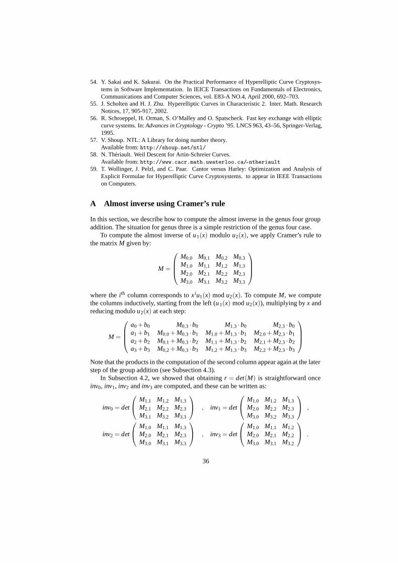
54. Y. Sakai and K. Sakurai. On the Practical Performance of Hyperelliptic Curve Cryptosys-tems in Software Implementation. In IEICE Transactions on Fundamentals of Electronics,Communications and Computer Sciences, vol. E83-A NO.4, April 2000, 692–703.

55. J. Scholten and H. J. Zhu. Hyperelliptic Curves in Characteristic 2. Inter. Math. ResearchNotices, 17, 905-917, 2002.

56. R. Schroeppel, H. Orman, S. O’Malley and O. Spatscheck. Fast key exchange with ellipticcurve systems. In: Advances in Cryptology - Crypto ’95. LNCS 963, 43–56, Springer-Verlag,1995.

57. V. Shoup. NTL: A Library for doing number theory.Available from: http://shoup.net/ntl/

58. N. Theriault. Weil Descent for Artin-Schreier Curves.Available from: http://www.cacr.math.uwaterloo.ca/~ntheriault

59. T. Wollinger, J. Pelzl, and C. Paar. Cantor versus Harley: Optimization and Analysis ofExplicit Formulae for Hyperelliptic Curve Cryptosystems. to appear in IEEE Transactionson Computers.

A Almost inverse using Cramer’s rule

In this section, we describe how to compute the almost inverse in the genus four groupaddition. The situation for genus three is a simple restriction of the genus four case.

To compute the almost inverse of u1(x) modulo u2(x), we apply Cramer’s rule tothe matrix M given by:

M =

M0,0 M0,1 M0,2 M0,3

M1,0 M1,1 M1,2 M1,3

M2,0 M2,1 M2,2 M2,3

M3,0 M3,1 M3,2 M3,3

where the ith column corresponds to xiu1(x) mod u2(x). To compute M, we computethe columns inductively, starting from the left (u 1(x) mod u2(x)), multiplying by x andreducing modulo u2(x) at each step:

M =

a0 +b0 M0,3 ·b0 M1,3 ·b0 M2,3 ·b0

a1 +b1 M0,0 +M0,3 ·b1 M1,0 +M1,3 ·b1 M2,0 +M2,3 ·b1

a2 +b2 M0,1 +M0,3 ·b2 M1,1 +M1,3 ·b2 M2,1 +M2,3 ·b2

a3 +b3 M0,2 +M0,3 ·b3 M1,2 +M1,3 ·b3 M2,2 +M2,3 ·b3

Note that the products in the computation of the second column appear again at the laterstep of the group addition (see Subsection 4.3).

In Subsection 4.2, we showed that obtaining r = det(M) is straightforward onceinv0, inv1, inv2 and inv3 are computed, and these can be written as:

inv0 = det

M1,1 M1,2 M1,3

M2,1 M2,2 M2,3

M3,1 M3,2 M3,3

, inv1 = det

M1,0 M1,2 M1,3

M2,0 M2,2 M2,3

M3,0 M3,2 M3,3

,

inv2 = det

M1,0 M1,1 M1,3

M2,0 M2,1 M2,3

M3,0 M3,1 M3,3

, inv3 = det

M1,0 M1,1 M1,2

M2,0 M2,1 M2,2

M3,0 M3,1 M3,2

.

36

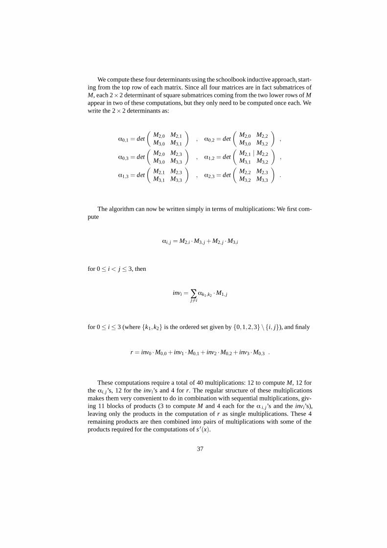
We compute these four determinants using the schoolbook inductive approach, start-ing from the top row of each matrix. Since all four matrices are in fact submatrices ofM, each 2×2 determinant of square submatrices coming from the two lower rows of Mappear in two of these computations, but they only need to be computed once each. Wewrite the 2×2 determinants as:

α0,1 = det

(M2,0 M2,1

M3,0 M3,1

), α0,2 = det

(M2,0 M2,2

M3,0 M3,2

),

α0,3 = det

(M2,0 M2,3

M3,0 M3,3

), α1,2 = det

(M2,1 | M2,2

M3,1 M3,2

),

α1,3 = det

(M2,1 M2,3

M3,1 M3,3

), α2,3 = det

(M2,2 M2,3

M3,2 M3,3

).

The algorithm can now be written simply in terms of multiplications: We first com-pute

αi, j = M2,i ·M3, j +M2, j ·M3,i

for 0≤ i < j ≤ 3, then

invi = ∑j �=i

αk1,k2 ·M1, j

for 0≤ i≤ 3 (where {k1,k2} is the ordered set given by {0,1,2,3} \ {i, j}), and finaly

r = inv0 ·M0,0 + inv1 ·M0,1 + inv2 ·M0,2 + inv3 ·M0,3 .

These computations require a total of 40 multiplications: 12 to compute M, 12 forthe αi, j’s, 12 for the invi’s and 4 for r. The regular structure of these multiplicationsmakes them very convenient to do in combination with sequential multiplications, giv-ing 11 blocks of products (3 to compute M and 4 each for the α i, j’s and the invi’s),leaving only the products in the computation of r as single multiplications. These 4remaining products are then combined into pairs of multiplications with some of theproducts required for the computations of s ′(x).

37

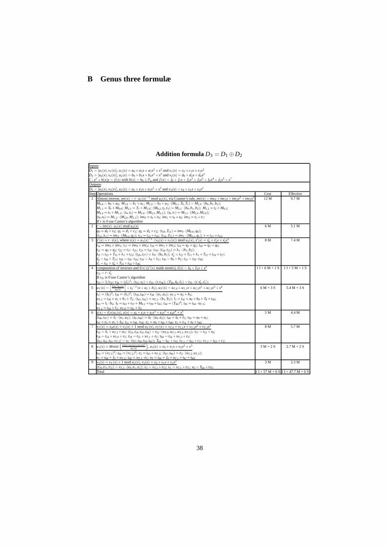
B Genus three formulæ

Addition formula D3 = D1⊕D2

Inputs:D1 = [u1(x),v1(x)], u1(x) = a0 +a1x+a2x2 + x3 and v1(x) = c0 + c1x+ c2x2

D2 = [u2(x),v2(x)], u2(x) = b0 +b1x+b2x2 + x3 and v2(x) = d0 +d1x+d2x2

C : y2 +h(x)y = f (x) with h(x) = h0 ∈ Fq and f (x) = f0 + f1x+ f2x2 + f3x3 + f4x4 + f5x5 + x7

Outputs:D3 = [u3(x),v3(x)], u3(x) = e0 + e1x+ e2x2 + x3 and v3(x) = ε0 + ε1x+ ε2x2

Step Operations Cost Effective1 Almost inverse, inv(x) = r ·u1(x)−1 mod u2(x), via Cramer’s rule, inv(x) = inv0 + inv1x+ inv2x2 + inv3x3 12 M 9.7 M

M0,0 = b0 +a0; M1,0 = b1 +a1; M2,0 = b2 +a2; (M0,1,T0,T1) = M2,0 · (b0,b1,b2);M1,1 = T0 +M0,0; M2,1 = T1 +M1,0; (M0,2,t2,t3) = M2,1 · (b0,b1,b2); M1,2 = t2 +M0,1;M2,2 = t3 +M1,1; (t4,t5) = M1,0 · (M2,2,M2,1); (t6, t7) = M1,1 · (M2,2,M2,0);(t8,t9) = M1,2 · (M2,0,M2,1); inv0 = t6 + t9; inv1 = t4 + t8; inv2 = t5 + t7;If r is 0 use Cantor’s algorithm

2 r = inv(x) ·u1(x) mod u2(x) 6 M 5.1 Mq0 = d0 + c0; q1 = d1 + c1; q2 = d2 + c2; (t10,T11) = inv0 · (M0,0,q0);(t12,λ1) = inv2 · (M0,2,q2); t13 = t12 + t10; (t14,T15) = inv1 · (M0,1,q1); r = t13 + t14;

3 s′(x) = r · s(x), where s(x) = u1(x)−1 · (v2(x)+ v1(x)) mod u2(x), s′(x) = s′0 + s′1x+ s′2x2 8 M 7.4 Mt16 = inv0 + inv1; t17 = inv0 + inv2; t18 = inv1 + inv2; t19 = q1 +q2; t20 = q1 +q0;t21 = q0 +q2; t22 = t17 · t21; t23 = t18 · t19; (t24,t25) = λ1 · (b1,b2);λ0 = t25 +T15 +λ1 + t23; (t26,t27) = λ0 · (b0,b2); s′2 = t22 +T11 +λ1 +T15 + t24 + t27;s′0 = t26 +T11; t28 = t20 · t16; t29 = λ0 +λ1; t30 = b0 +b1; t31 = t29 · t30;s′1 = t31 + s′0 +T15 + t24 + t28;

4 computation of inverses and s(x) (s ′(x) made monic), s(x) = s0 + s1x+ x2 1 I + 6 M + 1 S 1 I + 5 M + 1 St32 = r · s′2If t32 is 0 use Cantor’s algorithmt33 = 1/t32; t34 = (s′2)

2; (t35,s2) = t33 · (r,t34); (T36, s0, s1) = t35 · (r,s′0,s′1);5 uT (x) =

[s(x)2u1(x)

u2(x)

]+ s2

−2 (x+a2 +b2), uT (x) = uT,0 +uT,1x+uT,2x2 +uT,3x3 + x4 6 M + 3 S 5.4 M + 3 S

t37 = (s0)2; t38 = (s1)2; (t39,t40) = t38 · (a1,a2); uT,3 = a2 +b2;uT,2 = t38 +a1 +b1 +T1; (t41,t42) = uT,2 · (b1,b2); l1 = t42 +a0 +b0 +T0 + t40;t43 = l1 ·b2; l0 = t43 + t37 +M0,1 + t39 + t41; t44 = (T36)2; t45 = t44 ·uT,3;uT,1 = t44 + l1; uT,0 = t45 + l0;

6 z(x) = s(x)u1(x), z(x) = z0 + z1x+ z2x2 + z3x3 + z4x4 + x5 5 M 4.4 M(t46,t47) = s1 · (a1,a2); (z0,t48) = s0 · (a0,a2); t49 = s0 + s1; t50 = a0 +a1;t47 + z3 = a1 + s0; t51 = t49 · t50; z2 = a0 + t46 + t48; z1 = t51 + z0 + t46;

7 vT (x) = s3z(x)+ v1(x)+1 mod uT (x), vT (x) = vT,0 + vT,1x+ vT,2x2 + vT,3x3 8 M 5.7 Mt52 = s1 +uT,3 +a2; (t53,t54,t55,t56) = t52 · (uT,0,uT,1,uT,2,uT,3); t57 = t53 + z0;t58 = t54 +uT,0 + z1; t59 = t55 +uT,1 + z2; t60 = t56 +uT,2 + z3;(t61,t62,t63,vT,3) = s2 · (t57,t58,t59,t60); T64 = t61 + c0; vT,1 = t62 + c1; vT,2 = t63 + c2;

8 u3(x) = Monic(


uT (x)

), u3(x) = e0 + e1x+ e2x2 + x3 3 M + 2 S 2.7 M + 2 S

t65 = (vT,3)2; t66 = (vT.2)2; e2 = t65 +uT,3; (t67, t68) = e2 · (uT,2,uT,3);e1 = t68 + f5 +uT,2; t69 = uT,3 · e1; e0 = t66 + f4 +uT,1 + t67 + t69;

9 v3(x) = vT (x)+1 mod u3(x), v3(x) = ε0 + ε1x+ ε2x2 3 M 2.3 M(t70,t71,t72) = vT,3 · (e0,e1,e2); ε2 = vT,2 + t72; ε1 = vT,1 + t71; ε0 = T64 + t70;Total 1 I + 57 M + 6 S 1 I + 47.7 M + 6 S

38

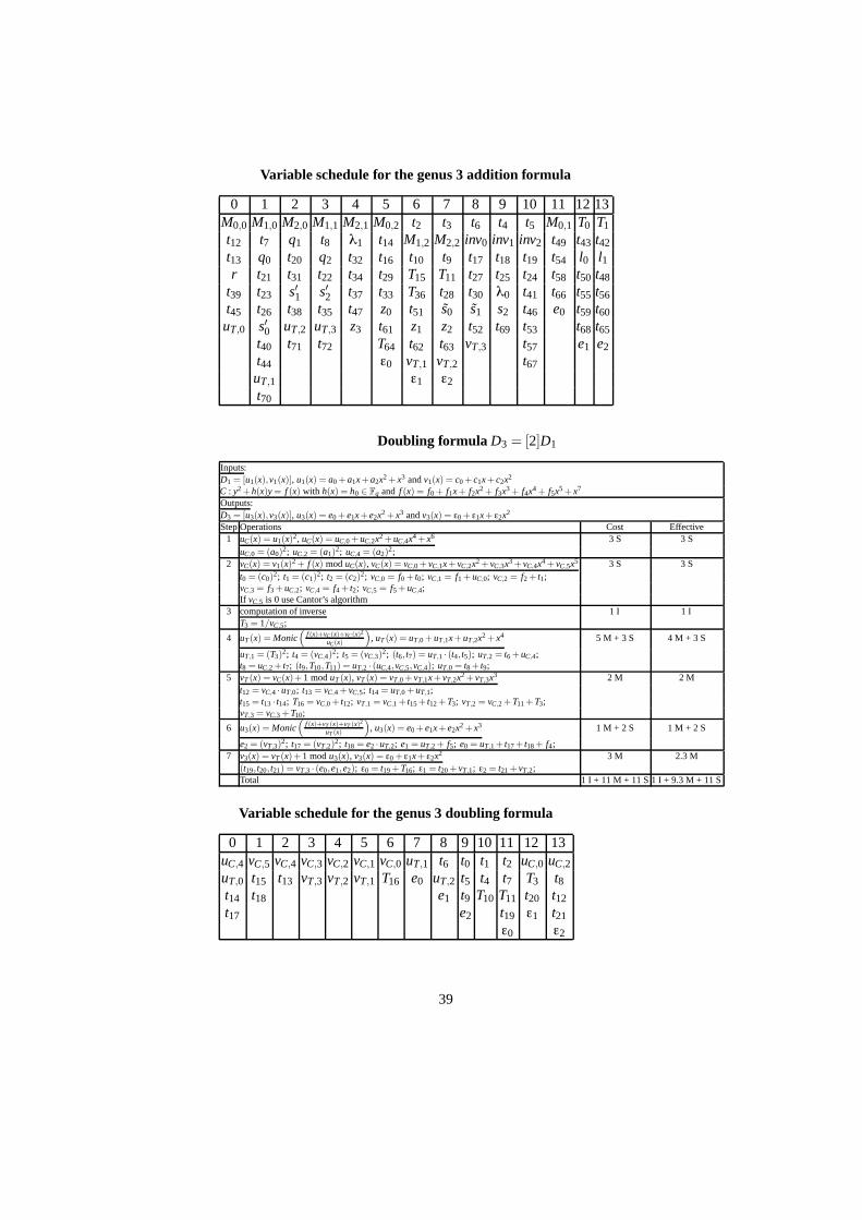
Variable schedule for the genus 3 addition formula

0 1 2 3 4 5 6 7 8 9 10 11 12 13M0,0 M1,0 M2,0 M1,1 M2,1 M0,2 t2 t3 t6 t4 t5 M0,1 T0 T1

t12 t7 q1 t8 λ1 t14 M1,2 M2,2 inv0 inv1 inv2 t49 t43 t42

t13 q0 t20 q2 t32 t16 t10 t9 t17 t18 t19 t54 l0 l1r t21 t31 t22 t34 t29 T15 T11 t27 t25 t24 t58 t50 t48

t39 t23 s′1 s′2 t37 t33 T36 t28 t30 λ0 t41 t66 t55 t56

t45 t26 t38 t35 t47 z0 t51 s0 s1 s2 t46 e0 t59 t60

uT,0 s′0 uT,2 uT,3 z3 t61 z1 z2 t52 t69 t53 t68 t65

t40 t71 t72 T64 t62 t63 vT,3 t57 e1 e2

t44 ε0 vT,1 vT,2 t67

uT,1 ε1 ε2

t70

Doubling formula D3 = [2]D1

Inputs:D1 = [u1(x),v1(x)], u1(x) = a0 +a1x+a2x2 + x3 and v1(x) = c0 + c1x+ c2x2

C : y2 +h(x)y = f (x) with h(x) = h0 ∈ Fq and f (x) = f0 + f1x+ f2x2 + f3x3 + f4x4 + f5x5 + x7

Outputs:D3 = [u3(x),v3(x)], u3(x) = e0 + e1x+ e2x2 + x3 and v3(x) = ε0 + ε1x+ ε2x2

Step Operations Cost Effective1 uC(x) = u1(x)2, uC(x) = uC,0 +uC,2x2 +uC,4x4 + x6 3 S 3 S

uC,0 = (a0)2; uC,2 = (a1)2; uC,4 = (a2)2;2 vC(x) = v1(x)2 + f (x) mod uC(x), vC(x) = vC,0 + vC,1x+ vC,2x2 + vC,3x3 + vC,4x4 + vC,5x5 3 S 3 S

t0 = (c0)2; t1 = (c1)2; t2 = (c2)2; vC,0 = f0 + t0; vC,1 = f1 +uC,0; vC,2 = f2 + t1;vC,3 = f3 +uC,2; vC,4 = f4 + t2; vC,5 = f5 +uC,4;If vC,5 is 0 use Cantor’s algorithm

3 computation of inverse 1 I 1 IT3 = 1/vC,5;

4 uT (x) = Monic(

f (x)+vC(x)+vC(x)2

uC(x)

), uT (x) = uT,0 +uT,1x+uT,2x2 + x4 5 M + 3 S 4 M + 3 S

uT,1 = (T3)2; t4 = (vC,4)2; t5 = (vC,3)2; (t6,t7) = uT,1 · (t4,t5); uT,2 = t6 +uC,4;t8 = uC,2 + t7; (t9,T10,T11) = uT,2 · (uC,4,vC,5,vC,4); uT,0 = t8 + t9;

5 vT (x) = vC(x)+1 mod uT (x), vT (x) = vT,0 + vT,1x+ vT,2x2 + vT,3x3 2 M 2 Mt12 = vC,4 ·uT,0; t13 = vC,4 + vC,5; t14 = uT,0 +uT,1;t15 = t13 · t14; T16 = vC,0 + t12; vT,1 = vC,1 + t15 + t12 +T3; vT,2 = vC,2 +T11 +T3;vT,3 = vC,3 +T10;

6 u3(x) = Monic(


uT (x)

), u3(x) = e0 + e1x+ e2x2 + x3 1 M + 2 S 1 M + 2 S

e2 = (vT,3)2; t17 = (vT,2)2; t18 = e2 ·uT,2; e1 = uT,2 + f5; e0 = uT,1 + t17 + t18 + f4;7 v3(x) = vT (x)+1 mod u3(x), v3(x) = ε0 + ε1x+ ε2x2 3 M 2.3 M

(t19,t20,t21) = vT,3 · (e0,e1,e2); ε0 = t19 +T16; ε1 = t20 + vT,1; ε2 = t21 + vT,2;Total 1 I + 11 M + 11 S 1 I + 9.3 M + 11 S

Variable schedule for the genus 3 doubling formula

0 1 2 3 4 5 6 7 8 9 10 11 12 13uC,4 vC,5 vC,4 vC,3 vC,2 vC,1 vC,0 uT,1 t6 t0 t1 t2 uC,0 uC,2

uT,0 t15 t13 vT,3 vT,2 vT,1 T16 e0 uT,2 t5 t4 t7 T3 t8t14 t18 e1 t9 T10 T11 t20 t12

t17 e2 t19 ε1 t21

ε0 ε2

39

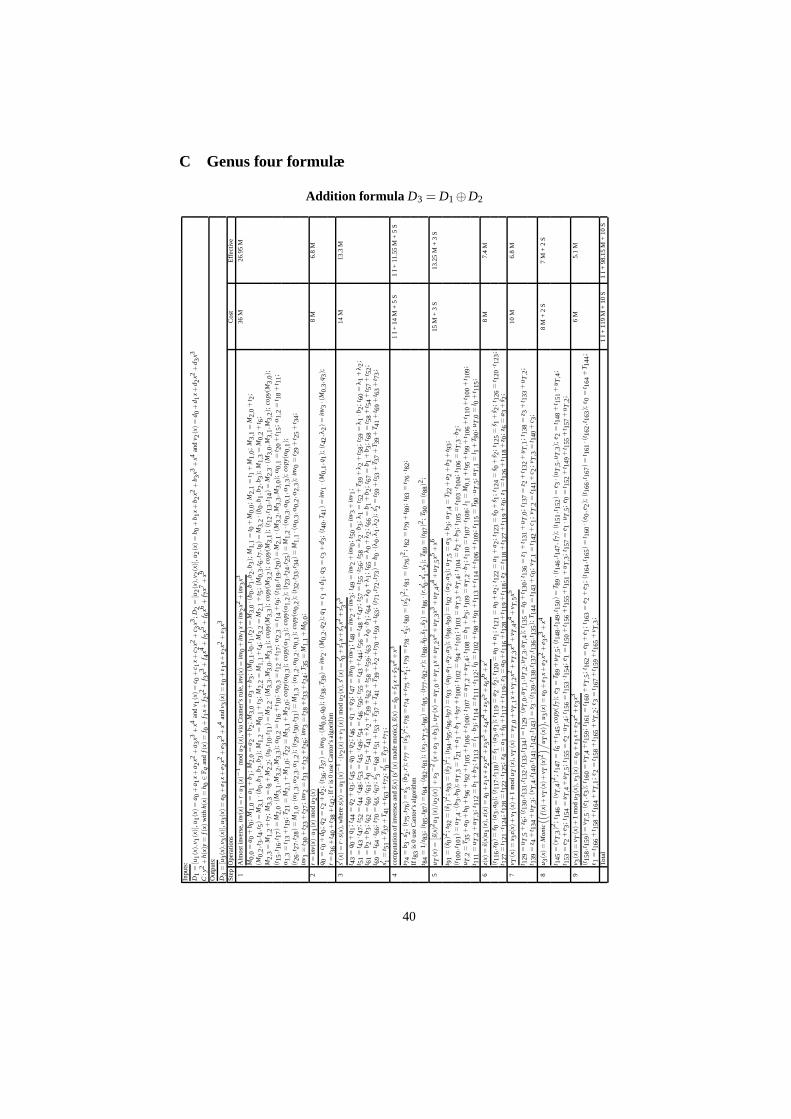
C Genus four formulæ

Addition formula D3 = D1⊕D2

Inpu

ts:

D1

=[u

1(x

),v 1

(x)]

,u1(x

)=

a 0+

a 1x+

a 2x2

+a 3

x3+

x4an

dv 1

(x)=

c 0+

c 1x+

c 2x2

+c 3

x3;D

2=

[u2(x

),v 2

(x)]

,u2(x

)=

b 0+

b 1x+

b 2x2

+b 3

x3+

x4an

dv 2

(x)=

d 0+

d 1x+

d 2x2

+d 3

x3

C:y

2+

h(x)

y=

f(x)

with

h(x)

=h 0∈

Fq

and

f(x)

=f 0

+f 1

x+

f 2x2

+f 3

x3+

f 4x4

+f 5

x5+

f 6x6

+f 7

x7+

x9

Out

puts

:

D3

=[u

3(x

),v 3

(x)]

,u3(x

)=

e 0+

e 1x+

e 2x2

+e 3

x3+

x4an

dv 3

(x)=

ε 0+ε 1

x+ε 2

x2+ε 3

x3

Step

Ope

ratio

nsC

ost

Eff

ectiv

e

1A

lmos

tinv

erse

,inv

(x)=

r·u

1(x

)−1

mod

u 2(x

),vi

aC

ram

er’s

rule

,inv

(x)=

inv 0

+in

v 1x+

inv 2

x2+

inv 3

x336

M26

.95

MM

0,0

=a 0

+b 0

;M

1,0

=a 1

+b 1

;M

2,0

=a 2

+b 2

;M

3,0

=a 3

+b 3

;(M

0,1,t

0,t 1

,t2)=

M3,

0·(b

0,b

1,b

2,b 3

);M

1,1

=t 0

+M

0,0

;M

2,1

=t 1

+M

1,0

;M

3,1

=M

2,0

+t 2

;(M

0,2,t

3,t 4

,t5)

=M

3,1·(b

0,b

1,b 2

,b3);

M1,

2=

M0,

1+

t 3;

M2,

2=

M1,

1+

t 4;

M3,

2=

M2,

1+

t 5;(M

0,3,t

6,t

7,t 8

)=M

3,2·(b

0,b

1,b

2,b 3

);M

1,3

=M

0,2

+t 6

;M

2,3

=M

1,2

+t 7

;M

3,3

=t 8

+M

2,2

;(t

9,t

10,t

11)=

M2,

2·(M

3,3,M

3,0,M

3,1);

copy

(M3,

3);

copy

(M3,

2);

copy

(M3,

1);

(t12

,t13

,t14

)=M

2,3·(M

3,0,M

3,1,

M3,

2);

copy

(M3,

0);

(t15

,t16

,t17

)=M

2,0·(M

3,1,M

3,2,M

3,3);

α0,

2=

t 16

+t 1

0;α

0,3

=t 1

2+

t 17

;α

2,3

=t 1

4+

t 9;(t

18,t

19,t

20)=

M2,

1·(M

3,2,M

3,3,M

3,0);

α0,

1=

t 20

+t 1

5;α

1,2

=t 1

8+

t 11

;α

1,3

=t 1

3+

t 19

;T 2

1=

M2,

1+

M1,

0;

T 22

=M

3,1

+M

2,0

;co

py(α

0,3);

copy

(α1,

3);

copy

(α1,

2);

(t23

,t24

,t25

)=

M1,

2·(α

0,3,α

0,1,α

1,3);

copy

(α0,

1);

(t26

,t27

,t28

)=M

1,0·(α

1,3,α

2,3,α

1,2);

(t29

,t30

,t31

)=M

1,3·(α

1,2,α

0,2,α

0,1);

copy

(α0,

2);

(t32

,t33

,t34

)=M

1,1·(α

0,3,α

0,2,α

2,3);

inv 0

=t 2

9+

t 25

+t 3

4;

inv 1

=t 3

0+

t 23

+t 2

7;

inv 2

=t 3

1+

t 32

+t 2

6;

inv 3

=t 2

8+

t 33

+t 2

4;

T 35

=M

1,1

+M

0,0

;

2r=

inv(

x)·u

1(x

)m

odu 2

(x)

8M

6.8

Mq 0

=c 0

+d 0

;q 2

=c 2

+d 2

;(t

36,T

37)=

inv 0·(M

0,0,q

0);

(t38

,T39

)=

inv 2·(M

0,2,q

2);

q 1=

c 1+

d 1;

q 3=

c 3+

d 3;(t

40,T

41)=

inv 1·(M

0,1,q

1);

(t42

,λ2)=

inv 3·(M

0,3,q

3);

r=

t 36

+t 4

0+

t 38

+t 4

2;I

fr

is0

use

Can

tor’

sal

gori

thm

3s′ (

x)=

r·s(

x),w

here

s(x)

=u 1

(x)−

1·(v

2(x

)+v 1

(x))

mod

u 2(x

),s′ (

x)=

s′ 0+

s′ 1x+

s′ 2x2

+s′ 3

x314

M13

.3M

t 43

=q 0

+q 1

;t 4

4=

q 2+

q 3;

t 45

=q 0

+q 2

;t 4

6=

q 1+

q 3;

t 47

=in

v 0+

inv 1

;t 4

8=

inv 2

+in

v 3;

t 49

=in

v 2+

inv 0

;t 5

0=

inv 3

+in

v 1;

t 51

=t 4

3·t 4

7;

t 52

=t 4

4·t 4

8;

t 53

=t 4

5·t 4

9;

t 54

=t 4

6·t 5

0;

t 55

=t 4

3+

t 44

;t 5

6=

t 48

+t 4

7;

t 57

=t 5

5·t 5

6;

t 58

=λ 2·b

3;λ

1=

t 52

+T 3

9+λ 2

+t 5

8;

t 59

=λ 1·b

2;

t 60

=λ 1

+λ 2

;t 6

1=

b 2+

b 3;

t 62

=t 6

0·t 6

1;λ

0=

t 54

+T 4

1+λ 2

+T 3

9+

t 62

+t 5

8+

t 59

;t 6

3=λ 0·b

1;

t 64

=λ 0

+λ 1

;t 6

5=

λ 0+λ 2

;t 6

6=

b 1+

b 2;

t 67

=b 1

+b 3

;t 6

8=

t 58

+t 5

4+

t 57

+t 5

2;

t 69

=t 6

4·t 6

6;

t 70

=t 6

5·t 6

7;

s′ 3=

t 68

+t 5

1+

t 53

+T 3

7+

T 41

+T 3

9+λ 2

+t 7

0+

t 59

+t 6

3;(t

71,t

72,t

73)=

b 0·(λ

0,λ

1,λ

2);

s′ 2=

t 59

+t 5

3+

T 37

+T 3

9+

T 41

+t 6

9+

t 63

+t 7

3;

s′ 1=

t 51

+T 3

7+

T 41

+t 6

3+

t 72

;s′ 0

=T 3

7+

t 71

;

4co

mpu

tatio

nof

inve

rses

and

s(x)

(s′ (x

)m

ade

mon

ic),

s(x)

=s 0

+s 1

x+

s 2x2

+x3

1I

+14

M+

5S

1I

+11

.55

M+

5S

t 74

=b 3·s′ 2

;(t

75,t

76)=

s′ 3·(b

2,r

);t 7

7=

(s′ 3)2

;t 7

8=

t 74

+t 7

5+

s′ 1;

t 79

=t 7

8·s′ 3

;t 8

0=

(s′ 2)2

;t 8

1=

(t76

)2;

t 82

=t 7

9+

t 80

;t 8

3=

t 76·t 8

2;

Ift 8

3is

0us

eC

anto

r’s

algo

rith

m

t 84

=1/

t 83

;(t

85,t

87)=

t 84·(t

82,t

81);

(s3,v

T,5

,t86

)=

t 85·(t

77,t

82,r

);(t

88,s

0,s

1,s

2)=

t 86·(r

,s′ 0,s′ 1,s′ 2);

T 89

=(t

87)2

;T 9

0=

(t88

)2;

5u T

(x)=[ s(

x)2

u 1(x

)/u 2

(x)] +

s 3−2( x

+a 3

+b 3) ,u

T(x

)=

u T,0

+u T

,1x+

u T,2

x2+

u T,3

x3+

u T,4

x4+

u T,5

x5+

x615

M+

3S

13.2

5M

+3

S

t 91

=(s

0)2

;t 9

2=

(s1)2

;t 9

3=

(s2)2

;(t

94,t

95,t

96,t

97)=

t 93·(a

0,a

1,a

2,a

3);

(t98

,t99

)=t 9

2·(a

2,a

3);

u T,5

=a 3

+b 3

;u T

,4=

T 22

+a 2

+b 2

+t 9

3;

(t10

0,t

101)=

u T,4·(b

3,b

0);

u T,3

=T 2

1+

a 1+

b 1+

t 97

+t 1

00;

t 102

=t 9

4+

t 101

;t 1

03=

u T,3

+u T

,4;

t 104

=b 2

+b 3

;t 1

05=

t 103·t 1

04;

t 106

=u T

,3·b

2;

u T,2

=T 3

5+

a 0+

b 0+

t 96

+t 9

2+

t 105

+t 1

06+

t 100

;t 1

07=

u T,2

+u T

,4;

t 108

=b 1

+b 3

;t 1

09=

u T,2·b

1;

t 110

=t 1

07·t 1

08;

l 1=

M0,

1+

t 95

+t 9

9+

t 106

+t 1

10+

t 100

+t 1

09;

t 111

=u T

,2+

u T,3

;t 1

12=

b 1+

b 2;

t 113

=l 1·b

3;

t 114

=t 1

11·t 1

12;

l 0=

t 102

+t 9

8+

t 91

+t 1

13+

t 114

+t 1

06+

t 109

;t 1

15=

T 90·u

T,5

;u T

,1=

l 1+

T 90

;u T

,0=

l 0+

t 115

;

6z(

x)=

s(x)

u 1(x

),z(

x)=

z 0+

z 1x+

z 2x2

+z 3

x3+

z 4x4

+z 5

x5+

z 6x6

+x7

8M

7.4

M

(t11

6,z

0)=

s 0·(a

3,a

0);(t

117,t

118)=

s 1·(a

3,a

1);

t 119

=a 2·s 2

;t 1

20=

a 0+

a 1;

t 121

=a 0

+a 2

;t 1

22=

a 1+

a 2;

t 123

=s 0

+s 1

;t 1

24=

s 0+

s 2;

t 125

=s 1

+s 2

;t 1

26=

t 120·t 1

23;

t 127

=t 1

21·t 1

24;

t 128

=t 1

22·t 1

25;

z 4=

a 1+

s 0+

t 117

+t 1

19;

z 3=

a 0+

t 116

+t 1

28+

t 119

+t 1

18;

z 2=

t 118

+t 1

27+

t 119

+z 0

;z 1

=t 1

26+

t 118

+z 0

;z 6

=a 3

+s 2

;

7v T

(x)=

s 3z(

x)+

v 1(x

)+1

mod

u T(x

),v T

(x)=

v T,0

+v T

,1x+

v T,2

x2+

v T,3

x3+

v T,4

x4+

v T,5

x510

M6.

8M

t 129

=u T

,5+

z 6;(t

130,t

131,t

132,t

133,t

134)=

t 129·(u

T,0

,uT,1

,uT,2

,uT,3

,uT,4

);t 1

35=

z 0+

t 130

;t 1

36=

z 1+

t 131

+u T

,0;

t 137

=z 2

+t 1

32+

u T,1

;t 1

38=

z 3+

t 133

+u T

,2;

t 139

=z 4

+t 1

34+

u T,3

;(v

T,4

,t14

0,t

141,t

142,t

143)=

s 3·(t

139,t

138,t

137,t

136,t

135);

T 144

=t 1

43+

c 0;

v T,1

=t 1

42+

c 1;

v T,2

=t 1

41+

c 2;

v T,3

=t 1

40+

c 3;

8u 3

(x)=

Mon

ic(( f(

x)+

v T(x

)+v T

(x)2)/

u T(x

)) ,u3(x

)=

e 0+

e 1x+

e 2x2

+e 3

x3+

x48

M+

2S

7M

+2

S

t 145

=(v

T,3

)2;

t 146

=(v

T,4

)2;

t 147

=f 6

+t 1

45,c

opy

(f7);

e 3=

T 89

+u T

,5;(t

148,t

149,t

150)=

T 89·(t

146,t

147,f 7

);(t

151,t

152)=

e 3·(u

T,5

,uT,3

);e 2

=t 1

48+

t 151

+u T

,4;

t 153

=e 2

+e 3

;t 1

54=

u T,4

+u T

,5;

t 155

=e 2·u

T,4

;t 1

56=

t 153·t 1

54;

e 1=

t 150

+t 1

56+

t 155

+t 1

51+

u T,3

;t 1

57=

e 1·u

T,5

;e 0

=t 1

52+

t 149

+t 1

55+

t 157

+u T

,2;

9v 3

(x)=

v T(x

)+1

mod

u 3(x

),v 3

(x)=

ε 0+ε 1

x+ε 2

x2+ε 3

x36

M5.

1M

(t15

8,t

159)=

v T,5·(e

1,e

3);

t 160

=v T

,4+

t 159

;t 1

61=

t 160

+v T

,5;

t 162

=e 0

+e 1

;t 1

63=

e 2+

e 3;(t

164,t

165)=

t 160·(e

0,e

2);

(t16

6,t

167)=

t 161·(t

162,t

163);

ε 0=

t 164

+T 1

44;

ε 1=

t 166

+t 1

58+

t 164

+v T

,1;ε 2

=t 1

58+

t 165

+v T

,2;ε 3

=t 1

67+

t 159

+t 1

65+

v T,3

;

Tota

l1

I+

119

M+

10S

1I

+98

.15

M+

10S

40

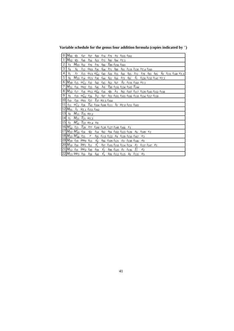
Variable schedule for the genus four addition formula (copies indicated by ∗)

0 M00 q1 t47 t57 t69 t74 t79 s3 t155 t1611 M02 q3 t48 t56 t63 t75 t80 t84 vT,52 t3 M03 t52 t70 t76 t86 T89 t156 t1633 t4 t6 t12 α03 t36 t64 t71 t88 t91 t119 t130 vT,4 t1604 t5 t7 t13 α13 α∗02 t40 t43 t55 t60 t65 t72 t78 t83 t85 s0 t131 t140 vT,3

5 t8 M33 t14 α23 t38 t44 t61 t66 t73 t81 s1 t126 t132 t141 vT,26 M30 t15 α∗12 t32 t42 t45 t62 t67 s2 t133 t142 vT,1

7 M31 t16 α02 t33 t46 λ0 T90 t116 t134 t143 T144

8 M32 t17 t18 α12 α∗01 t34 q0 λ1 t92 t107 t117 t129 t145 t152 t1589 t9 t19 α∗03 t26 λ2 t87 t93 t101 t103 t106 t118 t154 t157 t15910 t10 t20 α01 t27 T37 uT,5 t16411 t11 α∗13 t28 T41 t104 t108 t111 l0 uT,0 t151 t16512 M01 l1 uT,1 t153 t16213 t0 M11 T35 uT,2

14 t1 M21 T21 uT,315 t2 M∗31 T22 uT,4 ε0

16 M∗32 t23 T39 t77 t100 t120 t127 t148 t166 ε1

17 M22 M∗33 t24 q2 t54 t82 t94 t102 t123 t128 z6 t149 ε218 M23 M∗30 t25 r t95 t113 t122 z4 t139 t150 t167 ε3

19 M20 t29 inv0 t53 s′0 t96 t109 t121 z3 t138 t146 e020 M10 t30 inv1 t51 s′1 t97 t105 t110 t114 t124 z2 t137 t147 e1

21 M12 t31 inv2 t49 t59 s′2 t98 t125 z1 t136 f ∗7 e2

22 M13 inv3 t50 t58 t68 s′3 t99 t112 t115 z0 t135 e3

41

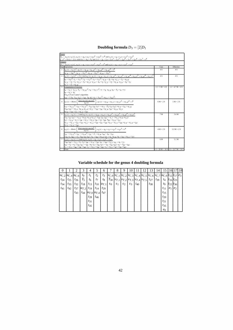
Doubling formula D3 = [2]D1

Inputs:

D1 = [u1(x),v1(x)], u1(x) = a0 +a1x+a2x2 +a3x3 + x4 and v1(x) = c0 + c1x+ c2x2 + c3x3

C : y2 +h(x)y = f (x) with h(x) = h0 ∈ Fq and f (x) = f0 + f1x+ f2x2 + f3x3 + f4x4 + f5x5 + f6x6 + f7x7 + x9

Outputs:

D3 = [u3(x),v3(x)], u3(x) = e0 + e1x+ e2x2 + e3x3 + x4 and v3 (x) = ε0 + ε1x+ ε2x2 + ε3x3

Step Operations Cost Effective

1 uC (x) = u1(x)2, uC (x) = uC,0 +uC,2x2 +uC,4x4 +uC,6x6 + x8 4 S 4 S

uC,0 = (a0)2; uC,2 = (a1)2; uC,4 = (a2)2; uC,6 = (a3)2 ;

2 vC (x) = v1(x)2 + f (x) mod uC (x), vC (x) = vC,0 + vC,1x+ vC,2x2 + vC,3x3 + vC,4x4 + vC,5x5 + vC,6x6 + vC,7x7 4 S 4 S

t0 = (c0 )2; t1 = (c1 )2; t2 = (c2)2; t3 = (c3)2; vC,0 = f0 + t0; vC,1 = f1 +uC,0;vC,2 = f2 + t1; vC,3 = f3 +uC,2; vC,4 = f4 + t2; vC,5 = f5 +uC,4; vC,6 = f6 + t3;vC,7 = f7 +uC,6;

3 computation of inverses 1 I + 5 M + 4 S 1 I + 4.7 M + 4 S

t4 = vC,7 · vC,5; T5 = (vC,6)2; t6 = (vC,7)2; t7 = t6 · uC,6; t8 = T5 + t4 + t7;t9 = vC,7 · t8;If t9 is 0 use Cantor’s algorithmt10 = 1/t9; (t11 , t12) = t10 · (t6, t8); e3 = (t11)2; uT,1 = (t12)2;

4 uT (x) = Monic

(f (x)+vC (x)+vC (x)2

uC(x)

), uT (x) = uT,0 +uT,1x+uT,2x2 +uT,4x4 + x6 6 M + 2 S 5 M + 2 S

t13 = (vC,5)2; t14 = (vC,4)2; (t15 , t16 , t17) = uT,1 · (T5, t13, t14); uT,4 = t15 +uC,6;(t18 , t19) = uT,4 · (uC,6,uC,4); uT,2 = t18 + t16 +uC,4; t20 = uC,6 · uT,2;uT,0 = t19 + t17 +uC,2 + t20;

5 vT (x) = vC (x)+1 mod uT (x), vT (x) = vT,0 + vT,1x+ vT,2x2 + vT,3x3 + vT,4x4 + vT,5x5 7 M 5.6 M

(t21 , t22, t23) = vC,6 · (uT,0,uT,4,uT,1); (t24 , t25, t26) = vC,7 · (uT,2,uT,0,uT,4);t27 = vC,6 + vC,7; t28 = uT,1 +uT,2; t29 = t27 · t28; T30 = vC,0 + t21;vT,1 = vC,1 + t23 + t25; vT,2 = vC,2 + t29 + t23 + t24; vT,3 = vC,3 + t24; vT,4 = vC,4 + t22;vT,5 = vC,5 + t26;

6 u3(x) = Monic

(f (x)+vT (x)+vT (x)2

uT (x)

), u3(x) = e0 + e1x+ e2x2 + e3x3 + x4 4 M + 2 S 3.3 M + 2 S

t31 = (vT,3)2; t32 = (vT,4)2; t33 = f7 +uT,4; t34 = f6 + t31;(t35 ,e1, t36) = e3 · (t34 , t33, t32); e2 = t36 +uT,4; t37 = e2 · uT,4; e0 = t35 +uT,2 + t37;

7 v3 (x) = vT (x)+1 mod u3(x), v3 (x) = ε0 + ε1x+ ε2x2 + ε3x3 6 M 5.1 M

(t38 , t39) = vT,5 · (e1 ,e3); t40 = vT,4 + t39; t41 = t40 + vT,5; t42 = e0 + e1 ;t43 = e2 + e3 ; (t44 , t45) = t40 · (e0 ,e2); (t46 , t47) = t41 · (t42 , t43); ε0 = T30 + t44;ε1 = vT,1 + t46 + t38 + t44; ε2 = vT,2 + t38 + t45; ε3 = vT,3 + t47 + t39 + t45;

Total 1 I + 28 M + 16 S 1 I + 23.7 M + 16 S

Variable schedule for the genus 4 doubling formula

0 1 2 3 4 5 6 7 8 9 10 11 12 13 14 15 16 17 18uC,2 uC,4 uC,6 t0 t1 t2 t3 vC,0 vC,1 vC,2 vC,3 vC,4 vC,5 vC,6 vC,7 uC,0 t12 t17 e3t24 t25 t26 T5 t6 t7 t8 T30 vT,1 vT,2 vT,3 vT,4 vT,5 t27 t39 t4 t16 t23t34 t33 t32 t18 t13 t10 uT,1 ε0 ε1 ε2 ε3 t40 t38 t9 t22 t36t41 t42 t37 uT,2 t19 t14 t29 t11 e1 e2

t43 t44 uT,0 uT,4 t47 t15t28 t46 t20t31 t21t45 t35

e0

42

Rethinking Low Genus Hyperelliptic Jacobian Arithmetic...

Documents

Transcript of Rethinking Low Genus Hyperelliptic Jacobian Arithmetic...