Equiangular lines, projective symmetries and nice error frameswaldron/Tuan/Thesis.pdf · Tuan-Yow...
203
U NIVERSITY OF AUCKLAND DOCTORAL T HESIS Equiangular lines, projective symmetries and nice error frames Author: Tuan-Yow C HIEN A thesis submitted in fulfilment of the requirements for the degree of Doctor of Philosophy in the Department of Mathematics “This thesis is for examination purposes only and is confidential to the examination process.” January 2015
Transcript of Equiangular lines, projective symmetries and nice error frameswaldron/Tuan/Thesis.pdf · Tuan-Yow...
UNIVERSITY OF AUCKLAND
DOCTORAL THESIS
Equiangular lines, projective symmetries andnice error frames
Author:
Tuan-Yow CHIEN
A thesis submitted in fulfilment of the requirements
for the degree of Doctor of Philosophy
in the
Department of Mathematics
“This thesis is for examination purposes only and is confidential to the examination
process.”
January 2015

“Rabbit’s clever,” said Pooh thoughtfully.
“Yes,” said Piglet, “Rabbit’s clever.”
“And he has Brain.”
“Yes,” said Piglet, “Rabbit has Brain.”
There was a long silence.
“I suppose,” said Pooh, “that that’s why he never understands anything.”
“Winnie-the-Pooh” by A. A. Milne.
Abstract
The existence of maximal sets of equiangular lines (SIC-POVMs) is of interest to the mathemat-
ics and physics communities due to their connection to quantum information theory, quantum
cryptography, spherical 2-designs and cubature rules. This thesis looks at a way to recover
analytic SIC-POVMs from numerical SIC-POVMs, including the discovery of a new analytic
SIC-POVM in 17 dimensions. It also develops a way to comprehensively find nice error bases
(used for finding SIC-POVMs). Finally, a general theory to classify sequences of vectors up to
projective unitary equivalence is developed and applied to study the projective symmetry groups
of sequences of vectors.

Acknowledgements
I would like to thank Shayne Waldron, my primary supervisor, for his guidance, advice, col-
laborations, support and his many invested hours bouncing and developing ideas together; Tom
ter Elst for his mathematical insight, kind advice and support; Marcus Appleby for sharing his
wealth of knowledge and experience regarding the SIC problem with me, as well as helping
to proof read the thesis; Huangjun Zhu for helpful discussions regarding symmetry groups;
Ingemar Bengtsson for discussions on MUBs, complex multiplication and hosting my stay in
Stockholm; Steve Flammia for hosting my stay in Sydney; Hwan Goh for proof reading the
whole thesis; Kieran Roberts for helping to proof read the thesis; my family and friends for
supporting me through the ups and downs; and the administrative staff for making the red tape
more bearable.
I am grateful for the financial support received. Part of this work is supported by the University
of Auckland Doctoral Scholarship and the Marsden Fund Council from Government funding
administered by the Royal Society of New Zealand.
iii
Contents
Abstract ii
Acknowledgements iii
List of Figures vii
List of Tables viii
Abbreviations ix
Symbols x
1 Introduction 1
2 Background 82.1 Frame theory . . . . . . . . . . . . . . . . . . . . . . . . . . . . . . . . . . . 82.2 SIC-POVM existence problem (Zauner’s conjecture) . . . . . . . . . . . . . . 122.3 Weyl-Heisenberg group . . . . . . . . . . . . . . . . . . . . . . . . . . . . . . 142.4 Clifford group . . . . . . . . . . . . . . . . . . . . . . . . . . . . . . . . . . . 162.5 Three dimensional SIC-POVMs . . . . . . . . . . . . . . . . . . . . . . . . . 20
3 Reverse engineering numerical SIC-POVMs 223.1 Galois theory fundamentals . . . . . . . . . . . . . . . . . . . . . . . . . . . . 23
3.1.1 Representing roots as radicals . . . . . . . . . . . . . . . . . . . . . . 263.2 SIC-POVM field structure . . . . . . . . . . . . . . . . . . . . . . . . . . . . 273.3 Methodology . . . . . . . . . . . . . . . . . . . . . . . . . . . . . . . . . . . 33
3.3.1 Precision bumping . . . . . . . . . . . . . . . . . . . . . . . . . . . . 333.3.2 Applying the Galois action . . . . . . . . . . . . . . . . . . . . . . . . 35
3.3.2.1 Parity and order 3 symmetries . . . . . . . . . . . . . . . . . 353.3.3 Constructing the splitting fields for the overlaps polynomials . . . . . . 36
3.3.3.1 Finding exact overlap polynomials . . . . . . . . . . . . . . 363.3.3.2 Constructing the tower of field extensions . . . . . . . . . . 37
3.3.4 Recovering roots . . . . . . . . . . . . . . . . . . . . . . . . . . . . . 383.4 Improvements . . . . . . . . . . . . . . . . . . . . . . . . . . . . . . . . . . . 38
3.4.1 Lowering the degree of overlaps polynomials . . . . . . . . . . . . . . 393.4.2 Simplifying the representation of solutions . . . . . . . . . . . . . . . 40
iv
Contents v
3.5 Results . . . . . . . . . . . . . . . . . . . . . . . . . . . . . . . . . . . . . . . 40
4 Projective unitary equivalences of frames 414.1 Complete frame graphs . . . . . . . . . . . . . . . . . . . . . . . . . . . . . . 444.2 Characterisation of projective unitary equivalence . . . . . . . . . . . . . . . . 484.3 Reconstruction from the m–products . . . . . . . . . . . . . . . . . . . . . . . 524.4 Similarity and m–products for vector spaces . . . . . . . . . . . . . . . . . . . 574.5 Projectively equivalent harmonic frames . . . . . . . . . . . . . . . . . . . . . 60
5 Projective symmetry groups 645.1 Introduction . . . . . . . . . . . . . . . . . . . . . . . . . . . . . . . . . . . . 645.2 Tight frames and the complement of a frame . . . . . . . . . . . . . . . . . . . 655.3 Projective invariants . . . . . . . . . . . . . . . . . . . . . . . . . . . . . . . . 705.4 The algorithm . . . . . . . . . . . . . . . . . . . . . . . . . . . . . . . . . . . 70
5.4.1 Algorithm . . . . . . . . . . . . . . . . . . . . . . . . . . . . . . . . . 725.5 The extended projective symmetry group . . . . . . . . . . . . . . . . . . . . . 745.6 Group frames, nice error bases, SIC-POVMs and MUBs . . . . . . . . . . . . 765.7 Harmonic frames . . . . . . . . . . . . . . . . . . . . . . . . . . . . . . . . . 83
6 Nice error frames 866.1 Background . . . . . . . . . . . . . . . . . . . . . . . . . . . . . . . . . . . . 866.2 Nice error frames and canonical abstract error groups . . . . . . . . . . . . . . 886.3 Calculations . . . . . . . . . . . . . . . . . . . . . . . . . . . . . . . . . . . . 95
6.3.1 Nice error bases and SIC-POVMs . . . . . . . . . . . . . . . . . . . . 976.4 SIC-POVMs from nonabelian group in 6 dimensions . . . . . . . . . . . . . . 98
6.4.1 Nice error bases and numerical SIC-POVMs . . . . . . . . . . . . . . 996.4.2 The analytic form of the SIC-POVM . . . . . . . . . . . . . . . . . . . 101
6.4.2.1 The determination of ξ2 . . . . . . . . . . . . . . . . . . . . 1056.4.3 The determination of ξ1 . . . . . . . . . . . . . . . . . . . . . . . . . 105
6.5 Equivalence to Heisenberg SIC-POVMs . . . . . . . . . . . . . . . . . . . . . 107
A Nice Error Groups 108A.1 Tables of canonical abstract error groups and index groups . . . . . . . . . . . 109A.2 Analytic Solutions For Dimension 8 . . . . . . . . . . . . . . . . . . . . . . . 111
A.2.1 One Canonical Abstract Error Group . . . . . . . . . . . . . . . . . . 112A.2.1.1 SmallGroup(64, 3) . . . . . . . . . . . . . . . . . . . . . . . 112A.2.1.2 SmallGroup(64, 8) . . . . . . . . . . . . . . . . . . . . . . . 113A.2.1.3 SmallGroup(64, 60) . . . . . . . . . . . . . . . . . . . . . . 113A.2.1.4 SmallGroup(64, 62) . . . . . . . . . . . . . . . . . . . . . . 114A.2.1.5 SmallGroup(64, 68) . . . . . . . . . . . . . . . . . . . . . . 115A.2.1.6 SmallGroup(64, 69) . . . . . . . . . . . . . . . . . . . . . . 116A.2.1.7 SmallGroup(64, 71) . . . . . . . . . . . . . . . . . . . . . . 117A.2.1.8 SmallGroup(64, 74) . . . . . . . . . . . . . . . . . . . . . . 118A.2.1.9 SmallGroup(64, 75) . . . . . . . . . . . . . . . . . . . . . . 119A.2.1.10 SmallGroup(64, 77) . . . . . . . . . . . . . . . . . . . . . . 120A.2.1.11 SmallGroup(64, 78) . . . . . . . . . . . . . . . . . . . . . . 121

Contents vi
A.2.1.12 SmallGroup(64, 91) . . . . . . . . . . . . . . . . . . . . . . 122A.2.1.13 SmallGroup(64, 193) . . . . . . . . . . . . . . . . . . . . . 123A.2.1.14 SmallGroup(64, 195) . . . . . . . . . . . . . . . . . . . . . 124
A.2.2 Two or More Canonical Abstract Error Groups . . . . . . . . . . . . . 125A.2.2.1 SmallGroup(64, 90) . . . . . . . . . . . . . . . . . . . . . . 125A.2.2.2 SmallGroup(64, 202) . . . . . . . . . . . . . . . . . . . . . 127
A.2.3 Canonical Abstract Error Group With No Solutions . . . . . . . . . . . 129A.2.3.1 SmallGroup(64, 67) . . . . . . . . . . . . . . . . . . . . . . 130
A.2.4 SmallGroup(64, 138) . . . . . . . . . . . . . . . . . . . . . . . . . . . 132A.3 Hoggar SIC-POVM in the Clifford group . . . . . . . . . . . . . . . . . . . . 134A.4 Dimension 16 . . . . . . . . . . . . . . . . . . . . . . . . . . . . . . . . . . . 135
B Projective symmetry groups of cyclic harmonic frames 136
C SIC-POVM in 17 dimensions 143C.1 The Scott-Grassl numerical solution for 17c . . . . . . . . . . . . . . . . . . . 143C.2 Analytic solution for 17c . . . . . . . . . . . . . . . . . . . . . . . . . . . . . 144
Bibliography 186

List of Figures
2.5.1 Hesse configuration.1 . . . . . . . . . . . . . . . . . . . . . . . . . . . . . . . 21
4.2.1 The frame graph of an orthonormal basis for C3 (Example 4.2.4) and the framegraph for three equiangular vectors in C2 (Example 4.2.5). . . . . . . . . . . . 51
4.3.1 The spanning trees Tp and Ts (and cycle completions) of Example 4.3.5. . . . . 534.3.2 The proof of Theorem 4.3.11 for MUBs B1,B2,B3 in C3. The frame graph Γ,
the spanning tree T and fundamental cycles of type 1 and 2. . . . . . . . . . . 564.3.3 A nonchordal graph for which each edge is on a 3–cycle. . . . . . . . . . . . . 57
vii
List of Tables
4.1 The number of unitary and projective unitary equivalence classes (up to rein-dexing) of cyclic harmonic frames of n vectors in Cd, d = 2, . . . , 7. When thegroup theoretic estimate of Theorem 4.5.6 is larger (because there are reindex-ings which are not automorphisms) it is given in the row below. . . . . . . . . . 63
5.1 The symmetry groups SymP (Φ) and SymEP (Φ) for Φ the tight frame of nvectors given by m MUBs in Cd, including the proper transitive subgroups ofSymP (Φ). The last column lists the transitive subgroups of SymP (Φ). Let<n,k> be the k–th group of order n in the Small Groups Library (as usedin MAGMA). When the MAGMA routine IdentifyGroup(G) is unable toidentify the group, the order of the group is given instead. . . . . . . . . . . . . 82
A.1 Nice error bases for d < 14, d 6= 8. HereH is the canonical abstract error group,G is the index group, and sic indicates that a SIC-POVM exists numerically. 109
A.2 The nice error bases for d = 8. Those which are subgroups of the Cliffordgroup are labelled with an *. All SIC-POVMs are the Hoggar lines, except forH = 〈512, 451〉, G = Z2
8 . . . . . . . . . . . . . . . . . . . . . . . . . . . . . 110A.3 The canonical abstract error groups and index groups for the first few nice error
frames, which are not bases, for 2 ≤ d ≤ 7. . . . . . . . . . . . . . . . . . . . 111
B.1 The erasure column is omitted. For 6 vectors the number of erasures is 0 and for7 vectors it is 1. Past this point, no computational data exists. . . . . . . . . . . 141
B.2 The erasure column is omitted. For 7 vectors the number of erasures is 0 and for8 vectors it is 1. Past this point, no computational data exists. . . . . . . . . . . 142
viii

Abbreviations
SIC-POVM Symmetric Informationally Complete Positive Operator Valued Measure. See page 12.
MUB Mutually Unbiased Bases See page 55.
NEB Nice Error Basis. See page 87.
ix

Symbols
〈p, q〉s Symplectic form p2q1 − p1q2 as defined in (2.3.2). See page 14.
Dp A Weyl-Heisenberg displacement operator. See page 14.
H(d) Weyl-Heisenberg group in d dimensions. See page 14.
C(d) Clifford group in d dimensions. See page 16.
ECL(d) Extended Clifford group. See page 16.
T One dimensional torus, i.e., all complex numbers of modulus 1. See page 20.
τ −eiπ/d. See page 15.
Π A SIC-POVM projector. See page 27.
χp A SIC-POVM overlap. See page 27.
Tr(A) The trace of the matrix A. See page 27.
a
√(d−3)(d+1)
k . See page 28.
E Smallest normal extension of Q containing the components of Π and τ . See page 28.
E E(√d). See page 28.
G Galois group of E over Q. See page 29.
SΠ Stabiliser of Π. See page 28.
SΠ
F ∈ ESL(2,Zd) : VF ∈ SΠ
. See page 30.
SΠ
(DetF )F : F ∈ SΠ
. See page 30.
CΠ Centraliser of SΠ. See page 31.
ρ In Chapter 3, they are polynomials with SIC-POVM overlaps as roots (see page 32).
ρ In Chapters 5 and 6 they are unitary representations (see pages 76 and 87).
ζ Polynomials with the coefficients of ρ as roots. See page 39.
Tijk Triple product (3-product). See page 42.
∆ m-product. See page 42.
Sym(Φ) Symmetry group of Φ. See page 64.
SymP (Φ) Projective symmetry group of Φ. See page 65.
x
Chapter 1
Introduction
The overarching motivation behind this thesis is to study the problem of the existence of max-
imal sets of equiangular lines in Cd. Consider a set of orthogonal basis vectors. The angle of
intersection between any two vectors in this set is 90 degrees. This set of vectors is equiangular
as the angle of intersection between any two vectors is constant. A natural question to ask is,
how many vectors can one have in a given dimension before it is no longer possible to have this
equiangular property. For example, the 3 spokes of the Mercedes-Benz logo is an example of a
maximal set of 3 equiangular lines in R2. This question of existence (for maximal sets of com-
plex equiangular lines) has been open for more than 10 years and has been of great academic
interest to the physics community.
A set of equiangular lines gives rise to a corresponding basis on the vector space of d × d
complex matrices (Md) with the property that the inner product between any two basis elements
is constant (and non zero). Moreover, it implies that in Cd there are at most d2 equiangular lines.
This is a desirable symmetry in quantum information theory (see introduction of [RBKSC04])
and has applications in the construction of optimal quantum error correcting codes (see Sec-
tion 5.4.2 of [Ren04]). They also exhibit rich structure and connections with several areas of
mathematics, including frame theory, number theory and algebra. It makes the problem fun and
interesting to study in its own right.
Proof on the existence of maximal sets of equiangular lines (in Cd) is only known in dimensions
1-16, 19, 24, 35 and 48. Historically, the approach to finding maximal sets of equiangular lines
has involved solving systems of polynomial equations by hand ([RBKSC04]), using Grobner
bases in a brute force computational search ([SG10]), or with specific geometric constructions
1
Introduction 2
([Hog98], [Hug07]). Amongst other things, this thesis contributes dimension 17 to this list.
This is done using a novel Ansatz, which turns numerical approximations of maximal sets of
equiangular lines into analytic expressions by studying certain algebraic extensions of Q in
which the numerical values are conjectured to live.
This thesis looks at four aspects of the existence problem (Chapters 3 to 6). Firstly, using numer-
ical approximations for sets of equiangular lines, how can one recover analytic expressions for
these equiangular lines? Secondly, how does one classify sequences of vectors up to projective
equivalence? Thirdly, how does one generate the group of symmetries of projective objects?
Fourthly, almost all known constructions of maximal sets of equiangular lines arise as orbits
of the Weyl-Heisenberg group. How could one generate equiangular lines with groups other
than the Weyl-Heisenberg group? These questions are elaborated under their relevant chapter
headings below.
Chapter 2, Background.
This chapter lays down common foundational definitions and theorems (without proof) for the
rest of the chapters. Section 2.1 is about the theory of frames. Frames are given in Definition
2.1.1 and equiangular lines are formally defined in Definition 2.1.12 with their link to frame
theory. There is then a survey of the key tools used to numerically construct equiangular lines
as orbits of group actions.
The next two sections give an overview of the problem of the existence of maximal equiangular
lines. Maximal equiangular lines (SIC-POVMs or Symmetric Informationally Complete Posi-
tive Operator Valued Measures) are formally defined in Definition 2.2.2, with a formulation of
the existence problem in Conjecture 2.2.3 (Zauner’s conjecture), which conjectures that for any
d ∈ N, there exists a set of d2 equiangular lines in Cd. Basic facts about the important Weyl-
Heisenberg group are presented as well as a look into the the normaliser of the Weyl-Heisenberg
group (Clifford group), along with the extended Clifford group.
Lastly, the curious black sheep of the existence problem (dimension 3 SIC-POVMs) is presented
in Section 2.5 with its continuous properties and its connection to elliptic curves.
Introduction 3
Chapter 3, Reverse engineering numerical SIC-POVMs.
This chapter presents new research conducted jointly with Marcus Appleby and Shayne Waldron
which obtains new analytic SIC-POVMs from numerical SIC-POVMs by studying the algebraic
extension fields of Q in which known SIC-POVMs reside. SIC-POVM existence is proved in
dimension 17 (previously unknown) by reverse engineering the numerical solutions and making
use of conjectures about the SIC-POVM fields.
The approach here is novel and takes a numerical SIC-POVM vector, attempts to construct the
exact values of the inner products of the SIC-POVM in order to reconstruct the original vector
analytically. This Ansatz relies on conjectures relating to the field structure of the SIC-POVM
and ad hoc calculations, in order to speculate a structure to the analytic solution. It essentially
reduces the problem down to a factorisation problem (of polynomials). The speculated solution
is then verified afterwards to be a SIC-POVM. While there is no formal proof that any of this
should work, “the proof is in the pudding (SIC-POVM)”, so to speak, since a SIC-POVM can in
fact be found using this process.
Section 3.1 establishes some fundamental Galois theory regarding the solubility of polynomials
by radicals. The key hypothesis on the structure of the SIC-POVM fields and the Galois groups
of those fields over Q is stated in Conjecture 3.2.17. Theorem 3.2.18 and Conjectures 3.2.20
and 3.2.21 then provide practical assistance in the reverse engineering efforts. Section 3.3 out-
lines the procedure developed for reverse engineering the new analytic SIC-POVMs, including
an algorithm for precision bumping numerical SIC-POVMs (algorithm 3.1). Potential improve-
ments to the method are discussed in Section 3.4 and the new SIC-POVM fiducial vectors for
dimension 17 is given in Appendix C.
Chapter 4, Projective unitary equivalences of frames.
When presented with two sequences of vectors, one could ask whether the two sequences are
fundamentally the same. This is often captured by the notion of unitary equivalence, since uni-
tary transformations preserve key geometric properties like the angle between vectors and their
lengths. For projective objects like lines, an analogous concept of projective unitary equivalence
arises. The additional complication arises where each vector is allowed to be scaled by any
arbitrary complex number of unit length. This complication makes the problem of classifying

Introduction 4
lines difficult, a feat some researchers thought to be impossible in a general setting (e.g., see
comments in Section 5, paragraph 2 of [VW10] regarding type III equivalences). Studying the
projective equivalence between sequences of vectors is important as it could be used to classify
frames and count distinct solutions in the SIC-POVM existence problem. It also makes it possi-
ble to compute the projective symmetry group (see Chapter 5), which is an important object of
study (e.g., can be used to determine whether a sequence of vectors is a group frame).
The seminal paper of [AFF11] (Theorem 3 and the remark on p. 13) first utilised (3–vertex)
Bargmann invariants (so called “triple products”) to classify SIC-POVMs up to projective uni-
tary equivalence. This chapter takes this idea of a Bargmann invariant and recasts it in language
of frame graphs (Definition 4.0.5)), paving the way for a general classification method.
The main theorems are presented in Sections 4.2 and 4.3. Whilst [AFF11] only gives a classifi-
cation for SIC-POVMs, Theorem 4.2.2 greatly generalises their result by characterising any two
sequences of vectors up to projective unitary equivalence via m–products. Theorem 4.3.6 gives
an indication of which m–products are sufficient. An algorithm to solve the inverse problem,
i.e., given a sufficient set of m–products, construct all sequences which give rise to these prod-
ucts, is provided by the proof of Theorem 4.2.2. The implications of this to the classification of
MUBs (Mutually Unbiased Bases) is later considered.
Section 4.4 extends the classification of sequences of vectors up to (projective) similarity and
Section 4.5 applies the theory to the classification of harmonic frames up to projective unitary
equivalence. In particular, projective unitary equivalence of harmonic frames is characterised up
to affine equivalence in Theorem 4.5.6. An explicit description of dimension 2 harmonic frames
up to projective unitary equivalence is then given by Proposition 4.5.7. Finally, tables of the
harmonic frame calculations are presented.
The research in this chapter was conducted jointly with Shayne Waldron and adapted from
[CW14a].
Chapter 5, Projective symmetry groups.
This chapter studies the projective symmetry group of a sequence of vectors. This group can
really only be computed once it is possible to compute projective unitary equivalence (e.g., by
the characterisation theorems of Chapter 4). These projective symmetry groups have only been
Introduction 5
computed previously for the SIC-POVM case in Chapter 10 of [Zhu12] and has hence received
little study. The results and algorithm in this chapter enable projective symmetry groups to be
computed for any finite sequence of vectors. These groups are important as they describe all
the symmetries present in a sequence of vectors. This can lead to the simplification of systems,
discovering new symmetries and even determine whether the sequence arises as the orbit of a
group.
Theorem 5.2.5 establishes that a frame and is complement have the same projective symmetry
group. Furthermore, Theorem 5.3.1 gives a set of projective invariants which determine a se-
quence of vectors up to projective similarity when the underlying field is closed under complex
conjugation.
Section 5.4 gives an algorithm for calculating the projective symmetry group from m–products
(projective invariants). The only other known algorithm (Section 10.2.3 of [Zhu12]) for comput-
ing projective symmetry groups is for the special case of sequences characterised by 3–products.
That algorithm was applied specifically to the situation of d2 equiangular vectors in Cd which
are given as a group orbit.
Section 5.5 briefly extends the analysis to “anti-linear symmetries” and the extended projec-
tive symmetry group. Section 5.6 considers simplifications to the algorithm in Section 5.4 for
group frames and computes the extended projective symmetry group of certain SIC-POVMs and
MUBs. Section 5.7 presents some results from extensive calculations of the projective symmetry
group and extended projective symmetry group of harmonic frames. The full table of harmonic
frame data is given in Appendix B.
The research in this chapter was conducted jointly with Shayne Waldron and adapted from
[CW14b].
Chapter 6, Nice error frames.
Most SIC-POVMs arise as the orbit of the Weyl-Heisenberg group. Other groups are also known
to give rise to SIC-POVMs. All of these groups are in a class of groups called nice error groups
and their associated nice error bases are sufficient to generate SIC-POVMs. A complete cata-
logue of nice error groups was previously difficult to find and the catalogue of nice error bases in
the web link in http://www.cs.tamu.edu/faculty/klappi/ueb/ueb.html had
Introduction 6
issues of over and under counting. This chapter rectifies these problems by introducing the
notion of a canonical nice error group, allowing for a systematic way to exhaustively find all
inequivalent nice error groups. This is applied to hunt for non Weyl-Heisenberg SIC-POVMs
in dimensions up to 16. Of the SIC-POVMs found, the analytic SIC-POVMs for index group
<36,11> and <64,78> were independently discovered by Grassl in Section 4.2 of [Gra05].
The numerical SIC-POVMs in dimensions 6 and 8 were independently discovered by Zhu in
Table 10.2 of [Zhu12].
While the excitement level of discovering these analytic SIC-POVMs (see Appendix A) dimin-
ished after being alerted of these independent discoveries, these analytic solutions still have
value. The comprehensive search conducted here was over all nice error groups in dimensions
up to (but not including dimension 16). This is an improvement on the catalogue computed
in http://faculty.cs.tamu.edu/klappi/ueb/ueb.html, which is an incomplete
catalogue of nice error bases in dimension 8. These analytic results also act as verification of
the numerical work done in Table 10.2 of [Zhu12].
The basic theory is presented in Sections 6.1. The nice error frame is introduced by Definition
6.2.1 and its canonical representation by Definition 6.2.3. Nice error frames are equivalent to
unitary faithful projective representations (Proposition 6.2.8) and equivalent error frames are
then shown have the same canonical error group (Proposition 6.2.6). A tensor construction of
nice error groups is also given. Theorem 6.2.14 characterises nice error frames with abelian
index groups. Section 6.3 then focuses on calculating nice error groups and a way of generating
equivalent nice error frames. Subection 6.3.1 discusses the connection to SIC-POVMs briefly
and a detailed calculation of a SIC-POVM in 6 dimensions is given in Section 6.4.
Section 6.5 concludes the chapter with some short remarks on the equivalence of known SIC-
POVMs with Weyl-Heisenberg SIC-POVMs. The exceptional case of the Hoggar SIC-POVM
is discussed. By using the theory of projective symmetry groups developed in this thesis, the
Hoggar lines were then found as a subgroup of the Clifford group, leading to a conjecture that
all group covariant SIC-POVMs are covariant to a subgroup of the normaliser of the Weyl-
Heisenberg group (Conjecture 6.5.1).
Tables of nice error groups, bases, and an extensive catalogue of SIC-POVMs for 8 dimensional
nice error bases are given in Appendix A.

Introduction 7
The research in this chapter was conducted jointly with Shayne Waldron and adapted from an
unpublished work in progress.
Chapter 2
Background
2.1 Frame theory
Unless otherwise stated, all vector spaces X in this thesis are finite dimensional and over a
subfield of C. The material in this section is found in standard textbooks on frame theory, cf.
Chapters 1-5 of [Chr03], Chapters 1-3, 5 of [CKE13], Chapters 1-3, 8, 10, 12 of [Wal15]. The
Hilbert spacesH here have Euclidean inner product.
Definition 2.1.1.
Let Φ := (vj)j∈J be a sequence of vectors in a real or complex Hilbert space H. Φ is a frame
forH with frame bounds A,B > 0 if
A‖f‖2 ≤∑j∈J|〈f, vj〉|2 ≤ B‖f‖2, ∀f ∈ H. (2.1.1)
If A = B, then Φ is a tight frame. If A = B = 1, then it is a normalised tight frame. If J is
finite, then Φ is a finite frame.
This definition of a frame is well defined for infinite dimensional Hilbert spaces. In finite di-
mensional spaces, any finite spanning sequence of vectors satisfies (2.1.1) and is a frame. Tight
frames are generalisations of orthonormal bases. Examples of tight frames containing more
vectors than a basis include SIC-POVMs, MUBs, and harmonic frames.
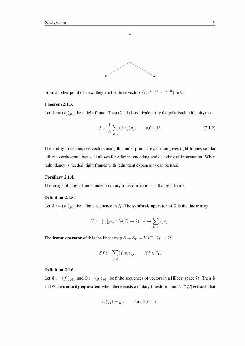
Example 2.1.2 (Mercedes Benz frame).
A classic example of a tight frame is the Mercedes Benz frame given by the three equally spaced
vectors in R2:
8
Background 9
From another point of view, they are the three vectors i, e7πi/6, e−πi/6 in C.
Theorem 2.1.3.
Let Φ := (vj)j∈J be a tight frame. Then (2.1.1) is equivalent (by the polarisation identity) to
f =1
A
∑j∈J〈f, vj〉vj , ∀f ∈ H. (2.1.2)
The ability to decompose vectors using this inner product expansion gives tight frames similar
utility to orthogonal bases. It allows for efficient encoding and decoding of information. When
redundancy is needed, tight frames with redundant expansions can be used.
Corollary 2.1.4.
The image of a tight frame under a unitary transformation is still a tight frame.
Definition 2.1.5.
Let Φ := (vj)j∈J be a finite sequence inH. The synthesis operator of Φ is the linear map
V := [vj ]j∈J : `2(J)→ H : a 7→∑j∈J
ajvj .
The frame operator of Φ is the linear map S = SV = V V ∗ : H → H,
Sf :=∑j∈J〈f, vj〉vj , ∀f ∈ H.
Definition 2.1.6.
Let Ψ := (fj)j∈J and Φ := (gj)j∈J be finite sequences of vectors in a Hilbert spaceH. Then Ψ
and Φ are unitarily equivalent when there exists a unitary transformation U ∈ U(H) such that
U(fj) = gj , for all j ∈ J.

Background 10
Definition 2.1.7.
Let Φ = (vj)j∈J be a sequence of n vectors. The Gramian of Φ is the n× n matrix
Gram(Φ) := V ∗V = [〈vk, vj〉]j,k∈J ,
i.e., the matrix containing inner products between the vectors of Φ.
Theorem 2.1.8.
A n× n matrix P = [pj,k]j,k∈J is the Gramian of a normalised tight frame (vj)j∈J if and only
if P is an orthogonal projection matrix.
Corollary 2.1.9.
Normalised tight frames are unitarily equivalent if and only if their Gramians are equal.
While the Gramian can quickly resolve whether two frames are unitarily equivalent (without
reindexing), it may still be an expensive exercise to compute equivalence when reindexing is
allowed. The Gramian also fails to identify when two sequences of vectors are essentially the
same, but one sequence has had its vectors arbitrarily scaled by a constant of modulus 1 (see
Chapter 4).
Theorem 2.1.10.
Every finite normalised tight frame is the orthogonal projection of an orthonormal basis.
Example 2.1.11.
The Gramian of a finite normalised tight frame Φ acting on the standard basis will produce a
frame which is unitarily equivalent to Φ.
Definition 2.1.12.
A tight frame is equiangular if its vectors have equal norms and there exists a C > 0 such that
|〈vj , vk〉| = C, ∀j 6= k.
If the vectors are of unit length, they are sometimes called equiangular lines.
Definition 2.1.13.
Let S = f ∈ H : ‖f‖ = 1 be the unit sphere in H, where H has dimension n. The frame
potential is the function
FP : Sn → [n,∞) : (vj)nj=1 7→
n∑j=1
n∑k=1
|〈vj , vk〉|2.
Background 11
Theorem 2.1.14 (Variational characterisation).
Let Φ := (vj)j∈J be a frame forH. Then
FP (Φ) ≥ 1
d
(∑j∈J‖vj‖2
)2, d = dim(H),
with equality, if and only if, Φ is a tight frame.
The frame potential was introduced by Benedetto and Fickus in Section 6 of [BF03]. It al-
lows tight frames to be found numerically by minimising the frame potential and applying the
variational characterisation. For example, by constructing a random sequence of vectors and
attempting to converge towards a tight frame through random perturbations of the vectors which
produce smaller frame potentials.
Definition 2.1.15.
Let Φ := (vj)j∈J be a frame forH. The second frame potential is the function
SFP : Sn → [0,∞) : (vj)nj=1 7→
n∑j=1
n∑k=1
|〈vj , vk〉|4.
Theorem 2.1.16 (Welch bound).
Let Φ := (vj)j∈J be a sequence of n = d2 unit vectors in Cd. Then
n∑j=1
n∑k=1
|〈vj , vk〉|4 ≥2d3
d+ 1,
with equality, if and only if, Φ is a sequence of equiangular lines, i.e., there exists a C > 0 such
that for all j 6= k, |〈vj , vk〉|2 = C.
By a similar approach to finding tight frames, numerical equiangular tight frames can be found
by minimising the second frame potential and checking whether they meet the Welch bound.
Definition 2.1.17.
Let G be a group. A group frame (or G–frame) for H is a frame Φ = (vg)g∈G where there
exists a unitary representation of G with
gvh := ρ(g)vh = vgh, ∀g, h ∈ G.

Background 12
Theorem 2.1.18.
Let ρ be an irreducible unitary representation of a group G on H and v 6= 0 ∈ H. Then
(ρ(g)v)g∈G is a tight frame forH.
This theorem allows for the efficient construction of tight frames as group orbits.
2.2 SIC-POVM existence problem (Zauner’s conjecture)
Equiangular lines always exist in all finite dimensions. A simple example is a sequence of
orthonormal basis vectors which have an inner product of 0 between any two distinct vectors.
Naturally one asks, what is the maximum allowable number of equiangular lines in any given
dimension? This will be considered for complex vector spaces.
Theorem 2.2.1.
Let d > 1 and (fj)j∈J be a sequence of n equiangular lines in Cd, where the fj are not collinear.
The orthogonal projections
Pj : f 7→ 〈f, fj〉fj , j = 1, . . . , n
are linearly independent and n ≤ d2 with equality, if and only if, Pjnj=1 is a basis for the d×d
Hermitian matrices.
Over complex vector spaces, an upper bound for the maximum number of equiangular lines in
any given dimension is d2 by Theorem 2.2.1. Over real vector spaces, an upper bound is d(d+1)2
(Theorem 2.2 of [Tre08]).
The real dimensional case exhibits several dimensions which do not meet this upper bound (they
have smaller upper bounds) and several which do. After more than 60 years of research, it is
still not clear for all dimensions what the maximum is.
The complex situation is somehow less dire. The recent computational study [SG10] produced
numerical approximations (to about 200 digit precision) of sequences of d2 equiangular lines in
every d ≤ 67. This strongly supports the conjecture that the maximum is d2.
Definition 2.2.2.
An equiangular tight frame Φ := (vj)j∈J for Cd having the maximal number of vectors (d2)
Background 13
is a maximal equiangular tight frame. When the vectors are of unit length they are maximal
equiangular lines. In quantum information theory, they (or their corresponding orthogonal
projections Pj = vjv∗j ) are known as a symmetric informationally complete positive operator
valued measure, SIC-POVM.
In light of [SG10] and Theorem 2.2.1, the remaining challenge is to show that d2 equiangular
lines can always be constructed for any finite dimension d.
Conjecture 2.2.3 (Zauner’s conjecture).
For each d ∈ N, there exists a sequence of d2 equiangular lines (SIC-POVM) in Cd.
Theorem 2.2.4.
Let Φ := (vj)j∈J be a tight frame with |J | = d2. Then Φ is a SIC-POVM if and only if
|〈vj , vk〉|2 =1
d+ 1, j 6= k.
Since SIC-POVMs are tight frames they might be constructed as the orbit of an irreducible group
action. Recent efforts have primarily focused on group constructions of SIC-POVMs.1
Definition 2.2.5.
A SIC-POVM is covariant to a group G if it is the orbit of G acting on some vector v ∈ H.
Definition 2.2.6.
Let H = Cd, G a group with irreducible representation ρ in H. A SIC-POVM fiducial is a
vector v ∈ H such that
Φ := ρ(g)v : g ∈ G
is a SIC-POVM forH, i.e., it is a vector whose orbit under the action of G is a SIC-POVM.
Definition 2.2.7.
Let F be a field and H a Hilbert space over F of dimension d. The space of homogeneous
multivariate polynomials (H → F) of degree t in z and z is
Hom(t, t) := spanz 7→ zαzβ : |α| = |β| = t,
where α and β are multi-indices, e.g., zα = zα11 zα2
2 · · · zαtt .
1Group independent searches of SIC-POVMs were done numerically by Zhu in Chapter 10 of [Zhu12] in asmall number of dimensions. All the SIC-POVMs found were covariant to the Weyl-Heisenberg group. One mightspeculate that only group covariant SIC-POVMs exist.
Background 14
Theorem 2.2.8.
Let Φ := (vj)j∈J be a frame satisfying Theorem 2.1.16. Then
∫Sp(x)dσ(x) =
1∑n`=1 ‖v`‖4
n∑j=1
p(vj), ∀p ∈ Hom(t, t), (2.2.1)
where σ(x) is the normalised surface area measure on S (see [Sei01]).
In design theory, sequences of vectors satisfying (2.2.1) are spherical 2-designs. SIC-POVMs
are examples of 2–designs (they are in fact minimal 2–designs). Spherical designs allow inte-
grals of homogeneous polynomials over the unit sphere to be readily computed by evaluating a
finite sum. See the classic Seidel paper [DGS77] for more information about spherical designs.
2.3 Weyl-Heisenberg group
Let ω := e2πi/d and (ei)di=1 be an orthonormal basis for H. Define the operators S and Ω so
that
S(ei) = ei+1 mod d, Ω(ei) = ωiei.
The S and Ω are cyclic shift and modulation operators with matrix representations:
S :=
0 0 · · · 0 1
1 0 · · · 0 0
0 1 · · · 0 0...
.... . .
......
0 0 · · · 1 0
, Ω :=
1
ω
ω2
. . .
ωd−1
. (2.3.1)
Definition 2.3.1.
Let p = (p1, p2), q = (q1, q2) ∈ Z2. Define the symplectic form
〈p, q〉s := p2q1 − p1q2. (2.3.2)
The Weyl-Heisenberg displacement operators are
Dp := τp1p2Sp1Ωp2 .
The displacement operators generate a discrete Weyl-Heisenberg group H(d) of order d3.

Background 15
Let τ = −eiπ/d. The Weyl-Heisenberg operators satisfy the relations
DpDq = τ 〈p,q〉sDp+q, (2.3.3)
D∗p = D−p, (2.3.4)
Dp+dq =
Dp, if d is odd;
(−1)〈p,q〉sDp, if d is even.(2.3.5)
Modulo the centre Z := Centre(H(d)), H(d)/Z is isomorphic to Zd × Zd of order d2.
The Weyl-Heisenberg group is of special interest to the SIC-POVM existence problem. Almost
all constructed SIC-POVMs are covariant to the Weyl-Heisenberg group or is projectively unitar-
ily equivalent (see Chapter 4) to a Weyl-Heisenberg SIC-POVM. Furthermore, the only known
exception (Hoggar lines) is covariant to a subgroup of the normaliser of the Weyl-Heisenberg
group (Clifford group) (see Section A.3 of Appendix A). This makes the Weyl-Heisenberg group
or the Clifford group central to the study of SIC-POVMs.
Theorem 2.3.2 (Theorem 8.1, [Zhu12]).
Any group covariant SIC-POVM in a prime dimension is covariant with respect to the Weyl-
Heisenberg group.
Definition 2.3.3 (Fourier matrix).
Let ω := e2πi/d. The Fourier matrix F = (f(jk))0≤j,k≤d−1 is the d × d matrix with entries
given by
fjk :=ωjk√d, 0 ≤ j, k ≤ d− 1.
Definition 2.3.4 (Zauner matrix).
Let F be the Fourier matrix and G = (grs)0≤r,s≤d−1 be the diagonal matrix with entries given
by
gss = eπi(d+1)s2/d, 0 ≤ s ≤ d− 1.
The Zauner matrix is the matrix:
Z := eiπ(d−1)/12FG.
Conjecture 2.3.5 (Zauner’s conjecture (stronger version)).
For every dimension, there exists a Weyl-Heisenberg covariant SIC-POVM fiducial which is an
eigenvector of the Zauner matrix Z .

Background 16
This stronger version of the conjecture is also supported by the numerical study [SG10]. It is
often used as an additional constraint when attempting to solve a polynomial system for SIC-
POVMs.
2.4 Clifford group
Definition 2.4.1.
Let K : Cd → Cd such that
Kz := z = (zj).
Then K is the complex conjugate operator. A product of a linear (unitary) map with complex
conjugation is an anti-linear (anti-unitary) map. Anti-unitary maps have the property that
〈Ux,Uy〉 = 〈x, y〉, ∀x, y ∈ H.
Since the product of two anti-linear (anti-unitary) maps is linear (unitary), the groups of linear
maps and unitary maps can be extended to
EGL(Cd) := LKs : L ∈ GL(Cd), s = 0, 1, EU(Cd) := UKs : L ∈ U(Cd), s = 0, 1.
Definition 2.4.2.
Let H(d) be the Weyl-Heisenberg group as defined by Definition 2.3.1. Then the Clifford group
is the normaliser of H(d) in the group of unitary matrices, i.e.,
C(d) := U ∈ U(d) : U−1H(d)U =H(d).
The extended Clifford group is all unitary and anti-unitary operators which normalise H(d),
i.e.,
ECL(d) := U ∈ EU(Cd) : U−1H(d)U = H(d).
The Clifford group is important to the study of SIC-POVMs for a variety of reasons. For exam-
ple, let U be a unitary in the Clifford group, v ∈ H a Weyl-Heisenberg SIC-POVM fiducial, ρ
Background 17
an irreducible representation of H(d) onH, then for all g ∈ H(d), g 6= 1,
|〈Uv,Uρ(g)Uv〉| = |〈v, U∗ρ(g)Uv〉| = |〈v, U−1ρ(g)Uv〉| = 1√d+ 1
,
i.e., the Clifford group maps a SIC-POVM to a SIC-POVM. Its action on a fiducial partitions
the Weyl-Heisenberg fiducials into projectively unitarily equivalent orbits. This is useful for
counting the number of projectively inequivalent solutions found (cf. Tables 1,2 of [SG10]). The
Clifford group also shows up in the study of projective symmetry groups of SIC-POVMs (see
Chapter 5), leads to additional symmetry equations to further constrain the polynomial system
to solve (for a SIC-POVM) and has played a role in the discovery of new analytic SIC-POVMs
(see Section 7 of [ABB+12]).
Define
d =
d if d is odd,
2d if d is even.
Let SL(2,Zd) be the special linear group of 2 × 2 matrices over Zd with determinant 1. Let
ESL(2,Zd) be the extended special linear group containing 2 × 2 matrices over Zd with deter-
minant ±1.
Remark 2.4.3.
ESL(2,Zd) = SL(2,Zd) ∪ J SL(2,Zd), where
J =
1 0
0 −1
. (2.4.1)
Define the semidirect product SL(2,Zd) n (Zd × Zd) with operation
(F1, χ1) (F2, χ2) := (F1F2, χ1 + F1χ2),
where F1, F2 ∈ SL(2,Zd), χ1, χ2 ∈ Zd × Zd and the entries of F1 are taken mod d before
computing F1χ2. Appleby in Lemma 1 of [App05] implicitly gives the following surjective
homomorphism to characterise the structure of the extended Clifford group:
fE : ESL(2,Zd) n (Zd × Zd)→ ECL(d), fE(F, χ) = U, (2.4.2)
Background 18
such that UDkU∗ = ω〈χ,Fk〉DFk, where F ∈ SL(2,Zd), k ∈ Z2 and D is a displacement
operator.
If d is odd, fE is an isomorphism. If d is even,
ker(fE) :=
1 + rd sd
td 1 + rd
,
sd/2td/2
: r, s, t ∈ 0, 1
.
Consider
F =
α β
γ δ
∈ ESL(2,Zd). (2.4.3)
Let ei be the standard basis vectors. Suppose F in (2.4.3) is in SL(2,Zd). If β is invertible in
Zd, the image of (F, χ) under fE is DχVF where:2
VF =1√d
d−1∑r,s=0
τβ−1(αs2−2rs+δr2)ere
∗s. (2.4.4)
If β is not invertible in Zd then VF = VF1VF2 where:3
F1 =
0 −1
1 x
, F2 =
γ + xα δ + xβ
−α −β
. (2.4.5)
Note that x can be chosen so that δ + xβ is invertible, so VF2 can be computed with (2.4.4).
Let J be from (2.4.1) and 0 =
0
0
, then fE(J,0) produces the complex-conjugation operator
J (equation 106 of [App05]):
J :
d−1∑r=0
arer 7→d−1∑r=0
a∗rer. (2.4.6)
If det(F ) = −1 then det(FJ) = 1 so (2.4.4) together with fE(J, 0), determines the elements
of ESL(2,Zd) n (Zd × Zd).
Under the Appleby homomorphism, the Zauner matrix (in dimension d) becomes
Fz =
0 d− 1
d+ 1 d− 1
.
2See Lemma 2 of [App05].3See Lemma 4 of [App05].
Background 19
Definition 2.4.4 (Clifford trace).
Let I(d) be the set of all matrices eθiId. Let [F, χ] ∈ ECL(d)/ I(d) be the image of (F, χ) under
fE . Then the Clifford trace of any U ∈ [F, χ] is Tr(F ) mod d.
The Clifford trace is interesting because with the exception of 3 dimensions, it is both necessary
and sufficient for Clifford unitaries of order 3 to have Clifford trace −1 (Lemma 7 of [App05]).
The sole exception in dimension 3 is due to the identity operator having Clifford trace−1. Non-
identity Clifford unitaries with Clifford trace −1 are sometimes referred to as canonical order
3 unitaries.
All known Weyl-Heisenberg SIC-POVM fiducials are eigenvectors of canonical order 3 ele-
ments of the Clifford group. In particular, the Zauner matrix Z is a canonical order 3 element.
Not all Weyl-Heisenberg SIC-POVM fiducials are eigenvectors of Z however. There exist other
canonical order 3 unitaries for which SIC-POVM fiducials are eigenvectors. For example (with
the Appleby indexing),
Fa :=
1 d+ 3
d+ 3k d− 2
, Fb :=
−k d
d d− k
, Fc :=
s d− 2s
d+ 2s d− s
,
where k ∈ Zd, s = 3k2±k+1, and d = 9k+3 for Fa, d = k2−1 for Fb and d = (3k±1)2 +3
for Fc (See (4.7), (4.8), (4.9) of [SG10]).
Definition 2.4.5.
A monomial (or generalised permutation) matrix is a d× d matrix with exactly one nonzero
entry (of modulus 1) in each row and column.
Theorem 2.4.6 (Theorem 3, [ABB+12]).
There exists a monomial representation of the Clifford group which contains the Weyl-Heisenberg
group as an irreducible subgroup if and only if the dimension is a square, i.e., d = n2.
Comparing Theorem 2.4.6 with Theorem A.2.2, note that it is possible to find monomial repre-
sentations for groups (e.g., nice error groups) which give rise to SIC-POVM orbits even when
not of square dimension. The significance of the Clifford group being monomial is that it allows
for canonical order 3 unitaries like the Zauner matrix to take a simplified representation. This
can lead to a reduced set of equations to solve.
An example is d = 16 where a new analytic solution was obtained by considering the monomial
representation of the Zauner matrix (Section 7 of [ABB+12]). The symmetry equations under
Background 20
the monomial representation were then used to form a system of multivariate polynomials and
the method of Grobner bases is applied to solve for the fiducial. This feat was not achievable
with the standard representation when attempted by the [SG10] study.
2.5 Three dimensional SIC-POVMs
The only known continuous families of SIC-POVMs exist in 3 dimensions. For every other
dimension, computational searches strongly suggest that the number of Weyl-Heisenberg SIC-
POVMs is finite ([SG10]).
Example 2.5.1.
The family of fiducial vectors
v(t) :=1√2
(0, 1,−eit)T , t ∈ T,
gives a continuous family of Weyl-Heisenberg SIC-POVMs.
Another curiosity of 3 dimensional SIC-POVMs arises when observed through the looking glass
of elliptic curves.
Definition 2.5.2.
An elliptic curve is a cubic of the form
P = x3 + y3 + z3 + txyz, t ∈ C.
The inflection points on the elliptic curve are given by the points where the Hessian H vanishes,
i.e.,
P = H = det ∂i∂jP = (63 + 2t3)xyz − 6t2(x3 + y3 + z3) = 0.
By Bezout’s theorem, two cubics in the complex projective plane intersect at nine points, the
nine inflection points. These are given by
x
y
z
=
0
1
−1
0
1
−q
,
0
1
−q2
,
−1
0
1
,
−q
0
1
,
−q2
0
1
,
1
−1
0
,
1
−q
0
,
1
−q2
0
,
Background 21
where q = e2πi/3 is a primitive third root of unity.
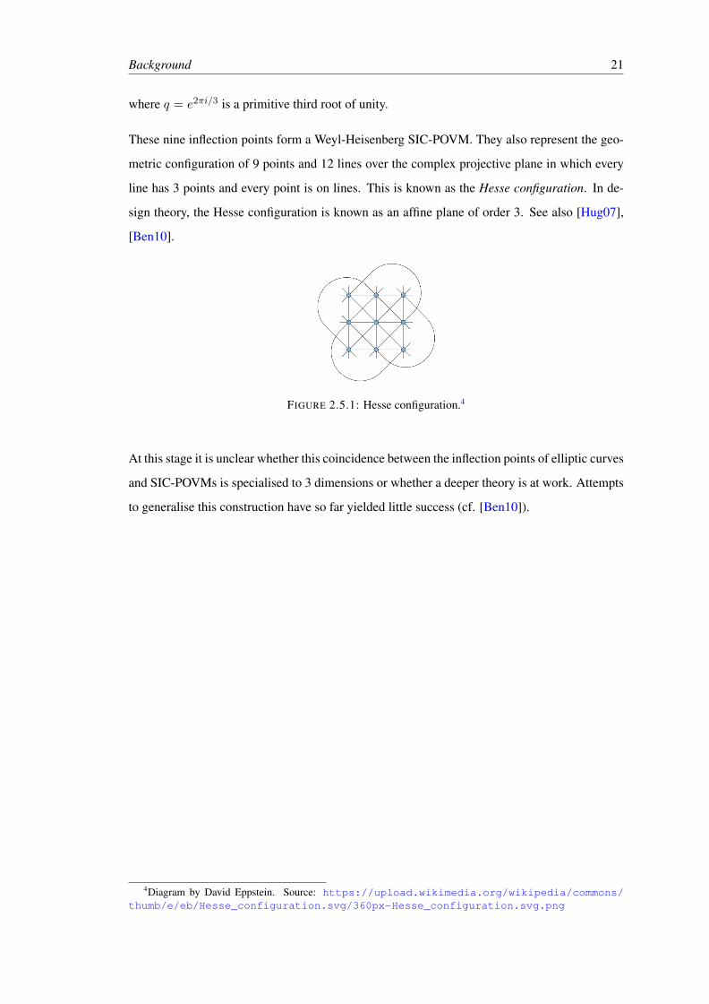
These nine inflection points form a Weyl-Heisenberg SIC-POVM. They also represent the geo-
metric configuration of 9 points and 12 lines over the complex projective plane in which every
line has 3 points and every point is on lines. This is known as the Hesse configuration. In de-
sign theory, the Hesse configuration is known as an affine plane of order 3. See also [Hug07],
[Ben10].
FIGURE 2.5.1: Hesse configuration.4
At this stage it is unclear whether this coincidence between the inflection points of elliptic curves
and SIC-POVMs is specialised to 3 dimensions or whether a deeper theory is at work. Attempts
to generalise this construction have so far yielded little success (cf. [Ben10]).
4Diagram by David Eppstein. Source: https://upload.wikimedia.org/wikipedia/commons/thumb/e/eb/Hesse_configuration.svg/360px-Hesse_configuration.svg.png
Chapter 3
Reverse engineering numerical
SIC-POVMs
In [RBKSC04], SIC-POVMs were numerically approximated (up to machine precision) for all
dimensions d ≤ 45 by minimising the second frame potential. The recent computational study
[SG10] extends this to d ≤ 67.
This chapter explores ways to utilise this information and attempt to recover analytic SIC-
POVMs from the numerical approximations to prove the existence of SIC-POVMs in new di-
mensions.
Numerical SIC-POVM data has proved to be very useful in the calculation of analytic SIC-
POVMs. In some cases, the components of a fiducial could be easily guessed (e.g., if a compo-
nent is 0). In other cases, various relationships emerged from the numerical data, allowing for
extra symmetries and reduced equations (e.g., Theorems 6.2 and 6.6 of [BW07] or the comments
on p. 8 of [SG10], which made SIC-POVMs in dimensions 24, 35, 48 viable to calculate).
Recent efforts to study the field structure of SIC-POVM fiducials ([SG10], [AYAZ13]) have led
to some remarkable conjectures (see Section 7 of [AYAZ13]). By leveraging these conjectures,
a systematic framework for attempting to reverse engineer SIC-POVM fiducials from numerical
SIC-POVMs was developed with Appleby et al. These ideas have fascinating analogies with the
theory of complex multiplication (see Chapter 6 of [ST92]).
22

Reverse engineering numerical SIC-POVMs 23
Using this framework, the aim will be to recover an analytic expression for a SIC-POVM using
its numerical approximation. This technique is applied to obtain a previously unknown SIC-
POVM in 17 dimensions.
3.1 Galois theory fundamentals
The material in this section can be found in standard algebra text books (e.g., Chapter 4 of
[Jac85], Chapters 5,6 and 7 of [Rom06], Chapter 32 of [Gal09], Chapter 9 of [Fra03] ). They
are reproduced without proof for completeness.
Definition 3.1.1.
Let E and F be fields such that F ⊂ E and E inherits the field operations of F. Then E is a field
extension of F.
Definition 3.1.2.
Let F be a field and α 6∈ F. Then E := F(α) is the smallest field extension of F containing α (F
is extended by α). If α is the root of a non zero polynomial with coefficients from F then E is
an algebraic extension.
Definition 3.1.3.
Let E be an algebraic extension of F and α ∈ E. The minimal polynomial of α is the monic
polynomial f of smallest degree in F [x], such that f(α) = 0.
Extension fields can be viewed as vector spaces over the base field and the degree of the exten-
sion is the dimension of the corresponding vector space. The degree of an extension E over F is
often written [E : F].
Proposition 3.1.4.
Let E := F(α). The degree of the minimal polynomial f of α over F is the degree of the
extension, i.e., [E : F] =deg(f ).
Theorem 3.1.5.
Let u be an element of an extension field E of a field F. Then u is algebraic over F if and only
if F(u) is finite dimensional over F.
Definition 3.1.6.
Let F be a field, f(x) a monic polynomial in F[x]. Then an extension field E over F (or E/F) is
Reverse engineering numerical SIC-POVMs 24
called a splitting field over F of f(x) ∈ E[x] if
f(x) = (x− r1)(x− r2) · · · (x− rn),
and
E = F(r1, r2, . . . , rn).
Definition 3.1.7.
A polynomial is separable if its roots are all distinct.
Definition 3.1.8.
Let E be an extension of F. Then E/F is separable if the minimal polynomial of every element
of E is separable. E/F is normal if every irreducible polynomial in F[x] which has a root in E
is a product of linear factors in E[x] (i.e., the polynomial “splits” in E[x]).
Note that all algebraic extensions of fields of characteristic 0 are separable. In particular, all
algebraic extensions of Q are separable, i.e., all extensions considered in this thesis are automat-
ically separable.
Definition 3.1.9.
An n–th root of unity is a root of the polynomial xn − 1.
Definition 3.1.10.
A cyclotomic extension is an extension of the form Q(ω), where ω is an n–th root of unity.
Definition 3.1.11.
Let G be a subgroup of the automorphism group of a field E. Then
Fix(G) := x ∈ E |ϕ(x) = x, ϕ ∈ G.
Theorem 3.1.12.
Let E be an extension field of a field F. Then the following conditions on E/F are equivalent:
1. E is a splitting field over F of a separable polynomial f(x).
2. F = Fix(G) for some finite group G of automorphisms of E.
3. E is finite dimensional, normal and separable over F.

Reverse engineering numerical SIC-POVMs 25
An extension satisfying one of the conditions of Theorem 3.1.12 is a Galois extension.
Definition 3.1.13 (Galois group).
Let E be a Galois extension of F and G the set of automorphisms of E/F, i.e., the automorphisms
of E that fix all elements of F. Then G is the Galois group of E over F and is sometimes written
Gal(E/F). Elements of G are called Galois automorphisms.
Theorem 3.1.14 (Fundamental theorem of Galois theory).
Let E be a Galois extension of F, G be the Galois group of E over F, Γ = H be the set of
subgroups of G, Σ be the set of subfields of E/F (intermediate fields between F and E). Then
there is a one-to-one correspondence between Σ and Γ. Furthermore,
1. H1, H2 ∈ Γ and H1 ⊂ H2 ⇐⇒ Fix(H2) ⊂ Fix(H1).
2. H ∈ Γ, |H| = [E : Fix(H)], [G : H] = [Fix(H) : F ].
3. H is normal in G ⇐⇒ Fix(H) is normal over F ⇐⇒ Gal(Fix(H)/F ) ' G/H .
Theorem 3.1.14 says that each subgroup of the Galois group of E over F corresponds to each
of the subfields in the tower of extensions from F to E. Furthermore, a normal subgroup of the
Galois group corresponds to a normal field extension over F.
Definition 3.1.15.
Let [E : F] be a finite Galois extension. Then E over F is an abelian extension if Gal(E/F) is
abelian.
Theorem 3.1.16 (Kronecker-Weber).
Every abelian extension of Q is contained in a cyclotomic extension.
Remark 3.1.17.
The Kronecker-Weber and the fundamental theorem of Galois theory are deep powerful theo-
rems in mathematics which took great time and effort from mathematicians to get a good handle
on and have interesting applications within other areas of mathematics.
Definition 3.1.18.
Let G be a group. A normal series is a sequence of subgroups such that
G = G1 G2 · · ·Gs Gs+1 = 1.
Reverse engineering numerical SIC-POVMs 26
Definition 3.1.19.
A group G is soluble (solvable) if it has a normal series and the factors in the sequence
G1/G2, G2/G3 . . . , Gs/Gs+1 ' Gs.
are all abelian.
Definition 3.1.20.
Let f(x) ∈ F[x] be monic of positive degree. The equation f(x) = 0 is said to be soluble by
radicals over F if there exists an extension field E/F possessing a tower of subfields
F = F1 ⊂ F2 ⊂ · · · ⊂ Fr+1 = E,
where each Fi+1 = Fi(di), dnii = ai ∈ Fi, and E contains a splitting field over F of f(x).
As each subfield in the tower from Definition 3.1.20 is generated by the previous field by adding
a radical ( ni√ai), the extension field E’s elements are always expressible as radical combinations
(potentially nested) of elements from F. Since f(x) splits over some intermediate extension of
F and E containing only radical combinations (potentially nested), its roots must be expressible
as radical combinations (potentially nested).
Theorem 3.1.21.
An equation f(x) = 0 is soluble by radicals over a field F of characteristic 0 if and only if its
Galois group is soluble.
Remark 3.1.22.
The theory of solutions to polynomial equations has been of great interest to mathematicians
over time and was of great interest to Galois. While Abel was the first to show that no gen-
eral algebraic solutions existed for quintic equations, Galois theory laid a pathway for a slick
characterisation of when polynomial equations would yield algebraic solutions.
3.1.1 Representing roots as radicals
Although Theorem 3.1.21 indicates when polynomial equations have radical roots, the statement
of the theorem alone gives no indication as to how such roots can be obtained from a polynomial
equation that is soluble by radicals.
Reverse engineering numerical SIC-POVMs 27
Given a polynomial equation f(x) = 0 that is soluble by radicals, one general approach to
recovering the roots as radicals is to formulate the splitting field E of f(x), calculate its Galois
group and the appropriate subgroup tower (normal series). Next, calculate the corresponding
subfield tower of E over F and at each level of the subfield tower, find the radical representation
of each cyclic extension as hinted by Definition 3.1.20. Once this is complete, each of the
extension field generators can be represented as radicals and the polynomial can be factorised
over E with the field generators converted to their radical representation.
In general this is not a trivial exercise, as it assumes one can readily compute things like the
Galois group, tower of field extensions or factorise polynomials easily over field extensions.
While some researchers have studied more sophisticated methods for approaching this problem
(c.f., [AY02], Problem 2.7.5 of [Stu08]), the naive approach outlined was sufficient for this
project.
3.2 SIC-POVM field structure
Let v be a SIC-POVM fiducial and Π := vv∗ be the corresponding fiducial projector. Consider
the minimal field extension (over Q) containing the elements of the projector (with standard
basis representation)1, τ = −eiπ/d and let the Galois group of this field extension over Q be G.
Let q = (i, j) ∈ Zd2, Πq be the SIC-POVM projector DqΠD
∗q , where Dq is a Weyl-Heisenberg
displacement operator.
Definition 3.2.1.
A SIC-POVM overlap is
χq := Tr(ΠDq).
Definition 3.2.2.
Let A,B be two square matrices in Md(C). The Hilbert-Schmidt (Frobenius) inner product
between A,B is
〈A,B〉 := trace(AB∗), A,B ∈Md(C).
Example 3.2.3.
The Weyl-Heisenberg displacement operators form an orthogonal basis for the space Md(C) of
d× d matrices relative to the Hilbert-Schmidt inner product.1the choice of basis is important as a complicated basis could even result in transcendental extensions

Reverse engineering numerical SIC-POVMs 28
The overlaps are the coefficients of the frame expansion (with Hilbert-Schmidt inner product)
Π =1
d
∑q∈Zd
2
〈Π, D∗q〉Dq =1
d
∑q∈Zd
2
χqDq. (3.2.1)
Because SIC-POVM overlaps are the coefficients for the frame expansion of a fiducial, they
uniquely determine a fiducial projector. The frame expansion formula also suggests a very close
relationship between the minimal field the overlaps reside in (as an extension of Q) and the
minimal field of the fiducial projectors. These fields were first studied in [SG10] and later by
[AYAZ13]. Although knowing the minimal fields does not prove SIC-POVM existence, it yields
interesting insight into the complexity of the fiducials and provides important information when
attempting to reverse engineer a numerical solution.
Unless otherwise indicated, the results in this section arise from [AYAZ13] and discussions with
Appleby.
Definition 3.2.4.
Let
a :=
√(d− 3)(d+ 1)
k,
where k is the biggest perfect square that divides (d− 3)(d+ 1). Let E be the smallest normal
extension of Q containing the components of Π (with respect to the standard basis), τ = −eiπ/d,
and E = E(√d).
Conjecture 3.2.5.
E and E are abelian extension fields of the real quadratic field Q(a).
This conjecture is true in all cases studied so far (see [AYAZ13]).
Definition 3.2.6.
Let Π be a fiducial projector. The stabiliser of Π is the group
SΠ := U ∈ ECL(d) : UΠU∗ = Π.
Definition 3.2.7.
Define UJ to be the anti-unitary which acts by complex conjugation on the standard basis, i.e.,
UJ(v) =∑r∈Zd
〈v, er〉er, for all vectors v.
Reverse engineering numerical SIC-POVMs 29
Definition 3.2.8.
Let G = GE be the Galois group of E over Q. For each g ∈ G and linear operator Γ defined in
terms of the standard basis and with its elements in E, define
g(Γ) =∑i,j∈Zd
g(〈Γ(ej), ei〉
)eie∗j .
If Γ is an anti-linear operator in E, define
g(Γ) = g(ΓUJ)UJ , UJ from Definition 3.2.7.
Definition 3.2.9.
Let gc ∈ G be the complex conjugation operator. Then Gc is the centraliser of gc.
Theorem 3.2.10.
If Π′ is a fiducial projector in E and g ∈ Gc then g(Π′) is also a fiducial projector.
In other words, as long as the Galois automorphisms considered commute with complex conju-
gation, fiducial vectors will be mapped to other fiducial vectors under the action of the Galois
automorphism.
Theorem 3.2.11.
Let G0 be the set of g ∈ Gc such that g(Π) is in the same extended Clifford orbit as Π. Then G0
is a subgroup of Gc.
Theorem 3.2.12.
For all g ∈ G0 and p ∈ Zd × Zd, there exists G ∈ GL(2,Zd) (depends on g) and a vector
rg ∈ Zd × Zd (depends on g) such that
g(χp) =
χGp, d 6= 0 mod 3
σ〈rg ,p〉χGp, d = 0 mod 3
where σ = e2πi/3.
Definition 3.2.13.
Let VF be of the form (2.4.4). A fiducial Π for which SΠ consists only of unitaries and anti-
unitaries of the form eiξVF is displacement-free.
Reverse engineering numerical SIC-POVMs 30
For displacement-free fiducials Π, define
SΠ =F ∈ ESL(2,Zd) : VF ∈ SΠ
,
and
SΠ =
(DetF )F : F ∈ SΠ
.
Lemma 3.2.14.
Let G ∈ ESL(2,Zd). Then the following statements are equivalent
1. G ∈ SΠ.
2. χGp = χp for all p ∈ Zd2 .
These lemmas and theorems provide a good understanding of the action of Galois groups on the
overlaps, aiding the reverse engineering efforts.
Definition 3.2.15.
A fiducial Π is simple if
1. SΠ contains a canonical order 3 unitary, and
2. SΠ is displacement-free.
Interestingly, all known Weyl-Heisenberg fiducial orbits in the extended Clifford group (both
numerical and analytic) contain simple fiducials. Many of the expressions involved simplify
when dealing with simple fiducials as the name suggests. The fiducials listed in the [SG10]
study are all simple fiducials.
Definition 3.2.16.
A singlet arises when a SIC-POVM orbit (under the Clifford group action) is stabilised by the
Galois group. A doublet is when two different SIC-POVM Clifford orbits are related via a
Galois automorphism, and a n–tuplet is when n orbits are related by Galois action.
While the possibility of there being n-tuplets (n > 2) is left open, it should be noted that all
analytic solutions found in the Scott-Grassl study have been singlets and doublets. This chapter
focuses primarily on the analysis of singlets.
Reverse engineering numerical SIC-POVMs 31
Conjecture 3.2.17.
Let CΠ be the centraliser of SΠ (as a subgroup of GL(2,Zd)). Then E has the following field
and Galois group structure (refer to equations 157, 158, 165 on pages 19-20 of [AYAZ13]).
Singlet situation:
QQ(a) E1 E,
where Gal(Q(a)/Q) = Z2, Gal(E1/Q(a)) = CΠ/SΠ and Gal(E/E1) = Z2.
Doublet situation:
QQ(a) E0 E1 E,
where Gal(Q(a)/Q) = Z2, Gal(E0/Q(a)) = Z2, Gal(E1/Q(a)) = CΠ/SΠ and Gal(E/E1)
= Z2.
When E 6= E, Gal(E/E) = Z2.
Note that these conjectures imply that the Galois group for E or E over Q is soluble.
Theorem 3.2.18.
Let Π be a simple fiducial such that SΠ is abelian and contains a matrix F conjugate to Fz . Then
CΠ consists of all matrices in GL(2,Zd) which can be written in the form
nI +mF
for some n,m ∈ Zd. In particular, CΠ and consequently CΠ/SΠ, are abelian.
Note that this theorem applies to SIC-POVM projectors with Zauner symmetry Fz . Interestingly,
in all known cases, SΠ is abelian.
Theorem 3.2.19.
Let d = 9k + 3 for some positive integer k and let F ∈ SL(2,Zd) be conjugate to Fa. Let CF
be the centraliser of 〈F 〉 considered as a subgroup of GL(2,Zd). Let G be any solution to the
equation 3G = F − I . Then CF consists of all matrices in GL(2,Zd) which can be written in
the form
nI +mG+d
3H,
for some n,m ∈ Zd and arbitrary matrix H .

Reverse engineering numerical SIC-POVMs 32
Unlike the previous theorem, this theorem only applies to non Zauner SIC-POVM projectors.
Note that CF is not always abelian and figuring out the structure of CF for non Fz symmetries
(e.g., Fa) is another reason why reverse engineering maybe a useful endeavour. However in the
two known analytic solutions where the symmetry is Fa instead of Fz (12b and 48g in the [SG10]
indexing), the group CF is abelian. For orbits 21e, 30d, 39i, j, 48e, where only numerical
solutions are known, the group appears to be non-abelian. Being able to obtain analytic solutions
in those 5 cases would also be interesting in order to learn about their CF structure.
The solubility of the Galois group is another key conjecture in pushing this forward. All known
analytic equiangular lines so far have had soluble Galois groups. If the Galois group was not
thought to be soluble, then this whole approach would not work.
Let p ∈ Zd × Zd. Then applying the action of the Galois group of E1 over Q(a) (for a singlet)
or E0 (for a doublet), i.e., letting CΠ/SΠ act on the overlaps, will split the overlaps into various
orbits. Within each of these orbits, the elements will be closed under the action of the Galois
group. This implies that the polynomials formed from∏p∈orbit
(x − χp) are invariant under the
Galois actions, and hence the coefficients of this polynomial must be in E0 (or Q(a)).
Conjecture 3.2.20 (Appleby).
Let G (the Galois group of E1 over Q(a)) act on the overlaps of a Weyl-Heisenberg SIC-POVM
fiducial Π (singlet or doublet) and O be one of the orbits under this action. Then Q(a) is the
base field of the polynomial
ρ :=∏χ∈O
(x− χ).
Observe that Conjecture 3.2.20 is a natural consequence of G fixing Q(a). Since G also fixes the
polynomial ρ, its coefficients must come from Q(a).
Conjecture 3.2.21 (Appleby).
For fiducials with Zauner symmetry, the Galois group of E over Q(a) when d = 5 mod 6 is
cyclic.
These results and theories about the Galois group and the overlaps conspire to direct most of
the focus to constructing overlaps polynomials and solving these polynomials for analytic roots.
The next section deals with this procedure in more detail.
Reverse engineering numerical SIC-POVMs 33
3.3 Methodology
The basic procedure for reverse engineering will be outlined with the details of each step in the
following subsections. It assumes that Conjectures 3.2.17, 3.2.20 and conj:5mod6cyclic hold . A
modified version will be presented in Section 3.4 which attempts to leverage Conjecture 3.2.21.
The procedure is outlined as follows:
(i) Precision bump the numerical fiducials to a high degree.
(ii) Generate overlaps and apply the action of the Galois group to the overlaps.
(iii) For each orbit, form a polynomial using all the overlaps as the roots.
(iv) Find and construct the necessary tower of field extensions to split the overlaps polynomials.
(v) Factorise the overlaps polynomials over the tower of extensions.
(vi) Match the analytic overlaps with the numerical ones.
(vii) Reconstruct the fiducial vector.
3.3.1 Precision bumping
The numerical SIC-POVMs found in [SG10] are of relatively low accuracy. One of the key ideas
in this procedure is to use the conjectured field structure to exactly identify what the overlaps
look like. Since field extensions are vector spaces, elements of extension fields over Q can be
written as Q-linear (and hence Z-linear) combinations of basis elements. This involves using
integer relation algorithms like LLL or PSLQ which have ready implementations in packages
like Mathematica or Maple. In order for these algorithms to function correctly, a threshold
precision must be present. This could be a few hundred digits of accuracy or sometimes more
than a thousand, so precision bumping is necessary. Figuring this out is an ad hoc process. For
the 17c SIC-POVM, 2000 digit precision was used.
To precision bump a SIC-POVM, a couple of known options are available. One option is to
let the numerical SIC-POVM be the initial starting vector for a method that attempts to find
a numerical SIC-POVM and demand a higher precision in the procedure. For example, by
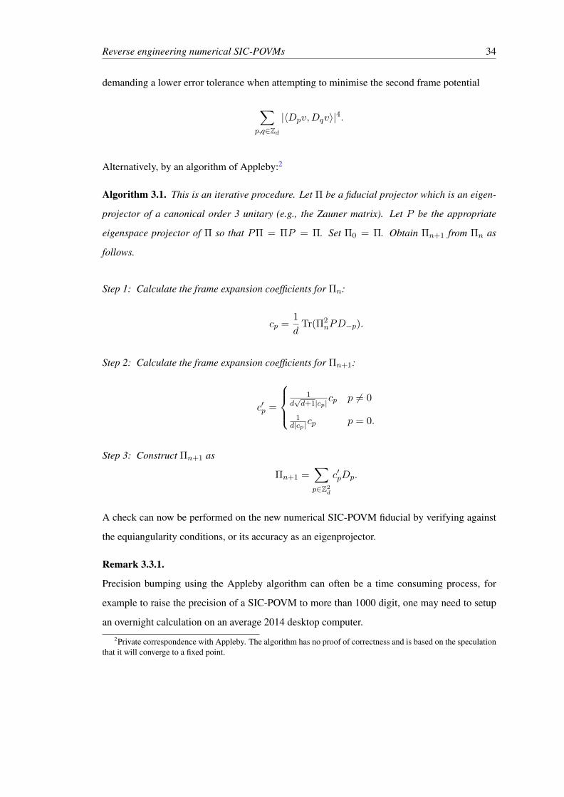
Reverse engineering numerical SIC-POVMs 34
demanding a lower error tolerance when attempting to minimise the second frame potential
∑p,q∈Zd
|〈Dpv,Dqv〉|4.
Alternatively, by an algorithm of Appleby:2
Algorithm 3.1. This is an iterative procedure. Let Π be a fiducial projector which is an eigen-
projector of a canonical order 3 unitary (e.g., the Zauner matrix). Let P be the appropriate
eigenspace projector of Π so that PΠ = ΠP = Π. Set Π0 = Π. Obtain Πn+1 from Πn as
follows.
Step 1: Calculate the frame expansion coefficients for Πn:
cp =1
dTr(Π2
nPD−p).
Step 2: Calculate the frame expansion coefficients for Πn+1:
c′p =
1
d√d+1|cp|
cp p 6= 0
1d|cp|cp p = 0.
Step 3: Construct Πn+1 as
Πn+1 =∑p∈Z2
d
c′pDp.
A check can now be performed on the new numerical SIC-POVM fiducial by verifying against
the equiangularity conditions, or its accuracy as an eigenprojector.
Remark 3.3.1.
Precision bumping using the Appleby algorithm can often be a time consuming process, for
example to raise the precision of a SIC-POVM to more than 1000 digit, one may need to setup
an overnight calculation on an average 2014 desktop computer.2Private correspondence with Appleby. The algorithm has no proof of correctness and is based on the speculation
that it will converge to a fixed point.

Reverse engineering numerical SIC-POVMs 35
3.3.2 Applying the Galois action
Assuming Conjecture 3.2.17, the Galois group G of E1 over Q(a) is CΠ. Note that G acts on
Zd×Zd as the overlaps of a SIC-POVM are indexed by p ∈ Zd×Zd. Now, by Theorem 3.2.18,
construct the centraliser (the Galois group). Apply the action of G to Zd×Zd to partition Zd×Zdinto various orbits.
Remark 3.3.2.
Note that in the doublet situation, one considers the Galois group of E1 over E0, so that Theo-
rem 3.2.18 can be used to partition Zd × Zd into orbits. However, the base field of the overlaps
polynomials ρ are no longer conjectured to have base field Q(a) (cf. Conjecture 3.2.20).
For every orbit B, and d 6= 0 mod 3, construct the overlaps polynomials as
ρB :=∏p∈B
(x− χp).
When d mod 3 = 0,
ρB :=∏p∈B
(x− χ3p).
While not essential, the cubing of the overlaps eliminates the need to deal with the technicality
of extra third roots of unity (Theorem 3.2.12). The original overlaps can be recovered once
the ρ polynomials are factorised by taking cube roots of the roots of ρ and then scaling by the
appropriate third root of unity.
3.3.2.1 Parity and order 3 symmetries
With the goal of factorising the various ρ in mind, it is beneficial to keep the degrees of ρ low
so the job of factorisation is more manageable. This can be accomplished by deleting the roots
of the ρB which are repeats, or are complex conjugates of other roots. The parity matrix
P :=
−1 0
0 −1
corresponding to the complex conjugation and the Zauner matrix Fz are elements of CΠ and
generate a subgroup
〈P, Fz〉 ⊂ CΠ
Reverse engineering numerical SIC-POVMs 36
of order 6. For fiducials stabilised by the Zauner symmetry, this allows for the degrees of the ρ
polynomials to decrease by up to a factor of 6.
If dealing with a different symmetry SIC-POVM (e.g., Fa), then use that symmetry in lieu of
Fz . The rest of the procedure will follow through.
3.3.3 Constructing the splitting fields for the overlaps polynomials
This step is the crux of the method, involving the most computational resources to accomplish.
Firstly, the exact (as opposed to numerical) overlaps polynomials need to be known. Then the
intermediate field extensions need to be recovered to build a tower of field extensions.
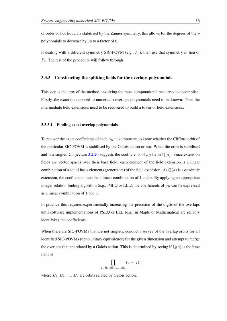
3.3.3.1 Finding exact overlap polynomials
To recover the exact coefficients of each ρB it is important to know whether the Clifford orbit of
the particular SIC-POVM is stabilised by the Galois action or not. When the orbit is stabilised
and is a singlet, Conjecture 3.2.20 suggests the coefficients of ρB lie in Q(a). Since extension
fields are vector spaces over their base field, each element of the field extension is a linear
combination of a set of basis elements (generators) of the field extension. As Q(a) is a quadratic
extension, the coefficients must be a linear combination of 1 and a. By applying an appropriate
integer relation finding algorithm (e.g., PSLQ or LLL), the coefficients of ρB can be expressed
as a linear combination of 1 and a.
In practice this requires experimentally increasing the precision of the digits of the overlaps
until software implementations of PSLQ or LLL (e.g., in Maple or Mathematica) are reliably
identifying the coefficients.
When there are SIC-POVMs that are not singlets, conduct a survey of the overlap orbits for all
identified SIC-POVMs (up to unitary equivalence) for the given dimension and attempt to merge
the overlaps that are related by a Galois action. This is determined by seeing if Q(a) is the base
field of ∏χ∈B1∪B2∪...∪Bk
(x− χ),
where B1, B2, . . ., Bk are orbits related by Galois action.
Reverse engineering numerical SIC-POVMs 37
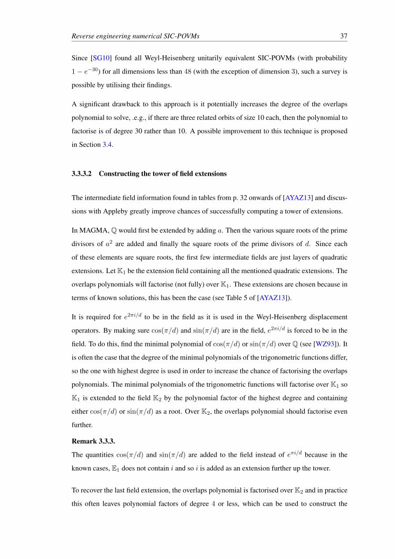
Since [SG10] found all Weyl-Heisenberg unitarily equivalent SIC-POVMs (with probability
1 − e−30) for all dimensions less than 48 (with the exception of dimension 3), such a survey is
possible by utilising their findings.
A significant drawback to this approach is it potentially increases the degree of the overlaps
polynomial to solve, .e.g., if there are three related orbits of size 10 each, then the polynomial to
factorise is of degree 30 rather than 10. A possible improvement to this technique is proposed
in Section 3.4.
3.3.3.2 Constructing the tower of field extensions
The intermediate field information found in tables from p. 32 onwards of [AYAZ13] and discus-
sions with Appleby greatly improve chances of successfully computing a tower of extensions.
In MAGMA, Q would first be extended by adding a. Then the various square roots of the prime
divisors of a2 are added and finally the square roots of the prime divisors of d. Since each
of these elements are square roots, the first few intermediate fields are just layers of quadratic
extensions. Let K1 be the extension field containing all the mentioned quadratic extensions. The
overlaps polynomials will factorise (not fully) over K1. These extensions are chosen because in
terms of known solutions, this has been the case (see Table 5 of [AYAZ13]).
It is required for e2πi/d to be in the field as it is used in the Weyl-Heisenberg displacement
operators. By making sure cos(π/d) and sin(π/d) are in the field, e2πi/d is forced to be in the
field. To do this, find the minimal polynomial of cos(π/d) or sin(π/d) over Q (see [WZ93]). It
is often the case that the degree of the minimal polynomials of the trigonometric functions differ,
so the one with highest degree is used in order to increase the chance of factorising the overlaps
polynomials. The minimal polynomials of the trigonometric functions will factorise over K1 so
K1 is extended to the field K2 by the polynomial factor of the highest degree and containing
either cos(π/d) or sin(π/d) as a root. Over K2, the overlaps polynomial should factorise even
further.
Remark 3.3.3.
The quantities cos(π/d) and sin(π/d) are added to the field instead of eπi/d because in the
known cases, E1 does not contain i and so i is added as an extension further up the tower.
To recover the last field extension, the overlaps polynomial is factorised over K2 and in practice
this often leaves polynomial factors of degree 4 or less, which can be used to construct the

Reverse engineering numerical SIC-POVMs 38
remaining field extension. Once this is done the overlaps polynomial will fully split over the full
extension field E. The final tower of extensions looks like:
Q ⊂ Q(a) ⊂ . . . ⊂ K1 ⊂ K2 ⊂ E.
Sometimes, in particular when not dealing with singlets, the last extension field will be harder
to find as factorising the overlaps polynomial over K2 may give factors of degree 5 or more. In
this case it is sometimes possible to find the missing polynomial of degree 4 or less by using
the same procedure to construct a tower of field extensions for a different overlap polynomial
(when more than one overlaps orbit exists). This occured in dimension 15 when solving for the
a, b fiducials (using Scott-Grassl indexing).
3.3.4 Recovering roots
Once E is constructed, it is possible to factorise the polynomial over E. The linear factors will
all be represented in terms of the generators of the intermediate fields. Since all of the generators
are known square roots, trigonometric functions or roots of polynomials of degree 4 or less, they
will be explicitly known and so the overlaps will be in radical form (plus the trigonometric part).
When these overlaps are found (as roots of the overlaps polynomial), they can be matched with
their numerical counterparts in order to find the right indexing for the overlaps. The overlaps
can then be fed into the frame expansion formula 3.2.1.
3.4 Improvements
The practical bottleneck for this technique is the computer’s ability to factorise polynomials
in a reasonable amount of time. The computation time for computing solutions varies greatly
depending on things like the degree of the polynomials and the complexity of the coefficients
and factors (e.g., the singlet solution for dimension 17 took much less computation time than
the doublets in dimension 15).
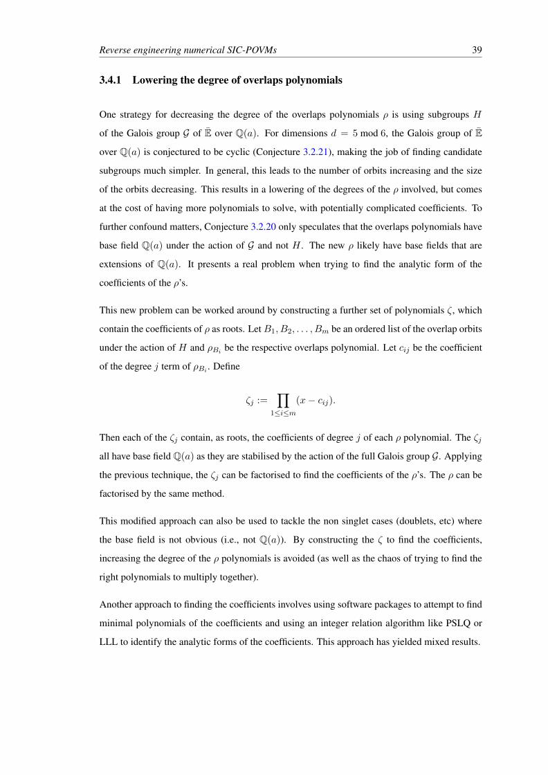
Reverse engineering numerical SIC-POVMs 39
3.4.1 Lowering the degree of overlaps polynomials
One strategy for decreasing the degree of the overlaps polynomials ρ is using subgroups H
of the Galois group G of E over Q(a). For dimensions d = 5 mod 6, the Galois group of E
over Q(a) is conjectured to be cyclic (Conjecture 3.2.21), making the job of finding candidate
subgroups much simpler. In general, this leads to the number of orbits increasing and the size
of the orbits decreasing. This results in a lowering of the degrees of the ρ involved, but comes
at the cost of having more polynomials to solve, with potentially complicated coefficients. To
further confound matters, Conjecture 3.2.20 only speculates that the overlaps polynomials have
base field Q(a) under the action of G and not H . The new ρ likely have base fields that are
extensions of Q(a). It presents a real problem when trying to find the analytic form of the
coefficients of the ρ’s.
This new problem can be worked around by constructing a further set of polynomials ζ, which
contain the coefficients of ρ as roots. LetB1, B2, . . . , Bm be an ordered list of the overlap orbits
under the action of H and ρBi be the respective overlaps polynomial. Let cij be the coefficient
of the degree j term of ρBi . Define
ζj :=∏
1≤i≤m(x− cij).
Then each of the ζj contain, as roots, the coefficients of degree j of each ρ polynomial. The ζj
all have base field Q(a) as they are stabilised by the action of the full Galois group G. Applying
the previous technique, the ζj can be factorised to find the coefficients of the ρ’s. The ρ can be
factorised by the same method.
This modified approach can also be used to tackle the non singlet cases (doublets, etc) where
the base field is not obvious (i.e., not Q(a)). By constructing the ζ to find the coefficients,
increasing the degree of the ρ polynomials is avoided (as well as the chaos of trying to find the
right polynomials to multiply together).
Another approach to finding the coefficients involves using software packages to attempt to find
minimal polynomials of the coefficients and using an integer relation algorithm like PSLQ or
LLL to identify the analytic forms of the coefficients. This approach has yielded mixed results.

Reverse engineering numerical SIC-POVMs 40
3.4.2 Simplifying the representation of solutions
Once various polynomials have been fully factorised, a secondary concern is whether it may
be possible to simplify the presentation of the solution. One way to achieve this is to look for
better field generators. Construct the Galois automorphisms of G and find the subgroups of
G (which will correspond to the field extensions). Using MAGMA, apply the automorphism
to a random element of an intermediate subfield to get a new element x. MAGMA is able to
construct the minimal polynomial of x and attempt to find a nicer minimal polynomial with
smaller coefficients by calling the OptimisedRepresentation function (attempts to find
a minimal polynomial that minimises the polynomial discriminant) [mag]. By first looking at
low index subgroups of the Galois group, i.e., the groups corresponding to low degree subfields,
simpler generators can be found first for those degree extensions. After rebuilding the tower of
extensions, the remaining higher degree extensions often simplify to some extent. The process
can be repeated on those higher degree extensions if necessary. In practice this method may not
always be fruitful as computations may take too long.
3.5 Results
The recovered analytic SIC-POVM for dimension 17 (17c) is given in Appendix C.
Factorising overlaps polynomials continues to be the major bottleneck in this project. Unless a
new approach is pioneered, or computer resources are significantly improved, it will remain a
barrier for reverse engineering higher dimensional numerical SIC-POVMs.
Chapter 4
Projective unitary equivalences of
frames
One natural question to consider when studying frames is when two frames are alike. A classic
notion to describe likeness is the idea of unitary equivalence. Unitary transformations are de-
sirable as they preserve the inner product relations and hence the geometry of the transformed
vectors. The unitary operators form a group as well.
When studying projective objects like lines, one hopes to be able to leverage the machinery of
vector spaces. This can be accomplished by considering the lines as vectors of a fixed length
(customarily unit length) and consider vectors scaled by arbitrary constants (of unit modulus) as
equivalent. The analogue is captured in the following definition.
Definition 4.0.1.
Let Ψ := (fj)j∈J and Φ := (gj)j∈J be finite sequences of vectors in a Hilbert space H. Then
Ψ and Φ are projectively unitarily equivalent if there exists a unitary operator U ∈ U(H) and
a sequence (cj)j∈J with |cj | = 1 such that
cjU(fj) = gj , for all j ∈ J.
Φ and Ψ are unitarily equivalent if and only if (cf. Corollary 2.1.9)
Gram(Φ) = Gram(Ψ). (4.0.1)
41

Projective unitary equivalences of frames 42
Φ and Ψ are projectively unitarily equivalent if and only if
Gram(Ψ) = C Gram(Φ)C∗, (4.0.2)
where C is the diagonal matrix with complex diagonal entries cj of unit modulus.
Prima facie, solving (4.0.2) looks promising, but for complex inner product spaces, the only
thing to work with is
〈wj , wk〉 = cjck〈vj , vk〉, ∀j, k.
From a survey of the literature, it appears that projective unitary equivalence has only been
previously calculated in a few situations using situation specific approaches.
These situations are: H = Rd by considering all possible cj = ±1 in (4.0.2) or by using two–
graphs in the case of equiangular lines (Chapter 11 of [GR01]), for a specific construction of
MUBs (using Weyl-Heisenberg or Clifford groups) via symplectic spreads, Hadamard matrices,
and for the equal–norm tight frames of n vectors in C2 robust to n − 2 erasures (Section 5 of
[CCKS97], Section 3 of [GR09], Section 3 of [Ben07], for SIC-POVMs Theorem 3 of [AFF11],
and Section 2 of [HP04]).
Following in the footsteps of [MACR01], a general method is developed for determining whether
any two finite sequence of vectors are projectively unitarily equivalent.
Definition 4.0.2.
The m–vertex Bargmann invariants or m–products of a sequence of n vectors Φ = (vj)j∈J
is
∆(vj1 , vj2 , . . . , vjm) := 〈vj1 , vj2〉〈vj2 , vj3〉 · · · 〈vjm , vj1〉, 1 ≤ j1, . . . , jm ≤ n. (4.0.3)
In particular, (adopting the terminology of [AFF11]), the triple products (3–products) are
Tjk` := ∆(vj , vk, v`) = 〈vj , vk〉〈vk, v`〉〈v`, vj〉. (4.0.4)

Projective unitary equivalences of frames 43
Remark 4.0.3.
The m–products are projective unitary invariants, e.g., for m = 3,
∆(cjUvj , ckUvk, c`Uv`) = 〈cjUvj , ckUvk〉〈ckUvk, c`Uv`〉〈c`Uv`, cjUvj〉
= cjck〈Uvj , Uvk〉ckc`〈Uvk, Uv`〉c`cj〈Uv`, Uvj〉
= 〈vj , vk〉〈vk, v`〉〈v`, vj〉
= ∆(vj , vk, v`). (4.0.5)
Remark 4.0.4.
The m–products are closed under complex conjugation, i.e.,
∆(vj1 , vj2 , . . . , vjm) = ∆(vjm , . . . , vj2 , vj1). (4.0.6)
The graph theory definitions and basic results in this Chapter can be found in a standard textbook
on graph theory, e.g., Chapter 1 of [Die10]. The key result in this chapter is Theorem 4.2.2 which
shows that a sequence of vectors (vj) is determined up to projective unitary equivalence by its
m–products for all m. While these results apply to arbitrary finite sequences of vectors, it is
sometimes convenient to refer to them as frames on the space that they span.
The proof of Theorem 4.2.2 identifies certain subsets of the m–products which classify the
sequences. These depend on which of the m–products are nonzero, a fact conveniently encap-
sulated by the notion of a frame graph.
Definition 4.0.5.
The frame graph (cf. Section 3 of [AN13]) of a sequence of vectors (vj)j∈J is the graph with
vertices vjj∈J (or the indices j themselves) and
an edge between vj and vk, j 6= k ⇐⇒ 〈vj , vk〉 6= 0.
Remark 4.0.6.
Projectively unitarily equivalent frames have the same frame graph.

Projective unitary equivalences of frames 44
4.1 Complete frame graphs
A generic sequence of vectors is unlikely to have any pairs of orthogonal vectors most of the
time. Hence, its corresponding frame graphs is often a complete graph. Appleby et al showed
that d2 equiangular vectors in Cd are characterised up to projective unitary equivalence by their
triple products (3–products) in [AFF11]. This section extends their proof to cover frames with
complete graphs, however these results do not extend to a general sequence of vectors.
Definition 4.1.1.
The angles of a sequence of vectors Φ = (vj)j∈J are the θjk ∈ R/(2πZ) defined by
〈vj , vk〉 = |〈vj , vk〉|eiθjk , 〈vj , vk〉 6= 0.
Since 〈vj , vk〉 = 〈vk, vj〉, these angles satisfy the relation
θjk = −θkj .
Remark 4.1.2.
A sequence of vectors might only have few angles, e.g., an orthogonal basis has no angles.
Lemma 4.1.3.
Let Φ = (vj)j∈J and Ψ = (wj)j∈J be finite sequences of vectors in Hilbert spaces, with angles
θjk and θ′jk. Then Φ and Ψ are projectively unitarily equivalent if and only if
1. Their Gramians have entries with equal moduli, i.e.,
|〈wj , wk〉| = |〈vj , vk〉|, ∀j, k.
2. Their angles are “gauge equivalent”, i.e., there exist φj ∈ R/(2πZ) with
θ′jk = θjk + φj − φk, ∀j, k.

Projective unitary equivalences of frames 45
Proof. Suppose Φ and Ψ are projectively unitarily equivalent, i.e., wj = cjUvj , where U is
unitary and cj = eiφj . Then
eiθ′jk |〈wj , wk〉| = 〈wj , wk〉 = 〈cjUvj , ckUvk〉 = cjck〈Uvj , Uvk〉 = ei(φj−φk)〈vj , vk〉
= ei(φj−φk)eiθjk |〈vj , vk〉|
By equating the moduli and then the arguments, 1 and 2 are obtained.
Conversely, suppose that 1 and 2 hold. Let vj := eiφjvj . Then
〈vj , vk〉 = 〈eiφjvj , eiφkvk〉 = ei(φj−φk)〈vj , vk〉 = ei(φj−φk)eiθjk |〈vj , vk〉|
= eiθ′jk |〈wj , wk〉| = 〈wj , wk〉.
Therefore (wj)j∈J is unitarily equivalent to (vj)j∈J , which is projectively unitarily equivalent
to (vj)j∈J , so Ψ and Φ are projectively unitarily equivalent.
|〈vj , vk〉| is calculated from the triple products of (4.0.4), as
Tjjj = 〈vj , vj〉3 = ‖vj‖6, Tjjk = 〈vj , vj〉|〈vj , vk〉|2 = T13jjj |〈vj , vk〉|
2. (4.1.1)
Theorem 4.1.4 (Characterisation).
Let Φ = (vj)j∈J and Ψ = (wj)j∈J be finite sequences of vectors in Hilbert spaces. Then
1. Φ and Ψ are unitarily equivalent if and only if their Gramians are equal, i.e.,
〈vj , vk〉 = 〈wj , wk〉, ∀j, k.
2. If the frame graphs of Φ and Ψ are complete, then they are projectively unitarily equivalent
if and only if their triple products are equal, i.e.,
〈vj , vk〉〈vk, v`〉〈v`, vj〉 = 〈wj , wk〉〈wk, w`〉〈w`, wj〉, ∀j, k, `.
Proof. The condition for unitary equivalence is well known. It is included for comparison. For
2, suppose that Φ and Ψ are projectively unitarily equivalent, i.e., wj = cjUvj . By (4.0.5), their
triple products are equal.
Projective unitary equivalences of frames 46
Conversely, suppose that Φ and Ψ have the same triple products and their common frame graph
is complete, i.e., all the triple products are nonzero.
It follows from (4.1.1) that their Gramians have entries with equal moduli, i.e.,
|〈vj , vk〉| = |〈wj , wk〉|, ∀j, k.
Let θjk and θ′jk be the angles of Φ and Ψ. Then
Tjk` = 〈vj , vk〉〈vk, v`〉〈v`, vj〉 = ei(θjk+θk`+θ`j)|〈vj , vk〉〈vk, v`〉〈v`, vj〉|,
implies
θjk + θk` + θ`j = θ′jk + θ′k` + θ′`j .
Fix ` and let φj := θ`j − θ′`j . Since θk` = −θ`k and θ′k` = −θ′`k,
θ′jk = θjk + (θ`j − θ′`j) + (θk` − θ′k`) = θjk + (θ`j − θ′`j)− (θ`k − θ′`k) = θjk + φj − φk,
i.e., the angles of Φ and Ψ are gauge equivalent. The conditions of Lemma 4.1.3 hold, so it
follows that Φ and Ψ are projectively unitarily equivalent.
The real case is closely connected with the theory of two–graphs (cf. Chapter 11 of [GR01]).
Example 4.1.5.
Recall from Example 2.5.1 that
v(t) :=1√2
(0, 1,−eit)T , t ∈ T,
gives a continuous family of Weyl-Heisenberg SIC-POVMs in 3 dimensions. By studying the
triple products, it is apparent that the v(t) give projectively unitarily inequivalent SIC-POVMs.
The Weyl-Heisenberg SIC-POVMs in 3 dimensions were studied extensively in Section 8.5 of
[Zhu12] and used to categorise the fiducials based on the angles (arguments of the complex
numbers) of the triple products.
Example 4.1.6 (Equiangular lines in Rd).
Let Φ = (vj)j∈J be a sequence of n > d equiangular unit vectors (lines) in Rd, i.e., there is an
α > 0 with
〈vj , vk〉 = ±α, j 6= k.
Projective unitary equivalences of frames 47
Then
GΦ = Gram(Φ) = I + αSΦ,
where S = SΦ is a Seidel matrix, i.e., S is symmetric, with zero diagonal and off diagonal en-
tries ±1. Each Seidel matrix is associated with a sequence of equiangular lines. S is associated
with the graph gr(S) which has an edge between j 6= k if and only if Sjk = −1. Let C be the
set of all diagonal matrices with diagonal entries ±1. Then the projective unitary equivalence
class of Φ is determined by all the possible Gram matrices conjugated by members of C, i.e.,
G := CGΦC∗ : C ∈ C,
and hence all the possible Seidel matrices
S := CSΦC∗ : C ∈ C,
and all the corresponding graphs gr(S).
The set of graphs gr(S) is called the switching class of gr(SΦ), or a two–graph.
Since the frame graph of Φ is complete, the projective unitary equivalence class of Φ (equiv-
alently G, S or gr(S)) is characterised by the triple products of Φ (Theorem 4.1.4). It is only
necessary to consider triple products with distinct indices. If an index is repeated twice or thrice,
by (4.1.1), the triple products depends only on α. These triple products are also independent of
the ordering of the indices.
Example 4.1.7 (Equiangular lines in Cd).
Let Φ be a sequence of n equiangular unit vectors (lines) in Cd, with C > 0. Then Φ is
determined by its triple products (up to projective unitary equivalence). When n = d2 (a SIC-
POVM), this is the result in Theorem 3 and its remarks in [AFF11].
Example 4.1.8 (n–cycle).
Let (ej)j∈J be the standard basis vectors in Cn. Fix |z| = 1 and let
vj :=
ej + ej+1, 1 ≤ j < n,
en + ze1, j = n.
Projective unitary equivalences of frames 48
The frame graph of (vj)j∈J is the n–cycle (v1, . . . , vn), so the only nonzero m–products for
distinct vectors are
∆(vj) = ‖vj‖2 = 2, 1 ≤ j ≤ n, (4.1.2)
∆(vj , vj+1) = |〈vj , vj+1〉|2 = 1, 1 ≤ j < n, (4.1.3)
∆(v1, v2, . . . , vn) = z, (4.1.4)
and their complex conjugates. Different choices of z give projectively inequivalent frames.
Thus, for n > 3, the vectors (vj)j∈J are not defined up to projective unitary equivalence by
their triple products.
4.2 Characterisation of projective unitary equivalence
A sequence of n vectors (vj)j∈J is determined up to projective unitary equivalence by its m–
products for all 1 ≤ m ≤ n. Verifying that two projectively unitarily equivalent frames
induce the same m–products is a standard fare calculation. The crux is in proving the con-
verse. The strategy will be to construct a sequence of vectors (wj)j∈J with given m–products
∆(vj1 , . . . , vjm). It amounts to reconstructing all Gramians for a given set of m–products.
Example 4.2.1.
A sequence of n vectors (vj)j∈J can be constructed in different ways for a given a Gram matrix
G. If V is a frame of n vectors spanning a dimension d space, then G is positive semidefinite of
rank d and unitarily diagonalisable.
G = U∗ΛU, Λ =
γ1
. . .
γn
, γ1, . . . , γd > 0, γd+1, . . . , γn = 0,
Taking V = [v1, . . . , vn] = Λ12U gives vectors (vj) in Cn which are zero in the last n − d
components and can be identified with vectors in Cd. Alternatively, take the Cholesky decom-
position G = V ∗V .
Projective unitary equivalences of frames 49
As the diagonal entries of the Gram matrices are given by the 1–products and the moduli of its
off diagonal entries by the 2–products with distinct arguments, i.e.,
∆(vj) = ‖vj‖2, ∆(vj , vk) = |〈vj , vk〉|2, j 6= k, (4.2.1)
it remains to choose arguments for the nonzero off diagonal entries of G, which are consistent
with the m–products for m ≥ 3. By choosing C in (4.0.2), some of these can be taken to
be arbitrary. When this is done fully, the remaining arguments will be determined by the m–
products.
Theorem 4.2.2 (Characterisation).
Two sequences (vj)j∈J and (wj)j∈J of n vectors are projectively unitarily equivalent if and only
if their m–products are equal, i.e.,
∆(vj1 , vj2 , . . . , vjm) = ∆(wj1 , wj2 , . . . , wjm), 1 ≤ j1, . . . , jm ≤ n, 1 ≤ m ≤ n.
Proof. It suffices to find a Gram matrix
G = [〈wk, wj〉] = C Gram(Φ)C∗
by using only the m–products of Φ = (vj)j∈J . The frame graph of Φ and the modulus of each
entry of G are known by (4.2.1). It remains to determine the arguments of the (nonzero) inner
products. These correspond to edges of the frame graph. Without loss of generality, assume the
frame graph of Φ is connected. Otherwise apply the method to each connected component of Γ.
Let T be a spanning tree of Γ with root vertex r. While fanning out from the root r (breadth-
first search), multiply the vertices v ∈ Γ \ r by unit scalars so that the arguments of the
inner products corresponding to the edges of Γ take arbitrarily assigned values. Continue in this
fashion until you have reached every vertex.
The remaining undefined entries of the Gram matrix G are given by the edges of Γ which are
not in T . Since T is a spanning tree, adding each such edge to T gives an m–cycle. The
corresponding nonzero m–product has all inner products already determined, except the one
corresponding to the edge added. It is therefore uniquely determined by the m–product.
Projective unitary equivalences of frames 50
Corollary 4.2.3.
A frame is projectively unitarily equivalent to a real frame if and only if its m–products are all
real.
Example 4.2.4.
Let Φ = (ej)j∈J be an orthonormal basis for C3, which has Gram matrix
Gram(Φ) =
1 0 0
0 1 0
0 0 1
.
The frame graph is totally disconnected (see Fig. 4.2.1), so each possible G (as in the proof of
Theorem 4.2.2) is determined by only 1–products and 2–products.
Example 4.2.5.
Let Φ = (vj)j∈J be three equiangular lines in C2. Then
Gram(Φ) =
1 1
2 −12
12 1 1
2
−12
12 1
.
A spanning tree with root v1 is given by the path v1, v2, v3. Working out from the root v1 = w1,
scale v2 and v3 to wj = cjvj , so that the arguments of 〈w1, w2〉 and 〈w2, w3〉 are arbitrary, say
a and b respectively with |a| = |b| = 1. The only inner product which is not yet determined is
〈w1, w3〉. This is obtained by completing the 3–cycle v1, v2, v3, v1, i.e.,
∆(w1, w2, w3) = ∆(v1, v2, v3) =⇒(1
2a)(1
2b)(1
2〈w3, w1〉
)=(1
2
)3
=⇒ 〈w1, w3〉 = ab.
The Gram matrices G of vectors (wj)j∈J which are projectively unitarily equivalent to Φ =
(vj)j∈J are given by
G =
1 1
2a12ab
12a 1 1
2b
12ab
12b 1
, |a| = |b| = 1.
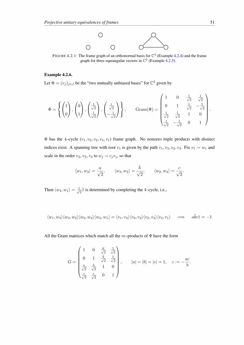
Projective unitary equivalences of frames 51
FIGURE 4.2.1: The frame graph of an orthonormal basis for C3 (Example 4.2.4) and the framegraph for three equiangular vectors in C2 (Example 4.2.5).
Example 4.2.6.
Let Φ = (vj)j∈J be the “two mutually unbiased bases” for C2 given by
Φ =
1
0
,
0
1
,
1√2
1√2
,
1√2
− 1√2
, Gram(Φ) =
1 0 1√
21√2
0 1 1√2− 1√
2
1√2
1√2
1 0
1√2− 1√
20 1
.
Φ has the 4–cycle (v1, v3, v2, v4, v1) frame graph. No nonzero triple products with distinct
indices exist. A spanning tree with root v1 is given by the path v1, v3, v2, v4. Fix v1 = w1 and
scale in the order v3, v2, v4 to wj = cjvj , so that
〈w1, w3〉 =a√2, 〈w3, w2〉 =
b√2, 〈w2, w4〉 =
c√2.
Then 〈w4, w1〉 = 1√2z is determined by completing the 4–cycle, i.e.,
〈w1, w3〉〈w3, w2〉〈w2, w4〉〈w4, w1〉 = 〈v1, v3〉〈v3, v2〉〈v2, v4〉〈v4, v1〉 =⇒ abcz = −1
All the Gram matrices which match all the m–products of Φ have the form
G =
1 0 a√
2z√2
0 1 b√2
c√2
a√2
b√2
1 0
z√2
c√2
0 1
, |a| = |b| = |c| = 1, z := −acb.

Projective unitary equivalences of frames 52
Φ is determined up to projective unitary equivalence by its 1–products and 2–products, since
Sylvester’s criterion for G to be positive semidefinite gives
det(G) = −1
4
(bz + ac)2
abcz= −1
4
∣∣∣∣bzac + 1
∣∣∣∣2 ≥ 0 =⇒ bz
ac+ 1 = 0 =⇒ z = −ac
b.
Contrast this to Example 4.1.8, which is not determined up to projective unitary equivalence by
its 1–products and 2–products.
4.3 Reconstruction from the m–products
Theorem 4.2.2 shows that only a small subset of the m–products is required to determine a
sequence of vectors up to projective unitary equivalence.
Definition 4.3.1.
A determining set is a subset of the m–products (or the corresponding indices) that can deter-
mine all m–products.
Corollary 4.3.2.
Let Γ be the frame graph of a sequence of n vectors Φ. For each connected component Γj of
Γ, let Tj be a spanning tree. Then Φ is determined up to projective unitary equivalence by the
following m–products
(i) The 2–products
(ii) The m–products, 3 ≤ m ≤ n, used to obtain Γj from Tj by completing m–cycles (these
have indices in Γj), as detailed in the proof of Theorem 4.2.2.
Remark 4.3.3.
If M is the number of edges of Γ which are not in any Tj , then it is sufficient to know all of the
2–products and M of the m–products, 3 ≤ m ≤ n.
Remark 4.3.4.
The m–products from (i) and (ii) are a determining set.
Although Example 4.2.6 shows the m–products of (ii) may not be a minimal set of m-products
needed to characterise a sequence of vectors, it is a minimal subset from which the m–products
can be determined using only the proof of Theorem 4.2.2.

Projective unitary equivalences of frames 53
Example 4.3.5.
Let Φ = (vj)j∈J be four equiangular vectors with C > 0. The frame graph of Φ is complete
and M = 6− 3 = 3. Spanning trees (see Fig. 4.3.1) include
Tp := the path v1, v2, v3, v4,
Ts := the star graph internal vertex v1 and leaves v2, v3, v4.
For Tp, complete either the 4–cycle v1, v2, v3, v4, v1 followed by any one of the four 3–cycles or
two of the 3–cycles, in order to determine the rest of the m–products. For example, a determin-
ing set is given by the 2–products and
∆(v1, v2, v3, v4), ∆(v1, v2, v3), ∆(v1, v2, v4). (4.3.1)
For Ts, adding any edge completes a 3–cycle containing v1. Then there are two edges which can
be added to complete a 3–cycle. Adding another edge afterwards completes the remaining two
3–cycles. For example, a determining set is given by the 2–products and
∆(v1, v2, v3), ∆(v1, v2, v4), ∆(v1, v3, v4). (4.3.2)
v1
v2
v3
v4
v1
v2
v3
v4
FIGURE 4.3.1: The spanning trees Tp and Ts (and cycle completions) of Example 4.3.5.
Note that the 4–product of (4.3.1) is decomposable into smaller m–products, e.g.,
∆(v1, v2, v3, v4) =∆(v1, v2, v3)∆(v1, v3, v4)
∆(v1, v3), (4.3.3)
Projective unitary equivalences of frames 54
so ∆(v1, v2, v3, v4) can be replaced by the 3–cycle ∆(v1, v3, v4), which gives the determining
set of (4.3.2).
The m–products of (ii) can be those corresponding to the fundamental cycles, i.e., the unique
cycle completed by adding an edge to Tj from Γj \ Tj . These fundamental cycles form a basis
for the cycle space, i.e., the Z2–formal linear combinations of cycles.
Leveraging this linear algebra framework, Theorem 4.2.2 is generalised as follows.
Theorem 4.3.6 (Characterisation II).
Two finite sequences of vectors (vj)j∈J and (wj)j∈J are projectively unitarily equivalent if and
only if their 2–products are equal and the m–products corresponding to the m–cycles that form
a basis for the cycle space of the frame graph are equal.
Proof. All cycles in the frame graph can be calculated from those in a basis and hence all m–
products can be calculated from those corresponding to a basis, as indicated in (4.3.3).
Example 4.3.7.
The fundamental cycles corresponding to the trees Tp and Ts of Example 4.3.5 give the following
m–products
∆(v1, v2, v3, v4), ∆(v1, v2, v3), ∆(v2, v3, v4), (4.3.4)
∆(v1, v2, v3), ∆(v1, v2, v4), ∆(v1, v3, v4), (4.3.5)
respectively.
Theorem 4.1.4 is restated as follows.
Theorem 4.3.8.
Let Φ = (vj)j∈J be a finite sequence of vectors. Then Φ is determined up to projective unitary
equivalence by its 3–products if the cycle space of its frame graph is spanned by 3–cycles (there
exists a basis of 3–cycles).
Example 4.3.9.
(Chordal graphs) A graph is chordal (or triangulated) if each of its cycles of four or more
vertices has a chord. The cycle space is spanned by the 3–cycles. If the frame graph of Φ is
chordal, (e.g., equiangular lines), then Φ is determined by its triple products.
The extreme cases are a totally disconnected graph (orthogonal bases) where there are no cycles
and the complete graph where all subsets of three vectors lie on a 3-cycle.
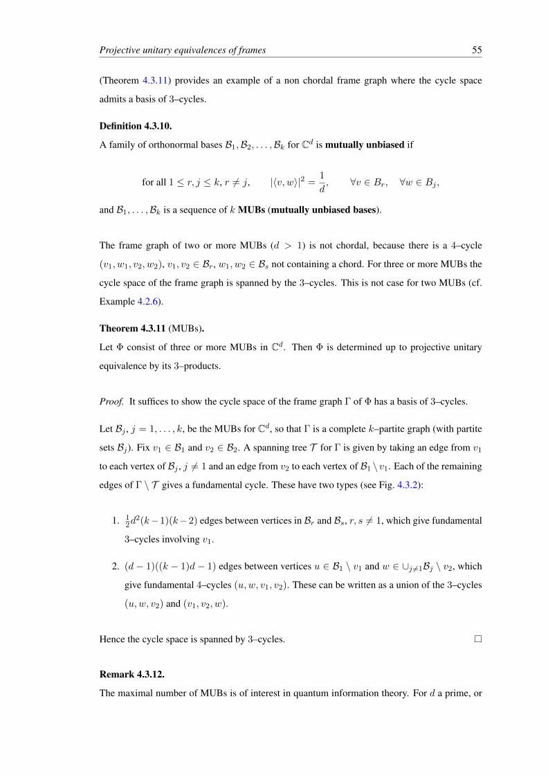
Projective unitary equivalences of frames 55
(Theorem 4.3.11) provides an example of a non chordal frame graph where the cycle space
admits a basis of 3–cycles.
Definition 4.3.10.
A family of orthonormal bases B1,B2, . . . ,Bk for Cd is mutually unbiased if
for all 1 ≤ r, j ≤ k, r 6= j, |〈v, w〉|2 =1
d, ∀v ∈ Br, ∀w ∈ Bj ,
and B1, . . . ,Bk is a sequence of k MUBs (mutually unbiased bases).
The frame graph of two or more MUBs (d > 1) is not chordal, because there is a 4–cycle
(v1, w1, v2, w2), v1, v2 ∈ Br, w1, w2 ∈ Bs not containing a chord. For three or more MUBs the
cycle space of the frame graph is spanned by the 3–cycles. This is not case for two MUBs (cf.
Example 4.2.6).
Theorem 4.3.11 (MUBs).
Let Φ consist of three or more MUBs in Cd. Then Φ is determined up to projective unitary
equivalence by its 3–products.
Proof. It suffices to show the cycle space of the frame graph Γ of Φ has a basis of 3–cycles.
Let Bj , j = 1, . . . , k, be the MUBs for Cd, so that Γ is a complete k–partite graph (with partite
sets Bj). Fix v1 ∈ B1 and v2 ∈ B2. A spanning tree T for Γ is given by taking an edge from v1
to each vertex of Bj , j 6= 1 and an edge from v2 to each vertex of B1 \v1. Each of the remaining
edges of Γ \ T gives a fundamental cycle. These have two types (see Fig. 4.3.2):
1. 12d
2(k−1)(k−2) edges between vertices in Br and Bs, r, s 6= 1, which give fundamental
3–cycles involving v1.
2. (d− 1)((k − 1)d− 1) edges between vertices u ∈ B1 \ v1 and w ∈ ∪j 6=1Bj \ v2, which
give fundamental 4–cycles (u,w, v1, v2). These can be written as a union of the 3–cycles
(u,w, v2) and (v1, v2, w).
Hence the cycle space is spanned by 3–cycles.
Remark 4.3.12.
The maximal number of MUBs is of interest in quantum information theory. For d a prime, or
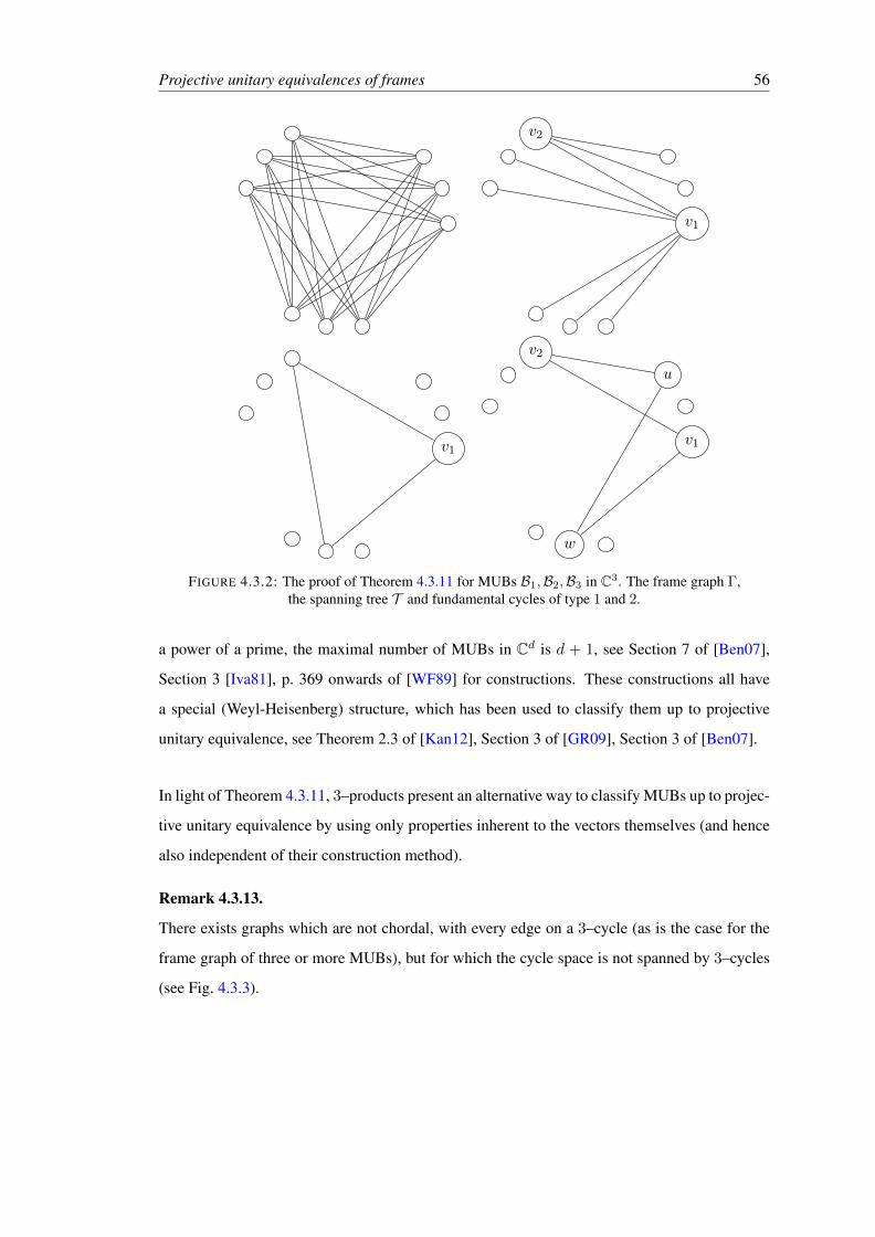
Projective unitary equivalences of frames 56
v1
v2
v1v1
u
v2
w
FIGURE 4.3.2: The proof of Theorem 4.3.11 for MUBs B1,B2,B3 in C3. The frame graph Γ,the spanning tree T and fundamental cycles of type 1 and 2.
a power of a prime, the maximal number of MUBs in Cd is d + 1, see Section 7 of [Ben07],
Section 3 [Iva81], p. 369 onwards of [WF89] for constructions. These constructions all have
a special (Weyl-Heisenberg) structure, which has been used to classify them up to projective
unitary equivalence, see Theorem 2.3 of [Kan12], Section 3 of [GR09], Section 3 of [Ben07].
In light of Theorem 4.3.11, 3–products present an alternative way to classify MUBs up to projec-
tive unitary equivalence by using only properties inherent to the vectors themselves (and hence
also independent of their construction method).
Remark 4.3.13.
There exists graphs which are not chordal, with every edge on a 3–cycle (as is the case for the
frame graph of three or more MUBs), but for which the cycle space is not spanned by 3–cycles
(see Fig. 4.3.3).

Projective unitary equivalences of frames 57
FIGURE 4.3.3: A nonchordal graph for which each edge is on a 3–cycle.
4.4 Similarity and m–products for vector spaces
Considering the more general setting of frames in vector spaces, the role of unitary equivalence
can be played by “similarity” [Wal11] and the role of m–products by “canonical m–products”.
So the “projective symmetry group” can be recast in a general setting.
Definition 4.4.1.
Let Φ = (vj)j∈J and Ψ = (wj)j∈J be finite sequences of vectors spanning vector spaces X
and Y over a subfield F of C. Then Φ and Ψ are similar if there is an invertible linear map
Q : X → Y with
wj = Qvj , ∀j,
and projectively similar if there is an invertible linear map Q : X → Y and unit scalars cj with
wj = cjQvj , ∀j.
Definition 4.4.2.
Let V be the synthesis map of Φ (see Definition 2.1.5). The subspace of all linear dependencies
between the vectors of Φ is
dep(Φ) := ker(V ) = a ∈ FJ :∑
j ajvj = 0,
and denote the orthogonal projection onto dep(Φ)⊥ (orthogonal complement) by PΦ.
The following characterisation of similarity is cast in terms of linear dependencies.
Projective unitary equivalences of frames 58
Lemma 4.4.3 (Lemma 3.3, [Wal11]).
Let Φ = (vj)j∈J and Ψ = (wj)j∈J be spanning sequences for the F–vector spaces X and Y .
The following are equivalent,
(a) Φ and Ψ are similar, i.e., there is a invertible linear map Q : vj 7→ wj .
(b) dep(Φ) = dep(Ψ) (the dependencies are equal).
(c) PΦ = PΨ (the associated projections are equal).
Φ = (vj) is similar to the columns of P = PΦ (proof of Lemma 4.4.3). These columns (Pej)
span a subspace of FJ inheriting the Euclidean inner product. Indeed
〈Pej , P ek〉 = Pjk,
i.e., the Gramian of (Pej) is P = PΦ.
Definition 4.4.4.
The m–products of (Pej)j∈J are the canonical m–products of (vj)j∈J , given by
∆C(vj1 , . . . , vjm) := ∆(Pej1 , . . . , P ejm) = Pj1j2Pj2j3 · · ·Pjmj1 . (4.4.1)
Theorem 4.4.5 (Characterisation).
Let Φ = (vj)j∈J and Ψ = (wj)j∈J be finite sequences of vectors in vector spaces over a subfield
F (of C) closed under complex conjugation. Then
1. Φ and Ψ are similar if and only if PΦ = PΨ.
2. Φ and Ψ are projectively similar if and only if their canonical m–products (for a deter-
mining set) are equal.
Proof. The first follows from Lemma 4.4.3 and implies that Φ and Ψ are projectively similar,
i.e.,
wj = cjQvj = Q(cjvj), ∀j,
if and only if Ψ = (wj)j∈J and Φ′ = (cjvj)j∈J are similar, for some choice of unit scalars (cj),
i.e.,
PΨ = P(cjvj) = C∗PΦC. (4.4.2)

Projective unitary equivalences of frames 59
Since Φ and Ψ are similar to (PΦej)j∈J and (PΨej)j∈J , (with Gram matrices PΦ and PΨ re-
spectively), it follows from (4.0.2) that (4.4.2) is equivalent to (PΦej)j∈J and (PΨej)j∈J being
projectively unitary equivalent. By Theorem 4.1.4, this is equivalent to their m–products, (i.e.,
the canonical m–products of (vj)j∈J and (wj)j∈J ) being equal.
For projective similarity, cj and Q in wj = cjQvj can be calculated explicitly.
Example 4.4.6.
Let Φ = (vj)j∈J span a 2–dimensional space, i.e.,
αv1 + βv2 + γv3 = 0, |α|2 + |β|2 + |γ|2 = 1.
Then dep(Φ) = spanu, u = (α, β, γ), so that
PΦ = I − uu∗ =
1− |α|2 −αβ −αγ
−αβ 1− |β|2 −βγ
−αγ −βγ 1− |γ|2
.
The canonical 2–products are uniquely determined by |a|, |b|, |c|, e.g.,
∆C(v1, v1) = (1− |α|2)2, ∆C(v1, v2) = | − αβ|2 = |α|2|β|2,
Likewise the canonical 3–product corresponding to the unique 3–cycle
∆C(v1, v2, v3) = (−αβ)(−βγ)(−αγ) = −|α|2|β|2|γ|2.
If Ψ = (wj)j∈J is given by
αw1 + βw2 + γw3 = 0, |α|2 + |β|2 + |γ|2 = 1,
then
1. Ψ is similar to Φ if and only if PΨ = PΦ, i.e.,
αβ = αβ, αγ = αγ, βγ = βγ.
Projective unitary equivalences of frames 60
2. Ψ is projectively similar to Φ if and only if their canonical m–products are equal, i.e.,
|α| = |α|, |β| = |β|, |γ| = |γ|.
When Ψ and Φ are projectively similar, i.e., wj = cjQvj (the canonical m–products are equal),
one has PΨ = C∗PΦC.
Suppose α, β, γ 6= 0, then the allowable scalings take the form:
c1c2αβ = αβ, c1c3αγ = αγ, c2c3βγ = βγ =⇒ c2 =α
α
β
βc1, c3 =
α
α
γ
γc1.
where Q is defined by
Qv1 := c1w1, Qv2 := c2w2 =α
α
β
βc1w2.
4.5 Projectively equivalent harmonic frames
The following definitions relating to harmonic frames can be found in [CW11].
Definition 4.5.1.
Let G be a finite abelian group of order n, with irreducible characters ξ ∈ G. G is the character
group and it is isomorphic to G. Let J ⊂ G, with |J | = d. The equal–norm tight frame for
CJ ≈ Cd given by
ΦJ = (ξ|J)ξ∈G
is a harmonic frame and cyclic if G is a cyclic group. Any frame that is unitarily equivalent to
a harmonic frame is also called a harmonic frame.
Harmonic frames are tight frames that are the orbit of a group of unitary transformations on
Cd, which is isomorphic to G (see Section 5 of [VW05], [CW11]). The harmonic frames were
studied up to unitary equivalence in [WH06], [CW11].
Definition 4.5.2.
Let G be a fixed finite abelian group. Subsets J and K of G are multiplicatively equivalent if
there is an automorphism σ : G→ G for which K = σJ . In this case,
σ : G→ G : χ 7→ χ σ−1

Projective unitary equivalences of frames 61
is an automorphism of G and
〈ξ|J , η|J〉 = 〈σξ|K , ση|K〉,
i.e., ΦJ and ΦK are unitarily equivalent after reindexing by the automorphism σ.
Definition 4.5.3.
The translations of G are the bijections
τb : G→ G : j 7→ j − b, b ∈ G,
and K is a translate of J if K = J − b, i.e., K = τbJ .
Definition 4.5.4.
The affine group of G is the group of bijections π : G → G generated by the translations and
automorphisms, i.e., the |G| |Aut(G)| maps of the form
π(g) = σ(g)− b, σ ∈ Aut(G), b ∈ G.
If K = πJ , for some π in the affine group, then J and K are affinely equivalent.
Lemma 4.5.5.
If J and K are subsets of a finite abelian group G, which are translates of each other, then the
harmonic frames ΦJ and ΦK are projectively unitarily equivalent.
Proof. Suppose K = J − b. Since ΦJ = (ξ|J)ξ∈G, it remains to prove
ξ|K = cξU(ξ|J), ξ ∈ G,
where U : CJ → CK is unitary. Let Ub : CJ → CK be the unitary map
(Ubv)(k) := v(k + b), k ∈ K.
Since ξ is a character,
(Ubξ|J)(k) = ξ|J(k + b) = ξ(k + b) = ξ(k)ξ(b) = ξ|K(k)ξ(b),
the map U = Ub and cξ = 1/ξ(b) will suffice.

Projective unitary equivalences of frames 62
Numerical evidence suggests the converse is true, i.e., that projective unitary equivalence implies
J and K are translates of each other.
Theorem 4.5.6.
Let J and K be subsets of a finite abelian group G.
1. If J and K are translates, then ΦJ and ΦK are projectively unitarily equivalent.
2. If J and K are multiplicatively equivalent, then ΦJ and ΦK are unitarily equivalent after
reindexing by an automorphism of G.
3. If J and K are affinely equivalent, then ΦJ and ΦK are projectively unitarily equivalent
after reindexing by an automorphism.
Proof. The first part is Lemma 4.5.5, the second is given in Theorem 3.5 of [CW11] and third
follows by combining the first two.
Proposition 4.5.7.
Let p > 2 be a prime. All harmonic frames of p vectors in C2 are projectively unitarily equiva-
lent up to reindexing (to p equally spaced vectors in Rd). There exists a unique affine map that
takes a sequence of two distinct elements of Zp to any other.
Proof. Let (vj)j∈J be a cyclic harmonic frame in C2 of p vectors, where J = 0, 1, 2, . . . , p−
1. Then vk = 1√p(ωsk, ωtk)T for some s 6= t. Consider the projectively unitarily equivalent
frame given by
v′k :=1
ωskvk = (1, ω(t−s)k)T .
Since p is prime, ω(t−s)k, k ∈ 0, 1, . . . , p − 1 are all the roots of unity. So (v′k)j∈J is a
reindexing of (1, ωk)T , k ∈ 0, 1, . . . , p− 1. Therefore all cyclic harmonic frames in C2 of p
vectors are projectively equivalent to each other.
Example 4.5.8.
After allowing for reindexing, the two harmonic frames of three vectors in C2 which are unitarily
inequivalent (one is real, one is complex) are projectively unitarily equivalent.
Using Theorem 4.5.6, the various equivalences between cyclic harmonic frames were calculated
using the computer algebra package MAGMA [BCP97]. The results are summarised in Fig. 4.1.
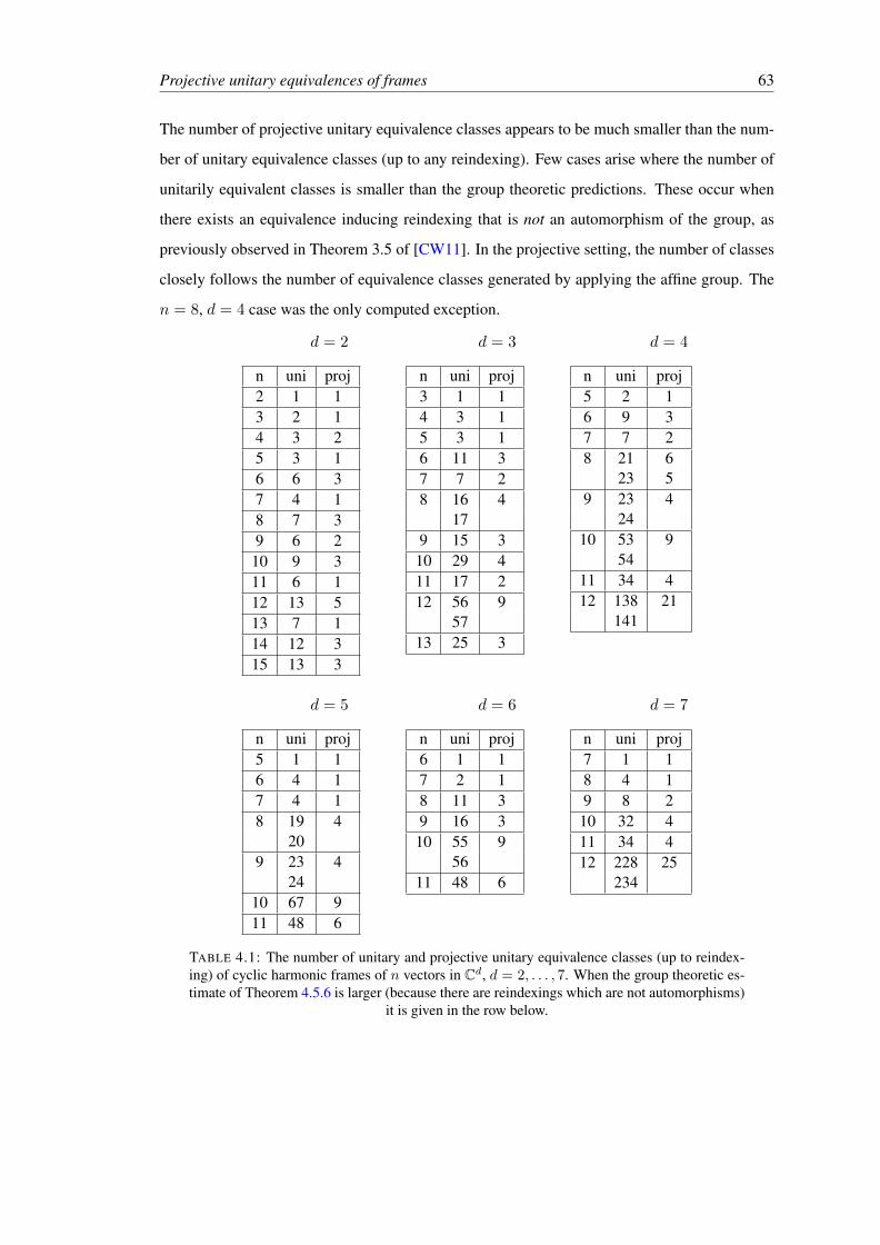
Projective unitary equivalences of frames 63
The number of projective unitary equivalence classes appears to be much smaller than the num-
ber of unitary equivalence classes (up to any reindexing). Few cases arise where the number of
unitarily equivalent classes is smaller than the group theoretic predictions. These occur when
there exists an equivalence inducing reindexing that is not an automorphism of the group, as
previously observed in Theorem 3.5 of [CW11]. In the projective setting, the number of classes
closely follows the number of equivalence classes generated by applying the affine group. The
n = 8, d = 4 case was the only computed exception.
d = 2 d = 3 d = 4
n uni proj2 1 13 2 14 3 25 3 16 6 37 4 18 7 39 6 210 9 311 6 112 13 513 7 114 12 315 13 3
n uni proj3 1 14 3 15 3 16 11 37 7 28 16 4
179 15 310 29 411 17 212 56 9
5713 25 3
n uni proj5 2 16 9 37 7 28 21 6
23 59 23 4
2410 53 9
5411 34 412 138 21
141
d = 5 d = 6 d = 7
n uni proj5 1 16 4 17 4 18 19 4
209 23 4
2410 67 911 48 6
n uni proj6 1 17 2 18 11 39 16 310 55 9
5611 48 6
n uni proj7 1 18 4 19 8 210 32 411 34 412 228 25
234
TABLE 4.1: The number of unitary and projective unitary equivalence classes (up to reindex-ing) of cyclic harmonic frames of n vectors in Cd, d = 2, . . . , 7. When the group theoretic es-timate of Theorem 4.5.6 is larger (because there are reindexings which are not automorphisms)
it is given in the row below.
Chapter 5
Projective symmetry groups
5.1 Introduction
Definition 5.1.1.
Let Φ = (vj)j∈J be a finite sequence of vectors. A projective symmetry of Φ is an invertible
linear map L such that, for all j,
Lvj = cjvσj , |cj | = 1, ∃σ ∈ SJ . (5.1.1)
The example Φ = (e1,−e1, e2,−e2) shows that the choice for L and (cj)j∈J is far from unique
and Φ = (e1, e1, e2, e2) shows choosing L and (cj)j∈J does not provide sufficient information
to determine a unique permutation σ. However, fixing σ will determine L and (cj)j∈J (if they
exist). Thus it makes sense to define the projective symmetry group as a group of permutations
on the index set J (or the vectors themselves).
Definition 5.1.2.
Let Φ = (vj)j∈J be a finite sequence of vectors with span X . Then
1. The projective symmetry group of Φ is
SymP (Φ) := σ ∈ SJ : ∃L ∈ GL(X), |cj | = 1 with Lvj = cjvσj , ∀j ∈ J.
64
Projective symmetry groups 65
2. The symmetry group of Φ is
Sym(Φ) := σ ∈ SJ : ∃L ∈ GL(X) with Lvj = vσj , ∀j ∈ J.
These groups are subgroups of SJ (the symmetric group on J) and the symmetry group is a
subgroup of the projective symmetry group, i.e.,
Sym(Φ) ⊂ SymP (Φ) ⊂ SJ .
An analogue for anti-linear maps is also possible (see Section 5.5).
Projectively similar sequences of vectors have the same projective symmetry group and similar
sequences of vectors have the same symmetry group.
The symmetry group and its calculation from the Gram matrix of the canonical tight frame was
studied in [VW05], [VW10]. At that time (cf. §5 of [VW10]), the authors believed that the pro-
jective symmetry group was generally incalculable (except over R) because of the nonunique-
ness of the L and (cj) in (5.1.1). It is now possible to perform such a calculation using Theo-
rem 4.2.2’s characterisation of projective similarity.
5.2 Tight frames and the complement of a frame
Definition 5.2.1.
Let Φ = (vj)j∈J be a frame. The frame operator S of Φ is invertible and the dual frame
Φ = (vj)j∈J is defined by
vj := S−1vj , ∀j ∈ J. (5.2.1)
The canonical tight frame Φcan = (vcanj )j∈J is defined by
vcanj = S−
12 vj , ∀j ∈ J. (5.2.2)
A frame and its dual satisfy the expansion
f =∑j∈J〈f, vj〉vj =
∑j∈J〈f, vj〉vj , ∀f ∈ H,

Projective symmetry groups 66
and the canonical tight frame is a normalised tight frame, i.e.,
f =∑j∈J〈f, vcan
j 〉vcanj , ∀f ∈ H.
A frame, its dual and canonical tight frame are all similar (Definitions (5.2.1) and (5.2.2)).
Normalised tight frames are similar if and only if they are unitarily equivalent, i.e., without a
loss of generality, the Q in Definition 4.4.1 is unitary.
Since SV invertible and V is onto if and only if V ∗ is one-to-one, RΦ is an invertible linear map.
A direct calculation shows that
RΦ = V ∗S−1V = V ∗(V V ∗)−1
takes the vectors of a frame Φ to the columns of
Gram(Φcan) = (S− 1
2V V )∗S
− 12
V V = V ∗(V V ∗)−1V,
i.e.,
RΦvj = V ∗(V V ∗)−1vj = Gram(Φcan)ej ,
where ej is the j–th standard basis vector.
Theorem 5.2.2 (Theorem 1.7, p. 26, [CKE13]).
A sequence of vectors is a normalised tight frame (for its span) if and only if its Gramian matrix
P is an orthogonal projection matrix, i.e., P 2 = P and P = P ∗.
To determine similarity, Φ can be replaced by the normalised tight frame given by the columns
of the orthogonal projection matrix Gram(Φcan). This is extendible to vector spaces (without
an inner product), by replacing Gram(Φcan) with the orthogonal projection matrix PΦ (cf. The-
orem 4.4.5, [Wal11]). It is necessary for the underlying field F of the vector space X to be a
subfield of C which is closed under conjugation, e.g., F = Q,R,C. For the rest of this chapter,
this is assumed to be the case.
Recall the orthogonal projection maps PΦ from Definition 4.4.2.
If X = span(Φ) and Λ : X → Fm is an injective linear map, then
PΦ = (ΛV )†ΛV,
Projective symmetry groups 67
where A† is the pseudoinverse of A. For Φ a frame, taking Λ = V ∗, gives
PΦ = Gram(Φcan).
The sequence Φ is similar to the normalised tight frame (for a subspace of FJ ) given by (Pej)j∈J ,
the columns of P = PΦ via the well defined injective linear map RΦ : X → FJ with
RΦvj = PΦej , ∀j. (5.2.3)
The Euclidean inner product between these vectors is
〈Pej , P ek〉 = Pkj ,
i.e., P is the Gram matrix of (Pej)j∈J .
Definition 5.2.3.
Two frames Φ and Ψ are complementary (or complements of each other) if PΦ and PΨ are
complementary projection matrices, i.e.,
PΦ + PΨ = I. (5.2.4)
The complement of a frame is well defined up to similarity and the complement of a tight frame
in the class of normalised tight frames is well defined up to unitary equivalence (Theorem 4.4.5).
The complement of a frame in the class of projectively similar frames is defined up to projective
similarity.
There is a bijection between permutations σ ∈ SJ and the J × J permutation matrices, given
by σ 7→ Pσ, where
Pσej := eσj .
Lemma 5.2.4.
Let Φ = (vj)j∈J be a finite frame for X . Then
1. σ ∈ Sym(Φ) ⇐⇒ P ∗σPΦPσ = PΦ.
2. σ ∈ SymP (Φ) ⇐⇒ P ∗σPΦPσ = C∗PΦC, for some unitary diagonal matrix C.

Projective symmetry groups 68
Proof. Observe that σ ∈ Sym(Φ) if and only if Φ = (vj)j∈J is similar to Ψ = (vσj)j∈J , and
σ ∈ SymP (Φ) if and only if Φ is projectively similar to Ψ = (vσj)j∈J . Let V = [vj ], and
Λ : X → Fm be an injective linear map. Then
[vσj ] = [V eσj ] = V [eσj ] = V Pσ,
so that
PΨ = (ΛV Pσ)†ΛV Pσ = P ∗σ (ΛV )†ΛV Pσ = P ∗σPΦPσ.
Applying (4.4.2) and Theorem 4.4.5 obtains the desired result.
Theorem 3.7 of [VW10] shows that if Ψ is a complement of Φ up to similarity, i.e., PΦ+PΨ = I,
then
Sym(Ψ) = Sym(Φ).
The next theorem is an analogous result for projective symmetry groups.
Theorem 5.2.5.
Suppose that Φ = (vj)j∈J is a finite frame for X . If Ψ is a complement of Φ up to projective
similarity, i.e., PΦ + CPΨC∗ = I , where C is a unitary diagonal matrix, then
SymP (Ψ) = SymP (Φ).
Proof. Since the definition of frames being complementary is symmetric, it suffices to show that
SymP (Φ) ⊂ SymP (Ψ). Suppose σ ∈ SymP (Φ). By Lemma 5.2.4,
P ∗σPΦPσ = C∗σPΦCσ,
for some unitary diagonal matrix Cσ. Now
P ∗σPΨPσ = P ∗σ (I − C∗PΦC)Pσ = I − P ∗σC∗PΦCPσ.
Let cj be the diagonal entries of the matrix C. Since (cjvj)j∈J is projectively similar to Φ =
(vj)j∈J , P(cjvj) = C∗PΦC, and σ ∈ SymP ((cjvj)) = SymP (Φ), then
P ∗σC∗PΦCPσ = C∗σC
∗PΦCCσ,

Projective symmetry groups 69
for some unitary diagonal matrix Cσ. Thus
P ∗σPΨPσ = I − C∗σC∗PΦCCσ = I − C∗σ(I − PΨ)Cσ = C∗σPΨCσ.
By Lemma 5.2.4, σ ∈ SymP (Ψ).
Example 5.2.6.
Let Φ = (vj)j∈J be an equal–norm tight frame of d + 1 vectors for Cd, e.g., the vertices of
the regular simplex. As PΦ has a constant diagonal, the complement Ψ of Φ consists of d + 1
equal–norm vectors (wj)j∈J in C1. Let wj = [aj ]. For any σ ∈ SJ ,
wj = cjwσj , cj := aja−1σj ,
so that σ ∈ SymP (Φ) and hence
SymP (Φ) = SymP (Ψ) = SJ .
Therefore all equal–norm tight frames Φ = (vj)j∈J of d + 1 vectors in Cd are projectively
similar, with projective symmetry group SymP (Φ) = SJ .
Proposition 5.2.7.
Let (vj)j∈J be a normalised tight frame with triple products Tjk`. The complement of (vj) has
triple products T cjk`:
T cjk` = −〈vj , vk〉〈vk, v`〉〈v`, vj〉 = −Tjk`, j 6= k 6= ` 6= j,
T cjjk = (1− ‖vj‖2)(δjk(1− 2‖vj‖2) + |〈vj , vk〉|2),
where ‖vj‖ and |〈vj , vk〉| are calculated using (4.1.1).
Proof.
T cjk` : = (δjk − 〈vj , vk〉)(δk` − 〈vk, v`〉)(δ`j − 〈v`, vj〉)
= δjkδk`δ`j − δjkδk`〈v`, vj〉 − δjkδ`j〈vk, v`〉 − δk`δ`j〈vj , vk〉
+ δjk〈vk, v`〉〈v`, vj〉+ δk`〈v`, vj〉〈vj , vk〉+ δ`j〈vj , vk〉〈vk, v`〉
− 〈vj , vk〉〈vk, v`〉〈v`, vj〉.
This gives the first equation. Letting ` = j leads to the second equation.
Projective symmetry groups 70
5.3 Projective invariants
To determine projective similarity between Φ = (vj)j∈J and Ψ = (wj)j∈J (and calculate
SymP (Φ)), Φ and Ψ are assumed to be normalised tight frames given by the columns of PΦ and
PΨ. If Φ and Ψ are projectively similar, i.e., wj = cjQvj (equivalently W = QV C), then Q is
unitary, since
I = WW ∗ = QV CC∗V ∗Q∗ = QV V ∗Q∗ = QQ∗.
Theorem 5.3.1.
Let Φ = (vj)j∈J be a finite frame for X . Then σ ∈ SymP (Φ) if and only if
∆C(vj1 , . . . , vjm) = ∆C(vσj1 , . . . , vσjm),
for all cycles (j1, . . . , jm) from a determining set for Φ.
Proof. Since σ ∈ SymP (Φ) if and only if Φ is projectively similar to Ψ = (vσj)j∈J , this
follows from Theorem 4.4.5.
5.4 The algorithm
For frames Φ = (vj)j∈J and Ψ = (wj)j∈J of n vectors, the algorithm presented will determine
the set of σ for which Φ and (wσj) are projectively similar, i.e.,
∆C(vj1 , . . . , vjm) = ∆C(wσj1 , . . . , wσjm), (5.4.1)
for all cycles (j1, . . . , jm) from a determining set for Φ. If Ψ = Φ, it calculates SymP (Φ).
A priori, the calculation of (5.4.1) seems like it requires considering all n! permutations σ ∈ SJ .
To help reduce the search space, the algorithm uses the m–product condition to prune down the
possibilities. The more distinct m–products exist, the more efficient the pruning.
Example 5.4.1.
An extreme example of fewm–products is when considering the vertices of a regular d–simplex

Projective symmetry groups 71
(cf. Example 5.2.6), where
(PΦ)jk =
dd+1 , j = k;
− 1d+1 , j 6= k,
SymP (Φ) = SJ .
Since them–products are all equal (for fixedm), it is relatively simple to check whether σ ∈ SJ
is a projective symmetry.
When SymP (Φ) is large, one could try to construct it by adding generators. Start with a sub-
group X containing only the identity. Generate a random permutation not in X and check
whether it is in SymP (Φ). If it is in SymP (Φ) but not in X , then add it as a group generator for
X to obtain a larger subgroup. If the index of SymP (Φ) in SJ is small then this method has a
high probability of discovering SymP (Φ) rather quickly.
The generic case is likely to have many distinct m–products, and this is where the algorithm
shines.
Definition 5.4.2.
For an index set J of size n, define a k–flag
f = (j1, j2, . . . , jk),
to be an ordering of k distinct elements of J .
For a fixed n–flag
fb = (j1, . . . , jn),
the permutation σ : j` 7→ σj` (giving a projective similarity or symmetry) is represented by the
n–flag
fσ = (σj1, . . . , σjn).
The problem of determining projective equivalence or similarity of Φ = (vj)j∈J and Ψ =
(wσj)j∈J can be refactored into a question about which of the n! permutations σ (n–flags fσ),
satisfy (5.4.1).

Projective symmetry groups 72
Each n–flag fσ = (σj1, . . . , σjn) can be built from the 0-flag () by concatenating successive
entries, e.g.,
f0σ = (), f1
σ = (σj1), f2σ = (σj1, σj2), . . . fnσ = (σj1, σj2, . . . , σjn).
The operation of transitioning from a set Fk−1 of (k − 1)–flags to a set Fk of k–flags (via
concatenation) is called growing. At the k–th stage there are n − k + 1 choices for the next
entry, so
|Fk| = (n− k + 1)|Fk−1|.
If | Sym(Φ)| < n!, then not all fkσ ∈ Fk can be grown to an n–flag satisfying (5.4.1) for all
cycles in a determining set. Removing elements from Fk for failing this condition is called
pruning.
5.4.1 Algorithm
To determine the n–flags Fn giving a projective similarity:
Let F0 := () consist of the empty flag
for k from 1 to n do
Grow Fk−1 to Fk
Prune Fk
end for
There is an art to how often to prune and which parts to prune along the way. For calculations
regarding Weyl-Heisenberg SIC-POVMs for example, pruning at each growth stage still returns
results in a reasonable amount of time.
The algorithm can be parallelised by partitioning Fk into smaller blocks, at any stage k, and
applying the procedure to each block.
Example 5.4.3.
The simplest example of a SIC-POVM (cf. Section 5.6) is the equiangular tight frame Φ :=

Projective symmetry groups 73
(v, Sv,Ωv, SΩv) of four vectors for C2, where
v :=1√6
√3 +√
3
eπ4i√
3−√
3
, S :=
0 1
1 0
, Ω :=
1 0
0 −1
.
Then
PΦ =1
2
1 1√
31√3− i√
3
1√3
1 −i√3
1√3
1√3
i√3
1 − 1√3
i√3
1√3− 1√
31
.
The empty flag (0–flag) F0 = () grows to the set of 1-flags
F1 = (1), (2), (3), (4).
The pruning rule preserves the norm, i.e., 〈v1, v1〉 = 〈wσ1, wσ1〉. Since SIC-POVM vectors are
unit length, there is no pruning. Growing gives
F2 = (1, 2), (1, 3), (1, 4), (2, 1), (2, 3), (2, 4), (3, 1), (3, 2), (3, 4), (4, 1), (4, 2), (4, 3),
and pruning gives no reduction as Φ is equiangular. Now consider the 2–flag (3, 2) (the others
being similar). This grows to the 3–flags (3, 2, 1), (3, 2, 4). Since
∆C(v1, v2, v3) =i
24√
3, ∆C(w3, w2, w1) = − i
24√
3, ∆C(w3, w2, w4) =
i
24√
3,
the 3–flag (3, 2, 1) is pruned. Repeating this procedure obtains
F3 = (1, 2, 3), (1, 3, 4), (1, 4, 2), (2, 1, 4), (2, 3, 1), (2, 4, 3),
(3, 1, 2), (3, 2, 4), (3, 4, 1), (4, 1, 3), (4, 2, 1), (4, 3, 2).
The final stage k = n does not increase the size of Fn−1 and in this case nothing gets pruned.
So the symmetry group of Φ is
SymP (Φ) = F4 = (1, 2, 3, 4), (1, 3, 4, 2), (1, 4, 2, 3), (2, 1, 4, 3), (2, 3, 1, 4), (2, 4, 3, 1),
(3, 1, 2, 4), (3, 2, 4, 1), (3, 4, 1, 2), (4, 1, 3, 2), (4, 2, 1, 3), (4, 3, 2, 1).
This is the alternating group A4.
Projective symmetry groups 74
Example 5.4.4.
Let Φ = (vj)j∈J be the maximal MUB (see Definition 4.3.10, Remark 4.3.12) in C2,
v1 = e1, v2 = e2, v3 =1√2
(e1 + e2), v4 =1√2
(e1 − e2).
Then
PΦ =1
2
1 0 1√
2− 1√
2
0 1 1√2
1√2
1√2
1√2
1 0
− 1√2
1√2
0 1
.
Like Example 5.4.3, the procedure up toF2 results in no pruning. The pruning rule now requires
the modulus of the inner product between v1 and v2 to be preserved, so the index pairs in F2
must correspond to pairs of orthogonal vectors, giving
F2 = (1, 2), (2, 1), (3, 4), (4, 3).
Growing again gives
F3 = (1, 2, 3), (1, 2, 4), (2, 1, 3), (2, 1, 4), (3, 4, 1), (3, 4, 2), (4, 3, 1), (4, 3, 2).
As all 3–products for distinct vectors are zero, there is no further pruning. Similarly, all 4–
products for distinct vectors are zero, so
SymP (Φ) = F4 = (1, 2, 3, 4), (1, 2, 4, 3), (2, 1, 3, 4), (2, 1, 4, 3),
(3, 4, 1, 2), (3, 4, 2, 1), (4, 3, 1, 2), (4, 3, 2, 1).
This group is isomorphic to the dihedral group of order 8 (the unique isomorphism class of order
8), generated by the permutations
(1324) (rotation through 90 degrees), (34) (reflection in the x–axis).
5.5 The extended projective symmetry group
Definition 5.5.1.
Let Φ = (vj)j∈J be a finite sequence of vectors with span Cd. Then the extended projective

Projective symmetry groups 75
symmetry group of Φ is
SymEP (Φ) := σ ∈ SJ : ∃A ∈ EGL(Cd), |cj | = 1 with Avj = cjvσj , ∀j ∈ J.
If A is anti-linear then σ is an anti-projective symmetry.
A permutation σ is an anti-projective symmetry of Φ = (vj)j∈J if and only if for some linear L
Lvj = cjvσj , ∀j ∈ J,
i.e., Φ = (vj)j∈J and (vσj)j∈J are projectively similar. Since PΦ = PΦ,
∆C(vj1 , . . . , vjm) = ∆C(vj1 , . . . , vjm) = ∆C(vjm , . . . , vj1).
By Theorem 4.4.5, σ is an anti-projective symmetry of Φ = (vj)j∈J if and only if
∆C(vjm , . . . , vj1) = ∆C(vσj1 , . . . , vσjm), (5.5.1)
for all cycles (j1, . . . , jm) from a determining set for Φ. Condition (5.5.1) is (5.4.1) with the or-
dering of (vj1 , . . . , vjm) reversed, so the algorithm can calculate the anti-projective symmetries
by replacing PΦ by its transpose P TΦ .
Example 5.5.2.
Applying the algorithm to Example 5.4.3, with the m–products ∆C(vj1 , . . . , vjm) replaced by
their conjugates gives the following anti-projective symmetries
F4 = (1, 2, 4, 3), (1, 3, 2, 4), (1, 4, 3, 2), (2, 1, 3, 4), (2, 3, 4, 1), (2, 4, 1, 3),
(3, 1, 4, 2), (3, 2, 1, 4), (3, 4, 2, 1), (4, 1, 2, 3), (4, 2, 3, 1), (4, 3, 1, 2).
Therefore,
SymP (Φ) = A4 ⊂ SymEP (Φ) = S4.
The product of two anti-projective symmetries is a projective symmetry. If there exists anti-
projective symmetries of Φ, then
|SymEP (Φ)| = 2| SymP (Φ)|.

Projective symmetry groups 76
SymEP (Φ) will be generated by either the projective symmetries alone or together with any
anti-projective symmetry, so that
SymP (Φ) / SymEP (Φ), [SymEP (Φ) : SymP (Φ)] = 1 or 2.
5.6 Group frames, nice error bases, SIC-POVMs and MUBs
When a tight frame comes as the orbit of a unitary group action on H = Rd,Cd the calculation
of SymP (Φ) can be simplified (See Chapter 5, [CKE13]).
LetG be a finite group and ρ : G→ U(H) be a unitary representation ofG. When ρ(G) contains
non-identity scalar matrices, there are repeated vectors (up to scalar multiples) in Φ = (gv)g∈G.
In this situation, it might be convenient to consider (gv)g∈ρ(G)/Z , where Z is the group of
scalar matrices in ρ(G) (cf. projective representations, nice error bases cf. [Kni96a], [KR02],
[CW14b]). The group frame Φ = (gv)gZ∈ρ(G)/Z is well defined if the vectors gv are identified
together when they are unit scalar multiples of each other. As the vectors are unit length, it is
formally in a projective space. In practise, one just selects a vector to use from the representative
class of vectors which are unit scalar multiples of each other. Note that the m–products are well
defined in this case as they are invariant under unit scalings of the vectors. Abusing notation
slightly, g ∈ G will also stand for gZ ∈ ρ(G)/Z when the context is clear.
Let Φ = (gv)g∈G be a group frame. The projective symmetries are permutations of G (as G
indexes Φ). Each h ∈ G induces a projective symmetry via the map
τh : G→ G : g 7→ hg,
with the subgroup τG = τhh∈G of SymP (Φ) acting transitively on G. Let σ ∈ SymP (Φ) and
h ∈ G, then σ is a product of an element of τG and a σh ∈ SymP (Φ) which fixes the vector hv,
i.e.,
σ = τσ(h)h−1σh, σh := τhσ(h)−1σ.
Proposition 5.6.1.
Let Φ = (gv)g∈G be a group frame, then SymP (Φ) is generated by the “translations” τG, and
Projective symmetry groups 77
the stabiliser of any vector hv, i.e.,
Stab(h) := σ ∈ SymP (Φ) : σ(h) = h.
In light of Proposition 5.6.1, computing SymP (Φ) boils down to finding the stabiliser of a vector
in your frame.
Example 5.6.2.
If |G| = n, the calculation of Stab(h) requires the examination of the (n − 1)! permutations
which fix h. Checking (5.4.1) for cycles in a determining set for Φ = (gv)g∈G which do not
involve h further improves the pruning efficiency.
Example 5.6.3.
Consider Example 5.4.3. This is a group frame of order 8 with ρ(G) = 〈S,Ω〉 and centre
Z = I,−I. ρ(G)/Z is isomorphic to Z2 × Z2 (as ΩS = −SΩ). Giving the elements the
order (Z, SZ,ΩZ, SΩZ), the translations are
τZ = I, τSZ = (12)(34), τΩZ = (13)(24), τSΩZ = (14)(23).
Considering only projective symmetries with σ1 = 1 (that fix the first vector), the algorithm
gives
F2 = (1, 2), (1, 3), (1, 4).
Growing and pruning gives
F3 = (1, 2, 3), (1, 3, 4), (1, 4, 2), F4 = (1, 2, 3, 4), (1, 3, 4, 2), (1, 4, 2, 3).
The stabliser of the first vector is generated by the cycle (234) and τρ(G)/Z is generated by
(12)(34) and (13)(24), so
SymP (Φ) = 〈(234), (12)(34), (13)(24)〉.
The rest of the chapter presents symmetry group calculations for SIC-POVMs and MUBs. These
were done with Maple and MAGMA.
It is natural to consider SIC-POVMs up to projective equivalence, i.e., as sequences of equian-
gular lines. Let G be the index group of the Weyl Heisenberg group (Weyl Heisenberg group

Projective symmetry groups 78
factored by its centre). Then Weyl Heisenberg SIC-POVMs are determined (up to projective
unitary equivalence) by their 3–products (cf. [AFF11], Theorem 4.3.8)
Λjg,h := d3‖v‖6∆C(jv, gv, hv) = 〈jv, gv〉〈gv, hv〉〈hv, jv〉, j, g, h ∈ G.
So a permutation σ : G→ G is a projective symmetry if and only if
Λσjσg,σh = Λjg,h, ∀j, g, h.
To compute the projective symmetry, it is sufficient to find the stabiliser of some fixed j ∈ G
(Proposition 5.6.1), i.e., the subgroup of σ satisfying
Λjσg,σh = Λjg,h, ∀g, h.
Zhu observed this in Chapter 10 of [Zhu12] and replaced the Hermitian G×G matrix [Λjg,h] by
the real antisymmetric matrix Λ(j), with entries
Λ(j)g,h := arg
( Λjg,h
|Λjg,h|
)∈ (−π, π].
Revisiting Example 5.6.3 (with the same ordering),
ΛI =1
8
1 1
313
13
13
13
i3√
3− i
3√
3
13 − i
3√
313
i3√
3
13
i3√
3− i
3√
313
, Λ(I) =
0 0 0 0
0 0 π2 −π
2
0 −π2 0 π
2
0 π2 −π
2 0
.
The angle matrix Λ can be viewed as a weighted (directed) graph with vertices G. In light of
this, the stabiliser of Λ(j)g,h, i.e., the set of permutations satisfying
Λ(j)σg,σh = Λ
(j)g,h, ∀g, h,
is the automorphism group of Λ(j), so the stabiliser problem is equivalent to the well studied
weighted graph isomorphism problem. Zhu’s algorithm in section 10.2.3 of [Zhu12] utilises the
machinery of the weighted graph isomorphism problem to calculate the stabiliser of Λ(j). Zhu
applied it to numerically known SIC-POVMs in dimensions d 6= 3 (see Table 10.2 of [Zhu12]).

Projective symmetry groups 79
The algorithm (5.4.1) presented here is able to compute the same extended projective symmetry.
Furthermore, it was possible to identify the subgroup of it that lies in the extended Clifford group
(the normaliser of the Weyl–Heisenberg group in the unitary and antiunitary matrices), as given
in [SG10].
Corollary 5.6.4.
Let Φ be a finite frame. Then a necessary condition for Φ to be a group frame for G/Z is that
SymP (Φ) has a transitive subgroup which is isomorphic to G/Z.
Lemma 5.6.5.
Let Φ = (vj)j∈J be a finite frame. If the frame graph of Φ is connected, then the map
SymP (Φ)→ PGL(n,C) given by σ 7→ Lσ, where Lσ is
Lvj = cjvσj , |cj | = 1, ∀j,
is well defined and a projective representation of SymP (Φ).
Proof. Let (vj)j∈J be a normalised tight frame. Then L = U is unitary and 〈vk, vj〉 =
〈PΦek, PΦej〉 = (PΦ)kj . Suppose
Uvj = cjvσj , Uvj = cjvσj , ∀j, (5.6.1)
with U , U unitary, and cj , cj unit scalars. Then
〈cjUvj , ckUvk〉 = 〈vσj , vσk〉 = 〈cjUvj , ckUvk〉, ∀j, k,
givingckcj〈vj , vk〉 =
ckcj〈vj , vk〉, ∀j, k.
Hence,
〈PΦej , PΦek〉 = 〈vj , vk〉 6= 0 =⇒ cjcj
=ckck. (5.6.2)
Since the frame graph of Φ is connected, for any j and k, there exists a sequence of vectors
vj , v`1 , v`2 , . . . , v`m , vk with
〈vj , v`1〉 6= 0, 〈v`1 , v`2〉 6= 0, . . . 〈v`m−1 , v`m〉 6= 0, 〈v`m , vk〉 6= 0,

Projective symmetry groups 80
so by (5.6.2),cjcj
=c`1c`1
=c`2c`2
= · · · = c`mc`m
=ckck.
Thus for some unit scalar α, cj = αcj for all j and by (5.6.1),
Uvj = cjvσj = αcjvσj = αUvj , ∀j,
i.e., U = αU .
For the general case, rewrite Lvj = cjvσj (with (5.2.3)) as
(RΦLR
−1Φ
)PΦej = cj(PΦej), ∀j,
where the inverse of the injective linear map RΦ is defined on its image (the range of PΦ). Since
(PΦej) is a normalised tight frame and U = RΦLR−1Φ is unitary,
RΦLR−1Φ = αRΦLR
−1Φ =⇒ L = αL.
The homomorphism property follows since
LσLτ (vj) = Lσ(Lτ (vj)) = cτjLσ(vτj) = cτj cσj vστj = Lστ (vj).
Theorem 5.6.6.
Let Φ = (vj)j∈J be a frame of n vectors for H. If the frame graph of (PΦej)j∈J is connected
and no vector in Φ is repeated (up to a unit scalar multiple), then Φ is a group frame for G/Z if
and only if SymP (Φ) has a transitive subgroup which is isomorphic toG/Z. In theG/Z–frame,
the vectors of Φ are repeated |G/Z|n times.
Proof. By Corollary 5.6.4, it is sufficient to show, for a given transitive subgroupH of SymP (Φ),
there exists a group G of linear maps such that, for all v ∈ Φ, the orbit of G acting on v, up to
repeats, is Φ. Let d be the dimension of H, and ω := e2πid . For each σ ∈ H , choose a Lσ as in
Lemma 5.6.5, with
det(Lσ) = 1.
Projective symmetry groups 81
There are d scalar multiples of Lσ with determinant 1, namely Lσ, ωLσ, . . . , ωd−1Lσ. Let
G := ωjLσ : j = 0, . . . , d− 1, σ ∈ H, Z := ωjId−1j=0 .
Since
Lστvj = cστj vστj , LσLτvj = Lσcτj vτj = cτj c
στjvστj ,
G is a group and G/Z ' H . As the vectors in Φ are not repeated, G has d|H| elements. By the
uniqueness of Lστ ,
LσLτ = αLστ , |α| = 1 =⇒ 1 = det(LσLτ ) = det(αLστ ) = αd
=⇒ α ∈ 1, ω, . . . , ωd−1, LσLτ ∈ G.
As H is transitive, Φ is the G–orbit of any one of its vectors (up to repeats).
Consider the generalisation of Example 5.4.4.
Example 5.6.7.
It is possible to add a third orthonormal basis to the MUB of Example 5.4.4, to obtain a maximal
set of MUBs for C2:
Φ = (vj)j∈J =(1
0
,
0
1
,1√2
1
1
,1√2
−1
1
,1√2
1
i
,1√2
1
−i
).The projective symmetry group SymP (Φ) has order 24 and is generated by the permutations
(13)(24)(56), (3645).
It has three transitive subgroups
H1 = 〈(12)(36)(45), (164)(253)〉 ≈ S3, |H1| = 6,
H2 = 〈(164)(253), (34)(56), (12)(56)〉, |H2| = 12,
H3 = SymP (Φ), |H3| = 24.
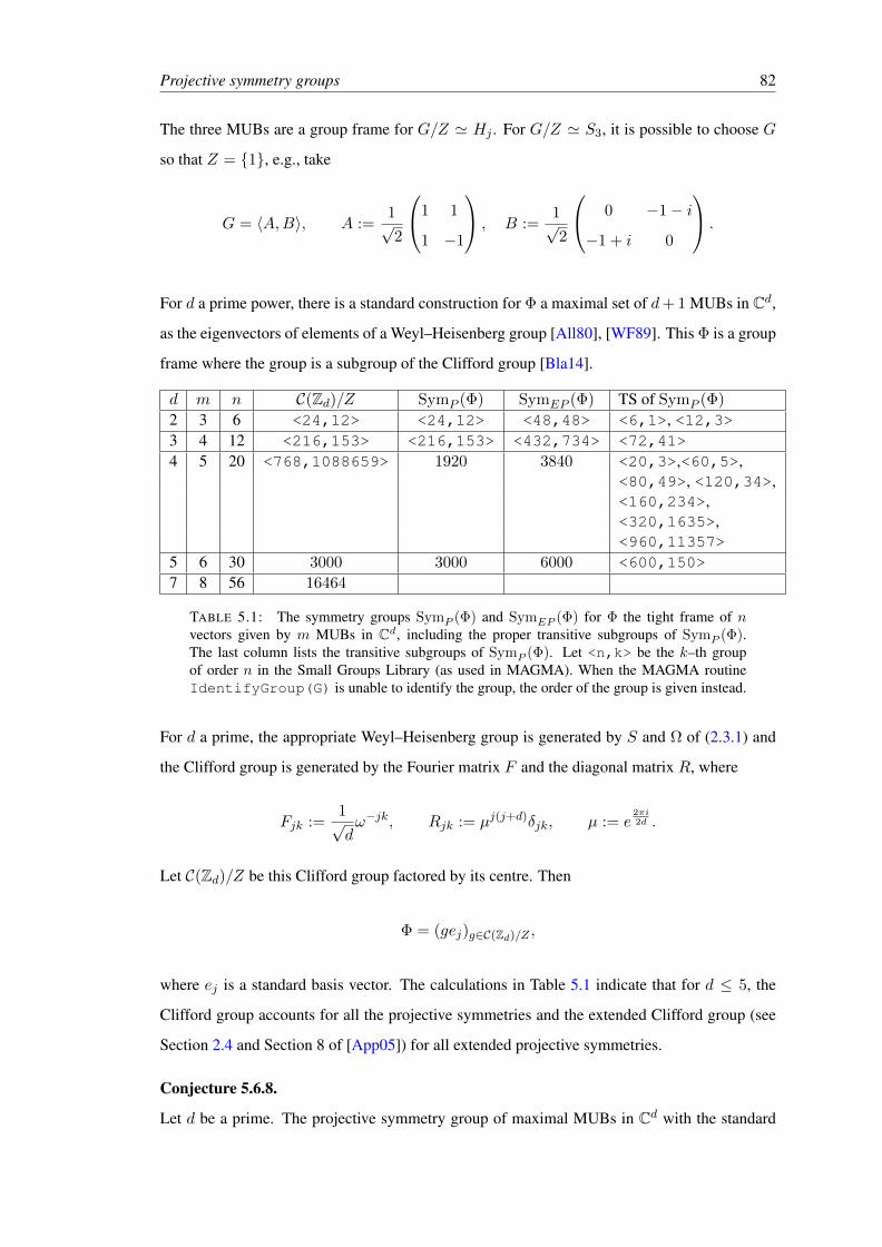
Projective symmetry groups 82
The three MUBs are a group frame for G/Z ' Hj . For G/Z ' S3, it is possible to choose G
so that Z = 1, e.g., take
G = 〈A,B〉, A :=1√2
1 1
1 −1
, B :=1√2
0 −1− i
−1 + i 0
.
For d a prime power, there is a standard construction for Φ a maximal set of d+ 1 MUBs in Cd,
as the eigenvectors of elements of a Weyl–Heisenberg group [All80], [WF89]. This Φ is a group
frame where the group is a subgroup of the Clifford group [Bla14].
d m n C(Zd)/Z SymP (Φ) SymEP (Φ) TS of SymP (Φ)
2 3 6 <24,12> <24,12> <48,48> <6,1>, <12,3>3 4 12 <216,153> <216,153> <432,734> <72,41>4 5 20 <768,1088659> 1920 3840 <20,3>,<60,5>,
<80,49>, <120,34>,<160,234>,<320,1635>,<960,11357>
5 6 30 3000 3000 6000 <600,150>7 8 56 16464
TABLE 5.1: The symmetry groups SymP (Φ) and SymEP (Φ) for Φ the tight frame of nvectors given by m MUBs in Cd, including the proper transitive subgroups of SymP (Φ).The last column lists the transitive subgroups of SymP (Φ). Let <n,k> be the k–th groupof order n in the Small Groups Library (as used in MAGMA). When the MAGMA routineIdentifyGroup(G) is unable to identify the group, the order of the group is given instead.
For d a prime, the appropriate Weyl–Heisenberg group is generated by S and Ω of (2.3.1) and
the Clifford group is generated by the Fourier matrix F and the diagonal matrix R, where
Fjk :=1√dω−jk, Rjk := µj(j+d)δjk, µ := e
2πi2d .
Let C(Zd)/Z be this Clifford group factored by its centre. Then
Φ = (gej)g∈C(Zd)/Z ,
where ej is a standard basis vector. The calculations in Table 5.1 indicate that for d ≤ 5, the
Clifford group accounts for all the projective symmetries and the extended Clifford group (see
Section 2.4 and Section 8 of [App05]) for all extended projective symmetries.
Conjecture 5.6.8.
Let d be a prime. The projective symmetry group of maximal MUBs in Cd with the standard

Projective symmetry groups 83
construction is the Clifford group C just defined.
For d a prime power pm, m > 1, the appropriate Clifford group is the Galoisian Clifford group
of [App09] (Section 2) and [KT12] (Section 6).
Example 5.6.9.
Let Φ be the five MUBs in C4 (unique up to projective similarity). The projective symmetry
group SymP (Φ) is transitive, with order 1920 = 27 · 3 · 5. The Galoisian Clifford group has
order 11520 = 28 · 32 · 5 (see Section 6 of [KT12]). Since Φ is a group frame for a subgroup of
the Galoisian Clifford group (see [WS07]), Φ is not a group frame for the full Galoisian Clifford
group. It is a group frame for groups with orders 20, 60, 80, 120, 160, 320, 960, 1920 (see
Table 5.1). Whether all of these groups appear as subgroups of the Galoisian Clifford group is
unknown.
5.7 Harmonic frames
Definition 5.7.1.
A frame Φ = (vj)j∈J is projectively real if all its m–products are real (i.e., projectively similar
to a frame in Rd). Otherwise it is projectively complex. Φ has projectively distinct vectors if
for any i, j ∈ J , i 6= j,
vi 6= cjvj , for all cj ∈ T,
i.e., none of the lines corresponding to vectors of equal length are equal.
Example 5.7.2.
The harmonic frame (for C2)
Φ = Φ0,1 = v0, v1, v2 =1
1
,
1
ω
,
1
ω2
, ω = e2π3 ,
is not similar to real frame, but is projectively similar to a real frame, since
Gram(Φ) =
2 1 + ω 1 + ω2
1 + ω2 2 1 + ω
1 + ω 1 + ω2 2
, 〈v0, v1〉〈v1, v2〉〈v2, v0〉 = (1 + ω2)3 = −1.

Projective symmetry groups 84
The classes of projectively equivalent cyclic harmonic frames (up to reordering) were calculated
in Figure 4.1. The projective symmetry group and the extended projective symmetry group were
calculated with the algorithm (5.4.1) for the cases with projectively distinct vectors. The results
for d = 2, . . . , 7 are summarised in the tables of the Appendix B.
Example 5.7.3.
For projectively complex cyclic harmonic frames the conjugation map gives an anti-projective
symmetry σ : k 7→ −k, since
vk = (ωkj1 , . . . , ωkjd) = (ω−kj1 , . . . , ω−kjd) = v−k, k ∈ Zn.
SymP (Φ) is an index 2 subgroup of SymEP (Φ) (and hence normal). In all of the cases con-
sidered so far (including Example 5.5.2), SymEP (Φ) is not isomorphic to the direct product
SymP (Φ)× Z2.
The following examples are about cyclic harmonic frames. The notation from Chapter 4, section
4.5 is adopted.
Example 5.7.4 (Four vectors in C2).
There are two projective equivalence classes, given by 0, 1 and 1, 3. The first has projec-
tively distinct vectors, is projectively real and requires the 4–products to calculate its projective
symmetry group <8,3>. The second does not have vectors which are projectively distinct.
Example 5.7.5 (Six vectors in C3).
There are three projective equivalence classes. The first, 1, 3, 5, does not have projectively
distinct vectors,. The second 1, 2, 3, has projectively distinct vectors, is projectively real and
requires the 4–products to calculate its projective symmetry group <12,4>. The third, 0, 1, 4,
is projectively complex, with projectively distinct vectors, none of which are orthogonal. Its
projective and extended projective symmetry groups are the symmetry groups <18,3> and
<36,10>. This is the first example of a projectively complex cyclic harmonic frame. For
d = 3, they also exist for n = 7, 8, 9, 10, 11, 12.
Example 5.7.6 (Eight vectors in C3).
The harmonic frame Φ = ΦJ of eight vectors for C3 given by J = 0, 1, 4 is projectively
complex, with
SymP (Φ) = <32,11>, SymEP (Φ) = <64,134>.

Projective symmetry groups 85
The projective symmetry group has transitive subgroups of order eight isomorphic to Z8, Z4 ×
Z2,D4 (dihedral group) andQ8 (quaternian group). Φ is a group frame for each of these groups.
The only other group of order eight is Z2 × Z2 × Z2, which occurs as a transitive subgroup of
SymEP (Φ).
Example 5.7.7 (Projectively real frames).
In 2 dimensions all cyclic harmonic frames of n vectors are projectively real. For all n > 4,
they are determined by their 3–products and all the 3–products are real. For d ≥ 3, projectively
complex cyclic harmonic frames of n projectively distinct vectors appear to always exist, with
the smallest n being n = d+ 3.
Example 5.7.8 (Erasures).
The erasures of a frame Φ of n vectors for Cd is the maximum number of vectors that can
be removed from Φ before it stops spanning Cd. Frames with a large number of erasures are
useful for robust data transmission [GVT98], [GKK01]. The cyclic harmonic frame given by
J = 0, 1, 2, . . . , d − 1 has n − d erasures. In general, this is not true, e.g., for six vectors in
C2 the erasures of a cyclic harmonic frame can be 2, 3, 4. However for n prime, the tabulated
data in Appendix B suggests the number of erasures is always n− d
Chapter 6
Nice error frames
SIC-POVMs can arise as orbits of groups which are not the Weyl-Heisenberg groups. One
category of groups where this phenomenon has occurred is the nice error groups. The Weyl-
Heisenberg groups belong to this category. All known constructions of SIC-POVMs have arisen
as the orbit of a nice error group or is equivalent to a SIC-POVM that is (e.g., Hoggar lines
in 8 dimensions, elliptic curve construction in 3 dimensions). The aim of this chapter is de-
velop a way to search for SIC-POVMs amongst the nice error groups. It has led to the natural
generalisation of “nice error frames”.
6.1 Background
Definition 6.1.1.
The Pauli matrices are
σ1 = σx :=
0 1
1 0
, σ2 = σy :=
0 −i
i 0
, σ3 = σz :=
1 0
0 −1
. (6.1.1)
The Pauli matrices are used to study spin in quantum mechanics. Together with the identity,
they form an orthonormal basis for the 2× 2 matrices.
Definition 6.1.2.
An error operator basis is an orthonormal basis for the d × d matrices Md(C) = Cd×d, with
respect to the (Hilbert-Schmidt/Frobenius) inner product (see Definition 3.2.2).
86

Nice error frames 87
A special class of the error operator basis called a “nice error basis” was defined by Knill in p.
3 of [Kni96b] and Section 2 of [Kni96a].
Definition 6.1.3 (p. 3 [Kni96b]).
Let G be a group of order d2. Then unitary matrices (Eg)g∈G in Md(C) are a nice (unitary)
error basis and G is referred to as the index group if
1. E1 is a scalar multiple of the identity I .
2. EgEh = wg,hEgh, ∀g, h ∈ G, where wg,h ∈ C.
3. Tr(Eg) = 0, g 6= 1, g ∈ G,
(i.e., they are an error operator basis.)
A group which gives rise to a nice error basis or nice error frame is called a nice error group.
In group theory terms (cf. Section 2 of [KR02], Section 2 of [Hig08]), this is equivalent to the
map
ρ : g 7→ Eg
being a unitary irreducible special faithful projective representation of G of degree d.
A motivating example is the Pauli matrices indexed by Z2 × Z2:
G = Z2 × Z2 7→M2(C) : (j, k) 7→ E(j,k) = SjΩk, S := σ1, Ω := σ3.
Condition 3 of Definition 6.1.3 guarantees that a nice error basis yields the following orthogonal
expansion
A =1
d
∑g∈G〈A,Eg〉Eg, ∀A ∈Md(C). (6.1.2)
The notion of a nice error frame is chosen so that the index group G can have order greater than
d2, so that (6.1.2) becomes the tight frame expansion
A =d
|G|∑g∈G〈A,Eg〉Eg, ∀A ∈Md(C).
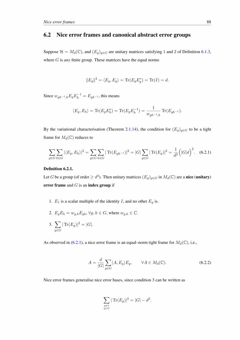
Nice error frames 88
6.2 Nice error frames and canonical abstract error groups
Suppose H = Md(C), and (Eg)g∈G are unitary matrices satisfying 1 and 2 of Definition 6.1.3,
where G is any finite group. These matrices have the equal norms
‖Eg‖2 = 〈Eg, Eg〉 = Tr(EgE∗g ) = Tr(I) = d.
Since wgh−1,hEgE−1h = Egh−1 , this means
〈Eg, Eh〉 = Tr(EgE∗h) = Tr(EgE
−1h ) =
1
wgh−1,hTr(Egh−1).
By the variational characterisation (Theorem 2.1.14), the condition for (Eg)g∈G to be a tight
frame for Md(C) reduces to
∑g∈G
∑h∈G|〈Eg, Eh〉|2 =
∑g∈G
∑h∈G|Tr(Egh−1)|2 = |G|
∑g∈G|Tr(Eg)|2 =
1
d2
(|G|d
)2. (6.2.1)
Definition 6.2.1.
LetG be a group (of order≥ d2). Then unitary matrices (Eg)g∈G inMd(C) are a nice (unitary)
error frame and G is an index group if
1. E1 is a scalar multiple of the identity I , and no other Eg is.
2. EgEh = wg,hEgh, ∀g, h ∈ G, where wg,h ∈ C.
3.∑g∈G|Tr(Eg)|2 = |G|.
As observed in (6.2.1), a nice error frame is an equal–norm tight frame for Md(C), i.e.,
A =d
|G|∑g∈G〈A,Eg〉Eg, ∀A ∈Md(C). (6.2.2)
Nice error frames generalise nice error bases, since condition 3 can be written as
∑g 6=1g∈G
|Tr(Eg)|2 = |G| − d2.

Nice error frames 89
Conditions 1 and 2 say that g 7→ Eg is a unitary faithful projective representation of G of degree
d. It is also irreducible, i.e., spanEgwg∈G = Cd, ∀w 6= 0. To see this, expand the matrix
A = vw∗, v ∈ Cd, using (6.2.2) to obtain
vw∗ =d
|G|∑g∈G〈vw∗, Eg〉Eg =⇒ v‖w‖2 =
d
|G|∑g∈G〈vw∗, Eg〉Egw.
These properties characterise nice error frames (Proposition 6.2.8).
In general, the matrices (Eg)g∈G of a nice error frame will not have finite order, and hence not
generate a finite group. By finding the right scalings, these matrices can have finite order.
Let ω be the d–th root of unity
ω := e2πid .
Remark 6.2.2.
Since det(cA) = cd det(A), c ∈ C, A ∈ Md(C), there are exactly d scalings of a given Eg
which have determinant 1, i.e.,
Eg =ωj
det(Eg)1/dEg, j = 0, 1, . . . , d− 1,
where det(Eg)1/d is any fixed d–th root of det(Eg). Knill calls a nice error basis very nice if
each matrix has unit determinant (p. 2, [Kni96a]).
From now on, let Eg refer to any of these scalings, so that
det(Eg) = 1, ∀g ∈ G.
Then the d|G| matrices
ωjEg : j = 0, . . . , d− 1, g ∈ G
are distinct. They form a group, since after scaling, condition 2 becomes
EgEh = wg,hEgh. ∀g, h ∈ G.
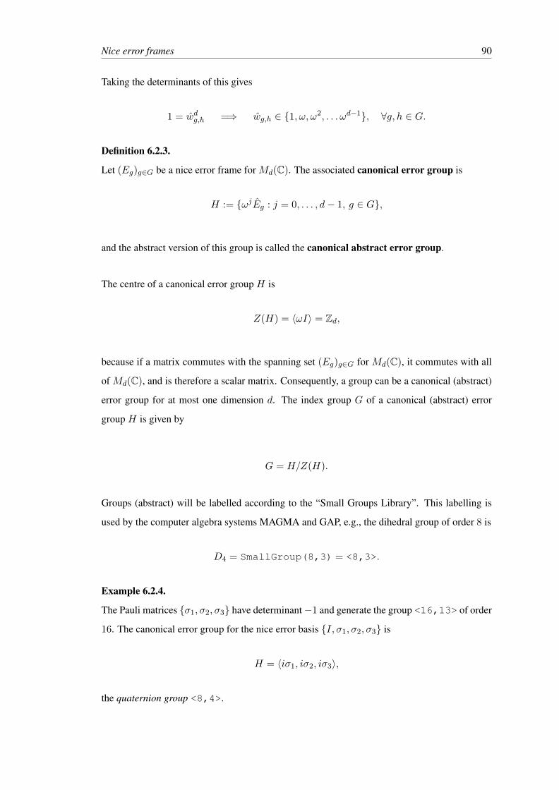
Nice error frames 90
Taking the determinants of this gives
1 = wdg,h =⇒ wg,h ∈ 1, ω, ω2, . . . ωd−1, ∀g, h ∈ G.
Definition 6.2.3.
Let (Eg)g∈G be a nice error frame for Md(C). The associated canonical error group is
H := ωjEg : j = 0, . . . , d− 1, g ∈ G,
and the abstract version of this group is called the canonical abstract error group.
The centre of a canonical error group H is
Z(H) = 〈ωI〉 = Zd,
because if a matrix commutes with the spanning set (Eg)g∈G for Md(C), it commutes with all
of Md(C), and is therefore a scalar matrix. Consequently, a group can be a canonical (abstract)
error group for at most one dimension d. The index group G of a canonical (abstract) error
group H is given by
G = H/Z(H).
Groups (abstract) will be labelled according to the “Small Groups Library”. This labelling is
used by the computer algebra systems MAGMA and GAP, e.g., the dihedral group of order 8 is
D4 = SmallGroup(8,3) = <8,3>.
Example 6.2.4.
The Pauli matrices σ1, σ2, σ3 have determinant−1 and generate the group <16,13> of order
16. The canonical error group for the nice error basis I, σ1, σ2, σ3 is
H = 〈iσ1, iσ2, iσ3〉,
the quaternion group <8,4>.
Nice error frames 91
The earlier works of [KR02],[Kni96a] would have considered all the groups <16,13>, <8,3>,
<8,4> to be abstract error groups or w–coverings of the nice error basis I, σ1, σ2, σ3. Cri-
teria will now be established for when nice error frames are considered “equivalent”.
Definition 6.2.5.
Nice error frames (Eg)g∈G and (Fh)h∈H for Md(C) are equivalent if there is bijection
σ : G→ H
between their index groups, scalars (cg)g∈G and an invertible T ∈Md(C), such that
Fσg = cgT−1EgT, ∀g ∈ G. (6.2.3)
This definition is more general than projective equivalence, where G = H and reindexing the
elements of (Eg)g∈G is not allowed.
Proposition 6.2.6.
Equivalent nice error frames have the same canonical abstract error group and the same index
group.
Proof. Suppose the nice error frames (Eg)g∈G and (Fh)h∈H for Md(C) are equivalent. Then
(6.2.3) scales to
Fσg = T−1(cgEg)T, ∀g ∈ G,
where cg ∈ 1, ω, ω2, . . . , ωd−1 (by considering its determinants). Thus the canonical error
groups are conjugate via T , and hence isomorphic. As the index group is the abstract error
group factored by its centre, the nice error frames also have the same index groups.
Example 6.2.7 (Heisenberg nice error basis).
A nice error basis (projective representation) is given by
G = Zd × Zd 7→Md(C) : (j, k) 7→ E(j,k) = SjΩk,
Nice error frames 92
where S is the cyclic shift matrix, and Ω is the modulation matrix, given by
(S)jk := δj,k+1, (Ω)jk = ωjδj,k, ω := e2πid .
This is the only nice error basis (up to equivalence) for Md(C) with index group G = Zd × Zd
(cf. Theorem 3.5 of [BK73]).
It is now possible to show condition 3 of Definition 6.2.1 is equivalent to the projective repre-
sentation g 7→ Eg being irreducible. Proposition 6.2.8 generalises Theorem 1 of [KR02], which
is the case of a nice error basis.
Proposition 6.2.8 (Characterisation).
Let G be a group and (Eg)g∈G be unitary matrices in Md(C). Then the following are equivalent
1. (Eg)g∈G is a nice error frame for Md(C).
2. g 7→ Eg is an irreducible unitary faithful projective representation of G of degree d.
The action of the canonical error group H on Cd is an irreducible unitary faithful ordinary
representation of the canonical abstract error group of dimension d.
Proof. It suffices to show condition 2 implies condition 1. If g 7→ Eg is an irreducible uni-
tary projective representation of G on Cd, then the canonical error group H is defined (Defi-
nition 6.2.3). Its action on Cd (via multiplication) gives an irreducible unitary ordinary repre-
sentation of H . The corresponding character χ is irreducible, hence its Euclidean inner product
with itself is |H| = d|G|, giving
〈χ, χ〉 =∑h∈H|Tr(h)|2 =
d−1∑j=0
∑g∈G|Tr(ωjEg)|2 = d
∑g∈G|Tr(Eg)|2 = d|G| = |H|.
which is condition 3 of Definition 6.2.1. Therefore conditions 1 and 2 are equivalent.
Example 6.2.9.
For d = 1, the only canonical abstract error group is H = 1.
Nice error frames 93
Example 6.2.10.
For d = 2, a canonical error group is given by the generalised quaternion group or dicyclic
group of order 4n (n > 1), generated by the matrices
ω2n 0
0 ω−12n
,
0 −1
1 0
, ω2n := e2πi2n .
A MAGMA calculation shows that the only other canonical abstract error groups of order≤ 200
(with d = 2) are
H = <24,3>, G = <12,3>, H = <48,28>, G = <24,12>.
These are the canonical abstract error groups obtained from the Shephard–Todd reflection groups
numbers 4 and 8, respectively.
Example 6.2.11.
Any irreducible group of d × d matrices which is finite after quotienting with its centre gives
rise to a canonical abstract error group. By the N/C theorem, the normaliser of such a group in
GLd(C) does too.
Take the Heisenberg group, generated by the matrices S and Ω of Example 6.2.7, and its nor-
maliser (the Clifford group). The canonical abstract error groups for the Heisenberg group and
its normaliser are
<8,4>,<48,28> (d = 2) <27,3>,<648,532> (d = 3).
For a general d, the Clifford group gives a canonical abstract error group H , with order
|H| = d6∏p|d
(1− 1
p2
), (where p is prime).
The subgroups of the Clifford group which contain the Heisenberg group give a family of nice
error frames. Tensor products provide another avenue for constructing nice error frames.
Proposition 6.2.12.
Let (Eg1)g1∈G1 ,(Fg2)g2∈G2 be nice error frames forMd1(C), Md2(C) respectively. Their tensor
Nice error frames 94
product
(Eg1 ⊗ Fg2)(g1,g2)∈G1×G2
is a nice error frame for Md1d2(C). In particular, a product of index groups is an index group.
The canonical error group is
H = ωj(h1 ⊗ h2) : 0 ≤ j < d− 1, h1 ∈ H1, h2 ∈ H2, ω := e2πid , d := d1d2,
where H1,H2 are the canonical error groups of the nice error frames.
Proof. By Proposition 6.2.8, the first part follows from the theory of (projective) representations,
or it can be verified directly. The tensor product satisfies condition 3 of Definition 6.2.1 since
∑(g1,g2)∈G1×G2
|Tr(Eg1 ⊗ Fg2)|2 =∑g1
∑g2
|Tr(Eg1) Tr(Fg2)|2
=(∑
g1
|Tr(Eg1)|2)(∑
g2
|Tr(Fg2)|2)
= |G| |H| = |G×H|.
The tensor product group H1 ⊗H2 consists of scalar multiples of each Eg1 ⊗ Eg2 , with deter-
minant 1. It might not contain all d–roots of unity (if d1 and d2 are not coprime), so these are
added.
Example 6.2.13.
The tensor product of the two nonabelian index groups for d = 4, with the (abelian) index group
for d = 2, gives two nonabelian index groups for d = 8, i.e.,
< 16, 3 >×< 4, 2 > = < 64, 193 >, < 16, 11 >×< 4, 2 > = < 64, 261 >.
Theorem 6.2.14 (Abelian index groups).
A nice error frame has an abelian index group only if it is a nice error basis.
Proof. Let H be the canonical abstract error group of a nice error frame, and χ : H → C be
the character of a faithful irreducible representation of degree χ(1) = d. Recall the centre of a
character χ : H → C is the subgroup
Z(χ) := h ∈ H : |χ(h)| = χ(1).
Nice error frames 95
If χ is irreducible,
Z(χ)/ ker(χ) = Z(H/ ker(χ)
), ker(χ) := h ∈ H : χ(h) = χ(1).
As χ is irreducible, ker(χ) = 1,
Z(χ) = Z(H),
so the index group is G = H/Z(χ) (Theorem 2.13 of [Isa94]). If G is abelian, then
|G| = [H : Z(χ)] = χ(1)2 = d2.
Remark 6.2.15.
A canonical error group is an example of a central group frame (see Section 5 of [VW08]). This
means
Φ =(ρ(g)
)h∈H , where ρ : H → SLd(C) : h→ ρ(h) is a represenation,
is a tight frame for Md(C) satisfying the “symmetry condition”
〈hφ, gφ〉 = 〈hψ, gψ〉, ∀g, h ∈ H, ∀φ, ψ ∈ Φ.
6.3 Calculations
Finding the centre of a group and its irreducible representations is fast. A representation can
be made unitary by an appropriate conjugation. Proposition 6.3.1 utilises these facts to give a
practical way for calculating abstract error groups.
Proposition 6.3.1.
A group H is a canonical abstract error group if and only if
1. Its centre Z(H) is cyclic of order d; and
2. it has a faithful irreducible ordinary representation ρ of degree d, which is special, i.e.,
det(h) = 1, ∀h ∈ H .
Nice error frames 96
Consequently, all canonical abstract error groups for d > 1 are nonabelian.
Remark 6.3.2.
To find all canonical abstract error groups in the small groups catalog of a given order, just iterate
through the list and the ones with a cyclic centre of order d and have faithful irreducible ordi-
nary representations of degree d will correspond to canonical abstract error groups (Proposition
6.3.1).
Nice error frames given by the representations in Proposition 6.3.1 are of the form (Eg)g∈G,
where
G := H/Z(H), Eg ∈ ρ(g).
The next question considered is, which nice error frames are equivalent?
Proposition 6.3.3 (Equivalence condition).
If ρ : H →Md(C) is a faithful irreducible special unitary ordinary representation of H , then so
is
ρσ : h 7→ ρ(σh), σ ∈ Aut(H),
where Aut(H) is the automorphism group ofH . Furthermore, ρ and ρσ are equivalent nice error
frames, even if the representations are not equivalent (e.g., if σ is an outer automorphism).
Proof. An automorphism σ of H fixes the centre Z(H) and induces an automorphism σG ∈
Aut(G) on the index group G = H/Z(H). So a nice error frame (Fg)g∈G for ρσ is just rein-
dexing a nice error frame for ρ, since
Fg ∈ ρσ(g) = ρ(σg) = ρ(σG(g)), ∀g ∈ G.
If σ is an inner automorphism, i.e., σh = k−1hk, then ρ and ρσ are equivalent ordinary repre-
sentations of H , since
ρσ(h) = ρ(k−1hk)) = ρ(k)−1ρ(h)ρ(k).
The ordinary representations of H can be calculated in MAGMA with
AbsolutelyIrreducibleModules(H,Rationals());
Nice error frames 97
6.3.1 Nice error bases and SIC-POVMs
All SIC-POVMs which have been constructed to date (see [SG10]) are G–covariant to a nice
error basis (Eg)g∈G for Md(C), i.e., of the form
Φ = (Egv)g∈G, for some fiducial vector v.
Klappenecker and Rotteler found all the nonabelian index groups and some (incomplete list)
of the nice error bases (up to equivalence as projective representations) for d ≤ 10 See the
Catalogue of Nice Error Bases at
http://faculty.cs.tamu.edu/klappi/ueb/ueb.html
Renes, et al in [RBKSC04] used this catalogue to construct G–covariant SIC-POVMs (to within
10−15) for G = Zd × Zd and for each d = 6, 8, 9 using a non abelian group. The non abelian
groups were not tested exhaustively.
In the literature, analytic SIC-POVMs have been proved for
d = 2, 3, 4, . . . , 16, 19, 24, 35, 48
by analytic constructions using the Weyl-Heisenberg nice error basis (index groupG = Zd×Zd).
Theorem 6.3.4 (Variational characterisation).
Let (Eg)g∈G be a nice error basis for Md(C), where G is an abstract error group factored by its
centre. Then the orbit (Egv)g∈G of v ∈ Cd is a SIC-POVM in Cd if and only if
∑g∈G|〈Egv, v〉|4 = 1 +
d2 − 1
(d+ 1)2=
2d
d+ 1, ‖v‖ = 1. (6.3.1)
In Tables A.1,A.2 of Appendix A, all the canonical abstract error groups for nice error bases
in dimensions d < 14 are listed. They were calculated using MAGMA by making use of the
small groups library. The small groups library does not contain groups of order 143 = 2744
calculations were not possible for dimensions d ≥ 14. By pruning out groups without non
trivial cyclic centres, it was relatively efficient to find all canonical error groups (irreducible
faithful special representations) using a list of all groups of order d3.

Nice error frames 98
The tabulated canonical abstract error groups allowed for a comprehensive search for numerical
SIC-POVMs using the variational approach of [RBKSC04] over all nice error bases in dimen-
sions d < 14.
The following observations were made about the tabulated data.
Example 6.3.5 (Inequivalent nice error bases).
There exist nice error bases with same index group G which are not equivalent. For d = 8, there
are 47 canonical abstract error groups, and only 42 index groups. In particular, there are three
canonical abstract error groups forG = 〈64, 67〉, and hence at least three inequivalent nice error
bases with this index group.
Example 6.2.10 for d = 2 shows the general position, that for each d ≥ 2 there is an infinite
family of canonical abstract error groups. These can be constructed as monomial representa-
tions. A set of monomial matrices with nonzero entries given by m–th roots of unity (m fixed)
generates a finite group. The group can be enlarged to ensure its action on Cd is irreducible. In
this way infinitely many canonical abstract error groups can be constructed for a given d.
Table A.3 of Appendix A, the first few canonical abstract error groups are listed as well as the
index groups for nice error frames (which are not bases) when 2 ≤ d ≤ 7.
Example 6.3.6 (Repeated index groups).
A group G may be the index group for nice error frames in more than one dimension, e.g.,
G = 〈12, 3〉 is the index group for a nice error frame for M2(C) (H = 〈24, 3〉), and also one
for M3(C) (H = 〈36, 11〉).
6.4 SIC-POVMs from nonabelian group in 6 dimensions
This section presents the calculations for a SIC-POVM obtained as the orbit of a nonabelian
nice error basis (with index group SmallGroup(36,11) and canonical abstract error group
SmallGroup(216,42)).
The calculations are presented to illustrate the recovery of a SIC-POVM from nice error groups
and as a historical comparison for Chapter 3.
The index group SmallGroup(36,11) is isomorphic to G = Z3 × A4. One corresponding
error group of G is H , consisting of 6× 6 matrices with blocks given by the Pauli matrices σ1,

Nice error frames 99
σ2, σ3 (see Definition 6.1.1). It has a fiducial vector of the form
v =
αr0
r0τ63
r1ξ1
αr1ξ1τ63
r2ξ2
αr2ξ2τ45
,
α ≈ 0.5176,
r0 ≈ 0.6774,
r1 ≈ 0.3690,
r2 ≈ 0.4400,
ξ1 ≈ −0.9170− 0.3988i, |ξ1| = 1,
ξ2 ≈ 0.2044 + 0.9789i, |ξ2| = 1,
τ9 = 1+i√2.
(6.4.1)
This SIC-POVM was numerically observed first by Joe Renes (cf. final comments in Section 5
of [RBKSC04]).
The rest of the section is outlined as follows. The group H is described with its associated nice
error basis (with nonabelian index group) with discussion on the key features of the numerical
SIC-POVMs obtained from it. Analytic solutions for α, r0, r1, r2, ξ1, ξ2 are derived (with some
help from MAPLE) and v (from (6.4.1)) is verified to be a SIC-POVM fiducial.
6.4.1 Nice error bases and numerical SIC-POVMs
Aside from SmallGroup(36,11) there is one other nonabelian index group for 6 dimen-
sions. Namely, G = SmallGroup(36, 13). Extensive calculations suggest SIC-POVMs do not
exist with this index group.
The nice error group used for G in these calculations is a variation of one in the catalogue of
nice error basis. Let
S2 =
0 0 1 0 0 0
0 0 0 1 0 0
0 0 0 0 1 0
0 0 0 0 0 1
1 0 0 0 0 0
0 1 0 0 0 0
,
0 τ16 0 0 0 0
τ52 0 0 0 0 0
0 0 0 τ22 0 0
0 0 τ22 0 0 0
0 0 0 0 τ10 0
0 0 0 0 0 τ46
, τ := e2πi/72.
The group generated by these matrices is SmallGroup(216,39). S2 does not have deter-
minant 1.
Nice error frames 100
Define matrices (with 2× 2 blocks) by
B :=
iσ1
iσ2
iσ3
, S2 :=
0 0 I
I 0 0
0 I 0
, A :=
I
ωI
ω2I
, ω := e2πi/3.
(6.4.2)
where the Pauli matrices σj of Definition 6.1.1 are normalised to have determinant 1.
Proposition 6.4.1 (Nice error basis).
Let B,S2, A be the matrices of (6.4.2), then
H := 〈B,S2, A〉 ⊂ SL6(C), |H| = 216 = 63,
gives a unitary faithful irreducible representation of SmallGroup(216,42), with centre
Z(H) = 〈−ωI〉, |Z(H)| = 6.
Taking a matrix Eg from each coset of
G := H/Z(H) = SmallGroup(36, 11)
gives a nice error basis (Eg)g∈G for M6(C) with index group G.
Since
A3 = (S2)3 = I, B2 = −I, AB = BA, AS2 = ωS2A,
H has normal subgroups H1 = 〈A,−ωI〉, H2 := 〈B,S2, ωI〉. So
H1 ∩H2 = Z(H), H1/Z(H) = Z3, H2/Z(H) = A4,
and by the third isomorphism theorem,
G = Z3 ⊕A4.

Nice error frames 101
By using the variational characterisation, SIC-POVMs are found numerically by minimising the
second frame potential and looking for the ones which meet the Welch bound exactly. This
yielded 864 numerical solutions (up to scaling).
6.4.2 The analytic form of the SIC-POVM
The ratio of successive pairs of entries of solutions v appeared (numerically) to take the form
v1
v2,v3
v4,v5
v6∈αj(1 + i√
2
)1+2k: j = ±1, k = 0, 1, 2, 3,
. (6.4.3)
The moduli of the entries are
|v1|, |v2|, |v3|, |v4|, |v5|, |v6|
=r0, αr0, r1, αr1, r2, αr2
and the signs of the ratios of entries from different pairs are
ξ1, ξ2,
1
ξ1,
1
ξ2,ξ1
ξ2,ξ2
ξ1
τ j : 0 ≤ j < 72, τ := e
2πi72 ,
where sign(z) := z/|z|.
This means all the found solutions can be constructed from α, r0, r1, r2, ξ1, ξ2 and τ .
Theorem 6.4.2.
Let (Eg)g∈G be the nice error basis of Proposition 6.4.1 with the nonabelian index group G :=
SmallGroup(36, 11). Then the unit vector
v :=
αr0
r01−i√
2
r1ξ1
αr1ξ11−i√
2
r2ξ2
αr2ξ2−1−i√
2
, (6.4.4)
where

Nice error frames 102
α :=
√2
1 +√
3=
√3−√
3√3 +√
3, r1 :=
1√14
√7−√
21√3−√
3,
r0 := r+, r2 := r−, r± :=
√7 +√
21±√
14√√
21− 3
2√
7√
3−√
3,
ξ1 = τ50 3
√β − i
√1− β2, ξ2 =
τ31
4
(√7−√
3− i√
6 + 2√
21), (6.4.5)
β := −1
8
√46− 6
√21 + 6
√6√
21− 18, τ := e2πi72 ,
where 3
√β − i
√1− β2 ≈ 0.680− 0.728i, gives a G–covariant SIC-POVM (Egv)g∈G for C6.
Proof. The strategy will be to use the system of equations that define a SIC-POVM, impose the
hypothesized structure of v in (6.4.4) and show this more restricted system has a solution with
the parameters given in the theorem. Motivated by the numerical fiducial vector (6.4.1), let v
have the form (6.4.4), where
α, r0, r1, r2 > 0, ξ1, ξ2 ∈ C, |ξ1| = |ξ2| = 1.
The condition that v have unit norm is
(r20 + r2
1 + r22)(1 + α2) = 1. (6.4.6)
Since (Eg)g∈G is a nice error basis,
|〈Egv,Ehv〉| = |〈v,E∗gEhv〉| = |〈v,E−1g Ehv〉| = |〈v,Eg−1hv〉|,
so the angle condition (Theorem 2.2.4) for v to be a fiducial vector becomes
|〈v,Egv〉|2 =1
7, ∀g ∈ G, g 6= 1. (6.4.7)
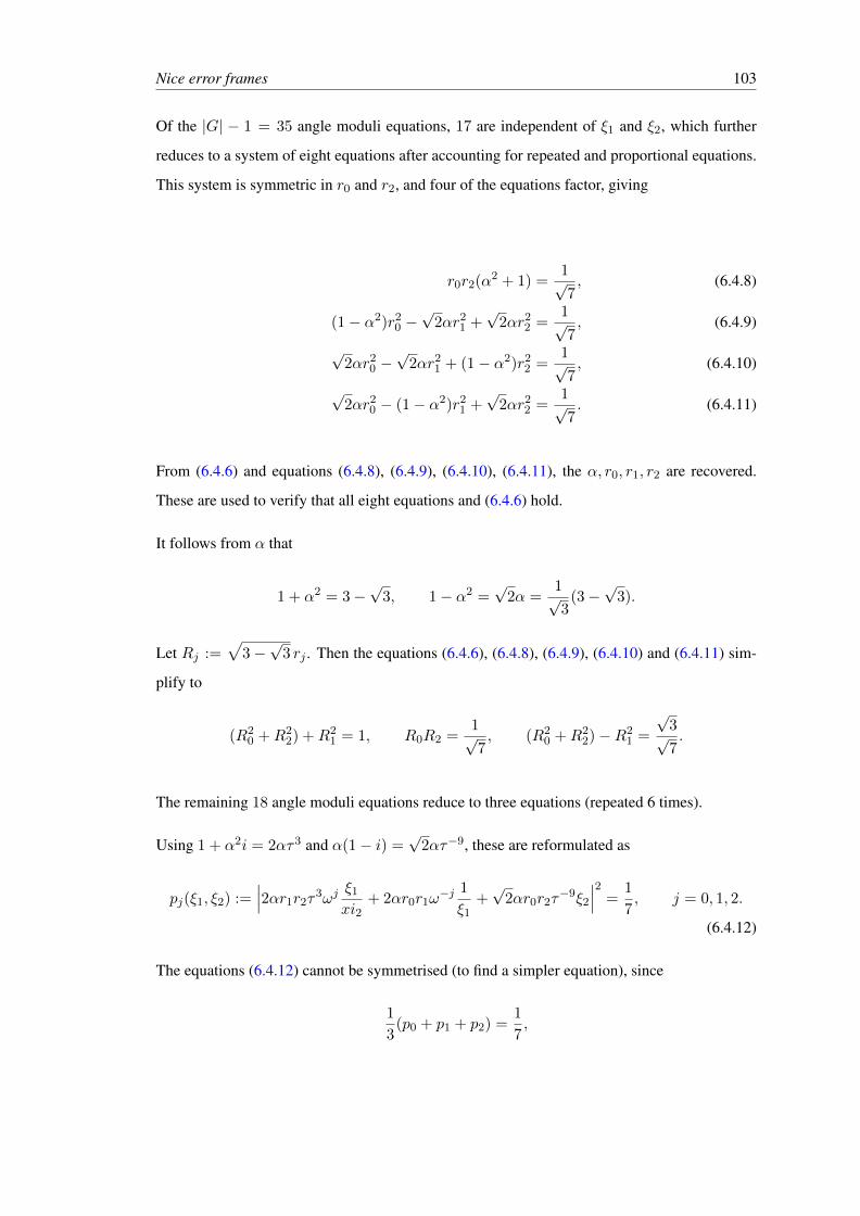
Nice error frames 103
Of the |G| − 1 = 35 angle moduli equations, 17 are independent of ξ1 and ξ2, which further
reduces to a system of eight equations after accounting for repeated and proportional equations.
This system is symmetric in r0 and r2, and four of the equations factor, giving
r0r2(α2 + 1) =1√7, (6.4.8)
(1− α2)r20 −√
2αr21 +√
2αr22 =
1√7, (6.4.9)
√2αr2
0 −√
2αr21 + (1− α2)r2
2 =1√7, (6.4.10)
√2αr2
0 − (1− α2)r21 +√
2αr22 =
1√7. (6.4.11)
From (6.4.6) and equations (6.4.8), (6.4.9), (6.4.10), (6.4.11), the α, r0, r1, r2 are recovered.
These are used to verify that all eight equations and (6.4.6) hold.
It follows from α that
1 + α2 = 3−√
3, 1− α2 =√
2α =1√3
(3−√
3).
Let Rj :=√
3−√
3 rj . Then the equations (6.4.6), (6.4.8), (6.4.9), (6.4.10) and (6.4.11) sim-
plify to
(R20 +R2
2) +R21 = 1, R0R2 =
1√7, (R2
0 +R22)−R2
1 =
√3√7.
The remaining 18 angle moduli equations reduce to three equations (repeated 6 times).
Using 1 + α2i = 2ατ3 and α(1− i) =√
2ατ−9, these are reformulated as
pj(ξ1, ξ2) :=∣∣∣2αr1r2τ
3ωjξ1
xi2+ 2αr0r1ω
−j 1
ξ1+√
2αr0r2τ−9ξ2
∣∣∣2 =1
7, j = 0, 1, 2.
(6.4.12)
The equations (6.4.12) cannot be symmetrised (to find a simpler equation), since
1
3(p0 + p1 + p2) =
1
7,
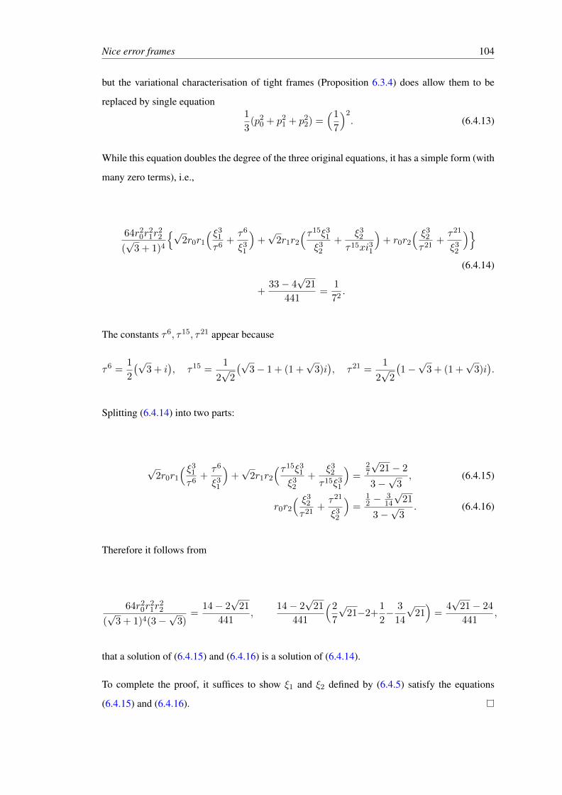
Nice error frames 104
but the variational characterisation of tight frames (Proposition 6.3.4) does allow them to be
replaced by single equation1
3(p2
0 + p21 + p2
2) =(1
7
)2. (6.4.13)
While this equation doubles the degree of the three original equations, it has a simple form (with
many zero terms), i.e.,
64r20r
21r
22
(√
3 + 1)4
√2r0r1
( ξ31
τ6+τ6
ξ31
)+√
2r1r2
(τ15ξ31
ξ32
+ξ3
2
τ15xi31
)+ r0r2
( ξ32
τ21+τ21
ξ32
)(6.4.14)
+33− 4
√21
441=
1
72.
The constants τ6, τ15, τ21 appear because
τ6 =1
2
(√3 + i
), τ15 =
1
2√
2
(√3− 1 + (1 +
√3)i), τ21 =
1
2√
2
(1−√
3 + (1 +√
3)i).
Splitting (6.4.14) into two parts:
√2r0r1
( ξ31
τ6+τ6
ξ31
)+√
2r1r2
(τ15ξ31
ξ32
+ξ3
2
τ15ξ31
)=
27
√21− 2
3−√
3, (6.4.15)
r0r2
( ξ32
τ21+τ21
ξ32
)=
12 −
314
√21
3−√
3. (6.4.16)
Therefore it follows from
64r20r
21r
22
(√
3 + 1)4(3−√
3)=
14− 2√
21
441,
14− 2√
21
441
(2
7
√21−2+
1
2− 3
14
√21)
=4√
21− 24
441,
that a solution of (6.4.15) and (6.4.16) is a solution of (6.4.14).
To complete the proof, it suffices to show ξ1 and ξ2 defined by (6.4.5) satisfy the equations
(6.4.15) and (6.4.16).
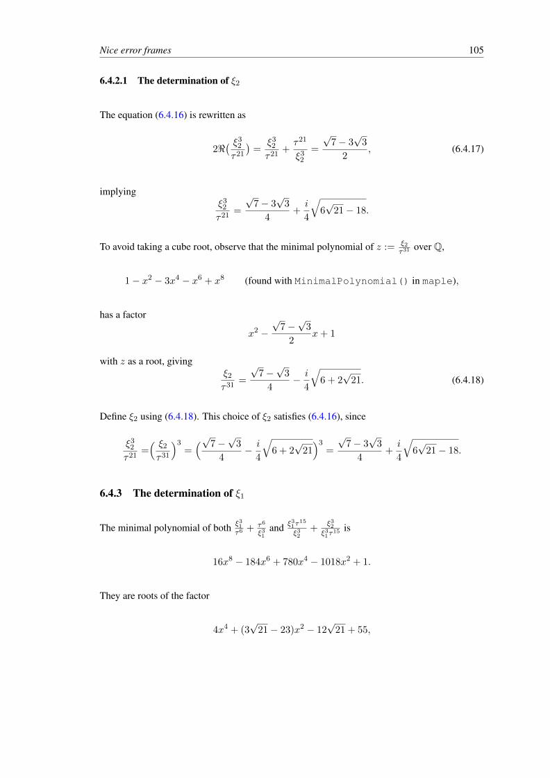
Nice error frames 105
6.4.2.1 The determination of ξ2
The equation (6.4.16) is rewritten as
2<( ξ3
2
τ21
)=
ξ32
τ21+τ21
ξ32
=
√7− 3
√3
2, (6.4.17)
implyingξ3
2
τ21=
√7− 3
√3
4+i
4
√6√
21− 18.
To avoid taking a cube root, observe that the minimal polynomial of z := ξ2τ31
over Q,
1− x2 − 3x4 − x6 + x8 (found with MinimalPolynomial() in maple),
has a factor
x2 −√
7−√
3
2x+ 1
with z as a root, givingξ2
τ31=
√7−√
3
4− i
4
√6 + 2
√21. (6.4.18)
Define ξ2 using (6.4.18). This choice of ξ2 satisfies (6.4.16), since
ξ32
τ21=( ξ2
τ31
)3=(√7−
√3
4− i
4
√6 + 2
√21)3
=
√7− 3
√3
4+i
4
√6√
21− 18.
6.4.3 The determination of ξ1
The minimal polynomial of both ξ31τ6
+ τ6
ξ31and ξ31τ
15
ξ32+
ξ32ξ31τ
15 is
16x8 − 184x6 + 780x4 − 1018x2 + 1.
They are roots of the factor
4x4 + (3√
21− 23)x2 − 12√
21 + 55,
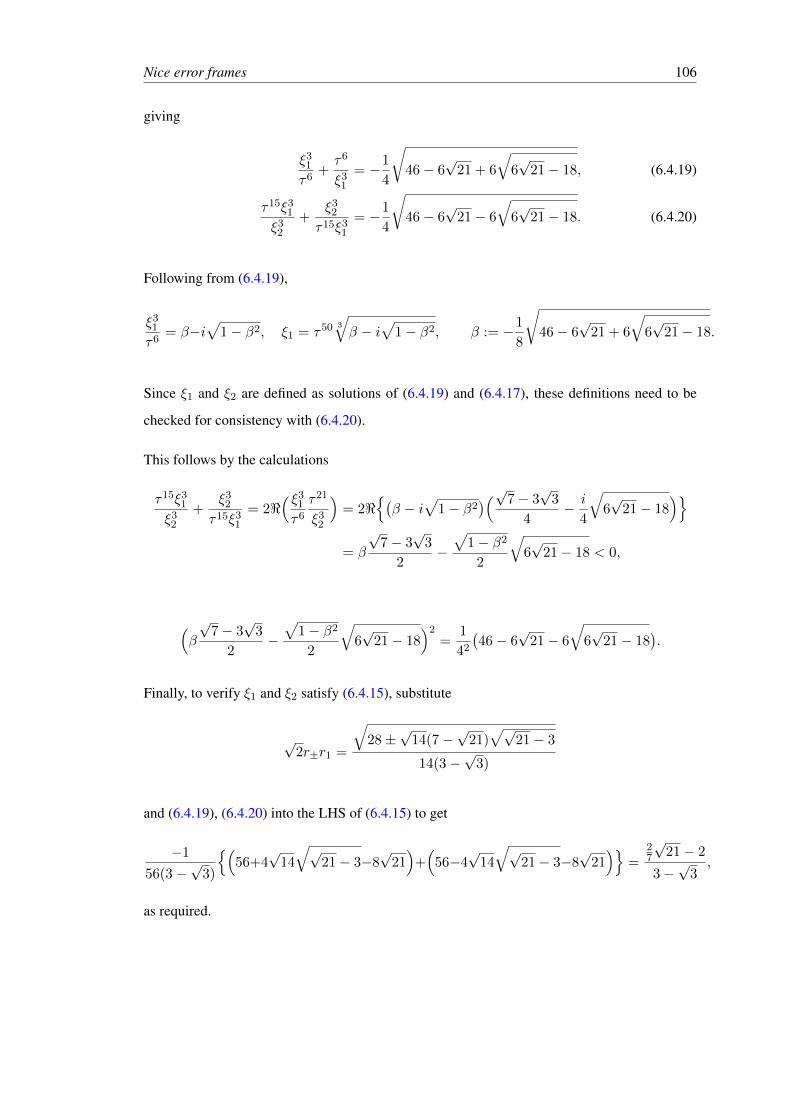
Nice error frames 106
giving
ξ31
τ6+τ6
ξ31
= −1
4
√46− 6
√21 + 6
√6√
21− 18, (6.4.19)
τ15ξ31
ξ32
+ξ3
2
τ15ξ31
= −1
4
√46− 6
√21− 6
√6√
21− 18. (6.4.20)
Following from (6.4.19),
ξ31
τ6= β−i
√1− β2, ξ1 = τ50 3
√β − i
√1− β2, β := −1
8
√46− 6
√21 + 6
√6√
21− 18.
Since ξ1 and ξ2 are defined as solutions of (6.4.19) and (6.4.17), these definitions need to be
checked for consistency with (6.4.20).
This follows by the calculations
τ15ξ31
ξ32
+ξ3
2
τ15ξ31
= 2<( ξ3
1
τ6
τ21
ξ32
)= 2<
(β − i
√1− β2
)(√7− 3√
3
4− i
4
√6√
21− 18)
= β
√7− 3
√3
2−√
1− β2
2
√6√
21− 18 < 0,
(β
√7− 3
√3
2−√
1− β2
2
√6√
21− 18)2
=1
42
(46− 6
√21− 6
√6√
21− 18).
Finally, to verify ξ1 and ξ2 satisfy (6.4.15), substitute
√2r±r1 =
√28±
√14(7−
√21)√√
21− 3
14(3−√
3)
and (6.4.19), (6.4.20) into the LHS of (6.4.15) to get
−1
56(3−√
3)
(56+4
√14
√√21− 3−8
√21)
+(
56−4√
14
√√21− 3−8
√21)
=27
√21− 2
3−√
3,
as required.

Nice error frames 107
Remark 6.4.3.
There are other relations between ξ1 and ξ2, e.g., the minimal polynomial of ξ1/ξ1/22 is
16x48 − 31x24 + 16,
leading to
ξ1
ξ1/22
= τ33 24
√31− 3
√7i
32,
but it is not clear how ξ1, ξ2 developed from this satisfy the angle equations.
6.5 Equivalence to Heisenberg SIC-POVMs
Many SIC-POVMs arise from nice error groups with a different index group to the Weyl-
Heisenberg group. An interesting question is whether they are projectively equivalent to a known
Weyl-Heisenberg solution. By using triple products, Zhu showed numerically in Section 10.4
of [Zhu12] that with the exception of the Hoggar lines, which occur with multiple instances in 8
dimensions, all other SIC-POVMs arising from different nice error bases are projectively equiv-
alent to known Weyl-Heisenberg covariant SIC-POVMs. The analytic fiducials in Appendix A,
and Section 6.4, which were independently discovered, can be used to verify Zhu’s numerical
claims.
As for the Hoggar lines, while they are not projectively equivalent to Weyl-Heisenberg SIC-
POVMs, they do not stray far from the Weyl-Heisenberg tree. By looking to the normaliser
of the Weyl-Heisenberg group (Clifford group), one finds canonical abstract error groups as
subgroups, which give the Hoggar lines (see Section A.3 in Appendix A). In fact, several abstract
error groups are realised as subgroups of the Clifford group. See Table A.2 of Appendix A.
This leads to the following conjecture.
Conjecture 6.5.1.
Let Φ be a SIC-POVM covariant to a group G. Then Φ is projectively unitarily equivalent to a
SIC-POVM that is covariant to a subgroup of the Clifford group.

108

Nice error groups 109
Appendix A
Nice Error Groups
A.1 Tables of canonical abstract error groups and index groups
TABLE A.1: Nice error bases for d < 14, d 6= 8. Here H is the canonical abstract error group,G is the index group, and sic indicates that a SIC-POVM exists numerically.
d H G 11 〈1331, 3〉 〈121, 2〉 = Z211 sic
1 〈1, 1〉 〈1, 1〉 = Z1 sic 12 〈1728, 1294〉 〈144, 68〉 sic
2 〈8, 4〉 〈4, 2〉 = Z22 sic 〈1728, 2011〉 〈144, 92〉
3 〈27, 3〉 〈9, 2〉 = Z23 sic 〈1728, 2079〉 〈144, 101〉 = Z2
12 sic
4 〈64, 19〉 〈16, 2〉 = Z24 sic 〈1728, 2983〉 〈144, 132〉
〈64, 94〉 〈16, 3〉 〈1728, 10718〉 〈144, 95〉
〈64, 256〉 〈16, 11〉 〈1728, 10926〉 〈144, 100〉
〈64, 266〉 〈16, 14〉 = (Z2 × Z2)2 〈1728, 11061〉 〈144, 102〉
5 〈125, 3〉 〈25, 2〉 = Z25 sic 〈1728, 13457〉 〈144, 136〉
6 〈216, 42〉 〈36, 11〉 sic 〈1728, 20393〉 〈144, 170〉
〈216, 66〉 〈36, 13〉 〈1728, 20436〉 〈144, 172〉
〈216, 80〉 〈36, 14〉 = Z26 sic 〈1728, 20556〉 〈144, 177〉
7 〈343, 3〉 〈49, 2〉 = Z27 sic 〈1728, 20771〉 〈144, 179〉
9 〈729, 24〉 〈81, 2〉 = Z29 sic 〈1728, 30353〉 〈144, 184〉
〈729, 30〉 〈81, 4〉 〈1728, 30562〉 〈144, 189〉
〈729, 405〉 〈81, 9〉 sic 〈1728, 30928〉 〈144, 193〉
〈729, 489〉 〈81, 12〉 〈1728, 30953〉 〈144, 194〉
〈729, 503〉 〈81, 15〉 = (Z3 × Z3)2 〈1728, 31061〉 〈144, 196〉
10 〈1000, 70〉 〈100, 15〉 〈1728, 31093〉 〈144, 197〉 = (Z2 × Z6)2
〈1000, 84〉 〈100, 16〉 = Z210 sic 13 〈2197, 3〉 〈169, 2〉 = Z2
13 sic
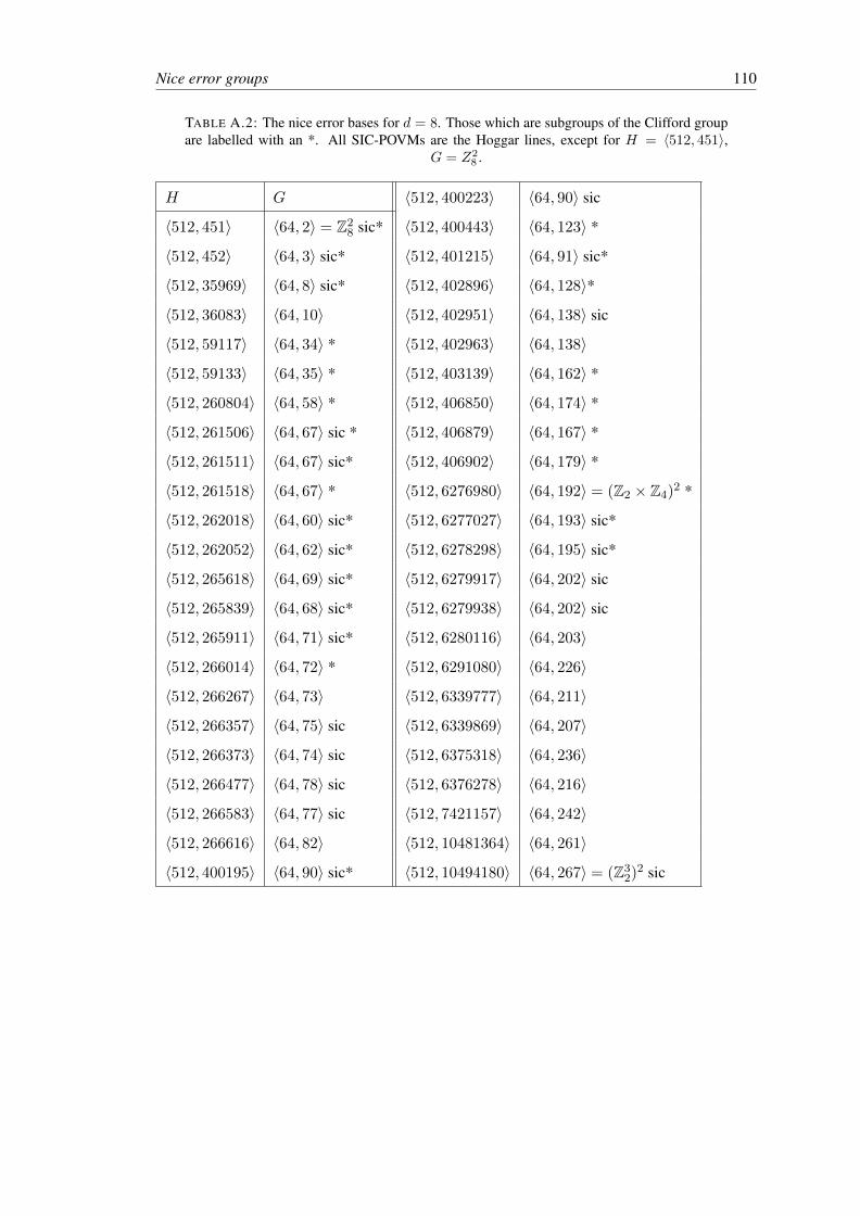
Nice error groups 110
TABLE A.2: The nice error bases for d = 8. Those which are subgroups of the Clifford groupare labelled with an *. All SIC-POVMs are the Hoggar lines, except for H = 〈512, 451〉,
G = Z28 .
H G 〈512, 400223〉 〈64, 90〉 sic
〈512, 451〉 〈64, 2〉 = Z28 sic* 〈512, 400443〉 〈64, 123〉 *
〈512, 452〉 〈64, 3〉 sic* 〈512, 401215〉 〈64, 91〉 sic*
〈512, 35969〉 〈64, 8〉 sic* 〈512, 402896〉 〈64, 128〉*
〈512, 36083〉 〈64, 10〉 〈512, 402951〉 〈64, 138〉 sic
〈512, 59117〉 〈64, 34〉 * 〈512, 402963〉 〈64, 138〉
〈512, 59133〉 〈64, 35〉 * 〈512, 403139〉 〈64, 162〉 *
〈512, 260804〉 〈64, 58〉 * 〈512, 406850〉 〈64, 174〉 *
〈512, 261506〉 〈64, 67〉 sic * 〈512, 406879〉 〈64, 167〉 *
〈512, 261511〉 〈64, 67〉 sic* 〈512, 406902〉 〈64, 179〉 *
〈512, 261518〉 〈64, 67〉 * 〈512, 6276980〉 〈64, 192〉 = (Z2 × Z4)2 *
〈512, 262018〉 〈64, 60〉 sic* 〈512, 6277027〉 〈64, 193〉 sic*
〈512, 262052〉 〈64, 62〉 sic* 〈512, 6278298〉 〈64, 195〉 sic*
〈512, 265618〉 〈64, 69〉 sic* 〈512, 6279917〉 〈64, 202〉 sic
〈512, 265839〉 〈64, 68〉 sic* 〈512, 6279938〉 〈64, 202〉 sic
〈512, 265911〉 〈64, 71〉 sic* 〈512, 6280116〉 〈64, 203〉
〈512, 266014〉 〈64, 72〉 * 〈512, 6291080〉 〈64, 226〉
〈512, 266267〉 〈64, 73〉 〈512, 6339777〉 〈64, 211〉
〈512, 266357〉 〈64, 75〉 sic 〈512, 6339869〉 〈64, 207〉
〈512, 266373〉 〈64, 74〉 sic 〈512, 6375318〉 〈64, 236〉
〈512, 266477〉 〈64, 78〉 sic 〈512, 6376278〉 〈64, 216〉
〈512, 266583〉 〈64, 77〉 sic 〈512, 7421157〉 〈64, 242〉
〈512, 266616〉 〈64, 82〉 〈512, 10481364〉 〈64, 261〉
〈512, 400195〉 〈64, 90〉 sic* 〈512, 10494180〉 〈64, 267〉 = (Z32)2 sic
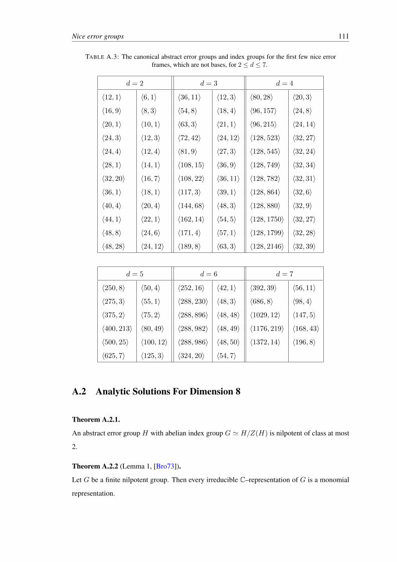
Nice error groups 111
TABLE A.3: The canonical abstract error groups and index groups for the first few nice errorframes, which are not bases, for 2 ≤ d ≤ 7.
d = 2 d = 3 d = 4
〈12, 1〉 〈6, 1〉 〈36, 11〉 〈12, 3〉 〈80, 28〉 〈20, 3〉
〈16, 9〉 〈8, 3〉 〈54, 8〉 〈18, 4〉 〈96, 157〉 〈24, 8〉
〈20, 1〉 〈10, 1〉 〈63, 3〉 〈21, 1〉 〈96, 215〉 〈24, 14〉
〈24, 3〉 〈12, 3〉 〈72, 42〉 〈24, 12〉 〈128, 523〉 〈32, 27〉
〈24, 4〉 〈12, 4〉 〈81, 9〉 〈27, 3〉 〈128, 545〉 〈32, 24〉
〈28, 1〉 〈14, 1〉 〈108, 15〉 〈36, 9〉 〈128, 749〉 〈32, 34〉
〈32, 20〉 〈16, 7〉 〈108, 22〉 〈36, 11〉 〈128, 782〉 〈32, 31〉
〈36, 1〉 〈18, 1〉 〈117, 3〉 〈39, 1〉 〈128, 864〉 〈32, 6〉
〈40, 4〉 〈20, 4〉 〈144, 68〉 〈48, 3〉 〈128, 880〉 〈32, 9〉
〈44, 1〉 〈22, 1〉 〈162, 14〉 〈54, 5〉 〈128, 1750〉 〈32, 27〉
〈48, 8〉 〈24, 6〉 〈171, 4〉 〈57, 1〉 〈128, 1799〉 〈32, 28〉
〈48, 28〉 〈24, 12〉 〈189, 8〉 〈63, 3〉 〈128, 2146〉 〈32, 39〉
d = 5 d = 6 d = 7
〈250, 8〉 〈50, 4〉 〈252, 16〉 〈42, 1〉 〈392, 39〉 〈56, 11〉
〈275, 3〉 〈55, 1〉 〈288, 230〉 〈48, 3〉 〈686, 8〉 〈98, 4〉
〈375, 2〉 〈75, 2〉 〈288, 896〉 〈48, 48〉 〈1029, 12〉 〈147, 5〉
〈400, 213〉 〈80, 49〉 〈288, 982〉 〈48, 49〉 〈1176, 219〉 〈168, 43〉
〈500, 25〉 〈100, 12〉 〈288, 986〉 〈48, 50〉 〈1372, 14〉 〈196, 8〉
〈625, 7〉 〈125, 3〉 〈324, 20〉 〈54, 7〉
A.2 Analytic Solutions For Dimension 8
Theorem A.2.1.
An abstract error group H with abelian index group G ' H/Z(H) is nilpotent of class at most
2.
Theorem A.2.2 (Lemma 1, [Bro73]).
Let G be a finite nilpotent group. Then every irreducible C–representation of G is a monomial
representation.
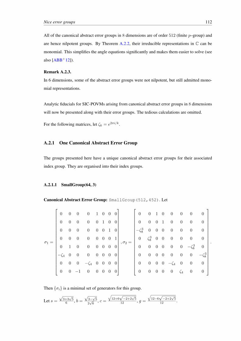
Nice error groups 112
All of the canonical abstract error groups in 8 dimensions are of order 512 (finite p–group) and
are hence nilpotent groups. By Theorem A.2.2, their irreducible representations in C can be
monomial. This simplifies the angle equations significantly and makes them easier to solve (see
also [ABB+12]).
Remark A.2.3.
In 6 dimensions, some of the abstract error groups were not nilpotent, but still admitted mono-
mial representations.
Analytic fiducials for SIC-POVMs arising from canonical abstract error groups in 8 dimensions
will now be presented along with their error groups. The tedious calculations are omitted.
For the following matrices, let ζk = e2πi/k.
A.2.1 One Canonical Abstract Error Group
The groups presented here have a unique canonical abstract error groups for their associated
index group. They are organised into their index groups.
A.2.1.1 SmallGroup(64, 3)
Canonical Abstract Error Group: SmallGroup(512,452). Let
σ1 =
0 0 0 0 1 0 0 0
0 0 0 0 0 1 0 0
0 0 0 0 0 0 1 0
0 0 0 0 0 0 0 1
0 1 0 0 0 0 0 0
−ζ4 0 0 0 0 0 0 0
0 0 0 −ζ4 0 0 0 0
0 0 −1 0 0 0 0 0
, σ2 =
0 0 1 0 0 0 0 0
0 0 0 1 0 0 0 0
−ζ38 0 0 0 0 0 0 0
0 ζ38 0 0 0 0 0 0
0 0 0 0 0 0 −ζ38 0
0 0 0 0 0 0 0 −ζ38
0 0 0 0 −ζ4 0 0 0
0 0 0 0 0 ζ4 0 0
.
Then σi is a minimal set of generators for this group.
Let s =
√3+3√
56 , b =
√3−√
5
2√
6, c =
√12+6√−2+2
√5
12 , g =
√12−6√−2+2
√5
12 .

Nice error groups 113
v =
(0, 0, sI,−b(1 + I), c− gI, b+
s√2I,√
2c, g(1 + I)
)Tis a fiducial vector giving rise to a SIC-POVM.
A.2.1.2 SmallGroup(64, 8)
Canonical Abstract Error Group: SmallGroup(512,35969).
Let σ1 = ζ8I8, and
σ2 =
0 1 0 0 0 0 0 0
ζ4 0 0 0 0 0 0 0
0 0 0 0 0 1 0 0
0 0 0 0 0 0 1 0
0 0 0 0 0 0 0 1
0 0 ζ4 0 0 0 0 0
0 0 0 ζ4 0 0 0 0
0 0 0 0 ζ4 0 0 0
, σ3 =
0 0 1 0 0 0 0 0
0 0 0 0 0 −ζ38 0 0
0 0 0 1 0 0 0 0
0 0 0 0 1 0 0 0
1 0 0 0 0 0 0 0
0 0 0 0 0 0 ζ8 0
0 0 0 0 0 0 0 ζ38
0 −ζ8 0 0 0 0 0 0
.
Then σi is a set of generators for this group.
Let α =
√6+3√
26 , β =
√6−3√
26 .
v =
(−βi, 0,−αi, α, β, 1
2
√2α+
1
2
√2βi, 0,
1
2
√2α+
1
2
√2βi
)Tis a fiducial vector giving rise to a SIC-POVM.
A.2.1.3 SmallGroup(64, 60)
Canonical Abstract Error Group: SmallGroup(512,262018).
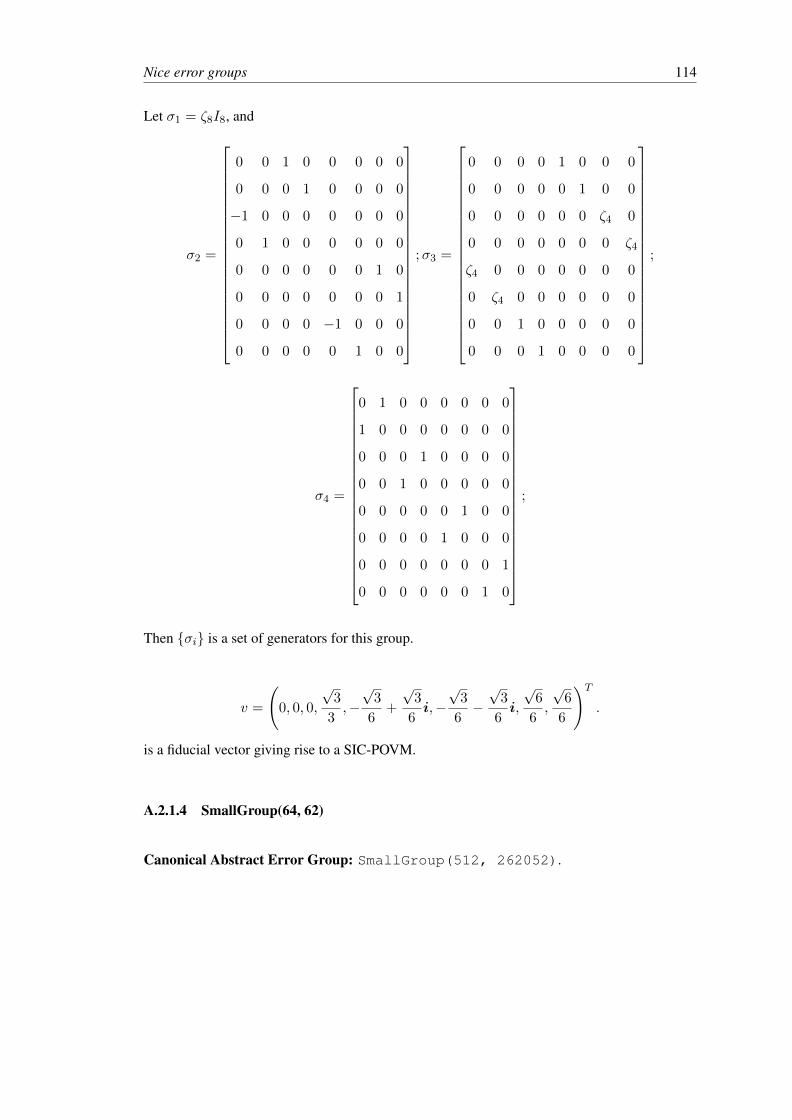
Nice error groups 114
Let σ1 = ζ8I8, and
σ2 =
0 0 1 0 0 0 0 0
0 0 0 1 0 0 0 0
−1 0 0 0 0 0 0 0
0 1 0 0 0 0 0 0
0 0 0 0 0 0 1 0
0 0 0 0 0 0 0 1
0 0 0 0 −1 0 0 0
0 0 0 0 0 1 0 0
;σ3 =
0 0 0 0 1 0 0 0
0 0 0 0 0 1 0 0
0 0 0 0 0 0 ζ4 0
0 0 0 0 0 0 0 ζ4
ζ4 0 0 0 0 0 0 0
0 ζ4 0 0 0 0 0 0
0 0 1 0 0 0 0 0
0 0 0 1 0 0 0 0
;
σ4 =
0 1 0 0 0 0 0 0
1 0 0 0 0 0 0 0
0 0 0 1 0 0 0 0
0 0 1 0 0 0 0 0
0 0 0 0 0 1 0 0
0 0 0 0 1 0 0 0
0 0 0 0 0 0 0 1
0 0 0 0 0 0 1 0
;
Then σi is a set of generators for this group.
v =
(0, 0, 0,
√3
3,−√
3
6+
√3
6i,−√
3
6−√
3
6i,
√6
6,
√6
6
)T.
is a fiducial vector giving rise to a SIC-POVM.
A.2.1.4 SmallGroup(64, 62)
Canonical Abstract Error Group: SmallGroup(512, 262052).

Nice error groups 115
Let σ1 = ζ8I8, and
σ2 =
0 0 1 0 0 0 0 0
0 0 0 1 0 0 0 0
−1 0 0 0 0 0 0 0
0 1 0 0 0 0 0 0
0 0 0 0 0 0 1 0
0 0 0 0 0 0 0 1
0 0 0 0 −1 0 0 0
0 0 0 0 0 1 0 0
;σ3 =
0 1 0 0 0 0 0 0
ζ4 0 0 0 0 0 0 0
0 0 0 1 0 0 0 0
0 0 ζ4 0 0 0 0 0
0 0 0 0 0 1 0 0
0 0 0 0 ζ4 0 0 0
0 0 0 0 0 0 0 1
0 0 0 0 0 0 ζ4 0
;
σ4 =
0 0 0 0 1 0 0 0
0 0 0 0 0 1 0 0
0 0 0 0 0 0 1 0
0 0 0 0 0 0 0 1
−1 0 0 0 0 0 0 0
0 −1 0 0 0 0 0 0
0 0 1 0 0 0 0 0
0 0 0 1 0 0 0 0
;
Then σi is a set of generators for this group.
v =
(0, 0,−
√6
6,
√3
6−√
3
6i, 0,
√3
3,
√6
6,
√3
6+
√3
6i
)T.
is a fiducial vector giving rise to a SIC-POVM.
A.2.1.5 SmallGroup(64, 68)
Canonical Abstract Error Group: SmallGroup(512, 265839).
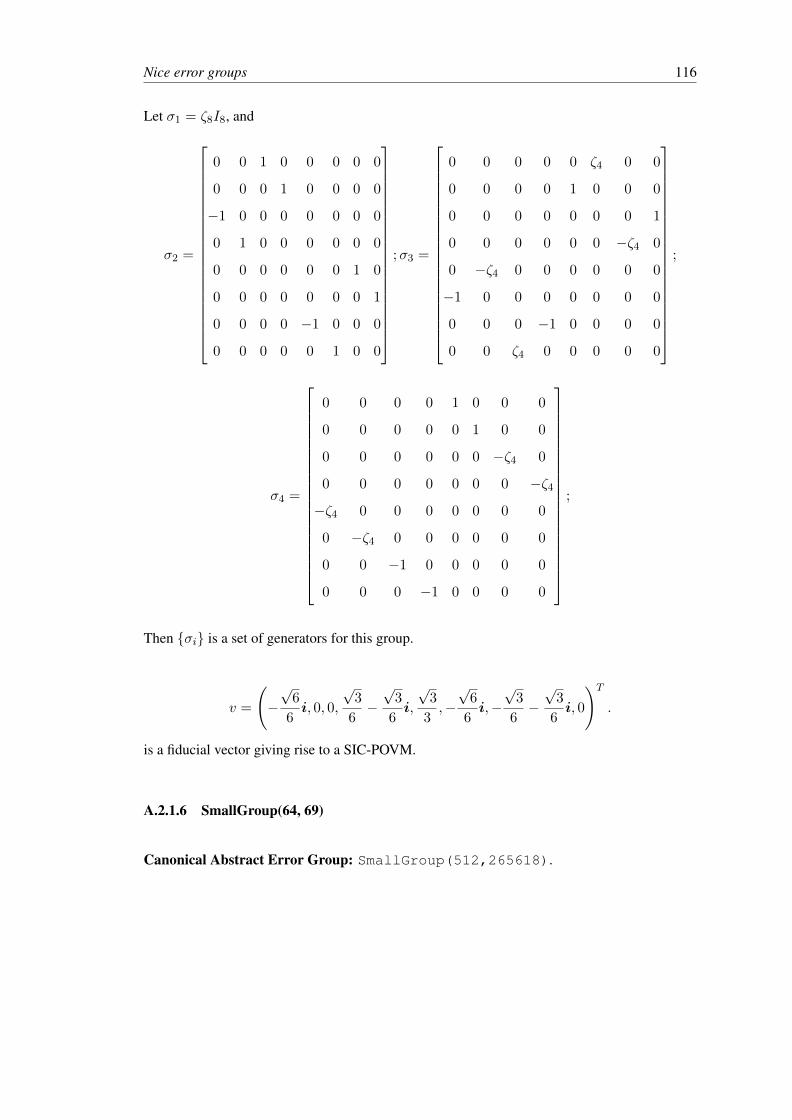
Nice error groups 116
Let σ1 = ζ8I8, and
σ2 =
0 0 1 0 0 0 0 0
0 0 0 1 0 0 0 0
−1 0 0 0 0 0 0 0
0 1 0 0 0 0 0 0
0 0 0 0 0 0 1 0
0 0 0 0 0 0 0 1
0 0 0 0 −1 0 0 0
0 0 0 0 0 1 0 0
;σ3 =
0 0 0 0 0 ζ4 0 0
0 0 0 0 1 0 0 0
0 0 0 0 0 0 0 1
0 0 0 0 0 0 −ζ4 0
0 −ζ4 0 0 0 0 0 0
−1 0 0 0 0 0 0 0
0 0 0 −1 0 0 0 0
0 0 ζ4 0 0 0 0 0
;
σ4 =
0 0 0 0 1 0 0 0
0 0 0 0 0 1 0 0
0 0 0 0 0 0 −ζ4 0
0 0 0 0 0 0 0 −ζ4
−ζ4 0 0 0 0 0 0 0
0 −ζ4 0 0 0 0 0 0
0 0 −1 0 0 0 0 0
0 0 0 −1 0 0 0 0
;
Then σi is a set of generators for this group.
v =
(−√
6
6i, 0, 0,
√3
6−√
3
6i,
√3
3,−√
6
6i,−√
3
6−√
3
6i, 0
)T.
is a fiducial vector giving rise to a SIC-POVM.
A.2.1.6 SmallGroup(64, 69)
Canonical Abstract Error Group: SmallGroup(512,265618).
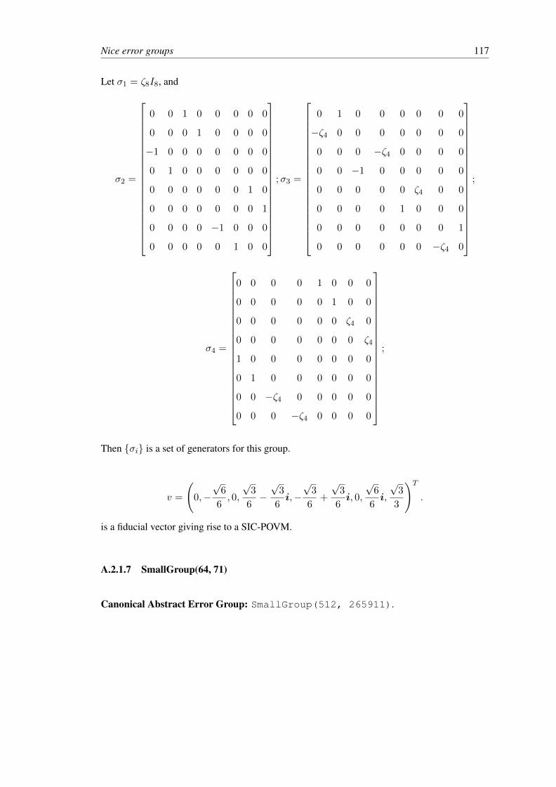
Nice error groups 117
Let σ1 = ζ8I8, and
σ2 =
0 0 1 0 0 0 0 0
0 0 0 1 0 0 0 0
−1 0 0 0 0 0 0 0
0 1 0 0 0 0 0 0
0 0 0 0 0 0 1 0
0 0 0 0 0 0 0 1
0 0 0 0 −1 0 0 0
0 0 0 0 0 1 0 0
;σ3 =
0 1 0 0 0 0 0 0
−ζ4 0 0 0 0 0 0 0
0 0 0 −ζ4 0 0 0 0
0 0 −1 0 0 0 0 0
0 0 0 0 0 ζ4 0 0
0 0 0 0 1 0 0 0
0 0 0 0 0 0 0 1
0 0 0 0 0 0 −ζ4 0
;
σ4 =
0 0 0 0 1 0 0 0
0 0 0 0 0 1 0 0
0 0 0 0 0 0 ζ4 0
0 0 0 0 0 0 0 ζ4
1 0 0 0 0 0 0 0
0 1 0 0 0 0 0 0
0 0 −ζ4 0 0 0 0 0
0 0 0 −ζ4 0 0 0 0
;
Then σi is a set of generators for this group.
v =
(0,−√
6
6, 0,
√3
6−√
3
6i,−√
3
6+
√3
6i, 0,
√6
6i,
√3
3
)T.
is a fiducial vector giving rise to a SIC-POVM.
A.2.1.7 SmallGroup(64, 71)
Canonical Abstract Error Group: SmallGroup(512, 265911).

Nice error groups 118
Let σ1 = ζ8I8, and
σ2 =
0 0 1 0 0 0 0 0
0 0 0 1 0 0 0 0
−1 0 0 0 0 0 0 0
0 1 0 0 0 0 0 0
0 0 0 0 0 0 1 0
0 0 0 0 0 0 0 1
0 0 0 0 −1 0 0 0
0 0 0 0 0 1 0 0
;σ3 =
0 0 0 0 1 0 0 0
0 0 0 0 0 1 0 0
0 0 0 0 0 0 ζ4 0
0 0 0 0 0 0 0 ζ4
1 0 0 0 0 0 0 0
0 1 0 0 0 0 0 0
0 0 −ζ4 0 0 0 0 0
0 0 0 −ζ4 0 0 0 0
;
σ4 =
0 1 0 0 0 0 0 0
1 0 0 0 0 0 0 0
0 0 0 1 0 0 0 0
0 0 1 0 0 0 0 0
0 0 0 0 0 −1 0 0
0 0 0 0 −1 0 0 0
0 0 0 0 0 0 0 1
0 0 0 0 0 0 1 0
;
Then σi is a set of generators for this group.
v =
(0, 0, 0,
√3
3,
√6
6i,
√6
6i,
√3
6+
√3
6i,
√3
6−√
3
6i
)T.
is a fiducial vector giving rise to a SIC-POVM.
A.2.1.8 SmallGroup(64, 74)
Canonical Abstract Error Group: SmallGroup(512, 266373).

Nice error groups 119
Let σ1 = ζ8I8, and
σ2 =
0 1 0 0 0 0 0 0
−ζ4 0 0 0 0 0 0 0
0 0 0 0 1 0 0 0
0 0 0 0 0 1 0 0
0 0 −ζ4 0 0 0 0 0
0 0 0 ζ4 0 0 0 0
0 0 0 0 0 0 0 1
0 0 0 0 0 0 ζ4 0
;σ3 =
0 0 1 0 0 0 0 0
0 0 0 0 −1 0 0 0
−1 0 0 0 0 0 0 0
0 0 0 0 0 0 1 0
0 1 0 0 0 0 0 0
0 0 0 0 0 0 0 1
0 0 0 1 0 0 0 0
0 0 0 0 0 1 0 0
;
σ4 =
0 0 0 1 0 0 0 0
0 0 0 0 0 1 0 0
0 0 0 0 0 0 1 0
1 0 0 0 0 0 0 0
0 0 0 0 0 0 0 1
0 1 0 0 0 0 0 0
0 0 1 0 0 0 0 0
0 0 0 0 1 0 0 0
;
Then σi is a set of generators for this group.
v =
(0, 0,
√3
3,
√3
6+
√3
6i, 0,
√6
6,
√3
6−√
3
6i,
√6
6
)T.
is a fiducial vector giving rise to a SIC-POVM.
A.2.1.9 SmallGroup(64, 75)
Canonical Abstract Error Group: SmallGroup(512,266357).

Nice error groups 120
Let σ1 = ζ8I8, and
σ2 =
0 1 0 0 0 0 0 0
ζ4 0 0 0 0 0 0 0
0 0 0 0 1 0 0 0
0 0 0 0 0 1 0 0
0 0 ζ4 0 0 0 0 0
0 0 0 ζ4 0 0 0 0
0 0 0 0 0 0 0 1
0 0 0 0 0 0 ζ4 0
;σ3 =
0 0 1 0 0 0 0 0
0 0 0 0 ζ4 0 0 0
1 0 0 0 0 0 0 0
0 0 0 0 0 0 1 0
0 −ζ4 0 0 0 0 0 0
0 0 0 0 0 0 0 ζ4
0 0 0 1 0 0 0 0
0 0 0 0 0 −ζ4 0 0
;
σ4 =
0 0 0 1 0 0 0 0
0 0 0 0 0 −ζ4 0 0
0 0 0 0 0 0 1 0
−ζ4 0 0 0 0 0 0 0
0 0 0 0 0 0 0 −ζ4
0 −1 0 0 0 0 0 0
0 0 ζ4 0 0 0 0 0
0 0 0 0 1 0 0 0
;
Then σi is a set of generators for this group.
v =
(−√
6
6i, 0,−
√6
6i, 0, 0,−
√3
6−√
3
6i,
√3
3,−√
3
6+
√3
6i
)T.
is a fiducial vector giving rise to a SIC-POVM.
A.2.1.10 SmallGroup(64, 77)
Canonical Abstract Error Group: SmallGroup(512, 266583).

Nice error groups 121
Let σ1 = ζ8I8, and
σ2 =
0 1 0 0 0 0 0 0
1 0 0 0 0 0 0 0
0 0 0 0 1 0 0 0
0 0 0 0 0 1 0 0
0 0 1 0 0 0 0 0
0 0 0 −1 0 0 0 0
0 0 0 0 0 0 0 1
0 0 0 0 0 0 −1 0
;σ3 =
0 0 1 0 0 0 0 0
0 0 0 0 −ζ4 0 0 0
−ζ4 0 0 0 0 0 0 0
0 0 0 0 0 0 1 0
0 −1 0 0 0 0 0 0
0 0 0 0 0 0 0 ζ4
0 0 0 ζ4 0 0 0 0
0 0 0 0 0 −1 0 0
;
σ4 =
0 0 0 1 0 0 0 0
0 0 0 0 0 1 0 0
0 0 0 0 0 0 1 0
1 0 0 0 0 0 0 0
0 0 0 0 0 0 0 1
0 1 0 0 0 0 0 0
0 0 1 0 0 0 0 0
0 0 0 0 1 0 0 0
;
Then σi is a set of generators for this group.
v =
(√6
6, 0, 0,−
√6
6i,−√
3
6+
√3
6i, 0,
√3
3,
√3
6−√
3
6i
)T.
is a fiducial vector giving rise to a SIC-POVM.
A.2.1.11 SmallGroup(64, 78)
Canonical Abstract Error Group: SmallGroup(512, 266477).

Nice error groups 122
Let σ1 = ζ8I8, and
σ2 =
0 1 0 0 0 0 0 0
ζ4 0 0 0 0 0 0 0
0 0 0 0 1 0 0 0
0 0 0 0 0 1 0 0
0 0 ζ4 0 0 0 0 0
0 0 0 ζ4 0 0 0 0
0 0 0 0 0 0 0 1
0 0 0 0 0 0 ζ4 0
;σ3 =
0 0 1 0 0 0 0 0
0 0 0 0 ζ4 0 0 0
−1 0 0 0 0 0 0 0
0 0 0 0 0 0 1 0
0 ζ4 0 0 0 0 0 0
0 0 0 0 0 0 0 ζ4
0 0 0 1 0 0 0 0
0 0 0 0 0 −ζ4 0 0
;
σ4 =
0 0 0 1 0 0 0 0
0 0 0 0 0 1 0 0
0 0 0 0 0 0 −1 0
−ζ4 0 0 0 0 0 0 0
0 0 0 0 0 0 0 −1
0 ζ4 0 0 0 0 0 0
0 0 −ζ4 0 0 0 0 0
0 0 0 0 ζ4 0 0 0
;
Then σi is a set of generators for this group.
v =
(0,
√6
6i,−√
3
6−√
3
6i, 0, 0,
√3
6+
√3
6i,−√
6
6i,
√3
3
)T.
is a fiducial vector giving rise to a SIC-POVM.
A.2.1.12 SmallGroup(64, 91)
Canonical Abstract Error Group: SmallGroup(512, 401215).

Nice error groups 123
Let σ1 = ζ8I8, and
σ2 =
0 0 1 0 0 0 0 0
0 0 0 1 0 0 0 0
0 0 0 0 1 0 0 0
0 0 0 0 0 1 0 0
0 0 0 0 0 0 1 0
0 0 0 0 0 0 0 1
1 0 0 0 0 0 0 0
0 1 0 0 0 0 0 0
;σ3 =
0 1 0 0 0 0 0 0
−1 0 0 0 0 0 0 0
0 0 0 −ζ4 0 0 0 0
0 0 ζ4 0 0 0 0 0
0 0 0 0 0 −1 0 0
0 0 0 0 1 0 0 0
0 0 0 0 0 0 0 ζ4
0 0 0 0 0 0 −ζ4 0
;
σ4 =
−1 0 0 0 0 0 0 0
0 1 0 0 0 0 0 0
0 0 1 0 0 0 0 0
0 0 0 −1 0 0 0 0
0 0 0 0 1 0 0 0
0 0 0 0 0 −1 0 0
0 0 0 0 0 0 1 0
0 0 0 0 0 0 0 −1
;
Then σi is a set of generators for this group.
v =
(0, 0,
√6
6i,−√
6
6, 0,
√3
3,−√
6
6i,
√6
6i
)T.
is a fiducial vector giving rise to a SIC-POVM.
A.2.1.13 SmallGroup(64, 193)
Canonical Abstract Error Group: SmallGroup(512, 6277027).
Let σ1 = ζ8I8, and
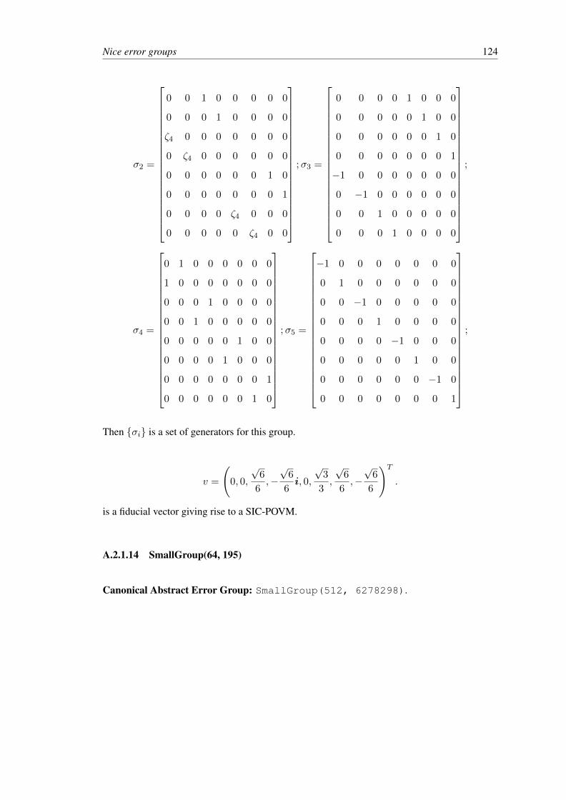
Nice error groups 124
σ2 =
0 0 1 0 0 0 0 0
0 0 0 1 0 0 0 0
ζ4 0 0 0 0 0 0 0
0 ζ4 0 0 0 0 0 0
0 0 0 0 0 0 1 0
0 0 0 0 0 0 0 1
0 0 0 0 ζ4 0 0 0
0 0 0 0 0 ζ4 0 0
;σ3 =
0 0 0 0 1 0 0 0
0 0 0 0 0 1 0 0
0 0 0 0 0 0 1 0
0 0 0 0 0 0 0 1
−1 0 0 0 0 0 0 0
0 −1 0 0 0 0 0 0
0 0 1 0 0 0 0 0
0 0 0 1 0 0 0 0
;
σ4 =
0 1 0 0 0 0 0 0
1 0 0 0 0 0 0 0
0 0 0 1 0 0 0 0
0 0 1 0 0 0 0 0
0 0 0 0 0 1 0 0
0 0 0 0 1 0 0 0
0 0 0 0 0 0 0 1
0 0 0 0 0 0 1 0
;σ5 =
−1 0 0 0 0 0 0 0
0 1 0 0 0 0 0 0
0 0 −1 0 0 0 0 0
0 0 0 1 0 0 0 0
0 0 0 0 −1 0 0 0
0 0 0 0 0 1 0 0
0 0 0 0 0 0 −1 0
0 0 0 0 0 0 0 1
;
Then σi is a set of generators for this group.
v =
(0, 0,
√6
6,−√
6
6i, 0,
√3
3,
√6
6,−√
6
6
)T.
is a fiducial vector giving rise to a SIC-POVM.
A.2.1.14 SmallGroup(64, 195)
Canonical Abstract Error Group: SmallGroup(512, 6278298).
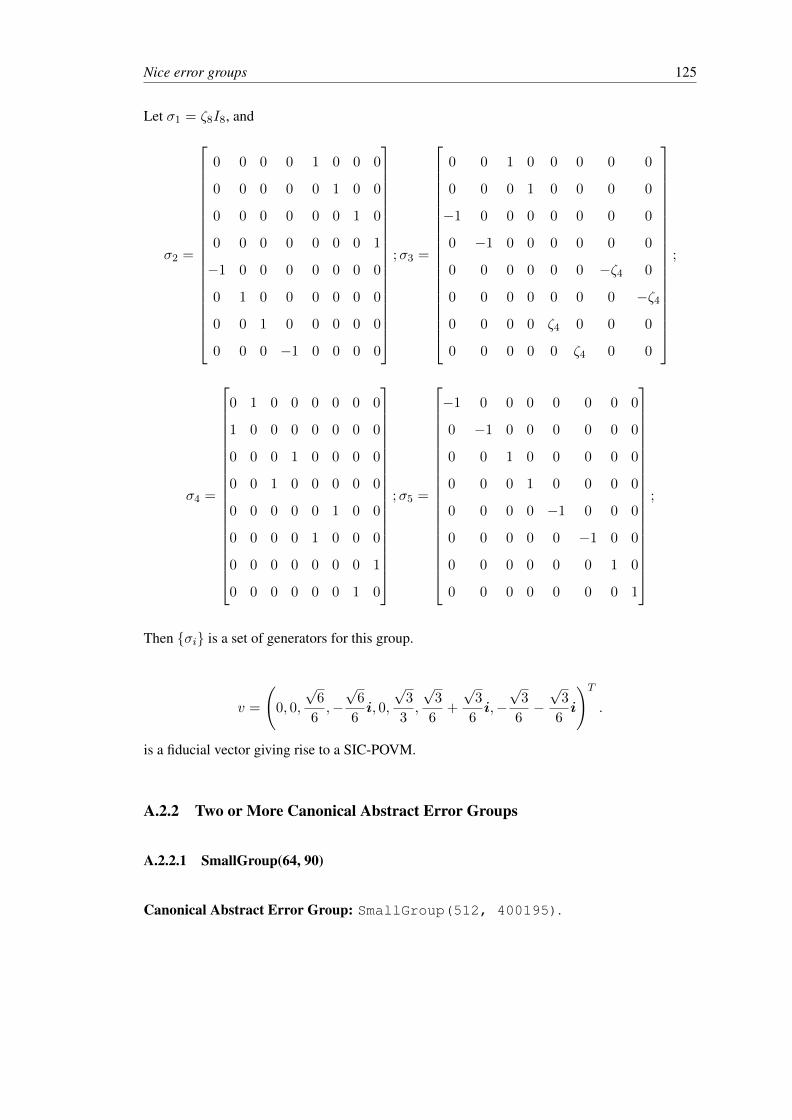
Nice error groups 125
Let σ1 = ζ8I8, and
σ2 =
0 0 0 0 1 0 0 0
0 0 0 0 0 1 0 0
0 0 0 0 0 0 1 0
0 0 0 0 0 0 0 1
−1 0 0 0 0 0 0 0
0 1 0 0 0 0 0 0
0 0 1 0 0 0 0 0
0 0 0 −1 0 0 0 0
;σ3 =
0 0 1 0 0 0 0 0
0 0 0 1 0 0 0 0
−1 0 0 0 0 0 0 0
0 −1 0 0 0 0 0 0
0 0 0 0 0 0 −ζ4 0
0 0 0 0 0 0 0 −ζ4
0 0 0 0 ζ4 0 0 0
0 0 0 0 0 ζ4 0 0
;
σ4 =
0 1 0 0 0 0 0 0
1 0 0 0 0 0 0 0
0 0 0 1 0 0 0 0
0 0 1 0 0 0 0 0
0 0 0 0 0 1 0 0
0 0 0 0 1 0 0 0
0 0 0 0 0 0 0 1
0 0 0 0 0 0 1 0
;σ5 =
−1 0 0 0 0 0 0 0
0 −1 0 0 0 0 0 0
0 0 1 0 0 0 0 0
0 0 0 1 0 0 0 0
0 0 0 0 −1 0 0 0
0 0 0 0 0 −1 0 0
0 0 0 0 0 0 1 0
0 0 0 0 0 0 0 1
;
Then σi is a set of generators for this group.
v =
(0, 0,
√6
6,−√
6
6i, 0,
√3
3,
√3
6+
√3
6i,−√
3
6−√
3
6i
)T.
is a fiducial vector giving rise to a SIC-POVM.
A.2.2 Two or More Canonical Abstract Error Groups
A.2.2.1 SmallGroup(64, 90)
Canonical Abstract Error Group: SmallGroup(512, 400195).

Nice error groups 126
Let σ1 = ζ8I8, and
σ2 =
0 1 0 0 0 0 0 0
ζ4 0 0 0 0 0 0 0
0 0 0 −1 0 0 0 0
0 0 −ζ4 0 0 0 0 0
0 0 0 0 0 −1 0 0
0 0 0 0 −ζ4 0 0 0
0 0 0 0 0 0 0 −1
0 0 0 0 0 0 −ζ4 0
;σ3 =
0 0 1 0 0 0 0 0
0 0 0 1 0 0 0 0
0 0 0 0 1 0 0 0
0 0 0 0 0 1 0 0
0 0 0 0 0 0 1 0
0 0 0 0 0 0 0 1
1 0 0 0 0 0 0 0
0 1 0 0 0 0 0 0
;
σ4 =
−1 0 0 0 0 0 0 0
0 1 0 0 0 0 0 0
0 0 −1 0 0 0 0 0
0 0 0 1 0 0 0 0
0 0 0 0 −1 0 0 0
0 0 0 0 0 1 0 0
0 0 0 0 0 0 −1 0
0 0 0 0 0 0 0 1
;
Then σi is a set of generators for this group.
v =
(0,−√
6
6i, 0,
√6
6, 0,
√6
6i,
√3
3,−√
6
6i
)T.
is a fiducial vector giving rise to a SIC-POVM.
Canonical Abstract Error Group: SmallGroup(512, 400223).
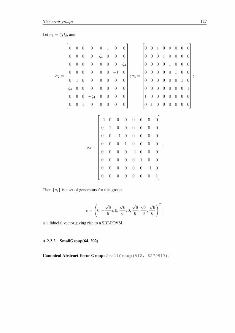
Nice error groups 127
Let σ1 = ζ8I8, and
σ2 =
0 0 0 0 0 1 0 0
0 0 0 0 ζ4 0 0 0
0 0 0 0 0 0 0 ζ4
0 0 0 0 0 0 −1 0
0 1 0 0 0 0 0 0
ζ4 0 0 0 0 0 0 0
0 0 0 −ζ4 0 0 0 0
0 0 1 0 0 0 0 0
;σ3 =
0 0 1 0 0 0 0 0
0 0 0 1 0 0 0 0
0 0 0 0 1 0 0 0
0 0 0 0 0 1 0 0
0 0 0 0 0 0 1 0
0 0 0 0 0 0 0 1
1 0 0 0 0 0 0 0
0 1 0 0 0 0 0 0
;
σ4 =
−1 0 0 0 0 0 0 0
0 1 0 0 0 0 0 0
0 0 −1 0 0 0 0 0
0 0 0 1 0 0 0 0
0 0 0 0 −1 0 0 0
0 0 0 0 0 1 0 0
0 0 0 0 0 0 −1 0
0 0 0 0 0 0 0 1
;
Then σi is a set of generators for this group.
v =
(0,−√
6
6i, 0,
√6
6, 0,
√6
6,
√3
3,
√6
6
)T.
is a fiducial vector giving rise to a SIC-POVM.
A.2.2.2 SmallGroup(64, 202)
Canonical Abstract Error Group: SmallGroup(512, 6279917).
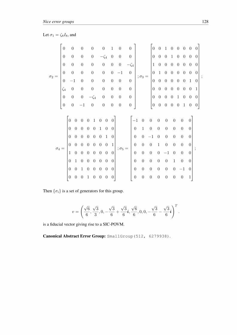
Nice error groups 128
Let σ1 = ζ8I8, and
σ2 =
0 0 0 0 0 1 0 0
0 0 0 0 −ζ4 0 0 0
0 0 0 0 0 0 0 −ζ4
0 0 0 0 0 0 −1 0
0 −1 0 0 0 0 0 0
ζ4 0 0 0 0 0 0 0
0 0 0 −ζ4 0 0 0 0
0 0 −1 0 0 0 0 0
;σ3 =
0 0 1 0 0 0 0 0
0 0 0 1 0 0 0 0
1 0 0 0 0 0 0 0
0 1 0 0 0 0 0 0
0 0 0 0 0 0 1 0
0 0 0 0 0 0 0 1
0 0 0 0 1 0 0 0
0 0 0 0 0 1 0 0
;
σ4 =
0 0 0 0 1 0 0 0
0 0 0 0 0 1 0 0
0 0 0 0 0 0 1 0
0 0 0 0 0 0 0 1
1 0 0 0 0 0 0 0
0 1 0 0 0 0 0 0
0 0 1 0 0 0 0 0
0 0 0 1 0 0 0 0
;σ5 =
−1 0 0 0 0 0 0 0
0 1 0 0 0 0 0 0
0 0 −1 0 0 0 0 0
0 0 0 1 0 0 0 0
0 0 0 0 −1 0 0 0
0 0 0 0 0 1 0 0
0 0 0 0 0 0 −1 0
0 0 0 0 0 0 0 1
;
Then σi is a set of generators for this group.
v =
(√6
6,
√3
3, 0,−
√3
6+
√3
6i,
√6
6, 0, 0,−
√3
6−√
3
6i
)T.
is a fiducial vector giving rise to a SIC-POVM.
Canonical Abstract Error Group: SmallGroup(512, 6279938).

Nice error groups 129
Let σ1 = ζ8I8, and
σ2 =
0 1 0 0 0 0 0 0
ζ4 0 0 0 0 0 0 0
0 0 0 −1 0 0 0 0
0 0 −ζ4 0 0 0 0 0
0 0 0 0 0 −1 0 0
0 0 0 0 −ζ4 0 0 0
0 0 0 0 0 0 0 −1
0 0 0 0 0 0 −ζ4 0
;σ3 =
0 0 1 0 0 0 0 0
0 0 0 1 0 0 0 0
1 0 0 0 0 0 0 0
0 1 0 0 0 0 0 0
0 0 0 0 0 0 1 0
0 0 0 0 0 0 0 1
0 0 0 0 1 0 0 0
0 0 0 0 0 1 0 0
;
σ4 =
0 0 0 0 1 0 0 0
0 0 0 0 0 1 0 0
0 0 0 0 0 0 1 0
0 0 0 0 0 0 0 1
1 0 0 0 0 0 0 0
0 1 0 0 0 0 0 0
0 0 1 0 0 0 0 0
0 0 0 1 0 0 0 0
;σ5 =
−1 0 0 0 0 0 0 0
0 1 0 0 0 0 0 0
0 0 −1 0 0 0 0 0
0 0 0 1 0 0 0 0
0 0 0 0 −1 0 0 0
0 0 0 0 0 1 0 0
0 0 0 0 0 0 −1 0
0 0 0 0 0 0 0 1
;
Then σi is a set of generators for this group.
v =
(0, 0, 0,
√3
3,
√6
6,
√3
6−√
3
6i,−√
6
6,−√
3
6−√
3
6i
)T.
is a fiducial vector giving rise to a SIC-POVM.
A.2.3 Canonical Abstract Error Group With No Solutions
The fiducial searching method used was to start with a random vector and perturb it in ways that
attempt to minimise the second frame potential. The number of perturbation cycles were around
2000. The program was then repeated 5000 times. When a group gave rise to a numerical SIC-
POVMs, it often occured very early on (less than 5 repeats). In some of the following cases,
no numerical SIC-POVMs were found. While it maybe possible that SIC-POVM fiducials exist
in the groups, for example if they existed with very specific parameter values that were hard to

Nice error groups 130
randomly converge on, it seems unlikely. The implication of the SIC-POVMs not existing with
certain canonical error groups but existing with others (with the same index group), is that it
demonstrates the importance of a detailed analysis of different canonical abstract error groups,
and not just the index groups.
A.2.3.1 SmallGroup(64, 67)
Canonical Abstract Error Group: SmallGroup(512,261506).
Let σ1 = ζ8I8, and
σ2 =
0 0 0 0 0 1 0 0
0 0 0 0 −ζ4 0 0 0
0 0 0 0 0 0 0 ζ4
0 0 0 0 0 0 1 0
0 −1 0 0 0 0 0 0
ζ4 0 0 0 0 0 0 0
0 0 0 ζ4 0 0 0 0
0 0 1 0 0 0 0 0
;σ3 =
0 0 1 0 0 0 0 0
0 0 0 1 0 0 0 0
−1 0 0 0 0 0 0 0
0 1 0 0 0 0 0 0
0 0 0 0 0 0 1 0
0 0 0 0 0 0 0 1
0 0 0 0 −1 0 0 0
0 0 0 0 0 1 0 0
;
σ4 =
0 0 0 0 1 0 0 0
0 0 0 0 0 1 0 0
0 0 0 0 0 0 1 0
0 0 0 0 0 0 0 1
1 0 0 0 0 0 0 0
0 1 0 0 0 0 0 0
0 0 1 0 0 0 0 0
0 0 0 1 0 0 0 0
;
Then σi is a set of generators for this group.
v =
(0,
√6
6,
√3
6+
√3
6i, 0,
√3
3,−√
6
6,−√
3
6+
√3
6i, 0
)T.
is a fiducial vector giving rise to a SIC-POVM.

Nice error groups 131
Canonical Abstract Error Group: SmallGroup(512,261511).
Let σ1 = ζ8I8, and
σ2 =
0 0 0 0 0 1 0 0
0 0 0 0 −ζ4 0 0 0
0 0 0 0 0 0 0 ζ4
0 0 0 0 0 0 1 0
0 −1 0 0 0 0 0 0
ζ4 0 0 0 0 0 0 0
0 0 0 ζ4 0 0 0 0
0 0 1 0 0 0 0 0
;σ3 =
0 0 1 0 0 0 0 0
0 0 0 1 0 0 0 0
−1 0 0 0 0 0 0 0
0 1 0 0 0 0 0 0
0 0 0 0 0 0 1 0
0 0 0 0 0 0 0 1
0 0 0 0 −1 0 0 0
0 0 0 0 0 1 0 0
;
σ4 =
0 0 0 0 1 0 0 0
0 0 0 0 0 1 0 0
0 0 0 0 0 0 1 0
0 0 0 0 0 0 0 1
1 0 0 0 0 0 0 0
0 1 0 0 0 0 0 0
0 0 1 0 0 0 0 0
0 0 0 1 0 0 0 0
;
Then σi is a set of generators for this group.
v =
(0, 0,−
√6
6,
√3
6−√
3
6i, 0,
√3
3,
√6
6i,
√3
6−√
3
6i
)T.
is a fiducial vector giving rise to a SIC-POVM.
Canonical Abstract Error Group: SmallGroup(512,261518).
NO SIC-POVM FOUND.
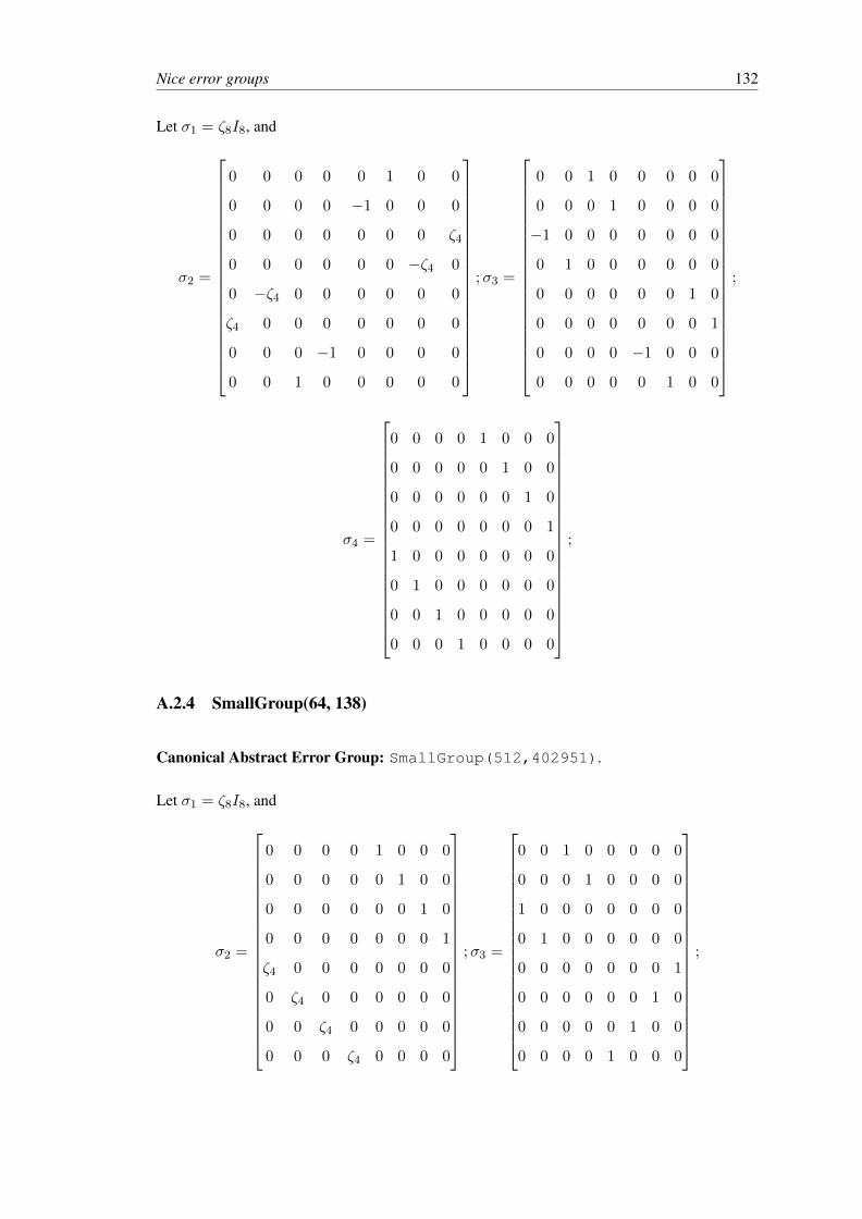
Nice error groups 132
Let σ1 = ζ8I8, and
σ2 =
0 0 0 0 0 1 0 0
0 0 0 0 −1 0 0 0
0 0 0 0 0 0 0 ζ4
0 0 0 0 0 0 −ζ4 0
0 −ζ4 0 0 0 0 0 0
ζ4 0 0 0 0 0 0 0
0 0 0 −1 0 0 0 0
0 0 1 0 0 0 0 0
;σ3 =
0 0 1 0 0 0 0 0
0 0 0 1 0 0 0 0
−1 0 0 0 0 0 0 0
0 1 0 0 0 0 0 0
0 0 0 0 0 0 1 0
0 0 0 0 0 0 0 1
0 0 0 0 −1 0 0 0
0 0 0 0 0 1 0 0
;
σ4 =
0 0 0 0 1 0 0 0
0 0 0 0 0 1 0 0
0 0 0 0 0 0 1 0
0 0 0 0 0 0 0 1
1 0 0 0 0 0 0 0
0 1 0 0 0 0 0 0
0 0 1 0 0 0 0 0
0 0 0 1 0 0 0 0
;
A.2.4 SmallGroup(64, 138)
Canonical Abstract Error Group: SmallGroup(512,402951).
Let σ1 = ζ8I8, and
σ2 =
0 0 0 0 1 0 0 0
0 0 0 0 0 1 0 0
0 0 0 0 0 0 1 0
0 0 0 0 0 0 0 1
ζ4 0 0 0 0 0 0 0
0 ζ4 0 0 0 0 0 0
0 0 ζ4 0 0 0 0 0
0 0 0 ζ4 0 0 0 0
;σ3 =
0 0 1 0 0 0 0 0
0 0 0 1 0 0 0 0
1 0 0 0 0 0 0 0
0 1 0 0 0 0 0 0
0 0 0 0 0 0 0 1
0 0 0 0 0 0 1 0
0 0 0 0 0 1 0 0
0 0 0 0 1 0 0 0
;

Nice error groups 133
σ4 =
1 0 0 0 0 0 0 0
0 −1 0 0 0 0 0 0
0 0 −1 0 0 0 0 0
0 0 0 1 0 0 0 0
0 0 0 0 −1 0 0 0
0 0 0 0 0 −1 0 0
0 0 0 0 0 0 1 0
0 0 0 0 0 0 0 1
;
Then σi is a set of generators for this group.
v =
(0, 0, 0,
√3
3,−√
6
6i,
√6
6i,−√
6
6i,−√
6
6
)T.
is a fiducial vector giving rise to a SIC-POVM.
Canonical Abstract Error Group: SmallGroup(512,402963).
NO SIC-POVM FOUND.
Let σ1 = ζ8I8, and
σ2 =
0 0 0 0 1 0 0 0
0 0 0 0 0 1 0 0
0 0 0 0 0 0 1 0
0 0 0 0 0 0 0 1
ζ4 0 0 0 0 0 0 0
0 ζ4 0 0 0 0 0 0
0 0 ζ4 0 0 0 0 0
0 0 0 ζ4 0 0 0 0
;σ3 =
0 0 1 0 0 0 0 0
0 0 0 1 0 0 0 0
1 0 0 0 0 0 0 0
0 1 0 0 0 0 0 0
0 0 0 0 0 0 0 −1
0 0 0 0 0 0 1 0
0 0 0 0 0 1 0 0
0 0 0 0 −1 0 0 0
;
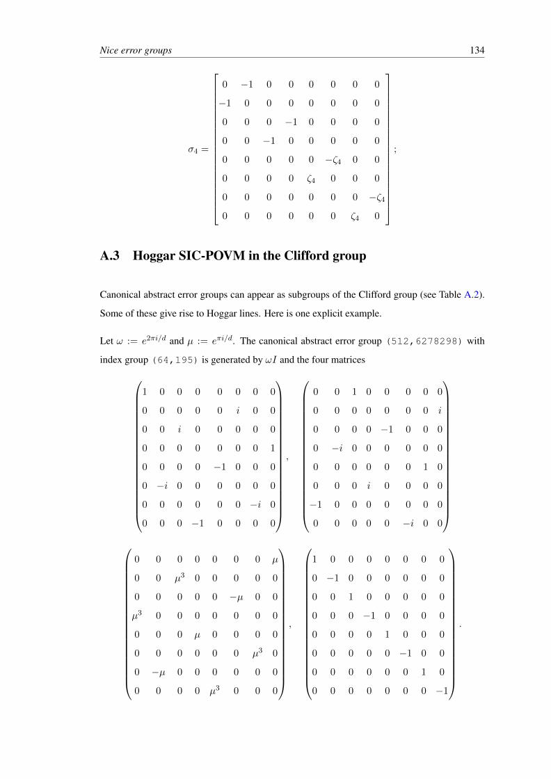
Nice error groups 134
σ4 =
0 −1 0 0 0 0 0 0
−1 0 0 0 0 0 0 0
0 0 0 −1 0 0 0 0
0 0 −1 0 0 0 0 0
0 0 0 0 0 −ζ4 0 0
0 0 0 0 ζ4 0 0 0
0 0 0 0 0 0 0 −ζ4
0 0 0 0 0 0 ζ4 0
;
A.3 Hoggar SIC-POVM in the Clifford group
Canonical abstract error groups can appear as subgroups of the Clifford group (see Table A.2).
Some of these give rise to Hoggar lines. Here is one explicit example.
Let ω := e2πi/d and µ := eπi/d. The canonical abstract error group (512,6278298) with
index group (64,195) is generated by ωI and the four matrices
1 0 0 0 0 0 0 0
0 0 0 0 0 i 0 0
0 0 i 0 0 0 0 0
0 0 0 0 0 0 0 1
0 0 0 0 −1 0 0 0
0 −i 0 0 0 0 0 0
0 0 0 0 0 0 −i 0
0 0 0 −1 0 0 0 0
,
0 0 1 0 0 0 0 0
0 0 0 0 0 0 0 i
0 0 0 0 −1 0 0 0
0 −i 0 0 0 0 0 0
0 0 0 0 0 0 1 0
0 0 0 i 0 0 0 0
−1 0 0 0 0 0 0 0
0 0 0 0 0 −i 0 0
0 0 0 0 0 0 0 µ
0 0 µ3 0 0 0 0 0
0 0 0 0 0 −µ 0 0
µ3 0 0 0 0 0 0 0
0 0 0 µ 0 0 0 0
0 0 0 0 0 0 µ3 0
0 −µ 0 0 0 0 0 0
0 0 0 0 µ3 0 0 0
,
1 0 0 0 0 0 0 0
0 −1 0 0 0 0 0 0
0 0 1 0 0 0 0 0
0 0 0 −1 0 0 0 0
0 0 0 0 1 0 0 0
0 0 0 0 0 −1 0 0
0 0 0 0 0 0 1 0
0 0 0 0 0 0 0 −1
.

Nice error groups 135
One fiducial vector is
√6
12 +(√
36 −
√6
12
)i
0√
36 (−1 + i)
16
√6− 3
√2 i
√6
12 −(√
36 +
√6
12
)i
0√
36 (1− i)
16
√6 + 3
√2
.
A.4 Dimension 16
In 16 dimensions, it is no longer possible to look for nice error groups using the Small Groups
Library since canonical nice error groups are of order 163 = 4096. Theorem 5 of [KR02] gives
one general class of abstract error groups of order 22n−2.
Theorem A.4.1 (Theorem 5 of [KR02]).
Let f , g : Z2n → Z2n , be maps such that
f := (x 7→ x+ 1 mod 2n), g := (x 7→ 5x mod 2n).
Let Hn := 〈f, g〉 be the group generated by compositions of f and g. Then Hn is an abstract
error group of order 22n−2. The index group Hn/Z(Hn) is nonabelian provided that n ≥ 5.
A numerical SIC-POVM search was conducted on H7 (of order 4096) and after more than 2000
searches, was unable to find any SIC-POVMs. However, due to other considerations (e.g., it may
just be harder to hit the Welch bound with higher dimensions), it is not yet wise to conclude this
group does not yield SIC-POVMs.

Appendix B
Projective symmetry groups of cyclic
harmonic frames
The tables summarise the calculations on projective symmetry groups of the cyclic harmonic
frames Φ = ΦJ of n vectors for Cd, d = 2, . . . , 7.
Column legend:
1. d – the dimension Cd.
2. n – the number of vectors in Φ.
3. real – whether Φ is projectively real.
4. orth – whether any vectors in Φ are orthogonal.
5. reps – whether the vectors in Φ projectively repeated, i.e., are not projectively distinct.
6. SymP (Φ) – the projective symmetry group of Φ, when the vectors of Φ are projectively
distinct.
7. SymEP (Φ) – the extended projective symmetry group of Φ, when Φ is projectively com-
plex with projectively distinct vectors.
8. J – a subset of Zn giving ΦJ (up to projective equivalence and reordering).
9. 4-cycle – whether 4–cycles were needed to define the projective equivalence class.
136

Projective symmetry groups of cyclic harmonic frames 137
d n real orth reps SymP (Φ) SymEP (Φ) J 4-cycle erasures2 2 yes y <2,1> 0, 1 02 3 y <6,1> 0, 1 12 4 y y <8,3> 0, 1 y 2
y y y 1, 3 12 5 y <10,1> 0, 1 32 6 y y 1, 3 3
y y <12,4> 1, 2 4y y y 1, 4 2
2 7 y <14,1> 1, 4 52 8 y y <16,7> 1, 6 6
y y y 1, 3 5y y y 1, 5 3
2 9 y <18,1> 1, 3 7y y 1, 4 5
2 10 y y 1, 5 7y y <20,4> 1, 4 8y y y 1, 6 4
2 11 y <22,1> 1, 10 92 12 y y y 1, 10 8
y y <24,6> 1, 8 10y y 1, 9 7y y y 1, 7 5y y y 1, 3 9
2 13 y <26,1> 1, 4 112 14 y y <28,3> 1, 2 12
y y 1, 5 11y y y 1, 8 6
2 15 y <30,3> 0, 1 13y y 1, 10 11y y 1, 6 9
10. erasures – the number of vectors that can be removed from Φ so that those remaining still
span Cd.1
1The erasures data was obtained from the catalogue of harmonic frames compiled by N. Hay and S. Waldron athttps://www.math.auckland.ac.nz/˜waldron/Harmonic-frames/framesN, where N in the urlis a natural number from 2 to 7.
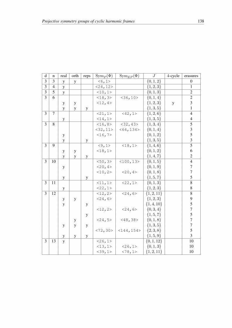
Projective symmetry groups of cyclic harmonic frames 138
d n real orth reps SymP (Φ) SymEP (Φ) J 4-cycle erasures3 3 y y <6,1> 0, 1, 2 03 4 y <24,12> 1, 2, 3 13 5 y <10,1> 0, 1, 3 23 6 <18,3> <36,10> 0, 1, 4 2
y y <12,4> 1, 2, 3 y 3y y y 1, 3, 5 1
3 7 <21,1> <42,1> 1, 2, 6 4y <14,1> 1, 3, 5 4
3 8 <16,8> <32,43> 1, 3, 4 5<32,11> <64,134> 0, 1, 4 3
y <16,7> 0, 1, 2 5y y 1, 3, 5 3
3 9 <9,1> <18,1> 1, 4, 6 5y y <18,1> 0, 1, 2 6y y y 1, 4, 7 2
3 10 <50,3> <100,13> 0, 1, 5 4y <20,4> 0, 1, 9 7
<10,2> <20,4> 0, 1, 8 7y y 1, 5, 7 5
3 11 <11,1> <22,1> 0, 1, 3 8y <22,1> 1, 2, 3 8
3 12 <12,2> <24,6> 1, 2, 11 8y y <24,6> 1, 2, 3 9y y 1, 4, 10 5
<12,2> <24,6> 0, 3, 4 7y 1, 5, 7 5
y <24,5> <48,38> 0, 1, 8 7y y y 1, 3, 5 7
<72,30> <144,154> 2, 3, 8 5y y y 1, 5, 9 3
3 13 y <26,1> 0, 1, 12 10<13,1> <26,1> 0, 1, 3 10<39,1> <78,1> 1, 2, 11 10
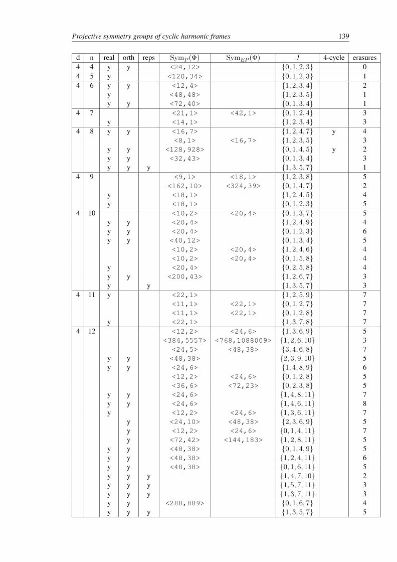
Projective symmetry groups of cyclic harmonic frames 139
d n real orth reps SymP (Φ) SymEP (Φ) J 4-cycle erasures4 4 y y <24,12> 0, 1, 2, 3 04 5 y <120,34> 0, 1, 2, 3 14 6 y y <12,4> 1, 2, 3, 4 2
y <48,48> 1, 2, 3, 5 1y y <72,40> 0, 1, 3, 4 1
4 7 <21,1> <42,1> 0, 1, 2, 4 3y <14,1> 1, 2, 3, 4 3
4 8 y y <16,7> 1, 2, 4, 7 y 4<8,1> <16,7> 1, 2, 3, 5 3
y y <128,928> 0, 1, 4, 5 y 2y y <32,43> 0, 1, 3, 4 3y y y 1, 3, 5, 7 1
4 9 <9,1> <18,1> 1, 2, 3, 8 5<162,10> <324,39> 0, 1, 4, 7 2
y <18,1> 1, 2, 4, 5 4y <18,1> 0, 1, 2, 3 5
4 10 <10,2> <20,4> 0, 1, 3, 7 5y y <20,4> 1, 2, 4, 9 4y y <20,4> 0, 1, 2, 3 6y y <40,12> 0, 1, 3, 4 5
<10,2> <20,4> 1, 2, 4, 6 4<10,2> <20,4> 0, 1, 5, 8 4
y <20,4> 0, 2, 5, 8 4y y <200,43> 1, 2, 6, 7 3y y 1, 3, 5, 7 3
4 11 y <22,1> 1, 2, 5, 9 7<11,1> <22,1> 0, 1, 2, 7 7<11,1> <22,1> 0, 1, 2, 8 7
y <22,1> 1, 3, 7, 8 74 12 <12,2> <24,6> 1, 3, 6, 9 5
<384,5557> <768,1088009> 1, 2, 6, 10 3<24,5> <48,38> 3, 4, 6, 8 7
y y <48,38> 2, 3, 9, 10 5y y <24,6> 1, 4, 8, 9 6
<12,2> <24,6> 0, 1, 2, 8 5<36,6> <72,23> 0, 2, 3, 8 5
y y <24,6> 1, 4, 8, 11 7y y <24,6> 1, 4, 6, 11 8y <12,2> <24,6> 1, 3, 6, 11 7
y <24,10> <48,38> 2, 3, 6, 9 5y <12,2> <24,6> 0, 1, 4, 11 7y <72,42> <144,183> 1, 2, 8, 11 5
y y <48,38> 0, 1, 4, 9 5y y <48,38> 1, 2, 4, 11 6y y <48,38> 0, 1, 6, 11 5y y y 1, 4, 7, 10 2y y y 1, 5, 7, 11 3y y y 1, 3, 7, 11 3y y <288,889> 0, 1, 6, 7 4y y y 1, 3, 5, 7 5

Projective symmetry groups of cyclic harmonic frames 140
d n real orth reps SymP (Φ) SymEP (Φ) J 4-cycle erasures5 5 y y <120,34> 0, 1, 2, 3, 4 05 6 y <720,763> 0, 1, 2, 3, 4 15 7 y <14,1> 0, 1, 2, 3, 5 25 8 <32,11> <64, 134> 1, 2, 3, 5, 6 2
y <16,7> 0, 1, 2, 6, 7 3<16,8> <32,43> 0, 1, 2, 3, 6 3
y <384,5602> 1, 2, 3, 5, 7 15 9 <9,1> <18,1> 0, 1, 2, 3, 7 4
<162,10> <324,39> 0, 1, 3, 4, 7 2y <18,1> 0, 1, 2, 3, 8 4y <18,1> 1, 2, 3, 4, 7 2
5 10 <10,2> <20,4> 1, 2, 5, 6, 9 4<10,2> <20,4> 1, 2, 4, 8, 9 4
y y <20,4> 1, 2, 4, 5, 8 y 5y <200,43> 1, 2, 3, 6, 8 3
<10,2> <204,> 1, 3, 4, 5, 8 4<50,3> <100,13> 1, 2, 3, 7, 8 3<10,2> <20,4> 0, 1, 3, 5, 9 3
y y <240,189> 0, 1, 2, 4, 8 3y y y 1, 3, 5, 7, 9 1
5 11 <11,1> <22,1> 0, 1, 2, 4, 5 6<11,1> <22,1> 0, 1, 2, 5, 9 6<55,1> <110,1> 1, 2, 3, 5, 8 6<11,1> <22,1> 1, 2, 3, 4, 10 6
y <22,1> 0, 1, 2, 3, 10 6y <22,1> 0, 1, 2, 4, 9 6
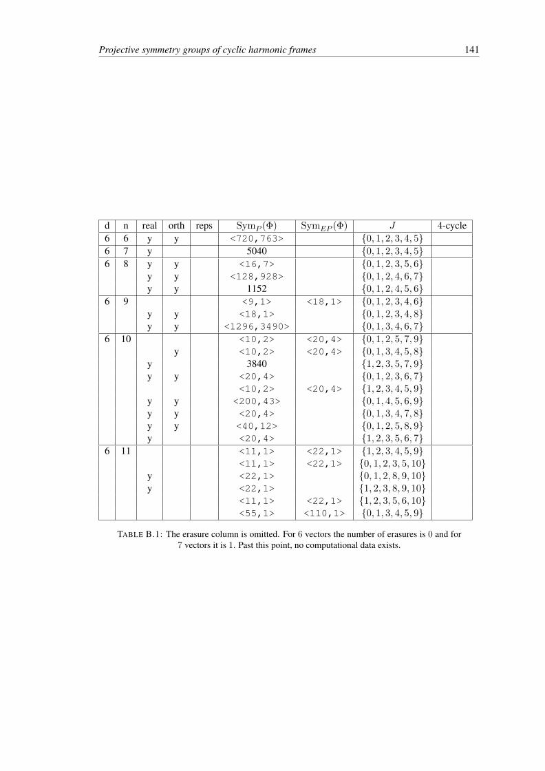
Projective symmetry groups of cyclic harmonic frames 141
d n real orth reps SymP (Φ) SymEP (Φ) J 4-cycle6 6 y y <720,763> 0, 1, 2, 3, 4, 56 7 y 5040 0, 1, 2, 3, 4, 56 8 y y <16,7> 0, 1, 2, 3, 5, 6
y y <128,928> 0, 1, 2, 4, 6, 7y y 1152 0, 1, 2, 4, 5, 6
6 9 <9,1> <18,1> 0, 1, 2, 3, 4, 6y y <18,1> 0, 1, 2, 3, 4, 8y y <1296,3490> 0, 1, 3, 4, 6, 7
6 10 <10,2> <20,4> 0, 1, 2, 5, 7, 9y <10,2> <20,4> 0, 1, 3, 4, 5, 8
y 3840 1, 2, 3, 5, 7, 9y y <20,4> 0, 1, 2, 3, 6, 7
<10,2> <20,4> 1, 2, 3, 4, 5, 9y y <200,43> 0, 1, 4, 5, 6, 9y y <20,4> 0, 1, 3, 4, 7, 8y y <40,12> 0, 1, 2, 5, 8, 9y <20,4> 1, 2, 3, 5, 6, 7
6 11 <11,1> <22,1> 1, 2, 3, 4, 5, 9<11,1> <22,1> 0, 1, 2, 3, 5, 10
y <22,1> 0, 1, 2, 8, 9, 10y <22,1> 1, 2, 3, 8, 9, 10
<11,1> <22,1> 1, 2, 3, 5, 6, 10<55,1> <110,1> 0, 1, 3, 4, 5, 9
TABLE B.1: The erasure column is omitted. For 6 vectors the number of erasures is 0 and for7 vectors it is 1. Past this point, no computational data exists.

Projective symmetry groups of cyclic harmonic frames 142
d n real orth reps SymP (Φ) SymEP (Φ) J 4-cycle7 7 y y 5040 0, 1, 2, 3, 4, 5, 67 8 y 40320 0, 1, 2, 3, 4, 5, 77 9 y <1296,3490> 0, 1, 2, 4, 5, 7, 8
y <18,1> 0, 1, 2, 3, 5, 7, 87 10 <10,2> <20,4> 1, 2, 3, 4, 5, 6, 8
<50,3> <100,13> 0, 1, 2, 5, 6, 7, 8y <320,1636> 1, 2, 3, 5, 6, 7, 9y <20,4> 1, 2, 4, 5, 6, 8, 9
11 <11,1> <22,1> 0, 1, 2, 3, 5, 6, 9<11,1> <22,1> 0, 1, 2, 6, 7, 8, 9
y <22,1> 1, 2, 3, 4, 5, 6, 8, 10y <22,1> 1, 2, 3, 4, 5, 8, 9
7 12 y y <24,6> 0, 1, 2, 4, 8, 10, 11<12,2> <24,6> 1, 2, 3, 4, 6, 7, 10<72,30> <144,154> 1, 2, 3, 4, 7, 8, 10<12,2> <24,6> 1, 3, 4, 5, 7, 8, 9<12,2> <24,6> 0, 1, 2, 4, 6, 10, 11<12,2> <24,6> 0, 1, 2, 3, 6, 10, 11<12,2> <24,6> 0, 1, 2, 3, 4, 8, 9<12,2> <24,6> 1, 2, 3, 4, 5, 6, 11
y <24,6> 0, 1, 2, 3, 4, 10, 11<12,2> <24,6> 1, 2, 3, 4, 6, 8, 9
y <96,187> 0, 1, 2, 4, 5, 6, 9<72,30> <144,154> 1, 2, 3, 5, 8, 9, 11<12,2> <24,6> 1, 2, 4, 5, 6, 10, 11<72,30> <144,154> 1, 2, 3, 7, 8, 9, 10<12,2> <24,6> 1, 2, 3, 4, 5, 7, 10<24,10> <48,38> 1, 2, 3, 4, 6, 7, 9<12,2> <24,6> 0, 1, 2, 3, 5, 6, 11
y <144,183> 0, 1, 2, 3, 4, 7, 9y 46080 1, 3, 4, 5, 7, 9, 11
<24,5> <48,38> 1, 2, 3, 4, 6, 7, 11y <24,5> <48,38> 1, 2, 3, 5, 7, 10, 11
y <288,889> 1, 2, 3, 5, 7, 8, 9<384,5557> <768, 1088009> 1, 2, 3, 6, 7, 10, 11
y y <192, 1472> 0, 1, 3, 4, 7, 8, 9 y<1944,3876> 3888 0, 1, 3, 4, 6, 7, 9
TABLE B.2: The erasure column is omitted. For 7 vectors the number of erasures is 0 and for8 vectors it is 1. Past this point, no computational data exists.
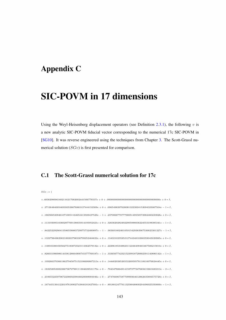
Appendix C
SIC-POVM in 17 dimensions
Using the Weyl-Heisenberg displacement operators (see Definition 2.3.1), the following v is
a new analytic SIC-POVM fiducial vector corresponding to the numerical 17c SIC-POVM in
[SG10]. It was reverse engineered using the techniques from Chapter 3. The Scott-Grassl nu-
merical solution (SGv) is first presented for comparison.
C.1 The Scott-Grassl numerical solution for 17c
SGv := (
+.48382980061662116217682602441506776537e + 0 + .00000000000000000000000000000000000000e + 0 ∗ I,
+ .27126484005469393538676883137444152309e + 0 + .69654983976200813223024153094325067504e− 1 ∗ I,
+ .18658653094610710051164653413508437529e− 1 + .23700687707779005149550572962460233826e + 0 ∗ I,
+ .11319309510366287709138835914195952421e + 0 + .32636202824922905988036224553198385341e− 1 ∗ I,
− .84225229290413586558883729975732400897e− 1− .90360180246105915429383967536823361227e− 1 ∗ I,
+ .13227984962902189203796538799252464632e + 0 + .13432103559521274434810260359045039985e + 0 ∗ I,
+ .14004538045056275183072523113362579132e + 0 + .22296185348823112246409465467506215810e + 0 ∗ I,
+ .82603198698614458128664900745377769187e− 1 + .33365677423215239918728902391140880142e− 1 ∗ I,
+ .10926637036618627945875152106606807213e + 0 + .14440203852655326959578110616076824445e + 0 ∗ I,
+ .18325895308228673672789111304629521170e + 0− .70434780649141597277247665615861683213e− 2 ∗ I,
+ .21065522597967223869239046620008904046e + 0− .27476696758770999364612862635894575720e + 0 ∗ I,
+ .16744513641220197618902743846181827091e + 0− .89188124779113258848800204496925350890e− 1 ∗ I,
143

SIC-POVM in 17 dimensions 144
+ .24359388765298324677017073863545845111e + 0− .98778919986922507345035476599550316894e− 1 ∗ I,
− .15216662789091992219769080826760384307e− 2 + .10096782395236138821142045805553955699e + 0 ∗ I,
+ .31930652975339555818323482188870297478e− 2− .35047984081599375367709829247485453467e + 0 ∗ I,
+ .12948876712345079950472823771660306613e + 0 + .22926607189219006777123769404536112165e− 2 ∗ I,
− .20814795522891847091328065519554133217e + 0− .66991642102649847248234875056855152662e− 1 ∗ I)T .
C.2 Analytic solution for 17c
Let a :=√
7, i :=√−1, r1 :=
√17, t := sin(π/17),
s := 3757 + 1411 ∗ a− 1479 ∗ r1− 561 ∗ a ∗ r1− 68 ∗ t− 119 ∗ a ∗ t− 2428 ∗ r1 ∗ t− 923 ∗ a ∗ r1 ∗ t− 25500 ∗ t2 − 9588 ∗ a ∗ t2 +
10572 ∗ r1 ∗ t2 + 4012 ∗ a ∗ r1 ∗ t2 + 20808 ∗ t3 + 8840 ∗ a ∗ t3 + 16744 ∗ r1 ∗ t3 + 6464 ∗ a ∗ r1 ∗ t3 + 45696 ∗ t4 + 17136 ∗ a ∗ t4 −
20640 ∗ r1 ∗ t4 − 7856 ∗ a ∗ r1 ∗ t4 − 68544 ∗ t5 − 28288 ∗ a ∗ t5 − 33600 ∗ r1 ∗ t5 − 13120 ∗ a ∗ r1 ∗ t5 − 26112 ∗ t6 − 9792 ∗ a ∗ t6 +
11904 ∗ r1 ∗ t6 + 4544 ∗ a ∗ r1 ∗ t6 + 47872 ∗ t7 + 19584 ∗ a ∗ t7 + 19200 ∗ r1 ∗ t7 + 7552 ∗ a ∗ r1 ∗ t7 ,
b1 := 8 ∗√s,
b2 := 17 ∗ ( 3√
117
(10 + 3 ∗ i ∗√21))−1 + 172/3
3√
10 + 3 ∗ i ∗√21 ≈ 32.338,
w := [w1, w2, w3, w4, w5, w6, w7, w8, w9, w10, w11, w12, w13, w14, w15, w16, w17]T ,
v := w/ ||w||,
w1 := (1/436968 ∗ (5 ∗ a− 7) ∗ r1 + 1/436968 ∗ (13 ∗ a− 7)) ∗ b22 + (1/436968 ∗ (−71 ∗ a+ 259) ∗ r1 + 1/25704 ∗ (a+ 35)) ∗ b2 +
1/6426 ∗ (−53 ∗ a + 154) ∗ r1 + 1/378 ∗ (−17 ∗ a + 56),
w2 := ((((1/40251494791862835497604 ∗ (2390569005052745227 ∗ a − 6274715912124044301) ∗ i + 1/40251494791862835497604 ∗
(3140356510548608341∗a−8182805022494548537))∗r1+(1/40251494791862835497604∗(−25449293721311900227∗a+67878053605415835929)∗
i + 1/40251494791862835497604 ∗ (6095408318187223927 ∗ a − 14412281383608493903))) ∗ t7 + ((1/40251494791862835497604 ∗
(−5174616347507284263∗a+13722555477385500193)∗i+1/958368923615781797562∗(−2675388956621709∗a+5224174754906894))∗
r1+(1/20125747395931417748802∗(5592126147766100912∗a−14733642377662638143)∗i+1/5750213541694690785372∗(747704864310938143∗
a − 2040229956970773211))) ∗ t6 + ((1/161005979167451341990416 ∗ (−20589722611921746273 ∗ a + 54214481831474310199) ∗
i + 1/23000854166778763141488 ∗ (−2838305488391356931 ∗ a + 7417129235112744479)) ∗ r1 + (1/161005979167451341990416 ∗
(174987584839772236753∗a−466717831483708329791)∗i+1/161005979167451341990416∗(−31815945074232327647∗a+72554432115740794835)))∗
t5 + ((1/161005979167451341990416 ∗ (36423739573932214129 ∗ a − 96541942747232286689) ∗ i + 1/80502989583725670995208 ∗
(743216710732381766∗a−1719758914826751183))∗r1+(1/161005979167451341990416∗(−89776208956530924375∗a+236936845853989116143)∗
i+1/80502989583725670995208∗ (−17512882541262701580∗a+47823297015739991669)))∗ t4 +((1/644023916669805367961664∗
(56961560213583650925∗a−150519805180552211341)∗i+1/214674638889935122653888∗(10923345520875531077∗a−28833442994936151971))∗
r1+ (1/644023916669805367961664 ∗ (−345334687402183256611 ∗a+920978128808018754011) ∗ i+1/92003416667115052565952 ∗
(3653360795098655089 ∗ a − 6655761637970056023))) ∗ t3 + ((1/644023916669805367961664 ∗ (−75369662159440958095 ∗ a +

SIC-POVM in 17 dimensions 145
199610900788086459658)∗i+1/644023916669805367961664∗(−6079477439371846044∗a+15478294797897129331))∗r1+(1/644023916669805367961664∗
(226268897934111322586∗a−598232236695523057425)∗i+1/214674638889935122653888∗(21337810960597229949∗a−58107419695479315896)))∗
t2+((1/2576095666679221471846656∗(−45995906681322685837∗a+121796693533416987645)∗i+1/368013666668460210263808∗
(−1707854581829808547 ∗ a + 4660701707985975529)) ∗ r1 + (1/2576095666679221471846656 ∗ (185506319642325530073 ∗ a −
495173417653824586957)∗i+1/2576095666679221471846656∗(17355961955320234181∗a−54779880690635077915)))∗t+((1/5152191333358442943693312∗
(87844634076506120143∗a−232405072641424794293)∗i+1/736027333336920420527616∗(1816116539143925149∗a−4828133107193657553))∗
r1+(1/5152191333358442943693312∗(−332282972236860299243∗a+879613385494378101189)∗i+1/5152191333358442943693312∗
(−57638587923446442463 ∗ a+ 155627165414523147583)))) ∗ b1 + (((1/54621 ∗ (64 ∗ a− 196) ∗ i+ 1/54621 ∗ (−24 ∗ a− 28)) ∗ r1 +
(1/7803 ∗ (28 ∗ a− 56) ∗ i+1/7803 ∗ (−12 ∗ a− 8))) ∗ t7 + ((1/18207 ∗ (a− 7) ∗ i+1/54621 ∗ (53 ∗ a− 133)) ∗ r1+ (1/18207 ∗ (−a+
7) ∗ i+ 1/18207 ∗ (−39 ∗ a+ 119))) ∗ t6 + ((1/54621 ∗ (−101 ∗ a+ 315) ∗ i+ 1/18207 ∗ (12 ∗ a+ 14)) ∗ r1 + (1/54621 ∗ (−255 ∗ a+
455) ∗ i+ 1/18207 ∗ (40 ∗ a+ 28))) ∗ t5 + ((1/31212 ∗ (−3 ∗ a+ 19) ∗ i+ 1/218484 ∗ (−373 ∗ a+ 959)) ∗ r1 + (1/218484 ∗ (33 ∗ a−
217) ∗ i+1/218484 ∗ (961 ∗ a− 2891))) ∗ t4 +((1/109242 ∗ (81 ∗ a− 266) ∗ i+1/72828 ∗ (−17 ∗ a− 21)) ∗ r1+ (1/218484 ∗ (191 ∗ a−
63) ∗ i+1/12138 ∗ (−8 ∗a− 7))) ∗ t3 +((1/62424 ∗ (3 ∗a− 17) ∗ i+1/109242 ∗ (97 ∗a− 259)) ∗ r1+ (1/436968 ∗ (−57 ∗a+329) ∗ i+
1/218484∗ (−620∗a+1827)))∗ t2 +((1/1747872∗ (−117∗a+427)∗ i+1/249696∗ (3∗a+5))∗ r1+(1/1747872∗ (359∗a− 1421)∗
i+1/1747872∗ (−3∗a+119)))∗ t+((1/582624∗ (−4∗a+21)∗ i+1/1747872∗ (−230∗a+651))∗ r1+(1/102816∗ (3∗a−14)∗ i+
1/1747872 ∗ (919 ∗ a− 2646))))) ∗ b22 +((((1/40251494791862835497604 ∗ (−16419990613303051759 ∗ a+43309923507881279823) ∗
i + 1/40251494791862835497604 ∗ (−39036517189970381107 ∗ a + 107266424458446531313)) ∗ r1 + (1/2367734987756637382212 ∗
(247925677780431515∗a+85322904020035913)∗i+1/2367734987756637382212∗(5794393102262351899∗a−14844217839616884397)))∗
t7+((1/40251494791862835497604∗(7949743185508015389∗a−23346951138992052943)∗i+1/958368923615781797562∗(625838116311685329∗
a−1692592185169597297))∗r1+(1/1183867493878318691106∗(−1742075389857139495∗a+4893185444080982629)∗i+1/338247855393805340316∗
(−1223658786509308601 ∗ a + 3295886034896043137))) ∗ t6 + ((1/161005979167451341990416 ∗ (106294528063042195245 ∗ a −
279283396607103442813)∗i+1/23000854166778763141488∗(39225985944970408445∗a−107371247903725435271))∗r1+(1/9470939951026549528848∗
(−3697573137526200041∗a+4748672926603082617)∗i+1/9470939951026549528848∗(−45161689581211108883∗a+117129455085330799769)))∗
t5 + ((1/161005979167451341990416 ∗ (−66163554460053438733 ∗ a+192973493098683209171) ∗ i+1/80502989583725670995208 ∗
(−100296218797333336544 ∗ a + 271477067867290334049)) ∗ r1 + (1/9470939951026549528848 ∗ (25438094502765231765 ∗ a −
71383200556498479103)∗i+1/4735469975513274764424∗(30775933732129850853∗a−82872019162047834544)))∗t4+((1/644023916669805367961664∗
(−188293644903635050455 ∗ a + 487763071828579352617) ∗ i + 1/214674638889935122653888 ∗ (−188680951967755323301 ∗ a +
512793730407050827189))∗r1+(1/37883759804106198115392∗(15617168515589965829∗a−32342874558948948211)∗i+1/5411965686300885445056∗
(15761886385783396771 ∗ a − 41580615253727777523))) ∗ t3 + ((1/644023916669805367961664 ∗ (174691091866334503147 ∗ a −
502305141991660366744) ∗ i + 1/644023916669805367961664 ∗ (471964389789235576284 ∗ a − 1278160932403064269945)) ∗ r1 +
(1/37883759804106198115392∗(−55396560404244926596∗a+155740791494158130967)∗i+1/12627919934702066038464∗(−44117991672526563397∗
a + 118731738122500538448))) ∗ t2 + ((1/2576095666679221471846656 ∗ (84721322039805509971 ∗ a − 209636787681486392745) ∗
i+ 1/368013666668460210263808 ∗ (46496810401572529915 ∗ a− 125045756777728369315)) ∗ r1 + (1/151535039216424792461568 ∗
(−16106802193492220211∗a+39691207455329431757)∗i+1/151535039216424792461568∗(−79121879086010585305∗a+212497605428668169477)))∗
SIC-POVM in 17 dimensions 146
t+((1/5152191333358442943693312∗(−270937412514173749249∗a+763197369683562255785)∗i+1/736027333336920420527616∗
(−92560898387575866853 ∗ a + 249917962165261701051)) ∗ r1 + (1/303070078432849584923136 ∗ (69116402936180655637 ∗ a −
195536499863446746753) ∗ i + 1/303070078432849584923136 ∗ (163246324692661647239 ∗ a − 439827851689933386365)))) ∗ b1 +
(((1/54621∗(536∗a−1988)∗i+1/3213∗(24∗a−28))∗r1+(1/459∗(4∗a−32)∗i+1/459∗(12∗a−8)))∗t7+((1/1071∗(−a−7)∗i+
1/54621∗(−635∗a+1645))∗r1+(1/1071∗(a+7)∗i+1/1071∗(25∗a−63)))∗t6+((1/54621∗(−817∗a+2961)∗i+1/1071∗(−12∗
a+14))∗r1+(1/3213∗ (−39∗a+329)∗ i+1/1071∗ (−40∗a+28)))∗ t5 +((1/1836∗ (3∗a+19)∗ i+1/218484∗ (4255∗a−11123))∗
r1+(1/12852∗ (−33∗a−217)∗ i+1/12852∗ (−611∗a+1519)))∗ t4 +((1/109242∗ (639∗a−2128)∗ i+1/4284∗ (17∗a−21))∗r1+
(1/12852∗ (47∗a−441)∗ i+1/714∗ (8∗a−7)))∗ t3 +((1/3672∗ (−3∗a−17)∗ i+1/109242∗ (−1033∗a+2737))∗ r1+(1/25704∗
(57∗a+329)∗i+1/12852∗(382∗a−945)))∗t2+((1/1747872∗(−825∗a+1673)∗i+1/14688∗(−3∗a+5))∗r1+(1/102816∗(−37∗
a+217)∗ i+1/102816∗ (3∗a+119)))∗ t+((1/34272∗ (4∗a+21)∗ i+1/1747872∗ (2300∗a−5985))∗r1+(1/6048∗ (−3∗a−14)∗
i+1/102816∗ (−527∗a+1344)))))∗ b2+(((1/1183867493878318691106∗ (−23715906842776845527∗a+60404882084096784591)∗
i + 1/1183867493878318691106 ∗ (40846349726057211121 ∗ a − 107683110140227104511)) ∗ r1 + (1/1183867493878318691106 ∗
(380961147325584773939∗a−1017943404822176612227)∗i+1/1183867493878318691106∗(−314519136276657805397∗a+815896341453286449251)))∗
t7+((1/2367734987756637382212∗(139783450988127571095∗a−373204046344411604917)∗i+1/37583095043756148924∗(−2029427772856309473∗
a + 5351750079406275181)) ∗ r1 + (1/2367734987756637382212 ∗ (−204378311956405861819 ∗ a + 555865666042652701981) ∗ i +
1/338247855393805340316∗(56904771520087183961∗a−146995915227768170177)))∗t6+((1/4735469975513274764424∗(231056182372870097829∗
a − 597258702027556072553) ∗ i + 1/676495710787610680632 ∗ (−46687017854385570497 ∗ a + 122862457095634699091)) ∗ r1 +
(1/4735469975513274764424∗(−2600312288825601668561∗a+6945750104739953681881)∗i+1/4735469975513274764424∗(2213458645871918524015∗
a− 5739997936689372914929))) ∗ t5 + ((1/4735469975513274764424 ∗ (−477360769144174126094 ∗ a+1275341193495890379271) ∗
i + 1/4735469975513274764424 ∗ (463200162530399946133 ∗ a − 1219765485505374252774)) ∗ r1 + (1/4735469975513274764424 ∗
(875492815353328163046 ∗ a − 2375202003955427837533) ∗ i + 1/4735469975513274764424 ∗ (−1509330694824794630559 ∗ a +
3905921077639150595242))) ∗ t4 + ((1/9470939951026549528848 ∗ (−362119114824784684887 ∗ a + 948416374354187530750) ∗ i +
1/350775553741724056624∗(15235578367368564826∗a−39958181802015058449))∗r1+(1/9470939951026549528848∗(2505743905389090560437∗
a− 6687452632290915804410) ∗ i+1/1352991421575221361264 ∗ (−328054953051039747994 ∗ a+851197867504469771463))) ∗ t3 +
((1/37883759804106198115392 ∗ (1882188777343628158297 ∗ a − 5035297370284068087571) ∗ i + 1/37883759804106198115392 ∗
(−2001761276190420696717 ∗ a + 5255867865685862768525)) ∗ r1 + (1/37883759804106198115392 ∗ (−4730302835912833840925 ∗
a + 12786775835367089541279) ∗ i + 1/12627919934702066038464 ∗ (2365586526072308533523 ∗ a− 6145483551760276725827))) ∗
t2 + ((1/75767519608212396230784 ∗ (642172092388719221339 ∗ a− 1695350809876267052649) ∗ i+ 1/10823931372601770890112 ∗
(−86558820246891040453 ∗ a+ 226014644041152485089)) ∗ r1 + (1/75767519608212396230784 ∗ (−2542413034597571926479 ∗ a+
6783359291648198823389) ∗ i + 1/75767519608212396230784 ∗ (2718375847961076114167 ∗ a − 7069026587817444828067))) ∗ t +
((1/151535039216424792461568 ∗ (−1023656328299865078941 ∗ a+ 2744127261911055658939) ∗ i+ 1/21647862745203541780224 ∗
(175853581999552236703 ∗ a − 460070660528379149667)) ∗ r1 + (1/151535039216424792461568 ∗ (3651615790241769475009 ∗ a −
9834066514780480195587)∗i+1/151535039216424792461568∗(−4900984841710613514361∗a+12790146915011278082473))))∗b1+
((1/3213∗(−2596∗a+7084)∗i+1/3213∗(1908∗a−2324))∗r1+(1/27∗(−68∗a+124)∗i+1/27∗(36∗a−20)))∗t7+((1/1071∗(−174∗
SIC-POVM in 17 dimensions 147
a+658)∗i+1/3213∗(−1382∗a+3766))∗r1+(1/63∗(30∗a−98)∗i+1/63∗(50∗a−98)))∗t6+((1/3213∗(4064∗a−11340)∗i+1/1071∗
(−996∗a+1288))∗r1+(1/189∗(636∗a−1036)∗i+1/63∗(−108∗a+28)))∗t5+((1/918∗(279∗a−1007)∗i+1/6426∗(4913∗a−13363))∗
r1+(1/378∗(−369∗a+1225)∗i+1/378∗(−625∗a+1379)))∗t4+((1/12852∗(−6453∗a+19033)∗i+1/476∗(177∗a−259))∗r1+(1/756∗
(−571∗a+315)∗i+1/84∗(25∗a+49)))∗t3+((1/1836∗(−315∗a+1081)∗i+1/12852∗(−5147∗a+13979))∗r1+(1/756∗(477∗a−1589)∗
i+1/756∗(841∗a−2079)))∗t2+((1/25704∗(1194∗a−3997)∗i+1/3672∗(−117∗a+232))∗r1+(1/1512∗(−148∗a+679)∗i+1/1512∗
(117∗a−406)))∗t+(1/672∗(19∗a−63)∗i+1/102816∗(5867∗a−15981))∗r1+1/6048∗(−711∗a+2303)∗i+1/6048∗(−1355∗a+3633),
w3 := ((((1/40251494791862835497604 ∗ (2032708796993678841 ∗ a − 5439126824113408727) ∗ i + 1/40251494791862835497604 ∗
(1962096605216186931∗a−5416407653427664859))∗r1+(1/4472388310206981721956∗(329802553874771227∗a−912196215169921297)∗
i + 1/40251494791862835497604 ∗ (5828224036634168909 ∗ a − 16428556309583548809))) ∗ t7 + ((1/40251494791862835497604 ∗
(−48258912780223168∗a+137033677318130397)∗i+1/40251494791862835497604∗(−44011331449658765∗a+279378079766194766))∗
r1 + (1/40251494791862835497604 ∗ (6103412458394036241 ∗ a − 16256670600286958450) ∗ i + 1/40251494791862835497604 ∗
(2685089790805721786 ∗ a − 7084358370056268217))) ∗ t6 + ((1/161005979167451341990416 ∗ (−12913423133103850087 ∗ a +
34651611668094699523)∗i+1/23000854166778763141488∗(−1725202006137560647∗a+4761802339652663689))∗r1+(1/9470939951026549528848∗
(−777301094064947733∗a+2211627514221275773)∗i+1/161005979167451341990416∗(−34635478457125801123∗a+97560711179423862657)))∗
t5+((1/80502989583725670995208∗(685341135520214680∗a−1889814418869966001)∗i+1/53668659722483780663472∗(230918402050263551∗
a − 974635666182973235)) ∗ r1 + (1/80502989583725670995208 ∗ (−19992063931713224061 ∗ a + 53167005662377091023) ∗ i +
1/161005979167451341990416 ∗ (−17800670278932845599 ∗ a + 47469547276876861157))) ∗ t4 + ((1/644023916669805367961664 ∗
(21579291599702136803∗a−58070474435484769909)∗i+1/644023916669805367961664∗(18287987611966595037∗a−50435052587635048445))∗
r1 + (1/644023916669805367961664 ∗ (−3602593737165311033 ∗ a + 4523257084745413035) ∗ i + 1/644023916669805367961664 ∗
(46141891588337301261 ∗ a − 130069768643681386961))) ∗ t3 + ((1/644023916669805367961664 ∗ (−6660777524916047175 ∗ a +
18111043082487485396)∗i+1/644023916669805367961664∗(−3143023102013247309∗a+10367588372094423274))∗r1+(1/92003416667115052565952∗
(10424619878541837916∗a−27696300630832638309)∗i+1/644023916669805367961664∗(32283908567177680778∗a−87925191244381131319)))∗
t2 +((1/2576095666679221471846656∗ (−8196117314629773503∗a+21936101845455721903)∗ i+1/2576095666679221471846656∗
(−4729086370597566331∗a+12811500666713077329))∗r1+(1/858698555559740490615552∗(10365384534228766985∗a−26999856410250381525)∗
i+1/2576095666679221471846656∗ (−4877842228008506301∗a+13129439189228456899)))∗ t+((1/5152191333358442943693312∗
(13419961957682462559∗a−36030095515019888009)∗i+1/736027333336920420527616∗(943509530710860337∗a−2753827852345367769))∗
r1 + (1/736027333336920420527616 ∗ (−9962928804965238465 ∗ a+ 26553379369306596007) ∗ i+ 1/1717397111119480981231104 ∗
(−10157647553349389273 ∗ a+ 29034274351818420769)))) ∗ b1 + (((1/54621 ∗ (−76 ∗ a+ 140) ∗ i+ 1/54621 ∗ (12 ∗ a− 28)) ∗ r1 +
(1/54621∗(−152∗a+392)∗i+1/54621∗(48∗a+56)))∗t7+((1/54621∗(−3∗a−7)∗i+1/54621∗(−25∗a+77))∗r1+(1/18207∗(a−
35)∗ i+1/54621∗ (153∗a−413)))∗ t6 +((1/54621∗ (122∗a−217)∗ i+1/54621∗ (−18∗a+49))∗r1+(1/54621∗ (188∗a−539)∗ i+
1/54621∗(−72∗a−133)))∗t5+((1/31212∗(3∗a+5)∗i+1/218484∗(193∗a−595))∗r1+(1/218484∗(−33∗a+665)∗i+1/31212∗
(−155∗a+433)))∗ t4 +((1/218484∗ (−208∗a+343)∗ i+1/218484∗ (27∗a−98))∗ r1+(1/72828∗ (−43∗a+210)∗ i+1/218484∗
(108∗a+385)))∗ t3 +((1/62424∗ (−3∗a−1)∗ i+1/218484∗ (−116∗a+357))∗r1+(1/145656∗ (19∗a−189)∗ i+1/109242∗ (293∗
a−854)))∗t2+((1/1747872∗(159∗a−203)∗i+1/582624∗(−5∗a+35))∗r1+(1/1747872∗(−213∗a−91)∗i+1/249696∗(−9∗a−
SIC-POVM in 17 dimensions 148
85)))∗t+((1/582624∗(4∗a−7)∗i+1/582624∗(55∗a−168))∗r1+(1/102816∗(−3∗a+14)∗ i+1/1747872∗(−730∗a+2233)))))∗
b22 +((((1/40251494791862835497604∗ (−26668614955502333757∗a+67460687263396561505)∗ i+1/40251494791862835497604∗
(9781467804429808467∗a−29908583768528474401))∗r1+(1/789244995918879127404∗(821126783952577199∗a−2273240715981201575)∗
i + 1/2367734987756637382212 ∗ (4083789220144608977 ∗ a − 11387113081875103503))) ∗ t7 + ((1/40251494791862835497604 ∗
(20977637993648674015∗a−53576953316674895814)∗i+1/40251494791862835497604∗(12947894868019905110∗a−35531332592569543415))∗
r1+(1/2367734987756637382212∗(−5796923552222173722∗a+15860277085904774131)∗i+1/2367734987756637382212∗(−832911771316622155∗
a + 1924553985850228544))) ∗ t6 + ((1/161005979167451341990416 ∗ (184297711718893317925 ∗ a − 468243968023893533311) ∗
i + 1/23000854166778763141488 ∗ (−7726909798866667313 ∗ a + 24212808102084260609)) ∗ r1 + (1/9470939951026549528848 ∗
(−20672135897191806465∗a+56139453957315145487)∗i+1/9470939951026549528848∗(−25133226571996146421∗a+70035603053968116873)))∗
t5 + ((1/10062873697965708874401 ∗ (−9932815368237247334 ∗ a + 25693163503862509571) ∗ i + 1/53668659722483780663472 ∗
(−29598919119311698257∗a+80334491546648266921))∗r1+(1/4735469975513274764424∗(21485603120563117365∗a−58303269454142468714)∗
i + 1/9470939951026549528848 ∗ (7793201801646646169 ∗ a − 19472296155150301855))) ∗ t4 + ((1/644023916669805367961664 ∗
(−370771590495714302549∗a+950103652483970186461)∗i+1/644023916669805367961664∗(52159185916895900943∗a−181228459145480740441))∗
r1 + (1/37883759804106198115392 ∗ (56147535445649437879 ∗ a − 149077628707238221011) ∗ i + 1/37883759804106198115392 ∗
(38915677456985855847 ∗ a − 107243491022275371869))) ∗ t3 + ((1/644023916669805367961664 ∗ (368687628088719543258 ∗ a −
969062928835078184135) ∗ i + 1/644023916669805367961664 ∗ (174588099820872102360 ∗ a − 468686774806364875789)) ∗ r1 +
(1/5411965686300885445056∗(−13689330232157816399∗a+36704317980666791478)∗i+1/37883759804106198115392∗(−23743038330148504837∗
a + 62029181537750565992))) ∗ t2 + ((1/2576095666679221471846656 ∗ (212541558500496948827 ∗ a − 551162345517534750013) ∗
i+ 1/2576095666679221471846656 ∗ (25292147183569401133 ∗ a− 50005068649491275481)) ∗ r1 + (1/50511679738808264153856 ∗
(−15184766560512792353∗a+39680132184911937915)∗i+1/151535039216424792461568∗(−11688164992237182009∗a+31319753064529686841)))∗
t+((1/5152191333358442943693312∗(−495134177947760303481∗a+1313258081514478353065)∗i+1/736027333336920420527616∗
(−26549512686497407405∗a+70445865326367419955))∗r1+(1/43295725490407083560448∗(17317654394062472379∗a−46041866837208406835)∗
i+1/101023359477616528307712∗ (13285809660310242585∗a− 35291833820492824463))))∗ b1+(((1/54621∗ (340∗a− 1484)∗ i+
1/3213∗ (−12∗a−28))∗r1+(1/3213∗ (40∗a+56)∗ i+1/3213∗ (−48∗a+56)))∗ t7+((1/3213∗ (3∗a−7)∗ i+1/54621∗ (−65∗a−
77))∗ r1+(1/1071∗ (−a−35)∗ i+1/3213∗ (−111∗a+301)))∗ t6 +((1/54621∗ (−548∗a+2611)∗ i+1/3213∗ (18∗a+49))∗ r1+
(1/3213∗(−34∗a−203)∗i+1/3213∗(72∗a−133)))∗t5+((1/1836∗(−3∗a+5)∗i+1/218484∗(317∗a+1015))∗r1+(1/12852∗(33∗
a+665)∗i+1/1836∗(97∗a−269)))∗t4+((1/218484∗(862∗a−5089)∗i+1/12852∗(−27∗a−98))∗r1+(1/4284∗(−13∗a+252)∗
i+1/12852∗(−108∗a+385)))∗t3+((1/3672∗(3∗a−1)∗ i+1/218484∗(26∗a−1071))∗r1+(1/8568∗(−19∗a−189)∗ i+1/6426∗
(−139∗a+406)))∗t2+((1/1747872∗(−393∗a+4907)∗i+1/34272∗(5∗a+35))∗r1+(1/102816∗(171∗a−1309)∗i+1/14688∗(9∗
a−85)))∗ t+((1/34272∗ (−4∗a−7)∗ i+1/582624∗ (−123∗a+742))∗r1+(1/6048∗ (3∗a+14)∗ i+1/102816∗ (212∗a−707)))))∗
b2 + (((1/1183867493878318691106 ∗ (−33043886295476661849 ∗ a + 88425032761705684261) ∗ i + 1/1183867493878318691106 ∗
(−73216733661406961457 ∗ a + 194184122150006571163)) ∗ r1 + (1/394622497959439563702 ∗ (−64651790880738418829 ∗ a +
174793685139920192633) ∗ i + 1/1183867493878318691106 ∗ (−292340021649041493583 ∗ a + 782195292827846440725))) ∗ t7 +
((1/2367734987756637382212∗(−49526843796303232067∗a+130110902573293038201)∗i+1/2367734987756637382212∗(−44421956170224168133∗
SIC-POVM in 17 dimensions 149
a + 113504353829151151993)) ∗ r1 + (1/2367734987756637382212 ∗ (−26606413841192490129 ∗ a + 80206998292782108251) ∗ i +
1/2367734987756637382212 ∗ (−143340865101000888695 ∗ a + 378431337229287886411))) ∗ t6 + ((1/4735469975513274764424 ∗
(186674649688499237687∗a−500937783543777401255)∗i+1/676495710787610680632∗(62552684782439812265∗a−165700975223659928399))∗
r1 + (1/4735469975513274764424 ∗ (1195801525750815543177 ∗ a − 3240358921401062075293) ∗ i + 1/4735469975513274764424 ∗
(1753120699310344226789 ∗ a − 4689704649663121217199))) ∗ t5 + ((1/2367734987756637382212 ∗ (83170139402601768403 ∗ a −
217160091690094295092)∗i+1/789244995918879127404∗(22550044224142729709∗a−57486085638833442654))∗r1+(1/1183867493878318691106∗
(−2819959402076936064∗a−252965450991318751)∗i+1/2367734987756637382212∗(208952839769955395077∗a−556100593050648220631)))∗
t4 + ((1/9470939951026549528848 ∗ (−104044872396228041378 ∗ a + 280853513326931848429) ∗ i + 1/9470939951026549528848 ∗
(−301677897249956231577 ∗ a + 796869297535656562616)) ∗ r1 + (1/9470939951026549528848 ∗ (−900747771500318789596 ∗ a +
2451480211158520044153) ∗ i+ 1/9470939951026549528848 ∗ (−1233237656076659115657 ∗ a+ 3301977494496498723710))) ∗ t3 +
((1/37883759804106198115392 ∗ (−616903704204500614299 ∗ a + 1596567560403550560469) ∗ i + 1/37883759804106198115392 ∗
(−394605773031132993081 ∗ a + 995449846265571941321)) ∗ r1 + (1/5411965686300885445056 ∗ (108926902080010549733 ∗ a −
271848734784861578775) ∗ i+ 1/37883759804106198115392 ∗ (−1018312081758447616475 ∗ a+ 2768689581905098041463))) ∗ t2 +
((1/75767519608212396230784∗(−38972295710221524281∗a+103940361014413569415)∗i+1/75767519608212396230784∗(84442712140089868997∗
a − 215890830785472372537)) ∗ r1 + (1/8418613289801377358976 ∗ (51479963857020237121 ∗ a − 140871783894345144151) ∗ i +
1/75767519608212396230784 ∗ (453786801244929492435 ∗ a − 1215711808645331076023))) ∗ t + ((1/151535039216424792461568 ∗
(306010806009230971533∗a−788216557847512798445)∗i+1/21647862745203541780224∗(10839671021518063243∗a−25638599209177622169))∗
r1 + (1/21647862745203541780224 ∗ (−141456680858966762847 ∗ a+ 363191954197234799275) ∗ i+ 1/50511679738808264153856 ∗
(−8341734540848507287 ∗ a− 5447154245536553711)))) ∗ b1 + ((1/3213 ∗ (3508 ∗ a− 9716) ∗ i+ 1/3213 ∗ (−828 ∗ a+ 2212)) ∗ r1 +
(1/189∗ (220∗a−700)∗ i+1/189∗ (−180∗a+140)))∗ t7 +((1/3213∗ (522∗a−1022)∗ i+1/3213∗ (1102∗a−2870))∗r1+(1/63∗
(−30∗a+154)∗i+1/189∗(−222∗a+742)))∗t6+((1/3213∗(−5828∗a+15946)∗i+1/3213∗(1242∗a−3556))∗r1+(1/189∗(−208∗
a+742)∗i+1/189∗(270∗a−112)))∗t5+((1/918∗(−279∗a+599)∗i+1/6426∗(−4121∗a+11291))∗r1+(1/378∗(369∗a−1673)∗
i+1/54∗ (119∗a−397)))∗ t4 +((1/12852∗ (10747∗a−28777)∗ i+1/12852∗ (−1863∗a+6167))∗r1+(1/252∗ (−61∗a+63)∗ i+
1/756∗ (−405∗a−203)))∗ t3 +((1/1836∗ (315∗a−775)∗ i+1/12852∗ (4637∗a−13503))∗r1+(1/84∗ (−53∗a+203)∗ i+1/756∗
(−983∗a+3227)))∗t2+((1/25704∗(−2517∗a+6503)∗ i+1/8568∗(81∗a−413))∗r1+(1/1512∗(285∗a−721)∗ i+1/216∗(9∗a+
29)))∗ t+(1/2016∗ (−57∗a+161)∗ i+1/34272∗ (−2045∗a+6335))∗r1+1/6048∗ (711∗a−2303)∗ i+1/6048∗ (1355∗a−4361),
w4 := ((((1/40251494791862835497604 ∗ (8380315164608538279 ∗ a− 22366597102958454563) ∗ i + 1/40251494791862835497604 ∗
(5435985856599437933∗a−14513734320895808355))∗r1+(1/5750213541694690785372∗(4906306763523151207∗a−13026151848980975083)∗
i + 1/40251494791862835497604 ∗ (21985414533050555375 ∗ a − 57719166067729788601))) ∗ t7 + ((1/11500427083389381570744 ∗
(783039152120492155∗a−2071637405661193221)∗i+1/4735469975513274764424∗(174695717202074069∗a−463993767105792301))∗
r1 + (1/80502989583725670995208 ∗ (19932584642733319981 ∗ a − 52556809040762058151) ∗ i + 1/80502989583725670995208 ∗
(8723863364095444697 ∗ a − 23022845586309193205))) ∗ t6 + ((1/161005979167451341990416 ∗ (−50157088747399926179 ∗ a +
133977617936173260431) ∗ i + 1/161005979167451341990416 ∗ (−32821220569229978407 ∗ a + 87752126364773025337)) ∗ r1 +
(1/23000854166778763141488∗(−28952545846974243387∗a+76834510043688670651)∗i+1/161005979167451341990416∗(−130872699284884695781∗

SIC-POVM in 17 dimensions 150
a + 342139666213163046655))) ∗ t5 + ((1/161005979167451341990416 ∗ (−16253244734770420611 ∗ a + 43024471525909459726) ∗
i+ 1/161005979167451341990416 ∗ (−9149577290151086125 ∗ a+ 24308938383571033864)) ∗ r1 + (1/161005979167451341990416 ∗
(−58167387594748854593 ∗ a + 153306351232951930916) ∗ i + 1/161005979167451341990416 ∗ (−24015444435941802859 ∗ a +
63430955627994598966))) ∗ t4 + ((1/214674638889935122653888 ∗ (23405051481658292591 ∗ a − 62660324955092784409) ∗ i +
1/644023916669805367961664 ∗ (46993467568913142215 ∗ a − 126188066235378311199)) ∗ r1 + (1/214674638889935122653888 ∗
(90464671722043415319∗a−239654461617409622665)∗i+1/644023916669805367961664∗(180309454923258465615∗a−465416234001250350343)))∗
t3 + ((1/644023916669805367961664 ∗ (22482844411475276875 ∗ a − 59606586748969961225) ∗ i + 1/80502989583725670995208 ∗
(1726693643224866822∗a−4599398888345870063))∗r1+(1/322011958334902683980832∗(37168778387633002693∗a−97785633823987027051)∗
i+1/644023916669805367961664∗ (24970365596935869605∗a−66273499047346451049)))∗ t2 +((1/1288047833339610735923328∗
(−6229419319272303827∗a+16869392026923726206)∗i+1/1288047833339610735923328∗(−4843829085385891142∗a+13435263380913215709))∗
r1+(1/1288047833339610735923328∗ (−15106337790916477241∗a+38920513679675258554)∗ i+1/1288047833339610735923328∗
(−14936337418450473570 ∗ a + 35300904236470902911))) ∗ t + ((1/5152191333358442943693312 ∗ (−7774038834413195759 ∗ a +
20872760767369769965)∗i+1/5152191333358442943693312∗(−6341203240114484233∗a+17062630561299896685))∗r1+(1/5152191333358442943693312∗
(−4447386884655783205∗a+10718929451814444259)∗i+1/5152191333358442943693312∗(14561349558998591121∗a−38446456426898195473))))∗
b1 + ((1/54621 ∗ (−4 ∗ a+ 28) ∗ i ∗ r1 + (1/54621 ∗ (248 ∗ a− 504) ∗ i+ 1/54621 ∗ (−12 ∗ a+ 140))) ∗ t7 + ((1/18207 ∗ (a+ 7) ∗ i+
1/18207 ∗ (−3 ∗ a− 7)) ∗ r1 + (1/18207 ∗ (−a− 7) ∗ i+ 1/7803 ∗ (−a+ 19))) ∗ t6 + ((1/109242 ∗ (15 ∗ a− 91) ∗ i+ 1/109242 ∗ (3 ∗
a+ 7)) ∗ r1 + (1/109242 ∗ (−891 ∗ a+ 1855) ∗ i+ 1/36414 ∗ (19 ∗ a− 161))) ∗ t5 + ((1/10404 ∗ (−a− 7) ∗ i+ 1/218484 ∗ (69 ∗ a+
133)) ∗ r1+ (1/10404 ∗ (a+11) ∗ i+1/218484 ∗ (−69 ∗ a− 721))) ∗ t4 +((1/31212 ∗ (−4 ∗ a+15) ∗ i+1/72828 ∗ (−2 ∗ a− 7)) ∗ r1+
(1/31212 ∗ (133 ∗ a− 286) ∗ i+ 1/218484 ∗ (−75 ∗ a+ 490))) ∗ t3 + ((1/62424 ∗ (3 ∗ a+ 22) ∗ i+ 1/436968 ∗ (−80 ∗ a− 119)) ∗ r1 +
(1/436968 ∗ (−27 ∗ a− 364) ∗ i+1/436968 ∗ (234 ∗ a+497))) ∗ t2 +((1/1747872 ∗ (81 ∗ a− 203) ∗ i+1/1747872 ∗ (3 ∗ a+49)) ∗ r1+
(1/1747872 ∗ (−1019 ∗ a+2205) ∗ i+1/1747872 ∗ (75 ∗ a− 595))) ∗ t+ ((1/166464 ∗ (−a− 9) ∗ i+1/3495744 ∗ (121 ∗ a+91)) ∗ r1+
(1/205632 ∗ (3 ∗ a+ 35) ∗ i+ 1/3495744 ∗ (−423 ∗ a− 413))))) ∗ b22 + ((((1/40251494791862835497604 ∗ (30807661735178699799 ∗
a − 85731372270206942461) ∗ i + 1/40251494791862835497604 ∗ (35284312758355798975 ∗ a − 87894591055764425583)) ∗ r1 +
(1/338247855393805340316∗(−968877002837125493∗a+2348320438354559255)∗i+1/2367734987756637382212∗(6519345082271921825∗
a − 16750854902062742881))) ∗ t7 + ((1/11500427083389381570744 ∗ (−3270596659169097211 ∗ a + 9471098440191305343) ∗ i +
1/80502989583725670995208∗(−7968011674679240179∗a+16051952586388246913))∗r1+(1/4735469975513274764424∗(7096635190702454995∗
a−16982064644454395899)∗i+1/4735469975513274764424∗(9671627506930106873∗a−25566976631056449407)))∗t6+((1/161005979167451341990416∗
(−227239968690754287355 ∗ a + 624127963118160353797) ∗ i + 1/161005979167451341990416 ∗ (−210740871587063762681 ∗ a +
523547515868163336389))∗r1+(1/1352991421575221361264∗(7302401383328770905∗a−18026837494017632267)∗i+1/9470939951026549528848∗
(−38708418830387061127 ∗ a + 100605952881110204143))) ∗ t5 + ((1/161005979167451341990416 ∗ (80599962787556169708 ∗ a −
229239072348646643899)∗i+1/161005979167451341990416∗(42736787776107830296∗a−95033772914290026607))∗r1+(1/9470939951026549528848∗
(−24047930777703114104∗a+58116626822317420553)∗i+1/9470939951026549528848∗(−33038394001035451720∗a+86948300155900133293)))∗
t4 +((1/214674638889935122653888 ∗ (167507768716757951719 ∗a− 450066740295488710219) ∗ i+1/644023916669805367961664 ∗
(296344274628820659217 ∗ a − 728784983587224027051)) ∗ r1 + (1/12627919934702066038464 ∗ (−38907941691794378621 ∗ a +
SIC-POVM in 17 dimensions 151
98715516439988749889)∗i+1/37883759804106198115392∗(52260289119018424893∗a−140121890951680541407)))∗t3+((1/322011958334902683980832∗
(−86448074755979524013 ∗ a + 237082738236626397010) ∗ i + 1/644023916669805367961664 ∗ (−142441985031666684531 ∗ a +
339538386265475188183))∗r1+(1/37883759804106198115392∗(47730457565061553523∗a−118347387593948704709)∗i+1/18941879902053099057696∗
(32220824260360816291 ∗ a− 84068803511147469462))) ∗ t2 + ((1/1288047833339610735923328 ∗ (−153897267029538411502 ∗ a+
402299785950350937985) ∗ i + 1/1288047833339610735923328 ∗ (−27009108636344698981 ∗ a + 61509914068433529006)) ∗ r1 +
(1/75767519608212396230784∗(37436179435380238558∗a−97750756674900337421)∗i+1/75767519608212396230784∗(−3606367432277986167∗
a+12224453181959684498))) ∗ t+ ((1/5152191333358442943693312 ∗ (219862431684114959165 ∗ a− 577782670317269627833) ∗ i+
1/5152191333358442943693312 ∗ (259660982292601655317 ∗ a − 652008134752865498895)) ∗ r1 + (1/303070078432849584923136 ∗
(−54974856042951657445 ∗ a + 141798107807861506309) ∗ i + 1/303070078432849584923136 ∗ (−68476717320754676433 ∗ a +
174799311240282076943)))) ∗ b1 + ((1/54621 ∗ (−212 ∗ a + 308) ∗ i ∗ r1 + (1/3213 ∗ (−136 ∗ a + 504) ∗ i + 1/3213 ∗ (12 ∗ a +
140)))∗ t7 +((1/1071∗ (−a+7)∗ i+1/18207∗ (233∗a−581))∗r1+(1/1071∗ (a−7)∗ i+1/459∗ (−13∗a+25)))∗ t6 +((1/109242∗
(711∗a−581)∗ i+1/6426∗ (−3∗a+7))∗ r1+(1/6426∗ (429∗a−1631)∗ i+1/2142∗ (−19∗a−161)))∗ t5 +((1/612∗ (a−7)∗ i+
1/218484∗(−5079∗a+12551))∗r1+(1/612∗(−a+11)∗i+1/12852∗(783∗a−1603)))∗t4+((1/31212∗(−86∗a−57)∗i+1/4284∗
(2 ∗ a− 7)) ∗ r1+ (1/1836 ∗ (−53 ∗ a+212) ∗ i+1/12852 ∗ (75 ∗ a+490))) ∗ t3 +((1/3672 ∗ (−3 ∗ a+22) ∗ i+1/436968 ∗ (5546 ∗ a−
13447))∗r1+(1/25704∗(27∗a−364)∗i+1/25704∗(−1032∗a+2261)))∗t2+((1/1747872∗(429∗a+1967)∗i+1/102816∗(−3∗a+
49))∗r1+(1/102816∗ (361∗a−1617)∗ i+1/102816∗ (−75∗a−595)))∗ t+((1/9792∗ (a−9)∗ i+1/3495744∗ (−6943∗a+16709))∗
r1+(1/12096∗ (−3∗a+35)∗ i+1/205632∗ (1473∗a−3395)))))∗b2+(((1/1183867493878318691106∗ (−224622182243001417069∗
a + 596235361853125562155) ∗ i + 1/1183867493878318691106 ∗ (−2214958461483411835 ∗ a + 8262259922987438235)) ∗ r1 +
(1/169123927696902670158∗(−93264090957705162461∗a+245424509679682429727)∗i+1/1183867493878318691106∗(−58010317928075194921∗
a + 141459703365608814389))) ∗ t7 + ((1/84561963848451335079 ∗ (−2649285923679505757 ∗ a + 7074882934392015510) ∗ i +
1/591933746939159345553∗(4367578852402827841∗a−11955617892549669842))∗r1+(1/591933746939159345553∗(−130481410306157773775∗
a + 346922125605080731013) ∗ i + 1/591933746939159345553 ∗ (−5317758823880746300 ∗ a + 16615213391546515270))) ∗ t6 +
((1/4735469975513274764424∗(1394281422508681217935∗a−3704052150377908169617)∗i+1/4735469975513274764424∗(2167294152811874693∗
a − 23557784327034005909)) ∗ r1 + (1/676495710787610680632 ∗ (524843285455817243691 ∗ a − 1378872687492592270541) ∗ i +
1/4735469975513274764424 ∗ (429171657445547588303 ∗ a − 1035473071915458942647))) ∗ t5 + ((1/4735469975513274764424 ∗
(203350727387663999061∗a−543491207610719333672)∗i+1/4735469975513274764424∗(−60562494426831547042∗a+167243485741599499267))∗
r1 + (1/4735469975513274764424 ∗ (1592327401325231046751 ∗ a − 4234546001462771519266) ∗ i + 1/4735469975513274764424 ∗
(101017917354956115020 ∗ a − 306245439844945968899))) ∗ t4 + ((1/3156979983675516509616 ∗ (−360885623522930466545 ∗ a +
960806446356755786907)∗i+1/9470939951026549528848∗(21930978233975155249∗a−37706418767960503659))∗r1+(1/3156979983675516509616∗
(−689753090541346842749 ∗ a + 1799705432382374021827) ∗ i + 1/9470939951026549528848 ∗ (−472262593834681393767 ∗ a +
1123471399801105672933))) ∗ t3 + ((1/37883759804106198115392 ∗ (−402437395822793134681 ∗ a + 1080179297595330407573) ∗
i+ 1/37883759804106198115392 ∗ (248708450605054413087 ∗ a− 694512984257071703297)) ∗ r1 + (1/37883759804106198115392 ∗
(−4790424598055087136995 ∗ a + 12739918114034615452067) ∗ i + 1/37883759804106198115392 ∗ (−629983276864865116895 ∗
a + 1847651209970949515685))) ∗ t2 + ((1/37883759804106198115392 ∗ (321848447737188643141 ∗ a − 863475058251496035352) ∗

SIC-POVM in 17 dimensions 152
i + 1/37883759804106198115392 ∗ (−29850111279244445516 ∗ a + 64263272018296691445)) ∗ r1 + (1/37883759804106198115392 ∗
(−241946302299403785893∗a+690813906598386552856)∗i+1/37883759804106198115392∗(322713315534878791044∗a−769760346935915308813)))∗
t+((1/151535039216424792461568∗ (−153465333892354632695∗a+402118264634914899379)∗ i+1/151535039216424792461568∗
(−164690730267401534659 ∗ a+ 460581418424528611077)) ∗ r1 + (1/151535039216424792461568 ∗ (1220927347313322590219 ∗ a−
3238730784999251749823) ∗ i+ 1/151535039216424792461568 ∗ (546850208593781953047 ∗ a− 1559888331136511808649)))) ∗ b1 +
((1/3213∗(388∗a−532)∗i+1/51∗(−4∗a+12))∗r1+(1/189∗(−580∗a+1764)∗i+1/189∗(108∗a−532)))∗t7+((1/1071∗(−174∗
a+182)∗i+1/1071∗(−38∗a+490))∗r1+(1/63∗(30∗a−70)∗i+1/27∗(14∗a−98)))∗t6+((1/3213∗(−843∗a+1631)∗i+1/3213∗
(369∗a−1379))∗r1+(1/189∗(1059∗a−3199)∗i+1/63∗(−75∗a+329)))∗t5+((1/306∗(87∗a−91)∗i+1/6426∗(423∗a−5705))∗
r1+(1/18∗(−15∗a+31)∗i+1/378∗(−267∗a+2233)))∗t4+((1/1836∗(379∗a−945)∗i+1/4284∗(−219∗a+1099))∗r1+(1/108∗
(−323∗a+965)∗i+1/756∗(549∗a−2177)))∗t3+((1/1836∗(−270∗a+283)∗i+1/12852∗(−509∗a+6916))∗r1+(1/756∗(342∗a−
581)∗i+1/756∗(165∗a−2072)))∗t2+((1/25704∗(−1392∗a+3773)∗i+1/25704∗(279∗a−1330))∗r1+(1/1512∗(646∗a−1911)∗i+
1/1512∗(−153∗a+644)))∗t+(1/48∗(a−1)∗i+1/51408∗(137∗a−4123))∗r1+1/3024∗(−225∗a+301)∗i+1/3024∗(−51∗a+1141),
w5 := ((((1/40251494791862835497604 ∗ (−674033425632271521 ∗ a + 1900198024318121773) ∗ i + 1/40251494791862835497604 ∗
(7265721164158254439∗a−19338392053384192817))∗r1+(1/5750213541694690785372∗(−1132873102987415081∗a+3064561836544164033)∗
i+ 1/40251494791862835497604 ∗ (40619384595179013573 ∗ a− 108400130546350466327))) ∗ t7 + ((1/20125747395931417748802 ∗
(−110440365744694896∗a+300694141821905671)∗i+1/40251494791862835497604∗(3969872624415170105∗a−10340421782162986647))∗
r1+(1/40251494791862835497604∗(1500300140162082589∗a−4024995918687960097)∗i+1/20125747395931417748802∗(4497476319659542848∗
a − 12135703201784797691))) ∗ t6 + ((1/53668659722483780663472 ∗ (1063315432791931359 ∗ a − 3061481008961538443) ∗ i +
1/7666951388926254380496∗(−1948780904722632905∗a+5186176767239431639))∗r1+(1/161005979167451341990416∗(54227905191839469943∗
a − 146447440972739064627) ∗ i + 1/161005979167451341990416 ∗ (−248670431969522873299 ∗ a + 663754729510800397981))) ∗
t5 + ((1/161005979167451341990416 ∗ (1431629784237178489 ∗ a − 3867523982580944315) ∗ i + 1/80502989583725670995208 ∗
(−12329932737987081961 ∗ a + 32017123813304168028)) ∗ r1 + (1/161005979167451341990416 ∗ (−9917617575125054089 ∗ a +
26799777970317582895)∗i+1/80502989583725670995208∗(−24032539020479908722∗a+65350561394417463353)))∗t4+((1/644023916669805367961664∗
(−688547262667681349∗a+2922250992850949907)∗i+1/644023916669805367961664∗(46198892424600344067∗a−122825107658480010763))∗
r1+(1/644023916669805367961664∗ (−104460404353240993569∗a+280753067819930725999)∗ i+1/644023916669805367961664∗
(372807060103996002111 ∗ a − 995420638845636114503))) ∗ t3 + ((1/644023916669805367961664 ∗ (−2647399668083339259 ∗ a +
7138334686256546500)∗i+1/644023916669805367961664∗(38597364672695304976∗a−99470285944966822319))∗r1+(1/644023916669805367961664∗
(18643438653960264888∗a−50591327090447808371)∗i+1/644023916669805367961664∗(42334632061148764675∗a−120178662698779988436)))∗
t2 + ((1/858698555559740490615552 ∗ (−1558759685040474471 ∗ a+ 4085779251770619613) ∗ i+ 1/2576095666679221471846656 ∗
(6444789098229463389∗a−17340562131907523341))∗r1+(1/368013666668460210263808∗(7911007039310633071∗a−21014462814708170145)∗
i+1/858698555559740490615552∗ (−31383403182697820647∗a+83821260210955143275)))∗ t+((1/5152191333358442943693312∗
(2607068184497974731∗a−7180604375790854771)∗i+1/5152191333358442943693312∗(−23267505224017332479∗a+58489400923944796449))∗
r1+(1/5152191333358442943693312∗ (−17944133300586717491∗a+48108370785736123415)∗ i+1/5152191333358442943693312∗
(48180668699473834679 ∗ a− 115934911358154878045)))) ∗ b1 + (((1/54621 ∗ (−64 ∗ a + 196) ∗ i + 1/54621 ∗ (24 ∗ a + 28)) ∗ r1 +
SIC-POVM in 17 dimensions 153
(1/7803 ∗ (−28 ∗ a + 56) ∗ i + 1/7803 ∗ (12 ∗ a + 8))) ∗ t7 + ((1/18207 ∗ (a − 7) ∗ i + 1/54621 ∗ (53 ∗ a − 133)) ∗ r1 + (1/18207 ∗
(−a+ 7) ∗ i+ 1/18207 ∗ (−39 ∗ a+ 119))) ∗ t6 + ((1/54621 ∗ (101 ∗ a− 315) ∗ i+ 1/18207 ∗ (−12 ∗ a− 14)) ∗ r1 + (1/54621 ∗ (255 ∗
a− 455) ∗ i+ 1/18207 ∗ (−40 ∗ a− 28))) ∗ t5 + ((1/31212 ∗ (−3 ∗ a+ 19) ∗ i+ 1/218484 ∗ (−373 ∗ a+ 959)) ∗ r1 + (1/218484 ∗ (33 ∗
a − 217) ∗ i + 1/218484 ∗ (961 ∗ a − 2891))) ∗ t4 + ((1/109242 ∗ (−81 ∗ a + 266) ∗ i + 1/72828 ∗ (17 ∗ a + 21)) ∗ r1 + (1/218484 ∗
(−191 ∗ a+ 63) ∗ i+ 1/12138 ∗ (8 ∗ a+ 7))) ∗ t3 + ((1/62424 ∗ (3 ∗ a− 17) ∗ i+ 1/109242 ∗ (97 ∗ a− 259)) ∗ r1 + (1/436968 ∗ (−57 ∗
a+ 329) ∗ i+ 1/218484 ∗ (−620 ∗ a+ 1827))) ∗ t2 + ((1/1747872 ∗ (117 ∗ a− 427) ∗ i+ 1/249696 ∗ (−3 ∗ a− 5)) ∗ r1 + (1/1747872 ∗
(−359 ∗ a + 1421) ∗ i + 1/1747872 ∗ (3 ∗ a − 119))) ∗ t + ((1/582624 ∗ (−4 ∗ a + 21) ∗ i + 1/1747872 ∗ (−230 ∗ a + 651)) ∗ r1 +
(1/102816 ∗ (3 ∗ a− 14) ∗ i+1/1747872 ∗ (919 ∗ a− 2646))))) ∗ b22 + ((((1/40251494791862835497604 ∗ (−75682478385681058569 ∗
a + 194384932148779404515) ∗ i + 1/40251494791862835497604 ∗ (39093768640790472125 ∗ a − 97838307524241123973)) ∗ r1 +
(1/338247855393805340316∗(1007555743528452643∗a−2733427259083459485)∗i+1/2367734987756637382212∗(1923569781793618275∗
a − 2519750304466298351))) ∗ t7 + ((1/10062873697965708874401 ∗ (9402802630314783828 ∗ a − 24758494939608500546) ∗ i +
1/40251494791862835497604∗(−6099602394957498443∗a+12341466215653865997))∗r1+(1/2367734987756637382212∗(−12089833773116559755∗
a+31610443834987857875)∗i+1/1183867493878318691106∗(2837183436643051539∗a−7689996871036634147)))∗t6+((1/53668659722483780663472∗
(176368354526895345107∗a−453407600400506297385)∗i+1/7666951388926254380496∗(−11924733825503476919∗a+30003375797873185359))∗
r1 + (1/9470939951026549528848 ∗ (−60531312736678275785 ∗ a + 162670954415410480851) ∗ i + 1/9470939951026549528848 ∗
(−6469185517498630609 ∗ a + 109188432524739505))) ∗ t5 + ((1/161005979167451341990416 ∗ (−285012083465545370089 ∗ a +
748414171255764050513)∗i+1/80502989583725670995208∗(29219048603610737332∗a−64394128521869479515))∗r1+(1/9470939951026549528848∗
(86445072201625782779∗a−226325598044413662515)∗i+1/4735469975513274764424∗(−19448201810627135736∗a+52599103284613058495)))∗
t4+((1/644023916669805367961664∗(−1077134662517341953799∗a+2776407569324826271359)∗i+1/644023916669805367961664∗
(423112889591584573347 ∗ a − 1085326647292969698701)) ∗ r1 + (1/37883759804106198115392 ∗ (165835185601959064857 ∗ a −
440564615868213184313) ∗ i + 1/37883759804106198115392 ∗ (−13349091739789173813 ∗ a + 64421257060111146475))) ∗ t3 +
((1/644023916669805367961664 ∗ (664737955982833469097 ∗ a − 1741249237771028187370) ∗ i + 1/644023916669805367961664 ∗
(−176765485861115428468 ∗ a+ 423571981393908723047)) ∗ r1 + (1/37883759804106198115392 ∗ (−183764902471494943314 ∗ a+
481620669957604668211)∗i+1/37883759804106198115392∗(76278793310361647815∗a−203982208957638274632)))∗t2+((1/858698555559740490615552∗
(204807122683319802827 ∗ a − 529895052677773170171) ∗ i + 1/2576095666679221471846656 ∗ (−159350622136546282623 ∗ a +
434999299546796323213)) ∗ r1 + (1/21647862745203541780224 ∗ (−18831609471271637279 ∗ a + 49627439071557450435) ∗ i +
1/50511679738808264153856 ∗ (10112859229628056777 ∗ a − 30195854621708950559))) ∗ t + ((1/5152191333358442943693312 ∗
(−899715038730429586839 ∗ a + 2353253780498610455165) ∗ i + 1/5152191333358442943693312 ∗ (300231583757051369333 ∗ a −
764524702836406335705)) ∗ r1 + (1/303070078432849584923136 ∗ (221872082141373243007 ∗ a − 581401522277882347489) ∗ i +
1/303070078432849584923136 ∗ (−81250230635238337261 ∗ a+ 211836334457166972973)))) ∗ b1 + (((1/54621 ∗ (−536 ∗ a+ 1988) ∗
i+1/3213∗(−24∗a+28))∗r1+(1/459∗(−4∗a+32)∗ i+1/459∗(−12∗a+8)))∗t7+((1/1071∗(−a−7)∗ i+1/54621∗(−635∗a+
1645))∗r1+(1/1071∗(a+7)∗ i+1/1071∗(25∗a−63)))∗t6+((1/54621∗(817∗a−2961)∗ i+1/1071∗(12∗a−14))∗r1+(1/3213∗
(39∗a−329)∗i+1/1071∗(40∗a−28)))∗t5+((1/1836∗(3∗a+19)∗i+1/218484∗(4255∗a−11123))∗r1+(1/12852∗(−33∗a−217)∗
i+1/12852∗ (−611∗a+1519)))∗ t4 +((1/109242∗ (−639∗a+2128)∗ i+1/4284∗ (−17∗a+21))∗r1+(1/12852∗ (−47∗a+441)∗

SIC-POVM in 17 dimensions 154
i+1/714∗(−8∗a+7)))∗t3+((1/3672∗(−3∗a−17)∗i+1/109242∗(−1033∗a+2737))∗r1+(1/25704∗(57∗a+329)∗i+1/12852∗
(382∗a−945)))∗t2+((1/1747872∗(825∗a−1673)∗i+1/14688∗(3∗a−5))∗r1+(1/102816∗(37∗a−217)∗i+1/102816∗(−3∗a−
119)))∗t+((1/34272∗(4∗a+21)∗i+1/1747872∗(2300∗a−5985))∗r1+(1/6048∗(−3∗a−14)∗i+1/102816∗(−527∗a+1344)))))∗
b2 + (((1/1183867493878318691106 ∗ (−50115412346638069983 ∗ a + 128430153952905160825) ∗ i + 1/1183867493878318691106 ∗
(−202165113215354068193 ∗ a + 535955793835177542001)) ∗ r1 + (1/169123927696902670158 ∗ (−90099641321111347427 ∗ a +
237826346594969026125) ∗ i + 1/1183867493878318691106 ∗ (−761681081852264191563 ∗ a + 2044233329704240729075))) ∗ t7 +
((1/2367734987756637382212∗(−188365463022403363209∗a+498271150436731064113)∗i+1/2367734987756637382212∗(−93595921589653893701∗
a + 240715384901364419907)) ∗ r1 + (1/2367734987756637382212 ∗ (−43235093770469538223 ∗ a + 116008143679503557251) ∗ i +
1/2367734987756637382212 ∗ (−606269534174930279103 ∗ a + 1615972021096366971373))) ∗ t6 + ((1/1578489991837758254808 ∗
(70307586148319034017∗a−176528146978021807171)∗i+1/225498570262536893544∗(57507282533045113821∗a−152290226860461524041))∗
r1 + (1/4735469975513274764424 ∗ (3993871822922867427013 ∗ a− 10547875430204247510627) ∗ i+ 1/4735469975513274764424 ∗
(4516937850115397795195 ∗ a − 12144924576791186283299))) ∗ t5 + ((1/4735469975513274764424 ∗ (623918917980593019112 ∗
a − 1651260208414733481677) ∗ i + 1/4735469975513274764424 ∗ (252336471226243011025 ∗ a − 642730284805052428740)) ∗ r1 +
(1/4735469975513274764424∗(−138123263369366414878∗a+357353875156663427665)∗i+1/4735469975513274764424∗(1885542536569514428887∗
a − 5034668039513934701642))) ∗ t4 + ((1/9470939951026549528848 ∗ (47533004406377040029 ∗ a − 151878656694465979320) ∗
i+ 1/9470939951026549528848 ∗ (−843111012384535007172 ∗ a+ 2223781440173603048137)) ∗ r1 + (1/9470939951026549528848 ∗
(−3293237405742699338205 ∗ a + 8713626403079495235170) ∗ i + 1/9470939951026549528848 ∗ (−3068468018181621467670 ∗ a +
8293024470464410043003))) ∗ t3 + ((1/37883759804106198115392 ∗ (−2281641709918610802489 ∗ a + 6040423380939500218169) ∗
i+1/37883759804106198115392∗ (−463485989650162261045∗a+1124669024464366332959))∗r1+(1/37883759804106198115392∗
(2730071742472180586853 ∗ a − 7194530513078586795901) ∗ i + 1/37883759804106198115392 ∗ (−5890179591956443487359 ∗ a +
15821149916234214045669))) ∗ t2 + ((1/25255839869404132076928 ∗ (−173772324333345263863 ∗ a + 467123884449108480419) ∗
i+ 1/75767519608212396230784 ∗ (278426322065480039571 ∗ a− 709611689223206784385)) ∗ r1 + (1/10823931372601770890112 ∗
(337996696332915559807∗a−899626967165843702403)∗i+1/8418613289801377358976∗(92444769349882495561∗a−260596006981851906939)))∗
t+((1/151535039216424792461568∗ (1063292533217063138907∗a−2814769150412643063059)∗ i+1/151535039216424792461568∗
(−234476776400706743525∗a+673277087651235615471))∗ r1+(1/151535039216424792461568∗ (−3438664965204803024219∗a+
9102717488961525923039) ∗ i+1/151535039216424792461568 ∗ (1778380165780106896697 ∗ a− 4897532564341795813799)))) ∗ b1+
((1/3213∗(2596∗a−7084)∗i+1/3213∗(−1908∗a+2324))∗r1+(1/27∗(68∗a−124)∗i+1/27∗(−36∗a+20)))∗t7+((1/1071∗(−174∗
a+658)∗i+1/3213∗(−1382∗a+3766))∗r1+(1/63∗(30∗a−98)∗i+1/63∗(50∗a−98)))∗t6+((1/3213∗(−4064∗a+11340)∗i+1/1071∗
(996∗a−1288))∗r1+(1/189∗(−636∗a+1036)∗i+1/63∗(108∗a−28)))∗t5+((1/918∗(279∗a−1007)∗i+1/6426∗(4913∗a−13363))∗
r1+(1/378∗(−369∗a+1225)∗i+1/378∗(−625∗a+1379)))∗t4+((1/12852∗(6453∗a−19033)∗i+1/476∗(−177∗a+259))∗r1+(1/756∗
(571∗a−315)∗i+1/84∗(−25∗a−49)))∗t3+((1/1836∗(−315∗a+1081)∗i+1/12852∗(−5147∗a+13979))∗r1+(1/756∗(477∗a−1589)∗
i+1/756∗(841∗a−2079)))∗t2+((1/25704∗(−1194∗a+3997)∗i+1/3672∗(117∗a−232))∗r1+(1/1512∗(148∗a−679)∗i+1/1512∗
(−117∗a+406)))∗t+(1/672∗(19∗a−63)∗i+1/102816∗(5867∗a−15981))∗r1+1/6048∗(−711∗a+2303)∗i+1/6048∗(−1355∗a+3633),
w6 := ((((1/40251494791862835497604 ∗ (3343857450724400027 ∗ a − 8644965679114083921) ∗ i + 1/5750213541694690785372 ∗

SIC-POVM in 17 dimensions 155
(88165583614664017∗a−199231673624024465))∗r1+(1/40251494791862835497604∗(38749558658278481025∗a−101576180544448022035)∗
i + 1/40251494791862835497604 ∗ (−6115204175244660007 ∗ a + 16641950197315174263))) ∗ t7 + ((1/11500427083389381570744 ∗
(1103325360974906881∗a−2969293885383787421)∗i+1/80502989583725670995208∗(−2614670925608197371∗a+6688368021651876385))∗
r1 + (1/80502989583725670995208 ∗ (9924895821951194351 ∗ a − 26800550910932083495) ∗ i + 1/80502989583725670995208 ∗
(9930518079159531641 ∗ a − 26393745230662573911))) ∗ t6 + ((1/161005979167451341990416 ∗ (−15016972322023903391 ∗ a +
38578790647798752113)∗i+1/23000854166778763141488∗(−712834623458405459∗a+1673413739060413423))∗r1+(1/161005979167451341990416∗
(−248571091789732284081∗a+652054621303686905843)∗i+1/161005979167451341990416∗(42062230711964926425∗a−113465471058120080473)))∗
t5 + ((1/161005979167451341990416 ∗ (−24243025284109320032 ∗ a+65260502707658897849) ∗ i+1/161005979167451341990416 ∗
(9710765245712872050∗a−24881539594903321981))∗r1+(1/23000854166778763141488∗(−3403149054821899468∗a+9175610280915108911)∗
i+ 1/23000854166778763141488 ∗ (−5310103214461816862 ∗ a+ 14059273339268811169))) ∗ t4 + ((1/644023916669805367961664 ∗
(−493381383445029365∗a+2601164249291598781)∗i+1/644023916669805367961664∗(12948981141504594327∗a−31845474796133365801))∗
r1+(1/644023916669805367961664∗ (419838897247241769439∗a−1103385058699344209383)∗ i+1/644023916669805367961664∗
(−82828803435894230501 ∗ a + 219932290146422901859))) ∗ t3 + ((1/322011958334902683980832 ∗ (19687282169303331536 ∗ a −
52999431179912315427)∗i+1/644023916669805367961664∗(−21612246536554767319∗a+55548068420067428807))∗r1+(1/644023916669805367961664∗
(5259309701711522791∗a−13612885345635772133)∗i+1/322011958334902683980832∗(42703428080859221720∗a−112451715328943012421)))∗
t2 +((1/1288047833339610735923328 ∗ (13344513170359051735 ∗a− 35220090412888949470) ∗ i+1/1288047833339610735923328 ∗
(−5017909310546270736 ∗ a + 12863931608288254333)) ∗ r1 + (1/1288047833339610735923328 ∗ (−79318495662303302837 ∗ a +
209392487529358959924)∗i+1/1288047833339610735923328∗(21620671766189471070∗a−55822614603167699231)))∗t+((1/5152191333358442943693312∗
(−27803799254747154167∗a+74992018697172634407)∗i+1/5152191333358442943693312∗(27138278414784298913∗a−70369382986735745759))∗
r1+(1/5152191333358442943693312∗ (71062726965108515447∗a−192503941561600548635)∗ i+1/5152191333358442943693312∗
(−113808068335231588581∗a+297102204537277500095))))∗ b1+((1/54621∗ (4∗a− 28)∗ i∗ r1+(1/54621∗ (−248∗a+504)∗ i+
1/54621∗(12∗a−140)))∗t7+((1/18207∗(a+7)∗i+1/18207∗(−3∗a−7))∗r1+(1/18207∗(−a−7)∗i+1/7803∗(−a+19)))∗t6+
((1/109242∗(−15∗a+91)∗i+1/109242∗(−3∗a−7))∗r1+(1/109242∗(891∗a−1855)∗i+1/36414∗(−19∗a+161)))∗t5+((1/10404∗
(−a−7)∗ i+1/218484∗ (69∗a+133))∗ r1+(1/10404∗ (a+11)∗ i+1/218484∗ (−69∗a−721)))∗ t4 +((1/31212∗ (4∗a−15)∗ i+
1/72828∗(2∗a+7))∗r1+(1/31212∗(−133∗a+286)∗i+1/218484∗(75∗a−490)))∗t3+((1/62424∗(3∗a+22)∗i+1/436968∗(−80∗
a−119))∗r1+(1/436968∗(−27∗a−364)∗i+1/436968∗(234∗a+497)))∗t2+((1/1747872∗(−81∗a+203)∗i+1/1747872∗(−3∗a−
49))∗r1+(1/1747872∗(1019∗a−2205)∗i+1/1747872∗(−75∗a+595)))∗t+((1/166464∗(−a−9)∗i+1/3495744∗(121∗a+91))∗
r1+(1/205632∗ (3∗a+35)∗ i+1/3495744∗ (−423∗a−413)))))∗b22 +((((1/40251494791862835497604∗ (53547195675643391413∗
a − 144774770711283634257) ∗ i + 1/5750213541694690785372 ∗ (4550287420828962221 ∗ a − 11964067458158508547)) ∗ r1 +
(1/2367734987756637382212∗(194893780776956571∗a−2341019571851985367)∗i+1/2367734987756637382212∗(−2186620657413811303∗
a + 5097599971689124977))) ∗ t7 + ((1/11500427083389381570744 ∗ (−2022135131245139743 ∗ a + 5768602016356197209) ∗ i +
1/80502989583725670995208∗(−2259356883997777245∗a+9054093943560243557))∗r1+(1/4735469975513274764424∗(13179022491628862903∗
a−34402679261056308349)∗i+1/4735469975513274764424∗(6136699242659547215∗a−16534352380173259107)))∗t6+((1/161005979167451341990416∗
(−358809022804395573889 ∗ a + 963393360891167129581) ∗ i + 1/23000854166778763141488 ∗ (−31267062823979257987 ∗ a +
SIC-POVM in 17 dimensions 156
82237131237782725229))∗r1+(1/9470939951026549528848∗(8867155695713699781∗a−11471810373510869389)∗i+1/9470939951026549528848∗
(20814921194937243909 ∗ a − 49590669993819800671))) ∗ t5 + ((1/161005979167451341990416 ∗ (65846207735972776451 ∗ a −
182574783267499577906)∗i+1/161005979167451341990416∗(11686571784886540911∗a−42352679768646935030))∗r1+(1/1352991421575221361264∗
(−6401471987837417701∗a+16743147974030208848)∗i+1/1352991421575221361264∗(−2771809089709507877∗a+7500930568964872720)))∗
t4 +((1/644023916669805367961664∗ (669616261627408281617∗a−1770749073667483924819)∗ i+1/644023916669805367961664∗
(428459506044401975931 ∗ a − 1126915804622434629215)) ∗ r1 + (1/37883759804106198115392 ∗ (−56147049320902825847 ∗ a +
127667331090605666885) ∗ i + 1/37883759804106198115392 ∗ (−62235046639395154613 ∗ a + 151333993104008706985))) ∗ t3 +
((1/644023916669805367961664 ∗ (−195508553770782020893 ∗ a + 527758930433692452327) ∗ i + 1/161005979167451341990416 ∗
(−10327707227081577020∗a+33981975851317449991))∗r1+(1/18941879902053099057696∗(43061177672789603951∗a−113148122967163226887)∗
i+1/37883759804106198115392 ∗ (32849411673919334917 ∗ a− 89489933525102514705))) ∗ t2 + ((1/1288047833339610735923328 ∗
(−162125616051255697450 ∗ a + 414647075408657519827) ∗ i + 1/1288047833339610735923328 ∗ (−111325388005232768673 ∗ a +
289736167182043455608))∗r1+(1/75767519608212396230784∗(32311471986117482128∗a−81434733872863868805)∗i+1/75767519608212396230784∗
(25412481411698361375 ∗ a − 63292043836349589926))) ∗ t + ((1/5152191333358442943693312 ∗ (321877788804682633283 ∗ a −
854834423788116801981) ∗ i + 1/5152191333358442943693312 ∗ (81077839848797025061 ∗ a − 244494783408850558045)) ∗ r1 +
(1/303070078432849584923136 ∗ (−86884480252548297031 ∗ a + 230499395709724120525) ∗ i + 1/303070078432849584923136 ∗
(−26740350405773344581 ∗ a+75440340465068897633)))) ∗ b1+ ((1/54621 ∗ (212 ∗ a− 308) ∗ i ∗ r1+ (1/3213 ∗ (136 ∗ a− 504) ∗ i+
1/3213 ∗ (−12 ∗ a− 140))) ∗ t7 + ((1/1071 ∗ (−a+ 7) ∗ i+ 1/18207 ∗ (233 ∗ a− 581)) ∗ r1 + (1/1071 ∗ (a− 7) ∗ i+ 1/459 ∗ (−13 ∗
a+ 25))) ∗ t6 + ((1/109242 ∗ (−711 ∗ a+ 581) ∗ i+ 1/6426 ∗ (3 ∗ a− 7)) ∗ r1 + (1/6426 ∗ (−429 ∗ a+ 1631) ∗ i+ 1/2142 ∗ (19 ∗ a+
161))) ∗ t5 + ((1/612 ∗ (a− 7) ∗ i+ 1/218484 ∗ (−5079 ∗ a+ 12551)) ∗ r1 + (1/612 ∗ (−a+ 11) ∗ i+ 1/12852 ∗ (783 ∗ a− 1603))) ∗
t4 + ((1/31212 ∗ (86 ∗ a + 57) ∗ i + 1/4284 ∗ (−2 ∗ a + 7)) ∗ r1 + (1/1836 ∗ (53 ∗ a − 212) ∗ i + 1/12852 ∗ (−75 ∗ a − 490))) ∗ t3 +
((1/3672∗ (−3∗a+22)∗ i+1/436968∗ (5546∗a− 13447))∗ r1+(1/25704∗ (27∗a− 364)∗ i+1/25704∗ (−1032∗a+2261)))∗ t2 +
((1/1747872 ∗ (−429 ∗ a− 1967) ∗ i+1/102816 ∗ (3 ∗ a− 49)) ∗ r1+ (1/102816 ∗ (−361 ∗ a+1617) ∗ i+1/102816 ∗ (75 ∗ a+595))) ∗
t+ ((1/9792 ∗ (a− 9) ∗ i+ 1/3495744 ∗ (−6943 ∗ a+ 16709)) ∗ r1 + (1/12096 ∗ (−3 ∗ a+ 35) ∗ i+ 1/205632 ∗ (1473 ∗ a− 3395))))) ∗
b2 + (((1/1183867493878318691106 ∗ (−154285129772087946577 ∗ a + 404990438523276270189) ∗ i + 1/169123927696902670158 ∗
(11878201992033712117∗a−31600700882607192767))∗r1+(1/1183867493878318691106∗(−676174856458875238179∗a+1764860487770144197475)∗
i + 1/1183867493878318691106 ∗ (822683988083777726357 ∗ a − 2187948165802105835499))) ∗ t7 + ((1/169123927696902670158 ∗
(−7305503558193491605∗a+19762923021220999589)∗i+1/1183867493878318691106∗(81960240000014947923∗a−215216395768136149093))∗
r1 + (1/1183867493878318691106 ∗ (−302905933491725952071 ∗ a + 805023796995081229237) ∗ i + 1/1183867493878318691106 ∗
(49857519420104324881 ∗ a − 134953166516481684357))) ∗ t6 + ((1/4735469975513274764424 ∗ (901905285437744400271 ∗ a −
2370762594155210005891)∗i+1/676495710787610680632∗(−58465301656707822647∗a+155557235557532571229))∗r1+(1/4735469975513274764424∗
(4039153031735814565749 ∗ a − 10534649597922489478537) ∗ i + 1/4735469975513274764424 ∗ (−5234731000467028014267 ∗ a +
13925446099663399513457))) ∗ t5 + ((1/4735469975513274764424 ∗ (278622316118790345607 ∗ a − 756547316563260740056) ∗ i +
1/4735469975513274764424∗(−527925313956245468958∗a+1384479095992866580469))∗r1+(1/676495710787610680632∗(269660968490546874773∗
a − 715606248394436703328) ∗ i + 1/676495710787610680632 ∗ (−17707921067006898026 ∗ a + 50358924519269706187))) ∗ t4 +
SIC-POVM in 17 dimensions 157
((1/4735469975513274764424∗(−294177482957362243784∗a+777097602009479942317)∗i+1/4735469975513274764424∗(46615602410863060989∗
a − 124409955563860382941)) ∗ r1 + (1/4735469975513274764424 ∗ (−1402872257889929335619 ∗ a + 3651189492563113437692) ∗
i+1/1183867493878318691106 ∗ (541840074270938356537 ∗ a− 1442414305810589694548))) ∗ t3 + ((1/37883759804106198115392 ∗
(−559333025883038826499 ∗ a + 1543636788277802233785) ∗ i + 1/37883759804106198115392 ∗ (1814390028955851242551 ∗ a −
4744242795224475025679)) ∗ r1 + (1/37883759804106198115392 ∗ (−5900609446429409534125 ∗ a + 15588840187128310868675) ∗
i+1/37883759804106198115392∗(−1289737368751231841059∗a+3294500003432263806663)))∗t2+((1/37883759804106198115392∗
(50748162622130651992∗a−144290632120237811257)∗i+1/37883759804106198115392∗(223696809951901807593∗a−595074826148473058612))∗
r1 + (1/37883759804106198115392 ∗ (433000237234228209904 ∗ a− 1105114114741899972675) ∗ i+ 1/37883759804106198115392 ∗
(−1553186232281140633125 ∗ a+ 4138950135723710035708))) ∗ t+ ((1/151535039216424792461568 ∗ (−161697977182036385057 ∗
a+402493146264364877463)∗ i+1/151535039216424792461568∗ (−735157618555847734315∗a+1914386089106633109751))∗r1+
(1/151535039216424792461568 ∗ (1749046563163046967557 ∗ a − 4543615529040422525411) ∗ i + 1/151535039216424792461568 ∗
(2357121561133201578399 ∗ a − 6136604624018173073419)))) ∗ b1 + ((1/3213 ∗ (−388 ∗ a + 532) ∗ i + 1/51 ∗ (4 ∗ a − 12)) ∗ r1 +
(1/189∗ (580∗a−1764)∗ i+1/189∗ (−108∗a+532)))∗ t7 +((1/1071∗ (−174∗a+182)∗ i+1/1071∗ (−38∗a+490))∗r1+(1/63∗
(30∗a− 70)∗ i+1/27∗ (14∗a− 98)))∗ t6 +((1/3213∗ (843∗a− 1631)∗ i+1/3213∗ (−369∗a+1379))∗ r1+ (1/189∗ (−1059∗a+
3199)∗ i+1/63∗ (75∗a−329)))∗ t5 +((1/306∗ (87∗a−91)∗ i+1/6426∗ (423∗a−5705))∗ r1+(1/18∗ (−15∗a+31)∗ i+1/378∗
(−267∗a+2233)))∗ t4 +((1/1836∗ (−379∗a+945)∗ i+1/4284∗ (219∗a−1099))∗r1+(1/108∗ (323∗a−965)∗ i+1/756∗ (−549∗
a+ 2177))) ∗ t3 + ((1/1836 ∗ (−270 ∗ a+ 283) ∗ i+ 1/12852 ∗ (−509 ∗ a+ 6916)) ∗ r1 + (1/756 ∗ (342 ∗ a− 581) ∗ i+ 1/756 ∗ (165 ∗
a− 2072))) ∗ t2 + ((1/25704 ∗ (1392 ∗ a− 3773) ∗ i+ 1/25704 ∗ (−279 ∗ a+ 1330)) ∗ r1 + (1/1512 ∗ (−646 ∗ a+ 1911) ∗ i+ 1/1512 ∗
(153 ∗a− 644))) ∗ t+(1/48 ∗ (a− 1) ∗ i+1/51408 ∗ (137 ∗a− 4123)) ∗ r1+1/3024 ∗ (−225 ∗a+301) ∗ i+1/3024 ∗ (−51 ∗a+1141),
w7 := ((((1/40251494791862835497604 ∗ (−1300066503397755587 ∗ a+ 3403542804620583471) ∗ i+ 1/40251494791862835497604 ∗
(2061798249678041607∗a−5344845882495937909))∗r1+(1/40251494791862835497604∗(−22563010430161697497∗a+59440876583024000337)∗
i + 1/40251494791862835497604 ∗ (13654386462961995013 ∗ a − 35127465755513920467))) ∗ t7 + ((1/80502989583725670995208 ∗
(−3543367090786939971∗a+9445809115797793921)∗i+1/80502989583725670995208∗(2752388624548805915∗a−7418620323072792631))∗
r1 + (1/80502989583725670995208 ∗ (−1360202791767310307 ∗ a + 3779029165913299333) ∗ i + 1/80502989583725670995208 ∗
(3834523421669499751∗a−11163647755662936247)))∗t6+((1/161005979167451341990416∗(4229651940404903289∗a−11033235737102752705)∗
i+1/161005979167451341990416 ∗ (−11544924609244510651 ∗ a+30062422010789372701)) ∗ r1+ (1/161005979167451341990416 ∗
(149265738759585921387∗a−393437617016660245295)∗i+1/53668659722483780663472∗(−28531992608169375271∗a+73375924095811497965)))∗
t5 + ((1/80502989583725670995208 ∗ (5627925022842717520 ∗ a − 14983946856905228643) ∗ i + 1/161005979167451341990416 ∗
(−8812511069960827429∗a+23674913108326903591))∗r1+(1/80502989583725670995208∗(292319353650976293∗a−988972039144824392)∗
i+1/161005979167451341990416∗ (−8400142822772670131∗a+25404053605563194821)))∗ t4 +((1/644023916669805367961664∗
(9851467912957379937∗a−26210427387720171757)∗i+1/644023916669805367961664∗(12590831079638673623∗a−33424321769534233797))∗
r1 + (1/92003416667115052565952 ∗ (−38566024498989316529 ∗ a+ 101665970224050940661) ∗ i+ 1/644023916669805367961664 ∗
(136819261455273814623 ∗ a− 351512040309474584365))) ∗ t3 + ((1/644023916669805367961664 ∗ (−18823240757308893716 ∗ a+
50117666054398673535)∗i+1/92003416667115052565952∗(2129106573103048561∗a−5667453595430710030))∗r1+(1/92003416667115052565952∗

SIC-POVM in 17 dimensions 158
(2108957550421680805∗a−5476745635847011144)∗i+1/644023916669805367961664∗(−2253105185632957198∗a+1238769313430830041)))∗
t2+((1/1288047833339610735923328∗(−10907712401095804191∗a+28858336737850629436)∗i+1/1288047833339610735923328∗
(1291093678388788948∗a−2997908528350708049))∗r1+(1/1288047833339610735923328∗(62922498520157254561∗a−165860804986315090246)∗
i+1/1288047833339610735923328∗(−22030143195312786958∗a+55725571423750759839)))∗t+((1/5152191333358442943693312∗
(13774615150544843951∗a−36638942070520215209)∗i+1/5152191333358442943693312∗(−12284326950567206407∗a+32277903163103030811))∗
r1+(1/5152191333358442943693312∗(−44363631982458322003∗a+117150555034266529377)∗i+1/5152191333358442943693312∗
(36422042115183541575 ∗ a − 93302489978421347239)))) ∗ b1 + (((1/54621 ∗ (76 ∗ a − 168) ∗ i + 1/54621 ∗ (−24 ∗ a + 28)) ∗ r1 +
(1/54621 ∗ (320 ∗ a− 980) ∗ i− 4/2023 ∗ a)) ∗ t7 + ((1/54621 ∗ (−3 ∗ a+ 7) ∗ i+ 1/54621 ∗ (−19 ∗ a+ 77)) ∗ r1 + (1/18207 ∗ (a+
35) ∗ i+1/54621 ∗ (−29 ∗ a− 77))) ∗ t6 + ((1/109242 ∗ (−235 ∗ a+497) ∗ i+1/109242 ∗ (75 ∗ a− 91)) ∗ r1+ (1/15606 ∗ (−143 ∗ a+
453) ∗ i+ 1/36414 ∗ (115 ∗ a+ 21))) ∗ t5 + ((1/10404 ∗ (a− 1) ∗ i+ 1/218484 ∗ (111 ∗ a− 497)) ∗ r1 + (1/31212 ∗ (−3 ∗ a− 97) ∗ i+
1/218484 ∗ (193 ∗ a+ 581))) ∗ t4 + ((1/109242 ∗ (94 ∗ a− 175) ∗ i+ 1/18207 ∗ (−5 ∗ a+ 7)) ∗ r1 + (1/72828 ∗ (267 ∗ a− 917) ∗ i+
1/218484 ∗ (−291 ∗ a− 175))) ∗ t3 + ((1/62424 ∗ (−3 ∗ a− 4) ∗ i+1/436968 ∗ (−76 ∗ a+441)) ∗ r1+ (1/436968 ∗ (27 ∗ a+602) ∗ i+
1/436968 ∗ (−166 ∗ a− 735))) ∗ t2 + ((1/194208 ∗ (−17 ∗ a + 21) ∗ i + 1/1747872 ∗ (45 ∗ a− 91)) ∗ r1 + (1/1747872 ∗ (−625 ∗ a +
2513) ∗ i+ 1/582624 ∗ (83 ∗ a+ 119))) ∗ t+ ((1/166464 ∗ (a+ 5) ∗ i+ 1/3495744 ∗ (25 ∗ a− 385)) ∗ r1 + (1/205632 ∗ (−3 ∗ a− 35) ∗
i+1/499392 ∗ (27 ∗ a+145))))) ∗ b22 +((((1/40251494791862835497604 ∗ (−23695630189160737075 ∗ a+64566096785659537257) ∗
i + 1/40251494791862835497604 ∗ (−17793635669035798335 ∗ a + 45089379492126638683)) ∗ r1 + (1/2367734987756637382212 ∗
(647501187025667591∗a−528150204273477009)∗i+1/2367734987756637382212∗(836020781748421699∗a−2406551623686017451)))∗
t7+((1/80502989583725670995208∗(935344457598283095∗a−5926017736059777643)∗i+1/80502989583725670995208∗(−3277744336122305381∗
a+6684377111628741343))∗r1+(1/4735469975513274764424∗(−3917362358168951309∗a+9670843201805365573)∗i+1/4735469975513274764424∗
(−513229578058252709 ∗ a + 1361148176376823163))) ∗ t6 + ((1/161005979167451341990416 ∗ (167311738592957962593 ∗ a −
448649847460879409219) ∗ i + 1/161005979167451341990416 ∗ (125360638368091324951 ∗ a − 319029479956151764723)) ∗ r1 +
(1/9470939951026549528848∗(−9761210640480991809∗a+18690174604722728359)∗i+1/350775553741724056624∗(−360405991978640033∗
a + 992755953426741273))) ∗ t5 + ((1/40251494791862835497604 ∗ (−2620443257584634072 ∗ a + 9197753527814126205) ∗ i +
1/161005979167451341990416∗(13323604153520065417∗a−29868215951341229623))∗r1+(1/2367734987756637382212∗(3351008111131206786∗
a−8387073441520680907)∗i+1/9470939951026549528848∗(500318129765083813∗a−1633623778793448911)))∗t4+((1/644023916669805367961664∗
(−342431810594207344827 ∗ a + 897184478822280539821) ∗ i + 1/644023916669805367961664 ∗ (−255514608282382441115 ∗ a +
653264786798389365915))∗r1+(1/5411965686300885445056∗(5643982997059999039∗a−13301683834188713257)∗i+1/37883759804106198115392∗
(33704711274236673969 ∗ a − 90764279658340636201))) ∗ t3 + ((1/644023916669805367961664 ∗ (47615234521226350955 ∗ a −
136518550376919981396)∗i+1/92003416667115052565952∗(−4890272246478931876∗a+12038870522969299669))∗r1+(1/5411965686300885445056∗
(−3722217273806760386∗a+9465329341195775297)∗i+1/37883759804106198115392∗(3608114394615243461∗a−8123611803544842234)))∗
t2 +((1/1288047833339610735923328∗ (99624027266045914533∗a−254192191563275451556)∗ i+1/1288047833339610735923328∗
(73305952178897131982 ∗ a − 186813007937186725591)) ∗ r1 + (1/75767519608212396230784 ∗ (−20425236361178115539 ∗ a +
51723499392778193750)∗i+1/75767519608212396230784∗(−15186035502179589484∗a+41146501886110194693)))∗t+((1/5152191333358442943693312∗
(−104688511722207156713 ∗ a + 276974774727682031945) ∗ i + 1/5152191333358442943693312 ∗ (54089520346743435331 ∗ a −

SIC-POVM in 17 dimensions 159
141139954525701151881))∗r1+(1/303070078432849584923136∗(28694677330942130705∗a−74569784277707992749)∗i+1/303070078432849584923136∗
(−13188259056743489127∗a+33083699401039720937))))∗b1+(((1/54621∗(−172∗a−336)∗i+1/3213∗(24∗a+28))∗r1+(1/3213∗
(−40∗a−308)∗i+4/119∗a))∗t7+((1/3213∗(3∗a+7)∗i+1/54621∗(a+175))∗r1+(1/1071∗(−a+35)∗i+1/3213∗(127∗a−287)))∗t6+
((1/109242∗(481∗a+931)∗i+1/6426∗(−75∗a−91))∗r1+(1/918∗(13∗a+159)∗i+1/2142∗(−115∗a+21)))∗t5+((1/612∗(−a−1)∗
i+1/218484∗(507∗a−2443))∗r1+(1/1836∗(3∗a−97)∗i+1/12852∗(−851∗a+1967)))∗t4+((1/109242∗(−184∗a−119)∗i+1/1071∗
(5∗a+7))∗r1+(1/4284∗(−a−399)∗i+1/12852∗(291∗a−175)))∗t3+((1/3672∗(3∗a−4)∗i+1/436968∗(−1466∗a+4641))∗r1+
(1/25704∗(−27∗a+602)∗i+1/25704∗(824∗a−1995)))∗t2+((1/582624∗(181∗a−511)∗i+1/102816∗(−45∗a−91))∗r1+(1/102816∗
(−145∗a+1463)∗ i+1/34272∗ (−83∗a+119)))∗ t+((1/9792∗ (−a+5)∗ i+1/3495744∗ (3257∗a−8519))∗r1+(1/12096∗ (3∗a−
35)∗ i+1/29376∗ (−141∗a+367)))))∗b2+(((1/1183867493878318691106∗ (26625704964214347157∗a−70564656420628570893)∗
i + 1/1183867493878318691106 ∗ (−18195804177587427819 ∗ a + 46186125311620393757)) ∗ r1 + (1/1183867493878318691106 ∗
(198766442073767798135∗a−519201741842362435395)∗i+1/1183867493878318691106∗(−378426204806324073005∗a+991167670657197954879)))∗
t7+((1/1183867493878318691106∗(11013583153752777174∗a−29660765781598066045)∗i+1/1183867493878318691106∗(−33364292769601746923∗
a + 88467669241997571274)) ∗ r1 + (1/1183867493878318691106 ∗ (10804518201751498046 ∗ a − 28117579125141848587) ∗ i +
1/1183867493878318691106∗(−25731847051247051653∗a+74913864382189952434)))∗t6+((1/4735469975513274764424∗(−140916393044499649113∗
a + 375896353367251487351) ∗ i + 1/4735469975513274764424 ∗ (50846235625683769205 ∗ a − 124137376706690774189)) ∗ r1 +
(1/4735469975513274764424∗(−1249928447897295656967∗a+3263921620734340973449)∗i+1/1578489991837758254808∗(838372698378966266473∗
a − 2197143238851945661697))) ∗ t5 + ((1/4735469975513274764424 ∗ (−65159062260208582699 ∗ a + 175120194741622774056) ∗
i + 1/4735469975513274764424 ∗ (210018794898836527994 ∗ a − 556205523319711588757)) ∗ r1 + (1/4735469975513274764424 ∗
(−65187918037319546457∗a+168177490153820192318)∗i+1/4735469975513274764424∗(102275144281304472544∗a−315077061302352507011)))∗
t4 + ((1/9470939951026549528848 ∗ (55766827099369132671 ∗ a − 152815012358190762482) ∗ i + 1/9470939951026549528848 ∗
(93285320745184206364∗a−251337736665549565479))∗r1+(1/1352991421575221361264∗(143113660607476018541∗a−372380573089876491326)∗
i+1/9470939951026549528848∗(−2293934865088649170116∗a+6017006252331193749049)))∗t3+((1/37883759804106198115392∗
(178524656512718179385∗a−482350255715547592401)∗i+1/5411965686300885445056∗(−97483143330573193693∗a+257234440857509745571))∗
r1 + (1/5411965686300885445056 ∗ (24169331618481161417 ∗ a − 63233890975164252449) ∗ i + 1/37883759804106198115392 ∗
(206756465090032076803 ∗ a − 398841001381846669485))) ∗ t2 + ((1/37883759804106198115392 ∗ (41256993293616545472 ∗ a −
105264788192651315249) ∗ i + 1/37883759804106198115392 ∗ (−181811421899087006123 ∗ a + 479398517416157837302)) ∗ r1 +
(1/37883759804106198115392∗(−351806827260632464664∗a+905509030016714508581)∗i+1/37883759804106198115392∗(1062732956505300307463∗
a− 2780933444304891651510))) ∗ t+ ((1/151535039216424792461568 ∗ (−3609808912981244719 ∗ a+11949171872517168079) ∗ i+
1/151535039216424792461568 ∗ (236332477579056310145 ∗ a − 620101397466643166403)) ∗ r1 + (1/151535039216424792461568 ∗
(−16474614922209030241 ∗ a + 44054129124011808585) ∗ i + 1/151535039216424792461568 ∗ (−640369315112559295881 ∗ a +
1640380205781590195699))))∗b1+((1/3213∗(−2668∗a+6468)∗i+1/3213∗(1404∗a−2716))∗r1+(1/189∗(−388∗a+1036)∗i+1/21∗
(52∗a−84)))∗t7+((1/3213∗(522∗a−1498)∗i+1/3213∗(394∗a−2366))∗r1+(1/63∗(−30∗a+14)∗i+1/189∗(−26∗a+238)))∗t6+
((1/3213∗(4331∗a−10297)∗i+1/3213∗(−2115∗a+4067))∗r1+(1/27∗(83∗a−225)∗i+1/21∗(−85∗a+133)))∗t5+((1/306∗(−87∗a+
227)∗i+1/6426∗(−1215∗a+7777))∗r1+(1/54∗(45∗a−29)∗i+1/378∗(59∗a−833)))∗t4+((1/12852∗(−7715∗a+17591)∗i+1/4284∗
SIC-POVM in 17 dimensions 160
(1023∗a−1981))∗r1+(1/252∗(−275∗a+791)∗i+1/756∗(1359∗a−1981)))∗t3+((1/1836∗(270∗a−589)∗i+1/12852∗(1019∗a−7392))∗
r1+(1/756∗(−342∗a+343)∗i+1/756∗(−23∗a+924)))∗t2+((1/4284∗(313∗a−658)∗i+1/12852∗(−207∗a+434))∗r1+(1/756∗(67∗a−
245)∗i+1/126∗(−27∗a+35)))∗t+(1/144∗(−3∗a+5)∗i+1/51408∗(−475∗a+4207))∗r1+1/3024∗(225∗a−301)∗i+1/432∗(−3∗a−83),
w8 := ((((1/4472388310206981721956∗(171375640105817135∗a−436848477143956045)∗i+1/5750213541694690785372∗(785972079820285165∗
a−2067414729694528041))∗r1+(1/40251494791862835497604∗(3488783610963010797∗a−8838533567423925043)∗i+1/13417164930620945165868∗
(9043910316722188219∗a−23992560283134552067)))∗t7+((1/80502989583725670995208∗(344280361718300753∗a−1026880688931250377)∗
i + 1/80502989583725670995208 ∗ (4282011902369140153 ∗ a − 11218558149857992815)) ∗ r1 + (1/80502989583725670995208 ∗
(7205621387330183273∗a−19610556932673027069)∗i+1/80502989583725670995208∗(7803272393481260413∗a−20464635469424233479)))∗
t6 + ((1/23000854166778763141488 ∗ (−1327911677586397931 ∗ a + 3393838091041388149) ∗ i + 1/23000854166778763141488 ∗
(−4586406526585571477 ∗ a + 12045925635294199045)) ∗ r1 + (1/161005979167451341990416 ∗ (−20167989993943339375 ∗ a +
51529201231353784141) ∗ i + 1/161005979167451341990416 ∗ (−165411879891744635557 ∗ a + 439203350645686188905))) ∗ t5 +
((1/26834329861241890331736∗(−120374927090820817∗a+370467266047938899)∗i+1/53668659722483780663472∗(−4448258793172824317∗
a + 11670744003483219179)) ∗ r1 + (1/80502989583725670995208 ∗ (−10780325850530551499 ∗ a + 29268451908479423815) ∗ i +
1/53668659722483780663472 ∗ (−6353590940025210645 ∗ a + 16672516004940046699))) ∗ t4 + ((1/644023916669805367961664 ∗
(13375520586536496183∗a−34316523188574485929)∗i+1/644023916669805367961664∗(41265175269727040479∗a−107735471294183891935))∗
r1 + (1/644023916669805367961664 ∗ (24246895916922644251 ∗ a − 63238709058576642941) ∗ i + 1/644023916669805367961664 ∗
(246478722125839240627 ∗ a − 655628904385078039059))) ∗ t3 + ((1/644023916669805367961664 ∗ (−130741661461866212 ∗ a −
18707586217227089)∗i+1/644023916669805367961664∗(21223131022316790071∗a−55862399147383538486))∗r1+(1/214674638889935122653888∗
(10931095509347574097∗a−29517985142796951122)∗i+1/644023916669805367961664∗(8103032132775046280∗a−21323205582765140131)))∗
t2 + ((1/429349277779870245307776 ∗ (−399311609707953833 ∗ a + 1025455198323060022) ∗ i + 1/1288047833339610735923328 ∗
(−1196853816998949364∗a+2629032736944748533))∗r1+(1/1288047833339610735923328∗(−370316586402060245∗a+1656854563403595374)∗
i+1/1288047833339610735923328∗ (−32134917355184501960∗a+85769178813170741119)))∗ t+((1/736027333336920420527616∗
(321335394385677451∗a−840552965843195499)∗i+1/5152191333358442943693312∗(−13808242176642508043∗a+36579686040075879449))∗
r1+(1/5152191333358442943693312∗ (−17906847631117647021∗a+47754573344447229169)∗ i+1/5152191333358442943693312∗
(43006418663612703079 ∗ a− 113655787180545352169)))) ∗ b1 + (((1/54621 ∗ (−76 ∗ a+ 168) ∗ i+ 1/54621 ∗ (24 ∗ a− 28)) ∗ r1 +
(1/54621∗ (−320∗a+980)∗ i+4/2023∗a))∗ t7 +((1/54621∗ (−3∗a+7)∗ i+1/54621∗ (−19∗a+77))∗ r1+(1/18207∗ (a+35)∗
i+1/54621∗ (−29∗a− 77)))∗ t6 +((1/109242∗ (235∗a− 497)∗ i+1/109242∗ (−75∗a+91))∗ r1+(1/15606∗ (143∗a− 453)∗ i+
1/36414 ∗ (−115 ∗a− 21))) ∗ t5 +((1/10404 ∗ (a− 1) ∗ i+1/218484 ∗ (111 ∗a− 497)) ∗ r1+ (1/31212 ∗ (−3 ∗a− 97) ∗ i+1/218484 ∗
(193∗a+581)))∗ t4 +((1/109242∗ (−94∗a+175)∗ i+1/18207∗ (5∗a−7))∗r1+(1/72828∗ (−267∗a+917)∗ i+1/218484∗ (291∗
a+175)))∗ t3 +((1/62424∗ (−3∗a−4)∗ i+1/436968∗ (−76∗a+441))∗ r1+(1/436968∗ (27∗a+602)∗ i+1/436968∗ (−166∗a−
735)))∗ t2 +((1/194208∗ (17∗a−21)∗ i+1/1747872∗ (−45∗a+91))∗r1+(1/1747872∗ (625∗a−2513)∗ i+1/582624∗ (−83∗a−
119))) ∗ t+ ((1/166464 ∗ (a+5) ∗ i+1/3495744 ∗ (25 ∗ a− 385)) ∗ r1+ (1/205632 ∗ (−3 ∗ a− 35) ∗ i+1/499392 ∗ (27 ∗ a+145))))) ∗
b22 + ((((1/13417164930620945165868 ∗ (−11818778957208122841 ∗ a+30824690095498180189) ∗ i+1/5750213541694690785372 ∗
(2971971984064302089∗a−7337012539204089267))∗r1+(1/2367734987756637382212∗(4295661290986923351∗a−11143163028311200999)∗
SIC-POVM in 17 dimensions 161
i+1/789244995918879127404∗(2075521268546996847∗a−5019727754174563801)))∗t7+((1/80502989583725670995208∗(27051800362393422289∗
a − 70586088246564050391) ∗ i + 1/80502989583725670995208 ∗ (17302714382629084859 ∗ a − 51261822675061659171)) ∗ r1 +
(1/4735469975513274764424∗(−8151357369461283475∗a+21301367039751247113)∗i+1/4735469975513274764424∗(1629992466533902075∗
a − 5834282907283084359))) ∗ t6 + ((1/23000854166778763141488 ∗ (36145224587857297895 ∗ a − 94153971788006004307) ∗ i +
1/23000854166778763141488∗(−17862967857152658781∗a+44581593563163426119))∗r1+(1/9470939951026549528848∗(−35564599430944594729∗
a + 92253335591956562065) ∗ i + 1/9470939951026549528848 ∗ (−36937444638472960489 ∗ a + 89162519480168723855))) ∗ t5 +
((1/26834329861241890331736∗(−16125693692176691918∗a+41982672808463476845)∗i+1/53668659722483780663472∗(−17513418093839801575∗
a + 51478572069886992093)) ∗ r1 + (1/4735469975513274764424 ∗ (14067822485809963201 ∗ a − 36787797873527779778) ∗ i +
1/3156979983675516509616∗(−1397218289036372137∗a+5198170489224090203)))∗t4+((1/644023916669805367961664∗(−535696367117934799743∗
a + 1395768762847355830003) ∗ i + 1/644023916669805367961664 ∗ (176874171441070309175 ∗ a − 456101850631407378797)) ∗
r1 + (1/37883759804106198115392 ∗ (93513414244158243553 ∗ a − 241684452901682868077) ∗ i + 1/37883759804106198115392 ∗
(50386471963871683855 ∗ a − 120886037675138229501))) ∗ t3 + ((1/644023916669805367961664 ∗ (208181092860207637043 ∗ a −
543975992548159751608)∗i+1/644023916669805367961664∗(80388466737357089308∗a−229226187618421357273))∗r1+(1/12627919934702066038464∗
(−18837797325232891136∗a+49062522376990503969)∗i+1/37883759804106198115392∗(2731875512412172397∗a−13137506968728731680)))∗
t2 +((1/429349277779870245307776 ∗ (54507122868754013009 ∗a− 141780270871259444606) ∗ i+1/1288047833339610735923328 ∗
(−20183716053348440318 ∗ a + 58881131975292741933)) ∗ r1 + (1/75767519608212396230784 ∗ (−36201053591074679171 ∗ a +
93215002894370905898)∗i+1/75767519608212396230784∗(−2967344540906982302∗a+5757251633743296127)))∗t+((1/736027333336920420527616∗
(−35959982340499316395 ∗ a + 94238167222132501797) ∗ i + 1/5152191333358442943693312 ∗ (−46135311116636483263 ∗ a +
123553910943014403859)) ∗ r1 + (1/303070078432849584923136 ∗ (61423519055110686321 ∗ a − 160125249760568709323) ∗ i +
1/303070078432849584923136 ∗ (7315872847875602167 ∗ a − 16329430340419942655)))) ∗ b1 + (((1/54621 ∗ (172 ∗ a + 336) ∗ i +
1/3213 ∗ (−24 ∗ a− 28)) ∗ r1+ (1/3213 ∗ (40 ∗ a+308) ∗ i− 4/119 ∗ a)) ∗ t7 + ((1/3213 ∗ (3 ∗ a+7) ∗ i+1/54621 ∗ (a+175)) ∗ r1+
(1/1071 ∗ (−a+ 35) ∗ i+ 1/3213 ∗ (127 ∗ a− 287))) ∗ t6 + ((1/109242 ∗ (−481 ∗ a− 931) ∗ i+ 1/6426 ∗ (75 ∗ a+ 91)) ∗ r1 + (1/918 ∗
(−13 ∗ a− 159) ∗ i+ 1/2142 ∗ (115 ∗ a− 21))) ∗ t5 + ((1/612 ∗ (−a− 1) ∗ i+ 1/218484 ∗ (507 ∗ a− 2443)) ∗ r1 + (1/1836 ∗ (3 ∗ a−
97) ∗ i+1/12852 ∗ (−851 ∗ a+1967))) ∗ t4 + ((1/109242 ∗ (184 ∗ a+119) ∗ i+1/1071 ∗ (−5 ∗ a− 7)) ∗ r1+ (1/4284 ∗ (a+399) ∗ i+
1/12852 ∗ (−291 ∗ a+ 175))) ∗ t3 + ((1/3672 ∗ (3 ∗ a− 4) ∗ i+ 1/436968 ∗ (−1466 ∗ a+ 4641)) ∗ r1 + (1/25704 ∗ (−27 ∗ a+ 602) ∗
i + 1/25704 ∗ (824 ∗ a− 1995))) ∗ t2 + ((1/582624 ∗ (−181 ∗ a + 511) ∗ i + 1/102816 ∗ (45 ∗ a + 91)) ∗ r1 + (1/102816 ∗ (145 ∗ a−
1463) ∗ i+1/34272 ∗ (83 ∗ a− 119))) ∗ t+ ((1/9792 ∗ (−a+5) ∗ i+1/3495744 ∗ (3257 ∗ a− 8519)) ∗ r1+ (1/12096 ∗ (3 ∗ a− 35) ∗ i+
1/29376 ∗ (−141 ∗ a + 367))))) ∗ b2 + (((1/394622497959439563702 ∗ (−33062241597029774973 ∗ a + 86236340359392360151) ∗
i + 1/169123927696902670158 ∗ (−15241133959361338787 ∗ a + 40302447974890106151)) ∗ r1 + (1/1183867493878318691106 ∗
(−640963778614832167497 ∗ a + 1693161653218325287151) ∗ i + 1/394622497959439563702 ∗ (−160322994594014815141 ∗ a +
428591010609675322493))) ∗ t7 + ((1/1183867493878318691106 ∗ (−54854238241697229950 ∗ a + 146274986890419448845) ∗ i +
1/1183867493878318691106∗(−37632749958759339817∗a+98125410171112040682))∗r1+(1/1183867493878318691106∗(−87240497393721179954∗
a + 233623164483332371419) ∗ i + 1/1183867493878318691106 ∗ (−68696640415454481079 ∗ a + 175442487870434128806))) ∗ t6 +
((1/676495710787610680632∗(77778717215440661647∗a−202391867705726788679)∗i+1/676495710787610680632∗(91574441616985611883∗
SIC-POVM in 17 dimensions 162
a − 241606408007936919605)) ∗ r1 + (1/4735469975513274764424 ∗ (4025452928707805739143 ∗ a − 10650258348774136588055) ∗
i+1/4735469975513274764424 ∗ (2871212202236664551243 ∗ a− 7684115358498385456573))) ∗ t5 + ((1/1578489991837758254808 ∗
(114404064371667978031∗a−305074919630464457362)∗i+1/1578489991837758254808∗(77504994735574919092∗a−202585840498951105931))∗
r1 + (1/4735469975513274764424 ∗ (402182785759110751085 ∗ a − 1077776271791135166418) ∗ i + 1/1578489991837758254808 ∗
(118112877300593799424 ∗ a − 300341432713804205535))) ∗ t4 + ((1/9470939951026549528848 ∗ (−271228441217180996721 ∗ a +
697004572878614395024) ∗ i + 1/9470939951026549528848 ∗ (−453913775527045822462 ∗ a + 1189386914984534522305)) ∗ r1 +
(1/9470939951026549528848∗(−3234285049720419197407∗a+8589352848472524223214)∗i+1/9470939951026549528848∗(−2012674137968655540928∗
a+5404361927318551874523)))∗t3+((1/37883759804106198115392∗(−1116028592574650012995∗a+2974742807678695064417)∗
i+1/37883759804106198115392∗ (−716652400225657998605∗a+1883656046291878122425))∗r1+(1/12627919934702066038464∗
(−50027053517544044335 ∗ a + 136162470809719411813) ∗ i + 1/37883759804106198115392 ∗ (−429896332023195701795 ∗ a +
1039273234782722252551))) ∗ t2 + ((1/12627919934702066038464 ∗ (−32008325098541565257 ∗ a + 88173137727286768212) ∗ i +
1/37883759804106198115392∗(89446296657840468110∗a−224361973486735086303))∗r1+(1/37883759804106198115392∗(1118769758213271339499∗
a − 3001177671940105760200) ∗ i + 1/37883759804106198115392 ∗ (346931684436412897246 ∗ a − 955071040849276708553))) ∗
t + ((1/21647862745203541780224 ∗ (56682032184474599023 ∗ a − 151001972758950349701) ∗ i + 1/151535039216424792461568 ∗
(206011868639821032631 ∗ a− 548861607488377092343)) ∗ r1 + (1/151535039216424792461568 ∗ (−1178620033356385073745 ∗ a+
3135208544802690396859)∗ i+1/151535039216424792461568∗ (−621518666792602480655∗a+1675773538211358611599))))∗ b1+
((1/3213∗(2668∗a−6468)∗i+1/3213∗(−1404∗a+2716))∗r1+(1/189∗(388∗a−1036)∗i+1/21∗(−52∗a+84)))∗t7+((1/3213∗
(522∗a−1498)∗i+1/3213∗(394∗a−2366))∗r1+(1/63∗(−30∗a+14)∗i+1/189∗(−26∗a+238)))∗t6+((1/3213∗(−4331∗a+10297)∗
i+1/3213∗(2115∗a−4067))∗r1+(1/27∗(−83∗a+225)∗i+1/21∗(85∗a−133)))∗t5+((1/306∗(−87∗a+227)∗i+1/6426∗(−1215∗
a+7777))∗r1+(1/54∗(45∗a−29)∗i+1/378∗(59∗a−833)))∗t4+((1/12852∗(7715∗a−17591)∗i+1/4284∗(−1023∗a+1981))∗r1+
(1/252∗(275∗a−791)∗i+1/756∗(−1359∗a+1981)))∗t3+((1/1836∗(270∗a−589)∗i+1/12852∗(1019∗a−7392))∗r1+(1/756∗
(−342∗a+343)∗i+1/756∗(−23∗a+924)))∗t2+((1/4284∗(−313∗a+658)∗i+1/12852∗(207∗a−434))∗r1+(1/756∗(−67∗a+245)∗
i+1/126∗(27∗a−35)))∗t+(1/144∗(−3∗a+5)∗i+1/51408∗(−475∗a+4207))∗r1+1/3024∗(225∗a−301)∗i+1/432∗(−3∗a−83),
w9 := ((((1/40251494791862835497604 ∗ (−5948386577558078403 ∗ a+ 15612112478919751375) ∗ i+ 1/4472388310206981721956 ∗
(−855094633052519799∗a+2286832874852413909))∗r1+(1/40251494791862835497604∗(−8740829761682819105∗a+22523429095700261729)∗
i+ 1/40251494791862835497604 ∗ (−30999517459558788073 ∗ a+ 82488286316072963431))) ∗ t7 + ((1/40251494791862835497604 ∗
(693746932438552386∗a−1802191366217008711)∗i+1/40251494791862835497604∗(−3480481111886776685∗a+9247257139153169220))∗
r1 + (1/40251494791862835497604 ∗ (−16276556172220848717 ∗ a + 43550714972590458920) ∗ i + 1/40251494791862835497604 ∗
(−11517281310578318972 ∗ a + 30583701576493588789))) ∗ t6 + ((1/161005979167451341990416 ∗ (37723266232917452193 ∗ a −
99064245197133857543)∗i+1/161005979167451341990416∗(45630366748040788785∗a−122153953550902054565))∗r1+(1/161005979167451341990416∗
(41453853952214679323∗a−105813523416825372953)∗i+1/161005979167451341990416∗(181968173127476650835∗a−484140960987763948211)))∗
t5+((1/5750213541694690785372∗(−277981347213892693∗a+731794795736927075)∗i+1/161005979167451341990416∗(21291773691266547823∗
a − 56520678626226207435)) ∗ r1 + (1/80502989583725670995208 ∗ (55620082820088410013 ∗ a − 148680841120826500430) ∗ i +
1/161005979167451341990416 ∗ (65355926019894241959 ∗ a − 173170043076099235481))) ∗ t4 + ((1/92003416667115052565952 ∗
SIC-POVM in 17 dimensions 163
(−8907996346076840823∗a+23433866827506031615)∗i+1/214674638889935122653888∗(−20534765267110511779∗a+55114129476165192405))∗
r1 + (1/644023916669805367961664 ∗ (−8038198817350810741 ∗ a + 15077891105423642321) ∗ i + 1/644023916669805367961664 ∗
(−237712257844100210089 ∗ a+ 631683965632527162299))) ∗ t3 + ((1/644023916669805367961664 ∗ (26573320501844401695 ∗ a−
70574309146024195022)∗i+1/644023916669805367961664∗(−31871672413008498419∗a+84559017639061696570))∗r1+(1/644023916669805367961664∗
(−216050216986099275166 ∗ a + 576493989784922081845) ∗ i + 1/644023916669805367961664 ∗ (−77300009523708815146 ∗ a +
204045282318660374949))) ∗ t2 + ((1/2576095666679221471846656 ∗ (22614114688593428669 ∗ a − 59818926472163565763) ∗ i +
1/2576095666679221471846656 ∗ (7183238123778286903 ∗ a − 19886361860674752947)) ∗ r1 + (1/2576095666679221471846656 ∗
(−65865569658195356369∗a+176098490905536142755)∗i+1/2576095666679221471846656∗(17975068085379151433∗a−46915751263524449985)))∗
t+((1/5152191333358442943693312∗(−48399152229255242057∗a+128904590236091213845)∗i+1/5152191333358442943693312∗
(15922118811924504553 ∗ a − 42316654463961708803)) ∗ r1 + (1/5152191333358442943693312 ∗ (226094659879850544561 ∗ a −
602498845422880072373)∗i+1/736027333336920420527616∗(−1324315753585547203∗a+3641088792884973945))))∗b1+(((1/54621∗
(76∗a−140)∗i+1/54621∗(−12∗a+28))∗r1+(1/54621∗(152∗a−392)∗i+1/54621∗(−48∗a−56)))∗t7+((1/54621∗(−3∗a−7)∗
i+1/54621∗(−25∗a+77))∗r1+(1/18207∗(a−35)∗ i+1/54621∗(153∗a−413)))∗t6+((1/54621∗(−122∗a+217)∗ i+1/54621∗
(18∗a−49))∗r1+(1/54621∗(−188∗a+539)∗i+1/54621∗(72∗a+133)))∗t5+((1/31212∗(3∗a+5)∗i+1/218484∗(193∗a−595))∗
r1+(1/218484∗(−33∗a+665)∗i+1/31212∗(−155∗a+433)))∗t4+((1/218484∗(208∗a−343)∗i+1/218484∗(−27∗a+98))∗r1+
(1/72828∗(43∗a−210)∗i+1/218484∗(−108∗a−385)))∗t3+((1/62424∗(−3∗a−1)∗i+1/218484∗(−116∗a+357))∗r1+(1/145656∗
(19 ∗a− 189) ∗ i+1/109242 ∗ (293 ∗a− 854))) ∗ t2 +((1/1747872 ∗ (−159 ∗a+203) ∗ i+1/582624 ∗ (5 ∗a− 35)) ∗ r1+ (1/1747872 ∗
(213∗a+91)∗i+1/249696∗(9∗a+85)))∗t+((1/582624∗(4∗a−7)∗i+1/582624∗(55∗a−168))∗r1+(1/102816∗(−3∗a+14)∗i+
1/1747872 ∗ (−730 ∗ a+2233))))) ∗ b22 +((((1/40251494791862835497604 ∗ (10515483055946737389 ∗ a− 24018521550351907411) ∗
i + 1/13417164930620945165868 ∗ (−2777084023194661127 ∗ a + 4875037296424303463)) ∗ r1 + (1/2367734987756637382212 ∗
(470747415385874491∗a−480305723808409177)∗i+1/2367734987756637382212∗(−12103233782062774663∗a+30319382149320394459)))∗
t7 + ((1/40251494791862835497604 ∗ (−6968650974348472233 ∗ a + 19488144082448483092) ∗ i + 1/40251494791862835497604 ∗
(−34267310599008293248∗a+93970933274028708849))∗r1+(1/2367734987756637382212∗(2766464678525410992∗a−7884591787598543395)∗
i + 1/2367734987756637382212 ∗ (2727948712399930303 ∗ a − 7018531109226886886))) ∗ t6 + ((1/161005979167451341990416 ∗
(−65843207552568833181∗a+148573219795915245149)∗i+1/161005979167451341990416∗(22153966608148156401∗a−13145540669886466555))∗
r1+(1/9470939951026549528848∗(−2057680514142099103∗a−37384558743548429)∗i+1/9470939951026549528848∗(77967097664131528499∗
a − 196354037277700296029))) ∗ t5 + ((1/11500427083389381570744 ∗ (4187706697037316356 ∗ a − 11621512398350973265) ∗ i +
1/161005979167451341990416 ∗ (236339007954501287201 ∗ a − 647188974202582092813)) ∗ r1 + (1/4735469975513274764424 ∗
(−10272578670121457121∗a+29335663879956955759)∗i+1/9470939951026549528848∗(−24386172166865393391∗a+63725227619104087729)))∗
t4 + ((1/92003416667115052565952 ∗ (14711731577831269275 ∗ a − 32761350487357222789) ∗ i + 1/214674638889935122653888 ∗
(32262553285022329893∗a−107930052592703242237))∗r1+(1/37883759804106198115392∗(−655658614981889719∗a+11700320053789962917)∗
i+1/37883759804106198115392∗(−134317472503257371305∗a+342480878508749144381)))∗t3+((1/644023916669805367961664∗
(−151461996092837153820 ∗ a + 419845542179456243711) ∗ i + 1/644023916669805367961664 ∗ (−469940314215745603576 ∗ a +
1282863094740542086793)) ∗ r1 + (1/37883759804106198115392 ∗ (45445148110655785319 ∗ a − 129509961841278251156) ∗ i +

SIC-POVM in 17 dimensions 164
1/37883759804106198115392 ∗ (69418178493217058843 ∗ a − 184325412840999255168))) ∗ t2 + ((1/2576095666679221471846656 ∗
(−30572248820944159187 ∗ a + 72778925659656250195) ∗ i + 1/2576095666679221471846656 ∗ (−184221378436043176723 ∗ a +
500285194995627470345))∗r1+(1/151535039216424792461568∗(4774169938524672355∗a−15068665750212393207)∗i+1/151535039216424792461568∗
(54840352510623684311 ∗ a − 145051992208703150697))) ∗ t + ((1/5152191333358442943693312 ∗ (227385598907410053989 ∗ a −
634628463263546894023) ∗ i + 1/5152191333358442943693312 ∗ (513623947237943387585 ∗ a − 1388793345764747563165)) ∗ r1 +
(1/303070078432849584923136∗(−57665470790752713345∗a+162316746657120648523)∗i+1/43295725490407083560448∗(−16072941940019453359∗
a+43355707591829678451))))∗b1+(((1/54621∗(−340∗a+1484)∗i+1/3213∗(12∗a+28))∗r1+(1/3213∗(−40∗a−56)∗i+1/3213∗
(48∗a−56)))∗t7+((1/3213∗(3∗a−7)∗ i+1/54621∗(−65∗a−77))∗r1+(1/1071∗(−a−35)∗ i+1/3213∗(−111∗a+301)))∗t6+
((1/54621∗ (548∗a−2611)∗ i+1/3213∗ (−18∗a−49))∗r1+(1/3213∗ (34∗a+203)∗ i+1/3213∗ (−72∗a+133)))∗ t5 +((1/1836∗
(−3∗a+5)∗ i+1/218484∗(317∗a+1015))∗r1+(1/12852∗(33∗a+665)∗ i+1/1836∗(97∗a−269)))∗t4+((1/218484∗(−862∗a+
5089)∗i+1/12852∗(27∗a+98))∗r1+(1/4284∗(13∗a−252)∗i+1/12852∗(108∗a−385)))∗t3+((1/3672∗(3∗a−1)∗i+1/218484∗
(26 ∗a− 1071)) ∗ r1+ (1/8568 ∗ (−19 ∗a− 189) ∗ i+1/6426 ∗ (−139 ∗a+406))) ∗ t2 +((1/1747872 ∗ (393 ∗a− 4907) ∗ i+1/34272 ∗
(−5∗a−35))∗r1+(1/102816∗(−171∗a+1309)∗i+1/14688∗(−9∗a+85)))∗t+((1/34272∗(−4∗a−7)∗i+1/582624∗(−123∗a+
742))∗r1+(1/6048∗ (3∗a+14)∗ i+1/102816∗ (212∗a−707)))))∗b2+(((1/1183867493878318691106∗ (201613655879478190239∗
a − 531017755560292445669) ∗ i + 1/394622497959439563702 ∗ (15051970177852416715 ∗ a − 41383127842876681015)) ∗ r1 +
(1/1183867493878318691106∗(664144334771141820265∗a−1745732826499198181323)∗i+1/1183867493878318691106∗(496654743154584439343∗
a − 1327339700816024603267))) ∗ t7 + ((1/2367734987756637382212 ∗ (119513958586618168197 ∗ a − 315742959229702272653) ∗
i + 1/2367734987756637382212 ∗ (172482157355754280025 ∗ a − 453750530115963305463)) ∗ r1 + (1/2367734987756637382212 ∗
(757343915744143194807∗a−2029843672310937891023)∗i+1/2367734987756637382212∗(−102355276375933154389∗a+266920235042757100091)))∗
t6 + ((1/4735469975513274764424 ∗ (−1220861710349390541891 ∗ a+3215905261995944897281) ∗ i+1/4735469975513274764424 ∗
(−215077237034624147361 ∗ a+ 598777193426641979869)) ∗ r1 + (1/4735469975513274764424 ∗ (−3798010645449514536505 ∗ a+
9971775661857499458031) ∗ i+ 1/4735469975513274764424 ∗ (−3120287837138356156375 ∗ a+ 8329341107673224110759))) ∗ t5 +
((1/676495710787610680632∗(−47271450554700409585∗a+124467374765298296633)∗i+1/4735469975513274764424∗(−587715890934228313241∗
a+ 1545528705503267477643)) ∗ r1 + (1/4735469975513274764424 ∗ (−2324201932811482463301 ∗ a+ 6235952374376381028155) ∗
i+ 1/4735469975513274764424 ∗ (617319619290968949927 ∗ a− 1619604812308461525995))) ∗ t4 + ((1/1352991421575221361264 ∗
(126267405216639680730∗a−332778249474790354783)∗i+1/3156979983675516509616∗(7598814529422116081∗a−28062096006868088942))∗
r1 + (1/9470939951026549528848 ∗ (2240596572604862551864 ∗ a − 5860949566092249922097) ∗ i + 1/9470939951026549528848 ∗
(2520372516550590002395 ∗ a− 6706310790549192539276))) ∗ t3 + ((1/37883759804106198115392 ∗ (699191823839258341407 ∗ a−
1813909787835312411307) ∗ i + 1/37883759804106198115392 ∗ (2277042683635944800591 ∗ a − 5986748050032520494325)) ∗ r1 +
(1/37883759804106198115392 ∗ (7095133517203754928589 ∗ a − 19091711022433800647869) ∗ i + 1/37883759804106198115392 ∗
(−4410579873431222190527 ∗ a+11593783828757549246625))) ∗ t2 + ((1/75767519608212396230784 ∗ (−363699319949847282301 ∗
a + 964263750255564078257) ∗ i + 1/75767519608212396230784 ∗ (323246229034951641631 ∗ a − 838992978836971140665)) ∗ r1 +
(1/75767519608212396230784∗(383581530073604817949∗a−1056423542117405980833)∗i+1/75767519608212396230784∗(−1754120466202979921791∗
a+4621654469084355632937)))∗ t+((1/151535039216424792461568∗ (159403849844533714291∗a−456040574664408167609)∗ i+
SIC-POVM in 17 dimensions 165
1/151535039216424792461568∗ (−1177795630799971165355∗a+3097326539526934965691))∗r1+(1/151535039216424792461568∗
(−1977446241270726833235 ∗ a + 5392192140230037547069) ∗ i + 1/21647862745203541780224 ∗ (592735449165230022353 ∗ a −
1558296272671819364085))))∗ b1+((1/3213∗ (−3508∗a+9716)∗ i+1/3213∗ (828∗a−2212))∗ r1+(1/189∗ (−220∗a+700)∗ i+
1/189 ∗ (180 ∗a− 140))) ∗ t7 +((1/3213 ∗ (522 ∗a− 1022) ∗ i+1/3213 ∗ (1102 ∗a− 2870)) ∗ r1+ (1/63 ∗ (−30 ∗a+154) ∗ i+1/189 ∗
(−222 ∗ a+742))) ∗ t6 + ((1/3213 ∗ (5828 ∗ a− 15946) ∗ i+1/3213 ∗ (−1242 ∗ a+3556)) ∗ r1+ (1/189 ∗ (208 ∗ a− 742) ∗ i+1/189 ∗
(−270 ∗ a+ 112))) ∗ t5 + ((1/918 ∗ (−279 ∗ a+ 599) ∗ i+ 1/6426 ∗ (−4121 ∗ a+ 11291)) ∗ r1 + (1/378 ∗ (369 ∗ a− 1673) ∗ i+ 1/54 ∗
(119 ∗ a− 397))) ∗ t4 + ((1/12852 ∗ (−10747 ∗ a+28777) ∗ i+1/12852 ∗ (1863 ∗ a− 6167)) ∗ r1+ (1/252 ∗ (61 ∗ a− 63) ∗ i+1/756 ∗
(405∗a+203)))∗ t3 +((1/1836∗ (315∗a−775)∗ i+1/12852∗ (4637∗a−13503))∗ r1+(1/84∗ (−53∗a+203)∗ i+1/756∗ (−983∗
a+3227)))∗ t2 +((1/25704∗ (2517∗a− 6503)∗ i+1/8568∗ (−81∗a+413))∗ r1+ (1/1512∗ (−285∗a+721)∗ i+1/216∗ (−9∗a−
29)))∗ t+(1/2016∗ (−57∗a+161)∗ i+1/34272∗ (−2045∗a+6335))∗r1+1/6048∗ (711∗a−2303)∗ i+1/6048∗ (1355∗a−4361),
w10 := ((((1/40251494791862835497604 ∗ (5948386577558078403 ∗ a− 15612112478919751375) ∗ i + 1/4472388310206981721956 ∗
(855094633052519799∗a−2286832874852413909))∗r1+(1/40251494791862835497604∗(8740829761682819105∗a−22523429095700261729)∗
i + 1/40251494791862835497604 ∗ (30999517459558788073 ∗ a − 82488286316072963431))) ∗ t7 + ((1/40251494791862835497604 ∗
(−693746932438552386∗a+1802191366217008711)∗i+1/40251494791862835497604∗(3480481111886776685∗a−9247257139153169220))∗
r1 + (1/40251494791862835497604 ∗ (16276556172220848717 ∗ a − 43550714972590458920) ∗ i + 1/40251494791862835497604 ∗
(11517281310578318972 ∗ a − 30583701576493588789))) ∗ t6 + ((1/161005979167451341990416 ∗ (−37723266232917452193 ∗ a +
99064245197133857543) ∗ i + 1/161005979167451341990416 ∗ (−45630366748040788785 ∗ a + 122153953550902054565)) ∗ r1 +
(1/161005979167451341990416 ∗ (−41453853952214679323 ∗ a + 105813523416825372953) ∗ i + 1/161005979167451341990416 ∗
(−181968173127476650835 ∗ a + 484140960987763948211))) ∗ t5 + ((1/5750213541694690785372 ∗ (277981347213892693 ∗ a −
731794795736927075)∗i+1/161005979167451341990416∗(−21291773691266547823∗a+56520678626226207435))∗r1+(1/80502989583725670995208∗
(−55620082820088410013 ∗ a + 148680841120826500430) ∗ i + 1/161005979167451341990416 ∗ (−65355926019894241959 ∗ a +
173170043076099235481)))∗t4+((1/92003416667115052565952∗(8907996346076840823∗a−23433866827506031615)∗i+1/214674638889935122653888∗
(20534765267110511779∗a−55114129476165192405))∗r1+(1/644023916669805367961664∗(8038198817350810741∗a−15077891105423642321)∗
i+1/644023916669805367961664∗(237712257844100210089∗a−631683965632527162299)))∗t3+((1/644023916669805367961664∗
(−26573320501844401695∗a+70574309146024195022)∗i+1/644023916669805367961664∗(31871672413008498419∗a−84559017639061696570))∗
r1+ (1/644023916669805367961664 ∗ (216050216986099275166 ∗ a− 576493989784922081845) ∗ i+1/644023916669805367961664 ∗
(77300009523708815146 ∗ a− 204045282318660374949))) ∗ t2 + ((1/2576095666679221471846656 ∗ (−22614114688593428669 ∗ a+
59818926472163565763)∗i+1/2576095666679221471846656∗(−7183238123778286903∗a+19886361860674752947))∗r1+(1/2576095666679221471846656∗
(65865569658195356369∗a−176098490905536142755)∗i+1/2576095666679221471846656∗(−17975068085379151433∗a+46915751263524449985)))∗
t+((1/5152191333358442943693312 ∗ (48399152229255242057 ∗a− 128904590236091213845) ∗ i+1/5152191333358442943693312 ∗
(−15922118811924504553 ∗ a+ 42316654463961708803)) ∗ r1 + (1/5152191333358442943693312 ∗ (−226094659879850544561 ∗ a+
602498845422880072373)∗i+1/736027333336920420527616∗(1324315753585547203∗a−3641088792884973945))))∗b1+(((1/54621∗
(76∗a−140)∗i+1/54621∗(−12∗a+28))∗r1+(1/54621∗(152∗a−392)∗i+1/54621∗(−48∗a−56)))∗t7+((1/54621∗(−3∗a−7)∗i+
1/54621∗(−25∗a+77))∗r1+(1/18207∗(a−35)∗i+1/54621∗(153∗a−413)))∗t6+((1/54621∗(−122∗a+217)∗i+1/54621∗(18∗a−49))∗

SIC-POVM in 17 dimensions 166
r1+(1/54621∗(−188∗a+539)∗i+1/54621∗(72∗a+133)))∗t5+((1/31212∗(3∗a+5)∗i+1/218484∗(193∗a−595))∗r1+(1/218484∗
(−33∗a+665)∗i+1/31212∗(−155∗a+433)))∗t4+((1/218484∗(208∗a−343)∗i+1/218484∗(−27∗a+98))∗r1+(1/72828∗(43∗a−
210)∗i+1/218484∗(−108∗a−385)))∗t3+((1/62424∗(−3∗a−1)∗i+1/218484∗(−116∗a+357))∗r1+(1/145656∗(19∗a−189)∗i+
1/109242∗(293∗a−854)))∗t2+((1/1747872∗(−159∗a+203)∗i+1/582624∗(5∗a−35))∗r1+(1/1747872∗(213∗a+91)∗i+1/249696∗
(9∗a+85)))∗t+((1/582624∗(4∗a−7)∗i+1/582624∗(55∗a−168))∗r1+(1/102816∗(−3∗a+14)∗i+1/1747872∗(−730∗a+2233)))))∗
b22 +((((1/40251494791862835497604∗ (−10515483055946737389∗a+24018521550351907411)∗ i+1/13417164930620945165868∗
(2777084023194661127∗a−4875037296424303463))∗r1+(1/2367734987756637382212∗(−470747415385874491∗a+480305723808409177)∗
i + 1/2367734987756637382212 ∗ (12103233782062774663 ∗ a − 30319382149320394459))) ∗ t7 + ((1/40251494791862835497604 ∗
(6968650974348472233∗a−19488144082448483092)∗i+1/40251494791862835497604∗(34267310599008293248∗a−93970933274028708849))∗
r1+(1/2367734987756637382212∗(−2766464678525410992∗a+7884591787598543395)∗i+1/2367734987756637382212∗(−2727948712399930303∗
a + 7018531109226886886))) ∗ t6 + ((1/161005979167451341990416 ∗ (65843207552568833181 ∗ a − 148573219795915245149) ∗
i + 1/161005979167451341990416 ∗ (−22153966608148156401 ∗ a + 13145540669886466555)) ∗ r1 + (1/9470939951026549528848 ∗
(2057680514142099103∗a+37384558743548429)∗i+1/9470939951026549528848∗(−77967097664131528499∗a+196354037277700296029)))∗
t5 + ((1/11500427083389381570744 ∗ (−4187706697037316356 ∗ a + 11621512398350973265) ∗ i + 1/161005979167451341990416 ∗
(−236339007954501287201 ∗ a + 647188974202582092813)) ∗ r1 + (1/4735469975513274764424 ∗ (10272578670121457121 ∗ a −
29335663879956955759)∗i+1/9470939951026549528848∗(24386172166865393391∗a−63725227619104087729)))∗t4+((1/92003416667115052565952∗
(−14711731577831269275∗a+32761350487357222789)∗i+1/214674638889935122653888∗(−32262553285022329893∗a+107930052592703242237))∗
r1+(1/37883759804106198115392∗(655658614981889719∗a−11700320053789962917)∗i+1/37883759804106198115392∗(134317472503257371305∗
a − 342480878508749144381))) ∗ t3 + ((1/644023916669805367961664 ∗ (151461996092837153820 ∗ a − 419845542179456243711) ∗
i+1/644023916669805367961664∗ (469940314215745603576∗a− 1282863094740542086793))∗ r1+(1/37883759804106198115392∗
(−45445148110655785319∗a+129509961841278251156)∗i+1/37883759804106198115392∗(−69418178493217058843∗a+184325412840999255168)))∗
t2 +((1/2576095666679221471846656 ∗ (30572248820944159187 ∗a− 72778925659656250195) ∗ i+1/2576095666679221471846656 ∗
(184221378436043176723 ∗ a − 500285194995627470345)) ∗ r1 + (1/151535039216424792461568 ∗ (−4774169938524672355 ∗ a +
15068665750212393207)∗i+1/151535039216424792461568∗(−54840352510623684311∗a+145051992208703150697)))∗t+((1/5152191333358442943693312∗
(−227385598907410053989 ∗ a + 634628463263546894023) ∗ i + 1/5152191333358442943693312 ∗ (−513623947237943387585 ∗ a +
1388793345764747563165)) ∗ r1 + (1/303070078432849584923136 ∗ (57665470790752713345 ∗ a − 162316746657120648523) ∗ i +
1/43295725490407083560448 ∗ (16072941940019453359 ∗ a− 43355707591829678451)))) ∗ b1 + (((1/54621 ∗ (−340 ∗ a+ 1484) ∗ i+
1/3213∗ (12∗a+28))∗r1+(1/3213∗ (−40∗a−56)∗ i+1/3213∗ (48∗a−56)))∗ t7 +((1/3213∗ (3∗a−7)∗ i+1/54621∗ (−65∗a−
77))∗ r1+(1/1071∗ (−a−35)∗ i+1/3213∗ (−111∗a+301)))∗ t6 +((1/54621∗ (548∗a−2611)∗ i+1/3213∗ (−18∗a−49))∗ r1+
(1/3213∗ (34∗a+203)∗ i+1/3213∗ (−72∗a+133)))∗ t5 +((1/1836∗ (−3∗a+5)∗ i+1/218484∗ (317∗a+1015))∗r1+(1/12852∗
(33 ∗ a+665) ∗ i+1/1836 ∗ (97 ∗ a− 269))) ∗ t4 + ((1/218484 ∗ (−862 ∗ a+5089) ∗ i+1/12852 ∗ (27 ∗ a+98)) ∗ r1+ (1/4284 ∗ (13 ∗
a− 252) ∗ i+ 1/12852 ∗ (108 ∗ a− 385))) ∗ t3 + ((1/3672 ∗ (3 ∗ a− 1) ∗ i+ 1/218484 ∗ (26 ∗ a− 1071)) ∗ r1 + (1/8568 ∗ (−19 ∗ a−
189) ∗ i+1/6426 ∗ (−139 ∗ a+406))) ∗ t2 + ((1/1747872 ∗ (393 ∗ a− 4907) ∗ i+1/34272 ∗ (−5 ∗ a− 35)) ∗ r1+ (1/102816 ∗ (−171 ∗
a+1309) ∗ i+1/14688 ∗ (−9 ∗a+85))) ∗ t+((1/34272 ∗ (−4 ∗a− 7) ∗ i+1/582624 ∗ (−123 ∗a+742)) ∗ r1+ (1/6048 ∗ (3 ∗a+14) ∗

SIC-POVM in 17 dimensions 167
i+1/102816 ∗ (212 ∗a− 707))))) ∗ b2+ (((1/1183867493878318691106 ∗ (−201613655879478190239 ∗a+531017755560292445669) ∗
i + 1/394622497959439563702 ∗ (−15051970177852416715 ∗ a + 41383127842876681015)) ∗ r1 + (1/1183867493878318691106 ∗
(−664144334771141820265 ∗ a + 1745732826499198181323) ∗ i + 1/1183867493878318691106 ∗ (−496654743154584439343 ∗ a +
1327339700816024603267))) ∗ t7 + ((1/2367734987756637382212 ∗ (−119513958586618168197 ∗ a + 315742959229702272653) ∗ i +
1/2367734987756637382212∗(−172482157355754280025∗a+453750530115963305463))∗r1+(1/2367734987756637382212∗(−757343915744143194807∗
a+ 2029843672310937891023) ∗ i+ 1/2367734987756637382212 ∗ (102355276375933154389 ∗ a− 266920235042757100091))) ∗ t6 +
((1/4735469975513274764424∗(1220861710349390541891∗a−3215905261995944897281)∗i+1/4735469975513274764424∗(215077237034624147361∗
a − 598777193426641979869)) ∗ r1 + (1/4735469975513274764424 ∗ (3798010645449514536505 ∗ a − 9971775661857499458031) ∗
i+ 1/4735469975513274764424 ∗ (3120287837138356156375 ∗ a− 8329341107673224110759))) ∗ t5 + ((1/676495710787610680632 ∗
(47271450554700409585∗a−124467374765298296633)∗i+1/4735469975513274764424∗(587715890934228313241∗a−1545528705503267477643))∗
r1 + (1/4735469975513274764424 ∗ (2324201932811482463301 ∗ a − 6235952374376381028155) ∗ i + 1/4735469975513274764424 ∗
(−617319619290968949927 ∗ a + 1619604812308461525995))) ∗ t4 + ((1/1352991421575221361264 ∗ (−126267405216639680730 ∗
a + 332778249474790354783) ∗ i + 1/3156979983675516509616 ∗ (−7598814529422116081 ∗ a + 28062096006868088942)) ∗ r1 +
(1/9470939951026549528848∗(−2240596572604862551864∗a+5860949566092249922097)∗i+1/9470939951026549528848∗(−2520372516550590002395∗
a+6706310790549192539276)))∗ t3 +((1/37883759804106198115392∗ (−699191823839258341407∗a+1813909787835312411307)∗
i+1/37883759804106198115392∗(−2277042683635944800591∗a+5986748050032520494325))∗r1+(1/37883759804106198115392∗
(−7095133517203754928589 ∗ a + 19091711022433800647869) ∗ i + 1/37883759804106198115392 ∗ (4410579873431222190527 ∗ a−
11593783828757549246625))) ∗ t2 + ((1/75767519608212396230784 ∗ (363699319949847282301 ∗ a− 964263750255564078257) ∗ i+
1/75767519608212396230784 ∗ (−323246229034951641631 ∗ a + 838992978836971140665)) ∗ r1 + (1/75767519608212396230784 ∗
(−383581530073604817949 ∗ a + 1056423542117405980833) ∗ i + 1/75767519608212396230784 ∗ (1754120466202979921791 ∗ a −
4621654469084355632937))) ∗ t+ ((1/151535039216424792461568 ∗ (−159403849844533714291 ∗ a+ 456040574664408167609) ∗ i+
1/151535039216424792461568 ∗ (1177795630799971165355 ∗ a− 3097326539526934965691)) ∗ r1 + (1/151535039216424792461568 ∗
(1977446241270726833235 ∗ a − 5392192140230037547069) ∗ i + 1/21647862745203541780224 ∗ (−592735449165230022353 ∗ a +
1558296272671819364085))))∗ b1+((1/3213∗ (−3508∗a+9716)∗ i+1/3213∗ (828∗a−2212))∗ r1+(1/189∗ (−220∗a+700)∗ i+
1/189 ∗ (180 ∗a− 140))) ∗ t7 +((1/3213 ∗ (522 ∗a− 1022) ∗ i+1/3213 ∗ (1102 ∗a− 2870)) ∗ r1+ (1/63 ∗ (−30 ∗a+154) ∗ i+1/189 ∗
(−222 ∗ a+742))) ∗ t6 + ((1/3213 ∗ (5828 ∗ a− 15946) ∗ i+1/3213 ∗ (−1242 ∗ a+3556)) ∗ r1+ (1/189 ∗ (208 ∗ a− 742) ∗ i+1/189 ∗
(−270 ∗ a+ 112))) ∗ t5 + ((1/918 ∗ (−279 ∗ a+ 599) ∗ i+ 1/6426 ∗ (−4121 ∗ a+ 11291)) ∗ r1 + (1/378 ∗ (369 ∗ a− 1673) ∗ i+ 1/54 ∗
(119 ∗ a− 397))) ∗ t4 + ((1/12852 ∗ (−10747 ∗ a+28777) ∗ i+1/12852 ∗ (1863 ∗ a− 6167)) ∗ r1+ (1/252 ∗ (61 ∗ a− 63) ∗ i+1/756 ∗
(405∗a+203)))∗ t3 +((1/1836∗ (315∗a−775)∗ i+1/12852∗ (4637∗a−13503))∗ r1+(1/84∗ (−53∗a+203)∗ i+1/756∗ (−983∗
a+3227)))∗ t2 +((1/25704∗ (2517∗a− 6503)∗ i+1/8568∗ (−81∗a+413))∗ r1+ (1/1512∗ (−285∗a+721)∗ i+1/216∗ (−9∗a−
29)))∗ t+(1/2016∗ (−57∗a+161)∗ i+1/34272∗ (−2045∗a+6335))∗r1+1/6048∗ (711∗a−2303)∗ i+1/6048∗ (1355∗a−4361),
w11 := ((((1/4472388310206981721956 ∗ (−171375640105817135 ∗ a + 436848477143956045) ∗ i + 1/5750213541694690785372 ∗
(−785972079820285165∗a+2067414729694528041))∗r1+(1/40251494791862835497604∗(−3488783610963010797∗a+8838533567423925043)∗
i + 1/13417164930620945165868 ∗ (−9043910316722188219 ∗ a + 23992560283134552067))) ∗ t7 + ((1/80502989583725670995208 ∗
SIC-POVM in 17 dimensions 168
(−344280361718300753∗a+1026880688931250377)∗i+1/80502989583725670995208∗(−4282011902369140153∗a+11218558149857992815))∗
r1 + (1/80502989583725670995208 ∗ (−7205621387330183273 ∗ a + 19610556932673027069) ∗ i + 1/80502989583725670995208 ∗
(−7803272393481260413∗a+20464635469424233479)))∗t6+((1/23000854166778763141488∗(1327911677586397931∗a−3393838091041388149)∗
i + 1/23000854166778763141488 ∗ (4586406526585571477 ∗ a − 12045925635294199045)) ∗ r1 + (1/161005979167451341990416 ∗
(20167989993943339375∗a−51529201231353784141)∗i+1/161005979167451341990416∗(165411879891744635557∗a−439203350645686188905)))∗
t5+((1/26834329861241890331736∗(120374927090820817∗a−370467266047938899)∗i+1/53668659722483780663472∗(4448258793172824317∗
a − 11670744003483219179)) ∗ r1 + (1/80502989583725670995208 ∗ (10780325850530551499 ∗ a − 29268451908479423815) ∗ i +
1/53668659722483780663472∗(6353590940025210645∗a−16672516004940046699)))∗t4+((1/644023916669805367961664∗(−13375520586536496183∗
a+ 34316523188574485929) ∗ i+ 1/644023916669805367961664 ∗ (−41265175269727040479 ∗ a+ 107735471294183891935)) ∗ r1 +
(1/644023916669805367961664∗(−24246895916922644251∗a+63238709058576642941)∗i+1/644023916669805367961664∗(−246478722125839240627∗
a + 655628904385078039059))) ∗ t3 + ((1/644023916669805367961664 ∗ (130741661461866212 ∗ a + 18707586217227089) ∗ i +
1/644023916669805367961664 ∗ (−21223131022316790071 ∗ a + 55862399147383538486)) ∗ r1 + (1/214674638889935122653888 ∗
(−10931095509347574097∗a+29517985142796951122)∗i+1/644023916669805367961664∗(−8103032132775046280∗a+21323205582765140131)))∗
t2 + ((1/429349277779870245307776 ∗ (399311609707953833 ∗ a − 1025455198323060022) ∗ i + 1/1288047833339610735923328 ∗
(1196853816998949364∗a−2629032736944748533))∗r1+(1/1288047833339610735923328∗(370316586402060245∗a−1656854563403595374)∗
i+1/1288047833339610735923328 ∗ (32134917355184501960 ∗ a− 85769178813170741119))) ∗ t+ ((1/736027333336920420527616 ∗
(−321335394385677451∗a+840552965843195499)∗i+1/5152191333358442943693312∗(13808242176642508043∗a−36579686040075879449))∗
r1+ (1/5152191333358442943693312 ∗ (17906847631117647021 ∗ a− 47754573344447229169) ∗ i+1/5152191333358442943693312 ∗
(−43006418663612703079 ∗ a+ 113655787180545352169)))) ∗ b1 + (((1/54621 ∗ (−76 ∗ a+ 168) ∗ i+ 1/54621 ∗ (24 ∗ a− 28)) ∗ r1 +
(1/54621∗ (−320∗a+980)∗ i+4/2023∗a))∗ t7 +((1/54621∗ (−3∗a+7)∗ i+1/54621∗ (−19∗a+77))∗ r1+(1/18207∗ (a+35)∗
i+1/54621∗ (−29∗a− 77)))∗ t6 +((1/109242∗ (235∗a− 497)∗ i+1/109242∗ (−75∗a+91))∗ r1+(1/15606∗ (143∗a− 453)∗ i+
1/36414 ∗ (−115 ∗a− 21))) ∗ t5 +((1/10404 ∗ (a− 1) ∗ i+1/218484 ∗ (111 ∗a− 497)) ∗ r1+ (1/31212 ∗ (−3 ∗a− 97) ∗ i+1/218484 ∗
(193∗a+581)))∗ t4 +((1/109242∗ (−94∗a+175)∗ i+1/18207∗ (5∗a−7))∗r1+(1/72828∗ (−267∗a+917)∗ i+1/218484∗ (291∗
a+175)))∗ t3 +((1/62424∗ (−3∗a−4)∗ i+1/436968∗ (−76∗a+441))∗ r1+(1/436968∗ (27∗a+602)∗ i+1/436968∗ (−166∗a−
735)))∗ t2 +((1/194208∗ (17∗a−21)∗ i+1/1747872∗ (−45∗a+91))∗r1+(1/1747872∗ (625∗a−2513)∗ i+1/582624∗ (−83∗a−
119))) ∗ t+ ((1/166464 ∗ (a+5) ∗ i+1/3495744 ∗ (25 ∗ a− 385)) ∗ r1+ (1/205632 ∗ (−3 ∗ a− 35) ∗ i+1/499392 ∗ (27 ∗ a+145))))) ∗
b22 + ((((1/13417164930620945165868 ∗ (11818778957208122841 ∗ a − 30824690095498180189) ∗ i + 1/5750213541694690785372 ∗
(−2971971984064302089∗a+7337012539204089267))∗r1+(1/2367734987756637382212∗(−4295661290986923351∗a+11143163028311200999)∗
i + 1/789244995918879127404 ∗ (−2075521268546996847 ∗ a + 5019727754174563801))) ∗ t7 + ((1/80502989583725670995208 ∗
(−27051800362393422289∗a+70586088246564050391)∗i+1/80502989583725670995208∗(−17302714382629084859∗a+51261822675061659171))∗
r1+(1/4735469975513274764424∗(8151357369461283475∗a−21301367039751247113)∗i+1/4735469975513274764424∗(−1629992466533902075∗
a + 5834282907283084359))) ∗ t6 + ((1/23000854166778763141488 ∗ (−36145224587857297895 ∗ a + 94153971788006004307) ∗ i +
1/23000854166778763141488∗(17862967857152658781∗a−44581593563163426119))∗r1+(1/9470939951026549528848∗(35564599430944594729∗
a − 92253335591956562065) ∗ i + 1/9470939951026549528848 ∗ (36937444638472960489 ∗ a − 89162519480168723855))) ∗ t5 +

SIC-POVM in 17 dimensions 169
((1/26834329861241890331736∗(16125693692176691918∗a−41982672808463476845)∗i+1/53668659722483780663472∗(17513418093839801575∗
a − 51478572069886992093)) ∗ r1 + (1/4735469975513274764424 ∗ (−14067822485809963201 ∗ a + 36787797873527779778) ∗ i +
1/3156979983675516509616∗(1397218289036372137∗a−5198170489224090203)))∗t4+((1/644023916669805367961664∗(535696367117934799743∗
a − 1395768762847355830003) ∗ i + 1/644023916669805367961664 ∗ (−176874171441070309175 ∗ a + 456101850631407378797)) ∗
r1 + (1/37883759804106198115392 ∗ (−93513414244158243553 ∗ a + 241684452901682868077) ∗ i + 1/37883759804106198115392 ∗
(−50386471963871683855 ∗ a + 120886037675138229501))) ∗ t3 + ((1/644023916669805367961664 ∗ (−208181092860207637043 ∗
a + 543975992548159751608) ∗ i + 1/644023916669805367961664 ∗ (−80388466737357089308 ∗ a + 229226187618421357273)) ∗
r1 + (1/12627919934702066038464 ∗ (18837797325232891136 ∗ a − 49062522376990503969) ∗ i + 1/37883759804106198115392 ∗
(−2731875512412172397 ∗ a + 13137506968728731680))) ∗ t2 + ((1/429349277779870245307776 ∗ (−54507122868754013009 ∗ a +
141780270871259444606)∗i+1/1288047833339610735923328∗(20183716053348440318∗a−58881131975292741933))∗r1+(1/75767519608212396230784∗
(36201053591074679171∗a−93215002894370905898)∗i+1/75767519608212396230784∗(2967344540906982302∗a−5757251633743296127)))∗
t + ((1/736027333336920420527616 ∗ (35959982340499316395 ∗ a − 94238167222132501797) ∗ i + 1/5152191333358442943693312 ∗
(46135311116636483263 ∗ a − 123553910943014403859)) ∗ r1 + (1/303070078432849584923136 ∗ (−61423519055110686321 ∗ a +
160125249760568709323) ∗ i + 1/303070078432849584923136 ∗ (−7315872847875602167 ∗ a + 16329430340419942655)))) ∗ b1 +
(((1/54621∗ (172∗a+336)∗ i+1/3213∗ (−24∗a−28))∗r1+(1/3213∗ (40∗a+308)∗ i−4/119∗a))∗ t7 +((1/3213∗ (3∗a+7)∗ i+
1/54621∗(a+175))∗r1+(1/1071∗(−a+35)∗ i+1/3213∗(127∗a−287)))∗t6+((1/109242∗(−481∗a−931)∗ i+1/6426∗(75∗a+
91))∗r1+(1/918∗(−13∗a−159)∗i+1/2142∗(115∗a−21)))∗t5+((1/612∗(−a−1)∗i+1/218484∗(507∗a−2443))∗r1+(1/1836∗
(3∗a−97)∗i+1/12852∗(−851∗a+1967)))∗t4+((1/109242∗(184∗a+119)∗i+1/1071∗(−5∗a−7))∗r1+(1/4284∗(a+399)∗i+
1/12852∗(−291∗a+175)))∗t3+((1/3672∗(3∗a−4)∗i+1/436968∗(−1466∗a+4641))∗r1+(1/25704∗(−27∗a+602)∗i+1/25704∗
(824∗a−1995)))∗ t2 +((1/582624∗ (−181∗a+511)∗ i+1/102816∗ (45∗a+91))∗ r1+(1/102816∗ (145∗a−1463)∗ i+1/34272∗
(83 ∗a− 119))) ∗ t+((1/9792 ∗ (−a+5) ∗ i+1/3495744 ∗ (3257 ∗a− 8519)) ∗ r1+ (1/12096 ∗ (3 ∗a− 35) ∗ i+1/29376 ∗ (−141 ∗a+
367)))))∗b2+(((1/394622497959439563702∗(33062241597029774973∗a−86236340359392360151)∗ i+1/169123927696902670158∗
(15241133959361338787∗a−40302447974890106151))∗r1+(1/1183867493878318691106∗(640963778614832167497∗a−1693161653218325287151)∗
i + 1/394622497959439563702 ∗ (160322994594014815141 ∗ a − 428591010609675322493))) ∗ t7 + ((1/1183867493878318691106 ∗
(54854238241697229950∗a−146274986890419448845)∗i+1/1183867493878318691106∗(37632749958759339817∗a−98125410171112040682))∗
r1 + (1/1183867493878318691106 ∗ (87240497393721179954 ∗ a − 233623164483332371419) ∗ i + 1/1183867493878318691106 ∗
(68696640415454481079 ∗ a − 175442487870434128806))) ∗ t6 + ((1/676495710787610680632 ∗ (−77778717215440661647 ∗ a +
202391867705726788679)∗i+1/676495710787610680632∗(−91574441616985611883∗a+241606408007936919605))∗r1+(1/4735469975513274764424∗
(−4025452928707805739143 ∗ a + 10650258348774136588055) ∗ i + 1/4735469975513274764424 ∗ (−2871212202236664551243 ∗
a+ 7684115358498385456573))) ∗ t5 + ((1/1578489991837758254808 ∗ (−114404064371667978031 ∗ a+ 305074919630464457362) ∗
i + 1/1578489991837758254808 ∗ (−77504994735574919092 ∗ a + 202585840498951105931)) ∗ r1 + (1/4735469975513274764424 ∗
(−402182785759110751085 ∗ a + 1077776271791135166418) ∗ i + 1/1578489991837758254808 ∗ (−118112877300593799424 ∗ a +
300341432713804205535))) ∗ t4 + ((1/9470939951026549528848 ∗ (271228441217180996721 ∗ a − 697004572878614395024) ∗ i +
1/9470939951026549528848∗(453913775527045822462∗a−1189386914984534522305))∗r1+(1/9470939951026549528848∗(3234285049720419197407∗

SIC-POVM in 17 dimensions 170
a− 8589352848472524223214)∗ i+1/9470939951026549528848∗ (2012674137968655540928∗a− 5404361927318551874523)))∗ t3 +
((1/37883759804106198115392 ∗ (1116028592574650012995 ∗ a − 2974742807678695064417) ∗ i + 1/37883759804106198115392 ∗
(716652400225657998605 ∗ a − 1883656046291878122425)) ∗ r1 + (1/12627919934702066038464 ∗ (50027053517544044335 ∗ a −
136162470809719411813) ∗ i + 1/37883759804106198115392 ∗ (429896332023195701795 ∗ a − 1039273234782722252551))) ∗ t2 +
((1/12627919934702066038464∗(32008325098541565257∗a−88173137727286768212)∗i+1/37883759804106198115392∗(−89446296657840468110∗
a+ 224361973486735086303)) ∗ r1 + (1/37883759804106198115392 ∗ (−1118769758213271339499 ∗ a+ 3001177671940105760200) ∗
i+1/37883759804106198115392 ∗ (−346931684436412897246∗a+955071040849276708553)))∗ t+((1/21647862745203541780224∗
(−56682032184474599023 ∗ a + 151001972758950349701) ∗ i + 1/151535039216424792461568 ∗ (−206011868639821032631 ∗ a +
548861607488377092343)) ∗ r1 + (1/151535039216424792461568 ∗ (1178620033356385073745 ∗ a − 3135208544802690396859) ∗ i +
1/151535039216424792461568 ∗ (621518666792602480655 ∗ a− 1675773538211358611599)))) ∗ b1+ ((1/3213 ∗ (2668 ∗ a− 6468) ∗ i+
1/3213∗ (−1404∗a+2716))∗r1+(1/189∗ (388∗a−1036)∗ i+1/21∗ (−52∗a+84)))∗ t7 +((1/3213∗ (522∗a−1498)∗ i+1/3213∗
(394∗a−2366))∗r1+(1/63∗(−30∗a+14)∗i+1/189∗(−26∗a+238)))∗t6+((1/3213∗(−4331∗a+10297)∗i+1/3213∗(2115∗a−
4067))∗r1+(1/27∗ (−83∗a+225)∗ i+1/21∗ (85∗a−133)))∗ t5 +((1/306∗ (−87∗a+227)∗ i+1/6426∗ (−1215∗a+7777))∗r1+
(1/54∗ (45∗a−29)∗ i+1/378∗ (59∗a−833)))∗ t4 +((1/12852∗ (7715∗a−17591)∗ i+1/4284∗ (−1023∗a+1981))∗r1+(1/252∗
(275∗a−791)∗ i+1/756∗(−1359∗a+1981)))∗t3+((1/1836∗(270∗a−589)∗ i+1/12852∗(1019∗a−7392))∗r1+(1/756∗(−342∗
a+343)∗i+1/756∗(−23∗a+924)))∗t2+((1/4284∗(−313∗a+658)∗i+1/12852∗(207∗a−434))∗r1+(1/756∗(−67∗a+245)∗i+
1/126∗(27∗a−35)))∗t+(1/144∗(−3∗a+5)∗i+1/51408∗(−475∗a+4207))∗r1+1/3024∗(225∗a−301)∗i+1/432∗(−3∗a−83),
w12 := ((((1/40251494791862835497604 ∗ (1300066503397755587 ∗ a− 3403542804620583471) ∗ i + 1/40251494791862835497604 ∗
(−2061798249678041607∗a+5344845882495937909))∗r1+(1/40251494791862835497604∗(22563010430161697497∗a−59440876583024000337)∗
i+ 1/40251494791862835497604 ∗ (−13654386462961995013 ∗ a+ 35127465755513920467))) ∗ t7 + ((1/80502989583725670995208 ∗
(3543367090786939971∗a−9445809115797793921)∗i+1/80502989583725670995208∗(−2752388624548805915∗a+7418620323072792631))∗
r1+(1/80502989583725670995208∗(1360202791767310307∗a−3779029165913299333)∗i+1/80502989583725670995208∗(−3834523421669499751∗
a + 11163647755662936247))) ∗ t6 + ((1/161005979167451341990416 ∗ (−4229651940404903289 ∗ a + 11033235737102752705) ∗
i+ 1/161005979167451341990416 ∗ (11544924609244510651 ∗ a− 30062422010789372701)) ∗ r1 + (1/161005979167451341990416 ∗
(−149265738759585921387∗a+393437617016660245295)∗i+1/53668659722483780663472∗(28531992608169375271∗a−73375924095811497965)))∗
t5 + ((1/80502989583725670995208 ∗ (−5627925022842717520 ∗ a + 14983946856905228643) ∗ i + 1/161005979167451341990416 ∗
(8812511069960827429∗a−23674913108326903591))∗r1+(1/80502989583725670995208∗(−292319353650976293∗a+988972039144824392)∗
i+ 1/161005979167451341990416 ∗ (8400142822772670131 ∗ a− 25404053605563194821))) ∗ t4 + ((1/644023916669805367961664 ∗
(−9851467912957379937∗a+26210427387720171757)∗i+1/644023916669805367961664∗(−12590831079638673623∗a+33424321769534233797))∗
r1 + (1/92003416667115052565952 ∗ (38566024498989316529 ∗ a − 101665970224050940661) ∗ i + 1/644023916669805367961664 ∗
(−136819261455273814623 ∗ a+ 351512040309474584365))) ∗ t3 + ((1/644023916669805367961664 ∗ (18823240757308893716 ∗ a−
50117666054398673535)∗i+1/92003416667115052565952∗(−2129106573103048561∗a+5667453595430710030))∗r1+(1/92003416667115052565952∗
(−2108957550421680805∗a+5476745635847011144)∗i+1/644023916669805367961664∗(2253105185632957198∗a−1238769313430830041)))∗
t2 +((1/1288047833339610735923328 ∗ (10907712401095804191 ∗a− 28858336737850629436) ∗ i+1/1288047833339610735923328 ∗

SIC-POVM in 17 dimensions 171
(−1291093678388788948 ∗ a + 2997908528350708049)) ∗ r1 + (1/1288047833339610735923328 ∗ (−62922498520157254561 ∗ a +
165860804986315090246)∗i+1/1288047833339610735923328∗(22030143195312786958∗a−55725571423750759839)))∗t+((1/5152191333358442943693312∗
(−13774615150544843951∗a+36638942070520215209)∗i+1/5152191333358442943693312∗(12284326950567206407∗a−32277903163103030811))∗
r1+(1/5152191333358442943693312∗ (44363631982458322003∗a−117150555034266529377)∗ i+1/5152191333358442943693312∗
(−36422042115183541575 ∗ a+ 93302489978421347239)))) ∗ b1 + (((1/54621 ∗ (76 ∗ a− 168) ∗ i+ 1/54621 ∗ (−24 ∗ a+ 28)) ∗ r1 +
(1/54621 ∗ (320 ∗ a− 980) ∗ i− 4/2023 ∗ a)) ∗ t7 + ((1/54621 ∗ (−3 ∗ a+ 7) ∗ i+ 1/54621 ∗ (−19 ∗ a+ 77)) ∗ r1 + (1/18207 ∗ (a+
35) ∗ i+1/54621 ∗ (−29 ∗ a− 77))) ∗ t6 + ((1/109242 ∗ (−235 ∗ a+497) ∗ i+1/109242 ∗ (75 ∗ a− 91)) ∗ r1+ (1/15606 ∗ (−143 ∗ a+
453) ∗ i+ 1/36414 ∗ (115 ∗ a+ 21))) ∗ t5 + ((1/10404 ∗ (a− 1) ∗ i+ 1/218484 ∗ (111 ∗ a− 497)) ∗ r1 + (1/31212 ∗ (−3 ∗ a− 97) ∗ i+
1/218484 ∗ (193 ∗ a+ 581))) ∗ t4 + ((1/109242 ∗ (94 ∗ a− 175) ∗ i+ 1/18207 ∗ (−5 ∗ a+ 7)) ∗ r1 + (1/72828 ∗ (267 ∗ a− 917) ∗ i+
1/218484 ∗ (−291 ∗ a− 175))) ∗ t3 + ((1/62424 ∗ (−3 ∗ a− 4) ∗ i+1/436968 ∗ (−76 ∗ a+441)) ∗ r1+ (1/436968 ∗ (27 ∗ a+602) ∗ i+
1/436968 ∗ (−166 ∗ a− 735))) ∗ t2 + ((1/194208 ∗ (−17 ∗ a + 21) ∗ i + 1/1747872 ∗ (45 ∗ a− 91)) ∗ r1 + (1/1747872 ∗ (−625 ∗ a +
2513) ∗ i+ 1/582624 ∗ (83 ∗ a+ 119))) ∗ t+ ((1/166464 ∗ (a+ 5) ∗ i+ 1/3495744 ∗ (25 ∗ a− 385)) ∗ r1 + (1/205632 ∗ (−3 ∗ a− 35) ∗
i+ 1/499392 ∗ (27 ∗ a+ 145))))) ∗ b22 + ((((1/40251494791862835497604 ∗ (23695630189160737075 ∗ a− 64566096785659537257) ∗
i + 1/40251494791862835497604 ∗ (17793635669035798335 ∗ a − 45089379492126638683)) ∗ r1 + (1/2367734987756637382212 ∗
(−647501187025667591∗a+528150204273477009)∗i+1/2367734987756637382212∗(−836020781748421699∗a+2406551623686017451)))∗
t7 + ((1/80502989583725670995208 ∗ (−935344457598283095 ∗ a + 5926017736059777643) ∗ i + 1/80502989583725670995208 ∗
(3277744336122305381∗a−6684377111628741343))∗r1+(1/4735469975513274764424∗(3917362358168951309∗a−9670843201805365573)∗
i + 1/4735469975513274764424 ∗ (513229578058252709 ∗ a − 1361148176376823163))) ∗ t6 + ((1/161005979167451341990416 ∗
(−167311738592957962593 ∗ a + 448649847460879409219) ∗ i + 1/161005979167451341990416 ∗ (−125360638368091324951 ∗ a +
319029479956151764723))∗r1+(1/9470939951026549528848∗(9761210640480991809∗a−18690174604722728359)∗i+1/350775553741724056624∗
(360405991978640033∗a−992755953426741273)))∗t5+((1/40251494791862835497604∗(2620443257584634072∗a−9197753527814126205)∗
i + 1/161005979167451341990416 ∗ (−13323604153520065417 ∗ a + 29868215951341229623)) ∗ r1 + (1/2367734987756637382212 ∗
(−3351008111131206786∗a+8387073441520680907)∗i+1/9470939951026549528848∗(−500318129765083813∗a+1633623778793448911)))∗
t4 +((1/644023916669805367961664 ∗ (342431810594207344827 ∗a− 897184478822280539821) ∗ i+1/644023916669805367961664 ∗
(255514608282382441115∗a−653264786798389365915))∗r1+(1/5411965686300885445056∗(−5643982997059999039∗a+13301683834188713257)∗
i+1/37883759804106198115392∗ (−33704711274236673969∗a+90764279658340636201)))∗ t3 +((1/644023916669805367961664∗
(−47615234521226350955∗a+136518550376919981396)∗i+1/92003416667115052565952∗(4890272246478931876∗a−12038870522969299669))∗
r1+(1/5411965686300885445056∗(3722217273806760386∗a−9465329341195775297)∗i+1/37883759804106198115392∗(−3608114394615243461∗
a+8123611803544842234)))∗ t2 +((1/1288047833339610735923328∗ (−99624027266045914533∗a+254192191563275451556)∗ i+
1/1288047833339610735923328 ∗ (−73305952178897131982 ∗ a + 186813007937186725591)) ∗ r1 + (1/75767519608212396230784 ∗
(20425236361178115539∗a−51723499392778193750)∗i+1/75767519608212396230784∗(15186035502179589484∗a−41146501886110194693)))∗
t+((1/5152191333358442943693312∗ (104688511722207156713∗a−276974774727682031945)∗ i+1/5152191333358442943693312∗
(−54089520346743435331 ∗ a + 141139954525701151881)) ∗ r1 + (1/303070078432849584923136 ∗ (−28694677330942130705 ∗ a +
74569784277707992749)∗i+1/303070078432849584923136∗(13188259056743489127∗a−33083699401039720937))))∗b1+(((1/54621∗

SIC-POVM in 17 dimensions 172
(−172∗a−336)∗ i+1/3213∗ (24∗a+28))∗r1+(1/3213∗ (−40∗a−308)∗ i+4/119∗a))∗ t7 +((1/3213∗ (3∗a+7)∗ i+1/54621∗
(a+175))∗r1+(1/1071∗(−a+35)∗i+1/3213∗(127∗a−287)))∗t6+((1/109242∗(481∗a+931)∗i+1/6426∗(−75∗a−91))∗r1+
(1/918∗(13∗a+159)∗i+1/2142∗(−115∗a+21)))∗t5+((1/612∗(−a−1)∗i+1/218484∗(507∗a−2443))∗r1+(1/1836∗(3∗a−97)∗
i+1/12852∗(−851∗a+1967)))∗t4+((1/109242∗(−184∗a−119)∗ i+1/1071∗(5∗a+7))∗r1+(1/4284∗(−a−399)∗ i+1/12852∗
(291∗a−175)))∗t3+((1/3672∗(3∗a−4)∗i+1/436968∗(−1466∗a+4641))∗r1+(1/25704∗(−27∗a+602)∗i+1/25704∗(824∗a−
1995)))∗ t2 +((1/582624∗ (181∗a−511)∗ i+1/102816∗ (−45∗a−91))∗r1+(1/102816∗ (−145∗a+1463)∗ i+1/34272∗ (−83∗a+
119)))∗ t+((1/9792∗ (−a+5)∗ i+1/3495744∗ (3257∗a− 8519))∗ r1+ (1/12096∗ (3∗a− 35)∗ i+1/29376∗ (−141∗a+367)))))∗
b2 + (((1/1183867493878318691106 ∗ (−26625704964214347157 ∗ a + 70564656420628570893) ∗ i + 1/1183867493878318691106 ∗
(18195804177587427819∗a−46186125311620393757))∗r1+(1/1183867493878318691106∗(−198766442073767798135∗a+519201741842362435395)∗
i + 1/1183867493878318691106 ∗ (378426204806324073005 ∗ a − 991167670657197954879))) ∗ t7 + ((1/1183867493878318691106 ∗
(−11013583153752777174∗a+29660765781598066045)∗i+1/1183867493878318691106∗(33364292769601746923∗a−88467669241997571274))∗
r1 + (1/1183867493878318691106 ∗ (−10804518201751498046 ∗ a + 28117579125141848587) ∗ i + 1/1183867493878318691106 ∗
(25731847051247051653∗a−74913864382189952434)))∗t6+((1/4735469975513274764424∗(140916393044499649113∗a−375896353367251487351)∗
i + 1/4735469975513274764424 ∗ (−50846235625683769205 ∗ a + 124137376706690774189)) ∗ r1 + (1/4735469975513274764424 ∗
(1249928447897295656967 ∗ a − 3263921620734340973449) ∗ i + 1/1578489991837758254808 ∗ (−838372698378966266473 ∗ a +
2197143238851945661697))) ∗ t5 + ((1/4735469975513274764424 ∗ (65159062260208582699 ∗ a − 175120194741622774056) ∗ i +
1/4735469975513274764424∗(−210018794898836527994∗a+556205523319711588757))∗r1+(1/4735469975513274764424∗(65187918037319546457∗
a − 168177490153820192318) ∗ i + 1/4735469975513274764424 ∗ (−102275144281304472544 ∗ a + 315077061302352507011))) ∗
t4 + ((1/9470939951026549528848 ∗ (−55766827099369132671 ∗ a + 152815012358190762482) ∗ i + 1/9470939951026549528848 ∗
(−93285320745184206364 ∗ a + 251337736665549565479)) ∗ r1 + (1/1352991421575221361264 ∗ (−143113660607476018541 ∗ a +
372380573089876491326) ∗ i + 1/9470939951026549528848 ∗ (2293934865088649170116 ∗ a − 6017006252331193749049))) ∗ t3 +
((1/37883759804106198115392∗(−178524656512718179385∗a+482350255715547592401)∗i+1/5411965686300885445056∗(97483143330573193693∗
a − 257234440857509745571)) ∗ r1 + (1/5411965686300885445056 ∗ (−24169331618481161417 ∗ a + 63233890975164252449) ∗ i +
1/37883759804106198115392 ∗ (−206756465090032076803 ∗ a + 398841001381846669485))) ∗ t2 + ((1/37883759804106198115392 ∗
(−41256993293616545472∗a+105264788192651315249)∗i+1/37883759804106198115392∗(181811421899087006123∗a−479398517416157837302))∗
r1 + (1/37883759804106198115392 ∗ (351806827260632464664 ∗ a − 905509030016714508581) ∗ i + 1/37883759804106198115392 ∗
(−1062732956505300307463 ∗ a+ 2780933444304891651510))) ∗ t+ ((1/151535039216424792461568 ∗ (3609808912981244719 ∗ a−
11949171872517168079) ∗ i + 1/151535039216424792461568 ∗ (−236332477579056310145 ∗ a + 620101397466643166403)) ∗ r1 +
(1/151535039216424792461568∗(16474614922209030241∗a−44054129124011808585)∗i+1/151535039216424792461568∗(640369315112559295881∗
a−1640380205781590195699))))∗b1+((1/3213∗(−2668∗a+6468)∗i+1/3213∗(1404∗a−2716))∗r1+(1/189∗(−388∗a+1036)∗i+
1/21∗(52∗a−84)))∗t7+((1/3213∗(522∗a−1498)∗i+1/3213∗(394∗a−2366))∗r1+(1/63∗(−30∗a+14)∗i+1/189∗(−26∗a+238)))∗t6+
((1/3213∗(4331∗a−10297)∗i+1/3213∗(−2115∗a+4067))∗r1+(1/27∗(83∗a−225)∗i+1/21∗(−85∗a+133)))∗t5+((1/306∗(−87∗a+
227)∗i+1/6426∗(−1215∗a+7777))∗r1+(1/54∗(45∗a−29)∗i+1/378∗(59∗a−833)))∗t4+((1/12852∗(−7715∗a+17591)∗i+1/4284∗
(1023∗a−1981))∗r1+(1/252∗(−275∗a+791)∗i+1/756∗(1359∗a−1981)))∗t3+((1/1836∗(270∗a−589)∗i+1/12852∗(1019∗a−7392))∗

SIC-POVM in 17 dimensions 173
r1+(1/756∗(−342∗a+343)∗i+1/756∗(−23∗a+924)))∗t2+((1/4284∗(313∗a−658)∗i+1/12852∗(−207∗a+434))∗r1+(1/756∗(67∗a−
245)∗i+1/126∗(−27∗a+35)))∗t+(1/144∗(−3∗a+5)∗i+1/51408∗(−475∗a+4207))∗r1+1/3024∗(225∗a−301)∗i+1/432∗(−3∗a−83),
w13 := ((((1/40251494791862835497604 ∗ (−3343857450724400027 ∗ a+ 8644965679114083921) ∗ i+ 1/5750213541694690785372 ∗
(−88165583614664017∗a+199231673624024465))∗r1+(1/40251494791862835497604∗(−38749558658278481025∗a+101576180544448022035)∗
i + 1/40251494791862835497604 ∗ (6115204175244660007 ∗ a − 16641950197315174263))) ∗ t7 + ((1/11500427083389381570744 ∗
(−1103325360974906881∗a+2969293885383787421)∗i+1/80502989583725670995208∗(2614670925608197371∗a−6688368021651876385))∗
r1 + (1/80502989583725670995208 ∗ (−9924895821951194351 ∗ a + 26800550910932083495) ∗ i + 1/80502989583725670995208 ∗
(−9930518079159531641 ∗ a + 26393745230662573911))) ∗ t6 + ((1/161005979167451341990416 ∗ (15016972322023903391 ∗ a −
38578790647798752113)∗i+1/23000854166778763141488∗(712834623458405459∗a−1673413739060413423))∗r1+(1/161005979167451341990416∗
(248571091789732284081∗a−652054621303686905843)∗i+1/161005979167451341990416∗(−42062230711964926425∗a+113465471058120080473)))∗
t5 + ((1/161005979167451341990416 ∗ (24243025284109320032 ∗ a− 65260502707658897849) ∗ i + 1/161005979167451341990416 ∗
(−9710765245712872050∗a+24881539594903321981))∗r1+(1/23000854166778763141488∗(3403149054821899468∗a−9175610280915108911)∗
i + 1/23000854166778763141488 ∗ (5310103214461816862 ∗ a − 14059273339268811169))) ∗ t4 + ((1/644023916669805367961664 ∗
(493381383445029365∗a−2601164249291598781)∗i+1/644023916669805367961664∗(−12948981141504594327∗a+31845474796133365801))∗
r1+(1/644023916669805367961664∗(−419838897247241769439∗a+1103385058699344209383)∗i+1/644023916669805367961664∗
(82828803435894230501 ∗ a − 219932290146422901859))) ∗ t3 + ((1/322011958334902683980832 ∗ (−19687282169303331536 ∗ a +
52999431179912315427)∗i+1/644023916669805367961664∗(21612246536554767319∗a−55548068420067428807))∗r1+(1/644023916669805367961664∗
(−5259309701711522791∗a+13612885345635772133)∗i+1/322011958334902683980832∗(−42703428080859221720∗a+112451715328943012421)))∗
t2+((1/1288047833339610735923328∗(−13344513170359051735∗a+35220090412888949470)∗i+1/1288047833339610735923328∗
(5017909310546270736∗a−12863931608288254333))∗r1+(1/1288047833339610735923328∗(79318495662303302837∗a−209392487529358959924)∗
i+1/1288047833339610735923328∗(−21620671766189471070∗a+55822614603167699231)))∗t+((1/5152191333358442943693312∗
(27803799254747154167∗a−74992018697172634407)∗i+1/5152191333358442943693312∗(−27138278414784298913∗a+70369382986735745759))∗
r1+(1/5152191333358442943693312∗(−71062726965108515447∗a+192503941561600548635)∗i+1/5152191333358442943693312∗
(113808068335231588581∗a−297102204537277500095))))∗b1+((1/54621∗(4∗a−28)∗i∗r1+(1/54621∗(−248∗a+504)∗i+1/54621∗
(12∗a−140)))∗t7+((1/18207∗(a+7)∗i+1/18207∗(−3∗a−7))∗r1+(1/18207∗(−a−7)∗i+1/7803∗(−a+19)))∗t6+((1/109242∗
(−15∗a+91)∗i+1/109242∗(−3∗a−7))∗r1+(1/109242∗(891∗a−1855)∗i+1/36414∗(−19∗a+161)))∗t5+((1/10404∗(−a−7)∗i+
1/218484∗(69∗a+133))∗r1+(1/10404∗(a+11)∗i+1/218484∗(−69∗a−721)))∗t4+((1/31212∗(4∗a−15)∗i+1/72828∗(2∗a+7))∗
r1+(1/31212∗(−133∗a+286)∗i+1/218484∗(75∗a−490)))∗t3+((1/62424∗(3∗a+22)∗i+1/436968∗(−80∗a−119))∗r1+(1/436968∗
(−27∗a−364)∗i+1/436968∗(234∗a+497)))∗t2+((1/1747872∗(−81∗a+203)∗i+1/1747872∗(−3∗a−49))∗r1+(1/1747872∗(1019∗
a−2205)∗i+1/1747872∗(−75∗a+595)))∗t+((1/166464∗(−a−9)∗i+1/3495744∗(121∗a+91))∗r1+(1/205632∗(3∗a+35)∗i+
1/3495744∗ (−423∗a−413)))))∗b22 +((((1/40251494791862835497604∗ (−53547195675643391413∗a+144774770711283634257)∗
i + 1/5750213541694690785372 ∗ (−4550287420828962221 ∗ a + 11964067458158508547)) ∗ r1 + (1/2367734987756637382212 ∗
(−194893780776956571∗a+2341019571851985367)∗i+1/2367734987756637382212∗(2186620657413811303∗a−5097599971689124977)))∗
t7+((1/11500427083389381570744∗(2022135131245139743∗a−5768602016356197209)∗i+1/80502989583725670995208∗(2259356883997777245∗
SIC-POVM in 17 dimensions 174
a − 9054093943560243557)) ∗ r1 + (1/4735469975513274764424 ∗ (−13179022491628862903 ∗ a + 34402679261056308349) ∗ i +
1/4735469975513274764424 ∗ (−6136699242659547215 ∗ a + 16534352380173259107))) ∗ t6 + ((1/161005979167451341990416 ∗
(358809022804395573889∗a−963393360891167129581)∗i+1/23000854166778763141488∗(31267062823979257987∗a−82237131237782725229))∗
r1+(1/9470939951026549528848∗(−8867155695713699781∗a+11471810373510869389)∗i+1/9470939951026549528848∗(−20814921194937243909∗
a + 49590669993819800671))) ∗ t5 + ((1/161005979167451341990416 ∗ (−65846207735972776451 ∗ a + 182574783267499577906) ∗
i + 1/161005979167451341990416 ∗ (−11686571784886540911 ∗ a + 42352679768646935030)) ∗ r1 + (1/1352991421575221361264 ∗
(6401471987837417701∗a−16743147974030208848)∗i+1/1352991421575221361264∗(2771809089709507877∗a−7500930568964872720)))∗
t4+((1/644023916669805367961664∗(−669616261627408281617∗a+1770749073667483924819)∗i+1/644023916669805367961664∗
(−428459506044401975931 ∗ a + 1126915804622434629215)) ∗ r1 + (1/37883759804106198115392 ∗ (56147049320902825847 ∗ a −
127667331090605666885)∗i+1/37883759804106198115392∗(62235046639395154613∗a−151333993104008706985)))∗t3+((1/644023916669805367961664∗
(195508553770782020893∗a−527758930433692452327)∗i+1/161005979167451341990416∗(10327707227081577020∗a−33981975851317449991))∗
r1 + (1/18941879902053099057696 ∗ (−43061177672789603951 ∗ a + 113148122967163226887) ∗ i + 1/37883759804106198115392 ∗
(−32849411673919334917 ∗ a+ 89489933525102514705))) ∗ t2 + ((1/1288047833339610735923328 ∗ (162125616051255697450 ∗ a−
414647075408657519827) ∗ i + 1/1288047833339610735923328 ∗ (111325388005232768673 ∗ a − 289736167182043455608)) ∗ r1 +
(1/75767519608212396230784∗(−32311471986117482128∗a+81434733872863868805)∗i+1/75767519608212396230784∗(−25412481411698361375∗
a+ 63292043836349589926))) ∗ t+ ((1/5152191333358442943693312 ∗ (−321877788804682633283 ∗ a+ 854834423788116801981) ∗
i+1/5152191333358442943693312∗(−81077839848797025061∗a+244494783408850558045))∗r1+(1/303070078432849584923136∗
(86884480252548297031∗a−230499395709724120525)∗i+1/303070078432849584923136∗(26740350405773344581∗a−75440340465068897633))))∗
b1 + ((1/54621 ∗ (212 ∗ a− 308) ∗ i ∗ r1 + (1/3213 ∗ (136 ∗ a− 504) ∗ i+ 1/3213 ∗ (−12 ∗ a− 140))) ∗ t7 + ((1/1071 ∗ (−a+ 7) ∗ i+
1/18207 ∗ (233 ∗a− 581)) ∗ r1+ (1/1071 ∗ (a− 7) ∗ i+1/459 ∗ (−13 ∗a+25))) ∗ t6 +((1/109242 ∗ (−711 ∗a+581) ∗ i+1/6426 ∗ (3 ∗
a− 7))∗ r1+ (1/6426∗ (−429∗a+1631)∗ i+1/2142∗ (19∗a+161)))∗ t5 +((1/612∗ (a− 7)∗ i+1/218484∗ (−5079∗a+12551))∗
r1+(1/612∗ (−a+11)∗ i+1/12852∗ (783∗a−1603)))∗ t4 +((1/31212∗ (86∗a+57)∗ i+1/4284∗ (−2∗a+7))∗r1+(1/1836∗ (53∗
a−212)∗ i+1/12852∗ (−75∗a−490)))∗ t3 +((1/3672∗ (−3∗a+22)∗ i+1/436968∗ (5546∗a−13447))∗ r1+(1/25704∗ (27∗a−
364)∗ i+1/25704∗ (−1032∗a+2261)))∗ t2 +((1/1747872∗ (−429∗a−1967)∗ i+1/102816∗ (3∗a−49))∗r1+(1/102816∗ (−361∗
a+1617)∗ i+1/102816∗ (75∗a+595)))∗ t+((1/9792∗ (a−9)∗ i+1/3495744∗ (−6943∗a+16709))∗r1+(1/12096∗ (−3∗a+35)∗
i+1/205632∗ (1473∗a− 3395)))))∗ b2+(((1/1183867493878318691106∗ (154285129772087946577∗a− 404990438523276270189)∗
i + 1/169123927696902670158 ∗ (−11878201992033712117 ∗ a + 31600700882607192767)) ∗ r1 + (1/1183867493878318691106 ∗
(676174856458875238179∗a−1764860487770144197475)∗i+1/1183867493878318691106∗(−822683988083777726357∗a+2187948165802105835499)))∗
t7+((1/169123927696902670158∗(7305503558193491605∗a−19762923021220999589)∗i+1/1183867493878318691106∗(−81960240000014947923∗
a + 215216395768136149093)) ∗ r1 + (1/1183867493878318691106 ∗ (302905933491725952071 ∗ a − 805023796995081229237) ∗ i +
1/1183867493878318691106 ∗ (−49857519420104324881 ∗ a + 134953166516481684357))) ∗ t6 + ((1/4735469975513274764424 ∗
(−901905285437744400271∗a+2370762594155210005891)∗i+1/676495710787610680632∗(58465301656707822647∗a−155557235557532571229))∗
r1+ (1/4735469975513274764424 ∗ (−4039153031735814565749 ∗a+10534649597922489478537) ∗ i+1/4735469975513274764424 ∗
(5234731000467028014267 ∗ a − 13925446099663399513457))) ∗ t5 + ((1/4735469975513274764424 ∗ (−278622316118790345607 ∗

SIC-POVM in 17 dimensions 175
a + 756547316563260740056) ∗ i + 1/4735469975513274764424 ∗ (527925313956245468958 ∗ a − 1384479095992866580469)) ∗ r1 +
(1/676495710787610680632∗(−269660968490546874773∗a+715606248394436703328)∗i+1/676495710787610680632∗(17707921067006898026∗
a − 50358924519269706187))) ∗ t4 + ((1/4735469975513274764424 ∗ (294177482957362243784 ∗ a − 777097602009479942317) ∗
i + 1/4735469975513274764424 ∗ (−46615602410863060989 ∗ a + 124409955563860382941)) ∗ r1 + (1/4735469975513274764424 ∗
(1402872257889929335619 ∗ a − 3651189492563113437692) ∗ i + 1/1183867493878318691106 ∗ (−541840074270938356537 ∗ a +
1442414305810589694548))) ∗ t3 + ((1/37883759804106198115392 ∗ (559333025883038826499 ∗ a− 1543636788277802233785) ∗ i+
1/37883759804106198115392 ∗ (−1814390028955851242551 ∗ a+ 4744242795224475025679)) ∗ r1 + (1/37883759804106198115392 ∗
(5900609446429409534125 ∗ a − 15588840187128310868675) ∗ i + 1/37883759804106198115392 ∗ (1289737368751231841059 ∗ a −
3294500003432263806663))) ∗ t2 + ((1/37883759804106198115392 ∗ (−50748162622130651992 ∗ a + 144290632120237811257) ∗ i +
1/37883759804106198115392 ∗ (−223696809951901807593 ∗ a + 595074826148473058612)) ∗ r1 + (1/37883759804106198115392 ∗
(−433000237234228209904 ∗ a + 1105114114741899972675) ∗ i + 1/37883759804106198115392 ∗ (1553186232281140633125 ∗ a −
4138950135723710035708))) ∗ t + ((1/151535039216424792461568 ∗ (161697977182036385057 ∗ a − 402493146264364877463) ∗ i +
1/151535039216424792461568 ∗ (735157618555847734315 ∗ a − 1914386089106633109751)) ∗ r1 + (1/151535039216424792461568 ∗
(−1749046563163046967557 ∗ a+4543615529040422525411) ∗ i+1/151535039216424792461568 ∗ (−2357121561133201578399 ∗ a+
6136604624018173073419))))∗b1+((1/3213∗(−388∗a+532)∗i+1/51∗(4∗a−12))∗r1+(1/189∗(580∗a−1764)∗i+1/189∗(−108∗a+
532)))∗t7+((1/1071∗(−174∗a+182)∗i+1/1071∗(−38∗a+490))∗r1+(1/63∗(30∗a−70)∗i+1/27∗(14∗a−98)))∗t6+((1/3213∗(843∗
a−1631)∗i+1/3213∗(−369∗a+1379))∗r1+(1/189∗(−1059∗a+3199)∗i+1/63∗(75∗a−329)))∗t5+((1/306∗(87∗a−91)∗i+1/6426∗
(423∗a−5705))∗r1+(1/18∗(−15∗a+31)∗i+1/378∗(−267∗a+2233)))∗t4+((1/1836∗(−379∗a+945)∗i+1/4284∗(219∗a−1099))∗r1+
(1/108∗(323∗a−965)∗i+1/756∗(−549∗a+2177)))∗t3+((1/1836∗(−270∗a+283)∗i+1/12852∗(−509∗a+6916))∗r1+(1/756∗(342∗
a−581)∗i+1/756∗(165∗a−2072)))∗t2+((1/25704∗(1392∗a−3773)∗i+1/25704∗(−279∗a+1330))∗r1+(1/1512∗(−646∗a+1911)∗
i+1/1512∗(153∗a−644)))∗t+(1/48∗(a−1)∗i+1/51408∗(137∗a−4123))∗r1+1/3024∗(−225∗a+301)∗i+1/3024∗(−51∗a+1141),
w14 := ((((1/40251494791862835497604 ∗ (674033425632271521 ∗ a − 1900198024318121773) ∗ i + 1/40251494791862835497604 ∗
(−7265721164158254439∗a+19338392053384192817))∗r1+(1/5750213541694690785372∗(1132873102987415081∗a−3064561836544164033)∗
i+1/40251494791862835497604∗ (−40619384595179013573∗a+108400130546350466327)))∗ t7 +((1/20125747395931417748802∗
(110440365744694896∗a−300694141821905671)∗i+1/40251494791862835497604∗(−3969872624415170105∗a+10340421782162986647))∗
r1 + (1/40251494791862835497604 ∗ (−1500300140162082589 ∗ a + 4024995918687960097) ∗ i + 1/20125747395931417748802 ∗
(−4497476319659542848 ∗ a + 12135703201784797691))) ∗ t6 + ((1/53668659722483780663472 ∗ (−1063315432791931359 ∗ a +
3061481008961538443)∗i+1/7666951388926254380496∗(1948780904722632905∗a−5186176767239431639))∗r1+(1/161005979167451341990416∗
(−54227905191839469943∗a+146447440972739064627)∗i+1/161005979167451341990416∗(248670431969522873299∗a−663754729510800397981)))∗
t5 + ((1/161005979167451341990416 ∗ (−1431629784237178489 ∗ a + 3867523982580944315) ∗ i + 1/80502989583725670995208 ∗
(12329932737987081961∗a−32017123813304168028))∗r1+(1/161005979167451341990416∗(9917617575125054089∗a−26799777970317582895)∗
i+ 1/80502989583725670995208 ∗ (24032539020479908722 ∗ a− 65350561394417463353))) ∗ t4 + ((1/644023916669805367961664 ∗
(688547262667681349∗a−2922250992850949907)∗i+1/644023916669805367961664∗(−46198892424600344067∗a+122825107658480010763))∗
r1+ (1/644023916669805367961664 ∗ (104460404353240993569 ∗ a− 280753067819930725999) ∗ i+1/644023916669805367961664 ∗
SIC-POVM in 17 dimensions 176
(−372807060103996002111 ∗ a + 995420638845636114503))) ∗ t3 + ((1/644023916669805367961664 ∗ (2647399668083339259 ∗ a −
7138334686256546500)∗i+1/644023916669805367961664∗(−38597364672695304976∗a+99470285944966822319))∗r1+(1/644023916669805367961664∗
(−18643438653960264888∗a+50591327090447808371)∗i+1/644023916669805367961664∗(−42334632061148764675∗a+120178662698779988436)))∗
t2 + ((1/858698555559740490615552 ∗ (1558759685040474471 ∗ a − 4085779251770619613) ∗ i + 1/2576095666679221471846656 ∗
(−6444789098229463389 ∗ a + 17340562131907523341)) ∗ r1 + (1/368013666668460210263808 ∗ (−7911007039310633071 ∗ a +
21014462814708170145)∗i+1/858698555559740490615552∗(31383403182697820647∗a−83821260210955143275)))∗t+((1/5152191333358442943693312∗
(−2607068184497974731∗a+7180604375790854771)∗i+1/5152191333358442943693312∗(23267505224017332479∗a−58489400923944796449))∗
r1+ (1/5152191333358442943693312 ∗ (17944133300586717491 ∗ a− 48108370785736123415) ∗ i+1/5152191333358442943693312 ∗
(−48180668699473834679 ∗ a+ 115934911358154878045)))) ∗ b1 + (((1/54621 ∗ (−64 ∗ a+ 196) ∗ i+ 1/54621 ∗ (24 ∗ a+ 28)) ∗ r1 +
(1/7803 ∗ (−28 ∗ a+56) ∗ i+1/7803 ∗ (12 ∗ a+8))) ∗ t7 + ((1/18207 ∗ (a− 7) ∗ i+1/54621 ∗ (53 ∗ a− 133)) ∗ r1+ (1/18207 ∗ (−a+
7) ∗ i+1/18207 ∗ (−39 ∗a+119))) ∗ t6 +((1/54621 ∗ (101 ∗a− 315) ∗ i+1/18207 ∗ (−12 ∗a− 14)) ∗ r1+ (1/54621 ∗ (255 ∗a− 455) ∗
i+1/18207 ∗ (−40 ∗a− 28))) ∗ t5 +((1/31212 ∗ (−3 ∗a+19) ∗ i+1/218484 ∗ (−373 ∗a+959)) ∗ r1+ (1/218484 ∗ (33 ∗a− 217) ∗ i+
1/218484 ∗ (961 ∗ a− 2891))) ∗ t4 +((1/109242 ∗ (−81 ∗ a+266) ∗ i+1/72828 ∗ (17 ∗ a+21)) ∗ r1+ (1/218484 ∗ (−191 ∗ a+63) ∗ i+
1/12138∗ (8∗a+7)))∗ t3 +((1/62424∗ (3∗a− 17)∗ i+1/109242∗ (97∗a− 259))∗ r1+(1/436968∗ (−57∗a+329)∗ i+1/218484∗
(−620 ∗ a+ 1827))) ∗ t2 + ((1/1747872 ∗ (117 ∗ a− 427) ∗ i+ 1/249696 ∗ (−3 ∗ a− 5)) ∗ r1 + (1/1747872 ∗ (−359 ∗ a+ 1421) ∗ i+
1/1747872 ∗ (3 ∗ a− 119))) ∗ t+ ((1/582624 ∗ (−4 ∗ a+ 21) ∗ i+ 1/1747872 ∗ (−230 ∗ a+ 651)) ∗ r1 + (1/102816 ∗ (3 ∗ a− 14) ∗ i+
1/1747872 ∗ (919 ∗ a− 2646))))) ∗ b22 + ((((1/40251494791862835497604 ∗ (75682478385681058569 ∗ a− 194384932148779404515) ∗
i + 1/40251494791862835497604 ∗ (−39093768640790472125 ∗ a + 97838307524241123973)) ∗ r1 + (1/338247855393805340316 ∗
(−1007555743528452643∗a+2733427259083459485)∗i+1/2367734987756637382212∗(−1923569781793618275∗a+2519750304466298351)))∗
t7 + ((1/10062873697965708874401 ∗ (−9402802630314783828 ∗ a + 24758494939608500546) ∗ i + 1/40251494791862835497604 ∗
(6099602394957498443∗a−12341466215653865997))∗r1+(1/2367734987756637382212∗(12089833773116559755∗a−31610443834987857875)∗
i + 1/1183867493878318691106 ∗ (−2837183436643051539 ∗ a + 7689996871036634147))) ∗ t6 + ((1/53668659722483780663472 ∗
(−176368354526895345107∗a+453407600400506297385)∗i+1/7666951388926254380496∗(11924733825503476919∗a−30003375797873185359))∗
r1 + (1/9470939951026549528848 ∗ (60531312736678275785 ∗ a − 162670954415410480851) ∗ i + 1/9470939951026549528848 ∗
(6469185517498630609∗a−109188432524739505)))∗t5+((1/161005979167451341990416∗(285012083465545370089∗a−748414171255764050513)∗
i + 1/80502989583725670995208 ∗ (−29219048603610737332 ∗ a + 64394128521869479515)) ∗ r1 + (1/9470939951026549528848 ∗
(−86445072201625782779∗a+226325598044413662515)∗i+1/4735469975513274764424∗(19448201810627135736∗a−52599103284613058495)))∗
t4+((1/644023916669805367961664∗(1077134662517341953799∗a−2776407569324826271359)∗i+1/644023916669805367961664∗
(−423112889591584573347 ∗ a + 1085326647292969698701)) ∗ r1 + (1/37883759804106198115392 ∗ (−165835185601959064857 ∗
a + 440564615868213184313) ∗ i + 1/37883759804106198115392 ∗ (13349091739789173813 ∗ a − 64421257060111146475))) ∗ t3 +
((1/644023916669805367961664 ∗ (−664737955982833469097 ∗ a+ 1741249237771028187370) ∗ i+ 1/644023916669805367961664 ∗
(176765485861115428468 ∗ a − 423571981393908723047)) ∗ r1 + (1/37883759804106198115392 ∗ (183764902471494943314 ∗ a −
481620669957604668211) ∗ i + 1/37883759804106198115392 ∗ (−76278793310361647815 ∗ a + 203982208957638274632))) ∗ t2 +
((1/858698555559740490615552 ∗ (−204807122683319802827 ∗ a+ 529895052677773170171) ∗ i+ 1/2576095666679221471846656 ∗
SIC-POVM in 17 dimensions 177
(159350622136546282623 ∗ a − 434999299546796323213)) ∗ r1 + (1/21647862745203541780224 ∗ (18831609471271637279 ∗ a −
49627439071557450435)∗i+1/50511679738808264153856∗(−10112859229628056777∗a+30195854621708950559)))∗t+((1/5152191333358442943693312∗
(899715038730429586839 ∗ a − 2353253780498610455165) ∗ i + 1/5152191333358442943693312 ∗ (−300231583757051369333 ∗ a +
764524702836406335705)) ∗ r1 + (1/303070078432849584923136 ∗ (−221872082141373243007 ∗ a + 581401522277882347489) ∗ i +
1/303070078432849584923136 ∗ (81250230635238337261 ∗a− 211836334457166972973)))) ∗ b1+ (((1/54621 ∗ (−536 ∗a+1988) ∗ i+
1/3213 ∗ (−24 ∗ a+28)) ∗ r1+ (1/459 ∗ (−4 ∗ a+32) ∗ i+1/459 ∗ (−12 ∗ a+8))) ∗ t7 + ((1/1071 ∗ (−a− 7) ∗ i+1/54621 ∗ (−635 ∗
a+1645)) ∗ r1+ (1/1071 ∗ (a+7) ∗ i+1/1071 ∗ (25 ∗ a− 63))) ∗ t6 + ((1/54621 ∗ (817 ∗ a− 2961) ∗ i+1/1071 ∗ (12 ∗ a− 14)) ∗ r1+
(1/3213∗ (39∗a−329)∗ i+1/1071∗ (40∗a−28)))∗ t5 +((1/1836∗ (3∗a+19)∗ i+1/218484∗ (4255∗a−11123))∗ r1+(1/12852∗
(−33∗a−217)∗ i+1/12852∗ (−611∗a+1519)))∗ t4 +((1/109242∗ (−639∗a+2128)∗ i+1/4284∗ (−17∗a+21))∗r1+(1/12852∗
(−47 ∗ a+441) ∗ i+1/714 ∗ (−8 ∗ a+7))) ∗ t3 +((1/3672 ∗ (−3 ∗ a− 17) ∗ i+1/109242 ∗ (−1033 ∗ a+2737)) ∗ r1+ (1/25704 ∗ (57 ∗
a+329) ∗ i+1/12852 ∗ (382 ∗ a− 945))) ∗ t2 + ((1/1747872 ∗ (825 ∗ a− 1673) ∗ i+1/14688 ∗ (3 ∗ a− 5)) ∗ r1+ (1/102816 ∗ (37 ∗ a−
217) ∗ i+1/102816 ∗ (−3 ∗a− 119))) ∗ t+((1/34272 ∗ (4 ∗a+21) ∗ i+1/1747872 ∗ (2300 ∗a− 5985)) ∗ r1+ (1/6048 ∗ (−3 ∗a− 14) ∗
i+1/102816 ∗ (−527 ∗a+1344))))) ∗ b2+ (((1/1183867493878318691106 ∗ (50115412346638069983 ∗a− 128430153952905160825) ∗
i + 1/1183867493878318691106 ∗ (202165113215354068193 ∗ a − 535955793835177542001)) ∗ r1 + (1/169123927696902670158 ∗
(90099641321111347427∗a−237826346594969026125)∗i+1/1183867493878318691106∗(761681081852264191563∗a−2044233329704240729075)))∗
t7 + ((1/2367734987756637382212 ∗ (188365463022403363209 ∗ a − 498271150436731064113) ∗ i + 1/2367734987756637382212 ∗
(93595921589653893701∗a−240715384901364419907))∗r1+(1/2367734987756637382212∗(43235093770469538223∗a−116008143679503557251)∗
i+ 1/2367734987756637382212 ∗ (606269534174930279103 ∗ a− 1615972021096366971373))) ∗ t6 + ((1/1578489991837758254808 ∗
(−70307586148319034017∗a+176528146978021807171)∗i+1/225498570262536893544∗(−57507282533045113821∗a+152290226860461524041))∗
r1+ (1/4735469975513274764424 ∗ (−3993871822922867427013 ∗a+10547875430204247510627) ∗ i+1/4735469975513274764424 ∗
(−4516937850115397795195 ∗ a+ 12144924576791186283299))) ∗ t5 + ((1/4735469975513274764424 ∗ (−623918917980593019112 ∗
a + 1651260208414733481677) ∗ i + 1/4735469975513274764424 ∗ (−252336471226243011025 ∗ a + 642730284805052428740)) ∗
r1 + (1/4735469975513274764424 ∗ (138123263369366414878 ∗ a − 357353875156663427665) ∗ i + 1/4735469975513274764424 ∗
(−1885542536569514428887 ∗ a + 5034668039513934701642))) ∗ t4 + ((1/9470939951026549528848 ∗ (−47533004406377040029 ∗
a + 151878656694465979320) ∗ i + 1/9470939951026549528848 ∗ (843111012384535007172 ∗ a − 2223781440173603048137)) ∗ r1 +
(1/9470939951026549528848∗(3293237405742699338205∗a−8713626403079495235170)∗i+1/9470939951026549528848∗(3068468018181621467670∗
a− 8293024470464410043003))) ∗ t3 +((1/37883759804106198115392 ∗ (2281641709918610802489 ∗ a− 6040423380939500218169) ∗
i+ 1/37883759804106198115392 ∗ (463485989650162261045 ∗ a− 1124669024464366332959)) ∗ r1 + (1/37883759804106198115392 ∗
(−2730071742472180586853 ∗ a + 7194530513078586795901) ∗ i + 1/37883759804106198115392 ∗ (5890179591956443487359 ∗ a −
15821149916234214045669))) ∗ t2 + ((1/25255839869404132076928 ∗ (173772324333345263863 ∗ a− 467123884449108480419) ∗ i+
1/75767519608212396230784 ∗ (−278426322065480039571 ∗ a + 709611689223206784385)) ∗ r1 + (1/10823931372601770890112 ∗
(−337996696332915559807∗a+899626967165843702403)∗i+1/8418613289801377358976∗(−92444769349882495561∗a+260596006981851906939)))∗
t+((1/151535039216424792461568∗(−1063292533217063138907∗a+2814769150412643063059)∗i+1/151535039216424792461568∗
(234476776400706743525 ∗ a − 673277087651235615471)) ∗ r1 + (1/151535039216424792461568 ∗ (3438664965204803024219 ∗ a −
SIC-POVM in 17 dimensions 178
9102717488961525923039)∗ i+1/151535039216424792461568∗(−1778380165780106896697∗a+4897532564341795813799))))∗b1+
((1/3213∗(2596∗a−7084)∗i+1/3213∗(−1908∗a+2324))∗r1+(1/27∗(68∗a−124)∗i+1/27∗(−36∗a+20)))∗t7+((1/1071∗(−174∗
a+658)∗i+1/3213∗(−1382∗a+3766))∗r1+(1/63∗(30∗a−98)∗i+1/63∗(50∗a−98)))∗t6+((1/3213∗(−4064∗a+11340)∗i+1/1071∗
(996∗a−1288))∗r1+(1/189∗(−636∗a+1036)∗i+1/63∗(108∗a−28)))∗t5+((1/918∗(279∗a−1007)∗i+1/6426∗(4913∗a−13363))∗
r1+(1/378∗(−369∗a+1225)∗i+1/378∗(−625∗a+1379)))∗t4+((1/12852∗(6453∗a−19033)∗i+1/476∗(−177∗a+259))∗r1+(1/756∗
(571∗a−315)∗i+1/84∗(−25∗a−49)))∗t3+((1/1836∗(−315∗a+1081)∗i+1/12852∗(−5147∗a+13979))∗r1+(1/756∗(477∗a−1589)∗
i+1/756∗(841∗a−2079)))∗t2+((1/25704∗(−1194∗a+3997)∗i+1/3672∗(117∗a−232))∗r1+(1/1512∗(148∗a−679)∗i+1/1512∗
(−117∗a+406)))∗t+(1/672∗(19∗a−63)∗i+1/102816∗(5867∗a−15981))∗r1+1/6048∗(−711∗a+2303)∗i+1/6048∗(−1355∗a+3633),
w15 := ((((1/40251494791862835497604∗(−8380315164608538279∗a+22366597102958454563)∗ i+1/40251494791862835497604∗
(−5435985856599437933∗a+14513734320895808355))∗r1+(1/5750213541694690785372∗(−4906306763523151207∗a+13026151848980975083)∗
i+ 1/40251494791862835497604 ∗ (−21985414533050555375 ∗ a+ 57719166067729788601))) ∗ t7 + ((1/11500427083389381570744 ∗
(−783039152120492155∗a+2071637405661193221)∗i+1/4735469975513274764424∗(−174695717202074069∗a+463993767105792301))∗
r1 + (1/80502989583725670995208 ∗ (−19932584642733319981 ∗ a + 52556809040762058151) ∗ i + 1/80502989583725670995208 ∗
(−8723863364095444697 ∗ a + 23022845586309193205))) ∗ t6 + ((1/161005979167451341990416 ∗ (50157088747399926179 ∗ a −
133977617936173260431)∗i+1/161005979167451341990416∗(32821220569229978407∗a−87752126364773025337))∗r1+(1/23000854166778763141488∗
(28952545846974243387∗a−76834510043688670651)∗i+1/161005979167451341990416∗(130872699284884695781∗a−342139666213163046655)))∗
t5 + ((1/161005979167451341990416 ∗ (16253244734770420611 ∗ a− 43024471525909459726) ∗ i + 1/161005979167451341990416 ∗
(9149577290151086125∗a−24308938383571033864))∗r1+(1/161005979167451341990416∗(58167387594748854593∗a−153306351232951930916)∗
i+1/161005979167451341990416 ∗ (24015444435941802859 ∗ a− 63430955627994598966))) ∗ t4 + ((1/214674638889935122653888 ∗
(−23405051481658292591∗a+62660324955092784409)∗i+1/644023916669805367961664∗(−46993467568913142215∗a+126188066235378311199))∗
r1+ (1/214674638889935122653888 ∗ (−90464671722043415319 ∗a+239654461617409622665) ∗ i+1/644023916669805367961664 ∗
(−180309454923258465615 ∗ a + 465416234001250350343))) ∗ t3 + ((1/644023916669805367961664 ∗ (−22482844411475276875 ∗
a + 59606586748969961225) ∗ i + 1/80502989583725670995208 ∗ (−1726693643224866822 ∗ a + 4599398888345870063)) ∗ r1 +
(1/322011958334902683980832∗(−37168778387633002693∗a+97785633823987027051)∗i+1/644023916669805367961664∗(−24970365596935869605∗
a + 66273499047346451049))) ∗ t2 + ((1/1288047833339610735923328 ∗ (6229419319272303827 ∗ a − 16869392026923726206) ∗ i +
1/1288047833339610735923328 ∗ (4843829085385891142 ∗ a − 13435263380913215709)) ∗ r1 + (1/1288047833339610735923328 ∗
(15106337790916477241∗a−38920513679675258554)∗i+1/1288047833339610735923328∗(14936337418450473570∗a−35300904236470902911)))∗
t + ((1/5152191333358442943693312 ∗ (7774038834413195759 ∗ a − 20872760767369769965) ∗ i + 1/5152191333358442943693312 ∗
(6341203240114484233∗a−17062630561299896685))∗r1+(1/5152191333358442943693312∗(4447386884655783205∗a−10718929451814444259)∗
i + 1/5152191333358442943693312 ∗ (−14561349558998591121 ∗ a + 38446456426898195473)))) ∗ b1 + ((1/54621 ∗ (−4 ∗ a + 28) ∗
i ∗ r1 + (1/54621 ∗ (248 ∗ a− 504) ∗ i+ 1/54621 ∗ (−12 ∗ a+ 140))) ∗ t7 + ((1/18207 ∗ (a+ 7) ∗ i+ 1/18207 ∗ (−3 ∗ a− 7)) ∗ r1 +
(1/18207 ∗ (−a− 7) ∗ i+1/7803 ∗ (−a+19))) ∗ t6 +((1/109242 ∗ (15 ∗a− 91) ∗ i+1/109242 ∗ (3 ∗a+7)) ∗ r1+ (1/109242 ∗ (−891 ∗
a+ 1855) ∗ i+ 1/36414 ∗ (19 ∗ a− 161))) ∗ t5 + ((1/10404 ∗ (−a− 7) ∗ i+ 1/218484 ∗ (69 ∗ a+ 133)) ∗ r1 + (1/10404 ∗ (a+ 11) ∗ i+
1/218484 ∗ (−69 ∗ a− 721))) ∗ t4 + ((1/31212 ∗ (−4 ∗ a + 15) ∗ i + 1/72828 ∗ (−2 ∗ a− 7)) ∗ r1 + (1/31212 ∗ (133 ∗ a− 286) ∗ i +

SIC-POVM in 17 dimensions 179
1/218484 ∗ (−75 ∗ a+490))) ∗ t3 + ((1/62424 ∗ (3 ∗ a+22) ∗ i+1/436968 ∗ (−80 ∗ a− 119)) ∗ r1+ (1/436968 ∗ (−27 ∗ a− 364) ∗ i+
1/436968 ∗ (234 ∗a+497))) ∗ t2 +((1/1747872 ∗ (81 ∗a− 203) ∗ i+1/1747872 ∗ (3 ∗a+49)) ∗ r1+ (1/1747872 ∗ (−1019 ∗a+2205) ∗
i + 1/1747872 ∗ (75 ∗ a− 595))) ∗ t + ((1/166464 ∗ (−a− 9) ∗ i + 1/3495744 ∗ (121 ∗ a + 91)) ∗ r1 + (1/205632 ∗ (3 ∗ a + 35) ∗ i +
1/3495744∗ (−423∗a−413)))))∗ b22 +((((1/40251494791862835497604∗ (−30807661735178699799∗a+85731372270206942461)∗
i + 1/40251494791862835497604 ∗ (−35284312758355798975 ∗ a + 87894591055764425583)) ∗ r1 + (1/338247855393805340316 ∗
(968877002837125493∗a−2348320438354559255)∗i+1/2367734987756637382212∗(−6519345082271921825∗a+16750854902062742881)))∗
t7+((1/11500427083389381570744∗(3270596659169097211∗a−9471098440191305343)∗i+1/80502989583725670995208∗(7968011674679240179∗
a − 16051952586388246913)) ∗ r1 + (1/4735469975513274764424 ∗ (−7096635190702454995 ∗ a + 16982064644454395899) ∗ i +
1/4735469975513274764424 ∗ (−9671627506930106873 ∗ a + 25566976631056449407))) ∗ t6 + ((1/161005979167451341990416 ∗
(227239968690754287355∗a−624127963118160353797)∗i+1/161005979167451341990416∗(210740871587063762681∗a−523547515868163336389))∗
r1+(1/1352991421575221361264∗(−7302401383328770905∗a+18026837494017632267)∗i+1/9470939951026549528848∗(38708418830387061127∗
a− 100605952881110204143))) ∗ t5 + ((1/161005979167451341990416 ∗ (−80599962787556169708 ∗ a+ 229239072348646643899) ∗
i + 1/161005979167451341990416 ∗ (−42736787776107830296 ∗ a + 95033772914290026607)) ∗ r1 + (1/9470939951026549528848 ∗
(24047930777703114104∗a−58116626822317420553)∗i+1/9470939951026549528848∗(33038394001035451720∗a−86948300155900133293)))∗
t4+((1/214674638889935122653888∗(−167507768716757951719∗a+450066740295488710219)∗i+1/644023916669805367961664∗
(−296344274628820659217 ∗ a + 728784983587224027051)) ∗ r1 + (1/12627919934702066038464 ∗ (38907941691794378621 ∗ a −
98715516439988749889) ∗ i + 1/37883759804106198115392 ∗ (−52260289119018424893 ∗ a + 140121890951680541407))) ∗ t3 +
((1/322011958334902683980832∗(86448074755979524013∗a−237082738236626397010)∗i+1/644023916669805367961664∗(142441985031666684531∗
a− 339538386265475188183)) ∗ r1 + (1/37883759804106198115392 ∗ (−47730457565061553523 ∗ a+ 118347387593948704709) ∗ i+
1/18941879902053099057696 ∗ (−32220824260360816291 ∗ a + 84068803511147469462))) ∗ t2 + ((1/1288047833339610735923328 ∗
(153897267029538411502∗a−402299785950350937985)∗i+1/1288047833339610735923328∗(27009108636344698981∗a−61509914068433529006))∗
r1 + (1/75767519608212396230784 ∗ (−37436179435380238558 ∗ a + 97750756674900337421) ∗ i + 1/75767519608212396230784 ∗
(3606367432277986167 ∗ a − 12224453181959684498))) ∗ t + ((1/5152191333358442943693312 ∗ (−219862431684114959165 ∗ a +
577782670317269627833) ∗ i + 1/5152191333358442943693312 ∗ (−259660982292601655317 ∗ a + 652008134752865498895)) ∗ r1 +
(1/303070078432849584923136∗(54974856042951657445∗a−141798107807861506309)∗i+1/303070078432849584923136∗(68476717320754676433∗
a−174799311240282076943))))∗b1+((1/54621∗(−212∗a+308)∗i∗r1+(1/3213∗(−136∗a+504)∗i+1/3213∗(12∗a+140)))∗t7+
((1/1071∗(−a+7)∗i+1/18207∗(233∗a−581))∗r1+(1/1071∗(a−7)∗i+1/459∗(−13∗a+25)))∗t6+((1/109242∗(711∗a−581)∗i+
1/6426∗(−3∗a+7))∗r1+(1/6426∗(429∗a−1631)∗i+1/2142∗(−19∗a−161)))∗t5+((1/612∗(a−7)∗i+1/218484∗(−5079∗a+12551))∗
r1+(1/612∗(−a+11)∗i+1/12852∗(783∗a−1603)))∗t4+((1/31212∗(−86∗a−57)∗i+1/4284∗(2∗a−7))∗r1+(1/1836∗(−53∗a+212)∗
i+1/12852∗(75∗a+490)))∗t3+((1/3672∗(−3∗a+22)∗i+1/436968∗(5546∗a−13447))∗r1+(1/25704∗(27∗a−364)∗i+1/25704∗
(−1032∗a+2261)))∗t2+((1/1747872∗(429∗a+1967)∗i+1/102816∗(−3∗a+49))∗r1+(1/102816∗(361∗a−1617)∗i+1/102816∗(−75∗
a−595)))∗t+((1/9792∗(a−9)∗i+1/3495744∗(−6943∗a+16709))∗r1+(1/12096∗(−3∗a+35)∗i+1/205632∗(1473∗a−3395)))))∗
b2 + (((1/1183867493878318691106 ∗ (224622182243001417069 ∗ a − 596235361853125562155) ∗ i + 1/1183867493878318691106 ∗
(2214958461483411835∗a−8262259922987438235))∗r1+(1/169123927696902670158∗(93264090957705162461∗a−245424509679682429727)∗

SIC-POVM in 17 dimensions 180
i + 1/1183867493878318691106 ∗ (58010317928075194921 ∗ a − 141459703365608814389))) ∗ t7 + ((1/84561963848451335079 ∗
(2649285923679505757∗a−7074882934392015510)∗i+1/591933746939159345553∗(−4367578852402827841∗a+11955617892549669842))∗
r1+(1/591933746939159345553∗(130481410306157773775∗a−346922125605080731013)∗i+1/591933746939159345553∗(5317758823880746300∗
a−16615213391546515270)))∗ t6 +((1/4735469975513274764424∗ (−1394281422508681217935∗a+3704052150377908169617)∗ i+
1/4735469975513274764424∗(−2167294152811874693∗a+23557784327034005909))∗r1+(1/676495710787610680632∗(−524843285455817243691∗
a + 1378872687492592270541) ∗ i + 1/4735469975513274764424 ∗ (−429171657445547588303 ∗ a + 1035473071915458942647))) ∗
t5 + ((1/4735469975513274764424 ∗ (−203350727387663999061 ∗ a + 543491207610719333672) ∗ i + 1/4735469975513274764424 ∗
(60562494426831547042 ∗ a − 167243485741599499267)) ∗ r1 + (1/4735469975513274764424 ∗ (−1592327401325231046751 ∗ a +
4234546001462771519266) ∗ i + 1/4735469975513274764424 ∗ (−101017917354956115020 ∗ a + 306245439844945968899))) ∗ t4 +
((1/3156979983675516509616∗(360885623522930466545∗a−960806446356755786907)∗i+1/9470939951026549528848∗(−21930978233975155249∗
a + 37706418767960503659)) ∗ r1 + (1/3156979983675516509616 ∗ (689753090541346842749 ∗ a − 1799705432382374021827) ∗ i +
1/9470939951026549528848 ∗ (472262593834681393767 ∗ a − 1123471399801105672933))) ∗ t3 + ((1/37883759804106198115392 ∗
(402437395822793134681 ∗ a − 1080179297595330407573) ∗ i + 1/37883759804106198115392 ∗ (−248708450605054413087 ∗ a +
694512984257071703297)) ∗ r1 + (1/37883759804106198115392 ∗ (4790424598055087136995 ∗ a − 12739918114034615452067) ∗ i +
1/37883759804106198115392 ∗ (629983276864865116895 ∗ a − 1847651209970949515685))) ∗ t2 + ((1/37883759804106198115392 ∗
(−321848447737188643141∗a+863475058251496035352)∗i+1/37883759804106198115392∗(29850111279244445516∗a−64263272018296691445))∗
r1 + (1/37883759804106198115392 ∗ (241946302299403785893 ∗ a − 690813906598386552856) ∗ i + 1/37883759804106198115392 ∗
(−322713315534878791044 ∗ a+ 769760346935915308813))) ∗ t+ ((1/151535039216424792461568 ∗ (153465333892354632695 ∗ a−
402118264634914899379) ∗ i + 1/151535039216424792461568 ∗ (164690730267401534659 ∗ a − 460581418424528611077)) ∗ r1 +
(1/151535039216424792461568 ∗ (−1220927347313322590219 ∗ a+ 3238730784999251749823) ∗ i+ 1/151535039216424792461568 ∗
(−546850208593781953047 ∗ a + 1559888331136511808649)))) ∗ b1 + ((1/3213 ∗ (388 ∗ a − 532) ∗ i + 1/51 ∗ (−4 ∗ a + 12)) ∗ r1 +
(1/189∗ (−580∗a+1764)∗ i+1/189∗ (108∗a−532)))∗ t7 +((1/1071∗ (−174∗a+182)∗ i+1/1071∗ (−38∗a+490))∗r1+(1/63∗
(30 ∗ a− 70) ∗ i+1/27 ∗ (14 ∗ a− 98))) ∗ t6 +((1/3213 ∗ (−843 ∗ a+1631) ∗ i+1/3213 ∗ (369 ∗ a− 1379)) ∗ r1+ (1/189 ∗ (1059 ∗ a−
3199)∗ i+1/63∗ (−75∗a+329)))∗ t5 +((1/306∗ (87∗a−91)∗ i+1/6426∗ (423∗a−5705))∗r1+(1/18∗ (−15∗a+31)∗ i+1/378∗
(−267 ∗ a+ 2233))) ∗ t4 + ((1/1836 ∗ (379 ∗ a− 945) ∗ i+ 1/4284 ∗ (−219 ∗ a+ 1099)) ∗ r1 + (1/108 ∗ (−323 ∗ a+ 965) ∗ i+ 1/756 ∗
(549 ∗ a− 2177))) ∗ t3 + ((1/1836 ∗ (−270 ∗ a+ 283) ∗ i+ 1/12852 ∗ (−509 ∗ a+ 6916)) ∗ r1 + (1/756 ∗ (342 ∗ a− 581) ∗ i+ 1/756 ∗
(165∗a−2072)))∗ t2 +((1/25704∗ (−1392∗a+3773)∗ i+1/25704∗ (279∗a−1330))∗ r1+(1/1512∗ (646∗a−1911)∗ i+1/1512∗
(−153∗a+644)))∗ t+(1/48∗ (a−1)∗ i+1/51408∗ (137∗a−4123))∗ r1+1/3024∗ (−225∗a+301)∗ i+1/3024∗ (−51∗a+1141),
w16 := ((((1/40251494791862835497604 ∗ (−2032708796993678841 ∗a+5439126824113408727) ∗ i+1/40251494791862835497604 ∗
(−1962096605216186931∗a+5416407653427664859))∗r1+(1/4472388310206981721956∗(−329802553874771227∗a+912196215169921297)∗
i + 1/40251494791862835497604 ∗ (−5828224036634168909 ∗ a + 16428556309583548809))) ∗ t7 + ((1/40251494791862835497604 ∗
(48258912780223168∗a−137033677318130397)∗i+1/40251494791862835497604∗(44011331449658765∗a−279378079766194766))∗
r1 + (1/40251494791862835497604 ∗ (−6103412458394036241 ∗ a + 16256670600286958450) ∗ i + 1/40251494791862835497604 ∗
(−2685089790805721786 ∗ a + 7084358370056268217))) ∗ t6 + ((1/161005979167451341990416 ∗ (12913423133103850087 ∗ a −
SIC-POVM in 17 dimensions 181
34651611668094699523)∗i+1/23000854166778763141488∗(1725202006137560647∗a−4761802339652663689))∗r1+(1/9470939951026549528848∗
(777301094064947733∗a−2211627514221275773)∗i+1/161005979167451341990416∗(34635478457125801123∗a−97560711179423862657)))∗
t5 + ((1/80502989583725670995208 ∗ (−685341135520214680 ∗ a + 1889814418869966001) ∗ i + 1/53668659722483780663472 ∗
(−230918402050263551∗a+974635666182973235))∗r1+(1/80502989583725670995208∗(19992063931713224061∗a−53167005662377091023)∗
i+1/161005979167451341990416 ∗ (17800670278932845599 ∗ a− 47469547276876861157))) ∗ t4 + ((1/644023916669805367961664 ∗
(−21579291599702136803∗a+58070474435484769909)∗i+1/644023916669805367961664∗(−18287987611966595037∗a+50435052587635048445))∗
r1 + (1/644023916669805367961664 ∗ (3602593737165311033 ∗ a − 4523257084745413035) ∗ i + 1/644023916669805367961664 ∗
(−46141891588337301261 ∗ a + 130069768643681386961))) ∗ t3 + ((1/644023916669805367961664 ∗ (6660777524916047175 ∗ a −
18111043082487485396)∗i+1/644023916669805367961664∗(3143023102013247309∗a−10367588372094423274))∗r1+(1/92003416667115052565952∗
(−10424619878541837916∗a+27696300630832638309)∗i+1/644023916669805367961664∗(−32283908567177680778∗a+87925191244381131319)))∗
t2 + ((1/2576095666679221471846656 ∗ (8196117314629773503 ∗ a− 21936101845455721903) ∗ i+ 1/2576095666679221471846656 ∗
(4729086370597566331∗a−12811500666713077329))∗r1+(1/858698555559740490615552∗(−10365384534228766985∗a+26999856410250381525)∗
i+1/2576095666679221471846656 ∗ (4877842228008506301 ∗ a− 13129439189228456899))) ∗ t+ ((1/5152191333358442943693312 ∗
(−13419961957682462559∗a+36030095515019888009)∗i+1/736027333336920420527616∗(−943509530710860337∗a+2753827852345367769))∗
r1 + (1/736027333336920420527616 ∗ (9962928804965238465 ∗ a − 26553379369306596007) ∗ i + 1/1717397111119480981231104 ∗
(10157647553349389273 ∗ a − 29034274351818420769)))) ∗ b1 + (((1/54621 ∗ (−76 ∗ a + 140) ∗ i + 1/54621 ∗ (12 ∗ a − 28)) ∗ r1 +
(1/54621∗ (−152∗a+392)∗ i+1/54621∗ (48∗a+56)))∗ t7 +((1/54621∗ (−3∗a−7)∗ i+1/54621∗ (−25∗a+77))∗r1+(1/18207∗
(a− 35) ∗ i+1/54621 ∗ (153 ∗ a− 413))) ∗ t6 +((1/54621 ∗ (122 ∗ a− 217) ∗ i+1/54621 ∗ (−18 ∗ a+49)) ∗ r1+ (1/54621 ∗ (188 ∗ a−
539)∗ i+1/54621∗ (−72∗a−133)))∗ t5 +((1/31212∗ (3∗a+5)∗ i+1/218484∗ (193∗a−595))∗ r1+(1/218484∗ (−33∗a+665)∗
i+1/31212 ∗ (−155 ∗a+433))) ∗ t4 +((1/218484 ∗ (−208 ∗a+343) ∗ i+1/218484 ∗ (27 ∗a− 98)) ∗ r1+ (1/72828 ∗ (−43 ∗a+210) ∗
i+ 1/218484 ∗ (108 ∗ a+ 385))) ∗ t3 + ((1/62424 ∗ (−3 ∗ a− 1) ∗ i+ 1/218484 ∗ (−116 ∗ a+ 357)) ∗ r1 + (1/145656 ∗ (19 ∗ a− 189) ∗
i+ 1/109242 ∗ (293 ∗ a− 854))) ∗ t2 + ((1/1747872 ∗ (159 ∗ a− 203) ∗ i+ 1/582624 ∗ (−5 ∗ a+ 35)) ∗ r1 + (1/1747872 ∗ (−213 ∗ a−
91) ∗ i+1/249696 ∗ (−9 ∗ a− 85))) ∗ t+((1/582624 ∗ (4 ∗ a− 7) ∗ i+1/582624 ∗ (55 ∗ a− 168)) ∗ r1+ (1/102816 ∗ (−3 ∗ a+14) ∗ i+
1/1747872 ∗ (−730 ∗ a+2233))))) ∗ b22 +((((1/40251494791862835497604 ∗ (26668614955502333757 ∗ a− 67460687263396561505) ∗
i + 1/40251494791862835497604 ∗ (−9781467804429808467 ∗ a + 29908583768528474401)) ∗ r1 + (1/789244995918879127404 ∗
(−821126783952577199∗a+2273240715981201575)∗i+1/2367734987756637382212∗(−4083789220144608977∗a+11387113081875103503)))∗
t7 + ((1/40251494791862835497604 ∗ (−20977637993648674015 ∗ a + 53576953316674895814) ∗ i + 1/40251494791862835497604 ∗
(−12947894868019905110∗a+35531332592569543415))∗r1+(1/2367734987756637382212∗(5796923552222173722∗a−15860277085904774131)∗
i + 1/2367734987756637382212 ∗ (832911771316622155 ∗ a − 1924553985850228544))) ∗ t6 + ((1/161005979167451341990416 ∗
(−184297711718893317925∗a+468243968023893533311)∗i+1/23000854166778763141488∗(7726909798866667313∗a−24212808102084260609))∗
r1+(1/9470939951026549528848∗(20672135897191806465∗a−56139453957315145487)∗i+1/9470939951026549528848∗(25133226571996146421∗
a − 70035603053968116873))) ∗ t5 + ((1/10062873697965708874401 ∗ (9932815368237247334 ∗ a − 25693163503862509571) ∗ i +
1/53668659722483780663472∗(29598919119311698257∗a−80334491546648266921))∗r1+(1/4735469975513274764424∗(−21485603120563117365∗
a + 58303269454142468714) ∗ i + 1/9470939951026549528848 ∗ (−7793201801646646169 ∗ a + 19472296155150301855))) ∗ t4 +
SIC-POVM in 17 dimensions 182
((1/644023916669805367961664 ∗ (370771590495714302549 ∗ a − 950103652483970186461) ∗ i + 1/644023916669805367961664 ∗
(−52159185916895900943 ∗ a + 181228459145480740441)) ∗ r1 + (1/37883759804106198115392 ∗ (−56147535445649437879 ∗ a +
149077628707238221011) ∗ i + 1/37883759804106198115392 ∗ (−38915677456985855847 ∗ a + 107243491022275371869))) ∗ t3 +
((1/644023916669805367961664 ∗ (−368687628088719543258 ∗ a + 969062928835078184135) ∗ i + 1/644023916669805367961664 ∗
(−174588099820872102360 ∗ a + 468686774806364875789)) ∗ r1 + (1/5411965686300885445056 ∗ (13689330232157816399 ∗ a −
36704317980666791478)∗i+1/37883759804106198115392∗(23743038330148504837∗a−62029181537750565992)))∗t2+((1/2576095666679221471846656∗
(−212541558500496948827 ∗ a + 551162345517534750013) ∗ i + 1/2576095666679221471846656 ∗ (−25292147183569401133 ∗ a +
50005068649491275481))∗r1+(1/50511679738808264153856∗(15184766560512792353∗a−39680132184911937915)∗i+1/151535039216424792461568∗
(11688164992237182009 ∗ a − 31319753064529686841))) ∗ t + ((1/5152191333358442943693312 ∗ (495134177947760303481 ∗ a −
1313258081514478353065)∗i+1/736027333336920420527616∗(26549512686497407405∗a−70445865326367419955))∗r1+(1/43295725490407083560448∗
(−17317654394062472379∗a+46041866837208406835)∗i+1/101023359477616528307712∗(−13285809660310242585∗a+35291833820492824463))))∗
b1 + (((1/54621 ∗ (340 ∗ a− 1484) ∗ i+ 1/3213 ∗ (−12 ∗ a− 28)) ∗ r1 + (1/3213 ∗ (40 ∗ a+ 56) ∗ i+ 1/3213 ∗ (−48 ∗ a+ 56))) ∗ t7 +
((1/3213∗(3∗a−7)∗ i+1/54621∗(−65∗a−77))∗r1+(1/1071∗(−a−35)∗ i+1/3213∗(−111∗a+301)))∗t6+((1/54621∗(−548∗
a+2611) ∗ i+1/3213 ∗ (18 ∗a+49)) ∗ r1+ (1/3213 ∗ (−34 ∗a− 203) ∗ i+1/3213 ∗ (72 ∗a− 133))) ∗ t5 +((1/1836 ∗ (−3 ∗a+5) ∗ i+
1/218484 ∗ (317 ∗ a+ 1015)) ∗ r1 + (1/12852 ∗ (33 ∗ a+ 665) ∗ i+ 1/1836 ∗ (97 ∗ a− 269))) ∗ t4 + ((1/218484 ∗ (862 ∗ a− 5089) ∗ i+
1/12852∗ (−27∗a−98))∗r1+(1/4284∗ (−13∗a+252)∗ i+1/12852∗ (−108∗a+385)))∗ t3 +((1/3672∗ (3∗a−1)∗ i+1/218484∗
(26∗a−1071))∗ r1+(1/8568∗ (−19∗a−189)∗ i+1/6426∗ (−139∗a+406)))∗ t2 +((1/1747872∗ (−393∗a+4907)∗ i+1/34272∗
(5∗a+35))∗ r1+ (1/102816∗ (171∗a− 1309)∗ i+1/14688∗ (9∗a− 85)))∗ t+((1/34272∗ (−4∗a− 7)∗ i+1/582624∗ (−123∗a+
742))∗ r1+(1/6048∗ (3∗a+14)∗ i+1/102816∗ (212∗a−707)))))∗ b2+(((1/1183867493878318691106∗ (33043886295476661849∗
a − 88425032761705684261) ∗ i + 1/1183867493878318691106 ∗ (73216733661406961457 ∗ a − 194184122150006571163)) ∗ r1 +
(1/394622497959439563702∗(64651790880738418829∗a−174793685139920192633)∗i+1/1183867493878318691106∗(292340021649041493583∗
a − 782195292827846440725))) ∗ t7 + ((1/2367734987756637382212 ∗ (49526843796303232067 ∗ a − 130110902573293038201) ∗
i + 1/2367734987756637382212 ∗ (44421956170224168133 ∗ a − 113504353829151151993)) ∗ r1 + (1/2367734987756637382212 ∗
(26606413841192490129∗a−80206998292782108251)∗i+1/2367734987756637382212∗(143340865101000888695∗a−378431337229287886411)))∗
t6 + ((1/4735469975513274764424 ∗ (−186674649688499237687 ∗ a + 500937783543777401255) ∗ i + 1/676495710787610680632 ∗
(−62552684782439812265 ∗ a + 165700975223659928399)) ∗ r1 + (1/4735469975513274764424 ∗ (−1195801525750815543177 ∗ a +
3240358921401062075293) ∗ i+ 1/4735469975513274764424 ∗ (−1753120699310344226789 ∗ a+ 4689704649663121217199))) ∗ t5 +
((1/2367734987756637382212∗(−83170139402601768403∗a+217160091690094295092)∗i+1/789244995918879127404∗(−22550044224142729709∗
a+57486085638833442654))∗r1+(1/1183867493878318691106∗(2819959402076936064∗a+252965450991318751)∗i+1/2367734987756637382212∗
(−208952839769955395077 ∗ a + 556100593050648220631))) ∗ t4 + ((1/9470939951026549528848 ∗ (104044872396228041378 ∗ a −
280853513326931848429)∗i+1/9470939951026549528848∗(301677897249956231577∗a−796869297535656562616))∗r1+(1/9470939951026549528848∗
(900747771500318789596∗a−2451480211158520044153)∗i+1/9470939951026549528848∗(1233237656076659115657∗a−3301977494496498723710)))∗
t3 + ((1/37883759804106198115392 ∗ (616903704204500614299 ∗ a− 1596567560403550560469) ∗ i+ 1/37883759804106198115392 ∗
(394605773031132993081 ∗ a − 995449846265571941321)) ∗ r1 + (1/5411965686300885445056 ∗ (−108926902080010549733 ∗ a +
SIC-POVM in 17 dimensions 183
271848734784861578775) ∗ i + 1/37883759804106198115392 ∗ (1018312081758447616475 ∗ a − 2768689581905098041463))) ∗ t2 +
((1/75767519608212396230784∗(38972295710221524281∗a−103940361014413569415)∗i+1/75767519608212396230784∗(−84442712140089868997∗
a + 215890830785472372537)) ∗ r1 + (1/8418613289801377358976 ∗ (−51479963857020237121 ∗ a + 140871783894345144151) ∗ i +
1/75767519608212396230784 ∗ (−453786801244929492435 ∗ a+ 1215711808645331076023))) ∗ t+ ((1/151535039216424792461568 ∗
(−306010806009230971533 ∗ a + 788216557847512798445) ∗ i + 1/21647862745203541780224 ∗ (−10839671021518063243 ∗ a +
25638599209177622169))∗r1+(1/21647862745203541780224∗(141456680858966762847∗a−363191954197234799275)∗i+1/50511679738808264153856∗
(8341734540848507287∗a+5447154245536553711))))∗b1+((1/3213∗(3508∗a−9716)∗i+1/3213∗(−828∗a+2212))∗r1+(1/189∗
(220∗a−700)∗ i+1/189∗ (−180∗a+140)))∗ t7 +((1/3213∗ (522∗a−1022)∗ i+1/3213∗ (1102∗a−2870))∗r1+(1/63∗ (−30∗a+
154) ∗ i+1/189 ∗ (−222 ∗a+742))) ∗ t6 +((1/3213 ∗ (−5828 ∗a+15946) ∗ i+1/3213 ∗ (1242 ∗a− 3556)) ∗ r1+ (1/189 ∗ (−208 ∗a+
742)∗ i+1/189∗ (270∗a−112)))∗ t5 +((1/918∗ (−279∗a+599)∗ i+1/6426∗ (−4121∗a+11291))∗r1+(1/378∗ (369∗a−1673)∗
i+1/54∗ (119∗a−397)))∗ t4 +((1/12852∗ (10747∗a−28777)∗ i+1/12852∗ (−1863∗a+6167))∗r1+(1/252∗ (−61∗a+63)∗ i+
1/756∗ (−405∗a−203)))∗ t3 +((1/1836∗ (315∗a−775)∗ i+1/12852∗ (4637∗a−13503))∗r1+(1/84∗ (−53∗a+203)∗ i+1/756∗
(−983∗a+3227)))∗t2+((1/25704∗(−2517∗a+6503)∗ i+1/8568∗(81∗a−413))∗r1+(1/1512∗(285∗a−721)∗ i+1/216∗(9∗a+
29)))∗ t+(1/2016∗ (−57∗a+161)∗ i+1/34272∗ (−2045∗a+6335))∗r1+1/6048∗ (711∗a−2303)∗ i+1/6048∗ (1355∗a−4361),
w17 := ((((1/40251494791862835497604 ∗ (−2390569005052745227 ∗a+6274715912124044301) ∗ i+1/40251494791862835497604 ∗
(−3140356510548608341∗a+8182805022494548537))∗r1+(1/40251494791862835497604∗(25449293721311900227∗a−67878053605415835929)∗
i + 1/40251494791862835497604 ∗ (−6095408318187223927 ∗ a + 14412281383608493903))) ∗ t7 + ((1/40251494791862835497604 ∗
(5174616347507284263∗a−13722555477385500193)∗i+1/958368923615781797562∗(2675388956621709∗a−5224174754906894))∗
r1 + (1/20125747395931417748802 ∗ (−5592126147766100912 ∗ a + 14733642377662638143) ∗ i + 1/5750213541694690785372 ∗
(−747704864310938143∗a+2040229956970773211)))∗t6+((1/161005979167451341990416∗(20589722611921746273∗a−54214481831474310199)∗
i + 1/23000854166778763141488 ∗ (2838305488391356931 ∗ a − 7417129235112744479)) ∗ r1 + (1/161005979167451341990416 ∗
(−174987584839772236753∗a+466717831483708329791)∗i+1/161005979167451341990416∗(31815945074232327647∗a−72554432115740794835)))∗
t5 + ((1/161005979167451341990416 ∗ (−36423739573932214129 ∗ a+ 96541942747232286689) ∗ i+ 1/80502989583725670995208 ∗
(−743216710732381766∗a+1719758914826751183))∗r1+(1/161005979167451341990416∗(89776208956530924375∗a−236936845853989116143)∗
i+ 1/80502989583725670995208 ∗ (17512882541262701580 ∗ a− 47823297015739991669))) ∗ t4 + ((1/644023916669805367961664 ∗
(−56961560213583650925 ∗ a + 150519805180552211341) ∗ i + 1/214674638889935122653888 ∗ (−10923345520875531077 ∗ a +
28833442994936151971)) ∗ r1 + (1/644023916669805367961664 ∗ (345334687402183256611 ∗ a − 920978128808018754011) ∗ i +
1/92003416667115052565952 ∗ (−3653360795098655089 ∗ a + 6655761637970056023))) ∗ t3 + ((1/644023916669805367961664 ∗
(75369662159440958095∗a−199610900788086459658)∗i+1/644023916669805367961664∗(6079477439371846044∗a−15478294797897129331))∗
r1+(1/644023916669805367961664∗ (−226268897934111322586∗a+598232236695523057425)∗ i+1/214674638889935122653888∗
(−21337810960597229949 ∗ a + 58107419695479315896))) ∗ t2 + ((1/2576095666679221471846656 ∗ (45995906681322685837 ∗ a −
121796693533416987645)∗i+1/368013666668460210263808∗(1707854581829808547∗a−4660701707985975529))∗r1+(1/2576095666679221471846656∗
(−185506319642325530073 ∗ a + 495173417653824586957) ∗ i + 1/2576095666679221471846656 ∗ (−17355961955320234181 ∗ a +
54779880690635077915))) ∗ t + ((1/5152191333358442943693312 ∗ (−87844634076506120143 ∗ a + 232405072641424794293) ∗ i +
SIC-POVM in 17 dimensions 184
1/736027333336920420527616 ∗ (−1816116539143925149 ∗ a + 4828133107193657553)) ∗ r1 + (1/5152191333358442943693312 ∗
(332282972236860299243∗a−879613385494378101189)∗i+1/5152191333358442943693312∗(57638587923446442463∗a−155627165414523147583))))∗
b1+(((1/54621∗(64∗a−196)∗i+1/54621∗(−24∗a−28))∗r1+(1/7803∗(28∗a−56)∗i+1/7803∗(−12∗a−8)))∗t7+((1/18207∗(a−
7)∗i+1/54621∗(53∗a−133))∗r1+(1/18207∗(−a+7)∗i+1/18207∗(−39∗a+119)))∗t6+((1/54621∗(−101∗a+315)∗i+1/18207∗
(12∗a+14))∗r1+(1/54621∗(−255∗a+455)∗ i+1/18207∗(40∗a+28)))∗t5+((1/31212∗(−3∗a+19)∗ i+1/218484∗(−373∗a+
959))∗r1+(1/218484∗(33∗a−217)∗i+1/218484∗(961∗a−2891)))∗t4+((1/109242∗(81∗a−266)∗i+1/72828∗(−17∗a−21))∗r1+
(1/218484∗(191∗a−63)∗i+1/12138∗(−8∗a−7)))∗t3+((1/62424∗(3∗a−17)∗i+1/109242∗(97∗a−259))∗r1+(1/436968∗(−57∗
a+329)∗i+1/218484∗(−620∗a+1827)))∗t2+((1/1747872∗(−117∗a+427)∗i+1/249696∗(3∗a+5))∗r1+(1/1747872∗(359∗a−
1421)∗i+1/1747872∗(−3∗a+119)))∗t+((1/582624∗(−4∗a+21)∗i+1/1747872∗(−230∗a+651))∗r1+(1/102816∗(3∗a−14)∗
i+1/1747872∗ (919∗a−2646)))))∗b22 +((((1/40251494791862835497604∗ (16419990613303051759∗a−43309923507881279823)∗
i + 1/40251494791862835497604 ∗ (39036517189970381107 ∗ a − 107266424458446531313)) ∗ r1 + (1/2367734987756637382212 ∗
(−247925677780431515∗a−85322904020035913)∗i+1/2367734987756637382212∗(−5794393102262351899∗a+14844217839616884397)))∗
t7 + ((1/40251494791862835497604 ∗ (−7949743185508015389 ∗ a + 23346951138992052943) ∗ i + 1/958368923615781797562 ∗
(−625838116311685329∗a+1692592185169597297))∗r1+(1/1183867493878318691106∗(1742075389857139495∗a−4893185444080982629)∗
i + 1/338247855393805340316 ∗ (1223658786509308601 ∗ a − 3295886034896043137))) ∗ t6 + ((1/161005979167451341990416 ∗
(−106294528063042195245 ∗ a + 279283396607103442813) ∗ i + 1/23000854166778763141488 ∗ (−39225985944970408445 ∗ a +
107371247903725435271))∗r1+(1/9470939951026549528848∗(3697573137526200041∗a−4748672926603082617)∗i+1/9470939951026549528848∗
(45161689581211108883 ∗ a − 117129455085330799769))) ∗ t5 + ((1/161005979167451341990416 ∗ (66163554460053438733 ∗ a −
192973493098683209171)∗i+1/80502989583725670995208∗(100296218797333336544∗a−271477067867290334049))∗r1+(1/9470939951026549528848∗
(−25438094502765231765∗a+71383200556498479103)∗i+1/4735469975513274764424∗(−30775933732129850853∗a+82872019162047834544)))∗
t4 +((1/644023916669805367961664 ∗ (188293644903635050455 ∗a− 487763071828579352617) ∗ i+1/214674638889935122653888 ∗
(188680951967755323301 ∗ a − 512793730407050827189)) ∗ r1 + (1/37883759804106198115392 ∗ (−15617168515589965829 ∗ a +
32342874558948948211)∗i+1/5411965686300885445056∗(−15761886385783396771∗a+41580615253727777523)))∗t3+((1/644023916669805367961664∗
(−174691091866334503147 ∗ a + 502305141991660366744) ∗ i + 1/644023916669805367961664 ∗ (−471964389789235576284 ∗ a +
1278160932403064269945)) ∗ r1 + (1/37883759804106198115392 ∗ (55396560404244926596 ∗ a − 155740791494158130967) ∗ i +
1/12627919934702066038464 ∗ (44117991672526563397 ∗ a − 118731738122500538448))) ∗ t2 + ((1/2576095666679221471846656 ∗
(−84721322039805509971 ∗ a + 209636787681486392745) ∗ i + 1/368013666668460210263808 ∗ (−46496810401572529915 ∗ a +
125045756777728369315))∗r1+(1/151535039216424792461568∗(16106802193492220211∗a−39691207455329431757)∗i+1/151535039216424792461568∗
(79121879086010585305 ∗ a − 212497605428668169477))) ∗ t + ((1/5152191333358442943693312 ∗ (270937412514173749249 ∗ a −
763197369683562255785)∗i+1/736027333336920420527616∗(92560898387575866853∗a−249917962165261701051))∗r1+(1/303070078432849584923136∗
(−69116402936180655637 ∗ a + 195536499863446746753) ∗ i + 1/303070078432849584923136 ∗ (−163246324692661647239 ∗ a +
439827851689933386365))))∗b1+(((1/54621∗(536∗a−1988)∗i+1/3213∗(24∗a−28))∗r1+(1/459∗(4∗a−32)∗i+1/459∗(12∗a−8)))∗
t7+((1/1071∗(−a−7)∗i+1/54621∗(−635∗a+1645))∗r1+(1/1071∗(a+7)∗i+1/1071∗(25∗a−63)))∗t6+((1/54621∗(−817∗a+2961)∗
i+1/1071∗(−12∗a+14))∗r1+(1/3213∗(−39∗a+329)∗i+1/1071∗(−40∗a+28)))∗t5+((1/1836∗(3∗a+19)∗i+1/218484∗(4255∗a−
SIC-POVM in 17 dimensions 185
11123))∗r1+(1/12852∗(−33∗a−217)∗i+1/12852∗(−611∗a+1519)))∗t4+((1/109242∗(639∗a−2128)∗i+1/4284∗(17∗a−21))∗r1+
(1/12852∗(47∗a−441)∗i+1/714∗(8∗a−7)))∗t3+((1/3672∗(−3∗a−17)∗i+1/109242∗(−1033∗a+2737))∗r1+(1/25704∗(57∗a+
329)∗i+1/12852∗(382∗a−945)))∗t2+((1/1747872∗(−825∗a+1673)∗i+1/14688∗(−3∗a+5))∗r1+(1/102816∗(−37∗a+217)∗i+
1/102816∗(3∗a+119)))∗t+((1/34272∗(4∗a+21)∗i+1/1747872∗(2300∗a−5985))∗r1+(1/6048∗(−3∗a−14)∗i+1/102816∗(−527∗a+
1344)))))∗b2+(((1/1183867493878318691106∗(23715906842776845527∗a−60404882084096784591)∗i+1/1183867493878318691106∗
(−40846349726057211121 ∗ a + 107683110140227104511)) ∗ r1 + (1/1183867493878318691106 ∗ (−380961147325584773939 ∗ a +
1017943404822176612227) ∗ i + 1/1183867493878318691106 ∗ (314519136276657805397 ∗ a − 815896341453286449251))) ∗ t7 +
((1/2367734987756637382212∗(−139783450988127571095∗a+373204046344411604917)∗i+1/37583095043756148924∗(2029427772856309473∗
a − 5351750079406275181)) ∗ r1 + (1/2367734987756637382212 ∗ (204378311956405861819 ∗ a − 555865666042652701981) ∗ i +
1/338247855393805340316∗(−56904771520087183961∗a+146995915227768170177)))∗t6+((1/4735469975513274764424∗(−231056182372870097829∗
a + 597258702027556072553) ∗ i + 1/676495710787610680632 ∗ (46687017854385570497 ∗ a − 122862457095634699091)) ∗ r1 +
(1/4735469975513274764424∗(2600312288825601668561∗a−6945750104739953681881)∗i+1/4735469975513274764424∗(−2213458645871918524015∗
a + 5739997936689372914929))) ∗ t5 + ((1/4735469975513274764424 ∗ (477360769144174126094 ∗ a − 1275341193495890379271) ∗
i+ 1/4735469975513274764424 ∗ (−463200162530399946133 ∗ a+ 1219765485505374252774)) ∗ r1 + (1/4735469975513274764424 ∗
(−875492815353328163046 ∗ a + 2375202003955427837533) ∗ i + 1/4735469975513274764424 ∗ (1509330694824794630559 ∗ a −
3905921077639150595242))) ∗ t4 + ((1/9470939951026549528848 ∗ (362119114824784684887 ∗ a − 948416374354187530750) ∗ i +
1/350775553741724056624∗(−15235578367368564826∗a+39958181802015058449))∗r1+(1/9470939951026549528848∗(−2505743905389090560437∗
a+ 6687452632290915804410) ∗ i+ 1/1352991421575221361264 ∗ (328054953051039747994 ∗ a− 851197867504469771463))) ∗ t3 +
((1/37883759804106198115392 ∗ (−1882188777343628158297 ∗ a + 5035297370284068087571) ∗ i + 1/37883759804106198115392 ∗
(2001761276190420696717 ∗ a− 5255867865685862768525)) ∗ r1 + (1/37883759804106198115392 ∗ (4730302835912833840925 ∗ a−
12786775835367089541279)∗ i+1/12627919934702066038464∗ (−2365586526072308533523∗a+6145483551760276725827)))∗ t2 +
((1/75767519608212396230784 ∗ (−642172092388719221339 ∗ a + 1695350809876267052649) ∗ i + 1/10823931372601770890112 ∗
(86558820246891040453 ∗ a − 226014644041152485089)) ∗ r1 + (1/75767519608212396230784 ∗ (2542413034597571926479 ∗ a −
6783359291648198823389) ∗ i+ 1/75767519608212396230784 ∗ (−2718375847961076114167 ∗ a+ 7069026587817444828067))) ∗ t+
((1/151535039216424792461568 ∗ (1023656328299865078941 ∗ a − 2744127261911055658939) ∗ i + 1/21647862745203541780224 ∗
(−175853581999552236703∗a+460070660528379149667))∗ r1+(1/151535039216424792461568∗ (−3651615790241769475009∗a+
9834066514780480195587)∗ i+1/151535039216424792461568∗ (4900984841710613514361∗a−12790146915011278082473))))∗ b1+
((1/3213∗(−2596∗a+7084)∗i+1/3213∗(1908∗a−2324))∗r1+(1/27∗(−68∗a+124)∗i+1/27∗(36∗a−20)))∗t7+((1/1071∗(−174∗
a+658)∗i+1/3213∗(−1382∗a+3766))∗r1+(1/63∗(30∗a−98)∗i+1/63∗(50∗a−98)))∗t6+((1/3213∗(4064∗a−11340)∗i+1/1071∗
(−996∗a+1288))∗r1+(1/189∗(636∗a−1036)∗i+1/63∗(−108∗a+28)))∗t5+((1/918∗(279∗a−1007)∗i+1/6426∗(4913∗a−13363))∗
r1+(1/378∗(−369∗a+1225)∗i+1/378∗(−625∗a+1379)))∗t4+((1/12852∗(−6453∗a+19033)∗i+1/476∗(177∗a−259))∗r1+(1/756∗
(−571∗a+315)∗i+1/84∗(25∗a+49)))∗t3+((1/1836∗(−315∗a+1081)∗i+1/12852∗(−5147∗a+13979))∗r1+(1/756∗(477∗a−1589)∗
i+1/756∗(841∗a−2079)))∗t2+((1/25704∗(1194∗a−3997)∗i+1/3672∗(−117∗a+232))∗r1+(1/1512∗(−148∗a+679)∗i+1/1512∗
(117∗a−406)))∗t+(1/672∗(19∗a−63)∗i+1/102816∗(5867∗a−15981))∗r1+1/6048∗(−711∗a+2303)∗i+1/6048∗(−1355∗a+3633).
Bibliography
[AN13] A. Abdollahi and H. Najafi. Frame graph. Preprint, 2013.
[All80] W. O. Alltop. Complex sequences with low periodic correlations. IEEE Trans.
Inform. Theory, 26(3):350–354, 1980.
[App05] D. M. Appleby. Symmetric informationally complete-positive operator valued
measures and the extended Clifford group. J. Math. Phys., 46(5):052107, 29,
2005.
[App09] D. M. Appleby. Properties of the extended clifford group with applications to
sic-povms and mubs. arXiv:0909.5233 [quant-ph], 2009.
[ABB+12] D. M. Appleby, I. Bengtsson, S. Brierley, M. Grassl, D. Gross, and J. Larsson.
The monomial representations of the Clifford group. Quantum Inf. Comput., 12(5-
6):404–431, 2012.
[AFF11] D. M. Appleby, S. T. Flammia, and C. A. Fuchs. The Lie algebraic significance of
symmetric informationally complete measurements. J. Math. Phys., 52(2):022202,
34, 2011.
[AYAZ13] D. M. Appleby, H. Yadsan-Appleby, and G. Zauner. Galois automorphisms of a
symmetric measurement. Quantum Inf. Comput., 13(7-8):672–720, 2013.
[AY02] H. Anai and K. Yokoyama. Radical representation of polynomial roots.
http://www.jssac.org/Editor/Suushiki/V09/No1/V9N1 108.pdf, 2002. Accessed:
14-11-2014.
[BK73] L. Baggett and A. Kleppner. Multiplier representations of abelian groups. J. Funct.
Anal., 14(3):299–324, 1973.
186

Bibliography 187
[BZ04] S. Ball and M. Zieve. Symplectic spreads and permutation polynomials. In Finite
fields and applications, volume 2948 of Lecture Notes in Comput. Sci., pages 79–
88. Springer, Berlin, 2004.
[BF03] J. J. Benedetto and M. Fickus. Finite normalized tight frames. Adv. Comput. Math.,
18(2-4):357–385, 2003.
[Ben07] I. Bengtsson. Three ways to look at mutually unbiased bases. In Foundations of
probability and physics—4, volume 889 of AIP Conf. Proc., pages 40–51. Amer.
Inst. Phys., Melville, NY, 2007.
[Ben10] I. Bengtsson. From sics and mubs to eddington. In J. Phys.: Conf. Ser., volume
254, page 012007. IOP Publishing, 2010.
[BC10] B. G. Bodmann and P. G. Casazza. The road to equal-norm Parseval frames. J.
Funct. Anal., 258(2):397–420, 2010.
[BP05] B. G. Bodmann and V. I. Paulsen. Frames, graphs and erasures. Linear Algebra
Appl., 404:118–146, 2005.
[Bla14] K. Blanchfield. Orbits of mutually unbiased bases. J. Phys. A, 47(13):135303, 15,
2014.
[BCP97] W. Bosma, J. Cannon, and C. Playoust. The Magma algebra system. I. The user
language. J. Symbolic Comput., 24(3-4):235–265, 1997. Computational algebra
and number theory (London, 1993).
[BW07] L. Bos and S. Waldron. Some remarks on Heisenberg frames and sets of equian-
gular lines. New Zealand J. Math., 36:113–137, 2007.
[Bro73] I. D. Brown. Representation of finitely generated nilpotent groups. Pacific J.
Math., 45:13–26, 1973.
[CCKS97] A. R. Calderbank, P. J. Cameron, W. M. Kantor, and J. J. Seidel. Z4-Kerdock
codes, orthogonal spreads, and extremal Euclidean line-sets. Proc. London Math.
Soc. (3), 75(2):436–480, 1997.
[CRSS97] A. R. Calderbank, E. M. Rains, P. W. Shor, and N. J. A. Sloane. Quantum error
correction and orthogonal geometry. Phys. Rev. Lett., 78(3):405–408, 1997.

Bibliography 188
[CK03] P. G. Casazza and J. Kovacevic. Equal-norm tight frames with erasures. Adv.
Comput. Math., 18(2-4):387–430, 2003.
[CKE13] P. G. Casazza and G. Kutyniok (Eds.). Finite Frames. Springer-Verlag, New York,
2013.
[CW11] T. Y. Chien and S. Waldron. A classification of the harmonic frames up to unitary
equivalence. Appl. Comput. Harmon. Anal., 30(3):307–318, 2011.
[CW14a] T. Y. Chien and S. Waldron. A characterisation of projective unitary equivalence
of finite frames. arXiv:1312.5393 [math.FA], 2014.
[CW14b] T. Y. Chien and S. Waldron. The projective symmetry group of a finite frame.
Preprint, 2014.
[Chr03] O. Christensen. An introduction to frames and Riesz bases. Applied and Numerical
Harmonic Analysis. Birkhauser Boston, Inc., Boston, MA, 2003.
[DGS77] P. Delsarte, J. M. Goethals, and J. J. Seidel. Spherical codes and designs. Geome-
triae Dedicata, 6(3):363–388, 1977.
[Die10] R. Diestel. Graph theory, volume 173 of Graduate Texts in Mathematics. Springer,
Heidelberg, fourth edition, 2010.
[FMT12] M. Fickus, D. G. Mixon, and J. C. Tremain. Steiner equiangular tight frames.
Linear Algebra Appl., 436(5):1014–1027, 2012.
[Fra03] J. B. Fraleigh. A first course in abstract algebra. Addison-Wesley, fifth edition,
2003.
[Gal09] J. A. Gallian. Contemporary abstract algebra. Brooks/Cole, Belmont, CA, sev-
enth edition, 2009.
[GR01] C. Godsil and G. Royle. Algebraic graph theory, volume 207 of Graduate Texts
in Mathematics. Springer-Verlag, New York, 2001.
[GR09] C. Godsil and A. Roy. Equiangular lines, mutually unbiased bases, and spin mod-
els. European J. Combin., 30(1):246–262, 2009.
[GKK01] V. K. Goyal, J. Kovacevic, and J. A. Kelner. Quantized frame expansions with
erasures. Appl. Comput. Harmon. Anal., 10(3):203–233, 2001.
Bibliography 189
[GVT98] V. K. Goyal, M. Vetterli, and N. T. Thao. Quantized overcomplete expansions in
RN : analysis, synthesis, and algorithms. IEEE Trans. Inform. Theory, 44(1):16–
31, 1998.
[Gra05] M. Grassl. Tomography of quantum states in small dimensions. In Proceed-
ings of the Workshop on Discrete Tomography and its Applications, volume 20
of Electron. Notes Discrete Math., pages 151–164 (electronic). Elsevier, Amster-
dam, 2005.
[Hal62] I. Halperin. On the Gram matrix. Canad. Math. Bull., 5:265–280, 1962.
[Han07] D. Han. Classification of finite group-frames and super-frames. Canad. Math.
Bull., 50(1):85–96, 2007.
[Hig08] R. J. Higgs. Nice error bases and Sylow subgroups. IEEE Trans. Inform. Theory,
54(9):4199–4207, 2008.
[Hog98] S. G. Hoggar. 64 lines from a quaternionic polytope. Geom. Dedicata, 69(3):287–
289, 1998.
[HP04] R. B. Holmes and V. I. Paulsen. Optimal frames for erasures. Linear Algebra
Appl., 377:31–51, 2004.
[How05] R. Howe. Nice error bases, mutually unbiased bases, induced representations, the
Heisenberg group and finite geometries. Indag. Math. (N.S.), 16(3-4):553–583,
2005.
[Hug07] L. Hughston. d = 3 sic povms and elliptic curves. http://pirsa.org/07100040/,
2007. Accessed: 30-10-2013.
[Isa94] I. M. Isaacs. Character theory of finite groups. Dover Publications, Inc., New
York, 1994. Corrected reprint of the 1976 original [Academic Press, New York].
[Iva81] I. D. Ivanovic. Geometrical description of quantal state determination. J. Phys. A,
14(12):3241–3245, 1981.
[Jac85] N. Jacobson. Basic algebra. I. W. H. Freeman and Company, New York, second
edition, 1985.
[JL01] G. James and M. Liebeck. Representations and characters of groups. Cambridge
University Press, New York, second edition, 2001.
Bibliography 190
[Kan12] W. M. Kantor. MUBs inequivalence and affine planes. J. Math. Phys.,
53(3):032204, 9, 2012.
[Kha08] M. Khatirinejad. On Weyl-Heisenberg orbits of equiangular lines. J. Algebraic
Combin., 28(3):333–349, 2008.
[KR02] A. Klappenecker and M. Rotteler. Beyond stabilizer codes. I. Nice error bases.
IEEE Trans. Inform. Theory, 48(8):2392–2395, 2002.
[Kni96b] E. Knill. Non-binary unitary error bases and quantum codes. arXiv:quant-
ph/9608048, 1996.
[Kni96a] E. Knill. Group representations, error bases and quantum codes. arXiv:quant-
ph/9608049, 1996.
[KT12] M. Korbelar and J. Tolar. Symmetries of finite Heisenberg groups for multipartite
systems. J. Phys. A, 45(28):285305, 18, 2012.
[KP11] N. O. Kotelina and A. B. Pevnyi. The Venkov inequality with weights and
weighted spherical half-designs. J. Math. Sci. (N. Y.), 173(6):674–682, 2011. Prob-
lems in mathematical analysis. No. 55.
[KC07] J. Kovacevic and A. Chebira. Life beyond bases: The advent of frames (part i).
Signal Processing Magazine, IEEE, 24(4):86–104, 2007.
[LS73] P. W. H. Lemmens and J. J. Seidel. Equiangular lines. J. Algebra, 24:494–512,
1973.
[MACR01] N. Mukunda, Arvind, S. Chaturvedi, and Simon R. Bargmann invariants and off-
diagonal geometric phases for multi-level quantum systems – a unitary group ap-
proach. Phys. Rev. A, 65(1):012102 1–012102 10, 2001.
[mag] The handbook of magma functions. https://magma.maths.usyd.edu.au/magma/documentation/.
Accessed: 10-6-2014.
[Ozo08] M. Ozols. Clifford group. http://home.lu.lv/ sd20008/papers/essays/Clifford group
[paper].pdf, 2008. Accessed: 14-11-2014.
[Ren04] J. M. Renes. Frames, Designs, and Spherical Codes in Quantum Information
Theory. PhD thesis, University of New Mexico, 2004.

Bibliography 191
[RBKSC04] J. M. Renes, R. Blume-Kohout, A. J. Scott, and C. M. Caves. Symmetric infor-
mationally complete quantum measurements. J. Math. Phys., 45(6):2171–2180,
2004.
[Rom06] S. Roman. Field theory, volume 158 of Graduate Texts in Mathematics. Springer,
New York, second edition, 2006.
[SG10] A. J. Scott and M. Grassl. Symmetric informationally complete positive-operator-
valued measures: a new computer study. J. Math. Phys., 51(4):042203, 16, 2010.
[Sei01] J. J. Seidel. Definitions for spherical designs. J. Statist. Plann. Inference, 95(1-
2):307–313, 2001. Special issue on design combinatorics: in honor of S. S.
Shrikhande.
[ST92] J. H. Silverman and J. Tate. Rational points on elliptic curves. Undergraduate
Texts in Mathematics. Springer-Verlag, New York, 1992.
[SH03] T. Strohmer and Robert W. Heath, Jr. Grassmannian frames with applications to
coding and communication. Appl. Comput. Harmon. Anal., 14(3):257–275, 2003.
[Stu08] B. Sturmfels. Algorithms in invariant theory. Texts and Monographs in Symbolic
Computation. SpringerWienNewYork, Vienna, second edition, 2008.
[Tre08] J. C. Tremain. Concrete constructions of real equiangular line sets.
arXiv:0811.2779 [math.MG], 2008.
[Tre10] J. C. Tremain. Concrete constructions of equiangular line sets ii.
http://www.framerc.org/papers/ConcreteConstructionsofEquiangularLineSetsII.pdf,
2010. Accessed: 14-11-2014.
[VW05] R. Vale and S. Waldron. Tight frames and their symmetries. Constr. Approx.,
21(1):83–112, 2005.
[VW08] R. Vale and S. Waldron. Tight frames generated by finite nonabelian groups. Nu-
mer. Algorithms, 48(1-3):11–27, 2008.
[VW10] R. Vale and S. Waldron. The symmetry group of a finite frame. Linear Algebra
Appl., 433(1):248–262, 2010.
[Wal03] S. Waldron. Generalized Welch bound equality sequences are tight frames. IEEE
Trans. Inform. Theory, 49(9):2307–2309, 2003.
Bibliography 192
[Wal11] S. Waldron. Frames for vector spaces and affine spaces. Linear Algebra Appl.,
435(1):77–94, 2011.
[Wal15] S. Waldron. An introduction to finite tight frames. Springer-Verlag, New York,
2015. (In preparation.)
[WH06] S. Waldron and N. Hay. On computing all harmonic frames of n vectors in Cd.
Appl. Comput. Harmon. Anal., 21(2):168–181, 2006.
[WZ93] W. Watkins and J. Zeitlin. The minimal polynomial of cos(2π/n). Amer. Math.
Monthly, 100(5):471–474, 1993.
[WF89] W. K. Wootters and B. D. Fields. Optimal state-determination by mutually unbi-
ased measurements. Ann. Physics, 191(2):363–381, 1989.
[WS07] W. K. Wootters and D. M. Sussman. Discrete phase space and minimum-
uncertainty states. arXiv:0704.1277 [quant-ph], 2007.
[Zhu10] H. Zhu. SIC POVMs and Clifford groups in prime dimensions. J. Phys. A,
43(30):305305, 24, 2010.
[Zhu12] H. Zhu. Quantum State Estimation and Symmetric Informationally Complete
POMs. PhD thesis, University of Vienna, 2012.