1

ENVIRONMENTAL VALUATION: DAMAGE SCHEDULES

Euston QuahDepartment of Economics

National University of SingaporeSingapore

Khye Chong TANDivision of Applied Economics

Nanyang Business SchoolNanyang Technological University

Singapore

and

Edward ChoaDepartment of Economics

National University of SingaporeSingapore

Paper to be presented at the Economics and EnvironmentNetwork National Workshop, May 2-3, 2003 at the AustralianNational University, Canberra, Australia

Copyright 2003

2

ENVIRONMENTAL VALUATION: DAMAGE SCHEDULES

Abstract

Increasing concerns over environmental degradation have

amplified the role of environmental economics and the

valuation of non-pecuniary environmental resources as tools

of analysis to facilitate the design of policies. To date,

however, environmental valuation methods have continued to

be unreliable, misleading and contentious as a guide to

resource allocations and damage compensations.

Damage schedules, however, offer several advantages

over most current post-incident economic valuation methods.

One such advantage is predictability by stipulating damage

or compensation awards and remedies in advance instead of

waiting until the damage has taken place.

In this paper, a damage schedule is developed based on

the scales of relative importance translated from people’s

judgments about values of various environmental damages or

losses. The variance stable rank method is applied to the

paired comparison responses to obtain the scale values as

well as the importance of rankings. Statistical tests of

significance are used to determine the level of the

agreement among the survey respondents and the degree of

correspondence between different respondent groups. This

will determine the number of relative importance scales

required to adequately represent the responses from all

respondents. The scales of relative importance will then be

translated into damage schedules.

3

ENVIRONMENTAL VALUATION: DAMAGE SCHEDULES

1. INTRODUCTION

Increasing concerns over environmental degradation

have amplified the role of environmental economics and the

valuation of non-pecuniary environmental resources as tools

of analysis to facilitate the design of policies. To date,

however, environmental valuation methods have continued to

be unreliable, misleading and contentious as a guide to

resource allocations and damage compensations.

Damage schedules, however, offer several advantages

over most current post-incident economic valuation methods.

One such advantage is predictability by stipulating damage

or compensation awards and remedies in advance instead of

waiting until the damage has taken place. In turn, this

advance knowledge can lead to more effective and efficient

deterrence incentives because parties responsible for

potential losses are now more aware of the penalties

involved, thereby causing them to be more cautious in their

planning and taking appropriate levels of precaution.

Similarly, enforceability of sanctions will prove to be

much easier. If the liability can be established in any

particular case, one simply needs to ‘foretell’ the

consequence from the pre-determined damage schedule. In the

same light, using damage schedules should be less costly

than engaging in present practices. One reason is that

lengthy and costly settlement disputes are averted. There

is also no need for new assessments and challenges for the

occurrence of new events or incidents as the schedule can

be expanded through interpolation and extrapolation from

4

previously assigned damages. Thus, the damage schedule

approach appears to be a serious contender in the domain of

environmental valuation.

This paper attempts to develop damage schedules based

on scales of relative importance translated from people’s

judgments about values of various environmental damages or

losses and further tests for the empirical feasibility of

developing such a schedule for a basket of environmental

goods on the basis of the perceptions of Singaporeans.

Damage schedules base damage assessments on a pre-

established fixed schedule of loss values to guide

environmental resource allocations and to determine damage

awards. It is a non-monetary valuation approach as

individuals are only required to indicate their preferences

and values about environmental losses in consideration

without any reference to monetary values of any kind. Thus,

it is not subjected to problems such as the empirical

inequivalence of willingness to pay (WTP) and willingness

to accept (WTA) measures (Knetsch, 1988). In addition, it

has been shown that comparing sums of money and goods using

the method of paired comparison can yield conservative but

robust estimates of WTA without loss aversion (Lomis, et

al., 1998; Champ and Loomis, 1998). In this paper, we

attempt to elicit minimum WTA without loss aversion (i.e.

from an individual’s reference point) using the method of

paired comparison as the underlying methodology of the

survey.

The variance stable rank method (Dunn-Rankin, 1983) is

applied to the paired comparison responses to obtain the

scale values as well as the importance of rankings.

Nonparametric statistical tests of significance are used to

determine the level of agreement among the survey

5

respondents and the degree of correspondence between

different respondent groups which will in turn determine

the number of relative importance scales required to

adequately represent the responses from all respondents.

Finally, the scales of relative importance will be

translated into damage schedules.

The next section reviews a selection of related

literature and outlines the various existing damage or

compensation schedules. The application of the methodology

adopted for this study and results of the empirical

analysis is presented in section three, with section four

providing concluding remarks as well as a discussion of

possible limitations and corresponding suggestions

pertaining to potential areas for future research.

2. LITERATURE REVIEW

2.1 Damage schedules

Many environmental policy and management issues focus

on the economic value of changes in environmental resources

and amenities that are consistent with community

preferences and objectives. Consequently, much attention

has centered on monetary assessments of their degradation

or changes in their provision (Knetsch, 1998).

Amongst various methods and techniques to account for

people’s environmental preferences and objectives, the

alternative of basing damage assessments on a pre-

established fixed schedule has, by far, received somewhat

limited attention, relative to other measures of providing

socially useful guidance to environmental management and

damage assessment. To the extent that damage schedules can

6

be made to reflect community preferences, they may capture

most of the benefits of more limited and problematic

monetary assessments with minimal costs (Knetsch, 1998).

In addition, there appears to be an intuitive appeal

in damage schedules which other alternatives fall short of.

Not only do these schedules exist in various forms but they

also have been widely utilized and applied in many other

areas. Hence, damage or compensation schedules are objects

of familiarity. They also seem to provide a widely accepted

basis for actions in various circumstances in which

monetary values or other indices of community values are

not readily apparent, costly to produce, or intractable.

Though damage schedules may not be a new concept, interest

in it has certainly been rekindled for a new area, i.e.

valuation of non-pecuniary environmental goods, as a more

reliable and less costly alternative to the prevalent

contingent valuation (CV) method typically plagued with

problems such as the anchoring bias and the embedding

effect (Knetsch, 1998).

2.2 Some examples

At present, damage or compensation schedules come in

various forms and have been extensively utilized in dealing

with non-pecuniary losses or damages. One area is in

workers’ compensation schemes. Other existing applications

of damage schedules include damage schedules for tort

reforms and environmental value schedules (Rutherford et

al., 1998).

The amount of compensation that can be claimed by

employees for permanent workplace injuries varies with the

level of severity specified in a predetermined workers’

compensation schedule. In the event of a permanent

7

workplace injury, the value of the injury in question will

typically not be assessed as employees are guaranteed ‘no-

fault’ administrative recovery of compensation for not only

economic losses such as lost wages and medical expenses but

also, implicitly, for non-pecuniary losses such as pain and

suffering. However, Rutherford et al. (1998) cautioned that

workers’ compensation schedules are, in principle, designed

to compensate pecuniary or economic losses implying that a

direct comparison with non-pecuniary environmental damage

schedules is not possible. On the other hand, they

maintained that the broad acceptance of these workers’

compensation schemes might substantiate the set-up of

monetary damage awards for losses that are found to be

exceptionally difficult to value based on the relative

importance of losses. Finally, it is believed that the

benefits derived from ‘predictability, efficiency and

dependability’ will outweigh the inherent inaccuracy of

such compensation schemes based on perceptions of average

losses when applied to unique circumstances.

Schedules of personal injury losses have also been

extended to tort reforms in several areas, for instance,

no-fault compensation for non-pecuniary losses as a part of

non-fault car insurance schemes in Canada. However, the

impairment in question must be objectively determined in

order for the appropriate no-fault compensation award to

take place. The key reason is that uncertainty and disputes

(hence, costs) can be minimized. Nonetheless, it ought to

be noted that the relative pain and agony will reflect,

quite fairly, the degree of impairment.

Tort reform in the United States has been triggered by

the high transaction costs of assessment and recovery as

well as the excessive variability of jury-determined

8

compensation awards for non-pecuniary damage. As Blumstein

et al. (1990) puts it, ‘determination of awards on an ad

hoc and unpredictable basis, especially for “non-economic”

losses, also tends to subvert the credibility of awards and

hinder the efficient operation of the tort law’s deterrence

function’. In light of this, Blumstein et al. propose three

alternatives in a bid to reduce the variability of personal

injury awards as well as to standardize these non-economic

personal injury awards. One such proposition includes the

specification of a fixed damage schedule for non-economic

losses. This proposition (as well as the other two proposed

alternatives) hopes to ensure a more just, predictable and

less costly compensation scheme for personal injuries.

Nonetheless, should the variability in jury awards be

partly due to the problem of making monetary assessments of

non-economic values, a fixed damage schedule based on past

values may in fact institutionalize errors instead of

advancing towards an accurate representation of the actual

values (Blumstein et al., 1990). Hence, if there exists

difficulty in expressing non-pecuniary losses in monetary

terms, a damage schedule established using judgments of

relative importance is a more superior tool of assessment

than one which is established upon past values. In New

Zealand, personal injury damage schedules have taken a step

further, displacing common law rights of action. In place

of it is a statutory compensation scheme which includes a

compensation schedule for non-pecuniary losses.

Environmental value damage schedules with the aim of

standardizing natural resource damage assessments and

reducing costs of assessment have been predominant in the

United States. Many states are found to have adopted pre-

established damage schedules based on formal replacement

9

cost calculations or on informal replacement cost tables.

Such damage schedules allow for easier, more effective and

less expensive post-incident damage assessments.

Some fifteen years ago, a survey revealed that nine US

states adopted damage schedules on the basis of formally

computed replacement costs while another thirteen states

relied on replacement cost tables as informal guides for

post-incident damage assessments. Furthermore, this survey

found that some jurisdictions did not rely on the use of

replacement cost but instead, establish arbitrary monetary

charges. On the other extreme, some states employed more

extensive measures of value (compared to replacement cost)

to set up pre-established charges for environmental harms.

An example of this can be found in Texas where species are

ranked according to a set of eight criteria of value. The

rankings are subsequently converted to a monetary

liquidated damages scale. Damage schedules for

environmental losses such as oil or other harmful liquid

spills attempt to ‘quantify and standardize the expected

damage from a given spill in a given area’. Thus the

damages in a given schedule are specified ‘in terms of the

type and volume of liquid spilled and the type of

environment affected’ (Rutherford et al., 1998). Meanwhile,

efforts are made to incorporate non-pecuniary values into

the assessment. Existing applications of environmental

damage schedules, as briefly discussed previously, specify

the compensation or damage awards based on the following:

replacement or restoration cost; openly arbitrary monetary

sums; estimates derived from contingent valuation studies

or other valuation methods; judgments of physical and

biological importance by different interest groups.

However, the pre-determined compensation figures set up

10

using these above approaches are either problematic or

limited in their applications to value assessments.

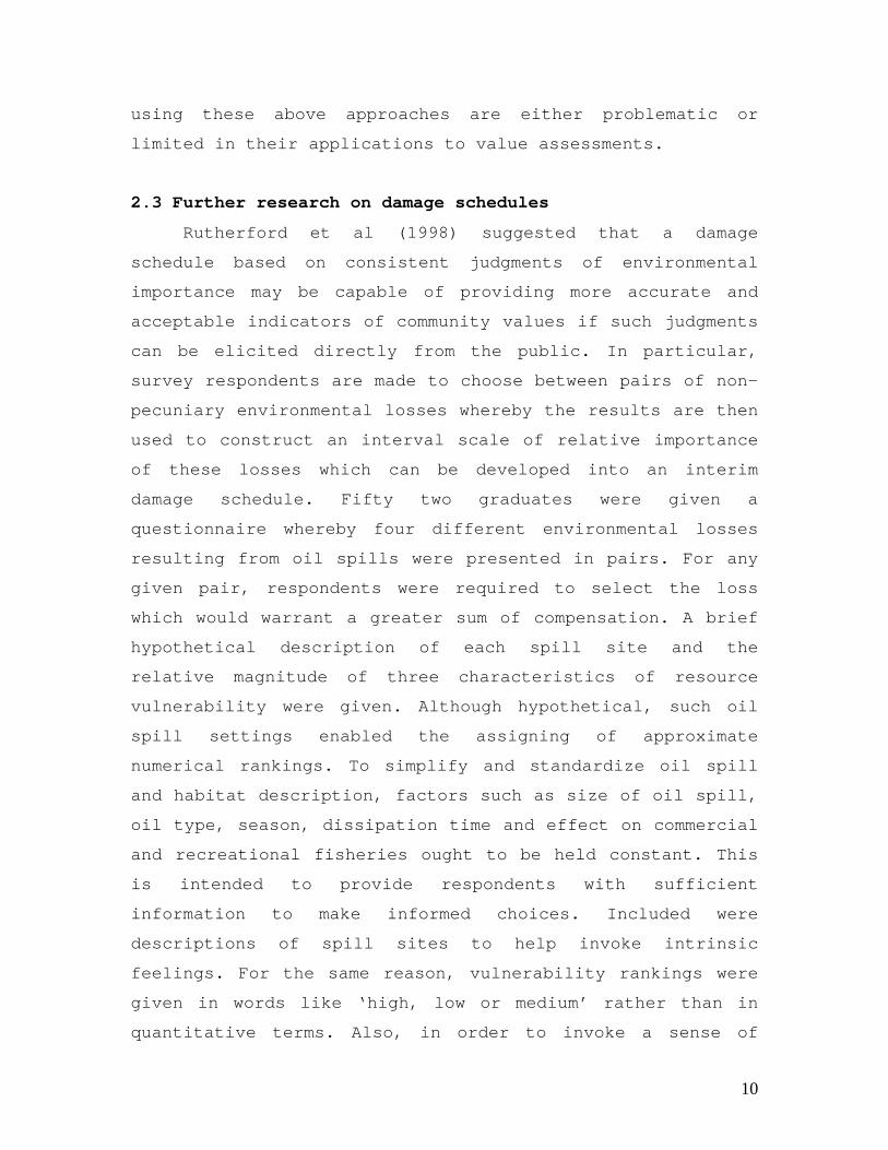
2.3 Further research on damage schedules

Rutherford et al (1998) suggested that a damage

schedule based on consistent judgments of environmental

importance may be capable of providing more accurate and

acceptable indicators of community values if such judgments

can be elicited directly from the public. In particular,

survey respondents are made to choose between pairs of non-

pecuniary environmental losses whereby the results are then

used to construct an interval scale of relative importance

of these losses which can be developed into an interim

damage schedule. Fifty two graduates were given a

questionnaire whereby four different environmental losses

resulting from oil spills were presented in pairs. For any

given pair, respondents were required to select the loss

which would warrant a greater sum of compensation. A brief

hypothetical description of each spill site and the

relative magnitude of three characteristics of resource

vulnerability were given. Although hypothetical, such oil

spill settings enabled the assigning of approximate

numerical rankings. To simplify and standardize oil spill

and habitat description, factors such as size of oil spill,

oil type, season, dissipation time and effect on commercial

and recreational fisheries ought to be held constant. This

is intended to provide respondents with sufficient

information to make informed choices. Included were

descriptions of spill sites to help invoke intrinsic

feelings. For the same reason, vulnerability rankings were

given in words like ‘high, low or medium’ rather than in

quantitative terms. Also, in order to invoke a sense of

11

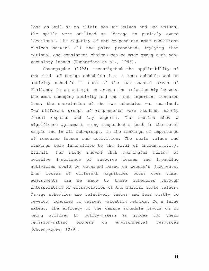
loss as well as to elicit non-use values and use values,

the spills were outlined as ‘damage to publicly owned

locations’. The majority of the respondents made consistent

choices between all the pairs presented, implying that

rational and consistent choices can be made among such non-

pecuniary losses (Rutherford et al., 1998).

Chuenpagdee (1998) investigated the applicability of

two kinds of damage schedules i.e. a loss schedule and an

activity schedule in each of the two coastal areas of

Thailand. In an attempt to assess the relationship between

the most damaging activity and the most important resource

loss, the correlation of the two schedules was examined.

Two different groups of respondents were studied, namely

formal experts and lay experts. The results show a

significant agreement among respondents, both in the total

sample and in all sub-groups, in the rankings of importance

of resource losses and activities. The scale values and

rankings were insensitive to the level of intransitivity.

Overall, her study showed that meaningful scales of

relative importance of resource losses and impacting

activities could be obtained based on people’s judgments.

When losses of different magnitudes occur over time,

adjustments can be made to these schedules through

interpolation or extrapolation of the initial scale values.

Damage schedules are relatively faster and less costly to

develop, compared to current valuation methods. To a large

extent, the efficacy of the damage schedule pivots on it

being utilized by policy-makers as guides for their

decision-making process on environmental resources

(Chuenpagdee, 1998).

12

In the next section, the methodology of the damage

schedule approach will be discussed in relation to its

findings when applied to a basket of environmental goods.

3. EMPIRICAL APPLICATION AND ANALYSIS

3.1 Methodology for the damage schedule approach

There are several methodologies that can be applied to

evaluate community preferences and choices. A simple and

promising method is the method of paired comparison. This

is a well established psychometric method for ordering

preferences among the elements of a choice set. Hence it is

by no means mere coincidence that the damage schedules

developed by Rutherford et al. (1998), Chuenpagdee (1998)

and Chuenpagdee et al. (2001) made use of this method to

elicit scales of relative environmental importance.

The paired comparison method is used primarily in

cases where subjective judgments are called upon to compare

between objects (David, 1988). The method involves

presenting a given set of objects independently in pairs as

binary choices to each respondent. The set of objects could

be gains, losses, activities, environmental resources or

whatever is being scaled. If the choice set does not

contain too many objects, all possible pairs can be

presented to each respondent. The total number of possible

pairs of n objects is n(n-1)/2.

Note that a simple ordinal ranking of all objects may

be preferred when the comparison of these objects

simultaneously can be easily achieved. However, when the

differences between objects are subtle, it is desirable to

13

make the comparison between the pair as free as possible

from any extraneous influences caused by the presence of

other objects. Thus, paired comparison offers certain

advantages when a fine judgment is needed. Nonetheless,

pair-wise ranking can only be done quickly when differences

between objects are fairly clear. Also, if there are too

many objects, pair-wise ranking becomes impracticable and

neither is it necessarily possible to achieve a wholly

satisfactory ranking (David, 1988).

An advantage of the paired comparison method is that

repetitive choices between different objects in the choice

set can reveal inconsistent choices as circular triads. If

no circular triads are produced, the result will be a

perfect rank ordering of the objects. However, we cannot

expect all the respondents to be perfectly consistent in

their choices. Inconsistency may be due to systematic

intransitive choice, incompetence of the respondent, random

choice when the pairs are too close to call or simply pure

errors. Systematic intransitive choice is more probable

when the objects are multidimensional such that the

prominence of different characteristics may vary according

to the pair of objects that is being compared (Kahneman et

al., 1999). In a study to evaluate the transitivity axiom

for the method of paired comparison, Peterson and Brown

(1998) found that a large proportion of the circular triads

in their data were due to close calls.

3.2 Experimental design

In this study, two series of paired comparison

questions were administered by means of two similar

computer programs. Tables 1 and 2 list the options and

14

provide brief descriptions. There are eight options in

Table 1 and fourteen options in Table 2. Respondents are to

refer to Table 1 for the first survey and to Table 2 for

the second.

(Tables 1 and Tables 2 here)

Both computer programs present the pairs of options on

the screen and require the respondents to make a choice. No

ties are allowed. The pairs of options are presented in

random order to the respondents so as to control for order

effects. The programs automatically record the respondents’

choice for each question. If there is an inconsistent

choice, the response will be marked as a contradiction.

Such inconsistent responses are repeated at the end when

all possible paired options have been asked. Three

consistent pairs, chosen at random by the computer, are

also repeated and randomly mixed with the repeats of the

inconsistent pairs. There is nothing to indicate when all

the possible paired comparisons ended and when the repeats

began. This is done to ascertain preference switches for

inconsistent choices.

A simple random sample of 100 respondents is taken for

each of the surveys. In each of the sample, the respondents

are then segregated by age, income and educational level.

At any point in time during the survey, respondents are

able to clarify with the investigator if any doubts arise.

The respondents only need to use the mouse to click on the

option selected. Several pre-tests were done to fine-tune

the procedures for the survey. From these pre-tests,

revisions were made to the procedures and instructions

until it was felt that the respondents were fully capable

of understanding what is required of them.

15

3.3 Empirical application of the damage schedule approach

A damage schedule is developed based on the

preferences of Singaporeans using the method of paired

comparisons. The first series of paired comparisons is

between different states of environmental quality for

different resources. A pilot survey was conducted to

determine the four most important environmental goods

perceived by Singaporeans. Table 3 shows the results of the

pilot survey.

(Table 3 here)

The four most important environmental problems are

degradation of coastal and marine environment, polluted

air, ozone depletion and unhygienic environment relating to

food and water. Each of the four different environmental

problems was further varied at two different levels of

environmental quality namely, moderate and severe. Hence,

there will be a total of eight options for comparison (see

Table 1), giving rise to a total of 28 possible pairs.

However, it is assumed that the severe environmental

problem of each type always matters more relative to the

moderate level of the same type. Thus, such pairs are

excluded leaving 24 possible pairs for comparison in the

first survey.

A simple way to evaluate paired comparison data is to

use the preference score for each item which is defined as

the number of times the respondent prefers that item over

other items in the choice set (Peterson and Brown, 1998).

Thus, each item has a maximum score of (n-1) where n is the

total number of items in the choice set. The individual

preference scores will be obtained from the paired

comparison results and aggregated across all respondents.

16

The most straightforward method that may be used to

summarize the respondents’ choices among the pairs is the

variance stable rank method (Dunn-Rankin, 1983). In this

method, the proportion of times that each item is chosen

relative to the maximum number of times it is possible to

be chosen by all respondents in the sample is calculated.

This proportion indicates the collective judgment of the

relative importance of the different items being compared

(Chuenpagdee, et al. 2001). A scale from 0 to 100 is

obtained when multiplying this proportion by 100.

3.4 Data analysis and results

The results from the 100 respondents are summarized in

Table 4 where the scale values for all eight losses are

listed for the entire sample and for each sub-sample

divided by age, monthly income and educational level. A

striking finding is the close correspondence of the scale

values across most of the sub-samples as indicated by the

relatively large Kendall’s W or coefficient of concordance.

(Table 4 here)

The null hypothesis that Kendall’s W is zero is rejected in

the each of the cases judging from the very small

associated asymptotic p-values. Hence, there is good

consensus among respondents in the ranking of the relative

importance of environmental problems. The close

correspondence of the scale values among the sub-samples is

further evident in the high Kendall’s Tau correlation

coefficients shown in Table 5. The null hypothesis of no

correlation is rejected at the 5% level of significance. It

is thus concluded that all sets of rankings were related.

(Table 5 here)

17

Severe air pollution is ranked either first or second

and has scale values of at least 80, except for the ‘Below

800 SGD’ sub-sample which appears to be specifically more

concerned with food and water contamination. Air pollution

is generally not perceived to be as important (ranked third

for severe and seventh for moderate). A plausible

explanation is that people with lower income may care more

for basic healthcare needs such as food and water hygiene.

Only for the ’31-40 years’ group is severe ozone depletion

viewed as slightly more important than severe food and

water contamination, even though ozone depletion is not a

prominent issue in Singapore. A possible reason could be

that respondents in this age group are more exposed to

international media and hence more aware and concerned

about international environmental issues.

Thirty six percent of the paired comparison responses

are found to be intransitive. The effects of intransitivity

was tested using Kendall’s W and Tau. For the transitive

respondents, Kendall’s W is 0.6379 and its asymptotic p-

value (based on a chi-square distribution with 7 degrees of

freedom) is 0.0022. Thus the null hypothesis of no

agreement among the respondents’ rankings can be rejected.

Agreement among intransitive respondents is also found to

be very significant as shown by the small asymptotic p-

value of 0.0059 and Kendall’s W of 0.6169. Next, the null

hypothesis of no correlation between these two respondent

groups is rejected as Kendall’s Tau is 0.7857 with a p-

value of 0.0062. Finally, the null hypothesis of no

correlation between the transitive group and the entire

sample is also rejected at the 1% level of significance.

The correlation coefficient for this two groups is 0.9286.

18

The findings suggest that inclusion of intransitive

responses into the sample did not significantly alter the

resulting scale values of the environmental problems in the

choice set. Out of a total of 60 inconsistent responses

recorded, 51 of them were reversed on retrial. Thus, a

large proportion of the inconsistent choices are, in fact,

switching behaviour on indifferent choices and hence do not

violate the transitivity axiom. Hence, it is appropriate to

use a single scale of relative importance to represent all

the respondents as shown in Figure 1.

(Figure 1 here)

3.5 Comparison of demographics across samples

Before applying the data from the second survey to

measure WTA, we need to test if the two samples are from

populations which are identically distributed in terms of

the demographics, namely, age, income and education. Using

the Kruskal-Wallis test, for age the test statistic was

0.04762 with p-value of 0.8273, for income the test

statistic was 0.0833 with p-value of 0.7728 and for

education the test statistic was 0.04762 with p-value of

0.8273. Thus the null hypothesis of the populations being

identically distributed cannot be rejected.

3.6 Using the paired comparison method to measure WTA

Using the paired comparisons in the second survey,

each respondent will be asked to make a choice between two

alternative gains, for example, a gain of 4,700SGD (i.e.

Singapore dollars) or an air quality improvement from an

unhealthy level to a good level (see Table 2 for the

complete list of gains). If air quality improvement is

chosen, one can infer that the lower bound for WTA for air

19

is greater than 4,700SGD. Given that the individual is

comparing two alternative gains, the apparent loss aversion

associated with the standard CV method is avoided as the

choice is made from the chooser reference point (Loomis et

al., 1998).

Only the two most important environmental problems,

air pollution as well as food and water contamination, from

the pilot survey results are included in the choice set

together with ten sums of money. Again, the environmental

problems are varied at two levels, moderate and severe,

each. Hence the total number of possible pairs for

comparison is 91. However, comparisons between the

environmental problems will not be needed as they have been

previously done in the first survey. Also, it is

unnecessary to include paired comparisons between sums of

money. Hence, the only meaningful comparisons are those

between environmental problems and monetary sums. The

number of such pairs for comparison reduces to 40. It was

carefully explained to the respondents that the different

levels of money are not used as compensation for not

receiving the environmental improvement.

The method used here allows us to bracket the WTA

within two values. For example, the point of indifference

can be identified by asking respondents if they would

choose 2,700SGD or an air quality improvement from a very

unhealthy to a good level, and a second choice between

3,200SGD or an air quality improvement from a very

unhealthy to a good level. Rejecting 2,700SDG but accepting

3,200SGD would imply that the minimum WTA lies between

2,700SGD and 3,200SDG. A nonparametric method is used to

calculate the WTA. From the responses, an empirical

20

cumulative distribution function is calculated and the

median estimated.

The median for each environmental gain for the total

and various sub-samples are rank ordered. Subsequently, the

WTA estimates will be determined by these median rankings.

For example, the median ranking of the entire sample for an

air quality improvement from a very unhealthy level to a

good level is 9. As it is only compared with the ten

monetary sums in the paired comparisons, the median ranking

of 9 implies that more than half of the sample of

respondents chose this particular air quality improvement

over the first nine monetary sums, that is from 700SGD to

4700SGD, except the tenth amount of 5200SGD. The minimum

WTA is thus estimated by calculating the mid-point of the

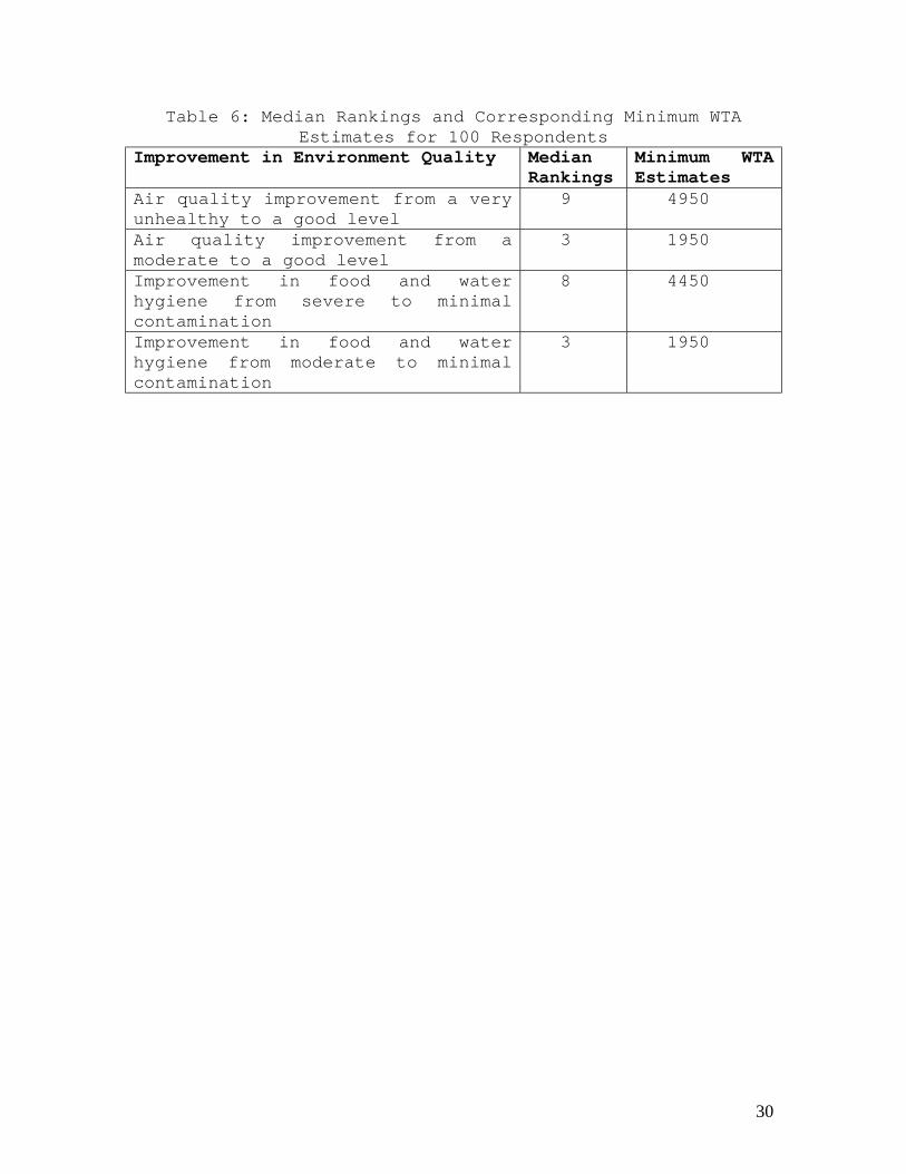
interval (4700 to 5200SGD) which is 4950SGD. Table 6 shows

the median rank orders for the total sample of 100

respondents and their corresponding minimum WTA estimates.

(Table 6 here)

The findings shown in Table 6 seem to be rather

consistent with those obtained in the first survey where

severe air pollution is ranked the most important (scale

value of 81), followed closely by severe food and water

contamination (scale value of 80). Moderate air pollution

(scale value of 33) is ranked just above moderate food and

water hygiene (scale value of 32) in the first survey while

in the second, the improvement in food and water hygiene

from moderate to minimal contamination and air quality

improvement from a moderate to a good level are equally

ranked.

In the second survey, inconsistency is no longer

detected by means of circular triads. A response is found

to be inconsistent when a resource gain is chosen as more

21

important than say 4700SGD but is chosen as less important

than any of the amounts less than 4700SGD. It is found that

only five respondents made inconsistent choices. All of

them switched their inconsistent choices on repeats,

implying that such inconsistencies are random and not

systematic. Hence, the overall consistency of all the

respondents is deemed to be quite high.

As in the first survey, the total sample is divided

using the three demographic characteristics, age income and

education. Tables 7, 8 and 9 give the median rank orders by

each of these characteristics and their corresponding

minimum WTA estimates.

(Table 7 here)

The median rankings of the various age groups are

rather similar, thereby inducing rather similar minimum WTA

estimates too. This suggests that the WTA of such

environmental goods does not vary much across individuals

of different ages. From Table 8, the median rankings of

different income groups are quite close, thus suggesting

that there are no large differences in their minimum WTA

estimates. It can also be noted that the two higher income

groups appear to rank air quality above food and water

hygiene. One suggestion could be that lower income groups

tend to be more concerned with basic healthcare needs while

greater affluence will induce one to be more

environmentally conscious. As can be seen from Table 9,

respondents with different educational levels do not seem

to differ much in their perceptions of WTA for air quality

as well as food and water hygiene. All three educational

groups ranked air quality improvement from a very unhealthy

level to a good level as the most important. This suggests

22

that regardless of educational level, individuals feel that

air quality matters the most to them.

In general, these findings show that minimum WTA

estimates do not vary by much across age, income and

education. Thus, it is evident that Singaporeans not only

display consistent judgments of relative importance for

various environmental problems and issues in the first

survey, but also consistent minimum WTA compensation to

forego improvements in air quality as well as food and

water hygiene across different age groups, income groups

and educational levels.

4. CONCLUSION

The damage schedule approach shows great promise in

the valuation of environmental goods. First, internally

consistent judgments of relative environmental importance

can be elicited without any reference to monetary values,

as shown by the findings of the first survey. Furthermore,

there exists a high degree of agreement among respondents

in the total and all various sub-samples, divided according

to age, income and education. Also, there is a relatively

high level of correspondence between all the different sets

of rank orders by all the various sub-samples. Intransitive

responses have a negligible impact on the scale values and

importance of rankings, implying that a single scale of

relative importance can be used to represent the entire

sample. The findings of the second survey show that

Singaporeans, regardless of age, income and educational

level, can provide consistent minimum WTA compensation to

forego improvements in air quality as well as food and

water hygiene.

23

The study found that Singaporeans perceived severe air

pollution (scale value of 81) as the most important

environmental problem followed closely by severe food and

water contamination (scale value of 80). Severe ozone

depletion (scale value of 78) ranks third followed by

severe damage to coastal and marine environment (scale

value of 49). Likewise, the same environmental problems at

the moderate level are ranked in a similar order with

moderate air pollution at fifth position (scale value of

33), followed by moderate food and water contamination

(scale value of 32), moderate ozone depletion (scale value

of 29) and moderate damage to coastal and marine

environment (scale value of 19). The computed minimum WTA

estimates that Singaporeans are willing to accept 4950SGD

to forego an air quality improvement from a very unhealthy

to a good level, 4450SGD to forego an improvement in food

and water hygiene from severe to minimal contamination,

1950SGD to forego either an air quality from a moderate to

a good level or an improvement in food and water hygiene

from moderate to minimal contamination. Though these WTA

estimates are very rough measures, they are at the very

least, reflect some form of monetary valuation based on

community preferences that can be used as provisional

damage or compensation awards.

Paired comparisons have the added advantage of

detecting inconsistent choices through circular triads in

the data. The results show that a large proportion of the

inconsistent responses are reversed on retrial, implying

that these inconsistencies are mostly not a consequence of

intransitivity but rather close calls or indifference.

When comparisons are only made between sums of money

and environmental problems, individuals may feel that the

24

two are incommensurate, implying an unwillingness to make

the trade-off between money and environmental goods.

However, as long as some form of comparison can be

consistently made either in terms of severity or

importance, a useful scaling can be attained (Sunstein,

1994).

The damage schedules established based on public

judgments of relative importance of changes in

environmental quality may not necessarily bring about

optimal deterrence as well as maximum efficiency in the

allocation of environmental resources. However, for many

purposes, inclusive of the provision of socially useful

incentives and dependable consistent compensations, the

objective of optimal deterrence and maximum efficiency is

not essential, provided that sanctions, incentives and

awards are in accord with the relative importance of

environmental changes.

25

REFERENCES

Blumstein, J.F., R.R. Bovbjerg and F.A. Sloan (1990) Beyond

tort reform: developing better tools for assessing damages

for personal injuries, Washington, D.C.: The Urban

Institute.

Champ, P.A. and J.B. Loomis (1998) “WTA Estimates Using the

Method of Paired Comparison: Tests of Robustness”

Environmental and Resource Economics, Vol.12, pp375-86.

Chuenpagdee, R. (1998) Damage schedules for Thai coastal

areas: an alternative approach to assessing environmental

values, Ottawa, Canada: EEPSEA.

Chuenpagdee, R., J.L. Knetsch, and T.C. Brown (2001)

“Environmental damage schedules: community judgments of

importance and assessment of losses” Land Economics,

Vol.77, No.1, pp1-11.

David, H.A. (1988) The method of paired comparisons,

London: C.Griffin & Co.

Dunn-Rankin, R. (1983) Scaling methods, New Jersey:

Lawrence Erlbaum Associates.

Kahneman, D.,I. Ritov and D. Schkade (1999) “Economic

Preferences or Attitude Expression? An Analysis of Dollar

Responses to Public Issues” Journal of Risk and

Uncertainty, Vol.19, pp220-42.

26

Knetsch, J.L. (1998) Environmental Valuation: Damage

Schedules, Conference at Vanderbilt University.

Loomis, J.B., G.L. Peterson, P.A. Champ, T. C. Brown and B.

Lucero (1998) “Paired Comparison Estimates of Willingness

to Accept versus Contingent Valuation Estimates of

Willingness to Pay” Journal of Economic Behaviour and

Organization, Vol. 35, pp501-15.

Peterson, G.L. and T.C. Brown (1998) “Economic Valuation by

the Method of Paired Comparison with Emphasis on Evaluation

of the Transitivity Axiom” Land Economics, Vol. 74, No. 2,

pp240-61.

Rutherford, M.B., J.L. Knetsch and T.C. Brown (1998)

“Assessing Environmental Losses: Judgments of Importance

and Damage Schedules” Harvard Environmental Law Review,

Vol.20, pp51-101.

Sunstein, C.R.(1994) “Incommensurability and Valuation in

Law” Michigan Law Review, Vol.92, pp779-861.

27

Table 1

Option A Severe food and water contamination causingdiseases such as cholera, typhoid etc with some

of them being contagiousOption B Moderate food and water contamination where

hygiene is not at its highest level. It may causeslight food poisoning or feeling of nausea.

Option C Moderate level of damage to coastal and marineenvironment where mangrove forests are only

partially cleared and coral reefs are marginallythreatened, implying that such losses are less

irreversible.Option D Severe damage to coastal and marine environment

where coral reefs are badly destroyed andmangrove forests are extensively cleared. Habitat

loss thus occurs, in turn causing losses ofvarious important marine and coastal species.

Option E Moderate level of air pollution, PSI between 51and 100, where the concentration of pollutants is

such that adverse health effects are notobserved. Unpleasant smells from landfills and

slight haze prevail.Option F Severe air pollution, PSI between 200 and 299,

where air quality is at a very unhealthy level.Respiratory health and vision is adversely

affected.Option G Severe ozone depletion leading to a sharp rise in

UV-B radiation (UV index above 7) where sunburntime is roughly 20 minutes or less, resulting inhealth problems like skin cancer, eye damage andpremature aging as well as harmful effects likeincreased global warming and climate change.

Option H Moderate ozone depletion where sunburn time ismore than 30 minutes, implying minimal biological

effects to living organisms. Adverse harmfuleffects such as skin cancer, eye damage may onlyresult after constant prolonged UV exposure.

28

Table 2

Option A A gain of 700SGD every year.

Option B A gain of 1200SGD every year.

Option C A gain of 1700SGD every year.

Option D A gain of 2200SGD every year.

Option E A gain of 2700SGD every year.

Option F A gain of 3200SGD every year.

Option G A gain of 3700SGD every year.

Option H A gain of 4200SGD every year.

Option I A gain of 4700SGD every year.

Option J A gain of 5200SGD every year.

Option K Air quality improvement from a very unhealthy

level (PSI between 200-299) to a good level (PSI

between 0-50). Adverse health effects are

completely removed. Air quality is restored to a

safe and healthy level.

Option L Air quality improvement from a moderate level

(PSI between 51-100) to a good level (PSI between

0-50). Unpleasant smells from landfills and

slight haze are eliminated in order to restore

air quality to a safe and healthy level.

Option M Improvement in food and water hygiene from severe

contamination to minimal contamination. Chances

of food and water borne diseases are being

greatly reduced so that food and water hygiene

are being restored to its highest level.

Option N Improvement in food and water hygiene from

moderate contamination to minimal contamination.

Chances of slight food poisoning are reduced in

order to restore food and water hygiene to its

highest level.

29

Table 3: Simple Ranking of Environmental Problems by SixtyRespondents

List of Environmental Problems Rank Frequency eachitem was chosen

Noisy environment 5 27Loss of scenery 8 15Degradation of coastal and marineenvironment

4 29

Loss of biodiversity 6 25Polluted waterways and surroundingseas

7 23

Polluted air 1 43Ozone depletion 3 38Unhygienic environment (relatingto food and water hygiene)

2 40

Others 9 0

30

Table 6: Median Rankings and Corresponding Minimum WTAEstimates for 100 Respondents

Improvement in Environment Quality MedianRankings

Minimum WTAEstimates

Air quality improvement from a veryunhealthy to a good level

9 4950

Air quality improvement from amoderate to a good level

3 1950

Improvement in food and waterhygiene from severe to minimalcontamination

8 4450

Improvement in food and waterhygiene from moderate to minimalcontamination

3 1950

31

Table 7: Median Rankings and Corresponding Minimum WTAEstimates for Various Age Groups

ImprovementinEnvironmentalQuality

15-20 years

21-30 years

31-40 years

Above 40years

Rank WTA Rank WTA Rank WTA Rank WTAAir qualityimprovementfrom a veryunhealthy toa good level

8 4450 9 4950 9 4950 9 4950

Air qualityimprovementfrom moderateto good level

2 1450 3 1950 3 1950 3 1950

Improvementin food andwater hygienefrom severeto minimalcontamination

8 4450 9 4450 8 4450 9 4950

Improvementin food andwater hygienefrom moderateto minimalcontamination

2 1450 3 1950 3 1950 3 1950

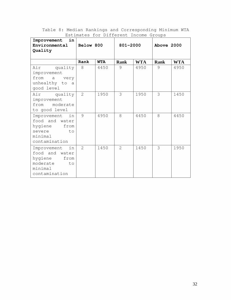
32

Table 8: Median Rankings and Corresponding Minimum WTAEstimates for Different Income Groups

Improvement inEnvironmentalQuality

Below 800 801-2000 Above 2000

Rank WTA Rank WTA Rank WTAAir qualityimprovementfrom a veryunhealthy to agood level

8 4450 9 4950 9 4950

Air qualityimprovementfrom moderateto good level

2 1950 3 1950 3 1450

Improvement infood and waterhygiene fromsevere tominimalcontamination

9 4950 8 4450 8 4450

Improvement infood and waterhygiene frommoderate tominimalcontamination

2 1450 2 1450 3 1950

33

Table 9:Median Rankings and Corresponding Minimum WTAEstimates for Different Educational Levels

Improvement inEnvironmentalQuality

SecondarySchool orbelow

A-level orDiploma

Degree

Rank WTA Rank WTA Rank WTAAir qualityimprovementfrom a veryunhealthy to agood level

9 4950 9 4950 9 4950

Air qualityimprovementfrom moderateto good level

2 1450 3 1950 3 1950

Improvement infood and waterhygiene fromsevere tominimalcontamination

9 4950 8 4450 8 4450

Improvement infood and waterhygiene frommoderate tominimalcontamination

3 1950 2 1450 3 1950

34

Figure 1: Scale of Relative Importance of EnvironmentalProblems Based on the Perceptions of Singaporeans

100 --------

--- Severe air pollution (81) Severe food & -------- Severe ozone depletion (78)water contamination (80) ---

---Severe damage tocoastal & marine --- 50environment (49) ---Moderate food & Moderate air pollution (33)water contamination --- Moderate ozone depletion (29)(32) ---Moderate damage tocoastal & marine ---environment (13) -------- 0

35

Table 4: Scale Values of Environmental Problems AGE (in years) INCOME (in SGD) EDUCATION

Environmentalproblem

Total 15-20 21-30 31-40 Above 40

Below800

801-2000

Above2000

Sec.Schoolorbelow

A-level/Diploma

Degree

Severe airpollution

81 83 85 84 80 74 88 87 84 80 87

Severe foodand watercontamination

80 90 80 80 82 83 80 82 79 82 82

Severe ozonedepletion

78 71 78 81 75 82 77 76 77 80 76

Severe damageto coastal andmarineenvironment

49 43 48 43 43 40 47 47 52 42 44

Moderate airpollution

33 27 37 34 35 34 37 33 30 33 37

Moderate foodand watercontamination

32 42 31 34 42 42 34 31 27 39 34

Moderate ozonedepletion

29 28 31 36 31 37 26 33 37 35 28

Moderatedamage tocoastal andmarineenvironment

13 17 11 8 13 8 12 12 13 9 12

Number ofrespondents

100 15 41 33 11 28 30 42 18 38 44

Kendall’scoefficient ofconcordance

.6240 .6050 .6336 .6559 .5517 .5895 .6626 .6451 .6383 .6156 .6473

36

Table 5: Kendall’s Tau Correlations of Scale Values of Environmental Problems AGE (inyears)

INCOME (in SGD) EDUCATION

15-20

21-30 31-40 40- <800

801-2000 >2000

Sec.Schoolorbelow

A-level/diploma

Degree

15-20 1.00 .7857 .7500 .9286 .8571 .7857 .7638 .7857 .9286 .785721-30 1.000 .7500 .8571 .6429 .9867 .9092 .8571 .7143 .989131-40 1.000 .6786 .6183 .7638 .8889 .9092 .6910 .7638AGE40- 1.000 .7857 .8571 .7638 .7143 .8571 .8570<800 1.000 .6429 .6071 .6429 .9285 .6407801-2000 1.000 .8929 .8571 .7140 .9823INCOME>2000 1.000 .9820 .6910 .9099Sec.School orbelow

1.000 .7143 .7143

A-level/diploma

1.000 .8571EDUCATION

Degree 1.000