This content has been downloaded from IOPscience. Please scroll down to see the full text.

Download details:

IP Address: 159.92.9.131

This content was downloaded on 15/10/2014 at 15:16

Please note that terms and conditions apply.

Entropies of tailored random graph ensembles: bipartite graphs, generalized degrees, and

node neighbourhoods

View the table of contents for this issue, or go to the journal homepage for more

2014 J. Phys. A: Math. Theor. 47 435101

(http://iopscience.iop.org/1751-8121/47/43/435101)

Home Search Collections Journals About Contact us My IOPscience

Entropies of tailored randomgraph ensembles: bipartite graphs,generalized degrees, and nodeneighbourhoods

E S Roberts1,2 and A C C Coolen1,3

1 Institute for Mathematical and Molecular Biomedicine, Kingʼs College London,Hodgkin Building, London SE1 1UL, UK2Randall Division of Cell and Molecular Biophysics, Kingʼs College London, NewHunts House, London SE1 1UL, UK3 London Institute for Mathematical Sciences, 35a South St, Mayfair, London W1K2XF, UK

E-mail: ekaterina.roberts@kcl.ac.uk and ton.coolen@kcl.ac.uk

Received 23 April 2014, revised 20 August 2014Accepted for publication 20 August 2014Published 9 October 2014

AbstractWe calculate explicit formulae for the Shannon entropies of several families oftailored random graph ensembles for which no such formulae were as yetavailable, in leading orders in the system size. These include bipartitegraph ensembles with imposed (and possibly distinct) degree distributions forthe two node sets, graph ensembles constrained by specified node neigh-bourhood distributions, and graph ensembles constrained by specified gen-eralized degree distributions.

Keywords: random graphs, networks, entropy, generalized degrees, bipartitegraphsPACS numbers: 89.70.Cf, 89.75.Fb, 64.60.aq

(Some figures may appear in colour only in the online journal)

1. Introduction

Networks are powerful and popular tools for characterizing large and complex interactingparticle systems. They have become extremely valuable in physics, biology, computer sci-ence, economics, and the social sciences. One approach is to quantify the implications ofhaving topological patterns in networks and graphs, by viewing these patterns as constraints

Journal of Physics A: Mathematical and Theoretical

J. Phys. A: Math. Theor. 47 (2014) 435101 (20pp) doi:10.1088/1751-8113/47/43/435101

1751-8113/14/435101+20$33.00 © 2014 IOP Publishing Ltd Printed in the UK 1

on a random graph ensemble. This provides a way to measure and compare topologicalfeatures from the rational point of view of whether they are present in a large or small numberof possible networks. Precise definitions of random graph ensembles with controlled topo-logical characteristics also allow us to generate systematically graphs and networks which aretailored to have features in common with those observed in a given application domain, eitherfor the purpose of statistical mechanical process modelling or to serve as ‘null models’ againstwhich to test the importance of observations in real-world networks.

A previous paper [1] considered tailored random graph ensembles with controlleddegree distribution and degree–degree correlations; the more recent [2] covered the case ofdirected networks. In each case, the strategy is to calculate the Shannon entropy, fromwhich we can deduce the effective number of graphs in the ensemble. Related quantitiessuch as complexity of typical graphs from the ensemble and information-theoretic distancesbetween graphs naturally follow from the entropy, or can be calculated using similarmethods.

In this paper we calculate, in leading order, the Shannon entropies of three as yetunsolved families of random graph ensembles, constrained by three different conditions: abipartite constraint with imposed degree distributions in the two nodes sets, a neighbourhooddistribution (where the neighbourhood of a node is defined as its own degree, plus the degreevalues of the nodes connected to it), and an imposed generalized degree distribution. Theseare each interesting in their own right as stand-alone results, and turn out to be closely linked.The first two cases can be resolved exactly, and give practical analytical expressions. Thegeneralized degree case was already partially studied in [3], with only limited success, andhere we require a plausible but as yet unproven conjecture to find an explicit formula for theentropy.

The generalized degrees concept appears in the literature in various forms. For example,the authors of [4], measured the number of direct neighbours s of a subset of t nodes. Theyderive conditions based on their definition of general degrees which can ensure that (for somegiven m and d ) there are at least m internally disjoint paths of length at most d. The diameterof the network is an obvious corollary—the smallest d corresponding to ⩾m 1. These resultscan be applied to questions of robustness of networks. The authors of [5] studied the spectraldensity of random graphs with hierarchically constrained topologies. This includes con-sideration of generalized degrees, as well as more general community structures. Using thereplica method, in a similar way to [3], they achieve a form analogous to equation (39). Theyproceed numerically from that point, hence our approach to an analytical solution presented inequation (48) is entirely novel.

2. Definitions and notation

We consider ensembles of directed and nondirected random graphs. Each graph is definedby its adjacency matrix =c c{ }ij , with ∈ …i j N, {1, , } and with ∈c {0, 1}ij for all (i,j).Two nodes i and j are connected by a directed link →j i if and only if =c 1ij . We put

=c 0ii for all i. In nondirected graphs one has =c cij ji for all (i,j), so c is symmetric. Thedegree of a node i in a nondirected graph is the number of its neighbours, = ∑k ci j ij. In

directed graphs we distinguish between in- and out-degrees, = ∑k ci j ijin and = ∑k ci j ji

out .They count the number of in- and out-bound links at a node i. A bipartite graph is one wherethe nodes can be divided into two disjoint sets, such that =c 0ij for all i and j that belong tothe same set.

J. Phys. A: Math. Theor. 47 (2014) 435101 E S Roberts and A C C Coolen

2

We define the set of neighbours of a node i in a nondirected graph as ∂ = =j c{ | 1}i ij .Hence = ∂k | |i i . To characterize a graphʼs topology near i in more detail we can define thegeneralized degree of i as the pair k m( , )i i , where = ∑m c ki j ij j counts the number of length-two paths starting in i. The concept of a generalized degree is discussed in [6]. Even moreinformation is contained in the local neighbourhood

ξ= ( ){ }n k ; , (1)i i is

in which the ordered integers ξ{ }is give the degrees of the ki neighbours j∈∂i. See also

figure 1. Since ξ= ∑ ⩽mi s k is

i, the neighbourhood ni provides more granular information

that complements that in the generalized degree k m( , )i i . We will use bold symbols whenlocal topological parameters are defined for every node in a network, e.g. = …k k k( , , )N1

and ξ ξ= …n k k(( ; { }), , ( ; { }))sN N

s1 1 . Generalization to directed graphs is straightforward.

Here ∂ = + >j c c{ | 0}i ij ji , and the local neighbourhood would be defined as

ξ= n k( ; { })i i is

with the ki pairs ξ = k k( , )is s s,in ,out now giving both the in- and out-degrees

of the neighbours of i.Our tailored random graph ensembles will be of the following form, involving N built-in

local (site specific) topological constraints of the type discussed above, which we will for nowwrite generically as cX ( )i , and with the usual abbreviation δ δ= ∏a b i a b, ,i i

∑ ∏

∑δ δ

= =

= =−

( )c X c X X

c X X X

p p p p p X

p Z Z

( ) ( ) ( ) ( ) ,

( ) ( ) , ( ) . (2)X

X X c

c

X X c

i

i

1, ( ) , ( )

The values Xi for the local features are for each i drawn randomly and independently from p(X), after which one generates a graph c randomly and with uniform probabilities from the

Figure 1. Illustration of our definitions of local topological characteristics innondirected graphs. At the minimal level one specifies for each node i (black vertexin the picture) only the degree = ∂ = ∑k c| |i i j ij (the number of its neighbours). At the

next level of detail one provides for each node the generalized degree k m( , )i i , in which= ∑ = ∑∈∂m k c ki j j j ij ji

is the number of length-two paths starting in i. This is then

generalized to include the actual degrees in the set ∂i, by giving ξ=n k( ; { })i i is (the

‘local neighbourhood’), in which the ki integers ξ{ }is give the degrees of the nodes

connected to i. To avoid ambiguities we adopt the ranking conventionξ ξ ξ⩽ ⩽ … ⩽i i i

k1 2 i. Note that ξ= ∑ = ∑∈∂ =m ki j j sk

is

1ii .

J. Phys. A: Math. Theor. 47 (2014) 435101 E S Roberts and A C C Coolen

3

set of graphs that satisfy the N demands =cX X( )i i. The empirical distributionδ= ∑−cp X N( | ) ci X X

1, ( )i of local features will be random, but the law of large numbers

ensures that for → ∞N it will converge to the chosen p(X) in (2) for any graph realization,and the above definitions guarantee that its ensemble average will be identical to p(X) forany N

∑ ∑∑ ∑δ

δ= =c c XX

p p XN

pZ

p X( ) ( )1

( )( )

( ). (3)c X c

X X cc

i

X X, ( )

, ( )i

If we aim to impose upon our graphs only a degree distribution we choose =c cX k( ) ( )i i .Building in a distribution of generalized degrees corresponds to =c c cX k m( ) ( ( ), ( ))i i i . Ifwe seek to prescribe the distribution of all local neighbourhoods (1) we choose

=c cX n( ) ( )i i .A further quantity which will play a role in subsequent calculations is the joint degree

distribution of connected nodes. For nondirected graphs it is defined as

δ δ′∣ =

∑

∑′

( )cW k kc

c, (4)

ij ij k k k k

ij ij

, ,i j

and its average over the ensemble (2) is given by

∑ ∑δ

′ = ′( ) ( )X cX

W k k p W k kZ

, ( ) ,( )

. (5)X c

X X c, ( )

In this paper we study the leading orders in the system size N of the Shannon entropy pernode of the above tailored random graph ensembles (2), from which the effective number ofgraphs with the prescribed distribution p(X) of features follows as = NSexp ( )

⎡

⎣

⎢⎢⎢⎢

⎤

⎦

⎥⎥⎥⎥⎡

⎣

⎢⎢⎢⎢

⎤

⎦

⎥⎥⎥⎥

∑

∑∏

∑ ∑∏

∑∏

∑∏

∑ ∑

δ δ

δ

= −

= −

′

′

= −

= −

′′

( )

( )

( )

( )

( )

c c

X X

X X

X X

SN

p p

N

p X

Z

p X

Z

N

p X

Z

p X

Z

p S p X p X

1( ) log ( )

1

( )log

1

( )log

( )

( ) ( ) ( ) log ( ) (6)

c

X c

X X c

X

X X c

X c

X X c

X

i

ij

j

i

ij

j

X

, ( ) , ( )

, ( )

with

∑δ= =X XSN

ZN

( )1

log ( )1

log . (7)c

X X c, ( )

The core of the entropy calculation is determining the leading orders in N of XS ( ), which isthe Shannon entropy per node of the ensemble c Xp ( | ) in which all node-specific values

= …X X X( , , )N1 are constrained. For =p X p k( ) ( ) this calculation has already been done in[1, 2]. For =p X p k m( ) ( , ) it has only partly been done [3]. Here we investigate the relation

J. Phys. A: Math. Theor. 47 (2014) 435101 E S Roberts and A C C Coolen

4

between the entropies of the p(k) and p k m( , ) ensembles and the entropy of the ensemble inwhich the distribution p(n) of local neighbourhoods (1) is imposed.

3. Building blocks of the entropy calculations

3.1. Relations between feature distributions for nondirected graphs

Since the generalized degrees k m( , )i i can be calculated from the local neighbourhoods (1) forany graph c, it is clear that the empirical distribution δ δ= ∑−cp k m N( , | ) c ci k k m m

1, ( ) , ( )i i for

any graph can be calculated from the empirical neighbourhood distributionδ= ∑−cp n N( | ) ci n n

1, ( )i . If we denote with k(n) the central degree k in ξ=n k( ; { })s , we

indeed obtain

∑ ∑ ∑δ δ δ δ δ= = ∑ ξ⩽cp k m

Np n( , )

1( ) . (8)c c

i

k k m m

n

n n

n

k k n m, ( ) , ( ) , , ( ) ,i i i s k ns

( )

Less trivial is the statement that also the distribution ′ cW k k( , | ) of (4) can be written in termsof cp n( | ). Using ∑ = cc Nk ( )ij ij , with = ∑−c ck N k¯ ( ) ( )i i

1 we obtain

∑ ∑∑

∑ ∑ ∑∑

∑ ∑∑

δ δ δ δ δ

δ δ

′∣ = =

=

′ ′

′

ξ

ξ

∈∂ ⩽

⩽

( )cc c

c

c

W k kN p n k n N p n k n

p n

p n k n

,( ) ( ) ( ) ( )

( )

( ) ( ). (9)

c c ci k k j k k

n

i n n n k k n s k n k

n

n k k n s k n k

n

, ( ) , ( ) , ( ) , ( ) ( ) ,

, ( ) ( ) ,

ii

j is

s

Given the symmetry of ′ cW k k( , | ) under permutation of k and ′k we then also have

δ δ′ =

∑ ∑

∑′ ξ⩽( )c

c

cW k k

p n

p n k n,

( )

( ) ( ). (10)

n k k n s k n k

n

, ( ) ( ) , s

The converse of the above statements is not true. One cannot calculate the neighbourhooddistribution cp n( | ) from cp k m( , | ) or from ′ cW k k( , | ) (or both). Note that by definition (andsince c is nondirected) we always have ′ = ′c cW k k W k k( , | ) ( , | ).

3.2. Decomposition of graphs into directed degree-regular subgraphs

Any nondirected graph c can always be decomposed uniquely into a collection of non-overlapping N-node subgraphs β ′kk , with ′ ∈k k, IN, which share the nodes … N{1, , } of c butnot all of the links. These subgraphs are defined for each ′k k( , ) by the adjacency matrices

β δ δ=′′c . (11)c cij

kkij k k k k, ( ) , ( )i j

Each graph β ′kk contains those links in c that go from a node with degree ′k to a node withdegree k. Clearly, all graphs β ′kk follow uniquely from c via (11). The converse uniqueness ofc, given the matrices β ′kk , is a consequence of the simple identity

∑ ∑ ∑δ δ δ δ β= = =′

′′

′′

′

⩾ ⩾ ⩾

c c c . (12)c c c cij ij

kk

k k k k

kk

k k k k ij

kkijkk

0

, ( ) , ( )

0

, ( ) , ( )

0i j i j

The graph β ′kk is directed if ≠ ′k k , and nondirected if = ′k k . From the symmetry of c itfollows moreover that β β=′ ′

jikk

ijk k for all ′i j k k( , , , ), so β ′k k is specified in full by β ′kk .

J. Phys. A: Math. Theor. 47 (2014) 435101 E S Roberts and A C C Coolen

5

Although each β ′kk is an N-node graph, most of the nodes in β ′kk will be isolated: all nodeswhose degrees in the original graph c were neither k nor ′k will have degree zero in β ′kk .

We now inspect the degree statistics of the decomposition graphs β ′kk , and their relationwith the structural features of c. If ≠ ′k k we find for the remaining degrees in β ′kk :

∑β βδ= = =′′

′

∈∂( ) ( )ck k k k( ) : , 0, (13)ci i

kk

j

k k ikkin

, ( )out

i

j

∑β βδ= ′ = =′ ′

∈∂( ) ( )ck k k k( ) : , 0. (14)cj j

kk

i

k k jkkout

, ( )in

j

i

Hence the joint in–out degree distribution of β ′kk can be writen in terms of the empiricaldistribution of neighbourhoods of c, viz. δ= ∑−cp n N( | ) ci n n

1, ( )i with ξ=n k( ; { })s

⎡⎣⎢

⎤⎦⎥

⎡⎣⎢

⎤⎦⎥

⎡⎣⎢

⎤⎦⎥

⎡⎣⎢

⎤⎦⎥

∑

∑

∑

∑

δ δ

δ δ

δ δ δ δ

δ δ δ δ

δ δ δ δ

δ δ δ δ

=

=

= + −

× + −

= + −

× + −

∑ ∑

∑

∑

∑

∑

′

′ ′

′ ′

β β

δ δ δ δ

δ

δ

δ

δ

ξ

ξ

′ ′

∈∂ ′ ′ ∈∂

∈∂ ′

∈∂

⩽ ′

⩽

( )

( )

( )

( )

( )

( ) ( )

c

p q qN

N

N

p n

,1

1

11

1

( ) 1

1 . (15)

c c

c c

kk

iq k q k

i

q q

i

k k q k k q

k k q k k q

n

k k n q k k n q

k k n q k k n q

in out, ,

, ,

, ( ) , , ( ) ,0

, ( ) , , ( ) ,0

, ( ) , , ( ) ,0

, ( ) , , ( ) ,0

c c c c

c

c

ikk

ikk

k ki j i k k j k ki j i k k j

i j i k k j i

i j i k k j i

s k n k s n

s k n k s n

in in out out

in, ( ) , ( )

out, ( ) , ( )

in, ( )

in

out, ( )

out

in( ) , ( )

in

out( ) , ( )

out

The two marginals of (15) are

⎡⎣⎢

⎤⎦⎥∑ δ δ δ δ= + −∑

′δ ξ⩽ ′ ( )cp q p n( ) ( ) 1 , (16)kk

n

k k n q k k n qin , ( ) , , ( ) ,0s k n k s n( ) , ( )

⎡⎣⎢

⎤⎦⎥∑ δ δ δ δ= + −∑

′′ ′δ ξ⩽ ( )cp q p n( ) ( ) 1 . (17)kk

n

k k n q k k n qout , ( ) , , ( ) ,0s k n k s n( ) , ( )

Hence =′ ′p q p q( ) ( )kk k kin out , as expected. The average degree

= ∑ = ∑′ ′ ′q q p q q q p q q¯ ( , ) ( , )kkq q

kkq q

kk,

in in out,

out in outin out in out of the graph β ′kk can be written,

using identity (10) and the symmetry of ′ cW k k( , | ), as

∑ ∑δ δ= = ′∣′′ ξ

⩽

( )c c cq p n k W k k¯ ( ) ¯ ( ) , . (18)kk

n

k n k

s k n

k n( ),

( )

, ( )s

If = ′k k , the decomposition matrix β ′kk is symmetric. Here we find

∑β δ δ=∈∂

( )k . (19)c cikk

k k

j

k k, ( ) , ( )i

i

j

J. Phys. A: Math. Theor. 47 (2014) 435101 E S Roberts and A C C Coolen

6

Hence the degree distribution of βkk becomes

⎡⎣⎢

⎤⎦⎥

⎡⎣⎢

⎤⎦⎥

∑

∑

∑

δ

δ δ δ δ

δ δ δ δ

=

= + −

= + −

∑

∑

∑

δ δ

δ

δ ξ

∈∂

∈∂

⩽

( )

( )c

p qN

N

p n

( )1

11

( ) 1 . (20)

c c

kk

i

q

i

k k q k k q

n

k k n q k k n q

,

, ( ) , , ( ) ,0

, ( ) , , ( ) ,0

c c

c

k ki j i k k j

i j i k k j i

s k n k s n

, ( ) , ( )

, ( )

( ) , ( )

The average degree in βkk is therefore

∑ ∑δ δ= =ξ⩽

c c cq p n k W k k¯ ( ) ¯ ( ) ( , ). (21)kk

n

k n k

s k n

k n( ),

( )

, ( )s

4. Entropy of ensembles of bipartite graphs

Here we calculate the leading orders in N of the entropy per node (6) for ensembles ofbipartite graphs with prescribed (and possibly distinct) degree distributions in the twonode sets. This is not only a novel result in itself, but will also form the seed of theentropy calculation for ensembles with constrained neighbourhoods in a subsequentsection.

In a bipartite ensemble the N nodes can be divided into two disjoint sets⊆ …A B N, {1, , } such that =c 0ij if ∈i j A, or ∈i j B, , leaving only links between A and

B. This constraint implies that there is a mapping from the set of bipartite graphs on… N{1, , } to the set of directed graphs on … N{1, , }, defined by assigning to each bipartite

link the direction of flow from A to B. This allows us to draw upon results on directedgraphs derived in [2]. The directed graph ′c associated with the bipartite graph c wouldhave

∈ ∈ ′ =j B i A cor : 0, (22)ij

∈ ∈ ′ =j A i B c cand : (23)ij ij

and hence the in- and out-degree sequence = …k k k k k(( , ), , ( , ))N N1in

1out in out of ′c can be

expressed in terms of the degree sequence k of c via

∈ = =( ) ( )i A k k k k: , 0, , (24)i i i iin out

∈ = =( ) ( )i B k k k k: , , 0 . (25)i i i iin out

This mapping can be shown to be bijective between the ensemble of all bipartite graphs with agiven degree sequence, and the ensemble of all directed graphs with the appropriately chosendirected degree sequence. The directed graph will have the joint degree distribution

⎜ ⎟⎛⎝

⎞⎠δ δ= + −( ) ( )( )p q q

A

Np q

A

Np q, 1 (26)q A B q

in out,0

out in,0in out

with the degree distributions δ= ∑−∈p k A( ) | | cA i A k k

1, ( )i and δ= ∑−

∈p k B( ) | | cB i B k k1

, ( )i in thesets A and B of the bipartite graph. Our bipartite ensemble is one in which we describe thedistributions pA(k) and pB(k), together with the probability ∈f [0, 1] for a node to be insubset A, and we forbid links within the sets A or B. Conservation of links demands that the

J. Phys. A: Math. Theor. 47 (2014) 435101 E S Roberts and A C C Coolen

7

two distributions cannot be independent, but must obey= − ∑ = ∑q f qp q f qp q¯ (1 ) ( ) ( ),q B q A where q is the average degree. Hence, the entropy of

any degree-constrained bipartite ensemble can be calculated by application of (6), (7) to theassociated ensemble of degree-constrained directed graphs, with τ=X k( , )i i i . Hereτ ∈ A B{ , }i gives the subset assignment of a node. We then find

⎡⎣⎢⎢

⎤⎦⎥⎥∑ ∏

∑ ∑

τ τ= − − − −

− − −τ

( )S p k S k f f f f

f p k p k f p k p k

, ( , ) log (1 ) log (1 )

( ) log ( ) (1 ) ( ) log ( ) (27)

k i

i i

kA A

kB B

,

with

τ δ δ= + −τ τp k f p k f p k( , ) ( ) (1 ) ( ), (28)A A B B, ,

⎛⎝⎜⎜

⎞⎠⎟⎟

⎛⎝⎜⎜

⎞⎠⎟⎟∑ ∏ ∏τ δ δ=

τ τ=

=( ) ( )S k

N( , )

1log . (29)

c i A

k k

i B

k k

,

, 0,

,

, ,0

i

i i

i

i i

The latter quantity follows from the calculation in [7], with the short-hand π = −q( ) e q q!qq q

¯¯

and modulo terms that vanish for → ∞N :

⎡⎣ ⎤⎦ ⎡⎣ ⎤⎦⎡⎣ ⎤⎦

∑

∑

∑ ∑

τ δ π

δ π

π π

= + + + −

+ + −

= + + −

( )

( )

S k q N q f f p q q

fp q f q

q N q f p q q f p q q

( , ) ¯ log ¯ 1 (1 ) ( ) log ( )

( ) (1 ) log ( )

¯ log ¯ ( ) log ( ) (1 ) ( ) log ( ). (30)

q

q B q

qA q q

qA q

qB q

,0 ¯

,0 ¯

¯ ¯

This then leads to our final result for the entropy per node of tailored bipartitegraph ensembles, with imposed bipartite degree distributions pA(k) and pB(k), average degreek , and a fraction f of nodes in the set A (modulo vanishing orders in N):

⎛⎝⎜

⎞⎠⎟

⎛⎝⎜

⎞⎠⎟∑ ∑

π π

= − − − −

− − −

( )S k N k f f f f

f p kp k

kf p k

p k

k

¯ log ¯ log (1 ) log (1 )

( ) log( )

( )(1 ) ( ) log

( )

( ). (31)

kA

A

k kB

B

k¯ ¯

If the sets A and B were to be specified explicity (as opposed to only their relative sizes), thecontribution = − − − −S f f f flog (1 ) log (1 )f would disappear from the above formula.

5. Entropy of ensembles with constrained neighbourhoods

We now turn to the Shannon entropy per node (6) of the ensemble (2) in which for theobservables cX ( )i we choose the local neighbourhood cn ( )i defined in (1). For this we need tocalculate the leading orders of δ= ∑−nS N( ) log c n n c

1, ( ) . We now use the one-to-one rela-

tionship between a graph c and its decomposition β= ∑ ′′c qq

qq , to write

∑ δ=β ′{ }

nSN

( )1

log . (32)n n c, ( )kk

J. Phys. A: Math. Theor. 47 (2014) 435101 E S Roberts and A C C Coolen

8

The next argument is the key to our ability to evaluate the entropy. It involves translating theconstraint =n n c( ) into constraints on the decomposition matrices β ′kk . Let us define the setsof nodes in c which have the same degree, viz. = ⩽ =n cI i N k k( ) { | ( ) }k i . The constraint

=n n c( ) in (32) prescribes:

(i) all the sets Ik of nodes with a given degree(ii) for each node ∈i Ik which sets ′Ik this node is (possibly multiply) connected to.

Hence the constraint =n n c( ) specifies exactly the in- and out-degree sequences of alldecomposition matrices β ′kk of c, which we will denote as =′ ′ ′q q q( , )kk kk kkin, out, , and whosedistributions we have already calculated in (15) and (20). We thus see that (32) can be written as

∑ ∏ δ=′β

β ′

′ ′( ){ }

nSN

( )1

log , (33)q qkk

,nkk

kk kk

in which ′qnkk are the in- and out-degree sequences that are imposed by the local environment

sequence n on the decomposition matrix β ′kk , and whose distributions are known to be (15),(20). Using the symmetry β β=′ ′( )kk k k† we may now write

⎪ ⎪⎪ ⎪

⎪ ⎪

⎪ ⎪

⎡

⎣⎢⎢

⎛⎝⎜⎜

⎞⎠⎟⎟

⎛⎝⎜⎜

⎞⎠⎟⎟

⎤

⎦⎥⎥

⎧⎨⎩

⎫⎬⎭

⎧⎨⎩

⎫⎬⎭

∏ ∑ ∏ ∑

∑ ∑ ∑ ∑

δ δ

δ δ

=

= +

′

′

ββ

ββ

ββ

ββ

<

<

′

′ ′

′

′ ′

( )

( )

( )

( )

nSN

N N

( )1

log

1log

1log . (34)

q q q q

q q q q

k k k

k k k

, ,

, ,

n n

n n

kk

kk kk

kk

kk kk

kk

kk kk

kk

kk kk

We see that the entropy nS ( ) can be written as the sum of the entropies of sub-ensembles,which are the decomposition matrices β ′kk with prescribed degree sequences. The second sumin (34) is over nondirected ensembles, the first over directed ones. The sub-entropies were allcalculated, respectively, in [1] and [2] 4. The entropy of an N-node nondirected randomgraph ensemble with degree sequence q was found to be (modulo terms that vanish for

→ ∞N ):

⎡⎣ ⎤⎦∑ ∑δ π= = + +( )SN

q N q p q q1

log1

2¯ log ¯ 1 ( ) log ( ) (35)q

c

q q c

q

q, ( ) ¯

in which = ∑−q N q¯ i i1 and π q( )q is the Poisson distribution with average q . The entropy of

an N-node directed random graph ensemble with in- and out-degree sequence q was found tobe (modulo terms that vanish for → ∞N ) :

⎡⎣ ⎤⎦ ⎡⎣ ⎤⎦

∑

∑

δ

π π

=

= + +

( ) ( ) ( )( )

SN

q N q p q q q q

1log

¯ log ¯ 1 , log . (36)

q

c

q q c

q q

q q

, ( )

,

in out¯

in¯

out

in out

The above entropies depend in leading orders only on the degree distributions (as opposed tothe degree sequences), and since these distributions were already calculated (15) and (20), wecan simply insert (36) and (36) into (34), with the correct distributions (15) and (20), and find

4 In [1, 2] the entropies were carried out for ensembles with prescribed degree distributions, but it was shown that, inanalogy with (6), this is simply the sum of the Shannon entropy of the degree distributions and the entropy of thecorresponding ensemble with prescribed sequences.

J. Phys. A: Math. Theor. 47 (2014) 435101 E S Roberts and A C C Coolen

9

an expression that depends only on the local environment distribution δ= ∑−p n N( ) i n n1

, i:

⎪ ⎪⎪ ⎪

⎪ ⎪

⎪

⎪

⎪ ⎪

⎪

⎪

⎧⎨⎩

⎡⎣ ⎤⎦ ⎡⎣ ⎤⎦⎫⎬⎭

⎧⎨⎩

⎡⎣ ⎤⎦⎫⎬⎭

⎡⎣ ⎤⎦

⎡⎣ ⎤⎦ ⎡⎣ ⎤⎦⎫⎬⎭

⎡⎣ ⎤⎦

⎡⎣ ⎤⎦⎫⎬⎭

⎡⎣ ⎤⎦⎡⎣⎢⎢

⎡⎣ ⎤⎦⎤⎦⎥⎥

⎡⎣ ⎤⎦⎡⎣⎢

⎤⎦⎥

⎡⎣ ⎤⎦⎡

⎣⎢⎢

⎛⎝⎜⎜

⎞⎠⎟⎟

⎤

⎦⎥⎥

∑ ∑

∑ ∑

∑

∑

∑

∑

∑

∑ ∑ ∑

∑

∑ ∑ ∑

∑

∑ ∑ ∑

π π

π

δ δ δ δ δ

δ

= + +

+ + +

= ′ ′ −

+ ′ ′ − +

+ −

+ ′ −

= − + ′ ′

− + +

= − + ′ ′

− + −

= − + ′ ′

−

∑

′

′ ′ ′

′

′ ′

′

′

′ ′

′

′′ ′

′

ξ

ξ

<

≠

≠

⩽

′ ′

⩽

{

{

( ) ( ) ( )

( )

( )

( )

( )

( )

( )

( )

( ) ( )

( ) ( )

( )

( ) ( )

( ) ( )

( ) ( )

nS q N q p q q q q

q N q p q q

kW k k N kW k k

kW k k kW k k p q p q q

kW k k N kW k k

kW k k kW k k p q q

k N k k W k k W k k

p q p q p q q

k N k k W k k W k k

p n q

k N k k W k k W k k

p n

( ) ¯ log ¯ 1 , log

1

2¯ log ¯ 1 ( ) log ( )

1

2¯ , log ¯ , 1

2 ¯ , log ¯ , ( ) ( ) log !

1

2¯ ( , ) log ¯ ( , ) 1

2 ¯ ( , ) log ¯ , 2 ( ) log !

1

2¯ log ( ¯ 1

1

2¯ , log ,

1

2( ) ( ) ( ) log !

1

2¯ log ¯ 1

1

2¯ , log ,

( ) 1 log !

1

2¯ log ¯ 1

1

2¯ , log ,

( ) log ! . (37)

k k

kk kk

q q

kkq q

k

kk kk

q

kkq

k k

q

kk kk

k

q

kk

k k

q k k

kk kk

k

kk

k k

q n k k

k k n q k n k k n q

k k

n k s k n

k n

,

in out¯

in¯

out

¯

in out

,

in out

,

,

, ( ) , , ( ) , ( ) ,0

,

( )

, ( )

kk kk

kk

s k ns

s

in out

( )

Insertion of this result into the general formula (6) gives us an analytical expression for theShannon entropy of the random graph ensemble with prescribed distribution p(n) of localneighbourhoods, modulo terms that vanish for → ∞N . This expression is fully explicit, sincek and ′W k k( , ) are both determined by the distribution p(n), via = ∑k p n k n¯ ( ) ( )n and (10)respectively:

⎡⎣ ⎤⎦⎡

⎣⎢⎢

⎛⎝⎜⎜

⎞⎠⎟⎟

⎤

⎦⎥⎥

∑

∑ ∑ ∑ ∑ δ

= − + ′ ′

− −

′

ξ⩽

( ) ( ) ( )S k N k k W k k W k k

p n p n p n

1

2¯ log ¯ 1

1

2¯ , log ,

( ) log ( ) ( ) log ! . (38)

k k

n n k s k n

k n

,

( )

, ( )s

J. Phys. A: Math. Theor. 47 (2014) 435101 E S Roberts and A C C Coolen

10

6. Entropy of ensembles of networks with specified generalized degreedistribution

In this section we consider an ensemble of nondirected networks with a specified generalizeddegree distribution δ δ= ∑−p k m N( , ) c ci k k m m

1, ( ) , ( )i i , where = ∑ck c( )i j ij and

= ∑m c c .i jk ij jk Previous work [3] began this calculation, and reached (in leading order) theintermediate form set out below:

⎡⎣ ⎤⎦⎛⎝⎜

⎞⎠⎟

⎛

⎝⎜⎜

⎞

⎠⎟⎟

∑

∑ ∑ ∏

π

δ γ ξ

= + −

+∑

ξ ξξ

==

( )

( )

S k N k p k mp k m

k

p k m k

1

2¯ log ¯ 1 ( , ) log

( , )

( )

( , ) log , (39)

k m k

k mm

s

ks

, ¯

, ,.,,

1ks

ks

11

k indicates the average degree; π k( )k is the Poissonian distribution with average degree k .The sum inside the logarithm in the final term of (39) runs over all sets of k nonnegativeintegers ξ ξ… k1 . The function γ (.,.) is defined as the nonnegative solution to the followingself-consistency relation:

⎡

⎣

⎢⎢⎢⎢⎢

⎤

⎦

⎥⎥⎥⎥⎥∑

∏

∏γ

δ γ ξ

δ γ ξ

′ =′ ′ ′

∑ ′

∑ ′′

′

′

′

′

ξ ξ ξ

ξ ξ ξ

− ∑=

−

∑=

′−=′−

′=′

( ) ( )( )

( )k k

k

kp k m

k

k

, ¯ ,

,

,

. (40)m

m k

s

ks

m

s

ks

... ,1

1

... ,1

ksk s

ksk s

1 111

11

This equation does not yield to a straightforward solution, and can only be evaluatednumerically or in certain special cases. Without a physical interpretation of γ ′k k( , ), thisintermediate answer is limited in how much insight it can provide. We will now show how theentropy can be expressed in terms of measurable quantities.

Within the notion of taking node properties from a specified distribution there is theinteresting question of whether it is even possible to realize a network with thegiven local topological properties. For simple degrees, this question is generally con-sidered to not be material in the → ∞N limit. For finite N, the Erdos–Gallai theoremfamously gives a necessary and sufficient condition for a degree sequence to be gra-phical. This question is not explicitly considered within the statistical mechanicsapproach—which makes it particularly interesting that there arises the self-consistencyequation (40), which seems to have a natural interpretation from the point of view ofgraphicality.

Our strategy is to derive an expression for the (observable) degree–degree corre-lations ′W k k( , ), and show that these can be expressed in terms of the order parameterγ ′k k( , ) that appears in equation (39). We calculate the average of this quantity in ourtailored ensembles of the form (2), where we now define topological characteristicsby specifying a generalized degree distribution p k m( , ). We follow closely thesteps taken in [3], and write for the ensemble a specified generalized degree sequencek m( , ):

J. Phys. A: Math. Theor. 47 (2014) 435101 E S Roberts and A C C Coolen

11

⎜ ⎟

⎜ ⎟

⎜ ⎟

⎜ ⎟⎜ ⎟

⎜ ⎟

⎜ ⎟

⎜ ⎟

⎜ ⎟

⎡⎣⎢

⎛⎝

⎞⎠

⎤⎦⎥

⎡⎣⎢

⎛⎝

⎞⎠⎤⎦⎥

⎛⎝

⎞⎠

⎛⎝

⎞⎠

⎛⎝⎜⎜

⎞⎠⎟⎟ ⎛

⎝⎞⎠

⎛⎝

⎞⎠

⎛⎝

⎞⎠

⎛⎝

⎞⎠

⎛⎝

⎞⎠

⎡⎣ ⎤⎦

⎡⎣ ⎤⎦

∫

∫

∫∫

∫

∫

∫

∫

∫ ∫ ∫∫

∑ ∑ ∑

∏

∑∑

∑

∑

∑ ∑

θ ϕ

θ ϕ

θ ϕ

θ ϕ

θ ϕ

θ ϕ

θ ϕ

θ ϕ

δ δ δ δ

δ δ

δ δ

δ δ

θ ϕ θ ϕ θ ϕ θ ϕ

′

= =

×

+ −

∏ + −

+

=+

+

+

= +

=

+

=′

+

∑ ∑

∑

∑

∑

∑

′ ′

′

′

′′

′′

′

θ ϕ

θ ϕ

θ ϕ

θ ϕ

θ ϕ

θ ϕ

θ ϕ

θ ϕ

π

πθ θ ϕ ϕ θ θ ϕ ϕ

π

πθ θ ϕ ϕ

π

πθ θ ϕ ϕ θ θ ϕ ϕ

π

πθ θ ϕ ϕ

π

πθ θ ϕ ϕ

π

π

π

πθ ϕ θ ϕ

π

π

Ψ θ ϕ θ ϕ

Ψ

+ − + + +

<

− + + +

+<

− + + +

+ − + + + − + + + +⋯

+ − + + + +⋯

+ +− + + +

+ +

+ +− + − +

+ +

− − − −

θ θ ϕ ϕ

θ θ ϕ ϕ

θ θ ϕ ϕ

θ θ ϕ ϕ

− + + +

− + + +

− + + +

− + + +

( )( ){ }

{ }

( )

( )

( )

( )

( )

( )

( )

( )

( )

( ) ( )

( )

( )

c k m

W k k

Nkp c

N

k

N

k

N

N

N

k

Nk

N

N

N

N

N N

N

P P P k P k

P P

N

,

1( , )

1

d d e 1 e 1

d d e 1 e 1

1

1d d e

2e

d d e2

e

1

d d e1

e

d d e

1

d d e1

e1

e

d d e

1

d d ˆ e d d ( , , )e d d , , e

d d ˆ e

1. (41)

c

k m

k m

k m

k m

k m

k m

k m

k m

rs

rs k c k c

rs

k k k k

k k

i j

k k

i ji k k

rs

k k k k

k kij

k k

ijk k

rs

k k k kk k

r k kk

s k kk

N P P k k

N P P

, , 2 , ,

i( · · ) i i

i( · · )

2 , ,

i( · · ) i i

i( · · ) i

i( · · ) e

2 , ,i

i( · · ) e

i( · · ) e

,i

,i

i( · · ) e

, ˆ i i i i

, ˆ

( )

ℓ rℓ ℓ sℓ r s

r s r s s r i j i j j i

i j i j j i

r s

r s r s i j i j j i

i j i j j i

kN

ij

i j ik j jki

r sr s r s

kN

ij

i j ik j jki

kN

ij

i j ik j jki

rr r

ss s

kN

ij

i j ik j jki

2i

2i

2i

2i( )

Taking the limit → ∞N therefore gives

∫∫

θ ϕ θ ϕ

θ ϕ θ ϕ

′ =

× ′

′θ ϕ

θ ϕ

Ψ

→∞− −

− −

‐

( )( )

( )

( ){ }

W k k P k

P k

lim , d d ( , , )e

d d , , e (42)

N

k

k

P P

i i

i i

saddle point , ˆ of

in which the function Ψ P P[ , ˆ] is identical to that found in [3]. Using the formulae in [3] thatrelate to the definition of the order parameter γ ′k k( , ), we then obtain for → ∞N theunexpected simple but welcome relation

J. Phys. A: Math. Theor. 47 (2014) 435101 E S Roberts and A C C Coolen

12

γ γ′ = ′ ′( ) ( ) ( )W k k k k k k, , , . (43)

A similar, although slightly more involved, calculation leads to an expression for the jointdistribution ′ ′W k m k m( , ; , ); see the appendix for details.

Our final aim is to use identity (43) to resolve equation (39) into observable quantities.Consider the nontrivial term in (39)

⎛⎝⎜⎜

⎞⎠⎟⎟∑ ∑ ∏Γ γ ξ δ= ∑

ξ ξξ

==

( )p k m k( , ) log , . (44)k m s

ks

m, ,., 1

,k

s

k s

11

At this point of the calculation, the effect of factorising across nodes has been to break theexpression down into terms which, for every generalized degree (k,m), enumerate all thepossible ways of dividing m second neighbours between k first neighbours. The term insidethe logarithm sums for each k over all configurations ξ ξ…{ }k1 which meet the condition

ξ∑ == msk s

1 . To formalize this idea, we may re-aggregate the expression for any graphicallyrealizable distribution p k m( , ) to write

⎧⎨⎪⎩⎪

⎛⎝⎜⎜

⎞⎠⎟⎟

⎫⎬⎪⎭⎪

⎛

⎝⎜⎜

⎡⎣⎢⎢

⎤⎦⎥⎥

⎞

⎠⎟⎟

⎧⎨⎪⎩⎪

⎛

⎝⎜⎜

⎞

⎠⎟⎟

⎫⎬⎪⎭⎪

∏ ∑ ∏

∏ ∑ ∏

∑ ∑ ∏ ∏ ∏

Γ γ ξ δ

γ ξ δ

δ γ ξ

=

=

= …

∑

∑

∑

ξ ξξ

ξ ξξ

ξ ξ ξ ξξ

=

… =

… … =

=

=

=

( )

( )

( )

Nk

Nk

Nk

1log ,

1log ,

1log , . (45)

k m s

ks

m

Np k m

i s

k

i is

m

im

i s

k

i is

, ,., 1,

( , )

1,

,1

ks

k s

i iki

i

i s

kiis

kN N

kN i

s

ki

is

i

11

1 1

11

11 1

1

We can now see that the separate terms precisely enumerate all the permutations of degreesand neighbour-degrees for networks with a generalized degree sequence consistent with anypair (k,m) appearing Np k m( , ) times. The Kronecker deltas δ ξ∑ =m ,i s

kiis

1tell us that each ξi

s inany nonzero term is to be interpreted as the degree of a node ∈ ∂j i, and must thereforeappear also as the left argument in another factor of the type γ k( ,.)j . This insight allows theexpression to be substantially simplified, since we already know thatγ γ′ ′ = ′k k k k W k k( , ) ( , ) ( , ), where ′W k k( , ) is the correlation between degrees of connectednodes. Hence, any nonvanishing contribution to the sum over all neighbourhoods inside thelogarithm of (45) will be equal to a repeated product of factors ′W k k( , ), with different ′k k( , ).Since we also know that the number of links between nodes with degree combination ′k k( , )equals ′NkW k k¯ ( , ) in leading order in N, we conjecture that in leading order we may make thefollowing replacement inside (45):

∏ ∏ ∏γ ξ → ′′

′

=( ) ( ) ( )k W k k, , , (46)

i s

k

i is

k k

W k k

1 ,

,i

kN¯2

(where the factor 1

2in the exponent reflects the fact that two γ (.,.) factors combine to form

each factor W (.,.).) With this conjecture we obtain, in leading order in N:

J. Phys. A: Math. Theor. 47 (2014) 435101 E S Roberts and A C C Coolen

13

⎜ ⎟⎧⎨⎪⎩⎪

⎛⎝

⎞⎠

⎫⎬⎪⎭⎪

⎛

⎝⎜⎜

⎞

⎠⎟⎟

∑ ∑ ∑

∑ ∑ ∑

Γ δ

δ

= … ∏ + ′ ′

= + ′ ′

∑

∑

′

′

ξ ξ ξ ξξ

ξ ξξ

… …=

=

( ) ( )

( ) ( )

Nk W k k W k k

p k m k W k k W k k

1log

1

2¯ , log ,

( , ) log1

2¯ , log , . (47)

i mk k

k mm

k k

,,

, ,.,,

,

kN N

kNi s

kiis

ks

ks

11

11 1 1

11

This implies that (39) simplifies to

⎡⎣ ⎤⎦

⎛⎝⎜

⎞⎠⎟

⎛⎝⎜⎜

⎞⎠⎟⎟

∑

∑ ∑ ∑π

δ

= + + ′ ′

− + ∑

′

ξ ξξ

=

( ) ( ) ( )S k N k k W k k W k k

p k mp k m

kp k m

1

2¯ log ¯ 1

1

2¯ , log ,

( , ) log( , )

( )( , ) log . (48)

k k

k m k k mm

,

, ¯ , ,.,,

ks

k s

11

Figure 2 applies equation (48), and related results from [1], to real protein–proteininteraction datasets, in order to demonstrate how these expressions can quantify the degree towhich each topological property constrains the ensemble. In appendix B we look at somesimple synthetic examples, where (48) can be compared with direct enumeration, or where theself-consistency equation (40) is soluble.

Figure 2. Results from applying equation (48) for the entropy of randomgraph ensembles—where the constraints are taken to match the relevant topologicalobservables of networks from [8–13]. From left to right the bars correspond to entropyper node of random graph ensembles tailored to match: average degree, degreedistribution, degree–degree correlation and generalized degrees. The generalizeddegrees constraint can be seen to be onerous for several of these networks. Thisobservation is based on the large reduction in entropy between the generalized degreeconstrained ensemble, and any of the other ensembles considered.

J. Phys. A: Math. Theor. 47 (2014) 435101 E S Roberts and A C C Coolen

14

7. Conclusion

Ensembles of tailored random graphs are extremely useful constructions in the modelling ofcomplex interacting particle systems in biology, physics, computer science, economics andthe social sciences. They allow us to quantify topological features of such systems and reasonquantitatively about their complexity, as well as define and generate useful random proxiesfor realistic networks in statistical mechanical analyses of processes.

In this paper we have derived, in leading two orders in N, explicit expressions for theShannon entropies of different types of tailored random graph ensembles, for which no suchexpressions had yet been obtained. This work builds on and extends the ideas and techniquesdeveloped in the three papers [1–3], which use path integral representations to achieve linkfactorization in the various summations over graphs. We show in this paper how the newensemble entropies can often be calculated by efficient use and combination of earlier results.

The first class of graph ensembles we studied consists of bipartite nondirected graphswith prescribed (and possibly nonidentical) distributions of degrees for the two node subsets.This case is handled by a bijective mapping from the ensemble of bipartite graphs with aspecified degree distribution to the ensemble of directed graphs with the associated specifieddirected degree distribution, for which formulae are available. The second class consists ofgraphs with prescribed distributions of local neighbourhoods, where the neighbourhood of anode is defined as its own degree plus the values of the degrees of its immediate neighbours.This problem was solved using a decomposition in terms of bipartite graphs, building on theprevious result. The final class of graphs, for which the entropy had in the past only partiallybeen calculated, consist of graphs with prescribed distributions of generalized degrees, i.e. ofordinary degrees plus the total number of length-two paths starting in the specified nodes.Here we derive two novel and exact identities linking the order parameters to macroscopicobservables, which lead to an explicit entropy formula based on a plausible but not yet provenconjecture,

Since completing this work, our attention has been drawn to a preprint [14] whichconsiders the question of the entropy of random graph ensembles constrained with a givendistribution of neighbourhoods by a probability theory route, via an adapted configurationmodel. In that case, the neighbourhoods were specified as graphlets of an arbitrary depth. [14]also retrieves the entropy of an ensemble constrained with a specified degree distribution, asoriginally derived by [1].

Acknowledgements

ESR gratefully acknowledges financial support from the Biotechnology and Biological Sci-ences Research Council of the United Kingdom under grant no BB/H018409/1.

Appendix A. Generalized degree correlation kernel for ensembles withprescribed generalized degrees

The generalized quantity ′ ′W k m k m( , ; , ) in the ensemble with presecribed generalizeddegree distributions p k m( , ) can be calculated along the same lines as the calculation of

′W k k( , ) in the main text. It is defined as

J. Phys. A: Math. Theor. 47 (2014) 435101 E S Roberts and A C C Coolen

15

∑ δ δ δ δ′ ′∣ = ∑ ∑ ∑ ∑′ ′( )cW k m k mNk

c, ; ,1

¯ (A.1)ij

ij k c k c m c k m c k, , , ,ℓ iℓ ℓ jℓ ℓ iℓ ℓ ℓ jℓ ℓ

and its ensemble average takes the form

⎜ ⎟

⎜ ⎟⎜ ⎟

⎜ ⎟

⎡

⎣

⎢⎢⎢⎢⎛⎝⎜

⎞⎠⎟

⎤

⎦

⎥⎥⎥⎥

⎛⎝

⎞⎠

⎡

⎣

⎢⎢⎢⎢⎛⎝

⎞⎠

⎛⎝

⎞⎠

⎤

⎦

⎥⎥⎥⎥

⎛⎝

⎞⎠

∫

∫

∫

∫

∑

∑ ∑

θ ϕ

θ ϕ

θ ϕ

θ ϕ

δ δ δ δ

δ δ δ δ

′ ′

=

+

=

+

∑

∑

∑

∑

′ ′′

′′ ′

θ ϕ

θ ϕ

θ ϕ

θ ϕ

π

π

θ θ ϕ ϕ

π

π

π

π

θ ϕ θ ϕ

π

π

+ +

− + + +

+ +

+ +

− + − +

+ +

θ θ ϕ ϕ

θ θ ϕ ϕ

θ θ ϕ ϕ

θ θ ϕ ϕ

− + + +

− + + +

− + + +

− + + +

W k m k m

N

N

N N

N

( , ; , )

d d e

1e

d d e

1

d d e

1e

1e

d d e

1. (A.2)

k m

k m

k m

k m

kN

rs k k k k m m m mk k

kN

kN

r k k m mk

s k k m mk

kN

i( · · )2

e

2 , , , ,i( )

i( · · )2

e

i( · · )2

e

, ,i( )

, ,i( )

i( · · )2

e

iji j ik j jki

r s r sr s r s

iji j ik j jki

iji j ik j jki

r rr r

s ss s

iji j ik j jki

i( )

i( )

i( )

i( )

Now we will want to introduce a generalized order parameter, namely

∑θ ϕ δ δ δ θ θ δ ϕ ϕ= − −( )( )P k mN

( , , , )1

, (A.3)r

k k m m r r, ,r r

The previous order parameter used in he calculation of ′W k k( , ) is a marginal of this, viaθ ϕ θ ϕ= ∑P k P k m( , , ) ( , , , )m . This definition will give us

⎜ ⎟

⎜ ⎟

⎛⎝

⎞⎠

⎛⎝

⎞⎠

∫

∫

θ ϕ θ ϕ

θ ϕ θ ϕ

′ ′ =

× ′ ′

′π

πθ ϕ

π

πθ ϕ

−− −

−− −

( )

( )

W k m k m P k m

P k m

, ; , d d ( , , , )e

d d , , , e , (A.4)

k

k

i i

i i

∑′ = ′ ′′

( ) ( )W k k W k m k m, , ; , (A.5)mm

in which the new order parameter and its conjugate are to be solved by extremization of thegeneralized surface

⎡⎣ ⎤⎦ ∫

∫

∫

∑

∑

∑

Ψ θ ϕ θ ϕ θ ϕ

θ ϕ

θ ϕ θ ϕ θ ϕ θ ϕ

=

+

+ ′ ′ ′ ′ ′ ′′ ′

′ ′ ′

π

π

π

πθ ϕ θ ϕ

θ θ ϕ ϕ

−

−+ −

− + + +( )

( )

( )

P P P k m P k m

P k m

k P k m P k m

, ˆ i d d ˆ ( , , , ) , , , )

( , ) log d d e

1

2¯ d d d d ( , , , ) , , , e . (A.6)

km

km

k m P k m

kk mm

k k

i ˆ ( , , , )

i

J. Phys. A: Math. Theor. 47 (2014) 435101 E S Roberts and A C C Coolen

16

Variation of Ψ gives the following saddle-point equations

∫ ∑θ ϕ θ ϕ θ ϕ= ′ ′ ′ ′ ′ ′′ ′

′ ′ ′θ θ ϕ ϕ− − + +( ) ( )P k m k P k mˆ ( , , , ) i ¯e d d , , , e , (A.7)k m

k ki i

∫θ ϕ

θ ϕ=

′ ′ ′ ′ ′ ′

θ ϕ θ ϕ

π

πθ ϕ θ ϕ

+ −

−+ −

( )( ( ))

P k m P k m( , , , ) ( , )e

d d e. (A.8)

k m P k m

k m P k m

i ˆ ( , , , )

i ˆ , , ,

Clearly θ ϕ θ ϕ=P k m P kˆ ( , , , ) ˆ ( , , ) (i.e. it is independent of m). We may therefore substituteθ ϕ ϕ= θ−P k k P kˆ ( , , ) i ¯e ˆ ( , )i and find

∫ ∑ϕ θ ϕ θ ϕ= ′ ′ ′ ′ ′ ′′ ′

′ ′ ′θ ϕ ϕ− + +( ) ( )P k P k mˆ ( , ) d d , , , e , (A.9)k m

k ki

∫θ ϕ

θ ϕ=

′ ′ ′ ′ ′

θ ϕ ϕ

π

πθ ϕ ϕ

+ +

−+ +

θ

θ

−

− ′( ) ( ))P k m P k m( , , , ) ( , )

e

d d e. (A.10)

k m k P k

k m k P k

i( ) ¯e ˆ ( , ))

i ¯e ˆ ,

i

i

We observe as before in [3] that

∫∫∫

∫

∫

∫

∫

∑

∑∑

∑

∑

∑

θ θ ϕθ

θ ϕ

ϕ θ

ϕθ ϕ

ϕ

ϕϕ

ϕ

ϕ ϕ

=′

=′

′

= −

′′

=′ ′

′ ′

′

′

′

π

πθ π

πθ ϕ ϕ

π

πθ ϕ ϕ

π

πθ ϕ

π

πθ ϕ θ

ϕ

π

πϕ

ϕ

π

πϕ

−− −

− + +

−+ +

⩾ −− − +

⩾ −+ −

− −

−−

−

θ

θ

−

−

( )

( )

( )

)( ) ( )

( )

P k P k m

P k m

k P k

ℓ

k P k

ℓ

P k m

k P k

k

k P k

k

k

kP k m

P k

P k

d ( , , )e ( , )d e

d d e

( , )

¯ ˆ ( , )

!d e

¯ ˆ ,

!d d e

( , )

¯ ˆ ( , )

( 1)!e

¯ ˆ ,

!d e

¯ ( , )ˆ ( , )e

d ˆ , e. (A.11)

m

k m k P k

k m k P k

m

ℓ

ℓ ℓk ℓ m

ℓ

ℓ ℓ

k m ℓ

m

k k

m

k k

m

m

k m

k m

i

i( ( 1) ) ¯e ˆ ( , ))

i ¯e ˆ ,

0i( ( 1 ) )

0i

1 1

i

i

1 i

i

i

i

Hence

∫∫

∑ϕϕ ϕ

ϕ ϕ=

′ ′ ′′ ′ ′

′ ′ ′′ ′

′

′ ′ ′

′ ′ ′ϕ π

πϕ

π

πϕ

− −

− −

−

( )( )

( )

( )

P kk

kP k m

P k

P kˆ ( , ) ¯ , e

d ˆ , e

d ˆ , e. (A.12)

k m

k

k m k

k m

i

1 i

i

After writing ϕ γ= ∑ ′ ϕ′

− ′P k k kˆ ( , ) ( , )ekki we recover our familiar equation

⎡⎣ ⎤⎦⎡⎣ ⎤⎦

∑∑

∑γ γ

γ δ δ

γ δ′ ′ =

′ ′∏ ′

∏ ′

∑

∑

′

′

… =

… =

′ ⩽ ′

′ ⩽ ′

( ) ( ) ( )( )

( )k k k k

k

kP k m

k k

k k, , ¯ ,

,

,. (A.13)

m

k k nk

n m k kk

k k nk

n m k

1 ,

1 ,

k n k n n

k n k n

1

1

J. Phys. A: Math. Theor. 47 (2014) 435101 E S Roberts and A C C Coolen

17

But now we can also work out the generalized kernel:

⎜ ⎟⎜ ⎟⎛⎝

⎞⎠

⎛⎝

⎞⎠

⎛

⎝

⎜⎜⎜

⎞

⎠

⎟⎟⎟⎛

⎝

⎜⎜⎜

⎞

⎠

⎟⎟⎟⎛

⎝⎜⎜⎜

⎡⎣ ⎤⎦⎡⎣ ⎤⎦

⎞

⎠⎟⎟⎟

⎛

⎝⎜⎜⎜

⎡⎣ ⎤⎦⎡⎣ ⎤⎦

⎞

⎠⎟⎟⎟

∫ ∫∫

∫∫

∫∑

∑

∑∑

θ ϕ θ ϕ θ ϕ θ ϕ

ϕ ϕ

ϕ ϕ

ϕ ϕ

ϕ ϕ

γ γ

γ δ δ

γ δ

γ δ δ

γ δ

′ ′ = ′ ′

=′ ′ ′

×′

′

=′ ′ ′

′ ′

∏

∏

×∏ ′

∏ ′

∑

∑

∑

∑

′

′

′ ′

′ ′

′

′′

′′

π

πθ ϕ

π

πθ ϕ

π

πϕ

π

πϕ

π

πϕ

π

πϕ

−− −

−− −

−

− −

−

−

− −

−

… =

… =

… =

… =

⩽

⩽

′ ⩽ ′ ′

′ ⩽ ′

( ) ( )

( )

( )

( )

( )( ) ( )

( )

( )

( )

( )

( )

( )

W k m k m d P k m P k m

kk

kP k m P k m

d P k

P k

P k

P k

kk

k

P k m P k m

k k k k

k k

k k

k k

k k

, ; , d ( , , , )e d d , , , e

¯( , ) ,

ˆ ( , )e

d ˆ ( , )e

d ˆ , e

d ˆ , e

¯

( , ) ,

, ,

,

,

,

,. (A.14)

k i k

k m k

k m

k m k

k m

k k nk

n m k k k

k k nk

n m k

k k nk

n m k k k

k k nk

n m k

i i i

2

1 i

i

1 i

i

2

1 , ,

1 ,

1 , ,

1 ,

k n k n k

k n k n

k n k n k

k n k n

1

1

1

1

We know that γ γ′ = ′ ′W k k k k k k( , ) ( , ) ( , ), and that =P k m k k W k m( , ) ¯ ( , ), so this can besimplified to

⎛

⎝⎜⎜⎜

⎡⎣ ⎤⎦⎡⎣ ⎤⎦

⎞

⎠⎟⎟⎟

⎛

⎝⎜⎜⎜

⎡⎣ ⎤⎦⎡⎣ ⎤⎦

⎞

⎠⎟⎟⎟

∑∑

∑∑

γ δ δ

γ δ

γ δ δ

γ δ

′ ′ =′ ′

′

∏

∏

×∏ ′

∏ ′

∑

∑

∑

∑

′

′′

′′

… =

… =

… =

… =

⩽

⩽

′ ⩽ ′ ′

′ ⩽ ′

( )( )

( )( )

( )

( )

( )

W k m k mW k m W k m

W k k

k k

k k

k k

k k

, ; ,( , ) ,

,

,

,

,

,. (A.15)

k k nk

n m k k k

k k nk

n m k

k k nk

n m k k k

k k nk

n m k

1 , ,

1 ,

1 , ,

1 ,

k n k n k

k n k n

k n k n k

k n k n

1

1

1

1

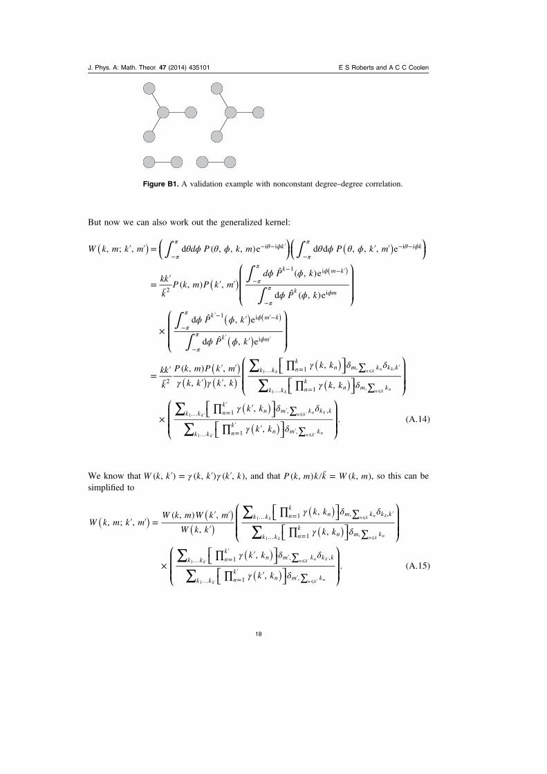
Figure B1. A validation example with nonconstant degree–degree correlation.

J. Phys. A: Math. Theor. 47 (2014) 435101 E S Roberts and A C C Coolen

18

Appendix B. Some synthetic examples evaluated directly and with the derivedformulae

Below we analyse some synthetic networks, where it is possible to evaluate the entropydirectly, and compare this to the results of applying equation (48). Consider a network basedon figure B1 as a repeating motif.

The self-consistency relations defined in equation (40) are straightforward

γ γ γ= = = =p

k

p

k(1, 1)

(1, 1)¯

1

4(1, 3) (3, 1)

3 (3, 3)¯

3

8(B.1)2

from which it follows that Γ defined in equation (44) is

⎜ ⎟⎡⎣⎢⎢

⎛⎝

⎞⎠

⎤⎦⎥⎥Γ γ γ γ= + + =log (1, 1)

3

log (1, 3)

2

log (3, 1)

6

1

6log

1

4

3

8. (B.2)

3 3

This evaluates to the same as the expression for Γ proposed in equation (47)

⎜ ⎟

⎛⎝⎜⎜

⎞⎠⎟⎟

⎡⎣⎢

⎤⎦⎥

⎡⎣⎢⎢

⎛⎝

⎞⎠

⎤⎦⎥⎥

∑ ∑ ∑Γ δ= + ′ ′

= + + + =

∑′ξ ξ

ξ=

( ) ( )p k m k W k k W k k( , ) log1

2¯ , log ,

8

6

1

2

1

4log

1

4

3

8log

3

8

3

8log

3

80

1

6log

1

4

3

8, (B.3)

k mm

k k, ,.,,

,

3

ks

k s

11

where ′W k k( , ) is defined in equation (5). A combinatorial argument can be used to count thenumber of networks in the ensemble—which is the same as evaluating the partition functionZ ( · ) that was defined in equation (2). The number of configurations can be obtained bycounting the number of labellings of the diagram, and then dividing by the symmetries, whichevaluates to:

=k mZ ( , )! !

!2! 3!.

N N

N N N

3 2

66 6

Applying Stirlingʼs formula, it follows that in leading order

⎜ ⎟ ⎜ ⎟ ⎜ ⎟⎛⎝

⎞⎠

⎛⎝

⎞⎠

⎛⎝

⎞⎠= + − − −

= − + −

k mN

ZN N N

N

1log ( , )

1

3log

3

1

2log

2

1

6log

6

1

6log(12)

4

64

6log

1

3[log 3 2 log 2]

2

3. (B.4)

This matches the analytic result, evaluated with the help of equation (48). The link between(48) and kZ ( ) is defined in equations (6) and (7). Consider the ensemble of networks definedby the general degree sequence set out in figure B2 . By combinatorics, argue that there are !N

3

Figure B2. A validation example based on a connected network.

J. Phys. A: Math. Theor. 47 (2014) 435101 E S Roberts and A C C Coolen

19

orderings of the centre nodes, and !N2

3orderings of the remaining nodes, divided by 2

N3 for

symmetry. It follows that in leading order

⎛

⎝

⎜⎜⎜

⎞

⎠

⎟⎟⎟=

= + − −

= − + −

k mN

ZN

N N

N N

N

1log ( , )

1log 3

!2

3!

2

1

3log

3

2

3log

2

3

1

3log 2 1

log log 31

3log 2 1. (B.5)

N3

The analytic formula evaluates to

= + − − −

= + − −

k mN

Z N

N

1log ( , ) log log 2 1

2

3log 2 log 3

log1

3log 2 log 3 1. (B.6)

References

[1] Annibale A, Coolen A C, Fernandes L P, Fraternali F and Kleinjung J 2009 J. Phys. A: Math.Theor. 42 485001

[2] Roberts E S, Schlitt T and Coolen A C 2011 J. Phys. A: Math. Theor. 44 5002[3] Bianconi G, Coolen A C and Vicente C J P 2008 Phys. Rev. E 78 016114[4] Faudree R J, Gould R J and Lesniak L M 1992 Discrete Appl. Math. 37-38 179–91[5] Rogers T, Vicente C P, Takeda K and Castillo I P 2010 J. Phys. A: Math. Theor. 43 195002[6] Newman M 2009 Networks: an Introduction (Oxford: Oxford University Press)[7] Roberts E S and Coolen A C 2012 Phys. Rev. E 85 046103[8] Titz B, Rajagopala S V, Goll J, Häuser R, McKevitt M T, Palzkill T and Uetz P 2008 PLoS One 3

e2292[9] Ito T, Chiba T, Ozawa R, Yoshida M, Hattori M and Sakaki Y 2001 Proc. Natl. Acad. Sci. USA 98

4569–74[10] LaCount D J et al 2005 Nature 438 103–7[11] Rual J F et al 2005 Nature 437 1173–8[12] Ewing R M et al 2007 Mol. Syst. Biol. 3 89[13] Arifuzzaman M et al 2006 Genome Res. 16 686–91[14] Bordenave C and Caputo P 2013 arXiv:1308.5725

J. Phys. A: Math. Theor. 47 (2014) 435101 E S Roberts and A C C Coolen

20