Package 'bipartite'

Package ‘bipartite’March 31, 2017

Type Package

Title Visualising Bipartite Networks and Calculating Some (Ecological)Indices

Version 2.08

Date 2017-03-30

Author Carsten F. Dormann, Jochen Fruend and Bernd Gruber, with additional code from Mari-ano Devoto, Jose Iriondo, Rouven Strauss and Diego Vazquez, also based on C-code devel-oped by Nils Bluethgen, Aaron Clauset/Rouven Strauss and Miguel Rodriguez-Girones

Maintainer Carsten F. Dormann <[email protected]>

Depends vegan, sna

Imports fields, igraph, MASS, methods, permute

LazyData TRUE

URL https://github.com/biometry/bipartite

DescriptionFunctions to visualise webs and calculate a series of indices commonly used to describe pat-tern in (ecological) webs. It focuses on webs consisting of only two levels (bipartite), e.g. polli-nation webs or predator-prey-webs. Visualisation is important to get an idea of what we are actu-ally looking at, while the indices summarise different aspects of the web's topology.

License GPL

NeedsCompilation yes

Repository CRAN

Date/Publication 2017-03-31 06:30:25 UTC

R topics documented:bipartite-package . . . . . . . . . . . . . . . . . . . . . . . . . . . . . . . . . . . . . . 3as.one.mode . . . . . . . . . . . . . . . . . . . . . . . . . . . . . . . . . . . . . . . . . 11as.tnet . . . . . . . . . . . . . . . . . . . . . . . . . . . . . . . . . . . . . . . . . . . . 13barrett1987 . . . . . . . . . . . . . . . . . . . . . . . . . . . . . . . . . . . . . . . . . 14betweenness_w . . . . . . . . . . . . . . . . . . . . . . . . . . . . . . . . . . . . . . . 15bezerra2009 . . . . . . . . . . . . . . . . . . . . . . . . . . . . . . . . . . . . . . . . . 16

1

https://github.com/biometry/bipartite

2 R topics documented:

C.score . . . . . . . . . . . . . . . . . . . . . . . . . . . . . . . . . . . . . . . . . . . 17closeness_w . . . . . . . . . . . . . . . . . . . . . . . . . . . . . . . . . . . . . . . . . 18clustering_tm . . . . . . . . . . . . . . . . . . . . . . . . . . . . . . . . . . . . . . . . 20compart . . . . . . . . . . . . . . . . . . . . . . . . . . . . . . . . . . . . . . . . . . . 21computeModules . . . . . . . . . . . . . . . . . . . . . . . . . . . . . . . . . . . . . . 22czvalues . . . . . . . . . . . . . . . . . . . . . . . . . . . . . . . . . . . . . . . . . . . 24degreedistr . . . . . . . . . . . . . . . . . . . . . . . . . . . . . . . . . . . . . . . . . . 26dfun . . . . . . . . . . . . . . . . . . . . . . . . . . . . . . . . . . . . . . . . . . . . . 28DIRT_LPA_wb_plus . . . . . . . . . . . . . . . . . . . . . . . . . . . . . . . . . . . . 30discrepancy . . . . . . . . . . . . . . . . . . . . . . . . . . . . . . . . . . . . . . . . . 32distance_w . . . . . . . . . . . . . . . . . . . . . . . . . . . . . . . . . . . . . . . . . 33elberling1999 . . . . . . . . . . . . . . . . . . . . . . . . . . . . . . . . . . . . . . . . 35empty . . . . . . . . . . . . . . . . . . . . . . . . . . . . . . . . . . . . . . . . . . . . 35endpoint . . . . . . . . . . . . . . . . . . . . . . . . . . . . . . . . . . . . . . . . . . . 37extinction . . . . . . . . . . . . . . . . . . . . . . . . . . . . . . . . . . . . . . . . . . 38fc . . . . . . . . . . . . . . . . . . . . . . . . . . . . . . . . . . . . . . . . . . . . . . 39frame2webs . . . . . . . . . . . . . . . . . . . . . . . . . . . . . . . . . . . . . . . . . 40genweb . . . . . . . . . . . . . . . . . . . . . . . . . . . . . . . . . . . . . . . . . . . 42grouplevel . . . . . . . . . . . . . . . . . . . . . . . . . . . . . . . . . . . . . . . . . . 43H2fun . . . . . . . . . . . . . . . . . . . . . . . . . . . . . . . . . . . . . . . . . . . . 49inouye1988 . . . . . . . . . . . . . . . . . . . . . . . . . . . . . . . . . . . . . . . . . 50junker2013 . . . . . . . . . . . . . . . . . . . . . . . . . . . . . . . . . . . . . . . . . 51kato1990 . . . . . . . . . . . . . . . . . . . . . . . . . . . . . . . . . . . . . . . . . . 52kevan1970 . . . . . . . . . . . . . . . . . . . . . . . . . . . . . . . . . . . . . . . . . . 53linklevel . . . . . . . . . . . . . . . . . . . . . . . . . . . . . . . . . . . . . . . . . . . 54listModuleInformation . . . . . . . . . . . . . . . . . . . . . . . . . . . . . . . . . . . 55memmott1999 . . . . . . . . . . . . . . . . . . . . . . . . . . . . . . . . . . . . . . . . 56mgen . . . . . . . . . . . . . . . . . . . . . . . . . . . . . . . . . . . . . . . . . . . . 56moduleWeb-class . . . . . . . . . . . . . . . . . . . . . . . . . . . . . . . . . . . . . . 58mosquin1967 . . . . . . . . . . . . . . . . . . . . . . . . . . . . . . . . . . . . . . . . 59motten1982 . . . . . . . . . . . . . . . . . . . . . . . . . . . . . . . . . . . . . . . . . 60ND . . . . . . . . . . . . . . . . . . . . . . . . . . . . . . . . . . . . . . . . . . . . . . 61nested . . . . . . . . . . . . . . . . . . . . . . . . . . . . . . . . . . . . . . . . . . . . 63nestedcontribution . . . . . . . . . . . . . . . . . . . . . . . . . . . . . . . . . . . . . . 65nestedness . . . . . . . . . . . . . . . . . . . . . . . . . . . . . . . . . . . . . . . . . . 67nestedrank . . . . . . . . . . . . . . . . . . . . . . . . . . . . . . . . . . . . . . . . . . 69networklevel . . . . . . . . . . . . . . . . . . . . . . . . . . . . . . . . . . . . . . . . . 70nodespec . . . . . . . . . . . . . . . . . . . . . . . . . . . . . . . . . . . . . . . . . . 79NOS . . . . . . . . . . . . . . . . . . . . . . . . . . . . . . . . . . . . . . . . . . . . . 81npartite . . . . . . . . . . . . . . . . . . . . . . . . . . . . . . . . . . . . . . . . . . . 82null.distr . . . . . . . . . . . . . . . . . . . . . . . . . . . . . . . . . . . . . . . . . . . 83null.t.test . . . . . . . . . . . . . . . . . . . . . . . . . . . . . . . . . . . . . . . . . . 85nullmodel . . . . . . . . . . . . . . . . . . . . . . . . . . . . . . . . . . . . . . . . . . 86olesen2002aigrettes . . . . . . . . . . . . . . . . . . . . . . . . . . . . . . . . . . . . . 88olesen2002flores . . . . . . . . . . . . . . . . . . . . . . . . . . . . . . . . . . . . . . 89ollerton2003 . . . . . . . . . . . . . . . . . . . . . . . . . . . . . . . . . . . . . . . . . 89PAC . . . . . . . . . . . . . . . . . . . . . . . . . . . . . . . . . . . . . . . . . . . . . 90PDI . . . . . . . . . . . . . . . . . . . . . . . . . . . . . . . . . . . . . . . . . . . . . 92

bipartite-package 3

plotModuleWeb . . . . . . . . . . . . . . . . . . . . . . . . . . . . . . . . . . . . . . . 93plotPAC . . . . . . . . . . . . . . . . . . . . . . . . . . . . . . . . . . . . . . . . . . . 95plotweb . . . . . . . . . . . . . . . . . . . . . . . . . . . . . . . . . . . . . . . . . . . 96plotweb2 . . . . . . . . . . . . . . . . . . . . . . . . . . . . . . . . . . . . . . . . . . 101printoutModuleInformation . . . . . . . . . . . . . . . . . . . . . . . . . . . . . . . . . 103projecting_tm . . . . . . . . . . . . . . . . . . . . . . . . . . . . . . . . . . . . . . . . 104r2dexternal . . . . . . . . . . . . . . . . . . . . . . . . . . . . . . . . . . . . . . . . . 105robustness . . . . . . . . . . . . . . . . . . . . . . . . . . . . . . . . . . . . . . . . . . 106Safariland . . . . . . . . . . . . . . . . . . . . . . . . . . . . . . . . . . . . . . . . . . 107schemske1978 . . . . . . . . . . . . . . . . . . . . . . . . . . . . . . . . . . . . . . . . 108second.extinct . . . . . . . . . . . . . . . . . . . . . . . . . . . . . . . . . . . . . . . . 109shuffle.web . . . . . . . . . . . . . . . . . . . . . . . . . . . . . . . . . . . . . . . . . 111slope.bipartite . . . . . . . . . . . . . . . . . . . . . . . . . . . . . . . . . . . . . . . . 113small1976 . . . . . . . . . . . . . . . . . . . . . . . . . . . . . . . . . . . . . . . . . . 114sortweb . . . . . . . . . . . . . . . . . . . . . . . . . . . . . . . . . . . . . . . . . . . 115specieslevel . . . . . . . . . . . . . . . . . . . . . . . . . . . . . . . . . . . . . . . . . 116strength . . . . . . . . . . . . . . . . . . . . . . . . . . . . . . . . . . . . . . . . . . . 123swap.web . . . . . . . . . . . . . . . . . . . . . . . . . . . . . . . . . . . . . . . . . . 124symmetrise_w . . . . . . . . . . . . . . . . . . . . . . . . . . . . . . . . . . . . . . . . 126tnet_igraph . . . . . . . . . . . . . . . . . . . . . . . . . . . . . . . . . . . . . . . . . 128togetherness . . . . . . . . . . . . . . . . . . . . . . . . . . . . . . . . . . . . . . . . . 129V.ratio . . . . . . . . . . . . . . . . . . . . . . . . . . . . . . . . . . . . . . . . . . . . 130vazarr . . . . . . . . . . . . . . . . . . . . . . . . . . . . . . . . . . . . . . . . . . . . 131vazcer . . . . . . . . . . . . . . . . . . . . . . . . . . . . . . . . . . . . . . . . . . . . 132vazllao . . . . . . . . . . . . . . . . . . . . . . . . . . . . . . . . . . . . . . . . . . . . 132vazmasc . . . . . . . . . . . . . . . . . . . . . . . . . . . . . . . . . . . . . . . . . . . 133vazmasnc . . . . . . . . . . . . . . . . . . . . . . . . . . . . . . . . . . . . . . . . . . 133vaznull . . . . . . . . . . . . . . . . . . . . . . . . . . . . . . . . . . . . . . . . . . . . 134vazquec . . . . . . . . . . . . . . . . . . . . . . . . . . . . . . . . . . . . . . . . . . . 135vazquenc . . . . . . . . . . . . . . . . . . . . . . . . . . . . . . . . . . . . . . . . . . 136vazquez.example . . . . . . . . . . . . . . . . . . . . . . . . . . . . . . . . . . . . . . 136versionlog . . . . . . . . . . . . . . . . . . . . . . . . . . . . . . . . . . . . . . . . . . 138visweb . . . . . . . . . . . . . . . . . . . . . . . . . . . . . . . . . . . . . . . . . . . . 147web2edges . . . . . . . . . . . . . . . . . . . . . . . . . . . . . . . . . . . . . . . . . . 150webs2array . . . . . . . . . . . . . . . . . . . . . . . . . . . . . . . . . . . . . . . . . 151wine . . . . . . . . . . . . . . . . . . . . . . . . . . . . . . . . . . . . . . . . . . . . . 152

Index 156

bipartite-package Analysis of bipartite ecological webs

Description

Bipartite provides functions to visualise webs and calculate a series of indices commonly used todescribe pattern in (ecological) networks, a.k.a. webs. It focusses on webs consisting of only twolevels, e.g. pollinator-visitation or predator-prey webs. Visualisation is important to get an idea ofwhat we are actually looking at, while the indices summarise different aspects of the webs topology.

4 bipartite-package

Details

Input for most analyses is an interaction matrix of m species from one group (“higher”) with nspecies from another group (“lower”), i.e. a n x m matrix, where higher level species are in columns,lower level species in rows. Column and row names can be provided. This is fundamentally differ-ent from “one-mode” webs, which are organised as k x k matrix, i.e. one group of species only, inwhich each species can interact with each other. Such a format is incompatible with the functionswe provide here. (Note, however, that functions as.one.mode and web2edges are conveniencefunctions to morph bipartite networks into one-mode webs. Furthermore, some indices build onone-mode networks and are called from bipartite.)

Before you start with the network, you have to get the data into the right shape. The functionframe2webs aims to facilitate this process. Arranging a web, e.g. by size, is supported by sortweb.

The typical first step is to visualise the network. Two functions are on offer here: one (visweb) sim-ply plots the matrix in colours depicting the strength of an interaction and options for re-arrangingcolumns and rows (e.g. to identify compartments or nesting). The other function (plotweb) plotsthe actual web with participants (as two rows of rectangles) connected by lines (proportional tointeraction strength). Both can be customised by many options.

The second step is to calculate indices describing network topography. There are three differentlevels this can be achieved at: the entire web (using function networklevel), at the level of eachgroup (also using function networklevel) or the individual species (using function specieslevel).Most other functions in the package are helpers, although some can be called on their own and returnthe respective result (dfun, H2fun and second.extinct with slope.bipartite).

The third step is to compare results to null models. Many interaction matrices are very incompletesnapshots of the true underlying network (e.g. a one-week sampling of a pollination network on apatch of 4 x 4 meters). As a consequence, many species were rarely observed, many are singletons(only one recording). To make analyses comparable across networks with different sampling inten-sity and number of species per group, we need a common yardstick. We suggest that users shoulduse a null model, i.e. an algorithm that randomises entries while constraining some web properties(such as dimensions, marginal totals or connectance). The function nullmodel provides a few suchnull models, but this is a wide field of research and we make no recommendations (actually, we do:see Dormann et al. 2009 and Dormann 2011, both shipping in the doc-folder of this package). Youcan also simulate networks using genweb or null.distr.

Finally, bipartite comes with 23 quantitative pollination network data sets taken from the NCEASinteraction webs data base (use data(package="bipartite") to show their names) and it has a fewmiscellaneous functions looking at some special features of bipartite networks (such as modularity:computeModules or apparent competition: PAC).

Speed: The code of bipartite is almost exclusively written in R. You can increase the speed a bit(by 30 to 50 %, depending on the functions you use) by compiling functions on-the-fly. To doso, you need to load the compiler package and type: enableJIT(3). The first time you call afunction, it will be compiled to bytecode (just-in-time: jit), which takes a few seconds, but thesecond call will be substantially faster than without compilation. In the few tests we have run,this improvement was NOT substantial (i.e. a few tens of percent), indicating, I guess, that ourR code wasn’t too bad. See compiler-help files or http://www.r-statistics.com/2012/04/speed-up-your-r-code-using-a-just-in-time-jit-compiler/ for details.

See help pages for details and examples.

For an overview of other computing resources, data, books, journals etc. check out this page:https://github.com/briatte/awesome-network-analysis.

http://www.r-statistics.com/2012/04/speed-up-your-r-code-using-a-just-in-time-jit-compiler/

http://www.r-statistics.com/2012/04/speed-up-your-r-code-using-a-just-in-time-jit-compiler/

https://github.com/briatte/awesome-network-analysis

bipartite-package 5

Package: bipartiteType: PackageVersion: 2.08Date: 2017-03-30License: GPL

versionlog

Please see help page versionlog for all changes and updates prior to version 2.00. This page willonly list most recent changes.

• 2.08 (release date: 30-Mar-2017)

New modularity algorithm called by computeModules. Although the excellent algorithm DIRT_LPA_wb_plusby Stephen Beckett has been around for a year, I never managed to find the time to put itinto bipartite. By now, Stephen has even written a wrapper code so that the output is fullycompatible with existing code for plotting (plotModuleWeb) there was really no argu-ment left to postpone it. Stephen’s DIRT_LPA_wb_plus will be the new default, replac-ing ’QuanBiMo’, which remains available under ‘method='DormannStrauss'’. WhileDIRT could be called recursively, thereby making modules-within-modules computable,this is not packaged yet. So currently the much slower DormannStrauss-option is the onlyway to get recursive modules. Many thanks to Stephen for making this code available!

networklevel and grouplevel inconsistently returned different values for secondary ex-tinction, because the former by default purged empty columns/rows, while the latterdidn’t. It does now. Thanks to Gianalberto Losapio for bringing this to my attention.

• 2.07 (release date: 08-Nov-2016)

Bug fixed in vaznull, filled the matrix with 1s instead of 0s (although it was a ‘sophisticated’logical mistake I made, not a simple typo). Thanks to Sandra Bibiana Corea for reporting!

Small patch in C++-code of binmatnest for compatibility with clang. Thanks to Brian Rip-ley for fixing one of these C++-things that I never will understand! (In this case, the origi-nal code (by Miguel Rodríguez-Gironés) defined a pointer to "vector", which caused am-biguities in which "vector" should be used during compilation: the such defined pointer,or the std::vector.)

Smaller typographic and referencing corrections/additions (e.g. in plotPAC).

• 2.06b (release date: 10-May-2016)

Some explanation addded to czvalues, where a z-value of NA is returned if a species isalone (in its trophic level) in a module. This is due to the way z-values are computed, andnot a bug.

Function nestedcontribution was not exported in the namespace. Fixed. Thanks to vari-ous people reporting this.

• 2.06 (release date: 29-Sep-2015)

Bug fix in C.score, which did not compute the maximum number of possible checkerboardscorrectly, and hence let the normalised C-score to be incorrect. Now it uses a brute-forceapproach, which works fine but takes its time.

Function nestedcontribution was not exported (i.e. not listed in the namespace file).Fixed. Thanks to Wesley Dátillo for reporting.

6 bipartite-package

Help page of specieslevel now correctly described a species’ degree as sum of its links.Thanks to Bernhard Hoiß for the correction!

C++-warnings addressed: outcommented some unused variables in dendro.h and removedsome fprintf-warnings in bmn5.cc

Little bug fix in vaznull: Threw an error when matrix was without 0s. Thanks to ThaisZanata for reporting.

• 2.05 (release date: 24-Nov-2014)

New function nestedcontribution which computes the contribution of each species to theoverall nestedness, based on Bascompte et al. 2003 and as used by Saavedra et al. 2011.Many thanks to Daniel Stouffer for contributing this function!

New function mgen: this function is based on R-code written by Diego Vázquez (many thanksfor sending the code), with a bit of brushing up options by CFD. The function takesa probability matrix generated by whatever mechanism and builds a null model from it.This is a niffty little idea, making null modelling concerned with generating ideas on whatmakes an interaction probable and leaving the step of producing and integer-network ofsimulated interactions to this function.

minor fixes in networklevel “weighted connectance” was only returned when “linkage den-sity” was in “index” call; now also available on its own. Also sligthly revised the helpfile.

nested with option ‘weighted NODF’ called the unsorted version of this function, while call-ing the same index in networklevel called the sorted. This is not nice (although notstrictly wrong). Now both call the sorted version and users have to directly invokenestednodf for the unsorted option. Many thanks to Julian Resasco for reporting!

Changes to the help page of vaznull: I (CFD) misread the original paper introducing thisnull model and hence assumed thatvaznull would constrain marginal totals and con-nectance. However, this was not intended in Diego Vázquez original implementation andnever stated anywhere (except in the help pages of this function here in bipartite). Hence,the help pages were changed to now reflect both intention and actual action of this func-tion. This also means that currently only one null model with constrained marginal totalsand connectance is available: swap.web. Many thanks to Diego for clearing this up!

Some example code had to be re-written to adapt to the upcoming/new structure of vegan,which got rid of function commsimulator (replaced by simulate). Many thanks to JariOksanen for informing me about this!

Added an error message to function second.extinct for the case that a user wants to pro-vide an extinction sequence for both trophic levels. There is no obvious way to simulatethis across the two groups, and hence it is not implemented. Also added error messagesfor non-matching vector/web dimensions and alike.


R-C++-communication bug fixed in computeModules: This bug has been a constant thornin my side. Somehow the C-code behind computeModules could only be called once. Onsecond call, it returned an error because somehow it kept some old files in memory. So far,I used a work-around (unloading and re-loading the dynamic library), which only workedon Windows and Mac. I still don’t fully understand it, but thanks to Tobias Hegemann(whom I paid for being more competent than myself) we now have a function runningbug-free on all platforms. (Deep sigh of relief.)

bipartite-package 7

The call of index “functional complementarity” through networklevel did not work. Fixedthis legacy issue, which was due to a confusion created by the index’ earlier name of“functional diversity”.

Help page to specieslevel gave incomplete name for one index: Should be ‘interaction push pull’;also the function itself had the “push pull”-bit messed up. Thanks to Natacha Chacoff forreporting!

Sequence of indices differed between lower and higher level. (Fixed.) Both should be thesame and should fit the description in the help file. Thanks to Jimmy O’Donnell forreporting!

• 2.03 (release date: 15-Jan-2014)Some ghost text led to conflicts with the updated package checking. Ghost text deleted. Thanks

to Brian Ripley of the R-Team and CRAN for not only reporting the issue but also point-ing to its solution!

Option ‘empty.web’ added to specieslevel: Similar to the argument in networklevel;non-interacting species from the network were always excluded so far; new option ‘FALSE’not fully tested yet.

Minor bug fix in specieslevel: “pollination support index” returned “PSI”; “PDI” now ref-erenced correctly as “paired differences index”.

Simplification in grouplevel and correspondingly in networklevel: Previously, index="generality"or "vulnerability" was identical to "effective partners" with option weighted=TRUE,but different for weighted=FALSE (to which only "effective partners" responded).We reduced this to one index called "generality" or "vulnerability" (depending on the fo-cal group), but which will now give the non-weighted mean if option weighted=FALSE.It can still be called by "effective partners" for backward compatibility.

Function grouplevel used fd wrongly! Instead of returning the value for rows, it returnedthe functional diversity for columns (and vice versa). We also used the opportunity torename the index to its correct name: “functional complementarity” and the function tofc. Help pages for fc and grouplevel were adapted accordingly. Thanks to MarianoDevoto for pointing out this mistake!

New index “weighted connectance” in function networklevel: This index is simply com-puted as linkage density divided by number of species in the network. Note that using‘empty.web=TRUE’ will affect this value (which is intended). Thanks to Becky Morris forsuggesting to add this index here.

Help page for function PDI corrected. Thanks to Timothy Poisot for reporting some issuesin the help page.

• 2.02 (release date: 30-Sep-2013)Glitch fixed in grouplevel (thus also affecting networklevel). Networks with only one species

in one of the two levels resulted in errors, rather than simply return NA for C-score andsecondary extinction computation. Thanks to whoever it was for reporting (at the IN-TECOL workshop).

Minor bug fixes in specieslevel: Gave error messages for closeness and betweenness ifthe network had no shortest path. Now returns a warning and NAs instead. Reported: JF.

Minor bux fix in networklevel: Failed to work when an index was listed twice in the func-tion call. Reported: JF.

New function r2dexternal: This function is a null model algorithm like Patefields (r2dtable,but it excepts externally measured abundances to compute the null model-expectation.Experimental.

8 bipartite-package

Memory leak in computeModules fixed. Because some object was not deleted, memory con-sumption of this function shot through the roof (with time). Since R has a somewhat weirdway of handling memory, I think that also subsequent operations were slower (becausethe dynamically expanded memory is not being shrunken again, which is a problem ifyou use the hard drive as RAM). Thanks to Florian Hartig for investing the time to fix it!

• 2.01 (release date: 28-Jun-2013) This release features smoothing of various glitches that wereintroduced when we cleaned up the code for version 2.00.

New index for specieslevel: Computes the nestedness rank (as proposed by Alarcon et al.2008). Can also be employed directly using the new function nestedrank with op-tions for weighting for number of interactions per link, normalising the rank and differentmethod to compute the nestedness-arranged matrix.

Polishing specieslevel: Now returns an error message if the index is not recognised, in-stead of an empty list.

Function plotweb received an option to plot additional individuals of a species in differentways. For a host-parasitoid network, some hosts are not parasitised. This data vector cannow be interpreted in two ways, making the plotting function a bit more flexible.

Function degreedistr can now be invoked for each level separately. Also arguments can bepassed to the plotting options.

New data set junker2013: a nice and large pollination network. Thanks to Robert Junkerfor providing this data set!

Fixed computation of secondary extinction slopes for both levels simultaneously for ran-dom extinction sequences. This was so far not possible, because the function did not com-bine extinction sequences of different lengths. This was simply an oversight, reported byRichard Lance. (Thanks!)

• 2.00 (release date: 15-Mar-2013) A new version number usually indicates substantial changes.In this case, we have re-named and re-grouped some of the output of networklevel andspecieslevel for greater consistency and transparency. Beware! Running the same functionsnow (2.00 and up) will yield different results to <2.00 (because the same values are now in adifferent sequence).We also started carefully renaming indices and re-writing help files. The main reason is thatwe started this work thinking of pollination networks. Over time, however, other types ofecological networks came into focus, and now also non-ecological networks are on the table.Thus, we started (and shall continue) referring to lower and higher levels, rather than plant andpollinators, hosts and predators or even trophic levels. Thus, in our emerging nomenclaturethe two levels are referred to as “groups” (their members remain “species” interacting withtheir “partners” in the other group).Please read (or at least skim) the help pages before using a function of version 2.00 for thefirst time.In function specieslevel indices can now be computed for levels separately (or together).Few user-visible changes, but complete re-structuring under the hood. Option ‘species number’was moved to grouplevel as ‘number of species’.In the new function grouplevel we collected all indices that can be computed for each of thetwo groups (i.e. trophic or other levels). Indices can be computed for each group separately orfor both simultaneously. All group-level indices are also accessible through networklevel!In the new function linklevel we collected all indices that can be computed for each cell ofthe bipartite matrix. Currently, there are few such indices, however.

bipartite-package 9

In function networklevel we dropped the plotting options. Users wanting to plot degree dis-tributions or extinction slopes are encouraged to use the functions degreedistr and slope.bipartite,respectively.Furthermore, due to licensing issues, we copy-pasted several functions from the package tnet,created and maintained by Tore Opsahl, to bipartite. We have so far called these functionsfrom tnet, but only recently did R start to enforce license compatibility, which caused thisstep (bipartite being GPL and tnet being CC by-NC 3.0). We are really very grateful to Torefor allowing us to include the following functions: as.tnet, betweenness_w, closeness_w,clustering_tm, distance_w, symmetrise_w, tnet_igraph.Here a more detailed list of changes:networklevel – Function call and output now more consistent in naming and sequence.

When higher and lower level indices are given (e.g. extinction slopes, number ofshared partners), the first will always be the one referring to the property of the lowerlevel. From a pollinator network perspective, the first value in such a pair describes aplant-level index, the second a pollinator-level index.

– Indices ‘mean interaction diversity’ dropped from networklevel. We foundno reference to this metric and saw little use for it. It is very similar to vulnera-bility/generality and can easily be computed from the output of specieslevel asmean(specieslevel(web, index="diversity")).

– Now also accepts non-integer values as input. The argument ‘H2_integer’ will thenautomatically be set to FALSE. Will return NA for those indices that cannot be com-puted (e.g. Fisher’s alpha). As a knock-on effect, H2fun had to be slightly adaptedto round to machine precision when searching for H2min. (A somewhat technicaldetail, but making H2fun getting caught sometimes.)

New function grouplevel in which we collected indices that can be computed for each ofthe two groups (i.e. trophic or other levels). Indices can be computed for each groupseparately or for both simultaneously. All group-level indices are also accessible throughnetworklevel!

New function linklevel in which we collect indices that can be computed for each cell ofthe bipartite matrix.

New option to PDI: ‘normalise=FALSE’ offers the option of using the index as originallyproposed, although we prefer to use TRUE and made this the default.

Corrected network bezerra2009. Network was actually the transpose of the correct net-work and hence wrongly had plant species as columns.

New function endpoint computes end-point degrees following Barrat et al. (2004); one ofthe indices computed at linklevel.

New function frame2webs helps organising data into one or more webs.New function webs2array helps organising webs into one array.Function specieslevel gained two new indices (thanks to Jochen Fründ): ‘proportional’

‘similarity’ and ‘proportional generality’. See help page of that function fordetails.

New function npartite Experimental function to analyse more-than-2-level networks.visweb now obeys the label size to make sure labels are always in the plotting area. Thanks

to Zachary Grinspan for drawing our attention to this issue.Little bug fix in second.extinct Function failed for argument ‘participant="both"’ be-

cause I filled the extinction sequence with the wrong number of 0s (to achieve always thesame dimensionality of results in repeated runs). Thanks to Carine Emer for reporting!

10 bipartite-package

specieslevel failed to work for non-matrix data (i.e. data.frames). It now coerces data.framesto matrix as a first step and hence should work also on data.frames. Thanks to MarinaWolowski for drawing our attention to this problem.

Minor bug fix in dfun: When external abundances were provided with a 0 in it, dfun couldthrow up Inf-values. Reported by Indrani Singh and fixed by Jochen Fründ.

Settings for functions called by nested are now enshrined in stone. The initial reason wasto set only the default for one function (nestedness) to a faster setting (‘null.models=FALSE’),but then I decided to restrict all settings to the defaults of the functions called (except forthis one option).

Bug fix for the rarely used function null.t.test: Did not work if only one index was given.

Author(s)

Carsten F. Dormann, Jochen Fründ and Bernd Gruber, with additional code from many others (re-ferred to in the respective help file), noticeably from Tore Opsahl’s tnet package.

Maintainer: Carsten Dormann <[email protected]>

References

Alarcon, R., Waser, N.M. and Ollerton, J. 2008. Year-to-year variation in the topology of a plant-pollinator interaction network. Oikos 117, 1796–1807

Almeida-Neto, M. and Ulrich, W. (2011) A straightforward computational approach for measuringnestedness using quantitative matrices. Environmental Modelling & Software, 26, 173–178

Bascompte, J., Jordano, P. and Olesen, J. M. (2006) Asymmetric coevolutionary networks facilitatebiodiversity maintenance. Science 312, 431–433

Beckett, S.J. 2016. Improved community detection in weighted bipartite networks. Royal Societyopen science 3, 140536

Bersier, L. F., Banasek-Richter, C. and Cattin, M. F. (2002) Quantitative descriptors of food-webmatrices. Ecology 83, 2394–2407

Blüthgen, N., Menzel, F. and Blüthgen, N. (2006) Measuring specialization in species interactionnetworks. BMC Ecology 6, 12

Blüthgen, N., Menzel, F., Hovestadt, T., Fiala, B. and Blüthgen, N. (2007) Specialization, con-straints, and conflicting interests in mutualistic networks. Current Biology 17, 1–6

Corso G., de Araújo A.I.L. and de Almeida A.M. (2008) A new nestedness estimator in communitynetworks. arXiv, 0803.0007v1 [physics.bio-ph]

Dalsgaard, B., A. M. Martín González, J. M. Olesen, A. Timmermann, L. H. Andersen, and J.Ollerton. (2008) Pollination networks and functional specialization: a test using Lesser Antilleanplant-hummingbird assemblages. Oikos 117, 789–793

Devoto M., Bailey S., Craze P. & Memmott J. (2012) Understanding and planning ecologicalrestoration of plant-pollinator networks. Ecology Letters 15, 319–328

Dormann, C.F., Fründ, J., Blüthgen, N., and Gruber, B. (2009) Indices, graphs and null models:analysing bipartite ecological networks. The Open Ecology Journal 2, 7–24

Dormann, C.F. (2011) How to be a specialist? Quantifying specialisation in pollination networks.Network Biology 1, 1–20

as.one.mode 11

Galeano J., Pastor J.M. and Iriondo J.M. (2008) Weighted-Interaction Nestedness Estimator (WINE):A new estimator to calculate over frequency matrices. arXiv 0808.3397v1 [physics.bio-ph]

Martín Gonzáles, A.M., Dalsgaard, B. and Olesen, J.M. (2009) Centrality measures and the impor-tance of generalist species in pollination networks. Ecological Complexity, 7, 36–43

Memmott, J., Waser, N. M. and Price, M. V. (2004) Tolerance of pollination networks to speciesextinctions. Proceedings of the Royal Society B 271, 2605–2611

Morris, R. J., Lewis, O. T. and Godfray, H. C. J. (2004) Experimental evidence for apparent com-petition in a tropical forest food web. Nature 428, 310–313

Morris, R. J., Lewis, O. T. and Godfray, H. C. J. (2005) Apparent competition and insect communitystructure: towards a spatial perspective. Annales Zoologica Fennici 42, 449–462.

Müller, C. B., Adriaanse, I. C. T., Belshaw, R. and Godfray, H. C. J. (1999) The structure of anaphid-parasitoid community. Journal of Animal Ecology 68, 346–370

Poisot, T., Lepennetier, G., Martinez, E., Ramsayer, J., and Hochberg, M.E. (2011a) Resourceavailability affects the structure of a natural bacteria-bacteriophage community. Biology Letters 7,201–204

Poisot, T., Bever, J.D., Nemri, A., Thrall, P.H., and Hochberg, M.E. (2011b) A conceptual frame-work for the evolution of ecological specialisation. Ecology Letters 14, 841–851

Tylianakis, J. M., Tscharntke, T. and Lewis, O. T. (2007) Habitat modification alters the structureof tropical host-parasitoid food webs. Nature 445, 202–205

Vázquez, D. P. and Aizen, M. A. (2004) Asymmetric specialization: A pervasive feature of plant-pollinator interactions. Ecology 85, 1251–1257

Vázquez, D.P., Chacoff, N.,P. and Cagnolo, L. (2009) Evaluating multiple determinants of the struc-ture of plant-animal mutualistic networks. Ecology 90, 2039–2046.

Examples

## Not run:data(Safariland)plotweb(Safariland)visweb(Safariland)networklevel(Safariland)specieslevel(Safariland)

## End(Not run)

as.one.mode Conversion of a network matrix

Description

This helper function converts a bipartite matrix into a one-mode matrix.

Usage

as.one.mode(web, fill = 0, project="full", weighted=TRUE)

12 as.one.mode

Arguments

web A matrix with lower trophic level species as rows, higher trophic level speciesas columns and number of interactions as entries.

fill What shall unobserved combinations be represented as in the one-mode matrix(see below)? Defaults to 0. Set to NA if links not possible for bipartite networksshould be masked (i.e. those within a level).

project There are different ways to convert a two-mode (bipartite) network into one-mode networks. The most common is to focus on one set (e.g. the n pollinators)and compute a n x n matrix with entries between species that pollinate the sameplant (“higher”). Similarly, one can compute a k x k matrix for the k plantspecies (“lower”). Or, finally and the default, one can compute an (n+k) x (n+k)matrix in which only the observed interactions are present (“full”). This is infact a near-trivial, symmetric matrix with 0s between species of the same trophiclevel.

weighted Logical; shall the strength of links be included in the one-mode output? Defaultsto TRUE, but can be set to FALSE to turn a weighted two-mode into a binaryone-mode network.

Details

In bipartite (or: two-mode) networks, participants are of different types (e.g. pollinators and plants,actors and parties in social research). Hence, a party cannot connect to another party except throughactors. A pollinator interacts with another pollinator only through the host plant.

Much network theory, however, is based on one-mode networks, where all participants are listedin one vector, i.e. plants and pollinators alike, actors together with events. This function heretransforms the more condensed bipartite representation into a one-mode-representation, filling theunobserved type of interactions (i.e. plants with plants and pollinators with pollinators) with 0(unless you specify it differently in ‘fill’).

The lower trophic level (e.g. plants or rows) is listed first, then the higher trophic level (e.g. pollina-tors or columns). Hence, pollinator 2 becomes species number r+2, where r is the number of rowsof the network matrix.

The benefit of this conversion is access to the wonderful R-package Social Network Analysis (sna),with its many one-mode indices (such as betweenness, closeness, centralization, degree,kpath.census and so forth). Furthermore, gplot in that package also provides cool network de-pictions well worth checking out.

With respect to bipartite, as.one.mode is employed in the function nodespec, which itself usesthe sna-function geodist.

Value

A matrix of dimension (n+k) x (n+k), where n and k are the dimensions of the input web. Bothdimensions are given the names of the original web (first the lower, then the higher trophic level).

Author(s)

Carsten F. Dormann <[email protected]>

as.tnet 13

See Also

Function projecting_tm in package tnet provide smarter ways of converting two-modes into one-modes. This function can be accessed after transforming the web-matrix into an edge list usingweb2edges.

Examples

data(Safariland)image(Safariland)image(as.one.mode(Safariland))

as.tnet Ensures that networks conform to the tnet stardards

Description

Checks that a network conforms to the tnet stardards, and attaches a label. If the type parameter isnot set, the network is assumed to be a binary two-mode network, a weighted one-mode network, ora longitudinal network if there are 2, 3, or 4 columns respectively. Moreover, if a matrix is entered(more than 4 columns and rows), it is assumed to be a weighted one-mode network if square or atwo-mode network if non-square.

Usage

as.tnet(net, type=NULL)

Arguments

net A network in an edgelist or matrix format. It can be a weighted one-modenetwork, a binary two-mode network, a weighted two-mode netork, or a lon-gitudinal network. If the data-object has two-columns, it is assumed to be abinary two-mode network; three columns, weighted one-mode network; fourcolumns, longitudinal; five or more and the same number of rows and columns,weighted one-mode network; five or more and –not– the same number of rowsand columns, it is assumed to be a two-mode network.

type If you would like to specify the type of network. This could be "weighted one-mode tnet", "binary two-mode tnet", "weighted two-mode tnet", or "longitudinaltnet".

Value

Returns the network with an attached lable.

Note

version 1.0.0, taken, with permission, from package tnet

14 barrett1987

Author(s)

Tore Opsahl; http://toreopsahl.com

Examples

## Load sample datasample <- rbind(c(1,2,4),c(1,3,2),c(2,1,4),c(2,3,4),c(2,4,1),c(2,5,2),c(3,1,2),c(3,2,4),c(4,2,1),c(5,2,2),c(5,6,1),c(6,5,1))

## Run the programmeas.tnet(sample)

barrett1987 Individuals caught in a pollination web in boreal Canada.

Description

This study took place in the boreal forest of central New Brunswick, Canada, from May to Septem-ber of 1978, 1979, and 1980. The objective was to investigate the role of animals in pollinationand seed dispersal. The study was designed to provide basic descriptive information on breedingsystems, pollination biology, and phenology of understory herbs.

The authors recorded their data by counting the number of individual flower visitors caught oneach plant species. The total number of individuals collected on each plant species provide a roughestimate of the level of visitation that each species received. Data are presented as an interactionfrequency matrix, in which cells with positive integers indicate the frequency of interaction betweena pair of species, and cells with zeros indicate no interaction.

Usage

data(barrett1987)

References

Barrett, S. C. H. and Helenurm, K. (1987) The Reproductive-Biology Of Boreal Forest Herbs. 1.Breeding Systems And Pollination. Canadian Journal of Botany 65, 2036–2046

betweenness_w 15

Examples

data(barrett1987)

betweenness_w Betweenness centrality in a weighted network

Description

This function calculates betweenness scores for nodes in a weighted network based on the distance_w-function.Note: This algorithm relies on the igraphs package’s implementation of Dijkstra’s algorithm. Cur-rently, it does not find multiple shortest paths if two exist.

Usage

betweenness_w(net, directed=NULL, alpha=1)

Arguments

net A weighted edgelist

directed logical, whether the network is directed or undirected. Default is NULL, thismeans that the function checks whether the edgelist is directed or not.

alpha sets the alpha parameter in the generalised measures from Opsahl, T., Agneessens,F., Skvoretz, J., 2010. Node Centrality in Weighted Networks: Generalizing De-gree and Shortest Paths. Social Networks. If this parameter is set to 1 (default),the Dijkstra shortest paths are used. The length of these paths rely simply on thetie weights and disregards the number of nodes on the paths.

Value

Returns a data.frame with two columns: the first column contains the nodes’ ids, and the secondcolumn contains the nodes’ betweenness scores.

Note


Author(s)


References

http://toreopsahl.com/2009/02/20/betweenness-in-weighted-networks/

16 bezerra2009

Examples

## Load sample datasampledata <- rbind(c(1,2,1),c(1,3,5),c(2,1,1),c(2,4,6),c(3,1,5),c(3,4,10),c(4,2,6),c(4,3,10))

## Run the programmebetweenness_w(sampledata)

bezerra2009 Individuals observed in a flower-visitation network of oil-collectingbees in a Brazilian steppe.

Description

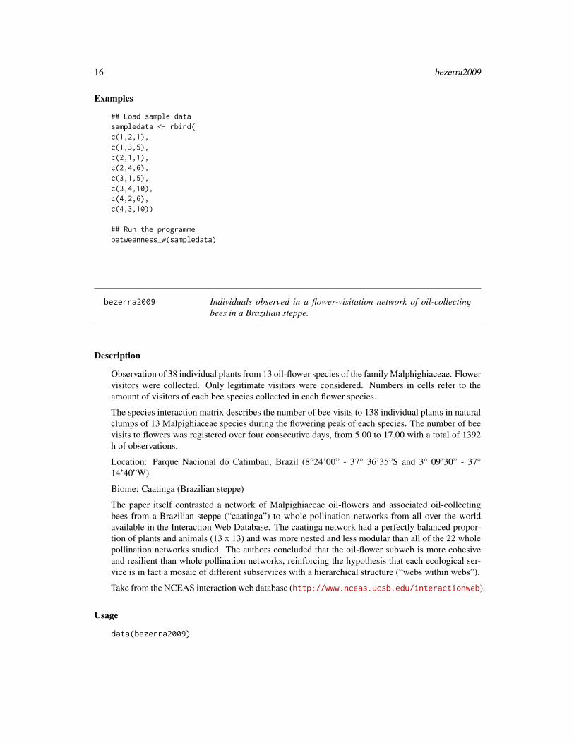
Observation of 38 individual plants from 13 oil-flower species of the family Malphighiaceae. Flowervisitors were collected. Only legitimate visitors were considered. Numbers in cells refer to theamount of visitors of each bee species collected in each flower species.

The species interaction matrix describes the number of bee visits to 138 individual plants in naturalclumps of 13 Malpighiaceae species during the flowering peak of each species. The number of beevisits to flowers was registered over four consecutive days, from 5.00 to 17.00 with a total of 1392h of observations.

Location: Parque Nacional do Catimbau, Brazil (8°24’00” - 37° 36’35”S and 3° 09’30” - 37°14’40”W)

Biome: Caatinga (Brazilian steppe)

The paper itself contrasted a network of Malpighiaceae oil-flowers and associated oil-collectingbees from a Brazilian steppe (“caatinga”) to whole pollination networks from all over the worldavailable in the Interaction Web Database. The caatinga network had a perfectly balanced propor-tion of plants and animals (13 x 13) and was more nested and less modular than all of the 22 wholepollination networks studied. The authors concluded that the oil-flower subweb is more cohesiveand resilient than whole pollination networks, reinforcing the hypothesis that each ecological ser-vice is in fact a mosaic of different subservices with a hierarchical structure (“webs within webs”).

Take from the NCEAS interaction web database (http://www.nceas.ucsb.edu/interactionweb).

Usage

data(bezerra2009)

http://www.nceas.ucsb.edu/interactionweb

C.score 17

References

Bezerra, E.L.S., Machado, I.C.S. and Mello, M.A.R. 2009. Pollination networks of oil-flowers: atiny world within the smallest of all worlds. Journal of Animal Ecology 78, 1096–1101.

Examples

data(bezerra2009)

C.score Calculates the (normalised) mean number of checkerboard combina-tions (C-score) in a matrix

Description

Calculates the C-score for all higher-level species; the C-score represents the average number ofcheckerboard units for each unique species pair.

Usage

C.score(web, normalise = TRUE, FUN = mean, ...)

Arguments

web A matrix with pollinators as columns and plants as rows. Alternatively, whenused on e.g. species occurrences across islands, rows are islands.

normalise Logical; if TRUE (default), the C-score is ranged between 0 (no checkerboards)and 1 (only checkerboards). For FALSE the standard value of mean numberof checkerboard pairs is returned. This is somewhat awkward for comparingdifferent data sets, that’s what the normalisation is for.

FUN Function to use when summarising the C-scores for each pairwise comparison.Defaults to mean, but other useful functions could be median (because C-scoresare rather skewed) or hist (for a nice graph).

... Options to be passed on to FUN, e.g. ‘na.rm=T’ for matrices with many zerosand ‘normalise=TRUE’.

Details

As a first step, any quantitative matrix is converted to a binary matrix of presences and absences.

Then, the formula given in Stone and Roberts (1990) is calculated for all species combinations, bycalling designdist from the package vegan. See code for details.

Value

Returns whatever the ‘FUN’ produces as output. Default would be a single value, i.e. the meanC-score of the web.

18 closeness_w

Note

The normalisation, since Jan. 2015, is by brute force: the 1s and 0s are distributed for each pairwisecomparison for maximum checkerboardness. (The previously used approach was incorrect!) As aconsequence, large matrices will take some time to compute.

The minimum is set to 0.

Author(s)

Carsten F. Dormann

References

Gotelli, N.J. and Rohde, K. (2002) Co-occurrence of ectoparasites of marine fishes: a null modelanalysis. Ecology Letters 5, 86–94

Stone, L. and Roberts, A. (1990) The checkerboard score and species distributions. Oecologia 85,74–79

Examples

m <- matrix(c(1,0,0, 1,1,0, 1,1,0, 0,1,1, 0,0,1), 5,3,TRUE)C.score(m)C.score(m, normalise=FALSE)C.score(m, normalise=FALSE, FUN=print)

closeness_w Closeness centrality in a weighted network

Description

This function calculates closeness scores for nodes in a weighted network based on the distance_w-function.

Usage

closeness_w(net, directed=NULL, gconly=TRUE, precomp.dist=NULL, alpha=1)

Arguments


directed Logical: whether the edgelist is directed or undirected. Default is NULL, thenthe function detects this parameter.

gconly Logical: whether to calculate closeness only on the main component (traditionalcloseness). Default is TRUE. If this parameter is set to FALSE, a closenessmeasure for all nodes is computed. For details, see http://toreopsahl.com/2010/03/20/closeness-centrality-in-networks-with-disconnected-components/

http://toreopsahl.com/2010/03/20/closeness-centrality-in-networks-with-disconnected-components/

http://toreopsahl.com/2010/03/20/closeness-centrality-in-networks-with-disconnected-components/

closeness_w 19

precomp.dist If you have already computed the distance matrix using distance_w-function,you can enter the name of the matrix-object here.

alpha sets the alpha parameter in the generalised measures from Opsahl, T., Agneessens,F., Skvoretz, J., 2010. Node Centrality in Weighted Networks: Generalizing De-gree and Shortest Paths. Social Networks. If this parameter is set to 1 (default),the Dijkstra shortest paths are used. The identification procedure of these pathsrely simply on the tie weights and disregards the number of nodes on the paths.

Value

Returns a data.frame with three columns: the first column contains the nodes’ ids, the second col-umn contains the closeness scores, and the third column contains the normalised closeness scores(i.e., divided by N-1).

Note


Author(s)


References

http://toreopsahl.com/2009/01/09/average-shortest-distance-in-weighted-networks/

Examples

## Load sample datasampledata <- rbind(c(1,2,4),c(1,3,2),c(2,1,4),c(2,3,4),c(2,4,1),c(2,5,2),c(3,1,2),c(3,2,4),c(4,2,1),c(5,2,2),c(5,6,1),c(6,5,1))

## Run the programmecloseness_w(sampledata)

20 clustering_tm

clustering_tm Redefined clustering coefficient for two-mode networks

Description

This function calculates the two-mode clustering coefficient as proposed by Opsahl (2010).

Usage

clustering_tm(net, subsample=1, seed=NULL)

Arguments

net A binary or weighted two-mode edgelist

subsample Whether a only a subset of 4-paths should we used when calculating the mea-sure. This is particularly useful when running out of memory analysing largenetworks. If it is set to 1, all the 4-paths are analysed. If it set to a value belowone, this is roughly the proportion of 4-paths that will be analysed. If it is set toan interger greater than 1, this number of ties that form the first part of a 4-paththat will be analysed. Note: The c++ functions are better as they analyse the fullnetwork.

seed If a subset of 4-paths is analysed, by setting this parameter, the results are repro-ducable.

Value

Returns the outcome of the equation presented in the paper

Note


Author(s)


References

Opsahl, T. 2010. Triadic closure in two-mode networks: Redefining the global and local clusteringcoefficients. arXiv,1006.0887

compart 21

compart Detects compartments

Description

Finds number of compartments, based on multivariate ordination techniques, and labels interactionsaccording to the compartment they belong to.

Usage

compart(web)

Arguments

web A bipartite interaction web, i.e.~a matrix with higher (cols) and lower (rows)trophic levels.

Details

Internal function, to be called by networklevel.

Value

Returns a list with two entries:

cweb A matrix similar to web, but now with compartment numbers instead of interac-tion values.

ncompart The number of compartments.

Note

Note that up to (and including) version 0.85 we used a code based on correspondence analysis (seeLewinsohn et al. 2006). This is, however, faulty for webs with many same-linked species. Hencewe resorted to a brute-force search for compartments, which is orders of magnitude slower, but atleast works correctly. Only in version 1.18 Juan M. Barreneche eventually found a solution that isfast and works with ties!

Author(s)

Juan M. Barreneche <[email protected]>, but please co-copy comments/questions to packagemaintainer: Carsten F. Dormann <[email protected]>

References

Lewinsohn, T. M., P. I. Prado, P. Jordano, J. Bascompte, and J. M. Olesen (2006) Structure inplant-animal interaction assemblages. Oikos 113, 174–184

22 computeModules

See Also

See also networklevel.

Examples

# make a nicely comparted web:web <- matrix(0, 10,10)web[1,1:3] <- 1web[2,4:5] <- 1web[3:7, 6:8] <- 1web[8:10, 9:10] <- 1web <- web[-c(4:5),] #oh, and make it asymmetric!web <- web[,c(1:5, 9,10, 6:8)] #oh, and make it non-diagonalcompart(web)

# or, standard, use Safariland as example:data(Safariland)compart(Safariland)

computeModules Function "computeModules"

Description

This function takes a bipartite weighted graph and computes modules by applying Newman’s mod-ularity measure in a bipartite weighted version to it. metaComputeModules re-runs the algorithmseveral times, returning the most modular result, to stabilise modularity computation.

Usage

computeModules(web, method="Beckett", deep = FALSE, deleteOriginalFiles = TRUE,steps = 1000000, tolerance = 1e-10, experimental = FALSE, forceLPA=FALSE)

metaComputeModules(moduleObject, N=5, method="DormannStrauss", ...)

Arguments

web web is the matrix representing the weighted bipartite graph (as an example, seee.g. web "small1976" in this package).

method Choice between the algorithm(s) provided by Stephen Beckett (2016) or Dor-mann & Strauss (2016). Defaults to the much faster and in the majority of casesbetter algorithm of Beckett. (Note the optional argument ‘forceLPA’ to use hisslightly inferior but even faster pure LPA algorithm.)

deep If deep is set to FALSE (default), a flat clustering is computed, otherwise sub-modules are identified recursively within modules. Works only with ‘method="DormannnStrauss"’.

deleteOriginalFiles

If deleteOriginalFiles is set to TRUE (default), the files mentioned above inthe description are deleted from the hard drive disk, otherwise not.

computeModules 23

steps steps is the number of steps after which the computation of modules stops if nobetter division into modules than the current one can be found.

tolerance How small should the difference between MCMC-swap results be? At somepoint computer precision fluctuations make the algorithm fail to converge, whichis why we choose a (very low) defaults of 1E-10.

experimental Logical; using an undescribed and untested version for which no detail is avail-able? (We suggest: not yet.)

moduleObject Output from running computeModules.

forceLPA Logical; should the even faster pure LPA-algorithm of Beckett be used? DIRT-LPA, the default, is less likely to get trapped in a local minimum, but is slightlyslower. Defaults to FALSE.

N Number of replicate runs; defaults to 5.

... Arguments passed on to computeModules, which is called internally.

Value

An object of class "moduleWeb" containing information about the computed modules. For details,please refer to the corresponding documentation file.

Note

For perfectly compartmentalised networks the algorithm may throw an error message. Please add alittle bit of noise (e.g. uniform between 0 and 1 or so) or a small constant (1E-5 or so) and it willwork again.

When using the method ‘DormannStrauss’, files are written onto the hard drive during the compu-tation. These files are by default deleted after the computation terminates, unless it breaks. Detailsof the modularity algorithm can be found in Dormann \& Strauß (2013).

Author(s)

Rouven Strauss, with fixes by Carsten Dormann and Tobias Hegemann; modified to accommodateBeckett’s algorithm by Carsten Dormann

References

Beckett, S.J. 2016 Improved community detection in weighted bipartite networks. Royal Societyopen science 3, 140536.

Dormann, C. F., and R. Strauß. 2014. Detecting modules in quantitative bipartite networks: theQuanBiMo algorithm. Methods in Ecology & Evolution 5 90–98 (or arXiv [q-bio.QM] 1304.3218.)

Liu X. & Murata T. 2010. An Efficient Algorithm for Optimizing Bipartite Modularity in BipartiteNetworks. Journal of Advanced Computational Intelligence and Intelligent Informatics (JACIII) 14408–415.

Newman M.E.J. 2004. Physical Review E 70 056131

24 czvalues

See Also

See also class "moduleWeb", function "listModuleInformation", function "printoutModuleInforma-tion", DIRT_LPA_wb_plus.

Examples

## Not run:data(small1976)(res <- computeModules(small1976))plotModuleWeb(res)

# slow:res2 <- metaComputeModules(small1976) # makes no sense for "Beckett"res2

## End(Not run)

czvalues Computes c and z for network modules

Description

Function to compute c and z values of module members according to Guimerà & Amaral (2005),with formulae taken from Olesen et al. (2007)

Usage

czvalues(moduleWebObject, weighted=FALSE, level="higher")

Arguments

moduleWebObject

A moduleWeb-class object as created by computeModules.

weighted logical; if TRUE computes c and z from quantitative (=weighted) data; in thiscase, it will compute strength, rather than degrees for each species.

level "higher" or "lower" trophic level to compute c and z values for; defaults to"higher"

Details

c = 1 - sum( (k.it/k.i)^2) # among-module connectivity = participation coefficient P in Guimerà &Amaral

z = (k.is - ks.bar) / SD.ks # within-module degree

k.is = number of links of i to other species in its own module s; ks.bar = average k.is of all speciesin module s; SD.ks = standard deviation of k.is of all species in module s; k.it = number of links ofspecies i to module t; k.i = degree of species i

czvalues 25

Note that for any species alone (in its level) in a module the z-value will be NaN, since then SD.ksis 0. This is a limitation of the way the z-value is defined (in multiples of degree/strength standarddeviations).

Olesen et al. (2006) give critical c and z values of 0.62 and 2.6, respectively. Species exceedingthese values are deemed connectors or hubs of a network. The justification of these thresholdsremains unclear to me. They may also not apply for the quantitative version.

Value

A list with two vectors, c and z, for all species of the selected trophic level.

Note

These indices were developed for one-mode networks; we’ll have to see whether they make sensefor bipartite networks, too! In particular, note that this function is based on a higher trophic levelperspective. While the modules are identified using both trophic levels, c and z are computedthrough the strengths/degrees of only one trophic level. It would be desirable to have a truly two-level version. Since there are usually very different numbers of species in the two trophic levels,simply averaging the values of each trophic level won’t do. But maybe a weighted average?

Consider the following problem for computing c and z for the higher trophic level: For moduleswith only one species from the lower trophic level, the z-values will be NaN, since SD.ks is 0! Idecided to SET these values to 0, since they only occur when all species in that module will havethe same number of links (which is obviously the case when there is only one lower-level species).Then the numerator is also 0. Thus, the value of 0 indicates that this species has no deviation fromthe rest of the module members (which is what I think z is supposed to represent).

Since computeModules is experimental, also czvalues may not always work (i.e. if object mod iscorrupted or ill-formed).

Author(s)

Carsten F. Dormann <[email protected]>, 20 Mar 2012

References

Guimerà, R. and Amaral, L.A.N. (2005) Functional cartography of complex metabolic networks.Nature 433, 895–900.

Olesen, J.M., Bascompte, J., Dupont, Y.L. and Jordano, P. (2007) The modularity of pollinationnetworks. Proceedings of the National Academy of Sciences of the USA 104, 19891-19896.

Examples

## Not run:data(memmott1999)set.seed(2)mod <- computeModules(memmott1999, steps=1E4)cz <- czvalues(mod)plot(cz[[1]], cz[[2]], pch=16, xlab="c", ylab="z", cex=0.8, xlim=c(0,1), las=1)abline(v=0.62) # threshold of Olesen et al. 2007abline(h=2.5) # dito

26 degreedistr

text(cz[[1]], cz[[2]], names(cz[[1]]), pos=4, cex=0.7)

## End(Not run)

degreedistr Fits functions to cumulative degree distributions of both trophic levelsof a network.

Description

This function first calculates degrees for each species, then constructs a cumulative distributionwith them, and finally fits three different functions to these distributions: exponential, power lawand truncated power law. Coefficients and fits are returned.

Usage

degreedistr(web, plot.it=TRUE, pure.call=TRUE, silent=TRUE, level="both", ...)

Arguments

web A bipartite network matrix.

plot.it Logical; returns graphs of fits when set to TRUE (default). Dark, median andlight grey lines refer to exponential, power and truncated power law, respec-tively.

pure.call Logical; adjusts par for two panels (for TRUE) or leaves this to the wrapperfunction (FALSE).

silent Logical; suppresses error reporting in the try-function around nls; defaults toTRUE.

level For which level shall the degree distributions be computed: ‘both’, ‘lower’ or‘higher’? Defaults to ‘both’.

... Arguments passed on to the plot function (e.g. ‘las=1’).

Details

Jordano et al. (2003) proposed that plant-animal networks may show scale invariance, as indicatedby the presence of a power law in species degrees. They report on consistently better fits of thetruncated power law, hypothesising that such patterns may arise from morphological mismatch orphenological uncoupling.

Most problematic with the use of this particular approach is the extreme demand for data. The ex-ample web Safariland in this package is large (1130 interactions), but it provides only 5 differentdegree levels (for plants, only 4 for pollinators). Hence fitting three different non-linear functionsto these few points is stretching it a bit.

Furthermore, the least-square-fit to the cumulative distribution is not ideal. While the most commonapproach, it has a bias (albeit much less so than a fit to the probability density function: see Clausetet al. 2009). In an ideal world, we would want to fit the power law properly. This would require a)

degreedistr 27

an estimation of the lower bound of the power law (xmin) and b) the maximum likelihood fit to theremaining data (x > xmin). The data demand is however such that is unlikely that any ecologicalbipartite network in the near future will match it. Clauset et al. state that hundreds to thousands ofdata points are required to yield satisfactory estimates for xmin and the slope itself. If you happento have this much data, please consult the software they provide (even in R!).

Value

For both trophic levels, a table:

... trophic level dd fits

Contains coefficient estimates, estimate’s standard error and P-value, R2 andAIC for each of the three model fits, for the respective trophic level.

If plots are returned, exponential, power law and truncated power law are given in black, dark greyand light grey, respectively.

Note

The truncated power law fits two coefficients: slope and cut-off. The function only returns the slope.R2-values for non-linear fits are not well liked among statisticians! See the discussion the R-helplist (e.g. https://stat.ethz.ch/pipermail/r-help/2002-July/023461.html). Finally, oftendata are too few to yield any fit. In this case the error message “singular gradient” is returned tosignal this problem!

Post finally, yes, I am aware that degrees are integers and unlikely to be normally distributed, andthat thus the nls procedure is not really a good idea. My (poor) excuse: I followed the implemen-tation of the above-cited paper and do not believe enough in degree distributions (and power laws,for that matter) to implement a proper likelihood-based approach. Check out the statnet bundle foralternative approaches to this problem.

Author(s)


References

Clauset, A., Shalizi, C. R., & Newman, M. E. (2009). Power-law distributions in empirical data.SIAM Review 51, 661–703

Jordano, P., Bascompte, J. and Olesen, J. M. (2003) Invariant properties in coevolutionary networksof plant-animal interactions. Ecology Letters 6, 69–81

See Also

networklevel, where degreedistr is called (without picturing the results)

Examples

data(Safariland)degreedistr(Safariland)

https://stat.ethz.ch/pipermail/r-help/2002-July/023461.html

28 dfun

dfun Calculates standardised specialisation index d’ (d prime) for eachspecies in the lower trophic level of a bipartite network.

Description

This function returns the specialisation index d’ for the lower level, which expresses how specialiseda given species is in relation to what partners in the higher level are on offer.

Usage

dfun(web, abuns=NULL)

Arguments

web Web is a matrix representing the interactions observed between higher levelspecies (columns) and lower level species (rows). Usually this will be num-ber of pollinators on each species of plants or number of parasitoids on eachspecies of prey.

abuns A vector of abundances for the HIGHER level, usually from additional infor-mation. If none is given (default) marginal sums are used. Note that if a webwith rows or columns without any interaction is provided, these will not bepurged when an independent abundances vector is given. As a consequence,these species will have a d’ of NA (see note below).

Details

The d’ index is derived from Kulback-Leibler distance (as is Shannon’s diversity index), and calcu-lates how strongly a species deviates from a random sampling of interacting partners available. Itranges from 0 (no specialisation) to 1 (perfect specialist). In the case of a pollination web, a polli-nator may be occurring only on one plant species, but if this species is the most dominant one, thereis limited evidence for specialisation. Hence this pollinator would receive a low value. In contrast,a pollinator that occurs only on the two rarest plants would have a very high value of d’.

The idea of this index is laid out in Blüthgen et al. (2006). It basically calculates the Shannon-diversity for each column (delivering the raw d-values) and re-ranges them between the theoreticalmaximum and minimum (yielding values between 0 and 1). dmax is given analytically (see paperor code), but dmin must be found ‘heuristically’, since the web can only contain integers. Theidea behind the heuristic minimum is that d will be minimal when observed values differ least fromexpected values based on marginal distributions.

The way this function is implemented, it calculates expected values for each cell based on theproduct of observed marginal sums (i.e. column and row sums) times sum(web). Then it rounds offto integers and allocates the remaining interactions in two steps: First, all columns and rows withmarginal sums of 0 obtain one interaction into the cell with the highest expected value. Secondly, allremaining interactions are distributed according to difference between present and expected value:those cells with highest discrepancy receive an interaction until the sum of all entries in the new

dfun 29

web equals those in the original web. Now the d-values for this web are calculated and used asdmin.

Simple rounding of expected values would lead to empty columns or rows, i.e. the dmin-web wouldbe of lower dimension than the original web.

dfun returns the d’ values for the lower trophic level. Use fun(t(web)) to get the d’-values for thehigher trophic level (as does specieslevel). If you want to provide external abundances, you mustprovide those of the OTHER trophic level! (This help file is written as if you were interested in thelower trophic level.)

d’ is one of several species-level network indices. It’s generalisation to the entire interaction web iscalled H2’.

The abundances vector allows to incorporate independent estimates of the abundances of theHIGHER trophic level. In a pollination web, pollinator abundances may be very different fromthose estimated by the interaction matrix column sums. This has also, obviously, large conse-quences for the specialisation: A plant being pollinated by a bee that is common on this plant, butvery rare in general, will show a low specialisation unless bee abundances are corrected for. Datagiven in the abundance vector are here used in replacement for the row sums, both in the d-functionitself, as well as in the calculation of the minimum ds.

In contrast to H2fun, finding the minimum value of d violates marginal totals. The idea is that welook at each species in turn. Then, we estimate how its observed number of interactions can bedistributed, given the marginal totals (i.e. if 5 interactions were observed, they cannot be put into alink that only has 3 interactions across all species). So, for each species the number of interactionsnever exceeds the total across all species, but if we would put the web together from this sequentialscan, it may well do so. In our view, this is irrelevant, because we are interested in the potentialof each species separately to be perfectly specialised (given the marginal totals), not for the entireweb. We leave this to H2fun.

Value

dprime d’-value for each species

d Raw d-value for each species, i.e. before ranging it between 0 and 1.

dmin Minimum d-value for each species, based on a perfect nesting of the matrix; seedetails.

dmax Maximum d-value theoretically possible given the observed number of interac-tions and the observed marginal distributions.

Note

When independent abundances were provided, the empty rows/columns are purposefully not re-moved from the web (because they now still contain information). Logically (and as implemented),this leads to d-values for these species of NA. This makes sense: the pollinator, say, has never beenobserved on any of the flowers, so how can we quantify its specialisation?

As detailed above, deriving the dmin-values ‘heuristically’ leaves room to some variation. We arevery happy with this implementation, but you may want to program something yourself ...

Author(s)

Jochen Fründ and Carsten F. Dormann

30 DIRT_LPA_wb_plus

References


See Also

H2fun for a similar function for the entire network. specieslevel for a method that, amongst otherindices, calls dfun.

Examples

data(Safariland)dfun(Safariland) # gives d-values for the lower trophic level# now using independent abundance estimates for higher trophic level:dfun(Safariland, abuns=runif(ncol(Safariland)))

dfun(t(Safariland)) #gives d-values for the higher trophic level

DIRT_LPA_wb_plus Functions "LPA_wb_plus" and "DIRT_LPA_wb_plus"

Description

Use computeModules to call this function! This function takes a bipartite weighted graph and com-putes modules by applying Newman’s modularity measure in a bipartite weighted version to it. Todo so, it uses Stephen J Beckett’s DIRTLPAwb+ (or LPAwb+) algorithm, which builds on Liu &Murata’s approach. In contrast to the tedious MCMC-swapping QuanBiMo algorithm, this algo-rithm works by aggregating modules until no further improvement of modularity can be achieved.

Usage

DIRT_LPA_wb_plus(MATRIX, mini=4, reps=10)LPA_wb_plus(MATRIX, initialmoduleguess=NA)convert2moduleWeb(MATRIX, MODINFO)

Arguments

MATRIX MATRIX is the matrix representing the weighted bipartite graph (as an example,see e.g. web "small1976" in this package).

mini Minimal number of modules the algorithm should start with; defaults to 4. Seeexplanation of ‘initialmoduleguess’ to understand why not starting with onemodule per species interaction makes sense.

reps Number of trials to run for each setting of ‘mini’; defaults to 10 but my benefitfrom higher values.

DIRT_LPA_wb_plus 31

initialmoduleguess

Optional vector with labels for the modules of the longer web dimension. The‘initialmoduleguess’ argument in LPA_wb_plus is used as an initial guess ofthe number of modules the network contains. The code then randomly assignsthis many labels across the nodes of one of the types. The classical algorithm(i.e. LPA_wb_plus) would use an initialmoduleguess of the maximum numberof modules a network can contain (i.e. assigning a different label to each nodeinitially). DIRT_LPA_wb_plus exploits this. By initially assigning fewer thanthe maximum number of modules in the first instance nodes that may not havebeen placed together by the classical algorithm are placed together - creatingdifferent start points from which to attempt to maximise modularity.Defaults toNA, i.e. as many modules as there are species in the smaller group.

MODINFO Object returned by modulesLPA.

Value

LPA_wb_plus computes the modules. DIRT_LPA_wb_plus is a wrapper calling LPA_wb_plus re-peatedly to avoid getting stuck in some local minimum. Both return a simple list of row and columnlabels for the modules, as well as the modularity value. Using convert2moduleWeb turns this intothe richer moduleWeb-class object produced by computeModules. For this object, the plotting func-tion plotModuleWeb and summary functions listModuleInformation and printoutModuleInformationare available.

Author(s)

Stephen J Beckett (https://github.com/sjbeckett/weighted-modularity-LPAwbPLUS), lifted, with con-sent by the author, by Carsten F. Dormann to bipartite

References

Beckett, S.J. 2016 Improved community detection in weighted bipartite networks. Royal Societyopen science 3, 140536.

Liu X. & Murata T. 2010. An Efficient Algorithm for Optimizing Bipartite Modularity in BipartiteNetworks. Journal of Advanced Computational Intelligence and Intelligent Informatics (JACIII) 14408–415.

Newman M.E.J. 2004. Physical Review E 70 056131

See Also

computeModules; see also class "moduleWeb", function "listModuleInformation", function "print-outModuleInformation"

Examples

## Not run:(res <- DIRT_LPA_wb_plus(small1976))mod <- convert2moduleWeb(small1976, res)plotModuleWeb(mod)

## End(Not run)

32 discrepancy

discrepancy Calculates discrepancy of a matrix

Description

Discrepancy is the number of mismatches between a packed (binary) matrix and the maximallypacked matrix (with same row sums)

Usage

discrepancy(mat)

Arguments

mat A matrix (or something that can be transformed into a matrix when as.matrixis called within the function) of species (in columns) on islands (in rows). Ifquantitative data are given (e.g. in a quantitative pollination network), these areinternally transformed into a binary matrix.

Details

Discrepancy is a way to measure the nestedness of a matrix. In a comparative study, Ulrich &Gotelli (2007) showed discrepancy to outperform all other measures and hence recommend its use(together with a fixed-columns, fixed-rows null model, such as implemented in commsimulator invegan, see example).

This function follows the logic laid out by Brualdi & Sanderson (1999), although, admittedly, I findtheir mathematical description highly confusing. Another implementation is given by the functionnesteddisc in vegan. The reason to write a new function is simple: I wasn’t aware of nesteddisc!(I was sitting on a train and I wanted to use this measure later on, so I put it into a function con-sulting only the orignal paper. When looking for the swap algorithm to create null models, which Isomehow knew to exist in vegan, I stumbled across nesteddisc. If you are interested in the swapalgorithm and come across this help page, let me re-direct you to oecosimu in vegan.)

Now that this function exists, too, I found it to differ in output from nesteddisc. Jari Oksanen wasquick to point out, that our two implementations differ in the way they handle ties in column totals.This function is, I think, closer to the results given in Brualdi & Sanderson. Jari also went on toimplement different strategies to deal with ties, so my guess is that his version may be (slightly)superior to this one. Having said that, values don’t differ much between the two implementations.

So what does it do: The matrix is sorted by marginal totals, yielding a matrix A. Then, all 1s in Aare “pushed” to the left to maximally compact the matrix, yielding P. Discrepancy is now simplythe number of disagreements between A and P, divided by two (to correct for the fact that every“wrong” 1 will necessarily generate a “wrong” 0).

Value

Returns the number of mismatches, i.e. the discrepancy of the matrix from perfecct nestedness.

distance_w 33

Note

Discrepancy is well-defined only for matrices that can be sorted uniquely. For matrices with ties nofoolproof way to handle them has been proposed. For small matrices, or large matrices with manyties, this will lead to different discrepancy values. See also how nesteddisc in vegan handles thisissue! (Thanks to Jari Oksanen for pointing this out!)

Author(s)

Carsten F. Dormann

References

Brualdi, R.A. and Sanderson, J.G. (1999) Nested species subsets, gaps, and discrepancy. Oecologia119, 256–264

Ulrich, W. and Gotelli, N.J. (2007) Disentangling community patterns of nestedness and speciesco-occurrence. Oikos 116, 2053–2061

See Also

nestednodf in vegan for the best nestedness algorithm in existence today (for both binary andweighted networks!); nestedness for the most commonly used method to calculate nestedness,wine for a new, unevaluated but very fast way to calculate nestedness; nestedtemp (another imple-mentation of the same method used in our nestedness) and nestedn0 (calculating the number ofmissing species, which has been shown to be a poor measure of nestedness) in vegan

Examples

## Not run:#nulls <- replicate(100, discrepancy(commsimulator(Safariland,method="quasiswap")))nulls <- simulate(vegan::nullmodel(Safariland, method="quasiswap"), nsim = 100)null.res <- apply(nulls, 3, discrepancy)hist(null.res)obs <- discrepancy(Safariland)abline(v=obs, lwd=3, col="grey")c("p value"=min(sum(null.res>obs), sum(null.res<obs))/length(null.res))# calculate Brualdi & Sanderson's Na-value (i.e. the z-score):c("N_a"=(unname(obs)-mean(null.res))/sd(null.res))

## End(Not run)

distance_w Distance in a weighted network

34 distance_w

Description

The shortest path length, or geodesic distance, between two nodes in a binary network is the min-imum number of steps you need to make to go from one of them to the other. This distance is thequickest connection between nodes when all ties are the same. However, in a weighted network, allties are not the same. See http://toreopsahl.com/2009/01/09/average-shortest-distance-in-weighted-networks/ for more deatails.

Usage

distance_w(net, directed=NULL, gconly=TRUE, subsample=1, seed=NULL)

Arguments


directed logical, whether the network is directed or undirected. Default is NULL, thismeans that the function checks whether the edgelist is directed or not.

gconly logical, whether the function should only be calculated for the giant component.Default is TRUE.

subsample Whether a only a subset of starting nodes should we used when calculating themeasure. This is particularly useful when running out of memory analysinglarge networks. If it is set to 1, all distances are analysed. If it set to a valuebelow one, this is roughly the proportion of starting noes that will be analysed.If it is set to an interger greater than 1, this number of starting nodes that will beanalysed.

seed If a subset of starting nodes is analysed, by setting this parameter, the results arereproducable.

Value

Returns a distance matrix.

Note


Author(s)


References

http://toreopsahl.com/2009/01/09/average-shortest-distance-in-weighted-networks/

elberling1999 35

elberling1999 No. of visits in a pollination web of arctic-alpine Sweden

Description

This study took place in the subarctic alpine zone of Latnjajaure, in northern Sweden. Field workwas conducted from May 21 to August 23, 1994. The objective was to describe the plant-flowervisitor interaction matrix of this area and compare it with the characteristics of other subarctic alpinesystems and with pollination systems of lower latitudes, especially in relation to the role of flies asflower visitors at high latitudes.

The authors recorded their data by counting the number of visits of each flower visitor species toeach plant species. Regardless of whether insects were observed to forage for nectar and pollen orto perform sun-basking, they were all classified as flower visitors and potential pollinators and theplant species visited were recorded. Data are presented as an interaction frequency matrix, in whichcells with positive integers indicate the frequency of interaction between a pair of species, and cellswith zeros indicate no interaction.

See also http://www.nceas.ucsb.edu/interactionweb/html/datasets.html

Usage

data(elberling1999)

Format

A data frame with 12 plant species (in rows) and 102 pollinators (columns).

References

Elberling H. and Olesen J.M. (1999) The structure of a high latitude plant-flower visitor system:the dominance of flies. Ecography 22, 314–323

Examples

data(barrett1987)## maybe str(barrett1987) ; plot(barrett1987) ...

empty Deletes empty rows and columns from a matrix.

Description

Gets rid of empty columns and rows in a matrix. Optionally counts removed rows and columns,and returns these values as attribute.

http://www.nceas.ucsb.edu/interactionweb/html/datasets.html

36 empty

Usage

empty(web, count=FALSE)

Arguments

web A matrix representing the interactions observed between higher trophic levelspecies (columns) and lower trophic level species (rows). Usually this will benumber of pollinators on each species of plants or number of parasitoids on eachspecies of prey.

count Logical. Shall be counted how many columns and rows were removed? Num-bers are returned in attribute. Defaults to FALSE.

Details

Helper function to remove empty (i.e. all-zero or all-NA) rows and columns, thereby concentratingthe matrix. This function is also invoked for its side effect by extinction to investigate the effectof removing a species from the network.

Value

Returns matrix without empty rows or columns. Its attribute ‘out’ (if count=TRUE) contains a namedvector with the number of rows removed and the number of columns removed.

Author(s)

Carsten F. Dormann

See Also

extinction and second.extinct, which repeatedly call empty.

Examples

data(Safariland)web <- Safarilandweb[,5] <- 0empty(web, count=TRUE)attr(empty(web), "empty")

endpoint 37

endpoint Computes end-point degrees for a bipartite network

Description

Computes end-point degrees for a bipartite network, following the suggestion of Barrat et al. (2004)

Usage

endpoint(web)

Arguments


Details

Computation follows the outline of Gitarranz et al. (2004): “the product k_i k_j of the degree of thetwo nodes connected by that link”. We then set additionally endpoint degrees for all non-existinglinks to 0! Thus, only for existing links endpoint degrees are computed. This is (to me) not obviousfrom the description in Gitarranz et al. (2004).

Value

A matrix of end-point degrees

Note

This approach is, AFAIK, not tested by simulation; whether it is useful has still to be shown.

Author(s)

Carsten F. Dormann

References

Barrat, A., M. Barthélemy, R. Pastor-Satorras, and A. Vespignani. 2004. The architecture of com-plex weighted networks. Proceedings of the National Academy of Sciences of the USA 101, 3747-–3752. doi: 10.1073/pnas.0400087101.

Gilarranz, L. J., J. M. Pastor, and J. Galeano. 2011. The architecture of weighted mutualisticnetworks. Oikos 121, 1154—1162. doi: 10.1111/j.1600-0706.2011.19592.x.

38 extinction

Examples

# reproduces the example of Gitarranz et al. (2011):data(memmott1999)ends <- endpoint(memmott1999)weights.mean <- tapply(memmott1999, ends, mean)ends.weights <- tapply(ends, ends, mean)plot(weights.mean, ends.weights, log="xy", pch=16)

extinction Simulates extinction of a species from a bipartite network

Description

Following (how I remember) the paper of Memmott et al. (2004), this function deletes a column(e.g. pollinator) or row (e.g. plant). Only a helper function for second.extinct, really.

Usage

extinction(web, participant = "both", method = "random", ext.row=NULL,ext.col=NULL)

Arguments


participant Which level of participant to remove: ‘lower’ removes a row, ‘higher’ removesa row, ‘both’ randomly picks either row or column.

method Determines sequence of extinctions: ‘random’ removes a random participant,while ‘abundance’ removes the least abundant species first. ‘external’ willuse the externally provided vector to determine extinction sequence.

ext.row Optional vector giving the sequence in which lower-level species are to be deleted.

ext.col Optional vector giving the sequence in which higher-level species are to bedeleted.

Details

In itself rather useless. Called repeatedly by second.extinct to build an extinction sequence andaccordingly a sequence of secondary extinctions.

Value

Returns the same matrix that was given as object, just with one row or column being turned intozeros.

fc 39

Author(s)

Carsten F. Dormann

References

Memmott, J., Waser, N. M. and Price, M. V. 2004 Tolerance of pollination networks to speciesextinctions. Proceedings of the Royal Society B 271, 2605–2611

See Also

second.extinct

Examples

## Not run:data(Safariland)(w <- extinction(Safariland, participant="lower", method="abun"))empty(w, count=TRUE)

## End(Not run)

fc Calculates the functional complementarity for the rows of a web

Description

A community-level measure of ecological niche complementarity measured as the total branchlength of a functional dendrogram based on qualitative differences in visitor assemblages betweenplants.

Usage

fc(web, dist="euclidean", method="average", weighted=TRUE)

Arguments


dist A distance accepted by the function dist.

method The linkage method to be used by hclust. Any option accepted by hclust isallowed; defaults to ‘"average"’.

weighted Option to analyse the web as binary or as weighted network. Default is ‘weighted=TRUE’,but analysis presented in Devoto et al. (2012) uses ‘weighted=FALSE’.

40 frame2webs

Details

fc measures community-level ecological niche complementarity as the total branch length of a func-tional dendrogram based on qualitative differences in visitor assemblages between plants. For de-tails see Devoto et al. (2012).

Value

The value of fc, which is not standardised and lies anywhere between 0 and a large number.

Author(s)

Mariano Devoto <[email protected]>

References

Devoto M., Bailey S., Craze P., and Memmott J. (2012) Understanding and planning ecologicalrestoration of plant-pollinator networks. Ecology Letters 15, 319–328

See Also

networklevel, which uses this function.

Examples

data(Safariland)fc(Safariland)fc(t(Safariland), dist="canberra", method="complete")

frame2webs Converts a table of observations into a network matrix

Description

Convenience function to convert a table of observations (typically compiled in a spreadsheet pro-gramm) into a network matrix for further use in bipartite.

Usage

frame2webs(dframe, varnames = c("lower", "higher", "webID", "freq"), type.out ="list", emptylist = TRUE)

frame2webs 41

Arguments

dframe table (i.e. data.frame) of observations, typically simply the data read by one ofthe read.* functions; see Details for details!

varnames a vector of characters giving the column names in the table (data.frame) thatcorrespond to

• species names in lower trophic level (e.g. plants),• species names in higher trophic level (e.g. pollinators),• the grouping factor for a web (e.g. the site on which interactions were

observed)• optionally, a fourth column indicating the number of times an interaction

was observed (or another link weight that can be summed);

If only three varnames are provided, it is assumed that each observed interactionis in a separate row and frequencies are calculated from the number of rows perlink. By default, the names “lower”, “higher”, “webID” and “freq” are used.

type.out defines the type of output; it could be ‘list’ (default) or an ‘array’ with aseparate slice for each network. Lists have the advantage that different webs donot have to include all species names, i.e. they can be of different dimensions(ragged). As such they are better suited for webs with non-comparable speciessets. An array has the advantage that dimensions are the same, and therefore (i)comparisons can be easily made among webs and (ii) webs can be pooled moreeasily. The ‘array’-option is more suitable for sets of networks from the samecommunity.

emptylist logical, defaults to ‘TRUE’; should, for each network in the list of networks,empty columns and rows be deleted? Since this function first builds an arrayand from that a list, each network contains all possible links between species ofthe higher and lower level. When set to ‘TRUE’, all species not observed for agiven network are removed.

Details

This function supports the easy handling of typical recording that are used to compose a network.The assumed structure of the underlying table is two columns for the names of the lower and higherlevel species, respectively, one column for a network ID (e.g. site, observer or any other groupingcode) and, optionally, a number that indicates how often this interaction was observed. If notgiven, the number of interactions is simply computed from the number of times the same interactionoccurred for each network ID. See example code below.

Typically, data are recorded (in a field book or external data logging device), read into a spreadsheetsoftware (such as MS Excel or Open/LibreOffice Spreadsheet), where names are checked, typoscorrected and so forth. This table is then imported into R and aggregated into one or more webs (oran array or a list of webs) using frame2webs.

Each link can have multiple entries or a single entry!

Value

A list or an array of networks, each to be used as input for other bipartite functions.

42 genweb

Note

Great care should be taken in checking species names, slightly different spellings will be assumed tobe different species! Common problems occur because a space was added to the name or lower andhigher case letters were mixed. For example, R is case sensitive and observes white space, while“Homo sapiens”, “Homo sapiens ” (with a trailing space) and “homo sapiens” are not recognizedas different in typical spreadsheet software (e.g. Excel).

Author(s)

Jochen Fründ

See Also

empty

Examples

testdata <- data.frame(higher = c("bee1","bee1","bee1","bee2","bee1","bee3"),lower = c("plant1","plant2","plant1","plant2","plant3","plant4"),webID = c("meadow","meadow","meadow","meadow","bog","bog"), freq=c(5,1,1,1,3,7))frame2webs(testdata,type.out="array")sapply(frame2webs(testdata,type.out="list"), networklevel, index=c("connectance", "C score"))

genweb Generate a random bipartite web

Description

Generates a random bipartite web, based on r2dtable and lognormal marginal distributions.

Usage

genweb(N1 = 10, N2 = 30, dens = 2)

Arguments

N1 Number of species in the lower trophic level; or a vector of length 2 givingnumber of lower and higher trophic level species. Defaults to 10. Large values(>70) will take much longer!

N2 Number of species in the higher trophic level. Ignored if N1 a vector of length2. Defaults to 30. Large values (>70) will take much longer!

dens Interaction density, i.e. how many interactions there shall be, on average, foreach link. Defaults to 2 (the median observed interaction density in the NCEASpollination webs). Large values (> 10) will take much longer to find matricesfor.

grouplevel 43

Details

This function can be used to create simple, but not necessarily realistic, bipartite webs for givendimensionality and interaction density. Marginal distributions are assumed to be lognormal, meanand standard deviation are calculated from ‘N1’, ‘N2’ and ‘dens’ (see code for details).

Value

A matrix with N1 x N2 species.

Note

Can be a bit time-consuming for large webs, because the absolute values for both dimensions haveto match perfectly. This involves a rather inelegant while-loop.

Author(s)

Jochen Fründ and Carsten F. Dormann

Examples

genweb()

grouplevel Analysis of bipartite webs at the level of each of the two levels (groups)of the network

Description

Calculates a variety of indices and values for each group of a bipartite network (one.grouplevelis the actual function to do the computations and is not intended to be called by the user)

Usage

grouplevel(web, index="ALLBUTDD", level="both", weighted=TRUE, empty.web=TRUE,dist="horn", CCfun=mean, logbase="e", normalise=TRUE, extinctmethod="r",nrep=100, fcdist="euclidean", fcweighted=TRUE)

Arguments

web Web is a matrix representing the interactions observed between higher trophiclevel species (columns) and lower trophic level species (rows). Usually this willbe number of pollinators on each species of plants or number of parasitoids oneach species of host.

index One or more of the following (exact match only!):

• ‘number of species’ in the respective trophic level,• ‘mean number of links’,• ‘mean number of shared partners’,

44 grouplevel

• ‘cluster coefficient’,• ‘weighted cluster coefficient’,• ‘togetherness’,• ‘C score’,• ‘V ratio’,• ‘discrepancy’,• ‘degree distribution’,• ‘extinction slope’,• ‘robustness’,• ‘niche overlap’,• ‘generality’,• ‘vulnerability’,• ‘partner diversity’,• ‘fc’ (or alternatively ‘functional complementarity’),• ‘ALL’ calculates all the above indices (returning a list (since degree distri-

bution fits are a table within this list and cannot be simplified)),• ‘ALLBUTDD’ (default) calculates all indices except degree distribution fits.

This latter has the advantage that the output can be simplified to a vector;

level For which of the two groups (“levels”) should these indices be computed? Op-tions are ‘lower’, ‘higher’ and ‘both’ (default). For index ‘robustness’, theindicated level is the one that will be exterminated in simulations (see second.extinct).Although grouplevel can be employed on its own, it typically will be calledthrough networklevel.

weighted logical; for those indices which are simply averaged across species to yield thegroup-level index (e.g. ‘niche overlap’), should this averaging take into ac-count the number of observations for a species? Defaults to TRUE. The logicbehind this default is that we have more faith in an index value when it is basedon many, rather than few, observations. Bersier et al. (2002) proposed thisweighting and it is also commonly used to compute vulnerability and generality(e.g. in Tylianakis et al. 2006).

empty.web Shall the empty columns and rows be deleted? Defaults to TRUE.

dist Distance metric to be used to calculate niche overlap (calling vegan::vegdist);defaults to Horn’s index, which is the recommendation of Krebs (1989); forother options see vegdist in vegan.

CCfun Method to use when calculating the clustering coefficient. Originally proposedas mean of cluster coefficients for each node. Defaults to ‘median’, becausecluster coefficients are strongly skewed.

logbase Shall various indices (partner diversity, generality/vulnerability) be calculated tothe base of e (default) or 2? Log2 is the proposal for generality and vulnerabilityby Bersier et al. (2002), while Shannon uses ln. The choice of the base will notaffect the results qualitatively, at most by a scaling factor.

normalise Logical; shall the C-score and togetherness metrics be normalised to a range of0 to 1? Defaults to TRUE.

grouplevel 45

extinctmethod Specifies how species are removed from matrix: ‘random’ or ‘abundance’ (par-tial matching), where abundance removes species in the order of increasingabundance (i.e. rarest first); see Memmott et al. (2004).

nrep Number of replicates for the extinction sequence analysis.

fcweighted Logical; when computing "functional complementarity" sensu function fc, shouldthe weights of the matrix be used. Defaults to TRUE, but original paper (Devotoet al. 2012) is based on FALSE.

fcdist Distance measure to be used to compute functional complementarity throughfc; any measure accepted by dist is acceptable.

Details

This function implements a variety of the many (and still procreating) indices describing networktopography at the group level.

Note that Bersier et al. (2002) have three levels of values for some of their indices: qualitative (i.e.based on binary networks), quantitative (based on networks with information on the number of in-teractions observed for each link), and weighted-quantitative (where each species is given a weightaccording to the number of interactions it has). At present, we implement a mixture of qualita-tive, quantitative and weighted-quantitative indices and offer the option ‘weighted’ to compute theweighted-quantitative version of some of them (‘mean number of links’, ‘mean number of shared partners’,‘cluster coefficient’, ‘partner diversity’, ‘generality / vulnerability’). For allothers, the mechanics behind the index do not allow a weighted mean to be computed (e.g. thedistance-matrix between all species combinations used to compute ‘niche.overlap’).

All indices in this function work with real as well as integer values.

Extinction slope works on a repeated random sequence of species extinctions (within one trophiclevel), and calculates the number of secondary extinctions (in the other level). These values arethen averaged (over the ‘nrep’ runs) and plotted against the number of species exterminated. Theproportion still recent (on the y-axis) regressed against the proportion exterminated (on the x-axis)is hence standardised to values between 0 and 1 each. Through this plot, a hyperbolic regression isfitted, and the slope of this regression line is returned as an index of extinction sensitivity. The largerthe slope, the later the extinction takes its toll on the other trophic level, and hence the higher theredundancy in the trophic level under consideration. Using ‘plot.it=F’ also returns the graphs (sethistory to recording in the plotting window). Changing the ‘extinctionmethod’ to “abundance”will always result in the same sequence (by increasing abundance) and hence does not requirereplication.

Most indices are straightforward, one-line formulae; some, such as betweenness, also require are-arranging of the matrix; and one, secondary extinction slope, internally requires iterative runs,making the function relatively slow. If you are not interested in the secondary extinction slopes,simply set ‘nrep=1’ to make it much faster.

Value

The suffixes LL and HL refer to lower and higher level, respectively. If values for both levels arerequested, those for the higher level are given first, followed immediately by those for the lowerlevel.

Depending on the selected indices, some or all of the below (returned as vector if “degree distribu-tion” was not requested, otherwise as list):

46 grouplevel

mean number of species

sic, possibly weighted (if ‘weighted=TRUE’; the weighted mean is not some-thing typically reported, but it seems a very plausible way to embrace the uncer-tainty introduced by species with very few interactions).

mean number of links

sic (sum of links for each species, averaged over all species in that level), possi-bly weighted (if ‘weighted=TRUE’).

mean number of shared partners

Based on the distance matrix between species, counting the number of speciesin the other level that both interact with; based on Roberts & Stone (1990) andStone & Roberts (1992), i.e. for pollinators will yield mean number of plantsshared by any two pollinators (Cannot be weighted.)

cluster coefficient

The cluster coefficient for a level is the (weighted) average cluster coefficientsof its members. The cluster coefficient for each species, in turn, is simplythe number of realised links divided by the number of possible links. Intro-duced by Watts & Strogatz (1998) and described in Wikipedia under http://en.wikipedia.org/w/index.php?title=Clustering_coefficient. If youwant to use Tore Opsahl’s adaptation to two-modes, please see the next index,based on his function clustering_tm in tnet. To my knowledge, so far everystudy has used the “wrong” one, i.e. the one presented here as ‘cluster coefficient’.

weighted cluster coefficient

When asking for “weighted cluster coefficient”, this version will automaticallyuse interactions as weights unless the data are binary. The computation is basedon clustering_tm in tnet. See there (and more on Tore Opsahl’s webpages)for help.

niche overlap Mean similarity in interaction pattern between species of that level, calculatedby default as Horn’s index (use ‘dist’ to change this.). Values near 0 indicateno common use of niches, 1 indicates perfect niche overlap.

togetherness Mean number of co-occupancies across all species-combinations; the wholematrix is scanned for submatrices of the form (0,0,1,1), representing perfectmatches of co-presences and co-absences. These are counted for each pairwisespecies combination, and averaged (without weighting). Since the number ofspecies differs between the levels, the same number of co-occupancies will leadto different togetherness-values for the two levels. Based on Stone & Roberts(1992).

C score (Normalised) mean number of checkerboard combinations across all species ofthe level. Values close to 1 indicate that there is evidence for disaggregation, e.g.through competition. Value close to 0 indicate aggregation of species (i.e. norepelling forces between species). Since the number of species differs betweenthe levels, the same number of checkerboard patterns will lead to different C-scores for the two levels. See Stone and Roberts (1990) for details.

V ratio Variance-ratio of species numbers to interaction numbers within species of alevel. Values larger than 1 indicate positive aggregation, values between 0 and 1indicate disaggregation of species. See Schluter (1984) for details.

discrepancy Discrepancy as proposed by Brualdi & Sanderson (1999); see discrepancy fordetails.

http://en.wikipedia.org/w/index.php?title=Clustering_coefficient


grouplevel 47

degree distribution

Coefficients and fits for three different functions to a level’s degree distributions:exponential, power law and truncated power law. See degreedistr for detailsand references.

extinction slope

Slope of the secondary extinction sequence in one level, following extermina-tion of species in the other level; extinction slope.HL refers to the robust-ness of the higher level to extinctions in the lower level (and vice versa); seeslope.bipartite and second.extinct for details.

robustness Calculates the area below the “secondary extinction” curve; robustness.HLrefers to the robustness of the higher level to extinctions in the lower level (andvice versa); see robustness for details. Corresponds to “extinction slope”.

functional complementarity

“Functional complementarity” for a given level. This measure of niche comple-mentarity (as described by Devoto et al. 2012), is computed as the total branchlength of a “functional dendrogram” based on qualitative differences of inter-actions of one level with the other. Thus, the “functional” aspect of functionalcomplementarity refers to the function of sharing interactions. Should be highlycorrelated with niche overlap, only binary.

partner diversity

(Weighted) mean Shannon diversity of the number of interactions for the speciesof that level. Choose ‘logbase=2’ to change to a log2-based version.

generality/vulnerability

(Weighted) mean effective number of LL species per HL species (generality; HLspecies per LL species for vulnerability), weighted by their marginal totals (rowsums); see Tylianakis et al. (2007) and Bersier et al. (2002). This is identicalto exp(“partner diversity”, i.e., simply the Jost (2006)-recommended version ofdiversity.

Note

If your web returns and NA for some of the indices, this can be because the index cannot be com-puted. For example, if the web is full (i.e. no 0-cells), extinction slopes cannot be fitted (singularityof gradient). Check if you can expect the index to be computable! If it is, and grouplevel doesn’tdo it, let me know.

Some indices require rather long computation times on large webs. If you want to increase thespeed by omitting some indices, here a rough guide: Ask only for the indices you are interested in!Otherwise, here is the sequence of most time-consuming indices:

1. For somewhat larger networks (i.e. more than 2 dozen species per level), ‘weighted cluster coefficient’is very time consuming (an exhaustive search for 4-loops in the one-mode projection of thenetwork). Omitting it can dramatically boost speed.

2. Typically, the slowest function is related to extinction slopes and robustness. Excluding bothmakes the function faster.

3. Degree distributions are somewhat time consuming.

48 grouplevel

Author(s)


References

Bascompte, J., Jordano, P. and Olesen, J. M. 2006. Asymmetric coevolutionary networks facilitatebiodiversity maintenance. Science 312, 431–433

Bersier, L. F., Banasek-Richter, C. and Cattin, M. F. 2002. Quantitative descriptors of food-webmatrices. Ecology 83, 2394–2407

Blüthgen, N. 2010. Why network analysis is often disconnected from community ecology: Acritique and an ecologist’s guide. Basic and Applied Ecology 11, 185–195

Blüthgen, N., Menzel, F., Hovestadt, T., Fiala, B. and Blüthgen N. 2007 Specialization, constraintsand conflicting interests in mutualistic networks. Current Biology 17, 1–6

Devoto M., Bailey S., Craze P., and Memmott J. (2012) Understanding and planning ecologicalrestoration of plant-pollinator networks. Ecology Letters 15, 319–328. http://dx.doi.org/10.1111/j.1461-0248.2012.01740.x

Dormann, C.F., Fründ, J., Blüthgen, N., and Gruber, B. (2009) Indices, graphs and null models:analysing bipartite ecological networks. The Open Ecology Journal 2, 7–24.

Dunne, J. A., R. J. Williams, and N. D. Martinez. 2002 Food-web structure and network theory:the role of connectance and size. Proceedings of the National Academy of Science USA 99, 12917–12922

Gotelli, N. J., and G. R. Graves. 1996 Null Models in Ecology. Smithsonian Institution Press,Washington D.C.

Jost, L. 2006. Entropy and diversity. Oikos 113, 363-–375. doi: 10.1111/j.2006.0030-1299.14714.x

Krebs, C. J. 1989 Ecological Methodology. Harper Collins, New York.

Memmott, J., Waser, N. M. and Price M. V. 2004 Tolerance of pollination networks to speciesextinctions. Proceedings of the Royal Society B 271, 2605–2611

Müller, C. B., Adriaanse, I. C. T., Belshaw, R. and Godfray, H. C. J. 1999 The structure of anaphid-parasitoid community. Journal of Animal Ecology 68, 346–370

Roberts, A. and Stone, L. 1990 Island-sharing by archipelago species. Oecologia 83, 560–567

Schluter, D. (1984) A variance test for detecting species associations, with some example applica-tions. Ecology 65, 998-1005.

Stone, L. and Roberts, A. (1990) The checkerboard score and species distributions. Oecologia 85,74–79.

Stone, L. and Roberts, A. (1992) Competitive exclusion, or species aggregation? An aid in deciding.Oecologia 91, 419–424

Tylianakis, J. M., Tscharntke, T. and Lewis, O.T. (2007) Habitat modification alters the structure oftropical host-parasitoid food webs. Nature 445, 202–205

Watts, D. J. and Strogatz, S. (1998) Collective dynamics of ‘small-world’ networks. Nature 393,440–442

H2fun 49

See Also

This function can (and typically will) be called, with all its arguments, by networklevel. Severalindices have their own function as implementation: second.extinct, degreedistr, C.score andV.ratio

Examples

## Not run:data(Safariland)grouplevel(Safariland)grouplevel(Safariland, level="lower", weighted=FALSE) #excludes degree distribution fits

## End(Not run)

H2fun Specialisation of a bipartite web.

Description

Calculates the overall level of specialisation of all interacting species in a bipartite web.

Usage

H2fun(web, H2_integer=TRUE)

Arguments


H2_integer logical; indicates whether web entries are integer numbers. If set to false, H2funcan be used also on rates, percentages and other non-integer values indicatingthe intensity of an interaction.

Details

H2’ is an index describing the level of “complementarity specialisation” (or should one say: se-lectiveness?) of an entire bipartite network (Blüthgen et al. 2006). It describes to which extentobserved interactions deviate from those that would be expected given the species marginal totals.The more selective a species, the larger is H2’ for the web.

H2’ is an extension of d’ (see dfun) for the entire network.

For non-integer values, H2 max can be readily computed and is thus more reliable and much faster.

For internet implementation see also: http://www.sys-bio.net/resources.

http://www.sys-bio.net/resources

50 inouye1988

Value

H2 The H2’-value for the web matrix.

H2min Heuristic minimum H2-value for the web matrix.

H2max Heuristic maximum H2-value for the web matrix.

H2uncorr Uncorrected H2-values (before ranging between min and max), rounded to threedigits.

Author(s)

Carsten F. Dormann and Jochen Fründ

References

Blüthgen, N., Menzel, F. and Blüthgen, N. (2006) Measuring specialization in species interactionnetworks. BMC Ecology 6, 9.

See Also

dfun following the same idea for each species in the web matrix.

Examples

data(Safariland)H2fun(Safariland)

inouye1988 A pollination network from the Snowy Mountains of New South Wales,Australia

Description

This data set reports a community-level study of the pollination biology of alpine plants in KosciuskoNational Park in the Snowy Mountains of south-eastern New South Wales, Australia. The flora andtheir associated insect pollinators were observed from December 1983 until March 1984.

Usage

data(inouye1988)

Format

A data frame with 41 observations on the following 83 variables, with plant species in rows andpollinators in columns.

junker2013 51

Details


Note

Male and female pollinators were summed when moving this data set from NCEAS to bipartite.

Source

NCEAS data base on interaction webs: http://www.nceas.ucsb.edu/interactionweb/html/datasets.html

References

Inouye, D.W. and G.H. Pyke (1988) Pollination biology in the Snowy Mountains of Australia:comparisons with montane Colorado, USA. Australian Journal of Ecology 13: 191–210.

Examples

data(inouye1988)plotweb(inouye1988)

junker2013 Flower visitation network

Description

A large (56 plant species by 257 visitor species) network published by Junker et al. (2013).

Usage

data(junker2013)

Format

The format is: int [1:56, 1:257] 0 0 0 0 0 0 1 0 0 0 ... - attr(*, "dimnames")=List of 2 ..$ : chr [1:56]"Achillea.millefolium" "Alliaria.petiolata" "Bellis.perennis" "Bunias.orientalis" ... ..$ : chr [1:257]"Agrypnus.murinus" "Ampedus.pomorum" "Anaspis.frontalis" "Anthaxia.nitidula" ...



52 kato1990

Details

I modified some entries in the table: (1) There were two instances of Prunus.sp.1.Kirsche (cherry),which I summed and represented as one. Similarly, there (2) two species named Apidae_sp._1 andApidae_sp.1 which I merged and (3) the exact same thing for Apidae_sp._2 and Apidae_sp.2. Inall cases, only one or two observations were added to the column containing more counts. I do notthink that these changes will have any effect on the analyses.

References

Junker, R. R., Blüthgen, N., Brehm, T., Binkenstein, J., Paulus, J., Schaefer, H. M. and Stang, M.2013. Specialization on traits as basis for the niche-breadth of flower visitors and as structuringmechanism of ecological networks. Functional Ecology 27, 329—341

Examples

data(junker2013)## Not run: plotweb(junker2013)

kato1990 No. of individuals caught in a pollination web of a Japanese beechforest

Description

The study took place at the Kyoto University Forest of Ashu, at the northeastern boundry of theKyoto Prefecture in Japan, between 1984 and 1987. The paper deals with the flowering phenologyof 91 plant species, the community structure of flower-visiting insects, and the spectrum of floralhosts for flower visitors. The emphasis is laid on the pattern of community organization of flower-visiting insects in a primary forest ecosystem of western Japan.

The authors recorded their data by counting the number of individual flower visitors caught oneach plant species. The total number of individuals collected on each plant species provide a roughestimate of the level of visitation that each species received. Data are presented as an interactionfrequency matrix, in which cells with positive integers indicate the frequency of interaction betweena pair of species, and cells with zeros indicate no interaction. For details and data see http://www.nceas.ucsb.edu/interactionweb/html/datasets.html

Usage

data(kato1990)

References

Kato, M., T. Makutani, T. Inoue, and T. Itino. 1990. Insect-flower relationship in the primary beechforest of Ashu, Kyoto: an overview of the flowering phenology and seasonal pattern of insect visits.Contr. Biol. Lab. Kyoto Univ. 27, 309–375



kevan1970 53

Examples

data(kato1990)## maybe str(kato1990) ; plot(kato1990) ...

kevan1970 A pollination network from Northern Ellesmere Island, Canada

Description

The total number of individuals collected on each plant species provide a rough estimate of the levelof visitation that each species received.

Usage

data(kevan1970)

Details

General information

This study sought to determine the importance of insect-flower relations to both plants and insectsin a high arctic community as well as the degree to which some of the more common arctic plantsare dependent on insects for pollination and reproduction. The research was conducted in 1967at Hazen Camp (81 49’N, 71 18’ W) near Lake Hazen on Northern Ellesmere Island, the mostnortherly island of the Canadian Arctic Archipelago.

Data type


References

Kevan, P. G. 1970. High Arctic Insect-Flower Visitor Relations: The Inter-Relationships of Arthro-pods and Flowers at Lake Hazen, Ellesmere Island, Northwest Territories. University of Alberta,Canada.

Examples

data(kevan1970)

54 linklevel

linklevel Indices of a bipartite network at the link level

Description

Computes various indices of a network at the link-level, i.e. for each cell of the network matrix

Usage

linklevel(web, index=c("dependence", "endpoint"))

Arguments


index Vector of indices to be computed at the link level; options are:

• ‘dependence’ to compute dependence-matrix for each group level;• ‘endpoint’ to compute end-point degrees following Barratt et al. (2004).

Details

For summaries of such indices see networklevel. It’s still early days for this function ...

Value

Returns a list of indices, each entry being a matrix of the same dimensions as the input web.

Note

This function aims to facilitate analyses at the link level. So far, most studies at this level did notcorrect for the fact that observations per cell are clearly non-independent, nor for the abundancesof the species, which also greatly affect indices. Room for improvement, but little room for newfindings ...

Author(s)


References

Barrat, A., Barthélemy, M., Pastor-Satorras, R. & Vespignani, A. (2004) The architecture of com-plex weighted networks. Proceedings of the National Academy of Sciences of the USA 101, 3747-–3752

See Also

endpoint, specieslevel

listModuleInformation 55

Examples

data(Safariland)linklevel(Safariland)

listModuleInformation Function "listModuleInformation"

Description

This function takes an object of class "moduleWeb" and returns information about the names of thenodes of which the computed modules exist.

Usage

listModuleInformation(moduleWebObject)

Arguments

moduleWebObject

Object of class "moduleWeb"

Value

The value of the function is a list of lists of lists of vectors representing the names of the nodesinvolved in a certain module.

value[[x]][[y]][[1]]

vector with the names of the "row nodes" comprised by the z.th module in depthx-1 (sic!)

value[[x]][[y]][[2]]

vector with the names of the "column nodes" comprised by the z.th module indepth x-1 (sic!)

Author(s)

Rouven Strauss

Examples

## Not run:data(small1976)

moduleWebObject = computeModules(small1976);moduleList = listModuleInformation(moduleWebObject);

## End(Not run)

56 mgen

memmott1999 Flower visitation network from a meadow near Bristol, UK

Description

This study was conducted in a 150 x 250 m meadow plot in the vicinity of Bristol, U.K. in July1997. The objective was to describe the plant-flower visitor interaction web of this area, takinginto account species abundances and their frequency of interaction. Twenty five plant species werestudied, and 79 flower visitor species were recorded visiting them.

Usage

data(memmott1999)

Details

The author recorded her data by counting the number of visits of each flower visitor species toeach plant species, and by independently measuring the abundance of plant and animal taxa. Dataare presented as an interaction frequency matrix, in which cells with positive integers indicate thefrequency of interaction between a pair of species, and cells with zeros indicate no interaction.

Source

NCEAS

References

Memmott, J. 1999. The structure of a plant-pollinator food web. Ecology Letters2, 276–280.

Examples

data(memmott1999)## maybe str(memmott1999) ; plot(memmott1999) ...

mgen Generate simulated network according to a given probability matrix

Description

Generic network simulating algorithm based on a probability matrix and a desired number of inter-actions.

Usage

mgen(web, n=sum(web), keep.species=TRUE, rep.cell=TRUE, autotransform="sum", trials=100)

mgen 57

Arguments

web a matrix with observation probabilities, emerging from some null model con-siderations external to this function; if an original network is used, this will beautomatically converted to a probability matrix by dividing it by the number ofinteractions (CFD); ORIGINAL: a probability matrix

n number of interactions to allocate into the new matrix

keep.species Random assignment of interactions may lead to empty columns or rows andhence reduce the dimensions of the simulated web. By default, this is preventedfrom happening, i.e. each row/column will receive at least one interaction. Set-ting keep.species to FALSE may (but need not) cause a loss of species.

rep.cell whether cells can be assign interactions repeatedly; defaults to TRUE

autotransform determines how a non-probability web is converted into probabilities; option’sum’ simply divides each entry by the sum of interactions in the web; option’equiprobable’ is the product of marginal probabilities (col/rowSums divided bysum(web) (in a sense this is the basis of the r2dtable null model, just without the’turn into integers’ bit)

trials allocating interactions (when rep.cell=TRUE) can be difficult or even impossi-ble. When the number of attempts to allocate them exceeds trials * n it will bestopped and an error message will be returned. Default is 100. Setting ’trials’ toa very large value may make this function run for hours and hours. Your choice!

Details

This is a generic function to build null models for mutualistic networks, used by Vázquez et al.(2009). It is general in the sense that it allows any type of probability matrix to be used for con-structing the simulated matrices. It does not, however, constrain rown and column totals, nor doesit constrain connectance.

If ‘rep.cell=TRUE’, repeated interactions are added, thus generating a quantitative matrix with cellvalues as positive integers. If ‘rep.cell=FALSE’, no repeated assignment of interactions is allowed,thus generating a binary matrix of zeros and ones. Note that when ‘rep.cell=FALSE’ the numberof interactions to be assigned must be equal or lower than the number of cells in the matrix.

References

Vázquez, D. P.; Chacoff, N. P. & Cagnolo, L. 2009. Evaluating multiple determinants of the struc-ture of mutualistic networks Ecology. 90: 2039-2046

Examples

## Generate simulated matrix from homogeneous probability matrixprobmat <- matrix(1/100, 10, 10)mgen(web=probmat, n=100)

## Generate binary matrix with probability proportional to degree## of an observed binary matrix mobs.mat <- matrix(c(1,1,1,1,1,1,1,1,1,0,1,1,1,0,0,1,1,0,0,0,1,0,0,0,0), 5, 5)rs <- rowSums(obs.mat)

58 moduleWeb-class

cs <- colSums(obs.mat)web <- rs %*% t(cs)web <- web/sum(web)n = sum(obs.mat)mgen(web, n, keep.species=FALSE, rep.cell=FALSE) # Allowing zero marginal sumsmgen(web, n, keep.species=TRUE, rep.cell=FALSE) # Not allowing zero marginal sums

## Generate quantitative matrix with probability proportional## to interaction frequency in an observed matrix m (which is the default of 'autotransform'):mgen(mosquin1967, keep.species=FALSE, rep.cell=TRUE) # Allowing zero marginal sumsmgen(mosquin1967, keep.species=TRUE, rep.cell=TRUE) # Not allowing zero marginal sums

moduleWeb-class Class "moduleWeb"

Description

This class is the output of an application of the function computeModules(...) to a graph. It consistsof the matrix representing the original graph which has been passed to computeModules(...) inorder to compute modules, a matrix representing the same graph but permutated according to theidentified modules, two vectors indicating the permutation of row and column indices, respectively,and information about the modules themselves.

Objects from the class

Objects from the class should only be created by using the function computeModules(...).

Slots

likelihood: Contains a number with the likelihood-equivalent of the final proposed module struc-ture. This value is the same value as Q (or M), the modularity as given by Newman or Guimerà& Amaral (2005).

originalWeb: Object of class "matrix" representing the original bipartite graph in which moduleshave been computed.

moduleWeb: Object of class "matrix" representing the original bipartite graph but reordered suchthat plotting modules is possible.

orderA: Object of class "vector" representing the permutation of the rows of the original graph.

orderB: Object of class "vector" representing the permutation of the columns of the originalgraph.

modules: Object of class "matrix" containing for each module the information about its depth andinvolved nodes. The first row is just a consecutive number, so of no information; the first twocolumns can also be ignored. This matrix shows ALL network players (in the sequence of theoriginal matrix, starting with rows), so first rows, then columns. There are as many rows asmodules. Each row writes a number if a species is in that module, or a 0 if it isn’t. For the mod-ules of Safariland (mod <- computeModules(Safariland); mod@modules[-1, -c(1,2) ]),the third module are species 3 and 24, i.e. Schinus patagonicus (third row) and Ichneu-monidae4 (24 - 9 column).

mosquin1967 59

Methods

Objects of this class are used in following functions:

listModuleInformation(moduleWebObject)

printoutModuleInformation(moduleWebObject)

plotModuleWeb(moduleWebObject, plotModules=TRUE, rank=FALSE, weighted=TRUE, display-Alabels=TRUE, displayBlabels=TRUE, labsize=1, plotsize=12, xlabel="", ylabel="", square.border="white",fromDepth=0, upToDepth=-1)

Author(s)

Rouven Strauss

Examples

showClass("moduleWeb")

mosquin1967 Flower visitation network from Melville Island, Northwest Territories,Canada

Description

This study took place on Melville Island, N.W.T., Canada from July 19 to July 31 1965. Whilecollecting plants the authors made some observations on the occurence and behavior of flowervisiting insects as well as on the scent and other target characteristics of flowers.

Usage

data(mosquin1967)

Details


Source

NCEAS

References

Mosquin, T., and J. E. H. Martin. 1967. Observations on the pollination biology of plants onMelville Island, N.W.T., Canada. Canadian Field Naturalist 81, 201–205

60 motten1982

Examples

data(mosquin1967)## maybe str(mosquin1967) ; plot(mosquin1967) ...

motten1982 A spring flower visitation network from North Carolina, USA

Description

This is a study of the interactions between insects visitors and spring wildflowers in piedmont NorthCarolina. Spring flowering, entomophilous herbs, shrubs, and understory trees were included in thestudy.

Usage

data(motten1982)

Details

The author recorded his data by counting the number of visits of each flower visitor species to eachplant species. Data are presented as an interaction frequency matrix, in which cells with positiveintegers indicate the frequency of interaction between a pair of species, and cells with zeros indicateno interaction.

References

Motten, A.F. (1982) Pollination Ecology of the Spring Wildflower Community in the DeciduousForests of Piedmont North Carolina. Doctoral Dissertation thesis, Duke University, Durham, NorthCarolina, USA.

Motten, A.F. (1986) Pollination ecology of the spring wildflower community of a temperate decid-uous forest. Ecological Monographs 56, 21–42.

Examples

data(motten1982)## maybe str(motten1982) ; plot(motten1982) ...

ND 61

ND Normalised degree, betweenness and closeness centrality

Description

Calculates normalised degrees, and two measures of centrality, betweenness and closeness. Thesetwo are based on one-mode representations of the network and invoke functions from sna.

Usage

ND(web, normalised=TRUE)BC(web, rescale=TRUE, cmode="undirected", weighted=TRUE, ...)CC(web, cmode="suminvundir", rescale=TRUE, weighted=TRUE, ...)

Arguments


normalised Shall the degrees be normalised? If so (default), the degree for a species isdivided by the number of species in the other level (see, e.g., Martín Gonzálezet al. 2010).

rescale If TRUE (default), centrality scores are rescaled such that they sum to 1.

cmode String indicating the type of betweenness/closeness centrality being computed(directed or undirected geodesics, or a variant form - see help for closenessand betweenness in sna for details). The default, ‘"suminvundir"’ for CC and‘"undirected"’ for BC, uses a formula that can also be applied to disconnected(=compartmented) graphs. Other cmodes may not.

weighted Logical; if TRUE, bipartite projection will include edge weights, i.e. number ofinteractions. Defaults to TRUE.

... Options passed on to betweenness and closeness, respectively. Notice thatin particular the option ‘ignore.eval=FALSE’ will yield VERY different valuesthan the default. BC and CC use defaults of sna::betweenness and sna::closeness,respectively, but that does not imply that these settings are per se the best!(Thanks to Michael Pocock for drawing my attention to this issue!)

Details

These functions are convenience functions to enable easy reproduction of the type of analyses byMartín González et al. (2010). BC and CC are wrappers calling two functions from sna, which usesone-mode, rather than bipartite data.

One-mode projections of two-mode networks are carried out by assigning a link to two species thatshare a interaction with a member of the other set (plant in case of pollinators, or pollinators incase of plants). There are different ways to do this (see as.one.mode), and many authors do notcommunicate well, which approach they have taken.

62 ND

If the network is fully connected, all species of the same level will be linked to each other throughonly one step and hence have the same betweenness. This leads to values of 0.

BC reflects the number of shortest paths going through the focal node. CC is the inverse of theaverage distance from the focal node to all other nodes.

Both BC and CC can be normalised so that they sum to 1 (using ‘rescale=TRUE’). This only affectsthe absolute values, but not the qualitative results.

The interested user may want to also have a look at the networkX homepage (http://networkx.lanl.gov) for an excellent, open, Python-based tool to analyse, depict and manipulate (one-mode)networks. It is not specifically meant for bipartite networks such as this package, though.

Value

A list with two entries, “lower” and “higher”, which contain a named vector of normalised degrees,betweenness centrality and closeness centrality, respectively. The lower-entry contains the lowertrophic level species, the higher analogously the higher trophic level species.

Note

Experimental. Should work most of the time, but not necessarily always. Also, on trials withthe same data as those of Martín González et al. (2010), numerical values differed. Whetherthis is due to rounding errors, different non-linear least square fits in JMP and R or whatever Icannot tell. See example for my attempt to reproduce their values for the network “Azores” (akaolesen2002flores).

Author(s)


References

Martín Gonzáles, A.M., Dalsgaard, B. and Olesen, J.M. 2010. Centrality measures and the impor-tance of generalist species in pollination networks. Ecological Complexity 7, 36–41

See Also

centralization, betweenness and closeness in sna; specieslevel which calls them

Examples

## example:data(olesen2002flores)(ndi <- ND(olesen2002flores))(cci <- CC(olesen2002flores))(bci <- BC(olesen2002flores))

cor.test(bci[[1]], ndi[[1]], method="spear") # 0.532cor.test(cci[[1]], ndi[[1]], method="spear") # 0.403

cor.test(bci[[2]], ndi[[2]], method="spear") # 0.738cor.test(cci[[2]], ndi[[2]], method="spear") # 0.827

http://networkx.lanl.gov

http://networkx.lanl.gov

nested 63

## Not run:## PLANTS:bc <- bci[[1]]cc <- cci[[1]]nd <- ndi[[1]]# CC:summary(nls(cc ~ a*nd+b, start=list(a=1,b=1))) # lower RSEsummary(nls(cc ~ c*nd^d, start=list(c=0.072,d=0.2)))# BC:summary(nls(bc ~ a*nd+b, start=list(a=1,b=1)))summary(nls(bc ~ c*nd^d, start=list(c=2,d=2))) # lower RSE

## ANIMALS:bc <- bci[[2]]cc <- cci[[2]]nd <- ndi[[2]]# CC:summary(nls(cc ~ a*nd+b, start=list(a=1,b=1)))summary(nls(cc ~ c*nd^d, start=list(c=0.2,d=2))) # lower RSE# BC:summary(nls(bc ~ a*nd+b, start=list(a=1,b=1)))summary(nls(bc ~ c*nd^d, start=list(c=0.2,d=2))) # lower RSE

## End(Not run)

nested Calculates any of several measures of nestedness

Description

Wrapper function calling one, several or all currently implemented nestedness measures

Usage

nested(web, method = "binmatnest2", rescale=FALSE, normalised=TRUE)

Arguments

web A matrix with elements of a set (e.g., plants) as rows, elements of a second set(e.g., pollinators) as columns and number of interactions as entries.

method One or more of the following: ‘discrepancy’, ‘discrepancy2’, ‘binmatnest’,‘binmatnest2’, ‘NODF’, ‘NODF2’, ‘C.score’, ‘checker’, ‘weighted NODF’, ‘wine’,‘ALL’. See details for details on each method.

rescale Should all measures be rescaled so that higher values mean higher nestedness?Defaults to FALSE, i.e. the standard interpretation of each measure is main-tained.

normalised Logical, defaulting to TRUE. Should C-scores be normalised to a value between0 and 1? See C.score for details.

64 nested

Details

There are five different measures currently available:

1 binmatnest calculates nestedness temperature following the function nestedness (0 = cold =highly nested; 100 = hot = not nested at all). It uses the original program of Miguel Rodriguez-Girones, only called from R; binmatnest2, in contrast, is the implementation in nestedtemp ofthe same algorithm by Jari Oksanen. Because binmatnest sometimes (and to us unexplicably)invert the matrix, we prefer the binmatnest2 option.

2 Discrepancy calculates the number of non-nested 0s and 1s. While discrepancy calls the func-tion with the same name, discrepancy2 calls nesteddisc, which handles ties differently. Mostof the time, these two should deliver very, very similar results. Higher values indicate lowernestedness.

3 NODF is the nestedness measure proposed by Almeida-Neto et al., correcting for matrix filland matrix dimensions. Values of 0 indicate non-nestedness, those of 100 perfect nesting.NODF2 sorts the matrix before calculating the measure. NODF is, I understand, closer tothe version presented in the paper, while NODF2 seems to make more sense for comparisonsacross different networks (because it is independent of the initial presentation of the matrix).Both call nestednodf in vegan. (Yes, I initially programmed NODF myself, only to find thatit was there already. Luckily, there was a perfect agreement between my (depricated) versionand nestednodf.) A weighted version is also now available (see point 6 below), following thepaper of Almeida-Neto and Ulrich (2010).

4 C.score calculates the number of checkerboard pattern in the matrix. As default, it normalisesthis value between min and max, so that values of 0 indicate no checkerboards (i.e. nesting),while a value of 1 indicates a perfect checkerboard. checker is the non-normalised version,based on nestedchecker.

5 wine is one of two nestedness measure using the information on the weight of a link. See winefor details.

6 weighted NODF is a version of 3, but now incorporating information on the weights of the link;it is the second quantitative nestedness measure, (chronologically) after wine. It uses thesorted matrix to compute NODF. If you want NODF of the unsorted, you have to directly usenestednodf in vegan.

Value

A vector with values for each of the selected nestedness measures.

Note

The idea behind this function is to encourage the comparison of different nestedness measures. Thatdoes not mean, we necessarily see much ecological sense in them (see, e.g., the paper by Blüthgenet al. 2008).

nested uses one non-default setting for the nestedness measures called: ‘null.models=FALSE’.This is simply to speed up the computation. Null models should be built for all nestedness measures,of course, not only for nestedness!

Author(s)


nestedcontribution 65

References

Almeida-Neto, M., Guimaraes, P., Guimaraes, P.R., Loyola, R.D. and Ulrich, W. 2008. A consistentmetric for nestedness analysis in ecological systems: reconciling concept and measurement. Oikos117, 1227–1239.

Almeida-Neto, M. and Ulrich, W. (2011) A straightforward computational approach for measuringnestedness using quantitative matrices. Environmental Modelling & Software, 26, 173–178

Blüthgen, N., J. Fründ, D. P. Vazquez, and F. Menzel. 2008. What do interaction network metricstell us about specialisation and biological traits? Ecology 89, 3387–3399.

Brualdi, R.A. and Sanderson, J.G. 1999. Nested species subsets, gaps, and discrepancy. Oecologia119, 256–264.

Galeano, J., Pastor, J.M., Iriondo and J.M. 2008. Weighted-Interaction Nestedness Estimator (WINE):A new estimator to calculate over frequency matrices. arXiv 0808.3397v2 [physics.bio-ph]

Rodríguez-Gironés, M.A. and Santamaría, L. 2006. A new algorithm to calculate the nestednesstemperature of presence-absence matrices. J. Biogeogr. 33, 924–935.

Stone, L. and Roberts, A. 1990. The checkerboard score and species distributions. Oecologia 85,74–79.

Almeida-Neto, M. and Ulrich, W. 2010. A straightforward computational approach for measuringnestedness using quantitative matrices. Environmental Modelling & Software, in press.

See Also

C.score, wine, nestedness, discrepancy; and, within vegan: nestedtemp, nestedchecker,nesteddisc, nestednodf

Examples

## Not run:data(Safariland)nested(Safariland, "ALL")nested(Safariland, "ALL", rescale=TRUE)# illustration that non-normalised C.score and checker are the same:nested(Safariland, c("C.score", "checker"), normalise=FALSE)

## End(Not run)

nestedcontribution Calculates the per-species contribution to nestedness (z-score relativeto null model)

Description

Estimates the degree to which the interactions of each row and column species increase or decreasecommunity nestedness.

66 nestedcontribution

Usage

nestedcontribution(web, nsimul = 99)

Arguments

web A matrix with elements of a set (e.g., plants) as rows, elements of a second set(e.g., pollinators) as columns and number of interactions as entries. Non-binarymatrices will be converted to 0/1 data.

nsimul Number of randomizations to use as the basis for each comparison.

Details

The idea behind nestedness contribution is to determine how individual species’ interactions changecommunity nestedness compared to a random null model that is designed to control for the effect ofdifferences in degree. For each row and column species, this function compares observed nestednessto an ensemble of nestedness values generated by randomizing the interactions of just that focalspecies. Nestedness contributions are the z-scores from this comparison. Therefore, a positivecontributor to community nestedness (i.e., a species whose interactions increase overall nestedness)will obtain values greater than 0 and negative contributors to nestedness will obtain values less than0.

Value

For both the “higher trophic level” and the “lower trophic level”, this function returns a data framewith the per-species nestedness contributions.

Note

This function calculates per-species nestedness contributions as described in Saavedra et al. 2011—namely it is based on the metric NODF to measure nestedness and employs a probabilistic nullmodel to randomize interactions (that is described in Bascompte et al. 2003). The underlyingmethodology is amenable to other choices in both of these cases; however, this is not implementedat present.

The currently implemented null model replaces the observed vector of 0/1s by a probabalistic drawof 0/1s as given by the mean of mean degree in the higher trophic level (rowSums(web)/ncol(web))and the mean degree for the target higher trophic level species i (colSums(web)[i]/nrow(web)).

Author(s)

Daniel B. Stouffer <[email protected]>

References

Bascompte, J., Jordano, P., Melián, C.J., and Olesen, J.M. 2003. The nested assembly of plant-animal mutualistic networks. Proceedings of the National Academy of Sciences of the USA 100,9383–9387

Saavedra, S., Stouffer, D.B., Uzzi, B., and Bascompte, J. 2011. Strong contributors to networkpersistence are the most vulnerable to extinction. Nature 478, 233–235

nestedness 67

Examples

data(Safariland)## Not run:

nestedcontribution(Safariland)

## End(Not run)

nestedness Calculates nestedness temperature of presence/absence matrices

Description

Calculates matrix temperature using the binmatnest programm of Miguel Rodríguez-Gironés

Usage

nestedness(m, null.models = TRUE, n.nulls = 100, popsize = 30,n.ind = 7, n.gen = 2000, binmatnestout=FALSE)

Arguments

m m is the matrix object for which the temperature is calculated. m will be convertedto a binary matrix as temperature is only based on binary data

null.models Logical; shall the three different null models to check for significance of thematrix temperature be calculated? The null models procedure is quite time con-suming and therefore we added this switch. Defaults to null.models=TRUE.

n.nulls How many null models should be calculated. Defaults to n.nulls=100.

popsize For the genetic algorithm some parameters have to be initialised. First is popsize,default is 30

n.ind Second is number of individuals picked for the next generation. Default ofn.ind is 7.

n.gen Third is the number of generations until the genetic algorithm stops. Default ofn.gen is 2000.

binmatnestout if set to TRUE a file "binmat.out" is saved in the current working directory ,which stores the original binmatnest output

Details

There are several implementations of nestedness-calculators, most noticeably NTC (nestednesstemperature calculator), BINMATNEST and aninhado (check Wikipedia’s entry on the subject:http://en.wikipedia.org/wiki/Nestedness). While we here use BINMATNEST, this doesnot disqualify any of the others. Miguel was simply the first we contacted and he was readilywilling to share his code.

Here we use BINMATNEST by calling a tweaked version of the C++ program binmatnest. Inprinciple nestedness temperature is calculated by using a line of perfect order (using a genetic algo-rithm) to determine the reordering of rows and columns that leads to minimum matrix temperature

http://en.wikipedia.org/wiki/Nestedness

68 nestedness

of given size and fills. The deviation from this minimun temperature is the matrix temperature.In addition nestedness uses different null models to check for statistical significance of the matrixtemperature. For details on what BINMATNEST does different, and better, than the original NTCsee reference below.

Notice also that the original software BINMATNEST is available as a stand-alone application, too.Check out Miguel’s homepage: http://www.eeza.csic.es/eeza/personales/rgirones.aspx

Value

returns a list of matrix descriptors, such as

temperature the matrix temperatureparameters of genetic algorithms

Parameters used for the genetic algorithmnullmodels switch if null models have been calculated, 1 for yes, 0 for nop, mean, var probability, mean temperature and variance of temperature for the three different

null modelspacking order the packing order of the most packed matrix (minimum temperature of a per-

fectly nested matrix using given size and fills.

Note

Make sure matrix m is valid, as error proofing in the C++ function does not fully work, and thereforeit is possible that R may crash when using strange types of matrices, such as matrices with only oneentry.

Also, while this function returns exactly the same values as binmatnest, there seems to be theoccasional glitch in the software, in that in inexplicable circumstances the matrix is inverted beforecalculating nestedness. We are currently trying to find the cause of this problem. Sorry!

In the meantime, use nestedtemp in vegan (as we do in networklevel)!

Author(s)

Bernd Gruber, based on C++-code by Miguel Rodriguez-Girones.

References

Rodríguez-Gironés M.A., and Santamaría L. 2006. A new algorithm to calculate the nestednesstemperature of presence-absence matrices. Journal of Biogeography 33, 924–935

Examples

## Not run:data(vazarr)nestedness(vazarr) # null models are calculated# no null models, much faster for bigger matrices:nestedness(vazarr, null.models=FALSE)nestedness(vazarr, n.nulls=300, n.gen=300)

## End(Not run)

http://www.eeza.csic.es/eeza/personales/rgirones.aspx

nestedrank 69

nestedrank Calculates the rank of a species in a matrix sorted for maximum nest-edness

Description

Ranks species according to their generality, which is measured as the position in the nestedness ma-trix. A generalist will interact with more species and thus have a rank closer to 1, while specialists(and rare species) will have ranks with higher values.

Usage

nestedrank(web, method = "NODF", weighted=TRUE, normalise=TRUE, return.matrix=FALSE)

Arguments


method One or more of the following: ‘NODF’, ‘nodf’, ‘binmatnest’, ‘wine’, ‘sort’.See details for details on each method.

weighted For NODF and wine only: should the number of interactions per link be used asweights? See help of nestednodf in vegan for details.

normalise Logical; defaulting to TRUE. Divides the rank-1 by the number of species -1,thereby ranging it between 0 (most generalist) and 1 (most specialised).

return.matrix Logical, defaulting to FALSE. Should the matrix resulting from the nestedness-sorting be returned as well?

Details

The idea is to re-arrange the network matrix according to its nestedness, so that the most “generalist”species with most links will be in the first row/column and decreasing from there. The nestednessmatrix can be computed in different ways. There are four different methods currently available:

NODF (or nodf) will use vegan’s nestednodf-function to arrange the matrix. With ‘weighted=TRUE’,which is the default, it will use the actual number of interactions, rather than the number oflinks

binmatnest will use the vegan’s nestedtemp-function to arrange the matrix. This is only usingbinary information, so weighting has no effect.

wine will use the wine-function to arrange the matrix. When ‘weighted=FALSE’, wine will beapplied to a binary matrix.

sort will simply sort the matrix by marginal totals (i.e. by number of interactions per species when‘weighted=TRUE’ or by number links (=degree) when ‘weighted=FALSE’. In this case therank simply represents the abundance of the species in this network.

70 networklevel

Value

A list of nestedness ranks vectors for the lower and higher trophic level (smallest value for the mostgeneralist). If ‘return.matrix=TRUE’, a third list entry will contain the nested matrix.

Note

Since nestedness is itself not a straight-forward measure of something ecologically meaningful, alsothese ranks may or may not be. At least there is a high chance that they represent merely abundanceof each species. See example for an idea on how to check for the effect of abundance as such.

Author(s)


References


See Also

nested; nestedrank is called by specieslevel

Examples

## Not run:ranks <- sapply(c("nodf", "binmatnest", "wine", "sort"), function(x)

nestedrank(Safariland, method=x)[[2]])cor(ranks) # high correlation between sort and other indicate that only abundance matters

## End(Not run)

networklevel Analysis of bipartite webs at the level of the entire network

Description

Calculates a variety of indices and values for a bipartite network

Usage

networklevel(web, index="ALLBUTDD", level="both", weighted=TRUE,ISAmethod="Bluethgen", SAmethod = "Bluethgen", extinctmethod = "r",nrep = 100, CCfun=median, dist="horn", normalise=TRUE, empty.web=TRUE,logbase="e", intereven="prod", H2_integer=TRUE, fcweighted=TRUE,fcdist="euclidean", legacy=FALSE)

networklevel 71

Arguments

web Web is a matrix representing the interactions observed between higher trophiclevel species (columns) and lower trophic level species (rows). Usually this willbe number of pollinators on each species of plants or number of parasitoids oneach species of prey.

index One or more of the following (exact match only!). First the group of “pure”network indices, then those computed for each level.

• ‘connectance’,• ‘web asymmetry’,• ‘links per species’,• ‘number of compartments’,• ‘compartment diversity’,• ‘cluster coefficient’, which will compute both the network-wide clus-

ter coefficient as well as those for each level,• ‘nestedness’,• ‘weighted nestedness’,• ‘weighted NODF’,• ‘ISA’ (or alternatively ‘interaction strength asymmetry’ or

‘dependence asymmetry’),• ‘SA’ (or alternatively ‘specialisation asymmetry’),• ‘linkage density’,• ‘weighted connectance’,• ‘Fisher alpha’,• ‘interaction evenness’,• ‘Alatalo interaction evenness’,• ‘Shannon diversity’,• ‘H2’;

and/or those invoked through grouplevel:

• ‘number of species’ in the respective trophic level,• ‘mean number of links’,• ‘mean number of shared partners’,• ‘weighted cluster coefficient’,• ‘degree distribution’,• ‘togetherness’,• ‘C score’,• ‘V ratio’,• ‘discrepancy’,• ‘extinction slope’,• ‘robustness’,• ‘niche overlap’,• ‘generality’,• ‘vulnerability’,

72 networklevel

• ‘fc’ (or alternatively ‘functional complementarity’).

Furthermore, there are some groups of indices that can be called:

• ‘ALL’ calculates all indices (returning a list (since degree distribution fitsare a table within this list and cannot be simplified)),

• ‘ALLBUTDD’ (default) calculates all indices except degree distribution fits.This latter has the advantage that the output can be simplified to a vector;

• ‘info’ returns more general information on the network;• ‘binary’ returns a best-of selection of indices based on a binary network;• ‘quantitative’ returns a best-of selection of indices based on quantitative

networks;• ‘topology’ returns indices more abstractly describing network properties.

Also CHECK details below!

level For which level should the level-specific indices be computed: ‘both’ (default),‘lower’ or ‘higher’?

weighted Logical; should the weighted average be computed for indices that are averagedacross species (at the group level)? Defaults to TRUE.

ISAmethod Method to use for calculating interaction strength (= dependence) asymmetry;original by ‘Bascompte’ is yielding artefact results based only on the asymme-try of the web (as shown by example in Blüthgen et al. 2007 analytically inBlüthgen 2010) and should hence be avoided; ‘Bluethgen’ (default) excludessingletons and corrects for low number of interactions (range -1 to 1).

SAmethod How to aggregate d’-based specialisation values: mean of log-transformed de-pendencies (‘log’) or Blüthgen’s marginal totals-weighted mean (default); seeBlüthgen et al. (2007).

extinctmethod Specifies how species are removed from matrix: ‘random’, ‘degree’ or ‘abundance’(partial matching). See second.extinct for details an option to predefine thesequence externally; idea from Memmott et al. (2004).

nrep Number of replicates for the extinction sequence analysis.

CCfun Method to use when calculating the clustering coefficient. Originally proposedas mean of cluster coefficients for each species. Defaults to ‘median’, becausecluster coefficients are strongly skewed.

dist Distance metric to be used to calculate niche overlap. Any of vegan’s vegdist-metrics can be used; defaults to Horn’s index, which is the recommendation ofKrebs (1989). Binary percent niche overlap would be computed with‘dist = "jaccard"’.

normalise Logical; shall the C-score and togetherness metrics be normalised to a range of0 to 1? Defaults to TRUE.

empty.web Shall the empty columns and rows be deleted? Defaults to TRUE.

logbase Shall the various diversity indices (linkage density, partner diversity, general-ity/vulnerability, interaction evenness) be calculated to the base of e (default) or2? Log2 is the proposal for generality and vulnerability by Bersier et al. (2002),while Shannon uses ln. The choice of the base will not affect the results qual-itatively, at most by a scaling factor. Note that for all these indices, we followcommon practice and define 0 * log(0) = 0.

networklevel 73

intereven Shall all cells of the matrix be used to calculate the interaction evenness(‘intereven = "prod"’)? Or, as given by Bersier et al. (2002) and Tylianakiset al. (2007), should only the realised links be used (‘intereven = "sum"’; de-fault)? Prod and sum refer to using the log of the product of matrix dimensions(i.e. all cells) or the log of the sum of non-zero cells (i.e. number of links) asdenominator in the evenness formula. See last paragraph of the details-sectionfor views on these two options!

H2_integer Logical; indicates whether values in web are integers. Passed on to H2fun; seethere for details.

fcweighted Logical; when computing “functional complementarity” sensu function fc, shouldthe weights of the matrix be used. Defaults to TRUE, but original paper (Devotoet al. 2012) is based on FALSE.

fcdist Distance measure to be used to compute functional complementarity throughfc; any measure accepted by dist is acceptable.

legacy Logical; should the old (pre-2.00) version of networklevel be used? To bebackward compatible, the old networklevel-function is still available (.networklevel)and can be called by setting ‘legacy=TRUE’. This is only for the transition pe-riod until all papers in the making have been published (or binned). Index namesand sometimes unclear focal level were downsides of the old implementation,which is now remedied. Thus, the use of ‘legacy=TRUE’ and the direct call of.networklevel are strongly discouraged!

Details

For explanations of any of the indices computed for a level (i.e. those with HL and/or LL suffix),please see grouplevel for details.

This function implements a variety of the many (and still procreating) indices describing networktopography. Some are embarrassingly simple and mere descriptors of a network’s outer appearance(such as number of species in each trophic level or the number of links (= non-zero cells) in theweb). Others are variations on Shannon’s diversity index applied to within column or within rows.Only extinction slope is newly implemented here, and hence described in a bit more detail.

Currently, you cannot get the qualitative version of quantitative indices such as vulnerability!

Integers or continuous values - what are the quantities in quantitative webs? Some web metricsexpect in their typical formulation that the entries in the web-matrix are integers - e.g. H2’ is de-fined relative to minimum and maximum based on marginal totals. Blüthgen et al. (2006) use analgorithm assuming values can only be integers. If your quantities are not constrained to be inte-gers, multiplication and rounding may or may not give consistent results, depending on roundingerrors and the factor applied. Multiplication with high numbers such as 10 000 seems to be OK.For H2’ a simplified calculation applicable to continuous numbers is available (by declaring option‘H2_integer=FALSE’ in H2fun). Note that values of H2’ based on integers are not directly com-parable to H2’ based on continuous values (for sparse webs, H2’_continuous is much higher thanH2’_integer). We tentatively think that other indices are hardly affected by non-integer values or bymultiplication and rounding. Please let us know your experience.

Value

The suffixes LL and HL refer to lower and higher level, respectively

74 networklevel

Depending on the selected indices, some or all of the below (returned as vector if “degree distribu-tion” was not requested, otherwise as list):

connectance Realised proportion of possible links (Dunne et al. 2002): sum of links dividedby number of cells in the matrix (= number of higher times number of lowertrophic level species). This is the standardised number of species combinationsoften used in co-occurrence analyses (Gotelli & Graves 1996)

web asymmetry Balance between numbers in the two levels: positive values indicate more higher-trophic level species, negative more lower-trophic level species; implemented as(ncol(web)-nrow(web))/sum(dim(web)); web asymmetry is a null model forwhat one might expect in dependence asymmetry: see Blüthgen et al. (2007).

links per species

Mean number of links per species (qualitative): sum of links divided by numberof species.

number of compartments

Compartments are sub-sets of the web which are not connected (through eitherhigher or lower trophic level) to another compartment. Mathematically, they areJordan blocks, but this implementation is rule-based (and fast). They are alsonicely visualised in the visweb function.

compartment diversity

Shannon’s diversity of compartment sizes (size = number of species from bothlevels); see Tylianakis et al. (2007).

cluster coefficient

The cluster coefficient for a network is the average cluster coefficients of itsmembers, i.e. simply the number of realised links devided by the number of pos-sible links. Introduced by Watts & Strogatz (1998) and described in Wikipediaunder http://en.wikipedia.org/w/index.php?title=Clustering_coefficient.The cluster coefficient can be computed both for the entire network, as well asfor each level (for the latter indicated by suffix HL or LL).

nestedness Nestedness temperature of the matrix (0 means cold, i.e. high nestedness, 100means hot, i.e. chaos). For details see nestedness and Rodriguez-Girones &Santamaría (2002). Notice that the function nestedness does not calculate anynull model, simply because it is too computer-intensive. networklevel callsnestedtemp! If you are interested in the different null models, please use thefunction nestedness or nestedtemp in vegan directly.

weighted nestedness

A nestedness version that considers interaction frequencies (and is hence weighted),proposed by Galeano et al. (2007) and implemented in wine. It ranges between1 (perfect nestedness) and 0 (perfect chaos). Note that this is the OPPOSITEinterpretation of nestedness temperature!

weighted NODF Another quantitative (=weighted) index for nestedness, building on NODF (seenestednodf in vegan). High values indicate nestedness. According to the anal-ysis of Almeida-Neto et al. (2008, 2010), NODF is more consistent and “better”than usual measures of nestedness.

interaction strength asymmetry

(selected using ‘index = "ISA"’) Explaining dependence asymmetry is also ameasure of specialisation, across both trophic levels. Proposed by Bascompte et


networklevel 75

al. (2006) and critised and alterations proposed by Blüthgen et al. (2007). Thelatter also show that dependence asymmetry can be almost entirely explained byweb asymmetry (see above). Positive values (only possible of ‘ISAmethod = "Bluethgen"’)indicate higher dependence in the higher trophic level. See function speciesleveland its index ‘interaction push/pull’, which quantifies the balance of affect-ing and being effected by other species. Similarly, index ‘strength’ quantifiesthe average effect of each species on all its partners.

specialisation asymmetry

(selected using ‘index="SA"’) Asymmetry (higher vs. lower trophic level) ofspecialisation now based on d’ (see dfun), which is insensitive to the dimen-sions of the web. Again, two options of calculation are available: the one pro-posed by Blüthgen et al. (2007), where they weight the specialisation value foreach species by its abundance (‘SAmethod="Bluethgen"’) or where d’-valuesare log-transformed (arguing that d’-values are indeed log-normally distributed:‘SAmethod="log"’). Since the mean d-value for the lower trophic level is sub-tracted from that of the higher, positive values indicate a higher specialisation ofthe higher trophic level.

linkage density

Marginal totals-weighted diversity of interactions per species (quantitative). Ac-tually, this is computed as the average of vulnerability and generality (Bersier etal. 2002). Does not respond to setting weighted=FALSE.

weighted connectance

Linkage density divided by number of species in the network (Tylianakis et al.2007). This will respond to whether non-interacting species (e.g. unparasitisedhosts) are included or not!

Fisher’s alpha An alternative measure of interaction diversity (using fisherfit from vegan).

interaction evenness

Shannon’s evenness for the web entries. Note that the two options are ratherdifferent. By definition, IE = H/Hmax; H = -sum(p.i.mat*log(p.i.mat)), wherep.i.mat = matrix/sum(entries in matrix). This means, when calculating H, do wetreat all possible links as species, and the interactions (cell values) as measureof their abundance? By definition, Hmax = ln(N). The key question is: What isthe right value for N? Since we treat the matrix cells as species, it is (clearly?)the number of matrix cells, i.e. number of higher trophic level species x numberof lower trophic level species. We think this logic justifies our default "prod".However, others argue in favour of N=number of links. Please see note for ourdiscussion on this point.

Alatalo interaction evenness

A different measure for web entry evenness, as proposed by Müller et al. (1999).Shannon diversity

Shannon’s diversity of interactions (i.e. network entries).

H2 H2’ is a network-level measure of specialisation. It ranges between 0 (no spe-cialisation) and 1 (complete specialisation). H2’ is a measure of discrimination,i.e. calculated in comparison of no specialisation (see H2fun for details. Toavoid confusion of keys (apostrophe vs. accent), we call the H2’ only H2 here.

76 networklevel

others now to come: all other indices are returned as output from grouplevel.Please see there for details, we here only provide minimal listing.

number of species

mean number of shared partners

in this levelcluster coefficient

for this level (same for both levels if ‘weighted=FALSE’).weighted cluster coefficient

niche overlap Mean similarity in interaction pattern between species of the same level, calcu-lated by default as Horn’s index (‘dist="horn"’).

togetherness Mean number of co-occupancies across all species combinations.

C score Mean (normalised) number of checkerboard combinations across all species.

V ratio Variance-ratio of species numbers to individual numbers within species for thatlevel.

discrepancy Discrepancy as proposed by Brualdi & Sanderson (1999); see discrepancy fordetails.

degree distribution

See degreedistr for details and references.extinction slope

Slope of the secondary extinction sequence in that level, following exterminationof species in the other level.

robustness Area below the “secondary extinction” curve; see robustness for details. Cor-responds to “extinction slope”.

functional complementarity

for a given level.

partner diversity

(Weighted) mean Shannon diversity of the number of interactions for the speciesof that level. Choose ‘logbase=2’ to change to a log2-based version.

generality/vulnerability

(Weighted) mean effective number of LL species per HL species (generality; HLspecies per LL species for vulnerability), weighted by their marginal totals (rowsums); see Tylianakis et al. (2007) and Bersier et al. (2002). This is identicalto exp(“partner diversity”, i.e., simply the Jost (2006)-recommended version ofdiversity.

Note

Sum or Prod: How to calculate interaction evenness? I shall first put down my argument for“prod” and then Jason Tylianakis’ arguments for “sum”.

Carsten: “I do not want to defend a position I cannot hold against the flood of qualified criticism,and shall be happy to change the default to option “sum” (i.e. Jason’s proposal). Nevertheless,I shall make a very brief attempt to defend my (and Nico’s point of view). Imagine a completely

networklevel 77

different situation: I have “counted” birds in a landscape. From a more meticulous colleague I knowthat there are 27 bird species breeding at the moment, but on that two mornings that I went out, Icould only hear 15. Now I want to calculate the Shannon diversity (and evenness) of birds in thatlandscape. The “normal” (in the sense of established) approach to use the data from my 15 species.But hold on: I KNOW there are more species out there. I don’t know how many (i.e. there may bemore than the 27 my colleague has found), but there are at least 27. If I only use the data from my15 species, I will get a higher evenness value than when I also include the 12 zeros. My conclusionwould be: I don’t want to overestimate evenness only because I couldn’t look long enough, thus Iuse all 27 values.”

Jason: “I would disagree because what you “know” is based on your meticulous colleague’s ‘sam-pling’, which will also have its limits. If all you wanted was to know the total number of speciesthere (assuming none have gone extinct), then what you propose is fine. However, the problemcomes when you want to compare sites, and then sampling effort should be standardised. In mostcases we know we don’t have a full representation of the diversity (or food web) of an area, butwe know for a given spatial or temporal sampling scale that one site differs from another in certainways, and to me that is the most important. Anyway, it is all a question of scale and the precisequestion being asked. So what about making it an option in bipartite that you can either choose todivide by the realised links (give our 2007 paper as a ref, so people know it’s comparable to that) ordivide by the number of potential links, if that’s the question people want to ask?” There you go:it’s your choice!

NA values: All error and warning messages are (or at least should be) suppressed! If your webreturns and NA for some of the indices, this can be because the index cannot be computed. For ex-ample, if the web is full (i.e. no 0-cells), extinction slopes cannot be fitted (singularity of gradient).Check if you can expect the index to be computable! If it is, and networklevel doesn’t do it, let meknow.

Reducing computation time: Some indices require rather long computation times on large webs.If you want to increase the speed by omitting some indices, here a rough guide: Ask only for theindices you are interested in! Otherwise, here is the sequence of most time-consuming indices:

1. The slowest function is related to extinction slopes and robustness. Excluding both makes thefunction faster.

2. ‘weighted cluster coefficient’ is also very time consuming (an exhaustive search for4-loops in the one-mode projection of the network). Omitting it can dramatically boost speed.

3. Degree distributions are somewhat time consuming.

4. Fisher’s alpha is computed iteratively and hence time consuming.

5. Nestedness and weighted nestedness are not the fastest of routines.

6. Number (and diversity) of compartments calls a recursive and hence relatively slow algorithm.

7. H2 and specialisation asymmetry require an iterative, heuristic search algorithm. Finally,excluding discrepancy can also moderately decrease computation time.

Author(s)


78 networklevel

References

Almeida-Neto, M., Loyola, R.D., Ulrich, W., Guimaraes, P., Guimaraes, Jr., P.R. 2008. A consistentmetric for nestedness analysis in ecological systems: reconciling concept and measurement. Oikos117, 1227–1239

Almeida-Neto, M. & Ulrich, W. (2011) A straightforward computational approach for measuringnestedness using quantitative matrices. Environmental Modelling & Software 26, 173–178

Bascompte, J., Jordano, P. and Olesen, J. M. 2006 Asymmetric coevolutionary networks facilitatebiodiversity maintenance. Science 312, 431–433

Bersier, L. F., Banasek-Richter, C. and Cattin, M. F. (2002) Quantitative descriptors of food-webmatrices. Ecology 83, 2394–2407

Blüthgen, N. (2010) Why network analysis is often disconnected from community ecology: Acritique and an ecologist’s guide. Basic and Applied Ecology 11, 185–195

Blüthgen, N., Menzel, F., Hovestadt, T., Fiala, B. and Blüthgen N. 2007 Specialization, constraintsand conflicting interests in mutualistic networks. Current Biology 17, 1–6

Burgos, E., H. Ceva, R.P.J. Perazzo, M. Devoto, D. Medan, M. Zimmermann, and A. Maria Delbue(2007) Why nestedness in mutualistic networks? Journal of Theoretical Biology 249, 307–313

Corso G, de Araújo AIL, de Almeida AM (2008) A new nestedness estimator in community net-works. arXiv 0803.0007v1 [physics.bio-ph]

Devoto M., Bailey S., Craze P., and Memmott J. (2012) Understanding and planning ecologicalrestoration of plant-pollinator networks. Ecology Letters 15, 319–328. http://dx.doi.org/10.1111/j.1461-0248.2012.01740.x

Dormann, C.F., Fründ, J., Blüthgen, N., and Gruber, B. (2009) Indices, graphs and null models:analysing bipartite ecological networks. The Open Ecology Journal 2, 7–24.

Dunne, J. A., R. J. Williams, and N. D. Martinez. 2002 Food-web structure and network theory:the role of connectance and size. Proceedings of the National Academy of Science USA 99, 12917–12922

Galeano, J., Pastor, J.M. and Iriondo, J.M. (2008) Weighted-Interaction Nestedness Estimator (WINE):A new estimator to calculate over frequency matrices. arXiv 0808.3397v1 [physics.bio-ph]

Gotelli, N. J., and G. R. Graves. 1996 Null Models in Ecology. Smithsonian Institution Press,Washington D.C.

Krebs, C. J. 1989. Ecological Methodology. Harper Collins, New York.

Memmott, J., Waser, N. M. and Price M. V. 2004 Tolerance of pollination networks to speciesextinctions. Proceedings of the Royal Society B 271, 2605–2611


Roberts, A. and Stone, L. 1990 Island-sharing by archipelago species. Oecologia 83, 560–567

Rodríguez-Girónes M.A., and Santamaría L. 2006. A new algorithm to calculate the nestednesstemperature of presence-absence matrices. Journal of Biogeography 33, 924–935

Schluter, D. (1984) A variance test for detecting species associations, with some example applica-tions. Ecology 65, 998-1005.

Stone, L. and Roberts, A. (1990) The checkerboard score and species distributions. Oecologia 85,74–79.

nodespec 79


Tylianakis, J. M., Tscharntke, T. and Lewis, O.T. (2007) Habitat modification alters the structure oftropical host-parasitoid food webs. Nature 445, 202–205

Watts, D. J. and Strogatz, S. (1998) Collective dynamics of ‘small-world’ networks. Nature 393,440–442

See Also

Some functions are implemented separately: H2fun, second.extinct, degreedistr, C.score andV.ratio

Examples

## Not run:data(Safariland)networklevel(Safariland)networklevel(Safariland, index="ALLBUTDD") #excludes degree distribution fits

## End(Not run)

nodespec Calculates the node-based specialisation index

Description

Calculates a specialisation index based on the node positions for all species in a bipartite network,separately for the higher and lower trophic level.

Usage

nodespec(web, inf.replace = NA)

Arguments


inf.replace What should infinite geodesic distances (e.g. between compartments) be repre-sented as? Defaults to ‘NA’; only currently implemented alternative is ‘inf.replace=Inf’,which replaces infinite distances by the maximum path length plus 1.

80 nodespec

Details

This index aims to describe the functional specialisation of pollinators and was proposed by Dal-gaard et al. (2008). It is a purely qualitative measure.

After calculating the geodesic distances between species, i.e. the minimum number of steps fromone species to another, these values are averaged for each species. This mean geodesic distance isinterpreted as functional specialisation (Dalgaard et al. 2008).

Notice that this “new” index is in fact little else than the inverse of (unscaled) closeness centralityin (poor) disguise.

Value

A list with two components, names “higher” and “lower”, both containing the node specialisationindex for each species.

Note

This index is as yet unevaluated. We don’t know how it responds to true specialisation at all. In fact,it is a rather good example of how to get a new thing published without even having demonstratedin which way it differs from existing indices of specialisation (such as standardised d included inthe function dfun), or how it performs on artificial data with known properties.

One major disadvantage of any index based on path lenghts is its difficulty with compartments, i.e.species not linked to the rest of the network. There are, generally speaking, three ways to handlethis: Firstly, ignore it (that is, set infinite distances to NA; our default). Secondly, leave it as it is(that is, leave infinite distances as infinite). This is not really an option, since then ALL specieswould have infinite specialisation values. Thirdly, replace infinite by the largest distance plus one(see comments in geodist in sna). That would probably be a plausible thing to do, since we couldargue that with a little bit extra observation we might have found a species linking a compartmentto the rest of the network. However, this solution is “not canonical”, as put in geodist and hencebiased to an unknown extent. To use this option, specify ‘inf.replace=Inf’.

Author(s)


References

Dalsgaard, B., Martín González, A. M., Olesen, J. M., Timmermann, A., Andersen, L. H. andOllerton, J. (2008) Pollination networks and functional specialization: a test using Lesser Antilleanplant-hummingbird assemblages. Oikos 117, 789–793

See Also

See also as specieslevel, which calls nodespec.

Examples

data(Safariland)nodespec(Safariland, inf.replace=Inf)

NOS 81

NOS Calculates the node overlap and separation according to Strona \&Veech (2015)

Description

This index computes a variation of nestedness, called node overlap and segragation, as well as amodularity measure

Usage

NOS(web, keep.Nij=FALSE, keep.diag=FALSE)

Arguments


keep.Nij Shall node overlap matrix for each trophic level be returned, too? Logical, de-faults to FALSE.

keep.diag Shall the diagonal of Nij be kept at a value of 1, or rather be omitted fromcomputations? If the diagnoal is kept, the index will not be centred on zero asdescribed in the paper. However, the paper is unclear about this point, and hencethe option to keep the diagonal (rather than setting omitting it from computation)is offered. Logical, defaults to FALSE.

Details

According to the authors, NOS is "a new statistical procedure to measure both [the tendency ofnetwork nodes to share interaction partners] and the opposite one (i.e. species’ tendency againstsharing interacting partners) that we call ‘node segregation’. In addition, our procedure providesalso a straightforwardmeasure of modularity, that is, the tendency of a network to be compartmentedinto separated clusters of interacting nodes."

Value

Nbar the NOS-value (referred to by the authors as a funny N (which with the fc-package in LaTeX is coded as \m{J}, apparently).

mod modularity, computed as mean standard deviation of the Nij-values for eachtrophic level.

Nbar_higher the NOS-value for the higher trophic level.Nbar_lower the NOS-value for the lower trophic level.mod_higher the mod-value for the higher trophic level.mod_lower the mod-value for the lower trophic level.N_ij_higher Optional; the matrix of NOS-values for each species pair, for the higher trophic

level.N_ij_lower Optional; the matrix of NOS-values for each species pair, for the lower trophic

level.

82 npartite

Author(s)


References

Strona, G., and Veech, J.A. (2015) A new measure of ecological network structure based on nodeoverlap and segregation. Methods in Ecology & Evolution 15, 319–328

See Also

grouplevel, which eventually shall use this function.

Examples

data(Safariland)# illustrate difference between keeping/removing the diagonal:NOS(Safariland)NOS(Safariland, keep.diag=TRUE)

npartite Computes indices for a masked-one-mode network

Description

Computes network indices for networks that are represented as stacks of bipartite networks (“npar-tite”), thus having many impossible links.

Usage

npartite(as.one.mode.web, index=c("connectance", "links per species", "mean degree"))

Arguments

as.one.mode.web

a one-mode representation of a network; if this is based on several bipartitenetworks, i.e. species in levels NOT interacting within that level OR withoutinteractions between separated levels (e.g. 1st and 3rd) then such forbidden linksmust be represented as NA! For bipartite networks this can easily be achievedusing as.one.mode(., fill=NA), but obviously for bipartite networks this functionis obsolete.

index Vector of names of indices to be computed for the npartite network. Currentlyonly ‘connectance’ and ‘links per species’ (=‘mean degree’) are avail-able.

Value

A named list of indices.

null.distr 83

Note

An attempt is made to ensure that these indices converge to the same value as returned for a bipartitenetwork!

Author(s)


See Also

as.one.mode.

Examples

image(aomw <- as.one.mode(Safariland, fill=NA))npartite(aomw)networklevel(Safariland, index=c("connectance", "links per species"))

null.distr Null model based on fitted marginal distribution

Description

Given a network, this function fits a distribution to the marginal totals and then draws randomlyfrom this distribution to yield a new network

Usage

null.distr(N, web, distr="lognormal")

Arguments

N Number of null model web to be generated.

web A (bipartite) network matrix.

distr The name of the distribution to be fitted to the marginal totals. Currently onlythe lognormal (‘"lognormal" or "log-normal"’) and the negative binomial(‘"negative binomial" or "negbin"’) are supported. Defaults to lognormal.

Details

This package provides several functions to generate null models for the observed data (see nullmodel).However, this function deviates from any of these in that it does not hold the marginal totals as con-stant. Rather, it sees them as a random draw of some underlying distribution. This distribution isfitted (in a very ad hoc manner) to the data. The inspiration for this function comes from Bl thgenet al. (2008).

84 null.distr

In the next step, the same number of species is drawn from this distribution randomly, and a newmatrix is generated as the cross-product of these new vectors. The matrix is then standardised tosum to 1. It now serves as probability of drawing an interaction for any of its cells.

As many interactions as were observed are drawn (given the above probabilities) and hence a new,null matrix is generated.

In case of the negative binomial fit (and random draw), some 0-values will result from the randomdraws. As a consequence, the dimension of the matrix can be dramatically lower than the observed.To avoid this, I simply add 1 to each marginal total value. Again, this is very ad hoc and notstatistically justified. In fact, values already large should not receive an additional observation (asshown by Dewdney 1998 in a very different context).

NOTE 1: The fitted distribution is not supposed to represent the true distribution behind the abun-dances, but merely one way to have new marginal totals. In fact, in many cases the marginal totalsaren’t lognormal (or negative binomial), but much more skewed than that!

NOTE 2: Although the dimensions of the new, null web CAN be the same as that of the original,quite often they will be lower. This is because some species have a very low probability of beingobserved, and only in webs with many observations they will be. Stochasticity may render somespecies unobserved. The consequences are potentially large! As species are lost, relative linkagedensity goes up automatically, which affects virtually every network index!

Value

A list of N new matrices with the same number of interactions, but possibly different dimensions.

Author(s)


References

Blüthgen, N., Fründ, J., Vázquez, D. P. and Menzel, F. 2008. What do interaction network metricstell us about specialisation and biological traits? Ecology, 89, 3387–3399.

Dewdney, A.K. 1998. A general theory of the sampling process with applications to the “veil line”.Theoretical Population Biology, 54, 294–302.

See Also

nullmodel

Examples

## Not run:data(Safariland)null.distr(N=2, Safariland)null.distr(N=2, Safariland, distr="negbin")

round(networklevel(Safariland, "info"), 3)sapply(null.distr(N=5, Safariland), function(x) networklevel(x, index="info"))# highly connectedsapply(null.distr(N=5, Safariland, distr="negbin"), function(x) networklevel(x,

null.t.test 85

index="info")[3])# similarly highly connected

## End(Not run)

null.t.test Compares observed pattern to random webs.

Description

A little null-model function to check, if the observed values actually are much different to what onewould expect under random numbers given the observed row and column totals (i.e.~informationin the structure of the web, not only in its species’ abundances). Random matrices are based on thefunction r2dtable. The test itself is a t-test (with all its assumptions).

Usage

null.t.test(web, N = 30, ...)

Arguments

web A matrix representing the interactions observed between higher trophic levelspecies (columns) and lower trophic level species (rows).

N Number of null models to be produced; see ‘Note’ below!

... Optional parameters to be passed on to the functions networklevel and t.test.

Details

This is only a very rough null-model test. There are various reasons why one may considerr2dtable as an incorrect way to construct null models (e.g.~because it yields very different con-nectance values compared to the original). It is merely used here to indicate into which directiona proper development of null models may start off. Also, if the distribution of null models is veryskewed, a t-test is obviously not the test of choice.

Finally, not all indices will be reasonably testable (e.g.~number of species is fixed), or are returnedby the function networklevel in a form that null.t.test can make use of (e.g.~degree distribu-tion fits).

Value

Returns a table with one row per index, and columns giving

obs observed value

null mean mean null model value

lower CI lower 95% confidence interval (or whatever level is specified in the function’scall)

upper CI upper 95% confidence interval (or whatever level is specified in the function’scall)

86 nullmodel

t t-statistic

P P-value of t statistic

Note

This function is rather slow. Using large replications in combination with iterative indices (degreedistribution, compartment diversity, extinction slope, H2) may lead to rather long runtimes!

Author(s)


Examples

data(mosquin1967)null.t.test(mosquin1967, index=c("generality", "vulnerability",

"cluster coefficient", "H2", "ISA", "SA"), nrep=2, N=10)

nullmodel Generates null models for network analysis

Description

A wrapper function for convenient generation of null models for quantitative and binary networks

Usage

nullmodel(web, N=1000, method="r2d", ...)

Arguments


N number of null models to be generated; defaults to 1000 (more might be better,less probably not).

method Null model type. Can be given as an integer or name: 1/"r2dtable", 2/"swap.web",3/"vaznull", 4/"shuffle.web", 5/"mgen"; allows for partial match of names; meth-ods 1 to 4 works for quantitative webs, 4 and 5 for binary.

... arguments to be passed to the function generating the specific null models, seethere for options.

nullmodel 87

Details

ADVICE: Look at the same-named function in vegan, as well as the long list of potential null mod-els described in commsim in that package. It offers a richer and more standardised implementationof null models than this (earlier) function.

This is only a wrapper function to facilitate and standardise the generation of null models.

These null models assume that integers represent frequencies that are ’individually’ counted, notdecimal numbers. Multiplication by 1000 (say) and rounding does NOT necessarily make yourvalue frequencies satisfy this assumption. Null models for ’continuously quantitative’ webs stillhave to be developed!

A warning is returned when all entries in a quantitative network are 0 or 1 (which suggests a binarynetwork).

Value

Returns a list of N null model-generated networks. Species names are (obviously) dropped.

Note

When a quantitative network contains only 1s (as may happen when sampling intensity is low), thequantitative null model will be extremely similar (often identical) to the observed network. Thisis no error. It is reflecting the fact that this network contains little (no) information beyond theabundances.

Author(s)


See Also

For the functions generating the null model network: shuffle.web, swap.web, vaznull, mgen,vegan::simulate and r2dtable

Examples

## Not run:data(Safariland)nullmodel(Safariland, N=2, method=1)nullmodel(Safariland>0, N=2, method=4)# analysis example:obs <- unlist(networklevel(Safariland, index="weighted nestedness"))nulls <- nullmodel(Safariland, N=100, method=1)null <- unlist(sapply(nulls, networklevel, index="weighted nestedness")) #takes a while ...

plot(density(null), xlim=c(min(obs, min(null)), max(obs, max(null))),main="comparison of observed with null model Patefield")abline(v=obs, col="red", lwd=2)

praw <- sum(null>obs) / length(null)ifelse(praw > 0.5, 1-praw, praw) # P-value

88 olesen2002aigrettes

# comparison of null model 4 and 5 for binary:nulls4 <- nullmodel(Safariland>0, N=100, method=4)nulls5 <- nullmodel(Safariland>0, N=100, method=5)null4 <- unlist(sapply(nulls4, networklevel, index="weighted nestedness"))null5 <- unlist(sapply(nulls5, networklevel, index="weighted nestedness"))

plot(density(null4), xlim=range(c(null4, null5)), lwd=2,main="comparison of null models")lines(density(null5), col="red", lwd=2)legend("topright", c("shuffle", "mgen"), col=c("black", "red"), lwd=c(2,2),bty="n", cex=1.5)abline(v=networklevel(Safariland>0, index="weighted nestedness"))

## End(Not run)

olesen2002aigrettes A flower visitation network from the Azores

Description

The structure of pollination networks were investigated for two oceanic islands, the Azorean Floresand the Mauritian Ile aux Aigrettes.

Usage

data(olesen2002aigrettes)

Details

The authors recorded their data by counting the number of visits of each flower visitor speciesto each plant species. Data are presented as an interaction frequency matrix, in which cells withpositive integers indicate the frequency of interaction between a pair of species, and cells with zerosindicate no interaction.

References

Olesen, J. M., L. I. Eskildsen, and S. Venkatasamy. 2002. Invasion of pollination networks onoceanic islands: importance of invader complexes and endemic super generalists. Diversity andDistributions 8:181-192.

Examples

data(olesen2002aigrettes)## maybe str(olesen2002aigrettes) ; plot(olesen2002aigrettes) ...

olesen2002flores 89

olesen2002flores Another flower visitation network from the Azores

Description

The structure of pollination networks were investigated for two oceanic islands, the Azorean Floresand the Mauritian Ile aux Aigrettes.

Usage

data(olesen2002flores)

Details


References

Olesen, J. M., L. I. Eskildsen, and S. Venkatasamy. 2002. Invasion of pollination networks onoceanic islands: importance of invader complexes and endemic super generalists. Diversity andDistributions 8:181-192.

Examples

data(olesen2002flores)## maybe str(olesen2002flores) ; plot(olesen2002flores) ...

ollerton2003 ollerton2003

Description

A flower visitation network from an upland grassland site in the KwaZulu-Natal reagion, SouthAfrica

Usage

data(ollerton2003)

Format

A data frame with 9 observations on the following 56 variables.

90 PAC

Details

The study was conducted in the KwaZulu-Natal region of South Africa. During 3 months of field-work the flower visitors and pollinators to a assemblage of nine asclepiads at an upland grasslandsite were studied Two of the specialized pollination systems that were documented are new to theasclepiads: fruit chafer pollination and pompilid wasp pollination (the latter is almost unique in theangiosperms).

The authors recorded their data by counting the number of individua flower visitors observed and/orcaught on each plant species. The total number of individuals observed on each plant speciesprovide a rough estimate of the level of visitation that each species received. Data are presentedas an interaction frequency matrix, in which cells with positive integers indicate the frequency ofinteraction between a pair of species, and cells with zeros indicate no interaction.

Source

NCEAS data base on interaction webs: http://www.nceas.ucsb.edu/interactionweb/html/datasets.html

References

Ollerton, J., S.D. Johnson, L. Cranmer and S. Kellie (2003) The pollination ecology of an assem-blage of grassland asclepiads in South Africa. Annals of Botany 92 807-834

Examples

data(ollerton2003)plotweb(ollerton2003)## maybe str(ollerton2003) ; plot(ollerton2003) ...

PAC Potential for Apparent Competition

Description

Quantifies, for each pair of lower trophic level species, the potential for showing apparent competi-tion with another species, mediated through the higher trophic level.

Usage

PAC(web)

Arguments

web A host-parasitoid network (or alike), where the entries represent the sum ofparasitoids emerging from the interactions between parasitoid and host (i.e.number of interactions * number of parasitoid individuals emerging from eachhost). Only if there is only one parasitoid per host this web will be the same asthat used in all other calculations in this package!



PAC 91

Details

Calculates the potential for apparent competition (Holt 1977), following the formula given in Mülleret al. (1999) and Morris et al. (2005). See also Morris et al. (2004) for an experimental test.

Value

Returns a k x k matrix with entries d.ij, where k is the number of species in the lower trophic leveland i and j are lower trophic level species. The matrix represents the effect of column species onrow species. Diagonal entries are “apparent intraspecific competition”.

Note

The idea is that in host-parasitoid networks one host also affects other hosts by the number ofparasitoid that hatch from it and are thus added to the pool of parasitoids. An abundant, largehost can (involuntarily) contribute many parasitoids to the pool, thus also increasing the parasitoidburden of other hosts. This looks like competition between the two hosts, while in fact it is mediatedthrough the other trophic level.

Whether this concept can be usefully applied to mutualist networks (such as flower visitation net-works, aka pollination webs) is still under-investigated. The study of Carvalheiro et al. (2014)provide an example for constructive use in mutualistic networks.

Author(s)


References

Carvalheiro, L.G., Biesmeijer, J.C., Benadi, G., Fründ, J., Stang, M., Bartomeus, I., Kaiser-Bunbury,C.N., Baude, M., Gomes, S.I.F., Merckx, V., Baldock, K.C.R., Bennett, A.T.D., Boada, R., Bom-marco, R., Cartar, R., Chacoff, N., Dänhardt, J., Dicks, L. V., Dormann, C.F., Ekroos, J., Hen-son, K.S.E., Holzschuh, A., Junker, R.R., Lopezaraiza-Mikel, M., Memmott, J., Montero-Castaño,A., Nelson, I.L., Petanidou, T., Power, E.F., Rundlöf, M., Smith, H.G., Stout, J.C., Temitope, K.,Tscharntke, T., Tscheulin, T., Vilà, M. & Kunin, W.E. 2014 The potential for indirect effects be-tween co-flowering plants via shared pollinators depends on resource abundance, accessibility andrelatedness. Ecology Letters 17, 1389–1399.

Holt, R. D. 1977 Predation, apparent competition and the structure of prey communities. Theoreti-cal Population Biology 12, 197–229.

Morris, R. J., Lewis, O. T. and Godfray, H. C. J. 2004 Experimental evidence for apparent compe-tition in a tropical forest food web. Nature 428, 310–313.

Morris, R. J., Lewis, O. T. and Godfray, H. C. J. 2005 Apparent competition and insect communitystructure: towards a spatial perspective. Annales Zoologica Fennici 42, 449–462.


Examples

data(Safariland)PAC(Safariland)

92 PDI

PDI Paired Differences Index

Description

Computes the Paired Differences Index

Usage

PDI(web, normalise=TRUE, log=FALSE)

Arguments


normalise Logical; divides for each species by the maximum of interactions. Therebyspecies can be compared among each other and values range between 0 and1. Defaults to TRUE, which differs from Poisot et al. (2011a). Note that TimPoisot also recommends the normalised computation as default.

log logical; since number of interactions is often highly skewed, the log yields amore even spread of PDI-values across species. Defaults to FALSE.

Details

There are many ways to skin a cat. This is a more recent addition proposed by Poisot et al. (2011a)and used for mutualistic network analysis by Poisot et al. (2011b). This function can be used aloneor through specieslevel.

If P is interaction strength (typically interaction frequency or proportion depending on argumentnormalized), then PDI for this species is computed as:

sum(P1 - Pi) /(H-1),

where P1 is the highest number of interactions in a link, while Pi are the remaining values. H is thenumber of potential interactors (e.g. plant species if the target species is a pollinator).

Value

Returns a vector with PDI values between 0 (perfect generalist) and 1 (perfect specialist).

Note

1. When a binary web is fed to this function (e.g. PDI(web>0)) this function returns Poisot etal.’s (2012) “resource range”. Resource range has a value of 0 when all resources are used,and a value of 1 when only one resource is used. It is thus more an “unused resource range”.

2. This index was originally proposed for performance estimates with standardized resource fre-quency. It aims to characterize the performance decay as an organism moves away from itsoptimal resource. As such, it is strongly influenced by the performance on the optimal resource(by its absolute value with option normalised=FALSE and by its relative value in relation to

plotModuleWeb 93

the sum of all performances with normalised=TRUE). It is less clear what this index means forresource use data with variation in resource availability. In typical plant-flower visitor webs,PDI values may be close to 1 simply due to highly skewed plant abundance distributions.

3. When interaction strength is estimated by a count variable (interaction frequency), PDI andmany other indices are problematic for species with only one observation (singletons). Inthis case P1 is 1 (all interactions are on one plant species), all Pi are 0 and hence PDI is 1 -independent of the species’ specialization. For a singleton we cannot estimate specificity, onlydiscrimination (i.e. whether it happens to visit a common or rare plant species), as is done byd’ (implemented in dfun).

Author(s)


References




Poisot, T., E. Canard, N. Mouquet, and M. E. Hochberg. 2012. A comparative study of ecologicalspecialization estimators. Methods in Ecology and Evolution 3, 537–544. doi: 10.1111/j.2041-210X.2011.00174.x.

See Also

See also specieslevel.

Examples

data(Safariland)PDI(Safariland) # for pollinatorsPDI(t(Safariland), log=TRUE) # for plants

plotModuleWeb Function "plotModuleWeb"

Description

This function takes an object of class "moduleWeb" and plots the modules found by functioncomputeModules(...) onto the graph.

94 plotModuleWeb

Usage

plotModuleWeb(moduleWebObject, plotModules = TRUE,rank = FALSE, weighted = TRUE, displayAlabels = TRUE,displayBlabels = TRUE, labsize = 1, xlabel = "", ylabel = "",square.border = "white", fromDepth = 0, upToDepth = -1)

Arguments

moduleWebObject

An object of class "moduleWeb".plotModules If plotModules is true, modules are plotted onto the graph, otherwise only the

graph itself is plotted.rank

weighted If weighted is true, the intensity of squares representing the edges correspondswith the edge weight, otherwise all squares representing existing edges haveequal intensity.

displayAlabels Row labels are plotted, iff displayAlabels is true.displayBlabels Column labels are plotted, iff displayBlabels is true.labsize labsize is the scalar factor with which the size of the plot labels can be changed.xlabel xlabel is the label for the x-axis.ylabel ylabel is the label for the y-axis.square.border Background color of area with squares.fromDepth Minimal depth of modules which should be plotted.upToDepth Maximal depth of modules which should be plotted. If upToDepth is smaller

then fromDepth, all modules are plotted.

Value

A plot window with appropriate size according to the dimensions of the web.

Author(s)

Rouven Strauss

See Also

See also function visweb.

Examples

## Not run:data(small1976)

moduleWebObject = computeModules(small1976);plotModuleWeb(moduleWebObject);

## End(Not run)

plotPAC 95

plotPAC Function to draw a circular plot to visualise potential apparent com-petition (PAC)

Description

Visualises the Potential for Apparent Competition as a circular graph with species represented bycircles and shared parasitoids/predators/pollinators as connecting lines. Area of circles is propor-tional to species’ abundance, filling of circles proportional to self-loops (e.g. parasitoids emergingfrom this species and then attacking it again) and width of connecting lines is proportional to “ex-port” of parasitoids. The function is modelled after the example given in Morris et al. (2005)

Usage

plotPAC(web, scaling = 1, plot.scale = 1, fill.col = rgb(0.2, 0.2, 0.2, 0.5),arrow.col = rgb(0.5, 0.5, 0.5, 0.5), outby = 1, text = TRUE,circles = FALSE, radius = 1)

Arguments

web A community matrix with lower trophic level in rows and higher trophic levelin columns.

scaling A factor scaling the size of species-circles. The default of 1 may cause overlapwhen there are many species or some are very large. Smaller values yield smallercircles.

plot.scale Scales the whole plot to the plotting region. If you want to add labels, you maywant more space around the plot and hence choose smaller values for plot.scale.

fill.col Colour of the species-circles. Note that the default is using transparency, whichis the fourth parameter in the rgb-function.

arrow.col Colour of the arrows (in fact polygons) connecting species. As for ‘fill.col’,the default uses transparency.

outby A factor determining by how much the text labels should be moved out from thespecies-circles. Values smaller than 1 will move them inside the circle-plot.

text Logical; if TRUE (default), a number will be plotted next to each species-circle.There usually is no space to put the full name next to it, so there is currently nooption to do so.

circles Logical; shall species labels be put into a circle (as in the original plot of Morriset al. 2005)? Defaults to FALSE.

radius A factor modifying the size of the label-circles.

Details

The function is modelled after Morris et al. (2005). The whole idea and application is explainedthere, too. The only change to their plotting is the default choice of transparency for clarity of thevisual effect.

96 plotweb

Value

None. The function is invoked for its side effects (i.e. printing).

Author(s)


References

Morris, R. J., Lewis, O. T. and Godfray, H. C. J. 2005 Apparent competition and insect communitystructure: towards a spatial perspective. Annales Zoologica Fennici 42, 449–462.

See Also

See also comments and notes in PAC!

Examples

## Not run:data(kevan1970)plotPAC(kevan1970)

data(Safariland)plotPAC(Safariland, plot.scale=1, fill.col="red", arrow.col="orange",circles=TRUE, radius=1)

## End(Not run)

plotweb Visualize a bipartite interaction matrix (e.g. a foodweb)

Description

A two dimensional matrix is plotted as a bipartite graph.

Usage

plotweb(web,method = "cca", empty = TRUE, labsize = 1, ybig = 1, y.width.low = 0.1,y.width.high = 0.1, low.spacing = NULL, high.spacing = NULL,arrow="no", col.interaction="grey80", col.high = "grey10",col.low="grey10", bor.col.interaction ="black", bor.col.high="black",bor.col.low="black", high.lablength = NULL, low.lablength = NULL,sequence=NULL, low.abun=NULL, low.abun.col="green",bor.low.abun.col ="black", high.abun=NULL, high.abun.col="red",bor.high.abun.col="black", text.rot=0, text.high.col="black",text.low.col="black", adj.high=NULL, adj.low=NULL, plot.axes = FALSE,low.y=0.5, high.y=1.5, add=FALSE, y.lim=NULL, x.lim=NULL, low.plot=TRUE,

plotweb 97

high.plot=TRUE, high.xoff = 0, low.xoff = 0, high.lab.dis = NULL,low.lab.dis = NULL, abuns.type="additional")

Arguments


method Default method is ‘cca’, which leads to as few crossings of interactions as pos-sible. The other option is ‘normal’, which leaves order as given by the matrix.

empty logical; should empty columns or empty rows be omitted from plotting; defaultsto true

labsize factor for size of labels, default is 1

ybig vertical distance between upper and lower boxes, default is 1

y.width.low width of lower boxes, default is 0.1

y.width.high width of upper boxes, default is 0.1

low.spacing distance between lower boxes, default is NULL, so automatically spaced thatlength of upper and lower boxes is the same. Be aware if set to any value thatx.lim may has to be adjusted to ensure that the network is not plotted outside theplotting region

high.spacing distance between upper and lower boxes, default is is NULL, so automaticallyspaced that length of upper and lower boxes is the same. Be aware if set to anyvalue that x.lim may has to be adjusted to ensure that the network is not plottedoutside the plotting region

arrow display type of connection between upper and lower boxes, options are ‘up’,‘down’, ‘both’, ‘up.center’, ‘down.center’, ‘both.center’ and ‘no’, defaultis ‘no’, which is a polygonal connection between boxes.

col.interaction

color of interaction, default is grey80.

col.high color of upper boxes, default is grey10.

col.low color of lower boxes, default is grey10.bor.col.interaction

border color of interaction, default is black

bor.col.high border color of upper boxes, default is black

bor.col.low border color of lower boxes, default is black

high.lablength number of characters of upper labels that should be plotted. If zero no labels areshown, default is NULL which plots the complete labels.

low.lablength number of characters of lower labels that should be plotted. If zero no labels areshown, default is NULL which plots the complete labels.

sequence list of two with two names vectors: seq.high and seq.low, which specify theorder in which species are plotted. Cannot be set for ‘method="cca"’. Defaultsto NULL, where the sequence remains as given or is determined by the CCAinternally.

98 plotweb

low.abun Named vector with independent abundance estimates for the lower trophic level,NULL if none exists. See Notes!

low.abun.col Colour for depicting the abundance estimates for the lower trophic level; defaultsto green.

bor.low.abun.col

border color for depicting the abundance estimates for the lower trophic level,default is black

high.abun Named vector with independent abundance estimates for the higher trophiclevel, NULL if none exists. See Notes!

high.abun.col Colour for depicting the abundance estimates for the lower trophic level; defaultsto red.

bor.high.abun.col

border color for depicting the abundance estimates for the higher trophic level,default is black

text.rot orientation of labels in the plot (to avoid overlapping of horizontal labels if di-mension of the webs are high), default is 0 for horizontal labels, use text.rot=90for vertical labels.

text.high.col Colour for text labels of higher trophic level, a vector of colours can be given

text.low.col Colour for text labels of lower trophic level. A vector of colours can be given

adj.high Adjust upper labels. See adj in ?text how to adjust labels

adj.low Adjust upper labels. See adj in ?text how to adjust labels

plot.axes axis are plotted. Sometimes useful to place boxes in higher order plots. Defaultsto FALSE

low.y Position of the higher boxes on the y-axis. Defaults to 1.5

high.y Position of the higher boxes on the y-axis. Defaults to 1.5

add if set to TRUE a new bipartite network is added to the previous plot. In this waymultitrophic webs can be plotted, see examples below. Defaults to FALSE.

y.lim To set limits for y-axis. Useful if labels are plotted outside the plotting regionand for multitrophic plots, see examples below

x.lim To set limits for x-axis. Useful if labels are plotted outside the plotting regionand for multitrophic plots, see examples below

low.plot Defines if lower boxes should be drawn. Use in multitrophic plots to avoidplotting boxes of some trophic levels - see examples below. Defaults to TRUE

high.plot Defines if higher boxes should be drawn. Use in multitrophic plots to avoidplotting boxes of some trophic levels - see examples below. Defaults to TRUE

high.xoff allows to set an offset to upper boxes. Useful if high.spacing is used to centreboxes manually. Use plot.axes=TRUE for easy centring

low.xoff allows to set an offset to lower boxes. Useful if low.spacing is used to centreboxes manually. Use plot.axes=TRUE for easy centring

high.lab.dis normally labels are staggered to avoid plotting over themselves. if set to 0,higher labels are all on one horizontal line. By using ad.low the position of thelabels can be adjusted. If set to any other value labels are staggered with thisdistance. Defaults to NULL

plotweb 99

low.lab.dis normally labels are staggered to avoid plotting over themselves. if set to 0, lowerlabels are all on one horizontal line. By using ad.low the position of the labelscan be adjusted. If set to any other value labels are staggered with this distance.Defaults to NULL

abuns.type How to plot abundances - are they ‘"independent"’ (e.g. flower cover) mea-surements or are they ‘"additional"’ (e.g. unparasitised hosts) measurements?Defaults to ‘"additional"’. Option ‘"none"’ is interpreted in the same way as‘"additional"’. See Notes!

Value

Returns a window with a bipartite graph of a food web. For all colours vectors can be used (whichare recycled if length differs. Now more trophic webs can be plotted by using plotweb and the‘add’ switch, which allows to add more webs and staggering them on top of each other. Preferredoption is here to order webs by yourself and use ‘method="normal"’ to keep your preferred order.See examples on three and four trophic networks.

Note

Note that in previous implementations, ‘low.abun’ and ‘high.abun’ was actually treated as ’addi-tional abundances’ (e.g. unparasitised hosts). We added the parameter ‘abuns.type’ to switch be-tween the classic function (values ‘"none"’ and ‘"additional"’, the default for backward compati-bility) and an alternative function that plots fully independent abundance estimates (‘abuns.type="independent"’).To change box (species) colors with ‘abuns.type='independent'’, use ‘low.abun.col’ and ‘high.abun.col’.The function will likely be revised again in the future, so feedback welcome.

If you have total abundance measure but want to plot used and unused resources, use ‘abuns.type='additional'’and ‘low.abun= your.low.abun - rowSums(web)’.

Author(s)

Bernd Gruber <[email protected]>

References

Tylianakis, J. M., Tscharntke, T. and Lewis, O. T. (2007) Habitat modification alters the structureof tropical host-parasitoid food webs. Nature 445, 202–205

See Also

For a different plot of food webs see visweb

Examples

data(Safariland)plotweb(Safariland)

# shorter labelsplotweb(Safariland, high.lablength=3, low.lablength=0, arrow="down")

# centered triangles for displaying interacions

100 plotweb

plotweb(Safariland, text.rot=90, arrow="down.center", col.interaction="wheat2",y.lim=c(-1,2.5))

#orginal sequence, up arrows and different box widthplotweb(Safariland, method="normal", arrow="up", y.width.low=0.3, low.lablength=4)# interactions as linesplotweb(Safariland, arrow="both", y.width.low=0.05, text.rot=90, col.high="blue",col.low="green")

# add an abundance vector for lower trophic specieslow.abun = round(runif(dim(Safariland)[1],1,40)) #createnames(low.abun) <- rownames(Safariland)plotweb(Safariland, text.rot=90, low.abun=low.abun, col.interaction="purple",y.width.low=0.05, y.width.high=0.05)

plotweb(Safariland, text.rot=90, low.abun=low.abun, col.interaction ="red",bor.col.interaction="red", arrow="down")

# now vectors for all colours can be given, to mark certain species or# interactions. Colour vectors are recycled if not of appropriate lengthplotweb(Safariland,col.high=c("orange","green"))plotweb(Safariland,col.low=c("orange","green"),col.high=c("white","grey","purple"),text.high.col=c("blue","red"), col.interaction=c("red",rep("green",26),rep("brown",242)),bor.col.interaction=c(rep("green",26),rep("brown",242)),method="normal",text.rot=90, low.lablength=10, high.lablength=5)

#example one (tritrophic)plotweb(Safariland,y.width.low=0.1, y.width.high=0.05,method="normal",y.lim=c(0,3), arrow="up", adj.high=c(0.5,1.5), col.high="orange",high.lablength=3,high.lab.dis=0)

plotweb(t(Safariland), y.width.low=0.05, y.width.high=0.1, method="normal",add=TRUE,low.y=1.5,high.y=2.5, col.low="green", text.low.col="red",low.lab.dis=0, arrow="down", adj.low=c(0.5,1.1),low.plot=FALSE)

#example two (4 trophic with abundance)low.abun = round(runif(dim(Safariland)[1],1,40)) #createnames(low.abun) <- rownames(Safariland)plotweb(Safariland, text.rot=90, high.abun=low.abun, col.interaction="purple",y.lim=c(0,4.5), high.lablength=0, arrow="up", method="normal",y.width.high=0.05)

plotweb(t(Safariland), y.width.low=0.05, y.width.high=0.1, method="normal",add=TRUE, low.y=1.7,high.y=2.7, col.low="green", text.low.col="black",low.lab.dis=0, arrow="down", adj.low=c(0.5,1.1), low.lablength=4,high.lablength=0)

plotweb(Safariland,y.width.low=0.05, y.width.high=0.1, method="normal",add=TRUE, low.y=2.95, high.y=3.95, col.low="green", text.low.col="black",low.lab.dis=0, arrow="down", adj.low=c(0.5,1.1), low.lablength=4)

# now some examples with the abuns.type-option:

plotweb2 101

plotweb(Safariland, abuns.type='independent',arrow="down.center")plotweb(Safariland, abuns.type='additional',arrow="down.center")

plotweb2 Visualize a tripartite interaction matrix (e.g. a tritrophic foodweb)

Description

Two two dimensional matrix are plotted as a tripartite graph.

Usage

plotweb2(web, web2, method = "cca", empty = FALSE, labsize = 1, ybig = 1,y_width = 0.1, spacing = 0.05, arrow="no", col.interaction="grey80",col.pred = "grey10", col.prey="grey10", lab.space=1, lablength = NULL,sequence=NULL, low.abun=NULL,low.abun.col="green", high.abun=NULL,high.abun.col="red", method2 = "cca", empty2 = TRUE, spacing2 = 0.05,arrow2="no", col.interaction2="grey80", col.pred2 = "grey30",col.prey2="grey20", lablength2 = NULL, sequence.pred2=NULL,low.abun2=NULL,low.abun.col2="green", high.abun2=NULL, high.abun.col2="red")

Arguments


web2 The other web to be included.

method Default method is ‘cca’, which leads to as few crossings of interactions as pos-sible. The other option is ‘normal’, which leaves order as given by the matrix.

empty logical; should empty columns or empty rows be omitted from plotting; defaultsto true

labsize factor for size of labels, default is 1

ybig vertical distance between upper and lower boxes, default is 1

y_width width of upper and lower boxes, default is 0.1

spacing horizonatal distance between upper and lower boxes, default is 0.05

arrow display type of connection between upper and lower boxes, options are ‘up’,‘down’, ‘both’ and ‘no’, default is ‘no’, which is a polygonal connection be-tween boxes.

col.interaction


col.pred color of upper boxes, default is grey10.

col.prey color of lower boxes, default is grey10.

102 plotweb2

lab.space sometimes it is neccessary to add additional space for labels below and above ofthe boxes, so all labels are shown, default is 1.

lablength number of characters of labels that should be plotted. If zero no labels are shown,default is NULL which plots the complete labels.

sequence list of two with two names vectors: seq.pred and seq.prey, which specify theorder in which species are plotted. Cannot be set for ‘method="cca"’. Defaultsto NULL, where the sequence remains as given or is determined by the CCAinternally.

low.abun Vector with independent abundance estimates for the lower trophic level, NULLif none exists.

low.abun.col Colour for depicting the abundance estimates for the lower trophic level; defaultsto green.

high.abun Vector with independent abundance estimates for the higher trophic level, NULLif none exists.

high.abun.col Colour for depicting the abundance estimates for the lower trophic level; defaultsto red.

method2 Default method is ‘cca’, which leads to as few crossings of interactions as pos-sible. The other option is ‘normal’, which leaves order as given by the matrix.

empty2 logical; should empty columns or empty rows be omitted from plotting; defaultsto true

spacing2 horizonatal distance between upper and lower boxes, default is 0.05

arrow2 display type of connection between upper and lower boxes, options are ‘up’,‘down’, ‘both’ and ‘no’, default is ‘no’, which is a polygonal connection be-tween boxes.

col.interaction2


col.pred2 color of upper boxes, default is grey10.

col.prey2 color of lower boxes, default is grey10.

lablength2 number of characters of labels that should be plotted. If zero no labels are shown,default is NULL which plots the complete labels.

sequence.pred2 list of two with two names vectors: seq.pred and seq.prey, which specify theorder in which species are plotted. Cannot be set for ‘method="cca"’. Defaultsto NULL, where the sequence remains as given or is determined by the CCAinternally.

low.abun2 Vector with independent abundance estimates for the lower trophic level, NULLif none exists.

low.abun.col2 Colour for depicting the abundance estimates for the lower trophic level; defaultsto green.

high.abun2 Vector with independent abundance estimates for the higher trophic level, NULLif none exists.

high.abun.col2 Colour for depicting the abundance estimates for the lower trophic level; defaultsto red.

printoutModuleInformation 103

Value

Returns a window with a tripartite graph of a food web.

Author(s)

Bernd Gruber <[email protected]>

See Also

For a different plot of food webs see visweb and plotweb

printoutModuleInformation

Function printoutModuleInformation

Description

This takes an object of the class "moduleWeb" and prints out the information about the modulesstored in this object. It is a formatted print-out of the information one gets as result of the functionlistModuleInformation(moduleWebObject).

Usage

printoutModuleInformation(moduleWebObject)

Arguments

moduleWebObject

An object of class "moduleWeb".

Value

None. This function is called for its side effects of printing the content of its object in a moreacceptable format.

Author(s)

Rouven Strauss

Examples

## Not run:data(small1976)moduleWebObject = computeModules(small1976)printoutModuleInformation(moduleWebObject)

## End(Not run)

104 projecting_tm

projecting_tm Projecting binary and weighted two-mode networks onto weightedone-mode networks.

Description

This function is the implemtation of the procedure outlined onhttp://toreopsahl.com/2009/05/01/projecting-two-mode-networks-onto-weighted-one-mode-networks/

Usage

projecting_tm(net, method = "sum")

Arguments

net A two-mode edgelist

method The method-switch control the method used to calculate the weights.binary sets all weights to 1sum sets the weights to the number of cooccurancesNewman bases the weights on Newman’s (2001) method of discounting for thesize of collaborations.

Value

Returns a one-mode network

Note


Author(s)


References

Opsahl. T., 2009. Projecting two-mode networks onto weighted one-mode networks. Available at:http://toreopsahl.com/2009/05/01/projecting-two-mode-networks-onto-weighted-one-mode-networks/

Examples

#please download and investigate tnet for examples!

r2dexternal 105

r2dexternal Generates null models for network analysis by considering externalabundances

Description

An extension of r2dtable which rescales marginal totals according to independent data

Usage

r2dexternal(N, web, abun.higher=NULL, abun.lower=NULL)

Arguments

N number of null models to be generated.

web Web is a matrix representing the interactions observed between higher levelspecies (columns) and lower level species (rows).

abun.higher Optional vector of externally measured abundances of the higher level. If miss-ing (NULL) it will be replaced by column totals.

abun.lower Optional vector of externally measured abundances of the lower level. If missing(NULL) it will be replaced by row totals.

Details

The underlying function is r2dtable, which requires a vector of row and column totals, respec-tively. In function nullmodel, these marginal totals are computed from the observed interactionmatrix. Here, external abundances can be provided. These will be rescaled and combined with theobserved marginal total to construct new row and column vectors for r2dtable.

If neither row nor column abundances are provided this function will be identical to r2dtable.

Value

Returns a list of N null model-generated networks. Species names are (obviously) dropped.

Note

Since the function contains a rounding operation, it also has to include a re-distribution of 1s to keepall species in the system. That means, if one species has been observed in the external abundancesextremely rarely (compared to the others), it will be overrepresented in this null model, becauseotherwise it would have to be dropped altogether! If you have a better solution, please let me know.

Author(s)


106 robustness

See Also

nullmodel, vaznull, mgen, vegan::simulate and r2dtable

Examples

## Not run:abun.lower <- c(15,5,2,7,4,8,6,0.01,6)set.seed(2)

(abun.higher <- rpois(27, lambda=4))abun.higher[1] <- 0.001sum(ext.polls)## note: external abundances do not sum up; this is intentional!!r2dexternal(2, Safariland, abun.higher=abun.higher, abun.lower=abun.lower)r2dexternal(2, Safariland, abun.higher=abun.higher)

## End(Not run)

robustness Robustness to species extinctions

Description

Calculates the area below the extinction curve generated by second.extinct.

Usage

robustness(object)

Arguments

object An object of type class bipartite, usually generated by second.extinct.

Details

This function calculates the area below the extinction curve generated by second.extinct as a mea-sure of the robustness of the system to the loss of species.

The curve, first proposed by Memmott et al. (2004), is based on the fact that if a given fractionof species of one guild (for instance, the pollinators) are eliminated, a number of species of theother guild (e.g. plants) which depend on their interactions become extinct. The slope and generalshape of the curve provided a straightforward graphic description of the tolerance of a system to theextinction of its component species.

An improvement of Memmott et al.’s curve was developed by Burgos et al. (2007) by introducing aquantitative measure of robustness with a single parameter R, defined as the area under the extinc-tion curve. It is intuitive that R = 1 corresponds to a curve that decreases very mildly until the pointat which almost all animal species are eliminated. This is consistent with a very robust system inwhich, for instance, most of the plant species survive even if a large fraction of the animal species is

Safariland 107

eliminated. Conversely R = 0 corresponds to an ATC that decreases abruptly as soon as any speciesis lost. This is consistent with a fragile system in which, for instance, even if a very small fractionof the animal species is eliminated, most of the plants loose all their interactions and go extinct.

Value

Returns the robustness of the web to the removal of species.

Note

This index complements the information given by slope.bipartite, although it has the advantageof not being constrained by the shape of the particular curve (concave or convex).

Author(s)

Mariano Devoto <[email protected]>

References

Burgos, E., H. Ceva, R.P.J. Perazzo, M. Devoto, D. Medan, M. Zimmermann, and A. Maria Delbue(2007) Why nestedness in mutualistic networks? Journal of Theoretical Biology 249, 307–313

Memmott, J., Waser, N. M. and Price, M. V. 2004 Tolerance of pollination networks to speciesextinctions. Proceedings of the Royal Society B 271, 2605–2611

See Also

second.extinct for generating the required input object and slope.bipartite for an alternative,but inferior measure

Examples

## Not run:data(Safariland)ex <- second.extinct(Safariland, participant="lower", method="random", nrep=100,details=FALSE)robustness(ex)

## End(Not run)

Safariland A pollination web from Argentina

Description

This pollination web was published by Vázquez and Simberloff (2003). See there for details onhow it was measured.

108 schemske1978

Usage

data(Safariland)

Details

The dataset consists of a matrix with 9 rows, representing plant species and 27 columns, represent-ing different pollinators. Values in the matrix are observed flower visitations.

This dataset is fairly representative of a pollination web: more pollinators than plants, and an awfullot of zeros in the matrix.

The study was conducted in four grazed and four ungrazed sites in and around Nahuel Huapi Na-tional Park and surrounding areas in Rio Negro, Argentina from September 1999 to February 2000.For each site, the plant-pollinator interaction network was described.


Source

These data can be downloaded, together with the other datasets, on the NCEAS interactionwebwebsite http://www.nceas.ucsb.edu/interactionweb/html/datasets.html. See also therefor further details, both on the data and their usage.

References

Vázquez, D. P. 2002 Interactions among Introduced Ungulates, Plants, and Pollinators: A FieldStudy in the Temperate Forest of the Southern Andes. Doctoral Dissertation Thesis, University ofTennessee, Knoxville, Tennessee, USA.

Vázquez, D. P., and D. Simberloff. 2002 Ecological specialization and susceptibility to disturbance:conjectures and refutations. American Naturalist 159, 606–623.

Vázquez, D. P., and D. Simberloff. 2003 Changes in interaction biodiversity induced by an intro-duced ungulate. Ecology Letters, 6, 1077–1083.

Examples

data(Safariland)plotweb(Safariland)

schemske1978 A flower visitation network from Urbana, IL, USA


second.extinct 109

Description

Populations of seven early flowering, low-growing, perennial woodland herbs were studied in a24 hectare sit in Brownfield Woods, close to Urbana, Illinois, U.S.A. The sequence and varietyof flowers visited by individual insects were recorded for the first foraging insect observed in arandomly selected, 1 m2 quadrat located within a 10x10 m grid that included representatives ofseveral plant species.

Usage

data(schemske1978)

Details


References

Schemske, D. W., M. F. Willson, M. N. Melampy, L. J. Miller, L. Verner, K. M. Schemske, and L.B. Best. 1978. Flowering Ecology of Some Spring Woodland Herbs. Ecology 59:351-366.

Examples

data(schemske1978)## maybe str(schemske1978) ; plot(schemske1978) ...

second.extinct Secondary extinctions in bipartite networks

Description

Calculates the consequences of removing a species from a bipartite network. With plotting andslope-estimation functionality.

Usage

second.extinct(web, participant = "higher", method = "abun", nrep = 10,details = FALSE, ext.row=NULL, ext.col=NULL)

110 second.extinct

Arguments


participant high (default) or low or both, depending if you want to exterminate highertrophic level species, lower trophic level species, or randomly choose species ofboth levels.

method Random deletion of a species (‘random’); according to its abundance, with leastabundant going extinct first (‘abundance’; default) or ‘"degree"’ to build a se-quence from the best-to-least connected species. This is the most extreme case,where the most generalist species goes extinct first (see Memmott et al. 1998).(Note that ‘method="abundance"’ does not work with ‘participant="both"’;in this case a random sequence of species from both trophic levels is generated.)‘external’ will use the externally provided vector to determine extinction se-quence.

nrep Number of replicates of extermination sequence. Will not be considered formethod abundance.

details Logical; returns details, i.e. for each replicate the sequence of secondary extinc-tions. If set to FALSE (default), replicated runs will be averaged. Using anythingbut FALSE will not yield the correct object for further analysis. This switch isreally only for understanding what second.extinct does and for possible de-bugging.

ext.row Optional vector giving the sequence in which lower-level species are to be deleted.ext.col Optional vector giving the sequence in which higher-level species are to be

deleted.

Details

The procedure of this function is simple. For example imagine the web to represent a pollinationweb, in which pollinators die one by one. Set all entries of a column to zero, see how may rows arenow also all-zero (i.e. species that are now not pollinated any more), and count these as secondaryextinctions of the primary exterminated pollinator.

Internally, each extermination is achieved by a call to extinction, followed by a call to empty,which counts the number of all-zero columns and rows.

Although written for pollination webs (hence the nomenclature of pollinator and plant), it can besimilarly applied to other types of bipartite networks. It is called by networklevel.

Value

Function returns an object of class “bipartite” to ensure proper working of function plot.bipartite.

If ‘details=FALSE’, the returned object contains a matrix with columns representing the numberof species going extinct from one step to the next, averaged across all runs.

If ‘details=FALSE’, the returned object will be a list of matrices containing the number of speciesgoing extinct at each step.

The objects attribute “exterminated” gives the name of the trophic level (pollinator or plant).

shuffle.web 111

Note

Note: The length of an extinction sequence is obviously given by the number of species in theselected trophic level. When setting ‘participant="both"’, lengths will differ for each replicaterun, since it is unpredictable in which sequence species go extinct, and hence how many secondaryextinctions will pre-empt further primary extinctions.

Note 2: Because external abundances can be fed to this function, the web is not emptied of all-empty rows or columns. Thus the results will be different to calls to networklevel or grouplevel,which by default empty the web!

Author(s)

Carsten F. Dormann

References

Memmott, J., Waser, N. M. and Price, M. V. (2004) Tolerance of pollination networks to speciesextinctions. Proceedings of the Royal Society B 271, 2605–2611.

See Also

networklevel calls second.extinct; extinction and empty are internal helper functions, andslope.bipartite calculates extinction slopes from the output of second.extinct.

Examples

## Not run:data(Safariland)(ex <- second.extinct(Safariland, participant="lower", method="random", nrep=50,details=TRUE))(ex <- second.extinct(Safariland, participant="lower", method="random", nrep=50,details=FALSE))

## End(Not run)

shuffle.web Shuffle web entries

Description

Shuffles (= relocates) entries in a web matrix whilst maintaining the dimensionality.

Usage

shuffle.web(web, N, legacy=TRUE)

112 shuffle.web

Arguments

web An interaction matrix.

N Number of desired shuffled matrices.

legacy Logical; use the old or new algorithm? Defaults to TRUE, i.e. the old algorithm.The new algorithm was written by Paul Rabie and is about 3 times faster (due toavoiding a loop). For consistency reasons, the old, slow algorithm remains thedefault.

Details

This function is designed to behave similar to r2dtable, i.e. it returns a list of randomised matrices.In contrast to r2dtable is does not keep marginal sums constant!

This function is thought of as a null model for the analysis of bipartite webs. It keeps two webproperties constant: The number of interactions and the number of links (and hence connectance).A comparison of shuffle.web- and r2dtable-based webs allows to elucidate the effect of marginalsums.

Value

A list of N randomised matrices with the same dimensions as the initial web.

Note

shuffle.web is not an extremely intelligent nullmodel. You may want to think of a better one foryour specific application!

Author(s)


References

This null model can be thought of as a quantitative version of Fortuna & Bascompte (2006) “nullmodel 1”:

Fortuna, M. A., and J. Bascompte. 2006. Habitat loss and the structure of plant-animal mutualisticnetworks. Ecology Letters 9: 281-286.

For a very nice and thorough overview of null models in general see:

Gotelli, N. J., and G. R. Graves. 1996. Null Models in Ecology. Smithsonian Institution Press,Washington D.C.

For null models and their application to webs/networks see, e.g.:

Vázquez, D. P., and M. A. Aizen. 2003. Null model analyses of specialization in plant-pollinatorinteractions. Ecology 84: 2493-2501.

Vázquez, D. P., C. J. Melian, N. M. Williams, N. Blüthgen, B. R. Krasnov, and R. Poulin. 2007.Species abundance and asymmetric interaction strength in ecological networks. Oikos 116: 1120-1127.

slope.bipartite 113

See Also

r2dtable

Examples

data(Safariland)

shuffle.web(Safariland, N=2)

slope.bipartite Slope of extinction simulation

Description

Fits a hyperbolic function to the extinction simulation of second.extinct.

Usage

slope.bipartite(object, plot.it = TRUE, ...)

Arguments

object An object of class “bipartite”, usually generated by second.extinct.

plot.it Logical; want to see the graph?

... Graphical parameters passed on to the plot command used for plotting, NOT tothe curve command used for overlaying the curve.

Details

Function scales extinction sequences to values between 0 and 1 for each participant. The x-axis ofthe graph features the proportion of exterminated participants, while the y-axis depicts the propor-tion of secondary extinctions. Since these curves usually follow a hyperbolic function (see examplesin Memmott et al. 2004), this is fitted to the data.

At present, only a function of type y ∼ 1 − xa is fitted (using nls), i.e. without offset. Whileusually this function provides very good fits, do check the graph and judge for yourself. Fitting thissimple function makes its parameter ‘a’ a measure of extinction vulnerability. The more gradual thesecondary extinctions, the lower the absolute value of ‘a’. Or, phrased differently, large absolutevalues of ‘a’ indicate a very abrupt die-off, indicative of high initial redundancy in the network.

Value

Returns one number, the exponent of the fitted hyperbolic model.

114 small1976

Note

This function is not as vigorously tested as it should probably be. It worked fine for large networks,but small ones it may behave strangely, I fathom.

Author(s)

Carsten F. Dormann

References

Memmott, J., Waser, N. M. and Price, M. V. (2004) Tolerance of pollination networks to speciesextinctions. Proceedings of the Royal Society B 271, 2605–2611

See Also

second.extinct for generating the required input object.

Examples

## Not run:data(Safariland)ex <- second.extinct(Safariland, participant="lower", method="random", nrep=100,details=FALSE)slope.bipartite(ex)

## End(Not run)

small1976 A flower visitation network from a peat bog in Ottawa, Canada

Description

The study took place in the Mer Bleue peat bog of Ottawa, Canada in 1973. The paper is a prelimi-nary evaluation of the pollination relationships of the major entomophilous plant species of the MerBleue.

Usage

data(small1976)

Details


sortweb 115

Source

http://www.nceas.ucsb.edu/interactionweb/html/small_1976.html

References

Small, E. 1976. Insect pollinators of the Mer Bleue peat bog of Ottawa. Canadian Field Naturalist90:22-28.

Examples

data(small1976)## maybe str(small1976) ; plot(small1976) ...

sortweb Function to sort bipartite webs

Description

This function sorts bipartite webs by either increasing/decreasing row and column totals or by agiven sequence

Usage

sortweb(web, sort.order="dec", sequence=NULL)

Arguments


sort.order sort.order can be eitherinc: sorted by increasing row/column totalsdec: sorted by decreasing row/column totalsseq: sorted by a given order, see sequence for how to specify an order

sequence list of two with two named vectors: seq.lower and seq.higher, which specifythe order in which species are sorted. To be able to sort by names obviouslythe given web must be a NAMED matrix, i.e. has column and row names.If you want to order an unnamed web, you can either order it by row/columntotals are you have to simply specify the sequence as follows (example puts lastrow/column to the front): web[c(9, 1:8), c(27, 1:26)]

Value

Returns an ordered bipartite web.

http://www.nceas.ucsb.edu/interactionweb/html/small_1976.html

116 specieslevel

Author(s)

Bernd Gruber

References

Vázquez, P.D., Chacoff, N.,P. and Cagnolo, L. (2009) Evaluating multiple determinants of the struc-ture of plant-animal mutualistic networks. Ecologyin press.

See Also

For plotting and ordered web see plotweb, ‘method="normal"’ or visweb, ‘type="none"’.

Examples

data(Safariland)web <- Safariland

sortweb(Safariland, sort.order="dec")#rarest species first:plotweb(sortweb(Safariland, sort.order="inc"), method="normal")visweb(sortweb(Safariland,sort.order="inc"), type="diagonal",square="compartment", text="none", frame=TRUE)

# sorted by a given (here random) sequencesequence <- list(seq.higher=sample(colnames(Safariland)),seq.lower=sample(rownames(Safariland)))web.ordered <- sortweb(web, sort.order="seq", sequence=sequence)

specieslevel Calculate various indices for network properties at the species level

Description

Apart from the properties of the entire web, also its participants can be described specifically. Vari-ous simple numbers and indices are calculated and returned.

Usage

specieslevel(web, index="ALLBUTD", level="both", logbase=exp(1), low.abun=NULL,high.abun=NULL, PDI.normalise=TRUE, PSI.beta=c(1,0), nested.method="NODF",nested.normalised=TRUE, nested.weighted=TRUE, empty.web=TRUE)

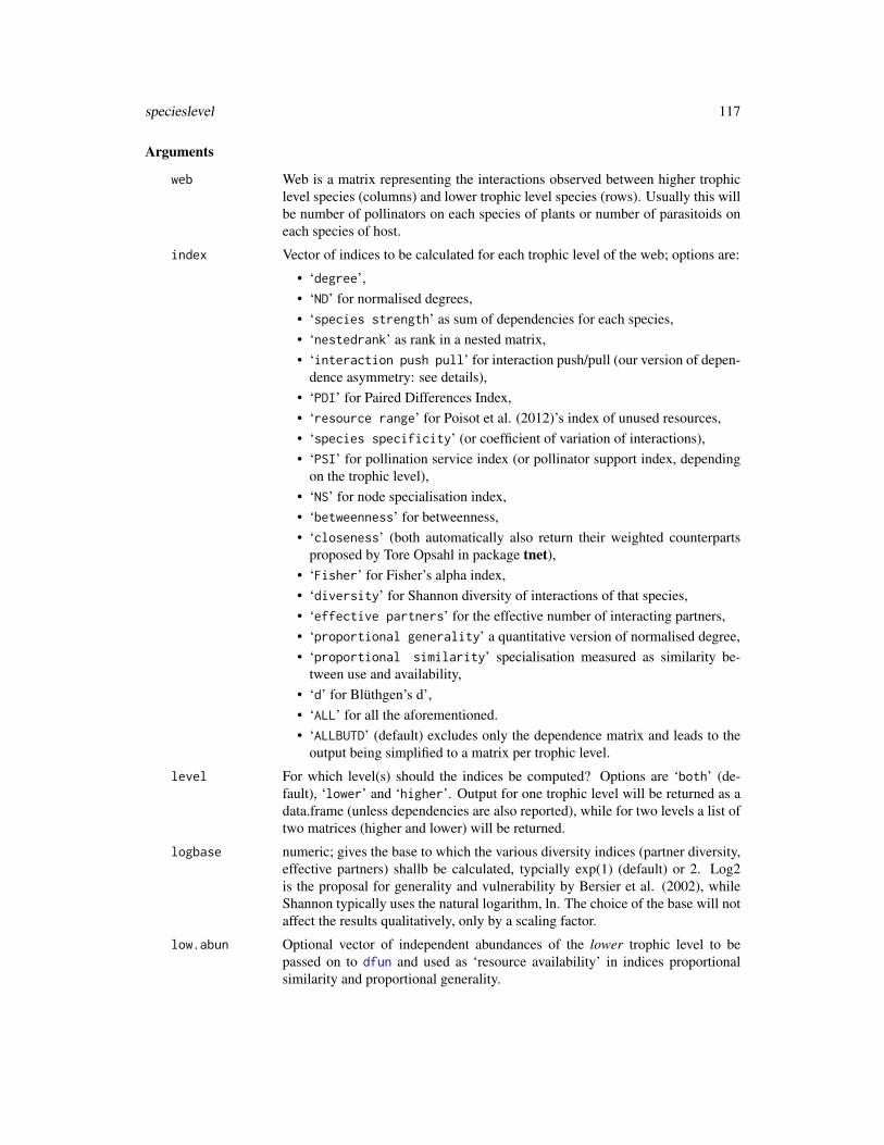
specieslevel 117

Arguments

web Web is a matrix representing the interactions observed between higher trophiclevel species (columns) and lower trophic level species (rows). Usually this willbe number of pollinators on each species of plants or number of parasitoids oneach species of host.

index Vector of indices to be calculated for each trophic level of the web; options are:

• ‘degree’,• ‘ND’ for normalised degrees,• ‘species strength’ as sum of dependencies for each species,• ‘nestedrank’ as rank in a nested matrix,• ‘interaction push pull’ for interaction push/pull (our version of depen-

dence asymmetry: see details),• ‘PDI’ for Paired Differences Index,• ‘resource range’ for Poisot et al. (2012)’s index of unused resources,• ‘species specificity’ (or coefficient of variation of interactions),• ‘PSI’ for pollination service index (or pollinator support index, depending

on the trophic level),• ‘NS’ for node specialisation index,• ‘betweenness’ for betweenness,• ‘closeness’ (both automatically also return their weighted counterparts

proposed by Tore Opsahl in package tnet),• ‘Fisher’ for Fisher’s alpha index,• ‘diversity’ for Shannon diversity of interactions of that species,• ‘effective partners’ for the effective number of interacting partners,• ‘proportional generality’ a quantitative version of normalised degree,• ‘proportional similarity’ specialisation measured as similarity be-

tween use and availability,• ‘d’ for Blüthgen’s d’,• ‘ALL’ for all the aforementioned.• ‘ALLBUTD’ (default) excludes only the dependence matrix and leads to the

output being simplified to a matrix per trophic level.

level For which level(s) should the indices be computed? Options are ‘both’ (de-fault), ‘lower’ and ‘higher’. Output for one trophic level will be returned as adata.frame (unless dependencies are also reported), while for two levels a list oftwo matrices (higher and lower) will be returned.

logbase numeric; gives the base to which the various diversity indices (partner diversity,effective partners) shallb be calculated, typcially exp(1) (default) or 2. Log2is the proposal for generality and vulnerability by Bersier et al. (2002), whileShannon typically uses the natural logarithm, ln. The choice of the base will notaffect the results qualitatively, only by a scaling factor.

low.abun Optional vector of independent abundances of the lower trophic level to bepassed on to dfun and used as ‘resource availability’ in indices proportionalsimilarity and proportional generality.

118 specieslevel

high.abun Optional vector of independent abundances of the higher trophic level to bepassed on to dfun and used as ‘resource availability’ in indices proportionalsimilarity and proportional generality.

PDI.normalise Logical; should the normalised PDI be computed? Defaults to TRUE. See func-tion PDI for details and reasoning.

PSI.beta A length 2 vector of parameter determining the effect of floral constancy andpollen mixing on the proportion of same-species pollen delivered to a plant.Defaults to c(1, 0). See section details for details.

nested.method One of ‘NODF’, ‘binmatnest’, ‘wine’ or ‘sort’. See nestedrank for details.nested.normalised

Logical; defaulting to TRUE. Divides the nestedrank-1 by the number of species-1, thereby ranging it between 0 (most generalist) and 1 (most specialised).Species sequences from different networks are now comparable.

nested.weighted

Logical; should the “nestedrank” be computed based on weighted network (de-fault) or binary version (FALSE)?

empty.web Shall the empty columns and rows be deleted? Defaults to TRUE. option FALSEnot yet fully tested

Details

This function implements a variety of the many (and still procreating) indices describing speciesproperties. Some are embarrassingly simple (such as number of interacting species for each species).Others are variations on Shannon’s diversity index applied to within species.

Indices based on graph theory (such as NDI, closeness, betweenness) require the data to form aconnected graph. When the network is compartmented (as would be seen when plotting it usingplotweb), these indices will be computed for the each compartment. However, single-link compart-ments (only one partner in each trophic level) will not form a proper graph and hence the indiceswill have a value of NA.

Most indices are straightforward, one-line formulae; some, such as d’, also require a re-arranging ofthe matrix. We (Dormann, Blüthgen, Gruber) came up with a new one, called “Pollination ServiceIndex” or psi, for which a few more details seem appropriate.

Pollination Service Index (PSI)This index estimates the importance of a pollinator for all plant species. PSI is comprised of threecalculation steps: firstly, we calculate, for each pollinator species, the proportion to which it visitseach plant species (or, phrased anthropomorphically, the number to the question: which proportionof my visits are to dandelion?). Secondly, we calculate the proportion to which a plant is visitedby each bee species (Which proportion of my pollinators are red mason bees?). Multiplying, thesetwo proportions gives the portion of own pollen for each plant species (because this depends bothon a pollinators specialisation (step 1) and the plant’s specific receptiveness (step 2). Finally, wesum the proportions own pollen delivered across all plant species. This value is the PSI-value. Atits maximum, 1, it shows that all pollen is delivered to one plant species that completely depends onthe monolectic pollinator. At its minimum, 0, it indicates that a pollinator is irrelevant to all plantspecies. Note that PSI can assume values from 0 to 1 for species of any frequency: a bee been foundonly once on a plant species visited by no-one else receives a PSI of 1, even if in total 14 millionvisits were recorded.

specieslevel 119

(This is all very complicated. So here is another attempt (by Jochen) to explain the PSI: ForPSI, importance of a pairwise interaction (for the plant) is calculated as: ’dependence’_i_on_j* per.visit.efficiency_i_visitedby_j, where per.visit.efficiency_i_visitedby_j = (average proportionvisits to i by j in all visits by j)^beta.

It assumes that the order of plant species visited is random (no mixing, no constancy). To accountfor that not being true, beta could be adjusted. However, this really waits for good empirical tests.)

We envisage a penalty for the fact that a pollinator has to make two (more or less successive) visitsto the same plant species: the first to take the pollen up, the second to pollinate the next. Thus,using beta=2 as an exponent in step 1 would simulate that a pollinator deposits all pollen at everyvisit. In a sense, beta=2 represents a complete turnover of pollen on the pollinator from one visitto the next; only the pollen of the last-visited species is transferred. That is certainly a very strongpenalisation. At present we set the exponent to beta=1, because the step of controlling for “pollenpurity” is already a major improvement. It assumes, implicitly, that pollen is perfectly mixed onthe pollinator and hence pollen deposited directly proportional to frequency of visits to the differentplants Also, we have no idea to which extent pollen gets mixed and/or lost during foraging flights,and the true exponent remains elusive. For a value of beta=0, PSI simplifies (and is equal) to speciesstrength.

For the perspective of the plant’s effect on pollinators (then PSI = pollinator support index), thisindex makes less sense. Here we would rather use beta=0, because pollen value is not related tonumber of visits, so we cannot compute it from the network. Similarly, for other networks, such ashost-parasitoids, beta=0 seems plausible, since for the host it does not matter, whether a parasitoidhas visited another species before or not. In this case (beta=0), PSI is simply equal to speciesstrength. Not just pollen turnover/carryover on the pollinator is important and influences beta,but all these considerations depend on the assumption how the proportion of conspecific pollenaffects pollination (assuming many visits per flower visitation sequence). (a) If only presence ofany conspecific pollen on bee is sufficient for pollination, carryover (how long pollen from onevisits remains on bee) matters, beta is anywhere between 0 (infinite carryover) and 2 (one-stepcarryover). (b) If the proportion of conspecific pollen on bee determines pollination success (linearrelationship), carryover does not matter, the proportion can be assumed to be in an equilibrium, andbeta=1.

Our choice of defaults (c(1,0)) will yield species strength for plants, and PSI for pollinators, assum-ing, for the latter, that pollen mixes perfectly.

Value

For both the “higher trophic level” and the “lower trophic level” a list with the following compo-nents:

species degree Sum of links per species.normalised degree

As degree, but scaled by the number of possible partners; see ND.

species strength

Sum of dependencies of each species (used, e.g., in Bascompte et al. 2006). Itaims at quantifying a species’ relevance across all its partners. The alternativeversion of Barrat et al. (2004; also used by Poisot et al. 2012) as the sumof interactions of a species seems too trivial a measure, reflecting abundancerather than anything else. Do not take this to be the much-discussed “interaction

120 specieslevel

strength” in food web papers, which focusses on pairwise interactions (reviewedin Berlow et al. 2004)!

interaction push pull

Direction of interaction asymmetry based on dependencies: positive values indi-cate that a species affects the species of the other level it interacts with strongerthen they affect it (“pusher”); negative values indicate that a species is, on av-erage, on the receiving end of the stick (“being pulled”); formula based onVázquez et al. (2007), but push/pull is our own nomenclature. Values are highlycorrelated with species strengths (see below), but standardised to fall between-1 (being pulled) and 1 (pushing). Compared to “strength”, this index quantifiesthe net balance, rather than the average effect.

nestedrank Quantifies generalism by the rank of a species in a network matrix re-arrangedfor maximal nestedness (Alarcon et al. 2008). A low rank (e.g. 1, 2) indicateshigh generality, while high ranks (up to the number of species in that level)indicate specialism or rarity.

PDI Paired Differences Index as proposed by Poisot et al. (2011a,b), by default usinga normalised version (‘PDI.normalise=TRUE’); ranges between 0 (generalist)and 1 (specialist); see PDI for details and comments.

resource range Poisot et al.’s (2012) “resource range” is a somewhat strange name for somethingthat has a value of 0 when all resources are used, but a value of 1 when onlyone resource is used. It is, in fact, closer to an “unused resource range”. Theaforementioned Paired Difference Index is a generalisation of resource range,which is equal to resource range when the web is binary.

species specificity

Coefficient of variation of interactions, normalised to values between 0 and 1,following the idea of Julliard et al. (2006), as proposed by Poisot et al. (2012).Values of 0 indicate low, those of 1 a high variability (and hence suggesting lowand high specificity). Since not corrected for number of observations, this indexwill yield high specificity for singletons, even though there is no information tosupport this conclusion.

PSI Pollination Service Index for the higher trophic level, and the equivalent Pol-linator Support Index for the lower trophic level. See Details above for moreexplanations.

node specialisation index

Another measure of specialisation, based on the path length between any twohigher-trophic level species. Species sharing hosts/prey have an FS-value of 1.See specific function nodespec for details, problems and reference.

betweenness A value describing the centrality of a species in the network by its positionbetween other nodes; see BC and betweenness in sna.

weighted betweenness

Computes betweenness (proportion of shortest paths through this species), butbased on weighted representation of the network. It calls betweenness_w fromtnet and often differs considerably from its binary counterpart!

closeness A value describing the centrality of a species in the network by its path lengthsto other nodes; see CC and closeness in sna.

specieslevel 121

weighted closeness

Computes closeness (in one of its varieties), but based on weighted representa-tion of the network. It calls closeness_w from tnet and is usually very similarto its binary counterpart. Note that NAs indicate that these species belong to adifferent compartment and hence no closeness distance could be calculated.

Fisher alpha Fisher’s alpha diversity for each species (see fisher.alpha in vegan for de-tails).

partner diversity

Shannon diversity (when using ‘logbase="e"’) or per-species generality/vulnerability(when using ‘logbase=2’) of the interactions of each species. See also networklevelfor the aggregated version of this index (i.e. averaged across all species in atrophic level).

effective partners

‘logbase’ to the power of “partner.diversity”: Bersier et al. (2002) interpretthis as the effective number of partners, if each partner was equally common.Note that “partner” is a bit euphemistic when it comes to predator-prey or host-parasitoid networks.

proportional generality

’Effective partners’ divided by effective number of resources (’logbase’ to thepower of ’resource diversity’; which is calculated from high.abun/low.abun ifprovided, and else from marginal totals); this is the quantitative version of pro-portional resource use or normalised degree (i.e., the number of partner speciesin relation to the potential number of partner species); note that this index canbe larger than 1, e.g. when a species selects for a balanced diet.

proportional similarity

Specialization measured as dissimilarity between resource use and availability(estimated from high.abun/low.abun if provided, else from marginal totals); pro-posed by Feinsinger et al. (1981).

d Specialisation of each species based on its discrimination from random selectionof partners. More specifically, it returns d’, which is calculated based on the rawd, dmin and dmax for each species (see dfun). See Blüthgen et al. (2006) fordetails.

Note

A comparison of specialisation indices is provided in Dormann (2011); the PDI is missing (since itwas published later).

Dependencies are still an open field of debate. Dependencies are calculated as the value in a matrixdivided by the rowSums (for the lower trophic level) or the colSums (for the higher trophic level).As such, any pollinator observed only once will receive a dependency-value of 1, indicating perfectdependence on this plant species. That may or may not be true. In any case it is based on a samplesize of 1, that is why the dependency asymmetry (which is based on the dependencies for bothtrophic levels) has come under criticism and may be rather sensitive to singletons.

We here provide the code to calculate the strength of a species (i.e. sum of its dependencies), basedon the current proposal by Bascompte et al. (2006). It may be a good idea to remove all singletonsfrom the web before calculating this index, to investigate whether it is indeed driven by those scarceobservations.

122 specieslevel

The maximum value of the uncorrected d (i.e. the maximal potential specialization defining d’=1)is not a trivial issue. We treat it here in the same way as given in the BMC Ecology paper, but pleasehave a look at the (raw) code for further comments.

Author(s)

Carsten F. Dormann <[email protected]> \& Jochen Fründ

References


Barrat, A., M. Barthélemy, R. Pastor-Satorras, and A. Vespignani. 2004. The architecture of com-plex weighted networks. Proceedings of the National Academy of Sciences of the USA 101, 3747—3752. doi: 10.1073/pnas.0400087101.

Bascompte, J., Jordano, P. and Olesen, J. M. (2006) Asymmetric coevolutionary networks facilitatebiodiversity maintenance. Science 312, 431–433

Berlow, E. L., A. M. Neutel, J. E. Cohen, P. C. de Ruiter, B. Ebenman, M. Emmerson, J. W. Fox,V. A. A. Jansen, J. I. Jones, G. D. Kokkoris, D. O. Logofet, A. J. McKane, J. M. Montoya & O.Petchey (2004) Interaction strengths in food webs: issues and opportunities. Journal of AnimalEcology 73, 585-–598



Feinsinger, P., Spears, E.E. and Poole,R. W. (1981) A simple measure of niche breadth. Ecology62, 27–32.

Julliard, R., Clavel, J., Devictor, V., Jiguet, F. and Couvet, D. (2006) Spatial segregation of special-ists and generalists in bird communities. Ecology Letters 9, 1237-–1244

Martín Gonzáles, A.M., Dalsgaard, B. and Olesen, J.M. (2010) Centrality measures and the impor-tance of generalist species in pollination networks. Ecological Complexity, 7, 36–43

Opsahl, T. & Panzarasa, P. (2009). Clustering in weighted networks. Social Networks, 31, 155–163



Poisot, T., E. Canard, N. Mouquet, and M. E. Hochberg (2012) A comparative study of ecologicalspecialization estimators. Methods in Ecology and Evolution 3, 537-–544. doi: 10.1111/j.2041-210X.2011.00174.x.

Vázquez, D. P., Melian, C. J., Williams, N. M., Blüthgen N., Krasnov B. R. and Poulin, R. (2007)Species abundance and asymmetric interaction strength in ecological networks. Oikos 116, 1120–1127

strength 123

See Also

networklevel for some further comments; dfun, nodespec, which are called by this function

Examples

data(Safariland)## Not run:specieslevel(Safariland)## End(Not run)specieslevel(Safariland, index="ALLBUTD")[[2]]

strength Computes species strength according to either of two definitions

Description

Computes species strength of the higher level species as a measure of how important a species is inthe network

Usage

strength(web, type="Bascompte")

Arguments


type Which definition of species strength should be used, ‘Bascompte’ (default) or‘Barrat’? See Details for definitions.

Details

There are two definitions of species strength, that of Bascompte et al. (2006) as the sum of depen-dencies of a species, and that of Barrat et al. (2004) as the weighted sum of links. As a consequence,Bascompte et al.’s strength sums to the number of species in the other group, while Barrat et al.’sstrength is simply the number of interactions, a trivial measure of a species importance.

In contrast to the claim of Gilarranz et al. (2012, p. 1155), this definition of strength gives noinformation of the centrality of a species within a network structure (and neither does Bascompte etal.’s).

Value

A vector of species strengths for the higher level. Employ this function on the transpose of the webto compute the strengths of the lower level (see example).

Author(s)


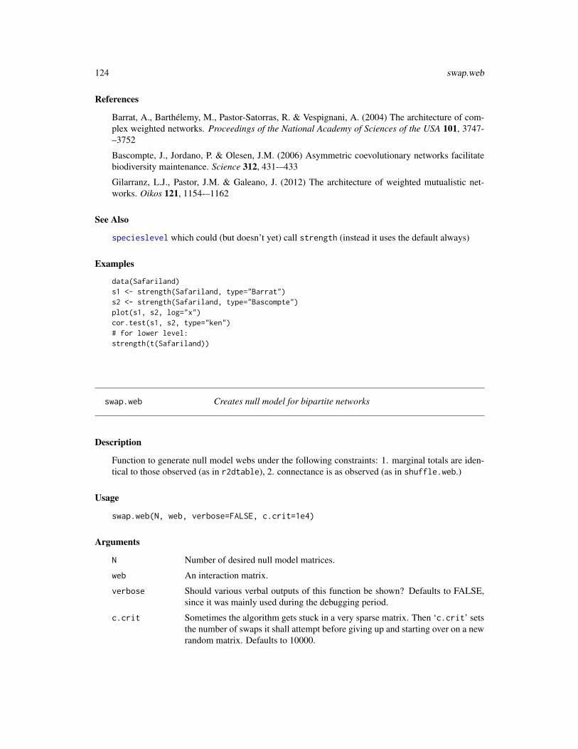
124 swap.web

References

Barrat, A., Barthélemy, M., Pastor-Satorras, R. & Vespignani, A. (2004) The architecture of com-plex weighted networks. Proceedings of the National Academy of Sciences of the USA 101, 3747-–3752

Bascompte, J., Jordano, P. & Olesen, J.M. (2006) Asymmetric coevolutionary networks facilitatebiodiversity maintenance. Science 312, 431-–433

Gilarranz, L.J., Pastor, J.M. & Galeano, J. (2012) The architecture of weighted mutualistic net-works. Oikos 121, 1154-–1162

See Also

specieslevel which could (but doesn’t yet) call strength (instead it uses the default always)

Examples

data(Safariland)s1 <- strength(Safariland, type="Barrat")s2 <- strength(Safariland, type="Bascompte")plot(s1, s2, log="x")cor.test(s1, s2, type="ken")# for lower level:strength(t(Safariland))

swap.web Creates null model for bipartite networks

Description

Function to generate null model webs under the following constraints: 1. marginal totals are iden-tical to those observed (as in r2dtable), 2. connectance is as observed (as in shuffle.web.)

Usage

swap.web(N, web, verbose=FALSE, c.crit=1e4)

Arguments

N Number of desired null model matrices.


verbose Should various verbal outputs of this function be shown? Defaults to FALSE,since it was mainly used during the debugging period.

c.crit Sometimes the algorithm gets stuck in a very sparse matrix. Then ‘c.crit’ setsthe number of swaps it shall attempt before giving up and starting over on a newrandom matrix. Defaults to 10000.

swap.web 125

Details

This function is designed to behave similar to r2dtable, i.e. it returns a list of randomised matrices.In addition to r2dtable is also keeps the connectance constant!

This function is thought of as a very constrained null model for the analysis of bipartite webs.It keeps two web properties constant: The marginal totals (as in r2dtable and the number oflinks (and hence connectance). A comparison of swap.web- and r2dtable-based webs allows toelucidate the effect of evolutionary specialisation, since the unrealised connections may represent“forbidden links”.

This null model is similar to the one employed by Vázquez et al. But while Vázquez starts byassigning 1s to the allowed connections and then fills the web, swap.web starts with an r2dtable-web and successively “empties” it. The two approaches should result in very similar null models,since both constrain marginal totals and connectance.

A few words on the way swap.web works. It starts with a random web created by r2dtable. Then,it finds, randomly, 2x2 submatrices with entries all larger than 0. Next, it subtracts the minimumvalue from the diagonal and adds it to the off-diagonal (minor diagonal). Thereby one cell becomes0, but the column and row sums do not change. This idea is adapted from the swap-algorithm usedin various binary null models by Nick Gotelli. If the random web has too few 0s (which is I haveyet to encounter), then the opposite strategy is applied.

The algorithm in our implementation has some variations on finding the submatrix and constrainingthe number of unsuccessfull trials before starting on a new random matrix, but they are only forspeeding up the process.

Value

A list of N randomised matrices with the same dimensions as the initial web.

Note

Long stories can be told about the swap algorithm. I am not the right person to do so, but for a muchmore detailed coverage of the topic, for many more ways to implement null models for binarymatrices, with various flavours of the swap and possible alternatives, first brew yourself a cup oftea and then check out the help pages of simulate in vegan. (As usual, Jari Oksanen has spendconsiderable care to implement even the most bizarre and abstruse way to move 0s and 1s around.His ecological advise between the lines make his package worthwhile already! I, personally, woulduse method="quasiswap", as is done in the example to discrepancy.)

When comparing the swap.web algorithm with that proposed by Vázquez et al. (2007, implementedin vaznull), we found that swap.web contains a certain bias. The subtraction of the swap willreduce the value of low-value cells, and increase that of high-value cells. As a consequence, itproduces somewhat of a dichotomy between very high and very low values. Using e.g. H2’ toquantify this pattern, swap.web will produce very specialised networks (around 0.5), while theVazquez-algorithm yields lower H2’ values and a more even distribution of interactions withincells. The ramifications are that swap.web will predict higher-than-necessary expectations. (Dateof this entry: 15.1.2010)

In fact, Artzy-Randrup & Stone (2005) have shown that the swap algorithm is fundamentally biased,because some swaps are more likely than others. This applies to this version of the swap as well asto the one implemented in vaznull. So, despite heavy citation, the approach of Miklós & Podani(2004) is thus also not ideal, as often claimed.

126 symmetrise_w

swap.web is a very constraint null model. You need to consider if it is the right one for yourapplication!

Author(s)


References

Artzy-Randrup, Y., and Stone, L. (2005) Generating uniformly distributed random networks. Phys-ical Review E 72, 1–7

Miklós, I. and Podani, J. (2004) Randomization of presence-absence matrices: comments and newalgorithms. Ecology 85, 86–92

Vázquez, D. P., and M. A. Aizen (2003) Null model analyses of specialization in plant-pollinatorinteractions. Ecology 84, 2493–2501

Vázquez, D. P., C. J. Melian, N. M. Williams, N. Blüthgen, B. R. Krasnov, and R. Poulin (2007)Species abundance and asymmetric interaction strength in ecological networks. Oikos 116, 1120–1127

For a very nice and thorough overview of null models in general see:

Gotelli, N. J., and G. R. Graves (1996) Null Models in Ecology. Smithsonian Institution Press,Washington D.C.

See Also

r2dtable, vaznull and shuffle.web

Examples

swap.web(Safariland, N=2)

symmetrise_w Symmetrise_w

Description

The symmetrise_w-function creates an undirected one-mode network from a directed one-modenetwork.

Usage

symmetrise_w(net, method="MAX")

symmetrise_w 127

Arguments

net A one-mode network

method the method used to decide the weight of the undirected edge. It can be: "MAX"sets the weight to the maximum of the weight(s) of the arc(s) "MIN" sets theweight to the minimumof the weight(s) of the arc(s) "AMEAN" sets the weightto the average (arithmetic mean) of the weight(s) of the arc(s) "SUM" sets theweight to the sum of the weight(s) of the arc(s) "PROD" sets the weight to theproduct of the weight(s) of the arc(s) "DIFF" sets the weight to the absolutedifference between the weight(s) of the arc(s)

Value

Returns the undirected network

Note


Author(s)


References

http://toreopsahl.com/2008/11/28/network-weighted-network/

Examples

## Load sample datasample <- rbind(c(1,2,2),c(1,3,2),c(2,1,4),c(2,3,4),c(2,4,1),c(2,5,2),c(3,1,2),c(3,2,4),c(5,2,2),c(5,6,1))

## Run the programmesymmetrise_w(sample, method="MAX")

128 tnet_igraph

tnet_igraph Exports a tnet network to an igraph object

Description

The tnet_igraph function creates an igraph object from a tnet network.

Usage

tnet_igraph(net,type=NULL, directed=NULL)

Arguments

net A tnet network

type type of tnet network, see as.tnet.

directed if a one-mode networks, this can be set to avoid testing whether the network isdirected.

Value

Returns the igraph object.

Note


Author(s)


References

http://toreopsahl.com/

Examples

## Load sample datasample <- rbind(c(1,2,4),c(1,3,2),c(2,1,4),c(2,3,4),c(2,4,1),c(2,5,2),c(3,1,2),c(3,2,4),c(4,2,1),c(5,2,2),

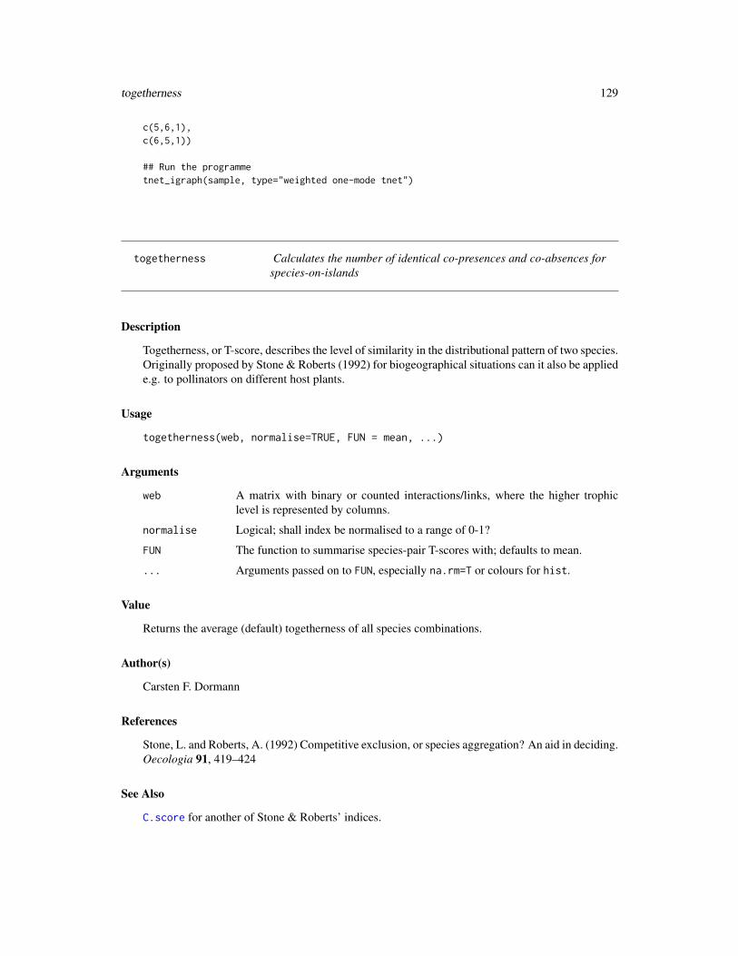
togetherness 129

c(5,6,1),c(6,5,1))

## Run the programmetnet_igraph(sample, type="weighted one-mode tnet")

togetherness Calculates the number of identical co-presences and co-absences forspecies-on-islands

Description

Togetherness, or T-score, describes the level of similarity in the distributional pattern of two species.Originally proposed by Stone & Roberts (1992) for biogeographical situations can it also be appliede.g. to pollinators on different host plants.

Usage

togetherness(web, normalise=TRUE, FUN = mean, ...)

Arguments

web A matrix with binary or counted interactions/links, where the higher trophiclevel is represented by columns.

normalise Logical; shall index be normalised to a range of 0-1?

FUN The function to summarise species-pair T-scores with; defaults to mean.

... Arguments passed on to FUN, especially na.rm=T or colours for hist.

Value

Returns the average (default) togetherness of all species combinations.

Author(s)

Carsten F. Dormann

References


See Also

C.score for another of Stone & Roberts’ indices.

130 V.ratio

Examples

(m <- matrix(c(0,1,0,0,1,1,0,1,1,0), ncol=2, byrow=TRUE))togetherness(m)# or, with two togethernesses:(n <- matrix(c(0,1,1,0,1,1,0,0,1,1,0,1,0,1), ncol=2, byrow=TRUE))togetherness(n, normalise=FALSE)

data(Safariland)togetherness(m)

V.ratio Calculates the variance-ratio as suggested by Schluter (1984)

Description

A of species association is provided by the ratio of the variance in total species number (or totaldensity of individuals) in samples to the sum of the variances of the individual species.

Usage

V.ratio(web)

Arguments

web A matrix with pollinators in columns and plants in rows. For biogeographicalapplications: rows are islands (or sites).

Details

This is a rather straight-forward index, which is described and evaluated extensively in Schluter(1984). He also warns against overinterpretation of the value. In principle, V-ratios larger than 1indicate positive, smaller than 1 negative associations. Ecologically, competition can lead to smallor large values, depending on their exact effects (see discussion in the Schluter paper).

Value

Returns the V-ratio, i.e. a single value representing the ratio of variance in species number andvariance in individual numbers within species.

Note

Any quantitative matrix is first transformed into a binary (presence-absence) matrix!

Do not interpret without first reading the paper! It’s worth it! See also applications in other studies,such as Gotelli and Rohde (2002).

Author(s)

Carsten F. Dormann

vazarr 131

References

Gotelli, N.J. and Rohde, K. (2002) Co-occurrence of ectoparasites of marine fishes: a null modelanalysis. Ecology Letters 5, 86–94

Schluter, D. (1984) A variance test for detecting species associations, with some example applica-tions. Ecology 65, 998–1005

See Also

C.score for another measure of species associations.

Examples

data(Safariland)V.ratio(Safariland)

vazarr A pollination network.

Description

[See documentation for Safariland.]

Usage

data(vazarr)

Format

The format is: num [1:10, 1:29] 85 0 94 0 0 0 0 0 0 0 ... - attr(*, "dimnames")=List of 2 ..$ : chr[1:10] "X2" "X1" "X13" "X4" ... ..$ : chr [1:29] "78" "65" "94" "66" ...

Examples

data(vazarr)## maybe str(vazarr) ; plot(vazarr) ...

132 vazllao

vazcer A pollination network.

Description


Usage

data(vazcer)

Format


Examples

data(vazcer)## maybe str(vazcer) ; plot(vazcer) ...

vazllao A pollination network.

Description


Usage

data(vazllao)

Format


Examples

data(vazllao)## maybe str(vazllao) ; plot(vazllao) ...

vazmasc 133

vazmasc A pollination network.

Description


Usage

data(vazmasc)

Format

The format is: num [1:8, 1:26] 73 0 0 0 0 0 0 0 0 6 ... - attr(*, "dimnames")=List of 2 ..$ : chr [1:8]"X2" "X1" "X13" "X4" ... ..$ : chr [1:26] "78" "65" "94" "32" ...

Examples

data(vazmasc)## maybe str(vazmasc) ; plot(vazmasc) ...

vazmasnc A pollination network.

Description


Usage

data(vazmasnc)

Format


Examples

data(vazmasnc)## maybe str(vazmasnc) ; plot(vazmasnc) ...

134 vaznull

vaznull Null model with constrained connectance and moderately constrainedmarginal totals

Description

Implements Diego Vazquez proposal of a null model for pollination networks

Usage

vaznull(N, web)

Arguments

N Number of desired null model webs.


Details

This function produces a null model network with the main constraint of a connectance that is thesame as in the original network. In the process of producing this null model, marginal totals willturn out to be different from the original network, less so for large, dense webs than for small, sparsewebs. vaznull is our implementation of the algorithm propose by Diego Vazquez, hence its name.vaznull differs from swap.web in that marginal totals are not strictly constraint! The algorithmused as well as the null model it outputs are different.

The algorithm was described as follows: "The algorithm randomized the total number of indi-vidual interactions observed in the original interaction matrix, F. To this end, the algorithm firstcreated a binary matrix, assigning interspecific interactions according to species-specific probabil-ities, requiring that each species had at least one interaction. As in Vazquez et al. (2005b), thespecies-specific probabilities were proportional to species’ relative abundances (probabilities are infact approximately proportional and not equal to relative abundances because of the requirementthat each species receives at least one interaction; this requirement causes probabilities to deviatefrom relative abundances, especially for rare species). Once the number of filled cells in the orig-inal matrix was reached, the remaining interactions were distributed among the filled cells, so thatconnectance in the original and randomized matrices was the same." (Vazquez et al. 2007, page1122-1123).

Value

A list of N randomised matrices with the same dimensions and connectivity as the initial web.

Author(s)

Bernd Gruber <[email protected]> & Carsten F. Dormann <[email protected]>

vazquec 135

References

Vázquez, D. P., C. J. Melian, N. M. Williams, N. Blüthgen, B. R. Krasnov, and R. Poulin. 2007.Species abundance and asymmetric interaction strength in ecological networks. Oikos 116: 1120-1127.

See Also

r2dtable, swap.web

Examples

## Not run:data(Safariland)networklevel(Safariland, index="info")networklevel(vaznull(1, Safariland)[[1]], index="info")system.time(vaznull(10, Safariland))system.time(swap.web(10, Safariland))

## End(Not run)

vazquec A pollination network.

Description


Usage

data(vazquec)

Format

The format is: num [1:8, 1:27] 31 0 34 150 11 66 2 4 0 63 ... - attr(*, "dimnames")=List of 2 ..$ :chr [1:8] "X1" "X13" "X4" "X15" ... ..$ : chr [1:27] "65" "94" "32" "66" ...

Examples

data(vazquec)## maybe str(vazquec) ; plot(vazquec) ...

136 vazquez.example

vazquenc A pollination network.

Description


Usage

data(vazquenc)

Examples

data(vazquenc)## maybe str(vazquenc) ; plot(vazquenc) ...

vazquez.example Examples for some analyses

Description

Describes how to use bipartite to calculate the statistics presented in Vázquez et al. (2009). Someof these functions are available in bipartite or other packages, and this help page will show how touse them in line with the publication.

Details

The functions used are:

confint: Is the same as quantile

intasymm: Can be extracted using specieslevel

intereven: Is similar to interaction evenness in networklevel, but only for a specific option

mlik: A specific call to dmultinom and the calculation of the AIC; the number of parameters en-tering the AIC-calculation is not obvious; this depends on the constraints used by the nullmodel. In the case of r2dtable, column and row totals are constrained, i.e. ncol+nrow pa-rameters must be given. In the case of swap.web, connectance is also constrained, but howmany parameters does that imply? One? In shuffle.web, we constrain the dimensionalityand connectance, i.e. 3 (?) parameters. Vázquez et al. (2009) argue that they constrain only2 parameters when producing the probability matrix given as pweb in the example below.We tend to disagree: the marginal probabilities of all columns and rows are given, hence k =(ncol(web) + nrow(web)). To our knowledge, there is no mathematical/statistical treatise ofthis problem.

netstats: A wrapper calling the other functions, in that sense similar to networklevel, but alsocalling some output from specieslevel.

vazquez.example 137

plotmat: Now part of visweb, using the right options.

quant2bin: A dedicated function to do a simple thing: (web>0)*1.

sortmatr: newly defined function: sortweb

sortmatrext: sort matrix by some given sequence; also part of sortweb

In the example below, we use the bipartite/standard R functions whenever possible.

Author(s)

Carsten F. Dormann <[email protected]> based on code and ideas of DiegoVázquez, Natacha P. Chacoff and Luciano Cagnolo

References

Vázquez, P.D., Chacoff, N.,P. and Cagnolo, L. (2009) Evaluating multiple determinants of the struc-ture of plant-animal mutualistic networks. Ecology 90, 2039–2046.

See Also

See also networklevel.

Examples

## Not run:data(Safariland)

# confint:N100 <- sapply(swap.web(100, Safariland), networklevel, index="nestedness")quantile(unlist(N100), c(0.025, 0.975))# intasymm: extract values for the asymmetry of interactions and the# dependency matrix for pollinators:specieslevel(Safariland)$"higher trophic level"$"interaction push/pull"specieslevel(Safariland)$"higher trophic level"$"dependence"# for plants:specieslevel(Safariland)$"lower trophic level"$"interaction push/pull"specieslevel(Safariland)$"lower trophic level"$"dependence"

#interevennetworklevel(Safariland, index="interaction evenness", intereven="sum")[2]# or, as we recommend (see help on networklevel):networklevel(Safariland, index="interaction evenness", intereven="prod")[2]

# mlik:# calculates the log-likelihood of observing a network, given a probability# matrix of the same size (pweb):dmultinom(Safariland>0, prob=pweb, log=TRUE)# AIC (the number of parameters is given by how many constraints are put onto the# null model; here, we constrain 9 rows and 27 columns, i.e. sum(dim(binweb))):-2*dmultinom(Safariland>0, prob=pweb, log=TRUE) + 2*(sum(dim(binweb)))

# netstats:

138 versionlog

networklevel(Safariland,index=c("connectance", "interaction evenness", "nestedness", "ISA"))

mean(specieslevel(Safariland)$"higher trophic level"$"interaction push/pull")mean(specieslevel(Safariland)$"lower trophic level"$"interaction push/pull")

#plotmat:visweb(t(unname(Safariland)), circles=TRUE, boxes=FALSE)

#sortmatr/sortmatrext:sortweb(Safariland, sort.order="inc") #rares species firstplotweb(sortweb(Safariland, sort.order="dec"), method="normal")plotweb(sortweb(web=Safariland, sort.order="seq",

sequence=list(seq.higher=sample(colnames(Safariland)),seq.lower=sample(rownames(Safariland)))),method="normal")

## End(Not run)

versionlog Log of bipartite versions and changes

Description

Log tracking changes, bug fixes and new functions in bipartite

Usage

versionlog()

versionlog

• 1.18 (release date: 06-Sep-2012)New function and index fd: fd computes the functional diversity for the rows of a web as a

measure of ecological niche complementarity (Devoto et al. 2012). Function written andprovided by Mariano Devoto. fd is also included in the computation of networklevel.

New function czvalues to compute c- and z-values of the higher trophic level for modu-lar networks. Requires a successful identification of modules through computeModules.These can then be used to identify connector species in a network.

Speed-up of plotweb: Thanks to Dirk Raetzel, whose smart improvement made this functionorders of magnitude faster! (Amazing how a total of 7 lines of code in a total of over 300for this function can make such a vast improvement!)

Speed-up of compart: Thanks to Juan M. Barreneche, whose smart improvement made thisfunction orders of magnitude faster while using dramatically less memory.

New option for simulating extinctions in second.extinct (and necessarily extinction):Use ‘method="external"’ to impose a specific sequence of exterminations onto thefunction. Provide this sequence as an index vector (e.g. c(4,2,3,1)) through the ar-gument ‘ext.row’ or ‘ext.col’ (for lower and higher species level, respectively). Re-quested/proposed by Matt Koski. (Implementation is far from elegant and will be cleanedup in a future version.)

versionlog 139

Modification of visweb: The user is now able to use user-defined colours (def.col) for inter-action ranks (‘square="d"’). Thereby the number of interactions can define the colourof the cell in the plot. Makes visweb-plot prettier.

Important bug fix in robustness and second.extinct: robustness sometimes interpretedwrongly which trophic level was subject to simulated extinction. That was easy to fix. Enroute, however, I also discovered unexpected behaviour in the second.extinct function:it gobbled up the last species to be removed from the web. I do not think that extinctionslope estimates are affected much, but robustness results may well be exhibiting a biastowards 0.5! Thanks to Silvia Santamaria for reporting this!

Little bug fix in functions BC and CC: Functions always used unweighted networks for com-puting betweenness and closeness. The default is now to use weighted information, anoption which can be switched off. Thanks to Michael Pocock for reporting and suggest-ing a fix! (Notice the help file for these functions and the large effect that the choice ofsettings can have on the results!)

Little bug fix in function computeModules: Failed to work for networks with empty columnsor rows. These will now be deleted (with a warning) before the analysis. Thanks to JulienRenoult for reporting.

Little bug fix in function plotweb: Failed to work for networks with only one column orrow. Thanks to Zhijiang Wang for reporting.

Minor bug fix in networklevel: Caused an error if a selection of indices was provided.Corrections in the help of networklevel: Web asymmetry was explained the wrong way

around (thanks to Bernhard Hoiß for reporting!) and there was some confusion in the helpfor whether quantitative or weighted-quantitative indices were implemented (YvonneFabian for correcting the clarification!).

• 1.17 (release date: 20-AUG-2011)New specialisation index at the species level in function PDI: Computes the Paired Differ-

ences Index proposed by Poisot et al. (2011a,b). Also automatically now included inspecieslevel.

Bug fix in specieslevel: Computation of betweenness was causing an error when the net-work was containing a single-link compartment. Thanks to Marco Mello for spotting!

Another PDF is included (Dormann 2011): This paper compares specialisation indices, basedon the function specieslevel. All source code to reproduce these results is included. Itcan serve as a guide to the specieslevel function and its interpretation.

• 1.16 (release date: 29-May-2011)Bug fix and extended documentation in dfun: 1. Sometimes d.min was larger than d.raw

yielding negative d’-values. Since the search for d.min is heuristic, it can sometimes failto yield lower values than d.raw. In these (rare) cases, d.min is now set to d.raw. 2.Documentation for a specific (but not uncommon or unreasonable) constellation added:When independent abundances were provided, the empty rows/columns are purposefullynot removed from the web (because they now still contain information). Logically (andas implemented), this leads to d-values for these species of NA. This makes sense: thepollinator, say, has never been observed on any of the flowers, so how can we quantify itsspecialisation? While reasonable, it was undocumented behaviour. Thanks to Ana MaríaMartín Gonzáles for drawing our attention to it!

Speed improvement in shuffle.web: Thanks to Paul Rabie, a faster implementation of theshuffle.web null model is available. Choosing the option ‘legacy=FALSE’ will deliverthe null models about 3 times faster.

140 versionlog


Bug fix in swap.web: Occasionally, an interaction too many was swapped, leading to a con-nectance slightly too low compared to the original matrix. Spotted and reported by SvenHanoteaux. (For “normal” webs, this bug has luckily caused only very small discrep-ancies between the realised and the intended null web. We thus regard this error to be(luckily) of virtually no influence on the results reported in our Open Ecology Journalpaper. Please also note that the help of swap.web recommends using vaznull.)

Bug fix in shuffle.web: Some interactions were lost when there were more rows than columns.Spotted and reported by Sven Hanoteaux. (Please note that while a shameful mistake, itluckily does not affect the results reported in our Open Ecology Journal paper, where allwebs analysed were asymmetric “in the right way”.)

Minor bug fix in networklevel: No output was provided when only index “Fisher alpha”or “mean interaction diversity” was selected. Thanks to Sven Hanoteaux for reportingand fixing!

• 1.14 (release date: 21-Dez-2010)

New function plotPAC: A plotting function to go with the PAC-function, providing a nice cir-cularly arranged bubble plot, which has been copied (in style) from Morris et al. (2005).Various colour options are available.

New index “weighted NODF” included in networklevel and nested: Gustavo Carvallo hasupdated the existing function nestednodf in vegan to compute a weighted (quantitative)version as proposed by Ulrich & Almeida Neto (2011 Env. Mod. Soft). This is nowlinked into bipartite.

New data set: bezerra2009 is a“full” flower-visitation network of oil-collecting bees in Brazil.See help for details.

Minor bug fix in specieslevel: The newly (1.13) added functionality for index “weightedcloseness” did not work for webs without column and row names (such as null models).Also “weighted betweenness” was occasionally playing up.

Minor bug fix in specieslevel: Betweenness and friends cannot be computed for fully com-partmented webs (i.e. where each species interacts only with its own partner in the othertrophic level). The function then failed instead of returning NA. Thanks to Nadine Sandaufor reporting.

Minor bug fix in dfun: When providing independent abundances, the computation of dminwas sometimes incorrect (particularly for small webs) due to a typo. Fixed by JochenFründ.

Minor time-saving improvement in degreedistr: When provided with 3 or less point tocompute the degree-distribution fit from now immediately returns NA-filled matrices.Saves the time of going through all starting values and still failing.

Change of name of function argument in web2edges: The former ‘quantitative’ did notreally reflect what it does, so it was changed to ‘weight.column’.

Minor improvements to networklevel: Robustness and weighted nestedness were wrappedin try-functions (for very small networks).

New functionality to find modules in networks. This is still experimental and proper refer-ences etc. will be added after testing! Please do not use for production yet (at least notwithout consultation). Thanks to Rouven Strauß for developing this.

• 1.13 (release date: 29-Sep-2010)

versionlog 141

Option added to H2fun to compute H2’ for non-integer web. Thanks to Jochen Fründ forproviding the inspiration and the code. This option is also now available in networklevel.

Changes to nullmodel: Upon using the modification entered in version 1.12, it turns out thisis no improvement but rather a step in the wrong direction. So this function is back to itspre-1.12 working with a little bug fixed in swap.web (the helper function ‘upswap’ got anoption too many) that caused the alteration in the 1.12 version. Thanks to Jochen Fründfor insisting on rolling this back.

Bug fix in networklevel: Alatalo interaction evenness could not be called separately due toa change of name within the function. Thanks to Rachel Gibson for reporting!

New index added to networklevel: In addition to the binary cluster coefficient, the func-tion now also (and automatically) computes the weighted clustering coefficient intro-duced by Tore Opsahl in his package tnet.

New function web2edges: Transforms a web-matrix into an edge list, as used in tnet or othersoftware (e.g. Pajek).

• 1.12 (release date: 21-May-2010)

Bug fix in vaznull: In very poorly sampled networks, vaznull could fail because after theinitial filling there were no more interactions to distribute. How an if-statement can some-times make a difference.

Error message in nullmodel changed to a warning. Up to this release, the function creatednull models as specified. However, when a supposedly quantitative network was in factbinary, it returned an error. Now it proceeds, using the null model generating algorithm“mgen”, and returns a warning.


Changes to function as.one.mode: Gains options to do projections of the bipartite (=two-mode) into the one-mode modus required e.g. by sna. In most publications, one focusseson only one trophic level (e.g. the pollinators) and represents the bipartite network as aone-mode, pollinators-only network. This can now be achieved using the various optionsin the function. See its help for details.

Bug fixes in BC and CC: Upon re-reading the paper motivating the inclusion of these func-tions, I noticed an error in the previous implementation. The key point, and one thatis contentious in network theory, is that there is no standard best way to project a two-mode (bipartite) network onto a one-mode network. Up until know, I used the default ofas.one.mode. However, Martín Gonzáles et al. (2010) use the more common projection(“higher” and “lower”, respectively), and this is also now implemented in BC and CC. Theinterested reader may want to follow this problem up by reading the pre-print of ToreOpsahl (“Triadic closure in two-mode networks”) to see that this one-mode projectionactually distorts the statistics employed on them.


New function null.distr: Fits a lognormal or negative binomial distribution to the marginaltotals of a network and then draws random values from the thus specified distribution.These values represent the marginal totals to be used for constructing a null model net-work. The function thus serves as a way to produce null models without maintainingexactly the marginal totals, but only their distribution. Please refer to the help for somecautionary remarks on its use! In particular, null model networks are likely to be smallerthan the original and there is obviously no guarantee that the marginal totals are actuallydistributed in the specified way!

142 versionlog

Polishing the Vázquez pollination networks: All species in these 8 networks are now con-sistently named (rather than numbered).

Polish to specieslevel: Requesting Fisher’s alpha sometimes causes convergence problemsin the underlying function. This is now caught by a try, returning NA.

Rescale in nested gave wrong scaling for NODF: Fixed.


Bug fix in degreedistr: Degree distributions for the higher trophic level were calculatedincorrectly. The main problem was that the scaling constant was omitted, leading toridiculous fits. (Thanks to Roberto Molowny for reporting, correction proposal and dis-cussion!) On improving this, I also ventured to provide multiple starting values and hencethe function returns a fit for all three curves more often (but not always).


Bug fix in ND: Rows and columns were mixed up and a +1 was missing- oh dear. (Thanks toMarco Mello for reporting!)

• 1.07 (release date: 18-Feb-2010)

New function vaznull: Null model with constrained totals and connectance proposed byDiego Vázquez, similar to swap.web, but “better”. See notes in swap.web-help for justi-fication of this statement. We recommend this null model for constraining both marginaltotals and connectance.

Added a new option to calculate extinction slopes: So far, random extinction sequences andthe rarest-to-commenest sequence were implemented. Now, second.extinct also in-cludes the option ‘method="degree"’ to build a sequence from the best-to-least con-nected species. This is the most extreme case, where the most generalist species goesextinct first (see Memmott et al. 1998). (In response to request by Simone Bazarian.)

Adaptations of nullmodel: Now includes the new vaznull as a method (3). This leads tochanges in the sequence of methods! Old code may hence have to be adapted accordingly!

• 1.06 (release date: 18-Dec-2009)

New functions ND, BC and CC: Simple functions to calculate normalised degree, betweennesscentrality and closeness centrality. These functions and the example allows a reproductionof the type of analysis carried out in Martín González et al. (2009).

Changes to specieslevel , which now calls ND, BC and CC, too.Bug fix in as.one.mode: now allows also data.frames to be turned into one-mode-style rep-

resentations. Previously, only matrices could be used.Suppression of errors and warnings in networklevel: When used on a full network (i.e.

one without zeros), some indices in networklevel are undefined (e.g. extinction slopes).This led to a long output of warning and error messages, although internally I used thetry-function to capture errors. Now, these messages are suppressed.


Help description for PAC was convoluted and its suggestions for the interpretation down-right wrong. Thanks to Matthew Wainhouse for reporting and simplifying it!

Resolved a long-standing issue of a warning message. This occurred when detaching thepackage (detach(package:bipartite)) and was caused by somehow wrongly using.Last.lib. Deleting it solved the problem.

Fixed bug in specieslevel: Calling this function with only one index caused it to returnempty lists. Simple mistake, but better without it.

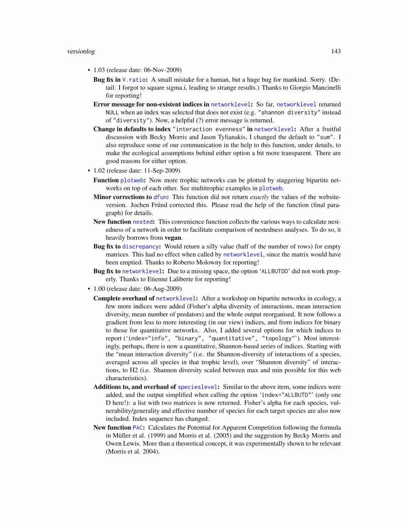
versionlog 143

• 1.03 (release date: 06-Nov-2009)Bug fix in V.ratio: A small mistake for a human, but a huge bug for mankind. Sorry. (De-

tail: I forgot to square sigma.i, leading to strange results.) Thanks to Giorgio Mancinellifor reporting!

Error message for non-existent indices in networklevel: So far, networklevel returnedNULL when an index was selected that does not exist (e.g. "shannon diversity" insteadof "diversity"). Now, a helpful (?) error message is returned.

Change in defaults to index "interaction evenness" in networklevel: After a fruitfuldiscussion with Becky Morris and Jason Tylianakis, I changed the default to "sum". Ialso reproduce some of our communication in the help to this function, under details, tomake the ecological assumptions behind either option a bit more transparent. There aregood reasons for either option.

• 1.02 (release date: 11-Sep-2009)Function plotweb: Now more trophic networks can be plotted by staggering bipartite net-

works on top of each other. See multitrophic examples in plotweb.Minor corrections to dfun: This function did not return exactly the values of the website-

version. Jochen Fründ corrected this. Please read the help of the function (final para-graph) for details.

New function nested: This convenience function collects the various ways to calculate nest-edness of a network in order to facilitate comparison of nestedness analyses. To do so, itheavily borrows from vegan.

Bug fix to discrepancy: Would return a silly value (half of the number of rows) for emptymatrices. This had no effect when called by networklevel, since the matrix would havebeen emptied. Thanks to Roberto Molowny for reporting!

Bug fix to networklevel: Due to a missing space, the option ‘ALLBUTDD’ did not work prop-erly. Thanks to Etienne Laliberte for reporting!

• 1.00 (release date: 06-Aug-2009)Complete overhaul of networklevel: After a workshop on bipartite networks in ecology, a

few more indices were added (Fisher’s alpha diversity of interactions, mean interactiondiversity, mean number of predators) and the whole output reorganised. It now follows agradient from less to more interesting (in our view) indices, and from indices for binaryto those for quantitative networks. Also, I added several options for which indices toreport (‘index="info", "binary", "quantitative", "topology"’). Most interest-ingly, perhaps, there is now a quantitative, Shannon-based series of indices. Starting withthe “mean interaction diversity” (i.e. the Shannon-diversity of interactions of a species,averaged across all species in that trophic level), over “Shannon diversity” of interac-tions, to H2 (i.e. Shannon diversity scaled between max and min possible for this webcharacteristics).

Additions to, and overhaul of specieslevel: Similar to the above item, some indices wereadded, and the output simplified when calling the option ‘index="ALLBUTD"’ (only oneD here!): a list with two matrices is now returned. Fisher’s alpha for each species, vul-nerability/generality and effective number of species for each target species are also nowincluded. Index sequence has changed.

New function PAC: Calculates the Potential for Apparent Competition following the formulain Müller et al. (1999) and Morris et al. (2005) and the suggestion by Becky Morris andOwen Lewis. More than a theoretical concept, it was experimentally shown to be relevant(Morris et al. 2004).

144 versionlog

Bug fix in H2fun and dfun: A line of code went missing at some point, so the maximumpacking density was not optimal (but still good) in these functions. As a result, reportedH2- and d-values were sometimes 0 when they should be only very close to 0.

Switch for error reporting in degreedistr: By default now suppresses error reporting whennls fails to fit a degree distribution due to too few data points. This leaves the user ofnetworklevel somewhat less confused. Warning message now also indicates for whichtrophic level there were too few data points.

Bug fix in C.score: Failed when the web was very dense or very sparse, because the maxi-mum number of checkerboard patterns was 0 then.

• 0.94 (release date: 01-Aug-2009)

New function nullmodel: A convenience wrapper function to generate different types ofnull models.

Small changes to networklevel: This function returns a list of indices. If we exclude thecomputation of degree distribution fits, this would be coerced to a vector. We addedthe option ‘index="ALLBUTDD"’ to calculate all indices BUT degree distributions. Theoutput is then returned as vector. This is much more convenient when using networklevelon many data sets (using sapply).

• 0.93 (release date: 30-Jun-2009)

bug fix in slope.bipartite and robustness: The function always selected column 3 ofthe object, instead of 2 for lower and 3 for higher trophic level; thanks to AntonioRivera for spotting and reporting this error! Notice that this error must have slippedin somewhere around version 0.90/0.91, because I checked and the results reported inthe Open Ecology Journal paper are valid! I seem to remember that I (CFD) modifiedslope.bipartite when robustness was added: never change a wining team!

• 0.92 (release date: 02-Jun-2009)

more colour options in visweb: the arguments ‘box.border’ and ‘box.col’ now allow aspecification of the colour of the boxes and their borders.

bug fix empty: the function returned 0 for a 1x1 matrix. Although not written for such a case,it should still do what it says on the tin. Thanks to Mariano Devoto for spotting andreporting!

bug fix wine: returned NA for square matrices.bug fix plot.wine: gave decimal places for row and column names for very small networks.


new function wine: This function replaces the (now deprecated) function nestedness.corsoin calculating a (weighted) nestedness for bipartite networks. It was developed and im-plemented by Marcelino de la Cruz, Juan M. Pastor, Javier Galeano and Jose Iriondo.It is also called by networklevel. A plotting function is also available, depicting thecontributions of each observed link to the web’s nestedness. - nestedness.corso is nowremoved from the package. The main reason is that it served as an interim solution forwine, and the Corso-way of calculating nestedness is just one more of already too many.If you intend to use wine on binary data and interpret that as a Corso-equivalent, bewareof the following two main differences (thanks to Jose Iriondo for summarising them):First, the nestedness of Corso et al. varies between 0 and 1, with the highest nestednessis reached at 0 and 1 corresponds to random, whereas in wine is just the opposite (thisis because the Manhattan distances are calculated with regard to opposite sides of the

versionlog 145

matrix). Secondly, the ‘d’ in the nestedness of Corso is the sums of the ‘dij’s whereasin wine, the ‘d’ (= ‘win’ value of the object produced by wine) is the average of the‘dij’s above 0. So, we recommend NOT to use wine for calculating Corso’s nestedness,but rather download the source code for nestedness.corso from an older version ofbipartite.

new function robustness: A better way to quantify the effect of species loss on the extinc-tions in the other trophic level; kindly provided by Mariano Devoto. This index is alsopart of networklevel.

new data set ollerton2003: Another quantitative pollination network from the NCEAS database(see ollerton2003).


example vazquez.example: We added several new functionalities mainly to be able to anal-ysis data and use network statistics as suggested by Vázquez et al. 2009. You can accessthis example by typing ?vazquez.example.

new feature in visweb: Can now plot different sized circles to represent interactions, as pro-posed by Vázquez et al. (2009).

new feature in networklevel: We added an option to calculate interaction evenness eitherbased on all possible links or just on realized links.

new function sortweb: Can be used to sort webs in different ways.data set inouye1988: Another pollination network from the NCEAS database (see inouye1988).Function compart: We replaced the CA-based approach to detecting compartments by a

comprehensive and recursive approach. The latter is not affected by ties in the data set(i.e. species with the same number of links). In quantitative webs and for the networksincluded in bipartite, the old function was working fine, but in more recent trials it failedto detect 2-species compartments. In turn, we had to adapt networklevel and plotweb.


Function plotweb New feature: text labels can now be printed in different colours. Allcolours can be passed as vectors and vectors are recycled if not of appropriate length

• 0.84 (release date: 25-Feb-2009)

Function plotweb New feature: arrow=“center.up”, arrow=“center.down”, arrow=“center.both”:this results in the standard presentation of bipartite networks, where interactions are dis-played as centered triangles.

• 0.83 (release date: 9-Feb-2009) pdf of OEJ-paper added as vignette

• 0.82 (release date: 27-Jan-2009)

Function plotweb Two new features: 1. colors of borders of boxes and interactions can bespecified via setting bor.col. 2. Labels can now be rotated by specifying text.rot=90.

• 0.81 (release date: 06-Jan-2009)

Function nodespec replaces the now obsolete function functspec. The inventor of func-tional specialisation, Bo Dalsgaard, understands the term ‘functional specialisation’ to berestricted to the way in which plants are specialised to pollinators. Although I disagree(and think that ‘functional’ actually means very little until defined for a given problem), Irenamed the ‘functional specialisation index’ into ‘node specialisation index’. This is nota particularly clever name, but at least it indicates that the position of nodes in a networkis important when it is calculated.

146 versionlog

Bug in networklevel: Call to nestedness.corso overwrote results of nestedness.Various changes related to the analysis of very small webs. Very small webs should prob-

ably not be used at all for testing theories! Indices are usually VERY sensitive to the exactnumber of species, number of observations etc. Still, sometimes we simply want to cal-culate some index, and then bipartite should handle such small networks, too. So, whengoing through several dozens of very small webs (sometimes only containing one speciesin one of the two trophic levels), several functions did not perform correctly (usually tosuch minor programming issues such as matrices being converted to vectors when [ wasused with ‘drop=TRUE’, i.e. the default). Changes affected the functions discrepancy,nestedness.corso, shuffle.web, compart and empty. Their output remains identical,only they now also work for small webs.

Changes to nestedness.corso with ‘weighted=TRUE’ Galeano et al. do not describe howto deal with ties, nor do they make clear if the packed matrix should be sorted by marginalsum of links or marginal sum of interactions! Previously, we used marginal sum of in-teractions (because it is a weighted index), but now we moved to marginal sum of links,because that is how I interpret their paper after a third (or forth) re-reading. Furthermore,because the real maximum chaos cannot be derived (to my knowledge) algorithmically,we use the 95% quantile of 500 randomisations as maximum. This will lead to a consis-tently overestimated nestedness, but it is less sensitive to the number of replicates thanthe max. (Also, there was an error in the description of the value returned: 0 is nested, 1is chaos!)


bug fix in shuffle.web Function didn’t work correctly when the web contained more rowsthan columns. (Thanks to Anna Traveset for spotting and reporting!)

minor modifications in networklevel Sometimes additional information is available and speciescan be included in a network, although they have no interactions with other species. In thiscase, one might want to use these species in the network, too. A new option (empty.web),allows to keep empty rows and columns, although for some functions an emptied webmust be used (e.g. degree distributions).

bug fix in H2fun As in the last H2fun bug fix, sometimes H2 became negative.bug (?) fix in networklevel Shannon diversity is based on the log of interactions. If this

value is 0, as it is for most network entries, an NA is produced. As a consequence,Shannon’s H (now also given in output) is based not on all interactions, but only those >0. In consequence, Shannon evenness should also only be SH divided by the number ofrealised interactions (log(sum(web>0))). That is now the case.

• 0.74 (release date: 24-Oct-2008)

functional specialisation (functspec) bug fix Paths were double the true length, hence min-imum was 2, rather than 1.

H2fun bug fix Since the search for H2min is heuristic, H2uncorr can sometimes be lower thanH2min; in that case, H2fun returned a value greater 1, while it should be one exactly.

new function nestedness.corso Calculates (weighted) nestedness according to Corso etal. (2008) and Galeano et al. (2008).

new function discrepancy Calculates discrepancy according to Brualdi & Sanderson (1999),deemed to be best ever measure of nestedness; also gives an example for a binary nullmodel analysis based on vegan’s commsimulator.

visweb 147

other Correction of several minor typos on the help pages; removal of "~" in help files; samecitation style throughout; new cross references (especially for the nestedness functions);in networklevel, nestedness is now calculated using vegan’s nestedtemp due to matrixinversion problems reported for binmatnest.

• 0.73 (release date: 1-Sept-2008)

new feature plotwebNamed abundance-vector for each level can be used.

new function plotweb2 (not debugged!) For plotting tripartite networks.

• 0.72 (release date: 12-June-2008)

new function: functional specialisation with functspec See Dalgaard et al. (2008).

new function: interface to sna through as.one.mode Allows calculation of path lengths,centrality, betweenness and other indices developed for one-mode networks.

bug-fix Error in plotweb when no species labels were given.

Note

This function is only invoked for its side effect of opening the help page. I simply didn’t know howto do it any other way ...

Author(s)


visweb Plotting function to visualize a bipartite food web

Description

This function draws a food web as a grid using a matrix. Colnames and rownames are used as labelsand entries in the matrix are visualized by text and colours. It can also be used to plot bipartite websin the style of Vázquez et al. (2009).

Usage

visweb(web, type="nested", prednames=TRUE, preynames=TRUE, labsize=1,plotsize=12, square="interaction", text="no", frame=NULL, textsize=1,textcol="red", pred.lablength=NULL, prey.lablength=NULL, clear=TRUE,xlabel="", ylabel="", boxes=TRUE, circles=FALSE, circle.col="black",circle.min=0.2, circle.max=2, outerbox.border="white",outerbox.col="white", box.border="black", box.col="black", def.col="blue",max.digits=4, NA.col="red")

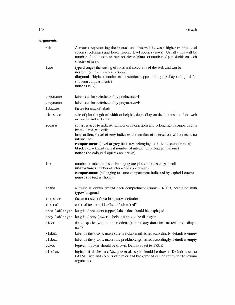
148 visweb

Arguments


type type changes the sorting of rows and coloumns of the web and can benested : (sorted by row/colSums)diagonal: (highest number of interactions appear along the diagonal, good forshowing compartments)none : (as is)

prednames labels can be switched of by prednames=F

preynames labels can be switched of by preynames=F

labsize factor for size of labels

plotsize size of plot (length of width or height), depending on the dimension of the webin cm, default is 12 cm.

square square is used to indicate number of interactions and belonging to compartmentsby coloured grid cellsinteraction: (level of grey indicates the number of intercation, white means nointeraction)compartment: (level of grey indicates belonging to the same compartment)black : (black grid cells if number of interaction is bigger than one)none : (no coloured squares are drawn)

text number of interactions or belonging are plotted into each grid cellinteraction: (number of interactions are drawn)compartment: (belonging to same compartment indicated by capitel Letters)none : (no text is shown)

frame a frame is drawn around each compartment (frame=TRUE), best used withtype=“diagonal”

textsize factor for size of text in squares, default=1

textcol color of text in grid cells, default =“red”

pred.lablength length of predators (upper) labels that should be displayed

prey.lablength length of prey (lower) labels that should be displayed

clear delete species with no interactions (compulsory done for “nested” and “diago-nal”)

xlabel label on the x-axis, make sure prey.lablength is set accordingly, default is empty

ylabel label on the y-axis, make sure pred.lablength is set accordingly, default is empty

boxes logical, if boxes should be drawn. Default is set to TRUE

circles logical, if circles in a Vazquez et al. style should be drawn. Default is set toFALSE, size and colours of circles and background can be set by the followingarguments

visweb 149

circle.col Colour of circles, works only if circles=TRUEcircle.min minimal size of circles, use to rescale circles appropriately, default is 0.2circle.max maximal size of circle, , use to rescale circles appropriately, default is 2outerbox.border

Colour of outerbox border if option circles=TRUEouterbox.col Colour of background if option circles=TRUEbox.border Colour of border of boxes, if option square=“b” is setbox.col Colour of boxes, if option square=“b” is setdef.col A user defined color vector for all ranks (starting from low to high) of occurring

values in the networkmax.digits defaults to 4.NA.col Which colour should be used for missing data (NAs)? Defaults to red.

Value

A plot window with appropriate size according to the dimensions of the web.

Note

If labels don’t fit, resize window by hand!

Author(s)

Bernd Gruber

References

Vázquez, P.D., Chacoff, N.,P. and Cagnolo, L. (2009) Evaluating multiple determinants of the struc-ture of plant-animal mutualistic networks. Ecology

See Also

For a different plot on food web see plotweb.

Examples

data(Safariland)visweb(Safariland)visweb(Safariland, type="diagonal", square="compartment", text="none",frame=TRUE)visweb(Safariland, type="nested", text="compartment")visweb(Safariland, circles=TRUE, boxes=FALSE, labsize=1, circle.max=3,text="no")visweb(Safariland,square="b",box.col="green",box.border="red")

#define your colors here,length has to be the numbers of different entriescols <-0:(length(table(Safariland))-1)visweb(Safariland, square="defined", def.col=cols)

150 web2edges

web2edges Conversion of a network matrix into a (weighted) edge list

Description

This helper function converts a bipartite matrix into an edge list, optionally weighted, as used byother packages and software, and writes this to the hard drive (optionally)

Usage

web2edges(web, webName=NULL, weight.column=TRUE, both.directions=FALSE,is.one.mode=FALSE, out.files=c("edges", "names", "groups")[1:2],return=FALSE, verbose=FALSE)

Arguments


webName An optional name for the data file generated by the function.

weight.column Logical; is the web quantitative and should hence a weighted edge list be pro-duced? Defaults to TRUE.

both.directions

Logical; shall each link be represented twice, i.e. once from A to B and alsofrom B to A? Defaults to FALSE.

is.one.mode Logical; if TRUE, labels for species will be used as they currently are in theweb; otherwise, species will be re-labelled so that the first column will havenumber NROW(web) + 1. This is also the default.

out.files String indicating which files to produce: "edges" writes an edge list, "names"writes a list with names belonging to the edges and "groups" writes a file assign-ing the species to higher and lower trophic levels. The default produces the edgelist and the names file.

return Logical; shall the edge list be returned by this function (for future use in R)?Defaults to FALSE. Setting ‘return’ to TRUE will prevent writing of files tothe hard drive!

verbose Logical; shall some feedback tell you that the files have been generated? De-faults to FALSE.

Details

Many network programs (e.g. Pajek) require input in the form of an edge list. Here each species is anumber. The edge list has two column, one with the target and one with the origin of the connection.That means an interaction between 1 and 6 would be written (in one line) as: "1 6". In a weightededge list, a third column represents the strength of the interaction: "1 6 4.77".

All this function does is to transform the typical interaction matrix used in bipartite into an edgelist. Within R this could be used e.g. in the package tnet; outside R by Pajek or others.

webs2array 151

Similar to as.one.mode this function is there to increase interchange between different codingstandards and packages.

Value

A matrix ("edge list") with two (unweighted) or three (weighted) columns.

If return=FALSE, this matrix (and possibly names and groups) are written to a text-file in the work-ing directory.

Note

The function is used as export helper (default) or as link to tnet (with return=TRUE).

Author(s)


Examples

data(Safariland)web2edges(Safariland, return=TRUE)

webs2array Puts two or more webs into one array of webs

Description

Function to put several webs into an array, blowing the dimensions up to the union of species

Usage

webs2array(...)

Arguments

... matrices containing webs (see example), separated by comma

Details

Some analyses may require a direct comparison of two webs, e.g. computing their similarity innumber of interactions per link (e.g. Poisot et al. 2012). To be able to do that, we first need to blowthe single webs up to have the same dimensions, i.e. padding all species not observed in this webwith 0s. This function produces a new raw matrix based on the union of species for each trophiclevel and puts these for all species into one array.

Value

An array of dimensions (number of species in lower level, number of species in higher level, numberof webs).

152 wine

Note

When building the webs from a table of observed interactions, function frame2webs allows to builda web-array when using ‘type.out="array"’. That would be preferable (faster and only one step)!

Combining webs into one array makes sense only for webs featuring overlapping communities!

Author(s)


References

Poisot, T., E. Canard, D. Mouillot, N. Mouquet, D. Gravel, and F. Jordan. 2012. The dissimilarityof species interaction networks. Ecology Letters 15, 1353—1361. doi: 10.1111/ele.12002

Examples

data(Safariland, vazquenc, vazquec)allin1 <- webs2array(Safariland, vazquenc, vazquec)

# now we can compute distance between two webs:vegdist(t(cbind(as.vector(allin1[,,1]), as.vector(allin1[,,2]), as.vector(allin1[,,3]))),

method="jacc")

wine Weighted-Interaction Nestedness Estimator

Description

Calculates the nestedness of a network taking into account the weight of the interactions, accordingto the method proposed by Galeano et al. (2008).

Usage

wine(web, nreps = 1)## S3 method for class 'wine'plot(x, ...)

Arguments


nreps Number of replicates for constructing random networks.

x An object resulting of applying wine function

... Additional graphical parameters to image.plot

wine 153

Details

Nestedness estimators use presence-absence (binary) adjacency matrices as the basis for calculat-ing nestedness, as they provide a simple description and characterization of the topology of thenetwork. However, networks are specified not only by their topology but also by the heterogeneityin the weight (or the intensity) of the connections (Barrat et al., 2004). Characterizing links just withpresence-absence data does not take into account the possible differences in intensity among links.WINE (Weighted-Interaction Nestedness Estimator) is a new nestedness estimator that takes intoaccount the weight or intensity of each interaction (e.g., in a plant-pollinator network, the numberof registered visits of a particular interaction). Thus, instead of using presence-absence matrices,WINE calculates nestedness from quantitative data matrices that include the number of events ofeach interaction. This is the first estimator that allows for the characterization of weighted nest-edness. WINE calculates a nestedness value that approaches zero when the nestedness pattern ofthe original data matrix is close that of equivalent random matrices, and it approaches one as itgets closer to the nestedness of the maximal nestedness matrix. Thus, this estimator evaluates therelative position of the data matrix between the corresponding random matrices and the maximalnestedness matrix. Negatives values for this estimator can be found in some synthetic matrices thathave been described as ‘anti-nestedness’ matrices (Almeida-Neto et al. 2007).

The calculation of the weighted-interaction nestedness estimator starts with the matrix containingthe number of events of each interaction, Mij. The matrix is packed by arranging rows and columnsfrom top to bottom and from left to right, respectively, in ascending order according to their marginaltotals. Nestedness is related to the proximity of existing links to one another in the packed matrix,so that the most nested matrix is the one that after packing shows a minimum mixing of filled cells(links) with empty cells (no links) (Corso et al., 2008, Ulrich et al., 2009). WINE is based on theconcept of estimating nestedness through the calculation of a Manhattan distance from each of thematrix cells containing a link to the cell corresponding to the intersection of the row and columnswith the lowest marginal totals (number of links). This concept resembles in a way the one used byCorso et al. (2008), although the distances are measured to the opposite corner of the packed matrix.Additionally, in WINE, the Manhattan distance is replaced by a weighted Manhattan distance. Thestatistical significance of this nestedness index value is tested against a null model that constrainsmatrix fill to observed values, retains the distribution of number of events in the links but does notconstrain marginal totals. Further details can be found in Galeano et al. (2008).

Value

wine returns an object of class wine, basically a list with the following components:

win Weighted-interaction nestedness of dataset (WIN)

wine Weighted-interaction nestedness estimator (WINE): The weighted-interactionnestedness estimator value. It will be 0 for random distribution and 1 for maxi-mal nestedness

zscore z-score of the weighted-interaction nestedness

pvalue probability of having a z-value equal to or greater than Z (from the tabulatedvalue of the cumulative function). Values of p<0.05 indicate that the dataset issignificantly nested.

dmax Weighted-interaction nestedness of the maximal nestedness matrix.

drnd Average weighted-interaction nestedness of random replicates

154 wine

dij.w Matrix of dijw values. These values provide a measure of the contribution ofeach interaction (link) to total nestedness

dij.max Maximal nestedness matrix

The S3 plot method for wine displays dij.w in a coloured image plot where red cells have highweights in the network and blue cells have minimum weights.

Note

This is the first approach to a weighted nestedness and a full ecological interpretation of its meaningis still lacking. It is not possible to perform a systematic comparison between this and other nest-edness indices because the latter rely just on presence absence data whereas the former feeds on aquantitative data matrix. For a well-performed comparison of other nestedness indices see Ulrich& Gotelli (2007).

wine may return NaN for different parameters essentially for two different reasons: a) if ‘nreps’ isnot specified, wine adopts nreps=1 by default and NaN is returned for z-score and p value. Thisis due to the fact that with nreps=1 the variance of drnd is zero and z-score becomes infinite. Thesame outcome may occur in some cases with very low values of nreps. To ensure proper values ofz-score and p-values nreps=100 or higher is suggested. b) if dw = drnd = dmax wine equals 0/0,and if drnd = dmax wine tends to infinity. In both cases, NaN is returned by wine. This is morelikely to occur in cases where the dimensions of the matrix are very low (e.g, (dim < c(4,4))because in those cases the number of possible values of dw, drnd and dmax is also reduced.

This is WINE version 3.2, available also in Matlab and C++ at the certificate-blocked site ‘http://hypatia.agricolas.upm.es/WINE/WINE.html’.

Author(s)

Marcelino de la Cruz <[email protected]>, Juan M. Pastor <[email protected]>,Javier Galeano <[email protected]> and Jose M. Iriondo <[email protected]>

References

Barrat, A., Barthelemy, M., Pastor-Satorras, R., and Vespignani, A. (2004) The architecture ofcomplex weighted networks. PNAS 101, 3747–3752

Corso G, de Araujo AIL, de Almeida AM (2008) A new nestedness estimator in community net-works. arXiv 0803.0007v1 [physics.bio-ph]

Galeano J, Pastor JM, Iriondo JM (2008) Weighted-Interaction Nestedness Estimator (WINE): Anew estimator to calculate over frequency matrices. arXiv 0808.3397v2 [physics.bio-ph]

Ulrich, W., Almeida-Neto, M., and Gotelli, N.J. (2009) A consumer’s guide to nestedness analysis.Oikos 118, 3-17

Ulrich, W. and Gotelli, N.J. (2007) Null model analysis of species nestedness patterns. Ecology 88,1824-1831

See Also

nestedness and discrepancy.

wine 155

Examples

data(Safariland, package="bipartite")safariland.w <- wine(Safariland, 10)plot.wine(safariland.w)

Index

∗Topic ClusteringcomputeModules, 22DIRT_LPA_wb_plus, 30listModuleInformation, 55plotModuleWeb, 93printoutModuleInformation, 103

∗Topic Methods and GenericFunctions

computeModules, 22DIRT_LPA_wb_plus, 30listModuleInformation, 55plotModuleWeb, 93printoutModuleInformation, 103

∗Topic classesmoduleWeb-class, 58

∗Topic datasetsbarrett1987, 14bezerra2009, 16elberling1999, 35inouye1988, 50junker2013, 51kato1990, 52kevan1970, 53memmott1999, 56mosquin1967, 59motten1982, 60olesen2002aigrettes, 88olesen2002flores, 89ollerton2003, 89Safariland, 107schemske1978, 108small1976, 114vazarr, 131vazcer, 132vazllao, 132vazmasc, 133vazmasnc, 133vazquec, 135vazquenc, 136

∗Topic htestdegreedistr, 26dfun, 28

∗Topic modularitymoduleWeb-class, 58

∗Topic moduleWebmoduleWeb-class, 58

∗Topic modulesmoduleWeb-class, 58

∗Topic packageas.one.mode, 11bipartite-package, 3C.score, 17compart, 21czvalues, 24discrepancy, 32empty, 35endpoint, 37extinction, 38fc, 39frame2webs, 40genweb, 42grouplevel, 43H2fun, 49linklevel, 54ND, 61nested, 63nestedcontribution, 65nestedness, 67nestedrank, 69networklevel, 70nodespec, 79NOS, 81npartite, 82null.distr, 83null.t.test, 85nullmodel, 86PAC, 90PDI, 92

156

INDEX 157

plotPAC, 95plotweb, 96plotweb2, 101r2dexternal, 105robustness, 106second.extinct, 109shuffle.web, 111slope.bipartite, 113sortweb, 115specieslevel, 116strength, 123swap.web, 124togetherness, 129V.ratio, 130vaznull, 134vazquez.example, 136versionlog, 138visweb, 147web2edges, 150webs2array, 151wine, 152

.networklevel (networklevel), 70

addEmptyColToMatrix (plotModuleWeb), 93addEmptyRowToMatrix (plotModuleWeb), 93as.one.mode, 4, 11, 61, 83, 141, 142, 147, 151as.tnet, 9, 13

BarbersMatrix (DIRT_LPA_wb_plus), 30barrett1987, 14BC, 120, 139, 141, 142BC (ND), 61betweenness_w, 9, 15bezerra2009, 9, 16bipartite (bipartite-package), 3bipartite-package, 3

C.score, 5, 17, 49, 63–65, 79, 129, 131, 144CC, 120, 139, 141, 142CC (ND), 61closeness_w, 9, 18clustering_tm, 9, 20cM (computeModules), 22compart, 21, 138, 145computeModules, 4–6, 8, 22, 24, 30, 31, 138,

139confint (vazquez.example), 136convert2moduleWeb (DIRT_LPA_wb_plus), 30czvalues, 5, 24, 138

degreedistr, 8, 9, 26, 47, 49, 76, 79, 140,142, 144

deleteModuleData (computeModules), 22dfun, 4, 10, 28, 49, 50, 75, 80, 93, 117, 118,

121, 123, 139, 140, 143, 144DIRT_LPA_wb_plus, 5, 24, 30discrepancy, 32, 46, 65, 76, 125, 143, 146,

154dist, 39, 45, 73distance_w, 9, 33DIVISION (DIRT_LPA_wb_plus), 30drawModules (plotModuleWeb), 93

elberling1999, 35empty, 35, 42, 110, 111, 144endpoint, 9, 37, 54extinction, 36, 38, 110, 111, 138

fc, 7, 39, 45, 73fd, 138fd (fc), 39frame2webs, 4, 9, 40, 152

genweb, 4, 42getModuleCoordinates (plotModuleWeb), 93grouplevel, 5, 7–9, 43, 71, 73, 76, 82, 111

H2fun, 4, 9, 29, 30, 49, 73, 75, 79, 141, 144,146

hclust, 39

image.plot, 152inouye1988, 50, 145intasymm (vazquez.example), 136intereven (vazquez.example), 136isCorrectModuleWebObject

(plotModuleWeb), 93

junker2013, 8, 51

kato1990, 52kevan1970, 53

linklevel, 8, 9, 54listModuleInformation, 31, 55LOCALMAXIMISATION (DIRT_LPA_wb_plus), 30LPA_wb_plus (DIRT_LPA_wb_plus), 30

memmott1999, 56metaComputeModules (computeModules), 22

158 INDEX

mgen, 6, 56, 87, 106mlik (vazquez.example), 136moduleWeb-class, 58mosquin1967, 59motten1982, 60

ND, 61, 119, 142nested, 6, 10, 63, 70, 140, 142, 143nestedcontribution, 5, 6, 65nestedness, 10, 33, 64, 65, 67, 74, 146, 154nestedrank, 8, 69, 70, 118netstats (vazquez.example), 136networklevel, 4–9, 21, 22, 27, 40, 44, 49, 54,

70, 85, 110, 111, 121, 123, 136–147nodespec, 12, 79, 120, 123, 145NOS, 81npartite, 9, 82null.distr, 4, 83, 141null.t.test, 10, 85nullmodel, 4, 83, 84, 86, 105, 106, 141, 142,

144

olesen2002aigrettes, 88olesen2002flores, 62, 89ollerton2003, 89, 145one.grouplevel (grouplevel), 43

PAC, 4, 90, 96, 140, 142, 143PDI, 7, 9, 92, 118, 120, 139plot.wine, 144plot.wine (wine), 152plotmat (vazquez.example), 136plotModuleWeb, 5, 31, 93plotPAC, 95, 140plotweb, 4, 8, 96, 103, 116, 118, 138, 139,

143, 145, 147, 149plotweb2, 101, 147prepareWebForPlottingModules

(plotModuleWeb), 93printoutModuleInformation, 31, 103projecting_tm, 104

quant2bin (vazquez.example), 136

r2dexternal, 7, 105r2dtable, 85, 113, 126, 135readModuleData (computeModules), 22robustness, 47, 76, 106, 139, 144, 145

Safariland, 107

schemske1978, 108second.extinct, 4, 6, 9, 36, 38, 39, 44, 47,

49, 72, 79, 106, 107, 109, 113, 114,138, 139, 142

shuffle.web, 87, 111, 126, 136, 139, 140, 146slope.bipartite, 4, 9, 47, 107, 111, 113, 144small1976, 114sortmatr (vazquez.example), 136sortmatrext (vazquez.example), 136sortweb, 4, 115, 137, 145specieslevel, 4, 6–10, 30, 54, 62, 70, 75, 80,

92, 93, 116, 124, 136, 139, 140, 142,143

StageOne_LPAwbdash (DIRT_LPA_wb_plus),30

StageTwo_LPAwbdash (DIRT_LPA_wb_plus),30

strength, 123swap.web, 6, 87, 124, 134–136, 140, 142symmetrise_w, 9, 126

t.test, 85tnet_igraph, 9, 128togetherness, 129TRACE (DIRT_LPA_wb_plus), 30

V.ratio, 49, 79, 130, 143vazarr, 131vazcer, 132vazllao, 132vazmasc, 133vazmasnc, 133vaznull, 5, 6, 87, 106, 125, 126, 134, 140–142vazquec, 135vazquenc, 136vazquez.example, 136versionlog, 5, 138visweb, 4, 9, 74, 99, 103, 116, 137, 139, 144,

145, 147

web2edges, 4, 13, 140, 141, 150webs2array, 9, 151WEIGHTEDMODULARITY (DIRT_LPA_wb_plus),

30WEIGHTEDMODULARITY2 (DIRT_LPA_wb_plus),

30wine, 33, 64, 65, 69, 74, 144, 145, 152

Package 'bipartite'

Documents

Transcript of Package 'bipartite'