Enhanced two-point resolution using optical eigenmode optimized pupil functions

This article has been downloaded from IOPscience. Please scroll down to see the full text article.

2011 J. Opt. 13 105707

(http://iopscience.iop.org/2040-8986/13/10/105707)

Download details:

IP Address: 152.78.75.100

The article was downloaded on 26/09/2011 at 10:29

Please note that terms and conditions apply.

View the table of contents for this issue, or go to the journal homepage for more

Home Search Collections Journals About Contact us My IOPscience

IOP PUBLISHING JOURNAL OF OPTICS

J. Opt. 13 (2011) 105707 (9pp) doi:10.1088/2040-8978/13/10/105707

Enhanced two-point resolution usingoptical eigenmode optimized pupilfunctionsS Kosmeier, M Mazilu, J Baumgartl and K Dholakia

School of Physics and Astronomy, University of St Andrews, North Haugh, St Andrews,Fife KY16 9SS, UK

E-mail: michael.mazilu@st-andrews.ac.uk

Received 14 June 2011, accepted for publication 15 August 2011Published 22 September 2011Online at stacks.iop.org/JOpt/13/105707

AbstractPupil filters have the capability to arbitrarily narrow the central lobe of a focal spot. Wedecompose the focal field of a confocal-like imaging system into optical eigenmodes todetermine optimized pupil functions, that deliver superresolving scanning spots. As aconsequence of this process, intensity is redistributed from the central lobe into side lobesrestricting the field of view (FOV). The optical eigenmode method offers a powerful way todetermine optimized pupil functions. We carry out a comprehensive study to investigate therelationship between the size of the central lobe, its intensity, and the FOV with the use of adual display spatial light modulator. The experiments show good agreement with theoreticalpredictions and numerical simulations. Utilizing an optimized sub-diffraction focal spot forconfocal-like scanning imaging, we experimentally demonstrate an improvement of thetwo-point resolution of the imaging system.

Keywords: pupil filter, spatial light modulator, imaging, optimization

(Some figures in this article are in colour only in the electronic version)

1. Introduction

Using pupil filters, the lateral diffraction limited point spreadfunction (PSF) or focal spot of an imaging or focusing systemcan be altered such that the width of the central lobe is reducedwhile the intensity is redistributed into the sidelobes [1–4].Indeed, given a suitable pupil modification, the centrallobe could in principle be made arbitrarily narrow and thesidelobes can be pushed arbitrarily far away from the center.Possible applications for this effect include e.g. superresolvedimaging [5] or increased optical data storage [6]. Somesuperresolving pupil filters have been demonstrated to workexperimentally [7–9]. However, squeezing the central lobeby a few tens of per cent beyond the diffraction limit inducesits intensity to drop by orders of magnitude, while theintensity of the sidelobes rises correspondingly. Thus thepractical implementation of this method remains difficult, as itrequires very accurate light shaping to achieve high resolutiongains [10].

Here, we investigate the use of a liquid crystal spatiallight modulator (SLM) as dynamic pupil filter in a systematicmanner for this purpose. The optical eigenmode (OEi)method [11] is used to calculate pupil functions that areoptimized for different intensities of the central lobe andvariable sizes of the field of view (FOV). These functionsare then encoded onto a dual display SLM system and theagreement between the theoretical and experimental focalspots is analyzed. We determine intensities and sizes of thecentral lobe and the FOV that can be experimentally realized.

To show a possible application of the OEi pupil filters,we have experimentally implemented a filter in the contextof a simple imaging setup. As the width of the centrallobe is reduced in the lateral direction, a suitable spot isused for confocal-like scanning of in-focus pairs of holes,demonstrating enhanced two-point resolution compared to theunobstructed pupil.

The paper is organized as follows: in section 2, we brieflyreview the OEi optimization method. Section 3 depicts the

2040-8978/11/105707+09$33.00 © 2011 IOP Publishing Ltd Printed in the UK & the USA1

J. Opt. 13 (2011) 105707 S Kosmeier et al

experimental setup used. The confocal-like scanning processand its numerical simulation is described in section 4. Insection 5, we present a comprehensive study of simulated andexperimentally acquired focal spots to determine the practicalbeam shaping limit of the configuration and its confocalimaging capabilities. The applicability of the filters for abroader range of imaging applications is discussed in section 6.The paper finishes with conclusions in section 7.

2. Focal spot optimization using optical eigenmodes

In order to calculate the pupil functions to be displayed on theSLM system, we employ the OEi method [11, 12] squeezinglaterally the central lobe of the focal spot. For a given setof input fields and parameters, this enables us to find ina single iteration the pupil modification which delivers thesmallest possible focal spot in a region of interest (ROI) whilekeeping the intensity of the spot maximum. To achieve lateralsqueezing, the size of the ROI is usually about the size ofthe diffraction limited focus. For the studies in this paper weconsider only radially dependent scalar fields F(rf) in the focalplane where rf is the lateral radius (however, the OEi methodis just as capable of treating the electromagnetic field as fullyvectorial [11]). Symmetry maintaining scalar propagationimplies that the field E(rp) does only depend on the lateralradius rp in the pupil plane.

To employ the OEi optimization method, the field E(rp)

in the pupil plane and the field F(rf) in the focal plane of thelens are decomposed into N fields Ei(rp) and Fi (rf),

E(rp) =N∑

i=1

ai Ei(rp), (1)

F(rf) =N∑

i=1

ai Fi (rf), (2)

with complex coefficients ai . Since the lens is a linear opticalsystem, the complex coefficients ai are identical for the fieldsin both planes. Using the decomposition in (2), the beamwidth w, expressed as the second order moment of the intensitydistribution in the focal plane, can be written as [11]

w = 2

√a†M(2)aa†M(0)a

(3)

with a = (a1 · · · aN )T, a† = (a∗1 · · · a∗

N ) and the N × Noperators M(0) and M(2) having elements

M (0)

i j =∫ Rf

0F∗

i (rf)Fj (rf)2πrf drf, (4)

M (2)i j =

∫ Rf

0r 2

f F∗i (rf) Fj(rf)2πrf drf, (5)

where the integration is carried out over a circular ROI withradius Rf. From the definitions in (4) and (5) it follows thatboth M(0) and M(2) are Hermitian and consequently featurea spectrum of real eigenvalues and orthogonal eigenvectors.Employing M(0) and M(2), the OEi optimization of the

coefficients ai is then performed in two stages: firstly, wedetermine a set of orthonormal optical eigenmodes with respectto the ROI. This step also delivers the maximum total intensityin the ROI. Secondly, using this orthonormal set, the spot sizein the ROI is minimized.

2.1. Maximizing the intensity

If a in (3) is one of the N eigenvectors v(0)k of M(0), then

its corresponding eigenvalue λ(0)

k equals the total intensityin the ROI. Hence M(0) is called intensity operator. Whenthe λ

(0)k are ordered by descending magnitude, a field F(rf)

composed according to (2) from the elements of v(0)

1 featuresthe maximum possible intensity in the ROI for the given set ofincident fields Ei (rf) and the constraint a†a = 1. Using v(0)

2results in the second highest intensity and so on. To minimizethe spot size while keeping the intensity maximal, the red firstM eigenvalues λ

(0)k > T λ

(0)1 are selected with T ∈ [0, 1]

representing a relative intensity threshold. Using the elementsv

(0)ki of their corresponding eigenvectors, within the ROI a set

of M orthonormal optical eigenmodes

F (0)k (rf) = 1√

λ(0)

k

N∑

i=1

v(0)ki Fi (rf) (6)

is composed, which we use in section 2.2 to minimize the spotsize.

2.2. Minimizing the spot size

To minimize the spot size in the ROI, the set of orthonormalmodes F (0)

k (rf) from (6) is used in the definitions (4) and (5)of the operators M(0) and M(2). If now a in (3) is anynormalized eigenvector v(2)

l of M(2), then the denominator ofthe second order moment in (3) is unity (as the modes F (0)

k (rf)

are orthonormal). In that case the spot size w defined in (3) isa function of the corresponding eigenvector λ

(2)l . Thus we term

M(2) the spot size operator. Consequently a superposition ofthe modes F (0)

k (rf) using the elements v(2)min k of the eigenvector

v(2)

min that corresponds to the minimum eigenvalue λ(2)

min exhibitsthe smallest possible spot in the ROI. In conclusion, andreferring to the initial set of fields Ei(rp) and Fi (rf) in (1)and (2), the field Fmin(rf) featuring the minimum focal widthin the chosen ROI results from the superposition

Emin(rp) =N∑

i=1

M∑

k=1

v(0)ki v

(2)min k√

λ(0)k

Ei(rp) (7)

of the fields Ei (rp) on the SLM.

3. Experimental setup

The setup used for the experiments is depicted in figure 1. Itconsists of two parts, one for creating the illumination and onefor detection and imaging.

In the illumination part, the beam of a linearly polarizedHeNe laser (λ = 633 nm) is expanded and is sent to the

2

J. Opt. 13 (2011) 105707 S Kosmeier et al

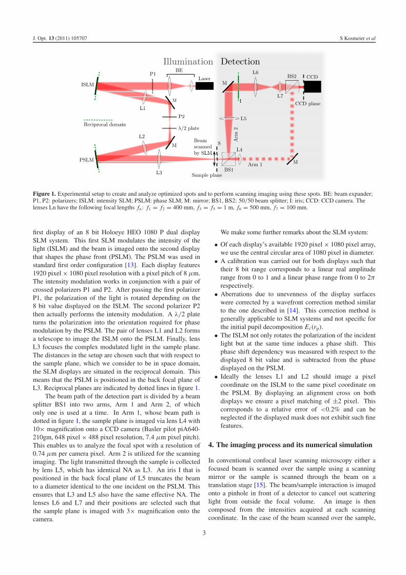
Figure 1. Experimental setup to create and analyze optimized spots and to perform scanning imaging using these spots. BE: beam expander;P1, P2: polarizers; ISLM: intensity SLM; PSLM: phase SLM; M: mirror; BS1, BS2: 50/50 beam splitter; I: iris; CCD: CCD camera. Thelenses Ln have the following focal lengths fn: f1 = f2 = 400 mm, f3 = f5 = 1 m, f6 = 500 mm, f7 = 100 mm.

first display of an 8 bit Holoeye HEO 1080 P dual displaySLM system. This first SLM modulates the intensity of thelight (ISLM) and the beam is imaged onto the second displaythat shapes the phase front (PSLM). The PSLM was used instandard first order configuration [13]. Each display features1920 pixel × 1080 pixel resolution with a pixel pitch of 8 μm.The intensity modulation works in conjunction with a pair ofcrossed polarizers P1 and P2. After passing the first polarizerP1, the polarization of the light is rotated depending on the8 bit value displayed on the ISLM. The second polarizer P2then actually performs the intensity modulation. A λ/2 plateturns the polarization into the orientation required for phasemodulation by the PSLM. The pair of lenses L1 and L2 formsa telescope to image the ISLM onto the PSLM. Finally, lensL3 focuses the complex modulated light in the sample plane.The distances in the setup are chosen such that with respect tothe sample plane, which we consider to be in space domain,the SLM displays are situated in the reciprocal domain. Thismeans that the PSLM is positioned in the back focal plane ofL3. Reciprocal planes are indicated by dotted lines in figure 1.

The beam path of the detection part is divided by a beamsplitter BS1 into two arms, Arm 1 and Arm 2, of whichonly one is used at a time. In Arm 1, whose beam path isdotted in figure 1, the sample plane is imaged via lens L4 with10× magnification onto a CCD camera (Basler pilot piA640-210gm, 648 pixel × 488 pixel resolution, 7.4 μm pixel pitch).This enables us to analyze the focal spot with a resolution of0.74 μm per camera pixel. Arm 2 is utilized for the scanningimaging. The light transmitted through the sample is collectedby lens L5, which has identical NA as L3. An iris I that ispositioned in the back focal plane of L5 truncates the beamto a diameter identical to the one incident on the PSLM. Thisensures that L3 and L5 also have the same effective NA. Thelenses L6 and L7 and their positions are selected such thatthe sample plane is imaged with 3× magnification onto thecamera.

We make some further remarks about the SLM system:

• Of each display’s available 1920 pixel × 1080 pixel array,we use the central circular area of 1080 pixel in diameter.

• A calibration was carried out for both displays such thattheir 8 bit range corresponds to a linear real amplituderange from 0 to 1 and a linear phase range from 0 to 2π

respectively.• Aberrations due to unevenness of the display surfaces

were corrected by a wavefront correction method similarto the one described in [14]. This correction method isgenerally applicable to SLM systems and not specific forthe initial pupil decomposition Ei (rp).

• The ISLM not only rotates the polarization of the incidentlight but at the same time induces a phase shift. Thisphase shift dependency was measured with respect to thedisplayed 8 bit value and is subtracted from the phasedisplayed on the PSLM.

• Ideally the lenses L1 and L2 should image a pixelcoordinate on the ISLM to the same pixel coordinate onthe PSLM. By displaying an alignment cross on bothdisplays we ensure a pixel matching of ±2 pixel. Thiscorresponds to a relative error of <0.2% and can beneglected if the displayed mask does not exhibit such finefeatures.

4. The imaging process and its numerical simulation

In conventional confocal laser scanning microscopy either afocused beam is scanned over the sample using a scanningmirror or the sample is scanned through the beam on atranslation stage [15]. The beam/sample interaction is imagedonto a pinhole in front of a detector to cancel out scatteringlight from outside the focal volume. An image is thencomposed from the intensities acquired at each scanningcoordinate. In the case of the beam scanned over the sample,

3

J. Opt. 13 (2011) 105707 S Kosmeier et al

the beam needs to be descanned for detection by sending thelight back over the same scanning mirror or the pinhole needsto be moved with the beam.

4.1. Confocal imaging and resolution limits with our setup

For the setup described in section 3 the SLM fulfils thescanning part and the pinhole is substituted by a 3 pixel ×3 pixel square on the CCD that moves together with the beam.This square is small compared to the diffraction limited focalspot featuring a FWHM of about 30 pixel. The scanningof the beam is realized by adding a linear phase gradient onthe PSLM, displacing the beam in the sample and the CCDplane. So the PSLM effectively acts as a scanning mirror.The image is then composed from the intensities, that for eachdisplacement are averaged in the small square.

The theoretical focal width of the scanning beam canbe calculated using the effective NA of lens L3. From theSLM specifications given in section 3 it follows that the beamdiameter incident on lens L3 equals 8.64 mm. With the focallength f3 = 1 m, lens L3 has an effective NA of 4.32 × 10−3.Regarding to the Abbe limit of 0.5λ/NA, the scanning beamthus features a diffraction limited full width at half maximum(FWHM) of wAiry = 73.3 μm. The two-point Rayleighresolution limit of the system for coherent confocal imagingwith the unobstructed pupil is defined by 0.56λ/NA [16],resulting in 82.1 μm with the given effective NA.

4.2. Simulation of the imaging process

To simulate the scanning process described in section 4.1,the transmissive sample is simulated as a binary distributionS(xf, yf) that is 1 in the sample’s transparent areas and 0 in theopaque ones. The intensity distribution Ic(xc, yc) on the CCDis then simulated as follows for each scanning position:

(i) The complex field A(xf, yf) in the sample plane isthe illuminating field F(xf, yf) modulated with thetransmission S(xf, yf) of the sample:

A(xf, yf) = F(xf, yf) S(xf, yf). (8)

(ii) The detection part of the setup in figure 1 is coherent.Thus the intensity distribution Ic(xc, yc) on the CCD isgiven by the square of the complex convolution of (8) withthe amplitude point spread function APSF of the detectionpart [17]:

Ic(xc, yc) = |[F(xf, yf)S(xf, yf)] ∗ APSF|2. (9)

As the APSF we use the complex field of the Airy disc.

5. Results

Past studies [1–4] have shown that the spot size, the spotintensity, and the distance to the sidelobes obey the qualitativerules of (1) decreasing the spot size results in a decreasedspot intensity and (2) moving the sidelobes further away fromthe spot decreases the spot intensity. In the following theseparameters are investigated first in simulations (section 5.1)

and then experimentally (section 5.2) for spots generatedwith our SLM system. Furthermore, the suitability of thespots for confocal-like imaging of in-focus objects is analyzedin simulations (section 5.1) and verified by experiments(section 5.3). More precisely, to quantify the resolutioncapabilities of an incoherent imaging system it is sufficientto determine its intensity PSF. However, in the case of acoherent detection process it is necessary to investigate atleast two points next to each other to correctly deal withinterference [18]. Thus, with respect to the applicationexample in section 5.3, we utilize the two-point resolutioncriterion to study the lateral resolution.

5.1. Simulations on sub-diffractive focal spots

In this section, we simulate the generation of sub-diffractivefocal spots and analyze their suitability for confocal-likeimaging of two in-focus pinholes. Therefore, we considershaping the intensity and phase of the field E(rp) in thebackfocal plane of lens L3 with a dynamic range of 8 bit anda radial resolution of 540 pixel (which maximizes the usedarea of the SLM). The SLM is divided into N = 540 non-overlapping rings of 1 pixel width, each of which representsone of the fields Ei(rp) in (1) and accounting for all ofthe system’s radial degrees of freedom. For each of therings the resulting field Fi (rf) in the focal plane is calculatedusing the scalar radial symmetric representation of Huygen’sintegral [19]. The simulation was carried out with a pixelpitch of 0.74 μm and a radial resolution of 244 pixel, whichequals half of the CCD sensor’s diameter. This corresponds toprojecting the focal plane of lens L3 with 10× magnificationonto the CCD camera, as it happens in Arm 1 of the setup infigure 1.

Using the fields Fi (rf), the OEi optimization was carriedout with the ROI radius Rf, varying in steps of 0.03wAiry,between 0.09wAiry and 2.30wAiry with the width of the Airydisc wAiry = 73.3 μm. The intensity thresholds were chosento be T = 10−p with p = 1, 2, . . . , 6. The threshold Tin combination with the ROI radius influences the numberM of OEi that are used to minimize the spot size (see alsosection 2.1). The optimized fields Fmin(rf) were azimuthallyinterpolated to 488 pixel × 488 pixel (corresponding to theCCD’s central area) and the following spot parameters werecalculated for each intensity distributions |Fmin(rf)|2:

• the width wspot of the central spot was quantified as theFWHM,

• the Strehl ratio S, defined as the quotient of the peakintensities of spot and the Airy disc [20],

• the distance dSL to the sidelobes was measured betweenthe central spot’s peak and the peak of the nearest sidelobe of at least 10% of the spot’s peak intensity,

• the relative spot intensity Irel was quantified as the ratiobetween the peak intensities of the central spot and theintensity of the nearest side lobe as defined in the previouspoint.

However, even with knowledge of these parameters it isnot trivial to decide whether or not a spot is suitable for animaging application. A small central spot is unusable if its

4

J. Opt. 13 (2011) 105707 S Kosmeier et al

Figure 2. Simulations: in each plot the color represents (a) the number M of modes, (b) the Strehl ratio S, (c) the relative spot intensity Irel ,and (d) the relative resolution Rrel in dependence on the spot size wspot and the distance dSL between spot and sidelobes.

intensity is too low compared to the surrounding sidelobesand/or these sidelobes are too close to the central spot. Toquantify the two-point resolution, we simulated the scan alonga 220 μm long line through two transmissive holes using a stepwidth of 1 μm between the scanning positions. The separationbetween the holes was varied in steps of 1 μm as well. Theabsolute two-point resolution limit Rabs was then quantified interms of the Rayleigh criterion as the distance for which thetwo-point sources were resolved with 26.5% contrast [21].

Figures 2(a)–(d) give an overview of the spot parametersand the achievable resolution. In each of the plots thehorizontal and vertical axis depict the spot size wspot and thedistance dSL to the sidelobes relative to the FWHM wAiry =73.3 μm of the Airy disc. The color codings in figures 2(a)–(d) show the number M of OEi used in the optimization(figure 2(a)), the Strehl ratio S (figure 2(b)), the spot intensityIrel relative to the side lobe intensity (figure 2(c)), andthe relative two-point resolution Rrel obtainable by confocalscanning (figure 2(d)). The latter is scaled as a ‘resolution gain’in the way Rrel = Rabs,Airy/Rabs,spot to the absolute resolutionlimit Rabs,Airy when scanning with the Airy disc. Thus a valueof Rrel = 2 would correspond to twofold increased resolution.From the simulations we obtained Rabs,Airy = 83 μm, whichis in agreement with the theoretical limit of 0.56 λ/NA =82.1 μm given in section 4.1. Furthermore, simulations of theAiry disc and three example spots are illustrated in figures 3(i)–(l) with their corresponding parameters listed as ‘S’ values intable 1.

In figure 2(a) we observe that with an increasing numberM of modes the sidelobes can be pushed further away froma central spot of constant size. At the same time the Strehlratio S in figure 2(b) and the relative spot intensity Irel in

Table 1. Simulated (S) and experimentally (E) measured spotparameters for the Airy disc and three example spots, which areillustrated in figures 3(m)–(o) (simulation) and figures 3(r)–(t)(experiment).

Param. Airy Spot 1 Spot 2 Spot 3

M — 2 3 4

wspot/wAiryS 1 0.61 0.71 0.60E 1 0.61 0.74 —

dSL/wAiryS — 1.21 1.84 1.62E — 1.25 1.85 —

S S 1 0.022 0.0038 1.7 × 10−5

E 1 0.021 0.0037 —

IrelS — 1.2 0.88 0.0083E — 1.3 0.91 —

Rabs/1 μm S 83 65 68 61Rrel S 1 1.28 1.22 1.36

figure 2(c) decrease. This is due to the lower intensity of thehigher order OEi (see section 2.1). Furthermore S and Irel

decrease with decreasing spotsize wspot. All these findingsagree with the qualitative rules stated at the beginning ofsection 5. The simulated relative resolution Rrel in figure 2(d)generally decreases with decreasing spot size. But at somepoint this effect stops due to a parameter combination in whichthe sidelobes are too close to the spot and/or the relative spotintensity Irel too low to resolve the two simulated holes withsufficient contrast. This parameter combination is different fordifferent M numbers and can be gathered from figure 2.

5.2. Experimental spot characterization

In this section, we explore to what extent the simulatedspots can be produced experimentally. The optimized fields

5

J. Opt. 13 (2011) 105707 S Kosmeier et al

Figure 3. (a)–(d) Real amplitude and (e)–(h) phase of fields E(rp) in the SLM plane, that correspond to ((a), (e)) the Airy disc and ((b)–(d),(f)–(h)) three example spots: ((b), (e)) Spot 1, ((c), (g)) Spot 2, and ((d), (h)) Spot 3. (i)–(l) Simulated and (m)–(p) experimentally resultingnormalized intensity distributions |F(rf)|2 in the focal plane: ((i), (m)) Airy disc, ((j), (n)) Spot 1, ((k), (o)) Spot 2, and ((l), (p)) Spot 3. Theparameters of the focal spots are listed in table 1. The interference fringes visible in (m)–(p) are due to multiple reflections of the coherentlaser light within the CCD sensor window.

Emin(rp) obtained in section 5.1 are azimuthally interpolated to1080 pixel × 1080 pixel (examples are shown in figures 3(a)–(h)) and encoded on the SLM system. For each of them theresulting intensity distribution |Fmin(rf)|2 is recorded with 10×magnification on the CCD using Arm 1 of the setup in figure 1.Then the parameters wspot, S, dSL, and Irel are measured asspecified in section 5.1.

The results are presented in figures 4(a)–(c), whichcorrespond to the simulated results in figures 2(a)–(c) (note thatcompared to figures 2(a)–(c), figures 4(a)–(c) have a smallerrange of the horizontal axes, but the same scaling relationship).In addition, the experimentally acquired intensity distributionsof the Airy disc and three example spots are illustrated infigures 3(m)–(p) with the measured parameters listed as ‘E’values in table 1.

Comparing the simulated results in figures 2(a)–(c) andthe experimental ones in figures 4(a)–(c), we observe good

agreement for Strehl ratios S > 0.003 and relative spotintensities Irel > 0.7. The more the spot intensity drops belowthese values, the bigger the mismatch between simulation andexperiment. Consequently the spots in figures 3(n) and (o)with S = 0.021 and 0.0037 also visually agree with theirsimulated counter parts in figures 3(j) and (k). On the contraryin figure 3(p), which should show a spot with simulated Strehlratio S = 1.7 × 10−5, no well defined central peak exists.This lack of agreement between simulations and experimentfor low spot intensities is not due to the pixelation and limiteddynamic range of the SLM system, as the simulations havebeen carried out with the actual SLM’s bit depth and resolution.Such limitations may arise due to residual phase and amplitudenoise induced by the SLM system. The beam shaping processitself might not be accurate enough e.g. due to pixel noise or thecalibrations not leading to the required precision. Furthermore,there might be residual aberrations which cannot be entirely

6

J. Opt. 13 (2011) 105707 S Kosmeier et al

Figure 4. Experiment (the color coding is the same as in figure 2): (a) number M of modes, (b) Strehl ratio S, and (c) relative spot intensityIrel in dependence on the spot size wspot and the distance dSL between spot and sidelobes. The dashed lines indicate the trend of thesimulations in figure 2.

canceled out by the wavefront correction. Thus in future,results could be improved using more accurate beam shapingdevices as well as more advanced calibration and aberrationcorrection methods.

5.3. Imaging with optimized focal spots

In this section, we experimentally analyze the suitability ofcomplex optimized focal spots for confocal-like imaging of athin in-focus object and compare the results to the simulations.A test target featuring pairs of 10 μm diameter transmissiveholes on black film with hole separations dholes varying in stepsof 1 μm was scanned as described in section 4.1 with theAiry disc and an optimized focal spot. For the latter, we havechosen Spot 1 (see figure 3 and table 1), which should givea good resolution gain and whose experimentally measuredparameters did not show any noticeable disagreement with thesimulations. The scanning was performed over a 220 μm ×110 μm sized area at 64 × 32 uniformly spaced points forhole separations of dholes = 83 and 65 μm. These separationscorrespond to the simulated two-point resolution limits of theAiry disc and Spot 1, as noted in table 1.

The top row of pictures in figure 5(a) shows the pairsof transmissive holes imaged with a widefield microscope(Nikon ECLIPSE Ti-S, Objective: Nikon Plan Fluor, 40 ×/0.75). Furthermore, figure 5(a) illustrates for each of thehole pairs the simulated and experimentally obtained intensitydistributions resulting from scans with the Airy disc and Spot1. Figures 5(b)–(e) depict profiles along a horizontal linethrough the simulated (figures 5(b) and (c)) and experimentallyacquired intensity images (figures 5(d) and (e)). For each ofthe utilized scanning spots the key in figures 5(b)–(e) featuresthe contrast C measured between the smaller of the two mainmaxima and the central minimum.

The simulated and experimentally acquired intensitydistributions and profiles look similar and the contrast valuesof simulation and experiment are in reasonable agreement. Theresults in figures 5(d) and (e) show that within a few per cent ofuncertainty the Rayleigh resolution criterion is experimentallyfulfilled for dholes = 83 μm by the Airy disc and dholes =65 μm when scanning with Spot 1. This is in agreement withthe simulated values in table 1.

6. Discussion

The optimization we carried out was aiming to reduce the focalwidth in the lateral direction similarly to past research [1–4].Usually a decrease of the spot size in the lateral directionresults in an axial elongation and vice versa [22, 23] andin [11] it has been shown that this is also the case for theOEi optimization. Thus the focal spots presented in thispaper are well suitable to confocally image a thin in-focussample. Extending the approach to high NA optics [12]would enable the imaging of thin stained tissue slices, forexample. However, applied to a 3D sample, the axial resolutionwould seriously suffer, losing the sectioning capabilities ofconfocal microscopes. It has been shown theoretically [24] andexperimentally [25], that pupil filters can also axially squeezethe focal spot. As the designs in [24, 25] were unoptimizedbinary filters with three zones, it would be interesting to applythe OEi optimization method [11] for axial optimization withmore degrees of freedom in the future and to practically explorethe 3D focusing limits stated in [22].

Extending the imaging to high NA optics, an applicationto fluorescence imaging would be interesting. Simulations(results not shown in this paper), in which the detection processwas assumed to be incoherent, proposed lateral two-pointresolution gains between 1.4 and 1.6 with the experimentallyproducible spots. However, potential photobleaching of thesample caused by the sidelobes and the reduced Strehl ratioof the optimized spots would require further investigations forany practical implementation. Higher resolution gains couldalso be achieved through multiphoton processes.

In general the OEi method in combination with an SLMsystem as dynamic pupil filter could add great flexibility toconfocal setups in terms of tailoring the focal spot for certainmeasurement tasks.

7. Conclusion

We systematically investigated the practical usage of a dualdisplay state-of-the-art SLM system utilized as a pupil filterto laterally squeeze the central lobe of a diffraction limitedfocal spot. The OEi method was employed in simulations

7

J. Opt. 13 (2011) 105707 S Kosmeier et al

Figure 5. The first row in part (a) shows images of the pairs of 10 μm sized holes with separations of dholes = 83 and 65 μm. The remainingpictures depict simulated and experimental intensity distributions resulting from scanning the hole pairs with the Airy disc and an optimizedspot. Pictures (b)–(e) show profiles through the ((b), (c)) simulated and ((d), (e)) experimentally acquired intensity distributions for the holeseparations of ((b), (d)) dholes = 83 μm and ((c), (e)) dholes = 65 μm.

to determine optimized pupil functions delivering focal spotswith a minimized width. Experimentally, encoding these pupilfunctions on the SLM system, we observed spots with Strehlratios down to 0.003 matching the numerically simulated data.In future results could be improved using more accurate beamshaping devices and advanced aberration correction methods,eventually also based on OEi optimization.

As an application example, an optimized spot was used toconfocally scan in-focus pairs of transmissive holes, yielding alateral two-point resolution gain of about 1.3 compared to theunobstructed pupil. The experimental results were verified bysimulations. In the context of confocal imaging the loss of axialresolution with laterally squeezed focal spots was discussed.

To address this, we proposed utilization of the OEi methodin future work to minimize focal spots axially and in 3D.Further future work includes extending the imaging to high NAoptics and investigating the practicability for fluorescence andmultiphoton imaging.

Acknowledgments

The authors thank the UK EPSRC for funding through theNanoscope Basic Technology grant. Rob Marchington isacknowledged for his help in designing the test target. KishanDholakia is a Royal Society-Wolfson Merit Award Holder.

8

J. Opt. 13 (2011) 105707 S Kosmeier et al

References

[1] Toraldo di Francia G 1952 Super-gain antennas and opticalresolving power Il Nuovo Cimento 9 426–38

[2] Frieden B R 1969 On arbitrarily perfect imagery with a finiteaperture J. Mod. Opt. 16 795–807

[3] Boyer G R 1976 Pupil filters for moderate superresolutionAppl. Opt. 15 3089–93

[4] Boivin R and Boivin A 1980 Optimized amplitude filtering forsuperresolution over a restricted field J. Mod. Opt.27 587–610

[5] Ding Z, Wang G, Gu M, Wang Z and Fan Z 1997Superresolution with an apodization film in a confocal setupAppl. Opt. 36 360–3

[6] Cox I J 1984 Increasing the bit packing densities of optical disksystems Appl. Opt. 23 3260–1

[7] Hegedus Z S and Sarafis V 1986 Superresolving filters inconfocally scanned imaging systems J. Opt. Soc. Am. A3 1892–6

[8] Gundu P, Hack E and Rastogi P 2005 High efficientsuperresolution combination filter with twin LCD spatiallight modulators Opt. Express 13 2835–42

[9] Liu H, Yan Y and Jin G 2006 Design and experimental test ofdiffractive superresolution elements Appl. Opt. 45 95–9

[10] Cox I J, Sheppard C J R and Wilson T 1982 Reappraisal ofarrays of concentric annuli as superresolving filters J. Opt.Soc. Am. 72 1287–91

[11] Mazilu M, Baumgartl J, Kosmeier S and Dholakia K 2011Optical eigenmodes; exploiting the quadratic nature of theenergy flux and of scattering interactions Opt. Express19 933–45

[12] Baumgartl J, Kosmeier S, Mazilu M, Rogers E T F,Zheludev N and Dholakia K 2011 Far field sub-wavelengthfocusing using optical eigenmodes Appl. Phys. Lett.98 181109

[13] Di Leonardo R, Ianni F and Ruocco G 2007 Computergeneration of optimal holograms for optical trap arrays Opt.Express 15 1913–22

[14] Cizmar T, Mazilu M and Dholakia K 2010 In situ wavefrontcorrection and its application to micromanipulation NaturePhoton. 4 388–94

[15] Sheppard C J R and Shotton D M 1997 Confocal LaserScanning Microscopy (Oxford: BIOS Scientific Publishers)pp 6–7

[16] Corle T R and Kino G S Confocal Scanning OpticalMicroscopy and Related Imaging Systems (San Diego, CA:Academic) p 180

[17] Born M and Wolf E 1999 Principles of Optics (Cambridge:Cambridge University Press) pp 543–7

[18] Sheppard C J R and Shotton D M 1997 Confocal LaserScanning Microscopy (Oxford: BIOS Scientific Publishers)p 41

[19] Siegman A E 1986 Lasers (Mill Valley: University ScienceBooks) p 727

[20] Mahajan V N 1982 Strehl ratio for primary aberrations: someanalytical results for circular and annular pupils J. Opt. Soc.Am. 72 1258–66

[21] Born M and Wolf E 1999 Principles of Optics (Cambridge:Cambridge University Press) p 597

[22] Sales T R M 1998 Smallest focal spot Phys. Rev. Let.81 3844–7

[23] Sheppard C J R and Hegedus Z S 1988 Axial behavior ofpupil-plane filters J. Opt. Soc. Am. A 5 643–7

[24] Martı́nez-Corral M 1995 Tunable axial superresolution byannular binary filters. Application to confocal microscopyOpt. Commun. 119 491–8

[25] Blanca C and Hell S 2002 Axial superresolution with ultrahighaperture lenses Opt. Express 10 893–8

9