NASA/CR- 1998-208741

ICASE Report No. 98-51

Eigenmode Analysis of Boundary Conditions for the

One-dimensional Preconditioned Euler Equations

David L. Darmofal

Massachusetts Institute of Technology, Cambridge, Massachusetts

Institute for Computer Applications in Science and Engineering

NASA Langley Research Center

Hampton, VA

Operated by Universities Space Research Association

National Aeronautics and

Space Administration

Langley Research Center

Hampton, Virginia 23681-2199

Prepared for Langley Research Centerunder Contract NAS 1-97046

November 1998

https://ntrs.nasa.gov/search.jsp?R=19990009053 2018-06-10T00:31:27+00:00Z

Available from the following:

NASA Center for AeroSpace Information (CASI)7121 Standard Drive

Hanover, MD 21076-1320

(301) 621-0390

National Technical Inh rmation Service (NTIS)

5285 Port Royal Road

Springfield, VA 22161.2171

(703) 487-4650

EIGENMODE ANALYSIS OF BOUNDARY CONDITIONS

FOR THE ONE-DIMENSIONAL PRECONDITIONED EULER EQUATIONS

DAVID L. DARMOFAL*

Abstract. An analysis of the effect of local preconditioning on boundary conditions for the subsonic,

one-dimensional Eulcr equations is prcscntcd. Dccay rates for the cigcnmodcs of the initial boundary valuc

problem arc determined for different boundary conditions. Ricmann invariant boundary conditions based

on the unprcconditioncd Eulcr cquations are shown to bc reflective with preconditioning, and, at low Mach

numbers, disturbances do not dccay. Other boundary conditions arc investigatcd which arc non-reflective

with preconditioning and numcrical results are prescntcd confirming the analysis.

Subject classification. Applied & Numerical Mathcmatics

Key words, local preconditioning, boundary conditions, Euler equations

1. Introduction. Local preconditioning has been successfully utilized to accelerate the convergence to

a steady-state for Eulcr and Navicr-Stokes simulations[15, 18, 2, 19, 17, 7, 11, 4, 3]. Local preconditioning

is introduced into a timc-dcpcndcnt problem as,

u, + P(u)r(u) = 0,

where u is the state vector of length m, r is the residual vector of length m, and P is the rn × m pre-

conditioning matrix. Since preconditioning cffectivcly alters the time-dcpcndcnt properties of thc governing

partial diffcrential equation, modifications of the numerical discretization can be rcquired. For examplc,

upwind mcthods for inviscid problcms must bc based on the characteristics of thc preconditioned equations

instead of the unpreconditioncd equations[18]. Similarly, the behavior of boundary conditions in conjunction

with preconditioning will also bc altered. While the effect of preconditioning on boundary conditions is

known[9, 6, 16], to date, no quantitative analysis has been performed.

The purposc of this paper is to analyze the effect of preconditioning on scveral different boundary condi-

tions commonly uscd in numerical simulations. Spccifically, we considcr the one-dimensional, preconditioned

Euler equations linearizcd about a steady, uniform, subsonic mean state. The work is an extension of thc

analysis of Giles[5] for the one-dimensional, unpreconditioned Euler equations. As discussed by Giles, the

exact eigenmodes and cigcnfrcqucncies for this initial boundary value problem can be analytically detcr-

mincd. From these, wc find the exponential decay rates for perturbations under different scts of boundary

conditions. Finally, we demonstratc the validity of thc analysis through numerical results.

2. Analysis. We first present the general analysis of the initial boundary value problem following the

work of Giles[5]. The linear, preconditioned Euler equations arc given by,

(2.1) _ +P 0 0 f-1 _ =0,

T 0 p(_2 q P x

*Massachusetts Institute of Technology, Cambridge, MA 02139 (cmail: darmofal(_mit.cdu). This research was supported by

the National Aeronautics and Space Administration undcr NASA Contract No. NAS1-97046 while the author was in residence

at the Institute for Computer Applications in Science and Engineering (ICASE), NASA Langley Research Centcr, Hampton,

VA 23681-2199.

where/5, _,/_ are the perturbation density, velocity, and pressm c, and fi, q, _ are the mean density, velocity,

and speed of sound. The speed of sound is related to the prcssurc and density through _2 = 3_p/p. The

subsonic inflow is located at X = 0 and the outflow is at X = J,.

Next, we define the following nomdimensionalizations to si_nplify the analysis,

(2.2) p = _ q = _ /5 X T, _, p_ X_ t_p c fi_" L ' L/c"

The non-dimensional version of Equation (2.1) is,

(2.3) ut + PAu_ = 0,

where,

u= q , A= 0 M 1 ,

p 0 1 M

and the mean flow Mach number is M = _/e. The boundary coilditions for subsonic flow require two inflow

quantities and one outflow quantity to be specified. The inflow boundary conditions can be expressed as,

(2.4) Cmu(0, t) = 0,

where Cm is a 2 × 3 matrix dependent on the specific choice of in_ow conditions. Similarly, the single outflow

boundary condition can be expressed as,

(2.5) Co=tu(1, t) = 0,

where Cout is a 1 × 3 matrix dependent on the specific choice oi" outflow conditions.

Equations (2.3), (2.4), and (2.5) represent the initial bouncary value problem which we wish to study.

An eigenmode of the initial boundary value problem is given by

3

(2.6) u = e -/wt E a_r/e_Z/ _'"t=l

r, and A/ are the right eigenvectors and eigenvalues, respectively, of the matrix PA, i.e.,

(PA -AiI) ri = O.

In the following developments, we assume that the eigenvalues h,ve been ordered such that the two forward-

moving characteristics are i = 1,2 (i.e. A1,2 > 0) and the backward-moving characteristic is i = 3 (i.e.

A3 < 0). The constants a/are the strengths of each eigenmode. Given an eigenmode of the initial boundary

value problem as in Equation (2.6), the strength ai can be determ/ned by multiplying u by the left eigcnvector,

li, where left and right eigenvectors are related by,

(2.7) (11 12 13 )T=( rl r2 r3) -1

Specifically, since Equation (2.7) implies that ITrj = (fq, we may find,

3

1Tu = ITe -i_vt V_ajrjeiWZ/)_ = c_/e/W(x/x,-t).i Z._j=l

The eigenfrequency w and cigenmode strengths ch arc determined by the boundary conditions. For the

inflow boundary, substitution of Equation (2.6) into Equation (2.4) leads to,

O_2 ---- 0_

b2t b22 b23

c_3

where

rlAs described by Giles[5], a necessary condition for the wcll-posedness of the initial boundary value problcm is

that the incoming characteristics, al and a2, can be determined as functions of the outgoing characteristic,

c_3. This requires that the 2 × 2 matrix,

b21 b22

is non-singular. Also, the boundary condition at the inflow will be non-reflecting if the outgoing characteristic

does not cause a perturbation in the incoming characteristics. In other words, a necessary condition for non-

reflecting inflow conditions is that b13 = b23 = 0.

For the outflow boundary, substitution of Equation (2.6) into Equation (2.5) leads to,

(o1)(2.10) (b31 b32 ) -2 : 0,C_3

where

(2.11) (b31 532 b3a)=Co_e(ei(_/_l)rl ei("_/X2)r2 ei(_/X3)r3).

In this case, wcll-poscdness of the initial boundary value problem requires that incoming characteristic, a3,

can bc determined as a function of the outgoing characteristics, al and a2. Thus, b33 must bc non-zero.

Also, the boundary condition at the outflow will bc non-reflecting if b31 = b32 = 0.

The inflow and outflow boundary conditions in Equations (2.8) and (2.10) can bc combined as,

(o1)(2.12) B(_) a2 =0.OLa

In order for a non-trivial solution of the initial boundary value problcm to exist, a non-zero vector, (al, a2, Ol3)T,

must exist which satisfies Equation (2.12). This is possible for values of w for which,

det B(w) = 0.

Separating the eigenfrequency into its real and imaginary parts, w = wr+ia;i, the amplitude of the cigenmodes

grows as exp(wit). Thus, in order for the eigenmodes to decay, wi < 0 for all possible values of a_.

Finally, we note that the steady-state problem is well-posed if and only if det B(0) is non-zero.[5].

3. Examples.In thisanalysis,wewill considertheone-c:imensionatversionof thevanLeer-Lee-Roepreconditioner[18]whichisdiscussedbyLee[8].Forthispreconditioncr,theresultantPA matrixis,

PA= 0 M 2 .

0 0 -M

The specific form of P is described in the Appendix. The eigeivalues of PA are N1,2,3 = M, M, -M, and

the cigenveetors are,

(10 ) (,IT)(lO_1)(3.1) (rl r2 r3 ) = 0 1 -1 , 12T = 0 1 1/M .

0 0 M 13T 0 0 1/M

Some physical interpretation can bc given to the preconditioned eigcnmodes by considering the strengths

of each mode in dimensional form, i.e.,

(3.2) llTu o( 15-- _2/_,

(3.3) 12Tu OC/5-- pqq,

(3.4) 13Tu oc 15.

The strength of the first eigenmode is proportional to the linearized change in entropy and, under this

preconditioning, is unchanged from the Euler equations without preconditioning. The second eigenmode

is proportional to the lincarized streamwise momentum, /5 + _5_. Finally, the third eigenmode is directly

proportional to the pressure. Thus, with preconditioning, the upstream-running wave is exactly a pressure

wave. As we will show in Section 3.2, this will have a signii.cant impact on the behavior of boundary

conditions for which a downstream pressure is specified.

3.1. Euler Riemann boundary conditions. We first consider the use of boundary conditions based

on the Ricmann invariants of the Eulcr equations. Without ]preconditioning, Giles[5J showed that these

boundary conditions are non-reflecting with wi = -oc. In otlter words, all perturbations arc eliminated

in the finite time required for them to propagate out of the d _main. Specifically, thc Riemann invariant

boundary conditions are,

p,/pm = p/fi.y 2 2X =O, q, + 2..3_c , X = i,, q'---c'= -"_-1 = q + _-_ "/-1 0- __1 e,

where the primed quantities are the sum of the mcan and pertu "bation states, i.e. p' = p +/5. Linearization

and non-dirnensionalization of these boundary conditions gives,

Cin= ( -1 0 1 ),-1 "/-1 3,

tout=( 1 "/-1 -'7).

/,From Ci,_ and Co,,t, we find the matrix B,

B ___

-1-1

eiw / M

0

_-1

(,_ - 1)ei,_/Mo )('r - 1)(M - 1)

-(_ - 1) M+ 1)e -i_/M

4

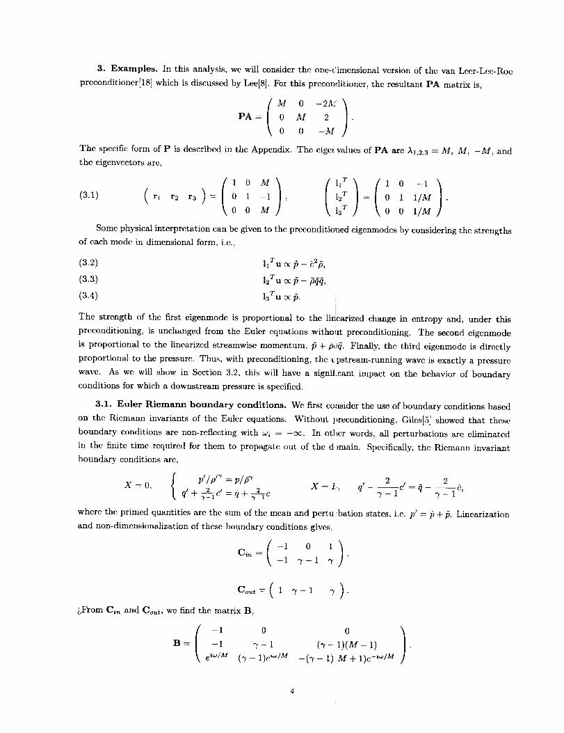
Thedeterminantof B is,

= -(q_- 1)2[(M- 1)ei"j/M + (M + 1)e-i_v/M],detB

and the eigcnfrequencies which result in a zero determinant arc,

ovr = 7rMn, for integer nM I+M

wi = - -_ log 1_"

In contrast to the unprcconditioncd Eulcr equations, thc Riemann invariant boundary conditions are reflective

for the preconditioned Eulcr equations since the value of wi is not -co. Within a computational simulation,

perhaps the best measure of the decay rate is actually the decay pcr time step. Assuming the time step is

given by a CFL condition of the form At = vAx/Arnax where v is a constant dependent on the tcmporal

integration, Ax is the cell size, and _max is the maximum eigenvalue, then wAt o( _i/Am_x. Since Am_ = M

for this preconditioned system,

1 I+Mw_/ Am_x = -- _ log 1_"

In particular, we note that as M --* 0, 0vi/Amax --* 0. Thus, at low Mach numbers, disturbances will not

decay indicating that the use of Riemann invariant boundary conditions based on the Euler equations is

likely to impede convergence to a steady state.

3.2. Entropy, stagnation enthalpy at inflow; pressure at outflow. Another common set of

boundary conditions for subsonic, internal flows is the specification of entropy and stagnation enthalpy at

the inflow and pressure at the outflow. Spccifically,

p,/p,_ = p/p-,X = O, 1_,2 __..7_K 1 -2 ___7_____q +.y-lp, = _q + 7-1p

For these boundary conditions, Cin and Cout are,

Ci,_ = ( - 1 0

\ 1 ('y- 1)M

X = L, p' = p.

1)Cout=(O 0 1 ).

/.From ein and Cout, we find the matrix B,

B =

-1 0 0 ]-1 (7- 1)M 0 •

0 0 Me -iw/M

We note that b13 = b23 = b31 = b32 : 0 for these boundary conditions. Thus, outgoing waves do not

generate incoming waves at either the inflow or outflow boundaries. At the inflow, specification of the

entropy guarantees that b12 = b13 = 0 since the change in entropy is proportional to the strength of the

first eigenmode as shown in Equation (3.2). Specification of the stagnation cnthalpy is also a non-reflecting

inflow condition since the change in stagnation enthalpy, /:/, can be written as a linear combination of the

first and second cigenmodcs, /t oc --llTu ÷ ('y -- 1)MI2Tu. Finally, as observed from Equation (3.4), the

pressurechangeisproportionalto thechangein thethird (upstJcam-running)cigenmode,thus,specificationofthepressureat theoutflowisnon-reflective.

Sincetheboundaryconditionsat inflowandoutflowarei ldividuallynon-reflective,theentiresystemwill haveinfinite,perturbationdecayrates.Specifically,thede'crminantof B is,

detB= -('7- 1)M2e-'È/M,

andtheeigcnfrequcncieswhichresultin azerodeterminantare,

w_ = 2rrMn, for inzcger n,

_)i _ --00.

Since wi = -oc, disturbances are eliminated via propagation m finite time. An interesting aspect of this

result is that these boundary conditions are actually reflective fc,r the unpreconditioned Euler equations (see

Giles[5]).

3.3. Velocity, temperature at inflow; pressure at outflow. The final set of boundary conditions

we consider is setting velocity and temperature at the inflow and pressure at the outflow. These conditions

are fairly common in low speed viscous flow applications. Spcc_cally,

X = O, _ P'/P' = pip

t q' = 0

For these boundary conditions, Ci,_ and Co_t axe,

Ci,_ = ( - 1

\ 0

_" = L, p' =p.

1 O J'

Cout-_ ( 0

/,From Ci,, and Co_,t, wc find the matrix B,

01)

-1 0 (3,-1)A!)B= 0 1 -1 .

0 0 Me -i'°/M

Unlike the boundary conditions in Section 3.2, the specification of velocity and temperature at the inflow is

a reflective condition and create reflections of the outgoing chara "_teristic wave. This is evident from the non-

zero values of b13 and b23. Specifically, at the inflow, al -= ('y - 1)Ma3 and c_2 = C_a. However, since bat =

b32 = 0, the outflow boundary condition does not create any perturbations in the incoming characteristics.

Thus, the reflected waves from the inflow conditions would bc emitted at the outflow boundary without

further reflection and all disturbances would be eliminated in fu ite time. Specifically, the determinant of B

is,

det B = -Me -i'_/M,

and the eigenfrequencies which result in a zero determinant are,

Wr = 2_Mn, for int _ger n,

a) i _ --OG.

While pcrturbations again have infinite decay rates for these boundary conditions, in practice, the reflec-

tive inflow condition may slow convergence somewhat compared to the non-reflecting boundary conditions

discussed in Section 3.2. This convergence slowdown is observed in the numerical results of the following

section.

4. Numerical Results. To illustrate the effect of different boundary conditions on numerical conver-

gence as well as check the accuracy of the analysis, wc simulate the two-dimensional flow in a duct with a

straight upper wall and a bump on the lower wall between 0 < x < 1 described by y = .042 sin2(Trx). The

domain is 5 unit lengths long and 2 lengths high. The grid is structured with clustering toward the wall

boundary.

Specifically, wc use the algorithm described by Darmofal and Siu[3] which employs the semi-coarsening

technique of Muldcr[12, 13] in conjunction with a multi-stage, block Jacobi relaxation[10, 1]. The dis-

cretization is a 2nd order upwind scheme with a Roe approximate Riemann solver[14]. Thc calculations are

performed on a grid of 32 × 16 cells. A three level, V-cycle is utilized with 2 prc and post smooths. All

calculations arc initialized to uniform flow.

A form of Turkel's preconditioner is employed which is smoothly turned off for Mach numbers above 0.5.

While this preconditioner is different than the one-dimensional van Leer-Lee-Roe preconditioner for which

the analysis was performed, we expect the low Mach number behavior of these preconditioners to be similar.

The major differences between the analysis and the numerical results will occur for higher subsonic Mach

numbers where the preconditioning is turned off in the numerical simulations.

We have implemented the boundary conditions described above by constructing a boundary face state

vector and calculating the boundary flux directly from this state vector. For example, for the enthalpy,

entropy, pressure boundary conditions at an inflow, entropy, cnthalpy, and the tangential velocity are pre-

scribed from the exterior and the prcssurc is extrapolated from the interior. At an outflow, we reverse the

procedure and specify pressure from the exterior and extrapolate entropy, enthalpy, and tangential velocity

from the interior. Note, regardless of the specific boundary conditions, we always use the tangential velocity

as the additional variable for the two-dimensional boundary implementation.

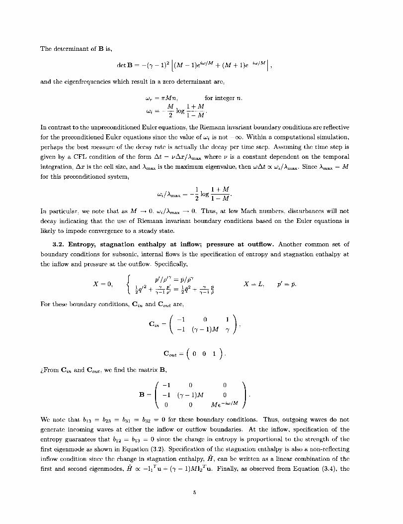
The number of cycles required to converge the solution six orders of magnitude from the initial residual

are given in Table 4.1. As can be clearly seen, the results are in good agreement with the analysis at

low Mach numbers. In particular, the Riemann boundary conditions are unstable at low Mach numbcrs.

The entropy, enthalpy, pressure (HSP) boundary conditions perform best while the velocity, temperature,

pressure boundary (QTP) conditions are about 75% more expensive. This would indicate that the reflective

nature of the inflow for the QTP boundary conditions does indeed slow the convergence.

At the higher Mach numbers (M > 0.2), the Ricmann boundary condition cases begin to converge and

the number of cycles decreases with increasing Mach. The QTP boundary conditions require an increasing

number of cycles for increasing Mach number. Also, for the _I_ = 0.5 test case, the amount of work required

to converge the HSP boundary conditions increased from 8 cycles to 10 cycles. These trends at higher Mach

numbers arc expected because the preconditioning which was implemented numerically was automatically

phased out at M = 0.5. Thus, the behavior of the different boundary conditions will bc described by the

unpreconditioned Euler equations. In this case, the Riemann boundary conditions are non-reflective while

the other boundary conditions are reflective.

5. Remarks. The present analysis of the preconditioned Euler equations shows the effect of precondi-

tioning on boundary conditions. Boundary conditions based on the Ricmann invariants of the Euler equations

are found to be reflective in conjunction with preconditioning. The problem is most detrimental at low Mach

.aeh'I emann0.001

0.01

0.i

0.2

0.3

0.4

0.5

UNS 8 13

UNS 8 13

UNS 8 13

20 8 14

14 8 15

Ii 8 18

9 10 20

TABLE 4.1

Number of cycles required to drop residual six orders of magnitude far different Mach numbers and boundary conditions.Riemann: Euler Riemann invariant boundary conditions from Section 3.:t. HSP: enthalpy, entropy, pressure boundary con-

ditions from Section 3._. QTP: velocity, temperature, pressure boundary conditions from Section 3.3. UNS: algorithm was

unstable and aborted with infinite residual.

numbers where the decay rate of perturbations approaches zero. Boundary conditions which specify entropy

and stagnation enthalpy at an inflow and pressure at an outflo_x _ are found to be non-reflective with precon-

ditioning. Numerical results were presented which are in good agreement with the analytic predictions.

Finally, an interesting possibility implied by this analysis would be to incorporate boundary condition

considerations into the design of preconditioners. For example, _iven a set of physical boundary conditions

which must be applied for a specific problem, a preconditioner Could be designed such that these conditions

are non-reflective.

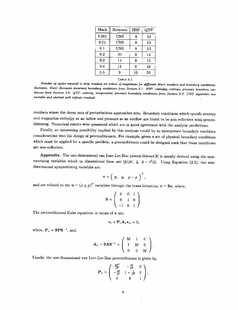
Appendix. The one-dimensional van Leer-Lee-Roe precontitioner[8] is usually derived using the sym-

metrizing variables which in dimensional form are (;5/p_, _, /5 - _2f). Using Equation (2.2), the non-

dimcnsional symmctrizing variables are,

F

and are related to the u = (p, q, p)r variables through the trans brmation, v = Su, where,

0 0 1)S= 0 1 0

-1 0 1

The preconditioned Euler equations in terms of v arc,

vt + P,_A,,vx = 0,

where, P, = SPS -x, and,

Av = SAS -1 =M 1 0 )1 M 0 •

0 0 M

Finally, the one-dimensional van Leer-Lee-Roe prcconditioncr is given by,

Pv

M 2 M /

M 1

-3_- 1 + _- 0 ,0 0 1

8

and, for use with the (p, q, p) variables,

P = S-1PvS =

wherefl2= 1-M 2.

I 1 M M 2 1

--_ _---iI M

0 1+_-_ _2 ,M M s

0 -_ _-

REFERENCES

[1] S ALLMARAS, Analysis of a local matrix preconditioner for the 2-D Navier-Stokes equations. AIAA

Paper 93-3330, 1993.

[2] Y. CnOl AND C. MERKLE, The application of preconditioning in viscous flows, Journal of Computa-

tional Physics, 105 (1993), pp. 203 223.

[3] D. DARMOFAL AND K. SIC, A robust locally preconditioned multigrid algorithm for the Euler equations.

AIAA Paper 98-2428, 1998.

[4] D. DARMOFAL AND B. VAN LEER, Local preconditioning: Manipulating Mother Nature to fool Fa-

ther Time, in Computing the Yhturc II: Advances and Prospects in Computational Aerodynamics,

M. Hafez and D. Caughey, cds., John Wiley and Sons, 1998.

[5] M. GILES, Eigenmode analysis of unsteady one-dimensional Euler equations. ICASE Report No. 83-47,

1983.

[6] A. GODFREY_ Steps toward a robust preconditioning. AIAA Paper 94-0520, 1995.

[7] D. JESPERSEN, W. PULLIAM, AND P. BUNING, Recent enhancements to OVERFLOW. AIAA Paper

97-0644, 1997.

[8] D. LEE, Local preconditioning of the Euler and Navier-Stokes equations, PhD thesis, University of

Michigan, 1996.

[9] W. LEE, Local preconditioning of the Euler equations, PhD thesis, University of Michigan, 1991.

[10] J. LYNN AND B. VAN LEER, Multi-stage schemes for the Euler and Navier-Stokes equations with optimal

smoothing. AIAA Paper 93-3355, 1993.

[11] D. MAVRIPLIS, Multigrid strategies for viscous flow solvers on anisotropie unstructured meshes. AIAA

Paper 97-1952, 1997.

[12] W. MULDER, A new approach to convection problems, Journal of Computational Physics, 83 (1989),

pp. 303 323.

[13] --, A high resolution Euler solver based on multigrid, semi-coarsening, and defect correction, Journal

of Computational Physics, 100 (1992), pp. 91 104.

[14] P. ROE, Approximate Riemann solvers, parametric vectors, and difference schemes, Journal of Compu-

tational Physics, 43 (1981), pp. 357 372.

[15] E. TURKEL, Preconditioned methods for solving the incompressible and low speed compressible equations,

Journal of Computational Physics, 72 (1987), pp. 277 298.

[16] E. TURKEL, R. RADESPIEL, AND N. KROLL, Assessment of two preconditioning methods for aerody-

namic problems, Computers and Fluids, 26 (1997), pp. 613 634.

[17] E. TURKEL, V. VATSA, AND R. RADESPIEL, Preconditioning methods for low-speed flows. AIAA Paper

96-2460, 1996.

[18] B. VAN LEER, W. LEE, AND P. ROE, Characteristic time-stepping or local preconditioning of the Euler

equations. AIAA Paper 91-1552, 1991.

[19] J. WEISS AND W. SMITH, Preconditioning applied to variable and constant density flows, AIAA Journal,

33 (1995), pp. 2050 2057.

lO

REPORT DOCUMENTATION PAGE Form ApprovedOMB No. 0704-0188

Publicreporting burdenfor thiscollection of informationis estimatedto average1hourperresponse,incl dingthe time for reviewinginstructions, searchingexistingdatasources,gather ngand maeta n ngthe data needed,andcompletingand revewingthe co ectonof information.<:nd commentsregardngthis burdenestimateor anyotheraspectof th scollectionof information, includingsuggestionsfor reducingthis burden,to Washington HeadquartersSet ices,Directoratefor InformationOperationsandReports.1215JeffersonDavisHighway,Suite1204, Arlington,VA 22202-4302. andto the Office of Managementand Budget,P;perworkReductionProject(0704-0188), Washington,DC 20503

1. AGENCY USE ONLY{Leave blank) 2. REPORT DATE 3. REPORT TYPE AND DATES COVERED

November 1998 Cont,'actor Report

4. TITLE AND SUBTITLE 5. FUNDING NUMBERS

Eigenmode Analysis of Boundary Conditions for the One-dimension_l

Preconditioned Euler Equations

6. AUTHOR(S)

David L. Darmofal

7. PERFORMING ORGANIZATION NAME(S) AND ADDRESS(ES)

Institute for Computer Applications in Science and Engineering

Mail Stop 403, NASA Langley Research Center

Hampton, VA 23681-2199

9. SPONSORING/MONITORING AGENCY NAME(S) AND ADDRESS(ES)

National Aeronautics and Space Administration

Langley Research Center

Hampton, VA 23681-2199

C NAS1-97046WU 505-90-52-01

8. PERFORMING ORGANIZATION

REPORT NUMBER

1CASE Report No. 98-51

10, SPONSORING/MONITORINGAGENCY REPORT NUMBER

NASA/CR-1998-208741

ICASE Report No. 98-51

11. SUPPLEMENTARY NOTES

Langley Technical Monitor: Dennis M. BushnellFinal Report

To be submitted to AIAA 1999 CFD Conference and SIAM Journai of Numerical Analysis.

12a. DISTRIBUTION/AVAILABILITY STATEMENT , 12b. DISTRIBUTION CODE

Unclassified Unlimited

Subject Category 64

Distribution: Nonstandard

Availability: NASA-CASI (301)621-0390

13. ABSTRACT (Maximum 200 words)

An analysis of the effect of local preconditioning on boundary con.litions for the subsonic, one-dimensional Euler

equations is presented. Decay rates for the eigenmodes of the initial boundary value problem are determined

for different boundary conditions. Riemann invariant boundary c_,nditions based on the unpreconditioned Euler

equations are shown to be reflective with preconditioning, and, at low Mach numbers, disturbances do not decay.

Other boundary conditions are investigated which are non-reflective with preconditioning and numerical results are

presented confirming the analysis.

14. SUBJECT TERMS

local preconditioning; boundary conditions; Euler equations

17, SECURITY CLASSIFICATION

OF REPORT

Unclassified

NSN 7540-01-280-5500

18. SECURITY CLASSIFICATION lg. SECURITY CLASSIFICATION

OF THIS PAGE OF ABSTRACT

Unclassified

1S. NUMBER OF PAGES

15

16. PRICE CODE

A0320. LIMITATION

OF ABSTRACT

'Standard Form 298(Rev. 2-89)Prescribedby ANSIStd Z39-18298-102