ENHANCED OIL RECOVERY OF VISCOUS OIL BY INJECTION OF WATER-IN-

OIL EMULSION MADE WITH USED ENGINE OIL

A Dissertation

by

XUEBING FU

Submitted to the Office of Graduate Studies of Texas A&M University

in partial fulfillment of the requirements for the degree of

DOCTOR OF PHILOSOPHY

Approved by:

Chair of Committee, Robert H. Lane

Committee Members, Maria A. Barrufet David E. Bergbreiter Akhil Datta-Gupta A. Daniel Hill Head of Department, A. Daniel Hill

December 2012

Major Subject: Petroleum Engineering

Copyright 2012 Xuebing Fu

ii

ABSTRACT

Solids-stabilized water-in-oil emulsions have been suggested as a drive fluid to

recover viscous oil through a piston-like displacement pattern. While crude heavy oil

was initially suggested as the base oil, an alternative oil – used engine oil was proposed

for emulsion generation because of several key advantages: more favorable viscosity that

results in better emulsion injectivity, soot particles within the oil that readily promote

stable emulsions, almost no cost of the oil itself and relatively large supply, and potential

solution of used engine oil disposal.

In this research, different types of used engine oil (mineral based, synthetic) were

tested to make W/O emulsions simply by blending in brine. A series of stable emulsions

was prepared with varied water contents from 40~70%. Viscosities of these emulsions

were measured, ranging from 102~104 cp at low shear rates and ambient temperature.

Then an emulsion made of 40% used engine oil and 60% brine was chosen for a series of

coreflood experiments, to test the stability of this emulsion while flowing through porous

media. Limited breakdown of the effluent was observed at ambient injection rates,

indicating a stability of the emulsion in porous media. Pressure drops leveled off and

remained constant at constant rate of injection, indicating steady-state flows under the

experimental conditions. No plug off effect was observed after a large volume of

emulsion passed through the cores.

Reservoir scale simulations were conducted for the emulsion flooding process

based on the emulsion properties tested from the experiments. Results showed

iii

significant improvement in both displacement pattern and oil recovery especially

compared to water flooding. Economics calculations of emulsion flooding were also

performed, suggesting this process to be highly profitable.

iv

DEDICATION

To Daulat D. Mamora

v

ACKNOWLEDGEMENTS

I would like to thank Dr. Daulat Mamora, for bringing me into the heavy oil area

and getting me started with my research project. I also want to thank my committee

chair, Dr. Robert Lane for continually challenging me and always having time for

discussions, and my committee members, Dr. Maria Barrufet, Dr. Akhil Datta-Gupta,

Dr. Daniel Hill, and Dr. David Bergbreiter for their generous support for me in

completing this project.

Thank you to my lab mates for making my research possible and enjoyable,

especially Matt Wiese and Hamid Rahnema. Many thanks to my friends, Xinwei Li, Cui

Song, Hongqian Nie and Guohua Ann for their constant support and encouragement. I

would also like to thank my parents, Zengchun Wu and Haitao Fu for their love and

understanding and my cousin, Qinghua Li for always believing in me.

Finally, thank you to everyone who has helped me to learn and grow over the last

six years at Texas A&M University.

vi

TABLE OF CONTENTS

Page

ABSTRACT .............................................................................................................. ii

DEDICATION .......................................................................................................... iv

ACKNOWLEDGEMENTS ...................................................................................... v

TABLE OF CONTENTS .......................................................................................... vi

LIST OF FIGURES ................................................................................................... viii

LIST OF TABLES .................................................................................................... xiv

CHAPTER

I INTRODUCTION ................................................................................ 1

1.1 Statement of Problem .................................................................. 1 1.2 Objectives of Research ................................................................ 2 1.3 Background and Literature Review ............................................. 2

II EXPERIMENTAL METHODS ........................................................... 15

2.1 Chemicals and Fluids .................................................................. 15 2.2 Experimental Apparatus .............................................................. 15 2.3 Experimental Procedures ............................................................. 21 III EXPERIMENTAL RESULTS ............................................................. 27

3.1 Emulsion Generation ................................................................... 27 3.2 Bench Tests ................................................................................. 28 3.3 Corefloods ................................................................................... 41 IV SIMULATION STUDIES .................................................................... 78

4.1 General Description ..................................................................... 78 4.2 Water Flooding ............................................................................ 81 4.3 Emulsion Flooding ...................................................................... 87

vii

CHAPTER Page

4.4 Sensitivity Analyses .................................................................... 97 4.5 Emulsion Flooding in a Water-flooded Reservoir ...................... 110

V ECONOMICS CALCULATIONS ....................................................... 117 5.1 Model Description ....................................................................... 117 5.2 Input Values ................................................................................ 118 5.3 Results ......................................................................................... 120 5.4 Sensitivity Analyses .................................................................... 122 5.5 Emulsion Flooding in a Water-flooded Reservoir ...................... 137

VI SUMMARY AND CONCLUSIONS ................................................... 141 6.1 Summary ..................................................................................... 141 6.2 Conclusions ................................................................................. 142 REFERENCES .......................................................................................................... 146

viii

LIST OF FIGURES

FIGURE Page

2.1 Silverson L4RT laboratory homogenizer .................................................. 16

2.2 Coreflood system ....................................................................................... 20

2.3 Snapshot of the emulsification process ..................................................... 22

2.4 Setup for packing a slimtube with sand .................................................... 25

3.1 Used engine oil (Pennzoil 5W-30) and W/O emulsions at different brine volume fractions .............................................................................. 28 3.2 Viscosities of the emulsions measured at 10˚C ......................................... 29

3.3 Viscosities of the emulsions measured at 25˚C ......................................... 30

3.4 Viscosities of the emulsions measured at 50˚C ......................................... 30

3.5 Microscopic images of a W/O emulsion (60 vol% water), taken right after made (left) and 6 months later (right) ...................................... 32 3.6 Densities of the emulsions ......................................................................... 33

3.7 Interfacial tensions between used engine oil/fresh engine oil and brine ... 34

3.8 Particle Size distribution of the soot particles within used engine oil ...... 36

3.9 Microscopic images of emulsions generated with brine A, B and C (from top to bottom) .................................................................................. 38 3.10 Viscosities of emulsions generated with brine A, B and C ....................... 39

3.11 Viscosities of emulsions generated with brine A, B and C, after 6 months ............................................................................................ 40 3.12 Bentheimer sandstone, Idaho sandstone and Boise sandstone from to t o ott om of si e 1 ..................................................... 42 3.13 Emulsion effluents collected at injection rate 1ft/d, 3 ft/d, 10 ft/d and 100ft/d (from left to right). ................................................................. 45

ix

FIGURE Page

3.14 ressure rof ile for emulsion in ection daho sandstone .................. 46

3.15 f fecti e is cosit of the emulsion daho sandstone ........................ 47

3.16 ressure rof ile for emulsion in ection oise sandstone ................. 49

3.17 Effective viscosity of the emulsion oise sandstone ........................ 50

3.18 ressure rof ile for emulsion in ection entheimer sandstone ...... 51

3.19 f fecti e is cosit of the emulsion entheimer sandstone ........... 51

3.20 Viscometer-measured is cosit of the emulsion effluents Bentheimer sandstone I ............................................................................. 52 3.21 Relative permeability curves ..................................................................... 54

3.22 Mobility factor curves in two phase flow .................................................. 55

3.23 ressure rof ile for emulsion in ection 12 entheimer sandstone .... 56

3.24 f fecti e is cosit of the emulsion 12 Bentheimer sandstone I .......... 57

3.25 Viscometer-measured viscosity of the emulsion and effluents: 12 entheimer sandstone .................................................................... 58 3.26 ressure rof ile for emulsion in ection 12 entheimer sandstone ... 61

3.27 Effective viscosity of the emulsion: 12 entheimer sandstone ........ 62

3.28 Bentheimer sandstone core right after emulsion flow experiment ............ 63

3.29 ressure rof ile for emulsion in ection entheimer sandstone ..... 64

3.30 f fecti e is cosit of the emulsion entheimer sandstone II .......... 65

3.31 ressure rof ile for emulsion in ection 12 entheimer sandstone . 66

3.32 f fecti e is cosit of the emulsion 12 entheimer sandstone ....... 66

3.33 ressure rof ile for emulsion in ection entheimer sandstone ... 67

x

FIGURE Page

3.34 f fecti e is cosit of the emulsion entheimer sandstone ......... 68

3.35 ressure rof ile for emulsion in ection 3ʹ sand a cked slimtu e ......... 71

3.36 f fecti e is cosit of the emulsion 3ʹ sand a cked slimtu e ............... 72

3.37 Viscometer-measured viscosity of the emulsion effluents: 3ʹ sand acked slimtu e ......................................................................... 73 3.38 ressure rof ile for emulsion in ection ʹ sand a cked slimtu e ......... 74

3.39 f fecti e is cosit of the emulsion ʹ sand a cked slimtu e ............... 75

3.40 Viscometer-measured viscosity of the emulsion effluents: ʹ sand acked slimtu e ......................................................................... 76 4.1 (a) 2D view of the gridblocks from top; (b) 3D view of the gridblocks ... 79

4.2 Liquid rates and well BHPs in water flooding .......................................... 81

4.3 Water cut in water flooding ....................................................................... 82

4.4 Cumulative oil production in water flooding ............................................ 83

4.5 Recovery performance for water flooding ................................................ 84

4.6 Oil saturation after two years of water flooding........................................ 85

4.7 Liquid rates and well BHPs in emulsion flooding .................................... 89

4.8 Comparison between emulsion flooding and water flooding: oil production rate ..................................................................................... 91 4.9 Comparison between emulsion flooding and water flooding: liquid injection rate .................................................................................... 92 4.10 Comparison between emulsion flooding and water flooding: water cut ... 92

4.11 Comparison between emulsion flooding and water flooding: cumulative oil production .......................................................................... 93

xi

FIGURE Page

4.12 Comparison between emulsion flooding and water flooding: oil recovery performance ................................................................................ 94 4.13 Crude oil fraction after two years in emulsion flooding ........................... 95

4.14 Oil production rates under different emulsion viscosities ......................... 98

4.15 Water cut under different emulsion viscosities ......................................... 99

4.16 Cumulative oil productions under different emulsion viscosities ............. 100

4.17 Injection and production rates at different emulsion breakdown .............. 102

4.18 Water cut in the produced fluids at different emulsion breakdown .......... 103

4.19 Oil production rates for reservoirs with different crude oil viscosities ..... 104

4.20 Cumulative oil productions for reservoirs with different crude oil viscosities ................................................................................... 105 4.21 Oil production rates for reservoirs with different porosities ..................... 107

4.22 Cumulative oil productions for reservoirs with different porosities ......... 108

4.23 Oil production rates for reservoirs with different permeabilities .............. 109

4.24 Cumulative oil productions for reservoirs with different permeabilities .. 110

4.25 Oil rate and water cut at the production well for emulsion flooding after water flooding ................................................................................... 111 4.26 Total liquid rate and BHP at the injection well for emulsion flooding after water flooding ................................................................................... 112 4.27 Emulsion rate at the production well for emulsion flooding after water flooding ................................................................................... 113 4.28 Cumulative oil production at the production well for emulsion flooding after water flooding ..................................................................... 114 4.29 Recovery performance for emulsion flooding after water flooding ......... 115

xii

FIGURE Page

5.1 Monthly liquid rates in water flooding ...................................................... 119

5.2 Monthly liquid rates in emulsion flooding ................................................ 120

5.3 Cash flow for water flooding and emulsion flooding ............................... 121

5.4 NPV for water flooding and emulsion flooding ........................................ 121

5.5 Sensitivity analyses of capital costs on cash flow ..................................... 123 5.6 Sensitivity analyses of capital costs on NPV ............................................ 123

5.7 Sensitivity analyses of water price on cash flow in water flooding .......... 125

5.8 Sensitivity analyses of water price on NPV in water flooding ................. 125

5.9 Sensitivity analyses of emulsion price on cash flow in emulsion flooding ..................................................................................... 127 5.10 Sensitivity analyses of emulsion price on NPV in emulsion flooding ...... 127 5.11 Sensitivity analyses of water disposal cost on cash flow in water flooding ........................................................................................... 129 5.12 Sensitivity analyses of water disposal cost on NPV in water flooding ..... 129

5.13 Sensitivity analyses of water disposal cost on cash flow in emulsion flooding ...................................................................................... 130 5.14 Sensitivity analyses of operating cost on cash flow in water flooding ..... 130

5.15 Sensitivity analyses of operating cost on cash flow in water flooding ..... 131 5.16 Sensitivity analyses of operating cost on cash flow in emulsion flooding ...................................................................................... 132 5.17 Sensitivity analyses of operating cost on NPV in water flooding ............. 132

5.18 Sensitivity analyses of operating cost on NPV in emulsion flooding ....... 133

5.19 Sensitivity analyses of annual interest rate on NPV in water flooding ..... 134

xiii

FIGURE Page

5.20 Sensitivity analyses of annual interest rate on NPV in emulsion flooding ...................................................................................... 134 5.21 Sensitivity analyses of emulsion viscosity on cash flow in emulsion flooding ...................................................................................... 135 5.22 Sensitivity analyses of emulsion viscosity on NPV in emulsion flooding ...................................................................................... 136 5.23 Monthly liquid rates during emulsion flooding in a water-flooded reservoir .......................................................................... 138 5.24 Cash flow for emulsion flooding in a water-flooded reservoir ................. 138

5.25 NPV for emulsion flooding in a water-flooded reservoir ......................... 139

xiv

LIST OF TABLES

TABLE Page 4.1 Reservoir and fluid properties ................................................................... 79 4.2 Reservoir fluid quantities in water flooding .............................................. 86 4.3 Reservoir fluid barrels in water flooding .................................................. 87 4.4 Reservoir fluid quantities in emulsion flooding ........................................ 96 4.5 Reservoir fluid barrels in emulsion flooding ............................................. 96 5.1 Input parameters for economics ................................................................ 118

1

CHAPTER I

INTRODUCTION

1.1 Statement of Problem

Heavy oil constitutes a large proportion of worldwide oil reserves (Chopra and

Lines, 2008). Cold production of such reserves is attractive in a number of locations for

economic or technical reasons, due to thin formation that would lead to excessive heat

loss or proximity to permafrost that could be melted during thermal recovery (Gondouin

and Fox III, 1991; Selby et al., 1989). Primary production recovers usually less than five

percent of heavy oil, while water flooding may add only another 5 – 10% recovery (Mai

et al., 2009)—the mobility ratio is very unfavorable in water flood recovery of heavy

oils, leading to high water cuts early in the process.

Polymer flooding is the most widely used EOR method for light to medium

viscous oil recovery (Du and Guan, 2004), but this process may not be suitable for heavy

oil having viscosity of 200 cp or higher, due to the uneconomically high concentration of

polymers required (Bragg, 1999). Alkali flooding or alkali-surfactant flooding is perhaps

a more promising approach than polymer flooding in cases where an emulsion may form

spontaneously in situ to mobilize heavy oil or divert flow to improve the recovery of

heavy oil (Bryan and Kantzas, 2007). However, high cost of chemicals and high

reaction/retention in the reservoir again limits their applications. Other methods include

the use of solvents, CO2, or inert gas to lower the viscosity of crude oil, but only with

very limited success (Selby et al., 1989).

2

A relatively recent approach involves generating high water percentage water-in-

oil crude oil emulsions by adding solid nanoparticles as a stabilizer (Bragg, 1999, 2000).

This crude oil emulsion is proven to be an effective drive fluid that displaces in-situ oil

through a piston-like displacement pattern and triples the net oil recovery of a water

flooding process. However, this crude oil emulsion system has its shortcomings. Besides

the requirement of adding nanoparticles, the viscosity of a crude oil emulsion is usually

much higher than the original crude and thus too far beyond the purpose of mobility

control and results in poor injectivity. Therefore, development of new non-thermal

methods or improvement of existing methods is required for enhanced recovery of

viscous oil that has viscosity of a few hundred to a few thousand centipoises.

1.2 Objectives of Research

The objectives of this research are the following:

Explore the possibility of generating stable emulsions from used engine oil

Characterize the stability and rheological behavior of used engine oil emulsions

with both bench tests and coreflood experiments

Evaluate the possibility of using this new emulsion system as a displacement

fluid for heavy oil EOR based on simulations and economics calculations

1.3 Background and Literature Review

Heavy oil deposits in Canada, Venezuela and the United States comprise several

trillion barrels (Chopra and Lines, 2008). Compared to light oil, the principal difficulty

3

of the recovery of heavy oil is the high oil viscosity that impedes its flow. Thermal

methods target at lowering oil viscosity by application of hot water (Harmsen, 1971),

steam (Liebe and Butler, 1991; Owens and Suter, 1965) or in situ combustion (Joseph N.

Breston, 1958). Among those methods, steam injection is the most successful and has

been widely applied in heavy oil fields. However, many reservoirs are not suitable for

thermal methods due to thin formation (< 10 m) or large depth (> 1000 m) which would

lead to excessive heat loss (Selby et al., 1989). For such reservoirs, non-thermal recovery

methods may be employed.

1.3.1 Overview of Non-thermal Methods

Water flooding is the most commonly used technique after primary recovery

even in heavy oil reservoirs. The primary recovery from heavy oil reservoirs is generally

low and water flooding is usually quite inefficient due to unfavorable mobility ratio

which results in severe channeling and early water breakthrough. In the Lloydminster

area the primary recovery was estimated to be 3-8% of the original oil in place (OOIP),

and water flooding, which was carried out in most major reservoirs in this area, only

added up an additional 1-2% of OOIP to the primary recovery (Adams, 1982). Because

of the simplicity and low cost of water flooding, it is still widely applied despite its poor

performance.

Carbon dioxide flooding was also suggested for heavy oil recovery and has been

tested in different fields, with varied extent of success (Khatib et al., 1981; Picha, 2007;

Reid and Robinson, 1981; Saner and Patton, 1986). Carbon dioxide can be applied to

4

recover oil by various techniques: carbonated water flooding, CO2 cyclic stimulation,

and immiscible CO2 flooding (Selby et al., 1989). The major mechanisms for improved

oil recovery by CO2 are: oil viscosity reduction, oil swelling, interfacial tension

reduction and emulsification (Selby et al., 1989). So far CO2 flooding is only applied to

limited number of reservoirs.

Polymer flooding consists of adding polymers into injection water to increase its

viscosity and thus to lower the water-oil mobility ratio. It has been successfully applied

to many light to medium light (approximately < 200 cp) oil fields in the world (Kang et

al., 2011; Leonard, 1986). Comparatively fewer attempts were made for heavy oil

recovery using polymers. It was once considered that very high concentrations of

polymer were required for highly viscous oils: the cost of chemical together with

increased difficulty of injection would make this process uneconomical. However,

polymer flooding for heavy oil recovery has become more promising in recent years due

to the wide application of horizontal wells in heavy oil production and higher oil prices

(Wassmuth et al., 2009; Wassmuth et al., 2007; Zaitoun, 1998).

Alkali flooding or caustic flooding involves injection of alkaline solutions into

the reservoir, which react with the organic acids within heavy oil and form in situ

surfactants, thus lowering the interfacial tension (IFT) and forming emulsions (Selby et

al., 1989). Johnson (Johnson Jr., 1976) proposed four different mechanisms by which

caustic flooding may improve oil recovery: (1) emulsification and entrainment, (2)

wettability reversal (oil-wet to water-wet), (3) wettability reversal (water-wet to oil-wet),

and (4) emulsification and entrapment. The actual mechanisms of this process depend on

5

reservoir conditions and rock/fluid properties and may include a few of them at the same

time. Although much success has been observed in laboratory experiments (Farouq Ali

et al., 1979; Jennings Jr. et al., 1974; Scott et al., 1965; Xie et al., 2008) and certain

fields reported promising results with this process (Edinga et al., 1980; Xie et al., 2008),

a majority of field applications of alkali flooding were unsuccessful (Alikhan and Farouq

Ali, 1983; Leonard, 1984; Selby et al., 1989). Caustic flooding usually does not

outperform polymer flooding but its price is much lower and thus may be considered in

certain cases.

Surfactant may be added to the injected alkali solutions and constitute a process

called Alkali-surfactant (AS) flooding. In alkali flooding the minimum IFT is often

achieved at very low concentrations of alkali. However, higher concentrations of alkali

are often injected due to large consumption by the rock (Drillet and Defives, 1991;

Mohnot et al., 1987; Novosad and Novosad, 1984), which leads to conditions that alkali

floods do not perform at optimal conditions. By adding surfactants the floods can be

stabilized by allowing higher concentrations of alkali to achieve minimum IFT (Bryan

and Kantzas, 2009; Nelson et al., 1984). Improved recovery of heavy oil by AS flooding

was observed in the lab (Bryan and Kantzas, 2009; Bryan and Kantzas, 2008; Mai et al.,

2009) but applications were rarely seen in the fields, likely due to the high cost of

surfactants especially in contrast to the low crude prices. Also, heavy oil itself may

contain asphaltene which is surface active, thus reduces the requirement for artificial

surfactants. Unlike chemical flooding of light oil, polymer is usually not part of the

6

formulation, as polymer would be less effective in heavy oil cases and mobility control

can come from emulsification.

Emulsion flooding is closely related to alkali or AS flooding. Sometimes the term

“emulsion flooding” ma indicate a chemical flooding r ocess that in ol e s in situ

emulsification (Kumar et al., 2010). Another category of emulsion flooding refers to an

emulsified fluid prepared above the ground, by which means the composition and quality

of emulsion can be better controlled. The emulsion flooding we focus on is under the

second category through this dissertation. As an emulsion is composed of both water and

oil (and often a small amount of stabilizer), injecting such a fluid means injecting a

fraction of oil into the reservoir. This type of risk makes an emulsion flooding process

unattractive and so far field applications are very limited. However, more frequent

applications may be seen in future as crude oil price increases and cheaper/better

emulsion systems are being developed.

1.3.2 Emulsion Flooding

Crude oil is the most common candidate for oil in generating emulsions because

of its availability in the field. Generally two types of emulsions could be generated

depending on the phase distribution: water-in-oil (W/O) or oil-in-water (O/W). In O/W

emulsions water is the continuous phase and oil exists as small droplets suspended in

water. This type of emulsion has viscosities closer to water. On the contrary, W/O

emulsions are mixtures of oil and water within which oil is the continuous phase. The

viscosity of a W/O emulsion would be closer to that of oil, and it increases as the water

7

fraction goes up (Isaacs and Chow, 1992). Both types of emulsions have been suggested

as displacement fluids for heavy oil recovery.

McAuliffe (McAuliffe, 1973b) conducted laboratory studies with oil-in-water

emulsions by injecting an O/W emulsion made with crude oil and dilute solutions of

sodium hydroxide into sandstone cores. Reduced water permeability was observed even

after many pore volumes of water being injected after the emulsion injection. Then a

field test (McAuliffe, 1973a) was reported by the same author, indicating positive

responses of flood pattern and incremental oil recovery from emulsion flooding. The

major cause was attributed to improvement of heterogeneity of reservoir by the oil

droplets plugging off higher permeability zones of the reservoir. The mechanism of this

r ocess is com a ra le to the “emulsification and entra ment” mechanism in caustic

flooding.

It has long been noticed that the pH of water has an effect on the type of

emulsion to be formed. Farouq Ali et al. (Farouq Ali et al., 1979) generated stable W/O

and O/W emulsions by using low pH (pH=2) and high pH (pH=10) water, respectively.

The emulsions were injected as slugs to recover crude heavy oil in coreflood

experiments. The results were compared with acid flooding and caustic flooding cases,

indicating higher efficiency of heavy oil recovery for the emulsion flooding cases. Also

W/O emulsion slugs were found to be more effective than O/W emulsions.

Similar adjustment of pH to generate stable emulsions was reported by D'Elia-S

and Ferrer-G (D'Elia-S and Ferrer-G, 1973). In their research, stable W/O emulsions

were made by mixing a heavy oil, a refined oil and low pH water without using any

8

commercial surfactant. The refined oil was added simply to lower viscosity of the

mixture. Then this emulsion was injected into a core as a slug to displace heavy oil,

indicating a high recovery of 75% of the original oil in place.

More recently, nanoparticles were used as stabilizers to generate stable emulsions

for the purpose of enhanced oil recovery (Bragg, 1999, 2000; Bragg and Varadaraj,

2006). In their patents, hydrophilic or oleophilic solid particles were used to promote

O/W and W/O emulsions, respectively. The low viscosity O/W emulsion can be used to

enhance production of oil from subterranean reservoirs, or the transportation of oil

through a pipeline. On the other hand, the high viscosity W/O emulsion was suggested

as a drive fluid for displacing hydrocarbons from the formation or to produce a barrier

for diverting flow of fluids in the formation. An W/O emulsion consisted of 58% water

and 42% crude heavy oil stabilized by proposed oleophilic nanoparticles was used as a

drive fluid to recover the same crude oil in coreflood experiments, and a nearly 100%

recovery was obtained at unit pore volume injection, indicating a piston-like flooding

pattern.

Kaminsky et al. (Kaminsky et al., 2010) reported a successful field test on using

W/O emulsions to recover heavy oil after lab testing and reservoir modeling. The

emulsion was generated on site using produced crude oil (3000 cp) and water. Small

amounts of added mineral fines were used to stabilize the emulsion. Propane was

dissolved into the oil to adjust the viscosity of the injected emulsion to be similar to that

of the in situ oil. Emulsion fluid displaced viscous oil in a miscible-like manner with

favorable mobility, which lead to improved displacement and recovery. The field

9

piloting confirmed the ability to generate and sustain injection of a solids-stabilized

emulsion in the field and to propagate stabilized emulsions in the reservoir.

All previous research came to the same conclusion on the high recovery

efficiency of W/O emulsions as displacement fluid to recover crude oil. As mentioned

above, the oil external nature of the emulsion enables a semi-miscible process, and the

high viscosity of emulsion allows sufficient mobility control during displacement. The

two factors together can promote piston-like flood pattern in ideal conditions. Therefore

for W/O emulsions of high water fractions (> 50%), their efficiency as displacement

fluids is so high that the net oil recoveries could be close to the water fraction. Even

though oil is being injected into the reservoir (in the form of emulsion), the net oil

recovery of this process is much greater than that from water flooding and at smaller

amount of fluid injection. However, problems are associated with high water fraction

W/O emulsions.

First of all, the viscosity of W/O emulsions increases quickly as the water

fraction gets higher. A 60% emulsion can be 20~50 times more viscous than the original

oil used for creating this emulsion. Since crude oil is the common option for emulsion

generation, the emulsion viscosity is usually unfavorably high for displacing the same

crude, which will result in low injectivity. To solve this problem, both D'Elia-S (D'Elia-S

and Ferrer-G, 1973) and Bragg (Bragg, 1999, 2000) suggested mixing in light

hydrocarbon components to lower the emulsion viscosity. This would add up cost as

light hydrocarbons are expensive, and may also complicate the emulsion generation

process if the added hydrocarbon is gas.

10

Secondly, some crude oil will not form stable emulsions just by adding solid

particles (Bragg, 1999, 2000) or adjusting the pH (Farouq Ali et al., 1979). As heavy oil

contains varied amount of asphaltene and other surface active agents, some may require

more effective stabilizers than nanoparticles or acid to form emulsions that are stable

enough for injection. Therefore this process will be limited by the chemical composition

of heavy crude produced from the reservoir. Also the solid nanoparticles may be

somewhat costly although less expensive than surfactants.

One possible solution for these problems is finding another candidate oil that is

moderately viscous, and can emulsify easily without too much additives. It also has to be

cheap and available in large quantities. Lead by those thoughts, we decided used engine

oil would be a good candidate for generating W/O emulsions.

Engine oil is mainly composed of hydrocarbons. Because it is used under high

temperatures and frequent frictions in engines, oil oxidation will occur. Oxidized

compounds like organic acids can reduce the IFT, and soot (organic carbon) in used

engine oil provides great oleophilic nanoparticles to stabilize the emulsion when water is

mixed in. Engine oil is also good in that it has moderate viscosities, ranging from 30

~100 cp at ambient temperature.

Large quantities of used engine oil are produced in the US every year. As waste

products, they have to be recycled to avoid polluting the environment. Nowadays almost

every mechanic shop serves as a used engine oil recycling center. Most of the collected

oil is simply burned as fuel for energy. Used engine oil seems to be more of a pollution

concern nowadays than being a useful material. All these facts added up and brought

11

about our motivation in finding the possibility of generating W/O emulsions with used

engine oil for heavy oil EOR purposes.

1.3.3 Used Engine Oil

Used engine oil is a complex mixture of low and high (C15 – C50) molecular

weight aliphatic and aromatic hydrocarbons (Kaplan et al., 2001). It also contains

additives, metals, and various organic and inorganic compounds (T-Taissi and

Raminsky, 2007). The additives are to minimize oxidation, control foaming, and resting

or improving viscosity of the oil (Mashava et al., 1989). Due to the toxins and heavy

metals contained in the oil, it is very harmful to the environment if not recycled properly.

It is estimated that one gallon of used engine oil can contaminate 1 million gallon of

water (http://www.recycleoil.org/). Recycling of used engine oil is required by law

(http://www.dallascityhall.com/html/used_motor_oil_text.html).

About 2.7 billion gallons of engine oil are sold annually in the United States and

about half of this oil becomes used oil (http://prose.eng.ua.edu/ed/pdf_file/tguide.pdf).

The other half is either burned or leaked from the engine. It was estimated that about

70% of the used engine oil was generated from automotive, and the rest from industrial

and other sources (http://prose.eng.ua.edu/ed/pdf_file/tguide.pdf) based on a study in

Alabama. The exact amount of used engine oil reported varies among different websites,

but a typical number is about 1.4 billion gallons per year.

Within the 1.4 billion gallons of used oil produced, about 780 million gallons are

used as fuel, 160 million gallons re-refined and 200 million gallons end up being

12

illegally dumped (http://www.americanrecycler.com/0110/used002.shtml). Estimated by

a long-time executive in the used oil business, over 50% of the oil goes to industrial

burning for energy, about 20% is re-refined into base lubricants, and another 15~18% is

used for on-site heating. Another website states that up to 74% of all oil recycling in the

U.S. is for burning in turbines, incinerators, power plants, cement kilns or manufacturing

facilities, and an additional 11% of used motor oil is burned in specifically designed

industrial space heaters (http://earth911.com/recycling/automotive/motor-oil/the-many-

uses-of-recycled-motor-oil/). Another interesting article about used engine oil in

California (http://www.cawrecycles.org/issues/used_motor_oil states that “more than

half of the used oil collected in California is shipped out of state or offshore to be burned

as fuel, resulting in toxic air pollution (such as phosphates, sulfur, and heavy metals

including zinc, cadmium, copper, lead and benzene) and CO2 being released into the

atmosphere. California's strict air emissions standards do not allow the burning of used

oil ” Those descri tio ns can lead us to the conclusion that used engine oil is more of a

pollution concern nowadays than being a useful material.

The price of used engine oil is also found in literatures. Lam et. al (Lam et al.,

2012) described used engine oil to be readily available at low cost and produced in high

volumes. T-Raissi (T-Taissi and Raminsky, 2007) stated used engine oil was available at

a relatively low cost of 10 cents/gallon delivered, and at the amount of 45 million

gallons per year in Florida. Breslin (Breslin, 2010) mentioned used oil from large

generators was sold to dealer at approximately 25 cents per gallon. Therefore it seems

13

reasonable to assume a price of 10 to 25 cents per gallon for used engine oil, if there

were no additional benefit from the government for the performance of recycling.

To relate to our research, for the purpose of heavy oil displacement, some

calculations are made below:

1. In the US, daily heavy oil production is 0.5 Mb/d (Huc, 2011), which amounts to

about 180 Mb/year. The annual production of used engine oil is 1.4 billion

gallons, which equals to 35 Mb/year. If all the used engine oil is used for

generating emulsions (60% water), then about 90 Mb/year can be supplied. This

may not be a proper assumption, but it at least demonstrates the similar scale of

the amount of used engine oil emulsion supply and the amount of heavy oil

production, especially considering this emulsion flooding method to be a

complementary method for thermal methods.

2. About 100 million gallons of used engine oil is produced in California each year

(http://www.cawrecycles.org/issues/used_motor_oil). Assuming half of this oil is

used for generating emulsions of 60% water cut, then about 3 million barrels of

used engine oil emulsions can be generated annually for the purpose of heavy oil

displacement. This could recover roughly the same amount of heavy crude oil – 3

Mb/year. For the type of reservoir studied in our simulations, this amount of used

engine oil emulsion could support heavy oil production from a field of 80 acres.

3. The price of used engine oil is 10 to 25 cents per gallon, which equals to $4.2/bbl

to $10.5/bbl. This price is low compared to the used engine oil price assumed in

our economics calculations ($10/bbl to $20/bbl). However, used engine oil

14

recycling seems to be constantly developing these days, and the price and

availability of used engine oil may vary as new recycling methods come into

play. Injecting used engine oil back into the reservoir (in the form of emulsions)

to displace crude may provide an alternative solution to used engine oil recycling

besides improved recovery of heavy oil.

15

CHAPTER II

EXPERIMENTAL METHODS

2.1 Chemicals and Fluids

Used Engine Oil I: a mineral based oil, Pennzoil 5W-30, collected from a 2003

Ford Focus engine after 3000 miles of use.

Used Engine Oil II: a synthetic engine oil, Mobil1 5W-20, collected from a 2006

Ford F-150 engine after 5000 miles of use.

Used Engine Oil III: a mixture of used engine oil (different brands) coming

directly from a recycling tank (mostly mineral based because of the same oil type

provided in the oil change center).

Brine: synthetic brine was prepared by adding sodium chloride and potassium

chloride into water. Total dissolved solids are 30,000 mg/kg brine, with 20,000 ppm

sodium chloride and 10,000 ppm potassium chloride included.

All measurements and results for part 3.1 and 3.2 were conducted with emulsions

made with Oil I, unless otherwise specified. All measurements and results for part 3.3

were conducted with emulsions made with Oil III.

2.2 Experimental Apparatus

Our experiments included emulsion generation, bench tests and coreflood

experiments, so the apparatus associated with these experiments were shown under the

same categorization.

16

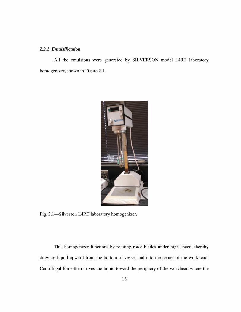
2.2.1 Emulsification

All the emulsions were generated by SILVERSON model L4RT laboratory

homogenizer, shown in Figure 2.1.

Fig. 2.1—Silverson L4RT laboratory homogenizer.

This homogenizer functions by rotating rotor blades under high speed, thereby

drawing liquid upward from the bottom of vessel and into the center of the workhead.

Centrifugal force then drives the liquid toward the periphery of the workhead where the

17

fluids meet a static screen An “emulsor” screen was used for the ur o se of

emulsification. When the liquid is forced through the screen under high rate, fine

droplets are created and one phase of fluid gets dispersed in another. Then the fluids

flow toward the sides of vessel and downward to replace the fluid sucked up in the

workhead. Therefore the fluids get cycled in the vessel and forced through the screen

thousands of times to create high quality emulsions with fine liquid droplets.

2.2.2 Bench Test Devices

After the emulsion was generated, a number of instruments were used to

characterize the properties of this emulsion. The devices involved in those measurements

are listed as follows.

2.2.2.1 Rheometer

Viscosity measurements were conducted by Brookfield digital rheometer Model

DV-III+. The operation principle of the rheometer is to drive a spindle (which is

immersed in the test fluid) through a calibrated spring at a certain shear rate. The shear

stress of fluid against the spindle can be measured by the spring deflection which is

further detected with a rotary transducer. Then the viscosity is obtained by dividing the

shear stress over the shear rate. Two spindles, CPE- 40 and CPE-52 were used to

measure the viscosities of the samples at different ranges. A water bath was coupled to

the rheometer so that different temperatures could be applied.

18

2.2.2.2 Microscope

The microscopic images of the emulsions were taken by Meiji Polarizing

Microscope Model MT9920. A trinocular head was installed to replace the original

binocular head of this model. The head is composed of 10× Widefield High Eyepoint

eyepieces, and a CCD camera, by which the live images can be transferred to computer

and seen from the computer screen. Three objective lenses with 10×, 40× and 100×

magnifications are linked to the headpiece, thereby generating images of 100×, 400×,

and 1000× magnifications. All measurements from the microscopic images were

calibrated with a stage micrometer, which was also provided by Meiji.

2.2.2.3 Density meter

Densities of fluids were measured by a high precision Anton Parr digital density

meter Model DMA 4100M. Only 1 ml of sample is required for density measurement.

The accuracy of this density meter is up to 0.0001 g/ml.

2.2.2.4 Tensiometer

Interfacial tension (IFT) measurements were conducted by a drop shape analysis

de ice Model SA30 Krűss For FT measurements of a dark nontrans a rent oil, an

oil bubble has to be forced through an inverted needle to enter the water phase and form

a drop upward. The shape of the drop depends on the IFT between the oil and water. By

taking an image of the drop and fitting the shape by the Laplace-Young equation, the

IFT can be calculated automatically by the software provided with the instrument.

19

2.2.2.5 Particle size analyzer

The sizes of soot particles in the used engine oil were measured by a particle size

analyzer Model 90Plus by Brookhaven. Particle sizes are measured by dynamic light

scattering method. A dilute solution of the fine particles needs to be prepared before

measurement and transferred into the sample cuvette. When the laser of the instrument

turns on, a laser light goes through the solution, and the scattered light is collected from

90˚ angle Small a rticles in the solution undergo Brownian motion, as a result the

scattered light intensity will fluctuate. Based on the time dependence of the intensity

fluctuation, the diffusion coefficient of the particles can be obtained. Knowing the

diffusion coefficient and the viscosity of the medium, the size (hydrodynamic radius) of

the particles can be calculated by the Stokes-Einstein equation.

2.2.3 Coreflood System

Our coreflood system consisted of several major components, shown in Figure

2.2. An ISCO pump was used to pump fluids, and an accumulator filled with emulsion

was connected to the pump. These two parts constituted the injection system. When

brine was the injectant, the accumulator was removed from the system and brine was

directly forced into the coreflood cell from the pump.

A house designed and fabricated coreflood cell was connected to the injection

system so that fluids can be pumped through. The coreflood cell was fabricated with

aluminum and can withhold pressure up to 3000 psi. It accommodated cores measuring 1

inch diameter and 1 foot in length. When setting up the experiment, a core has to be

20

placed in a nitrile sleeve and fit into the cell with both ends secured to the end plugs for

the cell. Then the annulus between the sleeve and the coreflood cell wall will be filled

with hydraulic oil, through which a confinement pressure is applied to the core sleeve by

a hydraulic pump.

Fig. 2.2— Coreflood system.

The production system was kept simple: no back pressure regulator was used as

the fluid system consisted of only liquid. A digital pressure gauge was connected to the

21

inlet of the coreflood cell so the pressure can be recorded during the experiments. As the

outlet pressure – atmospheric pressure was set to be 0 on the pressure gauge, the

pressure value read at the inlet would be equal to the pressure drop between the inlet and

outlet.

In our late experiments, sand-packed slim tubes of longer lengths were used to

take the place of the coreflood cell. No confinement pressure was applied on the slim

tubes. Preparation of these slimtubes will be introduced in the experimental procedures.

2.3 Experimental Procedures

The procedures on how to generate emulsions, how to prepare sand-packed

slimtubes and how to conduct coreflood experiments are specified below. Bench

measurements on the emulsion properties were rather straightforward thus not detailed

here. All tests and measurements were conducted at am i ent tem e rature 23 ± 0 5 ˚C

unless otherwise specified.

2.3.1 Emulsion Generation

Used engine oil was first placed in a container, then brine was added into the oil

in small amounts, while the high shear mixer (Silverson L4RT) was functioning to

homogenize the fluids at 5,000 RPM to emulsify the system. Figure 2.3 indicates a

snapshot of the emulsification process. After certain amount of brine was added, the

emulsion was blended for an additional 5-10 minutes before the sample was collected.

22

Fig. 2.3— Snapshot of the emulsification process.

2.3.2 Coreflood Experiments

The main purposes of coreflood experiments were testing the emulsion stability

and rheological properties in porous media. Different types of sandstone cores were used

to test the emulsion under a variety of conditions. The porosity and permeability of rock

were characterized before emulsion injection. The main steps for conducting coreflood

experiments were set as follows: experiments were set as follows:

1. Select a clean sandstone core.

23

2. Put the core in oven to remove any moisture, then measure the dry weight of the

core ( dm ).

3. Saturate a core with brine by leaving core in solution for a few days (use vacuum

pump to remove any air if necessary), then measure the weight of the brine-

saturated core ( bm ), from which the amount of water within the core could be

found. The volume of water is equal to the pore volume (PV) of the core. Given

the dimensions of the core, its porosity can be calculated.

4. Put the core into a core-holder and set up the coreflood system. A confinement

pressure of 1800 psi was applied through the hydraulic pump.

5. n ect r ine at a certain flow rate 5 ml/min until the r essure dro Δ

stabilizes, then record the this value. From the injection rate, pressure drop, and

dimensions of the core, the e rmea il it of the core can e estimated arc ’s

law.

6. Connect the accumulator that stores the emulsion into the injection system and

start injecting emulsions through the core. Inject over 2 PVs of emulsion to

ensure no more original free water is left in the core.

7. Set a certain flow rate at the pump. Record the pressure drop along the process

and collect the effluent in small vials. Keep injecting at least 1 PV after the

pressure drop stabilizes and save the effluent from this period of time for further

analysis.

8. Repeat step 7 at other injection rates.

24

The emulsion effluents were further characterized for free water breakout. Some

samples were tested with viscometer for viscosity measurements. The stabilized pressure

drop at any flow rate was taken to calculate the effective viscosity of the emulsion, under

that particular condition. Detailed calculations on effective viscosity of the emulsion as

well as other parameters during the coreflood experiment will be shown in the

experimental results.

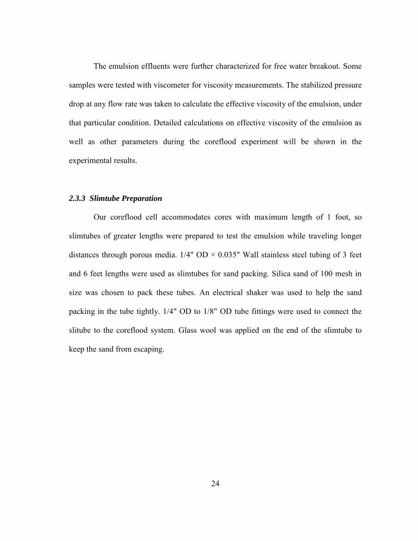
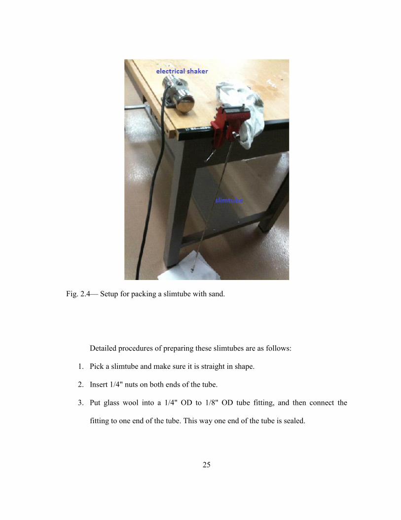
2.3.3 Slimtube Preparation

Our coreflood cell accommodates cores with maximum length of 1 foot, so

slimtubes of greater lengths were prepared to test the emulsion while traveling longer

distances through porous media. 1/4" OD × 0.035" Wall stainless steel tubing of 3 feet

and 6 feet lengths were used as slimtubes for sand packing. Silica sand of 100 mesh in

size was chosen to pack these tubes. An electrical shaker was used to help the sand

packing in the tube tightly. 1/4" OD to 1/8" OD tube fittings were used to connect the

slitube to the coreflood system. Glass wool was applied on the end of the slimtube to

keep the sand from escaping.

25

Fig. 2.4— Setup for packing a slimtube with sand.

Detailed procedures of preparing these slimtubes are as follows:

1. Pick a slimtube and make sure it is straight in shape.

2. Insert 1/4" nuts on both ends of the tube.

3. Put glass wool into a 1/4" OD to 1/8" OD tube fitting, and then connect the

fitting to one end of the tube. This way one end of the tube is sealed.

26

4. Fix the tube to a table vertically (the sealed end down), and fix an electrical

shaker close to the tube onto the same table

5. Start filling sand into the tube from top (the open end), while keeping the

electrical shaker on to shake the system for better packing. A picture of the setup

for sand packing is shown in Figure 2.4.

6. When the tube is filled up with sand, shake long enough time to make sure that

the sand line no longer fall below the top of the tube.

7. Apply another 1/4" OD to 1/8" OD tube fitting to the top of the tube. Again place

glass wool into the fitting before doing so.

During the preparation of a sand packed slimtube, it is also important to

characterize the porous media before injecting emulsion through. Similar concepts to

those in making coreflood cells were used in measuring and calculating the porosity and

permeability of the sand packed slimtubes. All measurements and calculations will be

shown in the experimental results.

27

CHAPTER III

EXPERIMENTAL RESULTS

3.1 Emulsion Generation

As mentioned earlier, used engine oil and brine were mixed together by a high

shear mixer functioning at 5,000 RPM. Under this blending speed, brine was easily

emulsified into the used engine oil. The color of mixture quickly changed from black to

light brown.

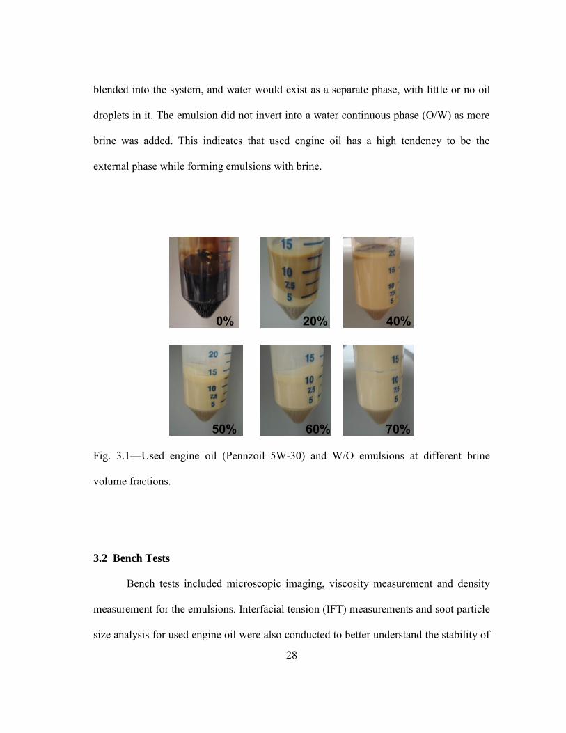
A series of W/O emulsion samples with water concentration (volume fraction) of

20%, 40%, 50%, 60% and 70% were obtained, shown in Figure 3.1. The 20% emulsion

“se a rated” into two la ers of liquid an u e r la er of a darker color and a lower la er

of a lighter color This indicates that the water dro lets could “ r eci i tate” when the

water concentration is low. It has to be noted that no water segregation was observed

even though those two layers were recognized. The division was simply due to

gravitational difference but not phase separation. At higher water concentrations, the

emulsions tend to be more stable in terms of apparel unity: only a thin layer of black oil

appeared on top of the 40% water content emulsion. No visible separation was

recognized for the 50%, 60% and 70% cases. All these emulsions last for months

without any visible water segregation.

As more brine was added and emulsified into the oil, the viscosity of the

emulsion increased significantly. Up to 75% of the brine could be added to the used

engine oil to form stable W/O emulsions. Beyond that point, brine could hardly be

28

blended into the system, and water would exist as a separate phase, with little or no oil

droplets in it. The emulsion did not invert into a water continuous phase (O/W) as more

brine was added. This indicates that used engine oil has a high tendency to be the

external phase while forming emulsions with brine.

Fig. 3.1—Used engine oil (Pennzoil 5W-30) and W/O emulsions at different brine

volume fractions.

3.2 Bench Tests

Bench tests included microscopic imaging, viscosity measurement and density

measurement for the emulsions. Interfacial tension (IFT) measurements and soot particle

size analysis for used engine oil were also conducted to better understand the stability of

29

the emulsion system. Major measurements were repeated for Emulsions made with

synthetic based oil, indicating very similar results to mineral based oil emulsions.

Emulsions made with different brine solutions were also tested to reveal the effect of

brine salinity and hardness on emulsion stability. All tests and measurements were

conducted at am i ent tem er ature 23 ± 0 5 ˚C unless otherwise s e cified

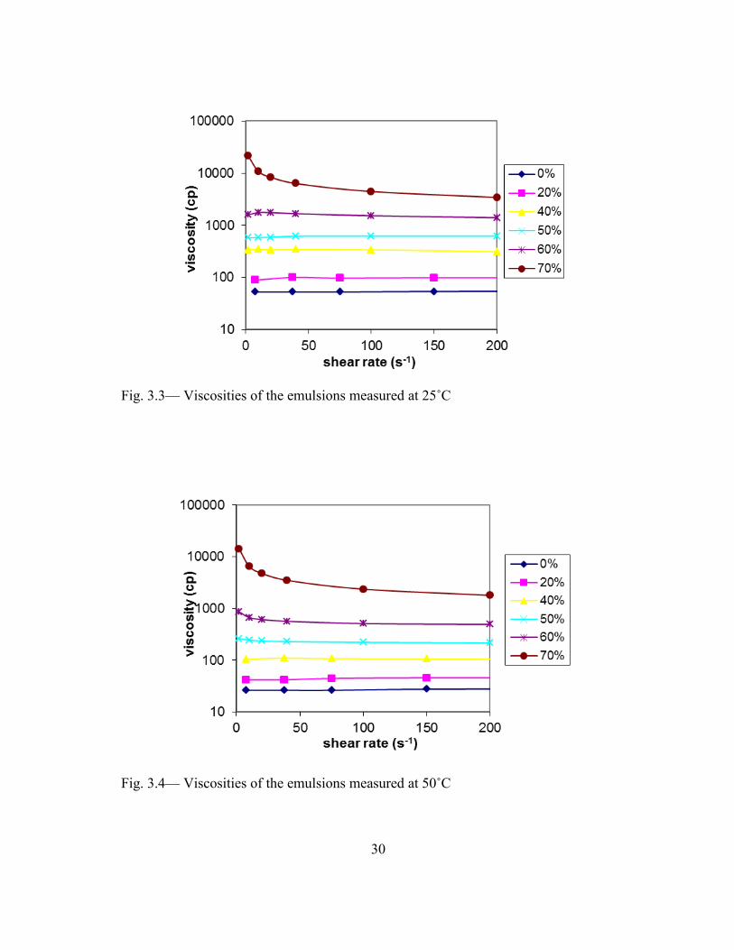
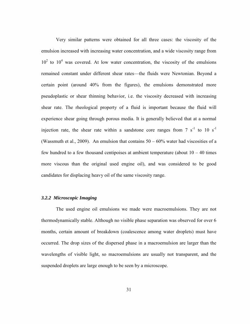
3.2.1 Viscosity Measurement

Viscosity measurements of these emulsions were conducted at three different

tem e ratures 10 ˚C, 25 ˚C, and 50 ˚C, shown in Figures 3 2 – 3.4. The percentages

indicate the water volume fractions of the emulsion samples.

Fig. 3.2— Viscosities of the emulsions measured at 10˚C

30

Fig. 3.3— Viscosities of the emulsions measured at 25˚C

Fig. 3.4— Viscosities of the emulsions measured at 50˚C

31

Very similar patterns were obtained for all three cases: the viscosity of the

emulsion increased with increasing water concentration, and a wide viscosity range from

102 to 104 was covered. At low water concentration, the viscosity of the emulsions

remained constant under different shear rates—the fluids were Newtonian. Beyond a

certain point (around 40% from the figures), the emulsions demonstrated more

pseudoplastic or shear thinning behavior, i.e. the viscosity decreased with increasing

shear rate. The rheological property of a fluid is important because the fluid will

experience shear going through porous media. It is generally believed that at a normal

injection rate, the shear rate within a sandstone core ranges from 7 s-1 to 10 s-1

(Wassmuth et al., 2009). An emulsion that contains 50 – 60% water had viscosities of a

few hundred to a few thousand centipoises at ambient temperature (about 10 – 40 times

more viscous than the original used engine oil), and was considered to be good

candidates for displacing heavy oil of the same viscosity range.

3.2.2 Microscopic Imaging

The used engine oil emulsions we made were macroemulsions. They are not

thermodynamically stable. Although no visible phase separation was observed for over 6

months, certain amount of breakdown (coalescence among water droplets) must have

occurred. The drop sizes of the dispersed phase in a macroemulsion are larger than the

wavelengths of visible light, so macroemulsions are usually not transparent, and the

suspended droplets are large enough to be seen by a microscope.

32

Fig. 3.5— Microscopic images of a W/O emulsion (60 vol% water), taken right after

made (left) and 6 months later (right).

Microscopic images of a 60% water content emulsion are shown in Figure 3.5.

The left picture was taken right after the emulsion was made, while the right picture was

taken after the emulsion remained stationary for 6 months. Very limited amount of

coalescence among water droplets occurred within the 6 months duration. When the

emulsion was first made, the water droplets were mostly around 1~1.5 micrometers in

diameter. After 6 months, larger droplets of 2 micrometers in diameter were formed.

Similar results were obtained for the emulsions of different water contents. The small

average size and narrow distribution of water droplets, and the long breakdown time

scale both indicated that the W/O emulsions made with the used engine oil were very

stable.

33

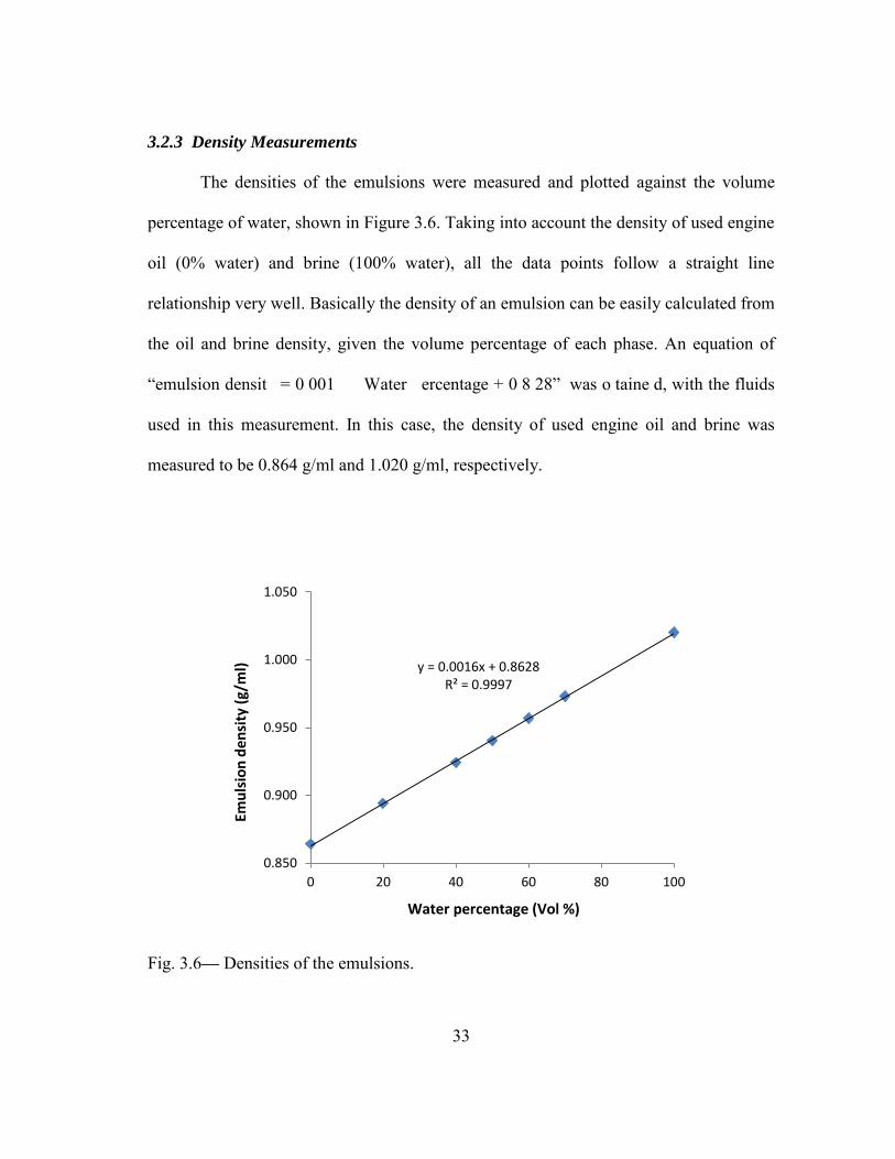
3.2.3 Density Measurements

The densities of the emulsions were measured and plotted against the volume

percentage of water, shown in Figure 3.6. Taking into account the density of used engine

oil (0% water) and brine (100% water), all the data points follow a straight line

relationship very well. Basically the density of an emulsion can be easily calculated from

the oil and brine density, given the volume percentage of each phase. An equation of

“emulsion densit = 0 001 Water ercentage + 0 8 28” was o taine d, with the fluids

used in this measurement. In this case, the density of used engine oil and brine was

measured to be 0.864 g/ml and 1.020 g/ml, respectively.

Fig. 3.6— Densities of the emulsions.

y = 0.0016x + 0.8628 R² = 0.9997

0.850

0.900

0.950

1.000

1.050

0 20 40 60 80 100

Emu

lsio

n d

en

sity

(g/

ml)

Water percentage (Vol %)

34

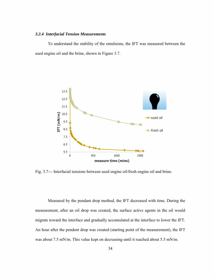
3.2.4 Interfacial Tension Measurements

To understand the stability of the emulsions, the IFT was measured between the

used engine oil and the brine, shown in Figure 3.7.

Fig. 3.7— Interfacial tensions between used engine oil/fresh engine oil and brine.

Measured by the pendant drop method, the IFT decreased with time. During the

measurement, after an oil drop was created, the surface active agents in the oil would

migrate toward the interface and gradually accumulated at the interface to lower the IFT.

An hour after the pendent drop was created (starting point of the measurement), the IFT

was about 7.5 mN/m. This value kept on decreasing until it reached about 5.5 mN/m.

35

For comparison, the IFT between a fresh engine oil (the same Pennzoil 5W-30)

and the brine was also tested and plotted on Figure 3.7. Similar trend of IFT drop with

time was also observed. The IFT value was measured to be 11.8 mN/m at one hour after

the pendant drop was created and this value decreased to about 9 mN/m after a day.

Apparently the IFT between the used engine oil and the brine was much lower than that

between the fresh engine oil and the brine.

3.2.5 Soot Particle Size Characterization

Lowered IFT was not the only reason for the stability of the emulsions. Rigid or

solid interfacial films could also be important in stabilizing macroemulsions. A term

interfacial viscosity is associated with this phenomenon (Kokal, 2005). When high

molecular weight polar molecules or fine solid particles are adsorbed at the interface,

they could behave like an insoluble skin on the water droplets, and prevent the water

droplets from coalescing into each other during collision.

Soot particles are abundant in any used engine oil. Soot is composed of

heterocyclic compounds that are produced from partial burning of hydrocarbons. They

are mostly oleophilic but can be partially hydrophilic because of the oxidation. The size

of the soot particles was measured to be around 200 nm, shown in Figure 3.8. These

particles are perfect oleophilic nanoparticles to promote relatively stable W/O emulsions.

Because of the functioning mechanism of the particle size analyzer, the sizes tend to be

overestimated due to less scattering of light from smaller sized particles.

36

Fig. 3.8— Particle Size distribution of the soot particles within used engine oil.

To better understand the cause of good stability of this emulsion system, we also

generated emulsions with fresh engine oil emulsions and made comparison with used

engine oil emulsions. Results indicated that fresh engine oil also formed relatively stable

W/O emulsions with brine, but the stability was found lower than the used engine oil

case, from much larger droplet sizes in microscopic images. Given the same amount of

shear, smaller droplet sizes normally imply better stability. Fresh engine oil contains

detergents, which are surface active, and then by functioning in the engine more surface

active agents are created (oxidized components and soot particles), so the used engine oil

became even more favorable toward forming emulsions with water.

37

The Total Acid Number (TAN) of the 5W-30 used engine oil was also measured,

which was found to be 0.4 mg KOH/ g oil. The acidity of oil may also be beneficial to

the formation of Water-in-Oil emulsions.

3.2.6 Salinity Effect on Emulsion Stability

To study the effect of brine salinity and hardness on the stability of emulsion,

three different solutions were used to generate emulsions, following the same procedures

as described in 2.1.2, and with the same water content (60% by volume). The three

solutions are:

A. 30,000 ppm brine made with NaCl (20,000 ppm) and KCl (10,000 ppm);

B. 33,000 ppm brine made with NaCl (20,000 ppm), KCl (10,000 ppm) and CaCl2

(3,000 ppm);

C. Fresh water.

The microscopic images of the three emulsions are shown in Figure 3.9.

Emulsions made with A and B had similar water droplet sizes, which were much smaller

than the droplet size in emulsion made with C. This indicates that the brine solutions

produced higher-quality emulsions than fresh water – certain amount of salinity is

beneficial for generating stable emulsions. Also, the 3,000 ppm CaCl2 had negligible

effect on the droplet size, indicating the emulsion system is not sensitive to the hardness

of brine solutions.

38

Fig. 3.9— Microscopic images of emulsions generated with brine A, B and C (from top

to bottom).

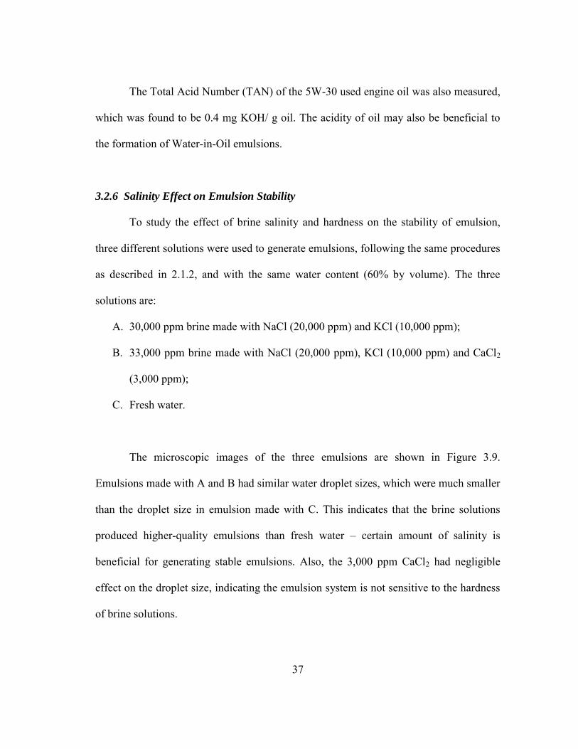
The stability of the emulsions could also be revealed from viscosity

measurements. The better the water phase is dispersed in the oil phase, the higher the

viscosity the emulsion will be. Figure 3.10 indicates the viscosity of emulsions made

with the three different solutions. The lower viscosity of the emulsion made with fresh

water lead to the same conclusion that certain amount of salinity is beneficial for

emulsion generation. The similar viscosities of the two brine solutions confirmed the

similar stabilities of emulsions made with/without calcium ion. The fact that the stability

of used engine oil emulsion is not sensitive to brine hardness, on the other hand,

39

indicates the benefits of having soot particles as stabilizer, as an emulsion stabilized by

surfactants alone is usually very sensitive to the concentration of hard ions.

Fig. 3.10— Viscosities of emulsions generated with brine A, B and C.

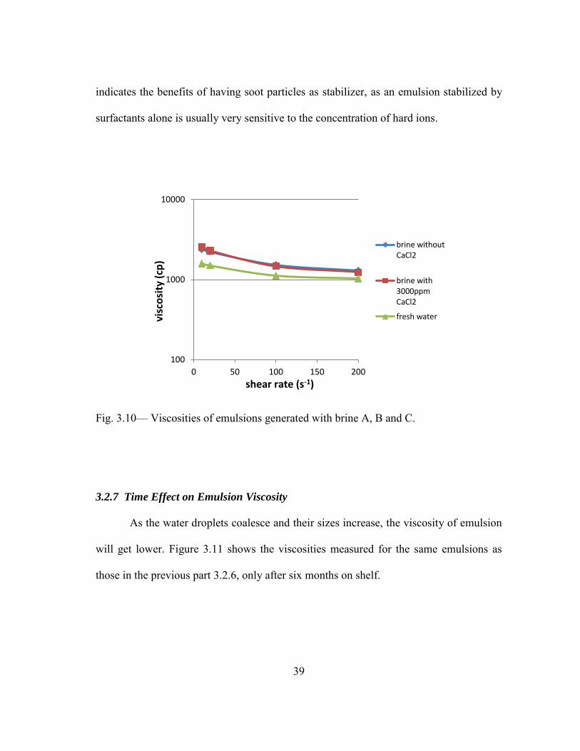
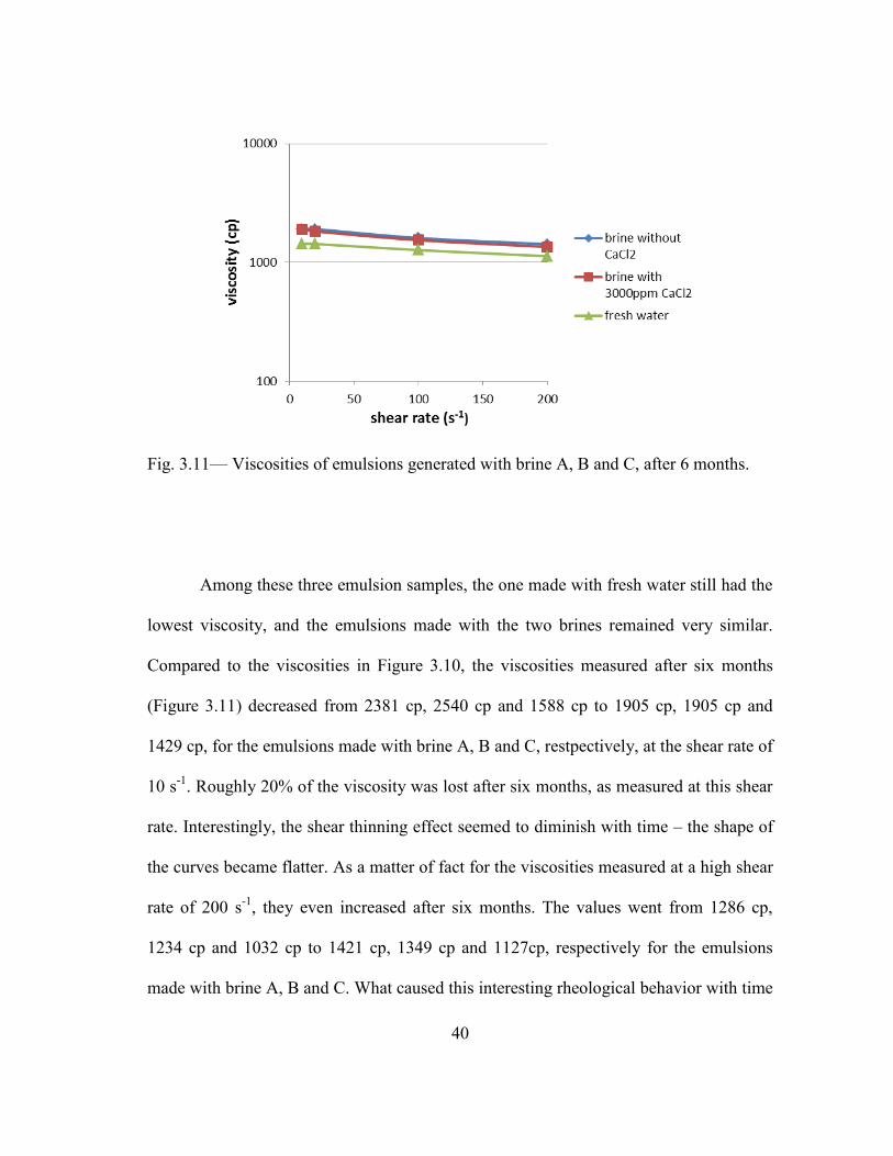
3.2.7 Time Effect on Emulsion Viscosity

As the water droplets coalesce and their sizes increase, the viscosity of emulsion

will get lower. Figure 3.11 shows the viscosities measured for the same emulsions as

those in the previous part 3.2.6, only after six months on shelf.

100

1000

10000

0 50 100 150 200

visc

osi

ty (

cp)

shear rate (s-1)

brine withoutCaCl2

brine with3000ppmCaCl2

fresh water

40

Fig. 3.11— Viscosities of emulsions generated with brine A, B and C, after 6 months.

Among these three emulsion samples, the one made with fresh water still had the

lowest viscosity, and the emulsions made with the two brines remained very similar.

Compared to the viscosities in Figure 3.10, the viscosities measured after six months

(Figure 3.11) decreased from 2381 cp, 2540 cp and 1588 cp to 1905 cp, 1905 cp and

1429 cp, for the emulsions made with brine A, B and C, restpectively, at the shear rate of

10 s-1. Roughly 20% of the viscosity was lost after six months, as measured at this shear

rate. Interestingly, the shear thinning effect seemed to diminish with time – the shape of

the curves became flatter. As a matter of fact for the viscosities measured at a high shear

rate of 200 s-1, they even increased after six months. The values went from 1286 cp,

1234 cp and 1032 cp to 1421 cp, 1349 cp and 1127cp, respectively for the emulsions

made with brine A, B and C. What caused this interesting rheological behavior with time

41

is not clear, but it may have to do with the size distribution evolution of the water

droplets.

3.3 Corefloods

After the bench tests proved the stability of used engine oil emulsions, a number

of coreflood experiments were conducted, to test the stability of the emulsions while

passing through porous media, and to obtain their flow behavior. Early experiments

focused on using different cores to see the porosity/permeability effect on emulsion

breakdown, later the experiments were conducted with a single type of sandstone core,

focusing on the effect of traveling distance on emulsion properties. Finally, two sand-

packed slimtubes were used to test the emulsion properties at much longer travelling

distances.

3.3.1 Fluids

Used Engine Oil III: A mixture of used engine oil (different brands) coming

directly from a recycling tank (mostly mineral based type because of the oil provided in

the oil change center).

Brine: Synthetic brine was prepared by adding sodium chloride and potassium

chloride into water. Total dissolved solids are 30,000 mg/kg brine, with 20,000 ppm

sodium chloride and 10,000 ppm potassium chloride included.

Emulsion: Emulsions in coreflood tests were generated with used engine oil III

and brine with similar procedures described in 2.1.2. As the emulsions were made in

42

larger batches, relatively longer time (about 10 minutes) of shear was applied to ensure

the quality of mixing. The volume fraction of brine was set to be 60%. This particular

value was somewhat arbitrarily chosen, but the idea is to generate emulsions of

moderately high viscosity and to keep a relatively large fraction of brine.

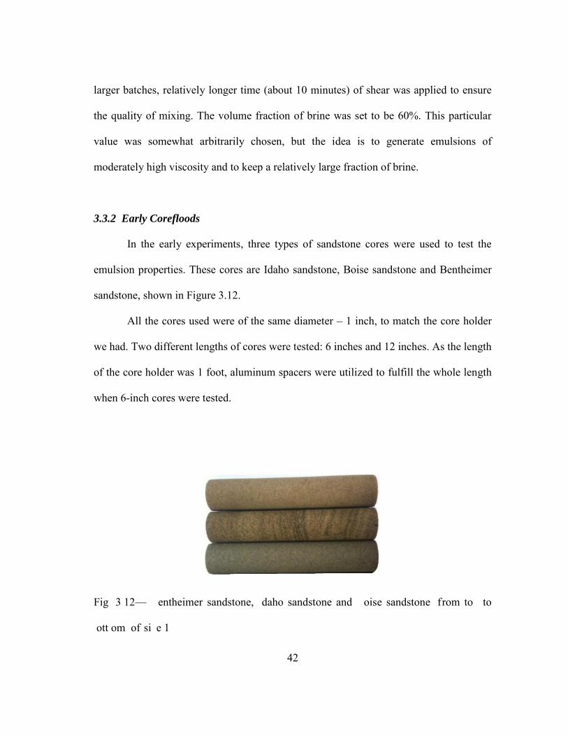
3.3.2 Early Corefloods

In the early experiments, three types of sandstone cores were used to test the

emulsion properties. These cores are Idaho sandstone, Boise sandstone and Bentheimer

sandstone, shown in Figure 3.12.

All the cores used were of the same diameter – 1 inch, to match the core holder

we had. Two different lengths of cores were tested: 6 inches and 12 inches. As the length

of the core holder was 1 foot, aluminum spacers were utilized to fulfill the whole length

when 6-inch cores were tested.

Fig 3 12— entheimer sandstone, daho sandstone and oise sandstone from to to

ott om of si e 1

43

Early corefloods followed the same procedures as introduced in 2.3.2. The

injection rates were set to be 1 ft/d, 3 ft/d, 10 ft/d and 100 ft/d, to observe the emulsion

flow behavior within a wide range of flow rates. The results and analyses for these early

corefloods are listed by core types in the subsections below.

3.3.2.1 Idaho sandstone

The dry and brine-saturated weight was measured to be 137.98 g and 156.12 g,

respectively. Knowing the density of brine and the bulk volume of the core, the porosity

of the rock could be obtained:

230.02.77

78.1724.15)27.1(1416.3

)/02.1/()98.13712.156(/)()()(

3

3

2

3

2

cm

cm

cmcm

cmggg

lr

mm

bulkVol

poreVol bdb

After the core was put into the core holder and the brine was injected through,

the pressure drop would stabilize at any fixed rate of injection. At the injection rate of 5

ml/min, the pressure drop stabilized around 9.8 psi. Therefore the water permeability of

the rock could be estimated:

mdm

psiPapsi

msPasmlmml

pA

lqk

370107.3)/68948.9()1027.1(1416.3

)1024.15()101()min/60/1/10min/5(

213

22

2336

Before the injection of our emulsion, the injection rates had to be calculated for

the pump. As the proceeding rates along the core were set to 1, 3, 10 and 100 ft/d, the

pump rates could be calculated correspondingly (ignoring irreducible water saturation):

44

min/025.0min6024

23.048.30)27.11416.3(/1 322

cmcmcm

dft

min/074.0/3 3cmdft

min/247.0/10 3cmdft

min/467.2/100 3cmdft

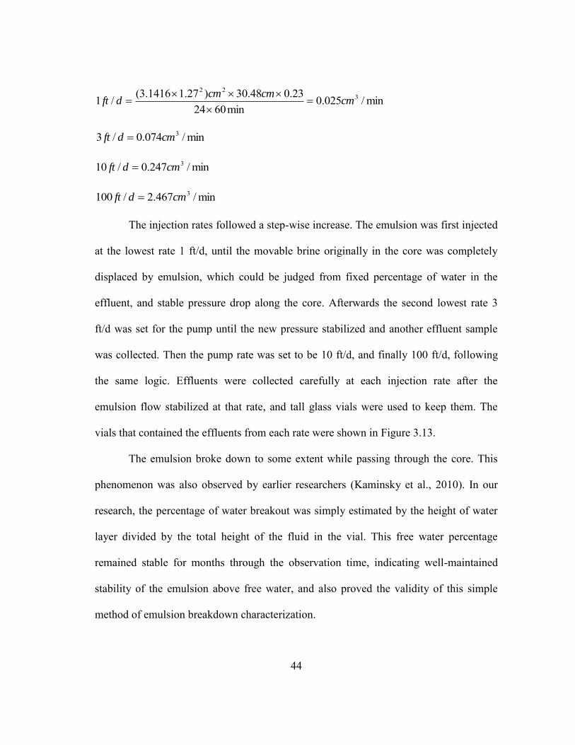
The injection rates followed a step-wise increase. The emulsion was first injected

at the lowest rate 1 ft/d, until the movable brine originally in the core was completely

displaced by emulsion, which could be judged from fixed percentage of water in the

effluent, and stable pressure drop along the core. Afterwards the second lowest rate 3

ft/d was set for the pump until the new pressure stabilized and another effluent sample

was collected. Then the pump rate was set to be 10 ft/d, and finally 100 ft/d, following

the same logic. Effluents were collected carefully at each injection rate after the

emulsion flow stabilized at that rate, and tall glass vials were used to keep them. The

vials that contained the effluents from each rate were shown in Figure 3.13.

The emulsion broke down to some extent while passing through the core. This

phenomenon was also observed by earlier researchers (Kaminsky et al., 2010). In our

research, the percentage of water breakout was simply estimated by the height of water

layer divided by the total height of the fluid in the vial. This free water percentage

remained stable for months through the observation time, indicating well-maintained

stability of the emulsion above free water, and also proved the validity of this simple

method of emulsion breakdown characterization.

45

The free water content were found to 3%, 4%, 8% and 18%, respectively at

injection rate of 1 ft/d, 3 ft/d, 10 ft/d and 100ft/d. The higher the flow rate, the higher

intensity of shear the emulsion experienced, and the more free water broke out of the

emulsion.

Fig. 3.13— Emulsion effluents collected at injection rate 1ft/d, 3 ft/d, 10 ft/d and 100ft/d

(from left to right).

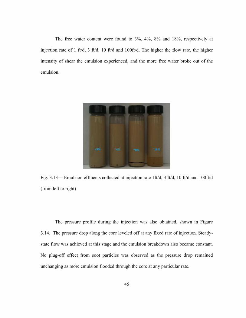
The pressure profile during the injection was also obtained, shown in Figure

3.14. The pressure drop along the core leveled off at any fixed rate of injection. Steady-

state flow was achieved at this stage and the emulsion breakdown also became constant.

No plug-off effect from soot particles was observed as the pressure drop remained

unchanging as more emulsion flooded through the core at any particular rate.

46

Fig 3 1 — ressure rofile for emulsion in ection daho sandstone

By taking a value of the pressure drop at any flat part, and the corresponding

flow rate at this oint , the effecti e iscosit can e estimated a rc ’s law,

assuming single phase flow. For example, the pressure drop was found to stabilize

around 34 psi at injection rate of 1 ft/d, so the effective viscosity was calculated as

follows:

cpsPa

msm

psiPapsimm

ql

PkAeff

692692.01024.15min)/60/(min)/10025.0(

/6895340127.01416.3107.3236

22213

47

It has to be noted that single phase flow assumption is not good for conditions of

higher flow rates, under which a larger amount of water breaks down from the emulsion

system. Also in the equation above, the permeability used for viscosity calculation

should be the relative permeability of emulsion, which is difficult to obtain from

experiments. As a result the absolute permeability measured with brine was used instead,

to roughly estimate the effective viscosity of the emulsion. Therefore the absolute value

of µeff is not accurate and comparison of this value among different cores may not be

very meaningful.

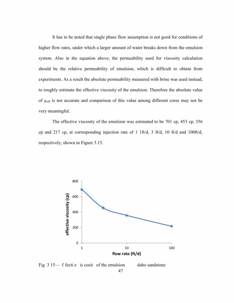
The effective viscosity of the emulsion was estimated to be 701 cp, 453 cp, 356

cp and 217 cp, at corresponding injection rate of 1 1ft/d, 3 ft/d, 10 ft/d and 100ft/d,

respectively, shown in Figure 3.15.

Fig 3 15— f fecti e is cosit of the emulsion daho sandstone

0

200

400

600

800

1 10 100

effe

ctiv

e vi

sco

sity

(cp

)

flow rate (ft/d)

48

The effective viscosity of the emulsion decreased at increasing injection rate. To

understand the flow behavior of this emulsion, the origin of shear thinning in corefloods

need to be clarified. This seemingly reasonable trend has its complex origins: at least

three factors could have caused this trend. First of all, the higher injection rate the more

free water breaks out from the emulsion and thus the water fraction in the emulsion gets

lower, and the emulsion viscosity gets lower. Secondly, as more free water coexists with

the emulsion while passing through the core, a bigger effect of two-phase flow will take

place, the influence of which will be discussed in more details later. Finally, the

emulsion itself is shear thinning, so the higher the flow rate, the higher shear it

experiences in the core, and the less viscosity will appear.

3.3.2.2 Boise sandstone

The porosity and permeability of the Boise sandstone core was measured to be

0.206 and 510 md, respectively. After the injection rates were translated into pump rates

and the emulsion flow experiments were conducted, the effluents were analyzed. The

free water contents of the effluents were found to be 7%, 15%, 16% and 32% at injection

rate of 1 ft/d, 3 ft/d, 10 ft/d and 100 ft/d, respectively.

The pressure profile was also obtained, shown in Figure 3.16. Similar to the

Idaho sandstone case, step-wise increases of pressure drops were obtained at increasing

rates of injection. Stabilized pressure drops were realized at each fixed rate of injection.

Smaller values of pressure drops were achieved at any identical rate of injection

compared to the Idaho sandstone case, due to the higher permeability of the Boise

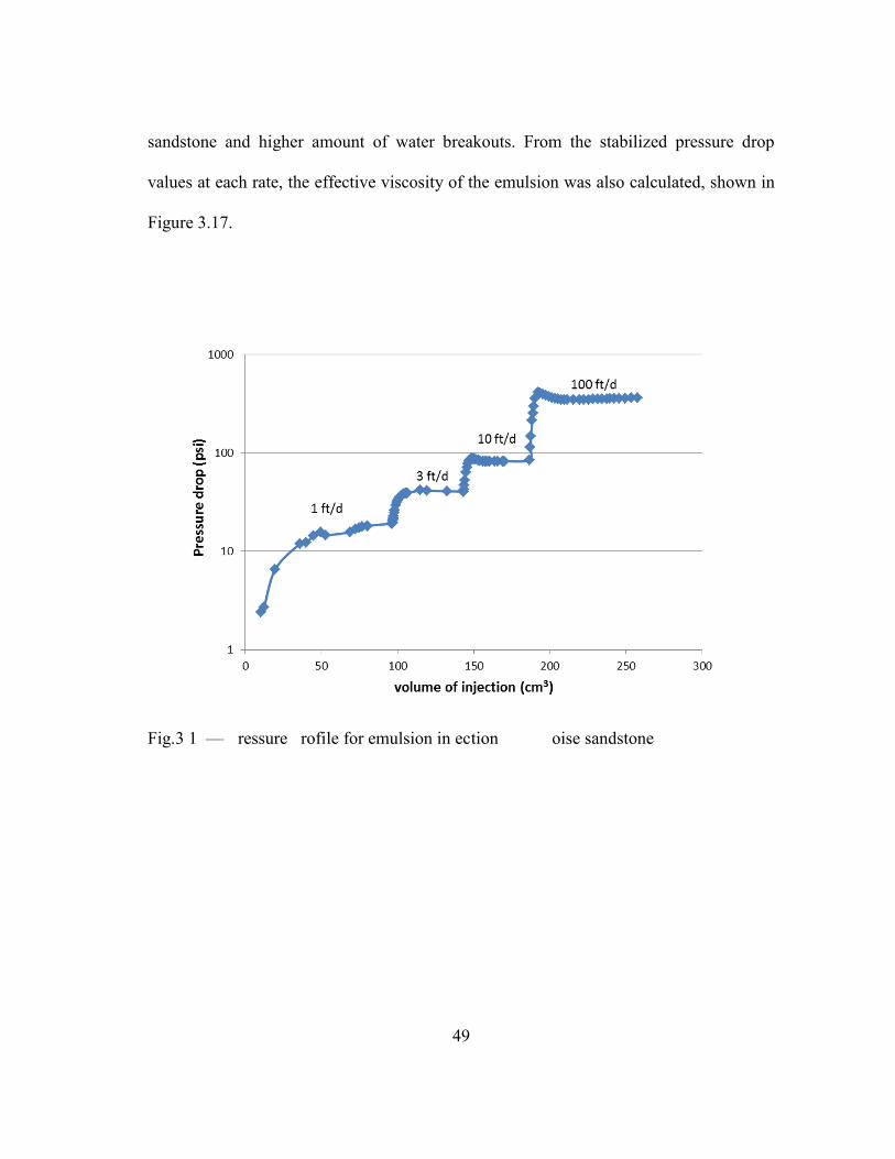
49

sandstone and higher amount of water breakouts. From the stabilized pressure drop

values at each rate, the effective viscosity of the emulsion was also calculated, shown in

Figure 3.17.

Fig.3 1 — ressure rofile for emulsion in ection oise sandstone

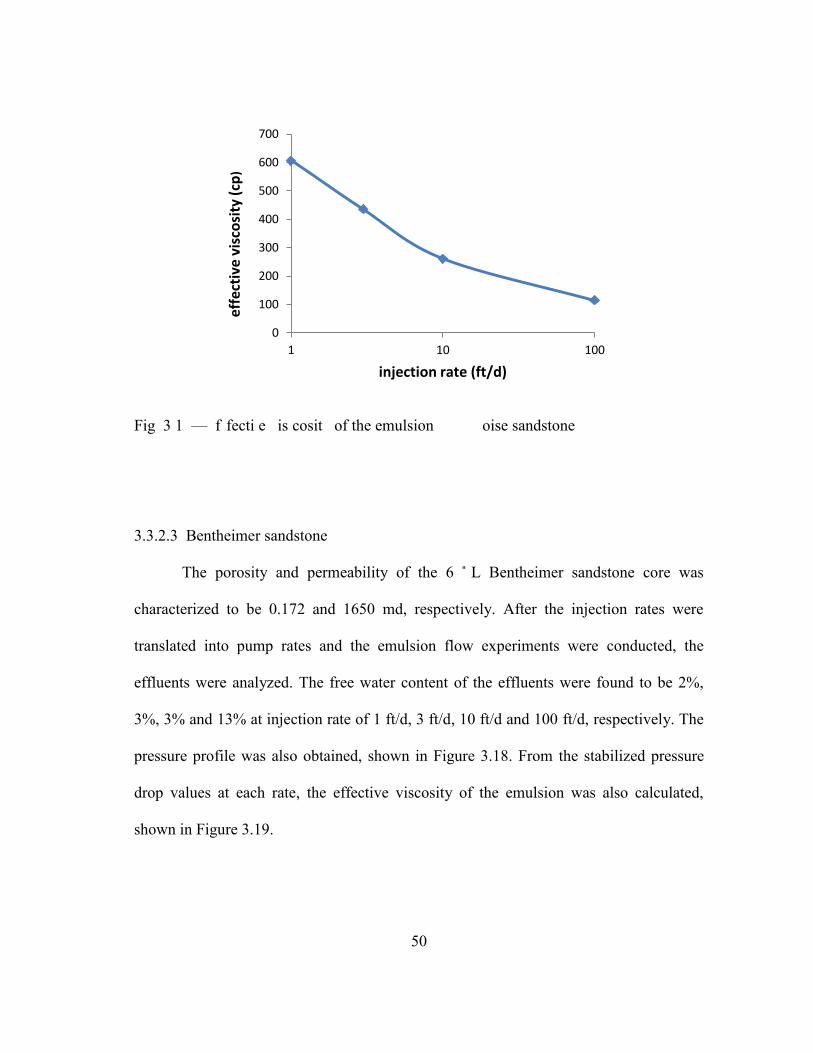
50

Fig 3 1 — f fecti e is cosit of the emulsion oise sandstone

3.3.2.3 Bentheimer sandstone

The porosity and permeability of the 6 L Bentheimer sandstone core was

characterized to be 0.172 and 1650 md, respectively. After the injection rates were

translated into pump rates and the emulsion flow experiments were conducted, the

effluents were analyzed. The free water content of the effluents were found to be 2%,

3%, 3% and 13% at injection rate of 1 ft/d, 3 ft/d, 10 ft/d and 100 ft/d, respectively. The

pressure profile was also obtained, shown in Figure 3.18. From the stabilized pressure

drop values at each rate, the effective viscosity of the emulsion was also calculated,

shown in Figure 3.19.

0

100

200

300

400

500

600

700

1 10 100

effe

ctiv

e vi

sco

sity

(cp

)

injection rate (ft/d)

51

Fig 3 18— r essure rof ile for emulsion in ection entheimer sandstone

Fig. 3.19— Effective viscosity of the emulsion entheimer sandstone

0

200

400

600

800

1000

1200

1 10 100

effe

ctiv

e vi

sco

sity

(cp

)

flow rate (ft/d)

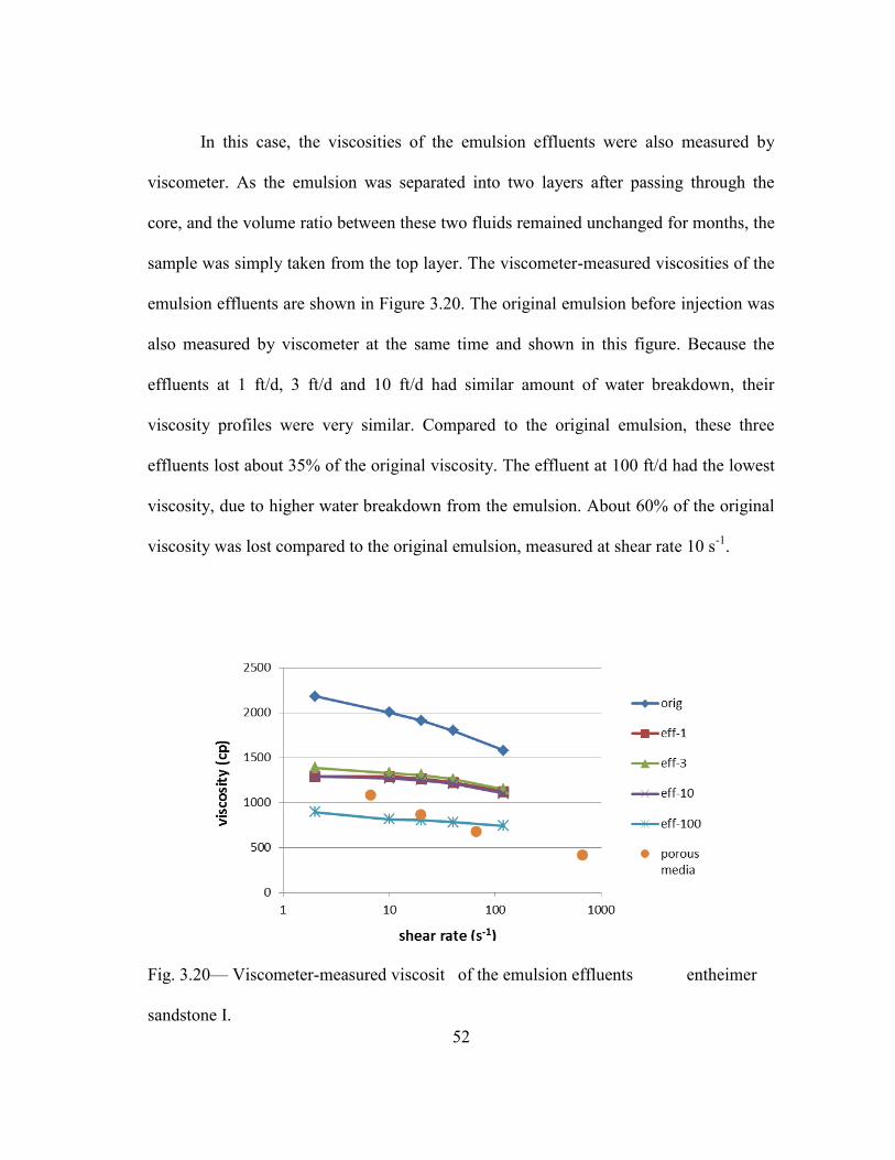
52

In this case, the viscosities of the emulsion effluents were also measured by

viscometer. As the emulsion was separated into two layers after passing through the

core, and the volume ratio between these two fluids remained unchanged for months, the

sample was simply taken from the top layer. The viscometer-measured viscosities of the

emulsion effluents are shown in Figure 3.20. The original emulsion before injection was

also measured by viscometer at the same time and shown in this figure. Because the

effluents at 1 ft/d, 3 ft/d and 10 ft/d had similar amount of water breakdown, their

viscosity profiles were very similar. Compared to the original emulsion, these three

effluents lost about 35% of the original viscosity. The effluent at 100 ft/d had the lowest

viscosity, due to higher water breakdown from the emulsion. About 60% of the original

viscosity was lost compared to the original emulsion, measured at shear rate 10 s-1.

Fig. 3.20— Viscometer-measured viscosit of the emulsion effluents entheimer

sandstone I.

53

In Figure 3.20, the effective viscosities of the emulsion calculated from coreflood

experiments were also included, shown as orange dots. Their corresponding shear rates

were calculated using correlating parameter 5.0)/( ku (Seright et al., 2010). Compared to

the effluent viscosities measured by viscometer, the effective viscosity results obtained

from coreflood experiments were roughly in the same range. The emulsion demonstrated

higher extent of shear-thinning during passing through the core than during viscometer

tests, likely due to the water breakout in the corefloods, which further reduced the

apparent viscosity of the emulsion. During measurements by viscometer, the emulsion

retained its integrity and did not breakdown like in corefloods.

To demonstrate the effect of co-existing water with emulsion on pressure drop

while flowing through porous media, a two-phase Darcy flow calculation was conducted

compared to single oil phase Darcy flow:

For single phase oil, o

o

oL

pAkq

Therefore, )(

o

okA

qLp

...................................................................................... (1)

For two phase flow of both oil and water,

o

o

oL

pAkq

w

w

wL

pAkq

wo qqq

54

Therefore, )(

w

w

o

o kkA

qLp

............................................................................ (2)

With the same flow rate and the same core dimensions, the pressure drops differ

between single phase flow and two phase flow by the mobility factors in equation 1 and

2. It has to be noted that o

ok

in these two equations are not the same, as relative

permeability of oil changes with water saturation, and the two equations are associated

with conditions with or without free water. Given a typical relative permeability diagram

(which is the same as used in our simulations) as shown in Figure 3.21, the mobility

factor of )(w

w

o

o kk

in two phase flow can be calculated for any given oil viscosity.

Fig. 3.21— Typical relative permeability curves.

0

0.1

0.2

0.3

0.4

0.5

0.6

0.7

0.8

0.9

1

0.2 0.4 0.6

k r

Sw

krw

kro

55

Fig. 3.22— Mobility factor curves in two phase flow.

The values for )(w

w

o

o kk

were calculated at different water saturations for three

different oil viscosities: 5 cp, 10 cp and 100 cp. The water viscosity was assumed to be 1

cp. For simplicity, unit absolute permeability was assumed so that roo kk and rww kk .

The results of )(w

w

o

o kk

for these three oil viscosity conditions are shown in Figure

3.22. At relatively low oil viscosities (5 cp and 10 cp), the mobility factor peaked at

single phase flow points (the two end points) and had a minimum value in the middle

where two phase flow occurred. On the other hand, for a more viscous oil (100 cp), the

mobility factor was the lowest at residual water saturation – any point that had higher

56

water saturation resulted in higher mobility. Therefore, for a highly viscous oil-external

emulsion in our case, its mobility would most likely increase as co-existing water

concentration goes up. That is why water breakout not only reduces the viscosity of

emulsion, but also affects the total mobility of the emulsion by two-phase flow.

3.3.2.4 Bentheimer sandstone 12

The porosity and permeability of the 12 L Bentheimer sandstone core was

characterized to be 0.170 and 1000 md, respectively. After the injection rates were

translated into pump rates and the emulsion flow experiments were conducted, the

effluents were analyzed. The free water content of the effluents were found to be 4%,

5%, 10% and 25% at injection rate of 1 ft/d, 3 ft/d, 10 ft/d and 100ft/d, respectively.

Fig. 3.23— ressure rofile for emulsion in ection 12 entheimer sandstone

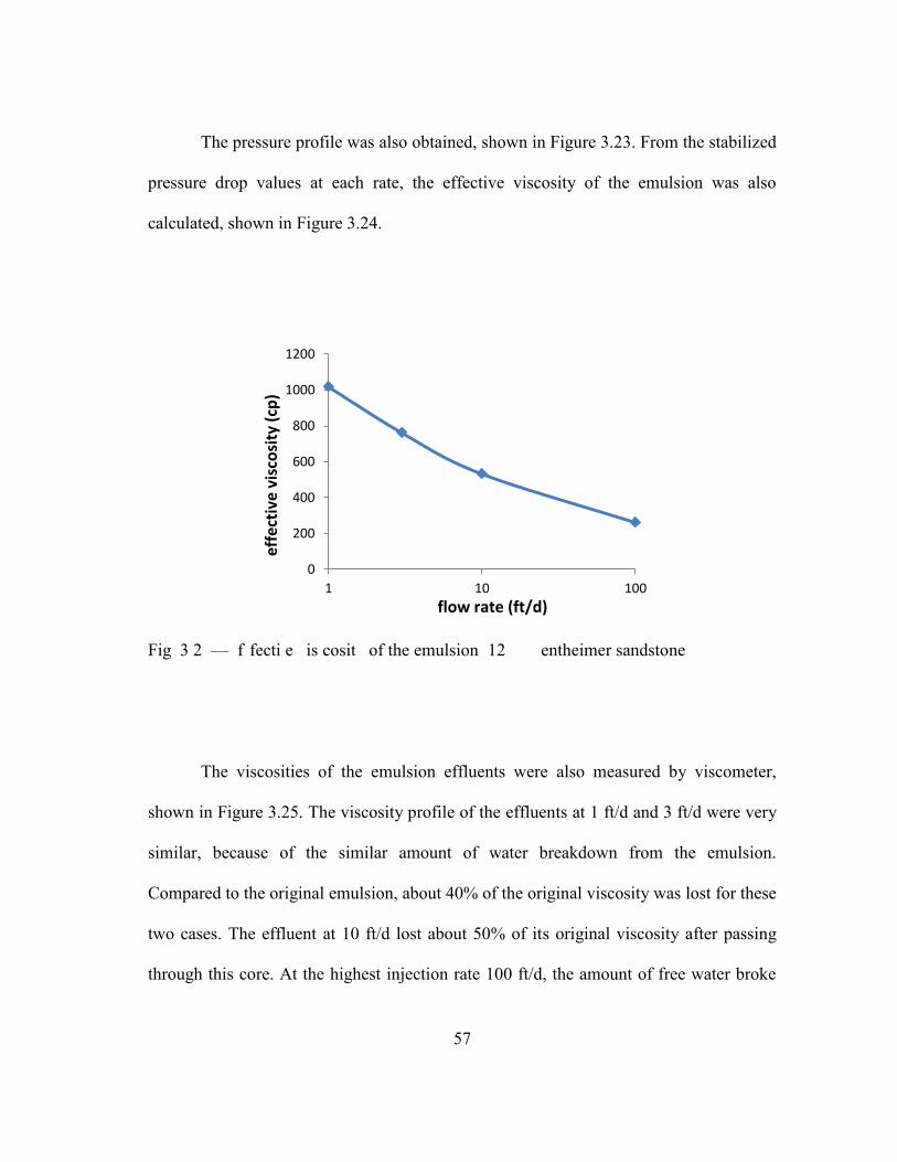
57

The pressure profile was also obtained, shown in Figure 3.23. From the stabilized

pressure drop values at each rate, the effective viscosity of the emulsion was also

calculated, shown in Figure 3.24.

Fig 3 2 — f fecti e is cosit of the emulsion 12 entheimer sandstone

The viscosities of the emulsion effluents were also measured by viscometer,

shown in Figure 3.25. The viscosity profile of the effluents at 1 ft/d and 3 ft/d were very

similar, because of the similar amount of water breakdown from the emulsion.

Compared to the original emulsion, about 40% of the original viscosity was lost for these

two cases. The effluent at 10 ft/d lost about 50% of its original viscosity after passing

through this core. At the highest injection rate 100 ft/d, the amount of free water broke

0

200

400

600

800

1000

1200

1 10 100

effe

ctiv

e vi

sco

sity

(cp

)

flow rate (ft/d)

58

out of the emulsion was as high as 25%, and the emulsion effluent lost over 70% of its

original viscosity.

Compared to viscosities measured by viscometer, the effective viscosities

obtained from corefloods (orange dots) again demonstrated higher extent of shear

thinning: the effective viscosity at 100 ft/d was as low as 263 cp in corefloods, while the

viscosity of effluent at this rate was measured to be above 500 cp. This could also be

explained by the effect of two phase flow discussed earlier.

Fig 3 25— Viscometer-measured iscosit of the emulsion and effluents 12

Bentheimer sandstone I.

59

The purpose of using different core lengths to conduct the e e riment was to

e tra olate the emulsion r o e rties a ssing through the formation, in which case the

tra e ling distance would e much longer Com ar ed to the entheimer sandstone

case, the 12 core caused larger e tents of water r eakdown at all in ection rates oth

the effecti e is cosit calculated from the ressure dro and the iscomete r-measured

iscosit of the effluents from the 12 core were found to e less than that from the

L core. However, the inconsistency in rock properties between the two tests made it hard

to conclude anything from the core length point of view. Therefore, cores of similar

properties need to be used to reveal the effect of traveling distance on emulsion

breakdown.

3.3.3 Late Corefloods

Bentheimer sandstone cores cut from the same block of rock were used to

conduct our later corefloods, in the aim of finding a relationship between the traveling

distance of the emulsion and its breakdown. Kaminsky (Kaminsky et al., 2010) reported

that similar amount of free water r oke out of the emulsion for a r ing core lengths

e tween 0 5 and 25 ft, for a e r similar emulsion s stem created with crude oil and

nano a rticles Therefore, we used and 12 entheimer cores of similar r o e rties

to conduct the emulsion flow experiment to see whether they would yield the same

amount of water breakdown.

The procedures of the late corefloods were modified from the early corefloods:

the injection rates were set to be 1 ft/d, 3 ft/d, 10 ft/d and finally back to 1 ft/d. The

60

highest rate was chosen to be 10 ft/d as the proceeding rate of the emulsion is likely to

stay below this rate in a field application. After the step-wise increase of injection rates,

the rate was set to be 1 ft/d in the last step, to further verify whether there is any

blockage effect from the emulsion injection by looking at the pressure profile.

The highest fluid velocity happens in the near wellbore region. The further away

from the wellbore, the slower the fluid front moves. Therefore an estimate of the fluid

velocity at the wellbore would give a reasonable value for our maximum flow rate in the

corefloods. If we assume the injection rate to be 50 bbl/d, and the well radius and height

to be 0.25 m and 5 m, respectively, and reservoir porosity to be 0.35, then the fluid

velocity at the wellbore can be calculated:

dftdmmmbblmdbblq /5.9/9.2)35.0525.014.32/()/159.0/50( 3

The injection rate or the well properties may vary, but for a viscous fluid like

this, the rate should not go very high limited by the injection pressure, and the wells can

be designed properly to accommodate the fluid velocity.

3.3.3.1 Bentheimer sandstone 12

The porosity and permeability of the 12 L Bentheimer sandstone core II was

characterized to be 0.153 and 730 md, respectively. After the injection rates were

translated into pump rates and the emulsion flow experiments were conducted, the

effluents were analyzed. The free water content of the effluents was found to be 5%, 6%

and 10% at injection rate of 1 ft/d, 3 ft/d and 10 ft/d, respectively. The pressure profile

was also obtained, shown in Figure 3.26. The same as the pressure profiles from early

61

corefloods, the pressure leveled off at any fixed rate of injection. In the final step, when

the injection rate was set to be 1 ft/d, which was the same as the rate set at the beginning,

the pressure drop declined even below the original pressure drop. At this point, about 10

PV of emulsion has been injected through the core. Therefore, the emulsion was further

proven to be non-plugging.

Fig 3 2 — ressure rofile for emulsion in ection 12 entheimer sandstone

From the stabilized pressure drop values at each rate, the effective viscosity of

the emulsion was also calculated, shown in Figure 3.27. Compared to the values

obtained from the 12 L Bentheimer sandstone core A in the early corefloods, the

62

effective viscosity values were a little lower, due to lower core permeability and slightly

higher water breakout.

Fig. 3.27— Effective viscosity of the emulsion 12 entheimer sandstone

A picture of the Bentheimer sandstone core was taken right after the emulsion

flow experiment, shown in Figure 3.28. For better illustration, the core was broken into

pieces and the fresh surfaces could be seen. The emulsion appeared very homogeneous

through the core, and no visible water drops were seen on any surface. As a matter of

fact, the free water fraction within the core would be much smaller than that in the

effluent, as the free water break out of the emulsion had a much higher velocity than the

rest of emulsion traveling through the core, due to its much higher mobility compared to

the oily emulsion phase.

0

200

400

600

800

1000

1200

1 10

effe

ctiv

e vi

sco

sity

(cp

)

flow rate (ft/d)

63

Fig. 3.28— Bentheimer sandstone core right after emulsion flow experiment.

3.3.3.2 Bentheimer sandstone

The porosity and permeability of the 6 L Bentheimer sandstone core was

characterized to be 0.152 and 620 md, respectively. After the injection rates were

translated into pump rates and the emulsion flow experiments were conducted, the

effluents were analyzed. The free water content of the effluents was found to be 3%, 9%

and 16% at injection rate of 1 ft/d, 3 ft/d and 10 ft/d, res ec ti e l Com a red to the 12

core, at injection rates of 3 ft/d and 10ft/d, the water breakout of this 6 L core was even

greater. Also compared to Bentheimer sandstone A (6 L), which was tested in the early

corefloods, the water breakout of this core at these two rate were more than tripled. This

abnormally high water breakdown for this core B might be explained by its lower

permeability. To verify the measurements though, the same test need to be repeated (see

2.3.4.3).

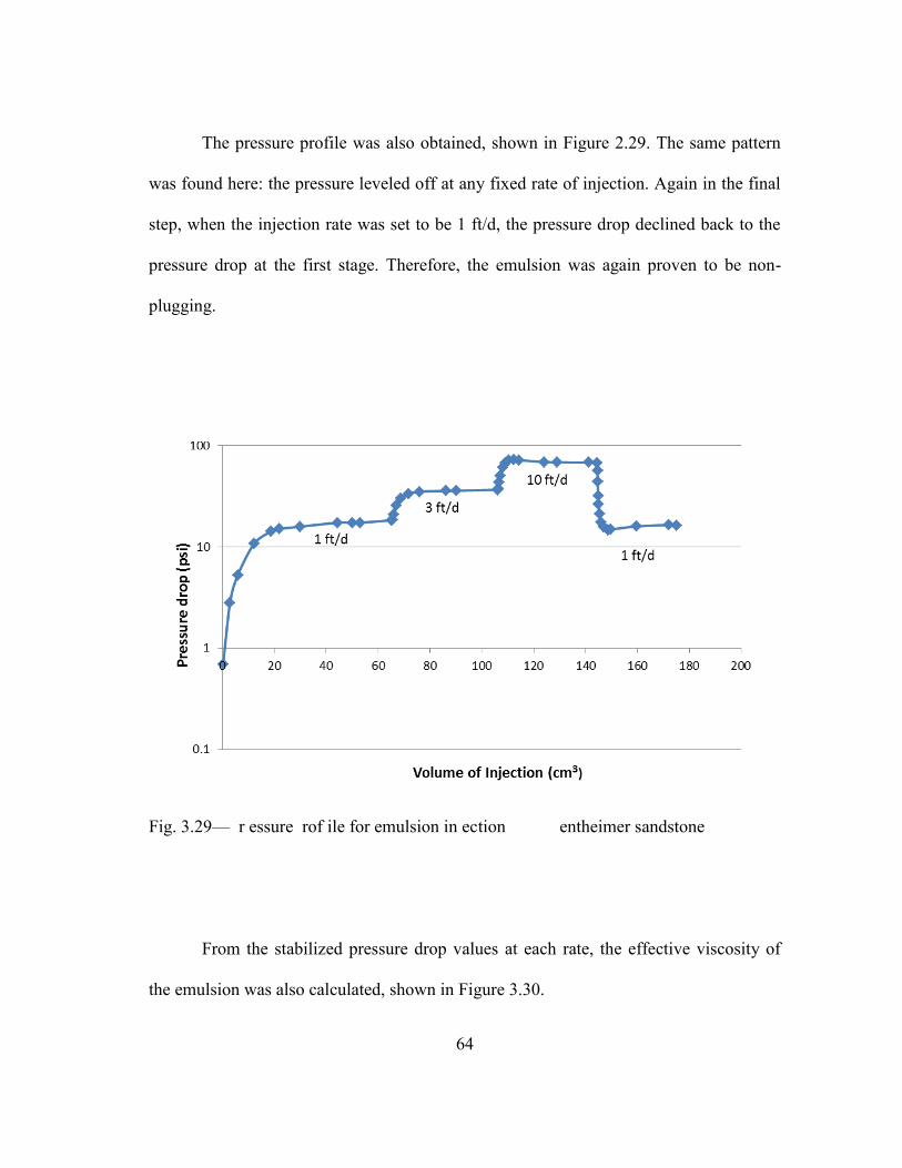
64

The pressure profile was also obtained, shown in Figure 2.29. The same pattern

was found here: the pressure leveled off at any fixed rate of injection. Again in the final

step, when the injection rate was set to be 1 ft/d, the pressure drop declined back to the

pressure drop at the first stage. Therefore, the emulsion was again proven to be non-

plugging.

Fig. 3.29— r essure rof ile for emulsion in ection entheimer sandstone

From the stabilized pressure drop values at each rate, the effective viscosity of

the emulsion was also calculated, shown in Figure 3.30.

65

Fig. 3.30— Effective viscosity of the emulsion entheimer sandstone

3.3.3.3 Bentheimer sandstone 12

The porosity and permeability of the 6 L Bentheimer sandstone core was

characterized to be 0.205 and 2420 md, respectively. After the injection rates were

translated into pump rates and the emulsion flow experiments were conducted, the

effluents were analyzed. The free water content of the effluents was found to be 3%, 5%

and 7% at injection rate of 1 ft/d, 3 ft/d and 10 ft/d, respectively.

The pressure profile was also obtained, shown in Figure 3.31. From the stabilized

pressure drop values at each rate, the effective viscosity of the emulsion was also

calculated, shown in Figure 3.32.

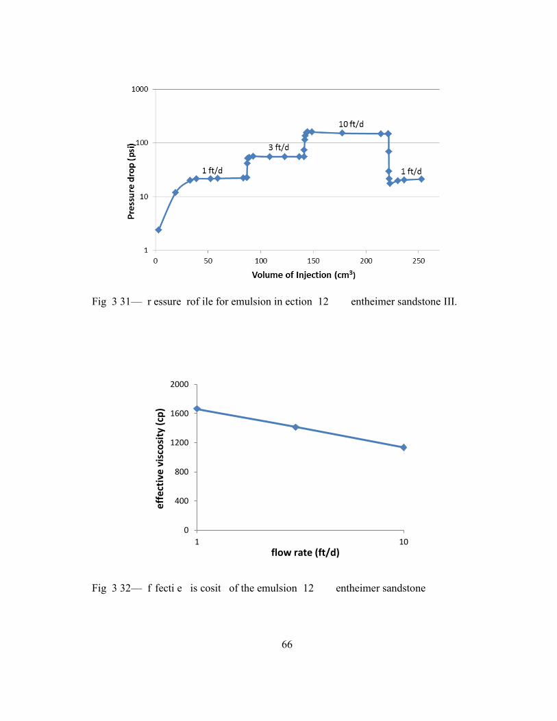
66

Fig 3 31— r essure rof ile for emulsion in ection 12 entheimer sandstone III.

Fig 3 32— f fecti e is cosit of the emulsion 12 entheimer sandstone

0

400

800

1200

1600

2000

1 10

eff

ect

ive

vis

cosi

ty (

cp)

flow rate (ft/d)

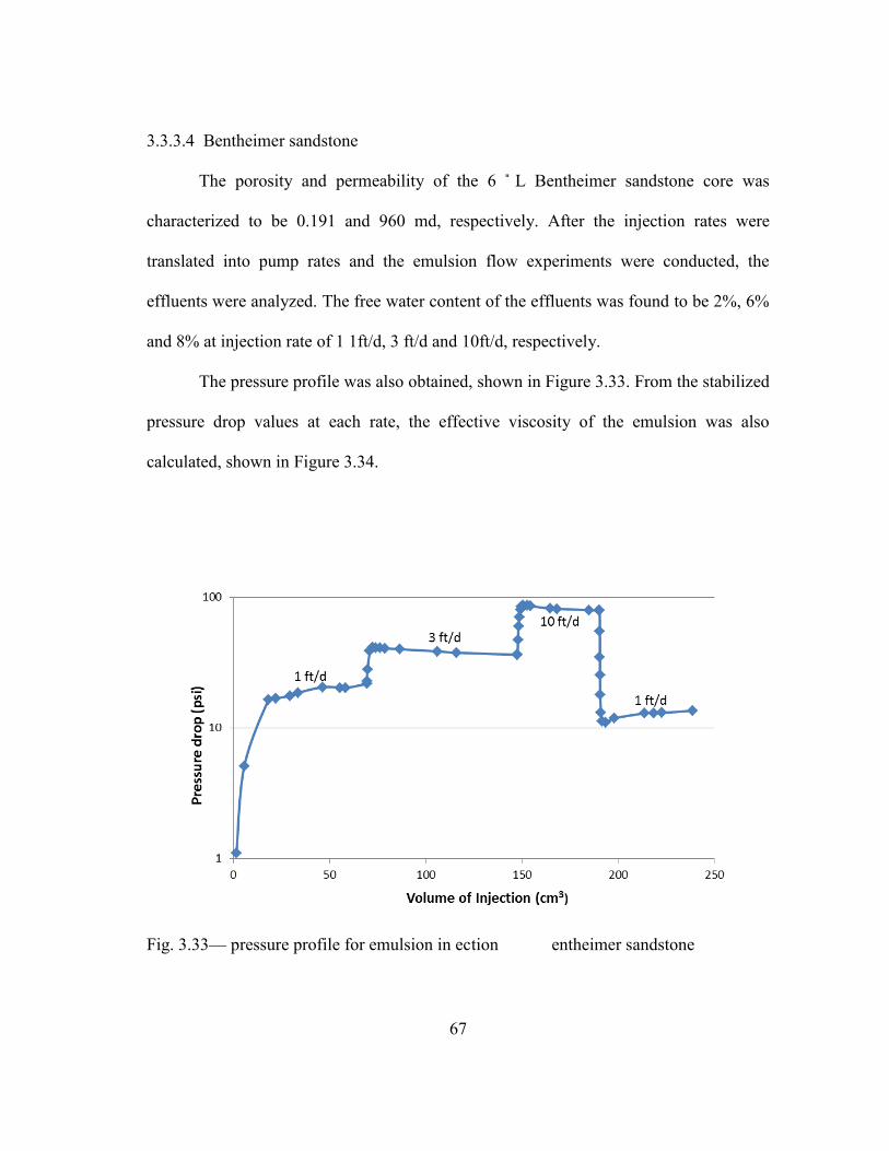
67

3.3.3.4 Bentheimer sandstone

The porosity and permeability of the 6 L Bentheimer sandstone core was

characterized to be 0.191 and 960 md, respectively. After the injection rates were

translated into pump rates and the emulsion flow experiments were conducted, the

effluents were analyzed. The free water content of the effluents was found to be 2%, 6%

and 8% at injection rate of 1 1ft/d, 3 ft/d and 10ft/d, respectively.

The pressure profile was also obtained, shown in Figure 3.33. From the stabilized

pressure drop values at each rate, the effective viscosity of the emulsion was also

calculated, shown in Figure 3.34.

Fig. 3.33— pressure profile for emulsion in ection entheimer sandstone

68

Fig 3 3 — f fecti e is cosit of the emulsion entheimer sandstone

3.3.4 Corefloods with Sandpacks

Sand a cked slimtu es o f 3ʹ and ʹ l engths were re a red for emulsion flow tests

Similar procedures were taken for preparation of the coreflood system, except no

overburden pressure could be applied for the slimtubes. The injection rates were also

modified to start with 3 ft/d, in order to accelerate these time consuming processes.

Injection rates followed the order of 3 ft/d, 6 ft/d, 9 ft/d, and finally back to 3 ft/d for

both sandpack cases.

3.3.4.1 Slimtu e A 3ʹ

The porosity of the sand pack was estimated in two ways in order to eliminate

possible errors.

First, Based on the volume of sand:

0

200

400

600

800

1000

1200

1400

1600

1 10

effe

ctiv

e vi

sco

sity

(cp

)

flow rate (ft/d)

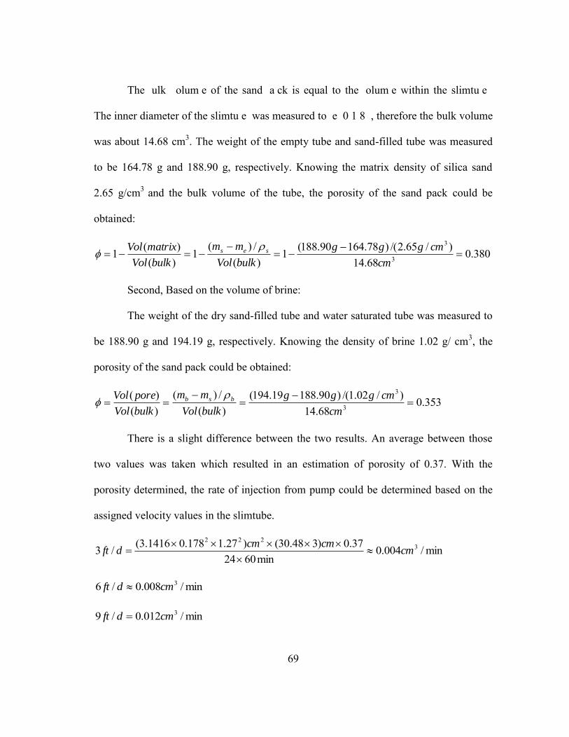
69

The ulk olum e of the sand a ck is equal to the olum e within the slimtu e

The inner diameter of the slimtu e was measured to e 0 1 8 , therefore the bulk volume

was about 14.68 cm3. The weight of the empty tube and sand-filled tube was measured

to be 164.78 g and 188.90 g, respectively. Knowing the matrix density of silica sand

2.65 g/cm3 and the bulk volume of the tube, the porosity of the sand pack could be

obtained:

380.068.14

)/65.2/()78.16490.188(1)(

/)(1

)()(1 3

3

cm

cmggg

bulkVol

mm

bulkVol

matrixVol ses

Second, Based on the volume of brine:

The weight of the dry sand-filled tube and water saturated tube was measured to

be 188.90 g and 194.19 g, respectively. Knowing the density of brine 1.02 g/ cm3, the

porosity of the sand pack could be obtained:

353.068.14

)/02.1/()90.18819.194()(

/)()()(

3

3

cm

cmggg

bulkVol

mm

bulkVol

poreVol bsb

There is a slight difference between the two results. An average between those

two values was taken which resulted in an estimation of porosity of 0.37. With the

porosity determined, the rate of injection from pump could be determined based on the

assigned velocity values in the slimtube.

min/004.0min6024

37.0)348.30()27.1178.01416.3(/3 3222

cmcmcm

dft

min/008.0/6 3cmdft

min/012.0/9 3cmdft

70

After the slimtube was connected to the coreflood system as the coreflood cell,

brine was injected through at fixed rate of 5 ml/min to test its permeability. The pressure

drop stabilized around 82.7 psi. Therefore the permeability of the sand pack could be

estimated:

md

m

psiPapsi

msPasmlmml

pA

lqk

8300103.8

)/68947.82()1027.1178.0(1416.3)10348.30()101()min/60/1/10min/5(

212

22

2336

After the test of permeability, the injectant was switched to emulsion from brine.

The emulsion was first injected at the lowest rate 3 ft/d, until the movable brine

originally in the core was completely displaced by emulsion, which could be judged

from fixed percentage of water in the effluent, and stable pressure drops along the

slimtube. Afterwards the rate was set to be 6 ft/d and 9 ft/d consecutively and finally

back to 3 ft/d. Several pore volumes of fluid were injected through the sand pack at each

rate to ensure stabilized flow at that rate, and effluents were collected at each rate after

stabilization.

The water breakout from the emulsions was measured from the effluents

collected at each rate. Free water content was found to be <<1%, <1% and 4%,

respectively at injection rate of 3 ft/d, 6 ft/d and 9ft/d. Despite the great length of

transport, the emulsion breakdown from flowing through the sand pack was very little.

This further proved the well-maintained stability of the emulsion in high permeability

reservoirs.

71

The pressure profile was also obtained, shown in Figure 3.35. The same as the

pressure profiles from sandstone corefloods, the pressure leveled off at any fixed rate of

injection. In the final step, when the injection rate went back to be 3 ft/d, the pressure

drop declined to values close to the pressure drop in the first step. The non-plugging

feature of the emulsion was further verified.

Fig. 3.35— ressure rofile for emulsion in ection 3ʹ sand a cked slimtu e

From the stabilized pressure drop value at each injection rate, the effective

viscosity of emulsion at that rate was calculated. The results are shown in Figure 3.36.

From this Figure, the shear thinning behavior of the emulsion was almost negligible.

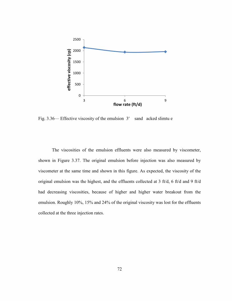
72

Fig. 3.36— Effective viscosity of the emulsion 3ʹ sand acked slimtu e

The viscosities of the emulsion effluents were also measured by viscometer,

shown in Figure 3.37. The original emulsion before injection was also measured by

viscometer at the same time and shown in this figure. As expected, the viscosity of the

original emulsion was the highest, and the effluents collected at 3 ft/d, 6 ft/d and 9 ft/d

had decreasing viscosities, because of higher and higher water breakout from the

emulsion. Roughly 10%, 15% and 24% of the original viscosity was lost for the effluents

collected at the three injection rates.

0

500

1000

1500

2000

2500

3 6 9

effe

ctiv

e vi

sco

sity

(cp

)

flow rate (ft/d)

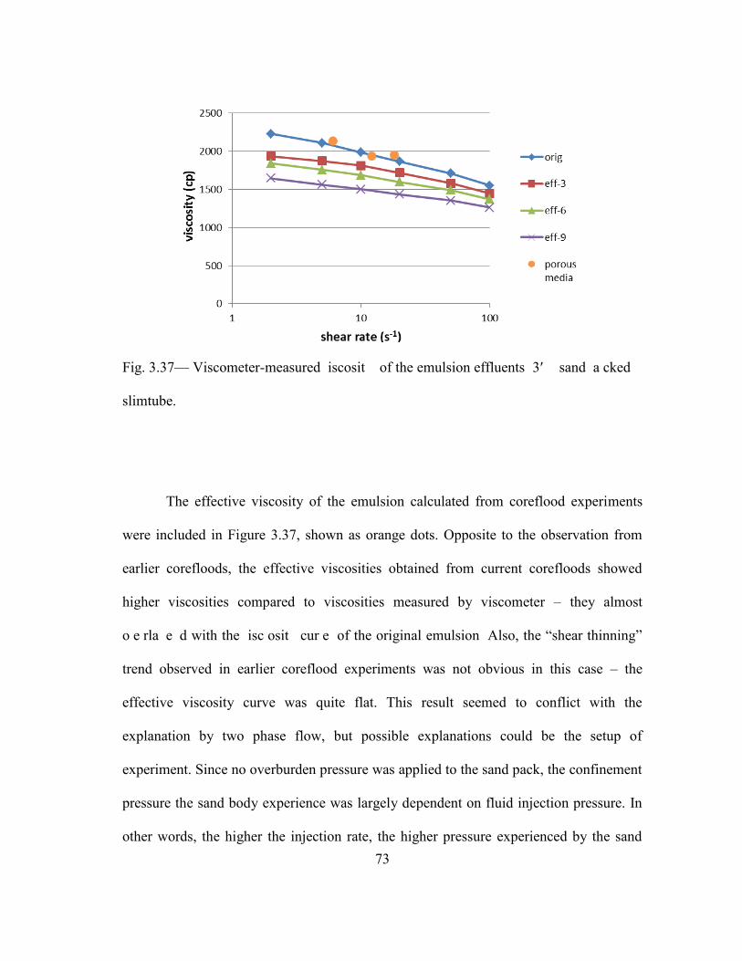
73

Fig. 3.37— Viscometer-measured iscosit of the emulsion effluents 3ʹ sand a cked

slimtube.

The effective viscosity of the emulsion calculated from coreflood experiments

were included in Figure 3.37, shown as orange dots. Opposite to the observation from

earlier corefloods, the effective viscosities obtained from current corefloods showed

higher viscosities compared to viscosities measured by viscometer – they almost

o e rla e d with the isc osit cur e of the original emulsion Also, the “shear thinning”

trend observed in earlier coreflood experiments was not obvious in this case – the

effective viscosity curve was quite flat. This result seemed to conflict with the

explanation by two phase flow, but possible explanations could be the setup of

experiment. Since no overburden pressure was applied to the sand pack, the confinement

pressure the sand body experience was largely dependent on fluid injection pressure. In

other words, the higher the injection rate, the higher pressure experienced by the sand

74

particles. Therefore, during emulsion injection, the sand pack might have become more

and more tightly packed, and this would very likely decrease the permeability of the

sand pack. Decrease of the sand pack permeability will lead to overestimate of the

effective viscosity of emulsion.

3.3.4.2 Slimtube B ʹ

The orosit and e rmea il it of the ʹ sand a cked slimtu e was estimated to

be 0.37 and 7600 md, respectively. After the injection rates were translated into pump

rates and the emulsion flow experiments were conducted, the effluents were analyzed for

emulsion breakdown. The free water content of the effluents was found to be <1%, 1%

and 7% at injection rate of 3 ft/d, 6 ft/d and 9 ft/d, respectively.

Fig. 3.38— ressure rof ile for emulsion in ection ʹ sand a cked slimtu e

75

The pressure profile was obtained during the coreflood experiment, shown in

Figure 3.38. Comparable to all earlier results, the pressure drop stabilized at each fixed

rate of injection. From those values, the effective viscosity of emulsion at each injection

rate was also calculated, shown in Figure 3 39 Similar to the 3ʹ sand acked slimtu e

case, of the emulsion demonstrated very little shear thinning behavior from the effective

viscosity calculations. It has to be noted that in sand pack experiments the flow rates had

a narrower range than that in corefloods, and the effective shear was also smaller due to

higher permeability and porosity.

Fig. 3.39— f fecti e is cosit of the emulsion ʹ sand acked slimtu e

The viscosities of the emulsion effluents were also measured by viscometer,

shown in Figure 3.40. The viscosity of the effluents collected at 3 ft/d and 6 ft/d had

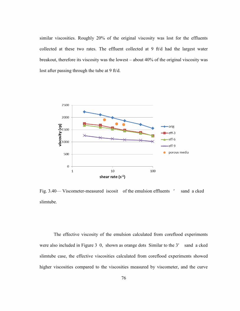
76

similar viscosities. Roughly 20% of the original viscosity was lost for the effluents

collected at these two rates. The effluent collected at 9 ft/d had the largest water

breakout, therefore its viscosity was the lowest – about 40% of the original viscosity was

lost after passing through the tube at 9 ft/d.

Fig. 3.40— Viscometer-measured iscosit of the emulsion effluents ʹ sand a cked

slimtube.

The effective viscosity of the emulsion calculated from coreflood experiments

were also included in Figure 3 0, shown as orange dots Similar to the 3ʹ sand a cked

slimtube case, the effective viscosities calculated from coreflood experiments showed

higher viscosities compared to the viscosities measured by viscometer, and the curve

77

was almost flat. As discussed before, this was likely due to experiment setup. However,

the viscosities obtained by the two methods were roughly in the same range. This allows

us to approximate emulsion properties in porous media from bench tests.

78

CHAPTER IV

SIMULATION STUDIES

4.1 General Description

Numerical study on emulsion flooding a homogeneous heavy oil reservoir was

conducted using black oil model with CMG STARS. A 1/8 of a five-spot well pattern

was used for this study. Since the emulsion was oil-external, and no plug-off effect was

observed during emulsion flow experiments, the emulsion was simply treated as single-

phase oil. The breakdown effect of the emulsion was simulated as a co-injection of water

together with this oil, to take into account of free water breakout from the emulsion

while passing through porous media. This is a reasonable assumption as most water

breakout will occur near the wellbore region where flow rates are the highest.

Some major input parameters for the reservoir and fluid properties are listed in

Table 4.1. The drainage area was 1/8 of 2.5 acres, and the netpay was 20 ft. The porosity

and horizontal permeability were set to be 0.3 and 5000 md, respectively. The vertical

permeability was set to be 1/10 of the horizontal permeability. Since this is a non-

thermal process, a tem erature of 90 ˚F was a li ed for oth in ected fluids and the

formation. The heavy oil was considered to have a viscosity of 1000 cp at this

temperature. The emulsion viscosity and free water breakout were set to be 1000 cp and

10%, respectively. Among these parameters, the emulsion viscosity, free water breakout,

heavy oil viscosity, reservoir porosity and permeability were set to different values in the

sensitivity analyses part.

79

TABLE 4.1 RESERVOIR AND FLUID PROPERTIES

Drainage area 1/8 of 2.5 acres

Netpay 20 ft

Porosity 0.30

Horizontal permeability 5000 md

Vertical permeability 500 md

Initial oil saturation 0.8

Temperature 90 ˚F

Heavy oil viscosity 1000 cp

Emulsion viscosity 1000 cp

Emulsion breakdown 10% (free water breakout)

Fig. 4.1— (a) 2D view of the gridblocks from top; (b) 3D view of the gridblocks.

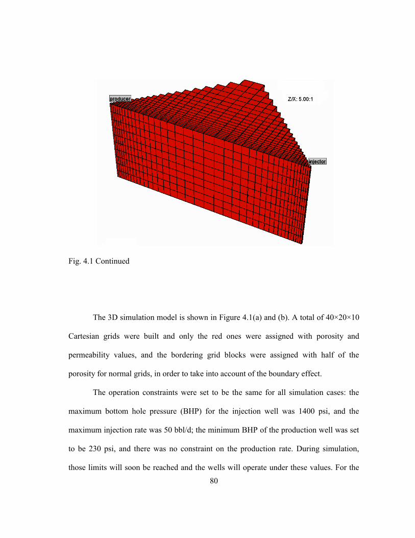
80

Fig. 4.1 Continued

The 3D simulation model is shown in Figure 4.1(a) and (b). A total of 40×20×10

Cartesian grids were built and only the red ones were assigned with porosity and

permeability values, and the bordering grid blocks were assigned with half of the

porosity for normal grids, in order to take into account of the boundary effect.

The operation constraints were set to be the same for all simulation cases: the

maximum bottom hole pressure (BHP) for the injection well was 1400 psi, and the

maximum injection rate was 50 bbl/d; the minimum BHP of the production well was set

to be 230 psi, and there was no constraint on the production rate. During simulation,

those limits will soon be reached and the wells will operate under these values. For the

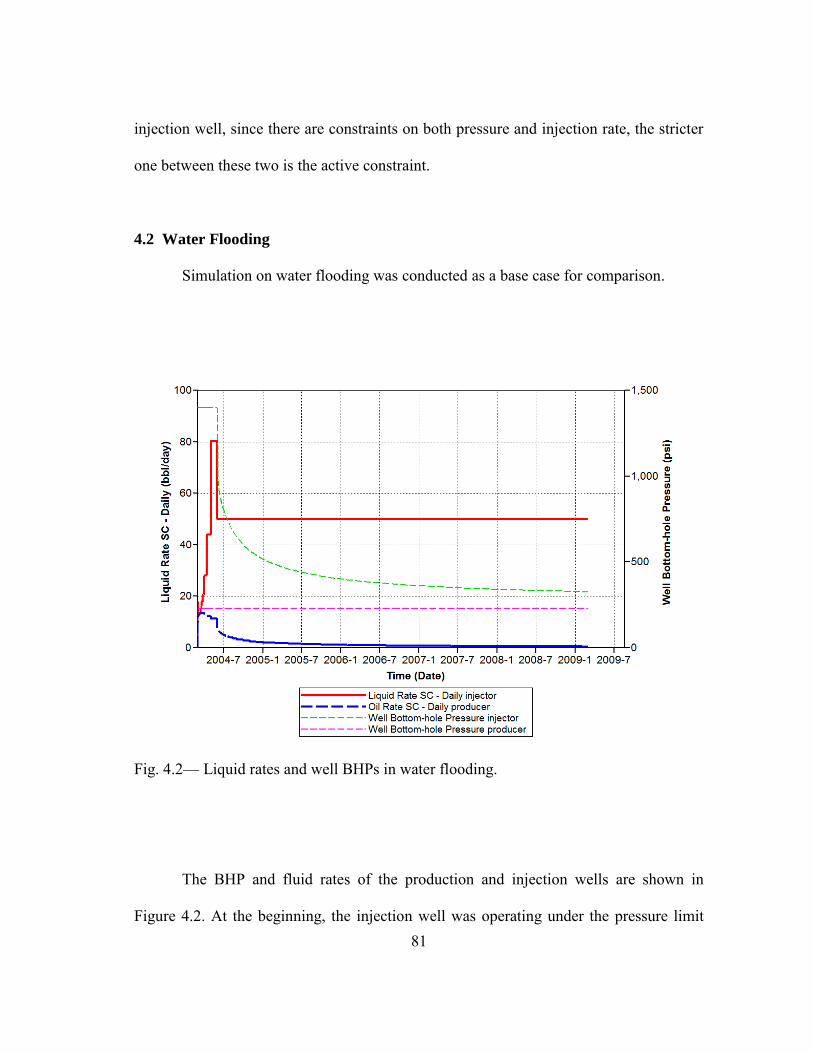
81

injection well, since there are constraints on both pressure and injection rate, the stricter

one between these two is the active constraint.

4.2 Water Flooding

Simulation on water flooding was conducted as a base case for comparison.

Fig. 4.2— Liquid rates and well BHPs in water flooding.

The BHP and fluid rates of the production and injection wells are shown in

Figure 4.2. At the beginning, the injection well was operating under the pressure limit

82

1400 psi. As more water was injected into the reservoir, the injectivity increased and the

injection rate also went up. When the injection rate exceeded 50 bbl/d, it fell back

rapidly and the well started to operate under the rate limit 50 bbl/d. The BHP at the

injection well started to drop after this point. The BHP of the production well was kept at

230 psi the whole time. The total liquid rate at the production well was almost the same

as that of the injection well thus not shown in this figure. The oil rate peaked at the

beginning of water flooding, and then it dropped rapidly after water breakthrough.

Fig. 4.3— Water cut in water flooding.

83

Figure 4.3 shows the water cut at the production well, together with the oil rate of

production. The water cut increased rapidly – within a year after the water injection, the

water cut had increased above 95%. In an actual case this water flooding project would

have been terminated within a year if we decide the limit for water cut to be around

95%.

Fig. 4.4— Cumulative oil production in water flooding.

The cumulative oil production is shown in Figure 4.4. About 2000 barrels of oil

had been produced after one ear’s water flooding The original oil in lac e OO of

the 1/8 of 2.5-acre field is calculated as:

84

bblB

SAhOOIP

o

w 116371

8.03.0205.28/17758)1(7758

Therefore, about 17% of the OOIP was recovered when the WOC reached above 95%.

The recovery performance curve relating the fraction of oil recovered and the

pore volumes of fluid injected was plotted, shown in Figure 4.5. Oil recovery at unit

pore volume water injection was only 16%, and this value increased very slowly to less

than 30% after over 6 pore volumes of water being injected.

Fig. 4.5— Recovery performance for water flooding.

To better illustrate the flood pattern, a 3D view of the oil saturation after two

years is shown in Figure 4.6. The gravity segregation between water and oil was not

severe in this case, due to a combination factor of small gravity difference (the oil was

85

assigned a density of 60 lb/ft3), thin pay zone (20 ft), and restrained vertical permeability

(500 md).

Fig. 4.6— Oil saturation after two years of water flooding.

The high viscosity of oil caused very adverse mobility ratio between oil and

water, therefore water channeled through between the injection and production well soon

after water injection. Once the channels were created, water would flood through those

zones much more easily than the rest of reservoir, due to high water mobility in the

water flooded zones. This is the main reason why heavy oil reservoirs have very low

recovery in a water flooding process. When there is heterogeneity in the reservoir, the

channeling effect would be even worse.

86

The simulation results were verified through conservation of fluid volume in the

reservoir by the reviewing the output file. For example, at two years of water flooding,

the amount of each component in the reservoir was taken from the output file, shown in

Table 4.2.

TABLE 4.2 RESERVOIR FLUID QUANTITIES IN WATER FLOODING Initial Total Current Total Net Inj/Prod H2O (lbmo) 5.65E+04 1.05E+05 4.87E+04 oil (lbmo) 8.51E+03 6.66E+03 -1.85E+03 emulsion (lbmo) 0.00E+00 0.00E+00 0.00E+00

The “initial total” column indicates the amount of each component in the

reser oir at time 0, and the “current total” column shows the amount of fluid at current

time – two ears after water flooding The “net in / rod” s e cifies the difference

between the amounts of fluid injected and produced, which is equal to the difference

e tween the “current total” and “initial total” for that fluid n our simulation, the densit

of both crude oil and emulsion was assigned to be 60 lb/ft3, and the molecular weight for

crude oil and emulsion was assumed to be 460 g/mol and 300 g/mol, respectively. By

converting the unit from lbmo into bbl, the volume of each fluid component within the

reservoir was obtained, shown in Table 4.3.

87

TABLE 4.3 RESERVOIR FLUID BARRELS IN WATER FLOODING Initial Total Current Total Net Inj/Prod H2O (bbl) 2.92E+03 5.43E+03 2.52E+03 oil (bbl) 1.16E+04 9.10E+03 -2.52E+03 emulsion (bbl) 0.00E+00 0.00E+00 0.00E+00

The volume increase of water equaled to the volume decrease of oil in the

reservoir (2.52E+03 bbl). This amount was also equal to the cumulative oil production at

two years from the production data shown earlier. Therefore, the conservation of volume

in our simulation was verified.

4.3 Emulsion Flooding

Before presenting the simulation results of emulsion flooding, some limitations

of our simulation need to be discussed. First of all, the emulsion was approximated as a

Newtonian fluid of fixed viscosity. In reality, the emulsion would be slightly shear-

thinning, and its viscosity would decrease as it flows through porous media by breaking

out water.

Secondly, the amount of emulsion breakdown was set to be a fixed value in the

simulation, and this breakdown was simply treated as co-injection of water – emulsion

breakdown was assumed to occur instantaneously and completely at the injection well.

In reality, the emulsion breaks down gradually as it travels through the reservoir

(although the emulsion breakdown would be the most intense near the wellbore region

88

where the emulsion has the highest velocity). This limitation is also related to the first

one mentioned above, as the emulsion breakdown has effect on the rheological behavior

of the emulsion phase itself. Because the proceeding rate of the injected fluid is very

slow (except near the wellbore region) in emulsion flooding, and given the high

horizontal permeability in the simulated reservoir, the amount of emulsion breakdown is

likely to stay very low and the assumptions should not be too far from reality. In fact,

sensitivity analyses on emulsion viscosity and amount of water breakout conducted later

were intended to partially resolve the two limitations mentioned above.

Thirdly, the mixing between the oil and emulsion was not controlled in our

simulation. In STARS, fluid flow is simulated based on its phase. Since both oil and

emulsion were set to e “oleic” in our simulation, the would mo e together arc ’s

law with the oil phase flow. Also the two components were fully mixed in each grid

lock following linear mi ing rule ln μo = Σi [ xi ∙ ln μoi) ]. In reality, the two

components do not necessarily mix in such a way. With those limitations discussed, the

simulation conditions and results for emulsion flooding are presented and compared with

the base case of water flooding in the followings.

89

Fig. 4.7— Liquid rates and well BHPs in emulsion flooding.

The BHP and fluid rates of the production and injection wells are shown in

Figure 4.7. Different from the water flooding case, the injection pressure remained

constant at 1400 psi through the emulsion flooding, as the liquid injection rate always

remained under the rate limit 50 bbl/d. The liquid injection rate included 90% of

emulsion, which was simply treated as an oil phase, and 10% water, which was included

to emulate the water breakout from the emulsion. The emulsion had a viscosity of 1000

cp in this case.

For the daily oil rate of production curves shown in blue, the dashed line

indicates the total rate of crude oil and emulsion, while the solid curve indicates the rate

of crude oil. At the beginning of emulsion flooding, only crude oil was produced in the

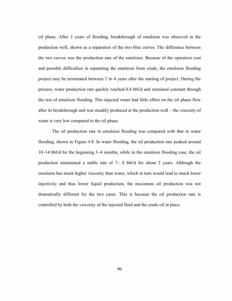
90

oil phase. After 2 years of flooding, breakthrough of emulsion was observed in the

production well, shown as a separation of the two blue curves. The difference between

the two curves was the production rate of the emulsion. Because of the operation cost

and possible difficulties in separating the emulsion from crude, the emulsion flooding

project may be terminated between 2 to 4 years after the starting of project. During the

process, water production rate quickly reached 0.8 bbl/d and remained constant through

the rest of emulsion flooding. This injected water had little effect on the oil phase flow

after its breakthrough and was steadily produced at the production well – the viscosity of

water is very low compared to the oil phase.

The oil production rate in emulsion flooding was compared with that in water

flooding, shown in Figure 4.8. In water flooding, the oil production rate peaked around

10~14 bbl/d for the beginning 3~4 months, while in the emulsion flooding case, the oil

production maintained a stable rate of 7~ 8 bbl/d for about 2 years. Although the

emulsion has much higher viscosity than water, which in turn would lead to much lower

injectivity and thus lower liquid production, the maximum oil production was not

dramatically different for the two cases. This is because the oil production rate is

controlled by both the viscosity of the injected fluid and the crude oil in place.

91

Fig. 4.8— Comparison between emulsion flooding and water flooding: oil production

rate.

The liquid injection rate in emulsion flooding was also compared with that in

water flooding, shown in Figure 4.9. Although given the same operation constraints, the

liquid injection rate in water flooding exceeded that in emulsion flooding greatly, due to

high injectivity of water. Water Cut in emulsion flooding was also compared with that in

water flooding, shown in Figure 4.10. The water cut in water flooding was greatly higher

than that in emulsion flooding.

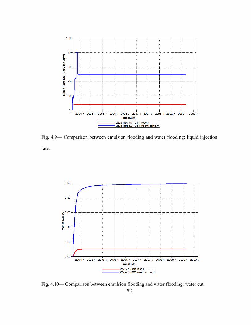
92

Fig. 4.9— Comparison between emulsion flooding and water flooding: liquid injection

rate.

Fig. 4.10— Comparison between emulsion flooding and water flooding: water cut.

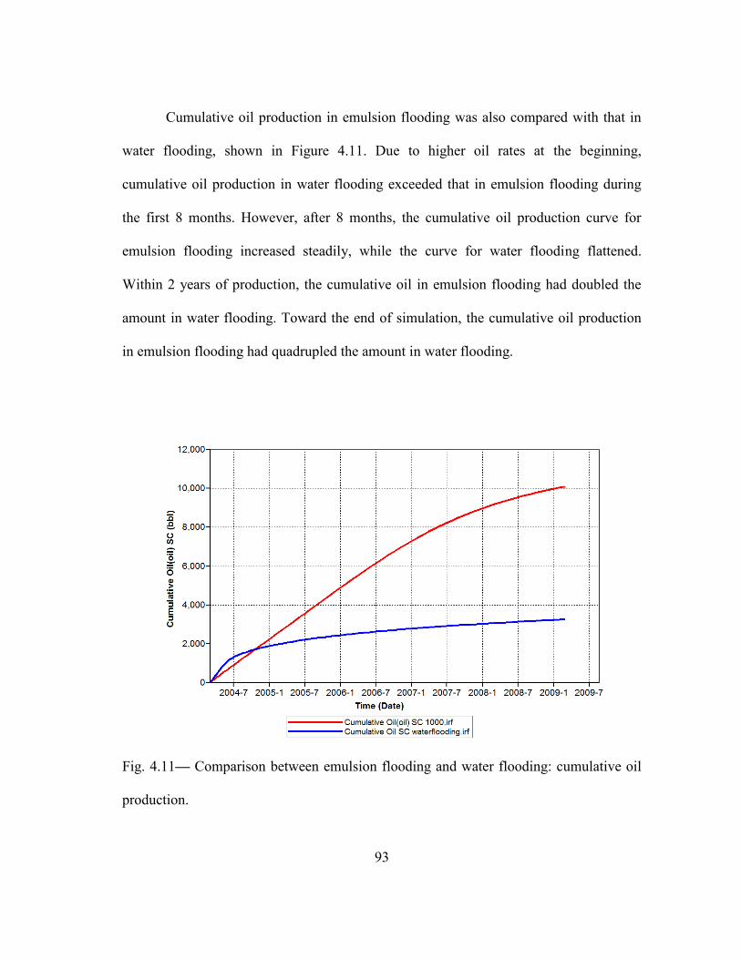
93

Cumulative oil production in emulsion flooding was also compared with that in

water flooding, shown in Figure 4.11. Due to higher oil rates at the beginning,

cumulative oil production in water flooding exceeded that in emulsion flooding during

the first 8 months. However, after 8 months, the cumulative oil production curve for

emulsion flooding increased steadily, while the curve for water flooding flattened.

Within 2 years of production, the cumulative oil in emulsion flooding had doubled the

amount in water flooding. Toward the end of simulation, the cumulative oil production

in emulsion flooding had quadrupled the amount in water flooding.

Fig. 4.11— Comparison between emulsion flooding and water flooding: cumulative oil

production.

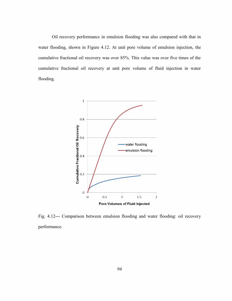
94

Oil recovery performance in emulsion flooding was also compared with that in

water flooding, shown in Figure 4.12. At unit pore volume of emulsion injection, the

cumulative fractional oil recovery was over 85%. This value was over five times of the

cumulative fractional oil recovery at unit pore volume of fluid injection in water

flooding.

Fig. 4.12— Comparison between emulsion flooding and water flooding: oil recovery

performance.

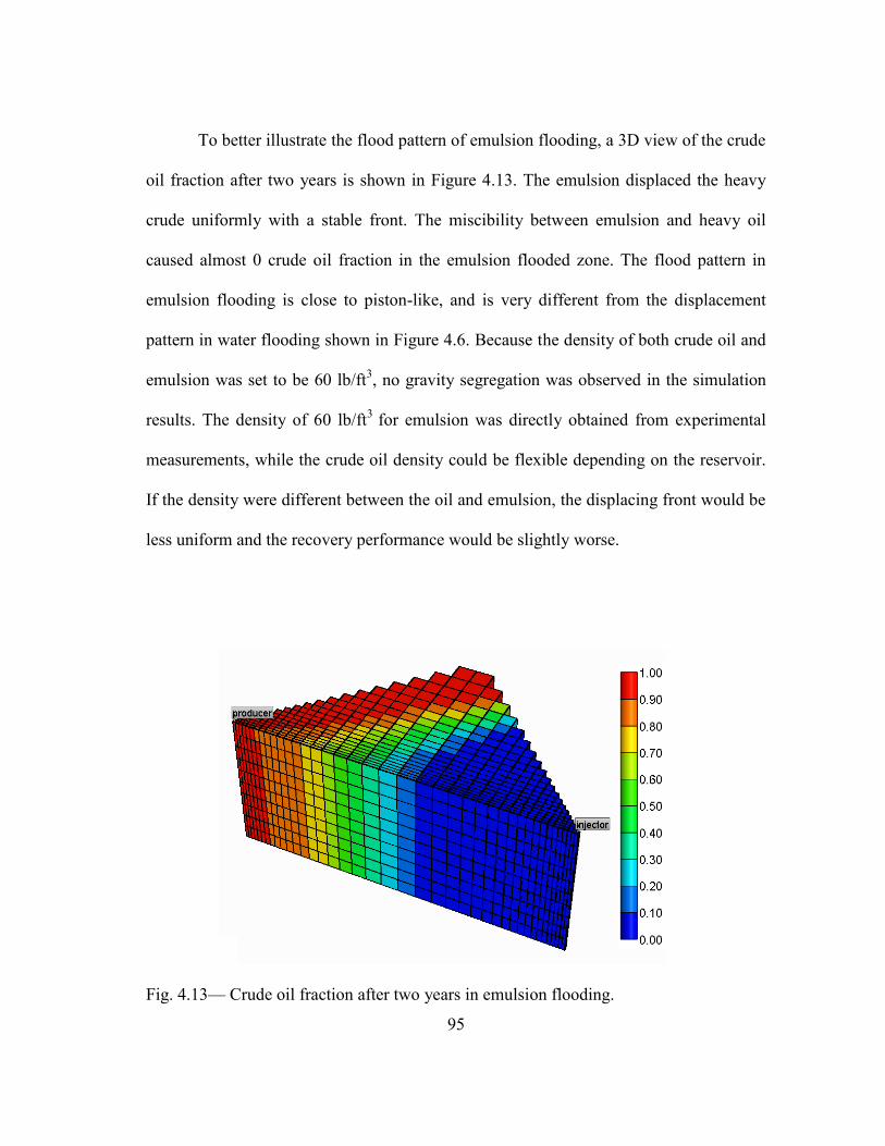
95

To better illustrate the flood pattern of emulsion flooding, a 3D view of the crude

oil fraction after two years is shown in Figure 4.13. The emulsion displaced the heavy

crude uniformly with a stable front. The miscibility between emulsion and heavy oil

caused almost 0 crude oil fraction in the emulsion flooded zone. The flood pattern in

emulsion flooding is close to piston-like, and is very different from the displacement

pattern in water flooding shown in Figure 4.6. Because the density of both crude oil and

emulsion was set to be 60 lb/ft3, no gravity segregation was observed in the simulation

results. The density of 60 lb/ft3 for emulsion was directly obtained from experimental

measurements, while the crude oil density could be flexible depending on the reservoir.

If the density were different between the oil and emulsion, the displacing front would be

less uniform and the recovery performance would be slightly worse.

Fig. 4.13— Crude oil fraction after two years in emulsion flooding.

96

Similar to the water flooding case, the simulation results of emulsion flooding

were verified through conservation of fluid volume in the reservoir by the reviewing the

output file. For example, at two years of emulsion flooding, the amount of each

component in the reservoir was taken from the output file, shown in Table 4.4.

TABLE 4.4 RESERVOIR FLUID QUANTITIES IN EMULSION FLOODING Initial Total Current Total Net Inj/Prod H2O (lbmo) 5.65E+04 5.71E+04 6.25E+02 oil (lbmo) 8.51E+03 4.59E+03 -3.91E+03 emulsion (lbmo) 0.00E+00 5.97E+03 5.97E+03

By taking into account of the molecular weight and the density of each

component, the unit was converted from lbmo into bbl so that the volume of each fluid

within the reservoir was obtained, shown in Table 4.5.

TABLE 4.5 RESERVOIR FLUID BARRELS IN EMULSION FLOODING Initial Total Current Total Net Inj/Prod

H2O (bbl) 2.92E+03 2.95E+03 3.23E+01 oil (bbl) 1.16E+04 6.28E+03 -5.34E+03 emulsion (bbl) 0.00E+00 5.32E+03 5.32E+03

97

The volume increase of emulsion (5.32E+03 bbl) and water (3.23E+01 bbl)

equaled to the volume decrease of oil in the reservoir (5.34E+03 bbl). This amount was

also equal to the cumulative oil production at two years of emulsion flooding from the

production data shown earlier. Therefore, the conservation of volume was verified. Also

to be noticed, the amount of water accumulated in the reservoir was two orders of

magnitude smaller than that of emulsion, due to its much higher mobility in the

reservoir. This on the other hand indicates that almost all the crude oil recovered was

due to displacement by emulsion although water co-injection constituted 10% of the

total fluid injected.

4.4 Sensitivity Analyses

Several parameters were chosen to conduct sensitivity analyses, including

emulsion viscosity, water breakout fraction, heavy oil viscosity, reservoir porosity and

permeability.

4.4.1 Emulsion Viscosity

Because the emulsion viscosity is sensitive to its water fraction, different

viscosities can be achieved by adjusting the water oil ratio in the emulsion. Also during

the process of flowing through the reservoir, the emulsion may lose some of its original

viscosity. Therefore it is useful to simulate the emulsion flooding process with different

emulsion viscosities. Four different values: 200 cp, 500 cp, 1000 cp and 2000 cp were

98

used in our simulations to cover the viscosity range observed in coreflood experiments.

All other parameters were set as defaults listed in Table 4.1.

Figure 4.14 indicates the oil production rates for emulsion flooding under

different emulsion viscosities. The oil rates from water flooding were also plotted in this

figure for comparison. All the curves from emulsion flooding had a long period of high

production rates followed by relatively smooth declines, while the curve for water

flooding peaked at the beginning for only a few months and then had a sharp decline.

Among the four different emulsion flooding cases, the lowest viscosity of 200 cp

resulted in the highest oil rate, but also had the earliest emulsion breakthrough and oil

rate decline.

Fig. 4.14— Oil production rates under different emulsion viscosities.

99

Fig. 4.15— Water cut under different emulsion viscosities.

The water cut in the produced liquids for all the simulation cases as well as water

flooding are shown in Figure 4.15. Compared to the high water cut in the water flooding

case, all the emulsion flooding cases were very similar in water cut – the four curves

almost overlapped from this figure.

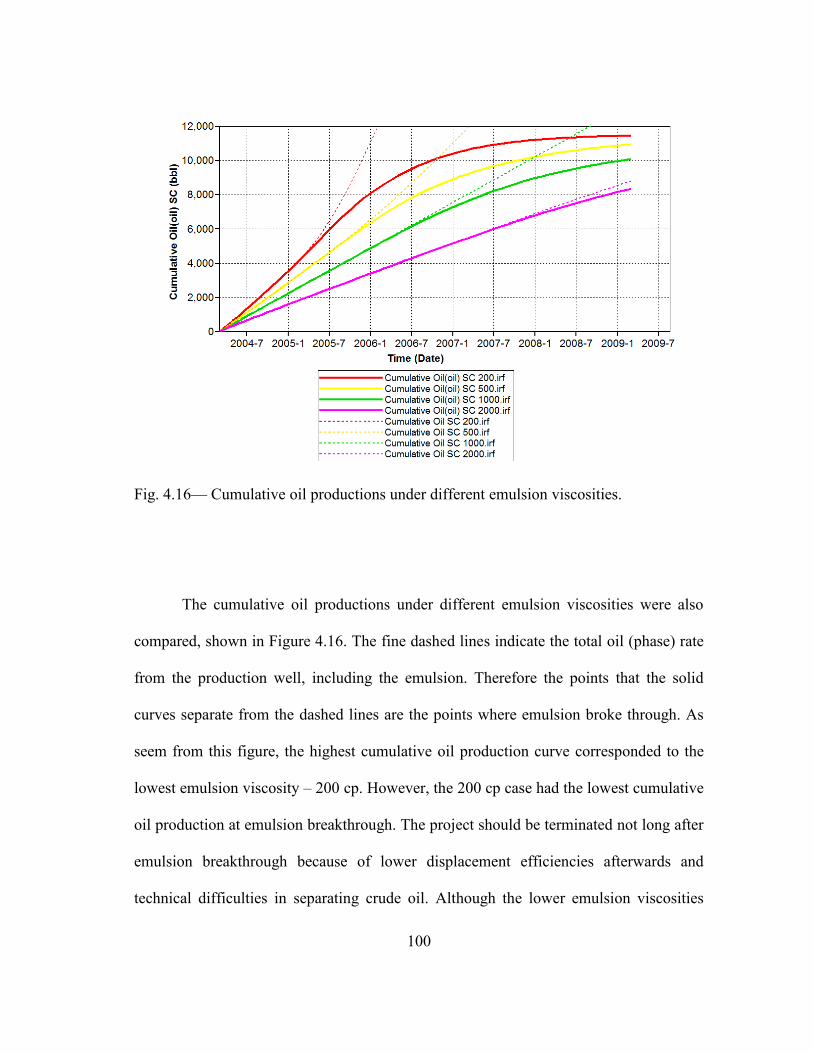
100

Fig. 4.16— Cumulative oil productions under different emulsion viscosities.

The cumulative oil productions under different emulsion viscosities were also

compared, shown in Figure 4.16. The fine dashed lines indicate the total oil (phase) rate

from the production well, including the emulsion. Therefore the points that the solid

curves separate from the dashed lines are the points where emulsion broke through. As

seem from this figure, the highest cumulative oil production curve corresponded to the

lowest emulsion viscosity – 200 cp. However, the 200 cp case had the lowest cumulative

oil production at emulsion breakthrough. The project should be terminated not long after

emulsion breakthrough because of lower displacement efficiencies afterwards and

technical difficulties in separating crude oil. Although the lower emulsion viscosities

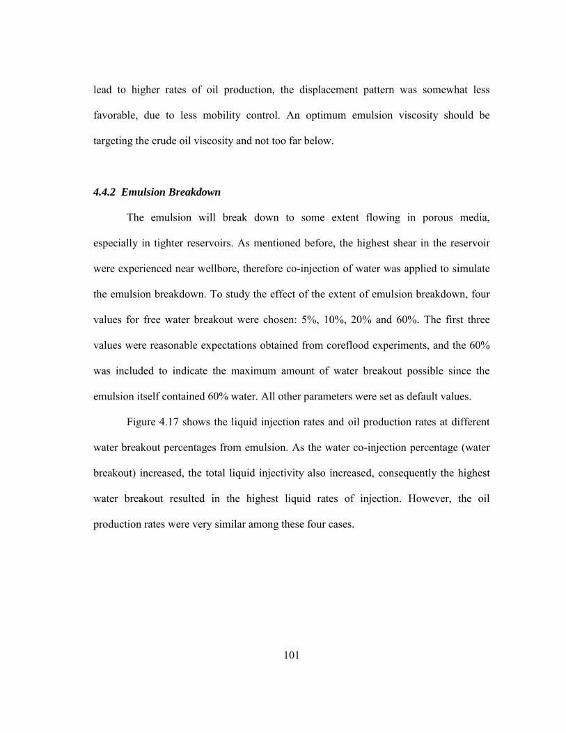
101

lead to higher rates of oil production, the displacement pattern was somewhat less

favorable, due to less mobility control. An optimum emulsion viscosity should be

targeting the crude oil viscosity and not too far below.

4.4.2 Emulsion Breakdown

The emulsion will break down to some extent flowing in porous media,

especially in tighter reservoirs. As mentioned before, the highest shear in the reservoir

were experienced near wellbore, therefore co-injection of water was applied to simulate

the emulsion breakdown. To study the effect of the extent of emulsion breakdown, four

values for free water breakout were chosen: 5%, 10%, 20% and 60%. The first three

values were reasonable expectations obtained from coreflood experiments, and the 60%

was included to indicate the maximum amount of water breakout possible since the

emulsion itself contained 60% water. All other parameters were set as default values.

Figure 4.17 shows the liquid injection rates and oil production rates at different

water breakout percentages from emulsion. As the water co-injection percentage (water

breakout) increased, the total liquid injectivity also increased, consequently the highest

water breakout resulted in the highest liquid rates of injection. However, the oil

production rates were very similar among these four cases.

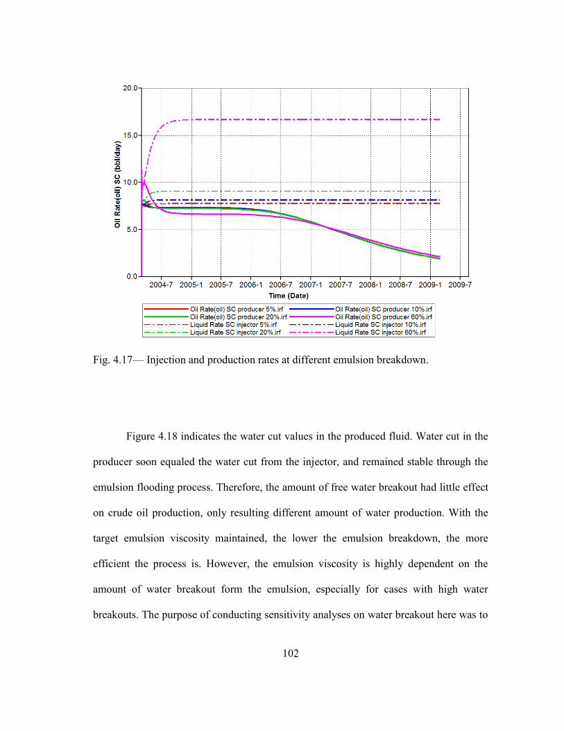
102

Fig. 4.17— Injection and production rates at different emulsion breakdown.

Figure 4.18 indicates the water cut values in the produced fluid. Water cut in the

producer soon equaled the water cut from the injector, and remained stable through the

emulsion flooding process. Therefore, the amount of free water breakout had little effect

on crude oil production, only resulting different amount of water production. With the

target emulsion viscosity maintained, the lower the emulsion breakdown, the more

efficient the process is. However, the emulsion viscosity is highly dependent on the

amount of water breakout form the emulsion, especially for cases with high water

breakouts. The purpose of conducting sensitivity analyses on water breakout here was to

103

simply illustrate the insignificant effect of water co-injection in terms of oil recovery,

and did not consider the viscosity dependence on water breakout.

Fig. 4.18— Water cut in the produced fluids at different emulsion breakdown.

4.4.3 Crude Oil Viscosity

The viscosity of crude oil in the reservoir would affect its production

significantly. Here we studied several emulsion flooding cases with different crude oil

viscosity values: 200 cp, 500 cp, 1000 cp and 2000 cp. All other parameters were set as

default values from Table 4.1.

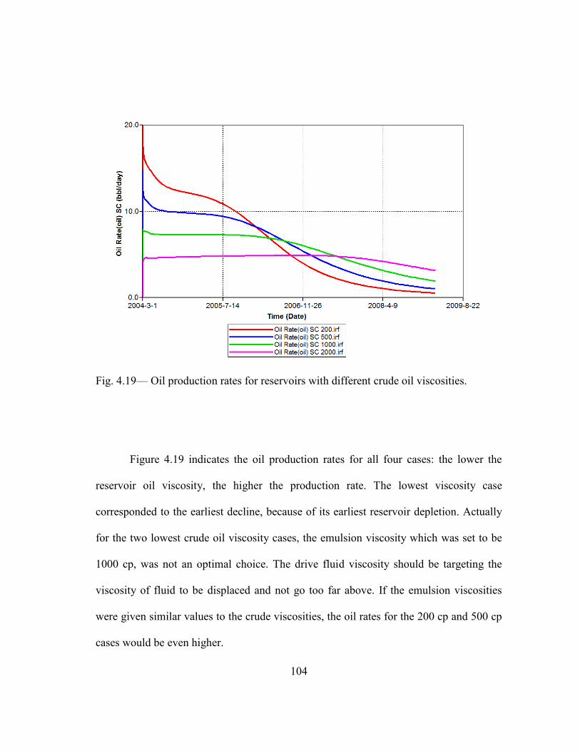
104

Fig. 4.19— Oil production rates for reservoirs with different crude oil viscosities.

Figure 4.19 indicates the oil production rates for all four cases: the lower the

reservoir oil viscosity, the higher the production rate. The lowest viscosity case

corresponded to the earliest decline, because of its earliest reservoir depletion. Actually

for the two lowest crude oil viscosity cases, the emulsion viscosity which was set to be

1000 cp, was not an optimal choice. The drive fluid viscosity should be targeting the

viscosity of fluid to be displaced and not go too far above. If the emulsion viscosities

were given similar values to the crude viscosities, the oil rates for the 200 cp and 500 cp

cases would be even higher.

105

For the two highest crude oil viscosity cases, the oil production rates from the

1000 cp oil reservoir did not quite double that from the 2000 cp oil reservoir, because of

the same viscosity of emulsion during injection. For high oil viscosity reservoirs, it

might be a good idea to inject emulsions that are somewhat less viscous, in order to

obtain reasonably high production rates.

Fig. 4.20— Cumulative oil productions for reservoirs with different crude oil viscosities.

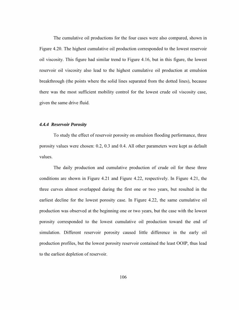
106

The cumulative oil productions for the four cases were also compared, shown in

Figure 4.20. The highest cumulative oil production corresponded to the lowest reservoir

oil viscosity. This figure had similar trend to Figure 4.16, but in this figure, the lowest

reservoir oil viscosity also lead to the highest cumulative oil production at emulsion

breakthrough (the points where the solid lines separated from the dotted lines), because

there was the most sufficient mobility control for the lowest crude oil viscosity case,

given the same drive fluid.

4.4.4 Reservoir Porosity

To study the effect of reservoir porosity on emulsion flooding performance, three

porosity values were chosen: 0.2, 0.3 and 0.4. All other parameters were kept as default

values.

The daily production and cumulative production of crude oil for these three

conditions are shown in Figure 4.21 and Figure 4.22, respectively. In Figure 4.21, the

three curves almost overlapped during the first one or two years, but resulted in the

earliest decline for the lowest porosity case. In Figure 4.22, the same cumulative oil

production was observed at the beginning one or two years, but the case with the lowest

porosity corresponded to the lowest cumulative oil production toward the end of

simulation. Different reservoir porosity caused little difference in the early oil

production profiles, but the lowest porosity reservoir contained the least OOIP, thus lead

to the earliest depletion of reservoir.

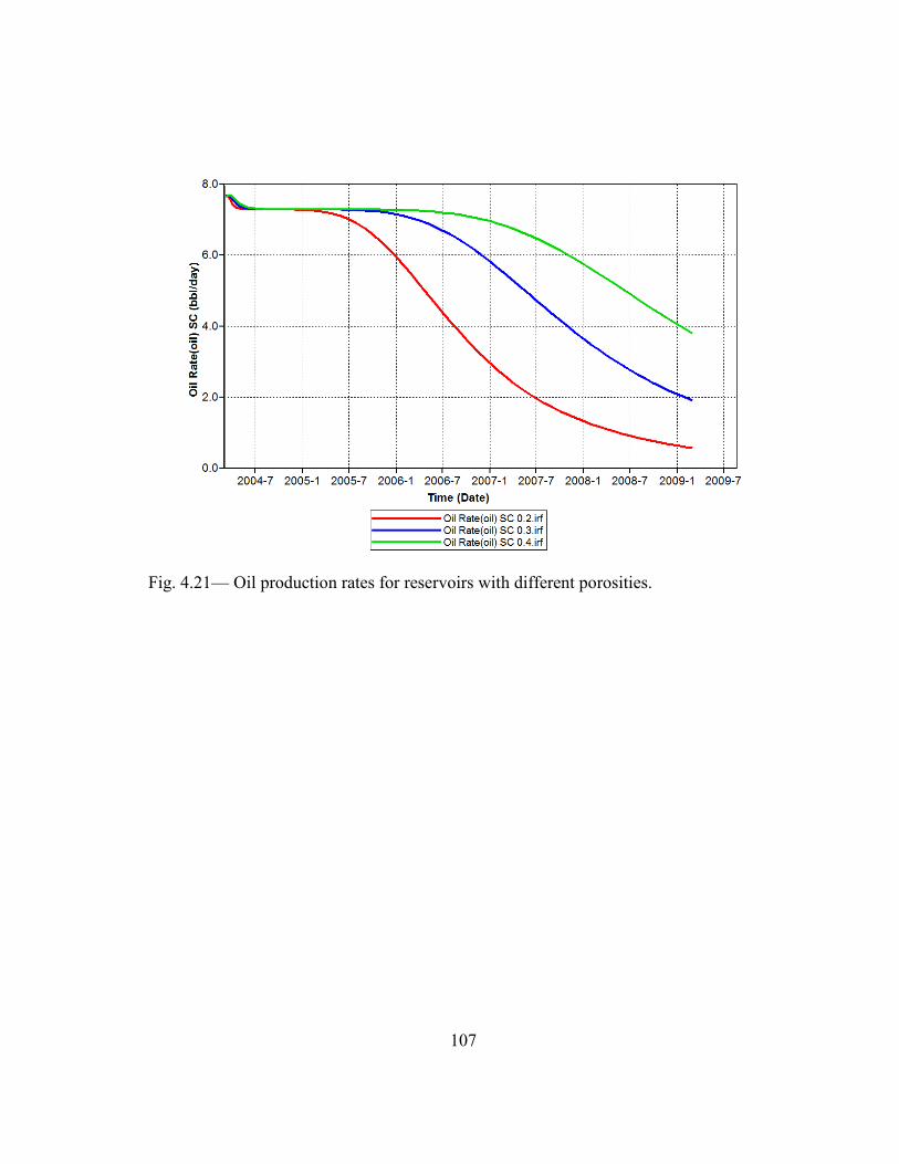
107

Fig. 4.21— Oil production rates for reservoirs with different porosities.

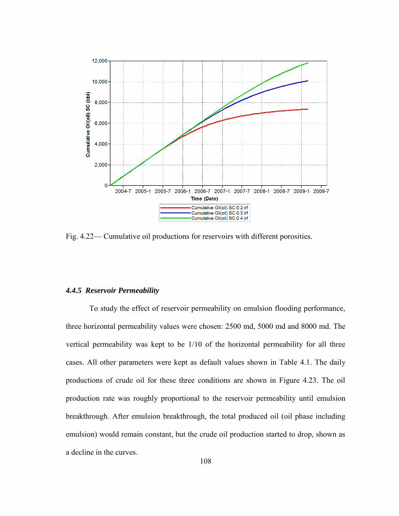
108

Fig. 4.22— Cumulative oil productions for reservoirs with different porosities.

4.4.5 Reservoir Permeability

To study the effect of reservoir permeability on emulsion flooding performance,

three horizontal permeability values were chosen: 2500 md, 5000 md and 8000 md. The

vertical permeability was kept to be 1/10 of the horizontal permeability for all three

cases. All other parameters were kept as default values shown in Table 4.1. The daily

productions of crude oil for these three conditions are shown in Figure 4.23. The oil

production rate was roughly proportional to the reservoir permeability until emulsion

breakthrough. After emulsion breakthrough, the total produced oil (oil phase including

emulsion) would remain constant, but the crude oil production started to drop, shown as

a decline in the curves.

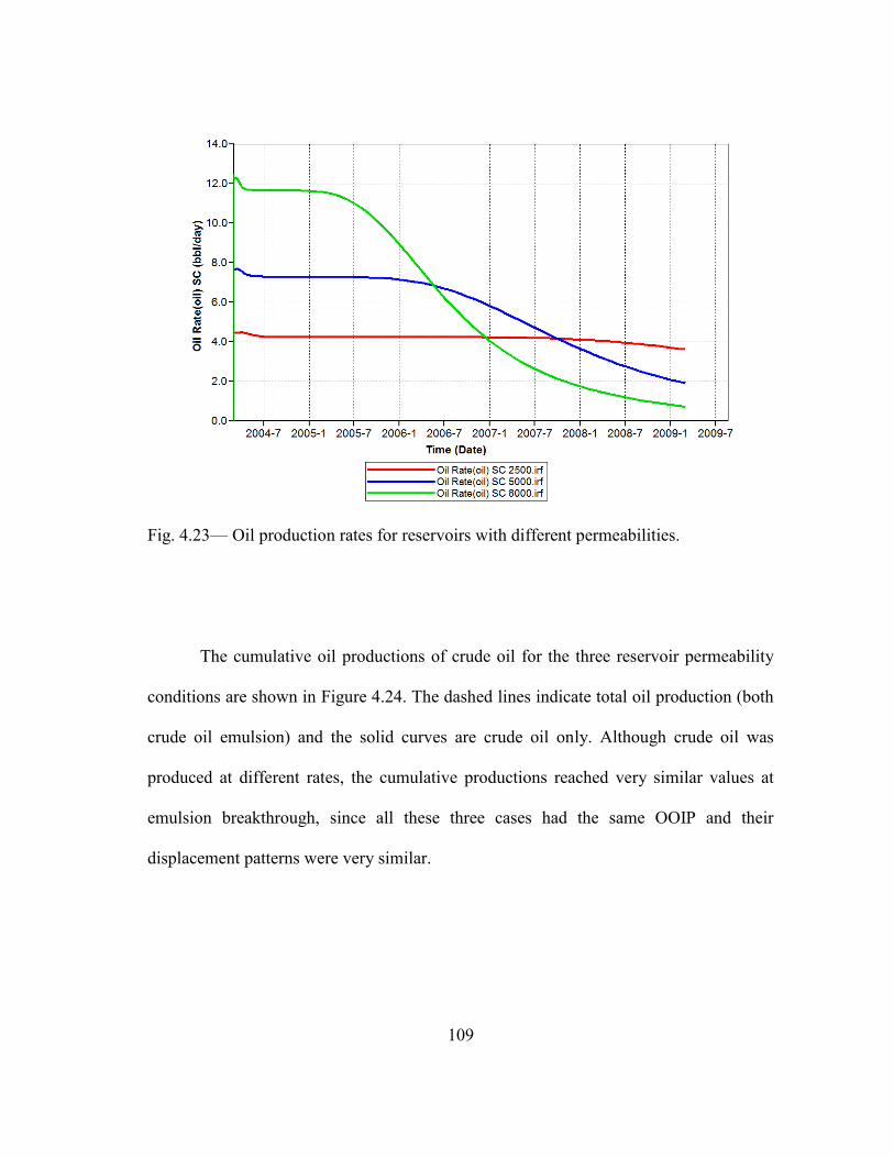
109

Fig. 4.23— Oil production rates for reservoirs with different permeabilities.

The cumulative oil productions of crude oil for the three reservoir permeability

conditions are shown in Figure 4.24. The dashed lines indicate total oil production (both

crude oil emulsion) and the solid curves are crude oil only. Although crude oil was

produced at different rates, the cumulative productions reached very similar values at

emulsion breakthrough, since all these three cases had the same OOIP and their

displacement patterns were very similar.

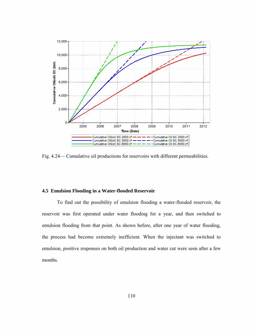
110

Fig. 4.24— Cumulative oil productions for reservoirs with different permeabilities.

4.5 Emulsion Flooding in a Water-flooded Reservoir

To find out the possibility of emulsion flooding a water-flooded reservoir, the

reservoir was first operated under water flooding for a year, and then switched to

emulsion flooding from that point. As shown before, after one year of water flooding,

the process had become extremely inefficient. When the injectant was switched to

emulsion, positive responses on both oil production and water cut were seen after a few

months.

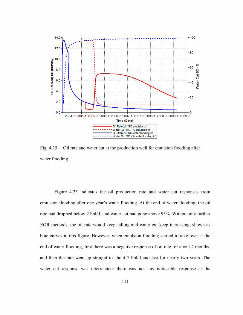
111

Fig. 4.25— Oil rate and water cut at the production well for emulsion flooding after

water flooding.

Figure 4.25 indicates the oil production rate and water cut responses from

emulsion flooding after one year’s water flooding At the end of water flooding, the oil

rate had dropped below 2 bbl/d, and water cut had gone above 95%. Without any further

EOR methods, the oil rate would keep falling and water cut keep increasing, shown as

blue curves in this figure. However, when emulsion flooding started to take over at the

end of water flooding, first there was a negative response of oil rate for about 4 months,

and then the rate went up straight to about 7 bbl/d and last for nearly two years. The

water cut response was interrelated: there was not any noticeable response at the

112

beginning 4 months of emulsion injection, and then water cut dropped rapidly to about

10%.

Fig. 4.26— Total liquid rate and BHP at the injection well for emulsion flooding after

water flooding.

Total liquid injection rate and BHP at the injection well during this process is

shown in Figure 4.26. With this figure, the production responses from Figure 4.25 can be

better explained. In Figure 4.25, the oil rate drop at the beginning of emulsion flooding

was due to a sudden decrease of liquid injection rate (limited by the injection pressure),

and the negligible water cut response within that period of time indicates no change in

113

liquid flow toward the production well – the movable water injected into the reservoir

within the first year was being depleted by emulsion injection during the first four

months of emulsion flooding, because of its much higher mobility compared to heavy oil

or emulsion.

After four months, very positive responses on both oil production and water cut

were seen in Figure 4.25. Correspondingly, the injection rate decreased again at that time

shown in Figure 4.26. As the movable water was depleted, the reservoir was filled with

high-viscosity liquid again, and the injection rate of emulsion in turn went down.

Fig. 4.27— Emulsion rate at the production well for emulsion flooding after water

flooding.

114

The production rate of emulsion was also analyzed, shown in Figure 4.27.

Although water channels were created at the beginning of emulsion flooding, the

emulsion injected did not appear in the production well until a year later. This means the

injected emulsion did not “fill in” those water channels directl , instead it ushe d hea

oil forward into those water flooded zones and improved reservoir fluid distribution and

thus the displacement pattern.

Fig. 4.28— Cumulative oil production at the production well for emulsion flooding after

water flooding.

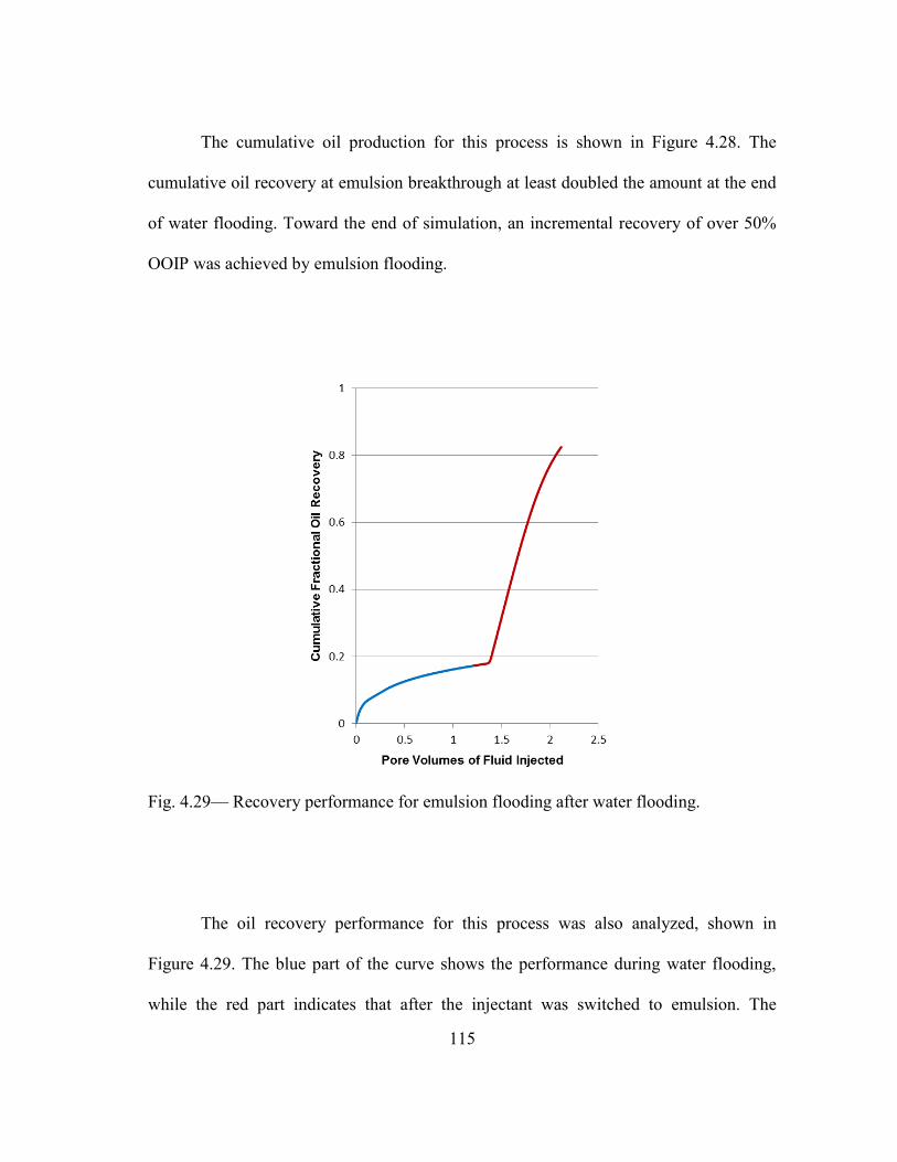
115

The cumulative oil production for this process is shown in Figure 4.28. The

cumulative oil recovery at emulsion breakthrough at least doubled the amount at the end

of water flooding. Toward the end of simulation, an incremental recovery of over 50%

OOIP was achieved by emulsion flooding.

Fig. 4.29— Recovery performance for emulsion flooding after water flooding.

The oil recovery performance for this process was also analyzed, shown in

Figure 4.29. The blue part of the curve shows the performance during water flooding,

while the red part indicates that after the injectant was switched to emulsion. The

116

recovery efficiency became very low shortly after the beginning of water flooding. One

year later, about 1.2 PV of water was injected, resulting in an oil recovery of 17% OOIP.

At this point, emulsion flooding started to take place. The recovery performance was

significantly improved after 0.15 PV of emulsion being injected, and the high

displacement efficiency lasted for 0.6 PV of emulsion injection, resulting in an

additional oil recovery of over 50% OOIP.

Despite the low injectivity of the emulsion, the recovery rate of crude oil was

reasonably high, even compared to the maximum rate during water flooding. More

importantly, this high rate could last for a long period of time, resulting in a consistent

steady increase of cumulative oil recovery. Because of the high efficiency of emulsion

flooding, the water cut problem also diminished compared to water flooding. Overall

speaking, emulsion flooding process demonstrated great potential in improved oil

recovery even after water flooding.

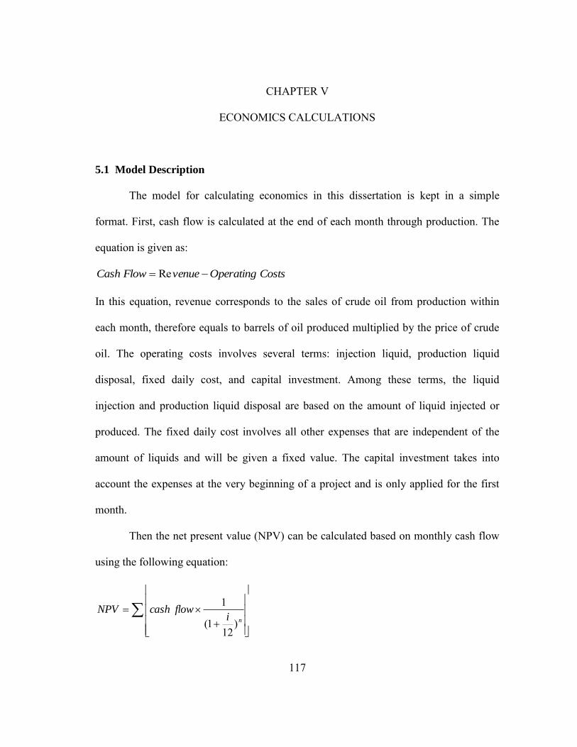
117

CHAPTER V

ECONOMICS CALCULATIONS

5.1 Model Description

The model for calculating economics in this dissertation is kept in a simple

format. First, cash flow is calculated at the end of each month through production. The

equation is given as:

CostsOperatingvenueFlowCash Re

In this equation, revenue corresponds to the sales of crude oil from production within

each month, therefore equals to barrels of oil produced multiplied by the price of crude

oil. The operating costs involves several terms: injection liquid, production liquid

disposal, fixed daily cost, and capital investment. Among these terms, the liquid

injection and production liquid disposal are based on the amount of liquid injected or

produced. The fixed daily cost involves all other expenses that are independent of the

amount of liquids and will be given a fixed value. The capital investment takes into

account the expenses at the very beginning of a project and is only applied for the first

month.

Then the net present value (NPV) can be calculated based on monthly cash flow

using the following equation:

ni

flowcashNPV

)12

1(

1

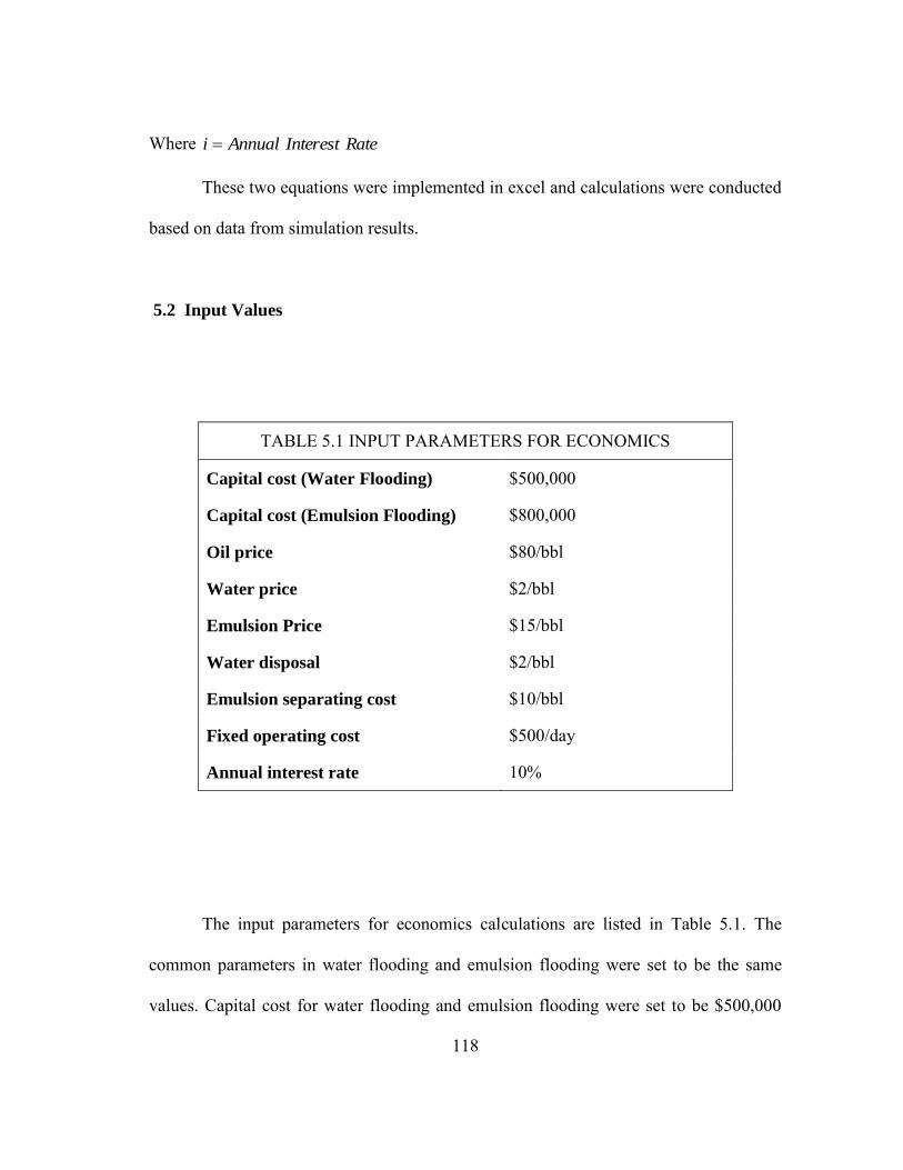
118

Where RateInterestAnnuali

These two equations were implemented in excel and calculations were conducted

based on data from simulation results.

5.2 Input Values

TABLE 5.1 INPUT PARAMETERS FOR ECONOMICS

Capital cost (Water Flooding) $500,000

Capital cost (Emulsion Flooding) $800,000

Oil price $80/bbl

Water price $2/bbl

Emulsion Price $15/bbl

Water disposal $2/bbl

Emulsion separating cost $10/bbl

Fixed operating cost $500/day

Annual interest rate 10%

The input parameters for economics calculations are listed in Table 5.1. The

common parameters in water flooding and emulsion flooding were set to be the same

values. Capital cost for water flooding and emulsion flooding were set to be $500,000

119

and $800,000, respectively. In emulsion flooding, an emulsion cost of $15/bbl was

assumed, including the cost for used engine oil (purchase and transportation), water and

mixing cost. Also, a cost of $10/bbl was assumed for emulsion separation from produced

oil.

The liquid flow rates in water flooding and emulsion flooding are shown in

Figure 5.1 and 5.2, respectively. These two figures were obtained from simulation

results exported into excel sheets and plotted on a monthly basis. Zero time

corresponded to the initial date of projects in simulation, which was set to be 03/01/2004

for all cases. The periodic fluctuation was due to variable number of days in different

months. The rates have been multiplied by 8 from the simulation results thus indicate the

liquid flow rates within the whole 2.5 acre pattern.

Fig. 5.1— Monthly liquid rates in water flooding.

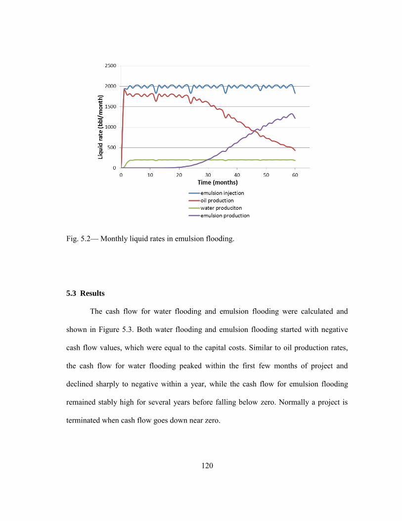
120

Fig. 5.2— Monthly liquid rates in emulsion flooding.

5.3 Results

The cash flow for water flooding and emulsion flooding were calculated and

shown in Figure 5.3. Both water flooding and emulsion flooding started with negative

cash flow values, which were equal to the capital costs. Similar to oil production rates,

the cash flow for water flooding peaked within the first few months of project and

declined sharply to negative within a year, while the cash flow for emulsion flooding

remained stably high for several years before falling below zero. Normally a project is

terminated when cash flow goes down near zero.

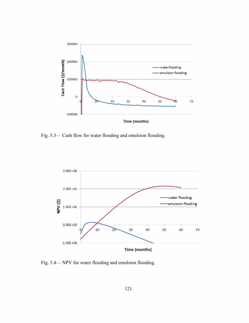
121

Fig. 5.3— Cash flow for water flooding and emulsion flooding.

Fig. 5.4— NPV for water flooding and emulsion flooding.

122

The NPV for water flooding and emulsion flooding were also calculated and

shown in Figure 5.4. As NPV is simply an accumulation of cash flow by taking into

account of interest rate, it increases as long as cash flow remains positive. The peak of

the NPV curve is at the point where cash flow goes down to zero. The maximum NPV

for water flooding was about $140,000 – the economics for water flooding such a thin

heavy oil reservoir was marginal. On the other hand, the maximum NPV for emulsion

flooding was $2,200,000. Compared to water flooding, the NPV for emulsion flooding

was significantly higher. This significant improvement mainly comes from the enhanced

production of heavy oil and much better controlled water cut.

5.4 Sensitivity Analyses

To combat the uncertainty of assigned values for input parameters, several

parameters were chosen to conduct sensitivity analyses, including capital costs, water

price, emulsion price, water disposal cost, fixed operating cost and annual interest rate.

The viscosity of the injected emulsion was also analyzed for sensitivity as this is a major

parameter to control in emulsion flooding projects.

5.4.1 Capital Costs

In this part the capital costs for water flooding and emulsion flooding were

assumed to be $1,000,000 and $1,600,000, respectively. Compared to the capital costs in

Table 5.1, both values were doubled. All other values were the same as given in Table

5.1.

123

Fig. 5.5— Sensitivity analyses of capital costs on cash flow.

Fig. 5.6— Sensitivity analyses of capital costs on NPV.

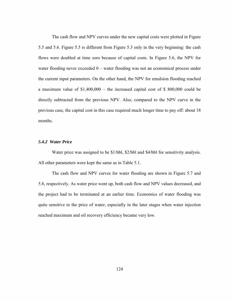
124

The cash flow and NPV curves under the new capital costs were plotted in Figure

5.5 and 5.6. Figure 5.5 is different from Figure 5.3 only in the very beginning: the cash

flows were doubled at time zero because of capital costs. In Figure 5.6, the NPV for

water flooding never exceeded 0 – water flooding was not an economical process under

the current input parameters. On the other hand, the NPV for emulsion flooding reached

a maximum value of $1,400,000 – the increased capital cost of $ 800,000 could be

directly subtracted from the previous NPV. Also, compared to the NPV curve in the

previous case, the capital cost in this case required much longer time to pay off: about 18

months.

5.4.2 Water Price

Water price was assigned to be $1/bbl, $2/bbl and $4/bbl for sensitivity analysis.

All other parameters were kept the same as in Table 5.1.

The cash flow and NPV curves for water flooding are shown in Figure 5.7 and

5.8, respectively. As water price went up, both cash flow and NPV values decreased, and

the project had to be terminated at an earlier time. Economics of water flooding was

quite sensitive to the price of water, especially in the later stages when water injection

reached maximum and oil recovery efficiency became very low.

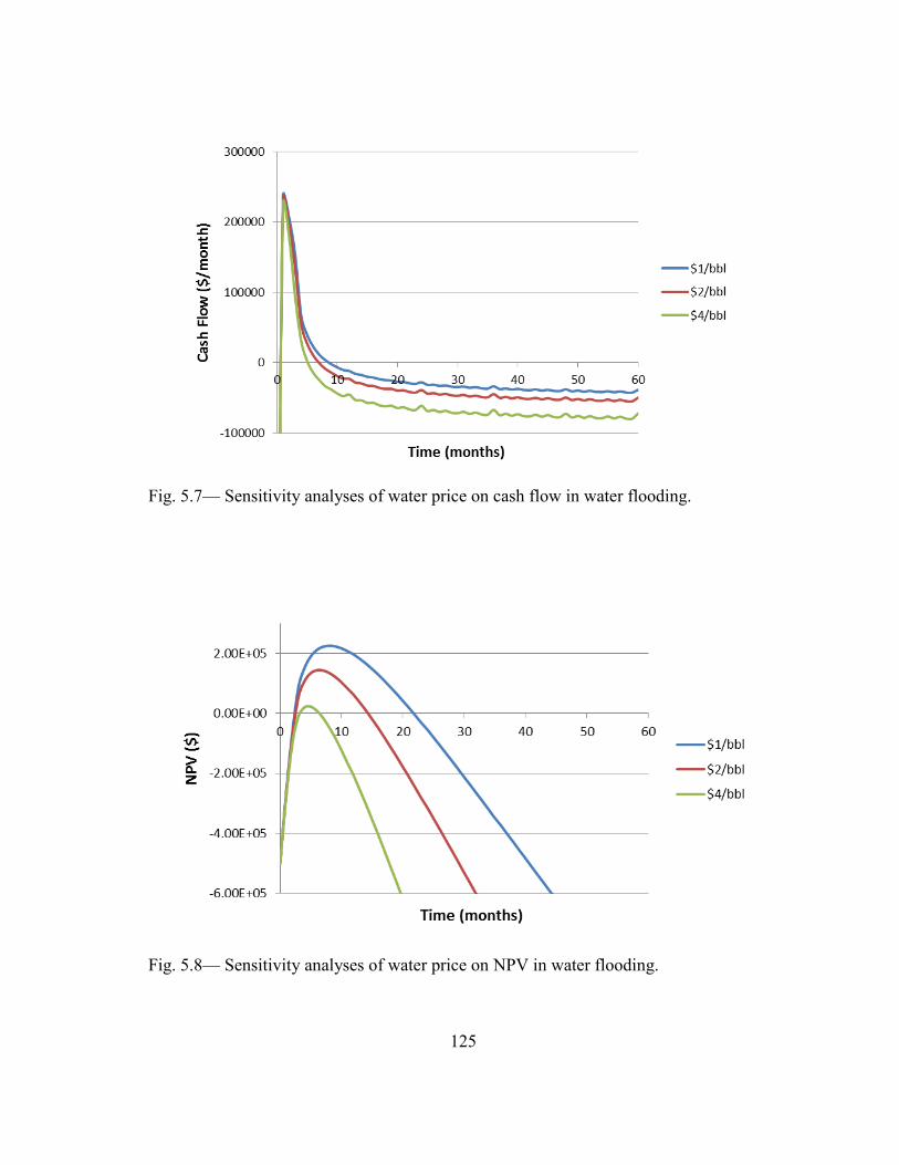
125

Fig. 5.7— Sensitivity analyses of water price on cash flow in water flooding.

Fig. 5.8— Sensitivity analyses of water price on NPV in water flooding.

126

In emulsion flooding, no water is being injected directly so the cash flow and

NPV curves will not be affected by the water price, and their figures will remain the

same as in Figures 5.3 and 5.4. The price of water does have some influence on emulsion

cost, as the emulsion consists of 60% water. However, water cost only contributes to a

small part of the cost for generating emulsions. In our calculations, the unit cost for

emulsion ($15/bbl) is much higher than that for water. Therefore, the economics of

emulsion flooding will not be sensitive to the price of water in general cases.

5.4.3 Emulsion Price

As mentioned before, the cost of emulsion included used engine oil purchase and

transportation, water cost and mixing cost. The cost for purchasing used engine oil can

be as low as 0, as used engine oil is collected mainly for environmental issues. The cost

for transportation could vary depending on the distance and transportation techniques.

To the extent of my knowledge, the cost for transporting a barrel of oil by railcar would

be around $10 to $20. Mixing cost is difficult to evaluate at this point, but this type of

emulsification has been conducted in the field and proven doable (Kaminsky et al.,

2010). If we assume the mixing cost ranges from $5 to $15 per barrel, by taking into

account of oil and water costs, the overall cost for emulsion would be approximately

between $10/bbl to $25/bbl. In this sensitivity study, three values of $10/bbl, $15/bbl

and $25/bbl were used for cash flow and NPV calculations. All other parameters were

kept the same values as shown in Table 5.1.

127

Fig. 5.9— Sensitivity analyses of emulsion price on cash flow in emulsion flooding.

Fig. 5.10— Sensitivity analyses of emulsion price on NPV in emulsion flooding.

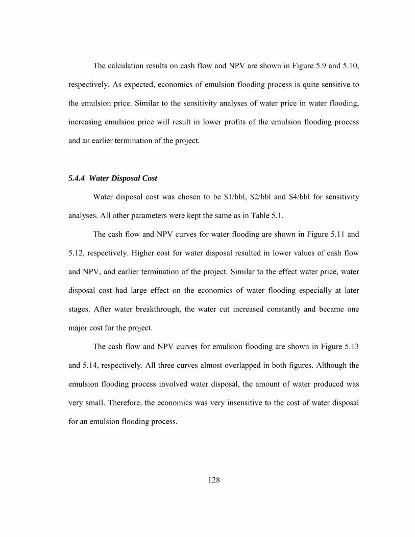
128

The calculation results on cash flow and NPV are shown in Figure 5.9 and 5.10,

respectively. As expected, economics of emulsion flooding process is quite sensitive to

the emulsion price. Similar to the sensitivity analyses of water price in water flooding,

increasing emulsion price will result in lower profits of the emulsion flooding process

and an earlier termination of the project.

5.4.4 Water Disposal Cost

Water disposal cost was chosen to be $1/bbl, $2/bbl and $4/bbl for sensitivity

analyses. All other parameters were kept the same as in Table 5.1.

The cash flow and NPV curves for water flooding are shown in Figure 5.11 and

5.12, respectively. Higher cost for water disposal resulted in lower values of cash flow

and NPV, and earlier termination of the project. Similar to the effect water price, water

disposal cost had large effect on the economics of water flooding especially at later

stages. After water breakthrough, the water cut increased constantly and became one

major cost for the project.

The cash flow and NPV curves for emulsion flooding are shown in Figure 5.13

and 5.14, respectively. All three curves almost overlapped in both figures. Although the

emulsion flooding process involved water disposal, the amount of water produced was

very small. Therefore, the economics was very insensitive to the cost of water disposal

for an emulsion flooding process.

129

Fig. 5.11— Sensitivity analyses of water disposal cost on cash flow in water flooding.

Fig. 5.12— Sensitivity analyses of water disposal cost on NPV in water flooding.

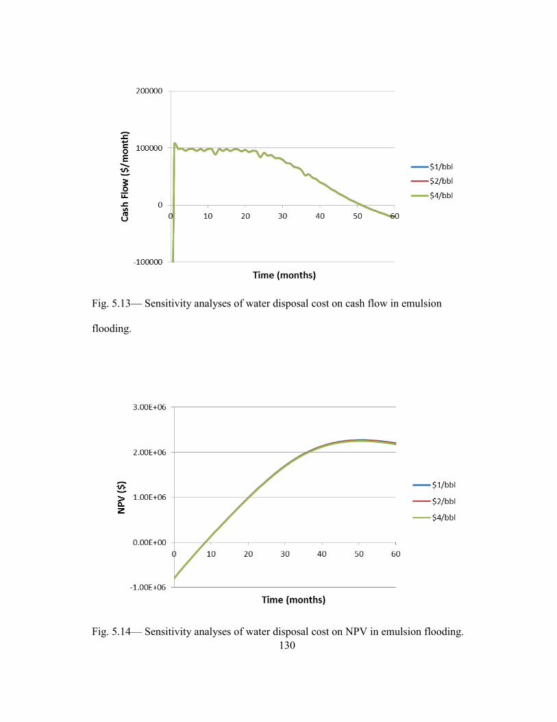
130

Fig. 5.13— Sensitivity analyses of water disposal cost on cash flow in emulsion

flooding.

Fig. 5.14— Sensitivity analyses of water disposal cost on NPV in emulsion flooding.

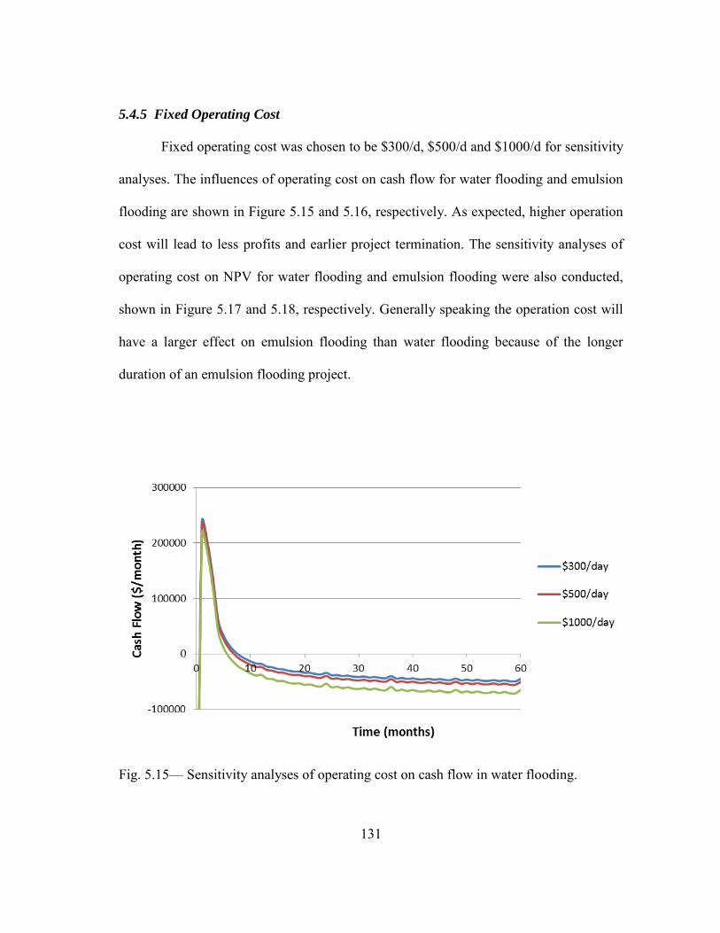
131

5.4.5 Fixed Operating Cost

Fixed operating cost was chosen to be $300/d, $500/d and $1000/d for sensitivity

analyses. The influences of operating cost on cash flow for water flooding and emulsion

flooding are shown in Figure 5.15 and 5.16, respectively. As expected, higher operation

cost will lead to less profits and earlier project termination. The sensitivity analyses of

operating cost on NPV for water flooding and emulsion flooding were also conducted,

shown in Figure 5.17 and 5.18, respectively. Generally speaking the operation cost will

have a larger effect on emulsion flooding than water flooding because of the longer

duration of an emulsion flooding project.

Fig. 5.15— Sensitivity analyses of operating cost on cash flow in water flooding.

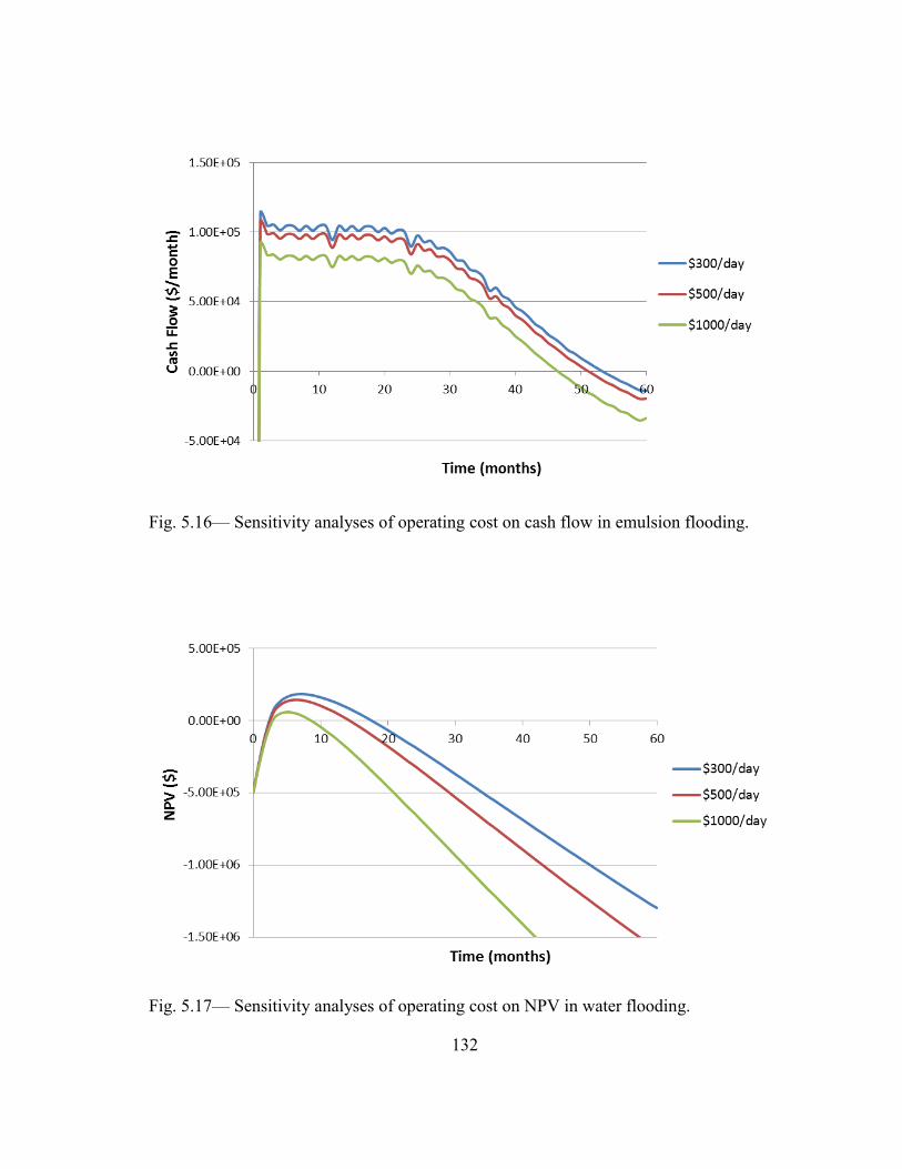
132

Fig. 5.16— Sensitivity analyses of operating cost on cash flow in emulsion flooding.

Fig. 5.17— Sensitivity analyses of operating cost on NPV in water flooding.

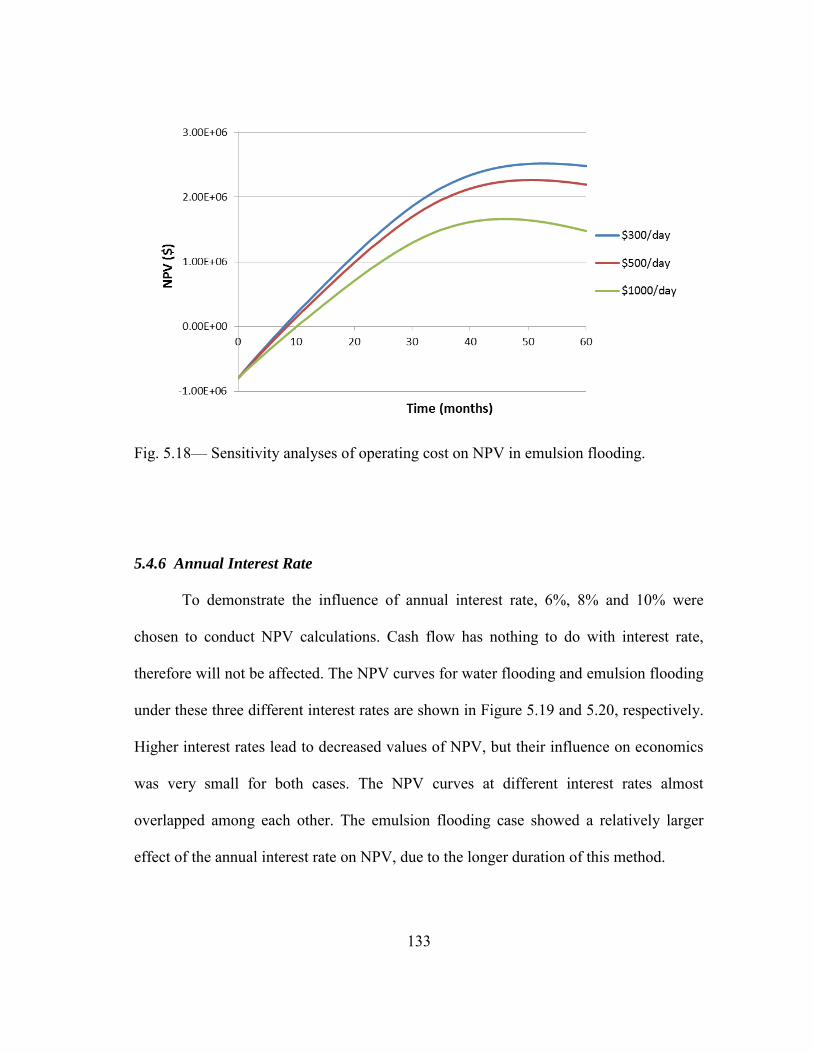
133

Fig. 5.18— Sensitivity analyses of operating cost on NPV in emulsion flooding.

5.4.6 Annual Interest Rate

To demonstrate the influence of annual interest rate, 6%, 8% and 10% were

chosen to conduct NPV calculations. Cash flow has nothing to do with interest rate,

therefore will not be affected. The NPV curves for water flooding and emulsion flooding

under these three different interest rates are shown in Figure 5.19 and 5.20, respectively.

Higher interest rates lead to decreased values of NPV, but their influence on economics

was very small for both cases. The NPV curves at different interest rates almost

overlapped among each other. The emulsion flooding case showed a relatively larger

effect of the annual interest rate on NPV, due to the longer duration of this method.

134

Fig. 5.19— Sensitivity analyses of annual interest rate on NPV in water flooding.

Fig. 5.20— Sensitivity analyses of annual interest rate on NPV in emulsion flooding.

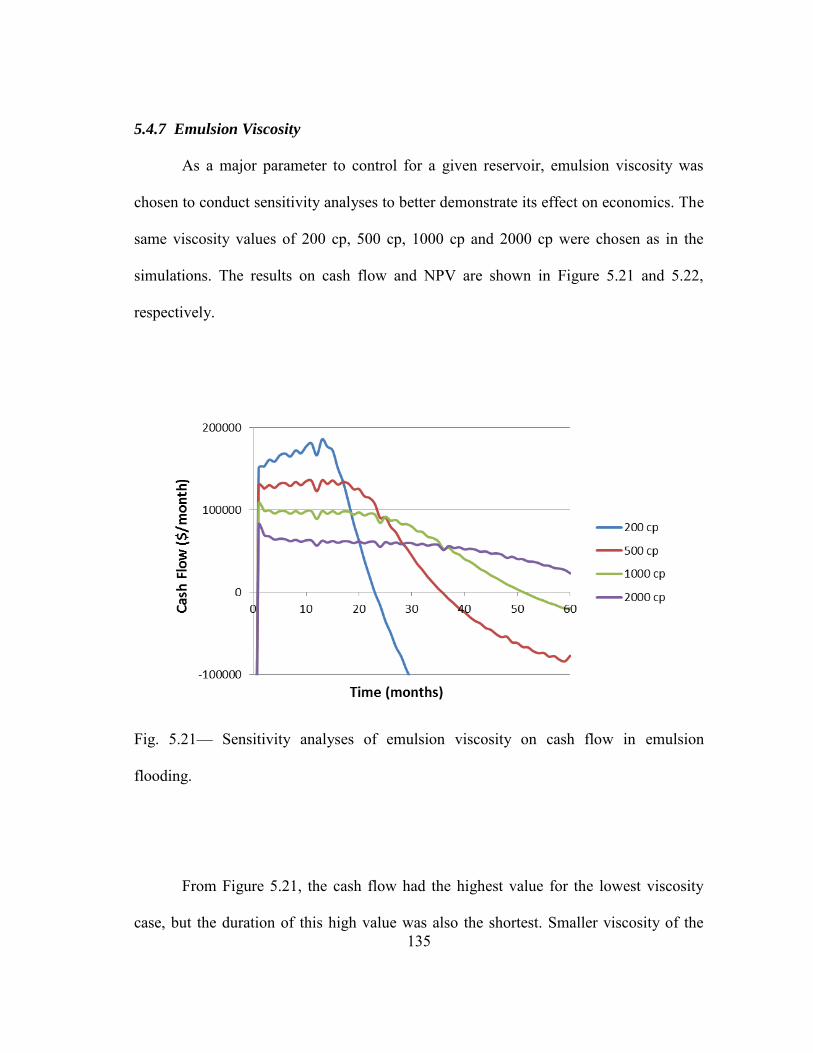
135

5.4.7 Emulsion Viscosity

As a major parameter to control for a given reservoir, emulsion viscosity was

chosen to conduct sensitivity analyses to better demonstrate its effect on economics. The

same viscosity values of 200 cp, 500 cp, 1000 cp and 2000 cp were chosen as in the

simulations. The results on cash flow and NPV are shown in Figure 5.21 and 5.22,

respectively.

Fig. 5.21— Sensitivity analyses of emulsion viscosity on cash flow in emulsion

flooding.

From Figure 5.21, the cash flow had the highest value for the lowest viscosity

case, but the duration of this high value was also the shortest. Smaller viscosity of the

136

emulsion resulted in better injectivity and thus the highest oil recovery rate at the

beginning of project, but faster and higher amount of oil emulsion mixing occurred at the

production well due to less mobility control provided by the emulsion.

Fig. 5.22— Sensitivity analyses of emulsion viscosity on NPV in emulsion flooding.

The overall comparison can be better demonstrated by NPV curves shown in

Figure 5.22. From this figure, the maximum NPV was clearly shown to be the 500 cp

emulsion case among the four cases. When the emulsion viscosity is low, the

displacement pattern gets poorer. On the other hand, if the emulsion viscosity is too

high, oil recovery will be very slow and the interest rate will have a bigger negative

137

effect on the economics because of the longer duration. Therefore, optimum viscosity

should be decided by balancing those two factors. Since the NPV is affected by many

other parameters, the best way to decide on emulsion viscosity is to conduct a sensitivity

analysis based on other given parameters. In this case, the optimal emulsion viscosity

was found to be around half of the crude oil viscosity (500 cp) in order to maximize the

profit.

5.5 Emulsion Flooding in a Water-flooded Reservoir

Economics calculations on emulsion flooding in a water-flooded reservoir were

conducted to evaluate the potential of this process in a reservoir that has been abandoned

after water flooding. The capital cost in this case would be additional facility cost to

generate and inject emulsions, which was assumed to be $300,000. All other input

parameters are kept the same as listed in Table 5.1.

The liquid rates in this process as input for conducting economics analyses are

shown in Figure 5.23. All these curves were obtained from simulation results (see 4.5 in

dissertation) that were exported into excel sheets and plotted on a monthly basis. Zero

time corresponded to the initial date of emulsion flooding, which was set to be

03/01/2005 in simulation, when the reservoir had already been produced under water

flooding for a year. All liquid rates in Figure 5.23 have been multiplied by 8 from the

simulation results thus indicate the total rates within the whole 2.5 acre pattern.

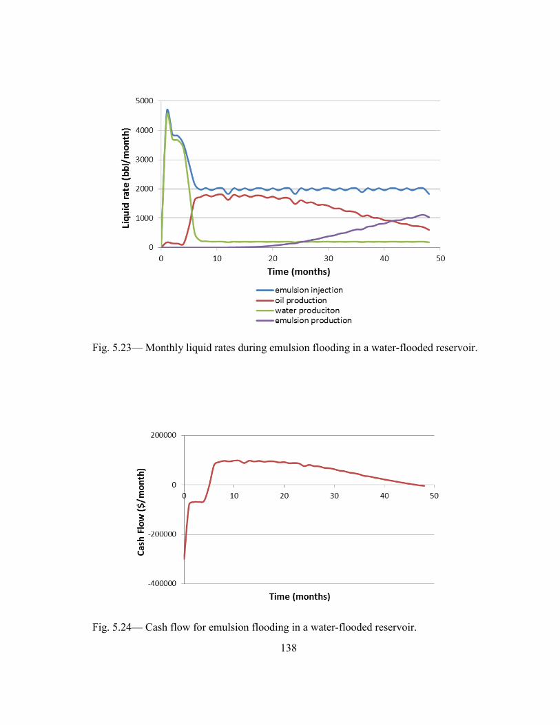
138

Fig. 5.23— Monthly liquid rates during emulsion flooding in a water-flooded reservoir.

Fig. 5.24— Cash flow for emulsion flooding in a water-flooded reservoir.

139

The cash flow for this process were calculated and shown in Figure 5.24. The

cash flow curve started at -$300,000, which was equal to the amount of capital

investment. Then the cash flow remained negative for five months and turned positive at

the 6th month. During this period of time, little oil was produced and most of the free

water in the reservoir was being depleted, because of its much higher mobility than the

oil phase. After the initial five months, oil rate went up rapidly to nearly 2000

bbl/month, coupled with a dramatic decrease of water production. Correspondingly, the

cash flow became positive, and remained positive for another three years, until the oil

production declined below economical rates.

Fig. 5.25— NPV for emulsion flooding in a water-flooded reservoir.

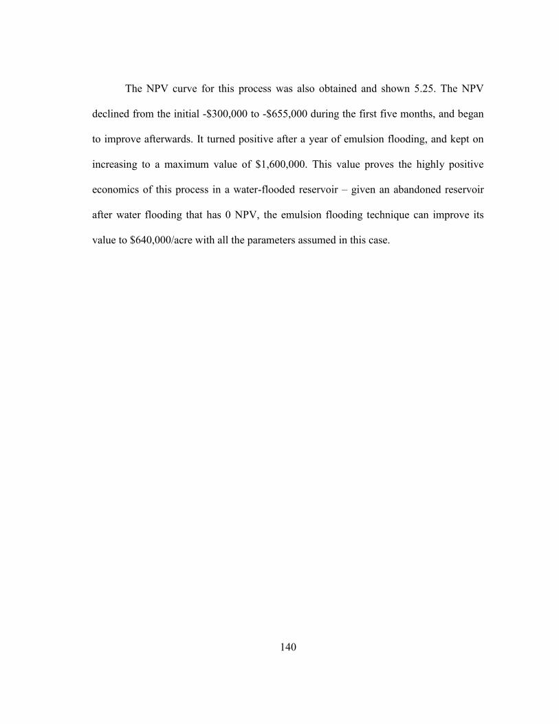
140

The NPV curve for this process was also obtained and shown 5.25. The NPV

declined from the initial -$300,000 to -$655,000 during the first five months, and began

to improve afterwards. It turned positive after a year of emulsion flooding, and kept on

increasing to a maximum value of $1,600,000. This value proves the highly positive

economics of this process in a water-flooded reservoir – given an abandoned reservoir

after water flooding that has 0 NPV, the emulsion flooding technique can improve its

value to $640,000/acre with all the parameters assumed in this case.

141

CHAPTER VI

SUMMARY AND CONCLUSIONS

6.1 Summary

A new candidate of drive fluid for heavy oil recovery was invented and tested by

a series of experiments. This new fluid is an emulsion system made of two inexpensive

components: used engine oil and brine. The stability of the emulsion was proven by

microscopic imaging and better understood by interfacial tension measurements and soot

particle size analyses. Viscosity measurements were also conducted for emulsions of

different water cut under various conditions.

An emulsion that contained 60% brine and 40% used engine oil was further

investigated in a number of coreflood experiments, to verify its stability and flow

properties in porous media. Several type of sandstone cores and two sand-packed

slimtubes were used in these coreflood experiments, and the emulsion was injected at

several rates in each experiment. Under each experimental condition, the emulsion

breakdown was analyzed, and the stabilized pressure drop was recorded, from which the

effective viscosity of the emulsion was calculated.

Based on the experimental results, numerical simulations were conducted on

emulsion flooding in a heavy oil reservoir. Because of the oil-external nature of the

emulsion and little plug-off effects from flowing through porous media, the emulsion

was simply treated as heavy oil, and the emulsion breakdown effect was included by co-

injection of water with this oil in simulation. Input parameters such as emulsion

142

viscosity and water breakout fractions were chosen based on experiments and sensitivity

analyses were conducted on those parameters to include their uncertainties. Simulation

results were compared with water flooding in terms of oil rate, water cut and cumulative

oil production. Emulsion flooding in a water-flooded reservoir case was also studied in

our simulations.

Finally, economics calculations were performed based on simulation results.

Cash flow and NPV curves for emulsion flooding were obtained and compared with

those for water flooding. Sensitivity analyses of certain input parameters were also

conducted. Economics of emulsion flooding in a water-flooded reservoir were also

calculated to reveal the potential of this method for abandoned reservoirs from water

flooding.

6.2 Conclusions

Based on our experimental studies, the following conclusions are made:

1. Stable W/O emulsions were generated with used engine oils simply by mixing in

brine under shear. No surfactant or any other chemicals were required in the

emulsification process.

2. Up to 75% brine by volume could be mixed into used engine oil to form

emulsions. Beyond this brine fraction, water existed as separate a separate phase

from the emulsion.

143

3. The viscosity of the emulsion increased with increasing water fraction. A wide

range of viscosity from 102 cp to 104 cp was covered for emulsions of 20% to

70% water cut.

4. At low water cut (< 40%), the emulsion was a Newtonian fluid; at higher water

cut the emulsion was shear thinning.

5. Used engine oil emulsions were macroemulsions. However, they were very

stable, as evident from the fact that no phase separation occurred after six months

and water droplet size remained fairly constant.

6. The stability of the emulsion was related to the presence of soot particles in used

engine oil and certain additives in engine oil.

7. An emulsion of 60% water cut had viscosities around 2000 cp at room

temperature, and was recommended as drive fluid for heavy oil displacement.

8. This emulsion passed through sandstone/sand without plugging off the porous

media, as evident from constant pressure drops along the core at constant rates of

injection, and similar pressure drop to the beginning of experiment after many

pore volumes of emulsion passing through.

9. This emulsion broke down to some extent by flowing through cores, and the

amount of water breakout depended on core properties and the flow rate.

10. Breakdown of emulsion resulted in reduced viscosities of the emulsion, and

could cause lower effective viscosity due to two-phase flow.

11. In high permeability matrixes (> 1000 md), emulsion breakdown was less than

10% at moderate rates of injection in all experiments. In sand packs

144

(permeability around 8000 md), emulsion breakdown from flowing through the

matrix was less than 1% at rates up to 6 ft/d.

12. Effective viscosities of the emulsion calculated from coreflood experiments

revealed 0~10% viscosity reduction from viscometer-measured viscosity of the

original emulsion (before injection) in sand packs, and larger extents of reduction

in sandstone cores. Calculated effective viscosities were comparable to

viscometer measurements.

Based on the experimental results, the emulsion was approximated as an oil

phase (and co-injection of a certain fraction of water) in numerical simulations of heavy

oil displacement, and economics calculations were conducted from the simulation

results. Major conclusions from simulations and economics calculations are drawn as

follows:

1. Emulsion flooding in a heavy oil reservoir was highly effective compared to

water flooding: oil production rate maintained at a reasonably high value until

close to crude oil depletion in the reservoir; water cut was dramatically reduced

through the process; cumulative oil production nearly quadrupled the amount

from water flooding at the end of simulation.

2. Economics calculations of emulsion flooding was highly positive, revealing an

increase of over $ 2,000,000 in NPV for a 2.5 acre pattern of a thin bed reservoir

compared to that for water flooding.

145

3. Oil production rates were controlled by the crude oil viscosity at the beginning of

injection, and later more dominated by the viscosity of injectant. The emulsion

viscosity needs to be carefully designed to maximize the NPV.

4. Emulsion flooding was found to be effective in water-flooded reservoirs.

Simulation results showed an incremental oil recovery of over 50% OOIP, and

economics calculations demonstrated an incremental NPV of $640,000/acre for

this thin bed reservoir.

146

REFERENCES

Adams, D.M. 1982. Experiences with Waterflooding Lloydminster Heavy-Oil Reservoirs. SPE Journal of Petroleum Technology 34 (8): 1643-1650.

Alikhan, A.A. and Farouq Ali, S.M. 1983. Current Status of Nonthermal Heavy Oil

Recovery. Paper SPE 11846 presented at the SPE Rocky Mountain Regional Meeting, Salt Lake City, Utah, 22-25 May.

Breston, J.N. 1958. Oil Recovery by Heat from in Situ Combustion. SPE Journal of

Petroleum Technology 10 (8): 13-17. Bragg, J.R. 1999. Oil Recovery Method Using an Emulsion. US Patent 5927404. Bragg, J.R. 2000. Oil Recovery Method Using an Emulsion. US Patent 6068054. Bragg, J.R. and Varadaraj, R. 2006. Solids-Stabilized Oil-in-Water Emulsion and a

Method for Preparing Same. US Patent 6988550. Breslin, M. 2010. Used Oil: An Often Overlooked Resource. http://www.americanrecycler.com/0110/used002.shtml. Bryan, J.L. and Kantzas, A. 2007. Enhanced Heavy-Oil Recovery by Alkali-Surfactant

Flooding. Paper SPE 110738 presented at the SPE Annual Technical Conference and Exhibition, Anaheim, California, 11-14 November.

Bryan, J.L. and Kantzas, A. 2008. Improved Recovery Potential in Mature Heavy Oil

Fields by Alkali-Surfactant Flooding. Paper SPE 117649 presented at the SPE/PS/CHOA International Thermal Operations and Heavy Oil Symposium, Calgary, Alberta, Canada, 20-23 October.

Bryan, J. and Kantzas, A. 2009. Potential for Alkali-Surfactant Flooding in Heavy Oil

Reservoirs through Oil-in-Water Emulsification. Journal of Canadian Petroleum

Technology 48 (2): 37-46. Chopra, S. and Lines, L. 2008. Special Section - Heavy Oil. The Leading Edge (Society

of Exploration Geophysicists) 27 (8): 1104-1106. D'Elia-S, R. and Ferrer-G, J. 1973. Emulsion Flooding of Viscous Oil Reservoirs. Paper

SPE 4674 presented at the Fall Meeting of the Society of Petroleum Engineers of AIME, Las Vegas, Nevada, 30 September-3 October.

147

Drillet, V. and Defives, D. 1991. Clay Dissolution Kinetics in Relation to Alkaline Flooding. Paper SPE 21030 presented at the SPE International Symposium on Oilfield Chemistry, Anaheim, California, 20-22 February.

Du, Y. and Guan, L. 2004. Field-Scale Polymer Flooding: Lessons Learned and

Experiences Gained During Past 40 Years. Paper SPE 91787 presented at the SPE International Petroleum Conference in Mexico, Puebla Pue., Mexico, 7-9 November.

Edinga, K.J., McCaffery, F.G., and Wytrychowski, I.M. 1980. Cessford Basal Colorado

a Reservoircaustic Flood Evaluation. SPE Journal of Petroleum Technology 32 (12): 2103-2110.

Farouq Ali, S.M., Figueroa, J.M., Azuaje, E.A. et al. 1979. Recovery of Lloydminster

and Morichal Crudes by Caustic, Acid and Emulsion Floods. Journal of

Canadian Petroleum Technology 18 (1): 53-59. Gondouin, M. and Fox III, J.M. 1991. The Challenge of West Sak Heavy Oil: Analysis

of an Innovative Approach. Paper SPE 22077 presented at the International Arctic Technology Conference, Anchorage, Alaska, 29-31 May.

Harmsen, G.J. 1971. Oil Recovery by Hot-Water and Steam Injection. Paper WPC-

14228 presented at the World Petroleum Congress, Moscow, USSR, 13-18 June. Huc, A.Y. 2011. Heavy Crude Oils: From Geology to Upgrading an Overview. Paris:

Editions Technip. Isaacs, E.E. and Chow, R.S. 1992. Practical Aspects of Emulsion Stability. ed. Schramm,

L.L. Emulsions: Fundamentals and Applications in the Petroleum Industry. Washington, DC: American Chemical Society.

Jennings Jr., H.Y., Johnson Jr., C.E., and McAuliffe, C.D. 1974. A Caustic

Waterflooding Process for Heavy Oils. SPE Journal of Petroleum Technology 26 (12): 1344-1352.

Johnson Jr., C.E. 1976. Status of Caustic and Emulsion Methods. SPE Journal of

Petroleum Technology 28 (1): 85-92. Joseph N. Breston, T.L. 1958. Oil Recovery by Heat from in Situ Combustion. SPE

Journal of Petroleum Technology 10 (8): 13-17. Kaminsky, R.D., Wattenbarger, R.C., Lederhos, J. et al. 2010. Viscous Oil Recovery

Using Solids-Stabilized Emulsions. Paper SPE 135284 presented at the SPE Annual Technical Conference and Exhibition, Florence, Italy, 19-22 September.

148

Kang, X., Zhang, J., Sun, F. et al. 2011. A Review of Polymer EOR on Offshore Heavy

Oil Field in Bohai Bay, China. Paper SPE 144932 presented at the SPE Enhanced Oil Recovery Conference, Kuala Lumpur, Malaysia, 19-21 July.

Kaplan, I.R., Lu, S.T., Alimi, H.M. et al. 2001. Fingerprinting of High Boiling

Hydrocarbon Fuels, Asphalts and Lubricants. Environmental Forensics 2: 231-248.

Khatib, A.K., Earlougher, R.C., and Kantar, K. 1981. CO2 Injection as an Immiscible

Application for Enhanced Recovery in Heavy Oil Reservoirs. Paper SPE 9928 presented at the SPE California Regional Meeting, Bakersfield, California, 25-27 March.

Kokal, S.L. 2005. Crude Oil Emulsions: A State-of-the-Art Review. SPE Production &

Operations 20 (1): 5-13. Kumar, R., Dao, E.K., and Mohanty, K.K. 2010. Emulsion Flooding of Heavy Oil. Paper

SPE 129914 presented at the SPE Improved Oil Recovery Symposium, Tulsa, Oklahoma, 24-28 April.

Lam, S.S., Russell, A.D., Lee, C.L. et al. 2012. Production of Hydrogen and Light

Hydrocarbons as a Potential Gaseous Fuel from Microwave-Heated Pyrolysis of Waste Automotive Engine Oil. International journal of hydrogen energy 37: 5011-5021.

Leonard, J. 1986. Increased Rate of EOR Brightens Outlook. Oil and Gas Journal 84

(15): 77-101. Liebe, H.R. and Butler, R. 1991. A Study of the Use of Vertical Steam Injectors in the

Steam-Assisted Gravity Drainage Process. Paper presented at the Annual Technical Meeting, Banff, 21-24 April.

Mai, A., Bryan, J., Goodarzi, N. et al. 2009. Insights into Non-Thermal Recovery of

Heavy Oil. Journal of Canadian Petroleum Technology 48 (3): 27-35. Mashava, P.M., Alonge, I.E., and Mlenga, F. 1989. Chemistry from Waste Products:

Fractional Distillation of Used Engine Oil. Journal of Chemical Education 66 (12): 1042.

McAuliffe, C.D. 1973a. Crude-Oil-Water Emulsions to Improve Fluid Flow in an Oil

Reservoir. SPE Journal of Petroleum Technology 25 (6): 721-726.

149

McAuliffe, C.D. 1973b. Oil-in-Water Emulsions and Their Flow Properties in Porous Media. SPE Journal of Petroleum Technology 25 (6): 727-733.

Mohnot, S.M., Bae, J.H., and Foley, W.L. 1987. A Study of Mineral/Alkali Reactions.

SPE Reservoir Engineering 2 (4): 653-663. Nelson, R.C., Lawson, J.B., Thigpen, D.R. et al. 1984. Cosurfactant-Enhanced Alkaline

Flooding. Paper SPE 12672 presented at the SPE Enhanced Oil Recovery Symposium, Tulsa, Oklahoma, 15-18 April.

Novosad, Z. and Novosad, J. 1984. Determination of Alkalinity Losses Resulting from

Hydrogen Ion Exchange in Alkaline Flooding. SPE Journal 24 (1): 49-52. Owens, W.D. and Suter, V.E. 1965. Steam Simulation for Secondary Recovery. Journal

of Canadian Petroleum Technology 4 (4): 227-235. Picha, M.S. 2007. Enhanced Oil Recovery by Hot CO2 Flooding. Paper SPE 105425

presented at the SPE Middle East Oil and Gas Show and Conference, Kingdom of Bahrain, 11-14 March.

Reid, T.B. and Robinson, H.J. 1981. Lick Creek Meakin Sand Unit Immiscible CO2

Waterflood Project. SPE Journal of Petroleum Technology 33 (9): 1723-1729. Saner, W.B. and Patton, J.T. 1986. CO2 Recovery of Heavy Oil: Wilmington Field Test.

SPE Journal of Petroleum Technology 38 (7): 769-776. Scott, G.R., Collins, H.N., and Flock, D.L. 1965. Improving Waterflood Recovery of

Viscous Crude Oils by Chemical Control. Journal of Canadian Petroleum

Technology 4 (4): 243-251. Selby, R., Alikhan, A.A., and Ali, S.M.F. 1989. Potential of Non-Thermal Methods for

Heavy Oil Recovery. Journal of Canadian Petroleum Technology 28 (4): 45-59. Seright, R.S., Fan, T., Wavrik, K.E. et al. 2011. New Insights into Polymer Rheology in

Porous Media. SPE Journal 16 (1): 35-42. T-Taissi, A. and Raminsky, K. 2007. Hydrogen Production from Used Lubricating Oils.

Catal Today 129 (365): 71. Wassmuth, F.R., Green, K., Hodgins, L. et al. 2007. Polymer Flood Technology for

Heavy Oil Recovery. Paper presented at the Canadian International Petroleum Conference, Calgary, Alberta, 12-14 June.

150

Wassmuth, F.R., Green, K., Arnold, W. et al. 2009. Polymer Flood Application to Improve Heavy Oil Recovery at East Bodo. Journal of Canadian Petroleum

Technology 48 (2): 55-61. Xie, J., Chung, B.C., and Leung, L. 2008. Design and Implementation of a Caustic

Flooding EOR Pilot at Court Bakken Heavy Oil Reservoir. Paper SPE 117221 presented at the SPE/PS/CHOA International Thermal Operations and Heavy Oil Symposium, Calgary, Alberta, Canada, 20-23 October.

Zaitoun, A., Tabary, R., Fossey, J.P. and Boyle, T. 1998. Implementing a Heavy-Oil

Horizontal-Well Flood in Western Canada. Paper presented at the the Seventh UNITAR International Conference on Heavy Crude and Tar Sands, Beijing, China, 27-30 October.