High Viscous Oil–Water Two–Phase Flow: Experiments ...
39
Published in HAMT, Aug 2018. DOI: 10.1007/s00231-018-2461-9 1 Corresponding author email: [email protected] High Viscous Oil–Water Two–Phase Flow: Experiments & Numerical Simulations Archibong Archibong-Eso a,b , Jing Shi a , Yahaya D. Baba a,c* , Aliyu M. Aliyu d , Yusuf O. Raji e , Hoi Yeung a a Oil and Gas Engineering Centre, Cranfield University, Cranfield, United Kingdom b Energy and Fluids Engineering Group, Department of Mechanical Engineering, Cross River University of Technology, Calabar, Nigeria c Department of Chemical/Petroleum Engineering, Afe Babalola University, PMB 5454, Ado-Ekiti, Nigeria d Faculty of Engineering, University of Nottingham, NG7 2RD, United Kingdom e Chemical Engineering Programme, Abubakar Tafawa Balewa University, PMB 0248, Bauchi, Nigeria Abstract An experimental study on viscous oil-water two-phase flow conducted in a 5.5 m long and 25.4 mm internal diameter (ID) pipeline is presented. Mineral oil with viscosity ranging from 3.5 Pa.s – 5.0 Pa.s and water were used as test fluid for this study. Experiments were conducted for superficial velocities of oil and water ranging from 0.06 to 0.55 m/s and 0.01 m/s to 1.0 m/s respectively. Axial pressure measurements were made from which the pressure gradients were calculated. Flow pattern determination was aided by high definition video recordings. Numerical simulation of experimental flow conditions is performed using a commercially available Computational Fluid Dynamics code. Results show that at high oil superficial velocities, Core Annular Flow (CAF) is the dominant flow pattern while Oil Plug in Water Flow (OPF) and Dispersed Oil in Water (DOW) flow patterns are dominant high water superficial velocities. Pressure Gradient results showed a general trend of reduction to a minimum as water superficial velocity increases before subsequently increasing on further increasing the superficial water velocity. The CFD results performed well in predicting the flow configurations observed in the experiments. Keywords: CFD, Flow Patterns, Pressure Gradient, Pipelines, Heavy Oil, Viscosity, Oil and Gas.
Transcript of High Viscous Oil–Water Two–Phase Flow: Experiments ...

Published in HAMT, Aug 2018. DOI: 10.1007/s00231-018-2461-9
1 Corresponding author email: [email protected]
High Viscous Oil–Water Two–Phase Flow: Experiments & Numerical Simulations
Archibong Archibong-Esoa,b, Jing Shia, Yahaya D. Babaa,c*, Aliyu M. Aliyud, Yusuf O. Rajie, Hoi Yeunga
a Oil and Gas Engineering Centre, Cranfield University, Cranfield, United Kingdom b Energy and Fluids Engineering Group, Department of Mechanical Engineering, Cross River University of Technology, Calabar, Nigeria
c Department of Chemical/Petroleum Engineering, Afe Babalola University, PMB 5454, Ado-Ekiti, Nigeria d Faculty of Engineering, University of Nottingham, NG7 2RD, United Kingdom
e Chemical Engineering Programme, Abubakar Tafawa Balewa University, PMB 0248, Bauchi, Nigeria
Abstract
An experimental study on viscous oil-water two-phase flow conducted in a 5.5 m long and
25.4 mm internal diameter (ID) pipeline is presented. Mineral oil with viscosity ranging from
3.5 Pa.s – 5.0 Pa.s and water were used as test fluid for this study. Experiments were
conducted for superficial velocities of oil and water ranging from 0.06 to 0.55 m/s and 0.01
m/s to 1.0 m/s respectively. Axial pressure measurements were made from which the
pressure gradients were calculated. Flow pattern determination was aided by high definition
video recordings. Numerical simulation of experimental flow conditions is performed using a
commercially available Computational Fluid Dynamics code. Results show that at high oil
superficial velocities, Core Annular Flow (CAF) is the dominant flow pattern while Oil Plug in
Water Flow (OPF) and Dispersed Oil in Water (DOW) flow patterns are dominant high water
superficial velocities. Pressure Gradient results showed a general trend of reduction to a
minimum as water superficial velocity increases before subsequently increasing on further
increasing the superficial water velocity. The CFD results performed well in predicting the
flow configurations observed in the experiments.
Keywords: CFD, Flow Patterns, Pressure Gradient, Pipelines, Heavy Oil, Viscosity, Oil and Gas.

Published in HAMT, Aug 2018. DOI: 10.1007/s00231-018-2461-9
2 Corresponding author email: [email protected]
1 Introduction
1.1 Background
Water usually accompanies crude oil during production especially during enhanced recovery
when water is deliberately injected into older or marginal wells to aid production. In some
cases, water is added for lubrication as this reduces pumping requirements for crude
transport in cases where heavy or highly viscous oils are involved. Based on the above
premise, the study of oil-water flow is therefore essential for production systems design and
crude oil pipeline transport networks. Concurrent flow of oil and water results in a wide
variety of flow patterns depending on the conditions during transportation.
The continuous depletion of light (conventional) oil reserves due to long term production
has in recent years, increased the attractiveness of unconventional fossil fuels (e.g. shale
gas, shale oil and especially heavy oil). Heavy oil, defined as a petroleum liquid with API
gravity of <22° and viscosity >100 cP, has generated so much interest due to its huge
reserves. The literature is awash with studies of light oils, but scarce in the case of heavy
oils. However due to significant differences in rheological characteristics between light and
heavy oils, research into the production and transportation of heavy oils has thus become
important. As stated earlier, water is used to assist the flow of highly viscous oils and hence
the study of the flow patterns, pressure gradients, and other characteristics is imperative
for heavy oil–water liquid–liquid flows.
1.2 Previous works
Bannwart et al. [1] studied flow patterns in high viscous oil-water two-phase flow in a
0.0284 m ID, 5.43 m long glass pipe. Oil with viscosity of 0.488 Pa.s was used in the study.

Published in HAMT, Aug 2018. DOI: 10.1007/s00231-018-2461-9
3 Corresponding author email: [email protected]
Superficial velocities for oil and water were 0.07 – 2.5 m/s & 0.04 – 0.5 m/s respectively.
Flow patterns observed in the horizontal test section are the stratified, bubbly stratified,
dispersed bubbles and annular flows. In stratified flow pattern, the upper walls of the glass
pipe were observed to be constantly lubricated by water; this was attributed to interfacial
phenomena and wettability effect. The bubbly stratified flow was intermittent in nature and
had characteristic packages of coalesced bubbles. Homogenously dispersed bubbles in a
continuous water phase were observed in the study; and the flow pattern was named the
dispersed bubble flow. The annular flow pattern was observed to have a smooth and
centered or wavy and off centered annulus of oil enveloped by a water phase.
Vuong et al. [2] studied high viscosity oil/water flow in horizontal and vertical pipes. Refined
mineral oil ND 50 with viscosity 0.44 – 0.10 Pa.s and Tulsa City tap water were used as test
fluids. The test section consisted of a U-shaped, stainless steel pipe inclined at angles
ranging from -2 – 90° to the vertical with 0.0525 m ID and length of 44 m. Graduated
cylinders, high speed video camera and differential pressure transducers were used to
determine the water holdup, flow regimes and pressure gradients in the study. Oil and
water superficial velocities ranged from 0.1 – 1 m/s for both horizontal and vertical flows.
Four main flow regimes were observed in the horizontal flow test: Stratified Wavy with Oil
Droplets at Interface; Dispersion of Oil in Water over a Water Layer flow; Dispersion of Oil
in Water; and Dispersion of Oil in Water with Oil Film at the pipe walls. They also noted that
pressure gradient was mainly influenced by flow patterns, flow rates and liquid viscosity.
Poesio et al. [3] studied two phase oil-water flow in a horizontal plastic pipeline with
internal diameter of 50 mm. Oil and water viscosities used in the studies were 0.9 Pa.s
(20°C) and 0.001 Pa.s respectively. Superficial oil and gas velocities ranged from 0.13 –
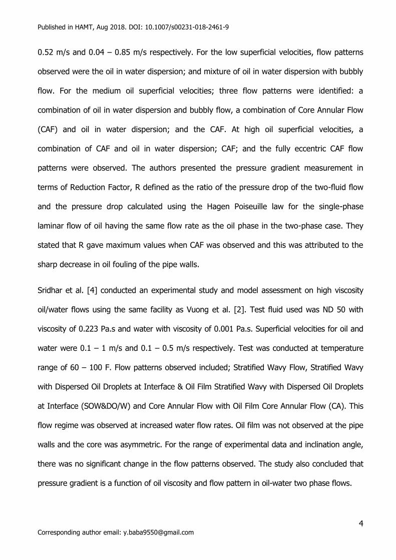
Published in HAMT, Aug 2018. DOI: 10.1007/s00231-018-2461-9
4 Corresponding author email: [email protected]
0.52 m/s and 0.04 – 0.85 m/s respectively. For the low superficial velocities, flow patterns
observed were the oil in water dispersion; and mixture of oil in water dispersion with bubbly
flow. For the medium oil superficial velocities; three flow patterns were identified: a
combination of oil in water dispersion and bubbly flow, a combination of Core Annular Flow
(CAF) and oil in water dispersion; and the CAF. At high oil superficial velocities, a
combination of CAF and oil in water dispersion; CAF; and the fully eccentric CAF flow
patterns were observed. The authors presented the pressure gradient measurement in
terms of Reduction Factor, R defined as the ratio of the pressure drop of the two-fluid flow
and the pressure drop calculated using the Hagen Poiseuille law for the single-phase
laminar flow of oil having the same flow rate as the oil phase in the two-phase case. They
stated that R gave maximum values when CAF was observed and this was attributed to the
sharp decrease in oil fouling of the pipe walls.
Sridhar et al. [4] conducted an experimental study and model assessment on high viscosity
oil/water flows using the same facility as Vuong et al. [2]. Test fluid used was ND 50 with
viscosity of 0.223 Pa.s and water with viscosity of 0.001 Pa.s. Superficial velocities for oil and
water were 0.1 – 1 m/s and 0.1 – 0.5 m/s respectively. Test was conducted at temperature
range of 60 – 100 F. Flow patterns observed included; Stratified Wavy Flow, Stratified Wavy
with Dispersed Oil Droplets at Interface & Oil Film Stratified Wavy with Dispersed Oil Droplets
at Interface (SOW&DO/W) and Core Annular Flow with Oil Film Core Annular Flow (CA). This
flow regime was observed at increased water flow rates. Oil film was not observed at the pipe
walls and the core was asymmetric. For the range of experimental data and inclination angle,
there was no significant change in the flow patterns observed. The study also concluded that
pressure gradient is a function of oil viscosity and flow pattern in oil-water two phase flows.

Published in HAMT, Aug 2018. DOI: 10.1007/s00231-018-2461-9
5 Corresponding author email: [email protected]
Wang et al. [5] studied the flow characteristics of heavy crude oil-water two-phase flow in a
0.0254 m pipe ID with length of 50 m. Oil viscosity used was 0.6 Pa.s. In their study, five
flow patterns were observed, water-in-oil emulsion dispersed flow (EW/O), intermittent flow
of (EW/O) and partial segregated water layers, EW/O with water stratified flow, EW/O and
water semi-annular flow and EW/O and water annular flow. Oil in water emulsion was
present for all the flow conditions investigated. For water cut below 50% and low mixture
velocities, a flow pattern in which water was dispersed in oil (DW/O) was observed. The
oil’s high viscosity was observed to retard the film drainage between dispersed drops
thereby reducing coalescence. An increase in the mixture velocity at low water cut saw a
transitions from DW/O to DW/O with partial segregated water flow. Pressure gradient in the
low water cut flow patterns generally increased with in-creasing water fraction but
decreased when the water in flow segregated and formed a layer. At high water fractions
(>50%), oil water emulsion was not formed
Rodriguez and Baldani [6] conducted experiments on two phase liquid-liquid flows using a
15.5-m long borosilicate glass pipe with 0.026 m ID. Oil and water viscosities used were
0.28 Pa.s and 0.001 Pa.s respectively. The mixture velocities ranged from 0.13 – 0.15 m/s
and water cut from 40 – 83%. Pressure gradient and holdup data were collected and
analyzed in the study with emphasis on the stratified flow pattern. Commercial CFD code,
ANSYS CFX was used to simulate a simplified liquid-liquid pipe flow with no interfacial
dispersion. Numerical simulation in the study captured the interfacial waves observed in
experimental video recordings and images. Generally, the qualitative and holdup predictions
of the CFD code were good however; the pressure gradient predictions were inaccurate.

Published in HAMT, Aug 2018. DOI: 10.1007/s00231-018-2461-9
6 Corresponding author email: [email protected]
From the aforementioned review, it is seen that oil-water flow studies using high viscosity
oils were mostly carried out for oil viscosities not exceeding 1.0 Pa.s, the present work will
experimentally investigate oil-water two-phase flow for oil viscosities ranging from 0.75 –
5.0 Pa.s. Additionally, only Rodriguez and Baldani [6] carried out numerical simulations of
experimental results to assess the performance of commercial code, in this work, numerical
simulation of flow patterns of some of the flow conditions will be presented in other to
evaluate the performance of a commercially available code.
2 Experimental setup
2.1 Test Facility Description
A test facility consisting of a 5.5-m long and 0.0254-m (1 inch) internal diameter pipe
fabricated from Perspex material is used in this study. The test facility’s observation and
measuring instruments are placed at a distance of at least 100 pipe diameters from the
water and oil injection points into the main test section. This is done to facilitate complete
flow development.
A progressive cavity pump (PCP) with capacity of 2.18 m3/hr. is used to pump water
through the test facility. Water volumetric flow rate is metered using an electromagnetic
meter manufactured by Endress+Hauser, Promag 50P50 D50, with a range of 0 – 2.18
m3/hr. Water is injected into the test facility through a vertically connected Tee section
upstream of the main test line about 110 pipe diameters from the viewing sections.
Oil is stored in a 0.15 m3 tank capacity manufactured from plastic material and insulated
with fibres on the periphery. A variable speed PCP with maximum capacity of 0.72 m3/hr, is
used in pumping oil while Endress+Hausser’s Promass 83I DN 50 (Coriolis flowmeter) with

Published in HAMT, Aug 2018. DOI: 10.1007/s00231-018-2461-9
7 Corresponding author email: [email protected]
range, 0 – 180 m3/hr, is used in oil metering and is capable of displaying three outputs;
mass flowrate, density and viscosity. Data collection is done through a Labview data
acquisition system with a HART output of 4 – 20 mA. Two main unit operations equipment
used in the flow loop include separators and temperature controller. The separator is a
rectangular shaped tank with viewing windows to allow for liquid level and separation
process monitoring, and an internal partition with weir for overflow. Initial separation by
gravity takes place in the first stage separator where the denser phase settles at the bottom
while the dense phase moves to the second stage separator for further separation. A
mixture of oil and water requires a residence time of at least 12–18 hours for complete
separation into its component phases. On complete separation of the phases, oil is
recovered and reused.
The temperature controller for oil and water is a refrigerated bath circulator manufactured
by Thermo Fisher Scientific®. Copper coils submerged in the oil and water tank are
connected to the circulator; by running cold or hot glycol in the coils for a certain period of
time, the temperature of oil and water in the tank can be controlled based on heat transfer.
The circulator temperature ranges from -5 to +50 0C. To ensure equitable temperature of
the oil, a recirculation flow for about 15 minutes is carried out. Two GE Druck pressure
transducers, PMP 1400, with pressure range 0–4 barg and accuracy 0.04 % over the full
scale is used to obtain the static pressure in the test section. The transducers are placed
2.17 m apart. A differential pressure transducer, Honeywell STD120, with minimum
pressure drop measurement of 100 Pa and accuracy of ± 0.05 % is used to measure the
differential pressure. J-type thermal couples with accuracy of ± 0.1 0C placed at different
locations were used in measuring the test fluid temperature. Data acquired from the

Published in HAMT, Aug 2018. DOI: 10.1007/s00231-018-2461-9
8 Corresponding author email: [email protected]
flowmeters, differential pressure transducers, pressure transducers and temperature
sensors are saved to a Desktop Computer using a Labview® version 8.6.1 based system.
The system consists of a National Instruments (NI) USB-6210 connector board interfaces
that output signals from the instrumentation using BNC coaxial cables and the desktop
computer. Three Sony camcorders, DSCH9 with 16 megapixels, high definition and 60 GB
HDD are used for video recordings during the test to aid visual observations. The test
facility schematic is shown in Fig. 1 below.
2.2 Test Materials
CYL 680, a mineral oil manufactured by TOTAL and water were used as the test fluids in this
study. Physical properties of the test fluids are shown in Table 1.
2.3 Test Matrix
In this work the oil and water superficial velocities varied from 0.06 – 0.6 and 0.03 – 1.0 m/s
respectively. Viscosity of the mineral oil used as the high viscosity liquid phase ranged from
3.40 – 5.10 Pa.s.
3 Description of CFD Model
Numerical modeling of high viscous oil-water flow was performed using the commercial CFD
code ANSYS Fluent Version 14.5 [7]. In multiphase flow systems simulations, two main
techniques are generally employed: The Eulerian-Eulerian and the Eulerian-Lagrangian. In
the later, the technique involves coupling the Eulerian model with a particle model while in
the former, the phases in flow are mathematically analyzed as interpenetrating continua
and the concept of phasic volume fraction is introduced. Volume of Fluid (VOF), Eulerian

Published in HAMT, Aug 2018. DOI: 10.1007/s00231-018-2461-9
9 Corresponding author email: [email protected]
and the mixture model (suspension, algebraic-slip and drift-flux) are some examples of the
existing Eulerian-Eulerian models in Fluent.
The Volume of Fluid (VOF) multiphase model is best suited for the surface tracking of two or
more immiscible fluids with the interfacial position being a key point of interest and especially
considering the hydrodynamics of the two phase oil-water flow in this study (Ghosh et al. [8];
Kaushik et al., [9]). The VOF method treats all phases as continuous, but does not allow the
phases to be inter-penetrating.
3.1 Governing Equations
In the VOF model, a single set of momentum equations is shared by the two fluids. The key
assumptions made in this model are: the flow is unsteady, immiscible liquid pair, isothermal,
no mass transfer and no phase change.
The governing equations are:
Continuity Equation:
𝜕(𝜌)
𝜕𝑡+ ∇ ∙ (𝜌𝑢) = ∑ 𝑆𝑛
𝑛
(1)
where 𝜌, 𝑢, 𝑡, 𝑆 and 𝑛 are the density, velocity, time, mass source and the fluid type
respectively. The mass source for this set up is considered to be zero based on initial
assumption of no mass transfer.
Momentum Equation:
𝜕(𝜌𝑢)
𝜕𝑡+ ∇ ∙ (𝜌𝑢 ∙ 𝑢) = ∇𝑝 + ∇ ∙ [𝜇(∇𝑢 + ∇𝑢𝑇)] + 𝜌𝑔 + 𝐹
(2)
where 𝜌, 𝑢, 𝑡, 𝑝, 𝜇, 𝑔 and 𝐹 are the density, velocity, pressure in the flow field, viscosity,
acceleration due to gravity and the body force respectively. The body force

Published in HAMT, Aug 2018. DOI: 10.1007/s00231-018-2461-9
10 Corresponding author email: [email protected]
3.2 Phase Tacking
Interfacial tracking of the primary (water) and secondary (oil) phases is accomplished by
finding the solution of the conservation equation for secondary phase. If the volume fraction
of the secondary phase is denoted by 𝛼𝑜, then the conservation equation is given by:
𝜕(𝜌𝑜𝑎𝑜)
𝜕𝑡+ ∇ ∙ (𝜌𝑜𝑎𝑜𝑢) = 0
(3)
The phase volume fraction has a value of 1 when a computational cell (control volume) is
entirely filled with the secondary phase, a value of 0 when the cell is void of the secondary
phase and a value between 0 and 1 if an interface is present in the computation al cell. It is
noted that the phase volume fraction does not uniquely identify the interface. The volume
fraction of the primary phase is computed from the relationship:
𝛼𝑜 + 𝑎𝑤 = 0 (4)
3.3 Fluid Property estimation
Properties of the fluid in each computational cell are determined from the volume fraction of
the different phases in the cell’s domain. For a two-phase oil-water flow as in the case of this
study, the physical properties of the fluid in a computational cell can be defined as:
𝜌 = 𝛼𝑜𝜌𝑜 + 𝑎𝑤𝜌𝑤 (5)
𝜇 = 𝛼𝑜𝜇𝑜 + 𝑎𝑤𝜇𝑤 (6)
3.4 Wall Adhesion and Surface Tension
The Continuum Surface Force (CSF) proposed by Brackbill et al [10] is used to model the
surface tension whose effect on the flow is included in the VOF model. A resultant source term
is included in the momentum equation as a result of adding the surface tension to the VOF
model computation. If the surface curvature is measured by two radii, 𝑅1 and 𝑅2, orthogonally

Published in HAMT, Aug 2018. DOI: 10.1007/s00231-018-2461-9
11 Corresponding author email: [email protected]
and the coefficient of the surface tension is given by 𝜎, the pressures on either sides of the
surface is given by 𝑃1and 𝑃2, then the pressure drop across the surface is deduced based on
the Young-Laplace equation as:
𝑃2 − 𝑃1 = 𝜎 (1
𝑅1+
1
𝑅2) (7)
If 𝛼𝑞 is the volume fraction of the 𝑞𝑡ℎ phase of the multiphase flow, the CSF model of the
surface curvature is computed from the local gradients of the surface normal to the interface.
If 𝑛 depicts the surface normal, then it can be expressed as (Fluent Theory Guide for Version
14.5 [7]):
𝑛 = ∇𝛼𝑞 (8)
The curvature 𝑘 can be defined in terms of the divergence of the unit normal, �̂� thus:
𝑘 = ∇�̂� (9)
�̂� =𝑛
|𝑛| (10)
The surface tension can be expressed in terms of the pressure drop across the surface. The
surface force can be expressed as a volume force using the divergence theorem where the
volume force is the source term, 𝐹 in the momentum equation. For two-phase oil-water, the
source term can be expressed as:
𝐹 = 𝜎𝑘𝜌∇𝛼𝑜
12
(𝜌𝑜 − 𝜌𝑤) (11)
Wall adhesion effect at the interfaces between the fluids and the rigid boundaries (pipe walls)
is accounted for within the CSF model proposed by Brackbill et al. [10]
3.5 Turbulence Model
In numerical simulations of multiphase flow, turbulence models must be considered if one or

Published in HAMT, Aug 2018. DOI: 10.1007/s00231-018-2461-9
12 Corresponding author email: [email protected]
more of the phases are in the turbulent regime. The modelling technique is used in this work.
The k-ω Shear Stress Transport (SST) turbulence model which is based on the Reynolds
Averaged Navier-Strokes (RANS) approach was chosen for the turbulent computations. This
decision was motivated by the physics of flow, relatively low computational resources
requirement and the time availability. The SST has the inherent advantage in high viscous oil-
water flow; it is designed to give better prediction of the onset and the amount of flow
separation under adverse pressure gradients by the inclusion of transport effects into the
formulation of the eddy-viscosity. This modification results in improvements on the flow
separation but is unproven in high viscosity oil-water two phase simulations (Alagbe, [11]).
Menter [12] developed the SST k-ω model based on the k-ω model developed by Wilcox
[13] and the free-stream independence of the k-ε model. By modifying the constant values
and the turbulent viscosity to account for the transport of the turbulent shear stress;
designing the blending function to be one in the near-wall and zero away from the surface
thus activating the k-ω and k-ε models respectively; and introducing a cross-diffusion
derivative term to the k-ω model, the SST k-ω model relatively more accurate and reliable
for a wide class of applications Alagbe [11]. The model is given by:
𝜕
𝜕𝑡(𝜌𝑘) +
𝜕
𝜕𝑥𝑖 (𝜌𝑘𝑢𝑖) =
𝜕
𝜕𝑥𝑗(𝛤𝑘
𝜕𝑘
𝜕𝑥𝑖) + �̃�𝑘 − 𝑌𝑘 + 𝑆𝑘 (12)
and
𝜕
𝜕𝑡(𝜌𝜔) +
𝜕
𝜕𝑥𝑖
(𝜌𝜔𝑢𝑖) =𝜕
𝜕𝑥𝑗(𝛤𝜔
𝜕𝜔
𝜕𝑥𝑗) + 𝐺𝜔 − 𝑌𝑤 + 𝐷𝜔 + 𝑆𝜔 (13)
𝐷𝜔 denotes the cross-diffusion term, calculated as described below. �̃�𝑘 and 𝐺𝜔 denotes
the generation of turbulence kinetic energy due to mean velocity gradients and the
generation of 𝜔 respectively. 𝛤𝑘 and 𝛤𝑤 represent the effective diffusivity of k and ω,

Published in HAMT, Aug 2018. DOI: 10.1007/s00231-018-2461-9
13 Corresponding author email: [email protected]
respectively. 𝑌𝑘 and 𝑌𝜔 represent the dissipation of k and ω due to turbulence. 𝑆𝑘 and 𝑆𝜔
are user-defined source terms. The effective diffusivities for k-ω are the same as in
standard k-ω model.
𝜎𝜔,1 = 2.0, 𝜎𝜔,2 = 1.168, 𝜎𝑘,1 = 1.176, 𝜎𝑘,2 = 1.0
𝑎1 = 0.31, 𝛽𝑖,1 = 0.075, 𝛽𝑖,2 = 0.0828
(14)
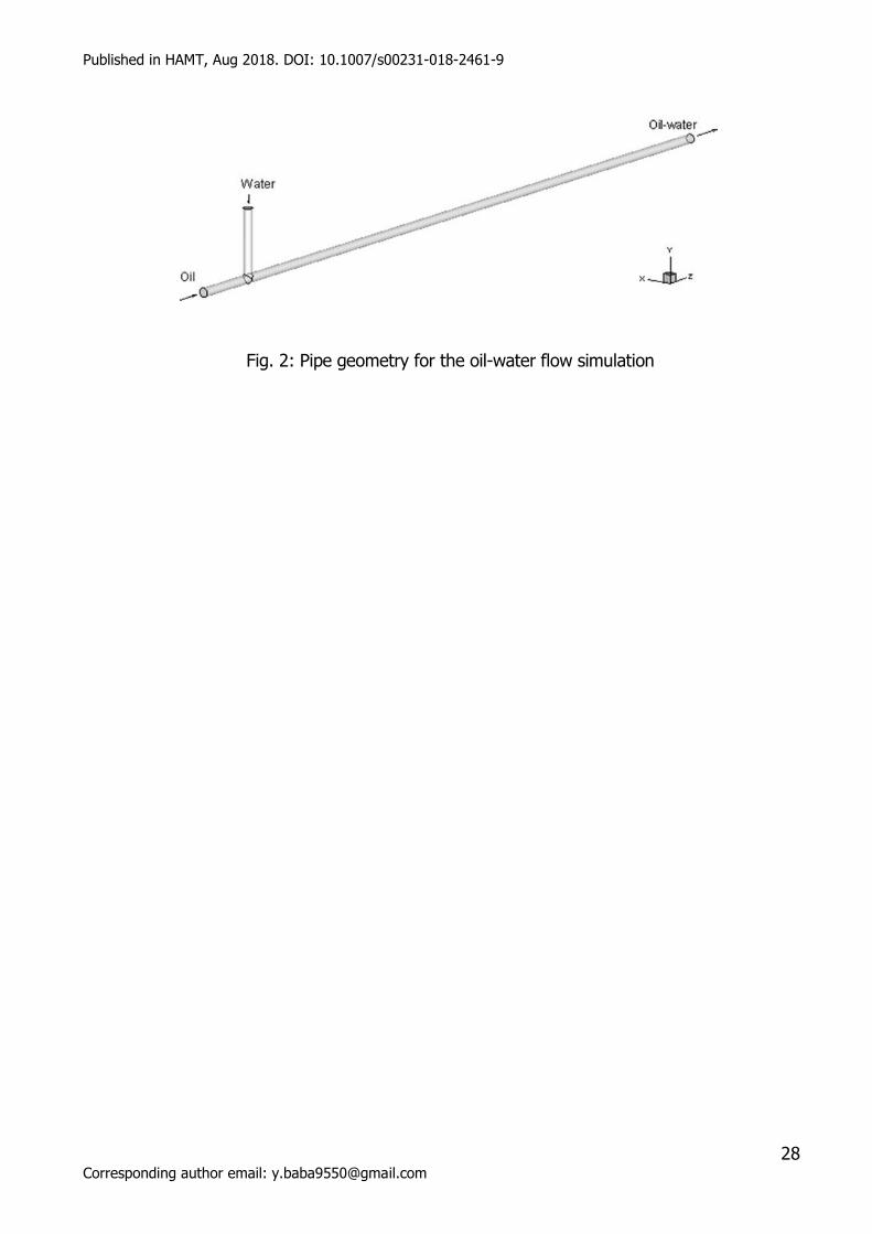
3.6 Model Geometry Design and Meshing
A three-dimensional geometry depicting the experimental test rig was created and shown in
Fig 2. The pipe internal diameter (ID) is 0.0254m; a length of 5 m (around 195D) after the
junction is used for the simulation. The junction is designed as a T-shaped inlet to mimic the
experimental test facility. Fig. 3 shows partial meshed geometry. A dependence study was
carried out using sensitivity analysis to determine the minimum mesh density that ensures that
the simulation results are independent of the mesh size. After the careful study, the mesh
used for the present simulations consisted of 1 197 440 hexahedral cells.
3.7 Numerical Simulation Setup
Boundary Conditions
The outlet pressure is applied at the outlet. No-slip boundary condition is implemented at the
wall. Velocity inlet boundary is set up at the two inlets. Material properties are set similarly to
the properties of experimental fluids. The tube is initialized with water from the water inlet at
a particular superficial velocity, then both fluids are introduced at their respective inlets and
the transient simulation is started. It is also worth stating that the developed flow profiles for
single phase oil and water are coded loaded to the solver to ensure a full flow development at
the junction. Due to its very high viscosity, oil flow is loaded as laminar while water is loaded

Published in HAMT, Aug 2018. DOI: 10.1007/s00231-018-2461-9
14 Corresponding author email: [email protected]
as laminar or turbulent depending on the water flowrate for the experimental condition to be
simulated. Convergence is judged based on the transport equation residuals. Besides, area-
averaged static pressures and water volume fractions at various cross sections are monitored
as well as mass flow rates. The hydraulic diameter and turbulence intensity are specified when
implementing the turbulence model. Fluent User’s Guide [7] estimates the turbulence intensity
for fully developed flow, 𝐼 based on the following equation:
𝐼 = 0.16𝑅𝑒−0.125 (15)
where 𝑅𝑒 is the Reynolds number for the fully developed flow.
Discretization Setup
In this study, following the hydrodynamics of the two-phase flow, all simulation runs are
conducted under transient conditions with time step used as the main controlling factor. The
explicit VOF scheme is used. A water inlet flow condition is initialized in the solution domain.
PRESTO (Pressure Staggering Option) and SIMPLE (Semi-Implicit Method for Pressure Linked
Equations) are the schemes used for the interpolation of pressure and the pressure-velocity
coupling respectively. First-order upwind spatial discretization scheme for momentum equation
is applied first and subsequently switched to second-order upwind scheme after convergence.
The interface shape is determined by the use of a Geo-Reconstruct scheme. Transient
simulation with a time step of 10−5s is initially used to obtain the convergence,
subsequently, it is increased to 10−4 and 10−3s with a global courant number ranging
from 0.6 − 0.8. Simulations are run until the monitored values have reached a stable solution
for sufficient sampling time.
4 Results and Discussion
Results obtained from experimental investigations carried out in this study are presented in

Published in HAMT, Aug 2018. DOI: 10.1007/s00231-018-2461-9
15 Corresponding author email: [email protected]
this section. Flow patterns and pressure gradients results are discussed, comparative analysis
of pressure gradient measured with that from models in literature is also carried out, a
comparative analysis of results obtained with CFD simulations for selected flow patterns are
presented and finally, conclusions and contributions of this research work is stated.
4.1 Flow Patterns
In this study, high speed video camera recordings and visual observations were utilized for
flow pattern identification. Six flow patterns were identified namely Water Plugs in Oil
continuous phase (WPO), Rivulet, Stratified Wavy Flow (SWF), Core Annular Flow (CAF), Oil
Plugs in Water Flow (OPW) and Dispersed Oil in Water Flow (DOW) flow. Table 2 shows
representative images obtained from high speed video recordings for each of the flow
patterns.
Characteristic feature of the flow patterns observed in the study are described below with
pictures obtained from video recordings shown in Table 2 below:
Water Plug in Oil Flow Pattern (WPO): This flow pattern was observed at the lowest water
superficial velocity in this study. WPO is characterized by an oil continuous phase with
intermittent water plugs flowing at the pipe’s bottom. Observably, the plugs increased in size
with increase in water superficial velocity and diminished at relatively higher oil superficial
velocity.
Rivulet flow (RIV) is characterized by a spiral motion of oil and water. This flow pattern was
observed to be the transition flow pattern from an oil dominant to a water dominant flow.
Stratified Wavy Flow (SWF) was identified at higher water superficial velocities relative to the
WPO and RIV. It is characterized by two distinct and segregated layers of oil and water with
the former flowing at the top and the latter at the bottom. A further increase in water
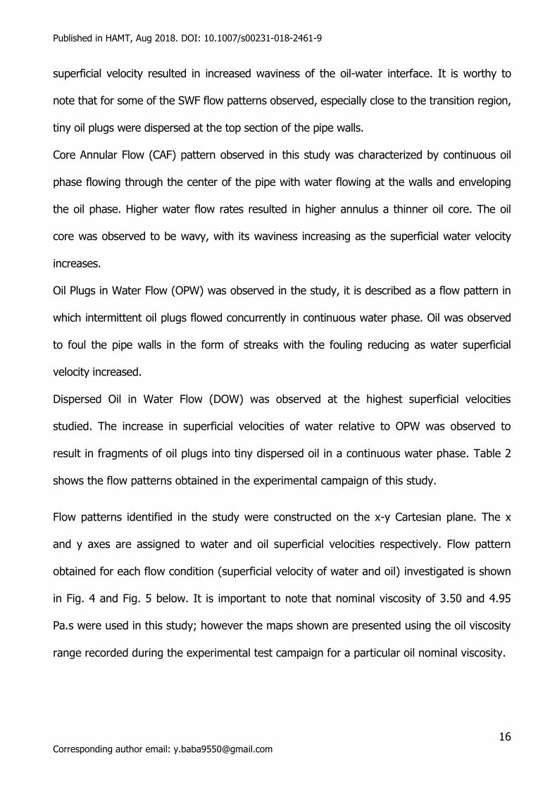
Published in HAMT, Aug 2018. DOI: 10.1007/s00231-018-2461-9
16 Corresponding author email: [email protected]
superficial velocity resulted in increased waviness of the oil-water interface. It is worthy to
note that for some of the SWF flow patterns observed, especially close to the transition region,
tiny oil plugs were dispersed at the top section of the pipe walls.
Core Annular Flow (CAF) pattern observed in this study was characterized by continuous oil
phase flowing through the center of the pipe with water flowing at the walls and enveloping
the oil phase. Higher water flow rates resulted in higher annulus a thinner oil core. The oil
core was observed to be wavy, with its waviness increasing as the superficial water velocity
increases.
Oil Plugs in Water Flow (OPW) was observed in the study, it is described as a flow pattern in
which intermittent oil plugs flowed concurrently in continuous water phase. Oil was observed
to foul the pipe walls in the form of streaks with the fouling reducing as water superficial
velocity increased.
Dispersed Oil in Water Flow (DOW) was observed at the highest superficial velocities
studied. The increase in superficial velocities of water relative to OPW was observed to
result in fragments of oil plugs into tiny dispersed oil in a continuous water phase. Table 2
shows the flow patterns obtained in the experimental campaign of this study.
Flow patterns identified in the study were constructed on the x-y Cartesian plane. The x
and y axes are assigned to water and oil superficial velocities respectively. Flow pattern
obtained for each flow condition (superficial velocity of water and oil) investigated is shown
in Fig. 4 and Fig. 5 below. It is important to note that nominal viscosity of 3.50 and 4.95
Pa.s were used in this study; however the maps shown are presented using the oil viscosity
range recorded during the experimental test campaign for a particular oil nominal viscosity.

Published in HAMT, Aug 2018. DOI: 10.1007/s00231-018-2461-9
17 Corresponding author email: [email protected]
From the maps shown in Fig. 4, it is observed that at the lowest oil superficial velocity in
this study (0.06 m/s) and water superficial velocity of 0.035 m/s, flow pattern observed is
WPO. An increase in water superficial velocity to 0.05 m/s resulted in a transition to the
RIV. Beyond this to a water superficial velocity of 0.7 m/s, flow pattern observed is SWF.
Additional increase in water superficial velocity saw a transition to the OPW and DOW.
Similar flow behaviour is observed in Fig. 5, however, at different superficial velocities.
CAF flow was not observed at the low oil superficial velocity, this is attributed to the
relatively smaller in situ oil holdup which results in the inability of the oil in the flow line to
form and maintain a core. At increased oil superficial velocities, this was not the case as the
oil in situ holdup were sufficient hence enabling a core formation and thus CAF.
Additionally, it is observed that at higher oil superficial velocities within this experimental
test matrix, CAF flow was the dominant flow pattern.
In comparison to flow patterns reported in other high viscosity oil-water studies conducted
by Sridhar et al. [4] and Vuong et al. [2], it is noted that the RIV flow patterns was not
observed in their studies. Additionally, Vuong et al. [2] studies over predicted the DOW flow
region. For flow conditions where CAF was observed in the present study, the Vuong et al.
[2] classified similar conditions DOW. The differences in flow patterns observed in the
present study and the two studies referenced is attributed to the fluid physical properties
especially the Oil viscosity. It is also noted that their studies was conducted a 2-inch pipe
internal diameter was used in their study.
Comparatively, from both flow pattern maps of Fig 4 and 5, it is observed that as viscosity
is increased from 3.4 – 3.6 Pa.s to 4.81 – 5.10 Pa.s, the CAF is observed at relatively lower
oil and water superficial velocities. For the 3.4 – 3.6 Pa.s and 4.81 – 5.10 Pa.s, it is seen

Published in HAMT, Aug 2018. DOI: 10.1007/s00231-018-2461-9
18 Corresponding author email: [email protected]
that CAF flow is first observed at oil superficial velocities of 0.15 m/s and 0.10 m/s
respectively, thus indicating that an increase in oil viscosity may favour the formation of the
CAF pattern within this experimental study range.
4.2 Pressure Gradient
Pressure gradient obtained in the study were plotted as functions of water cut for different
oil superficial velocities and are as shown in Fig. 6 and 7 below. It is observed that the
pressure gradient is a strong function of the water cut & flow patterns.
Generally, for water cut below 20% (most of which correspond to water superficial
velocities less than 0.15 m/s), flow patterns observed were oil dominant, this results in
increased shear on the pipe walls and thus, the relatively high pressure gradient observed
for these flow conditions. As the water cut (and thus the water superficial velocity) is
further increased, pressure gradient reduces as water helps to lubricate and thus reduce
shear on the pipe wall.
The most significant reduction in pressure gradient is observed mostly around the CAF flow
pattern region, this is attributed to water being constantly in contact with the pipe walls and
thus reducing the pipe wall shear. Beyond the minimum pressure gradient, oil at the core
fragments and moves in flow as either oil plugs or dispersed oil in continuous water flow
(OPW and DOW respectively), this results in a gradually increasing pressure gradient due
mainly to the fact that some of the dispersed oil and oil plugs are now in contact with the
pipe walls and the increased flow mixture velocity results in a more turbulent flow thereby
contributing to this increase.

Published in HAMT, Aug 2018. DOI: 10.1007/s00231-018-2461-9
19 Corresponding author email: [email protected]
4.3 Comparison of Current Pressure Gradient with Previous Studies
Shi et al [16] did an extensive study of water-lubricated flow using the same experimental
rig but with a different lube oil (also see Al-Awadi, [17]). They used the Colebrook–White
equation (Colebrook [18]) to approximate the friction factor of single water flow in both
hydraulic smooth pipes and rough pipes. For checking the consistency of the current
results, the friction factors of both studies were compared, and they exhibited a similar
trend. For the experimental Reynolds number range between 5000 and 35,000, the friction
factor of water-lubricated transport of high-viscosity oil is reaches up to two times higher
than that of single water flow. With increase of the Reynolds number hence the mixture
velocity, the friction factor of the water-lubricated flow declines faster than that of single
water flow. This is due to the fact that the oil fouling on the pipe wall reduces with increase
in mixture velocity.
At developed water-lubricated flow conditions, increasing concentricity is established at
larger oil superficial velocities, resulting in less oil contact with the pipe walls. Furthermore,
a higher water velocity can flush oil fouling films on the pipe wall more effectively. As two
groups of data were conducted in the same pipeline, it is suspected that the difference
shown is due to different wettability of the pipe wall by the two different oils, and these
results in different degrees of oil fouling. The wettability between the Perspex pipe and oils
were not measured quantitatively in the present study. Nevertheless, we noticed that the oil
fouling on the pipe wall was generally more severe for experiments with CYL 1000 oil. A
quantitative study on the influence of wettability on the pressure gradient of water-
lubricated flow is recommended for future studies.
Pressure gradient models by Bannwart et al. [1], Arney et al. [14], Joseph et al. [15] and

Published in HAMT, Aug 2018. DOI: 10.1007/s00231-018-2461-9
20 Corresponding author email: [email protected]
Yusuf et al. [16] are evaluated against measured pressure gradient data obtained in this
studies experiment. A plot of predicted pressure gradient as a function of the measured
pressure gradient is shown in Fig. 8. The plot shows large disparity between the measured
and the predicted pressure gradient. This discrepancy may be attributable to the large
differences in viscosity between the present study and the studies in which
models/correlations were based on as a result of the differences in flow patterns. Another
key reason for the discrepancies is as a result of the pipeline fouling. In this study, it was
observed that oil fouled the inside walls of the pipelines, for flow patterns were water was
not the continuous phase, this effect was very prominent. This will ensure that the friction
factor of the pipe walls will increase and hence the pressure gradient, a factor not
accounted for in the pressure gradient prediction correlations evaluated, for oil-water flow
in pipelines as earlier explained. This work therefore establishes a need for future
experimental and theoretical work to be carried out on two-phase high viscosity oil-water
flow to ensure deeper understanding of the flow hydrodynamics for a very wide viscosity
range and to ensure further development of predictive models are based on this
experimental dataset. This will form a framework on future research work in this field.
4.4 Comparison of CFD Simulation and Experiments
In this section, CFD simulation results for selected flow patterns are presented. Flow
patterns simulated include the stratified wavy flow (SWF), the Core Annular Flow (CAF) and
Oil Plugs in Water Flow (OPW). Results obtained for pressure gradient from each of the
simulated flow condition is also presented.
4.5 Flow Pattern Predictions from CFD Simulation
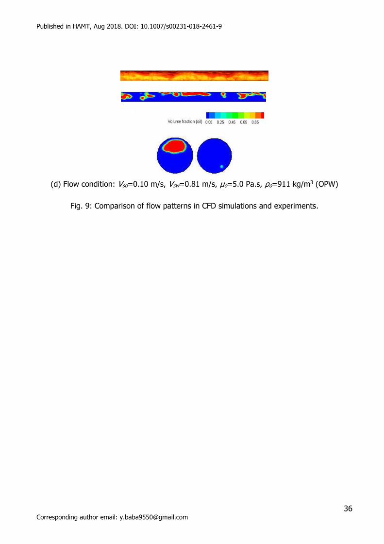
Fig. 9 below shows predicted contour plots of oil volume fraction as well as the

Published in HAMT, Aug 2018. DOI: 10.1007/s00231-018-2461-9
21 Corresponding author email: [email protected]
corresponding snapshots from recorded experimental videos for four different flow
conditions. For a nominal oil viscosity of 5.0 Pa.s and superficial oil velocity around 0.1 m/s
and at different superficial velocities, the flow patterns in the two-phase flow are reasonably
predicted. Fig. 9 (a) shows the SWF with discontinuous thin water film at the top. From
video recordings as shown in flow pattern map of Fig. 4, SWF was predicted. This
dissimilarity may be as a result of SWF proximity to the CAF region and hence a transition.
Oil drops at the interface between the top oil layer and the bottom water layer can be
observed in experiments, while these drops are not captured from the modelling. This may
be as a result of the mesh density near the predicted interface not being denser; it may
also be as result of VOF model limitation. The model uses the same set of momentum
equations for the two phases. The present pipe mesh is made finer near the pipe wall to be
suitable for the turbulence model selected and coarser away from the pipe wall to optimise
computational time. Improved prediction may be attained with a finer meshing.
With an increase water superficial velocity from 0.05 m/s to 0.1 m/s, Fig. 9 (b) shows a
thicker top water film and wavier interface compared to Fig. 6(a); CAF is formed and
predicted. In Fig. 9 (c), at water superficial velocity of about 0.20 m/s (input water volume
fraction of 0.67), fluctuations of the oil core as a whole is observed; heavy oil fouling on the
internal pipe wall is seen due to oil core intermittently making contact with the pipe walls.
CFD prediction is consistent with the experimental observations. The oil core is much wavier
(especially at the top interface) compared to Fig. 9 (b). Additionally, a bit of oil fouling is
captured. On further increasing the water superficial velocity, the oil core fragments into oil
plugs as shown in Fig. 9 (d). Oil film can be seen from experimental videos, while for this
condition no oil film is captured. This may be as a result of the mesh density. In general,
CFD simulation gives a good prediction of the flow patterns observed in experiments.

Published in HAMT, Aug 2018. DOI: 10.1007/s00231-018-2461-9
22 Corresponding author email: [email protected]
Similar conclusions were also made for CFD simulation comparison with experiments
reported by [6] for oil viscosity of 0.28 Pa.s. This implies that the VOF model is reasonably
sufficient for the prediction of flow patterns in oil-water two phase flows for oil viscosity up
to 5.0 Pa.s.
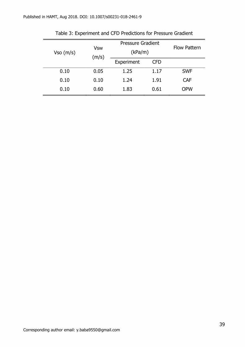
4.6 Pressure Gradient Prediction from CFD Simulation
Pressure gradient results predicted from CFD simulation is shown in Table 3 below. Results
show that CFD numerical simulation overestimates pressure gradient for the CAF flow
pattern and underestimates pressure gradients in the SWF and OPW flow patterns. In
general, unlike the flow pattern configurations, pressure gradient prediction from CFD
numerical simulation gave not as much similarity when compared to the experimental
measurements. Hence, more advanced numerical approaches will need to be implemented
in future studies. These include the use of finer meshes near the wall for all flow rates, and
for CAF flow patterns, this should be extended to cover regions of expected liquid film flow.
5 Conclusions
High viscous oil-water two phase flow has been experimentally investigated. New
experimental results have been presented. Water Plug in Oil Flow (WPO), Rivulet flow
(RIV), Stratified Wavy Flow (SWF), Core Annular Flow (CAF), Oil Plugs in Water Flow (OPW)
and Dispersed Oil in Water Flow (DOW) were the flow patterns observed in the study. At
high oil superficial velocities, CAF flow was observed to be the dominant flow pattern while
the OPW and DOW were dominant at high superficial water velocities. Practically, this
indicates that for heavy oil fields with low water cut, producing such fields using the CAF
technology may be promising while the emulsion techniques may be promising for fields
with high water cut.

Published in HAMT, Aug 2018. DOI: 10.1007/s00231-018-2461-9
23 Corresponding author email: [email protected]
Pressure Gradient results showed a general trend of reduction to a minimum as water
superficial velocity increases before subsequently increasing on further increasing the
superficial water velocity. Pressure gradient predictive models found in literature were
compared with present experimental dataset, huge discrepancies in were observed and a
need to develop new models or modify existing ones is established. CFD numerical
simulation performed moderately well in predicting the flow configurations observed in this
study. However, results for the pressure gradient predictions were not as good.
Acknowledgement
The authors are grateful to BP Exploration Operating Company Ltd., Sunbury, UK for
originally funding the test facility for a research project. We also acknowledge the immense
assistance from laboratory and research staff in the Oil and Gas Engineering Centre at
Cranfield University in this work especially the tireless efforts of Mr. Stan Collins. Y. Baba,
AM Aliyu and O. Alagbe are grateful to the Petroleum Technology Development Fund,
Nigeria for funding their PhD research work. J. Shi equally appreciates the sponsorship the
Chinese Government provided for her PhD research work.
Conflict of Interest Statement
On behalf of all authors, the corresponding author states that there is no conflict of interest.

Published in HAMT, Aug 2018. DOI: 10.1007/s00231-018-2461-9
24 Corresponding author email: [email protected]
References
1. Bannwart AC, Rodriguez OMH, de Carvalho CHM, Wang IS, Vara RMO. Flow Patterns in
Heavy Crude Oil-Water Flow. Journal of Energy Resources Technology. J. Energy
Resour. Technol. 2004 Oct 19; 126(3); 184-189.
2. Vuong, DH, Zhang, HQ, Sarica, C, Li, M. Experimental Study on High Viscosity Oil/Water
Flow in Horizontal and Vertical Pipes. Presented at SPE Annual Technical Conference and
Exhibition, New Orleans, Louisiana, USA; 2009 Oct. 4-7.
3. Poesio P, Strazza D, Sotgia G. Two and Three-Phase Mixtures of Highly Viscous-
Oil/Water/Air in a 50 mm ID Pipe. Journal of Applied Thermal Engineering. 2012 Dec.31;
49; 41 – 47.
4. Sridhar S, Zhang H-Q, Sarica C, Pereyra, E. Experiments and Model Assessment on
High-Viscosity Oil/Water Inclined Pipe Flow. SPE Annual Technical Conference and
Exhibition. Denver, Colorado, USA. 2011 Oct 30 – Nov. 2.
5. Wang W, Gong J, Angeli P. Investigation of Heavy Crude-Water Two Phase Flow and
Related Flow Characteristics. International Journal of Multiphase Flow. 2011 Nov.;
37(9);1156 – 1164
6. Rodriguez OMH, Baldani LS. Prediction of pressure gradient and holdup in wavy
stratified liquid–liquid inclined pipe flow. Journal of Petroleum Science and Engineering.
2012 Oct. 96(97); 140–151.
7. ANSYS Fluent, release 14.5, ANSYS Fluent Theory Guide (2012), ANSYS Inc.,
Canonsburg, USA.
8. Ghosh S., Das G., Das, PK. Simulation of core annular down flow through CFD – A
comprehensive study. Journal of Chemical Engineering and Processing: Process

Published in HAMT, Aug 2018. DOI: 10.1007/s00231-018-2461-9
25 Corresponding author email: [email protected]
Intensification. 2010 Nov. 49(11); 1222-1228.
9. Kaushik VVK, Ghosh S, Das G, Das PK. CFD Simulation of core annular flow through
sudden contraction and expansion. Journal of Petroleum Science and Engineering. 2012
May; 86(87); 153 – 164.
10. Brackbill, J., Kothe, DB. Zemach, C. A continuum method for modelling surface tension.
Journal of computational physics, 2012; 100 (2); 335 – 354.
11. Alagbe SO. Experimental and numerical investigation of high viscosity oil-based
multiphase flows. PhD Thesis, Cranfield University, UK. 2014.
12. Menter FR. Two-equation eddy-viscosity turbulence models for engineering applications.
AIAA Journal, 1994; 32 (8); 1598 – 1605.
13. Wilcox, DC. Turbulence modeling for CFD. Fluid dynamic measurements California; DCW
industries, 1994.
14. Arney M. S., Bai R, Guevara E, Joseph, D, Liu K. Friction factor and holdup studies for
lubricated pipelining—I. Experiments and correlations. International journal of
multiphase flow, 1993; 19(6), 1061 – 1076.
15. Joseph D., Renardy Y. Fundamentals of two-fluid dynamics. Pt. II: Lubricated transport,
drops and miscible liquids New York: Springer-Verlag.1993.
16. Shi, J., Lao, L., Yeung, H., Water-lubricated transport of high-viscosity oil in horizontal
pipes:
The water holdup and pressure gradient, International Journal of Multiphase Flow 96
(2017) 70-85
17. Al-Awadi, H., 2011. Multiphase Characteristics of High Viscosity Oil PhD thesis. Cranfield
University, UK.

Published in HAMT, Aug 2018. DOI: 10.1007/s00231-018-2461-9
26 Corresponding author email: [email protected]
18. Colebrook, C.F., 1939. Turbulent flow in pipes, with particular reference to the transition
region between the smooth and rough pipe laws. J. ICE 11 (4), 133–156.

Published in HAMT, Aug 2018. DOI: 10.1007/s00231-018-2461-9
27 Corresponding author email: [email protected]
Fig. 1: Flow Schematics of the 1 inch Test Facility.
Published in HAMT, Aug 2018. DOI: 10.1007/s00231-018-2461-9
28 Corresponding author email: [email protected]
Fig. 2: Pipe geometry for the oil-water flow simulation

Published in HAMT, Aug 2018. DOI: 10.1007/s00231-018-2461-9
29 Corresponding author email: [email protected]
Fig. 3: Mesh for oil-water flow simulation

Published in HAMT, Aug 2018. DOI: 10.1007/s00231-018-2461-9
30 Corresponding author email: [email protected]
Fig. 4: Experimental flow pattern map for oil nominal viscosity of 3.5 Pa.s.

Published in HAMT, Aug 2018. DOI: 10.1007/s00231-018-2461-9
31 Corresponding author email: [email protected]
Fig. 5: Experimental flow pattern map for oil nominal viscosity of 5.0 Pa.s.

Published in HAMT, Aug 2018. DOI: 10.1007/s00231-018-2461-9
32 Corresponding author email: [email protected]
Fig. 6. Experimental pressure gradient as a function of water cut (μo = 3.5 Pa.s).

Published in HAMT, Aug 2018. DOI: 10.1007/s00231-018-2461-9
33 Corresponding author email: [email protected]
Fig. 7: Experimental pressure gradient as a function of water cut (μo = 5.0 Pa.s).

Published in HAMT, Aug 2018. DOI: 10.1007/s00231-018-2461-9
34 Corresponding author email: [email protected]
Fig. 8: Model predicted pressure gradients compared to various reported measurements.

Published in HAMT, Aug 2018. DOI: 10.1007/s00231-018-2461-9
35 Corresponding author email: [email protected]
(a) Flow c condition: Vso=0.10 m/s, Vsw=0.05 m/s, μo=5.0 Pa.s, ρo=911 kg/m3 (SWF)
(b) Flow condition: Vso=0.10 m/s, Vsw=0.10 m/s, μo=5.0 Pa.s, ρo=911 kg/m3 (CAF)
(c) Flow condition: Vso=0.10 m/s, Vsw=0.20 m/s, μo=5.0 Pa.s, ρo=911 kg/m3 (CAF)
Published in HAMT, Aug 2018. DOI: 10.1007/s00231-018-2461-9
36 Corresponding author email: [email protected]
(d) Flow condition: Vso=0.10 m/s, Vsw=0.81 m/s, μo=5.0 Pa.s, ρo=911 kg/m3 (OPW)
Fig. 9: Comparison of flow patterns in CFD simulations and experiments.

Published in HAMT, Aug 2018. DOI: 10.1007/s00231-018-2461-9
37 Corresponding author email: [email protected]
Table 1: Physical Properties of Test Fluids
Test fluids Density at 25 ̊C
(kg/m3)
Viscosity at
25 °C (Pa.s)
Interfacial
tension at
19 °C,(N/m)
API
gravity
Water ≈ 998 0.00103
0.029
---
CYL680 ≈ 917 1.83 22.67

Published in HAMT, Aug 2018. DOI: 10.1007/s00231-018-2461-9
38 Corresponding author email: [email protected]
Table 2: Representative images for the observed flow patterns
Flow Patterns
Water Plug in Oil Flow
Rivulet Flow
Stratified Wavy Flow
Core Annular Flow
Oil Plugs in Water Flow
Dispersed Oil in Water Flow
Published in HAMT, Aug 2018. DOI: 10.1007/s00231-018-2461-9
39 Corresponding author email: [email protected]
Table 3: Experiment and CFD Predictions for Pressure Gradient
Vso (m/s) Vsw
(m/s)
Pressure Gradient
(kPa/m) Flow Pattern
Experiment CFD
0.10 0.05 1.25 1.17 SWF
0.10 0.10 1.24 1.91 CAF
0.10 0.60 1.83 0.61 OPW