Engineering Growth:Innovative Capacity and Development in the Americas∗

William F. Maloney† Felipe Valencia Caicedo‡

March 9, 2016

Abstract

This paper offers the first systematic historical evidence on the role of a central actor inmodern growth theory- the engineer. We collect cross-country and state level data onthe population share of engineers for the Americas, and county level data on engineeringand patenting for the US during the Second Industrial Revolution. These are robustlycorrelated with income today after controlling for literacy, other types of higher orderhuman capital (e.g. lawyers, physicians), demand side factors, and instrumentingengineering using the Land Grant Colleges program. We support these results withhistorical case studies from the US and Latin America.

Keywords: Innovative Capacity, Human Capital, Engineers, Technology Diffusion,Patents, Growth, Development, History.

JEL: O11,O30,N10,I23

∗Corresponding author Email: wmaloney@worldbank.org. We thank Ufuk Akcigit, Leo Feler, ClaudioFerraz, Christian Fons-Rosen, Oded Galor, Steve Haber, Lakshmi Iyer, David Mayer-Foulkes, SteliosMichalopoulos, Guy Michaels, Petra Moser, Giacomo Ponzetto, Luis Serven, Andrei Shleifer, MoritzShularick, Enrico Spolaore, Uwe Sunde, Bulent Unel, Nico Voigtlander, Hans-Joachim Voth, FabianWaldinger, David Weil and Gavin Wright for helpful discussions. We are grateful to William Kerr formaking available the county level patent data. We thank audiences at the London School of Economics,London Business School, Williams College, SAEe 2013 and FRESH 2013 (Valencia). Our thanks to CarlosAndres Molina, Melissa Rubio, and Mauricio Sarrias for meticulous research assistance. This paper waspartly supported by the regional studies budget of the Office of the Chief Economist for Latin America andKnowledge for Change (KCP) trustfund.†Development Economics Research Group and Chief Economist, EFI, The World Bank.‡Department of Economics and Institute of Macroeconomics and Econometrics, University of Bonn.

“You have all the elements, but you cannot make steel”

—Andrew Carnegie (1900)1

1 Introduction

Carnegie’s taunt to the owners of the Birmingham Steel Company suggests the difficulties

the American South faced in absorbing the knowledge required to establish dynamic indus-

tries and converge to the North. This remains the case in today’s developing regions- a vast

literature now puts barriers to technological adoption at the center of explanations of the

distribution of income globally.2 Most recently Comin et al. (2008); Comin & Ferrer (2013)

argue that the diverging measured intensity of use of new technologies plausibly explains

observed TFP differentials and can drive simulations that closely track the magnitudes of

the Great Divergence of the last two centuries (e.g. Pritchett, 1997; Galor & Weil, 2000;

Galor, 2011).3

That human capital is a critical ingredient in technology adoption also enjoys a sub-

stantial supporting literature.4 There is no consensus, however, on what type of human

capital is most important and, in particular, the role of the upper tails of the education

distribution, including higher order technical skills. Modern growth theory (Romer, 1990),

1Cited in Wright (1986) p.171. Wright also documents similar difficulties in the textile and lumberindustries.

2See also, Parente & Prescott (1994); Eaton & Kortum (1999, 2001); Caselli (2001); Comin & Hobijn(2004); Keller (2004); Klenow & Rodriguez-Clare (2005); Comin et al. (2008, 2010a); Comin & Hobijn (2010);Comin et al. (2012).

3Though not clear on the underlying determinants, recently Acemoglu et al. (2013) argue for theimportance of a the shift in industrial composition from those with low to high innovative capacity as criticalto growth.

4See, for example, Nelson & Phelps (1966); Foster & Rosenzweig (1996); Cohen & Levinthal (1989);Benhabib & Spiegel (1994); Basu & Weil (1998); Temple & Voth (1998); Howitt (2000); Acemoglu & Zilibotti(2001); Krueger & Lindahl (2001); Caselli (2001); Jones (2002); Comin & Hobijn (2004); Benhabib & Spiegel(2005); Aghion et al. (2005); Howitt & Mayer-Foulkes (2005); Aghion et al. (2009); Ciccone & Papaioannou(2009); Goldin & Katz (2009); Barro & Lee (2015).

1

empirical studies of technological transfer and innovation, and historical accounts of the

Industrial Revolution put the engineer and associated scientific institutions at the center of

the growth process, especially during the Second Industrial Revolution (see, for example,

Mokyr, 1998).5 Yet, despite recent empirical work rigorously documenting the importance

of some of these factors,6 there is no systematic evidence on the historical prevalence of

engineers and hence, their plausible importance to explaining the geographical patterns of

development that we see today.

In this paper we first make this very basic contribution. We establish the stylized facts

surrounding the relative density (population share) of engineers during the second wave

of the Industrial Revolution (circa 1900) at the national level for the Western Hemisphere

and representative benchmark countries of Europe, and the same at the sub-national level

for six countries in the Americas.7 The engineering data collection is done in a systematic

way drawing on graduation records, membership in professional societies, and census data.

We see these estimates, first, as a measure of what they are: the stock of higher level

scientifically oriented human capital available during the second wave of the Industrial

Revolution. Second, because our national measures are based on graduates of domestic

engineering schools, they also proxy for the universities and institutions that support them,

and for which data are more elusive. Further, we are sympathetic to the use in Murphy

et al. (1991) of engineering density as a proxy for “good entrepreneurship.” In sum, we see it

as a broad proxy for innovative capacity defined as the capacity to absorb new technologies

from abroad and modify as necessary, as well as invent. We document the extraordinary

variance in engineering density across countries of very similar income levels in 1900-for

instance Argentina, Chile, Denmark, Sweden and the southern US- that correlates to their

5See Gordon (2016) for a discussion of the centrality of this period to US and world growth.

6Becker et al. (2011); Cantoni & Yuchtman (2014); Voigtlander & Squicciarini (2014); Yuchtman (2014).

7We focus on this geographical area partly because of the centrality of the very disaggregated US analysisdiscussed below, and partly because, as noted by Engerman & Sokoloff (1994); Acemoglu et al. (2001, 2002),the colonized New World provides an experiment yielding strikingly divergent development outcomes acrossstates.

2

divergent income positions today.

To more confidently establish the importance of engineers and innovative capacity as a

determinant of income, we then develop a rich data set for the United States at the county

level. The increased degrees of freedom allow controlling for an extensive set of geographical,

growth related, and human capital variables that may be confounded with engineering. We

instrument for possible endogeneity of engineering using the Morrill Land Grant Colleges

program. This program had an important long run impact on establishing engineering

training institutions, however this was not its initial intent and the location of the colleges

was largely independent of demand considerations. We further incorporate geo-located

patenting density as collected by Acemoglu et al. (2013). Patenting appears only weakly

explained by county engineering density and hence, we treat it as capturing human capital

more dedicated to invention (Griliches, 1990; Sokoloff, 1988) while engineering may arguably

be capturing more adoptive activities.

Both variables show an important and robust effect: a one standard deviation in

engineering density in 1900 accounts for a 16% rise in income today, and patenting capacity,

though not instrumented, perhaps another 10%. We find very similar coefficients at

the “state” level both for the US, suggesting migration issues among geographical units

are not critical, and for a broader sample of countries in the hemisphere. Applying the

well-estimated US county-level coefficient to the national level data, 1 standard deviation

in engineering density in 1900 accounts for a 36% difference in income today. We then use

historical evidence to validate our ranking of innovative capacity and through case studies

document the divergent development outcomes arising within industries and even identical

goods (e.g. copper) in countries with the differing innovative capacities we quantify. Finally,

we present some suggestive findings on the historical determinants of innovative capacity.

3

2 Literature

The economics literature has postulated several types of human capital that may be

important to growth. Literacy, and accumulated years of schooling or enrollment have

received the most attention (see Krueger & Lindahl, 2001; Barro & Lee, 2015), although

as Vandenbussche et al. (2006); Aghion et al. (2009), the composition among levels of

education matter as well depending on distance from the frontier. Other dimensions figure

importantly as well: Lucas (1993); Young (1993) and Foster & Rosenzweig (1995), among

others, stress the importance of accumulated “learning by doing”; Ben Zeev et al. (2015);

de la Croix et al. (2015) focus on apprenticeship; and Baumol (1990) and Murphy et al.

(1991), entrepreneurial skills and orientation. In in his classic article on endogenous growth

Romer (1990) highlights the research engineer and Mokyr (2005), the minority of “trained

engineers, capable mechanics and dexterous craftsmen on whose shoulders the inventors

could stand” (pg.16, see also Meisenzahl & Mokyr (2011)). Rosenberg (2000) and Nelson

(2005) stress the accumulated ability and scientific institutions to manage new ideas for

innovation and invention and Cohen & Levinthal (1989); Griffith et al. (2004), the capacity

for research and development needed for technological transfer.

Several authors including Mokyr (1998), and Howitt & Mayer-Foulkes (2005) stress that

higher-order human capital and the institutions that generated and housed it may have

had an even more determinant role at the dawn of the Second Industrial Revolution (circa

1870-1914), which saw an increased emphasis on more structured scientific inquiry such as

laboratory-based R&D.8 This scientifically oriented human capital, and a technologically

savvy entrepreneurial class were necessary to tap into the expanding and increasingly

sophisticated global stock of knowledge and convert it into local growth.9 The technological

8Rosenberg (2000) and Nelson (2005) stress the incremental and cumulative nature of technologicalprogress and related institutions more generally as a central dynamic of industrialization.

9As numerous authors have stressed from Schumpeter (1934) to the present, technological progresswithout entrepreneurs to take it to market does not lead to growth (see Aghion & Howitt, 1992; Baumol,1990, 2010; Glaeser, 2007; Glaeser et al., 2009, 2010; Braunerhjelm et al., 2010; Iyigun & Owen, 1998, 1999).Over the longer term this reflects the accumulation of a specific kind of human capital, at the very least,suited to the evaluation and management of risk, but extending to skills for managing people, credit, and

4

leap forward also meant an erosion in the efficacy of existing levels of human capital and

innovative capacity relative to that needed to continue to adopt (see Howitt (2000); Aghion

et al. (2005)). Building on this insight, Howitt & Mayer-Foulkes (2005) argue for multiple

equilibria in innovation where countries whose human capital evolved with the frontier at

the time of the technological leap forward could innovate or adopt, but those whose frontier

adjusted human capital did not keep up slipped to an equilibrium where even the adoption

of technologies was difficult, and stagnation followed (see Annex I and Section 6 for a sketch

of the model).10 Iyigun & Owen (1998, 1999) relatedly argue that if the the initial stock

of both professional (scientific) and entrepreneurial human capital is too low, the return to

accumulating human capital will be low and economies can find themselves in a development

trap in the long run.

Empirically, documenting the impact of even very basic measures of human capital on

growth or relative incomes has proved surprisingly complex since the seminal studies of

Barro (1991) and Mankiw et al. (1992).11 Most recently, and in a similar spirit to the present

work, Hanushek et al. (2015) find that differences in human capital account for 20-35 percent

of the current variation in per-capita GDP among US states. Further, there have been

relatively few efforts to systematically capture what kind of human capital matters, or even

to document the stocks of different types of capital. Goldin & Katz (2011); Goldin (1999);

Goldin & Katz (1999) have documented the evolution of secondary and tertiary education

in the context of US growth. Judson (1998), Wolff & Gittleman (1993), Self & Grabowski

(2004), Castello-Climent & Mukhopadhyay (2013) attempt to document whether tertiary

education matters more or less than primary education. Closest to this work, Murphy et al.

technologies which need to be learned.

10Also Gancia et al. (2008) for related discussion of convergence clubs resulting from education-technologycomplementarities.

11For overviews see Krueger & Lindahl (2001); Sianesi & VanReenen (2003); Stevens & Weale (2004)and Acemoglu & Zilibotti (2001); Pritchett (2001); Easterly (2002); Benhabib & Spiegel (1994). A recentliterature has sought to explain the often small measured impact by incorporating measures of the qualityof human capital (see, for example Hanushek & Woessmann, 2007; Behrman & Birdsall, 1983; Hanushek &Woessmann, 2012).

5

(1991) document that countries with a higher proportion of engineers grow faster relative

to those with a higher proportion of law concentrators. Most recently, Hsieh et al. (2013)

argue that the rise in higher level skills among particularly women and African Americans

resulting from reduced barriers to occupational allocation raised US growth substantially

since 1960.

The problem is exacerbated when a longer historical perspective is taken. Cantoni

& Yuchtman (2014) show that areas closer to the first German universities around 1386

experienced increased economic activity. Campante & Glaeser (2009) argue that the “lion’s

share” of the differences in long run income level between the cities of Buenos Aires and

Chicago is human capital, but they lament that literacy remains the primary, albeit coarse,

measure (see, for example, Mariscal & Sokoloff (2000)). Voigtlander & Squicciarini (2014)

show that mid-18th century French cities with more subscriptions to the Encyclopedie, cap-

turing higher order human capital, grew faster after the dawn of the Industrial Revolution.

Becker et al. (2011) show basic education in Prussia in the 19th century to be associated

with industrialization. Yuchtman (2014) shows that in early 20th century China, engineers

enjoyed massive wage premia over all other classes of higher education and that modern

Western education and engineers in particular were critical to China’s ability to adopt

Western technologies.12 Waldinger (2012) shows that the dismissal of scientists in Nazi

Germany led to a permanent decrease in growth while Moser et al. (2014) show that their

immigration to the US substantially increased invention there.

To date, however, neither the historical prevalence of Romer’s research engineers or

Mokyr’s engineers and mechanics, nor Rosenberg’s and Nelson’s systems of innovation have

been quantified in a globally comparable form and, in particular during periods of intense

technological change such as the Second Industrial Revolution. That is, the profession has

no systematic historical evidence on allegedly the central actor in modern economic growth,

12Similarly Braguinsky & Hounshell (2015) note that engineers were the highest paid employees in in theflagship Japanese textile industry in the 1880s and were critical for technology transfer in the dominant firm.

6

or even the relative importance of the upper tails of technical knowledge for growth.13

Remedying this is the focus of the present paper.

3 Data

3.1 Measuring Engineering/Innovative Capacity

Our primary measure of innovative capacity at the national level across all countries is the

number of engineers with domestically emitted university degrees per 100,000 male workers.

Unlike literacy data, which countries sometimes collect as part of the census, countries do

not tabulate such information in a uniform fashion. Hence, we construct these series using

three sources of data.

Engineering Graduates : To the degree possible, calculations are done with actual gradu-

ates of engineering colleges and universities within the country. Clearly, many engineers even

in the US acquired valuable training on the ground, or may have had partial degrees from

some type of technical program. However, such skills are difficult to capture with any degree

of commonality across geographical units. As a more consistent metric across countries,

we take the number of degrees awarded.14 Though most countries also employed foreign

engineers, we are interested in indigenous technical capacity and the institutional structure to

generate it, so we focus on domestically trained engineers.15 Some nationals studied abroad,

however the historical evidence from Argentina, Chile, Colombia and Mexico suggests the

numbers are small and difficult to document. Since the working life of an engineer is roughly

40 years, we begin accumulating the stock in 1860, discounting the stock in each period by

13Collected articles in Fox & Guagnini (1993) have examined the evolution of engineering capacity inseveral advanced countries although the comparability of the measures across countries is not always clear,and there is no attempt to establish a link to economic performance.

14Fox & Guagnini (1993) tabulate for several advanced countries the number of students enrolled. However,we find often that the difference between students enrolled and eventual graduates can differ greatly soenrollment rates are not as reliable.

15For Argentina we have data on both foreign and domestic engineers and including the former leaves theresults unchanged.

7

.983 as the rate of death/attrition in each year. In some cases, we have a long series of grad-

uation records which make this procedure straightforward. In Bolivia, Denmark, Mexico,

New York, Peru, Spain, Sweden, Venezuela, or Mexico, the flow of graduated engineers is

available for the 1860-1900 period. We refer to Ahlstrom (1982)’s estimates for Germany and

France, the frontier countries, which are allegedly generated in a virtually identical manner,

yet we do not have access to his data and these are not our calculations.16 In other cases, for

instance, Argentina, Brazil, Chile, Colombia, Ecuador, and the US as a whole, the informa-

tion is less complete and we bring other sources of data to bear to fill in the gaps in the series.

Membership in Engineering Societies : Data on membership in Engineering societies

or official registries validate broad orders of magnitude of our generated stocks. In some

cases, such as Brazil, registry with the government was required to be a practicing engineer.

What is considered an engineer, however, is less clear and hence these measures are less

definitionally tight. In other countries, such as Colombia or Argentina, membership in

Engineering associations was not required so registration likely underestimates.

Census Data: Census data are also available in several countries. Census data have the

advantage of being collected over time by several countries and across sub-national units.

However, here, also, it is the individual respondent who is deciding whether he is an engineer

or not with limited institutional confirmation, or detail on the actual level of education.

This is fine for within country analysis but less reliable for cross-country comparisons.17

Sub-national data derive from the Argentine census of 1895, Mexican National Census of

1895, Chilean Census of 1907, Colombian census of 1912, Venezuelan Census of 1926, and

US Census of 1900. For the US county level data, we use the census of 1880 to generate

measures of literacy, and density of engineers, lawyers and medical doctors.

16In fact, he calculates the stock for France, Germany as well as Sweden for which we do have the rawunderlying data and hence can verify that we are doing the calculations in a virtually identical fashion.

17As numerous local historians have noted (Serrano (1993) in Chile, Bazant de Saldana (1993) in Mexico)and in the case for which we have the best information, the US, censuses are often substantially higher thanthe actual graduates of engineering programs.

8

Annex II discusses how these three sources of data were employed for each country in

detail.

Patenting : For the US, we also construct a measure of average patenting activity from

1890-1910 drawing on patents granted by the United States Patent and Trademark Office

(USPTO) again, at the county level, provided by Acemoglu et al. (2013). This is likely to

capture Mokyr’s more structured scientific inquiry at the frontier that began to assume a

central role in the Second Industrial Revolution in addition to its direct interpretation as

new ideas. It does not appear driven by engineers or the other human capital variables

and hence interpret it as captures a distinct type of human capital (see Sokoloff, 1988),

or alternatively as a measure of institutions that promote it. Comparable patent data is

not available for the Latin American countries and hence the variable only enters in the

county-level US analysis.

3.2 Sub-national Income per Capita

Income in 2005 PPP US Dollars is drawn from a highly disaggregated spatial data set on

population, income and poverty constructed on the basis of national census data by the

World Bank (2009) for the World Development Report on Reshaping Economic Geography.18

Modern county level US income in dollars is mean household income taken from the 2000

US Census.

3.3 Controls

As controls in our regressions, we also employ data on:

Literacy : Aggregate literacy rates we take from (Mariscal & Sokoloff, 2000; Nunez,

18For further detail see Maloney & Valencia (2015).

9

2005). Sub-national literacy rates for Argentina, Chile, Mexico, Venezuela, and the US

taken from same census data as above. County level from 1880 census.

Secondary Schooling : Similar to Goldin & Katz (2011); Goldin (1999) for the US we

construct a proxy for secondary schooling by the share of 14-17 years olds who report that

they are attending school (1880 US census).

Higher Level Non-Engineering Human Capital : For the US, this is measured as number

of lawyers and medical doctors per 100,000 inhabitants (US Census 1880). We also aggregate

across occupational categories the EDSCOR50 measure that indicates the percentage of

people in the respondent’s occupational category who had completed one or more years of

college. Together these allow us to ensure that our engineering measure is not proxying for

the availability of higher order human capital in general.

Railroads : At the national level, we employ the density of railroads measured as

kilometers of track per 1000 square kilometers in 1900 (Pachon & Ramırez, 2006; Thorp,

1998). At the sub-national level, we employ the Interstate Commerce Commission’s data

on miles of track per 100 square miles converted to the same units above for consistency in

1899 (ICC, 1899). Individual country sub-national data is not available for Latin America.

At the county level we use an indicator variable showing the presence, or not, of a railroad.

Mining : For the US state level it is the total mining output in 1880 in $US 100,000.

Manufacturing output per capita: The value of manufactured products and labor in

manufacturing in 1870 taken from NHGIS to compute the per capita and per unit of labor

labor manufacturing product.19

19https://www.nhgis.org/documentation/gis-data

10

Population Density in 1900 : These are collected from census data from the individual

countries. Argentina (1895), Brazil (1900), Chile (1907), Colombia (1912), Mexico (1895),

Peru (1876), Venezuela (1926), and the US (1900).

Pre-colonial Population Density : This measures the estimated number of indigenous

people per square kilometer just before colonization. See Maloney & Valencia (2015) for

more detail.

Slavery : As a measure of institutions that is available for the United States sample, we

used the 1860 Census as well as the data compiled in Nunn (2008).

Geographical Controls : in addition to the set of sub-national geographical variables

collected by Bruhn & Gallego (2011) including temperature, altitude, and annual rainfall,

we add a measure of agricultural suitability and river density as developed in Maloney &

Valencia (2015). Clearly, populations could also be sustained by marine-based economies

where farmland and rivers were of less importance. Hence proximity to the coast for

saltwater trade, transport, fishing potential and amenities potentially persists in importance,

much as it was subsequently for European settlement, and to capture this we employ a

measure of distance to the coast as calculated by Gennaioli et al. (2013). We further include

a measured of ruggedness of terrain from Nunn & Puga (2012).

Table 1 presents the summary statistics at the state level and Table 2 at the US county

level.

4 Historical Innovative Capacity as a Potential Driver

of Present Income Differences: National Data

Figure 1 plots our measure of national innovative capacity against GDP per capita,

11

both in 1900.20 The availability of data means that our effective sample going forward is

restricted to the relatively larger countries depicted here. Several facts merit note.

First, there is substantial variance in the stock of engineers that is weakly related to

income in 1900. The Northern United States with a density of 160 is the highest in our

sample, roughly double the average for the country as a whole, 84, while the US South

shows over a third of the engineering density of the North at 60. Lagging as it is, the

American South is miles ahead of the Latin American countries who average under 20.

What is most striking is that countries that we tend to associate with declining relative

position across the previous century, especially Argentina and to a lesser degree Chile and

Mexico, show densities below countries of very similar levels of income: Argentina and Chile

had roughly the same level of income as the American South, Sweden and Denmark yet

had roughly a third of its engineering capacity of the South, and a fifth of the Scandinavian

countries (100). Even if the number of engineers were underestimated by a factor of two,

the lag with the US and Scandinavia would still be dramatic. We argue that that natural

resource rents, while elevating income, were not being deployed as they were in the US or

Scandinavia to the development of innovative capacity that would prepare them for the

next phase of industrialization. In Howitt & Mayer-Foulkes (2005)’s framework, we have

countries with similar levels of Schumpeterian backwardness, but with radically different

levels of absorptive capacity.

Second, the dominance of the US in the Western Hemisphere is clearly not being driven

by some idiosyncratic US data issue that would exaggerate its density. The US average

is broadly in the same league as Denmark and Sweden, and even the North is below the

20Maddison does not tabulate a separate series for the American South, but Mitchener & McLean (2003)estimates place the US South roughly 50% below the national average and New England 50% above. Imposingthese differentials on Maddison’s data, places the South roughly 15% higher than Spain and the North roughlytriple. Clearly, issues can be taken with even Maddison’s Herculean effort, however, the available alternativesdo not suggest that the picture would change much. Prados de la Escosura (2000) PPP based estimates withthe OECD correlate .89 with those of Maddison, and do not significantly change the level of Spain relativeto the US, although they move Portugal up perhaps 40%, now above Mexico but still 20% below Spain.

12

calculations by Ahlstrom (1982) for France (200) and Germany (250),the frontier countries

of the era. Nor is some sort of idiosyncratic data issue driving the consistently low scores of

Latin America. All cluster very near each other and the colonial mother countries.

4.1 Consistency with Historical Evidence

Our engineering estimates are consistent with historical evidence. France and Germany

were acknowledged leaders in the sciences and engineering. The relative positions of the two

peripheral areas- Scandinavia vs. the Iberian peninsula correspond closely to Landes (1998)’

characterization of their attitudes towards science and the Enlightenment. Both Sweden

and Denmark’s institutions of higher technical learning date from the 1700s. Sweden’s high

density is consistent with the characterization by Sandberg (1979) of the country as the

“Impoverished Sophisticate.” The overproduction of engineers led many to emigrate to

the US and 19th century Swedish engineers are credited with inventing the blowtorch, ball

bearings, ship propellers, the safety match, the revolver, the machine gun, dynamite, and

contributing to the development of bicycles, steam turbines, early calculators, telephony

(Ericsson) among others.

The US started relatively early and energetically in the training of engineers. The

first institution of engineering education emerged from the Revolutionary War at West

Point, established in 1802, which trained engineers for both military and civilian purposes.

Subsequently the American Literary, Scientific and Military Academy at Norwich, Vermont

awarded its first Civil Engineering degrees in 1837, and Rensselaer School in New York,

in 1835. By 1862 there were roughly a dozen engineering schools in the East, but also

as far west as Michigan and south as Maryland. The Polytechnic College of the State of

Pennsylvania, founded in 1853 granted degrees in Mechanical Engineering in 1854, and

Mining Engineering in 1857.

The passage of the Morrill Land Grant Act in 1862 led to an acceleration in the

13

establishment of engineering programs, roughly sextupling the number in the decade after

passage. The Act led to the establishment of the Columbia School of Mines in 1864,

Worcester Polytechnic in 1868, Thayer School of Civil Engineering at Dartmouth College in

1867, Cornell University as well as new universities in Iowa, Nebraska, Ohio, and Indiana. It

also gave impetus to the foundation and consolidation of engineering schools in the South.

As early as 1838 the University of Tennessee was teaching courses in Civil Engineering,

but in 1879 it began awarding doctorate degrees in Civil and Mining Engineering. Texas

AM awarded its first degree in Civil Engineering in 1880, Virginia Tech in 1885 in Mining

Engineering, and the University of Kentucky, although having an engineering program

dating from 1869, graduated their first civil engineer in 1890. Auburn University in Alabama

began its engineering program in 1872, and North Carolina State in 1887. In sum, the

post-Civil War period saw the expansion of engineering education throughout the country.

We further explore the use of the Morrill Land Grant as an instrument in subsequent sections.

The period also saw a deepening, as the profession in the U.S. diversified further into

sub-branches. For example, the University of Missouri established both Civil and Military

Engineering departments in 1868, and the first department of Electrical Engineering in

1886. The establishment of professional societies in Civil Engineering (1852), Mining (1871),

Mechanical (1880) and Electrical (1884), testifies the the consolidation of a process of

specialization and diversification. By 1890, a modern and world class engineering profession

was firmly established in the US. What is also striking is that this was all done long before

the high school movement in the 1920s. That is, high engineering density in the US is not

simply reflecting a larger pipeline.

Canada’s degree of sophistication is probably higher than that suggested by the density

numbers. Although the first graduates were in the 1870s, substantial engineering courses

were in place by the 1850s. Further, the articulation of the different fields of engineering

14

occurred later than in the US but not much.21 It is also the case that the four principal

Canadian Universities emitting graduates- McGill, University of Toronto, Ecole Polytech-

nique in Montreal, and Queen’s University in Kingston Ontario- lay within a circle of 350

mile radius with Cornell University at its center, and that includes many of the principal

US departments of the time. Hence, Canada was likely part of the greater New England

scientific community.

The data for Latin America are consistent with the observation by Safford (1976) in

his classic Ideal of the Practical that “Latin American societies in general, and the upper

classes in particular, have been considered weak in those pursuits that North Americans

consider practical, such as the assimilation, creation, and manipulation of technology and

business enterprise in general”(p 3). The national scientific establishments and professional

training of civil engineers appeared much later and on a smaller scale. As an example,

perhaps the richest country in Latin America at the time, Argentina, began graduating

engineers only in 1870, and Peru, one of the premier mining centers of the hemisphere, in

1880, roughly on the same time line as Alabama. Further, in countries like Colombia and

Mexico, political instability undermined programs begun relatively early leading to very low

levels of graduation. In addition, the process of diversification and specialization was not as

advanced as was the case, for example, in Missouri. General engineering associations were

set up in many countries around the same time that, in the US, associations in individual

sub-fields were established.

Graham (1981) argues that Brazil, consistent with our estimates, lagged far behind

the American South in every aspect of industrialization, transportation and agricultural

technology (p. 634). In agriculture, there was little use of plows, scrapers, cultivators or

mechanical seeders until the 20th century, partly because the low level of literacy rendered

pointless the agricultural journals found commonly in the American South. A long literature

21The development of, for instance, mechanical engineering as a separate course occurred about 20 yearsafter in the US, and Electrical Engineering 10-15 years after.

15

has focused on Argentina’s weakness in innovation effort in comparison to countries such as

Australia and Canada seen as similarly endowed. (see, for example Diaz Alejandro, 1985;

Duncan & Fogarty, 1986; Campante & Glaeser, 2009). The determined efforts in both these

countries to achieve widespread literacy in the prairies had no analogue in Latin America,

nor did the extensive expansion in the form of experiment stations, seed testing services,

and technical assistance.

4.2 Aggregate National Correlations

In sum, the historical evidence confirms that lagged as the American South was relative to the

North, as Carnegie suggests above, Latin America lagged even more. As a quick check, basic

correlations suggest that these differences in engineering densities for 11 countries are indeed

correlated with present income. Since we have population density and income variables at

the subnational level, we run a simple regression as a panel and bootstrap the clustered SEs

at the country level (the results also hold with simple OLS):

Y2005,ij = α + γEEng1900i + γpopPop1900,ij + γRRail1900i + +βLLit1900,i + εij(1)

where the variables are defined as above for country i and sub-national unit j: the

dependent variable is income per capita today; the explanatory variables are Literacy,

Engineering density in 1900, Railroad density in 1900, Population density in 1900, and a

set of geographical controls. Table 3 shows that engineering in 1900 appears significantly

in explaining today’s income per capita despite controlling sequentially and then together

for population density and railroad density. Were we to include Denmark and Sweden,

whose density we have confidence in, not to mention France and Germany, the results

would be even stronger. Columns 4 suggests that with few observations, it is impossi-

ble to separate the impact of engineering and literacy although in subsequent exercises we do.

16

5 Establishing the Importance of Engineering and

Patenting Capacity: US County Level Data

We construct engineering and patenting density data for 2380 US counties.22 Table 4

presents the OLS estimates including the core controls for geography, economic activity and

education which reduce the number of observations to 1905. All specifications have robust

errors and are clustered at the state level and include both OLS and fixed effect estimators.

We estimate:

Y2000,i = α+γEEng1900,i + γPPat1900,i + Geoi′γGe + Y1900,i

′γGr + HC1900,i′γH + µstate + εi(2)

To be consistent with the other samples, we begin with an OLS specification of engineering

density along with a vector of geographical controls. As we will use these estimates for

inference out of the US sample, we standardize the data and coefficients capture impact of

1 SD change. In column 1, engineering emerges strongly significantly and of expected sign

in the OLS specification. Temperature and distance from the coast both enter negatively

and significantly. Column 2 replicates the specification but with the smaller sample lim-

ited by slavery and education and results in only minor change in significance and magnitude.

Column 3 then includes the set of income related controls that together work to reduce

the correlation that may occur simply because denser, richer areas with more infrastructure

and in particular manufacturing and railroads, may be correlated both with engineers in 1900

and also with income today through non-innovation related channels. We further include

a measure of slavery as an institutional variable that may be correlated with low human

capital but also provides other institutional channels to present income. Population density,

our measure of lagged economic activity, and railroads enter positively and significantly and

will remain so throughout the analysis. Slavery, which enters significantly and negatively

22A small number of counties change their borders in the last century and we drop them.

17

with just geographical controls (not shown) loses significance.

The next 3 columns seek to ensure that the engineering measure is not simply a proxy

for human capital more generally. Column 4 includes literacy which enters positively and

significantly and reduces the engineering coefficient by just over 10%. Column 5 then

includes a proxy for secondary education whose importance across the next century Goldin

& Katz (2011) and Goldin (1999) have stressed and which enters significantly and positively.

Goldin & Katz (1999) also discuss the importance of the expansion in higher education

across the earlier 1890-1940 period and in Column 6 we include several variables to ensure

that engineers is not picking up higher order human capital more generally: the share of

individuals who report attending at least one year of college, the density of lawyers (see

Murphy et al., 1991; Cantoni & Yuchtman, 2014), and density of physicians. The first

two enter significantly and positively. Finally, column 7 includes all the human capital

variables together. Literacy and lawyers remains significant although now neither secondary

education, the college proxy, nor physicians do. Either literacy or college attendance can

eliminate secondary education suggesting that, at this point in history, it is broadly proxying

for literacy, or perhaps college readiness. The same remains true in column 8 which controls

for state fixed effects which effectively controls for more local unobservables. The positive

effect of lawyers (also found in the patent regressions, Table A1) may arise, as posited by

Cantoni & Yuchtman (2014) to the fact that in earlier periods, they were critical to the

establishment of institutions and economic rules of the game. Perhaps counter intuitively,

slavery now enters positively and significantly. This may imply that it was picking up a

negative “Southern” effect which fixed effects now eliminate, but also that its negative

impact works importantly through that channel.

In all cases, engineering retains its significance at the 1% level although losing perhaps

50% of its magnitude from the initial specification and, as expected, substantially smaller

than the 11 observation cross country regression where we could control for few likely

18

correlated variables. The relative robustness of engineering vs. secondary education suggests

that a small well-educated technological class was, at this time, more important than broad

based post-literacy skills. The consolidation of higher education in engineering occurred well

before the major expansion of secondary education which Goldin & Katz (2011); Goldin

(1999) document rose from only 18% in 1910 to 71% in 1940. Across our period, the

corresponding average for the country is 7% with a maximum of 26%.

Table 5 next explores the interaction of the engineering term with patents. Annex

Table A1 suggests that engineering density is significantly correlated with patenting, but

it explains perhaps 5% of the variance across counties and is not robust to instrumenting.

Further, even with a complete specification including all measures of formal human capital,

we explain 50% of the variance. This suggests that, as in Sokoloff (1988) there may be a

particular entrepreneurial or inventive human capital not captured by our engineering term,

or, perhaps, institutions that encourage it. Columns 1 and 2 of Table 5 repeat the last two

full specifications but replace engineering density with patenting density as the innovation

capacity measure. Patenting enters significantly at 1% again in all specifications and both

remain significant at at least the 5% level with and without fixed effects. Both measures

decline 15-20% in magnitude suggesting that one channel through which engineering density

operates is through patenting (as suggested by Table A1) and that some of the effect of

patenting is as a proxy for engineering density perhaps working through non-patenting

channels. However, that each continues to enter very significantly and independently sug-

gests that they are capturing different types of human capital: perhaps more technological

adoption in engineering and inventive activity in patenting. We fully accept the argument

of Moser (2013) that much innovation including patentable invention is done outside the

patent system and hence such distinctions cannot be drawn too sharply. However, our

results suggest that there is a particular type of human capital captured by patents not

captured by our other measures.

19

5.1 Instrumenting Engineering

Though we have attempted to control for other channels through which our engineering

measure may be correlated with present income beside the capacity to manage and generate

new technologies, we attempt to control for residual upward bias by instrumenting engineers.

There may be additional bias in the opposite direction since the large share of counties

reporting zero engineers is more likely to reflect measurement error, rather than that there

was absolutely no capacity of any kind to adopt technologies.23

In the spirit of Moretti (2004); Cantoni & Yuchtman (2014), we also attempt to

instrument engineering density using the log distance to the nearest Morrill Land Grant

colleges and universities.24 As discussed earlier, the Morrill Program was introduced in 1868

precisely to remedy the perceived shortfalls in regional technical assistance in agricultural

and mechanical innovation. It was to an important degree supply driven. Its motivation was

driven by both democratic ideals of educating the working man, and by observation that the

US had none of the agricultural and technical schools found in Europe (Nevins et al., 1962;

Nienkamp, 2010). Early years saw struggles over definition of what form that education

should take, and precarious finance suggesting little initial impulse from the private sector.

Further, prior to the Civil War, the South had actively opposed the bill, fearing greater

interference in matters such as universal primary education and only the withdrawal of the

Confederate States from the US Congress allowed the bill to be passed. However, during

Reconstruction, recognizing its technological lag, the South started privately institutes

such as Georgia Tech, and actively embraced the Morrill Program. Hence, while public

functionaries may have broadly felt that the structure of their economies would reward

2350% of the countries report zeros. The vast majority are found in small counties which, in 1900, may nothave had the scale to generate an engineer. The maximum county size is 1,240,403 with the 99th percentileat 140,000. 88.9% of zeros are found in counties below 20,000 of of counties with 5,000 inhabitants, 75%are zeros. The zeros also pose an issue in comparability of the OLS and IV estimates since IVs offer a localestimate over the support where there is variance in both the instrument and the variable to be instrumented.In the present case, this may also push up the IV estimates.

24See Aghion et al. (2009) for a strategy instrumenting education using political variables.

20

such investment (although the long absence of agricultural institutes suggest this is far

from obvious), there is little evidence of organized industry lobbying, for example, that

would suggest causality from industry demand for engineers to the establishment of these

universities.

Further, though the promoters of the Morrill Program did not envisage it as fomenting

engineering per se, it would would eventually finance the first engineering departments in the

West, Midwest and Especially the South and would become a central driver in developing

the higher order scientific and Engineering capacity of the country. Nienkamp (2010) in

Land-Grant Colleges and American Engineers argues that, especially the Mid-Western

schools “provided the foundation, both in training and number, for twentieth-century

American professional engineering” and were critical in defining their identity and ushering

in the modern scientific, laboratory-based approach to technical education. Nevins et al.

(1962) argues that the Morrill Program “promoted the emergence of the most effective

engineering schools on the globe.” Goldin & Katz (1999) notes that while the majority of

new universities of the time were privately started and Morrill cannot explain the expansion

of higher education, as of 1908 they also note 60% of the nation’s engineering students were

found in public universities and the “geographical dispersion of engineering students came

mainly from those enrolled in public schools” the rise of which they attribute to the Morrill

Program (Goldin, 1999). Hence, the instrument is conceptually closely linked to engineering

density, while the its amorphous early motivation and supply driven nature can explain, for

instance, the lack of a significant positive correlation with manufacturing activity, at the

county level.

The first stage of a basic 2SLS reveals a strong positive correlation between engineering

density and the Morrill proxy with very high Cragg-Donald F-tests (1% level) and acceptable

F-tests suggesting a strong instrument. Column 5 presents the second stage results for the

complete specification with fixed effects and engineers enter again at the 1% level with a

21

modest increase in value to .11. We do not present all previous specifications simply because,

as with the OLS specifications, both engineering and patenting retain their significance and

broad magnitudes throughout.

Column 6 presents the results of a Buchinsky quantile regression model with selection

into being a zero on the instrument stage. This specification is also desirable because it

relaxes the assumption of joint normality implicit in the standard Heckman model. The

first stage again suggests a strong instrument at the 1% level. The coefficient on engineering

retains its strong significance and increases to .16. As before, the first stage is strongly

significant.

In the spirit of the next section that works at the “state” level, we replicate the exercise

for the 1900 5% subsample (again, which does not permit us to work at the county level),

with the number of covariates reflecting the reduced degrees of freedom. This higher level of

aggregation allows for more mobility of labor among units of analysis as discussed by Aghion

et al. (2009). Though, a high degree of mobility among counties could importantly reduce

the impact of our instrumented engineering variable, again, it does not seem to prevent the

emergence of a very robust and significant coefficient. Second, it allows another 20 years of

impact of the Morrill Program and the full consolidation of the engineering infrastructure.

Third it allows introducing a measure of mining activity which is available at the state,

but not country level. Finally, the aggregation also offers an alternative approach to the

zeros. The OLS and instrument estimates at .1 and .2 are significant are very close to the

corresponding county level estimates1 respectively (Annex Tables A2 and A3).

Taken together, the US data suggests that innovative capacity, spanned by engineering

and patenting density, has a strong and independent effect on future income levels. More

specifically, running specification 6 in standard deviations suggests that a one standard

deviation rise in engineering density leads to a 16% increase in income. Though not

22

instrumented, patenting capacity leads to another 9.7%. Hence higher level human capital

plausibly accounts for large differences in state level income per capita. This does not imply

the unimportance of lower level capital. A 1 SD increase in literacy accounts for 51%. A

comparable increase in secondary schooling leads to only a 4.5% increase although, again,

the high school movement began substantially later and the variance in 1880 is very small.

As a final back-of-the-envelope exercise, taking the coefficient from the well saturated US

regressions and applying it to the international data in Figure 1, a one standard deviation

rise in engineers in 1900 leads to an difference of 36% in 2000 income. Clearly, we cannot

put too much weight on this result, but again, it is suggestive that differing endowments of

higher level scientific capital potentially contribute importantly to income differences.

6 International Sub-national Engineering Data

To see whether innovative capacity retains its predictive power beyond the US, we collect

engineering data at the sub-national (state) level for Argentina, Chile, Colombia, Mexico,

Venezuela and the US for which census data are available. To give a feel for the disparities,

Figure 2 maps this data for the US and Mexico by decile of engineering density and

strikingly confirms that the border divided worlds apart. In fact, the data likely understate

the true difference since our calculated stocks in Figure 1 suggest substantial overstatement

in the Mexican census data. Perhaps predictably, the advanced New England states and

the heavily mining dependent and generally less populated Western states show the highest

density while the emerging industrial centers of the Midwest are close behind. The South is

concentrated in the lower ranks with South Carolina, Georgia, Arkansas and Alabama in the

bottom deciles- the lowest density in the US. What is striking, however, is that the country

that was the principal mining center of the Spanish empire is almost entirely concentrated

in the first and second quintiles with Sonora and the two Baja Californias appearing in the

third and fourth deciles. Taking out Mexico City and the border states, Mexico is almost

uniformly below even the American South in density of engineers. As we discuss next,

23

despite four centuries of mining, it had not acquired a corpus of trained professionals in the

field compared to relative newcomer, the American West. The other countries show similar

patterns.

Table 6 employs the sub-national data and comes to similar conclusions to those previous.

We estimate:

Y2005,ij = α + γEEng1900ij + γpopPop1900,ij + γLLit1900,ij + µi + εij(3)

Engineering density enters persistently significantly and very close to the magnitude of

the OLS estimates from the US county and state level samples. The finding of continued

significance even after controlling for a measure of population density (column 2) is consistent

with Comin et al. (2010a). In column 3, Literacy again enters positively and significantly

and reduces the coefficient on engineering by 30%, again, broadly consistent with the US

results. Though we cannot control for a more complete set of human capital measures,

the county level exercises above suggest that, in fact, engineering is capturing innovation

related human capital and not human capital accumulation more generally. We also run the

regressions with a complete set of geographical controls but these absorb substantial degrees

of freedom and do not enter significantly so we omit them.

In sum, the various estimations suggest that our county level US findings resonate

internationally: both literacy and higher order human capital related to engineering and

science and technology are important determinants of long run income. The mechanisms

for persistence may be many besides patents. Annex IV (Table A4) documents persistence

in several measures of innovative capacity across countries-R&D spending, firm innovative

capacity, modern management techniques, patents and technological adoption- and the next

section again reviews some theoretical frameworks for convergence clubs suggesting why.

To flesh out the mechanisms further, the next section presents several case studies that

document stunted long run within sector productivity growth and of frustrated structural

24

transformation as a result of deficient innovative capacity.

7 Support from History: Case Studies

This section offers historical evidence that confirms that innovative capacity was a critical

barrier to taking advantage of the advances of the Industrial Revolution. The interaction

of lost learning by doing, weak higher level human capital, and underdeveloped technical

institutions emerges in explanations of the lag of the US South as well as Latin America.

However, it also offers support for more complex view of how innovative capacity affects

steady state growth. Numerous models exist for modeling the micro economics of adoption.

Comin et al. (2010b); Comin & Hobijn (2010); Comin et al. (2010a) for instance are closely

aligned with the opening stylized facts (theirs) about divergence at the intensive margin.

Human capital shortfalls are embedded in a scalar that reflects barriers to adoption for

the agent that adapts the technology to the idiosyncrasies of the country or for individual

producers that find a profitable use for the technology. The models of Howitt (2000);

Aghion et al. (2005); Howitt & Mayer-Foulkes (2005) add a feature central to this paper-

that as the technological frontier shifts out, the skill level required to maintain the same

level of absorptive capacity increases as well. Howitt & Mayer-Foulkes (2005) further add

that 1) the efficacy of education is a function of the level of technological advance and 2)

the introduction of a new method of technological change, loosely termed “modern R&D”

such as culminated in the late 19th century with the modern R&D laboratory (the rise of

institution such as government research agencies, scientific academies, universities with close

ties to industry etc.) gives rise to the possibility of an important and discrete shift in the

productivity of innovation technology. This gives rise to three equilibria: countries with a

threshold level of skill could undertake this “modern R&D”’ and innovate; countries with

less may still adopt and grow but with a persistent income gap relative to the innovators;

countries with insufficient absorptive capacity cannot even adopt and stagnate (see also

Howitt (2000) for a model of complete stagnation). Further, advances in the frontier not

accompanied by a rise in local human capital can cause a country to lose its absorptive

25

capacity and slide to a worse equilibrium (see again Annex I for a sketch of this model.)

Our data do not permit testing explicitly for convergence clubs and we must be satisfied

with a correlation with present income. However, the historical case studies do suggest the

importance of these dynamics and these ideas help organize what happened around 1900

in the US South and Latin America vs. the US North. The initial conditions in terms of

skills broadly defined allowed the latter to fully adopt modern R&D technologies, while in

the former, they did not. In the South they were unable in some cases to undertake the

necessary R&D to adapt some new technologies to local conditions, for instance, in steel.

In Latin America, the erosion of their frontier adjusted human capital was so severe when

faced with new technologies in metallurgy and chemistry that they were forced to abandon

critical industries, in our case mining, altogether and could not, in many cases, mount a

manufacturing effort.

7.1 The American South

An extensive literature deals with Southern development and we present only a brief

summary to draw the parallel with other cases. Wright (1986) casts much of his work

explaining the US South’s persistent lag exactly in terms of an innovative capacity frame-

work. “The fundamental reason for [protracted lack of uptake of technologies] is that early

industrialization is a matter of learning in the broadest sense of that term: in management,

in technology, in marketing and certainly-though this is often underestimated- in learning

on the part on the part of the labor force”(pp. 124-125). The South came relatively late

to industrialization and lacked the indigenous technical capacity necessary for rapid catch

up.25 The emblematic failure was of the Birmingham Steel industry, which Carnegie taunted

“You have all the elements, but you cannot make steel”(ited in Wright (1986) p.171). The

25Wright (1986) argues that “Having missed the formative phases of the ‘American System’, the Southwas lacking a machine-tools and capital-goods sector almost entirely and therefore was bypassed by the kindof adaptive, dynamic, path-breaking series of technological breakthroughs that made ‘the American system’distinctive.”(p. 124-125).

26

problems were manifold-high labor costs, product quality and marketing- all of which reflect

the low level of collective, accumulated learning by doing. But also central was that the low

iron, high phosphorous nature of Alabama red hematite required substantial adaptations

of technology to the Southern context which the local innovative capacity was not able

to engineer. Nor was it able to develop Southern versions of new inventions in the paper

and textile industries. By way of contrast, Japan also initially imported technology and

processes, but over time it generated distinctive technologies and, by the 1920s, was making

its own textile machinery. In lumbering and iron making, as well, Southern producers of

the 1920s were not only not innovative, they were using methods phased out decades earlier

elsewhere. Arguably, the big push by the federal government, ranging from the Land Grant

colleges to selective location of advanced industries, and migration of higher order human

capital, raised innovative capacity toward the frontier and permitted catch up.

7.2 Multiple Equilibria in Mining: Latin America vs. the US

The potentially catastrophic impact of a dearth of innovative capacity is nowhere more in

evidence than in the industry in which Latin America for centuries had a true comparative

advantage, yet by the turn of the 20th century had completely stagnated: mining. Close

observation by numerous historians offers a particularly compelling window on how a

similar inability to adapt new technologies in the face of declining ore quality nearly

destroyed the Chilean mining industry as well. As Figure 3 illustrates, Chile saw its world

market share of copper fall from 40% to under 4 percent by 1911, and even as early as

1884 the Sociedad de Minerıa (Mining Association) wondered openly whether Chile’s

copper mines would survive at all (Collier & Sater, 1996). Chilean historians date this

technological slippage to the beginning of the nineteenth century, when “the work of mining

was not very systematic” and the “receipt of industrial innovations [from abroad] was

slow and without visible influence”(Villalobos et al., 1990, p. 95-96).26 One of Chile’s

26Charles Lambert, a representative of a British mining company in La Serena who was trained in theEcole Polytechnique in Paris, noted in 1819 the primitive mining practice, scarce knowledge of minerals, and

27

most venerated historians, Francisco Encina noted that “from the point of view of capital

and of technical and administrative aptitude, the copper industry is as demanding as the

most complicated manufacturing industry” (Encina, 1972, p. 62). However, his studies

revealed “an extraordinary economic ineptitude in the national population consequence of

an education completely inadequate to meet the demands of contemporary life.”(Idem, p.

17). Another prominent historian, Pinto Santa Cruz (1959) argued that Chileans failed to

take advantage of opportunities for learning by doing and to evolve the innovative capacity

required to confront the technological revolution in mining and hence became dependent on

foreign firms.27

Figure 3 captures this importing of technical ability, first in the 1870s and 80s as Britain

expanded in the nitrate and coal industry, and then after 1905 when major foreign copper

companies took over the copper industry. The census data shows the density of foreign

entrepreneurs increased from almost zero in 1870 to 80 in 1920, the last census which per-

mitted disaggregating by nationality/profession, or roughly 4 times Chile’s domestic density

in 1900. Local capacity was increasing as well, however, the share of foreign engineers in the

country total increased sharply from 1% of total engineers in the country to around 40%

across this period. These movements emerged concomitant with Chilean production reaching

new highs and market share of an expanding global supply staging and important recovery.

As in Mexico, below, and consistent with Howitt & Mayer-Foulkes (2005)’s education

externality, both the quantity and the quality of the engineering graduates produced by local

universities were thought inferior to the talent imported from Europe and the US (Serrano,

inefficient smelting, all of which represented poor technique relative to that employed in Europe. See alsoMaloney (2002).

27“The technological demands of the period, in contrast to what is occurring today in some areas of miningor industry, were relatively modest and thus not too costly. What could and had to be done in the nationalmining companies and in agriculture was perfectly compatible with the resources accumulated in the longperiods of bonanza. If the process had been initiated and maintained adequately, without doubt it wouldhave created the means to confront more challenging tasks, such as those posed by copper mining when itwas necessary to exploit less rich veins. However, faced with the technological revolution, the local miningcompanies did not have either sufficient accumulated resources or organizational and administrative capacity-both of which were indispensable. In these circumstances, there was no other option but the introduction offoreign capital and expertise.”Pinto Santa Cruz (1959)(p. 71)

28

1993; Bazant de Saldana, 1993). Increasingly frustrated by the creeping influence of

foreigners across the major industries, it is perhaps not surprising that Chileans developed a

self-perception that they were perhaps “unfit for the modern era”(Monteon, 1982, p. 62 and

35).28 By 1918, American interests controlled 87% of Chilean copper output (O’Brien, 1989).

Similar stories of an inability to exploit new technologies leading to decline in the mining

industry can be found throughout the region. The engineering data in Figure 1 supports

the historical evidence that in Mexico local entrepreneurs lost share in the industry they

had dominated for centuries precisely due to lacking the capacity to master emerging

technologies (Ruiz Larraguivel, 2004; Brading, 1971; Marichal, 1997). Even in Zacatecas,

San Luis de Potosı, and Guanajuato, long centers of mining, engineering density was at low

levels compared to the newcomers in the US West. Around 1900, abandoned, underexploited

and newly discovered mines fell to foreign hands that could bring new global technologies

to bear. As an example, the Guggenheim interests opened smelters in Monterrey (1892)

and Aguascalientes (1894) purchased the largest Mexican Smelting and Refining company

in 1906, introduced modern methods of extracting and refining silver ores and in addition,

started the production of lead and zinc mining (Bernstein, 1964; O’Brien, 1989). By the

early 20th century, the Americans absolutely dominated the industry.29 In Upper Peru

(now Bolivia), the decline of silver production in some of the most famous mines, like

those at Potosı, arose from the “failure to apply new mining techniques, heavy mortality

among Indian laborers and the exhausting of previous rich veins” (Scobie, 1964, p. 59). In

Ecuador, Hurtado (2007) argues that the discovery of new mineral deposits was hindered by

a resistance to scientific methods.30

28Prominent intellectual Tancredo Pinochet Le-Brun(1909), granting that Chileans were inferior toEuropeans, still wondered, “Don’t we have minds in this country that can go to Europe to learn whatprofessors, whom we have imported and continue importing, have studied? Are we truly incapable of steeringour own ship?” La Conquista de Chile en el Siglo XX, Santiago, La Ilustracion, page 81 cited in Monteon(1982).

29See Maloney (2015) for data on nationality of owners.

30More generally, Di Tella (1985) argues that Argentina proved unable to move beyond a state of exploitingthe pure rents of a frontier or extraction of mineral riches, and beyond the “collusive rents” offered by state-sanctioned or otherwise imposed monopolies to tap the “unlimited source of growth” found in exploiting the

29

The US eventual dominance of the Chilean copper and Mexican mining industries

strikingly illustrates the road that could have been taken with the same homogenous

product. Not only does Wright (1999) argue that US in the 19th century “parlayed its

[natural] resource-based industrial prosperity into a well-educated labor force, an increasingly

sophisticated science-based technology, and world leadership in scientific research itself”

(Wright, 1987, p. 665), but he uses precisely the US copper industry as an example of

national learning and of innovation as a network phenomenon. Wright stresses that in

the post civil war period, the US became the foremost location for education in mining

engineering and metallurgy. It was the revolution in metallurgy (e.g. the Bessemer process

and the introduction of electrolysis on a commercial scale for the refining of copper)

overwhelmingly an American achievement, that propelled the copper industry during the

last decades of the 19th century. The transference of these technologies by US firms to their

mines and smelters in Chile and Mexico revolutionized the antiquated industries in both

countries, dramatically increased production, and left them dominant in both.31

7.3 Retrogression in Industry in Brazil: Minas Gerais

In iron manufacturing, Baer (1969); Rogers (1962); Birchal (1999) argue that despite a

tradition of iron smelting dating from the mid-sixteenth century, the techniques used at the

end of the nineteenth century were primitive. While particularly the Northern US colonies

engaged in a sustained process of learning by doing and innovation in both iron and steel

quasi-rents of innovation, as the US, Canada and Australia were able to do. They remained in an adoption or,perhaps, stagnation equilibrium. The same phenomenon is seen in agriculture where the absence of innovativeinfrastructure was recognized by contemporary Argentines as key to explaining the lagging performance ofthe wheat industry compared to that in Canada and Australia. Fogarty et al. (1985) attributes to weakinnovative capacity the outcome of a quasi-experiment whereby the Spanish Merino sheep were introducedinto New South Wales, Australia, and Argentina’s River Plate region in the same year and had the sameaccess to European capital, but by 1885 showed yields of only half the wool per sheep in Argentina.

31The Guggenheim’s El Teniente mine was the first in the world to apply the flotation process inconcentrating low-grade ores. Mechanizing digging made Chuquicamata in the North the largest open pitmine and, again, a new concentration process was introduced using sulfuric acid and electrolytic precipitationto treat the mine’s ore. From 1912-1926, copper production in Chile quintupled as a result, reversing a 25year period of stagnation (O’Brien, 1989).

30

(Swank, 1965) from the early 18th century on, from 1830 to 1880 Brazil actually experienced

a “retrogression in technique”(Rogers, 1962, p. 183). Unable to innovate, Brazilian firms

instead lobbied for protection from cheaper iron imports.32 The critical innovation for

the development of the native steel industry was the foundation in 1879 of the Escola de

Minas (Mining School) at Ouro Preto, Minas Gerais, which, as the Escuela de Minas de

Antioquia was a major diffuser of new practices and led to the establishment of the first

new blast furnace since the failures at the beginning of the century. On the other hand,

the textile industry for which we have entrepreneurship data above was less fortunate. As

(Birchal, 1999, p. 183) notes “the existing informal and spontaneous technological innovative

system was not developed enough to take the process of technological assimilation farther

in the direction of a profound modification of existing foreign technologies, or to create a

more complex indigenous technological alternative” again, much as Wright argues for the

American South.

7.4 Weak Innovative Capacity and Potemkin Industrialization

This raises the larger question of, given the sheer disparity of our innovative capacity

numbers, if it was so hard for the American South to start competitive industries with

its innovative capacity captured by 60 engineers per 100,000 individuals, how did Latin

America’s industry expand so quickly at the turn of the 20th century with an average of 10?

Much also may lie in the Potemkin nature of much of Latin American industrialization that,

as in the American South, was dependent on imported capital goods and innovated little.

Across the region, blocks in the input-output table were rapidly filled in but, as Haber (2005,

2006) notes, these industries were not modern in the sense of being at the technological

frontier or being able to export to other countries. Much as Wright notes in the American

South, Latin America relied heavily on foreign technology imports, and was sluggish in

32Of the thirty ironworks in the headwater region of the Rio Doce in 1879, only seven used Italianforging methods, while the rest used the old African cadinho (crucible) technique. Graduates of the Escolade Engenharia do Exercito (Military Engineering School) established in 1930 led the steel industry as itdeveloped through the 1960s.

31

developing an indigenous local machine and capital goods industry, a result attributed to

low innovative capacity.33 The fact that Latin America evolved the highest levels of tariffs in

the world prior to World War I –on average five times the rates in Europe– is arguably the

result of the need to protect an industry erected on weak foundations of entrepreneurship,

accumulated learning by doing, and higher level human scientific capital.34 This supports

Haber’s theory that the standard view of protectionism stimulating industrialization is

potentially backwards. An emerging, but technologically backward and uncompetitive

industry demanded protection. In turn, lack of exposure to foreign competition blunted the

need to upgrade quality and technical capacity.

8 Drivers of Innovative Capacity

8.1 The US

Though a detailed examination of the factors determining innovative capacity at the turn of

the century are beyond the scope of the paper, we briefly explore select potential drivers.

Table 7 presents, first, the results for the US county patents for both engineers and patents.

As a predetermined measure of agglomeration or economic activity, we introduce population

density prior to colonization. We further introduce slavery as well as a Southern dummy (at

the state level), plus geographical controls. Because of the zeros in engineers, we present

both OLS (Column 1) as well as quantile estimates with selection to report a zero (Column

2). Column 3 reports OLS for patents and Column 4 the corresponding quantile regressions.

Somewhat strikingly, pre-colonial population enters strongly significantly and positively

in all specifications with both engineers and patents. This offers a channel through which

33“Since... capital goods industries now required well-developed scientific and engineering capabilities,Mexico had little choice but to import its capital equipment. The blast furnaces and rolling mills camefrom the United States, the high-speed cigarette machinery from France, the paper-making machinery fromSwitzerland, the textile looms, spindles, and other equipment from England, Belgium, the United States, orGermany.” Haber (1997), p. 18.

34Coatsworth and Williamson and Clemson and Williamson, cited in Haber (2005).

32

agglomerations and arguably economic activity persist over time (see Maloney & Valencia

(2015)). Slavery enters negatively and very significantly in all specifications confirming that

reduced investment in higher level human capital is a channel through which slavery had

a depressing impact on future incomes. South continues to enter significantly in all except

the engineers selection model suggesting an impact beyond the set of factors associated with

slavery. The geographical controls tell a mixed story. For engineers, only ruggedness enters

positively while for patenting it enters negatively, perhaps reflecting the importance of

engineers to mining, but not necessarily the likelihood that mining would generate patents.

Temperature enters positively and significantly, and rainfall negatively in almost all specifica-

tions. For patents, altitude enters positively and significantly, and coastal distance negatively.

8.2 The Role of Colonial Heritage?

The degrees of freedom available in the international data are insufficient to generate com-

parable results with any degree of confidence. However, the remarkable similarity between

the engineering density in Spain and Portugal and their colonial dependencies is consonant

with the inheritance of values and institutions related to educational and entrepreneurial

capital formation from the Peninsular powers to their colonies, and in striking parallels in

development outcomes among them. Spain and Portugal, confronted with the Industrial

Revolution in England, failed to develop a scientific vocation nor the complementary

innovation promoting institutions essential to industrialization. Most recently in this spirit,

Benabou et al. (2015) model the nexus of religion, scientific progress and coalitional politics

and argue that Spain falls into a category of “Theocratic” regime with knowledge stagnation,

extreme religiosity with no modernization effort, and high public spending on religious

public goods. Strikingly Spain’s own development path shows the exact same issues of

inability to manage new technologies and external dominance characterizing Latin America

(Tortella Casares, 2000) suggesting a high degree of commonality in underlying factors. For

example, the evolution of the Spanish mining industry precisely foreshadows the subsequent

experience in Chile and elsewhere discussed earlier. Though Spanish mines were rich, and

33

mercury had been worked for a thousand years, the lack of technical capacity and capital, and

the slow growth of domestic metallurgical know how led Spanish entrepreneurs to work close

to the surface and then sell out to foreigners once easy veins had been exhausted. In 1873, a

UK and German led conglomerate purchased the mines on the Rio Tinto river in Andalucia,

introduced new technologies, and from 1877-1891, became the world’s largest producer of

copper, contributing the to fall in Chile’s global share in Figure 3. As (Tortella Casares,

2000, pp. 96, 213-215) summarizes: “extraction and processing constitute a classic example

of the failure of Spanish entrepreneurs to confront the problems of developing an indus-

trial sector with complex technology, intensive use of capital, [and] a fast-expanding horizon.”

The colonies, legally cut off from direct commerce and interaction with Northern Europe-

even trade with Cadiz was through peninsular intermediaries- were unlikely to absorb an

alternate set of institutions and values from the industrializing center or evolve indigenous

analogues, as the US did. Mass education was not prioritized on either side of the Atlantic:

in both mother countries literacy lagged even the black (often freed slave) population in

the American South, and is of similar magnitude to that of the Latin American colonies.35

The Peninsular tradition of higher education was largely religiously based, focused on law,

philosophy, and theology, proved resistant to attempts to introduce Enlightenment-informed

technical curricula,36 and was exported to the colonies. As Safford continues (p. 3) “The

Latin American upper classes have been noted for their devotion to the study of law, the

humanities, and the arts and their lack of interest in the natural sciences and technology. In

35Tortella (1994) notes that in 1900 Spain had a literacy rate of 44%. This is slightly below that ofArgentina (48 %) and blacks in the American South (49%) (Collins & Margo, 2006), and not dramaticallyahead of Peru (38%), Chile (37%), Colombia (32%), or Mexico (22%). Portugal’s low level of literacy, 22%,is essentially identical to that of its colony Brazil (20%).

36In Portugal, the flagship university at Coimbra briefly established a more technical curriculum in 1759under the Marquis of Pombal in the context of radical political, education and ecclesiastical reform tomodernize the state and energize the economy. However, in 1777 there was a reaction against the reformsand the emphasis on natural science was abandoned and civil law regained its ancient prestige. The SpanishEnlightenment in the same period saw the establishment of groups of autonomous sociedades economicas(economic societies) that sought to diffuse technology from abroad and establish libraries throughout thecountry, as well as some Royal Societies emphasizing applied science. But Spain began training engineersseriously only in the 1850s, and by 1867 the country had only one functioning School of Industrial Engineers,located in Barcelona (Riera i Tuebols, 1993).

34

the hands of the upper classes, Latin America’s educational systems, at least in times past,

have been dedicated to forming and maintaining the political elite and have been only mildly

effective in furthering such economically practical aims as the broad diffusion of literacy

and technical capacities.”37 In sum, in the patterns of human capital accumulation and

of development trajectories, the similarities are so close as to suggest a dominant role for

inherited attitudes and institutions.

9 Conclusion

Much of the growth literature stresses differences in the capacity to generate, import, and

apply new technologies as central to explaining relative growth performance. In particular,

Aghion et al. (2005) document that different frontier adjusted endowments of human capital

broadly construed dictate very distinct growth trajectories and Howitt & Mayer-Foulkes

(2005) argue that at the time of a radical shift in technological progress, such differences

lead to convergence clubs of high growth and stagnant economies. To date, however, there

has been little data generated on the higher level human capital and institutions required

to make this possible, especially in a historical context, and none to attempt to verify its

impact on income differentials.

This paper first generates national level engineering data for the Americas in 1900

that suggests that differences in innovative capacity plausibly can explain the disparate

development trajectories of countries which, at the time, had very similar levels of income.

This measure, compiled using graduates of local engineering universities, professional

37Spanish America saw universities established from the moment of conquest, yet they were largelycommitted to the training of ministers to convert Indians, and lawyers to staff the empire (Benjamin, 1965).As (Will, 1957, p.17) documents for Chile, although it applies with greater generality “With the exceptionof the inadequate facilities provided by a few religious organizations, there did not exist before the middle ofthe eighteenth century an institution capable of furnishing the youth of the colony with the barest essentialsof a secular education.” The majority of the relatively few university educated members of the Brazilianelite at independence trained at Coimbra in the reinstated legal theological tradition (Carvalho, 1982). InEcuador, (Hurtado, 2007, p. 115) argues that education quality even among the elite was poor and unfocusedon practical elements. Again, he cites the American ambassador to Quito in the 1850s who found “conventsinstead of presses, barracks in place of schools.” See comparable accounts in Will (1957) for Chile; Safford(1976) for Colombia; and Lopez Soria (2012) for Peru.

35

associations and censuses, is arguably the first to offer international comparability for this

key period around the Second Industrial Revolution. We see it as a measure of higher level

scientifically oriented human capital per se and supporting institutions, as well as arguably

a more general measure of technological sophistication of the entrepreneurial class.

To more conclusively establish the link, we employ county and state level data from

the US and establish the robust explanatory power of engineering density and patenting,

controlling for a variety of economic and geographic variables; measures of secondary and

tertiary education that may be correlated, as well as attempting to control directly for

endogeneity. Finally, we show the persistence of the impact of engineering density in a

multi-country panel working at the “state” level. Hence, we find evidence of the importance

of engineering density at the national, state and county levels.

We then provide historical evidence that broadly confirms the ranking of countries

emerging from our engineering data and which suggests that precisely an inability to manage

the new technologies emerging from the Second Industrial Revolution slowed growth in the US

South, and led to a loss of competitiveness in a sector long an area of comparative advantage

in Latin America– mining. The fact that the US was able to leverage this sector into a

well-educated workforce, and world leadership in scientific research while Latin America lost

the industry confirms the importance of innovative capacity, and the persistent effect of early

high level human capital investments. Thus it also speaks to the issue of the sequencing

of education investment. The US had a well articulated engineering research and training

establishment long before it began serious expansion of secondary education. This higher

level capacity emerges as central in key industries in the countries of Latin America, even

those quite far from the frontier in the aggregate.

36

References

Acemoglu, D., Akcigit, U., Bloom, N., & Kerr, W. R. (2013). Innovation, reallocation andgrowth. Technical report, National Bureau of Economic Research.

Acemoglu, D., Johnson, S., & Robinson, J. A. (2001). The Colonial Origins of ComparativeDevelopment: An Empirical Investigation. American Economic Review, 91(5), 1369–1401.

Acemoglu, D., Johnson, S., & Robinson, J. A. (2002). Reversal of Fortune: Geography andInstitutions in The Making of The Modern World Income Distribution. The QuarterlyJournal of Economics, 117(4), 1231–1294.

Acemoglu, D. & Zilibotti, F. (2001). Productivity Differences. The Quarterly Journal ofEconomics, 116(2), 563–606.

Adkins, D. (1975). The great American degree machine: an economic analysis of thehuman resource output of higher education : a technical report sponsored by the CarnegieCommission on Higher Education. The Commission.

Aghion, P., Boustan, L., Hoxby, C., & Vandenbussche, J. (2009). The causal impact ofeducation on economic growth: Evidence from the united states.

Aghion, P. & Howitt, P. (1992). A Model of Growth Through Creative Destruction.Econometrica, 60(2), 323–51.

Aghion, P., Mayer-Foulkes, D., & Howitt, P. (2005). The Effect of Financial Developmenton Convergence: Theory and Evidence. Quarterly Journal of Economics, 120, 173–222.

Ahlstrom, G. (1982). Engineers and Industrial Growth: Higher Technical Education andthe Engineering Profession during the Nineteenth and Early Twentieth Centuries: France,Germany, Sweden and England. Croom Helm.

Ahlstrom, G. (1993). Technical Education, Engineering and Industrial Growth: Sweden inthe Nineteenth and Early Twentieth Centuries. In R. Fox & A. Guagnini (Eds.), Technologyand Human Capital in Historical Perspective (pp. 115–142). Cambridge University Press.

Akcigit, U., Kerr, W. R., & Nicholas, T. (2013). The Mechanics of Endogenous Innovationand Growth: Evidence from Historical US Patents. Technical report, Working Paper.

Almada, M. & Zalduendo, E. (1962). El Estudio de los recursos humanos de niveluniversitario y tecnico en la Republica Argentina.

Baer, W. (1969). The Development of the Brazilian Steel Industry. Vanderbilt UniversityPress, [Nashville, Tenn.].

Barro, R. J. (1991). Economic growth in a cross section of countries. The Quarterly Journalof Economics, 106(2), 407–443.

Barro, R. J. & Lee, J.-W. (2015). Education Matters:Global Schooling Gains from the 19thto the 21st Century. Oxford University Press.

37

Basu, S. & Weil, D. (1998). Appropriate Technology and Growth. The Quarterly Journal ofEconomics, 113(4), 1025–1054.

Baumol, W. J. (1990). Entrepreneurship: Productive, Unproductive, and Destructive.Journal of Political Economy, 98(5), 893–921.

Baumol, W. J. (2010). The Microtheory of Innovative Entrepreneurship. Princeton: PrincetonUniversity Press.

Bazant de Saldana, M. (1993). Historia de la Educacion Durante el Porfiriato. Serie Historiade la educacion. Colegio de Mexico, Centro de Estudios Historicos.

Becker, S. O., Hornung, E., & Woessmann, L. (2011). Education and catch-up in theindustrial revolution. American Economic Journal: Macroeconomics, 3(3), 92–126.

Behrman, J. & Birdsall, N. (1983). The Quality of Schooling: Quantity Alone is Misleading.The American Economic Review, (pp. 928–946).

Ben Zeev, N., Mokyr, J., & Van der Beek, K. (2015). Flexible supply of apprenticeship inthe british industrial revolution. Available at SSRN 2602133.

Benabou, R., Ticchi, D., & Vindigni, A. (2015). Forbidden Fruits: The Political Economy ofScience, Religion, and Growth. Technical report, National Bureau of Economic Research.

Benhabib, J. & Spiegel, M. (1994). The Role of Human Capital in Economic DevelopmentEvidence from Aggregate Cross-country Data. Journal of Monetary economics, 34(2),143–173.

Benhabib, J. & Spiegel, M. (2005). Human Capital and Technology Diffusion. Handbook ofeconomic growth, 1, 935–966.

Benjamin, H. R. (1965). Higher Education in the American Republics. McGraw-Hill, NewYork ; Sydney.

Bernstein, M. D. (1964). The Mexican Mining Industry, 1890-1950 : A Study of theInteraction of Politics, Economics, and Technology. State University of New York.

Birchal, S. d. O. (1999). Entrepreneurship in Nineteenth-century Brazil: the formation of abusiness environment. London.

Bloom, N. & Van Reenen, J. (2010). Why do Management Practices Differ across Firms andCountries? The Journal of Economic Perspectives, 24(1), 203–224.

Brading, D. A. (1971). Miners and Merchants in Bourbon Mexico, 1763-1810. UniversityPress, Cambridge.

Braguinsky, S. & Hounshell, D. A. (2015). History and nanoeconomics in strategy research:Lessons from the meiji-era japanese cotton spinning industry. Strategic ManagementJournal.

Braunerhjelm, P., Acs, Z., Audretsch, D., & Carlsson, B. (2010). The Missing Link:Knowledge Diffusion and Entrepreneurship in Endogenous Growth. Small BusinessEconomics, 34(2), 105–125.

38

Bruhn, M. & Gallego, F. A. (2011). Good, Bad, and Ugly Colonial Activities : StudyingDevelopment Across the Americas. Review of Economics and Statistics.

Campante, F. & Glaeser, E. L. (2009). Yet Another Tale of Two Cities: Buenos Aires andChicago. NBER Working Papers 15104, National Bureau of Economic Research, Inc.

Cantoni, D. & Yuchtman, N. (2014). Medieval universities, legal institutions, and thecommercial revolution. The Quarterly Journal of Economics, 129(2), 823–887.

Carvalho, J. M. d. (1982). Political Elites and State Building: The Case of Nineteenth-Century Brazil. Comparative Studies in Society and History, 24(3), pp. 378–399.

Caselli, F. (2001). Cross-Country Technology Diffusion: The Case of Computers. TheAmerican Economic Review.

Castello-Climent, A. & Mukhopadhyay, A. (2013). Mass Education or a Minority WellEducated Elite in the Process of Growth: The Case of India. Journal of DevelopmentEconomics.

Centro Argentino de Ingenieros (1981). Historia de laIngenierıa Argentina: Edicion EspecialPublicada. Centro Argentino de Ingenieros.

Ciccone, A. & Papaioannou, E. (2009). Human capital, the structure of production, andgrowth. The Review of Economics and Statistics, 91(1), 66–82.

Cohen, W. & Levinthal, D. (1989). Innovation and Learning: the Two Faces of R & D. Theeconomic journal, 99(397), 569–596.

Collier, S. & Sater, W. F. (1996). A History of Chile, 1808-1994. Cambridge UniverstiyPress. 1996.

Collins, W. J. & Margo, R. A. (2006). Historical perspectives on racial differences in schoolingin the united states. Handbook of the Economics of Education, 1, 107–154.

Comin, D., Easterly, W., & Gong, E. (2010a). Was the Wealth of Nations Determined in1000 BC? American Economic Journal. Macroeconomics, 2(3), 65–97.

Comin, D., Ferrer, M., & Mestieri, M. (2010b). TheIntensiveMargin of Technology Adoption.Technical report, Harvard Business School.

Comin, D. & Hobijn, B. (2004). Cross-Country Technology Adoption: Making the TheoriesFace the Facts. Journal of Monetary Economics, 51(1), 39–83.

Comin, D. & Hobijn, B. (2010). An Exploration of Technology Diffusion. The AmericanEconomic Review, 100(5), 2031–59.

Comin, D., Hobijn, B., & Rovito, E. (2008). Technology Uusage Lags. Journal of EconomicGrowth, 13(4), 237–256.

Comin, D. A., Dmitriev, M., & Rossi-Hansberg, E. (2012). The Spatial Diffusion ofTechnology. Technical report, National Bureau of Economic Research.

39

Comin, D. A. & Ferrer, M. M. (2013). If Technology Has Arrived Everywhere, Why HasIncome Diverged? Technical report, National Bureau of Economic Research.

Contreras, M. E. (1993). The bolivian tin mining industry in the first half of the twentiethcentury. ISA Research Papers, (32).

de la Croix, D., Doepke, M., & Mokyr, J. (2015). Clans, guilds, and markets: Apprenticeshipinstitutions and growth in the pre-industrial economy.

Di Tella, G. (1985). Rents, Quasi Rents, Normal Profits and Growth: Argentina and theAreas of Recent Settlement. In Argentina, Australia, and Canada : studies in comparativedevelopment, 1870-1965. D.C.M. Platt and Guido di Tella.

Diaz Alejandro, C. F. (1985). Argentina, Australia and Brazil Before 1929. In Argentina,Australia and Canada: Studies in Comparative Develpment, 1870-1965. D.C.M Platt andGuido di Tella.

Diogo, M. (2007). Aprender a ser ingeniero: La ensenanza de la ingenierıa en el portugal delos siglos xviii y xix. In A. Lafuente, A. Cardoso, & T. Saraiva (Eds.), Maquinismo iberico,Visiones hispanas. Doce Calles.

Duncan, T. & Fogarty, J. (1986). Australia and Argentina: On Parallel Paths. The HispanicAmerican Historical Review, 66(2), pp. 353–355.

Easterly, W. (2002). The Elusive Quest for Growth: Economists’ Adventures andMisadventures in the Tropics. MIT Press.

Eaton, J. & Kortum, S. (1999). InternationalTechnology Diffusion: Theory andMeasurement. International Economic Review, 40(3), 537–570.

Eaton, J. & Kortum, S. (2001). Technology, Trade, and Growth: A Unified Framework.European Economic Review, 45(4), 742–755.

Edelstein, M. (2009). The production of engineers in new york colleges and universities,1800-1950. In D. Eltis, F. Lewis, & K. Sokoloff (Eds.), Human Capital and Institutions:A Long-Run View. Cambridge University Press.

Encina, F. A. (1972). Nuestra Inferioridad Economica : Sus Causas, Sus Consecuencias.Universitaria , Santiago de Chile, 3 edition.

Engerman, S. L. & Sokoloff, K. L. (1994). Factor Endowments: Institutions, and DifferentialPaths of Growth Among New World Economies: A View from Economic Historians of theUnited States. Working Paper 66, National Bureau of Economic Research.

Facultad de Ingenierıa (2011). Innovacion, Excelencia Tradicion: Facultad de Ingenierıa1861-2011. Universidad Nacional, Bogota.

Fogarty, John Di Tella, G., Platt, D. C. M., & of Americanists, I. C. (1985). Staples,Super-Staples and the Limits of Staple Theory: The Experiences of Argentina, Australiaand Canada Compared. In Argentina, Australia, and Canada : studies in comparativedevelopment, 1870-1965. D.C.M. Platt and Guido di Tella.

40

Foster, A. D. & Rosenzweig, M. R. (1995). Learning by Doing and Learning from Others:Human Capital and Technical Change in Agriculture. Journal of Political Economy,103(6), 1176–1209.

Foster, A. D. & Rosenzweig, M. R. (1996). Technical Change and Human-Capital Returnsand Investments: Evidence from the Green Revolution. The American Economic Review,86(4), pp. 931–953.

Fox, R. & Guagnini, A. (1993). Education, Technology and Industrial Performance in Europe,1850-1939. Cambridge University Press.

Galor, O. (2011). Unified Growth Theory. Princeton Univ Press.

Galor, O. & Weil, D. N. (2000). Population, technology, and growth: From malthusianstagnation to the demographic transition and beyond. American economic review, (pp.806–828).

Gancia, G., Zilibotti, F., & Acemoglu, D. (2008). Technology-Skill Complementarity andCompetition Policy. Technical report.

Gennaioli, N., La Porta, R., Lopez-de Silanes, F., & Shleifer, A. (2013). Human Capital andRegional Development. The Quarterly Journal of Economics, 105, 164.

Glaeser, E. L. (2007). Entrepreneurship and the City. NBER Working Papers 13551, NationalBureau of Economic Research, Inc.

Glaeser, E. L., Kerr, W., & Ponzetto, G. A. (2010). Clusters of Entrepreneurship. Journalof Urban Economics, 67(1), 150–168.

Glaeser, E. L., Rosenthal, S. S., & Strange, W. C. (2009). Urban Economics andEntrepreneurship. NBER Working Papers 15536, National Bureau of Economic Research,Inc.

Goldin, C. (1999). A brief history of education in the united states.

Goldin, C. & Katz, L. (1999). The shaping of higher education: The formative years in theunited states, 1890 to 1940. Journal of Economic Perspectives, 13(1), 36–61.

Goldin, C. & Katz, L. F. (2009). The Race between Education and Technology. Cambridge,MA: Belknap of the Harvard U.

Goldin, C. & Katz, L. F. (2011). Mass secondary schooling and the state: the role of statecompulsion in the high school movement. In Understanding Long-Run Economic Growth:Geography, Institutions, and the Knowledge Economy (pp. 275–310). University of ChicagoPress.

Gordon, R. J. (2016). The Rise and Fall of American Growth: The US Standard of Livingsince the Civil War. Princeton University Press.

Graham, R. (1981). Slavery and Economic Development: Brazil and the United StatesSouth in the Nineteenth Century. Comparative Studies in Society and History. CambridgeUniversity Press.

41

Griffith, R., Redding, S., & Reenen, J. (2004). Mapping the Two Faces of R&D: ProductivityGrowth in a Panel of OECD Industries. Review of Economics and Statistics, 86(4), 883–895.

Griliches, Z. (1990). Patent statistics as economic indicators: A survey. Journal of EconomicLiterature, (pp. 1661–1707).

Haber, S. (1997). Financial Markets and Industrial Developoment: A Comparative Studyof Government Regulation, Financial Innovation and Industrial Structure in Brazil andMexico, 1840-1930. Stanford, CA:Stanford University Press.

Haber, S. (2005). Development Strategy or Endogenous Process? The Industrialization ofLatin Americ. Technical report.

Haber, S. (2006). The Political Economy of Industrialization. The Cambridge EconomicHistory of Latin America, 2, 537–84.

Hanushek, E. & Woessmann, L. (2007). The Role of Education Quality for Economic Growth.World Bank Policy Research Working Paper, (4122).

Hanushek, E. & Woessmann, L. (2012). Schooling, Educational Achievement, and the LatinAmerican Growth Puzzle. Journal of Development Economics, 99(2), 497–512.

Hanushek, E. A., Ruhose, J., & Woessmann, L. (2015). Human Capital Quality and AggregateIncome Differences: Development Accounting for U.S. States. NBER Working Papers21295, National Bureau of Economic Research, Inc.

Harnow, H. (1997). The Role of the Engineer in Danish Modernisation, 1850–1920.Scandinavian Economic History Review, 45(3), 224–243.

Howitt, P. (2000). Endogenous Growth and Cross-country Income Differences. AmericanEconomic Review, (pp. 829–846).

Howitt, P. & Mayer-Foulkes, D. (2005). R&D, Implementation, and Stagnation: ASchumpeterian Theory of Convergence Clubs. Journal of Money, Credit and Banking,37(1), 147–77.

Hsieh, C.-T., Hurst, E., Jones, C. I., & Klenow, P. J. (2013). The allocation of talent and useconomic growth. Technical report, National Bureau of Economic Research.

Hurtado, O. (2007). Las Costumbres de los Ecuatorianos. Quito: Editorial Ecuador FTB.

ICC (1899). Annual Report of the Interstate Commerce Commission. United States InterstateCommerce Commission.

Iyigun, M. F. & Owen, A. L. (1998). Risk, entrepreneurship, and human-capitalaccumulation. American Economic Review, (pp. 454–457).

Iyigun, M. F. & Owen, A. L. (1999). Entrepreneurs, professionals, and growth. Journal ofEconomic Growth, 4(2), 213–232.

42

Jones, C. I. (2002). Sources of us economic growth in a world of ideas. American EconomicReview, (pp. 220–239).

Judson, R. (1998). Economic Growth and Investment in Education: How Allocation Matters.Journal of Economic Growth, 3(4), 337–359.

Keller, W. (2004). International Technology Diffusion. Journal of Economic Literature,42(3), 752–782.

Klenow, P. J. & Rodriguez-Clare, A. (2005). Externalities and growth. Handbook of economicgrowth, 1, 817–861.

Krueger, A. B. & Lindahl, M. (2001). Education for growth: Why and for whom? Journalof Economic Literature, 39, 1101–1136.

Landes, D. S. (1998). The Wealth and Poverty of Nations : Why Some are so Rich and Someso Poor. W.W. Norton, New York, 1 edition.

Lopez, C., Carreras, A., Tafunell, X., & Fundacion, B. F. (2005). Estadısticas historicas deEspana: Siglos XIX-XX. Fundacion BBVA.

Lopez Soria, I. (2012). Historia de la Universidad Nacional de Ingenierıa, los aı¿12os

Fundamentales, 1876-1909. Vol. 1. Lima: Universidad Nacional de Ingenierıa, ProyectoHistoria UNI.

Lucas, R. E. (1993). Making a Miracle. Econometrica, 61(2), 251–72.

Maloney, W. F. (2002). Missed Opportunities - Innovation and Resource-Based Growth inLatin America. Policy Research Working Paper Series 2935, The World Bank.

Maloney, W. F. (2015). Techno-literate Entrepreneurship and Development in Latin America.World Bank Mimeo.

Maloney, W. F. & Valencia, F. (2015). The Persistence of (Subnational) Fortune: Geography,Agglomeration, and Institutions in the New World. Economic Journal.

Mankiw, N. G., Romer, D., & Weil, D. N. (1992). A Contribution to theEempirics ofEconomic Growth. The Quarterly Journal of Economics, 107(2), 407–437.

Mann, C. (1918). A study of engineering education: prepared for the Joint committee onengineering education of the national engineering societies. Bulletin (Carnegie Foundationfor the Advancement of Teaching). Merrymount Press.

Marichal, C. (1997). Avances Recientes en la Historia de las Grandes Empresas y suImportancia para la Historia Economica de Mexico. In C. Marichal & M. Cerutti (Eds.),Historia de las grandes empresas en Mexico, 1850-1930. Universidad Autonoma de NuevoLeon - Fondo de Cultura Economica.

Mariscal, E. & Sokoloff, K. (2000). Schooling, Suffrage and the Persistence of Inequality inthe Americas, 1800-1945. In Political Institutions and Economic Growth in Latin America:Essays in Policy, History, and Political Economy, ed. Stephen Haber. Stanford, CA: HooverInstitution Press.

43

McInnis, M. (2004). Engineering Expertise and the Canadian Exploitation of the Technologyof the Second Industrial Revolution. In J. Ljungberg & J.-P. Smits (Eds.), Technologyand Human Capital in Historical Perspective (pp. 49–78). Palgrave Macmillan.

Meisenzahl, R. & Mokyr, J. (2011). The Rate and Direction of Invention in the BritishIndustrial Revolution: Incentives and Institutions. Working Paper 16993, National Bureauof Economic Research.

Mendez, N. (2013). Historia de la Tecnologıa en Venezuela. Universidad Central deVenezuela.

Mitchener, K. J. & McLean, I. W. (2003). The Productivity of US States since 1880. Journalof Economic Growth, 8(1), 73–114.

Mokyr, J. (1998). The Second Industrial Revolution, 1870-1914. Northwestern UniversityManuscript. Evason, 1st edition.

Mokyr, J. (2005). The intellectual origins of modern economic growth. In A. Quadrio Curzio& M. Fortis (Eds.), Research and Technological Innovation (pp. 17–80). Physica-VerlagHD.

Monteon, M. (1982). Chile in the Nitrate Era: The Evolution of Economic Dependence,1880-1930. University of Wisconsin Press Madison, Wisc.

Moretti, E. (2004). Estimating the Social Return to Higher Education: Evidence fromLongitudinal and Repeated Cross-Sectional Data.

Moser, P. (2013). Patents and innovation: evidence from economic history. The Journal ofEconomic Perspectives, (pp. 23–44).

Moser, P., Voena, A., & Waldinger, F. (2014). German jewish ı¿12migrı¿1

2s and us invention.

American Economic Review, 104(10), 3222–55.

Murphy, K. M., Shleifer, A., & Vishny, R. W. (1991). The allocation of talent: Implicationsfor growth. The Quarterly Journal of Economics, 106(2).

Nelson, R. R. (2005). Technology, Institutions, and Economic Growth. Harvard UniversityPress, Cambridge, Mass.

Nelson, R. R. & Phelps, E. S. (1966). Investment in humans, technological diffusion, andeconomic growth. The American Economic Review, (pp. 69–75).

Nevins, A. et al. (1962). The state universities and democracy. University of Illinois PressUrbana.

Nienkamp, P. (2010). Land-grant colleges and american engineers: Redefining professionaland vocational engineering education in the american midwest, 1862-1917. AmericanEducational History Journal, 37(1/2), 313.

Nunez, J. (2005). Signed with an x: Methodology and data sources for analyzing the evolutionof literacy in latin america and the caribbean, 1900-1950. Latin American Research Review,40(2), pp. 117–135.

44

Nunn, N. (2008). Slavery, Inequality, and Economic Development in the Americas: AnExamination of the Engerman-Sokoloff Hypothesis. In E. Helpman (Ed.), Institutions andEconomic Performance (pp. 148–180). Harvard University Press.

Nunn, N. & Puga, D. (2012). Ruggedness: The Blessing of Bad Geography in Africa. Reviewof Economics and Statistics, 94(1), 20–36.

O’Brien, T. (1989). Rich beyond the dreams of avarice: the guggenheims in chile. BusinessHistory Review, 63(1), 122–159.

Pachon, A. & Ramırez, M. T. (2006). La Infraestructura de Transporte en Colombia Duranteel Siglo XX. Bogota : Fondo de Cultura Economica.

Parente, S. L. & Prescott, E. C. (1994). Barriers to Technology Adoption and Development.Journal of political Economy, (pp. 298–321).

Pinto Santa Cruz, A. (1959). Chile, un Caso de Desarrollo Frustrado. Santiago :Universitaria, 1959.

Poveda Ramos, G. (1993). Historia Social de las Ciencias en Colombia: Ingenierıa e historiade las tecnicas, Vol. IV y V. Colciencias.

Prados de la Escosura, L. (2000). International Comparisons of Real Product, 1820-1990:An Alternative Data Set. Explorations in Economic History, 37(1), 1–41.

Pritchett, L. (1997). Divergence, Big Time. Journal of Economic Perspectives, 11(3), 3–17.

Pritchett, L. (2001). Where Has All the Education Gone? The World Bank EconomicReview, 15(3), 367–391.

Riera i Tuebols, S. (1993). Industrialization and Technical Education in Spain, 1850-1914.Cambridge University Press.

Rogers, E. (1962). The Iron and Steel Industry in Colonial and Imperial Brazil. The Americas,1(2), 172–184.

Romer, P. M. (1990). Endogenous technological change. Journal of Political Economy, 98(5pt 2).

Rosenberg, N. (2000). Schumpeter and the Endogeneity of Technology : Some AmericanPerspectives. Routledge, London.

Ruiz Larraguivel, E. (2004). Los Ingenieros en la Industria Manufacturera. Formacion,Profesion y Actividad Laboral. CESU-Plaza y Valdes.

Safford, F. (1976). The Ideal of the Practical : Colombia’s Struggle to Form a TechnicalElite. University of Texas Press, Austin.

Sandberg, L. G. (1979). The Case of theIimpoverished Sophisticate: Human Capital andSwedish Economic Growth before World War i. Journal of Economic History, 39(1),225–241.

45

Santa-Maria Alvarez, P. (1994). Origen, Desarrollo y Realizacion de la Escuela de Minas deMedellın. Ediciones Dike LTDE.

Schumpeter (1934). The Theory of Economic Development. (trans R. Opie). Boston: HarvardUniversity Press.

Scobie, J. R. (1964). Argentina : A City and a Nation. Oxford University Press, New York.

Self, S. & Grabowski, R. (2004). Does education at all levels cause growth? india, a casestudy. Economics of Education Review, 23(1), 47 – 55.

Serrano, S. (1993). Universidad Y Nacion:. Coleccion Imagen de Chile. EditorialUniversitaria.

Sianesi, B. & VanReenen, J. (2003). The Returns to Education: Macroeconomics. Journalof economic surveys, 17(2), 157–200.

Sokoloff, K. L. (1988). Inventive activity in early industrial america: evidence from patentrecords, 1790–1846. The Journal of Economic History, 48(04), 813–850.

Stevens, P. & Weale, M. (2004). 4 Education and Economic Growth. International handbookon the economics of education, 1830(1850), 164.

Swank, J. M. (1965). History of the Manufacture of Iron in all Ages, and Particularly in theUnited States from Colonial Times to 1891. B. Franklin New York,, [2d ed.] edition.

Telles, P. C. d. S. (1994). Historia da Engenharia no Brasil, Seculos XVI a XIX. Clavero,Rio de Janeiro.

Temple, J. & Voth, H.-J. (1998). Human Capital, Equipment Investment, and Industrializa-tion. European Economic Review, 42(7), 1343–1362.

Thorp, R. (1998). Progreso, Pobreza y Exclusion. Una Historia Economica de America Latinaen el siglo XX. Washington D.C. BID- Unian Europea.

Tortella, G. (1994). Patterns of Economic Retardation and Recovery in South-WesternEurope in the Nineteenth and Twentieth Centuries. The Economic History Review,47(1), pp. 1–21.

Tortella Casares, G. (2000). The Development of Modern Spain : An Economic History ofthe Nineteenth and Twentieth Centuries. Harvard University Press, Cambridge, Mass. :.

Vandenbussche, J., Aghion, P., & Meghir, C. (2006). Growth, distance to frontier andcomposition of human capital. Journal of Economic Growth, 11(2), 97–127.

Villalobos, S. R., , & Beltran, L. (1990). Historia de la Ingenierıa en Chile. Hachette.Santiago.

Voigtlander, N. & Squicciarini, M. (2014). Knowledge elites, enlightenment, andindustrialisation. NBER.

Waldinger, F. (2012). Bombs, brains, and science.

46

Will, R. M. (1957). Some Aspects of the Development of Economic Thought in Chile (ca.1775-1878). Technical report.

Wolff, E. & Gittleman, M. (1993). The Role of Education in Productivity Convergence: DoesHigher Education Matter? Contributions to Economic Analysis, 214, 147–147.

World Economic Forum, Schwab, K. et al. (2012). TheGlobal Competitiveness Report 2010–2011. Geneva, Switzerland.

Wright, G. (1986). Old South, New South : Revolutions in the Southern Economy since theCivil War. Basic Books, New York.

Wright, G. (1987). The Economic Revolution in the American South. Journal of EconomicPerspectives, 1(1), 161–78.

Wright, G. (1999). Can a nation learn? american technology as a network phenomenon. InLearning by doing in markets, firms, and countries (pp. 295–332). University Of ChicagoPress.

Young, A. (1993). Invention and Bounded Learning by Doing. Journal of political economy,(pp. 443–472).

Yuchtman, N. (2014). Teaching to the tests: An economic analysis of traditional and moderneducation in late imperial and republican china.

47

10 Annex I: Modeling micro economics of technological

adoption

Numerous models exist for modeling the micro economics of adoption. Comin et al. (2010b);Comin & Hobijn (2010); Comin et al. (2010a) for instance are closely aligned with theopening stylized facts about divergence at the intensive margin. Human capital shortfallsare embedded in a scalar that reflects barriers to adoption for the agent that adapts thetechnology to the idiosyncrasies of the country or for individual producers that find aprofitable use for the technology. Howitt & Mayer-Foulkes (2005) further unpack thisparameter and investigate the effects that introducing a new technology of scientific inquiry,such as happened in the Second Industrial Revolution, can have in generating convergenceclubs of advancing and lagging countries or regions. To briefly sketch their argument, theprobability that an entrepreneur innovates is

µt = λSηt z1−ηt /At+1 (4)

where λ represents the productivity of the innovation technology; St the skill level of theentrepreneur broadly construed; zt the quantity of material inputs to the innovation process;and η the Cobb-Douglas exponent in the innovation technology. As in Howitt (2000); Aghionet al. (2005), the division by At+1 represents a crucial “fishing out” effect where the moreadvanced the technological frontier, the more difficult it is to innovate. In turn St = ξAtwhere ξ is the “effective education time,” the product of schooling years and quality, andthe multiplication by the local level of technological advance reflects an externality that inmore advanced countries, teachers will be better versed in modern techniques, classrooms,curricula etc. are up to date and this will lead to more educational output per unit of effectiveeducation time.

µt =µAt

At

1 + g(5)

which states that µt, the innovation rate, is function of overall competitiveness µ (which isin turn a function of policy distortion, incentives to innovate, overall profits, the incentiveto save, and education.) The “normalized productivity, At/At captures increasing absorp-tive capacity with proximity to the frontier arising from the fishing out and educationexternalities. Finally, the denominator (1+g) captures the growth rate of the frontier andreflects that local skills are proportional to productivity this period, whereas the skill levelrequired to innovate depends on the global frontier next period. Hence, the faster thegrowth of the frontier, the larger the effort necessary to maintain a constant innovation rate.38

38µ is a measure of the country’s “competitiveness” in the sense that a higher value of µ means moreinnovation for any given relative distance from the frontier and world growth rate.

µ = λ1η

[1− η

1− φβπ

]( 1η )−1

ξ (6)

where φ is a proxy for distortions and policies that impinge on the incentive to innovate and π is a profitparameter that suggests that in countries where geography, policies and institution make productivity higher,competitiveness rises, even if they do not affect the innovation process directly. Hence, µ is increased bythe incentive to innovate, the profitability of innovation; the productivity of the innovation process, λ, theincentive to save β, and the quantity or quality of education ξ.

48

For our purposes, there are two key results. First, as the global technology frontieradvances and becomes more complex, a country needs to increase its skill levels to preventthe erosion of its absorptive capacity and the offsetting of Schumpeterian gains frombackwardness. Second, the introduction of a new method of technological change, looselytermed “modern R&D” such as culminated in the late 19th century with the modern R&Dlaboratory (the rise of institution such as government research agencies, scientific academies,universities with close to industry etc.) gives rise to the possibility of an important anddiscrete shift in λ’ >λ. However, only countries with with a threshold level of skill couldundertake this “modern R&D”’ and Howitt & Mayer-Foulkes (2005) show that this results inthe emergence of three equilibria. Countries with a skilled enough labor force to undertakemodern R&D immediately start growing faster. Countries with skills too low to do R&Dbut not too far behind will have the absorptive capacity to continue to implement foreigntechnologies, and will follow a growth path parallel to the first country, but with a magnifiedinitial gap in level. Countries with even lower absorptive capacity will grow less than thecommon growth rate of the first two countries and diverge.39

39Howitt (2000) offers a similar result of complete stagnation.

49

11 Annex II: Construction of Engineering Data

11.1 Argentina

The principal source is Historia de la Ingenierıa Argentina (Centro Argentino de Ingenieros,1981). At the end of the 19th century, there were three universities that granted the title ofcivil engineer which was their omnibus term for engineers- Buenos Aires, Cordoba and LaPlata as well as a school of mining engineers in San Juan. The CAI documents that from1870, the year when the first engineers graduated in the country, until 1900, 250 engineersreceived their diplomas. We do not know the distribution of these degrees across years so weimpute uniform graduation rates after which the attrition adjustment leaves 196 or a densityof 12.40

11.2 Bolivia

In Bolivia, the first engineering school, the Escuela Nacional de Ingenieria in Oruro, beganin 1917 and hence Bolivia has 0 locally trained engineers by 1900. As late as 1937, 84%of engineers in the Patio Tin mines (accounting for 10 of world production) were foreign(Contreras, 1993).

11.3 Brazil

Telles (1994) Historia da Engenharia no Brasil, Seculos XVI a XIX is the principal source.In 1858 the Royal Academy of Artillery, Fortification and Drawing, established in Riode Janeiro in 1792, dedicated itself to civil engineering for the first time, studying steamengines and railroads, and in 1874 it became independent of the Military and became thePolytechnical School of Rio (today the School of Engineering of the Federal University ofRio de Janeiro). This was the dominant institution for training engineers. Brazil’s secondengineering school was founded around Mining in Ouro Preto. However, the low motivationfor technical teaching of the time the school’s isolation, among other social factors, made itdifficult to recruit students and it graduated few. From 1894 to 1896 four new schools werestarted in Sao Paolo, Pernambuco, Porto Alegre and Salvador. Telles (1994) suggestion thatthese schools would eventually end the Polytechnical School of Rio’s monopoly confirms thedominance of the latter in the production of engineers up to that point. We do not, however,have a long time series on graduates from any program. Telles reports the average annualnumber of domestic engineering graduates in Brazil as a whole for the period after 1890 at45 per year, half of them produced in Rio by 1900. To estimate graduation rates for the1860-1890 period, we rely on evidence from reported stocks. Telles tabulates the number ofengineers in Rio as reported in Almanaque Laemmert, a periodical dealing with governance,commerce and industry in Rio, for 1854, 1870, 1883 and from the official Almanak dosEngenheiros an official publication of the government for the whole country in 1906. In Rioin 1854, there were 6 engineers and in Sao Paolo, the other principle locus of engineeringtalent, in 1857, there were 5. We therefore set 11 as our initial stock for the country in 1860.In 1870, the Almanaque Laemmert notes that Rio had grown to 28 engineers and by 1883,126 (page 593). Given the rough earlier parity of Rio and Sao Paolo in 1854-57, we doublethe Rio numbers figures to get national figures for these periods. While the Almanak may

40A later data point is offered by Almada & Zalduendo (1962), which, when adjusted to be compatiblewith our data, yields a density of 41.25 in 1925. Given the rapid increase in output of engineers in thebeginning decades of the 20th century in most countries, this supports our 1900 estimate.

50

be overstating the stock by including non degreed engineers, the implicit graduation rateleading up to 1883 is roughly 15 per year which is substantially below Telles’ documentedgraduation rate of 45 beginning in 1890. On the other hand, the consolidation of the OuroPreto School of Mines and the new schools established after 1890 doubled whatever Rio’scapacity was and that was likely substantially more in 1890 than prior. Hence, a three-foldincrease over the last two decades seems plausible. We interpolate an average value betweenthe known values of 1883-1890. Together, these lead to a total stock in 1900 of 786. Ifwe extrapolate at the same graduation rate, the terminal stock in 1906 is 968 or slightlyabove the value reported by the official Almanak (941) suggesting that we may, again, beoverstating the stock somewhat. Density 12.

11.4 Canada

McInnis (2004) is perhaps the most complete of a thin literature. Substantial engineeringcurricula had been introduced at King’s College (UNB), at McGill College, and the Uni-versity of Toronto in the 1850s although demand for engineering education gained tractiononly in the 1870s. McGill offered a full diploma course by 1863 although the first fivestudents graduated only in 1874. Four year courses were implemented in Civil Engineering,Mechanical Engineering, Practical Chemistry and Mining by 1878, Electrical engineeringin 1891, Chemical Engineering and Metallurgical Engineering in 1908. The University ofToronto School of Practical Science opened in 1878 and offered the degree of civil engineerin 1885. In 1874, Laval University established an Ecole Polytechnique which emitted itsfirst graduates in 1877. Other smaller programs also emerged at the same time. Also ofimportance, The Royal Military College in Kingston Ontario, established in 1876, withWest Point as a model, explicitly had the dual object of providing scientific training tomilitary officers as well as producing civilian engineers.41 If we take the discounted sum ofthe licensed graduates plus half the military graduates 42 by 1900 we reach a total density ofabout 41. This is relatively low by US standards especially given the number of institutionsoffering engineering courses, as well as the articulation of the different fields of engineeringat a relatively early phase. The development of, for instance, mechanical engineering asa separate course about 20 years after in the US, Electrical Engineering 10-15 years after,but still far ahead of any of the Latin Universities in the sample. Electrical engineeringappears more or less at the same time as in the US. It is worth noting, however, that thefour principle Canadian Universities emitting graduates lay within a circle of 350 mile radiuswith Cornell at its center and including many of the principle US universities of the time.Density: 41

11.5 Chile

As Serrano (1993) notes in Universidad y Nacion: Chile en el Siglo IX, training at theUniversidad de Chile (University of Chile), the principal source of engineers in the 19thcentury, began in the mid-1850s. Prior to this, there were effectively no schools in Chile andthose engineers trained abroad were very few. From 1846-50 there had been 2 fellowships to

41http://www.warmuseum.ca/education/online-educational-resources/dispatches/the-royal-military-college-of-canada-1876-to-the-present

42our thanks to Marvin McInnis for discussions on this

51

study abroad with uneven results. Serrano notes (p. 216) that between 1856 and 1879, 100geographical engineers (surveyors/geographers), 61 mining engineers and 4 civil engineersplus 11 general assayers graduated. This gives us a graduation rate for the first 20 years ofour exercise. To anchor the subsequent 20 years, Villalobos et al. (1990) collaborating withSerrano in Historia de la Ingenierıa en Chile, offers that “in the 19th century there were 130Chilean engineers and toward 1938, the country had a list of 270 professionals graduatingfrom the University of Chile. They created, in 1930, the Institute of Mining Engineers ofChile ” (p. 198). The context may be taken to suggest that we are talking exclusively aboutmining engineers, although in personal communication, Serrano confirms that it is totalgraduated engineers. This is consistent with the fact that the implicit graduation rates fromthe pre -1879 period, 2.3 mining engineers per year, respectively accumulates to only halfof the 130 number cited by Villalobos at end century. Clearly, this gap could be made upby a rapid expansion in number of graduates from 1879 on, but as Serrano notes, in 1867the government expressed concern that the numbers of graduates in physical studies andmathematics was actually decreasing (page 212) so this would have represented a reversalin trend. Geographical engineers translate broadly as surveyors/geographers which are notgenerally treated as engineers per se and hence, to the degree that they are included in the130 number, this overstates installed capacity. Density: 17.

11.6 Colombia

As Safford (1976) notes in his The Ideal of the Practical: Colombia’s Struggle to Form andTechnical Elite, the process of establishing a technical class was undermined by recurrentcivil wars which often whipsawed the ideological foundations of the schools when they werenot closing them, and perennial shortages of funding. The Universidad Nacional (NationalUniversity), founded in 1867, was the dominant source of degreed engineers. It was built onthe Colegio Militar (Military College) which operated over two brief periods, 1848-1854, andthen in 1861. In the early 1880s, the Congress also authorized the creation of mining schoolsin Antioquia, Rionegro, Popayan and Ibague but most were aborted by the civil war of 1885.Safford (1976). The exception was the Escuela Nacional de Mineria (National Mining Schoolin Antioquia set up in 1887 to 1895, that would eventually close due to a lack of financing,among other factors, and become part of the Escuela de Ingenierıa de la Universidad deAntioquia (Engineering School of the University of Antioquia). Poveda Ramos (1993) inHistoria Social de la Ciencias en Colombia: Ingenierıa e Historia de las Tecnicas summarizes“By the end of the century, there were only three schools of engineering in Colombia: theUniversidad Nacional, the Escuela Nacional de Mineria, and the Universidad Republicana(Republican University) in Bogota. The number of students was small, so much so thatthe National University, the largest of all, the number of students fluctuated from one yearto another between 25 and 50.”(p.55). The Universidad Republicana (now the UniversidadLibre Free University) was begun in 1890 but it nearly collapsed financially by 1910 and itscontribution to our accumulated stock is likely to be small. Facultad de Ingenierıa (2011)tabulates that from 1868-1870 enrollments in the National University averaged 35 per year,yet graduates in the 1871-1875 period average about 4 per year. Though the authors note thattheir tabulations may not be complete, the virtual absence of graduates from 1876 to 1888 isplausible as from 1876 to 1884 the school was again taken over by the military and orientedaway from industry related training. In 1880, despite 56 enrolled, higher mathematics andengineering classes contained only 4 students. (p. 195). In the National School of Mines,

52

from 1887 to 1890 average enrollment was 25 students. Safford notes 63 alumnai of the 1888-1894 period, which is confirmed by Santa-Maria Alvarez (1994) as the number of ”egresados”(exiters) of the program. However the same text notes that only five of these had graduatedwith thesis across the period (in 1893 and 1894) and none again until 1906 (Annex 5 page103). Poveda Ramos (1993) confirms the lower numbers noting that the first 3 degrees ofMining Engineer were granted in 1893. The two schools together yield an accumulated stockof 75 Engineers by 1900. This is broadly consistent with Safford’s finding of “more than 200Colombian engineers and surveyors ”in 1887 derived from the Anales de Ingeneirıa (Annalsof Engineering), the organ of the Colombian Engineering Association Safford (1976) page219) which, again does not discriminate by whether or not the inscribed had completed adegree, nor separate out surveyors. However, we also know that both the University of Caucaas well as the Republican University in Bogota were generating some unknown quantity ofgraduates. We round to 100 as number that would incorporate these and missing graduatesfrom Antioquia and the National University. Density: 5.

11.7 Denmark

The Polyteknisk Laereanstalt was founded in 1829 as the first university level technical schoolin Copenhagen and was one of the first of its kind in Europe and was heavily influenced bythe French Ecole Polytecnique. Harnow (1997) in his study of the impact of engineers inDenmark only focuses on this school, arguing that from 1850 to 1920 it was by far the mostimportant Danish technical institution. He tabulates the number of graduates across theperiod 1832-69 and then for roughly 10 year periods after. Taking the yearly graduation rateas the average of each period and then applying the usual discounting yields a density of 92.

11.8 Ecuador

The Escuela Politecnica Nacional (National Polytechnical School) was founded in 1869 bythe President Gabriel Garcıa Moreno with the aim of establishing a center for research andtraining of engineers and scientists at a high level. German Jesuits were brought for thepurpose but the school was closed in 1876 for political reasons and was only reopened in1935. This trajectory is not so different from that of Colombia’s School of Mines, althoughthat country had two other universities for more or less three times the population. Wecan’t know the number of graduates of the program, over these seven years, but the densitywould have to be less that than of Colombia, including that until 1935 there was effectivelyno local training capacity which is part of what we’re trying to capture here. http ://www.epn.edu.ec/index.php?option = comcontentview = articleid = 1129Itemid = 378.We assign a value of 2.

11.9 Mexico

The earliest technical training in Mexico was the Colegio de Mineria formerly the RealSeminario de Mineria (College of Mining, Royal Seminary of Mining) in Mexico city whichopened in 1792 and was perhaps the most secular and highest quality technical institutionin the hemisphere at the time. Bazant de Saldana (1993) in her Historia de la EducacionDurante el Porfiriato has best documented the subsequent evolution. Wars of independence,foreign invasion, and perilous fiscal situations led to a steady decline and by the time it wastransformed into the into the Escuela Nacional de Mineria (National School of Mines) in1867 under Benito Juarez, the number of students was so low that the government consideredclosing it and sending the 8-10 students abroad. Porfirio Diaz would subsequently put great

53

emphasis on engineering as part of his modernization compaign. Despite this, by 1902, stillonly 18 engineers were graduating per year. Flows from the National School of Mines from1876-1901 total 327. From 1876 to 1880 (41); 1881-1890 (106); 1891-1901 (180). Most otheruniversities in other areas contributed very few. Allowing for another 16 years prior at the1877 rate, which likely overstates the case, gives a total stock in 1900 of 336 or a surprisinglylow density of 5. Other figures broadly corroborate. The census reports 884 engineers forMexico city or roughly half the total that it reports for the entire country. Applying thatratio to the stock above gives 159. By comparison, Bazant cites the Massey Blue Book,an English language director of Mexico (City) as giving a total of 91 engineers and theDirectorio de Vecinos de la Ciudad de Mexico as 183, both including some unspecified numberof foreigners. The Association de Ingenieros (Engineering Association) in 1910 counted 255members which, again, is not clear on the level of education of its members and may alsoinclude both the acceleration in graduation at the turn of the century in many countries. Inall, the magnitudes do not suggest that our stocks are importantly underestimated. Densityof 5.

11.10 Peru

Although there were institutions teaching technical skills in various parts of the country,modern engineering began in Peru in 1852 two French and one Polish engineer to designand undertake public works of engineering. The need to import talent for these tasks,as was the case elsewhere in Latin America, testifies to the dearth of locally generatedqualified human capital. The first school of engineers was discussed in the early 1850s,but only became reality when the Peruvian state in 1876 invited Polish engineer, EdwardJohn Habich, to advise on irrigation, railways and other projects as well as the founding ofa school of mines. Lopez Soria (2012) in Historia de la Universidad Nacional de Ingenieria,los Anos Fundamentales, 1876-1909 notes that the resulting School of Civil Constructionand Mining Engineers (now the National Engineering University-Universidad National deIngenieria) opened in 1876 and graduated its first class of 4 in 1880. The school was heavilydamaged when used by the invading Chilean forces in 1880 and took several years to rebuild,only graduating one more student by 1882. Lopez Soria (2012) tabulates annual list ofgraduates going forward, disaggregated by specialty and allowing us to take out surveyorsand include only industrial, mining and civil engineers, giving a total net of attrition of100. This broadly confirms the statement by the Sociedad de Ingeneiros Del Peru(PeruvianEngineering Society) (established 1898) of ”more than 80” engineers in the country. Thisgives us a density of 5.

11.11 Portugal

Formal training of non military engineering in Portugal did not begin until the turn ofthe 20th century with the Instituto de Lisboa (Institute of Lisbon) which started trainingindustrial engineers in 1903 (Heitor et al), and the Instituto Superior Tecnico (HigherTechnical Institute) founded in 1917 Diogo (2007)). Hence, we are unable to generate astock of graduates as in many of the other cases. Diogo argues, however, that militaryengineers were responsible for most civil engineering projects and hence military engineersshould be counted in this case. The Associacao dos Engenheiros Civis Portuguezes - AECP(Portuguese Association of Civil Engineers) also did register the majority of those whoconsidered themselves non-military engineers. Though registration in the AECP was notmandatory to be a practicing engineer, it was mandatory in the organization that followed,

54

the Ordem dos Engenheiros (OE) (Order of Engineers). In 1870 the AECP reports 150inscribed; in 1926, 733. We take the average growth rate between the two points and imputethe value for 1900. After 1900, we are able to compare the rates between the AECP andthe mandatory OE: in 1930, there were 845 members (AECP) and in 1936, 1127 members(OE). Imputing the same growth rate between 1930 and 1936 as previous suggests that theAECP is understating the stock of practicing engineers by roughly 20%. We apply this tothe stock value generated using the AECP data for 1900 to yield 579 or a density of 22. Thisis likely to be an overstatement since we do not know what fraction of these had any highereducational training.

11.12 Spain

We offer two estimates of the stock of Spanish engineers derived from Riera i Tuebols (1993)from 1867 Industrialization and Technical Education in Spain, 1850-1914 and Lopez et al.(2005) Estadisticas Historicas de Espana: Siglos XIX-XX from 1857. The estimates differin scope. Riera i Tuebols reports graduates of escuelas de ingenierıa engineering schools assuch, starting with Spain’s first, founded in Barcelona in 1867, to train industrial engineers(see also Riera, 2008). He also offers data from mining and civil engineer graduates primarilyfrom institutions in Madrid. Though Riera’s tabulations are the most accurate count ofcertifiably degreed engineers from university programs available, the resulting stock, 892,may be a lower bound. Lopez et al. (2005) casts a broader net, including informationfrom all technical schools (including Escuelas Nacionales, Escuelas Superiores, EscuelasEspeciales, Escuelas Centrales, Escuelas Profesionales and Escuelas Elementales). Althoughthis compendium is more comprehensive geographically, the estimates include graduatesfrom other technical disciplines potentially miscategorized as engineers as well as includinggraduates of indeterminate level of training. We treat the resulting estimate of 3,089 as anupper bound. The Riera number is roughly half of the number of engineers and architectscombined reported in the 1900 census. The Lopez is about 50% higher, which makes it theonly case among our countries where the accumulated estimate is above that reported in thecensus. Since, as noted, self-reported census definitions are looser than documented degreesconferred, we find this improbable. Density either 12 or 42 respectively and we plot theaverage of the two. In our regressions, the Spanish influence is accounted for by a dummy soour results are unaffected by these estimates.

11.13 Sweden

The reference here is Ahlstrom (1993) who tabulates graduates of the two principalengineering programs. The Kungl Tekniska Hogskolan (KTH) or Royal Technical Universityin Stockholm has roots in the Laboratorium Mechanicum founded in 1697, which later becamethe Mechanical school (1798). The Chalmers Institution in Gothenburg, founded in 1829,provided technical education equal to that of the KTH. Ahlstrom argues that in the mid 19thcentury, ”...anyone in Sweden who sought an internationally reputable technical educationcould find it in these institutions.” Density is 99.

11.14 United States

11.14.1 National data

We draw on several sources for the US engineering numbers. First, Mann (1918), in hisStudy of Engineering Education done for the Joint Committee on Engineering Education,

55

tabulated graduates from US schools until 1915. As of 1900 this gives a total of 14,679, whichgives a density per 100,000 workers of 50. However, as Adkins (1975) in The Great AmericanDegree Machine: An Economic Analysis of the Human Resource Output of Higher Educationnotes, before 1940, the Office of Education made no effort to maintain comparability acrossyears or completeness of coverage of educational institutions. It is not clear how theyidentified the universe of relevant institutions and, if an institution did not respond to theirsurvey two years in a row, it was dropped from the interview rolls. Hence, Mann’s estimatesunderestimate the true stock by a potentially significant amount. To bring to bear othersources of information, we use more reliable graduation data in select states or periods tocalibrate the Census numbers, and then impute engineering stocks for the country in 1900.First, Adkins’ tabulations for the US in 1930 yield a stock that is .53 of the census declarationof occupations in engineering at that time. Second, Edelstein (2009) in The Production ofEngineers in New York Colleges and Universities, 1800-1950 offers a full and comprehensivestock accounting for the state of New York for our time period 1900. His tabulations yield adensity of 179 which is .67 of the US census number corresponding to New York that year.It is likely that New York’s number may have a higher density of fully degreed engineers self-reporting in the census than the country as a whole so this number may be somewhat high.Similarly, Adkins’ estimates for the whole country in 1930 may reflect that, in the ensuing30 years, a higher share of self-declared engineers actually had degrees. Mann’s numbersyield a ratio of .39 which we expect to be too low for the reasons outlined above. Hence, wetake an intermediate value of .5 as the national ratio of actual graduates to Census declaredengineers in 1900 and the data for the South and the North are projections based on this ra-tio. This yields a density of 84 for the entire country, 160 for the North, and 60 for the South.

11.14.2 County level data

Innovative capacity: As elsewhere we calculate density by engineers per 100.000 maleworkers. We use OCC1950 variable of IPUMS USA for 1880 census and we aggregate allcategories for set up engineers: Engineering, chemical engineers, civil engineers, electricalengineers, industrial engineers, mechanical engineers, metallurgical and metallurgistsengineers, mining engineers, and other engineers. We use as proxy of male workers the40% of population because there are inconsistencies in labor force variable. Patenting isthe collected number of patents between 1890 and 1910 like proportion to 1880 population.Number of patents was collected from Akcigit et al. (2013) and include all patents grantedby the USPTO.

Sub-national Income in 2005 US Dollars is the household mean income drawn from 2000USA Census.

Geographical Controls: we include temperature, altitude and rainfall taken from Worldcrim.We use distance to river (distance between the county centroid to the near medium or bigsize river) derived from HydroSHEDS (USGS 2011). We employ a measure of distance tothe coast calculated like distance between centroid and the near coast similar to Gennaioliet al. (2013). We further include a measured of ruggedness of terrain from Nunn Puga (2012).

Growth variables: Population Density in 1880 as a measure of agglomeration is takenfrom the 1880 census data. As a measure of lagged economic activity, we calculate two

56

measures using manufacturing output, taken from the 1870 NHGIS. Per capita yields ameasure of structural transformation, per manufacturing output a measure of productivity.The extreme values and high variance of manufacturing employment suggests some lack ofconfidence in the 1880 labor allocation data so we report only the first measure. However,the results do not change appreciably using the other. We use slavery as a measure ofinstitutions taken from the 1860 Census as well as Nunn (2008). For railroads, we employtwo variables from the Nebraska-Lincoln University railroads data. An identifier variable ifthe county has railroad or a railroad density variable.

Human capital: Aggregate literacy rates we take from 1880 Census. As with engineers,we measured lawyers and physicians density per 100.000 habitants. We use the OCC1950variable of IPUMS USA for 1880 census. Lawyers and Physicians categories are used fromOCC1950.

Instrument: we compute the distance between the county centroid to the near the 57 1862Land Grant Colleges.

11.15 Venezuela

Mendez (2013) in Historia de la Tecnologıa en Venezuela notes that the Universidad Centralde Venezuela (UCV) (Central University of Venezuela), as it would eventually be known,become the primary source of engineering graduates from 1867 on: 8 from 1867 to 1879 ; 80from 1880 to 1889; 102 from 1890 to 1899. Other universities that graduated engineers werela Universidad del Zulia (University of Zulia) (1 in 1892) and the Universidad de Valencia(University of Valencia) (4 between 1892 y 1904); Colegio Federal de Maracaibo (FederalCollege of Maracaibo) 1886 (5) who submitted their these to the UCV for approval. To fillin the 1860-1866 period, we take the average of graduates from Academia de Matematicasde Caracas (Academy of Mathematics of Caracas)from 1831 to 1872 (97 graduates) perhapshalf of which were employed in civil or industrial work. Applying our usual discountinggives about 185 engineers. The engineering association gives 196 although this may includeforeigners and members of undetermined educational attainment. Density: 11.

57

12 Annex III: The US at the State LevelWe now look more closely at the US sub-sample alone since the 1900 census offers severalother correlates that allow us to test the robustness of the engineering results (TableA2). The cost of these additional covariates is the reduced number of observations (51).The geographic variables for this sample are not significant as a block and we drop themto preserve degrees of freedom.43 The magnitudes of the remaining coefficients are notsensitive to this omission. In columns 1-3, Engineering enters significantly freestanding,with population density, and literacy included sequentially and entering significantly andpositively as before.

We test the robustness of this result in two ways. First, the US sample allows progres-sively adding a richer group of controls. Following Murphy et al. (1991) for the presentday, in column 4 we include the density of lawyers. This does not alter the magnitude ofthe engineering variable suggesting that we are not picking up simply higher order humancapital. In column 5 we add state-level measures of railroad density and mining activitywhich, again, capture infrastructure or industrial activity that engineering may be proxyingfor. The former enters significantly and positively although mining does not and engineeringcontinues to remain significant and of similar magnitude.

It is also possible that engineering is proxying for the institutional differences acrossstates, and in particular, the legacy of slavery. We employ slavery data from Nunn (2008)which reduces our sample to 38 observations. Consistent with Nunn (2008), slavery alone(not shown) enters negatively and significantly. However adding engineering eliminatesits importance, while engineering density itself remains strongly significant (Column 6).This suggests that weak engineering capacity is one possible channel through which theinstitution of slavery depressed Southern incomes.44

Including all variables (Column 7) renders many insignificant although engineeringprevails. Though we are pushing the data hard given the limited degrees of freedom, engi-neering retains its significance after controlling for agglomeration effects, other higher orderhuman capital, sectors using engineers that may have an independent effect, and institutions.

Second, though we have controlled for the two activities most related to engineering,we also attempt to instrument engineering density using the number of Morrill Land Grantcolleges and universities found in each state. As discussed earlier, the Morrill programwas introduced in 1868 precisely to remedy the perceived shortfalls in regional technicalassistance in agricultural and mechanical innovation. In practice, this program financed thefirst engineering departments in the emerging West and Midwest and especially in the South.It was to an important degree supply driven. Prior to the Civil War, the South had activelyopposed the bill, fearing greater interference in matters such as universal primary education.

43Given the small number of observations, we also bootstrap the standard errors. The results remainunchanged.

44Taking the parameter value on engineering from the most complete specification (Column 7), thedifference in engineering density between the North and the South could account for a log difference of.12 or roughly 13 percent which is, in fact, larger than the difference that currently exists between the tworegions.

58

The withdrawal of the Confederate States from the US Congress allowed the bill to bepassed. However, during Reconstruction, recognizing its technological lag, the South startedprivately some universities such as Georgia Tech, and actively embraced the Morrill Program.

The first stage reveals a strong and negative correlation between engineering densityand the Morrill uptake, suggesting the role of the program as a remedial supply sideeffort.45 As discussed earlier, Morrill financed programs in Texas, Virginia, Kentucky, andNorth Carolina began awarding degrees in the 1880s and 1890s which means that theiraccumulated engineering stock would still be low in 1900. Table A3 presents the secondstage results. Though we have few degrees of freedom, engineering enters significantly in allspecifications despite sequential addition of agglomeration, literacy and lawyers as controls.The coefficient is significantly higher in all specifications suggesting that the instrument is,in fact, helping to overcome an important downward bias.

In sum, the various estimations offer support to the idea that higher order human capitaland institutions related to engineering and science and technology at the turn of the 20thcentury plausibly are important to explaining present prosperity.

13 Annex IV: Mechanisms of influence todayTable A4 offers some suggestive mechanisms through which these engineering densities in1900 could continue to affect output today. We collect five indicators at the country levelthat broadly capture modern day innovation-related inputs and outputs and calculate thesimple correlation. The first is the dynamism of the system of research and developmentmeasured as total R&D expenditures as a share of GDP. The second asks about firmcapacity for innovation ranging from pure licensing to pioneering their own new productsand processes.46 These two, arguably, correspond most closely to Howitt & Mayer-Foulkes(2005)’s R&D model. The third draws from a globally consistent measure of managementquality from Bloom & Van Reenen (2010) and in particular, the sum of the scores on the twoquestions dealing with how firms identify new production processes to adopt. On the outputside, we have Comin & Hobijn (2010); Comin & Ferrer (2013); Comin et al. (2008)’s measureof technological adoption at the extensive margin, averaging their industrial and sectoralscores,47 and finally patent applications filed under the Patent Cooperation Treaty (PCT)per million population as tabulated by the World Economic Forum (World Economic Forumet al., 2012). Together, these give an impression of measure of national absorptive andinventive capacity in the present. In virtually every case, the correlation between ourengineering numbers in 1900 and these indicators today is above .9.

45With 51 observations, this exercise is somewhat heroic and diagnostics should be taken as suggestive.Both the first stage Cragg-Donald F test and Anderson-Rubin test of joint significance of regressors aremarginally acceptable suggesting that attempting to instrument is informative. Using the second wave 1890Morrill grants yields stronger diagnostics although there is less clarity on the selection criteria and hence weprefer using the 1868 wave. Both yield similar second stage results.

46“In your country, how do companies obtain technology? [1 = exclusively from licensing or imitatingforeign companies; 7 = by conducting formal research and pioneering their own new products and processes].

47Their data on the arguably more relevant intensive margin is not yet available

59

14 Figures and Tables

Figure 1: Income 1900 and Engineering Density 1900

Note: Plot of GDP per capita in 1900 from Maddison. Engineering Density is accumulated graduates ofengineering programs per 100,000 male workers around 1900 as described in the Annex.

60

Figure 2: Sub-national Engineering Density, US and Mexico, in 1900

Note: Engineering Density at the subnational level for North America. Derived from census reported engineers per 100,000 male workers around 1900.

61

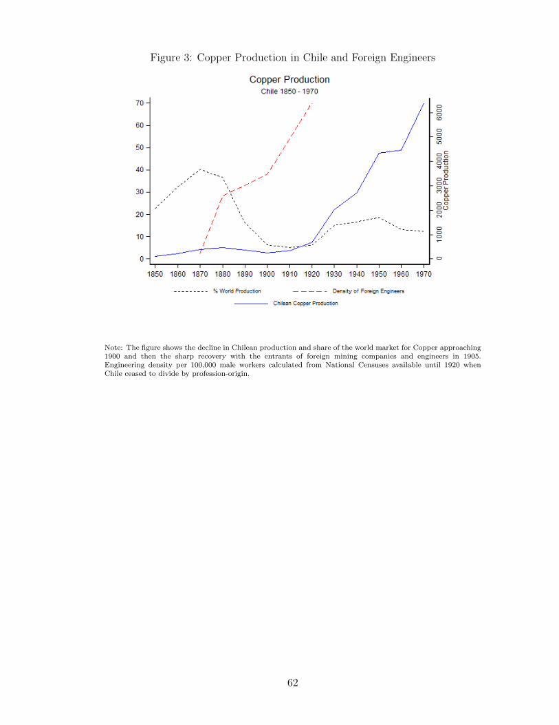
Figure 3: Copper Production in Chile and Foreign Engineers

Note: The figure shows the decline in Chilean production and share of the world market for Copper approaching1900 and then the sharp recovery with the entrants of foreign mining companies and engineers in 1905.Engineering density per 100,000 male workers calculated from National Censuses available until 1920 whenChile ceased to divide by profession-origin.

62

Table 1: Summary Statistics (State Level, Americas)

Variable mean p50 sd min max ObsLn Income 9.03 8.92 0.91 7.13 11.18 377Engineers 23.38 11.00 30.08 0.00 84.00 275Engineers (sub) 82.07 39.68 105.70 0.00 472.59 170Population Density (1900) 41.06 4.44 243.20 0.00 3319.27 235Population Density (1500) 8.88 2.00 26.13 0.00 392.34 365Literacy 40.85 34.00 23.95 11.30 86.70 337Literacy (sub) 49.06 39.96 30.10 4.60 98.31 175Railroads 3.15 1.80 2.71 0.30 9.30 377Railroads (sub) 65.12 48.54 57.46 5.16 309.20 49south 0.15 0.00 0.36 0.00 1.00 111Slavery 20.67 3.28 25.16 0.00 72.66 83Lawyers 218.92 139.22 210.93 1.64 1156.44 114Mine Output 0.47 0.12 1.06 0.00 6.49 45Spain 0.81 1.00 0.39 0.00 1.00 390Land Suitability 0.56 0.58 0.28 0.00 1.00 384River Density 3.28 3.29 1.23 0.00 6.92 386Average Temperature 19.97 20.40 5.83 2.38 29.00 332Rainfall 1.28 1.10 0.95 0.00 8.13 332Altitude 0.66 0.19 0.92 0.00 4.33 332Dist. from Coast 0.87 0.91 0.12 0.45 1.00 383Ruggedness 126.89 99.33 103.53 0.00 474.34 378

Notes: Log Income per capita in 2000 (PPP 2005 US dollars). Engineering density measured by engineers per 100.000 maleworkers. Engineering density measured by engineers per 100.000 male workers, sub-national. Engineering density measuredby engineers per 100.000 male workers, sub-national, scaled by national estimates of engineering stock. Population density isnumber of individuals per square kilometer in 1900. Pre-colonial population density measures the number of natives per squarekilometer in 1492. Literacy share of the population that is literate in 1900. Literacy share of the population that is literatein 1900, sub-national. Railroad density measured as miles of track per 1000 square kilometers. Railroad density measured asmiles of track per 1000 square kilometers, sub-national. South is a dummy variable for whether the US state is a Southern stateaccording to the US census. Slavery is measured as a fraction of the population and is taken from Bergad (2008) and Nunn(2008). Lawyer density measured by lawyers per 100.000 individuals. Mining is total mining output in 1860 in hundred thousanddollars. Spain is a dummy for whether the country was a Spanish colony: Argentina, Chile, Mexico and Venezuela. AgricultureSuitability is an index of probability of cultivation given cultivable land, climate and soil composition, from Ramankutty, Foleyand McSweeney (2002). Rivers captures the density of rivers as a share of land area derived from HydroSHEDS (USGS 2011).Temperature is a yearly average in degrees celsius; Altitude measures the elevation of the capital city of the state in kilometers;and Rainfall captures total yearly rainfall in meters, all are from Bruhn and Gallego (2011). Distance from the Coast from(Gennaioli et al., 2013); Ruggedness of Terrain from Nunn & Puga (2012) .

63

Table 2: Summary Statistics (County Level, US)

Variable mean p50 sd min max ObsLn Income 10.043 10.032 0.219 9.165 11.360 1905Engineers 0.022 0.000 0.038 0.000 0.299 1905Patents 0.453 0.274 0.602 0.000 6.041 1905Ln LGC distance 0.176 0.281 0.683 -5.450 1.765 1905Rainfall 0.077 0.076 0.042 0.009 0.393 1905Altitude 0.025 0.023 0.019 0.000 0.175 1905Ruggedness 0.005 0.003 0.006 0.000 0.043 1905Distance to river 0.017 0.014 0.014 0.000 0.141 1905Average Temperature -0.002 -0.006 0.061 -0.160 0.188 1905Dist. from Coast 0.027 0.023 0.020 0.000 0.102 1905Population Density 0.003 0.001 0.049 0.000 2.055 1905Manufacturing GDP 0.042 0.018 0.066 0.000 0.576 1905Slavery 0.153 0.019 0.215 0.000 0.925 1905Railroads 0.584 1.000 0.493 0.000 1.000 1905Literacy 0.759 0.829 0.203 0.151 1.000 1905School Assistance 12-17 0.051 0.055 0.018 0.000 0.090 1905Educational Score 0.073 0.073 0.019 0.035 0.168 1905Lawyers 0.001 0.001 0.001 0.000 0.005 1905Physicians 0.002 0.002 0.001 0.000 0.004 1905

Notes: Log Income per capita in 2000. Engineering density measured by engineers per 100,000 male workers. Patents densitymeasured by patents per 100 habitants. Dist. to LGC is distance to Land Grant College measured by distance between the nearLGC and the county centroid. Population density is number of individuals per 100 square kilometers in 1880. Literacy share ofthe population that is literate in 1880. Secondary is share of 14-17 years olds who report that they are attending school. Tertiaryis- percentage of workers who report completing one or more years of college. Railroad is a identifier variable if the county hasrailroad. Slavery to county level is taken from Nunn (2008). Lawyer density measured by lawyers per 100.000 individuals.Physicians density measured by physicians per 100.000 individuals. Mining is total mining output in 1860 in hundred thousanddollars. Rivers captures the distance between the near river and the county. Rivers taken from HydroSHEDS (USGS 2011).Temperature is a yearly average in degrees celsius; Altitude measures the elevation of the capital city of the state in kilometers;and Rainfall captures total yearly rainfall in meters. Dist. to Coast is distance between the coast and the county centroid;Ruggedness of Terrain from Nunn & Puga (2012). Manuf. Output is the manufacturing output per capita in 1880 taken fromNHGIS.

64

Table 3: Summary Regressions: Innovation Capacity (1900) vs Income per capita (2000)(National Level, Americas)

(1) (2) (3) (4) (5)Engineering 0.9** 0.9** 0.9** 0.7 0.9***

(0.42) (0.44) (0.38) (0.76) (0.32)Pop Density 0.06* 0.06*

(0.03) (0.03)Railroads 0.2 0.2

(0.14) (0.16)Literacy 0.2

(0.42)N 273 248 273 273 248N Countries 11 11 11 11 11R2 0.82 0.82 0.88 0.83 0.88

Notes: Dependent Variable is log subnational income per capita (2000). Engineering density measured by engineers per 100,000male workers. Population density is number of individuals per square kilometer in 1900. Railroad density measured as milesof track per 1000 square kilometers. Literacy share of the population that is literate in 1900. Beta coefficients. Robust andclustered SE in parenthesis. ∗ p < 0.1, ∗∗ p < 0.05, ∗∗∗ p < 0.01.

65

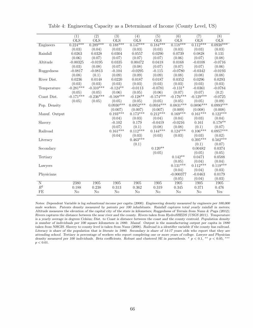
Table 4: Engineering Capacity as a Determinant of Income (County Level, US)

(1) (2) (3) (4) (5) (6) (7) (8)OLS OLS OLS OLS OLS OLS OLS OLS

Engineers 0.224*** 0.289*** 0.188*** 0.147*** 0.184*** 0.118*** 0.112*** 0.0938***(0.03) (0.04) (0.03) (0.03) (0.03) (0.03) (0.03) (0.03)

Rainfall 0.0263 0.0328 0.0304 0.0557 0.0290 0.0739 0.0828 0.131(0.06) (0.07) (0.07) (0.07) (0.07) (0.06) (0.07) (0.08)

Altitude -0.00325 -0.0195 0.0335 0.00472 0.0418 0.0168 -0.0108 -0.0716(0.03) (0.08) (0.07) (0.08) (0.07) (0.07) (0.07) (0.06)

Ruggedness -0.0817 -0.0813 -0.104 -0.0295 -0.115 -0.0780 -0.0342 -0.0193(0.08) (0.1) (0.09) (0.09) (0.09) (0.08) (0.08) (0.08)

River Dist. 0.0236 0.0148 0.0220 0.0187 0.0187 0.0352 0.0296 0.0293(0.03) (0.03) (0.03) (0.03) (0.03) (0.03) (0.03) (0.03)

Temperature -0.281*** -0.310*** -0.124** -0.0113 -0.0781 -0.131* -0.0361 -0.0784(0.05) (0.05) (0.06) (0.05) (0.06) (0.07) (0.07) (0.2)

Coast Dist. -0.171*** -0.236*** -0.168*** -0.128** -0.174*** -0.176*** -0.129*** -0.0725(0.05) (0.05) (0.05) (0.05) (0.05) (0.05) (0.05) (0.09)

Pop. Density 0.0930*** 0.0952*** 0.0934*** 0.0831*** 0.0896*** 0.0993***(0.007) (0.007) (0.007) (0.009) (0.008) (0.008)

Manuf. Output 0.193*** 0.173*** 0.212*** 0.169*** 0.161*** 0.122***(0.04) (0.03) (0.04) (0.04) (0.03) (0.04)

Slavery -0.102 0.179 -0.0419 -0.0216 0.161 0.178**(0.07) (0.1) (0.08) (0.08) (0.1) (0.07)

Railroad 0.161*** 0.112*** 0.144*** 0.124*** 0.106*** 0.0957***(0.04) (0.03) (0.03) (0.03) (0.03) (0.02)

Literacy 0.463*** 0.395*** 0.502***(0.1) (0.1) (0.07)

Secondary 0.120** 0.00482 0.0374(0.05) (0.05) (0.05)

Tertiary 0.142** 0.0471 0.0588(0.05) (0.04) (0.04)

Lawyers 0.131*** 0.112*** 0.119***(0.04) (0.04) (0.03)

Physicians -0.000377 -0.0463 0.0179(0.05) (0.04) (0.03)

N 2380 1905 1905 1905 1905 1905 1905 1905R2 0.188 0.238 0.313 0.362 0.319 0.345 0.371 0.476FE No No No No No No No Yes

Notes: Dependent Variable is log subnational income per capita (2000). Engineering density measured by engineers per 100,000male workers. Patents density measured by patents per 100 inhabitants. Rainfall captures total yearly rainfall in meters;Altitude measures the elevation of the capital city of the state in kilometers; Ruggedness of Terrain from Nunn & Puga (2012);Rivers captures the distance between the near river and the county. Rivers taken from HydroSHEDS (USGS 2011). Temperatureis a yearly average in degrees Celsius; Dist. to Coast is distance between the coast and the county centroid. Population densityis number of individuals per 100 square kilometers in 1880. Manuf. Output is the manufacturing output per capita in 1880taken from NHGIS. Slavery to county level is taken from Nunn (2008). Railroad is a identifier variable if the county has railroad.Literacy is share of the population that is literate in 1880. Secondary is share of 14-17 years olds who report that they areattending school. Tertiary is percentage of workers who report completing one or more years of college. Lawyer and Physiciandensity measured per 100 individuals. Beta coefficients. Robust and clustered SE in parenthesis. ∗ p < 0.1, ∗∗ p < 0.05, ∗∗∗

p < 0.01.

66

Table 5: Engineering and Patenting Capacity as Determinants of Income: Patents & IV(County Level, US)

(1) (2) (3) (4) (5) (6)OLS OLS OLS OLS IV IV-Buchinsky

Engineers 0.0959*** 0.0817*** 0.111*** 0.161***(0.03) (0.02) (0.03) (0.04)

Patents 0.125*** 0.114*** 0.105** 0.101*** 0.120*** 0.0974**(0.04) (0.04) (0.04) (0.04) (0.04) (0.04)

Rainfall 0.0860 0.142 0.0815 0.145* 0.145* 0.147*(0.08) (0.08) (0.07) (0.08) (0.08) (0.08)

Altitude -0.0370 -0.0964 -0.0359 -0.0932 -0.105* -0.0873(0.07) (0.06) (0.08) (0.06) (0.05) (0.06)

Ruggedness -0.00177 0.00274 -0.0115 -0.000973 -0.00529 -0.000402(0.08) (0.07) (0.08) (0.07) (0.07) (0.07)

River Dist. 0.0306 0.0268 0.0276 0.0256 0.0310 0.0292(0.03) (0.03) (0.02) (0.03) (0.03) (0.03)

Temperature -0.0248 -0.0681 -0.0385 -0.0731 -0.0507 -0.0750(0.07) (0.2) (0.06) (0.2) (0.2) (0.2)

Coast Dist. -0.119** -0.0537 -0.118** -0.0493 -0.0411 -0.0740(0.05) (0.09) (0.05) (0.09) (0.09) (0.08)

Pop. Density 0.0889*** 0.0983*** 0.0891*** 0.0985*** 0.0946*** 0.102***(0.007) (0.008) (0.008) (0.008) (0.008) (0.008)

Manuf. Output 0.135*** 0.0886** 0.119*** 0.0770* 0.0829* 0.0503(0.04) (0.04) (0.04) (0.04) (0.04) (0.04)

Slavery 0.175 0.189** 0.174 0.193*** 0.175*** 0.166**(0.1) (0.07) (0.1) (0.07) (0.07) (0.07)

Railroad 0.117*** 0.106*** 0.114*** 0.103*** 0.189*** 0.155***(0.03) (0.02) (0.03) (0.02) (0.04) (0.04)

Literacy 0.408*** 0.512*** 0.401*** 0.516*** 0.509*** 0.506***(0.1) (0.07) (0.1) (0.07) (0.07) (0.07)

Secondary 0.0147 0.0448 0.0148 0.0470 0.0285 0.0445(0.05) (0.05) (0.05) (0.05) (0.05) (0.05)

Tertiary 0.0397 0.0533 0.0290 0.0446 0.0502 0.0297(0.04) (0.04) (0.04) (0.04) (0.04) (0.04)

Lawyers 0.113*** 0.117*** 0.0916** 0.0986*** 0.112*** 0.102***(0.04) (0.04) (0.04) (0.03) (0.04) (0.03)

Physicians -0.0496 0.0152 -0.0441 0.0161 0.0127 0.0155(0.04) (0.03) (0.04) (0.03) (0.03) (0.03)

N 1905 1905 1905 1905 1905 1905R2 0.370 0.476 0.376 0.480FE No Yes No Yes Yes YesF statistical (robust) 14.023 25.45F statistical (robust and cluster) 7.755F Cragg-Donald 20.34

Notes: Dependent Variable is log subnational income per capita (2000). Standardized Beta coefficients. Engineering densitymeasured by engineers per 100,000 male workers. Patents density measured by patents per 100 inhabitants. Rainfall capturestotal yearly rainfall in meters; Altitude measures the elevation of the capital city of the state in kilometers; Ruggedness of Terrainfrom Nunn & Puga (2012); Rivers captures the distance between the near river and the county. Rivers taken from HydroSHEDS(USGS 2011). Temperature is a yearly average in degrees Celsius; Dist. to Coast is distance between the coast and the countycentroid. Population density is number of individuals per 100 square kilometers in 1880. Manuf. Output is the manufacturingoutput per capita in 1880 taken from NHGIS. Slavery to county level is taken from Nunn (2008). Railroad is a identifier variableif the county has railroad. Literacy share of the population that is literate in 1880. Secondary is share of 14-17 years olds whoreport that they are attending school. Tertiary is percentage of workers who report completing one or more years of college.Lawyer and Physician density measured per 100 individuals. Engineers instrumented using log distance to nearest Land GrantCollege measured by distance between the near LGC and the county centroid, estimated by 2SLS and Buchinsky quantile 2SLS.Beta coefficients. Robust and clustered SE in parenthesis. ∗ p < 0.1, ∗∗ p < 0.05, ∗∗∗ p < 0.01. In Column 5, F statistical ofinstrument’s relevance is 14.023 with robust standard errors and 7.755 with robust and clustered to state level standard errors.Cragg-Donald F statistical is 20.34. Using quantile regression in Column 6 F statistical of instrument’s relevance is 25.45 withrobust standard errors.

67

Table 6: Innovative Capacity as a Determinant of Income (State Level, Americas)

(1) (2) (3)Engineering 0.1*** 0.1*** 0.07***

(0.04) (0.03) (0.02)Pop Density 0.08** 0.06***

(0.03) (0.02)Literacy 0.4***

(0.14)N 170 166 166N Countries 6 6 6R2 0.11 0.18 0.37

Notes: Dependent Variable is log subnational income per capita (2000). Data for Argentina, Chile, Colombia, Mexico, US andVenezuela. Engineering density measured by engineers per 100,000 male workers. Population density is log number of individualsper square kilometer in 1900. Literacy is share of the population that is literate in 1900. Beta coefficients. Bootstrapped clusteredSE in parenthesis. ∗ p < 0.1, ∗∗ p < 0.05, ∗∗∗ p < 0.01.

68

Table 7: Determinants of Innovative Capacity (County Level, US)

Engineers PatentsOLS Buchinsky OLS Quantile

Pop. Density 0.02∗∗∗ 0.01∗∗∗ 0.3∗∗∗ 0.2∗∗∗

(0.004) (0.002) (0.06) (0.02)South -0.02∗∗∗ -0.001 -0.2∗∗∗ -0.2∗∗∗

(0.004) (0.002) (0.05) (0.02)Slavery -0.02∗∗∗ -0.009∗∗ -0.7∗∗∗ -0.3∗∗∗

(0.005) (0.004) (0.07) (0.05)River dist. -0.09 -0.03 -1.7 -0.7

(0.08) (0.04) (1.3) (0.5)Temperature 0.09∗∗∗ 0.02 0.4 0.4∗∗

(0.03) (0.01) (0.6) (0.2)Rainfall -0.08∗ -0.03 -1.2∗ -1.3∗∗∗

(0.04) (0.02) (0.7) (0.3)Altitude -0.09 -0.05 3.8∗ 2.4∗∗∗

(0.10) (0.05) (2.1) (0.6)Coast Dist. -0.06 0.02 -4.5∗∗∗ -0.7∗

(0.06) (0.03) (0.9) (0.4)Ruggedness 0.5∗ 0.2 -16.0∗∗∗ -9.1∗∗∗

(0.3) (0.1) (5.3) (1.9)N 1912 1912 1907 1907R2 0.140 0.231

Notes: Dependent Variable is innovative capacity measured by engineers per 100,000 male workers and patents per 100inhabitants. Pre-colonial population density measures the number of natives per square kilometer in 1492. South a dummycapturing Southern US states; slavery as tabulated from the 1860 Census as compiled in Nunn (2008). Rainfall captures totalyearly rainfall in meters; Altitude measures the elevation of the capital city of the state in kilometers; Ruggedness of Terrainfrom Nunn & Puga (2012); Rivers captures the distance between the near river and the county. Rivers taken from HydroSHEDS(USGS 2011). Temperature is a yearly average in degrees celsius; Dist. to Coast is distance between the coast and the countycentroid. Population density is number of individuals per 100 square kilometers in 1880. Geographical controls include riverdensity, average temperature, rainfall, altitude, distance from a coast, and ruggedness of terrain. Robust SE in parenthesis. ∗

p < 0.1, ∗∗ p < 0.05, ∗∗∗ p < 0.01.

69

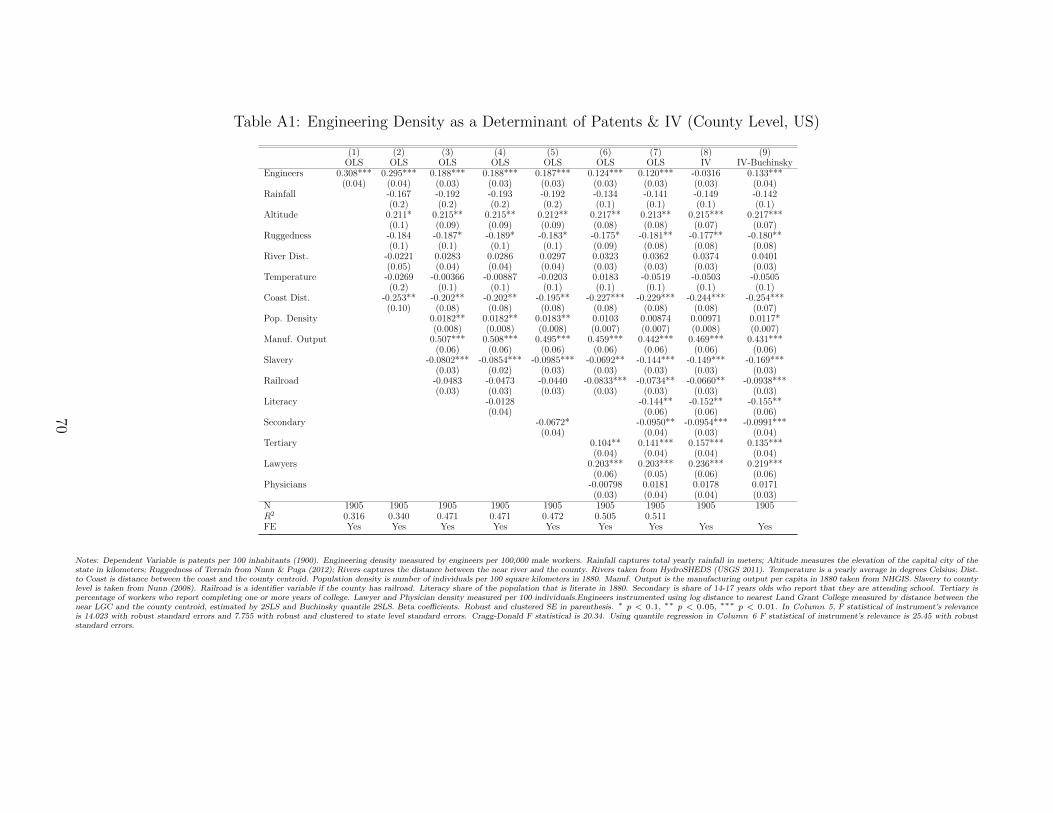
Table A1: Engineering Density as a Determinant of Patents & IV (County Level, US)

(1) (2) (3) (4) (5) (6) (7) (8) (9)OLS OLS OLS OLS OLS OLS OLS IV IV-Buchinsky

Engineers 0.308*** 0.295*** 0.188*** 0.188*** 0.187*** 0.124*** 0.120*** -0.0316 0.133***(0.04) (0.04) (0.03) (0.03) (0.03) (0.03) (0.03) (0.03) (0.04)

Rainfall -0.167 -0.192 -0.193 -0.192 -0.134 -0.141 -0.149 -0.142(0.2) (0.2) (0.2) (0.2) (0.1) (0.1) (0.1) (0.1)

Altitude 0.211* 0.215** 0.215** 0.212** 0.217** 0.213** 0.215*** 0.217***(0.1) (0.09) (0.09) (0.09) (0.08) (0.08) (0.07) (0.07)

Ruggedness -0.184 -0.187* -0.189* -0.183* -0.175* -0.181** -0.177** -0.180**(0.1) (0.1) (0.1) (0.1) (0.09) (0.08) (0.08) (0.08)

River Dist. -0.0221 0.0283 0.0286 0.0297 0.0323 0.0362 0.0374 0.0401(0.05) (0.04) (0.04) (0.04) (0.03) (0.03) (0.03) (0.03)

Temperature -0.0269 -0.00366 -0.00887 -0.0203 0.0183 -0.0519 -0.0503 -0.0505(0.2) (0.1) (0.1) (0.1) (0.1) (0.1) (0.1) (0.1)

Coast Dist. -0.253** -0.202** -0.202** -0.195** -0.227*** -0.229*** -0.244*** -0.254***(0.10) (0.08) (0.08) (0.08) (0.08) (0.08) (0.08) (0.07)

Pop. Density 0.0182** 0.0182** 0.0183** 0.0103 0.00874 0.00971 0.0117*(0.008) (0.008) (0.008) (0.007) (0.007) (0.008) (0.007)

Manuf. Output 0.507*** 0.508*** 0.495*** 0.459*** 0.442*** 0.469*** 0.431***(0.06) (0.06) (0.06) (0.06) (0.06) (0.06) (0.06)

Slavery -0.0802*** -0.0854*** -0.0985*** -0.0692** -0.144*** -0.149*** -0.169***(0.03) (0.02) (0.03) (0.03) (0.03) (0.03) (0.03)

Railroad -0.0483 -0.0473 -0.0440 -0.0833*** -0.0734** -0.0660** -0.0938***(0.03) (0.03) (0.03) (0.03) (0.03) (0.03) (0.03)

Literacy -0.0128 -0.144** -0.152** -0.155**(0.04) (0.06) (0.06) (0.06)

Secondary -0.0672* -0.0950** -0.0954*** -0.0991***(0.04) (0.04) (0.03) (0.04)

Tertiary 0.104** 0.141*** 0.157*** 0.135***(0.04) (0.04) (0.04) (0.04)

Lawyers 0.203*** 0.203*** 0.236*** 0.219***(0.06) (0.05) (0.06) (0.06)

Physicians -0.00798 0.0181 0.0178 0.0171(0.03) (0.04) (0.04) (0.03)

N 1905 1905 1905 1905 1905 1905 1905 1905 1905R2 0.316 0.340 0.471 0.471 0.472 0.505 0.511FE Yes Yes Yes Yes Yes Yes Yes Yes Yes

Notes: Dependent Variable is patents per 100 inhabitants (1900). Engineering density measured by engineers per 100,000 male workers. Rainfall captures total yearly rainfall in meters; Altitude measures the elevation of the capital city of thestate in kilometers; Ruggedness of Terrain from Nunn & Puga (2012); Rivers captures the distance between the near river and the county. Rivers taken from HydroSHEDS (USGS 2011). Temperature is a yearly average in degrees Celsius; Dist.to Coast is distance between the coast and the county centroid. Population density is number of individuals per 100 square kilometers in 1880. Manuf. Output is the manufacturing output per capita in 1880 taken from NHGIS. Slavery to countylevel is taken from Nunn (2008). Railroad is a identifier variable if the county has railroad. Literacy share of the population that is literate in 1880. Secondary is share of 14-17 years olds who report that they are attending school. Tertiary ispercentage of workers who report completing one or more years of college. Lawyer and Physician density measured per 100 individuals.Engineers instrumented using log distance to nearest Land Grant College measured by distance between thenear LGC and the county centroid, estimated by 2SLS and Buchinsky quantile 2SLS. Beta coefficients. Robust and clustered SE in parenthesis. ∗ p < 0.1, ∗∗ p < 0.05, ∗∗∗ p < 0.01. In Column 5, F statistical of instrument’s relevanceis 14.023 with robust standard errors and 7.755 with robust and clustered to state level standard errors. Cragg-Donald F statistical is 20.34. Using quantile regression in Column 6 F statistical of instrument’s relevance is 25.45 with robuststandard errors.

70

Table A2: Innovative Capacity as a Determinant of Income (US)

(1) (2) (3) (4) (5) (6) (7)Engineering 0.06*** 0.09*** 0.05*** 0.04** 0.07*** 0.1*** 0.1***

(0.02) (0.02) (0.02) (0.02) (0.01) (0.05) (0.04)Pop Density 0.1*** -0.02

(0.03) (0.06)Literacy 0.1* 0.4

(0.06) (0.32)Lawyers 0.04 -0.05

(0.05) (0.05)Railroads 0.1*** 0.08

(0.02) (0.05)Mining -0.02 -0.03***

(0.01) (0.01)Slavery -0.004 0.2

(0.06) (0.14)South -0.001 -0.02

(0.04) (0.03)N 51 51 51 51 44 38 34R2 0.14 0.40 0.17 0.17 0.47 0.41 0.60

Notes: Dependent Variable is log subnational income per capita (2000). Engineering density measured by engineers per 100,000male workers. Population density is log number of individuals per square kilometer in 1900. Literacy share of the populationthat is literate in 1900. Lawyer density measured by lawyers per 100.000 individuals. Institutional Controls: Slavery and South;Railroad density measured as miles of track per 1000 square kilometers. Mining is total mining output in 1880 in US 100,000dollars. Beta coefficients. Robust SE in parenthesis. ∗ p < 0.1, ∗∗ p < 0.05, ∗∗∗ p < 0.01.

71

Table A3: Innovative Capacity as a Determinant of Income (US, instrumented)

(1) (2) (3) (4) (5)Engineering 0.1*** 0.1*** 0.09** 0.1** 0.2***

(0.03) (0.03) (0.04) (0.05) (0.07)Pop Density 0.1*** 0.2***

(0.03) (0.05)Literacy 0.08 -0.06

(0.07) (0.10)Lawyers -0.005 -0.05

(0.07) (0.05)N 51 51 51 51 51R2 0.02 0.29 0.12 0.01 0.11

Notes: Dependent Variable is log subnational income per capita (2000). Engineering density measured by engineers per maleworkers. Population density is log number of individuals per square kilometer in 1900. Literacy share of the population that isliterate in 1900. Lawyer density measured by lawyers per 100.000 individuals. Beta coefficients. Robust SE in parenthesis. ∗

p < 0.1, ∗∗ p < 0.05, ∗∗∗ p < 0.01. R2 in specification 5 is close to 1 but not calculated.

72

Table A4: Mechanisms through which Engineering in 1900 Drives Income in 2000.

All New World

InputsR&D/GDP 0.94 0.96Firm Innovative Capacity 0.94 0.94Modern Management 0.93 0.93

OutputsPatents 0.95 0.98Technological Adoption 0.84 0.94

Notes: Table reports the correlation between engineering density in 1900 and three inputs and two outputs in the 2000. Inputs:1. R&D expenditures as a share of GDP. 2. Firm capacity for innovation ranging from pure licensing to pioneering their ownnew products and processes. “In your country, how do companies obtain technology? [1 = exclusively from licensing or imitatingforeign companies; 7 = by conducting formal research and pioneering their own new products and processes]. 3. A globallyconsistent measure of management quality from Bloom & Van Reenen (2010) and in particular, the sum of the scores on thetwo the questions dealing with how firms identify new production processes to adopt. On the output side, we have 1. Comin& Hobijn (2010); Comin & Ferrer (2013); Comin et al. (2008)’s measure of technological adoption at the extensive margin,averaging their industrial and sectoral scores and 2. patent applications filed under the Patent Cooperation Treaty (PCT) permillion population as tabulated by the World Economic Forum (2008-9)(World Economic Forum et al., 2012).

73