19 Jul 11 F-H.1

ENERGY STATES OF ATOMS – THE FRANCK-HERTZ EXPERIMENT Atoms in excited states emit radiation at discrete frequencies. The frequency of the radiation, , is related to the change in the atomic energy levels by E = h. The fact that only certain discrete frequencies are emitted is evidence of the quantization of atomic energy levels. In the present experiment, this quantization is examined by bombarding mercury vapour with electrons of known, variable energy. This experiment is a repeat of one originally performed by Franck and Hertz in 1914. They set out to show that: i) it is possible to excite atoms by low-energy electron bombardment; ii) the excitation energy transferred from the electrons to the atoms always has discrete values; and iii) the values obtained for the energy levels are in agreement with spectroscopic results. Theory: When particles travel through matter there are two possible types of collisions, elastic and inelastic, between the incident particles and those forming the substance. In an elastic collision kinetic energy is conserved and the initial energy is divided between the particles according to the relation of their masses. If an electron (small mass) collides elastically with an atom (large mass), from conservation of momentum and kinetic energy it is seen that the electron’s direction of motion is changed but that the amount of kinetic energy lost by the electron and imparted to the atom is very small. If an electron collides inelastically with an atom, the energy lost by the electron is not converted into kinetic energy of the atom, but rather is the cause for excitation, ionization, radiation, or particle production. Quantum theory postulates that an atom can only be excited in discrete energy steps, i.e. there is a small but finite energy required to bring an atom from its ground state into an excited state. If, in a collision, the energy available to be transferred to the atom is less than the difference between the ground and first excited states, the collision remains elastic. However, an electron having a kinetic energy larger than the energy difference between the ground state and the first excited state of an atom can excite this atom by means of an inelastic collision. There are other ways to excite atoms. Illumination with light of the appropriate wavelength (given by = hc/E, where E = energy difference between ground and an excited state) would cause a transition. The inconvenience of using light to excite an atom is that this light must have the exact wavelength corresponding to the energy difference between the ground state and the state to be excited. In using the energy loss due to an inelastic collision as the energy transport mechanism, this drawback does not occur since the kinetic energy of the electron is not quantized either before or after the collision. Apparatus:

There are two sets of equipment. One set enables examination of the collisions between electrons and mercury atoms and the other set of equipment enables examination of the collisions between electrons and neon atoms.

19 Jul 11 F-H.2

Franck-Hertz Experiment in Mercury

19 Jul 11 F-H.3

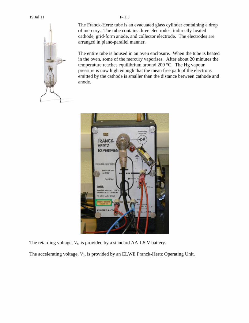
The Franck-Hertz tube is an evacuated glass cylinder containing a drop of mercury. The tube contains three electrodes: indirectly-heated cathode, grid-form anode, and collector electrode. The electrodes are arranged in plane-parallel manner. The entire tube is housed in an oven enclosure. When the tube is heated in the oven, some of the mercury vaporises. After about 20 minutes the temperature reaches equilibrium around 200 °C. The Hg vapour pressure is now high enough that the mean free path of the electrons emitted by the cathode is smaller than the distance between cathode and anode.

The retarding voltage, Vr, is provided by a standard AA 1.5 V battery. The accelerating voltage, Va, is provided by an ELWE Franck-Hertz Operating Unit.

19 Jul 11 F-H.4

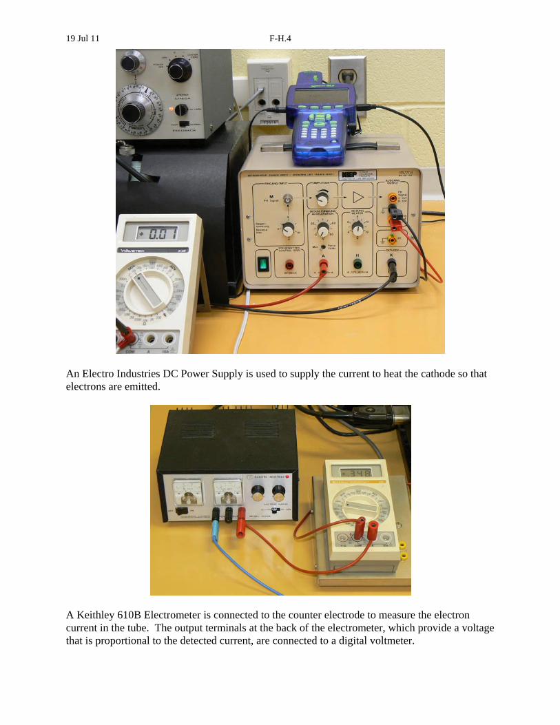
An Electro Industries DC Power Supply is used to supply the current to heat the cathode so that electrons are emitted.

A Keithley 610B Electrometer is connected to the counter electrode to measure the electron current in the tube. The output terminals at the back of the electrometer, which provide a voltage that is proportional to the detected current, are connected to a digital voltmeter.

19 Jul 11 F-H.5

Data is collected by an Xplorer GLX computer interface. One input of the GLX is used to collect the accelerating voltage data from the UB/10 output of the F-H Operating Unit and the other input of the GLX is used to collect electrometer current data.

Franck-Hertz Experiment in Neon The equipment used to study the electron-atom interactions in neon is similar to that used for the Franck-Hertz in Mercury experiment, except that an oven is not required and the Franck-Hertz Operating Unit is used to provide all the necessary voltages. The operating unit also contains a high-sensitivity DC amplifier for measuring the electron current at the counter electrode.

19 Jul 11 F-H.6

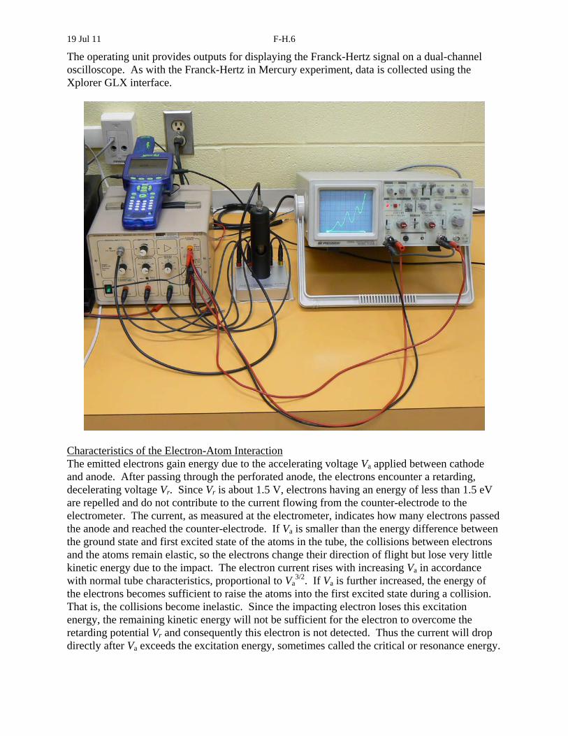
The operating unit provides outputs for displaying the Franck-Hertz signal on a dual-channel oscilloscope. As with the Franck-Hertz in Mercury experiment, data is collected using the Xplorer GLX interface.

Characteristics of the Electron-Atom Interaction The emitted electrons gain energy due to the accelerating voltage Va applied between cathode and anode. After passing through the perforated anode, the electrons encounter a retarding, decelerating voltage Vr. Since Vr is about 1.5 V, electrons having an energy of less than 1.5 eV are repelled and do not contribute to the current flowing from the counter-electrode to the electrometer. The current, as measured at the electrometer, indicates how many electrons passed the anode and reached the counter-electrode. If Va is smaller than the energy difference between the ground state and first excited state of the atoms in the tube, the collisions between electrons and the atoms remain elastic, so the electrons change their direction of flight but lose very little kinetic energy due to the impact. The electron current rises with increasing Va in accordance with normal tube characteristics, proportional to Va

3/2. If Va is further increased, the energy of the electrons becomes sufficient to raise the atoms into the first excited state during a collision. That is, the collisions become inelastic. Since the impacting electron loses this excitation energy, the remaining kinetic energy will not be sufficient for the electron to overcome the retarding potential Vr and consequently this electron is not detected. Thus the current will drop directly after Va exceeds the excitation energy, sometimes called the critical or resonance energy.

19 Jul 11 F-H.7

If the accelerating voltage is raised further, the electron current increases since the electrons can gain enough energy after the inelastic collision to reach the counter-electrode. If Va exceeds twice the excitation energy, electrons will undergo a second inelastic collision and consequently the current will drop once more. This pattern will repeat as Va is increased. The figure shows the expected plot of electrometer current I versus accelerating voltage Va.

Mercury Source – Detailed Procedure: 1. Plug in the oven, if this has not already been done, and allow approximately 20 minutes for

the temperature to reach equilibrium before taking measurements. 2. Check that the Keithley 610B Electrometer is set as follows:

Zero Control Medium (inner) – Fully CW Fine (outer) – Fully CCW Range control 3 10–10 A FEEDBACK switch FAST ZERO CHECK switch LOCK position (push and turn) Turn on the electrometer by turning the Meter switch to the “–” position and allow five to ten

minutes for warm-up. Unlock the ZERO CHECK switch. 3. The cathode current is supplied by the Electro Industries Regulated DC Power Supply.

Check that the VOLTAGE RANGE switch is set to 0-15 V, that the current control is at minimum (fully counterclockwise), and that the voltage control is set at midrange (indicator on knob pointing vertically upward). Turn on the digital multimeter connected to this supply by setting it to the 2 DCA position. Turn on the power supply. Slowly increase the current until the ammeter reads about 0.350 A.

19 Jul 11 F-H.8

4. The accelerating voltage is provided by the Franck-Hertz Operating Unit. Set the ACCELERATION control to 0 and put the toggle switch in the Man. (manual) position. Connect the A (anode) terminal of the operating unit to the anode connection on the tube cabinet. Connect the K (cathode) terminal of the operating unit to the rightmost cathode terminal on the tube cabinet. Turn on the multimeter that is connected across the anode-cathode terminals on the tube cabinet and set the meter to display DC voltage.

5. Turn on the multimeter that is connected to the electrometer. Set the voltmeter to the

20 DCV position. This multimeter measures a voltage that is proportional to the number of electrons reaching the counter electrode. Connect the voltage sensor on the side of the Xplorer GLX computer interface to the voltmeter terminals.

6. The Analog Adapter of the Xplorer GLX is connected to a CI-6503 voltage sensor. Connect

the leads from the voltage sensor to the UB/10 and ground outputs of the Franck-Hertz Operating Unit.

7. Turn on the Franck-Hertz Operating Unit. 8. Connect the Xplorer GLX to a USB port on the computer. 9. Turn on the Explorer GLX. 10. Double-click the DataStudio icon on the desktop of the computer.

Click “Create Experiment” If the “Choose sensor or instrument…” window pops up, close it by clicking “Cancel”.

Close any other windows that pop up. Click the Setup button Click the voltage sensor icon corresponding to the CI-6503 sensor Set the Sample Rate to 50 Hz and select Low (1) Click the voltage sensor icon corresponding to the GLX PS-2002 sensor Set the Sample Rate to 50 Hz Minimise the Experiment Setup window In the Data section double-click the top Voltage (V) and change the Measurement Name

to “Accelerating Voltage” Double-click the lower Voltage (V) and change the Measurement Name to “F-H Tube

Current”

11. The equipment is now ready for use. 12. Click the Start button in the DataStudio software and slowly and steadily increase the

accelerating voltage by turning the ACCELERATION control on the operating unit.

13. When the accelerating voltage reaches about 25 V click the Stop button in DataStudio.

14. Under “Displays” in the left-hand column of DataStudio double-click Graph, select Run #1 under “F-H Tube Current” as the source, and click OK. The graph shows the electrometer output (proportional to F-H tube current) as a function of elapsed time. To obtain the desired graph of electrometer output versus accelerating voltage, in the “Data” section of the left-

19 Jul 11 F-H.9

hand column of DataStudio click Run #1 under Accelerating Voltage and drag to the x-axis of the graph.

15. Sample graph:

16. The data can either be analysed within DataStudio or saved to a file for later analysis using a spreadsheet program such as Microsoft Excel.

17. To analyse the data within DataStudio, note that the graph can be easily manipulated:

clicking and dragging the plot area near either of the axes allows adjustment of the starting values on the graph axes;

clicking and dragging the numbers on each of the axes allows the axes scales to be adjusted independently.

18. To save the data as a tab-delimited text file, click File, Export Data…, select Run #1 under F-H Tube Current vs. Accelerating Voltage, and click OK. Choose an appropriate location for the data file, give it a descriptive filename, and click Save. The data file can be opened in Excel for graphing and analysis at a later time.

19 Jul 11 F-H.10

When finished recording your data, turn off the equipment as follows:

Operating Set voltage to 0 Unit: Turn off unit Cathode Current Reduce cathode current to 0 Supply: Turn off supply Electrometer: ZERO CHECK to LOCK position (push and turn) POWER OFF Oven: unplug the cord from the wall outlet Multimeters: switch to OFF

Mercury Source – Analysis: From the plot of Electrometer Output versus Accelerating Voltage determine an average value for the peak separations, and hence for the energy difference between the ground state and the first excited state of mercury. Based on your experimental value for the energy of the first excited state of mercury, calculate the wavelength of light that would be emitted when mercury de-excites from the first excited state to the ground state. Compare with the accepted value of 253.7 nm. What do you notice about the location of the first peak compared to the average peak separation? Attempt to explain this discrepancy. Why does the current decrease gradually, rather than suddenly, at the critical energies? Do you expect to see effects due to excitation of the second and higher excited states of mercury? Explain your answer. Neon Source – Detailed Procedure: 1. If necessary, unplug the leads connecting the A and K terminals of the Franck-Hertz

Operating Unit to the F-H Mercury tube.

2. Connect the leads from the F-H Neon tube to the appropriate terminals of the operating unit.

3. If necessary, disconnect the GLX voltage sensor leads from the electrometer output voltmeter and connect them to the FH signal terminals of the operating unit.

4. Connect the coax signal cable from the neon tube to the FH Signal input of the operating unit.

5. Connect CH1 of the oscilloscope to the UB/10 output terminals of the operating unit and connect CH2 of the oscilloscope to the FH signal output terminals.

19 Jul 11 F-H.11

6. Set the operating unit controls and the oscilloscope as follows:

Reverse Bias: just over 4 (just past indicator mark between 2 and 6)

Acceleration Voltage: ~65 V switch set to Ramp 50 Hz

Heater Voltage: ~8.3 V tube behaviour and output trace are strongly dependent on heater voltage

Amplitude: set about halfway between and (about 25% of full scale)

Oscilloscope Settings (x-y mode): X: 1 V/cm Y: 0.5 V/cm Note that the horizontal output of the control unit is one-tenth of the accelerating voltage.

7. Turn on the F-H Operating Unit and the oscilloscope and allow approximately 10 minutes for the equipment to stabilize.

8. Adjust the oscilloscope scales as necessary to obtain a stable trace showing the neon excitation peaks:

9. From the oscilloscope display, measure the accelerating voltages corresponding to as many

excitation peaks as are visible. Note that the voltage along the x-axis of the oscilloscope display is one-tenth of the actual accelerating voltage that is being applied to the F-H tube.

19 Jul 11 F-H.12

10. Decrease the accelerating voltage to zero. Slowly increase the accelerating voltage while

carefully observing the tube through the viewing port. You may need to dim the room lights. The following image shows the F-H Neon tube in operation.

11. Record your observations in as much detail as possible. In particular, ensure you have

enough information to answer the following questions. What colour is the light produced in the tube? Where is the light first produced? Does the location of the light depend on accelerating voltage? If so, how? Do you observe bands of light in the tube?

12. To acquire, analyse, and save data using the GLX, use the same settings as for the F-H Mercury experiment, except that the accelerating voltage is varied from 0 to 70 V (after setting the toggle switch to Man.).

Graph of typical data:

19 Jul 11 F-H.13

13. When finished recording your data, turn off the oscilloscope, reduce the accelerating voltage to 0, and turn off the Franck-Hertz Operating Unit.

14. Close DataStudio and disconnect the GLX from the computer. The GLX will turn off automatically once its battery is fully-charged. Do not disconnect the GLX power supply from the power bar/wall outlet.

Neon Source – Analysis: Determine an average value for the peak separations, and hence for the energy difference between the ground state and the excited state of neon. Remember that the output of the accelerating voltage terminals of the F-H Operating Unit is one-tenth of the actual accelerating voltage that was applied to the tube. Calculate the wavelength of light that would be emitted when neon de-excites from the excited state to the ground state. Is this wavelength in the appropriate part of the visible spectrum to account for the colour of light that is observed to be emitted by the excited neon? If not, note that there is a band of neon states at ~16.7 eV. Calculate the wavelength of light that would be emitted for transitions between the excited state that you measured and the states at 16.7 eV. Does this wavelength correspond to the colour of light emitted by the neon? References: Melissinos, Experiments in Modern Physics, QC 33 Harnwell, Experimental Atomic Physics, QC 173