End-to-end Predictability and Efficiency in Low-power ...End-to-end Predictability and Eciency ... I...
162
Diss. ETH No. 22857 End-to-end Predictability and Efficiency in Low-power Wireless Networks A dissertation submitted to ETH Zurich for the degree of Doctor of Sciences presented by MARCO ZIMMERLING Diploma in Computer Science, Technische Universität Dresden born August 14, 1982 citizen of Germany accepted on the recommendation of Prof. Dr. Lothar Thiele, examiner Prof. Dr. Tarek Abdelzaher, co-examiner 2015
Transcript of End-to-end Predictability and Efficiency in Low-power ...End-to-end Predictability and Eciency ... I...

Diss. ETH No. 22857
End-to-end Predictability and E�ciencyin Low-power Wireless Networks
A dissertation submitted toETH Zurich
for the degree ofDoctor of Sciences
presented byMARCO ZIMMERLING
Diploma in Computer Science,Technische Universität Dresden
born August 14, 1982citizen of Germany
accepted on the recommendation ofProf. Dr. Lothar Thiele, examiner
Prof. Dr. Tarek Abdelzaher, co-examiner
2015


Institut fur Technische Informatik und KommunikationsnetzeComputer Engineering and Networks Laboratory
TIK-SCHRIFTENREIHE NR. 156
Marco Zimmerling
End-to-end Predictability and E�ciencyin Low-power Wireless Networks

A dissertation submitted toETH Zurichfor the degree of Doctor of Sciences
Diss. ETH No. 22857
Prof. Dr. Lothar Thiele, examinerProf. Dr. Tarek Abdelzaher, co-examiner
Examination date: July 10, 2015

To my family.


AbstractThe confluence of networked embedded computing, low-power wirelesscommunications, and sensor technology has spawned a whole spectrumof powerful applications that are commonly believed to radically changethe way we perceive and interact with the physical world. Data collectionapplications, for example, enable the monitoring of physical phenomenawith unprecedented spatial and temporal resolutions, and cyber-physicalsystems (CPS) applications can control physical processes by integratingsensing and computation with actuation into distributed feedback loops.Application domains include transportation, healthcare, and buildings.
Data collection and CPS applications alike demand predictability ande�ciency from the wireless communication substrate to function correctlyand e↵ectively. In particular, these applications require a certain energye�ciency, reliability, and timeliness of end-to-end packet transmissions.Meeting perhaps multiple such non-functional requirements is, however,extremely challenging. This is due to, for example, the need for multi-hopcommunication over lossy low-power wireless channels, unpredictableand non-deterministic changes in the environment, and limited resourcesof the employed devices in terms of computation, memory, and energy.
Dedicated solutions have been proposed that attempt to tackle thesechallenges in order to satisfy the needs of either non-critical data collectionor critical CPS applications. As for the former, adapting the operationalparameters of the MAC protocol proved to be highly e↵ective; however,current e↵orts focus only on a single performance metric or consider localmetrics, whereas applications often exhibit requirements along multiplemetrics that are most naturally expressed in global, network-wide terms.As for the latter, state-of-the-art solutions including industry standards donot provide hard end-to-end real-time guarantees because of a localizedoperation, or can hardly keep up with dynamic changes in the network.
To address these problems, this thesis presents new analytical resultsas well as real implementations of novel protocols and systems that makeuse of them. Specifically, we make three main contributions:
• We design pTunes, a framework that meets multiple soft applicationrequirements on network lifetime, end-to-end reliability, and end-to-end latency by adapting the MAC protocol parameters at runtimein response to changes in the network and the tra�c load. pTunesexploits a centralized approach that is similar in spirit to a model-

ii Abstract
predictive controller. Results from testbed experiments show thatrelative to carefully chosen fixed MAC parameters pTunes extendsnetwork lifetime by up to 3⇥, and reduces packet loss by 70–80 %during periods of wireless interference or when multiple nodes fail.
• A new breed of protocols that utilize synchronous transmissions hasbeen shown to enhance the reliability and e�ciency of protocols thatuse link-based transmissions. We find that these emerging protocolsalso enable simpler and more accurate models, which play a key rolein system design, verification, and runtime adaptation to meet givenrequirements. We show through testbed experiments and statisticalanalyses that unlike link-based transmissions, packet receptions andlosses using synchronous transmissions with Glossy can largely beconsidered statistically independent events. This property greatlysimplifies the accurate modeling of protocols based on synchronoustransmissions. We demonstrate this by obtaining an unprecedentederror below 0.25 % in the energy model of the Glossy-based Low-power Wireless Bus (LWB), and providing su�cient conditions forprobabilistic guarantees on LWB’s end-to-end reliability.
• We present Blink, the first protocol that provides hard guarantees onend-to-end packet deadlines in large multi-hop low-power wirelessnetworks. Built on top of LWB as communication support, we mapthe scheduling problem in Blink to uniprocessor scheduling. Wedevise earliest deadline first (EDF) based scheduling policies thatBlink employs to compute online a schedule that provably meets alldeadlines of packets released by admitted real-time packet streamswhile minimizing the network-wide energy consumption withinthe limits of LWB, tolerating changes in the network and the set ofstreams. An e�cient priority queue data structure and algorithmswe design prove instrumental for a viable implementation of thesepolicies on resource-constrained nodes. Our experiments show thatBlink meets nearly 100 % of packet deadlines on a large multi-hoptestbed, and achieves speed-ups of up to 4.1⇥ over a conventionalscheduler implementation on state-of-the-art microcontrollers.

ZusammenfassungDie Zusammenführung von eingebetteten vernetzten Computern, ener-giee�zienter drahtloser Kommunikation und Sensortechnologie hat einganzes Spektrum leistungfähiger Anwendungen hervorgebracht. DieseAnwendungen werden aller Voraussicht nach die Art, mit der wirunsere Umwelt wahrnehmen und auf sie einwirken, nachhaltig ver-ändern. So ermöglichen beispielsweise Data-Collection-Anwendungendie Beobachtung von physikalischen Prozessen mit einer noch nie da-gewesenen räumlichen und zeitlichen Auflösung. Cyber-Physikalische-Anwendungen können dazu steuernd in diese Prozesse eingreifen, indemsie Sensoren, Computer und Aktoren in verteilten Regelkreisen mitein-ander verknüpfen. Zu den vielen Einsatzgebieten dieser Anwendungenzählen das Transport- und Gesundheitswesen sowie die Gebäudetechnik.
Um korrekt und e↵ektiv arbeiten zu können bedürfen sowohl Data-Collection- als auch Cyber-Physikalische-Anwendungen einer drahtlosenKommunikationsinfrastruktur, die sich durch Vorhersagbarkeit und E�-zienz auszeichnet. Dabei sind besonders Energiee�zienz, Zuverlässigkeitund Pünktlichkeit bei der Ende-zu-Ende-Übertragung von Datenpa-keten unerlässlich. Mehreren solcher nichtfunktionalen Anforderungengleichzeitig gerecht zu werden stellt jedoch eine große Herausforderungdar. Dies liegt zum Beispiel an der Notwendigkeit für eine Multi-Hop-Kommunikation über verlustbehaftete drahtlose Übertragungskanäle,unvorhersehbaren und nichtdeterministischen Veränderungen in derUmgebung sowie an den eingeschränkten Berechnungs-, Speicher- undEnergieressourcen der üblicherweise verwendeten Geräte.
Dedizierte Ansätze wurden bereits vorgeschlagen, um diese Problemefür nicht kritische Data-Collection-Anwendungen oder für kritischeCyber-Physikalischen-Anwendungen zu lösen. Bei nicht kritischen Data-Collection-Anwendungen hat sich die Anpassung der Betriebsparameterdes Medium Access Control (MAC)-Protokolls als besonders e↵ektiverwiesen. Allerdings beschränken sich die gegenwärtigen Bemühungenauf eine einzige Leistungsmetrik oder betrachten lediglich lokale Metri-ken. Die Anwendungen stellen jedoch oft Anforderungen hinsichtlichmehrerer Metriken, die am ehesten aus einer globalen, netzweiten Sichtangegeben werden. Für kritische Cyber-Physikalische-Anwendungengilt, dass selbst die modernsten Ansätze einschließlich der gängigenIndustriestandards keine harten Echtzeitgarantien geben können. Das

iv Zusammenfassung
liegt meist an ihrer lokal begrenzten Funktionsweise oder daran, dass siekaum mit den rasanten Verändungen im Netz Schritt halten können.
Um diese Defizite zu überwinden stellt die vorliegende Dissertationsowohl neue analytische Erkenntnisse als auch reale Implementierungenneuartiger Kommunikationsprotokolle und darauf aufbauender Systemevor. Nachfolgend werden die wichtigsten wissenschaftlichen Beiträge derDissertation zusammenfassend beschrieben.
• Zunächst stellt die Dissertation pTunes vor. pTunes ist ein System,welches mehrere Anforderungen hinsichtlich der Betriebsdauer desNetzes, der Ende-zu-Ende-Zuverlässigkeit und der Ende-zu-Ende-Latenzzeit erfüllen kann. pTunes erreicht dies, indem es zur Laufzeitdie Parameter des MAC-Protokolls an die Veränderungen im Netzund das aktuelle Verkehrsaufkommen anpasst. Dabei nutzt pTuneseinen zentralisierten Ansatz, dessen Funktionsweise dem einesmodellprädiktiven Regelkreises ähnelt. Umfangreiche Experimenteauf einem Testbed haben unter anderem gezeigt, dass pTunes imVergleich zu sorgfältig ausgewählten aber unveränderlichen MAC-Parametern die Betriebsdauer des Netzes bis um den Faktor dreiverlängert und den Verlust an Datenpaketen durch Interferenz oderdem gleichzeitigen Ausfall mehrerer Geräte um 70–80 % verringert.
• Es wurde festgestellt, dass eine neue Art von Protokollen basierendauf gleichzeitigen Übertragungen zuverlässiger und e�zienter istals Protokolle, die Datenpakete über Punkt-zu-Punkt-Verbindungensenden. Die vorliegende Dissertation kommt zu dem Schluss, dassdiese neuartigen Protokolle auch erheblich einfachere und genauereModelle zulassen, die eine Schlüsselrolle beim Systementwurf, beider Verifikation und bei der Anpassung zur Laufzeit spielen, um diejeweiligen Anforderungen zu erfüllen. Durch Testbed-Experimenteund statistische Zeitreihenanalysen wird gezeigt, dass, anders alsbei Punkt-zu-Punkt-Übertragungen, aufeinanderfolgende Empfän-ge und Verluste bei gleichzeitig übertragenen Datenpaketen mittelsGlossy weitgehend als statistisch unabhängige Ereignisse betrachtetwerden können. Dies erleichtert die hochgenaue Modellierung vonProtokollen, die gleichzeitige Übertragungen verwenden. Validiertwird diese These durch die Beschreibung eines Energiemodells desauf Glossy basierenden Low-Power Wireless Bus (LWB), dessenVorhersagen nur 0.25 % von den realen Messwerten abweicht unddie Formulierung hinreichender Bedingungen für probabilistischeGarantien hinsichtlich der Ende-zu-Ende-Zuverlässigkeit von LWB.
• Abschliessend stellt die Dissertation Blink vor. Blink ist das ersteProtokoll, welches harte Garantien hinsichtlich der Einhaltung von

v
Zeitschranken bei der Ende-zu-Ende-Kommunikation von Daten-paketen in großen Multi-Hop-Netzen bietet. Blink benutzt LWB alsKommunikationsinfrastruktur und erlaubt so die Betrachtung desScheduling-Problems wie bei einem Einkernprozessor. Die Disserta-tion entwickelt neuartige Scheduling-Strategien basierend auf demEarliest Deadline First (EDF)-Verfahren. Mithilfe dieser berechnetBlink online einen Schedule, der beweisbar alle Zeitschranken vonDatenpaketen einhält, die von zugelassenen Echtzeit-Paketströmenausgelöst werden, und den netzweiten Energieverbrauch innerhalbder von LWB abgesteckten Möglichkeiten minimiert. Dabei toleriertBlink ohne Weiteres dynamische Veränderungen im Netz sowie inder Menge von zugelassenen Paketströmen. Um diese Scheduling-Strategien auf stark ressourcenbeschränkten Geräten ausführen zukönnen, präsentiert die Dissertation eine e�ziente Datenstrukturfür eine Vorrangwarteschlange und mehrere Algorithmen, die dieseDatenstruktur benutzen. Durch viele Experimente auf einem großenMulti-Hop-Testbed wird zeigt, dass Blink nahezu 100 % der Paket-Zeitschranken einhält und darüber hinaus die Ausführungszeit desSchedulers auf modernen Mikrokontrollern im Vergleich zu einerkonventionellen Implementierung bis um den Faktor 4.1 verringert.

vi Zusammenfassung

AcknowledgmentsIt is a great pleasure and a great challenge to thank all those who havegiven me the opportunity, support, and time to work on this thesis.
I am grateful to Lothar Thiele for giving me the freedom to pursue myown research interests. Since my first day in the Computer EngineeringGroup at ETH Zurich, he has been a great source of inspiration, whileproviding me with independence, patience, and understanding. He hasalways been able to o↵er a di↵erent perspective on ideas and push themone level further. It has been a true honor to work together with him,and to learn from his approach and experience in the research process. Iwould also like to thank Tarek Abdelzaher for being on my examinationcommittee, and for his positive and encouraging comments.
This thesis is the result of collaboration with several people. It has beenvery rewarding to work together with Federico Ferrari. I have benefiteda lot from our numerous discussions and inspiring working atmospherein our o�ce. I am particularly thankful to him for sharing some of hismathematical intuition and MATLAB skills. I am profoundly grateful toLuca Mottola for many stimulating Skype calls, late-night paper writingsessions, and his invaluable advice on all aspects of research. Luca hasalso helped me limit my investigations when I was too ambitious andcheer me up when I felt a sense of despair. I am thankful to PratyushKumar for introducing me to the field of real-time scheduling theory, andto Thiemo Voigt for his support and the initiation of valuable contacts.
Beyond collaborators on the papers this thesis is based upon, manyother people have contributed to my PhD research. I am thankful to OlafLandsiedel, who has been a great collaborator on the Chaos project. I havealso been fortunate enough to work on di↵erent projects with Roman Lim,Felix Sutton, Reto Da Forno, Olga Saukh, David Hasenfratz, Tonio Gsell,Andreas Meier, Matthias Woehrle, Georgia Giannopoulou, ChristophWalser, Matthias Keller, Jan Beutel, Philipp Sommer, Ben Buchli, FelixJonathan Oppermann, Carlo Alberto Boano, and Kay Römer. Thank youall for giving me the opportunity to learn from your insights.
I would also like to take the opportunity to thank all current and pastmembers of the Computer Engineering Group for having provided mewith such a creative and friendly atmosphere that has made my PhD anunforgettable experience. Special thanks to Beat Futterknecht, FriederikeBrütsch, Tanja Lantz, and Monica Fricker, who have helped me with many

viii Acknowledgments
practical arrangements, and to Thomas Steingruber, Benny Gächter, andDamian Friedli for providing excellent computer facilities.
Finally, I would like to thank my family, to whom I dedicate this thesis,for their support and love. The care and down-to-earthness of my parentsare important ingredients of my life. Above all, thank you Berit and ourthree children, Clara, Erik, and Henrik, for many great moments and forproviding me with a place I call home.

Contents
Abstract i
Zusammenfassung iii
Acknowledgments vii
List of Figures xi
List of Tables xiii
1 Introduction 11.1 Application Requirements . . . . . . . . . . . . . . . . . . . . . . . 21.2 Challenges to Meeting Requirements . . . . . . . . . . . . . . . . 41.3 State of the Art . . . . . . . . . . . . . . . . . . . . . . . . . . . . . 61.4 Thesis Contributions and Road Map . . . . . . . . . . . . . . . . . 9
2 pTunes: Runtime Parameter Adaptation for Low-power MAC Protocols 132.1 Optimization Problem . . . . . . . . . . . . . . . . . . . . . . . . . 162.2 Modeling Framework . . . . . . . . . . . . . . . . . . . . . . . . . 172.3 System Support . . . . . . . . . . . . . . . . . . . . . . . . . . . . . 292.4 Implementation Details . . . . . . . . . . . . . . . . . . . . . . . . 322.5 Experimental Results . . . . . . . . . . . . . . . . . . . . . . . . . . 332.6 Discussion . . . . . . . . . . . . . . . . . . . . . . . . . . . . . . . . 442.7 Related Work . . . . . . . . . . . . . . . . . . . . . . . . . . . . . . 452.8 Summary . . . . . . . . . . . . . . . . . . . . . . . . . . . . . . . . 47
3 Modeling Protocols Based on Synchronous Transmissions 493.1 Background and Related Work . . . . . . . . . . . . . . . . . . . . 513.2 Bernoulli Assumption . . . . . . . . . . . . . . . . . . . . . . . . . 533.3 Low-power Wireless Bus . . . . . . . . . . . . . . . . . . . . . . . 593.4 End-to-end Reliability in LWB . . . . . . . . . . . . . . . . . . . . 603.5 Energy Consumption in LWB . . . . . . . . . . . . . . . . . . . . . 633.6 Validation . . . . . . . . . . . . . . . . . . . . . . . . . . . . . . . . 683.7 Summary . . . . . . . . . . . . . . . . . . . . . . . . . . . . . . . . 73
4 Blink: Real-time Communication in Multi-hop Low-power Wireless 754.1 Problem Statement . . . . . . . . . . . . . . . . . . . . . . . . . . . 794.2 Foundation . . . . . . . . . . . . . . . . . . . . . . . . . . . . . . . 814.3 Overview . . . . . . . . . . . . . . . . . . . . . . . . . . . . . . . . 83

x Contents
4.4 Design and Implementation . . . . . . . . . . . . . . . . . . . . . . 854.5 Evaluation . . . . . . . . . . . . . . . . . . . . . . . . . . . . . . . . 1034.6 Discussion and Limitations . . . . . . . . . . . . . . . . . . . . . . 1144.7 Summary . . . . . . . . . . . . . . . . . . . . . . . . . . . . . . . . 1154.A Synchronous Busy Period Computation . . . . . . . . . . . . . . . 1154.B Supporting Sub-second Deadlines . . . . . . . . . . . . . . . . . . 117
5 Conclusions and Outlook 1215.1 Contributions . . . . . . . . . . . . . . . . . . . . . . . . . . . . . . 1215.2 Possible Future Directions . . . . . . . . . . . . . . . . . . . . . . . 122
Bibliography 125
List of Publications 139

List of Figures
1.1 Tmote (also known as Tmote Sky) embedded device . . . . . . 51.2 Multi-hop low-power wireless network . . . . . . . . . . . . . 6
2.1 Overview of pTunes framework . . . . . . . . . . . . . . . . . 142.2 Layered modeling framework of pTunes . . . . . . . . . . . . . 172.3 Successful unicast transmission in X-MAC . . . . . . . . . . . . 232.4 Successful unicast transmission in LPP . . . . . . . . . . . . . . 262.5 Layout of testbed with 44 nodes used to evaluate pTunes . . . . 342.6 Impact of pTunes on queue overflows and goodput . . . . . . . 362.7 Performance of pTunes as tra�c load changes . . . . . . . . . . 402.8 Reliability and X-MAC parameters with pTunes under interference 412.9 Reliability and parent switches with pTunes as nodes fail . . . . 43
3.1 Link-based transmissions versus synchronous transmissions . . 503.2 Example of a weakly stationary and a non-stationary trace . . . 553.3 Sample autocorrelation of two packet reception traces . . . . . . 573.4 Percentage of weakly stationary traces for which the Bernoulli
assumption does not hold . . . . . . . . . . . . . . . . . . . . . 583.5 Time-triggered operation of LWB . . . . . . . . . . . . . . . . . 593.6 Slots and activities during a LWB round . . . . . . . . . . . . . 603.7 FSM modeling the behavior of a LWB node . . . . . . . . . . . 653.8 DTMC corresponding to FSM in Figure 3.7 . . . . . . . . . . . . 673.9 Stationary distribution of the DTMC in Figure 3.8 . . . . . . . . 683.10 Measured and guaranteed end-to-end reliability of LWB . . . . 713.11 Measured and estimated radio on-time per LWB round . . . . . 723.12 Fraction of time in FSM states when discarding 50 % of schedules 73
4.1 Time-triggered operation and sequence of slots in a LWB round 814.2 Illustration of important problems Blink needs to address . . . . 844.3 Discrete-time model of LWB . . . . . . . . . . . . . . . . . . . 854.4 Example motivating EDF traversal of the set of stream . . . . . 884.5 Illustration of proof of Theorem 1 . . . . . . . . . . . . . . . . . 894.6 Bucket queue implemented as circular array of doubly-linked lists 904.7 Illustration of second termination criterion in Algorithm 1 . . . 914.8 Example execution comparing CS, GS, and LS policies . . . . . 93

xii List of Figures
4.9 Illustration of how LS computes start time of next round . . . . 944.10 Illustration of how far LS needs to look into the future . . . . . 954.11 Example of a stream set that is not schedulable . . . . . . . . . 1004.12 Main steps in Blink’s real-time scheduler . . . . . . . . . . . . . 1034.13 Real trace of Blink dynamically scheduling streams . . . . . . . 1054.14 Average radio duty cycle of Blink with LS, GS, and CS . . . . . 1084.15 Maximum synchronous busy period against bandwidth demand 1104.16 Execution time of LS scheduler against bandwidth demand . . . 1134.17 Slots and processing in a complete LWB round in Blink . . . . . 1174.18 Illustration of a Glossy flood in a 3-hop network . . . . . . . . . 1194.19 Round length against network diameter and number of data slots 120

List of Tables
2.1 Terms denoting network state and protocol-dependent quantities 182.2 Fixed MAC parameters for X-MAC and LPP used for comparison 352.3 Average absolute errors of network-wide performance model . . 362.4 Lifetime gains of pTunes relative to fixed MAC parameters . . . 38
3.1 Number of non-stationary and weakly stationary traces . . . . . 563.2 Meaning and radio on-times of FSM states in Figure 3.7 . . . . . 64
4.1 Operations on set of streams needed for EDF scheduling in Blink 874.2 Stream profiles used in the experiment of Section 4.5.3 . . . . . 1124.3 Constants of CC2420 radio and Glossy implementation on TelosB 119

xiv List of Tables

1Introduction
Low-power wireless communications has been a key enabling technologyfor innovative applications over the last 15 years. First and foremost, low-power wireless has been the primary choice for networking embeddedlow-power sensing devices in distributed wireless sensor networks. Thesenetworks have given rise to di↵erent classes of important applications.
A prominent example is the class of data collection applications, wheretens to hundreds of sensing devices gather information to monitor physicalprocesses. Real data collection applications range from habitat [MCP+02],soil ecology [METS+06], permafrost [BGH+09], microclimate [TPS+05],vital sign [CLBR10] as well as structural health monitoring [CFP+06] totra�c [SMR+12], fire [HHSH06], and wildlife tracking [DEM+10]. Manyof these applications exploit the possibility of collecting sensor data withunprecedented spatio-temporal resolution using networked devices thatare deeply embedded into the environment around us or even inside ourbodies to gain a deeper understanding of certain physical phenomena.
Another representative example is the emerging class of cyber-physicalsystems (CPS) applications. These systems are facilitated by augmentingtraditional wireless sensor networks with actuating devices such thatsensing, computation, and actuation can jointly work in concert withindistributed feedback loops to control physical processes. CPS applicationsinclude factory and building automation, infrastructure control, precisionagriculture, distributed robotics, assisted living, tra�c safety, industrialprocess control, and advanced automotive and avionic systems [Lee08,Sta08]. It is widely anticipated that CPS will be key to solving a numberof significant societal challenges in the 21st century [NAE, RLSS10].
Irrespective of the application class, low-power wireless communica-

2 Chapter 1. Introduction
tion is what glues everything together by allowing devices to exchangeapplication and protocol data over short distances at low energy cost.
1.1 Application RequirementsThe utility of any real-world low-power wireless application is judged onthe grounds of requirements that are specified by the user, which could bean environmental scientist or a control engineer. This thesis deals withnon-functional requirements put on the wireless communication substratethat express the desired energy e�ciency, reliability, and timeliness ofpacket transmissions. Both data collection and CPS applications exhibitrequirements along these key dimensions, although to varying degrees.
Metric #1: energy. Two tangible benefits of low-power wireless are higherflexibility and lower costs by avoiding any sort of wiring, and this notablyincludes power cables. At the same time, the vast majority of applicationsneeds to operate without interruption and possibly unattended for severalmonths or even multiple years [CMP+09, CCD+11]. As an example, forintelligent telemetry of freight railroad trains to be economically viable,railroad cars should not be hauled in just to service the networkinginfrastructure; rather, replacing or recharging batteries is only plausibleduring regular maintenance of a railroad car [RC10]. Thus, the networklifetime must be at least as long as the maintenance cycle of a car, whichcan easily exceed five years [ZDR08]. To achieve this, reducing the energyconsumption due to communication is an important requirement, becausethe radio transceiver is one of the most power-hungry components on atypical low-power wireless platform [Lan08].
Metric #2: reliability. In general, an application would like to see as manypackets as possible being delivered from the sources to the destination(s).However, successful delivery of all packets cannot be guaranteed over achannel that is lossy because of fading, interference, and environmentale↵ects [SDTL10]. To account for this, a low-power wireless applicationshould tolerate a reasonable amount of packet loss [RCCD09], yet someapplications are inherently more resilient to packet loss than others.For instance, when monitoring relatively slow-changing environmentalparameters such as temperature and humidity, meaningful long-termanalyses may be possible even with 10–20 % of packet loss. However, inhigh data rate applications such as acoustic source localization [AYC+07]and structural health monitoring [CFP+06], much smaller packet loss ratescan adversely a↵ect the accuracy of the corresponding algorithms [PG07].Similarly, CPS applications typically require a packet reliability well above99 % to make well-informed control decisions [SSF+04].
1.1. Application Requirements 3
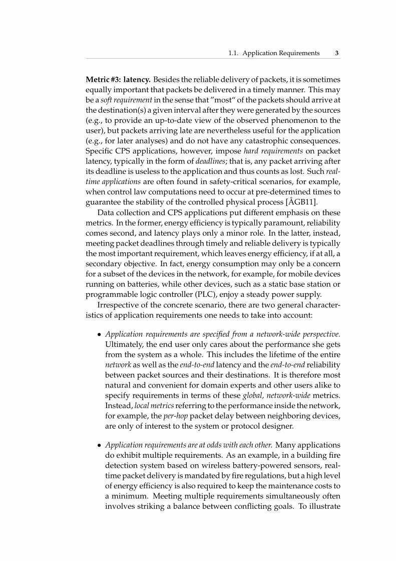
Metric #3: latency. Besides the reliable delivery of packets, it is sometimesequally important that packets be delivered in a timely manner. This maybe a soft requirement in the sense that ”most“ of the packets should arrive atthe destination(s) a given interval after they were generated by the sources(e.g., to provide an up-to-date view of the observed phenomenon to theuser), but packets arriving late are nevertheless useful for the application(e.g., for later analyses) and do not have any catastrophic consequences.Specific CPS applications, however, impose hard requirements on packetlatency, typically in the form of deadlines; that is, any packet arriving afterits deadline is useless to the application and thus counts as lost. Such real-time applications are often found in safety-critical scenarios, for example,when control law computations need to occur at pre-determined times toguarantee the stability of the controlled physical process [ÅGB11].
Data collection and CPS applications put di↵erent emphasis on thesemetrics. In the former, energy e�ciency is typically paramount, reliabilitycomes second, and latency plays only a minor role. In the latter, instead,meeting packet deadlines through timely and reliable delivery is typicallythe most important requirement, which leaves energy e�ciency, if at all, asecondary objective. In fact, energy consumption may only be a concernfor a subset of the devices in the network, for example, for mobile devicesrunning on batteries, while other devices, such as a static base station orprogrammable logic controller (PLC), enjoy a steady power supply.
Irrespective of the concrete scenario, there are two general character-istics of application requirements one needs to take into account:
• Application requirements are specified from a network-wide perspective.Ultimately, the end user only cares about the performance she getsfrom the system as a whole. This includes the lifetime of the entirenetwork as well as the end-to-end latency and the end-to-end reliabilitybetween packet sources and their destinations. It is therefore mostnatural and convenient for domain experts and other users alike tospecify requirements in terms of these global, network-wide metrics.Instead, local metrics referring to the performance inside the network,for example, the per-hop packet delay between neighboring devices,are only of interest to the system or protocol designer.
• Application requirements are at odds with each other. Many applicationsdo exhibit multiple requirements. As an example, in a building firedetection system based on wireless battery-powered sensors, real-time packet delivery is mandated by fire regulations, but a high levelof energy e�ciency is also required to keep the maintenance costs toa minimum. Meeting multiple requirements simultaneously ofteninvolves striking a balance between conflicting goals. To illustrate

4 Chapter 1. Introduction
this, consider a protocol using radio duty cycling, whereby the radiotransceiver is put into a low-power mode as often and for as long aspossible. However, two devices can only talk with each other whenthey both have their radios on. Thus, while radio duty cycling savesenergy, it can increase latency and negatively a↵ect reliability, too.
1.2 Challenges to Meeting RequirementsMeeting the requirements of real-world low-power wireless applicationsis far from trivial. This is due to the need for multi-hop communicationprotocols that constantly adapt their functioning to unpredictable and non-deterministic changes in the environment, while operating very close to theresource limits of the employed devices. We next discuss these challengesbefore moving on to a high-level review of prior attempts to tackling themwith the goal of meeting soft and hard application requirements.
Low-power wireless links are volatile. Low-power wireless communica-tions are notoriously unreliable. Fading because of multipath propagationor shadowing can reduce the power of the received signal to a point wheresuccessful reception is impossible; interference from wireless transmittersoperating on almost the same frequency at the same time can destroy theinformation encoded in signals; and meteorological conditions such as airtemperature and humidity a↵ect the link quality, too [BKM+12, WHR+13].As a result, low-power wireless links are volatile with coherence timesas small as a few hundred milliseconds [SKAL08], thus su↵ering fromunpredictable packet loss that can vary significantly over time [SDTL10].
A common approach to combat packet loss is to possibly transmit apacket more than once. Such a packet retransmission is triggered by thesender when no acknowledgment from the receiver has arrived within apredetermined time interval [GFJ+09]. Another possibility is the use ofan error-correction code, such as Reed-Solomon, whereby multiple checksymbols are added to the packet by the sender to detect a certain number oferroneous symbols at the receiver [LPLT10]. While both retransmissionsand coding help improve packet reliability, they increase average packetlatency and energy consumption. These two examples already show thatparameters of communication protocols, such as the maximum number ofretransmissions per packet or the number of check symbols to be added,could be important for meeting the application requirements, yet it maybe non-trivial to find the right trade-o↵ between all performance metrics.
Resource-constrained devices. To benefit the most from low costs, highflexibility, and deep embedding in the environment, low-power wirelessdevices often come in small form factors with severely limited resources.

1.2. Challenges to Meeting Requirements 5
Figure 1.1: A TelosB (also known as Tmote Sky) fits an 8 MHz microcontrollerand a 2.4 GHz low-power wireless radio within a few square centimeters.
Typical platforms feature a low-power microcontroller (MCU), a low datarate radio with a relatively short range, and a limited amount of code anddata memory. For example, the TelosB [PSC05] shown in Figure 1.1—stillone of the most widely used platforms in low-power wireless researchtoday despite its release a decade ago—has a 16-bit MSP430 MCU runningat a speed of up to 8 MHz, an IEEE 802.15.4 compliant CC2420 wirelessradio operating in the 2.4 GHz ISM band at a fixed data rate of 250 kbps,10 kB of RAM, 48 kB of program memory, and 1 MB of non-volatile flashstorage. In addition, energy is often limited by the battery capacity or themaximum possible intake in an energy harvesting scenario [BSBT14].
These resource constraints put limits on what can be computed, stored,and communicated using low-power wireless platforms. Although thereare increasingly more powerful yet very e�cient MCUs appearing on themarket, including the recent ARM Cortex-M0+, these represent only themiddle to upper end of the spectrum. At the lower end, there will soonbe true “Smart Dust” chips that integrate computation, communication,storage, and sensing in a cubic-millimeter [LBL+13]. It is clear that thesedevices will be even more resource-constrained than the smallest devicesthat challenge the designers of communication protocols today.
Multi-hop communication. One limit that deeply a↵ects communicationprotocol design is the transmission range of low-power wireless radios ofa few tens of meters indoors and a little over a hundred meters outdoors.The locations of nodes in a real deployment are, however, dictated by theapplication, which may require to cover significantly larger distances. Forinstance, intelligent telemetry of freight railroad trains requires networksthat span the length of a train, which can be up to 2.7 kilometers [ZDR08];a network for monitoring and controlling a modern paper mill needs toextend across about 150 meters; and process control in chemical plants or

6 Chapter 1. Introduction
source
destination link
Figure 1.2: Example of a multi-hop low-power wireless network with 16 nodes.Arrows represent physical communication links between neighboring devices;circles represent the nodes’ communication ranges. Due to the limited transmissionrange of low-power wireless radios, the source relies on intermediate nodes that relay itspackets along a routing path to the destination. The quality of each link on the path variesunpredictably over time because of fading, interference, and environmental factors.
refineries and building automation scenarios require network diametersthat are multiples of a node’s transmission range. Therefore, as shown inFigure 1.2, end-to-end packet delivery in these networks relies on multi-hop communication, where intermediate nodes relay packets on behalf ofsources that cannot directly communicate with the intended destinations.
In a multi-hop setting, the amount of network state—that is, informationabout the instantaneous conditions at the physical layer—that determinethe success or failure of an end-to-end packet transmission is a functionof the number of intermediate hops (or link) connecting the source withthe destination. However, as explained before, the quality of low-powerwireless links can fluctuate significantly over time even in a static network.Links can also vanish completely when devices suddenly fail because ofbattery depletion or damage, or when nodes move out of communicationrange. All these factors concur and make the network state a continuouslychanging unknown, which complicates multi-hop communication [AY05].
1.3 State of the ArtAs discussed in the following, three important problems remain unsolvedby prior work on low-power wireless communication protocols:

1.3. State of the Art 7
1. Support for non-critical data collection applications with multiplesoft requirements on global, network-wide performance metrics.
2. Support for critical CPS applications having hard requirements onend-to-end packet deadlines and possibly also energy constraints.
3. Addressing problems 1. and 2. above in the face of unpredictableand non-deterministic changes in the environment.
Architecture of layered low-power wireless networking stacks. Numer-ous low-power wireless communication protocols have been developed totackle the inherent network-level challenges discussed above. Traditionalsolutions that have been deployed with great success in the real worldand also those that are freely available as part of the open source TinyOSand Contiki distributions typically include multiple protocols organizedinto layers [ASSC02]. In low-power wireless, such a networking stack oftencomprises only the three lower layers: physical, data link, and network.The physical layer includes the radio hardware and the software driver fortransmitting individual bits, often grouped into symbols as defined by themodulation scheme, between two devices within communication range.The link layer, implemented by a media access control (MAC) protocol, usestechniques like carrier sense multiple access (CSMA) to arbitrate access tothe shared wireless medium to let multiple neighboring devices exchangepackets with one another. Low-power MAC protocols additionally use radioduty cycling and distinguish between unicast and broadcast to conserveenergy, and use per-hop packet retransmissions to help improve reliability[Lan08]. The routing protocol at the network layer is then responsible forthe end-to-end delivery of packets across multiple hops, for example, byestablishing a routing tree that maintains a path from every source to thedestination, which represents the root of the tree [AY05]. Only very fewtransport layer protocols exist, providing services like rate control andend-to-end acknowledgments to further help packet reliability [PG07].Primary focus on energy. As for meeting the non-functional requirementsof low-power wireless applications, the primary focus of existing low-power wireless communication stacks has been on reducing the nodes’energy consumption. Two techniques are commonly employed: radioduty cycling at the data link layer and finding routes that minimize thetotal number of transmissions per packet at the network layer [Lan08,AY05]. It has been shown that in particular the parameters of the low-power MAC protocol operating at the link layer largely determine notonly the energy cost of communication, but also the per-hop latency andreliability of and the bandwidth available for communication [LM10].The need to adapt. However, identifying a set of MAC parameters suchthat the resulting performance matches the application requirements is

8 Chapter 1. Introduction
cumbersome and error-prone, but most importantly, a particular choice ofMAC parameters may become unfit as the tra�c load and/or the networkstate changes. A few works thus propose to adapt specific MAC protocolparameters at runtime in response to such changes, mostly with the solegoal of keeping the energy consumption to a minimum [JBL07, CWW10].
Focus on single or local metrics. There is even less work incorporatingadditional metrics, such as per-hop latency and per-hop reliability, intothe adaptation decisions [PFJ10]. While these e↵orts are an importantstep in the right direction, they fall short of meeting the requirements oflow-power applications in that they either focus only on a single metricor consider only local metrics. Nevertheless, as described in Section 1.1,low-power wireless applications often have requirements along multiplemetrics, which are most naturally specified in global, network-wide terms.
No hard performance guarantees in multi-hop networks. Despite theusefulness of traditional networking stacks in enabling non-critical (datacollection) applications, their complexity makes it almost impossible toprovide hard guarantees on the end-to-end performance over multiplehops, which are definitely needed to support critical CPS scenarios. Theroot cause of this complexity is the wireless link abstraction: Many protocolson all layers of the stack adopt concepts from wired networks like unicasttransmission and routing path, as shown in Figure 1.2, thereby treating thewireless channel between two devices as a point-to-point link [KRH+06].The end-to-end behavior of these protocols, then, depends on the qualityof multiple links, each of which is subject to several unpredictable factors.
The inability to keep up with the ever-changing network state is indeedthe primary reason why previous solutions cannot support applicationsthat require packets to be delivered within hard real-time deadlines. Bothindustry standards [har, isa] and research prototypes [OBB+13, SNSW10]exist that compute at runtime transmission schedules tailored for eachnode in the network at a central entity, based on information about theglobal network state. Assuming the latter would not change at all, theseapproaches could in principle guarantee end-to-end packet deadlines. Inthe real world, however, the network state changes, and because it takesconsiderable time from when such change occurs until when a change isreflected in new transmissions schedules—on the order of several minutesbased on anecdotal evidence reported by our contacts at ABB Research—these routing-based solutions are fundamentally incapable of supportinghard real-time applications. This is also acknowledged by major industryplayers who contributed to the WirelessHART standard: “. . . none of thetechnologies provide any hard guarantees on deadlines, which is neededif you should dare to use the technology in critical applications” [Per].

1.4. Thesis Contributions and Road Map 9
1.4 Thesis Contributions and Road MapTo address these shortcomings, this thesis makes three key contributions.
Meeting soft network-wide performance requirements (Chapter 2). Toserve the needs of real-world data collection applications, we introducepTunes, a framework for runtime adaptation of low-power MAC protocolparameters. Compared with prior solutions, pTunes takes a more holisticapproach by allowing the user to specify multiple performance goals froma global, network-wide perspective. These performance goals, specified interms of network lifetime, end-to-end reliability, and end-to-end latency,represent soft requirements that are to be satisfied in the long run. Given aconcrete requirements specification and a traditional low-power wirelessstack running at each node, pTunes adapts the operational parameters ofthe low-power MAC protocol at runtime to meet the requirements againstdynamic changes in network state, tra�c load, and routing topology.
As detailed in Chapter 2, pTunes rests upon three building blocks:
• The design of pTunes revolves around a centralized approach thatis similar in spirit to a model-predictive controller. To reason aboutnetwork-wide performance, pTunes periodically collects at a centralentity (e.g., the base station in a deployment) reports from each nodethat contain local routing and network state, among others. Basedon the thus obtained global network view and an accurate performancemodel, pTunes first checks whether the application requirements areviolated. If so, it automatically solves a multi-objective optimizationproblem in order to determine MAC parameters so that the predictedperformance matches again the application requirements under thecurrent global network view. The determined MAC parameters arethen distributed in the network and installed on all devices.
• We structure the aforementioned performance model in a layeredfashion, clearly separating application-level, protocol-independent,and protocol-dependent modeling quantities. This way, we simplifythe integration of a di↵erent MAC protocol into pTunes by reusingcommon expressions and identifying the minimum set of quantitiesthat needs to be altered. We show the e↵ectiveness of our modelingapproach by applying it to two state-of-the-art protocols, X-MACand LPP, based on their implementations in Contiki.
• We design an e�cient runtime support to “close the loop” in pTunes.Our approach uses fast and reliable Glossy floods [FZTS11] to collectnetwork state and disseminate new MAC parameters. This enablespTunes to gather consistent snapshots of network state, taken with

10 Chapter 1. Introduction
microsecond accuracy at all nodes simultaneously, with low energycosts and independent of other protocols running concurrently.
We demonstrate using testbed experiments that pTunes can achieveseveralfold improvements in network lifetime over fixed MAC parame-ters, while satisfying soft end-to-end latency and reliability requirementsin the long run despite unforeseen changes in the network caused by, forexample, wireless interference and multiple node failures.
Modeling protocols that utilize synchronous transmissions (Chapter 3).The e↵ectiveness of pTunes is fundamentally dependent on the accuracyof the performance model, which maps the global network view and theMAC protocol parameters to the three performance metrics we target. Inessence, it is the performance model that closes the large conceptual gapbetween the high-level application requirements and the low-level MACprotocol parameters, and the solver exercises the model while computingthe latter in order to satisfy the former. More generally, accurate modelsof a network’s end-to-end performance can greatly aid in the design andverification of emerging systems, including CPS that “. . . must operatedependably, safely, securely, e�ciently, and in real-time. [RLSS10]”
Unfortunately, traditional multi-hop low-power wireless protocols asconsidered in Chapter 2 are intricate and di�cult to model. This is becausetheir operation is conditional on the ever-changing network state, whichleads to unpredictable and often uncoordinated changes in the protocol’sbehavior, for example, when some node in the routing tree locally decidesto forward packets to a di↵erent parent [GFJ+09]. As a result, previousmodeling e↵orts often stop at the link layer, where distributed interactionsspan only a single hop and hence reasoning is still manageable, achievingmodel errors in the range of 2–7 % (see Section 2.5.2). Only a few worksmodel higher-layer functionality [YZDPHg11, GB12], but their validationis limited to simulations, which lack precisely the real-world dynamics oflow-power wireless that complicate the modeling in the first place.
Fueled by our own work on the Glossy flooding architecture [FZTS11]and the Low-Power Wireless Bus (LWB) [FZMT12], a radically di↵erentbreed of communication protocols has emerged that utilizes synchronoustransmissions. Rather than one sender transmitting over a dedicated wire-less link to a receiver, using synchronous transmissions multiple senderstransmit simultaneously to the receiver. The sender diversity [RHK10] andtwo physical-layer phenomena, constructive baseband interference andcapture e↵ects [WLS14], let synchronous transmissions achieve a higherone-hop packet reliability than link-based transmissions [DDHC+10].
Chapter 3 of this thesis shows that certain protocols using synchronoustransmissions are also simpler to model than link-based protocols with anunparalleled accuracy. Specifically, Chapter 3 contributes the following:

1.4. Thesis Contributions and Road Map 11
• Using statistical time series analyses of a large set of packet receptiontraces collected through extensive testbed experiments, we find thatpacket receptions and losses in Glossy largely adhere to a sequenceof independent and identically distributed (i.i.d.) Bernoulli trials.This so-called Bernoulli assumption is typically made to simplify themodeling, yet we find that this assumption is significantly less validwhen modeling protocols that operate on individual wireless links.
• Leveraging the validity of the Bernoulli assumption to synchronoustransmissions, we devise a simple Markovian model that estimatesLWB’s long-term energy consumption with an unparalleled errorof 0.25 % relative to real measurements, and su�cient conditions togive probabilistic guarantees on LWB’s end-to-end packet reliability.In doing so, we demonstrate for the first time the accurate modelingof a complete multi-hop low-power wireless networking solution.
These results are particularly relevant to CPS applications employingfeedback control. Many control algorithms can be designed to tolerate asmall fraction of packet loss, say, less than 1 %, without sacrificing controlperformance and stability. Nevertheless, this assumes that the few lossesdo not happen as a longer burst of multiple consecutive losses [SSF+04].The validity of the Bernoulli assumption for synchronous transmissionsessentially says that such adverse bursts virtually never occur when using,for example, Glossy to communicate packets throughout the network.
Meeting hard real-time requirements with low energy costs (Chapter 4).Since LWB employs only Glossy for communication and has been shownto keep end-to-end packet loss rates below 1 % [FZMT12], LWB could be agood candidate protocol for supporting CPS applications. Indeed, LWB’soperation resembles that of wired fieldbusses, such as FlexRay [MT06] andTime-Triggered Protocol [KG93], which are used in classical embeddedsystems with high dependability and real-time requirements. Using LWB,nodes are synchronized and an appointed host node repeatedly computesa communication schedule that globally allocates non-overlapping timeslots to nodes that have pending packets. That is, there is just one globalschedule that applies to all nodes in the network, and every time slot inthis schedule corresponds to a distinct network-wide Glossy flood. Whileworking with Glossy and LWB over the past years, we began to nourishthe hope that it could be possible to support CPS applications with hardreal-time requirements by leveraging LWB’s bus-like operation.
To show that our intuition was correct, we design Blink, the first low-power wireless protocol providing hard real-time guarantees on end-to-end packet deadlines in large multi-hop networks, while simultaneouslyincurring low energy costs. Blink uses LWB as underlying communication

12 Chapter 1. Introduction
support, yet the original LWB scheduler is completely oblivious of packetdeadlines. The key observation that makes Blink immune to the problemthat prevents prior solutions from providing real-time guarantees acrossmultiple hops (see Section 1.3) is that because Glossy’s protocol logic isindependent of the current network state, we do not need to consider thetime-varying network state as an input to the scheduling problem either.
As detailed in Chapter 4, Blink’s design rests upon three components:
• In LWB all nodes follow the same schedule, while Glossy providesvery accurate network-wide time synchronization and allows us toignore the network state. Due to these properties we can treat anentire multi-hop low-power wireless network as a single resource thatruns on a single clock. This abstraction is powerful in that it allowsus to map the real-time scheduling problem in Blink to uniprocessorscheduling, which is well known and easier to solve than the multi-processor scheduling problem found in prior work [SXLC10].
• We conceive scheduling policies based on the earliest deadline first(EDF) principle [LL73]. Blink uses these policies to compute onlinea schedule that provably meets all deadlines of admitted packetstreams, while minimizing the network-wide energy consumptionwithin the limits of the underlying LWB communication support,tolerating changes in both the network state and the set of streams.
• We design and implement a highly e�cient priority queue as well asalgorithms that make use of it to enable EDF scheduling on resource-poor devices. Based on these, we can demonstrate the first workingimplementation of EDF on low-power embedded platforms.
We evaluate a Blink prototype on two testbeds, showing that it meetsnearly 100 % of packet deadlines; the few deadline misses are entirely dueto packet loss, which cannot be completely avoided in a wireless setting.Moreover, experiments on three state-of-the-art MCUs show that, thanksto our data structures and algorithms, Blink achieves speed-ups of up to4.1⇥ relative to a conventional scheduler implementation. These speed-ups prove instrumental to the viability of EDF-based real-time schedulingon specific low-power embedded platforms.
2pTunes:
Runtime Parameter Adaptationfor Low-power MAC Protocols
Media access control (MAC) protocols play a key role in determining theperformance of low-power wireless networks, but very few of the manyproposed solutions have been used in real deployments [KGN09, RC08].
Challenges. There exists a significant conceptual gap between the high-level application requirements on the one hand and the low-level MACprotocol operation on the other [KGN09]. In particular, it requires expertknowledge to find operating parameters of the low-power MAC protocolsuch that the performance satisfies given application requirements.
In most deployments today, the choice of MAC parameters is basedon experience and rules of thumb involving a coarse-grained analysisof expected network load and topology dynamics. This can yield aperformance far o↵ the application requirements [LM10]. Alternatively,system designers conduct several field trials in order to identify suitableMAC parameters [CCD+11]. This time-consuming and deployment-specific practice, however, is hardly sustainable in the long term.
Even if the MAC parameters are appropriate at one time, they are likelyto perform poorly when the network state changes. The quality of low-power wireless links varies greatly over time, leading to unpredictablepacket loss [ZG03]; harsh environmental conditions cause nodes to betemporarily disconnected or to fail [BGH+09]; and changes in the routingtopology or the sensing activity result in fluctuating tra�c load. Statically

14 Chapter 2. pTunes: Runtime Parameter Adaptation for Low-power MAC Protocols
Base Station
RequirementsApplication
Network State
MAC Parameters
pTunes
Network
OptimizationTrigger
Solver
Network-wide
ModelPerformance
Figure 2.1: Overview of the pTunes framework. pTunes takes advantage of acentralized approach that shares some similarities with a model-predictive controller.
configured MAC protocols cannot cope with these dynamics.To perform e�ciently at all times, MAC protocols must adapt their
operating parameters at runtime. One way to approach this problem is toembed adaptivity within the protocol operation [HB10]. This, however,hard-codes the adaptation policies and hence limits their applicability.Instead, separating adaptivity from the protocol operation enables higher-layer services to dynamically adjust the operating parameters [PHC04].Although a few mechanisms utilize these “control knobs,” they eitherfocus on a single performance metric—typically energy [JBL07, MWZT10,CWW10]—or consider only local metrics, such as per-hop latency [PFJ10,BYAH06]. Real-world applications, however, often need to balancemultiple conflicting performance metrics, such as reliability, energy, andlatency, expressed on a network-wide scale [CMP+09, SMP+04, WALJ+06].
Contributions and road-map. To tackle the issues above, we presentpTunes, a framework for runtime adaptation of low-power MAC protocolparameters. pTunes allows users to specify application requirementsin terms of network lifetime, end-to-end reliability, and end-to-end latency,which are key performance metrics in real-world applications [CCD+11,CMP+09, SMP+04, WALJ+06, TPS+05]. Based on information about thecurrent network state, pTunes automatically determines optimized MACparameters whose performance meets the requirements specification.
This chapter makes the following contributions:
• We introduce the pTunes framework, targeting data collectionsystems employing tree routing atop low-power MAC protocols.As shown in Figure 2.1, using pTunes a base station collects reportson the network state, such as topology and link quality information,to evaluate the network-wide metrics we target. The optimizationtrigger decides when to carry out the parameter optimization, based

15
on a periodic timer or some mechanism that uses the network-wide performance model to check if the application requirements areviolated under the current network state. The solver determinesoptimized MAC parameters, which are disseminated in the networkand installed on all nodes. Section 2.1 further characterizes themulti-objective parameter optimization problem in pTunes.
• We design a well-structured modeling framework to solve theparameter optimization problem. Our layered modeling approach,described in Section 2.2, separates application-level, protocol-independent, and protocol-dependent quantities. This increasesgenerality and flexibility, as it cleanly determines what needsto be changed to account for a di↵erent MAC protocol. Weapply this modeling approach to two state-of-the-art protocols,X-MAC [BYAH06] and LPP [MELT08], based on their implemen-tations in Contiki. We use these models throughout this chapter,ultimately demonstrating that they are both practical and accurate.
• We present the design and implementation of an e�cient systemsupport to address the system-level challenges arising in pTunes.These include, for instance, the timely collection of accurate networkstate with little energy overhead and minimum disruption for theapplication operation. As described in Section 2.3, unlike mostapproaches in the literature, we meet these requirements witha novel solution for collecting network state and disseminatingnew MAC parameters independent of other protocols runningconcurrently. Our approach utilizes fast and reliable Glossy networkfloods [FZTS11], allowing pTunes to collect consistent networkstate snapshots, taken with microsecond accuracy at all nodessimultaneously, with very low energy cost.
After illustrating implementation details in Section 2.4, we evaluatepTunes in Section 2.5 using experiments with X-MAC and LPP on a 44-node testbed. For instance, we find that adapting their parameters usingpTunes enables up to three-fold lifetime gains over static MAC parametersoptimized for peak tra�c, the latter being current practice in many realdeployments [KGN09]. pTunes promptly reacts to changes in tra�c loadand link quality, meeting application-level requirements through an 80 %reduction in packet loss during periods of controlled wireless interference.Moreover, we find that pTunes helps the routing protocol recover fromcritical network changes, reducing the total number of parent switchesand settling quickly on a stable, high-quality routing topology. Thisreduces packet loss by 70% in a scenario where multiple core routingnodes fail simultaneously.

16 Chapter 2. pTunes: Runtime Parameter Adaptation for Low-power MAC Protocols
We discuss design trade-o↵s of pTunes in Section 2.6, review relatedwork in Section 2.7, and provide brief concluding remarks in Section 2.8.
2.1 Optimization ProblemIn pTunes, we simultaneously consider three key performance metrics ofreal-world applications [CCD+11, CMP+09, SMP+04, WALJ+06, TPS+05]:network lifetime T, end-to-end reliability R, and end-to-end latency L.The MAC parameter optimization problem thus becomes a multi-objectiveoptimization problem (MOP). This involves optimizing the objectivefunctions T(c), R(c), and L(c), where c is a vector of MAC parameters,or MAC configuration for short. There may exist not one unique optimalsolution to this MOP, but rather a set of solutions that are optimal inthe sense that no other solution is superior in all objectives. These areknown as Pareto-optimal solutions and represent di↵erent optimal trade-o↵s among T, R, and L.
Given the many Pareto-optimal solutions, a natural question is whichsolution best serves the application demands. pTunes needs to makethis decision at runtime in an automated fashion, without involvingthe user (e.g., to manually select a solution from a set of candidates).With this requirement in mind, we adopt from among the manyMOP solving techniques an approach inspired by the epsilon-constraintmethod [HLW71]. This method treats all but one objective as constraints,and thus provides a natural interface for specifying typical requirementsof low-power wireless systems such as “batteries should last for at least6 months.” Using this approach, pTunes solves the MOP by optimizingone objective subject to constraints on the remaining objectives
Maximize/Minimize M1(c)Subject to M2(c) �, C1
M3(c) �, C2
(2.1)
where each Mi is one among {T,R,L} and {C1,C2} are soft requirements tobe satisfied in the long run, corresponding to the best-e↵ort operation ofmany data collection systems [GFJ+09]. By varying {C1,C2}, all Pareto-optimal solutions can be generated. Based on concrete values for {C1,C2}set by the user on some objectives, pTunes translates the applicationrequirements into a solution that optimizes the remaining objective.The resulting solution is Pareto-optimal while representing the trade-o↵provided by the user.
As an example, in long-term structural monitoring the major concernis typically network lifetime, but domain experts also require a certain

2.2. Modeling Framework 17
Network State
MAC Parameters
transmission pl
Rl TnLl
Drx,nDtx,nTftx,l
Tstx,l
ps,l Nftx,lProtocol-
independent
Protocol-
Application-
level
Probability of successful dependent
MAC configuration c
TopologyN ,M, LPacket generation rate Fn
Network-wide Performance Model
R TLModel Output
Figure 2.2: Modeling framework of pTunes with inputs, output, and mappingbetween the di↵erent modeling layers. The layered modeling approach simplifies theintegration of new MAC protocols into pTunes by fostering reuse of common expressionsand clearly identifying the minimum set of quantities that needs to be changed.
reliability in delivering sensed data [CMP+09]. Instantiating (2.1), theuser would specify the maximization of network lifetime subject to aminimum end-to-end reliability as follows
Maximize T(c)Subject to R(c) � Rmin
(2.2)
In addition, the user may impose an additional constraint on end-to-endlatency, L(c) Lmax, in case timely data delivery is also relevant.
2.2 Modeling FrameworkTo facilitate using pTunes with di↵erent low-power MAC protocols, webreak up the modeling into three distinct layers, as shown in the modelframe in Figure 2.2. The upper layer defines application-level metrics(R, L, T) as functions of link and node-specific metrics (Rl, Ll, Tn). Themiddle layer expresses these metrics in a protocol-independent manner,and provides the entry point for the modeling of a concrete MAC protocolby exposing six terms to the lower protocol-dependent layer. Bindingthese terms to concrete protocol-specific expressions is su�cient to adaptthe network-wide performance model in pTunes to a given MAC protocol.
Model inputs are the MAC parameters and the network state,comprising information about routing topology, tra�c volumes, and linkqualities. As a measure of the latter, we take the probability of successfultransmission pl over the link to the parent in the routing tree. To keep

18 Chapter 2. pTunes: Runtime Parameter Adaptation for Low-power MAC Protocols
Table 2.1: Terms denoting network state and protocol-dependent quantities.Term DescriptionN Set of all nodes in the network excluding the sinkM Set of source nodes generating packetsL Set of all links forming the routing treeFn Packet generation rate of node npl Probability of successful transmission over link lps,l Probability of successful unicast transm. over link l
Nftx,l Number of failed unicast transmissions before success over link lTftx,l Time for a failed unicast transmission over link lTstx,l Time for a successful unicast transmission over link lDrx,n Fraction of time radio is in receive mode at node nDtx,n Fraction of time radio is in transmit mode at node n
our models simple and practical, we assume the delivery of individualpackets to be independent of their size, of the delivery of any other packet,and of the link direction they travel along. As illustrated in Section 2.3,our runtime evaluation of pl captures the impact of channel contentionon link quality, allowing us not to consider it explicitly in our models.Testbed experiments in Section 2.5.2 show that this approach results inhighly accurate models for both X-MAC and LPP.
2.2.1 Application-level Metrics
In a typical data collection scenario with static nodes, a tree-shapedrouting topology provides a unique path from every sensor node toa sink node. These paths are generally time-varying, as the routingprotocol adapts them according to link quality estimates among otherthings [GFJ+09, PH10]. In the following, we use N to denote the set ofall nodes in the network excluding the sink, and M ✓ N to denote theset of source nodes generating packets. We also indicate with L the set ofcommunication links that form the current routing tree. The path Pn ✓ Loriginating at node n 2 M includes all intermediate links that connectnode n to the sink. Table 2.1 lists these and other modeling terms we useto denote network state and protocol-dependent quantities.
End-to-end reliability and latency. The reliability RPn of path Pn is theexpected fraction of packets delivered from node n 2 M to the sinkalong Pn. Thus, RPn is the product of per-hop reliabilities Rl, l 2 Pn. We

2.2. Modeling Framework 19
define the end-to-end reliability R as the average reliability of all paths Pn.
R =1|M|
X
n2MRPn =
1|M|
X
n2M
0BBBBB@Y
l2Pn
Rl
1CCCCCA (2.3)
Likewise, the latency LPn of path Pn is the expected time between thefirst transmission of a packet at node n 2M and its reception at the sink.Thus, LPn is the sum of per-hop latencies Ll, l 2 Pn. Similar to (2.3),we define the end-to-end latency L for successfully delivered packets as theaverage latency of all paths Pn, and omit the formula.
We define R and L as averages of all source-sink paths since the global,long-term performance is of ultimate interest for most data collectionsystems [WALJ+06, TPS+05, SMP+04]. Local, short-term deviations fromthe requirements are usually tolerated, provided they are compensatedin the long run. In other scenarios (e.g., industrial settings), it might bemore appropriate to define R and L as the minimum reliability and themaximum latency among all source-sink paths, which would only requiremodifying the two definitions above.
Network lifetime. Similar to prior work [ML06], we define the networklifetime T as the expected shortest node lifetime Tn, n 2 N . We assume thesink has infinite energy supply.
T = minn2N
(Tn) (2.4)
This choice is motivated by the fact that a single node failure can lead tonetwork partition and service interruption. It is also possible to expressother notions of network lifetime in pTunes, such as the time until somefraction of nodes fails, again requiring only to modify (2.4).
2.2.2 Protocol-independent ModelingThe section above expressed the application-level metrics R, L, and T asfunctions of per-hop reliability Rl, per-hop latency Ll, and node lifetime Tn
(see Figure 2.2). We now define the latter three in a protocol-independentmanner, which increases flexibility and generality by isolating protocol-dependent quantities.
Per-hop reliability and latency. Several factors influence these metrics:(i) the MAC operation when transmitting packets, (ii) packet queuingthroughout the network stack due to insu�cient bandwidth, and(iii) application-level bu↵ering, for example, to perform in-networkprocessing. The MAC parameters have an impact on (i) and may avoidthe occurrence of (ii), provided a MAC configuration exists that provides

20 Chapter 2. pTunes: Runtime Parameter Adaptation for Low-power MAC Protocols
su�cient bandwidth for the current tra�c load. Application-specific in-network functionality akin to (iii) is out of the scope of this work.
We present next expressions for per-hop reliability and latency due tothe MAC operation, corresponding to (i). Additionally, pTunes includesmodels to detect situations akin to (ii). In fact, as we show in Section 2.5.2,pTunes automatically adjusts the MAC parameters to provide higherbandwidth against increased tra�c, thus avoiding the occurrence of localpacket queuing until the network capacity attainable in our experimentalsetting is fully exhausted.
We define the per-hop reliability Rl of link l 2 L, which connects node n 2N to its parent m in the routing tree, as the probability that n successfullytransmits a packet to m.
Rl = 1 � (1 � ps,l)N+1 (2.5)
Here, ps,l represents the MAC-dependent probability that a single unicasttransmission over link l succeeds, and N is the maximum number ofretransmissions per packet, modeling automatic repeat request (ARQ)mechanisms used by many MAC protocols to improve reliability.
Furthermore, we define the per-hop latency Ll of link l as the time fornode n to deliver a message to its parent m.
Ll = Nftx,l · Tftx,l + Tstx,l (2.6)
Here, Tftx,l and Tstx,l are the MAC-dependent times needed for each failedand the final successful transmission, and Nftx,l is the expected number offailed transmissions before the final successful one.
To derive an expression for Nftx,l, let pf ,l = 1 � ps,l be the probabilitythat a single transmission over link l fails, and pf ,l(k) = pf ,l(0) · pk
f ,l theprobability of k, 0 k N, consecutive failed transmissions, wherepf ,l(0) denotes the probability that already the first transmission succeeds(i.e., no transmission fails). There can be between 0 and N failed packettransmissions. To compute the expectation Nftx,l, we sum over all possiblevalues 0 k N, weighted by their probabilities of occurrence pf ,l(k).
Nftx,l =NX
k=0
k · pf ,l(k)
= pf ,l(0) · pf ,l ·NX
k=0
k · pk�1f ,l (2.7)
Since we consider the per-hop latency Ll in (2.6) only for delivered packets,that is, for packets that are eventually successfully transmitted, the sum

2.2. Modeling Framework 21
of the di↵erent probabilities pf ,l(k) for all possible k amounts to 1.
1 =NX
k=0
pf ,l(k)
= pf ,l(0) ·1 � pN+1
f ,l
1 � pf ,l(2.8)
From this, we immediately obtain an expression for the probability pf ,l(0)that the first packet transmissions succeeds.
pf ,l(0) =1 � pf ,l
1 � pN+1f ,l
(2.9)
Replacing pf ,l(0) in (2.7) with the expression in (2.9) we get
Nftx,l =pf ,l · (1 � pf ,l)
1 � pN+1f ,l
·NX
k=0
k · pk�1f ,l
=pf ,l · (1 � pf ,l)
1 � pN+1f ,l
·0BBBBB@
1 � pN+1f ,l
(1 � pf ,l)2 �(N + 1) · pN
f ,l
1 � pf ,l
1CCCCCA
=pf ,l
1 � pf ,l� (N + 1) ·
pN+1f ,l
1 � pN+1f ,l
(2.10)
Node lifetime. Sensor nodes consume energy by communicating,sensing, processing, and storing data. Adapting the MAC parameters hasno significant impact on the latter three, but a↵ects energy expenditureson communication to a large extent, as the radio is typically a major energyconsumer. Given a battery capacity Q, we define the node lifetime Tn ofnode n 2 N as
Tn = Q/(Dtx,n · Itx +Drx,n · Irx +Didle,n · Iidle) (2.11)
where Itx, Irx, and Ii are the current draws of the radio in transmit, receive,and idle mode. Tn is thus the expected node lifetime based on the fractionsof time in each mode Dtx,n, Drx,n, and Didle,n = 1�Dtx,n�Drx,n, which dependon the MAC protocol and the tra�c volume at node n.
The tra�c volume is the rate at which nodes send and receive packets.A node n 2 N generates packets at rate Fn and receives packets from itschildren Cn ✓ N in the routing tree, if any. The rate of packet receptiondepends on each child’s packet transmission rate Ftx,c and the individualper-hop reliabilities Rlc of links lc, c 2 Cn, connecting each child c with n.Thus, node n transmits packets at rate
Ftx,n = (Nrtx,l + 1) ·0BBBBB@Fn +
X
c2Cn
Ftx,c · Rlc
1CCCCCA (2.12)

22 Chapter 2. pTunes: Runtime Parameter Adaptation for Low-power MAC Protocols
Here, Nrtx,l is the expected number of retransmissions per packet overlink l. To compute it, we have to sum over all possible values, weightedby their probabilities of occurrence. The probability of k, 0 k < N,retransmissions is pk
rt,l · (1 � prt,l); that is, the first k packet transmissionsfail (each with probability prt,l) and the last one succeeds (with probability1 � prt,l). With pN
rt,l denoting the probability that the maximum numberof packet retransmissions is exhausted without delivering the packet, wederive the expected number of retransmissions per packet as follows.
Nrtx,l = N · pNrt,l +
N�1X
k=0
k · pkrt,l · (1 � prt,l)
= N · pNrt,l + prt,l · (1 � prt,l) ·
N�1X
k=0
k · pk�1rt,l
= N · pNrt,l + prt,l · (1 � prt,l) ·
0BBBB@
1 � pNrt,l
(1 � prt,l)2 �N · pN�1
rt,l
1 � prt,l
1CCCCA
=prt,l · (1 � pN
rt,l)
1 � prt,l(2.13)
Packet queuing. Whenever node n enqueues packets at a higher rate thanit forwards (i.e., dequeues) packets, packets start to queue up at node n.The former rate is given by
F0 = Fn +X
c2Cn
Ftx,c · Rlc (2.14)
adding up the local packet generation rate Fn and the rate at whichpackets are received from n’s child nodes Cn. The latter rate, that is,the upper bound on the rate at which node n can forward (dequeue)packets, is the inverse of the expected MAC-dependent time needed fora packet transmission Ttx, including retransmissions and packets that areeventually dropped when the maximum number of retransmissions Nhas been exhausted. Thus, by imposing the constraint
1(Nrtx,l + 1) · Ttx
� F0 (2.15)
where Nrtx,l is given by (2.13), we enforce that pTunes selectsMAC parameters such that MAC-dependent queuing does not occur.Furthermore, if (2.15) is not satisfiable when estimating the network-wideperformance based on the collected network state, pTunes essentiallyknows and can thus detect that there is MAC-dependent queuing withinthe network. High-layer functionality, such as data aggregation and other

2.2. Modeling Framework 23
Ts Tsl Td
tTsaTo↵ Tda
Tx mode
Rx mode
Tonh1i
h2i
h3i
h6i
h4i h5i h7i
ts-ack d-ackstrobe data
Receiver
Sender
Figure 2.3: Sequence of radio modes and packet exchanges during a successfulunicast transmission in X-MAC.
in-network processing, may introduce additional packet bu↵ering, whichis however independent of the MAC operation.
We demonstrate next the modeling of a concrete MAC protocol. Thisrequires to find expressions for six protocol-specific terms, as shown inFigure 2.2 and described in Table 2.1.
2.2.3 Protocol-specific ModelingWe use two state-of-the-art MAC protocols to exemplify the protocol-specific modeling. X-MAC [BYAH06] is representative of many sender-initiated MAC protocols based on low-power listening (LPL) [PHC04]that proved viable in real-world deployments [KGN09]. More recentwork focuses on receiver-initiated MAC protocols such as low-powerprobing (LPP) [MELT08]. In the following, we refer to implementationsof X-MAC and LPP in Contiki 2.3, which we also use in our experimentsin Section 2.5.
2.2.3.1 Sender-initiated: X-MAC
Figure 2.3 shows a successful unicast transmission in X-MAC. Nodeswake up periodically for Ton to poll the channel h1i, where To↵ is thetime between two channel polls. To send a packet, a node transmitsa sequence of strobes h2i, short packets containing the identifier of thereceiver. Strobing continues for a period su�cient to make at leastone strobe overlap with a receiver wake-up h3i. The receiver replieswith a strobe acknowledgment (s-ack) h4i and keeps the radio on awaitingthe transmission of the data packet h5i. The sender transmits the datapacket upon receiving the s-ack h6i and waits for the data acknowledgment(d-ack) h7i from the receiver. Afterward, both nodes turn o↵ their radios.
Failed s-ack, d-ack, and data packet transmissions are handled by
24 Chapter 2. pTunes: Runtime Parameter Adaptation for Low-power MAC Protocols
timeouts. When a timeout occurs, the sender backs o↵ for a randomperiod and retries beginning with the strobing phase, for at most N times.Broadcasts proceed similarly to unicast transmissions, but the strobingphase lasts for Tm = 2 · Ton + To↵ to make a strobe overlap with the wake-up of all neighboring nodes. Nodes receiving a broadcast strobe keeptheir radio on until they receive the data packet at the end of the sender’sstrobing phase.
Several variables are adjustable in the X-MAC implementation weconsider. However, three specific parameters a↵ect its performance to amajor extent.
c = [Ton,To↵ ,N] (2.16)
We let pTunes adapt these parameters at runtime, leveraging the X-MACspecific models presented next.
Per-hop reliability. We determine ps,l in (2.5), the probability that a singleunicast from node n to its parent m succeeds. This is the case if m hears astrobe (with probability ps,l), the s-ack reaches n, and m receives the datapacket. Each of the latter two succeeds with probability pl, collected atruntime as part of the network state (see Section 2.3).
ps,l = ps,l · p2l (2.17)
The probability of receiving at least one strobe is
ps,l = 1 � (1 � pl)(Ton�Ts)/Tit (2.18)
where Tit = Ts + Tsl is the duration of a strobe iteration at the sender,which includes the length of a strobe transmission Ts and listening Tsl foran s-ack.
Per-hop latency. We determine Tftx,l and Tstx,l in (2.6), the times spentfor failed and successful transmissions. Tftx,l depends on whether node nreceives an s-ack. If so, n stops strobing, sends the data packet, and timesout after Tout. Otherwise, n sends strobes for Tm. In either case, node nbacks o↵ for Tb before retransmitting.
Tftx,l = (NitTit + Td + Tout)ps,l + Tm(1 � ps,l) + Tb (2.19)
Here, Nit = (Ton + To↵ )/(2 · Tit) is the average number of strobe iterationsbefore m possibly replies with an s-ack.
The time for a successful transmission Tstx,l includes the time to waitfor the s-ack and to send the data packet.
Tstx,l = Nit · Tit + Td (2.20)
Node lifetime. We determine Dtx,n and Drx,n in (2.11), the fractions of timespent by the radio in transmit and receive mode. Both quantities depend

2.2. Modeling Framework 25
on the rate Farx,lc at which node n attempts to receive a packet from child cover link lc
Farx,lc =�Nrtx,lc + 1
� · Ftx,c · ps,lc (2.21)
where Ftx,c and ps,lc are given by (2.12) and (2.18).We start with Dtx,n. Node n transmits during packet receptions from
child c and during packet transmissions to its parent m. Letting Trxt,lc andTtxt,l denote the expected times the radio is in transmission mode duringreceptions over link lc and transmissions over link l, we thus have
Dtx,n = Ftx,n · Ttxt,l +X
c2Cn
Farx,lc · Trxt,lc (2.22)
Trxt,lc includes the times to transmit the s-ack and, provided s-ack and datapacket are successfully transmitted, to send the d-ack, which happenswith probability plc
2.Trxt,lc = Tsa + Tda · plc
2 (2.23)
To compute Ttxt,l, we distinguish whether node n’s parent m receives oneof its strobes and successfully replies with a s-ack, which happens withprobability ps-ack,l = ps,l · pl. If so, n is in transmit mode for sending Nit
strobes and the data packet. Otherwise, n is in transmit mode for sendingas many strobes as fit into the maximum length of the strobing period Tm.
Ttxt,l = (Nit · Ts + Td) · ps-ack,l +✓Tm
Tit· Ts
◆· �1 � ps-ack,l
�(2.24)
Next we consider Drx,n. Node n is in receive mode during packettransmissions to its parent m and packet receptions from child c. Let Ttxr,l
and Trxr,lc be the expected times spent by the radio in reception modeduring transmissions over link l and receptions over link lc. The fractionof time in receive mode for actual communication is
Drxc,n = Ftx,n · Ttxr,l +X
c2Cn
Farx,lc · Trxr,lc (2.25)
To compute Trxr,lc , we note that n is in receive mode during receptionsfrom child c along link lc to receive a strobe and the data packet. Weaccount for the time to receive a strobe in the time for channel checks,as per (2.28). Thus, if the s-ack sent by node n and the data packet sentby c are successfully transmitted, n is in receive mode to receive the datapacket; otherwise, n is in receive mode for Tout until a timeout expires.Additionally, we consider the turnaround time Tturn for switching betweentransmit and received modes time in receive mode.
Trxr,lc = 2 · Tturn + (Tturn + Td) · plc2 + (Tout) ·
⇣1 � plc
2⌘
(2.26)

26 Chapter 2. pTunes: Runtime Parameter Adaptation for Low-power MAC Protocols
Tl
t
Tp TdaTo↵
Td
h1i
h4ih3i h6i
h5i h7i
h2i
probe d-ackdata
t
Tx mode
Rx modeSender
Receiver
Figure 2.4: Sequence of radio modes and packet exchanges during a successfulunicast transmission in LPP.
Next, we look at the expected time Ttxr,l node n is in receive mode duringtransmissions to its parent m along link l. If m eventually receives a strobeand successfully replies with a s-ack, n spends time in receive mode whilewaiting Tsl for m to reply with a s-ack between two strobes, to receive thed-ack from m, or to wait for the d-ack but timeout after Tsl. Otherwise,if either strobe or s-ack transmission fails, n spends time in receive modeduring back-to-back strobe transmissions.
Ttxr,l = (Nit · (2 · Tturn + Tsl)) · ps-ack,l
+⇣2 · Tturn + Tda · p2
l + Tsl ·⇣1 � p2
l
⌘⌘· ps-ack,l (2.27)
+✓Tm
Tit· (2 · Tturn + Tsl)
◆· �1 � ps-ack,l
�
Finally, node n is in receive mode for Fcc = Ton/(Ton + To↵ ) duringchannel checks, which leads to
Drx,n = Drxc,n +�1 �Drxc,n
� · Fcc (2.28)
Expected time needed for transmission. To instantiate the constraint in(2.15) to prevent MAC-dependent packet queuing, we give an expressionfor the expected time needed for a single transmission attempt in X-MAC.
Ttx =hNit · Tit + 2 · Tturn + Td + Tda · p2
l + (Tout + Tb) · (1 � p2l )i· ps-ack,l
+ (Tm + Tb) · (1 � ps-ack,l) (2.29)
2.2.3.2 Receiver-initiated: LPP
Figure 2.4 shows a successful unicast transmission in LPP. Nodesperiodically turn on their radio for Tl and transmit a short probe h1i

2.2. Modeling Framework 27
containing their own identifier. To send a packet, a node turns on itsradio h2i and listens for a probe from the intended receiver h3i, for atmost Ton. Then the sender transmits the data packet h4i, waits for thed-ack from the receiver h5i, and goes back to sleep h6i. After sending thed-ack, the receiver keeps the radio on until a timeout signals the end of theactive phase h7i. Between two active phases nodes sleep for To↵ . To senda broadcast, the sender keeps its radio on for Tm = 2 · Tl + To↵ to receive aprobe from every neighbor, immediately replying to each received probewith the data packet. We let pTunes adapt the same set of LPP parametersc in (2.16) as for X-MAC (note that Ton has now a di↵erent meaning asexplained above).
Per-hop reliability. A single LPP unicast from node n to its parent msucceeds if n receives a probe from m (with probability pp,l) and thensuccessfully transmits the data packet (with probability pl).
ps,l = pp,l · pl (2.30)
The probability that n receives a probe is given by
pp,l = 1 � (1 � pl)k (2.31)
where k = (Ton � Tp)/T is the number of possible probe receptions whilenode n listens for at most Ton. The term T = Tl + To↵ + Trm/2 denotesthe LPP duty cycle period, which is the sum of radio on-time, radio o↵-time, and a small random quantity with uniform distribution {0, . . . ,Trm}to scatter probe transmissions.
Per-hop latency. We determine the time for a failed transmission. Ifnode n receives a probe after waiting for Tpw,l, it sends the data packetand times out after Tout. Otherwise, n listens for Ton. Node n retransmitsafter backing o↵ for Tb.
Tftx,l = (Tpw,l + Td + Tout)pp,l + Ton
⇣1 � pp,l
⌘+ Tb (2.32)
On average, node n receives a probe from its parent m after
Tpw,l = Tp +bkc+1X
i=1
pi · Ti (2.33)
where pi is the probability that n receives the i-th probe, and Ti is theexpected time to await the i-th probe. To compute pi, we first write thepossible terms as a function of the probability p1 to receive the first probe.
pi =
(p1 · (1 � pl)i�1 if 1 i bkcp1 · (1 � pl)bkc · (k � bkc) if i = bkc + 1
(2.34)

28 Chapter 2. pTunes: Runtime Parameter Adaptation for Low-power MAC Protocols
Assuming a probe is eventually received,Pbkc+1
i=1 pi = 1 holds, and byexpanding the sum we find an expression for p1.
p1 = pl ·h1 � (1 � pl)bkc ·
�1 � pl · (k � bkc)
�i�1(2.35)
By substituting (2.35) in (2.34), we obtain a general expression for pi. Theexpected time needed to receive the i-th probe is given by
Ti =
((i � 1
2 ) · T if 1 i bkck+bkc
2 · T if i = bkc + 1(2.36)
The time for a successful transmission includes the time to wait for aprobe and to send the data packet.
Tstx,l = Tpw,l + Td (2.37)
Node lifetime. We determine the fractions of time in transmit and receivemode. Both depend on the rate Farx,lc at which node n receives packetsfrom child c over link lc
Farx,lc =�Nrtx,lc + 1
� · Ftx,c · ps,lc (2.38)
where Ftx,c and ps,lc are given by (2.12) and (2.30).Node n transmits a probe every duty cycle period T and sends d-acks
to child c with frequency Farx,lc . Further, n is in transmit mode for Ttxt,l tosend packets to m.
Dtx,n = Tp/T + Tda
X
c2Cn
Farx,lc + Ftx,n · Ttxt,l (2.39)
Node n is in transmit mode for Ttxt,l during packet transmissions for thetime needed to transmit the data packet Td if it receives a probe from itsparent m, which happens with probability pp,l.
Ttxt,l = pp,l · Td (2.40)
Node n is in receive mode when the radio is turned on but does nottransmit probes or d-acks. Additionally, node n is in receive mode for Ttxr,l
during packet transmissions.
Drx,n = (Tl � Tp)/T � Tda
X
c2Cn
Farx,lc + Ftx,n · Ttxr,l (2.41)
We define Don = Tl ·Fdc as the average fraction of time a node has its radioturned on, where Fdc = 1/T is the duty cycle frequency. With this, we canexpress the time in receive mode during packet transmissions as follows
Ttxr,l = pp,l ·hTpw,l · (1 �Don) + 4 · Tturn + p2
l · Tda + (1 � p2l ) · Tout
i
+ (1 � pp,l) · [(Ton � 2 · Tturn) · (1 �Don) + 2 · Tturn] (2.42)
2.3. System Support 29
Expected time needed for transmission. To instantiate the constraint in(2.15) to prevent MAC-dependent packet queuing, we give an expressionfor the expected time needed for a single transmission attempt with LPP.
Ttx =hTpw,l + 4 · Tturn + Td + Tda · p2
l + (Tout + Tb) · (1 � p2l )i· pp,l
+ (Ton + Tb) · (1 � pp,l) (2.43)
2.3 System SupportpTunes must tackle several system-level challenges to obtain an e�cientruntime operation. This section highlights these challenges and presentsthe system support we design to meet them. This includes a novelapproach for collecting network state information and disseminatingnew MAC parameters, and the techniques and tools we use to solvethe parameter optimization problem e�ciently.
2.3.1 ChallengesMinimum disruption. pTunes must reduce the amount of disruptionperceived by the application, particularly with respect to application datatra�c, to avoid influencing its behavior beyond the adaptation of MACparameters. This is in itself a major challenge in low-power wirelessnetworks [CKJL09].
Timeliness. Timely collection of accurate network state, computation ofoptimized MAC parameters, and their reliable and rapid disseminationare fundamental to pTunes. Only this way pTunes can provide MACoperating parameters that do match the current network state. However,it is di�cult to perform the above operations in a timely manner,especially when involving resource-constrained devices.
Consistency. pTunes requires consistent snapshots of network state,possibly captured by all nodes at the same time. Otherwise,optimizing MAC parameters based on information di↵erent from theactual network conditions may even negatively a↵ect the systemperformance. Coordinating distributed sensor nodes to achieveconsistency is challenging, given their bandwidth and energy constraints.
Energy e�ciency. pTunes must meet all the previous challenges whileintroducing only a limited, possibly predictable, energy overhead at thesensor nodes. To be viable, the overhead of pTunes must not outweighthe gains obtained from adapting the MAC parameters.

30 Chapter 2. pTunes: Runtime Parameter Adaptation for Low-power MAC Protocols
2.3.2 Collection and DisseminationpTunes uses Glossy network floods [FZTS11] to collect network stateinformation and disseminate MAC parameters. In particular, pTunesexploits Glossy’s time synchronization service to schedule and executeboth operations within short time frames, repeated every collectionperiod Tc. Every frame starts with a Glossy flood initiated by the sink,which serves to time-synchronize the nodes and disseminate new MACparameters. Following the initial flood by the sink, each of the othernodes initiates a flood in turn within exclusive slots, reporting networkstate for the subsequent trigger decision and parameter optimization.
The collection period Tc can range from a few tens of seconds toseveral minutes depending on network dynamics and application needs,and represents a trade-o↵ between the energy overhead of pTunes andits responsiveness to changes in the network: a shorter Tc permits morefrequent parameter updates but increases the energy consumption of thenodes. The e�ciency of Glossy allows us to limit the length of the periodiccollection and dissemination frames, thus keeping the energy overheadto a minimum. For instance, we measure on a 44-node testbed an averageduration of 5.2 ms for a single flood, and an average radio duty cycleof 0.35 % due to pTunes collection and dissemination for Tc = 1 minute,which reduces to about 0.07 % for Tc = 5 minutes. Given that state-of-the-art low-power MAC protocols exhibit duty cycles of 3–7 % in testbedsettings comparable to ours [GFJ+09, DDHC+10], the energy overhead ofpTunes is marginal.
An alternative to our approach may be to piggyback network state onapplication packets and to use a variant of Trickle [LPCS04] to disseminateMAC parameters. We employed this approach at an early stage ofthis work, but found it inadequate for our purposes. For instance,running Trickle concurrently with data collection increases contention,especially during parameter updates, which degrades application datayield [CKJL09]. Moreover, piggybacking on data packets induces adependency on the rate and reliability of application tra�c. In low-rate applications, it may take a very long time until network state from allnodes becomes available for optimization. Packets may also be generatedat di↵erent times and experience varying end-to-end delays (e.g., due tocontention or routing loops), so the collected network state is likely tobe out-of-date and inconsistent. Our approach avoids these problemsby temporally decoupling collection and dissemination from applicationtasks, and by leveraging consistent network state snapshots taken withmicrosecond accuracy at all nodes independently of application tra�c.
In particular, pTunes collects three pieces of network state from eachnode: (i) the node id and the id of the routing parent, to allow pTunes

2.3. System Support 31
to learn about the current routing tree (N , M, L); (ii) the number ofpackets generated per second Fn, allowing pTunes to determine the tra�cvolumes; and (iii) the ratio Hs,l/Ht,l of successful and total number oflink-layer handshakes over link l to the routing parent. There are twohandshakes in X-MAC, strobe/s-ack and data/d-ack; LPP features onlythe latter (see Figs. 2.3 and 2.4). To account for parent switches and linkdynamics, a node maintains counters Hs,l and Ht,l in a way similar to anexponentially weighted moving average (EWMA). Based on their ratioreceived from each node and by taking the square root, pTunes obtainsestimates of the probability of successful transmission pl of all links in thecurrent routing tree. The collected information totals 6 bytes per node.
2.3.3 Optimization Tools
Applying the optimization problem in (2.1) to our X-MAC and LPP mod-els in Section 2.2 leads to a mixed-integer nonlinear program (MINLP)with non-convex objective and constraint functions. To solve it e�ciently,we use the ECLiPSe constraint programming system [AW07]. Its high-level programming paradigm allows for a succinct modeling of ouroptimization problem. We use modules to separate protocol-independentfrom protocol-dependent code; the latter amounts to about 100 lines foreach X-MAC and LPP.
We use the branch-and-bound algorithm coupled with a completesearch routine, both provided by the interval constraint (IC) solver ofECLiPSe. The running time of the optimization depends to a largeextent on the size of the search space. To reduce it, we exploit thefact that low-power MAC protocols are commonly implemented usinghardware timers. The resolution of these timers determines the maximumgranularity required for the timing parameters. We therefore discretizethe domains of Ton and To↵ considered for adaptation, letting ECLiPSe
determine values with millisecond granularity. Based on the literatureand our own experience, we set the upper bounds of N and To↵ to 10retransmissions and 1 s; Ton is chosen such that a node listens long enoughto overlap with exactly one receiver wake-up in LPP, and with at leastone but not more than three strobe transmissions in X-MAC. For thesesettings and in the scenarios we tested, representative of a large fractionof deployed sensor networks, ECLiPSe finds optimized MAC parameterswithin a few tens of seconds on a standard laptop computer. Comparedwith our current approach, which leverages general-purpose algorithmsand o↵-the-shelf implementations, dedicated solution techniques andimplementations are likely to improve significantly on this figure.

32 Chapter 2. pTunes: Runtime Parameter Adaptation for Low-power MAC Protocols
2.4 Implementation Details
On the sensor nodes, we deploy Contiki v2.3. We extended the existingX-MAC implementation in Contiki with link-layer retransmissions and aninterface that allows to adjust the parameters in (2.16) at runtime. Sincethe existing LPP implementation su↵ered from performance problemsthat could bias our results, we re-implemented LPP within the Contikistack and extended it in the same way as X-MAC. For data collection weuse Contiki Collect, which maintains a tree-based routing topology usingthe expected number of transmissions (ETX) [DCABM03] as cost metric.
The pTunes control application that runs on the base station isimplemented in Java. It retrieves collected network state from the sink,starts the optimization process depending on the trigger decision, andtransfers new MAC parameters back to the sink for dissemination.
An important decision for pTunes is when to trigger the parameteroptimization. In general, we would like to optimize as often as possible tomake the MAC parameters closely match the changing network state. Atthe same time, we would like to minimize the energy overhead of networkstate collection and parameter dissemination, while taking into accoutthat running the solver takes time. Therefore, pTunes includes three basicoptimization triggers to decide when to start the optimization process.Nevertheless, pTunes users can implement their own application-specifictriggers against a set of basic interfaces we provide.
Among the triggers pTunes includes, TimedTrigger optimizes periodi-cally, where the period is typically a multiple of the collection period Tc.In this way, a TimedTrigger can launch the solver immediately afterthe collection of network state, and pTunes can flood the new MACparameters in the next dissemination phase. Depending on application-specific requirements and performance goals, users may also want tocombine a TimedTrigger with one of the following two triggers.
A ConstraintTrigger uses themodel to estimate the current networkperformance based on the collected network state, and launches the solveronly if any of the constraints in (2.1) is violated. A ConstraintTrigger canbe implemented to tolerate short-term violations of a constraint, or aviolation within some threshold around the constraint. Alternatively, aNetworkStateTrigger can infer directly from the network state if the MACparameters should be updated. For example, a NetworkStateTrigger mayfire if it detects a significant increase in tra�c volume, thus starting thesolver to find MAC parameters that provide higher bandwidth.

2.5. Experimental Results 33
2.5 Experimental ResultsThis section uses measurements from a 44-node testbed to study both thee↵ectiveness of pTunes and the interactions of MAC parameter adaptationwith the routing protocol. Our key findings are the following:
• Validation against real measurements shows that our performancemodels of X-MAC and LPP are highly accurate.
• pTunes automatically determines MAC parameters that providehigher bandwidth in response to an increase in the tra�c load. Thisavoids the occurrence of packet queuing until the network capacityattainable in our specific setting is fully exhausted.
• In the scenarios we tested, pTunes achieves up to three-fold lifetimegains over static MAC parameters that are carefully optimized forthe peak tra�c loads.
• In a scenario where the packet rates vary across nodes and fluctuateover time, pTunes satisfies given end-to-end latency and reliabilityrequirements at peak tra�c load while simultaneously prolongingthe network lifetime at lower tra�c loads.
• During periods of controlled wireless interference, pTunes reducespacket loss by 80 % compared to static MAC parameters that arecarefully optimized for the applied tra�c load without interference,thus satisfying given end-to-end reliability requirements.
• By adapting the MAC parameters, pTuneshelps the routing protocolrecover from critical network changes, reducing the number ofparent switches and settling quickly on a stable routing topology.This reduces packet loss by 70% in a scenario where multiple nodesthat are important for tree routing fail simultaneously.
2.5.1 Setting and MetricsTestbed. Our testbed spans one floor in an ETH building [LFZ+13b,DBK+07]. Figure 2.5 shows the positions of the 44 TelosB nodesdistributed in several o�ces, passages, and storerooms; two nodes arelocated outside on the rooftop. The sink is connected to a laptop computerthat acts as the base station. Paths between nodes and the sink are between1 to 5 hops in length. Nodes transmit at the highest power setting of0 dBm, using channel 26 to limit the interference with co-located Wi-Fi.
Metrics. Our evaluation is based on the metrics defined in Section 2.2.1.To measure network lifetime, we use Contiki’s energy profiler to obtain

34 Chapter 2. pTunes: Runtime Parameter Adaptation for Low-power MAC Protocols
23
22 21
20
171819
1413
1512
11
43
27262524
28
3231
34
33 3736
3538
39
40
41 43
42
44
108792
1Sink
Interferer
5 6
1629
30
Figure 2.5: Layout of the testbed used to experimentally evaluate pTunes. Nodes31 and 32 are located outside on the rooftop; the interferer is only used in Section 2.5.6.
the fractions of time the radio is in receive, transmit, and idle mode. Then,we compute projected node lifetimes using (2.11) and current draws fromthe CC2420 data sheet, assuming batteries constantly supply 2000 mAhat 3 V. When pTunes is enabled, the measured network lifetime includesthe energy overhead of pTunes collection and dissemination, performedevery Tc = 1 minute in all experiments. We measure end-to-end reliabilitybased on the sequence numbers of data packets received at the sink. Tomeasure end-to-end latency, we exploit Glossy’s time synchronizationservice and timestamp data packets at the source.
Requirements. We consider typical requirements of real-world datacollection applications: maximize network lifetime while providing acertain end-to-end reliability [CMP+09, TPS+05]. We also enforce aconstraint on end-to-end latency, accounting for applications that requiretimely delivery [CCD+11].
Maximize T(c)Subject to R(c) � 95 % and L(c) 1 s
(2.44)
pTunes solves (2.44) at runtime to determine optimized MAC parameters.If there exists no solution because either constraint in (2.44) is unsatisfiable(e.g., due to low link qualities), pTunesmaximizes R without constraints.This serves to exemplify the capabilities of pTunes; other policies can beimplemented based on the optimization triggers we provide.

2.5. Experimental Results 35
Table 2.2: Static MAC configurations of X-MAC and LPP optimized for variousperformance trade-o↵s and tra�c loads given our specific testbed and setup.
NameParameter Values Performance Trade-O↵
[Ton
, To↵ ,N ] (R,L,T )
X-M
AC
S1 [ 16 ms, 100 ms, 8] (high, low, low)S2 [ 11 ms, 250 ms, 5] (medium, medium, medium)S3 [ 6 ms, 500 ms, 2] (low, high, high)S4 [ 6 ms, 100 ms, 3] optimized for IPI = 30 sS5 [ 11 ms, 350 ms, 2] optimized for IPI = 300 sS6 [ 16 ms, 20 ms, 10] (very high, very low, very low)
LPP S7 [116 ms, 100 ms, 8] (high, low, low)
S8 [266 ms, 250 ms, 5] (medium, medium, medium)S9 [516 ms, 500 ms, 2] (low, high, high)
Methodology. We compare pTunes with several static MAC configu-rations optimized for a variety of di↵erent tra�c loads and applicationrequirements, as listed in Table 2.2. We found these MAC configurationsusing pTunes and extensive experiments on our testbed. Existing MACadaptation approaches, on the other hand, consider only per-link and per-node metrics [PFJ10, BYAH06] or focus solely on energy [JBL07, MWZT10,CWW10], rendering the comparison against pTunes purposeless.
2.5.2 Model ValidationBefore evaluating pTunes under tra�c fluctuations, wireless interference,and node failures, we validate our models and assumptions fromSection 2.2 on real nodes.
Scenario. We run experiments in which we let pTunes periodicallyestimate the application-level metrics based on the collected networkstate, and compare the model estimation e(Mi) against the actualmeasurement m(Mi) by computing the absolute model error �(Mi) =m(Mi) � e(Mi) for each metric Mi 2 {R,L,T}. Using � we assess the modelaccuracy depending on MAC configuration and network state.
To evaluate the dependency on the former, we use three static MACconfigurations for each protocol (S1–S3 and S7–S9 in Table 2.2). We alsoperform one run with pTunes enabled, using a TimedTrigger to adaptthe MAC parameters every 10 minute. To evaluate the dependency onnetwork state, in each run we progressively decrease the inter-packetinterval (IPI) at all nodes, from 300 s to 180, 60, 30, 20, 10, 5, and 2 s. Inthis way, we also validate our models against di↵erent probabilities of

36 Chapter 2. pTunes: Runtime Parameter Adaptation for Low-power MAC Protocols
Table 2.3: Average absolute errors of the network-wide performance modelin testbed experiments, with pTunes and six static MAC configurations. OurX-MAC and LPP models are highly accurate in all metrics.
X-MAC LPPS1 S2 S3 pTunes S7 S8 S9 pTunes
�(R) [%] -0.68 -0.18 0.09 0.24 4.77 -0.22 0.49 0.41�(L) [s] 0.37 0.04 0.18 0.05 -0.12 0.07 0.04 0.08�(T ) [d] 0.25 0.64 0.65 -0.50 0.37 -0.91 0.96 -0.73
0 0.5 1 1.5 210
0
101
102
103
104
105
20 s 10 s 5 s 2 s
Time [h]
To
tal q
ue
ue
ove
rflo
ws
PTUNES
S1
S2
S3
(a) Total number of queue overflows.
0 0.5 1 1.5 20
2
4
620 s 10 s 5 s 2 s
Time [h]
Goodput [k
bps]
PTUNES
S1
S2
S3
(b) Goodput at the sink.
Figure 2.6: Total number of queue overflows across all nodes and goodput atthe sink with X-MAC as the tra�c increases, using pTunes and three static MACconfigurations. pTunes triples the goodput and avoids the occurrence of local packetqueuing until the network capacity is fully exhausted.
successful transmission pl: a shorter IPI increases contention and thuslowers the link success rates. We conduct repeatable experiments byenforcing the same static routing topology across all runs.
Results. Table 2.3 lists average model errors in R, L, and T for X-MACand LPP. We see that both models are highly accurate in all metrics.For example, with pTunes enabled, our LPP models estimate R, L, andT with average absolute errors of 0.41 %, 0.08 s, and -0.73 d. Note thatnode dwell times, which are included in the measurements but ignoredin the model of L, introduce only a negligible error since pTunes aims atavoiding packet queuing, as explained next.
2.5.3 Impact on Bandwidth and Queuing
Based on the experiments above, we study also the impact of the MACconfiguration on bandwidth and local packet queuing. To this end, weanalyze queuing statistics collected from the nodes and the goodputmeasured at the sink (application packets carry 69 bytes of data).

2.5. Experimental Results 37
Results. Figure 2.6 plots total queue overflows and goodput for X-MAC asthe IPI decreases. We can see from Figure 2.6(a) that pTunes avoids queueoverflows up to IPI = 2 s, whereas S1–S3 fail to prevent overflows alreadyat longer IPIs. The increasing tra�c requires more and more bandwidth,leading to local packet queuing and ultimately to queue overflows whenthe bandwidth becomes insu�cient. Unlike S1–S3, pTunes tolerates suchincreasing bandwidth demands by automatically adjusting the MACparameters to provide higher bandwidth. By doing so, pTunes avoids theoccurrence of packet queuing until even the MAC parameters providingthe highest bandwidth (S6 in Table 2.2), based on the settings and X-MACimplementation we use, are insu�cient.
This is also confirmed by looking at the goodput seen by the sink,which is shown in Figure 2.6(b). First, we note that pTunes achieves amore than three-fold increase in goodput over MAC configurations S1–S3at IPI = 5 s. When queuing occurs also with pTunes at IPI = 2 s, goodputdrops from 4.6 kbps to 3.1 kbps, because increased contention leads tomore transmission failures and queue overflows. This confirms that thenetwork capacity is fully exhausted at this point. To keep satisfying therequirements in such situations, an application needs to employ higher-layer mechanisms, such as a rate-controlled transport layer that reducesthe transmission rate in response to congestion [PG07].
2.5.4 Lifetime GainIn real deployments, it is common practice to overprovision the MACparameters based on the highest expected tra�c load [KGN09]. Thegoal is to provide su�cient bandwidth during periods of peak tra�c, forexample, when an important event causes nodes to temporarily generatemore sensor data. However, because such tra�c peaks are usually rareand short compared to the total system lifetime, overprovisioning theMAC parameters results in a significant waste of energy resources [LM10].We now analyze how pTunes helps alleviate this problem.
Scenario. We conduct two experiments in which nodes gradually increasethe IPI from 10 s to 20 s, 30 s, 60 s, 3 minute, 5 minute, and 20 minute. Inthe first experiment, we use pTunes exactly once at the very beginningto determine MAC parameters optimized for the initial IPI of 10 s, andthen keep this overprovisioned MAC configuration until the end of theexperiment. In the second experiment, we let pTunes adapt the MACparameters, using a TimedTrigger with a period of 10 minute; pTunesmaximizes T subject to R � 95 % and no constraint on L. We enforcethe same static routing topology in both experiments to factor out e↵ectsrelated to routing topology changes, an aspect we consider in Secs. 2.5.5

38 Chapter 2. pTunes: Runtime Parameter Adaptation for Low-power MAC Protocols
Table 2.4: Lifetime gains achieved by pTunes relative to static MAC parametersthat are carefully optimized for peak tra�c load, depending on baseline tra�cload and the fraction of time at peak tra�c load. pTunes achieves up to three-foldlifetime gains in settings with extremely rare tra�c peaks and low baseline tra�c.
Fraction of time X-MAC LPPat peak tra�c Baseline IPI [min] Baseline IPI [min](IPI = 10 s) 1 3 5 20 1 3 5 20
75% 1.05 1.17 1.24 1.43 1.14 1.27 1.35 1.5750% 1.14 1.36 1.50 1.88 1.24 1.50 1.65 2.0825% 1.21 1.55 1.75 2.33 1.33 1.72 1.95 2.600% 1.29 1.74 2.01 2.77 1.42 1.94 2.24 3.11
and 2.5.7. We then compute the lifetime gain as the ratio between themeasured network lifetime with and without pTunes.
Results. Table 2.4 lists lifetime gains for X-MAC and LPP, including theenergy overhead of pTunes collection and dissemination phases. We seethat the lifetime gain achieved by pTunes increases as (i) the system spendsless time at peak tra�c (75–0 % from top to bottom), and (ii) the di↵erencebetween the shortest, overprovisioned IPI of 10 s and the longest, baselineIPI increases (1–20 minute from left to right). For instance, for a baselinetra�c at IPI = 20 minute and extremely rare tra�c peaks at IPI = 10 s,the lifetime gain is close to 2.77 for X-MAC and close to 3.11 for LPPcompared to static MAC parameters overprovisioned for peak tra�c.
The above experimental results reveal that pTunes enables significantlifetime gains, not least due to its energy-e�cient system support (seeSection 2.3). The following sections examine how pTunes trades possiblegains in network lifetime for satisfying end-to-end reliability and latencyrequirements under varying network conditions.
2.5.5 Adaptation to Changes in Tra�c LoadTra�c fluctuations are characteristic of many sensor network applica-tions, where the data rate often depends on time-varying external stimuli.The following experiments investigate the benefits pTunes brings to theseapplications.
Scenario. All nodes send packets with IPI = 5 minute for 5 hours.However, during two periods of 30 minute each, two clusters of 10 and5 spatially close nodes (14–23 and 40–44 in Figure 2.5) send packets withIPI = 10 s, emulating the detection of an important event that deservesreporting more sensor data.
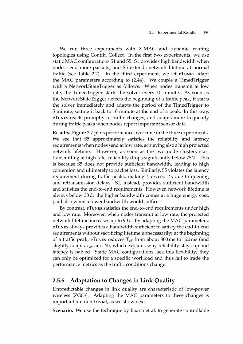
2.5. Experimental Results 39
We run three experiments with X-MAC and dynamic routingtopologies using Contiki Collect. In the first two experiments, we usestatic MAC configurations S1 and S5: S1 provides high bandwidth whennodes send more packets, and S5 extends network lifetime at normaltra�c (see Table 2.2). In the third experiment, we let pTunes adaptthe MAC parameters according to (2.44). We couple a TimedTriggerwith a NetworkStateTrigger as follows. When nodes transmit at lowrate, the TimedTrigger starts the solver every 10 minute. As soon asthe NetworkStateTrigger detects the beginning of a tra�c peak, it startsthe solver immediately and adapts the period of the TimedTrigger to5 minute, setting it back to 10 minute at the end of a peak. In this way,pTunes reacts promptly to tra�c changes, and adapts more frequentlyduring tra�c peaks when nodes report important sensor data.
Results. Figure 2.7 plots performance over time in the three experiments.We see that S5 approximately satisfies the reliability and latencyrequirements when nodes send at low rate, achieving also a high projectednetwork lifetime. However, as soon as the two node clusters starttransmitting at high rate, reliability drops significantly below 75 %. Thisis because S5 does not provide su�cient bandwidth, leading to highcontention and ultimately to packet loss. Similarly, S5 violates the latencyrequirement during tra�c peaks, making L exceed 2 s due to queuingand retransmission delays. S1, instead, provides su�cient bandwidthand satisfies the end-to-end requirements. However, network lifetime isalways below 30 d: the higher bandwidth comes at a huge energy cost,paid also when a lower bandwidth would su�ce.
By contrast, pTunes satisfies the end-to-end requirements under highand low rate. Moreover, when nodes transmit at low rate, the projectednetwork lifetime increases up to 90 d. By adapting the MAC parameters,pTunes always provides a bandwidth su�cient to satisfy the end-to-endrequirements without sacrificing lifetime unnecessarily: at the beginningof a tra�c peak, pTunes reduces To↵ from about 300 ms to 120 ms (andslightly adapts Ton and N), which explains why reliability stays up andlatency is halved. Static MAC configurations lack this flexibility; theycan only be optimized for a specific workload and thus fail to trade theperformance metrics as the tra�c conditions change.
2.5.6 Adaptation to Changes in Link QualityUnpredictable changes in link quality are characteristic of low-powerwireless [ZG03]. Adapting the MAC parameters to these changes isimportant but non-trivial, as we show next.
Scenario. We use the technique by Boano et al. to generate controllable

40 Chapter 2. pTunes: Runtime Parameter Adaptation for Low-power MAC Protocols
0 0.5 1 1.5 2 2.5 3 3.5 4 4.5 560
70
80
90
100
Trafficpeak
Trafficpeak
Time [h]
End−
to−
end r
elia
bili
ty R
[%
]
PTUNES
S1
S5
(a) End-to-end reliability, R � 95 %.
0 0.5 1 1.5 2 2.5 3 3.5 4 4.5 50
1
2
3 Trafficpeak
Trafficpeak
Time [h]
End−
to−
end la
tency
L [s]
PTUNES
S1
S5
(b) End-to-end latency, L 1 s.
0 0.5 1 1.5 2 2.5 3 3.5 4 4.5 50
20
40
60
80
100
120
140 Trafficpeak
Trafficpeak
Time [h]
Pro
ject
ed n
etw
ork
life
time T
[d]
PTUNES
S1
S5
(c) Projected network lifetime.
Figure 2.7: Performance of pTunes against two static MAC configurations as thetra�c load changes. pTunes satisfies the end-to-end requirements at high tra�c whileextending network lifetime at low tra�c. Fixed MAC parameters optimized for a specifictra�c load fail to meet the application requirements as the tra�c conditions change.
interference patterns [BVT+10], making the link quality fluctuate in arepeatable manner. To this end, we deploy an additional interferer nodein a position where it a↵ects the communication links of at least onefourth of the nodes in our testbed, as shown in Figure 2.5. When active,the interferer transmits a modulated carrier on channel 26 for 1 ms at thehighest power setting. Then, it sets the radio to idle mode for 10 ms beforetransmitting the next carrier.
All nodes generate packets with IPI = 30 s for 4 hours. The interfereris active during two periods of 1 hours each. In a first experiment, weuse static MAC configuration S4, optimized for IPI = 30 s (see Table 2.2).

2.5. Experimental Results 41
0 0.5 1 1.5 2 2.5 3 3.5 450
60
70
80
90
100
Interferer on Interferer on
Time [h]
En
d−
to−
end
re
liab
ility
R [
%]
PTUNES
S4
(a) End-to-end reliability, R � 95 %.
0
5
10
15
Interferer on Interferer on
To
n [
ms]
PTUNES
S4
0
50
100
Interferer on Interferer on
To
ff [
ms]
PTUNES
S4
0 0.5 1 1.5 2 2.5 3 3.5 40
5
10
Interferer on Interferer on
Time [h]
N
PTUNES
S4
(b) Trace of X-MAC parameters.
Figure 2.8: End-to-end reliability and trace of X-MAC parameters with pTunes asthe link qualities in the network change. pTunes reduces packet loss by 80 % duringperiods of controlled wireless interference in comparison with static MAC parametersoptimized for the applied tra�c load without interference.
We enable pTunes in a second experiment, using a TimedTrigger with aperiod of 1 minute to adapt the MAC parameters according to (2.44). Wedeliberately enforce a static routing tree to separate e↵ects related to linkquality changes from those related to topology changes. We investigatethe latter in detail in Section 2.5.7.
Results. Figure 2.8 shows end-to-end reliability and the trace of X-MACparameters. Looking at Figure 2.8(a), we see that S4 and pTunes satisfythe reliability requirement when the interferer is o↵. When the interfereris on, reliability starts to drop below 95 %. However, as soon as pTunes

42 Chapter 2. pTunes: Runtime Parameter Adaptation for Low-power MAC Protocols
collects network state, it detects a decrease in link quality and adapts theX-MAC parameters accordingly. In particular, as shown in Figure 2.8(b),pTunes increases N from 3 or 4 to values between 6 and 10. Ton is alsoincreased (from 6 ms to 10–16 ms) to further help satisfy the reliabilityrequirement. Moreover, pTunes decreases To↵ (from 100 ms to 20–90 ms)to provide more bandwidth and combat increased channel contention,which is a consequence of numerous retransmission attempts over low-quality links. Indeed, these low-quality links make (2.44) temporarilyunsatisfiable (while Ton = 16 ms in the first interference phase), triggeringpTunes to instead maximize R as explained in Section 2.5.1. As a resultof these decisions, pTunes achieves an average end-to-end reliability of95.4 % also in presence of interference.
S4, instead, fails to meet the reliability requirement when the interfereris active: reliability ranges between 70 % and 80 %, and never recoverswhile the interferer is on. In total, 2252 packets are lost with S4 duringinterference. pTunes reduces this number to 418—a reduction of morethan 80 %.
2.5.7 Interaction with RoutingSeveral studies emphasize the significance of cross-layer interactions tothe overall system performance [DPR00]. We study this aspect betweenbest-e↵ort tree routing and parameter adaptation of an underlying low-power MAC protocol with pTunes. To do so, during each of thefollowing experiments, we temporarily remove multiple core routingnodes important for forwarding packets. In this way, we emulate nodefailures, which are common in deployed systems [BGH+09], and force therouting protocol to find new routes.
Scenario. We run two 4-hour experiments with Contiki Collectand X-MAC. After 30 minute, we turn o↵ eight nodes within thesink’s neighborhood that forward most packets in the network (1–8 inFigure 2.5). We turn them on again after 60 minute, and repeat the on-o↵pattern after 1 hours. Nodes generate packets with IPI = 30 s. In the firstexperiment, we use static MAC configuration S4, optimized for this tra�cload (see Table 2.2). In the second experiment, we enable pTunes and usea TimedTrigger to solve (2.44) every minute.
Results. Figure 2.9(a) shows end-to-end reliability over time, accountingfor packets from nodes that are currently turned on. During thefirst 30 minute, both S4 and pTunes satisfy the reliability requirement.However, when nodes are removed, reliability starts to drop below 70 %.Many packets are indeed lost since children of removed nodes fail totransmit packets: the routing protocol needs to find new routes.

2.5. Experimental Results 43
0 0.5 1 1.5 2 2.5 3 3.5 440
50
60
70
80
90
100
Nodes fail Nodes fail
Time [h]
En
d−
to−
end
re
liab
ility
R [
%]
PTUNES
S4
(a) End-to-end reliability, R � 95 %.
0 0.5 1 1.5 2 2.5 3 3.5 40
25
50
75
100
125
150 Nodes fail Nodes fail
Time [h]
Nu
mbe
r o
f p
are
nt
switc
he
s
PTUNES
S4
(b) Distribution of parent switches.
Figure 2.9: End-to-end reliability and distribution of parent switches when eightcore routing nodes fail simultaneously. pTunes helps the routing protocol recoverfrom node failures by settling quickly on a stable routing topology, thus reducing packetloss by 70 % compared with static MAC parameters optimized for the applied tra�c load.
We see from Figure 2.9(a) that end-to-end reliability recovers muchfaster when pTunes is enabled. During the two periods when eight nodesare removed, S4 fails to deliver in total 2673 packets from the remaining35 nodes. pTunes reduces this number to 813—a reduction of 70 %.
To further investigate this behavior, we plot in Figure 2.9(b) thedistribution of parent switches. pTunes reduces the total number ofparent switches compared to S4 (from 631 to 165), and shifts them tothe beginning of the periods in which nodes are removed. At this point,pTunes quickly realizes a significant drop in link quality, reported bynodes whose parent disappeared. pTunes thus increases Ton and N toimprove reliability, and decreases To↵ to provide more bandwidth forretransmissions and route discovery.
As a result of increasing the maximum number of retransmissionsper packet N, transmission attempts of nodes with a dead parent failwith a higher number of retries. This causes the corresponding ETXvalues to drop more severely than with S4 (which has a lower N), andso nodes switch much faster to a new parent. Moreover, the MACparameters provided by pTunes help deliver packets over the remaining

44 Chapter 2. pTunes: Runtime Parameter Adaptation for Low-power MAC Protocols
links. Delivering more packets also enables the routing protocol to quicklydetect route inconsistencies and eventually settle on a stable topology. Asthe topology stabilizes, pTunes gradually relaxes the MAC parameters(reduce Ton and N, increase To↵ ) to extend network lifetime.
These results demonstrate that, by adapting the MAC parameters,pTunes helps the routing protocol recover faster from critical networkchanges. Protocols like CTP [GFJ+09] and Arbutus [PH10] also utilizefeedback from unicast transmissions to compute the ETX. In addition,CTP uses data path validation to detect possible loops based on ETXvalues embedded in data packets [GFJ+09]. Our findings with ContikiCollect, which uses similar techniques, suggest that these protocols couldalso benefit from pTunes.
Additionally, the results demonstrate the advantage of decouplingnetwork state collection from application packet routing, as we arguein Section 2.3.2. As long as the network remains connected, Glossyprovides up-to-date network state to the base station with very highreliability [FZTS11]. Changes in the routing tree do no a↵ect networkflooding: information about faulty links is collected even when therouting protocol fails to deliver packets from nodes whose parent died,allowing pTunes to react promptly and thus e↵ectively.
2.6 DiscussionDesigning a MAC adaptation framework involves striking a balancebetween goals typically at odds with each other. We discuss some ofthe trade-o↵s we make in pTunes and the implications of our decisions.
Feasibility vs. scalability. We adopt a centralized approach rather thana likely more scalable distributed solution; in return for this, pTunesallows users to express their requirements in terms of network-widemetrics, which better reflect the way domain experts are used to stateperformance objectives compared to per-node or per-link metrics. In fact,distributing the tasks of collecting global information, computing MACparameters optimized for network-wide objectives, and coordinating theconsistent installation of new parameters would hardly be feasible, if atall, on resource-constrained devices. Instead, pTunes exploits the betterresources of a central base station, which is already present in many realdeployments [RC08], and achieves simplicity of in-network functionalityby moving most of its intelligence from the nodes into the base station.
Flexibility vs. optimality. We focus on existing MAC protocolsrather than on the design or adaptation of cross-layer solutions (e.g.,coupling link and network layer) which may, in principle, achieve better

2.7. Related Work 45
performance; in return for this, pTunes allows system designers to choosethe MAC and routing protocol independently from existing code bases.In comparison, cross-layer solutions tend to enjoy little generality andflexibility, as they are often designed for very specific scenarios (e.g.,periodic, low-rate data collection [BvRW07]).
Robustness vs. optimality. We determine network-wide parametersrather than per-node parameters, which may better match the currentrole of a node in the routing tree (e.g., with respect to tra�c load); inreturn for this, the parameters pTunes provides are much more robustto changes in the routing topology. It is not unlikely that, even in themost benign environment, slight variations in the link qualities triggerdrastic changes in the routing topology. For instance, Ceriotti et al.observe that nodes serving many children suddenly become leaves inthe routing tree [CMP+09]. In such a case, per-node MAC parametersbecome inappropriate and must be quickly updated. Similar situationscan happen frequently, even several times per minute [GGL10], whichwould render per-node parameter adaptation impractical.
As a consequence of the design decisions above, pTunes represents oneparticular point in a multi-dimensional design space. Corresponding tothis point is a large fraction of deployed low-power wireless networkscomprising tens of nodes, leveraging protocols such as X-MAC andLPP, and yet failing to meet the application requirements often due tocommunication issues ultimately related to inadequate MAC parameterchoices and lack of adaptiveness [RC08, KGN09]. pTunes is directly andimmediately applicable in these settings.
2.7 Related WorkpTunes uses a model to predict how changes in the MAC parametersa↵ect the network-wide performance given the current network state.Based on iterative runtime optimization, it selects MAC parameterssuch that the predicted performance satisfies the application require-ments. This approach is similar to the concept of model predictivecontrol (MPC) [GPM89], with the di↵erences that pTunes computes onlythe next step of the control law and uses no information about past controlsteps or measured system responses.
Several recent systems incorporate centralized control in their design,much like pTunes does. For example, Koala implements a network-wide routing control plane, where the base station computes end-to-endpaths used for packet forwarding [MELT08]. RACNet uses centralizedtoken passing to sequence data downloads [LLL+09]. In RCRT, the sink

46 Chapter 2. pTunes: Runtime Parameter Adaptation for Low-power MAC Protocols
detects congestion and adapts the rates of individual sources [PG07]. PIPdetermines schedule and channel assignment for each flow centrally atthe base station [RCBG10]. Like pTunes, these systems exploit globalknowledge and ample resources of the base station to achieve highperformance and manageability.
Looking at the large body of prior work on adaptive low-powerMAC protocols, we find solutions embedding adaptivity or separatingadaptivity from the protocol operation.
In the former category, for instance, Woo and Culler propose anadaptive rate control mechanism, where nodes inject more packetsif previous attempts were successful and fewer packets if theyfailed [WC01]. Van Dam and Langendoen introduce an adaptive listenperiod in T-MAC [DL03] to overcome the drawbacks of the fixed dutycycle of S-MAC [YHE02]. El-Hoiydi and Decotignie adapt radio wake-upsin WiseMAC to shorten the LPL preamble [EHD04]. More recently, Hurniand Braun propose MaxMAC, which schedules additional X-MAC wake-ups at medium tra�c and switches to pure CSMA at high tra�c [HB10].Such hard-coded adaptivity mechanisms can be highly e↵ective in specificscenarios, but lack general applicability and bear no direct connection tothe high-level application demands. pTunes is more general by addingparameter adaptation atop existing MAC protocols, thus leveragingavailable implementations, and by explicitly incorporating user-providedapplication requirements.
Polastre et al. instead separate adaptivity from the protocol operationand present a model of node lifetime for B-MAC [PHC04]. Jurdak et al. usethis model to dynamically recompute check interval and preamble length,showing substantial energy savings [JBL07]. Buettner et al. demonstrateenergy savings in X-MAC by adapting the wake-up interval to tra�cload for one sender-receiver pair [BYAH06]. Meier et al. [MWZT10] andChallen et al. [CWW10] extend network lifetime by adjusting the wake-upinterval to tra�c load in a static routing tree. Park et al. present numericalresults that indicate the potential of adaptation policies for IEEE 802.15.4MAC protocols, based on per-link and per-node metrics [PFJ10]. pTunesbuilds on these foundations but extends them in several ways. First,pTunes considers multiple network-wide metrics and adapts multipleMAC parameters. Second, our modeling is more realistic by accountingfor packet loss and ARQ mechanisms, and more flexible by isolatingprotocol-dependent from protocol-independent functionality. Third, weevaluate pTunes in real-world scenarios, including dynamic routing trees,wireless interference, and node failures.

2.8. Summary 47
2.8 SummaryThis chapter presented pTunes, a novel framework that provides runtimeparameter adaptation for low-power MAC protocols. pTunes automat-ically translates an application’s end-to-end performance requirementsinto MAC parameters that meet these requirements and achieve verygood performance across a variety of scenarios, ranging from low tra�cto high tra�c, from good links to bad links, and wireless interference tonode failures. pTunes thus greatly aids in meeting soft requirements ofreal-world low-power wireless applications by eliminating the need fortime-consuming, and yet error-prone, manual MAC configuration beforeevery single deployment and when the network conditions change.

48 Chapter 2. pTunes: Runtime Parameter Adaptation for Low-power MAC Protocols

3Modeling Protocols Based on
Synchronous TransmissionsLow-power wireless networks facilitate advanced CPS applications thatuse wirelessly interconnected sensors and actuators to monitor and acton the physical world, such as environmental control, assisted living,and intelligent transportation [Lee08]. E↵ectively employing low-powerwireless in these applications requires a thorough understanding of thebehavior of the protocols that power the network operation. For example,the ability to estimate the energy consumption is crucial to self-sustainingsystems based on energy scavenging [MTBB10], and certain guaranteeson packet delivery are key to dependable wireless automation [BJ87].
Unfortunately, the current literature falls short in modeling multi-hoplow-power wireless protocols. Two aspects concur:
• Low-power wireless transmissions are subject to a number of un-predictable environmental factors, including wireless interference,presence of obstacles and persons, and temperature and humiditychanges [HRV+13]. As a result, low-power wireless links su↵erfrom unpredictable packet loss that varies in time and space [SDTL10].This, in combination with failure-prone devices (e.g., due to batterydepletion or damage), makes the network topology highly dynamic.
• To tame this unpredictability, existing multi-hop communicationprotocols gather substantial information about the network state,such as link quality estimates [GFJ+09] and the filling levels of packetqueues [RGGP06]. Protocols use this information, for example,to form multi-hop routing paths [GFJ+09] and to adapt packet

50 Chapter 3. Modeling Protocols Based on Synchronous Transmissions
1
2 3
4R
(a) Link-based transmissions.
R
(b) Synchronous transmissions.
Figure 3.1: Link-based transmissions (LT) versus synchronous transmissions(ST). Using ST, multiple nodes transmit simultaneously toward the same receiver R, asopposed to pairwise LT 1, 2, 3, and 4 from each sender to R.
transmission rates [RGGP06]. However, the network state mustbe updated at runtime against the topology dynamics.. For scalabilityreasons, the network state is often distributed across the nodes, whichoperate concurrently with little or no coordination.
These reasons render multi-hop low-power wireless protocols intricateand di�cult to model [GB12]. As a result, existing models often stop at thelink layer, achieving model errors in the range of 2–7 % in real experiments(see Chapter 2). Only a few attempts have been made to model alsohigher-layer functionality [GB12, BSB+12, GCB08, YZDPHg11]; however,validation of these models is limited to numerical simulations, which lackprecisely those real-world dynamics that complicate the modeling.
A new breed of communication protocols has emerged over the pastfew years that utilize synchronous transmissions (ST) [LW09, DDHC+10,FZTS11, WHM+12, LFZ13a, FZMT12, DCL13, CCT+13]. As illustratedin Figure 3.1, unlike single transmissions over sender-receiver links in (a),using ST multiple nodes transmit simultaneously towards the same receiverin (b). Because of two physical-layer phenomena of low-power wirelesscommunications, constructive baseband interference [DDHC+10] andcapture e↵ects [LW09], ST vastly improve the one-hop packet reliabilitycompared with link-based transmissions (LT) [DDHC+10].
As we further discuss in Section 3.1, the salient features of ST enablemulti-hop communication protocols that require very little network stateand outperform LT-based protocols. The open question is whether STalso simplify the accurate modeling of these protocols. To answer thisquestion, this chapter puts forward two key contributions:
1. We investigate in Section 3.2 to what extent the Bernoulli assumptionapplies to ST. The assumption stipulates that subsequent packetreceptions and losses at a receiver adhere to a sequence of i.i.d.

3.1. Background and Related Work 51
Bernoulli trials. Models of communication protocols often make thisassumption to simplify the specification [PHC04, ZFM+12], but priorwork suggests that this is often invalid for LT [CWPE05, SDTL10].Up to now, nothing is known about ST in this regard. By studyinga specific flavor of ST, Glossy network floods [FZTS11], throughexperiments on a 139-node testbed, we show that the Bernoulliassumption is largely valid for ST, and way more than for LT.
2. We build upon these findings to demonstrate that modeling an ST-based protocol is in fact simpler and yields significantly higheraccuracy than models of LT-based protocols. We do so byconsidering LWB [FZMT12], a representative protocol, describedin Section 3.3, of a growing number of solutions [WHM+12,LFZ13a, DCL13, CCT+13] that build upon Glossy. Specifically,we present in Section 3.4 su�cient conditions for providingprobabilistic guarantees on LWB’s end-to-end packet reliability,and in Section 3.5 a discrete-time Markov chain (DTMC) model toestimate LWB’s expected long-term energy consumption. Resultsfrom our validation based on real-world experiments in Section 3.6indicate that the end-to-end reliability guarantees are correctlymatched, and that the estimates of the energy model are within0.25 % of the real measurements. This error margin is unparalleledin the low-power wireless literature we are aware of.
3.1 Background and Related WorkThis chapter builds on recent work in low-power wireless communica-tions. In this section, we provide the necessary background on multi-hopprotocols exploiting di↵erent flavors of ST, contrast these with the existingliterature on LT, and review related modeling e↵orts. We conclude withan outlook on how this chapter fills the gaps in the current literature.
3.1.1 Synchronous TransmissionsLittle work exists to deeply understand the behavior of ST in low-powerwireless. For example, Son et al. [SKH06] conduct an experimental studyof the capture e↵ect, a physical layer phenomenon that allows a receiver tocorrectly decode a packet despite interference from other transmitters. Inlow-power wireless, this is typically due to power capture, which occurswhen the received signal from a node is 3 dB stronger than the sum ofthe signals from all other nodes [SKH06]. Several protocols exploit thecapture e↵ect, for example, to implement fast network flooding [LW09]

52 Chapter 3. Modeling Protocols Based on Synchronous Transmissions
and e�cient all-to-all communication [LFZ13a].Precisely overlapping transmissions of identical packets enable another
phenomenon in low-power wireless: constructive baseband interference ofIEEE 802.15.4 symbols. This enables a receiver to correctly decode thepacket also in the absence of capture e↵ects, significantly boosting thetransmission reliability. Using resource-constrained devices, however,the required timing accuracy of ST is di�cult to achieve. One way toaddress this challenge is by using hardware-generated acknowledgments,a mechanism that has been employed to better resolve contention in low-power MAC protocols [DDHC+10, CT11].
Glossy, instead, uses a careful software design to make ST of thesame packet precisely overlap, thus taking advantage of both con-structive baseband interference and capture e↵ects for e�cient networkflooding and time synchronization with microsecond accuracy [FZTS11].Several protocols extend and improve Glossy, for example, in densenetworks [WHM+12], for distributing large data objects [DCL13], forpoint-to-point communication [CCT+13], and for in-network processingand all-to-all data sharing [LFZ13a]. LWB, which we use to examinethe impact of ST on modeling multi-hop protocols, e�ciently supportsmultiple tra�c patterns by globally scheduling Glossy floods [FZMT12].
3.1.2 Link-based TransmissionsIn contrast to ST, a large body of work exists on understanding thebehavior of LT [BKM+12]. Srinivasan et al. [SDTL10], for example,conduct an empirical study of IEEE 802.15.4 transmissions to provideguidelines for fine-grained design decisions such as the scheduling oflink-layer packet retransmissions. The � factor [SKAL08] measuresthe link burstiness over time, which may be used by a protocol todetermine how long to pause after a transmission failure to preventunnecessary retransmissions. Cerpa et al. [CWPE05] examine both short-and long-term temporal aspects to improve simulation models and forenhancing point-to-point routing. Dually, the factor [SJC+10] measuresthe degree of correlation of packet receptions across di↵erent receivers—hence exploring LT’s spatial diversity—which can possibly be used todesign better opportunistic routing and network coding schemes.
Despite the significant knowledge about LT, obtaining full-fledgedmodels of LT-based multi-hop protocols is very di�cult [GB12]. Severalattempts stop at the MAC layer, where distributed interactions span onlyone hop and hence reasoning is still manageable. For example, pTunesprovides runtime tuning of MAC parameters based on application-levelperformance goals, leveraging MAC protocol models (see Chapter 2).Similarly, Polastre et al. [PHC04] present a model of node lifetime for
3.2. Bernoulli Assumption 53
B-MAC, and Buettner et al. [BYAH06] model reliability and energy in X-MAC. Gribaudo et al. [GCB08] use interacting Markovian agents to modela generic sender-initiated low-power MAC protocol [ZFM+12]; they alsoacknowledge that the opportunistic operation of this class of protocolsgreatly complicates the modeling using standard techniques.
The dynamics of the network topology render the modeling of higher-layer functionality, where interactions typically extend across multiplehops, very complex. As a result, accurate models of the end-to-end ornetwork-wide performance are largely missing. Some exceptions modelthe Collection Tree Protocol (CTP) [GFJ+09] to improve its performance inindustrial scenarios [YZDPHg11], analyze swarm intelligence algorithmsfor sensor networks based on the Markovian agent model [BSB+12], applydi↵usion approximation techniques to estimate the end-to-end packettravel times assuming opportunistic packet forwarding rules [Gel07], ormodel generic multi-hop functionality through population continuous-time Markov chains [GB12]. Nevertheless, the validation of these modelsis limited to numerical simulations, which lack precisely those real-world dynamics of low-power wireless links that make accurate protocolmodeling so complex and di�cult in the first place.
3.1.3 OutlookMotivated by the lack of a deeper understanding of ST, in the remainderof this chapter we provide a thorough account on the behavior of ST andits impact on the modeling of emerging ST-based multi-hop protocols.To this end, we start by analyzing in Section 3.2 to what extent a key,yet sometimes illegitimate assumption in modeling low-power wirelessprotocols applies to ST. We base this study upon Glossy’s specificincarnation of ST [FZTS11], because it serves as the communicationprimitive for a growing class of multi-hop protocols [WHM+12, FZMT12,DCL13, CCT+13, LFZ13a]. We then apply the corresponding findingswhile closely examining LWB [FZMT12], one specific such protocol weillustrate in Section 4.2 that exceeds the performance, reliability, andversatility of prior LT-based protocols. In doing so, we analyze end-to-endpacket reliability in Section 3.4 and energy consumption in Section 3.5—two key performance indicators in low-power wireless [GFJ+09].
3.2 Bernoulli AssumptionBecause wireless networks are very complex, researchers make simplify-ing assumptions about their behavior when reasoning about a protocol.One common assumption is the Bernoulli assumption [SDTL10]. Let the

54 Chapter 3. Modeling Protocols Based on Synchronous Transmissions
reception of packets sent in a sequence be a random event with success orfailure as the only possible outcomes. The Bernoulli assumption stipulatesthat a receiver observes a sequence of i.i.d. Bernoulli trials. In practicalterms, success means a packet is received (with probability p), and failuremeans a packet is lost (with probability 1 � p).
However, several studies have shown that the Bernoulli assumptionis not always valid in low-power wireless, because links have temporallycorrelated receptions and losses when they occur close in time (i.e., on theorder of a few tens of milliseconds) [CWPE05, SDTL10]. In this section,we show empirically that the Bernoulli assumption is (i) in fact highlyvalid for ST in Glossy, and (ii) more appropriate in Glossy than for LT.
We first describe how we collect large sets of packet reception traceson a real-world sensor network testbed. Next, we discuss our analysisof these traces for weak stationarity, which is a necessary condition forfurther statistical analysis. We then construct a statistical test for packetreception independence based on the sample autocorrelation metric, anduse this test to assess the validity of the Bernoulli assumption in our traces.
3.2.1 Experimental MethodologyWe perform 80 hours of packet reception measurements on Indriya, a largetestbed of 139 TelosB nodes deployed across three floors in the School ofComputing at the National University of Singapore [DCA11]. Indriyaprovides a mixture of dense and sparse node clusters, as well as realisticinterference from the presence of people and co-located Wi-Fi.
We conduct two types of experiments that match the building blocksof multi-hop communication in ST- and LT-based protocols:
1. ST-Type. We select 70 nodes that are equally distributed acrossthe three floors on Indriya and let them, one at a time, initiate50,000 Glossy network floods. According to Glossy’s operation, theremaining 138 nodes blindly relay the flooding packet, eventuallydelivering it to all nodes in the network.
2. LT-Type. All 139 nodes available on Indriya broadcast, one at a time,50,000 packets, while the remaining nodes passively listen. As LTare bound by the transmission range of the broadcasting node, onlyits one-hop neighbors can receive the packet.
In both types of experiments, packets are 20 bytes long and carrya unique sequence number. The sender transmits at a fixed inter-packetinterval (IPI) of 20 ms, which corresponds to the typical minimum intervalbetween consecutive Glossy floods in ST-based protocols [WHM+12,CCT+13, DCL13, FZMT12]. All other nodes record received and lost

3.2. Bernoulli Assumption 55
0 200 400 600 800 10000.2
0.4
0.6
0.8
1
Time (seconds)
Pack
et re
ceptio
n r
ate
Weakly stationary Non−stationary Linear fit
Figure 3.2: Example of a weakly stationary and a non-stationary trace. Packetreception rate is a moving average with a window size of 2,000 packets (40 s).
packets based on the sequence number. We use IEEE 802.15.4 channel26 to reduce the influence of Wi-Fi interference, whose extent we cannotcontrol and is di�cult to assess afterwards [HRV+13]. We repeat bothtypes of experiments for two transmit powers: 0 dBm is the maximumtransmit power of a TelosB node, and -15 dBm is the lowest transmitpower at which the network on Indriya remains connected. The resultingnetwork diameters are 5 and 11 hops, respectively.
We record in total more than 1,200,000,000 events, grouped into packetreception traces of length n =50,000. We represent every collected traceas a discrete-time binary time series {xi}ni=1, where xi is 1 if the i-th packetwas received and 0 if it was lost. This time series representation formsthe basis for our statistical analysis.
3.2.2 Weak StationarityA necessary condition for well-founded statistical analyses of time seriesis weak stationarity [BD91]. A weakly stationary time series has constantmean, constant variance, and the autocovariance between two valuesdepends only on the time interval between those values. We investigatewhether our traces conform to these criteria based on the packet receptionrate (PRR), computed on a trace as a moving average of the fraction ofreceived packets over a window of 2,000 packets (40 s).
Visual inspection of our traces reveals obvious violations of thesecriteria. For example, Figure 3.2 shows the PRR for a stationary and a non-stationary trace. The latter has several abrupt changes and a significanttrend in the mean, as evident from the linear fit. To avoid biases in our

56 Chapter 3. Modeling Protocols Based on Synchronous Transmissions
Table 3.1: Number of non-stationary and weakly stationary traces.Type Transmit power Total Non-stationary Weakly stationary
ST 0 dBm 9660 47 9613ST -15 dBm 9660 256 9404LT 0 dBm 4189 1418 2771LT -15 dBm 1777 588 1189
analysis, we need to identify and exclude such non-stationary traces.While there is a number of formal tests for stationarity, they often fail
in practice due to their inability to detect general non-stationarity [Det13].Thus, similar to [YMKT99], we apply two empirical tests to identify non-stationary traces. To test for trends in the mean, we compute a linearfit using ordinary least squares and declare a trace as non-stationary ifthe PRR changes by 0.015 or more over the entire trace of 50,000 packets(1,000 s). Then, we test for non-constant variance by checking whether thePRR decreases or rises by more than 0.05 within a window of 2,000 packets(40 s), which we interpret as an indication of non-stationarity. Table 3.1summarizes the sets of traces before and after applying the two empiricaltests for non-stationarity; we removed about 9 % of non-stationary traces.
3.2.3 Validating the Bernoulli AssumptionTo confirm or refute the Bernoulli assumption for a given trace, we usethe sample autocorrelation, which measures the linear dependence betweenvalues of a weakly stationary time series as a function of the interval (lag)between those values. As we explain below, the Bernoulli assumption isvalid if the values in the time series are independent already at lag 1.
For a discrete-time binary time series {xi}ni=1 of length n, the sampleautocorrelation ⇢ at lag ⌧ = 1, 2, . . . ,n � 1 is
⇢(⌧) =
8>><>>:�(⌧)/�(0) if �(0) , 00 if �(0) = 0
(3.1)
where �(⌧) is the estimated autocovariance given by
�(⌧) =1n
Xn�⌧
i=1(xi+⌧ � x)(xi � x)
and x = 1/nPn
i=1 xi is the sample mean.The sample autocorrelation in (3.1) ranges between -1 and 1. Negative
values indicate anti-correlation in packet reception: as more packets arereceived (lost), the next packet reception is more likely to fail (succeed).

3.2. Bernoulli Assumption 57
0 5 10 15 20−0.05
0
0.05
0.1
Lag
Sam
ple
auto
corr
ela
tion
Trace 1Trace 2Bounds
Figure 3.3: Sample autocorrelation up to lag 20 for two of our collected packetreception traces. The Bernoulli assumption holds for Trace 2, because its sampleautocorrelation falls within the confidence bounds starting from lag 1.
Positive values indicate positive correlation: packet receptions (losses)tend to be followed by more packet receptions (losses).
Values close to zero indicate independence among packet receptionsat a given lag, assuming the xi are i.i.d. Bernoulli random variables. Let{xi}ni=1 be a realization of an i.i.d. sequence {Xi}1i=1 of random variableswith finite variance. It can be shown that, for a large number of samplesn, about 95 % of the sample autocorrelation values should lie withinthe confidence bounds ±1.96/
pn [BD91]. Based on this, we define the
correlation lag as the smallest lag at which the sample autocorrelation lieswithin ±1.96/
pn. Like [YMKT99], we consider the Bernoulli assumption
valid if the correlation lag is 1. Formally: Given a time series {xi}ni=1, theBernoulli assumption holds at the 0.05 significance level if |⇢(1)| 1.96/
pn.
As an example, Figure 3.3 plots ⇢ for two of our traces of lengthn = 50, 000. The dashed lines at ±1.96/
p50, 000 ⇡ ±0.0088 represent the
confidence bounds. The figures shows that Trace 1 is dependent up to lag5, but starting from lag 6 the autocorrelation values become insignificantexcept for a few stray points. By contrast, Trace 2 has an insignificantautocorrelation already at lag 1, indicating that there is no dependencebetween consecutive packets nor between any other packets in the trace.Thus, the Bernoulli assumption holds for Trace 2 but not for Trace 1.
3.2.4 ResultsBased on the above reasoning, we analyze the validity of the Bernoulliassumption for our weakly stationary traces (see Table 3.1). Figure 3.4shows the percentage of traces with correlation lag greater than 1 (for

58 Chapter 3. Modeling Protocols Based on Synchronous Transmissions
20 200 10000
10
20
30
40
Inter−packet interval (milliseconds)
Perc
enta
ge o
f tr
ace
s
ST−Type 0 dBmST−Type −15 dBmLT−Type 0 dBmLT−Type −15 dBm
Figure 3.4: Percentage of weakly stationary traces for which the Bernoulliassumption does not hold, for di↵erent IPIs and transmit powers. The Bernoulliassumption is highly valid for ST, and significantly more legitimate for ST than for LT.
which the Bernoulli assumption does not hold) when examining di↵erentIPIs in our traces. We see that the Bernoulli assumption is significantlymore legitimate for synchronous transmissions (ST-Type) than for link-based transmissions (LT-Type). For example, at the highest transmitpower of 0 dBm, the Bernoulli assumption holds for more than 99 % ofthe ST-Type traces irrespective of the IPI, whereas it holds only for 60 %of the LT-Type traces at the smallest IPI of 20 ms.
We also see that at the lower transmit power there are more ST-Typetraces for which the Bernoulli assumption does not hold. This is mostlybecause nodes have fewer neighbors and hence benefit less from senderdiversity [RHK10]. Indeed, at -15 dBm about 24 % of nodes have at mostfour well-connected neighbors, which makes their reception behaviorapproach the one of LT. This is also confirmed by a significant negativePearson correlation of -0.31 between the number of well-connectedneighbors and the percentage of traces for which the Bernoulli assumptiondoes not hold. Finally, Figure 3.4 shows that the autocorrelation decreasesas the IPI increases, and becomes negligible at IPI = 1 s also for LT-Typetraces. This observation is in line with prior studies on low-power wirelesslinks [SDTL10], thus validating our methodology.
In summary, our results show that the Bernoulli assumption holds toa large extent for ST due to sender diversity [RHK10]. This implies thatpacket receptions in Glossy can be considered largely independent, soa single parameter is su�cient to precisely characterize the probabilityof receiving a packet. By contrast, packet receptions in LT are often notindependent, which necessitates more complex models, such as high-

3.3. Low-power Wireless Bus 59
(C)
(B)
n1n1 n1
(A)T
nnnn nn
n3
n2
n3 n3
n2 n2
tn1
Communication rounds
n2 nnn3
Figure 3.5: LWB’s time-triggered operation. Communication rounds occur witha possibly varying round period T (A); each round consists of a varying numberof communication slots (B); every slot corresponds to a Glossy flood (C).
order Markov chains [YMKT99], to accurately capture their behavior.The next section describes LWB, a Glossy-based protocol that we use
throughout Sections 3.4 and 3.5 to demonstrate how the validity of theBernoulli assumption for ST enables simple, yet highly accurate modelsof multi-hop low-power wireless protocols.
3.3 Low-power Wireless BusThe basic idea behind LWB is to abstract a network’s multi-hop natureby employing only ST for communication [FZMT12]. To this end, LWBmaps all communication demands onto Glossy network floods [FZTS11].Glossy always and blindly propagates every message from one node to allother nodes in the network, e↵ectively creating the perception of a single-hop network for higher-layer protocols and applications. The resultingprotocol operation of LWB is similar to a shared bus, where all nodesare potential receives of all messages; delivery to the intended recipientshappens by filtering messages at the receivers.
LWB exploits Glossy’s accurate time synchronization for a time-triggered scheme that arbitrates access to the (wireless) bus. Nodescommunicate according to a global communication schedule. A dedicatedhost node computes the schedule online based on the current tra�cdemands and distributes it to the nodes, determining when a node isallowed to initiate a flood.
As shown in Figure 4.1 (A), communication occurs in rounds that repeatwith a possibly varying round period T. All nodes keep their radios o↵between two rounds to save energy. Every round consists of a possibly

60 Chapter 3. Modeling Protocols Based on Synchronous Transmissions
contentiondatahost computes t
data
new schedule
schedulenewschedule
Ts Td Td Td Ts
Tl
Figure 3.6: Communication slots and activities during a single LWB round.
varying number of communication slots, as shown in Figure 4.1 (B). In everyslot, at most one node puts a message on the bus (i.e., initiates a flood),while the remaining nodes read the message from the bus (i.e., receiveand relay the flooding packet), as illustrated in Figure 4.1 (C).
Figure 3.6 shows the di↵erent communication slots within one roundof length Tl. Each round starts with a slot of length Ts in which the hostdistributes the communication schedule. The nodes use the scheduleto time-synchronize with the host and to be informed of (i) the roundperiod T and (ii) the mapping of source nodes to the following data slotsof length Td. A non-allocated contention slot of length Td follows; nodesmay contend in this slot to inform the host of their tra�c demands. Thehost uses these to compute the schedule for the next round, which ittransmits in a final slot of length Ts.
The host computes the communication schedule by determining asuitable round period T and allocating data slots to the current streams. Astream represents a tra�c demand, characterized by a starting time and aninter-packet interval (IPI), as LWB targets the periodic tra�c pattern typicalof many low-power wireless applications [GGB+10]. A node can sourcemultiple streams and individually add or remove streams at runtime.
3.4 End-to-end Reliability in LWBEnd-to-end reliability refers to a protocol’s ability to deliver packets fromsource to destination, perhaps over multiple hops. It is a key performancemetric in low-power wireless [GFJ+09], indicating the level of serviceprovided to users. Many applications do require probabilistic guarantees onthis metric, for example, to allow for post-processing of data in structuralhealth monitoring [CFP+06] or enable stable control loops [SSF+04].
End-to-end reliability, however, is subject to unpredictable packetloss [SDTL10]. LT-based protocols, therefore, rely on per-hopretransmissions to achieve a certain end-to-end reliability, yet thenecessary number of retransmissions depends on the ever-changing lossrates of the individual links along the routing paths. Further, LT-basedprotocols constantly adapt the routes in response to such changes, whichrenders reasoning about end-to-end guarantees extremely complex.

3.4. End-to-end Reliability in LWB 61
By contrast, ST-based protocols, such as LWB, often have no routesto adapt. This facilitates reasoning about end-to-end guarantees, evenacross multiple hops. To show this, we extend LWB with a retransmissionscheme and derive su�cient conditions to provide reliability guarantees.The key insight we use is that the validity of the Bernoulli assumption forST greatly simplifies the specification of these conditions.
Packet retransmissions in LWB. We consider a typical data collectionsetting where the LWB host is also the sink [GGB+10]. We augment LWBwith packet retransmissions by modifying the scheduling algorithm usedat the host to compute the schedule for the next round. Originally, LWBallocates exactly one data slot for each data packet, regardless of the actualreception at the host [FZMT12]. In our modification, the host first checkswhether in the current round it received every data packet assigned aslot. For each lost packet, it reallocates a slot in the next round, in whichthe source node retransmits the lost packet, provided that fewer than kmax
slots have already been allocated for it. Then, the host allocates data slotsfor new packets as before.
Consider now an application that requires a minimum end-to-endreliability pd > 0 on data packets. We derive su�cient conditions on theminimum kmax and overall available bandwidth to provide such guaranteein a probabilistic sense.
Su�cient condition #1: retransmissions. The validity of the Bernoulliassumption for ST in Glossy allows us to consider consecutive retransmis-sions as independent events. Thus, based on our retransmission scheme,the probability that the host receives a packet from stream s within ks � 1(re)transmissions is 1� (1�pd,s)ks , where pd,s is the probability that the hostreceives a packet from stream s in one slot (i.e., during one Glossy flood).To provide the desired guarantee pd > 0, we require
1 � (1 � pd,s)ks � pd (3.2)
where 0 < pd < 1 and 0 < pd,s < 1. Then, (3.2) holds if
ks �log(1 � pd)log(1 � pd,s)
(3.3)
Thus, the host must allocate ks slots to each packet of stream s to providean end-to-end packet reliability of at least pd.
Because LWB needs to set an integer upper bound kmax on the numberof data slots allocated to each packet, the reliability guarantee can only beprovided if for all existing streams s
dkse kmax (3.4)

62 Chapter 3. Modeling Protocols Based on Synchronous Transmissions
Example. Assume one stream with pd,s = 0.9, and the host allocates atmost kmax = 2 slots for each packet. In this case, a reliability guaranteeof pd = 0.99 can be provided, because 1 � (1 � 0.9)2 = 0.99. To guaranteepd = 0.9999, we need to increase kmax to dlog(1 � 0.9999)/ log(1 � 0.9)e = 4.
Su�cient condition #2: bandwidth. The bandwidth available in LWBis a function of how often communication rounds unfold: the shorterthe round period T, the more data slots are available, yielding increasedoverall bandwidth. Due to platform-specific constraints on timings andsize of the schedule packet, however, at most B data slots can be allocatedin a round.
The original scheduling policy minimizes energy while providingenough bandwidth to all tra�c demands whenever possible. Specifically,given N streams, the host first computes
Topt =B
PNs=1(1/IPIs)
(3.5)
where 1/IPIs is the number of data slots allocated to stream s per timeunit, because without retransmissions LWB allocates exactly one slot foreach packet. Then, the host obtains the new round period by computingT = dmax(Tmin,min(Topt,Tmax))e. The lower bound Tmin ensures that T islonger than the duration of a round Tl, and the upper bound Tmax ensuresthat the nodes stay time-synchronized with the host. If Topt < Tmin, thenetwork is saturated, that is, the maximum bandwidth provided by LWBis insu�cient to support the current tra�c demands. If saturation occurs,the host sets T = Tmin and informs the nodes.
On the other hand, if a packet must be transmitted ks � 1 times toprovide a guarantee on the end-to-end packet reliability, every streams requires ks/IPIs data slots per time unit; and all N streams togetherrequire
PNs=1(ks/IPIs). Therefore, to account for packet (re)transmissions,
we modify (3.5) as follows
Topt =B
PNs=1(ks/IPIs)
(3.6)
As described above, Topt cannot be smaller than the minimum roundperiod Tmin. Therefore, the total bandwidth is su�cient for ks packettransmissions only if XN
s=1
ks
IPIs B
Tmin(3.7)
Only if both conditions (3.4) and (3.7) are satisfied, it is guaranteedthat packets are delivered with at least probability pd.
Example. Consider streams s1 and s2 that generate packets with IPI1 =8 s and IPI2 = 12 s, and deliver packets to the host with probabilities

3.5. Energy Consumption in LWB 63
pd,1 = 0.99 and pd,2 = 0.9. The host allocates up to kmax = 16 slots perpacket and up to B = 5 slots per round. The minimum round periodis Tmin = 2 s. Can LWB guarantee an end-to-end packet reliability ofpd = 0.9999 for both streams? The condition in (3.4) is satisfied for bothstreams, because the required numbers of slots k1 = 2 and k2 = 4 aresmaller than kmax. The condition in (3.7) is satisfied as well, because theoptimal round period Topt =
52/8+4/12 ⇡ 8.57 s is longer than the minimum
round period Tmin. Thus, pd = 0.9999 can be guaranteed for both streams.
3.5 Energy Consumption in LWBEnergy is a primary concern in low-power wireless systems. Thus, theability to accurately model a protocol’s energy consumption is important,for example, to dimension a system’s power sources before deployment,or to estimate the remaining system lifetime during operation [GGB+10].
The major factor contributing to a node’s energy consumption in low-power wireless is the time spent with the radio on, because the wirelesstransceiver may draw several orders of magnitude more power than othercomponents [LM10]. Therefore, we use the radio on-time as a proxy forenergy in this chapter. The actual energy is obtained by multiplying theradio on-time with the transceivers’ power draw when on.
Deriving a model that precisely estimates the radio on-time of a LT-based low-power wireless protocol is, however, di�cult. Nodes generallyexperience di↵erent radio on-times depending on their position in therouting topology, and sudden route changes trigger actions that need tobe coordinated across di↵erent nodes [BKM+12]. ST simplify a protocol’soperation by sparing the need for routes, thus making modeling simpler.
We now demonstrate the above for LWB. This is because a singleevent—the reception of schedule packets from the host—drives most of anode’s actions, as illustrated in Section 3.5.1. As shown in Section 3.5.2, wecan derive precise radio on-times for each of the protocol’s operationalstates. The validity of the Bernoulli assumption for ST allows us toconsider consecutive schedule receptions as independent. This facilitatescomputing the long-term frequency of visits to these states, as describedin Section 3.5.3, ultimately yielding the expected radio on-time.
3.5.1 Operational States of LWBThe radio on-time of a LWB node depends only on the reception ofschedules from the host, which allows a node to time-synchronize andto learn the mapping of nodes to slots for the current round. Based onthis, a node knows when communication occurs and activates the radio

64 Chapter 3. Modeling Protocols Based on Synchronous Transmissions
Table 3.2: Meaning and radio on-times of FSM states in Figure 3.7.
State DescriptionWorst-caseradio on-time
Bb Bootstrapping: not synced, radio always on Tl
Be Bootstrapping: not synced, radio always on T � Tl
Rb Received schedule, drift not estimated Tg(m)+Ts + Tc
Re Received schedule, drift not estimated Tg(m)+Ts
Sb Synced: received schedule, drift estimated Tg(0) +Ts + Tc
Se Synced: received schedule, drift estimated Tg(0) +Ts
Mb Missed schedule at beginning of current round Tg(m)+Ts + �m1Tc
Me Missed schedule at end of previous round Tg(m)+Ts
accordingly. A node that misses a schedule in a round refrains fromcommunicating during that round, since communication outside of theallocated slots (e.g., due to inaccurate time information) may cause packetloss due to collisions with other transmissions.
Clock drift prevents a node from having perfect time information,even when it constantly receives schedule packets [LSW09]. Thesynchronization error often increases when missing several schedulesin a row, as the e↵ects of clock drift accumulate over time. To compensatefor these, a LWB node uses predefined guard times in order to turn theradio on shortly before a round is bound to begin, and increases themin discrete steps as it misses more schedules in a row. After more thanm consecutive missed schedules, a node permanently keeps the radio onuntil it receives a schedule and time-synchronizes again.
This behavior is reflected in the finite state machine (FSM) in Figure 3.7,which models the behavior of a LWB node depending on received (r) ormissed (¬ r) schedule packets. Table 3.2 lists the meaning of each stateand the corresponding worst-case radio on-time. Key to the model iswhether the schedule packet is received (or missed) at the end of theprevious round or at the beginning of the current round. To di↵erentiatethe two cases, a node reaches a state labeled Xb following schedules sentat the beginning of a round, and a state labeled Xe following schedulessent at the end of a round. We now derive the radio on-times reported inTable 3.2 for every state in the FSM.
3.5.2 Radio On-time of LWB StatesA node starts in state Be with the radio turned on until it receives aschedule at the beginning of a round (Be ! Rb) and synchronizes withthe host. As shown in Figure 4.1, communication rounds occur every T.

3.5. Energy Consumption in LWB 65
Mb
¬ r /m = 1
¬ r
¬ r
r
¬ r rr>
Bb
¬ r /m = 1
(¬ r) ^ (m == m)
(¬ r) ^ (m == m)
Rb
Re
(¬ r) ^ (m < m)/m = m + 1
r
rBe
r
r
Sb
Se
Me
Figure 3.7: FSM modeling the behavior of a LWB node depending on received(r) and missed (¬ r) schedules. A LWB node reaches states labeled Xb after receiving ormissing schedules sent at the beginning of a round, and states labeled Xe after receivingor missing schedules sent at the end of a round. The number of consecutively missedschedules m is updated on every transition to Mb or Me. When m reaches the predefinedthreshold m, a LWB node returns to one of the two bootstrapping states Be or Bb.
Therefore, a node remains in Be for at most T�Tl, where Tl is the durationof a round illustrated in Figure 3.6. If a node misses such schedule(Be ! Bb), it keeps the radio on for Tl before it tries again to receive aschedule at the beginning of a round (Bb ! Be).
As shown in Table 3.2, in all non-bootstrapping states the radio on-time includes the length of a schedule slot Ts and two additional terms:the guard time to compensate for synchronization errors and the radioon-time due to communication.
Guard times. A platform-specific guard time function Tg(m) specifies theguard time before a schedule slot, based on the number of consecutivemissed schedules m, with 0 m m. Tg(m) is non-decreasing in m, sincethe synchronization error typically increases with more missed schedules,as discussed before. For example, if schedules are always received, a nodealternates between states Sb and Se using the smallest guard time Tg(0),but switches to a longer guard time Tg(1) if it misses the schedule at thebeginning of the current round (Se ! Mb) or at the end of the previousround (Sb !Me).
An exception to this processing occurs when a node has insu�cientinformation to compute the drift of the local clock compared to the clock ofthe host. This is the case in states Rb and Re, when a node has received onlyone schedule sent at the beginning of a round since the last bootstrappingstate (see Figure 3.7). As a result, it cannot estimate the drift of thelocal clock, because at least two time references are required [LSW09].Therefore, a node prudently uses the largest possible guard time Tg(m) instate Rb or Re, as shown in Table 3.2.

66 Chapter 3. Modeling Protocols Based on Synchronous Transmissions
Radio on-time due to communication. The radio on-time for data andcontention slots is Tc = (dr+dk)Td, where dr is the expected number of dataslots per round, dk is the average number of contention slots per round,and Td is the length of data and contention slots (see Figure 3.6). Asshown in Table 3.2, Tc is accounted for only when a node participates in around, after receiving the schedule at the beginning of the current round(state Rb or Sb) or at the end of the previous round (state Mb with m = 1;the Kronecker delta �m1 in Table 3.2 equals 1 if m = 1 and 0 otherwise).We now derive dk and dr.
The host schedules one contention slot every Tk > T to save energyunder stable tra�c conditions [FZMT12]. The average number ofcontention slots per round is thus dk = T/Tk. The average number of dataslots per round dr depends on whether the network is saturated or not. Ifsaturated, the host allocates all available B slots in every round, so dr = B.Without saturation, given that each data packet can be (re)transmitted upto kmax times, on average ds kmax data slots are allocated to each datapacket of stream s. The expected number of data slots allocated per timeunit to stream s is ds/IPIs. The general expression for dr is thus
dr = min(B,TXN
s=1ds/IPIs) (3.8)
As described in Section 3.4, the host allocates data slots for each packetof stream s across multiple rounds until either it receives the packet or kmax
slots are allocated. Thus, the expected number of data slots ds allocated toa packet of stream s depends on the probability pd,s that the host receivesfrom stream s and on the maximum number of transmissions kmax. For0 < pd,s 1, it can be shown that the host allocates
ds =1 � (1 � pd,s)kmax
pd,s(3.9)
slots on average to each packet of stream s. Note that for pd,s = 1 thehost receives the packet always at the first attempt and ds = 1, whereas ds
approaches kmax as pd,s goes to 0.Exploiting the Bernoulli assumption validated in Section 3.2, we
estimate next how frequently a LWB node is expected to visit eachoperational state in the long run. This information, together with theradio on-times we just derived for every state, allows us to estimate theexpected radio on-time per round.
3.5.3 Expected Radio On-time of a LWB RoundAccording to Section 3.2, packet reception with Glossy-based ST can bemodeled with high confidence as a Bernoulli trial. We thus characterize

3.5. Energy Consumption in LWB 67
1�ps,l
1�ps,l
1�ps,l
1�ps,l 1�ps,l
1�ps,l
1�ps,l
1�ps,l M3e
M3bM2e
M2bM1e
M1bSe
SbRe
RbBe
Bb
ps,l
ps,l
ps,l
ps,l
ps,l
ps,l
ps,l1�ps,l ps,lps,lps,l
ps,l
1�ps,l
1�ps,l
Figure 3.8: DTMC corresponding to FSM in Figure 3.7 for a node that receivesschedules from the host with probability ps,l and starts bootstrapping anew aftermissing more than m = 3 schedules in a row.
the reception of schedules at a node through a single parameter ps,l, thesuccess probability of Glossy-based ST from the host. As a result, the FSMin Figure 3.7 translates into a discrete-time Markov chain (DTMC) wherean event r (or¬ r), corresponding to a successful (failed) reception of theschedule, occurs with probability ps,l (or 1�ps,l).
Our LWB implementation retains the original setting for m, in whicha node returns to one of the bootstrapping states after missing more thanm = 3 consecutive schedules. Figure 3.8 shows the corresponding DTMC.States {M1b,M2b,M3b} are equivalent to state Mb in the original FSM form = {1, 2, 3}; the same applies to states {M1e,M2e,M3e} and state Me. Notethat the DTMC in Figure 3.8 is periodic with period 2: the host sendsschedules at the beginning and at the end of a round, thus a node alwaysvisits state Xe after state Xb and vice versa.
Knowing the radio on-time for each LWB state as per Table 3.2, we cancompute the expected radio-on time per round
Ton = 2(ton · ⇡) (3.10)
where ton = (tonBb , tonBe , . . . , tonM3e) is a vector containing the radio on-timesof all DTMC states, · is the dot product, and ⇡ is the DTMC’s stationarydistribution. The factor 2 is because, during a round, a node always visitstwo states of the DTMC as the host transmits two schedules per round.
We can obtain ⇡ by determining the normalized left eigenvector witheigenvalue 1 of the DTMC’s transition matrix. For m = 3, we have ⇡ =(⇡Bb ,⇡Be , . . . ,⇡M3e), where ⇡s denotes the long-run frequency of visits tostate s 2 {Bb,Be, . . . ,M3e}. Figure 3.9 plots the stationary distribution ⇡against actual values for the probability ps,l. For example, we can seethat when ps,l approaches 1, a node visits more often states Sb and Se,as it consistently receives schedule packets, whereas it visits more often

68 Chapter 3. Modeling Protocols Based on Synchronous Transmissions
0 0.2 0.4 0.6 0.8 10
0.2
0.4
0.6
0.8
1
Probability of receiving a schedule ps
Sta
tion
ary
dis
trib
utio
n π
BbBeRbReSbSeM1bM1eM2bM2eM3bM3e
Figure 3.9: Stationary distribution ⇡ of the DTMC in Figure 3.8 against theprobability of receiving a schedule ps,l.
states Bb and Be when ps,l is close to 0. Typical values for ps,l measuredin practice, however, range above 0.99 with Glossy [FZTS11], making itvery unlikely that a node ever returns to a bootstrapping state.
The DTMC in Figure 3.8 and the expression in (3.10) confirm ourhypothesis that ST simplify the modeling of multi-hop protocols. This isdue to (i) the validity of the Bernoulli assumption for Glossy-based ST,and (ii) the absence of routes in LWB. In the following, we demonstratethat the resulting energy model is not only simple but also highly accurate.
3.6 Validation
To verify accuracy and practicality, we compare estimates of our modelswith real measurements. Prior to deployment, analyzing the su�cientconditions for a given end-to-end reliability against foreseeable networkconditions can, for example, drive the node placement to increaseconnectivity; moreover, exercising the energy model for di↵erent networktra�c settings can help designers dimension the power sources. Atrun-time, monitoring the expected network performance allows systemoperators to proactively perform maintenance tasks (e.g., replacing nodesor batteries), and to adjust system parameters in response to changes inthe network conditions. Our model validation mimics these scenarios.

3.6. Validation 69
3.6.1 Settings and MetricsWe use the FlockLab testbed, which consists of 30 TelosB nodes deployedboth inside and outside a university building [LFZ+13b]. We use thehighest transmit power of 0 dBm, yielding a network diameter of 4 hops.To reduce sources of packet loss we cannot control, we use IEEE 802.15.4channel 26 to minimize interference from co-located Wi-Fi networks.Instead, we artificially induce packet loss during ad-hoc experiments.In all experiments, data packets carry a payload of 15 bytes.
We extend the original LWB implementation with packet retransmis-sions, as described in Section 3.4, and measure: (i) the end-to-end reliability,the fraction of generated data packets successfully delivered at the host;and (ii) the radio on-time per round. We measure the former based on packetsequence numbers received at the host and the latter using establishedsoftware-based methods [DOTH07]. Unless otherwise stated, we set themaximum number of transmissions per packet kmax to 50.
Most of our model’s inputs are implementation constants: the guardtimes Tg({0, 1, 2, 3}) = {1, 3, 5, 20}ms, the lengths of schedule and dataslots Ts = 15 ms and Td = 10 ms, the length of a round Tl = 1 s, and themaximum number of data slots per round B = 45. However, a few inputsare precisely known only at run-time:
• The probability of receiving a schedule ps,l. A node n estimates ps,n
locally based on past schedule receptions, and reports it to the hostby piggybacking it on data packets.
• The round period T and the expected number of data slots per rounddr. Both are determined by the scheduling policy, and depend on thestreams’ IPIs and the probability pd,s that the host receives a packetfrom stream s. The host estimates pd,s like nodes estimate ps,n.
• The radio on-times during schedule and data slots Ts,n and Td,n,which are generally shorter than the lengths of schedule and dataslots Ts and Td, because nodes may turn o↵ the radio before the endof a slot depending on their position in the network [FZMT12]. Eachnode n estimates Ts,n and Td,n locally, and reports them to the hostas it does for the probability ps,l of receiving a schedule.
When using our models o✏ine, one can consider conservativeestimates for ps,n, pd,s, Ts,n, and Td,n based on coarse-grained deploymentinformation or data from exploratory experiments [BKM+12]. Fromthese and the streams’ IPIs defined in the requirements specification,one can determine T and dr based on the scheduling policy. Duringsystem operation, one can refine these values using up-to-date run-timeestimates. Specifically, in our experiments, nodes maintain two counters

70 Chapter 3. Modeling Protocols Based on Synchronous Transmissions
to estimate ps,n: the number of received rs and the number of expected es
schedule packets. Nodes embed rs/es into data packets and halve bothcounters whenever es reaches a threshold, which behaves similarly to anexponentially weighted moving average (EWMA). The nodes estimateTs,n and Td,n in a similar way, and so does the host to estimate pd,s.
We run experiments on FlockLab to assess the accuracy of ourintentionally simple parameter estimations. To test di↵erent networkconditions, three nodes at the edge of the testbed randomly discard upto 50 % of schedule packets. Such high loss rates are very unlikely givenGlossy’s typical reliability of more than 99 % [FZTS11]. Nevertheless, wefind that our parameter estimates are accurate to within less than 1 %across all settings, including the case of 50 % missed schedules.
3.6.2 End-to-end ReliabilityWe study how significant network unreliability and changes in tra�cload may a↵ect the guarantee on end-to-end packet reliability. To test theformer, we let 29 nodes generate packets with IPI = 7 s, while the hostdiscards between 0 % and 20 % of the received data packets to emulatenetwork unreliability. The round period is T = 6 s. To analyze changes intra�c load, all nodes generate packets with an increasing IPI in di↵erentruns: from 7 s to 15 s in steps of 2 s, while the host discards 5 % of thedata packets. The round period is set to T = 10 s. Both settings mirrorconditions found in real deployments [GGB+10]. The experiments take 1.5hours, and the maximum number of transmissions per packet is kmax = 3.
Figure 3.10 shows for both experiments the measured end-to-endreliability and the maximum end-to-end reliability that can be guaranteedaccording to our analysis in Section 3.4. As for the measured values,the slight drop in Figure 3.10(a) is because the maximum number oftransmissions kmax = 3 is insu�cient to deliver all packets to the host,whereas the slight drop in Figure 3.10(b) at the smallest IPI is due toinsu�cient bandwidth.
While the results confirm that our specific LWB executions neverprovide an end-to-end packet reliability lower than the guaranteed values,the figure also shows that the latter drop more severely than the measuredones. This is expected, as the analysis for guarantees on end-to-end packetreliability entails over-provisioning the number of data slots allocated toa packet, although often only a small fraction thereof is actually neededto receive it. In the experiments where we emulate network unreliability,for example, we compute from (3.7) that the host can allocate at mostks = 1.81 slots for a packet of each stream s. Based on (3.2), this valueguarantees an end-to-end reliability of pd = 94.57 % when 20 % of datapackets are discarded, as shown in Figure 3.10(a). However, according to

3.6. Validation 71
0 5 10 15 2094
95
96
97
98
99
100
Percentage of discarded data packets
En
d−
to−
en
d r
elia
bili
ty (
%)
MeasuredGuaranteed
(a) Varying percentage of artificially discarded data packets at the host.
7 9 11 13 1594
95
96
97
98
99
100
Inter−packet interval (seconds)
En
d−
to−
en
d r
elia
bili
ty (
%)
MeasuredGuaranteed
(b) Varying inter-packet interval (IPI) of generated data packets at the nodes.
Figure 3.10: Measured end-to-end reliability of LWB and maximum end-to-endreliability that can be guaranteed according to the analysis of Section 3.4.
(3.9) packets are actually received after ds = 1.24 slots on average.The conclusion is that the gap between the real executions and the
guaranteed values provides, in a sense, information in advance about howworse the system may possibly perform under worst-case assumptions.Thus, system operators can take appropriate countermeasures beforea problem, although highly unlikely, manifest in the measurements, toe↵ectively satisfy the application requirements at all times.
3.6.3 Energy Consumption
We evaluate the accuracy of our energy model in 5-hour experiments: 29nodes generate packets with IPI = 6 s, and the round period is T = 6 s.In our model, the probabilities of receiving schedule and data packets

72 Chapter 3. Modeling Protocols Based on Synchronous Transmissions
0 5 10 15 200
100
200
300
400
500
Percentage of discarded schedule and data packetsRa
dio
on
−tim
e p
er
rou
nd
(m
s)
MeasuredEstimated
Figure 3.11: Estimated and measured radio on-time per round when artificiallydiscarding schedule and data packets. The average model error is 0.25 %.
ps,n and pd,s are the most critical inputs. To test the model output againstdi↵erent probability values, we let three nodes at the edge of the testbedrandomly discard between 0 % and 20 % of schedules, while the hostalso discards the same percentage of data packets. Exercising the energymodel against di↵erent IPIs and round periods T simply scales the modeloutput proportionally.
Figure 3.11 plots the estimated and measured radio on-time averagedover the three nodes. Overall, the results show that our energy model ishighly accurate, with an average relative error of 0.25 %. In comparison,recent work on modeling LT-based multi-hop protocols reports relativeerrors in energy consumption between 2 and 7 % [ZFM+12]—one orderof magnitude larger than ours. Considering also that our work spansa complete multi-hop protocol rather than individual components, asdiscussed in Section 4.1, this confirms our initial hypothesis that ST enablehighly accurate protocol modeling.
We maintain that this is mainly due to the accuracy of the parameterestimation, as discussed in Section 3.6.1, and to the validity of the DTMCmodel. To verify the latter, we additionally run a 3-hour experiment withthree nodes at the edge of the testbed discarding 50 % of schedule packets.Using FlockLab’s tracing facility [LFZ+13b], we precisely measure thefractions of time these nodes spend in each of the twelve DTMC statesshown in Figure 3.8. Figure 3.12 shows these measurements next to whatthe DTMC model predicts for ps,l = 0.5; for better visibility, we mergethe corresponding states at the beginning and at the end of a round intosingle states, leaving six instead of twelve states in the plot. We see thatexpectations and measurements indeed match very well, and would doso even better for longer experiments as the long-term behavior of thesystem emerges.
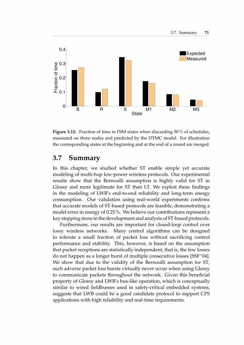
3.7. Summary 73
B R S M1 M2 M30
0.1
0.2
0.3
0.4
State
Fra
ctio
n o
f tim
e
ExpectedMeasured
Figure 3.12: Fraction of time in FSM states when discarding 50 % of schedules,measured on three nodes and predicted by the DTMC model. For illustrationthe corresponding states at the beginning and at the end of a round are merged.
3.7 SummaryIn this chapter, we studied whether ST enable simple yet accuratemodeling of multi-hop low-power wireless protocols. Our experimentalresults show that the Bernoulli assumption is highly valid for ST inGlossy and more legitimate for ST than LT. We exploit these findingsin the modeling of LWB’s end-to-end reliability and long-term energyconsumption. Our validation using real-world experiments confirmsthat accurate models of ST-based protocols are feasible, demonstrating amodel error in energy of 0.25 %. We believe our contributions represent akey stepping stone in the development and analysis of ST-based protocols.
Furthermore, our results are important for closed-loop control overlossy wireless networks. Many control algorithms can be designedto tolerate a small fraction of packet loss without sacrificing controlperformance and stability. This, however, is based on the assumptionthat packet receptions are statistically independent, that is, the few lossesdo not happen as a longer burst of multiple consecutive losses [SSF+04].We show that due to the validity of the Bernoulli assumption for ST,such adverse packet loss bursts virtually never occur when using Glossyto communicate packets throughout the network. Given this beneficialproperty of Glossy and LWB’s bus-like operation, which is conceptuallysimilar to wired fieldbusses used in safety-critical embedded systems,suggests that LWB could be a good candidate protocol to support CPSapplications with high reliability and real-time requirements.

74 Chapter 3. Modeling Protocols Based on Synchronous Transmissions

4Blink: Real-time Communication
in Multi-hop Low-power WirelessThe tangible benefits of low-power wireless technology in CPS andespecially in automation and control are, by now, widely acknowledged.Key industry players argue: ". . . the possibilities are endless:wireless technology will unlock value in one’s process chain farbeyond merely avoiding the wiring costs" [hon]. Such benefits includeimproved control safety and process reliability, lower installation andmaintenance costs, and unprecedented flexibility in selecting sensing

76 Chapter 4. Blink: Real-time Communication in Multi-hop Low-power Wireless
and actuation points [ÅGB11, Sve]. Example applications range fromlevel control of dangerous liquids to protect against environmentalthreats [hon] through rapid prototyping of automation solutions inretrofitting buildings [ABD+11] to minimally invasive monitoring ofsafety-critical assets [HSE]. Because of lower costs and ease of installation,battery-powered embedded platforms with low-power wireless radiotransceivers and computationally constrained MCUs are preferred in realdeployments [hon, Sve].
A trait common to all these applications is that packets must bedelivered within hard end-to-end deadlines [But11], for example, to ensurethe stability of the controlled processes [ÅGB11]. Hard deadlines entailthat packets not meeting their deadlines have no value to the applicationand hence count as lost. Support for this type of real-time tra�c ismainstream in wired fieldbusses [CAN, Fle], but hard to attain in a low-power wireless network. This is due to, for example, the dynamics of low-power wireless links [BKM+12], the need for multi-hop communicationto cover large areas, and the resource scarcity of the employed devices.
Prior WorkExisting e↵orts to address these challenges can be broadly classifieddepending on whether they require local or global knowledge as an inputfor computing packet schedules.
Local knowledge. In SPEED [HSLA05], each node continuously monitorsother nodes within its direct radio range, for example, to detect transientcongestion. Using only this node-local information, each node computesand follows its own transmission schedule. On a conceptual level,this fully localized approach of SPEED is also adopted by numerousMAC-layer solutions [GHLX09, KLS+01, LBA+02, WC01] and by systemsdesigned to support specific tra�c patterns [HLR03].
Albeit these solutions scale very well because of their localized nature,they cannot support applications that rely on tra�c with hard real-timedeadlines. As described in Section 4.1, those requirements are indeedspecified from an end-to-end perspective. However, a device that reasonsbased on local information and that can only influence its surroundingsis oblivious of the global picture and has limited means to a↵ect it.
Global knowledge. By contrast, the WirelessHART [har], ISA 100 [isa],and IEEE 802.15.5e TSCH [tsc] standards and other solutions [OBB+13,SNSW10] compute communication schedules based on global informa-tion about the network state: the instantaneous conditions at the physicallayer that possibly enable communication between any two nodes inthe network. Global network state information thus takes the form of

77
a connectivity graph, where the weight of edge A ! B represents thequality of the link from node A to node B, for example, in terms of thepacket reception rate seen by B when receiving packets from A.
Using this global network state as an input, in WirelessHART andsimilar solutions a central network manager computes and distributescommunication schedules tailored to each node, thereby forming end-to-end routing paths from sources to destination(s). Then, each node followsits own schedule locally. This approach has two fundamental problems:
1. Global network state is time-varying due to fluctuating low-powerwireless links [SDTL10], environmental influences [BKM+12], anddevice outages or device mobility [XTLS08]. Any such change in thenetwork state must first be detected and then communicated to thecentral manager for updating the connectivity graph and possiblyre-computing and re-distributing communication schedules to eachdevice. While this happens new changes may occur, requiring tore-iterate the same processing over and over again. Meanwhile,packets are lost because of inconsistent routing paths or miss theirdeadlines because of stale communication schedules.
2. The need to compute per-node communication schedules alsocauses severe scalability problems in deep multi-hop networks.Existing works map the problem of scheduling real-time tra�c in awireless multi-hop network to the problem of scheduling tasks ona multiprocessor machine [SXLC10]. As a result, in WirelessHARTnetworks for example, computing optimal schedules takes time atleast exponential in the network diameter [SXLC10]. Although someattempts have been made to address this issue [CWLG11, SXLC10,ZSJ09], WirelessHART schedulers are hardly practical in networksthat extend across more than three hops [CWLG11].
Because of these fundamental problems, any solution relying on globalnetwork state information cannot support hard real-time applicationseither. This fact is also acknowledged by major industry players whocontributed to the WirelessHART standard: ". . . none of the technologiesprovide any hard guarantees on deadlines, which is needed if you shoulddare to use the technology in critical applications" [Per].
Thus, the problem of providing hard real-time guarantees in multi-hoplow-power wireless networks remains unsolved.
Contribution and Road MapThis chapter introduces Blink, the first real-time low-power wirelessprotocol that provides hard guarantees on end-to-end packet deadlines

78 Chapter 4. Blink: Real-time Communication in Multi-hop Low-power Wireless
in large multi-hop networks, while simultaneously achieving low energyconsumption. Blink seamlessly handles dynamic changes in the networkstate and in the application’s real-time requirements, and readily supportsscenarios with multiple controllers and actuators.
The approach we adopt in Blink is radically di↵erent from prior art:Blink uses global knowledge to compute a single global schedule thatapplies to all nodes in the network. The key idea is to detach Blink’soperation from the global network state, whose rapid variations wouldlead to the same problems we observe in prior solutions. To this aim, anenabling factor is our choice of the LWB [FZMT12] as Blink’s underlyingcommunication support. As described in Section 4.2, LWB is an existingbest-e↵ort protocol that exclusively employs network-wide Glossy floodsfor communication [FZTS11]. Crucially, Glossy’s operation allows us notto consider the time-varying global network state information as an inputto the scheduling problem in Blink.
Building upon this foundation, we describe Blink’s overall designin Section 4.3, while Section 4.4 details Blink’s e�cient protocol operation,which rests upon three key contributions:
• Problem mapping. In LWB all nodes are time-synchronized andcommunicate according to the same global schedule. Moreover,Glossy allows us to abstract away the network state, as if it was avirtual single-hop network. Because of these two observations, wecan treat the entire network as a single resource that runs on a singleclock. Unlike previous approaches, we can thus map the real-timescheduling problem in Blink to the problem of scheduling tasks ona uniprocessor, making it easier to solve than prior art [SXLC10].
• Real-time scheduling policies. We conceive scheduling policies basedon the EDF principle [LL73]. Using these policies, Blink computesonline a communication schedule that provably meets all deadlinesof packets released by a set of admitted real-time packet streams,while minimizing the network-wide energy consumption within thelimits of the underlying LWB communication support. At the sametime, Blink tolerates dynamic changes in both the network state andthe set of streams.
• Data structures and algorithms. We design and implement a highlye�cient priority queue data structure and algorithms that utilize itto enable EDF scheduling on resource-constrained devices. Basedon these, we demonstrate the first implementation of EDF on low-power embedded platforms. This is notable per se: due to its run-time overhead, EDF has seen little adoption even on commodityhardware, despite its realtime-optimality [But05, SAÅ+04].

4.1. Problem Statement 79
Section 4.5 reports on the evaluation of our Blink prototype on twotestbeds of up to 94 nodes [BVJ+10, LFZ+13b], three state-of-the-art MCUs,and using a timing-accurate instruction-level emulator [EOF+09]. Ourresults show that Blink meets almost 100 % of packet deadlines; the fewdeadline misses are due to packet loss, which cannot be fully avoided overa lossy wireless channel. Further, by using our dedicated data structuresand algorithms, Blink achieves speed-ups of up to 4.1⇥ compared to aconventional implementation of our scheduling policies on state-of-the-art MCUs, which prove to be instrumental to the viability of EDF-basedreal-time scheduling on certain low-power embedded platforms.
We discuss trade-o↵s and limitations of our current Blink prototypein Section 4.6 and conclude in Section 4.7.
4.1 Problem StatementThe scheduling problem is a function of the application requirements, thecharacteristics of the deployment, and the devices employed. We discussthese aspects next.
Applications. CPS are increasingly deployed as a means to embedsophisticated feedback loops into the physical environment [SLMR05].CPS devices achieve this by tightly orchestrating computing, control, andphysical elements through sensors and actuators. Example applicationdomains range from static installations in industrial and buildingautomation, process control, or smart grids [ÅGB11, Whi08] to settingsinvolving highly mobile autonomous computing elements [MMWG14].
These applications place hard real-time requirements on end-to-endcommunication. Embedded devices periodically stream sensor data orcontrol signals under given timing constraints. Every device may sourcemultiple such streams. The data is then used for monitoring or to feedtime-critical control loops. These control loops may execute right on theactuators that a↵ect the environment, or on a few dedicated controllerdevices that periodically distribute control signals to the actuators, againsubject to hard real-time constraints.
Let ⇤ denote the set of all n streams in the network. Each streamsi 2 ⇤ releases one packet at a regular periodic interval Pi, called the periodof stream si. The start time Si is the time when stream si releases thefirst packet. Every packet released by stream si must be delivered to thedestination(s) within the same relative deadline Di. The next packet is onlyreleased after the absolute deadline of the previous packet, so deadlinesare less than or equal to periods (i.e., Di Pi). We often refer to theabsolute deadline of a stream as a shorthand for the absolute deadline

80 Chapter 4. Blink: Real-time Communication in Multi-hop Low-power Wireless
of the most recent packet released by the stream. Overall, each streamsi 2 ⇤ is characterized by its profile hSi,Pi,Dii. If there are k streams withthe exact same profile, we also write kh·, ·, ·i.1
The actual real-time requirements determining the stream profilesare highly application-dependent. The physical dimension recordedthrough sensors or the nature of the feedback loop often dictate a stream’speriod Pi. For example, temperature control in liquid volumes [PL10]demands periods on the order of minutes, and coordinated multi-robotcontrol runs with periods of at most tens of seconds [MMWG14]. Onthe other hand, compressor speed control requires periods down to afew microseconds [ÅGB11]. Low-power wireless is applicable with thegreatest advantages in the former type of applications [Whi08]. Themonitoring or control process governs a stream’s deadline Di and startingtime Si. For example, closed-loop control typically requires shorterdeadlines than open-loop control [Oga01].
Deployments and platforms. Resource-constrained embedded devicesamplify the benefits with regards to flexibility and ease of installationand maintenance [ÅGB11, PL10]. Typical devices feature a 16- or 32-bit MCU, a few kB of data memory, and rely on non-renewable energysources [ÅGB11, Whi08]. This motivates the use of low-power wireless,which reduces the energy costs but limits the bandwidth and makes thesystem susceptible to interference and environmental factors [BKM+12].
Deployments consist of tens to hundreds of devices. The devices aretypically installed at fixed locations as determined by the applicationand control requirements. Because of energy constraints that limit theindividual radio ranges, designers rely on multi-hop networking toensure overall connectivity. Nodes may also be added or moved on thefly to optimize measurement locations or prototype improvements overexisting installations [XTLS08]. The network can therefore exhibit somedegree of mobility. Emerging CPS scenarios, instead, feature partiallyor completely mobile networks, for example, swarms of arial drones toenable precision agriculture [Vil12]. These characteristics further add tothe temporal dynamics of low-power wireless links [BKM+12, SDTL10].
Problem. Thus, a solution to support real-time low-power wireless mustmeet the application-defined packet deadlines, while also achieving:
• scalability in terms of the number of streams, nodes, and the size ofthe deployment area;
1For simplicity, we assume a stream releases one packet at a time. If a stream hSi,Pi,Diireleases k packets at a time, we implicitly transform this into khSi,Pi,Dii streams eachreleasing one packet.

4.2. Foundation 81
Data N1 Nn Schedule Data N2 Contention …" Compute schedule
Figure 4.1: Time-triggered operation and sequence of slots in a LWB round.
• adaptiveness to accommodate dynamic changes in the set of activestreams and the global network state;
• energy e�ciency to achieve long system lifetimes in the face of limitedenergy resources;
• viability with respect to the limited bandwidth and computationalresources of the employed devices.
Subject to these, we can formulate the problem as finding communica-tion schedules such that, given n streams, n = |⇤|, for every stream si 2 ⇤,every packet released by stream si is delivered within Di time units.
4.2 FoundationTo detach the operation of Blink from the time-varying network state, weleverage LWB as the underlying communication support [FZMT12]. LWBis an existing non-real-time protocol that, conceptually, turns a multi-hopwireless network into a shared bus, where all nodes are potential receiversof all packets. The nodes are time-synchronized and communicate in atime-triggered fashion according to a global communication schedule. Toimplement the shared bus abstraction, LWB maps all communicationsonto e�cient Glossy floods [FZTS11]. Glossy propagates a packet fromone node to all other nodes within a few milliseconds. Crucially, in doingso, Glossy’s protocol logic is independent of the network state [FZTS11],as opposed to almost all existing low-power wireless protocols.
LWB operation. As shown in Figure 4.1 (A), LWB’s operation unfolds in aseries of communication rounds of fixed duration, executed simultaneously

82 Chapter 4. Blink: Real-time Communication in Multi-hop Low-power Wireless
by all nodes. Nodes keep their radios o↵ between rounds to save energy.Each round consists of a sequence of non-overlapping communication slots,as shown in Figure 4.1 (B). All nodes engage in the communication inevery slot: the node to which a slot was assigned places a packet on thebus (i.e., initiates a flood), and all other nodes read the packet from thebus (i.e., receive and relay the packet), as shown in Figure 4.1 (C). At theend of a round, only the intended receivers, which are encoded in thepackets, deliver the packet to the application.
Each round starts with a slot allocated to a specific node, called host,for distributing the communication schedule, as shown in Figure 4.1 (B).The schedule specifies when the next round starts and which nodes cansend application data in the following data slots; there are at most B dataslots in a round. Since nodes can only send during a round, B and thetime between rounds determine the bandwidth provided by LWB. Theshorter this time the more bandwidth is o↵ered to nodes, and vice versa.The time between rounds is upper-bounded to let the nodes update theirsynchronization state often enough to compensate for clock drifts.
If a node receives the communication schedule, it time-synchronizeswith the host and participates in the round; otherwise, it does not takeany action until the beginning of the next round. To inform the host abouttheir tra�c demands, nodes may compete in a final contention slot. Dueto capture e↵ects [LF76], with high probability one node succeeds despitecontention and its request reaches the host. Based on all tra�c demandsreceived thus far, the host computes the schedule for the next round.
A key observation is that the energy overhead of LWB is exclusivelydetermined by how often the communication rounds unfold over time.Indeed, it is not necessarily the case that all B data slots in a round areused. This occurs only when an application’s instantaneous bandwidthdemands align perfectly with LWB’s o↵ered bandwidth. Otherwise, somedata slots may remain unused, so nodes can turn o↵ their radios duringthese unused slots to save energy. Thus, the energy overhead consists ofthe energy needed to compute (host) and transmit schedules (all nodes).
Although this purely flooding-based approach to multi-hop commu-nication in LWB may seem wasteful, LWB outperforms prior solutions inend-to-end reliability and energy e�ciency; for example, LWB’s reliabilityranges above 99.9 % in real-world experiments, with energy consumptionon par with or even better than state-of-the-art solutions [FZMT12].
Benefits to Blink. Our design choice of building Blink on top of LWB asthe communication support brings three assets:
• The use of network-wide Glossy floods for all communications inplace of point-to-point transmissions creates, in essence, a virtualsingle-hop network whose operational logic is independent of the state

4.3. Overview 83
of individual wireless links. As a result, the host can take schedulingdecisions without considering the network state as an input.
• The previous point, together with LWB’s time-triggered operation,allow us to abstract a multi-hop low-power wireless network as asingle resource that runs on a single clock. This, in turn, allows usto map the real-time scheduling problem in Blink to the well-knownproblem of uniprocessor task scheduling, making it simpler to solvethan the multiprocessor formulation found in prior works [SXLC10].
• LWB o↵ers useful system-level functionality. It supports di↵erenttra�c patterns, such as one-to-many, many-to-one, and many-to-many, which makes it an appropriate choice for scenarios involvingmultiple actuators or controllers. Unlike existing solutions [har, isa],LWB also features mechanisms to resume its operation after a hostfailure, overcoming single point of failure problems [FZMT12].
4.3 OverviewIrrespective of its benefits, we need to address two issues to make LWBready for real-time. First, the existing LWB scheduler is oblivious of packetdeadlines, and only meant to reduce energy consumption [FZMT12]. Wemust therefore conceive a suitable policy to schedule packets such thatall deadlines are met without unnecessarily sacrificing energy e�ciency.Second, such a real-time scheduler must execute within strict time limitson a severely resource-constrained platform. As shown in Figure 4.1 (B),the longer it takes to compute the schedule for the next round, the fewerdata slots are available given the fixed duration of a round, thus reducingthe available bandwidth. We must thus provision an e�cient schedulerimplementation that is fully cognizant of the platform restrictions.
To this end, our design of Blink is driven by two important goals thatwe must achieve simultaneously:
1. Realtime-optimal [SAÅ+04] scheduling, which entails to admit a newstream if and only if there exists a scheduling policy able to deliverall packets by their deadlines, and to deliver all packets released bythe admitted streams by their deadlines.
2. Minimum network-wide energy consumption, which in LWB entails tominimize the number of rounds over any given interval, becauseevery round incurs a constant energy overhead regardless of thenumber of packets sent in the round, as discussed in Section 4.2.
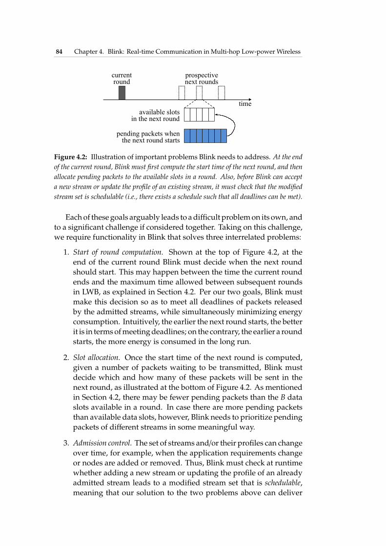
84 Chapter 4. Blink: Real-time Communication in Multi-hop Low-power Wireless
time
current round
prospective next rounds
pending packets when the next round starts
available slots in the next round
Figure 4.2: Illustration of important problems Blink needs to address. At the endof the current round, Blink must first compute the start time of the next round, and thenallocate pending packets to the available slots in a round. Also, before Blink can accepta new stream or update the profile of an existing stream, it must check that the modifiedstream set is schedulable (i.e., there exists a schedule such that all deadlines can be met).
Each of these goals arguably leads to a di�cult problem on its own, andto a significant challenge if considered together. Taking on this challenge,we require functionality in Blink that solves three interrelated problems:
1. Start of round computation. Shown at the top of Figure 4.2, at theend of the current round Blink must decide when the next roundshould start. This may happen between the time the current roundends and the maximum time allowed between subsequent roundsin LWB, as explained in Section 4.2. Per our two goals, Blink mustmake this decision so as to meet all deadlines of packets releasedby the admitted streams, while simultaneously minimizing energyconsumption. Intuitively, the earlier the next round starts, the betterit is in terms of meeting deadlines; on the contrary, the earlier a roundstarts, the more energy is consumed in the long run.
2. Slot allocation. Once the start time of the next round is computed,given a number of packets waiting to be transmitted, Blink mustdecide which and how many of these packets will be sent in thenext round, as illustrated at the bottom of Figure 4.2. As mentionedin Section 4.2, there may be fewer pending packets than the B dataslots available in a round. In case there are more pending packetsthan available data slots, however, Blink needs to prioritize pendingpackets of di↵erent streams in some meaningful way.
3. Admission control. The set of streams and/or their profiles can changeover time, for example, when the application requirements changeor nodes are added or removed. Thus, Blink must check at runtimewhether adding a new stream or updating the profile of an alreadyadmitted stream leads to a modified stream set that is schedulable,meaning that our solution to the two problems above can deliver

4.4. Design and Implementation 85
2 2 3 4 B 1 3 1
rounds
time
…
0 1 2
slots
1 allocated slot free slot
ti ti + 1 …
… B4 i
Figure 4.3: Discrete-time model of LWB used throughout Section 4.4. Each roundis of unit length and comprises B data slots, each of which is either allocated to a packetor free. Here, the i-th round with three allocated slots is scheduled to start at time ti andthus ends at time ti + 1, where ti is a non-negative integer.
all packets of all streams by their deadlines. In essence, Blink needsto make sure that given the modified stream set it will never be thecase that all streams together demand a bandwidth that exceeds themaximum available bandwidth over any interval of time.
To realize these functionality, Blink builds on LWB as communicationsupport as well as on novel scheduling policies that are provably realtime-optimal and minimize the network-wide energy consumption within thelimits set by LWB, and e�cient data structures and algorithms that letthe new real-time scheduling policies run “in a blink” even on a resource-constrained platform. We discuss in the next section how these techniqueshelp us achieve the three necessary functionality above.
4.4 Design and ImplementationIn the following, Sections 4.4.1 and 4.4.2 describe our solutions to theslot allocation and start of round computation problems, respectively,assuming the set of streams is schedulable. Section 4.4.3 describes howwe ensure this condition through online admission control.
Discrete-time model. Throughout the discussion, we consider a discrete-time model of LWB in which (i) each round is atomic and of unit length,and (ii) rounds start at an integer multiple of the unit length of a round,as illustrated in Figure 4.3. The reason for (i) is that the single MCU ontoday’s low-power wireless platforms is responsible for both applicationprocessing and interacting with the radio. These radio interactions aretime-critical and occur frequently during a Glossy flood [FZMT12]. Sinceeach slot in a round consists of a Glossy flood, the MCU has very littletime for application processing during a round. So to avoid interference,the application must release packets before a round and can only handlereceived packets after a round. We thus consider rounds atomic. Further,(ii) is beneficial in a practical LWB implementation. For example, it allows

86 Chapter 4. Blink: Real-time Communication in Multi-hop Low-power Wireless
a node that just got out-of-sync to selectively turn on the radio in order toreceive the next schedule (and thereby time-synchronize again with thehost) rather than keeping the radio on all the time, which consumes moreenergy but is unavoidable if rounds can start at arbitrary times.
Besides the specific model, our analyses and algorithms in this sectionenjoy general validity. In particular, they also hold for streams with starttimes Si, periods Pi, and deadlines Di that are not integer multiples of theunit length of a round. For example, fractional packet release times aresimply postponed to the next discrete time (by taking the ceiling), andfractional packet deadlines are preponed to the previous discrete time(by taking the floor). Thus, the atomicity of rounds does not prevent anypacket from meeting its deadline. This is essential to the validity of ourEDF-based scheduling policies, because preemptions in the execution ofthe underlying resource (i.e., the network, which we abstract as a singleresource that runs on a single clock) can only occur at discrete times.
4.4.1 Slot AllocationFor ease of exposition, let us momentarily assume that the start time ofthe next round was already computed. We now need to determine theconcrete schedule for that next round, which raises two questions: With Bslots available per round, how many packets should we actually allocate?How should we prioritize pending packets of di↵erent streams?
Algorithms. To answer the first question, we note that delaying a packetby not sending it in an otherwise empty slot does not lead to improvedschedulability or lower energy overhead in Blink. In the following round,the set of pending packets to schedule will be the same or larger, whichcan only worsen the overall schedulability. Furthermore, as explained inSection 4.2, the energy overhead in LWB over any given interval depends onthe number of rounds within that interval, not on the number of allocatedslots. Thus, it is best to allocate as many pending packets as possible tothe available slots in any given round.
As described in Section 4.3, the approach we adopt in Blink allows usto abstract the entire network as a single resource that runs on a singleclock. We can thus resort to uniprocessor scheduling policies to answerthe second question. Among these, earliest deadline first (EDF) is provablyrealtime-optimal [Der74]; that is, if a set of streams can be scheduled suchthat all packets meet their deadlines, then EDF also meets all deadlines.This holds also for sets of streams demanding the full bandwidth, whereasother well-known policies, such as rate-monotonic (RM), may fail to meetall deadlines at significantly lower bandwidth demands [LL73]. Finally,as the packets’ priorities are computed while the system executes, EDF

4.4. Design and Implementation 87
Table 4.1: Operations required on the set of streams ⇤ to e�ciently implementEDF in Blink. The key represents the absolute deadline of a stream’s current packet.
Operation Description
Insert(s) Insert a new stream s into stream set ⇤
Delete(s) Delete stream s from stream set ⇤
DecreaseKey(s, �) Propagate an increment of � in the key ofstream s in stream set ⇤
FindMin() Return a reference to the stream with theminimum key in stream set ⇤
First(t) Position traverser t at the stream with theminimum key in stream set ⇤
Next(t) Advance traverser t to the stream with the nextlarger key in stream set ⇤
can readily deal with dynamic changes in the set of streams [SAÅ+04],which is crucial when the set of streams changes because of, for example,varying application requirements or failures of nodes sourcing streams.
Using EDF in Blink entails allocating the next free data slot in a roundto the packet whose deadline is closest to the start time of the round, untilthe round is full or there are no more pending packets. This seeminglysimple logic, however, bears a significant run-time overhead [But05]. Toimplement EDF e�ciently, one should maintain the streams in increasingorder of absolute deadline while the latter is being updated from onepacket to the next as they are allocated to slots. This overhead is one ofthe reasons why EDF is rarely used in real systems, such as operatingsystem kernels [But05]. We describe next how we tackle this issue.
Design and implementation in Blink. Key to enabling EDF in Blink isthe provision of a data structure that can e�ciently maintain the currentset of streams in order of increasing absolute deadline. A suitable datastructure must support all operations required to manipulate the streamset ⇤ during EDF-based slot allocation, as listed in Table 4.1.
Besides operations to insert and delete a stream, EDF crucially requiresa FindMin() operation to retrieve the stream with the earliest absolutedeadline, which is to be served first. A priority queue is thus the mostnatural choice, where streams with smaller absolute deadline are givenhigher priority and hence served first. Moreover, after serving a stream s,the absolute deadline of s needs to be set to the deadline of its next packet.We therefore require a DecreaseKey(s, �) operation that propagates anincrement of � (typically the period of stream s) in the absolute deadline

88 Chapter 4. Blink: Real-time Communication in Multi-hop Low-power Wireless
Stream si
t
Stream sj
time packet arrival packet deadline
Figure 4.4: Example motivating EDF traversal of the set of stream during slotallocation. Stream sj has a higher priority than stream si because it has an earlierabsolute deadline. Nevertheless, sj requires no slot in the next round starting at time t,because it releases its next packet only after the start of the next round.
of stream s in the priority queue. The result of this operation is that thepriority of stream s is decreased relative to all other streams in the queue.
These four operations are supported by almost all standard priorityqueue data structures [Bro13]. Nevertheless, because the highest-prioritystream returned by FindMin() may release its packet only after the startof the next round, as illustrated in Figure 4.4, we also require operationsto perform an e�cient EDF traversal of the stream set while only thosestreams with pending packets are updated. Specifically, it should bepossible to position a traverser t at the highest-priority stream with First(t),and then to visit all streams in order of increasing absolute deadlinethrough repeated Next(t) calls. During the EDF traversal, the priority ofany stream t with a pending packet is updated using DecreaseKey(t, �).
Finding a data structure that supports all required operations e�cientlyin terms of time and memory is challenging. A review of widely used andhighly e�cient priority queue data structures, ranging from the classicalbinary heap to red-black trees used in the Linux scheduler [lin], revealsthat the EDF traversal (also known as in-order traversal) is the main culprit.In particular, updating a stream using DecreaseKey(t, �) is likely to alterthe relative ordering of streams, which triggers structural changes insidethese data structures. Thus, a runtime stack or pointers (e.g., on a threadedbinary tree) used for the traversal becomes invalid [Pfa], so the traversalmust start anew after any such change, which becomes highly ine�cient.
While looking for a practical solution to these challenges, we foundthat the following properties of our specific problem allow us to use asimple yet e�cient data structure as the basis for our priority queue:
1. A stream’s absolute deadline, henceforth referred to as the key of astream, is a non-negative integer.
2. The key of a stream increases monotonically as it is being updatedfrom one packet to the next.
3. The range of keys in the priority queue at any one time is bounded,as stated in the following theorem.

4.4. Design and Implementation 89
Stream si
t
Stream sj
time di dj di + Pi
packet arrival packet deadline
Figure 4.5: Illustration of the proof of Theorem 1.
Theorem 1. With ⇤ denoting the set of streams, let P be an upper bound on theperiod Pi of any stream si 2 ⇤. Then, there are never more than 2P � 1 distinctkeys (i.e., absolute deadlines) in the priority queue at any one time.
Proof. Let di be the absolute deadline of stream si at some point in time; thatis, di is the deadline of si’s current packet. Since si’s relative deadline Di canbe shorter than its period Pi, the current packet may not yet have arrivedat this point in time. To determine the maximum number of distinct keys(i.e., absolute deadlines) in the priority queue at any one time, we mustupper-bound the di↵erence between the absolute deadlines of any twostreams, that is, maximize �ij = di � dj for any two streams si, sj 2 ⇤.
The value of �ij is larger when packets with later deadlines are sentbefore packets with earlier deadlines, due to the order of packet arrival.Let us consider the example in Figure 4.5. Assume at time t the currentpacket of stream si with deadline di is sent, while the current packet ofstream sj with an earlier deadline dj < di is yet to be sent. This can happenif and only if si’s packet arrives strictly before sj’s packet; that is, at timet, sj’s packet is yet to arrive. After sending the packet of stream si, itsabsolute deadline becomes di + Pi, while the absolute deadline of streamsj is still dj. Thus, we have �ij = di + Pi � dj. What is the upper boundon �ij? As si’s packet has arrived by time t, we have di t + Pi. Also, assj’s packet has not yet arrived by time t, we have dj > t. With these twoconditions, we can establish the following bound
�ij = di + Pi � dj < t + Pi + Pi � t 2P, (4.1)
where P is an upper bound on the period of any stream. Since absolutedeadlines are integers, the strict inequality in (4.1) implies that �ij is atmost 2P � 1. ⇤
Given the three properties above, we can consider using a monotoneinteger priority queue. Similar observations apply to problems in discreteevent simulation [Bro88] and image processing [FaSdAL04] but, to thebest of our knowledge, have not been leveraged for real-time scheduling.
Specifically, we use a simple one-level bucket queue [Dia69] implementedas a circular array B of 2P doubly-linked lists, as shown in Figure 4.6,

90 Chapter 4. Blink: Real-time Communication in Multi-hop Low-power Wireless
0 1
2
3
4
7 6
5
14 15
8 9
10
11
12
13
mod 16
s2: 34
s1: 36
s4: 37
s3: 41
s7: 34
s6: 44
s5: 30 L
Figure 4.6: Illustration of a one-level bucket queue implemented as a circulararray of 2P doubly-linked lists. In this example, the largest period of any stream P is8, so the queue consists of 2P = 16 buckets. The queue contains seven streams orderedby increasing key as follows: s5, s2, s7, s1, s4, s3, s6. Operation FindMin() sets index Lto 14, because this bucket contains the stream(s) with the smallest key in the queue.
where P is an upper bound on the period of any stream. Stream si withkey di is stored in B[di mod 2P]. Because a stream’s relative deadline Di isno longer than its period Pi, all keys in the bucket queue are always in therange [dmin, dmin + 2P � 1], where dmin is the smallest key currently in thequeue. Thus, all streams in a bucket have the same key. As an example,the keys in the bucket queue shown in Figure 4.6 are in the range [30, 45],and the two streams in bucket B[2] have the same key, namely 34.
Because buckets are implemented as doubly-linked lists, operationsInsert(s), Delete(s), and DecreaseKey(s, �) take constant time. Insert(s)inserts a stream s with key d into bucket B[d mod 2P].2 Delete(s) removesstream s from the list containing it. DecreaseKey(s, �) first performs aDelete(s) and then re-inserts stream s into bucket B[(d + �) mod 2P].
We implement FindMin() using an index L, which is initialized to 0. Ifbucket B[L] is empty, FindMin() increments L (modulo 2P) until it findsthe first non-empty bucket; otherwise, it returns the first stream on the listin bucket B[L]. First(t) works similarly, using a second index I. Next(t)moves the traverser t to the next stream on the list in bucket B[I]. Whenthe end of the list is reached, Next(t) increments I (modulo 2P) until itfinds the next non-empty bucket and then lets t point to the first streamon the list in bucket B[I]. Unlike the vast majority of priority queues, thislogic enables a smooth continuation of an EDF traversal despite streamupdates. The three operations run in O(2P) worst-case time.
2If 2P is a power of two, the modulo operation required to compute the bucket indexis equivalent to a bit-wise AND of d with 2P � 1 as the mask, which is highly e�cient.

4.4. Design and Implementation 91
Algorithm 1 Perform EDF-based Slot AllocationInput Bucket queue representing the current set of streams, where a smaller
absDeadline implies that the stream has a higher priority, the start time of thenext round ti+1, and the upper bound on any stream’s period P.
Output Allocation of packets released by ti+1 in EDF order to at most B slots.initialize slot counter c to 0position traverser t at highest-priority stream using First(t)horizon = t.absDeadline + P � 1while (c < B) and (t.absDeadline horizon) do
if t.releaseTime ti+1 thenallocate a slot to stream t and set c = c + 1t.releaseTime = t.releaseTime + t.periodt.absDeadline = t.absDeadline + t.periodupdate t’s priority with DecreaseKey(t, t.period)
end ifadvance t to next stream in EDF-order using Next(t)
end while
at most P
ti+1
Stream si
time horizon
dmin di
packet arrival packet deadline
Figure 4.7: Illustration of the second termination criterion of the while loopin Algorithm 1. Any stream si that has an absolute deadline di greater than thehorizon = dmin + P � 1 releases its current packet after the start of the next round attime ti+1, and hence need not be considered for slot allocation in the next round.
Using this dedicated priority queue data structure, Algorithm 1 showsthe pseudocode to allocate as many pending packets as possible to the Bavailable slots in the next round. The algorithm operates on the current setof streams, maintained in a bucket queue in order of increasing absolutedeadline. Starting from the stream with the earliest absolute deadline,it visits streams in EDF-order through repeated Next(t) calls. When itsees a stream t with a pending packet, it allocates a slot to stream t andupdates its priority within the queue using DecreaseKey(t, t.period). Thealgorithm stops when all B data slots available in a round are allocated,or when it sees a stream with an absolute deadline larger than the horizon.
The second termination criterion using the horizon is needed becausethere may be less than B pending packets by the time the next roundstarts. Algorithm 1 determines the horizon initially, horizon = dmin+P�1,where dmin is the earliest absolute deadline of all streams at this time and

92 Chapter 4. Blink: Real-time Communication in Multi-hop Low-power Wireless
P is an upper bound on the period of any stream. As shown in Figure 4.7,the next round starts before dmin, that is, ti+1 dmin � 1. So stream si withabsolute deadline di > horizon releases its current packet no earlier than
di � P > dmin + P � 1 � P � ti+1. (4.2)
The strict inequality in (4.2) implies that stream si releases its currentpacket only after the start of the next round. Thus, stream si need notbe considered for slot allocation in the next round. As Algorithm 1 visitsstreams in EDF-order, it can terminate when it sees the first such stream.
As described in the following sections, our bucket queue implementa-tion underpins not merely the EDF-based slot allocation step, but rather allAlgorithms 1, 2, 3, and 4 required for energy-e�cient real-time schedulingin Blink. Despite enabling a smooth EDF traversal, the e�ciency of ourbucket queue implementation stems primarily from two key properties.First, DecreaseKey(s, �) is a frequently used operation and at the sametime extremely e�cient in our design due to its constant, short runningtime. Second, the cost of searching for a non-empty bucket amortizes. Tosee why, we note that Next(t) needs to increment index I in the worst case2P�1 times; however, the following n calls to Next(t) require no searchingat all since all n streams are necessarily in B[I]. With these implementationchoices, we empower Blink to schedule hundreds of streams using EDFon resource-constrained devices even when the system is in a continuousstate of change, which we show through experiments in Section 4.5.
4.4.2 Start of Round ComputationWe now turn to the problem of computing the start time of the next round.To illustrate the problem, we use an example with B = 5 slots availableper round and the following twelve streams with three distinct profiles:3h0, 5, 4i, 4h2, 7, 5i, and 5h1, 15, 12i. Figure 4.8 indicates the release timesand deadlines of packets generated by these streams in the first 14 timeunits. We seek an answer to the following question: Using our EDF-basedslot allocation policy from Section 4.4.1, when should a round start to meetall deadlines while minimizing energy (i.e., the number of rounds)?
Algorithms. One option, called contiguous scheduling (CS), is to start thenext round immediately after the previous one has ended. CS o↵ers thehighest possible bandwidth and therefore necessarily meets all deadlines,provided the set of streams is schedulable. However, CS wastes energy,because it may trigger more rounds than necessary. Looking at Figure 4.8,we see that 8 out of the first 14 rounds are empty (i.e., contain only freeslots) when using CS, causing unnecessary energy overhead.
Another possibility, referred to as greedy scheduling (GS), improves on

4.4. Design and Implementation 93
GS
3 3 3
4 4
5
CS
0,5,4 3
2,7,5 4
1,15,12 5
0 14 13 12 11 10 9 8 7 6 5 4 3 2 1 time
release x packets x
deadline allocated slot free slot
LS
Figure 4.8: Example execution comparing the CS, GS, and LS policies. CS
and GS waste energy by scheduling more rounds than necessary. Instead, LS meets alldeadlines while also minimizing energy (i.e., minimizing the number of rounds).
CS by delaying the next round until there are one or more pending packetsready to be sent. GS is realtime-optimal just like CS as it schedules packetsas soon as possible. Moreover, CS can reduce the energy consumptioncompared with CS in certain situations. For instance, in Figure 4.8 usingGS results in only 6 rounds in the first 14 time units. However, there arestill 8 free slots, raising the question whether we can do even better.
The crucial observation is that GS starts the next round no matter how“urgent” it is. If there was still some time until the earliest deadline of allpending packets, we could delay the next round further. Meanwhile, wecould await more packet arrivals and thus allocate more slots in the nextround. This strategy, however, may do more harm than good: Withoutknowing the future bandwidth demand, we may end up delaying thenext round to a time where the number of packets to be sent is larger thanthe available bandwidth. This situation would inevitably cause deadlinemisses. To prevent this, we need to forecast the bandwidth demand.
A policy we call lazy scheduling (LS) is precisely based on this intuition.At the heart of LS is the notion of future demand hi(t) that quantifies thenumber of packets that must be sent (or served) between the end of round iand some future time t. The future demand includes all packets that haveboth their release time and deadline no later than time t, and have not beenserved until the end of round i, as captured by the following definition
hi(t) =nX
j=1
8>><>>:
j(t � dj)/Pj
k+ 1, if dj t
0, otherwise(4.3)
where Pj is the period and dj is the absolute deadline of stream sj (or moreprecisely, dj is the deadline of sj’s current packet).

94 Chapter 4. Blink: Real-time Communication in Multi-hop Low-power Wireless
7 21 19 17 15 13 11 9 time
8 10 12 14 16 18 20
2 4 6 8
10
14 16 18 20
12
futu
re d
eman
d (#
slo
ts) h2(t)
start time of the third round
Figure 4.9: Graphical illustration of how LS computes the latest possible starttime of the third round in Figure 4.8.
LS uses hi(t) to forecast the bandwidth demand and, based on this,computes the latest possible start time of the next round without missingany deadline. As a concrete example, say we want to compute the starttime of the third round t3 in Figure 4.8 using LS. We proceed as follows:
1. Compute h2(t). As illustrated in Figure 4.9, h2(13) = 5 because t = 13is the absolute deadline of the 5h1, 15, 12i streams whose packets arestill pending at the end of the second round; h2(14) = h2(13)+7 = 12,since t = 14 is the deadline of the 7 packets released by the otherstreams at t = 9 and t = 10; and so on.
2. Determine a set of latest possible start times {ti3}. For instance, h2(13) = 5
packets must be served no later than time 13. With B = 5 slotsavailable in each round, serving this demand takes dh2(13)/Be = 1round. Thus, we get a first latest possible start time t1
3 = 13� 1 = 12.We indicate this in Figure 4.9 by casting a shadow back on the timeaxis. Further, h2(14) = 12 packets must be served before time 14,which takes dh2(14)/Be = 3 rounds. So, a second latest possible starttime of the third round is t2
3 = 14 � 3 = 11. The same reasoningrepeats, thus identifying more latest possible start times.
3. Take the minimum of the computed latest possible start times as t3. Basedon the reasoning in step 2., pushing the start of the third roundbeyond the beginning of the shady area at min{ti
3} = 11 in Figure 4.9would cause deadline misses. Indeed, if we had served h2(13) =5 packets only between times 12 and 13, we would be left withh2(14) � h2(13) = 7 packets to serve between times 13 and 14, butthese do not fit in a round with B = 5 slots. Alternatively, an earlier

4.4. Design and Implementation 95
ti + 1 Tmax Tb
hi(t)
futu
re d
eman
d time
Figure 4.10: Illustration of how far LS needs to look into the future whencomputing the start time of the next round.
start time could, in the long run, lead to more rounds than needed,thereby wasting energy. Thus, the third round should start at t3 = 11.
The example illustrates the main reasoning behind LS. Nevertheless,we still need to address two questions: Which times t do we really needto inspect in steps 1. and 2.? How far do we need to look into the future?
To answer the first question, we observe that the future demand hi(t)is a step function: the value of hi(t) increases only at times of deadlines,as visible in Figure 4.9. Thus, to speed up the computation, we can safelyskip all intervals between steps where hi(t) is constant.
The answer to the second question involves two observations. First,as described in Section 4.2, we can delay the start of the next round byat most Tmax time units after the start of the previous round since LWBrequires to update the nodes’ synchronization state su�ciently often tocompensate for clock drift [FZMT12]. To find out whether we can indeeddelay the next round by Tmax, we need to evaluate hi(t) for at least Tmax
time units after the end of the previous round at ti + 1, as illustrated inFigure 4.10. Second, we also have to consider any demand arising aftert = ti+1+Tmax that could possibly prevent us from delaying the next roundby Tmax. Thus, we must evaluate hi(t) for another Tb time units beyondt = ti + 1 + Tmax, also illustrated in Figure 4.10. The value of Tb is knownas the synchronous busy period [Spu96]. Informally, this is the minimumtime needed to serve the maximum demand that a given stream set canpossibly create.3 By looking up to t = ti + 1+ Tmax + Tb into the future, weultimately ensure that all deadlines are met.
The following theorem formally specifies the way LS computes thelatest possible start time of the next round without missing any deadline.
3The maximum demand arises when all streams release their packets at the sametime. CS essentially serves this demand "as fast as possible." Tb is then the time betweenthe simultaneous arrival of packets from all streams and the first idle time where nopacket is pending under CS scheduling.

96 Chapter 4. Blink: Real-time Communication in Multi-hop Low-power Wireless
Theorem 2. Let Tb be the synchronous busy period of the stream set⇤, Tmax thelargest time by which the start of the next round can be delayed after the start ofthe previous one, and B the number of slots available in a round. Using LS, thestart time of each round ti for all i = 0, 1, . . . is computed as
ti+1 = min(ti + Tmax,Ti), (4.4)
where t0 = �1 and Ti is given by
Ti = mint2Di
t �
&hi(t)
B
'!. (4.5)
Di denotes the set of deadlines in the interval [ti+ 1, ti+Tmax+Tb+ 1] of packetsthat are unsent until the end of round i; hi(t) is the future demand as per (4.3).
Proof. Because of time synchronization constraints imposed by the LWBcommunication support [FZMT12], the start of the next round at time ti+1
can be delayed at most Tmax after the start of the previous round at timeti. This implies the first component of the min-operation in (4.4).
We now show that the second component of the min-operation in (4.4)ensures that all packets meet their deadlines. The number of packets thatmust be sent between the end of round i and some time t � ti + 1 is givenby the future demand hi(t). The available bandwidth in the interval [ti+1, t]is B(t� ti+1), where B is the number of slots available per round. To ensurethat all packets meet their deadlines, the future demand hi(t) must notexceed the available bandwidth for any time t � ti + 1, that is,
B(t � ti+1) � hi(t). (4.6)
Dividing both sides by the positive quantity B,
t � ti+1 � hi(t)/B. (4.7)
Since m � x if and only if m � dxe for any integer m and real number x,
t � ti+1 � dhi(t)/Be . (4.8)
Rearranging terms,ti+1 t � dhi(t)/Be . (4.9)
In particular,ti+1 min
t�ti+1^ hi(t)>0(t � dhi(t)/Be) . (4.10)
The min-operation in (4.10) is to be performed for every time t largerthan ti + 1 at which the future demand hi(t) is greater than zero. Wecan restrict this in two ways. First, we need to apply the min-operationonly at every time t in the interval [ti + 1, ti + Tmax + Tb + 1], where Tb

4.4. Design and Implementation 97
is the synchronous busy period of the stream set ⇤. We prove this bycontradiction. Let for some t > ti + Tmax + Tb + 1,
t = arg mint�ti+1^ hi(t)>0
(t � dhi(t)/Be) . (4.11)
Let the quantity t �lhi(t)/B
mbe equal to the start time of the next round
ti+1 and strictly less than ti + Tmax,
ti+1 = t �lhi(t)/B
m< ti + Tmax. (4.12)
Rearranging terms, lhi(t)/B
m= t � ti+1. (4.13)
Since dxe = m if and only if m � 1 < x m for any integer m and realnumber x,
t � ti+1 � 1 < hi(t)/B. (4.14)
Multiplying both sides by the positive quantity B,
(t � ti+1 � 1)B < hi(t). (4.15)
We can interpret (4.15) as follows. The future demand hi(t) exceeds thebandwidth available in the interval [ti+1 + 1, t]. This means that if onewere to contiguously serve a demand as large as hi(t), the required timewould exceed the length of the interval [ti+1 + 1, t]. We can thus considerinterval [ti+1+1, t] a busy period of length t� ti+1�1 > t� (ti+Tmax)�1 > Tb,because we have ti+1 < ti + Tmax according to (4.12). However, Tb is thelength of the synchronous busy period, which is the longest possible busyperiod [Spu96]. This contradicts the supposition on the existence of t.
Second, we need to perform the min-operation in (4.10) only at timeswhen hi(t) has discontinuities. In fact, hi(t) is a right-continuous functionwith discontinuities only at times that coincide with packet deadlines.Thus, we can restrict the domain of the min-operation to all deadlinesDi
in the interval [ti + 1, ti + Tmax + Tb + 1] of packets that are unsent until theend of round i. Since (4.10) yields the largest possible ti+1 in the case ofequality, we obtain the second component of the min-operation in (4.4)
Ti = mint2Di
(t � dhi(t)/Be) . (4.16)
Finally, because EDF is realtime-optimal [Der74, LL73], the necessarycondition in (4.16) is also a su�cient one. ⇤
We are now in the position to state the main result about the LS policy,showing that it meets the two goals set out in Section 4.3.

98 Chapter 4. Blink: Real-time Communication in Multi-hop Low-power Wireless
Theorem 3. The LS policy is real-time optimal and minimizes the network-wideenergy consumption within the limits set by the LWB communication support.
Proof. A schedule S specifies for each round i its start time ti and the set ofpackets to be sent in the round. Let SLS denote the schedule computed byLS. We prove this theorem by contradiction; that is, we show that therecannot be any schedule S0 , SLS such that S0 is realtime-optimal and someround starts later in S0 than in SLS. If we show this, it follows that amongstall realtime-optimal schedules, SLS delays the start of each round the mostand thus minimizes the network-wide energy consumption using LWB.
Let tLSi and t0i denote the start times of the i-th round in SLS and S0, and
let hLSi and h0i denote the future demands after the end of the i-th round in
SLS and S0, respectively.Assume some round in S0 starts later than in SLS. Let the m-th round
be the first such round, that is,
m = min{i | t0i > tLSi }. (4.17)
In SLS, the m-th round starts at tLSm since, according to Theorem 2, at
least one of the following two conditions holds:
1. tLSm � tLS
m�1 = Tmax, where Tmax is the largest interval between the startof consecutive rounds supported by LWB [FZMT12],
2. hLSm�1(t⇤) > B(t⇤ � tLS
m � 1) for some time t⇤ > tLSm .
Assume condition 1. holds. Then, from the definition of m in (4.17),we have t0m � t0m�1 > tLS
m � tLSm�1 = Tmax. This violates the constraint that the
time between the start of consecutive rounds in S0 does not exceed Tmax.Assume condition 2. holds. Then, the interval [tLS
m , t⇤] is a busy periodin SLS, so the number of packets sent in this interval, denoted ⌘LS(tLS
m , t⇤),is lower-bounded as
⌘LS(tLSm , t
⇤) > B(t⇤ � tLSm � 1). (4.18)
On the other hand, since t0m > tLSm according to the definition of m in (4.17),
the number of packets transmitted in S0 in the interval [t0m, t⇤], denoted⌘0(t0m, t⇤), is upper-bounded as
⌘0(t0m, t⇤) B(t⇤ � t0m) B(t⇤ � tLS
m � 1). (4.19)
From (4.18) and (4.19) follows a strict inequality
⌘LS(tLSm , t
⇤) > ⌘0(t0m, t⇤). (4.20)

4.4. Design and Implementation 99
Algorithm 2 Compute Start Time of Next Round According to LSInput A bucket queue based copy of the current set of streams, where a smaller
absDeadline means that the stream has a higher priority, the start time of thecurrent round ti, and the synchronous busy period Tb.
Output The start time of the next round ti+1 according to the LS policy.initialize futureDemand to 0 and minSlack to1set s to highest-priority stream using s = FindMin()t = s.absDeadlinewhile t ti + Tmax + Tb + 1 do
futureDemand = futureDemand + 1s.absDeadline = s.absDeadline + s.periodupdate priority of s using DecreaseKey(s, s.period)set s to highest-priority stream using s = FindMin()if s.absDeadline > t then
minSlack = min((t � ti)B � futureDemand,minSlack)end ift = s.absDeadline
end whileti+1 = ti +min(bminSlack/Bc,Tmax)
We also know that ⌘LS(0, tLSm ) � ⌘0(0, t0m), because each round 1, 2, . . . ,m�1
starts no earlier in SLS than in S0, and in SLS as many pending packets aspossible are sent in each round. Combining this with (4.20), we have
⌘LS(0, t⇤) > ⌘0(0, t⇤). (4.21)
This shows that SLS tightly meets all deadlines at time t⇤, while sendingmore packets than S0. Since SLS prioritizes packets using EDF, whichis realtime-optimal [Der74, LL73], S0 necessarily misses a deadline at orbefore time t⇤. This contradicts the assumption that S0 is realtime-optimal.
For either condition that impacts the choice of tLSm , we have shown that
the assumptions on S0 are contradicted. ⇤
Design and implementation in Blink. The primary systems challengein leveraging LS’s optimality is to e�ciently compute the future demandhi(t). The corresponding expression in (4.3) is obtained by applying well-known concepts from the real-time literature [SRS98]. We implementedthis conventional method on a TelosB [PSC05] and observed prohibitiverunning times due to many time-consuming divisions. This behavior isexpected also on other resource-constrained platforms that lack hardwaresupport for accelerating divisions. Experiments in Section 4.5.3 show thatthe approach we describe next can outperform the conventional methodeven on recent, powerful platforms, including a 32-bit ARM Cortex-M4.
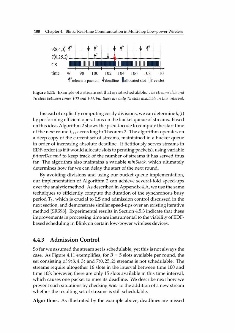
100 Chapter 4. Blink: Real-time Communication in Multi-hop Low-power Wireless
96 110 108 106 104 102 100 98 time
9 9 9
7
release x packets x
deadline allocated slot free slot
CS
8,4,3 9
0,25,2 7
9
Figure 4.11: Example of a stream set that is not schedulable. The streams demand16 slots between times 100 and 103, but there are only 15 slots available in this interval.
Instead of explicitly computing costly divisions, we can determine hi(t)by performing e�cient operations on the bucket queue of streams. Basedon this idea, Algorithm 2 shows the pseudocode to compute the start timeof the next round ti+1 according to Theorem 2. The algorithm operates ona deep copy of the current set of streams, maintained in a bucket queuein order of increasing absolute deadline. It fictitiously serves streams inEDF-order (as if it would allocate slots to pending packets), using variablefutureDemand to keep track of the number of streams it has served thusfar. The algorithm also maintains a variable minSlack, which ultimatelydetermines how far we can delay the start of the next round.
By avoiding divisions and using our bucket queue implementation,our implementation of Algorithm 2 can achieve several-fold speed-upsover the analytic method. As described in Appendix 4.A, we use the sametechniques to e�ciently compute the duration of the synchronous busyperiod Tb, which is crucial to LS and admission control discussed in thenext section, and demonstrate similar speed-ups over an existing iterativemethod [SRS98]. Experimental results in Section 4.5.3 indicate that theseimprovements in processing time are instrumental to the viability of EDF-based scheduling in Blink on certain low-power wireless devices.
4.4.3 Admission ControlSo far we assumed the stream set is schedulable, yet this is not always thecase. As Figure 4.11 exemplifies, for B = 5 slots available per round, theset consisting of 9h8, 4, 3i and 7h0, 25, 2i streams is not schedulable. Thestreams require altogether 16 slots in the interval between time 100 andtime 103; however, there are only 15 slots available in this time interval,which causes one packet to miss its deadline. We describe next how weprevent such situations by checking prior to the addition of a new streamwhether the resulting set of streams is still schedulable.
Algorithms. As illustrated by the example above, deadlines are missed

4.4. Design and Implementation 101
if, over some time interval, the demand exceeds the available bandwidth.As explained before, the CS policy o↵ers the highest possible bandwidth.Therefore, admission control under all scheduling policies discussed inSection 4.4.2 amounts to checking if CS can meet all deadlines.
We must perform this check over an interval in which the demand ishighest. The intuition is that if the available bandwidth is su�cient evenin this extreme situation, we can safely admit the new stream. Preciselyidentifying when this situation occurs is, however, non-trivial, in that thedi↵erent start times and periods of the streams may defer this situationuntil some arbitrary time. For example, for the stream set in Figure 4.11,it is not until time t = 100 that an interval of highest demand begins.
To tackle this problem, we deliberately create an interval of maximumdemand by forcing all streams to release a packet at time t = 0. Usingthe concept of synchronous busy period Tb, we then check if CS can meetall deadlines in the interval [0,Tb]. From this intuition follows a theorem,whose proof descends from existing results [Spu96]:
Theorem 4. For a set of streams ⇤ with arbitrary start times Si, let ⇤0 be thesame set of streams except all start times are set to zero. With B slots availablein each round, ⇤ is schedulable if and only if
8t 2 D, h0(t) t ⇥ B, (4.22)
whereD is the set of deadlines in the interval [0,Tb] of packets released by streamsin ⇤0, h0(t) is the number of packets that have both release time and deadline in[0, t], and t ⇥ B is the bandwidth available in the interval [0, t].
Design and implementation in Blink. An e�cient implementation ofTheorem 4 faces the same challenges as mentioned before in Section 4.4.2.The closed-form expression found in the literature [But11]
h0(t) =nX
i=1
� t + Pi �Di
Pi
⌫(4.23)
involves many costly divisions, so using (4.23) can result in a performancehog on certain resource-constrained platforms.
For this reason, we perform admission control again by performinge�cient bucket queue operations instead of costly divisions. Algorithm 3takes as input a deep copy of the current set of streams, including thenew stream to be admitted, and the new synchronous busy period Tb. Allstreams start at time t = 0 to trigger an interval of maximum demand, sothe absolute deadline of each stream si is initialized to the relative deadlineDi. Using a bucket queue to keep streams in EDF-order, the algorithmrepeatedly updates the absolute deadline of the highest-priority stream

102 Chapter 4. Blink: Real-time Communication in Multi-hop Low-power Wireless
Algorithm 3 Perform Admission ControlInput A bucket queue based copy of the current set of streams including the new
stream, with s.absDeadline initialized to Di for all streams si (smaller absDeadlineimplies higher priority), the utilization as well as the deadline-based utilizationof that stream set, and the new synchronous busy period Tb.
Output Whether the new stream is to be admitted or rejected.if utilization exceeds 1 then
return "reject"end ifif deadline-based utilization does not exceed 1 then
return "admit"end ifinitialize demand, availableBandwidth, and t to 0while demand availableBandwidth do
set s to highest-priority stream using s = FindMin()if s.absDeadline > t then
if s.absDeadline > Tb thenreturn "admit"
end ifavailableBandwidth = t ⇥ Bt = s.absDeadline
end ifdemand = demand + 1s.absDeadline = s.absDeadline + s.periodupdate priority of s using DecreaseKey(s, s.period)
end whilereturn "reject"
as if it were executing CS. In doing so, the algorithm keeps track of thenumber of deadlines seen until time t, which correspond to the demand.If this quantity exceeds the availableBandwidth in the interval [0, t] for anyt in the interval [0,Tb], the new stream cannot be admitted.
Algorithm 3 contains two optimizations that help improve its average-case performance. First, it checks if the end of interval [0,Tb] has beenreached and updates the availableBandwidth only when t has advanced.This avoids unnecessary processing when multiple packet deadlinescoincide. Second, the algorithm performs two simple checks before theloop. The new stream can be rejected without further processing if theutilization, defined as 1
BPn
i=11Pi
, exceeds one [LL73]. Further, since Di Pi
for any stream si, the new stream can be admitted if the deadline-basedutilization, defined as 1
BPn
i=11
Di, does not exceed one [SRS98]. We update
both types of utilizations as streams are added and removed at runtime.

4.5. Evaluation 103
Yes Stream request?
No
Start End
Compute synchronous busy period
Admission control
Compute start time of next round
Slot allocation
Figure 4.12: Main steps in Blink’s real-time scheduler executed by the host atthe end of each round (see Figure 4.1). The algorithm to compute the start time of thenext round depends on whether CS, GS, or LS is used. In case of LS, the synchronousbusy period Tb is carried over to subsequent rounds unless the set of streams changes.
4.4.4 Blink in PracticeAt the end of each round, the algorithms described above unfold as shownin Figure 4.12. With a pending request for a new stream s, the schedulercomputes the (new) synchronous busy period for the stream set ⇤ [ {s}and checks if s can be admitted. In any case, the scheduler computes thestart time of the next round and then allocates slots to pending packets.In the worst case, a single scheduler execution needs to proceed throughall four steps in Figure 4.12. Experiments in Section 2.5 show that ourimplementation can schedule hundreds of streams with a wide range ofrealistic bandwidth demands within the time bounds of Blink prototype.
We implement the processing in Figure 4.12 in a Blink prototype ontop of the Contiki [DGV04] operating system. Our prototype targets theTelosB platform available on large public testbeds, which comes with aMSP430 MCU. We use the default settings in LWB [FZMT12], includingthe fixed 1 second duration of a round that corresponds to the time unitused throughout Section 4.4. We set the number of data slots in a roundto B = 51, which leaves about 100 ms to compute the schedule at the endof a round. We slightly modify the time synchronization mechanism ofLWB to support frequently varying intervals between rounds in Blink.
4.5 EvaluationIn this section, we evaluate Blink along four lines: (i) the ability to dealwith dynamic changes in the set of streams, (ii) the level of real-timeservice provided to applications in terms of meeting packet deadlines, (iii)the energy e�ciency of our scheduling policies, and (iv) the scalabilityproperties of our implementation of the LS policy. We find that:
• Blink promptly adapts to dynamic changes in the set of streams

104 Chapter 4. Blink: Real-time Communication in Multi-hop Low-power Wireless
without unnecessarily increasing energy consumption.
• Blink meets on average 99.97 % of the packet deadlines; misses areentirely due to unavoidable packet loss in a wireless setting.
• LS improves the energy consumption by up to a factor of 2.5⇥ overCS and GS, depending on the profiles of the streams.
• Using our bucket queue implementation, our implementation ofthe LS policy executes up to 4.1⇥ faster than a conventional LSimplementation on state-of-the-art MCUs.
We note that dynamic changes in the network state because of, forexample, link quality changes, wireless interference, node mobility, andnode failures, are already e↵ectively dealt with by the underlying LWBcommunication support, as experimentally shown in [FZMT12].
4.5.1 Adaptivity to Changes in the Set of StreamsIn our first experiment, we demonstrate how Blink dynamically adaptsto runtime changes in the set of streams. We use 29 TelosB nodes on theFlockLab testbed [LFZ+13b], which has a diameter of 5 hops. One nodeacts as the host to run the scheduler, and three randomly chosen nodesserve as destinations. The remaining 25 nodes act as sources generating2h0, 6, 6i streams each. Eventually, we also let two of these sources requestand update a third and then a fourth stream with di↵erent profiles.
Execution. Figure 4.13(a) shows the number of slots allocated in eachround in the first 4 minutes of the experiment, while Figure 4.13(b) showsa breakdown of the execution time of the LS scheduler in each round.
In Phase 1, the system is bootstrapping after powering on the devices.Blink schedules rounds contiguously to enable all nodes to quickly time-synchronize and submit their stream requests. This happens for the veryfirst time after 3 seconds, as visible in Figure 4.13(b) from the increase inprocessing time to perform admission test and slot allocation. During thefollowing rounds, the host gradually receives all initial stream requestsand, consequently, admission test and slot allocation take longer.
In Phase 2, because no new stream request has recently arrived, Blinkadapts its functioning to the normal operation and starts to dynamicallycompute the start time of rounds based on the LS policy. Figure 4.13(b)shows that this takes about 10 ms. Given the profiles of admitted streams,Blink schedules a round every 6 seconds, postponing rounds until rightbefore the packets’ deadlines, which minimizes energy consumption.
At the beginning of Phase 3, a request for a new stream h0, 6, 3i arrives.Admission control executes as visible in Figure 4.13(b) at time t = 131

4.5. Evaluation 105
06
12
90
96
102
108
114
120
126
132
138
144
150
156
162
168
174
180
186
192
198
204
210
216
222
228
0
25
51
13
950
50
50
50
50
50
50
50
51
51
51
51
51
51
151
151
151
151
251
151
151
151
151
1
Tim
e (
seco
nds)
# allocated slots
Phase 1
Phase 2
Phase 3
Phase 4
Phase 5
(a)
Num
ber
ofal
loca
ted
slot
sin
each
roun
d,fo
rB=
51av
aila
ble
slot
spe
rro
und.
06
12
90
96
102
108
114
120
126
132
138
144
150
156
162
168
174
180
186
192
198
204
210
216
222
228
0
10
20
30
Tim
e (
seco
nds)
Execution time (ms)
Phase 1
Phase 2
Phase 3
Phase 4
Phase 5
Ad
mis
sio
n c
on
tro
lS
tart
of
rou
nd
co
mp
.S
lot
allo
catio
n
(b)
Brea
kdow
nof
sche
dule
rex
ecut
ion
time
inea
chro
und.
Figu
re4.
13:
Are
altr
ace
ofBl
ink
dyna
mic
ally
sche
dulin
gst
ream
sw
ithva
ryin
gre
al-t
ime
requ
irem
ents
onth
eFl
ockL
abte
stbe
d.A
fter
boot
stra
ppin
gth
enet
wor
k,Bl
ink
uses
LS
tosa
veen
ergy
,whi
lem
eetin
gal
ldea
dlin
esof
thec
hang
ing
stre
amse
ts.

106 Chapter 4. Blink: Real-time Communication in Multi-hop Low-power Wireless
seconds. Blink admits the new stream and accounts for it starting fromt = 140 seconds. Rounds are scheduled again every 6 seconds and with allB = 51 available slots allocated. Unlike most existing systems, Blink hasaccommodated a new stream without jeopardizing the existing ones, andstill maintains the minimum energy consumption. In WirelessHART, forexample, changes in the set of streams are more disruptive, likely a↵ectingexisting streams [ZSJ09], and thus take much longer to accommodate.
In Phase 4, another requests for a stream h0, 6, 6i arrives and passesadmission control. Blink allocates the first slot to the new stream startingfrom t = 170 seconds. However, now there are 52 pending packets, 1 morethan the B = 51 available slots. Due to this, Blink schedules the followingrounds every 3 seconds, with the number of allocated slots alternatingbetween 51 and 1. This shows that Blink seamlessly copes with dynamicchanges in the stream set that result in drastic changes in its operation.
In Phase 5, the node that requested a second stream in Phase 3 extendsthat stream’s deadline from 3 to 6 seconds. Thus, the current 52 streamsall have the same deadline and period. Again, because 52 packets do notfit into a single round, Blink schedules a complete round with 51 allocatedslots 2 seconds before the packets’ deadlines, followed by another roundfor the remaining packet. This shows that a seemingly minor change inthe real-time requirements of one stream can have a significant impact onhow rounds unfold over time, which Blink handles quickly and e↵ectively.
4.5.2 Meeting Packet Deadlines at Minimum Energy CostWe next evaluate Blink’s ability to meet packet deadlines and the energyconsumption when using the LS policy compared with CS and GS.
Metrics and settings. We use two key performance metrics in real-timelow-power wireless [SXLC10]. First, the deadline success ratio measures thefraction of packets that meet their deadlines, indicating the level of real-time service provided to the application. We compute this figure basedon sequence numbers embedded into packets and timestamps taken atboth communication end points. Second, the radio duty cycle is definedas the fraction of time a node has the radio on, which is widely used as aproxy for energy consumption [GFJ+09]. This metric indicates the energycost Blink incurs to provide a given level of real-time service. We measureradio duty cycles in software using Contiki’s power profiler [DOTH07].
We conduct several experiments with 94 TelosB nodes on the w-iLab.ttestbed [BVJ+10], which has a diameter of 6 hops. We let 90 nodes act assources, one as the host, and three as sinks, mimicking a scenario withmultiple controllers or actuators [PL10]. Each source has two streams, sothere are in total 180 streams generating packets with a 10-byte payload.

4.5. Evaluation 107
We conduct two types of experiments. First, we set all starting timesSi to zero and vary the number of distinct periods across di↵erent runs,resembling configurations used when combining primary and secondarycontrol [Oga01]. In this way, we generate varying demands between 2.9%and 19.4% of the available bandwidth. Then, we set the period Pi of allstreams to 2 minutes and vary the number of distinct starting times from1 to 120. This emulates situations where, for example, sources are addedto a running system over time with no explicit alignment in the packetrelease times [PL10]. Deadlines are equal to periods in all runs. Each runlasts for 50 minutes. To be fair across runs, we give nodes enough time tosubmit their stream requests and start measuring only after 20 minutes.
Results. The average deadline success ratio is 99.97 %, with a minimum of99.71 % in one of the 36 runs. These figures are noteworthy in at least tworespects. First, most modern control applications, including the ones wementioned in Section 4.1, can and do tolerate such small fraction of packetsnot meeting their deadlines [SSF+04]. We thus demonstrate that Blink cane↵ectively operate in several of these scenarios. Moreover, we verify thatdeadline misses are entirely due to packet losses over the wireless channel,a phenomenon that is orthogonal to packet scheduling (see Chapter 3) andthat cannot be completely avoided. Overall, these experiments confirmthe reasoning and theoretical results from Section 4.4.
Looking at radio duty cycle, Figure 4.14(a) shows the average acrossall 94 nodes for LS, CS, and GS. We see that the energy costs generallyincrease with the number of distinct periods, since the bandwidth demandincreases as well. Di↵erences among the policies stem from schedulingfewer rounds. LS and GS perform similarly here: Since all streams startat the same time and because of the choice and distribution of periods, LShas little opportunity to spare more rounds than GS. Nonetheless, bothLS and GS significantly improve over CS—they need 2.5⇥ less energywhen all streams have the same period. This gap shrinks to 1.2⇥ with10 distinct periods, mostly because the energy overhead of unnecessaryrounds plays a less important role at higher bandwidth demands.
Figure 4.14(b) shows the average radio duty cycle as the number ofdistinct starting times increases. The bandwidth demand is constant, soCS consumes the same energy across all settings. This time, however,LS and GS perform di↵erently. The energy costs of GS increase as thenumber of distinct starting times increases, because packets are releasedat increasingly di↵erent times and hence GS schedules more and morerounds. LS, instead, benefits from aggregating packets over subsequentrelease times and sending them in the same round. As a result, the energycosts of LS remain low and constant across all settings, whereas the energycosts of GS increase and eventually approach those of CS.

108 Chapter 4. Blink: Real-time Communication in Multi-hop Low-power Wireless
1 2 4 6 8 100
2
4
6
8
10
12
# distinct periods
Ave
rage r
adio
duty
cyc
le (
%)
Lazy scheduling (LS)Greedy scheduling (GS)Contiguous scheduling (CS)
(a) Varying number of distinct periods.
1 24 48 72 96 1200
1
2
3
4
5
# distinct starting times
Ave
rage r
adio
duty
cyc
le (
%)
Lazy scheduling (LS)Greedy scheduling (GS)Contiguous scheduling (CS)
(b) Varying number of distinct start times.
Figure 4.14: Average radio duty cycle of Blink with LS, GS, and CS across 94nodes and 6 hops in the w-iLab.t testbed. Depending on the stream set, LS achievesup to 2.5⇥ reduction in energy consumption compared with the GS and CS policies.
Overall, these results show that LS is most energy-e�cient irrespectiveof the stream set, achieving severalfold improvements over GS and CS insome settings. However, in settings with only a few distinct periods andstarting times, GS might also be an option from an energy standpoint andalso because it reduces latency by sending packets as soon as possible.
4.5.3 Scheduler Execution TimeFinally, we look at the scalability of our implementation of the LS policy.This is an important aspect since the scheduler’s execution time is a keyparameter a↵ecting the available bandwidth. As detailed in Section 4.3and shown in Figure 4.1 (B), the longer the scheduling takes, the fewerdata slots are available given the fixed duration of a round.
Method: overview. In the worst case, a single scheduler execution mustproceed through all four steps in Figure 4.12. A careful analysis of the

4.5. Evaluation 109
respective Algorithms 1, 2, 3, and 4 reveals that the execution time of theLS scheduler increases with the number of streams n, the largest possibleperiod of a stream P, the total bandwidth demand of the streams denotedu, and the synchronous busy period Tb of the set of streams.
Precisely quantifying how the combination of these four parametersdetermines the total running time of the LS scheduler is non-trivial. Wetherefore opt for an empirical approach that confidently approximatesthe worst-case execution time of the LS scheduler. Specifically, n and Pare application-specific, yet the memory available on a given platformdetermines their maximum value. For example, in our Blink prototype,memory scales linearly with n and P, and for P = 255 seconds it supportsup to n = 200 streams on a TelosB. Let N denote the maximum numberof streams supported for a given upper bound the streams’ period P.Quantities u and Tb, instead, vary depending on the streams’ profiles.Thus, to approximate the worst-case execution time of the LS scheduler,we compute, for a given bandwidth demand u, N stream profiles withperiods no larger than P that maximize the synchronous busy period Tb.Method: determining worst-case stream profiles. To this end, we solvetwo integer linear programs (ILPs). The decision variables are the periodsof the streams, which are integers from the interval [1,P]. We encode theperiods through variables x1, x2, . . . , xP , where xi is the number of streamswith period i. The start times of streams are zero, and deadlines are equalto periods. First, we minimize the bandwidth demand u of N streams,given their synchronous busy period Tb, by solving the following ILP:
minimize{x1,x2,...,xP }
PX
i=1
xi/i
subject toPX
i=1
xi = N
PX
i=1
xid1/ie > B
PX
i=1
xid2/ie > 2B
...
PX
i=1
xid(Tb � 1)/ie > (Tb � 1)B
PX
i=1
xidTb/ie TbB

110 Chapter 4. Blink: Real-time Communication in Multi-hop Low-power Wireless
0 10 20 30 40 50 60 70 80 90 100
0
10
20
30
40
50
Bandwidth demand (%)
Max.synchronousbusyperiodTb(seconds)
Figure 4.15: The maximum synchronous busy period Tb as a function of thebandwidth demand, for N = 200 streams, a maximum stream period of P =
255 seconds, and B = 51 data slots available per round.
The objective function is the bandwidth demand u. The inequalityconstraints ensure that at the end of each interval [0, t], t 2 {1, 2, . . . ,Tb�1},there is at least one pending packet, while there is no pending packet atthe end of interval [0,Tb].4 Solving this ILP for di↵erent values of Tb, weobtain a function f (u) that gives the maximum Tb for a given bandwidthdemand u, as shown in Figure 4.15. We now want to invert this function,that is, compute a stream set with a bandwidth demand as close as possibleto a given target bandwidth demand u, and with the maximum possibleTb. To this end, we solve the following modified ILP:
minimize{x1,x2,...,xP }
PX
i=1
xi/i
subject toPX
i=1
xi = N
PX
i=1
xi/i � u
PX
i=1
xid1/ie > B
4Although the non-linear ceiling function appears in the ILP, it does not operate onthe variables xi and Tb is a known input. Thus, the left-hand sides of the inequalities arelinear in the variables, and the program is e�ciently solved by an ILP solver.

4.5. Evaluation 111
PX
i=1
xid2/ie > 2B
...
PX
i=1
xid( f (u) � 1)/ie > ( f (u) � 1)B
PX
i=1
xid f (u)/ie f (u)B
We solve the two ILPs above to determine worst-case stream profilesconsidering the maximum number of streams N = 200 supported by ourBlink prototype on the TelosB for a maximum stream period of P = 255seconds. We determine di↵erent sets of N = 200 streams for bandwidthdemands between 5 % and 95 %, with B = 51 available slots per round.Table 4.2 lists the stream sets we compute and use for the experimentstogether with their synchronous busy period Tb.
Method: comparison implementation. To assess the e↵ectiveness of ourbucket queue implementation of the LS scheduler, we also implementthe first three steps in Figure 4.12 following the conventional approachthat is based on analytical computations like those in (4.3). This includesan implementation of the fastest analytic EDF schedulability test knowntoday [ZB09] for admission control.
Method: execution. We benchmark both implementations in 2.5 hoursexecutions with Blink. During those, requests for each of the 200 streamsare submitted one by one in consecutive rounds, and we measure in eachround the individual execution times of the four di↵erent steps in the LSscheduler. Then, we take for each step individually the maximum executiontime we measured throughout the 2.5 hours. The results we report aresums of these individual maximum execution times, which are higher thanthe maximum total execution time we measured across all rounds.
Method: platforms. We use three diverse MCUs. A 16-bit MSP430F1611running at 4 MHz, which is available on the TelosB and representative ofthe class of MCUs currently used to achieve the lowest possible energyconsumption in the applications outlined in Section 4.1. We also considera 32-bit ARM Cortex-M0 clocked at 48 MHz and a 32-bit ARM Cortex-M4running at 72 MHz. The two ARM cores o↵er higher processing powerbut also incur higher energy consumption; nevertheless, yet they mightrepresent a viable option in scenarios where some energy overhead canbe traded for better computing capabilities [KKR+12].

112 Chapter 4. Blink: Real-time Communication in Multi-hop Low-power Wireless
Table4.2:
Streamprofiles
usedin
theexperim
entofSection4.5.3
toapproxim
atethe
worst-case
executiontim
eofthe
LSscheduler.For
all200stream
ssi 2⇤
,thestarttimeS
i issetto0
andthedeadlineD
i isequaltotheperiod
Pi ,w
hichisshow
nin
thetable.B
andwidth
SynchronousPeriods
ofthew
orst-casestream
profilesdem
and(%
)busy
period(s)
(numberofstream
sw
itha
givenperiod
inseconds,w
rittenas
#streams⇥
period)5
51⇥
2,4⇥3,195⇥
25510
55⇥
3,11⇥4,184⇥
25515
54⇥
1,8⇥3,1⇥
4,187⇥255
205
4⇥1,15⇥
3,2⇥4,179⇥
25525
53⇥
1,1⇥2,25⇥
3,1⇥4,170⇥
25530
63⇥
1,1⇥2,6⇥
3,36⇥4,1⇥
5,153⇥255
356
3⇥1,39⇥
3,5⇥4,153⇥
25540
67⇥
1,36⇥3,4⇥
5,153⇥255
457
19⇥1,1⇥
2,4⇥3,5⇥
4,1⇥5,170⇥
25550
715⇥
1,24⇥3,6⇥
4,2⇥5,153⇥
25555
811⇥
1,44⇥3,1⇥
4,8⇥5,136⇥
25560
927⇥
1,6⇥6,14⇥
7,153⇥255
6510
31⇥1,3⇥
2,166⇥255
7011
31⇥1,1⇥
6,14⇥7,18⇥
9,136⇥255
7513
35⇥1,1⇥
5,1⇥8,1⇥
9,10⇥10,14⇥
11,138⇥255
8015
36⇥1,1⇥
3,44⇥11,119⇥
25585
1939⇥
1,1⇥3,1⇥
5,1⇥7,1⇥
12,40⇥14,5⇥
17,112⇥255
9028
42⇥1,5⇥
2,4⇥13,4⇥
24,9⇥25,136⇥
25595
5046⇥
1,3⇥3,2⇥
8,3⇥40,5⇥
41,2⇥42,5⇥
43,5⇥44,2⇥
45,5⇥46,5⇥
47,117⇥255

4.5. Evaluation 113
Bandwidth demand (%)0 10 20 30 40 50 60 70 80 90 100
Exe
cutio
n t
ime
(m
s)
0
200
400
600
800
4.1x speed-upBucket queue based implementationConventional implementation
Figure 4.16: Execution time of LS scheduler against bandwidth demand on a16-bit MSP430 running at 4 MHz, for our bucket queue-based implementationand a conventional one. Our implementation using simple bucket queues consistentlyoutperforms the conventional approach that uses only analytical computations, achievingspeed-ups of up to 4.1⇥.
We compile the exact same code by using msp430-gcc v4.6.3 for theMSP430 and IAR build tools for the two ARM cores; we always choosethe highest possible optimization level that makes the binaries still fit intoprogram memory. We deploy these binaries in the MSPsim time-accurateinstruction-level emulator [EOF+09] for the MSP430, and on evaluationboards from STMicroelectronics for the two ARM cores. In all cases, wemeasure execution times in software with microsecond accuracy.
Results. Figure 4.16 plots the total execution time of the two LS schedulerimplementations on the MSP430 as the bandwidth demand increases from5 % to 95 %. We see that the total execution time increases slightly in thebeginning, but ramps up severely for the conventional implementationas the bandwidth demand exceeds 65 %. This is due to an increase inthe times needed for synchronous busy period computation, admissioncontrol, and start of round computation, whereas the time needed for slotallocation remains almost constant.
As a consequence, our bucket queue-based implementation consis-tently outperforms the conventional one, culminating in a 4.1⇥ speed-upat 95 % bandwidth demand. At this high demand, the reduced schedulerexecution time (182 ms versus 756 ms) means there is space for 44 insteadof only 3 data slots per round. Simulating analytical computations usingour e�cient bucket queue implementation is thus mandatory for a viableimplementation of the LS policy on this class of devices, which in turnensures minimal network-wide energy consumption given the operationof the underlying LWB communication support.

114 Chapter 4. Blink: Real-time Communication in Multi-hop Low-power Wireless
While useful for approximating the worst-case execution time of theLS scheduler, the stream sets in Table 4.2 are not often seen in low-powerwireless applications. Our review in Section 4.1 indicates that the typicaldemands would rarely exceed 20 % of the maximum bandwidth. In thisregime, we measure execution times below 43 ms with the bucket queueimplementation: well below the upper bound of 100 ms in our currentBlink prototype. Thus, due to a 2.3⇥ speed-up over the conventionalimplementation in this regime, there is still plenty of room for employingmore constrained ultra-low-power platforms, or for considerably scalingup the number of streams with more available memory.
This also holds for the ARM cores. As one would expect, especiallythe conventional implementation benefits from the more powerfulinstruction sets, in particular on the Cortex-M4, which features a smallset of SIMD instructions and also a hardware divide. This explainswhy we consistently measure scheduler execution times below 30 ms.Nevertheless, our bucket queue based implementation achieves speed-ups of 1.6–2⇥ on both cores for realistic bandwidth demands of up to20 %. This is mostly because using the bucket queues, the next time t thatthe loop in Algorithm 2 should examine is readily available because of theEDF-based ordering of the streams. By contrast, using the conventionalapproach, the next time t must be explicitly computed, which costs asmuch as computing the future demand hi(t) itself via (4.3). In conclusion,a bucket queue based implementation of the LS scheduler is beneficialeven on less constrained state-of-the-art platforms, allowing to increasethe bandwidth or to schedule more streams in the same amount of time.
4.6 Discussion and LimitationsOur current Blink prototype supports streams with relative deadlinesbetween 1 and 255 seconds. Thus, it already satisfies the needs of manyCPS applications characterized by time-critical monitoring and controlfunctionality, especially in case of installations with many nodes acrosslarge areas [ÅGB11, Oga01, PL10, Whi08]. In specific closed-loop controlsettings, however, the networks are often smaller containing some tens ofnodes, and tighter deadlines of 10–500 ms are commonplace [ÅGB11].
Our prototype can also support these scenarios by reducing the lengthof a round. This essentially means to reduce the number and size of slots ina round and the time allotted to the scheduler, as shown in Figure 4.1 (B).We detail in Appendix 4.B how the former two are influenced by factorssuch as packet size and network diameter. As a concrete example, in a3-hop network, B = 20 slots per round, 40 ms for computing the schedule,

4.7. Summary 115
and 10-byte packets—su�cient for sensor readings and control signals—we can tune our Blink prototype to support deadlines as short as 200 ms.
4.7 SummaryThis chapter presented Blink, the first low-power wireless protocol thatsupports hard real-time tra�c in large multi-hop networks at low energycosts. Blink overcomes the fundamental limitations of prior approacheswith respect to the scalability against time-varying network state and theability to smoothly adapt to dynamic changes in the application’s real-time requirements. We demonstrated through real-world experimentsthat our Blink prototype meets nearly 100 % of packet deadlines regardlessof changes in the set of streams or the network state, while maintainingthe minimum energy consumption within the limits set by LWB, whichwe leverage as communication support in Blink. Our e�cient priorityqueue data structure enables speed-ups of up to 4.1⇥ over a conventionalscheduler implementation based on analytical computations on popularlow-power microcontrollers. We thus maintain that our work provides amajor stepping stone towards a widespread deployment of reliable andtime-critical low-power wireless applications in emerging CPS scenarios.
4.A Synchronous Busy Period ComputationThe duration of the synchronous busy period Tb is crucial to admissioncontrol and computing the start time of the next round according to the LSpolicy. It denotes the time needed to contiguously serve the maximumdemand that a given set of streams creates when all streams release apacket at the exact same time. The real-time literature suggests computingthe synchronous busy period Tb through an iterative process [SRS98]
!0 =nB
and !m+1 =1B
nX
i=1
⇠!m
Pi
⇡(4.24)
which terminates when !m+1 = !m; then, Tb = d!me.As discussed in Section 4.4.2, implementing this iterative method on
a resource-constrained platform leads to prohibitive running times dueto many costly divisions. To overcome this problem, we compute Tb bysimulating the execution of CS, which essentially entails going throughthe same processing that underlies (4.24) in a step-by-step manner. Tothis end, we trigger the maximum demand by letting all streams release

116 Chapter 4. Blink: Real-time Communication in Multi-hop Low-power Wireless
Algorithm 4 Compute Synchronous Busy PeriodInput A bucket queue based copy of the current set of streams, where
s.releaseTime is initialized to 0 for all streams si and streams with smallerreleaseTime are given higher priority.
Output The synchronous busy period Tb of the set of streams.initialize Tb and slot counter c to 0set s to highest-priority stream using s = FindMin()while (s.releaseTime = 0) or (s.releaseTime < Tb and c = 0) or (s.releaseTime Tband c > 0) do
if current round has only one free slot (c = B � 1) thenset Tb = Tb + 1 and c = 0 to "start" a new round
elseset c = c + 1 to "allocate" a slot in the current round
end ifs.releaseTime = s.releaseTime + s.periodupdate priority of s using DecreaseKey(s, s.period)set s to highest-priority stream using s = FindMin()
end whileif current round has at least one allocated slot (c > 0) then
set Tb = Tb + 1 to round up to the next discrete timeend if
a packet at time t = 0. Using CS, we then serve this demand “as fast aspossible” until we find the first idle time where no packet is pending.
Algorithm 4 shows the pseudocode. The algorithm operates on a deepcopy of the current set of streams, maintained in a bucket queue in orderof increasing release time.5 It fictitiously allocates slots to packets in theorder in which they are released. Tb keeps track of the number of fullrounds that contain no free slot, and slot counter c keeps track of thenumber of allocated slots in the current round. The algorithm executesas long as there is a stream s whose initial packet is still to be sent (i.e.,s.releaseTime = 0), or there is a packet that was already pending beforethe new round started (i.e., s.releaseTime < Tb and c = 0), or there is anypending packet while the current round has at least one allocated slot (i.e.,s.releaseTime Tb and c > 0). Otherwise, the algorithm has encounteredthe first idle time, which marks the end of the synchronous busy period.
5This results in high e�ciency, because in each iteration the algorithm needs to lookat the earliest release time of all streams to check whether it has encountered the firstidle time where no packet is pending.

4.B. Supporting Sub-second Deadlines 117
…"
Tsched Tother Tgap Tother
Data 1
Data 2
Data B
Cont- ention
time
Schedule of current round
Schedule of next round
Compute schedule for next round
Tsched Tcomp
Stream ack
Tother
Tround
Figure 4.17: Communication slots and processing in a complete LWB round inour Blink prototype.
4.B Supporting Sub-second DeadlinesThe fixed length of a round, T, determines the shortest possible period Pi
and relative deadline Di Pi of a stream si in Blink. To make our Blinkprototype support shorter deadlines than T = 1 second, we must reducethe length of a round while carefully considering a number of influencingfactors, as discussed in the following.
Length of a round. To reason about (a lower bound on) T, we mustconsider a complete round composed of all possible slots and processingactivities. Figure 4.17 provides a zoomed-in view of Figure 4.1 (B),showing the slots and activities in a complete round in our prototype.
Every round starts with a slot in which the host distributes the schedulefor the current round. This schedule allows each node to update itssynchronization state and specifies the nodes that send in the followingslots. Next, there is a slot in which the host sends a possible streamacknowledgment, informing a node whether its requested stream hasbeen admitted or not. Nodes send their data packets in the following Bdata slots. In the contention slot, nodes compete to transmit their streamrequests.6 Based on received stream requests and all streams admittedthus far, the host computes the schedule for the next round. Finally, thehost distributes the new schedule, so nodes know when the next roundstarts and can thus turn o↵ their radios until then to save energy.7
As visible in Figure 4.17, there is a small gap between consecutiveslots. This gap gives LWB just enough time to put a received packet intothe incoming packet queue (at the intended receives) and to fetch thepacket that is to be sent in the next slot from the outgoing packet queue(at the respective senders). To enable this operation, the application
6A node uses the contention slot only to submit its first stream request. Once a nodehas an admitted stream, it submits further request to add, remove, or update streams bypiggybacking on data packets [FZMT12].
7Like in the original LWB [FZMT12], Blink’s real-time scheduler allocates slots for astream acknowledgment and data packets as needed, and schedules the contention slotless often if no stream request recently arrived, without changing the length of a round.

118 Chapter 4. Blink: Real-time Communication in Multi-hop Low-power Wireless
must ensure that all released packets are in LWB’s outgoing queue beforea round starts. Conversely, LWB ensures that when a round ends, allreceived packets are in the incoming queue. In fact, as mentioned earlier,it is not until this time that the application gains control of the MCU toprocess received packets.
Using the notation in Figure 4.17, we add up the durations of thedi↵erent slots, gaps, and schedule computation to obtain an expressionfor the (minimum) length of round
T = 2Tsched + (B + 2)(Tother + Tgap) + Tcomp. (4.25)
From (4.25) follows that we can make a round shorter by reducing(i) the number of data slots in a round B, (ii) the time for computing theschedule Tcomp, or (iii) the size of schedule Tsched and other slots Tother. (i)is an application-specific trade-o↵ between a higher energy overhead perround (relative to the B useful data slots) and the possibility to supportshorter periods and deadlines. (ii) depends on the scheduling policy andthe processing demand induced by the application-dependent streams.Finally, (iii) is a function of several application, deployment, and platformcharacteristics, as discussed next.
Length of a slot. Each slot within a round consists of a Glossy flood. Toobtain (a lower bound on) the length of a slot, we need to briefly recapthe operation of Glossy.
As shown in Figure 4.18, the initiator (i.e., the node that is to send in aslot according to the schedule) starts the flood by transmitting its packet,while all other nodes, the receivers, have their radios turned on. Nodeswithin the initiator’s radio range, the 1-hop receivers, receive the packetat the same time and, by ensuring a constant processing time across allnodes, they also relay the packet at the same time. As this operationcontinues, nodes that are two, three, or more hops away from the initiatoralso receive and relay the packet. To achieve reliabilities above 99.9 %,each node transmits the packet up to N times during a Glossy flood[FZTS11]. For example, in Figure 4.18, each node transmits N = 2 times.
The length of a slot, Tslot, should be su�cient to allow also the nodesfarthest away from the initiator to receive N times. Let H be the networkdiameter (i.e., the maximum hop distance between any two nodes), andlet Thop be the time between consecutive transmissions during a flood (seeFigure 4.18). Thop is constant during a flood, since nodes do not alter thepacket size. Thus, the length of a slot such that each node in a H-hopnetwork gets the chance to receive the packet N times during a flood is
Tslot = (H + 2N � 2)Thop. (4.26)

4.B. Supporting Sub-second Deadlines 119
Thop
Tx Rx
Tx
Tx
Tx
Tx
Rx
Rx
Rx
Tx
Tx
Tx
Rx
Rx
Rx
Initiator
1-hop receivers
2-hop receivers
3-hop receivers time
Tslot
Figure 4.18: Illustration of a Glossy flood in a 3-hop network, where each nodetransmits N = 2 times. The length of a slot Tslot should be su�cient to give all nodesin the network the chance to receive the packet N times.
We obtain an expression for Thop by adding up the time required forthe actual packet transmission (or reception) Ttx, the processing delay ofthe radio at the beginning of a packet reception Td, and the software delayintroduced by Glossy when triggering a packet transmission Tsw
Thop = Ttx + Td + Tsw. (4.27)
Td is a radio-dependent constant and Tsw is a constant specific to theGlossy implementation for a given platform; Table 4.3 lists their valuesfor the TelosB and the CC2420 radio. The time needed by the CC2420 totransmit an IEEE 802.15.4-compliant packet is the sum of the time neededto calibrate the radio’s internal voltage controlled oscillator Tcal, the timefor transmitting the 5-byte synchronization header and the 1-byte PHYheader Theader, and the time for transmitting the MAC protocol data unitTpayload, which contains the actual payload
Ttx = Tcal + Theader + Tpayload. (4.28)
The values of Tcal and Theader are listed in Table 4.3. The time required totransmit a payload of size Lpayload (between 1 and 127 bytes in IEEE 802.15.4)
Table 4.3: Constants specific to the CC2420 radio and the Glossy implementationfor the TelosB platform we use.
Name ValueTd 3µsTsw 23.5µsTcal 192µs
Theader 192µsRbit 250 kbps

120 Chapter 4. Blink: Real-time Communication in Multi-hop Low-power Wireless
1 2 3 40
0.1
0.2
0.3
0.4
Network diameter (hops)
Le
ng
th o
f a
ro
un
d (
ms)
B = 10B = 20B = 30B = 40
Figure 4.19: Length of a round in Blink depending on network diameter andnumber of data slots in a round B.
using a radio that has a transmit bit rate of Rbit (see Table 4.3) is
Tpayload = 8Lpayload/Rbit. (4.29)
Discussion. We use the above expressions to obtain an estimate of thelength of a round T in our current Blink prototype, targeting the TelosBplatform and the CC2420 radio. T determines the shortest possible periodPi and deadline Di of a stream in Blink. Since short periods are particularlyimportant in specific closed-loop control scenarios [ÅGB11], we considertypical characteristics of those.
The networks are relatively small, containing up to 50 nodes [ÅGB11].Assuming the number of streams in the system is on the same order, ourresults from Section 4.5.3 with 200 streams suggest that the LS schedulercompletes for sure within Tcomp = 40 ms for a wide range of realisticbandwidth demands. Discussions with control experts indicate that apayload of Lother
payload = 10 bytes is often enough for actuation signals, sensorreadings, stream requests, and stream acknowledgments. A schedulepacket consists of a 7-byte header and a sequence of node/stream IDs, sothe payload of schedule packets is Lsched
payload = 7+2(B+2) bytes. We set Tgap =3 ms and want every node in the network to receive the packet at leastN = 2 times—at this setting, Glossy provides a packet reliability above99.9 % in real-world experiments with more than 100 nodes [FZTS11].
Given these settings, Figure 4.19 plots the length of a round Tdepending on network diameter H and number of data slots in a roundB. For example, in a 3-hop network and B = 20 slots per round, wecan tune our Blink prototype to support periods and deadlines as shortas 200 ms. Thus, under given assumptions, Blink satisfies the needs ofspecific closed-loop control scenarios in terms of high refresh rates andhard end-to-end packet deadlines [ÅGB11].

5Conclusions and Outlook
Collections of small, embedded devices with low-power wireless networkinterfaces enable applications that are expected to have a profound impacton the world. Data collection applications employ sensing devices that aredeeply embedded into the environment for monitoring physical processesat unprecedented spatio-temporal resolutions, from habitats to manmadestructures. Cyber-physical systems (CPS) applications, on the other hand,use sensing and actuating devices to control physical processes, usuallyvia feedback loops in scenarios such as building and factory automation.
To successfully deploy these applications, designers must ensure thatthe network’s global, end-to-end performance matches given application-specific performance goals. In particular, requirements in terms of reliableand timely yet energy-e�cient packet delivery have to be met in the faceof severe resource constraints of the employed devices and unpredictableand non-deterministic changes in the environment. Unfortuntely, existinglow-power wireless communication protocols and systems typically focuson meeting a single application-defined performance goal (e.g., minimumenergy) or consider only local metrics (e.g., per-hop latency), and provideno hard guarantees on end-to-end packet deadlines which are necessary touse multi-hop low-power wireless networks in critical CPS applications.
5.1 ContributionsTo fill these gaps, we have made three main contributions in this thesis.
pTunes. We designed pTunes, a framework that adapts the operational

122 Chapter 5. Conclusions and Outlook
parameters of a given low-power MAC protocol at runtime in response todynamic changes in the network state and the tra�c load. Targeting datacollection applications employing tree-based routing, pTunes thus meetsmultiple soft application requirements specified in terms of global, end-to-end performance metrics. pTunes achieves this with a novel flooding-based solution for e�ciently and reliably collecting consistent networkstate at a central controller and distributing new MAC parameters back tothe nodes independent of the network state, and determining optimizedMAC parameters using a network-wide performance model.
Simple yet accurate modeling of ST-based protocols. Given the need foraccurate performance models and the inherent di�culties to obtain themfor protocols using link-based transmissions (LT), we examined whetherthis situation improves for the rapidly growing class of protocols utilizingsynchronous transmissions (ST). Indeed, we empirically showed that theBernoulli assumption, which can simplify protocol modeling to a greatextent, is largely valid for ST in Glossy. We could thus devise a Markovianmodel to estimate LWB’s energy costs with an unparalleled accuracy, andsu�cient conditions to provide probabilistic guarantees on LWB’s end-to-end reliability. As a recent example that demonstrates the simplicity andpracticality of our models, Filieri et al. have successfully used them withina runtime e�cient probabilistic model checking framework that executesright on resource-constrained low-power wireless devices [FTG15].
Blink. Finally, we extended LWB’s best-e↵ort operation to built Blink,which is, to the best of our knowledge, the first protocol that provideshard guarantees on end-to-end packet deadlines in multi-hop low-powerwireless networks. LWB’s globally time-triggered operation allowed us toabstract the entire network as a single resource that runs on a single clock.We could thus map the scheduling problem in Blink to the well-knownproblem of scheduling tasks on a uniprocessor. We devised schedulingpolicies that Blink leverages to determine online a schedule that provablymeets all deadlines of admitted packet streams at minimum energy cost,while tolerating changes in both the network state and the set of streams.Supported by e�cient data structures and algorithms we designed, Blinkthus provides timing-predictable wireless communication across multiplehops, which is crucial for the correctness of critical CPS applications.
5.2 Possible Future DirectionsEnd-to-end communication performance is what really matters for manyreal-world low-power wireless applications, from data collection to CPSscenarios. We maintain that this thesis contributes key stepping stones to

5.2. Possible Future Directions 123
support these applications. A key lesson from our work on pTunes is thata centralized approach is both necessary to satisfy end-to-end applicationrequirements and can indeed be implemented in a highly e�cient manner.The surprisingly low energy overhead of pTunes’s runtime support basedon Glossy floods compared to the energy footprint of state-of-the-art MACprotocols was enlightening, and partially triggered and motivated us toreally pursue the idea of a wireless bus, which is now embodied by LWB.Conceptually, the feedback control approach we adopted in pTunes canalso be found in LWB: The host computes and distributes schedules basedon the tra�c demands and application requirements, such as minimizingenergy consumption as in the original LWB scheduler or meeting packetdeadlines at minimum energy costs as with Blink’s real-time scheduler.However, things become way simpler in LWB, because there is no time-varying network state to collect or consider in the scheduling decisions,despite nodes with streams joining or leaving the network. Additionally,the modeling becomes easier and also more accurate, owing to the validityof the Bernoulli assumption in combination with the time-triggered andhighly deterministic behavior of a LWB node being largely independentof the volatile network state. Like in pTunes, our models could be usedat runtime to, for example, detect violations of application requirementsor guide the scheduling decisions in LWB. In addition, we discuss herethree directions that we believe deserve further investigation.
Deeper understanding of ST. We exploited and empirically showed inthis thesis how a physical-layer innovation, namely ST in Glossy, impactsprotocol design and modeling. To further enhance the performance andreliability of ST and take full advantage of their salient characteristics inthe design and implementation of higher-level mechanisms, we believeit is worthwile to conduct further systematic studies of ST, both throughcontrolled experiments, for example, using a wireless channel emulatoror in an anechoic chamber, and using analytical models and simulations.This could, for example, provide insights into the development of “ST-friendly” physical layers (modulations scheme, transceiver design, etc.)or the applicability of (analog) network coding schemes to ST.
Distributed scheduling. Although LWB includes mechanisms to resumeits operation after a host failure, a distributed scheduling approach whereevery node computes the communication schedule locally could makeLWB even more resilient, more reactive, and more bandwidth e�cient. Akey challenge to realizing this idea is to ensure a consistent input to thedistributed scheduling logic across all nodes. This entails the delivery ofstream requests to and the detection of failed nodes by all nodes at thesame time, among other things. Using Chaos [LFZ13a] for these all-to-allinteractions and to keep nodes time-synchronized could be a promising

124 Chapter 5. Conclusions and Outlook
starting point. Also, based on our experimental results with Chaos, webelieve integrating it side-by-side with Glossy into LWB could improvethe e�ciency of some distributed interactions within LWB and providesupport for even shorter deadlines than possible with our Blink prototype.
Unify delivery and real-time guarantees. Many CPS rely on real-timecommunication for stable closed-loop control, as enabled by Blink. Beingresilient against failures of the controller, in turn, requires replicating thecontroller across di↵erent physical devices and reliable ordered deliveryof sensor readings to all replicas, as enabled by Virtus [FZMT13]. Itappears beneficial but challenging to unify these separate solutions. Forexample, Blink currently uses no packet retransmissions at all, whereasVirtus relies on possibly infinite retransmissions per packet to provablyprovide delivery guarantees. Nevertheless, we believe it is possible tointegrate the two within an extended LWB, for instance, by providingreal-time guarantees for some streams and delivery guarantees for others,or by resorting to probabilistic versions of these guarantees based oninformation about the minimum transmission reliability in the network.

Bibliography
[ABD+11] Y. Agarwal, B. Balaji, S. Dutta, R. K. Gupta, and T. Weng. Duty-cycling buildings aggressively: The next frontier in HVAC control.In Proceedings of the 10th ACM/IEEE International Conference onInformation Processing in Sensor Networks (IPSN), 2011.
[ÅGB11] J. Åkerberg, M. Gidlund, and M. Björkman. Future researchchallenges in wireless sensor and actuator networks targetingindustrial automation. In Proceedings of the 9th IEEE InternationalConference on Industrial Informatics (INDIN), 2011.
[ASSC02] I. F. Akyildiz, W. Su, Y. Sankarasubramaniam, and E. Cayirci. Asurvey on sensor networks. IEEE Communications Magazine, 40(8),2002.
[AW07] K. R. Apt and M. G. Wallace. Constraint Logic Programming usingEclipse. Cambridge University Press, 2007.
[AY05] K. Akkaya and M. Younis. A survey on routing protocols forwireless sensor networks. Elsevier Ad Hoc Networks, 3(3), 2005.
[AYC+07] A. M. Ali, K. Yao, T. C. Collier, C. E. Taylor, D. T. Blumstein, andL. Girod. An empirical study of collaborative acoustic sourcelocalization. In Proceedings of the 6th ACM/IEEE InternationalConference on Information Processing in Sensor Networks (IPSN), 2007.
[BD91] P. J. Brockwell and R. A. Davis. Time Series: Theory and Methods.Springer, 1991.
[BGH+09] J. Beutel, S. Gruber, A. Hasler, R. Lim, A. Meier, C. Plessl, I. Talzi,L. Thiele, C. Tschudin, M. Woehrle, and M. Yuecel. PermaDAQ:A scientific instrument for precision sensing and data recoveryunder extreme conditions. In Proceedings of the 8th ACM/IEEEInternational Conference on Information Processing in Sensor Networks(IPSN), 2009.
[BJ87] K. P. Birman and T. A. Joseph. Exploiting virtual synchrony indistributed systems. In Proceedings of the 11th ACM Symposium onOperating Systems Principles (SOSP), 1987.
126 Bibliography
[BKM+12] N. Baccour, A. Koubâa, L. Mottola, M. A. Zúñiga, H. Youssef, C. A.Boano, and M. Alves. Radio link quality estimation in wirelesssensor networks: A survey. ACM Transactions on Sensor Networks,8(4), 2012.
[Bro88] R. Brown. Calendar queues: A fast o(1) priority queue implemen-tation for the simulation event set problem. Communications of theACM, 31(10), 1988.
[Bro13] G. S. Brodal. A survey on priority queues. In A. Brodnik,A. López-Ortiz, V. Raman, and A. Viola, editors, Space-E�cientData Structures, Streams, and Algorithms. Springer, 2013.
[BSB+12] D. Bruneo, M. Scarpa, A. Bobbio, D. Cerotti, and M. Gribaudo.Markovian agent modeling swarm intelligence algorithms inwireless sensor networks. Performance Evaluation, 69(3–4), 2012.
[BSBT14] B. Buchli, F. Sutton, J. Beutel, and L. Thiele. Dynamic powermanagement for long-term energy neutral operation of solarenergy harvesting systems. In Proceedings of the 12th ACMConference on Embedded Networked Sensor Systems (SenSys), 2014.
[But05] G. Buttazzo. Rate monotonic vs. EDF: Judgment day. Real-TimeSystems, 29(1), 2005.
[But11] G. Buttazzo. Hard Real-Time Computing Systems: PredictableScheduling Algorithms and Applications. Springer, 2011.
[BVJ+10] S. Bouckaert, W. Vandenberghe, B. Jooris, I. Moerman, andP. Demeester. The w-iLab.t testbed. In Proceedings of the 6th ICSTInternational Conference on Testbeds and Research Infrastructures forthe Development of Networks and Communities (TridentCom), 2010.
[BvRW07] N. Burri, P. von Rickenbach, and R. Wattenhofer. Dozer: Ultra-low power data gathering in sensor networks. In Proceedings of the6th ACM/IEEE International Conference on Information Processing inSensor Networks (IPSN), 2007.
[BVT+10] C. A. Boano, T. Voigt, N. Tsiftes, L. Mottola, K. Römer, andM. Zuniga. Making sensornet MAC protocols robust againstinterference. In Proceedings of the 7th European Conference on WirelessSensor Networks (EWSN), 2010.
[BYAH06] M. Buettner, G. V. Yee, E. Anderson, and R. Han. X-MAC: A shortpreamble MAC protocol for duty-cycled wireless sensor networks.In Proceedings of the 4th ACM Conference on Embedded NetworkedSensor Systems (SenSys), 2006.
[CAN] ISO 11898—Controller Area Network (CAN). http://www.iso.org/iso/catalogue_detail.htm?csnumber=59165.

Bibliography 127
[CCD+11] M. Ceriotti, M. Corrà, L. D’Orazio, R. Doriguzzi, D. Facchin,S. Guna, G. P. Jesi, R. Lo Cigno, L. Mottola, A. L. Murphy,M. Pescalli, G. P. Picco, D. Pregnolato, and C. Torghele. Isthere light at the ends of the tunnel? Wireless sensor networksfor adaptive lighting in road tunnels. In Proceedings of the 10thACM/IEEE International Conference on Information Processing inSensor Networks (IPSN), 2011.
[CCT+13] D. Carlson, M. Chang, A. Terzis, Y. Chen, and O. Gnawali.Forwarder selection in multi-transmitter networks. In Proceedingsof the 9th IEEE International Conference on Distributed Computing inSensor Systems (DCOSS), 2013.
[CFP+06] K. Chintalapudi, T. Fu, J. Paek, N. Kothari, S. Rangwala, J. Ca↵rey,R. Govindan, E. Johnson, and S. Masri. Monitoring civil structureswith a wireless sensor network. IEEE Internet Computing, 10(2),2006.
[CKJL09] J. I. Choi, M. A. Kazandjieva, M. Jain, and P. Levis. The case fora network protocol isolation layer. In Proceedings of the 7th ACMConference on Embedded Networked Sensor Systems (SenSys), 2009.
[CLBR10] O. Chipara, C. Lu, T. C. Bailey, and G.-C. Roman. Reliable clinicalmonitoring using wireless sensor networks: Experiences in a step-down hospital unit. In Proceedings of the 8th ACM Conference onEmbedded Networked Sensor Systems (SenSys), 2010.
[CMP+09] M. Ceriotti, L. Mottola, G. P. Picco, A. L. Murphy, S. Guna,M. Corrà, M. Pozzi, D. Zonta, and P. Zanon. Monitoring heritagebuildings with wireless sensor networks: The Torre Aquiladeployment. In Proceedings of the 8th ACM/IEEE InternationalConference on Information Processing in Sensor Networks (IPSN), 2009.
[CT11] D. Carlson and A. Terzis. Flip-MAC: A density-adaptivecontention-reduction protocol for e�cient any-to-one communi-cation. In Proceedings of the 7th IEEE International Conference onDistributed Computing in Sensor Systems (DCOSS), 2011.
[CWLG11] O. Chipara, C. Wu, C. Lu, and W. Griswold. Interference-aware real-time flow scheduling for wireless sensor networks. InProceedings of the 23rd Euromicro Conference on Real-Time Systems(ECRTS), 2011.
[CWPE05] A. Cerpa, J. Wong, M. Potkonjak, and D. Estrin. Temporalproperties of low power wireless links: Modeling and implicationson multi-hop routing. In Proceedings of the 4th ACM/IEEEInternational Conference on Information Processing in Sensor Networks(IPSN), 2005.

128 Bibliography
[CWW10] G. W. Challen, J. Waterman, and M. Welsh. IDEA: Integrateddistributed energy awareness for wireless sensor networks. InProceedings of the 8th ACM International Conference on MobileSystems, Applications, and Services (MobiSys), 2010.
[DBK+07] M. Dyer, J. Beutel, T. Kalt, P. Oehen, L. Thiele, K. Martin,and P. Blum. Deployment support network: A toolkit for thedevelopment of WSNs. In Proceedings of the 4th European Conferenceon Wireless Sensor Networks (EWSN), 2007.
[DCA11] M. Doddavenkatappa, M. Chan, and A. Ananda. Indriya: A low-cost, 3D wireless sensor network testbed. In Proceedings of the 7thICST International Conference on Testbeds and Research Infrastructuresfor the Development of Networks and Communities (TridentCom), 2011.
[DCABM03] D. De Couto, D. Aguayo, J. Bicket, and R. Morris. A high-throughput path metric for multi-hop wireless routing. InProceedings of the 9th ACM International Conference on MobileComputing and Networking (MobiCom), 2003.
[DCL13] M. Doddavenkatappa, M. C. Chan, and B. Leong. Splash: Fastdata dissemination with constructive interference in wirelesssensor networks. In Proceedings of the 10th USENIX Symposiumon Networked Systems Design and Implementation (NSDI), 2013.
[DDHC+10] P. Dutta, S. Dawson-Haggerty, Y. Chen, C.-J. M. Liang, andA. Terzis. Design and evaluation of a versatile and e�cientreceiver-initiated link layer for low-power wireless. In Proceedingsof the 8th ACM Conference on Embedded Networked Sensor Systems(SenSys), 2010.
[DEM+10] V. Dyo, S. A. Ellwood, D. W. Macdonald, A. Markham, C. Mascolo,B. Pásztor, S. Scellato, N. Trigoni, R. Wohlers, and K. Yousef.Evolution and sustainability of a wildlife monitoring sensornetwork. In Proceedings of the 8th ACM Conference on EmbeddedNetworked Sensor Systems (SenSys), 2010.
[Der74] M. L. Dertouzos. Control robotics: The procedural control ofphysical processes. In Proceedings of IFIP Congress, 1974.
[Det13] M. Dettling. Applied time series analysis, 2013. Onlineat http://stat.ethz.ch/education/semesters/ss2013/atsa/ATSA-Scriptum-SS2013_130324.pdf.
[DGV04] A. Dunkels, B. Grönvall, and T. Voigt. Contiki - A lightweightand flexible operating system for tiny networked sensors. InProceedings of the 1st IEEE Workshop on Embedded Networked Sensors(EmNetS-I), 2004.

Bibliography 129
[Dia69] R. B. Dial. Algorithm 360: Shortest path forest with topologicalordering. Communications of the ACM, 12(11), 1969.
[DL03] T. Dam and K. Langendoen. An adaptive energy-e�cient MACprotocol for wireless sensor networks. In Proceedings of the 1st ACMConference on Embedded Networked Sensor Systems (SenSys), 2003.
[DOTH07] A. Dunkels, F. Österlind, N. Tsiftes, and Z. He. Software-basedon-line energy estimation for sensor nodes. In Proceedings of the4th IEEE Workshop on Embedded Networked Sensors (EmNets), 2007.
[DPR00] S. R. Das, C. E. Perkins, and E. M. Royer. Performance comparisonof two on-demand routing protocols for ad hoc networks. InProceedings of the 19th Annual Joint Conference of the IEEE Computerand Communications Societies (INFOCOM), 2000.
[EHD04] A. El-Hoiydi and J.-D. Decotignie. WiseMAC: An ultra lowpower MAC protocol for multi-hop wireless sensor networks. InProceedings of the 1st International Workshop on Algorithmic Aspectsof Wireless Sensor Networks (ALGOSENSORS), 2004.
[EOF+09] J. Eriksson, F. Österlind, N. Finne, N. Tsiftes, A. Dunkels, T. Voigt,R. Sauter, and P. J. Marrón. COOJA/MSPSim: Interoperabilitytesting for wireless sensor networks. In Proceedings of the 2ndICST International Conference on Simulation Tools and Techniques(SIMUTools), 2009.
[FaSdAL04] A. X. Falcão, J. Stolfi, and R. de Alencar Lotufo. The image forestingtransform: Theory, algorithms, and applications. IEEE Transactionson Pattern Analysis and Machine Intelligence, 26(1), 2004.
[Fle] ISO 17458—FlexRay Communications System. http:
//www.iso.org/iso/home/store/catalogue_tc/catalogue_
detail.htm?csnumber=59804.
[FTG15] A. Filieri, G. Tamburrelli, and C. Ghezzi. Supporting self-adaptation via quantitative verification and sensitivity analysisat run time. IEEE Transactions on Software Engineering, 2015. Toappear.
[FZMT12] F. Ferrari, M. Zimmerling, L. Mottola, and L. Thiele. Low-powerwireless bus. In Proceedings of the 10th ACM Conference on EmbeddedNetworked Sensor Systems (SenSys), 2012.
[FZMT13] F. Ferrari, M. Zimmerling, L. Mottola, and L. Thiele. Virtualsynchrony guarantees for cyber-physical systems. In Proceedingsof the 32nd IEEE International Symposium on Reliable DistributedSystems (SRDS), 2013.

130 Bibliography
[FZTS11] F. Ferrari, M. Zimmerling, L. Thiele, and O. Saukh. E�cientnetwork flooding and time synchronization with Glossy. InProceedings of the 10th ACM/IEEE International Conference onInformation Processing in Sensor Networks (IPSN), 2011.
[GB12] M. C. Guenther and J. T. Bradley. PCTMC models of wirelesssensor network protocols. In Proceedings of the 28th UK PerformanceEngineering Workshop (UKPEW), 2012.
[GCB08] M. Gribaudo, D. Cerotti, and A. Bobbio. Analysis of on-o↵policies in sensor networks using interacting Markovian agents.In Proceedings of the 6th IEEE International Conference on PervasiveComputing and Communications (PerCom), 2008.
[Gel07] E. Gelenbe. A di↵usion model for packet travel time in a randommultihop medium. ACM Transactions on Sensor. Networks, 3(2),2007.
[GFJ+09] O. Gnawali, R. Fonseca, K. Jamieson, D. Moss, and P. Levis.Collection tree protocol. In Proceedings of the 7th ACM Conferenceon Embedded Networked Sensor Systems (SenSys), 2009.
[GGB+10] E. Gaura, L. Girod, J. Brusey, M. Allen, and G. Challen, editors.Wireless Sensor Networks: Deployments and Design Frameworks.Springer, 2010.
[GGL10] O. Gnawali, L. Guibas, and P. Levis. A case for evaluating sensornetwork protocols concurrently. In Proceedings of the 5th ACMInternational Workshop on Wireless Network Testbeds, ExperimentalEvaluation and Characterization (WiNTECH), 2010.
[GHLX09] Y. Gu, T. He, M. Lin, and J. Xu. Spatiotemporal delay control forlow-duty-cycle sensor networks. In Proceedings of the 30th IEEEReal-Time Systems Symposium (RTSS), 2009.
[GPM89] C. E. Garciá, D. M. Prett, and M. Morari. Model predictive control:Theory and practice—a survey. Automatica, 25(3), 1989.
[har] HART communication foundation. http://en.hartcomm.org/main_article/wirelesshart.html.
[HB10] P. Hurni and T. Braun. MaxMAC: A maximally tra�c-adaptiveMAC protocol for wireless sensor networks. In Proceedings of the7th European Conference on Wireless Sensor Networks (EWSN), 2010.
[HHSH06] C. Hartung, R. Han, C. Seielstad, and S. Holbrook. FireWxNet:A multi-tiered portable wireless system for monitoring weatherconditions in wildland fire environments. In Proceedings of the 4thACM International Conference on Mobile Systems, Applications, andServices (MobiSys), 2006.

Bibliography 131
[HLR03] Q. Huang, C. Lu, and G.-C. Roman. Mobicast: Just-in-timemulticast for sensor networks under spatiotemporal constraints.In Proceedings of the 2nd IEEE International Conference on InformationProcessing in Sensor Networks (IPSN), 2003.
[HLW71] Y. Y. Haimes, L. S. Lasdon, and D. A. Wismer. On a bicriterionformulation of the problems of integrated system identificationand system optimization. IEEE Transactions on Systems, Man, andCybernetics, 1(3), 1971.
[hon] Honeywell Inc: Honeywell Process Solutions—White Pa-per. https://www.honeywellprocess.com/library/support/
Public/Documents/WirelessWhitePaper_Nov2006.pdf.
[HRV+13] F. Hermans, O. Rensfelt, T. Voigt, E. Ngai, L.-Å. Nordén, andP. Gunningberg. SoNIC: Classifying interference in 802.15.4sensor networks. In Proceedings of the 12th ACM/IEEE InternationalConference on Information Processing in Sensor Networks (IPSN), 2013.
[HSE] Health and safety legislation—laws in the workplace. http://www.hse.gov.uk/legislation/.
[HSLA05] T. He, J. A. Stankovic, C. Lu, and T. F. Abdelzaher. Aspatiotemporal communication protocol for wireless sensornetworks. IEEE Transactions on Parallel and Distributed Systems,16(10), 2005.
[isa] ISA-100 Wireless Compliance Institute. http://www.isa100wci.org/.
[JBL07] R. Jurdak, P. Baldi, and C. V. Lopes. Adaptive low powerlistening for wireless sensor networks. IEEE Transactions on MobileComputing, 6(8), 2007.
[KG93] H. Kopetz and G. Grünsteidl. TTP - A time-triggered protocolfor fault-tolerant real-time systems. In Proceedings of the 23rdInternational Symposium on Fault-Tolerant Computing (FTCS-23),1993.
[KGN09] R. Kuntz, A. Gallais, and T. Noel. Medium access control facingthe reality of WSN deployments. ACM SIGCOMM ComputerCommunication Review, 39(3), 2009.
[KKR+12] J. Ko, K. Klues, C. Richter, W. Hofer, B. Kusy, M. Bruening,T. Schmid, Q. Wang, P. Dutta, and A. Terzis. Low power orhigh performance? a tradeo↵ whose time has come (and nearlygone). In Proceedings of the 9th European Conference on WirelessSensor Networks (EWSN), 2012.

132 Bibliography
[KLS+01] V. Kanodia, C. Li, A. Sabharwal, B. Sadeghi, and E. Knightly.Distributed multi-hop scheduling and medium access withdelay and throughput constraints. In Proceedings of the 7thACM International Conference on Mobile Computing and Networking(MobiCom), 2001.
[KRH+06] S. Katti, H. Rahul, W. Hu, D. Katabi, M. Médard, and J. Crowcroft.XORs in the air: Practical wireless network coding. In Proceedingsof the ACM SIGCOMM Conference, 2006.
[Lan08] K. Langendoen. Medium access control in wireless sensornetworks. In Medium Access Control in Wireless Networks. NovaScience Publishers, 2008.
[LBA+02] C. Lu, B. M. Blum, T. F. Abdelzaher, J. A. Stankovic, and T. He. RAP:A real-time communication architecture for large-scale wirelesssensor networks. In Proceedings of the 12th IEEE Real-Time andEmbedded Technology and Applications Symposium (RTAS), 2002.
[LBL+13] Y. Lee, S. Bang, I. Lee, Y. Kim, G. Kim, M. H. Ghaed, P. Pannuto,P. Dutta, D. Sylvester, and D. Blaauw. A modular 1 mm3
die-stacked sensing platform with low power I2C inter-diecommunication and multi-modal energy harvesting. IEEE Journalof Solid-State Circuits, 48(1), 2013.
[Lee08] E. A. Lee. Cyber physical systems: Design challenges. InProceedings of the 11th IEEE Symposium on Object Oriented Real-TimeDistributed Computing (ISORC), 2008.
[LF76] K. Leentvaar and J. H. Flint. The capture e↵ect in FM receivers.IEEE Transactions on Communications, 24(5), 1976.
[LFZ13a] O. Landsiedel, F. Ferrari, and M. Zimmerling. Chaos: Versatile ande�cient all-to-all data sharing and in-network processing at scale.In Proceedings of the 11th ACM Conference on Embedded NetworkedSensor Systems (SenSys), 2013.
[LFZ+13b] R. Lim, F. Ferrari, M. Zimmerling, C. Walser, P. Sommer, andJ. Beutel. FlockLab: A testbed for distributed, synchronizedtracing and profiling of wireless embedded systems. In Proceedingsof the 12th ACM/IEEE International Conference on InformationProcessing in Sensor Networks (IPSN), 2013.
[lin] The Linux Completely Fair Scheduler (CFS). https:
//www.kernel.org/doc/Documentation/scheduler/
sched-design-CFS.txt.
[LL73] C. L. Liu and J. W. Layland. Scheduling algorithms formultiprogramming in a hard-real-time environment. Journal ofthe ACM, 20(1), 1973.

Bibliography 133
[LLL+09] C.-J. M. Liang, J. Liu, L. Luo, A. Terzis, and F. Zhao. RACNet: Ahigh-fidelity data center sensing network. In Proceedings of the 7thACM Conference on Embedded Networked Sensor Systems (SenSys),2009.
[LM10] K. Langendoen and A. Meier. Analyzing MAC protocols for lowdata-rate applications. ACM Transactions on Sensor Networks, 7(2),2010.
[LPCS04] P. Levis, N. Patel, D. Culler, and S. Shenker. Trickle: A self-regulating algorithm for code propagation and maintenance inwireless sensor networks. In Proceedings of the 1st USENIXSymposium on Networked Systems Design and Implementation (NSDI),2004.
[LPLT10] C.-J. M. Liang, N. B. Priyantha, J. Liu, and A. Terzis. SurvivingWi-Fi interference in low power ZigBee networks. In Proceedingsof the 8th ACM Conference on Embedded Networked Sensor Systems(SenSys), 2010.
[LSW09] C. Lenzen, P. Sommer, and R. Wattenhofer. Optimal clocksynchronization in networks. In Proceedings of the 7th ACMConference on Embedded Networked Sensor Systems (SenSys), 2009.
[LW09] J. Lu and K. Whitehouse. Flash flooding: Exploiting thecapture e↵ect for rapid flooding in wireless sensor networks. InProceedings of the 28th IEEE International Conference on ComputerCommunications (INFOCOM), 2009.
[MCP+02] A. Mainwaring, D. Culler, J. Polastre, R. Szewczyk, andJ. Anderson. Wireless sensor networks for habitat monitoring.In Proceedings of the 1st ACM International Workshop on WirelessSensor Networks and Applications (WSNA), 2002.
[MELT08] R. Musaloiu-E., C.-J. M. Liang, and A. Terzis. Koala: Ultra-lowpower data retrieval in wireless sensor networks. In Proceedings ofthe 7th ACM/IEEE International Conference on Information Processingin Sensor Networks (IPSN), 2008.
[METS+06] R. Musaloiu-E., A. Terzis, K. Szlavecz, A. Szalay, J. Cogan, andJ. Gray. Life under your feet: A wireless soil ecology sensornetwork. In Proceedings of the 3rd IEEE Workshop on EmbeddedNetworked Sensors (EmNets), 2006.
[ML06] R. Madan and S. Lall. Distributed algorithms for maximumlifetime routing in wireless sensor networks. IEEE Transactionson Wireless Communications, 5(8), 2006.

134 Bibliography
[MMWG14] L. Mottola, M. Moretta, K. Whitehouse, and C. Ghezzi. Team-levelprogramming of drone sensor networks. In Proceedings of the 12thACM Conference on Embedded Networked Sensor Systems (SenSys),2014.
[MT06] R. Makowitz and C. Temple. Flexray - A communication networkfor automotive control systems. In Proceedings of the 7th IEEEInternational Workshop on Factory Communication Systems (WFCS),2006.
[MTBB10] C. Moser, L. Thiele, D. Brunelli, and L. Benini. Adaptivepower management for environmentally powered systems. IEEETransactions on Computers, 59(4), 2010.
[MWZT10] A. Meier, M. Woehrle, M. Zimmerling, and L. Thiele. ZeroCal:Automatic MAC protocol calibration. In Proceedings of the 6th IEEEInternational Conference on Distributed Computing in Sensor Systems(DCOSS), 2010.
[NAE] NAE grand challenges for engineering. http://
engineeringchallenges.org/cms/challenges.aspx.
[OBB+13] T. O’Donovan, J. Brown, F. Büsching, A. Cardoso, J. Cecilio,J. Do Ó, P. Furtado, P. Gil, A. Jugel, W.-B. Pöttner, U. Roedig,J. Sá Silva, R. Silva, C. J. Sreenan, V. Vassiliou, T. Voigt, L. Wolf, andZ. Zinonos. The GINSENG system for wireless monitoring andcontrol: Design and deployment experiences. ACM Transactionson Sensor Networks, 10(1), 2013.
[Oga01] K. Ogata. Modern Control Engineering. Prentice Hall PTR, 4thedition, 2001.
[Per] Personal communication with Tomas Lennval of ABB CorporateResearch.
[Pfa] B. Pfa↵. An introduction to binary search trees and balanced trees.Online at http://adtinfo.org/libavl.html/.
[PFJ10] P. Park, C. Fischione, and K. Johansson. Adaptive IEEE 802.15.4protocol for energy e�cient, reliable and timely communications.In Proceedings of the 9th ACM/IEEE International Conference onInformation Processing in Sensor Networks (IPSN), 2010.
[PG07] J. Paek and R. Govindan. RCRT: Rate-controlled reliable transportfor wireless sensor networks. In Proceedings of the 5th ACMConference on Embedded Networked Sensor Systems (SenSys), 2007.
[PH10] D. Puccinelli and M. Haenggi. Reliable data delivery in large-scalelow-power sensor networks. ACM Transactions on Sensor Networks,6(4), 2010.

Bibliography 135
[PHC04] J. Polastre, J. Hill, and D. Culler. Versatile low power mediaaccess for wireless sensor networks. In Proceedings of the 2nd ACMConference on Embedded Networked Sensor Systems (SenSys), 2004.
[PL10] M. Paavola and K. Leiviska. Wireless Sensor Networks in IndustrialAutomation. Springer, 2010.
[PSC05] J. Polastre, R. Szewczyk, and D. Culler. Telos: Enabling ultra-low power wireless research. In Proceedings of the 4th ACM/IEEEInternational Symposium on Information Processing in Sensor Networks(IPSN), 2005.
[RC08] B. Raman and K. Chebrolu. Censor networks: A critique of "sensornetworks" from a systems perspective. ACM SIGCOMM ComputerCommunication Review, 38(3), 2008.
[RC10] J. M. Reason and R. Crepaldi. Ambient intelligence for freightrailroads. IBM Journal of Research and Development, 53(3), 2010.
[RCBG10] B. Raman, K. Chebrolu, S. Bijwe, and V. Gabale. PIP: A connection-oriented, multi-hop, multi-channel TDMA-based MAC for highthroughput bulk transfer. In Proceedings of the 8th ACM Conferenceon Embedded Networked Sensor Systems (SenSys), 2010.
[RCCD09] J. M. Reason, H. Chen, R. Crepaldi, and S. Duri. Intelligenttelemetry for freight trains. In Proceedings of the 1st ICSTInternational Conference on Mobile Computing, Applications, andServices (MobiCASE), 2009.
[RGGP06] S. Rangwala, R. Gummadi, R. Govindan, and K. Psounis.Interference-aware fair rate control in wireless sensor networks.In Proceedings of the ACM SIGCOMM Conference, 2006.
[RHK10] H. Rahul, H. Hassanieh, and D. Katabi. SourceSync: A distributedwireless architecture for exploiting sender diversity. In Proceedingsof the ACM SIGCOMM Conference, 2010.
[RLSS10] R. Rajkumar, I. Lee, L. Sha, and J. Stankovic. Cyber-physicalsystems: The next computing revolution. In Proceedings of the47th ACM/IEEE Design Automation Conference (DAC), 2010.
[SAÅ+04] L. Sha, T. Abdelzaher, K.-E. Årzén, T. Cervin, Anton adn Baker,A. Burns, G. Buttazzo, M. Caccamo, J. Lehoczky, and A. K. Mok.Real time scheduling theory: A historical perspective. Real-TimeSystems, 28(2–3), 2004.
[SDTL10] K. Srinivasan, P. Dutta, A. Tavakoli, and P. Levis. An empiricalstudy of low-power wireless. ACM Transactions on Sensor Networks,6(2), 2010.

136 Bibliography
[SJC+10] K. Srinivasan, M. Jain, J. I. Choi, T. Azim, E. S. Kim, P. Levis, andB. Krishnamachari. The factor: Inferring protocol performanceusing inter-link reception correlation. In Proceedings of the 16thACM International Conference on Mobile Computing and Networking(MobiCom), 2010.
[SKAL08] K. Srinivasan, A. Kazandjieva, S. Agarwal, and P. Levis. The �-factor: measuring wireless link burstiness. In Proceedings of the 6thACM Conference on Embedded Networked Sensor Systems (SenSys),2008.
[SKH06] D. Son, B. Krishnamachari, and J. Heidemann. Experimentalstudy of concurrent transmission in wireless sensor networks. InProceedings of the 4th ACM Conference on Embedded Networked SensorSystems (SenSys), 2006.
[SLMR05] J. Stankovic, I. Lee, A. Mok, and R. Rajkumar. Opportunitiesand obligations for physical computing systems. IEEE Computer,38(11), 2005.
[SMP+04] R. Szewczyk, A. Mainwaring, J. Polastre, J. Anderson, andD. Culler. An analysis of a large scale habitat monitoringapplication. In Proceedings of the 2nd ACM Conference on EmbeddedNetworked Sensor Systems (SenSys), 2004.
[SMR+12] R. Sen, A. Maurya, B. Raman, R. Mehta, R. Kalyanaraman,N. Vankadhara, S. Roy, and P. Sharma. Kyun queue: A sensornetwork system to monitor road tra�c queues. In Proceedingsof the 10th ACM Conference on Embedded Networked Sensor Systems(SenSys), 2012.
[SNSW10] S. Shahriar Nirjon, J. Stankovic, and K. Whitehouse. IAA:Interference-aware anticipatory algorithm for scheduling androuting periodic real-time streams in wireless sensor networks.In Proceedings of the 7th IEEE International Conference on NetworkedSensing Systems (INSS), 2010.
[Spu96] M. Spuri. Analysis of deadline scheduled real-time systems.Technical Report 2772, INRIA, 1996.
[SRS98] J. A. Stankovic, K. Ramamritham, and M. Spuri. DeadlineScheduling for Real-Time Systems: EDF and Related Algorithms.Kluwer Academic Publishers, 1998.
[SSF+04] B. Sinopoli, L. Schenato, M. Franceschetti, K. Poolla, M. I. Jordan,and S. S. Sastry. Kalman filtering with intermittent observations.IEEE Transactions on Automatic Control, 49(9), 2004.
[Sta08] J. A. Stankovic. When sensor and actuator networks cover theworld. ETRI Journal, 30(5), 2008.

Bibliography 137
[Sve] S. Svensson. ABB Corporate Research: Challenges of wirelesscommunication in industrial systems. Keynote talk at ETFA 2011,online at http://www.iestcfa.org/presentations/etfa2011/keynote_Svensson.pdf.
[SXLC10] A. Saifullah, Y. Xu, C. Lu, and Y. Chen. Real-time scheduling forWirelessHART networks. In Proceedings of the 31st IEEE Real-TimeSystems Symposium (RTSS), 2010.
[TPS+05] G. Tolle, J. Polastre, R. Szewczyk, D. Culler, N. Turner, K. Tu,S. Burgess, T. Dawson, P. Buonadonna, D. Gay, and W. Hong.A macroscope in the redwoods. In Proceedings of the 3rd ACMConference on Embedded Networked Sensor Systems (SenSys), 2005.
[tsc] IEEE 802.15.4e Wireless Standard - Amandment1: MACsublayer. http://standards.ieee.org/findstds/standard/
802.15.4e-2012.html.
[Vil12] J. Villasenor. Observations from above: Unmanned aircraftsystems. Harvard Journal of Law and Public Policy, 2012.
[WALJ+06] G. Werner-Allen, K. Lorincz, J. Johnson, J. Lees, and M. Welsh.Fidelity and yield in a volcano monitoring sensor network. InProceedings of the 7th Symposium on Operating Systems Design andImplementation (OSDI), 2006.
[WC01] A. Woo and D. Culler. A transmission control scheme for mediaaccess in sensor networks. In Proceedings of the 7th ACM/IEEEInternational Conference on Mobile Computing and Networking(MobiCom), 2001.
[Whi08] T. Whittaker. What do we expect from wireless in the factory? InETSI Wireless Factory, 2008.
[WHM+12] Y. Wang, Y. He, X. Mao, Y. Liu, Z. Huang, and X. Y. Li.Exploiting constructive interference for scalable flooding inwireless networks. In Proceedings of the 31st IEEE InternationalConference on Computer Communications (INFOCOM), 2012.
[WHR+13] H. Wennerström, F. Hermans, O. Rensfelt, C. Rohner, andL.-Å. Nordèn. A long-term study of correlations betweenmeteorological conditions and 802.15.4 link performance. InProceedings of the 9th IEEE International Conference on Sensing,Communication and Networking (SECON), 2013.
[WLS14] M. Wilhelm, V. Lenders, and J. B. Schmitt. On the receptionof concurrent transmissions in wireless sensor networks. IEEETransactions on Wireless Communications, 13(12), 2014.

138 Bibliography
[XTLS08] F. Xia, Y.-C. Tian, Y. Li, and Y. Sun. Wireless sensor/actuatornetwork design for mobile control applications. IEEE Sensors,7(10), 2008.
[YHE02] W. Ye, J. Heidemann, and D. Estrin. An energy-e�cient MACprotocol for wireless sensor networks. In Proceedings of the 21stAnnual Joint Conference of the IEEE Computer and CommunicationsSocieties (INFOCOM), 2002.
[YMKT99] M. Yajnik, S. Moon, J. Kurose, and D. Towsley. Measurementand modeling of the temporal dependence in packet loss. InProceedings of the 18th Annual Joint Conference of the IEEE Computerand Communications Societies (INFOCOM), 1999.
[YZDPHg11] W. Yi-Zhi, Q. Dong-Ping, and H. Han-guang. Pareto optimalcollection tree protocol for industrial monitoring WSNs. InProceedings of IEEE GLOBECOM Workshops, 2011.
[ZB09] F. Zhang and A. Burns. Schedulability analysis for real-timesystems with EDF scheduling. IEEE Transactions on Computers,58(9), 2009.
[ZDR08] M. Zimmerling, W. Dargie, and J. M. Reason. Localized power-aware routing in linear wireless sensor networks. In Proceedings ofthe 2nd ACM International Workshop on Context-Awareness for Self-Managing Systems (CASEMANS), 2008.
[ZFM+12] M. Zimmerling, F. Ferrari, L. Mottola, T. Voigt, and L. Thiele.pTunes: Runtime parameter adaptation for low-power MACprotocols. In Proceedings of the 11th ACM/IEEE InternationalConference on Information Processing in Sensor Networks (IPSN), 2012.
[ZG03] J. Zhao and R. Govindan. Understanding packet deliveryperformance in dense wireless sensor networks. In Proceedingsof the 1st ACM Conference on Embedded Networked Sensor Systems(SenSys), 2003.
[ZSJ09] H. Zhang, P. Soldati, and M. Johansson. Optimal link schedulingand channel assignment for convergecast in linear WirelessHARTnetworks. In Proceedings of the 7th IEEE International Symposium onModeling and Optimization in Mobile, Ad Hoc, and Wireless Networks(WiOPT), 2009.

List of PublicationsThe following list includes publications that form the basis of this thesis.The corresponding chapters are indicated in parentheses.
M. Zimmerling, F. Ferrari, L. Mottola, T. Voigt, and L. Thiele. pTunes:Runtime Parameter Adaptation for Low-power MAC Protocols. InProceedings of the 11th ACM/IEEE International Conference on InformationProcessing in Sensor Networks (IPSN/IP Track). Beijing, China, April 2012.Best paper runner-up. (Chapter 2)
M. Zimmerling, F. Ferrari, L. Mottola, and L. Thiele. On Modeling Low-power Wireless Protocols Based on Synchronous Packet Transmissions.In Proceedings of the 21st IEEE International Symposium on Modeling, Analysisand Simulation of Computer and Telecommunication Systems (MASCOTS).San Francisco, CA, USA, August 2013. (Chapter 3)
M. Zimmerling, F. Ferrari, L. Mottola, and L. Thiele. Poster Abstract:Synchronous Packet Transmissions Enable Simple Yet AccurateProtocol Modeling. In Proceedings of the 11th ACM Conference onEmbedded Networked Sensor Systems (SenSys). Rome, Italy, November2013. (Chapter 3)
M. Zimmerling, P. Kumar, L. Mottola, F. Ferrari, and L. Thiele.Energy-e�cient Real-time Communication in Multi-hop Low-powerWireless Networks. Under Submission at the 13th ACM Conferenceon Embedded Networked Sensor Systems (SenSys) Seoul, South Korea,November 2015. (Chapter 4)

140 List of Publications
The following list includes publications that are not part of this thesis.
M. Zimmerling, F. Ferrari, M. Woehrle, and L. Thiele. Poster Abstract:Exploiting Protocol Models for Generating Feasible CommunicationStack Configurations. In Proceedings of the 9th ACM/IEEE InternationalConference on Information Processing in Sensor Networks (IPSN). Stockholm,Sweden, April 2010.
D. Hasenfratz, A. Meier, M. Woehrle, M. Zimmerling, and L. Thiele.Poster Abstract: If You Have Time, Save Energy with Pull. InProceedings of the 8th ACM Conference on Embedded Networked SensorSystems (SenSys). Zurich, Switzerland, November 2010.
A. Meier, M. Woehrle, M. Zimmerling, and L. Thiele. ZeroCal:Automatic MAC Protocol Calibration. In Proceedings of the 6th IEEEInternational Conference on Distributed Computing in Sensor Systems(DCOSS). Santa Barbara, CA, USA, June 2010.
J. Beutel, B. Buchli, F. Ferrari, M. Keller, L. Thiele, and M. Zimmerling.X-Sense: Sensing in Extreme Environments. In Proceedings of theConference on Design, Automation and Test in Europe (DATE). Grenoble,France, March 2011. Invited paper.
F. Ferrari, M. Zimmerling, L. Thiele, and O. Saukh. E�cient NetworkFlooding and Time Synchronization with Glossy. In Proceedings of the10th ACM/IEEE International Conference on Information Processing in SensorNetworks (IPSN/IP Track). Chicago, IL, USA, April 2011. Best paper award.
F. Ferrari, M. Zimmerling, L. Thiele, and L. Mottola. The BusGoes Wireless: Routing-free Data Collection with QoS Guaranteesin Sensor Networks. In Proceedings of the 4th International Workshop onInformation Quality and Quality of Service for Pervasive Computing (IQ2S),in conjunction with IEEE PerCom. Lugano, Switzerland, March 2012.
F. Ferrari, M. Zimmerling, L. Thiele, and L. Mottola. Poster Abstract:The Low-power Wireless Bus: Simplicity is (Again) the Soul ofE�ciency. In Proceedings of the 11th ACM/IEEE International Conferenceon Information Processing in Sensor Networks (IPSN). Beijing, China, April2012.

141
F. Ferrari, M. Zimmerling, L. Mottola, and L. Thiele. Low-powerWireless Bus. In Proceedings of the 10th ACM Conference on EmbeddedNetworked Sensor Systems (SenSys). Toronto, Canada, November 2012.
O. Landsiedel, F. Ferrari, and M. Zimmerling. Poster Abstract:Capture E↵ect-based Communication Primitives. In Proceedings of the10th ACM Conference on Embedded Networked Sensor Systems (SenSys).Toronto, Canada, November 2012. Best poster award.
R. Lim, C. Walser, F. Ferrari, M. Zimmerling, and J. Beutel. DemoAbstract: Distributed and Synchronized Measurements with FlockLab.In Proceedings of the 10th ACM Conference on Embedded Networked SensorSystems (SenSys). Toronto, Canada, November 2012.
R. Lim, F. Ferrari, M. Zimmerling, C. Walser, P. Sommer, and J. Beutel.FlockLab: A Testbed for Distributed, Synchronized Tracing andProfiling of Wireless Embedded Systems. In Proceedings of the 12thACM/IEEE International Conference on Information Processing in SensorNetworks (IPSN/SPOTS Track). Philadelphia, PA, USA, April 2013.
F. Ferrari, M. Zimmerling, L. Mottola, and L. Thiele. Virtual SynchronyGuarantees for Cyber-physical Systems. In Proceedings of the 32nd IEEEInternational Symposium on Reliable Distributed Systems (SRDS). Braga,Portugal, October 2013.
O. Landsiedel, F. Ferrari, and M. Zimmerling. Chaos: Versatileand E�cient All-to-all Data Sharing and In-network Processing atScale. In Proceedings of the 11th ACM Conference on Embedded NetworkedSensor Systems (SenSys). Rome, Italy, November 2013. Best paper award.
M. Zimmerling, F. Ferrari, R. Lim, O. Saukh, F. Sutton, R. Da Forno,R. S. Schmidt, and M. A. Wyss. Poster Abstract: A Reliable WirelessNurse Call System: Overview and Pilot Results from a Summer Campfor Teenagers with Duchenne Muscular Dystrophy. In Proceedings ofthe 11th ACM Conference on Embedded Networked Sensor Systems (SenSys).Rome, Italy, November 2013.
F. Sutton, R. Da Forno, R. Lim, M. Zimmerling, and L. Thiele. PosterAbstract: Automatic Speech Recognition for Resource-constrainedEmbedded Systems. In Proceedings of the 13th ACM/IEEE InternationalConference on Information Processing in Sensor Networks (IPSN). Berlin,Germany, April 2014.

142 List of Publications
F. J. Oppermann, C. A. Boano, M. Zimmerling, and K. Römer.Poster Abstract: Automatic Configuration of Controlled InterferenceExperiments in Sensornet Testbeds. In Proceedings of the 12th ACMConference on Embedded Networked Sensor Systems (SenSys). Memphis, TN,USA, November 2014.
F. Sutton, R. Da Forno, M. Zimmerling, R. Lim, T. Gsell, F. Ferrari,J. Beutel, and L. Thiele. Poster Abstract: Predictable WirelessEmbedded Platforms. In Proceedings of the 14th ACM/IEEE InternationalConference on Information Processing in Sensor Networks (IPSN). Seattle,WA, USA, April 2015.
R. Lim, M. Zimmerling, and L. Thiele. Passive, Privacy-preserving Real-time Counting of Unmodified Smartphones via ZigBee Interference.In Proceedings of the 11th IEEE International Conference on DistributedComputing in Sensor Systems (DCOSS). Fortaleza, Brazil, June 2015.
F. Sutton, M. Zimmerling, R. Da Forno, R. Lim, T. Gsell, G. Giannopoulou,F. Ferrari, J. Beutel, and L. Thiele. Bolt: A Stateful ProcessorInterconnect. In Proceedings of the 13th ACM Conference on EmbeddedNetworked Sensor Systems (SenSys). Seoul, South Korea, November 2015.
F. Sutton, M. Zimmerling, R. Da Forno, R. Lim, T. Gsell, G. Giannopoulou,F. Ferrari, J. Beutel, and L. Thiele. Demo: Building Reliable WirelessEmbedded Platforms using the Bolt Processor Interconnect. InProceedings of the 13th ACM Conference on Embedded Networked SensorSystems (SenSys). Seoul, South Korea, November 2015.