Employment, and Family In comes - Brookings Institution · 2017-02-22 · Employment, and Family In...

EDWARD M. GRAMLICH

University of Michigan

Impact of Minimum

Wages on Other Wages,

Employment, and

Family In comes

ONE OF THE ISSUES that has traditionally split politicians from economists, and now splits radical economists from traditional economists, is the minimum wage. As the passage of the Fair Labor Standards Act in 1938 testified, many politicians have seen the minimum wage as a direct means of reducing poverty and providing decent living standards to low- wage workers. In this belief they have recently been joined by economists asserting that higher wages will prod firms to create better and more productive jobs for workers, that the marginal product of labor is basically unmeasurable anyway, or that labor demand is simply quite inelastic. Other economists have objected strenuously to such ideas, insisting that the long-run distortions and disemployment effects of minimum wages far outweigh any supposed short-run benefits.

For all the controversy engendered by minimum wages, the United States has not pursued the policy very aggressively, at least in an aggregate sense. In 1975 the head of a family working full time at the basic minimum of $2.10 per hour would have earned $4,368, 20 percent less than the poverty standard for a nonfarm family of four. This minimum

Note: I am indebted to Leonard Herk for help with the computer, to Michael Barth, Paul Ryscavage, and Michael Wachter for supplying and helping to interpret data, and to Daniel Hamermesh, Fred Siskind, and Wayne Vroman for making comments on an earlier draft. Much of the work here was supported by a grant from the U.S. Depart- ment of Health, Education, and Welfare.

409

410 Brookings Papers on Economic Activity, 2:1976

was 46 percent of average hourly earnings in the private nonagricultural sector, a ratio substantially below that attained with the increase in the minimum wage way back in 1950. However, U.S. minimum-wage policy has had profound effects on some segments of the labor force. For one thing, the law's coverage has been broadened greatly over the postwar period, bringing in industries with lower and lower wages. For another, since the minimum is the same regardless of the age of the worker, it has very different impacts on different age groups: in 1975 the same $2.10 minimum wage was 94 percent of the median wage for those 16 to 19 years old.

Although the minimum wage is favored or opposed for a wide variety of reasons, it appears to be basically an attempt to alter the distribution of income, and in this paper I try to evaluate it from that standpoint. Minimum wages do, of course, distort relative prices, and hence com- promise economic efficiency, but so do all other attempts to redistribute income through the tax-and-transfer system. The important question is not whether minimum wages distort, but whether the benefits of any income redistribution they bring about are in some political sense sufficient to outweigh the efficiency costs. Economists may still be able to devise tax-and-transfer schemes that do the job better-that is, bring about the same redistribution with less distortion-but if minimum wages do the job reasonably well, who is to say that the politicians are making a big blunder?

The single most important issue in determining the distributional effect of minimum wages is the disemployment impact, and this has been the topic of a long string of economic evaluations.' But, though this phenomenon has been discussed many times, to my knowledge nobody has ever dealt with the question of whether prevailing estimates of disemployment are high enough to make low-wage workers worse off from increases in the minimum wage, a topic I try to address here. I also treat issues that have had less attention, or none at all, in the journals: the importance of an uncovered sector, the interaction of minimum-wage policy with the transfer system, the variance of wage income, compliance, the reaction of other wages to changes in the minimum, the reshuffling of full- and part-time work, and the complex relationship between wages and family incomes.

1. For a convenient summary, see Robert S. Goldfarb, "The Policy Content of Quantitative Minimum Wage Research," in Industrial Relations Research Association, Proceedings of the Twenty-seventhl Annual Meeting, 1974, pp. 261-68.

Edward M. Gramlich 411

The first section of the paper deals with many of these issues from a theoretical standpoint. The empirical sections that follow deal sequentially with the impact of minimum wages on the wage structure, employment demands, and the family-income distribution. The final section sum- marizes implications.

The Theory of Minimum Wages

A recent proliferation of theoretical papers on the minimum wage has made it increasingly difficult to keep things straight. Various theories can be distinguished according to whether or not they assume the existence of an uncovered sector and whether or not unemployment is allowed to exist, assumptions that drastically affect the outcome. I will discuss the implications of these theories, focusing on the conditions under which certain policy changes make low-wage workers better off. The broad question is whether the benefits of higher wage rates compensate for the costs of a reduced probability of working; but the comparison can become complicated, as will be seen below. In making statements about utility levels of groups of workers, I have tried to deal with the issue of uncertainty-that is, whether the utility of a certain expected income must be downgraded if actual income varies; but I have omitted some other, nonquantifiable, benefits and costs of minimum-wage legislation. Most economists allege that these noneconomic considerations set up a prima facie case that increases in the minimum wage are harmful-because they reduce employment, eliminate opportunities for on-the-job training, saddle workers with "involuntary" intermittent job histories, impair the self-respect that comes from having a job, and the like. Yet equally im- pressive, and equally vague, considerations can be marshaled on the other side. A boost in the minimum wage will give workers more leisure time, perhaps enhance a worker's pride in his job, curtail job quitting and hence improve employment histories, prod employers into creating more productive, if somewhat fewer, jobs, and so forth. At the present level of ignorance, it is difficult to know which type of bias is more serious, and my approach will be to stick with objective concepts, such as the mean and variance of worker's disposable income and the value of lost employment opportunities.


UNCOVERED SECTOR, NO UNEMPLOYMENT

The theory that includes a sector not covered by the minimum wage but does not take note of the existence of any unemployment has been developed most fully by Finis Welch.2 In the diagram below, the equilibrium wage in the absence of a minimum is assumed to be WO in both sectors. The initiation of a minimum at W, in the covered sector creates Sc-d, of excess labor there, and this labor is willing to transfer to the uncovered sector. But, given positively sloped supply curves, that much labor will be added to the uncovered sector only if the uncovered wage is W,. As that wage is bid down, the addition to the uncovered supply, SU, declines by an amount that depends on who gets the covered jobs. (If the covered jobs went to those with the lowest reservation wages, the workers on the covered supply curve to the right of d, would move to the uncovered sector and shift out the supply by an appropriate amount above their reservation wages. If the covered jobs were allocated randomly, the uncovered supply would shift out in the manner drawn.)

Covered sector Uncovered sector

wu~~~~~~~~~~~~~~

de ~~~~SC

Obviously, the equilibrium uncovered wage in this case is Wu, slightly below WO. But even though uncovered wages fall, it is not clear whether low-wage laborers as a group are better or worse off: those getting the

2. Finis Welch, "Minimum Wage Legislation in the United States," Economic In- quiry, vol. 12 (September 1974), pp. 285-318.


higher covered wage are clearly better off; those getting the lower uncovered wages and those dropping out of the labor force are worse off. The overall result depends on the time spent in covered and uncovered employment, job turnover rates in the labor force, and workers' risk aversion- topics to which I return below.

UNCOVERED SECTOR, UNEMPLOYMENT, RISK NEUTRALITY

A more realistic model can be constructed along lines applied to minimum wages by Jacob Mincer. This theory postulates that wages in the uncovered sector would not fall all the way to the level that equates demand and supply, but would remain above that level as those workers who do not have covered jobs prefer to remain unemployed until covered jobs open up.3 In equilibrium the free flow of labor between the two sectors should operate to equate the utility of a relatively certain but lower-wage job in the uncovered sector with that of a less certain but higher-wage job in the covered sector. Since in equilibrium the utility of jobs in the two sectors is equated, one can determine whether low-wage workers are better off as a result of a legislative change simply by measuring changes in the uncovered wage. (To borrow a phrase, that wage forms a "certainty equivalent" to the covered-sector package.)

To develop this idea, define p as the probability of a participant in the covered sector having a covered job, or

(1) P Dc + U

where U is the amount of unemployment and D. is covered employment. If there were no uncovered unemployment or any other difficulty in getting an uncovered job, no risk aversion, no cost to job switching, and no state minimum wages, the uncovered wage would be

(2) Wi = pWlm + (ra-tp) rWur

where r is the wage-income replacement rate for unemployment insurance

3. Jacob Mincer, "Unemployment Effects of Minimum Wages," Journal of Political Economy, vol. 84 (August 1976, pt. 2), pp. S87-S104. A similar model has been developed by James F. Ragan, Jr., "Minimum Wage Legislation and the Youth Labor Market," Center for the Study of American Business, Working Paper 8 (Washington University, 1976; processed). The underlying view of unemployment is also characteristic of many job-search models that have been developed lately.


and similar transfer programs.4 When r = 0 this expression reverts to a simple comparison of probabilities, but as r increases-as the government picks up some of the cost of a worker's unsuccessful search for a covered job-the uncovered reservation wage increases. This simple expression shows the interaction between the transfer system and the minimum wage, which could be very important in any empirical assessmeent of the benefits to low-wage workers from altering minimum wages.5

Equation 2 ignores risk aversion and is in that sense oversimplified. If workers valued the certain income of uncovered jobs more than uncertain covered incomes yielding the same expected wage, equilibrium W. would be somewhat below the value of the right side of 2. In terms of levels, this impact would be counteracted by the existence of state minimum wages tending to hold W. above the right side of 2.6 In terms of changes, however, which is how I use the model here, the incremental uncertainty of covered employment associated with an increase in the minimum wage would be ignored and for that reason the model is likely to overstate the utility to workers of such an increase.

Since actual series on uncovered wages are not compiled, the utility implications of any specific minimum-wage policy must be derived by filling

4. In principle, r should also include the welfare gain unemployed workers receive from having more leisure time.

5. There are two differences between equation 2 and the comparable equation in Mincer: (a) Mincer ignores unemployment transfers, and thus implicitly assumes that income and the value of leisure time during a spell of unemployment are zero; (b) he makes p equal to the probability of getting a covered job, given that a worker is explic- itly searching, or

dD,

dD, + U

where d is both the job-separation and vacancy rate, a number less than one and generally very small. The problem here is that a worker is ignoring the higher probability that once he gets a covered job he can keep it, hence making the overall package much more attractive and the certainty-equivalent uncovered wage higher. In the long run he might more reasonably assume that the appropriate probability is the unconditional one that on any randomly chosen date he will have a covered job-D,/(D, + U).

6. These minima now exist in forty states, at a level that averages about 85 percent of the national minimum, though coverage is often far from complete. A second factor that would tend to hold W. above the right side of 2 is the existence of any unemployment in the uncovered sector that workers there must be compensated for: in principle, p above should be a relative, and not an absolute, probability of covered employment.


out the model and solving for the reduced-form expression for uncovered wages. This is done by introducing demand expressions for the covered and uncovered sectors, respectively:

(3) Oln DC = 1O1n W0+ Oln c[1 +1 (WC _)]

(4) Oln D. = Ocln W. - _-c'

where X is the wage elasticity of demand for low-wage employees and c = DC/(DC + D.) is the coverage ratio. If X = 0, coverage changes of 9c will simply raise DC proportionately and lower D. by the proportion Ocl(l - c). If X < 0, the more realistic case, there is no further effect on uncovered employment because the newly covered workers are no longer in that sector; but the increase in covered employment is lower by an amount that depends on the increase in the wages of the newly covered workers and on employers' response to it.

Combining 3 and 4 yields an expression for total employment(DC + D.):

(5) Odn (Dc + Du)= [cOln Wc + (1-c) Oln W + Oc (Wc )].

Notice here that if the dependent variable is the logarithm of total employment, the basic minimum and the coverage terms have different coefficients, and the coverage ratio is entered not logarithmically but linearly. As described below, previous empirical studies that have tried to deal with coverage changes have not done this, but have entered coverage changes logarithmically and forced them to have the same coefficient as changes in the basic minimum, a procedure that probably biases estimates of -J downward.

A determination of whether the utility of low-wage workers is raised or lowered following a change in the minimum calls for finding

aln W. Oln W,

This requires knowing howp varies in response to changes in the minimum wage, which in turn requires an expression for U; the covered labor force (D, + U); or the total labor force (Da + D. + U). Adopting the simplest possible procedure-that the total labor force remains unchanged in re-


sponse to a change in either the basic minimum or its coverage-gives

(6) dU+ aDc + aDu = 0

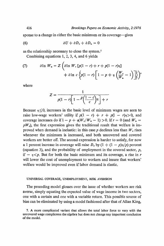
as the relationship necessary to close the system.7 Combining equations 1, 2, 3, 4, and 6 yields

(7) aln W = Z (ln Wc [p(l-r) + r + p(l-r)]

+ aln c {(l -r) [1- P + v (WC-)}

where

1

p(l -r)l I -p(lc)7 ] + r

Because n <0, increases in the basic level of minimum wages are seen to raise low-wage workers' utility if p(l - r) + r + p(l - r) > 0, and coverage increases do if 1 - p + n(Wc/W, - 1) >0. If r = 0 (and W, = pWc), the first expression gives the traditional result that welfare is improved when demand is inelastic: in this case p declines less than Wc rises whenever the minimum is increased, and both uncovered and covered workers are better off. The second expression is harder to satisfy, for now a 1 percent increase in coverage will raise DC by (1 + (1 - p)r/p) percent (equation 3), and the probability of employment in the covered sector, p, if - n <p. But for both the basic minimum and its coverage, a rise in r will lower the cost of unemployment to workers and insure that workers' welfare would be improved even if labor demand is elastic.

UNIVERSAL COVERAGE, UNEMPLOYMENT, RISK AVERSION

The preceding model glosses over the issue of whether workers are risk averse, simply equating the expected value of wage income in two sectors, one with a certain and one with a variable return. This possible source of bias can be eliminated by using a model fashioned after that of Allan King,

7. A more complicated variant that allows the total labor force to vary with the uncovered wage complicates the algebra but does not change any important conclusion of the model.


which assumes no uncovered sector but tries to evaluate the utility of changes in minimum-wage legislation directly.8

Assume that every year low-wage workers make m independent random drawings from the job lottery to determine if they are employed in the covered sector or unemployed. Expected wage income is then

(8) E(Y) = Wc[p + (1-p)r],

with a standard deviation of

(9) o(Y) = 0c(l - r) p(1 -p)/rM

for m market or job-recontracting periods. Since there are no uncovered wages to influence labor supply, a(D, + U)-aL = 0 and

(10) a aDO

0(1 - ) = DC

= _ ,p,

alnp = aD . D0c = ln D, = naln Wc, L *L

aln (1 - p) = -aln D, (1 P) =- P p) aln W,.

S. C. Tsiang has shown that a sufficient condition for a welfare gain when both the mean and standard deviation are increasing is that OF>a.9 Dividing each side by o-E and transforming yields this condition as

(11) dlnE> E alno- El

or, after substitution from equations 8, 9, and 10,

(12) 1~ + p(l - r) N

(12) 1+ ( p(1-r)+ r > (1 -r) Vp(l-p)/rm

2(1 ) p(l -r)+r 1

+ nt

2(1 - P) an expression similar to that of King except that it again incorporates the partial protection provided by transfer payments against losses of wage

8. Allan G. King, "Minimum Wages and the Secondary Labor Market," Southern Economic Journal, vol. 41 (October 1974), pp. 215-19.

9. S. C. Tsiang, "The Rationale of the Mean-Standard Deviation Analysis, Skewness Preference, and the Demand for Money," American Econiomic Review, vol. 62 (June 1972), pp. 354-71.


income of unemployed workers. But whereas expression 7 overstates the welfare gains of a legislative increase in the minimum wage by ignoring risk aversion, expression 12 understates these gains because it is based on the improvement required to guarantee that workers will be better off, and hence would be unwarrantedly conservative for all but the most risk-averse workers."0

Differentiation of this expression with respect to m shows that for any p, a greater number of market periods shortens the average spell of unemployment, reduces the variance of wage income, and raises the "break- even" elasticity at which the most risk-averse workers are indifferent between raising and not raising the minimum wage. If the actual elasticity is higher than the break-even value, the most risk-averse workers are still opposed to increases in the minimum; otherwise, they are still in favor. As before, this break-even elasticity is also increased by an unemployment compensation system or by taking account of the value of increased leisure time, both of which lower the expected income loss from a spell of unemployment.

EVALUATION

This analysis can be summarized by inserting reasonable values for p, m, and r into 7 and 12 to find the values of X that will make workers indifferent about wage increases. The calculations are performed both for the risk-neutrality model (which overstates the absolute value of break-even elasticity by ignoring risk aversion) and for the risk-aversion model (which understates it) so as to bracket the true elasticity. The calculations are also performed separately for teenagers, adult males, and adult females.

Inferences about employment rates and the number of market periods can be made from the U.S. Manpower Administration's National Longi- tudinal Survey of selected groups in the labor force. Robert Frank and Richard Freeman have recently used the retrospective work history question on this survey to compute the mean lengths of spells of employment and unemployment for various groups." From these mean spells employ-

10. An indication of just how conservative this standard is comes from the fact that it would not value an equal-probability (0, $4) bet (with E(Y) = $2, ( Y) = $2) any more highly than an equal-probability (0, $2) bet (with E( Y) = $1, ( Y) = $1).

11. See Robert H. Frank and Richard T. Freeman, "Distribution of the Unemploy- ment Burden: Are the Last Hired Fired First?" (Cornell University, 1976; processed).


ment rates can be derived for the same groups by dividing the average length of time a worker is employed by the average time he is either employed or unemployed. Since the Frank-Freeman estimate of the employment rate, if, is for the entire labor force, whether or not covered by the minimum wage, I have computed employment probabilities within the covered sector (p) by inserting estimates of c into the expressionff = pc + (1 - c), where employment rates are assumed to be one in the uncovered sector."2 The length of a market period is then equated to the length of an average spell of unemployment, under the assumption that workers recontract their job situation at these intervals and do not recontract for a new spell of unemployment. The resultant number of market periods per year (m) is thus 8.0 for teenagers (average unemployment spell of 6.5 weeks), 5.8 for adult males (9 weeks), and 4.0 for adult females (13 weeks).

The replacement rate (r) is derived by finding, for workers who are eligible for unemployment insurance and other transfer benefits, the ratio of after-tax transfer income during a spell of unemployment to after-tax wage income. These ratios range from 0.6 to 0.75 for the three groups, somewhat higher than the supposed 0.5 rate for unemployment insurance because transfers are not taxable and because some workers also get food stamps and public assistance. No value is placed on leisure time, which may mean that the break-even elasticities are understated. Values for r for the entire low-wage population are then derived by multiplying the replacement rates for eligible workers by the probability that workers will be eligible for transfers (0.15 for teenagers, 0.5 for low-wage adult males, and 0.3 for low-wage adult females) on the basis of work that I have previously done."3

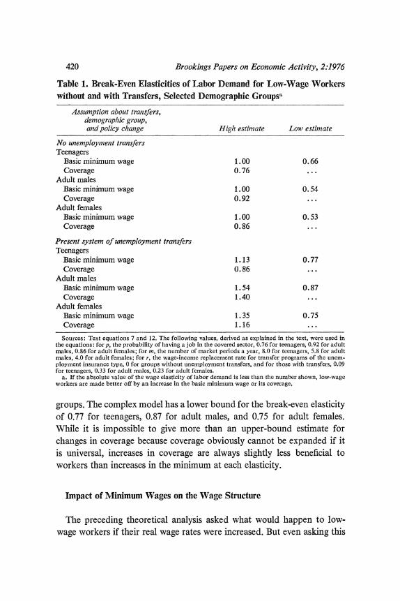
The break-even elasticities using these assumptions are given in table 1. A comparison of the top and the bottom panels shows that unemployment insurance programs and the like always raise the elasticities, for reasons described above, while adjustment for the variance in wage income in the risk-aversion model always lowers them. On balance, these deviations approximately cancel each other, as the high and low estimates bracket the simple-minded value of 1 (in response to wage increases) for all three

12. I did sensitivity checks on this assumption by assuming that the uncovered employment rate is the same as the covered rate, and hence that if = p. The results are little changed.

13. "The Distributional Effects of Higher Unemployment," BPEA, 2:1974, pp. 293-336.


Table 1. Break-Even Elasticities of Labor Demand for Low-Wage Workers without and with Transfers, Selected Demographic Groupsa

Assumption about transfers, demographic group, and policy change High estimate Low estimate

No unemployment transfers Teenagers

Basic minimum wage 1.00 0.66 Coverage 0.76 ...

Adult males Basic minimum wage 1.00 0.54 Coverage 0.92 ...

Adult females Basic minimum wage 1.00 0.53 Coverage 0.86 ...

Present system of unemployment transfers Teenagers

Basic minimum wage 1.13 0.77 Coverage 0.86 ...

Adult males Basic minimum wage 1.54 0.87 Coverage 1.40 ...

Adult females Basic minimum wage 1.35 0.75 Coverage 1.16 ...

Sources: Text equations 7 and 12. The following values, derived as explained in the text, were used in the equations: for p, the probability of having a job in the covered sector, 0.76 for teenagers, 0.92 for adult males, 0.86 for adult females; for m, the number of market periods a year, 8.0 for teenagers, 5.8 for adult males, 4.0 for adult females; for r, the wage-income replacement rate for tratnsfer programs of the unemployment insurance type, 0 for groups without unemployment transfers, and for those with transfers, 0.09 for teenagers, 0.33 for adult males, 0.23 for adult females.

a. If the absolute value of the wage elasticity of labor demand is less than the number shown, low-wage workers are made better off by an increase in the basic minimum wage or its coverage.

groups. The complex model has a lower bound for the break-even elasticity of 0.77 for teenagers, 0.87 for adult males, and 0.75 for adult females. While it is impossible to give more than an upper-bound estimate for changes in coverage because coverage obviously cannot be expanded if it is universal, increases in coverage are always slightly less beneficial to workers than increases in the minimum at each elasticity.

Impact of Minimum Wages on the Wage Structure

The preceding theoretical analysis asked what would happen to low- wage workers if their real wage rates were increased. But even asking this


question requires assessing the degree to which the government can alter the wage distribution in the first place. There are several reasons why the government's influence on relative wages may be limited. On one side, spillovers to the uncovered sector or even noncompliance with the law might prevent low wages from rising much as the minimum is increased. On the other, changes in the minimum may force up other wages so much- in emulation of minimum increases by higher-wage unions or from Wal- rasian demand and supply adjustments-that rather than alter the wage structure they simply raise overall wage and price levels enough to nullify the increase in the minimum. In this section I try to deal with both matters from a more empirical standpoint.

NONCOMPLIANCE AND PARTIAL COVERAGE

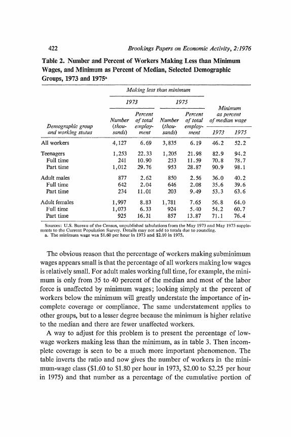
The first thing turned up by any examination of data is that the wages of a large number of workers are below the legislative minimum. This point is illustrated in tables 2 through 4, which are based on U.S. Bureau of the Census tabulations of answers to the supplemental questions asked each May in conjunction with the regular monthly Current Population Survey. This information on usual hourly wage rates is available beginning only in 1973; and since the 1974 survey week started just twelve days after the minimum wage was increased (when many workers might not yet have realized it) the tables give information only for 1973 and 1975.1'

The first line of table 2 gives the simple percentages of the work force receiving less than the minimum wage of $1.60 per hour in 1973 and $2.10 per hour in 1975. In both years this value is only 2 percent for adult males working full time; it reaches a peak of about 30 percent for teenagers on part-time work. Overall, from 6 to 7 percent of the labor force appears to work at subminimum wages. Although this seems low enough to be trivial, such an impression would be far from the truth.

14. U.S. Bureau of the Census, unpublished tabulations from the May 1973 and May 1975 supplements to the Current Population Survey. The CPS tabulates both actual and usual hourly earnings. The concept used here, usual hourly earnings, is either taken from or consistent with answers to questions on usual weekly earnings and usual weekly hours, and covers the entire labor force except for nonrespondents. In 1974, answers to this set of questions were given by about 61.2 million workers (after the sampling weights were applied). For some purposes, it would be better to confine the data on hourly wage rates to people paid that way; that series is called actual hourly earnings and is available for 32.1 million workers in 1974.


Table 2. Number and Percent of Workers Making Less than Minimum Wages, and Minimum as Percent of Median, Selected Demographic Groups, 1973 and 1975a

Making less than minimum

1973 1975 Minimum

Percenit Percent as percent Nuimber of total Number of total of median wage

Demographic group (thou- einploy- (thou- employ- and working status sands) ment sands) inent 1973 1975

All workers 4,127 6.69 3,835 6.19 46.2 52.2

Teenagers 1,253 22.33 1,205 21.98 82.9 94.2 Full time 241 10.90 253 11.59 70.8 78.7 Part time 1,012 29.76 953 28.87 90.9 98.1

Adult males 877 2.62 850 2.56 36.0 40.2 Full time 642 2.04 646 2.08 35.6 39.6 Part time 234 11.01 203 9.49 53.3 63.6

Adult females 1,997 8.83 1,781 7.65 56.8 64.0 Full time 1,073 6.33 924 5.40 54.2 60.7 Part time 925 16.31 857 13.87 71.1 76.4

Sources: U.S. Bureau of the Census, unpublished tabulations from the May 1973 and May 1975 supplements to the Current Population Survey. Details may not add to totals due to roundinlg.

a. The minimum wage was $1.60 per hour in 1973 and $2.10 in 1975.

The obvious reason that the percentage of workers making subminimum wages appears small is that the percentage of all workers making low wages is relatively small. For adult males working full time, for example, the minimum is only from 35 to 40 percent of the median and most of the labor force is unaffected by minimum wages; looking simply at the percent of workers below the minimum will greatly understate the importance of incomplete coverage or compliance. The same understatement applies to other groups, but to a lesser degree because the minimum is higher relative to the median and there are fewer unaffected workers.

A way to adjust for this problem is to present the percentage of low- wage workers making less than the minimum, as in table 3. Then incomplete coverage is seen to be a much more important phenomenon. The table inverts the ratio and now gives the number of workers in the minimum-wage class ($1.60 to $1.80 per hour in 1973, $2.00 to $2.25 per hour in 1975) and that number as a percentage of the cumulative portion of


Table 3. Number of Workers in Minimum-Wage Class, and Workers in the Class as a Percent of Cumulative Frequency up through That Class, Selected Demographic Groups, 1973 and 1975a

1973 1975

Percent Percent Number of cumu- Number of cumu-

Demizographic grouip (thou- lative (thou- lative and workinig status sands) frequency sands) frequency

All workers 3,045 42.5 5,444 58.7

Teenagers 1,071 46.1 1,637 57.6 Full time 210 46.6 422 62.5 Part time 861 46.0 1,215 56.0

Adult males 488 35.8 1,059 55.5 Full time 341 34.7 703 52.1 Part time 147 38.6 356 63.7

Adult females 1,486 42.7 2,748 60.7 Ful time 918 46.1 1,488 61.7 Part time 568 38.0 1,260 59.5

Source: Same as table 2. a. Minimum-wage class was $1.60-$1.80 in 1973 and $2.00-$2.25 in 1975.

workers in all wage classes up to the minimum class (all up to $1.80 per hour in 1973 and all up to $2.25 per hour in 1975). All high-wage workers who would not be affected by the minimum are kept out of the comparison.

The remarkable revelation of table 3 is that, when viewed relative to low- wage workers, coverage or compliance is both surprisingly narrow and surprisingly constant across groups. If answers to the survey can be believed, only 43 percent of all low-wage workers were in the minimum-wage class in 1973, and the ratio for any group was never below 35 or above 47. Even these percentages may tend to overstate the genuine coverage or compliance because they record in the numerator many workers who would have gotten the minimum in any case and thus were not truly part of the coverage or compliance universe. This fact could explain the paradoxical finding that the percentage is lower for adult males on full time, of whom there would be fewer such workers. More strikingly, as the minimum is increased relative to the median, as it was in 1975, the number of such "free riders" might be expected to rise, and hence all percentages to rise as they


Table 4. Number of Workers in Minimum-Wage Class and Workers in the Class as a Percent of Cumulative Frequency up through That Class, Selected Industries, 1973 and 1975a

1973 1975

Percent Percent Number of cumu- Number of cumu- (thou- lative (thou- lative

Industry and working statusb sands) frequency sands) frequency

Full coverage

Mining and manufacturing 430 63.6 672 77.9 Full time 356 68.9 532 80.6 Part time 74 46.5 139 68.8

Transportation 49 41.5 89 54.9 Full time 28 38.9 52 54.7 Part time 22 46.8 37 56.1

Construction 46 47.4 97 64.2 Full time 33 50.0 64 64.0 Part time 12 41.4 33 62.3

Expanded coverage

Retail trade 1,192 45.7 2,121 59.4 Full time 453 44.7 856 60.0 Part time 739 46.3 1,265 58.9

Public administration 50 41.7 87 63.5 Full time 23 43.4 50 65.8 Part time 27 40.3 37 60.7

Private household services 80 9.0 266 29.7 Full time 22 7.2 26 11.7 Part time 58 10.0 240 35.6

Source: Same as table 2. Details may not add to totals due to rounding. a. Minimum-wage class was $1.60-$1.80 in 1973 and $2.00-$2.25 in 1975. b. The percentage of employment covered throughout was about 97 for mining and manufacturing,

98 for transportation, and 99 for construction; for retail trade, about 64 in 1973, 69 in 1975; for public administration, about 41 in 1973 and 100 in 1975; for household services, zero in 1973 and about 73 in 1975. See Peyton Elder, "The 1974 Amendments to the Federal Minimum Wage Law," Monthly Labor Review, vol. 97 (July 1974), p. 35.

in fact do."5 Thus a proper interpretation of the information in table 3 is that in 1973 the minimum wage was no more than 43 percent effective and

15. A less elegant, but possibly better, reason for the rise in this ratio is that in 1975 the lower boundary of the minimum-wage class was $0.10 below the actual minimum wage. A very slight underestimate of gross wages by a large number of workers could also account for the rise in the compliance rates. But even this estimate leaves the proportion of covered workers making the minimum well below one.


in 1975 it was no more than 59 percent effective. Whatever the case, the minimum-wage law is far from universally effective-actually raising the wages of about half of all low-wage workers.

Two possible reasons could explain why so many workers make subminimum wages: incomplete coverage, a phenomenon already discussed from a theoretical standpoint, and simple failure to comply with the law. Orley Ashenfelter and Robert Smith have dealt with the latter problem, arguing that at least for employers accused for the first time and not con- victed of falsifying data, penalties for noncompliance are probably lower than the cost of paying the minimum wage, an anomaly that certainly plagues compliance officers.'6 If noncompliance is the basic problem, coverage ratios should differ little between legally covered and noncovered industries (with the same underlying wage distribution). If incomplete coverage is the problem, there should be a difference.

This matter is investigated with the aid of table 4, which gives the same coverage statistics for three industries that were virtually completely covered in both 1973 and 1975 and three in which coverage expanded significantly. For the fully covered industries-mining and manufacturing, transportation, and construction-compliance ratios are again low in both years but do improve between 1973 and 1975, presumably again because of the larger number of free riders or because of the reduction in the bottom bracket of the minimum-wage class in this categorization below the actual minimum wage.'7 To be sure, the fact that the ratio in manufacturing-a very large industry with high wages and hence proportionately fewer free riders-is above the national average indicates that the minimum wage must be having some impact on the wage distribution. But this impact is a good deal less than might be imagined. For one thing, compliance rates in fully covered industries like transportation and construction are not very different from those in industries that are partially uncovered like

16. Orley Ashenfelter and Robert Smith, "Compliance with the Minimum Wage Law (Progress Report)," Technical Analysis Paper 19A (U.S. Department of Labor, Office of the Assistant Secretary for Policy, Evaluation and Research, April 1974; processed).

17. Ashenfelter and Smith give compliance ratios based on actual hourly earnings in fully covered industries in 1973 that are slightly above that given in the table for manufacturing. They do not report estimates for years other than 1973 or separately for partially covered industries.

Just before this paper was typeset, Fred Siskind showed me compliance-ratio estimates from the newly available data for 1976. In line with my free-rider prediction, most ratios have slipped right back to their 1973 levels.


retail trade.'8 Only in the remaining incompletely covered industry, private household services, is the percent of noncoverage appreciably below the national average, and even here it did not rise much more than in the other industries despite the extension of coverage to most of that industry by the 1974 minimum-wage amendments. Again, the message is that a very high percentage of low-wage workers make subminimum wages, and now it can be added that industrial variations in the percentage of low-wage workers covered seem to be only modestly influenced by whether or not the industry is covered by the legislation.

What this surprising degree of noncoverage or noncompliance implies is another question, one that can only be speculated on here. It is always possible that people simply do not know what they get paid, though Ashen- felter and Smith have reproduced essentially the same results from establishment data, which seems to rule out that possibility.'9 Bearing out those who favor more government intervention, it could mean widespread ignoring of the minimum-wage law and point to the need for bigger compliance staffs and more severe penalties for violations. Or, for those who favor less government intervention, it could emphasize the inherent difficulty the government has in enforcing even a relatively straightforward policy like the minimum wage. Employees may simply be agreeing to take subminimum wages out of fear of losing their jobs, laws to the contrary notwithstanding. In any case, the minimum is simply less of a force for good or evil than people have believed.

IMPACT ON HIGHER WAGES

With this demonstration that minimum-wage laws have much less impact on low wages than might be expected, the next question is whether the minimum is attenuated even further by consequent changes in wage rates above the minimum and then prices. This could happen either because

18. Even though the compliance ratios are similar for fully covered transportation and construction and partially covered retail trade, the proportion of low-wage workers in the first two industries is so much lower than that in the last that ambiguities re- garding the definition of the industry or its coverage are more likely to distort the comparison.

19. Ashenfelter and Smith, "Compliance." For other evidence that the CPS household survey wage data agree fairly well with establishment data, see Paul 0. Flaim, "Earnings Data from the CPS: New Collection Efforts and Some Findings" (paper presented at the 1976 annual meeting of the American Statistical Association; processed).


unions and other groups above the minimum emulate the wage increases stipulated in the law, or through a more traditional demand-supply route following substitution by employers away from low-wage labor toward skilled labor.

The matter can be crudely investigated by seeing whether any extraor- dinary increases occur in overall wage levels subsequent to the increase in the minimum, and then comparing such changes with the implied direct impact of the change in the minimum. If the direct impact can account for all of the overall incremental changes, other wages are not emulating the minimum increase; if not, there is some emulation.

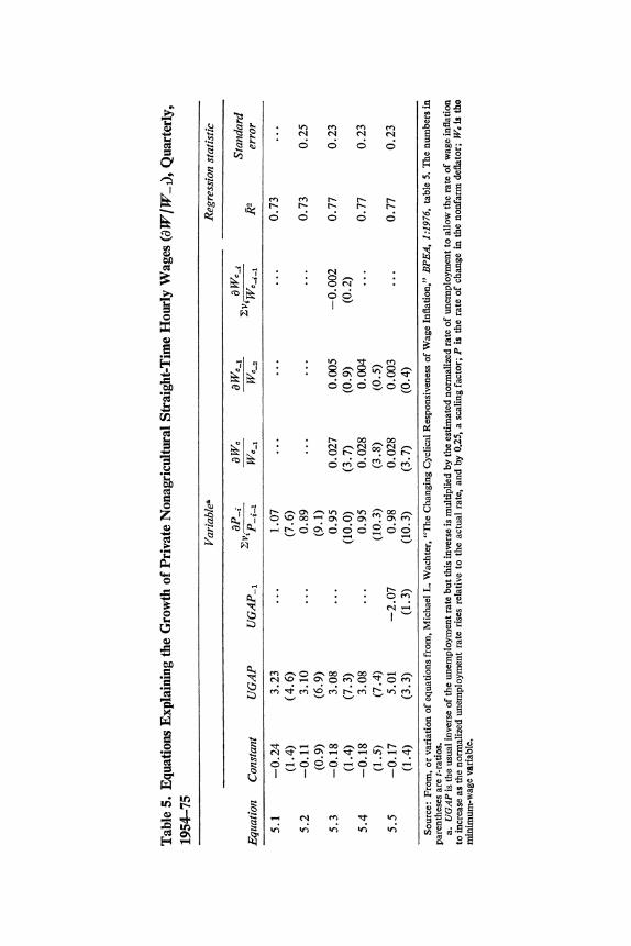
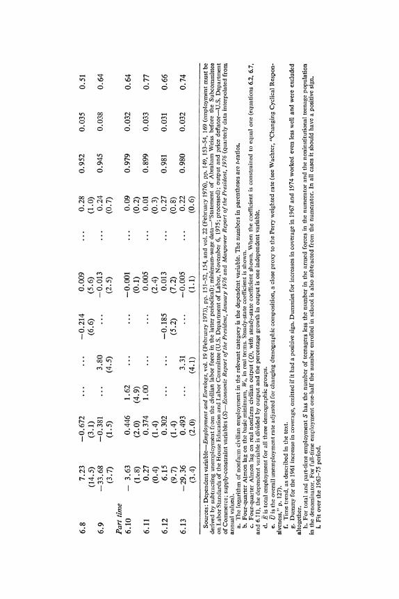
The first step is relatively straightforward: to see whether changes in the minimum can help explain changes in overall wage rates. Table 5 presents some Phillips-curve equations of the sort recently estimated by Michael Wachter.20 The first equation is the one given in Wachter's paper (his equation 5.3), and the second is that with his Almon lag on prices shortened from twenty-four to seventeen quarters and made into a polynomial of slightly lower degree. In all respects, this equation is indistinguishable from Wachter's own. The third equation adds a four-quarter Almon lag on the basic minimum wage and finds the impact coefficient to be 0.027 with a t-ratio of 3.7, the second-period coefficient to be barely positive and insignificant, and all coefficients lagged more than one period to be very slightly negative and extremely insignificant. Attempts to impose a longer lag on the minimum-wage variable are not shown here but had similar outcomes. The fourth and fifth equations then drop the Almon lag on the basic minimum and simply include the current value and a one-period lag -once with UGAP lagged, once without-with essentially similar results.

Those who are motivated by the quest to reduce the noise in the Phillips curve should note that minimum wages do work as a variable: the impact coefficient is consistently around 0.028, the t-ratio is nearly 4, the standard error is cut by 10 percent, and the R2 is raised by 5 percent. What works, however, is the current-period impact: it seems impossible to find significant follow-on effects of lagged minimum wages. This suggests that any substantial emulation effects are not long delayed, which seems plausible because increases in the minimum are well-advertised in advance. To exanline the matter further, I ask whether an impact coeff-cient of 0.028,

20. Michael L. Wachter, "The Changing Cyclical Responsiveness of Wage Infla- tion," BPEA, 1:1976, table 5.

>~~ U2 to 4-.2 .0

Ps .:2~ 6666 ocq

-~~~~~~~~~ . ~ ~ ~ ~ ~ ~ ~ ~ ~ ~ ~ ~ .

0~~~~~~~~~~~~~~~~~~~~~~~~~~~~0

.P.4~~~~~~~~~~~~~~~~~~~~~~~~~4 0

m 0 a0

4-i~~~~~~~~~~~~~~~~~~~~~~~~~~~~~~~~) 2 AC

m C) OC) OC) ~ *)3 C,

0 ..

4)4 0~~~~~~~~~~~~~~~~~~~~~~~~~~~~~~~~~~~~~~~C 1

'7


or a long-run coefficient of 0.032, is more than would be accounted for simply by the direct impact of increases in the minimum.

Again the CPS wage distributions provide the relevant information. On May 1, 1974, the minimum was increased by 25 percent from $1.60 to $2.00-a change that would be estimated to raise the overall wage bill by (0.032)(25) = 0.8 percent, according to the equations in table 5. After adjustment for incomplete coverage and noncompliance and for 1974 underreporting, about half of this impact could be directly accounted for by the change in the minimum, with the remainder due to emulation. (The calculations are given in footnote 21.) There is, in other words, a "multiplier" of 2 for the impact of minimum wages on the overall wage bill.

This multiplier is high or low, depending upon the implications one is examining. On one side, even though the multiplier is 2, the minimum wage still has a substantial effect on the relative wage structure. The reason is that changes in the minimum wage affect the bottom tail of the wage distribution, where their weight in terms of both number of workers and dollars of wage bill is very small. Hence very large changes in low wages have the same effect on the overall wage bill as do much smaller percentage increases in the fatter part of the wage distribution. In the 1973-74 case, for example, all workers covered prior to the 1967 amendments who were previously making $1.60 per hour received 25 percent increases, and even if all of the indirect effect had been confined exclusively to those originally in the $2.00-$2.50 bracket, it would have amounted to only a 3.5 percent increase for those workers.2' The multiplier is high, but so is the impact on relative wages in the bottom part of the wage distribution. In line with the preceding theory, the multiplier of 2 could also imply that uncovered wages are rising and uncovered workers better off.

But this reasoning suggests that minimum wages could, if they get very high, have important effects on overall wages and prices. Historically, minimum wages have not had such effects precisely because the minimum has been kept in the low part of the wage distribution, affecting a large share of neither workers nor wage income, and getting a relatively low coefficient

21. These calculations were done as follows: Between 1973 and 1974, the percent of workers in the $1.60-$1.80 class fell by 2.56 points and the percent in the $1.80- $2.00 class fell by 1.25 points. If the former group received a $0.35 increase, the latter a $0.10 increase, and all other workers no direct increase, the implied change in overall wage income would be 0.25 percent, or 0.4 percent after adjusting for 1974 underreporting. Computing the dollar effect of this change and spreading it over the $2.00- $2.50 class gives a 3.5 percent increase for those workers.


in a time-series regression. Had the minimum not been kept so low, its impact on overall wages and prices would grow much more than proportionately. In 1974, for example, the 25 percent increase in the minimum to $2.00, 54 percent of the median wage, was seen to raise the wage bill directly by only 0.4 percent and indirectly by another 0.4 percent. Had the minimum been increased to $3.00, 81 percent of the median wage, the direct impact on the wage bill alone would have been more like 6.0 percent, even with a generous allowance for noncoverage and noncompliance. Whether the indirect effect would have again doubled the direct effect is highly uncertain; but even if it did not, a change in overall wage, and presumably price, levels of this magnitude presents an important drawback to such a large change in the minimum.22 If nothing else, the adaptive-expectations terms in the wage-setting equations estimated above are high enough that this supposed one-shot change in the overall price level would be converted into a nearly permanent one-shot change in the rate of price inflation.23

Impact on Employment

The next question concerns the employment impact of changes in the wage structure. In terms of the preceding theory, is the wage elasticity of demand for low-skilled labor (-q) small enough that affected workers are better off as a result of an increase in the minimum wage?

The literature on this topic, for employment in general and for the minimum wage in particular, is so voluminous that there are already a fair

22. The more the hypothetical change deviates from the actual change, the more difficult it becomes to determine exactly what would happen. These calculations first of all assume no employment effects, a matter taken up in the next section. They also assume that noncompliance ratios in the $2.00-$3.00 range are similar to those now experienced in the below-$2.00 range. The whole issue, of course, suggests that the coefficient of the minimum is nonlinear, depending on where in the wage distribution the minimum is. In principle, I could have experimented with forms to test this non- linearity, but in practice the minimum has remained in such a narrow band relative to the median that I did not bother.

23. If the steady-state coefficient of the lagged price-increase terms in the Phillips- curve equations of table 5 equals one, such would be the case. As can be seen, they are close enough to provide only cold comfort to those wishing to raise the minimum substantially. On the other hand, the fact that prices rise at a steady rate need not imply that the real minimum would fall to its former level: What is to prevent subsequent changes in the minimum from keeping up with the inflation the first change may have started and subsequent changes may have abetted? As usual, inflation is a giant merry- go-round.


number of surveys of it. Daniel Hamermesh has recently surveyed fifteen papers that attempt to estimate how overall employment demand depends on the relative price of capital and labor, and finds elasticities of substitution ranging from a low value of 0.15 to a high value of 1.0, with a long- run median estimate of close to 0.75.24 Although the two distributions overlap somewhat, these elasticities are generally below the relevant break- even elasticities in table 1, suggesting that low-wage workers benefit from an increase in the minimum wage.

Studies that have tried to estimate the effect of minimum wages more directly have until now focused almost exclusively on teenagers. These studies most commonly estimate time-series regressions of the form

(13) En E

In U, InCWc ) N=

where E is usually teenage employment, N is the teenage population, U is the adult unemployment rate, W is average wages in the private sector, and Z might be a variety of other variables. The coefficient of cW0/W can be interpreted as the minimum-wage elasticity of demand for the whole group of teenagers, and it usually comes out somewhere between -0.05 and -0.25.25

24. Daniel S. Hamermesh, "Econometric Studies of Labor Demand and their Application to Policy Analysis," Journal of Humna Resources, forthcoming, table 3. He presents o(1 - s), where s is labor's share of output and a- is the elasticity of substitution with respect to real wages with the real price of capital held constant. The elasticity is multiplied by (1 - s) because Hamermesh makes price levels endogenous and assumes that an increase of x percent in the money wage causes an sx percent increase in prices, and raises real wages by only (1 - s)x percent. For my purposes the passthrough to product prices will normally be very small, so I simply used the estimates of af summarized in the paper.

For those who take R. G. D. Allen's work as their bible on this matter, the case I am referring to can be found in Allen's Mathematical Ancalysis for Economists (Mac- millan, 1938), p. 373, the footnote in which his ap/apa = 0.

25. See the Goldfarb summary, "Policy Content," p. 266. Recent studies not included in Goldfarb's survey article have estimated the following employment elasticities for teenagers: Welch, "Minimum Wage Legislation," as corrected by Frederic B. Siskind, "Minimum Wage Legislation in the United States: Comment," Technical Analysis Paper 4A (U.S. Department of Labor, Office of the Assistant Secretary for Policy, Evaluation and Research, May 1976; processed), p. 1-2, -0.05; Mincer, "Unemploy- ment Effects," p. S104, -0.25; Ragan, "Minimum Wage Legislation," pp. 35-36, -0.20; and Terence F. Kelly, "Youth Employment Opportunities and the Minimum Wage: An Econometric Model of Occupational Choice," Working Paper 3608-1 (Urban Institute, n.d.; processed), p. 23, -0.18.

In "The Minimum Wage, Teenage Unemployment, and the Business Cycle," Westernt


Applying any of these results to the analysis of the break-even elasticity offered above poses several problems. The most glaring is that even for teenagers, the dependent variable includes a large number of workers not working at low wages, which would dilute the estimated elasticity for two reasons. The first is that many workers who get better than low wages would be simply unaffected by changes in the minimum, and some adjustment in the coefficient must be made to determine its meaning solely for the low-wage workers in the sample. But even that adjustment may not be enough. The second reason is that some substitution presumably may occur infavor of the high-wage workers in the sample, at least if minimum wages do not immediately force up these higher wages. Hence simply weighting up the estimated time-series elasticity by the inverse of the proportion of low-wage teenagers will yield an underestimate of the actual elasticity. But for what it is worth, weighting the standard estimates does lead to an elasticity for low-wage teenagers of about 0.4 (0.17/0.45, where 0.17 is the average elasticity of the studies cited in footnote 25, and 0.45 is the average proportion of low-wage teenagers during the historical period), still below the lower bound of the break-even elasticity for teenagers. A more direct cross-section estimate by Arnold Katz, which is not diluted by the inclusion of unaffected workers, comes up with an elasticity for teenagers of 0.6, still below the break-even level but closer.26

A second problem, or really gap, in the previous empirical work is that it focuses almost entirely on teenagers, who now constitute only about 30 percent of all low-wage workers (see table 3). Adult males (20 percent) and females (50 percent) are given almost no attention. The reason for this gap is easy to understand, for even though most low-wage workers are adults, the dilution problem is much greater for adults. Philip Cotterill has made one of the few attempts to deal with the problem, by excluding high-wage workers in a cross-section analysis for adults, and he finds elasticities that average 0.76, now just about equal to the lower bound of the break-even elasticity.27

Economic Journal, vol. 10 (December 1972), pp. 414-27, Michael C. Lovell has analyzed time-series studies that use teenage unemployment as the dependent variable and has also generally found that minimum wages do not significantly raise unemployment.

26. Arnold Katz, "Teenage Employment Effects of State Minimum Wages," Journal of Human Resources, vol. 8 (Spring 1973), pp. 250-56.

27. Philip Cotterill, "The Elasticity of Demand for Low-Wage Labor," Southernt Economic Journal, vol. 41 (January 1975), pp. 520-25.


There are other important problems that, as far as I know, nobody has dealt with. One is that when total employment is the dependent variable, the coverage variable c should not be combined with the basic minimum in the way described in equation 13. The discussion above of equation 5 indicates that this specification is inappropriate and may bias Xj downward. Another problem is that in all existing studies of employment or unemployment, whether based on time-series or cross-section data, the dependent variable is numbers of workers. But what if the minimum wage closes or opens up more full- or part-time employment? In terms of the above theory it might be more appropriate to take full-time employment as employment, and to consider part-time employment-with involuntarily lower hours, lower wages, and presumably more jobs that are characteristic of the secondary labor market-as essentially no different from unemployment. It would then be better to estimate separate regressions explaining full- and part-time employment for the three demographic groups.

I have tried to estimate time-series regressions that deal with each of these complications. The regressions are patterned after the inverted CES (constant elasticity of substitution) production-function model of labor demand, which makes employment a positive function of output and a negative function of real wages. Applied to minimum wages, this pattern leads to regressions of the form (14) In Ei = g [L(ln Q), L (In Wc/P), t, D,,,, In S],

where

Ei= civilian nonfarm employment of 16-19-year-olds, adult males, and adult females, with each group broken down by full- or part- time status28

Q = civilian nonfarm real output (that is, total output excluding farm and military value added)

P the price deflator for civilian nonfarm real output 28. This breakdown has been published only since 1963. In fact, it is available only

for total civilian employment with no disaggregation into agricultural and nonagricultural sectors. Thus, the dependent variable in the part-time employment regressions is total part-time, including a small amount of agricultural part-time employment. The full- time nonagricultural employment variable is formed by subtracting that part-time series from total nonfarm employment, thus understating full-time nonagricultural employment by the amount of part-time agricultural employment. The series appears in Em- ployment and Earnings, vol. 19 (February 1973), p. 154, and vol. 22 (February 1976), pp. 149, 169. Employment must be derived by subtracting unemployment from the civilian labor force in the latter periodical.


=C = the basic minimum wage t = a time trend that serves as a proxy for productivity and trend

changes in employment or its demographic composition

D,01,=a dummy for changes in coverage, as described in more detail below

S - a supply-constraint variable, described in detail below.

The variable L indicates a four- or six-quarter Almon distributed lag, whichever length appeared to fit best. This may seem a short lag for factor- substitution analysis; but again, since changes in the minimum are advertised in advance, it is presumably consistent with a slower and more reasonable pace of factor substitution. The equations for total employment were usually estimated with quarterly time series for the full 1948-75 period, but those for full- and part-time employment could be estimated only for the period starting in 1963, the first year for which this breakdown was available.

Since there were three legislative coverage changes in the period (1961, 1967, and 1974), in each case extending the minimum to a different part of the wage distribution and no doubt complied with imperfectly, I have simply used dummy variables, D,,,, for the three changes. Unfortunately, all had very small, usually positive, coefficients and I left them in the final specification only if they did have the anticipated negative effect on total employment. For teenagers and adult females I also included supply- constraint variables: for the first, all teenagers less those in the military as a proportion of the total noninstitutional population of teenagers; for the second, the number of children aged 1 to 5 as a proportion of the total noninstitutional population of adult females. The first should have a positive effect on teenage employment and the second should have a negative effect on adult female employment, reflecting child-raising responsibilities.29

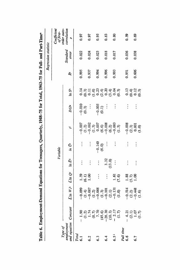
The equations are given in tables 6, 7, and 8 for teenagers, adult males, and adult females, respectively. All use an autoregressive transformation; the computed value of p is shown in the last column. Equation 6.1 explains total employment with the basic form of equation 14. Since the coefficients of output vary widely-as expected, being highly sensitive to cyclical changes in output for teenagers but not for adults-equation 6.2 is designed

29. The teenage supply variable also deducted half of those enrolled in school from the numerator when it was used to explain full-time employment. In principle, each supply-constraint variable should also be in the other equations (if there are more employed teenagers, adult employment would be lower), but this seemed to be going too far.

Edward AM. Gramlich 435

to determine the sensitivity of the coefficient on the minimum wage to changes in the output coefficient by constraining the latter to equal unity (as it would in a production function based on constant returns to scale). Equation 6.3 then splits the trend and cycle in output differently by simply using time and a close proxy to the Perry weighted unemployment rate, U, as independent variables. Equation 6.4 focuses more directly on the composition of unemployment by using total employment (teenagers plus adults), E, as the independent variable along with time. Equation 6.5 reestimates equation 6.1 over the shorter period used in the full-time- part-time breakdowns. Equations 6.6 through 6.9 give the four basic forms for full-time employment and equations 6.10 through 6.13 give them for part-time employment. The equations in tables 7 and 8 have parallel structures.

The important coefficients in these tables are those for minimum wages, and they are generally affected little by changes in the specification of the independent variables, though greatly by the choice of the dependent variable. Information on these elasticities is summarized in table 9. For each group the first row of the panel reproduces the low-wage break-even brackets given in table 1. The next row converts these break-even elasticities into the implied elasticity for total employment and also gives, in the last column, the elasticity estimated from the total employment equation. The reduced-form solution of text equation 5-found by inserting text equation 7-indicates that the coefficient of In W, is approximately 'q if the sample is confined to low-wage workers. Hence, to make a proper comparison between the estimated elasticities and the break-even values, I have multiplied the break-even values by F(W,), the proportion of low-wage workers in the dependent variable during the period 1973-75, and then compared this band with the average of the minimum-wage elasticities for total employment in equations 1 through 4 of tables 6, 7, or 8. The third row then conducts precisely the same comparison in terms of full-time employment, under the assumption that this concept might be a better indication of true employment.

The results in table 9 give one ambiguous but probably negative verdict on increases in the minimum wage (for teenagers), one fairly clear positive verdict (for adult males), and one very clear positive verdict (for adult females). For teenagers the average adjusted total employment elasticity is below the break-even range, as it is in other studies; teenagers appear to be better off after an increase. Such appearances could be quite deceiving,

r r- (In t e 0 a ON L.; 0% ON 00 00 m o

e e -

:> 0 t m o N 0 0 0 0 5

EH~~~ S t 'o _ oeoo

C e ^ ^ g 0? O g

1f i 0 0 0 0 0 5 5l?O

X ~ ~~ 6 t t

8 ~~ 000 t100O

F ~~ ;E1 : : : ?

- 00

16.1.

Cg O tON O ?O^ N t W

S~~~C 1- 00 '9 1 t 00 I

R Q m? N t b b? W m? m Nzt CN f o f 00 ~ ~ ~ _ 00 _ 0 ~ _ - ,

V-4 tt- c - m t '000Cf 0

eFJ

P . . . . . . . . . . ~

on ~ ~ ~ ~ ~ ~ ~ o~ o~

O O O O O O O A ,<S

~~~~~~~~~0 _ CG>) 0

E: cQ z u e :x? <-~~~~~~i c

t^ 0 r t U Q s., r~u 00 df) N C, QO 00C'so; ev a > e

O O O O O O AK aX~~~~~~~~~~~~~~c 0 9 0 t =

* . . . . . * ; ev v ~~~~~~~~~C3 U)

cl c' 0e: > E ; , a.

r >;2 3to ,

0~~~~~~=- C) E s)33rr? i>?

ON ) ON 0>> _I ON It O, CZ O) -CAU<*i )

C; C>> <; ) 0 ? 3M e>SU

_ E u t ? ? 5 * o < t O X g:~co m 4) ~ W

? tn v 8 > r ? R r ? , E ~~~~~~~~~~~~~~~~~.o , ,a., , . . t E

O ^ O _s O bi 0 _z O _z O > g m; <, - e < r g~~~~~0ct C1

A~~~~~~~C CdUEaOno

00 v O Nl t- N 0 2 0 0 o 3s t_ t <> _e O O t o > *; *5 .t~~~~~~~~~~~~~Cs (i E E 1;f >

o N ^ O o > : .m .m ̂ E ! ?to : ?? C; C;s C; ?; C. C; C C; Q aQ==* W W tf W \0 W W r O W0 cX X 'ce sd s~~~~~~~~~~~~~~~~~~~~$.

0)~~~~~~~50

-. 0 0 0 00 0 0o

~~.. '1 0 ~~~~~~~~e ef c 00

v c oo oo oo O

- tt o 5 5 5. 5 o o 00 00 00 O O C ON ON ON ON O N O o ~ ~ ~ ~ ~ ON ON ~~~~~~~~~ ON ON O N ON

If) o 5 5 00

tr) ~Cl t- C) CD .

- ~~~ o o o5o5o5

I) 0 _ I 0_

t~~~~~~~~~~~~~~ c; c;C4, C t-

. . . .. .. .... .C.

0 - 0 CP

|.0C ) *

00 00 1(.)0 4n

00 00 0 C . i Cn

a ~ ~~~~~~~~~~~ . .8 .* . . . . ..

en o 00o oC l55n

S:~~~~~~~~~~~~0 tl lt " tn tn o 0 0o o

E~~~~~~~~~~Z C1 ON^--4 -

ON en C nX O S:~~ 00r- ClCCl"tN00N 00 m 0 t g~~~~C Cl- N '- f CN

C.-A, ('-.-

E-4 qj 4 l C ~ ~ -~O I

X ~ ~ ~ 0 . . .E .

b ~ ~ ~ ~ k- ?- I- r- r- -' r -

oo N 00 00 00 00

0 4) 00 t N 00 N 0 cl

O 4

ON 0% N ON N o 0 > ~~ 0% 0% N 0%~O as

0

0

O S ~~~~~o

en 00 ~ ~~~~~ 0

ri 0~2

* * * * . * = X 4 ' U >.

0 N C> C> 0 00 C> .0 ..

*f * *-*4 * 0~ i 0 r

800 0 w ,o

NOt CI 5i 5 O Ooo5- .0 2: G .

,,w = C ; Ol C

> = SS0 0 m ~* . * . m O-Q

* ~ ~~~~~~ 0' . w 4-

? ) 3 c 0. 0 o 2, . e r Q o o

2'0 2 0 4)0

*~~~~~~~~ 0- - =a a .

.4 -44*0 L :z

40

O toN o _ o o - x.

. O O; aa s

2 0

* * K . 00 E o1 - t C N - > N t N o o

x , > t ? _, eq n j 2 C U >: ::" YQa

0 b Pm b b b b b 0

2 M ). . 00 - -.~~00.4)>

0)~~~~~~~~~~~~~~~~~~~0

'-.0 - CI e'.4 ~ 0 *a I "V 00 0% L. - - - 0...~~~~~. 40 44.0 4) '9 x )- N N Q~~~~~~~~~N N N N~~~~~~~1

C) C) O O O C-) C)

C; C;

ON tn CN ON 00 CN c CS

0 (ZN (ZN ON Ch Ch

C;

v) '-s 00 C) O C) 0 r-- tn tn cq CN

6 C'i c;

CN t- en 0 C) C) O 0

CN 0 \10 0 r- 0 0 N

W-4

N

0-0

rA (D

14

C;

424 r-4

C; 06 C; 6

w C) 00 C14 en -t

C) \C C) en C) 00 C)

C;

CN Z . . . . . . . . . .

00 C rnm 00 tn 00 kn

zt

rz), pI1- W-4

;211

40. 06 06 C 06 08 06

~~~.o ~~~~~b 06 0 0 0 0 0

00 * . 0 . 0 00

o-- 8 8) o --

o o O

?? C) Ca C0 0 1 Q U ~~~~~o

00 tn 00 tn 0~~) 0)

00~~ CN oo O0 00 00 0 o

*****. .. 0 . * 0r

O~ O~ O7 CN O- N CN

L. 0 0

Cd 0 0.

O O

t- m O - O-q O O

O O n E a) .0

C~~~~~I~w O a. - ;0

C;~ ~ ~ ~~~~~~' C; C; C; cl

o

WI ~oeco" c 0 a - .0 * 0 * * * ' O a _ ) o

0 0

I _ I _,x, V.00 o0 .

a. 0 . 0

o 0 0 .2

8 . . . 8 . . U r?

en~~~ w 3 z

C~~~~ ~ ~~~~ ~ ) Oo w m(= X

* 0 * ?

0 r* .U _; c_ ___i _ 082a?o 0 0

0 0.

o -

0. 0

o N ~~~~~~~~n o X

22 C .. .0

- . 6t,i.-; * . ~~~~~~~~~~~~~~~~00t C3 .

0 .2.

F oo as Cy -1 CQ X n Q r r 0o A~~~~~~~~> ; OD

04 oo so Noo6oo o6oo

00 0 0,

0~~~~~~~~~~~~~~~~~~~~~~~~~~~~~~~~~~~~~~~~~~~~~~~~~~~~~~~~~~~~2 ~~a . ~~ ~~~O?OC1r-000e1 a)~~~~~~~~~~~~~~o 0 >20 a.. i

2 >,o C00.

~~a.0 - Cl era o,~~~~~;j- - W

00 00 00 ~~~~~~~~00 00 00 00 a)~~~~~00


Table 9. Comparison of Break-Even and Estimated Elasticities of Labor Demand, Selected Demographic Groups, 1973-75 Period

Break-even elasticity Demographic group Estimated and working status Upper bound Lower bound elasticity

Teenagers Low-wage workers 1.13 0.77 ... Total employment 0.52 0.34 0.09 Full-time employment 0.29 0.20 0.50 Adult males Low-wage workers 1.54 0.87 ... Total employment 0.08 0.04 0.02 Full-time employment 0.06 0.03 0.03 Adult females Low-wage workers 1.35 0.75 ... Total employment 0.23 0.13 0.00 Full-time employment 0.18 0.10 -0.03

Sources: Low-wage workers, table 1; wage distribution for total and full-time employment, U.S. Bureau of the Census, unpublished tabulations from the May 1973 and May 1975 supplements to the Current Population Survey. Estimated elasticities for total employment are averages of minimum-wage coefficients (with sign changes) in equations 1 through 4 of tables 6 through 8; for full-time employment, equations 6 through 9 of the same tables were used.

The values for p, the probability of having a job in the covered sector, and r, the wage-income replacement rate for unemployment insurance and similar transfer programs, are from table 1; values of c are averages derived from the cumulative frequency percentages in table 3; F( W,) is the proportion of low- wage workers in the dependent variable for total employment, derived from the May 1973 and May 1975 supplements to the Current Population Survey; F is the proportion of low-wage workers in the dependent variable for full-time employment. The values used are:

F( W,)

p r c Total Full tinme Teenagers 0.76 0.09 0.52 0.46 0.26 Adult males 0.92 0.33 0.46 0.05 0.04 Adult females 0.86 0.23 0.52 0.17 0.13

however, because the full-time employment elasticity is above the range, indicating that teenagers are worse off after an increase. What is happening, as can be seen more clearly in table 6, is that high minimum wages reduce full-time employment of teenagers substantially, forcing many of them into part-time employment. The net result is the relatively slight overall disemployment impact typically found in other studies."0 If this is why disem-

30. For what it is worth, the overall employment elasticity for teenagers of 0.09 indicates that the 25 percent increase in the minimum in 1974 lowered teenage employment by 2.3 percent and raised the teenage unemployment rate by only 2 percentage points (even less if labor supply was affected). Moreover, minimum wages cannot explain rising teenage unemployment rates over time because the minimum wage is no higher relative to the median wage than it was in the mid-fifties (apart from changes in coverage, which are here found to be unimportant in influencing employment demand).


ployment is so slight, the most reasonable verdict is that teenagers have more to lose than to gain from higher minimum wages: they appear to be forced out of the better jobs, denied full-time work, and paid lower hourly wage rates; and all these developments are probably detrimental to their income prospects in both the short and the long run. If one of the goals of minimum-wage legislation is to eliminate sweatshop low-wage jobs, for teenagers the law appears to be counterproductive.

Again, for adult males, there is a noticeable increase in part-time employment, presumably mainly in the 20-25 and over-65 age brackets (the dependeilt variable is not published any more finely than for all male and female adults over 20, so this presumption cannot be tested). Even with the full-time employment equations, the average elasticity is only approximately equal to the lower bound of the break-even bracket, so a reasonable guess is that adult males benefit somewhat from an increase inthe minimum.3L

For adult females, the group that accounts for half of all low-wage workers, most estimated minimum-wage coefficients are not even negative, let alone large enough to be in the break-even range. Moreover, there is no substitution away from higher-wage, full-time employment toward part- time employment. To the contrary. A plausible, though untested, explanation might be that a higher minimum brings adult females from the part- time into the full-time labor force, forcing even lower-wage teenagers out into the part-time jobs that they have vacated. Whether it happens in just this way, the evidence suggests that adult females are the main beneficiaries of increases in the minimum wage. Can it be that George Meany is really a feminist?

Income Distribution

Up to this point I have followed the literature in discussing the impact of minimum wages on low-wage workers. But even though the main appeal of the minimum wage appears to be its effect on income distribution, its

31. Since this is a fairly close call, it may be well to review the biases: On the one hand, the lower bound for the break-even elasticity is biased downward because it ignores any value of leisure time and is computed only for the most risk-averse of workers. On the other hand, the actual estimate is biased downward too because it assumes no substitution in favor of high-wage adult males. Maybe somebody will be able to determine how it all nets out, but I can't.


impact on those with low family incomes has received almost no discussion. Are the low-wage workers being helped or hurt by minimum-wage legislation also in low-income families? Even casual reflection suggests many reasons why the correlation between an individual's wages and family income would not be perfect: irregular hours, low-wage secondary workers in high-income families, varying family sizes and numbers of earners per family, varying amounts of unearned income, and so forth.

Lack of data has accounted for lack of attention to the implications of wage policies for income distribution. There is now, however, a complete ongoing survey of both wage rates (the May supplement to the Current Population Survey) and family incomes (the March supplement), but no ongoing survey of both wage rates and family incomes for the same people. Because both surveys are tied to the CPS, which, in its regular monthly interviews, surveys the same household for four consecutive months, these two data sources could be merged; in fact, this has recently been done by the U.S. Department of Labor for 1973.32

The basic wage-family income matrices for adults and teenagers from this merged data tape are given in tables 10 and 11, respectively. Again, the correlations for the two groups differ markedly. For adults the correlation between low wages and low family incomes is not perfect, but fairly strong. The median family income for adult workers earning below $2.00 an hour in 1973 was $7,576 (a weighted average of the medians-$6,352 and $8,560 -that appear in the last column in table 10), 1.77 times the poverty line 'for a family of four in 1972. The median family income for workers making more than $4.00 was $15,100, twice as high. About 23 percent of the low- wage workers were also in poverty status, but less than 2 percent of the high-wage workers were.33 Even with this fairly strong correlation, however, 12 percent of the low-wage adult workers were in families with incomes over $15,000 and 25 percent were in families with incomes above the

32. The data file was prepared and supplied to me by Michael Barth, who is still using it for a similar analysis. Because the March income statement refers to income in the previous year, it is not quite correct to merge data for the same year, as was done. It would be more precise to merge the May 1973 data with the March 1974 data, though the merged sample would be only half as large.

33. This statement too is not quite precise because poverty should be defined in regard to family needs, which depend on the number in the household. Since that number is not included in these data, I have approximated poverty status by the number of workers with family incomes below $4,000, just slightly below the poverty line for a family of four in 1972.


median for the whole economy, indicating that minimum wages, wage subsidies, or any other policy aimed at benefiting low-wage workers will have some nontrivial "spillover" benefits for high-income families.

But for teenagers this spillover becomes a flood (table 11). Now, the median family income for low-wage teenagers is $12,900, higher than the median family income for high-wage teenagers by $1,400. Whereas less than 7 percent of low-wage teenagers are in poverty-line families, 10 percent of high-wage teenagers are. And fully 40 percent of low-wage teenagers are in families with incomes above $15,000.

These interesting differences are examined further in table 12. For each of the three basic groups-teenagers, adult males, and adult females-the table gives the number of low-wage workers in 1973, the percent with family incomes below the overall median family income ($12,620) in 1972, and the ratio of median family income for low-wage workers to that for high-wage workers, in each case broken down by whether the worker is a family head and whether he or she works full time or part time.

For teenagers the results are much as before. Again, a very slight majority of low-wage teenagers have family incomes above the median, with the overall median above that for high-wage teenagers. The relationship holds even for teenagers who are heads of families (could they be communes?), though there are so few that such a finding should not be taken very seriously. For adults, on the other hand, data for males and females, heads and nonheads, full- and part-time workers, reflect the same modest correlation between wages and family incomes. Particularly surprising is that females who are not family heads show only a slightly less tight relationship between wages and family incomes than males (or females) who are family heads. These low-wage females appear to "need" the income just as much as males do.34

The generally loose correlation between wages and family incomes implies that minimum wages will never have strong redistributive effects. For every billion dollars that a boost in the minimum brings to low-wage workers, $0.3 billion goes to teenagers, who either do not benefit at all (if the elasticity results can be believed) or who are so spread out along the

34. This result strikes a point in favor of the feminists who object to designating the male the head when both the male and female are present and working. Objectionable as this convention may be, the Census Bureau could at least defend it if male "head" wages were seen to be more closely related to family incomes, but such appears not to be the case.

Table 10. Matrix of Income Distribution, 1972, and Wage Distribution, 1973, for Adults

Family inicome (dollars) Total, Hourly wage all

(dollars) Below 4,000- 8,000- 15,000- 25,000 income and item 4,000 8,000 15,000 25,000 and over groups

Below 1.60 Numbera 788 764 653 243 25 2,473 Percent of totalb 1.4 1.4 1.2 0.4 * 4.4 Median annual income? ... ... ... ... ... 6,352 1.60-2.00 Number 684 1,102 1,490 423 112 3,811 Percent of total 1.2 2.0 2.7 0.8 0.2 6.9 Median annual income ... ... ... ... ... 8,560 2.00-2.50 Number 658 1,176 2,615 1,154 172 6,375 Percent of total 1.2 3.2 4.7 2.1 0.3 11.5 Median annual income ... ... ... ... ... 10,016 2.50-3.00 Number 418 1,622 2,715 1,645 249 6,649 Percent of total 0.8 2.9 4.9 3.0 0.4 12.0 Median annual income ... ... ... ... ... 11,311 3.00-3.50 Number 215 1,518 2,887 1,642 323 6,585 Percent of total 0.4 2.7 5.2 3.0 0.6 11.9 Median annual income ... ... ... ... ... 11,780 3.50-4.00 Number 167 1,007 2,654 1,680 238 5,746 Percent of total 0.3 1.8 4.8 3.0 0.4 10.3 Median annual income ... ... ... ... ... 12,480 4.00-5.00 Number 208 837 4,239 2,666 573 8,523 Percentoftotal 0.4 1.5 7.6 4.8 1.0 15.3 Median annual income ... ... ... ... ... 13,320 5.00-6.00 Number 69 311 3,415 2,381 598 6,774 Percent of total 0.1 0.6 6.1 4.3 1.1 12.2 Median annual income ... ... ... ... ... 14,062 6.00 and over Number 140 302 2,397 4,016 1,867 8,722 Percent of total 0.3 0.5 4.3 7.2 3.4 15.7 Median annual income ... ... ... ... ... 18,790 All hourly wage groups Number 3,347 9,239 23,065 15,850 4,157 55,658 Percent of total 6.1 16.6 41.5 28.6 7.4 100.0 Median annual income ... ... ... ... ... 12,620 Median hourly wage 2.15 2.80 3.72 4.43 5.64 3.67

Source: U.S. Bureau of the Census, tabulations based on the merged March and May 1973 supplemiients to the Current Population Survey.

a. Thousands. b. Percent of all families; for example, the 788,000 adults whose 1973 hourly wage was below $1.60

and whose 1972 family income was below $4,000 account for 1.4 percent of the total 55,658,000 working adults. Details may not add to totals due to rounding.

c. Dollars. L Less than 0.05 percent.

Table 11. Matrix of Income Distribution, 1972, and Wage Distribution, 1973, for Teenagers

Family income (dollars) Total, Hourly wage all

(dollars) Below 4,000- 8,000- 15,000- 25,000 income and item 4,000 8,000 15,000 25,000 and over groups

Below 1.60 Numbers 83 238 539 393 ... 1,253 Percent of totalb 1.5 4.2 9.6 7.0 ... 22.3 Median annual incomec ... ... ... ... ... 11,976 1.60-2.00 Number 106 228 562 607 106 1,609 Percent of total 1.9 4.1 10.0 10.8 1.9 28.7 Median annual income ... ... ... ... ... 13,880 2.00-2.50 Number 125 238 463 430 130 1,386 Percent of total 2.2 4.2 8.2 7.7 2.3 24.6 Median annual income ... ... ... ... ... 12,991 2.50-3.00 Number 52 149 142 187 75 605 Percent of total 0.9 2.7 2.5 3.3 1.3 10.7 Median annual income ... ... ... ... ... 13,026 3.00-3.50 Number 54 12 127 115 30 338 Percent of total 1.0 0.2 2.3 2.0 0.5 6.0 Median annual income ... ... ... ... ... 13,670 3.50-4.00 Number 12 23 46 40 17 138 Percent of total 0.2 0.4 0.8 0.7 0.3 2.4 Median annual income ... ... ... ... ... 13,180 4.00-5.00 Number 11 23 45 28 17 124 Percent of total 0.2 0.4 0.8 0.5 0.3 2.2 Median annual income ... ... ... ... ... 12,340 5.00-6.00 Number 9 9 ... 44 9 71 Percent of total 0.2 0.2 ... 0.8 0.2 1.4 Median annual income ... ... ... ... ... 18,860 6.00 and over Number 8 50 20 12 ... 90 Percent of total 0.1 0.9 0.4 0.2 ... 1.6 Median annual income ... ... ... ... ... 6,690 All houirly wage groups Number 460 970 1,944 1,856 384 5,614 Percentoftotal 8.2 17.3 34.6 33.0 6.8 100.0 Median annual income ... ... ... ... ... 12,956 Median hourly wage 2.16 2.04 1.90 1.95 2.33 1.98

Source: Same as table 10. a. Thousands. b. Percent of all families; for example, the 83,000 teenagers whose 1973 hourly wage was below $1.60

and whose 1972 family income was below $4,000 account for 1.5 percent of the total 5,614,000 working teenagers. Details may not add to totals due to rounding.

c. Dollars.


Table 12. Relation between Wages and Family Incomes, Selected Demographic Groups, 1972 and 1973 Dataa

Low-wage workersb

Percent with Median family income

family income Low-wage High-wage Ratio, below workers workersd low to

Demographic group Number overall (1972 (1972 highoD anzd working status (thousands) median? dollars) dollars) (percent)

All workers 9,547 67.4 9,032 15,063 60.0

Teenagers 2,861 48.1 12,928 11,500 112.4 Head offamilyf Full-time worker 21 34.5 9,715 8,980 108.2 Part-time worker 8 50.0 20,000 11,500 173,9

Nonihead offamily Full-time worker 663 51.0 12,466 12,431 100.3 Part-time worker 2,169 47.4 13,131 7,500 175.1

Adult males 1,893 76.5 7,364 15,490 47.5 Head offaniilyf Full-time worker 1,065 79.5 6,752 15,580 43.3 Part-time worker 393 75.0 7,408 13,250 55.9

Nonhead offamily Full-time worker 278 67.4 9,960 13,908 71.6 Part-time worker 157 76.3 7,164 13,495 53.1

Aduiltfemales 4,793 75.3 7,440 14,510 51.3 Head of familyf Full-time worker 666 78.1 6,680 15,600 42.8 Part-time worker 388 73.0 8,280 11,374 72.8

Nonhzead offamily Full-time worker 2,224 75.7 7,400 14,563 50.8 Part-time worker 1,515 73.9 7,972 13,915 57.3

Sources: Same as table 10. a. The numbers in this table are slightly different from those in tables 2, 3, 4, 10, and 11 because of sample-

weighting problems. b. Usual hourly earnings below $2.00 per hour in 1973. c. Family income below $12,620 in 1972, the median for the whole sample. d. Usual hourly earnings above $4.00 per hour in 1973. e. Ratio of the median family income of low-wage workers to that of high-wage workers. f. The data refer to a family head or an unrelated individual.

distribution as to prevent effective income redistribution. Of the $0.7 billion received by adults, 25 percent goes to families with incomes above the median, requiring 25 percent to families with incomes below the median just to cancel the distributional impact of this leakage, and leaving only


half as a net absolute gain to the latter group. Hence this net gain from the minimum-wage boost is only $350 million. When it is recalled that the 25 percent increase in the minimum in 1974 added only 0.4 percent to the aggregate wage bill, its redistributive impact of 0.14 percent of the wage bill (0.4 X 0.35) easily gets lost in the shuffle.35

While it would be a mistake to emphasize heavily the one-year wage- income correlation for teenagers-today's low-wage workers may head tomorrow's low-income families-these results buttress the preceding reser- vations about the impact of high minimum wages on teenagers. Even if minimum wages did raise the incomes of low-wage teenagers, as much of this income would go to high-income families as to low-income families. When this observation is combined with the evidence on the shifting composition of teenage employment, it becomes hard to see the merit in trying to raise incomes of teenagers through a "cdistortionary" policy of this sort.

For adults, however, the tenuous argument in favor of minimum wages is preserved. There is indeed some disemployment effect, but not enough to make low-wage adults worse off on balance. Similarly, there is indeed some unintended support for high-income families, but that is outweighed by the benefits for low-income families. Yet the spillover of benefits into high-income families-who are not likely to become tomorrow's low- income families-is not trivial and does sharply reduce the efficiency of the minimum wage as a means of redistributing income. The inflationary potential of large increases in the minimum wage is likely to become serious long before the redistributive potential becomes significant.

Implications

Two important questions arise in the determination of minimum-wage policy. The first is obviously how high the minimum should be set. While the results here do not give a precise answer because one cannot put utility weights on all the outcomes, the basic facts are clear. As the minimum wage

35. If the multiplier portion of the minimum-wage boost also went to workers with very low wages-say, in the uncovered sector-the redistributive impact of 0.3 (0.8 X 0.35) would be larger, but still trivial. Incidentally, calculating the impact on Gini coefficients of any redistribution induced by the minimum wage is more complicated because families below the median income do not get half of all other income, the standard I have used as determining redistribution.


is increased beyond its historical range of 40 to 50 percent of the median wage, more and more workers confront the grab-bag combination of a higher wage but a reduced probability of having a job. This uncertainty is not innately disturbing, but it magnifies many of the undesirable implications of minimum wages that have appeared throughout this paper: compliance difficulties will no doubt intensify; more workers will either lose their jobs or have to take part-time jobs; more of the benefits will go to high-income families; and the impact on factor costs and product prices will grow disproportionately. At some point these complications make it unwise to boost the minimum wage any more, and that point is likely to be not much above the present minimum.

The second important policy question is whether the minimum should be differentiated according to the age of the worker. The results here suggest casting a moderately strong vote for a differential. If anything, minimum wages seem too low or about right for adults and too high for teenagers. The practical problem in introducing a differential has been the fear of internal substitution: What is to prevent employers from laying off high-wage adults to hire teenagers? The employment-demand relationships estimated here suggest some existing substitution of this sort between low- wage teenagers and adult females, though the prevailing low elasticities estimated here and in most other studies of labor demand also provide evidence to the contrary.36 Whatever the case, the "youth differential" seems a desirable goal-in effect evening out teenage and adult wages less and unemployment rates more; and it seems eminently feasible to introduce this differential gradually, monitoring the internal substitution and stop- ping when and if adult disemployment becomes too great.

While the results for adults are sufficiently mixed that different observers would arrive at different conclusions, my own view is that as long as minimum wages are kept low relative to other wages, they are not terribly harmful and in fact even have slightly beneficial effects both on low-wage workers and on the overall distribution of income. They are far from the best way of redistributing income, however, and there are definite limits to

36. Some indirect evidence supporting the idea that teenager-adult substitution elasticities are not terribly high is given in Philip G. Cotterill and Walter J. Wadycki, "Teen- agers and the Minimum Wage in Retail Trade," Journal of Human Resources, vol. 11 (Winter 1976), pp. 69-85; and Alan A. Fisher, "Adult Disemployment Effects of a Youth Minimum Wage Differential" (U.S. Department of Labor, Office of the Assistant Secretary for Policy, Evaluation and Research, June 1976; processed).


how high the minimum can be raised. Usually, the important limit is the disemployment effect, but in my results this limitation is overshadowed by others. On balance, disemployment does not seem sufficient to negate the benefits to low-wage workers of higher minimum wages. But a whole series of other complications does cause problems: employers resist paying the minimum in the first place; the minimum can have noticeable impacts on overall wages and prices; it can produce undesirable changes in the composition of jobs for teenagers and some adults; and it can provide income support for families who do not need it. These, more than the disemployment impact, make the most persuasive empirical case against raising the minimum wage too sharply.

Comments and Discussion

Robert J. Flanagan: When I began this paper I was skeptical that the minimum wage provided redistributive benefits for low-wage workers. I was also skeptical that the marginal return to yet another study of the impact of minimum wages could be very high. The second skepticism proved un- warranted, for Gramlich has given us an interesting and wide-ranging examination of the distributional aspects of the minimum wage. In reex- amining a topic that has been heavily worked over in the past, he has developed a number of novel results. Even those readers who have trudged through the earlier literature on the impact of minimum wages-in fact, particularly those readers-will find a close study of the paper rewarding.

The paper builds upon modern theoretical analyses of minimum-wage impacts to derive a method for making welfare judgments as to whether low-wage workers as a group are better off with an increase in the level or coverage of the minimum wage. Gramlich computes two estimates of the maximum wage elasticity of labor demand at which the welfare of low- wage workers can be improved by wage or coverage extensions. In the high estimate, workers are assumed to be neutral toward risk; the model is applied to a minimum-wage law that covers only part of the economy. Here workers have the option of employment in the covered sector, unemployment while waiting for jobs in the covered sector, or employment in the uncovered sector. In the low estimate, workers are taken to be very risk-averse; that view is then applied to a world of full labor-force coverage in which the only alternative to a minimum-wage job is unemployment, and the only other income is transfers.

I do not find the particular full-coverage model in the paper entirely plausible. The model assumes that each time they change jobs workers draw a lottery ticket to determine whether they will be employed at cov-

452


ered-sector wages or unemployed with government transfer payments. If each low-wage worker recontracts a sufficient number of times during the year, the dispersion of expected income among low-wage workers will be quite small. But this formulation overlooks the effects of likely diversity- particularly skill diversity-within the low-wage group. In fact, p, the probability of having a covered-sector job, is likely to vary with the skill and possibly the race of low-wage individuals, tending to yield a market in which one group of low-wage workers recontracts regularly within the covered sector (or drawing on the study's empirical results, within the full- time covered sector), while the other group "recontracts" in unemployment (or in part-time work in the covered sector). The welfare judgment clearly changes when periods of low-income unemployment (or part-time work) are unlikely to be offset by the earnings from periods of full-year employment in the covered sector. If p is an increasing function of skill, then the low "break-even" estimates in table 1 are not low enough for the least- skilled workers subject to the law, and are not high enough for the most skilled. The main point is that the model and estimated welfare effects are probably overoptimistic for workers who were earning the lowest wages initially. The same general comment applies to the computation of m. Work with longitudinal data indicates significant serial correlation in the turnover behavior of individuals, so that the number of job-recontracting periods varies substantially within the low-wage labor force.

Some of the more striking evidence in the paper concerns the number of workers who report receiving wages that are less than the minimum. Our judgment on the noncompliance issue would be more certain if we had a more precise picture of the lower tail of the distribution of wages. If the distribution is truncated and clustered at, or just below, the statutory minimum in covered industries, one might well attribute some of Gramlich's findings to reporting error rather than noncompliance. If no substantial clustering or truncation appears, the noncompliance interpretation is more persuasive. Gramlich's data for 1975 offer some evidence on this point, since the range extends ten cents below the minimum. Yet there still were substantial numbers below that range, suggesting significant noncompliance in the covered sector.

In the partially covered sectors, it is difficult to judge whether the data result from reallocation to the uncovered sector or noncompliance, since there is no standard for the wage distribution in the absence of minimum- wage legislation. Some of Gramlich's statements assume the same under-


lying wage distribution in each sector. But why should sectors that differ in skill structure, unionization, geographical distribution, and so on, have the same wage distribution? In general, these data give us a strong sense of the leakage from the minimum wage, but no way to allocate it between noncompliance and noncoverage.

After absorbing the paper's empirical results, I began the final paragraph and read with astonishment that minimum wages "are not terribly harmful and in fact even have slightly beneficial effects both on low-wage workers and on the overall distribution of income." Rereading the manu- script does not reduce the impression that the sentence belongs at the end of someone else's paper. Gramlich's conclusion is apparently dominated by the finding of a possible net benefit for adult women under the program. In part, I am not persuaded, because I am skeptical of the low estimates of the break-even elasticity for reasons reviewed above. But even if one accepts these estimates, the net benefit surely must be balanced against the finding that changes in the minimum wage are associated with increased part-time work for teenagers, one of the more important results of the study. The legislation has the effect of forcing inexperienced workers into jobs in which the employer's investment per worker is lowest, and therefore probably of precluding meaningful on-the-job training. While the short- run distributional implications of this influence may not be serious, the long-run implications are. The steepness of experience-earnings profiles depends on the rate of human-capital investment in early years. Legislation that has the effect of channeling teenagers into low-training jobs has the effect of flattening the lifetime earnings profiles of these workers. A familiar feature of these profiles is the divergence of earnings over time for workers with different amounts of training. The data that Gramlich presents in tables 10 to 12 indicate that the correlation of wages and income becomes tighter with age. Thus, policies that restrict workers to part-time employment today are likely to be influential in defining tomorrow's low-income population.

Generally, I cannot find any major criteria by which to award the minimum wage even "slightly beneficial" effects on distributional grounds, and Gramlich's own interesting results have reinforced my original skepticism on this issue.

Michael L. Wachter: The Gramlich article on minimum wages is a useful analysis of the effects of the program in a world with different demo-


graphic groups and government transfer payments to the unemployed. A particularly strong point of the paper is its comprehensiveness, encom- passing the myriad aspects of the minimum-wage program including employment displacement, compliance and coverage, income distribution, and inflationary effects. Placing minimum wages in the context of the broad economic environment allows Gramlich to comment on the overall impact of the program in a meaningful way.

In general, Gramlich finds that minimum wages have both positive and negative aspects but suggests that at current levels they may be "slightly beneficial." My reading of Gramlich's empirical work as well as the general literature leads me to a different conclusion. Whereas I am impressed with his treatment of the minuses on the issue, I find the evidence to support the pluses quite weak. In my comments I concentrate on the areas on which we disagree-namely, on the alleged favorable effects of minimum wages.

Gramlich focuses on the fact that although minimum wages may force some workers out of a job, all low-wage workers may benefit. The reason is that workers in a newly covered industry face three potential outcomes. They can retain their jobs in the covered sector at the new high wage. Or if they are displaced, they have a choice: they can either queue for a job in the high-wage, covered sector and receive unemployment compensation while waiting, or they can fall back on a sure job in the low-wage, uncovered sector.

Under certain conditions, wages in the uncovered sector may actually rise. For example, the smaller the displacement effect in covered employment, the more likely that the low-wage group will gain from the minimum- wage program. In addition, the higher the government unemployment- insurance rate, the greater the attractiveness of being unemployed on the queue of the high-wage sector. Essentially, for the low-wage workers to gain, the chance of finding a job in the covered industries-given unemployment compensation to ease the cost of being out of work-must be great enough to avoid an increase in the supply of labor to the uncovered sector. An interesting section of Gramlich's paper is the calculation of the conditions under which all low-wage workers are made better off by an increase in the minimum wage.

My major disagreement with Gramlich's paper involves his claim that the displacement effect is relatively small. The problem with this key link in his analysis is the difficulty of extracting an estimate of the employment loss in the covered sector from the time-series data. This should encourage


an agnostic position on the size of the employment loss. Gramlich, however, attempts to estimate the displacement effect, but due to errors of observation in his minimum-wage variables, his measure of the employment loss is likely to be seriously biased downward.

Gramlich splits the minimum-wage variable into two components, the level of the minimum and its coverage. The first is expressed as a ratio of the minimum relative to wages elsewhere in the economy. The second is often measured in the literature as the percentage of the employed who are in industries covered by minimum wages. Gramlich prefers to utilize dummy variables, one for each year in which coverage was extended.

Each of Gramlich's minimum-wage constructs has serious limitations. The first variable, the relative minimum wage, suffers from its small real variation over the estimation period. Minimum wages are set at discrete intervals. From 1950 to 1968, however, each new law restored the minimum to approximately 55 percent of the values of average hourly earnings in the private nonfarm economy. Between revisions in the minimum, that ratio obviously fell below 55 percent. It is most unlikely that firms respond to the slippage in minimum wages between revision dates by substituting un- skilled for skilled labor or for capital, only to restore the old factor-input ratio after the law is updated. Indeed, I would argue that, given the typical lags of adjustment, the effective value of the relative-minimum-wage term has been virtually a constant and not a variable between 1950 and 1968. In any case, the observed variation in the data is due solely to the timing of changes in the minimum wage, and should have little predictive value in isolating the displacement effect that might be expected if minimum wages were increased secularly.

From 1968 to 1974, on the other hand, the level of the minimum was unchanged and thus suffered erosion in relative-wage terms. With the 1974 law, the minimum was set at only 47 percent of average hourly earnings in the total private economy. Ceteris paribus, that downward relative move- ment should have increased employment. As I indicate below, however, the effect is more than offset by change in coverage. If the relative level of minimum wages has caused much of a loss in employment, most of that loss should have occurred before 1950. The relative minimum wage increased in value only in the years between the initial act in 1938 and 1950. These years, however, are largely outside Gramlich's sample period. In summary, over the sample period 1948-75, the relative minimum wage does not have the kind of variability that allows for a reliable estimate of the displacement effect.


The major event in the story of minimum wages between 1948 and 1975 is the change in coverage that took place in 1967 (and to a lesser extent in 1961). The 1967 legislation instituted a major extension centered on low- wage workers in the retail and service sectors. It is generally estimated that many of these workers were actually earning wages below the minimum.

Prior to 1967, the Congress made a practice of excluding those industries in which minimum wages would have a real impact on employment. Hear- ings would be held and representatives of the relevant service industries would troop down to Washington to explain that they would have to lay off numerous workers, especially teenagers, if they were not excluded from coverage. In every instance before 1967 (with some small exceptions in 1961) Congress granted the exemptions. One might surmise that Congress passed minimum-wage laws for political reasons, but attempted to mini- mize their economic effects. In 1967 the ax fell and Congress greatly extended the reach of minimum wages.

Yet Gramlich finds only a slight effect for 1961 and none at all for 1967. This is a disturbing finding and casts doubts on the validity of Gramlich's employment equations in general. Since minimum wages fell relative to average wages between 1967 and 1975, without a coverage variable Gram- lich's model is forced to predict that minimum wages, ceteris paribus, had the effect of reducing unemployment of teenagers and secondary workers over the last decade-that is, there is a replacement rather than a displacement effect. This is difficult to believe, given both the significant extension of coverage into the lower-wage sectors in 1967 and the finding by most other studies of a displacement effect after 1967.

My second disagreement with Gramlich involves his specification of the model to calculate the welfare loss to low-wage workers. Specifically, he assumes that all workers in covered industries are equally likely to be laid off or rehired. In a sense, all workers have a right to place a marble in the urn and all have an equal chance of being chosen for the high-wage covered job. This is not the case. Seniority systems operate even without unions so that the probability of being retained in the covered sector varies enor- mously among individuals and demographic groups.

The unequal probabilities change the nature of the income-distribution game that Gramlich is playing. Most workers are not involved in an uncertainty situation. Internal labor markets are hierarchical. Those at the bottom are those who are dropped when minimum wages are introduced. In other words, some workers know with a probability close to unity that they will stay in a covered job. Others know with a similar probability that


they will be fired. In this framework, Gramlich's statement that all low- wage workers can benefit from minimum wages is not supported by the empirical results. Teenagers (nonpoor and poor) and blacks (mostly poor) tend to be the losers. In the Gramlich analysis they lose by being shunted into part-time jobs. To the extent that his displacement effect is strongly understated, they also lose by receiving lower wages in the uncovered sector.'

In this context, I believe that the historical effects of minimum wages and, in particular, the extensions in coverage that took place in 1961 and 1967 can be identified. Whether purposeful or not, the extension of coverage coincided with the massive influx of young workers and females into the lower-wage industries. This increase in supply meant that wages in the low-wage occupations and industries should have suffered erosion. The extension of coverage mitigated this erosion and protected the wages of the established workers. This effectively closed out some of the new workers, driving up their relative unemployment rates and rendering them struc- turally unemployed at prevailing wage rates. Relative wages were not per- mitted to adjust to clear the markets and the established workers main- tained their relative wage positions.

One might infer from Gramlich's paper that minimum wages have had the effect of increasing the "utility" of low-wage workers, but this, I believe, would be unjustified. First, because his findings understate the displacement effect, wages in the uncovered sector are not likely to rise. Second, the displacement effect falls very unevenly across demographic groups.

My criticisms of Gramlich's paper have dealt solely with his positive claims for minimum wages. Gramlich himself develops an eloquent statement of the potential minuses of minimum-wage laws. He argues that they are very difficult to enforce, are probably not well enforced today, and do not really help low-income families since many low-wage workers are not from such families. Clearly, minimum wages are not an efficient device for redistributing income. In addition, he argues that minimum wages have been slightly inflationary, but only slightly because of the slow rise of the minimum wage from 1950 to 1975. More relevant, however, is Gramlich's

1. Unfortunately, Gramlich did not break the sample down by race. Other researchers find that blacks as well as teenagers lose out. Gramlich's finding that females do relatively well under the minimum-wage regime appears somewhat optimistic. For a study show- ing adverse effects, see J. Peter Mattila, "The Effect of Extending Minimum Wages to Cover Household Maids," Journal of Human Resources, vol. 8 (Summer 1973), pp. 365-82.


warning that minimum wages could be highly inflationary if raised significantly above their current levels. I would add that this is especially true given the extensions in coverage since 1960. Finally, I would note that minimum wages increase the noninflationary unemployment rate by encourag- ing workers to remain unemployed or on welfare while waiting for a job in the covered sector.

To conclude, I find that Gramlich's arguments in favor of minimum wages are not supported by the evidence. His most interesting and novel findings strengthen the case against minimum wages. The economic support for the minimum-wage program remains very weak indeed.

General Discussion

Robert Hall said that he had learned a lot from Gramlich's paper: in particular, it confirmed that the direct use of taxes and grants is the only effective method of income redistribution. It is inefficient to attempt to redistribute income by redistributing its determinants. Hall felt that Christo- pher Jencks had shown this with respect to education, and Gramlich now extended the finding with respect to hourly earnings. Hall stressed that the potential for redistribution through minimum wages is small because the relationship between hourly wages and annual family incomes is so loose; in particular, low-wage teenagers tend to come from high-income families.

Marina Whitman felt that the relevant policy question was not whether the minimum wage should be abolished, but rather what the appropriate levels should be for adults and teenagers. Martin Feldstein suggested that for the design of appropriate policy, a more detailed disaggregation is required: for example, the part-time workers should be divided to identify students, who might actually prefer part-time employment. Feldstein felt that such information would highlight the advantage over minimum wages of measures such as subsidized training that would increase employers' incentives to hire teenagers.

Hall encouraged Gramlich to try to quantify the social costs of minimum wages, including the unemployment-compensation costs to taxpayers, the output forgone, and the additional inflation. Arthur Okun remarked that the extra inflation Gramlich attributed to the 1974 rise in minimum wages far exceeded the estimated impact of a drop of 1 percentage point in the unemployment rate for a year.


Whitman noted the additional complexity of calculating the adverse effect on lifetime earnings of the training opportunities that were forgone when workers moved from the covered into the uncovered sector. Gramlich acknowledged that, by including only the effects that are easily quantifi- able, he had engaged in some oversimplification; but he stressed that this did not necessarily bias the results in favor of the minimum wage. Among the effects omitted, for example, were the possible gain in people's self- respect resulting from higher wages, and the incentives to employers to create better jobs. Edmund Phelps argued that the proper evaluation of effectiveness would compare the costs of the minimum wage, not merely with its benefits, but with the costs of alternative policies that yielded the same increase in the welfare of low-wage workers. One might conclude that the minimum wage was better than nothing and yet worse than alternative redistributive policies.

Gramlich replied to a concern expressed by Flanagan and Wachter that his treatment of low-wage workers as a single group might obscure important skill and racial differences that would significantly affect their probabilities of obtaining covered jobs. While this aggregation did bother him, he felt that it was appropriate to focus on a group of people who are similar because they all make low wages and to see whether minimum wages made them better off as a group. As long as the uncovered wage was increased, he could be confident that, on balance, most low-wage workers were better off. He also reminded Flanagan that his low estimate of the break-even elasticity was based on extreme risk aversion and to that extent was biased downward. Gramlich explained to Wachter that he had introduced the concept of the relative minimum wage only as a way of char- acterizing other studies. In his own work, he used the real level, as is appropriate for an explanation of labor demand in terms of an inverted production function. The real minimum wage is definitely not constant over the period, although it may well be collinear with other variables and does move in a bumpy pattern.

Michael Wiseman questioned the accuracy of the figures for wages and the inferences about compliance. In household survey data, the widespread reports of low wages might be attributed to response errors. But it was particularly surprising that firms would report a high degree of noncompliance with the minimum-wage law, as other studies cited by Gramlich indicated. Gramlich suggested that specialization within a firm-one person filling out the survey forms and another person dealing with minimum-


wage compliance-might be an explanation. Also, on the compliance issue, Gramlich informed Flanagan that the distribution of wages below the minimum was not clustered just below that statutory floor but extended far below it. Okun questioned the weight of the evidence on widespread noncompliance, since only about 8 percent of all jobs with wages below the minimum-wage interval were in the three fully covered industries included in table 4.

Several participants were puzzled by the differences between Gramlich's results and those of Jacob Mincer, who had combined the measure of the degree of coverage with that for the level of the minimum wage. Gramlich said he had separated these effects because they should enter into the employment function in different ways. The effect of a change in coverage depends on the size of the uncovered sector, on previously prevailing wages in the newly covered area, and the like. There is no valid way to collapse coverage and the minimum level into a single variable. Gramlich reported that he had tried to include coverage, but that it had not worked well. He suggested that changes are not so important as some of the participants seemed to believe on a priori grounds; perhaps they are poorly enforced.

Employment, and Family In comes - Brookings Institution · 2017-02-22 · Employment, and Family In...

Documents

Transcript of Employment, and Family In comes - Brookings Institution · 2017-02-22 · Employment, and Family In...