University of Twente

Empirical study on the existence of Tuned RiskAversion in option pricing

AuthorJelle Klein Teeselink

SupervisorsDr. B. Roorda

Dr. R.A.M.G. Joosten

December 6, 2017

Abstract

We combine Tuned Risk Aversion and Conic Finance into a discrete-time optionpricing model. The model values bid and ask prices by distorted expectationswith non-static risk aversion under a weaker form of consistency. With staticrisk aversion imposed by strong dynamic consistency, spreads will explode due tothe unnecessary build-up of conservatism. With Tuned Risk Aversion we intro-duce an alternative that is able to produce prices that reflect market quotationswhile remaining consistent. We show that we are able to capture the completeprobability adjustment of implied volatility by distortion, which we believe tobe more intuitive. The bridging of Tuned Risk Aversion with Conic Financeprovides a very promising outlook into finding a realistic uniform framework forpricing derivatives.

Keywords Tuned Risk Aversion · Conic Finance · Two price valuations · Optionpricing · Weak time consistency · Implied distortion · Implied volatility

i

Acknowledgement

The most valuable thing someone can give to you, is the gift of an inspiring andexciting education; a passport for life itself. During the course of the last sixyears, and especially the last five months, Berend and Reinoud fulfilled a criticalrole during this journey.

The past six years have been an unforgettable experience. I would like to thankmy parents for supporting and encouraging me during all steps on the bumpyroad called life, Liz for all her love and kindness, the boys from Beurd for beingmy second familiy, Yunophiat for all incredible Mondays and terrible Tuesdays,my highschool friends for unconditional friendship, the Student Union for a greatand rewarding year, and both 3i and Nordian Capital Partners for internshipsthat made me fell in love with private equity. You all contributed in one way oranother.

Jelle Klein Teeselink30-11-2017

ii

List of Figures

1.1 Research methods overview . . . . . . . . . . . . . . . . . . . . . 4

2.1 Distortion by MINMAXVAR distortion function for different γ. . 112.2 Distortion of probabilities for a call option bid price (Madan et al.,

2016). . . . . . . . . . . . . . . . . . . . . . . . . . . . . . . . . . 122.3 Valuation under strong dynamic and sequential consistency. . . . 152.4 Spread (risk-neutral price - bid price) for different times to matu-

rity under constant γ = 0.15 and budget equation 2.39. . . . . . . 172.5 TRA versus sdc for γ = 0.2. Distribution of budgets shows the

budget of risk aversion left to allocate during every step. . . . . . 18

3.1 Graphical representation of [3 0] payoff under distortion for severallevels of gamma. . . . . . . . . . . . . . . . . . . . . . . . . . . . 20

3.2 Illustration of strong dynamic consistency and Tuned Risk Aversion. 213.3 Sensitivity of tuning-sets to γ (20 steps). . . . . . . . . . . . . . . 233.4 Sensitivity of pricing under hedging to step-size. . . . . . . . . . 23

4.1 Overview dataset CBOE Options Exchange (2017). Historicallevel S&P 500 (a), historical distribution of daily returns S&P500 (b), and plot on implied volatility of call options on the S&P500 (c). . . . . . . . . . . . . . . . . . . . . . . . . . . . . . . . . 25

4.2 Historical daily returns (a), historical and forecasted day σ2 (b)and bandwith calibrated implied variance from our model versusGARCH(1,1) forecast (c). . . . . . . . . . . . . . . . . . . . . . . 26

4.3 Calibrated Implied volatility. . . . . . . . . . . . . . . . . . . . . 284.4 Calibrated implied distortion (γ) versus moneyness (Trinomial). . 284.5 Calibrated implied distortion (γI) versus time to maturity (trino-

mial). . . . . . . . . . . . . . . . . . . . . . . . . . . . . . . . . . 294.6 Bid-ask spread as % of ask price (orange) versus fitting error ask

price (blue) for different moneyness. TRA-1, 2-10-2017 for a one-week option valued by a trinomial tree. . . . . . . . . . . . . . . 30

4.7 Implied volatility of farthest ITM option illustrated by black circle. 304.8 Implied distortion (γI) after constant volatility calibration. Left

y-axis is SDC, right y-axis is TRA. . . . . . . . . . . . . . . . . . 314.9 Fitting error ask price in % of spread versus moneyness (sdc). . . 314.10 Bid and ask price operators with constant forecasted volatility.

The graph shows which valuation operator is used in differentareas of the quoted implied volatility. . . . . . . . . . . . . . . . . 32

4.11 Graphical representation of γ for bid and ask prices under newsetup. γ’s-ask are multiplied by -1 for illustrative purposes. . . . 33

6.1 Indicative risk aversion in normal and implied binomial tree. . . 37

iii

Table of contents

Abstract i

Acknowledgement ii

Table of Figures iii

1 Research design 11.1 Problem context . . . . . . . . . . . . . . . . . . . . . . . . . . . 11.2 Research objectives . . . . . . . . . . . . . . . . . . . . . . . . . . 21.3 Research questions . . . . . . . . . . . . . . . . . . . . . . . . . . 31.4 Thesis outline and methodology . . . . . . . . . . . . . . . . . . . 4

2 From Classical Derivative Valuation Towards a Two Price Frame-work 52.1 Conclusions and foundations for model development . . . . . . . 52.2 Fundamental building blocks in traditional discrete-time deriva-

tive pricing . . . . . . . . . . . . . . . . . . . . . . . . . . . . . . 62.2.1 Traditional pricing models . . . . . . . . . . . . . . . . . . 62.2.2 Binomial tree model . . . . . . . . . . . . . . . . . . . . . 72.2.3 Extension of the CRR-framework . . . . . . . . . . . . . . 7

2.3 A two price framework . . . . . . . . . . . . . . . . . . . . . . . . 82.3.1 Axiomatic introduction of one-period acceptability measures 92.3.2 Pricing based on acceptability . . . . . . . . . . . . . . . . 92.3.3 Operationalizing acceptability . . . . . . . . . . . . . . . . 10

2.4 Consistency and Tuned Risk Aversion . . . . . . . . . . . . . . . 132.4.1 Consistency . . . . . . . . . . . . . . . . . . . . . . . . . . 132.4.2 Risk aversion in option pricing . . . . . . . . . . . . . . . 152.4.3 Introduction of Tuned Risk Aversion . . . . . . . . . . . . 16

3 From Theory to Practice 193.1 Outline Model and building blocks . . . . . . . . . . . . . . . . . 19

3.1.1 Methods of distortion . . . . . . . . . . . . . . . . . . . . 193.1.2 Tuning-sets . . . . . . . . . . . . . . . . . . . . . . . . . . 20

3.2 Binomial and trinomial modeling . . . . . . . . . . . . . . . . . . 213.3 Value enhancement by hedging . . . . . . . . . . . . . . . . . . . 223.4 Stylized example . . . . . . . . . . . . . . . . . . . . . . . . . . . 22

4 Model Calibration and Results 244.1 Dataset and calibration parameters . . . . . . . . . . . . . . . . . 254.2 Calibration methodology . . . . . . . . . . . . . . . . . . . . . . . 26

4.2.1 Volatility . . . . . . . . . . . . . . . . . . . . . . . . . . . 264.2.2 Distortion . . . . . . . . . . . . . . . . . . . . . . . . . . . 26

4.3 Empirical results . . . . . . . . . . . . . . . . . . . . . . . . . . . 274.3.1 Implied volatility . . . . . . . . . . . . . . . . . . . . . . . 284.3.2 Implied distortion . . . . . . . . . . . . . . . . . . . . . . 284.3.3 Reflection principle . . . . . . . . . . . . . . . . . . . . . . 29

4.4 Constant implied volatility setup . . . . . . . . . . . . . . . . . . 30

iv

4.4.1 Results . . . . . . . . . . . . . . . . . . . . . . . . . . . . 304.5 Alternative use of Reflection Principle . . . . . . . . . . . . . . . 32

4.5.1 Results . . . . . . . . . . . . . . . . . . . . . . . . . . . . 33

5 Conclusion 345.1 Main insights . . . . . . . . . . . . . . . . . . . . . . . . . . . . . 35

6 Further Research and Model Improvement 366.1 Model Improvement . . . . . . . . . . . . . . . . . . . . . . . . . 38

7 Appendix 437.1 Binomial tree set-up . . . . . . . . . . . . . . . . . . . . . . . . . 437.2 Trinomial tree set-up . . . . . . . . . . . . . . . . . . . . . . . . . 447.3 Description Algorithm . . . . . . . . . . . . . . . . . . . . . . . . 44

7.3.1 Procedure . . . . . . . . . . . . . . . . . . . . . . . . . . . 447.4 GARCH . . . . . . . . . . . . . . . . . . . . . . . . . . . . . . . . 44

7.4.1 GARCH parameters used for constant volatility forecastein Chapter 4.5 . . . . . . . . . . . . . . . . . . . . . . . . 45

7.5 Nelder-Mead calibration method . . . . . . . . . . . . . . . . . . 457.6 Model performance standard setup . . . . . . . . . . . . . . . . . 46

v

Chapter 1

Research design

We follow the research design proposed by Verschuren et al. (2010). First, weconceptualize our framework in terms of Research Context (Section 1.1), Re-search Objective (Section 1.2) and Research Questions (Section 1.3). In thesecond part of this chapter (Section 1.4) we propose our technical design inorder to carry out our study in terms of planning and methodology.

1.1 Problem context

“The purely economic man is indeed close to being a social moron. Economictheory has been much preoccupied with this rational fool.” Thaler (2015).

Long since the introduction of Risk-Neutral Pricing by Merton, Black and Sc-holes in 1973 (Black and Scholes, 1973) & (Merton, 1973), it is well-recognizedby practitioners and academics that theoretical prices deviate from prices ob-served in the market. Because of, for instance: non-deterministic volatility (Hes-ton, 1993), non-lognormally distributed stock-prices (Jackwerth and Rubinstein,1996) and a required (non-existing) frictionless market (Derman and Taleb, 2005)& (Leland, 1985). But the most important deviation is the fact that when welook at real markets, derivatives always have two prices instead of one.

With Conic Finance, Madan and Schoutens (2010) present a theory that is morein line with how real markets behave by recognizing that prices depend on thedirection of trade, opposed to traditional one price frameworks. In a two priceframework the difference between prices reflects the cost of holding unhedgeablerisk due to market incompleteness and consistent application of risk aversion.In order to price financial contracts, we need to formulate which risk we believeis acceptable to hold. Risk aversion is modeled as a distortion of probabiltydistributions on the risk-neutral measure. Although the framework presents asignificant breakthrough, the theory still requires some weaker assumptions.

Because Conic Finance is relatively new (Madan and Schoutens, 2010), researchon valuation methods within this framework is very limited. Current applica-tions are built upon two assumptions: (I) strong dynamic consistency such thatpositions with identical risk adjusted values in every state at a future date musthave the same value today, and (II) the reflection principle where buying a con-tingent claim equals selling its negative.

(I) Strong dynamically consistent valuations require risk aversion to be a con-stant equal for every step of a valuation. Roorda, Joosten and Schumacher showin several recent articles that strong dynamic consistency potentially leads tothe accumulation of conservatism in risk assessment, and theoretical choice pref-erences that are not in line with observed choice preferences like the Allais andEllsberg paradoxes (Roorda and Schumacher, 2016) & (Roorda and Joosten,

1

2017). In order to overcome these limitations they introduce a framework calledTuned Risk Aversion (TRA) that operates under a weaker form of consistencycalled sequential consistency. Under sequential consistency risk aversion is notnecessarily a constant, but can be distributed over time. We develop a modelthat bridges the theory of Conic Finance with TRA and test whether there existsempirical proof that markets price under sequential consistency.

(II) Conic Finance assumes that bid and ask prices are connected by the as-sumption that buying a random cash flow equals selling its negative. Understrong dynamic consistency this equals that bid prices today only depend on to-morrows’ conditional bid prices. We try to investigate whether this relationshipis reflected in market quotations. Perhaps different relationships are possible,for instance dependency on the risk-neutral price.

Besides these weaker assumptions and unexplored territory of modeling bestpractices, the empirical evidence whether Conic Finance pricing models are ableto produce prices close to market quotations is limited. Most of the currentliterature is based on simulation experiments, for instance Madan and Schoutens(2017) and Bielecki et al. (2013). With this thesis we seek to contribute to twotheories which we believe to be a good step forward into pushing the field ofmathematical finance towards more realistic and intuitive models.

1.2 Research objectives

This thesis is an explorative journey to empirically test dynamically and sequen-tially consistent Conic Finance models in their ability to produce prices close tomarket quotations. Research steps can be summarized in the following way:

Summarize the current work done in Conic Finance and time consistencyfor multi-period valuation models.

Develop a Conic Finance option pricing model that is able to produce bidand ask prices and extend it with the application of Tuned Risk Aversion.

Calibrate the model against market data and see whether we are able toproduce prices that are close to market quotations.

Investigate implied distortion patterns to see if there exists a relationshipbetween the amount of distortion needed to produce a quoted bid price andoption charachteristics like moneyness and time to maturity that we cancapture with the additional flexibility provided by Tuned Risk Aversion.

Propose ideas and research recommendations based on our results. Be-cause of the explorative character of our study, we expect interesting in-sights that could help further research in both Tuned Risk Aversion andConic Finance.

During these five steps we try to achieve the following four research objectives:

1. Develop a pricing model that is able to price under both strong and se-quential consistency.

2. Test whether the model is able to produce prices close to market quota-tions.

3. Investigate if there is empirical proof for the reflection principle.

4. See if there exists a functional relationship between distortion and optioncharacteristics which we can capture by the additional flexibility providedby Tuned Risk Aversion.

2

1.3 Research questions

In order to achieve our research goals we formulated the following main researchquestion:

Does there exist empirical evidence that markets price with TunedRisk Aversion?

We broke down the main research question into sub-questions in order to answerthe main research question incrementally (Remler and van Ryzin, 2015).

1. From classical derivative valuation towards a two price frame-work

1. What are the fundamental building blocks in valuation theory?

2. How do we adjust these building blocks into a two price model?

3. How do we define Tuned Risk Avesion in a valuation context?

4. How do we define consistency in multi-period frameworks?

The first question provides an overview on the recent work done on two priceframeworks and explains how it is related to traditional pricing models. Wedefine several types of consistency and the role of acceptancy of risk.

2. From theory to a pricing model

1. How do we model option prices in Conic Finance?

2. How do we apply Tuned Risk Aversion within Conic Finance?

3. Which assumptions do we need to make in our numerical implemen-tation?

4. How does our model behave with a stylized case?

This question transforms theory into a practical pricing model. We explainthe modeling choices made and define the most important building blocks uponwhich our model is based. At the end we demonstrate how the model behavesin a stylized valuation case.

3. Model calibration and parameter sensitivity

1. Which parameters do we need to calibrate?

2. How can we calibrate these parameters against market quotations?

3. What are the theoretical consequences of the modeling assumptionsand calibration sequence?

We calibrate our model against market quotations. In order to do so we have tomake modeling choices which potentially have an impact on the generality andvalidity of our findings.

4. Testing model performance

1. What are methods to measure performance of pricing models?

2. Are Conic Finance models, both under sequential- and strong dy-namic consistency, able to produce prices close to market quotations?

3. Can we find empirical evidence that bid and ask prices are connectedthrough the reflection principle?

4. Do we find empirical proof that markets price under Tuned Risk Aver-sion when we look at implied distortion patterns?

We work towards the answering of our central research question. We are going toassess whether there exists empirical evidence that markets price under TunedRisk Aversion. We also test if we can find empirical proof for the reflectionprinciple.

3

1.4 Thesis outline and methodology

We use a combination of research methods to fulfill our research objective. Inorder to grasp the theoretical aspects and foundations of our thesis subject, westart with a literature research and use this freshly gained knowledge to developan option pricing model both under strong dynamic and sequential consistency.We test the workings of our model on a stylized case and we conduct a quan-titative case study on S&P 500 option data to provide an answer to our mainresearch question.

We present our thesisoutline and methodol-ogy used per chapter inFigure 1.1. In Chapter2 we present our liter-ature study. In orderto test our assump-tions in practice, wedevelop a model whichwe present in Chapter3. Subsequently, wecalibrate and test thismodel against marketdata in Chapter 4 andcompare the modelwith existing pricingmethods in Chapter 5.Finally, we present ourconclusions and pro-pose recommendationsand ideas for furtherresearch in Chapter 6.

Figure 1.1: Research methods overview

4

Chapter 2

From Classical DerivativeValuation Towards a TwoPrice Framework

For our literature review we used the framework proposed by Webster and Wat-son (2002). First we start with developing key constructs related to our researchquestions and use these to find relevant articles. Then we go backwards by re-viewing the citations used by the articles identified. Finally we go forward byidentifying articles that cite the key articles found in the first two steps. Westart this chapter by presenting our conclusions.

2.1 Conclusions and foundations for model de-velopment

Conic Finance is a paradigm shift from a theoretical one price risk-neutral worldtowards a more realistic one. However, the framework is still subject to sev-eral assumptions that we believe to be less convincing. Below we present ourconclusions.

1. Recent developments in mathematical finance try to improverisk-neutral pricing frameworks while holding on to the law ofone price. It has long been accepted that the Black, Scholes & Merton(BSM) framework is not fit for finding prices in line with observed pricesin the market. Recent developments within the risk-neutral pricing frame-work focus on building models that adjust one or more of the assumptionswithin the BSM framework, for instance Heston-models (allow for non-deterministic volatility) or Levy-models (allow for jumps). The problem isthat even with these models we only find one unique ‘correct’ price whilewe observe two prices (bid and ask) in the market.

2. Conic Finance abandons the law of one price by recognizingthat risk cannot be eliminated completely and therefore investorsneed to determine the acceptability of risk. When we think of themarket as being the counterparty in all trades, one way to model bid andask prices is by taking them as infimum and supremum expectations over aset of probability measures. Usually bid and ask prices are then connectedby the equality that buying is the same as selling its negative.

3. Studies that present empirical results on both Conic Financemodels and Tuned Risk Aversion are very limited. Most ConicFinance studies show evidence based on simulated options prices basedon calibrated probability distributions. For instance there is no academic

5

literature at all that investigates whether there is a distortion relation-ship between long- and short-term options (which is indirectly assumedby strong dynamic consistency. At the same time, empirical studies thatapply Tuned Risk Aversion in a valuation or risk measure context arenon-existent sofar.

4. Acceptability of risk is operationalized by distortion of a prob-ability measure by concave or convex functions which is similarto the foundations of Behavioral Finance. For bid prices the mar-ket determines its price to buy a future non-negative contingent claim andtherefore it shifts its perspective to the area of gains. The market thereforeapplies a concave distortion function and distorts its upward probabilitiesor payoffs downwards. The use of convexity and concavity is broadly in linewith the general idea of Kahneman and Tversky on Cumulative ProspectTheory, however there is no effect of wealth accumulation, and distortionis strictly concave while usually S-shaped in behavioral finance. Our per-ception is that the existence of two prices is nothing else than consistentrisk aversion applied in both selling and buying.

5. Both traditional and Conic Finance frameworks all require dy-namic consistency. For Conic Finance this leads to static risk aversionand potentially the unnecessary build-up of conservatism, and thereforevaluations not in line with real market behavior. An alternative approachis to require a weaker form of consistency which allows for a more flexibledistribution of risk aversion, but still provides unique updates of valua-tions.

2.2 Fundamental building blocks in traditionaldiscrete-time derivative pricing

Traditional asset pricing theory is built around two cornerstones called the Firstand Second Fundamental Theorem of Asset Pricing (FTAP) (Follmer et al.,2004):

1. No-Arbitrage: A finite time financial market is arbitrage-free if there ex-ists at least one equivalent probability measure1 Q on a discrete probabilityspace (Ω,F ,P) such that every discounted price process is a martingale.

2. Complete Markets: A market is arbitrage-free and complete if thisequivalent probability measure Q is unique. Within this market everyderivative can be replicated by the underlying security and the moneymarket account.

These two theorems form the basis of the no-arbitrage pricing framework devel-oped by Merton (1973), Black and Scholes (1973), Harrison and Kreps (1979)and Ross (1978) in which the price of a derivative equals the discounted expectedvalue of its future payoff under the unique equivalent martingale measure.

2.2.1 Traditional pricing models

Within this thesis we focus on the pricing of derivatives within discrete-timetree option pricing frameworks. Therefore we will spend little time on providingan extensive overview of other option pricing models and focus solely on theintroduction of tree models. The interested reader is referred to Madan andSchoutens (2016) for an extensive overview of option pricing methods within atwo price framework and to Eberlein et al. (2014) & Madan et al. (2013) forcontinuous-time option pricing with Variance-Gamma and Sato models.

1Also refered to as the risk-neutral measure in literature.

6

2.2.2 Binomial tree model

The binomial tree model has been introduced by Cox et al. (1979) (CRR model)as a no-arbitrage pricing framework to price derivatives in a discrete-time settingand converges to the BSM when we take the limit of the stepsize to zero (Follmeret al., 2004). The model is arbitrage-free and complete under the followingconditions (Follmer et al., 2004);

1. u < e−r∆t = B(∆t)−1 < d under exponential discounting.

2. There exists a unique equivalent martingale measure Q under which theprobability of an upwards movement2 equals p∗ = B−d

u−d .

We follow Duffie (2001) and Shreve (1996) in further explanation of derivativevaluation within the CRR-model. Due to market completeness we can replicatea derivative X by a self-financing strategy which we will call ϕ. The no-arbitrageprice φ(t) of X, and the value of the self-financing replicating strategy coincideand are given by the martingale property expressed in the following equation:

φ(T )

B(t)=φϕ(t)

B(t)= EQ

[X(T )

B(T )|Ft]. (2.1)

We can price the derivative by computing the expectation under the risk-neutralmeasure Q or we exploit backward recursive characteristics by pricing the repli-cating portfolio. Backward recursion exploits that the discounted value of anEuropean derivative is a martingale. The value of a derivative at maturityequals the contingent claim at maturity (2.2) and for intermediate time-steps(2.3)

φ(T )

B(T )=X(T )

B(T ), (2.2)

φ(t)

B(t)= EQ

[φ(t+ 1)

B(t+ 1)|Ft]. (2.3)

The change in the value of the undiscounted and discounted replicating portfo-lio equals the price of the derivative where the replicating portfolio consists ofthe risky underlying security and the risk-free asset. The exact equations thatprovide the recursivity scheme can be found in Appendix 7.1.

2.2.3 Extension of the CRR-framework

The CRR-model depends on several key assumptions;

1. The purchase price of the risky security equals the selling price of the riskysecurity, i.e. market is frictionless (Shreve, 1996).

2. At any time-step the underlying can only take two possible values in thenext period, i.e. underlying cannot keep the same value as the step before.(Shreve, 1996).

3. Logarithmic spacing between nodes, i.e. volatility is constant over thecomplete times-span (Derman et al., 1996).

Trinomial trees provide an alternative to binomial trees. The extra parameter(mid-node) makes it possible for the price process to remain at the same pricefor one period (Derman et al., 1996). Schwartz (1977) showed that a trinomialtree approach is equivalent to the explicit finite difference method. The modelingparameters of the trinomial tree can be found in Appendix 7.2 and have originallybeen presented in Boyle (1986). Another type of models is the class of impliedtrees. When we plot implied volatilities for traded options, we observe that

2u = eσ√

∆t & d = 1u

.

7

volatility is not constant and vary with both strike and expiration creating animplied volatility surface (Derman et al., 1996). Implied tree theory was firstproposed by Dupire (1994) and extends the CRR/BSM framework in a way thatit is consistent with the shape of the smile. Consistency is achieved by extractingan implied evolution for the stock price from market prices of traded options onthe underlying security with varying volatility over different time-steps (Dermanet al., 1996). An interesting additional feature of implied trees is that once wehave a tree that fits the smile, we are able to extract the risk-neutral distributionof future stock prices as implied by the market.

2.3 A two price framework

Traditional valuation models rely, amongst several other weaker assumptions, onthe requirement of a frictionless market indicating where buying and selling canbe done against the same price (Haug and Taleb, 2011). These theories price byeliminating all risk such that there exist no preference over the required return,and derivatives can be perfectly replicated which leads to the law of one price.Nevertheless, actual markets show two prices (even in the most liquid marketslike ATM S&P 500 options); a price for buying (ask) and a price for selling (bid).A lot has been written about the meaning and decomposition of spreads, butthe purpose of this thesis is not to replicate this discussion so we will refer toMadan and Schoutens (2010) for an exentisive overview on this topic. In thisthesis we build on the standpoint of Madan and Cherny:

‘The differences between bid and ask prices can be quite large and may have littleconnection to processing, inventory, transaction cost or information considera-tions. The differences instead reflect the very real and substantial cost of holdingunhedgeable risk’ (Madan and Schoutens, 2010).

The psychological difference that people face when selling or buying is also in-troduced by Miller and Shapira (2004) and is broadly in line with the work onCumulative Prospect Theory (CPT) by Tversky and Kahneman (1992) as weexplain later on and can also be seen as a protection mechanism in line withthe work of Nassim Taleb on antifragility (Taleb, 2013) where the market seeksconvexity in buying and concavity in selling.

Our viewpoint is that having two prices for the same financial product is notirrational, but quite logical or even ‘rational’. It is being consistent in applyingrisk aversion when buying and selling a future contingent claim. Consider beingin the position of selling a lottery where the person on the buy-side has thepossibility either to win 500 or 0 euros by equal probability. When we are riskaverse, we only sell this lottery against3 250+ε. The other way around, whensomeone offers this particular lottery, we only want to buy it for 250-ε, becausenow again we apply risk aversion.

Conic Finance provides a framework to determine such buying and selling prices.The determination of pricing is always done from the perspective of ‘the market’that acts as a counterparty in all trades (Madan, 2010). Fundamental in the the-ory of Conic Finance is the principle of coherent risk measures and acceptabilityindices. The concept of one-period static coherent risk measures can be tracedback to the early work of Artzner et al. (1999). Because the primary focus ofthis thesis will be on valuation, we will rely on the work of Jobert and Rogers(2008) into defining dynamic valuation measures.4

3The expected value plus a small amount.4A valuation measure is simply the negative of risk measure explained by Jobert and Rogers

(2008) & Artzner et al. (2007) & Artzner et al. (1999).

8

2.3.1 Axiomatic introduction of one-period acceptabilitymeasures

Let Ω be a finite state set where X(Ω) represents the outcome generated when thestate of nature ω ∈ Ω materializes. An acceptability measure is a non-negativenumber that maps X(Ω) to R. We define φ(X) as the degree of acceptabilityassociated to a position X. An acceptability measure is called coherent if itstatisfies the following four axioms:

A1 Concavity φ(λX + (1− λ)Y

)≥ λφ(X) + (1− λ)φ(Y ) , (0 ≤ λ ≤ 1),

A2 Positive homogeneity φ(λX) = λφ(X) , λ ≥ 0,

A3 Monotonicity X ≤ Y =⇒ φ(X) ≤ φ(Y ),

A4 Translation invariance φ(X +m) = φ(X) +m , m ∈ R.

The risk adjusted value of a position is then defined by computing EQ[X] undereach test probability measure Q ∈M. Then we take the minimum of all expec-tations which corresponds to the following valuation operator (Artzner et al.,2007).

φ(X) = infQ∈M

EQ[X]. (2.4)

Recent, a lot of work has been done in extending static one-period frameworksinto dynamic ones. In a dynamic framework measurements are done throughouttime and adapt to the flow of new information (Bielecki et al., 2017). Themajority of these contributions work in an axomiatic framework that requiresstrong dynamic consistency (sdc). Examples are Riedel (2004), Bielecki et al.(2014) and Artzner et al. (2007). In Chapter 2.4 we define different types ofconsistency and introduce the concept of Tuned Risk Aversion (TRA) under aweaker form of consistency.

2.3.2 Pricing based on acceptability

Consider a set of random payoffs X of a derivative paid out at maturity T. Theset of random variables X are defined on (Ω,F , P ). If X is a set of non-negativerandom variables that can be obtained against zero-initial cost, it should bydefinition always be acceptable at all levels, because it is in fact an arbitrage op-portunity (Cherny and Madan, 2009); an investor obtains a potentially positivecash flow against zero cost wich should be a no-brainer! However investors arealso willing, and able, to do non-arbitrage trades. Therefore we need to definethe fundamental concept of acceptable risk defined by Artzner et al. (1999) &Cherny and Madan (2009) in order to determine when a non-arbitrage tradeis acceptable. Like we stated earlier, in traditional theory (under deterministicdiscounting) the price of a derivative equals:

φ(X) = EQ[X(T )

B(T )|F]

= B(T )−1EQ[X(T )|F

]. (2.5)

Then the market is respectively willing to buy/sell at initial zero cost5 the fol-lowing trade (Madan and Schoutens, 2016):

Zbuying = X −B(T )b, for b ≤ φ(X), (2.6)

Zselling = B(T )a−X, for a ≥ φ(X). (2.7)

It is very important to understand that these bid and ask prices are determinedfrom the market’ perspective. A bid price is the price the market is willing to pay

5If a set future payoffs (X) has a non-zero initial cost we introduce ‘b’ as price to paid. Thedifference ’Z’ is having zero-initial cost.

9

to obtain a potential future payoff X. Based on the above equations, a potentialcandidate for acceptable risk is the set zero-cost cash flows defined as:

A1t =

Z | φt(Z) = Bt(T )−1EQt

[Z | Ft

]≥ 0. (2.8)

However, market prices for buying and selling are not the risk-neutral ones, butdepend on the direction of trade. Therefore we need to consider convex propersubsets of the set of risk of non-negative risk-neutral value that still contain thenon-negative random variables as models for the set of potentially acceptablezero-cost cash flows by the market (Madan and Schoutens, 2016). This subsetA2 is modeled as a convex cone and defined by Artzner et al. (1999) & Chernyand Madan (2009) under a convex set of probability measures6 M.

Z ∈ A2 , B(T )−1EQ[Z]≥ 0 , ∀ Q ∈M. (2.9)

When the market then respectively accepts to buy (bid) or to sell (ask) againstprice ‘b’ and ‘a’ we get:

B(T )−1EQ[X − bB(T )−1

]= B(T )−1EQ

[X]− b ≥ 0, (2.10)

B(T )−1EQ[aB(T )−1 −X

]= a−B(T )−1EQ

[X]≥ 0. (2.11)

Or in terms of acceptability for Q ∈M:

X − bB(T )−1 ∈ A2, (2.12)

aB(T )−1 −X ∈ A2. (2.13)

An index of acceptability assigns a level of acceptability to a number X ∈ Rby α(X) with X being acceptable if α(X) ≥ γ where γ represents a fixed ac-ceptability level. Acceptability indices and families of probability measures arerelated by the relationship that if α is an index of acceptability, and γ ≥ 0 isa level of acceptability, there exist a set of M measures such that a randomvariable X ∈ R is acceptable at level γ if and only if it has posive expectationunder Q ∈Mγ (Cherny and Madan, 2009). By employing a fixed acceptabilityindex α with a fixed level of acceptability γ we are able to price the residual riskof X. When the market sells X it wants a in return. Therefore the residual cashflow a−X must have an acceptability set by index α above fixed level γ. Thisminimal price equals the ask price of X (Madan and Schoutens, 2010).

bid(X) = B(T )−1 supQ∈M

EQ[X]

= infb : α(X − b) ≥ γ

, (2.14)

ask(X) = B(T )−1 infQ∈M

EQ[X]

= supa : α(a−X) ≥ γ

, (2.15)

ask(X) = −bid(−X) i.e. Reflection principle. (2.16)

2.3.3 Operationalizing acceptability

When we assume law invariance, the only information we need in order to testacceptability at level γ for a cash flow X, is the distribution function FX (Madanand Schoutens, 2010). Cherny and Madan (2009) proposed the use of distortionfunctions in order to operationalize the index of acceptability. We denote thedistortion function by Ψγ (·). The distortion function is increasing and concaveon the unit interval

[0,1]

and zero at zero, and unity at unity for γ ≥ 0. SeeFigure 2.1 for an example of a probability distortion function under differentlevels of γ.

6The higher the acceptability hurdle, the larger the supporting set M and the smaller thecone of acceptability (Cherny and Madan, 2009). The widest set is the set of one measure. Inthis case we have for acceptability the complete half-space.

10

Figure 2.1: Distortion by MINMAXVAR distortion function for different γ.

When we apply a distortion function on a cumulative distribution function (cdf)it ‘distorts’ values dependent on γ, the higher γ the more distorted it will be.Due to the concave character, lower quantiles are being reweighted upwardswhere higher quantiles are reweighted downwards which leads to lower expecta-tions7. The acceptability index α(X) is then the largest γ such that the distortedexpectation of X remains positive (Madan and Schoutens, 2010):

α(X) = supγ ≥ 0 ,

∫ ∞−∞

xdΨγ(FX(x)

)≥ 0. (2.17)

Now we can define acceptability via distortion functions in the following way:for a random variable X, the family of measures Qγ distorts the cumulative dis-tribution function of X by γ. The value α(X) is the maximal level of distortionsuch that the distorted expectation defined in Equation 2.17 remains positive.For an overview of possible distortion functions we refer to Cherny and Madan(2009) & Madan and Schoutens (2016).

Under the assumption of law-invariance and comonotone additivity (Kusuoka,2001), bid and ask prices follow directly from distorted expectations that we willuse to operationalize indices of acceptability:

rn(X) = B(T )−1

∫ ∞−∞

xdFX(x), (2.18)

bid(X) = B(T )−1

∫ ∞−∞

xdΨγ(FX(x)), (2.19)

ask(X) = −B(T )−1

∫ ∞−∞

xdΨγ(F−X(x)). (2.20)

Due to the concavity of the distortion function, domination of ask prices overbid prices is automatically sustained (Madan, 2010). Now we are gong to apply

these definitions on a plain vanilla call option with payout(S −K

)+. We price

the option against its distorted expectation in case we cannot form a perfectreplication strategy. The ask and bid prices of options then become:

askγ(C) =

∫ ∞K

Ψγ(1− FS(x))dx, (2.21)

bidγ(C) =

∫ ∞K

(1−Ψγ(FS(x)))dx. (2.22)

This application of distortion functions is in line with the general idea of CPT,where in the area of gains people are risk averse (concave) while in the area oflosses people are risk seeking (convex) (Tversky and Kahneman, 1992). For the‘market’ acting as a counterparty in all trades, buying a potential future payoffagainst a bid pricef means the market acts in the area of gains when it needs toassess the possibilities of a future payoff. Therefore the market will adjust the

7γ = 0 gives the standard expectation which is in our case the standard risk-neutral one.

11

probability of an upward movement downwards and the probability of a down-ward movement upwards. When the market is selling a future obligation it actsin the area of losses (convex). There it adjusts the upward movement upwardsand reduces the probability of a downward movement.

Figure 2.2 presents the distorted cdf of the above one-step binomial tree of anATM call option where Si represents the level of the underlying, and fi the payoffin state i. We see that when the market offers its price (bid) for which it acceptsto buy this option, it adjusts the probability of the lowest outcome upwardsΨ(1− p) = 0.6629 versus the base probability (1− p) = 0.5072, and lowers theupward probability to 1− ψ(1− p) = 0.3371 versus the base p = 0.4928.

Figure 2.2: Distortion of probabilities for a call option bid price (Madan et al.,2016).

The bridging of CPT and option valuation is actually not something new andalready introduced in the following papers: (Versluis and Lehnert, 2010) and(Nardon and Pianca, 2014).

Delta hedging in a two-price framework

Hedging in Conic Finance is completely different than it is in traditional risk-neutral frameworks. In Conic Finance one seeks to design hedges that maximize

12

the concave bid prices for positions held, or minimize the convex ask prices forpositions promised for one-step ahead risk (Madan and Schoutens, 2016). Theconcept of hedging applies to add positions that enhance current market valueswhere risk-neutral finance seek to zero out risk to price derivatives in a risk-neutral setting (Madan et al., 2016). As a result derivatives get five differentprices in Conic Finance framework; unhedged (bid/ask), hedged (bid/ask) andthe risk-neutral one.

Lets consider a tree setting with a portfolio π consisting of a long position inthe derivative, in our case an option C, and a ∆ short position (negative) in theunderlying S. The idea of hedging in Conic Finance is to find the optimal ∆∗

where the bid price is maximized or the ask price is minimized (Madan et al.,2016).

When the stock price moves up/down the portfolio value becomes respectively:

πup = Cu + ∆Su, (2.23)

πdown = Cd + ∆Sd. (2.24)

Where the bid and the ask price become:

askγ = B(T )−1

(Ψγ(p)πup + (1−Ψγ(p))πdown

). (2.25)

bidγ = B(T )−1

((1−Ψγ(1− p))πup + Ψγ(1− p)πdown

). (2.26)

2.4 Consistency and Tuned Risk Aversion

When we extend one-period frameworks into multi-period frameworks an impor-tant role is played by time consistency. In a dynamic set-up, measurements aredone throughout time and adapt to the flow of available information, where theassessment of value should be updated in a consistent way over time (Bieleckiet al., 2017). Consistency is important, because we seek preferences that areconsistent when we evaluate investment opportunities. We follow the work ofRoorda and Schumacher (2013) and Roorda and Schumacher (2016) in order todefine consistency and corresponding update rules. For the interested reader wewill refer to a very recent and extensive literature study on time consistency byBielecki et al. (2017).

We will define two types of consistency in a dynamic valuation context:

1. Strong dynamic consistency.

2. Sequential consistency.

2.4.1 Consistency

Strong dynamic consistencyStrong dynamic consistency (sdc) is imposed by the strictly monotonicity axiomof preference relations and is closely related to the law of iterated expectationsand the Bellman principle (for American-stye options) and enables backwardrecursive solving (Artzner et al., 2007). It requires that evaluations under a givenacceptability measure should not change when the payoffs following a given eventin the future are replaced by their evaluations conditional on that same event.It basically means that two positions with identical conditional values in everystate at some future date must have the same value today (Roorda and Joosten,2015) that leads to non-linear valuations that only depend on conditional values.In most of the recent work on multi-period dynamically consistent valuations,

13

the requirement of sdc is imposed upon the developed frameworks, examples areArtzner et al. (2007) and Bielecki et al. (2014). At the same time, several studiesshowed the shortcomings and restrictiveness of sdc (Roorda and Schumacher,2007) and for an extensive and recent overview we refer to Machina and Viscusi(2014). We define sdc as:

φt(X) = φs(φt(X)

), s ≤ t. (2.27)

or equivalently

φt(X) = φt(Y ) =⇒ φs(X) = φs(Y ), (2.28)

φt(X) ≤ φt(Y ) =⇒ φs(X) ≤ φs(Y ). (2.29)

Under dynamic consistency, valuations are updated per time-step according to aBayesian updating scheme.8 In Conic Finance the bid price at an intermediatedate is valued by:

φs(X) = infQ∈M

EQ[φt(X) | Ft

]t ≥ s. (2.30)

Roorda and Schumacher (2007) showed in a rather easy way that sdc automat-ically imposes sequential consistency.

Sequential consistencySequential consistency is introduced by Roorda and Schumacher (2007) and re-quires that a position cannot be evaluated positively if all conditional evaluationsat later stages are negative. It is called sequential to express that values at agiven position in a sequence of time instants should not change sign predictably.It combines the notions of ‘weak acceptance’ and ‘weak rejection consistency’into one that can be defined as:

φt(X) = 0 =⇒ φs(X) = 0 , s ≤ t. (2.31)

That is basically the combination of the following two conditions that applydirectly to respectively acceptance and rejection consistency:

φt(X) ≥ 0 =⇒ φs(X) ≥ 0, (2.32)

φt(X) ≤ 0 =⇒ φs(X) ≤ 0. (2.33)

(2.34)

As defined by Roorda and Schumacher (2013), an update is sequentially consis-tent when

φt(X) = 0 =⇒ φs(X) = 0, (2.35)

inf φt(X) ≤ φs(X) ≤ supφt(X). (2.36)

ExampleIn order to clarify the difference between sequential and sdc we present an ex-ample inspired by example 3.8 presented in Roorda and Schumacher (2013).Consider two nonrecombinding two-step binomial trees with probability 99% formoving to an upward node during all time-steps. X has payoff profile (0, 0,

0, -10) and Y = (0, 0, -10, -10). We take φ0 and φ1 as single-step worst-caseoperators between time intervals [0,1] and [1,2].

8Updates according to Bayes rule.

14

We define two valuation operators φ in the following way (Roorda and Schu-macher, 2013):

sequential φ1 = φ1 , φ0(X) = min[E0(φ1(X)), φ0(E1(X))

], (2.37)

sdc φ1 = φ1 , φ0(X) = φ0

(φ1(X)

). (2.38)

Figure 2.3: Valuation under strong dynamic and sequential consistency.

Intuitively we would always favor X over Y if we would be offered the choice.However, when we assess the risk of the bets under sdc, both bets carry the samerisk φ0(X) = φ0(Y ) = −10 which appears to be very conservative for X. Wecan see in Figure 2.3 that the obvious difference in risk is better captured undersequential consistency: φ0(X) = −0.1 > φ0(Y ) = −10 with φ1(X) = φ1(Y ) =−10.

2.4.2 Risk aversion in option pricing

Dynamic risk aversion

A valuation measure φt is risk averse in the valuation of a future payoff X,at time t, with respect to some measure Q, when φt(X) ≤ EQt [X] holds. Thedifference between EQt (X)−φt(X) is called the risk margin (Follmer et al., 2004).

A dynamic valuation φt exhibits consistent risk aversion with respect to a mea-sure Q under the assumption that the supermartingale property9 holds; ∀t φs ≤EQs φt (Detlefsen and Scandolo, 2005), which is in line with the consistent riskaversion argument made in Roorda and Schumacher (2007) that requires thataverage risk premiums at given level of information could not exceed the riskpremium that is required without the new information. Risk premiums shouldtherefore on average decrease by the obtaining of new information.

In all current Conic Finance applications, risk aversion is parameterized by γ asa rectangular set requiring it to be fixed for every time-step. This rectangularityof γ is imposed by the strong dynamic consistency requirement. We, however,

9Threshold function θmint (Q) = 0.

15

believe that imposing sdc could be too restrictive and unrealistic in practice.

For instance, Roorda, Joosten and Schumacher showed in several recent articlesthat requiring sdc comes at a price. Roorda and Schumacher (2007) show that itcould lead to the accumulation of conservatism and therefore to overly conserva-tive measures of risk that could potentially also result in valuations of derivativesthat are too conservative, like we showed in Figure 2.3. At the same time, sdcleads to normative choice preferences that are not in line with descriptive ex-perimental choice preferences showed by Roorda and Joosten (2015). In orderto overcome these shortcomings they introduced a concept called TRA wherewe are allowed to use more flexible distributions of risk and therefore allow non-rectangular tuning-sets under sequential consistency. We also suspect that theadditional flexibility of TRA enables us to build functional relationships betweendistortion and option characteristics like time to maturity and moneyness.

2.4.3 Introduction of Tuned Risk Aversion

In TRA the outcomes of valuation functions are compared under patterns ofrisk aversion with a risk aversion parameter for each single period. The crux,explained in Roorda and Schumacher (2016), is that single-period dynamic con-sistency does not dictate long-term features of the valuation. Because opposedto sdc, it is not a requirement to keep the level of risk aversion the same dur-ing every time-step. The key is that valuations become set-recursive where riskaversion is stored in an auxiliary vector. The method of storing additional pa-rameters in option valuation is similar to the forward shooting grid method usedfor the pricing of path-dependent options like lookback options. The maximumvalue conditioned on time is stored and updated in an auxiliary vector. Thismethod is defined in Bormetti et al. (2004) and Barraquand and Pudet (1996).We still value recursively, but risk aversion is not longer a constant over all time-steps.

We define Ψγt as the one-step conditional valuation corresponding to MINMAX(γ)

for γ ∈ N . When we set γ = 0, we price under the original non-distorted mea-sure, usually the risk-neutral one i.e., Ψ0

t (X) = EQt [X]. Under sdc, γ is equalduring every time-step (rectangular tuning-set) and the backward-recursive val-uation becomes:

φ(X) =

Ψγt

(..(ΨγT−1(X)

)...)|

t∑i=((T−1)−t)

γi = nγ. (2.39)

Under sdc multi-step valuations are just the sum of single-step valuations interms of risk-aversion. In order to be truly sdc the risk aversion budget needs toincrease linearly with an increase in time. For instance when we value optionsby equal step-size (20 steps every week) risk aversion budgets under sdc become:

20∑i=1

γi ≤ n ∗ γ one-week, (2.40)

40∑i=1

γi ≤ 2 ∗ n ∗ γ two-week, (2.41)

T∗20∑i=1

γi ≤ T ∗ n ∗ γ T-week. (2.42)

Under sdc it is highly unlikely that the one-week option γ equals the T-weekoption γ, because this will make spreads (risk-neutral versus bid price) blow up

16

due to the increase in γ.10 In Figure 2.4 we plotted the spread development ofan ATM call option with different time to maturities, constant step-size (0.35days) and a constant γ = 0.15. Due to the blow-up behavior we will never beable to find a functional relationship between γ and time to maturity, while atthe same time remaining strong dynamically consistent.

Figure 2.4: Spread (risk-neutral price - bid price) for different times to maturityunder constant γ = 0.15 and budget equation 2.39.

Under TRA we can distribute γ over periods of time. The restrictions on howto do this are defined by tuning-sets. A possible tuning-set is to limit the totalamount of γ we can distribute over the complete time interval while at the sametime cap the amount of γ we can apply during single-steps. In order to producebid prices we distribute risk aversion such that we minimize the conditionalexpected outcome as follows:

φ(X) = inf

Ψγtt

(..(ΨγT−1

T−1 (X))...)|

t∑i=((T−1)−t)

γi ≤ Γ, γi ≤ Γstep. (2.43)

The major advantage of TRA over sdc is that we can model different budgetdependencies and therefore have a way to solve the blow up behavior we faceunder sdc. Therefore TRA provides a promising framework in order to build auniform valuation framework in Conic Finance. Below we provide an examplethat shows the difference between sdc and TRA. Lets assume we are offered tobuy a derivative with the following payoff profile (50, 50, 0, 0, 0) and equal prob-ability of moving up and down. In Figure 2.5 we show the difference betweenTRA and sdc in producing a bid price for this derivative.

Under sdc risk aversion is set equal during every time-step γ = 0.2 where underTRA we can distribute the γ = 0.2 over the different time-steps. In order tocome up with a price, we need to determine the residual risk we feel comfortableto hold (X − bid) by setting a price which makes α(X − bid) ≥ γ. Because weare buying, we act in the area of gains and therefore we decrease the probabilityof an upward movement by applying risk aversion there where it has the mostimpact, because in Conic Finance a bid price is the infimum of a set of expectedvalues under a set of probability measures.

10Spreads for longer-term options are bigger due to the higher level of uncertainty, but theydo not grow linearly with time.

17

Figure 2.5: TRA versus sdc for γ = 0.2. Distribution of budgets shows thebudget of risk aversion left to allocate during every step.

Because applying risk aversion has no effect on zero-outcomes, the algorithmdistributes risk aversion in the top nodes of the tree where we face the possibilityof earning 50 and therefore lowering the probability to end up in that state. Wesee that after the first backward-recursive step we are left with only γ = 0.1.All other budget is already spent in previous state. For ask prices we see anopposite distribution where risk aversion is applied low in the tree, because weface the risk of losing 50 and we want set a price that reflects this residual riskthat we hold α(ask −X) ≥ γ.

18

Chapter 3

From Theory to Practice

In this chapter we describe the workings of our model based on the theorypresented in the previous chapter. We start by explaining the building blocksand assumptions followed by its dynamics and sensitivities. The exact numericaldescription of the model can be found in Appendix 7.3. All versions of thealgorithm are modeled in Matlab.

3.1 Outline Model and building blocks

Within a two price framework bid and ask prices represent respectively theinfimum and supremum of distorted expectations over the set of supportingmeasures (Madan and Schoutens, 2010). In line with the work of Madan et al.(2016), we start with the risk-neutral measure as base probability distribution.We model acceptability1 with (concave) distribution functions for bid prices pro-posed by Cherny and Madan (2009), and bid and ask prices become expectationsunder convave distortion (Kusuoka, 2001):

bid =

n∑i=1

Ψγ(pi)fi. (3.1)

Alternatively we may use an entropic risk-measure (Follmer et al., 2004):

bid = − 1

γlog( n∑i=1

pie−γfi

). (3.2)

Within this thesis we follow the first method, because we want to test the dif-ference between the earlier work done in Conic Finance compared to our newapproach.

3.1.1 Methods of distortion

In our model we use the proposed distortion functions presented by Cherny andMadan (2009). In Table 3.1 we present an overview of possible concave distortionfunctions which are graphically presented in Figure 3.1.

Table 3.1: Overview distortion functions | γ ≥ 0

Distortion Ψ(p)MINVAR 1− (1− p)1+γ

MAXVAR p1

1+γ

MAXMINVAR (1− (1− p)1+γ)1

1+γ

MINMAXVAR 1−(1− p

11+γ)1+γ

1Under the assumptions of Comonotone additivity and law invariance.

19

Figure 3.1: Graphical representation of [3 0] payoff under distortion for severallevels of gamma.

3.1.2 Tuning-sets

By imposing a weaker form of consistency we allow backward recursion withflexible risk aversion for every time-step. Because this approach is completelynew, there are no suggestions on the shape tuning-sets should or could havewhatsoever. Within this thesis we test two different sequential consistent tuning-sets as alternatives for strong dynamic consistency. We define γt as the amount ofrisk aversion we apply during a time-step.2 Tuning-sets are calibrated against γwhere γ caps γt that can be applied during a single period of time (Equation 3.3,3.5 and 3.7), and determines the amount of risk aversion that can be appliedover all time-steps together (Equation 3.4, 3.6 and 3.8). See Figure 3.2 for agraphical representation of risk distribution under all three scenarios.

δ = 1 (sdc) γt ≤ γ, (3.3)

N∗T∑0

γt ≤ N ∗ T ∗ γ, (3.4)

δ =1

2(TRA1) γt ≤ γ, (3.5)

N∗T∑0

γt ≤√N ∗ T ∗ γ, (3.6)

δ = 0 (TRA2) γt ≤ γ, (3.7)

N∗T∑0

γt ≤ γ. (3.8)

Under strong dynamic consistency (δ = 1 sdc) we are allowed to apply γ (orlower) during every time-step where the sum of risk aversion applied during alltime-steps needs to be below the total budget of risk aversion which is simply thetotal number of steps multiplied by γ. One can easily understand that this leadsto applying γ (the maximum allowed amount) every time-step when we modelbid prices as the infimum of a conditional expectation. Under TRA-1 (δ = 0.5)single-step risk aversion is still capped at γ, but the multistep budget constraintis more restrictive, see Equation 3.6. This limits the amount of risk aversionthat can be applied and prevents the blow-up of spreads when we extend time.TRA-2 (δ = 0) is even more restrictive where the total amount of γ that canbe distributed is equal to the single-step maximum γ, but we are still free todistribute this small amount of γ over all time-steps or apply it all at once as in(δ = 0).

2N equals the total number steps during a single time-period (a week), and n equals thetotal number of steps during the complete time period (N*T).

20

Figure 3.2: Illustration of strong dynamic consistency and Tuned Risk Aversion.

We can see that the single-step maximum is the same under all three tuning-sets,but budget functions are different. This again is the difference between TRA andstrong dynamic consistency; single-period dynamic consistency does not dictatelong-term features of valuations. The tuning-sets under TRA (δ ∈ 0, 0.5) aremore restrictive in the total amount of risk aversion that can be applied overtime-periods. Therefore by equal γ for all three tuning-sets, we face the followingprice ranking where δ = 1 provides the lowest bid price (b) and δ = 0 the highest:

bδ=0 < bδ=0.5 < bδ=1. (3.9)

3.2 Binomial and trinomial modeling

Most of the recent work in Mathematical Finance aims at improving the BSMframework while still working under the law of one price. A good example is thework on Heston models where volatility is no longer deterministic (or constant),but modeled as a correlated stochastic process. We start with simple intuitivebinomial and trinomial tree models where we seek empirical fitting with the ad-ditional flexibility provided by TRA. The most important reason is that treescan be solved backwardly and they are perfectly suited to distribute risk overdifferent time-step positions.

The binomial tree is simple and intuitive, but quite rigid while it allows underly-ings only to jump up or down. Binomial trees converge to the BSM model whenincrements are taken infinitesimal. It is therefore a discrete approximiation ofgeometric Brownian motion. While the binomial tree framework is a complete-market model, the trinomial tree framework is an incomplete market model(Madan et al., 2016) and therefore no unique equivalent martingale measureexist. Every time-step the underlying can move up, down or to a middle statewhich creates an extra flexibility parameter to fit risk-neutral transition prob-

21

abilities (Derman et al., 1996). Trinomial trees converge faster than binomialtrees to the risk-neutral valuation EQ

[S]

= SerT which increases computationalspeed (Rubinstein, 2000).

3.3 Value enhancement by hedging

Conic hedging aimes at value enhancement of bid and ask prices offered by themarket for derivatives in stead of eliminating exposure completely. Within ConicFinance hedging aimes at maximizing the bid price of a future contingent claimas a functional of the risk held Madan et al. (2016) while at the same time mini-mizing the ask price as a functional of the risk promised. Madan et al. (2016) andMadan and Schoutens (2016) show that under the assumption of a frictionlesshedging instrument and no short-selling restrictions, delta hedging does narrowbid and ask spreads, but there is no evidence for pricing improvement.

We hedge by adding a position in the future contract on the underlying. Wetherefore not only price the derivative but a package. By borrowing the priceand paying it the next step with interest, we ensure initial zero-cost while thehedge position is self-financing (Madan et al., 2016). The main idea is to seek a∆∗ position where the bid price is maximized or the ask price is minimized. Thedelta position in the future has close to zero contribution to the mid-packagepayoff due to the minor movement of the underlying in this case.

3.4 Stylized example

Below we present the results of our model under a stylized case which is anextension of the example used in Madan et al. (2016). We value a plain vanillaATM two-month call option with the following parameters:

Table 3.2: Modeling parameters

σ = 0.2 rf = 0.01 n = 4 N = 2 ∆t = 0.0417 T = 2 S0 = 100

We set γ = 0.2. Under strong dynamic consistency (sdc) we therefore applyγt = γ during every time-step. Under TRA the total budget depends on thetuning-set.

TRA-1 = γt ≤ 0.2, (3.10)

4∑0

γt ≤√

4 ∗ 0.2, (3.11)

TRA-2 = γt ≤ 0.2, (3.12)

4∑0

γt ≤ 0.2. (3.13)

Based on Table 3.3 and Figure 3.3, we can draw some conclusions. All tuning-sets are very sensitive to changes in γ and bid prices show a convex decreasingprofile when we increase γ. As expected sdc has the strongest dependency onγ. We also found that by applying hedging in trinomial trees, bid prices becomevery close to risk-neutral valuations when we decrease step-size, see Figure 3.4.This introduces a problem when we move from discrete to continuous pricingmodels and complicates pricing of options with significant spreads.

22

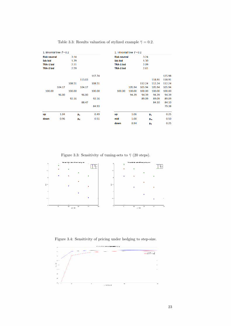
Table 3.3: Results valuation of stylized example γ = 0.2.

Figure 3.3: Sensitivity of tuning-sets to γ (20 steps).

Figure 3.4: Sensitivity of pricing under hedging to step-size.

23

Chapter 4

Model Calibration andResults

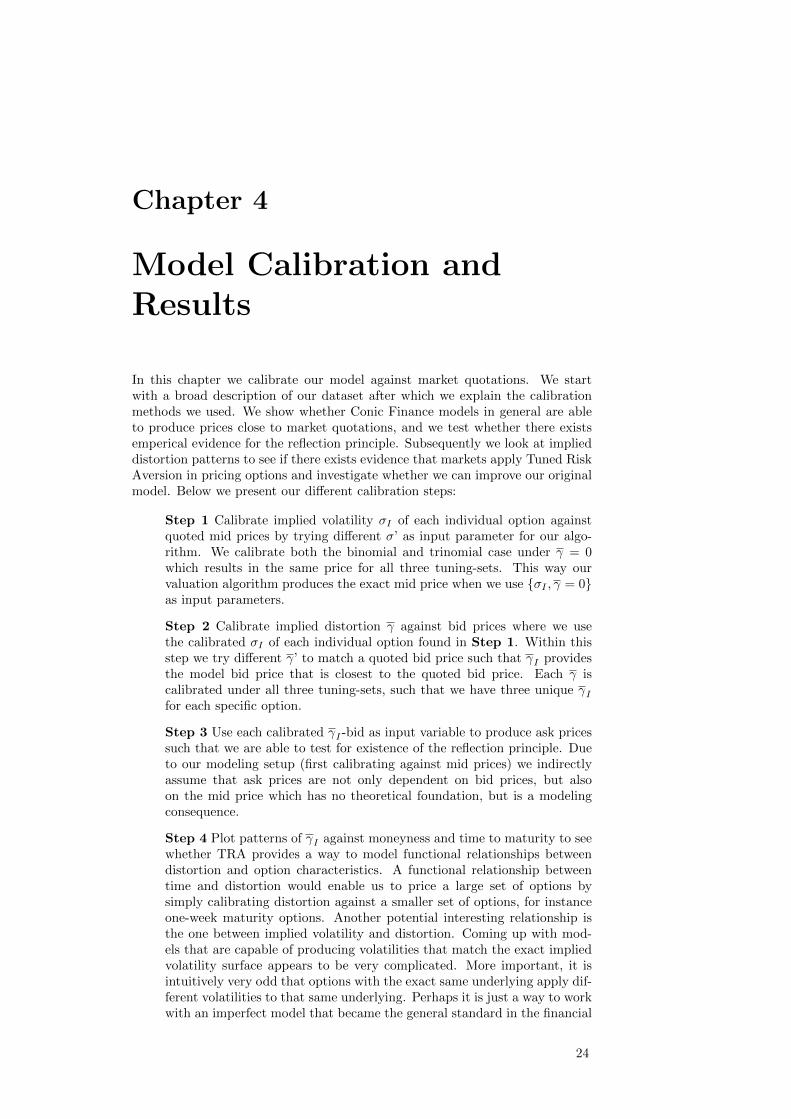
In this chapter we calibrate our model against market quotations. We startwith a broad description of our dataset after which we explain the calibrationmethods we used. We show whether Conic Finance models in general are ableto produce prices close to market quotations, and we test whether there existsemperical evidence for the reflection principle. Subsequently we look at implieddistortion patterns to see if there exists evidence that markets apply Tuned RiskAversion in pricing options and investigate whether we can improve our originalmodel. Below we present our different calibration steps:

Step 1 Calibrate implied volatility σI of each individual option againstquoted mid prices by trying different σ’ as input parameter for our algo-rithm. We calibrate both the binomial and trinomial case under γ = 0which results in the same price for all three tuning-sets. This way ourvaluation algorithm produces the exact mid price when we use σI , γ = 0as input parameters.

Step 2 Calibrate implied distortion γ against bid prices where we usethe calibrated σI of each individual option found in Step 1. Within thisstep we try different γ’ to match a quoted bid price such that γI providesthe model bid price that is closest to the quoted bid price. Each γ iscalibrated under all three tuning-sets, such that we have three unique γIfor each specific option.

Step 3 Use each calibrated γI -bid as input variable to produce ask pricessuch that we are able to test for existence of the reflection principle. Dueto our modeling setup (first calibrating against mid prices) we indirectlyassume that ask prices are not only dependent on bid prices, but alsoon the mid price which has no theoretical foundation, but is a modelingconsequence.

Step 4 Plot patterns of γI against moneyness and time to maturity to seewhether TRA provides a way to model functional relationships betweendistortion and option characteristics. A functional relationship betweentime and distortion would enable us to price a large set of options bysimply calibrating distortion against a smaller set of options, for instanceone-week maturity options. Another potential interesting relationship isthe one between implied volatility and distortion. Coming up with mod-els that are capable of producing volatilities that match the exact impliedvolatility surface appears to be very complicated. More important, it isintuitively very odd that options with the exact same underlying apply dif-ferent volatilities to that same underlying. Perhaps it is just a way to workwith an imperfect model that became the general standard in the financial

24

industry. Distortion potentially provides the key to solve this problem bykeeping volatility a constant and adjust probability distributions solely bydistortion.

Our modeling setup is based on five important simplifying assumptions:

1. Discrete approximation of lognormal distribution for the underlying.

2. Relatively small number of steps during every period of time (20 per week).

3. Discretization of γ by a linearly spaced vector of 20-steps.

4. Constant risk-free rate for all maturities of 1% which equals the annualrisk-free rate in the US (USA Department of Treasury, 2017).

5. Algorithm keeps track on complete sum of used γ budget used and avail-able, but not of intermediate sub-budgets. For instance we know the γ-budget used between [T-5,T], but not on sub-interval [T-5, T-2] whichpotentially leads to inconsistent budget allocations.

4.1 Dataset and calibration parameters

The SPX is one of the most liquid financial instruments and its traded in a al-most frictionless way (spread less than 1%). We use a dataset of historical optionprices on the SPX obtained via CBOE Options Exchange (2017). The datasetcontains historical end-of-day option chains between June 2017 - October 2017.Index levels of the S&P 500 are obtained via Yahoo Finance (2017). Because ofthe explorative character of this study, and the computational heaviness of themodel, our test-case only contained 219 options (October 2017).

Figure 4.1: Overview dataset CBOE Options Exchange (2017). Historical levelS&P 500 (a), historical distribution of daily returns S&P 500 (b), and plot onimplied volatility of call options on the S&P 500 (c).

We need to calibrate both volatility (σ) and distortion (γ) in order to test ourmodel performance. Volatility determines the tree parameters; probability dis-tribution for underlying pu, pm, pd and the change in the level of the underlyingSu, Sm, Sd, where distortion (γ) adjusts the base probability distribution.

25

4.2 Calibration methodology

4.2.1 Volatility

We calibrated volatility against mid quotes in order to ensure that the risk-neutral case (γ = 0) delivers the mid price which is necessary for our distortionapproach. By first calibrating against mid prices we follow the work of Madanet al. (2016). Our approach differs in the fact that we calibrate σ for a lognor-mal distribution (underlying assumption for trees) where Madan et al. (2016)calibrate a fmidvariance gamma process. Alternatively we could calibrate σ byeconometric models like ARCH and GARCH to forecast volatility based on his-torical return data (Cumby et al., 1993) and (Noh et al., 1994). The problemwith this approach is that we will never be able to fit prices due to the existenceof the implied volatility surface, because GARCH produces single unique vari-ance forecasts, see Appendix 7.4 for GARCH parameters. In Figure 4.2.c. weshow the difference between the GARCH forecasted variance and our calibratedimplied variance.

Figure 4.2: Historical daily returns (a), historical and forecasted day σ2 (b)and bandwith calibrated implied variance from our model versus GARCH(1,1)forecast (c).

A second alternative is to use the markets’ forecast of volatility by using theimplied volatility calculated from quoted market prices. Research on the fore-cast quality of implied volatility is however quite mixed (Fleming, 1998) andthis would result in multiple mid quotes outside the bid-ask spread. A thirdalternative is to model volatility as a stochastic process (Heston, 1993). Thisapproach is however quite contradictive in our case, because by using a treemodel we indirectly assume volatility to be deterministic. We used the Nelder-Mead calibration scheme presented in Olsson and Nelson (1975) and Kienitzand Wetterau (2013). This method is widely applied for non-linear optimizationproblems. The advantage is that the method is based on simplex optimizationrather than derivatives of an objective function. This is necessary due to thefact that we don’t price by a closed form formula, but by a recursive algorithm.

4.2.2 Distortion

Recently several articles have appeared on the calibration of distortion parame-ters. Madan and Schoutens (2010) and Madan et al. (2016) start by calibratinga risk-neutral variance-gamma distribution by historical stock returns and thencalibrate γ by bid and ask prices of options on that same underlying index whereeach option type in terms of maturity and moneyness is calibrated individually.The difference with our setting is that they work in continuous time and cali-brate closed forms for bid and ask prices, see Madan and Schoutens (2010) for

26

proof of Equations 4.1 and 4.21:

bγ(C) =

∫ ∞K

(1−Ψγ(FS(x))

)dx, (4.1)

aγ(C) =

∫ ∞K

Ψγ(1− FS(x)

)dx. (4.2)

An alternative approach is proposed by Bannor and Scherer (2014). An extrafeature of this method is the ability to obtain the shape of a market-implieddistortion function. They use a piecewise linear approximation of a distortionfunction by using market quotes of option prices. Then the bid ask price calibra-tion problem corresponds to minimizing the dinstance between model bid-askprices and quoted market prices. The differences between the results obtainedby the two methods are minor according to Bannor and Scherer (2014).

We combine both methods of Bannor and Scherer (2014) & Madan and Schoutens(2017) and execute them with a Nelder-Mead simplex calibration scheme. Firstwe calibrate volatility against the mid quote (γ = 0 case) in order to make sureour bid-ask spread entails the mid quote. Subsequently we calibrate γ for eachindividual option against bid prices where we use the implied volatility calibratedin the step before as volatility input parameter in our algorithm. The differencewith the approach used by Madan and Schoutens (2010) is that we work with alognormally distributed underlying imposed by the tree-framework, instead of avariance gamma distribution. Then we calibrate our distortion budget againstbid quotations and test the reflection principle by applying the same amount ofdistortion for producing ask prices. We look for evidence of TRA by plottingcalibrated implied distortion profiles against moneyness and time to maturity.

4.3 Empirical results

We measure the goodness of fit by the Average Absolute Error (EEA) (Kienitzand Wetterau, 2013) of the model price compared to the quoted market priceand the EEA as percentage of the absolute spread2, see Equation 4.3 and 4.4.

AAE =1

N

N∑i=1

|Pmarketi − Pmodeli (x)|, (4.3)

AAE as % of spread =1

N

N∑i=1

( |Pmarketbidi − Pmodelbidi (x)||Pmarketbidi − Pmarketmidi |

) . (4.4)

where x = (x1..xn)T represents the vector with option parameters belonging tooption i. We calibrate σ against mid prices and we calibrate γ against bid prices.We test for the reflection principle by using the implied calibrated distortionfound through bid prices to produce the corresponding ask price. Within thischapter we left out the results after hedging, because hedging made the algorithminflexible for small step-sizes and pricing performance decreases when spreadsbecome significant.

1FS represent the distribution of the underlying S.2Spread is defined as the difference between the bid and ask price.

27

4.3.1 Implied volatility

In Figure 4.3 we show the calibrated implied volatility skew which correspondsto implied volatility skews we would expect to find for call options (Hull, 2012).

Figure 4.3: Calibrated Implied volatility.

The option prices produced by volatility calibration are very close to mid quoteswith marginal fitting error, which shows that our models are able to produceprices that are close to quoted mid prices of SPX options. Calibrated impliedvolatilities for the trinomial tree setting show a smoother pattern than the bin-iomial setting, due to the fact the we used a relative small number of modelingsteps during every time period and trinomial trees converge faster to stable pric-ing profiles. When we decrease step-size we will see that implied volatilites undertrinomial and binomial become roughly the same.

4.3.2 Implied distortion

Conic Finance models are able to produce bid prices that empirically fit marketprices when the right amount of distortion is applied, both under strong andsequential consistency, see Table 7.2 in Appendix 7.6. The difference betweenTRA and sdc is that a wider set of distortion budget dependencies is allowedand therefore risk aversion is not necessary a constant over all time-steps. Thisenables us to model different relationships between γ and time to maturity andprevent spreads from blowing up as under sdc.

Moneyness

When we look at moneyness versus implied volatility in Figure 4.4, we observepatterns similar to the implied volatility skew. The implied volatility exists, be-cause traders consider that the lognormal distribution understates probabilitiesof extreme events (Hull, 2012), which we can consider as a type of risk aversionthat we can potentially capture with distortion, see Chapter 4.4.

Figure 4.4: Calibrated implied distortion (γ) versus moneyness (Trinomial).

28

TRA-2 and sdc show similar profiles, because for one-week options TRA-2 isjust a scaled version of sdc where the single-step γ of sdc is the maximum riskaversion that can be distributed over all time-steps for TRA-2. TRA-1 shows adifferent more stable pattern, because the limit is a squaroot sum of all γ’s.

Time to maturity

In Figure 4.5 we plotted the calibrated implied distortion (γI) for options withequal moneyness, but different time to maturities.

Figure 4.5: Calibrated implied distortion (γI) versus time to maturity (trino-mial).

Implied distortion γI under sdc shows a sharply decreasing profile in order tomatch longer-term quoted bid prices. If we kept γI constant we would endup with bid prices significantly below the quoted bid price due to the blow upbehavior described in Chapter 2.4.3. Under TRA we observe flatter profilesfor γI . This seems promising in order to find a uniform functional relationshipbetween time and distortion such that we prevent spreads from blowing up. Forfurther research purposes it would be interesting to test a wider set of budgetequations and time dependencies.

4.3.3 Reflection principle

One fundamental modeling choice in current Conic Finance frameworks is thereflection principle, which assumes that bid and ask prices are connected by theequality that buying is the same as selling its negative:

bid(X) = −ask(−X). (4.5)

We test if there exists empirical proof for this assumption by applying eachindividual calibrated amount of bid price distortion (γI) to produce its cor-responding ask price and compare this ask price with the ask price quotationprovided by the market. An important assumption within our modeling setupis that our bid price depends on the mid price (because we first calibrated themid price σ) and therefore ask prices not only depend on bid prices imposed bythe reflection principle, but also on the mid price as a modeling consequence.In Appendix 7.6 we present the performance of our model in fitting ask prices.It shows that the reflection principle holds for close-to ATM options, but fittingperformance decreases significantly for OTM options, see Figure 4.6. A possibleexplanation is that spreads are not necessarily symmetric around mid quotes inConic Finance (Madan and Schoutens, 2017). This is indeed not the case whenwe look at implied spreads as % of the model ask price versus moneyness. InFigure 4.6 we see a similar increase of spreads compared to the increase in fittingerror for different moneyness.

29

Figure 4.6: Bid-ask spread as % of ask price (orange) versus fitting error askprice (blue) for different moneyness. TRA-1, 2-10-2017 for a one-week optionvalued by a trinomial tree.

We found no statistical evidence3 that models under TRA produce better askprices (under calibrated bid distortion) than the sdc one, nor a difference betweenbinomial and trinomial models.

4.4 Constant implied volatility setup

Based on our findings on the implied distortion (γI) versus implied volatility(σI), we want to test another modeling setup in which we keep implied volatilityconstant and try to fit the complete adjustment of the probability distributionwith our γI parameter. In order to do so we undertake the following steps:

Step 1 We take one volatility level that we thereafter use for all strikesand maturities which is the implied volatility of the farthest ITM option,see Figure 4.7. We could also take the σ of the farthest OTM options, aslong as we ensure that all other mid prices modeled with this specific σIare above their bid price which is a necessity for our algorithm.

Step 2 Calibrate γ for each individual option with the one unique σI thatwe found in Step 1.

Step 3 Test if we could fit the total adjustment on the probability distri-bution with γ and investigate if our ask price fitting performance increases.

Figure 4.7: Implied volatility of farthest ITM option illustrated by black circle.

4.4.1 Results

We plotted the results of two different options on two separate days in Figure4.8. It shows that we are able to capture the complete adjustment of the under-lying probability distribution necessary to fit bid prices by only changing γ andkeeping σ constant. We believe implied distortion to be a much more intuitiveadjustment parameter, because it represents risk aversion which is likely to bedifferent for options with different moneyness, where it theoretically impossiblethat one underlying has multiple volatilities.

32-sample t-test at 99% significance level.

30

Figure 4.8: Implied distortion (γI) after constant volatility calibration. Lefty-axis is SDC, right y-axis is TRA.

Again we see that TRA-2 (square-root budget) shows the most stable patternwhere TRA-1 and sdc show more divergent profiles with significant changesin distortion around ATM strikes. Within this setup ask pricing performancedecreases dramatically, because of two reasons:

• Implied distortion levels increase around ATM strikes in order to adjustthe relatively high mid price into a bid price. But because the mid priceis already relatively close to the quoted ask prices at these points, theamount of distortion calibrated against bid prices is far too high to adjustthat same mid price into an ask price and therefore ask prices explodecompared to quoted ones, see Figure 4.9.

• For options with low implied volatilities, especially around ATM strikes,mid prices lay sometimes above ask prices. This happens because we useda relatively high implied volatility (the one for the farthest ITM option)that delivers a disproportionate high mid price for options with low impliedvolatilities.

Figure 4.9: Fitting error ask price in % of spread versus moneyness (sdc).

31

4.5 Alternative use of Reflection Principle

In the previous section we showed that we are able to capture the completeadjustment of the probability measure by changing γ instead of σ, however thereflection principle makes it impossible to produce ask prices with the calibratedbid γ. In order to solve this problem we introduce an alternative use of thereflection principle.

Conic Finance is built upon the assumption that bid and ask prices exist due tothe existence of unhedgeable risk. In order to assess this risk, we apply constantrisk aversion both for selling and buying. However, in Conic Finance the amountof risk aversion is the same for bid and ask by the reflection principle. We believethere is room to deviate from this principle. The level of risk aversion is notnecessary the same for buying and selling. It is widely accepted in normativeBehavioral Finance theories that the perception of losing (negative contingentclaim/selling) is different than for winning (positive contingent claim/buying).We therefore propose that bid and ask prices could have their own level of riskaversion (γ). We introduce a different setup where we price with a forecastedunderlying volatility (again the same for all strikes) provided by GARCH(1,1).We already know that this volatility will produce mid prices that are too lowfor ITM options, but too high for ATM options. The price point γ = 0 is thepoint where the forecasted volatility provides the exact (or closest to) bid-price.We fit prices around this point by applying the reflection principle for the pointswhere we are not able price with normal valuation operators; φγ(X) (bid) orφγ(−X) (ask). For instance on the points in the red-marked area in Figure 4.10we cannot price with φγ(X) and therefore we price with φγ(−X). We define thepoints priced by the reflection principle in the following way:

bid φ−γ(X) = φγ(−X), (4.6)

ask φ−γ(X) = φγ(X). (4.7)

Figure 4.10: Bid and ask price operators with constant forecasted volatility. Thegraph shows which valuation operator is used in different areas of the quotedimplied volatility.

32

4.5.1 Results

Figure 4.11 shows the results of the bid and ask price γ after calibration wherewe applied the reflection principle, not to find the complementary ask price,but to find the bid/ask prices that we can’t price with their standard valuationoperator. We see that we are able to price both bid and ask prices with aforecasted σ and capture the complete adjustment of the probability measureby γ. We observe that as we expected, bid and ask prices don’t have the sameamount of risk aversion. We also see that the spread between the γ‘s for bidand ask widens when we move away from the ATM strikes. Probably becausevaluation uncertainty increases for OTM and ITM options. Again we observethe most stable pattern under TRA-1.

Figure 4.11: Graphical representation of γ for bid and ask prices under newsetup. γ’s-ask are multiplied by -1 for illustrative purposes.

33

Chapter 5

Conclusion

This chapter provides an answer to the sub-research questions posed in our re-search design. The answering of our main research question accompanied withmain insights gained during this research project follows logically.

From classical derivative valuation towards a two price framework

Traditional valuation models are built on the fundamental theories of asset pric-ing in which the pricing of financial products is based on the law of one price.However, when we look at real financial markets we observe two prices, one forselling and one for buying. We believe this to be logical when people apply riskaversion consistently in both selling and buying. Conic Finance provides a frame-work that aims at producing these two prices such that bid-ask spreads reflectthe cost of unhedgeable risk. Financial contracts are then priced in terms of amarketed cone which is operationalized by acceptability indices under the mod-eling assumption that buying equals selling the negative (reflection principle),and strong dynamic consistency. Strong dynamic consistency potentially leadsto the build-up of conservatism and introduces complications when we want tobuild functional relationships between time to maturity and risk aversion. TunedRisk Aversion provides a framework that still provides unique updates of pricesin multi-period valuations, but is more flexible and able to produce results morein line with experimental choice behavior. The extra flexibility of Tuned RiskAversion also provides the possibility to build other more feasible functional re-lationships between risk aversion and time to maturity.

From theory to a pricing model

Bid and ask prices are respectively the infimum and supremum of distorted ex-pectations in Conic Finance, where distortion depends on the degree of riskaversion. We developed a model that is able to price plain vanilla options bothin a binomial and trinomial tree setting. The pricing algorithm has two possi-ble tuning-sets under Tuned Risk Aversion with different time and risk aversiondependencies. Strong dynamic consistency has been modeled by keeping theamount of distortion constant during every time-step. The model has beentested on a stylized case where we showed the difference between tuning-setsunder Tuned Risk Aversion and strong dynamic consistency in pricing a two-month call option.

Model calibration and pricing performance

We calibrated our model against a dataset of call options on the S&P 500 (SPX)in October-2017 by the following steps:

Step 1 Calibrate implied volatility (σI) of each individual option againstquoted mid-prices by testing different σ’ as input parameter for our algo-rithm. Calibration executed through a Nelder-Mead simplex calibrationscheme.

34

Step 2 Calibrate implied distortion (γ) against bid prices where we usethe calibrated σI of each individual option found in Step 1 also througha Nelder-Mead simplex calibration scheme.

Step 3 Use each calibrated γI -bid as input-variable to produce ask pricessuch that we are able to test for existence of the reflection principle.

Step 4 Plot patterns of γI against moneyness and time to maturity to seeif TRA provides a way to model functional relationships between distortionand option characteristics and to see if markets price with TRA.

Our model is able to produce bid prices close to market prices, both understrong dynamic consistency and TRA. By applying the calibrated amount ofbid-distortion, we were able to match ask prices around ATM strikes, but fit-ting performance decreased for OTM options. This can be explained by the factthat in Conic Finance bid-ask spreads are not necessarily symmetric around midprices, which we indirectly assumed in our calibration setup.

We looked at patterns of implied distortion and found profiles similar to theimplied volatility skew. We tested two alternative modeling setups where wekept volatility constant and captured the complete probability distribution ad-justment, normally provided by changing σ of the underlying, by solely applyingdistortion γ. Within this modeling setup we were able to fit all bid and askprices of different strikes in a model with a single volatility for the underlying.Also implied distortion patterns under TRA showed a significantly flatter pro-file compared to sdc and therefore TRA provides a way to model a functionalrelationship between time to maturity and distortion, while at the same remainconsistent and prevent spreads from blowing up. TRA provides a very promis-ing framework into finding a uniform model for derivative pricing that is able toprice with a single volatility for the underlying and a feasible way to relate riskaversion and time to maturity.

5.1 Main insights

1. Spreads under strong dynamic consistency blow up if we increase timeto maturity and therefore it is impossible to model a truly consistent re-lationship between time to maturity and distortion that matches marketprices.

2. Conic Finance models are able to produce bid and ask prices close tomarket quotations, both under sequential and strong dynamic consistencyby applying the right amount of distortion.

3. Implied distortion patterns show that with TRA, we are able to solvethe blow up behavior that we face under sdc which provides promisingresults for finding a functional relationship between distortion and time tomaturity.

4. The probability adjustment (implied volatility skew), normally providedby different volatilities for the underlying, can be completely captured bydistortion γ. We are able to price all strikes of an option chain by a singleforecasted volatility.

5. Market quotations for ATM options provide evidence for the reflectionprinciple as modeling relationship between bid and ask prices. However,we believe that for OTM and ITM options, bid and ask prices could havedifferent levels of risk aversion.

35

Chapter 6

Further Research andModel Improvement

Empirical studies on both Conic Finance and Tuned Risk Aversion are scarce andtheoretical ones that try to combine these two theories even non-existent. To ourknowledge this study is the first attempt to bridge Tuned Risk Aversion and thefield of derivative pricing, especially Conic Finance. We can say that the studywas an explorative journey and therefore many new ideas and improvementscame to our minds during the process. This final chapter captures all theserecommendations and ideas for further research.

1. Flexibility Allow for a wider range of tuning-sets and distortion functions.Because of the explorative character of this study we restricted ourselves totwo types of tuning-sets and one distortion function MINMAX (the mostconservative one). The model can be extended by trying different distor-tion functions, for instance: MAXMIN, MAXVAR and MINVAR (Chernyand Madan, 2009). We can also model different tuning-sets where we cal-ibrate both δ and γ (Equation 6.1) or use different single-step restrictionsfor risk aversion (Equation 6.2):

N∗T∑0

γt ≤ (N ∗ T )δ ∗ γ | γt ≤ γ, (6.1)

N∗T∑0

γt ≤ (N ∗ T )δ ∗ γ | γt ≤√γ. (6.2)

2. Connection with Behavorial Finance An extension would be to incor-porate S-shaped distortion instead of strictly concave which is more in linewith general theories in Behavioral Finance. By applying this type of dis-tortion functions we need to be careful if no-arbitrage conditions still hold(Madan et al., 2016). Another potential extra research dimension wouldbe to incorporate the accumulation of wealth within the TRA framework.We would expect utility of ‘extra gains’ for highly ITM options to be lessthan the gains obtained by for instance ATM options. In other words, theaccumulation of wealth plays a role in the risk aversion of investors. Con-sider a binomial pricing framework as a compound choice lottery wherein every time-step an investor has the hypothetical choice of holding hisposition, or to close/sell it. The choice to hold his position means that hecontinues the ‘gamble’ at least one more period of time. When we are highin the tree the investor gained a lot, so his reference point changes andutility of gains diminishes in line with Cumulative Prospect Theory (Tver-sky and Kahneman, 1992). Therefore risk aversion should differ when weare somewhere high in the tree compared to when we are somewhere low.

36

Especially for derivatives with intermediate payoffs like swaps this wouldbe an interesting point for further research.

Figure 6.1: Indicative risk aversion in normal and implied binomial tree.

3. Functional relationship distortion Use the insights from implied dis-tortions patterns under TRA to find a functional relationship between time(tuning-set) and moneyness. Especially the relationship between distortionand implied volatility looks very promising which could be the key to de-velop a model that is able to price options with different strikes, but thesame underlying volatility. A first and easy attempt could be to look atthe development of historical implied distortion levels to see if this changesover time and whether it is forecastable.

4. Hedging improvement The hedging strategy in this thesis is the oneproposed by Madan et al. (2016), but whether this approach is optimalremains questionable, especially in the presence of transaction cost forthe underlying. Therefore we propose to improve the model with moreadvanced hedging strategies for trinomial trees presented in: Schulmerichand Trautmann (2003), Huang and Guo (2013) and Follmer and Leukert(2000).

5. Validity Develop a model that does not require ‘knowing’ the exact midquote parameterization. Even by using a single σ, like we tested in Chapter4.4 and 4.5, we still use the mid price as starting point for distortion.Modeling the implied volatility surface is a constantly developing field.Especially the article Carr and Wu (2016) looks very promising and is veryclose to approaches used by practitioners (Vega-Vanna-Volga method).

6. Generality Test the model on more complicated derivatives like struc-tured products. A first attempt has already been made by Madan andSchoutens (2012). Also the dataset we used was very limited both in typeof options, maturity (less than two months) and dates (only one). In orderto increase generality we need to test the model on larger datasets.

37

6.1 Model Improvement

1. Finite difference Extend the model towards a finite-difference modelwhere the underlying is modeled on a grid. This way we would be ableto price options with other underlying processes like: variance-gamma orLevy, but are still able to distribute risk aversion every time-step. Theapplication of Conic Finance in grid methods is further explained in Madanand Schoutens (2016).

2. Time dependency Within our model we searched for time dependenciesin terms of week-maturities and calibrated γ budgets at weeks. We wouldsuggest to decrease this to day-dependency which potentially increasesprecision and allow us to calibrate against a wider set of options. Thismodeling-setup is already possible in our current algorithm.

3. Detailed consistency Improve the algorithm such that also intermedi-ate budgets are stored, see introduction Chapter 4 for explanation of thismodeling assumption. This way we can ensure that we are completelyconsistent over all time-steps.

4. Calibration (I) Test whether there is a significant improvement whenvolatility is calibrated against the volume weighted-average mid quote in-stead of the standard mid quote.

5. Calibration (II) Only use OTM options of put and calls and apply theput-call parity to price ITM options, because they are more competitivelypriced (Aıt-Sahalia et al., 2001).

6. Precision (I) Increase granularity of possible γ values the model canassign every time-step. This can lead to better pricing performance andbetter implied distortion patterns due to the fact that risk aversion can beapplied more precisely.

7. Precision (II) We took the risk-free rate as constant for all maturitiesand used γ as calibration parameter to fit the lognormal distribution suchthat our model produced the exact mid-price. It would be better to use theexact risk-free term-structure, for instance the EONIA in Europe (ECB,2014). For equity derivatives it is not necessary to model stochastic interestrates, because the main driver of value is the equity underlying opposedto, for instance, interest rate derivatives (Brigo and Mercurio, 2006).

8. Model Performance The current model is programmed in Matlab whichis a relatively slow programming language compared to C++ or Python.Especially for calibration purposes performance can be increased by recod-ing it to a faster programming language.

38

Bibliography

Aıt-Sahalia, Y., Wang, Y., and Yared, F. (2001). Do option markets correctlyprice the probabilities of movement of the underlying asset? Journal ofEconometrics, 102(1):67–110.

Artzner, P., Delbaen, F., Eber, J., and Heath, D. (1999). Coherent Measures ofRisk. Mathematical Finance, 9(3):203–228.

Artzner, P., Delbaen, F., Eber, J., Heath, D., and Ku, H. (2007). Coherent mul-tiperiod risk adjusted values and Bellman’s principle. Annals of OperationsResearch, 152(1):5–22.

Bannor, K. F. and Scherer, M. (2014). On the calibration of distortion riskmeasures to bid-ask prices. Quantitative Finance, 14(7):1217–1228.

Barraquand, J. and Pudet, T. (1996). Pricing of American Path DependentContingent Claims. Mathematical Finance, 6(1):17–51.

Bielecki, T., Cialenco, I., and Pitera, M. (2017). A survey of time consistencyof dynamic risk measures and dynamic performance measures in discretetime: LM-measure perspective. Probability, Uncertainty and QuantitativeRisk, 2.1(1):3.

Bielecki, T., Cialenco, I., and Zhang, Z. (2014). Dynamic coherent acceptabilityindices and their applications to finance. Mathematical Finance, 24(3):411–441.

Bielecki, T. R., Cialenco, I., Iyigunler, I., and Rodriguez, R. (2013). DynamicConic Finance: Pricing and Hedging in Market Models With TransactionCosts Via Dynamic Coherent Acceptability Indices. International Journalof Theoretical and Applied Finance, 16(01):1350002, 36.

Black, F. and Scholes, M. (1973). The Pricing of Options and Corporate Liabil-ities. Journal of Political Economy, 81(3):637–654.

Bormetti, G., Montagna, G., Moreni, N., and Nicrosini, O. (2004). Pricing ExoticOptions in a Path Integral Approach. Quantitative Finance, 6(1):55–66.

Boyle, P. (1986). Option Valuation Using a Three-Jump Process. InternationalOptions Journal, 3:7–12.

Brigo, D. and Mercurio, F. (2006). Interest rate models-theory and practice:with smile, inflation and credit. Springer Science and Business Media, thirdedition.

Carr, P. and Wu, L. (2016). Analyzing volatility risk and risk premium in optioncontracts. Journal of Financial Economics, 120(1):1–20.

CBOE Options Exchange (2017). CBOE optian chain on S&P500. https ://datashop.cboe.com/option− quotes− end− of − day − with− calcs.

Cherny, A. and Madan, D. (2009). New measures for performance evaluation.In Review of Financial Studies, volume 22, pages 2571–2606.

39

Cox, J. C., Ross, S. A., and Rubinstein, M. (1979). Option pricing: A simplifiedapproach. Journal of Financial Economics, 7(3):229–263.

Cumby, R., Figlewski, S., and Hasbrook, J. (1993). Forecasting Volatilities andCorrelations with EGARCH Models. Journal of Derivatives, 1(2):51–63.

Derman, E., Kani, I., and Chriss, N. (1996). Implied Trinomial Trees of theVolatility Smile. The Journal of Derivatives, 3(4):7–22.

Derman, E. and Taleb, N. (2005). The illusions of dynamic replication. Quan-titative Finance, 5(4):323–326.

Detlefsen, K. and Scandolo, G. (2005). Conditional and dynamic convex riskmeasures. Finance and Stochastics, 9(4):539–561.

Duffie, D. (2001). Dynamic Asset Pricing Theory. Princeton University Press,third edition.

Dupire, B. (1994). Pricing and hedging with smiles. Mathematics of derivativesecurities, 1(1):103–111.

Eberlein, E., Madan, D., Pistorius, M., Schoutens, W., and Yor, M. (2014). Twoprice economies in continuous time. Annals of Finance, 10(1):71–100.

ECB (2014). Euro Area Risk-Free Interest Rates: Measurement Issues , RecentDevelopments and Relevance to Monetary Policy. Technical Report 7 (July).

Fleming, J. (1998). The quality of market volatility forecasts implied by S&P100 index option prices. Journal of Empirical Finance, 5(4):317–345.

Follmer, H. and Leukert, P. (2000). Efficient hedging: Cost versus shortfall risk.Finance and Stochastics, 4(2):117–146.

Follmer, H., Schied, A., and Lyons, T. J. (2004). Stochastic finance. an intro-duction in discrete time, volume 26. Walter de Gruyter.

Harrison, J. and Kreps, D. (1979). Martingales and arbitrage in multi-periodsecurity markets. Journal of Economic Theory, 20(3):381–408.

Haug, E. G. and Taleb, N. N. (2011). Option traders use (very) sophisticatedheuristics, never the Black-Scholes-Merton formula. Journal of EconomicBehavior and Organization, 77(2):97–106.

Heston, S. L. (1993). A Closed-Form Solution for Options with StochasticVolatility with Applications to Bond and Currency Options. Review ofFinancial Studies, 6(2):327–343.

Huang, S. F. and Guo, M. (2013). An optimal multi-step quadratic risk-adjustedhedging strategy. Journal of the Korean Statistical Society, 42(1):37–49.

Hull, J. (2012). Options, Futures and other Derivatives. Pearson, Toronto, eighthedition.

Jackwerth, J. and Rubinstein, M. (1996). Recovering Probability Distributionsfrom Option Prices. The Journal of Finance, 51(5):1611–1631.

Jobert, A. and Rogers, L. C. G. (2008). Valuations and dynamic convex riskmeasures. Mathematical Finance, 18(1):1–22.

Kienitz, J. and Wetterau, D. (2013). Financial Modelling: Theory, Implemen-tation and Practice. John Wiley & Sons, first edition.

Kusuoka, S. (2001). On law invariant coherent risk measures. Advances inMathematical Economics, 3:83–95.

40

Leland, H. (1985). Option Pricing and Replication with Transactions Costs. TheJournal of Finance, 40(5):1283–1301.

Machina, M. and Viscusi, W. (2014). Economics of risk and uncertainty. Else-vier, Amsterdam, first edition.

Madan, D. (2010). Pricing and hedging basket options to prespecified levels ofacceptability. Quantitative Finance, 10(6):607–615.

Madan, D., Pistorius, M., and Schoutens, W. (2013). The valuation of structuredproducts using Markov chain models. Quantitative Finance, 13(1):125–136.

Madan, D., Pistorius, M., and Schoutens, W. (2016). Dynamic conic hedging forcompetitiveness. Mathematics and Financial Economics, 10(4):405–439.

Madan, D. and Schoutens, W. (2010). Markets As a Counterparty: an Intro-duction To Conic Finance. International Journal of Theoretical and AppliedFinance, 13(08):1149–1177.

Madan, D. and Schoutens, W. (2016). Applied Conic Finance. CamebridgeUniversity Press, Clays, first edition.

Madan, D. and Schoutens, W. (2017). Conic Option Pricing (Robert H. SmithSchool of Business).

Madan, D. B. and Schoutens, W. (2012). Structured products equilibria in conictwo price markets. Mathematics and Financial Economics, 6(1):37–57.

Merton, R. (1973). Theory of Rational Option Pricing. The Bell Journal ofEconomics and Management Science, 4(1):141–183.

Miller, K. D. and Shapira, Z. (2004). An Empirical Test of Heuristics andBiases Affecting Real Option Valuation. Strategic Management Journal,25(3):269–284.

Nardon, M. and Pianca, P. (2014). A behavioural approach to the pricing ofEuropean options. In Mathematical and Statistical Methods for ActuarialSciences and Finance, pages 219–230. Springer.

Nelson, D. B. (1991). Conditional Heteroskedasticity in Asset Returns: A NewApproach. Econometrica: Journal of the Econometric Society, 59(2):347–370.

Noh, J., Engle, F., and Kane, A. (1994). Forecasting Volatility and OptionPrices on the S&P 500 index. Journal of Derivatives, 2(1):17–30.

Olsson, D. M. and Nelson, L. S. (1975). The Nelder-Mead simplex procedure forfunction minimization. Technometrics, 17(1):45–51.

Remler, D. and van Ryzin, G. (2015). Research Methods in Practice: Strategiesfor Description and Causation. Sage, Thousand Oaks, second edition.

Riedel, F. (2004). Dynamic coherent risk measures. Stochastic Processes andtheir Applications, 112(2):185–200.

Roorda, B. and Joosten, R. (2015). Dynamically Consistent Non-Expected Util-ity Preferences with Tuned Risk Aversion (University of Twente).

Roorda, B. and Joosten, R. (2017). Consistent Preferences with Fixed PointUpdates (University of Twente).

Roorda, B. and Schumacher, J. (2013). Membership conditions for consistentfamilies of monetary valuations. Statistics & risk modeling, 30(3):255–280.

41

Roorda, B. and Schumacher, J. (2016). Weakly time consistent concave valu-ations and their dual representations. Finance and Stochastics, 20(1):123–151.

Roorda, B. and Schumacher, J. M. (2007). Time consistency conditions foracceptability measures, with an application to Tail Value at Risk. Insurance:Mathematics and Economics, 40(2):209–230.

Ross, S. (1978). A simple approach to the valuation of risky streams. Journalof business, 51(3):453–475.

Rubinstein, M. (2000). On the Relation Between Binomial and Trinomial OptionPricing Models. The Journal of Derivatives, 8(2):47–50.

Schulmerich, M. and Trautmann, S. (2003). Local expected shortfall-hedging indiscrete time. In European Finance Review, volume 7, pages 75–102.

Schwartz, E. (1977). The valuation of Warrants: Implementing a new approach.Journal of Financial Economics, 4(1):79–93.

Shreve, S. E. (1996). Stochastic Calculus and Finance. Springer Finance, firstedition.

Taleb, N. N. (2013). Philosophy: ‘Antifragility’ as a mathematical idea. Nature,494(7438):430.

Thaler, R. H. (2015). Misbehaving: The Making of Behavioral Economics, vol-ume 57. W. W. Norton & Company, sixth edition.

Tversky, A. and Kahneman, D. (1992). Advances in prospect theory: Cumulativerepresentation of uncertainty. Journal of Risk and Uncertainty, 5(4):297–323.

USA Department of Treasury (2017). Daily treasury yield curve T-bills.

Verschuren, P., Doorewaard, H., and Mellion, M. (2010). Designing a ResearchProject. Eleven International Publishing, The Hague, second edition.

Versluis, C. and Lehnert, T. (2010). A Cumulative Prospect Theory Approachto Option Pricing (Luxembourg School of Finance).

Webster, J. and Watson, R. (2002). Analyzing the Past to Prepare for theFuture: Writing a Literature Review. MIS Quarterly, 26(2):13–23.

Yahoo Finance (2017). Yahoo Finance historical option data S&P500. https ://finance.yahoo.com/quote/5ESPX/.

42

Chapter 7

Appendix

7.1 Binomial tree set-up

Backward recursion is determined by the following four equations:

φ(T ) = X(T ) (7.1)

φ(t) = EQ[φ(t+ 1)|Ft

](7.2)

ϕ2(t) =

CovQ[φ(t+ 1),∆S(t)|Ft

]VarQ

[∆S(t)|Ft

] (7.3)

ϕ1(t) = φ(t)− ϕtS(t) (7.4)

We now observe that ϕ2(t) is the regression coefficient of the value of the deriva-tive and the underlying, also called delta. For an option in the binomial frame-work, Equation 7.3 reduces to the following simplified well-known expression ofdelta:

ϕ2(t) =φ(t+ 1, S(t)u)− φ(t+ 1, S(t)d)

S(t)u− S(t)d(7.5)

In our implementation we followed the setup presented by Cox et al. (1979)

Su = Seσ√

(∆t) (7.6)

Sd = Se−σ√

(∆t) (7.7)

pu =er∆t − SdSu − Sd

(7.8)

pd = 1− pu (7.9)

43

7.2 Trinomial tree set-up

Presented in Boyle (1986)

Su = Seσ√

(2∆t) (7.10)

Sd = Se−σ√

(2∆t) (7.11)

Sm = S (7.12)

pu = (er∆t

12 − e−σ

√∆t 12

eσ∆t 12 − e−σ√

∆t 12

)2 (7.13)

pm = 2/3 (7.14)

pd == (eσ√

∆t 12 − e−r∆t 12

eσ∆t 12 − e−σ√

∆t 12

)2 (7.15)

(7.16)

7.3 Description Algorithm

7.3.1 Procedure

SDCUnder SDC the valuation model applies the same amount of gamma duringevery time-step. The starting point is the risk-neutral probability distributionwith equal distortion in terms of gamma during every step. The option is valuedbackward recursively just like we do in normal traditional one price tree frame-works.

TRAEvery time-step the model calculates the intermediate value of an option bycalculating all the possible valuations under all possible gamma budget applica-tions. Then the model evaluates the possible values and takes the worst value,because bid prices are the infimum of expected values. For ask prices we choosethe highest price (supremum). When we found the worst intermediate value (incase of bid), we store the corresponding gamma budget and store the prices forall possible gamma budgets used. The next time step we evaluate the optimalgamma budget used in the previous step against all possible gamma budgetsused in the current step to see whether the old gamma budget allocation isstill optimal. In case two gamma budget applications lead to the same pricing,the algorithm choses the lowest gamma application in the current step (whichmeans the highest in te previous step). Values that are produced by gammabudget allocations that violate the budget equations are automatically ignoredby the algorithm.

7.4 GARCH

The GARCH(1,1) model is an extension of the ARCH(1) model where the fore-cast is based on a long run average variance rate and recent observations ofreturns. The model is mean reverting and therefore more in line with generalbehavior of volatility compared to methods like exponentially weighted movingaverage models. GARCH(1,1) is based on the following equation:

σ2t = ω + α1ε

2t−1 + β1σ

2t−1 (7.17)

µt =StSt−1

− 1 (7.18)

We estimated ω, ε and β via the maximum likelihood method which choosesvalues that maximize the likelihood of data occuring (Nelson, 1991).

44

7.4.1 GARCH parameters used for constant volatility fore-caste in Chapter 4.5

Table 7.1: Garch(1,1) parameters

7.5 Nelder-Mead calibration method

The Nelder-Mead is a direct search method that aims at minimizing a givenproblem of an objective funtion. The method does not rely on derivatives ofthe objective function which is in our case impossible, because pricing is donethrough an algorithm. The method starts from a simplex S0 and tries iterativelyto find the optimal solution (minimization problem), where each iteration stepis indexed by k identifies a vertex vkmin determined by:

vkmin = arg minx∈vk0 ..vknf(x) (7.19)

f(x) = abs(bid− price.m) (7.20)

f(x) = abs(wmad− price.m) (7.21)

‘wmad’ equals the mid quote against which the volatility parameter is calibrated(Chapter 4.2.1) and ‘bid’ equals the bid price against which the distortion pa-rameter is calibrated. Price.m stands for the pricing algorithm. vkmin representsthe vertex where the function takes the minimum. In Matlab the search methodis already precoded by fminsearch. The functions stops when the maximum ab-solute difference between two tries is less compared to a pre-set tolerance andthe maximum distance of any of the vertex subjects compared to the best vertexis small enough (Kienitz and Wetterau, 2013).

45

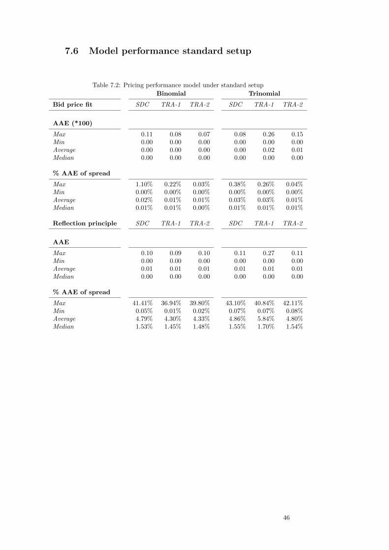
7.6 Model performance standard setup

Table 7.2: Pricing performance model under standard setup

Binomial Trinomial

Bid price fit SDC TRA-1 TRA-2 SDC TRA-1 TRA-2

AAE (*100)

Max 0.11 0.08 0.07 0.08 0.26 0.15Min 0.00 0.00 0.00 0.00 0.00 0.00Average 0.00 0.00 0.00 0.00 0.02 0.01Median 0.00 0.00 0.00 0.00 0.00 0.00

% AAE of spread

Max 1.10% 0.22% 0.03% 0.38% 0.26% 0.04%Min 0.00% 0.00% 0.00% 0.00% 0.00% 0.00%Average 0.02% 0.01% 0.01% 0.03% 0.03% 0.01%Median 0.01% 0.01% 0.00% 0.01% 0.01% 0.01%

Reflection principle SDC TRA-1 TRA-2 SDC TRA-1 TRA-2

AAE

Max 0.10 0.09 0.10 0.11 0.27 0.11Min 0.00 0.00 0.00 0.00 0.00 0.00Average 0.01 0.01 0.01 0.01 0.01 0.01Median 0.00 0.00 0.00 0.00 0.00 0.00

% AAE of spread

Max 41.41% 36.94% 39.80% 43.10% 40.84% 42.11%Min 0.05% 0.01% 0.02% 0.07% 0.07% 0.08%Average 4.79% 4.30% 4.33% 4.86% 5.84% 4.80%Median 1.53% 1.45% 1.48% 1.55% 1.70% 1.54%

46