Empirical Evidence on the Austrian Business Cycle Theory · Empirical Evidence on the Austrian...

The Review of Austrian Economics, 14:4, 331–351, 2001.c© 2001 Kluwer Academic Publishers. Manufactured in The Netherlands.

Empirical Evidence on the Austrian BusinessCycle Theory

JAMES P. KEELER [email protected] of Economics, Kenyon College, Gambier, OH, 43022, USA

Abstract. The Austrian business cycle theory suggests that a monetary shock disturbs relative prices, such as theterm structure of interest rates, systematically altering profit rates across economic sectors. Resource use respondsto those changes, generating a cyclical pattern of real income. The divergence of the interest rate structure, fromthe previous and unchanged time preferences, means that the expansion is unsustainable and must end in recession.Quarterly data for eight U.S. business cycles, 1950:1 through 1991:1 are standardized by time period and used toexplore business cycle facts and relations between money, interest rates, capacity utilization and income. Resultsare consistent with the hypotheses of the Austrian theory of a business cycle caused by a monetary shock andpropagated by relative price changes.

JEL classification: E3.

The Austrian theory of the business cycle, as originally presented by Mises (1966, 1971)and Hayek (1967), implies several distinctive hypotheses about patterns of relative prices,the response of the income level and its composition, and the role of resource constraints.Business cycle theories demonstrate their power of explanation by hypothesis testing orby simulation in comparison to actual cycles. Since Burns and Mitchell (1946), “stylizedfacts” of cycles have become the behavior that needs to be explained. Austrian theoryoffers distinctive stylized facts about the cyclical behavior of real interest rates, changesin composition of capital structure, the relation of short-term to long-term interest rates,and the endogenous nature of expansion and contraction phases. Garrison (1986:449–450),Tullock (1988:74–76), and others have considered the empirical question of the explanatorypower of the Austrian theory and whether the mechanism of price induced changes in thecomposition of the capital stock is sufficient in magnitude to account for the macroeconomicphenomenon of a business cycle. There is a clear need to consider how well the Austriantheory can explain observed cyclical behavior.

There have been few empirical analyses of the Austrian theory, due to limited ability toexpress Austrian concepts in operational terms and to methodological opposition to empiri-cal testing of hypotheses. Mises (1966:56) claimed that “the impracticality of measurementis not due to the lack of technical methods for the establishment of measure. It is due tothe absence of constant relations.... Statistical figures referring to economic events are his-torical data. They tell us what happened in a non-repeatable historical case.” Within thismethodology, empirical behavior could confirm or illustrate theory or characterize historicalepisodes, but would not be considered evidence in the evaluation of theory. The conceptsof subjective economic behavior present widely recognized problems for measurement and

332 KEELER

statistical estimation, and the approach of methodological individualism places limits onthe empirical analysis of macroeconomic phenomena. The Austrian business cycle theory,with its emphasis on the microeconomic structure of production over time is particularlysusceptible to aggregation problems, with the implication that empirical analysis of businesscycle phenomena should explore less aggregated macroeconomic data.

With awareness of these methodological issues, the statistical analysis presented hereoffers empirical evidence on the magnitude and reliability of Austrian explanations of thecharacteristics of the eight most recent U.S. business cycles. Could monetary policy shocksexplain these cycles? Are there consistent relative price signals that guide the business cycleprocess? Are the responses large enough to explain business cycle behavior? Preliminaryempirical evidence about the business cycle process supports the Austrian tenet that resourceuse and aggregate income respond to cyclical changes in interest rates.

Theory and Hypotheses

Hayek analyzed permanent real causes of changes in aggregate economic activity, suchas changes in time preferences or the productivity of new technology, can which generateeconomic expansions. Since adequate saving is provided by such permanent real changes,price signals are not distorted, and there is not the inconsistency of plans and ultimaterecession that monetary shocks create. To the extent that changes in post-war U.S. incomewere generated or affected by permanent real causes, the empirical analysis of this paperwill only represent their patterns through the trends of real natural income.

Business cycle behavior has only monetary causes in the Austrian theory. Equilibriumin the credit market requires the balance of real flows of funds from saving and the de-mand for loans for investment, including changes in money supply and demand. The realinterest rate represents several margins of productivity and preference, including the pricemargins between different stages of production (Rothbard 1970:315–316 ) and the marginalreturn to extending the time dimension of production processes. Wicksellian interest rateconcepts (Trautwein 1996) may be explicitly adapted to the Austrian business cycle theoryin developing empirical hypotheses. The value of the interest rate observed in the marketwhen all monetary flows of funds are balanced is Wicksell’s market rate. When asset stocksare unchanged and money supply and demand are balanced, the interest rate is Wicksell’snatural rate which equates real flows of planned saving and investment. Only in generalequilibrium will the natural rate be equal to the market rate.

An excess supply of money, due to a monetary shock, shifts the supply of loanable fundsmore than demand and depresses the market rate below the natural rate. The change in thevalue of the real money supply is temporary until the aggregate price level adjusts. The fallin the market interest rate may appear to be a permanent real change due to a change in therate of savings and time preference. People may incorrectly perceive the lower, observablemarket rate to mean that the natural rate has fallen. People may view a change in the marketinterest rate as permanent or may incorrectly perceive the time path of the interest rateor the time length of the opportunity to profit from the low market rate. These sorts ofmonetary misperceptions are the origin of the cycle. The monetary shock version of theAustrian theory relies on the existence and empirical importance of the liquidity effect.

EMPIRICAL EVIDENCE ON AUSTRIAN BUSINESS 333

A business cycle fact is that rapid increases in the money supply constitute a shock andgenerate a liquidity effect. In the Wicksellian expression, the hypothesis is that a monetaryshock causes the market interest rate to decrease relative to the natural interest rate duringthe expansion phase of the business cycle.

The credit market model can accommodate different interest rates for the short-termand long-term. The expectations hypothesis of the term structure of interest rates is thatthe interest rate on a long-term loan will equal the geometric average of expected interestrates on short-term loans over the intervening time period. Liquidity preference and relatedtheories add a term premium for risk and liquidity adjustments. If market participants arerisk averse and prefer more liquid to less liquid assets, the term premium reflects greaterrisk and less liquidity in long-term credit markets. The yield curve arrays rates of return bymaturity of the financial instrument, and in general equilibrium, the yield curve would becharacterized by a positive slope as term premiums increase with maturity. Then a monetaryexpansion will have a liquidity effect that lowers short-term interest rates to a greater degreethan long-term interest rates (Romer 1996:395–396). Long-term interest rates are affectedsince they are an average of short-term rates, but the effect is moderated. Relative to itsposition and shape in equilibrium, the yield curve can be expected to shift down as bothshort-term and long-term rates fall, and to become steeper as short-term rates fall relativeto long-term rates as a result of the monetary shock.

The Austrian concept of capital as multidimensional in value and time, heterogeneousin design, and inconvertible among uses requires a disaggregated model of investment. Inthe Asset Price model, as developed by Keynes and James Witte (1963), the supply of anddemand for capital stock determine the asset price, desired capital stock and productionof new capital. A fall in the market rate of interest increases the expected return to capitaland increases both the asset demand and the asset price for capital. Given the higher assetprice and the supply function for new capital goods, suppliers of new capital increasequantity supplied and the flow of investment increases. The business cycle should exhibitprocyclical investment flows. With a heterogeneous concept of capital, there are differentialshifts in demand by capital type, in response to a change in the interest rate, as illustrated byHayek’s graphs (1967:80). More capitalistic processes, with longer time periods until thefinal product is available, will experience a greater shift of demand for capital stock thanwill less capitalistic processes which are closer in time to final consumption. Hayek (1967:82–83) related the interest rate directly to price margins between stages in the productionstructure: “The price of a factor which can be used in most early stages and whose marginalproductivity there falls very slowly will rise more in consequence of a fall in the rate ofinterest than the price of a factor which can only be used in relatively lower stages ofreproduction or whose marginal productivity in the earlier stages falls very rapidly.”

The change in the interest rate causes a change in the allocation of investment resources,and cumulatively in the structure of capital stock. A distinctly Austrian hypothesis is thatwhen the market rate is depressed below the natural rate, investment in more capital intensiveproduction processes increases relative to investment in less capital intensive productionprocesses. Sectoral patterns of resource use may be measured by labor unemployment ratesand plant Capacity Utilization Rates; the proportion of an industry’s estimated full capacitycurrently in use. In the expansion phase, the low market interest rate and relative increases

334 KEELER

in profit rates induce increases in plant capacity utilization rates in more capital intensivesectors relative to rates in less capital intensive sectors.

These sectoral shifts of investment and labor resources are patterned responses to thechange in the interest rate. The differences in capital goods prices and investment flowsare not random, and specifically, they are not the result of random productivity shocks.Contrary to the research on sectoral shifts and on real business cycles, the sectoral shiftsimplied by the Austrian theory are governed by relative prices, in particular the interest rate.The general hypothesis is that resource allocation responds to relative price changes as themain process of the cycle.

In a recent review of business cycle theory, Zarnowitz (1999:82–83) expressed his beliefthat the emphasis on shocks and exogenous causes of the cycles is excessive and it neglectsthe endogenous mechanisms that may generate the paths of cycles. The Austrian businesscycle theory is an endogenous approach. Low short-term interest rates induce investment,which creates the macroeconomic phenomenon of cyclical aggregate income. However,the new investment is excessive and allocatively inefficient because of the inconsistency ofplans for saving and investing, and that will ultimately reverse the growth of income andlead to the recession phase. The expansion phase of the cycle creates the conditions for therecession phase (Hayek 1967:54–62), and there is no requirement of an exogenous shockto convert expansion to recession. Another distinctly Austrian concept is the endogenousreversal of the expansion leading to recession, through the Ricardo Effect. Specifically,levels of interest rates should fall and the slope of the yield curve will increase duringexpansion, and these patterns are reversed during contraction. As resource use responds tothe changes in relative prices of current and future goods, the ratio of more capital intensiveto less capital intensive sector capacity utilization will follow the same pattern.

Excess demand for both consumer goods and producer goods will increase prices. Mises(1971:362) at first suggested that the expansion phase of the cycle should be characterizedby a rise in final goods prices relative to investment goods and commodity prices: “Theincreased productivity that sets in when the banks start the policy of granting loans at lessthan the natural rate of interest at first causes the prices of production goods to rise while theprices of consumption goods, although they rise also, do so only in a moderate degree, viz.,only in so far and they are raised by the rise in wages.” Later statements by Mises (1966:553)were more ambiguous, perhaps because there is not a clear guideline for the timing anddegree of these price changes. From the perspective of Real Business Cycle theory, Kydlandand Prescott (1991:17) suggest that “any theory in which procyclical prices figure cruciallyin accounting for postwar business cycle fluctuations is doomed to failure.” The notion thatprices will not convey the signals of real behavior is one of several similarities betweenAustrian and Real business cycle theories, as Garrison (1991) noted. There may be no generalhypothesis that can be stated about these relative prices during the phases of the cycle.

As the price level for final goods and services rises through the expansion phase, the realsupply of credit decreases and the apparent additional supply represented by the monetaryshock disappears. The liquidity effect is short-term; contained within the expansion phaseof the cycle. Wicksell’s cumulative process (Trautwein 1996:31–33) explains how the lowmarket rate is raised and adjusted to the natural rate, through the actions of banks in responseto endogenous currency and reserve shortages. The divergence of market and natural rates,


which creates an increase in Aggregate Demand and the price level, also entails the meansfor resolving the interest rate difference.

Hayek added to that the role of relative factor prices through the Ricardo Effect. Thegrowth of investment demand and of aggregate income at rates more rapid than the trend ofpotential income increases consumers’ incomes. Rising consumer prices later in the expan-sion phase mean that profit rates for less capital intensive production, and the correspondinginternal rates of return, increase. The inconsistency of plans implies that eventually therewill be shortages of particular types of capital and raw materials for the production of con-sumer goods, raising the cost of production of current goods. In the Asset Price model ofinvestment, quantity supplied of new capital goods has increased. But unless the supplycurves for new capital are perfectly elastic, costs of resources for new investment projectsincrease as the expansion continues. In addition to rising demand for consumer goods, costsof production increase. Considering interest rates as the premium for current relative to fu-ture consumption, market interest rates rise also. Certainly the shape of this basic pattern,of the decline and then rise of market interest rates, will be affected by monetary policy.The difference between natural and market rates will depend on the magnitude of the shock,and can be prolonged or varied by repetitions of the monetary shock.

While real interest rates are often considered constant or acyclical (Mishkin 1981), theAustrian theory implies a pattern of interest rates over the cycle. An Austrian businesscycle concept is that changes in income and the composition of Aggregate Demand affectthe interest rate and are the mechanism for the adjustment of market to natural interestrates. Market forces cause the short-term and long-term rates to move toward the structureconsistent with aggregate time preferences and the use of income for spending and saving.The implied hypothesis is that in the absence of a change in time preference or productivity,the recession phase of the cycle moves the level and term structure of interest rates towardthe original position and slope of the yield curve. Since resource supplies of different typesof capital have been altered during the cycle, the new equilibrium will be different.

According to Austrian business cycle theory, a cycle caused by a monetary shock shouldexhibit the following patterns: 1) the liquidity effect lowers market interest rates below thenatural interest rate, and creates a steeper yield curve at a lower position; 2) investmentflows and capacity utilization are systematically increased for more capitalistic productionprocesses in the expansion; 3) short-term interest rates adjust to long-term interest rateswith a mechanism related to the cycle; and 4) the expansion phase entails the contractionphase as resource allocations are reversed. These hypotheses emphasize the role of pricesignals; that the cycle is generated by a distortion of relative prices, the cycle is propagatedby responses to relative price changes, and that the cycle is endogenously resolved by aprice adjustment mechanism. Empirical evidence is necessary, if not to evaluate the validityof the theory, then to assess whether the processes identified by the theory are of sufficientmagnitude to be observable and to account for business cycle behavior.

Measuring Austrian Macroeconomic Concepts

Interest rate behavior has been measured in a variety of ways: nominal, ex-post real orex-ante real, or as a spread between interest rates on securities of different maturities. Burns

336 KEELER

and Mitchell (1946:191) examined several short-term and long-term rates in nominal formand found mild evidence that long-term railroad bond yields are pro-cyclical with a lag.However, across 15 cycles covering 1882–1929, long-term rates were often rather steadyduring the expansion, then displayed a great deal of variability in either rising or fallingduring contraction stages (Burns and Mitchell 1946:469–473). Their charts of the rates showmuch greater amplitude of short-term rates than for long-term rates (Burns and Mitchell1946:247).

Mishkin’s (1981:165–167, 191–192) analysis rejected the notion that real interest rateswere constant over a long period (1953–1979). Significant changes in the level of long-term interest rates indicate that some changes in aggregate income had real causes; eitherchanges in technological progress or time preferences would alter long-term rates. He founda negative relation between real short-term interest rates and the inflation rate, as well as withmoney supply growth rates, and although those influences could not easily be separated,they are consistent with a liquidity effect. He did not find a relation between real interestrates and other real variables, and ascribed that to the relatively small variation of the interestrates, which may have been peculiar to the sample period.

Zarnowitz (1992) noted that the distinction between real and nominal interest rates mayhave changed over time. When inflation was at low rates, the nominal interest rates couldhave been a reasonable proxy for real interest rates, but since the 1960s, higher actual andexpected inflation rates have made that an unreliable indicator. He found “small cyclicalvariations” in ex-post real interest rates in general, as did Burns and Mitchell, and only“mixed and weak” evidence of a liquidity effect of a monetary shock on real interest ratesor output.

Lionel Robbins (1934) analyzed the Great Depression as an illustration of Austrianbusiness cycle theory. In describing the causes of the Depression and the subsequent declinein prices, he employed data primarily on the U.S. and Great Britain to show that resource useand consumption expenditure had changed as hypothesized. Robbins provided an extensivedata appendix, but did not use statistical tests of hypotheses. Instead he treated the “case”of the Great Depression as more than a unique historical event, one from which behaviorpatterns could be identified and generalized. Hughes (1997) showed that in the expansionprior to the U.S. recession of 1990–91, credit flows went primarily to more capitalisticsectors, and that less capitalistic sectors increased borrowing late in the cycle. The monetaryshock had predicted effects on allocation of credit and on relative prices between producersand consumers.

Wainhouse (1984) reviewed Austrian theory and identified nine hypotheses, six of whichwere tested using monthly data from January 1959 through June 1981. Granger causalitytests identified a sequence of events beginning with monetary shocks and leading to changesin interest rates and output levels. Multiple definitions of the concepts of saving, credit,interest rates and outputs of specific producers’ goods created the different test “cases”in the study, though clearly they were not independent samples. Null hypotheses, thatmonetary shocks do not affect interest rates and that interest rates do not affect output, wererejected in all or a high percent of “cases”, and other hypotheses on relative price changeswere qualitatively evaluated. He concluded that these results provide “substantial” support,again confirming Austrian theory. Le Roux and Levin (1998) have applied Wainhouse’s


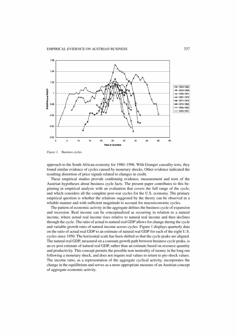
Figure 1. Business cycles.

approach to the South African economy for 1980–1996. With Granger causality tests, theyfound similar evidence of cycles caused by monetary shocks. Other evidence indicated theresulting distortion of price signals related to changes in credit.

These empirical studies provide confirming evidence, measurement and tests of theAustrian hypotheses about business cycle facts. The present paper contributes to this be-ginning in empirical analysis with an evaluation that covers the full range of the cycle,and which considers all the complete post-war cycles for the U.S. economy. The primaryempirical question is whether the relations suggested by the theory can be observed in areliable manner and with sufficient magnitude to account for macroeconomic cycles.

The pattern of economic activity in the aggregate defines the business cycle of expansionand recession. Real income can be conceptualized as occurring in relation to a naturalincome, where actual real income rises relative to natural real income and then declinesthrough the cycle. The ratio of actual to natural real GDP allows for change during the cycleand variable growth rates of natural income across cycles. Figure 1 displays quarterly dataon the ratio of actual real GDP to an estimate of natural real GDP for each of the eight U.S.cycles since 1950. The horizontal scale has been shifted so that the cycle peaks are aligned.The natural real GDP, measured on a constant growth path between business cycle peaks, isan ex-post estimate of natural real GDP, rather than an estimate based on resource quantityand productivity. This concept permits the possible non-neutrality of money in the long runfollowing a monetary shock, and does not require real values to return to pre-shock values.The income ratio, as a representation of the aggregate cyclical activity, incorporates thechange in the equilibrium and serves as a more appropriate measure of an Austrian conceptof aggregate economic activity.

338 KEELER

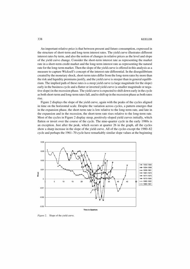
An important relative price is that between present and future consumption, expressed inthe structure of short-term and long-term interest rates. The yield curve illustrates differentinterest rates by term, and also the notion of changes in relative prices as the level and slopeof the yield curve change. Consider the short-term interest rate as representing the marketrate in a short-term credit market and the long-term interest rate as representing the naturalrate for the long-term market. Then the slope of the yield curve is offered in this analysis as ameasure to capture Wicksell’s concept of the interest rate differential. In the disequilibriumcreated by the monetary shock, short-term rates differ from the long-term rates by more thanthe risk and liquidity premiums justify, and the yield curve is steeper than in general equilib-rium. The implied path of these rates is a steep yield curve (a large magnitude for the slope)early in the business cycle and a flatter or inverted yield curve (a smaller magnitude or nega-tive slope) in the recession phase. The yield curve is expected to shift down early in the cycleas both short-term and long-term rates fall, and to shift up in the recession phase as both ratesrise.

Figure 2 displays the slope of the yield curve, again with the peaks of the cycles alignedin time on the horizontal scale. Despite the variation across cycles, a pattern emerges thatin the expansion phase, the short-term rate is low relative to the long-term rate, and late inthe expansion and in the recession, the short-term rate rises relative to the long-term rate.Most of the cycles in Figure 2 display steep, positively-sloped yield curves initially, whichflatten or invert over the course of the cycle. The nine-quarter cycle in the early 1980s isan exception. Just after the peak, which occurs at quarter 26 in the graph, all the cyclesshow a sharp increase in the slope of the yield curve. All of the cycles except the 1980–82cycle and perhaps the 1961–70 cycle have remarkably similar slope values at the beginning

Figure 2. Slope of the yield curve.


and show convergence to a flat or inverted slope at the peak of the cycle. Both Figures 1and 2 reveal the variety of business cycle experience within these basic patterns, in length,amplitude, and time profile.

Changes in short-term rates are volatile and temporary. Adjustments for inflation showthat short-term real rates frequently take on positive and negative values. Bernanke (1990)surveys several interest rate concepts, and suggests that the changes in short-term rates, andespecially the interest rate spread, are dominated by monetary policy and current defaultrisk conditions. His correlations are confirmed by the data set for this study: levels of short-term interest rates are more highly correlated with the measure of money supply growththan are long-term interest rates (0.29–0.33 compared to 0.06–0.20). Bernanke found thattwo measures of the yield curve, the interest rate spread and the slope of the yield curve,were highly correlated with his measures of monetary policy. For the current data set, theslope of the yield curve shows the highest correlation with money supply growth at 0.55.Short-term rates are volatile and directly influenced by current credit market conditions.

The time period of long-term interest rates, ten years for corporate bonds and U.S.Treasury bond rates, corresponds to the longer time period for the life of capital goods.Assuming that changes in the marginal physical productivity of the existing capital stockare slow, of low volatility and long lived, that behavior is matched by market long-terminterest rates. The misperceptions which cause business cycle phenomena, as discussedearlier, include errors in financing capital investments. One of the decisions that investorsmust make is matching the availability of funds with the cost requirements in the buildingprocess for a capital investment project. The risk of that choice may be reduced by aligningthe term of borrowing with the occurrence of expected costs of the project during thetime-to-build. Long-term financing for capital projects avoids the problems of increases inshort-term interest rates before the completion of the project, and appropriate matching offlows of costs and benefits will immunize the project from interest rate risk. The demandfor credit for financing capital projects with a long-term flow of benefits and with a longtime-to-build will occur in long-term credit markets and be coordinated with the naturalrate of interest or expected profit rate.

Long-term interest rates exhibit quite different behavior than short-term rates. Data forthe eight U.S. business cycles show both nominal and real long-term interest rates to becomparatively stable during each cycle. Most cycles show a slight cyclical pattern of a slowand steady rise in the level of the rate through the business cycle peak and then a decline, butthree of the eight cycles have long-term rates that are either flat or decrease steadily. Onlytwo cycles exhibit a rise in long-term rates at the end of the cycle. Most cycles show nominaland real long-term rates in a similar range with the exception of the 1980–82 and 1983–91cycles, which have much higher levels. A variety of inflation adjustments calculates a fewnegative real long-term rates during the 1950–54, 54–58, 71–75 and 75–80 cycles. Theexpectations hypothesis implies a pattern of a shift down of the yield curve at the start ofthe cycle followed by a shift up during the recession, and that is not apparent across theeight U.S. cycles. There is no consistent evidence that long-term rates respond to monetaryshocks.

These data confirm earlier evaluations by Mishkin that long-term interest rates are acycli-cal but not constant, and by Burns and Mitchell that long-term interest rates have lower

340 KEELER

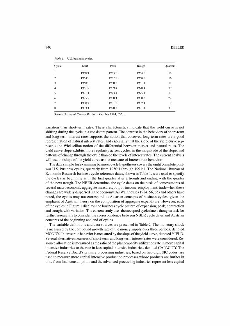
Table 1. U.S. business cycles.

Cycle Start Peak Trough Quarters

1 1950:1 1953:2 1954:2 18

2 1954:3 1957:3 1958:2 16

3 1958:3 1960:2 1961:1 11

4 1961:2 1969:4 1970:4 39

5 1971:1 1973:4 1975:1 17

6 1975:2 1980:1 1980:3 22

7 1980:4 1981:3 1982:4 9

8 1983:1 1990:2 1991:1 33

Source: Survey of Current Business, October 1994, C-51.

variation than short-term rates. These characteristics indicate that the yield curve is notshifting during the cycle in a consistent pattern. The contrast in the behaviors of short-termand long-term interest rates supports the notion that observed long-term rates are a goodrepresentation of natural interest rates, and especially that the slope of the yield curve rep-resents the Wicksellian notion of the differential between market and natural rates. Theyield curve slope exhibits more regularity across cycles, in the magnitude of the slope, andpatterns of change through the cycle than do the levels of interest rates. The current analysiswill use the slope of the yield curve as the measure of interest rate behavior.

The data sample for examining business cycle hypotheses covers the eight complete post-war U.S. business cycles, quarterly from 1950:1 through 1991:1. The National Bureau ofEconomic Research business cycle reference dates, shown in Table 1, were used to specifythe cycles as beginning with the first quarter after a trough and ending with the quarterof the next trough. The NBER determines the cycle dates on the basis of comovements ofseveral macroeconomic aggregate measures, output, income, employment, trade when thesechanges are widely dispersed in the economy. As Wainhouse (1984: 56, 65) and others havenoted, the cycles may not correspond to Austrian concepts of business cycles, given theemphasis of Austrian theory on the composition of aggregate expenditure. However, eachof the cycles in Figure 1 displays the business cycle pattern of expansion, peak, contractionand trough, with variation. The current study uses the accepted cycle dates, though a task forfurther research is to consider the correspondence between NBER cycle dates and Austrianconcepts of the beginning and end of cycles.

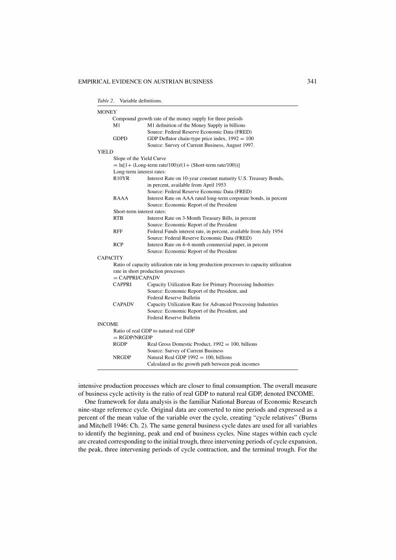
The variable definitions and data sources are presented in Table 2. The monetary shockis measured by the compound growth rate of the money supply over three periods, denotedMONEY. Interest rate behavior is measured by the slope of the yield curve, denoted YIELD.Several alternative measures of short-term and long-term interest rates were considered. Re-source allocation is measured as the ratio of the plant capacity utilization rate in more capitalintensive industries to the rate in less capital intensive industries, denoted CAPACITY. TheFederal Reserve Board’s primary processing industries, based on two-digit SIC codes, areused to measure more capital intensive production processes whose products are further intime from final consumption, and the advanced processing industries represent less capital


Table 2. Variable definitions.

MONEYCompound growth rate of the money supply for three periodsM1 M1 definition of the Money Supply in billions

Source: Federal Reserve Economic Data (FRED)GDPD GDP Deflator chain-type price index, 1992 = 100

Source: Survey of Current Business, August 1997.YIELD

Slope of the Yield Curve= ln[1+ (Long-term rate/100))/(1+ (Short-term rate/100))]Long-term interest rates:R10YR Interest Rate on 10-year constant maturity U.S. Treasury Bonds,

in percent, available from April 1953Source: Federal Reserve Economic Data (FRED)

RAAA Interest Rate on AAA rated long-term corporate bonds, in percentSource: Economic Report of the President

Short-term interest rates:RTB Interest Rate on 3-Month Treasury Bills, in percent

Source: Economic Report of the PresidentRFF Federal Funds interest rate, in percent, available from July 1954

Source: Federal Reserve Economic Data (FRED)RCP Interest Rate on 4–6 month commercial paper, in percent

Source: Economic Report of the PresidentCAPACITY

Ratio of capacity utilization rate in long production processes to capacity utilizationrate in short production processes= CAPPRI/CAPADVCAPPRI Capacity Utilization Rate for Primary Processing Industries

Source: Economic Report of the President, andFederal Reserve Bulletin

CAPADV Capacity Utilization Rate for Advanced Processing IndustriesSource: Economic Report of the President, andFederal Reserve Bulletin

INCOMERatio of real GDP to natural real GDP= RGDP/NRGDPRGDP Real Gross Domestic Product, 1992 = 100, billions

Source: Survey of Current BusinessNRGDP Natural Real GDP 1992 = 100, billions

Calculated as the growth path between peak incomes

intensive production processes which are closer to final consumption. The overall measureof business cycle activity is the ratio of real GDP to natural real GDP, denoted INCOME.

One framework for data analysis is the familiar National Bureau of Economic Researchnine-stage reference cycle. Original data are converted to nine periods and expressed as apercent of the mean value of the variable over the cycle, creating “cycle relatives” (Burnsand Mitchell 1946: Ch. 2). The same general business cycle dates are used for all variablesto identify the beginning, peak and end of business cycles. Nine stages within each cycleare created corresponding to the initial trough, three intervening periods of cycle expansion,the peak, three intervening periods of cycle contraction, and the terminal trough. For the

342 KEELER

trough and peak periods, three months’ data are averaged or one quarterly observation isused directly as the value for the observation. For periods I (initial trough), V (peak) and IX(terminal trough), each observation always corresponds to one quarter of data. Whatever thetime lengths between the initial trough and the peak and between the peak and the terminaltrough, the observations were divided into three equal segments for the remaining periods,II–IV and VI–VIII.

Several problems are created by this method. The “cycle relatives”, expressed as a percentof the average value for the variable over the cycle, assume stationarity. For data seriesthat have a trend, the average value of the series for the cycle is meaningless in this use,unless the series have been detrended. Burns and Mitchell recognized that some variablesexhibit a trend during the cycle, and included it as part of the calculation, but the trendwas only evident in steps from one cycle to the next. Second, the variables often exhibitvarying patterns across cycles. The “cycle pattern” tables and charts provide measures ofthe differences between a particular series and the general business cycle, and Burns andMitchell identified regular occurrences of variables with turning points that lead or lag thebusiness cycle. The NBER method revealed how the lead and lag structure of variablesmay change across cycles. However, the reference cycle method often uses data that areaverages for each variable across all the cycles as the main unit of analysis. The greaterdegree of aggregation obscures the particular characteristics of a cycle, if all business cyclesare not alike. Third, the reference cycle stages do not have a consistent time length acrosscycles. Since the time length of six of the nine intervals is not fixed, there can be variationwithin the cycle that would not appear in the reference cycle data. The Austrian theory inparticular suggests that the magnitude of later changes in income depend on the length oftime that an expansion and allocatively inefficient investment have occurred. The referencecycle method would not permit examination of that important relation. Burns and Mitchell(1946:185–197) recognized that the nine-stage reference cycles constrict this element ofbehavior, and considered alternatives that would standardize the time period, but theirinterest in long-term cycles and the characteristics of particular variables across cycles wasa high priority in their choice of technique. The NBER business cycle relatives frameworkis a particularly poor method for analysis of Austrian business cycle theory because ofits distortion of the timing of changes through the cycle. In the post-war cycles, policyinfluences are more important, and the length of the cycle may be affected, for example, ifmonetary policy stimulus were extended or repeated. Then the effect of a monetary shockmay have a varying lag length which would be difficult to evaluate, given business cyclesof such different length and time patterns.

Instead of the NBER reference cycle framework, the data for the present analysis wereconverted to a standardized cycle length to permit a more consistent exploration of the lagstructure. Standardizing the period of the cycles, allowing each cycle and each variable tohave its unique time profile, may reveal regularities in the time path of response. The datawere standardized to 17 time periods for each cycle, chosen because it is the number ofquarters for one of the cycles, 1971:1–1975:1, so that these data required no adjustment, andtwo other cycles of 16 and 18 quarters each, required little adjustment. For the three shortercycles, each quarterly observation was extended to apply to more than one of the standard-ized observations to result in 17 periods. For the four longer cycles, two or more quarterly


observations were averaged and condensed into fewer periods. Since all variables are stan-dardized by the same weighted averages, this adjustment preserves the correspondence intiming across variables during each cycle. Each standardized time period refers to the sameactual time period for each variable. Although across cycles, a standardized time periodrefers to different actual time lengths, each of the 17 periods within a cycle refers to a standardproportion of the cycle. This method of standardizing the time length preserves the originaltime pattern of each cycle and the relative movements of all variables within the cycle.

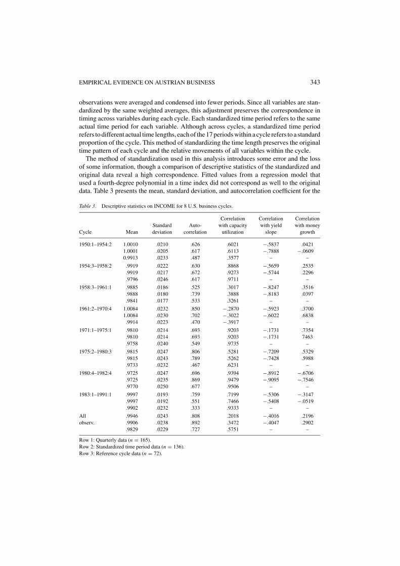
The method of standardization used in this analysis introduces some error and the lossof some information, though a comparison of descriptive statistics of the standardized andoriginal data reveal a high correspondence. Fitted values from a regression model thatused a fourth-degree polynomial in a time index did not correspond as well to the originaldata. Table 3 presents the mean, standard deviation, and autocorrelation coefficient for the

Table 3. Descriptive statistics on INCOME for 8 U.S. business cycles.

Correlation Correlation CorrelationStandard Auto- with capacity with yield with money

Cycle Mean deviation correlation utilization slope growth

1950:1–1954:2 1.0010 .0210 .626 .6021 −.5837 .04211.0001 .0205 .617 .6113 −.7888 −.06090.9913 .0233 .487 .3577 – –

1954:3–1958:2 .9919 .0222 .630 .8868 −.5659 .2535.9919 .0217 .672 .9273 −.5744 .2296.9796 .0246 .617 .9711 – –

1958:3–1961:1 .9885 .0186 .525 .3017 −.8247 .3516.9888 .0180 .739 .3888 −.8183 .0397.9841 .0177 .533 .3261 – –

1961:2–1970:4 1.0084 .0232 .850 −.2870 −.5923 .37001.0084 .0230 .702 −.3022 −.6022 .6838

.9914 .0223 .470 −.3917 – –

1971:1–1975:1 .9810 .0214 .693 .9203 −.1731 .7354.9810 .0214 .693 .9203 −.1731 7463.9758 .0240 .549 .9735 – –

1975:2–1980:3 .9815 .0247 .806 .5281 −.7209 .5329.9815 .0243 .789 .5262 −.7428 .5988.9733 .0232 .467 .6231 – –

1980:4–1982:4 .9725 .0247 .696 .9394 −.8912 −.6706.9725 .0235 .869 .9479 −.9095 −.7546.9770 .0250 .677 .9506 – –

1983:1–1991:1 .9997 .0193 .759 .7199 −.5306 −.3147.9997 .0192 .551 .7466 −.5408 −.0519.9902 .0232 .333 .9333 – –

All .9946 .0243 .808 .2018 −.4016 .2196observ. .9906 .0238 .892 .3472 −.4047 .2902

.9829 .0229 .727 .5751 – –

Row 1: Quarterly data (n = 165).Row 2: Standardized time period data (n = 136).Row 3: Reference cycle data (n = 72).

344 KEELER

INCOME variable and correlations between INCOME and the other three variables. Foreach cycle in the Table, the first row presents statistics on the original quarterly data, thesecond row is for the standardized data with 17 periods for each cycle, and the third row is fordata constructed according to the NBER method with 9 observations (or stages) per cycle.Means for the standardized data are uniformly closer to those of the original data than are theNBER data. As a weighted average, the standardized series exhibits slightly less volatility onevery cycle and throughout the sample. In contrast, the NBER reference cycle data are morevolatile for cycles 1, 2, 5 and 7 but less volatile for others and for the series overall. For somereference cycles, only two quarterly observations were available for the three interveningperiods between a trough and a peak, and for other reference cycles, as many as 11 quarterlyobservations were averaged into one of the intervening periods. That transformation didnot preserve the volatility patterns as well as the standardized period method. The samedistortion appears in the autocorrelations on INCOME and in the correlations betweenINCOME and CAPACITY (the only other variable with all positive values). For somecycles the correlations are more closely matched by the reference cycle data, but thereare not cycles for which the reference cycle method is consistently more accurate acrossthe measures. When the correlations of the reference cycle data differ from the originaldata, they often differ substantially. Judged by these summary statistics, the method ofstandardizing time periods retains more information and performs better than the NBERreference cycle method at preserving the time series characteristics of the original data.

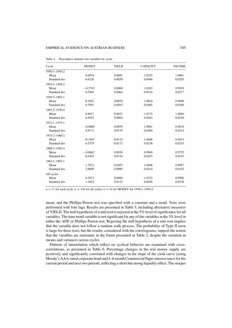
The data transformed for a standardized time period are used to describe patterns ofrelative price changes, resource utilization and income that are common over the eightbusiness cycles. Descriptive statistics for the variables used in the analysis are given inTable 4, for each cycle as well as the entire sample of 136 observations (eight cycles of17 periods each). All the variables display significant differences in mean and all exceptINCOME display significant differences in variance across the eight cycles. No furtheradjustments were made for these differences. The variations in means for different cyclesdo not indicate a trend in any of the four variables across the full sample.

Empirical Evidence on the Austrian Business Cycle Facts

Time series properties of the variables were evaluated with correlograms and unit root tests.Many macroeconomic variables are nonstationary in their level form but are stationary whentransformed. The measures described in Table 2 are expressed in growth rates and ratios,which contributes to their stationarity. The autocorrelation functions of each of the variablesin the sample exhibit a taper from a significant autocorrelation at lag one to non-significantautocorrelation by lag five for INCOME, by lag six for MONEY and YIELD, and lag eightfor CAPACITY. Each variable has significant partial autocorrelations only at lag one or lagsone and two. Evidence from the correlograms indicates the variables are stationary.

Each variable was tested for the presence of a unit root. The null hypothesis of the availabletests is that the variable has a unit root, and if true the behavior of the variable would beconsistent with a random walk process. Then the changes in the value of the variable fromone time period to the next would show non-stationarity. The Augmented Dickey-Fullertest was specified with only a constant since all series exhibit no trend but a non-zero


Table 4. Descriptive statistics for variables by cycle.

Cycle MONEY YIELD CAPACITY INCOME

1950:1–1954:2Mean 0.0918 0.0081 1.0255 1.0001Standard dev. 0.6326 0.0030 0.0466 0.0205

1954:3–1958:2Mean −0.2743 0.0060 1.0383 0.9919Standard dev. 0.5565 0.0064 0.0316 0.0217







All cyclesMean 0.2673 0.0084 1.0332 0.9906Standard dev. 1.1022 0.0123 0.0456 0.0238

n = 17 for each cycle, n = 136 for all cycles, n = 14 for MONEY for 1950:1–1954:2.

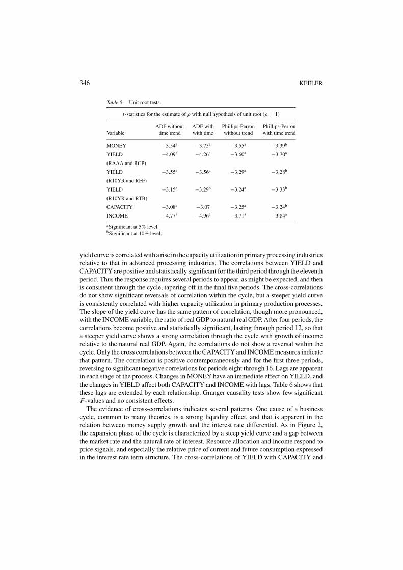
mean, and the Phillips-Perron test was specified with a constant and a trend. Tests wereperformed with four lags. Results are presented in Table 5, including alternative measuresof YIELD. The null hypothesis of a unit root is rejected at the 5% level of significance for allvariables. The time trend variable is not significant for any of the variables at the 5% level ineither the ADF or Phillips-Perron test. Rejecting the null hypothesis of a unit root impliesthat the variable does not follow a random walk process. The probability of Type II erroris large for these tests, but the results, considered with the correlograms, support the notionthat the variables are stationary in the forms presented in Table 2, despite the variation inmeans and variances across cycles.

Patterns of interrelation which reflect on cyclical behavior are examined with cross-correlations, as presented in Table 6. Percentage changes in the real money supply arepositively and significantly correlated with changes in the slope of the yield curve (usingMoody’s AAA-rated corporate bond and 4–6 month Commercial Paper interest rates) for thecurrent period and next two periods, reflecting a short but strong liquidity effect. The steeper

346 KEELER

Table 5. Unit root tests.

t-statistics for the estimate of ρ with null hypothesis of unit root (ρ = 1)

ADF without ADF with Phillips-Perron Phillips-PerronVariable time trend with time without trend with time trend

MONEY −3.54a −3.75a −3.55a −3.39b

YIELD −4.09a −4.26a −3.60a −3.70a

(RAAA and RCP)

YIELD −3.55a −3.56a −3.29a −3.28b

(R10YR and RFF)

YIELD −3.15a −3.29b −3.24a −3.33b

(R10YR and RTB)

CAPACITY −3.08a −3.07 −3.25a −3.24b

INCOME −4.77a −4.96a −3.71a −3.84a

aSignificant at 5% level.bSignificant at 10% level.

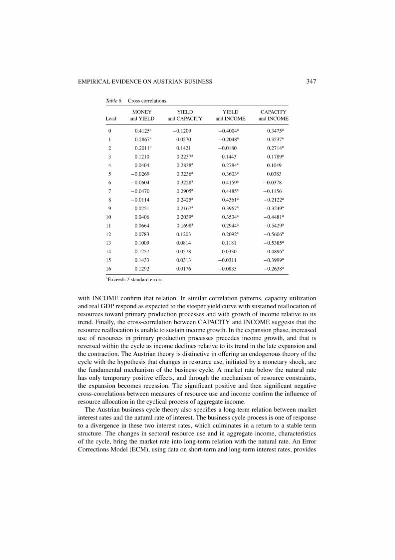
yield curve is correlated with a rise in the capacity utilization in primary processing industriesrelative to that in advanced processing industries. The correlations between YIELD andCAPACITY are positive and statistically significant for the third period through the eleventhperiod. Thus the response requires several periods to appear, as might be expected, and thenis consistent through the cycle, tapering off in the final five periods. The cross-correlationsdo not show significant reversals of correlation within the cycle, but a steeper yield curveis consistently correlated with higher capacity utilization in primary production processes.The slope of the yield curve has the same pattern of correlation, though more pronounced,with the INCOME variable, the ratio of real GDP to natural real GDP. After four periods, thecorrelations become positive and statistically significant, lasting through period 12, so thata steeper yield curve shows a strong correlation through the cycle with growth of incomerelative to the natural real GDP. Again, the correlations do not show a reversal within thecycle. Only the cross correlations between the CAPACITY and INCOME measures indicatethat pattern. The correlation is positive contemporaneously and for the first three periods,reversing to significant negative correlations for periods eight through 16. Lags are apparentin each stage of the process. Changes in MONEY have an immediate effect on YIELD, andthe changes in YIELD affect both CAPACITY and INCOME with lags. Table 6 shows thatthese lags are extended by each relationship. Granger causality tests show few significantF-values and no consistent effects.

The evidence of cross-correlations indicates several patterns. One cause of a businesscycle, common to many theories, is a strong liquidity effect, and that is apparent in therelation between money supply growth and the interest rate differential. As in Figure 2,the expansion phase of the cycle is characterized by a steep yield curve and a gap betweenthe market rate and the natural rate of interest. Resource allocation and income respond toprice signals, and especially the relative price of current and future consumption expressedin the interest rate term structure. The cross-correlations of YIELD with CAPACITY and


Table 6. Cross correlations.

MONEY YIELD YIELD CAPACITYLead and YIELD and CAPACITY and INCOME and INCOME

0 0.4125a −0.1209 −0.4004a 0.3475a

1 0.2867a 0.0270 −0.2048a 0.3537a

2 0.2011a 0.1421 −0.0180 0.2714a

3 0.1210 0.2237a 0.1443 0.1789a

4 0.0404 0.2838a 0.2784a 0.1049

5 −0.0269 0.3236a 0.3603a 0.0383

6 −0.0604 0.3228a 0.4159a −0.0378

7 −0.0470 0.2905a 0.4485a −0.1156

8 −0.0114 0.2425a 0.4361a −0.2122a

9 0.0251 0.2167a 0.3967a −0.3249a

10 0.0406 0.2039a 0.3534a −0.4481a

11 0.0664 0.1698a 0.2944a −0.5429a

12 0.0783 0.1203 0.2092a −0.5606a

13 0.1009 0.0814 0.1181 −0.5385a

14 0.1257 0.0578 0.0330 −0.4896a

15 0.1433 0.0313 −0.0311 −0.3999a

16 0.1292 0.0176 −0.0835 −0.2638a

aExceeds 2 standard errors.

with INCOME confirm that relation. In similar correlation patterns, capacity utilizationand real GDP respond as expected to the steeper yield curve with sustained reallocation ofresources toward primary production processes and with growth of income relative to itstrend. Finally, the cross-correlation between CAPACITY and INCOME suggests that theresource reallocation is unable to sustain income growth. In the expansion phase, increaseduse of resources in primary production processes precedes income growth, and that isreversed within the cycle as income declines relative to its trend in the late expansion andthe contraction. The Austrian theory is distinctive in offering an endogenous theory of thecycle with the hypothesis that changes in resource use, initiated by a monetary shock, arethe fundamental mechanism of the business cycle. A market rate below the natural ratehas only temporary positive effects, and through the mechanism of resource constraints,the expansion becomes recession. The significant positive and then significant negativecross-correlations between measures of resource use and income confirm the influence ofresource allocation in the cyclical process of aggregate income.

The Austrian business cycle theory also specifies a long-term relation between marketinterest rates and the natural rate of interest. The business cycle process is one of responseto a divergence in these two interest rates, which culminates in a return to a stable termstructure. The changes in sectoral resource use and in aggregate income, characteristicsof the cycle, bring the market rate into long-term relation with the natural rate. An ErrorCorrections Model (ECM), using data on short-term and long-term interest rates, provides

348 KEELER

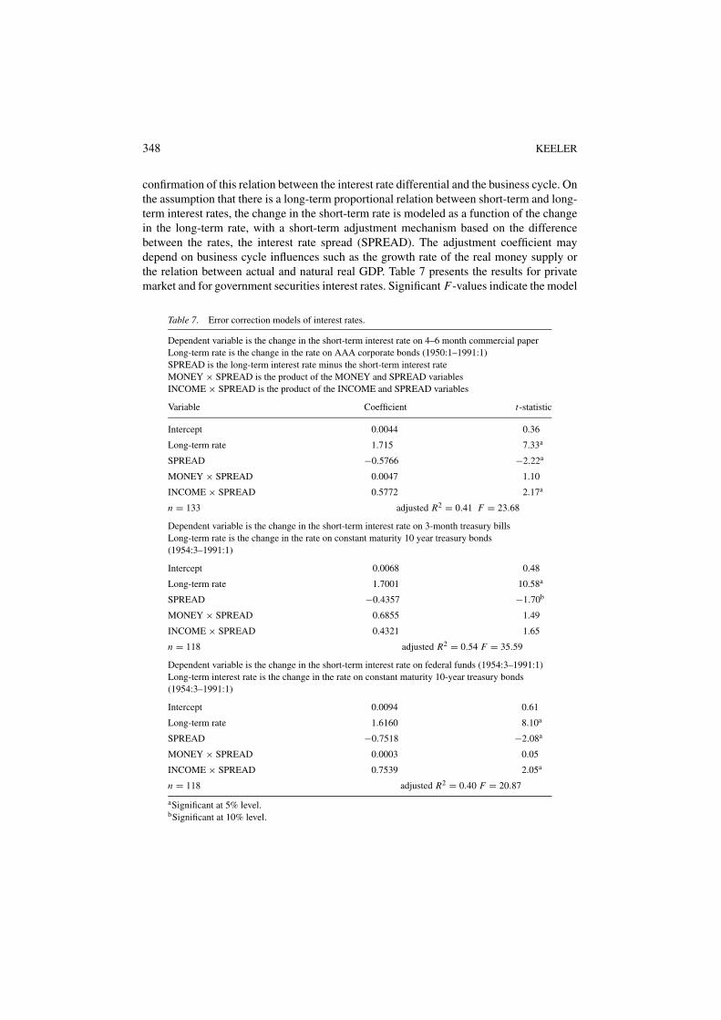
confirmation of this relation between the interest rate differential and the business cycle. Onthe assumption that there is a long-term proportional relation between short-term and long-term interest rates, the change in the short-term rate is modeled as a function of the changein the long-term rate, with a short-term adjustment mechanism based on the differencebetween the rates, the interest rate spread (SPREAD). The adjustment coefficient maydepend on business cycle influences such as the growth rate of the real money supply orthe relation between actual and natural real GDP. Table 7 presents the results for privatemarket and for government securities interest rates. Significant F-values indicate the model

Table 7. Error correction models of interest rates.

Dependent variable is the change in the short-term interest rate on 4–6 month commercial paperLong-term rate is the change in the rate on AAA corporate bonds (1950:1–1991:1)SPREAD is the long-term interest rate minus the short-term interest rateMONEY × SPREAD is the product of the MONEY and SPREAD variablesINCOME × SPREAD is the product of the INCOME and SPREAD variables

Variable Coefficient t-statistic

Intercept 0.0044 0.36

Long-term rate 1.715 7.33a

SPREAD −0.5766 −2.22a

MONEY × SPREAD 0.0047 1.10

INCOME × SPREAD 0.5772 2.17a

n = 133 adjusted R2 = 0.41 F = 23.68

Dependent variable is the change in the short-term interest rate on 3-month treasury billsLong-term rate is the change in the rate on constant maturity 10 year treasury bonds(1954:3–1991:1)



SPREAD −0.4357 −1.70b


INCOME × SPREAD 0.4321 1.65

n = 118 adjusted R2 = 0.54 F = 35.59

Dependent variable is the change in the short-term interest rate on federal funds (1954:3–1991:1)Long-term interest rate is the change in the rate on constant maturity 10-year treasury bonds(1954:3–1991:1)



SPREAD −0.7518 −2.08a


INCOME × SPREAD 0.7539 2.05a

n = 118 adjusted R2 = 0.40 F = 20.87

aSignificant at 5% level.bSignificant at 10% level.


contributes to the explanation of short-term rates, though the adjusted R2 values show thata substantial portion of the variation is not explained. The simple ECM has statisticallysignificant coefficient estimates for the change in the long-term interest rate and the short-term adjustment component. The magnitudes of these coefficients are large relative to thechange in the short-term interest rate, and imply that the effects of one standard deviationchanges in these influences are empirically important. The rate of real money supply growthdoes not have a statistically significant effect on the rate of adjustment between interest ratesin any specification. For the YIELD measures using the private market interest rates andthe Federal Funds rate, the phase of the business cycle, expressed through the INCOMEX SPREAD variable, does affect adjustment. The ratio of actual to natural real GDP hasa positive and significant effect on the rate of adjustment of the short-term rate toward thelong-term rate, and again the magnitude of the effect of a one standard deviation changeis substantial. As real income increases relative to its trend, short-term or market ratesadjust faster toward the long-term or natural rate. The Austrian theory contains such anadjustment of market to natural rates of interest, and the ECM estimate exhibits not only ashort-term adjustment mechanism but also an important role of income growth in resolvingterm structure distortions.

Conclusions

The Austrian theory offers distinctive hypotheses about economic behavior following amonetary shock. Misperceptions generate a change in relative prices, a distortion inconsis-tent with individuals’ time preferences and rates of productivity of capital. The liquidityeffect causes systematic changes in resource use, particularly in investment flows and therates of utilization of capital. By that mechanism, the structure of the capital stock andconsequently all real values are permanently changed. The expansion phase generates theforces which result in recession, through resource constraints and the pressure of incomeand price changes on interest rates. Rather than shocks such as changes in the productivityor scarcity of resources or changes in Aggregate Demand, changes in relative prices are theprimary organizing principle of the business cycle. This paper has examined data on recentU.S. business cycles and develops evidence that confirms these hypotheses.

It has been suggested that “all business cycles are alike” in patterns of the co-movement ofvariables, but cycles with monetary causes of different degrees or sustain may have dramati-cally different effects and less uniformity across cycles. Changes in economic and historicalconditions will alter the characteristics of cyclical behavior over time. Broad patterns of theco-movement of macroeconomic variables cannot capture the structure of responses to rela-tive price changes. Empirical analysis should express Austrian macroeconomic concepts interms of available data measures and still permit non-neutrality as a result of the monetarycycle. To a large extent the empirical concepts in the present analysis have allowed forthat by using measures such as the ratio of actual income to a changing natural incomeand the slope of the yield curve which permits the levels of interest rates to change acrosscycles.

There is evidence of consistent behavior across the eight complete post-war U.S. businesscycles. Stationary measures of interest rates are offered to express Wicksell’s notion of the

350 KEELER

relation between market and natural rates of interest. That concept is shown here to becyclically related to capacity utilization rates and to real GDP through time-series cross-correlations. The estimate of an Error Correction Model indicates that short-term interestrates have a strong adjustment process toward long-term interest rates, and that the cyclicalbehavior of income is an element of that adjustment. The empirical evidence availablein these estimates suggests that there are consistent patterns of relative price change, asexhibited by interest rate adjustment, and that there are systematic changes in the utilizationof resources and the cyclical behavior of income. The evidence confirms the Austrianhypothesis that relative price changes, expressed in the structure of interest rates, induce asystematic response in resource utilization and income.

A common criticism of the Austrian theory is that while relative price changes may exist,they and the changes in investment flows are not large enough to cause the business cyclemovements of aggregate economic activity. The evidence of cross-correlations and errorcorrection is significant and substantial in magnitude, and indicates the contribution of theseeffects. The major finding of this paper is that there are reliable and empirically importantrelations among Austrian macroeconomic concepts. It provides a basis for measuring themagnitude of these effects, by identifying the sequence of macroeconomic measures thatexhibit cyclical behavior. Estimation of a more complete model is necessary to evaluatewhether the Austrian process can account for business cycle behavior.

Acknowledgments

I am grateful to two anonymous referees for their constructive comments, and I wouldlike to thank Seth Seabury, Emiko Nagai, Michael Hickcox and Jennifer Chen for researchassistance.

References

Bernanke, B. S. (1990) “On the Predictive Power of Interest Rates and Interest Rate Spreads.” New EnglandEconomic Review, 51–68.

Burns, A. F., and Mitchell, W. C. (1946) Measuring Business Cycles. New York: National Bureau of EconomicResearch.

Council of Economic Advisors (various issues). Economic Report of the President. Washington, D.C.: U.S.Government Printing Office.

Federal Reserve Economic Data (FRED). St. Louis: Federal Reserve Bank of St. Louis.Federal Reserve Bulletin (various issues). Washington, D. C.: Board of Governors of the Federal Reserve System.Garrison, R. W. (1986) “Hayekian Trade Cycle Theory: A Reappraisal.” Cato Journal, 6(2): 437–459.Garrison, R. W. (1991) “New Classical and Old Austrian Economics: Equilibrium Business Cycle Theory in

Perspective.” The Review of Austrian Economics, 5(1): 91–103.Hayek, F. A. [1967 (1935)] Prices and Production, 2nd edn. New York: Augustus M. Kelley.Hughes, A. M. (1997) “The Recession of 1990: An Austrian Explanation.” Review of Austrian Economics, 10(1):

107–123.Kydland, F. E., and Prescott, E. C. (1990) “Business Cycles: Real Facts and a Monetary Myth.” Federal Reserve

Bank of Minneapolis. Quarterly Review, 14(2): 3–18.le Roux, P., and Levin, M. (1998) “The Capital Structure and the Business Cycle: Some Tests of the Validity of the

Austrian Business Cycle in South Africa.” Journal for Studies in Economics and Econometrics, 22(3): 91–109.Mises, L. von. [1966 (1949)] Human Action, 3rd revised edn. Chicago: Henry Regnery Company.


Mises, L. von. [1971 (1912)] The Theory of Money and Credit. Irvington-on-Hudson, New York: The Foundationfor Economic Education Inc.

Mishkin, F. S. (1981) “The Real Interest Rate: An Empirical Investigation.” In: Brunner, K., and Meltzer, A.(eds.) The Costs and Consequences of Inflation. Carnegie-Rochester Conference on Public Policy: Vol. 15,pp. 151–200. Amsterdam: North-Holland.

Robbins, L. (1934) The Great Depression. London: MacMillan.Romer, D. (1996) Advanced Macroeconomics. New York: McGraw-Hill.Rothbard, M. N. (1970) Man, Economy and State. Los Angeles: Nash Publishing Co.Survey of Current Business (various issues). Washington, D.C.: U.S. Department of Commerce, Bureau of

Economic Analysis.Trautwein, H. M. (1996) “Money, Equilibrium, and the Business Cycle: Hayek’s Wicksellian Dichotomy.” History

of Political Economy, 28(1): 27–55.Tullock, G. (1988) “Why the Austrians Are Wrong about Depressions.” Review of Austrian Economics, 2(1):

73–78.Wainhouse, C. (1984) “Empirical Evidence for Hayek’s Theory of Economic Fluctuations.” In: Siegel, B. (ed.)

Money in Crisis, pp. 37–71. San Francisco: Pacific Institute for Public Policy Research.White, L. H. (1984) The Methodology of the Austrian School Economists. Auburn, AL: Ludwig von Mises Institute.Witte, J. G. (1963) “The Microfoundations of the Social Investment Function.” Journal of Political Economy,

LXXI(5): 441–456.Zarnowitz, V. (1992) Business Cycles: Theory, History, Indicators and Forecasting. Chicago: University of Chicago

Press.Zarnowitz, V. (1999) “Theory and History Behind Business Cycles: Are the 1990s the Onset of the Golden Age?”

Journal of Economic Perspectives, 13(2): 69–90.

Empirical Evidence on the Austrian Business Cycle Theory · Empirical Evidence on the Austrian...

Documents

Transcript of Empirical Evidence on the Austrian Business Cycle Theory · Empirical Evidence on the Austrian...