Modeling Austrian Business Cycle Theory.

Outline of the Goods Side/Money Side Model

Antony P. Mueller

Paper prepared for the Austrian Economics Research Conference (AERC) 2014

March 20-23. The Ludwig von Mises Institute, Auburn

ABSTRACT

Despite the attention that the Austrian business cycle theory has been receiving

from academic economists and financial market operators over the past couple of decades,

its analytical knowledge has remained obscure because of the lack of an analytical model

similar to the ISLM/AS model of textbook economics. The goods side/money side

(GS/MS) approach represents such a model, which should make the Austrian theory of

the business cycle accessible to those who have a formal education in economics but are

unfamiliar with the Austrian business cycle theory. Different from the ISLM/AS analysis,

which serves to design monetary and fiscal policy intervention in order to obtain

macroeconomic policy goals, the GSMS model is non-interventionist. In the perspective

of the GSMS model, macroeconomic policies are the sources of economic disturbances.

The present paper gives an outline of the GSMS model and shows the perils of

macroeconomic policies be it inflation targeting and Taylor rule or nominal national

income targeting.

Dr. Antony P. Mueller

Professor of economics

Federal University of Sergipe (UFS)

Department of Economics

Cidade Universitária

São Cristóvão-SE

CEP 49100-000

Brazil-

E-mail: antonymueller@gmail.com

phone: (55) 79.9601.3131

Modeling Austrian Business Cycle Theory.

Outline of the Goods Side/Money Side Model

ABSTRACT

Despite the attention that the Austrian business cycle theory has been receiving

from academic economists and financial market operators over the past couple of decades,

its analytical knowledge has remained obscure because of the lack of an analytical model

similar to the ISLM/AS model of textbook economics. The goods side/money side

(GSMS) approach represents such a model, which should make the Austrian theory of the

business cycle accessible to those who have a formal education in economics but are

unfamiliar with the Austrian business cycle theory. Different from the ISLM/AS analysis,

which serves to design monetary and fiscal policy intervention in order to obtain

macroeconomic policy goals, the GSMS model is non-interventionist. In the perspective

of the GSMS model, macroeconomic policies are the sources of economic disturbances.

The present paper gives an outline of the GSMS model and shows the perils of

macroeconomic policies be it inflation targeting and Taylor rule or nominal national

income targeting.

1. Introduction

It is not only the financial crisis and the difficulties of mainstream

macroeconomics to provide consistent explanations and remedies that revived the interest

in Austrian economics as an alternative model. In fact, there has been a rising interest in

the Austrian business cycle theory over the past couple of decades. Austrian economics

was an integral part of classical economics before the Keynesian revolution swept it away

almost overnight. Yet while there has been a resurrection of classical economics, the

rehabilitation of the Austrian school of economics is still wanting. Prominent academic

economists still feel vindicated when they admit their ignorance about Austrian

Economics or enunciate outright erroneous versions of its business cycle theory. One

reason that the Austrian business cycle theory is not yet part of the mainstream comes

from not having a persuasive analytical model. There is a need for a model that presents

the main features of the Austrian theory of the business cycle theory in a manner that

facilitates its understanding particularly for those academic economists who are

unfamiliar with Austrian economics.

A model does not tell the whole story, and this is the case with the GS/MS model

as well. The main function of this macroeconomic model is to show the links among the

main parts of the economy. As such, the GSMS model serves as a guide for teaching and

research and offers a framework for the critical discussion of economic policy concepts.

2. Modeling Austrian business cycle theory

The starting point of the Austrian business cycle theory is the question how a

multitude of economic agents simultaneously could commit the same type of error. How

is it possible that entrepreneurs misdirect investments on a large scale? Why do

consumers overestimate systematically their future income streams? Rejecting

psychological explanations, Austrians argue that economic agents must have followed

guidelines, which as a rule prove reliable but failed at the onset of the cycle (Hayek

1975:142). Relative prices and the interest rate in particular must have conveyed false

signals. Market forces by themselves hardly can account for extreme disruptive price

swings, particularly as to the formation of the interest rate, which guides inter-temporal

allocation. The Austrian business cycle theory claims that with more liquidity in the

economy than provided by authentic savings, the intentions of consumers clash with those

of the investors. When monetary authorities push the market interest rate below the

natural rate, real savings fall short of credit demand. This discrepancy disrupts the

perception of resource availability and instigates misallocation of investment. With the

monetary rate of interest below its free market level, investment plans collide with

consumption plans. While consumers have no intention to reduce consumption,

entrepreneurs will want to invest more. The economy gets stimulated, indeed, but what

happens is an artificial boom (Garrison 2000). In as much as economic activity moves

towards full capacity utilization, the more costs and consequently prices will rise. When

interest and wage rates adapt to the higher degrees of scarcity of the factors of production

and when economic actors consequently revise expectations, profit rates come under

pressure and indicate that the earlier calculations of profitability were the result of an

overestimation of the economy’s capacity to grow.

Balance sheets deteriorate for both borrowers and lenders. Economic agents

realize in the bust that they have less wealth than expected. At the inflection point from

boom to bust, the lending and borrowing excitement turns into gloom. Sentiments change

from optimism to pessimism, yet it is not psychology that drives the business cycle. Mood

swings accompany the up and down of the cycle. The actual motor of the business cycle

is the expansion and contraction of macroeconomic liquidity. Inflation and deflation in

their original meaning as expansions and contractions of the circulating means of

payments drive the cycle. Monetary expansion initiates the inception of the business cycle

and financial markets accelerate the economic expansion with a credit bonanza when all

the while the contraction builds up due to bad investment that bring about the reversal of

the inflationary boom into deflationary contraction. Both, expansion and contraction

develop their own dynamics as cumulative self-feeding processes.

The Austrian business cycle theory structures the story of boom and bust around

inflationary monetary creation at the inception of the boom, while monetary contraction

marks the bust (de Soto 2012). Consequently, the focus of the present model lies on the

effects of the variations of the means of payment on output and prices.

3. Outline of the GSMS model

What moves the economy are not aggregates and averages, but individual human

action (Mises 2010). Telling the story in terms of human action is the prime domain of

Austrian economics. The whole story must be told in terms of human action, yet it the

model, which provides the plot in terms of the structure of the story. The criteria of a good

model is to serve as a tool of analysis. Such a model leaves much space for what a good

teacher and analyst should be able to do: to fill the structure with life in terms of human

action.

The quantity theory of money forms the basis for the present approach. This theory

goes back to the 16th century. Over the centuries, the quantity theory of money has

experienced its own cycle with highs, downs and a persistent comeback, particularly at

times when declared as dead. The quantity theory relates (M) to national income (Y) and

transactions (T) and links money to these variables with the concept of velocity of

circulation (V) or cash balance (k).

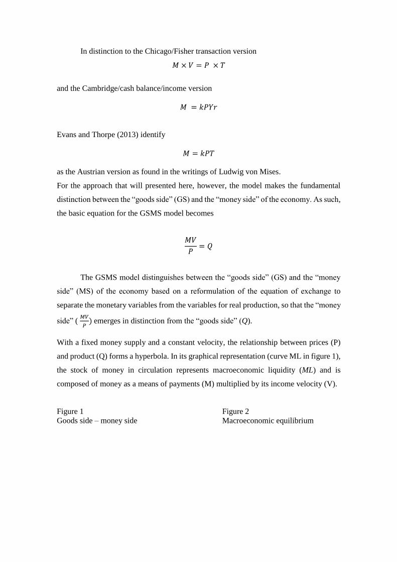
In distinction to the Chicago/Fisher transaction version

𝑀 × 𝑉 = 𝑃 × 𝑇

and the Cambridge/cash balance/income version

𝑀 = 𝑘𝑃𝑌𝑟

Evans and Thorpe (2013) identify

𝑀 = 𝑘𝑃𝑇

as the Austrian version as found in the writings of Ludwig von Mises.

For the approach that will presented here, however, the model makes the fundamental

distinction between the “goods side” (GS) and the “money side” of the economy. As such,

the basic equation for the GSMS model becomes

𝑀𝑉

𝑃= 𝑄

The GSMS model distinguishes between the “goods side” (GS) and the “money

side” (MS) of the economy based on a reformulation of the equation of exchange to

separate the monetary variables from the variables for real production, so that the “money

side” ( 𝑀𝑉

𝑃) emerges in distinction from the “goods side” (Q).

With a fixed money supply and a constant velocity, the relationship between prices (P)

and product (Q) forms a hyperbola. In its graphical representation (curve ML in figure 1),

the stock of money in circulation represents macroeconomic liquidity (ML) and is

composed of money as a means of payments (M) multiplied by its income velocity (V).

Figure 1 Figure 2

Goods side – money side Macroeconomic equilibrium

Given that nominal national income (Y) is equal to real production (Q) multiplied

by the price level (P), nominal income is the rectangle of the area with the price level and

production as its sides. In order to capture nominal national income, the basic model

experiences an extension in the form of

𝑀 × 𝑉 = 𝑄 × 𝑃 = 𝑌

A further extension of the equation by the components of expenditures for

consumption (C), investment (I) and government (G) reveals how the standard Keynesian

analysis relates to the money side and the goods side of the economy.

𝑄 × 𝑃 = 𝑌 = 𝐶 + 𝐼 + 𝐺 = 𝑃𝐶 × 𝑄𝐶 + 𝑃𝐼 × 𝑄𝐼 + 𝑃𝐺 × 𝑄𝐺 + 𝑃𝐸𝑋 × 𝑄𝐸𝑋 − 𝑃𝐼𝑀 × 𝑄𝐼𝑀

Likewise, one can extend the left side in order to include the sources of liquidity.

Macroeconomic liquidity (ML) in the money side of the equation is the result of the

monetary base (MB) multiplied by the financial market or banking multiplier (mb) and the

velocity of circulation (V).

𝑀𝐿 = 𝑀𝐵 × 𝑚𝑏 × 𝑉

At this stage, the macroeconomic story to tell includes the account of money,

prices and goods that begins with the monetary base and continues with the structure of

production.

𝐵𝑀 × 𝑚𝑏 × 𝑉 = 𝑄 × 𝑃 = 𝑌 = 𝐶 + 𝐼 + 𝐺 = 𝑃𝐶 × 𝑄𝐶 + 𝑃𝐼 × 𝑄𝐼 + 𝑃𝐺 × 𝑄𝐺 …

In terms of actors and decisions, the equation contains, beginning at the left and

moving to the right, the central bank, which decides on the monetary base, the actors in

the financial market, which determine the banking multiplier, and all those economic

agents, which decide about cash holdings. At the right side of the equation, the black box

of overall production (Q), price level (P) and nominal national income (Y), opens up in

terms of relative prices, such as PC/PI or PI/PQ, and so on at the level of intermediate

aggregation. In detailed form, the extension of the model beyond the intermediate

aggregation in terms of consumption, investment and government, and the addition of the

external sector, would lead to the analysis of the structure of production.

While the natural production frontier depends on the efficiency of the factors of

production, current output comes from firms as entities where entrepreneurs and

managers combine labor (L), capital (K) and knowhow (A) in order to have an output (q)

that are sold at a price (p) with the intention of earning a profit (Π).

Defining costs in terms of labor and capital with the wage rate (w) and the quantity

of labor (L) along with the interest rate (i) and the capital stock (K), ceteris paribus, both

a higher price (p) and more quantity sold (q) will increase profits. Likewise higher profits

will result from a lower wage rate (w), less use of labor (L) as well as from lower interest

rates and less use of capital. Higher productivity shows up as a reduction of costs. Ceteris

paribus, the productivity variable (A) determines profits when the stock of labor and

capital are fixes and wage and interest rates remain unchanged. Taxes (T) add to costs

and consequently diminish profits. For business, the tax rate (t) typically falls on profits

so that a company pays taxes (T) as a component of its profits (tΠ).

Π − tΠ = (𝑝 × 𝑞) − (𝑤𝐿 + 𝑖𝐾) + 𝐴

An increase of the wage rate (w) will raise prices (p), the more production

approaches capacity limits as a reflection of increasing scarcity. The GSMS model thus

distinguishes between a “natural” and a “cyclical” production frontier (NPF and CPF

respectively in figure 1). The distinction between the normal or regular course of affairs

and exceptional business activity either beyond or below this level is fundamental to the

conduct of a firm. The more economic activity approaches the limits of capacity, the more

costs will rise as the result of increasing scarcity, and the more it will be necessary to

obtain higher prices in order to maintain profitability. Likewise, when activity falls below

its normal level, unused capacity exist and competition drives down prices. Different from

the cyclical production frontier (CPF), which indicates the variation of current production

in relation to the price level, the natural production frontier (NPF) is independent of the

price level and shifts according to changes of the quantity and quality of the factors of

production.

3. Dynamics of the GSMS model

The GS/MS model is composed of the money side (MS), and the goods side (GS)

with the differentiation between the natural production frontier (NPF), the absolute

production frontier (APF), and the cyclical production frontier (CPF).

The dynamic version of the equation of exchange reads as:

𝑔𝑀 + 𝑔𝑉 = 𝑔𝑄 + 𝜋

Given that macroeconomic liquidity (ML) is composed of money multiplied by its

velocity, the equation becomes

𝜋 = 𝑔𝑀𝐿 − 𝑔𝑄

In this reduced form, price changes result from the relationship between growth

of liquidity and real economic growth (gML - gQ), while when applying the determinants

elaborated above, the equation for price inflation becomes:

𝜋 = (𝑔𝑀𝐵 + 𝑔𝑚𝑏+ 𝑔𝑣) − (𝑔𝑄𝑛

+ 𝑔𝑄𝑐)

In order to obtain price stability with an inflation rate of zero (π=0), the condition

is:

(𝑔𝑀𝐵 + 𝑔𝑚𝑏+ 𝑔𝑣) = (𝑔𝑄𝑛

+ 𝑔𝑄𝑐)

The rate of unemployment is inverse to economic expansion, i.e. to cyclical

growth, while natural economic growth (shift of the NPF-curve to the right) comes with

steady employment or an employment rate that remains at its natural level (un). Therefore,

the current unemployment rate (ut) is a function of cyclical economic activity (𝑔𝑄𝑐)),

while the natural unemployment rate (un) coincides with the natural production frontier

(NPF). Finally, nominal national income (Y) is the product of real production and the

price level, or, specified by the model, its growth rate (gY) is:

𝑔𝑌 = 𝑔𝑄 + 𝜋 = 𝑔𝑄𝑛+ 𝑔𝑄𝐶

+ 𝜋

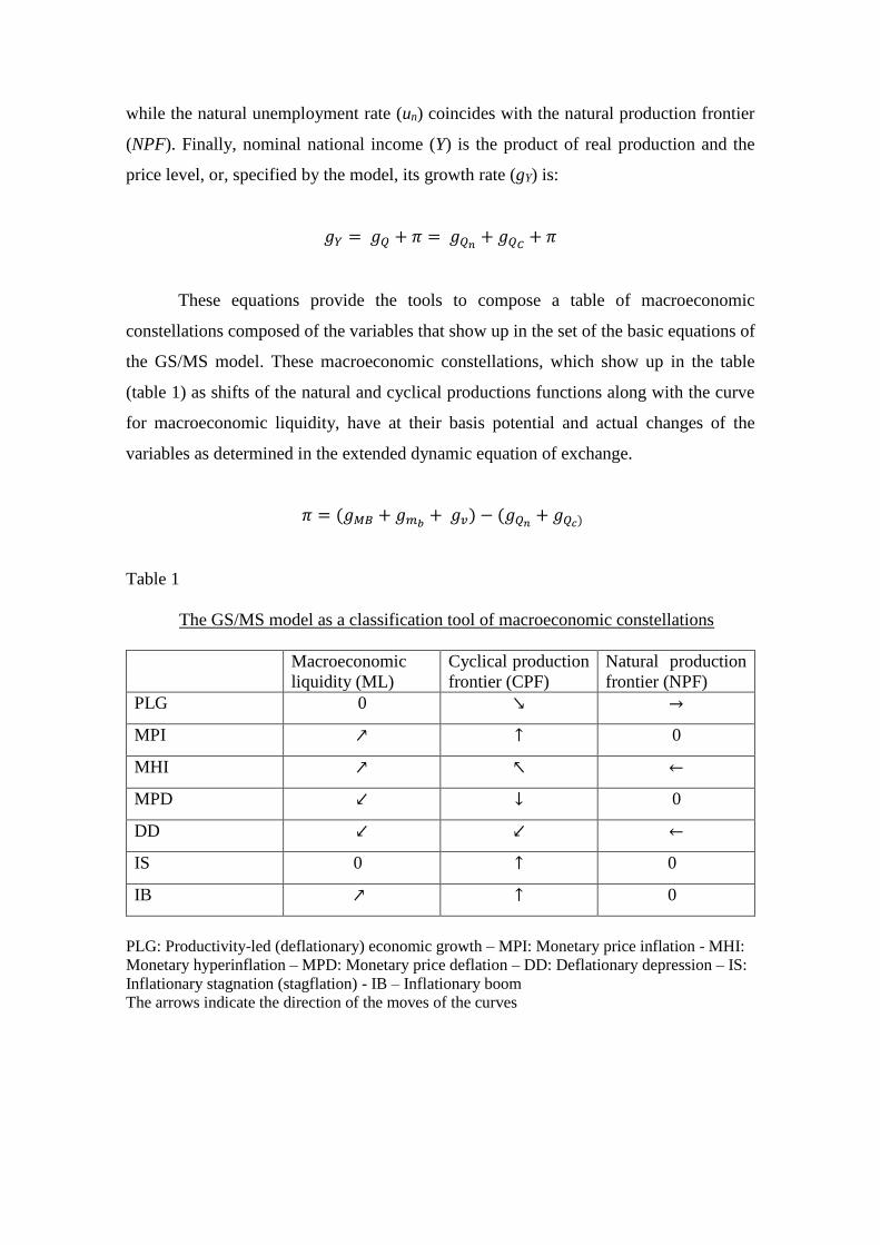
These equations provide the tools to compose a table of macroeconomic

constellations composed of the variables that show up in the set of the basic equations of

the GS/MS model. These macroeconomic constellations, which show up in the table

(table 1) as shifts of the natural and cyclical productions functions along with the curve

for macroeconomic liquidity, have at their basis potential and actual changes of the

variables as determined in the extended dynamic equation of exchange.

𝜋 = (𝑔𝑀𝐵 + 𝑔𝑚𝑏+ 𝑔𝑣) − (𝑔𝑄𝑛

+ 𝑔𝑄𝑐)

Table 1

The GS/MS model as a classification tool of macroeconomic constellations

Macroeconomic

liquidity (ML)

Cyclical production

frontier (CPF)

Natural production

frontier (NPF)

PLG 0 ↘ →

MPI ↗ ↑ 0

MHI ↗ ↖ ←

MPD ↙ ↓ 0

DD ↙ ↙ ←

IS 0 ↑ 0

IB ↗ ↑ 0

PLG: Productivity-led (deflationary) economic growth – MPI: Monetary price inflation - MHI:

Monetary hyperinflation – MPD: Monetary price deflation – DD: Deflationary depression – IS:

Inflationary stagnation (stagflation) - IB – Inflationary boom

The arrows indicate the direction of the moves of the curves

The GSMS model serves to identify specific macroeconomic configurations and

to orient their analysis. The following table (table 2) shows the variables of the model in

order to analyze the links among the different parts of the macro-economy.

Table 2

Macroeconomic constellations in terms of the variables of the GS/MS model

gMB gmb gV gQc gQn π Q Y

PLG 0 0 0 + + - + 0

MPI + + 0 0 0 + 0 +

MHI + + + - - + - +

MPD - - - - 0 - - -

DD - - - - - - - -

IS 0 0 0 - - + - -

IB + + + + 0 + + +

PLG: Productivity-led (deflationary) economic growth – MPI: Monetary price inflation - MHI:

Monetary hyperinflation – MPD: Monetary price deflation – DD: Deflationary depression – IS:

Inflationary stagnation (stagflation) - IB – Inflationary boom with g: growth rate – MB:

Monetary base – mb: banking multiplier – V: velocity of circulation – Qc: cyclical production –

Qn: natural production – π: price inflation rate – Q: Current output – Y: nominal national

income

The tables (table 1 and table 2) provide a sample of typical macroeconomic

configurations. One can also capture specific macroeconomic constellations, such as the

current Great Recession, for example, which would show up as strong growth of the

monetary base, which does not transform into equivalent higher liquidity because of a

low banking multiplier and negative velocity. Consequently, the effect of monetary policy

on output and prices remains flat.

Classifications and categorizations are an important part of science but science

must go beyond schemes and models. This is also the case with the tables above. There

is the need to come up with approaches that capture complexity on the one hand and of

filling the lacunae of the models with human actions. The difficulties of mainstream

economics not only not to foresee the present crisis but also being largely helpless in

dealing with the crisis has led to the expectations that mainstream economics will change

its face (Colander et al. 2004). However, so it seems, a basic model will always be at the

heart of these endeavors to capture reality. This is particularly the case when it comes to

the business cycle.

4. Business Cycle Analysis

In terms of the GS/MS model, “deflationary economic growth” (figure 3a)

represents the dynamic equilibrium of the system. Productivity-led deflationary economic

growth develops in a slow manner and allows the continuous adaptation of expectations.

In contrast to this “beneficial deflation”, a “malicious depression” represents a slide into

a deflationary depression as consequence of a preceding inflationary boom that typically

takes place as a collapse compressed in a short time span (figure 3d). The unexpected

collapse of liquidity disrupts economic contracts in nominal terms and leaves no sufficient

time for revision.

Figure 3a Figure 3b

Productivity-led expansion Inflationary boom

Figure 3c Figure 3d

Inflationary contraction Deflationary contraction

The four graphs (figure 3) present a sequential analysis of the business cycle in

the context of the GS/MS model. Without monetary intervention, increases in

productivity would lead to deflationary economic growth (figure 3a). Such an expansion

would come with increasing purchasing power of money. Monetary authority bring about

an inflationary boom when they try to maintain “price stability” by expanding the money

supply that moves economic activity beyond the natural production frontier (figure 3b).

Economic activity that exceeds the natural level (Q’>Q*) will raise production

prices as consequence of higher degrees of scarcity given the increased amount of

macroeconomic liquidity that is available. In due course, the cyclical production frontier,

which otherwise would have fallen, moves back in direction towards its original position

(CPF*). At this stage, the hidden monetary inflation would become open price inflation

as the economy moves towards stagflation (figure 3c).

The inflationary boom that turned into a bust comes with an overhang of bad debts.

When central banks try to re-inflation the deflationary contraction of liquidity, they

actually commit the same errors twice. The first time, when they warded off beneficial

productivity-led deflationary economic growth, which instigated the inflationary boom

(move from A to C in figure 3b). The second time, when the bust has come, when

monetary policy makers confront malicious deflation and hamper its swift elimination in

their endeavor to re-inflate the economy making the economy stick a point E in the bust

(figure 3d).

Macroeconomic policies that fabricate monetary expansion and push the interest

rate below the free market rate stimulate economic expansion beyond the economy’s

natural production frontier. The original error is the inflationary boom and not the

deflationary contractions. The bust serves to rectify the errors committed in the

inflationary boom. The deflationary contraction is the consequence of the inflationary

boom. Rather than quicken recovery, monetary and fiscal stimuli will hamper the return

to self-sustained economic growth and actually prolong stagnation. In terms of the model

(figure 3d), the natural way of the adaptation would go from D over E to F. Trying to

avoid this process of deflationary expansion, monetary authorities commit in the bust the

same error that initiated the boom.

Since the Keynesian revolution, macroeconomics has found its main raison d’être

in providing tools for policy makers. The central focus of modern macroeconomic is the

thesis that when left on its own, the economy will plunge into depression because of wide

swings of business cycle. Macroeconomic policy must stabilize the economy and prevent

it from falling into deflationary depression. In light of the GSMS model, however,

interventionist macroeconomic policy concepts are flawed. Instead of stabilizing the

economy, macroeconomic policy interventions tends to be ineffective or they will even

contribute to instability.

5. The GS/MS model and monetary policy concept

5.1 Inflation targeting and Taylor rule

Either by default or intent, monetary policy will become excessively expansive in

the face of productivity gains, which in its natural way would move the economy to the

new equilibrium of P’/Q* at point B (figure 3a). With the aim of maintaining a certain

inflation target, central banks apply expansive monetary policy measures (shift of ML to

ML’) that will move the economy from A to C instead of to B. This way, a sustainable

deflationary expansion turns into an inflationary boom (figure 3b). Point C, however, is

not stable because it lies outside of the natural production frontier (NPF*). Rising scarcity

provokes an upward shift of the cyclical production frontier and moves the economy into

stagflation at point D (figure 3c). In the final stage of the cycle, stagflation transforms

into deflationary depression because the malinvestment of the past and the debt overhang

produce a contraction of liquidity and move the economy back into direction of point E

(figure 3d). Different from the situation at the inception of the boom point E marks

deflationary depression and fiscal and monetary policies prove ineffective in instigating

another boom. While at the beginning of the business cycle, expansive monetary policy

pushed the economy into an inflationary boom, they now keep the economy stuck in the

bust.

The so-called Taylor rule includes the goods side into the policy model and

provides a trade-off rule between monetary stability and economic growth. The purpose

of the original version of the Taylor formula (Taylor 1993) was to model the setting of

the federal funds rate over the period 1987 to 1992 by taking into account a rate of two

per cent for the inflation target and the long-run average of the real interest rate. The

Taylor formula includes policy reaction coefficients for the deviation of the prior four-

quarter inflation rate from the target and for the output gap defined as the percentage of

deviation of real gross domestic product from the trend of potential output. Taylor put the

values of both reaction coefficients original at 0.5, yet modified this value for inflation

rate to over one per cent claiming that effective inflation targeting would require a

coefficient of more than one. In normative terms, monetary authorities will set the policy

interest rate (which for the United States would be the Federal Funds Rate), to check

deviations of the current inflation rate from the central bank’s target and of current output

from its trend potential.

Applied to the GSMS model, the last term of the Taylor equation corresponds to

the deviation of the cyclical production frontier from its equilibrium with the natural

production frontier. In the case of inflationary boom (IB), for example, as classified in

table 2 above, the cyclical production frontier rises different from the natural production

frontier. For the Taylor rule, such a deviation would require a raise of the policy interest

rate even more so that in the GSMS model the deviation of current production from the

natural production frontier would show up a price increases. This way, in addition to the

Taylor rule, the GSMS model would reveal the mechanisms that are at work at the

deviation and its correction.

Yet the Taylor model would lead to the same type of error like simple inflation

targeting in the case of productivity gains. There would appear no output gap because in

the case of a productivity-led expansion, higher current output comes along with a

corresponding shift of the production potential as represented by the natural production

frontier. Yet the current price level (πt) would deviate from the target (π*) with πt < π*

and induce monetary policy makers to lower the policy rate of interest (it) and expand the

money supply thereby fabricating an inflationary boom.

5.2 Nominal GDP-targeting

Nominal national income (or gdp) targeting (is a broader monetary policy concept

than the Taylor rule. As such, it includes the Taylor rule as a special as (Koenig 2012).

The GSMS model serves also quite well to analyze targeting nominal gross domestic

product. This macroeconomic policy concept aims at keeping the nominal gross domestic

product constant. As the nominal gross domestic product in equivalent to national income

(Y) and in terms of the GS/MS model, it is graphically (see figure 2 above) the rectangular

area formed by current production (Q) and the price level (P). Nominal gdp-targeting

would inhibit expansive monetary policies in the case of a productivity-led expansion in

as much as nominal income would not change because higher output compensates for

lower prices and nominal national income remains constant with this kind of economic

expansion (Y = Y’). In as much as nominal gdp-targeting advocates a laissez-faire

position, it is compatible with the Austrian position. In fact, nominal national income

targeting would avoid the inception of the inflation-targeting cycle. Beyond that, the

targeting of nominal gross domestic product suffers from the same ailments as any of the

many other interventionist macroeconomic policy concept that call for anti-cyclical

monetary and fiscal policy.

The deficiency of a macroeconomic policy that targets nominal national income

becomes particularly visible when the economy is stuck in deflationary depression (point

E in figure 3d). The size of nominal gdp has come down from the P”/Q*’ to P*/Q*. In

terms of GSMS analysis it would be correct to maintain the size of nominal gross

domestic product as the economy follows its path of natural adaptation and moves from

A to B with gdp unchanged at Q*’/P’. Yet when point A marks the completion of the

cycle instead of its inception, nominal national income targeting would take point D as

reference and try to inflate the economy to the size of P”/Q*. Yet in the light of the

Austrian theory of the business cycle and consequently seen through the lens of the GSMS

model, such as policy would not cure but exacerbate the crisis. Monetary expansion and

fiscal stimuli in the bust would perpetuate the maladjustment of the economy and instead

of bringing the debt burden down, would increase the debt overhang if not of the private

than definitely of the public sector.

5.3 The GSMS model and monetarism

Different from the GSMS model, which extends the basic equation of the

quantitative theory of money to include velocity, monetarism reduces the equation of

exchange by assuming trend-stable velocity. In this interpretation, the price level

becomes a simple function of the money supply.

The practical design of monetarist policy, however, requires the calibration of the money

supply. To do this, monetary authorities must take the velocity of circulation into

consideration in order to calculate the variation of the monetary aggregate in order to

bring the inflation to the target. At the time when Milton Friedman (1968) proposed his

rule, velocity of circulation was highly trend stable, a tendency, which continued until

1979. That time the US central bank began to apply monetarism and volatility became

highly erratic. (see figures 5 and 6)

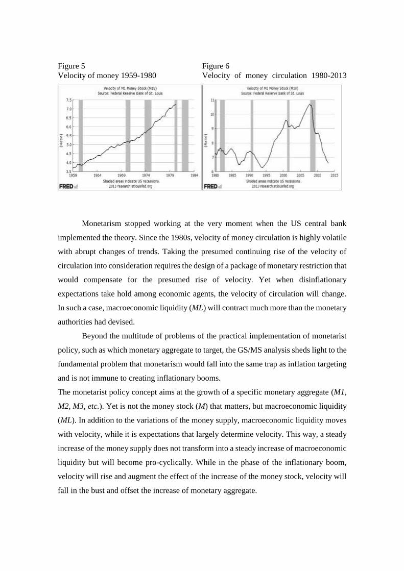
Figure 5 Figure 6

Velocity of money 1959-1980 Velocity of money circulation 1980-2013

Monetarism stopped working at the very moment when the US central bank

implemented the theory. Since the 1980s, velocity of money circulation is highly volatile

with abrupt changes of trends. Taking the presumed continuing rise of the velocity of

circulation into consideration requires the design of a package of monetary restriction that

would compensate for the presumed rise of velocity. Yet when disinflationary

expectations take hold among economic agents, the velocity of circulation will change.

In such a case, macroeconomic liquidity (ML) will contract much more than the monetary

authorities had devised.

Beyond the multitude of problems of the practical implementation of monetarist

policy, such as which monetary aggregate to target, the GS/MS analysis sheds light to the

fundamental problem that monetarism would fall into the same trap as inflation targeting

and is not immune to creating inflationary booms.

The monetarist policy concept aims at the growth of a specific monetary aggregate (M1,

M2, M3, etc.). Yet is not the money stock (M) that matters, but macroeconomic liquidity

(ML). In addition to the variations of the money supply, macroeconomic liquidity moves

with velocity, while it is expectations that largely determine velocity. This way, a steady

increase of the money supply does not transform into a steady increase of macroeconomic

liquidity but will become pro-cyclically. While in the phase of the inflationary boom,

velocity will rise and augment the effect of the increase of the money stock, velocity will

fall in the bust and offset the increase of monetary aggregate.

5.4.The GSMS model and the principle of effective demand

The Keynesian revolution of macroeconomics swept away not only Austrian

economics but with it Say’s law and the respect for scarcity. The principle of effective

demand, which lies at the heart of the basic Keynesian approach, says that aggregate

demand determines aggregate production. The magic of Keynesian economics exists in

the formula that the identification of the cause uno actu promises the cure. When lack of

effective demand is the cause of the depression, all that it takes to get out of the bust is to

produce economic expansion with the help of additional demand. If private business

cannot exert enough demand, government must do it. Debt is the key to prosperity. When

John Hicks (1937), who actually was very sympathetic to Austrian ideas, presented the

Keynesian claim in a graphic model, actually more out of a whim than by conviction

(Hicks 1980/81) there was no longer any halt for the triumph of Keynesianism. In this

spirit, the currently dominant ISLM-AS approach of mainstream economics is more an

engineering tool than a model of the economy (Mankiw 2006).

Despite its triumph, the basic tenet of the Keynesian idea is flawed. The synthesis of the

ISLM model with aggregate supply did not eliminate the faults but added new

inconsistencies (Colander 1995). The GSMS model can help to reveal the contradictions

and omissions of the Keynesian approach. Different from the GSMS model, there is a

profound confusion in Keynesian standard models such as the ISLM scheme about which

variables represent “real” and which “nominal” values. Keynesian models suffer from

obfuscation concerning time when variations of aggregate demand determine production.

Yet while with more money in the economy, demand indeed can augment instantly,

production takes time and its realization confronts a plethora of specific scarcities.

Furthermore, also the aggregate supply and demand model (AS/AD), which was to

substitute and complement the ISLM model, could not do away with fundamental

inconsistencies. While the ISLM model only works as intended when prices are constant,

variations of the price level determine the aggregate demand side of the AS/AD model.

These and many other problems that diminish the analytical value of the Keynesian

models and their derivatives do not show up in the GSMS approach.

In the early decades of the Keynesian revolution, there was an almost complete negation

of money as a macroeconomic factor until the beginning of the monetarist

counterrevolution. Yet what Keynesians did not see or did not want to see was that money

indeed also matters with fiscal policy. Spending is a monetary concept as the term

“expenditure” includes side by side with the good the price component. Deficit spending

implies the creation of additional money that government spends. This way, the principle

of effective demand shows up in the GSMS model as a shift of the ML curve upward to

the right. Yet different from the Keynesian cross or the ISLM model, the GS/MS analysis

draws automatically attention to the question to which degrees such a fiscal stimulus

would stimulus would affect the price level in distinction to real production.

In contrast to the Keynesian approach, the GSMS model makes, firstly, a clear

distinction between the money side and the goods side of the economy. Secondly, with

its crucial distinction between the cyclical and natural production frontier, the GSMS

model discards the illusion of the Keynesian models that sustainable economic growth

could simply come from more spending. Thirdly, the GSMS model opens up the black

boxes of both Keynesianism and monetarism. While the production side evaporates

completely in monetarism, Keynesianism fabricates the illusion of spending as

production.

6. Conclusion

The GSMS analysis differentiates systematically between expenditures that go

into prices and that part which goes into real production. Concerning macroeconomic

policy, the GSMS model is non-interventionist. By letting beneficial deflation happen,

malicious deflation will not show up. The GSMS model highlights the quintessence of

the Austrian business cycle theory according to which inflationary economic expansions

are the result of monetary stimuli (which includes public deficit spending) that provoke

unsustainable booms that revert into busts. While expansionary policy measures function

to initiate a boom, they are ineffective in the bust as the deflationary depression is the

direct consequence of the earlier inflationary boom and the economy suffers from an

overhang of bad debts as the result of misdirected investments. As to its policy

implications, the GSMS model is non-interventionist. Therefore, the GSMS model is

immune to the Lucas critique because the ineffectiveness of macroeconomic policies lies

at the heart of this model.

References

Colander, David (1995). “The Stories We Tell. A Reconsideration of AS/AD Analysis”.

Journal of Economic Perspectives. Volume 9, Number 3. Summer 1995. Pp. 169–188

Colander, David et al (2004). David Colander, Richard P. F. Holt, J. Berkeley Rosser

Jr., The changing face of mainstream economics. Review of Political Economy. Vol. 16,

No. 4, October 2004, pp. 485-499

Evans, Anthony J. and Robert Thorpe (2013). The (quantity) theory of money and

credit. Review of Austrian Economics, Vol. 26, No. 4, pp. 463-481

Friedman, Milton (1968). The Role of Monetary Policy. American Economic Review.

Vol. LVIII March 1968. No 1, pp. 1-17

Garrison, Roger (2000). Time and Money. The Macroeconomics of Capital Structure.

Routledge Foundations of the Market Economy. London: Routledge

Hayek, Friedrich A. (1975). Price Expectations, Monetary Disturbances and

Malinvestments (1933), in: Profits, Interest and Investment and Other Essays on the

Theory of Industrial Fluctuations. Clifton, N.J. 1975: August M. Kelly Publishers

(Reprints of Economic Classics), pp. 135-156

Hicks, John (1937). Mr. Keynes and the “Classics”. A Suggested Interpretation.

Econometrica. Vol. 5, Issue 2, April 1937, pp. 147-159

Hicks, John (1980/81). IS-LM: An Explanation. Journal of Post-Keynesian Economics.

Vol. III, No. 2, pp. 139-154

Koenig, Evan F. (2012). All in the Family: The Close Connection Between Nominal-

GDP Targeting and the Taylor Rule. Staff Papers of the Federal Reserve Bank of Dallas

No. 17, March 2012

Mankiw, Gregory N. (2006). The Macroeconomist as Scientist and Engineer. Journal of

Economic Perspectives. Volume 20, Number 4, Fall 2006, pp. 29-46

Mises, Ludwig von (2010). Human Action. A Treatise on Economics. The Scholar’s

Edition. Auburn, Ala.: The Ludwig von Mises Institute

Rothbard, Murray (2009). Man, Economy and the State. A Treatise On Economic Principles

with Power and Market. Auburn, Ala: Ludwig von Mises Institute, Scholar’s Edition

Solow, Robert M. (1987). Growth Theory and After. Prize Lecture for the Sveriges

Riksbank Prize in Economic Sciences in Memory of Alfred Nobel 1987. http://www.nobelprize.org/nobel_prizes/economic-sciences/laureates/1987/solow-lecture.html

Soto, Huerta de Jesus (2012). Money, Bank Credit, and Economic Cycles. 3rd. edition.

Auburn, Ala.: The Ludwig von Mises Institute

Taylor, John B. (1999). A Historical Analysis of Monetary Policy Rules. In: Monetary

Policy Rules. Chicago. University of Chicago Press, pp. 319-47