Emotion Recognition in EEG
91
Emotion Recognition in EEG A neuroevolutionary approach Stian Pedersen Kvaale Master of Science in Computer Science Supervisor: Asbjørn Thomassen, IDI Department of Computer and Information Science Submission date: June 2012 Norwegian University of Science and Technology
-
Upload
zamzarith-binti-abdul-mutalib -
Category
Documents
-
view
242 -
download
1
description
rsregagerxdf
Transcript of Emotion Recognition in EEG

Emotion Recognition in EEGA neuroevolutionary approach
Stian Pedersen Kvaale
Master of Science in Computer Science
Supervisor: Asbjørn Thomassen, IDI
Department of Computer and Information Science
Submission date: June 2012
Norwegian University of Science and Technology


Problem Description
Study how to recognize emotions defined by an accepted psychological model, in
EEG, by the use of an artificial neural network. This entails an investigation of the
problem areas (Emotions, EEG, and Brain Computer Interfaces), commonly used
computational methods in these areas, and an overview of systems previously de-
scribed in the literature with similar goals. This should result in a method and an
implementation that accomplish the goal of recognizing different emotions in EEG.
Assignment given: January 16th, 2012
Supervisor: Asbjørn Bløtekjær Thomassen
i

ii
Abstract
Ever since the invention of EEG have constant attempts been made to give meaning
to the oscillating signal recorded. This has resulted in the ability to detect a wide
range of different psychological and physiological phenomenon. The goal of this
thesis is to be able to recognize different emotions in EEG by the use of a computer
and artificial intelligence.
Emotions are an especially interesting phenomenon because of the huge impact
they have on humans on the daily basis. They constantly guides and modulates our
rationality, and is thus in some sense an important part of the definition of human
rationality, which again plays an important role in how we behave intelligently and
especially how we behave intelligently when interacting with other humans.
Machines that interact with humans do however not base their decisions on a
rationality that incorporates live human emotions. The effect of this mismatch
in rationality between humans and machines results in unwanted behaviour from
the machines, and is something most have experienced. The system we propose
in this thesis could be used to allow machines to incorporate an interpretation of
human emotions in their principles of rationality, in the form of a recognized two-
dimensional model of emotions, which could result in a more intelligent interaction
with humans. We further restricted our system to the hardware limitations of the
commercially available Emotiv EPOC EEG headset, in order to get an indication
of the commercial value and general implications of our method.
Both unsuccessful and successful systems with similar goals have previously been
described in the literature. These systems typically rely on computationally expen-
sive feature extractions, which make them less attractive when a relatively quick
response is needed. Moreover, the act of choosing what methods to use in order
to extract features entails a degree of subjectivity from the creator, which becomes
clear by looking at the share variety of completely different methods used in the
different systems.
Our system effectively minimizes both of these issues by presenting the signal
as it is, expressed in the frequency domain, to an artificial neural network trained
by a neuroevolutionary method called HyperNEAT, with promising results. This
highlights the importance of using a method that is truly in line with nature of the
problem.
iii

iv

Sammendrag
Helt siden oppfinnelsen av EEG har det kontinuerlig blitt gjort forsøk pa a tolke
signalet man har registrert. Resultatet av dette har gitt oss mulighet til a oppdage et
bredt spekter av ulike psykologiske og fysiologiske fenomen via EEG. Malet i denne
oppgaven er a gjenkjenne forskjellige følelser i EEG, ved bruk av en datamaskin og
kunstig intelligens.
Følelser er et spesielt interessant fenomen pa grunn av den store pavirkningen
de har pa oss mennesker. Siden var rasjonalitet kontinuerlig blir guidet og modulert
av følelser, er de dermed til en viktig del av definisjonen av menneskelig rasjonalitet.
Dette spiller igjen en viktig rolle i hvordan vi oppfører oss intelligent, og spesielt
hvordan vi oppfører oss intelligent nar vi er i interaksjon med andre mennesker.
Maskiner som er i interaksjon med mennesker baserer i midlertidig ikke sine
beslutninger pa en rasjonalitet som inkluderer menneskelige følelser. Disse forskjel-
lene i rasjonalitetsprinsipper mellom mennesker og maskiner kan enkelt sees gjennom
uønsket atferd fra maskiner, noe som de fleste har opplevd. Systemet vi foreslar i
denne avhandlingen kan brukes til a tillate maskiner a innlemme en tolkning av
menneskelige følelser i sine prinsipper om rasjonalitet, i form av en anerkjent to-
dimensjonal modell av følelser, noe som kan resultere i en mer intelligent interaksjon
med mennesker. For a fa en indikasjon pa den kommersielle verdien og de generelle
implikasjonene av var metode, har vi begrenset vart system til a kunne støtte det
kommersielt tilgjengelige Emotiv EPOC EEG-apparatet.
Bade mislykkede og vellykkede systemer med lignende mal har tidligere blitt
beskrevet i litteraturen. De fleste av disse er avhengige av mal og beskrivelser av
signalet som er kostbare beregningsmessig, noe som gjør dem mindre attraktive nar
en trenger relativt rask responstid. Dette innebærer ogsa en viss subjektivitet fra
skaperen av systemet nar man skal velge hvilke mal og beskrivelser man skal bruke,
noe som kommer tydelig frem ved a se pa alle de ulike metodene som brukes i de
ulike systemene.
Vart system minimerer effekten av begge disse problemene ved a presentere sig-
nalet som det er, uttrykt i frekvenser, til et kunstig nevralt nettverk som er trent av
en nevroevolusjonær metode som kalles HyperNEAT, med lovende resultater. Dette
understreker viktigheten av a bruke en metode som virkelig er i trad med problemets
natur.
v

vi

Preface
This master thesis is a continuation of my specialization project conducted in the au-
tumn 2012, and is a part of my degree in Computer Science, with a specialization in
Intelligent Systems, at the Department of Computer and Information Science (IDI),
in the Faculty of Information Technology, Mathematics and Electrical Engineering
(IME), at the Norwegian University of Science and Technology (NTNU).
My motivations for writing this thesis are my general interest in psychology
(including most sub-disciplines), computational models of mental phenomena, and
their link to bio-inspired artificial intelligence methods, as well as sub-symbolic
artificial intelligence in general. I am also intrigued by intelligent user interfaces,
and what the field of affective computing can contribute to this field, when dealing
with people in real-life situations.
I would especially like to thank my supervisor, assistant professor Asbjørn Bløtekjær
Thomassen for the valuable guidance and feedback throughout this process, and for
supporting me in taking a multi-disciplinary approach to the challenges entailed by
the problems investigated in this thesis. I would also like to thank my dear family,
friends, and fellow AI students, for the supportive, inspirational, and constructive
feedback throughout this process period.
Trondheim, June 11th, 2012
Stian P. Kvaale
vii

viii

Contents
1 Introduction 1
2 Background 5
2.1 Emotions . . . . . . . . . . . . . . . . . . . . . . . . . . . . . . . . . 5
2.2 A Window On The Mind . . . . . . . . . . . . . . . . . . . . . . . . . 10
2.3 The Brain and The Computer . . . . . . . . . . . . . . . . . . . . . . 15
2.4 Neuroevolution . . . . . . . . . . . . . . . . . . . . . . . . . . . . . . 24
3 Implementation & Methodology 29
3.1 Getting familiar . . . . . . . . . . . . . . . . . . . . . . . . . . . . . . 29
3.2 Implementation . . . . . . . . . . . . . . . . . . . . . . . . . . . . . . 34
3.3 Exploration of geometrical generalization . . . . . . . . . . . . . . . . 39
3.4 The model . . . . . . . . . . . . . . . . . . . . . . . . . . . . . . . . . 45
4 Experimental Results & Discussion 51
4.1 The Experiment . . . . . . . . . . . . . . . . . . . . . . . . . . . . . . 51
4.2 A Qualitative Explanation . . . . . . . . . . . . . . . . . . . . . . . . 60
5 Conclusion & Future Work 69
A Parameters 73
Bibliography 74
ix

Let’s not forget that the little emotions are the great captains of our
lives, and that we obey them without realizing it.
— Vincent Van Gogh (1889)
x

Chapter 1
Introduction
As early as in 1924 did Hans Berger, a German neurologist, record the first elec-
troencephalogram (EEG) from a human being. An EEG shows the synchronized
neuronal activity from a region of a brain, recorded by an electrode as an oscillating
signal reflecting the electric potential from the group of neurons situated in close
proximity to the electrode. This recording was in the early days only suitable for
detecting large differences seen in the pattern produced, such as epileptic seizures,
because the quality of the recording instrument and the fact that one had to man-
ually inspect the waveform produced in order to identify changes in the rhythms
of the brain. Along with more precise recording equipment, empirical studies of
EEG, and the availability of sufficient computational power in modern computers,
came the rise of the ability to detect even more subtle changes in the electric po-
tential recorded. These subtle changes have been recognized to encode for cognitive
processes such as selective attention, working memory, mental calculations, as well
as specific cognitive states and different types of behaviour (Nunez and Srinivasan,
2006, 2007).
Motivated by the detection of progressively more subtle and intricate changes in
EEG that encodes for even more subtle and intricate mental phenomena, we start
our ambitious quest of detecting human emotions in EEG. There are many mental
phenomena that we find interesting, but emotions stand out from all of these as the
most interesting and important to us because of the huge impact they have on the
daily basis of humans. Emotions constantly guides and modulates our rationality,
and is thus in some sense an important part of the definition of human rationality,
which again plays an important role in how we behave intelligently and especially
how we behave intelligently when interacting with other humans.
This implies that emotions probably must be incorporated in machines in order
1

2 CHAPTER 1. INTRODUCTION
to achieve strong artificial intelligence (human like intelligence). While the thought
of giving machines the ability to base their decisions and behaviour on a rational-
ity that includes their own register of emotions is compelling, we find it even more
important that they base their decisions and behaviour on a rationality that in-
corporates human emotions when they are directly or indirectly interacting with
humans through an interface.
We believe that most have seen how wrong things can go because of the rational-
ity mismatch between machines and humans, but let us illustrate it with a typical
scenario. John Smith buys a new computer with the most common operating sys-
tem (OS) pre-installed. Eager to get started with his new technological investment,
he quickly accepts the recommendation from the machine that all future updates
of the OS should be handled automatically in the background by the system itself.
Then one day when he gets back from lunch, he discovers that the machine has
rebooted by itself. Unfortunately, John Smith does only make backups every after-
noon before going home from work, so half a day worth of work is lost along with
his train of thought. When he logs in on his account on the machine, a festive (but
totally inappropriate) note appears in the lower right corner of the screen stating:
“Congratulations! The OS has successfully been updated, and you are now safe
from outside threats.”
The machine found it rational to reboot even though John Smith was in the
middle some important work, and that losing this work would clearly upset him.
An ideal scenario would be that the machine assessed how upset John Smith would
be if he lost the unsaved work, compared to how upset he would be because of the
consequences of not updating the system immediately. A sub-optimal behaviour
could be that the machine actually made the reboot, but learnt from John’s frus-
tration after losing his work, and modulated its behaviour to never again reboot
without permission.
So by allowing the machine to incorporate an interpretation of human emotions,
a more mutual understanding of what is rational could be achieved, which again
could result in less unwanted behaviour from the machine when interacting with
humans.
We have, up until now, used the word emotions quite recklessly under the as-
sumption that there is a universal consensus in how to describe different emotions.
This is not the case; emotions are indeed a subjective experience, and the ability to
communicate any emotion felt is limited by a person’s psychological and physiolog-
ical abilities, as well as prior experiences and the language used. The word happy
3
is often used to describe an emotion, and most would agree that there is an approx-
imately universal consensus about the meaning of this particular word. However,
when dealing with self-reported data on emotions, it turns out that there is a great
variation in the data collected because of the different interpretations of descriptions
of emotions, which leads to uncertainty in the results from any analysis of this data.
This has led to research on universal models of emotions, which accounts for most
of the variance introduced by self-assessments of emotions.
We rely on one of these models in this thesis in order to get reliable answers when
testing our method of automatically detecting emotions through EEG. By doing so,
we allow the system to generalize over the (more or less) universal cognitive interpre-
tation of emotions, instead of a system that generalizes over pure subjectivity. We
believe that this is an important aspect, because comparing the results from differ-
ent subjects in a system that is not based on a statistically sound model of emotions
would lead to answers that comes with an uncertainty that is not accounted for.
This thesis does also explore brain-computer interfaces (BCI) in order to find
commonly used computational methods for interpretation and analysis of data that
stems from brain activity, and to recognize what different types of systems that exist.
The most interesting parts of this exploration are of course the systems that use EEG
and artificial neural networks, as it is the main focus given our problem description.
To add further constrains, should the methodology we use be compatible with the
commercially available Emotiv EPOC EEG-headset, which has considerably less
electrodes than the EEGs used for medical applications, and will thus indirectly
give clues whether or not the methodology used is capable of detecting emotions
with equipment anyone can get their hands on.
During the exploration of BCI systems, we found that many of the systems were
based on a large variety of features extracted from the EEG signal of subjects. Some
of these were just simple measurements, while others were more sophisticated and
advanced in nature, but all have in common that they were chosen by the creators
of the systems because they are believed to give some meaningful descriptions of
the data. Many of these may very well be highly descriptive, but we believe that it
is possible to avoid this subjectivity (of choosing what methods to use in order to
extract features) by using a method capable of generalizing over the nature of the
problem as is. Avoiding features does also mean a reduction in the computational
overhead they pose, which is important in systems that require a quick response.
Looking back to what EEG is makes it clear that we are dealing with signals that
are read from different positions of the skull of a subject. This makes it a problem

4 CHAPTER 1. INTRODUCTION
that is geometrical in nature. A neuroevolutionary method called HyperNEAT that
directly evolve solutions on the basis of the basic geometry of the problem is then
our choice of method to evolve ANNs that are capable of detecting and outputting
values encoding for different emotions, based on the model of emotions we rely on.
Our research question is then to investigate if HyperNEAT is a viable technique
for detecting emotions in EEG with the hardware limitations posed by the Emotiv
EPOC headset, and by that find out if it is possible to avoid the subjectivity involved
with choosing methods for feature extractions and the computational overhead they
pose, as well as an indication of the commercial value and impact of our system.
a
The structure of the thesis is as follows. This chapter will gives a brief introduc-
tion to the problem areas, our motivation for this specific problem, and our research
question.
Chapter 2, Background, starts with exploring different models and notions of
emotions, followed by an introduction to EEG and common computational methods
used in EEG analysis. We then give an introduction to BCI and commonly used
methods for BCIs in general and for emotion recognition. Lastly comes an intro-
duction to neuroevolution and a detailed explanation of the HyperNEAT method,
and where it stem from.
Chapter 3 is called Implementation and Methodology, where we first get familiar
with the EEG signal, followed by a description of how we implemented HyperNEAT,
a brief test of the capabilities of the implementation, and finally the formal config-
uration of our model.
Chapter 4, Experimental Results and Discussion, presents our experiment and
displays the quantitative results, followed by a qualitative investigation in order to
highlight interesting findings in the results.
Chapter 5, Conclusion and Future Work, is the concluding chapter of this thesis
where our formal conclusion appears along with comments on limitations and future
work.

Chapter 2
Background
Psychology, neurophysics, neuropsychology, physics, and computer science, are all
part of the multidisciplinary approach to this thesis. More specifically: Emo-
tions, electroencephalography (EEG), neuroevolution (NE), brain computer inter-
faces (BCI), affective computing, and intelligent user interfaces (IUI), are all subjects
or fields that influence and motivate this work to such an extent that we feel that
it is necessary to present them, both from a scientific and philosophically point of
view, to the reader before venturing into the main chapters.
This chapter will serve as a theoretical background, projecting our justification
for the methodology chosen and our motivation for investigating this highly chal-
lenging problem—why we find this particular research area important in general.
By tying together the previous mentioned fields and topics, alongside an analysis
of related work which we consider important or state of the art, an overview of the
problem area arises, which do elicit our research question as posed in Chapter 1.
2.1 Emotions
What are emotions and mood? –This question, when generalizing in to the broad
term affect, has intrigued mankind ever since the ancient philosophers, and probably
even earlier, if one consider a general increase in self-consciousness alongside the
evolutionary increase in the intelligence of humans. It is however hard to document
these early thoughts on affect—a cave painting may display affective states, but it
is surly unclear if those paintings merely displays affective states as experienced by
the painter, or if they display the painter’s self-conscious thought on the experience
of the states. We will thus focus on well documented (written), and hence work
5

6 CHAPTER 2. BACKGROUND
on affect and emotions which are easily referenceable when deducting a notion of
emotions to rely on in this thesis.
Aristotle was one of these early philosophers with clear ideas about emotion, and
wrote in Rhetoric (1378b, English translation by W. Rhys Roberts):
”The Emotions are all those feelings that so change men as to affect
their judgements, and that are also attended by pain or pleasure. Such
are anger, pity, fear and the like, with their opposites.”
This statement itself is not unproblematic, as discussed in (Leighton, 1982), but more
interestingly in this context: he identifies (even ever so vaguely) distinct emotions
(anger, pity, and fear) as emotions felt by human beings. No such distinct emotions
are mentioned in the Republic of Plato. However, the emotive part seems to be one
of his three basic components of the human mind, while Aristotle on the other hand
had no such vision of a separate module of mind, but did instead see emotions as
important when it comes to moral (De Sousa, 2012). Descartes, with his dualism
(separation of mind and body, which occasionally meets in a gland at the stem
of the brain), refers to emotions as a type of ”passion”, where his six ”primitive”
passions are: love, hatred, joy, sadness, desire, and wonder (Solomon, 2010). The
gland he referred to was the ”communication point” of mind and body, allowing
bodily manifestation of passions (emotions) and vice versa, which helped keeping
his theory of dualism valid.
It is evident that all the great thinkers had their unique theories on emotions.
Some thin lines could be drawn between Aristotle’s distinct emotions and Descartes’s
primitive passions, if one is ignorant on their different perspectives on mind and
body—where emotions stem from, what they are in the realm of the human mind,
and how they manifest. Even the meaning of the words ”emotion” and ”passion”
have changed sufficiently through millennia and centuries, and thus contributing
further to the uncertainty regarding early affective studies and how to compare
them to each other (Solomon, 2010).
It is also evident, by reading modern research, that these great thinkers should
not have their theories on emotions completely discarded; some of their insight is
still valid. The invalid theories just prove the difficulties in trying to understand, and
model, human emotions. Some of these difficulties may have a generational origin,
that is, the overall focus of the creator of the theory seem to be heavily influenced
by the areas that the society in general was concerned with (e.g. different views
on morale and ethics). Another generational issue is the limitations posed by the
scientific progress in other research fields. A good example of this is Descartes with
2.1. EMOTIONS 7
his slightly confused view of the actual functions of the pineal gland, which was by
that generational standard, based on state of the art science on human anatomy
(Solomon, 2010).
The other main ingredient in the soup of uncertainty of human emotions is nat-
urally subjectivity. An emotion is indeed a subjective experience, and the ability to
communicate an emotional state to others is severely limited by the subject’s phys-
iological and psychological capabilities, previous experiences, and the uncertainty
about the code used to communicate (e.g. the actual meaning of a written or spo-
ken word). Unfortunately, creating a model of emotions which is generalizable to
most in the total human population requires self-reported data (possibly lots of it),
given the complexity of the problem. Considering the previous mentioned causes
of uncertainty in self-reported data, it is clear that a perfectly reasonable model of
emotions may suffer badly in terms of accuracy and generalizability just because of
the variance introduced by this uncertainty. More precisely: a sound model might
be falsely rejected because of uncertainty in self-reported data that is not accounted
for.
Psychology—the science of mind—base its research, and thus its universal the-
ories of the human mind, on observed or self-reported data. As emotions receive a
constant attention in psychology, constant attempts have been made to identify a
universal notion of emotions which accounts for the variance in self-reported data
on affect, and hence reducing the uncertainty of the data itself. The basis for psy-
chological research (or any types of research) on emotions is lost without a universal
notion of emotion; research without sufficient statistical power have in best cases
only a weak influence on its field (or any field) in modern science.
Motivated by an interest for an adjective check list for self-report data on mood,
Nowlis and Nowlis (1956) conducted factor-analysis on data gathered from subjects,
in a quest for some independent factors of mood. As shown in (Russell, 1980), this
triggered a relatively large group of psychologist to conduct similar studies, where all
concluded with 6 to 12 independent mono-polar independent factors of affect. As an
example of these factors, Russell (1980) lists the following of what this group found:
the degree of anxiety, tension, anger, sadness and elation. This is an important
step in the attempt to create a notion of emotion which accounts for the variance
in the self-reported data—it is the beginning of the theory of discrete categories of
emotions, and its underlying assumption (Russell, 1980).
Paul Ekman, inspired by Darwin, did in his cross-cultural work on universal facial
expressions, find six basic emotions: anger, disgust, happiness, sadness, surprise

8 CHAPTER 2. BACKGROUND
and fear (Ekman and Friesen, 1971), where disgust and surprise are debated as too
simple to be called emotions (De Sousa, 2012). Ekman did in (1992) state: ”It
should be clear by now that I do not allow for ”non-basic” emotions”, yet later he
proposed in (Ekman, 1999) an extended list of 15 ”emotion families” which could
by his definition be thought of as basic. This could be an example of challenges met
when dealing discrete categories of emotions, and leads to the following questions
about this notion: do the labels (words) change over time, and if they do change
over time, how can one be sure that the labels used are valid as per now? Another
important question is: are all or most emotions basic, and if they are, would not
the universal labels of the basic emotions just capture a consensus of the meaning
of the few labels listed as basic by Ekman and likes? We will not attempt to answer
these questions, but we do identify them as important ones regarding this notion.
Anyhow, discrete categories of emotions do provide a statistical sound notion of
emotions which account for some of the variance in self-reported data on affect,
even though the number of categories/labels may restrict the resolution and share
number of universal emotions.
Interestingly, alongside this notion exists the notion that emotions are better
described by a few dependent bi-polar dimensions, than by a range of indepen-
dent mono-polar factors. Schlosberg presented a three-dimensional model of af-
fect: sleep-tension, attention-rejection and pleasantness-unpleasantness (Schlosberg,
1952, 1954). Inspired by this model, Russell (1980) presented his two-dimensional
circumplex model of affect. The first of the two dimensions are pleasure-displeasure,
which is analogous to Schlosberg’s pleasantness-unpleasantness. The second, arousal-
sleep, is a combination of the other two dimensions in Schlosberg’s model, as Russell
in his work found the two of them so correlated (r=.85) and therefore not differ-
entiable (Russell, 1980). Even more valuable than a reduction of dimensions, he
discovered that the model accounted for much of the variance in self-reported data,
which makes the model quite robust. Conte and Plutchik’s work on a circumplex
model of personality traits (Conte and Plutchik, 1981), and Plutchik’s later ”wheel
of emotion” or ”solid of emotion” (Plutchik, 2000, 2001) does further support this
notion of emotions.
We will rely on this notion through this thesis, and target Russell’s model when
considering test-data and classification. That is, using his model as a metric for
emotions. The model itself is based on the internal representation of affect of the
persons tested, their cognitive structure of the interpretation of emotions, and not
a description of their current affective state (Russell, 1980). A universal and easily
transferable metric is then achieved, compared to a metric from the notion of some

2.1. EMOTIONS 9
Arousal
Sleepiness
PleasureMisery
Distress
Depression
Excitement
Contentment
Figure 2.1: The two dimensional notion of emotions we rely on in this thesis (from
Russell, 1980)
specialized mono-polar factors.
Going back to the great thinkers, it is easy to unveil their insight and their
influence on the research on emotions. Descartes with his primitive passions are
much in line with the notion of mono-polar discrete factors of emotions, even though
the exact meaning of the labels (words) is unclear. Aristotle’s statement about
emotions could actually be interpreted as valid to both notions; he lists a few distinct
emotions on the one hand, but on the other hand he does end the statement about
emotions rather open. By open, we mean that is unclear whether or not the opposites
of the emotions mentioned was independent mono-polar factors, or just at the other
end of a dependent bi-polar dimension. This will remain unanswered.

10 CHAPTER 2. BACKGROUND
2.2 A Window On The Mind
By calling Electroencephalography (EEG) for ”a window on the mind”, Nunez and
Srinivasan (2006) captures the essentials of what EEG is: a ”window” invented by
Hans Berger in 1924, which allow us to take a closer look of what is really going on
inside a brain.
The window is created by attaching electrodes at different positions on the scalp
of the subject which reveals the mesoscopic (in the world of neurons) regional differ-
ence in electric potentials. Assuming that different cognitive patterns create unique
activation patterns makes the oscillating signal from the electrodes the electric man-
ifestation of our brain activity, and thus to some degree our mind. However, as with
a house and its windows, EEG is limited by the density (spacing between) of elec-
trodes; it is easier to get the correct picture of what is inside a greenhouse, than it
is with a bunker. Another important factor is the placement of the electrodes on
the scalp. If we consider a range of subjects to have their EEG recorded for a defi-
nite time window, then the recordings would be practically useless when comparing
results, if the electrodes were placed at random.
In an attempt to reduce the uncertainty of what (as a result of where) that is
being measured, a standard called the ”10-20 system” was introduced (Malmivuo
and Plonsey, 1995). This is the current working electrode placement system when
recording EEG signals on human beings, and takes its basis on universal landmarks
on the human skull (nasion and inion). The ”10-20” in the name, indicates that the
first electrode placed should be separated from the landmark with a distance of 1/10
of the total distance from one landmark to the other, while the rest of the electrodes
should be separated by 1/5 of the total distance. Each electrode in this system got
a unique id which is a combination of characters and numbers, where the characters
encodes for the specific region (lobe) of the brain, and the number encodes for the
specific position on that particular lobe. The numbers do also indicate on which
part of the right/left homologues hemispheres of the brain an electrode is located,
where even numbers encode for right hemisphere and odd numbers encode for left
hemisphere.
As pointed out earlier, and by Nunez and Srinivasan (2007), researchers do often
want to achieve as high as possible resolution, and thereby density, of the electrodes
when collecting data. This has led to extended versions of the 10-20 system, like
the 10% system proposed by the American Electroencephalographic Society (AES)
(Sharbrough et al., 1991). This system, with its increased resolution, follows the ba-
sic principles from the 10-20 system both in approach and in the naming convention
2.2. A WINDOW ON THE MIND 11
of the electrodes. Few direct conflicts exist between these systems, so it is possible
to compare the result between the two of them. The choice of which of the systems
to use, do often come naturally by the number of electrodes available, as they both
achieve the same by using the same technique: relative positioning of the electrodes
which minimizes the variance in the data from different recordings, from possibly
different subjects with different skull shapes.
We will rely on the 10-20 system in this thesis, since both our EEG setup and
data do so.
So with an idea of what EEG is, and how electrode placement systems allow
quantitative research by creating a similar ”window on the mind”, it is time to
investigate some commonly used computational methods which gives meaning to
the oscillating signal received from the electrodes. Nunez and Srinivasan (2007)
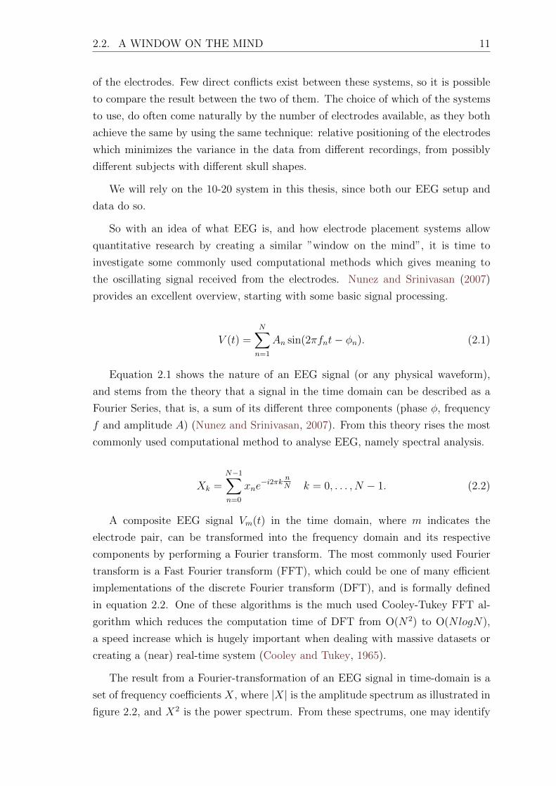
provides an excellent overview, starting with some basic signal processing.
V (t) =N∑n=1
An sin(2πfnt− φn). (2.1)
Equation 2.1 shows the nature of an EEG signal (or any physical waveform),
and stems from the theory that a signal in the time domain can be described as a
Fourier Series, that is, a sum of its different three components (phase φ, frequency
f and amplitude A) (Nunez and Srinivasan, 2007). From this theory rises the most
commonly used computational method to analyse EEG, namely spectral analysis.
Xk =N−1∑n=0
xne−i2πk n
N k = 0, . . . , N − 1. (2.2)
A composite EEG signal Vm(t) in the time domain, where m indicates the
electrode pair, can be transformed into the frequency domain and its respective
components by performing a Fourier transform. The most commonly used Fourier
transform is a Fast Fourier transform (FFT), which could be one of many efficient
implementations of the discrete Fourier transform (DFT), and is formally defined
in equation 2.2. One of these algorithms is the much used Cooley-Tukey FFT al-
gorithm which reduces the computation time of DFT from O(N2) to O(NlogN),
a speed increase which is hugely important when dealing with massive datasets or
creating a (near) real-time system (Cooley and Tukey, 1965).
The result from a Fourier-transformation of an EEG signal in time-domain is a
set of frequency coefficients X, where |X| is the amplitude spectrum as illustrated in
figure 2.2, and X2 is the power spectrum. From these spectrums, one may identify

12 CHAPTER 2. BACKGROUND
0 20 40 60 80 100 120 140Time t
−400
−300
−200
−100
0
100
200
300
Ele
ctri
c pote
nti
al
(a) 128ms EEG signal in time-domain
0 10 20 30 40 50 60 70Frequency (Hz)
0
1000
2000
3000
4000
5000
6000
Am
plit
ude
(b) 128ms EEG signal in frequency-domain
Figure 2.2: A 128 data point EEG in the time domain (a), and the same signal in the
frequency domain (b). The Cooley-Tukey algorithm with N = 128 is used to transform
the signal
the typical EEG-ranges (bands) used for analysis: delta (0–4 Hz), theta (4–8 Hz),
alpha (8–13 Hz), beta (13–20 Hz) and potentially gamma (30–40+ Hz) (Nunez
and Srinivasan, 2006). We say ”typical” about these infamous bands, because, as
pointed out by Nunez and Srinivasan (2007), unique combinations of these bands
are found to encode for cognitive states, behaviour, location on the brain, and so
forth. In other words, combinations of these bands do seem to encode for interesting
psychological and physiological (neurological) phenomena.
Rather than just accepting this as a computational method that clearly works,
we want to explore the obvious questions: (a) from where do these qualitative labels
have their origin, and; (b) why is it such that a (potential) loss of information and
precision is preferred to the output from the transformation as it is?
The answer to (a) lies in the history of EEG from when it was printed out
continuously on paper, and experts in interpreting the print manually counted zero-
crossings within a given time interval, where the ranges served as qualitative labels
(Klonowski, 2009; Nunez and Srinivasan, 2006). An answer to (b) is however not so
simple but may be explained as a result of the nature of the EEG signal and how it
is transformed.
From Klonowski (2009) and Sanei and Chambers (2008), we have that an EEG
signal, and many bio-signals in general, is described by the ”3 Ns” (noisy, non-linear,
and non-stationary)1. Klonowski argues that many researchers do agree that the
human brain is one of the most complex systems known to humans, and therefore
1A more detailed explanation of noise and artifacts in EEG, and how to automatically reduce
them, can be found in (Kvaale, 2011)

2.2. A WINDOW ON THE MIND 13
treating it as a linear system seems unreasonable, which as an argument seems
reasonable. As a side note, this highlight an interesting paradox—we know (or
think we know) more of the universe as a highly complex system, than of the system
(human brain) that is producing that knowledge.
Treating a non-linear system as linear will naturally not capture its dynamics
correctly. Hence using linear methods like FFT, do in best case capture a simplified
view of the dynamics in an EEG signal. While this sound unoptimistic, let us not
forget that this simplified view is what the main portion of EEG research have been
using with promising and statistically sound results. However, this only highlights
a problem using linear methods, and provides no direct clue to (b).
A basic assumption for FFT is that the signal is stationary (no change in sta-
tistical distribution over time), which is clearly violated since EEG signals is non-
stationary. The effect of this violation is clear in (Klonowski, 2009), where he illus-
trates this by applying FFT to a 12Hz signal with its amplitude modulated with 1
Hz, resulting in two harmonic signals of 11Hz and 13Hz with half the amplitude of
the original 12Hz signal (fig. 2.3). This is where we might find a clue in an attempt
to answer (b) and why research using this technique appears to get some valid find-
ings, even though treating the system with a lower complexity than what it actually
is (linear), and violates the basic assumptions of FFT (stationary). From the exam-
ple, if one considers 11-13Hz as a band, then the sum of the band will be equal to
the original 12Hz frequency, and does therefore yield the same result as if the signal
was stationary, so the bands functions as ”safety nets” for the non-stationarity. It
is also evident that a smearing from neighbouring bands and frequencies will distort
the total sum, adding uncertainty to the results, but is anyhow a better estimate
than looking at the single 12Hz (which appear as zero).
The answer to (b) may then be that what appear to be the most descriptive
ranges of EEG-signals, are actually the ranges where the smearing produced by the
non-stationarity is of lowest variance, or where the borders of the ranges minimize
overlapping, and hence providing the most stable results. So the ranges are actually
the most descriptive ranges of the EEG-signal with regards to linear, and possibly
stationary, time-frequency transformation methods. Although a loss in precision is
inevitable (what is the exact frequency coeffecient?), one must say that this compu-
tational method is a perfect example of where a naıve approach to a system with an
unknown scale of complexity, is producing viable results, and thus making headway
in the general knowledge of the system itself.
Researchers like Klonowski (2007, 2009), Nunez and Srinivasan (2007) and Nunez

14 CHAPTER 2. BACKGROUND
Figure 2.3: A 12Hz signal with its amplitude modulated by 1Hz results in two harmonic
waves of half the amplitude, when transformed with FFT, because of the violation of the
basic assumption that the signal is stationary (from Klonowski (2009)).
and Srinivasan (2006) do all indicate that EEG research on non-linear and dynamic
systems will contribute to an increase in our general understanding of brain function,
and its physical aspects. Dynamic behaviour of sources (brain dynamics) and brain
volume conduction are mentioned as computational methods in EEG by (Nunez and
Srinivasan, 2007), and they are essentially the study of the physical aspects of EEG.
The study of brain dynamics is concerned with the understanding and the devel-
opment of models that correctly describes the time-dependent behaviour of brain
current sources (e.g. the propagation speed in brain tissue, interaction between hi-
erarchical, local and global networks, frequency dependence, resonant interactions,
and so forth)(Nunez and Srinivasan, 2007). Many plausible mathematical theories
have been proposed regarding brain dynamics that helps in the understanding at a
conceptual level, but a comprehensive theory on the subject is yet to be developed
(Nunez and Srinivasan, 2007). Brain volume conduction is on the other hand con-
cerned with the relationship between the brain current sources and scalp potentials,
and how the fundamental laws of volume conduction are applied to this non-trivial
environment of inhomogeneous media (Nunez and Srinivasan, 2006). It is thus di-
rectly linked to the forward problem and the inverse problem in EEG, which is the
problem of modelling and reconstruction of the underlying brain current sources,
respectively. The laws of brain volume conduction do by its idea of linear super-
position allow for a vast simplification in EEG, and is like stated in (Nunez and
Srinivasan, 2006) one dry island in the sea of brain ignorance. It should be treasured
in a manner similar to Reynolds number in fluid mechanics.

2.3. THE BRAIN AND THE COMPUTER 15
2.3 The Brain and The Computer
Where the invention of EEG opened up a window on the mind, the increase in
computational power from computers and digitization of EEG and other technologies
which measure brain activity, led to a new type of human-computer interaction—
Brain-computer interfaces (BCI). The first use of the term BCI as a description
for an interface between brain activity and a computer can be traced back to 1970
and Jacques Vidal, when he proposed a system trained on a triggered change in
the recorded electric potential from subjects, when presented with visual stimuli
(McFarland and Wolpaw, 2011). A diamond shaped board with flashing lights in
each corner was the stimuli presented, where the distinct change in electric potential
from looking at the different corners represented up, down, left and right commands
in a graphic maze navigation program.
This early example highlights a commonly used method in BCI: the analysis of
evoked potentials (EP), that is, the analysis of the distinct waveform produced by
the synchronous neural activity over a region, phase-locked to an external stimulus
(McFarland and Wolpaw, 2011). Since the actual voltage of an EP might be low
compared to the other on going activity or noise/artifacts, one typically has to repeat
the same stimuli-event several times, and the averaging of all these events in the
time-domain elicit the underlying EP. Different EPs are often referred to by what
type of stimuli that triggered the potential (e.g visual evoked potential), and by their
internal negative and positive components (P300 potential). These components are
the actual peaks of the transient waveform, where P or N code for positive and
negative peaks in voltage respectively, and the number following the letter is simply
the elapsed time in milliseconds after the presented stimuli. A universal syntax
and semantic like this, is essential for the progression of the fields dependent on
evoked potentials, because it allows for direct comparing of similar studies, and has
led to dictionaries of distinct EPs, and what different combinations of the temporal
alignment and voltage of these distinct EPs encode for in terms of physiological and
psychological properties of a subject when presented with a standardized stimuli
(e.g. duration of a flashing light, from a certain angle). An example of this can be
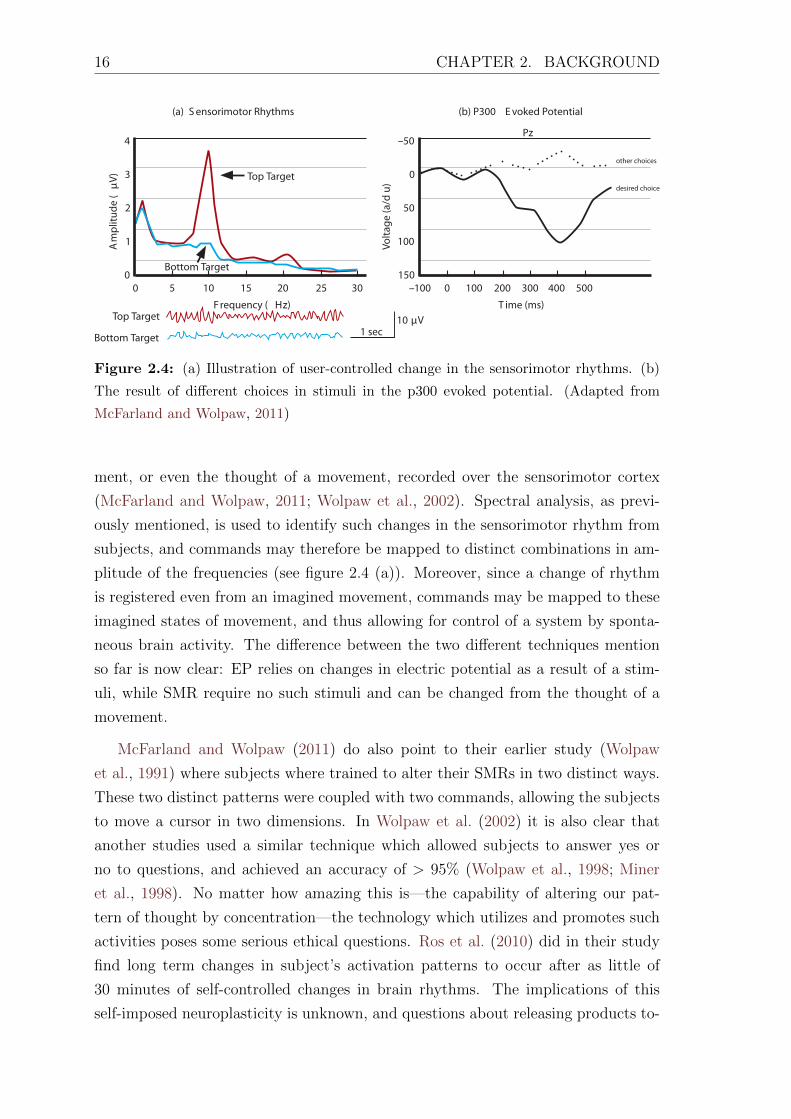
seen in figure 2.4 (b).
So since different stimuli produce slightly different waveforms, it is possible to
exploit this by training a classifier to separate them, which is the essential theory
behind BCI systems using EP.
Another commonly used technique in BCI is based on changes in sensorimotor
rhythms (SMRs), where SMRs are rhythms in an EEG-signal as a result of move-
16 CHAPTER 2. BACKGROUND
other choices
desired choice
4
3
2
1
0
–50
0
50
100
1500 –100
Top Target
Top Target
Bottom Target
(a) S ensorimotor Rhythms (b) P300 E voked Potential
Bottom Target
5 010 100 20015 30020 40025 50030
1 sec10 μV
Am
plitu
de (
μV)
Volta
ge (a
/d u
)
F requency ( Hz) T ime (ms)
Pz
Figure 2.4: (a) Illustration of user-controlled change in the sensorimotor rhythms. (b)
The result of different choices in stimuli in the p300 evoked potential. (Adapted from
McFarland and Wolpaw, 2011)
ment, or even the thought of a movement, recorded over the sensorimotor cortex
(McFarland and Wolpaw, 2011; Wolpaw et al., 2002). Spectral analysis, as previ-
ously mentioned, is used to identify such changes in the sensorimotor rhythm from
subjects, and commands may therefore be mapped to distinct combinations in am-
plitude of the frequencies (see figure 2.4 (a)). Moreover, since a change of rhythm
is registered even from an imagined movement, commands may be mapped to these
imagined states of movement, and thus allowing for control of a system by sponta-
neous brain activity. The difference between the two different techniques mention
so far is now clear: EP relies on changes in electric potential as a result of a stim-
uli, while SMR require no such stimuli and can be changed from the thought of a
movement.
McFarland and Wolpaw (2011) do also point to their earlier study (Wolpaw
et al., 1991) where subjects where trained to alter their SMRs in two distinct ways.
These two distinct patterns were coupled with two commands, allowing the subjects
to move a cursor in two dimensions. In Wolpaw et al. (2002) it is also clear that
another studies used a similar technique which allowed subjects to answer yes or
no to questions, and achieved an accuracy of > 95% (Wolpaw et al., 1998; Miner
et al., 1998). No matter how amazing this is—the capability of altering our pat-
tern of thought by concentration—the technology which utilizes and promotes such
activities poses some serious ethical questions. Ros et al. (2010) did in their study
find long term changes in subject’s activation patterns to occur after as little of
30 minutes of self-controlled changes in brain rhythms. The implications of this
self-imposed neuroplasticity is unknown, and questions about releasing products to-

2.3. THE BRAIN AND THE COMPUTER 17
day that rely on self-controlled brain rhythms commercially to the gaming marked,
which is the biggest marked for BCI as of now, should be asked.
Even though invasive technologies exist (e.g. intra-cortical electrodes) that are
suitable for BCIs, and research on this has found interesting topographic potentials
useable in BCI systems (Levine et al., 1999; Wolpaw et al., 2002), it is clear that
that more testing is needed to determine its effectiveness and what the long terms
effect of having implants have on humans (McFarland and Wolpaw, 2011). We will
thus not further explore this branch of BCI, for now, and leave it for future growth.
Conceptually, three types of BCI systems exist according to (McFarland and
Wolpaw, 2011): (1) the system adapts to the user; (2) the user adapts to the system,
and; (3) both user and system adapt to each other. Ideally would all BCIs be
classified as the first, acting as the ultimate ”mind reader”, knowing when to function
as a control and when to passively adjust what is presented to the user, or when to
not do anything at all. Realistically, specialised systems are spread over all three
categories. Systems monitoring cognitive states, medical conditions, or in some
way silently gather information about the user, in order to produce a specialized
output about/to the user, will I most cases go under the first category. If the BCI
is to be used as a direct controlling interface for some hardware or software, then
it will typically end up in the second or last category. A good example of this
could be a thought of BCI system, which controls a mouse-cursors movement on
a computer screen by change in gazing in two dimensions. It will be classified as
the second category if the movement speed of the cursor was modulated by user
training, and classified as the last category if the system itself recognized the user’s
desired movement speed.
EEG is by far the most common choice for BCI systems, but Van Erp et al.
(2012) as well as McFarland and Wolpaw (2011) mentions the following as technology
encountered in the literature of BCI research:
• electrocorticography (ECoG)
• intracortical electodes (ICE)
• functional near-infrared spectroscopy (fNIRS)
• functional magnetic resonance imaging (fMRI)
• magnetoencephalography (MEG)
All of these are however restricted to medical use or research, due to bulkiness
(MEG), being intra-cranial (ECoG, ICE), or suffers from low temporal resolution

18 CHAPTER 2. BACKGROUND
due to being an indirect measurement of activity (fNIRS, fMRI), where most of
these technologies easily falls into several of these reasons. Future technology and
advancements may however change this list completely, but until then, EEG stands
out as the appropriate BCI for commercial and non-medical use (Van Erp et al.,
2012).
Such facts do not go unnoticed by the industry, and has led to the development
of cheaper and more portable EEG systems, possibly with high resolution, like
Nurosky and Emotiv EPOC. The Emotiv EPOC headset is the targeted hardware
of this model and consists of 14 electrodes, plus two electrodes used as reference,
with standard placement according to the 10-20 system (see figure 2.5). Its sample
rate is 128Hz (2048Hz internal) with a precision of 16bit. Digital notch filters is used
to filter the frequency to a range of 0.2-45Hz, which makes the sample rate adequate
according to the Nyquist frequency (critical frequency), and thus aliasing free after a
discrete transformation. The headset itself is wirelessly connected to a computer by
USB-dongle in the 2.4GHz band, so some degree of portability—freedom for users
to move around as they want—is achieved (few meters). Although this makes the
headset less intrusive to a user compared to a traditional wired EEG system, it may
contribute to an increase in artifacts included in data recorded due to myogenic and
oculogenic potentials, as well as the movement and friction of the electrode itself.
This means that what is gained in data quality by the increased naturalness for
the user when recording, might actually be lost in the increase of uncertainty about
the signal. We cannot seem to find any direct studies on the relations between
naturalness in the user environment and its effect on recorded data, and only a few
indirect studies mentioning movement artifacts when using a wireless EEG (Gwin
et al., 2010; Berka et al., 2004, e.g.). A conclusion to whether a wireless solution
is a good or bad thing, in terms of naturalness of brain rhythms versus increase
in unwanted signal, is therefore not possible. One thing however, that is certainly
for sure, is that people tends to behave unnaturally in unnaturally environments,
leaving a minimally intrusive interface as the best choice.
The new inexpensive and commercially available EEG systems, in our case Emo-
tiv EPOC, makes research on EEG based BCI systems much more available as min-
imal funding is required to get started, and the result is a more than linear growth
in publications with a great variety of focus areas and methods, such as the system
proposed by Dan and Robert (2011) that uses Emotiv EPOC to control a Parallax
Scibbler2 robot. They recorded 10 seconds time frames, where a subject blinked
its eyes, and presented these cases to a two-layer neural network with a training
2 Parallax Scribler: http://www.parallax.com/tabid/455/Default.aspx

2.3. THE BRAIN AND THE COMPUTER 19
Nz
CPz
Fpz
AFz
Fz
FCz
Cz
Pz
POz
Oz
Iz
Fp1 Fp2
AF3 AF4AF7 AF8
F7F5 F3 F1 F2 F4 F6
F8F9
FT9 FT7 FC5 FC3 FC1 FC2 FC4 FC6 FC8
F10
FT10
A1 T9 T7 C5 C3 C1 C2 C4 C6 T8 T10 A2
TP10
P10
TP8
P8
PO8
O2
PO4
P2 P4 P6
CP2 CP4 CP6TP9 TP7 CP5 CP3 CP1
P9
P7P5 P3 P1
PO7PO3
O1
Figure 2.5: The solid orange electrodes is the available electrodes in the Emotiv EPOC
headset, with positions and labels from the 10-20 system. The orange circles are the
reference nodes.
accuracy of 65%. It should be noted that they only used one channel, because vi-
sual inspection of the cases revealed that it was the channel with the highest change
in amplitude following a blink. A 100% training accuracy was achieved by further
reduce the 10 second windows down to 1.60 seconds to minimize the effect of the
temporal alignment of the blinks. One has to question whether this is a “real” BCI
or not; EPOC does easily pick up strong myogenic potentials from its front sensors,
which then makes this system an electromyography (EMG) based interface. Never-
theless, the system is a clever use of technology which require little to no training
to operate, even though it based on strong artifacts in the world of EEG.
Another example is Juan Manuel et al. (2011), who do in their Adaptive Neu-
rofuzzy Inference System (ANFIS) based system reveals that the P300 evoked po-
tential can successfully be detected by using EPOC. In their experimental setup,
the P300 EP is triggered on subjects using visual stimuli, and the data recorded
was pre-processed and classified by the ANFIS with 85% accuracy (65% when ac-
counting for false positive). The pre-processing in this system is quite substantial
as it first involves band pass filtering, then blind source separation (independent
component analysis), and last a discrete wavelet transform in order to decompose
the signal. The ANFIS itself is quite interesting, as it combines a Sugeno-type sys-

20 CHAPTER 2. BACKGROUND
tem with four linguistic variables and an artificial neural network trained by hybrid
learning (back-propagation and least-square) to approximate the parameters in the
membership functions.
The P300 EP is also successfully detected by the system presented by Grierson
(2011). Unlike (Juan Manuel et al., 2011), they use the low-resolution Neurosky
Mindset headset in their experiments, where subjects were presented with visual
stimuli to trigger the EP. Traditional averaging of many similar time frames is
performe in order to elicit the underlying waveforms, which is then used to train a
simple linear classifier based on the area under the distinct curves. An accuracy of
78.5% is achieved when trained on two different stimuli (blue circle and red square).
While we could have extended this list of illustrative and interesting BCI systems
using commercially available EEG headset with great success, we will now turn our
focus to BCI systems that involves detection of emotions through EEG, since our
overall goal is to be able to do so. This overall goal is motivated by the fact that
machines do not incorporate live human emotions in their principles of rationality,
even though they play and important role in modulating human rationality, and is
thus to some degree a part of the definition of human rationality which makes us
capable of behaving intelligently, especially when interacting with other humans. We
believe that most have experienced the rationality mismatch between machines that
do not incorporate human emotions in their principles of rationality and humans,
which is illustrated with an example in Chapter 1. Another example could be
automated advertising solutions in online newspapers, where an ad typically appears
next to an article about the same basic topic as the product in the ad. The unwanted
behaviour from the machine here, is when it matches an ad and an article that is
about the same topics, but is together found totally inappropriate. We recently
saw an example of this, where an article about hundreds of stranded dolphins was
matched with an ad for frozen fish. There is no wonder why both the consumer and
the company see this as unwanted behaviour from the machine.
If we look at the definition of Intelligent user interfaces by Maybury (1999), stat-
ing that Intelligent user interfaces (IUI) are human-machine interfaces that aim to
improve the efficiency, effectiveness, and naturalness of human-machine interac-
tion by representing, reasoning, and acting on models of the user, domain, task,
discourse, and media (e.g., graphics, natural language, gesture), it is quite clear
that affective computing and the recognition of human emotions can contribute in
achieving those goals.
We will now describe BCI systems that aim to detect human emotions in EEG,

2.3. THE BRAIN AND THE COMPUTER 21
starting with Sourina and Liu (2011) who proposes as system for emotion recognition
by the use of Support Vector Machine (SVM) trained on features extracted from
EEG recordings using Fractional Dimension (FD). Their hardware setup was the
Emotiv EPOC headset, which they used to record the EEG of 10 and 12 participants
while they listened to audio stimuli thought to elicit emotions. This was done in
two different recordings, where the first was segments of music that was labelled by
other subjects than the actual participants, and the second used sound clips from
the International Affective Digitized Sounds3 (IADS) that comes with normative
ratings for each clip. The four classes of emotions they use are the four quadrants
in the two-dimensional model of emotion (arousal-valence), and were gathered from
the participants using the self-assessment mannequin (SAM) after each clip.
The pre-processing of the signal is a 2-42Hz band-pass filter, and the features
was extracted from each recording using both the Higuachi Algorithm and the Box-
counting Algorithm, on a 99% overlapping 1024 data point sliding window. This
was however only done for three of the electrodes (Af3, F4 and Fc6), where they
used Fc6 for the arousal dimension, and Af3 and F4 for the arousal dimension. By
training the SVM on randomly selected 50% of the cases per subject, and testing
on the other half, they report a performance of 100% on the best subject(s), and
around 70% on the worst, where both of the feature extraction algorithms performed
almost equally.
Petersen et al. (2011) uses features extracted by Independent Component Anal-
ysis (ICA), and the K-means algorithm, to distinguish emotions in EEG. Their
hardware setup was the Emotiv EPOC headset, which was used to record the event
related potential (ERP) in 8 subjects when viewing a randomized list of 60 images
from the international affective picture system4 (IAPS). These 60 images come with
a normative rating which indicates how pleasant or unpleasant they are, or if they
are rated as neutral. The set of 60 images used, is a perfectly balanced set with 20
pictures from each class. A repeated one-way ANOVA analysis revealed that the
difference seen in the averaged ERPs is statistically significant (p < 0.05) in the P7
and F8 electrodes, which shows that their method are able to correctly distinguish
between active and neutral images, as well as unpleasant and pleasant images. They
further find that clustering the ICA components based power spectrum and scalp
maps, revealed four distinct clusters which was completely covered by 3 standard de-
viations from their respective centroids, which gives an indication of the consistency
in correctly identifying different activation patterns.
3IADS: http://csea.phhp.ufl.edu/media.html#midmedia.html4IAPS: http://csea.phhp.ufl.edu/media.html#topmedia

22 CHAPTER 2. BACKGROUND
As an interesting touch, they couple the Emotiv EPOC headset with a smart
phone. They also implement a client-server model where the phone is the client
and a standard PC is the server. This allow them to estimate and reconstruct the
underlying sources in the EEG signal on the server side, and present them on a
realistic 3d head model on the smartphone. The estimated activation plots on the
3d head model, from the ERPs when viewing the IAPS images, was found consistent
with previous findings in neuroimaging.
Horlings et al. (2008) investigates the use of the naıve Bayes classifier, SVM, and
ANN to detect different emotions in EEG. The hardware setup used in this study
is the Deymed Truscan325 diagnostic EEG system that supports 24–128 electrodes.
They recorded the EEG from 10 participants when viewing 54 selected pictures
from the IAPS database, where each trail was followed by a self-assessment by the
use of SAM and the two-dimensional model of emotions. From each sample, the
frequency band power was measured along with the cross-correlation between EEG
band powers, the peak frequencies in the alpha band, and the Hjorth parameters
(Hjorth, 1970). A vast amount of 114 features per sample was the result of this
extraction, where 40 of these were selected as the most relevant by the max relevance
min redundancy algorithm. They report a 100% and 93% training accuracy for
valence and arousal respectively, and a testing accuracy of 31% and 32%, for the
SVM classifier. The neural network had a testing accuracy of 31% and 28%, while
the naıve Bayes had an accuracy of 29% and 35%, so it is hard to conclude on what
is the definite best classifier from the results. However, when manually removing
potentially ambiguous cases located near a neutral emotional state from their set,
they achieved an accuracy of 71% and 81% when testing the SVM. The reason
for this behaviour is of course less need for robustness from the classifier, but the
underlying cause of why these cases creates ambiguity is more intricate and may
stem from the images seen, the EEG recordings, or because of the nature of the
features extracted.
Mustafa et al. (2011) proposes a system that uses an ANN to detect levels of
brain-asymmetry in EEG. While brain-asymmetry is not directly related to emo-
tions, they are found to give an indication of schizophrenia, dyslexia, language ca-
pabilities and other motoric and mental phenomenon (Toga and Thompson, 2003),
and the methodology used here show one way of detecting distinct patterns in brain
activity in EGG by ANN. Their hardware setup was an EEG with two electrodes
(Fp1 and Fp2), which they used to record samples from 51 volunteers, which was
5Truscan: http://www.deymed.com/neurofeedback/truscan/specifications

2.3. THE BRAIN AND THE COMPUTER 23
classified by the use of the Brain-dominance Questionnaire6. Spectrograms from
these samples was then created using short time Fourier transform, and Grey Level
Co-occurrence Matrices (GLCMs)(Haralick et al., 1973) in four orientations was
computed based on these spectrograms. A range of 20 different features from these
four GLCMs per recording was then computed, and the best 8 features from these
80 features was selected based on eigenvalue of components outputted by Principal
Component Analysis. The ANN which had 8 input nodes, 6 hidden nodes and one
output node was then trained on the training cases to 98.3% accuracy which gives
indication that this methodology is capable of detecting distinct patterns in EEG.
Khosrowabadi et al. (2010) proposes a system for recognition of emotion in EEG,
based on self-organizing map (SOM) and the k-nearest neighbour (k-nn) classifier.
Their hardware setup was an 8 channel device, which was used to record the EEG
of 31 subjects who listened to music that is thought to elicit emotions, simultaneous
to looking at different pictures from the IAPS dataset. A self-assessment by the
use of SAM was used after each trail in order to classify the recording in four
different classes. These samples was then processed with a band-pass filter to exclude
frequencies above 35Hz, and features was then extracted by the magnitude squared
coherence estimate (MSCE) between all permutations of pairs of electrodes from the
8 available electrodes. The SOM was then used to create boundaries between the
different classes based on the features extracted and the SAM scores, and the result
from the SOM was then used by the k-nn to classify the recordings. Testing with
5-fold cross-validation revealed an accuracy of 84.5%, which is a good indication of
the systems abilities to correctly distinguish between the four distinct emotions in
EEG.
We can clearly identify a process in how the systems described typically approach
the problem of detecting emotions or distinct patterns in EEG. The first step is to
pre-process and extract features from the recorded signal, possibly followed by a
reduction of features based on measurements of their relevancy. The second step
is to train the chosen method for classification based on the features extracted
for each subject and recording. This process is also seen in systems investigated
in our preliminary studies (Kvaale, 2011). The act of choosing what methods to
use in order to extract features depends on a subjective opinion of what the most
descriptive features are, which clearly is disputed based on the variety of different
features seen. Looking back at the actual nature of EEG (oscillating signal), and
how it is recorded (electrodes at distinct position on the skull), reveals that it is
indeed a geometrical problem. We want to investigate if it is possible to minimize
6http://www.learningpaths.org/questionnaires/lrquest/lrquest.htm

24 CHAPTER 2. BACKGROUND
the subjectivity involved with extensive feature extraction, and thereby also the
computational overhead they pose, by using the spatial information encoded in
multi-channel directly, and let a method proven to perform well on geometrical
problems generalize over this information. In other words, use a method more in
line with the nature of the problem. We find such a method in the next section.
2.4 Neuroevolution
Traditional ANNs, with a hardwired structure and its weights learned by back-
propagation, may perform excellent on a specific problem. However, if the problem
changes its characteristics ever so slightly, then the previous excellent performance
is likely to not be so excellent anymore. Another serious shortcoming of traditional
ANNs learned by gradient descent is the scaling problem, that is, an increased com-
plexity in input data results in in a loss in accuracy. Montana and Davis (1989)
explains this phenomenon by pointing to the obvious shortcomings in gradient based
search; it easily gets trapped in local minima. Motivated by this fact, they designed
the first system that finds the weights of ANNs by an evolutionary algorithm (EA),
which tends to more easily avoid local minima, and thus giving birth to neuroevo-
lution.
A lot of different systems, with different complexity, have been proposed since
then: Miller et al. (1989) proposed a system that used a genetic algorithm to evolve
the connection topology for a neural network, followed by training (weight adjust-
ment) by backpropagation. A similar approach is found in (Kitano, 1990) who also
evolved the connection topology by evolution, and trained weights by backpropaga-
tion. A difference between these systems can be seen in their genotype encoding,
where Miller et al. used a direct encoding (a complete connection table), and Kitano
used grammatical rules to create a phenotype from a genotype. It is clear what is
preferable in terms of scalability and modularity. Gruau et al. (1996) used evolu-
tion to find both topology (connections and nodes), and weights of the connections
using cellular encoding. This encoding is also based on grammatical rules, but in
this case for cellular division, or more precisely, the effects a cellular division has on
topology and weights. Their results where impressive, and the system solved a pole-
balancing problem that fixed topology networks was unable to solve, thus arguing
for that evolving the structure was essential in solving difficult problems. Gomez
and Miikkulainen (1999) did however solve the same problem with a fixed topol-
ogy with their system called Enforced Sub-population, resulting in an inconclusive
answer to what is better.

2.4. NEUROEVOLUTION 25
Another challenge in NE is the permutation problem (competing conventions
problem), as pointed out in (Floreano et al., 2008; Stanley and Miikkulainen, 2002a).
As the name suggest, this involves permutation of individuals in a population—how
different genotypes that results in different phenotypes, may produce similar out-
puts. The problem arrives when two such individuals are selected for reproduction
by the EA, and a crossover operator mixes their genes when producing offspring,
resulting in a new individual with considerably lower fitness than its parents. This
happens because of a too big a distance in solution space, resulting in crossover of
genes that are not meaningful given the appearance of the parents, and thus low
heritability.
NeuroEvolution of Augmenting Topologies (NEAT), as presented by Stanley and
Miikkulainen (2002b,a), addresses both these issues. It is designed to increase the
performance of NE by evolving both weights and topology, increase the heritability
by addressing the permutation problem, and doing so with a minimized number of
nodes and connections.
The genome encoding in NEAT is direct, and consists of node genes and connec-
tion genes. Node genes does simply specify available nodes that can used either as
sensors (input nodes), hidden nodes, or output nodes. Connection genes specify the
connection topology of the network, where each gene includes a reference to both pre
and post-synaptic nodes, its connection weight, a bit indicator used to enable and
disable connections, and its innovation number. The innovations number is a clever
trick in NEAT to prevent the permutation problem. Each time a mutation occurs
that changes the structure of the network, and thus the appearance of new genes,
a global innovation number is incremented and assigned to these new genes. This
number is never changed after it is first set, and do even persist when reproduction
combines two parent’s genes, by the rules of the crossover operator, in an offspring.
NEAT will hence always have a chronological list of all genes in the system, which
results in meaningful crossovers of genes, and thus good heritability.
Like mentioned earlier, NEAT is designed to minimize the network topology.
By starting with a minimally complex network (in terms of number of nodes and
connections), the system is allowed to effectively explore a gradually larger search
space by introducing new genes through mutations, and ends up with an efficient
structure that approximate the correct behaviour for a given problem. However,
this bias towards less complexity, by starting minimally, poses a problem compared
to systems that starts with an arbitrary topology size. It is easier for an arbitrarily
large structure to remove excess nodes in order to maximize fitness, than it is for
a minimal structure to add un-optimized connections or nodes that might in many

26 CHAPTER 2. BACKGROUND
cases cause a temporary loss in fitness. Many mutations that eventually would have
led to a better approximation of the behaviour, if allowed to be optimized over a few
generations, may be lost due to a relatively too high selection pressure in Darwinian
evolution (survival of the slightly fitter than the mutated individual).
NEAT counter this problem by speciation, where the global innovation number
once again plays an important role. Instead of a tedious and inefficient comparison
of actual topology, NEAT uses the global innovation number of the genes to line up
a new individual with a random representative for a species. Their similarity is then
computed according to the distance measure (equation 2.3), where E is the number
of excess genes, D is the number of disjoint genes, and W is the average difference in
connection weights. The importance of each of these variables can be adjusted by the
c1, c2 and c3 coefficients. If the distance δ is found to be under some given threshold,
then two individuals compared are found to be the same species. This allows new
individuals to compete for reproduction primarily with other similar individuals in
terms of innovations, instead of competing with the entire population, which gives
any new individual a better chance to survive until it has it newly mutated genes
optimized.
δ =c1E
N+c2D
N+ c3 ×W (2.3)
To prevent early convergence, and hence a population totally dominated by one
species, NEAT employs fitness sharing, which means that individuals within one
specie must share the same fitness. This is implemented by dividing the raw fitness
values of the individuals by the population size of the species that the individual
belongs to. Then the amount of offspring to spawn is calculated by dividing the sum
of all the adjusted fitness values within a species by the average fitness of the entire
population. This means, in other words, that a single species will gradually lose
their fitness as their population size increases, allowing new species and innovations
to exist alongside possibly fitter species, and thus maintaining the overall diversity
which is essential in evolution.
The main insight of NEAT is quite clear if we sum up the abilities of the method.
First, the direct encoding with a global innovation number handles the problem of
competing conventions, and hence ensures good heritability. Second, NEAT allow
for incremental complexification by speciation, and does therefore explore the search
space efficiently for the minimal topology needed to achieve the correct behaviour.
Last, speciation does also play an important role in preventing premature conver-
gence and thus maintaining diversity in the overall population. It is now clear that

2.4. NEUROEVOLUTION 27
it is the exploitation of the historical markings of genes that makes this NE system
unique and light computational wise.
However, Stanley (2007) extends NEAT to produce what he calls Compositional
Pattern Producing Networks (CPPNs) motivated by findings that suggests that
developmental methods plays an important role in complexification in nature. This
is intuitive; the human DNA is not a direct blueprint on how to construct a human,
but instead an abstraction of the processes on how to do it. Like mentioned earlier,
the human brain itself is argued as one of the most complex, if not the most complex,
system known. If human DNA included a direct representation on how to create
this system (e.g. the position of all neurons and how they are connected) along with
the rest of the body, then it would be the utter most complex description known,
which it is clearly not. The key is in the abstraction on how such developmental
processes are encoded.
CPPNs are an attempt to create such a developmental encoding abstraction.
Without regards to theory involved, then a CPPN is simply a network of connection
and nodes, much like a traditional ANN. Its nodes however, deviate from typical
ANN nodes. Where ANNs often use sigmoid or threshold activation functions,
CPPNs may have activation functions that are symmetrical (Gaussian), periodical
(sine and cosine), linear (scaled within a certain range) or any other simple function
that makes sense given the properties of a specific problem area. The CPPN is then
simply a compositional function, composed by the topology of the network itself.
What this entails, with regards to encoding, is better explained by an example. The
goal of the example is to write a character on a canvas in Cartesian coordinates. A
direct encoding would have to explicitly store a value for each of the N x M points—
a blueprint of the canvas and the character. An indirect encoding that relies on
local interaction would have to store rules for the least complex possible way to
describe the specified character and its temporal unfolding (from starting point to
end point). CPPN on the other hand, uses only the coordinates of the canvas itself
as input, and outputs the target character without the need for explicitly knowing
how single points in space align, and when to draw them (local interaction and
temporal unfoldment).
This is quite impressive; CPPNs draws a character given a canvas, and do by
the geometry of the canvas implicitly know the local interactions and growth needed
to create that character. A similarity to how people draw a character is present.
Humans do not have to start at one end of a character to be able to correctly draw
an approximation to a perfect version of that character (even though we often do due
to the speed increase we gain trough enhanced motoric capabilities when repeating
28 CHAPTER 2. BACKGROUND
the same motoric task over and over again). Also, humans do not have to measure,
for example, the angle between different points on a canvas to be able to end up
with the character we are to draw.
Built on the theory that a neural network with two hidden layers can approximate
any function, where more complexity improves accuracy, Stanley (2007) gradually
evolves CPPNs from minimal topology by using NEAT, and should thus in theory
be able to approximate any compositional function. In a series of experiments in
(Stanley, 2007) he shows that CPPNs evolved with NEAT are capable of displaying
regularity, symmetry and repetition, which are thought to be essential in develop-
mental encoding with regards to complexity of the phenotype, by using symmetric
and periodic functions. Further, Stanley (2007) does also suggest that the spatial
pattern produced by a CPPN encoding may be used as connectivity patterns for a
2 x 2 dimensional hypercube by allowing four inputs (two x and y pairs).
This is the origin to a method called HyperNEAT (Stanley et al., 2009; Gauci
and Stanley, 2010), and is its main idea. Gauci and Stanley (2010) expresses this
insight as concisely as possible: “2n-dimensional spatial patterns are isomorphic to
connectivity patterns in n dimensions”. This entails that regularities, symmetries
and repetitions found in spatial patterns produced by CPPNs that uses the 2n-
dimensional coordinates as inputs, is directly transferable if the spatial pattern is
interpreted as a connectivity pattern for a 2n-dimensional hypercube, from which
the coordinates inputted to the CPPN stem from.
CPPNs evolved by NEAT can therefore be used as an encoding for ANNs, where a
CPPN computes the connection between each node in a network with fixed topology
as a product of the pair on nodes queried. However, traditional ANNs do not have a
specification of the relative positions of its nodes; it is a flat structure with no spatial
properties. By giving the nodes in ANNs a relative position in space and use these
coordinates as inputs to CPPNs, HyperNEAT is able to train ANNs with spatial
awareness, and thus reflect a structure with more resemblance to biological brains
where the relative position of neurons indeed plays an important role with regards to
connectivity. Experiments in (Gauci and Stanley, 2010), reveals that if the geometry
of the ANN is situated as the basic geometry of the problem (e.g. a checkers board),
then HyperNEAT effectively use this geometrical knowledge about the problem to
train ANNs that more easily handles geometrical relations and regularities.

Chapter 3
Implementation & Methodology
3.1 Getting familiar
We mentioned earlier that the EEG signal could be classified by the 3 Ns (noisy, non-
linear and non-stationary), and that this could result in some issues when applying
FFT to an EEG signal. An analysis of the effect of the violation of an assumed
stationary (periodic) signal is the appropriate way to get familiar with what to
expect from a classifier based on an EEG signal that has been transformed by FFT
to the frequency domain.
Let us first of all introduce the dataset we will use to train and test our model.
Koelstra et al. (2011) have made a database publicly available that consists of physio-
logical signals (including EEG) and video recordings of 32 participants watching dif-
ferent music videos. The videos watched are a collection of 40 videos chosen among
120, because these 40 was found to induce the most emotions trough large scale
screening. This screening was performed online, where participants rated movies on
continuous scales for valance and arousal. Each movie was then segmented into 60
seconds time frames with a 55 seconds overlap, where the 40 segments that had the
maximum emotional content was chosen. A relevance vector machine was trained
on features such as colour variance, video rhythm, shadow proportions , and other
similar features found to evoke emotions (see Koelstra et al. (2011) section 6.2 for a
complete overview), to detect the maximum emotional content.
The participants were a population of 32 healthy individuals (50% female), with
age between 19 and 37 (26.9 mean). Each participant was presented with a trial
case, followed by a 2 minutes baseline recording without the experimenter, which
allowed them to familiarize with the system before the actual recordings. After this,
29

30 CHAPTER 3. IMPLEMENTATION & METHODOLOGY
the 40 trials was performed, and included the following steps: (1) informing the
participant of their progress; (2) 5 seconds baseline recording; (3) displaying one of
the 40 music video segments, and; (4) self-assessment of valance, arousal, dominance
and liking. Self-reported data was gathered using the well establish method of self-
assessment manikins (SAM)(Bradley and Lang, 1994), where arousal and valance
was continuous scales with values from 1 to 9, and thus easily transferrable to
Russell’s circumplex model.
Considering their EEG setup, which had a sample rate of 512Hz over 32 elec-
trodes with positions given by the 10-20 system, then the EEG part of the dataset
consist of 32 participants each with 40 trails, where each trail consists of 33280 data
points (2560 baseline and 30720 with video stimuli) for each of the 32 electrodes.
This makes up a vast amount of raw data and is, by the authors, described as the
largest publicly available dataset of affective data. A pre-processed edition of this
dataset is however available. This is down-sampled to 128Hz, had its EoG artifacts
removed, and was filtered to 4-45 Hz. The EEG signals is also averaged to the
common reference, and a 3 seconds baseline was removed from data.
By choosing the 14 available electrodes in the Emotiv EPOC headset, from the
list of 32 available electrodes according to the 10-20 system, then the final dataset
we use includes 32 participants with 40 trials, where each trail has 14 electrodes
with 8640 datapoints (384 baseline and 7860 with video stimuli respectively). The
same self-reported levels of valence and arousal are accompanied both the raw and
pre-processed dataset.
So with a clear picture of the formatting of the dataset, we can begin to investi-
gate the actual signals. According to (Nunez and Srinivasan, 2006), the assumption
of stationary (periodic) signal may be misleading; if we force the signal to be peri-
odic by creating time frames and apply FFT on these time frames, then one does not
have to care about how the signal behaves outside that interval, and thus to some
extent forcing the signal to be periodic. This does however produce smearing into
other frequencies, by the frequencies within the time frame that do not complete and
integer number periods. To counter this, (Nunez and Srinivasan, 2006) displays the
use of a windowing function (Hanning) that forces the signal towards zero at each
end of the time frame, which removes the smearing from the aperiodic frequencies by
artificially forcing them to be closer to periodic. The use of windowing functions has
the effect of lowering the frequency resolution, and may therefore produce smearing
in other frequencies, but as pointed out by (Nunez and Srinivasan, 2006), the use
of a windowing is naturally more important as the total length of the time frames
decreases. Figure 3.1 (a) and (b) displays the effect of a 128 definite time frame

3.1. GETTING FAMILIAR 31
0 20 40 60 80 100 120Time t
−1.5
−1.0
−0.5
0.0
0.5
1.0
Ele
ctri
c pote
nti
al
(a) 128ms EEG signal in time-domain
3 9 15 21 27 33 39 45Frequency (Hz)
0.0
0.2
0.4
0.6
0.8
1.0
Am
plit
ude
(b) 128ms EEG signal in frequency-domain
0 20 40 60 80 100 120Time t
−1.5
−1.0
−0.5
0.0
0.5
1.0
Ele
ctri
c pote
nti
al
(c) 128ms EEG signal in time-domain
3 9 15 21 27 33 39 45Frequency (Hz)
0.0
0.2
0.4
0.6
0.8
1.0
Am
plit
ude
(d) 128ms EEG signal in frequency-domain
Figure 3.1: EEG signal before and after transformation. (a) Is the original signal from
128 datapoints, and (b) is the signal in frequency domain transformed with FFT. (c) Is
the signal modulated with a window function (green) that forces the signal to be more
periodic, and (d) is the modulated signal in the frequency domain transformed with FFT
that has been transformed from time domain to frequency domain without the use
of a window function. Figure 3.1 (c) displays the same time frame in time domain
multiplied by a window (green), and (d) displays the result of the transformation
to this modulated window. It is clear from this lone example that the windowing
function has an effect on the result. The most easily detectable changes are the
increase in amplitude in 9Hz and 44Hz, and the decrease in amplitude in 13Hz and
25Hz, and the overall lower resolution compared to the transformed signal without
a windowing function.
The previous example is very descriptive in in qualitative terms, but provides
no quantitative measures of the effects of a windowing function. That is, it gives
no direct indication of whether to use such a function or not. A more quantitative
approach can be seen in figure 3.2. It displays the mean standard deviation for
the amplitude of every whole frequency, for every 128 data point window, for every
channel, for every trail and every participant in the reduced 14 channel dataset.
It is here evident that the windowing functions works as expected; it does lower
the variability of the dataset, by a good portion, by forcing the time frames to be
periodic. Its effect is most noticeable in the 4-14Hz band, especially between 4-
8Hz, but is quite noticeable among the whole spectrum with a lower mean standard
deviation.
It is also evident in either case, that the standard deviation of frequencies from
4-14Hz has a greater variation than those from 14-45Hz, which is an interesting ob-
servation and points in a direction for what portion of the signal that is appropriate

32 CHAPTER 3. IMPLEMENTATION & METHODOLOGY
4 5 6 7 8 9 10 11 12 13 14 15 16 17 18 19 20 21 22 23 24 25 26 27 28 29 30 31 32 33 34 35 36 37 38 39 40 41 42 43 44 45frequency (Hz)
0
2
4
6
8
10
standard
devia
tion
(a) Standard deviation per frequency (with window)
4 5 6 7 8 9 10 11 12 13 14 15 16 17 18 19 20 21 22 23 24 25 26 27 28 29 30 31 32 33 34 35 36 37 38 39 40 41 42 43 44 45frequency (Hz)
0
2
4
6
8
10
standard
devia
tion
(b) Standard deviation per frequency (without window)
Figure 3.2: The mean standard deviation per frequency from each 128 datapoint time
frame transformed by FFT, for each of the 14 available channels, for each of the 40 trails,
for each of the 32 participants. (a) Is modulated with a windowing function (Hanning)
before transformation, and (b) is transformed using only the raw signal.
to generalize over. We say point in a direction here, because a conclusive answer
is hard to obtain, and the reason for this uncertainty is quite intricate. First, we
have that each trial is classified by a single self-assessment, that is, one class per 60
seconds trail. Whether or not this is reasonable may be debated, but is never the
less the appearance of the largest dataset on affective data available to date. A rea-
sonable assumption is, however, that the rhythms of the brain do change during the
duration of the video; it is indeed a dynamically shifting visual and auditory stimu-
lus, and will most certainly produce variations among the recorded samples within
a trail. We further saw that the frequencies in the range 4-14Hz was the frequencies
with the highest variations in the 4-45Hz EEG band, which also means that they
will be difficult to extract some sort of underlying rhythm from, that encodes for
an emotional state. Nunez and Srinivasan (2006) does further complicate things by
stating that as long as obvious artifacts are removed, then high amplitudes usually
mean a high signal-to-noise ratio in EEG. As we have seen in previous examples,
and in figure 3.3 which displays the mean amplitude for every participants (includ-
ing each of the 14 channels and each of the 40 trails), it is clear that the highest
amplitude waves is located in the first few frequencies, as expected (slow frequency,
high amplitude). By using the statement by (Nunez and Srinivasan, 2006) directly,
one may be lead to the conclusion that the lower frequencies naturally have a high
signal-to-noise ratio; that may well be the case, but for completely other reasons.
The statement should be interpreted as high amplitude compared to a default level

3.1. GETTING FAMILIAR 33
4 5 6 7 8 9 10 11 12 13 14 15 16 17 18 19 20 21 22 23 24 25 26 27 28 29 30 31 32 33 34 35 36 37 38 39 40 41 42 43 44 45frequency (Hz)
−1
0
1
2
3
4
5
6
am
plit
ude
(a) Mean amplitude per frequency (with window)
Figure 3.3: The mean amplitude for every frequency from each 128 datapoint time frame
transformed by FFT (with window function), for each of the 14 available channels, for each
of the 40 trails, for each of the 32 participants
Theta Alpha Beta Gammafrequency band
−5
0
5
10
15
20
standard
devia
tion
(a) Standard deviation per frequency band (with window)
Theta Alpha Beta Gammafrequency band
−5
0
5
10
15
20
25
30
standard
devia
tion
(b) Standard deviation per frequency band (without window)
Figure 3.4: The mean standard deviation per frequency band from each 128 datapoint
time frame transformed by FFT, for each of the 14 available channels, for each of the 40
trails, for each of the 32 participants. (a) is with the use of Hanning window, and (b) is
withouty
of amplitude, which then makes perfect sense: whenever a frequency has higher
amplitude than normally seen, then it is easier to distinguish from default noise and
same-frequency artifacts. The total signal-to-noise ratio will thus not directly be
lowered by excluding some frequency areas. A total loss of information is however
inevitable, but may well be worth it in terms of accuracy in a model, if the remain-
ing frequencies holds enough information to correctly identify the model’s target
phenomena.
By summing up the amplitudes in the typical EEG-bands, theta (4-8Hz), alpha
(8-13), beta(13-30) and gamma (30+) (Koelstra et al., 2011), and measure the stan-
dard deviation with the same procedure as 3.2, as shown in 3.4, it becomes evident
that if using these bands, then their order of inclusion is gamma, beta, alpha and
theta, respectively. That is, finding the most descriptive combination of bands in
terms of accuracy by starting with gamma and gradually including more bands in
the order of minimized variation, and thus maximizing accuracy.
34 CHAPTER 3. IMPLEMENTATION & METHODOLOGY
Another interesting observation is that the high frequency EEG bands which we
have identified as the lowest in variation in the reduced dataset used, typically the
beta band, has a change (increase) in activity when a subject is under the influence
of benzodiazepines which is a drug commonly prescribed for general anxiety, panic
attacks, insomnia and as a muscle relaxant, all of which could be related to temporal
emotional states (Sanei and Chambers, 2008; Stern and Engel, 2005; Van Lier et al.,
2004; Mohler et al., 2002). In fact, Van Lier et al. (2004) points to studies that find
increasing beta and gamma activity when attention and arousal increases in subjects,
even in drug free conditions. Even though being contradictory findings, a sedative
drug and increased arousal do both increase activity, it does point in a tendency
where the change in beta and gamma activity reflects the change in behaviour of the
subjects through modulated intensity of arousal and attention. While this supports
the high frequency bands as being informative, Nunez and Srinivasan (2006) states
that even though these bands are included as important for general brain function,
their low amplitude makes them harder to distinguish from artifacts than bands
that typically has higher amplitude.
3.2 Implementation
We decided to implement HyperNEAT ourselves in the Python programming lan-
guage, with the Python implementation of NEAT, as published on Stanley’s NEAT
user page1, as the basic underlying NEAT module. The reasons for not using one of
the implementations from the HyperNEAT users page2 are in our case many. Quite
subjectively, we prefer to use Python as it combines expressiveness from multi-
paradigms, dynamic typing, and a clear syntax with a reasonable performance. It
is also easily compatible with Matlab and C++. More objectively, emokit, the only
open-source project developed to enable gathering of raw data from the Emotiv
EPOC headset without the use of the expensive software from Emotiv, is written in
Python. Our implementation could therefore directly be integrated in emokit in the
future, without the need for any tedious cross-language imports or compilations.
3.2.1 From NEAT to NEAT-CPPN
NEAT are able to effectively evolve CPPNs by gradual complexification, like men-
tioned earlier. The transition of going from a NEAT system that evolves ANNs, to
1NEAT users page: http://www.cs.ucf.edu/~kstanley/neat.html2HyperNEAT users page: http://eplex.cs.ucf.edu/hyperNEATpage/HyperNEAT.html

3.2. IMPLEMENTATION 35
a NEAT system that evolves CPPNs is quite simply to allow for a diverse repertoire
of activation functions in the evolved networks, where the choice of which activation
function to use in a newly introduced node (gene) is random. So any new node
introduced by gradual complexification (mutation) is assigned a random activation
function, from a set of available functions that typically are symmetrical, periodic,
or linear. Gauci and Stanley (2010, 2011) did in their checkers and scalable go ex-
periments use Sine, Gaussian, sigmoid and linear functions. The same set appears
in Woolley and Stanley (2011) which evolves a robot arm controller. Stanley et al.
(2009) used a combination of sigmoid, Gaussian, absolute value, sine and linear.
This list, with small variations, appears as a solid foundation for a set of activation
functions. Our set of activation functions is then as follows:
Table 3.1: Set of activation functions
Name Function
Gaussian e−x2
Tanh tanhx
Sine sinx
Linear min(max(x,−3.0),3.0)3.0
Bool if x > 0 then 1 else 0
where the Gaussian and Linear functions are a direct implementation from the
source used in (Gauci and Stanley, 2010). This means that for any new node added
through mutation, a random choice decides which of these functions that will serve
as the activation function for that particular node trough the lifetime of that gene
(constant as long as the node is still included in an individual in the population).
We also decided to use signed activation with a range from -1.0 to 1.0, to ensure a
predictable output range from the CPPNs. The tanh function serves well for this
task, and is thus our choice for output nodes.
To summarize, CPPNs evolved by our system can then have an arbitrary number
of inputs, with an arbitrary number hidden nodes with different activation functions,
and an arbitrary number of output nodes with the hyperbolic tangent as activation
function. The number of input and output nodes is naturally given by the nature
of the problem one is investigating. Take for instance an intensity map restricted
by N x M values. If a CPPN was to be evolved to approximate its underlying
function, then a typical setup for the CPPN could be two input nodes which take
the coordinates of the two different dimensions as input. A normalized range from -
1.0 to 1.0 is preferable here since it facilitates the evolvement symmetry and periodic
behaviour from the network. The output node could then simply be a single node

36 CHAPTER 3. IMPLEMENTATION & METHODOLOGY
with an unsigned activation function that outputs the intensity at point x y in the
range from 0.0 to 1.0.
3.2.2 Using NEAT-CPPN to evolve Substrates
Algorithm 1 HyperNEAT algorithm (Adapted from Gauci and Stanley, 2010)
Input: Substrate Configuration
Output: Solution CPPN
Initialize population of minimal CPPNs with random weights
1: while Stoppingcritaria is no met do
2: for each CPPN in the population do
3: for each Possible connection in the substrate do
4: Query the CPPN for weight w of connection
5: if Abs(w) > Threshold then
6: Create connection with weight scaled proportionally to w
7: end if
8: end for
9: Run the substrate as an ANN in the task domain to ascertain fitness
10: end for
11: Reproduce CPPNs according to NEAT
12: end while
This part of the implementation consists of using CPPNs evolved by NEAT to
encode for the connection topology of a substrate (ANN) and is the heart of the
HyperNEAT methodology. We will here explain our implementation by a stepwise
referral to the basic HyperNEAT algorithm as presented in Algorithm 1.
Starting with the substrate configuration, which is the input in Algorithm 1, we
decided to separate the geometrical and actual configuration of the substrate. This
means that we store all the coordinate pairs for all available connections in a sub-
strate separate from the definition of the network in terms of activation functions,
actual connections, and nodes. The reason for doing this is strictly due to perfor-
mance and allows us to make a pre-defined list of inputs to the CPPNs, as inputs
to the CPPNs are not necessarily restricted to the coordinates of the problem. Such
additional inputs, along with the coordinates, may be the coordinates distance from
centrum, their relative distance from each other, as well as other primitive helper
functions to the CPPNs. Stanley (2006, 2007) uses distance to the centre as an

3.2. IMPLEMENTATION 37
extra parameter when evolving symmetric and periodic patterns with good results.
He explains the gain of giving the CPPN a value that it could easily approximate
by itself (distance from centre), by pointing out that functions higher in a gradually
evolved CPPN have a direct reference to the absolute distance at any time, even
though their inputs may be periodic. It is a helper function in other words. The
separation does therefore allow us to restrict the computational overhead of such a
helper function by only performing it only once in the beginning of each run.
Line 1 and 2 in Algorithm 1 is naturally given by the problem one are to inves-
tigate, but a stopping criteria is typically a threshold in number of generations and
evaluations, or an appropriate threshold in fitness. Line 3 is related to the previous
mentioned separation of substrate configuration, where the enumerable list of possi-
ble connections is in our implementation substituted with the pre-calculated list of
coordinates of the endpoints for every possible connection, along with the possible
helper estimates.
We implemented line 5 and 6 according to (Gauci and Stanley, 2010), which
means that any connection whose weight, as outputted by the CPPN, with absolute
value is above 0.2, results in a connection in the substrate scaled proportionally to
a range of 0 to 3, and that any connection with a weight less than this threshold
results in a weight of 0.0. This effectively allow HyperNEAT to disable connections
if found beneficial. A formal definition of this operation is shown in equation 3.1.
wscaled =
scale(w) if 0.2 < |w|,
0 if 0.2 > w > −0.2 .(3.1)
Line 9 is naturally given by the specific problem, and our implementation allows
for any types of functions or modules to be used here. Line 10 is given by the
implementation of NEAT-python, and follows the implementation in (Stanley and
Miikkulainen, 2002b) with the modifications needed to implement the NEAT-CPPN
according to (Stanley, 2007) and as described in the previous section.
3.2.3 Optimization
Tournament selection is, when used in evolutionary systems, a local selection mech-
anism which is highly controllable in terms of selection pressure. Selection pressure
is intuitively referring to the likelihood that a given individual, with a given fit-
ness, is chosen for reproduction. That is, if the pressure is high, then mostly the
fit individuals (highest fitness according to the fitness function) will be selected for
38 CHAPTER 3. IMPLEMENTATION & METHODOLOGY
reproduction. If the pressure is low, then those individuals with mediocre or poor
fitness have a higher probability of reproducing. Heritability and diversity—how
genes are passed on, and the total available gene pool within the population—is
therefore naturally affected by the selection mechanism. By definition, tournament
selection is controlling the selection pressure with two available parameters: k and p,
where k is the tournament size in terms of numbers of individuals drawn at random
from the population, and p is the probability that the individual with the highest
fitness in the tournament is selected. Knowing this, it is easy to see that if both
k and p are at their lowest functional value (e.g. k = 1 and p = 0), the selection
of parent(s) for reproduction is done at random, and is therefore projecting the un-
derlying fitness distribution of the population in question. A high value of k and p
(e.g. k = N and p = 1) will then project only the best fit individual(s).
NEAT-Python, which is our underlying NEAT module, implements tournament
selection as the primary selection mechanism, or at least partially implements it.
The population is first sorted by fitness before performing truncation (removal of
a fraction of the total individuals which are considered too poor performers) and
elitism (copying of the best individual(s) from the current generation to the next,
to ensure that a good solution is not lost in the reproduction process). The entire
population within a species is then randomly shuffled, and the best fit individual
of the first k individuals is the chosen for reproduction. Considering the entire
population N of different species, this has to be done at least 2×N times to avoid a
reduction of N , as each couple of parents produce one offspring. Two key aspects of
tournament selection are lost by this implementation: (a) the controlling of selection
pressure, simply because p = 1 and k is hardcoded to two; (b) the natural lightness
in computational complexity that tournament selection holds, because it requires
no sorting of the population. In defence of the authors of NEAT-Python, we must
include that it is a work in progress and should be treated thereafter. However,
we feel that it was necessary to re-implement tournament selection, and make the
parameters easily available when testing. This new implementation allow for the
adjustment of both p and k through the config file, as well as replacing the shuffling
of the entire population within a specie, by instead randomly picking individuals
from the same population k times.

3.3. EXPLORATION OF GEOMETRICAL GENERALIZATION 39
3.3 Exploration of geometrical generalization
Implementing a pre-defined methodology like HyperNeat, partly from scratch, in-
stead of using an open source distribution does both have its advantages and dis-
advantages. The obvious disadvantages are mainly that fewer persons get to look
at the actual code, and even fewer get to run independent experiments with the
finished implementation. We are in effect the only quality control for ourselves,
and before defining our model formally in next section, we would like to present
an exploratory test which is designed to highlight the implementations abilities to
produce ANNs that are trained by the geometry of a problem. Keep in mind that
this is only exploratory test, and not meant as a statistical proof of concept.
In the spirit of the checkers experiment in (Gauci and Stanley, 2010), we decided
to test our implementation by a 4×4 connect four game versus an existing computer
component. Unlike checkers with its 5×10²⁰ possible positions, our 4×4 grid connect
four has 161029, so it is quite less complex. Never the less, both are geometric in
nature, and both are strongly solved (checkers by Schaeffer et al. (2007) and connect
four by John Tromp3 (1995))
The choice of a 4 × 4 grid is not arbitrary, where the reason for choosing these
numbers stem from the basic geometry of the EEG-specifications in our setup. The
basic electrode count in Emotiv EPOC is 14, and these exact electrodes are the one
we use in our reduced dataset for later testing. A 4× 4 grid is then just above the
complexity of our EEG-data in terms of geometrical positions, and might therefore
tell us something about the implementations capabilities to generalize over this scale
of geometrical inputs.
A worthy opponent is found in Al Sweigart’s connect four game4, which is a
python implementation of connect four that allows a human player to play against
a computer opponent. The computer opponent is making its decisions based on
a depth first search in a n-ply game three, where each move is assigned 1, -1 and
0, coding for win, loss and neither. From the returned list of potential moves, the
move with the highest returned value is chosen as candidate. However, if the list of
potential moves got more than one candidate with the same value, then a random
choice between the moves decides the final candidate. Two interesting aspects can
be seen here: (a) the computer does return 0 for any other moves that does not
directly lead to a winning or losing position, and; (b) the computer player is non-
deterministic. The first aspect (a) is clearly exploitable by an evolutionary system,
3Connect four db: http://archive.ics.uci.edu/ml/datasets/Connect-44Connect four game: http://inventwithpython.com/fourinarow.py

40 CHAPTER 3. IMPLEMENTATION & METHODOLOGY
but (b) makes it troublesome to assess the fitness of an individual in the population,
which clearly leads to distortions in the search space.
The HyperNEAT evolved substrates that will be the opponents to Al’s AI, follows
the three layered configuration in (Gauci and Stanley, 2010). This means that the
input layer is 4× 4 nodes, where each node is situated at the available board fields,
and that the hidden layer has the exact same appearance as the input layer. The
output layer is simply just one node that outputs an estimate of the desirability of
any given board state. Both the hidden layer and the output layer uses tanh as
activation function, so the output from the network is restricted between -1.0 and
1.0. Board states are inputted to the network by letting every empty space have the
value of 0, and spaces occupied by red and black pieces have the value of 1 and -1
respectively.
We had to restrict the n-ply search of the game tree to 3 moves look-ahaed, since
the original experiment does not implement any pruning which leads to an exponen-
tial growth of the trees, and therefore also an exponential growth in execution time.
We could have implemented the pruning ourselves, to allow for faster execution and
possibly deeper game-trees, but that would essentially ruin the idea of rapidly test-
ing our implementation versus a pre-defined opponent. More important is that the
goal with this test is not to evolve a perfect connect four player, but instead see
the implementation’s ability to generalize over geometry in order to produce a good
player versus the opponent given. To make it even more interesting, did we not
allow the evolved substrates to look ahead in a game tree, and thereby forcing more
long term tactics. This is unlike the substrates evolved in (Gauci and Stanley, 2010)
where both the substrate and the opponent was allowed to assess every board state
in a 4-ply game tree.
Every individual in the HyperNEAT population had their fitness determined by
playing complete games versus the existing AI, where a win was given 1 in fitness, a
tie was given 0.5 and a loss resulted in 0. The results were averaged over ten runs in
order to better cope with the non-determinism in the opponent. Parameters used in
this test can be found in appappendix 1 which is a combination of previously used
parameters for NEAT (Stanley, 2007) and HyperNEAT (Gauci and Stanley, 2010),
found to be robust for many experiments, and parameters found to perform well in
preliminary tests.
Running a population of 100 individuals through 100 generations revealed a
solution with 0.9 in fitness according to the fitness function, as the best individ-
ual. Allowing this solution to play against the existing AI for 100 complete runs

3.3. EXPLORATION OF GEOMETRICAL GENERALIZATION 41
resulted in 63 wins, 31 defeats and 6 draws. This is quite impressive against a
non-deterministic 3 move look-ahead opponent.
One important finding in (Gauci and Stanley, 2010) is that general players per-
formed better than specialized players in checkers, and that the general CPPNs had
a smooth connectivity patterns, while the less general players had a discontinuous
and jagged connectivity pattern. Figure 3.5(a) and 3.5(b) shows the connectivity
patterns produced by the winning individual in our 4 × 4 connect four problem,
where (a) is the connectivity pattern between the input layer and the output layer
and (b) is the connectivity pattern between the hidden layer and the output layer.
Both of these patterns are smooth and continuous, so the winning individual is in-
deed a general connect four player. Closer examination of the figures reveals that
the tactics involve a desirability of controlling the game from left to right from the
connectivity pattern between the hidden layer and the output layer, and a desir-
ability of controlling the rows from the bottom up in prioritized order between the
input layer and hidden layer.
Such connectivity patterns give unique insight in solutions evolved by Hyper-
NEAT. The connectivity patterns produced by an individual give meaningful expla-
nations of the behaviour of the substrate. This is possible because the networks are
trained by the basic geometry of the problem, and the layers of the networks are
configured to be situated at this geometry, which reveals the attractiveness of posi-
tions and specially the attractiveness of a position with regards to how the opponent
is positioned.
Figure 3.6–3.8 shows different game states from a single run that is very descrip-
tive in how the overall strategy, as seen from the connectivity patterns, results in a
good connect four player for our particular setup. The top row of the figures (a)–(c)
stems from the evaluation of the game state before performing a move, where: (a)
is the receptive field of the hidden layer (how the hidden layer sees its inputs); (b)
is the receptive field of the output layer; (c) is the activation levels of the hidden
layer. The second row (d)–(F) displays the same types of patterns as the above row,
where the difference is that these patterns stems from the evaluation of the board
state that led to the actual move. The last row displays the pre-move board state
(g), and the post-move board state (h).
Figure 3.6 shows the response to the first enemy move. The substrate performs a
counter move in vertical direction, which is the result of the maximization from the
evaluations of the four allowed moves from the pre-move board state. A comparison
of the two first rows reveals the explanation for this move. The receptive fields

42 CHAPTER 3. IMPLEMENTATION & METHODOLOGY
X
−1.00
−0.33
0.33
1.00
Y
−1.00
−0.33
0.33
1.00
Weight
−2.0
−1.5
−1.0
−0.5
0.0
0.5
1.0
1.5
2.0
−1.00 −0.33 0.33 1.00X
−1.00
−0.33
0.33
1.00
Y
-0.800
-0.400
0.000
0.400
0.800
−1.0−0.8−0.6−0.4−0.20.0 0.2 0.4 0.6 0.8 1.0
(a) Evolved connective pattern (Input-to-Hidden)
X
−1.00
−0.33
0.33
1.00
Y
−1.00
−0.33
0.33
1.00
Weight
−2.0
−1.5
−1.0
−0.5
0.0
0.5
1.0
1.5
2.0
−1.00 −0.33 0.33 1.00X
−1.00
−0.33
0.33
1.00
Y
-0.800
-0.4000.0000.4000.800
−1.0−0.8−0.6−0.4−0.20.0 0.2 0.4 0.6 0.8 1.0
(b) Evolved connective pattern (Hidden-to-Output)
Figure 3.5: The connective patterns produced by the winning individual in the 4 × 4
experiment, visualized as planes and topographic maps, where (a) is the connective pattern
between the input layer and the hidden layer, and (b) is the connective pattern between
the hidden layer and the output layer.
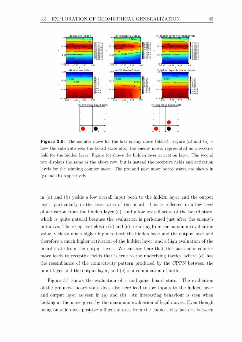
3.3. EXPLORATION OF GEOMETRICAL GENERALIZATION 43
−1.00 −0.33 0.33 1.00X
−1.00
−0.33
0.33
1.00
Y
0.003
0.005
0.007
0.007
0.010
0.010
0.013
0.013
(a) Input-to-Hidden
0.00150.00300.00450.00600.00750.00900.01050.01200.0135
−1.00 −0.33 0.33 1.00X
−1.00
−0.33
0.33
1.00
Y
0.003
0.005
0.007
0.007
0.010
0.0100.013
(b) Hidden-to-Output
0.00150.00300.00450.00600.00750.00900.01050.01200.0135
−1.00 −0.33 0.33 1.00X
−1.00
−0.33
0.33
1.00
Y
0.003
0.005
0.007
0.007
0.010
0.010
0.013
0.013
(c) Hidden layer Activation levels
0.00150.00300.00450.00600.00750.00900.01050.01200.0135
−1.00 −0.33 0.33 1.00X
−1.00
−0.33
0.33
1.00
Y
-0.500-0.250
0.000
0.250
0.500
0.750
(d) Input-to-Hidden
−0.6−0.4−0.20.00.20.40.60.8
−1.00 −0.33 0.33 1.00X
−1.00
−0.33
0.33
1.00
Y
-0.400-0.200
0.000
0.200
0.400
0.6
00
(e) Hidden-to-Output
−0.45−0.30−0.150.000.150.300.450.60
−1.00 −0.33 0.33 1.00X
−1.00
−0.33
0.33
1.00
Y
-0.500
-0.250
0.000
0.250
0.500
(f) Hidden layer Activation levels
−0.60−0.45−0.30−0.150.000.150.300.450.60
1234
1
2
3
4
(g) Pre-move board state
1234
1
2
3
4
(h) Post-move board state
Figure 3.6: The counter move for the first enemy move (black). Figure (a) and (b) is
how the substrate sees the board state after the enemy move, represented as a recetive
field for the hidden layer. Figure (c) shows the hidden layer activation layer. The second
row displays the same as the above row, but is instead the receptive fields and activation
levels for the winning counter move. The pre and post move board states are shown in
(g) and (h) respectively
in (a) and (b) yields a low overall input both to the hidden layer and the output
layer, particularly in the lower area of the board. This is reflected in a low level
of activation from the hidden layer (c), and a low overall score of the board state,
which is quite natural because the evaluation is performed just after the enemy’s
initiative. The receptive fields in (d) and (e), resulting from the maximum evaluation
value, yields a much higher input to both the hidden layer and the output layer and
therefore a much higher activation of the hidden layer, and a high evaluation of the
board state from the output layer. We can see here that this particular counter
move leads to receptive fields that is true to the underlying tactics, where (d) has
the resemblance of the connectivity pattern produced by the CPPN between the
input layer and the output layer, and (e) is a combination of both.
Figure 3.7 shows the evaluation of a mid-game board state. The evaluation
of the pre-move board state does also here lead to low inputs to the hidden layer
and output layer as seen in (a) and (b). An interesting behaviour is seen when
looking at the move given by the maximum evaluation of legal moves. Even though
being outside most positive influential area from the connectivity pattern between

44 CHAPTER 3. IMPLEMENTATION & METHODOLOGY
−1.00 −0.33 0.33 1.00X
−1.00
−0.33
0.33
1.00
Y-0.100-0.080-0.060-0.040
-0.020
(a) Input-to-Hidden
−0.120−0.105−0.090−0.075−0.060−0.045−0.030−0.015
−1.00 −0.33 0.33 1.00X
−1.00
−0.33
0.33
1.00
Y
-0.100-0.080-0.060-0.040
-0.020
(b) Hidden-to-Output
−0.105−0.090−0.075−0.060−0.045−0.030−0.015
−1.00 −0.33 0.33 1.00X
−1.00
−0.33
0.33
1.00
Y
-0.100-0.080-0.060-0.040
-0.020
(c) Hidden layer Activation levels
−0.105−0.090−0.075−0.060−0.045−0.030−0.015
−1.00 −0.33 0.33 1.00X
−1.00
−0.33
0.33
1.00
Y
-0.500-0.250
0.000
0.250
0.500
0.750
(d) Input-to-Hidden
−0.6−0.4−0.20.00.20.40.60.8
−1.00 −0.33 0.33 1.00X
−1.00
−0.33
0.33
1.00
Y
-0.400-0.200
0.000
0.200
0.400
0.6
00
(e) Hidden-to-Output
−0.45−0.30−0.150.000.150.300.450.60
−1.00 −0.33 0.33 1.00X
−1.00
−0.33
0.33
1.00
Y
-0.500
-0.250
0.000
0.250
0.500
(f) Hidden layer Activation levels
−0.60−0.45−0.30−0.150.000.150.300.450.600.75
1234
1
2
3
4
(g) Pre-move board state
1234
1
2
3
4
(h) Post-move board state
Figure 3.7: A mid game board state can be seen here. Notice that the two stacked
pieces in cloumn 3 shows that the substrate took initiative in the previous move. The
figure follows the same layout as in 3.6
the input layer and hidden layer, it is still the move that results in a pattern with
the most resemblance to the original connectivity patterns and thus the original
strategy, as seen in (d) and (e). The behaviour prioritizes to counter enemy threats
by placing a piece directly on top of the enemy piece, instead of stacking from the
bottom up regardless of the opponents moves.
The winning move can be seen in figure 3.8. While the move itself is not very
interesting (it is indeed the only legal move), it does nevertheless show that the win-
ning move does also show a great resemblance to the original connectivity patterns
and therefore the original strategy. A closer look on the board states reveals that an
enemy move occurred at some point that posed little threat to the strategy, with the
stacking of red pieces as a result (column 3 in (h)). The behaviour of the substrate
is therefore passive-aggressive, and does only take initiative when beneficial.
This exploration of our implementation by the use of a geometrical problem that
is slightly more complexity in terms of inputs, displays that our implementation is
indeed capable of generalizing over the geometry of such a problem. The winning
CPPN from the Connect 4 problem encoded for a substrate with a passive-aggressive
behaviour with regards to the geometry and the opponent. It stacked pieces in
columns above enemy pieces when appropriate, and above own pieces when ben-
eficial. The stacking in height in separate columns is the result of the long-term

3.4. THE MODEL 45
−1.00 −0.33 0.33 1.00X
−1.00
−0.33
0.33
1.00
Y
-0.700-0.700
-0.600
-0.600
-0.500-0.400-0.300
-0.200
-0.100
(a) Input-to-Hidden
−0.72−0.64−0.56−0.48−0.40−0.32−0.24−0.16−0.08
−1.00 −0.33 0.33 1.00X
−1.00
−0.33
0.33
1.00
Y
-0.500
-0.500
-0.400-0.300
-0.200
-0.100
(b) Hidden-to-Output
−0.56−0.48−0.40−0.32−0.24−0.16−0.08
−1.00 −0.33 0.33 1.00X
−1.00
−0.33
0.33
1.00
Y
-0.600
-0.500
-0.500
-0.400-0.300
-0.200
-0.100
(c) Hidden layer Activation levels
−0.56−0.48−0.40−0.32−0.24−0.16−0.08
−1.00 −0.33 0.33 1.00X
−1.00
−0.33
0.33
1.00
Y
-0.800
-0.400
0.000
0.400
0.800
(d) Input-to-Hidden
−1.00−0.75−0.50−0.250.000.250.500.75
−1.00 −0.33 0.33 1.00X
−1.00
−0.33
0.33
1.00
Y
-0.750
-0.500
-0.2500.000
0.2500.500
(e) Hidden-to-Output
−0.6−0.4−0.20.00.20.40.6
−1.00 −0.33 0.33 1.00X
−1.00
−0.33
0.33
1.00
Y
-0.750
-0.500
-0.2500.000
0.2500.500
(f) Hidden layer Activation levels
−0.6−0.4−0.20.00.20.40.6
1234
1
2
3
4
(g) Pre-move board state
1234
1
2
3
4
(h) Post-move board state
Figure 3.8: The winning move can be seen in this figure. The substrate has correctly
avoided the 3 move look ahead of the oppnent, and managed to place the pieces in such
way that a win is certain.
strategy needed to defeat the 3 move look-ahead opponent, exploiting the fact that
there is no assessment of intermediate states (the opponent sees any other board
states than states that directly lead to a win or loss as equal). By the time the op-
ponent sees the threat it is usually too late, where any combination of moves leads
to a victory to the substrate evolved by the winning CPPN.
3.4 The model
We have in the previous sections seen a familiarization with the nature of EEG-
signals, and examined what to expect when transforming the signal to the frequency
domain by the use of FFT. We have also described our implementation of Hyper-
NEAT and tested it on a problem with similar complexity in terms of number of
inputs, with promising results. This section will formally define how the EEG-signal
is presented to the substrate, and the configuration of the substrate itself.
3.4.1 Pre-processing
In the investigation of the EEG-signals we found several clues on how to get the most
stable cases to generalize over by looking at what part of the signal in frequencies
46 CHAPTER 3. IMPLEMENTATION & METHODOLOGY
that is the least variable, and how to reduce the variability of the dataset as a whole
by forcing the signal to be periodic with a windowing function. This turns out to be
crucial observations because the dataset only contains one self-assessment (class) per
trail (example), which we want to use as ground truth for the assumed underlying
waveforms encoding for the emotional states of the subjects.
The training examples is created by using averaging of the signal to uncover the
underlying waveforms of the different subjects and trails, which is proven to perform
reasonably well in other studies with lower electrode resolution than our EEG setup
(Grierson, 2011). Even though it might sounds strange to apply averaging to a
dataset gathered by showing continuously changing videos, one must assume that
near identical emotions are felt within a trail, and thus making the changes in the
waveform, caused by the the video and audio stimuli, just a varying and unwanted
part of the signal.
More formally, the averaging technique consists of first segmenting the signal
from a trail into equal length time frames, where the length of the time frame
determine the statistical power of the result of the averaging of all time frames.
The number of data points in the time frame does also determine the resolution
of the frequency coefficients resulting from a FFT of a time frame. This indicates
that there is a balance between statistical power of averaging, and the resolution of
the frequency coefficients, where a more data points in a time frame gives a higher
resolution in frequency coefficients, but lowers the statistical power of the averaging
by restricting the number of time frames within a single trail. We naturally seek as
high statistical power as practical with regards the resolution.
Let us first explain what this statistical power is in the context of averaging time
frames from an EEG signal that have been transformed by FFT. The result X from
a FFT of an N data point time frame is N/2 frequency coefficients with both a
real part and an imaginary part (or complex conjugates for real valued FFT). The
amplitude spectrum is obtained by taking the absolute value of X, and the power
spectrum is obtained by squaring the amplitude spectrum like mentioned in Chapter
2.2. A power spectrum is thus an estimate of the power (and variance) of the signal
as a function of frequency (Nunez and Srinivasan, 2006). An estimation of the power
spectrum of the underlying stochastic process encoding for the emotional state of a
subject is then obtained by averaging K number of time frames from the original
trail, where an increase in K yields a more correct result (more statistical power).
It is also clear from the explanation above why the resolution is affected by the
length of the time frames. A further restriction of the length is posed by the Cooley-

3.4. THE MODEL 47
Tukey FFT algorithm which works most efficient for any power of two. So we have
three restrictions: (1) maximization of K by a low N; (2) high enough N to at least
have whole separable frequencies, up to the maximum frequency; (3) N has to be a
power of two.
Solving for all reveals that when N = 128, then K is 60 (60 seconds trails, with
128Hz sampling rate), and every frequency in X is outputted as whole frequencies, in
the most efficient way according to the specifications of the Cooley-Tukey algorithm.
If we then apply the window function (as found to reduce the variance) before the
FFT of each individual time frame, then it is evident that we use Welch’s method
(Welch, 1967) with zero overlap to get an estimate of the spectral density. The trails
in the dataset can therefore be reduced to a set of frequencies and their respective
power estimates. However, we want to look at the overall band activity from the
typical EEG bands as presented in section 3.1, which allow us to further reduce
the complexity of the problem by assuming that the total activation of the bands is
sufficient to describe the underlying process. This assumption is naturally causing
a reduction in resolution, but it do allow us to see the data from a more generalized
perspective, which refers the Chapter 2 and our dissection of what these bands
are, and that combinations of these bands are found to encode for cognitive states,
behaviour, location on the brain, and so forth. The trails are therefore reduced to a
set of the four EEG bands available from the frequency range from the dataset.
We feel that is appropriate to mention that treating the bands as complete en-
tities is debated such as in (Nunez and Srinivasan, 2006) where an argument is
proposed to show that one cannot safely treat the alpha band as a unitary phe-
nomenon. This argument stating that different combinations of high and low (Hz)
activity in the alpha band encodes for different cognitive processes are reasonable
and may well be the ground truth. However, to our best knowledge, the use of a
neuroevolutionary methodology in the task of generalizing over multi-channel EEG
geometry has never been attempted before. Being first entails that the resolution
needed to get the results wanted is unknown, where a natural starting point would
be a method with relatively low resolution when choosing from the range of proven
existing methods and gradually use more sophisticated methods if they improve the
results.
To summarize, the pre-processing involves: (1) segmentation of the trails into
128 data point epochs; (2) Welch’s method with zero overlap to estimate the power
spectrum of the four bands (theta, alpha, beta and gamma).

48 CHAPTER 3. IMPLEMENTATION & METHODOLOGY
Nz
CPz
Fpz
AFz
Fz
FCz
Cz
Pz
POz
Oz
Iz
Fp1 Fp2
AF3 AF4AF7 AF8
F7F5 F3 F1 F2 F4 F6
F8F9
FT9 FT7 FC5 FC3 FC1 FC2 FC4 FC6 FC8
F10
FT10
A1 T9 T7 C5 C3 C1 C2 C4 C6 T8 T10 A2
TP10
P10
TP8
P8
PO8
O2
PO4
P2 P4 P6
CP2 CP4 CP6TP9 TP7 CP5 CP3 CP1
P9
P7P5 P3 P1
PO7PO3
O1
(a) The basic geometry of the Emotiv
EPOC headset
AF3 AF4
F3
F7
F4
F8
FC5 FC6
T8
P8
O2
T7
P7
O1
(b) The adapted basic beometry
Figure 3.9: These two figures shows how the basic geometry of the Emotiv EPOC headset
(a), as seen in two dimensions, is adapted for the basic geometry of the substrate’s input
and hidden layer (b).
3.4.2 Inputs
From the investigation of the signal, we have that the variance in the theta and alpha
bands are higher (especially theta), than the variance in the beta and gamma bands,
which leads to a higher degree of uncertainty in the estimated power spectrum from
the theta and alpha bands. We also found interesting connections between emotions
and the beta and gamma bands. Koelstra et al. (2011) has also found beta and
gamma bands to have the highest number of electrodes in EEG to significantly
correlate with emotions. Based on these findings, the final inputs to the system will
be the estimated mean power of the beta and gamma bands for each trail, for each
electrode in the 14 channel setup.
3.4.3 Substrate configuration
The substrate configuration in terms of geometry is by convention situated at the
basic geometry of the problem in HyperNEAT. This means that our substrate will
have layers that resemble the geometry of the EEG setup. Figure 3.9(a) shows
in two dimensions the position of the electrodes in our EEG setup, while 3.9(b)
displays how we adapt this geometry in HyperNEAT. The difference in electrodes
AF3, F3, FC5, and their matching even numbered electrodes, is done to easily allow
CPPN to exploit symmetry, asymmetry and periodic patterns in the input. The

3.4. THE MODEL 49
AF3 AF4
F3
F7
F4
F8
T9 FC5 FC6
T8
P8
O2
T7
P7
O1
AF3
F3
F7
FC5
T7
P7
O1 O2
P8
P8
FC6
F8
F4
AF4
Figure 3.10: The adapted basic geometry, with the extension of two bands. The orange
nodes are the beta band, and the green nodes are the gamma band. Both of these halos
are defined by the same X and Y coordinates, where a parameter R, the distance from
center, is the only indirect difference.
basic geometry of the substrate is therefore a halo in two dimensions with the 14
input nodes evenly distributed at each semicircle, where each position is given by
Cartesian coordinates.
Figure 3.10 shows how we incorporate the two bands (beta and gamma) that
stem from the same position when recorded. Instead of changing the Cartesian
coordinates directly for the outer band, which is interpreted as at different positions
by the CPPN, we included another dimension which is the radius R from the centre.
The two bands do therefore have the same X and Y coordinates, but is indirectly
different when R is supplemented to the CPPN. The CPPN can then decide if and
when the separation of the two bands is beneficial, instead of starting with two
different positions and approximating their similarity by polar coordinates.
Both the input layer and the output layer share the previously described basic
layout, while the output layer is simply two nodes situated at equal but opposite
positions, encoding for the outputs in the continuous two-dimensional model of
emotions, as presented by Russell (1980), and used in the testing dataset recorded
by Koelstra et al. (2011). The three layers are separated by their own dimension
H, where -1 is the input layer, 0 is the hidden layer and 1 is the output layer. This
is also done to allow the CPPN to easily distinguish between them, and use this
information if needed.
From the defined layout, we now have that each CPPN must allow for 8 inputs,

50 CHAPTER 3. IMPLEMENTATION & METHODOLOGY
which is the X and Y coordinate of an endpoint, along with R to separate the
two bands and H which encodes for the layer the endpoint is member of. This
makes 8 inputs for the two endpoints in a connection. The last piece of information
given to the CPPNs is the relative distance between two endpoints of a connection,
which makes sure that the CPPNs always have easy access to this value in higher
functions (nodes), as discussed in section 3.2.2. So the total inputs to the CPPNs is
9, which means that the CPPNs draws the connective patterns for 2×4 dimensional
hypercubes (excluding the helper function).

Chapter 4
Experimental Results &
Discussion
This chapter will investigate the performance of the model from a quantitative per-
spective, supplemented by a qualitative dissection of one of the evolved individuals,
in order to build a meaningful and reasonable answer to our research question as
posed in Chapter 1.
4.1 The Experiment
The problem posed to the substrate is the task of detecting two different emotions
from the subjects in the reduced test set, as presented in Chapter 3, and then output
the correct values for each emotion in the two-dimensional scales of emotions that
we and the dataset rely on. The two distinct emotions from each subject are chosen
from the subject’s list of self-assessments for all of the 40 trails with the basis of
the sum of the values from the two dimensions, where the highest and lowest sum is
chosen. This means that the two trails chosen from each subject is the highest and
lowest scoring trails, as a combination of the two dimensions, based on the subject’s
own rating. An argument stating that two cases chosen on the basis of extremes
are more easily distinguishable from one another than two cases with more similar
ratings, is of course reasonable (but speculative). However, we are not testing to find
out how the model perform on very similar cases, but instead true to our research
question and therefore exploring if this methodology is a viable technique in our
problem area. Choosing the extremes in terms of rating is then just an appropriate
and objective selection protocol which allows us to compare the results from different
participants, using the self-assessment of the participants as the ground truth.
51

52 CHAPTER 4. EXPERIMENTAL RESULTS & DISCUSSION
−1.0 −0.5 0.0 0.5 1.0Valence
−1.0
−0.5
0.0
0.5
1.0A
rousa
l
Training cases
Figure 4.1: The training cases represented as points in the two dimensions of emotions.
Red points indicates that this is the maximum rating of a pair of max/min ratings, while
blue is the minimum.
Figure 4.1 shows the distribution of ratings from all the selected trails from the
subjects, where red indicates that the rating is a maximum of a pair, and blue
indicates a minimum (note that some are overlaying as the result of similar ratings).
One interesting case can be seen here, where the maximum (red) rated trail is
actually negative in valence. Table 4.1 displays each participant’s maximum and
minimum rating in trail numbers, as well as the actual rating for both of these
trails. The ratings are in the dataset reported in a range from 1 to 9, but we have
scaled them proportionally to a range of -1 to 1 to later facilitate the use of tanh as
activation function in the output layer of the substrate.
The substrate configuration used in this experiment is the configuration deducted
in Chapter 3, which means that the input layer and hidden layer of the substrate has
a circular geometry where each electrode position is given in Cartesian coordinates.
The circular geometry is two halos, one for each band included in the test cases,
where the 14 electrodes are evenly distributed in their respective pairs on each
semicircle, on both halos. The X and Y coordinates of the electrodes is identical on

4.1. THE EXPERIMENT 53
Table 4.1: Selected trails from each participant
Sub. num. Trails Max Min
01 [20, 28] [ 0.99, 0.73013] [-0.9009, -0.67568]
02 [2, 20] [ 0.99, 0.99] [-0.99, -0.99]
03 [33, 24] [-0.0693, 0.7722] [-0.38362, -0.88853]
04 [2, 36] [ 0.97762, 0.76725] [-0.99, -0.99]
05 [1, 37] [ 0.99, 0.99] [-0.99 , -0.26977]
06 [6, 22] [ 0.80685, 0.80932] [-0.37867, -0.36135]
07 [35, 27] [ 0.76725, 0.99 ] [-0.73013, -0.7425 ]
08 [8, 29] [ 0.93555, 0.5544 ] [-0.891, -0.46283]
09 [12, 32] [ 0.77963, 0.5049 ] [-0.4752, -0.23265]
10 [6, 24] [ 0.9801, 0.63855] [-0.7623, -0.24503]
both halos, where a distance R is the only separation of the two bands. This allows
us to indirectly inform the CPPNs that there is a distinct difference between the
two points without explicitly giving the CPPNs separate coordinates. In fact, to
explicitly give different coordinates for the same electrode for the different two bands
to the CPPNs would not be in line with the basic geometry of the problem area,
which is a direct violation of the HyperNEAT methodology, since both the bands
stem from the same electrode and therefore also the same geometrical position. The
output layer is simply two nodes; one for the arousal scale and one for the valence
scale. Both the hidden layer and the output layers in the substrate uses tanh as
activation fuction. An overall figure of the substrate, as well as a visualization of
parameter H can be seen in Figure 4.2(a). Parameter R is visualized in Figure
4.2(b), along with the basic geometry of the substrate.
The CPPNs used in this test is also configured as described in Chapter 3, where
the 9 inputs is the pair of X and Y coordinates from the endpoints of a connection
in the substrate along with the separation parameter R, the layer indicator H, and
the distance between the two endpoints. The outputs from the CPPNs is separated
by two output nodes, where one is used to create the connective pattern between
the input layer and the hidden layer of the substrate, and the other is used to create
the connective pattern between the hidden layer and the output layer. We chose to
allow the CPPNs to be fully connected from initialization, that is, allow the input
layer to be fully connected to the output layer. This design choice might sound
counterintuitive with regards to NEAT’s philosophy of starting from a minimally
complex topology, but by allowing the CPPNs to be fully connected from start we
do ensure that there is no bias towards any particular input after the initialization,
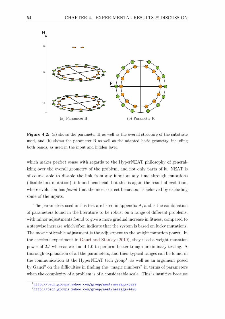
54 CHAPTER 4. EXPERIMENTAL RESULTS & DISCUSSION
AF3
AF4
F3F7
F4
F8
T9FC5
FC6 T8P8
O2
T7
P7
O1
AF3
F3F7FC5
T7
P7
O1
O2
P8 P8FC6
F8
F4
AF4
AF3
AF4
F3F7
F4
F8
T9FC5
FC6 T8P8
O2
T7
P7
O1
AF3
F3F7FC5
T7
P7
O1
O2
P8 P8FC6
F8
F4
AF4
O1 O2
H
0.0
1.0
-1.0
(a) Parameter H
AF3 AF4
F3
F7
F4
F8
T9 FC5 FC6
T8
P8
O2
T7
P7
O1
AF3
F3
F7
FC5
T7
P7
O1 O2
P8
P8
FC6
F8
F4
AF4
R
(b) Parameter R
Figure 4.2: (a) shows the parameter H as well as the overall structure of the substrate
used, and (b) shows the parameter R as well as the adapted basic geometry, including
both bands, as used in the input and hidden layer.
which makes perfect sense with regards to the HyperNEAT philosophy of general-
izing over the overall geometry of the problem, and not only parts of it. NEAT is
of course able to disable the link from any input at any time through mutations
(disable link mutation), if found beneficial, but this is again the result of evolution,
where evolution has found that the most correct behaviour is achieved by excluding
some of the inputs.
The parameters used in this test are listed in appendix A, and is the combination
of parameters found in the literature to be robust on a range of different problems,
with minor adjustments found to give a more gradual increase in fitness, compared to
a stepwise increase which often indicate that the system is based on lucky mutations.
The most noticeable adjustment is the adjustment to the weight mutation power. In
the checkers experiment in Gauci and Stanley (2010), they used a weight mutation
power of 2.5 whereas we found 1.0 to perform better trough preliminary testing. A
thorough explanation of all the parameters, and their typical ranges can be found in
the communication at the HyperNEAT tech group1, as well as an argument posed
by Gauci2 on the difficulties in finding the “magic numbers” in terms of parameters
when the complexity of a problem is of a considerable scale. This is intuitive because
1http://tech.groups.yahoo.com/group/neat/message/52992http://tech.groups.yahoo.com/group/neat/message/4498
4.1. THE EXPERIMENT 55
when the complexity of the problem results in relatively long execution times per
run, then the task of finding a “magic number” for any given parameter, for a total of
33 parameters and all of their permutations, is at least as time consuming as running
the problem itself. Since our problem is of considerable complexity, where single runs
easily could last for around 20 minutes, we had to restrict our preliminary testing of
parameters to a qualitative analysis of the performance of a few runs with parameter
values within the typical ranges that converged to relatively stable solutions.
Each run involved 100 individuals (CPPNs that encodes for a substrate) which
were allowed to evolve for 100 generations. The fitness of each individual, for each of
the 100 generations, was determined by the distance between the vectors outputted
by the substrate and the target vectors. Equation 4.1 is the formal definition of our
fitness function.
fitness(I) =1
1 +∑2
i=1
√∑nj=0 |uij − vij|2
(4.1)
The problem of detecting and correctly outputting the two dimensional value of
the two emotions per subject was performed 20 times for each subject included, in
order to get a bigger picture of the actual performance and robustness of our model.
From the 200 runs performed, an average fitness of 0.806± 0.117 is achieved. This
is calculated by taking the average of the winning solutions from each of the 20 runs
for each of the subjects, with all their different pairs of affective ratings. Figure 4.3
shows the result of this quantitative approach as a fitness progression per generation,
where the blue lines is the average of the 20 runs from one subject, accompanied by
the standard deviation from each of these 20 runs (green lines). The red line is the
overall average, as explained above, with the magenta line representing the standard
deviation for the overall average. We chose include all the single subject runs and
their standard deviation in the graph, in order to make a graphical representation
of the variation in the results.
Three distinct run types can be seen from the single subject curves (blue) in
figure 4.3. The first is the type where evolution quickly finds a good solution,
typically within the first 10-20 generations, and ends up with a high winning fitness
(> 0.95). The second is the type where the first 30+ generations is below the mean
curve (red), and has an overall more linear growth from the starting fitness until
approximately 0.8 where it gradually stabilizes. The third type is represented by
the curves that are situated around the overall mean, and has a strong resemblance
to the progression of the overall mean.

56 CHAPTER 4. EXPERIMENTAL RESULTS & DISCUSSION
0 20 40 60 80 100Generation
0.0
0.2
0.4
0.6
0.8
1.0Fi
tnes
sAverage max �tness
MeanStDev
Figure 4.3: The fitness progression from all the runs. Blue curves are the mean of the
best fitness for each of the 20 runs for one subject, accompanied by the standard deviation
(green). The red curve is the overall mean fitness prograssion for all of the included
subjects and runs, accomapnied by its standard deviation (magenta)
A difference in the initial fitness, and the initial rate of growth in fitness, from
single runs in evolutionary systems is normally due to the randomized initial setup;
some individuals gets a lucky start while others do not. However, the difference
in the rate of growth in fitness in the three types mentioned above can probably
not be explained by this phenomenon since the progression is an average of a sub-
stantial amount of runs, pointing towards a tendency that this average is in fact a
good representation for the progression of a run with that distinct subject and trail
combination. It is thus a representation of the difficulties in correctly detecting the
patterns presented, in terms of the geometry, projected as a fitness value through
the HyperNEAT methodology.
Table 4.2 shows how the results from each subject contribute to the total esti-
mated fitness, where the first column is the subject number followed by the maximum
and minimum fitness for the 20 runs performed on that subject’s max/min pair of
rating and EEG data. We can see here that even if the range restricted by the

4.1. THE EXPERIMENT 57
maximum and minimum, in terms of the fitness from each of the 20 runs (which de-
notes the best and worst performing solutions), is relatively large, the inter-subject
standard deviation is relatively low with a 0.04 ± 0.026 mean. This highlights two
important aspects, where the first is that there is a tendency that solutions evolved
for the same subject and same EEG-data are located near the mean for that partic-
ular setup. This gives confidence in the overall stability of this training method and
setup; one can expect similar performance given similar data. The second is that
the stability mentioned above is limited by qualitatively looking at the min/max
ranges, which shows that there is no guarantee for a lowest performing solution with
evolutionary function approximation within a finite time window (which of course
any practical and useable system is restricted by)
Table 4.2: Performance per subject
Sub. num. Max fit. Min fit. Mean fit. St. dev.
01 0.883 0.725 0.774 0.031
02 0.996 0.980 0.984 0.003
03 0.804 0.502 0.638 0.086
04 0.983 0.963 0.970 0.006
05 0.986 0.728 0.926 0.054
06 0.974 0.770 0.840 0.065
07 0.856 0.800 0.823 0.018
08 0.869 0.634 0.693 0.063
09 0.732 0.592 0.696 0.040
10 0.800 0.648 0.720 0.034
Mean: 0.888 0.734 0.806 0.040
St. dev.: 0.088 0.145 0.117 0.026
Figure 4.4 shows our further investigation of the errors of the system. This is
plotted in a similar fashion as figure 4.1, where the large dots is the target values
given by the subject’s ratings. The different colors of the large dots indicate different
subjects and matching colors indicate the pairwise max/min ratings. The small dots
are the actual ratings as outputted by the trained substrates, and a line is drawn
from the outputs to the targets to illustrate their membership and to easily show the
distance between the desired output and the actual output. Going back to figure 4.1
we noted that there was an interesting case where the maximum rating of subject
3 actually has negative valence (-0.0693), whereas the others cluster nicely between
0.5 and 1 in both the valence and arousal scale. A closer look at table 4.2 reveals
that subject 3 also have the lowest mean fitness (0.638), and the highest standard
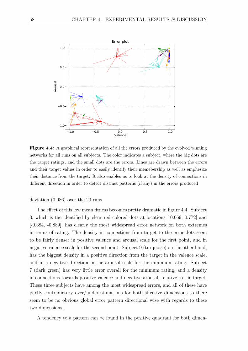
58 CHAPTER 4. EXPERIMENTAL RESULTS & DISCUSSION
−1.0 −0.5 0.0 0.5 1.0Valence
−1.0
−0.5
0.0
0.5
1.0
Aro
usa
l
Error plot
Figure 4.4: A graphical representation of all the errors produced by the evolved winning
networks for all runs on all subjects. The color indicates a subject, where the big dots are
the target ratings, and the small dots are the errors. Lines are drawn between the errors
and their target values in order to easily identify their memebership as well as emphesize
their distance from the target. It also enables us to look at the density of connections in
different direction in order to detect distinct patterns (if any) in the errors produced
deviation (0.086) over the 20 runs.
The effect of this low mean fitness becomes pretty dramatic in figure 4.4. Subject
3, which is the identified by clear red colored dots at locations [-0.069, 0.772] and
[-0.384, -0.889], has clearly the most widespread error network on both extremes
in terms of rating. The density in connections from target to the error dots seem
to be fairly denser in positive valence and arousal scale for the first point, and in
negative valence scale for the second point. Subject 9 (turquoise) on the other hand,
has the biggest density in a positive direction from the target in the valence scale,
and in a negative direction in the arousal scale for the minimum rating. Subject
7 (dark green) has very little error overall for the minimum rating, and a density
in connections towards positive valence and negative arousal, relative to the target.
These three subjects have among the most widespread errors, and all of these have
partly contradictory over/underestimations for both affective dimensions so there
seem to be no obvious global error pattern directional wise with regards to these
two dimensions.
A tendency to a pattern can be found in the positive quadrant for both dimen-

4.1. THE EXPERIMENT 59
−0.6 −0.4 −0.2 0.0 0.2 0.4 0.6Valence
−0.6
−0.4
−0.2
0.0
0.2
0.4
0.6
Arousal
0
10
20
30
40
50
60
70
80
90
0 10 20 30 40 50 60 70 80 90
Figure 4.5: The distribution of all the 400 outputs produced by the 200 runs, where the
offset from the middle is the relative distance from the target values to the output values
produced by the winning individuals
sions, where the substrates evolved for dark green and turquoise seems to have a
problem with separating the two outputs, and ends up with a similar value for both
arousal and valence. This problem is apparent for turquoise in the negative quadrant
as well, in a symmetrical but opposite direction and might suggest a problem with
rotation because of overgeneralization with this subject. The dark green’s target in
the negative quadrant has near identical values in both directions, and is approx-
imated quite well. One may be lead to the conclusion that it is symmetry that
forces the dark green’s approximations to the maximum rating to end up with near
identical outputs for both dimensions, which may be the case. However, a quick
look at light green (subject 5) reveals that even if the maximum rating has equal
values in both dimensions [0.99, 0.99], the minimum value is approximated quite
good even though being asymmetrical, which is contradictory to the assumptions of
that symmetry on one of the ratings (maximum of minimum) results in symmetry of
a potential asymmetric opposite rating. The relative distance from the asymmetric
part of dark green is then again closer to being symmetric, so a definite conclusion
is hard to obtain.
Figure 4.5 shows the relative distribution of errors from all the 400 outputs

60 CHAPTER 4. EXPERIMENTAL RESULTS & DISCUSSION
produced by the 200 winning solutions in the two dimensions, where every blue dot
is a single output (from either a maximum or a minimum rating), and the width
of the histogram bins is 0.01 in actual distance in the dimension measured. This is
an interesting plot because it allows us to investigate if the model has any biases or
weaknesses in any directions in the two dimensions of emotion.
It is quite clear from figure 4.5 that most of the errors occurs within a ±0.03
range, with a clear peak within ±0.01, and thus speaks in favour of the accuracy of
the model. An outer ring-like distribution can also be seen around the main cluster
with a lowest accuracy of about ±0.20, and makes up for most of the remaining
error. The rest of the errors seem to be scattered in a randomly fashion, with only
a couple of minor cluster in the negative part of the arousal dimension.
4.2 A Qualitative Explanation
The quantitative analysis shows a decent overall performance of the model with
some minor errors evenly distributed in both dimensions, but was unable to explain
or describe the standard deviation in performance per subject. We feel thus it is
appropriate to investigate one of the individuals as an effort to uncover if there is
any underlying explanation to the variations in the results.
From the previous section, we found that the substrates evolved for subject 3
resulted in a poor overall result and the highest intra-subject standard deviation
(0.638± 0.086) for the 20 runs performed with the data from this subject. Subject
3 is therefore an interesting candidate to investigate. From the list of 20 runs from
subject 3, the winning individual from run 8 with a fitness of 0.658 is chosen due to
being closest to the overall mean fitness from all the 20 runs, and is hence close to
an average performer for subject 3.
Figure 4.6 shows the winning CPPN from subject 3 run 8. It consists of 8 hidden
nodes and 38 connections. There is a distinct difference between the two output
nodes and how they are connected to the input nodes. The output node that paints
the connective pattern between the input layer and output layer (right) is directly
coupled to many of the input nodes, while the output node that paints the connective
pattern between the hidden layer and the output layer (left) have considerably less
such direct connections. This implicates that the function approximated for each of
the two connective patterns have quite different complexity which naturally leads
to patterns with quite different topologies.
The patterns painted by the CPPN are quite interesting by themselves, but they

4.2. A QUALITATIVE EXPLANATION 61
1
tanhtanh
2
singauss
3
tanh
4
sin
56 7
sin
8 9
tanh
linea
sin
Figure 4.6: The pheontype (CPPN) from the winning individual, where squares represent
the input nodes. The number of the input nodes are as follows: [1, 2, 3, 4] = [x1, y1, R1, H1],
[4, 5, 6, 7, 8] = [x2, y2, R2, H2], and 9 = distance(endpoint1, endpoint2). The blue circles
are the output nodes, where the left paints the connective pattern between the hidden
layer and the output layer, and the right paints the connective pattern between the input
layer and the hidden layer. The solid lines are active connections, and the dotted blue
lines are disabled connections (as a result of mutation)
become more meaningful by first looking at the two trails from subject 3. Figure
4.8(a)–4.8(d) displays the activation topology for the two bands for each of the two
trails, where (a) and (b) is the activation topology for the maximum rated trail,
and (c) and (d) is for the minimum rated trail. Note that the activation maps are
transformed back to the original 10-20 system in order to get standardized scalp
plots. At first glance it is apparent that we are dealing with very similar, but not
identical, activation patterns. There are clear peaks at Fc5 and P7 on the left
hemisphere, and at Fc6 on the right hemisphere, for both trails and both bands.
The peaks at Fc5 and P7 are slightly more intense at trail 33 than at trail 24, and
the Fc6 at trail 24 beta activities is more intense than those from trail 33 beta
activities. Moreover, the internal differences in Fc6 are clearer in trail 24 than what
is seen in trail 33. The two cases are therefore separable, but only by small margins
(< 0.1).
Figure 4.8(e)–4.8(h) shows the connective patterns produced by the CPPN in
4.6, where (e) shows the pattern as seen from the beta band (halo) in the hidden
layer and (f) shows the pattern as seen from the gamma band (halo) in hidden
layer. The two figures (g) and (h) show how the pattern between the hidden layer
and output layer is seen from output node 1 (valence) and output node 2 (arousal)
respectively.
From (e) and (f) we can see that the connective pattern between the input layer
and hidden layer put an emphasis on the differences between the left and right
62 CHAPTER 4. EXPERIMENTAL RESULTS & DISCUSSION
hemispheres, where (e) shows that the beta band has the least negative influence on
the right hemisphere, and (f) shows that the gamma band has a positive influence
on the right hemisphere and negative on the left hemisphere. Moving to (g) and (h)
shows that the connective pattern between the hidden layer and the output layer
is clearly more intricate, as predicted from the previous investigation of the CPPN.
Furthermore, the difference in how the connective pattern is seen as receptive fields
for the two output nodes, compared to how it is seen as receptive fields for the hidden
layer, reveals that the connective pattern between the input layer and the hidden
layer is following a global pattern between the two layers, and that the connective
pattern between the hidden layer and the output layer is more specialized for each
of the outputs.
The strategy of the substrate was easy to identify when looking at the receptive
fields between the two first layers; it was a weighted difference between the left and
right hemispheres. The strategy, as seen from the two output nodes are however
harder to identify. If we look at figure 4.8(g) (valence), we can see that there
is a strong positive influence from the Fc6 channel and an even stronger positive
influence from the front/left channels (Af3, Af4, F3, F7, Fc5), as projected trough
the hidden layer. The negative influence is located from T7 trough O2, in counter
clockwise direction. This is an interesting observation, because if we look back at
figure 4.8(a)–4.8(a), which show the difference in the two trails presented, we can
see that the strongest positive influence is actually situated at a low activity area,
where Fc5 is the only peak area (partly) included. Even though some differences
between the two cases are apparent in this region, it is quite clear that this poses
some problems with precision because of the similarity they exhibit.
Figure 4.8(h) shows a much simpler strategy for output node 2 (arousal), where
it has the main positive influence from the Fc5 channel which we identified as easily
differentiable from the two trails based on the visual inspection of the activation
maps. One should then expect a better performance in the arousal dimension, but
it turns out that both has a near identical relative error in both direction in total
for both cases (approximately 0.3). The strategies combined are clearly not giving
the desired performance in terms of precision of the outputs. One could of course be
ignorant and blame it all on evolution by stating that evolutionary approximations
come with no guarantee of finding a (near) optimal solution to the problem posed,
but that would be akin to stating that evolutionary systems in general, and in this
case neuroevolution, are poor problem-solvers. This is not the case, as we also have
seen in the quantitative analysis, where the overall mean performance is good, along
with excellent individual performance from the solutions found for specific subjects.
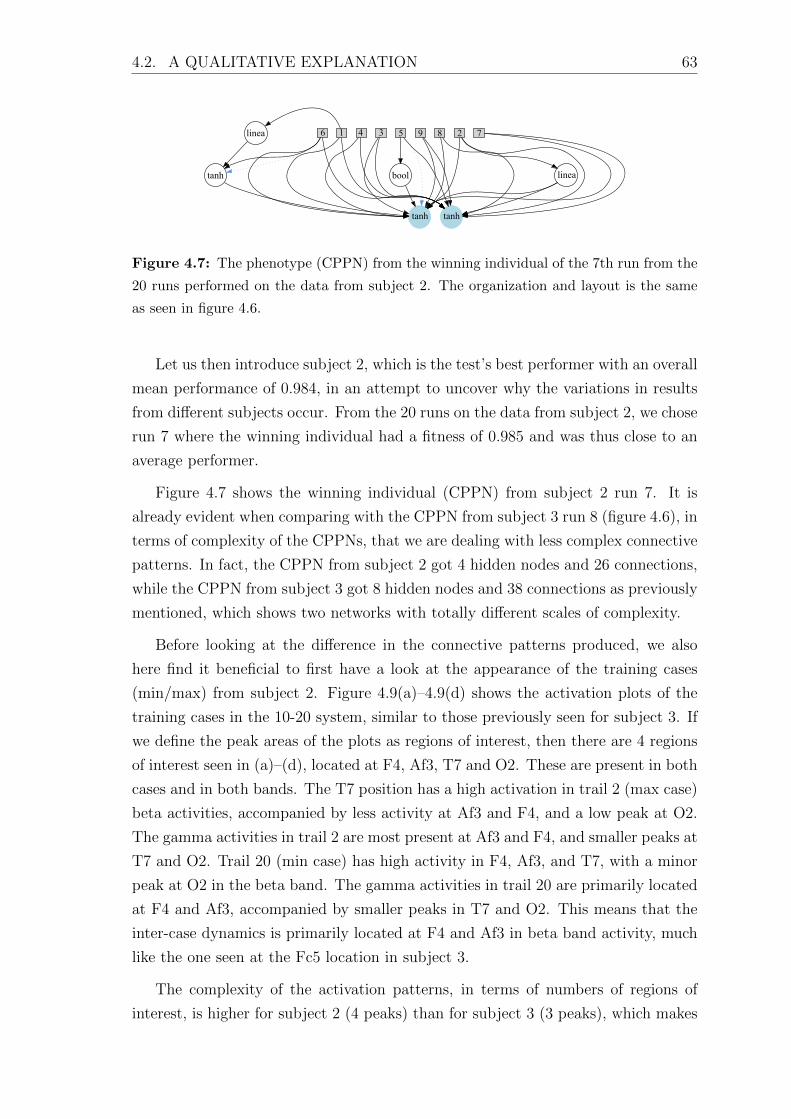
4.2. A QUALITATIVE EXPLANATION 63
1
tanhtanh
linea
tanh
2
linea
34 5
bool
6 789
Figure 4.7: The phenotype (CPPN) from the winning individual of the 7th run from the
20 runs performed on the data from subject 2. The organization and layout is the same
as seen in figure 4.6.
Let us then introduce subject 2, which is the test’s best performer with an overall
mean performance of 0.984, in an attempt to uncover why the variations in results
from different subjects occur. From the 20 runs on the data from subject 2, we chose
run 7 where the winning individual had a fitness of 0.985 and was thus close to an
average performer.
Figure 4.7 shows the winning individual (CPPN) from subject 2 run 7. It is
already evident when comparing with the CPPN from subject 3 run 8 (figure 4.6), in
terms of complexity of the CPPNs, that we are dealing with less complex connective
patterns. In fact, the CPPN from subject 2 got 4 hidden nodes and 26 connections,
while the CPPN from subject 3 got 8 hidden nodes and 38 connections as previously
mentioned, which shows two networks with totally different scales of complexity.
Before looking at the difference in the connective patterns produced, we also
here find it beneficial to first have a look at the appearance of the training cases
(min/max) from subject 2. Figure 4.9(a)–4.9(d) shows the activation plots of the
training cases in the 10-20 system, similar to those previously seen for subject 3. If
we define the peak areas of the plots as regions of interest, then there are 4 regions
of interest seen in (a)–(d), located at F4, Af3, T7 and O2. These are present in both
cases and in both bands. The T7 position has a high activation in trail 2 (max case)
beta activities, accompanied by less activity at Af3 and F4, and a low peak at O2.
The gamma activities in trail 2 are most present at Af3 and F4, and smaller peaks at
T7 and O2. Trail 20 (min case) has high activity in F4, Af3, and T7, with a minor
peak at O2 in the beta band. The gamma activities in trail 20 are primarily located
at F4 and Af3, accompanied by smaller peaks in T7 and O2. This means that the
inter-case dynamics is primarily located at F4 and Af3 in beta band activity, much
like the one seen at the Fc5 location in subject 3.
The complexity of the activation patterns, in terms of numbers of regions of
interest, is higher for subject 2 (4 peaks) than for subject 3 (3 peaks), which makes

64 CHAPTER 4. EXPERIMENTAL RESULTS & DISCUSSION
the fact that the runs from subject 2 ended up with a much higher fitness than the
runs from subject 3 even more interesting.
Figure 4.9(e)–4.9(h)shows the connective patterns produced between the layers
of the substrate as receptive fields, from the different parts of the substrate which is
identical in layout to those earlier seen for subject 3. From the hidden layer receptive
fields, shown in (e) and (f), we can see that there is a main positive influence from
the left hemisphere in the back area (T7, P7 and O1) in both hidden layer receptive
fields. The negative influence extends from Af3 trough Fc5 for the hidden layer beta
receptive field, and from Fc6 trough O2 for the hidden layer gamma receptive field.
Even though there are differences in the negative influence area, the overall strategy
from the connective pattern between the input layer and the hidden layer is clear,
with a distinct line between the left back area and the front right area.
If we look at figure 4.9(g) and 4.9(h), we can also easily identify the overall
strategy from the connective pattern between the hidden layer and the output layer.
From the receptive fields for both output nodes we can see that there is a strong
positive influence from the front right area (Af3 trough Fc5), with a negative in-
fluence in the left back area (Fc6 trough O2) for valence. This area is extended
to include O2 for the second output node (arousal). The strategy does also easily
counter low activity areas from the training cases, by giving them near zero influence
which appears as green in (g) and (h).
The strategies evolved for subject 2 compared to subject 3 are much more gen-
eral, and appear as smooth topologies in the receptive fields. Interestingly, the most
general patterns evolved the most general (and best) players in the checkers experi-
ment in (Gauci and Stanley, 2010), which also seems to be the case for the CPPNs
evolved for detecting emotions in EEG signals. The general patterns produced for
subject 2 do effectively use the regions of interest in their strategies (as weighted in-
fluence) and at the same time avoids low activity areas by giving them low influence.
The less general patterns, as evolved from the data of subject 3, do not manage to
use the regions of interest as effectively, and does in fact rely on low activity areas as
part of their overall strategy instead of avoiding them, which results in lower mean
performance with higher variations.
Another interesting finding is that the complexity of the training cases seems to
be of little significance to the strategies evolved; the more complex training cases
from subject 2 resulted in a more general solution and an overall higher mean per-
formance than the solutions found for the less complex training cases from subject
3. One main difference between the cases from the different subjects is the relative

4.2. A QUALITATIVE EXPLANATION 65
difference in power from the peak regions between the intra-subject minimum and
maximum case, where the difference is biggest in the cases from subject 2. This
suggests that precision is a potential problem when evolving substrates with Hyper-
NEAT, and that this is causing the evolved solutions to be less general and lower
performing than solutions evolved for substrates where the problem of finding a
good solution requires less precision.
The explanation for this problem might be intricate, but a look back at how
NEAT evolves networks might give an indication of where to start. NEAT explores
the search space for a solution from a minimal structure, and gradually increases
this space by adding new nodes and connection to individuals through mutations.
If the current search space is not investigated thoroughly, when high precision is
required (low relative distance between a poor and an excellent performance), then
mutations that only slightly increase the fitness of an individual stands out as the
current best solution. This will gradually lead to the disappearance of the genes
from individuals in the populations that are close to the most general and/or near
optimal solution, but are unable to find it unless a lucky mutation occurs. We can
find traces of this in the runs performed on the data from subject 3, where the best
run resulted in a fitness of 0.804 and the worst run resulted in a fitness of 0.502,
with a mean overall fitness of 0.638.
This problem is essentially quite similar to having a too high learning rate in
supervised learning algorithms like backpropagation, where any adjustment to the
weight is causing the algorithm to miss the lowest point on the error curve. One
solution to this problem in NEAT could then be to lower the weight mutation power
(how much a weight are allowed to change in one mutation), but this could again
lead to very slow convergence and the potential for that adding new nodes and
connections would still be the most effective way to slightly (but inappropriately)
increase the fitness, which again could lead to the loss of the genes that are close
to a general and good solution and takes us back to square one. Another problem
with fine-tuning the weight mutation power is finding the correct mutation rate for
all the cases posed, which will be more time consuming than the actual solving
of the problem, as mentioned earlier. An adaptive change in the mutation power
seems to be more appropriate. This could be realized by the same principles as
the adjustments of the momentum term often used in backpropagation, and thereby
allow the mutation power to be high or low depending on the previous relative gains.
Another approach to this problem is to modify NEAT to allow for learning
algorithms in the postnatal state, before the fitness assessment. The changes made
through learning could easily be stored, since NEAT after all uses direct encoding.
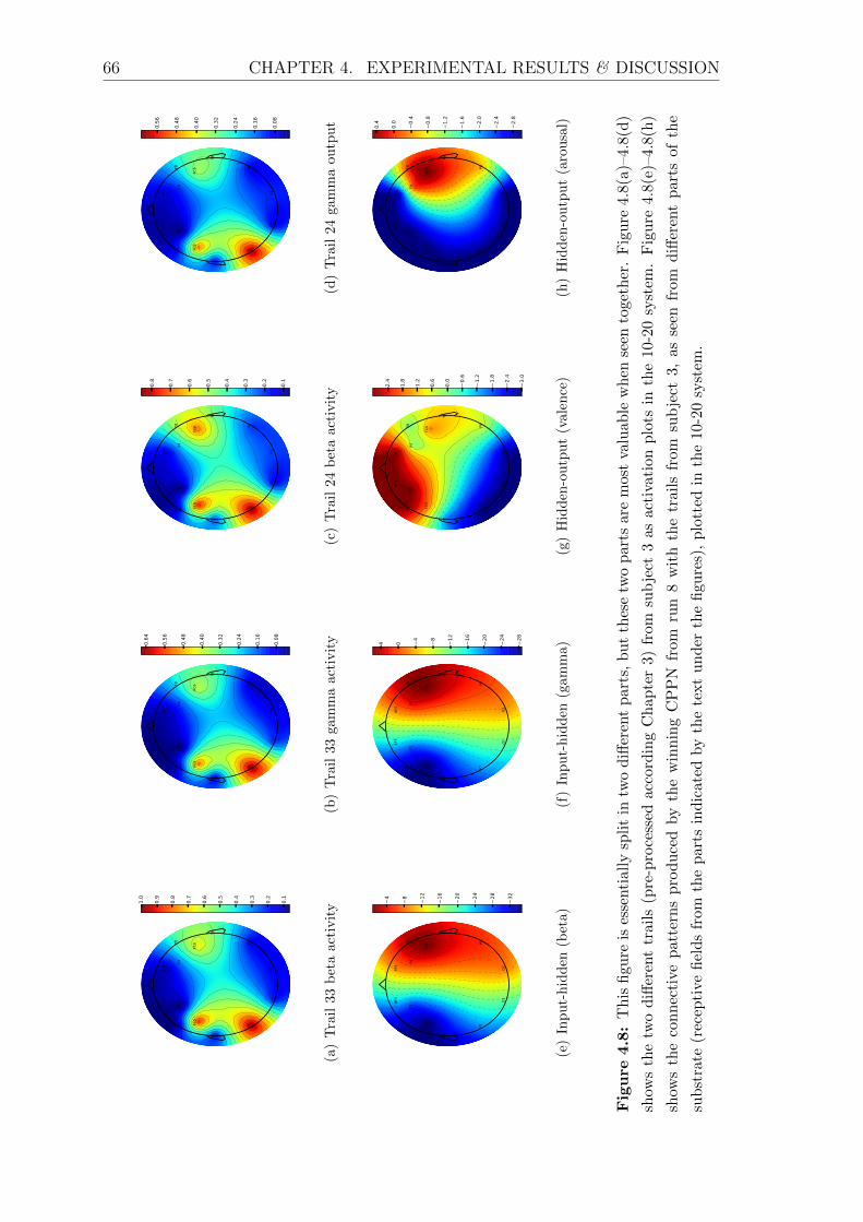
66 CHAPTER 4. EXPERIMENTAL RESULTS & DISCUSSION
AF3
F3
F7 FC5
T7
P7
O1
O2
P8
T8
FC6F8
F4
AF4
0.1
0.2
0.3
0.4
0.5
0.6
0.7
0.8
0.9
1.0
(a)
Tra
il33
bet
aac
tivit
y
AF3
F3
F7 FC5
T7
P7
O1
O2
P8
T8
FC6F8
F4
AF4
0.08
0.16
0.24
0.32
0.40
0.48
0.56
0.64
(b)
Tra
il33
gam
ma
act
ivit
y
AF3
F3
F7 FC5
T7
P7
O1
O2
P8
T8
FC6F8
F4
AF4
0.1
0.2
0.3
0.4
0.5
0.6
0.7
0.8
(c)
Tra
il24
bet
aact
ivit
y
AF3
F3
F7 FC5
T7
P7
O1
O2
P8
T8
FC6F8
F4
AF4
0.08
0.16
0.24
0.32
0.40
0.48
0.56
(d)
Tra
il24
gam
ma
ou
tpu
t
AF3
F3
F7 FC5
T7
P7
O1
O2
P8
T8
FC6F8
F4
AF4
−32
−28
−24
−20
−16
−12
−8
−4
(e)
Inp
ut-
hid
den
(bet
a)
AF3
F3
F7 FC5
T7
P7
O1
O2
P8
T8
FC6F8
F4
AF4
−28
−24
−20
−16
−12
−8
−4
04
(f)
Inp
ut-
hid
den
(gam
ma)
AF3
F3
F7 FC5
T7
P7
O1
O2
P8
T8
FC6F8
F4
AF4
−3.0
−2.4
−1.8
−1.2
−0.6
0.0
0.6
1.2
1.8
2.4
(g)
Hid
den
-ou
tpu
t(v
ale
nce
)
AF3
F3
F7 FC5
T7
P7
O1
O2
P8
T8
FC6F8
F4
AF4
−2.8
−2.4
−2.0
−1.6
−1.2
−0.8
−0.4
0.0
0.4
(h)
Hid
den
-ou
tput
(aro
usa
l)
Figure
4.8:
Th
isfi
gure
ises
senti
ally
spli
tin
two
diff
eren
tp
arts
,b
ut
thes
etw
op
arts
are
mos
tva
luab
lew
hen
seen
toget
her
.F
igu
re4.8
(a)–
4.8
(d)
show
sth
etw
odiff
eren
ttr
ails
(pre
-pro
cess
edac
cord
ing
Ch
apte
r3)
from
sub
ject
3as
acti
vati
onp
lots
inth
e10
-20
syst
em.
Fig
ure
4.8
(e)–
4.8
(h)
show
sth
eco
nn
ecti
vep
atte
rns
pro
duce
dby
the
win
nin
gC
PP
Nfr
omru
n8
wit
hth
etr
ails
from
sub
ject
3,as
seen
from
diff
eren
tp
art
sof
the
sub
stra
te(r
ecep
tive
fiel
ds
from
the
par
tsin
dic
ated
by
the
text
un
der
the
figu
res)
,p
lott
edin
the
10-2
0sy
stem
.

4.2. A QUALITATIVE EXPLANATION 67
AF3
F3
F7 FC5
T7
P7
O1
O2
P8
T8
FC6F8
F4
AF4
0.1
0.2
0.3
0.4
0.5
0.6
0.7
0.8
0.9
1.0
(a)
Tra
il2
bet
aac
tivit
y
AF3
F3
F7 FC5
T7
P7
O1
O2
P8
T8
FC6F8
F4
AF4
0.05
0.10
0.15
0.20
0.25
0.30
0.35
0.40
0.45
(b)
Tra
il2
gam
ma
act
ivit
y
AF3
F3
F7 FC5
T7
P7
O1
O2
P8
T8
FC6F8
F4
AF4
0.08
0.16
0.24
0.32
0.40
0.48
0.56
0.64
(c)
Tra
il20
bet
aact
ivit
y
AF3
F3
F7 FC5
T7
P7
O1
O2
P8
T8
FC6F8
F4
AF4
0.04
0.08
0.12
0.16
0.20
0.24
0.28
0.32
(d)
Tra
il20
gam
ma
ou
tpu
t
AF3
F3
F7 FC5
T7
P7
O1
O2
P8
T8
FC6F8
F4
AF4
−20
−10
010
20
30
40
50
60
(e)
Inp
ut-
hid
den
(bet
a)
AF3
F3
F7 FC5
T7
P7
O1
O2
P8
T8
FC6F8
F4
AF4
−50
−40
−30
−20
−10
010
20
(f)
Inp
ut-
hid
den
(gam
ma)
AF3
F3
F7 FC5
T7
P7
O1
O2
P8
T8
FC6F8
F4
AF4
−3.0
−2.4
−1.8
−1.2
−0.6
0.0
0.6
1.2
1.8
2.4
3.0
(g)
Hid
den
-ou
tpu
t(v
ale
nce
)
AF3
F3
F7 FC5
T7
P7
O1
O2
P8
T8
FC6F8
F4
AF4
−3.0
−2.4
−1.8
−1.2
−0.6
0.0
0.6
1.2
1.8
2.4
3.0
(h)
Hid
den
-ou
tpu
t(a
rou
sal)
Figure
4.9:
4.9(
a)–4
.9(d
)sh
ows
the
two
diff
eren
ttr
ails
from
sub
ject
2,as
acti
vati
onp
lots
inth
e10
-20
syst
em.
Fig
ure
4.8
(e)–
4.8
(h)
show
s
the
con
nec
tive
pat
tern
sp
rodu
ced
by
the
win
nin
gC
PP
Nfr
omru
n7
wit
hth
etr
ails
from
sub
ject
2,as
seen
from
diff
eren
tp
art
sof
the
sub
stra
te
(rec
epti
vefi
eld
sfr
omth
ep
arts
ind
icat
edby
the
text
un
der
the
figu
res)
,p
lott
edin
the
10-2
0sy
stem
.

68 CHAPTER 4. EXPERIMENTAL RESULTS & DISCUSSION

Chapter 5
Conclusion & Future Work
We have in this thesis conducted a thorough investigation of the problem areas in
order to propose a model for detecting emotions by the use of ANN. This resulted in a
better understanding of what emotions are, and how such a subjective phenomenon
can be measured and described in terms of a recognized universal model. The
dependent two-dimensional model of emotions allowed us to generalize over the
cognitive structure of interpretations of emotions, instead of a subjective description.
We have by that avoided a generalization over pure subjectivity, and thus reduced
the uncertainty about the results we have seen when testing. This reduction in
uncertainty is however limited by the validity of the two-dimensional model as a
universal model of emotion.
The investigation of EEG resulted in an overview of the common computational
methods used for analysis of the signal, and what to expect as result when trans-
forming a signal that is non-stationary, non-linear, and noisy by nature. Further,
the analysis of the actual EEG signal allowed us to identify frequency ranges with
minimized variance, and hence the identification of the most appropriate frequency
ranges to generalize over in terms of the accuracy of the power estimates of the
underlying stochastic processes.
Our exploration of BCIs provided a foundation for the most common techniques
used to enable humans to communicate with machines, in a meaningful manner,
through brain activity. The model we created for detecting of emotions through EEG
can easily be placed in the first category from the three categories of BCIs listed in
Chapter 2.3. The first category is where the system adapts to the user completely, so
our model does therefore avoid the ethical question we raised concerning self-inflicted
neuroplasticity from uncontrolled use, because there is no training or adaptation
needed from a user in order to achieve full functionality from the system.
69

70 CHAPTER 5. CONCLUSION & FUTURE WORK
The related BCI systems we found do mostly rely on features extracted from
the signal. This entails a subjectivity involved when choosing methods to extract
the features, and that an ANN trained on these features approximates a function of
these features instead of the problem itself. Our model minimizes this subjectivity
by expressing the signal by its mean power as a function of frequencies, linearly
transformed by FFT, and presenting it to the ANN in an adapted version of the
basic geometry of the problem. The only assumptions made here, is that the signal
is better described when transformed into the frequency domain, and that the mean
of N transformed time frames of the signal is a better estimate of the underlying
rhythms encoding for an emotional state, than what each of the single time frames
or the total trail is. The nature of the signal, and therefore also the problem, is
hence preserved.
This highlights an important aspect of this thesis; the preservation of geometrical
information in the multi-channel signal, through pre-processing instead of extensive
feature extraction, allow us to use a method for detection of emotions that evolves
ANNs on the basis of the basic geometry of the problem, which is more in line
with the true nature of the problem. Seen the other way around, reveals that by
identifying EEG as a geometrical problem (oscillating signal recorded from different
positions on the skull), and using a method (HyperNEAT) that is proven to perform
well on geometrical problems, allowed us to reduce the computational overhead of
feature extraction to lightweight pre-processing, as well as avoiding the subjectivity
involved with choosing what features to extract.
An interesting bi-product of this approach is that because the ANNs is evolved
on the basis of the basic geometry of the problem, which entails that the nodes in the
ANNs have distinct positions in space, the connective patterns as seen as receptive
fields from any chosen part of the system can easily be interpreted into meaningful
strategies. This allow for an investigation and understanding of the behaviour of
ANNs that we not have seen this clearly with any other methods for evolving or
training ANNs.
The experimental results in this thesis shows a promising high mean overall
performance (0.806 in fitness), with some variations (0.116 standard deviation) in-
troduced by the different performance from the individual 20 runs per subject. Our
investigation of the errors produced, revealed that these variations was not caused by
any problems with detecting any of the two-dimensions in both directions, and that
only 6 of 400 outputs ended up in a wrong quadrant. Further, we found that most
of the errors occur within a precision range of ±0.01 in both dimensions. A possible
explanation for the standard deviation in the overall performance was found during
71
our qualitative analysis of the individuals produced for the best and worst overall
performance per subject. This qualitative analysis of training cases and strategies
evolved (seen as receptive fields from different parts of the ANNs), points in a di-
rection where HyperNEAT struggles to evolve general strategies that use regions of
interest (peak activation areas) when high precision is needed in order to correctly
distinguish them from one another in the training cases. The underlying cause of
this problem may stem from how CPPN-NEAT gradually evolves more complex pat-
terns, and thereby a gradually bigger search space. If the search space that contains
the most general and/or near optimal solution is not correctly investigated, then a
gradual loss of genes from the individuals in that particular search space may occur
if evolution finds slightly fitter individuals by adding nodes or connections.
We suggest that a possible solution to this NEAT-specific problem is to lower
the weight mutation power, and allow for smaller movements in the search space.
This may however result in a too slow convergence, and a possibility for that adding
nodes and connections provides the fastest (but inappropriate) increase in fitness,
which could lead to bloating and the loss of the same genes as with high weight
mutation power. Also, building statistics around different values of weight mutation
power (and possibly other parameters) for a given problem in order to determine
a magic number, is at least as time consuming as solving the problem itself, and
thus becomes less and less attractive as the complexity of the problem increases.
We hence consider our two other suggestions, adaptive change in weight mutation
power (which could be extended to other parameters as well), and/or the inclusion
of learning in the postnatal state of the CPPNs, as more interesting and probable
solutions which we find worth pursuing on a general basis in the future.
Even though the experimental results are promising with regards to the capa-
bility of HyperNEAT as a method used in the area of detecting human emotions
through EEG, it is clear that more testing is needed before we can conclude on its
general viability in the problem area. We do also recognize that the standard devi-
ation in the overall results is an indicator of some limitations of using HyperNEAT
to evolve ANNs that require a relatively high degree of precision in order to cor-
rectly approximate the function needed to get the outputs in the precision desired,
when only small margins separates the training cases, and is thus a limitation in
our model. This limitation can possibly be addressed by the suggestions we made
earlier regarding CPPN-NEAT, and is our first priority in the future work of tuning
and stabilizing our model.
The results do also give strong indications that a commercially available EEG
headset such as Emotiv EPOC with limited resolution in terms of electrodes, in

72 CHAPTER 5. CONCLUSION & FUTURE WORK
combination with our model, is indeed sufficient to detect emotions from humans.
Adding the fact that our model, as a BCI, poses no ethical issues because it com-
pletely adapts to the user, means that our (or similar) model can both freely and
safely be distributed to the public. This supports our vision and desires of inte-
grating human emotions in the concept of rationality in machines that interact with
humans, in an attempt to address the problems associated with rationality mismatch,
which could lead to more intelligent interaction between man and machine.
a

Appendix A
Parameters
[ HyperNEAT parameters \
[phenotype]
input_nodes = 9
output_nodes = 2
fully_connected = 1
max_weight = 5
min_weight = -5
feedforward = 1
hidden_nodes = 0
weight_stdev = 2.9
[genetic]
pop_size = 100
max_fitness_threshold = 0.98
elitism = 1
tournament_size = 2
tournament_p = 1.0
prob_addconn = 0.05
prob_addnode = 0.03
prob_mutatebias = 0.26
bias_mutation_power = 0.21
prob_mutate_weight = 0.8
weight_mutation_power = 1.0
prob_togglelink = 0.05
73

74 APPENDIX A. PARAMETERS
[genotype compatibility]
compatibility_threshold = 6.0
compatibility_change = 0.3
excess_coeficient = 2.0
disjoint_coeficient = 2.0
weight_coeficient = 1.0
[species]
species_size = 6
survival_threshold = 0.2
old_threshold = 30
youth_threshold = 10
old_penalty = 0.2
youth_boost = 1.2
max_stagnation = 15

Bibliography
Berka, C., Levendowski, D. J., Cvetinovic, M. M., Petrovic, M. M., Davis, G., Lumicao,
M. N., Zivkovic, V. T., Popovic, M. V., and Olmstead, R. (2004). Real-time analysis of
eeg indexes of alertness, cognition, and memory acquired with a wireless eeg headset.
International Journal of Human-Computer Interaction, 17(2):151–170.
Bradley, M. M. and Lang, P. J. (1994). Measuring emotion: the self-assessment manikin
and the semantic differential. Journal of behavior therapy and experimental psychiatry,
25(1):49–59.
Conte, H. and Plutchik, R. (1981). A circumplex model for interpersonal personality traits.
Journal of Personality and Social Psychology, 40(4):701.
Cooley, J. W. and Tukey, J. W. (1965). An algorithm for the machine calculation of
complex fourier series. Math. Comput, 19(90):297–301.
Dan, S. and Robert, S. (2011). An exploration of the utilization of electroencephalography
and neural nets to control robots. An Exploration of the Utilization of Electroencephalog-
raphy and Neural Nets to Control Robots, 6949.
De Sousa, R. (2012). Emotion. The Stanford Encyclopedia of Philosophy.
Ekman, P. (1992). An argument for basic emotions. Cognition & Emotion, 6(3-4):169–200.
Ekman, P. (1999). Basic Emotions, chapter 3, pages 45–60. John Wiley & Sons, Ltd.
Ekman, P. and Friesen, W. V. (1971). Constants across cultures in the face and emotion.
Journal of Personality and Social Psychology, 17(2):124–129.
Floreano, D., Durr, P., and Mattiussi, C. (2008). Neuroevolution: from architectures to
learning. Evolutionary Intelligence, 1(1):47–62.
Gauci, J. and Stanley, K. O. (2010). Autonomous evolution of topographic regularities in
artificial neural networks. Neural Computation, 22(7):1860–1898.
Gauci, J. and Stanley, K. O. (2011). Indirect encoding of neural networks for scalable go.
Parallel Problem Solving from Nature–PPSN XI, pages 354–363.
75

76 BIBLIOGRAPHY
Gomez, F. J. and Miikkulainen, R. (1999). Solving non-markovian control tasks with
neuroevolution. volume 16, pages 1356–1361. LAWRENCE ERLBAUM ASSOCIATES
LTD.
Grierson, M. (2011). Better brain interfacing for the masses: progress in event-related
potential detection using commercial brain computer interfaces. CHI EA ’11: Proceed-
ings of the 2011 annual conference extended abstracts on Human factors in computing
systems.
Gruau, F., Whitley, D., and Pyeatt, L. (1996). A comparison between cellular encoding
and direct encoding for genetic neural networks. pages 81–89. MIT Press.
Gwin, J. T., Gramann, K., Makeig, S., and Ferris, D. P. (2010). Removal of movement
artifact from high-density eeg recorded during walking and running. J Neurophysiol,
103(6):3526–34.
Haralick, R., Shanmugam, K., and Dinstein, I. (1973). Textural features for image classi-
fication. Systems, Man and Cybernetics, IEEE Transactions on, 3(6):610–621.
Hjorth, B. (1970). Eeg analysis based on time domain properties. Electroencephalography
and clinical neurophysiology, 29(3):306–310.
Horlings, R., Datcu, D., and Rothkrantz, L. J. M. (2008). Emotion recognition using
brain activity. In Proceedings of the 9th International Conference on Computer Systems
and Technologies and Workshop for PhD Students in Computing, pages II.1–1, 1500888.
ACM.
Juan Manuel, R.-C., Vicente, A.-A., Gerardo, R.-C., Pilar, G.-G., and Jorge, E.-A. (2011).
Anfis-based p300 rhythm detection using wavelet feature extraction on blind source
separated eeg signals. Anfis-Based P300 Rhythm Detection Using Wavelet Feature Ex-
traction on Blind Source Separated Eeg Signals, 103.
Khosrowabadi, R., Hiok Chai, Q., Wahab, A., and Kai Keng, A. (2010). Eeg-based emotion
recognition using self-organizing map for boundary detection. In Pattern Recognition
(ICPR), 2010 20th International Conference on, pages 4242–4245.
Kitano, H. (1990). Designing neural networks using genetic algorithms with graph gener-
ation system. Complex Systems Journal, 4:461–476.
Klonowski, W. (2007). From conformons to human brains: an informal overview of non-
linear dynamics and its applications in biomedicine. Nonlinear Biomed Phys, 1(1):5.
Klonowski, W. (2009). Everything you wanted to ask about eeg but were afraid to get the
right answer. Nonlinear Biomed Phys, 3(1):2.

BIBLIOGRAPHY 77
Koelstra, S., Muhl, C., Soleymani, M., Lee, J., Yazdani, A., Ebrahimi, T., Pun, T., Nijholt,
A., and Patras, I. (2011). Deap: A database for emotion analysis using physiological
signals. Affective Computing, IEEE Transactions on, (99):1–15.
Kvaale, S. P. (2011). Detection of mood through analysis of brainwaves. Technical report,
Norwegian University of Science and Technology.
Leighton, S. R. (1982). Aristotle and the emotions. Phronesis, 27(2):144–174.
Levine, S. P., Huggins, J. E., BeMent, S. L., Kushwaha, R. K., Schuh, L. A., Passaro,
E. A., Rohde, M. M., and Ross, D. A. (1999). Identification of electrocorticogram
patterns as the basis for a direct brain interface. J Clin Neurophysiol, 16(5):439–47.
Malmivuo, J. and Plonsey, R. (1995). Bioelectromagnetism: principles and applications of
bioelectric and biomagnetic fields, chapter 13, pages 257–264. Oxford University Press,
USA.
Maybury, M. (1999). Intelligent user interfaces: an introduction. In Proceedings of the 4th
international conference on Intelligent user interfaces, pages 3–4, 291081. ACM.
McFarland, D. J. and Wolpaw, J. R. (2011). Brain-computer interfaces for communication
and control. Commun. ACM, 54(5):60–66.
Miller, G. F., Todd, P. M., and Hegde, S. U. (1989). Designing neural networks using
genetic algorithms. In Proceedings of the third international conference on Genetic
algorithms, pages 379–384, 94034. Morgan Kaufmann Publishers Inc.
Miner, L. A., McFarland, D. J., and Wolpaw, J. R. (1998). Answering questions with
an electroencephalogram-based brain-computer interface. Arch Phys Med Rehabil,
79(9):1029–33.
Mohler, H., Fritschy, J. M., and Rudolph, U. (2002). A new benzodiazepine pharmacology.
J Pharmacol Exp Ther, 300(1):2–8.
Montana, D. J. and Davis, L. (1989). Training feedforward neural networks using genetic
algorithms. volume 1, pages 762–767. San Mateo, CA.
Mustafa, M., Taib, M. N., Murat, Z. H., Sulaiman, N., and Aris, S. A. M. (2011). The
analysis of eeg spectrogram image for brainwave balancing application using ann. In
Computer Modelling and Simulation (UKSim), 2011 UkSim 13th International Confer-
ence on, pages 64–68.
Nowlis, V. and Nowlis, H. H. (1956). The description and analysis of mood. Annals of the
New York Academy of Sciences, 65(4):345–355.
78 BIBLIOGRAPHY
Nunez, P. L. and Srinivasan, R. (2006). Electric fields of the brain: the neurophysics of
EEG. Oxford University Press, USA.
Nunez, P. L. and Srinivasan, R. (2007). Electroencephalogram. Scholarpedia, 2:1348.
Petersen, M., Stahlhut, C., Stopczynski, A., Larsen, J., and Hansen, L. (2011). Smart-
phones Get Emotional: Mind Reading Images and Reconstructing the Neural Sources
Affective Computing and Intelligent Interaction, volume 6975 of Lecture Notes in Com-
puter Science, pages 578–587. Springer Berlin / Heidelberg.
Plutchik, R. (2000). A psychoevolutionary theory of emotion, chapter 4, pages 59–79.
American Psychological Association, Washington, DC, US.
Plutchik, R. (2001). The nature of emotions: Human emotions have deep evolutionary
roots, a fact that may explain their complexity and provide tools for clinical practice.
American Scientist, 89(4):344–350.
Ros, T., Munneke, M. A. M., Ruge, D., Gruzelier, J. H., and Rothwell, J. C. (2010). En-
dogenous control of waking brain rhythms induces neuroplasticity in humans. European
Journal of Neuroscience, 31(4):770–778.
Russell, J. A. (1980). A circumplex model of affect. Journal of Personality and Social
Psychology, 39(6):1161–1178.
Sanei, S. and Chambers, J. A. (2008). EEG Signal Processing. Wiley, Hoboken, NJ, USA.
Schaeffer, J., Burch, N., Bjornsson, Y., Kishimoto, A., Muller, M., Lake, R., Lu, P., and
Sutphen, S. (2007). Checkers is solved. Science, 317(5844):1518–1522.
Schlosberg, H. (1952). The description of facial expressions in terms of two dimensions.
Journal of Experimental Psychology; Journal of Experimental Psychology, 44(4):229.
Schlosberg, H. (1954). Three dimensions of emotion. Psychological review, 61(2):81.
Sharbrough, F., Chatrian, G. E., Lesser, R. P., Luders, H., Nuwer, M., and Picton, T. W.
(1991). American electroencephalographic society guidelines for standard electrode po-
sition nomenclature. Clinical Neurophysiology, (8):200–202.
Solomon, R. C. (2010). The philosophy of emotions, chapter 1, pages 3–15. Guilford Press,
3 edition.
Sourina, O. and Liu, Y. (2011). A fractal-based algorithm of emotion recognition from
eeg using arousal-valence model. In Biosignals 2011, pages 209–214. Springer.
Stanley, K. O. (2006). Exploiting regularity without development. In AAAI Fall Sympo-
sium on Developmental Systems. AAAI Press.

BIBLIOGRAPHY 79
Stanley, K. O. (2007). Compositional pattern producing networks: A novel abstraction of
development. Genetic Programming and Evolvable Machines, 8(2):131–162.
Stanley, K. O., D’Ambrosio, D. B., and Gauci, J. (2009). A hypercube-based encoding for
evolving large-scale neural networks. Artif. Life, 15(2):185–212.
Stanley, K. O. and Miikkulainen, R. (2002a). Efficient evolution of neural network topolo-
gies. volume 2, pages 1757–1762. IEEE.
Stanley, K. O. and Miikkulainen, R. (2002b). Evolving neural networks through augment-
ing topologies. Evolutionary computation, 10(2):99–127.
Stern, J. M. and Engel, J. (2005). Atlas of EEG patterns. Lippincott Williams & Wilkins,
Philadelphia.
Toga, A. and Thompson, P. (2003). Mapping brain asymmetry. Nature Reviews Neuro-
science, 4(1):37–48.
Van Erp, J., Lotte, F., and Tangermann, M. (2012). Brain-computer interfaces: Beyond
medical applications. Computer, 45(4):26–34.
Van Lier, H., Drinkenburg, W. H. I. M., van Eeten, Y. J. W., and Coenen, A. M. L.
(2004). Effects of diazepam and zolpidem on eeg beta frequencies are behavior-specific
in rats. Neuropharmacology, 47(2):163–174.
Welch, P. (1967). The use of fast fourier transform for the estimation of power spec-
tra: a method based on time averaging over short, modified periodograms. Audio and
Electroacoustics, IEEE Transactions on, 15(2):70–73.
Wolpaw, J. R., Birbaumer, N., McFarland, D. J., Pfurtscheller, G., and Vaughan, T. M.
(2002). Brain-computer interfaces for communication and control. Clin Neurophysiol,
113(6):767–91.
Wolpaw, J. R., McFarland, D. J., Neat, G. W., and Forneris, C. A. (1991). An eeg-
based brain-computer interface for cursor control. Electroencephalography and clinical
neurophysiology, 78(3):252–259.
Wolpaw, J. R., Ramoser, H., McFarland, D. J., and Pfurtscheller, G. (1998). Eeg-based
communication: improved accuracy by response verification. Rehabilitation Engineer-
ing, IEEE Transactions on, 6(3):326–333.
Woolley, B. and Stanley, K. O. (2011). Evolving a single scalable controller for an octopus
arm with a variable number of segments. Parallel Problem Solving from Nature–PPSN
XI, pages 270–279.


![Data Augmentation for EEG-Based Emotion …futuremedia.szu.edu.cn/assets/files/Data Augmentation for...Machine as a classifier to build EEG-based emotion recognition systems [22].](https://static.fdocuments.us/doc/165x107/5ed36f9c0339371bce117787/data-augmentation-for-eeg-based-emotion-augmentation-for-machine-as-a-classiier.jpg)