Electromagnetic Inversion Strategies for Antenna Design ...
193
Electromagnetic Inversion Strategies for Antenna Design and Characterization by Chaitanya Narendra A Thesis submitted to the Faculty of Graduate Studies of The University of Manitoba in partial fulfilment of the requirements of the degree of Doctor of Philosophy Department of Electrical and Computer Engineering University of Manitoba Winnipeg, Manitoba, Canada Copyright © 2021 by Chaitanya Narendra
Transcript of Electromagnetic Inversion Strategies for Antenna Design ...
Electromagnetic Inversion Strategies for
Antenna Design and Characterization
by
Chaitanya Narendra
A Thesis submitted to the Faculty of Graduate Studies of
The University of Manitoba
in partial fulfilment of the requirements of the degree of
Doctor of Philosophy
Department of Electrical and Computer Engineering
University of Manitoba
Winnipeg, Manitoba, Canada
Copyright © 2021 by Chaitanya Narendra

Abstract
In this work, we use the electromagnetic inversion (EI) framework to develop/improve
algorithms for the purpose of antenna design and characterization. Broadly speaking,
antennas are any device, object, or system that can transform energy in the form of
guided waves to energy in the form of radiated waves in space. In our increasingly wireless
technology landscape, many different types of antennas are being analyzed and developed
for a variety of applications. Therefore a flexible design/characterization methodology is
required to support our future wireless engineering needs.
To this end, we employ an EI methodology that allows the flexibility to develop novel
antenna characterization and design algorithms in a variety of applications. In gen-
eral, electromagnetic inversion enables the determination of an electromagnetic property
of interest (e.g., relative permittivity or equivalent current distribution) in an investi-
gation domain by processing some type of electromagnetic data (e.g., complex electric
field, phaseless data, or far-field performance criteria) on a separate measurement/desired
data domain wherein the investigation and data domains can be arbitrarily shaped; our
methodology allows for this flexibility to be utilized. Through the use of this methodology
and the electromagnetic surface and volume equivalence principles we develop EI algo-
rithms to contribute to the areas of metasurface design, microwave imaging, and dielectric
lens/antenna design.
Specifically, (i) we develop and demonstrate a gradient-based EI algorithm that can di-
rectly design the circuit admittance profiles of metasurfaces from desired complex or
phaseless (magnitude-only) magnetic field data on an external data domain, (ii) we de-
velop and verify inverse scattering algorithms to reconstruct dielectric profiles from phase-
less synthetic and experimentally measured data, and finally (iii) we introduce a combined
inverse source and scattering technique to tailor electromagnetic fields by designing pas-
sive, lossless, and reflectionless dielectric profiles to transform an existing electromagnetic
field distribution from a known feed to one that satisfies desired far-field performance cri-
teria such as main beam directions, null locations, and half-power beamwidth.

Acknowledgements
First, I would like thank my advisor and friend Dr. Puyan Mojabi for his guidance
throughout my academic journey and for inspiring me to begin the journey in the first
place all those years ago in his antennas course at the end of my B.Sc. Thanks also to my
friends and colleagues Dr. Trevor Brown, Chen Niu, and Dr. Nozhan Bayat for making
my time at the University of Manitoba an absolute joy.
I would like to express my gratitude to my Ph.D. internal committee members Dr. Ian
Jeffrey, Dr. Jason Fiege, and my external committee member Dr. Andrea Massa for
taking the time to help me improve my thesis.
Lastly, I’d like to thank the University of Manitoba Electromagnetic Imaging Laboratory
and Dr. Joe LoVetri for providing experimental data for this work, the University of
Manitoba Graduate Fellowship, the University of Manitoba GETS program, Natural
Sciences and Engineering Research Council of Canada, and the Canada Research Chair
program for financially supporting this work, and finally the Canadian Microelectronics
Corporation (CMC) for providing the use of ANSYS Electronics Desktop.
ii

Contents
Abstract i
Acknowledgements ii
List of Tables vii
List of Figures viii
Important Abbreviations xiv
Important Symbols xv
1 Introduction 1
1.1 Antennas . . . . . . . . . . . . . . . . . . . . . . . . . . . . . . . . . . . 1
1.2 Antennas and Radiation . . . . . . . . . . . . . . . . . . . . . . . . . . . 3
1.3 Electromagnetic Equivalence Principles . . . . . . . . . . . . . . . . . . . 5
1.3.1 Surface Equivalence Principle . . . . . . . . . . . . . . . . . . . . 5
1.3.2 Volume Equivalence Principle . . . . . . . . . . . . . . . . . . . . 7
1.4 Electromagnetic Inversion . . . . . . . . . . . . . . . . . . . . . . . . . . 8
1.4.1 Types of Electromagnetic Inverse Problems . . . . . . . . . . . . . 9
1.4.2 Difficulties . . . . . . . . . . . . . . . . . . . . . . . . . . . . . . . 11
1.4.3 Benefits and Motivation . . . . . . . . . . . . . . . . . . . . . . . 13
1.4.4 Solution Methodology Overview . . . . . . . . . . . . . . . . . . . 14
1.5 Thesis Outline . . . . . . . . . . . . . . . . . . . . . . . . . . . . . . . . . 17
2 Background and Application Areas 18
2.1 Antenna Design and Characterization Philosophy . . . . . . . . . . . . . 18
2.2 Design and Characterization using Surface Equivalence . . . . . . . . . . 19
2.2.1 Metasurface Fundamentals . . . . . . . . . . . . . . . . . . . . . . 20
2.2.2 Metasurface Design Using Inverse Source . . . . . . . . . . . . . . 24
iii

Contents iv
2.2.3 Metasurface Design UsingInverse Scattering . . . . . . . . . . . . . . . . . . . . . . . . . . . 29
2.3 Design and Characterization by Volume Equivalence . . . . . . . . . . . . 30
2.3.1 Microwave Imaging: Characterization by Volumetric Currents . . 31
2.3.2 Dielectric Lens/Antenna Design: Design by Volumetric Currents . 34
2.4 Summary . . . . . . . . . . . . . . . . . . . . . . . . . . . . . . . . . . . 35
3 Multi-Layer Metasurface Design Using An Inverse Scattering Tech-nique 36
3.1 Introduction . . . . . . . . . . . . . . . . . . . . . . . . . . . . . . . . . . 38
3.2 General Problem Description and Scope . . . . . . . . . . . . . . . . . . 41
3.3 Problem Statement . . . . . . . . . . . . . . . . . . . . . . . . . . . . . . 43
3.4 Forward Model . . . . . . . . . . . . . . . . . . . . . . . . . . . . . . . . 43
3.4.1 Circuit model . . . . . . . . . . . . . . . . . . . . . . . . . . . . . 43
3.4.2 Field model . . . . . . . . . . . . . . . . . . . . . . . . . . . . . . 46
3.4.3 Complete forward model . . . . . . . . . . . . . . . . . . . . . . . 47
3.5 Inverse Problem . . . . . . . . . . . . . . . . . . . . . . . . . . . . . . . . 49
3.5.1 Data Misfit Cost Functional . . . . . . . . . . . . . . . . . . . . . 49
3.5.2 Passive Lossless Metasurfaces . . . . . . . . . . . . . . . . . . . . 50
3.5.3 Enforcing Love’s Condition . . . . . . . . . . . . . . . . . . . . . . 50
3.5.4 Local Power Conservation (LPC) . . . . . . . . . . . . . . . . . . 52
3.5.5 Favouring Smooth Equivalent Currents . . . . . . . . . . . . . . . 53
3.5.6 Admittance Regularization . . . . . . . . . . . . . . . . . . . . . . 54
3.5.7 Minimizing the Total Cost Functional . . . . . . . . . . . . . . . . 54
3.5.8 Scaling the Incident Field . . . . . . . . . . . . . . . . . . . . . . 57
3.5.9 Adaptive Control of the Love’s Constraint Weight . . . . . . . . . 57
3.5.10 Initialization and Truncation of the Algorithm . . . . . . . . . . . 58
3.6 Results and Discussion . . . . . . . . . . . . . . . . . . . . . . . . . . . . 59
3.6.1 Problem Setup . . . . . . . . . . . . . . . . . . . . . . . . . . . . 60
3.6.2 Field Pattern Synthesis Examples . . . . . . . . . . . . . . . . . . 61
3.6.3 Power Pattern Synthesis Examples . . . . . . . . . . . . . . . . . 63
3.7 Conclusion . . . . . . . . . . . . . . . . . . . . . . . . . . . . . . . . . . . 65
4 Phaseless Gauss-Newton Inversion for Microwave Imaging 67
4.1 Introduction . . . . . . . . . . . . . . . . . . . . . . . . . . . . . . . . . . 69
4.1.1 Full Data (Complex) Inversion . . . . . . . . . . . . . . . . . . . . 70
4.1.2 Phaseless Data Inversion - Overview . . . . . . . . . . . . . . . . 70
4.1.3 Phaseless Data Inversion - Strategies . . . . . . . . . . . . . . . . 71
4.2 GNI – A Review . . . . . . . . . . . . . . . . . . . . . . . . . . . . . . . 74
4.3 Phaseless GNI . . . . . . . . . . . . . . . . . . . . . . . . . . . . . . . . . 76
4.3.1 Phaseless Data Misfit Cost Functional . . . . . . . . . . . . . . . 76
4.3.2 Regularization . . . . . . . . . . . . . . . . . . . . . . . . . . . . . 78

Contents v
4.3.3 PGNI Algorithm . . . . . . . . . . . . . . . . . . . . . . . . . . . 79
4.3.4 SL-PGNI Algorithm . . . . . . . . . . . . . . . . . . . . . . . . . 79
4.3.5 SP-PGNI Algorithm . . . . . . . . . . . . . . . . . . . . . . . . . 80
4.4 Calibration of the Experimental Data . . . . . . . . . . . . . . . . . . . . 82
4.4.1 Classification – Review . . . . . . . . . . . . . . . . . . . . . . . . 82
4.4.2 SRM Calibration . . . . . . . . . . . . . . . . . . . . . . . . . . . 83
4.4.3 Calibration Limitation . . . . . . . . . . . . . . . . . . . . . . . . 83
4.5 Results . . . . . . . . . . . . . . . . . . . . . . . . . . . . . . . . . . . . . 84
4.5.1 Synthetic Concentric Squares Data Set . . . . . . . . . . . . . . . 85
4.5.2 Experimental FoamDielIntTM Data Set . . . . . . . . . . . . . . 86
4.5.3 Experimental FoamTwinDielTM Data Set . . . . . . . . . . . . . 88
4.5.4 Experimental Skinless Bovine Leg Data Set . . . . . . . . . . . . 89
4.6 Conclusion . . . . . . . . . . . . . . . . . . . . . . . . . . . . . . . . . . . 91
5 A Combined Inverse Source and Scattering Technique for DielectricProfile Design to Tailor Electromagnetic Fields 98
5.1 Introduction . . . . . . . . . . . . . . . . . . . . . . . . . . . . . . . . . . 100
5.2 Problem Description . . . . . . . . . . . . . . . . . . . . . . . . . . . . . 103
5.3 Methodology . . . . . . . . . . . . . . . . . . . . . . . . . . . . . . . . . 105
5.3.1 Step I: Specify Fields on ROI1 . . . . . . . . . . . . . . . . . . . . 105
5.3.1.1 Desired complex field is known on ROI1 . . . . . . . . . 105
5.3.1.2 Desired far-field specifications are known . . . . . . . . . 107
5.3.2 Step II: Total Power Conservation . . . . . . . . . . . . . . . . . . 109
5.3.3 Step III: Perform Inverse Scattering . . . . . . . . . . . . . . . . . 111
5.4 Results . . . . . . . . . . . . . . . . . . . . . . . . . . . . . . . . . . . . . 113
5.4.1 Line source to plane wave transformation . . . . . . . . . . . . . . 117
5.4.2 Far-field specifications . . . . . . . . . . . . . . . . . . . . . . . . 123
5.4.2.1 Single main beam . . . . . . . . . . . . . . . . . . . . . . 124
5.4.2.2 Two main beams . . . . . . . . . . . . . . . . . . . . . . 126
5.5 Conclusion . . . . . . . . . . . . . . . . . . . . . . . . . . . . . . . . . . . 127
6 Conclusions and Suggested Future Work 128
6.1 Conclusion . . . . . . . . . . . . . . . . . . . . . . . . . . . . . . . . . . . 128
6.1.1 Summary of Main Contributions . . . . . . . . . . . . . . . . . . . 129
6.2 Suggested Future Work . . . . . . . . . . . . . . . . . . . . . . . . . . . . 130
A Appendix for Gradient-Based Electromagnetic Inversion for Metasur-face Design Using Circuit Models 133
A.1 Derivation of Gradient Vectors . . . . . . . . . . . . . . . . . . . . . . . . 133
A.2 Derivation of Step Length . . . . . . . . . . . . . . . . . . . . . . . . . . 137

Contents vi
B Appendix for Phaseless Gauss-Newton Inversion for Microwave Imag-ing 140
B.1 Required Derivative Operators . . . . . . . . . . . . . . . . . . . . . . . . 140
B.1.1 First Order Derivative Operators . . . . . . . . . . . . . . . . . . 142
B.1.2 Second Order Derivative Operators . . . . . . . . . . . . . . . . . 144
B.2 Convergence Behaviour . . . . . . . . . . . . . . . . . . . . . . . . . . . . 146
C Antenna Characterization using Multi-Plane Near-Field Data 148
C.1 Introduction . . . . . . . . . . . . . . . . . . . . . . . . . . . . . . . . . . 149
C.2 Theory . . . . . . . . . . . . . . . . . . . . . . . . . . . . . . . . . . . . . 150
C.3 Results . . . . . . . . . . . . . . . . . . . . . . . . . . . . . . . . . . . . . 151
C.4 Conclusion and Future Work . . . . . . . . . . . . . . . . . . . . . . . . . 152
D List of Publications 154
Bibliography 158

List of Tables
3.1 Transmission Efficiency of Simulated Examples. . . . . . . . . . . . . . . 62
B.1 Comparison of Average Iteration Time Between the PGNI, SL-PGNI, andSP-PGNI Algorithms for the Concentric Square Example . . . . . . . . . 147
vii

List of Figures
1.1 The surface electromagnetic equivalence principle. The original problem(left) where a true source (can include more than one radiator) is boundedby an arbitrary surface S ′ and is radiating the true electromagnetic field( ~E0 and ~H0) can be replaced with an equivalent problem (right) where the
same field ( ~E0 and ~H0) is being radiated outside S ′ but the field inside S ′( ~E1 and ~H1) can be arbitrary. The discontinuity in the fields is supported
by a set of electric and magnetic current densities ( ~J and ~M) on S ′. Notethat in the boundary condition equations, n is the outward facing normalunit vector to S ′. . . . . . . . . . . . . . . . . . . . . . . . . . . . . . . . 6
1.2 An overview of electromagnetic inversion wherein certain properties in aninvestigation domain are calculated from known electromagnetic data onan external data domain. The properties in the investigation domain area cause (or part of the cause) for the electromagnetic data on the datadomain. Examples of the properties of interest could be the electric ormagnetic current densities on the investigation domain, while the electro-magnetic data could be the complex electric field distribution or magneticfield distribution. . . . . . . . . . . . . . . . . . . . . . . . . . . . . . . . 8
1.3 Electromagnetic inversion and applications. This figure is slightly modifiedfrom the one that appears in [1].© 2020 IEEE. . . . . . . . . . . . . . . 11
2.1 A transmitting metasurface. The input field, which is the sum of theincident and reflected fields (~Ψinc + ~Ψref) is transformed to an output field
(~Ψtr) by a metasurface of subwavelength thickness. The metasurface can
be designed if the tangential electric and magnetic fields ( ~E−t , ~H−t , ~E+t ,
~H+t ) on the metasurface input boundary Σ− and output boundary Σ+ are
known. This illustration is reprinted, with permission, from the one in [2,Figure 1] with minor modifications. © 2019 IEEE. . . . . . . . . . . . . 21
2.2 A comparison of the normalized far-field (FF) power pattern (phaseless)produced by the FDFD-GSTC simulation of the designed metasurface(solid blue curve) and the desired power pattern (solid red curve withcircular markers). This figure also appears in [2] © 2019 IEEE. . . . . . 28
viii

List of Figures ix
2.3 A typical MWI apparatus. A set of co-resident transceivers (Tx/Rx) are onthe measurement/data domain S surrounding the imaging domain D. Theproperty of interest is the complex dielectric profile in the D. Analyzingthe reconstructed dielectric profile often provides valuable information onthe targets or objects of interest (OIs) in D. . . . . . . . . . . . . . . . . 32
3.1 Overview of the metasurface design problem. The input and output sur-faces of the metasurface are denoted by Σ− and Σ+. ROI denotes theregion of interest which is the far-field zone in this paper. (Herein, u = z,v = −y and n = x.) . . . . . . . . . . . . . . . . . . . . . . . . . . . . . 42
3.2 Each metasurface unit cell is modeled as a two-port network wherein theoutput of each network is dependent on the circuit parameters that com-prise them. Note that Y1, Y2, and Y3 can vary from unit cell to unit cell.. . . . . . . . . . . . . . . . . . . . . . . . . . . . . . . . . . . . . . . . . 42
3.3 The full forward model used in this work is composed of two separatemodels: the circuit and field models, respectively. . . . . . . . . . . . . . 44
3.4 The two-port circuit model of the metasurface unit cells (not-to-scale). . 45
3.5 Field (amplitude and phase) pattern synthesis examples. The power (leftcolumn) and the associated phase (right column) patterns from ϕ = −90◦
to 90◦ (at θ = 90◦ plane) are shown for two metasurface design problems.The desired field patterns are shown in red-dashed curve. The first exam-ple (top row) has a main beam at ϕ = 40◦ whereas the second example(bottom row) has a main beam at ϕ = 60◦. The required admittanceprofile is reconstructed by the inversion algorithm with the parameter val-ues of (γTV, γl) set to (1, 8) and (1.2, 8) for the first and second examplesrespectively. The predicted field pattern from the resulting metasurfaceis calculated using two different methods: the forward model (blue), andANSYS HFSS simulation (black). . . . . . . . . . . . . . . . . . . . . . . 59
3.6 Absolute value of the real part of the total electric field in the simulationdomain for the first field pattern synthesis example. The metasurface ex-tends along x = 0 from y = −2.5λ to y = 2.5λ. Along x = 0 and for|y| > 2.5λ, absorbing metasurfaces were placed. The left and right sides ofthe simulation domain consist of periodic boundaries. The top and bottomsides of the simulation domain are Floquet ports. . . . . . . . . . . . . . 63
3.7 Power (phaseless) pattern synthesis example. The power pattern from ϕ =−90◦ to 90◦ (at θ = 90◦ plane) is shown. The desired power pattern (dashedred) has main beams at ϕ = 30◦ and ϕ = −25◦. The required admittanceprofile is reconstructed by the inversion algorithm with parameter valuesof γTV = 1.0 and γl = 7. The predicted power pattern from the resultingmetasurface is calculated using two different methods: the forward model(blue), and ANSYS HFSS simulation (black). . . . . . . . . . . . . . . . 63

List of Figures x
3.8 Power (phaseless) pattern synthesis example with admittance regulariza-tion. The desired power pattern is the same as that shown in Figure 3.7.The required admittance profile is reconstructed by the inversion algorithmwith parameter values of γTV = 1.0 and γl = 7 in conjunction with an ad-mittance regularization of τ3 = 5 × 10⁻⁶. The predicted power patternfrom the resulting metasurface is calculated using two different methods:the forward model (blue), and ANSYS HFSS simulation (black). . . . . . 64
3.9 A graph comparing the admittances in the middle layer of the metasurfacesdesigned for the power pattern synthesis example. The blue and dashedred curves represent the reconstructed admittances in the presence andabsence of admittance regularization respectively. . . . . . . . . . . . . . 65
4.1 The real (left) and imaginary (right) parts of the reconstructed relativepermittivity from the inversion of the synthetically generated phaselesstotal field data from two lossy concentric squares (first row) at 4 GHz usingthe PGNI (second row), SL-PGNI (third row), and SP-PGNI (fourth row)algorithms, respectively. . . . . . . . . . . . . . . . . . . . . . . . . . . . 92
4.2 The FoamDielIntTM Fresnel data [3], without the phase of the measuredtotal field, are inverted. An illustration of the true target is shown (top row)before showing the reconstructed permittivity results for a single frequencyof 2 GHz from the PGNI (second row), SL-PGNI (third row), and SP-PGNI(fourth row) algorithms. The real (left) and imaginary (right) parts of thereconstructed relative permittivity from the inversion are reported. . . . 93
4.3 The spatial priors (SP) used in conjunction with the SP-PGNI algorithmfor (a) FoamDielIntTM, (b) FoamTwinDielTM, and (c) skinless bovine leg.The colorbar indicates three spatial regions denoted by R1, R2, and R3.(Some of these spatial regions contain errors, e.g., the black region withinR3 in (c) is likely to be an error.) . . . . . . . . . . . . . . . . . . . . . . 94
4.4 The FoamTwinDielTM dataset [3] without the phase of the measured totalfield, are inverted. An illustration of the true target (top row) is presented.The real (left) and imaginary (right) parts of the reconstructed relativepermittivity from inversions at 4 GHz using the PGNI (second row), SL-PGNI (third row), and SP-PGNI (fourth row) algorithms are shown. . . 95
4.5 Experimental inversion results for a skinless bovine leg in a salt watermedium [4]. The real (left) and imaginary (right) parts of the reconstructedrelative permittivity at 0.8 GHz using the full data (complex) MR-GNI(first row), and the phaseless SL-PGNI (second row) and SP-PGNI (thirdrow) algorithms are shown. . . . . . . . . . . . . . . . . . . . . . . . . . . 96

List of Figures xi
4.6 The (a) squared magnitudes of the measured total field, the measuredincident field, and simulated total field from the SL-PGNI algorithm areshown to be very similar showing the lack of information present about thebovine target in the measured magnitude data. The (b) phase distributionsare then shown to be more varied (even if this phase difference is reducedby considering a phase shift of 2π at Rx number 9 for the simulated ormeasured total field). This is shown for one transmitter but the sameplots are similar for all transmitters. . . . . . . . . . . . . . . . . . . . . 97
5.1 The schematic of the design problem. A dielectric profile in the designdomain D (shown by a dashed rectangle) with a width of d3 and a height
of d4 is to be determined such that it can transform an incident field ~Ψinc
to a desired output/transmitted field (~Ψtr) when illuminated by a knownsource/feed (black circle) from a distance d1. The feed is on the input sideV − of D and the transmitted field is on the output side V +. The inputboundary of D is denoted by D−. The dielectric profile is designed byutilizing the desired complex field on a region of interest ROI1 with a sizeof d4 a distance d2 fromD with the appropriate inverse scattering algorithmand regularization methods. If only far-field specifications are known (e.g.,main beam direction, null locations, etc.), then an inverse source problemis first solved to obtain the fields on ROI1 from the specifications on ROI2
before the dielectric profile is designed with the inverse scattering algorithm.103
5.2 A flowchart summarizing the proposed inverse design framework presentedin Section 5.3. The diamond decision box represents the two scenariosconsidered herein. . . . . . . . . . . . . . . . . . . . . . . . . . . . . . . . 106
5.3 Near-field results for a line source to plane wave transformation exampleunder blind inversion are shown. The designed permittivity profile in thedesign domain D is shown in (a), the electric field magnitude (|Ez|) isshown in (b), and the phase of Ez is shown in (c). In (b) and (c) theblack border represents the design domain D, the black dot represents theposition of the line source, and the crosses represent the position of ROI1.The MR-CSI algorithm was used in the inverse scattering design step andthe frequency of operation was 10.5 GHz. . . . . . . . . . . . . . . . . . . 114
5.4 Near-field results for a line source to plane wave transformation exampleunder binary inversion are shown. The designed permittivity profile inthe design domain D is shown in (a), the electric field magnitude (|Ez|)is shown in (b), and the phase of Ez is shown in (c). In (b) and (c) theblack border represents the design domain D, the black dot represents theposition of the line source, and the crosses represent the position of ROI1.The BMR-GNI algorithm was used in the inverse scattering design stepand the frequency of operation was 10.5 GHz. The expected permittivityvalues that were used were εr = 1.7 and εr = 1 (background). . . . . . . . 115

List of Figures xii
5.5 The electric field Ez magnitude (a) and phase (b) are shown on ROI1 for theline source to plane wave transformation example using the MR-CSI andBMR-GNI inverse scattering algorithms at a frequency of 10.5 GHz. Thedesired field corresponds to the desired Ez magnitude and phase neededon ROI1 to achieve a normally incident plane wave. The obtained fieldcorresponds to the Ez achieved by illuminating the designed permittivityprofile shown in Figure 5.3(a) (Obtained) and Figure 5.4(a) (Obtained -Binary). The obtained magnitude plots were also scaled by a real scalarvalue to increase the maximum magnitude of Ez to one to allow for a moremeaningful comparison with the desired magnitude distribution. . . . . . 116
5.6 Near-field results for a far-field (single) beam forming example describedin Section 5.4.2.1 is shown. The designed permittivity profile in the designdomain D is shown in (a), the electric field magnitude (|Ez|) is shown in(b), and the phase of Ez is shown in (c). In (b) and (c) the black borderrepresents the design domain D, the black dot represents the position of theline source, and the crosses represent the position of ROI1. The MR-CSIalgorithm was used in the inverse scattering design step and the frequencyof operation was 10.5 GHz. . . . . . . . . . . . . . . . . . . . . . . . . . . 120
5.7 The electric field Ez magnitude (a) and phase (b) are shown on ROI1 forthe beam forming example described in Section 5.4.2.1 using the MR-CSIinverse scattering algorithm at a frequency of 10.5 GHz. The desired fieldcorresponds to the desired Ez magnitude and phase needed on ROI1 toachieve the desired far-field specifications. The obtained field correspondsto the Ez achieved by illuminating the designed permittivity profile shownin Figure 5.6(a). The obtained magnitude plot was also scaled by a realscalar value to increase the maximum magnitude of Ez to one to allow fora more meaningful comparison with the desired magnitude distribution. . 121
5.8 Near-field results for a far-field (double) beam forming described in Sec-tion 5.4.2.2 are shown. The first beam is required to be in the ϕ = −50◦
direction with a HPBW of 50◦ and nulls at ϕ = −85◦ and ϕ = −15◦. Thesecond is required to be at ϕ = 25◦, with a HPBW of 30◦ with nulls atϕ = 0◦ and ϕ = 50◦. The designed permittivity profile in the design do-main D is shown in (a), the electric field magnitude (|Ez|) is shown in (b),and the phase of Ez is shown in (c). In (b) and (c) the black border rep-resents the design domain D, the black dot represents the position of theline source, and the crosses represent the position of ROI1. The MR-CSIalgorithm was used in the inverse scattering design step and the frequencyof operation was 10.5 GHz. . . . . . . . . . . . . . . . . . . . . . . . . . . 122

List of Figures xiii
5.9 The electric field Ez magnitude (a) and phase (b) are shown on ROI1 forthe beam forming example described in Section 5.4.2.2 using the MR-CSIinverse scattering algorithm at a frequency of 10.5 GHz. The desired fieldcorresponds to the desired Ez magnitude and phase needed on ROI1 toachieve the desired far-field specifications. The obtained field correspondsto the Ez achieved by illuminating the designed permittivity profile shownin Figure 5.8(a). The obtained magnitude plot was also scaled by a realscalar value to increase the maximum magnitude of Ez to one to allow fora more meaningful comparison with the desired magnitude distribution. . 123
5.10 The far-field power patterns are shown for the far-field single beam exampledescribed in Section 5.4.2.1 (a) and the far-field double beam example de-scribed in Section 5.4.2.2 (b). The far-field from the reconstructed electricand magnetic current densities on ROI1 after the inverse source step (bluesolid line). This inverse source step tries to match the desired far-fieldspecifications by first translating the specifications into desired far-fieldpoints (black circle markers) in a normalized power vector f and then min-imizing the appropriate data-misfit cost functional with respect to electricand magnetic current densities on ROI1 (see Section 5.3.1). Finally, thefar-field from illuminating the designed permittivity profile in D after theinverse scattering step, measuring the resulting fields on ROI1, and thenpropagating these near-fields to the far-field is shown (red dash-dot line). 124
C.1 A diagram of the inset-fed patch antenna and the six planes upon whichsynthetic magnetic field data is generated. The direction of the main beamis toward the positive z-axis (i.e. toward the highlighted plane). . . . . . 151
C.2 A comparison of the patch antenna far-field radiation pattern produced by:SRM using only one plane (z = 4 cm) of measurement data (dash-dottedline), SRM using six planes of measurement data (dashed line), and HFSS(solid line). The E-plane pattern (ϕ = 0◦) is shown in (a) while the H-planepattern (ϕ = 90◦) is shown in (b). . . . . . . . . . . . . . . . . . . . . . . 152

Important Abbreviations
2D 2 Dimensional
3D 3 Dimensional
AUT Antenna Under Test
CSI Contrast Source Inversion
EI Electromagnetic Inversion/ Inverse
GSTC Generalized Sheet Transition Conditions
HPBW Half-Power Beamwidth
LPC Local Power Conservation
MoM Method of Moments
MWI Microwave Imaging
PGNI Phaseless Gauss-Newton Inversion
ROI Region of Interest
SL-PGNI Shape and Location PGNI
SRM Source Reconstruction Method
SP-PGNI Spatial Priors PGNI
TEz Transverse Electric to the z direction
TMz Transverse Magnetic to the z direction
TV Total Variation
xiv

Important Symbols
λ Wavelength
~E Electric field intensity in the time domain
~H Magnetic field intensity in the time domain
ε Permittivity
µ Permeability
~J Electric current density in the time domain
Qv Volumetric charge density
~E Electric field intensity phasor
~H Magnetic field intensity phasor
~J Electric current density phasor
~M Magnetic current density phasor
f frequency
ω angular frequency
t time
j√−1
S Measurement/Data Domain
D Imaging domain for microwave imaging
χ Contrast from microwave imaging
L2 The Euclidean norm
xv

To my parents, my sister, and Keeley. . .
xvi
Chapter 1
Introduction
This thesis uses the electromagnetic inversion (EI) framework for antenna design and
characterization. In this chapter we present an overview of the common methodology
we use to solve a diverse set of problems. We begin by briefly reviewing antennas and
what it means to characterize or design them. Next, we present the basic concept and
subcategories of EI and a summary of the framework’s challenges. Finally, the benefits of
the EI framework and general methodology we adopted to solve EI problems are discussed.
1.1 Antennas
In this work, we focus on the problem of characterizing and designing antennas. Antennas
are essential to much of today’s modern technology, and with the current trend toward
a more wireless world, their use is only increasing. Broadly speaking, antennas can be
defined as transitional devices that serve as a bridge between energy in the form of guided
electromagnetic waves (e.g., in a two-wire transmission line) to energy in the form of
electromagnetic radiation in space [5]. Consequently, antennas can be characterized by
circuit and spatial properties. The circuit properties of an antenna relate to its overall
1

1.1. Antennas 2
energy use and storage, which is useful for cases where the antenna needs to be seen as a
lumped element in a larger circuit/network.1 However, in this work we are interested in
characterizing and designing radiators with respect to their spatial properties.
The spatial properties of an antenna are those describing how it distributes electromag-
netic radiation in space (e.g., far-field radiation pattern, near-field distribution, main-
beam direction, etc.) [5]. Depending on the design, antennas send and receive electromag-
netic radiation in certain directions more than others. Consequently, different antennas
are designed and used for wireless applications based on the required spatial properties.
For example, cellular base station antennas often require the reception of signals from
all directions equally to ensure reliable communication within a certain radius, while re-
flector antennas that are used for space communication applications need to accentuate
signals in a specific direction. In this work, we implement the EI framework through
a methodology that can facilitate the design or analysis of different antennas and their
spatial properties.
According to the definition of an antenna presented above, they can take many forms.
Common antenna types for example include dipole antennas, patch antennas and horn
antennas [5]. These antennas are composed of a single radiating element, however, an-
tennas can also be composed of feed elements and a field modifier such as a reflector,
metasurface [6–8], or dielectric material [9, 10] that works in conjunction with the feed
to produce the intended spatial properties. The human body can also be thought of as
part of an antenna as it will affect the original incident field distribution of a source (e.g.,
the electromagnetic field distribution of a cell-phone is different if it is in the presence of
a human compared to when it is radiating in free-space).2 Next, let us explore how we
can characterize the spatial properties of these different types of antennas.
1For example, like other lumped elements, an antenna can be characterized by its input impedance.2The incident field of a source is its electromagnetic field distribution in isolation, i.e., when there are
no other sources or material in its presence. In the context of microwave imaging the incident fields arethe fields of the source in the absence of the object of interest.

1.2. Antennas and Radiation 3
1.2 Antennas and Radiation
The spatial properties of an antenna are related to the electromagnetic field distribution
it generates. Therefore, let us consider how an antenna produces an electromagnetic field.
The following are Maxwell’s equations in the time domain combined with the constitutive
relationships in a linear and isotropic medium [11]
∇× ~E (~r, t) = −∂µ(~r) ~H (~r, t)
∂t, ∇ · µ(~r) ~H (~r, t) = 0,
∇× ~H (~r, t) =∂ε(~r) ~E (~r, t)
∂t+ ~J (~r, t), ∇ · ε(~r) ~E (~r, t) = Qv(~r, t).
(1.1)
In (1.1), ~E (~r, t) is the electric field intensity and can vary as a function of position ~r and
time t (henceforth, we suppress the explicit reference to the arguments ~r and t for brevity),
ε is the permittivity, ~H is the magnetic field intensity, µ is the permeability, ~J is the
electric current density, and Qv is the volumetric charge density. The two equations
on the left (Faraday’s law and Ampere-Maxwell’s law) are coupled, and describe how
electromagnetic waves propagate. However, a source is needed to start the propagation
process, i.e., we need to generate ~J .3
With some manipulation of Ampere-Maxwell’s law and Gauss’ Law, it can be shown that
∇ · ~J = −∂Qv
∂t, (1.2)
which is referred to as the equation of continuity. In this form, it shows that there must
be movement of charge (−∂Qv
∂t), to create ~J (i.e., −∂Qv
∂tis the source of ~J ). A steady
current (i.e. Qv is moving with a constant velocity) can generate a static magnetic or
electromagnetic radiation in special cases.4 However, it can be shown that to generate
electromagnetic radiation in general, there must be a time-varying current, or acceleration
of charge [5]. This is the purpose of antennas: they generate electromagnetic radiation
3Note that for simplicity we have assumed zero conductivity for the medium in (1.1). When the
conductivity σ is present, ~J consists of two components including the impressed current and σ ~E .4If there is a steady current but the conducting path is bent, there can be radiation [5].
1.2. Antennas and Radiation 4
by supporting the needed time-varying current distributions. Therefore, if we are able to
represent an antenna by the appropriate current distribution, we can characterize any of
its spatial properties. This is why the current distribution of a radiator is often referred
to as its fundamental spatial property.
Antennas often support time-harmonic current as a means to create electromagnetic ra-
diation. Consequently, the electromagnetic responses of the antennas are often stud-
ied in the frequency domain wherein we can substitute the instantaneous quantities in
Maxwell’s equations with their phasor counterparts. For example, the equation ~E (~r, t) =
Re(~E(~r)ejωt
)describes how the instantaneous ( ~E (~r, t)) and phasor representation of the
electric field ( ~E(~r)) are related, where Re(.) is an operator extracting the real part of a
complex quantity, j =√−1, and ω = 2πf is the angular frequency of operation. Note
that throughout this work we assume ejωt time dependency. Now we can write Maxwell’s
equations in the frequency domain combined with the constitutive relationships in a linear
and isotropic medium as
∇× ~E(~r) = −jωµ(~r) ~H(~r), ∇ · µ(~r) ~H(~r) = 0,
∇× ~H(~r) = jωε(~r) ~E(~r) + ~J(~r), ∇ · ε(~r) ~E(~r) = ρv(~r),(1.3)
where all the instantaneous quantities save been replaced with their phasor counterparts
and we have explicitly written that these quantities are a function of position for clarity.
(As previously stated we continue to suppress the explicit reference to ~r except when
required for clarity.) For the sake of analysis, Faraday’s law is often written as
∇× ~E = −jωµ ~H − ~M, (1.4)
where ~M denotes the magnetic current density. Although natural magnetic sources have
not been documented, they are often used to simplify analysis.5 Throughout the course
of this thesis, we will assume that we are in the frequency domain.6
5Infinitesimal loops of electric current may be represented by magnetic currents.6In the above, we have written the electric flux density ~D as ε ~E. For bi-isotropic material, this can
be extended to ~D = ε ~E+ ξ ~H. We will then have a similar relation for the magnetic flux density ~B based

1.3. Electromagnetic Equivalence Principles 5
1.3 Electromagnetic Equivalence Principles
In the previous section, it was explained why the current distribution of an antenna is so
important to antenna design and characterization. In many cases, it may be unnecessary
to find the exact current distribution flowing through the antenna in order to characterize
the necessary spatial properties. Instead, we may use the concept of equivalent currents
as defined by the electromagnetic surface and volume equivalence principles.
1.3.1 Surface Equivalence Principle
It is possible to leverage the surface electromagnetic equivalence principle [11], which
allows for the replacement of the original problem wherein the true source or sources in
a region bounded by a surface S ′ is/are radiating the true electromagnetic field ( ~E0 and
~H0) with an equivalent problem wherein the same true electromagnetic fields are radiated
outside S ′, but the field inside S ′ can be arbitrary; the discontinuity in fields is supported
by electric and magnetic surface current densities ( ~J and ~M) on the region’s boundaries.
This is summarized in Figure 1.1.
Because ~J and ~M generate the same electromagnetic fields as the true source outside of
S ′, they are often referred to as equivalent currents. Furthermore, since we can remove the
original sources, the equivalent currents radiate in a homogeneous background medium
(such as free space), making it easy to find the Green’s function.7 Therefore the surface
equivalence principle enables the characterization of spatial properties with equivalent
currents, and it is not always necessary to find the true currents of the antenna.
It is often desirable to utilize a special case of the surface equivalence principle, namely,
Love’s equivalence principle. In this special case, the fields ~E1 and ~H1 in the equivalent
on ~E and ~H [12]. As will be seen later, this magneto-electric coupling is typically used in the designof metasurfaces. Finally, for the anisotropic (or bi-anisotropic) medium, the material properties such asthe permittivity ε needs to be written in the form of a tensor ε.
7The Green’s function maps a point source in a medium to the electromagnetic field created by thatsource [11].

1.3. Electromagnetic Equivalence Principles 6
Figure 1.1: The surface electromagnetic equivalence principle. The original prob-lem (left) where a true source (can include more than one radiator) is bounded
by an arbitrary surface S ′ and is radiating the true electromagnetic field ( ~E0 and~H0) can be replaced with an equivalent problem (right) where the same field ( ~E0
and ~H0) is being radiated outside S ′ but the field inside S ′ ( ~E1 and ~H1) canbe arbitrary. The discontinuity in the fields is supported by a set of electric andmagnetic current densities ( ~J and ~M) on S ′. Note that in the boundary conditionequations, n is the outward facing normal unit vector to S ′.
problem are enforced to be zero. Doing so presents certain advantages. For example,
if Love’s condition is enforced, we can directly relate the electric and magnetic current
densities ~J and ~M to the field outside S ′ using a simplified version of the boundary
condition equations
~J = n× ~H0,
~M = −n× ~E0.(1.5)
Consequently, this form of the equivalence principle allows for the determination of an
outward propagating (dependent on time convention) electromagnetic aperture field on
S ′, in contrast to finding a set of current densities ~J and ~M that may affect the region
inside S ′. This is advantageous for design applications where a desired transmitted field
(and not currents) are required on the output side of the device being created as will be
seen in Chapter 3 and 5.

1.3. Electromagnetic Equivalence Principles 7
1.3.2 Volume Equivalence Principle
Another type of equivalence principle is the volume equivalence principle for penetrable
scatterers [13]. This principle is used in the design of dielectric lenses and microwave
imaging, and replaces an inhomogeneous permittivity (and/or permeability) profile of
a scatterer with equivalent induced polarization currents. To see how this is possible,
consider Maxwell’s equations with no impressed sources as shown below
∇× ~E = −jωµ ~H,
∇× ~H = jωε ~E,(1.6)
where µ = µ0µr and ε = ε0εr. Therefore the permittivity and permeability can be
decomposed into the permittivity and permeability of free space (ε0, µ0) and the relative
permittivity and permeability (εr, µr). Recall that εr and µr can be a function of space.
For example, within a penetrable scatterer (such as a human body or a dielectric lens)
εr 6= 1 whereas in free space εr = 1. However, we can re-write Maxwell’s equations to
include the effect of the scatterer in a set of equivalent currents
∇× ~E = −jωµ0~H − jωµ0(µr − 1) ~H︸ ︷︷ ︸
~Meq
,
∇× ~H = jωε0 ~E + jωε0(εr − 1) ~E︸ ︷︷ ︸~Jeq
,(1.7)
where ~Meq and ~Jeq are the equivalent currents that are a function of the scatterers internal
electromagnetic properties. It is also instructive to note that both the right hand side
terms can be thought of as contributing to the total field on the left hand side. Therefore,
the total field is composed of the incident field (field that would be present if there were
no scatterer, i.e., εr = 1 and µr = 1) and scattered field (field generated by ~Meq and
~Jeq). Finally, we note that the other advantage of making use of ~Meq and ~Jeq is that they
radiate in free-space, once again simplifying the process of obtaining a Green’s function.

1.4. Electromagnetic Inversion 8
In summary, the surface and volume equivalence principle are useful in characterizing and
designing the spatial properties of antennas as they can represent the true source/scatterer
with an equivalent problem. In order to use these equivalence principles to solve practical
problems, we apply them through an electromagnetic inversion framework.
1.4 Electromagnetic Inversion
Electromagnetic inversion is the process by which specific properties of an investigation
domain are calculated from electromagnetic data obtained outside that investigation do-
main; the properties of interest are also a cause (or part of the cause) for the measured
electromagnetic data (the effect) [2, 14].8 The properties of interest, investigation do-
main, and type of electromagnetic data can vary depending on the application. This is
summarized in Figure 1.2.
Figure 1.2: An overview of electromagnetic inversion wherein certain propertiesin an investigation domain are calculated from known electromagnetic data on anexternal data domain. The properties in the investigation domain are a cause (orpart of the cause) for the electromagnetic data on the data domain. Examplesof the properties of interest could be the electric or magnetic current densities onthe investigation domain, while the electromagnetic data could be the complexelectric field distribution or magnetic field distribution.
8The flow of information is important when defining an inverse problem. In such problems, we aretrying to find the cause from some effect. If instead, we are trying to calculate the effect (e.g., the far-fieldpattern of a source) from the cause (e.g., the true antenna), then this is referred to as a forward problem.

1.4. Electromagnetic Inversion 9
For a specific example, consider the application of near-field antenna measurements,
wherein the spatial properties (e.g. far-field pattern or directivity) of an antenna un-
der test (AUT) are to be inferred from near-field measurements [15, 16]. One way we
can solve this problem is to solve an electromagnetic inverse problem to reconstruct the
equivalent (surface) current distribution of the AUT. Once we have inferred the equiva-
lent current distribution, we can calculate the AUT’s electromagnetic field distribution,
and therefore, its spatial properties.9 The property of interest in this application is the
equivalent current distribution of the AUT, the investigation domain is often a recon-
struction surface enclosing the AUT, and the electromagnetic data are tangential electric
and/or magnetic field measurements on some domain outside that reconstruction sur-
face [17, 18].10 It should also be clear that the surface equivalence principle is being used
in this application.
In general, electromagnetic inverse problems can be categorized depending on their prop-
erty of interest. This is explained in the following sections.
1.4.1 Types of Electromagnetic Inverse Problems
Electromagnetic inverse problems can be separated into two different types based on the
property of interest: (I) inverse source problems, and (II) inverse scattering problems. In
(I) sources that generate specific electromagnetic data are the property of interest (e.g.,
seeking an equivalent current distribution in antenna diagnostics or contrast sources in
microwave imaging [14, 19]). Therefore, inverse source problems are formulated as
fdata = L (Usources) , (1.8)
9If the AUT’s equivalent current distribution is known, we can calculate the associated electromagneticfields using the Green’s function of free space and the electric/magnetic field integral equations. Thiswill be described in detail in later chapters.
10It is clear in this case that the equivalent current distribution, which can replace the true source, isthe cause of the electromagnetic field comprises the measured data.

1.4. Electromagnetic Inversion 10
where fdata is a known function describing the electromagnetic data, Usources is the un-
known function representing the sources (e.g., this could be the equivalent current dis-
tribution on the antenna), and L is the operator that maps the sources to the data. In
contrast, (II) tries to recover material properties of scatterers that produce a specific
electromagnetic field when in the presence of known sources (e.g., reconstructing the di-
electric profile in microwave imaging [19, 20]).11 In inverse scattering applications, in
addition to a formulation mapping some type of sources to the electromagnetic data as
in (1.8), there is a relation
Usources = K (Xmaterial) , (1.9)
where Xmaterial is the unknown function representing the sought after material parameters
(e.g., this could be the relative permittivity distribution), and K is an operator mapping
Xmaterial to sources that radiate.
All applications that make use of electromagnetic inversion can be characterized into one
of these two types of problems. Figure 1.3 summarizes the above discussion and also lists
some applications that use electromagnetic inversion.12 It is important to note that the
applications in Figure 1.3 can be divided into characterization and design applications.
Characterization problems involve the analysis of an existing antenna, while design in-
volves the synthesis of an antenna. Consequently, in EI characterization applications,
the electromagnetic data is some form of measured data, while in EI design applications,
desired electromagnetic data is used.
As can be seen from Figure 1.3, electromagnetic inverse source and scattering problems
have been used in many applications, however, there are difficulties that must be overcome
when solving these types of problems.
11One way to distinguish between inverse source and scattering problems is to consider whether moreinformation can be gathered about the property of interest by further experimentation. In inverse scat-tering problems, one can obtain more information about the physical scatterers in the ROI by changingthe known sources, changing the position of the known sources, and changing the frequency of operation.However, in inverse source problems, one can only gain extra information by thorough and accuratesampling of the associated electromagnetic field [19].
12For a discussion on the advantages of the electromagnetic inversion framework for antenna patternsynthesis, see [21].

1.4. Electromagnetic Inversion 11
Electromagnetic Inversion
Inverse Scattering
ApplicationsCharacterization, imaging, and design
ExamplesMicrowave imaging [4], cloaking [22], dielec-tric lens design [9], remote sensing [23], etc.
Inverse Source
ApplicationsCharacterization, imaging, and design
ExamplesAntenna measurements and diagnostics [24],
reflectarray design [25], metasurface design [2],specific absorption rate characterization [26], etc.
Figure 1.3: Electromagnetic inversion and applications. This figure is slightlymodified from the one that appears in [1].© 2020 IEEE.
1.4.2 Difficulties
All electromagnetic inverse problems are ill-posed [19, 27]. Consequently, these problems
deal with the issues of uniqueness, existence, and instability. Furthermore, the issue of
uniqueness or existence may become more prominent based on whether we apply the elec-
tromagnetic inversion framework to characterization or design applications.13 Consider,
for example, an inverse source problem where one is trying to solve for a set of currents
for an antenna diagnostics problem from measured electric field data; due to the non-
uniqueness of the problem [28], there would be many such current distributions (e.g., a
small dipole antenna with a uniform current distribution will produce an electromagnetic
field indistinguishable from a small dipole with twice the length of the previous one, with
a triangular current distribution after some distance [5]). This is clearly problematic for
this application because the true solution is one among many possible solutions. Note
that since this is a characterization problem, there is a true source and thus existence
is not an issue. However, consider a scenario where a dielectric lens is being designed
to scatter a given electromagnetic field to form a desired far-field pattern. There can
be many dielectric profiles that can be used to generate the desired field for a given
13We remind the reader that characterization problems involves analysis while design involves synthesis.In EI characterization applications, the electromagnetic data is some form of measured data, while in EIdesign applications, desired electromagnetic data used.
1.4. Electromagnetic Inversion 12
source. However, in this design application, certain solutions can help facilitate the lens
fabrication process more than others. For example, a dielectric profile wherein only two
permittivity values are used may be easier to fabricate than one where many different
values are needed. In this problem, existence is an issue: it may not be possible for a
dielectric profile of a specific size to meet the user’s desired field specifications. Addition-
ally, electromagnetic inverse problems also suffer from instability [19]. This means that
a small change in the measured electromagnetic data, can result in a large change in the
solution of the property of interest. This can cause problems numerically when solving
the inverse problem and lead to erroneous solutions.
Regularization methods enable a way to alleviate these issues.14 These methods facilitate
the choice of an appropriate solution to the inverse problem by incorporating information
into the solution of electromagnetic inverse problems [29]. This information can either be
about the desired behaviour in the solution (e.g., standard weighted L2 norm total vari-
ation multiplicative regularization is used in microwave imaging and near-field antenna
measurements for its smoothing and edge preserving properties [24, 30, 31]) or to incorpo-
rate prior information about the problem (e.g., a multiplicative regularization scheme has
been used in microwave imaging to incorporate information about the expected relative
permittivity values of objects being imaged [32]). The implementation of regularization
methods often involves the use of regularization parameter weights to define the amount
of emphasis given to a particular regularization method during the inversion process, e.g.,
if a higher weight is used with an additive L2 norm total variation regularizer, there will
be more emphasis on finding a solution that is smooth as compared to the case where
a lower weight is used. The process of choosing the appropriate regularization weights
poses another challenge in the inversion process.15
14They, for example, achieve this by filtering out smaller singular values of the associated (linearized)ill-posed operator via augmenting the main data-misfit cost functional with a penalty term.
15The methods used to choose the appropriate weights are often referred to as regularization parameterchoice methods [33].

1.4. Electromagnetic Inversion 13
1.4.3 Benefits and Motivation
Despite the general difficulties outlined in the previous section, EI-based algorithms are
widely used due to their many advantages. The specific advantages that can be gained
by the EI framework depend on the methodology that is taken to implement algorithms
within this framework. For example, machine learning approaches to solving EI problems
will have different benefits (and disadvantages) than physics based approaches. In this
section we will outline the main common benefits.
Firstly, EI-based algorithms can be formulated to use many different forms of electro-
magnetic data to solve for the same property of interest. This is often beneficial because
one type of data may be more useful in certain situations. For example, consider the
case of using inverse source algorithms for near-field antenna measurements. Many of
these algorithms have been developed that make use of complex electromagnetic field
data [15, 34–36], but algorithms that make use of phaseless (magnitude only) electro-
magnetic data have also been developed and demonstrated for the same purpose [24, 37]
where the lower cost of measuring magnitude-only electromagnetic data motivated the
research. Similarly, we developed an EI-based methodology for metasurface design that
can make use of desired complex, phaseless, and far-field criteria [2]. This helps facilitate
the metasurface design process as designers are sometimes only interested in tailoring a
specific power pattern or meeting specifications like main beam direction or null location.
EI-based algorithms can also be formulated to solve for different properties of interest
for the same application. Consider the application of metasurface design wherein these
devices can be represented by (but not limited to) a surface susceptibility profile or a
circuit admittance profile (see Chapter 2 and Chapter 3) if a specific type of model is
assumed. Each representation method for the metasurface has different benefits, and EI
algorithms have been developed to solve for both properties of interest [2, 38, 39]
The electromagnetic data is often specified on a measurement/desired data domain and
the property of interest is often solved for on an investigation domain. Another benefit

1.4. Electromagnetic Inversion 14
of EI-based algorithms is that these domains can be arbitrary in shape.16 For example,
consider the case of near-field antenna measurements where modal expansion algorithms
are traditionally used for near-field to far-field transformations. These modal expansion
algorithms traditionally require canonical measurement domain shapes, whereas, there
are applications where more irregularly shaped measurement domains may be required.
Inverse source antenna measurement algorithms in the literature have been shown to be
capable of using arbitrarily shaped measurement domains [35]. To this end, in [15], we
developed a near-field antenna measurement inverse source algorithm that makes use of
multiple planes of magnetic field measurements to potentially increase the accuracy of an
existing planar, bench top antenna measurement system (see Appendix C).
In summary, the EI framework enables extraordinary flexibility that can be used to benefit
many applications. With rapidly changing needs of wireless technology, this framework
is well suited to keep pace and provide utility to the engineers working in this area. Next,
we provide the methodology we use throughout this work to implement the advantages
above to various applications.
1.4.4 Solution Methodology Overview
We employ a common framework to characterize and design sources and scatterers in
different applications. Throughout this thesis, we contribute to the literature by adding
novel aspects to this general framework, or applying it in a novel manner to solve a
problem. These contributions will be made clear in the chapter introductions before we
present the main body of the chapter. The steps we take in our approach are shown
below.
1. Determine the type of the measured/desired electromagnetic data
16These domains can be arbitrarily shaped and the inversion algorithm can still calculate a solution,but certain domain geometries may lead to better results. For example, in antenna measurements it isbeneficial to have tangential electromagnetic data on a measurement domain completely enclosing thetrue source.
1.4. Electromagnetic Inversion 15
This step requires the choice of electromagnetic data that will be used in the inver-
sion process. For example, the data could be complex electric field data, phaseless
electric field data, complex magnetic field data, or performance criteria (such as
main beam direction, null locations etc.) Note that for design problems this is
desired data, while for characterization, this is measured data.
2. Determine the form of the property of interest
We must decide what we are solving for using the known electromagnetic data.
For example, in inverse source problems we are solving for the equivalent electric
and magnetic current densities and for inverse scattering problems we could be
interested in reconstructing the permittivity distribution in an investigation do-
main [31, 40, 41], circuit admittance profile of a metasurface [38, 42, 43], or surface
susceptibilities [2, 6] of a metasurface (these applications are discussed in further
detail in the next chapter).
3. Determine a physical model to relate the property of interest to the
electromagnetic data
The first two steps that were presented are necessary for solving any inverse problem;
this is the first step where we choose specific methods. Throughout the work we
relate the properties of interest to the electromagnetic data through a physical
model. In order to model the behaviour of electromagnetic fields we use Maxwell’s
equations in the integral form and utilize the method of moments (MoM) to develop
discrete operators that transform sources to fields. This process is explained in more
detail throughout the remainder of the thesis.
Note that there are other methods to relate the knowns to unknowns when solv-
ing inverse problems including data driven/machine learning methods and physical
solutions using differential equations. However, in the electromagnetic characteri-
zation and design applications we contributed to in this work, it is often difficult
to obtain the large amounts of data needed for a data driven solution. For exam-
ple, if the application is near-field antenna measurements, obtaining many different

1.4. Electromagnetic Inversion 16
types of antennas and measuring their electromagnetic near and far-fields would be
a time consuming, expensive endeavour. Additionally, more general solutions often
require more data. For these reasons, we chose to use physical models in this work,
however, many machine learning solutions to electromagnetic inverse problems have
been reported in the literature [44–46]. We use MoM solvers because in both char-
acterization and design problems, the electromagnetic data is usually defined on
a surface domain. Therefore, we often require field operators to map sources to
electromagnetic data on an external surface. Because we do not need to know the
field between the sources and measured/desired surface domain, we have not made
use of differential equation based operators.
4. Construct an appropriate data-misfit cost functional and minimize using
gradient-based optimization
In order to solve for the property of interest using the physical model developed
in the previous step, we formulate an appropriate data-misfit cost functional and
minimize the functional with respect to the property of interest. We may utilize
additive, multiplicative and Krylov subspace regularization in conjunction with the
data-misfit part of the cost functional. Finally, to minimize the cost-functional we
use iterative gradient-based methods.
This methodology has successfully been used to solve many different types of EI problems
in the literature. In this thesis, we apply these techniques in unique ways and add to this
framework so that we can characterize and design antennas. Specifically, we contribute
to the areas of microwave imaging, metasurface design, and dielectric antenna design. In
the next chapter, the reasoning behind choosing these applications is explained and a
brief introduction on each of the topics is presented to ready the reader for more detailed
explanations of the contributions in each area in the subsequent chapters.

1.5. Thesis Outline 17
1.5 Thesis Outline
This thesis is a grouped manuscript or sandwich-style thesis defined by the University of
Manitoba. Consequently, chapters 3 to 5 are the author’s published or submitted peer-
reviewed journal papers; a complete list of the author’s published and submitted papers
and contributions thereof can be found in Appendix D. Due to the use of the grouped
manuscript style, some general information and concepts as well as theory/background
may be repeated throughout this thesis.
This chapter presented the main purpose of this thesis: to develop new and improve
existing electromagnetic inversion based methods to characterize and design antennas.
In Chapter 2, a brief introduction of the three different application areas that are con-
tributed to by this work are presented to prepare the reader for a more detailed expla-
nations of the contributions in subsequent chapters. Next, in Chapter 3, we present a
gradient-based EI algorithm to design metasurfaces utilizing a three-layer impedance/ad-
mittance model. This algorithm enables the calculation of circuit admittances directly,
a property of interest that can be more useful when designing metasurfaces than the
existing inversion algorithms for metasurface design that we presented previously that
reconstruct the necessary transmitted field on the output boundary on the metasurface.
Following this, in Chapter 4 we present a novel phaseless Gauss-Newton Inversion inverse
scattering algorithm for microwave imaging. The purpose of this work was to leverage
the EI framework to be able to reconstruct the complex permittivity in a region from
phaseless/magnitude-only measured data; this can result in more cost effective imaging
systems. Next we move to dielectric lens/antenna design applications. In Chapter 5, we
present a combined inverse source and scattering technique for dielectric profile design to
tailor electromagnetic fields. In this work we clearly show the advantages of and a way
to combine inverse source and scattering techniques to design dielectric profiles (i.e. lens
antennas). Finally, in Chapter 6, the work in the thesis is summarized, the contributions
are clearly presented, and future work is suggested.

Chapter 2
Background and Application Areas
In this work, we contribute to the areas of metasurface design, microwave imaging,
and dielectric antenna/lens design by applying the electromagnetic inversion framework
methodology described in the previous chapter. Herein, we explain the reasoning behind
the choice of contributing to these specific applications while briefly introducing them to
prepare the reader for the latter chapters that describe our contributions to each area in
detail.
2.1 Antenna Design and Characterization
Philosophy
As was explained in Section 1.2, an antenna’s current distribution can be thought of
as its fundamental spatial property as it determines the way the antenna radiates in
space. According to the surface equivalence theorem (summarized in Section 1.3.1), a
true source can be replaced with a set of equivalent currents that are still capable of
producing the same spatial properties as the true source. Additionally, according to the
volume equivalence principle (summarized in Section 1.3.2), penetrable scatterers can
18

2.2. Design and Characterization using Surface Equivalence 19
be characterized by a set of volumetric currents (i.e., the currents that are internal to
the volume of the scatterer) that are related to the material properties of that scatterer.
Therefore, it can be seen that whether we seek to solve an inverse source problem, or
an inverse scattering problem to calculate material properties of a scatterer, the currents
(whether or not equivalent) are fundamental to the process of design and characterization.
To this end, we believe that to use the EI framework to design and characterize radiators
in the best manner, the focus should be on how to implement (for design) or discover
(for characterization) the appropriate current distribution (whether or not equivalent).
Since these currents generate the incident field, total field, or the scattered field, they can
be thought of as antennas for the problem of interest. For example, in the metasurface
design approach discussed in this chapter, the equivalent surface currents are responsible
for generating the desired far-field pattern (total field). On the other hand, the equiva-
lent volumetric currents in the case of microwave imaging and dielectric lens design are
responsible for generating the scattered field data that when added to the incident field
data should result in the measured or desired data.
In the next sections within this chapter, we explain why we chose to contribute to the
areas of metasurface design, microwave imaging, and dielectric lens/antenna design. We
will also focus on how the aspect of solving for currents (either directly or indirectly) can
show how these applications are related.
2.2 Design and Characterization using Surface
Equivalence
As a starting point, let us consider the electromagnetic surface equivalence principle
as explained in Section 1.3.1. This principle allows for the solution of a set of surface
currents that supports a discontinuity between an output and input field. The output field
distribution can be specified with measured or desired electromagnetic data depending

2.2. Design and Characterization using Surface Equivalence 20
on the application. The surface currents can then be solved for using an EI algorithm
with the constraint that the currents must produce the specified measured or desired
electromagnetic data.
The idea of using inverse source algorithms that make use of the surface equivalence
principle and solve for a specific set of surface currents is often seen in antenna char-
acterization applications [15, 47–50]. For example, in near-field antenna measurement
applications, an inverse source problem can be solved to reconstruct a set of surface cur-
rents that produce the measured data on a surface in the near field; these currents can
then be used to calculate the far-field and other spatial properties of the antenna under
test. We reiterate that we developed a multi-plane magnetic near-field antenna charac-
terization using these principles in Appendix C. To this end, the use of the inverse source
framework enabled us to be able to handle a non-canonical measurement domain.
However, let us now consider using this approach for design. We can also solve for a set
of equivalent currents that produce desired electromagnetic data, however, the challenge
lies in determining a way to physically implement them. For this reason we turn to the
contemporary topic of metasurface design.
2.2.1 Metasurface Fundamentals
In recent decades, metamaterials have proposed to control and tailor electromagnetic
waves [51, 52]. More recently, metasurfaces, which are the electrically thin version of
metamaterials, have become popular because of their lower profile and loss properties
when compared to metamaterials [6, 7, 53–55]. These planar devices can provide a sys-
tematic means of transforming an input electromagnetic field distribution to a desired
output field distribution. They work by providing the necessary surface boundary con-
ditions enabled by their subwavelength elements, i.e., metasurfaces can be viewed as
an attempt to physically implement the electromagnetic equivalence principle to tailor
electromagnetic fields (design) [2]. Metasurfaces have been used to achieve a variety of

2.2. Design and Characterization using Surface Equivalence 21
Figure 2.1: A transmitting metasurface. The input field, which is the sum of theincident and reflected fields (~Ψinc + ~Ψref) is transformed to an output field (~Ψtr)by a metasurface of subwavelength thickness. The metasurface can be designed ifthe tangential electric and magnetic fields ( ~E−t , ~H−t , ~E+
t , ~H+t ) on the metasurface
input boundary Σ− and output boundary Σ+ are known. This illustration isreprinted, with permission, from the one in [2, Figure 1] with minor modifications.© 2019 IEEE.
field transformations (e.g., reflection [56], refraction [54, 56], polarization control [57],
absorption [58, 59]) for advanced applications such as cloaking [60], the development of
smart radio environments [61]. In summary, due to their ability to achieve a variety of
field transformations with their low profile and low loss properties, metasurfaces have the
potential to impact wireless technology in the near future, and therefore we sought to
contribute the area of metasurface design utilizing EI.
An illustration of a transmitting metasurface is shown in Figure 2.1. The input field is
the addition of the incident field from a known source and the reflected field. The output
field is the desired transmitted field on the other side of the metasurface.
Because metasurfaces are electrically very thin, they are often modelled as two-dimensional
planar sheet discontinuities. Consequently, they cannot be described by the conventional

2.2. Design and Characterization using Surface Equivalence 22
boundary conditions that describe the field discontinuity between two different types of
media, and do not describe a sheet discontinuity in a medium [62, 63]. Instead, the gen-
eralized sheet transition conditions (GSTCs), which were developed by Idemen [64], can
be used to model metasurfaces [65]. The full form of the GSTCs, shown in (2.1), relate
the electromagnetic field differences across the metasurface (i.e., ∆ ~H, ∆ ~E, ∆ ~D, and ∆ ~B)
to the electric and magnetic surface polarization densities (~P e and ~Pm, respectively) of
the metasurface:
n×∆ ~H = jω ~P et − n×∇t(n · ~Pm), (2.1a)
∆ ~E × n = jωµ0~Pmt −
1
ε0∇t(n · ~P e)× n, (2.1b)
n ·∆ ~D = −∇ ·~P et , (2.1c)
n ·∆ ~B = −µ0∇ ·~Pmt . (2.1d)
Note that n is the normal component to the metasurface (locally n = u × v as in Fig-
ure 2.1), the subscript t specifies that the tangential components (u and v) of the corre-
sponding quantity are required, ω is the angular frequency of operation, ~D is the electric
flux density, ~B is the magnetic flux density, and ε0 and µ0 are the permittivity and perme-
ability of free space, respectively. The ‘∇t’ operator calculates the gradient with respect
to tangential directions only and the ‘∆’ operator can be defined in terms of the trans-
mitted, incident, and reflected fields on the metasurface input and output boundaries [63]
(see Figure 2.1)
∆~Ψ , ~Ψtr|Σ+ −(~Ψinc|Σ− + ~Ψref|Σ−
). (2.2)
Furthermore, it has been shown that a macroscopically valid relation for the electric and
magnetic surface polarization densities can be written as [63]
~P e = ε0χee~Eav + χem
√µ0ε0 ~Hav, (2.3a)
~Pm = χmm~Hav + χme
√ε0µ0
~Eav, (2.3b)
2.2. Design and Characterization using Surface Equivalence 23
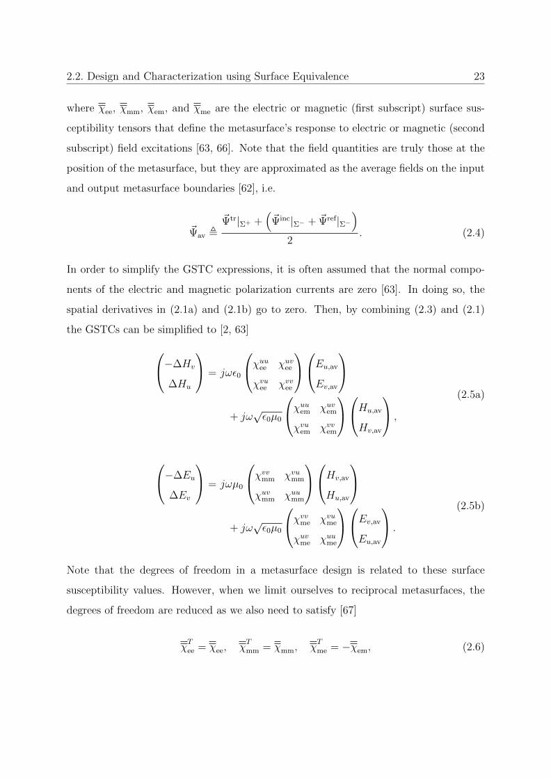
where χee, χmm, χem, and χme are the electric or magnetic (first subscript) surface sus-
ceptibility tensors that define the metasurface’s response to electric or magnetic (second
subscript) field excitations [63, 66]. Note that the field quantities are truly those at the
position of the metasurface, but they are approximated as the average fields on the input
and output metasurface boundaries [62], i.e.
~Ψav ,~Ψtr|Σ+ +
(~Ψinc|Σ− + ~Ψref|Σ−
)2
. (2.4)
In order to simplify the GSTC expressions, it is often assumed that the normal compo-
nents of the electric and magnetic polarization currents are zero [63]. In doing so, the
spatial derivatives in (2.1a) and (2.1b) go to zero. Then, by combining (2.3) and (2.1)
the GSTCs can be simplified to [2, 63]
−∆Hv
∆Hu
= jωε0
χuuee χuvee
χvuee χvvee
Eu,av
Ev,av
+ jω
√ε0µ0
χuuem χuvem
χvuem χvvem
Hu,av
Hv,av
,
(2.5a)
−∆Eu
∆Ev
= jωµ0
χvvmm χvumm
χuvmm χuumm
Hv,av
Hu,av
+ jω
√ε0µ0
χvvme χvume
χuvme χuume
Ev,av
Eu,av
.
(2.5b)
Note that the degrees of freedom in a metasurface design is related to these surface
susceptibility values. However, when we limit ourselves to reciprocal metasurfaces, the
degrees of freedom are reduced as we also need to satisfy [67]
χTee = χee, χ
Tmm = χmm, χ
Tme = −χem, (2.6)

2.2. Design and Characterization using Surface Equivalence 24
where the superscript T denotes the transpose operator. In addition, if we would like to
satisfy the conditions for lossless and passive metasurfaces, we need to have [63, 67]
χTee = χ
∗ee, χ
Tmm = χ
∗mm, χ
Tme = χ
∗em, (2.7)
where the superscript ∗ denotes the complex conjugate operator.
In the next sections, we explain how metasurfaces can be designed using the inverse source
and inverse scattering techniques.
2.2.2 Metasurface Design Using Inverse Source
According to (2.5), if one knows the incident, reflected, and desired transmitted fields on
the metasurface boundaries, we can use the GSTCs to calculate the surface susceptibility
profile that is required to implement the metasurface.1 However, the desired transmitted
field is not always known on the output boundary of the metasurface. For example, in
many applications such as mobile communication, the far-field radiation pattern of the
antenna is most important. In these cases, one may be able to use modal expansion
methods to back-propagate the desired data to the output boundary of the metasurface,
however, it is difficult to use these methods if the desired data is not on a canonical
surface, if only phaseless desired data are known, or if only far-field criteria such as main
beam direction and/or null locations are known [2]. Instead, we have recently showed
that we can use the EI framework to solve an inverse source problem to find the desired
transmitted field on the output boundary of the metasurface [2]. Then the GSTCs can
be used to calculate the surface susceptibility profile that will represent the metasurface.
To clarify this from the EI standpoint, in [2], we used the flexibility of the EI framework
to develop a metasurface design methodology that could make use of a variety of elec-
tromagnetic data including complex magnetic field data, phaseless magnetic field data,
1In this work, we showed the GSTCs written in terms of surface susceptibilities, but they may alsobe represented with surface impedances and polarizabilities [7, 56].

2.2. Design and Characterization using Surface Equivalence 25
and far-field criteria to calculate the property of interest which was the transmitted field
on the output boundary of the metasurface ( ~Etr|Σ+ and ~Htr|Σ+). This method also al-
lows us to make use of arbitrarily shaped surfaces/regions for the locations of the desired
data and metasurface shape. As this work was a precursor to the work in Chapter 3, an
overview of the methods taken are presented next.
The main steps taken to solve the EI problem in [2] to calculate the desired transmitted
field on the output metasurface boundary were outlined in Section 1.4.4. We presented
design algorithms for three cases wherein the desired electromagnetic data was specified
as: complex tangential electromagnetic data, phaseless data, or far-field criteria (such
as main beam direction and half-power beam width) [2, Section VII]. The property of
interest in all these cases was the tangential transmitted field on the output boundary of
the metasurface ( ~Etr|Σ+ and ~Htr|Σ+), or equivalently, the electric and magnetic current
densities on the output metasurface boundary ( ~J |Σ+ and ~M |Σ+ , respectively) contingent
on the enforcement of Love’s condition.2 To obtain a physical model/operator to map
the sought-after currents to the different types of electromagnetic data, we first needed
an operator (G) to map the currents to fields [2]. To this end, we used the electric field
integral equations3 (EFIE) [47], which in the full three-dimensional case, can be expressed
as [35]
G( ~J, ~M) =− jη0k0
∫Σ+
[~J(~r ′) +
1
k20
∇∇′s · ~J(~r ′)
]g(~r, ~r ′)ds′
−∇×∫
Σ+
~M(~r ′)g(~r, ~r ′)ds′ (2.8)
where ~r is a position vector belonging to the desired data domain/surface and ~r ′ is a
position vector on Σ+. The operators ‘∇×’ and ‘∇’ are the curl and gradient operator,
respectively, while ‘∇′s·’ is the surface divergence operator with respect to the ~r ′ coor-
dinates. Finally, g(., .) is the Green’s function, η0 is the wave impedance, and k0 is the
2Note that in this method we are focused on calculating a set of equivalent currents for the purposesof design utilizing the surface equivalence principle.
3If the operator mapping to magnetic field data is required, one can use the EFIE with the principleof duality [11].
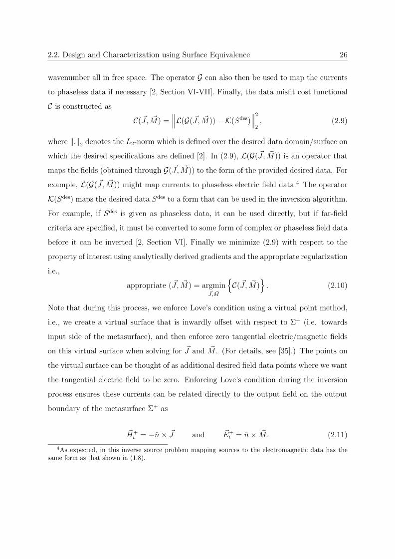
2.2. Design and Characterization using Surface Equivalence 26
wavenumber all in free space. The operator G can also then be used to map the currents
to phaseless data if necessary [2, Section VI-VII]. Finally, the data misfit cost functional
C is constructed as
C( ~J, ~M) =∥∥∥L(G( ~J, ~M))−K(Sdes)
∥∥∥2
2, (2.9)
where ‖.‖2 denotes the L2-norm which is defined over the desired data domain/surface on
which the desired specifications are defined [2]. In (2.9), L(G( ~J, ~M)) is an operator that
maps the fields (obtained through G( ~J, ~M)) to the form of the provided desired data. For
example, L(G( ~J, ~M)) might map currents to phaseless electric field data.4 The operator
K(Sdes) maps the desired data Sdes to a form that can be used in the inversion algorithm.
For example, if Sdes is given as phaseless data, it can be used directly, but if far-field
criteria are specified, it must be converted to some form of complex or phaseless field data
before it can be inverted [2, Section VI]. Finally we minimize (2.9) with respect to the
property of interest using analytically derived gradients and the appropriate regularization
i.e.,
appropriate ( ~J, ~M) = argmin~J, ~M
{C( ~J, ~M)
}. (2.10)
Note that during this process, we enforce Love’s condition using a virtual point method,
i.e., we create a virtual surface that is inwardly offset with respect to Σ+ (i.e. towards
input side of the metasurface), and then enforce zero tangential electric/magnetic fields
on this virtual surface when solving for ~J and ~M . (For details, see [35].) The points on
the virtual surface can be thought of as additional desired field data points where we want
the tangential electric field to be zero. Enforcing Love’s condition during the inversion
process ensures these currents can be related directly to the output field on the output
boundary of the metasurface Σ+ as
~H+t = −n× ~J and ~E+
t = n× ~M. (2.11)
4As expected, in this inverse source problem mapping sources to the electromagnetic data has thesame form as that shown in (1.8).

2.2. Design and Characterization using Surface Equivalence 27
Now that we know the transmitted fields on Σ+, we can use the GSTCs to calculate the
surface susceptibility profile to design the metasurface.
To show an example of what is possible with this inversion method, let us briefly show the
metasurface design example from [2, Section IX]. In this example, the goal was to design
a metasurface that was 10λ in length (λ is the free-space wavelength) and discretized into
λ/6 subwavelength element segments. Therefore, there were 60 reconstruction points and
a total of 120 unknowns (60 for ~J and 60 for ~M). Note that if we are using the GSTCs to
design a metasurface in this manner, it is assumed that it has zero thickness. The incident
field is a ‘tapered’ normally incident transverse electric (TEz) plane wave, i.e., the z-
component of the magnetic field (Hz) amplitude of the plane wave is 1 A/m for 14λ (past
the extents of the metasurface) and decays linearly to zero thereafter.5 Additionally, the
reflected field was assumed to be zero. The desired far-field power pattern was generated
by an array of 13 z-directed elementary dipoles that were uniformly spaced on a 6λ
line. The power pattern of Hz produced by this array was calculated on a semicircular
region of radius 500λ from −90◦ ≤ ϕ ≤ 90◦ as shown in Figure 2.2 where ϕ is in the
spherical coordinate system. At this point in the design process, the incident field and
reflected field are known on the metasurface input boundary and the desired phaseless
magnetic far-field is known. To design the metasurface, we use the inverse source method
outlined above, by constructing the appropriate cost functional and minimizing this cost
functional with respect to the electric and magnetic currents on Σ+ while enforcing Love’s
condition [2]. Next we calculate the fields from the currents according to (2.11), and use
the GSTCs to solve for the susceptibilities. We simulated the designed metasurface using
a full-wave finite difference frequency domain solver that was capable of simulating the
GSTC boundary conditions (FDFD-GSTC) developed by Vahabzadeh et. al. [66]. The
magnitude of Hz at a moment in time from this simulation is shown in [2, Figure 8].
The far-field pattern was then calculated by propagating the near-field to the far-field.
This far-field is shown in Figure 2.2. It can be seen that the far-field generated by
5This was done to reduce interaction between the plane wave and the perfectly matched layer boundaryconditions in the simulation and therefore avoid numerical error during the verification process [2].
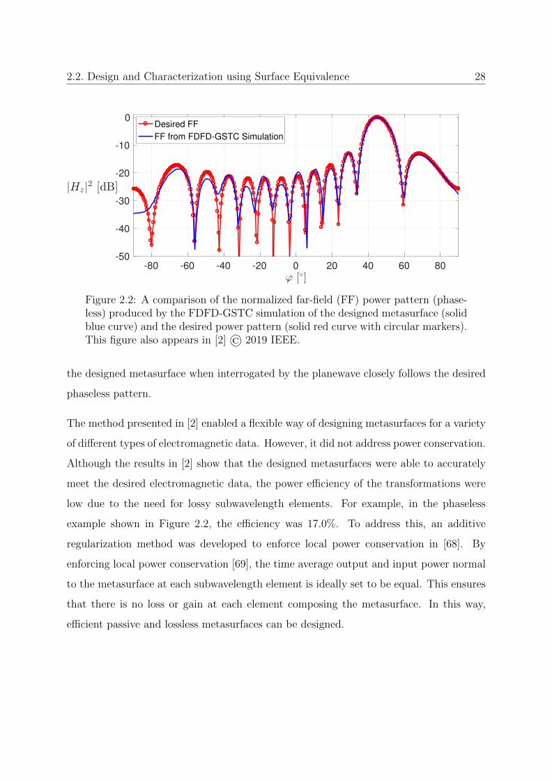
2.2. Design and Characterization using Surface Equivalence 28
-80 -60 -40 -20 0 20 40 60 80-50
-40
-30
-20
-10
0Desired FF
FF from FDFD-GSTC Simulation
Figure 2.2: A comparison of the normalized far-field (FF) power pattern (phase-less) produced by the FDFD-GSTC simulation of the designed metasurface (solidblue curve) and the desired power pattern (solid red curve with circular markers).This figure also appears in [2] © 2019 IEEE.
the designed metasurface when interrogated by the planewave closely follows the desired
phaseless pattern.
The method presented in [2] enabled a flexible way of designing metasurfaces for a variety
of different types of electromagnetic data. However, it did not address power conservation.
Although the results in [2] show that the designed metasurfaces were able to accurately
meet the desired electromagnetic data, the power efficiency of the transformations were
low due to the need for lossy subwavelength elements. For example, in the phaseless
example shown in Figure 2.2, the efficiency was 17.0%. To address this, an additive
regularization method was developed to enforce local power conservation in [68]. By
enforcing local power conservation [69], the time average output and input power normal
to the metasurface at each subwavelength element is ideally set to be equal. This ensures
that there is no loss or gain at each element composing the metasurface. In this way,
efficient passive and lossless metasurfaces can be designed.

2.2. Design and Characterization using Surface Equivalence 29
2.2.3 Metasurface Design Using
Inverse Scattering
Metasurfaces can also be designed using an inverse scattering approach as will be demon-
strated in Chapter 3. To understand how the metasurface design problem can be viewed
as an inverse scattering problem, one can compare the full form of the GSTCs in (2.1a)
and (2.1b) to (1.9). We remind the reader that in Section 1.4.1 we stated that inverse
scattering problems have some means of mapping currents to the material property of
interest, i.e. Usources = K (Xmater). It can be seen that the left hand side of (2.1a) and
(2.1b) are simply the surface currents supported by the metasurface (see the boundary
condition equations in (3.6)). Additionally, keeping in mind that the electric and mag-
netic surface polarization densities are functions of the surface susceptibilities (see (2.3)),
we have a mapping from the unknown surface susceptibilities to the surface currents
supported by the metasurface.6 Note that posing the metasurface design problem as an
inverse scattering problem allows for the direct solution of the surface susceptibility profile
or related parameters. This was done in [39] where the surface impedances, admittances
and magneto-electric coupling parameters are found to satisfy far-field criteria.7
Note that up until now we have been assuming an ideal, zero-thickness (single layer)
model for the metasurface. However, it has been shown that metasurfaces are typically
implemented as multi-layered printed circuit boards, e.g., see the three-layered dogbone
structures shown in [70]. This is due to the required degrees of freedom to enable such
transformations.8 These types of metasurfaces can not be directly designed with the
above inverse source approaches.
6These currents are actually supported by the metasurface (internal) and should not be confused withthe output currents/fields (aperture) on the metasurface boundary Σ+ that we solved for in (2.11). Notethat this can be seen as another example of the volume equivalence principle that was described in 1.3.2,but for a surface because we are dealing with a 2D scatterer.
7The surface impedances, admittances and magneto-electric coupling parameters serve the same pur-pose as the surface susceptibilities; they both describe the relation between the surface currents supportedby the metasurface to the fields on the metasurface.
8If we want to transform complex input fields ~E1 and ~H1 to complex output fields ~E2 and ~H2 weneed four degrees of freedom. Assuming local power conservation for the design of passive, lossless andreflectionless metasurfaces, we have three degrees of freedom [68] (see Section 2.2.1).

2.3. Design and Characterization by Volume Equivalence 30
Multi-layer metasurfaces can be approximately modelled with a circuit-based modelling
technique. The metasurface is seen as a set of adjacent two-port network [71] models
that are composed of circuit elements representing the different layers in each subwave-
length element; it is assumed that the metasurface is composed of dielectric layers (e.g.,
for substrate and bondply) and admittance layers (representing the metal trace of a sub-
wavelength element). The circuit admittances are often the parameters that are tuned
to design the metasurface, i.e., the dielectric layers are consistent throughout the meta-
surface and only the admittance of each metasurface element is tuned. This is explained
in detail in Chapter 3.
Note that modelling the metasurface in this way allows for the mapping of the unknown
circuit admittances (material property of interest) to the electric and magnetic surface
current densities on the output boundary of the metasurface. In Chapter 3, we demon-
strate an inverse scattering approach that uses this simplified model for the metasurface
to solve directly for the circuit admittances. This approach also adds the ability to add
constraints directly to the circuit admittances during the inversion process, this can fa-
cilitate the design of the subwavelength elements needed to physically implement the
metasurface.
2.3 Design and Characterization by Volume
Equivalence
Metasurfaces are a means to support surface currents that can tailor electromagnetic
fields, i.e., they can be seen as a method to physically implement the surface equivalence
principle. However, most antennas/scatterers are not so electrically thin that they can
be analyzed as metasurfaces.9 Additionally, there are many cases where the internal
electromagnetic properties of a radiator need to be analyzed or synthesized, (e.g., in
9It may also be beneficial to model metasurfaces as having finite thickness as they do so in reality.Metasurface circuit models do this, however, more accurate full-wave physics solvers may also be usedin the future so mutual coupling between layers can be taken into account.

2.3. Design and Characterization by Volume Equivalence 31
the application of microwave imaging the complex dielectric profile of volume scatterers
are the property of interest). For these cases, and cases where perfect electric/magnetic
conductors are not the only radiators, surface current approaches may not be sufficient.
Instead, we can look to use the volume equivalence principle to model antennas/scatterers
where some internal properties of the scatterer are required. The volumetric equivalent
currents are related to the electromagnetic data as in (1.8), and also related to the prop-
erty of interest as in (1.9). This is demonstrated in Section 1.3.2 where the equivalent
currents that radiate the scattered fields are a function of the relative permittivity and per-
meability. Therefore, using these equivalent currents, we can develop an inverse scattering
problem to solve for the property of interest from the measured/desired electromagnetic
data.
The above methods are often used for the applications of microwave imaging and dielectric
lens/antenna design. Next we present a brief overview of these applications to ready the
reader for later chapters.
2.3.1 Microwave Imaging: Characterization by Volumetric
Currents
In microwave imaging (MWI), the property of interest is often the complex dielectric
profile in a region of interest (i.e., investigation domain) referred to as the imaging domain
D. The electromagnetic data that are to be processed in the inversion algorithm are
the electric and/or magnetic field data collected by receivers on a measurement domain
S outside D. The electromagnetic data are generated by successively illuminating the
targets in D by transmitters and collecting the resulting total electric and/or magnetic
field data for each transmitter at the receivers. The same experiment is also often repeated
without any targets in D to collect the incident field on the measurement domain. The
resulting scattered field data, where the scattered field is the difference of the total and
incident fields (e.g., in the case of electric fields: Escat = E − Einc), is then given to
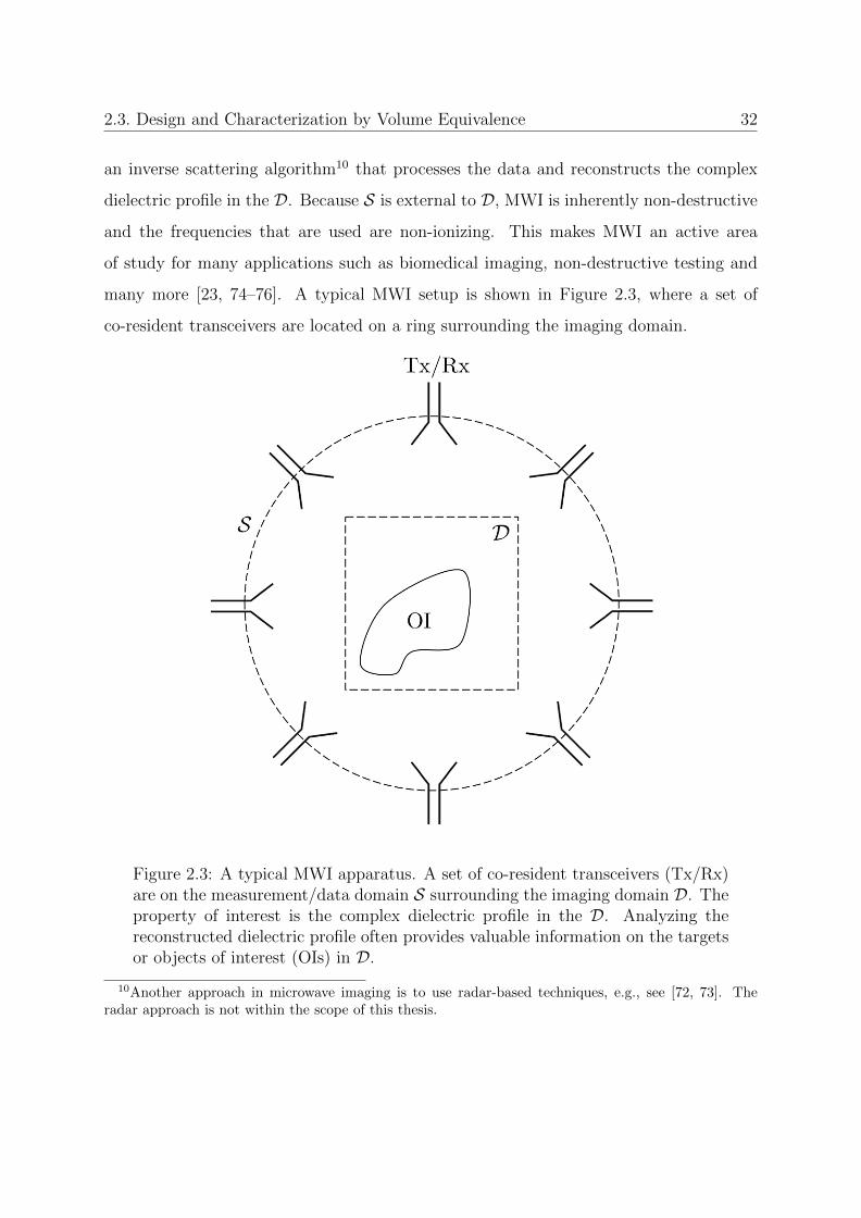
2.3. Design and Characterization by Volume Equivalence 32
an inverse scattering algorithm10 that processes the data and reconstructs the complex
dielectric profile in the D. Because S is external to D, MWI is inherently non-destructive
and the frequencies that are used are non-ionizing. This makes MWI an active area
of study for many applications such as biomedical imaging, non-destructive testing and
many more [23, 74–76]. A typical MWI setup is shown in Figure 2.3, where a set of
co-resident transceivers are located on a ring surrounding the imaging domain.
Figure 2.3: A typical MWI apparatus. A set of co-resident transceivers (Tx/Rx)are on the measurement/data domain S surrounding the imaging domain D. Theproperty of interest is the complex dielectric profile in the D. Analyzing thereconstructed dielectric profile often provides valuable information on the targetsor objects of interest (OIs) in D.
10Another approach in microwave imaging is to use radar-based techniques, e.g., see [72, 73]. Theradar approach is not within the scope of this thesis.

2.3. Design and Characterization by Volume Equivalence 33
To understand how the application of MWI can be set up as an electromagnetic inverse
problem, consider the data equation for a non-magnetic, homogeneous background [19, 77]
Escat(r ∈ S) = k2b
∫Dg(r ∈ S, r′ ∈ D)E(r′ ∈ D)
εr(r′ ∈ D)− εbεb
dr′ (2.12)
that maps the relative permittivity of the scatterers in D to the scattered field on the
measurement domain S for a typical tomographic (2D) MWI configuration. Here, g(r, r′)
is the two dimensional Green’s function of the background medium that has a relative
permittivity εb. There are two unknowns: E(r′), the total field in D, and the (property of
interest) relative permittivity εr(r′) in D. Finally kb is the wavenumber of the background
medium. It is instructive to note that contrast sources that represent the volumetric
currents that generate the scattered field as described by volume equivalence principle
can be defined as
W (r′ ∈ D) = E(r′ ∈ D)εr(r
′)− εbεb
. (2.13)
Therefore, we can rewrite (2.12) as producing a scattered field due to a set of contrast
sources. Also, E(r′ ∈ D) is itself related to εr(r′) and the incident field Einc via the
domain equation [19, 77]:
E(r′ ∈ D) = Einc(r′ ∈ D)+k2b
∫Dg(r′ ∈ D, r′′ ∈ D)E(r′′ ∈ D)
εr(r′′ ∈ D)− εbεb
dr′′. (2.14)
We can see that with (2.12), (2.13), and (2.14) we have a means of relating sources to
the electromagnetic data, and the sources to the property of interest as in all inverse
scattering problems. Another advantage with using these equations are that they are full
wave, and so they take into account mutual coupling and multiple scattering as opposed
to simpler models such as the circuit model we used to approximately model a muti-layer
metasurface. Therefore, by using this formulation, we may be able to more accurately
characterize and design antennas.
In order to calculate the dielectric profile, many inverse scattering algorithms have been
put forth that utilize the data equation, domain equation, different approximations of

2.3. Design and Characterization by Volume Equivalence 34
E(r′), optimization methods, and regularization schemes (some examples of the vast
amount of inverse scattering methods are found in [19, 30, 78, 79]). In Chapter 4 we
use the flexibility of the EI framework to develop phaseless Gauss-Newton inversion al-
gorithms that can be used with microwave imaging. In this work phaseless data are used
on S to reconstruct the relative permittivity in D. Note that measuring phaseless data
generally requires less expensive equipment compared to measuring data with phase.
2.3.2 Dielectric Lens/Antenna Design: Design by Volumetric
Currents
Inverse scattering algorithms can also be used to design dielectric objects in D. Instead
of using measured data collected at the receivers in Figure 2.3, we can instead provide
the inverse scattering algorithm with desired data. From this point, many of the same
algorithmic techniques that can be used to solve MWI problems can be used to design
dielectric profiles in D. This application is especially logical as the non-uniqueness that
is problematic in the imaging case, can be advantageous in the case of design (e.g. the
availability of different dielectric profiles for a single set of desired data may facilitate di-
electric lens fabrication).11 Recently, research on inverse scattering for design of dielectric
lenses, cloaks, etc has been reported [9, 22, 80, 81].
As was previously shown in [2], it is often beneficial to be able to make use of a variety
of electromagnetic data to solve for the property of interest. To this end, in [82] we
briefly explored using the phaseless Gauss-Newton inversion algorithm that was devel-
oped for Chapter 4 for dielectric lens design. However, to further increase the variety
of electromagnetic data that is available for use in the inversion process and to increase
the capability of the dielectric lens/antenna designer, in Chapter 5 we present a novel
combined inverse source and scattering technique to design dielectric lens antennas. This
11There is a trade-off that occurs here, the once issue of non-uniqueness may be an advantage fordesign, but now the issue of existence presents itself. There may not be a dielectric profile that can dowhat the designer desires.

2.4. Summary 35
technique is capable of using multiple inverse scattering algorithms, is capable of utilizing
complex, phaseless, and far-field criteria data in the inversion process, and can design
passive, lossless and reflectionless lenses.
2.4 Summary
In this chapter, we briefly described the antenna design and characterization applications
addressed in this thesis. All these applications are connected in their direct or indirect
solution of a set of sources that relate to the electromagnetic data through EI; if an inverse
scattering problem is being solved, then the material parameters of the scatterer are in
turn related to the sources contributing to the electromagnetic data.
First we contributed to the area of metasurface design using an inverse source, then inverse
scattering method to be able to directly design the admittance layers of the metasurface.
Then, to continue to more directly design and characterize electrically thicker scatterers,
we moved to the areas of microwave imaging and dielectric lens/antenna design. In the
next chapter, we present our EI algorithm that is capable of designing the admittance
layers of a metasurface in more detail.

Chapter 3
Multi-Layer Metasurface Design
Using An Inverse Scattering
Technique
Preface
In this chapter, we present an EI algorithm for the purpose of metasurface design. As
mentioned in Section 2.2, metasurfaces are a way to physically implement the surface
equivalence principle to tailor electromagnetic fields. Previously, we presented an inverse
source method to design these surfaces (see Section 2.2.2 and [2]), but we could not
directly design multi-layer metasurfaces or any material parameters directly using this
method. To this end, in this work we present an electromagnetic inversion scattering
algorithm that can design the circuit admittances of a three-layer admittance metasurface
directly. Because we are directly solving for the material parameters of the metasurface,
this can be considered as an inverse scattering approach. This can be seen in Section 3.4
as the circuit model allows us to relate the circuit admittances to the output/aperture
36
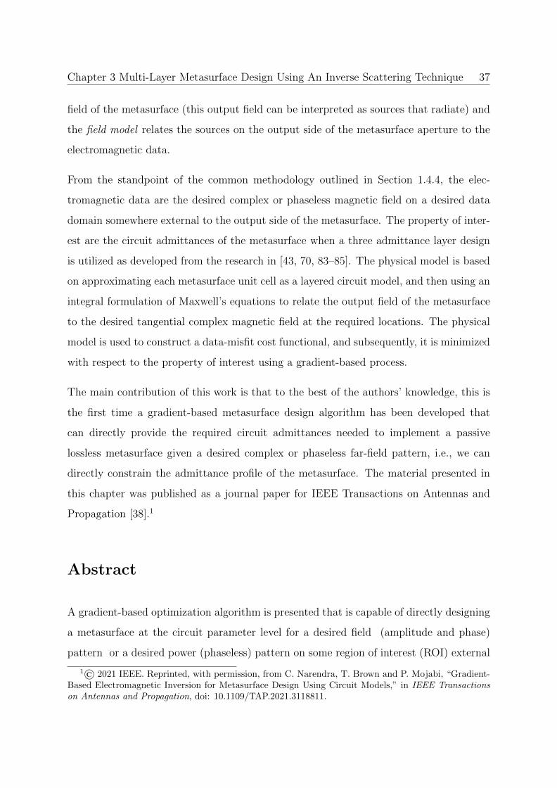
Chapter 3 Multi-Layer Metasurface Design Using An Inverse Scattering Technique 37
field of the metasurface (this output field can be interpreted as sources that radiate) and
the field model relates the sources on the output side of the metasurface aperture to the
electromagnetic data.
From the standpoint of the common methodology outlined in Section 1.4.4, the elec-
tromagnetic data are the desired complex or phaseless magnetic field on a desired data
domain somewhere external to the output side of the metasurface. The property of inter-
est are the circuit admittances of the metasurface when a three admittance layer design
is utilized as developed from the research in [43, 70, 83–85]. The physical model is based
on approximating each metasurface unit cell as a layered circuit model, and then using an
integral formulation of Maxwell’s equations to relate the output field of the metasurface
to the desired tangential complex magnetic field at the required locations. The physical
model is used to construct a data-misfit cost functional, and subsequently, it is minimized
with respect to the property of interest using a gradient-based process.
The main contribution of this work is that to the best of the authors’ knowledge, this is
the first time a gradient-based metasurface design algorithm has been developed that
can directly provide the required circuit admittances needed to implement a passive
lossless metasurface given a desired complex or phaseless far-field pattern, i.e., we can
directly constrain the admittance profile of the metasurface. The material presented in
this chapter was published as a journal paper for IEEE Transactions on Antennas and
Propagation [38].1
Abstract
A gradient-based optimization algorithm is presented that is capable of directly designing
a metasurface at the circuit parameter level for a desired field (amplitude and phase)
pattern or a desired power (phaseless) pattern on some region of interest (ROI) external
1© 2021 IEEE. Reprinted, with permission, from C. Narendra, T. Brown and P. Mojabi, “Gradient-Based Electromagnetic Inversion for Metasurface Design Using Circuit Models,” in IEEE Transactionson Antennas and Propagation, doi: 10.1109/TAP.2021.3118811.

3.1. Introduction 38
to the metasurface boundary. Specifically, the inversion algorithm designs the microwave
admittance profile of each subwavelength element of the metasurface when a three-layer
admittance model is assumed. To this end, a forward model is developed that maps the
admittance profile of each layer of the metasurface to the desired field on the ROI. Then,
for the inverse design problem, a data misfit cost functional is defined and minimized over
the unknown admittance profile using analytically derived gradients and step lengths.
The developed inversion algorithm is then utilized to design metasurfaces capable of
beam forming in the far-field zone.
3.1 Introduction
Metasurfaces are devices of subwavelength thickness that are capable of systematically
transforming an incoming electromagnetic field distribution to a desired outgoing field
distribution [8, 54, 65, 86–88]. This is made possible by the lattice of subwavelength
elements that comprise the metasurface. Metasurfaces enable the implementation of a
vast amount of field transformations such as controlling reflection [56], refraction [54, 56],
absorption [89, 90], polarization transformation [57], and much more. These abilities can
then facilitate many applications such as tailoring radiation patterns of antennas [91],
cloaking [60], and the development of smart radio environments [61].
In order to utilize metasurface technology towards different applications, general de-
sign methodologies are needed and some have recently been proposed [6, 7]. In these
approaches, the tangential electromagnetic field components present on the input and
output boundaries of the metasurface are required. (For a discussion on the normal com-
ponents, see [92].) Once these fields have been defined, the generalized sheet transition
conditions (GSTCs) [65] are used to calculate either the surface impedance [7], suscepti-
bility [6], or polarizability [56] profiles that represent the discontinuity needed to support
the specified field transformation assuming a metasurface of zero-thickness. In this paper,
we will refer to these quantities as GSTC parameters.

3.1. Introduction 39
In the general design methodologies mentioned above, a procedure for relating desired
field specifications (e.g., power pattern, main beam direction, null directions, etc.) some-
where external to the metasurface (e.g., in the far-field zone) to the fields on the output
boundary of the metasurface is not described. The development of such a link would
promote the use and design of metasurfaces because the field on the output boundary of
the metasurface is not always known; rather, a set of specifications on a region somewhere
external to the metasurface is what is important and typically known to the designer.
For example, many antenna applications require specific far-field patterns such as nulls in
desired directions or a specific half-power beamwidth (HPBW). To this end, in [2, 68, 93],
the general metasurface design framework described above was extended to leverage elec-
tromagnetic inversion for design scenarios where different types of field specifications are
required on a region of interest (ROI) external to the metasurface, e.g., in its far-field
zone. This framework is referred to as inversion because it infers a cause (equivalent
currents on the metasurface boundary) from an external effect (desired specifications).
It was also demonstrated how this inversion framework can enable the design of passive
and lossless metasurfaces by enforcing local power conservation (LPC) [69, 94] in the
inversion process via augmenting the original cost functional with an extra term [68].
Therefore, the work in [2, 68] introduced a flexible field model to the metasurface design
framework: using this framework, it is possible to infer the required output fields on the
metasurface boundary from the knowledge of field specifications on a ROI. Thus, the
required GSTC parameters can be obtained. However, this is usually not sufficient to
complete the metasurface design process. Physically implementing a metasurface directly
from its associated GSTC parameter profile is not done in practice, instead, the GSTC
parameters are often transformed to microwave circuit parameters such as impedance,
admittance, or scattering parameters [7, 43, 83–85, 95] so that the appropriate subwave-
length metasurface elements can be designed in a separate step [7, 43].
Alternatively, instead of having equivalent currents as the unknowns of the inverse design
problem, we may reformulate the problem such that its unknowns become the circuit
parameters associated with different unit cells. To understand the advantage of such a

3.1. Introduction 40
reformulation, let us assume that we desire to create a null in a certain direction using a
metasurface to be later fabricated on a specific dielectric substrate (e.g., Rogers RO3010)
and specific metallic trace geometry (e.g., dogbone traces [70, 85]).2 Given the substrate
and trace types, we often know beforehand the range of capacitance and inductance
values [85] that can be supported. Therefore, if the inverse design can be done directly at
the circuit parameter level, we will have the opportunity to limit the optimization space
to those practically feasible capacitance and inductance values. On the other hand, if the
inverse design is performed at the field level (i.e., optimizing over equivalent currents), it is
not straightforward to impose such circuit-level constraints on field-level unknowns during
the optimization process. As another example, when the inverse design is performed at
the field level, ensuring a passive and lossless metasurface requires augmenting the cost
functional by an extra LPC term [68]. On the other hand, at the circuit level, we can
simply limit the search space to purely imaginary impedance values.
Herein, we make use of research introduced in [43, 70, 83–85] to model metasurfaces
as an array of subwavelength elements composed of a network of circuit admittances
in combination with concepts developed in [2, 68] to develop a forward model that can
relate these microwave circuit parameters to the desired output field (amplitude and
phase) or power (phaseless) pattern. Next, we use this forward model to develop a
novel gradient-based electromagnetic inversion algorithm used to design a metasurface by
directly optimizing the circuit admittance profile of the metasurface. This work aims to
keep the flexibility of meeting desired field constraints external to the metasurface as well
as facilitating the design of metasurface subwavelength elements. We begin by describing
the general metasurface design problem in Section 3.2 as well as a brief description of
the employed forward model and scope of this paper. Then, the problem statement is
presented in Section 3.3. Next, the forward model is described in detail in Section 3.4
2Dogbone traces are a common choice to implement these admittance layers. This is partly due tothe fact that their fabrication is relatively easy and they can be implemented with printed circuit boardtechnology. To implement various admittance values the geometrical parameters of the dogbone trace,such as its height and width, are changed to create a lookup table. Once a lookup table is formed, it canbe used for an initial design which then needs to be further optimized to take into account other effectssuch as mutual coupling.

3.2. General Problem Description and Scope 41
and the novel inversion algorithm is presented in Section 3.5. Results are then shown
and discussed in Section 5.4 wherein the developed inversion algorithm is used to design
metasurfaces to meet desired field (amplitude and phase) or power (phaseless) patterns.
Finally, we summarize this work in Section 3.7.
3.2 General Problem Description and Scope
The general metasurface design problem is shown in Figure 3.1. A metasurface separates
two volumetric regions of space; the input side V −, and the output side V +. The source
is in V −, while the ROI, a fictitious region of space containing the set of desired field or
power specifications lies in V +. The known quantities of this problem are the incident
field ~Ψinc produced by the source, the reflected field ~Ψref (in our work we assume ~Ψref =
0) and the desired specifications on the ROI. The tangential fields on the metasurface
boundaries are denoted by ~E−t and ~H−t on Σ−, and ~E+t and ~H+
t on Σ+. The tangential
coordinates on the metasurface are u and v, while the outward facing normal direction is
n. (In this work, u = z, v = −y and n = x.)
Microwave two-port networks normally relate an input voltage and current to an output
voltage and current, and because ~Et and ~Ht are analogous quantities, we can use these
networks to model metasurface unit cells. Furthermore, the unit cells (and thus, the two-
port networks) can be defined by a network of circuit elements as in [43, 84, 85]. Therefore,
the output fields of a unit cell are related to the circuit elements that comprise that cell and
the input fields. In this work, the unit cells will be composed of three parallel admittances
which are optimized to meet the desired specifications. Thus, we can represent the output
fields of each unit cell as a function of three admittances, g(Y1, Y2, Y3), as summarized in
Figure 3.2. In the scope of this work, we assume a two-dimensional transverse-electric
to the z direction (TEz) design problem. Thus, the problem can be formulated based on
Hz.
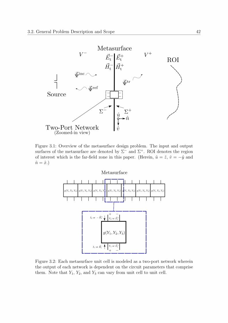
3.2. General Problem Description and Scope 42
Figure 3.1: Overview of the metasurface design problem. The input and outputsurfaces of the metasurface are denoted by Σ− and Σ+. ROI denotes the regionof interest which is the far-field zone in this paper. (Herein, u = z, v = −y andn = x.)
Figure 3.2: Each metasurface unit cell is modeled as a two-port network whereinthe output of each network is dependent on the circuit parameters that comprisethem. Note that Y1, Y2, and Y3 can vary from unit cell to unit cell.

3.3. Problem Statement 43
3.3 Problem Statement
Given (i) desired field (amplitude and phase) Hz or power (phaseless) |Hz|2 specifications
on the ROI, (ii) a known incident field, (iii) a known dielectric substrate, and (iv) a
known dielectric bondply (adhesive), we attempt to determine the admittance profile of a
passive, lossless, and reflectionless omega-type bianisotropic metasurface [94] to transform
the incident field to an output field that meets the specifications on the ROI (as closely
as possible).3 Therefore, each unit cell consists of three unknown admittance values with
two known dielectric substrates and one known dielectric bondply layer. Denoting the
total number of unit cells by N , the admittance profile will then consist of 3N admittance
values. That is, the problem is concerned with determining 3N unknowns from the desired
specifications on the ROI.
3.4 Forward Model
To solve this inverse problem, we first need to build a forward model to relate a given
admittance profile to the data on the ROI. Our forward model to be explained below is
composed of a circuit and field model, see Figure 3.3.
3.4.1 Circuit model
Each subwavelength element of the metasurface is modeled as a two-port network com-
posed of a network of three admittances. As in [43, 96], the three admittance layers are
separated by dielectric layers. The three admittances are needed to obtain the degrees
3Note that since we have considered a TEz configuration the problem has been formulated with respectto the Hz component.

3.4. Forward Model 44
Figure 3.3: The full forward model used in this work is composed of two separatemodels: the circuit and field models, respectively.
of freedom necessary to match the input and output fields [43].4 Note that this design
facilitates physical implementation with two printed circuit boards: one board will have
two trace layers (on either side of the substrate) and it can be bonded to another board
with one trace layer.
To represent each unit cell as a two-port network, three layers of admittance elements
can be linked in parallel with the dielectric layers as shown in Figure 3.4. The dielectric
layers (dielectric substrate of the traces and bondply) can be modeled as transmission
lines of length l. The wavenumber β and the characteristic impedance Z associated with
these dielectric layers are then defined as
β =2π
λ=
2πf√εr
c0
, Z =η0√εr, (3.1)
4We note that for some applications it might be necessary to increase the degrees of freedom indesign by adding a fourth admittance layer to the utilized unit cell, e.g., see [57, 97]. The overallmethodology presented herein remains the same if an extra admittance layer is added, however, newgradient operators need to be found. Also, adding an extra admittance layer may increase the non-linearity of the optimization problem. Therefore, the chance of encountering inappropriate local minimacan increase. Finally let us justify the use of three admittance layers. When we want to convert a given(E, H) to desired fields we need a two-port transformation. A two-port matrix consists of four elements.Due to reciprocity one of these elements is dependent on the remaining three, thus having three degreesof freedom. Therefore three layers have been used.
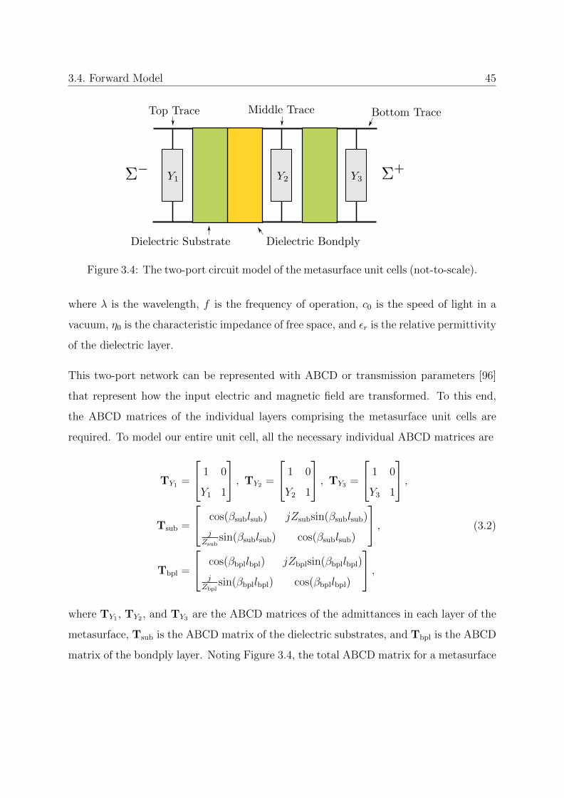
3.4. Forward Model 45
Figure 3.4: The two-port circuit model of the metasurface unit cells (not-to-scale).
where λ is the wavelength, f is the frequency of operation, c0 is the speed of light in a
vacuum, η0 is the characteristic impedance of free space, and εr is the relative permittivity
of the dielectric layer.
This two-port network can be represented with ABCD or transmission parameters [96]
that represent how the input electric and magnetic field are transformed. To this end,
the ABCD matrices of the individual layers comprising the metasurface unit cells are
required. To model our entire unit cell, all the necessary individual ABCD matrices are
TY1 =
1 0
Y1 1
, TY2 =
1 0
Y2 1
, TY3 =
1 0
Y3 1
,Tsub =
cos(βsublsub) jZsubsin(βsublsub)
jZsub
sin(βsublsub) cos(βsublsub)
,Tbpl =
cos(βbpllbpl) jZbplsin(βbpllbpl)
jZbpl
sin(βbpllbpl) cos(βbpllbpl)
,(3.2)
where TY1 , TY2 , and TY3 are the ABCD matrices of the admittances in each layer of the
metasurface, Tsub is the ABCD matrix of the dielectric substrates, and Tbpl is the ABCD
matrix of the bondply layer. Noting Figure 3.4, the total ABCD matrix for a metasurface

3.4. Forward Model 46
subwavelength element (unit cell) can be calculated as
Telem = TY1 Tsub Tbpl TY2 Tsub TY3 . (3.3)
Now with Telem, it is possible to relate the input field, admittances, and output fields of
each metasuface subwavelength element as [43]
~E−t~H−t
= Telem
~E+t
~H+t
. (3.4)
To model the metasurface in its entirety, Telem must be defined for all the subwavelength
elements. In this work, we assume that the dielectric layers (substrates and bondply)
are spatially invariant. Therefore, to model the complete metasurface, Y1, Y2, and Y3 for
every metasurface element must be known. We also replace the left hand side of (3.4)
with the incident field since we desire reflectionless metasurfaces. Finally, note that
since Y1 can be different than Y3, the algorithm may yield an omega-type bianisotropic
metasurface [94].
3.4.2 Field model
Now that it is possible to relate the input and output fields of each subwavelength element,
the fields on the output boundary of the metasurface Σ+ are available. Then, as in [2],
we use the well-known electric field integral equations and the principle of duality [47]
to obtain expressions relating the electric and magnetic current densities on Σ+ to Hz
on the ROI through the Green’s function of free space. In the discrete domain, this
transformation between currents on Σ+ to Hz on the ROI can be represented as the
following matrix operator
Hz︸︷︷︸on ROI
=[AHzJy AHzMz
] Jy
Mz
︸ ︷︷ ︸on Σ+
, (3.5)

3.4. Forward Model 47
where Hz is a vector containing all the Hz values on the ROI, AHzJy operates on the
electric current density vector Jy on Σ+ to produce the electric current contribution of
Hz, and AHzMz operates on the magnetic current density vector Mz on Σ+ to produce
the magnetic current contribution of Hz.
In order to make use of (3.5), we must be able to calculate the electric and magnetic
surface current densities from the output fields on Σ+. In the case where Love’s condition
is enforced, we can relate these two quantities as
Jy = n× ~H+t = −Hz
∣∣∣Σ+,
Mz = −n× ~E+t = −Ey
∣∣∣Σ+,
(3.6)
where n is the unit outward normal on the output side of the metasurface. The method
and importance of enforcing Love’s condition will be explained later on in this paper.
3.4.3 Complete forward model
The circuit and field models described above are now put together to demonstrate the
complete relationship between the input field, admittances, and the field at the ROI.
First, note that Telem of each metasurface element can be explicitly written in terms of
its ABCD parameters, and its inverse can also be expressed as
Telem =
A B
C D
=⇒ T−1elem =
1
∆
D −B−C A
, (3.7)
where ∆ = AD − BC. Because in this problem the two-port network at each element
is reciprocal, ∆ = 1. Once the individual ABCD parameters are found for each element
from (3.3), by combining (3.4), (3.5), (3.6), and (3.7), the field at the ROI can be found
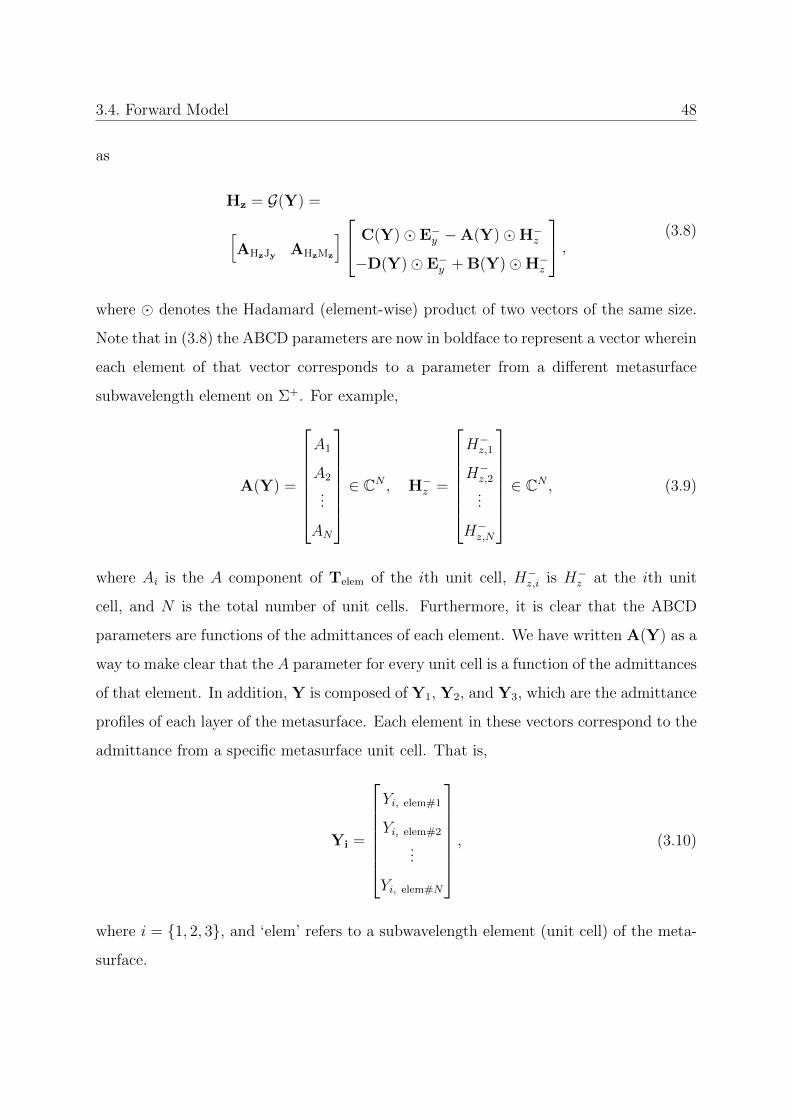
3.4. Forward Model 48
as
Hz = G(Y) =[AHzJy AHzMz
] C(Y)� E−y −A(Y)�H−z
−D(Y)� E−y + B(Y)�H−z
, (3.8)
where � denotes the Hadamard (element-wise) product of two vectors of the same size.
Note that in (3.8) the ABCD parameters are now in boldface to represent a vector wherein
each element of that vector corresponds to a parameter from a different metasurface
subwavelength element on Σ+. For example,
A(Y) =
A1
A2
...
AN
∈ CN , H−z =
H−z,1
H−z,2...
H−z,N
∈ CN , (3.9)
where Ai is the A component of Telem of the ith unit cell, H−z,i is H−z at the ith unit
cell, and N is the total number of unit cells. Furthermore, it is clear that the ABCD
parameters are functions of the admittances of each element. We have written A(Y) as a
way to make clear that the A parameter for every unit cell is a function of the admittances
of that element. In addition, Y is composed of Y1, Y2, and Y3, which are the admittance
profiles of each layer of the metasurface. Each element in these vectors correspond to the
admittance from a specific metasurface unit cell. That is,
Yi =
Yi, elem#1
Yi, elem#2
...
Yi, elem#N
, (3.10)
where i = {1, 2, 3}, and ‘elem’ refers to a subwavelength element (unit cell) of the meta-
surface.

3.5. Inverse Problem 49
3.5 Inverse Problem
The process of calculating an appropriate admittance profile to achieve a desired complex
field or phaseless power pattern is now explained. To this end, a data misfit cost functional
is defined, and a method of enforcing Love’s condition and smoothing regularizers are
described. Then, the gradient descent minimization process is presented.
3.5.1 Data Misfit Cost Functional
We form a cost functional that compares the modeled pattern due to a predicted meta-
surface admittance profile with the desired pattern. The modeled pattern due to a set
of microwave admittances can be calculated using (3.8). The desired pattern is stored
in the vector fROI for the field pattern synthesis and in the vector |fROI|2 for the power
pattern synthesis. The data misfit cost functional will then be
Cdata(Y) =
ζf ‖G(Y)− fROI‖2 field pattern synthesis
ζp ‖|G(Y)|2 − |fROI|2‖2power pattern synthesis
(3.11)
where ‖.‖ denotes the L2 norm over the ROI, Y represents the unknown admittance
profile, and the normalization constants ζf and ζp are defined as ‖fROI‖−2 and ‖|fROI|2‖−2
respectively.
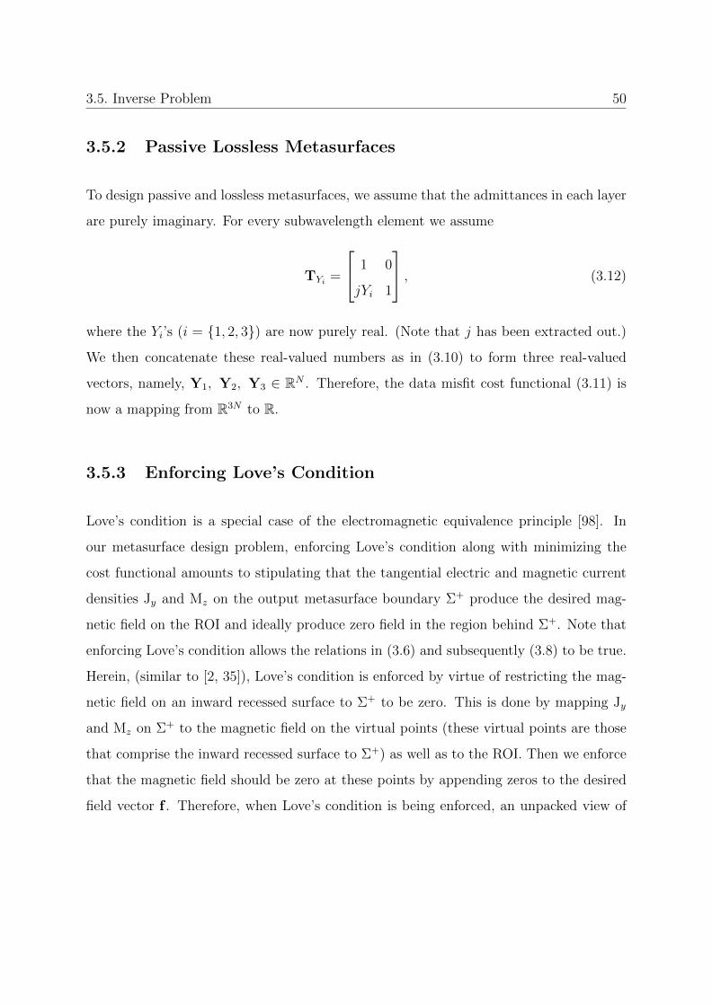
3.5. Inverse Problem 50
3.5.2 Passive Lossless Metasurfaces
To design passive and lossless metasurfaces, we assume that the admittances in each layer
are purely imaginary. For every subwavelength element we assume
TYi =
1 0
jYi 1
, (3.12)
where the Yi’s (i = {1, 2, 3}) are now purely real. (Note that j has been extracted out.)
We then concatenate these real-valued numbers as in (3.10) to form three real-valued
vectors, namely, Y1, Y2, Y3 ∈ RN . Therefore, the data misfit cost functional (3.11) is
now a mapping from R3N to R.
3.5.3 Enforcing Love’s Condition
Love’s condition is a special case of the electromagnetic equivalence principle [98]. In
our metasurface design problem, enforcing Love’s condition along with minimizing the
cost functional amounts to stipulating that the tangential electric and magnetic current
densities Jy and Mz on the output metasurface boundary Σ+ produce the desired mag-
netic field on the ROI and ideally produce zero field in the region behind Σ+. Note that
enforcing Love’s condition allows the relations in (3.6) and subsequently (3.8) to be true.
Herein, (similar to [2, 35]), Love’s condition is enforced by virtue of restricting the mag-
netic field on an inward recessed surface to Σ+ to be zero. This is done by mapping Jy
and Mz on Σ+ to the magnetic field on the virtual points (these virtual points are those
that comprise the inward recessed surface to Σ+) as well as to the ROI. Then we enforce
that the magnetic field should be zero at these points by appending zeros to the desired
field vector f . Therefore, when Love’s condition is being enforced, an unpacked view of

3.5. Inverse Problem 51
G(Y) is
G(Y) = Hz(Y) =
HROIz (Y)
HLovez (Y)
=
AROIHzJy
ALoveHzJy
AROIHzMz
ALoveHzMz
C(Y)�E−y −A(Y)�H−z
−D(Y)�E−y + B(Y)�H−z
,(3.13)
where HLovez is the magnetic field at Love’s virtual points, HROI
z is the magnetic field on
the ROI, and ALoveHzJy
and ALoveHzMz
are operators that map Jy and Mz to the magnetic field
at Love’s virtual points, respectively. Similarly, AROIHzJy
and AROIHzMz
are operators that map
Jy and Mz to the magnetic field on the ROI.
Similarly, the data vectors fROI and |fROI|2 in (3.11) will be changed to f and |f |2 respec-
tively as
f =
fROI
fLove
, |f |2 =
|fROI|2
fLove
, fLove =
0
0...
0
, (3.14)
where fLove is the part of f that enforces Love’s condition. The length of fLove is equal to
the number of virtual points on Love’s surface. Finally, it is instructive to note that the
augmentation of G(Y) by the Love’s component makes the minimization of Cdata(Y) in
(3.11) for the field and power pattern syntheses equivalent to minimizing
ζf{∥∥HROI
z (Y)− fROI
∥∥2+∥∥HLove
z (Y)∥∥2}, (3.15)
ζp{∥∥|HROI
z (Y)|2 − |fROI|2∥∥2
+∥∥|HLove
z (Y)|2∥∥2}, (3.16)
respectively.

3.5. Inverse Problem 52
3.5.4 Local Power Conservation (LPC)
Local power conservation [94] requires that the real power entering the unit cell in the
normal direction be equal to the real power leaving the unit cell in the normal direction.
As shown in [94], if LPC is satisfied between the incident field Einct and H inc
t and E+t and
H+t , we are able to transform the incident field to the output field using a reflectionless
lossless passive omega-type bianisotropic metasurface. The proposed inversion algorithm
inherently permits only those solutions that satisfy LPC. This can be easily verified by
considering (3.4) and (3.7) and finding the real power density entering the metasurface
(in the normal direction) as
Re{E−t H−∗
t } = Re{(AC∗|E+t |2 + AD∗E+
t H+∗
t
+BC∗H+t E
+∗
t +BD∗|H+t |2)}. (3.17)
Since the admittances of the three layers are only allowed to be purely imaginary, and
the dielectric substrates and bondply are assumed to be lossless, A and D are purely
real and B and C are purely imaginary. In addition, since E−t and H−t are set to be the
tangential incident fields (Einct and H inc
t ) and noting the reciprocity of each unit cell, we
can simplify (3.17) as
Re{Einct H inc∗
t } = Re{(ADE+t H
+∗
t −B∗C∗H+t E
+∗
t )} =
Re{(ADE+t H
+∗
t −BCH+∗
t E+t )} = Re{E+
t H+∗
t }. (3.18)
This shows that the LPC is satisfied. Note that the above analysis implicitly requires
that E+t and H+
t form a wavefront that propagates away from the metasurface in free
space. That is why the data misfit cost functional has been augmented by the Love’s
constraint.

3.5. Inverse Problem 53
3.5.5 Favouring Smooth Equivalent Currents
If there is more spatial variation in the equivalent currents (i.e., less smooth currents),
there will be more spatial variations in E+t and H+
t when moving from one unit cell
to the neighboring unit cell, which can be challenging to achieve in practice. To this
end, we utilize a total variation (TV) regularizer to favour smoother equivalent currents
by minimizing the norm of the derivative of the current along the metasurface (similar
to [99]). The cost functionals used to smooth the electric current densities J and magnetic
current densities M are respectively
CJTV(Yi) = τ1
3∑i=1
∥∥∥∥ ∂∂y (J(Yi))
∥∥∥∥2
= τ1
3∑i=1
∥∥∥∥ ∂∂y (C(Yi)� E−y −A(Yi)�H−z )
∥∥∥∥2
= τ1
3∑i=1
∥∥∥∥ ∂∂y (zi1Yi + hJi)
∥∥∥∥2
,
(3.19)
CMTV(Yi) = τ2
2∑i=1
∥∥∥∥ ∂∂y (M(Yi))
∥∥∥∥2
= τ2
2∑i=1
∥∥∥∥ ∂∂y (−D(Yi)� E−y + B(Yi)�H−z )
∥∥∥∥2
= τ2
2∑i=1
∥∥∥∥ ∂∂y (zi2Yi + hMi)
∥∥∥∥2
,
(3.20)
where ∂∂y
is the derivative operator along the y direction, and the above L2 norms are taken
along the metasurface. Also, note that in (3.19) i = {1, 2, 3} and in (3.20), i = {1, 2}.(The reason that i = {1, 2} for CMTV is that M is not a function of Y3; see (A.1) in
Appendix A.1.) In addition, τ1 and τ2 are real weighting parameters and hJiand hMi
are
vectors of constants that are formed after Yi has been factored from the currents J and
M, respectively. The expressions for z vectors are available in (A.9) in Appendix A.1.
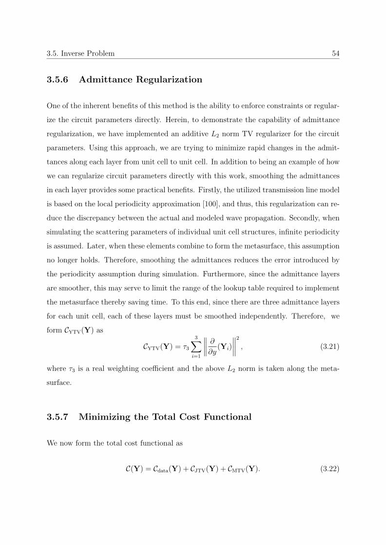
3.5. Inverse Problem 54
3.5.6 Admittance Regularization
One of the inherent benefits of this method is the ability to enforce constraints or regular-
ize the circuit parameters directly. Herein, to demonstrate the capability of admittance
regularization, we have implemented an additive L2 norm TV regularizer for the circuit
parameters. Using this approach, we are trying to minimize rapid changes in the admit-
tances along each layer from unit cell to unit cell. In addition to being an example of how
we can regularize circuit parameters directly with this work, smoothing the admittances
in each layer provides some practical benefits. Firstly, the utilized transmission line model
is based on the local periodicity approximation [100], and thus, this regularization can re-
duce the discrepancy between the actual and modeled wave propagation. Secondly, when
simulating the scattering parameters of individual unit cell structures, infinite periodicity
is assumed. Later, when these elements combine to form the metasurface, this assumption
no longer holds. Therefore, smoothing the admittances reduces the error introduced by
the periodicity assumption during simulation. Furthermore, since the admittance layers
are smoother, this may serve to limit the range of the lookup table required to implement
the metasurface thereby saving time. To this end, since there are three admittance layers
for each unit cell, each of these layers must be smoothed independently. Therefore, we
form CYTV(Y) as
CYTV(Y) = τ3
3∑i=1
∥∥∥∥ ∂∂y (Yi)
∥∥∥∥2
, (3.21)
where τ3 is a real weighting coefficient and the above L2 norm is taken along the meta-
surface.
3.5.7 Minimizing the Total Cost Functional
We now form the total cost functional as
C(Y) = Cdata(Y) + CJTV(Y) + CMTV(Y). (3.22)

3.5. Inverse Problem 55
If the designer would like to apply some admittance regularization, e.g., via CYTV(Y),
that should also be added to the above cost functional. The total cost functional is then
minimized over Y; i.e.,
Ydesign = arg minY
{C(Y)} , (3.23)
where Ydesign is the final designed admittance profile. Herein, we solve (3.23) by utilizing
a gradient descent method. However, finding the gradient of C(Y) with respect to the
complete set of circuit admittances is difficult. Therefore we solve (3.23) by minimizing
the functional over each separate admittance layer.
At the kth iteration of the algorithm, the admittances of the ith layer (i = {1, 2, 3}) are
updated as
Y(k+1)i = Y
(k)i + α
(k)i g
(k)Yi, (3.24)
where Y(k)i ∈ RN is the known admittance of the ith layer at the kth iteration5, α
(k)i ∈ R is
the step length, and g(k)Yi∈ RN is the gradient direction at the kth iteration corresponding
to minimization of C(Y) with respect to the ith admittance layer. Consequently, one full
update of the admittance profile includes three sequential layer updates. To this end, the
gradient of the functional (3.22) is needed with respect to each admittance layer Y1, Y2,
and Y3, i.e., we need to calculate
gYi= gdata
Yi+ gJTV
Yi+ gMTV
Yi, (3.25)
where gYiis the gradient of C(Y) with respect to the admittance layer Yi. Similarly,
gdataYi
, gJTVYi
and gMTVYi
are the gradients of Cdata, CJTV, and CMTV with respect to the
admittance layer Yi, respectively.
5Note that the actual admittance is jY(k)i and is purely imaginary; however, we have factored out j
for formulation simplicity, thus, Y(k)i is purely real.

3.5. Inverse Problem 56
For the field pattern synthesis, the gradient of the data misfit cost functional will be
gdataYi
= 2ζfRe{LHi (G(Y)− f)}, (3.26)
where Re is an operator that extracts the real part of the complex vector argument
and the superscript H denotes the Hermitian (complex conjugate transpose) operator.
Also, the expressions for the matrix operators L1, L2, and L3 can be found in (A.8) in
Appendix A.1. On the other hand, for the power pattern synthesis problem, the gradient
of the data misfit cost functional will be
gdataYi
= 4ζpRe(LHi (G(Y)� (|G(Y)|2 − |f |2))
). (3.27)
The derivation of these gradients can be found in Appendix A.1. In addition, the gradients
for the current smoothing functional are
gJTVYi
= −2τ1Re{ ∂2
∂y2(zi1Yi + hJi
) � z∗i1}, i = {1, 2, 3} (3.28)
and
gMTVYi
= −2τ2Re{ ∂2
∂y2(zi2Yi + hMi
) � z∗i1}, i = {1, 2} (3.29)
where the expression for the z vectors can also be found in Appendix A.1. Furthermore,
the gradients of the L2 norm total variation smoothing functionals introduced in (3.21)
are
gYTVYi
= −2τ3∂2
∂y2(Yi), i = {1, 2, 3} (3.30)
where ∂2
∂y2is a second derivative operator along the y direction. Finally, the required step
lengths are derived analytically and are discussed in Appendix A.2.

3.5. Inverse Problem 57
3.5.8 Scaling the Incident Field
In pattern synthesis, it is the relative angular distribution of the pattern—not the absolute
pattern amplitude level—that is desired. However, the data vector f or |f |2 that is fed
to the inversion algorithm has absolute values, and the inversion algorithm will naturally
try to meet those absolute values to yield a solution. To handle this, we set our incident
field as ν(k)~Ψinc where ν(k) is a coefficient to be determined at the kth iteration of the
algorithm. (This has also been used in the context of inverse scattering for design [101].)
The presence of this coefficient can be also loosely viewed as an attempt to satisfy the
total power conservation between the desired pattern and the incident field level. To this
end, we choose ν(k) so as to minimize the data misfit cost functional, which results in
ν(k) =
∥∥G(Y(k))
∥∥−2[G(Y(k))]HfROI Field synth.∥∥|G(Y(k))|2∥∥−2
[|G(Y(k))|2]T |fROI|2 Power synth.
(3.31)
Note that the other cost functionals such as CJTV that use the incident field now need to
use ν(k)~Ψinc.
3.5.9 Adaptive Control of the Love’s Constraint Weight
As can be seen in (3.15) and (3.16), the relative weight of the Love’s constraint with
respect to the data misfit norm is one. From our numerical experience, we noticed that it
is better to give more weight to the Love’s constraint in earlier iterations of the inversion
algorithm and then gradually decrease the relative weight back to one. Thus, at the kth
iteration of the algorithm, we change (3.15) and (3.16) to
ζf{∥∥HROI
z (Y)− fROI
∥∥2+ χ(k)
∥∥HLovez (Y)
∥∥2} (3.32)
and
ζp{∥∥|HROI
z (Y)|2 − |fROI|2∥∥2
+ χ(k)∥∥|HLove
z (Y)|2∥∥2}, (3.33)

3.5. Inverse Problem 58
respectively where the weight χ(k) is set to
χ(k) =
(1 +∥∥HLove
z (Y(k))∥∥2
)/γl Field synthesis
(1 +∥∥|HLove
z (Y(k))|2∥∥2
)/γl Power synthesis
(3.34)
where γl ∈ R is a constant to be explained below. As can be seen, if the Love’s constraint
is poorly satisfied,∥∥HLove
z (Y(k))∥∥ will be a large number, and therefore χ(k) increases,
thus, guiding the inversion algorithm to favour satisfying Love’s condition. If Love’s
condition is perfectly satisfied, then HLovez = 0, and thus χ(k) will become one. This
non-zero weight is necessary so that the inversion algorithm does not deviate from Love’s
condition while trying to minimize the data misfit cost functional. The constant γl is
chosen so that the initial weight of χ(k) is not too large. In the authors’ experience, if γl
is not used, the algorithm will initially only focus on enforcing Love’s condition, leading
to an unacceptable solution with a large data error. Furthermore, τ1 and τ2 in (3.19) and
(3.20) at the kth iteration of the algorithm are set to γTVχ(k)×10−10 and γTVχ
(k)×10−14
where γTV ∈ R.6 This is done to have more TV emphasis in early iterations to guide the
inversion algorithm toward smoother equivalent currents. The constant γTV can be used
to scale the TV emphasis as well. Note that the constants γl and γTV do not change in
the minimization process.
3.5.10 Initialization and Truncation of the Algorithm
In this work, the initial guess for the gradient descent algorithm is a vector of zeros, i.e.
all the admittances for every unit cell are initially assumed to be zero. This means that
we initially assume that only the dielectric layers (two substrate and one bondply layers)
exist in the circuit model. It may be possible to use more sophisticated initial guesses
in future work. In addition, the gradient-based admittance reconstruction algorithm is
6The choice of 10−10 and 10−14 has been done in an ad-hoc manner through numerical trials. If theseare chosen to be much higher the algorithm can not properly minimize the data-misfit cost functional(over-regularization). On the other hand if they are chosen to be too low, the smoothness will becompromised (under-regularization).

3.6. Results and Discussion 59
-80 -60 -40 -20 0 20 40 60 80-50
-40
-30
-20
-10
0
Desired FF Model HFSS
(a)
-80 -60 -40 -20 0 20 40 60 80
-4
-2
0
2
4
Desired FF Model HFSS
(b)
-80 -60 -40 -20 0 20 40 60 80-50
-40
-30
-20
-10
0
Desired FF Model HFSS
(c)
-80 -60 -40 -20 0 20 40 60 80
-4
-2
0
2
4
Desired FF Model HFSS
(d)
Figure 3.5: Field (amplitude and phase) pattern synthesis examples. The power(left column) and the associated phase (right column) patterns from ϕ = −90◦
to 90◦ (at θ = 90◦ plane) are shown for two metasurface design problems. Thedesired field patterns are shown in red-dashed curve. The first example (top row)has a main beam at ϕ = 40◦ whereas the second example (bottom row) has amain beam at ϕ = 60◦. The required admittance profile is reconstructed by theinversion algorithm with the parameter values of (γTV, γl) set to (1, 8) and (1.2, 8)for the first and second examples respectively. The predicted field pattern fromthe resulting metasurface is calculated using two different methods: the forwardmodel (blue), and ANSYS HFSS simulation (black).
iterative in nature and therefore requires a stopping criterion. In the current version of
this work we truncate the algorithm in an ad-hoc manner, although this can be changed
in the future.
3.6 Results and Discussion
Herein, the gradient-based admittance reconstruction algorithm is used to solve two-
dimensional metasurface design problems. To this end, the capability of the inversion

3.6. Results and Discussion 60
algorithm to design metasurfaces that produce desired field pattern (amplitude and phase)
as well as power (phaseless) patterns is demonstrated.
3.6.1 Problem Setup
The incident field ~Ψinc is chosen to be a plane wave normally incident upon the metasur-
face.7 The metasurface’s center is placed at the origin and the surface runs along the y
direction while the plane wave propagates in the x direction; see Figure 3.1. The plane
wave is assumed to be transverse-electric to the z direction allowing the Ey, Ex, and
Hz field components. The desired field or power patterns (represented by Hz or |Hz|2
respectively) on the ROI were created from arrays of nine Hertzian dipoles located along
the y-direction with a spacing of 0.5λ. The phases of the dipoles were varied to obtain the
different beam directions in the far-field zone. All tests were performed at a frequency of
10.5 GHz.
The metasurface is made up of 30 subwavelength elements, each with a width of λ/6 (total
length of 5λ or 0.1428 m). Consequently, for each example there are total of 90 unknowns:
30 unknowns for each of the top (Y1), middle (Y2), and bottom (Y3) admittance layers.
We assumed the use of a Rogers RO3010 substrate (thickness of 1.28 × 10⁻³ m) and
Rogers RO2929 bondply (thickness of 76 × 10−6 m) layers in the circuit model part of
the forward solver. We assumed lossless dielectrics in the forward model for simplicity,
but included realistic loss when verifying with a full-wave solver8. For all of the following
examples, we make use of 180 virtual Love’s points; i.e., fLove ∈ R180.
The ROI is on the output side of the metasurface in the far-field and is a set of points on
a semicircle: the ROI’s distance from the origin is 500λ, and the points are located on the
plane where θ = 90◦ and −90◦ ≤ ϕ ≤ 90◦. Finally, for each problem the gradient-based
7Absorbers are used on either side of the metasurface in order to isolate the fields on the input andoutput sides. Thus, the actual incident field is a plane wave in the presence of the absorbers measuredat the reconstruction points.
8These dielectric substrate layers are low loss and thin compared to wavelength, so assuming no lossin the forward model is reasonable.

3.6. Results and Discussion 61
solver was run for a total of 3 × 10⁴ iterations using MATLAB on a 16 core Windows
machine with a 2.10 GHz processor and 128 GB of RAM. Full-wave verification was done
with ANSYS HFSS using the same computer. We now present our results under two
categories: field and power pattern syntheses.
3.6.2 Field Pattern Synthesis Examples
The inversion algorithm is first used to reconstruct the admittance profiles of metasurfaces
capable of transforming an incident plane wave to two different desired field (amplitude
and phase) patterns. The first desired field pattern is shown in Figure 3.5(a)-(b) with
a red dashed curve. Note that the amplitude part of the desired field pattern has been
shown in the form of amplitude-squared (power) pattern. As can be seen, the main
beam of the desired pattern is directed toward ϕ = 40◦. This desired field pattern is
then given to the inversion algorithm in the form of the complex-valued data vector
fROI. The inversion algorithm will then reconstruct an admittance profile to support
this transformation. The blue curve in Figure 3.5(a)-(b) shows the predicted pattern
calculated by the forward model shown in (3.8) upon the convergence of the inversion
algorithm. The black curve in Figure 3.5(a)-(b) shows the obtained pattern by modeling
the designed metasurface in ANSYS HFSS9, extracting the fields on the output side of
the metasurface from the HFSS simulation, and then forward propagating those fields to
the far-field zone by constructing an equivalent problem and using Green’s function. It
can be seen from Figure 3.5(a)-(b) that the obtained pattern (black) shows higher side
lobes as compared to the side lobes in the desired pattern (dashed red). However, the
obtained pattern is close to the desired pattern around the main beam area.
9The HFSS model treats the admittance profile via the impedance boundary conditions similar to[91]. That is, these admittances have not been implemented using copper traces such as dogbones. Inaddition, similar to [85], metallic (perfect electric conductor) baffles are placed between the neighbouringunit cells. In our full-wave simulation, we also used volumetric objects to simulate the dielectric bondplyand substrate layers. These materials included realistic loss. We used absorbers (4λ) on either side ofthe metasurface to better isolate the input and output fields, while also providing separation from theperiodic boundary condition (the excitation was done using floquet ports). Only propagating modeswere taken into account. The tangential fields on the output side of the metasurface were recorded at adistance of ≈ λ/10 (from Y3). These tangential fields were then used to find the far-field pattern.

3.6. Results and Discussion 62
Table 3.1: Transmission Efficiency of Simulated Examples.
Example ηTX [%]
First Field Pattern Synthesis (amplitude and phase) 90.2Second Field Pattern Synthesis (amplitude and phase) 91.3
Power Pattern Synthesis (phaseless) 87.5Power Pattern Synthesis with Admittance Regularization 88.3
The transmission efficiency is defined as
ηTX[%] = 100× Pout
Pin
, (3.35)
where Pout and Pin are the power out (i.e., on Σ+) and the power incident on the meta-
surface, respectively. For this field pattern synthesis example, the achieved transmission
efficiency is 90.2% as shown in Table 3.1. To visualize this relatively high efficiency, the
real part (absolute value) of the total electric field in the simulation domain is shown in
Figure 3.6, which shows small reflections on the input side of the metasurface (i.e., x < 0
region).
The second example is still a field pattern synthesis case whose desired amplitude and
phase patterns are shown in Figure 3.5(c)-(d) as the dashed red curves. As can be seen,
the main beam of the desired pattern is along ϕ = 60◦. Upon the convergence of the
inversion algorithm, the obtained field pattern of the designed metasurface (black curve)
has a main beam along the intended direction but generally shows higher side lobes as
compared to the desired pattern. In addition, the amplitude and phase are not matched
as closely as the first field synthesis example. The main difference in the design process
of these two examples was that the TV parameter weights τ1 and τ2 were chosen to be
greater for the second example. This was done by scaling γTV from 1.0 for the first
example to 1.2 in the second example. (See Section 3.5.9 for the description of γTV.)
This greater emphasis enabled the authors to achieve a transmission efficiency of 91.3%
as shown in Table 3.1, whereas if γTV = 1.0 the efficiency decreased below 90%.

3.6. Results and Discussion 63
0
1500
600
900
300
1200
-6.5
-2
-1
0
2
1
6.50-2.5 2.5
|E| [V/m]
Figure 3.6: Absolute value of the real part of the total electric field in the sim-ulation domain for the first field pattern synthesis example. The metasurfaceextends along x = 0 from y = −2.5λ to y = 2.5λ. Along x = 0 and for |y| > 2.5λ,absorbing metasurfaces were placed. The left and right sides of the simulation do-main consist of periodic boundaries. The top and bottom sides of the simulationdomain are Floquet ports.
-80 -60 -40 -20 0 20 40 60 80-50
-40
-30
-20
-10
0
Desired FF Model HFSS
Figure 3.7: Power (phaseless) pattern synthesis example. The power patternfrom ϕ = −90◦ to 90◦ (at θ = 90◦ plane) is shown. The desired power pattern(dashed red) has main beams at ϕ = 30◦ and ϕ = −25◦. The required admittanceprofile is reconstructed by the inversion algorithm with parameter values of γTV =1.0 and γl = 7. The predicted power pattern from the resulting metasurface iscalculated using two different methods: the forward model (blue), and ANSYSHFSS simulation (black).
3.6.3 Power Pattern Synthesis Examples
Next, the inversion algorithm is used to synthesize a desired power pattern. The ability
to synthesize power patterns is advantageous in cases where there is no required phase
constraint. Let us consider the desired power pattern shown in dashed red curve in
Figure 3.7. As can be seen, this power pattern consists of two main beams at ϕ = 30◦

3.6. Results and Discussion 64
-80 -60 -40 -20 0 20 40 60 80-50
-40
-30
-20
-10
0
Desired FF Model HFSS
Figure 3.8: Power (phaseless) pattern synthesis example with admittance regu-larization. The desired power pattern is the same as that shown in Figure 3.7.The required admittance profile is reconstructed by the inversion algorithm withparameter values of γTV = 1.0 and γl = 7 in conjunction with an admittanceregularization of τ3 = 5 × 10⁻⁶. The predicted power pattern from the resultingmetasurface is calculated using two different methods: the forward model (blue),and ANSYS HFSS simulation (black).
and ϕ = −20◦. This desired power pattern is provided to the inversion algorithm in the
form of the real-valued data vector |fROI|2. Similar to the field pattern synthesis examples,
when the inversion algorithm converges, we have a reconstructed admittance profile. The
power pattern associated with the designed metasurface calculated by the forward model
is shown in Figure 3.7 in blue. In addition, the power pattern calculated from HFSS data
are shown in black. As can be seen in Figure 3.7, the designed metasurface produces a
power pattern that follows the desired pattern; the two main beams are in the correct
locations. However, there is an unwanted side lobe at about −6 dB which is not present
in the desired pattern. Better solutions may be achievable through parameter tuning or
by choosing a more sophisticated initial guess10. The achieved transmission efficiency for
this example is 87.5% as listed in Table 3.1.
Next, the ability of this method to regularize the admittance profile directly is shown.
The same desired power pattern is given to the inversion algorithm, but this time TV
regularization is applied to each admittance layer as described in Section 3.5.6 with a
weight of τ3 = 5 × 10⁻⁶. The resulting power pattern from the new metasurface are
10Additional degrees of freedom may also be required for some transformations as enforcing LPCrestricts changes to the power distribution profile [99, 102].

3.7. Conclusion 65
-0.1 -0.05 0 0.05 0.1-0.04
-0.03
-0.02
-0.01
0
0.01
0.02
0.03
0.04
Y2 (mid)
Y2 (mid) smoothed
Figure 3.9: A graph comparing the admittances in the middle layer of the meta-surfaces designed for the power pattern synthesis example. The blue and dashedred curves represent the reconstructed admittances in the presence and absenceof admittance regularization respectively.
shown in Figure 3.8. As can be seen the power pattern produced by this metasurface is
similar to the previous example shown in Figure 3.7, however the admittance profiles are
different. This is most easily seen if one compares the middle admittance layers for the
two metasurfaces. This comparison is shown in Figure 3.9 where the smoother admittance
profile belongs to the metasurface where TV was applied to each admittance layer. We
may change τ3 to achieve an even smoother profile, and other types of regularization
may also be added in the future. Finally, the achieved transmission efficiency of this
power pattern synthesis example under admittance regularization was slightly increased
to 88.3% as noted in Table 3.1.
3.7 Conclusion
A gradient-based inversion algorithm was introduced for metasurface design that process
the desired field or power patterns and then reconstructs an appropriate metasurface
admittance profile. The unique aspect of this inversion algorithm lies in its ability to
directly reconstruct the three-layer admittance profile of the metasurface from the knowl-
edge of the desired pattern specifications. To this end, the gradient operators and step
lengths of the inversion algorithm were analytically derived for both field and power pat-
tern syntheses. The inversion algorithm was tested for the design of metasurfaces that

3.7. Conclusion 66
transform an incident plane wave into desired field and power patterns. In addition, L2
norm total variation additive regularizers were introduced to the optimization process
to smoothen field variations over the metasurface boundary. Full-wave simulations were
used to evaluate the method’s ability to meet far-field magnitude-and-phase as well as
phaseless constraints. In general, the obtained patterns around the main beam(s) were
quite similar to the desired patterns; however, the inversion algorithm were not able to
completely satisfy the side lobes and null constraints. This may be fixed by increas-
ing the degrees of freedom in design, e.g., through the use of a metasurface pair. The
main advantage of the proposed inverse design approach is the possibility of applying
constraints (regularization) to the unknown admittance profile of the metasurface during
the optimization procedure. To this end, we have demonstrated admittance smoothing
functionality. More advanced admittance regularization, such as constraining the upper
and lower ranges of admittance values, can be considered in a future work.

Chapter 4
Phaseless Gauss-Newton Inversion
for Microwave Imaging
Preface
In the previous chapter we focused on designing metasurfaces, which are electrically thin
devices. To characterize and design radiators with a larger electrical cross section we move
to developing electromagnetic inverse scattering algorithms using the data and domain
equations as described in Section 2.3.1. Note that this is an inverse scattering method
as we are directly solving for the material properties in a region of interest. Because we
are using the data and domain equations, we are inherently making use of the volume
equivalence principle in this method, although the contrast sources are not used directly.
In this chapter, we present novel phaseless Gauss-Newton inversion (GNI) algorithms for
microwave imaging applications (this is a characterization method). From the standpoint
of the common EI methodology outlined in Section 1.4.4, the phaseless electric field data
(electromagnetic data) is utilized to reconstruct the property of interest, which is the
67
Chapter 4 Phaseless Gauss-Newton Inversion for Microwave Imaging 68
complex relative permittivity of a region of interest1. The physical model is constructed
using Maxwell’s equations in the form of the data and domain equations. A data misfit
cost functional is then constructed to compare the measured phaseless total electric field
data to the simulated phaseless total electric field data. This is minimized using a Gauss-
Newton inversion scheme wherein analytic gradient information is utilized. It is shown in
the results that regularization is important to supplement the missing phase information
in the desired data.
At the time of publishing, to the best of our knowledge this was the first time that
a phaseless multiplicatively-regularized Gauss-Newton inversion imaging algorithm had
been developed. In addition we have considered the use of prior information in conjunction
with phaseless inversion. The EI framework was utilized to be able to make use of
phaseless electric field data with a GNI algorithm, instead of complex measured data. The
material presented in this chapter is based on the paper published in IEEE Transactions
on Antennas and Propagation in September 2020 [41].2
Abstract
A phaseless Gauss-Newton inversion (GNI) algorithm is developed for microwave imag-
ing applications. In contrast to full-data microwave imaging inversion that uses complex
(magnitude and phase) scattered field data, the proposed phaseless GNI algorithm in-
verts phaseless (magnitude-only) total field data. This phaseless Gauss-Newton inversion
(PGNI) algorithm is augmented with three different forms of regularization, originally
developed for complex GNI. First, we use the standard weighted L2 norm total variation
multiplicative regularizer which is appropriate when there is no prior information about
the object being imaged. We then use two other forms of regularization operators to
1The algorithm actually calculates the contrast of the region of interest, which is directly related tothe relative permittivity (see Section 4.2).
2© 2021 IEEE. Reprinted, with permission, from C. Narendra and P. Mojabi, “Phaseless Gauss-Newton Inversion for Microwave Imaging,” in IEEE Transactions on Antennas and Propagation, vol. 69,no. 1, pp. 443-456, Jan. 2021, doi: 10.1109/TAP.2020.3026427.

4.1. Introduction 69
incorporate prior information about the object being imaged into the PGNI algorithm.
The first one, herein referred to as SL-PGNI, incorporates prior information about the ex-
pected relative complex permittivity values of the object of interest. The other, referred
to as SP-PGNI, incorporates spatial priors (structural information) about the objects
being imaged. The use of prior information aims to compensate for the lack of total field
phase data. The PGNI, SL-PGNI, and SP-PGNI inversion algorithms are then tested
against synthetic and experimental phaseless total field data.
4.1 Introduction
Electromagnetic inverse scattering algorithms are used in the microwave imaging (MWI)
modality to calculate a quantitative image of the complex dielectric (permittivity) profile
in a region of interest (ROI). The ROI, which is commonly referred to as the imag-
ing/investigation domain, contains unknown objects that can often be characterized by
analyzing these dielectric reconstructions.
In a microwave imaging system, transmitting antennas successively interrogate the ROI
with incident microwave radiation and the resulting total electric (and/or magnetic) fields
are measured by receiving antennas on a measurement domain S outside the ROI. Inverse
scattering algorithms then process the measured data, as well as the known incident field
data on S to reconstruct the complex dielectric profile in the ROI. Therefore, these
algorithms inherently enable a non-destructive and non-ionizing imaging modality that
can be used in many applications such as biomedical imaging, non-destructive evaluation,
and remote-sensing [23, 74–76].

4.1. Introduction 70
4.1.1 Full Data (Complex) Inversion
Typically, inverse scattering algorithms use the magnitude and phase (i.e. complex data)
of the measured total and incident electric fields to reconstruct the complex permittiv-
ity profile within the ROI. (The total and incident fields refer to the measured fields in
the presence and absence of the objects being imaged, respectively.) The availability
of these complex data enable the calculation of the scattered field data, defined as the
difference between the total and incident fields on S. The scattered field data facilitate
the imaging process; these data can be thought of as being generated solely by the ob-
jects being imaged based on the electromagnetic volume equivalence principle. Therefore,
the (complex) scattered field data are processed (inverted) to reconstruct the unknown
complex permittivity profile in the ROI. The availability of the scattered field data also
enable the use of the so-called scattered field calibration technique [103], which has shown
promise to calibrate raw microwave imaging data. Several inverse scattering algorithms
(or, simply, inversion algorithms) have been proposed to invert complex scattered field
data [30, 78, 79, 104–107]. Some of these inversion algorithms utilize multiplicative reg-
ularization, e.g., the multiplicatively-regularized contrast source inversion (MR-CSI) [30]
and multiplicatively-regularized Gauss-Newton inversion (MR-GNI) [78, 79] algorithms.
Due to the use of the multiplicative regularization scheme, these algorithms offer auto-
mated adaptive regularization [31, 108]. Furthermore, in conjunction with the scattered
field data, these algorithms have also been modified to take into account prior informa-
tion regarding the ROI. For example, the multiplicative regularization schemes of these
two methods have been modified to incorporate prior information about the expected
complex permittivity values within the ROI [32, 40].
4.1.2 Phaseless Data Inversion - Overview
Although these state-of-the-art full data inverse scattering algorithms show promise with
many applications, their requirement of using both magnitude and phase data can be
4.1. Introduction 71
limiting in some ways. For example, measuring phase information is generally challeng-
ing at high frequencies and typically requires expensive equipment, e.g., vector network
analyzers, as compared to magnitude-only measurements using affordable power meters.
The affordability is, in particular, important depending on the specific imaging applica-
tion. For example, it may not be reasonable for microwave biomedical imaging to be
phaseless due to its required high sensitivity and specificity, however, for some industrial
non-destructive testing applications the achievable accuracy from an affordable phaseless
microwave imaging system can be sufficient and may be desirable. The use of phaseless
data has also been considered in another area that is closely related to microwave imag-
ing: near-field antenna measurements and diagnostics. Near-field antenna measurements
generally require both magnitude and phase data for near-field to far-field transforma-
tion. However, phaseless near-field antenna measurement techniques can be helpful when
phase data is not accurate or when near-field measurement system cost must be reduced.
In particular, in planar near-field antenna measurements when relatively high probe po-
sitioning errors are present, it has been shown that a phaseless approach can outperform
the full data (magnitude and phase) approach [109]. This is generally due to the fact
that the measured phase data are more sensitive to probe positioning errors as com-
pared to measured magnitude data [109]. For these reasons, phaseless (also known as
magnitude-only, amplitude-only or intensity-only) approaches to inverse source and in-
verse scattering algorithms have been considered. In particular, many phaseless inverse
scattering algorithms, such as phaseless MR-CSI [110, 111] have been reported in previous
years [112–123].
4.1.3 Phaseless Data Inversion - Strategies
Broadly speaking, two main strategies are used in phaseless data inverse scattering al-
gorithms [118]. The first strategy is a two-step process where the first step retrieves the
phase data from measured magnitude-only data, and then standard full data (complex) in-
verse scattering algorithms invert the retrieved complex scattered field data in the second
4.1. Introduction 72
step [117, 120]. This phaseless strategy in microwave imaging is similar to the iterative
Fourier technique [124] in phaseless planar near-field antenna measurements in which the
phase data on measurement planes are directly retrieved from two sets of magnitude-only
data based on the correlation between the magnitude of the data on two different mea-
surement planes via the iterative use of the plane wave spectrum. The second strategy
(the focus of this paper) is a one-step process where the phaseless data are directly in-
verted to reconstruct the complex permittivity profile of the ROI [110, 112, 114]. This
phaseless approach in microwave imaging is similar to the phaseless source reconstruction
method in near-field antenna measurements where the phaseless data are directly inverted
to reconstruct the equivalent currents of the antenna under test [24]. Herein, we provide
a method that falls under the second strategy.
From an information point of view, it is clear that when the phase data are not available,
we ideally need to provide the inversion algorithm with some extra information. For
example, in phaseless planar near-field antenna measurements, the magnitude data are
collected on two measurement planes as opposed to one measurement plane for the case
of complex (magnitude and phase) near-field antenna measurements [24, 124]. Although
having two planes of measured phaseless data is practical in antenna measurements due
to the use of a mechanically scanning probe, this approach is not practical in typical
microwave imaging systems because microwave imaging systems typically use co-resident
stationary antenna elements [105, 125] to accelerate data collection in order to minimize
image artefacts that may be caused from the potential movement of the objects being
imaged. In addition, the use of a second measurement domain in phaseless microwave
imaging, such as two rings of co-resident antennas, can result in blockage effects. Recently,
the use of specialized probes to recover the phase from magnitude-only data has been
proposed and experimentally tested with cylindrical dielectric targets [126, 127]. However,
it is still worthwhile in phaseless microwave imaging, to investigate other methods to inject
information into the inversion algorithm to compensate for the lack of phase data, without
having to alter the hardware of existing microwave imaging systems.
4.1. Introduction 73
In this paper, we first present a phaseless GNI algorithm (there is no explicit phase
retrieval step). The phaseless GNI algorithm is then augmented with different forms of
multiplicative regularization techniques in order to handle the inherent ill-posedness of
the problem and to add prior information to make up for the lack of phase information. To
the best of the authors’ knowledge, this is the first time that a multiplicatively-regularized
phaseless GNI algorithm has been developed. As will be seen, the presented phaseless
GNI algorithm starts from a trivial initial guess (relative permittivity of the background)
for the ROI, as opposed to a more sophisticated initial guess3.
The first regularization scheme used herein is weighted L2 norm total variation multi-
plicative regularization. When the basic phaseless GNI algorithm is augmented with this
regularization scheme, we refer to it as PGNI (‘p’haseless GNI). We emphasize that PGNI
uses the same regularization technique as the phaseless MR-CSI algorithm in [110]. Then,
we incorporate prior information into the PGNI algorithm to compensate for the lack of
the phase data. First, the PGNI algorithm is augmented with another multiplicative
regularizer that incorporates prior information about the expected complex permittivity
values (shape and location regularization) in the ROI. We refer the resulting algorithm
as SL-PGNI. Finally the PGNI is also augmented with a multiplicative regularizer that
takes into account prior structural (spatial prior regularization) information in the ROI.
Herein, this algorithm is referred to as SP-PGNI. These regularization methods, originally
developed for full data (complex) inversion, are explained in more detail in later sections.
We start by briefly reviewing the full data (complex) MR-GNI algorithm in Section 4.2
for the sake of completeness. Then, in Section 4.3, the phaseless GNI formulation is
developed, along with an overview of the different forms of regularization schemes used
to augment this phaseless GNI algorithm. Section 4.4 will explain how the raw experi-
mental data are calibrated prior to the inversion process and Section 4.4.3 will explain
3In contrast to the GNI algorithm, the standard initial guess for CSI relies on the back propagationtechnique which requires the phase of the data. Therefore, CSI’s initial guess is not directly applicableto the phaseless implementation. In [110], an ad hoc procedure based on numerical simulations has beensuggested to adapt this initial guess to the phaseless case. In particular, in [110], an ad hoc phase hasbeen assumed for the total field data. Based on this assumption, the scattered data are formed and usedfor back propagation.

4.2. GNI – A Review 74
the limitation of our phaseless GNI implementation. Next in Section 4.5, reconstruction
results obtained from the inversion of synthetic and experimental data sets are shown and
discussed. Finally, the conclusions of this paper are presented in Section 4.6. A time-
dependency of exp(jωt) is considered in this paper along with a 2D scalar configuration
for the imaging setup where the electric field is assumed to be perpendicular to the cross
section being imaged.
4.2 GNI – A Review
First, we formally define some terms and then briefly review the standard Gauss-Newton
inversion (GNI) algorithm that utilizes full (complex) field data (i.e., magnitude and phase
information). Let us denote the incident and total fields by Einc and E respectively.4 The
difference between the total and incident fields, i.e., the scattered field, is then denoted
by Escat. For full data (FD), the inverse scattering problem may then be defined as the
minimization of the following data misfit cost functional
CFD(χ) = η∥∥F − Escat(χ)
∥∥2(4.1)
over χ where ‖·‖ is the L2 norm taken over the measurement domain S. In addition, F is a
complex vector that stores the measured scattered field data on S, and the normalization
factor η is set to ‖F‖−2. Moreover, Escat(χ) represents the simulated scattered field due
to a predicted relative complex permittivity contrast χ. The contrast χ(r) in the ROI
(the unknown we seek) is defined as
χ(r) ,ε(r)− εb
εb(4.2)
where ε(r) and is the relative complex permittivity at position r within the ROI. In
addition, εb is the relative complex permittivity of the background medium. When the
4Due to the TMz assumption the electric field vector in the formulation reduces to the z-component.

4.2. GNI – A Review 75
GNI algorithm is applied to minimize (4.1), the contrast at the nth iteration is updated
as χn+1 = χn + νn∆χn where νn is the step length (calculated as in [128, Section 9]), and
∆χn is the correction found by solving
[JHn Jn]∆χn = −JHn dn. (4.3)
In the above equation, Jn denotes the Jacobian (sensitivity) matrix that represents the
derivative of the scattered field data on S with respect to the contrast χ. The subscript
n of Jn indicates that this derivative is evaluated at χ = χn and the superscript ‘H’
denotes the Hermitian (complex conjugate transpose) operator. Furthermore, dn repre-
sents the complex discrepancy vector at the nth iteration; i.e., dn = Escat(χn)− F . Due
to the ill-posedness of the inverse scattering problem, (4.1) needs to be augmented with a
regularization term. For example, at the nth iteration of the GNI algorithm, CFD(χ) may
be multiplicatively regularized as Cregn (χ) = CFD(χ)CMR
n (χ) where CMRn is the weighted L2
norm total variation multiplicative regularizer (MR) given as [4, 78, 79]
CMRn (χ) =
1
A
∫ROI
|∇χ(r)|2 + δ2n
|∇χn(r)|2 + δ2n
ds. (4.4)
In the above equation, A denotes the area of the ROI, and δ2n is the steering parameter
set to CFD(χn)/(∆x∆y) where ∆x∆y is the area of a single rectangular cell within the
discretized ROI; the integration is performed over the area of the ROI. Applying the GNI
algorithm to the multiplicatively-regularized cost functional Cregn , (4.3) will change to the
following regularized form
[JHn Jn + βnLn]∆χn = −JHn dn − βnLnχn (4.5)
where Ln is the regularization operator. This operator, when operated on a vector of
appropriate size, say x, is defined as
Lnx = − 1
A∇ ·(
1
|∇χn(r)|2 + δ2n
∇x). (4.6)

4.3. Phaseless GNI 76
In the above expression, ‘∇·’ and ‘∇’ denote the divergence and gradient operators, re-
spectively. Finally, the weight of this operator in (4.5), i.e., βn, is CFD(χn)/η. Herein, we
refer to this algorithm as the MR-GNI algorithm. We emphasize that the abbreviation
MR-GNI, when used in this paper, implies the use of full (complex) data. This completes
our review of the MR-GNI algorithm which was mainly based on [4, 78, 79]. It is in-
structive to note that the right hand side of (4.5) consists of two components. The first
one represents the (negative) gradient of the data misfit cost functional CFD(χ), thus,
helping the algorithm extract the information within F to reconstruct χ. The second
term represents the (negative) gradient of the regularization term CMRn which helps the
algorithm stabilize the inversion process and apply some edge-preserving operations. The
relative weight of these two gradients are controlled by βn which comes directly from the
multiplicative nature of the regularized cost functional Creg. Finally, the left hand side of
(4.5) represents the operation of the Hessian matrix5 on ∆χn. As expected, the Hessian
consists of two parts as well: one for the data misfit cost functional, and the other for the
regularization term.
4.3 Phaseless GNI
4.3.1 Phaseless Data Misfit Cost Functional
Herein, we begin to discuss the phaseless GNI algorithm. The lack of phase information
prevents the scattered field data from being calculated. Therefore, the data to be inverted
for the phaseless GNI algorithm will be the magnitude of the total field data. Herein the
magnitude of the total field data is stored in the vector M . We then form the phaseless
5In the GNI algorithm, the Hessian matrix is obtained by ignoring the second derivative of Escat
with respect to χ, e.g., see [129]. In other words, the GNI algorithm applies Newton optimization tothe regularized data misfit cost functional. However, the second-order derivative of the cost functionalis calculated under the approximation that the second derivative of the scattered field (not the costfunctional) with respect to χ is zero.
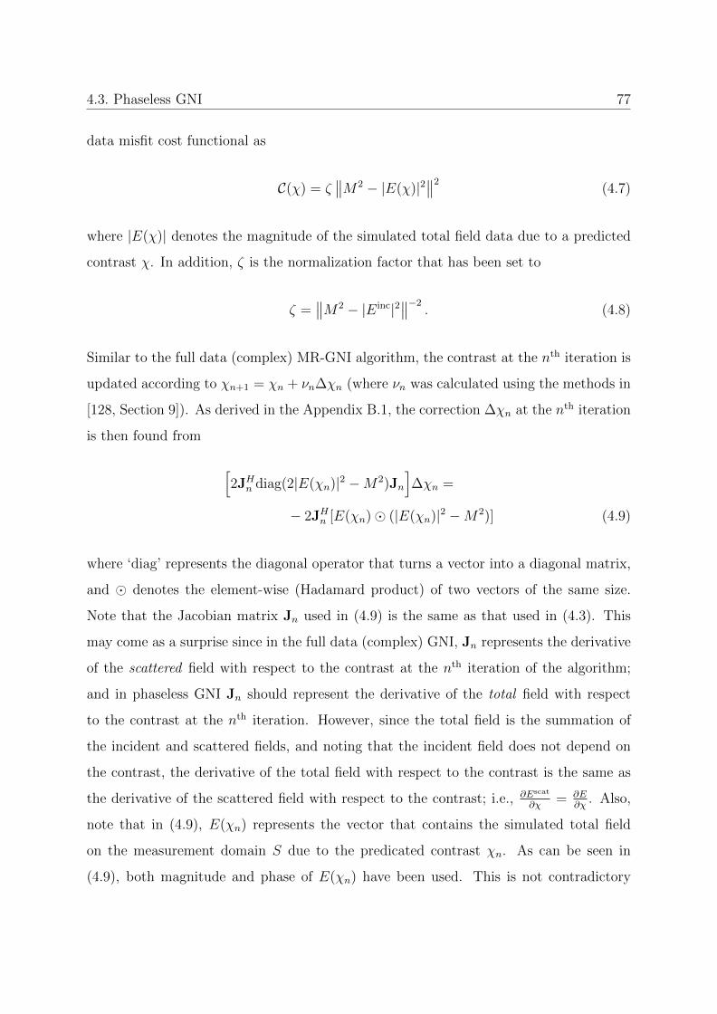
4.3. Phaseless GNI 77
data misfit cost functional as
C(χ) = ζ∥∥M2 − |E(χ)|2
∥∥2(4.7)
where |E(χ)| denotes the magnitude of the simulated total field data due to a predicted
contrast χ. In addition, ζ is the normalization factor that has been set to
ζ =∥∥M2 − |Einc|2
∥∥−2. (4.8)
Similar to the full data (complex) MR-GNI algorithm, the contrast at the nth iteration is
updated according to χn+1 = χn + νn∆χn (where νn was calculated using the methods in
[128, Section 9]). As derived in the Appendix B.1, the correction ∆χn at the nth iteration
is then found from
[2JHn diag(2|E(χn)|2 −M2)Jn
]∆χn =
− 2JHn [E(χn)� (|E(χn)|2 −M2)] (4.9)
where ‘diag’ represents the diagonal operator that turns a vector into a diagonal matrix,
and � denotes the element-wise (Hadamard product) of two vectors of the same size.
Note that the Jacobian matrix Jn used in (4.9) is the same as that used in (4.3). This
may come as a surprise since in the full data (complex) GNI, Jn represents the derivative
of the scattered field with respect to the contrast at the nth iteration of the algorithm;
and in phaseless GNI Jn should represent the derivative of the total field with respect
to the contrast at the nth iteration. However, since the total field is the summation of
the incident and scattered fields, and noting that the incident field does not depend on
the contrast, the derivative of the total field with respect to the contrast is the same as
the derivative of the scattered field with respect to the contrast; i.e., ∂Escat
∂χ= ∂E
∂χ. Also,
note that in (4.9), E(χn) represents the vector that contains the simulated total field
on the measurement domain S due to the predicated contrast χn. As can be seen in
(4.9), both magnitude and phase of E(χn) have been used. This is not contradictory
4.3. Phaseless GNI 78
to phaseless inversion since E(χn) represents the simulated total field data due to the
predicted contrast χ, and not the phaseless measured data. Finally, we note that in all
the examples shown herein, we use a trivial initial guess, χ = 0, to start the phaseless
GNI algorithm.
4.3.2 Regularization
Similar to the full data (complex) GNI algorithm that required regularization, the phase-
less GNI algorithm also requires the regularization of its cost functional (4.7). Note that
regularization is typically performed on the contrast χ; therefore, the regularization op-
erators for the phaseless problem can be the same as the complex problem. Herein, we
consider three types of multiplicative regularization schemes. The first is the weighted
L2 norm total variation multiplicative regularizer given in (4.4), which does not assume
any particular prior information about the contrast profile in the ROI. The second is de-
veloped for shape and location reconstruction [32, 40]. This regularization assumes prior
information about the complex permittivity values (thus, the contrast values) within the
ROI. The problem then becomes one of finding the shape and location of the dielectric
scatterers within the ROI. The third assumes prior information about the shape (struc-
tural information) of the target’s regions of identical relative permittivity [130, 131]. If
this spatial prior regularizer is used, the problem becomes one of reconstructing the ap-
propriate complex permittivity values within the known regions of the ROI. When the
phaseless GNI algorithm is used with each of these three regularization schemes, we refer
to the resulting three different regularized algorithms as PGNI, SL-PGNI and SP-PGNI,
respectively.

4.3. Phaseless GNI 79
4.3.3 PGNI Algorithm
Similar to the complex GNI algorithm, we multiplicatively regularize the phaseless data
misfit cost functional as
Cregn (χ) = C(χ) CMR
n (χ). (4.10)
Applying the GNI algorithm to this regularized phaseless cost functional, (4.9) will turn
into the following regularized form
[2JHn diag(2|E(χn)|2 −M2)Jn + τnLn
]∆χn =
−2JHn [E(χn)� (|E(χn)|2 −M2)]− τnLnχn (4.11)
where τn is C(χn)/ζ. Herein, we refer to this phaseless algorithm as the PGNI algorithm.
Note that the PGNI algorithm does not use any particular prior information about the
ROI, and can therefore be considered as a blind phaseless inversion algorithm.
4.3.4 SL-PGNI Algorithm
This regularization scheme incorporates prior information about the expected contrast
values within the ROI.6 Therefore, it is mainly used to reconstruct the shape and location
of the dielectric scatterers within the ROI. To this end, we augment (4.10) with an extra
regularization term
CSL,regn (χ) = C(χ) CMR
n (χ) CSLn (χ) (4.12)
6In microwave biomedical imaging we might know the expected permittivity values of the objects beingimaged. For example, for microwave breast imaging we are mainly reconstructing fatty, fibroglandular,and perhaps cancerous tissues. Depending on the frequency and the achievable resolution, we may be ableto reconstruct skin tissue as well. Therefore, it is possible to know a priori some expected permittivityvalues in the inversion process.

4.3. Phaseless GNI 80
where the superscript ‘SL’ notes the suitability of this regularizer for shape and location
reconstruction. This regularization term is given as [32, 40]
CSLn (χ) =
1
A
∫ROI
L∏`=1
|χ(r)− χ`|2 + α2n
|χn(r)− χ`|2 + α2n
ds (4.13)
where χ` for ` = 1 to L denotes the expected values of the complex contrast, and∏L
`=1
denotes the product of L different functions. The simplest form of this regularization term
is binary regularization in which we are dealing with two values of the contrast: χ1 = 0
which is for the background medium, and χ2 which represents the expected contrast value
of the scatterer. We emphasize that the given prior information χ` contains no knowledge
about the shape and location of the scatterers. In addition, α2n is the steering parameter
which is set to α2n = C(χn). Applying the GNI algorithm to (4.12) will change (4.11) to
[2JHn diag(2|En|2 −M2)Jn + τnLn + τn
∑L`=1Rn,`
]∆χn
=− 2JHn
[En � (|En|2 −M2)
]− τnLnχn
− τn∑L
`=1Rn,`(χn − χ`) (4.14)
where the regularization operators Rn,` when operating on a vector x of appropriate size
are given as [32]
Rn,`x =1
Adiag
(1
|χn(r)− χ`|2 + α2n
)x. (4.15)
We refer to this phaseless GNI algorithm with prior expected contrast values as SL-PGNI.
4.3.5 SP-PGNI Algorithm
In contrast to the above shape and location regularization scheme which assumed prior
information about the expected complex permittivity values, we now consider a spatial
prior regularization scheme which assumes prior spatial (or structural) information in the

4.3. Phaseless GNI 81
ROI without making any assumptions regarding their complex permittivity values. In
this prior information approach, the shapes of the regions having identical permittivity
are assumed to be known.7 If this regularization scheme is used, the resulting inverse
scattering algorithm attempts to reconstruct the relative complex permittivity values
within these regions. Intuitively, one can think of this regularizer as reducing the amount
of χ variables in the ROI, because there are fewer regions of identical permittivity than
the original number of discrete cells in the ROI. To this end, (4.10) is augmented with
an extra regularization term
CSP,regn (χ) = C(χ) CMR
n (χ) CSPn (χ) (4.16)
where the superscript ‘SP’ denotes the spatial prior information given to the regularizer.
This regularization term is given as [130, 131]
CSPn (χ) =
‖p� (Aχ)‖2 + γ2n
‖p� (Aχn)‖2 + γ2n
. (4.17)
In CSPn (χ), A is a sparse matrix consisting of only zeros and ±1. Its purpose is to enforce
equality between contrast values in the specified regions of identical permittivity. In
other words, the prior structural information of the ROI is stored in the matrix A via
several 0 and ±1 elements. (This choice of A was also utilized in [133, 134] in the form
of an additive regularization scheme for complex GNI.) The probability vector p contains
elements 0 ≤ pi ≤ 1. In this work, pi has been set to 1 for all i’s. Finally, γ2n is a steering
parameter chosen to be γ2n = C(χn)N where N is the length of the vector χ [130, Section
D]. Applying the GNI algorithm to (4.16) will result in
[2JHn diag(2|En|2 −M2)Jn + τnLn + τnSn
]∆χn =
−2JHn [En � (|En|2 −M2)]− τnLnχn − τnSnχn (4.18)
7For example, in a combined magnetic resonance imaging (MRI) and microwave imaging system, thehigh resolution structural information obtained from the MRI can be given as spatial prior informationto the microwave imaging system [132].

4.4. Calibration of the Experimental Data 82
where the operator Sn acting on a vector x of appropriate size is
Snx =1
‖p� (Aχn)‖2 + γ2n
AH (p� (p� (Ax))) . (4.19)
Herein, we refer to this phaseless GNI algorithm with prior spatial information as SP-
PGNI.
4.4 Calibration of the Experimental Data
4.4.1 Classification – Review
In microwave imaging, there will always be some discrepancy between the actual measure-
ment environment, and the numerical model used in the inversion algorithm. To alleviate
these discrepancies, so-called data calibration techniques such as the scattered field or
the incident field calibration methods [103] are used.8 For phaseless inversion, the scat-
tered field data are not available, and therefore, the scattered field calibration technique
cannot be used. Therefore, we decided to use the incident field calibration technique
for our experimental data. There are at least two ways that incident field calibration
can be applied. In the first method, a simulated incident field, such as a zeroth-order
Hankel function of the second kind is assumed for the incident field, and then complex
calibration coefficients are found to reduce the discrepancy between the simulated and
measured incident field data. These calibration coefficients are then used to modify the
raw experimental data. The second method is a more general way, which is based on the
so-called source reconstruction method (SRM).9
8Similar to the calibration object in radar cross section measurements, the scattered field calibrationtechnique in microwave imaging uses an object, such as a metallic cylinder [135], for which the complexscattered fields are analytically known. These analytical expressions and the measured scattered fielddata are then compared to construct complex-valued calibration coefficients, which will then used tocalibrate the actual measured data.
9The source reconstruction method is, in fact, an electromagnetic inverse source algorithm [36].

4.4. Calibration of the Experimental Data 83
4.4.2 SRM Calibration
In the SRM-based calibration method, the SRM is used to find equivalent surface current
distributions for the transmitting antennas that can also generate the measured incident
field data. Once these equivalent currents are found, they can be used in the GNI al-
gorithm to represent the actual antennas. Since these equivalent currents are associated
with the raw incident field data, the raw phaseless total field data are directly given to
the inversion algorithm to be inverted. Therefore, as opposed to the previous calibra-
tion methods, the SRM-based calibration method makes it possible to invert the raw
experimental data directly.
Herein, we have used the second method; i.e., the SRM for incident field calibration. The
details of this calibration method can be found in [50]. To this end, we have utilized
the SRM to replace each transmitting antenna with its equivalent currents. That is,
for example, if 24 antennas are present in a microwave imaging setup, we have replaced
them with 24 sets of equivalent currents. We have used both the magnitude and phase
of the measured incident field. Thus, the inverse source problem associated with the
SRM becomes a linear inverse source problem. Due to the fact that the L-curve method
is particularly suited for linear ill-posed problems [33, 108], we have used the L-curve
method to choose an appropriate solution when performing SRM.10
4.4.3 Calibration Limitation
Note that the above calibration method requires the magnitude and phase of the incident
field data (not the phase of the total field data). The presence of the phase data for
the incident field is not a bad assumption since it can be regarded as part of system
characterization (antenna characterization) prior to performing imaging. This assumption
is also present in many other phaseless microwave imaging algorithms [110, 111, 117, 118,
10The L-curve method requires determining the knee point of the L-curve; in our implementation theknee point is chosen in an ad hoc manner.
4.5. Results 84
120]. In all of these algorithms, the total field data, but not the incident field data,
are assumed to be phaseless. If this assumption is not made, we would have to use
a phaseless SRM algorithm, e.g., see [24], to characterize the antennas using measured
phaseless incident fields. Once the equivalent currents of the antennas are obtained using
phaseless incident fields, it can be used in the phaseless GNI algorithm similar to the
above. Therefore, in summary, similar to other phaseless microwave imaging algorithms,
this paper assumes phaseless total field data but considers complex incident field data.
4.5 Results
Herein, we show synthetic and experimental results to evaluate the performance of our
phaseless GNI algorithms. First, the PGNI, SL-PGNI, and SP-PGNI algorithms are used
to reconstruct images of a pair of lossy concentric squares in the ROI using synthetically
generated data. Next, experimental data collected from the Institut Fresnel in France [3]
are used to validate the PGNI, SL-PGNI, and SP-PGNI algorithms. Because the experi-
mental data from Institut Fresnel are from lossless targets, we then consider experimental
data obtained from a skinless bovine leg [4] to evaluate the performance of the PGNI,
SL-PGNI, and SP-PGNI algorithms against a lossy object. In addition to lossy versus
lossless objects, there are two other differences between these two data sets: (I) the Fres-
nel data sets use a mechanical scanning probe to collect the data whereas the bovine leg
data are collected by 24 co-resident dipole antennas; (II) the background medium in the
Fresnel data sets is air whereas the background medium in the bovine leg data set is salty
water.11
Since these experimental data sets all contained measured magnitude and phase data, we
removed the phase of the measured total field data, and only worked with the measured
11To reduce unwanted reflections, the Fresnel data sets were collected in an anechoic chambers withabsorbers. On the other hand, for the bovine leg data, salt has been added to water to make it lossy, thusreducing the reflections from the imaging chamber wall. This is necessary since the imaging algorithmassumes a free space Green’s function that does not take into account the reflections from the walls ofthe imaging chamber.
4.5. Results 85
magnitude-only total field data. Finally, we note that the iterative nature of the phaseless
inversion algorithms means that a stopping condition is necessary. In this work, we
stopped the algorithm when C(χn) decreased below 10−3 or when the change in the
reconstructed contrast was smaller than 10−4 after two consecutive iterations. More detail
on the convergence behaviour of the proposed algorithms can be found in Appendix B.2.12
4.5.1 Synthetic Concentric Squares Data Set
To validate our phaseless GNI algorithms, synthetic data at 4 GHz were created from
a pair of concentric dielectric squares with a background of free-space (εr = 1). This
experiment is similar to the synthetic examples in [110, Section IV] and [111, Section 5].
The relative complex permittivities of the outer and inner squares were εr = 1.3 − 0.4j
and εr = 1.6− 0.2j, respectively, see Figure 4.1(a)-(b). For phaseless data collection, 36
transceivers were located on a circle of radius 76 cm around the origin. (The transceivers
are assumed to be infinite line sources, thus, they are numerically modelled by zeroth-
order Hankel functions of the second kind.) The ROI was discretized into 43 by 43 square
elements and was 166 mm by 166 mm in size. The inversion was done at a single frequency
of 4 GHz.13 The results from attempting to reconstruct the lossy concentric squares from
phaseless total field data using the PGNI, SL-PGNI, and SP-PGNI algorithms are shown
in Figure 4.1(c)-(h). As noted earlier, the PGNI is blind phaseless inversion (no prior
information is given to the algorithm). In the case of SL-PGNI, the phaseless inversion
algorithm was provided with the true three contrast values as prior information, i.e., the
contrast value of the background medium and the contrasts of the two squares. The
SL-PGNI then reconstructs the shape and location of the objects being imaged. Finally,
in the case of the SP-PGNI, the spatial map of the target (i.e. the regions of identical
12In this work we have not investigated the convergence behaviour of these phaseless GNI algorithmsfor various contrast values and imaging domain sizes. We speculate that with increasing contrast valuesand/or imaging domain sizes the degree of non-linearity of the problem increases; thus the algorithmmight experience convergence to inappropriate local minima. To alleviate this the use of a non-trivialinitial guess can be a potential solution.
13The synthetic data were created on a different grid to avoid the so-called inverse crime.
4.5. Results 86
permittivity) was provided to the phaseless inversion algorithm as prior structural infor-
mation. The SP-PGNI then reconstructs the complex permittivity values in these spatial
regions. As can be seen, the SL-PGNI and SP-PGNI reconstructions were more accurate
than that of the PGNI algorithm. This is to be expected as the latter two algorithms
include more information about the objects being imaged whereas the PGNI algorithm
is a blind inversion.
4.5.2 Experimental FoamDielIntTM Data Set
To study the performance the phaseless GNI algorithms with experimental data, we
consider the measured data provided by the Institut Fresnel in France [3]. The phase of
the measured total field was disregarded and only its magnitude data were used. The
first target consists of two dielectric cylinders, one inside the other, and the background
is air. The inner-most cylinder is 31 mm in diameter with a relative permittivity of
εr = 3 ± 0.3, and is slightly offset from being concentric with the outer cylinder by 5
mm in the x-direction. The outer cylinder has a relative permittivity of εr = 1.45± 0.15
and a diameter of 80 mm. This target is referred to as FoamDielIntTM by [3] and is
shown in Figure 4.2(a). Note that the imaginary parts of the complex permittivities
of these cylinders are zero, and therefore, the objects being imaged are lossless. The
experimental dataset used for the FoamDielIntTM inversions included eight transmitters
and 241 receivers for each transmitter. The transmitters and receivers were located 1.67
m from the centre of the ROI [3] and the ROI was discretized into 65 by 65 elements and
was 150 mm by 150 mm in size. The frequency of inversion was 2 GHz.
In Figure 4.2(b)-(c) the result of inverting the FoamDielIntTM data with PGNI are shown
and the reconstructed overall shape and permittivities are reasonable; however, they are
not very accurate. For example, the reconstructed size of the inner cylinder is greater
than the actual one, and its reconstructed permittivity is smaller than its true permittiv-
ity. In addition, there is a small imaginary part present in the reconstructed permittivity.

4.5. Results 87
In Figure 4.2(d)-(e), the reconstructed permittivity using SL-PGNI is shown. In the SL-
PGNI algorithm, the relative permittivities of the cylinders are assumed to be known
and are given as prior information to the phaseless inversion algorithm. As a result, the
SL-PGNI algorithm reconstructs the shape and location of the target more accurately
compared to the blind phaseless inversion algorithm (PGNI). Similar to the PGNI recon-
struction, the SL-PGNI reconstruction also shows small imaginary parts in the complex
permittivity (i.e., some small loss).14
We now invert these phaseless measured data using the SP-PGNI algorithm. To this
end, we need to give the structural information of this target as prior information to SP-
PGNI. Ideally, this spatial prior information should come from a higher resolution imaging
modality such as magnetic resonance imaging (MRI). Once high resolution structural
information is given to SP-PGNI, this inversion algorithm will aim to find the complex
permittivity values in different regions from phaseless data. However, since MRI data
were not available for this target, we use a different method to create the spatial prior
map; we used the full data (complex) MR-GNI algorithm to invert the data set at 4 GHz,
6 GHz and 10 GHz simultaneously. The achieved inversion result is then used to create
spatial priors for this target as shown in Figure 4.3(a) where R1, R2, and R3 denotes
the three spatial regions.15 (Note that we do not provide any prior information regarding
the complex permittivity values for SP-PGNI.) These spatial priors are then given to the
SP-PGNI algorithm to find the complex permittivity at these regions. The reconstruction
results using the SP-PGNI algorithm are shown in Figure 4.2(f)-(g).
14The fact that there are small imaginary parts in the reconstructed permittivity using the SL-PGNIalgorithm may come as a surprise. This is due to the fact that the SL-PGNI gets the value of thepermittivity as the prior information. In this particular inversion, we have provided the SL-PGNIalgorithm with the relative permittivity of 3 and 1.45 (and, of course the relative permittivity of 1for the background). That is, the imaginary parts of the relative complex permittivities in the priorinformation were zero. However, these values are only enforced as soft regularization in the sense thatthe inversion algorithm will favour these values but still has the chance to not completely enforce them.
15The procedure to extract these spatial priors has been described in [130] which applies a MATLABkmeans function to the final reconstruction obtained from full data inversion.

4.5. Results 88
4.5.3 Experimental FoamTwinDielTM Data Set
Next, inversion results for the FoamTwinDielTM experimental data from the Institut
Fresnel are shown [3]. (Note that we once again disregard the phase and invert just
the magnitude of the total field data.) For this experiment, the target is similar to the
FoamDielIntTM case, except there is another small cylinder with the same dielectric
properties and size as the inner-most cylinder external to the outer cylinder. The two
small cylinders are 55.5 mm apart. An illustration of the FoamTwinDielTM target is
shown in Figure 4.4(a). The data collection for this test included 18 transmitters with
241 receivers each. Once again, the transmitters and receivers are located on a circle of
radius 1.67 m and the ROI was discretized into a 65 by 65 grid with side lengths of 150 mm
each. The results of the inversion using the PGNI, SL-PGNI and SP-PGNI algorithms are
shown in Figure 4.4(b)-(g) for a frequency of 4 GHz. (Similar to the previous example,
the spatial priors for the SP-PGNI algorithm, shown in Figure 4.3(b), were obtained
through a multi-frequency full-data MR-GNI algorithm.) In addition, similar to the
previous example, the relative permittivity values given as prior information to the SL-
PGNI algorithm are 3, 1.45, and 1. It can be observed once again that adding more
information through more sophisticated regularization schemes with the SL-PGNI and
SP-PGNI algorithms enables sharper reconstructions, with more evidence of the larger
cylinder. Comparing the reconstructions from the SL-PGNI and SP-PGNI algorithms
shows that for the SL-PGNI algorithm, the permittivities are smooth but the shape of
the reconstructed cylinders is not completely circular. In contrast the SP-PGNI algorithm
has a much more accurate shape, but the permittivity is not as smooth overall for the
small dielectric cylinders as the SL-PGNI algorithm. This result is expected as both
algorithms do well reconstructing what they have been informed is prior information.

4.5. Results 89
4.5.4 Experimental Skinless Bovine Leg Data Set
In order to test the phaseless GNI algorithms with a lossy target and background medium
in the ROI, we use the experimental data collected from a skinless bovine leg in a salt-
water medium using 24 co-resident dipole antennas [4]. (Similar to the previous cases, we
ignore the phase of the measured total field data, and invert only its magnitude data.)
The ROI is a square discretized into a 50 by 50 grid with a total length of 120 mm. The
data was collected at 0.8 GHz with the relative complex permittivity of the background
being εr = 76− 14j. The expected relative permittivity values of the bone (centre-most
region of the bovine leg) is εr = 26− 8j, and flexor (region around bone) is εr = 54− 18j
[4]. Prior to showing the phaseless inversions, let us take a look at the inversion of the
full data (magnitude and phase) as shown in Figure 4.5(a)-(b).16
For this lossy experimental data set, the blind phaseless inversion algorithm (i.e., the
PGNI algorithm) failed to provide any meaningful reconstruction; thus, it is not shown
here. We then tried the phaseless inversion algorithms incorporating prior information;
i.e., the SL-PGNI and SP-PGNI algorithms; the reconstruction results using these phase-
less algorithms are shown in Figure 4.5(c)-(f). It can be seen that the SL-PGNI algorithm
performed poorly when compared with the SP-PGNI algorithm. This is an indication that
the spatial prior information, shown in Figure 4.3(c), may have been more useful in re-
constructing the true target than the prior knowledge of expected permittivities. Also, in
the reconstruction process, we have limited the variation of the allowed relative complex
permittivity as follows: 1 ≤ Re(εr) ≤ 80 and −30 ≤ Im(εr) ≤ 0. Due to this enforce-
ment, the reconstructed permittivity of the bone using the SP-PGNI method shown in
Figure 4.5(e)-(f) looks very uniform, but is mistakenly similar to free-space and not bone
(i.e., εr = 26 − 8j) as it should be. In addition, the phaseless inversion of the skinless
16Herein, for the full data (complex) case, we have also used the SRM-based incident field calibrationmethod. We note that the inversion of these full data using the scattered field calibration method, asshown in [4], seems to be better than the inversion shown in Figure 4.5(a)-(b) (and, also shown in [50]).However, since the use of the scattered field calibration method was not possible for the phaseless case, wehave also calibrated the full data using the SRM-based incident field calibration method for consistency.

4.5. Results 90
bovine leg data set had another challenge: the steering parameters of the phaseless in-
version algorithms (i.e., δ2n, α2
n, and γ2n) had to be modified for this particular example to
work.17 That is, the phaseless inversion of this data set was more sensitive to the overall
regularization weight as compared to the other cases. This was perhaps due to the lossy
nature of the complex permittivities which further reduces the information content of the
measured data.
It is instructive to investigate the information content available for the phaseless inversion
in this skinless bovine leg data set. To this end, let us take a look at Figure 4.6(a), where
the measured squared magnitude of the total field (black) and the measured squared
magnitude of the incident field (blue) are shown for a given transmitter. On the other
hand, Figure 4.6(b) shows the phase of the total measured (black) and incident (blue)
field data for the same transmitter. As can be seen, as opposed to the phase data,
the magnitude data of the total and incident fields are quite similar, and therefore, the
information content of the imaging experiment is mainly encoded in the phase data that
cannot be used for phaseless inversion. This is the main reason behind the difficulty of
performing phaseless inversion on this data set. Let us now take a look at the phaseless
inversion result using the SL-PGNI algorithm shown in Figure 4.5(c)-(d). As can be seen
this phaseless inversion was relatively unsuccessful, however, if we now take a look at the
simulated squared magnitude of the total field data at the last iteration of this inversion
algorithm, i.e., the red curve in Figure 4.6(a), we understand that the simulated data
are quite similar to the measured magnitude data. Therefore, the phaseless inversion
17This modification was done in an ad hoc manner. Note that in the multiplicative regularizationscheme, the steering parameter is the only parameter related to the regularization weight that the user hascontrol over. (The other regularization-weight related parameter is τn which is automatically determinedby the convergence behaviour of the algorithm; thus, the user has no control over this parameter.) If aninversion algorithm does not work properly, a likely reason is over-regularization or under-regularization.In this particular example, due to having a lossy object (skinless bovine leg) and a lossy matching fluid(salt-water), the problem is more ill-posed. In addition, due to the phaseless approach, the problem isalso more nonlinear as compared to its full data counterpart. Since the phaseless SL-PGNI and SP-PGNIof the skinless bovine leg using the standard steering parameters did not work properly, our speculationwas that the regularization scheme needs to be applied with a stronger weight. To this end, we madethe steering parameters smaller for the skinless bovine leg example thereby changing the weight of theregularization operators. For example, consider the steering parameter for the spatial prior case, i.e.,the SP-PGNI algorithm. If we make γ2n smaller, then the weight of the regularization operator Sn canincrease due to having γ2n in the denominator of (4.19).

4.6. Conclusion 91
algorithm performed well; however, there was not a great deal of information left to be
extracted from the magnitude-only data to improve the reconstruction result. Now, if we
look at the simulated phase of the total field data at the last iteration of this phaseless
algorithm, i.e., red curve in Figure 4.6(b), we see that the simulated phase data are
different than the phase of the measured total field data (even if this phase difference is
reduced by considering a phase shift of 2π at Rx number 9 for the simulated or measured
total field). Since these measured phase data were not provided to the SL-PGNI inversion
algorithm, the algorithm was not able to take advantage of the embedded information
content in this dataset to improve its reconstruction.
4.6 Conclusion
A novel phaseless GNI algorithm was developed and was augmented with three forms of
multiplicative regularization: (i) weighted L2 norm total variation regularization, (ii)
weighted L2 norm total variation regularization combined with prior information re-
garding the expected complex permittivity values of the objects being imaged, and (iii)
weighted L2 norm total variation regularization combined with prior information regard-
ing the structural information of the regions of identical permittivity of the objects being
imaged. We have referred to these three implementations of the phaseless GNI algorithm
as the PGNI, SL-PGNI, and SP-PGNI algorithms, respectively. These algorithms were
shown to be able to invert synthetic phaseless data, experimental phaseless data from
lossless and lossy targets. The incorporation of prior information was shown to play a
strong role with these phaseless GNI algorithms to compensate for the lack of phase of
the total field data.
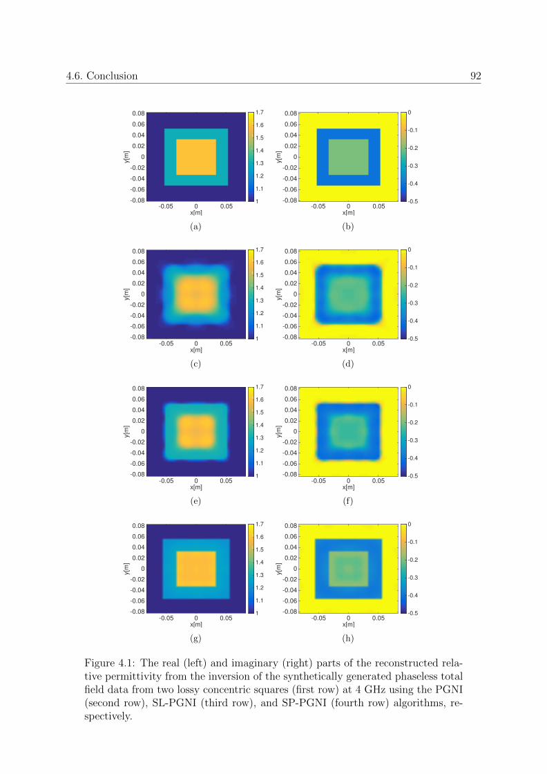
4.6. Conclusion 92
x[m]-0.05 0 0.05
y[m
]
-0.08
-0.06
-0.04
-0.02
0
0.02
0.04
0.06
0.08
1
1.1
1.2
1.3
1.4
1.5
1.6
1.7
(a)
x[m]-0.05 0 0.05
y[m
]
-0.08
-0.06
-0.04
-0.02
0
0.02
0.04
0.06
0.08
-0.5
-0.4
-0.3
-0.2
-0.1
0
(b)
x[m]-0.05 0 0.05
y[m
]
-0.08
-0.06
-0.04
-0.02
0
0.02
0.04
0.06
0.08
1
1.1
1.2
1.3
1.4
1.5
1.6
1.7
(c)
x[m]-0.05 0 0.05
y[m
]
-0.08
-0.06
-0.04
-0.02
0
0.02
0.04
0.06
0.08
-0.5
-0.4
-0.3
-0.2
-0.1
0
(d)
x[m]-0.05 0 0.05
y[m
]
-0.08
-0.06
-0.04
-0.02
0
0.02
0.04
0.06
0.08
1
1.1
1.2
1.3
1.4
1.5
1.6
1.7
(e)
x[m]-0.05 0 0.05
y[m
]
-0.08
-0.06
-0.04
-0.02
0
0.02
0.04
0.06
0.08
-0.5
-0.4
-0.3
-0.2
-0.1
0
(f)
x[m]-0.05 0 0.05
y[m
]
-0.08
-0.06
-0.04
-0.02
0
0.02
0.04
0.06
0.08
1
1.1
1.2
1.3
1.4
1.5
1.6
1.7
(g)
x[m]-0.05 0 0.05
y[m
]
-0.08
-0.06
-0.04
-0.02
0
0.02
0.04
0.06
0.08
-0.5
-0.4
-0.3
-0.2
-0.1
0
(h)
Figure 4.1: The real (left) and imaginary (right) parts of the reconstructed rela-tive permittivity from the inversion of the synthetically generated phaseless totalfield data from two lossy concentric squares (first row) at 4 GHz using the PGNI(second row), SL-PGNI (third row), and SP-PGNI (fourth row) algorithms, re-spectively.
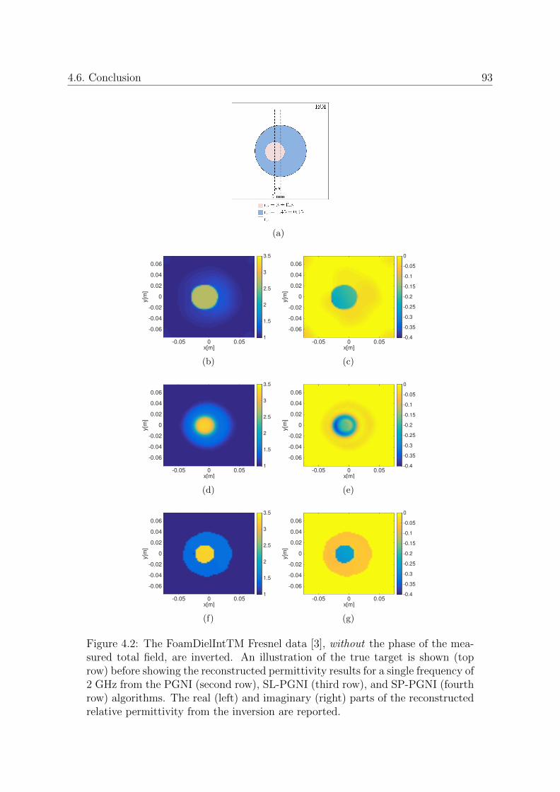
4.6. Conclusion 93
(a)
x[m]-0.05 0 0.05
y[m
]
-0.06
-0.04
-0.02
0
0.02
0.04
0.06
1
1.5
2
2.5
3
3.5
(b)
x[m]-0.05 0 0.05
y[m
]
-0.06
-0.04
-0.02
0
0.02
0.04
0.06
-0.4
-0.35
-0.3
-0.25
-0.2
-0.15
-0.1
-0.05
0
(c)
x[m]-0.05 0 0.05
y[m
]
-0.06
-0.04
-0.02
0
0.02
0.04
0.06
1
1.5
2
2.5
3
3.5
(d)
x[m]-0.05 0 0.05
y[m
]
-0.06
-0.04
-0.02
0
0.02
0.04
0.06
-0.4
-0.35
-0.3
-0.25
-0.2
-0.15
-0.1
-0.05
0
(e)
x[m]-0.05 0 0.05
y[m
]
-0.06
-0.04
-0.02
0
0.02
0.04
0.06
1
1.5
2
2.5
3
3.5
(f)
x[m]-0.05 0 0.05
y[m
]
-0.06
-0.04
-0.02
0
0.02
0.04
0.06
-0.4
-0.35
-0.3
-0.25
-0.2
-0.15
-0.1
-0.05
0
(g)
Figure 4.2: The FoamDielIntTM Fresnel data [3], without the phase of the mea-sured total field, are inverted. An illustration of the true target is shown (toprow) before showing the reconstructed permittivity results for a single frequency of2 GHz from the PGNI (second row), SL-PGNI (third row), and SP-PGNI (fourthrow) algorithms. The real (left) and imaginary (right) parts of the reconstructedrelative permittivity from the inversion are reported.

4.6. Conclusion 94
x[m]-0.05 0 0.05
y[m
]
-0.06
-0.04
-0.02
0
0.02
0.04
0.06
R1
R2
R3
(a)
x[m]-0.05 0 0.05
y[m
]
-0.06
-0.04
-0.02
0
0.02
0.04
0.06
R1
R2
R3
(b)
x[m]-0.05 0 0.05
y[m
]
-0.06
-0.04
-0.02
0
0.02
0.04
R1
R2
R3
(c)
Figure 4.3: The spatial priors (SP) used in conjunction with the SP-PGNI algo-rithm for (a) FoamDielIntTM, (b) FoamTwinDielTM, and (c) skinless bovine leg.The colorbar indicates three spatial regions denoted by R1, R2, and R3. (Someof these spatial regions contain errors, e.g., the black region within R3 in (c) islikely to be an error.)
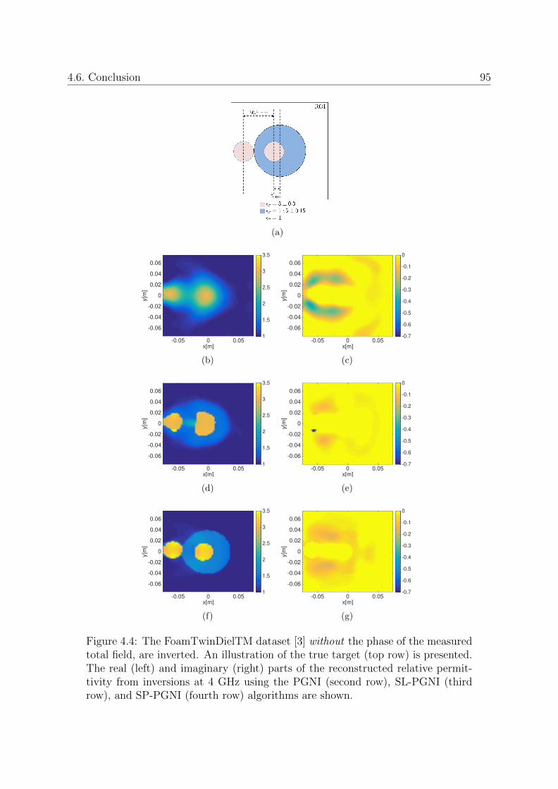
4.6. Conclusion 95
(a)
x[m]-0.05 0 0.05
y[m
]
-0.06
-0.04
-0.02
0
0.02
0.04
0.06
1
1.5
2
2.5
3
3.5
(b)
x[m]-0.05 0 0.05
y[m
]
-0.06
-0.04
-0.02
0
0.02
0.04
0.06
-0.7
-0.6
-0.5
-0.4
-0.3
-0.2
-0.1
0
(c)
x[m]-0.05 0 0.05
y[m
]
-0.06
-0.04
-0.02
0
0.02
0.04
0.06
1
1.5
2
2.5
3
3.5
(d)
x[m]-0.05 0 0.05
y[m
]
-0.06
-0.04
-0.02
0
0.02
0.04
0.06
-0.7
-0.6
-0.5
-0.4
-0.3
-0.2
-0.1
0
(e)
x[m]-0.05 0 0.05
y[m
]
-0.06
-0.04
-0.02
0
0.02
0.04
0.06
1
1.5
2
2.5
3
3.5
(f)
x[m]-0.05 0 0.05
y[m
]
-0.06
-0.04
-0.02
0
0.02
0.04
0.06
-0.7
-0.6
-0.5
-0.4
-0.3
-0.2
-0.1
0
(g)
Figure 4.4: The FoamTwinDielTM dataset [3] without the phase of the measuredtotal field, are inverted. An illustration of the true target (top row) is presented.The real (left) and imaginary (right) parts of the reconstructed relative permit-tivity from inversions at 4 GHz using the PGNI (second row), SL-PGNI (thirdrow), and SP-PGNI (fourth row) algorithms are shown.
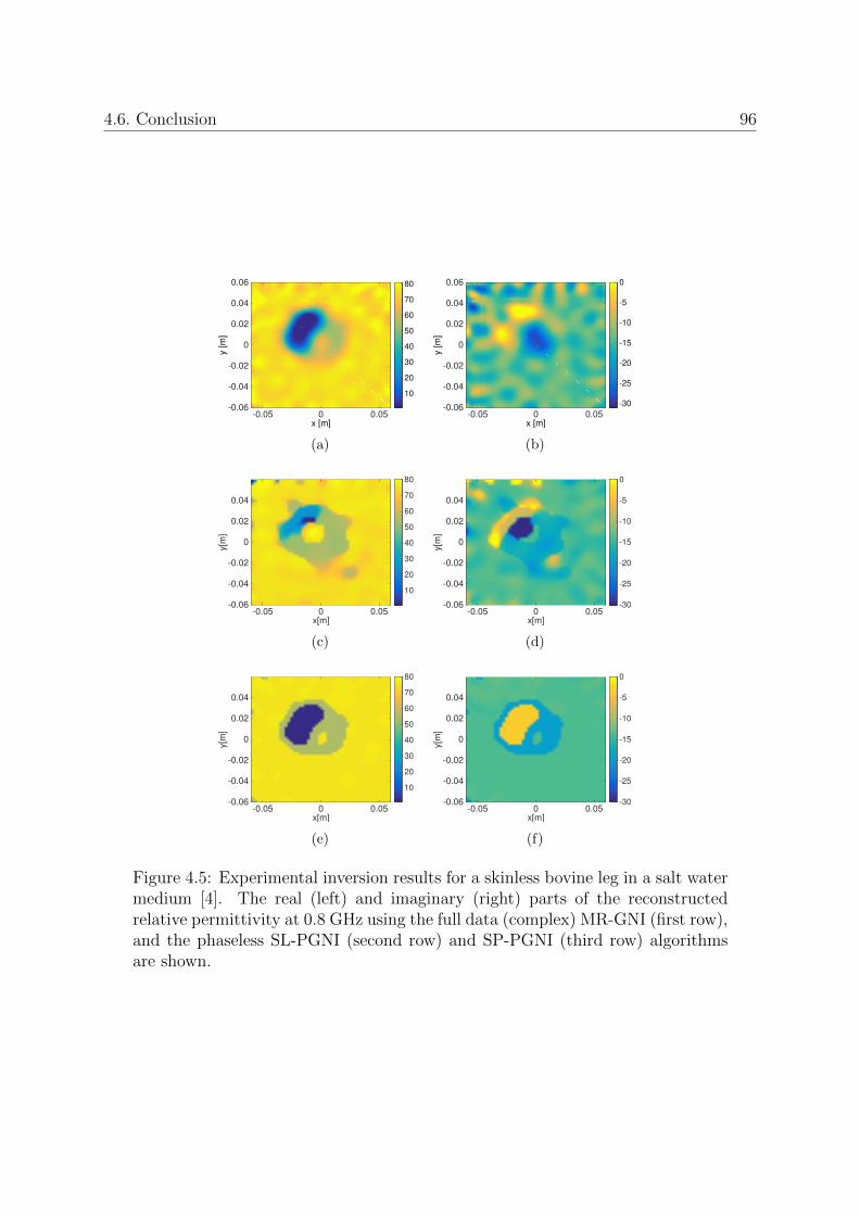
4.6. Conclusion 96
x [m]-0.05 0 0.05
y [
m]
-0.06
-0.04
-0.02
0
0.02
0.04
0.06
10
20
30
40
50
60
70
80
(a)
x [m]-0.05 0 0.05
y [
m]
-0.06
-0.04
-0.02
0
0.02
0.04
0.06
-30
-25
-20
-15
-10
-5
0
(b)
x[m]-0.05 0 0.05
y[m
]
-0.06
-0.04
-0.02
0
0.02
0.04
10
20
30
40
50
60
70
80
(c)
x[m]-0.05 0 0.05
y[m
]
-0.06
-0.04
-0.02
0
0.02
0.04
-30
-25
-20
-15
-10
-5
0
(d)
x[m]-0.05 0 0.05
y[m
]
-0.06
-0.04
-0.02
0
0.02
0.04
10
20
30
40
50
60
70
80
(e)
x[m]-0.05 0 0.05
y[m
]
-0.06
-0.04
-0.02
0
0.02
0.04
-30
-25
-20
-15
-10
-5
0
(f)
Figure 4.5: Experimental inversion results for a skinless bovine leg in a salt watermedium [4]. The real (left) and imaginary (right) parts of the reconstructedrelative permittivity at 0.8 GHz using the full data (complex) MR-GNI (first row),and the phaseless SL-PGNI (second row) and SP-PGNI (third row) algorithmsare shown.
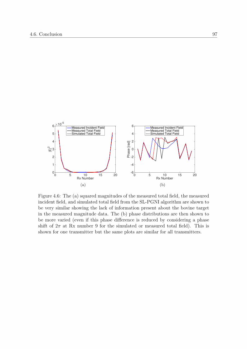
4.6. Conclusion 97
Rx Number0 5 10 15 20
|E|2
×10-5
0
1
2
3
4
5
6Measured Incident FieldMeasured Total FieldSimulated Total Field
(a)
Rx Number0 5 10 15 20
Phase [ra
d]
-6
-4
-2
0
2
4
6Measured Incident FieldMeasured Total FieldSimulated Total Field
(b)
Figure 4.6: The (a) squared magnitudes of the measured total field, the measuredincident field, and simulated total field from the SL-PGNI algorithm are shown tobe very similar showing the lack of information present about the bovine targetin the measured magnitude data. The (b) phase distributions are then shown tobe more varied (even if this phase difference is reduced by considering a phaseshift of 2π at Rx number 9 for the simulated or measured total field). This isshown for one transmitter but the same plots are similar for all transmitters.

Chapter 5
A Combined Inverse Source and
Scattering Technique for Dielectric
Profile Design to Tailor
Electromagnetic Fields
Preface
In the previous chapter, an inverse scattering approach was presented that could char-
acterize dielectric objects with phaseless data. In this chapter we look to the design of
dielectric lens/antennas using similar principles. One possibility to explore this concept
was to use the algorithms developed in the previous chapter with desired electromagnetic
data instead of measured data for inversion; we briefly explored this in [82]. However,
to be able to facilitate the design of passive, lossless, and reflectionless dielectric lenses
using a variety of different types of electromagnetic data, we develop a combined inverse
source and scattering technique in this chapter.
98

Chapter 5 A Combined Inverse Source and Scattering Technique for Dielectric ProfileDesign to Tailor Electromagnetic Fields 99
In the developed method, complex electric field, phaseless electric field, and far-field
criteria data can be used as the electromagnetic data to reconstruct a dielectric profile
as the main property of interest. The physical model is based on Maxwell’s equations in
integral form, specifically, the data and domain equation are used for the inverse scattering
part and the electric-field integral equations are used for the inverse source part. Two
cost functionals need to be minimized separately: one for the inverse source problem,
and one for the inverse scattering problem. Regularization techniques are utilized to bias
the solution of a dielectric profile that can facilitate physical implementation. Note that
in this method we are using the surface and volume equivalence principles separately to
design the lens.
To the best of the authors’ knowledge this is the first time a combined inverse source and
scattering methodology has been presented that is capable of designing dielectric profiles
that when illuminated by a single feed can satisfy user specified far-field performance cri-
teria, including main beam direction, null locations, and half-power beam width (HPBW).
The presented framework is capable of using existing inverse scattering algorithms that
are used for characterization applications such as microwave imaging without much mod-
ification. In fact, in this chapter we show examples using contrast source inversion and
Gauss-Newton inversion type inverse scattering algorithms.1 The material presented in
this chapter was published as a journal paper for IEEE Transactions on Antennas and
Propagation [136].2
Abstract
This paper augments existing gradient-based inverse scattering algorithms to enable the
design of reflectionless lossless permittivity profiles within a given design domain that can
1Contrast source inversion directly uses of the volume equivalence principle while it can be perceivedthat Gauss-Newton inversion algorithms use this principle indirectly.
2© 2021 IEEE. Reprinted, with permission, from C. Narendra and P. Mojabi, “A Combined InverseSource and Scattering Technique for Dielectric Profile Design to Tailor Electromagnetic Fields,” in IEEETransactions on Antennas and Propagation, doi: 10.1109/TAP.2021.3119049.
5.1. Introduction 100
transform an input incident field into an output field of desired characteristics. These
desired characteristics are often some user-defined far-field performance criteria such as
main beam directions, null directions, and half-power beamwidth (HPBW). To this end,
two extra steps will be performed prior to the inverse scattering step. Firstly, an in-
verse source algorithm inverts the desired far-field performance criteria to infer a set of
equivalent surface currents on a boundary close to the design domain. These equivalent
currents are then converted to a set of fields values that constitute the required aperture
fields. Secondly, these aperture fields are scaled such that the input incident power to the
design domain is approximately equal to the output power leaving the design domain.
Finally, the desired scattered fields are formed and then inverted by an inverse scatter-
ing algorithm to reconstruct a lossless reflectionless dielectric profile within the design
domain. We also show that the inverse scattering algorithm can employ appropriate reg-
ularization methods, in particular a binary regularization term, to facilitate the physical
implementation of reconstructed dielectric profiles.
5.1 Introduction
In electromagnetic inverse scattering, the goal is to infer the internal properties of an un-
known irradiated domain from external electromagnetic fields. To this end, the unknown
domain is illuminated by electromagnetic fields and the resulting emanating scattered
electromagnetic fields of the domain are recorded. The desired internal properties of the
domain are then found from these external scattered electromagnetic fields; for example,
the domain’s dielectric properties are often calculated. Electromagnetic inverse scattering
techniques have been commonly used for imaging applications [107, 137, 138] within a
wide range of frequencies, e.g., from a few Hertz [139] to the optical frequency range [140].
For example, in microwave breast imaging [74] these algorithms are used to infer (recon-
struct) the dielectric profile (relative complex permittivity) of the breast from external
measured scattered field data. To this end, inverse scattering algorithms iteratively up-
date a predicted dielectric profile so that its simulated scattered fields match (ideally)

5.1. Introduction 101
the measured scattered fields. This is done by minimizing a data misfit cost functional
within an iterative process. Upon its convergence, this minimization yields a recon-
structed dielectric profile [4, 30]. Several optimization approaches have been proposed to
minimize the data misfit cost functional, which can be broadly classified into global [141]
and gradient-based optimization approaches [142]. The latter has found more use in the
literature due to its computational efficiency, and it is thus considered in this paper.
We also note that inverse scattering can be done in a non-iterative fashion under some
approximations such as the Born approximation (weak scatterers). These non-iterative
inversion approaches are mainly concerned with creating qualitative reconstruction (as
opposed to quantitative), and are therefore not considered in this paper.
More recently, the electromagnetic inverse scattering framework has been used for design
applications [9, 22, 80–82, 143–145]. In such problems, the purpose is to design a dielectric
profile that is capable of transforming the incident field of a feed antenna into a desired
field. In this scenario, the inverse scattering algorithms are attempting the same procedure
as in the imaging case, except that instead of measured scattered fields, we now use the
desired scattered fields. Consequently, in this design problem, the non-uniqueness [28]
of this inverse problem can be advantageous. In contrast to the imaging problem, a
specific true dielectric profile is not sought; instead, an appropriate one needs to be
found. Therefore, the non-uniqueness of the problem can be exploited through different
regularization techniques to choose a dielectric profile that may be, for example, easier to
fabricate. However, the problem of existence is more of an issue in the design problem than
the imaging case: one must ensure that the desired fields must be physically realizable by
interrogation of a dielectric profile of certain size. For example, to be able to transform an
incident field to a power pattern of high directivity, we first need to make sure that the size
of the dielectric profile provides a sufficient effective aperture size for this transformation;
e.g., see [9] for a method to avoid super directivity.
There are also certain practical challenges that must be addressed when using inverse
scattering for design. Firstly, it would be advantageous if the design framework could
make use of different types of desired data. In previous work, the desired field pattern is
5.1. Introduction 102
specified as either (i) complex field values or (ii) power or amplitude values [9, 22, 82]. For
example, in inverse scattering for dielectric cloak design [22], the desired scattered field
is conveniently known: it needs to be zero to represent no scattering signature. However,
in most practical design problems, only certain (far-field) specifications such as the main
beam direction, half-power beam width (HPBW), and null locations are known. In such
cases, obtaining desired scattered fields are not straightforward, and consequently it is
not clear how to apply existing state-of-the-art gradient-based inverse scattering algo-
rithms to such design problems. This is in particular due to the complexity of finding the
gradient operators (and the Hessian matrix) for such general cases3, and the enforcement
of power conservation for the input and output fields. Therefore, a more flexible design
framework is necessary to enable the use of gradient-based inverse scattering algorithms
for the design of dielectric profiles from the knowledge of performance criteria such as
HPBW or null directions. Secondly, there is the challenge of facilitating the physical
implementation of the designed dielectric profile. It would be preferred that a given in-
verse scattering design technique make it easy for the designers to not only generate the
desired field specifications, but also reduce the effort of physically implementing the final
dielectric profile. This can be seen in [9, 80, 143], where the unknown of interest is ex-
panded on a set of basis functions to simplify the fabrication process. For example, in one
case the dielectric profile is implemented with a set of dielectric rods (projection-based
regularization) [80]. This is easier to implement than a continuously varying dielectric
profile. As another example, appropriate regularization terms have been used with in-
verse scattering algorithms to favour positive permittivity values [9] or to favour circular
symmetry etc [143].
In this work, we present a flexible gradient-based inverse scattering design methodology
that can address the challenges stated above. The method involves three main steps: (i)
determine the desired electromagnetic fields in the required form at the required locations
using an inverse source algorithm, (ii) enforce total power conservation, and (iii) solve the
inverse scattering problem using the appropriate algorithm and regularization to facilitate
3Note that this is not the case for global optimization algorithms, e.g., in [146, 147] a genetic algorithmand a particle swarm optimization algorithm are used for dielectric lens design.

5.2. Problem Description 103
Figure 5.1: The schematic of the design problem. A dielectric profile in thedesign domain D (shown by a dashed rectangle) with a width of d3 and a height
of d4 is to be determined such that it can transform an incident field ~Ψinc to adesired output/transmitted field (~Ψtr) when illuminated by a known source/feed(black circle) from a distance d1. The feed is on the input side V − of D andthe transmitted field is on the output side V +. The input boundary of D isdenoted by D−. The dielectric profile is designed by utilizing the desired complexfield on a region of interest ROI1 with a size of d4 a distance d2 from D withthe appropriate inverse scattering algorithm and regularization methods. If onlyfar-field specifications are known (e.g., main beam direction, null locations, etc.),then an inverse source problem is first solved to obtain the fields on ROI1 fromthe specifications on ROI2 before the dielectric profile is designed with the inversescattering algorithm.
physical implementation. We start by defining the problem and scope in Section 5.2. Then
we explain our inverse scattering methodology in detail in Section 5.3 before using it to
design dielectric objects capable of near-field and far-field transformations in Section 5.4.
In this paper, we consider the two-dimensional (2D) transverse magnetic (TMz) problem
with the time dependency of exp(jωt).
5.2 Problem Description
Let us consider the design domain D shown in Figure 5.1. This is the domain that
will support a lossless non-magnetic permittivity profile to transform an incident field
5.2. Problem Description 104
generated by a source (feed) located in the input side V − to a desired field in the output
side V +. In V −, the source, shown by a black circle in Figure 5.1, is placed at a distance
d1 from the input side of D, and generates an incident field ~Ψinc where Ψ = {E,H}(i.e., Ψ refers to the set of electric and magnetic fields). In addition, there could be a
reflected field from D, which is denoted by ~Ψref. Since the feed is known, ~Ψinc is known.
Furthermore, in this work, we desire minimal reflections from the design domain D; thus,
we assume ~Ψref = 0.4
In terms of desired data to be given to the inversion algorithm, we consider two sce-
narios. Let us begin by the simpler scenario where we assume that the desired complex
electric and magnetic fields are specified on the first region of interest denoted by ROI1
in Figure 5.1. The region ROI1 is in V + and at a distance d2 from the output side of
D. It is here where the desired transmitted field ~Ψtr needs to be defined. As will be
seen later, ROI1 needs to be electrically close to the design domain D so that we can
scale the desired output field to equalize the input and output powers.5 However, in most
practical applications, the designer does not know the complex fields on ROI1; instead,
the designer knows some performance criteria often located in the far-field zone. This will
then bring us to the second case where only some desired far-field performance criteria
are known. For example, consider the case in which we wish to convert the incident
field to an output field which exhibits a certain HPBW, main beam and null directions
in the far-field zone. These desired performance criteria cannot be easily represented by
complex fields on ROI1. In such situations, we take advantage of the second region of
interest, denoted by ROI2, and construct a desired power pattern on ROI2 that meets the
desired performance criteria. We will then use an inverse source algorithm (also known
as a source reconstruction method) to infer the required field values on ROI1 from the
knowledge of the desired specifications on ROI2.6
4As will be seen later, we implicitly enforce this zero reflection (matched condition) by requiring thatthe power going into D in the x direction to be the same as the power leaving D toward x direction.Since D is a passive domain, this will automatically favour zero reflection.
5For example, in our examples, d2 has been set to 0.14λ where λ denotes the wavelength in free space.6This step is similar to the inverse source algorithm used for the design of electromagnetic metasurfaces
from far-field performance criteria [2, 68].

5.3. Methodology 105
Once we have the total complex desired fields on ROI1, we make sure that the total power
of the field on the input side of D (denoted by D−) is conserved by comparing it to the
output power on ROI1. This step is crucial for inverse scattering for design as it links the
magnitude of the desired output field to the known incident field magnitude of the feed.
For example, if we wish to convert a given incident field to a normalized power pattern,
we would only know the relative amplitude of the fields, and not its actual values. (This
is in contrast to imaging applications where the actual field values are measured, and
thus are known.) Once the total power conservation is enforced, the desired scattered
field on ROI1 can be obtained and can then be given to an inverse scattering algorithm
to reconstruct an appropriate passive and lossless permittivity profile in D. The next
section explains each of these steps in detail.
5.3 Methodology
Herein, we utilize a three-step method to design permittivity profiles in D capable of
transforming a known source incident field to a desired output field that satisfies user-
defined specifications. These steps are explained in detail below. In addition, the overall
procedure is shown in the form of a flowchart in Figure 5.2.
5.3.1 Step I: Specify Fields on ROI1
In this step there are two possible scenarios depending on the type of known desired field
information.
5.3.1.1 Desired complex field is known on ROI1
In this scenario we assume that the total complex desired field (tangential electric and
magnetic field) is fully defined on ROI1 or can easily be inferred. For example, in a plane
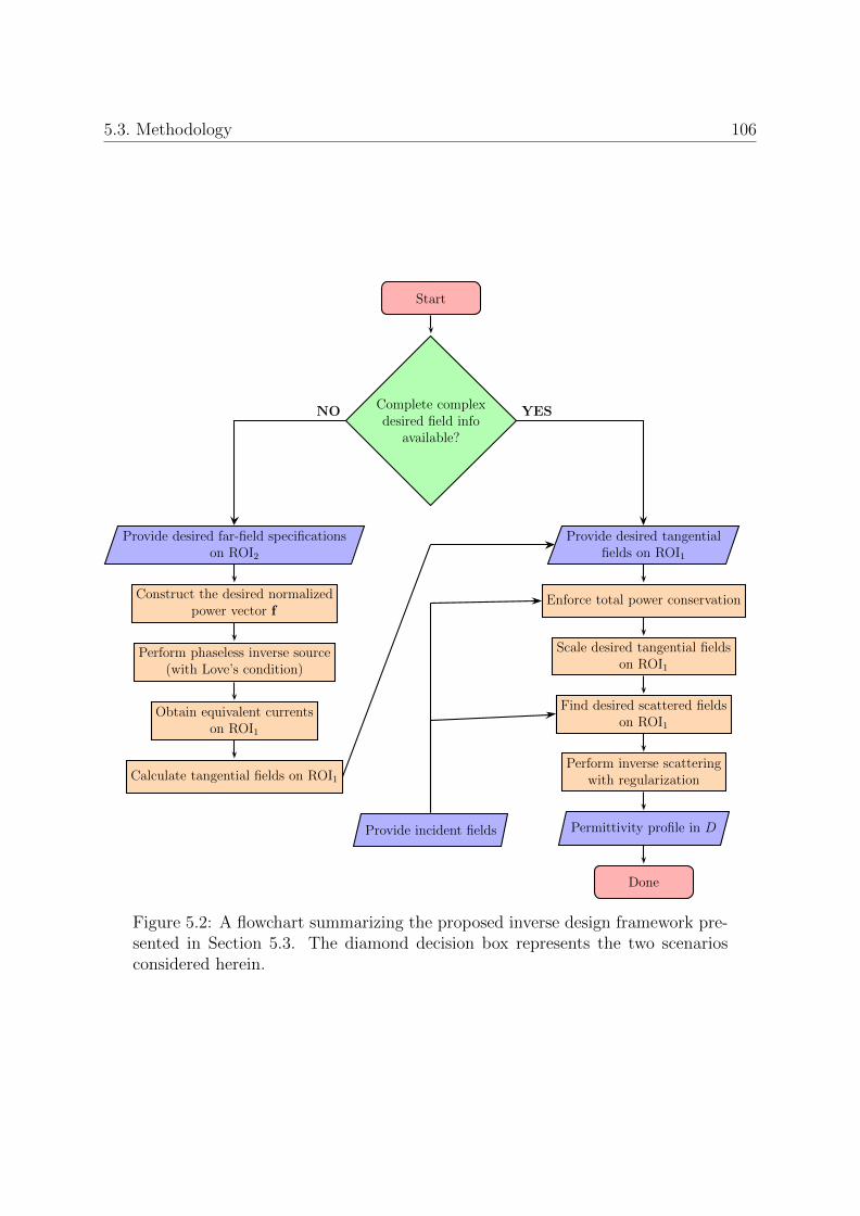
5.3. Methodology 106
Start
Complete complexdesired field info
available?
Provide desired far-field specificationson ROI2
Construct the desired normalizedpower vector f
Perform phaseless inverse source(with Love’s condition)
Obtain equivalent currentson ROI1
Calculate tangential fields on ROI1
Provide desired tangentialfields on ROI1
Enforce total power conservation
Scale desired tangential fieldson ROI1
Provide incident fields
Find desired scattered fieldson ROI1
Perform inverse scatteringwith regularization
Permittivity profile in D
Done
YESNO
Figure 5.2: A flowchart summarizing the proposed inverse design framework pre-sented in Section 5.3. The diamond decision box represents the two scenariosconsidered herein.

5.3. Methodology 107
wave refraction design example it is easy to mathematically define the desired field on
ROI1 if one knows the intended refraction angle and the frame of reference. Or if we desire
to transform the incident field emanating from a line source, which can be described with
a zeroth order Hankel function of the second kind H20 (·), to a plane wave travelling in
the x direction, we can simply assume that the electric field on ROI1 is 1∠0◦ (uniform
amplitude and phase).7 In these and similar cases, the field can already be specified in the
desired form for the next step so no further action is needed. (This scenario corresponds
to the right side of the diamond-shape decision box in the flowchart shown in Figure 5.2.)
5.3.1.2 Desired far-field specifications are known
If far-field specifications must be satisfied, we first perform an intermediate step to infer
the associated complex field components on ROI1 from the specifications on ROI2, thereby
transforming the given desired specifications into a form that may be used with existing
inverse scattering algorithms. (This scenario corresponds to the left side of the diamond-
shape decision box in the flowchart shown in Figure 5.2.) To solve for the complex
tangential electric and magnetic fields on ROI1 from far-field specifications (e.g. main
beam direction, null locations, etc.) on ROI2 we use the process outlined in [2, Section
VII-C] which is briefly outlined here for completeness. First, we transform the given
far-field specifications to a normalized power pattern that can be used to formulate the
appropriate data misfit cost functional for the next step. To this end, we construct a
real-valued vector f in which each element represents a desired normalized power value at
a specific location. For example, main beam directions are met by setting the elements of
f to 1 (0 dB) in the appropriate location and nulls are specified by setting the appropriate
elements of f to a small value such as 10−6 (−60 dB). Also, the HPBW criterion for each
main beam is met by modelling each beam as a cosine distribution and symmetrically
varying the beam from 1 at the max to 0.5 (−3 dB) at the appropriate locations in f [2,
Section VII-C].
7The notation A∠θ◦ is the phasor representation of a quantity with the magnitude of A and the phaseof θ.

5.3. Methodology 108
Once the vector f is constructed, we formulate an inverse source problem with the follow-
ing objective: determining a set of equivalent electric and magnetic current densities on
ROI1 that can create a power pattern on ROI2 to meet constraints set in f . To this end,
we represent the discretized equivalent electric (J) and magnetic (M ) current densities
on ROI1 with the complex vector x = [J ;M ] over which we minimize the following cost
functional
Cspec(x) =∥∥W (
|Ax|2 − f)∥∥2
2. (5.1)
In the above cost functional, ‖.‖2 denotes the L2 norm, and A is an operator mapping
equivalent electric and magnetic current densities x on ROI1 to Ez on ROI2. Note that
since we consider TMz, the calculation of Ez is sufficient. In addition, as described in
[2, 35], this operator is augmented so as to map the electric and magnetic current densities
on ROI1 to Ez values on an inward surface with respect to ROI1 in order to enforce Love’s
condition. Consequently, the vector f needs to be augmented by zero elements to represent
null fields associated with Love’s condition. Due to the enforcement of Love’s condition,
the equivalent currents on ROI1 are directly related to the tangential fields on ROI1, i.e.,
Ez and Hy. Finally, W is a diagonal weighting matrix that allows the nulls and main
beams to be more evenly considered during the minimization of Cspec(x) [2, Section VII-
C]. We then minimize Cspec(x) with respect to x on ROI1, iteratively using a conjugate
gradient method with analytically derived gradients [2, Section VII-C] thereby solving for
a set of sources on ROI1 that can produce the required far-field specifications on ROI2.
Once the equivalent currents x are determined, we need to convert them to equivalent
electric and magnetic fields. The enforcement of Love’s condition allows us to relate the
current densities on ROI1 to the tangential fields according to the following relations
y Hy|ROI1 = −x× z Jz|ROI1 ,
z Ez|ROI1 = x× y My|ROI1 ,(5.2)
where Hy|ROI1 and Ez|ROI1 are the magnetic and electric fields tangential to ROI1, re-
spectively. Similarly, Jz|ROI1 and My|ROI1 are the reconstructed equivalent electric and
magnetic current densities on ROI1, respectively. (Note that the vector x is the result of

5.3. Methodology 109
concatenation of the discretized Jz and My vectors.) In addition to providing a way of
relating the current densities on ROI1 to the fields, we also enforce Love’s condition as a
way of reducing reflections.8
It should be noted that this step (to some extent) addresses the existence issue of ill-
posedness that will be encountered in the inverse scattering step. If we are able to find
a current distribution on ROI1 that can satisfy the required far-field specifications, it is
likely that we can design a permittivity profile in D that can produce the field distribution
on ROI1. This is because these currents are solved using full-wave physics operators and
so they will be close to physical (they can not be exactly physical due to the presence
of numerical error) and if these currents can satisfy the constraints on ROI2 while being
confined to ROI1 with a size of d4 (the same length as D) the inverse scattering algorithm
should be able to find a solution. (Note that the size of ROI1 determines the aperture
size of the radiating system, thus, directly affecting the HPBW in the far-field zone.) The
other item that affects the existence of the solution is the thickness of the design domain,
denoted by d3 in Figure 5.1, which will be discussed in Section 5.3.3.
Now that we have inferred the required tangential fields on ROI1, we can move on to the
next step.
5.3.2 Step II: Total Power Conservation
Once we have the tangential electric and magnetic fields on ROI1, we ensure that the
total input power going into D in V − is approximately equal to the output power on
ROI1.9 This is necessary to ensure that the field transformation can be done using a
passive and lossless permittivity profile. In order to do this we calculate the electric and
magnetic field on the input boundary of D, denoted by D− in Figure 5.1. To this end,
8Note that when Love’s condition is enforced when solving the inverse source problem, it favours thecurrent density distributions that do not direct energy back toward the design domain D from ROI1.This serves to reduce reflections towards the source.
9This is similar to the total power conservation used in the design of metasurface pairs or cascadedmetasurfaces [99, 102].

5.3. Methodology 110
D− is discretized into m = 1, 2 · · · ,M edges where the tangential fields on the mth edge
are denoted by Ez,m|D− and Hy,m|D− . Then, the power going into D− in the x direction
is approximated by
x Pin ≈1
2
M∑m=1
∣∣Re(z Ez,m|D− × y H∗y,m|D−
)∣∣∆Am (5.3)
where Re(.) is an operator extracting the real component of a complex number and ∗represents the complex conjugate operator. In addition, ∆Am denotes the element area10
at the mth edge on D−. Note that since we are assuming a reflectionless design domain
(i.e., Ψref = 0), the field on D− will be the incident field of the feed which is known.
Similarly, we can calculate the output power Pout leaving ROI1 in the x direction.11
However, note that Ez|ROI1 and Hy|ROI1 can be scaled by any number, say α ∈ R, and
they will still satisfy the required desired specifications, such as a normalized power
pattern or HPBW, on ROI2. Therefore, in a more general form, Pout can be written as
x Pout ≈1
2
M∑m=1
∣∣Re(z αEz,m|ROI1 × y αH∗y,m|ROI1
)∣∣∆Am (5.4)
where ROI1 is discretized to m = 1, · · · ,M edges. Note that so far the incident field
is completely decoupled from the tangential fields on ROI1. The way that we relate the
incident field to the required tangential fields on ROI1 is by enforcing that the input power
needs to be equal to the output power, i.e., Pin = Pout. This results in determination of
the scaling parameter α as follows
α =
√√√√ ∑Mm=1
∣∣Re(Ez,m|D− H∗y,m|D−
)∣∣∑Mm=1
∣∣Re(Ez,m|ROI1 H
∗y,m|ROI1
)∣∣ . (5.5)
10Due to the 2D framework assumed in this paper, this reduces to element length in the implementation.11The choice of x direction (i.e., the normal direction) for comparing the input and output power levels
is inspired by a similar approach in [94].

5.3. Methodology 111
Once we have α, the desired scattered electric field on ROI1 can be determined as follows
Escat,desiredz |ROI1 = αEz|ROI1 − Einc
z |ROI1 , (5.6)
where Eincz |ROI1 is the z component of the incident electric field on ROI1. This is the
scattered field that will be used by the inverse scattering algorithm to reconstruct a
dielectric profile within the design domain D. Note that since the problem is 2D TMz,
the above scattered electric field is sufficient for inverse scattering algorithms. (We note
that in [80, 143], the scaling parameter has been included as an extra unknown in the
iterative optimization process associated with the contrast source inversion algorithm.)
5.3.3 Step III: Perform Inverse Scattering
In the final step, we solve for the permittivity profile in the design domain D with
the knowledge of the desired scattered field on ROI1, see (5.6), and the source (inci-
dent) field. To this end we use the multiplicatively-regularized contrast source inversion
(MR-CSI) [30] and multiplicatively-regularized Guass-Newton Inversion (MR-GNI) al-
gorithms [4, 79], but other inverse scattering algorithms may also be used. Note that
the major difference between the use of the inverse scattering framework for this design
problem versus the imaging problem lies in the fact that in imaging we often use multiple
illuminations; however, in the considered design problem, we have only one illumination.
This increases the non-uniqueness of the inverse problem which is not an issue for the
design problem as we need a solution, as opposed to the true solution. In the inverse
scattering step, the main purpose is to find the dielectric profile contrast χ defined as
χ(r) , ε(r)− 1 (5.7)
where r is the position vector spanning the design domain D, ε is the relative permit-
tivity at location r ∈ D, and the right hand side “1” denotes the relative permittivity
of the background medium (air). For a predicted χ(r), let us assume that the simulated

5.3. Methodology 112
scattered field on ROI1 is denoted by Escat,simz . Inverse scattering algorithms typically
attempt to iteratively minimize the discrepancy between the simulated and desired scat-
tered fields. For example, in the case of GNI-type algorithms, they minimize the following
nonlinear data misfit cost function over the unknown contrast χ
∥∥Escat,simz (χ)− Escat,desired
z
∥∥2
2subject to regularization. (5.8)
The augmentation of the above data misfit cost functional by a regularization term [108]
projects the solution into a subspace which often limits high spatial frequency compo-
nents to avoid solution instability. In addition, the use of regularization can facilitate
the physical implementation of the object in D. Herein we use the following forms of
regularization.
• The weighted L2 norm total variation regularization scheme: this regularizer at-
tempts to preserve the edges of permittivity profiles in D, and also has smoothing
effects [30] that can lead to permittivity profiles that are easier to physically imple-
ment. Because this regularization scheme does not assume any prior information
about the dielectric profile in D, we refer to this as ‘blind’ regularization.
• The expected permittivity regularization: this regularizer assumes knowledge of
a finite set of permittivity values that are present in D, and tries to place these
values in D at the correct locations to achieve the scattered fields [32, 40, 41]. This
regularizer is especially helpful for design, as one can specify the permittivity values
they have access to for physical implementation. In this paper, we show an example
wherein we utilize the binary MR-GNI or BMR-GNI algorithm [32] that favours only
two permittivity values, one of which will be air. Therefore, if a designer has access
to nylon (ε = 3), the BMR-GNI algorithm favours two permittivity contrast values:
0 (air) and 2 (nylon).

5.4. Results 113
The way that these regularization schemes work is (partly)12 through the modification
of the gradient of the cost functional. For example, in the case of the BMR-GNI where
we favour the contrast value of χh, the gradient of the cost functional will be additively
augmented by (χ − χh) (with an appropriate weight) [32], thus, aiming to bring the
contrast value χ closer to the preferred contrast value χh.
In addition to what was noted in Section 5.3.2 (aperture size), the other item that affect
the existence of the solution is the thickness of the design domain, denoted by d3 in
Figure 5.1. In fact, the incident field needs to go through sufficient electrical length to be
able to tailor itself to the desired field on ROI1. From our numerical experience, we have
found that if d3 is smaller, the inverse scattering algorithm tends to reconstruct higher
dielectric values to increase the electrical length (i.e., d3/λ) of the system.13 Finally, note
that we do not explicitly enforce the reflections from the design domain D to be zero.
However, as will be shown in Section 5.4, these reflections are in fact very small. This is
due to the fact that the enforcement of total power conservation between the input and
output sides of D implicitly enforces the reflections to be small.
5.4 Results
Herein, we implement the aforementioned inverse design methodology for two scenarios.
In the first scenario, we design a dielectric profile that can transform the electric field of a
line source to a plane wave. In this transformation, the desired complex field is known on
ROI1, and therefore we do not solve an inverse source problem. In the second scenario,
we solve for a dielectric profile in D that can transform the electric field of a line source
12The other aspect of regularization schemes is the choice of the regularization weight. That is, therelative weight between the gradient of the data misfit cost functional and that of the regularizationterm. This is done in an automatic fashion in multiplicative regularization. (Also, note that in additionto modifying the gradient vector, the regularization scheme modifies the Hessian matrix in the GNIalgorithm.)
13Note that if d3 goes to zero, we enter the realm of metasurfaces, which are described by surfaceelectric, magnetic, and magneto-electric susceptibilities [6, 148]. However, herein, we only rely on apermittivity profile which is related to volumetric electric susceptibility.

5.4. Results 114
(a) Relative permittivity (b) |Ez| at a fixed phase (V/m)
(c) Phase of Ez (radians)
Figure 5.3: Near-field results for a line source to plane wave transformation ex-ample under blind inversion are shown. The designed permittivity profile in thedesign domain D is shown in (a), the electric field magnitude (|Ez|) is shown in(b), and the phase of Ez is shown in (c). In (b) and (c) the black border representsthe design domain D, the black dot represents the position of the line source, andthe crosses represent the position of ROI1. The MR-CSI algorithm was used inthe inverse scattering design step and the frequency of operation was 10.5 GHz.
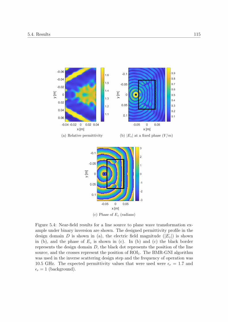
5.4. Results 115
(a) Relative permittivity (b) |Ez| at a fixed phase (V/m)
(c) Phase of Ez (radians)
Figure 5.4: Near-field results for a line source to plane wave transformation ex-ample under binary inversion are shown. The designed permittivity profile in thedesign domain D is shown in (a), the electric field magnitude (|Ez|) is shownin (b), and the phase of Ez is shown in (c). In (b) and (c) the black borderrepresents the design domain D, the black dot represents the position of the linesource, and the crosses represent the position of ROI1. The BMR-GNI algorithmwas used in the inverse scattering design step and the frequency of operation was10.5 GHz. The expected permittivity values that were used were εr = 1.7 andεr = 1 (background).
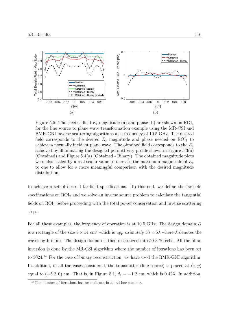
5.4. Results 116
(a) (b)
Figure 5.5: The electric field Ez magnitude (a) and phase (b) are shown on ROI1
for the line source to plane wave transformation example using the MR-CSI andBMR-GNI inverse scattering algorithms at a frequency of 10.5 GHz. The desiredfield corresponds to the desired Ez magnitude and phase needed on ROI1 toachieve a normally incident plane wave. The obtained field corresponds to the Ezachieved by illuminating the designed permittivity profile shown in Figure 5.3(a)(Obtained) and Figure 5.4(a) (Obtained - Binary). The obtained magnitude plotswere also scaled by a real scalar value to increase the maximum magnitude of Ezto one to allow for a more meaningful comparison with the desired magnitudedistribution.
to achieve a set of desired far-field specifications. To this end, we define the far-field
specifications on ROI2 and we solve an inverse source problem to calculate the tangential
fields on ROI1 before proceeding with the total power conservation and inverse scattering
steps.
For all these examples, the frequency of operation is at 10.5 GHz. The design domain D
is a rectangle of the size 8× 14 cm2 which is approximately 3λ× 5λ where λ denotes the
wavelength in air. The design domain is then discretized into 50× 70 cells. All the blind
inversion is done by the MR-CSI algorithm where the number of iterations has been set
to 3024.14 For the case of binary reconstruction, we have used the BMR-GNI algorithm.
In addition, in all the cases considered, the transmitter (line source) is placed at (x, y)
equal to (−5.2, 0) cm. That is, in Figure 5.1, d1 = −1.2 cm, which is 0.42λ. In addition,
14The number of iterations has been chosen in an ad-hoc manner.

5.4. Results 117
for all the cases, ROI1 is the vertical line x = 4.4 cm. In other words, d2 ≈ 0.14λ in
Figure 5.1. On ROI1, we consider 30 equally-spaced data points. Given that the length
of the ROI1 is about 5λ, the separation between the data points on ROI1 is about λ/6.
Furthermore, note that the reconstructed permittivity is, in general, complex. Since we
desire a lossless dielectric profile, we enforce the imaginary part of ε to be zero at each
iteration of the inverse scattering algorithm.15 In addition, since we would like to use
practical dielectric values, we enforce the minimum of the real part of ε to be one and
the maximum to be three at each iteration of the inverse scattering algorithm.
5.4.1 Line source to plane wave transformation
In this example, the objective is to find a lossless relative permittivity profile in D to
transform the electric field emitted by a line source (cylindrical waves) to a plane wave
propagating along the x direction. Since the electric field of a plane wave (uniform
amplitude, phase, and polarization) is analytically known, we assign Ez on ROI1 to be
1∠0◦. Next we utilize the parameter α to ensure that the input and output powers are
equal. Having found α, the desired total electric field Ez on ROI1 will then be α∠0◦.
Knowing the incident field (line source), we can determine the desired scattered field on
ROI1 which can then be given to the inverse scattering algorithm for inversion.
In the first set of results, the inverse scattering method utilized to invert the data on
ROI1 was MR-CSI. Note that this algorithm makes use of the multiplicative L2 norm
total variation regularizer to influence the permittivity profile solution in D to be easier
to fabricate, and to regularize the inverse problem. Figure 5.3(a) shows the reconstructed
dielectric profile in D. As can be seen, we have an inhomogeneous relative permittivity
15We are also implicitly enforcing a lossless medium via applying total power conservation.

5.4. Results 118
profile ranging from one to three.16 Figure 5.3(b) shows the normalized magnitude of
Ez in the near-field in and around D where D has been identified by a black rectangle
and the source by a black circle on the left side of D.17 It is worthwhile to note that
the domain D is almost reflectionless and has not perturbed the cylindrical waves on
D−. In addition, on the right side of D, we see that Ez forms a planar wavefront. The
small crosses just outside and on the right side of D marks the discretized locations on
ROI1 on which we have enforced the desired scattered field. It can be observed that the
generated planar wavefront is approximately the size of the ROI1 which is partly related
to the size of ROI1. Similarly, Figure 5.3(c) shows the phase of Ez in the near-field in and
around D where the design domain D has been again shown by a black rectangle, and
the source is identified by a black circle located just to the left of D. As can be seen, the
phase distribution is close to uniform as the waves arrive at ROI1 shown by small black
crosses just to the right of D. The permittivity profile successfully achieves the desired
transformation.
Next, in order to achieve the same transformation we use a binary inversion algorithm
(BMR-GNI) where a multiplicative expected permittivity regularizer as in [32, 40] is
used to regularize the data misfit cost functional. Through the use of the expected
permittivity regularizer, we favour two relative permittivity values in D: εr = 1.7 and
εr = 1 (air/background). This can further facilitate fabrication as the designer can choose
the permittivity values they have available and there is only one other permittivity value
in the profile other than the background (air). The reconstructed permittivity profile for
this case is shown in Figure 5.4(a). By looking at this figure, it can be seen that the
inverse scattering algorithm favoured a permittivity profile with the previously specified
16Note that the practical implementation of a lens, for example via 3D printing, would involve somelevel of permittivity value discretization. We expect that the performance of the lens degrades aftersuch post-processing. This is especially the case for continuously varying profiles relative to the profilesdesigned using expected permittivity regularization. We speculate that the amount of degradation woulddepend on the level of discretization and the range of the required relative permittivity values actuallycovered by the available materials, but this requires further study.
17Note that in the absence of the dielectric object we only have the fields of the line source which arein the form of cylindrical waves. Since the dielectric lens is (almost) reflectionless these cylindrical wavesare still visible on the input side of the dielectric lens. However, as can be seen in Figure 5.3(b), oncethe input field enters the dielectric lens, it is tailored to become a truncated plane wave.

5.4. Results 119
values.18 Also, comparing the reconstructed dielectric profile in Figure 5.4(a) with that in
Figure 5.3(a) clearly demonstrates the non-uniqueness of this inverse scattering problem.
Then looking at the normalized magnitude and phase of Ez in Figure 5.4(b)-(c), we can
see that the profile in D appears to be able to transform the line source electric field
to a plane wave despite its relative simplicity compared to the previous example when a
continuous set of relative permittivity values were allowed in D.
To show the difference between the two line source transformation examples in more
detail, Figures 5.5(a)-(b) show the magnitude and phase of the desired and obtained Ez
on ROI1 for both the binary and blind inverse scattering cases. Let us first focus on
Figure 5.5(a) where we can compare the desired normalized magnitude (i.e. a flat blue
line of magnitude one) with what has been obtained from the blind inversion (red dash-
dot curve) and the binary inversion (black dashed curve). As can be seen, the magnitude
distribution that was obtained in the blind inversion is closer to an ideal plane wave than
the binary case. This is expected as the blind inverse scattering algorithm has a wide
range of permittivity values to choose from, whereas the binary case sacrifices degrees of
freedom to facilitate physical implementation.
Note that in both cases (blind and binary inversion cases), the magnitude of Ez on ROI1
is below the desired level. This is an indication of power loss in the transformation. Since
the reconstructed permittivity is lossless, this power loss cannot be attributed to the
loss within the dielectric materials. The other source of power loss is through reflections
at the interface of D−. However, as can be seen in Figure 5.3(b) and Figure 5.4(b),
there is minimal reflected energy. The major source of power loss between D− and ROI1
is the power that escapes through the top and bottom edges of the design domain D.
This is visible in Figure 5.3(b) and Figure 5.4(b) and (its interference with the desired
radiation) can be practically reduced by placing absorbers along the top and bottom sides
18Note that the binary inversion performed herein may be considered soft regularization as the inver-sion algorithm is not forced to choose between only two values. That’s why the final reconstruction haspermittivity values other than εr = 1.7 and εr = 1. As post-processing one may convert this reconstruc-tion to a perfect binary image for the ease of fabrication. Although not investigated here, it is expectedthat the performance will degrade after such post-processing.
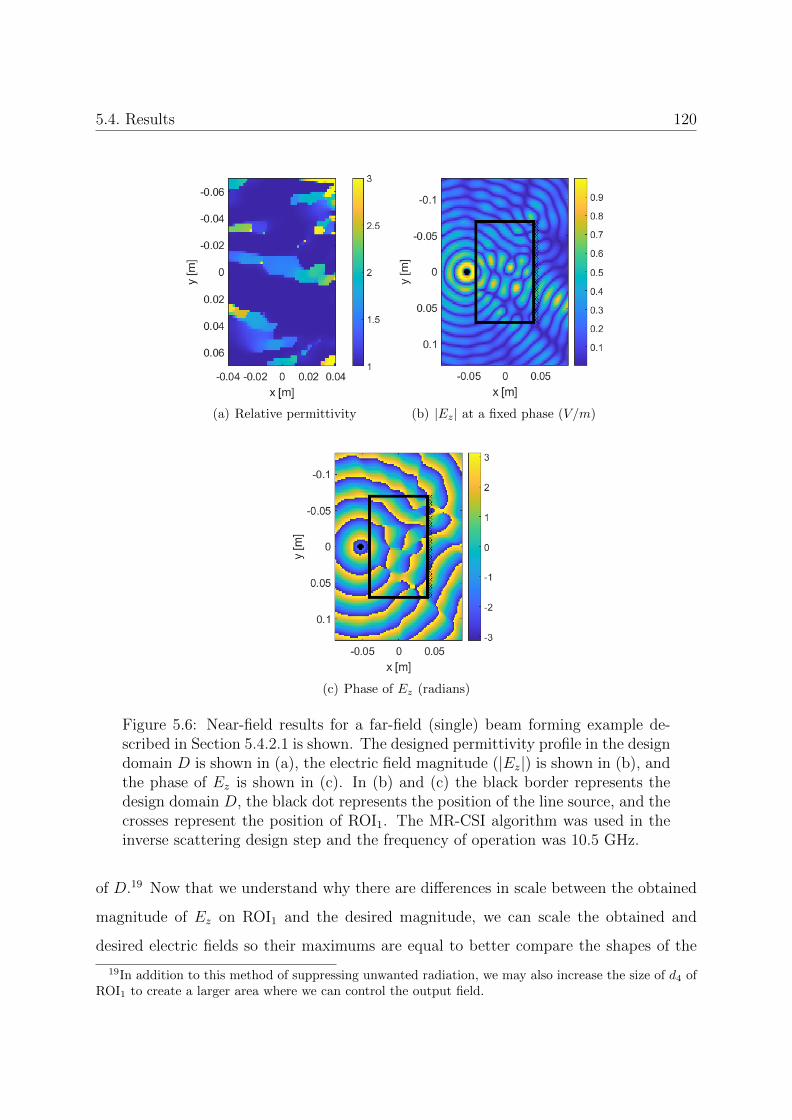
5.4. Results 120
(a) Relative permittivity (b) |Ez| at a fixed phase (V/m)
(c) Phase of Ez (radians)
Figure 5.6: Near-field results for a far-field (single) beam forming example de-scribed in Section 5.4.2.1 is shown. The designed permittivity profile in the designdomain D is shown in (a), the electric field magnitude (|Ez|) is shown in (b), andthe phase of Ez is shown in (c). In (b) and (c) the black border represents thedesign domain D, the black dot represents the position of the line source, and thecrosses represent the position of ROI1. The MR-CSI algorithm was used in theinverse scattering design step and the frequency of operation was 10.5 GHz.
of D.19 Now that we understand why there are differences in scale between the obtained
magnitude of Ez on ROI1 and the desired magnitude, we can scale the obtained and
desired electric fields so their maximums are equal to better compare the shapes of the
19In addition to this method of suppressing unwanted radiation, we may also increase the size of d4 ofROI1 to create a larger area where we can control the output field.
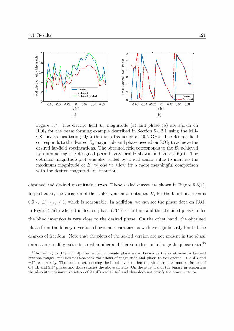
5.4. Results 121
(a) (b)
Figure 5.7: The electric field Ez magnitude (a) and phase (b) are shown onROI1 for the beam forming example described in Section 5.4.2.1 using the MR-CSI inverse scattering algorithm at a frequency of 10.5 GHz. The desired fieldcorresponds to the desired Ez magnitude and phase needed on ROI1 to achieve thedesired far-field specifications. The obtained field corresponds to the Ez achievedby illuminating the designed permittivity profile shown in Figure 5.6(a). Theobtained magnitude plot was also scaled by a real scalar value to increase themaximum magnitude of Ez to one to allow for a more meaningful comparisonwith the desired magnitude distribution.
obtained and desired magnitude curves. These scaled curves are shown in Figure 5.5(a).
In particular, the variation of the scaled version of obtained Ez for the blind inversion is
0.9 < |Ez|ROI1 ≤ 1, which is reasonable. In addition, we can see the phase data on ROI1
in Figure 5.5(b) where the desired phase (∠0◦) is flat line, and the obtained phase under
the blind inversion is very close to the desired phase. On the other hand, the obtained
phase from the binary inversion shows more variance as we have significantly limited the
degrees of freedom. Note that the plots of the scaled version are not present in the phase
data as our scaling factor is a real number and therefore does not change the phase data.20
20According to [149, Ch. 4], the region of pseudo plane wave, known as the quiet zone in far-fieldantenna ranges, requires peak-to-peak variations of magnitude and phase to not exceed ±0.5 dB and±5◦ respectively. The reconstruction using the blind inversion has the absolute maximum variations of0.9 dB and 5.1◦ phase, and thus satisfies the above criteria. On the other hand, the binary inversion hasthe absolute maximum variation of 2.1 dB and 17.55◦ and thus does not satisfy the above criteria.
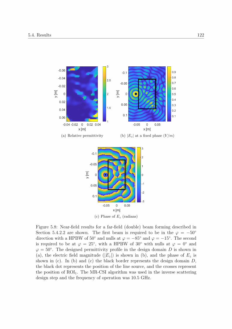
5.4. Results 122
(a) Relative permittivity (b) |Ez| at a fixed phase (V/m)
(c) Phase of Ez (radians)
Figure 5.8: Near-field results for a far-field (double) beam forming described inSection 5.4.2.2 are shown. The first beam is required to be in the ϕ = −50◦
direction with a HPBW of 50◦ and nulls at ϕ = −85◦ and ϕ = −15◦. The secondis required to be at ϕ = 25◦, with a HPBW of 30◦ with nulls at ϕ = 0◦ andϕ = 50◦. The designed permittivity profile in the design domain D is shown in(a), the electric field magnitude (|Ez|) is shown in (b), and the phase of Ez isshown in (c). In (b) and (c) the black border represents the design domain D,the black dot represents the position of the line source, and the crosses representthe position of ROI1. The MR-CSI algorithm was used in the inverse scatteringdesign step and the frequency of operation was 10.5 GHz.
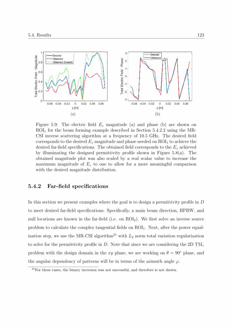
5.4. Results 123
(a) (b)
Figure 5.9: The electric field Ez magnitude (a) and phase (b) are shown onROI1 for the beam forming example described in Section 5.4.2.2 using the MR-CSI inverse scattering algorithm at a frequency of 10.5 GHz. The desired fieldcorresponds to the desired Ez magnitude and phase needed on ROI1 to achieve thedesired far-field specifications. The obtained field corresponds to the Ez achievedby illuminating the designed permittivity profile shown in Figure 5.8(a). Theobtained magnitude plot was also scaled by a real scalar value to increase themaximum magnitude of Ez to one to allow for a more meaningful comparisonwith the desired magnitude distribution.
5.4.2 Far-field specifications
In this section we present examples where the goal is to design a permittivity profile in D
to meet desired far-field specifications. Specifically, a main beam direction, HPBW, and
null locations are known in the far-field (i.e. on ROI2). We first solve an inverse source
problem to calculate the complex tangential fields on ROI1. Next, after the power equal-
ization step, we use the MR-CSI algorithm21 with L2 norm total variation regularization
to solve for the permittivity profile in D. Note that since we are considering the 2D TMz
problem with the design domain in the xy plane, we are working on θ = 90◦ plane, and
the angular dependency of patterns will be in terms of the azimuth angle ϕ.
21For these cases, the binary inversion was not successful, and therefore is not shown.

5.4. Results 124
' [/]-100 -50 0 50 100
jEzj2
inth
efa
r--eld
[dB]
-60
-50
-40
-30
-20
-10
0
Inv Source Jz and My
Illuminating Designed DDesired Points in fNull Locations
(a)
' [/]-100 -50 0 50 100
jEzj2
inth
efa
r--eld
[dB]
-60
-50
-40
-30
-20
-10
0
Inv Source Jz and My
Illuminating Designed DDesired Points in fNull Locations
(b)
Figure 5.10: The far-field power patterns are shown for the far-field single beamexample described in Section 5.4.2.1 (a) and the far-field double beam exampledescribed in Section 5.4.2.2 (b). The far-field from the reconstructed electric andmagnetic current densities on ROI1 after the inverse source step (blue solid line).This inverse source step tries to match the desired far-field specifications by firsttranslating the specifications into desired far-field points (black circle markers) ina normalized power vector f and then minimizing the appropriate data-misfit costfunctional with respect to electric and magnetic current densities on ROI1 (seeSection 5.3.1). Finally, the far-field from illuminating the designed permittivityprofile in D after the inverse scattering step, measuring the resulting fields onROI1, and then propagating these near-fields to the far-field is shown (red dash-dot line).
5.4.2.1 Single main beam
In this example we desire a main beam at ϕmain = 30◦ and a HPBW of ∆ϕ|3dB =
30◦. In addition we require nulls at ϕnull1 = 55◦ and ϕnull2 = 5◦. Note that these are
performance criteria and not explicit field values. The lossless relative permittivity profile
calculated by the inverse scattering algorithm (MR-CSI) is shown in Figure 5.6(a). The
normalized magnitude and phase of Ez around and within the design domain D are
shown in Figures 5.6(b) and 5.6(c) respectively. Similar to the line source to plane wave
transformation example, the amount of reflected energy is low. In Figure 5.7(a)-(b) the
magnitude and phase of the desired and obtained Ez on ROI1 (near-field zone) is shown.
There is again unwanted power dispersion from the the top and bottom sides of D that
can be seen in Figure 5.6(b). Because our final objective is to satisfy the aforementioned

5.4. Results 125
performance criteria in the far-field zone, the shape of the magnitude distribution of Ez
on ROI1 must match the desired magnitude curve closely. For this reason, we have also
shown the scaled version of the obtained Ez on ROI1 in Figure 5.7(a). (We scale Ez by
a real number so the maximum of the obtained |Ez| is one.) As can be seen, the scaled
version of the obtained |Ez| is relatively close to the desired one. Similarly, the desired
and obtained phase of Ez on ROI1 are reasonably close. In summary, since the obtained
and desired |Ez|∠Ez are relatively close on ROI1, we expect to be able to satisfy our
far-field performance criteria.
To this end, the far-field pattern obtained when the reconstructed dielectric profile is
interrogated by the line source is required. To calculate the far-field we use the obtained
fields on the ROI1, which is defined on an edge that is at x = 4.4 cm and spans from
−7 < y < 7 [cm]. The fields along the ROI1 (i.e., along x = 4.4 cm) and spanning
|y| ≥ 7 [cm] are assumed to be zero. Using this assumption, we can calculate the far-field
pattern simply by propagating 2My values along ROI1 to the far-field; i.e., we are using the
electromagnetic equivalence principle and the assumption that there is a perfect electric
conductor behind the ROI1. Figure 5.10(a) shows three different curves. The black circle
markers show the enforcement of the desired performance criteria, which later on form
the desired normalized power vector f . For example, the two black circles at −60 dB level
indicate the two desired nulls at ϕnull1 = 55◦ and ϕnull2 = 5◦. Note that this means we
could have a main beam with the maximum magnitude of 1, and desired null levels set
to 10−6 in the vector f . This wide dynamic range of 1 to 10−6 shows the importance of
the weighting matrix W in (5.1).
As noted before in Section 5.3, our first step is to reconstruct a set of equivalent currents
on ROI1 (see the unknown vector x in (5.1)) that can meet the far-field constraints on
ROI2. It is instructive to check the far-field pattern of these equivalent currents. This
is shown in Figure 5.10(a) with a blue solid line. The main beam is quite accurate;
however, although we see some nulls at 5◦ and 55◦, they are not as deep as we have

5.4. Results 126
desired (−60 dB).22 Lastly, once we transform the near-field data that we have obtained
after illumination of the reconstructed dielectric profile to the far-field zone, we get the
radiation pattern shown by the red dash-dot line. As can be seen, this curve satisfies
the main beam direction and null locations. However, the null levels are not as deep
as originally desired and the obtained HPBW is ∆ϕ|3dB = 26◦ instead of the required
∆ϕ|3dB = 30◦ (this level of accuracy may be appropriate for many applications).
5.4.2.2 Two main beams
In this example, we desire two separate main beams in the far-field zone. The first beam
is required to be in the ϕ|main = −50◦ direction with a HPBW of ∆ϕ|3dB = 50◦ and nulls
at ϕ|null1 = −85◦ and ϕ|null2 = −15◦. The second beam is required to be at ϕ|main = 25◦,
with a HPBW of ∆ϕ|3dB = 30◦ with nulls at ϕnull1 = 0◦ and ϕnull2 = 50◦. Note that
in this example, there are more performance criteria than the previous example, but we
maintain the same amount of unknowns in D and the same amount of sampling on ROI1.
Figure 5.8(a) shows the reconstructed relative permittivity profile. The normalized mag-
nitude and phase of Ez within and around the near field of D (shown as a black rectangle)
are shown in Figure 5.8(b)-(c). As can be seen by looking at the left side of the design
domain (i.e, D−), the design domain is still almost reflectionless. Similar to what we
did in the previous single beam example, let us now compare the desired and obtained
fields on ROI1 in Figure 5.9(a)-(b): the obtained electric field magnitude and phase dis-
tributions on ROI1 follow the same shape as the desired magnitude and phase, but less
so than the previous example. Specifically, the magnitude curve is not as accurate in
this example when compared with the what was obtained in Figure 5.7(a). This is an
indication that we were not able to construct a permittivity profile in D that can produce
the required far-field when illuminated by our line source. The far-field results, shown in
Figure 5.10(b), which were obtained in the same way as the previous example support
22It is instructive to note that we do not know whether it is possible to meet the null level of −60 dBalong with the other performance criteria with any set of equivalent currents on ROI1, i.e. there maynot be enough degrees of freedom.
5.5. Conclusion 127
this theory. The two main beam shapes are present in the intended direction, but there
are imperfections within the beams. The nulls are present, but their locations are shifted
more than the previous example. Also, similar to the previous example, the nulls are
not as deep as the desired level. One way we might go about improving this result is to
increase the size of D to perhaps gain more degrees of freedom to produce the required
electric field magnitude and phase on ROI1.
5.5 Conclusion
We presented an inverse design framework that is capable of constructing lossless permit-
tivity profiles that can achieve far-field and near-field transformations when illuminated
with a single source/feed. This design methodology can achieve far-field specifications
including main beam direction, null location, and HPBW. This framework utilizes ex-
isting gradient-based inverse scattering algorithms that have been primarily used for
microwave imaging applications. However, this inverse scattering process requires two
extra steps: (i) the use of an inverse source algorithm to convert desired performance
criteria to equivalent currents in close proximity to the design domain, and (ii) ensuring
total power conservation between the input and output power levels. In addition, the
latter step implicitly favours the reconstruction of reflectionless lossless dielectric profiles
within the design domain.
Herein, we utilized this inversion method to design permittivity profiles that are capable of
transforming the electric field from a line source to a plane wave, and meeting two different
sets of far-field specifications. Furthermore it was shown that this method cannot always
meet all the desired far-field specifications and may require more degrees of freedom to do
so. It was also demonstrated that different forms of regularization such as the weighted L2
norm total variation regularization and expected permittivity regularization can be used
to reconstruct different dielectric profiles for the same transformation, thus, benefiting
from the non-uniqueness of the problem.

Chapter 6
Conclusions and Suggested Future
Work
6.1 Conclusion
The purpose of this thesis was to improve upon and develop new antenna characteriza-
tion and design techniques by utilizing the EI framework. In Chapter 1, it was explained
how the current distribution of an antenna is its fundamental spatial property. We then
explained that in many cases, equivalent currents may be used instead of the true inter-
nal currents of a radiator. Next, we introduced the Electromagnetic Surface and Volume
Equivalence Principles; it was explained that EI algorithms use these principles for an-
tenna design and characterization applications. Following this, we outlined our common
EI methodology that we used to contribute to EI algorithms in different antenna design
and characterization applications. In Chapter 2 we presented a brief overview of the
antenna design and characterization applications contributed to by this work, while ex-
plaining how they are unified in their need/use of equivalent currents. This chapter also
served to explain why the applications of metasurface design, microwave imaging, and
128
6.1. Conclusion 129
dielectric lens/antenna design were chosen for this thesis. Next, in Chapter 3 we used
the surface equivalence principle to contribute to the area of metasurface design wherein
we developed a novel gradient-based EI metasurface design algorithm that is capable of
designing the circuit admittance profile of a three admittance layer metasurface from
desired magnetic field data. We showed that our method could meet the magnitude and
phase constraints in the desired data. To be able to characterize and design radiators of
a larger cross-section, we then turned to the volume equivalence principle. To this end,
we indirectly used this principle in Chapter 4 to contribute to the area of dielectric scat-
terer characterization through the context of microwave imaging. Specifically, a phaseless
Gauss-Newton inversion algorithm was developed to reconstruct a dielectric profile (the
unknown scatter) in a region of interest from a set of phaseless measured electric field
data. Finally, to apply these principles to the design of dielectric lenses/antennas, we
introduced a combined inverse source and scattering technique for the purpose of tailor-
ing electromagnetic fields in Chapter 5. This technique is capable of designing passive,
lossless, and reflectionless dielectric scatterers from complex, phaseless, or far-field crite-
ria data. In summary, we showed that EI framework’s flexibility allows for the design
and characterization of antennas in many applications. This can be helpful in our ever
expanding wireless technology landscape. The main contributions that resulted from this
work are summarized in the next section.
6.1.1 Summary of Main Contributions
• Metasurface Design Algorithm: In Chapter 3, a novel gradient-based meta-
surface design algorithm was developed that can directly calculate the required
circuit admittance profile needed to implement a passive lossless three admittance
layer metasurface using complex or phaseless desired field data. To this end, we
constrain the algorithm to reconstruct only purely-imaginary admittances necessi-
tating a metasurface design without loss or gain, and local power conservation is

6.2. Suggested Future Work 130
inherently enforced in contrast to previous work that may enforce this with addi-
tive regularization. In addition, the ability to reconstruct the circuit admittances
directly enables constraints to be placed, which could not be done previously.
• Antenna Characterization/Microwave Imaging Algorithm: In Chapter 4,
a novel phaseless multiplicatively-regularized Gauss-Newton inversion imaging al-
gorithm was developed and verified with synthetic and experimental data. The
flexibility of the EI framework was used to be able to make use of phaseless elec-
tric field data with a GNI algorithm, instead of complex measured data. It was
demonstrated that more regularization is necessary to overcome the lack of phase
information in the measured data for some imaging experiments.
• Dielectric Lens/Antenna Design Algorithm: In Chapter 5, a new combined
inverse source and scattering methodology has been presented that is capable of
designing dielectric profiles that when illuminated by a single feed can satisfy user
specified far-field performance criteria, including main beam direction, null loca-
tions, and half-power beam width (HPBW). In addition, the technique is capable
of designing, passive, lossless, and reflectionless dielectric profiles. The presented
framework is also capable of using existing inverse scattering algorithms that are
used for microwave imaging without much modification.
6.2 Suggested Future Work
This work can be extended in several ways. Herein, avenues for extending the work
specifically for certain algorithms, and for all the algorithms in general.
• Metasurface Design Algorithm: This EI algorithm can design metasurfaces to
meet complex and phaseless desired data. To increase its utility, it could extended
to meet desired far-field criteria such as main beam direction, HPBW and null
location. Furthermore, this algorithm introduced the ability to apply constraints

6.2. Suggested Future Work 131
to the admittance profile that define the metasurface directly, and an example
was shown where the admittance profile of the metasurface was smoothed within
each layer. However, there may be cases where there are maximum and minimum
limits to the admittances that can be physically implemented. To this end, a
regularizer can be developed to take this type of constraint into account. In this
work passive, lossless, reflectionless metasurfaces were being sought to match the
magnitude and phase of the desired magnetic field pattern. As can be seen from
the results in Chapter 3, an ideal solution could not be found that completely met
all the constraints (magnitude, phase, and full efficiency). Therefore, a means of
determining what the best possible solution is/can be should be explored.
• Antenna Characterization/Microwave Imaging Algorithm: It was demon-
strated that regularization methods were important in supplementing the magni-
tude only information in some scenarios while using the developed phaseless GNI
algorithms for MWI. Further research could be conducted on what the best possible
reconstruction could be based on a set of phaseless measurements. For example, in
Section 4.5.4 it was shown that there was little information content in the measured
phaseless total field data as it was very similar to the phaseless incident field. It
would be instructive to know what the most accurate reconstruction could be in
these types of scenarios. This could also help determine how much regularization
is needed to achieve a reconstruction to a desired accuracy.
Additionally, in this work, we are able to characterize dielectric scatterers, but we
could extend this to include metallic/perfect electric conductor scatterers as well.
This would allow the characterization of more types of devices, including electronics.
Being able to work with metals and dielectrics may also facilitate design.
• Dielectric Lens/Antenna Design Algorithm: The presented technique was
developed to design passive, lossless, and reflectionless dielectric profiles to tailor
electromagnetic fields, however, there may be cases where a specific reflected field is
desired. To this end, it can be investigated how a dielectric profile could be designed
if a desired transmitted and reflected field are required.

6.2. Suggested Future Work 132
• General: These algorithms make use of additive and multiplicative regulariza-
tion terms, and therefore, multi-objective optimization concepts can be used to
determine appropriate solutions. For example, if we can determine multiple Pareto
optimal solutions, we can offer a set of feasible solutions for the metasurface design
problem or the dielectric lens design problem. In addition, other than some pre-
liminary 3D work ( see [2, 150]), the presented algorithms were presented in a 2D
framework and so they can be fully extended to a 3D framework.

Appendix A
Appendix for Gradient-Based
Electromagnetic Inversion for
Metasurface Design Using Circuit
Models
The material in this appendix is published in [38].1
A.1 Derivation of Gradient Vectors
We first show a detailed derivation of the gradient gdataY1
for the field (amplitude and
phase) pattern synthesis case. (The gradients with respect to layers Y2 and Y3 can be
derived in a similar manner.) To this end, we first isolate Y1 from Cdata(Y) by writing
1© 2021 IEEE. Reprinted, with permission, from C. Narendra, T. Brown and P. Mojabi, “Gradient-Based Electromagnetic Inversion for Metasurface Design Using Circuit Models,” in IEEE Transactionson Antennas and Propagation, doi: 10.1109/TAP.2021.3118811.
133

A.1. Derivation of Gradient Vectors 134
A(Y), B(Y), C(Y), and D(Y) as
A(Y) = (mp11m11 + jmp
12m11Y2 +mp12m21
+ jmp11m12Y3 −mp
12m12Y2 �Y3 + jmp12m22Y3)
B(Y) = (mp11m12 +mp
12m22 + jmp12m12Y2)
C(Y) = (jmp11m11Y1 +mp
21m11 −mp12m11Y1 �Y2
+ jmp22m11Y2 + jmp
12m21Y1 +mp22m21
−mp11m12Y1 �Y3 + jmp
21m12Y3
− jmp12m12Y1 �Y2 �Y3 −mp
22m12Y2 �Y3
−mp12m22Y1 �Y3 + jmp
22m22Y3)
D(Y) = (jmp11m12Y1 +mp
21m12 −mp12m12Y1 �Y2
+ jmp22m12Y2 + jmp
12m22Y1 +mp22m22)
(A.1)
where the constants mij and mpij can be found as
m11 m12
m21 m22
= Tsub,
mp11 mp
12
mp21 mp
22
= Tsub ·Tbpl (A.2)
Therefore, we can rewrite (3.11) for the field pattern synthesis case as a linear function
of Y1 and obtain
Cdata(Y1) = ζf ||L1Y1 + h1︸ ︷︷ ︸G(Y)
−f ||2, (A.3)
where the discrete operator L1 and vector h1 arise from factoring Y1 from G(Y). (The
expression for the operator L1 will be provided later.) This also means that L1 and the
vector h1 can be functions of Y2 and/or Y3, but not Y1. (Note that Y2 and Y3 are
treated as constant vectors in the derivation of the gradient with respect to Y1.)
To find gdataY1
, we first start by finding the differential of the functional with respect to
Y1 as
δCdata = ζf limε→0
‖L1(Y1 + εΨ)− f ′‖2 − ‖L1Y1 − f ′‖2
ε(A.4)

A.1. Derivation of Gradient Vectors 135
where ε is a real number, f ′ = f − h1, and Ψ is a vector of the same size as Y1 along
which we perturb Y1. The above limit can be calculated as
δCdata = ζf limε→0
1
ε(‖L1Y1 − f ′‖2
+ ε2 ‖L1Ψ‖2
+ 2εRe 〈L1Y1 − f ′,L1Ψ〉
− ‖L1Y1 − f ′‖2)
(A.5)
where 〈·, ·〉 denotes the inner product on the ROI. The above differential can then be
simplified as
δCdata = 2ζfRe⟨LH
1 (L1Y1 − f ′),Ψ⟩
(A.6)
which shows the variation in Cdata due to a small perturbation in Y1 along the auxiliary
vector Ψ. Then, similar to [129, Appendix D.5], the gradient vector for the field pattern
synthesis case can be identified as
gdataY1
= 2ζfRe{LH1 (L1Y1 − f ′)}
= 2ζfRe{LH1 (L1Y1 + h1 − f)}
= 2ζfRe{LH1 (G(Y)− f)}
(A.7)
which is what is shown in (3.26).
The expression for the matrix L1 and the other two similar matrices needed to calculate
the gradient with respect to Y2 and Y3 are
L1 = AHzJydiag (z11) + AHzMzdiag (z12) ,
L2 = AHzJydiag (z21) + AHzMzdiag (z22) ,
L3 = AHzJydiag (z31) ,
(A.8)
A.1. Derivation of Gradient Vectors 136
where diag(·) is an operator that takes a vector and converts it to a matrix with the
original elements of the vector on the diagonal. Also, the above z vectors are defined as
z11 = (jmp11m11 −mp
12m11Y2 + jmp12m21 −mp
11m12Y3
− jmp12m12Y2 �Y3 −mp
12m22Y3)� E−y
z12 = (mp12m12Y2 − jmp
11m12 − jmp12m22)� E−y
z21 = (−mp12m11Y1 + jmp
22m11 − jmp12m12Y1 �Y3
−mp22m12Y3)� E−y
− (jmp12m11 +mp
12m21 −mp12m12Y3)�H−z
z22 = (jmp12m12) H−z − (−mp
12m12Y1 + jmp22m12)� E−y
z31 = (−mp11m12Y1 + jmp
21m12 − jmp12m12Y1 �Y2
−mp22m12Y2 −mp
12m22Y1 + jmp22m22)� E−y
− (jmp11m12 −mp
12m12Y2 + jmp12m22)�H−z
(A.9)
where the constants mij and mpij are shown in (A.2).
The derivation of the gradient vector with respect to Y1 is now presented for the power
pattern synthesis case. We begin by calculating the following differential
δCdata = ζp limε→0
1
ε(∥∥|L1(Y1 + εΨ) + h1|2 − |f |2
∥∥2
−∥∥|L1Y1 + h1|2 − |f |2
∥∥2)
(A.10)
which can be simplified to
δCdata = 4ζpRe⟨|L1Y1 + h1|2 − |f |2,Re(L1Ψ� h∗1)
⟩+ 4ζpRe
⟨|L1Y1 + h1|2 − |f |2,Re(L1Y1 � (L1Ψ)∗)
⟩= 4ζpRe
⟨LH
1 ((L1Y1 + h1)� (|L1Y1 + h1|2 − |f |2)),Ψ⟩.
(A.11)

A.2. Derivation of Step Length 137
Thus, the gradient vector of the data misfit cost functional with respect to Y1 for the
power pattern synthesis case can be identified as
gdataY1
= 4ζpRe(LH1 ((L1Y1 + h1)� (|L1Y1 + h1|2 − |f |2)))
= 4ζpRe(LH1 (G(Y)� (|G(Y)|2 − |f |2)))
(A.12)
which is what is shown in (3.27).
We use the same procedure to find gJTVYi
, gMTVYi
, and gYTVYi
. For example, for the case of
gJTVY1
, we first find the differential of CJTV where Y1 is perturbed by εΨ. The differential
can then be simplified as
δCJTV = −2Re〈 ∂2
∂y2(zi1Yi + hJi)� z∗i1,Ψ〉. (A.13)
Thus, gJTVY1
can be identified as
gJTVY1
= −2Re{ ∂2
∂y2(zi1Yi + hJi)� z∗i1}. (A.14)
For the details of the gradient of TV-based cost functional, we refer the reader to similar
derivations available in [129, Appendix D.3] and [99].
A.2 Derivation of Step Length
Herein, we show the derivation of the step length α1 used in the update of the Y1 layer
according to (3.24) assuming all quantities are in the kth iteration. (The step lengths
corresponding to the update for Y2 and Y3 are derived in the same manner.) To this
end, we need to minimize C(Y1 + α1gY1) over α1. Note that the total cost functional Cis the summation of a few cost functionals as shown in (3.22). Herein, for brevity, we
perform the procedure merely on its data misfit component, i.e., Cdata. Let us first begin

A.2. Derivation of Step Length 138
by the data misfit cost functional for the field pattern synthesis case as
Cdata(Y1 + α1gY1) = ζf ‖L1(Y1 + α1gY1) + h1 − f‖2
= ζf ‖G(Y)− f‖2 + α21ζf ‖L1gY1‖2
+ 2αζfRe{〈G(Y)− f ,L1gY1〉}
(A.15)
where L1 and h1 have been already defined for (A.3). To solve for the step length, we
take the derivative with respect to α1, set the expression to zero, and solve for α1 as
α1 =Re{〈G(Y)− f ,L1gY1〉}
‖L1gY1‖2 . (A.16)
As noted above, the above expression needs to be augmented due to the presence of other
cost functionals.
Similarly, for the power pattern synthesis case, let us focus merely on the data misfit cost
functional for brevity and write Cdata(Y1 + α1gY1) as
ζp∥∥|L1(Y1 + α1gY1) + h1|2 − |f |2
∥∥2. (A.17)
Expanding the above norm, taking the derivative with respect to α1, and equating the
resulting equation to zero, we arrive at the following equation
a3α31 + a2α
21 + a1α1 + a0 = 0 (A.18)

A.2. Derivation of Step Length 139
where the coefficients are
a3 = 4∥∥|L1gY1|2
∥∥2
a2 = 12Re{⟨|L1gY1|2, (L1gY1)� (h∗1 + (L1Y1)∗)
⟩}
a1 = 8 ‖Re{(L1gY1)� (h∗1 + (L1Y1)∗)}‖2
+ 4⟨|L1Y1|2 + |h1|2 + 2Re(L1Y1 � h∗1)− |f |2, |L1gY1 |2
⟩a0 = 4Re〈|L1Y1|2 + |h1|2 + 2Re(L1Y1 � h∗1)− |f |2,
(L1gY1)� (h∗1 + (L1Y1)∗)〉
(A.19)
Once we solve (A.18), its real root serves as our step length for the update of Y1 in the
power pattern synthesis case. Note that for the complete implementation, the expressions
in (A.19) need to be augmented by some other components due to the involvement of the
other cost functionals.

Appendix B
Appendix for Phaseless
Gauss-Newton Inversion for
Microwave Imaging
The material in this appendix is published in [41].1
B.1 Required Derivative Operators
Herein, we show in more detail how we minimize the phaseless data misfit cost functional
C(χ) using the Gauss-Newton inversion framework. In particular, we aim to derive the
main (unregularized) update equation given in (4.9). At the nth iteration, we update
our latest χn as χn+1 = χn + νn∆χn by minimizing the regularized form of C(χ). This
requires the derivative operators of both the phaseless data misfit functional and the
regularization terms. Since the regularizations terms for full data (complex) inversion
1© 2021 IEEE. Reprinted, with permission, from C. Narendra and P. Mojabi, “Phaseless Gauss-Newton Inversion for Microwave Imaging,” in IEEE Transactions on Antennas and Propagation, vol. 69,no. 1, pp. 443-456, Jan. 2021, doi: 10.1109/TAP.2020.3026427.
140

B.1. Required Derivative Operators 141
and phaseless inversion are the same, we focus on the required derivative operators for
the phaseless data misfit cost functional. The phaseless cost functional C(χ) maps the
complex vector χ to a real number and is not analytic with respect to χ in the complex
domain. Therefore, in order to calculate ∆χn within the GNI framework, we use Wirtinger
calculus [129, 151–153] to define the required derivative operators. This is based on
treating χ and its complex conjugate χ∗ as two independent functions (or, vectors in the
discrete domain).2 The GNI framework calculates the update ∆χn by approximating
C(χ + ∆χn) by a quadratic model. The update ∆χn is then found for the minimum of
this quadratic model. Within the Wirtinger calculus framework, we consider the cost
functional C(χ, χ∗) = C(χ), where C(χ, χ∗) is analytic with respect to χ for a fixed χ∗and also analytic with respect to χ∗ for a fixed χ. Minimizing C(χ, χ∗) is equivalent to
minimizing C(χ). Applying Newton optimization to the phaseless cost functional leads
to ∆χn obeying the following relation∂2C∂χ∂χ
∂2C∂χ∂χ∗
∂2C∂χ∗∂χ
∂2C∂χ∗∂χ∗
∆χn
∆χ∗n
= −
∂C∂χ
∂C∂χ∗
(B.1)
where ∂C∂χ
and ∂C∂χ∗
are the derivative operators with respect to χ and χ∗, respectively at the
nth iteration. These derivative operators, in the discrete domain, act on a complex vector
and output a complex number. Similarily, ∂2C∂χ∂χ
is a second derivative operator, in this
case, with respect to χ and then χ again evaluated at the nth iteration of the algorithm.
In the discrete domain, the second order derivative operators act on a complex vector
and output a complex vector.
2An alternative approach would be to optimize over the real and imaginary parts of the contrast. Thishas been shown to be the same as treating χ and χ∗ as two independent functions (vectors), see [129,Appendix D.5].

B.1. Required Derivative Operators 142
B.1.1 First Order Derivative Operators
In order to derive the required first order derivative operators, we use the following relation
δC = limε→0
C(χ+ εψ)− C(χ)
ε(B.2)
where ε ∈ R is a scalar, and ψ is an arbitrary function (vector) that is used to modify χ.
Since we are treating χ and χ∗ as two independent functions, δC will be3
δC =∂C∂χ
(ψ) +∂C∂χ∗
(ψ∗). (B.3)
As will be seen later, the two terms on the right hand side of (B.3) are complex conjugates
of each other. Therefore, δC will be a real number. This is expected since C(χ) ∈ R.
Also, note that the range of these two first order derivative operators will be complex
numbers. In other words, the operation of these derivative operators can be represented
by inner products. In our case, the inner product over the ROI is defined as
〈ϕ, ψ〉 =
∫ROI
ϕ ψ∗ds. (B.4)
Based on this, the right hand side of (B.3) can be represented by two inner products,
from which we can obtain the expression for the first order derivative operators. In (B.5),
we have shown how to write δC based on two inner products. It should be noted that ∂E∂χ
in (B.5) should be evaluated at the current estimate of χ, and ‘Re’ denotes the real-part
operator. For example, when we are at the nth iteration, this derivative operator should
be evaluated at χ = χn. In addition, the second order derivative ∂2E∂χ2 has been neglected
(GNI approximation) in (B.5). Noting (B.5) and the definition of the inner product over
the ROI given in (B.4), it is now possible to identify our first order derivative operators.
3To understand this better, let us consider a function such as f(x, y), then δf = ∂f∂xδx+ ∂f
∂y δy. Since
we have treated χ and χ∗ as two independent functions, we have a similar form for δC as shown in (B.3).

B.1. Required Derivative Operators 143
δC = limε→0
ζ
ε
(∥∥∥M2 − |E(χ+ εψ)|2∥∥∥2−∥∥∥M2 − |E(χ)|2
∥∥∥2)
= limε→0
ζ
ε
∥∥∥∥∥M2 −∣∣∣∣E(χ) + ε
∂E
∂χψ
∣∣∣∣2∥∥∥∥∥
2
−∥∥∥M2 − |E(χ)|2
∥∥∥2
= lim
ε→0
ζ
ε
∥∥∥∥∥M2 −(|E(χ)|2 +
∣∣∣∣ε∂E∂χ ψ∣∣∣∣2 + 2εRe
{E(χ)∗
∂E
∂χψ
})∥∥∥∥∥2
−∥∥∥M2 − |E(χ)|2
∥∥∥2
= lim
ε→0
ζ
ε
(4ε2∥∥∥∥Re
{E(χ)∗
∂E
∂χψ
}∥∥∥∥2
+ 2Re
⟨M2 − |E(χ)|2 ,−2ζεRe
{E(χ)∗
∂E
∂χψ
}⟩)
= −2ζRe
⟨M2 − |E(χ)|2 , 2Re
{E(χ)∗
∂E
∂χψ
}⟩= −2ζ
⟨M2 − |E(χ)|2 , E(χ)∗
∂E
∂χψ + E(χ)
(∂E
∂χψ
)∗⟩= −2ζ
⟨M2 − |E(χ)|2 , E(χ)∗
∂E
∂χψ
⟩− 2ζ
⟨M2 − |E(χ)|2 , E(χ)
(∂E
∂χψ
)∗⟩=
⟨2ζ
(∂E
∂χ
)a (E(χ)
(|E(χ)|2 −M2
)), ψ
⟩︸ ︷︷ ︸
∂C∂χ∗ (ψ∗)
+
⟨2ζ
((∂E
∂χ
)a (E(χ)
(|E(χ)|2 −M2
)))∗, ψ∗⟩
︸ ︷︷ ︸∂C∂χ
(ψ)=(∂C∂χ∗ (ψ∗)
)∗(B.5)
In the discrete domain, the first order derivative operators evaluated at χn are
∂C∂χ∗
∣∣∣∣χ=χn
= 2ζJHn[E(χn)� (|E(χn)|2 −M2)
]∂C∂χ
∣∣∣∣χ=χn
=
(∂C∂χ∗
∣∣∣∣χ=χn
)∗ (B.6)
where ζ is the normalization coefficient of the phaseless data misfit cost functional, see
(4.8), and Jn denotes the Jacobian (sensitivity) matrix that represents the derivative of
the total field data on the measurement domain with respect to the contrast χ (i.e., ∂E∂χ
).4
4The derivation and expression for the Jacobian matrix can be found in [129, Appendix D.1]. Thisrequires the calculation of the so-called inhomogeneous (or, distorted) Green’s function. Also, we remindthe reader that the derivative of the total field with respect to the contrast is the same as the derivativeof the scattered field with respect to the contrast.
B.1. Required Derivative Operators 144
δ2C1 = lim
ε→0
1
ε
[⟨2ζ∂E
∂χ
∣∣∣∣χ+εψ
(ϕ),[E(χ + εψ)(|E(χ + εψ)|2 −M2
)]⟩−⟨2ζ∂E
∂χ(ϕ),
[E(χ)(|E(χ)|2 −M2
)]⟩]
= limε→0
1
ε
[2ζ
⟨(∂E
∂χ+ ε
∂2E
∂χ2(ψ)
)(ϕ),
(E(χ) + ε
∂E
∂χ(ψ)
)(∣∣∣∣E(χ) + ε∂E
∂χ(ψ)
∣∣∣∣2 −M2
)⟩. . .
− 2ζ
⟨∂E
∂χ(ϕ), E(χ)
(|E(χ)|2 −M2
)⟩]
= limε→0
1
ε
[2ζ
⟨∂E
∂χ(ϕ),
(E(χ) + ε
∂E
∂χ(ψ)
)(|E(χ)|2 + ε
2∣∣∣∣ ∂E∂χ
(ψ)
∣∣∣∣2 + 2εRe
(E(χ)
∗ ∂E
∂χ(ψ)
)−M2
)⟩. . .
− 2ζ
⟨∂E
∂χ(ϕ), E(χ)(|E(χ)|2 −M2
)
⟩]= limε→0
1
ε
[2ζ
⟨∂E
∂χ(ϕ),
(E(χ)2εRe
(E(χ)
∗ ∂E
∂χ(ψ)
))⟩+ 2ζ
⟨∂E
∂χ(ϕ), ε
∂E
∂χ(ψ)
(|E(χ)|2 −M2
)⟩]= 2ζ
⟨∂E
∂χ(ϕ), E(χ)E(χ)
∗ ∂E
∂χ(ψ)
⟩+ 2ζ
⟨∂E
∂χ(ϕ), E(χ)E(χ)
[ ∂E∂χ
(ψ)]∗⟩
+ 2ζ
⟨∂E
∂χ(ϕ),
∂E
∂χ(ψ)
(|E(χ)|2 −M2
)⟩=
⟨2ζ
(∂E
∂χ
)a (2 |E(χ)|2 −M2
) ∂E∂χ
(ϕ), ψ
⟩︸ ︷︷ ︸
∂2C∂χ∗∂χ (ϕ)(ψ∗)
+
⟨2ζ
((∂E
∂χ
)aE
2(χ)
(∂E
∂χ(ϕ)
)∗)∗, ψ∗⟩
︸ ︷︷ ︸∂2C∂χ∂χ
(ϕ)(ψ)
(B.8)
B.1.2 Second Order Derivative Operators
To calculate the second order derivative operators required to calculate ∆χn, we first
calculate a second order differential as [129, Appendix D.2]
δ2C1 = limε→0
∂C∂χ|χ+εψ(ϕ)− ∂C
∂χ|χ(ϕ)
ε, (B.7)
where the vertical lines denote that the derivative operators are evaluated at χ+εψ and χ
respectively. Note that the first order derivative operators are operating on an arbitrary
function ϕ (or, vector in the discrete domain). Also, note that the expressions for the
first-order derivative operators have been derived in (B.5), which will now be used to
find the second-order derivative operators. Similar to the first order derivative case, some
of the intermediate steps are shown in (B.8). (For simplicity of notation, the derivative
operator ∂E∂χ
when used without a vertical line indicates that this operator is evaluated
at χ as opposed to at χ + εψ.) Using the result in (B.8), the second order derivative
operators can be found by noting that δ2C can be written as

B.1. Required Derivative Operators 145
δ2C =
δ2C1︷ ︸︸ ︷[∂2C∂χ∗∂χ
(ϕ)(ψ∗) +∂2C∂χ∂χ
(ϕ)(ψ)
]+
[∂2C
∂χ∗∂χ∗(ϕ∗)(ψ∗) +
∂2C∂χ∂χ∗
(ϕ∗)(ψ)
]︸ ︷︷ ︸
δ2C2=(δ2C1)∗
= 2Re(δ2C1).
(B.9)
Thus, it follows that, in the discrete domain, the second order derivative operators derived
from (B.8) are∂2C∂χ∗∂χ
(ϕ)(ψ∗) = 2ζJHn diag(2|E(χn)|2 −M2)Jn, (B.10)
∂2C∂χ∂χ
(ϕ)(ψ) = 2ζJTndiag(E2(χ))∗Jn, (B.11)
∂2C∂χ∂χ∗
(ϕ∗)(ψ) =
(∂2C∂χ∗∂χ
(ϕ)(ψ∗)
)∗, (B.12)
∂2C∂χ∗∂χ∗
(ϕ∗)(ψ∗) =
(∂2C∂χ∂χ
(ϕ)(ψ)
)∗. (B.13)
In addition to assuming that ∂2E∂χ2 is negligible in (B.8), we make the following extra
assumption: ∂2C∂χ∂χ
and consequently ∂2C∂χ∗∂χ∗
are disregarded since they are not hermitian
(self adjoint) operators.5
Based on the above approximation and assumption, (B.1) at the nth iteration will simplify
to
∂2C∂χ∗∂χ
∣∣∣∣χ=χn
(∆χn
)= − ∂C
∂χ∗
∣∣∣∣χ=χn
. (B.14)
Note that the above equation in the continuous domain indicates the equality of two
operators. However, in the discrete domain, it represents the equality of two vectors. In
5Note that this extra assumption was not needed in the development of the complex GNI algo-
rithm [129, Equation (D.33)]. In fact, in the complex GNI algorithm, the assumption of a negligible ∂2E∂χ2
is sufficient to have ∂2C∂χ∂χ and ∂2C
∂χ∗∂χ∗ as zero.

B.2. Convergence Behaviour 146
particular, using (B.10) and (B.6), the discrete form of (B.14) will become
[2ζJHn diag(2|E(χn)|2 −M2)Jn
]∆χn =
−2ζJHn[E(χn)� (|E(χn)|2 −M2)
]. (B.15)
This is the main update equation (in un-regularized form) which was shown in (4.9).
B.2 Convergence Behaviour
Herein, we provide some more detail on the convergence and computational requirements
for the proposed phaseless GNI algorithms. First, since these algorithms are iterative by
nature, they require stopping criteria. In this work, we chose to stop the algorithm when
C(χn) decreased below a tolerance of 10−3 (to ensure the functional error had decreased
appropriately) or when the change in C value was smaller than a tolerance of 10−4 after
two consecutive iterations (to stop the algorithm when the cost functional is stagnant).
The actual tolerance values were chosen in an ad hoc manner from past experience.
All of these results were generated on a laptop computer with a 2.4 GHz Intel Core
i5 processor and 16 GB 1600 MHz DDR3 RAM in MATLAB. To compare the perfor-
mance of each of the proposed phaseless GNI imaging schemes, Table B.1 shows the
average iteration time for the PGNI, SL-PGNI, and SP-PGNI algorithms from the syn-
thetic concentric square examples in Section 4.5.1. As can be seen, in this example, all
the algorithms show a similar average iteration time. This is expected because all these
algorithms, at each iteration, require the same number of forward scattering solver runs.
(The utilized forward solver is a CG-FFT accelerated method of moments.) However,
their computational time per iteration are not identical since each inversion algorithm re-
quires a different matrix-vector multiplication to solve for ∆χn. It should be noted that in
some cases, one of the phaseless methods can take many more iterations due to the differ-
ence of the regularization schemes. For example, for the experimental FoamTwinDielTM

B.2. Convergence Behaviour 147
Table B.1: Comparison of Average Iteration Time Between the PGNI, SL-PGNI,and SP-PGNI Algorithms for the Concentric Square Example
PGNI SL-PGNI SP-PGNITime [s] 12.27 11.30 12.76
Total Iterations 7 8 8
dataset shown in Section 4.5.3, the SL-PGNI algorithm took 19 iterations to converge
in a time of 8495.58 seconds, however, the functional error at convergence was 0.029 as
compared to a functional value of 0.043 in the SP-PGNI case which converged in only
8 iterations. In this case, the SL-PGNI regularization technique was able to decrease
the functional more than others and this resulted in more iterations and a longer total
solution time (this was the longest solution time of all the results in the paper).
We note that it is not possible to make a general statement about if a particular regular-
ization scheme will always converge more quickly than others based on the experiments
that were carried out. However, the SL-PGNI, and SP-PGNI algorithm always converged
to a lower C(χn) value than the PGNI algorithm. This is to be expected as the former
two algorithms incorporate more information into the inverse scattering problem.

Appendix C
Antenna Characterization using
Multi-Plane Near-Field Data
Preface
This work is a demonstration of using an electromagnetic inverse source algorithm for
the purpose of antenna characterization. The material presented in this appendix was
published as a conference paper for the 2018 18th International Symposium on Antenna
Technology and Applied Electromagnetics (ANTEM) conference in December 2018 [15].1
Abstract
We deal with a specific planar near-field measurement system where magnetic field data
is collected by a compact 2-D array of magnetic probes. To enable this planar system to
1© 2018 IEEE. Reprinted, with permission, from C. Narendra, T. Brown, N. Bayat and P. Mojabi,“Multi-Plane Magnetic Near-Field Data Inversion Using the Source Reconstruction Method,” 2018 18thInternational Symposium on Antenna Technology and Applied Electromagnetics (ANTEM), 2018, pp.1-2, doi: 10.1109/ANTEM.2018.8572920.
148
C.1. Introduction 149
utilize a more complete set of magnetic field data, we present a method that can invert
multiple planes of magnetic data collected by rotating the antenna under test. It is then
synthetically shown that by using the presented method the far-field accuracy of an inset-
fed patch antenna can be improved compared to the original case where only one plane
of magnetic data is utilized.
C.1 Introduction
Near-field antenna measurement systems and techniques are commonly utilized in indus-
trial applications and research communities due to their many advantages such as: re-
quiring less physical space than most far-field measurement systems, generally being less
expensive than far-field systems because they don’t require as much specialized equipment
(e.g. reflectors in compact ranges) and space, and readily enabling antenna diagnostics.
These benefits make near-field systems sought after tools for antenna engineers.
EMSCAN Corp. has developed compact, bench-top, fast magnetic near-field measure-
ment systems [154]. For example, their RFxpert system measures the tangential magnetic
field data produced by the antenna under test (AUT) over a single planar surface. This
magnetic field data is then processed using modal expansion techniques to calculate (in
quasi real-time) the far-field pattern of the AUT for the user. This method is more suited
for directive AUTs because most of the energy emitted from the device can be measured
by the planar array of magnetic probes.
In this work we present a method (based on simulation studies) that demonstrates the
potential to use EMSCAN bench-top measurement systems with less directive antennas.
Our method requires the rotation of the AUT on the EMSCAN measurement system to
acquire multiple planes of magnetic data. Then we use the source reconstruction method
(SRM) [47, 155] with a method of moments (MoM) based solver to invert the complete
set of magnetic measurement data to find equivalent sources that produce the far-field of
the AUT.

C.2. Theory 150
We first briefly explain the theory behind our technique, then we show synthetic tests
that demonstrate the far-field accuracy improvement afforded by incorporating multiple
planes of magnetic field measurement data from an inset-fed patch antenna.
C.2 Theory
The SRM is founded from the electromagnetic equivalence principle [11]. It enables
the calculation of a set of equivalent currents on an enclosing reconstruction surface D
that replaces the original source. This is done by measuring the tangential electric or
magnetic field components on a measurement surface S (of arbitrary shape) and solving
an electromagnetic inverse source problem to calculate the equivalent currents. The
currents can then be used for diagnostics or in a forward solver to calculate the far-field
radiation pattern [47].
In our case, we assume that we have multiple planes of tangential magnetic field data
which can be acquired, for example, from EMSCAN’s RFxpert system. The consolidation
of the individual planes defines the complete measurement surface S. We also assume to
know the approximate geometry of the AUT so we can define a reconstruction surface D
enclosing the AUT. The magnetic field measurements on S are related to the equivalent
currents on D according to equations that can be found from the well-known electric field
integral equations (EFIE) and the principle of duality [11, 47].
When solving these integral equations for the equivalent electric and magnetic currents
on D, we discretize the problem using the MoM and we use Rao-Wilton-Glisson (RWG)
basis functions to represent the currents [156]. Once discretized we are left with a linear
matrix equation where an operator matrix maps the electric and magnetic currents to the
measured magnetic field data. The resulting inverse source problem is solved by applying
the conjugate gradient method [29]. Once a set of equivalent currents have been found,
we can create an operator to map the currents to the far-field by using the EFIE.
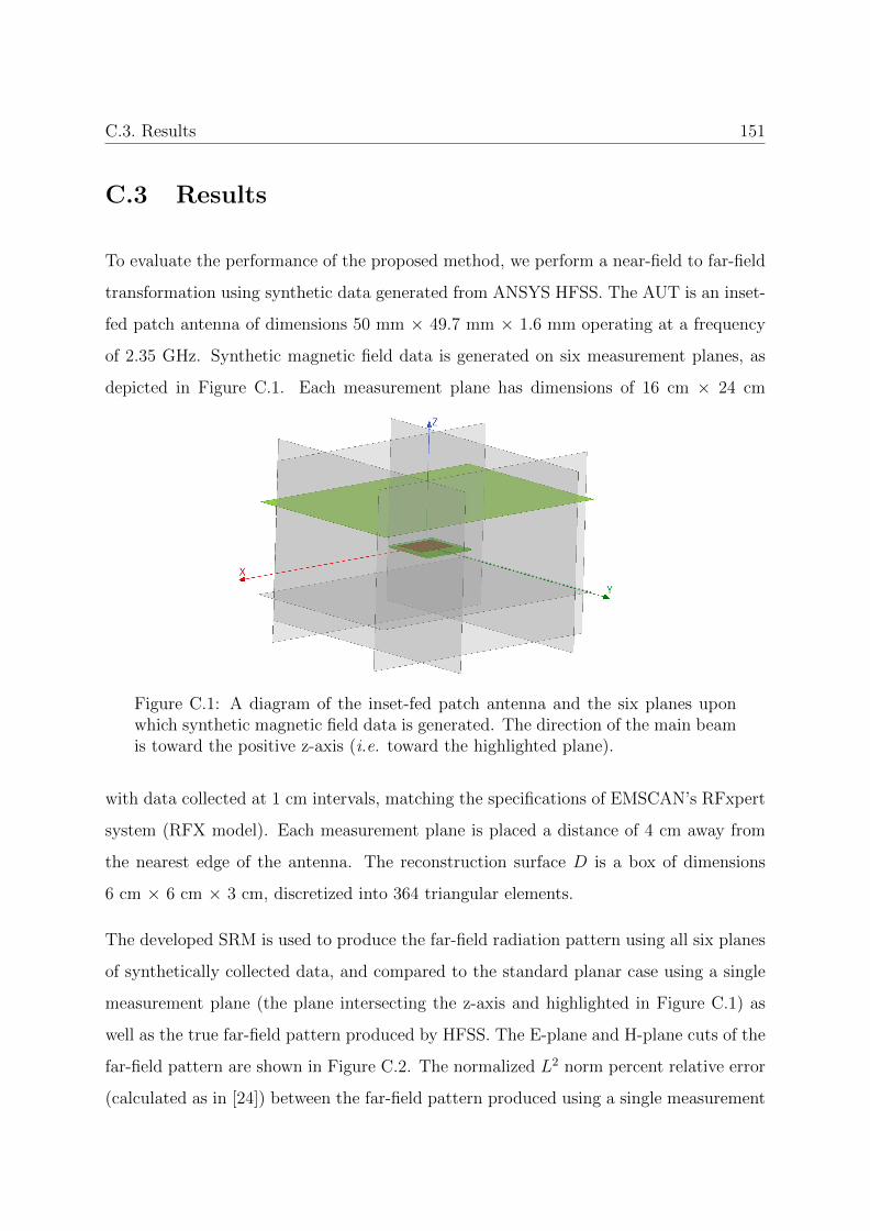
C.3. Results 151
C.3 Results
To evaluate the performance of the proposed method, we perform a near-field to far-field
transformation using synthetic data generated from ANSYS HFSS. The AUT is an inset-
fed patch antenna of dimensions 50 mm × 49.7 mm × 1.6 mm operating at a frequency
of 2.35 GHz. Synthetic magnetic field data is generated on six measurement planes, as
depicted in Figure C.1. Each measurement plane has dimensions of 16 cm × 24 cm
Figure C.1: A diagram of the inset-fed patch antenna and the six planes uponwhich synthetic magnetic field data is generated. The direction of the main beamis toward the positive z-axis (i.e. toward the highlighted plane).
with data collected at 1 cm intervals, matching the specifications of EMSCAN’s RFxpert
system (RFX model). Each measurement plane is placed a distance of 4 cm away from
the nearest edge of the antenna. The reconstruction surface D is a box of dimensions
6 cm × 6 cm × 3 cm, discretized into 364 triangular elements.
The developed SRM is used to produce the far-field radiation pattern using all six planes
of synthetically collected data, and compared to the standard planar case using a single
measurement plane (the plane intersecting the z-axis and highlighted in Figure C.1) as
well as the true far-field pattern produced by HFSS. The E-plane and H-plane cuts of the
far-field pattern are shown in Figure C.2. The normalized L2 norm percent relative error
(calculated as in [24]) between the far-field pattern produced using a single measurement

C.4. Conclusion and Future Work 152
−150 −100 −50 0 50 100 150−25
−20
−15
−10
−5
0
θ [◦] ϕ = 0◦
|E|[dB]
HFSS
SRM (1 Plane)
SRM (6 Planes)
(a)
−150 −100 −50 0 50 100 150−25
−20
−15
−10
−5
0
θ [◦] ϕ = 90◦
|E|[dB]
HFSS
SRM (1 Plane)
SRM (6 Planes)
(b)
Figure C.2: A comparison of the patch antenna far-field radiation pattern pro-duced by: SRM using only one plane (z = 4 cm) of measurement data (dash-dotted line), SRM using six planes of measurement data (dashed line), and HFSS(solid line). The E-plane pattern (ϕ = 0◦) is shown in (a) while the H-planepattern (ϕ = 90◦) is shown in (b).
plane and the pattern generated using HFSS is 14.96%, while using six measurement
planes reduced the difference to 0.972%.
C.4 Conclusion and Future Work
We presented a method that has the potential to enable an existing compact planar mag-
netic near-field measurement system to utilize more data. By rotating the antenna on this
system, multiple planes of magnetic field data can be collected. Then this consolidated set
of data can be inverted using the source reconstruction method and the far-field pattern
of the AUT can be calculated. It was synthetically shown that this method provides an

C.4. Conclusion and Future Work 153
improvement in the calculated far-field accuracy of an inset-fed patch antenna when com-
pared to the original case where a single plane of magnetic data is used to calculate the
far-field. We intend to improve this work by validating it with experimental data from the
RFxpert system. It is also our goal to modify our method to be capable of de-embedding
the effect of RFxpert’s ground plane from the multiple planes of magnetic field data that
our method requires. This can be, for example, based on the work presented in [157] and
will be discussed at the conference.

Appendix D
List of Publications
A list of publications resulting from the work herein is listed below as well the contribu-
tions of the authors:
Journal Papers:
1. Chaitanya Narendra and Puyan Mojabi, “A Combined Inverse Source and
Scattering Technique for Dielectric Profile Design to Tailor Electromagnetic
Fields,” in IEEE Transactions on Antennas and Propagation,
doi: 10.1109/TAP.2021.3119049.
– Chaitanya Narendra: manuscript preparation, algorithm development,
simulations
– Puyan Mojabi: advisory role, simulations
2. Chaitanya Narendra, Trevor Brown and Puyan Mojabi, “Gradient-Based
Electromagnetic Inversion for Metasurface Design Using Circuit Models”, in
IEEE Transactions on Antennas and Propagation,
doi: 10.1109/TAP.2021.3118811.
– Chaitanya Narendra: manuscript preparation, algorithm development,
simulations
154

Appendix D List of Publications 155
– Trevor Brown: manuscript preparation, gradient derivation
– Puyan Mojabi: advisory role
3. Chaitanya Narendra and Puyan Mojabi, “Phaseless Gauss-Newton Inver-
sion for Microwave Imaging,” in IEEE Transactions on Antennas and Propa-
gation, vol. 69, no. 1, pp. 443-456, Jan. 2021,
doi: 10.1109/TAP.2020.3026427.
– Chaitanya Narendra: manuscript preparation, algorithm development,
verification
– Puyan Mojabi: advisory role, algorithm development, manuscript prepa-
ration
4. Trevor Brown, Chaitanya Narendra, Yousef Vahabzadeh, Christophe Caloz,
and Puyan Mojabi, “On the Use of Electromagnetic Inversion for Metasurface
Design”, IEEE Transactions on Antennas and Propagation, vol. 68, no. 3, pp.
1812-1824, 2020.
– Trevor Brown: manuscript preparation, inversion framework development
and evaluation, simulations
– Chaitanya Narendra: manuscript preparation, conjugate gradient algo-
rithm
– Yousef Vahabzadeh: finite-difference frequency domain simulation code
– Christophe Caloz and Puyan Mojabi: advisory role
Conference Papers:
1. P. Mojabi, T. Brown and C. Narendra, “Phaseless Electromagnetic Inversion
for Imaging, Characterization, and Design,” 2021 IEEE 19th International
Symposium on Antenna Technology and Applied Electromagnetics (ANTEM),
2021, pp. 1-2.
– Puyan Mojabi: main author, manuscript preparation
– Trevor Brown: provided advice and access to past results for this review
paper
Appendix D List of Publications 156
– Chaitanya Narendra: provided advice and access to past results for this
review paper
2. C. Narendra and P. Mojabi, “A Phaseless Gauss-Newton Inversion Algo-
rithm for Imaging and Design,” 2020 14th European Conference on Antennas
and Propagation (EuCAP), 2020, pp. 1-5.
– Chaitanya Narendra: manuscript preparation, algorithm development,
verification
– Puyan Mojabi: advisory role, algorithm development, manuscript prepa-
ration
3. Trevor Brown, Chaitanya Narendra, Yousef Vahabzadeh, Christophe Caloz,
and Puyan Mojabi, “Metasurface Design Using Electromagnetic Inversion”,
2019 IEEE International Symposium on Antennas and Propagation and USNC-
URSI Radio Science Meeting, pp. 1817-1818, 2019.
– Trevor Brown: manuscript preparation, algorithm development and eval-
uation, simulations
– Chaitanya Narendra: conjugate gradient algorithm manuscript prepara-
tion
– Yousef Vahabzadeh: finite-difference frequency domain simulation code
– Christophe Caloz and Puyan Mojabi: advisory role
4. Trevor Brown, Chaitanya Narendra, Chen Niu, and Puyan Mojabi, “On the
Use of Electromagnetic Inversion for Near-Field Antenna Measurements: A Re-
view”, 2018 Conference on Antenna Measurements and Applications (CAMA),
pp. 1-4, 2018.
– Trevor Brown: manuscript preparation, phaseless measurements and data-
prescaling algorithms
– Chaitanya Narendra: irregular measurement domain algorithms
– Chen Niu: development, construction of and examples from a pendulum-
based planar near-field antenna measurement system

Appendix D List of Publications 157
– Puyan Mojabi: advisory role
5. Chaitanya Narendra, Trevor Brown, Nozhan Bayat, and Puyan Mojabi,
“Multi-Plane Magnetic Near-Field Data Inversion Using the Source Recon-
struction Method”, 2018 18th International Symposium on Antenna Technol-
ogy and Applied Electromagnetics (ANTEM), pp. 1-2, 2018.
– Chaitanya Narendra: manuscript preparation, algorithm development and
evaluation
– Trevor Brown: inversion framework
– Nozhan Bayat: HFSS simulations
– Puyan Mojabi: advisory role
6. Trevor Brown, Chaitanya Narendra, and Puyan Mojabi, “On the Use of the
Source Reconstruction Method for Metasurface Design”, 2018 18th European
Conference on Antennas and Propagation (EuCAP), pp. 302-306, 2018.
– Trevor Brown: manuscript preparation, algorithm development and eval-
uation, simulations
– Chaitanya Narendra: conjugate gradient algorithm
– Puyan Mojabi: advisory role

Bibliography
[1] C. Narendra and P. Mojabi, “A phaseless gauss-newton inversion algorithm for
imaging and design,” in 2020 14th European Conference on Antennas and Propa-
gation (EuCAP), 2020, pp. 1–5.
[2] T. Brown, C. Narendra, Y. Vahabzadeh, C. Caloz, and P. Mojabi, “On the use of
electromagnetic inversion for metasurface design,” IEEE Transactions on Antennas
and Propagation, vol. 68, no. 3, pp. 1812–1824, 2019.
[3] J.-M. Geffrin, P. Sabouroux, and C. Eyraud, “Free space experimental scattering
database continuation: experimental set-up and measurement precision,” inverse
Problems, vol. 21, no. 6, p. S117, 2005.
[4] M. Ostadrahimi, P. Mojabi, A. Zakaria, J. LoVetri, and L. Shafai, “Enhancement of
gauss–newton inversion method for biological tissue imaging,” IEEE Transactions
on Microwave Theory and Techniques, vol. 61, no. 9, pp. 3424–3434, 2013.
[5] C. A. Balanis, Antenna theory: analysis and design. John wiley & sons, 2016.
[6] K. Achouri, M. A. Salem, and C. Caloz, “General metasurface synthesis based on
susceptibility tensors,” IEEE Transactions on Antennas and Propagation, vol. 63,
no. 7, pp. 2977–2991, 2015.
[7] A. Epstein and G. V. Eleftheriades, “Huygens’ metasurfaces via the equivalence
principle: design and applications,” Journal of the Optical Society of America B,
vol. 33, no. 2, pp. A31–A50, 2016.
158
Bibliography 159
[8] K. Achouri and C. Caloz, “Design, concepts and applications of electromagnetic
metasurfaces,” Nanophotonics, vol. 7, no. 6, pp. 1095–1116, 2018.
[9] O. M. Bucci, I. Catapano, L. Crocco, and T. Isernia, “Synthesis of new variable
dielectric profile antennas via inverse scattering techniques: a feasibility study,”
IEEE transactions on antennas and propagation, vol. 53, no. 4, pp. 1287–1297,
2005.
[10] R. Palmeri and T. Isernia, “Volumetric invisibility cloaks design through spectral
coverage optimization,” IEEE Access, vol. 7, pp. 30 860–30 867, 2019.
[11] R. F. Harrington, Time-harmonic electromagnetic fields. McGraw-Hill, 1961.
[12] E. J. Rothwell and M. J. Cloud, Electromagnetics. CRC Press, 2018.
[13] A. F. Peterson, S. L. Ray, and R. Mittra, Computational Methods for Electromag-
netics. Wiley-IEEE Press, 1998.
[14] P. Mojabi, N. Firoozy, N. Bayat, T. Brown, C. Narendra, P. Mojabi, C. Niu,
T. Tiede, T. Neusitzer, X. Li et al., “Electromagnetic inversion for biomedical
imaging, antenna characterization, and sea ice remote sensing applications,” in 2016
URSI Asia-Pacific Radio Science Conference (URSI AP-RASC). IEEE, 2016, pp.
586–589.
[15] C. Narendra, T. Brown, N. Bayat, and P. Mojabi, “Multi-plane magnetic near-field
data inversion using the source reconstruction method,” in 2018 18th International
Symposium on Antenna Technology and Applied Electromagnetics (ANTEM), Aug
2018, pp. 1–2.
[16] T. Brown, C. Narendra, C. Niu, and P. Mojabi, “On the use of electromagnetic
inversion for near-field antenna measurements: A review,” in 2018 IEEE Conference
on Antenna Measurements & Applications (CAMA). IEEE, 2018, pp. 1–4.
Bibliography 160
[17] E. Jørgensen, P. Meincke, C. Cappellin, and M. Sabbadini, “Improved source re-
construction technique for antenna diagnostics,” in Proceeedings of the 32nd ESA
Antenna Workshop, 2010.
[18] L. Foged, L. Scialacqua, F. Saccardi, J. A. Quijano, G. Vecchi, and M. Sabbadini,
“Practical application of the equivalent source method as an antenna diagnostics
tool [amta corner],” IEEE Antennas and Propagation Magazine, vol. 54, no. 5, pp.
243–249, 2012.
[19] M. Oristaglio and H. Blok, “Wavefield imaging and inversion in electromagnetics
and acoustics,” Course Notes TU Delft, 1995.
[20] P. Mojabi, M. Ostadrahimi, L. Shafai, and J. LoVetri, “Microwave tomography
techniques and algorithms: A review,” in 2012 15 International Symposium on
Antenna Technology and Applied Electromagnetics, 2012, pp. 1–4.
[21] O. M. Bucci, G. D’Elia, G. Mazzarella, and G. Panariello, “Antenna pattern synthe-
sis: a new general approach,” Proceedings of the IEEE, vol. 82, no. 3, pp. 358–371,
March 1994.
[22] L. Di Donato, T. Isernia, G. Labate, and L. Matekovits, “Towards printable natural
dielectric cloaks via inverse scattering techniques,” Scientific reports, vol. 7, no. 1,
p. 3680, 2017.
[23] N. Firoozy, T. Neusitzer, D. S. Desmond, T. Tiede, M. J. L. Lemes, J. Landy,
P. Mojabi, S. Rysgaard, G. Stern, and D. G. Barber, “An electromagnetic detection
case study on crude oil injection in a young sea ice environment,” IEEE Transactions
on Geoscience and Remote Sensing, vol. 55, no. 8, pp. 4465–4475, Aug 2017.
[24] T. Brown, I. Jeffrey, and P. Mojabi, “Multiplicatively regularized source reconstruc-
tion method for phaseless planar near-field antenna measurements,” IEEE Trans-
actions on Antennas and Propagation, vol. 65, no. 4, pp. 2020–2031, 2017.
Bibliography 161
[25] M. Salucci, A. Gelmini, G. Oliveri, N. Anselmi, and A. Massa, “Synthesis of shaped
beam reflectarrays with constrained geometry by exploiting nonradiating surface
currents,” IEEE Transactions on Antennas and Propagation, vol. 66, no. 11, pp.
5805–5817, Nov 2018.
[26] M. Phaneuf and P. Mojabi, “Electromagnetic inversion for noninvasive specific ab-
sorption rate characterization,” IEEE Journal of Electromagnetics, RF and Mi-
crowaves in Medicine and Biology, vol. 4, no. 4, pp. 254–259, 2020.
[27] J. Hadamard, Lectures on Cauchy’s problem in linear partial differential equations.
Courier Corporation, 2014.
[28] A. Devaney and G. Sherman, “Nonuniqueness in inverse source and scattering prob-
lems,” IEEE Transactions on Antennas and Propagation, vol. 30, no. 5, pp. 1034–
1037, 1982.
[29] P. C. Hansen, “Regularization tools: A matlab package for analysis and solution of
discrete ill-posed problems,” Numerical algorithms, vol. 6, no. 1, pp. 1–35, 1994.
[30] A. Abubakar, P. M. van den Berg, and J. J. Mallorqui, “Imaging of biomedical data
using a multiplicative regularized contrast source inversion method,” IEEE Trans.
Microwave Theory Tech., vol. 50, no. 7, pp. 1761–1777, July 2002.
[31] A. Abubakar and P. M. van den Berg, “Iterative forward and inverse algorithms
based on domain integral equations for three–dimensional electric and magnetic
objects,” J. Comput. Phys., vol. 195, pp. 236–262, 2004.
[32] P. Mojabi, J. LoVetri, and L. Shafai, “A multiplicative regularized Gauss–Newton
inversion for shape and location reconstruction,” IEEE Transactions on Antennas
and Propagation, vol. 59, no. 12, pp. 4790–4802, 2011.
[33] P. C. Hansen, “Analysis of discrete ill-posed problems by means of the L-curve,”
SIAM Review, vol. 34, no. 4, pp. 561–580, Dec 1992.

Bibliography 162
[34] T. K. Sarkar and A. Taaghol, “Near-field to near/far-field transformation for arbi-
trary near-field geometry utilizing an equivalent electric current andMOM,” IEEE
Trans. Antennas Propag., vol. 47, no. 3, 1999.
[35] J. L. A. Quijano and G. Vecchi, “Improved-accuracy source reconstruction on arbi-
trary 3-D surfaces,” IEEE Antennas Wireless Propag. Lett., vol. 8, pp. 1046–1049,
2009.
[36] T. Brown, C. Narendra, C. Niu, and P. Mojabi, “On the use of electromagnetic
inversion for near-field antenna measurements: A review,” in 2018 IEEE Conference
on Antenna Measurements Applications (CAMA), Sep. 2018, pp. 1–4.
[37] T. Brown, “Antenna characterization using phaseless near-field measurements,”
Master’s thesis, University of Manitoba, 2016. [Online]. Available: http:
//hdl.handle.net/1993/31693
[38] C. Narendra, T. Brown, and P. Mojabi, “Gradient-based electromagnetic inversion
for metasurface design using circuit models,” IEEE Transactions on antennas and
propagation, pp. 1–13, IEEE Early Access, Oct. 2021.
[39] S. Pearson and S. V. Hum, “Optimization of scalar and bianisotropic elec-
tromagnetic metasurface parameters satisfying far-field criteria,” arXiv preprint
arXiv:2011.09016, 2020.
[40] A. Abubakar and P. M. van den Berg, “The contrast source inversion method for
location and shape reconstructions,” Inverse Problems, vol. 18, no. 2, pp. 495–510,
Mar 2002.
[41] C. Narendra and P. Mojabi, “Phaseless Gauss-Newton inversion for microwave
imaging,” IEEE Transactions on Antennas and Propagation, vol. 69, no. 1, pp.
443–456, 2021.
[42] M. Selvanayagam and G. V. Eleftheriades, “Circuit modeling of Huygens surfaces,”
IEEE Antennas and Wireless Propagation Letters, vol. 12, pp. 1642–1645, 2013.

Bibliography 163
[43] M. Chen, E. Abdo-Sanchez, A. Epstein, and G. V. Eleftheriades, “Theory, design,
and experimental verification of a reflectionless bianisotropic Huygens’ metasurface
for wide-angle refraction,” Physical Review B, vol. 97, no. 12, p. 125433, 2018.
[44] Z. Wei and X. Chen, “Deep-learning schemes for full-wave nonlinear inverse scat-
tering problems,” IEEE Transactions on Geoscience and Remote Sensing, vol. 57,
no. 4, pp. 1849–1860, 2018.
[45] L. Li, H. Ruan, C. Liu, Y. Li, Y. Shuang, A. Alu, C.-W. Qiu, and T. J. Cui,
“Machine-learning reprogrammable metasurface imager,” Nature communications,
vol. 10, no. 1, pp. 1–8, 2019.
[46] X. Chen, Z. Wei, M. Li, and P. Rocca, “A review of deep learning approaches for in-
verse scattering problems (invited review),” Progress In Electromagnetics Research,
vol. 167, pp. 67–81, 2020.
[47] Y. Alvarez, F. Las-Heras, and M. R. Pino, “Reconstruction of equivalent currents
distribution over arbitrary three-dimensional surfaces based on integral equation
algorithms,” Antennas and Propagation, IEEE Transactions on, vol. 55, no. 12, pp.
3460–3468, 2007.
[48] Y. A. Lopez, F. Las-Heras Andres, M. R. Pino, and T. K. Sarkar, “An improved
super-resolution source reconstruction method,” IEEE Trans. Instrum. Meas.,
vol. 58, no. 11, pp. 3855–3866, 2009.
[49] T. F. Eibert, E. Kaliyaperumal, C. H. Schmidt et al., “Inverse equivalent surface
current method with hierarchical higher order basis functions, full probe correction
and multilevel fast multipole acceleration,” Progress In Electromagnetics Research,
vol. 106, pp. 377–394, 2010.
[50] C. Narendra, I. Jeffrey, and P. Mojabi, “Using the source reconstruction method
to model incident fields in microwave tomography,” IEEE Antennas and Wireless
Propagation Letters, vol. 16, pp. 46–49, 2016.

Bibliography 164
[51] N. Engheta and R. W. Ziolkowski, Metamaterials: Physics and Engineering Explo-
rations. Wiley-IEEE Press, 2006.
[52] G. V. Eleftheriades, A. K. Iyer, and P. C. Kremer, “Planar negative refractive
index media using periodically l-c loaded transmission lines,” IEEE Transactions
on Microwave Theory and Techniques, vol. 50, no. 12, pp. 2702–2712, 2002.
[53] N. Yu, P. Genevet, M. A. Kats, F. Aieta, J.-P. Tetienne, F. Capasso, and
Z. Gaburro, “Light propagation with phase discontinuities: Generalized laws of
reflection and refraction,” Science, vol. 334, no. 6054, pp. 333–337, 2011. [Online].
Available: https://science.sciencemag.org/content/334/6054/333
[54] C. Pfeiffer and A. Grbic, “Metamaterial Huygens’ surfaces: Tailoring wave fronts
with reflectionless sheets,” Phys. Rev. Lett., vol. 110, p. 197401, May 2013.
[55] A. K. Iyer, A. Alu, and A. Epstein, “Metamaterials and metasurfaces—historical
context, recent advances, and future directions,” IEEE Transactions on Antennas
and Propagation, vol. 68, no. 3, pp. 1223–1231, 2020.
[56] V. S. Asadchy, M. Albooyeh, S. N. Tcvetkova, A. Dıaz-Rubio, Y. Ra’di, and
S. Tretyakov, “Perfect control of reflection and refraction using spatially disper-
sive metasurfaces,” Physical Review B, vol. 94, no. 7, p. 075142, 2016.
[57] C. Pfeiffer and A. Grbic, “Bianisotropic metasurfaces for optimal polarization con-
trol: Analysis and synthesis,” Physical Review Applied, vol. 2, no. 4, p. 044011,
2014.
[58] Y. Ra’di, C. R. Simovski, and S. A. Tretyakov, “Thin perfect absorbers for electro-
magnetic waves: Theory, design, and realizations,” Phys. Rev. Applied, vol. 3, p.
037001, Mar 2015.
[59] K. M. Kossifos, L. Petrou, G. Varnava, A. Pitilakis, O. Tsilipakos, F. Liu,
P. Karousios, A. C. Tasolamprou, M. Seckel, D. Manessis, N. V. Kantartzis,

Bibliography 165
D. Kwon, M. A. Antoniades, and J. Georgiou, “Toward the realization of a pro-
grammable metasurface absorber enabled by custom integrated circuit technology,”
IEEE Access, vol. 8, pp. 92 986–92 998, 2020.
[60] M. Dehmollaian, N. Chamanara, and C. Caloz, “Wave scattering by a cylindri-
cal metasurface cavity of arbitrary cross-section: Theory and applications,” IEEE
Transactions on Antennas and Propagation, 2019.
[61] M. Di Renzo, A. Zappone, M. Debbah, M.-S. Alouini, C. Yuen, J. de Rosny,
and S. Tretyakov, “Smart radio environments empowered by reconfigurable intel-
ligent surfaces: How it works, state of research, and road ahead,” arXiv preprint
arXiv:2004.09352, 2020.
[62] Y. Vahabzadeh, N. Chamanara, K. Achouri, and C. Caloz, “Computational analy-
sis of metasurfaces,” IEEE Journal on Multiscale and Multiphysics Computational
Techniques, vol. 3, pp. 37–49, 2018.
[63] T. Brown, “Metasurface design using electromagnetic inversion,” Ph.D. disserta-
tion, University of Manitoba, Winnipeg, Canada, 2020.
[64] M. M. Idemen, Discontinuities in the electromagnetic field. John Wiley & Sons
(IEEE Press series on electromagnetic wave theory; 40), 2011.
[65] E. F. Kuester, M. A. Mohamed, M. Piket-May, and C. L. Holloway, “Averaged
transition conditions for electromagnetic fields at a metafilm,” IEEE Transactions
on Antennas and Propagation, vol. 51, no. 10, pp. 2641–2651, 2003.
[66] Y. Vahabzadeh, K. Achouri, and C. Caloz, “Simulation of metasurfaces in finite
difference techniques,” IEEE Trans. Antennas Propag, vol. 64, no. 11, pp. 4753–
4759, 2016.
[67] K. Achouri, “Synthesis and applications of electromagnetic metasurfaces,” Ph.D.
dissertation, Ecole Polytechnique de Montr’/eal, Montreal, Canada, 2017.
Bibliography 166
[68] T. Brown, Y. Vahabzadeh, C. Caloz, and P. Mojabi, “Electromagnetic inversion
with local power conservation for metasurface design,” IEEE Antennas and Wireless
Propagation Letters, 2020.
[69] A. Epstein and G. V. Eleftheriades, “Passive lossless Huygens metasurfaces for
conversion of arbitrary source field to directive radiation,” IEEE Transactions on
Antennas and Propagation, vol. 62, no. 11, pp. 5680–5695, 2014.
[70] G. Lavigne, K. Achouri, V. S. Asadchy, S. A. Tretyakov, and C. Caloz, “Susceptibil-
ity derivation and experimental demonstration of refracting metasurfaces without
spurious diffraction,” IEEE Transactions on Antennas and Propagation, vol. 66,
no. 3, pp. 1321–1330, 2018.
[71] D. M. Pozar, Microwave engineering. John wiley & sons, 2011.
[72] E. Porter, M. Coates, and M. Popovic, “An early clinical study of time-domain
microwave radar for breast health monitoring,” IEEE Transactions on Biomedical
Engineering, vol. 63, no. 3, pp. 530–539, 2016.
[73] E. C. Fear, X. Li, S. C. Hagness, and M. A. Stuchly, “Confocal microwave imaging
for breast cancer detection: localization of tumors in three dimensions,” IEEE
Transactions on Biomedical Engineering, vol. 49, no. 8, pp. 812–822, 2002.
[74] S. P. Poplack, T. D. Tosteson, W. A. Wells, B. W. Pogue, P. M. Meaney, A. Har-
tov, C. A. Kogel, S. K. Soho, J. J. Gibson, and K. D. Paulsen, “Electromagnetic
breast imaging: results of a pilot study in women with abnormal mammograms,”
Radiology, vol. 243, no. 2, pp. 350–359, 2007.
[75] E. C. Fear, S. C. Hagness, P. M. Meaney, M. Okoniewski, and M. A. Stuchly, “En-
hancing breast tumor detection with near-field imaging,” IEEE Microwave Mag.,
vol. 3, no. 1, pp. 48–56, Mar 2002.
[76] W. H. Weedon, W. C. Chew, and P. E. Mayes, “A step-frequency radar imag-
ing system for microwave nondestructive evaluation,” Progress In Electromagnetics
Research, vol. 28, pp. 121–146, 2000.

Bibliography 167
[77] N. Bayat, “Advancing microwave imaging algorithms and techniques,” Ph.D. dis-
sertation, University of Manitoba, 2019.
[78] A. Abubakar, T. Habashy, V. Druskin, L. Knizhnerman, and D. Alumbaugh, “2.5 D
forward and inverse modeling for interpreting low-frequency electromagnetic mea-
surements,” Geophysics, vol. 73, no. 4, pp. F165–F177, 2008.
[79] P. Mojabi and J. LoVetri, “Microwave biomedical imaging using the multiplica-
tive regularized gauss–newton inversion,” IEEE Antennas and Wireless Propagation
Letters, vol. 8, pp. 645–648, 2009.
[80] R. Palmeri, M. T. Bevacqua, A. F. Morabito, and T. Isernia, “Inverse scattering
methods as a tool for the design of GPCs devices,” in 2017 IEEE Conference on
Antenna Measurements & Applications (CAMA). IEEE, 2017, pp. 130–132.
[81] T. Isernia and R. Palmeri, “Inverse scattering as a way to artificial dielectrics based
devices,” in 2018 12th International Congress on Artificial Materials for Novel
Wave Phenomena (Metamaterials). IEEE, 2018, pp. 185–187.
[82] C. Narendra and P. Mojabi, “A phaseless gauss-newton inversion algorithm for
imaging and design,” in 2020 14th European Conference on Antennas and Propa-
gation (EuCAP), 2020, pp. 1–5.
[83] F. Monticone, N. M. Estakhri, and A. Alu, “Full control of nanoscale optical trans-
mission with a composite metascreen,” Physical review letters, vol. 110, no. 20, p.
203903, 2013.
[84] M. Selvanayagam and G. V. Eleftheriades, “Circuit modeling of Huygens surfaces,”
IEEE Antennas and Wireless Propagation Letters, vol. 12, pp. 1642–1645, 2013.
[85] G. Xu, S. V. Hum, and G. V. Eleftheriades, “Augmented Huygens? metasurfaces
employing baffles for precise control of wave transformations,” IEEE Transactions
on Antennas and Propagation, vol. 67, no. 11, pp. 6935–6946, 2019.

Bibliography 168
[86] C. L. Holloway, E. F. Kuester, J. A. Gordon, J. O’Hara, J. Booth, and D. R. Smith,
“An overview of the theory and applications of metasurfaces: The two-dimensional
equivalents of metamaterials,” IEEE Antennas and Propagation Magazine, vol. 54,
no. 2, pp. 10–35, 2012.
[87] M. Selvanayagam and G. Eleftheriades, “Discontinuous electromagnetic fields us-
ing orthogonal electric and magnetic currents for wavefront manipulation,” Optics
Express, pp. 14 409–14 429, 2013.
[88] S. Tretyakov, “Metasurfaces for general transformations of electromagnetic fields,”
Philos. Trans. Royal Soc. A: Mathematical, Physical and Engineering Sciences, vol.
373, no. 2049, p. 20140362, 2015.
[89] M. Yazdi, M. Albooyeh, R. Alaee, V. Asadchy, N. Komjani, C. Rockstuhl, C. R.
Simovski, and S. Tretyakov, “A bianisotropic metasurface with resonant asymmetric
absorption,” IEEE Transactions on Antennas and Propagation, vol. 63, no. 7, pp.
3004–3015, 2015.
[90] V. S. Asadchy, I. A. Faniayeu, Y. Ra?Di, S. Khakhomov, I. Semchenko, and
S. Tretyakov, “Broadband reflectionless metasheets: frequency-selective transmis-
sion and perfect absorption,” Physical Review X, vol. 5, no. 3, p. 031005, 2015.
[91] V. G. Ataloglou, A. H. Dorrah, and G. V. Eleftheriades, “Design of compact Huy-
gens’ metasurface pairs with multiple reflections for arbitrary wave transforma-
tions,” IEEE Transactions on Antennas and Propagation (Early Access), 2020.
[92] K. Achouri and O. J. Martin, “Angular scattering properties of metasurfaces,” IEEE
Transactions on Antennas and Propagation, vol. 68, no. 1, pp. 432–442, 2019.
[93] S. Pearson and S. V. Hum, “Using augmented Lagrangian methods to design elec-
tromagnetic surfaces with far field constraints,” in 2020 IEEE International Sympo-
sium on Antennas and Propagation and USNC-URSI Radio Science Meeting, 2020,
pp. 969–970.
Bibliography 169
[94] A. Epstein and G. V. Eleftheriades, “Arbitrary power-conserving field transforma-
tions with passive lossless omega-type bianisotropic metasurfaces,” IEEE Transac-
tions on Antennas and Propagation, vol. 64, no. 9, pp. 3880–3895, 2016.
[95] T. Brown, Z. Liu, and P. Mojabi, “Full-wave verification of an electromagnetic
inversion metasurface design method,” 2020.
[96] J. P. Wong, A. Epstein, and G. V. Eleftheriades, “Reflectionless wide-angle refract-
ing metasurfaces,” IEEE Antennas and Wireless Propagation Letters, vol. 15, pp.
1293–1296, 2015.
[97] E. Abdo-Sanchez, M. Chen, A. Epstein, and G. V. Eleftheriades, “A leaky-wave an-
tenna with controlled radiation using a bianisotropic huygens’ metasurface,” IEEE
Trans. Antennas Propag., vol. 67, no. 1, pp. 108–120, 2019.
[98] S. R. Rengarajan and Y. Rahmat-Samii, “The field equivalence principle: Illustra-
tion of the establishment of the non-intuitive null fields,” Antennas and Propagation
Magazine, IEEE, vol. 42, no. 4, pp. 122–128, 2000.
[99] T. Brown and P. Mojabi, “Cascaded Metasurface Design Using Electromagnetic
Inversion with Gradient-Based Optimization,” Available online at techrxiv, 2020.
[100] J. Y. Lau and S. V. Hum, “Reconfigurable transmitarray design approaches for
beamforming applications,” IEEE Trans. Antennas Propag., vol. 60, no. 12, pp.
5679–5689, 2012.
[101] R. Palmeri, M. T. Bevacqua, A. F. Morabito, and T. Isernia, “Design of artificial-
material-based antennas using inverse scattering techniques,” IEEE Transactions
on Antennas and Propagation, vol. 66, no. 12, pp. 7076–7090, Dec 2018.
[102] V. G. Ataloglou, A. H. Dorrah, and G. V. Eleftheriades, “Design of compact Huy-
gens’ metasurface pairs with multiple reflections for arbitrary wave transforma-
tions,” IEEE Transactions on Antennas and Propagation, 2020.
Bibliography 170
[103] M. Ostadrahimi, P. Mojabi, C. Gilmore, A. Zakaria, S. Noghanian, S. Pistorius,
and J. LoVetri, “Analysis of incident field modeling and incident/scattered field
calibration techniques in microwave tomography,” IEEE Antennas and Wireless
Propagation Letters, vol. 10, pp. 900–903, 2011.
[104] X. Chen, “Subspace-based optimization method for solving inverse-scattering prob-
lems,” IEEE Transactions on Geoscience and Remote Sensing, vol. 48, no. 1, pp.
42–49, Jan 2010.
[105] T. Rubæk, P. M. Meaney, P. Meincke, and K. D. Paulsen, “Nonlinear microwave
imaging for breast-cancer screening using Gauss-Newton’s method and the CGLS
inversion algorithm,” IEEE Trans. Antennas Propag., vol. 55, no. 8, pp. 2320–2331,
Aug 2007.
[106] W. C. Chew and Y. M. Wang, “Reconstruction of two-dimensional permittivity dis-
tribution using the distorted born iterative method,” IEEE Transactions on Medical
Imaging, vol. 9, no. 2, pp. 218–225, June 1990.
[107] M. Pastorino, Microwave imaging. John Wiley & Sons, 2010, vol. 208.
[108] P. Mojabi and J. LoVetri, “Overview and classification of some regularization tech-
niques for the Gauss-Newton inversion method applied to inverse scattering prob-
lems,” IEEE Transactions on Antennas and Propagation, vol. 57, no. 9, pp. 2658–
2665, Sept 2009.
[109] S. F. Razavi and Y. Rahmat-Samii, “Resilience to probe-positioning errors in planar
phaseless near-field measurements,” IEEE Transactions on Antennas and Propaga-
tion, vol. 58, no. 8, pp. 2632–2640, 2010.
[110] L. Li, H. Zheng, and F. Li, “Two-dimensional contrast source inversion method with
phaseless data: TM case,” IEEE Transactions on Geoscience and Remote Sensing,
vol. 47, no. 6, pp. 1719–1736, 2009.
Bibliography 171
[111] Z. Hu, L. Lianlin, and L. Fang, “A multi-frequency MRCSI algorithm with phaseless
data,” Inverse Problems, vol. 25, no. 6, p. 065006, 2009.
[112] M. H. Maleki, A. J. Devaney, and A. Schatzberg, “Tomographic reconstruction from
optical scattered intensities,” JOSA A, vol. 9, no. 8, pp. 1356–1363, 1992.
[113] M. H. Maleki and A. J. Devaney, “Phase-retrieval and intensity-only reconstruction
algorithms for optical diffraction tomography,” JOSA A, vol. 10, no. 5, pp. 1086–
1092, 1993.
[114] T. Takenaka, D. J. Wall, H. Harada, and M. Tanaka, “Reconstruction algorithm of
the refractive index of a cylindrical object from the intensity measurements of the
total field,” Microwave and optical technology letters, vol. 14, no. 3, pp. 182–188,
1997.
[115] G. Gbur and E. Wolf, “Hybrid diffraction tomography without phase information,”
JOSA A, vol. 19, no. 11, pp. 2194–2202, 2002.
[116] S. Caorsi, A. Massa, M. Pastorino, and A. Randazzo, “Electromagnetic detection
of dielectric scatterers using phaseless synthetic and real data and the memetic
algorithm,” IEEE transactions on geoscience and remote sensing, vol. 41, no. 12,
pp. 2745–2753, 2003.
[117] L. Crocco, M. D’Urso, and T. Isernia, “Inverse scattering from phaseless measure-
ments of the total field on a closed curve,” JOSA A, vol. 21, no. 4, pp. 622–631,
2004.
[118] G. Franceschini, M. Donelli, R. Azaro, and A. Massa, “Inversion of phaseless total
field data using a two-step strategy based on the iterative multiscaling approach,”
IEEE Transactions on Geoscience and Remote Sensing, vol. 44, no. 12, pp. 3527–
3539, 2006.
[119] A. Litman and K. Belkebir, “Two-dimensional inverse profiling problem using
phaseless data,” JOSA A, vol. 23, no. 11, pp. 2737–2746, 2006.

Bibliography 172
[120] O. M. Bucci, L. Crocco, M. D’Urso, and T. Isernia, “Inverse scattering from phase-
less measurements of the total field on open lines,” JOSA A, vol. 23, no. 10, pp.
2566–2577, 2006.
[121] M. d’Urso, K. Belkebir, L. Crocco, T. Isernia, and A. Litman, “Paseless imaging
with experimental data: facts and challenges,” JOSA A, vol. 25, no. 1, pp. 271–281,
2008.
[122] L. Li, W. Zhang, and F. Li, “Tomographic reconstruction using the distorted ry-
tov iterative method with phaseless data,” IEEE Geoscience and Remote Sensing
Letters, vol. 5, no. 3, pp. 479–483, 2008.
[123] W. Zhang, L. Li, and F. Li, “Multifrequency imaging from intensity-only data
using the phaseless data distorted rytov iterative method,” IEEE Transactions on
Antennas and Propagation, vol. 57, no. 1, pp. 290–295, 2009.
[124] R. G. Yaccarino and Y. Rahmat-Samii, “Phaseless bi-polar planar near-field mea-
surements and diagnostics of array antennas,” IEEE Transactions on Antennas and
Propagation, vol. 47, no. 3, pp. 574–583, March 1999.
[125] C. Gilmore, P. Mojabi, A. Zakaria, M. Ostadrahimi, C. Kaye, S. Noghanian,
L. Shafai, S. Pistorius, and J. LoVetri, “A wideband microwave tomography sys-
tem with a novel frequency selection procedure,” IEEE Transactions on Biomedical
Engineering, vol. 57, no. 4, pp. 894–904, April 2010.
[126] S. Costanzo and G. Di Massa, “Wideband phase retrieval technique from amplitude-
only near-field data.” Radioengineering, vol. 17, no. 4, 2008.
[127] S. Costanzo, G. Di Massa, M. Pastorino, and A. Randazzo, “Hybrid microwave
approach for phaseless imaging of dielectric targets,” IEEE Geoscience and Remote
Sensing Letters, vol. 12, no. 4, pp. 851–854, April 2015.
[128] T. M. Habashy and A. Abubakar, “A general framework for constraint minimization
for the inversion of electromagnetic measurements,” Progress in electromagnetics
Research, vol. 46, pp. 265–312, 2004.
Bibliography 173
[129] P. Mojabi, “Investigation and development of algorithms and techniques for mi-
crowave tomography,” Ph.D. dissertation, University of Manitoba, Winnipeg, Man-
itoba, Canada, 2010.
[130] N. Bayat and P. Mojabi, “Incorporating spatial priors in microwave imaging via
multiplicative regularization,” IEEE Transactions on Antennas and Propagation,
2019.
[131] P. Mojabi and N. Bayat, “A multiplicative regularizer to incorporate prior spa-
tial data in microwave imaging reconstruction,” in 13th European Conference on
Antennas and Propagation, April 2019, pp. 1–5.
[132] A. H. Golnabi, P. M. Meaney, S. D. Geimer, and K. D. Paulsen, “3-d microwave to-
mography using the soft prior regularization technique: Evaluation in anatomically
realistic mri-derived numerical breast phantoms,” IEEE Transactions on Biomedi-
cal Engineering, vol. 66, no. 9, pp. 2566–2575, Sep. 2019.
[133] L. M. Neira, B. D. Van Veen, and S. C. Hagness, “High-resolution microwave breast
imaging using a 3-d inverse scattering algorithm with a variable-strength spatial
prior constraint,” IEEE Transactions on Antennas and Propagation, vol. 65, no. 11,
pp. 6002–6014, Nov 2017.
[134] A. H. Golnabi, P. M. Meaney, and K. D. Paulsen, “Tomographic microwave imaging
with incorporated prior spatial information,” IEEE Transactions on Microwave
Theory and Techniques, vol. 61, no. 5, pp. 2129–2136, May 2013.
[135] C. Gilmore, A. Zakaria, P. Mojabi, M. Ostadrahimi, S. Pistorius, and J. LoVetri,
“The University of Manitoba microwave imaging repository: A two-dimensional mi-
crowave scattering database for testing inversion and calibration algorithms [Mea-
surements Corner],” IEEE Antennas and Propagation Magazine, vol. 53, no. 5, pp.
126–133, Oct 2011.
Bibliography 174
[136] C. Narendra and P. Mojabi, “A combined inverse source and scattering technique
for dielectric profile design to tailor electromagnetic fields,” IEEE Transactions on
Antennas and Propagation, pp. 1–12, IEEE Early Access, Oct. 2021.
[137] N. K. Nikolova, Introduction to Microwave Imaging. Cambridge University Press,
2017.
[138] X. Chen, Computational Methods for Electromagnetic Inverse Scattering. Wiley
and IEEE Press, 2018.
[139] A. Abubakar, T. M. Habashy, V. L. Druskin, L. Knizhnerman, and D. Alumbaugh,
“2.5D forward and inverse modeling for interpreting low-frequency electromagnetic
measurements,” Geophysics, vol. 73, no. 4, pp. F165–F177, July–Aug 2008.
[140] P. van den Berg and A. Abubakar, “Optical microscopy imaging using the contrast
source inversion method,” Journal of Modern Optics, vol. 57, pp. 756–764, 05 2010.
[141] M. Pastorino, A. Massa, and S. Caorsi, “A microwave inverse scattering technique
for image reconstruction based on a genetic algorithm,” IEEE Transactions on
Instrumentation and Measurement, vol. 49, no. 3, pp. 573–578, 2000.
[142] P. M. van den Berg and R. E. Kleinman, “A contrast source inversion method,”
Inverse Probl., vol. 13, pp. 1607–1620, 1997.
[143] R. Palmeri, M. T. Bevacqua, A. F. Morabito, and T. Isernia, “Design of artificial-
material-based antennas using inverse scattering techniques,” IEEE Transactions
on Antennas and Propagation, vol. 66, no. 12, pp. 7076–7090, 2018.
[144] R. Palmeri and T. Isernia, “Inverse design of artificial materials based lens antennas
through the scattering matrix method,” Electronics, vol. 9, no. 4, p. 559, 2020.
[145] N. M. Estakhri and N. Engheta, “Tunable metasurface-based waveplates-a proposal
using inverse design,” Comptes Rendus. Physique, pp. 1–15, 2020.
Bibliography 175
[146] H. Mosallaei and Y. Rahmat-Samii, “Nonuniform luneburg and two-shell lens an-
tennas: radiation characteristics and design optimization,” IEEE Transactions on
Antennas and Propagation, vol. 49, no. 1, pp. 60–69, 2001.
[147] J. Budhu and Y. Rahmat-Samii, “A novel and systematic approach to inhomo-
geneous dielectric lens design based on curved ray geometrical optics and particle
swarm optimization,” IEEE Transactions on Antennas and Propagation, vol. 67,
no. 6, pp. 3657–3669, 2019.
[148] F. Yang and Y. Rahmat-Samii, Eds., Surface Electromagnetics: With Applications
in Antenna, Microwave, and Optical Engineering. Cambridge University Press,
2019.
[149] C. Parini, S. Gregson, J. McCormick, and D. Janse van Rensburg, Theory and
Practice of Modern Antenna Range Measurements. The Institution of Engineering
and Technology, 2014.
[150] T. Brown, C. Narendra, and P. Mojabi, “On the use of the source reconstruc-
tion method for metasurface design,” 12th European Conference on Antennas and
Propagation (EuCAP), pp. 302–306, April 2018.
[151] A. Van Den Bos, “Complex gradient and hessian,” IEE Proceedings-Vision, Image
and Signal Processing, vol. 141, no. 6, pp. 380–382, 1994.
[152] P. Mojabi and J. LoVetri, “Use of Wirtinger calculus in Gauss-Newton inversion
of microwave tomography data,” in 2014 XXXIth URSI General Assembly and
Scientific Symposium (URSI GASS), Aug 2014, pp. 1–4.
[153] J. De Zaeytijd, A. Franchois, C. Eyraud, and J. Geffrin, “Full-wave three-
dimensional microwave imaging with a regularized Gauss–Newton method – Theory
and experiment,” IEEE Transactions on Antennas and Propagation, vol. 55, no. 11,
pp. 3279–3292, Nov 2007.
Bibliography 176
[154] E. Corp. Emscan products. [Online]. Available: https://www.emscan.com/
products/
[155] P. Petre and T. K. Sarkar, “A planar near-field to far-field transformation using
an equivalent magnetic current approach,” in Antennas and Propagation Society
International Symposium, 1992. AP-S. 1992 Digest. Held in Conjuction with: URSI
Radio Science Meeting and Nuclear EMP Meeting., IEEE. IEEE, 1992, pp. 1534–
1537.
[156] S. Rao, D. Wilton, and A. Glisson, “Electromagnetic scattering by surfaces of
arbitrary shape,” IEEE Transactions on antennas and propagation, vol. 30, no. 3,
pp. 409–418, 1982.
[157] A. Kiaee, R. R. Alavi, M. M. Honari, R. Mirzavand, and P. Mousavi, “Ground de-
embedded source reconstruction using a planar array of h-field probes,” in Antennas
and Propagation & USNC/URSI National Radio Science Meeting, 2017 IEEE In-
ternational Symposium on. IEEE, 2017, pp. 133–134.