ELECTRO-OPTIC PHASE MODULATION, FREQUENCY COMB

GENERATION, NONLINEAR SPECTRAL BROADENING, AND

APPLICATIONS

A Dissertation

Submitted to the Faculty

of

Purdue University

by

Oscar E. Sandoval

In Partial Fulfillment of the

Requirements for the Degree

of

Doctor of Philosophy

August 2019

Purdue University

West Lafayette, Indiana

ii

THE PURDUE UNIVERSITY GRADUATE SCHOOL

STATEMENT OF DISSERTATION APPROVAL

Dr. Andrew M. Weiner, Chair

School of Electrical and Computer Engineering

Dr. Peter Bermel

School of Electrical and Computer Engineering

Dr. Sunil A. Bhave

School of Electrical and Computer Engineering

Dr. Daniel S. Elliott

School of Electrical and Computer Engineering

Approved by:

Dr. Dimitrios Peroulis

Head of the School of Electrical and Computer Engineering

iii

This work is dedicated to my family & friends who made this dream a reality. I

missed a lot of birthdays, celebrations, and just days I could have been surrounded

by all of you. I love you all, and thank you for supporting me in this endeavor. I

hope you know you were always on my mind, and I hope you are proud of what I

have done here. I strive to make sure I keep making you proud in the future. Los

quiero mucho.

I want to especially thank my parents, Oscar and Georgina Sandoval, and younger

brother, Jesse Sandoval. You sacrificed the most. You didn’t question me when I

told you I wanted to go to northwest Indiana and pursue my graduate studies. You

let me go, through tears. Tears that we both shed, and do so every time we say

goodbye. I hope you feel like this sacrifice was worth it. I hope I make you proud. I

carry you with me everyday, and will for the rest of my life.

And to my grandparents Donato and Margarita Sandoval. Gracias por todos sus

sacrificios. Gracias por siempre estar preocupados por mi. Los quiero mucho.

Purdue will always be a special place for me, it is here that I met the love of my life,

Katie Hummel. I can’t wait to see what the future has in store for us. You made the

tough times a bit easier and the good times sweeter. Thank you for allowing me to

be your teammate through life. Thank you for making me a better person. I hope

you know that this is worth it because I get to share it with you. I love you! A lot!

What’s next?

iv

ACKNOWLEDGMENTS

I want to thank Professor Weiner for his continued support, his guidance, and for

always treating me with empathy. Many professors would not have sacrificed their

Friday mornings to go over E&M problems in order to ensure preparation for the

QE. I leave here a better scientist because of his continued mentorship, thank you

Professor.

Thank you to Dr. Dan Leaird for his help and for the enlightening research

conversations. Dan is our lab manager, but he is much more than that. He is a

reassuring presence.

To all my collaborators, it has been a pleasure to work alongside all of you.

To my committee members, Professor Bermel, Professor Elliott, and Professor

Bhave, thank you for your guidance in the completion of this work.

And to the members of the Ultrafast Optics and Optical Fiber Communications

Laboratory, it has been my privilege to be your colleague.

v

TABLE OF CONTENTS

Page

LIST OF FIGURES . . . . . . . . . . . . . . . . . . . . . . . . . . . . . . . . . viii

ABBREVIATIONS . . . . . . . . . . . . . . . . . . . . . . . . . . . . . . . . . . xiv

ABSTRACT . . . . . . . . . . . . . . . . . . . . . . . . . . . . . . . . . . . . . xvi

1 INTRODUCTION . . . . . . . . . . . . . . . . . . . . . . . . . . . . . . . . 1

1.1 The Optical Frequency Comb, from Self-Referenced to High RepetitionRate Combs . . . . . . . . . . . . . . . . . . . . . . . . . . . . . . . . . 1

1.2 Generating High Repetition Rate Optical Frequency Combs via Electro-Optic Modulation . . . . . . . . . . . . . . . . . . . . . . . . . . . . . . 3

1.3 Spectral Broadening High Repetition Rate OFC . . . . . . . . . . . . . 6

1.3.1 Methods for spectral broadening . . . . . . . . . . . . . . . . . . 7

1.4 Generation of Optical Frequency Combs in Microresonators via FourWave Mixing . . . . . . . . . . . . . . . . . . . . . . . . . . . . . . . . 10

1.5 Dual Comb Spectroscopy . . . . . . . . . . . . . . . . . . . . . . . . . . 13

1.6 Biphoton Frequency Combs . . . . . . . . . . . . . . . . . . . . . . . . 15

1.7 Organization of Work . . . . . . . . . . . . . . . . . . . . . . . . . . . . 17

2 SPECTRAL BROADENING OF HIGH REPETITION RATE OPTICALFREQUENCY COMBS EMPLOYING A NONLINEAR OPTICAL LOOPMIRROR . . . . . . . . . . . . . . . . . . . . . . . . . . . . . . . . . . . . . 18

2.1 Spectral Broadening With the Aid of a Nonlinear Optical Loop Mirror 19

2.2 Nonlinear Optical Loop Mirror Scattering Matrix Formulation . . . . . 21

2.3 Simulations of Effect of Number of Phase Modulators on NonlinearOptical Loop Mirror Performance . . . . . . . . . . . . . . . . . . . . . 27

3 CHARACTERIZATION OF SINGLE-SOLITON KERR COMBS VIA DUALCOMB ELECTRIC FIELD CROSS-CORRELATION . . . . . . . . . . . . . 32

3.1 Achieving Mode-Locking in Microresonators . . . . . . . . . . . . . . . 33

3.1.1 Bright soliton formation in anomalous dispersion microresonators 33

vi

Page

3.1.2 Pump line phase offset of single soliton Kerr comb . . . . . . . . 35

3.2 Dual Comb Electric Field Cross-Correlation Measurement for Studyon Pump Line Phase Offset in Soliton Kerr Combs . . . . . . . . . . . 37

3.2.1 Dual comb interferometry via electric field cross-correlation . . . 37

3.2.2 Signal comb - single-soliton Kerr comb sampled through dropport of silicon nitride microresonator . . . . . . . . . . . . . . . 40

3.2.3 Reference comb - spectrally broadened electro-optic frequencycomb . . . . . . . . . . . . . . . . . . . . . . . . . . . . . . . . . 41

3.2.4 Retrieving phase of single-soliton Kerr comb via dual comb in-teferometry . . . . . . . . . . . . . . . . . . . . . . . . . . . . . 46

3.2.5 Study on pump line phase offset of single-soliton Kerr comb . . 49

4 POLARIZATION DIVERSITY PHASE MODULATOR FOR MEASUR-ING FREQUENCY-BIN ENTANGLEMENT OF BI-PHOTON FREQUENCYCOMBS IN A DEPOLARIZED CHANNEL . . . . . . . . . . . . . . . . . . 52

4.1 Motivation . . . . . . . . . . . . . . . . . . . . . . . . . . . . . . . . . . 53

4.2 Polarization Diversity Phase Modulator . . . . . . . . . . . . . . . . . . 54

4.3 Frequency Bin Entanglement Measurements . . . . . . . . . . . . . . . 57

4.4 Cross-Polarized Signal and Idler Photon Pairs . . . . . . . . . . . . . . 64

4.5 Co- and Cross-Polarized Signal and Idler Photon Pairs in a DepolarizedBiphoton Frequency Comb . . . . . . . . . . . . . . . . . . . . . . . . . 65

4.6 Active Stabilization of Inteferometer . . . . . . . . . . . . . . . . . . . 69

4.6.1 Interferometer active stabilization technique . . . . . . . . . . . 69

4.6.2 Stabilization of classical light out of interferometer . . . . . . . 71

4.6.3 Stabilization of classical light through the polarization diversityphase modulator . . . . . . . . . . . . . . . . . . . . . . . . . . 76

4.6.4 Effect of RF delay imbalance on the polarization state of lightexiting the PDPM . . . . . . . . . . . . . . . . . . . . . . . . . 80

5 CONCLUSION . . . . . . . . . . . . . . . . . . . . . . . . . . . . . . . . . . 84

5.1 Brief Summary . . . . . . . . . . . . . . . . . . . . . . . . . . . . . . . 84

5.2 Future Outlook . . . . . . . . . . . . . . . . . . . . . . . . . . . . . . . 85

REFERENCES . . . . . . . . . . . . . . . . . . . . . . . . . . . . . . . . . . . . 88

vii

VITA . . . . . . . . . . . . . . . . . . . . . . . . . . . . . . . . . . . . . . . . 100

viii

LIST OF FIGURES

Figure Page

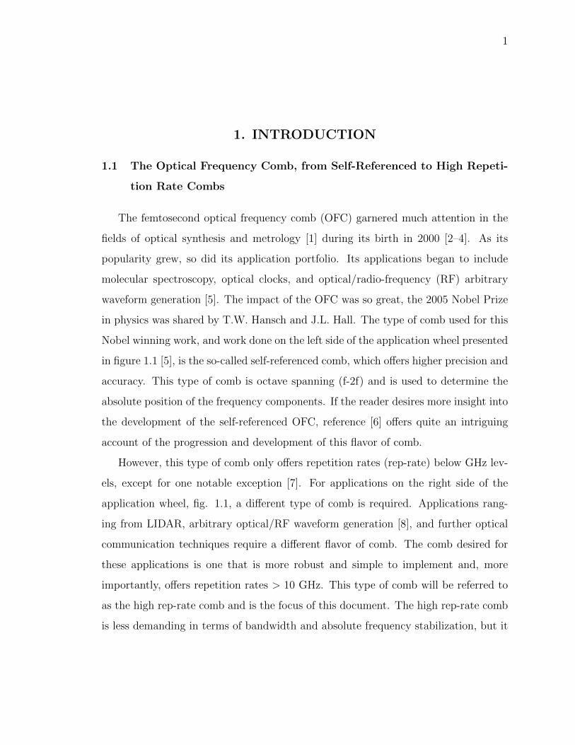
1.1 Application Wheel [5]. The applications on the left side of the wheelbelong to the self-referenced frequency comb. The applications on theright belong to the higher rep-rate combs. . . . . . . . . . . . . . . . . . . 2

1.2 Cartoon depicting what an OFC looks like in the time domain (top), andin the frequency domain (bottom) [10]. The top figure also depicts theCEO arising from the shift between fast oscillating electric field and pulseenvelope. . . . . . . . . . . . . . . . . . . . . . . . . . . . . . . . . . . . . . 3

1.3 Depiction of the two types of four wave mixing taking place inside a mi-croresonator, degenerate and nondegenerate four wave mixing [38]. . . . . . 10

1.4 A cartoon depicting a microring resonator with a bus waveguide [43]. . . . 12

1.5 (a) Cartoon depicting the basic concept of dual comb spectroscopy (DCS).The goal of DCS is to map the optical information to the RF domain. (b)The two types of DCS, asymmetric and symmetric [60]. . . . . . . . . . . . 14

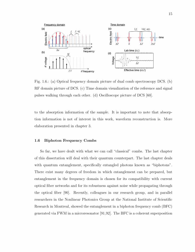
1.6 (a) Optical frequency domain picture of dual comb spectroscopy DCS. (b)RF domain picture of DCS. (c) Time domain visualization of the referenceand signal pulses walking through each other. (d) Oscilloscope picture ofDCS [60]. . . . . . . . . . . . . . . . . . . . . . . . . . . . . . . . . . . . . 15

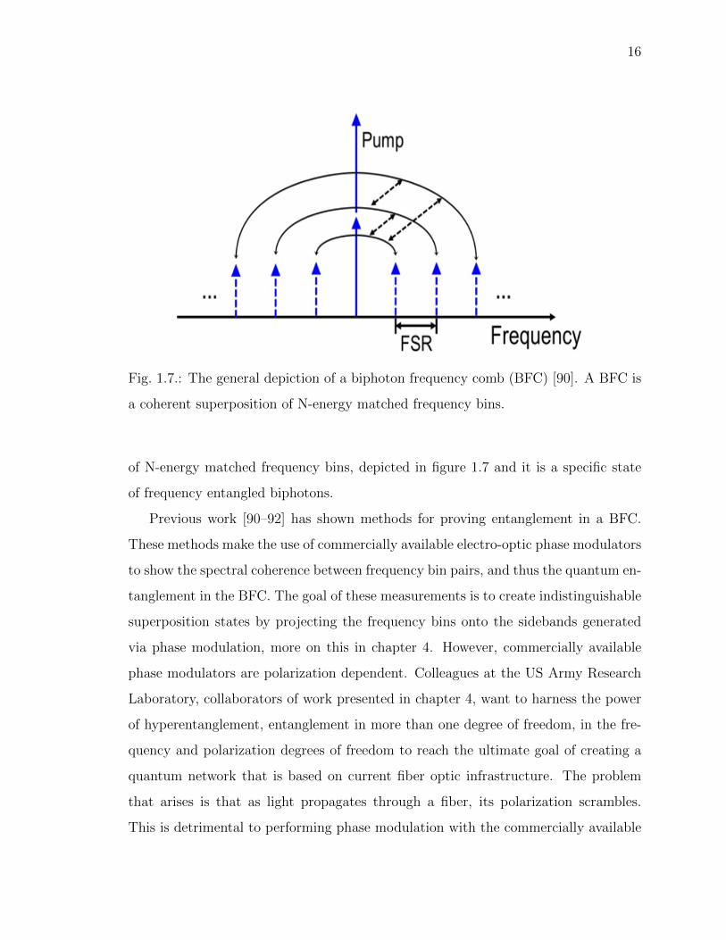
1.7 The general depiction of a biphoton frequency comb (BFC) [90]. A BFCis a coherent superposition of N-energy matched frequency bins. . . . . . . 16

2.1 Example of broadened frequency comb with spectral ripple associated withresidual third order phase. The residual third order phase manifests astemporal wings in the time domain. . . . . . . . . . . . . . . . . . . . . . . 19

2.2 Experimental setup for spectral broadening employing one NOLM stageand one NALM stage. [93]. . . . . . . . . . . . . . . . . . . . . . . . . . . . 20

2.3 Cartoon depicting NOLM comprised of a 2x2 power coupler and a lengthof HNLF. The NOLM is a Sagnac interferometer. . . . . . . . . . . . . . . 22

2.4 Plot of NOLM transmission; note the oscillatory behavior. . . . . . . . . . 24

2.5 Experimental setup for removing residual third order wings via the NOLM. 25

ix

Figure Page

2.6 (a) OFC generated from 1 IM and 1 PM. (b) Comparison of AC traceof compressed pulse out of the EO comb generator. The compressionis performed via a Fourier transform pulse shaper. Only linear chirp iscompensated for. . . . . . . . . . . . . . . . . . . . . . . . . . . . . . . . . 26

2.7 (a) Spectrum out of the NOLM. (b) Corresponding time domain trace outof the NOLM; notice the removal of the third order dispersion wings. . . . 26

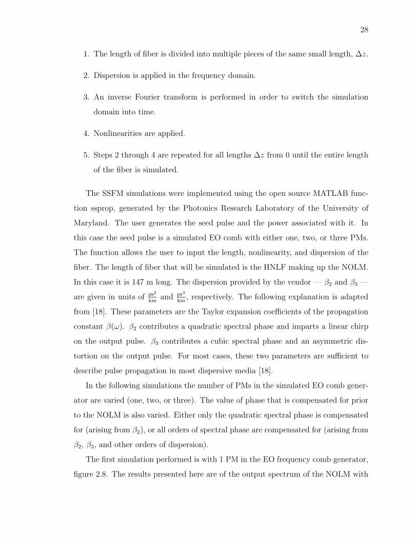
2.8 Simulated spectral results of one PM and one IM. The solid spectrumcorresponds to compensating for all orders of spectral phase. And thedotted spectrum corresponds to compensating for only quadratic spectralphase. . . . . . . . . . . . . . . . . . . . . . . . . . . . . . . . . . . . . . . 29

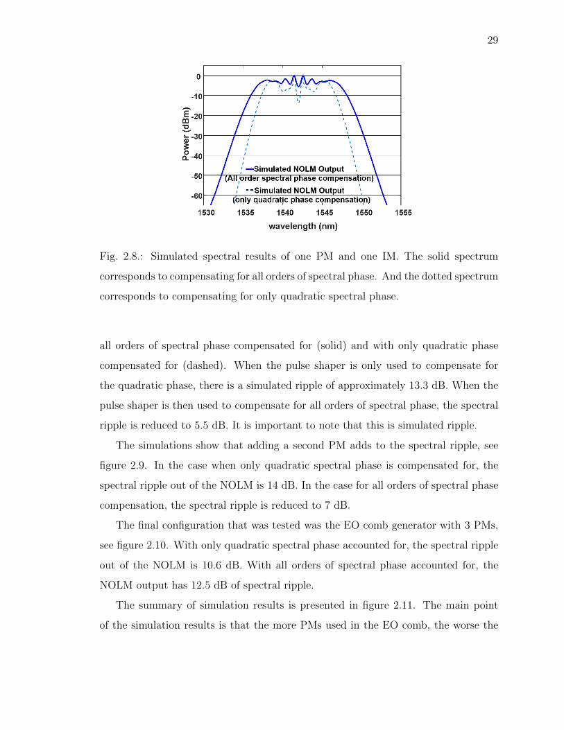
2.9 Simulated spectral results of two PMs and one IM. The two different spec-tra correspond to either compensation of all orders of spectral phase (solid)or only quadratic spectral phase compensation (dotted). . . . . . . . . . . 30

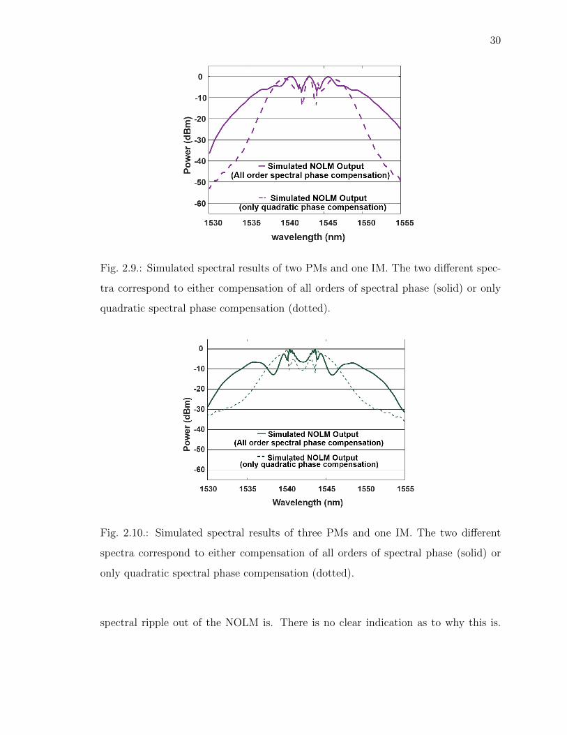
2.10 Simulated spectral results of three PMs and one IM. The two differentspectra correspond to either compensation of all orders of spectral phase(solid) or only quadratic spectral phase compensation (dotted). . . . . . . 30

2.11 Summary of simulation results. The lowest spectral ripple is from usingonly one PM. However, two PMs seems like a good compromise for lowripple and broad spectrum. . . . . . . . . . . . . . . . . . . . . . . . . . . 31

3.1 The signature of soliton generation. The transitions from a noisy chaoticstate to N solitons. Further red detuning eventually leads to the singlesoliton regime [106]. . . . . . . . . . . . . . . . . . . . . . . . . . . . . . . 34

3.2 Microscopic image of microresonator with through and drop ports. . . . . . 35

3.3 (a) Optical spectra after EDFA and pulse shaper for pump wavelengthof 1551.27nm (b) Autocorrelation data (blue) and simulation (red) basedon measured spectrum assuming flat phase. Autocorrelation data with πphase shift applied to the pump (green). . . . . . . . . . . . . . . . . . . . 36

3.4 Cartoons depicting the (a) setup and (b) spectra of the dual comb EFXC. 39

3.5 Single soliton generated in SiN microring resonator depicted in figure 3.2.This spectrum is taken from the drop port. Note the slight offset of thepump line arising from Raman interactions. The free spectral range (FSR)is 227.5 GHz. . . . . . . . . . . . . . . . . . . . . . . . . . . . . . . . . . . 41

3.6 Experimental setup for spectrally broadening electro-optic frequency combfor use as reference comb in the dual comb interferometry measurements. . 42

3.7 Spectrum of electro-optic frequency comb generated from two phase mod-ulators and one intensity modulator. . . . . . . . . . . . . . . . . . . . . . 43

x

Figure Page

3.8 Apodized EO comb and corresponding compressed AC trace. . . . . . . . . 43

3.9 The output of the nonlinear optical loop mirror. . . . . . . . . . . . . . . . 44

3.10 The reference pulse used in the dual comb interferometry measurements. . 45

3.11 The experimental setup for performing dual comb interferometry for char-acterization of single-soliton Kerr-comb [103]. . . . . . . . . . . . . . . . . 46

3.12 (a) A portion of the measured time domain interferogram. (b) The re-constructed interferogram after compensating for fiber dispersion. Thedashed box in (a) and (b) represent one period of the interferogram andthe orange lines are the envelope of the interferogram. (c) The blue traceis the power spectrum of the interferogram. The orange trace is the re-trieved phase of the different optical modes. The pump line exhibits aphase offset. The inset in (c) is the reconstructed intracavity waveformusing the retrieved comb phase [103]. . . . . . . . . . . . . . . . . . . . . . 47

3.13 Results of pump line phase offset study with increasing pump wavelength.The data point indicated by the arrow corresponds to the data presentedin figure 3.12c. . . . . . . . . . . . . . . . . . . . . . . . . . . . . . . . . . 50

4.1 Schematic of the polarization diversity phase modulator (PDPM) – single-mode and polarization-maintaining fiber are depicted in red and blue,respectively. PBS - polarization beam splitter, VOA - variable opticalattenuator, VODL - variable optical delay line, PM - phase modulator. . . 54

4.2 Progression of spectral ripple removal, signifying balancing the lengths ofthe arms of the PDPM. . . . . . . . . . . . . . . . . . . . . . . . . . . . . 55

4.3 Experimental setup for measuring frequency-bin entanglement in a BFC.Note that either a standalone phase modulator (PM) or polarization diver-sity phase modulator (PDPM) is used to mix frequencies in this arrangement.57

4.4 (A), (D) show the change in power scattered into the +1 sideband, as afunction of polarization, for a standalone PM and the PDPM, respectively.(B)-(C) show the change in coincidence and count rates for frequency-binentanglement measurements using a standalone PM. (E)-(F) are analogousto (B)-(C) but for the PDPM and include data for two values of the jointphase – φS2 + φI2 = 0 (solid) and φS2 + φI2 = π (hollow). Results areplotted on an azimuthal slice of the Poincare sphere corresponding tolinearly polarized light. (SA – slow axis and FA – fast axis) . . . . . . . . 60

xi

Figure Page

4.5 Results from frequency-bin entanglement measurements. (A) Coincidences(blue) and counts (red) when using the standalone PM for three differentorientations of the polarization - 0◦ (solid), 90◦ (dotted), and an interme-diate state (dashed). (B) Coincidences and counts when using the PDPMfor two cases - one where photons are equally likely to be in either arm(dashed) and the other where photons go entirely through one arm (solid).The insets show the relative orientation between the polarization of signaland idler bins. . . . . . . . . . . . . . . . . . . . . . . . . . . . . . . . . . . 62

4.6 The figures, going from left to right, contrast the performance of a stan-dalone PM with the PDPM. Data for the PDPM is presented for twovalues of the joint phase (φ = φS2 + φI2) on S2I2. Data for the the φ = πpoint was recorded to clearly establish that the coincidences recorded in(b) are the result of two-photon interference and not leakage from neigh-boring frequency-bins. (a) Coincidences and count rate, as a functionof BFC polarization, in two-photon interference experiments when usingstandalone PM. (b)-(c) analogous to (a) but for the PDPM. . . . . . . . . 63

4.7 Frequency-bin entanglement measurements on orthogonally polarized signal-idler pairs using (A) a standalone PM and (B) the PDPM. Dashed andsolid red lines correspond to the signal and idler count rates, respectively.The insets show the relative orientation between the polarization of signaland idler bins. . . . . . . . . . . . . . . . . . . . . . . . . . . . . . . . . . . 64

4.8 Experimental setup for state preparation and measurement of frequency-bin entanglement. PC – polarization controller and PMF – polarizationmaintaining fiber. . . . . . . . . . . . . . . . . . . . . . . . . . . . . . . . . 66

4.9 The effect of the polarization scrambler on the polarization state of thefrequency-bin pairs when the launch condition is changed from 0◦ to 45◦.PC – polarization controller and PMF – polarization maintaining fiber.The polarization scrambler effectively rotates the global polarization ofthe BFC. . . . . . . . . . . . . . . . . . . . . . . . . . . . . . . . . . . . . 67

4.10 Interference traces and visibilities from measurements of frequency-binentanglement in a BFC. The performance of a standalone PM (blue) wascompared with that of the PDPM (red). The experiments were carriedout for both co– (A) and cross–polarized (B) signal idler pairs. . . . . . . . 68

4.11 Block diagram of the feedback control loop for actively stabilizing the PDPM.69

xii

Figure Page

4.12 Measured path length fluctuations through the PDPM when the inter-ferometer is not stabilized. The top plot shows the photodetector (PD)voltage as a function of time. The data was recorded over 500 secondsand sampled every 0.5 ms. The bottom plot shows the spectrum of thepath length fluctuations, the spectrum shows that the fluctuations are inthe order seconds. . . . . . . . . . . . . . . . . . . . . . . . . . . . . . . . . 71

4.13 Setup to achieve and show active stabilization of classical light in an inter-ferometer. DPC - deterministic polarization controller, PBS - polarizationbeam splitter, CW - continuous wave laser, PZT - piezo electric transducer(fiber phase shifter), PID - proportional integration derivative. λCW1 =1555 nm and λCW2 = 1545 nm. . . . . . . . . . . . . . . . . . . . . . . . . 72

4.14 20 minute measurement of the output power of the stabilization laser(backwards path - orange arrows). This shows the interferometer beingstabilized for the first 10 minutes and not being stabilized for last 10 min-utes. For the data with stabilization on, the standard deviation of thefluctuations is 2.57 µW, and for the stabilization off data the standarddeviation is 150.36 µW. . . . . . . . . . . . . . . . . . . . . . . . . . . . . 74

4.15 20 minute measurement of optical power of classical light (forward prop-agation - purple arrows). This shows the interferometer being stabilizedfor the first 10 minutes and not being stabilized for last 10 minutes. Thepolarization setting on the DPC is set to a polarization ensuring lightthrough both arms of the PDPM and causes this power imbalance be-tween output ports of the test PBS. a - port A of the test PBS, b - portB of the test PBS. . . . . . . . . . . . . . . . . . . . . . . . . . . . . . . . 75

4.16 Polarization stability of the classical light through the test interferometeras its polarization is swept from −90◦ to +90◦ in 10◦ increments. Poweris recorded out of each port of the test PBS for 10 minutes at each po-larization setting. a – port A of the test PBS. b – port B of the testPBS. . . . . . . . . . . . . . . . . . . . . . . . . . . . . . . . . . . . . . . . 76

4.17 Experimental setup for active stabilization of the PDPM. The RF compo-nents necessary to balancing the PDPM electrically are now incorporated.This setup is used to demonstrate that the polarization transformationobserved in figure 4.21 is due to the RF delay mismatch between the PMs. 77

4.18 20 minute measurement of stabilization laser output. The first ten minutesare with stabilization on (and RF delay balanced), and the last ten minutesare with stabilization off. For the data with stabilization on, the standarddeviation of the fluctuations is 0.032 µW, and for the stabilization off datathe standard deviation is 152.36 µW. . . . . . . . . . . . . . . . . . . . . . 78

xiii

Figure Page

4.19 20 minute measurement of the polarization stability of the classical lightin the forward propagation direction (purple arrow). a - port A of the testPBS. b - port B of the test PBS. . . . . . . . . . . . . . . . . . . . . . . . 79

4.20 Polarization stability of the classical light through the PDPM with thePMs on and RF delay balanced as its polarization is swept from −60◦ to+60◦ in 10◦ increments (measured and controlled with the DPC at theforward input of the PDPM). Power is recorded out of each port of thetest PBS for 5 minutes at each polarization setting. a – port A of the testPBS. b – port B of the test PBS. The extinction between the output portsof the test PBS is increased when the RF delay is balanced. . . . . . . . . 80

4.21 Polarization stability of the classical light through the PDPM with thePMs on and RF delay (purposefully) imbalanced. Polarization is sweptfrom −50◦ to +50◦ in 10◦ increments (measured and controlled via DPCat input of PDPM). Power is recorded out of each port of the test PBSfor 5 minutes at each polarization setting. a – port A of the test PBS. b– port B of the test PBS. Notice that in this iteration, there exists lessextinction between the two output ports of the test PBS. . . . . . . . . . . 81

5.1 Example of dark pulse spectrum generated from a normal dispersion mi-croresonator. . . . . . . . . . . . . . . . . . . . . . . . . . . . . . . . . . . 85

5.2 We expect to visualize the breathing dynamics of the dark breather byobserving (purple) sidebands on the retrieved RF comb from the DualComb EFXC measurement. . . . . . . . . . . . . . . . . . . . . . . . . . . 86

xiv

ABBREVIATIONS

OFC optical frequency comb

EO electro-optic

FWM four-wave mixing

RF radio frequency

CEO carrier envelope offset

PM phase modulator

IM intensity modulator

DDF dispersion decreasing fiber

HNLF highly nonlinear fiber

SPM self-phase modulation

GVD group velocity dispersion

CW continuous wave

CMA-ES covariance matrix adaptation evolution strategy

WGM whispering gallery mode

SiN silicon nitride

EFXC electric field cross-correlation

DCS dual comb spectroscopy

LLE Lugiato-Lefever equation

NOLM nonlinear optical loop mirror

NALM nonlinear amplifying loop mirror

SMF single mode fiber

AC autocorrelation

FWHM full width at half maximum

SSFM split-step Fourier method

xv

SHG second-harmonic generation

BPD balanced photo-detector

PDPM polarization diversity phase modulator

VOA variable optical attenuator

VODL variable optical delay line

PBS polarization beam splitter

SPDC spontaneous parametric down conversion

PPLN periodically poled lithium niobate

InP indium phosphide

AWG arrayed waveguide grating

MLL mode-locked laser

xvi

ABSTRACT

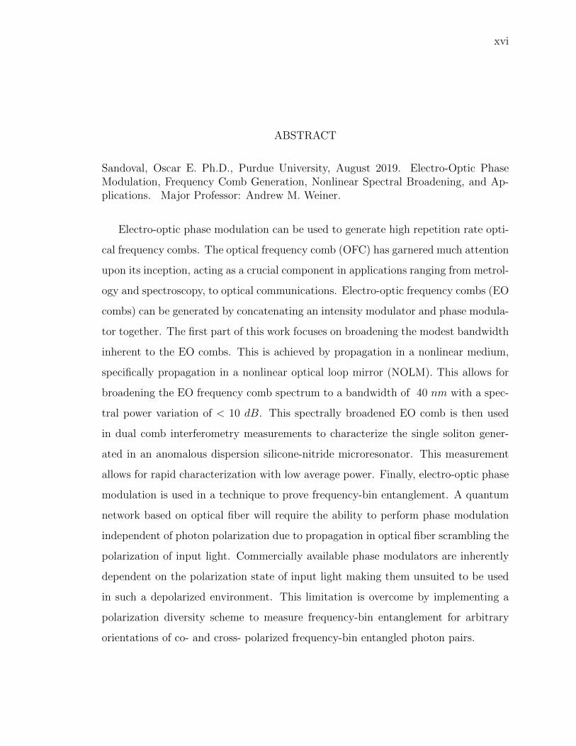
Sandoval, Oscar E. Ph.D., Purdue University, August 2019. Electro-Optic PhaseModulation, Frequency Comb Generation, Nonlinear Spectral Broadening, and Ap-plications. Major Professor: Andrew M. Weiner.

Electro-optic phase modulation can be used to generate high repetition rate opti-

cal frequency combs. The optical frequency comb (OFC) has garnered much attention

upon its inception, acting as a crucial component in applications ranging from metrol-

ogy and spectroscopy, to optical communications. Electro-optic frequency combs (EO

combs) can be generated by concatenating an intensity modulator and phase modula-

tor together. The first part of this work focuses on broadening the modest bandwidth

inherent to the EO combs. This is achieved by propagation in a nonlinear medium,

specifically propagation in a nonlinear optical loop mirror (NOLM). This allows for

broadening the EO frequency comb spectrum to a bandwidth of 40 nm with a spec-

tral power variation of < 10 dB. This spectrally broadened EO comb is then used

in dual comb interferometry measurements to characterize the single soliton gener-

ated in an anomalous dispersion silicone-nitride microresonator. This measurement

allows for rapid characterization with low average power. Finally, electro-optic phase

modulation is used in a technique to prove frequency-bin entanglement. A quantum

network based on optical fiber will require the ability to perform phase modulation

independent of photon polarization due to propagation in optical fiber scrambling the

polarization of input light. Commercially available phase modulators are inherently

dependent on the polarization state of input light making them unsuited to be used

in such a depolarized environment. This limitation is overcome by implementing a

polarization diversity scheme to measure frequency-bin entanglement for arbitrary

orientations of co- and cross- polarized frequency-bin entangled photon pairs.

1

1. INTRODUCTION

1.1 The Optical Frequency Comb, from Self-Referenced to High Repeti-

tion Rate Combs

The femtosecond optical frequency comb (OFC) garnered much attention in the

fields of optical synthesis and metrology [1] during its birth in 2000 [2–4]. As its

popularity grew, so did its application portfolio. Its applications began to include

molecular spectroscopy, optical clocks, and optical/radio-frequency (RF) arbitrary

waveform generation [5]. The impact of the OFC was so great, the 2005 Nobel Prize

in physics was shared by T.W. Hansch and J.L. Hall. The type of comb used for this

Nobel winning work, and work done on the left side of the application wheel presented

in figure 1.1 [5], is the so-called self-referenced comb, which offers higher precision and

accuracy. This type of comb is octave spanning (f-2f) and is used to determine the

absolute position of the frequency components. If the reader desires more insight into

the development of the self-referenced OFC, reference [6] offers quite an intriguing

account of the progression and development of this flavor of comb.

However, this type of comb only offers repetition rates (rep-rate) below GHz lev-

els, except for one notable exception [7]. For applications on the right side of the

application wheel, fig. 1.1, a different type of comb is required. Applications rang-

ing from LIDAR, arbitrary optical/RF waveform generation [8], and further optical

communication techniques require a different flavor of comb. The comb desired for

these applications is one that is more robust and simple to implement and, more

importantly, offers repetition rates > 10 GHz. This type of comb will be referred to

as the high rep-rate comb and is the focus of this document. The high rep-rate comb

is less demanding in terms of bandwidth and absolute frequency stabilization, but it

2

Fig. 1.1.: Application Wheel [5]. The applications on the left side of the wheel belong

to the self-referenced frequency comb. The applications on the right belong to the

higher rep-rate combs.

does require the ability to independently tune the central frequency and repetition

rate.

A high repetition rate OFC with relatively broad optical bandwidth and low noise

level offers a huge new avenue of possibilities not only in microwave photonics [9], but

also in applications that will be presented in the following document. However, the

high rep-rate comb is not as broad as its self-referenced counterpart. Therefore,

methods for broadening the spectrum of these high-rep rate combs is of interest.

The aim of this work was not to create a very broad (> 100 nm) comb with

extremely low spectral flatness (< 5 dB). Instead, the aim of this work is to present

a relatively broad frequency comb comprised of commercially available components

that can be used in applications needing the ability to tune the center wavelength

and repetition rate of the OFC. Before diving into the rest of this work, the following

3

section will introduce the reader to an overview of generating high rep-rate OFC via

electro-optic modulation.

1.2 Generating High Repetition Rate Optical Frequency Combs via Electro-

Optic Modulation

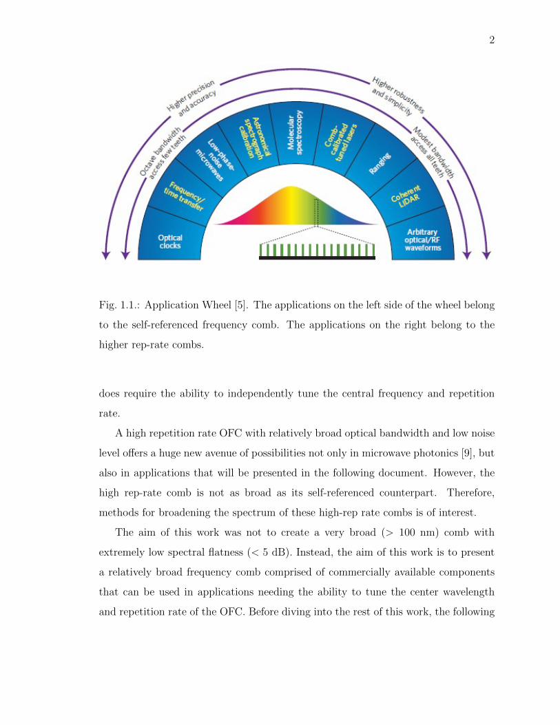
Fig. 1.2.: Cartoon depicting what an OFC looks like in the time domain (top), and

in the frequency domain (bottom) [10]. The top figure also depicts the CEO arising

from the shift between fast oscillating electric field and pulse envelope.

A frequency comb is a light source, whose spectrum consists of evenly spaced

components [5]. However, for a light source to be labeled a frequency comb, it must

also meet the following parameters [9]. Figure 1.2 shows that an OFC in the frequency

domain looks like a series of evenly spaced delta Dirac functions, and in the time

domain, like a series of optical pulses.

1. Maintain high spectral coherence across the entire bandwidth.

4

2. Possess the ability to synthesize in an independent manner the repetition rate

of the comb.

A frequency comb can be thought of as an equidistant array of delta-function, see

equation 1.1.

E (ω) =∑N

ANδ (ω − ωN) ejφN (1.1)

Where AN and φN are the amplitude and spectral phase of the Nth comb line,

respectively. δ is the Kronecker delta function, ω is the carrier frequency, and ωN is

the position of the Nth comb line. If the pulses generated by the laser were identical,

then the absolute positions of the spectral components would be integer multiples of

the laser repetition rate. However, due to dispersion and nonlinearities, there is a slip,

known as the Carrier Envelope Offset (CEO). This arises from the constant shifts in

the oscillation of the electric field with respect to the pulse envelope. Therefore, the

position of the Nth comb, ωN , is given by equation 1.2.

ωN = N∆ω + δω (1.2)

Where N is an integer, ∆ω is the frequency spacing of the lines, and is defined as

∆ω = frep2π

, where frep is the rep-rate of the frequency comb. Finally, δω is the CEO

frequency. In 2005 T. W. Hanch and J. L. Hall were awarded half of the Nobel Prize

in physics for their efforts in determining the CEO frequency via Self-Referencing.

In Self-Referencing, the phases of frequency components spaced by an octave (f to

2f) are compared to determine and lock the CEO frequency. This allows for precise

stabilization of the frequency components at a known location. The reader is pointed

to their Nobel lectures for further insight [11,12].

The second parameter that needs to be met for a light source to be labeled a

frequency comb is the possibility to change the repetition rate i.e. the frequency

spacing of the lines in an independent manner. For these self-referenced combs,

the ability to change the repetition rate is a difficult process, usually involving the

5

stabilization of the laser cavity. Therefore, the need for a different flavor of comb is

re-iterated.

Reference [9] reviews the idea of opto-electronic frequency comb generators. The

idea is to send a CW laser into an opto-electronic system driven by an RF source. At

the output of the opto-electronic system a frequency comb will be generated. This

idea was first proposed in the 60s [13] and in the 70s and 80s was researched as a

means of generating picosecond pulses [14, 15]. Usually the opto-electronic system

will be comprised of an electro-optic intensity or phase modulator, or a combination

of both. In 2003 Fujiwara et al. developed a flat top high rep-rate frequency comb

by concatenating an intensity modulator (IM) and a PM phase modulator (PM)

[16]. This is the method our group employs to generate high rep-rate combs electro-

optically. The idea is that the IM carves out a train of pseudo square pulses from the

input CW laser. The PM imparts a quadratic phase on each pulse. The carving of the

pulses is timed so that it occurs when the chirping imparted by the PM is linear. This

is the impetus that creates the flat top spectrum. Previously, only phase modulation

was used in generating these electro-optic combs, but by phase modulation alone, the

spectral lines suffer from significant line-to-line amplitude variations [17].

The phase imparted onto the CW laser is given by equation 1.3.

Φ =πV

Vπcos(2πft) (1.3)

Where V and f are the maximum voltage and frequency of the RF signal from

the RF oscillator, respectively. And Vπ is an important parameter inherent to the

electro-optic coefficient of the material and the waveguide structure of the modulator,

known as the Half-Wave Voltage. This parameter gives information on the amount of

RF power needed for generation of a π phase shift.

Another important parameter in these electro-optic modulated frequency combs

is the modulation index, given in equation 1.4.

∆θ =πV

Vπ(1.4)

6

To obtain a broad optical bandwidth, the modulation index must be high. To

maximize the value of the modulation index, a modulator with a low Vπ and capable

of accepting a high RF voltage (V ) is desired.

One way to increase the value of the modulation index is by placing multiple PMs

in tandem. This is because the effective Vπ is given by equation 1.5.

Vπeff =

(1∑N

i=1 Vπi

)−1

(1.5)

Therefore, as more phase modulators are cascaded, the effective Vπ is decreased

and the modulation index is increased.

1.3 Spectral Broadening High Repetition Rate OFC

Many of the high repetition rate comb generators provide a spectrum of modest

bandwidth. For some applications a broader comb may be needed. Therefore, broad-

ening these types of combs is an area of research that has garnered much attention. A

brief review of different methods for achieving spectral broadening of high repetition

rate frequency combs follows. Most take advantage of the fact that these types of

OFC generators output optical pulses in the 1 ∼ 10 ps regime, making them useful

in achieving spectral broadening in a highly nonlinear passive medium [9].

The passive medium in which spectral broadening is realized can have two types

of dispersion. To briefly describe the differences between the two, the following ex-

planation has been adapted from [18, 19]. Presuming a Fourier transform limited

pulse, upon propagation in an anomalous dispersion material, the higher frequency

components travel faster than the lower frequency components, i.e., the leading edge

of the pulse is blue shifted and the trailing edge of the pulse is red shifted. D is

the dispersion parameter and it has units of ps/nm/km. For anomalous dispersion

D > 0. In the case of propagation in a normal dispersion material, the higher fre-

quency components of the pulse travel slower than the lower frequency components,

i.e., the leading edge of the pulse is red shifted and the trailing edge of the pulse is

7

blue shifted. For normal dispersion D < 0. In each of these dispersion regimes, the

method for achieving spectral broadening is different. Here we begin the brief review

on methods for achieving spectral broadening of high repetition rate frequency combs.

1.3.1 Methods for spectral broadening

In anomalous dispersion, modulation instability can lead to amplification of small

amounts of input noise that can lead to the degradation of the spectral coherence of

the comb [20]. Therefore, the dispersion profile of the external nonlinear fiber must

be carefully chosen, which is why dispersion decreasing fibers (DDF) are attractive

for nonlinear broadening in the anomalous dispersion regime. These types of fibers

can lead to significant broadening [21, 22] and pulse compression through a process

known as adiabatic soliton compression [18]. Further examples of broadening in DDF

are shown in [23] and [24].

In the normal dispersion regime, modulation instability is not a problem. In this

regime, spectral broadening can be achieved by launching the short pulses into a

highly nonlinear fiber (HNLF). In normal dispersion HNLF, the physical mechanism

leading to spectral broadening is self-phase modulation (SPM) [18, 25]. SPM stems

from the optical Kerr effect, which is a change in the refractive index due to an applied

electric field. It is important to note that SPM is also present in the anomalous

dispersion regime, but the interplay between the group velocity dispersion (GVD)

and SPM balance each other and can lead to the formations of solitons [18]. In the

normal dispersion regime, SPM and GVD act in concert and lead to a time varying

phase that modifies the spectrum by adding new spectral components, i.e., spectral

broadening. SPM is dependent on the intensity of the optical pulse. Therefore,

increasing the power of the pulse will lead to an increase in spectral broadening. This

is the method of choice for the spectral broadening in this work, because it is simple

to implement with commercially available HNLF.

8

In reference [26], the authors show spectral broadening in 1km of normal dispersion

HNLF. And more recently, at CLEO in 2017, Metcalf et al., [27], showed spectral

broadening in normal dispersion HNLF at the 1 µm wavelength.

Along with employing normal dispersion HNLF, work has been done in shaping or

apodizing the seed pulse prior to being launched into the nonlinear fiber. In [26,28],

and [29] the seed spectrum was shaped into a parabola prior to being launched into

the HNLF. By seeding the HNLF with a pulse having a spectrum that is nearly

Gaussian, this can lead to a flat broadened spectrum by taking advantage of the

notions of optical wave-breaking [30]. In optical wave-breaking, different frequency

components generated by SPM meet and interfere at the same time location. This

occurrence can lead to an enhancement of the flatness of the central region of the

spectrum [31].

Alternatively, another nonlinear effect called four-wave mixing (FWM) can be

exploited to achieve broadening. In FWM the χ(3) response of the nonlinear medium is

used to reshape the complex field of the input waveform in order to obtain the desired

spectral profile. In an example of this work, reference [32], two narrow bandwidth

combs are centered at different wavelengths and are mixed in a length of HNLF. The

nonlinear interaction leads to the generation of new frequency combs centered about

other frequency components through a cascade of FWM. If the system is properly

phase matched, this can lead to a power enhancement that simultaneously broadens

the comb and preserves flatness. Further examples of this method can be found

in [28, 33, 34]. It should be noted, however, that the two seed combs need to be

phase-locked in order to achieve a broader comb that can retain long term frequency

stability [9], thus adding to the intricacy of this method.

Further increasing the complexity of the nonlinear medium, in 2011 Kuo et al.,

reference [35], introduced a technique based on two-pump parametric mixing. By

precisely managing the dispersion of the HNLF that served as the mixer, they gen-

erated a broadened comb with 140 nm bandwidth. Along the same path, in 2012

Myslevits et al. re-hashed the precise dispersion management of the HNLF. In this

9

two stage HNLF setup, they controlled the dispersion characteristics of the HNLF by

inserting strain on the fiber [36]. In this work, two CW tones can be spaced arbitrarily

apart to generate a comb frequency pitch (rep-rate). By inducing strain-synthesized

dispersion, they can induce phase matching, and thus generate a 150 nm broad fre-

quency comb. This broadening is impressive, but it should be noted that the HNLF

used in this work is a specialty fiber and the strain-induced dispersion increases the

complexity of this scheme.

The above references used two CW lasers for parametric mixing in HNLF to gen-

erate a frequency comb. In the following technique for spectral broadening, they also

use two CW lasers for seeding a broadening stage [17]. One CW (CW1) laser is used

in an electro-optic comb generator comprised of one intensity modulator (IM) and one

PM. The second CW (CW2) laser is not modulated, and combined with the generated

frequency comb from CW1. This is the same FWM scheme in [32]. The difference

is that instead of using 100m of HNLF to spectrally broaden the FWM generated

comb, a 1cm long silicon waveguide is used. They claim the silicon waveguide has

a nonlinear parameter 3 orders of magnitude greater than the HNLF. The nonlinear

parameter of the silicon waveguide is 103 radW·km

and the nonlinear parameter of the

HNLF is 1.72 radW·km

. They generated a broadened frequency comb with more than

100 lines at a rep-rate of 10 GHz.

Finally, one last interesting method of generating spectrally broadened frequency

combs is via a technique called adaptive pulse shaping [37]. The idea is to pre-

shape the comb being launched into the HNLF to obtain the desired spectral shape

after the HNLF. They use an algorithm based off the covariance matrix adaptation

evolution strategy (CMA-ES). By monitoring the spectrum out of the HNLF, they

can continually shape the spectrum before the HNLF, via a pulse shaper, until they

achieve a flat broadened comb. This method generated a 26nm broad comb at a

rep-rate of 10 GHz.

10

1.4 Generation of Optical Frequency Combs in Microresonators via Four

Wave Mixing

Looking to the future of optical frequency comb generators, the next approach

will require reducing their size, cost, weight, and power consumption. This will

allow for the application of optical frequency generators outside of the laboratory

environment [9].

A new principle has emerged that uses parametric frequency conversion in high

resonance quality factor microresonators [38]. This new approach may allow for chip-

scale integration and applications in astronomy, microwave photonics, and telecommu-

nications [38]. Of note, two different references have shown on-chip comb generation

with an incorporated compact pump laser, [39] and [40].

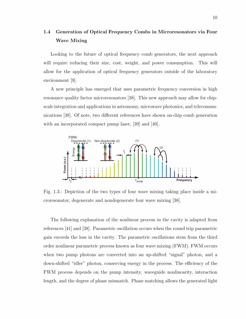
Fig. 1.3.: Depiction of the two types of four wave mixing taking place inside a mi-

croresonator, degenerate and nondegenerate four wave mixing [38].

The following explanation of the nonlinear process in the cavity is adapted from

references [41] and [38]. Parametric oscillation occurs when the round trip parametric

gain exceeds the loss in the cavity. The parametric oscillations stem from the third

order nonlinear parametric process known as four wave mixing (FWM). FWM occurs

when two pump photons are converted into an up-shifted “signal” photon, and a

down-shifted “idler” photon, conserving energy in the process. The efficiency of the

FWM process depends on the pump intensity, waveguide nonlinearity, interaction

length, and the degree of phase mismatch. Phase matching allows the generated light

11

to add up constructively along the length of the waveguide. Parametric gain requires

not only phase matching, but also requires relatively high optical intensity and long

interaction length.

An advantage of the optical microresonator is the fact that the threshold for comb

generation scales with the inverse of the quality (Q) factor squared. Therefore, a high

Q leads to a dramatic reduction in required optical power.

The parametric oscillation leads to spectra containing multiple sidebands, i.e.,

frequency combs. Two nonlinear processes lead to comb generation, see figure 1.3.

The first is the “degenerate” FWM process. This process generates photons from the

same frequency i.e., the signal and idler photon have the same parent photon. The

second process is the “nondegenerate” FWM. In this process photons are generated

from different frequencies. It is termed nondegenerate FWM because the two pump

photons have different frequencies.

In an ideal setting, the cavity would confine light indefinitely, and would have

resonant frequencies at precise values [42]. However, due to dispersion, this ideal

case is not possible. The dispersion of the cavity leads to variations of the free

spectral range (FSR) of the cavity and limits the conversion process, thus limiting the

bandwidth of the generated comb. FWM becomes less efficient when the comb modes

are no longer in resonance with the cavity modes. Therefore, having the ability to

control the dispersion of the cavity by controlling the thickness of the waveguide, [41],

allows for better phase matching and FWM enhancement.

Resonance in microresonators occur when the optical path length of the resonator

is exactly a whole number of wavelengths, or when the waves in the microresonator

interfere constructively due to the accumulation of a phase shift that is an integer

multiple of 2π [43]. The microresonators support multiple resonances, and the spac-

ing between these resonances is the FSR, which is dependent on the length of the

resonator.

Microresonators employ different geometries. For instance, the geometry used in

the seminal work by Del’Haye et al., [44], was toroidal. This type of microresonator be-

12

longs to a certain subset known as whispering gallery mode (WGM) microresonators.

This geometry confines light by total internal reflection around an air-dielectric inter-

face and relies on the curvature of the surface to reflect the light [38]. This type of mi-

croresonator was demonstrated in reference [45] using microspheres having ultra-high

Q factors (>100 million). Further examples of WGM microresonators are microdisks

and microspheres [44].

Fig. 1.4.: A cartoon depicting a microring resonator with a bus waveguide [43].

An example of a different type of microresonator geometry is the microring res-

onator, which is an optical waveguide that is looped back on itself [43], depicted in

figure 1.4. In this geometry, evanescent coupling is leveraged to couple light between

a bus waveguide and a ring resonator. The light will be stored in the ring resonator

due to its high Q. This is the type of geometry employed in the work presented in

chapter 3.

Microresonators also employ different materials. Examples of different materi-

als are silica [44, 46–49], calcium fluoride [50–52], magnesium fluoride [53–55], fused

quartz [56], and silicon nitride (SiN) [41,57–59].

Silicon nitride waveguide resonators offer the possibility of being integrated onto

photonic chips that can generate and transfer optical signals directly on chips. They

are also typically compact, low-cost, and a convenient way to develop future telecom-

munication and optical interconnects. Silicon nitride is compatible with the CMOS

fabrication standard. This offers the possibility for integration with other subsystems

all in one chip [9]. Examples of these subsystems are multiplexers and modulators.

13

Due to their ultra-high repetition rates and compactness, they have become attractive

as a multi-wavelength source for [38] optical communications, optical interconnects,

astronomical spectrometers, and broad-band RF photonics. Therefore, it is the plat-

form of choice for the microring resonators used in the work presented in chapter

3.

1.5 Dual Comb Spectroscopy

The single soliton physics in a SiN microring is of interest. To study the phase of

such a phenomena, a dual comb electric field cross-correlation technique (EFXC) is

employed. The measurements technique is based off of dual comb spectroscopy (DCS),

which is why the following review, adapted from [60], is presented. This review focuses

on DCS applied to linear spectroscopy as a broadband coherent system. But recently,

DCS has been modified to characterize telecommunication components, fiber gratings,

and microresonators [61–63]. Further modification to the DCS approach has allowed

for the monitoring of active sources, such as static and fast-swept CW waveforms

[64–66], pulsed or incoherent sources [67,68], and arbitrary optical waveforms [69–71].

All these techniques, including the dual comb EFXC, possess the underlying dual-

comb/single-receiver architecture of DCS. And they are ultimately no more than

a simple extension of standard heterodyne laser interferometry to frequency comb

sources [60].

In DCS, the strengths of conventional broadband spectroscopy and tunable laser

spectroscopy are combined into a single platform allowing for a broad range of the

optical spectrum to be analyzed with the use of only one single photodetector [60].

DCS can provide comb-tooth-resolved spectra [72, 73] and high signal-to-noise ratio

(SNR) over broad optical bandwidths in the near-IR [74, 75]. Since its first demon-

strations, [76–79], DCS has an application portfolio including ultrabroadband near-

IR spectroscopy [75], near-field microscopy for subwavelength spatial resolution [80],

precision line centers [75,81,82], spectral LiDAR [83,84], and greenhouse gas monitor-

14

ing [85,86]. And most recently, DCS has been extended to nonlinear spectroscopy for

stimulated Raman scattering based coherent anti-Stokes Raman spectroscopy [87,88]

and two-photon spectroscopy [89].

Fig. 1.5.: (a) Cartoon depicting the basic concept of dual comb spectroscopy (DCS).

The goal of DCS is to map the optical information to the RF domain. (b) The two

types of DCS, asymmetric and symmetric [60].

Figure 1.5 depicts the basic concept of DCS. Two frequency combs with different

repetition rates are beat together at a photodiode. This beating generates an RF

comb that is composed of distinguishable heterodyne beats between pairs of optical

comb components. This RF comb can easily be characterized with RF electronics,

and holds all necessary information of the optical comb spectra. Spectroscopy is

performed by either having both optical beams pass through the sample (symmetric)

or only one (asymmetric).

Figure 1.6 gives a frequency and time domain view of the DCS. Two combs are

beat to produce an RF comb. The intensity and phase of the detected RF comb are

proportional to the product of the electric fields of the two optical combs. In essence,

DCS maps the optical combs to the RF domain. The repetition rate difference de-

termines the time to acquire a single spectrum. In the time domain, a large burst

corresponds to simultaneous arrival of two pulses and in the tails ringing corresponds

15

Fig. 1.6.: (a) Optical frequency domain picture of dual comb spectroscopy DCS. (b)

RF domain picture of DCS. (c) Time domain visualization of the reference and signal

pulses walking through each other. (d) Oscilloscope picture of DCS [60].

to the absorption information of the sample. It is important to note that absorp-

tion information is not of interest in this work, waveform reconstruction is. More

elaboration presented in chapter 3.

1.6 Biphoton Frequency Combs

So far, we have dealt with what we can call “classical” combs. The last chapter

of this dissertation will deal with their quantum counterpart. The last chapter deals

with quantum entanglement, specifically entangled photons known as “biphotons”.

There exist many degrees of freedom in which entanglement can be prepared, but

entanglement in the frequency domain is chosen for its compatibility with current

optical fiber networks and for its robustness against noise while propagating through

the optical fiber [90]. Recently, colleagues in our research group, and in parallel

researchers in the Nonlinear Photonics Group at the National Institute of Scientific

Research in Montreal, showed the entanglement in a biphoton frequency comb (BFC)

generated via FWM in a microresonator [91,92]. The BFC is a coherent superposition

16

Fig. 1.7.: The general depiction of a biphoton frequency comb (BFC) [90]. A BFC is

a coherent superposition of N-energy matched frequency bins.

of N-energy matched frequency bins, depicted in figure 1.7 and it is a specific state

of frequency entangled biphotons.

Previous work [90–92] has shown methods for proving entanglement in a BFC.

These methods make the use of commercially available electro-optic phase modulators

to show the spectral coherence between frequency bin pairs, and thus the quantum en-

tanglement in the BFC. The goal of these measurements is to create indistinguishable

superposition states by projecting the frequency bins onto the sidebands generated

via phase modulation, more on this in chapter 4. However, commercially available

phase modulators are polarization dependent. Colleagues at the US Army Research

Laboratory, collaborators of work presented in chapter 4, want to harness the power

of hyperentanglement, entanglement in more than one degree of freedom, in the fre-

quency and polarization degrees of freedom to reach the ultimate goal of creating a

quantum network that is based on current fiber optic infrastructure. The problem

that arises is that as light propagates through a fiber, its polarization scrambles.

This is detrimental to performing phase modulation with the commercially available

17

electro-optic phase modulators. Therefore, to reach the goal of a fiber optic quantum

network, a phase modulator capable of phase modulation irrespective of polarization

state is needed. The final chapter of this dissertation introduces the polarization

diversity phase modulator (PDPM), a device that can perform such polarization in-

dependent phase modulation.

1.7 Organization of Work

Chapter 2 will introduce the reader to the nonlinear optical loop mirror and how it

is used to spectrally broaden frequency combs generated electro-optically. In chapter

3, the spectrally broadened EO comb is used as a reference in a dual comb EFXC

measurement to characterize single soliton pulses generated in SiN microring res-

onators. In chapter 4, a polarization diversity phase modulator will be introduced

to circumvent the intrinsic property of polarization dependence of commercial phase

modulators. Finally, in chapter 5, the conclusion and an outlook of future work is

presented.

18

2. SPECTRAL BROADENING OF HIGH REPETITION

RATE OPTICAL FREQUENCY COMBS EMPLOYING A

NONLINEAR OPTICAL LOOP MIRROR

In the previous chapter various methods for broadening the modest bandwidth of

electro-optic frequency combs were presented. Various applications require more

bandwidth, but they also require a flat spectrum. By having a flat spectrum it is

meant that each comb line has the same intensity. In communication applications,

data will be imparted on each frequency component (comb line). If the intensity of

the lines are different, then this will lead to errors in the data transmission. There-

fore, the goal of most spectral broadening experiments is to increase the bandwidth

while preserving its flatness. This is a difficult task due to the spectral ripple, power

variation among spectral lines, stemming from dispersion and other effects in the

fiber propagation. Very impressive techniques were presented that allowed for excess

of 100 nm bandwidths with very low spectral ripple. However, the complexity, and

cost, of these techniques makes them difficult to implement. Therefore, in this chap-

ter, the nonlinear optical loop mirror is presented. This all fiber device allows for

removal of the third-order dispersion that is the culprit for spectral ripple formation.

It is a simple setup, that when implemented successfully allowed for the broadening

of an electro-optic frequency comb. Simulations are presented in which the number

of phase modulators in the electro-optic frequency comb generator is varied. This

allows for the determination of the best configuration to get the best balance between

spectral flatness and broadening.

19

2.1 Spectral Broadening With the Aid of a Nonlinear Optical Loop Mir-

ror

The goal of spectral broadening is to generate more spectral lines while preserving

flatness. When launching a pulse into a nonlinear medium, HNLF for instance, the

seed pulse should be transform limited, i.e., chirp free. Residual chirp on the seed

pulse can lead to amplitude variations in the spectrum out of the nonlinear medium.

These amplitude variations will be known as spectral ripple in this work, and an

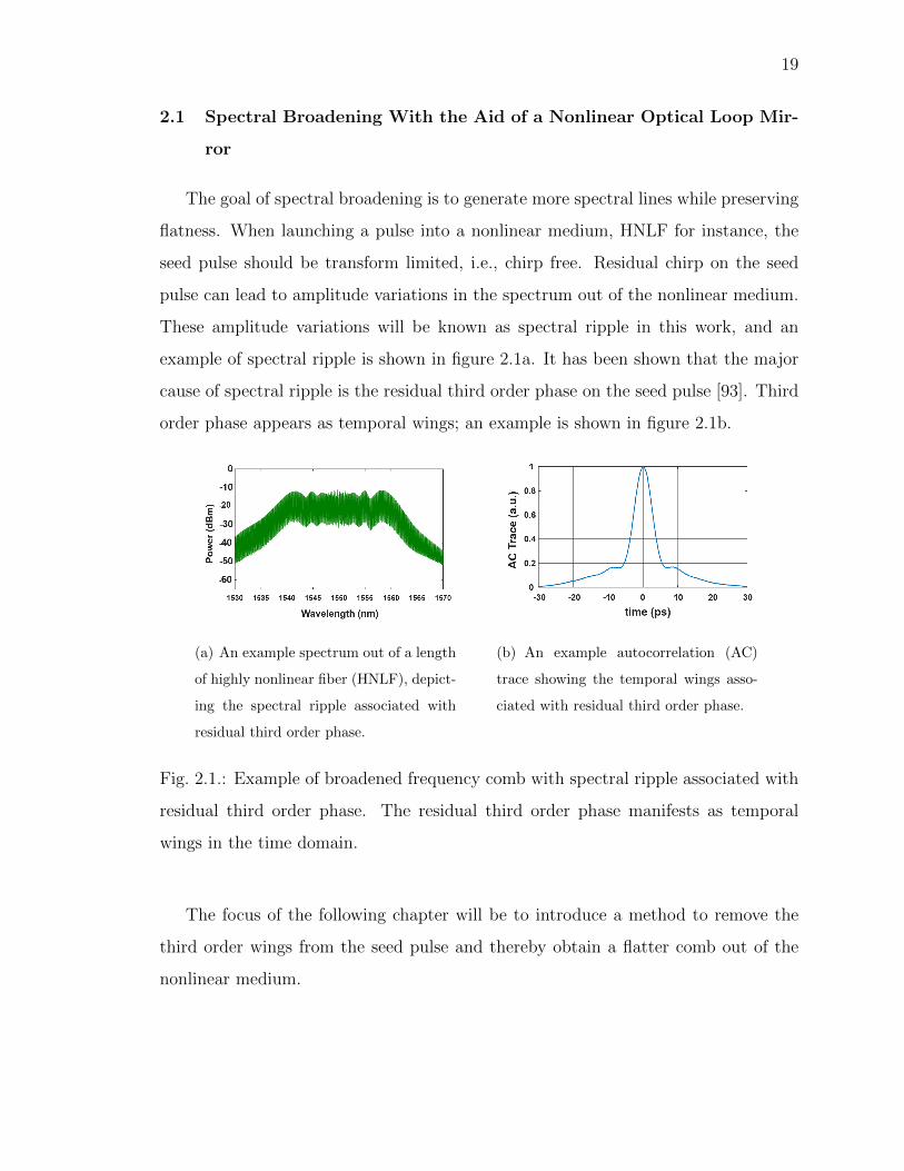
example of spectral ripple is shown in figure 2.1a. It has been shown that the major

cause of spectral ripple is the residual third order phase on the seed pulse [93]. Third

order phase appears as temporal wings; an example is shown in figure 2.1b.

(a) An example spectrum out of a length

of highly nonlinear fiber (HNLF), depict-

ing the spectral ripple associated with

residual third order phase.

(b) An example autocorrelation (AC)

trace showing the temporal wings asso-

ciated with residual third order phase.

Fig. 2.1.: Example of broadened frequency comb with spectral ripple associated with

residual third order phase. The residual third order phase manifests as temporal

wings in the time domain.

The focus of the following chapter will be to introduce a method to remove the

third order wings from the seed pulse and thereby obtain a flatter comb out of the

nonlinear medium.

20

In 1988 Doran and Wood introduced the nonlinear optical loop mirror (NOLM)

[94]. In its introduction, it garnered attention for applications in fast optical switching

for signal processing and communications [94, 95] and as a means for mode locking

a laser as a fast-saturable absorber [96]. But the application that makes the NOLM

attractive for the work in this document is its capability of re-shaping optical pulses.

Smith, Doran, and Wigley introduced the pulse shaping concept [97]. In this work,

optical pulses with temporal pedestals are launched into the NOLM comprised of fiber

that has low and normal dispersion. Upon exiting the NOLM, the pulses are cleaned

up i.e., the temporal pedestals are removed. But the NOLM’s effectiveness in pedestal

suppression does not have to only apply to applications in optical communications.

It can be used to facilitate more effective spectral broadening, as was shown by Ataie

et al. in 2014.

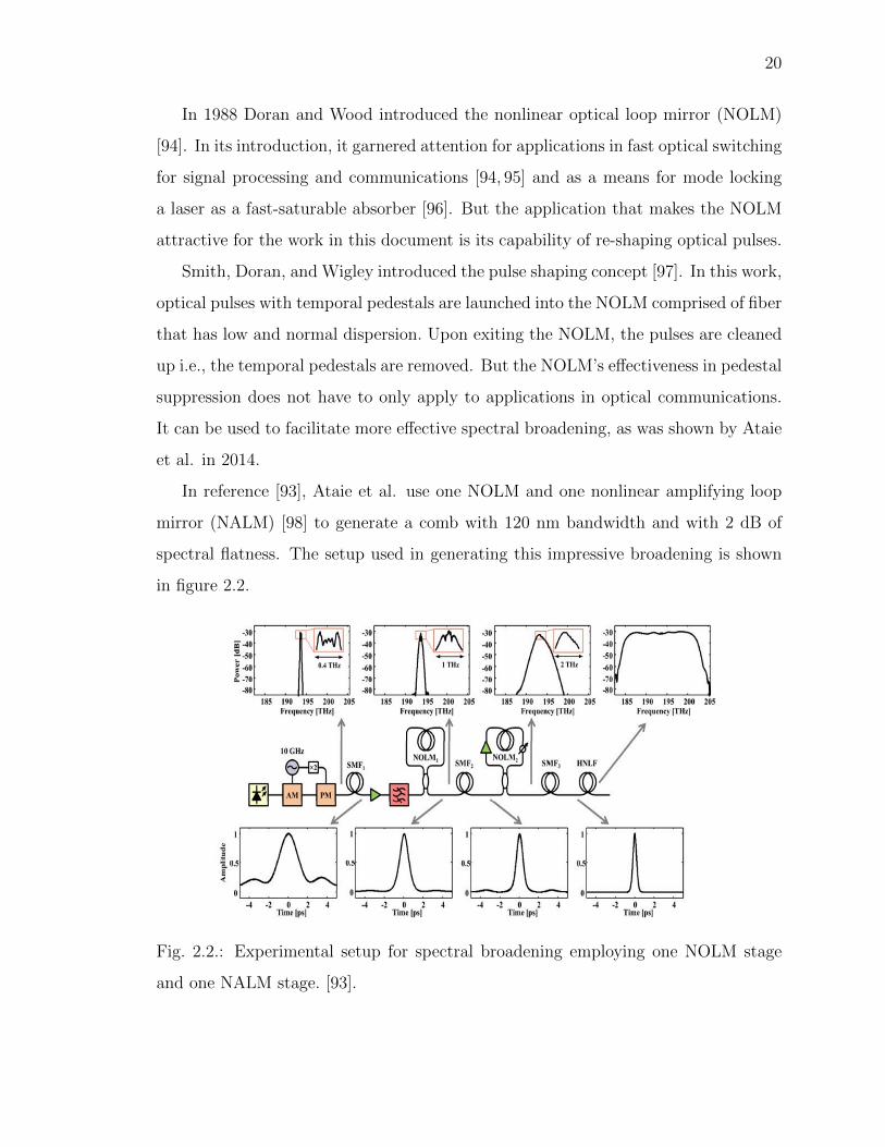
In reference [93], Ataie et al. use one NOLM and one nonlinear amplifying loop

mirror (NALM) [98] to generate a comb with 120 nm bandwidth and with 2 dB of

spectral flatness. The setup used in generating this impressive broadening is shown

in figure 2.2.

Fig. 2.2.: Experimental setup for spectral broadening employing one NOLM stage

and one NALM stage. [93].

21

They generate an OFC electro-optically and compress the output pulse via a

length of single mode fiber (SMF). This length of SMF will account for the second

order dispersion, leaving residual third order on the pulse. After which, the pulse

is sent to an erbium-doped fiber amplifier (EDFA) and an optical filter to remove

any amplified spontaneous emission (ASE) introduced by the EDFA. The amplified

pulse is launched into the NOLM, which is made up of a 2x2 power coupler, with

65 : 35 split ratio, and 60 m of specialty dispersion flattened HNLF (DF-HNLF). The

pulse is cleaned up by the NOLM and then travels through another length of SMF

before being launched into the NALM. The NALM is made up of a 50 : 50 2x2 power

coupler, 50 m of HNLF, and an EDFA. At the output of the last DF-HNLF the 2

dB 120 nm wide spectrum is generated. In the same figure, the progression of the

spectrum (top) and temporal pulse (bottom) is shown. The main takeaways should

be how the pulse looks before and after the NOLM and NALM. The temporal wings

or pedestals are removed after propagating through either device. The NOLM is an

all-fiber way of suppressing the pedestals or wings that are a signature of third order

phase. Suppressing these pedestals will lead to more effective spectral broadening. In

the following section, the NOLM formulation will be presented.

2.2 Nonlinear Optical Loop Mirror Scattering Matrix Formulation

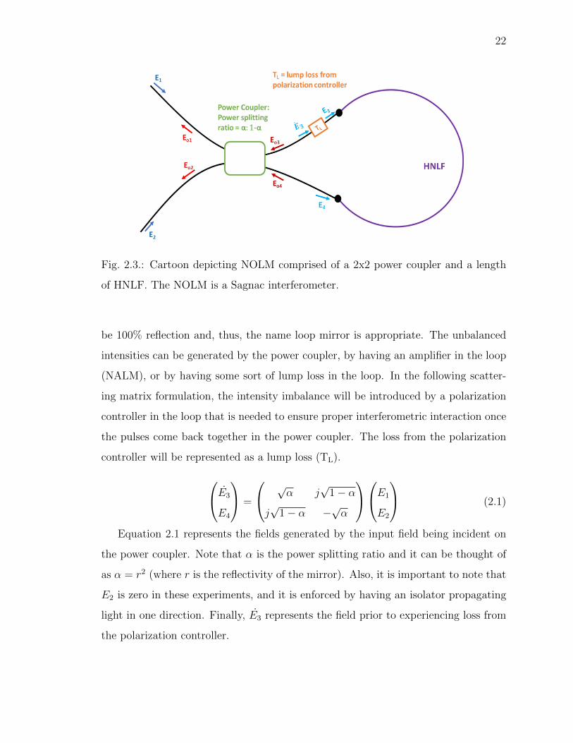
The NOLM, depicted in figure 2.3, is constructed with a 2x2 power coupler and

a length of HNLF [94]. The output ports are connected together (via the length of

HNLF), making the NOLM a Sagnac interferometer [95,99].

In the following section the NOLM scattering matrix formulation, presented in

[18], will be outlined.

The 2x2 power coupler in the NOLM creates two counter-propagating fields in the

HNLF. The counter-propagating fields will have different intensities and will there-

fore obtain different phases, via SPM. It needs to be noted that the intensities of the

pulses need to be unbalanced. If the pulse intensities are the same, then the result will

22

Fig. 2.3.: Cartoon depicting NOLM comprised of a 2x2 power coupler and a length

of HNLF. The NOLM is a Sagnac interferometer.

be 100% reflection and, thus, the name loop mirror is appropriate. The unbalanced

intensities can be generated by the power coupler, by having an amplifier in the loop

(NALM), or by having some sort of lump loss in the loop. In the following scatter-

ing matrix formulation, the intensity imbalance will be introduced by a polarization

controller in the loop that is needed to ensure proper interferometric interaction once

the pulses come back together in the power coupler. The loss from the polarization

controller will be represented as a lump loss (TL).

E3

E4

=

√α j

√1− α

j√

1− α −√α

E1

E2

(2.1)

Equation 2.1 represents the fields generated by the input field being incident on

the power coupler. Note that α is the power splitting ratio and it can be thought of

as α = r2 (where r is the reflectivity of the mirror). Also, it is important to note that

E2 is zero in these experiments, and it is enforced by having an isolator propagating

light in one direction. Finally, E3 represents the field prior to experiencing loss from

the polarization controller.

23

E3 =√TL√αE1 (2.2)

Equation 2.2 represents the field after the lump loss of the polarization controller.

Eo3Eo4

=

0 ejγL(1−α)P )

ejγL(TLα)P ) 0

E3

E4

(2.3)

Equation 2.3 represents the fields propagating through the HNLF. γ is the non-

linearity of the fiber, and P is the optical peak power of the input field. Because of

the lump loss from the polarization controller, it is evident that the phase acquired

by the counter-propagating fields is different.

Eo3 =√TLE4e

jγL(1−α)P (2.4)

Equation 2.4 represents the field going through the polarization controller and

incurring its loss.

Eo1Eo2

=

√α j

√1− α

j√

1− α −√α

Eo3Eo4

(2.5)

Finally, equation 2.5 represents the fields incident upon the power coupler again.

The output field that is of interest is Eo2. This is the output port that has the pulse

with the temporal pedestals removed. Through port 1, Eo1, is the junk. This port

will have the temporal wings that were removed from the pulse.

The transmission equation of the NOLM is given by equation 2.6.

T =Pout

Pin

=|Eo2|2

|E1|2= TL [1− 2α (1− α) {1 + cos ([(1− α)TL − α]φ)}] (2.6)

The transmission equation is dependent on the power coupler splitting ratio (α),

the lump loss (in our case from the polarization controller), and by φ, the nonlinear

phase induced by SPM in the HNLF.

φ = γPinL (2.7)

24

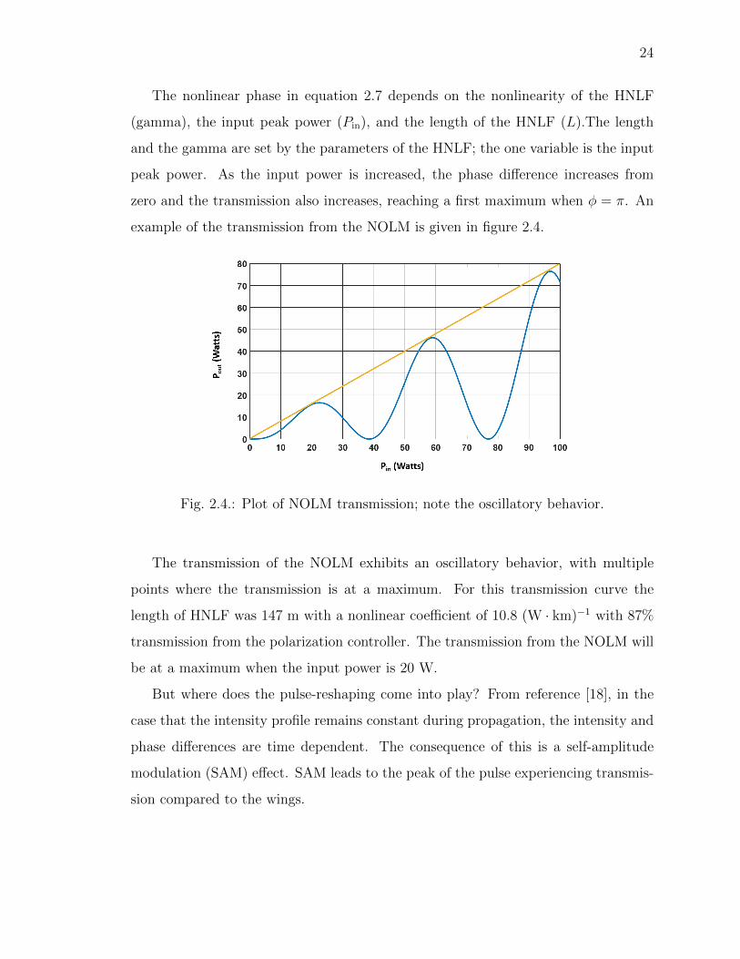
The nonlinear phase in equation 2.7 depends on the nonlinearity of the HNLF

(gamma), the input peak power (Pin), and the length of the HNLF (L).The length

and the gamma are set by the parameters of the HNLF; the one variable is the input

peak power. As the input power is increased, the phase difference increases from

zero and the transmission also increases, reaching a first maximum when φ = π. An

example of the transmission from the NOLM is given in figure 2.4.

Fig. 2.4.: Plot of NOLM transmission; note the oscillatory behavior.

The transmission of the NOLM exhibits an oscillatory behavior, with multiple

points where the transmission is at a maximum. For this transmission curve the

length of HNLF was 147 m with a nonlinear coefficient of 10.8 (W · km)−1 with 87%

transmission from the polarization controller. The transmission from the NOLM will

be at a maximum when the input power is 20 W.

But where does the pulse-reshaping come into play? From reference [18], in the

case that the intensity profile remains constant during propagation, the intensity and

phase differences are time dependent. The consequence of this is a self-amplitude

modulation (SAM) effect. SAM leads to the peak of the pulse experiencing transmis-

sion compared to the wings.

25

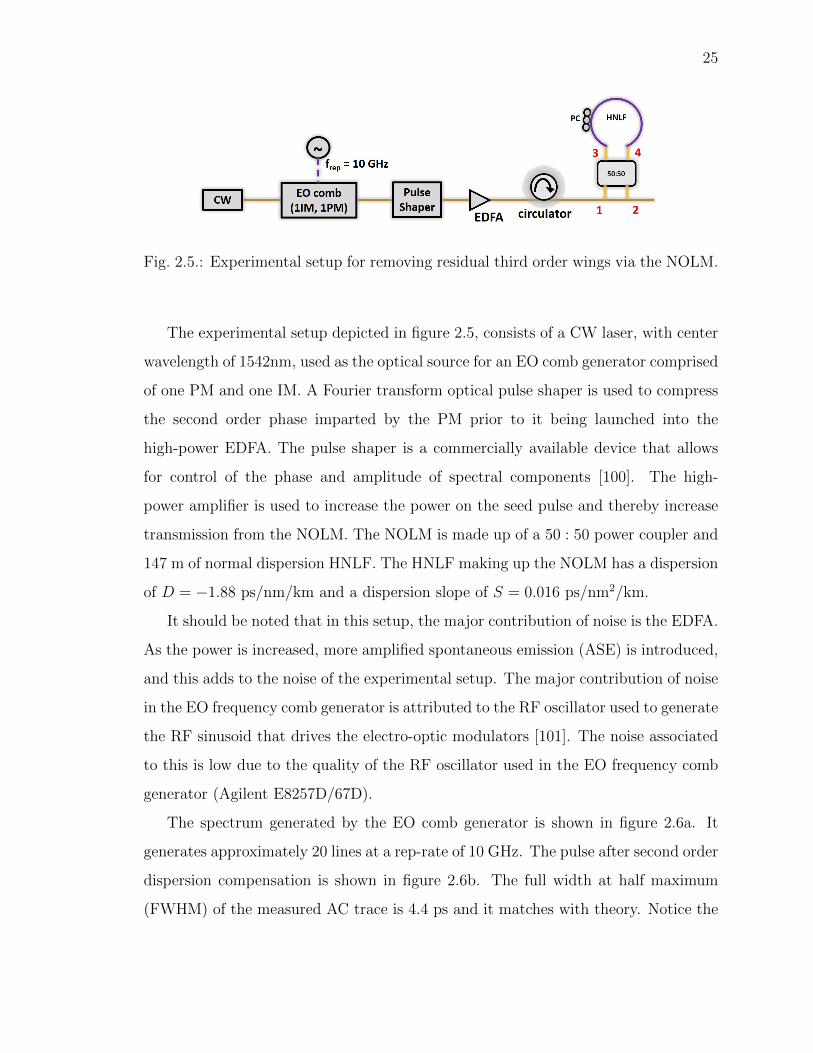
Fig. 2.5.: Experimental setup for removing residual third order wings via the NOLM.

The experimental setup depicted in figure 2.5, consists of a CW laser, with center

wavelength of 1542nm, used as the optical source for an EO comb generator comprised

of one PM and one IM. A Fourier transform optical pulse shaper is used to compress

the second order phase imparted by the PM prior to it being launched into the

high-power EDFA. The pulse shaper is a commercially available device that allows

for control of the phase and amplitude of spectral components [100]. The high-

power amplifier is used to increase the power on the seed pulse and thereby increase

transmission from the NOLM. The NOLM is made up of a 50 : 50 power coupler and

147 m of normal dispersion HNLF. The HNLF making up the NOLM has a dispersion

of D = −1.88 ps/nm/km and a dispersion slope of S = 0.016 ps/nm2/km.

It should be noted that in this setup, the major contribution of noise is the EDFA.

As the power is increased, more amplified spontaneous emission (ASE) is introduced,

and this adds to the noise of the experimental setup. The major contribution of noise

in the EO frequency comb generator is attributed to the RF oscillator used to generate

the RF sinusoid that drives the electro-optic modulators [101]. The noise associated

to this is low due to the quality of the RF oscillator used in the EO frequency comb

generator (Agilent E8257D/67D).

The spectrum generated by the EO comb generator is shown in figure 2.6a. It

generates approximately 20 lines at a rep-rate of 10 GHz. The pulse after second order

dispersion compensation is shown in figure 2.6b. The full width at half maximum

(FWHM) of the measured AC trace is 4.4 ps and it matches with theory. Notice the

26

(a) Output spectrum of EO comb generator

comprised of one IM and one PM.

(b) Comparison of measured and expected AC

trace of the compression out of EO comb gen-

erator. Only quadratic spectral phase was

compensated for.

Fig. 2.6.: (a) OFC generated from 1 IM and 1 PM. (b) Comparison of AC trace of

compressed pulse out of the EO comb generator. The compression is performed via

a Fourier transform pulse shaper. Only linear chirp is compensated for.

pronounced third order wings on the temporal profile of the pulse. The responsibility

of the NOLM will be to remove these wings.

(a) Output spectrum of NOLM (b) Corresponding time domain trace out of

the NOLM

Fig. 2.7.: (a) Spectrum out of the NOLM. (b) Corresponding time domain trace out

of the NOLM; notice the removal of the third order dispersion wings.

27

The output of the NOLM is shown in figure 2.7a. The spectrum is slightly (8 nm

wide, within 10 dB, compared to 3 nm wide at the input) broader than the input,

but it shows a slightly Gaussian profile. More importantly, the temporal profile of

the NOLM output no longer has the third order pedestals. The measured AC trace,

shown in figure 2.7b, has a FWHM of 1 ps, and this matches with the expected AC

trace. The NOLM did its job successfully.

The presented results were obtained by using one PM in the electro-optic comb

generator. The question raised is, how many PMs is too much? The thought process

is having more PMs will lead to a broader comb, as discussed in the comb generation

section of this work, and having a broader comb to begin with may facilitate broad-

ening in the long run. However, there is a concern as to how short of a pulse can be

launched into the NOLM.

The other question that arises when analyzing the setup in figure 2.5 is, will using

the pulse shaper to not only compensate for quadratic spectral phase but higher

order spectral phase affect the performance of the NOLM? The pulse shaper can

be used to ensure that the spectrum has a flat phase, i.e., all orders of spectral

phase are compensated. Will this, along with changing the number of PMs, affect the

performance of the NOLM? These are questions that were tackled with the assistance

of an undergraduate researcher, Yiyun Zhang.

2.3 Simulations of Effect of Number of Phase Modulators on Nonlinear

Optical Loop Mirror Performance

To answer these questions, simulations were done to determine what effect in-

creasing the number of PMs has on the effectiveness of the NOLM. The simulations

are based on the split step Fourier method (SSFM) [18, 19]. In its simplest form the

SSFM allows for the simulation of a pulse propagating through a fiber in which the

effects of nonlinearities and dispersion can both be included. The process by which

the simulation is performed is as follows:

28

1. The length of fiber is divided into multiple pieces of the same small length, ∆z.

2. Dispersion is applied in the frequency domain.

3. An inverse Fourier transform is performed in order to switch the simulation

domain into time.

4. Nonlinearities are applied.

5. Steps 2 through 4 are repeated for all lengths ∆z from 0 until the entire length

of the fiber is simulated.

The SSFM simulations were implemented using the open source MATLAB func-

tion ssprop, generated by the Photonics Research Laboratory of the University of

Maryland. The user generates the seed pulse and the power associated with it. In

this case the seed pulse is a simulated EO comb with either one, two, or three PMs.

The function allows the user to input the length, nonlinearity, and dispersion of the

fiber. The length of fiber that will be simulated is the HNLF making up the NOLM.

In this case it is 147 m long. The dispersion provided by the vendor — β2 and β3 —

are given in units of ps2

kmand ps3

km, respectively. The following explanation is adapted

from [18]. These parameters are the Taylor expansion coefficients of the propagation

constant β(ω). β2 contributes a quadratic spectral phase and imparts a linear chirp

on the output pulse. β3 contributes a cubic spectral phase and an asymmetric dis-

tortion on the output pulse. For most cases, these two parameters are sufficient to

describe pulse propagation in most dispersive media [18].

In the following simulations the number of PMs in the simulated EO comb gener-

ator are varied (one, two, or three). The value of phase that is compensated for prior

to the NOLM is also varied. Either only the quadratic spectral phase is compensated

for (arising from β2), or all orders of spectral phase are compensated for (arising from

β2, β3, and other orders of dispersion).

The first simulation performed is with 1 PM in the EO frequency comb generator,

figure 2.8. The results presented here are of the output spectrum of the NOLM with

29

Fig. 2.8.: Simulated spectral results of one PM and one IM. The solid spectrum

corresponds to compensating for all orders of spectral phase. And the dotted spectrum

corresponds to compensating for only quadratic spectral phase.

all orders of spectral phase compensated for (solid) and with only quadratic phase

compensated for (dashed). When the pulse shaper is only used to compensate for

the quadratic phase, there is a simulated ripple of approximately 13.3 dB. When the

pulse shaper is then used to compensate for all orders of spectral phase, the spectral

ripple is reduced to 5.5 dB. It is important to note that this is simulated ripple.

The simulations show that adding a second PM adds to the spectral ripple, see

figure 2.9. In the case when only quadratic spectral phase is compensated for, the

spectral ripple out of the NOLM is 14 dB. In the case for all orders of spectral phase

compensation, the spectral ripple is reduced to 7 dB.

The final configuration that was tested was the EO comb generator with 3 PMs,

see figure 2.10. With only quadratic spectral phase accounted for, the spectral ripple

out of the NOLM is 10.6 dB. With all orders of spectral phase accounted for, the

NOLM output has 12.5 dB of spectral ripple.

The summary of simulation results is presented in figure 2.11. The main point

of the simulation results is that the more PMs used in the EO comb, the worse the

30

Fig. 2.9.: Simulated spectral results of two PMs and one IM. The two different spec-

tra correspond to either compensation of all orders of spectral phase (solid) or only

quadratic spectral phase compensation (dotted).

Fig. 2.10.: Simulated spectral results of three PMs and one IM. The two different

spectra correspond to either compensation of all orders of spectral phase (solid) or

only quadratic spectral phase compensation (dotted).

spectral ripple out of the NOLM is. There is no clear indication as to why this is.

31

Fig. 2.11.: Summary of simulation results. The lowest spectral ripple is from using

only one PM. However, two PMs seems like a good compromise for low ripple and

broad spectrum.

The two fiber parameters of the HNLF in the NOLM used in the simulations are

dispersion and nonlinearity, and they remain the same for every simulation.

However, it is clear that using one or two PMs still meets the goal of this work.

To reiterate, the goal is to achieve a broadened spectrum with spectral ripple less

than 10 dB. Therefore, in the next section, an EO comb generator with two PMs and

a NOLM will be used to characterize single-soliton Kerr combs generated in silicon

nitride microring resonators.

Acknowledgement of Collaboration

The work on the construction and characterization of the NOLM was performed

by the author of the document. The simulations were a collaboration between the

author and an undergraduate researcher, Yiyun Zhang.

32

3. CHARACTERIZATION OF SINGLE-SOLITON KERR

COMBS VIA DUAL COMB ELECTRIC FIELD

CROSS-CORRELATION

In the previous chapter, it was shown that the NOLM can be used to remove third

order dispersion wings associated with spectral ripple formation. In this chapter, the

NOLM will be employed to generate a frequency comb with spectral ripple less than

10 dB and with a bandwidth of 40 nm. This comb will be used to retrieve the phase

of a single-soliton Kerr comb generated in an anomalous dispersion silicon nitride

microresonator. The phase is retrieved via dual comb interferometry via electric-field

cross-correlation. The single-soliton Kerr comb is sampled via the drop-port of the

silicon nitride microresonator, allowing for access to a direct replica of the intracav-

ity pump field. The single-soliton Kerr comb inherently offers high repetition-rates

and low power. This makes it difficult and time consuming to characterize the pulse

via typical measurement techniques that require high pulse energies due to the mea-

surements relying on optical nonlinearities. The dual comb interferometry technique

presented in this chapter is an all-linear method allowing for rapid (µs) phase re-

trieval of a low power (20 µW) soliton Kerr comb. The measurement technique relies

on the spectral broadening of an EO comb and the pre-characterization of its spectral

phase. The methods for performing these tasks are presented in this chapter. First,

an explanation of soliton formation in microresonators is presented, as well as an ex-

planation of the measurement technique. The results presented in this chapter have

been adapted from the various publications this work has appeared in [102,103].

33

3.1 Achieving Mode-Locking in Microresonators

There exist two routes to frequency comb generation [57, 59, 104]. The combs

generated by these two different routes are differentiated by either type I or type II

classification.

The type I comb is characterized by being less noisy during the generation pro-

cess and offers coherent comb generation. Its counterpart, the type II comb, is noisier

during the generation process and suffers from degraded coherence. This reduced co-

herence is attributed to the imperfect frequency division process of the non-degenerate

FWM involved in the comb generation. However, this does not mean that type II

combs are of no value. In the following section, the generation of mode-locked pulses

(solitons) from these type II combs will be discussed.

3.1.1 Bright soliton formation in anomalous dispersion microresonators

Studies have been performed on generating short coherent pulses in microres-

onators from type I and type II combs, [57], in both normal [54], and anoma-

lous [105, 106] dispersion cavities. In anomalous dispersion cavities, several works

have shown the possibility of passively mode-locked combs analogous to soliton for-

mation [105–110]. Solitons in optical fibers in the anomalous dispersion regime are

pulses that can propagate without distortion under the joint effect of nonlinearity

and dispersion [18]. The solitons formed inside the microresonator cavities are known

as dissipative solitons, due to their reliance on the Kerr effect and the continual out-

coupling. These are formed from the balance of cavity dispersion and nonlinearity,

and input power and cavity loss. This balance leads to a broad bandwidth and low-

noise comb operation [111]. It is important to note that these mode-locked like pulses

are generated from the chaotic type II comb. Soliton formation has been theoreti-

cally presented via simulations employing the standard Lugiato-Lefever model [112].

Solitons are one of many possible solutions to the Lugiato-Lefever equation.

34

The first demonstration of solitons in anomalous dispersion microresonators was

published in 2014 [106]. In this work, correlations between the mode-locked generation

and the transmission spectra and response of comb power were presented, see figure

3.1.

Fig. 3.1.: The signature of soliton generation. The transitions from a noisy chaotic

state to N solitons. Further red detuning eventually leads to the single soliton regime

[106].

As the wavelength of the pump is tuned from blue to red, more light is coupled

into the cavity, and there is an increase in intra-cavity power. This increase in power

leads to a modification of the refractive index in the resonator, which then leads to

modification of the cavity resonance. This modified resonance has a high and low

energy state, the high energy state being the state that produces soliton formation.

With this increasing power, primary sidebands and then secondary sidebands are

generated via the cascaded FWM process. Continuing to increase the intra-cavity

power leads to an important occurrence, an abrupt jump to a minimal fluctuations

state in the optical power. Further pushing the pump detuning to the red causes the

cavity to step through further drops in the intra-cavity power. These steps are the

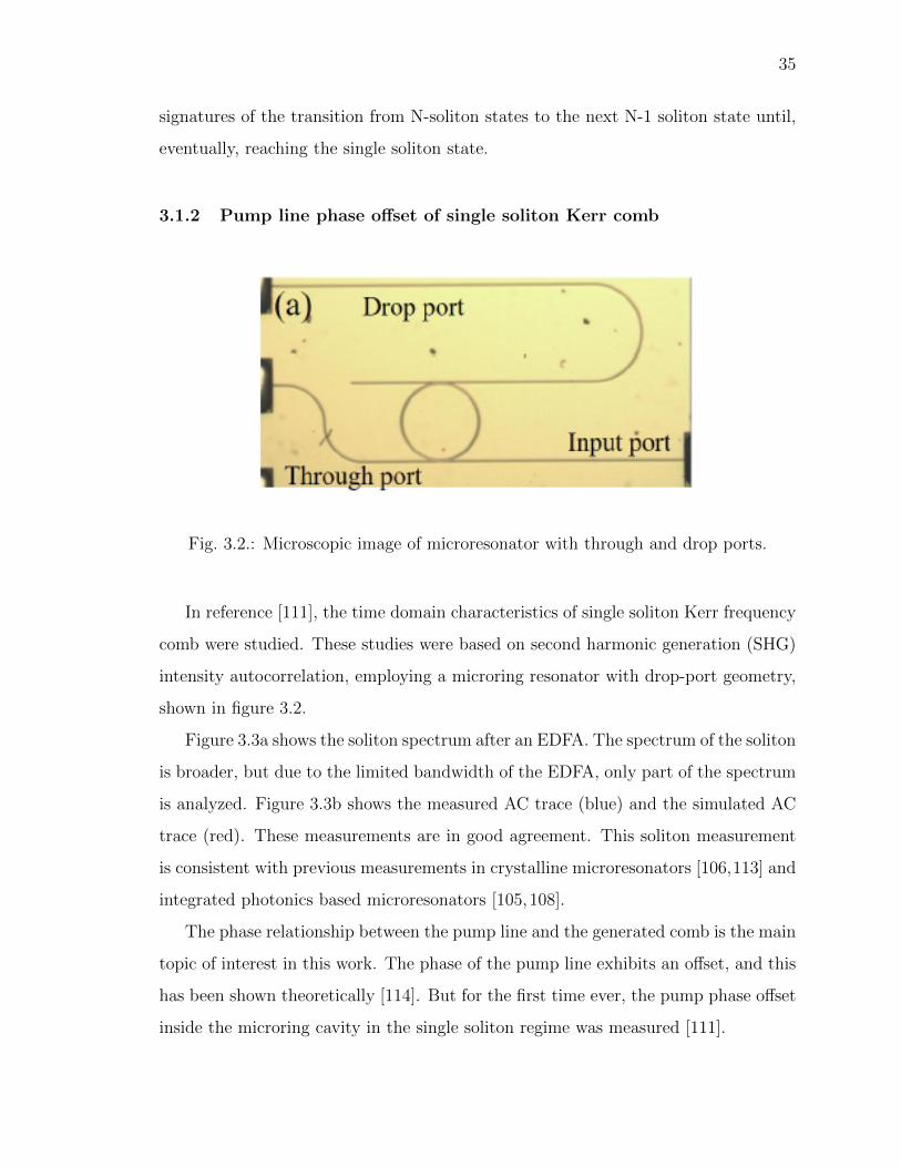
35

signatures of the transition from N-soliton states to the next N-1 soliton state until,

eventually, reaching the single soliton state.

3.1.2 Pump line phase offset of single soliton Kerr comb

Fig. 3.2.: Microscopic image of microresonator with through and drop ports.

In reference [111], the time domain characteristics of single soliton Kerr frequency

comb were studied. These studies were based on second harmonic generation (SHG)

intensity autocorrelation, employing a microring resonator with drop-port geometry,

shown in figure 3.2.

Figure 3.3a shows the soliton spectrum after an EDFA. The spectrum of the soliton

is broader, but due to the limited bandwidth of the EDFA, only part of the spectrum

is analyzed. Figure 3.3b shows the measured AC trace (blue) and the simulated AC

trace (red). These measurements are in good agreement. This soliton measurement

is consistent with previous measurements in crystalline microresonators [106,113] and

integrated photonics based microresonators [105,108].

The phase relationship between the pump line and the generated comb is the main

topic of interest in this work. The phase of the pump line exhibits an offset, and this

has been shown theoretically [114]. But for the first time ever, the pump phase offset

inside the microring cavity in the single soliton regime was measured [111].

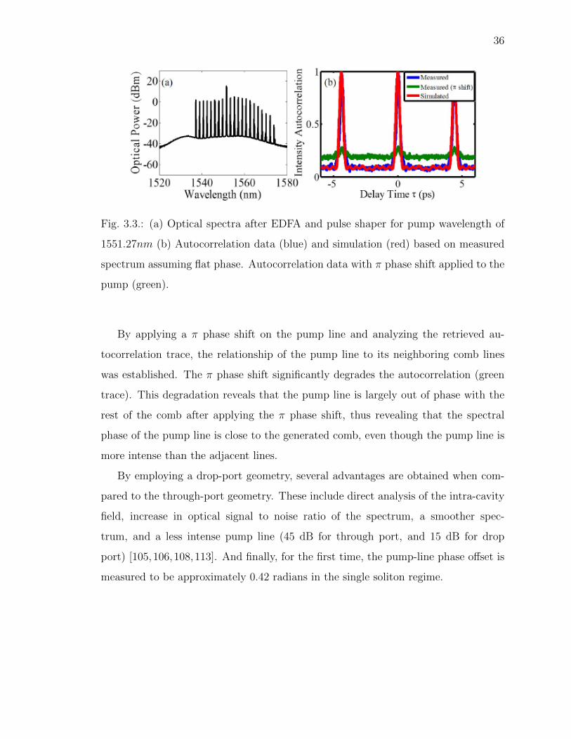
36

Fig. 3.3.: (a) Optical spectra after EDFA and pulse shaper for pump wavelength of

1551.27nm (b) Autocorrelation data (blue) and simulation (red) based on measured

spectrum assuming flat phase. Autocorrelation data with π phase shift applied to the

pump (green).

By applying a π phase shift on the pump line and analyzing the retrieved au-

tocorrelation trace, the relationship of the pump line to its neighboring comb lines

was established. The π phase shift significantly degrades the autocorrelation (green

trace). This degradation reveals that the pump line is largely out of phase with the

rest of the comb after applying the π phase shift, thus revealing that the spectral

phase of the pump line is close to the generated comb, even though the pump line is

more intense than the adjacent lines.

By employing a drop-port geometry, several advantages are obtained when com-

pared to the through-port geometry. These include direct analysis of the intra-cavity

field, increase in optical signal to noise ratio of the spectrum, a smoother spec-

trum, and a less intense pump line (45 dB for through port, and 15 dB for drop

port) [105,106,108,113]. And finally, for the first time, the pump-line phase offset is

measured to be approximately 0.42 radians in the single soliton regime.

37

3.2 Dual Comb Electric Field Cross-Correlation Measurement for Study

on Pump Line Phase Offset in Soliton Kerr Combs

As was detailed in the previous section, the pump line phase offset was demon-

strated experimentally via intensity SHG autocorrelation [111]. This measurement

corroborated the theoretical model that predicted this phase offset [114].

These measurements provide the basis for a new method. The SHG pump phase

offset measurements, although informative, were difficult to implement. This is be-

cause conventional methods of characterizing the phase profile of ultrafast pulses often

rely on optical nonlinearity and thus, these methods usually apply to optical wave-

forms that have relatively high peak power and low duty cycle. In the case of Kerr

combs, or solitons generated in microresonators, these waveforms are often character-

ized by low average power and very high repetition-rates, making them difficult to be

characterized via conventional methods. A new method for characterizing the phase

profile of low average power and high repetition-rate waveforms is presented [102,103].

This new method allows for all linear phase retrieval of Kerr solitons through a tech-

nique called dual comb electric field cross-correlation (EFXC), which reduces the

demand on signal power and offers rapid data acquisition. The first iteration of this

new technique was used to characterize the phase profile of Kerr solitons, and was

demonstrated at CLEO 2018 [102]. After fine tuning the setup and paying closer at-

tention to the noise associated with the measurement technique, the second iteration

was published in reference [103] and is the focus of this chapter. This new measure-

ment technique is closely related to the dual comb EFXC demonstrated in [70] for

the characterization of optical arbitrary waveforms.

3.2.1 Dual comb interferometry via electric field cross-correlation

The dual comb EFXC technique allows for the independent sweeping of phase and

group delays without any mechanical stages. Spectral phase can be retrieved from

38

the data acquired in tens of microseconds [70]. This method is related to absorption

measurements in [73], and in linear optical sampling in [61].

The following introduction to EFXC was adopted from [18, 70]. EFXC measures

the interference between two fields: a signal field as, the field that is to be measured,

and a reference field ar. These fields are interfered in the time domain as a function

of relative delay, τ . Traditionally, the delay is swept using a mechanical stage.

〈Po (τ)〉 =1

2

[Us + Ur +

∫ {as (t) a∗r (t− τ) ejωoτ + c.c.

}dt

](3.1)

Equation 3.1 is the expression for the resulting time-average power obtained at

the output of a slow photo-detector as a function of delay [18]. In this expression,

Us and Ur are the pulse energies, and ωo is the carrier frequency. The point to

emphasize is that an unknown signal pulse can be fully recovered from a known and

well-characterized reference pulse [70].

In the dual comb EFXC scheme, two frequency combs with a difference in repe-

tition rate, ∆frep, are used. This ∆frep causes the two pulses to walk through each

other in time 1∆frep

. By controlling the difference in rep-rate, the group-delay sweep

can be controlled. To control the phase-delay sweep, the difference in center frequen-

cies, ∆fcenter, can also be swept, thus being able to control the group and phase-delay

independently.

In the spectral domain, the conventional EFXC time average power can be re-

trieved by performing a Fourier transform on equation 3.1.

F [〈Po (τ)〉] = ...+1

2{As (ω − ωo)A∗

r (ω − ωo) + A∗s (−ω − ωo)Ar (−ω − ωo)} (3.2)

In equation 3.2, the non-interferometric terms are omitted. In this implementation

the first and second terms inside the brackets correspond to +∆fcenter and −∆fcenter,

respectively. In the analysis, only the +∆fcenter is considered. This corresponds to

a series of RF comb lines that are separated by ∆frep. These discrete lines, referred

to as the RF comb from now on, demonstrate the preservation of phase coherence.

39

From this RF comb, the phase of the signal comb can be retrieved. To do so, the

reference comb must be pre-characterized. In this work, a pulse shaper is used to

phase compensate individual frequency components [23] and thus obtain a transform

limited pulse, i.e., flat spectral phase. The RF comb is retrieved by performing

a Fourier transform on the photo-detected signal. The phase is then extracted by

performing post processing.

Particulars of the dual comb interferometry measurements

(a) Generalized setup for dual comb EFXC

measurement.

(b) (top) Beating of two combs in the optical

domain, (bottom) leading to an RF comb after

photo-detection. There is a mirrored version

of the RF comb that is omitted for simplicity.

Fig. 3.4.: Cartoons depicting the (a) setup and (b) spectra of the dual comb EFXC.

The generalized experimental setup for the dual comb EFXC measurements is

shown in figure 3.4a. The reference and signal combs are interfered in a 50 : 50

coupler and then detected by a balanced photo-detector (BPD). The signal out of the

BPD is detected in an oscilloscope, and post processing allows for the retrieval of the

phase of the signal comb. In these experiments, the reference comb is an EO comb

spectrally broadened with the aid of a nonlinear optical loop mirror (NOLM). The

reference comb is characterized via line-by-line pulse shaping, analogous to [57].

40

Figure 3.4b depicts the optical to RF mapping of the dual comb EFXC technique.

This figure is analogous to figure 1.6a, except in this measurement there is no absorp-

tion as spectroscopy is not the goal of this work, waveform reconstruction is. The

signal comb (blue), with rep-rate fsig, is beat with a reference comb (green) having a

rep-rate of fref. The beating occurs in the 50 : 50 coupler, and this beating is mapped

onto the RF domain. This RF comb is separated by ∆frep, the difference in rep-rate

between the two combs.

IRF ∝ EsigErefcos [(ωsig − ωref) t+ ϕsig − ϕref] (3.3)

The current, for one particular set of reference and signal comb lines, out of the

BPD is expressed in equation 3.3. ωsig and ωref correspond to the angular frequency

of the signal and reference comb line, respectively. One important note that is not

pictured in figure 3.4b is that the difference in carrier frequencies, ∆fcenter, of the two

combs determines where in the RF domain the RF comb is mapped to.

ϕRF = ϕsig − ϕref (3.4)

The phase of the RF comb is expressed in equation 3.4, and it is the difference

between the signal phase and reference phase. By characterizing the reference comb

to have flat spectral phase i.e., ϕref = 0, the RF phase is then simply ϕRF = ϕsig.

This allows the phase of the signal comb to be reconstructed by finding the phase of

the RF comb.

3.2.2 Signal comb - single-soliton Kerr comb sampled through drop port

of silicon nitride microresonator

The signal comb is a Kerr soliton generated from a silicon nitride microresonator

(radius 100 µm and loaded-Q 2.4 million), depicted in figure 3.5. The ring resonator

employs drop-port geometry, allowing for the direct sampling of the intra-cavity field

and avoids interference from the strong pump line [111]. The spectrum has a secant

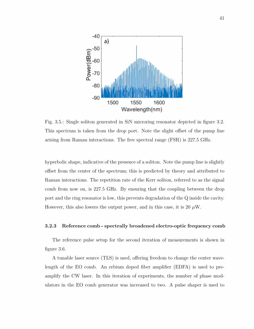
41

Fig. 3.5.: Single soliton generated in SiN microring resonator depicted in figure 3.2.

This spectrum is taken from the drop port. Note the slight offset of the pump line

arising from Raman interactions. The free spectral range (FSR) is 227.5 GHz.

hyperbolic shape, indicative of the presence of a soliton. Note the pump line is slightly

offset from the center of the spectrum; this is predicted by theory and attributed to

Raman interactions. The repetition rate of the Kerr soliton, referred to as the signal

comb from now on, is 227.5 GHz. By ensuring that the coupling between the drop

port and the ring resonator is low, this prevents degradation of the Q inside the cavity.

However, this also lowers the output power, and in this case, it is 20 µW.

3.2.3 Reference comb - spectrally broadened electro-optic frequency comb

The reference pulse setup for the second iteration of measurements is shown in

figure 3.6.

A tunable laser source (TLS) is used, offering freedom to change the center wave-

length of the EO comb. An erbium doped fiber amplifier (EDFA) is used to pre-

amplify the CW laser. In this iteration of experiments, the number of phase mod-

ulators in the EO comb generator was increased to two. A pulse shaper is used to

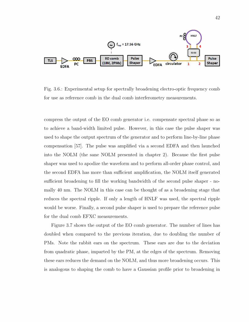
42

Fig. 3.6.: Experimental setup for spectrally broadening electro-optic frequency comb

for use as reference comb in the dual comb interferometry measurements.

compress the output of the EO comb generator i.e. compensate spectral phase so as

to achieve a band-width limited pulse. However, in this case the pulse shaper was

used to shape the output spectrum of the generator and to perform line-by-line phase

compensation [57]. The pulse was amplified via a second EDFA and then launched

into the NOLM (the sane NOLM presented in chapter 2). Because the first pulse

shaper was used to apodize the waveform and to perform all-order phase control, and

the second EDFA has more than sufficient amplification, the NOLM itself generated

sufficient broadening to fill the working bandwidth of the second pulse shaper - no-

mally 40 nm. The NOLM in this case can be thought of as a broadening stage that

reduces the spectral ripple. If only a length of HNLF was used, the spectral ripple

would be worse. Finally, a second pulse shaper is used to prepare the reference pulse

for the dual comb EFXC measurements.

Figure 3.7 shows the output of the EO comb generator. The number of lines has

doubled when compared to the previous iteration, due to doubling the number of

PMs. Note the rabbit ears on the spectrum. These ears are due to the deviation

from quadratic phase, imparted by the PM, at the edges of the spectrum. Removing

these ears reduces the demand on the NOLM, and thus more broadening occurs. This

is analogous to shaping the comb to have a Gaussian profile prior to broadening in

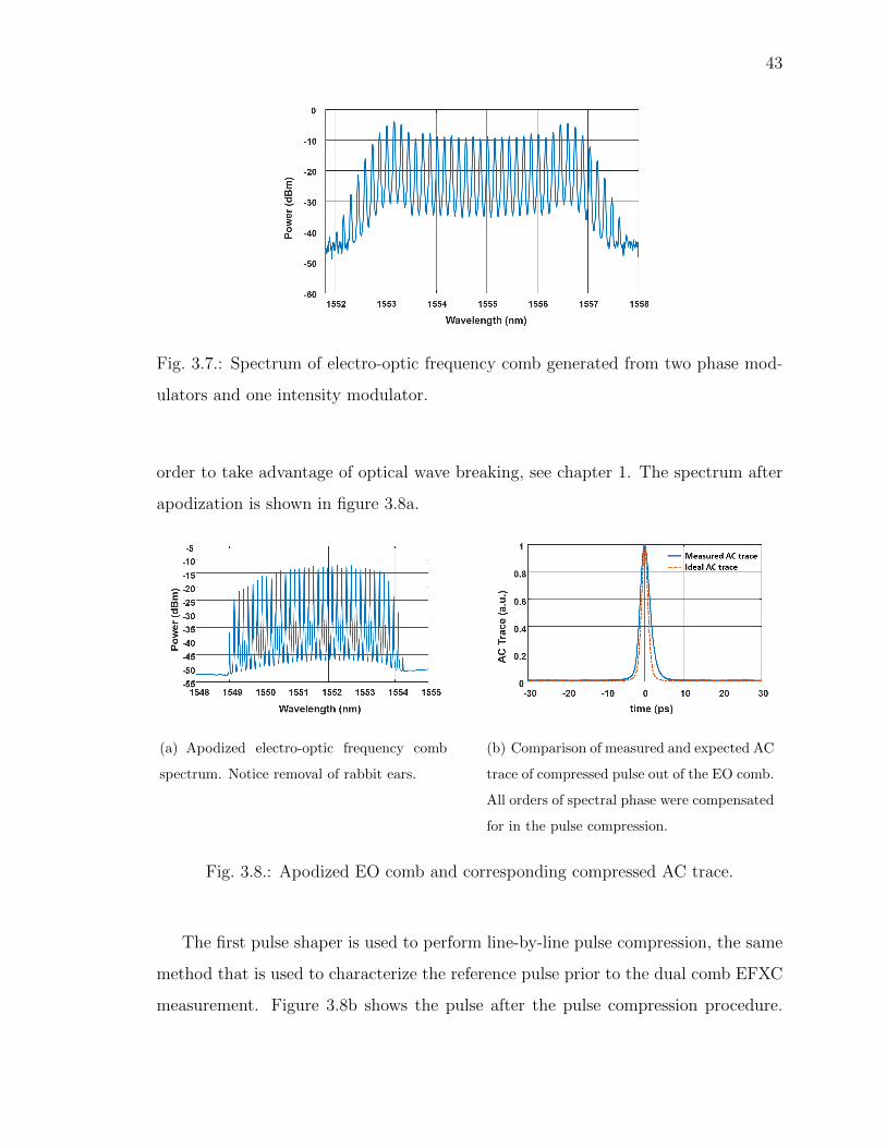
43

Fig. 3.7.: Spectrum of electro-optic frequency comb generated from two phase mod-

ulators and one intensity modulator.

order to take advantage of optical wave breaking, see chapter 1. The spectrum after

apodization is shown in figure 3.8a.

(a) Apodized electro-optic frequency comb

spectrum. Notice removal of rabbit ears.

(b) Comparison of measured and expected AC

trace of compressed pulse out of the EO comb.

All orders of spectral phase were compensated

for in the pulse compression.

Fig. 3.8.: Apodized EO comb and corresponding compressed AC trace.

The first pulse shaper is used to perform line-by-line pulse compression, the same

method that is used to characterize the reference pulse prior to the dual comb EFXC

measurement. Figure 3.8b shows the pulse after the pulse compression procedure.

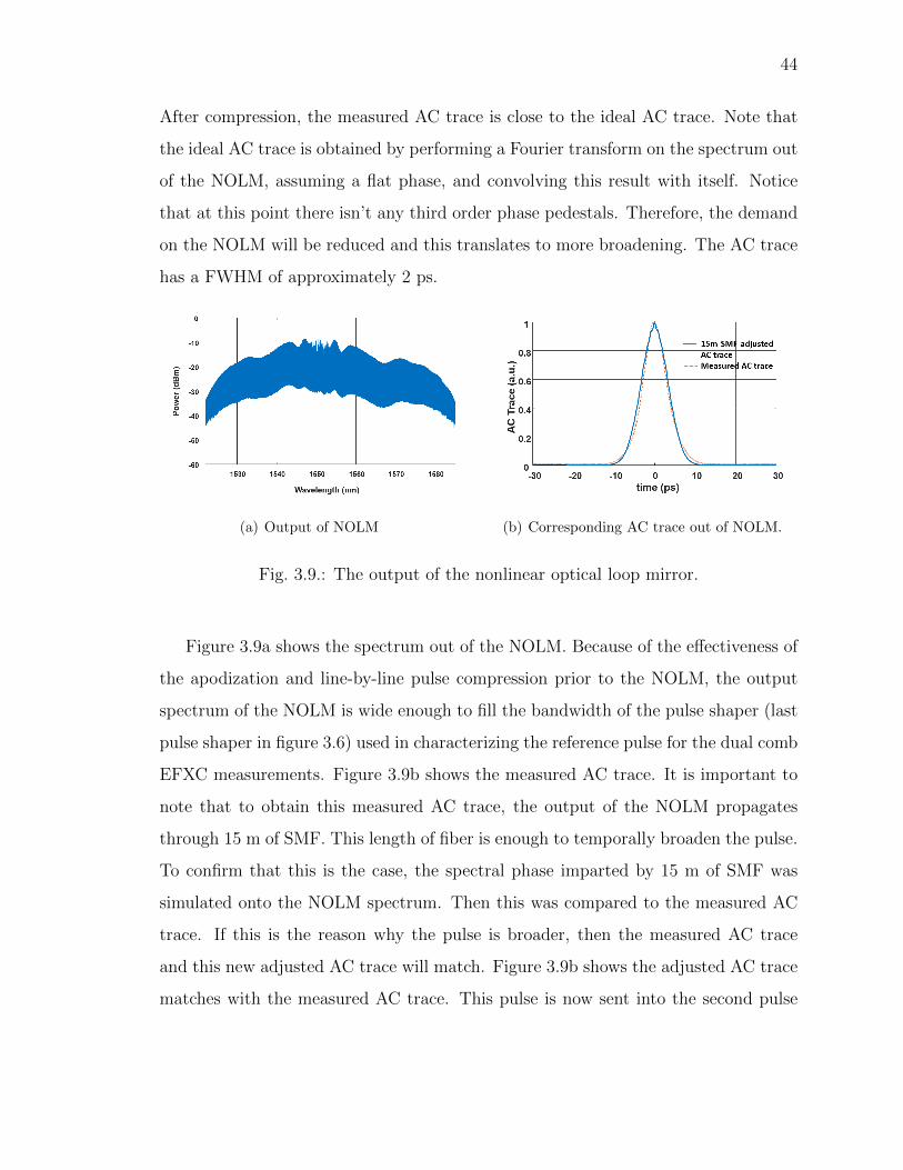
44

After compression, the measured AC trace is close to the ideal AC trace. Note that

the ideal AC trace is obtained by performing a Fourier transform on the spectrum out

of the NOLM, assuming a flat phase, and convolving this result with itself. Notice

that at this point there isn’t any third order phase pedestals. Therefore, the demand

on the NOLM will be reduced and this translates to more broadening. The AC trace

has a FWHM of approximately 2 ps.

(a) Output of NOLM (b) Corresponding AC trace out of NOLM.

Fig. 3.9.: The output of the nonlinear optical loop mirror.

Figure 3.9a shows the spectrum out of the NOLM. Because of the effectiveness of

the apodization and line-by-line pulse compression prior to the NOLM, the output

spectrum of the NOLM is wide enough to fill the bandwidth of the pulse shaper (last

pulse shaper in figure 3.6) used in characterizing the reference pulse for the dual comb

EFXC measurements. Figure 3.9b shows the measured AC trace. It is important to

note that to obtain this measured AC trace, the output of the NOLM propagates

through 15 m of SMF. This length of fiber is enough to temporally broaden the pulse.

To confirm that this is the case, the spectral phase imparted by 15 m of SMF was

simulated onto the NOLM spectrum. Then this was compared to the measured AC

trace. If this is the reason why the pulse is broader, then the measured AC trace

and this new adjusted AC trace will match. Figure 3.9b shows the adjusted AC trace

matches with the measured AC trace. This pulse is now sent into the second pulse

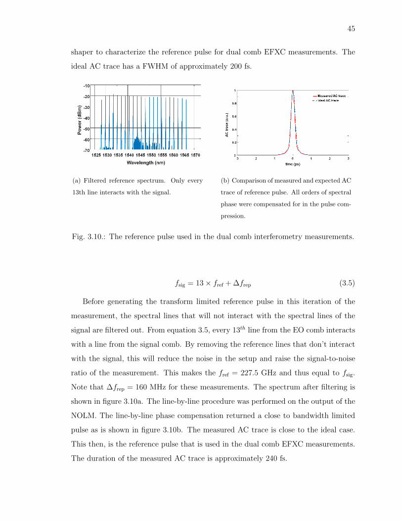
45

shaper to characterize the reference pulse for dual comb EFXC measurements. The

ideal AC trace has a FWHM of approximately 200 fs.

(a) Filtered reference spectrum. Only every

13th line interacts with the signal.

(b) Comparison of measured and expected AC

trace of reference pulse. All orders of spectral

phase were compensated for in the pulse com-

pression.

Fig. 3.10.: The reference pulse used in the dual comb interferometry measurements.

fsig = 13× fref + ∆frep (3.5)

Before generating the transform limited reference pulse in this iteration of the

measurement, the spectral lines that will not interact with the spectral lines of the

signal are filtered out. From equation 3.5, every 13th line from the EO comb interacts

with a line from the signal comb. By removing the reference lines that don’t interact

with the signal, this will reduce the noise in the setup and raise the signal-to-noise

ratio of the measurement. This makes the fref = 227.5 GHz and thus equal to fsig.

Note that ∆frep = 160 MHz for these measurements. The spectrum after filtering is

shown in figure 3.10a. The line-by-line procedure was performed on the output of the

NOLM. The line-by-line phase compensation returned a close to bandwidth limited

pulse as is shown in figure 3.10b. The measured AC trace is close to the ideal case.

This then, is the reference pulse that is used in the dual comb EFXC measurements.

The duration of the measured AC trace is approximately 240 fs.

46

3.2.4 Retrieving phase of single-soliton Kerr comb via dual comb intefer-

ometry

Fig. 3.11.: The experimental setup for performing dual comb interferometry for char-

acterization of single-soliton Kerr-comb [103].

The experimental setup for performing the dual comb interferometry measurement

(dual comb EFXC)is depicted in figure 3.11 [103]. The dual comb interferometry

is performed with signal comb power of 20 µW and a reference comb power of 1

mW. The resulting interferogram is detected with a balanced photo detector with 20

GHz bandwidth and it is recorded with a digital serial analyzer with 20 GHz analog

bandwidth and 12.5 Gs/s sampling rate. The 20 ns sample of the interferogram is

shown in figure 3.12a [103]. Due to the dispersion of the 7.5 m of fiber needed to send

the Kerr comb from the output of the drop port to the 50 : 50 coupler, depicted in

figure 3.11, the soliton contributions broaden and blend due to the dispersion and are

not clearly visible. However, this dispersion effect does not prevent an RF comb from

being visualized. By performing a Fourier transform on the entire 3.2 µs duration

interferogram the RF comb’s power spectrum is shown in figure 3.12c. The RF comb

power spectrum shows 23 lines, which corresponds to an optical bandwidth of 5 THz,

47

limited to the passband of the second pulse shaper used in the compression of the

broadened reference comb. The RF comb line corresponding to the pump line of the

Kerr comb has an SNR exceeding 40 dB, while the other lines have SNRs ranging

between 17 and 30 dB.

Fig. 3.12.: (a) A portion of the measured time domain interferogram. (b) The re-

constructed interferogram after compensating for fiber dispersion. The dashed box

in (a) and (b) represent one period of the interferogram and the orange lines are the

envelope of the interferogram. (c) The blue trace is the power spectrum of the inter-

ferogram. The orange trace is the retrieved phase of the different optical modes. The

pump line exhibits a phase offset. The inset in (c) is the reconstructed intracavity

waveform using the retrieved comb phase [103].

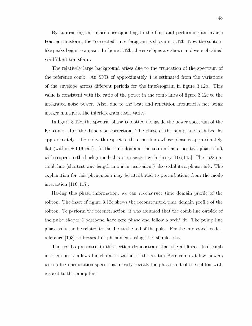
48

By subtracting the phase corresponding to the fiber and performing an inverse

Fourier transform, the “corrected” interferogram is shown in 3.12b. Now the soliton-

like peaks begin to appear. In figure 3.12b, the envelopes are shown and were obtained

via Hilbert transform.

The relatively large background arises due to the truncation of the spectrum of

the reference comb. An SNR of approximately 4 is estimated from the variations

of the envelope across different periods for the inteferogram in figure 3.12b. This

value is consistent with the ratio of the power in the comb lines of figure 3.12c to the

integrated noise power. Also, due to the beat and repetition frequencies not being

integer multiples, the interferogram itself varies.

In figure 3.12c, the spectral phase is plotted alongside the power spectrum of the

RF comb, after the dispersion correction. The phase of the pump line is shifted by

approximately −1.8 rad with respect to the other lines whose phase is approximately

flat (within ±0.19 rad). In the time domain, the soliton has a positive phase shift

with respect to the background; this is consistent with theory [106,115]. The 1528 nm

comb line (shortest wavelength in our measurement) also exhibits a phase shift. The

explanation for this phenomena may be attributed to perturbations from the mode

interaction [116,117].

Having this phase information, we can reconstruct time domain profile of the

soliton. The inset of figure 3.12c shows the reconstructed time domain profile of the

soliton. To perform the reconstruction, it was assumed that the comb line outside of

the pulse shaper 2 passband have zero phase and follow a sech2 fit. The pump line

phase shift can be related to the dip at the tail of the pulse. For the interested reader,

reference [103] addresses this phenomena using LLE simulations.

The results presented in this section demonstrate that the all-linear dual comb

interferometry allows for characterization of the soliton Kerr comb at low powers

with a high acquisition speed that clearly reveals the phase shift of the soliton with

respect to the pump line.

49

3.2.5 Study on pump line phase offset of single-soliton Kerr comb

Due to the rapid nature of the measurement, it allows for the study of the depen-

dence of the pump phase offset on pumping conditions. Measurements of the pump

line phase offset are of interest as they will allow for understanding the time domain

characteristics of the single-soliton Kerr comb. The inset in figure 3.12c, shows the

reconstructed time profile of the single-soliton in the cavity. Note that there is a

background level of -20 dB (or approximately 1 %). The intracavity field can be

thought of as a superposition of two components; a CW background resulting from

pump light being continually coupled into the cavity and the soliton state [106]. This

is different than the soliton in optical fiber, in that the time domain profile of the

fiber soliton does not have this CW background [18]. Performing the study on the

pump lime phase offset allows for better understanding of the time domain profile of

the cavity soliton under different pumping conditions.

By averaging the retrieved phase of 100 independently captured interferograms,

the pump phase offset at a given pumping condition can be measured. The measure-

ment results are shown in figure 3.13 for on-chip pump powers of 350 and 400 mW for

the full range of wavelengths at which a stable single soliton can be generated. The

error bars are 0.08 rad and are taken from the standard deviation among retrieved

phase with linear and constant terms removed.

When the pump power is fixed at 400 mW, the phase offset is observed to change

from −1.8 rad to −1.2 rad as the pump wavelength is increased. The magnitude

of the pump phase offset is larger as the pump power is increased. From the power

spectrum of the Kerr comb and the data of the pump phase offset study, the time

domain behavior can be estimated.

By using the power spectra and the pump phase offsets, the behavior of the

soliton in the time domain can be estimated. The ratio of the soliton peak power

to the background increases from 100 at small detuning by a factor of two as the

detuning is increased. The soliton phase with respect to the background is positive

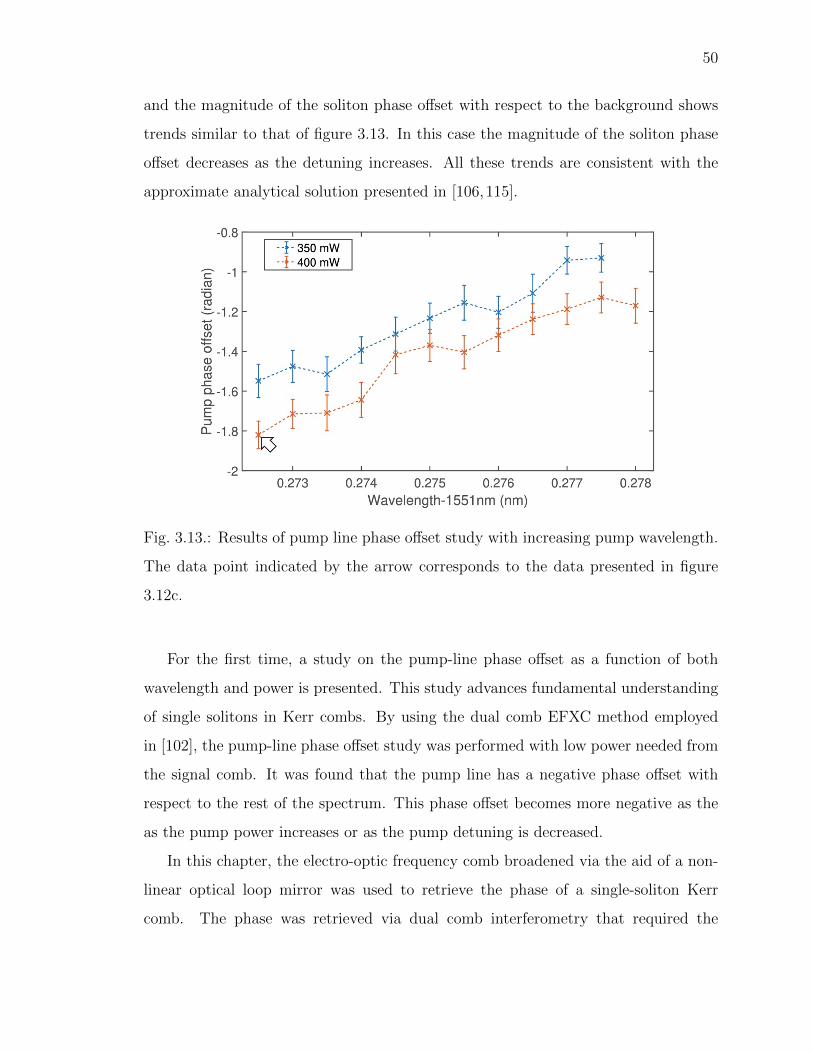
50

and the magnitude of the soliton phase offset with respect to the background shows

trends similar to that of figure 3.13. In this case the magnitude of the soliton phase

offset decreases as the detuning increases. All these trends are consistent with the

approximate analytical solution presented in [106,115].

Fig. 3.13.: Results of pump line phase offset study with increasing pump wavelength.

The data point indicated by the arrow corresponds to the data presented in figure

3.12c.

For the first time, a study on the pump-line phase offset as a function of both

wavelength and power is presented. This study advances fundamental understanding

of single solitons in Kerr combs. By using the dual comb EFXC method employed

in [102], the pump-line phase offset study was performed with low power needed from

the signal comb. It was found that the pump line has a negative phase offset with

respect to the rest of the spectrum. This phase offset becomes more negative as the

as the pump power increases or as the pump detuning is decreased.

In this chapter, the electro-optic frequency comb broadened via the aid of a non-

linear optical loop mirror was used to retrieve the phase of a single-soliton Kerr

comb. The phase was retrieved via dual comb interferometry that required the

51

pre-characterization of the phase of the spectrally broadened electro-optic frequency

comb. The broadening and pre-characterization techniques were presented. The re-

sults of the dual comb interferometry measurements show that the pump line has a

negative phase offset with respect to the rest of the spectrum that becomes more neg-

ative as the pump power is increased or pump-detuning is decreased. This measure-

ment technique allows for the rapid characterization of waveforms with high repetition

rates and low power.

Acknowledgement of Collaboration

The author was tasked with providing and characterizing the broadened reference

comb. Bohao Liu was responsible for the preparation of the reference pulse i.e., ensur-

ing a flat spectral phase. Ziyun Kong and Chengying Bao are the leads of the project

and their responsibility was the oversight of the collaboration. Specifically, Ziyun

was tasked with the retrieval of the phase and pumpline phase offset, and Chengying

generated the single soliton for the work presented in [102]. Jose Jaramillo and Cong

Wang were responsible for the generation of the single soliton in the pumpline phase

offset study.

52

4. POLARIZATION DIVERSITY PHASE MODULATOR

FOR MEASURING FREQUENCY-BIN

ENTANGLEMENT OF BI-PHOTON FREQUENCY

COMBS IN A DEPOLARIZED CHANNEL

In this chapter the polarization diversity phase modulator (PDPM) is introduced.

This device allows for phase modulation to be performed, irrespective of the polariza-

tion state of input light, thus allowing for the circumvention of the inherent problem

of commercial electro-optic phase modulators being polarization dependent. The ul-

timate goal is to create a quantum network based on current optical fiber technology,

and be able to show frequency-bin entanglement and distribute entanglement over

fiber. However, as light propagates through the fiber, its polarization will scramble,

making it detrimental to use commercial electro-optic phase modulators for the pur-

pose of showing and distributing entanglement in optical fiber. In this chapter, the

effectiveness of the PDPM in performing polarization independent phase modulation

with classical light and entangled photons is demonstrated. In the case of entangled

photons (biphotons) in the frequency degree of freedom, the PDPM is used in projec-

tive measurements to prove the entanglement in a specific biphoton state known as

the biphoton frequency comb (BFC). The robustness of the PDPM is demonstrated

by showing that the efficiency at which the projective measurements are carried out is

unaffected by the polarization state of the entangled photons. Finally, the results of

actively stabilizing the PDPM are shown, ensuring that the polarization of the light

exiting the PDPM is stable. The work presented in this chapter was adapted from

the various publications this work has appeared in [118–120].

53

4.1 Motivation

Entanglement in the frequency degree of freedom is compatible with modern fiber-

optic networks but has largely been untapped as a resource for quantum commu-

nication. Recently, our colleagues at the Oakridge National Laboratory outlined

ways to perform quantum information processing in the spectral domain using only

Fourier transform pulse shapers and phase modulators (PMs) [121]. Although the

spectral domain has been widely untapped for entanglement preparation, it is cho-

sen for its compatibility with standard telecommunication equipment, compatibility

with current fiber optic technology, and for its robustness against noise in fiber prop-

agation [122]. Fourier transform pulse shapers are used to act on each frequency

individually and the electro-optic phase modulators are used to move the photons

across different frequencies. Colleagues at the US Army Research Laboratory (ARL)

want to harness the power of hyperentanglement (entanglement in more than one

degree of freedom) in the frequency and polarization degrees of freedom in order to

achieve the ultimate goal of a quantum network based on current optical fiber tech-

nology. Polarization-entangled photons are a popular choice for quantum networking

protocols owing to their compatibility with standard telecommunications equipment.

Recently, on-chip microresonators have been shown to be an excellent source for

generating frequency-bin entangled photon pairs [91,92]. One state that is of partic-

ular interest is the biphoton frequency comb (BFC) which is a coherent superposition

state of N-energy matched comb line pairs. The general state of the BFC can be

written as equation 4.1, αk is a complex number that represents the joint amplitude

and joint phase of the kth comb line pair [90].

|Ψ〉BFC =N∑k=1

αk |k, k〉SI (4.1)

Recent work has shown that electro-optic phase modulation can be used to mix

frequencies from different modes to generate indistinguishable superposition states

in frequency and carry out projective measurements that are sensitive to the phase

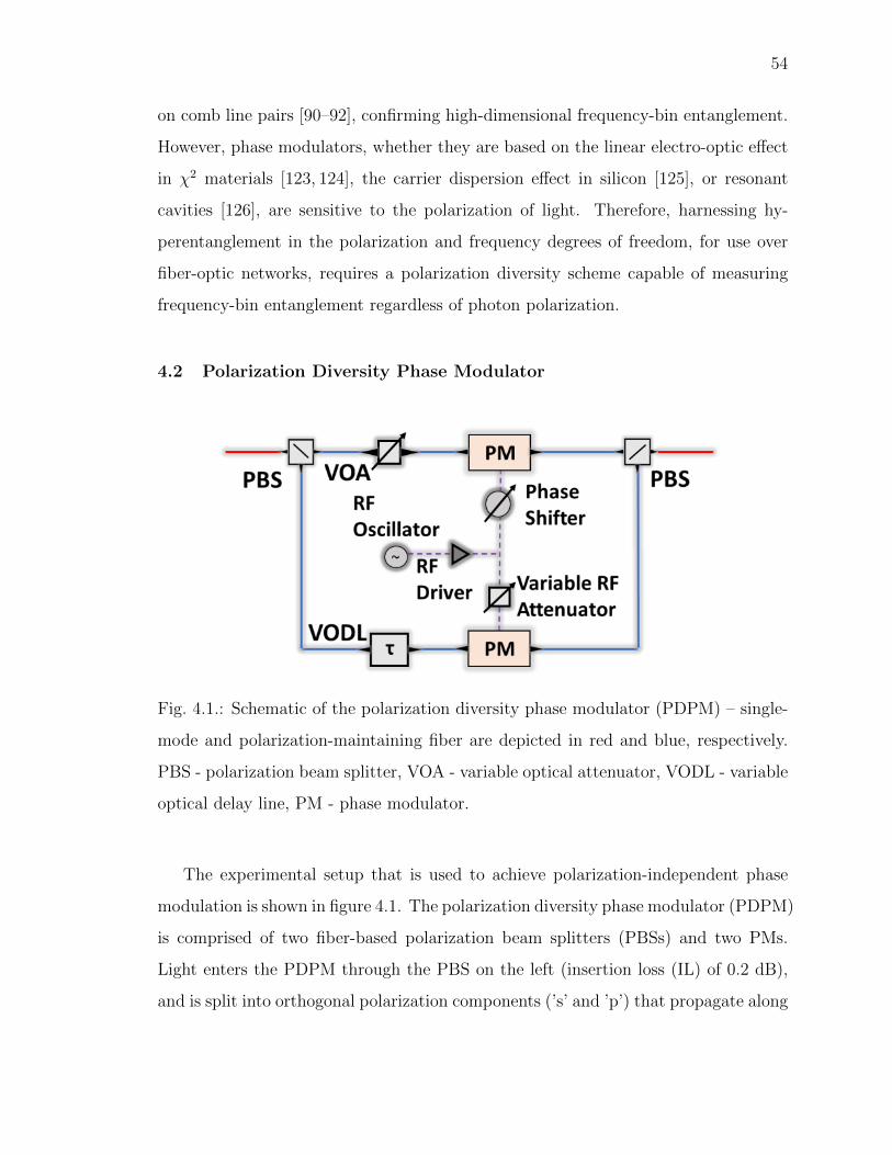
54

on comb line pairs [90–92], confirming high-dimensional frequency-bin entanglement.

However, phase modulators, whether they are based on the linear electro-optic effect

in χ2 materials [123, 124], the carrier dispersion effect in silicon [125], or resonant

cavities [126], are sensitive to the polarization of light. Therefore, harnessing hy-

perentanglement in the polarization and frequency degrees of freedom, for use over

fiber-optic networks, requires a polarization diversity scheme capable of measuring

frequency-bin entanglement regardless of photon polarization.

4.2 Polarization Diversity Phase Modulator

Fig. 4.1.: Schematic of the polarization diversity phase modulator (PDPM) – single-

mode and polarization-maintaining fiber are depicted in red and blue, respectively.

PBS - polarization beam splitter, VOA - variable optical attenuator, VODL - variable

optical delay line, PM - phase modulator.

The experimental setup that is used to achieve polarization-independent phase

modulation is shown in figure 4.1. The polarization diversity phase modulator (PDPM)

is comprised of two fiber-based polarization beam splitters (PBSs) and two PMs.

Light enters the PDPM through the PBS on the left (insertion loss (IL) of 0.2 dB),

and is split into orthogonal polarization components (’s’ and ’p’) that propagate along

55

separate channels. Both channels of the device use polarization-maintaining fiber, and

the light in each channel is modulated independently by a different PM (IL = 2.7 and

3.7 dB). A second fiber PBS (IL = 0.4 dB) recombines light from the two channels

to return a phase modulated version of the arbitrarily polarized input signal [118].

Fig. 4.2.: Progression of spectral ripple removal, signifying balancing the lengths of

the arms of the PDPM.

To carry out polarization-independent phase modulation on frequency-bin entan-

gled photons, the two paths through the PDPM need to be sufficiently indistinguish-

able so that path information cannot be gleaned from the system [127, 128]. The

path length and optical loss through the two arms of the PDPM need to be nearly

identical. Also, the RF drive to the two PMs in terms of modulation index and RF

delay need to be matched too.

A variable optical attenuator (VOA, min. IL = 1.5 dB) was tuned until the optical

loss through each arm was the same. To determine the path length difference between

the arms of the PDPM, broadband light was launched into the PDPM, so that at

least some light entered each arm. The output of the PDPM was sampled with a

polarizer (oriented at 45◦ relative to the polarization in PDPM channels) and sent to

an optical spectrum analyzer (OSA). The path length difference between the arms was

estimated from the spacing of the spectral fringes [18]. The two polarization modes

56

propagating in the different arms of the interferometer will accrue different phases

in a manner analogous to polarization mode dispersion (PMD) [129, 130], when the

interferometer is unbalanced. Any difference in path length between the arms of the

interferometer will manifest as ripple in the output spectrum. By varying the delay

introduced by the variable optical delay line (VODL, IL = 1.0 dB), the path length

difference is minimized by eliminating ripple in the output spectrum. A progression

of the spectral ripple elimination is shown in figure 4.2. The green spectrum shows a

delay of approximately 24 ps, after varying the VODL, the delay is reduced to 1.3 ps

(black) until finally reaching a delay less than 0.1 ps (red). We were able to set the

relative delay to zero with a precision of ≈ 60fs, limited by slow delay fluctuations in

the ambient environment. Although there are fluctuations in polarization of photons

exiting the PDPM, this does not affect the efficacy of the frequency-bin entanglement

measurement as long as polarization-independent single photon detectors are used.

However, work at the end of this chapter outlines the results of active stabilization in

order to ensure the polarization of light out of the PDPM is stable. Another reason

for setting the path length difference to zero, is that it allows for a larger working

bandwidth for the PDPM. When the path length difference is set to approximately

zero, the ripple is removed in the spectrum, see figure 4.2, and more wavelegnths can

be launched into the PDPM for phase modulations. Otherwise, one must choose the

wavelength of the input light to be aligned with one of the maxima in the spectral

ripple, thus reducing the bandwidth of the PDPM.

Each PM in the PDPM has its own modulation efficiency, or modulation index,

(Vπ). Consequently, when both modulators are driven with the same RF waveform

and continuous wave (CW) optical test signal, frequency combs with slightly different

spectra are generated. To ensure that both PMs impart identical phase shifts, an RF

attenuator was used to adjust the power delivered to the PM with higher modulation

efficiency. To minimize the RF delay between the driving waveforms, the output of the

PDPM was sampled in a manner similar to that described above. Any delay between

the RF driving waveforms induces a linear spectral phase shift, which manifests as

57

asymmetry in the comb spectrum. An RF phase shifter was used to reduce the RF

delay between the driving waveforms.

As currently constructed, the PDPM has an IL of 5.6 dB. However, one of the

larger sources of loss stems from the fact that the PMs in the PDPM have different

ILs (2.7 and 3.7 dB). Matching their losses to the lower value would save a dB in the

overall system loss.

4.3 Frequency Bin Entanglement Measurements

Fig. 4.3.: Experimental setup for measuring frequency-bin entanglement in a BFC.

Note that either a standalone phase modulator (PM) or polarization diversity phase

modulator (PDPM) is used to mix frequencies in this arrangement.

After matching both arms of the PDPM, the polarization diversity scheme was

used to characterize frequency-bin entanglement in a BFC in a manner similar to

that presented in references [90–92], where different frequency modes are mixed using

electro-optic phase modulation. If, for example, the frequency of phase modulation

equals one-half the frequency spacing between the frequency bin pairs i.e. the free

spectral range (FSR) of the BFC, one can project adjacent signal and idler pairs on top

of each other, thereby creating indistinguishable superposition states at frequencies

halfway between the original modes (I12 and S12 in figure 4.3). By varying the joint

phase on one of the BFC comb line pairs, it is possible to vary the overall amplitude

58

of this superposition state and, therefore, the probability of detecting coincidences

at intermediate frequencies I12 and S12. The result is a sinusoidal variation in the

number of coincidences, an interference trace, as a function of the joint phase on one

of the comb line pairs [92]. To claim 2-dimensional frequency-bin entanglement, the

visibility of the interference trace must exceed the 71% classical limit [131]. This limit

is attributed to Collins et. al. (reference [131]) in which a method for inferring a Bell

state violation in terms of the visibility of an interference trace is presented. Bell

states, or inequalities, are maximally entangled states, [132], and violation of these

states (inequalities) can be seen as a witness of useful entanglement [133].

The setup for carrying out the projective measurements and visualizing the frequency-

bin entanglement across comb line pairs is shown in figure 4.3. A CW laser pumps a

periodically poled lithium niobate (PPLN) waveguide, which generates a broadband

(5 THz) spontaneous parametric downconversion (SPDC) spectrum. A BFC is carved

from this continuous spectrum by a pulse shaper (Pulse Shaper 1, IL = 6 dB) that is

set to yield a BFC with an FSR of 36 GHz, and each frequency mode has a bandwidth

of 12 GHz. A polarization controller was placed after the pulse shaper and used to

vary the polarization of the BFC at the input of the PDPM (or standalone PM).

The PDPM (or standalone PM) was driven at half the FSR of the BFC (18 GHz) in

order to overlap adjacent frequency modes. A second pulse shaper (Pulse Shaper 2,

IL = 6 dB) was used to route the output of the PDPM (or standalone PM) and send

signal and idler photons at the intermediate frequencies to a pair of InGaAs single

photon detectors. An event timer was used to tag single photon events and generate

a histogram of two-photon coincidences.

The losses through the elements in figure 4.3 add up to around 18 dB. However,

photonic integration can play a significant role in lowering the component and system

losses. For example, a channel in a pulse shaper can be realized with a pair of filters

and a phase shifting element between. In a silicon photonics platform, such a device

could have an IL less than 0.45 dB [134]. Furthermore, there have been impressive

advances in the last year with regard to low loss PMs [10]. Consequently, low loss

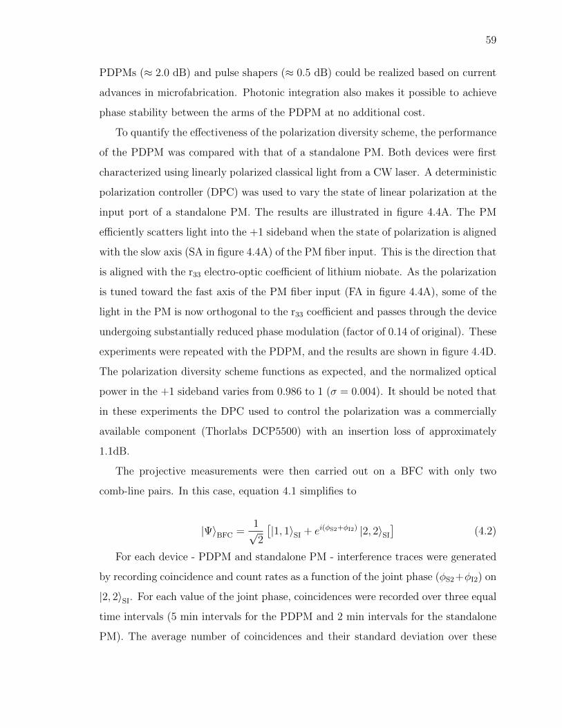
59

PDPMs (≈ 2.0 dB) and pulse shapers (≈ 0.5 dB) could be realized based on current

advances in microfabrication. Photonic integration also makes it possible to achieve

phase stability between the arms of the PDPM at no additional cost.

To quantify the effectiveness of the polarization diversity scheme, the performance

of the PDPM was compared with that of a standalone PM. Both devices were first

characterized using linearly polarized classical light from a CW laser. A deterministic

polarization controller (DPC) was used to vary the state of linear polarization at the

input port of a standalone PM. The results are illustrated in figure 4.4A. The PM

efficiently scatters light into the +1 sideband when the state of polarization is aligned

with the slow axis (SA in figure 4.4A) of the PM fiber input. This is the direction that

is aligned with the r33 electro-optic coefficient of lithium niobate. As the polarization

is tuned toward the fast axis of the PM fiber input (FA in figure 4.4A), some of the

light in the PM is now orthogonal to the r33 coefficient and passes through the device

undergoing substantially reduced phase modulation (factor of 0.14 of original). These

experiments were repeated with the PDPM, and the results are shown in figure 4.4D.

The polarization diversity scheme functions as expected, and the normalized optical

power in the +1 sideband varies from 0.986 to 1 (σ = 0.004). It should be noted that

in these experiments the DPC used to control the polarization was a commercially

available component (Thorlabs DCP5500) with an insertion loss of approximately

1.1dB.

The projective measurements were then carried out on a BFC with only two

comb-line pairs. In this case, equation 4.1 simplifies to

|Ψ〉BFC =1√2

[|1, 1〉SI + ei(φS2+φI2) |2, 2〉SI

](4.2)

For each device - PDPM and standalone PM - interference traces were generated

by recording coincidence and count rates as a function of the joint phase (φS2 +φI2) on

|2, 2〉SI. For each value of the joint phase, coincidences were recorded over three equal

time intervals (5 min intervals for the PDPM and 2 min intervals for the standalone

PM). The average number of coincidences and their standard deviation over these

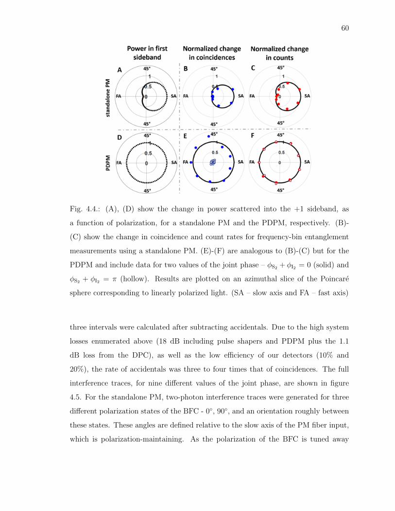
60

Fig. 4.4.: (A), (D) show the change in power scattered into the +1 sideband, as

a function of polarization, for a standalone PM and the PDPM, respectively. (B)-

(C) show the change in coincidence and count rates for frequency-bin entanglement

measurements using a standalone PM. (E)-(F) are analogous to (B)-(C) but for the

PDPM and include data for two values of the joint phase – φS2 + φI2 = 0 (solid) and

φS2 + φI2 = π (hollow). Results are plotted on an azimuthal slice of the Poincare

sphere corresponding to linearly polarized light. (SA – slow axis and FA – fast axis)

three intervals were calculated after subtracting accidentals. Due to the high system

losses enumerated above (18 dB including pulse shapers and PDPM plus the 1.1

dB loss from the DPC), as well as the low efficiency of our detectors (10% and

20%), the rate of accidentals was three to four times that of coincidences. The full

interference traces, for nine different values of the joint phase, are shown in figure

4.5. For the standalone PM, two-photon interference traces were generated for three

different polarization states of the BFC - 0◦, 90◦, and an orientation roughly between

these states. These angles are defined relative to the slow axis of the PM fiber input,

which is polarization-maintaining. As the polarization of the BFC is tuned away

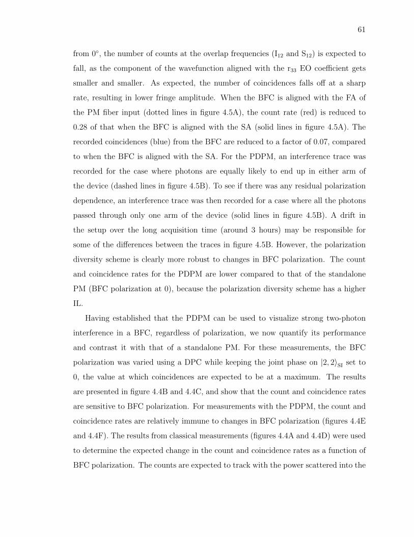
61

from 0◦, the number of counts at the overlap frequencies (I12 and S12) is expected to

fall, as the component of the wavefunction aligned with the r33 EO coefficient gets

smaller and smaller. As expected, the number of coincidences falls off at a sharp

rate, resulting in lower fringe amplitude. When the BFC is aligned with the FA of

the PM fiber input (dotted lines in figure 4.5A), the count rate (red) is reduced to

0.28 of that when the BFC is aligned with the SA (solid lines in figure 4.5A). The

recorded coincidences (blue) from the BFC are reduced to a factor of 0.07, compared

to when the BFC is aligned with the SA. For the PDPM, an interference trace was

recorded for the case where photons are equally likely to end up in either arm of

the device (dashed lines in figure 4.5B). To see if there was any residual polarization

dependence, an interference trace was then recorded for a case where all the photons

passed through only one arm of the device (solid lines in figure 4.5B). A drift in

the setup over the long acquisition time (around 3 hours) may be responsible for

some of the differences between the traces in figure 4.5B. However, the polarization

diversity scheme is clearly more robust to changes in BFC polarization. The count

and coincidence rates for the PDPM are lower compared to that of the standalone

PM (BFC polarization at 0), because the polarization diversity scheme has a higher

IL.

Having established that the PDPM can be used to visualize strong two-photon

interference in a BFC, regardless of polarization, we now quantify its performance

and contrast it with that of a standalone PM. For these measurements, the BFC

polarization was varied using a DPC while keeping the joint phase on |2, 2〉SI set to

0, the value at which coincidences are expected to be at a maximum. The results

are presented in figure 4.4B and 4.4C, and show that the count and coincidence rates

are sensitive to BFC polarization. For measurements with the PDPM, the count and

coincidence rates are relatively immune to changes in BFC polarization (figures 4.4E

and 4.4F). The results from classical measurements (figures 4.4A and 4.4D) were used

to determine the expected change in the count and coincidence rates as a function of

BFC polarization. The counts are expected to track with the power scattered into the

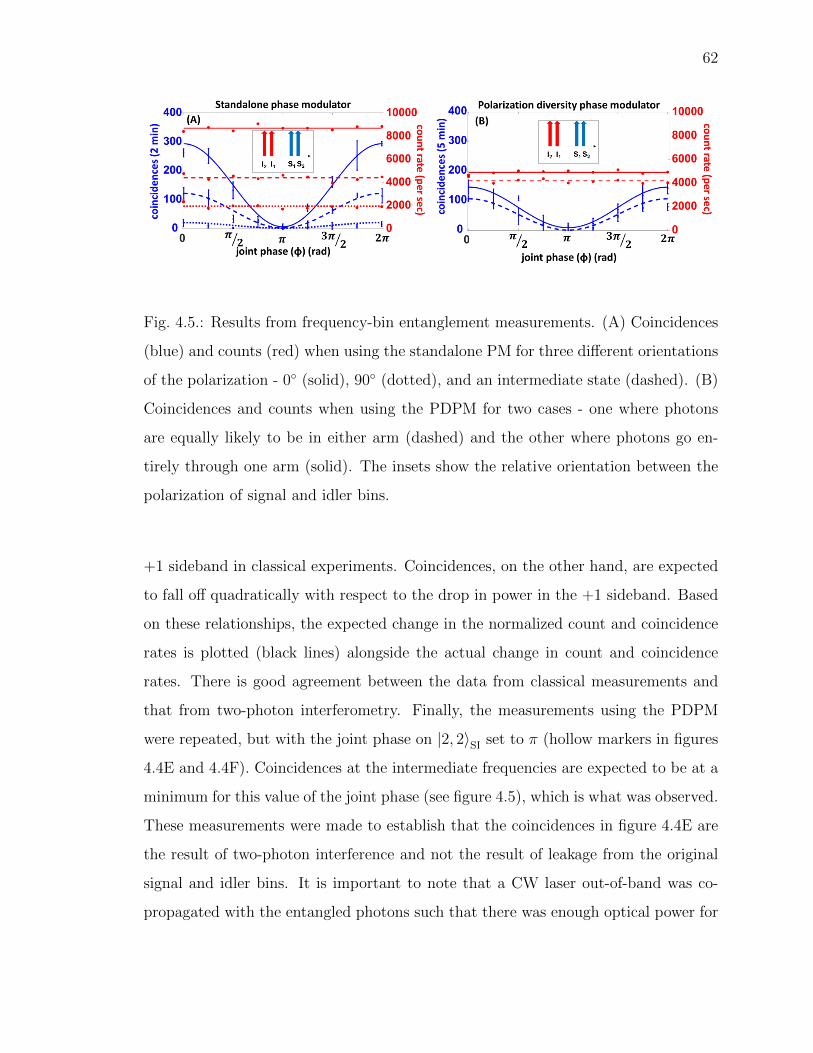
62

Fig. 4.5.: Results from frequency-bin entanglement measurements. (A) Coincidences

(blue) and counts (red) when using the standalone PM for three different orientations

of the polarization - 0◦ (solid), 90◦ (dotted), and an intermediate state (dashed). (B)

Coincidences and counts when using the PDPM for two cases - one where photons

are equally likely to be in either arm (dashed) and the other where photons go en-

tirely through one arm (solid). The insets show the relative orientation between the

polarization of signal and idler bins.

+1 sideband in classical experiments. Coincidences, on the other hand, are expected

to fall off quadratically with respect to the drop in power in the +1 sideband. Based

on these relationships, the expected change in the normalized count and coincidence

rates is plotted (black lines) alongside the actual change in count and coincidence

rates. There is good agreement between the data from classical measurements and

that from two-photon interferometry. Finally, the measurements using the PDPM

were repeated, but with the joint phase on |2, 2〉SI set to π (hollow markers in figures

4.4E and 4.4F). Coincidences at the intermediate frequencies are expected to be at a

minimum for this value of the joint phase (see figure 4.5), which is what was observed.

These measurements were made to establish that the coincidences in figure 4.4E are

the result of two-photon interference and not the result of leakage from the original

signal and idler bins. It is important to note that a CW laser out-of-band was co-

propagated with the entangled photons such that there was enough optical power for

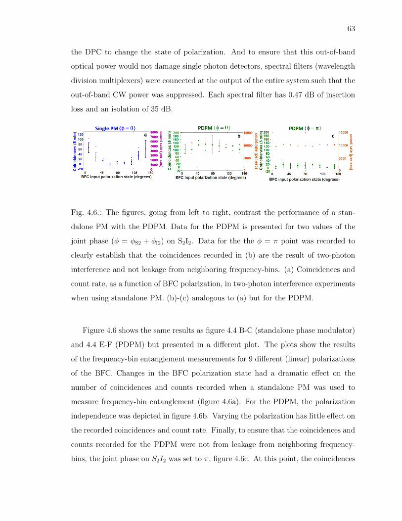
63

the DPC to change the state of polarization. And to ensure that this out-of-band

optical power would not damage single photon detectors, spectral filters (wavelength

division multiplexers) were connected at the output of the entire system such that the

out-of-band CW power was suppressed. Each spectral filter has 0.47 dB of insertion

loss and an isolation of 35 dB.

Fig. 4.6.: The figures, going from left to right, contrast the performance of a stan-

dalone PM with the PDPM. Data for the PDPM is presented for two values of the

joint phase (φ = φS2 + φI2) on S2I2. Data for the the φ = π point was recorded to

clearly establish that the coincidences recorded in (b) are the result of two-photon

interference and not leakage from neighboring frequency-bins. (a) Coincidences and

count rate, as a function of BFC polarization, in two-photon interference experiments

when using standalone PM. (b)-(c) analogous to (a) but for the PDPM.

Figure 4.6 shows the same results as figure 4.4 B-C (standalone phase modulator)

and 4.4 E-F (PDPM) but presented in a different plot. The plots show the results

of the frequency-bin entanglement measurements for 9 different (linear) polarizations

of the BFC. Changes in the BFC polarization state had a dramatic effect on the

number of coincidences and counts recorded when a standalone PM was used to

measure frequency-bin entanglement (figure 4.6a). For the PDPM, the polarization

independence was depicted in figure 4.6b. Varying the polarization has little effect on

the recorded coincidences and count rate. Finally, to ensure that the coincidences and

counts recorded for the PDPM were not from leakage from neighboring frequency-

bins, the joint phase on S2I2 was set to π, figure 4.6c. At this point, the coincidences

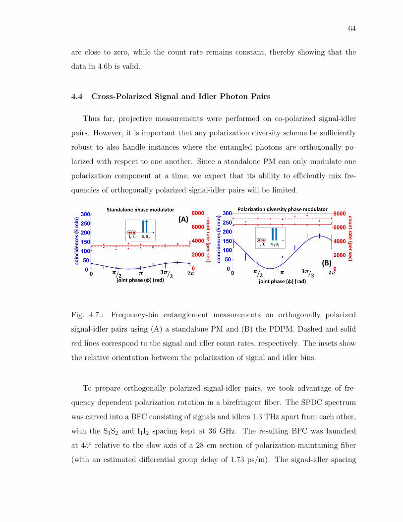
64

are close to zero, while the count rate remains constant, thereby showing that the

data in 4.6b is valid.

4.4 Cross-Polarized Signal and Idler Photon Pairs

Thus far, projective measurements were performed on co-polarized signal-idler

pairs. However, it is important that any polarization diversity scheme be sufficiently

robust to also handle instances where the entangled photons are orthogonally po-

larized with respect to one another. Since a standalone PM can only modulate one

polarization component at a time, we expect that its ability to efficiently mix fre-

quencies of orthogonally polarized signal-idler pairs will be limited.

(A)

(B)

Fig. 4.7.: Frequency-bin entanglement measurements on orthogonally polarized

signal-idler pairs using (A) a standalone PM and (B) the PDPM. Dashed and solid

red lines correspond to the signal and idler count rates, respectively. The insets show

the relative orientation between the polarization of signal and idler bins.

To prepare orthogonally polarized signal-idler pairs, we took advantage of fre-

quency dependent polarization rotation in a birefringent fiber. The SPDC spectrum

was carved into a BFC consisting of signals and idlers 1.3 THz apart from each other,

with the S1S2 and I1I2 spacing kept at 36 GHz. The resulting BFC was launched

at 45◦ relative to the slow axis of a 28 cm section of polarization-maintaining fiber

(with an estimated differential group delay of 1.73 ps/m). The signal-idler spacing

65

was chosen so that the number of Poincare sphere rotations undergone by the signal

and idler polarizations differed by one-half rotation at the output of the section of po-

larization maintaining fiber. The 1.3 THz frequency spacing is chosen to ensure that

the polarization between the signal and idler pairs is rotated and not the polarization

between S1S2 (and similarly I1I2). Interference traces similar to those recorded in fig-

ure 4.5 were then generated, but with the signal and idler polarizations orthogonal to

one another. Figure 4.7 shows that the amplitude of the two-photon trace generated

using a standalone PM is very low since a standalone PM is unable to efficiently mix

the frequencies of both signal and the idler photons simultaneously. The PDPM is

clearly not limited in this regard.

4.5 Co- and Cross-Polarized Signal and Idler Photon Pairs in a Depolar-

ized Biphoton Frequency Comb

Since propagation over fiber may scramble the polarization of light, in the previous

sections the polarization diversity phase modulator (PDPM) was used to carry out

projective measurements in the frequency domain for arbitrary, but static, states of

polarization; this work was presented in reference [118]. We now demonstrate these

projective measurements in the presence of fluctuations in the polarization state, as

well as for the case of cross-polarized signal-idler pairs. This work was presented at

CLEO 2019 [119] and presented below.

To demonstrate the robustness of the PDPM, frequency-bin entanglement in a

biphoton frequency comb (BFC) under two important scenarios was measured. First

note that the BFC was passed through a polarization scrambler to simulate either

fast fluctuations in the state of photon polarization that may result from fiber-optic

channel impairments or a stream of polarization-encoded qubits [128]. Second, to

determine whether the PDPM is compatible with hyperentangled photons in the po-

larization and frequency degrees of freedom [135], the projective measurements in the

frequency domain were carried out for both co- and cross-polarized signals and idler

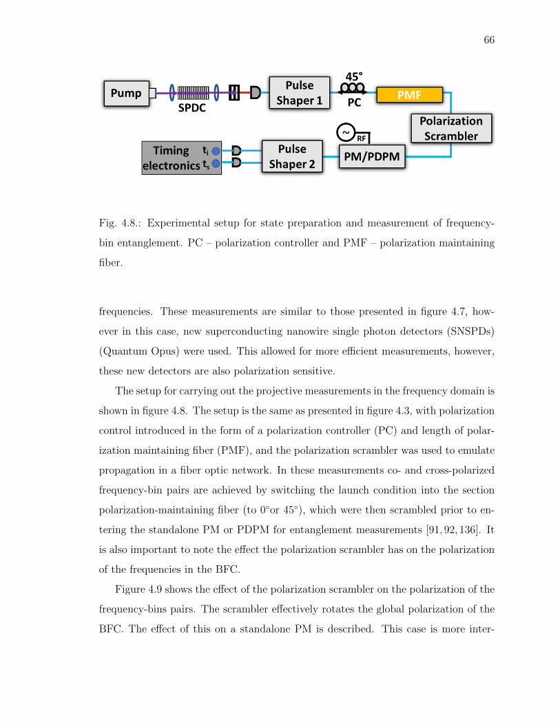
66

Fig. 4.8.: Experimental setup for state preparation and measurement of frequency-

bin entanglement. PC – polarization controller and PMF – polarization maintaining

fiber.

frequencies. These measurements are similar to those presented in figure 4.7, how-

ever in this case, new superconducting nanowire single photon detectors (SNSPDs)

(Quantum Opus) were used. This allowed for more efficient measurements, however,

these new detectors are also polarization sensitive.

The setup for carrying out the projective measurements in the frequency domain is

shown in figure 4.8. The setup is the same as presented in figure 4.3, with polarization

control introduced in the form of a polarization controller (PC) and length of polar-

ization maintaining fiber (PMF), and the polarization scrambler was used to emulate

propagation in a fiber optic network. In these measurements co- and cross-polarized

frequency-bin pairs are achieved by switching the launch condition into the section

polarization-maintaining fiber (to 0◦or 45◦), which were then scrambled prior to en-

tering the standalone PM or PDPM for entanglement measurements [91, 92, 136]. It

is also important to note the effect the polarization scrambler has on the polarization

of the frequencies in the BFC.

Figure 4.9 shows the effect of the polarization scrambler on the polarization of the

frequency-bins pairs. The scrambler effectively rotates the global polarization of the

BFC. The effect of this on a standalone PM is described. This case is more inter-

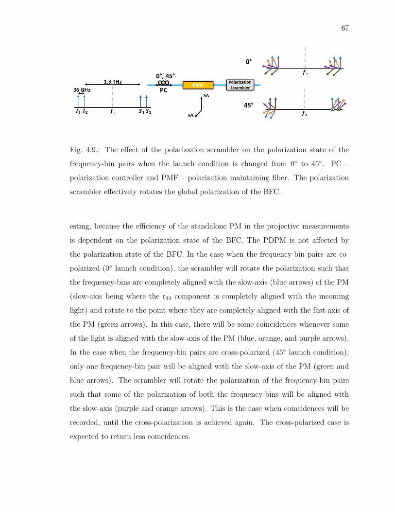
67

Fig. 4.9.: The effect of the polarization scrambler on the polarization state of the

frequency-bin pairs when the launch condition is changed from 0◦ to 45◦. PC –

polarization controller and PMF – polarization maintaining fiber. The polarization

scrambler effectively rotates the global polarization of the BFC.

esting, because the efficiency of the standalone PM in the projective measurements

is dependent on the polarization state of the BFC. The PDPM is not affected by

the polarization state of the BFC. In the case when the frequency-bin pairs are co-

polarized (0◦ launch condition), the scrambler will rotate the polarization such that

the frequency-bins are completely aligned with the slow-axis (blue arrows) of the PM

(slow-axis being where the r33 component is completely aligned with the incoming

light) and rotate to the point where they are completely aligned with the fast-axis of

the PM (green arrows). In this case, there will be some coincidences whenever some

of the light is aligned with the slow-axis of the PM (blue, orange, and purple arrows).

In the case when the frequency-bin pairs are cross-polarized (45◦ launch condition),

only one frequency-bin pair will be aligned with the slow-axis of the PM (green and

blue arrows). The scrambler will rotate the polarization of the frequency-bin pairs

such that some of the polarization of both the frequency-bins will be aligned with

the slow-axis (purple and orange arrows). This is the case when coincidences will be

recorded, until the cross-polarization is achieved again. The cross-polarized case is

expected to return less coincidences.

68

Fig. 4.10.: Interference traces and visibilities from measurements of frequency-bin

entanglement in a BFC. The performance of a standalone PM (blue) was compared

with that of the PDPM (red). The experiments were carried out for both co– (A)

and cross–polarized (B) signal idler pairs.

The results from projective measurements are shown in figures 4.10A and 4.10B.

Coincidences were recorded over 60 seconds and the results are reported without

background subtraction. In all cases, the visibility of the fringes exceeded the classical

limit of 71% [131], signifying frequency-bin entanglement across comb line pairs |1, 1〉SI

and |2, 2〉SI [90]. From both figures it is clear that the ability of the PDPM (red

traces) to carry out projective measurements in the frequency domain is unaffected

by whether the signal-idler pairs are co- or cross-polarized. Equivalent traces for the

standalone phase modulator is shown in blue. The fringe amplitude is lower in both

figures, indicating that fluctuations in the state of polarization introduced by the

polarization scrambler reduce the efficiency with which entanglement measurements

can be made. Furthermore, the maximum coincidences retrieved for the co-polarized

case were 457, while those for the cross-polarized case were 290. Therefore, the relative

orientation between signal and idler affects the efficiency with which a standalone

phase modulator can measure entanglement.

In sum, it was demonstrated that the polarization scrambling and the polarization

state of the BFC mix together to reduce the efficiency at which the standalone PM

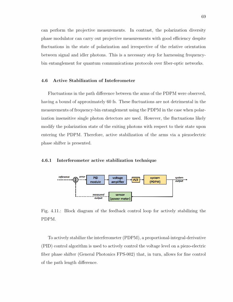
69

can perform the projective measurements. In contrast, the polarization diversity

phase modulator can carry out projective measurements with good efficiency despite

fluctuations in the state of polarization and irrespective of the relative orientation

between signal and idler photons. This is a necessary step for harnessing frequency-

bin entanglement for quantum communications protocols over fiber-optic networks.

4.6 Active Stabilization of Inteferometer

Fluctuations in the path difference between the arms of the PDPM were observed,

having a bound of approximately 60 fs. These fluctuations are not detrimental in the

measurements of frequency-bin entanglement using the PDPM in the case when polar-

ization insensitive single photon detectors are used. However, the fluctuations likely

modify the polarization state of the exiting photons with respect to their state upon

entering the PDPM. Therefore, active stabilization of the arms via a piezoelectric

phase shifter is presented.

4.6.1 Interferometer active stabilization technique

Fig. 4.11.: Block diagram of the feedback control loop for actively stabilizing the

PDPM.

To actively stabilize the interferometer (PDPM), a proportional-integral-derivative

(PID) control algorithm is used to actively control the voltage level on a piezo-electric

fiber phase shifter (General Photonics FPS-002) that, in turn, allows for fine control

of the path length difference.

70

The PID algorithm is a closed loop system that uses a sensor to read a signal.

The desired output is obtained by calculating three responses (or variables) P (for

proportional), I (for integration parameter), and D (for derivative parameter). The

sum of the three responses are used to compute the output [137].

Figure 4.11 shows the block diagram of the feedback control loop used to actively

stabilize the PDPM. Starting at the output of the block diagram (“system output”),

the optical output of the system (PDPM) is sent to a sensor (power meter). The

sensor transforms the optical signal to an electrical signal that is then compared to

the reference or set point. The difference between the reference and the sensor output

is the error signal that is sent to the PID module (New Focus - LB1005-S High-Speed

Servo Controller), and its output is sent to a voltage amplifier. The voltage amplifier

is connected electrically to the PZT and this amplified voltage allows for the active

control of the phase shift imparted by the PZT. The PZT is connected optically to

the system (in one arm of the PDPM) and the loop starts again after the voltage was

updated by the PID module.

It is important to confirm that the PID control loop can keep up with the fluc-

tuations in the path length of the PDPM. To be convinced that the response speed

of the feedback loop is fast enough, the path length fluctuations were measured by

photo-detecting the light exiting the PDPM after being sampled by a polarizer. This

sampling by a polarizer allows for the orthogonal polarization components to interfere,

thus demonstrating the phase accrued between the orthogonal polarization compo-

nents due to the constant path length fluctuations in the arms of the PDPM. The

top plot in figure 4.12 shows the path length fluctuations. This data was recorded

over 500 seconds and sampled every 0.5 ms. The bottom plot of figure 4.12 shows the

power spectrum of the path length fluctuations. The spectrum reveals that the path

length fluctuations are concentrated between DC and 0.2 Hz, thus demonstrating that

the speed of the fluctuations are several seconds. All the components in the feedback

loop are fast enough to keep up with these fluctuations. The PZT has a bandwidth

of 20 kHz, the power meter allows the user to choose either a 25 Hz or 100 kHz

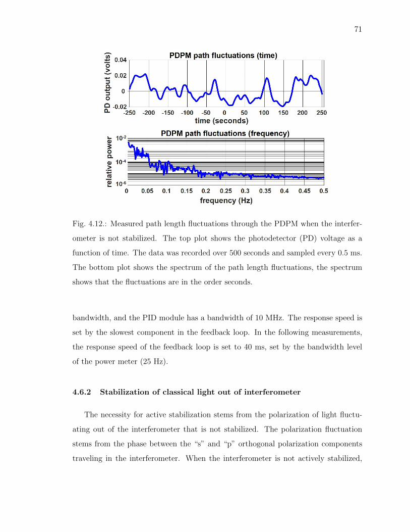
71

Fig. 4.12.: Measured path length fluctuations through the PDPM when the interfer-

ometer is not stabilized. The top plot shows the photodetector (PD) voltage as a

function of time. The data was recorded over 500 seconds and sampled every 0.5 ms.

The bottom plot shows the spectrum of the path length fluctuations, the spectrum

shows that the fluctuations are in the order seconds.

bandwidth, and the PID module has a bandwidth of 10 MHz. The response speed is

set by the slowest component in the feedback loop. In the following measurements,

the response speed of the feedback loop is set to 40 ms, set by the bandwidth level

of the power meter (25 Hz).

4.6.2 Stabilization of classical light out of interferometer

The necessity for active stabilization stems from the polarization of light fluctu-

ating out of the interferometer that is not stabilized. The polarization fluctuation

stems from the phase between the “s” and “p” orthogonal polarization components

traveling in the interferometer. When the interferometer is not actively stabilized,

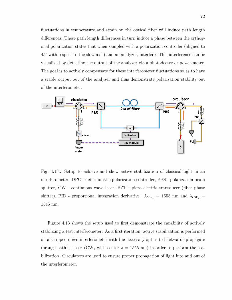
72

fluctuations in temperature and strain on the optical fiber will induce path length

differences. These path length differences in turn induce a phase between the orthog-

onal polarization states that when sampled with a polarization controller (aligned to

45◦ with respect to the slow-axis) and an analyzer, interfere. This interference can be

visualized by detecting the output of the analyzer via a photodector or power-meter.

The goal is to actively compensate for these interferometer fluctuations so as to have

a stable output out of the analyzer and thus demonstrate polarization stability out

of the interferometer.

Fig. 4.13.: Setup to achieve and show active stabilization of classical light in an

interferometer. DPC - deterministic polarization controller, PBS - polarization beam

splitter, CW - continuous wave laser, PZT - piezo electric transducer (fiber phase

shifter), PID - proportional integration derivative. λCW1 = 1555 nm and λCW2 =

1545 nm.

Figure 4.13 shows the setup used to first demonstrate the capability of actively

stabilizing a test interferometer. As a first iteration, active stabilization is performed

on a stripped down interferometer with the necessary optics to backwards propagate

(orange path) a laser (CW1 with center λ = 1555 nm) in order to perform the sta-

bilization. Circulators are used to ensure proper propagation of light into and out of

the interferometer.

73

The input circulator, in this case, takes into port 1 the classical light (CW2 with

center λ = 1545 nm) out of the deterministic polarization controller (DPC) and

sends it out of port 2 and into the first polarization beam splitter (PBS). This is the

“forward path” and is denoted by the purple arrows. This light continues into the

interferometer and out of the second PBS. It continues its course into port 2 of the

output circulator until it exits port 3. After this, the light is sent into a test PBS in

which the polarization stability is tested when the interferometer is and is not actively

stabilized. To visualize this, two power meters are connected to the two output ports

of the test PBS (PA and PB).

Continuing with figure 4.13, attention is now turned to the “backwards path”

denoted by the orange arrows. This is the path taken by the stabilization laser

(CW1). This is the laser that is detected by the sensor that is then used by the PID

module to actively control the PZT voltage and actively stabilize the interferometer.

Starting at port 1 of the output circulator, the light travels out of port 2 and into

the output PBS of the interferometer. The light is launched such that each arm

has equal power i.e. the polarization controller connected to port 1 of the output

circulator is varied until achieving a polarization state of 45◦ with respect to the slow

axis. The light continues through the interferometer and out of the input PBS where

the two orthogonal polarization states are recombined. The light travels into port 2

and out of port 3 of the input circulator. The light is then sampled by a polarizer

(also typically called an “analyzer”) so as to visualize the effect of the phase between

the orthogonal polarization states. A polarization controller (PC) is used to ensure

sampling of both orthogonal polarization through the interferometer, thus inducing

their interference that is indicative of the phase difference between the orthogonal

polarizations. This sampled light is then detected by a power meter and the electrical

signal is sent to the PID module. When the interferometer is not stabilized, the

environmental fluctuations imparted onto the fibers of the interferometer will cause a

phase difference between the two polarizations. This is visualized by a large variation

in optical power detected by the power meter. The goal is to reduce these large

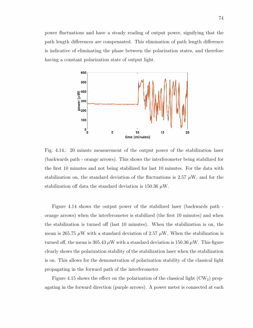
74

power fluctuations and have a steady reading of output power, signifying that the

path length differences are compensated. This elimination of path length difference

is indicative of eliminating the phase between the polarization states, and therefore

having a constant polarization state of output light.

Fig. 4.14.: 20 minute measurement of the output power of the stabilization laser

(backwards path - orange arrows). This shows the interferometer being stabilized for

the first 10 minutes and not being stabilized for last 10 minutes. For the data with

stabilization on, the standard deviation of the fluctuations is 2.57 µW, and for the

stabilization off data the standard deviation is 150.36 µW.

Figure 4.14 shows the output power of the stabilized laser (backwards path -

orange arrows) when the interferometer is stabilized (the first 10 minutes) and when

the stabilization is turned off (last 10 minutes). When the stabilization is on, the

mean is 265.75 µW with a standard deviation of 2.57 µW. When the stabilization is

turned off, the mean is 305.43 µW with a standard deviation is 150.36 µW. This figure

clearly shows the polarization stability of the stabilization laser when the stabilization

is on. This allows for the demonstration of polarization stability of the classical light

propagating in the forward path of the interferometer.

Figure 4.15 shows the effect on the polarization of the classical light (CW2) prop-

agating in the forward direction (purple arrows). A power meter is connected at each

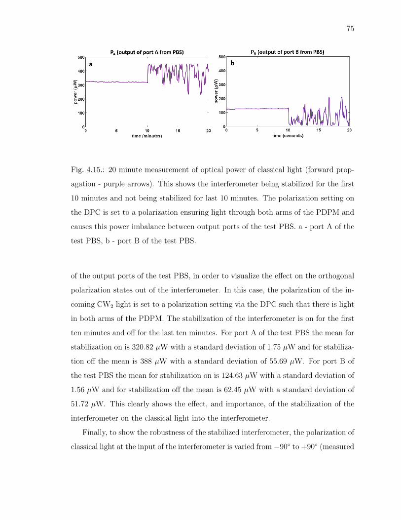
75

Fig. 4.15.: 20 minute measurement of optical power of classical light (forward prop-

agation - purple arrows). This shows the interferometer being stabilized for the first

10 minutes and not being stabilized for last 10 minutes. The polarization setting on

the DPC is set to a polarization ensuring light through both arms of the PDPM and

causes this power imbalance between output ports of the test PBS. a - port A of the

test PBS, b - port B of the test PBS.

of the output ports of the test PBS, in order to visualize the effect on the orthogonal

polarization states out of the interferometer. In this case, the polarization of the in-

coming CW2 light is set to a polarization setting via the DPC such that there is light

in both arms of the PDPM. The stabilization of the interferometer is on for the first

ten minutes and off for the last ten minutes. For port A of the test PBS the mean for

stabilization on is 320.82 µW with a standard deviation of 1.75 µW and for stabiliza-

tion off the mean is 388 µW with a standard deviation of 55.69 µW. For port B of

the test PBS the mean for stabilization on is 124.63 µW with a standard deviation of

1.56 µW and for stabilization off the mean is 62.45 µW with a standard deviation of

51.72 µW. This clearly shows the effect, and importance, of the stabilization of the

interferometer on the classical light into the interferometer.

Finally, to show the robustness of the stabilized interferometer, the polarization of

classical light at the input of the interferometer is varied from−90◦ to +90◦ (measured

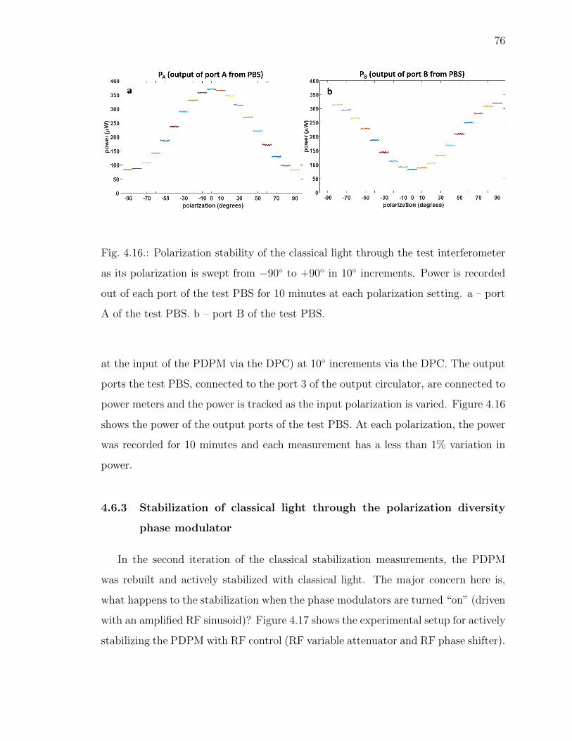
76

Fig. 4.16.: Polarization stability of the classical light through the test interferometer

as its polarization is swept from −90◦ to +90◦ in 10◦ increments. Power is recorded

out of each port of the test PBS for 10 minutes at each polarization setting. a – port

A of the test PBS. b – port B of the test PBS.

at the input of the PDPM via the DPC) at 10◦ increments via the DPC. The output

ports the test PBS, connected to the port 3 of the output circulator, are connected to

power meters and the power is tracked as the input polarization is varied. Figure 4.16

shows the power of the output ports of the test PBS. At each polarization, the power

was recorded for 10 minutes and each measurement has a less than 1% variation in

power.

4.6.3 Stabilization of classical light through the polarization diversity

phase modulator

In the second iteration of the classical stabilization measurements, the PDPM

was rebuilt and actively stabilized with classical light. The major concern here is,

what happens to the stabilization when the phase modulators are turned “on” (driven

with an amplified RF sinusoid)? Figure 4.17 shows the experimental setup for actively

stabilizing the PDPM with RF control (RF variable attenuator and RF phase shifter).

77

In this case, the RF parameters – delay and modulation index – are balanced for each

PM in the PDPM. Optical balancing was also performed by matching the insertion

loss in each arm and the optical path length between the arms.

Fig. 4.17.: Experimental setup for active stabilization of the PDPM. The RF com-

ponents necessary to balancing the PDPM electrically are now incorporated. This

setup is used to demonstrate that the polarization transformation observed in figure

4.21 is due to the RF delay mismatch between the PMs.

The stabilization performed in this iteration employs the same experimental prin-

ciple outlined in the previous section, and depicted in figure 4.13. A stabilization laser

(CW1 – λCW1 = 1555 nm) propagates backwards (orange arrows) through the PDPM

and is sampled by a polarizer. This sampled light is the error signal used by the PID

module to actively stabilize the PDPM. The polarization stability achieved by the

active stabilization is confirmed by analyzing the polarization of classical light (CW2

– λCW1 = 1545 nm) out of the PDPM in the forward (purple arrows) propagation

direction by monitoring the power out of the output ports of a test PBS. In all results

shown in this section, the PMs are “on” (driven with RF sinusoid – RF frequency =

18 GHz and RF power = 27 dB), unless otherwise stated.

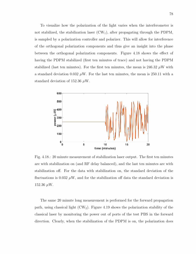
78

To visualize how the polarization of the light varies when the interferometer is

not stabilized, the stabilization laser (CW1), after propagating through the PDPM,

is sampled by a polarization controller and polarizer. This will allow for interference

of the orthogonal polarization components and thus give an insight into the phase

between the orthogonal polarization components. Figure 4.18 shows the effect of

having the PDPM stabilized (first ten minutes of trace) and not having the PDPM

stabilized (last ten minutes). For the first ten minutes, the mean is 246.32 µW with

a standard deviation 0.032 µW. For the last ten minutes, the mean is 250.11 with a

standard deviation of 152.36 µW.

Fig. 4.18.: 20 minute measurement of stabilization laser output. The first ten minutes

are with stabilization on (and RF delay balanced), and the last ten minutes are with

stabilization off. For the data with stabilization on, the standard deviation of the

fluctuations is 0.032 µW, and for the stabilization off data the standard deviation is

152.36 µW.

The same 20 minute long measurement is performed for the forward propagation

path, using classical light (CW2). Figure 4.19 shows the polarization stability of the

classical laser by monitoring the power out of ports of the test PBS in the forward

direction. Clearly, when the stabilization of the PDPM is on, the polarization does

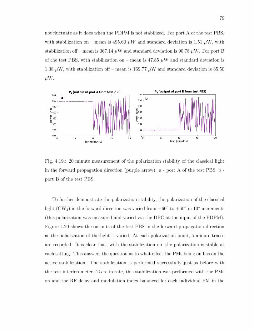
79

not fluctuate as it does when the PDPM is not stabilized. For port A of the test PBS,

with stabilization on – mean is 495.60 µW and standard deviation is 1.51 µW, with

stabilization off – mean is 367.14 µW and standard deviation is 90.78 µW. For port B

of the test PBS, with stabilization on – mean is 47.85 µW and standard deviation is

1.38 µW, with stabilization off – mean is 169.77 µW and standard deviation is 85.50

µW.

Fig. 4.19.: 20 minute measurement of the polarization stability of the classical light

in the forward propagation direction (purple arrow). a - port A of the test PBS. b -

port B of the test PBS.

To further demonstrate the polarization stability, the polarization of the classical

light (CW2) in the forward direction was varied from −60◦ to +60◦ in 10◦ increments

(this polarization was measured and varied via the DPC at the input of the PDPM).

Figure 4.20 shows the outputs of the test PBS in the forward propagation direction

as the polarization of the light is varied. At each polarization point, 5 minute traces

are recorded. It is clear that, with the stabilization on, the polarization is stable at

each setting. This answers the question as to what effect the PMs being on has on the

active stabilization. The stabilization is performed successfully just as before with

the test interferometer. To re-iterate, this stabilization was performed with the PMs

on and the RF delay and modulation index balanced for each individual PM in the

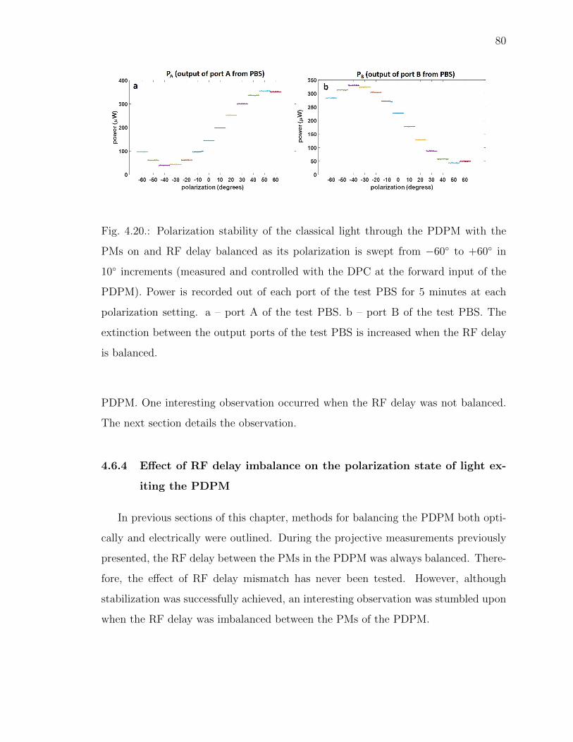
80

Fig. 4.20.: Polarization stability of the classical light through the PDPM with the

PMs on and RF delay balanced as its polarization is swept from −60◦ to +60◦ in

10◦ increments (measured and controlled with the DPC at the forward input of the

PDPM). Power is recorded out of each port of the test PBS for 5 minutes at each

polarization setting. a – port A of the test PBS. b – port B of the test PBS. The

extinction between the output ports of the test PBS is increased when the RF delay

is balanced.

PDPM. One interesting observation occurred when the RF delay was not balanced.

The next section details the observation.

4.6.4 Effect of RF delay imbalance on the polarization state of light ex-

iting the PDPM

In previous sections of this chapter, methods for balancing the PDPM both opti-

cally and electrically were outlined. During the projective measurements previously

presented, the RF delay between the PMs in the PDPM was always balanced. There-

fore, the effect of RF delay mismatch has never been tested. However, although

stabilization was successfully achieved, an interesting observation was stumbled upon

when the RF delay was imbalanced between the PMs of the PDPM.

81

The polarization of the classical light (CW2) was varied from −50◦ to +50◦ via the

DPC connected at the input of the PDPM. The output of the PDPM was connected

to the test PBS and the power out of its output ports was monitored. This time,

to reiterate, the RF delay between the PMs was imbalanced. Figure 4.21 shows the

results of these classical light polarization stability measurements. The power out of

both ports of the test PBS (port A and port B) is recorded for 5 minutes at each

polarization setting and the polarization is kept constant at each setting.

Fig. 4.21.: Polarization stability of the classical light through the PDPM with the

PMs on and RF delay (purposefully) imbalanced. Polarization is swept from −50◦

to +50◦ in 10◦ increments (measured and controlled via DPC at input of PDPM).

Power is recorded out of each port of the test PBS for 5 minutes at each polarization

setting. a – port A of the test PBS. b – port B of the test PBS. Notice that in this

iteration, there exists less extinction between the two output ports of the test PBS.

Comparing the results between output ports of the test PBS in the case when

the RF delay is balanced, figure 4.20, to the case when the RF delay is imbalanced,

figure 4.21, a reduction in extinction is observed. In the case when the RF delay is

balanced depicted in figure 4.20, for port A the maximum power recorded (on average

over the 5 minute measurement) was 355.04 µW and the minimum power recorded

was 39.74 µW. For port B the maximum power recorded was 330.23 µW and the

minimum power recorded was 43.40 µW. In the case when the RF delay is imbalanced,

82

shown in figure 4.21, the maximum power recorded out of port A was 268.84 µW,

and the minimum power recorded was 146.02 µW. For port B the maximum power

recorded was 282.47 µW, and the minimum power recorded was 159.79 µW. From

these recorded power values, it is clear that the power extinction out of the test PBS

is greater when the RF delay is balanced.

It is hypothesized that when the RF delay is different between the individual

PMs of the PDPM, the RF sinusoids reach their respective PMs at different times.

This means that light in the different paths of the PDPM incur a phase difference

due to this delay in the RF signal. When the light recombines at the output of

the PDPM, the phase between the light in each path is manifested as a polarization

transformation out of the PDPM. This polarization transformation is attributed to

the reduced power extinction out of the test PBS, depicted in figure 4.21. If the

RF delay between the individual PMs is balanced, then the phase difference will not

be incurred, and the phase transformation manifested as a reduction in extinction

between the ports of the PBS, will not occur, see figure 4.20.

It was previously stated that in order to preserve indistinguishability between the

paths of the PDPM, the optical insertion loss and path lengths must be balanced,

and so too the modulation indices and RF delay between the individual PMs must

be balanced. This is done so that no information can be observed as to what path

the photons take through the PDPM. Therefore, a balanced PDPM, both optically

and electrically, is the default state at which the PDPM will be operated. The RF

delay dependent polarization transformation evident in figure 4.21 is an interesting

phenomenon that allowed for the understanding of what effect the RF delay has on

the output polarization state. Whether this unbalanced RF state is detrimental to

the frequency-bin entanglement measurement is not known. The next step is for

the actively stabilized PDPM to be used in the projective measurements to show

frequency-bin entanglement in a BFC.

It was shown, in this chapter, that the PDPM can perform phase modulation

irrespective of the polarization state of classical light, figure 4.4, irrespective of the

83

polarization state of entangled photons, figure 4.6, and irrespective of the polarization

state between the frequency-bin pairs of the BFC, figure 4.7 and 4.10. Finally, active

stabilization of the PDPM was demonstrated by propagating a stabilization laser

(CW laser) backwards through the PDPM and using a PID controller to minimize

an error signal. This was performed to ensure the polarization stability of the output

photons. The next step is to perform frequency-bin entanglement measurements with

the actively stabilized PDPM, and to demonstrate that the power of the PDPM lies in

its ability to perform phase modulation on bi-photons hyperentangled in polarization

and frequency.

Acknowledgement of Collaboration

The author was tasked with the classical stabilization of the PDPM. The other

aspects of this work were a collaborative effort with colleague Navin Lingaraju.

84

5. CONCLUSION

5.1 Brief Summary

In this dissertation electro-optic phase modulation was used to generate high rep-

rate electro-optic frequency combs. The goal of the work was to broaden these so-

called EO combs in the spectral domain. Chapter 1 of this work offers a brief review

of methods for achieving this spectral broadening. In chapter 2, the nonlinear optical

loop mirror (NOLM) is introduced. The NOLM is an all fiber device that allows

for broadening the spectrum of the electro-optic frequency comb to a bandwidth of

40 nm with a spectral ripple, power variation among spectral lines, to be less than

10 dB. In chapter 3, this broadened electro-optic frequency comb was used as a

reference comb in dual comb interferometry measurements to characterize the single-

soliton Kerr-frequency comb generated in a silicon-nitride microresonator. This dual

comb interferometry technique allowed for rapid characterization of the single soliton

with low average power out of the ring resonator. In chapter 4, electro-optic phase

modulation is used to show the entanglement in a biphoton frequency comb. The

fact that commercial standalone phase modulators are polarization dependent was

demonstrated, and to circumvent this, the polarization diversity phase modulator

(PDPM) was introduced. The polarization diversity of the PDPM was demonstrated

both classically and in the quantum regime. The final aspect of the PDPM project, in

this work, was to actively stabilize the interferometer to ensure polarization stability

out of the PDPM.

85

5.2 Future Outlook

Chapter 2 is matured results, and there are no experiments that can be done to

move this forward. However, it is the hope of the author of this dissertation that

colleagues at the lab will find this useful and continue to use it in future experiments,

specifically with work related to measurements introduced in chapter 3.

An interesting extension of the dual comb interferometry technique presented

in chapter 3 is characterizing dark pulses generated in normal dispersion microres-

onators, an example spectrum being shown in figure 5.1. In 2015, Xue et al. demon-

strated mode-locking transitions, as those reported for bright soliton generation, and

the generation of dark pulses in a normal dispersion SiN ring resonator [138].

Fig. 5.1.: Example of dark pulse spectrum generated from a normal dispersion mi-

croresonator.

The goal is to measure the phase of the dark pulse, the same way the phase

of the single bright soliton was retrieved in [102]. This would require only a slight

modification to the setup presented in chapter 3, the modification being the center

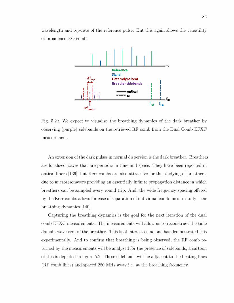
86

wavelength and rep-rate of the reference pulse. But this again shows the versatility

of broadened EO comb.

Fig. 5.2.: We expect to visualize the breathing dynamics of the dark breather by

observing (purple) sidebands on the retrieved RF comb from the Dual Comb EFXC

measurement.

An extension of the dark pulses in normal dispersion is the dark breather. Breathers

are localized waves that are periodic in time and space. They have been reported in

optical fibers [139], but Kerr combs are also attractive for the studying of breathers,

due to microresonators providing an essentially infinite propagation distance in which

breathers can be sampled every round trip. And, the wide frequency spacing offered

by the Kerr combs allows for ease of separation of individual comb lines to study their

breathing dynamics [140].

Capturing the breathing dynamics is the goal for the next iteration of the dual

comb EFXC measurements. The measurements will allow us to reconstruct the time

domain waveform of the breather. This is of interest as no one has demonstrated this

experimentally. And to confirm that breathing is being observed, the RF comb re-

turned by the measurements will be analyzed for the presence of sidebands; a cartoon

of this is depicted in figure 5.2. These sidebands will be adjacent to the beating lines

(RF comb lines) and spaced 280 MHz away i.e. at the breathing frequency.

87

In regard to the PDPM presented in chapter 4, because it can operate on pho-

tons irrespective of their polarization state, the PDPM can potentially be used in

schemes where information is encoded in both the polarization and frequency-bin de-

grees of freedom (DoF). For example, such encoding has been carried out using the

polarization and transverse spatial modes DoF [141]. To date, such demonstrations

have not been carried out using polarization and frequency-bin – both of which being

compatible with optical fiber. Our group has previously implemented communication

protocols where information was encoded in the frequency DoF of entangled photons

using Fourier transform pulse shapers [142]. With the PDPM, we plan to build on

this work by encoding information in both polarization and frequency-bin. In such

an arrangement, the PDPM would measure the relative phase between frequency

bins without altering neither their polarization nor any information encoded in this

DoF. The PDPM could also be used in more complex schemes in which one needs to

carry out projective measurements in the frequency domain on photons that are also

entangled in polarization.

Lastly, colleagues at ARL want these PDPMs to be in a “plug and play” box for

future delivery. Therefore, smaller, and preferably more affordable, components will

need to be used. One of these components is the lock-box used in the current active

stabilization technique. An alternative to this, is using an FPGA (Red-Pitaya) with a

built in PID controller. This task will be given to an undergraduate summer research

scholar that our lab will have the privilege of mentoring. These are the last projects

the author will focus on, as his time here comes to an end.

REFERENCES

88

REFERENCES

[1] T. Udem, R. Holzwarth, and T. W. Hansch, “Optical frequency metrology,”Nature, vol. 416, no. 6877, p. 233, 2002.

[2] D. J. Jones, S. A. Diddams, J. K. Ranka, A. Stentz, R. S. Windeler, J. L. Hall,and S. T. Cundiff, “Carrier-envelope phase control of femtosecond mode-lockedlasers and direct optical frequency synthesis,” Science, vol. 288, no. 5466, pp.635–639, 2000.

[3] R. Holzwarth, T. Udem, T. W. Hansch, J. Knight, W. Wadsworth, and P. S. J.Russell, “Optical frequency synthesizer for precision spectroscopy,” Physicalreview letters, vol. 85, no. 11, p. 2264, 2000.

[4] S. A. Diddams, D. J. Jones, J. Ye, S. T. Cundiff, J. L. Hall, J. K. Ranka,R. S. Windeler, R. Holzwarth, T. Udem, and T. Hansch, “Direct link betweenmicrowave and optical frequencies with a 300 thz femtosecond laser comb,”Physical Review Letters, vol. 84, no. 22, p. 5102, 2000.

[5] N. R. Newbury, “Searching for applications with a fine-tooth comb,” Naturephotonics, vol. 5, no. 4, pp. 186–188, 2011.

[6] J. Ye and S. T. Cundiff, Femtosecond optical frequency comb: principle, opera-tion and applications. Springer Science & Business Media, 2005.

[7] A. Bartels, D. Heinecke, and S. A. Diddams, “10-ghz self-referenced opticalfrequency comb,” Science, vol. 326, no. 5953, pp. 681–681, 2009.

[8] S. T. Cundiff and A. M. Weiner, “Optical arbitrary waveform generation,”Nature Photonics, vol. 4, no. 11, p. 760, 2010.

[9] V. Torres-Company and A. M. Weiner, “Optical frequency comb technologyfor ultra-broadband radio-frequency photonics,” Laser & Photonics Reviews,vol. 8, no. 3, pp. 368–393, 2014.

[10] J. Hecht. (2012) Photonic frontiers: Frequency combs: Fre-quency combs make their way to the masses. [Online].Available: https://www.laserfocusworld.com/articles/print/volume-48/issue-01/features/frequency-combs-make-their-way-to-the-masses.html

[11] J. L. Hall, “Nobel lecture: Defining and measuring optical frequencies,” Reviewsof Modern Physics, vol. 78, no. 4, p. 1279, 2006.

[12] T. W. Hansch, “Einstein lecture–passion for precision,” Annalen der Physik,vol. 15, no. 9, pp. 627–652, 2006.

[13] E. Gordon and J. Rigden, “The fabry-perot electrooptic modulator,” Bell LabsTechnical Journal, vol. 42, no. 1, pp. 155–179, 1963.

89

[14] T. Kobayashi, T. Sueta, Y. Cho, and Y. Matsuo, “High-repetition-rate opticalpulse generator using a fabry-perot electro-optic modulator,” Applied PhysicsLetters, vol. 21, no. 8, pp. 341–343, 1972.

[15] T. Kobayashi, H. Yao, K. Amano, Y. Fukushima, A. Morimoto, and T. Sueta,“Optical pulse compression using high-frequency electrooptic phase modula-tion,” IEEE journal of quantum electronics, vol. 24, no. 2, pp. 382–387, 1988.

[16] M. Fujiwara, M. Teshima, J.-i. Kani, H. Suzuki, N. Takachio, and K. Iwatsuki,“Optical carrier supply module using flattened optical multicarrier generationbased on sinusoidal amplitude and phase hybrid modulation,” Journal of light-wave technology, vol. 21, no. 11, pp. 2705–2714, 2003.

[17] Y. Liu, A. J. Metcalf, R. Wu, L. Fan, L. T. Varghese, M. Qi, A. M. Weineret al., “Bandwidth scaling of a phase-modulated continuous-wave comb throughfour-wave mixing in a silicon nano-waveguide,” Optics letters, vol. 39, no. 22,pp. 6478–6481, 2014.

[18] A. Weiner, Ultrafast optics. John Wiley & Sons, 2011, vol. 72.

[19] G. P. Agrawal, Fiber-optic communication systems. John Wiley & Sons, 2012,vol. 222.

[20] K. R. Tamura, H. Kuhota, and M. Nakazawa, “Fundamentals of stable contin-uum generation at high repetition rates,” IEEE journal of quantum electronics,vol. 36, no. 7, pp. 773–779, 2000.

[21] Y. Ozeki, S. Takasaka, M. Sakano, and S. Namiki, “Repetition rate variableand wavelength-tunable picosecond optical pulse source employing square-wave-driven intensity modulator and comb-like profiled fiber,” IEEE photonics tech-nology letters, vol. 17, no. 12, pp. 2736–2738, 2005.

[22] I. Morohashi, T. Sakamoto, H. Sotobayashi, T. Kawanishi, I. Hosako,and M. Tsuchiya, “Widely repetition-tunable 200 fs pulse source using amach–zehnder-modulator-based flat comb generator and dispersion-flatteneddispersion-decreasing fiber,” Optics letters, vol. 33, no. 11, pp. 1192–1194, 2008.

[23] C.-B. Huang, S.-G. Park, D. E. Leaird, and A. M. Weiner, “Nonlinearly broad-ened phase-modulated continuous-wave laser frequency combs characterized us-ing dpsk decoding,” Optics express, vol. 16, no. 4, pp. 2520–2527, 2008.

[24] Z. Jiang, C.-B. Huang, D. E. Leaird, and A. M. Weiner, “Optical arbitrarywaveform processing of more than 100 spectral comb lines,” Nature Photonics,vol. 1, no. 8, p. 463, 2007.

[25] R. W. Boyd, Nonlinear optics. Academic press, 2003.

[26] A. M. Clarke, D. G. Williams, M. A. Roelens, and B. J. Eggleton, “Reconfig-urable optical pulse generator employing a fourier-domain programmable op-tical processor,” Journal of Lightwave Technology, vol. 28, no. 1, pp. 97–103,2010.

[27] A. J. Metcalf, C. D. Fredrick, R. C. Terrien, S. B. Papp, and S. A. Diddams,“30 ghz frequency comb spanning 160 thz in the near-infrared,” in Lasers andElectro-Optics (CLEO), 2017 Conference on. IEEE, 2017, pp. 1–1.

90

[28] S. Pitois, C. Finot, J. Fatome, B. Sinardet, and G. Millot, “Generation of 20-ghz picosecond pulse trains in the normal and anomalous dispersion regimes ofoptical fibers,” Optics Communications, vol. 260, no. 1, pp. 301–306, 2006.

[29] F. Parmigiani, C. Finot, K. Mukasa, M. Ibsen, M. A. Roelens, P. Petropoulos,and D. J. Richardson, “Ultra-flat spm-broadened spectra in a highly nonlinearfiber using parabolic pulses formed in a fiber bragg grating,” Optics Express,vol. 14, no. 17, pp. 7617–7622, 2006.

[30] W. Tomlinson, R. H. Stolen, and A. M. Johnson, “Optical wave breaking ofpulses in nonlinear optical fibers,” Optics letters, vol. 10, no. 9, pp. 457–459,1985.

[31] C. Finot, B. Kibler, L. Provost, and S. Wabnitz, “Beneficial impact of wave-breaking for coherent continuum formation in normally dispersive nonlinearfibers,” JOSA B, vol. 25, no. 11, pp. 1938–1948, 2008.

[32] V. Supradeepa and A. M. Weiner, “Bandwidth scaling and spectral flatness en-hancement of optical frequency combs from phase-modulated continuous-wavelasers using cascaded four-wave mixing,” Optics letters, vol. 37, no. 15, pp.3066–3068, 2012.

[33] G. A. Sefler and K.-I. Kitayama, “Frequency comb generation by four-wavemixing and the role of fiber dispersion,” Journal of lightwave technology, vol. 16,no. 9, pp. 1596–1605, 1998.

[34] T. Yang, J. Dong, S. Liao, D. Huang, and X. Zhang, “Comparison analysisof optical frequency comb generation with nonlinear effects in highly nonlinearfibers,” Optics express, vol. 21, no. 7, pp. 8508–8520, 2013.

[35] B. P.-P. Kuo, E. Myslivets, N. Alic, and S. Radic, “Wavelength multicasting viafrequency comb generation in a bandwidth-enhanced fiber optical parametricmixer,” Journal of Lightwave Technology, vol. 29, no. 23, pp. 3515–3522, 2011.

[36] E. Myslivets, B. P. Kuo, N. Alic, and S. Radic, “Generation of wideband fre-quency combs by continuous-wave seeding of multistage mixers with synthesizeddispersion,” Optics express, vol. 20, no. 3, pp. 3331–3344, 2012.

[37] X. Yang and P. Petropoulos, “An ultra-flat frequency comb generated usingnonlinear broadening and adaptive pulse shaping,” in Optical Fiber Communi-cation Conference. Optical Society of America, 2012, pp. OW4H–5.

[38] T. J. Kippenberg, R. Holzwarth, and S. A. Diddams, “Microresonator-basedoptical frequency combs,” Science, vol. 332, no. 6029, pp. 555–559, 2011.

[39] B. Stern, X. Ji, Y. Okawachi, A. L. Gaeta, and M. Lipson, “Fully integratedultra-low power kerr comb generation,” arXiv preprint arXiv:1804.00357, 2018.

[40] J. Liu, A. S. Raja, M. Karpov, B. Ghadiani, M. H. Pfeiffer, N. J. Engelsen,H. Guo, M. Zervas, and T. J. Kippenberg, “Ultralow-power photonic chip-basedsoliton frequency combs,” arXiv preprint arXiv:1805.00069, 2018.

[41] J. S. Levy, A. Gondarenko, M. A. Foster, A. C. Turner-Foster, A. L. Gaeta,and M. Lipson, “CMOS-compatible multiple-wavelength oscillator for on-chipoptical interconnects,” Nature photonics, vol. 4, no. 1, p. 37, 2010.

91

[42] K. J. Vahala, “Optical microcavities,” Nature, vol. 424, no. 6950, pp. 839–846,2003.

[43] W. Bogaerts, P. De Heyn, T. Van Vaerenbergh, K. De Vos, S. Kumar Selvaraja,T. Claes, P. Dumon, P. Bienstman, D. Van Thourhout, and R. Baets, “Siliconmicroring resonators,” Laser & Photonics Reviews, vol. 6, no. 1, pp. 47–73,2012.

[44] P. Del’Haye, A. Schliesser, O. Arcizet, T. Wilken, R. Holzwarth, and T. J.Kippenberg, “Optical frequency comb generation from a monolithic microres-onator,” Nature, vol. 450, no. 7173, p. 1214, 2007.

[45] V. B. Braginsky, M. L. Gorodetsky, and V. S. Ilchenko, “Quality-factor andnonlinear properties of optical whispering-gallery modes,” Physics Letters A,vol. 137, no. 7-8, pp. 393–397, 1989.

[46] I. H. Agha, Y. Okawachi, M. A. Foster, J. E. Sharping, and A. L. Gaeta, “Four-wave-mixing parametric oscillations in dispersion-compensated high- Q silicamicrospheres,” Physical Review A - Atomic, Molecular, and Optical Physics,vol. 76, no. 4, pp. 1–4, 2007.

[47] P. Del’Haye, O. Arcizet, A. Schliesser, R. Holzwarth, and T. J. Kippenberg,“Full stabilization of a microresonator-based optical frequency comb,” PhysicalReview Letters, vol. 101, no. 5, pp. 1–4, 2008.

[48] L. Razzari, D. Duchesne, M. Ferrera, R. Morandotti, S. Chu, B. E. Little,and D. J. Moss, “CMOS-compatible integrated optical hyper-parametricoscillator,” Nature Photonics, vol. 4, no. 1, pp. 41–45, 2010. [Online]. Available:http://dx.doi.org/10.1038/nphoton.2009.236

[49] P. Del’Haye, T. Herr, E. Gavartin, M. L. Gorodetsky, R. Holzwarth, and T. J.Kippenberg, “Octave spanning tunable frequency comb from a microresonator,”Physical Review Letters, vol. 107, no. 6, pp. 1–4, 2011.

[50] A. A. Savchenkov, A. B. Matsko, V. S. Ilchenko, I. Solomatine, D. Seidel,and L. Maleki, “Tunable optical frequency comb with a crystalline whisperinggallery mode resonator,” Physical Review Letters, vol. 101, no. 9, pp. 1–4, 2008.

[51] I. S. Grudinin, N. Yu, and L. Maleki, “Generation of optical frequency combswith a CaF 2 resonator,” Optics Letters, vol. 34, no. 7, p. 878, 2009. [Online].Available: https://www.osapublishing.org/abstract.cfm?URI=ol-34-7-878

[52] A. A. Savchenkov, A. B. Matsko, W. Liang, V. S. Ilchenko, D. Seidel, andL. Maleki, “Kerr combs with selectable central frequency,” Nature Photonics,vol. 5, no. 5, pp. 293–296, 2011.

[53] W. Liang, A. A. Savchenkov, A. B. Matsko, V. S. Ilchenko, D. Seidel, andL. Maleki, “Generation of near-infrared frequency combs from a MgF 2 whis-pering gallery mode resonator,” Optics letters, vol. 36, no. 12, pp. 2290–2292,2011.

[54] C. Y. Wang, T. Herr, P. Del’Haye, A. Schliesser, J. Hofer, R. Holzwarth, T. W.Hansch, N. Picque, and T. J. Kippenberg, “Mid-infrared optical frequencycombs at 2.5 µm based on crystalline microresonators,” Nature Communica-tions, vol. 4, 2013.

92

[55] I. S. Grudinin, L. Baumgartel, and N. Yu, “Frequency comb from a microres-onator with engineered spectrum,” Optics express, vol. 20, no. 6, pp. 6604–6609,2012.

[56] S. B. Papp and S. A. Diddams, “Spectral and temporal characterization ofa fused-quartz-microresonator optical frequency comb,” Physical Review A,vol. 84, no. 5, p. 053833, 2011.

[57] F. Ferdous, H. Miao, D. E. Leaird, K. Srinivasan, J. Wang, L. Chen, L. T.Varghese, and A. M. Weiner, “Spectral line-by-line pulse shaping of on-chipmicroresonator frequency combs,” Nature Photonics, vol. 5, no. 12, p. 770,2011.

[58] M. A. Foster, J. S. Levy, O. Kuzucu, K. Saha, M. Lipson, and A. L. Gaeta,“Silicon-based monolithic optical frequency comb source,” Optics Express,vol. 19, no. 15, pp. 14 233–14 239, 2011.

[59] T. Herr, K. Hartinger, J. Riemensberger, C. Wang, E. Gavartin, R. Holzwarth,M. L. Gorodetsky, and T. Kippenberg, “Universal formation dynamics and noiseof kerr-frequency combs in microresonators,” Nature Photonics, vol. 6, no. 7, p.480, 2012.

[60] I. Coddington, N. Newbury, and W. Swann, “Dual-comb spec-troscopy,” Optica, vol. 3, no. 4, p. 414, 2016. [Online]. Available:https://www.osapublishing.org/abstract.cfm?URI=optica-3-4-414

[61] I. Coddington, W. C. Swann, L. Nenadovic, and N. R. Newbury, “Rapid andprecise absolute distance measurements at long range,” Nature Photonics, vol. 3,no. 6, pp. 351–356, 2009.

[62] V. Michaud-Belleau, J. Roy, S. Potvin, J.-R. Carrier, L.-S. Verret,M. Charlebois, J. Genest, and C. N. Allen, “Whispering gallery mode sensingwith a dual frequency comb probe,” Optics Express, vol. 20, no. 3, p. 3066, 2012.[Online]. Available: https://www.osapublishing.org/abstract.cfm?URI=oe-20-3-3066

[63] N. Kuse, A. Ozawa, and Y. Kobayashi, “Static FBG strain sensor withhigh resolution and large dynamic range by dual-comb spectroscopy,”Optics Express, vol. 21, no. 9, p. 11141, 2013. [Online]. Available:https://www.osapublishing.org/oe/abstract.cfm?uri=oe-21-9-11141

[64] J. L. Peng, T. A. Liu, and R. H. Shu, “Optical frequency counter based on twomode-locked fiber laser combs,” Applied Physics B: Lasers and Optics, vol. 92,no. 4, pp. 513–518, 2008.

[65] F. R. Giorgetta, I. Coddington, E. Baumann, W. C. Swann, and N. R.Newbury, “Fast high-resolution spectroscopy of dynamic continuous-wave lasersources,” Nature Photonics, vol. 4, no. 12, pp. 853–857, 2010. [Online].Available: http://dx.doi.org/10.1038/nphoton.2010.228

[66] I. Coddington, F. R. Giorgetta, E. Baumann, W. C. Swann, and N. R. Newbury,“Characterizing fast arbitrary cw waveforms with 1500 thz/s instantaneouschirps,” IEEE Journal on Selected Topics in Quantum Electronics, vol. 18,no. 1, pp. 228–238, 2012.

93

[67] S. Boudreau and J. Genest, “Referenced passive spectroscopy using dualfrequency combs.” Optics express, vol. 20, no. 7, pp. 7375–87, 2012.[Online]. Available: http://www.osapublishing.org/viewmedia.cfm?uri=oe-20-7-7375&seq=0&html=true

[68] A. Klee, J. Davila-Rodriguez, C. Williams, and P. J. Delfyett, “Characteriza-tion of semiconductor-based optical frequency comb sources using generalizedmultiheterodyne detection,” IEEE Journal on Selected Topics in Quantum Elec-tronics, vol. 19, no. 4, 2013.

[69] V. Duran, S. Tainta, and V. Torres-Company, “Ultrafast electrooptic dual-comb interferometry,” Optics Express, vol. 23, no. 23, p. 30557, 2015. [Online].Available: https://www.osapublishing.org/abstract.cfm?URI=oe-23-23-30557

[70] F. Ferdous, D. E. Leaird, C.-B. Huang, and A. Weiner, “Dual-comb electric-fieldcross-correlation technique for optical arbitrary waveform characterization.”Optics letters, vol. 34, no. 24, pp. 3875–7, 2009. [Online]. Available:http://www.ncbi.nlm.nih.gov/pubmed/20016643

[71] A. Klee, M. Bagnell, and P. J. Delfyett, “Self - referenced Spectral Phase Re-trieval of Dissimilar Optical Frequency Combs via Multiheterodyne Detection,”vol. 2, pp. 491–492, 2012.

[72] T. Yasui, Y. Kabetani, E. Saneyoshi, S. Yokoyama, and T. Araki, “Terahertzfrequency comb by multifrequency-heterodyning photoconductive detection forhigh-accuracy, high-resolution terahertz spectroscopy,” Applied Physics Letters,vol. 88, no. 24, pp. 86–89, 2006.

[73] I. Coddington, W. C. Swann, and N. R. Newbury, “Coherent multiheterodynespectroscopy using stabilized optical frequency combs,” Physical Review Letters,vol. 100, no. 1, pp. 11–14, 2008.

[74] A. M. Zolot, F. R. Giorgetta, E. Baumann, J. W. Nicholson, W. C.Swann, I. Coddington, and N. R. Newbury, “Direct-comb molecularspectroscopy with accurate, resolved comb teeth over 43 THz.” Op-tics letters, vol. 37, no. 4, pp. 638–40, 2012. [Online]. Available:http://www.ncbi.nlm.nih.gov/pubmed/22344132

[75] S. Okubo, K. Iwakuni, H. Inaba, K. Hosaka, A. Onae, H. Sasada, and F. L.Hong, “Ultra-broadband dual-comb spectroscopy across 1.0-1.9 µm,” AppliedPhysics Express, vol. 8, no. 8, 2015.

[76] F. Keilmann, C. Gohle, and R. Holzwarth, “Time-domain mid-infraredfrequency-comb spectrometer,” vol. 29, no. 13, pp. 1542–1544, 2004.

[77] A. Schliesser, M. Brehm, F. Keilmann, and D. W. van der Weide, “Frequency-comb infrared spectrometer for rapid, remote chemical sensing.” Optics express,vol. 13, no. 22, pp. 9029–9038, 2005.

[78] T. Yasui, E. Saneyoshi, and T. Araki, “Asynchronous optical sampling ter-ahertz time-domain spectroscopy for ultrahigh spectral resolution and rapiddata acquisition,” Applied Physics Letters, vol. 87, no. 6, pp. 1–4, 2005.

94

[79] S. Lee and B. Widiyatmoko, “Ultrahigh scanning speed optical co-herence tomography using optical frequency comb generators,” JapaneseJournal of . . . , vol. 40, no. 8, pp. 878–880, 2001. [Online]. Available:http://adsabs.harvard.edu/abs/2001JaJAP..40..878L

[80] M. Brehm, A. Schliesser, and F. Keilmann, “Spectroscopic near-field microscopy using frequency combs in the mid-infrared,” Op-tics Express, vol. 14, no. 23, p. 11222, 2006. [Online]. Available:https://www.osapublishing.org/oe/abstract.cfm?uri=oe-14-23-11222

[81] E. Baumann, F. R. Giorgetta, W. C. Swann, A. M. Zolot, I. Coddington, andN. R. Newbury, “Spectroscopy of the methane ν 3 band with an accurate midin-frared coherent dual-comb spectrometer,” Physical Review A - Atomic, Molec-ular, and Optical Physics, vol. 84, no. 6, 2011.

[82] A. M. Zolot, F. R. Giorgetta, E. Baumann, W. C. Swann, I. Coddington,and N. R. Newbury, “Broad-band frequency references in the near-infrared:Accurate dual comb spectroscopy of methane and acetylene,” Journal ofQuantitative Spectroscopy and Radiative Transfer, vol. 118, pp. 26–39, 2013.[Online]. Available: http://dx.doi.org/10.1016/j.jqsrt.2012.11.024

[83] M. Godbout, J.-D. Deschenes, and J. Genest, “Spectrally resolved laserranging with frequency combs,” Opt Express, vol. 18, no. 15, pp. 15 981–15 989,2010. [Online]. Available: http://www.ncbi.nlm.nih.gov/pubmed/20720982

[84] S. Boudreau, S. Levasseur, C. Perilla, S. Roy, and J. Genest, “Chem-ical detection with hyperspectral lidar using dual frequency combs,”Optics Express, vol. 21, no. 6, p. 7411, 2013. [Online]. Available:https://www.osapublishing.org/oe/abstract.cfm?uri=oe-21-6-7411

[85] F. Zhu, A. Bicer, R. Askar, J. Bounds, A. A. Kolomenskii, V. Kelessides,M. Amani, and H. A. Schuessler, “Mid-infrared dual frequency combspectroscopy based on fiber lasers for the detection of methane in ambientair,” Laser Physics Letters, vol. 12, no. 9, p. 95701, 2015. [Online]. Available:http://dx.doi.org/10.1088/1612-2011/12/9/095701

[86] F. R. Giorgetta, G. B. Rieker, E. Baumann, W. C. Swann, L. C. Sinclair,J. Kofler, I. Coddington, and N. R. Newbury, “Broadband Phase Spectroscopyover Turbulent Air Paths,” Physical Review Letters, vol. 115, no. 10, pp. 1–5,2015.

[87] T. Ideguchi, B. Bernhardt, G. Guelachvili, T. W. Hansch, and N. Picque,“Raman-induced Kerr-effect dual-comb spectroscopy,” Optics Letters, vol. 37,no. 21, pp. 4498–4500, 2012.

[88] T. Ideguchi, S. Holzner, B. Bernhardt, G. Guelachvili, N. Picque, and T. W.Hansch, “Coherent Raman spectro-imaging with laser frequency combs,” Na-ture, vol. 502, no. 7471, pp. 355–358, 2013.

[89] A. Hipke, S. A. Meek, T. Ideguchi, T. W. Hansch, and N. Picque, “BroadbandDoppler-limited two-photon and stepwise excitation spectroscopy with laser fre-quency combs,” Physical Review A - Atomic, Molecular, and Optical Physics,vol. 90, no. 1, pp. 1–5, 2014.

95

[90] P. Imany, O. D. Odele, J. A. Jaramillo-Villegas, D. E. Leaird, and A. M. Weiner,“Characterization of coherent quantum frequency combs using electro-opticphase modulation,” Physical Review A, vol. 97, no. 1, pp. 1–5, 2018.

[91] M. Kues, C. Reimer, P. Roztocki, L. R. Cortes, S. Sciara, B. Wetzel, Y. Zhang,A. Cino, S. T. Chu, B. E. Little, D. J. Moss, L. Caspani, J. Azana, andR. Morandotti, “On-chip generation of high-dimensional entangled quantumstates and their coherent control,” Nature, vol. 546, no. 7660, pp. 622–626,2017. [Online]. Available: http://dx.doi.org/10.1038/nature22986

[92] P. Imany, J. A. Jaramillo-Villegas, O. D. Odele, K. Han, D. E. Leaird, J. M.Lukens, P. Lougovski, M. Qi, and A. M. Weiner, “50-ghz-spaced comb of high-dimensional frequency-bin entangled photons from an on-chip silicon nitridemicroresonator,” Optics Express, vol. 26, no. 2, pp. 1825–1840, 2018.

[93] V. Ataie, E. Myslivets, B. P. P. Kuo, N. Alic, and S. Radic, “Spectrally equalizedfrequency comb generation in multistage parametric mixer with nonlinear pulseshaping,” Journal of Lightwave Technology, vol. 32, no. 4, pp. 840–846, 2014.

[94] N. J. Doran and D. Wood, “Nonlinear-optical loop mirror.” Optics letters,vol. 13, no. 1, pp. 56–58, 1988.

[95] M. Jinno and T. Matsumoto, “Ultrafast all-optical logic operationsin a nonlinear Sagnac interferometer with two control beams.” Op-tics letters, vol. 16, no. 4, pp. 220–2, 1991. [Online]. Available:http://www.ncbi.nlm.nih.gov/pubmed/19773888

[96] I. Duling, “Subpicosecond all-fibre erbium laser,” Electronics Letters,vol. 27, no. 6, p. 544, 1991. [Online]. Available: http://digital-library.theiet.org/content/journals/10.1049/el 19910342

[97] K. Smith, N. J. Doran, and P. G. Wigley, “Pulse shaping, compression, andpedestal suppression employing a nonlinear-optical loop mirror.” Optics letters,vol. 15, no. 22, pp. 1294–1296, 1990.

[98] M. E. Fermann, F. Haberl, M. Hofer, and H. Hochreiter, “Nonlinearamplifying loop mirror,” Optics Letters, vol. 15, no. 13, p. 752, 1990.[Online]. Available: http://www.osapublishing.org/viewmedia.cfm?uri=ol-15-13-752&seq=0&html=true

[99] I. N. Duling, C. J. Chen, P. K. Wai, and C. R. Menyuk, “Operation of a Non-linear Loop Mirror in a Laser Cavity,” IEEE Journal of Quantum Electronics,vol. 30, no. 1, pp. 194–199, 1994.

[100] A. M. Weiner, “Femtosecond pulse shaping using spatial light modulators,”Review of scientific instruments, vol. 71, no. 5, pp. 1929–1960, 2000.

[101] A. J. Metcalf, V. Torres-Company, D. E. Leaird, and A. M. Weiner, “High-power broadly tunable electrooptic frequency comb generator,” IEEE Journalof Selected Topics in Quantum Electronics, vol. 19, no. 6, pp. 231–236, 2013.

[102] Z. Kong, C. Bao, O. Sandoval, B. Liu, M. Qi, and A. M. Weiner, “All-linearphase retrieval of a single-soliton kerr comb,” in CLEO: Science and Innova-tions. Optical Society of America, 2018, pp. STh4N–4.

96

[103] Z. Kong, C. Bao, O. E. Sandoval, B. Liu, C. Wang, J. A. Jaramillo-Villegas,M. Qi, and A. M. Weiner, “Characterizing pump line phase offset of a single-soliton kerr comb by dual comb interferometry,” Optics letters, vol. 44, no. 6,pp. 1460–1463, 2019.

[104] F. Ferdous, H. Miao, P.-H. Wang, D. E. Leaird, K. Srinivasan, L. Chen,V. Aksyuk, and A. M. Weiner, “Probing coherence in microcavity frequencycombs via optical pulse shaping,” Optics express, vol. 20, no. 19, pp. 21 033–21 043, 2012.

[105] K. Saha, Y. Okawachi, B. Shim, J. S. Levy, R. Salem, A. R. Johnson, M. A. Fos-ter, M. R. Lamont, M. Lipson, and A. L. Gaeta, “Modelocking and femtosecondpulse generation in chip-based frequency combs,” Optics express, vol. 21, no. 1,pp. 1335–1343, 2013.

[106] T. Herr, V. Brasch, J. D. Jost, C. Y. Wang, N. M. Kondratiev, M. L. Gorodet-sky, and T. J. Kippenberg, “Temporal solitons in optical microresonators,”Nature Photonics, vol. 8, no. 2, p. 145, 2014.

[107] V. Brasch, M. Geiselmann, T. Herr, G. Lihachev, M. H. Pfeiffer, M. L. Gorodet-sky, and T. J. Kippenberg, “Photonic chip–based optical frequency comb usingsoliton cherenkov radiation,” Science, vol. 351, no. 6271, pp. 357–360, 2016.

[108] X. Yi, Q.-F. Yang, K. Y. Yang, M.-G. Suh, and K. Vahala, “Soliton frequencycomb at microwave rates in a high-q silica microresonator,” Optica, vol. 2,no. 12, pp. 1078–1085, 2015.

[109] M. Karpov, H. Guo, A. Kordts, V. Brasch, M. Pfeiffer, M. Zervas, M. Geisel-mann, and T. J. Kippenberg, “Raman induced soliton self-frequency shift inmicroresonator kerr frequency combs,” arXiv preprint arXiv:1506.08767, 2015.

[110] M. H. Pfeiffer, A. Kordts, V. Brasch, M. Zervas, M. Geiselmann, J. D. Jost,and T. J. Kippenberg, “Photonic damascene process for integrated high-q mi-croresonator based nonlinear photonics,” Optica, vol. 3, no. 1, pp. 20–25, 2016.

[111] P.-H. Wang, J. A. Jaramillo-Villegas, Y. Xuan, X. Xue, C. Bao, D. E. Leaird,M. Qi, and A. M. Weiner, “Intracavity characterization of micro-comb genera-tion in the single-soliton regime,” Optics Express, vol. 24, no. 10, p. 10890, 2016.[Online]. Available: https://www.osapublishing.org/abstract.cfm?URI=oe-24-10-10890

[112] L. A. Lugiato and R. Lefever, “Spatial dissipative structures in passive opticalsystems,” Physical review letters, vol. 58, no. 21, p. 2209, 1987.

[113] T. Herr, V. Brasch, J. D. Jost, I. Mirgorodskiy, G. Lihachev, M. L. Gorodet-sky, and T. J. Kippenberg, “Mode spectrum and temporal soliton formationin optical microresonators,” Physical Review Letters, vol. 113, no. 12, pp. 1–6,2014.

[114] Y. H. Wen, M. R. Lamont, S. H. Strogatz, and A. L. Gaeta, “Self-organization inkerr-cavity-soliton formation in parametric frequency combs,” Physical ReviewA, vol. 94, no. 6, p. 063843, 2016.

[115] S. Wabnitz, “Suppression of interactions in a phase-locked soliton optical mem-ory,” Optics letters, vol. 18, no. 8, pp. 601–603, 1993.

97

[116] A. B. Matsko, W. Liang, A. A. Savchenkov, D. Eliyahu, and L. Maleki, “Opti-cal cherenkov radiation in overmoded microresonators,” Optics letters, vol. 41,no. 13, pp. 2907–2910, 2016.

[117] C. Bao, Y. Xuan, D. E. Leaird, S. Wabnitz, M. Qi, and A. M. Weiner, “Spatialmode-interaction induced single soliton generation in microresonators,” Optica,vol. 4, no. 9, pp. 1011–1015, 2017.

[118] O. E. Sandoval, N. B. Lingaraju, P. Imany, D. E. Leaird, M. Brodsky, and A. M.Weiner, “Polarization diversity phase modulator for measuring frequency-binentanglement of a biphoton frequency comb in a depolarized channel,” OpticsLetters, vol. 44, no. 7, pp. 1674–1677, 2019.

[119] O. E. Sandoval, N. B. Lingaraju, P. Imany, D. Leaird, M. Brodsky, and A. M.Weiner, “Measuring frequency-bin entanglement in depolarized biphoton fre-quency combs,” in CLEO: QELS Fundamental Science. Optical Society ofAmerica, 2019, pp. FTh1A–2.

[120] ——, “Polarization diversity phase modulator for measuring frequency-binentanglement of biphoton frequency combs in in a depolarized channel,” in Fron-tiers in Optics / Laser Science. Optical Society of America, 2018, p. JTu3A.69.[Online]. Available: http://www.osapublishing.org/abstract.cfm?URI=FiO-2018-JTu3A.69

[121] J. M. Lukens and P. Lougovski, “Frequency-encoded photonic qubits for scalablequantum information processing,” Optica, vol. 4, no. 1, pp. 8–16, 2017.

[122] L. Olislager, J. Cussey, A. T. Nguyen, P. Emplit, S. Massar, J. M. Merolla, andK. P. Huy, “Frequency-bin entangled photons,” Physical Review A - Atomic,Molecular, and Optical Physics, vol. 82, no. 1, pp. 1–7, 2010.

[123] E. L. Wooten, K. M. Kissa, A. Yi-Yan, E. J. Murphy, D. A. Lafaw, P. F.Hallemeier, D. Maack, D. V. Attanasio, D. J. Fritz, G. J. McBrien et al., “Areview of lithium niobate modulators for fiber-optic communications systems,”IEEE Journal of selected topics in Quantum Electronics, vol. 6, no. 1, pp. 69–82,2000.

[124] C. Wang, M. Zhang, X. Chen, M. Bertrand, A. Shams-Ansari, S. Chan-drasekhar, P. Winzer, and M. Loncar, “Integrated lithium niobate electro-opticmodulators operating at cmos-compatible voltages,” Nature, vol. 562, no. 7725,p. 101, 2018.

[125] H. Fukuda, K. Yamada, T. Tsuchizawa, T. Watanabe, H. Shinojima, and S.-i.Itabashi, “Silicon photonic circuit with polarization diversity,” Optics express,vol. 16, no. 7, pp. 4872–4880, 2008.

[126] C. Haffner, D. Chelladurai, Y. Fedoryshyn, A. Josten, B. Baeuerle, W. Heni,T. Watanabe, T. Cui, B. Cheng, S. Saha et al., “Low-loss plasmon-assistedelectro-optic modulator,” Nature, vol. 556, no. 7702, p. 483, 2018.

[127] M. Brodsky, E. C. George, C. Antonelli, and M. Shtaif, “Loss of polarizationentanglement in a fiber-optic system with polarization mode dispersion in oneoptical path,” Optics letters, vol. 36, no. 1, pp. 43–45, 2011.

98

[128] D. E. Jones, B. T. Kirby, and M. Brodsky, “Tuning quantum channels to maxi-mize polarization entanglement for telecom photon pairs,” npj Quantum Infor-mation, vol. 4, no. 1, p. 58, 2018.

[129] C. D. Poole, “Measurement of polarization-mode dispersion in single-modefibers with random mode coupling,” Optics Letters, vol. 14, no. 10, p. 523, 1989.[Online]. Available: https://www.osapublishing.org/abstract.cfm?URI=ol-14-10-523

[130] C. D. Poole and D. L. Favin, “Polarization-Mode Dispersion MeasurementsBased on Transmission Spectra Through a Polarizer,” Journal of LightwaveTechnology, vol. 12, no. 6, pp. 917–929, 1994.

[131] D. Collins, N. Gisin, N. Linden, S. Massar, and S. Popescu,“Bell inequalities for arbitrarily high dimensional systems,” no. 2,pp. 5–8, 2001. [Online]. Available: http://arxiv.org/abs/quant-ph/0106024%0Ahttp://dx.doi.org/10.1103/PhysRevLett.88.040404

[132] M. Fox, Quantum optics: an introduction. OUP Oxford, 2006, vol. 15.

[133] R. T. Thew, A. Acin, H. Zbinden, and N. Gisin, “Bell-type test of energy-timeentangled qutrits,” Physical review letters, vol. 93, no. 1, p. 010503, 2004.

[134] “Silicon Photonics Process Design Kit (APSUNY PDKv2.5a),http://www.aimphotonics.com/pdk/,” AIM Photonics. [Online]. Available:http://www.aimphotonics.com/pdk/

[135] T. F. Da Silva, D. Vitoreti, G. Xavier, G. Do Amaral, G. Temporao, andJ. Von Der Weid, “Proof-of-principle demonstration of measurement-device-independent quantum key distribution using polarization qubits,” Physical Re-view A, vol. 88, no. 5, p. 052303, 2013.

[136] S. Walborn, S. Padua, and C. Monken, “Hyperentanglement-assisted bell-stateanalysis,” Physical Review A, vol. 68, no. 4, p. 042313, 2003.

[137] “Pid theory explained.” [Online]. Available: http://www.ni.com/en-us/innovations/white-papers/06/pid-theory-explained.html

[138] X. Xue, Y. Xuan, Y. Liu, P.-H. Wang, S. Chen, J. Wang, D. E. Leaird, M. Qi,and A. M. Weiner, “Mode-locked dark pulse kerr combs in normal-dispersionmicroresonators,” Nature Photonics, vol. 9, no. 9, p. 594, 2015.

[139] A. Weiner, J. Heritage, R. Hawkins, R. Thurston, E. Kirschner, D. Leaird, andW. Tomlinson, “Experimental observation of the fundamental dark soliton inoptical fibers,” Physical review letters, vol. 61, no. 21, p. 2445, 1988.

[140] C. Bao, Y. Xuan, C. Wang, A. Fulop, D. E. Leaird, V. Torres-Company, M. Qi,and A. M. Weiner, “Observation of breathing dark pulses in normal dispersionoptical microresonators,” Phys. Rev. Lett., vol. 121, p. 257401, Dec 2018.[Online]. Available: https://link.aps.org/doi/10.1103/PhysRevLett.121.257401

[141] C. Souza, C. Borges, A. Khoury, J. Huguenin, L. Aolita, and S. Walborn,“Quantum key distribution without a shared reference frame,” Physical ReviewA, vol. 77, no. 3, p. 032345, 2008.

99

[142] J. M. Lukens, A. Dezfooliyan, C. Langrock, M. M. Fejer, D. E. Leaird, andA. M. Weiner, “Orthogonal spectral coding of entangled photons,” Physicalreview letters, vol. 112, no. 13, p. 133602, 2014.

VITA

100

VITA

Oscar E. Sandoval graduated with a B.S. degree - cum laude - in electrical en-

gineering from the California State Polytechnic University, Pomona in 2013 and a

Masters degree in electrical and computer engineering from Purdue University in

2015. He is currently pursuing a Ph.D. degree in electrical engineering from Purdue

University, and is a research assistant in the Ultrafast Optics and Optical Fiber Com-

munications Laboratory under the supervision of distinguished Professor Andrew M.

Weiner. Oscar’s research has led to various co-authorships and conference submis-

sions. In addition to his research, Oscar has mentored undergraduate researchers and

has taught an undergraduate optics lab. Oscar’s current interests include electro-

optics, frequency combs, mentorship, horology, and spending time with his partner

(Katie Hummel) and her family down the Jersey Shore, and his familia back home

on the southeast side of Los Angeles, CA.