Electrical Engineering Departmentmatoshrielectrical.yolasite.com/resources/NMCP Lab Mnual...

Matoshri Education Society’s

Matoshri College of Engineering and Research Centre, Nashik

Electrical Engineering Department

Second Year

Numerical Method & Computer Programming

PRACTICAL BOOK

Year 2014 – 2015

Name of Student:

Roll No: Exam No:

Electrical Engineering Department,

Matoshri College of Engineering and

Research Centre, Nashik

CERTIFICATE

This is to certify that Mr/Ms. __________________________________________________

Seat No.____________________________ Roll No._________ from Second Year Electrical

Engineering of Academic Year 2014 - 15 has successfully completed his /

her Practical work on Numerical Method & Computer Programming at

Matoshri College of Engineering and Research Centre, Nashik in the partial

fulfillment of the Bachelors Degree in Engineering.

(Prof. S. S. Hadpe) (Prof. S. S. Khule) (Dr. G. K. Kharate)

Practical In-charge Head of Department Principal

Matoshri Education Society’s

Matoshri College of Engineering & Research Center, Nashik Electrical Engineering Department

INDEX

Sub: Numerical Method & Computer Programming Class: S.E.Electrical

Expt. No.

Name of the Experiment Page No.

Date Remark

1 Solution of a transcendental equation using Bisection or Regula-falsi method

2 Solution of a polynomial equation using Birge-Vieta method

3 Second order curve fitting using Least square approximation

4 Program for interpolation using Newton’s forward or backward interpolation

5 Solution of two variable non-linear equation using N-R method.

6 Solution of Numerical Integration using Simpson’s (1/3)rd or (3/8)th rule

7 Solution of second order ODE using 4th order RK method.

8 Solution of simultaneous equation using Gauss Seidel or Jacobi method

9 To find Eigen values and vector using Jacobi method

Numerical Method & Computer Programming Electrical Engineering Department

Matoshri College of Engineering & Research Center, Nasik Page | 1

Experiment No: 01 Date: - Aim: Solution of a transcendental equation using Bisection. Title: Use bisection method to determine the root of equation f(x) = X 3 – 5X - 7. Theory: The root of f(x) = 0 has been bracketed in the interval (a, b). Bisection method can be used to close in on it. The Bisection method accomplishes this by successfully halving the interval until it becomes sufficiently small. Once a and b has been bracketed, Bisection method will always close in on it.

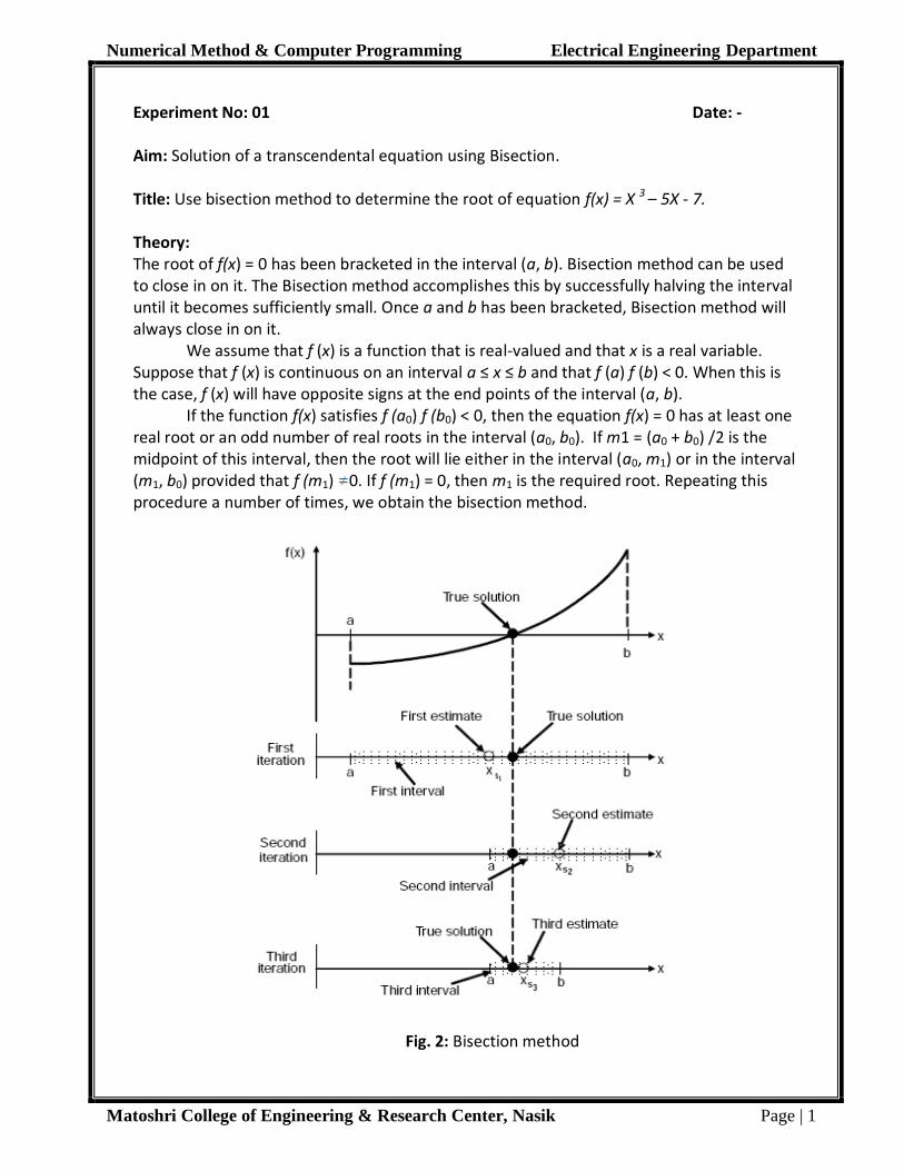
We assume that f (x) is a function that is real-valued and that x is a real variable. Suppose that f (x) is continuous on an interval a ≤ x ≤ b and that f (a) f (b) < 0. When this is the case, f (x) will have opposite signs at the end points of the interval (a, b).

If the function f(x) satisfies f (a0) f (b0) < 0, then the equation f(x) = 0 has at least one real root or an odd number of real roots in the interval (a0, b0). If m1 = (a0 + b0) /2 is the midpoint of this interval, then the root will lie either in the interval (a0, m1) or in the interval (m1, b0) provided that f (m1) 0. If f (m1) = 0, then m1 is the required root. Repeating this procedure a number of times, we obtain the bisection method.

Fig. 2: Bisection method



The method of finding a solution with the Bisection method is illustrated in Fig. 2. It starts by finding point a0 and b0 that define an interval where a solution exists. The midpoint of the interval m1 is then taken as the first estimate for the numerical solution. The true solution is either in the portion between point a0 and m1, or in the portion between points m1 and b. If the solution obtained is not accurate enough, a new interval that contains the true solution is defined. The new interval selected is the half of the original interval that contains the true solution, and its midpoint is taken as the new (second) estimate of the numerical solution. The procedure is repeated until the numerical solution is accurate enough according to a certain criterion that is selected. Procedure for the Bisection Method 1. Compute the first estimate a0 + b0 of the numerical solution m1 by

2. Determine whether the true solution is between a and m1or between m1 and b by

checking the sign of the product f (a) f (m1) has following conditions.

If f (a) f (m1) < 0, the true solution is between a and m1. If f (a) f (m1) > 0, the true solution is between m1 and b. If b – c ≤ error, then accept c as the root and stop. is the error tolerance, ∈ > 0.

3. Choose the subinterval that contains the true solution (a to m1) or (m1 to b) as the new

interval (a1, b1), and go back to step 1.

Steps 1 through 3 are repeated until a specified tolerance or error bound is attained. Advantages of Bisection method

The method is guaranteed to Accuracy. The method always to an answer, provided a root

was bracketed in the interval (a, b) to start with. In addition, the error bound, is

guaranteed to decrease by one-half with each iteration.

Disadvantage of Bisection method

The method may fail when the function is tangent to the axis and does not cross the x-axis

at f (x) = 0.

The disadvantage of the Bisection method is that it generally more slowly than most other

methods. For functions f (x) that have a continuous derivative, other methods are usually

faster.

Bisection method requires large number of iteration.

Bisection method requires two initial guess.

initial guess a and b of f(x) must be bound as f (a) f (b) < 0

Algorithm for the Bisection Method: Given a continuous function f(x)

1. Find points a and b such that a < b and f(a) * f(b) < 0. 2. Take the interval [a, b] and find its midpoint c. 3. If f(c) = 0 then x1 is an exact root, else if f(c) * f(b) < 0 then let a = c, else if f(a) * f(c) <

0 then let b = c. 4. Repeat steps 2 & 3 until f(c) = 0 or |f(c)| <= degree of accuracy.



Calculation:

………………………………………………………………………………………………………………………………………………

………………………………………………………………………………………………………………………………………………

………………………………………………………………………………………………………………………………………………

………………………………………………………………………………………………………………………………………………

………………………………………………………………………………………………………………………………………………

………………………………………………………………………………………………………………………………………………

………………………………………………………………………………………………………………………………………………

………………………………………………………………………………………………………………………………………………

………………………………………………………………………………………………………………………………………………

………………………………………………………………………………………………………………………………………………

………………………………………………………………………………………………………………………………………………

………………………………………………………………………………………………………………………………………………

………………………………………………………………………………………………………………………………………………

………………………………………………………………………………………………………………………………………………

………………………………………………………………………………………………………………………………………………

………………………………………………………………………………………………………………………………………………

………………………………………………………………………………………………………………………………………………

………………………………………………………………………………………………………………………………………………

………………………………………………………………………………………………………………………………………………

………………………………………………………………………………………………………………………………………………

………………………………………………………………………………………………..……………………………………………

………………………………………………………………………………………………………………………………………………

………………………………………………………………………………………………………………………………………………

………………………………………………………………………………………………..……………………………………………

………………………………………………………………………………………………………………………………………………

………………………………………………………………………………………………………………………………………………

Practical In-charge Sign



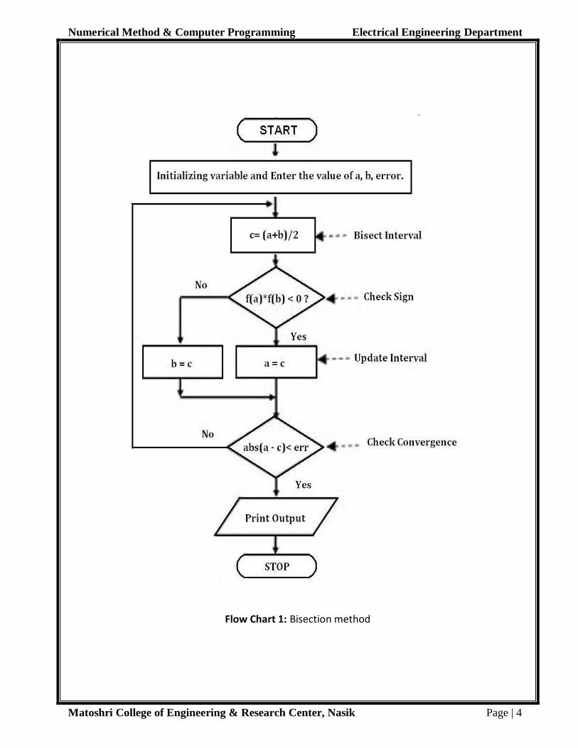
Flow Chart 1: Bisection method



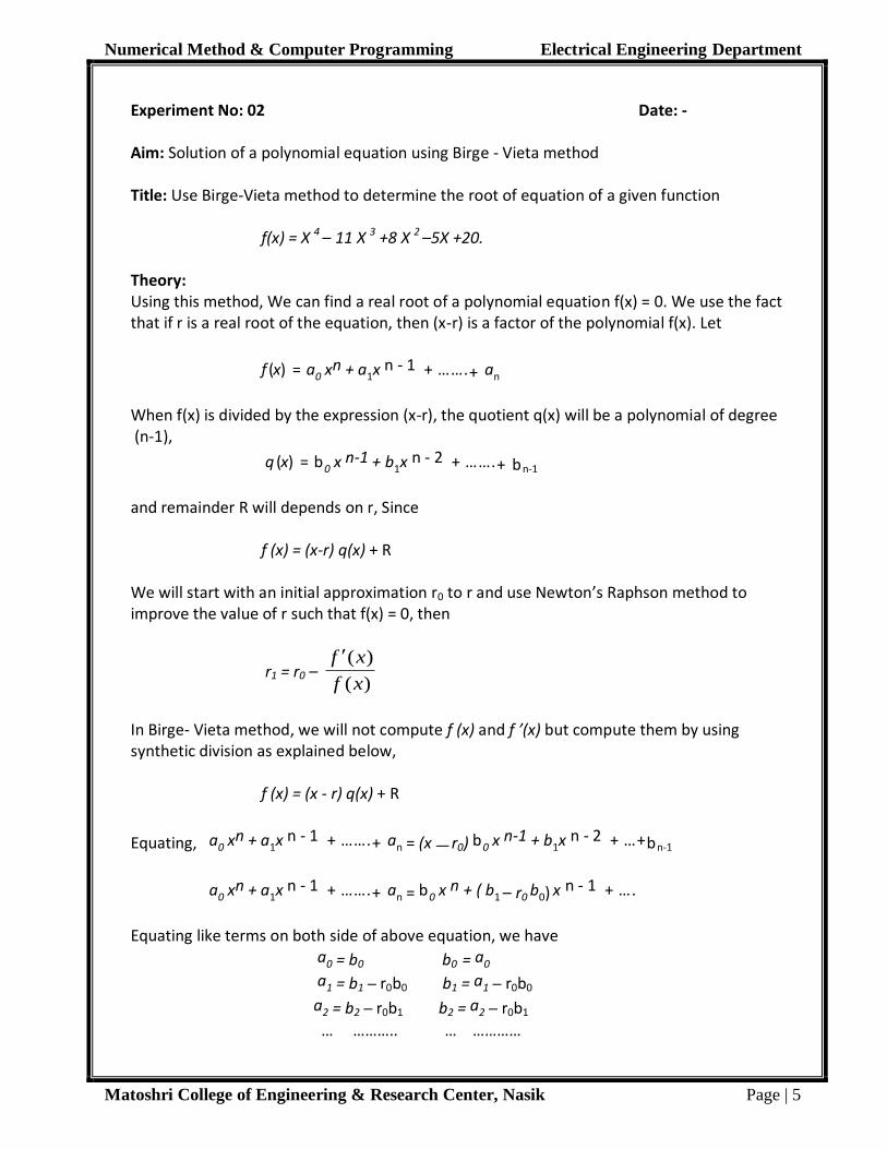
Experiment No: 02 Date: - Aim: Solution of a polynomial equation using Birge - Vieta method Title: Use Birge-Vieta method to determine the root of equation of a given function

f(x) = X 4 – 11 X 3 +8 X 2 –5X +20. Theory: Using this method, We can find a real root of a polynomial equation f(x) = 0. We use the fact that if r is a real root of the equation, then (x-r) is a factor of the polynomial f(x). Let

f (x) = a0 xn + a1x n - 1 + …….+ an

When f(x) is divided by the expression (x-r), the quotient q(x) will be a polynomial of degree (n-1),

q (x) = b0 x n-1 + b1x n - 2 + …….+ bn-1 and remainder R will depends on r, Since

f (x) = (x-r) q(x) + R

We will start with an initial approximation r0 to r and use Newton’s Raphson method to improve the value of r such that f(x) = 0, then

r1 = r0 – )(

)(

xf

xf

In Birge- Vieta method, we will not compute f (x) and f ’(x) but compute them by using synthetic division as explained below,

f (x) = (x - r) q(x) + R

Equating, a0 xn + a1x n - 1 + …….+ an = (x r0) b0 x n-1 + b1x n - 2 + …+bn-1

a0 xn + a1x n - 1 + …….+ an = b0 x n + ( b1 – r0 b0) x n - 1 + …. Equating like terms on both side of above equation, we have a0 = b0 b0 = a0 a1 = b1 ‒ r0b0 b1 = a1 ‒ r0b0

a2 = b2 ‒ r0b1 b2 = a2 ‒ r0b1

… ……….. … …………



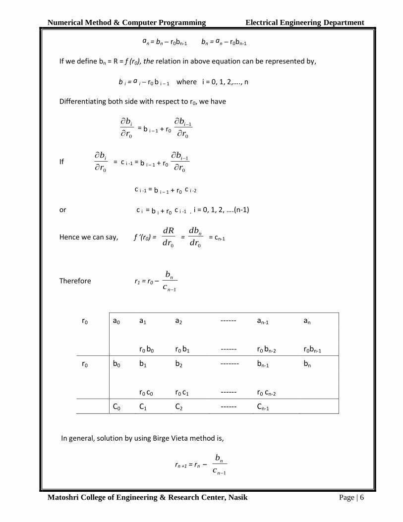
an = bn ‒ r0bn-1 bn = an ‒ r0bn-1

If we define bn = R = f (r0), the relation in above equation can be represented by,

b i = a i ‒ r0 b i – 1 where i = 0, 1, 2,…., n

Differentiating both side with respect to r0, we have

0r

bi

= b i – 1 + r0

0

1

r

bi

If 0r

bi

= c i -1 = b i – 1 + r0

0

1

r

bi

c i -1 = b i – 1 + r0 c i -2

or c i = b i + r0 c i -1 , i = 0, 1, 2, ….(n-1)

Hence we can say, f ‘(r0) = 0dr

dR =

0dr

dbn = cn-1

Therefore r1 = r0 – 1n

n

c

b

r0 a0 a1 a2 ------ an-1 an

r0 b0 r0 b1 ------ r0 bn-2 r0bn-1

r0 b0 b1 b2 ------- bn-1 bn

r0 c0 r0 c1 ------ r0 cn-2

C0 C1 C2 ------ Cn-1

In general, solution by using Birge Vieta method is,

rn +1 = rn – 1n

n

c

b



Algorithm for the Birge-Vieta Method: Given a continuous polynomial equation f(x) 1. Arrange the coefficient of given polynomial equation. 2. Perform the synthetic division with initial value r0.

3. Find next approximate root by rn +1 = rn – 1n

n

c

b

4. Repeat step 2 & step 3 r having minimum error. Calculation:

………………………………………………………………………………………………………………………………………………

………………………………………………………………………………………………………………………………………………

………………………………………………………………………………………………………………………………………………

………………………………………………………………………………………………………………………………………………

………………………………………………………………………………………………………………………………………………

………………………………………………………………………………………………………………………………………………

………………………………………………………………………………………………………………………………………………

………………………………………………………………………………………………………………………………………………

………………………………………………………………………………………………………………………………………………

………………………………………………………………………………………………………………………………………………

………………………………………………………………………………………………………………………………………………

………………………………………………………………………………………………………………………………………………

………………………………………………………………………………………………………………………………………………

………………………………………………………………………………………………………………………………………………

………………………………………………………………………………………………………………………………………………

………………………………………………………………………………………………………………………………………………

………………………………………………………………………………………………………………………………………………




Flow Chart 2: Birge-Vieta method



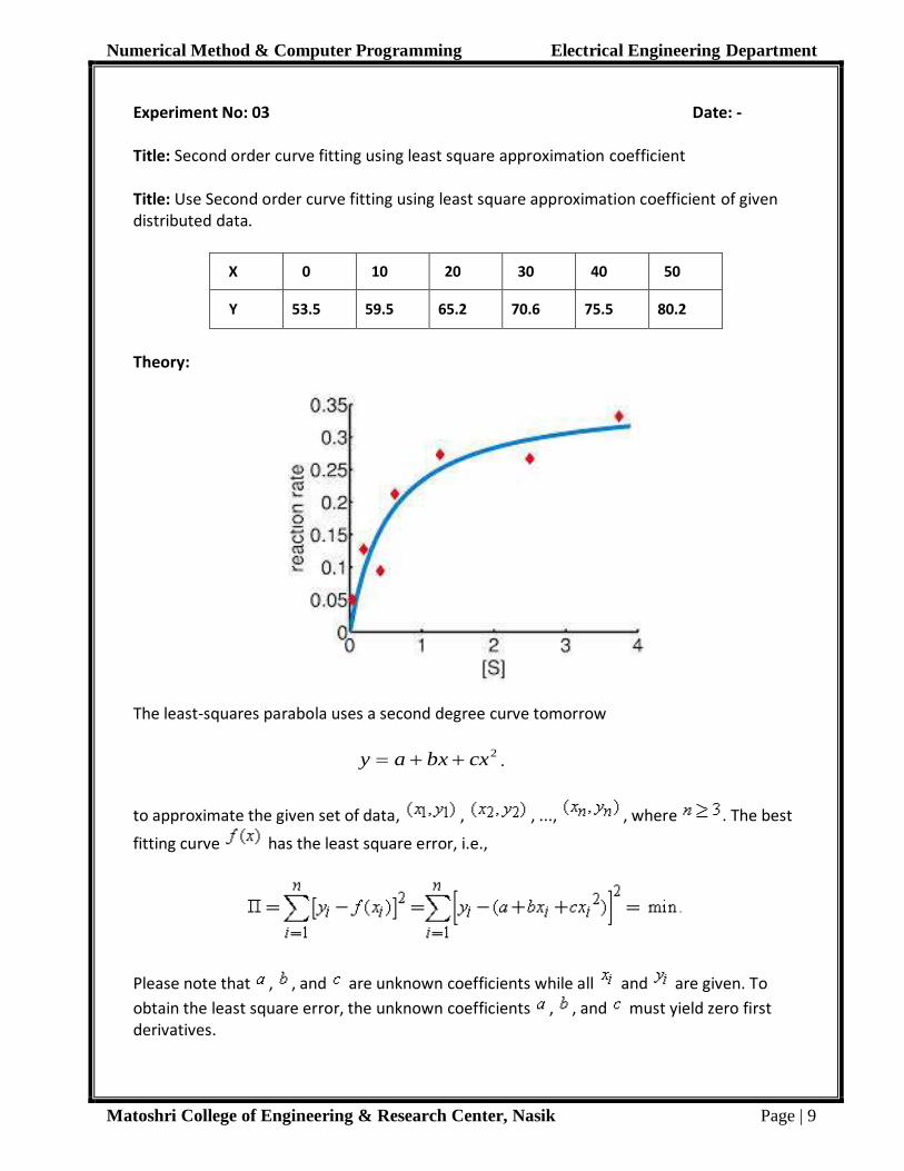
Experiment No: 03 Date: - Title: Second order curve fitting using least square approximation coefficient Title: Use Second order curve fitting using least square approximation coefficient of given distributed data.

X 0 10 20 30 40 50

Y 53.5 59.5 65.2 70.6 75.5 80.2

Theory:

The least-squares parabola uses a second degree curve tomorrow

2cxbxay .

to approximate the given set of data, , , ..., , where . The best

fitting curve has the least square error, i.e.,

Please note that , , and are unknown coefficients while all and are given. To

obtain the least square error, the unknown coefficients , , and must yield zero first derivatives.



Expanding the above equations, we have

The unknown coefficients , , and can hence be obtained by solving the above linear equations.

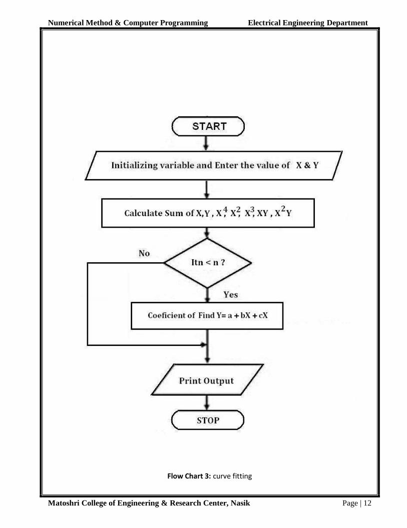
Algorithm for the Second order curve fitting : From the given a distributed data. 1. Enter the values of x corresponds to y.

2. Calculate the values of yxxyxxxx 2432 ,,,,, from the given distributed

data. 3. Calculate the value of coefficient a, b, c by least square equation

4. Print the result as 2cxbxay .

Calculation:

………………………………………………………………………………………………………………………………………………

………………………………………………………………………………………………………………………………………………

………………………………………………………………………………………………………………………………………………

………………………………………………………………………………………………………………………………………………

………………………………………………………………………………………………………………………………………………

………………………………………………………………………………………………………………………………………………



………………………………………………………………………………………………………………………………………………

………………………………………………………………………………………………………………………………………………

………………………………………………………………………………………………………………………………………………

………………………………………………………………………………………………………………………………………………

………………………………………………………………………………………………………………………………………………

………………………………………………………………………………………………………………………………………………

………………………………………………………………………………………………………………………………………………

………………………………………………………………………………………………………………………………………………

………………………………………………………………………………………………………………………………………………

………………………………………………………………………………………………………………………………………………

………………………………………………………………………………………………………………………………………………

………………………………………………………………………………………………………………………………………………

………………………………………………………………………………………………………………………………………………

………………………………………………………………………………………………………………………………………………

………………………………………………………………………………………………..……………………………………………

………………………………………………………………………………………………………………………………………………

………………………………………………………………………………………………………………………………………………

………………………………………………………………………………………………..……………………………………………

………………………………………………………………………………………………………………………………………………

……………………………………………………………………………………………………………………………………

………………………………………………………………………………………………………………………………………………

………………………………………………………………………………………………..……………………………………………

………………………………………………………………………………………………………………………………………………

………………………………………………………………………………………………………………………………………………

………………………………………………………………………………………………………………………………………………

………………………………………………………………………………………………..……………………………………………

………………………………………………………………………………………………………………………………………………




Flow Chart 3: curve fitting



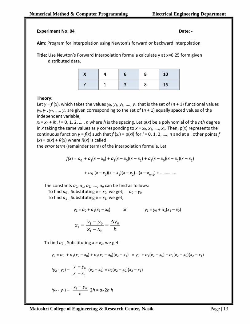
Experiment No: 04 Date: - Aim: Program for interpolation using Newton’s forward or backward interpolation Title: Use Newton’s Forward Interpolation formula calculate y at x=6.25 form given

distributed data.

X 4 6 8 10

Y 1 3 8 16

Theory: Let y = f (x), which takes the values y0, y1, y2, …., yn that is the set of (n + 1) functional values y0, y1, y2, …., yn are given corresponding to the set of (n + 1) equally spaced values of the independent variable, xi = x0 + ih, i = 0, 1, 2, …., n where h is the spacing. Let p(x) be a polynomial of the nth degree in x taking the same values as y corresponding to x = x0, x1, …., xn. Then, p(x) represents the continuous function y = f(x) such that f (xi) = p(xi) for i = 0, 1, 2, …., n and at all other points f (x) = p(x) + R(x) where R(x) is called the error term (remainder term) of the interpolation formula. Let

f(x) = a0 + a1(x – x0) + a2(x – x0)(x – x1) + a3(x – x0)(x – x1)(x – x2)

+ an (x – x0)(x – x1)(x – x2)…(x – xn–1) + …………..

The constants a0, a1, a2, …., an can be find as follows:

To find a0 , Substituting x = x0, we get, a0 = y0 To find a1 , Substituting x = x1, we get,

y1 = a0 + a1(x1 – x0) or y1 = y0 + a1(x1 – x0)

h

y

xx

yya 0

01

011

To find a2 , Substituting x = x2, we get

y2 = a0 + a1(x2 – x0) + a2(x2 – x0)(x2 – x1) = y0 + a1(x2 – x0) + a2(x2 – x0)(x2 – x1)

(y2 - y0) – 01

01

xx

yy

(x2 – x0) = a2(x2 – x0)(x2 – x1)

(y2 - y0) – h

yy 01 2h = a2 2h h



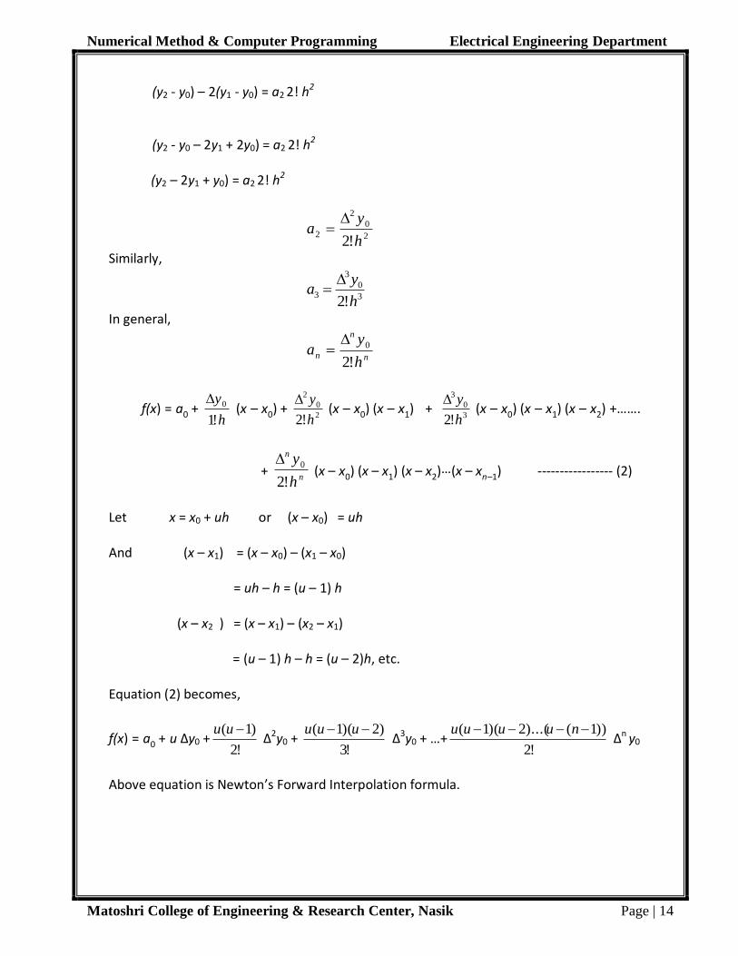
(y2 - y0) – 2(y1 - y0) = a2 2! h2

(y2 - y0 – 2y1 + 2y0) = a2 2! h2

(y2 – 2y1 + y0) = a2 2! h2

2

0

2

2!2 h

ya

Similarly,

3

0

3

3!2 h

ya

In general,

n

n

nh

ya

!2

0

f(x) = a0 + h

y

!1

0 (x – x0) +

2

0

2

!2 h

y (x – x0) (x – x1) +

3

0

3

!2 h

y (x – x0) (x – x1) (x – x2) +…….

+ n

n

h

y

!2

0 (x – x0) (x – x1) (x – x2)…(x – xn–1) ----------------- (2)

Let x = x0 + uh or (x – x0) = uh And (x – x1) = (x – x0) – (x1 – x0)

= uh – h = (u – 1) h (x – x2 ) = (x – x1) – (x2 – x1) = (u – 1) h – h = (u – 2)h, etc. Equation (2) becomes,

f(x) = a0 + u Δy0 +!2

)1( uu Δ2y0 +

!3

)2)(1( uuu Δ3y0 + …+

!2

))1()...(2)(1( nuuuu Δn y0

Above equation is Newton’s Forward Interpolation formula.



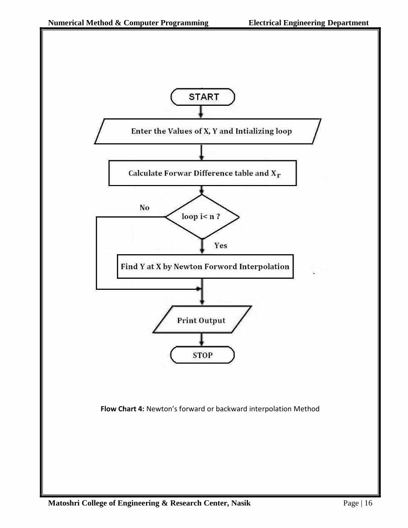
Algorithm for the Newton’s Forward Interpolation Method: From the given a distributed data. 1. Enter the values of x corresponds to y. 2. Calculate the values of Newton’s forward difference table from the given distributed

data. 3. Calculate the value of y at a given value of x. 4. Print the result. Calculation:

………………………………………………………………………………………………………………………………………………

………………………………………………………………………………………………………………………………………………

………………………………………………………………………………………………………………………………………………

………………………………………………………………………………………………………………………………………………

………………………………………………………………………………………………………………………………………………

………………………………………………………………………………………………………………………………………………

………………………………………………………………………………………………………………………………………………

………………………………………………………………………………………………………………………………………………

………………………………………………………………………………………………………………………………………………

………………………………………………………………………………………………………………………………………………

………………………………………………………………………………………………………………………………………………

………………………………………………………………………………………………………………………………………………

………………………………………………………………………………………………………………………………………………

………………………………………………………………………………………………………………………………………………

………………………………………………………………………………………………………………………………………………

………………………………………………………………………………………………………………………………………………

………………………………………………………………………………………………………………………………………………

………………………………………………………………………………………………………………………………………………

………………………………………………………………………………………………………………………………………………

………………………………………………………………………………………………………………………………………………




Flow Chart 4: Newton’s forward or backward interpolation Method



Experiment No: 05 Date: - Aim: Newton’s Raphson’s method for two variables Title: Find the root of equation using N R Method for two variables. f(x, y) = X2 + XY – 10 , g( x, y) = Y + 3XY2- 57. Solve upto two iteration only take initial value X0 = 1.5 and Y0 = 3.5. Theory: Let them be f (x,y) = 0 and g (x,y) = 0. Now (x0, y0) be an initial approximate solution of the equation.

Let (x0+h, y0+k) be the actual solution. Using Taylor’s series ,

f (xi+1) = f (xi) + h f’(xi) + h2 f’’(xi) +… + h n f’n (xi)

For a two function of two variables and omitting h2 and higher order

f (xi+1, yi+1) = f (xi, yi) + h f’(xi) + k f’(yi)

g (xi+1, yi+1) = g (xi, yi) + h g’(xi) + k g’(yi) Where,

f x = f’(xi) =x

yxf

),( │y = const. f y = f’(yi) =

y

yxf

),(│x = const.

g x = g’(xi) = x

yxg

),(│y = const. g x = g’(yi) =

y

yxg

),(│x = const.



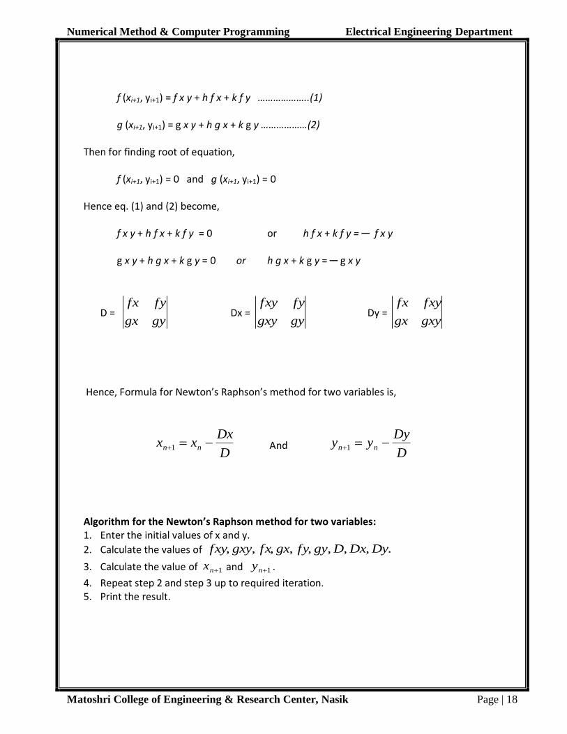
f (xi+1, yi+1) = f x y + h f x + k f y ………………..(1)

g (xi+1, yi+1) = g x y + h g x + k g y ………………(2)

Then for finding root of equation,

f (xi+1, yi+1) = 0 and g (xi+1, yi+1) = 0 Hence eq. (1) and (2) become,

f x y + h f x + k f y = 0 or h f x + k f y = ─ f x y g x y + h g x + k g y = 0 or h g x + k g y = ─ g x y

D = gygx

fyfx Dx =

gygxy

fyfxy Dy =

gxygx

fxyfx

Hence, Formula for Newton’s Raphson’s method for two variables is,

D

Dxxx nn 1 And

D

Dyyy nn 1

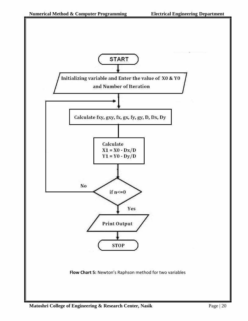
Algorithm for the Newton’s Raphson method for two variables: 1. Enter the initial values of x and y.

2. Calculate the values of .,,,,,,,, DyDxDgyfygxfxgxyfxy

3. Calculate the value of 1nx and 1ny .

4. Repeat step 2 and step 3 up to required iteration. 5. Print the result.



Calculation:

………………………………………………………………………………………………………………………………………………

………………………………………………………………………………………………………………………………………………

………………………………………………………………………………………………………………………………………………

………………………………………………………………………………………………………………………………………………

………………………………………………………………………………………………………………………………………………

………………………………………………………………………………………………………………………………………………

………………………………………………………………………………………………………………………………………………

………………………………………………………………………………………………………………………………………………

………………………………………………………………………………………………………………………………………………

………………………………………………………………………………………………………………………………………………

………………………………………………………………………………………………………………………………………………

………………………………………………………………………………………………………………………………………………

………………………………………………………………………………………………………………………………………………

………………………………………………………………………………………………………………………………………………

………………………………………………………………………………………………………………………………………………

………………………………………………………………………………………………………………………………………………

………………………………………………………………………………………………………………………………………………

………………………………………………………………………………………………………………………………………………

………………………………………………………………………………………………………………………………………………

………………………………………………………………………………………………………………………………………………

………………………………………………………………………………………………..……………………………………………

………………………………………………………………………………………………………………………………………………

………………………………………………………………………………………………………………………………………………

………………………………………………………………………………………………..……………………………………………

………………………………………………………………………………………………………………………………………………

………………………………………………………………………………………………………………………………………………




Flow Chart 5: Newton’s Raphson method for two variables



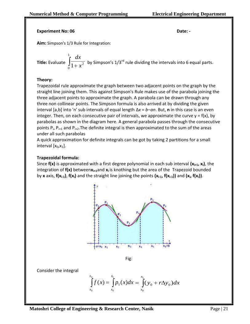
Experiment No: 06 Date: - Aim: Simpson's 1/3 Rule for Integration:

Title: Evaluate

1

0

21 x

dx by Simpson’s 1/3rd rule dividing the intervals into 6 equal parts.

Theory: Trapezoidal rule approximate the graph between two adjacent points on the graph by the straight line joining them. This against Simpson's Rule makes use of the parabola joining the three adjacent points to approximate the graph. A parabola can be drawn through any three non collinear points. The Simpson formula is also arrived at by dividing the given interval [a,b] into 'n' sub intervals of equal length Δx = b−an. But, n in this case is an even integer. Then, on each consecutive pair of intervals, we approximate the curve y = f(x), by parabolas as shown in the diagram here. A general parabola passes through the consecutive points Pi, Pi+1 and Pi+2.The definite integral is then approximated to the sum of the areas under all such parabolas A quick approximation for definite integrals can be got by taking 2 partitions for a small interval [x0,x1]. Trapezoidal formula: Since f(x) is approximated with a first degree polynomial in each sub interval (xi+1, xi), the integration of f(x) betweenxi+1and xi is knothing but the area of the Trapezoid bounded by x axis, f(xi-1), f(xi) and the straight line joining the points (xi-1, f(xi-1)) and (xi, f(xi)).

Fig: Consider the integral

nx

x

x

x

dxxpxf

0

1

0

)()( 1 1

0

)( 00

x

x

dxyry



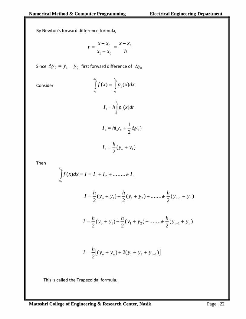
By Newton's forward difference formula,

h

xx

xx

xxr 0

01

0

Since 010 yyy first forward difference of 0y

Consider nx

x

x

x

dxxpxf

0

1

0

)()( 1

1

0

11 )( drxphI

)2

1( 01 yyhI o

)(2

11 yyh

I o

Then

nx

x

nIIIIdxxf

0

.........)( 21

)(2

........)(2

)(2

1211 nno yyh

yyh

yyh

I

)(2

........)(2

)(2

1211 nno yyh

yyh

yyh

I

)(2)(2

121 nno yyyyyh

I

This is called the Trapezoidal formula.



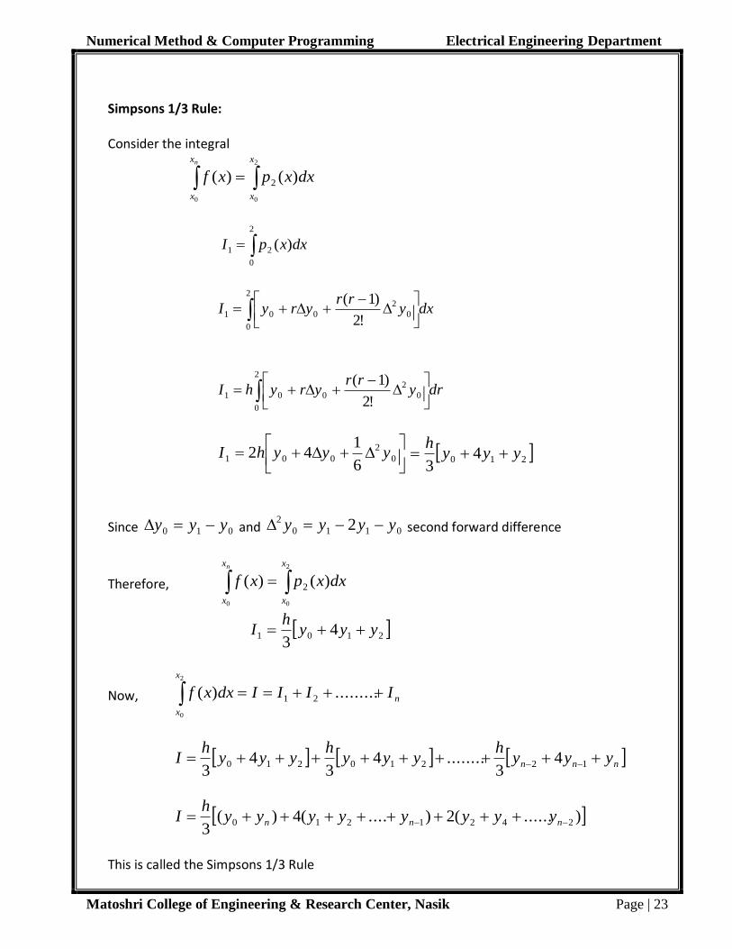
Simpsons 1/3 Rule: Consider the integral

nx

x

x

x

dxxpxf

0

2

0

)()( 2

2

0

21 )( dxxpI

dxyrr

yryI

2

0

0

2

001!2

)1(

dryrr

yryhI

2

0

0

2

001!2

)1(

0

2

0016

142 yyyhI 210 4

3yyy

h

Since 010 yyy and 0110

2 2 yyyy second forward difference

Therefore, nx

x

x

x

dxxpxf

0

2

0

)()( 2

2101 43

yyyh

I

Now, 2

0

.........)( 21

x

x

nIIIIdxxf

nnn yyyh

yyyh

yyyh

I 12210210 43

........43

43

)......(2)....(4)(3

2421210 nnn yyyyyyyyh

I

This is called the Simpsons 1/3 Rule



Simpsons 3/8 Rule: Consider the integral

nx

x

x

x

dxxpxf

0

3

0

)()( 3

3

0

21 )( dxxpI

dxyrrr

yrr

yryI

3

0

0

3

0

2

001!3

)2)(1(

!2

)1(

dryrrr

yrr

yryhI

3

0

0

3

0

2

001!3

)2)(1(

!2

)1(

0

3

0

2

0018

1

2

3

2

33 yyyyhI

Since 010 yyy and 0110

2 2 yyyy second forward difference

Therefore, nx

x

x

x

dxxpxf

0

3

0

)()( 3

32101 338

3yyyy

hI

Now,

3

0

.........)( 21

x

x

nIIIIdxxf

)...(2)....(3)(8

336312542101 nnnn yyyyyyyyyyyy

hI

This is called the Simpsons 3/8 Rule. The no. of data points needed for this rule are 3n+1 for any n > 0.



Observe here that the order of the error in both Simpson's one third rule and three eighth rule is four (O(h4)). Moreover the coefficient in one third rule (-1/90) is less then the corresponding three eighth rule (-3/80) hence Simpson's 1/3 rule performs better than the Simpson's 3/8 rule. In fact this phenomina is true for all even-order Newton-cotes formulae. Hence Newton-cotes even order formulae are more useful than odd order formulae.

Algorithm for the Simpson's 1/3 Rule for Integration: 1. Enter the initial values upper limit and lower limit. 2. Calculate the values of x corresponds to y according to value step size(h).

3. Calculate the sum of odd term value of oddy and sum of even term value of eveny .

4. Print the result. Calculation:

………………………………………………………………………………………………………………………………………………

………………………………………………………………………………………………………………………………………………

………………………………………………………………………………………………………………………………………………

………………………………………………………………………………………………………………………………………………

………………………………………………………………………………………………………………………………………………

………………………………………………………………………………………………………………………………………………

………………………………………………………………………………………………………………………………………………

………………………………………………………………………………………………………………………………………………

………………………………………………………………………………………………………………………………………………

………………………………………………………………………………………………………………………………………………

………………………………………………………………………………………………………………………………………………

………………………………………………………………………………………………………………………………………………

………………………………………………………………………………………………………………………………………………

………………………………………………………………………………………………………………………………………………

………………………………………………………………………………………………………………………………………………




Flow Chart 6: Simpson's 1/3 Rule for Integration method



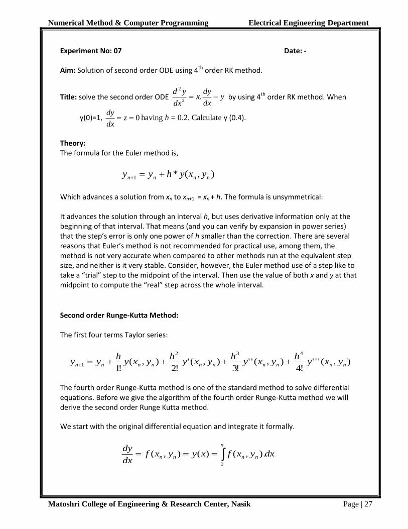
Experiment No: 07 Date: - Aim: Solution of second order ODE using 4th order RK method.

Title: solve the second order ODE ydx

dyx

dx

yd .

2

2

by using 4th order RK method. When

y(0)=1, 0 zdx

dyhaving h = 0.2. Calculate y (0.4).

Theory: The formula for the Euler method is,

),(*1 nnnn yxyhyy

Which advances a solution from xn to xn+1 = xn + h. The formula is unsymmetrical: It advances the solution through an interval h, but uses derivative information only at the beginning of that interval. That means (and you can verify by expansion in power series) that the step’s error is only one power of h smaller than the correction. There are several reasons that Euler’s method is not recommended for practical use, among them, the method is not very accurate when compared to other methods run at the equivalent step size, and neither is it very stable. Consider, however, the Euler method use of a step like to take a “trial” step to the midpoint of the interval. Then use the value of both x and y at that midpoint to compute the “real” step across the whole interval.

Second order Runge-Kutta Method: The first four terms Taylor series:

),('''!4

),(''!3

),('!2

),(!1

432

1 nnnnnnnnnn yxyh

yxyh

yxyh

yxyh

yy

The fourth order Runge-Kutta method is one of the standard method to solve differential equations. Before we give the algorithm of the fourth order Runge-Kutta method we will derive the second order Runge Kutta method.

We start with the original differential equation and integrate it formally.

n

nnnn dxyxfxyyxfdx

dy

0

).,()(),(



Omitting the term from h2 of Taylor’s series, we get,

hyxyyy nnnn ),(1

1

11 ).,(

n

n

nn dxyxfhyy

We essentially changed the task at hand from performing a differentiation to an integration. To do this we expand f(t) in a second order Taylor series around the midpoint of the integration subinterval.

dx

dyxxyxfyxf nnn )(),(),( 2/12/12/1 ……………………….. (1)

Yet since the integral of (X – Xn-1/2 ) vanishes when evaluated about the midpoint, we automatically get improved precision using only the first term in (1).

),(),( 2/12/1 nn yxfyxf

Therefore, ),(* 2/12/11 nnnn yxfhyy

),2

(* 2/1 nnn yh

xfhy

This algorithm cannot be applied immediately since it requires a knowledge of 2/1ny which

is not in the scheme of things. We thus approximate 2/1ny with Euler's algorithm.

22/1

h

dx

dyyx

dx

dyyy nnn

),(*2

nnn yxfh

y

Hence the second order Runge-Kutta

)(*2

211 kkh

yy nn ------------------------- (2)

Where, ),(1 nn yxfk

),( 112 kyxfk nn



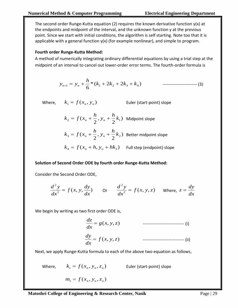
The second order Runge-Kutta equation (2) requires the known derivative function y(x) at the endpoints and midpoint of the interval, and the unknown function y at the previous point. Since we start with initial conditions, the algorithm is self starting. Note too that it is applicable with a general function y(x) (for example nonlinear), and simple to program.

Fourth order Runge-Kutta Method:

A method of numerically integrating ordinary differential equations by using a trial step at the

midpoint of an interval to cancel out lower-order error terms. The fourth-order formula is

)22(*6

43211 kkkkh

yy nn ------------------------ (3)

Where, ),(1 nn yxfk Euler (start-point) slope

)2

,2

( 12 kh

yh

xfk nn Midpoint slope

)2

,2

( 23 kh

yh

xfk nn Better midpoint slope

),( 34 hkyhxfk nn Full step (endpoint) slope

Solution of Second Order ODE by fourth order Runge-Kutta Method: Consider the Second Order ODE,

),,(2

2

dx

dyyxf

dx

yd Or ),,(

2

2

zyxfdx

yd Where,

dx

dyz

We begin by writing as two first order ODE is,

),,( zyxgdx

dz ----------------------------- (i)

),,( zyxfdx

dy ----------------------------- (ii)

Next, we apply Runge-Kutta formula to each of the above two equation as follows,

Where, ),,(1 nnn zyxfk Euler (start-point) slope

),,(1 nnn zyxfm



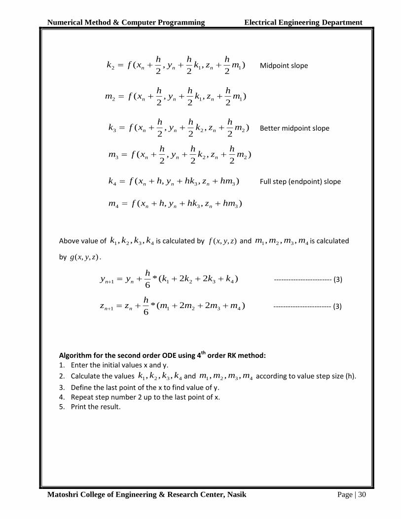
)2

,2

,2

( 112 mh

zkh

yh

xfk nnn Midpoint slope

)2

,2

,2

( 112 mh

zkh

yh

xfm nnn

)2

,2

,2

( 223 mh

zkh

yh

xfk nnn Better midpoint slope

)2

,2

,2

( 223 mh

zkh

yh

xfm nnn

),,( 334 hmzhkyhxfk nnn Full step (endpoint) slope

),,( 334 hmzhkyhxfm nnn

Above value of 4321 ,,, kkkk is calculated by ),,( zyxf and 4321 ,,, mmmm is calculated

by ),,( zyxg .

)22(*6

43211 kkkkh

yy nn ------------------------ (3)

)22(*6

43211 mmmmh

zz nn ------------------------ (3)

Algorithm for the second order ODE using 4th order RK method: 1. Enter the initial values x and y.

2. Calculate the values 4321 ,,, kkkk and 4321 ,,, mmmm according to value step size (h).

3. Define the last point of the x to find value of y. 4. Repeat step number 2 up to the last point of x. 5. Print the result.



Calculation:

………………………………………………………………………………………………………………………………………………

………………………………………………………………………………………………………………………………………………

………………………………………………………………………………………………………………………………………………

………………………………………………………………………………………………………………………………………………

………………………………………………………………………………………………………………………………………………

………………………………………………………………………………………………………………………………………………

………………………………………………………………………………………………………………………………………………

………………………………………………………………………………………………………………………………………………

………………………………………………………………………………………………………………………………………………

………………………………………………………………………………………………………………………………………………

………………………………………………………………………………………………………………………………………………

………………………………………………………………………………………………………………………………………………

………………………………………………………………………………………………………………………………………………

………………………………………………………………………………………………………………………………………………

………………………………………………………………………………………………………………………………………………

………………………………………………………………………………………………………………………………………………

………………………………………………………………………………………………………………………………………………

………………………………………………………………………………………………………………………………………………

………………………………………………………………………………………………………………………………………………

………………………………………………………………………………………………………………………………………………

………………………………………………………………………………………………..……………………………………………

………………………………………………………………………………………………………………………………………………

………………………………………………………………………………………………………………………………………………

………………………………………………………………………………………………..……………………………………………

………………………………………………………………………………………………………………………………………………

………………………………………………………………………………………………………………………………………………




Flow Chart 7: Solution of second order ODE using 4th order RK method



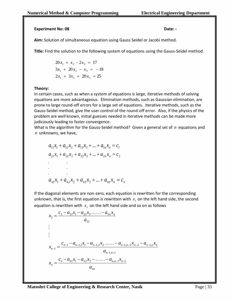
Experiment No: 08 Date: - Aim: Solution of simultaneous equation using Gauss Seidel or Jacobi method. Title: Find the solution to the following system of equations using the Gauss-Seidel method.

17220 321 x x x

18203 321 x x x

252032 321 x x x

Theory: In certain cases, such as when a system of equations is large, iterative methods of solving equations are more advantageous. Elimination methods, such as Gaussian elimination, are prone to large round-off errors for a large set of equations. Iterative methods, such as the Gauss-Seidel method, give the user control of the round-off error. Also, if the physics of the problem are well known, initial guesses needed in iterative methods can be made more judiciously leading to faster convergence. What is the algorithm for the Gauss-Seidel method? Given a general set of n equations and n unknowns, we have,

11313212111 ... cxaxaxaxa nn

22323222121 ... cxaxaxaxa nn

. .

. .

. .

nnnnnnn cxaxaxaxa ...332211

If the diagonal elements are non-zero, each equation is rewritten for the corresponding unknown, that is, the first equation is rewritten with 1x on the left hand side, the second

equation is rewritten with 2x on the left hand side and so on as follows

nn

nnnnnn

n

nn

nnnnnnnnn

n

nn

a

xaxaxacx

a

xaxaxaxacx

a

xaxaxacx

11,2211

1,1

,122,122,111,11

1

22

232312122



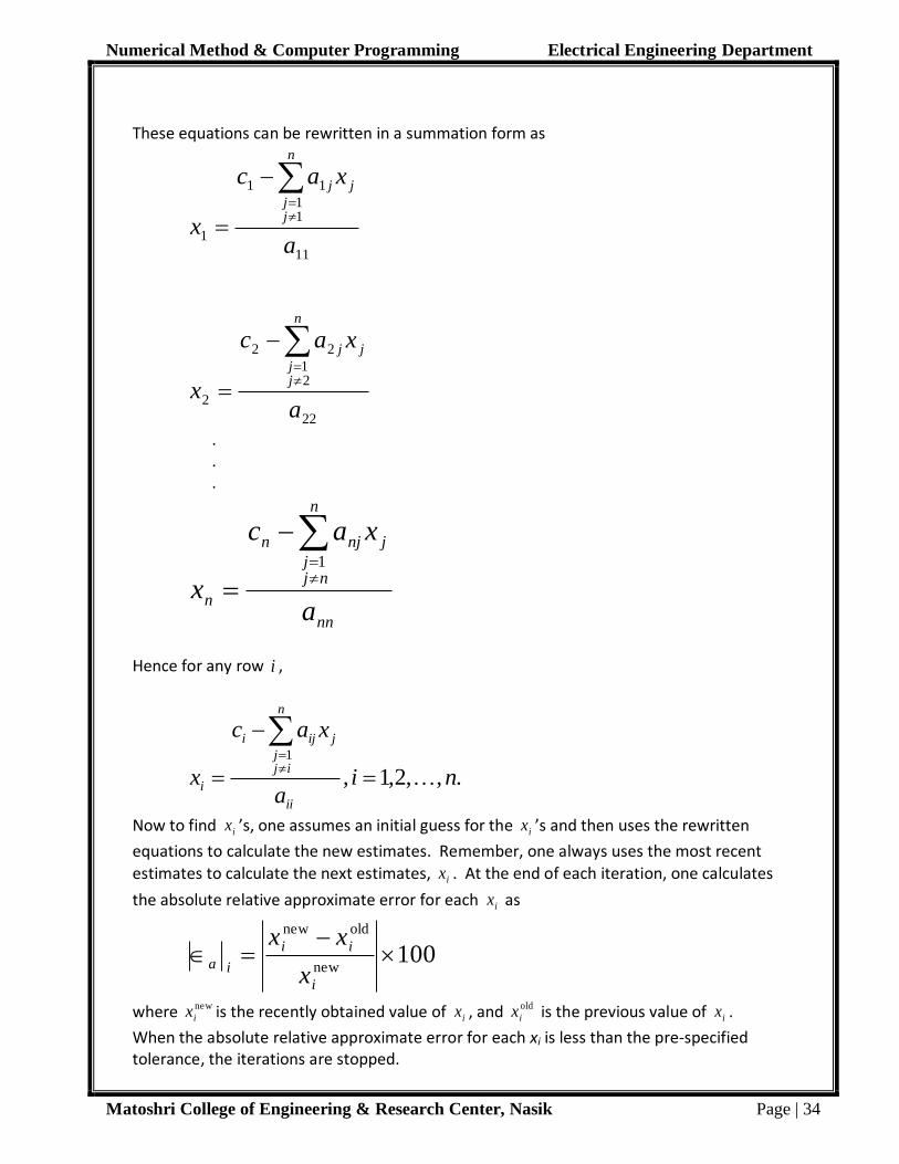
These equations can be rewritten in a summation form as

11

11

11

1a

xac

x

n

jj

jj

22

21

22

2a

xac

x

j

n

jj

j

. .

.

nn

n

njj

jnjn

na

xac

x

1

Hence for any row i ,

.,,2,1,1

nia

xac

xii

n

ijj

jiji

i

Now to find ix ’s, one assumes an initial guess for the ix ’s and then uses the rewritten

equations to calculate the new estimates. Remember, one always uses the most recent

estimates to calculate the next estimates, ix . At the end of each iteration, one calculates

the absolute relative approximate error for each ix as

100new

oldnew

i

ii

iax

xx

where new

ix is the recently obtained value of ix , and old

ix is the previous value of ix .

When the absolute relative approximate error for each xi is less than the pre-specified tolerance, the iterations are stopped.



Calculation:

………………………………………………………………………………………………………………………………………………

………………………………………………………………………………………………………………………………………………

………………………………………………………………………………………………………………………………………………

………………………………………………………………………………………………………………………………………………

………………………………………………………………………………………………………………………………………………

………………………………………………………………………………………………………………………………………………

………………………………………………………………………………………………………………………………………………

………………………………………………………………………………………………………………………………………………

………………………………………………………………………………………………………………………………………………

………………………………………………………………………………………………………………………………………………

………………………………………………………………………………………………………………………………………………

………………………………………………………………………………………………………………………………………………

………………………………………………………………………………………………………………………………………………

………………………………………………………………………………………………………………………………………………

………………………………………………………………………………………………………………………………………………

………………………………………………………………………………………………………………………………………………

………………………………………………………………………………………………………………………………………………

………………………………………………………………………………………………………………………………………………

………………………………………………………………………………………………………………………………………………

………………………………………………………………………………………………………………………………………………

………………………………………………………………………………………………..……………………………………………

………………………………………………………………………………………………………………………………………………

………………………………………………………………………………………………………………………………………………

………………………………………………………………………………………………..……………………………………………

………………………………………………………………………………………………………………………………………………

………………………………………………………………………………………………………………………………………………




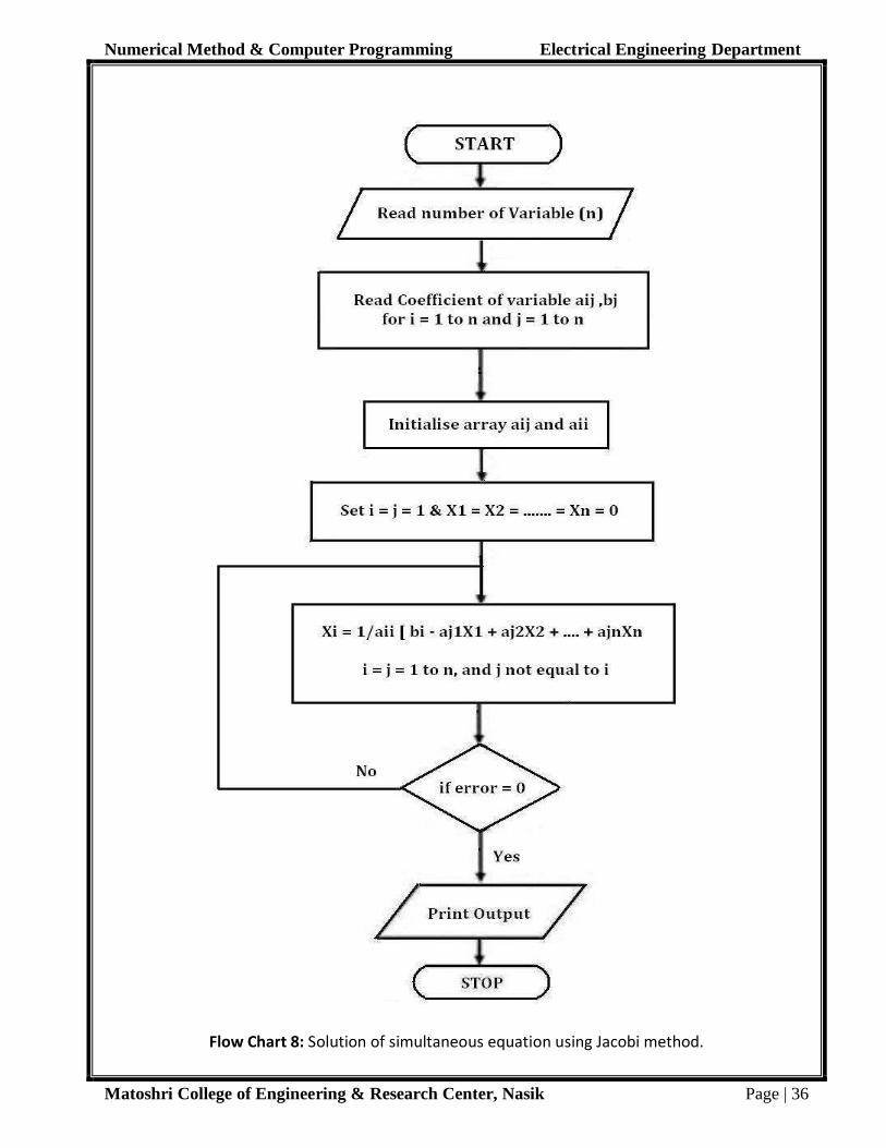
Flow Chart 8: Solution of simultaneous equation using Jacobi method.



Experiment No: 09 Date: - Aim: To find Eigen values and vector using Jacobi method. Title: Determine the largest Eigen value and corresponding Eigen vector of the following matrix.

300

021

161

By Jacobi method.

Theory:

If the action of a matrix on a (nonzero) vector changes its magnitude but not its direction, then the vector is called an eigenvector of that matrix. A vector which is "flipped" to point in the opposite direction is also considered an eigenvector. Each eigenvector is, in effect, multiplied by a scalar, called the eigenvalue corresponding to that eigenvector. The eigenspace corresponding to one eigenvalue of a given matrix is the set of all eigenvectors of the matrix with that eigenvalue.

Many kinds of mathematical objects can be treated as vectors: ordered pairs, functions, harmonic modes, quantum states, and frequencies are examples. In these cases, the concept of direction loses its ordinary meaning, and is given an abstract definition. Even so, if this abstract direction is unchanged by a given linear transformation, the prefix "eigen" is used, as in eigenfunction, eigenmode, eigenstate, and eigenfrequency.

When a transformation is represented by a square matrix A, the eigenvalue equation can be expressed as ( A x – λ I x) = 0. This can be rearranged to

( A – λ I ) x = 0. If there exists an inverse,

( A – λ I ) -1 = 0.

Then both sides can be left multiplied by the inverse to obtain the trivial solution: x = 0. Thus we require there to be no inverse by assuming from linear algebra that the determinant equals zero:

Det (A – λ I ) = 0.

The determinant requirement is called the characteristic equation (less often, secular equation) of A, and the left-hand side is called the characteristic polynomial. When expanded, this gives a polynomial equation for λ. The eigenvector x or its components are not present in the characteristic equation.

http://en.wikipedia.org/wiki/Eigenfunction

http://en.wikipedia.org/wiki/Eigenmode

http://en.wikipedia.org/wiki/Linear_algebra

http://en.wikipedia.org/wiki/Determinant

http://en.wikipedia.org/wiki/Characteristic_equation

http://en.wikipedia.org/wiki/Secular_equation



http://en.wikipedia.org/wiki/Characteristic_polynomial

http://en.wikipedia.org/wiki/Polynomial



In vector calculus, the Jacobian matrix is the matrix of all first-order partial derivatives of a vector-valued function. Suppose F : Rn → Rm is a function from Euclidean n-space to Euclidean m-space. Such a function is given by m real-valued component functions, y1(x1,...,xn), ..., ym(x1,...,xn). The partial derivatives of all these functions (if they exist) can be organized in an m-by-n matrix, the Jacobian matrix J of F, as follows:

This matrix is also denoted by and . The i th row (i = 1, ...,

m) of this matrix is the gradient of the ith component function yi: .

The Jacobian determinant (often simply called the Jacobian) is the determinant of the Jacobian matrix.

The Jacobian of a function describes the orientation of a tangent plane to the function at a given point. In this way, the Jacobian generalizes the gradient of a scalar valued function of multiple variables which itself generalizes the derivative of a scalar-valued function of a scalar. Likewise, the Jacobian can also be thought of as describing the amount of "stretching" that a transformation imposes. For example, if (x2,y2) = f(x1,y1) is used to transform an image, the Jacobian of f, J(x1,y1) describes how much the image in the neighborhood of (x1,y1) is stretched in the x, y, and xy directions.

If a function is differentiable at a point, its derivative is given in coordinates by the Jacobian, but a function doesn't need to be differentiable for the Jacobian to be defined, since only the partial derivatives are required to exist.

The importance of the Jacobian lies in the fact that it represents the best linear approximation to a differentiable function near a given point. In this sense, the Jacobian is the derivative of a multivariate function. For a function of n variables, n > 1, the derivative of a numerical function must be matrix-valued, or a partial derivative.

If p is a point in Rn and F is differentiable at p, then its derivative is given by JF(p). In this case, the linear map described by JF(p) is the best linear approximation of F near the point p, in the sense that

http://en.wikipedia.org/wiki/Vector_calculus

http://en.wikipedia.org/wiki/Matrix_%28mathematics%29

http://en.wikipedia.org/wiki/Partial_derivative

http://en.wikipedia.org/wiki/Vector_space

http://en.wikipedia.org/wiki/Function_%28mathematics%29

http://en.wikipedia.org/wiki/Euclidean_space

http://en.wikipedia.org/wiki/Gradient

http://en.wikipedia.org/wiki/Tangent_plane

http://en.wikipedia.org/wiki/Gradient

http://en.wikipedia.org/wiki/Partial_derivative

http://en.wikipedia.org/wiki/Linear_map

http://en.wikipedia.org/wiki/Derivative

http://en.wikipedia.org/wiki/Linear_map

http://en.wikipedia.org/wiki/Linear_approximation



for x close to p and where o is the little o-notation (for , not ) and

is the distance between x and p.

In a sense, both gradient and Jacobian are "first derivatives", the former of a scalar function of several variables and the latter of a vector function of several variables. Jacobian of the gradient has a special name: the Hessian matrix which in a sense is the "second derivative" of the scalar function of several variables in question. (More generally, gradient is a special version of Jacobian; it is the Jacobian of a scalar function of several variables.)

According to the inverse function theorem, the matrix inverse of the Jacobian matrix of a function is the Jacobian matrix of the inverse function. That is, for some function F : Rn → Rn and a point p in Rn,

.

It follows that the (scalar) inverse of the Jacobian determinant of a transformation is the Jacobian determinant of the inverse transformation.

Calculation:

………………………………………………………………………………………………………………………………………………

………………………………………………………………………………………………………………………………………………

………………………………………………………………………………………………………………………………………………

………………………………………………………………………………………………………………………………………………

………………………………………………………………………………………………………………………………………………

………………………………………………………………………………………………………………………………………………

………………………………………………………………………………………………………………………………………………

………………………………………………………………………………………………………………………………………………

………………………………………………………………………………………………………………………………………………

………………………………………………………………………………………………………………………………………………

………………………………………………………………………………………………………………………………………………

………………………………………………………………………………………………………………………………………………

………………………………………………………………………………………………………………………………………………


http://en.wikipedia.org/wiki/Big_O_notation#Little-o_notation

http://en.wikipedia.org/wiki/Euclidean_distance

http://en.wikipedia.org/wiki/Hessian_matrix

http://en.wikipedia.org/wiki/Second_derivative

http://en.wikipedia.org/wiki/Inverse_function_theorem

http://en.wikipedia.org/wiki/Invertible_matrix



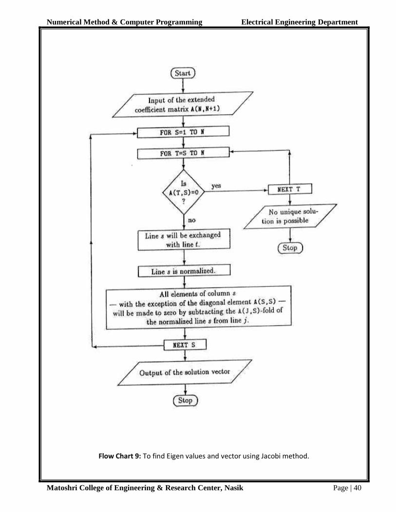
Flow Chart 9: To find Eigen values and vector using Jacobi method.

Electrical Engineering Departmentmatoshrielectrical.yolasite.com/resources/NMCP Lab Mnual...

Documents

Transcript of Electrical Engineering Departmentmatoshrielectrical.yolasite.com/resources/NMCP Lab Mnual...