Eindhoven University of Technology MASTER Automatic ... · Thesis Report Automatic Segmentation of...

Eindhoven University of Technology

MASTER

Automatic segmentation of hippocampal substructures

Santiago Flores, G.

Award date:2012

DisclaimerThis document contains a student thesis (bachelor's or master's), as authored by a student at Eindhoven University of Technology. Studenttheses are made available in the TU/e repository upon obtaining the required degree. The grade received is not published on the documentas presented in the repository. The required complexity or quality of research of student theses may vary by program, and the requiredminimum study period may vary in duration.

General rightsCopyright and moral rights for the publications made accessible in the public portal are retained by the authors and/or other copyright ownersand it is a condition of accessing publications that users recognise and abide by the legal requirements associated with these rights.

• Users may download and print one copy of any publication from the public portal for the purpose of private study or research. • You may not further distribute the material or use it for any profit-making activity or commercial gain

Take down policyIf you believe that this document breaches copyright please contact us providing details, and we will remove access to the work immediatelyand investigate your claim.

Download date: 31. May. 2018

Thesis Report

Automatic Segmentation of HippocampalSubstructures

Gerardo Santiago Floresemail : [email protected]

Student ID 0757324

Technische Universiteit Eindhoven

Prof. Dr. Gerard de Haan

Technische Universiteit Eindhoven

Philips Research Eindhoven

Dr. Radu Jasinschi and Dr. Octavian Soldea

Philips Research Eindhoven

July 2, 2012

Abstract

Segmentation of brain structures is an important component in the field of medical imagingbecause it provides support for diagnosis and treatment as well as therapy evaluation guidance.Modern technology allows acquisition of MR images with very high resolution up to 0.3 mm ofspacing between voxels. In this context, we propose a fully automatic segmentation method fo-cused on substructures of the Hippocampal Formation. For this purpose, we present the develop-ment and implementation of three relevant contributions. First, we introduce a fast registrationmethod based on moments. Second, we present a multi-level initialization scheme for obtain-ing initial contours required for segmentation; this procedure is fully automatic and it requiresa training set of images with manual annotations of the substructures of interest. Third, weintroduce a new segmentation algorithm, which is based on active contours driven by momentsprior. We minimize an energy cost function in order to get optimal segmentation employingsignatures based on moments. We compared our results to state-of-the-art tools and show sig-nificantly improvement in time performance. In addition, we tested our method with patientswith Alzheimer Disease.

Keywords: Substructures segmentation, Hippocampal formation, Moments prior, Active Con-tours Initialization

Acknowledgements

First and foremost, I would like to express my sincere gratitude to my company supervisors,Dr. Radu Jasinschi and Dr. Octavian Soldea, whose guidance and tutelage considerably helpme in the development of my research work. I have learnt plenty of things from them. In thetechnical side, their expertise in the field of medical imaging were fundamental to achieve thegoals of this project and in the personal side, I received valuable advice from them that mademe considered both as my friends.

I would also like to thank Prof. Dr. Gerard de Haan, not only for giving me the opportunityto work at Philips Research, but also for all the insightful contributions and suggestions thathe made to improve my work.

My special thanks to all my fellow interns for all the great time that we spent in the office,it was a great experience to work in such a nice environment. Very special thanks to my bestfriend Nitejat, she has always been there for me when I need her. Her advice and patience haveassisted me for many years.

Finally, I would like to thank my parents and my brother for all the support that I havereceived from them in my entire life. Everything I have done has been thanks to my family. Allthe achievements that I have made are dedicated to them.

ii

Contents

1 Introduction 11.1 Problem Description . . . . . . . . . . . . . . . . . . . . . . . . . . . . . . . . . . 21.2 Related Work . . . . . . . . . . . . . . . . . . . . . . . . . . . . . . . . . . . . . . 21.3 Report Organization . . . . . . . . . . . . . . . . . . . . . . . . . . . . . . . . . . 3

2 Background 42.1 Hippocampal Formation . . . . . . . . . . . . . . . . . . . . . . . . . . . . . . . . 4

2.1.1 Motivation . . . . . . . . . . . . . . . . . . . . . . . . . . . . . . . . . . . 42.1.2 Hippocampal Anatomy . . . . . . . . . . . . . . . . . . . . . . . . . . . . 4

2.2 Moments and Pose Information . . . . . . . . . . . . . . . . . . . . . . . . . . . . 42.2.1 Definition of Moments . . . . . . . . . . . . . . . . . . . . . . . . . . . . . 52.2.2 Definition of Pose Information . . . . . . . . . . . . . . . . . . . . . . . . 52.2.3 Discrete Implementation of Moments . . . . . . . . . . . . . . . . . . . . . 7

2.3 Registration . . . . . . . . . . . . . . . . . . . . . . . . . . . . . . . . . . . . . . . 72.3.1 Similarity Metrics . . . . . . . . . . . . . . . . . . . . . . . . . . . . . . . 82.3.2 Transformation Types . . . . . . . . . . . . . . . . . . . . . . . . . . . . . 9

2.4 Validation Metric . . . . . . . . . . . . . . . . . . . . . . . . . . . . . . . . . . . . 10

3 Method proposed 113.1 Overview of the method . . . . . . . . . . . . . . . . . . . . . . . . . . . . . . . . 113.2 Training Set . . . . . . . . . . . . . . . . . . . . . . . . . . . . . . . . . . . . . . . 123.3 Fast Moments Based Registration . . . . . . . . . . . . . . . . . . . . . . . . . . . 12

3.3.1 Formal Definition of Registration based on Moments . . . . . . . . . . . . 133.4 Initialization . . . . . . . . . . . . . . . . . . . . . . . . . . . . . . . . . . . . . . 15

3.4.1 Relation between Registration and Initialization. . . . . . . . . . . . . . . 163.4.2 Multi-level Registration Scheme . . . . . . . . . . . . . . . . . . . . . . . . 163.4.3 Implementation Details of Initialization . . . . . . . . . . . . . . . . . . . 20

3.5 Segmentation Algorithm . . . . . . . . . . . . . . . . . . . . . . . . . . . . . . . . 213.5.1 Gradient Flow . . . . . . . . . . . . . . . . . . . . . . . . . . . . . . . . . 223.5.2 Update Step . . . . . . . . . . . . . . . . . . . . . . . . . . . . . . . . . . 23

4 Results 244.1 Results of Registration Based on Moments . . . . . . . . . . . . . . . . . . . . . . 24

4.1.1 Experiment Description . . . . . . . . . . . . . . . . . . . . . . . . . . . . 244.1.2 IBSR Results . . . . . . . . . . . . . . . . . . . . . . . . . . . . . . . . . . 254.1.3 ADAB Results . . . . . . . . . . . . . . . . . . . . . . . . . . . . . . . . . 264.1.4 Optimizations . . . . . . . . . . . . . . . . . . . . . . . . . . . . . . . . . . 28

4.2 Results of Initialization . . . . . . . . . . . . . . . . . . . . . . . . . . . . . . . . 294.2.1 Input Data Description . . . . . . . . . . . . . . . . . . . . . . . . . . . . 294.2.2 Experiments Description . . . . . . . . . . . . . . . . . . . . . . . . . . . . 30

iii

4.2.3 Results . . . . . . . . . . . . . . . . . . . . . . . . . . . . . . . . . . . . . 304.2.4 Performance Metrics . . . . . . . . . . . . . . . . . . . . . . . . . . . . . . 33

4.3 Results of Segmentation . . . . . . . . . . . . . . . . . . . . . . . . . . . . . . . . 334.3.1 Evaluation on Healthy Patients . . . . . . . . . . . . . . . . . . . . . . . . 344.3.2 Evaluation on Patients with Alzheimer Disease . . . . . . . . . . . . . . . 364.3.3 Performance Metrics . . . . . . . . . . . . . . . . . . . . . . . . . . . . . . 364.3.4 Comparison with Existing Method . . . . . . . . . . . . . . . . . . . . . . 36

5 Conclusions and Future Work 395.1 Future work . . . . . . . . . . . . . . . . . . . . . . . . . . . . . . . . . . . . . . . 40

Appendix 41

A Acronyms 41

B Parameter File Elastix 42B.1 Affine Registration Elastix Parameter . . . . . . . . . . . . . . . . . . . . . . . . 42B.2 BSpline Registration Elastix Parameter . . . . . . . . . . . . . . . . . . . . . . . 43.

iv

List of Figures

1.1 Example of brain segmentation . . . . . . . . . . . . . . . . . . . . . . . . . . . . 1

2.1 Hippocampal Formation . . . . . . . . . . . . . . . . . . . . . . . . . . . . . . . . 52.2 Manual Annotation of Hippocampal Formation . . . . . . . . . . . . . . . . . . . 52.3 Discrete implementation of moments . . . . . . . . . . . . . . . . . . . . . . . . . 72.4 Registration Procedure . . . . . . . . . . . . . . . . . . . . . . . . . . . . . . . . . 82.5 Registration Framework . . . . . . . . . . . . . . . . . . . . . . . . . . . . . . . . 82.6 Dice Coefficient . . . . . . . . . . . . . . . . . . . . . . . . . . . . . . . . . . . . . 10

3.1 Segmentation Method Overview . . . . . . . . . . . . . . . . . . . . . . . . . . . . 113.2 Skull Strip . . . . . . . . . . . . . . . . . . . . . . . . . . . . . . . . . . . . . . . . 123.3 Example of training image . . . . . . . . . . . . . . . . . . . . . . . . . . . . . . . 123.4 Initialization results step 1 . . . . . . . . . . . . . . . . . . . . . . . . . . . . . . . 173.5 Initialization results step 2 . . . . . . . . . . . . . . . . . . . . . . . . . . . . . . . 183.6 VOI selection . . . . . . . . . . . . . . . . . . . . . . . . . . . . . . . . . . . . . . 183.7 Example Volume Of Interest . . . . . . . . . . . . . . . . . . . . . . . . . . . . . . 193.8 Initialization results step 3 . . . . . . . . . . . . . . . . . . . . . . . . . . . . . . . 193.9 Initialization results step 4 . . . . . . . . . . . . . . . . . . . . . . . . . . . . . . . 20

4.1 Registration results DC from IBSR data set . . . . . . . . . . . . . . . . . . . . . 254.2 Registration results Computation Time from IBSR data set . . . . . . . . . . . . 264.3 Registration results DC from ADAB data set . . . . . . . . . . . . . . . . . . . . 274.4 Registration results Computation Time from ADAB data set . . . . . . . . . . . 274.5 Optimizations on IBSR data set . . . . . . . . . . . . . . . . . . . . . . . . . . . 284.6 Optimizations on ADAB data set . . . . . . . . . . . . . . . . . . . . . . . . . . . 294.7 Initialization Results Left Side . . . . . . . . . . . . . . . . . . . . . . . . . . . . 304.8 Initialization Results Right Side . . . . . . . . . . . . . . . . . . . . . . . . . . . . 314.9 Initialization results both sides . . . . . . . . . . . . . . . . . . . . . . . . . . . . 314.10 Average DC with standard deviation of DG substructure (Initialization Stage) . 334.11 Qualitative Analysis Initialization . . . . . . . . . . . . . . . . . . . . . . . . . . . 334.12 Left Side Segmentation Results . . . . . . . . . . . . . . . . . . . . . . . . . . . . 344.13 Right Side Segmentation Results . . . . . . . . . . . . . . . . . . . . . . . . . . . 344.14 Qualitative Analysis Segmentation Result . . . . . . . . . . . . . . . . . . . . . . 354.15 Segmentation Result 3D Visualization . . . . . . . . . . . . . . . . . . . . . . . . 354.16 Segmentation Results on Patients with AD . . . . . . . . . . . . . . . . . . . . . 374.17 Comparison with existing method [1] . . . . . . . . . . . . . . . . . . . . . . . . . 38

v

CHAPTER 1

Introduction

Segmentation of brain structures from MR images is an important component in the field ofmedical image analysis due to the fact that it is used in plenty of applications such as diagno-sis, surgical guidance and therapy evaluation [2]. For example, segmentation of hippocampalformation is motivated by the fact that hippocampal atrophy is known to occur at early stagesof Alzheimer disease (AD) [3] [4] [5]. Hence, the analysis of hippocampal structure providesimportant information at the diagnosis phase. Figure 1.1 is an example of brain segmentation.In Figure 1.1 different colors represent different structures, left-hippocampus is marked withblue, left-lateral-ventricle is green, left-putamen is shown in red.

Figure 1.1: Example of brain segmentation

Although segmentation can be performed manually, it is a tedious and time-consuming taskwhich does not provide entirely replicable results [2]. Moreover, continuous use of manual agilityand hand-eye coordination makes the expert rater quickly fatigued [3]. Thus segmentationof a large number of MR images by an expert is not practical. Therefore, automatic andsemiautomatic segmentation tools have begun to emerge [2], [6], [7], [8]. On one hand, thesemethods are based on training sets from ground truth annotations made by experts and theirresults are still not comparable to manual segmentation. On the other hand, the speed providedby (semi)automatic methods offers the opportunity to evaluate a large number of patients. This

1

information can be used to create statistics over trends of diseases’ evolution from which medicaldiagnosis and treatment benefit.

Automatic segmentation results are strongly influenced by the quality of the images. Onone hand, low contrast areas and different acquisition parameters have a negative impact onannotations results from automatic methods. On the other hand, the modern resolution of MRimages, with physical spacing between voxels of 0.3 mm. , provide extremely good level of detail[1]; this allows for segmentation of substructures. In this context, we propose to segment thehippocampal formation at the subfield level.

1.1 Problem Description

In this thesis, we treat the problem of fully automatic segmentation of Hippocampal Forma-tion (HF). The final goal is to develop and implement a tool that is able to automaticallysegment hippocampal substructures. This problem implies major challenges: First, due to thevery small size of the analyzed substructures, information may be lost during the procedurethat we employ. Second, we aim at providing a robust method in terms of performance andquality of the results. In addition, we also consider computational resources limitations in orderto make our tool optimized. Furthermore, an efficient solution is required in terms of speed andprecision, these parameters will be compared to existing methods

1.2 Related Work

In this section, we discuss some methods previously proposed in order to solve the problemof segmentation of HF at the substructure level. To the best of our knowledge, there are twopublications that were proposed to solve substructure segmentation of HR!. We discuss thembriefly.

1. Nearly automatic segmentation of hippocampal subfields in in vivo focal T2-weighted MRI [8]

In this publication, the authors proposed a segmentation method which is based on acombination of multi-atlas segmentation, similarity-weighted voting and a learning-basedbias correction technique. The method is not fully automatic due to the fact that theauthors manually divided MRI slices of the HF into three main partitions, namely Head,Tail and Body. After this stage the fully automatic method comprises four steps.

In the first step, the authors create an initial segmentation of the hippocampal subfieldsby using a multi-atlas segmentation technique. Given a set of training MR Images withmanual annotations of HF subfields, the method produces a candidate segmentation foreach of the patients in the training set. In order to combine these candidate segmentationinto a single segmentation, the authors used a voting scheme, where the candidate withhigher similarity metric influences more in the final consensus segmentation image. In thisstage, the authors make use of both types of weighted images T1 and T2, since, accordingto them, using both types of images provides complementary information. The authorsnamed this step as Multi-atlas segmentation and voting (MASV).

In the second step, the authors use the initial segmentation produced in step 1 in order totrain AdaBoost classifiers. The goal of these classifiers is to detect and correct mislabeledvoxels. The classifiers use image texture, initial segmentation results and spatial location

2

features. In the third step, the authors used MASV to produce initial segmentation foreach of the patients in the testing set. Finally in the fourth step, the authors used theclassifiers trained in step 2 in order to improve the results from step 3.

One important point from this method is that the ROI that surrounds the HF is fixed.The authors proposed to use different reference spaces for each of the HF namely Left andRight. Each of these reference spaces has dimensions of 40 x 55 x 40 mm3, this referencespace is used along the entire procedure.

The results in terms of DC are around 0.873 for DG, 0.875 for CA1, 0.770 for Sub and0.787 for EC. We consider that the manual intervention plays an important role in gettingthis high value results. The fastest computation time reported in this publication is 19hours for the training time and 8 hours for the testing time for a training set of 20 subjectsand a testing set of 10, using a cluster of 8 CPUs with 8 cores each.

2. Automated Segmentation of Hippocampal Subfields From Ultra-High Resolu-tion In Vivo MRI [1]

In this publication, the authors proposed a fully automatic method to solve the HF sub-fields segmentation problem. This method is based on a Bayesian modeling approach.The authors employed a likelihood distribution to assign a single neuroanatomical to eachof the voxels in the image.

In order to build the likelihood distribution, the authors proposed a tetrahedrical meshwhich covers the ROI. This mesh is deformed from its reference position by a Markovrandom field model. The authors find the ROI by using affine registration. Once a ROIis found, they employed a tissue classification algorithm to discard all voxels which donot belong to any of the subfields. Finally they employ the likelihood model to the voxelsthat remain available. Similar to [8], in [1] the authors proposed a fixed ROI which hasdimensions 94 x 66 x 144 voxels.

The results obtained in terms of DC are: 0.68 for DG, 0.62 for CA1 and 0.74 for Sub.Note that the authors employed a different protocol than [9], therefore no result for ECis reported. For each patient, the computation time of the algorithm was about 5 hours.

1.3 Report Organization

The organization of this report is as follows: In Chapter 2, we introduce some backgroundrequired to defined the method proposed. We briefly explain the structure of interest as well asthe mathematical definition of moments, registration and the metric that we use to validate ourresults. In Chapter 3, we describe the proposed method to solve substructures segmentation. InChapter 4, we present the results obtained with the proposed method, as well as a comparisonwith existing methods. Finally, in Chapter 5 we present conclusions and future work.

3

CHAPTER 2

Background

In this chapter, we explain the background required for the segmentation method that wepropose. The background explain here consists of Hippocampal Formation, moments and poseinformation, registration and one validation metric.

2.1 Hippocampal Formation

In this section we describe the motivation behind the study of the HF as well as a brief descrip-tion of its anatomy.

2.1.1 Motivation

The analysis of the HF is important due to the fact that this structure takes part in manyfunctions of the brain: following [5], the hippocampus is involved in propositional memory, andneuronal and synaptic plasticity. In addition, due to the pathological processes of conditionssuch as epilepsy and Alzheimer’s disease, that occur in this formation, its analysis offers theopportunity to provide novel diagnosis.

2.1.2 Hippocampal Anatomy

The hippocampal formation is a structure from the brain which is formed by the following sub-structures: the dentate gyrus (DG), hippocampus, subiculum(Sub), presubiculum(Pre), para-subiculum(Para), and entorhinal cortex (EC) [5]. The hippocampus has three subdivisions:CA1, CA2, and CA3, (CA means cornu ammonis). Figure 2.1 shows the hippocampal forma-tion.

In this work, we focused on four substructures, namely DG, CA, EC and Sub. We mergeCA1, CA2, CA3 into a single substructure CA for validation purposes. In Figure 2.2, we showleft and right HF from coronal view.

2.2 Moments and Pose Information

In this section we describe the concepts of moments and pose information which are relevantconcepts for the segmentation method that we propose.

4

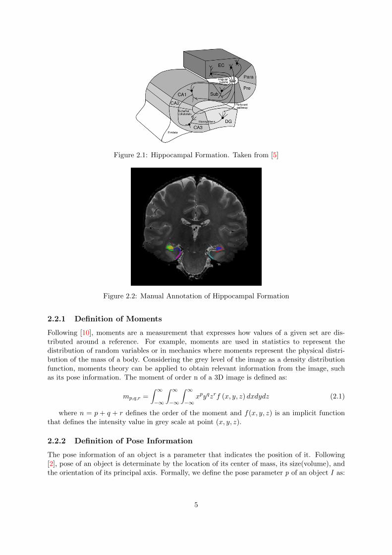
Figure 2.1: Hippocampal Formation. Taken from [5]

Figure 2.2: Manual Annotation of Hippocampal Formation

2.2.1 Definition of Moments

Following [10], moments are a measurement that expresses how values of a given set are dis-tributed around a reference. For example, moments are used in statistics to represent thedistribution of random variables or in mechanics where moments represent the physical distri-bution of the mass of a body. Considering the grey level of the image as a density distributionfunction, moments theory can be applied to obtain relevant information from the image, suchas its pose information. The moment of order n of a 3D image is defined as:

mp,q,r =

∫ ∞−∞

∫ ∞−∞

∫ ∞−∞

xpyqzrf (x, y, z) dxdydz (2.1)

where n = p + q + r defines the order of the moment and f(x, y, z) is an implicit functionthat defines the intensity value in grey scale at point (x, y, z).

2.2.2 Definition of Pose Information

The pose information of an object is a parameter that indicates the position of it. Following[2], pose of an object is determinate by the location of its center of mass, its size(volume), andthe orientation of its principal axis. Formally, we define the pose parameter p of an object I as:

5

pI = [V, cx, cy, cz, θ] (2.2)

where V is the volume, cx cy cz are the coordinates of the center of mass and Θ is the orientationof the object.

We use moments computation in order to find the pose information of an object. The volumeis defined by:

V = m0,0,0 (2.3)

The center of mass of an object is defined by:

cx =m1,0,0

m0,0,0cy =

m0,1,0

m0,0,0cz =

m0,0,1

m0,0,0(2.4)

Second-order moments are used to define object’s orientation. We use second-order momentsto find the inertia moments which are required to find the inertia tensor. The eigenvectors ofthe inertia tensor are the principal axes of the object. By knowing the principal axes of theobject we can define its orientation. Following [11], inertia moments are expressed as:

Ixx = m020 +m002 −m2

010

m000− m2

001

m000

Iyy = m200 +m002 −m2

100

m000− m2

001

m000

Izz = m200 +m020 −m2

100

m000− m2

010

m000

Ixy = Iyx = m110 −m100m010

m000

Ixz = Izx = m101 −m100m001

m000

Iyz = Izy = m011 −m010m001

m000

(2.5)

The inertia tensor is:

I =

Ixx −Ixy −Ixz−Iyx Iyy −Iyz−Izx −Izy Izz

(2.6)

By finding the eigenvectors of the inertia tensor, we obtain the principal axes of the object.The orientation matrix θ of an object I is the matrix formed by the eigenvectors of the inertiatensor I.The eigenvalues λ of the matrix I are given by:

det(I − λI

)= 0 (2.7)

The eigenvectors v are found with:I v = λv (2.8)

Then, we define the orientation matrix θ of the object I as:

θ =[v1 v2 v3

](2.9)

6

2.2.3 Discrete Implementation of Moments

In order to compute the moments of an image, we employ a discrete version of equation 2.1,namely:

mpqr =L−1∑z=0

M−1∑y=0

N−1∑x=0

xpyqzrg (x, y, z) (2.10)

where mpqr is the moment of order n = p+ q+ r, L,M and N are the number of sample voxelsin each direction, and g(x, y, z) is the intensity value of the voxel located in x, y, z.

The precision of moments computation is proportional to the resolution of the image. Fur-thermore, in the case of medical imaging, the available discrete data is given by the acquisitionquality of the scans. Moreover, we can modify the amount of discrete data by changing theamount of voxels in the image. In this work, we control the amount of voxels used to computemoments by increasing or decreasing the physical space between them. On one hand, by de-creasing the physical spacing between voxels, the number of voxels is increased, this means thatcomputation of moments is more precise, however, this also implies more computation time. Onthe other hand, increasing the physical spacing between voxels decreases the total number ofvoxels used for moments computation and, as a consequence, the precision of moments. Figure2.3 illustrates the effect of modifying the spacing between sample voxels.

Figure 2.3: Discrete implementation of moments. a) shows discrete image with a certain spacing(X) between sample voxels. b) shows the same image but with a spacing of 2X. In both casesthe green points are the points considered for moments calculation

2.3 Registration

In this section, we describe the concept of registration, which is an important concept due to thefact that we use registration at the initialization phase as well as in the segmentation algorithm.

Image registration aims at finding the best transformation by which we align one image(moving) to a reference image (fixed). Aligning images is a required preprocessing step beforedeveloping any further image treatment [12]. In this thesis, we employ registration in two main

7

parts. First, we use registration for aligning new brain images to the training set. By doingthis, we obtain the initial contours required for the segmentation algorithm, see Section 3.4.Second, we use registration at the substructure level, in order to obtain relevant informationabout how a substructure is distributed around the ensemble of substructures, this informationis needed for the Segmentation algorithm, see Section 3.5. Figure 2.4 depicts the registrationconcept.

Figure 2.4: Registration Procedure. In (a) images are not aligned. Part (b) shows the resultafter registration.

Usually, the problem of finding the best aligning transformation is treated as an optimization.For example, in Elastix tool [13], the authors follow the optimization scheme which shown inFigure 2.5. At each iteration a transformation is obtained, this transformation is applied tothe moving image. The interpolator is needed in order to obtain intensity values at non-gridpositions, then the quality of alignment is obtained by making use of a similarity metric. Finallythe optimizer is responsible for optimizing the transformation. In the following sections we givea brief description of some possible types of similarity metrics and transformations.

Figure 2.5: Registration Framework. Taken from [14].

2.3.1 Similarity Metrics

As mentioned in Section 2.3, a similarity metric is required in order to evaluate the quality ofthe alignment. Some possible metrics of this type are:

Sum of Square Differences SDDSDD is defined as:

SDD(IF , IM ) =1

|ΩF |∑xiεΩF

(IF (xi)− IM (xi))2 (2.11)

8

where ΩF is the domain of the fixed image IF , |ΩF | the number of voxels and IF (xi) andIM (xi) the voxel values of the fixed and moving image respectively.

Normalized Correlation Coefficient NCCNCC is defined as:

NCC (IF , IM ) =

∑xiεΩF

(IF (xi)− IF )(IM (xi)− ¯IM )√∑xiεΩF

(IF (xi)− IF )2∑xiεΩF

(IM (xi)− ¯IM )2(2.12)

where IF = 1ΩF

∑xiεΩF

IF (xi) is the average intensity value of the fixed image and ¯IM =1

ΩF

∑xiεΩF

IM (xi) is the intensity average of the moving image.

Mutual InformationFollowing [14] and [15], MI is defined as:

MI(IF , IM ) =∑mεLM

∑fεLF

p(f,m)log2

(p(f,m)

pF (f)pM (m)

)(2.13)

where LF and LM are sets of regularly spaced intensity bin centers, p is the discrete jointprobability, and pF and pM are the marginal discrete probabilities of the fixed and movingimages, obtained by summing p over m and f , respectively. The joint probabilities are estimatedusing B-Spline Parzen windows:

p(f,m) =1

ΩF

∑xiεΩF

wF (f/σF − IF (xi)/σF )× wM (m/σM − IM (xi)/σM ) (2.14)

where wF and wM represent the fixed and moving Bspline Parzen windows. The scalingconstants σF and σM must equal the intensity bin widths defined by LF and LM .

2.3.2 Transformation Types

There exist a number of possible transformation in order to map the moving image into thefixed one. In this thesis we use the following transformation types:

Rigid transformations Rigid transformations use the same transformation for mappingeach of the voxels in the moving image.

SimilaritySimilarity transformation is defined as:

T (x) = sR(x− c) + t+ c (2.15)

where t is the translation vector, s is the scaling factor, c is the center of the transformationand R is a rotation matrix. In this type of transformation the image is treated as a rigid body,it can be translated, rotated and scaled. However, the scaling factor is the same in all directions(isotropic).

9

AffineAffine transformation is defined as:

T (x) = A(x− c) + t+ c (2.16)

The main difference between the similarity transformation and Affine Transformation is thatmatrix A has no restrictions. This means that besides rotation we can apply anisotropic scalingfactors.

Non-Rigid TransformationsThe characteristic of the Non-Rigid Transformations is that different transformations are usedfor different parts of the image; this allows local deformations.

BSplineA possible parametrization of a non-rigid transformations is by means of Bsplines, following[16]:

T (x) = x+∑xkεNx

pkβ3(x− xkσ

)(2.17)

where xk are control points, β3(x) is a cubic multidimensional Bspline polynomial, pk arethe Bspline coefficient vectors, σ is the spacing between control points and Nx is the set ofcontrol points support of the Bspline at point x.

The control points xk form a regular grid with resolution σ. The resolution of the gridinfluences heavily on the transformation. On one hand, a finer control points grid will focus onsmall localized transformation. On the other hand, a coarser grid will allow larger displacementsin the transformation.

2.4 Validation Metric

In order to evaluate the result of registration and segmentation we use Dice Coefficient DC,which is a common metric for validating segmentation algorithms. DC is defined as:

DC(A,B) =2 |A ∩B||A|+ |B|

(2.18)

where A and B are two objects to be compared, and |X| is the volume of the object X.DC measures the overlap between two sets, in our case volumes. A value of 0 represents no

overlap, a value of 1 represents a perfect overlap. The goal of a segmentation algorithm is toobtain DC close to 1, when the results are compared to a manual annotation segmentation.

Figure 2.6: Dice Coefficient. a) No overlapping. b) Partial overlapping. c) Complete overlapping

10

CHAPTER 3

Method proposed

In this section we describe the algorithms that we propose in order to achieve fully automaticsegmentation of HF Substructures. We make three relevant contributions. First, we proposea fast Registration method which is based on Moments. Second, we propose a Initializationscheme. Finally we use a Segmentation Algorithm, which is based on Pose Information Prior.

3.1 Overview of the method

The work flow of the Segmentation Method that we propose is depicted in Figure 3.1. As input,we use an MR volumetric image of the brain. We first apply a preprocessing step in whichwe remove the skull and non-brain tissue from the image obtaining only the parenchyma, seeFigure 3.2. For this preprocessing step we use the tool Brain Extraction Tool BET from FmribSoftware Library FSL.

Figure 3.1: Segmentation Method Overview

After the preprocessing, we start with the segmentation algorithm which consists of twomain stages, namely Initialization and Segmentation. In both stages we use a Training Set, see3.2. At the Initialization phase, we create initial contours. We predict the location of theseinitial contours by using the contours from the Training Set. At the Segmentation stage, weapply the algorithm proposed in order to deform the initial contours in such a way that thesegmentation is optimized. The result of this procedure is a volumetric image which containsthe segmentation of the substructures of interest.

We implemented the algorithms in C++, using ITK and VTK libraries. For the Affine andBSpline registrations required in the Initialization stage, we use Elastix [13].

11

Figure 3.2: Skull Strip

3.2 Training Set

The training set that we employed is a set of MR images of healthy brains with manual annota-tions of the substructures of the HF, see Figure 3.3. The images were provided by UniversitairMedisch Centrum Utrecht (UMC) and Leids Universitair Medisch Centrum (LUMC) Thesemanual annotations were performed by experts following the protocol in described in [9]. More-over, the training set contains substructure signatures based on moments which describe howeach of the substructure is distributed around the ensemble 1 of all substructures combined.These signatures are used in the segmentation method proposed and they are computed usingMoments of each substructure as related to the ensemble.

Figure 3.3: Example of training image. Coronal View. Each of the colors represent a differentsubstructure: CA is red; DG is blue; Sub is yellow and EC is green

3.3 Fast Moments Based Registration

As mentioned in Section 2.3, the goal of registration is to find the best transform T to align amoving object to a fixed one. In this context, we propose a fast method to find the parametersof an affine transformation, see Section 2.3.2. The method that we propose uses the pose infor-mation of moving and fixed object, see Section 2.2.2. Because we employ registration at many

1We consider the ensemble as a structure which is formed by all the substructures of the HF .

12

steps of the method proposed, we require a fast registration method to decrease computationtime. We use this fast registration method in the Segmentation algorithm, see Section 3.5.

3.3.1 Formal Definition of Registration based on Moments

We define the registration transformation T as:

pMT = pF (3.1)

where pM is the pose information, see 2.2.2, of the moving object and pF is the pose informationof the fixed object.

The transformation that we use is a concatenation of three parts: translation, rotation andscaling. We obtain the transformation parameters to build the transformation matrix as follows.

3.3.1.1 Translation

Translation is required to align both objects to a common center of mass. Since both centers ofmass are known by its pose information parameter, we can define the vector for the translationas:

T = [cMx − cFx, cMy − cFy, cMz − cFz] (3.2)

where cM is the center of mass of the moving image and cF is the center of mass of the fixedimage.

3.3.1.2 Rotation

We require a rotation transformation in order to align the orientations of the objects. Theorientation of both objects, fixed and moving, is known by their pose parameters: θF , θM ,hence the following equation needs to be solved:

θF = RθM (3.3)

Rotation transformation is then defined as:

R = θF θ−1M (3.4)

3.3.1.3 Scaling

Scaling is required to obtain images of similar dimensions. We describe two methods to findthe scaling factors.A simple way to obtain the difference of scale is to work with the volumes of the images (m0,0,0).Therefore the scale required to register the moving image to the fixed one is given by:

s = 3

√mM

000

mF000

(3.5)

In Equation 3.5, we consider that the scaling factor is isotropic, i.e., the same in the threeaxes. However, the scale required in each of the axes can be different; therefore different scale

13

factors are needed among the different axes. In order to find these different scaling factors, weemploy second order moments. Following [10], a scaling change in an image modifies the valueof its moments as follows.

Consider f(x, y, z) as the original intensity function of a 3D image, the function that resultsafter scaling by a factor of α on X axis, β on Y axis, and γ on Z axis is given by:

f′(x, y, z) = f(

x

α,y

β,z

γ) (3.6)

The relation between the moment values of the original and transformed functions is ex-pressed as:

m′pqr = α1+pβ1+qγ1+rmpqr (3.7)

By considering the second-order moments of both, fixed and moving objects, the followingequations are derived:

m′002 = αβγ3m002,

m′020 = αβ3γm020,

m′200 = α3βγm200

(3.8)

where m′pqr are the moments of the fixed image and mpqr are the moments of the movingimage.

Thus, from Equation 3.8 α, β and γ can be expressed as a function the second-order momentsas follows:

α =

(m′200) (m′002)14 (m′020)

14

(m200) (m002)14 (m020)

14

25

,

β = 3

√m′020

αγm020,

γ = 8

√√√√ m020(m′002)3

m′020(m002)3α2

(3.9)

Finally, we express the parameters for the transformation in terms of 4x4 matrixes, thisallows us to concatenate transformation easily.

Translation Matrix =

1 0 0 Tx0 1 0 Ty0 0 1 Tz0 0 0 1

Rotation Matrix =

θ11 θ12 θ13 0θ21 θ22 θ21 0θ31 θ32 θ33 00 0 0 1

14

Scaling Matrix =

α 0 0 00 β 0 00 0 γ 00 0 0 1

(3.10)

The final transformation matrix is built by multiplying the three previous matrixes, result-ing in:

T =

αθ11 αθ12 αθ13 Txβθ21 βθ22 βθ21 Tyγθ31 γθ32 γθ33 Tz

0 0 0 1

(3.11)

We describe the outline of the moments based registration scheme in Algorithm 1.

Algorithm 1 Moments Based Registration Function

Input:F - a 3D image, which is the Moving ImageM - a 3D image, which is the Fixed Image

Output:T [p] - a function T [p] : R3 → R3 that represents the function that aligns M to F

1: Compute the Pose Information of F and M: pF and pM , see Equation 2.22: Compute the translation vector T , by using Equation 3.23: Compute the rotation matrix R, by using Equation 3.44: Compute the scale factors S, by using Equation 3.5 (isotropic) or 3.9 (anisotropic)5: Form the Affine transformation matrix T using Equation 3.11

3.4 Initialization

In this section we describe the procedure to obtain the initial contours which are required tostart the segmentation algorithm properly.

Initial contours are essential components in the proposed segmentation method since theyindicate the position in which the segmenting algorithm begins. A good positioning of the initialcontours is needed due to fact that the proposed Segmentation Method is very sensitive to theinitial contours. Initializing the algorithm with a contour distant from the target structure mayyield into unsatisfactory results because of the existence of sub-optimal local minima. In orderto find the initial contours closest to the target structure, we employed a multi-level registrationscheme in which we used both, global and local transformations. In addition, we explore thesubstructure level in order to find best contours for all substructures.

The algorithm that we propose is fully automatic, it requires a training set as explained in3.2. For the implementation of the registration steps (Affine and BSpline) we used Elastix [13].

15

3.4.1 Relation between Registration and Initialization.

As mentioned in Section 2.3, registration aims at finding the best transformation that alignsa moving image to a fixed image. By using this transformation we predict the position of thestructures to be segmented. This procedure is explained as follows.

Consider PT a target MRI volumetric image to be segmented. Furthermore, consider a setPi of training volumes , where i = 1..N . Each one of the i volumes has j manual annotatedstructures, we call Sji the binary volume representing the manual annotation of structure j of

volume i. The objective of the initialization phase is to obtain the set of binary volumes SjTwhich are the annotations of the j structures of the target volume T .

By registering a patient Pi from the training set Pi (moving image) to the target patientPT (fixed image), we obtain a transformation Ti. We apply the transformation Ti to the set ofmanual annotations Sji in order to obtain SjTi , which is the set of j structures of volume T, thatare predicted by using manual annotated structures of training volume i..

The problem to solve is to find Ti that predicts the best position of SjTi . We explain themethod that we employed to find Ti in the following sections.

3.4.2 Multi-level Registration Scheme

The motivation of a multi-level registration scheme is that using a single (coarse) step of regis-tration is not sufficient in order to find a proper transformation Ti for initializing the structuresof the HF. We validate this statement in Section 3.4.2.1. For this reason, we developed ascheme that consists of 4 steps. At each stage, we apply a new registration operation takinginto account the result of the previous step. This means that the final Ti is a concatenation of4 intermediate transformations.

3.4.2.1 Step 1. Affine Registration on Global Data

The fist step of the scheme is used to cope with large differences between volumes. For doingthis, we register full brain volumes (only skull was removed from original MR scans) using affinetransformation.

Figure 3.4 shows typical results after applying the transformation found in Step 1, to atraining contour. From Figure 3.4, it can be seen that the predicted structures are close to thetarget ones but the overlapping is minimum, as in Figure 3.4a; or in some cases none, as inFigure 3.4b. By looking at Figure 3.4, it is clear that the contours predicted by a global affineregistration are not close enough to the target contours. For this reason, we employed a secondregistration step.

3.4.2.2 Step 2. BSpline Registration on Global Data

In the second step, we used BSpline registration to bring the training contours closer to thetarget ones. BSpline registration depends heavily on the resolution of the control points mesh,as explained in [16], large spacing between control points allows global deformation, while smallspacing allows local deformations. The decision between a coarse or a fine mesh depends on theexpected amount of displacement. By looking at the results from Step 1, we observe that thetransformed structures are still far (3 to 7 millimeters) from the target, this means that largedisplacements are still required. Moreover using a finer mesh implies more computation timeand since we are working on high resolution images this tasks becomes not feasible. For these

16

(a) CA structure (b) DG structure (c) 4 structures

Figure 3.4: Initialization results step 1. Coronal slice of Step 1 result. The target structuresare shown in white. The transformed structures from one patient of the training set are shownin grey.

reasons, at this step we employ a relative coarse control points mesh (spacing between controlpoints of 8 millimeters) using the full brain images.

Figure 3.5 shows typical results after applying the transformation found in Step 2. Weobserve a major improvement when we compare Figure 3.5 with the results after Step 1 inFigure 3.4. In most of the cases, all structures overlap to the target. However, these resultsare still not entirely satisfactory because the overlapping between the target and the predictedstructure is low in terms of DC. For this reason we employ a third registration step in whichwe use only the volume of interest surrounding the HF.

3.4.2.3 Selection of Volume of Interest

After Step 2, the predicted structures generally overlap the target ones, thus the displacementsneeded to improve this overlapping are smaller than the ones required in previous steps andthey depend heavily on local data i.e. data from the close surrounding of the structures. Forthis reasons, we selected the surrounding area of the structures of interest and apply registrationon this small selected volume of interest data.

In order to select the data of interest we employed the following procedure: From the train-ing set we know the spacial location of the manual annotations, we built a Volume of Interest(VOI) around these manual annotations by locating the set of points Pi that surround the man-ual annotation. Then we apply the transformation Ti, which was previously obtained in Step 1and Step 2, to the set of points Pi obtaining the set of points P ′i that surround the new VOI.This procedure is depicted in Figure 3.6.

Once we know the location of the VOI, we extracted the data surrounded by the VOI fromboth, the Fixed and Moving full volumes. The result are small images that only contain thestructure of interest, this means that we can use these images to perform finer registration

17



Figure 3.6: VOI selection

without spending much computation time. Figure 3.7 shows typical results of the VOI that weobtained.

3.4.2.4 Step 3. Affine Registration on Local Data

With the images obtained from the procedure of Section 3.4.2.3 we continue the registrationscheme. Since now we are entirely focused only on the volume of interest, we can apply finerregistration procedures without requiring a large amount of computation time. We apply againaffine transformation but this time the transformation T depends only on local data, i.e., datasurrounding the structures of interest.

Figure 3.8 shows typical results of the predicted contours obtained after Step 3. By lookingat Figure 3.8 we see an improvement compared with the results obtained after Step 2. The

18

(a) Fix data (b) Moving data

Figure 3.7: VOI for the from fixed (a) and the moving (b) images.



19



predicted contours clearly overlap to the target ones. However, small modifications are stillrequired in order to obtain better overlapping. As Figure 3.8 shows, this modifications cannotbe solved with rigid transformations, thus we employ BSpline registration in the next step.

3.4.2.5 Step 4. BSpline Registration on Local Data

The final Step in this scheme involves a BSpline registration on local data. By doing this weexpect to obtain the closest predicted contours to the target structures. Since we are workingon small localized data, we can use high resolution mesh of the control points for the BSplineregistration. We used a spacing between control points of 4 mm, with this parameter we expectonly small deformations.

Typical results after Step 4 are depicted in Figure 3.9. From Figure 3.9 we observe that thepredicted contours are strongly overlapping with the target structures, nevertheless this over-lapping is still not complete. The active contours algorithm is proposed to solve the differencesbetween initial contours and the target structures.

3.4.3 Implementation Details of Initialization

We used Elastix [13] to implement each of the registration steps. We present the input files usedfor Elastix in appendix B. Elastix is an Image Registration Tool, based on ITK. We made useof this tool because it allows us to define precisely the type of registration that we define, thismeans that we are able to choose the Transformation Type and the Similarity Metric amongother parameters. Depending on the step in which the registration is applied, we used differentregistration types. The main difference is the Transformation Type, for steps 1 and 3 we usedAffine Transformation and for steps 2 and 4 we used BSpline Transformation. Another impor-tant difference is the resolution of the grid of control point for BSpline registration. At step 2,

20

we used a coarse grid (spacing = 32 voxels ) and at step 4 we used a finer grid (spacing = 8 vox-els ). After a number of experiments, we chose these resolutions of the grid since they producebest results. In addition, we made experiments on different similarity metrics to optimize regis-tration, we finally decided to use advanced mattes mutual information, see Section 2.3.1, sincethis metric produced better results; this can be explained due to the fact that mutual informa-tion can cope better with differences in intensity values produced by the different acquisitionparameters of the MR scans. Once we found the transformation, we apply that transforma-tion to the contours of the training set by using Transformix, which is a tool provided by Elastix.

We describe the outline of the Multi-Level Initialization scheme in Algorithm 2.

Algorithm 2 Multi-Level Initialization scheme

Input:PT - a 3D image, which is the test imagePi - a 3D image, which is the training image of patient i from the training setSji - a 3D image, which is image that contains the labels of the manual annotations of the j

substructures of patient iOutput:SjTi - a 3D image, which is image that contains the predicted contours of the j substructures

for PT obtained from patient i

1: Find Ti1 by computing affine registration on complete images, considering PT as fixed imageand Pi as moving image. Apply transformation Ti1 to Sji , the result is ST1 , see Section 3.4.2.1

2: Find Ti2 by computing bspline registration on complete images, considering PT as fixedimage and Pi as moving image. Apply transformation Ti2 to ST1 , the result is ST2 , seeSection 3.4.2.2

3: Find the VOI surrounding Sji2 , obtain the VOI from PT and Pi, see Section 3.4.2.34: Find Ti3 by computing affine registration on VOI images, considering VOI of PT as fixed

image and VOI of Pi as moving image. Apply transformation Ti3 to ST2 , the result is ST3 ,see Section 3.4.2.4

5: Find Ti4 by computing bspline registration on VOI images, considering VOI of PT as fixedimage and VOI of Pi as moving image. Apply transformation Ti4 to ST3 , the result is SjTi ,see Section 3.4.2.5

3.5 Segmentation Algorithm

The final part of the method proposed is the segmentation algorithm. The goal of this stage isto improve the segmentation given by the initialization. The segmentation algorithm that weuse is based on active contours [17], following a moments-based prior as described in [6]. Thismeans that the segmentation process involves the minimization of an energy cost functional. Inorder to minimize the energy cost we employed an iterative algorithm. Similar to [2] and [6],we define the energy cost functional in a maximum a posteriori estimation framework as

E(C) = − logP (C, data) (3.12)

where C is a set of evolving contours which represent the image segmentation of the structuresof interest and data is the intensity image in gray scale. The main difference between [2] and

21

[6] is that our energy functional combines the data term and the prior in one single term. Themain idea of the method is to evolve the contours C in order to minimize the cost functionwhich is equivalent to maximize a probability density function.

We define the joint kernel density estimate of m shapes as:

P (C, data) =1

N

N∑i=1

M∏j=1

kji

(d(φj , φji

), σj)

(3.13)

where N is the number of training patients, M is the number of substructures and k(·, σj) isa Gaussian kernel with standard deviation σ. We use Signed Distance Function SDF (φ) torepresent the active contour at each iteration. In Equation 3.13 φj is the SDF of the j th objectand φji is the SDF of the j th object from the ith member of the training set.

We make use of a distance function d(·, ·) which is defined as:

d(φj , φji

)=

√√√√ ∑r+s+t≤L

wr,s,t(m′r,s,t(φ

j)−m′r,s,t(φji))2

(3.14)

where m′r,s,t(φ

j) is the value of moments of structure j taken into account the intensity valuein gray scale, this is:

m′r,s,t =

∫Ω

xrysztg(x, y, z) (H (−φ (x, y, z))) dxdydz (3.15)

where g(x, y, z) is the intensity value in gray scale and H(·) is the Heaviside function

We implement the distance function in Equation 3.14 by using the relative pose information,see 2.2.2. This means that we consider d

(φj , φji

)= d

(pj , pji

), where pj is the relative pose

of substructure j th and pji is the relative pose of the j th structure from the ith memberof the training set. In order to compute the relative pose for each substructure, we registerthat substructure to the ensemble of all substructures of interest and then compute momentsfollowing Equation 3.15. At this stage, we use the fast registration method proposed in Section3.3.

We express the Gaussian kernel function in Equation 3.13 as:

kji =1√

2πσj2exp

− 1

2σj2

∑r+s+t≤L

wjr,s,t

(m′jr,s,t −m

′jir,s,t

)2

(3.16)

where wjr,s,t are weights. These weights sum up to one and are defined in such a way thatthe structures from the training set that are more similar to the test image have more relevancein the summation.

3.5.1 Gradient Flow

In order to minimize Equation (3.12), we define a Gradient Flow for the joint kernel in Equation(3.13). Following [6], we use the fact that logP (C, data) = log 1

N

∑Ni=1

∏Mj=1 k

ji , then

22

∂

∂tlogP (C, data) =

1

N

N∑i=1

m∑j=1

∂∂tk

ji

m∏l=1,l 6=j

kli

P (C, data)

(3.17)

Using Equation (3.16) and the definition of moments given in Equation (3.15), we obtain:

∂

∂tkji =

kjiσj2

∫R3

∑m

′jr,s,t∈ML

wr,s,t g(x, y, z) xryszt

[(m

′jr,s,t −m

′jir,s,t

)δε (φCj )

]φ

′

Cjdxdydz. (3.18)

Inserting Equation (3.18) into Equation (3.17):

∂φCj

∂t=

N∑i=1

m∏l=1

kliMPF (j, i) δε

(φCj

)σj2P

(C)·N

∣∣∣∇φCj

∣∣∣ , (3.19)

where MPF (j, i) =∑

r+s+t≤Lwjr,s,tx

rysztg(x, y, z)(m′jr,s,t −m

′jir,s,t

)for each j ∈ 1, . . . ,m.

3.5.2 Update Step

At each iteration the gradient given in Equation (3.19) is computed. As a result an updateterm for each substructure is obtained with:

φC =∂φCj

∂t·∆t (3.20)

φCj is added to the result of the previous iteration yielding in:

φi+1 = φi + φC (3.21)

We describe the segmentation algorithm in Algorithm 3.

Algorithm 3 The segmentation algorithm.

Input:t := 0; Ct=0;Initial contours give by Algorithm 2

Cji;training set of manual annotated contours, where i = 1, . . . , N and j = 1, . . . ,M,N is the number of patients and M is the number

of substructures of interest.

∆t; ε− a threshold for steady stateOutput:Ct a set of segmenting contours

1: repeat2: for all j=1,. . . ,m, (i.e. for each structure of interest) do

3: Compute shape and relative pose according to Equation (3.19) :

∂φCj

∂t=

N∑i=1

m∏l=1

kliMPF (j, i) δε

(φCj

)σj2P

(C)·N

∣∣∣∇φCj

∣∣∣4: Update the signed distance functions of each structure

φi+1 = φi +∂φCj

∂t·∆t

5: end for

6: until(

steady state is achieved, i.e. d(φt, φt+1

)< ε, for all j ∈ 1, . . . ,m

)

23

CHAPTER 4

Results

In this chapter we present the results obtained for each of the methods proposed in Chapter 3.We start by validating the registration based on moments from Section 3.3. Then, we presentthe results obtained for the initialization scheme of Section 3.4. Finally, we show the results ofthe segmentation algorithm of Section 3.5. At each step, we first describe the experiment usedto validate the results.

All the experiments were performed using a 3.33 GHz Intel Xeon Processor (64-bits). Weemployed Python scripts for running the algorithms through the patients in the training set.

4.1 Results of Registration Based on Moments

In this section, we present the results for the validation of our registration method which isbased on moments. For this purpose we make use of two data sets namely the Internet BrainSegmentation Repository IBSR [18] and 7T data provided by Leiden University (ADAB).

IBSR is a open data set composed by 18 subjects; each subject contains normalized T1-weighted volumetric images and segmentation ground truths for a number of brain structures.The set is composed by 14 men and 4 women, with ages from 8 to 71 years. The resolution ofthe images is 1.5 mm. ADAB is a set of T1-weighted volumetric images, it comprises 18 scans,7 women and 11 men. The resolution of the images is 0.35mm. As a preprocessing step weremoved non-brain tissue using BET.

4.1.1 Experiment Description

For both data sets the following process was done. One brain was considered as the fixed orreference one, then all the others were registered to it. DC was used as metric to evaluatethe performance of the method proposed, see Section 2.4. Scaling was made isotropic andanisotropic, see Section 3.3.1. Better DC values are expected from anisotropic scaling becauseanisotropic scaling considers the difference of scaling among axes. In addition the method thatwe proposed is compared to a state-of-art tool called Linear Image Registration Tool FLIRT [19].

24

Moreover, as an optimization, we compute the parameters of the transformation by calculat-ing moments using different resolution on the images, this means that we took different numberof sample voxels from the images in order to compute moments when using equation 2.10. Bydoing this procedure, the computation time was reduced, due to the fact that less operationswhere required to calculate moments since less voxels were considered.

4.1.2 IBSR Results

Figure 4.1 shows the result of global moments-based registration applied to IBSR data set. Weobtained the results of isotropic and anisotropic methods by discretizing the image to a spac-ing of 1mm, this means sample voxel was taken every millimeter. Each column in Figure 4.1,represents the average DC obtained from the registration to that specific patient, applying thedifferent methods previously described (isotropic, anisotropic and FLIRT).

Figure 4.1: Registration results DC from IBSR data set

From Figure 4.1 it can be observed that, according to the metric that we employed, theanisotropic scheme produces slightly better results than the isotropic scheme. The anisotropicDC average is 0.93552 and the isotropic DC average is 0.92911. This means an improvement of0.68%. From Figure 4.1, it can also be observed that FLIRT method yields in slightly betterresults than the method that we proposed in both scaling schemes (isotropic and anisotropic).The average DC obtained with FLIRT in all patients is 0.94284, this is 0.78% better than DCobtained with anisotropic scheme.

Figure 4.2 shows the average computation time that the registration procedure took for eachpatient.

From Figure 4.2 it can be observed that the computation time that FLIRT spends is muchhigher than the one of the method proposed. The average time used by FLIRT is 118.50 sec-onds, while our proposed method spends only 31.03 seconds with isotropic scheme and 31.09with anisotropic scheme. Thus the execution time that our method needs is only 26.15% ofthe time that FLIRT requires. Moreover our method can be even faster when a fewer number

25

Figure 4.2: Registration results Computation Time from IBSR data set

of samples voxels are considered in moments computation, this results are shown in Section 4.1.4.

4.1.3 ADAB Results

Figure 4.3 depicts the results obtained for ADAB data set. Similar to Figure 4.1, in Figure 4.3each column represents the average DC obtained from the registration to that specific patient,applying the different methods previously described (isotropic, anisotropic and FLIRT).

Similar to IBSR results, in ADAB data set a small improvement can be seen from isotropic toanisotropic scaling. The average DC of isotropic scaling is 0.87844 and for anisotropic is 0.88286.Our method does not perform as good as FLIRT, the average DC of FLIRT is 0.90089, thisrepresent a difference of 2.04% in respect to anisotropic scaling. Moreover there is a generaldecrease in performance of all methods when compared to IBSR data set. A possible reason isthat IBSR data set contains standardized test images while ADAB images are scans withoutany preprocessing and with different scan parameters.

Figure 4.4 shows the average computation time that the registration procedure took for eachpatient in ADAB data set.

From Figure 4.4, it is clear that the computation time required by our method is muchsmaller than the one that FLIRT consumes. The average time that FLIRT utilized for this dataset is 220 seconds and out method spent only 24.35 in isotropic scheme and 25.05 seconds inthe anisotropic one. This means that out method proposed is 8.82 times faster.

26

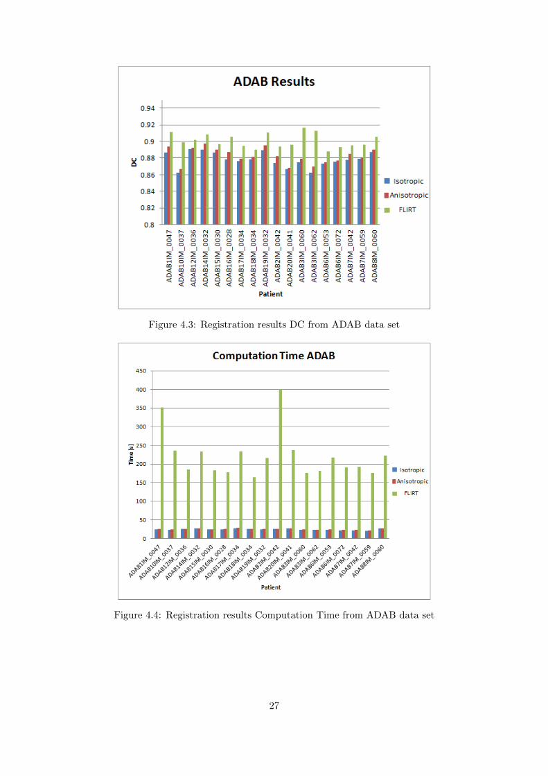
Figure 4.3: Registration results DC from ADAB data set

Figure 4.4: Registration results Computation Time from ADAB data set

27

4.1.4 Optimizations

In this section, we show the results obtained when a fewer number of sample voxels were usedin order to compute moments. The idea behind this optimization is that the computation timedecreases when a fewer number of voxels are used to calculate moments, however the precisionof the computation also decreases. This reduction is obtained by increasing the spacing in whichthe sample voxels are taken, see Section 2.2.3.

Figure 4.5 shows the results of DC and computation time that we obtained by using differentspacing sizes for computing moments.

Figure 4.5: Optimizations on IBSR data set

In Figure 4.5 it can be observed that decreasing the samples voxels used for momentscalculation decreases drastically the computation time. Using a spacing of 0.5 mm requiresin average 233 seconds, using 1 mm as spacing takes 31 seconds in average and using a spacingof 3 mm takes only 3.66 seconds. This reduction in precision on moments computation does notdecrease drastically the final result of registration. In the three previously mentioned cases theDC scored is in average 0.935. Even with a very coarse grid with a spacing of 20 mm, the DCdoes not decreases too much. The result obtained with this spacing is a DC of 0.9211 which is1.57% less than the score obtained with 0.5 mm of spacing.

Moments computation is only a part of the complete registration method. This meansthat the optimizations done on moments computations do not cover the entire computationtime that the registration method spends. For this reason, there is a limit in which increasingthe spacing between sample voxels does not decrease computation time any more. This can beseen in Figure 4.5 where after spacing of 4 mm a steady state of the computation time is reached.

Figure 4.6 shows the results of DC and computation time that we obtained by using dif-ferent spacing sizes in ADAB data set. Similar to the IBSR data set, in ADAB the reductionof precision in moments calculation does not modify severely the DC results keeping a valuehigher than 0.88 in spacing from 0.5 mm to 5 mm. However, the time consumed by moments

28

computation changes significantly when modifying the spacing of the sample voxels, from 96seconds using a spacing of 0.5 mm to 5.7 seconds when using a spacing of 4.

Figure 4.6: Optimizations on ADAB data set

In both cases it can be observed that sometimes a decrease in precision of moments doesnot decrease the DC values. This is explained by the fact that moments computation is usedto obtain the transformation matrix but after that, interpolation is required to apply the trans-formation previously found, this means that there is still room to errors due to interpolationwhich modify the DC result.

4.2 Results of Initialization

In this section we describe the results to validate our initialization scheme. First we describethe input data that we used. Second, we describe the experiment. Then, we present the resultsin terms of DC. Finally we show performance indicators.

4.2.1 Input Data Description

In order to detect the substructures of the HF we require images with very high resolution, forthis reason we employ images obtained with MR scans with strength of 7 Tesla. The resolutionof the images that we use is commonly 720 x 720 x 543 pixels, with a spacing in millimeters of0.35 x 0.35 x 0.35. Due to this very high resolution of images, the normal memory size of eachimage is in the range of 500 MB to 1GB.

29

4.2.2 Experiments Description

In order to validate the scheme proposed, we used leave-one-out cross validation. Starting froma training set of 3 patients, see 3.2, with manual annotation of 4 structures of the HF, namelyDG, CA, Sub and EC, from both left and right side, we applied the Multi-level RegistrationScheme proposed, taking one patient as Test image and the other two as Training set. Wepredict the contours for the Test image by using the manual annotations of the Training set.Then, we obtained average DC of the overlapping between the predicted substructures and thetarget ones.

4.2.3 Results

We present the average DC obtained for each structure at each step of the method, for bothsides left and right.

Figure 4.7 shows the results obtained for the left side HF.

Figure 4.7: Initialization Results Left Side

From Figure 4.7, we can observed how the overlapping metrics increases at each step of ini-tialization. It is clear that the registration scheme proposed increases the overlapping betweenthe predicted structure and the ground truth.

Figure 4.8 shows the results obtained for the right side. By looking at Figure 4.8 we observea decrease of DC in the DG substructure. The explanation for this situation is that while doingregistration, we consider volume of interest that includes all the substructures. This means thatthe transformation obtained is focused on finding the best alignment for the entire volume, as aconsequence for some substructures, in this case DG, the overlapping decreases but the overallaverage increases.

The complete results (average of left and right) are shown in Figure 4.9. Figure 4.9 depictsthe evolution of overlapping between the predicted and target structures over the steps of theprocedure proposed. It is clear that the overlapping increases accordingly to the steps taken.The largest improvement occurs between Step 1 and Step 2, where BSpline registration is em-ployed for the first time. For example, after Step 1, the overlapping of DG structure is only0.27 DC and after Step 2 the overlapping is 0.61 DC.

30

Figure 4.8: Initialization Results Right Side

Figure 4.9: Initialization results both sides

Figure 4.10 shows the evolution of the average DC for all patients for substructure DG aswell as the standard deviation. From Figure 4.10 we can see that there is an increase of DCalong the steps and also, the standard deviation becomes smaller, this means that after step 4,the initial result is good no matter which training patient is used to predict it.

A qualitative analysis can be done by looking at Figure 4.11. From Figure 4.11 it can beseen that there exists overlapping between the substructures, however, the overlapping is notthe same accurate for all of them. It is clear that DG and CA have better quality of overlappingwhen compared with Sub and EC. We consider that the reason of this discrepancy is that thereexists high anatomical differences, among the patients in the training set, in substructures Suband EC. For this reason, it is more difficult to find a correct transformation to predict thecontours of those substructures.

31

Table 4.1: Initialization Results Left

Left Side

Structure Step 1 Step 2 Step 3 Step 4DG 0.362 0.453 0.509 0.626CA 0.179 0.272 0.266 0.434Sub 0.147 0.216 0.345 0.412EC 0.162 0.199 0.306 0.417

Table 4.2: Initialization Results Right

Right Side


Table 4.3: Initialization Results Both Sides

Both Sides


32

Figure 4.10: Average DC with standard deviation of DG substructure (Initialization Stage)

(a) Ground Truth (b) Predicted Contour

Figure 4.11: Qualitative Analysis Initialization

4.2.4 Performance Metrics

The initialization took 50 minutes per subject. The experiment was done using a 6 cores IntelXeon Processor with 6GB RAM.

4.3 Results of Segmentation

By using the initials contours obtained from 3.4, we apply the algorithm described in 3.5. Wepresent results for two sets, healthy patients and patients with Alzheimer Disease. For validat-ing our tool on healthy patients, we make use of the training set and validate the method bymeans of cross validation and DC. We also tested our tool in patients with Alzheimer Disease,however, we do not have ground truths for those patients, for this reason we employ visualvalidation to evaluate the results in them.

In both cases, we made use of different modalities of prior, taking into account moments upto order 2. We present the best results obtained for each of the sides and substructures.

33

4.3.1 Evaluation on Healthy Patients

In this experiment we made cross validation from the training set, see 3.2. Figure 4.12 showsthe DC with standard deviation for the segmentation results of Left HF.

Figure 4.12: Left Side Segmentation Results

Figure 4.13 shows the DC with standard deviation for the segmentation results of Right HF.

Figure 4.13: Right Side Segmentation Results

By looking at Figure 4.12 and 4.13, it becomes clear that the best results from our method

34

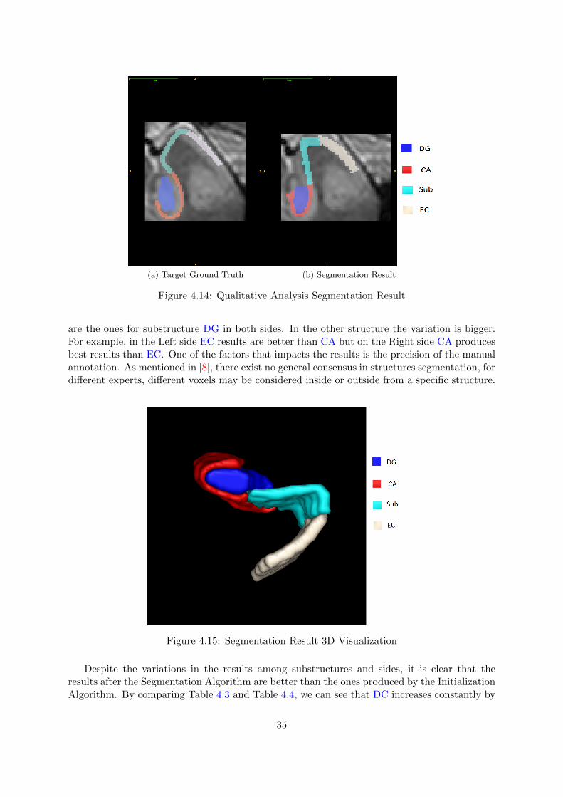
(a) Target Ground Truth (b) Segmentation Result

Figure 4.14: Qualitative Analysis Segmentation Result

are the ones for substructure DG in both sides. In the other structure the variation is bigger.For example, in the Left side EC results are better than CA but on the Right side CA producesbest results than EC. One of the factors that impacts the results is the precision of the manualannotation. As mentioned in [8], there exist no general consensus in structures segmentation, fordifferent experts, different voxels may be considered inside or outside from a specific structure.

Figure 4.15: Segmentation Result 3D Visualization

Despite the variations in the results among substructures and sides, it is clear that theresults after the Segmentation Algorithm are better than the ones produced by the InitializationAlgorithm. By comparing Table 4.3 and Table 4.4, we can see that DC increases constantly by

35

using the Segmentation Algorithm.Moreover, we consider that the quality of the results obtained are affected by the reduced

Training Set that we employed. We used only 3 patients, however, having more patients in theTraining Set increases the probability of finding a patient similar to the test one.

Table 4.4: Add caption

Structure Left Right Both

DG 0.672 0.727 0.699CA 0.414 0.466 0.440Sub 0.419 0.509 0.464EC 0.481 0.383 0.432

4.3.2 Evaluation on Patients with Alzheimer Disease

In this section we present the results obtained when using images of patients with AlzheimerDisease.

Figure 4.16 shows the result on Right HF in a patient that presents atrophy. We can observethat the results are still not optimal. The label of the substructures are not correctly locatedover the real ones. Another important fact is that the size of the labels are almost the same asthe original from the training set, the shrinking caused by AD is not entirely coped with themethod proposed. The reason behind the not optimal results is that the brain that we tested,present large anatomical differences with the training set, probably because of atrophy causedby AD. This makes extremely difficult to find a correct transformation from training to thetest patient.

4.3.3 Performance Metrics

The iterative process of the Segmentation Algorithm took in average 5 minutes. The experimentwas done using a 6 cores Intel Xeon Processor with 6GB RAM.

4.3.4 Comparison with Existing Method

Figure 4.17 shows the comparison in terms of DC with the fully automatic method for segmen-tation described in [1].

By looking at Figure 4.17, we can observe that in two substructures (CA and Sub), themethod described in [1] achieves better DC than our method. However, for substructure DGour method performs slightly better. In [1], the authors employed a different anatomical defi-nition of HF, for this reason no comparison is possible for EC substructure.

When we analyze the computation time that each of the method requires, we can see a bigdifference between [1] and our method. While in [1], the procedure takes 5 hours for one patient,in our method the procedure takes, in average, only 55 minutes (50 in the Initialization and 5in the Segmentation). This means that our method is 5.4 times faster that the one proposed in[1].

36

(a) Only Data (b) Data + Segmentation

(c) Only Data (d) Data + Segmentation

Figure 4.16: Segmentation Results on Patients with AD, (a) and (b) show Right HF and (c)and (d) show Left HF

37

Figure 4.17: Comparison with existing method [1]

38

CHAPTER 5

Conclusions and Future Work

We developed and implemented a Fully Automatic Segmentation Tool for Brain Substructuresfocusing on the HF. In order to solve this problem, we made three relevant contributions:

• First, we proposed a fast registration method based on moments. We validate our resultsby means of DC and compared our results to a state-of-the-art tool called FLIRT. By usingtwo different data sets, namely IBSR and ADAB, we showed that our proposed methodachieves similar results to the ones from FLIRT but spending much less computation time.

• Second, we introduced an Initialization scheme which is based on a Multi-Level Reg-istration approach. At this stage, we made use of different types of transformationsand different resolutions. We implemented this framework using Elastix. Our proposedmethod predicts the contours of the substructures of interest from a set of training con-tours, the overlapping coefficient shows that this initial prediction is good enough to startthe segmentation algorithm.

• Third, we proposed a Segmentation Algorithm based on relative Pose Information, similarto [6] and [2]. The relevant contribution that we made is that the intensity term is mergedwith the prior based on Moments into a single term. We obtained results using leave-one-out cross validation experiments. We compared our results to the fully automatic methodproposed in [1]. We showed that for a specific substructure from the HF out tool performsbetter in terms of DC. Although our results in the rest of the substructures are not asgood as the ones from [1], our tool spends much less computation time, being 5 timesfaster than the one proposed in [1]. In addition, we validate our tool using volumetricimages of patients with Alzheimer Disease that present atrophy in the HF. We showedthat the results produced by our tool come close to the real substructures even when somelevel of atrophy is present. However, we cannot conclude that out tool is robust enoughto cope with high atrophy levels.

• For the validating our segmentation tool, we employed 7T images T2-weighted. For theanatomical description of the HF, we followed the protocol described in [9].

39

5.1 Future work

One of the aspects that can be improved is the Registration base on Moments. In the methodproposed, we employed moments up to order 2, a possible improvement can be achieved byusing higher order moments which give us more insight about the objects of an image.

One open question from our tool is the stopping criteria in the iterative process of the seg-mentation algorithm. So far, we fixed a certain number of iterations for it, by doing this we arestill not assuring optimum results for this algorithm.

Another important missing component is the optimization for coping with images of pa-tients with Alzheimer Disease. In this specific cases the substructures present shrinking, so oursegmentation algorithm should be able to detect the real volume of each substructure.

Relative to performance, we can improve the computation time by making use of a GraphicsProcessing Unit (GPU). The algorithms proposed are highly parallalizable because most of theoperations are computed voxel by voxel, this means that using a GPU for accelerating certainparts of the tool would be beneficial.

At the Initialization stage, we used each of the patients from the training set in order toobtain different predicted contours for a test patient, based on the overlapping with the targetcontours we selected the best element from the training set to continue with the segmentationalgorithm . However, we do have yet a method to select the most appropriate candidate a priori.Finding such method becomes relevant when the training set is very large and it is not possibleto analyze all possible candidates.

40

APPENDIX A

Acronyms

AD Alzheimer’s Disease

BET Brain Extraction Tool

CA Cornu Ammonis

CA1 Cornu Ammonis 1

CA2 Cornu Ammonis 2

CA3 Cornu Ammonis 3

DC Dice Coefficient

DG Dentate Gyrus

EC Entorhinal Cortex

FLIRT Linear Image Registration Tool

FSL Fmrib Software Library

HF Hippocampal Formation

IBSR Internet Brain Segmentation Repository

LUMC Leids Universitair Medisch Centrum

MASV Multi-atlas segmentation and voting

MRI Magnetic Resonance Image

NCC Normalized Cross Correlation

ROI Region Of Interest

Sub Subiculum

SDF Signed Distance Function

UMC Universitair Medisch Centrum Utrecht

41

APPENDIX B

Parameter File Elastix

B.1 Affine Registration Elastix Parameter

(FixedInternalImagePixelType "float")

(MovingInternalImagePixelType "float")

(FixedImageDimension 3)

(MovingImageDimension 3)

(UseDirectionCosines "true")

(Registration "MultiResolutionRegistration")

(Interpolator "BSplineInterpolator")

(ResampleInterpolator "FinalBSplineInterpolator")

(Resampler "DefaultResampler")

(FixedImagePyramid "FixedRecursiveImagePyramid")

(MovingImagePyramid "MovingRecursiveImagePyramid")

(Optimizer "AdaptiveStochasticGradientDescent")

(Transform "AffineTransform")

(Metric "AdvancedMattesMutualInformation")

(AutomaticScalesEstimation "true")

(AutomaticTransformInitialization "true")

(HowToCombineTransforms "Compose")

(NumberOfHistogramBins 32)

(ErodeMask "false")

(NumberOfResolutions 1)

(MaximumNumberOfIterations 250)

(NumberOfSpatialSamples 2048)

(NewSamplesEveryIteration "true")

(ImageSampler "Random")

(BSplineInterpolationOrder 1)

(FinalBSplineInterpolationOrder 3)

(DefaultPixelValue 0)

(WriteResultImage "true")

(ResultImagePixelType "short")

(ResultImageFormat "nii")

42

B.2 BSpline Registration Elastix Parameter

(FixedInternalImagePixelType "float")

(MovingInternalImagePixelType "float")

(FixedImageDimension 3)

(MovingImageDimension 3)

(UseDirectionCosines "true")

(Registration "MultiResolutionRegistration")

(Interpolator "BSplineInterpolator")

(ResampleInterpolator "FinalBSplineInterpolator")

(Resampler "DefaultResampler")

(FixedImagePyramid "FixedRecursiveImagePyramid")

(MovingImagePyramid "MovingRecursiveImagePyramid")

(Optimizer "AdaptiveStochasticGradientDescent")

(Transform "BSplineTransform")

(Metric "AdvancedMattesMutualInformation")

(FinalGridSpacingInVoxels 32)

(HowToCombineTransforms "Compose")

(NumberOfHistogramBins 32)

(ErodeMask "false")

(NumberOfResolutions 1)

(MaximumNumberOfIterations 500)

(NumberOfSpatialSamples 2048)

(NewSamplesEveryIteration "true")

(ImageSampler "Random")

(BSplineInterpolationOrder 1)

(FinalBSplineInterpolationOrder 3)

(DefaultPixelValue 0)

(WriteResultImage "true")

(ResultImagePixelType "short")

(ResultImageFormat "nii")

43

Bibliography

[1] K. Van Leemput, A. Bakkour, T. Benner, G. Wiggins, L. L. Wald, J. Augustinack, B. C.Dickerson, P. Golland, and B. Fischl, “Automated segmentation of hippocampal subfieldsfrom ultra-high resolution in vivo mri,” Hippocampus, vol. 19, no. 6, pp. 549–557, 2009.[Online]. Available: http://dx.doi.org/10.1002/hipo.20615

[2] M. Uzunbas, O. Soldea, D. Unay, M. Cetin, G. Unal, A. Ercil, and A. Ekin, “Couplednonparametric shape and moment-based intershape pose priors for multiple basal gangliastructure segmentation,” Medical Imaging, IEEE Transactions on, vol. 29, no. 12, pp. 1959–1978, dec. 2010.

[3] O. T. Carmichael, H. A. Aizenstein, S. W. Davis, J. T. Becker, P. M. Thompson, C. C.Meltzer, and Y. Liu, “Atlas-based hippocampus segmentation in alzheimers disease andmild cognitive impairment,” NeuroImage, vol. 27, pp. 979–990, 2005.

[4] L. Wang, J. S. Swank, I. E. Glick, M. H. Gado, M. I. Miller, J. C. Morris, and J. G.Csernansky, “Changes in hippocampal volume and shape across time distinguish dementiaof the alzheimer type from healthy aging,” NeuroImage, vol. 20, no. 2, pp. 667 – 682, 2003.[Online]. Available: http://www.sciencedirect.com/science/article/pii/S1053811903003616

[5] P. Andersen, R. Morris, D. Amaral, T. Bliss, and J. O’Keefe, The Hippocampus Book,1st ed., ser. Oxford Neuroscience. Oxford University, 2006.

[6] O. Soldea, N. Doan, A. Webb, M. Van Buchem, and R. Milles, Jasinschi, “Simultaneousbrain structures segmentation combining shape and pose factors,” vol. 1, Jun. 2005, pp.886–893 vol. 1. [Online]. Available: http://dx.doi.org/10.1109/CVPR.2005.177

[7] K. Van Leemput, “Encoding probabilistic brain atlases using bayesian inference,” MedicalImaging, IEEE Transactions on, vol. 28, no. 6, pp. 822 –837, june 2009.

[8] P. A. Yushkevich, H. Wang, J. Pluta, S. R. Das, C. Craige, B. B. Avants, M. W. Weiner,and S. Mueller, “Nearly automatic segmentation of hippocampal subfields in in vivo focalt2-weighted mri.” NeuroImage, vol. 53, no. 4, pp. 1208–1224, 2010. [Online]. Available:http://www.ncbi.nlm.nih.gov/pubmed/20600984

[9] J. Pluta, S. Mueller, C. Craige, and P. Yushkevich, Hippocampal Subfield SegmentationProtocol at 4T.

44

http://dx.doi.org/10.1002/hipo.20615

http://www.sciencedirect.com/science/article/pii/S1053811903003616

http://dx.doi.org/10.1109/CVPR.2005.177

http://www.ncbi.nlm.nih.gov/pubmed/20600984

[10] J. Prokop and A. P. Reeves, “A survey of moment-based techniques for unoccluded objectrepresentation and recognition,” in CVGIP: Graphical Models and Image Processing, 1992,pp. 438–460.

[11] J. Meriam and K. L.G., Engineering Mechanics Dynamics 5th Edition. John Wiley &Sons, Incorporated, 2003.

[12] S. Strother, “Evaluating fmri preprocessing pipelines,” Engineering in Medicine and Biol-ogy Magazine, IEEE, vol. 25, no. 2, pp. 27 –41, march-april 2006.

[13] S. Klein, M. Staring, K. Murphy, M. Viergever, and J. Pluim, “elastix: A toolbox forintensity-based medical image registration,” Medical Imaging, IEEE Transactions on,vol. 29, no. 1, pp. 196 –205, jan. 2010.

[14] L. Ibanez, W. Schroeder, L. Ng, and J. Cates, The ITK Software Guide, 2nd ed., Kitware,Inc. ISBN 1-930934-15-7, http://www.itk.org/ItkSoftwareGuide.pdf, 2005.

[15] P. Thevenaz and M. Unser, “Optimization of mutual information for multiresolution imageregistration,” Image Processing, IEEE Transactions on, vol. 9, no. 12, pp. 2083 – 2099, dec2000.

[16] D. Rueckert, L. Sonoda, C. Hayes, D. Hill, M. Leach, and D. Hawkes, “Nonrigid registrationusing free-form deformations: application to breast mr images,” Medical Imaging, IEEETransactions on, vol. 18, no. 8, pp. 712 –721, aug. 1999.

[17] T. Chan and L. Vese, “Active contours without edges,” Image Processing, IEEE Transac-tions on, vol. 10, no. 2, pp. 266 –277, feb 2001.

[18] The internet brain segmentation repository ibsr. [Online]. Available: http://www.cma.mgh.harvard.edu/ibsr/

[19] Flirt- fmrib’s linear image registration tool. [Online]. Available: http://fsl.fmrib.ox.ac.uk/fsl/flirt/

[20] H. Wang, S. Das, J. Pluta, C. Craige, M. Altinay, M. Weiner, S. Mueller, and P. Yushkevich,“Shape-based semi-automatic hippocampal subfield segmentation with learning-based biasremoval,” in Biomedical Imaging: From Nano to Macro, 2010 IEEE International Sympo-sium on, april 2010, pp. 424 –427.

[21] P. Viola and W. M. Wells, III, “Alignment by maximization of mutual information,”Int. J. Comput. Vision, vol. 24, pp. 137–154, September 1997. [Online]. Available:http://dl.acm.org/citation.cfm?id=263008.263015

[22] Y. Chen, S. Thiruvenkadam, F. Huang, K. Gopinath, and R. Brigg, “Simultaneous seg-mentation and registration for functional mr images,” in Pattern Recognition, 2002. Pro-ceedings. 16th International Conference on, vol. 1, 2002, pp. 747 – 750 vol.1.

[23] J. Flusser and T. Suk, “A moment-based approach to registration of images with affinegeometric distortion,” Geoscience and Remote Sensing, IEEE Transactions on, vol. 32,no. 2, pp. 382 –387, mar 1994.

[24] K. Van Leemput, “Probabilistic brain atlas encoding using bayesian inference,” inProceedings of the 9th international conference on Medical Image Computing and Computer-Assisted Intervention - Volume Part I, ser. MICCAI’06. Berlin, Heidelberg: Springer-Verlag, 2006, pp. 704–711. [Online]. Available: http://dx.doi.org/10.1007/11866565 86

45

http://www.cma.mgh.harvard.edu/ibsr/

http://www.cma.mgh.harvard.edu/ibsr/

http://fsl.fmrib.ox.ac.uk/fsl/flirt/

http://fsl.fmrib.ox.ac.uk/fsl/flirt/

http://dl.acm.org/citation.cfm?id=263008.263015

http://dx.doi.org/10.1007/11866565_86

[25] A. Akselrod-Ballin, M. Galun, J. M. Gomori, A. Brandt, and R. Basri, “Priorknowledge driven multiscale segmentation of brain mri,” in Proceedings of the 10thinternational conference on Medical image computing and computer-assisted intervention,ser. MICCAI’07. Berlin, Heidelberg: Springer-Verlag, 2007, pp. 118–126. [Online].Available: http://dl.acm.org/citation.cfm?id=1775835.1775853

[26] T. Rohlfing, D. Russakoff, and C. Maurer, “Performance-based classifier combination inatlas-based image segmentation using expectation-maximization parameter estimation,”Medical Imaging, IEEE Transactions on, vol. 23, no. 8, pp. 983 –994, aug. 2004.

[27] Brain extraction tool. [Online]. Available: http://www.fmrib.ox.ac.uk/fsl/bet2/index.html

[28] Fmrib software library. [Online]. Available: http://www.fmrib.ox.ac.uk/fsl/

[29] Insight segmentation and registration toolkit. [Online]. Available: http://www.itk.org/

[30] Visualization toolkit. [Online]. Available: http://www.vtk.org/

46

http://dl.acm.org/citation.cfm?id=1775835.1775853

http://www.fmrib.ox.ac.uk/fsl/bet2/index.html

http://www.fmrib.ox.ac.uk/fsl/

http://www.itk.org/

http://www.vtk.org/

Eindhoven University of Technology MASTER Automatic ... · Thesis Report Automatic Segmentation of...

Documents

Transcript of Eindhoven University of Technology MASTER Automatic ... · Thesis Report Automatic Segmentation of...