EIGENVALUE PROBLEMS AND QUADRATIC FORMSuser.engineering.uiowa.edu/~kkchoi/Chapter_3.pdf... or...

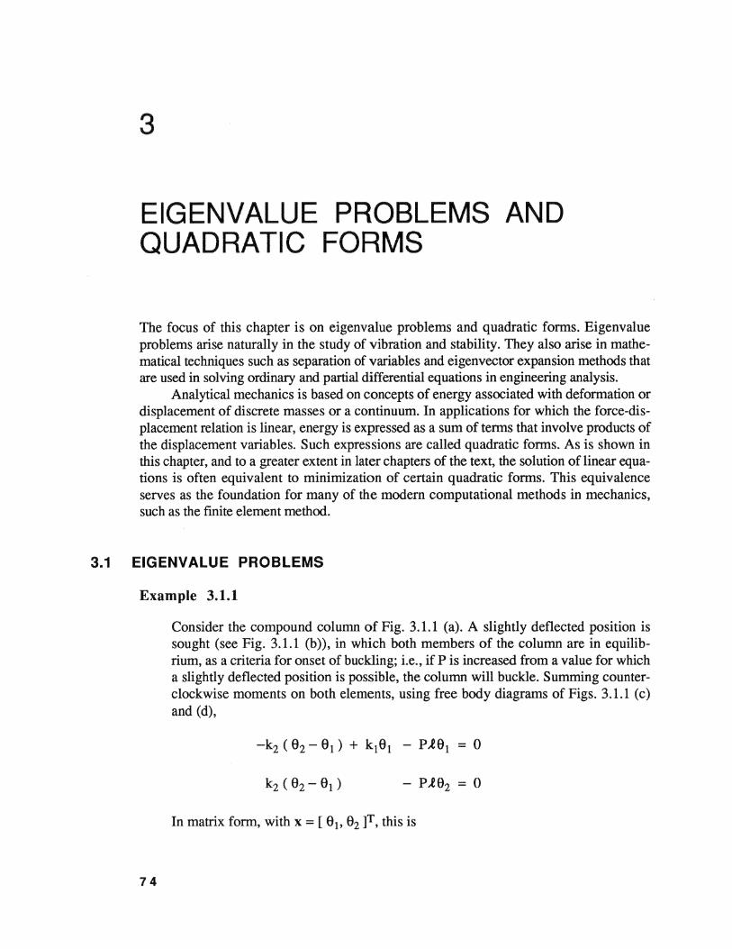
3

EIGENVALUE PROBLEMS AND QUADRATIC FORMS

The focus of this chapter is on eigenvalue problems and quadratic forms. Eigenvalue problems arise naturally in the study of vibration and stability. They also arise in mathematical techniques such as separation of variables and eigenvector expansion methods that are used in solving ordinary and partial differential equations in engineering analysis.

Analytical mechanics is based on concepts of energy associated with deformation or displacement of discrete masses or a continuum. In applications for which the force-displacement relation is linear, energy is expressed as a sum of terms that involve products of the displacement variables. Such expressions are called quadratic forms. As is shown in this chapter, and to a greater extent in later chapters of the text, the solution of linear equations is often equivalent to minimization of certain quadratic forms. This equivalence serves as the foundation for many of the modem computational methods in mechanics, such as the fmite element method.

3.1 EIGENVALUE PROBLEMS

Example 3.1.1

74

Consider the compound column of Fig. 3.1.1 (a). A slightly deflected position is sought (see Fig. 3.1.1 (b)), in which both members of the column are in equilibrium, as a criteria for onset of buckling; i.e., if P is increased from a value for which a slightly deflected position is possible, the column will buckle. Summing counterclockwise moments on both elements, using free body diagrams of Figs. 3.1.1 (c) and (d),

In matrix form, with X= [ el, e2 ]T, this is

Sec. 3.1 Eigenvalue Problems 75

where A= Pl.

~p ~p

(a) (b)

Figure 3.1.1 Buckling of Compound Column • Eigenvalues and Eigenvectors

A frequently encountered problem, as illustrated in Example 3.1.1, is determining values of a constant A for which there is a nontrivial solution of a homogeneous set of equations of the form

Ax= AX (3.1.1)

where A is an nxn real matrix, xis an nx1 column vector (real or complex), and A is a constant (real or complex).

Definition 3.1.1. Equation 3.1.1 for A and x is known as an eigenvalue problem. Values of A for which solutions x :1: 0 of Eq. 3.1.1 exist are called eigenvalues, or characteristic values, of the matrix A. The corresponding nonzero solutions x are called eigenvectors of the matrix A. •

In many applications in which such problems arise, the matrix A is symmetric.

76 Chap. 3 Eigenvalue Problems and Quadratic Forms

Characteristic Equations

Equation 3.1.1 may be written as

(A-AI)x=O (3.1.2)

where I is the nxn identity matrix. According to Theorem 2.3.5, this homogeneous equation for x has nontrivial solutions if and only if the determinant of the coefficient matrix A - AI vanishes. That is, if and only if A. satisfies

( a11 - A) a12 aln

lA-AII a21 (a22-A) a2n - . . . . . . ...... . ..... anl Rn2 (Rnn-A)

= An A.n-1 c0 + c1 + ... + en = 0 (3.1.3)

which is called the characteristic equation of the eigenvalue problem of Eq. 3.1.1. The left side of Eq. 3.1.3 is called the characteristic polynomial for the eigenvalue problem. This condition requires that A is the solution of a polynomial equation of degree n. The n solutions A1, A2, ... , A.n. which need not all be distinct, are the eigenvalues of the matrix A.

Example 3.1.2

The characteristic equation for the buckling problem of Example 3.1.1 is

lkt+kz-A -k21 2 -kz k2-A = A - ( k1 + 2k2 ) A + k1k2 = 0

There are two eigenvalues, A1 and A.z. Recalling that P = A I.e, the buckling loads of the compound column of Example 3.1.1 are

P 1 = ( k 1 + 2kz - ,J k? + 4ki ) /2.e

P2 = ( k1 + 2k2 + ,J k? + 4ki ) / 2-t

where P1 < P2. Substituting P1 into the equilibrium equations of Example 3.1.1,

-k2

kl Jki+ 4k~ -T+ 2

[:~] = [~]


From the first equation,

for any value of 81. A simple check shows that the second equation is also satisfied by this solution, which is expected since the matrix was caused to be singular. Setting 81 = 1 yields an eigenvector corresponding to P1,

Similarly, an eigenvector for P2 is

These ei envectors are called buckling modes of the structure. Noting that

k; + 4k~ > k1, the forms of buckling modes x1 and x2 are shown in Figs. 3.1.2

(a) and (b), respectively.

(a) (b)

Figure 3.1.2 Buckling Modes of Compound Column


It is physically clear that, since 0 < P1 < P2, if Pis increased slowly from zero, buckling in the mode shown in Fig. 3.1.2 (a) will occur when Preaches P1. •

Example 3.1.3

The characteristic equation for the 3x3 matrix

[ 1 2 OJ A= 2 2 2

0 2 3

is

1-A. 2 0

I A - A.I I = 2 2-A. 2 0 2 3-A.

= (1-A.)(2-A.)(3-A.)-4(3-A.)-4(1-A.)

= A,3 - 6A.2 + 3A. + 10 = 0

This equation has three solutions,

• The sum of the diagonal elements of a matrix A is called the trace of A and is de

noted by tr ( A ). It is shown in Ref. 4 that the coefficients of the characteristic equation of Eq. 3.1.3, for an nxn matrix, are given by

c0 = 1

Ct = - tl

c2 = - ( 1 I 2 ) ( c1 t1 + t2 )

c3 = - ( 1 I 3 ) ( c2t1 + c1 t2 + t3 ) (3.1.4)

and that

n

L A.i = tr(A) i=l


where

tk = tr ( Ak ), k = 1, ... , n

and the kth power of a matrix A is

Ak = A A ... A (k-times)

Equations 3.1.4 are called Bocher's formulas for the coefficients of the characteristic polynomial.

Example 3.1.4

Applying Eq. 3.1.4 to the matrix A of Example 3.1.3,

t 1 = tr ( A ) = 1 + 2 + 3 = 6

and, with

A2 = [~ 162 1~] , A3 = [~~ ~~ ~:]

4 10 13 24 54 59

t2 = tr ( A2 ) = 5 + 12 + 13 = 30

t3 = tr ( A3) = 17 + 56 + 59 = 132

Eq. 3.1.4 yields

c0 = 1

c1 = -6 c2 = -( 1/2)[(-6) x 6 + 30] = 3 c3 = - ( 1 I 3 ) [ 3 x 6 + ( - 6 ) x 30 + 132 ] = 10

Hence, the characteristic equation for A is

}} - 6}.,2 + 3A. + 10 = 0

which agrees with Example 3.1.3. Furthermore, the trace of A equals the sum of all eigenvalues "-i [1]; i.e., from the result of Example 3.1.3,

A.1 + A.2 + ~ = -1 + 2 + 5 = 6 = tr ( A ) • From Eq. 1.4.2, the determinant of a matrix is equal to the determinant of its trans

pose. Thus, I A - A.I I = I AT- A.I I and the eigenvalues of A are also the eigenvalues of AT.


Eigenvector Orthogonality for Symmetric Matrices

Corresponding to each eigenvalue A.k, there exists at least one eigenvector xk :;:. 0 from Eq. 3.1.1, or Eq. 3.1.2, which is determined only to within an arbitrary multiplicative constant; i.e., axk is also an eigenvector, for any constant a :1: 0. Let Aa and A.p be two distinct eigenvalues of a symmetric matrix A and denote corresponding eigenvectors by xa

and xP, respectively; i.e., Aa :;:. A.p and

(3.1.5)

(3.1.6)

Taking the transpose ofEq. 3.1.5 and multiplying both sides on the right by xP,

(3.1.7)

Multiplying both sides ofEq. 3.1.6 on the left by xaT,

(3.1.8)

Subtracting Eq. 3.1.7 from Eq. 3.1.8 and noting that for a symmetric matrix AT= A,

(3.1.9)

Since Aa :!: A.p. the following important result holds.

Theorem 3.1.1. Eigenvectors xi and xj of a real symmetric matrix that correspond to distinct eigenvalues A.i:;:. A.j are orthogonal; i.e.,

Furthermore, the eigenvalues and eigenvectors of a symmetric matrix are real.

(3.1.10)

• To prove the second part of Theorem 3.1.1, suppose that A.= a+ iJ3 is a root of Eq.

3.1.3, where a and J3 are real and i = .V -1. Let x :!: 0 be a corresponding eigenvector; i.e.,

Ax = A.x

which may be complex. Taking the complex conjugate (denoted by*) of both sides of this equation yields

Ax* = A.*x*

since the conjugate of a product is the product of the conjugates and A is real. Thus,


A* = a- iP is also an eigenvalue of A, with x* as the associated eigenvector. Multiplying the first relation on the left by x*T and multiplying the transpose of the second relation on the right by x yields

*T *T x Ax = Ax x

*T T "l * *T x Ax=A.X x (3.1.11)

Subtracting the second of Eqs. 3.1.11 from the first and using symmetry of A,

( A - 'A* ) x*T x = 0 (3.1.12)

Since the product x*Tx = x-*x· = (a·- ib·) (a·+ ib·) = a·a· + b·b· :t: 0 is real it follows * J J J J J J JJ JJ , that A- A = 2iP = 0, so 'A must be real. Accordingly, all eigenvalues of A are real.

Let the eigenvector x be written in the form

x=y+iz

where y and z are real vectors. Since A and A are real, Ax = 'Ax can be written as

Ay - 'Ay = - i ( Az - 'Az )

where the left side is real and the right side is imaginary. Thus, both sides are zero; i.e.,

Ay - AY = 0 = Az - Az

so the real vectors y and z are eigenvectors corresponding to the real eigenvalue A. Thus, the eigenvectors of a symmetric matrix may be chosen to be real. •

Example 3.1.5

Consider the real symmetric matrix

[ 0 0 -2] A =·= 0 -2 0

-2 0 3

The characteristic equation for its eigenvalues is

I A -- AI I = - ( A + 2 ) ( A - 4 ) ( 'A + 1 ) = 0

Once an eigenvalue is found, it may be substituted into

[-A 0 -2] [xl] ( A- AI ) x = 0 -2-A 0 x2

-2 0 3-'A x3

0


to determine associated eigenvectors x. The eigenvalues and corresponding eigenvectors for this 3x3 matrix are

A1 - 2, x1 = [ 0, a, 0 ]T

A2 = 4, x2 = [ -b/2, 0, b ]T

A3 - 1, x3 == [ 2c, 0, c ]T

where any nonzero scalars a, b, and c may be selected. Note that xl, x2, and x3 are mutually orthogonal. •

If an eigenvalue A1 of a symmetric matrix is a multiple root of multiplicity s; i.e., if the left side of Eq. 3.1.3 contains the factor ( A- A1 ) 8 , then there are s linearly independent eigenvectors associated with A1. The proof of this result is postponed to Section 3.2 (see Theorem 3.2.2).

Example 3.1.6

For the symmetric matrix

the characteristic equation is

-A 1 0 I A-- AI I = 1 -A 0

0 0 1-A

= A2 ( 1 -A) - ( 1- A)

= - ( A + 1 ) ( A - 1 )2 = 0

Thus, there is a multiple root

Substituting this result into Eq. 3.1.2,

[-1 1 OJ lxl] 1 -1 0 x2

0 0 0 x3

0

The rank of the coefficient matrix is one, so two lineariy independent eigenvectors are obtained for the multiple root A1 = ~.

Sec. 3.1 Eigenvalue Problems

are obtained for the multiple root A.1 = A.z, X 1 = [ 1, 1, 0 ]T

x2 = [ 1, 1, 1 ]T

For A.3 = -1, Eq. 3.1.2 is

[ ~ ~ ~] [ ::] = 0 0 0 2 x3

and the associated eigenvector is

x3 = [ 1, -1, 0 ]T

83

Note that x3 is orthogonal to both xl and x2. However, xl and x2 are not orthogonru. •

Eigenvector Expansion

By the Gram-Schmidt orthogonruization process of Section 2.4, it is possible to choose s orthonormal eigenvectors of a symmetric matrix A that correspond to an eigenvalue of multiplicity s. By Theorem 3.1.1, rul these eigenvectors are orthogonal to rul other eigenvectors. Thus, if multiple roots of Eq. 3.1.3 are counted separately, exactly n mutually orthogonru eigenvectors may be found. By virtue of the results of Section 2.2, this set of vectors forms a basis for Rn. Thus, any vector in Rn can be expressed as a linear combination of n eigenvectors of a symmetric nxn matrix.

In particular, if each of the n orthogonru eigenvectors has been multiplied by the inverse of its norm, so that it is a unit vector, the resulting set of vectors is orthonormal. These vectors may be denoted by xl, x2, ... , xn, with

(3.1.13)

Thus, the ith coefficient in the representation, called an eigenvector expansion,

(3.1.14)

for a vector x in Rn is obtained by forming the scalar product of xi with both sides of Eq. 3.1.14,

a· = xiTx 1

Consider now the nonhomogeneous equation

Ax - ~x = c

(3.1.15)

(3.1.16)


where A is a real symmetric matrix. IfEq. 3.1.16 has a solution, then it can be expressed as a linear combination of the eigenvectors of A. Suppose that n orthonormal eigenvectors xl, x2, ... , xn are known, satisfying the equations

Since the vectors {xi} form a basis of Rn, the solution ofEq. 3.1.16 can be expressed in the form

(3.1.17)

where the constants ak are to be determined. Substituting Eq. 3.1.17 into Eq. 3.1.16,

n

I o~.k- 13 ) akxk = c k=l

By forming the scalar product of any xa with both sides of Eq. 3.1.18,

( Aa - 13 ) aa = xaT C, a = 1' 2, ... ' n

(3.1.18)

(3.1.19)

Hence, if 13 is not an eigenvalue, the solution of Eq. 3.1.16 is obtained in the form

n kT ~ X C k

X=""" (A _A) X k=l k ....

(3.1.20)

Thus, a unique solution of the nonhomogeneous equation of Eq. 3 .1.16 is obtained if 13 is not an eigenvalue. If A, = 13, no solution exists unless the vector c is orthogonal to all eigenvectors that correspond to A,. If this condition is satisfied, Eq. 3.1.19 shows that the corresponding coefficient (or coefficients) 11p may be chosen arbitrarily, so infinitely many solutions exist. In particular, if 13 = 0, Eq. 3.1.16 reduces to

Ax= c

which was studied previously. This equation has a unique solution, unless 13 = 0 is an eigenvalue of A; i.e., unless the equation Ax= 0 has non-trivial solutions. In this exceptional situation, no solution exists unless c is orthogonal to all vectors x that satisfy Ax = 0, in which case infinitely many solutions exist. This result is a special case of the Theorem of the Alternative [1] for symmetric matrices. This existence criterion, in the more general case 13 = A,. can also be obtained by replacing A by A - y and noticing that the latter matrix is symmetric.

Example 3.1. 7

Consider the matrix equation of Example 2.3.10; i.e.,


(3.1.21)

The characteristic equation for the eigenvalues of matrix A is

(3.1.22)

Thus,

Consider the case in which k1 = k2 = 1. Then the matrix A is symmetric,

(3.1.23)

and the associated orthogonal eigenvectors are

(3.1.24)

An eigenvector expansion for the solution ofEq. 3.1.21 may be written in the form

x = ~xi

and Eq. 3.1.21 becomes

2

Ax = aiAxi = L ~A.ixi = c i=l

Taking the scalar product of both sides of this equation with xa,

Thus, the solution is

(3.1.25)

(3.1.26)


Consider the case f1 = f2 = 10 and f 3 = 0. Then, c = [ 40,-500 ]T and

X= ( -125~-135 )[ 1 ] + ( 135-125-fi )[ _1 ] ..J2+1 -1--fi -fi-1 ..J2-1

= [-230] 270

(3.1.27)

• Another method of solving linear and nonlinear equations is Galerkin's method.

It is illustrated here with matrix equations. In order to solve the equation

Ax= c (3.1.28)

where xis in Rn and A is an nxn symmetric matrix, first define the residual as

r=Ax-c

By Theorem 2.4.4, Eq. 3.1.28 is satisfied if and only if rTxi = 0, for all eigenvectors xi of the matrix A, since they form a basis of Rn. That is,

"TA .T 0 . xJ x - xJ c = , J = 1, ... , n

As before, let x = 3.j_Xi and substitute it into Eq. 3.1.28, to obtain

(3.1.29)

Since the xi are orthogonal, Eq. 3.1.29 reduces to

which is the result obtained in Eq. 3.1.25. Thus, in this case, the Galerkin method yields the same result as the eigenvector expansion method.

EXERCISES 3.1

1. Show that the eigenvalue problem

x1 - 2x2 = A.x1

x1 - x2 = A.x2

does not have a real nontrivial solution for x1 and x2, for any value of A..


2. (a) Determine the eigenvalues A.1 and "-2 and the corresponding normalized eigenvectors xl and x2 of the matrix

A=[~ ~] (b) Verify that xl and x2 are orthogonal.

(c) If y = [ 1, 1 ]T, determine a.1 and~ so that

(d) Use the results of part (a), together with Eq. 3.1.20, to obtain the solution of the following set of equations:

5x1 + 2x2 = A.x1 + 2

2x 1 + 2x2 = A.x2 + 1

3. For the linear elastic system shown;

(a) Write the static equilibrium equations in matrix form.

(b) For k1 = k2 = k3 = 1lb/in, construct an eigenvector expansion for the solution.

(c) For what forces f1 and f2 does the problem have a solution?

4. If A. is an eigenvalue of a matrix A, with an associated eigenvector x, prove that A. k

(k-th power of A.) is an eigenvalue of the matrix Ak =A A ... A (k products of A) with the associated eigenvector x, where k is any positive integer.

5. Find the eigenvalues and eigenvectors of A 2 and verify the result of Exercise 4, where

[2 2 3] A= 1 2 1

2 -2 1

6. Show that a square matrix is singular if and only if it has zero as an eigenvalue.


7. Let A be a symmetric nxn matrix and Ax«= A.axa, a.= 1, 2, ... , n, where all eigenvalues are distinct.

(a) Write the eigenvector expansion of a vector c e Rn.

(b) Is the eigenvector expansion unique or not? Why?

3.2 QUADRATIC FORMS

Matrix Quadratic Forms

Definition 3.2.1. A linear combination of products of variables xi of the form

J = anx12 + a22x22 + ... + ~xn2 + a12x1x2 + ... + a13X1X3 + • • • + ~.n-2XnXn-2 + ~.n-1XnXn-1 (3.2.1)

is called a quadratic form in x 1, x2, . . . , xn, where the ~j are real. The quadratic form ofEq. 3.2.1 can be written in matrix form as

J = xTAx

au a12 a1n xl

[ x1, x2, ... 'xn] a21 a22 a2n x2

=

~1 ~2 ~ Xn

= ~jXiXj (3.2.2)

where x = [ x1, x2, ... , Xn ]T and A= [ ~j] is the matrix of the quadratic form. •

Example 3.2.1

Construct the quadratic form J = x TAx for the matrix

By Eq. 3.2.2,

• For a general nxn matrix B that is not necessarily symmetric, consider the quadratic

form

Sec. 3.2 Quadratic Forms

Defining a symmetric matrix, called the symmetrized matrix associated with B,

B* = ( 1 I 2 ) ( B + BT )

the related quadratic form

can be formed. Since x TBT x is a scalar, it is equal to its transpose, so

xTBTx = ( xTBTx )T = ( BTx )Tx = xTBx

Substituting Eq. 3.2.4 into the definition of J*,

J* = xTB*x = xTBx = J

This result may be summarized as follows.

89

(3.2.3)

(3.2.4)

(3.2.5)

Theorem 3.2.1. A nonsymmetric matrix B in a quadratic form can always be replaced by the symmetrized matrix of Eq. 3.2.3, without affecting the value of the quadratic furm. •

The fact that a quadratic form can always be written with a symmetric matrix is of fundamental importance. It provides the basis for restricting attention to symmetric matrices in large classes of applications.

Example 3.2.2

Theorem 3.2.1 may be illustrated using Example 3.2.1, with

Then,

• Strain Energy

The energy stored in an elastic mechanical element, such as the elastic spring shown in Fig. 3.2.1, is of interest in many applications. The force required to deform the spring from its free length is f = kx, where k is called the spring constant and x is the deformation of the spring. Integrating for the work done in stretching the spring from its free


length by an amount x,

Jx f x 1 U = wk = 0 f d~ = 0 k~ d~ = 2 kx2

This work is equal to the energy stored in the spring, called its strain energy.

k (lb{m)

Figure 3.2.1 Linear Spring

Example 3.2.3

f

•

(3.2.6)

Consider the elastic system in Exercise 3 of Section 3.1. The sum of the strain energies stored in the three springs is

(3.2.7)

which is a quadratic form. The matrix K is called the system stiffness matrix. •

Trusses in structural engineering [5] consist of tension or compression members called bars, as shown in Fig. 3.2.2, that deform as stiff elastic springs. The force-deflection relation is [ 6]

o.t = Ul AE

where .t is the length of the bar, o.t is the change in length, f is the applied load, A is the cross-sectional area of the bar, and E is Young's Modulus of the material. This relation may be rewritten as

f = ( AE I), ) o),

so k = AE I), is the spring constant for the bar. Thus, the strain energy of the bar is

U = ( 1 I 2 ) ( AE I;, ) ( o.t )2 (3.2.8)

Sec. 3.2 Quadratic Forms

~

%/1~==============~~~~--~~.f ~)- PZIZ.d .,....

I• Figure 3.2.2 Deflection of a Bar

Example 3.2.4

91

Consider the simple three bar truss structure of Fig 3.2.3. From trigonometric relations and using small displacement approximations,

T a

!

Figure 3.2.3 Three Bar Truss

Since 1 1 = 13 = v2a and 12 =a, using Eq. 3.2.8, the total strain energy is


= ~ [ ( ~ + 1 ) xi + ~2 xi J

1 ~(~+1) 2 [ xl, x2]

0

0 AEVI --a 2

1 T - Ix Kx (3.2.9)

• These elementary examples of strain energy as quadratic forms typify considerations

that arise throughout the study of mechanics of deformable bodies.

Example 3.2.5

Analysis of the bending of beams becomes important, because many structures are constructed of, or can be approximated by assemblages of beams. Therefore, consider the beam element of Fig. 3.2.4, with its four displacement coordinates x = [ xl, x2, x3, x4 ]T

w

~

x2 x4

s

I• l ~ Figure 3.2.4 Beam Element

Since no lateral loads are applied to the beam and its Young's Modulus E and its centroidal cross-sectional moment of inertia I are constant, the beam bending equation [6] is Elw(4) = 0, where w is beam deflection. Thus, the bent shape of the beam, which is defined by w(s), is a cubic polynomial. To have w(O) = x1o w'(O) = x2, w(l) = x3, and w'(l) = x4, the displacement must be

w(s) = x~ ( 2s3 - 3ls2 + .t3 ) + x2 ( s3 - 2ls2 + .t2s) l _t2

- ~(2s3 - 3.ts2 ) + x4 (s3 -.ts2 ) (3.2.10) 13 _t2

Sec. 3.2 Quadratic Forms 93

The strain energy of a bent beam is [ 6]

(3.2.11)

Substituting from Eq. 3.2.10 into Eq. 3.2.11 and integrating to obtain a quadratic expression in x = [ x1, x2, x3, x4 ]T, it is left to the reader to verify that

12 61 -12 61

6..t 412 -61 212 1 x=-xTKbx

-12 -61 12 -61 2 (3.2.12)

6..t 212 -61 412

where K b is the beam element stiffness matrix. • Canonical (Diagonal Matrix) Forms

In many applications, it is desirable to make a change of variables, writing x 1, x2, ••• , Xn as linear combinations of variables x1', x2', ..• , xn'· Let x = [ xi> ... , Xn ]T be expressed in terms of x' = [ x1', ... , xn' ]T by the transformation

x = Qx' (3.2.13)

where Q is an nxn matrix. Substituting Eq. 3.2.13 into Eq. 3.2.2, where A is symmetric,

= x'TA'x' (3.2.14)

The matrix A' of the quadratic form in x', which is also symmetric, is thus

A' = QTAQ (3.2.15)

It is often desirable to simplify the quadratic form J in x' so that it involves only squares of the variables xi'. To do this, the transformation matrix Q must be chosen so that QT AQ is a diagonal matrix; i.e., ~j· = 0 if i '# j. If the eigenvalues and corresponding eigenvectors of the symmetric matrix A are known, a matrix Q that has this property can be easily constructed. Suppose that the eigenvalues of A are A.1, A.2, .•. , An· repeated roots of the characteristic equation being numbered separately, and that the corresponding

h 1 . 12 n· ort onorma eigenvectors are x , x , ... , x ; 1.e.,

(3.2.16)


Let a matrix Q be constructed so that xl, x2, ... , xn are the columns ofQ; i.e.,

Q = [ x 1' x 2' . . . ' xn ]

Then, from Eq. 3.2.16,

AQ = [ Alxl' A2X2, ... ' AnXn]

0

0

Multiplying both sides ofEq. 3.2.18 on the left by QT,

0

0

Since Q is made up of orthonormal column vectors xi,

QTQ = [ ± X:Xx~] = [ xiTxj] = [ Oij] = I a=l

(3.2.17)

(3.2.18)

. (3.2.19)

(3.2.20)

so QT = Q-1 and Q is an orthogonal matrix. Therefore, the transformed matrix A' ofEq. 3.2.15 is a diagonal matrix and the quadratic form ofEq. 3.2.14, in terms of the variable x', is

At 0 0

J = x'T 0 A2 0

Ai ( x'i )2 x' = (3.2.21)

0 0 An

which is the desired result. This is called the canonical form of the quadratic form J.

Modal Matrices

A matrix whose columns are n linearly independent eigenvectors of a given nxn matrix A is called a modal matrix of A. When these n eigenvectors are orthonormal, the modal matrix is orthogonal. Thus the matrix Q of Eq. 3.2.17 is an orthogonal modal matrix


of A. Since Q is orthogonal, the variable x' is related to the variable x, in accordance with Eq. 3.2.13, as

(3.2.22)

or, in component form,

xi' = (xi, x ), i = 1, 2, ... , n

Example 3.2.6

To illustrate the preceding reduction in a specific numerical case, consider the quadratic form

The symmetric matrix A of the form is

[25 0 0 ]

A = 0 34 -12 0 -12 41

The characteristic equation I A - AI I = 0 is

( 25 - A. ) ( A,2 - 75A. + 1250 ) = 0

from which the eigenvalues are

At = A.z = 25, ~ = 50

With A.= At= A.2 = 25, the equation Ax- A.x = 0 becomes

Oxt = 0

9x2 - 12x3 = 0

-12x2 + 16x3 = 0

The general solution is Xt = Ct, x2 = c2, x3 = 3c2/4. In vector form, x = Ctxt + c2x2, where xt= [ 1, 0, 0 ]T and x2 = [ 0, 4/5, 3/5 ]T, which are orthonormal eigenvectors. In a similar way, a normalized eigenvector corresponding to A.3 = 50 is found to be

x3 = [ 0, 3/5, -4/5 ]T

The orthonormal modal matrix Q ofEq. 3.2.17 is


1 0 0

0 4 3 Q = 5 5

0 l 4 5 -5

and the coordinates defined by Eq. 3.2.22 are

= xl

= ( 4 I 5 ) x2 + ( 3 I 5 ) x3

= ( 3 I 5 ) x2 - ( 4 I 5 ) x3

With this choice of the coordinates, Eq. 3.2.21 yields

• The tools needed to establish an assertion that was made in Section 3.1 are now

available.

Theorem 3.2.2. A real symmetric matrix A with an eigenvalue A.1 of multiplicity s has s linearly independent eigenvectors corresponding to A.1• •

To prove Theorem 3.2.2, suppose first that A is a symmetric nxn matrix, such that the characteristic equation

IA-A.II=O

has ( A. - At )2 as a factor and let x t be one normalized eigenvector of A that corresponds to "-t· Then, if Q is any nxn orthogonal matrix having x 1 as its first column, it follows that

Since each vector whose elements comprise a row ofQT, except the first, is orthogonal to the column At x 1, each element of the first column of the product, except the leading element, will vanish. Thus, the result will be of the form


At a12 ... <Xtn

0 a22 <X2n

QTAQ =

0 an2 <Xnn

Since symmetry of A implies symmetry of QT AQ, the elements a 12, ... , a 1n must also vanish. Hence, if Q is any orthogonal matrix having x 1 as its first column, the product QTAQ = Q-tAQ is of the form

At 0 0

0 a22 a2n

Q-tAQ =

0 an2 <Xnn

Thus,

At-A 0 0

0 a22-A a2n

Q-1AQ- AI=

0 an2 a -A nn

Next, note that

Q-lAQ- AI = Q-1 ( A - AI ) Q

Thus,

I Q-lAQ - AI I = I Q-111 A - AI II Q I = I A - AI I

since I Q-111 Q I= I Q-lQ I= I I I= 1. FromEq. 3.2.24,

AcA 0 0

0 a22-A a2n

lA-AII=

0 a -A nn

(3.2.23)

(3.2.24)


(3.2.25)

a -A. nn

By hypothesis, the left side of Eq. 3.2.25 has ( At -A. )2 as a factor, so it follows that the determinant on the right ofEq. 3.2.25 has (At- A.) as a factor, hence it vanishes when A. = At· Thus, the largest submatrix with a nonzero determinant on the right of Eq. 3.2.25 is of dimension (n-2) x (n-2), for A.= At· But then the largest possible square submatrix in A- A.11 with nonzero determinant has dimension (n-2) x (n-2) and the matrix Q-tAQ- A.I in Eq. 3.2.24 is of rank: n-2 or less. Thus, a second eigenvector x2 can be chosen that is orthogonal to x t and normalized. There are thus two orthonormal eigenvectors corresponding to At·

If the multiplicity of A.1 is greater than two, then by taking Q to be any orthogonal matrix having two eigenvectors xt and x2 corresponding to At as its first two columns, it is deduced in an analogous way that

A. cA. 0 0 0

0 A. cA. 0 0

0 0 a33-A. a3n Q-1AQ - A.I =

0 0 a -A. nn

The same argument leads to the conclusion that the matrix A - A.I is of rank not greater than n-3 when A.= At, so at least a three-parameter family of corresponding eigenvectors exists when the multiplicity of A. is at least three.

By induction, if At is an eigenvalue of a symmetric matrix A of multiplicity s, then the rank of the matrix A - AI is not greater than n-s when A. = At· Thus, at least s linearly independent eigenvectors corresponding to At exist. However, the rank cannot be less than n-s. Otherwise, more than s linearly independent eigenvectors would correspond to At> in which case the total number of linearly independent eigenvectors corresponding to all eigenvalues would exceed the dimension of n-space, which is impossible. Thus, if At is an eigenvalue of an nxn symmetric matrix A of multiplicity s, then the rank of the matrix A - A.I is exactly n-s when A. = At· That is, there exist exactly s linearly independent eigenvectors corresponding to At· •

Example 3.2. 7

The matrix


A = [~ ~ ~] 0 1 0

has the eigenvalues A.1 = ~ = 1 and A.3 = -1. Two linearly independent eigenvectors of A corresponding to A.1 and ~ are

and an eigenvector for A.3 = -1 is x3 = [ 0, 1, -1 ]T • EXERCISES 3.2

1. Write each of the following quadratic forms as J = xT Ax, where A is a symmetric matrix:

(a) J = -3x12 + 5x1x2 - 2x22

(b) J = 2x12 + 3x1x2 - 5x1x3 + ?x2x3 (c) J = 3x12 + x1x2 - 2x1x3 + x22 - 4x2x3 - 2x32

2. Construct an orthonormal modal matrix corresponding to the matrix

[1 0 0] A= 0 3 -1

0 -1 3

3. Reduce the quadratic form J = x 12 + 3x22 + 3x32 - 2x2x3 to canonical form.

4. Prove that if A and Bare nxn orthogonal matrices, then AB is orthogonal. If A is also nonsingular, show that A -1 is orthogonal.

5. Calculate the total strain energy in the vertical bars of the structure shown, due to displacement x1 and rotation x2, where the horizontal beam is presumed to be rigid.

l ///..J III/

.t A1E1

T x2

x1

~a


6. Calculate the total strain energy in the bars of the structure shown, due to the symmetric displacement x = [ x1, x2, x3 ]T.

7. If AT =-A; i.e., if A is skew symmetric, show that the quadratic form x TAx is zero for all x.

8. Find the eigenvalues and eigenvectors of the matrix

A = [~ ~] and find a transformation that reduces x TAx to a sum of squares.

9. If A is a symmetric nxn matrix, show that the eigenvalue equation Ax = A.x can be transformed to D y = A.y, by the linear transformation x = Q y, where D = diag ( Ah ... , An ) is a diagonal matrix and Q is the modal matrix of A.

3.3 POSITIVE DEFINITE QUADRATIC FORMS

Positive Definite and Semidefinite Matrices

Definition 3.3.1. If x TAx ~ 0 for all vectors x in Rn and if x TAx = 0 only if x = 0, then the quadratic form, equivalently the symmetric matrix A, is said to be positive definite; i.e.,

xTAx ~ 0, for all x in Rn

xTAx = 0, only ifx = 0 (3.3.1)

•

Sec. 3.3 Positive Definite Quadratic Forms

Example 3.3.1

Let

where

A = [ 1 -2] -2 7

This quadratic form can be factored as

for all x in R2. If J = 0, then each of the squared terms must be zero; i.e.,

Thus x = 0 and the quadratic form is positive defmite.

101

• Theorem 3.3.1. A symmetric matrix A is positive definite if and only if all its

eigenvalues are positive. •

To prove Theorem 3.3.1, recall the orthogonal transformation matrix Q of Eq. 3.2.17, whose columns are orthonormal eigenvectors of A. This transformation defines variables x' by Eqs. 3.2.13 and 3.2.22,

x = Qx'

x' = QTx

From Eq. 3.2.21,

If A.i > 0 for all i, then J ~ 0 and J = 0 implies all terms in the sum are zero. Hence x' = 0. But then x = Qx' = QO = 0. Thus, the quadratic form is positive definite.

Conversely, if J > 0 for all x '¢ 0, then J = A.i (xi' )2 > 0 for all x' = QTx. For proof by contradiction, assume A.k ~ 0 for some k. Then, let x' = [ oik ] and observe that J = A.i ( xi' )2 = A.i ( oik )2 = A.k ~ 0. This contradicts the hypothesis that J is positive definite, hence A.i > 0, i = 1, ... , n. •

A test for positive definiteness can be stated [1] in terms of signs of determinants.

Theorem 3.3.2. Let Si be an ixi submatrix of an nxn symmetric matrix A that is formed from the first i rows and first i columns of A. Submatrix Si is called a principal


minor of matrix A. The matrix A is positive definite if and only if the determinants of S1, S2, ... , Sn are all positive. •

Example 3.3.2

Determine whether the matrix A in Example 3.2.5 is positive definite, using both Theorems 3.3.1 and 3.3.2.

First, recall that the matrix

[25 0 0 ]

A= 0 34 -12 0 -12 41

is symmetric and, by the result of Example 3.2.5, A.1 = A.2 = 25 and A.3 = 50 are all positive. Thus, Theorem 3.3.1 implies A is positive definite.

To apply the test of Theorem 3.3.2, determinants of the principle minors of A are

I S1 I = a11 = 25 > 0

I S21 = 1::: :::I = I~ ~41 = 850 > 0

au a12 a13 25 0 0 I S3l = a21 a22 a23 = 0 34 -12 = 31250 > 0

a31 a32 a33 0 -12 41

Therefore, A is positive defmite. • Definition 3.3.2. A quadratic form with the symmetric matrix A is said to be

positive semidefinite when it takes on only nonnegative values for all values of the variables, but vanishes for some nonzero value of the variable; i.e.,

xTAx ;:::: 0, for all x in Rn

xTAx = 0, for some x ::1= 0 (3.3.2)

• The preceding arguments lead to the conclusion that a positive semidefinite matrix is

singular and possesses only nonnegative eigenvalues, at least one of which is zero.

Example 3.3.3

The strain energy in the three spring system of Exercise 3 in Section 3.1 was shown in Example 3.2.3 to be U = ( 1 I 2 ) x TKx, where

Sec. 3.3 Positive Definite Quadratic Forms 103

Presume for this example that~> 0, i = 1, 2, 3. Using the test of Theorem 3.3.2,

I S1 I = k1 + k2 > o

I s2 I = C kl + k2 ) C k2 + k3 ) - ki

Thus K is positive definite. Physically, this says that in order to displace the system from its undeformed state; i.e., to deform it, requires that a positive amount of work (work done equals strain energy) must be done.

Note that the stiffness matrix of the strain energy quadratic form of Eq. 3.2.9, for the three bar truss of Example 3.2.4, is positive definite. ,S;imce it is a diagonal matrix with positive elements, its eigenvalues are those elements and are positive. •

Example 3.3.4

It might be expected that the beam stiffness matrix Kb of Eq. 3.2.12 would be positive definite. In fact, even without examining the matrix, note from Eq. 3.2.11 that since ( w" )2 ~ 0, U ~ 0. Thus, Kb is either positive semidefinite or positive defi-nite.

Applying the test of Theorem 3.3.2,

I S1l = 12EI/.t3 > 0

IS2I = 12EI/.t > 0

I S3l = 0

I S4l = 0

Thus, Kb is not positive definite, but it is positive semidefinite, so there is a vector x ':F. 0 such that the strain energy is zero.

Does this say that it is possible to deform the beam without doing a positive amount of work? To see that the answer is no, consider the vectors

x1 = [ 1, 0, 1, 0 ]T

x2 = [ -.t/2, 1, .t/2, 1 ]T

Referring to Fig. 3.2.4, note that x1 defines an undeformed (rigid) translation of the beam and x2 defines an undeformed (rigid) rotation (within the limits of small displacement linear theory). In fact, direct evaluations show that


This result agrees with the physical wisdom that the beam remains undeformed in rigid body displacement, which requires no work.

As a final check with reality, let the beam be cantilevered at its left end; i.e., x1 = x2 = 0, as shown in Fig. 3.3.1. Denoting y1 = x3 and y2 = x4 and carrying out the expansion of Eq. 3.2.12 with x = [ 0, 0, y1, y2 ]Tandy= [ Yt> y2 ]T, for the cantilever beam,

1 T El [ 12 -6.t] u = -y - y 2 .t3 -61 4.t2

(3.3.3)

Direct application of the test of Theorem 3.3.2 shows that this quadratic form is positive definite.

Figure 3.3.1 Cantilever Beam

The reduction from displacements x in R4 to y in R2 for the cantilever beam is typical of the general concept of defining boundary conditions in specific applications. A vector y "# 0 in R2 for the cantilever beam defines a deformed beam, consistent with the boundary conditions at the left end. Thus the strain energy, which is the work required to deform the cantilever beam, must be positive. •

Energy Scalar Product and Norm

In Section 2.4, the scalar product

(X, y) = xTy (3.3.4)

was defmed on Rn and satisfies all the properties of Definition 2.4.1; i.e., Eq. 2.4.2. Example 2.4.1, however, demonstrated that a different scalar product could be defined on R2• In fact, many different scalar products are possible.

Theorem 3.3.3. Let A be an nxn symmetric, positive definite matrix. Then,

is a scalar product on Rn, called the A-scalar product.

(3.3.5)

•

Sec. 3.3 Positive Definite Quadratic Forms 105

To prove Theorem 3.3.3, it must be shown that ( •, • )A satisfies Eq. 2.4.2. Proceeding step by step, since the transpose of a scalar is the scalar and A is symmetric,

Using the distributive properties of matrix multiplication,

( X, y + z ) A :: X T A ( y + Z ) = X T Ay + X T Az = ( X, y ) A + ( X, Z ) A

(ax, y )A = (ax )T Ay = axTAy = a ( x, y )A

Since A is positive defmite,

( X, X ) A :: X TAx = 0, if and only if X = 0

Thus, ( •, • ) A is a scalar product.

Example 3.3.5

The scalar product introduced for R 2 in Example 2.4.1 is a quadratic form

[X, Y] :: X1Y1 - X1Y2 - XzYl + 2xzyz

= XT [ !1 ~1] y

- (X, Y )A

where

A = [ 1 -1] -1 2

is a positive definite matrix.

•

• Recall that strain energies of the spring system, three bar truss, and cantilever beam

in Examples 3.3.3 and 3.3.4 were positive definite quadratic forms,

U = ( 1/ 2 ) ( X Tl{x ) (3.3.6)

The associated scalar product

( X, y )K :: ( 1 /2 ) ( X TKy ) (3.3.7)


is called the energy scalar product and the norm it defines, by Eq. 2.4.4, is

(3.3.8)

which is called the energy norm. These concepts of energy scalar product and energy norm can be used with conceptual and computational benefit in applications. They permit what might otherwise be seen as abstract mathematical methods to be viewed as intuitively clear and natural analytical methods in engineering. These concepts are developed in detail in Chapters 9 through 12 of this text.

EXERCISES 3.3

1. Determine whether the quadratic form

J = x12 + 2x22 + x32 - 2x1x3 + 2x2x3

is positive definite.

2. Determine which of the following matrices is positive definite:

A=[~ ~ ~1] 0 -1 1

B = [~ ~ ~] 1 0 0

3. If A is a positive definite matrix, show that the matrix B-lAB is positive definite, for any orthogonal matrix B (Hint: Show that the eigenvalues of A and B-1 AB are the same).

4. Detennine whether the following quadratic form is positive defmite:

[2 1 1] J = XT 1 4 2 X

1 2 4

5. Find the eigenvalues and corresponding eigenvectors of the matrix

[0 1 OJ A= 1 1 1

0 1 0

Is the matrix positive definite? Why?

Sec. 3.4 Generalized Eigenvalue Problems 107

6. Show that if the columns bl, ...• bJl of the matrix B = [ bl, ...• bn] are linearly independent, then the matrix BTB is positive definite (Hint: Note that Bx = bixi and that x T ( BTB ) x = ( Bx )T ( Bx )).

7. Prove that if the nxn symmetric matrix A is positive definite, then the matrix Q T AQ is positive definite if and only if the nxm matrix Q has full column rank (Hint: It may be helpful to define an nxm matrix Q = [ xl, x2, ...• xm] and note that Qx = xixi for x in Rm. Since Qx = xixi• Q has full column rank if and only if Qx = 0 implies X= 0).

8. Show that if a symmetric matrix A is positive definite, so are A2 and A-1.

3.4 GENERALIZED EIGENVALUE PROBLEMS

Example 3.4.1

Consider vibration of the rigid bar in Fig. 3.4.1, with mass m and moment of inertia I = m.t2 I 12, where the effect of gravity is ignored.

tY1 tY2

.. 1•--- ..e ----.!~

Figure 3.4.1 Vibrating Bar

The equations of motion are obtained, by summing forces in the vertical direction and moments about the center of the bar, as

kt ( Y2 - Yt ) ,.e = -----::----2

Equivalent equations can be obtained by multiplying the first equation by 6 and the second equation by 12, adding the second equation to the first, and then subtracting the second from the first. In matrix form, the following equations are obtained:


If harmonic motion is to occur, which is the definition of natural vibration, then Yi(t) =xi sin rot, i = 1, 2, where the xi are constants. Substituting this form of solution in the equations of motion, with x = [xi> x2 ]T, and dividing both sides by sin rot,

where A= 2mro2 I 3. Note that this is not quite the standard eigenvalue problem, since B '*I. •

Generalized Eigenvalue Equations

In many applications, a generalized eigenvalue problem of the form

Ax = ABx (3.4.1)

is encountered, where A and B are nxn matrices. If Eq. 3.4.1, or equivalently ( A - AB ) x = 0, is to have a nontrivial solution x, then A must satisfy the characteristic equation

IA-ABI=O (3.4.2)

Example 3.4.2

The characteristic equation for the generalized eigenvalue problem of Example 3.4.1 is

IA-ABI=

The solutions are

Recalling from Example 3.4.1 that the natural frequency ro is related to A by A= 2mro2 /3,


Olt=~. ~=~ To find the associated eigenvectors, first substitute At in Eq. 3.4.1 and solve for xt; i.e.,

so

is an eigenvector corresponding to At, or rot. Similarly, an eigenvector associated with A.2, or ro2, is

• B-Orthogonality of Eigenvectors

Let Aa :t: Ap be distinct eigenvalues of Eq. 3.4.1 with symmetric matrices A and B, corresponding to eigenvectors xa and xP; i.e.,

Forming the matrix products

xaTAxP = ApxaTBxP

and making use of symmetry of A and B,

xaTAxP = AaXaTBxp

xaT Axp = ApXaTBxp

Subtracting the first of Eqs. 3.4.4 from the second,

Since Aa :t: Ap, xaTBxP = 0. This establishes the following theorem.

(3.4.3)

(3.4.4)

(3.4.5)


Theorem 3.4.1. Eigenvectors xi and xj that correspond to two distinct eigenvalues A.i ::~= A.j of the generalized eigenvalue problem Ax = A.Bx, where A and B are symmetric, are orthogonal with respect to B, or are B-orthogonal; i.e.,

(3.4.6)

• A direct calculation verifies that the eigenvectors of Example 3.4.2 are B-orthogonal. If B is positive definite, the left side of Eq. 3.4.6 is the B-scalar product of xi and

xj, as defined in Eq. 3.3.5; i.e.,

( X, X )B :: X TB X (3.4.7)

Note that when Eq. 3.4.6 is satisfied, the eigenvectors xi and xj are also orthogonal relative to matrix A.

Example 3.4.3

For the generalized eigenvalue problem

the characteristic equation is

1 1 -A., = -1 - A.2 = 0 -A. -1

and the eigenvalues are complex; i.e.,

• Example 3.4.3 shows that the second result of Theorem 3.1.1 does not extend to the

generalized eigenvalue problem. Even though A and B are symmetric, the eigenvalues may be complex. The following theorem, however, provides a result that holds in many engineering applications.

Theorem 3.4.2. If matrices A and B are symmetric and if B is positive definite, the eigenvalues of Eq. 3.4.1 are real. •

To prove Theorem 3.4.2, repeat the manipulations that lead to Eq. 3.1.12, but with the generalized eigenvalue problem of Eq. 3.4.1, to obtain

(A. - A.*) x*TBx = 0

Writing the possibly complex eigenvector x ::1= 0 as x = a + ib, direct expansion yields

Sec. 3.4 Generalized Eigenvalue Problems 1 1 1

Thus, A. = A.* and A. is real. • By methods completely analogous to those of Section 2.4, the set of eigenvectors

can be orthogonalized and normalized, relative to B.lf B is positive definite, the characteristic equation of Eq. 3.4.2 is of degree n [1]. Hence, if B is positive definite, there are always n mutually B-orthonormal eigenvectors xl, x2, ... , xn.

A B-orthogonal modal matrix Q associated with Eq. 3.4.1 may be defined as

Q = [ xl, x2, ... 'xn]

where

It follows that

and

0

0 = BQD

Diagonallzatlon of a Pair of Quadratic Forms

With the change of variables

X= Qy (3.4.8)

where Q is a B-orthogonal modal matrix associated with Eq. 3.4.1, A is symmetric, and B is positive definite, the quadratic forms

J = xTAx (3.4.9)

are reduced simultaneously to the canonical forms


T 2 2 2 2 K = Y Y = Y1 + Y2 + Y3 + · · · + Yn

To verify that this is true, note that

and

From the identity QTBQ = I, it follows that

1 IQI =±-=

VI B I

(3.4.10)

Further, this identity shows that Q-1 = QTB. The solution ofEq. 3.4.8 may, therefore, be conveniently written as

y = QTBx

Example 3.4.4

(3.4.11)

Reduce the following quadratic forms simultaneously to canonical form, using Eqs. 3.4.8 to 3.4.11:

where

[ 1 -2 1 ] [ 1 0 0]

A = -2 4 -2 , B = 0 2 0 1 -2 1 0 0 1

The characteristic equation ofEq. 3.4.2 is

1-A. -2 1 I A - A.B I = -2 4-2A. -2 = A.2 (A. - 4) = 0

1 -2 1-A.

Thus, the eigenvalues are


and associated B-orthonormal eigenvectors are

2 1 T X = 2 [ 1, 1, 1 ]

3 1 T X = 2 [ 1, -1, 1 ]

The B-orthogonal modal matrix is thus

{2 1 1 2 2 2

Q= 0 1 1 2 2

~2 1 1 2 2 2

The transformation from x to y of Eq. 3.4.11 is then

~2 0

{2

2 2

[1 0 OW'] T 1 1 1 0 2 0 x2 y = Q Bx = 2 2 2

0 0 1 x 3 1 1 1 2 2 2

and the canonical forms of J and K are

• Theorem 3.4.3. If the matrices A and B are symmetric and positive definite, all

the eigenvalues of Eq. 3.4.1 are positive. •

Theorem 3.4.3 may be proved by noting that for xa -:1: 0,

114 Chap. 3 EigenvaJue Problems and Quadratic Forms

Multiplying both sides on the left by xaT,

Since both xaT Axa and xaTBxa are positive if A and B are positive definite, the same is ~~~ .

If A and Bare symmetric and B is positive definite, then Theorem 3.2.2 can be extended to the generalized eigenvalue problem of Eq. 3.4.1. In this case, there are n B-orthonormal eigenvectors { xi } , which are linearly independent. Since the eigenvectors xl, x2, ... , xn are linearly independent they form a basis for Rn. Thus, any vector yin Rn can be expressed as a linear combination of these vectors; i.e.,

(3.4.12)

In order to evaluate a coefficient 8r in Eq. 3.4.12, form the B-scalar product of xr with both sides of Eq. 3.4.12 and use Eq. 3.4.6 and the fact that the xi are B-normalized to obtain

ar = ( xr, y )8 = xrTBy, r = 1, 2, ... , n (3.4.13)

A case that is frequently encountered in practice; e.g., see Example 3.4.4, is that B is a diagonal matrix,

B =

0

0

where bi > 0, i = 1, ... , n. Thus Eq. 3.4.1 takes the special form

where aji = ~j· The B-scalar product ( x, y )8 then takes the form

Second Order Linear Differential Equations of Vibration

(3.4.14)

(3.4.15)

Matrix theory provides a valuable conceptual and computational tool for solution of systems of second order linear differential equations that arise in a variety of vibrat-


ing systems. Consider the linear equations of motion

My+ Ky = F (3.4.16)

with a positive definite nxn stiffness matrix K and a positive defmite nxn mass matrix M. There are n M-orthonormal eigenvectors xi of the generalized eigenvalue problem*

Kx = A.Mx (3.4.17)

with the associated eigenvalues ~ > 0. The M-orthogonal modal matrix Q is formed with columns xi. Then, by Eq. 3.4.8, the transformation

y = Qz

reduces Eq. 3.4;16 to

.. MQz + KQz = F

Multiplying both sides on the left by QT,

which can be rewritten as

.. T -z + Dz = Q F = F

where D = diag ( A.1, A.2, ..• , An), or in scalar form,

Zu + Aa Za = Fa, a.= 1, 2, ... , n

which are uncoupled equations of motion in the variables Za·

(3.4.18)

(3.4.19)

The uncoupled dynamic equations of Eq. 3.4.19 can be solved in closed form as

Za(t) = Aa sin ,Jr;,. t + Ba cos ,Jr;,. t

1 J t-+ f7r Fit) sin ,Jr;,. ( t- t ) dt, a.= 1, ... , n II/ Aa 0

(3.4.20)

* IfF = 0 in Eq. 3.4.16 and if the dynamic response of the system is harmonic; i.e., it is in natural vibration, y(t) = x sin rot and Eq. 3.4.16 becomes ( - ro2Mx + Kx ) sin rot= 0, for all t. Since sin rot is not always zero if ro :F. 0, with A.= ro2, this yields Eq. 3.4.17. Thus, Eq. 3.4.17 governs natural vibration of the unforced (F = 0) dynamic system.


The solution y(t) of Eq. 3.4.16 is then computed from Eq. 3.4.18. While this technique requires considerable computation, it provides a direct method for solving rather complex problems. In the case of realistic engineering problems, the dimension n can be of the order of hundreds or even thousands. A high speed computer is thus required to construct the solution.

Example 3.4.5

Consider vibration of the bar in Example 3.4.1, with external excitation forces F1 (t) and F2(t), as shown in Fig. 3.4.2.

kt k2 kt

•• ~ .. :>: ... :>.O::;o . .

tY1 tY2

Fl t i F2

Figure 3.4.2 Vibrating Bar with External Forces

The differential equations of motion, in matrix form, are

(3.4.21)

2m [2 1] [4kl +k2 k2 ] where M = 3 1 2 and K = k2 4k1 + k2 . TheM-orthonormal eigen-

vectors of Eq. 3.4.17 can be obtained from Example 3.4.2 as

XI = [ .{£, '-.[I;f. X2 = [ 21' 2,kr 6kl 2kl + k2

with eigenvalues A.1 =-and A.2 = . Thus, theM-orthogonal modal ma-m m

trix is

.[£ 1

2..fiii Q=

-.{£ 1 4m 2..fiii


Then, Eq. 3.4.19 can be written as

(3.4.22)

The solutions of Eq. 3.4.22 are obtained from Eq. 3.4.20 as

and

where Ai and Bi, i = 1, 2, are arbitrary constants that can be determined from initial conditions. The solution y(t) is then obtained from

Jln 1

y(t) = 2{iil [ Zt(t)]

z2(t) (3.4.25)

-Jl;n 1 -4m 2{iil

• Next, consider a linear dynamic system with harmonic excitation, so that the dy

namic system equation is

.. My + Ky = F sin rot (3.4.26)

where ro is the excitation frequency and F is a constant vector. Using the transformation of Eq. 3.4.18, the system ofEq. 3.4.26 can be decoupled to obtain

118 Chap. 3 Eigenvafue Problems and Quadratic Forms

~ + AaZa = Fa sin rot, a= 1, 2, ... , n (3.4.27)

where :F = Q T F and Aa are eigenvalues of the generalized eigenvalue problem of Eq. 3.4.17. A solution of Eq. 3.4.27 can be obtained by assuming that the steady-state solution (or particular solution) is harmonic and in phase with the loading; i.e.,

(3.4.28)

in which the amplitude Ca is to be evaluated. Substituting Eq. 3.4.28 into Eq. 3.4.27leads to

Dividing by sin rot and rearranging,

a= 1, 2, ... , n

Thus, the solutions of Eq. 3.4.27 are

Fa z - ---- sin rot,

a - -ro2 +A a

a= 1, 2, ... , n

The solution ofEq. 3.4.26 can now be obtained from Eq. 3.4.18.

(3.4.29)

(3.4.30)

(3.4.31)

Equation 3 .4.31 reveals the important fact that if the excitation frequency ro is equal to any of the system natural frequencies; i.e., roa = ~, then resonance occurs and the solution Za in Eq. 3.4.31 diverges. The associated physical behavior of the system is that the amplitude of motion grows until nonlinear effects dominate or failure of the system occurs.

EXERCISES 3.4

1. Show that if a set of nonzero vectors xl, x2, ... , xn in Rn are mutually orthogonal with respect to a positive definite nxn matrix B, then they are linearly independent.

2. Find the eigenvalues and eigenvectors of the generalized eigenvalue problem

Construct a coordinate transformation that reduces the quadratic forms x TAx and x TBx to canonical form.

Sec. 3.5 Minimum Principles for Matrix Equations 119

3. Obtain a transformation that simultaneously diagonalizes the quadratic form J = xT Ax and K = xTBx, where the matrices A and B are given in Exercise 2 of Section 3.3.

4. Find a transformation that reduces the quadratic forms J = 2x12 + 4x1x2 + 2x22 and K = 3x12 + 2x1x2 + x22 simultaneously to canonical forms. Find the canonical forms.

5. Write and decouple the equations of motion for a spring-mass system that is similar to that of Exercise 3 of Section 3.1, but with the upper spring removed and k2 = k 1 andm2=m1•

6. Write and decouple the equations of motion for a spring-mass system that is similar to that of Exercise 3 of Section 3.1, but with both the upper and lower left springs removed. What is the physical significance of the eigenvalue A. = 0 in this case?

3.5 MINIMUM PRINCIPLES FOR MATRIX EQUATIONS

The theory of quadratic forms introduced in this chapter for matrix equations plays a central role in modern computational methods in mechanics. More specifically, consider the equation

Ax= c (3.5.1)

where the matrix A is symmetric and positive definite. If the vector x is a displacement and the vector c is the corresponding applied force, then the virtual work done by force c, acting through a virtual displacement ox, is

OW = cTox = xTAox

Integrating the differential of Eq. 3.5.2,

W = ( l/2)xTAx

(3.5.2)

Since the work done by the applied forces in causing displacement of a stable mechanical system should be positive if the displacement is different from zero,

W=(l/2)xTAx>O (3.5.3)

if x '#- 0, which is just the statement that the matrix A is positive definite. This observation forms the basis for special methods of solving equations whose coefficient matrices are positive defmite.

Minimum Functional Theorem

Theorem 3.5.1 (Minimum Functional Theorem). Let A be a symmetric positive definite matrix. Then x* is the solution of Eq. 3.5.1 if and only if x* minimizes

1 2 0 Chap. 3 Eigenvalue Problems and Quadratic Forms

F(x) = xTAx - 2xTc (3.5.4)

• To prove Theorem 3.5.1, first let x* be the solution of Eq. 3.5.1. Substituting

c = Ax* into Eq. 3.5.4 and performing an algebraic manipulation,

F(x) = xTAx- 2xTAx* = (x-x* )T A (x-x*)- x*TAx* (3.5.5)

Noting that the last term in Eq. 3.5.5 does not depend on x, selection of x to minimize F(x) requires only that the first term on the right of Eq. 3.5.5 be minimized. Since the matrix A is positive definite, this first quadratic term is greater than or equal to zero and achieves its minimum value 0 only when x - x* = 0. Thus, x* minimizes F(x).

Conversely, let x* minimize F(x). Note that

F( x* + ty ) = ( x* + ty )T A ( x* + ty ) - 2 ( x* + ty )T c

for any y e Rn and t e R I. For any y, 't = 0 minimizes this function. Thus, it is necessary that

dF I T T dt -t=O = 2y Ax* - 2y c = 2 ( y, Ax*- c) = 0

Since this must hold for any y e Rn, in particular for each vector yi in a basis for Rn, Theorem 2.4.4 implies that Ax* - c = 0 and x* is the solution of Eq. 3.5.1. •

Example 3.5.1

Let a symmetric positive defmite matrix A and a vector c be given as

The function ofEq. 3.5.5 is

F(x) = ( x - x* )T A ( x - x* ) - x*T Ax*

= [ (XI- 1/4) + ( X2- 314 )]2 + [ (XI- 114) + ( x3 + 1/4) ]2

+ 2 [ ( x2 - 314 ) + ( x3 + 1/4 ) ]2 - 312

The vector x that minimizes F(x), hence the solution of Ax = c, is obtained as

xi = 1 I 4, x2 = 3 I 4, x3 = -1 I 4 •


Note from Eq. 3.5.3 that if A is the stiffness matrix of an elastic system, the quadratic term in Eq. 3.5.4 is twice the work done in deforming the system and the function F(x) of Eq. 3.5.4 is twice the total potential energy of the system. Theorem 3.5.1, therefore, is a statement of the principle of minimum total potential energy for a linear mechanical system.

Ritz Method

A major application of the principle of minimum total potential energy is in construction of an approximate solution of a system of equations with a large number of variables, through a lower dimensional approximation. For example, let the dimension of the vector x in Eq. 3.5.1 ben and let x 1, x2, ... , xm be linearly independent vectors in Rn, where m < n. Consider an approximation to the solution x of the form

(3.5.6)

Them unknown coefficients~ are to be selected to best approximate the solution x ofEq. 3.5.1. As a definition of best approximation, Theorem 3.5.1 can be used. The idea is to select the coefficients ai to minimize the function of Eq. 3.5.4. This idea is supported by the fact that if m = n, the precise solution of Eq. 3.5.1 will be obtained. This technique is called the Ritz method.

Substituting Eq. 3.5.6 into Eq. 3.5.4, the function F(aixi) becomes a function of a= [ a1, ... , ~ ]T; i.e.,

= a·a·xiT Axj - 2a·xiT c 1 J 1 (3.5.7)

In order for f(a) to be minimum with respect to the coefficients ai, it is necessary that the derivative of this function with respect to each component ~ be equal to 0, which results in the following equations:

or, noting that xkT Axj = xjT A~. in A-scalar product notation as

(3.5.8)

Note that these equations are precisely the same as Eq. 3.1.29, which resulted from application of the Galerkin method to the same equation. Therefore, for linear equations with a positive definite coefficient matrix, the Galerkin and Ritz techniques are equivalent.

Equations 3.5.8 can be written in matrix form as

Aa = c* (3.5.9)


where

(3.5.10) c* = [ ( xi, c ) ]

It is important to note that the matrix A in Eq. 3.5.10 is the Gram matrix of Eq. 2.4.24, constructed with the A-scalar product of Eq. 3.3.5. Theorem 2.4.3 guarantees that it is nonsingular, providing the matrix A is positive definite and the vectors xi are linearly independent.

Minimization of the Rayleigh Quotient

Definition 3.5.1. For a positive definite matrix A, the Rayleigh quotient is defined for vectors x '# 0 as

(3.5.11)

• Let the Rayleigh quotient take on its minimum value A. at some x = x * '# 0; i.e.,

(3.5.12)

for all x :1:0 in Rn. Let y be any vector in Rn and form the function

( X* + 'ty ) T A ( X* + 'ty ) R( x* + 'ty) = * T ( * )

( X + 'ty ) X + 'ty (3.5.13)

where 't is a real variable. This function takes on its minimum at 't = 0, so it is necessary that

dR 1 = 0 = 2 ( x *T x * ) ( x *T Ay ) - 2 ( x *TAx* ) ( x *T y ) d 0 2 (3.5.14) 't 't= ( X *T X* )

Using Eq. 3.5.12 in Eq. 3.5.14,

(3.5.15)

Since Eq. 3.5.15 must hold for ally in Rn, in particular for a basis { yi } of Rn, Theorem


2.4.4 implies that

Ax* = A.x* (3.5.16)

This proves the following result.

Theorem 3.5.2. The vector x * :;:. 0 that minimizes the Rayleigh quotient of Eq. 3.5.11, for a symmetric positive definite matrix A, is an eigenvector corresponding to the smallest eigenvalue A. of A. •

Let

(3.5.17)

be an approximation of the eigenvector of the positive definite nxn matrix A corresponding to its smallest eigenvalue, where x 1, x 2, •.. , xm with m < n are given orthonormal vectors in Rn. The coefficients a;_ are to be chosen to minimize the Rayleigh quotient ofEq. 3.5.11; i.e.,

r(a) (3.5.18)

where

A

A = [ ( xi, xj ) A ] (3.5.19)

Setting the partial derivatives of r(a) with respect to aa to zero, as a condition for minimization, yields

(3.5.20)

Since A is the Gram matrix of the linearly independent vectors xi with respect to the A-scalar product, it is positive definite. Thus, Eq. 3.5.20 may be written in the form

a= 1, ... , m (3.5.21)

Defining

(3.5.22)


Eq. 3.5.21 may be written in matrix form as

A A

Aa = A.a (3.5.23)

Thus, a is an eigenvector of A and t is its smallest eigenvalue. This is called the Ritz method for the eigenvalue problem Ax = AX.

The Ritz method is often used for high dimensional applications; i.e., for n very large, to reduce the dimension of the eigenvalue problem. The dimension of the matrix A in Eq. 3.5.23 is mxm, whereas that in Eq. 3.5.16 is nxn. This method is used in practice with m much less than n.

EXERCISES 3.5

1. Verify the identity ofEq. 3.5.5.

2. Show that setting the derivative ofF(x) in Eq. 3.5.4 with respect to each component of the vector x equal to zero yields Eq. 3.5.1.

T

3. Show that if the vector x* minimizes the Rayleigh quotient x TAx with A and B x Bx

symmetric and positive defmite, then it is an eigenvector corresponding to the smallest eigenvalue A of the generalized eigenvalue problem Ax = ABx.

4. Let xl, x2, ... , xm, m < n, be linearly independent vectors in Rn and let A and B be symmetric positive definite matrices. Find equations for the coefficients of x = ~xi to minimize the Rayleigh quotient of Problem 3. This is called the Ritz method for the generalized eigenvalue problem Ax= ABx.

EIGENVALUE PROBLEMS AND QUADRATIC FORMSuser.engineering.uiowa.edu/~kkchoi/Chapter_3.pdf... or...

Documents

Transcript of EIGENVALUE PROBLEMS AND QUADRATIC FORMSuser.engineering.uiowa.edu/~kkchoi/Chapter_3.pdf... or...