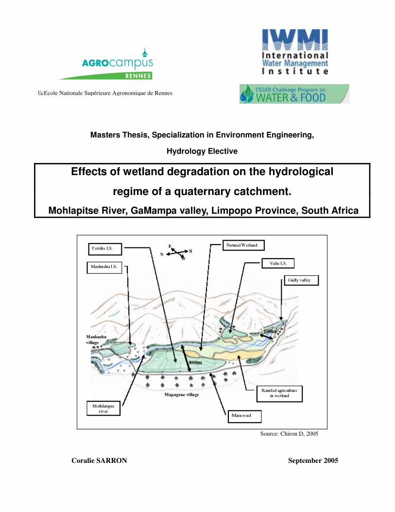
Source: Chiron D, 2005

Masters Thesis, Specialization in Environment Engineering,

Hydrology Elective

Effects of wetland degradation on the hydrological

regime of a quaternary catchment.

Mohlapitse River, GaMampa valley, Limpopo Province, South Africa

Coralie SARRON September 2005

EcEcole Nationale Supérieure Agronomique de Rennes

Acknowledgments

I would like to thank warmly Dominique Rollin, my supervisor in South Africa for

his support, his attention, his advices and his friendship. I want to thank his family too,

Cathy, Marie-Lou, Margaux (and Snoopy…) for their so nice welcome.

I thank also Jean-Marie Fritsch (IRD South Africa) and Matthew McCartney

(IWMI South Africa) for their hydrological support, their patience and their availability.

I especially thank Charles Perrin from the CEMAGREF Antony for always helping

me by Internet, his patience and his so clear explications.

I would like to thank Thulani Magagula for his help in satellite images processing.

I would like to thank also Amy Sullivan for her help in the English writing of this

report.

I would like to thank Christo Harmse from the DWAF to have made available data

without which I would not have realised this study.

Thank you Edouard and Marie to have answered to my common idiotic questions.

I would like to thank the IWMI, which welcomed me and made my study in South

Africa possible.

This study being undertaken as part of Challenge Program Project - Wetlands based

livelihoods in the Limpopo basin: balancing social welfare and environmental security.

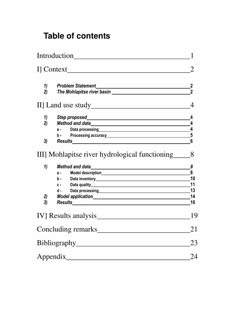
Table of contents

Introduction 1

I] Context 2

1) Problem Statement 2 2) The Mohlapitse river basin 2

II] Land use study 4

1) Step proposed 4 2) Method and data 4 a - Data processing 4 b - Processing accuracy 5 3) Results 6

III] Mohlapitse river hydrological functioning 8

1) Method and data 8 a - Model description 8

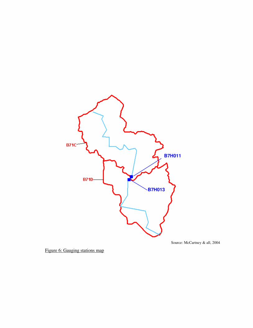
b - Data inventory 10

c - Data quality 11

d - Data processing 13

2) Model application 14 3) Results 16

IV] Results analysis 19

Concluding remarks 21

Bibliography 23

Appendix 24

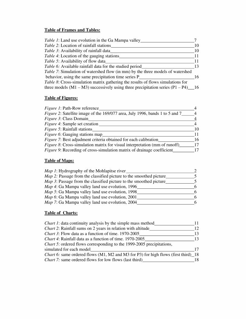
Table of Frames and Tables:

Table 1: Land use evolution in the Ga Mampa valley 7

Table 2: Location of rainfall stations 10

Table 3: Availability of rainfall data 10

Table 4: Location of the gauging stations 11

Table 5: Availability of flow data 11

Table 6: Available rainfall data for the studied period 13

Table 7: Simulation of watershed flow (in mm) by the three models of watershed

behavior, using the same precipitation time series P 16

Table 8: Cross-simulation matrix gathering the results of flows simulations for

three models (M1 – M3) successively using three precipitation series (P1 – P4) 16

Table of Figures:

Figure 1: Path-Row reference 4

Figure 2: Satellite image of the 169/077 area, July 1996, bands 1 to 5 and 7 4

Figure 3: Class Domain 4

Figure 4: Sample set creation 4

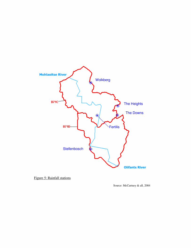
Figure 5: Rainfall stations 10

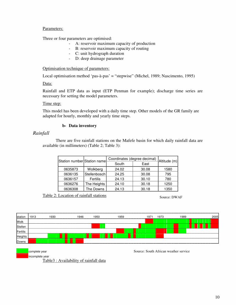
Figure 6: Gauging stations map 11

Figure 7: Best adjudment criteria obtained for each calibration 16

Figure 8: Cross-simulation matrix for visual interpretation (mm of runoff) 17

Figure 9: Recording of cross-simulation matrix of drainage coefficient 17

Table of Maps:

Map 1: Hydrography of the Mohlapitse river 2

Map 2: Passage from the classified picture to the smoothed picture 5

Map 3: Passage from the classified picture to the smoothed picture 5

Map 4: Ga Mampa valley land use evolution, 1996 6

Map 5: Ga Mampa valley land use evolution, 1998 6

Map 6: Ga Mampa valley land use evolution, 2001 6

Map 7: Ga Mampa valley land use evolution, 2004 6

Table of Charts:

Chart 1: data continuity analysis by the simple mass method 11

Chart 2: Rainfall sums on 2 years in relation with altitude 12

Chart 3: Flow data as a function of time. 1970-2005 13

Chart 4: Rainfall data as a function of time. 1970-2005 13

Chart 5: ordered flows corresponding to the 1999-2005 precipitations,

simulated for each model 17

Chart 6: same ordered flows (M1, M2 and M3 for P3) for high flows (first third) 18

Chart 7: same ordered flows for low flows (last third) 18

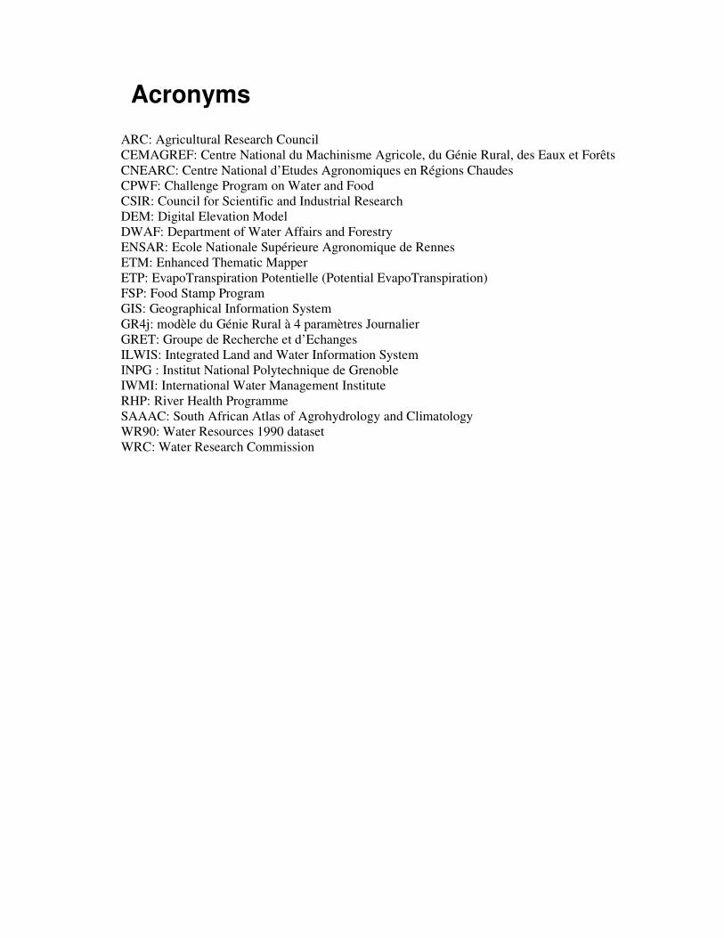
Acronyms

ARC: Agricultural Research Council

CEMAGREF: Centre National du Machinisme Agricole, du Génie Rural, des Eaux et Forêts

CNEARC: Centre National d’Etudes Agronomiques en Régions Chaudes

CPWF: Challenge Program on Water and Food

CSIR: Council for Scientific and Industrial Research

DEM: Digital Elevation Model

DWAF: Department of Water Affairs and Forestry

ENSAR: Ecole Nationale Supérieure Agronomique de Rennes

ETM: Enhanced Thematic Mapper

ETP: EvapoTranspiration Potentielle (Potential EvapoTranspiration)

FSP: Food Stamp Program

GIS: Geographical Information System

GR4j: modèle du Génie Rural à 4 paramètres Journalier

GRET: Groupe de Recherche et d’Echanges

ILWIS: Integrated Land and Water Information System

INPG : Institut National Polytechnique de Grenoble

IWMI: International Water Management Institute

RHP: River Health Programme

SAAAC: South African Atlas of Agrohydrology and Climatology

WR90: Water Resources 1990 dataset

WRC: Water Research Commission

Introduction

For many years the effort to overcome water shortages in South Africa has resulted

in some farmers utilizing wetlands for crop production. These wetlands are attractive units

because of their rich soils and year round soil moisture, which is favourable for crops

during both the “normal” dry season and the years of drought. However, wetlands serve

many functions that are beneficial to the environment and to humans, and if used unwisely

these benefits will disappear (Morardet S, Koukou-Tchamba A, 2004).

Wetlands are among the most threatened aquatic habitats in South Africa, with

estimates of up to 50% having been lost countrywide. On-going threats to wetlands include

human activities such as canalisation, drainage, crop production, effluent disposal and

water abstraction. Loss of wetlands reduces biodiversity as the plants and animals that are

adapted to wetland habitats are often unable to adapt to new environmental conditions, or

to move to more suitable ones. Loss of harvestable resources also occurs when wetlands are

lost. Reduction of water quality and flow regulation is a further consequence of loss of

wetlands, and may result in greater extent or severity of flooding.

Of the more than 800 naturally occurring freshwater wetlands in South Africa, 14%

have full protection within a national park, provincial nature reserve or wildlife sanctuary,

while 4% are partially protected. South Africa currently has 16 wetlands designated as

wetlands of international importance in accordance with the Ramsar Convention.1

This paper is part of the Wetlands Project of the Challenge Program for Water and

Food, and is based on the hypothesis that wetlands can be managed in a sustainable

manner, achieving a balance between protection and agricultural production, thereby

ensuring optimal use of wetlands (Morardet S, Koukou-Tchamba A, 2004). The focus of

the study is facilitating sustainable wetland management and development by quantifying

the effects of land use change (wetlands use) on the hydrological functioning of the river.

In order to do so, satellite images were studied to analyse land use changes while a

hydrological model, GR4j, was used to analyse changes in the hydrological function of the

river. The last part of the report explores interactions between both, land use and

hydrology, and concludes by answering the question: what is the link between wetland uses

and hydrological river functioning?

1 RHP- http://www.csir. co.za/rhp/state_of_rivers/state _of_crocsabieolif_ 01/Info _wetlands.html

1

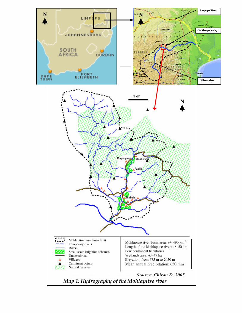
Mohlapitse river basin area: +/- 490 km 2

Length of the Mohlapitse river: +/- 50 km

Few permanent tributaries

Wetlands area: +/- 49 ha

Elevation: from 675 m to 2050 m

Mean annual precipitation: 630 mm

Map 1: Hydrography of the Mohlapitse river Source: Chiron D, 2005

Mohlapitse river basin limit

Temporary rivers

Rivers

Small scale irrigation schemes

Untarred road

Villages

Culminant points

Natural reserves

N

N

N

I] Context

1) Problem Statement

The International Water Management Institute (IWMI) is a non-profit, scientific

research organization specializing in water use in agriculture and integrated management of

water and land resources. IWMI works with partners in the South to develop tools and

methods to help these countries eradicate poverty and ensure food security through more

effective management of their water and land resources.

The Challenge Program for Water and Food (CPWF) is a partnership between

national and international research institutes, NGOs and river basin communities. Its goal is

to identify and encourage practices and institutional strategies that improve water

productivity – or to grow more food with less water.

This report is part of the Sustainable Management of Wetlands in Southern Africa

for Poverty Alleviation project, part of the CPWF. This project aims to address the lack of

scientific data needed to provide ecologically sound options for wetland-based livelihood

strategies in southern Africa. An initial inventory of wetland resources in three countries

will be made, followed by detailed hydrologic, agronomic, biophysical, socio-economic,

and institution investigations at representative sites.

2) The Mohlapitse river basin

The Mohlapitse River basin covers 490km² mainly composed of the Mohlapitse

River (50km long), bushveld in the mountains and cultivation in the valley (Chiron D,

2005). The Mohlapitse River descends from an elevation of 2050m above sea level to

675m at the gabion dam of Fertilis, 3/5 of the way through its run. From this point, the

slope average is around 0,6% down to the Olifants River confluence. Some 3 to 5

permanent tributaries are connected to the Mohlapitse River and 10 to 15 small-scale

irrigation schemes use the water of these rivers.

The river runs quickly to the end of the abrupt mountains then flowing in a sinuous,

stony riverbed from the north to the south. The minimum width of the riverbed ranges from

10 to 30 m and with a maximum of 50m to 100m at the natural wetland level (cf. Appendix

1). At the downstream Ga Mampa area, there is a gully mountain, which likely has

hydrological consequences. In fact, the gully section reduces the water flow and allows the

stony riverbed to recharge itself with water while the upstream aquifer grows quickly

during the rainy season (cf. Map 1).

The Ga Mampa Valley history can be told in five main steps (Chiron D, 2005):

The local population of the Ga Mampa Valley lived near the river and practiced rain

fed agriculture (sorghum). At the beginning of the 20th century, white farmers came and

evicted the local population leaving the valley under cultivation by white farmers up to

1959. The local population took refuge in the mountains and provided labour for the white

farms.

In 1964, the government created natural reserves in the mountains while the local

population returned to the river that the white farmers had left. During the 1960s, the

natural wetland covered an area downstream of Fertilis and Valis of more than 90 ha.

Irrigated agriculture dominated and rain fed (wetland access) production was rare in the

2

valley. The Fertilis irrigation scheme grew by 10 more farmers with an area of 92 ha. At

this point, farmers began occupying the natural wetland at Fertilis and Vallis downstream.

In 1994, with the end of the apartheid era and the dawn of new political

programmes, civil servants responsible for the irrigation scheme retired or were removed

(cf. Appendix 2). The government decided to transfer the irrigation management to the

black community. However, most of the Ga Mampa citizens were unaware that they had to

manage the irrigation scheme by themselves. The irrigation management was transferred to

farmers too quickly which resulted in the decline of the irrigation scheme including

deterioration of hydraulic equipment. This combined with decreasing water supply, stray

animals, difficulties organizing farmers, and the 1995 flood, caused some farmers to

discontinue winter crop production while others opted to cultivate the wetland. This

‘migration’ corresponds to the first significant wetland conquest in the mid 1990s. As a

result, fallow land area has increased inside the irrigation scheme while part of the wetland

was transformed into cultivated land. At the end of the 1990s, the natural wetland had been

reduced by a quarter with about 70ha of wetland remaining.

In 1999, a local Extension Officer found funds to build a gabion weir for the Fertilis

and Mashushu irrigation schemes. Farmers participated by providing the stones, but these

dams were destroyed by the 2000 flood. The 2001 season was a bad one for farmers and

with a similar fate in 2002 most farmers lost money. Following these bad years, farmers

asked the wetland committee for plots in the wetland signaling the second natural wetland

conquest.

In 2004, the wetland was divided into two parts: 1) the remaining natural wetland;

and 2) the cultivated wetland. More than half of cultivated area is devoted to coriander

production during the winter and maize during the summer (cf. Appendix 3,4,5 and 6).

3

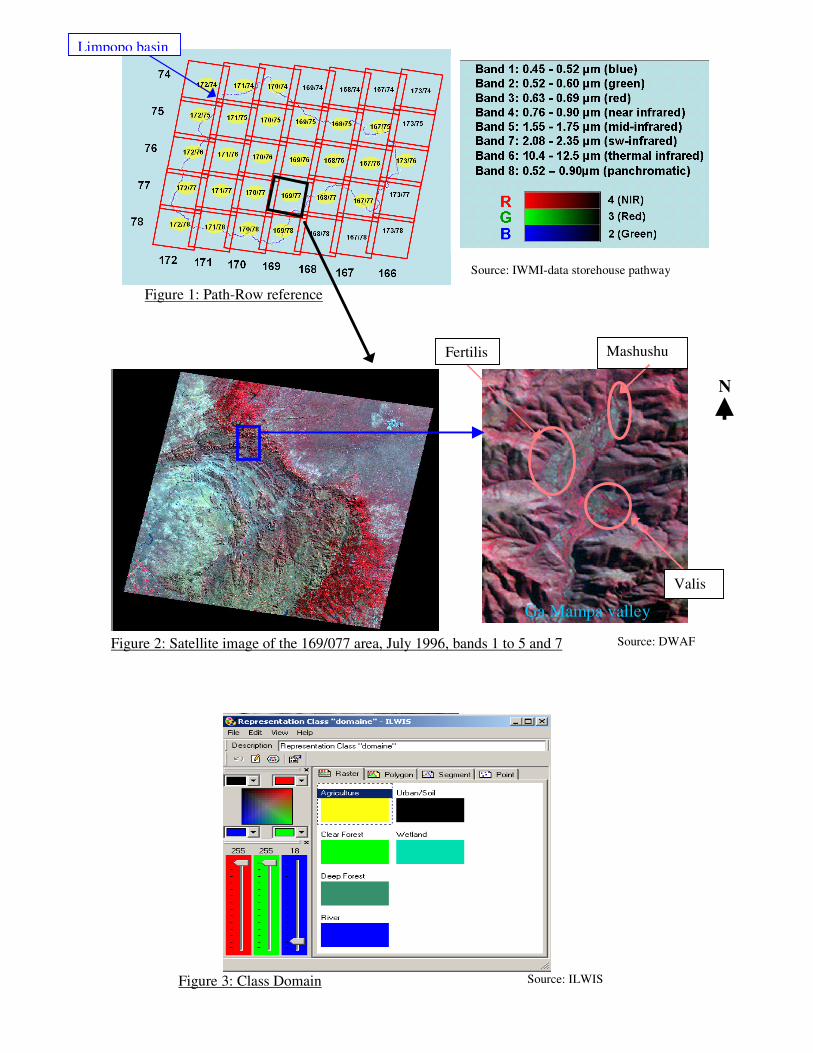
Figure 2: Classes domain Source: ILWIS

Figure 3: Class Domain Source: ILWIS

Limpopo basin

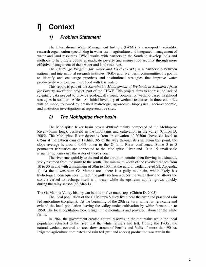
Figure 1: Path-Row reference

Source: IWMI-data storehouse pathway

Figure 2: Satellite image of the 169/077 area, July 1996, bands 1 to 5 and 7 Source: DWAF

Ga Mampa valley

Fertilis Mashushu

Valis

N

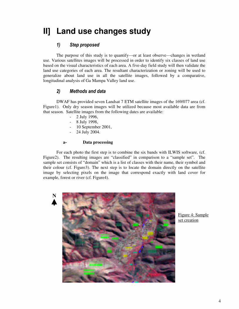
II] Land use changes study

1) Step proposed

The purpose of this study is to quantify—or at least observe—changes in wetland

use. Various satellites images will be processed in order to identify six classes of land use

based on the visual characteristics of each area. A five-day field study will then validate the

land use categories of each area. The resultant characterization or zoning will be used to

generalize about land use in all the satellite images, followed by a comparative,

longitudinal analysis of Ga Mampa Valley land use.

2) Methods and data

DWAF has provided seven Landsat 7 ETM satellite images of the 169/077 area (cf.

Figure1). Only dry season images will be utilized because most available data are from

that season. Satellite images from the following dates are available:

- 2 July 1996,

- 8 July 1998,

- 10 September 2001,

- 24 July 2004.

a- Data processing

For each photo the first step is to combine the six bands with ILWIS software, (cf.

Figure2). The resulting images are “classified” in comparison to a “sample set”. The

sample set consists of “domain” which is a list of classes with their name, their symbol and

their colour (cf. Figure3). The next step is to locate the domain directly on the satellite

image by selecting pixels on the image that correspond exactly with land cover for

example, forest or river (cf. Figure4).

4

Figure 4: Sample

set creation

N

This method is useful as it creates a new sample set for each photo, providing

greater precision. Indeed, from one image to another pixel colour can change, indicating a

change in class of land use.

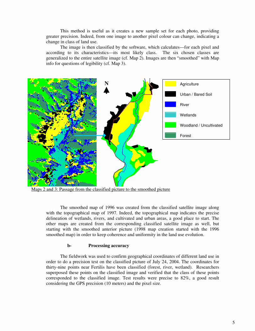
The image is then classified by the software, which calculates—for each pixel and

according to its characteristics—its most likely class. The six chosen classes are

generalized to the entire satellite image (cf. Map 2). Images are then “smoothed” with Map

info for questions of legibility (cf. Map 3).

The smoothed map of 1996 was created from the classified satellite image along

with the topographical map of 1997. Indeed, the topographical map indicates the precise

delineation of wetlands, rivers, and cultivated and urban areas, a good place to start. The

other maps are created from the corresponding classified satellite image as well, but

starting with the smoothed anterior picture (1998 map creation started with the 1996

smoothed map) in order to keep coherence and uniformity in the land use evolution.

b- Processing accuracy

The fieldwork was used to confirm geographical coordinates of different land use in

order to do a precision test on the classified picture of July 24, 2004. The coordinates for

thirty-nine points near Fertilis have been classified (forest, river, wetland). Researchers

superposed these points on the classified image and verified that the class of these points

corresponded to the classified image. Test results were precise to 82%, a good result

considering the GPS precision (10 meters) and the pixel size.

Agriculture

Urban / Bared Soil

River

Wetlands

Woodland / Uncultivated

Forest

Maps 2 and 3: Passage from the classified picture to the smoothed picture

5

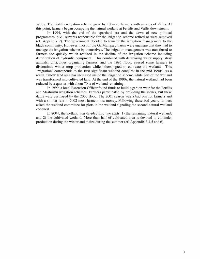
N

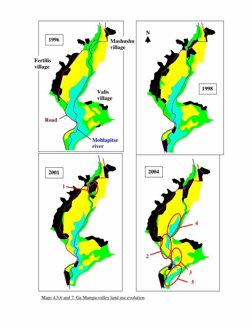
1996

1998

2004 2001

Maps 4,5,6 and 7: Ga Mampa valley land use evolution

1

2

3

Road

Mohlapitse

river

Fertilis

village

Valis

village

Mashushu

village

N

4

1998

5

3) Results

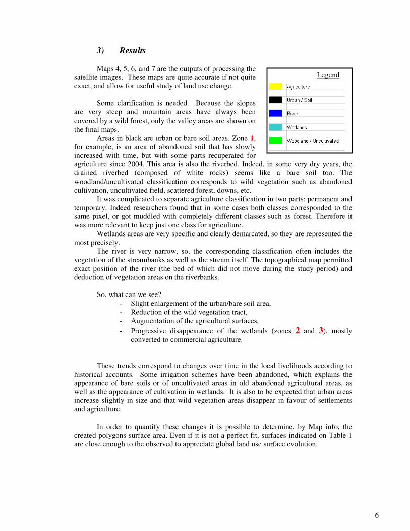
Maps 4, 5, 6, and 7 are the outputs of processing the

satellite images. These maps are quite accurate if not quite

exact, and allow for useful study of land use change.

Some clarification is needed. Because the slopes

are very steep and mountain areas have always been

covered by a wild forest, only the valley areas are shown on

the final maps.

Areas in black are urban or bare soil areas. Zone 1,

for example, is an area of abandoned soil that has slowly

increased with time, but with some parts recuperated for

agriculture since 2004. This area is also the riverbed. Indeed, in some very dry years, the

drained riverbed (composed of white rocks) seems like a bare soil too. The

woodland/uncultivated classification corresponds to wild vegetation such as abandoned

cultivation, uncultivated field, scattered forest, downs, etc.

It was complicated to separate agriculture classification in two parts: permanent and

temporary. Indeed researchers found that in some cases both classes corresponded to the

same pixel, or got muddled with completely different classes such as forest. Therefore it

was more relevant to keep just one class for agriculture.

Wetlands areas are very specific and clearly demarcated, so they are represented the

most precisely.

The river is very narrow, so, the corresponding classification often includes the

vegetation of the streambanks as well as the stream itself. The topographical map permitted

exact position of the river (the bed of which did not move during the study period) and

deduction of vegetation areas on the riverbanks.

So, what can we see?

- Slight enlargement of the urban/bare soil area,

- Reduction of the wild vegetation tract,

- Augmentation of the agricultural surfaces,

- Progressive disappearance of the wetlands (zones 2 and 3), mostly

converted to commercial agriculture.

These trends correspond to changes over time in the local livelihoods according to

historical accounts. Some irrigation schemes have been abandoned, which explains the

appearance of bare soils or of uncultivated areas in old abandoned agricultural areas, as

well as the appearance of cultivation in wetlands. It is also to be expected that urban areas

increase slightly in size and that wild vegetation areas disappear in favour of settlements

and agriculture.

In order to quantify these changes it is possible to determine, by Map info, the

created polygons surface area. Even if it is not a perfect fit, surfaces indicated on Table 1

are close enough to the observed to appreciate global land use surface evolution.

6

Legend

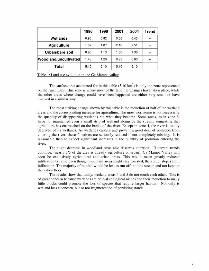
1996 1998 2001 2004 Trend

Wetlands 0.90 0.82 0.66 0.43 -

Agriculture 1.82 1.87 2.16 2.51 +

Urban/bare soil 0.95 1.13 1.36 1.36 +

Woodland/uncultivated 1.43 1.28 0.92 0.80 -

Total 5.10 5.10 5.10 5.10

The surface area accounted for in this table (5.10 km2) is only the zone represented

on the final maps. This zone is where most of the land use changes have taken place, while

the other areas where change could have been happened are either very small or have

evolved in a similar way.

The most striking change shown by this table is the reduction of half of the wetland

areas and the corresponding increase for agriculture. The most worrisome is not necessarily

the quantity of disappearing wetlands but what they become. Some areas, as in zone 3,

have not maintained even a small strip of wetland alongside the stream, suggesting that

agriculture has encroached on the banks of the river. Except in zone 4, the river is totally

deprived of its wetlands. As wetlands capture and prevent a good deal of pollution from

entering the river, these functions are seriously reduced if not completely missing. It is

reasonable then to expect significant increases in the quantity of pollution entering the

river.

The slight decrease in woodland areas also deserves attention. If current trends

continue, (nearly 3/5 of the area is already agriculture or urban), Ga Mampa Valley will

soon be exclusively agricultural and urban areas. This would mean greatly reduced

infiltration because even though mountain areas might stay forested, the abrupt slopes limit

infiltration. The majority of rainfall would be lost as run off into the stream and not kept on

the valley floor.

The results show that today, wetland areas 4 and 5 do not touch each other. This is

of great concern because wetlands are crucial ecological niches and their reduction to many

little blocks could promote the loss of species that require larger habitat. Not only is

wetland loss a concern, but so too fragmentation of persisting stands.

Table 1: Land use evolution in the Ga Mampa valley

7

1+(Sk / A).tanh(Pn / A)

Sk+tanh(Pn / A)

1+(Sk / A).tanh(Pn / A)

Sk+tanh(Pn / A)

1+(Sk / A).tanh(Pn / A)

Sk+tanh(Pn / A)

III] Mohlapitse river hydrological functioning

The purpose of this study was to quantify the impact of changes in the wetlands (i.e.,

from natural to cultivated) on the hydrology of the river. The history of the valley provides

three study periods:

- 1970/1990: natural wetlands, active irrigation schemes,

- 1990/2000: transition,

- 2000/2005: cultivated wetlands, unserviceable irrigation schemes.

The GR4j rainfall-runoff model was used to evaluate the change in hydrological

functioning between each time period. The model was calibrated separately for each period

and then run using the actual rainfall of the two other periods in order to assess the impact

of land-use changes. The difference between the simulated flows and the actual observed

flows for each period might be interpreted, among other possible reasons, as a consequence

of land use change.

1) Method and data

a- Model description

The model used was GR4j, (modèle du Génie Rural à 4 paramètres Journaliers)

developed by Nasciemento (1995) and modified by Edijanto and al (1999). It is a rainfall-

runoff model with few parameters, developed for utilisation on scarce data catchments.

Nascimento (1995) version description of the GR4j model is presented here, followed

by the Edijatno and al. (1999) modifications.

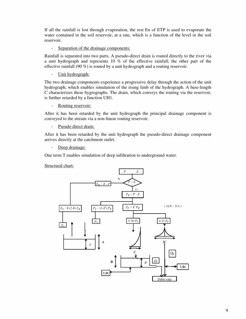
- Rainfall interception:

Rainfall falling on the catchment undergoes potential evapotranspiration ETP (cf.

Appendix 7). Net rainfall, Pn is determined by:

- if P ε E then Pn = P - E and En = 0

- if P < E then Pn = 0 ad En = E – P

With En, net evapotranspiration

- Soil reservoir:

If net rainfall is greater than zero (i.e., dPn > 0), the part that goes to the soil reservoir is

dPs and the other part dPn is conveyed towards the outlet:

dPn=(S/A)2. dPn

dPs=[1-(S/A)2]. dPn

Where S is the level in the soil reservoir and A the maxim capacity of this reservoir. The

soil reservoir level variation is dS = dPs and the level is updated following:

St+1= -----------------------------

8

8

If all the rainfall is lost through evaporation, the rest En of ETP is used to evaporate the

water contained in the soil reservoir, at a rate, which is a function of the level in the soil

reservoir.

- Separation of the drainage components:

Rainfall is separated into two parts. A pseudo-direct drain is routed directly to the river via

a unit hydrograph and represents 10 % of the effective rainfall; the other part of the

effective rainfall (90 %) is routed by a unit hydrograph and a routing reservoir.

- Unit hydrograph:

The two drainage components experience a progressive delay through the action of the unit

hydrograph, which enables simulation of the rising limb of the hydrograph. A base-length

C characterizes these hygrographs. The drain, which conveys the routing via the reservoir,

is further retarded by a function UH1.

- Routing reservoir:

After it has been retarded by the unit hydrograph the principal drainage component is

conveyed to the stream via a non-linear routing reservoir.

- Pseudo direct drain:

After it has been retarded by the unit hydrograph the pseudo-direct drainage component

arrives directly at the catchment outlet.

- Deep drainage:

One term T enables simulation of deep infiltration to underground water.

Structural chart:

9

Source:

Figure 5: Rainfall stations

map

Mohlapitse River

Olifants River

Wolkberg

The Heights

The Downs

Stellenbosch

Fertilis

Source: McCartney & all, 2004

Parameters:

Three or four parameters are optimised:

- A: reservoir maximum capacity of production

- B: reservoir maximum capacity of routing

- C: unit hydrograph duration

- D: deep drainage parameter

Optimisation technique of parameters:

Local optimisation method ‘pas-à-pas’ = “stepwise” (Michel, 1989; Nascimento, 1995)

Data:

Rainfall and ETP data as input (ETP Penman for example); discharge time series are

necessary for setting the model parameters.

Time step:

This model has been developed with a daily time step. Other models of the GR family are

adapted for hourly, monthly and yearly time steps.

b- Data inventory

Rainfall

There are five rainfall stations on the Mafefe basin for which daily rainfall data are

available (in millimeters) (Table 2; Table 3):

Table 2: Location of rainfall stations

station 1913 1930 1946 1950 1959 1971 1973 1989 2005

Wolk

Stellen

Fertilis

Heights

Downs

complete year

incomplete year

Table3 : Availability of rainfall data

Coordinates (degree decimal) Station number Station name

South East Altitude (m)

0635873 Wolkberg 24.02 30.08 1580

0636135 Stellenbosch 24.25 30.08 795

0636157 Fertilis 24.13 30.10 780

0636276 The Heights 24.10 30.18 1250

0636308 The Downs 24.13 30.18 1350

Source: DWAF

Source: South African weather service

10

Source: McCartney & all, 2004

Figure 6: Gauging stations map

B7H011

B7H013

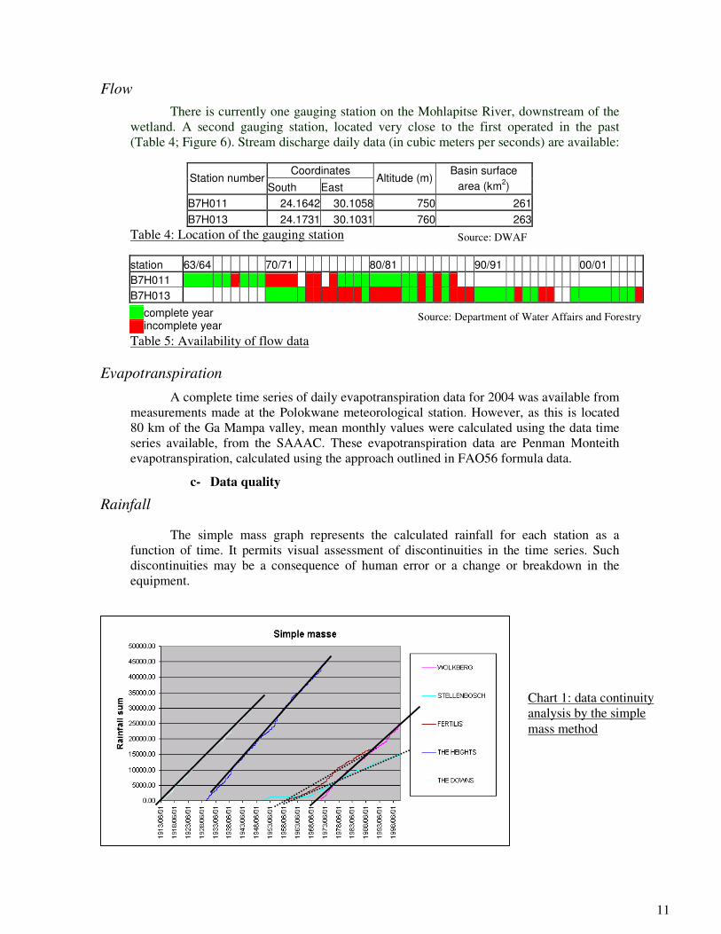
Chart 1: data continuity

analysis by the simple

mass method

Flow

There is currently one gauging station on the Mohlapitse River, downstream of the

wetland. A second gauging station, located very close to the first operated in the past

(Table 4; Figure 6). Stream discharge daily data (in cubic meters per seconds) are available:

Coordinates Basin surface Station number

South East Altitude (m)

area (km2)

B7H011 24.1642 30.1058 750 261

B7H013 24.1731 30.1031 760 263

Table 4: Location of the gauging station

station 63/64 70/71 80/81 90/91 00/01

B7H011

B7H013

Table 5: Availability of flow data

Evapotranspiration

A complete time series of daily evapotranspiration data for 2004 was available from

measurements made at the Polokwane meteorological station. However, as this is located

80 km of the Ga Mampa valley, mean monthly values were calculated using the data time

series available, from the SAAAC. These evapotranspiration data are Penman Monteith

evapotranspiration, calculated using the approach outlined in FAO56 formula data.

c- Data quality

Rainfall

The simple mass graph represents the calculated rainfall for each station as a

function of time. It permits visual assessment of discontinuities in the time series. Such

discontinuities may be a consequence of human error or a change or breakdown in the

equipment.

complete year

incomplete year Source: Department of Water Affairs and Forestry

11

Source: DWAF

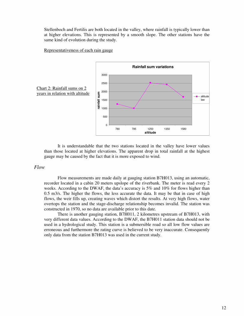
Chart 2: Rainfall sums on 2

years in relation with altitude

Stellenboch and Fertilis are both located in the valley, where rainfall is typically lower than

at higher elevations. This is represented by a smooth slope. The other stations have the

same kind of evolution during the study.

Representativeness of each rain gauge

It is understandable that the two stations located in the valley have lower values

than those located at higher elevations. The apparent drop in total rainfall at the highest

gauge may be caused by the fact that it is more exposed to wind.

Flow

Flow measurements are made daily at gauging station B7H013, using an automatic,

recorder located in a cabin 20 meters upslope of the riverbank. The meter is read every 2

weeks. According to the DWAF, the data’s accuracy is 5% and 10% for flows higher than

0.5 m3/s. The higher the flows, the less accurate the data. It may be that in case of high

flows, the weir fills up, creating waves which distort the results. At very high flows, water

overtops the station and the stage-discharge relationship becomes invalid. The station was

constructed in 1970, so no data are available prior to this date.

There is another gauging station, B7H011, 2 kilometres upstream of B7H013, with

very different data values. According to the DWAF, the B7H011 station data should not be

used in a hydrological study. This station is a submersible road so all low flow values are

erroneous and furthermore the rating curve is believed to be very inaccurate. Consequently

only data from the station B7H013 was used in the current study.

Rainfall sum variations

0

500

1000

1500

2000

2500

3000

780 795 1250 1350 1580

altitude

rain

fall

su

maltitude

law

12

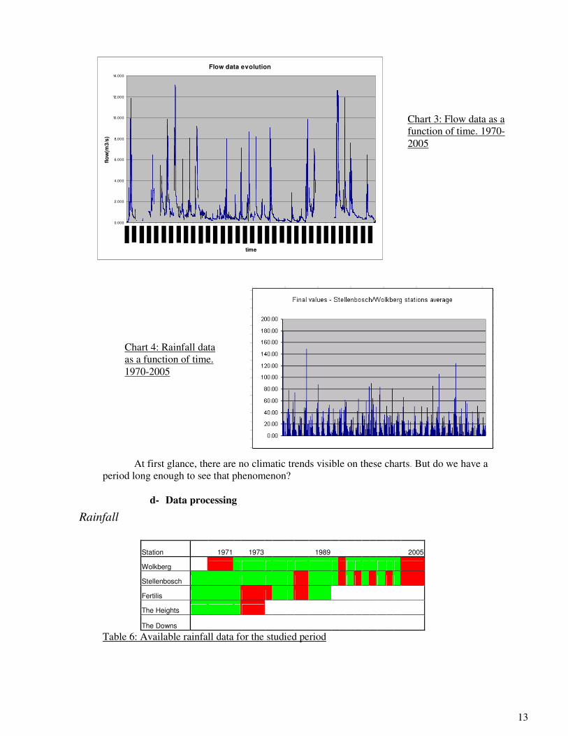
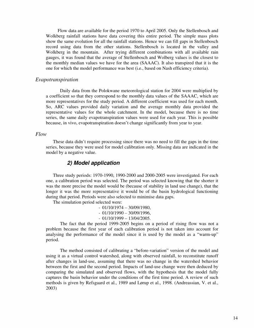
Chart 3: Flow data as a

function of time. 1970-

2005

Chart 4: Rainfall data

as a function of time.

1970-2005

At first glance, there are no climatic trends visible on these charts. But do we have a

period long enough to see that phenomenon?

d- Data processing

Rainfall

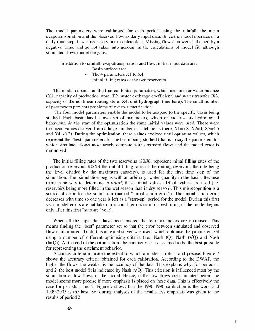
Station 1971 1973 1989 2005

Wolkberg

Stellenbosch

Fertilis

The Heights

The Downs

Table 6: Available rainfall data for the studied period

Flow data evolution

0.000

2.000

4.000

6.000

8.000

10.000

12.000

14.000

time

flo

w(m

3/s

)

13

Flow data are available for the period 1970 to April 2005. Only the Stellenbosch and

Wolkberg rainfall stations have data covering this entire period. The simple mass plots

show the same evolution for all the rainfall stations. Hence we can fill gaps in Stellenbosch

record using data from the other stations. Stellenbosch is located in the valley and

Wolkberg in the mountain. After trying different combinations with all available rain

gauges, it was found that the average of Stellenbosch and Wolberg values is the closest to

the monthly median values we have for the area (SAAAC). It also transpired that it is the

one for which the model performance was best (i.e., based on Nash efficiency criteria).

Evapotranspiration

Daily data from the Polokwane meteorological station for 2004 were multiplied by

a coefficient so that they correspond to the monthly data values of the SAAAC, which are

more representatives for the study period. A different coefficient was used for each month.

So, ARC values provided daily variation and the average monthly data provided the

representative values for the whole catchment. In the model, because there is no time

series, the same daily evapotranspiration values were used for each year. This is possible

because, in vivo, evapotranspiration doesn’t change significantly from year to year.

Flow

These data didn’t require processing since there was no need to fill the gaps in the time

series, because they were used for model calibration only. Missing data are indicated in the

model by a negative value.

2) Model application

Three study periods: 1970-1990, 1990-2000 and 2000-2005 were investigated. For each

one, a calibration period was selected. The period was selected knowing that the shorter it

was the more precise the model would be (because of stability in land use change), that the

longer it was the more representative it would be of the basin hydrological functioning

during that period. Periods were also selected to minimise data gaps.

The simulation period selected were:

- 01/10/1974 – 30/09/1980,

- 01/10/1990 – 30/09/1996,

- 01/10/1999 – 13/04/2005.

The fact that the period 1999-2005 begins on a period of rising flow was not a

problem because the first year of each calibration period is not taken into account for

analysing the performance of the model since it is used by the model as a “warm-up”

period.

The method consisted of calibrating a “before-variation” version of the model and

using it as a virtual control watershed, along with observed rainfall, to reconstitute runoff

after changes in land-use, assuming that there was no change in the watershed behavior

between the first and the second period. Impacts of land-use change were then deduced by

comparing the simulated and observed flows, with the hypothesis that the model fully

captures the basin behavior under the conditions of the first time period. A review of such

methods is given by Refsgaard et al., 1989 and Lørup et al., 1998. (Andreassian, V. et al.,

2003)

14

The model parameters were calibrated for each period using the rainfall, the mean

evapotranspiration and the observed flow as daily input data. Since the model operates on a

daily time step, it was necessary not to delete data. Missing flow data were indicated by a

negative value and so not taken into account in the calculations of model fit, although

simulated flows model the gaps.

In addition to rainfall, evapotranspiration and flow, initial input data are:

- Basin surface area,

- The 4 parameters X1 to X4,

- Initial filling rates of the two reservoirs.

The model depends on the four calibrated parameters, which account for water balance

(X1, capacity of production store; X2, water exchange coefficient) and water transfer (X3,

capacity of the nonlinear routing store; X4, unit hydrograph time base). The small number

of parameters prevents problems of overparametrization.

The four model parameters enable the model to be adapted to the specific basin being

studied. Each basin has his own set of parameters, which characterise its hydrological

behaviour. At the start of the optimisation the same initial values were used. These were

the mean values derived from a huge number of catchments (here, X1=5.8; X2=0; X3=4.5

and X4=-0.2). During the optimisation, these values evolved until optimum values, which

represent the “best” parameters for the basin being studied (that is to say the parameters for

which simulated flows most nearly compare with observed flows and the model error is

minimised).

The initial filling rates of the two reservoirs (S0/X1 represent initial filling rates of the

production reservoir, R0/X3 the initial filling rates of the routing reservoir, the rate being

the level divided by the maximum capacity), is used for the first time step of the

simulation. The simulation begins with an arbitrary water quantity in the basin. Because

there is no way to determine, a priori, these initial values, default values are used (i.e.

reservoirs being more filled in the wet season than in dry season). This misrecognition is a

source of error for the simulation (named “initialisation error”). The initialisation error

decreases with time so one year is left as a “start-up” period for the model. During this first

year, model errors are not taken in account (errors sum for best fitting of the model begins

only after this first “start-up” year).

When all the input data have been entered the four parameters are optimised. This

means finding the “best” parameter set so that the error between simulated and observed

flow is minimised. To do this an excel solver was used, which optimise the parameters set

using a number of different optimising criteria (i.e., Nash (Q), Nash (√Q) and Nash

(ln(Q)). At the end of the optimisation, the parameter set is assumed to be the best possible

for representing the catchment behavior.

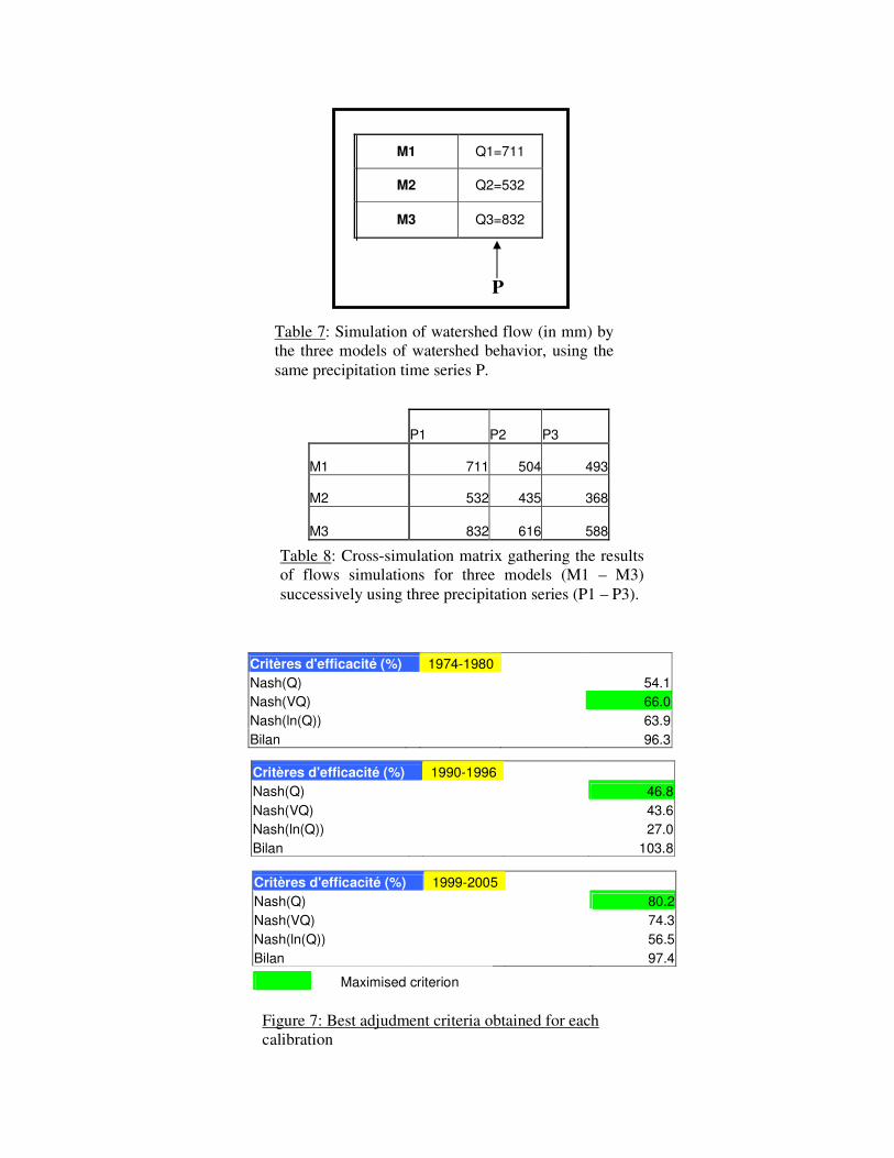
Accuracy criteria indicate the extent to which a model is robust and precise. Figure 7

shows the accuracy criteria obtained for each calibration. According to the DWAF, the

higher the flows, the weaker is the accuracy of the data. This explains why, for periods 1

and 2, the best model fit is indicated by Nash (√Q). This criterion is influenced most by the

simulation of low flows in the model. Hence, if the low flows are simulated better, the

model seems more precise if more emphasis is placed on these data. This is effectively the

case for periods 1 and 2. Figure 7 shows that the 1990-1996 calibration is the worst and

1999-2005 is the best. So, during analyses of the results less emphasis was given to the

results of period 2.

e-

15

M1 Q1=711

M2 Q2=532

M3 Q3=832

P

Table 7: Simulation of watershed flow (in mm) by

the three models of watershed behavior, using the

same precipitation time series P.

P1 P2 P3

M1 711 504 493

M2 532 435 368

M3 832 616 588

Table 8: Cross-simulation matrix gathering the results

of flows simulations for three models (M1 – M3)

successively using three precipitation series (P1 – P3).

Critères d'efficacité (%) 1974-1980

Nash(Q) 54.1

Nash(VQ) 66.0

Nash(ln(Q)) 63.9

Bilan 96.3

Critères d'efficacité (%) 1990-1996

Nash(Q) 46.8

Nash(VQ) 43.6

Nash(ln(Q)) 27.0

Bilan 103.8

Critères d'efficacité (%) 1999-2005

Nash(Q) 80.2

Nash(VQ) 74.3

Nash(ln(Q)) 56.5

Bilan 97.4

Maximised criterion

Figure 7: Best adjudment criteria obtained for each

calibration

3) Results

The approach adopted to analyse results was that described in “A new approach

involving resampling of model simulations to assess trends in watershed behavior”

(Andreassion et al., 2003).

1. Cross simulations as a basis for statistical testing

The method works in three steps:

1. The period of study is divided into n successive periods of equal length; each

sufficiently long to enable proper calibration of the rainfall-runoff model. In the

current study, 1970-2005 was the total period, with three subperiods, each of 5

(hydrological) years: 1974-1980, 1990-1996 and 1999-2005. Calibration of the

GR4j model provided three successive models of watershed behavior (i.e.,

defined by three different parameters sets): M1, M2 and M3.

2. Observed rainfall time series are then used as input to the model in conjunction with

the three optimised parameter sets to obtain the corresponding total streamflows

simulated by the three models of watershed behavior (cf. Table 7 as an example).

Note that direct comparisons of these model outputs are possible because they

have been simulated with the same precipitation time series as input.

3. This operation can be repeated as long as independent precipitation time series are

available, and the results can be displayed in matrix form. The more rows in the

matrix, the more exhaustive the description of watershed behavior. In the current

study a 3x3 square matrix was obtained (cf. Table 8), since the time series that

were used for calibration were also used as precipitation input in the analysis of

impacts. In this “cross-simulation matrix” in each cell (i, j) comprises the total

streamflow simulated with the model Mj (representative of watershed behavior

during period j) using precipitation Pi.

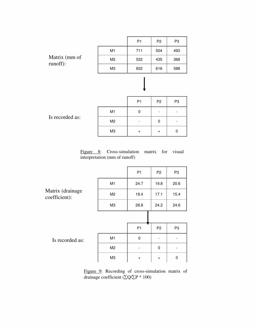
2. Visual analysis of cross-simulation matrices

A great deal in information on possible changes can be gained visually, by simply

transforming the cross-simulation matrix figures into signs (plus or minus). Remember that

for each row of the matrix, flows can be compared since they were simulated with the same

precipitation input. In each row, the value found on the matrix diagonal was taken as a

reference value, i.e., the value simulated by model Mi using precipitation Pi (since Pi is

used to calibrate Mi, the value Qi, i seems the most logical reference for the comparison).

Thus, in case of an apparent positive trend, Qi,j is replaced with a plus sign. This

happens for j < i, if Qi,j < Qi,i; and for j > i, if Qi,j > Qi,i. In case of an apparent negative

trend, Qi,j is replaced with a minus sign. This happens for j < i, if Qi,j > Qi,i; and for j > i,

if Qi,j < Qi,i. If Qi,j = Qi,i, replace Qi,j is replaced with a letter O. An example of recoding

is shown in Figure 8.

The same cross-simulation matrix approach was used for drainage coefficients (∑Q/∑P

* 100). This coefficient represents the percentage of rainfall water ending up in the river

(cf. Figure 9) and so provides insight into infiltration and evapotranspiration within the

catchment.

16

P1 P2 P3

M1 711 504 493

M2 532 435 368

M3 832 616 588

P1 P2 P3

M1 0 - -

M2 - 0 -

M3 + + 0

Matrix (mm of

runoff):

Is recorded as:

Figure 8: Cross-simulation matrix for visual

interpretation (mm of runoff)

P1 P2 P3

M1 24.7 19.8 20.6

M2 18.4 17.1 15.4

M3 28.8 24.2 24.6

P1 P2 P3

M1 0 - -

M2 - 0 -

M3 + + 0

Matrix (drainage

coefficient):

Is recorded as:

Figure 9: Recording of cross-simulation matrix of

drainage coefficient (∑Q/∑P * 100)

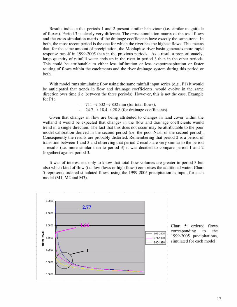
Results indicate that periods 1 and 2 present similar behaviour (i.e. similar magnitude

of fluxes). Period 3 is clearly very different. The cross-simulation matrix of the total flows

and the cross-simulation matrix of the drainage coefficients have exactly the same trend. In

both, the most recent period is the one for which the river has the highest flows. This means

that, for the same amount of precipitation, the Mohlapitse river basin generates more rapid

response runoff in 1999-2005 than in the previous periods. As a result a proportionately,

large quantity of rainfall water ends up in the river in period 3 than in the other periods.

This could be attributable to either less infiltration or less evapotranspiration or faster

routing of flows within the catchments and the river drainage system during this period or

both.

With model runs simulating flow using the same rainfall input series (e.g., P1) it would

be anticipated that trends in flow and drainage coefficients, would evolve in the same

direction over time (i.e. between the three periods). However, this is not the case. Example

for P1:

- 711 → 532 → 832 mm (for total flows),

- 24.7 → 18.4→ 28.8 (for drainage coefficients).

Given that changes in flow are being attributed to changes in land cover within the

wetland it would be expected that changes in the flow and drainage coefficients would

trend in a single direction. The fact that this does not occur may be attributable to the poor

model calibration derived in the second period (i.e. the poor Nash of the second period).

Consequently the results are probably distorted. Remembering that period 2 is a period of

transition between 1 and 3 and observing that period 2 results are very similar to the period

1 results (i.e. more similar than to period 3) it was decided to compare period 1 and 2

(together) against period 3.

It was of interest not only to know that total flow volumes are greater in period 3 but

also which kind of flow (i.e. low flows or high flows) comprises the additional water. Chart

5 represents ordered simulated flows, using the 1999-2005 precipitation as input, for each

model (M1, M2 and M3).

Chart 5: ordered flows

corresponding to the

1999-2005 precipitations,

simulated for each model

1.5665

0.7875

17

1

2.77

1.66

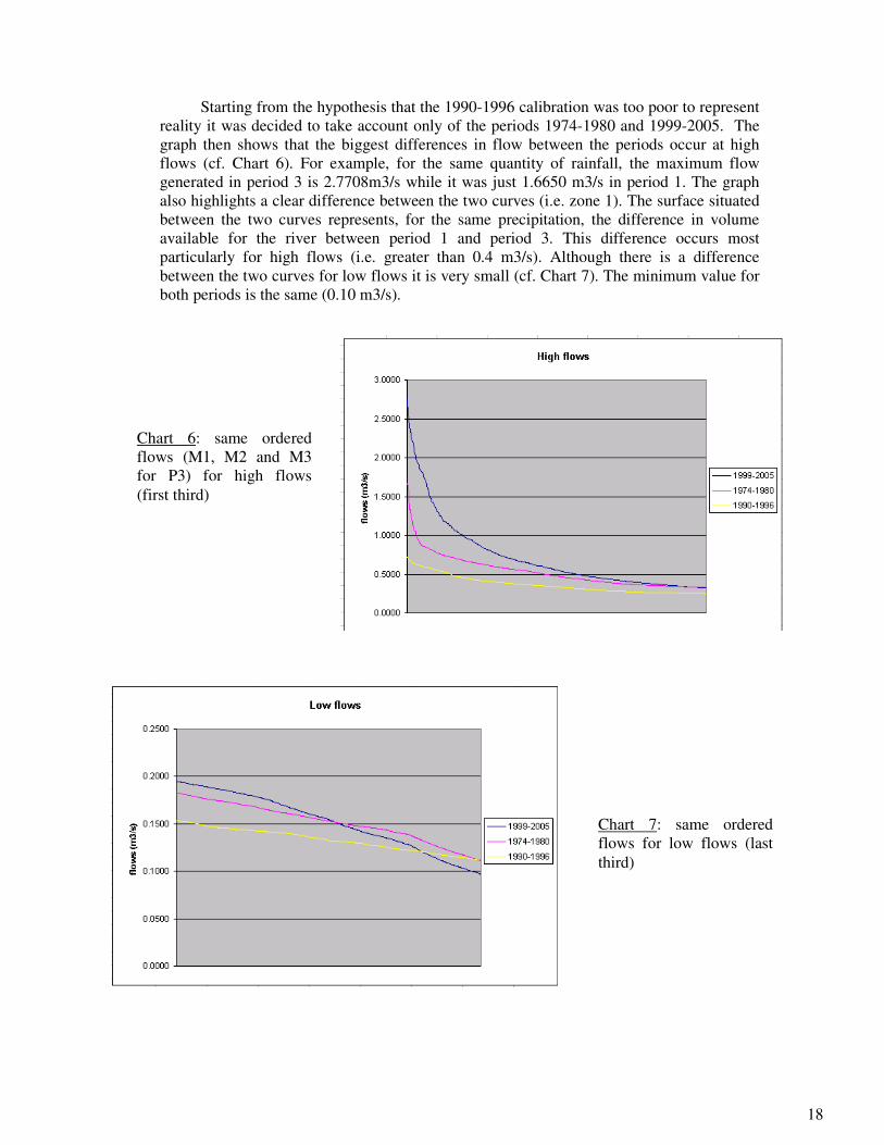
Starting from the hypothesis that the 1990-1996 calibration was too poor to represent

reality it was decided to take account only of the periods 1974-1980 and 1999-2005. The

graph then shows that the biggest differences in flow between the periods occur at high

flows (cf. Chart 6). For example, for the same quantity of rainfall, the maximum flow

generated in period 3 is 2.7708m3/s while it was just 1.6650 m3/s in period 1. The graph

also highlights a clear difference between the two curves (i.e. zone 1). The surface situated

between the two curves represents, for the same precipitation, the difference in volume

available for the river between period 1 and period 3. This difference occurs most

particularly for high flows (i.e. greater than 0.4 m3/s). Although there is a difference

between the two curves for low flows it is very small (cf. Chart 7). The minimum value for

both periods is the same (0.10 m3/s).

Chart 6: same ordered

flows (M1, M2 and M3

for P3) for high flows

(first third)

Chart 7: same ordered

flows for low flows (last

third)

18

IV] Results analysis

It has been shown (i.e. in the chapter II “Land use changes study”) that between

1996 and 2004, the Ga Mampa valley lost half of its wetlands. Often this loss occurred at

very bad places like riverbanks. It is also apparent that agriculture is rising contrary to

woodlands, which have decreased over time.

It has also been shown (i.e., in the chapter III “Mohlapitse river hydrological

functioning”) that flows in the Mohlapitse river basin are greater now (i.e. 1999-2005) than

they were in the past (i.e., 1974-1980); flows are higher and drainage coefficients have also

increased. It is possible that this is a consequence of reduced evapotranspiration and/or

lower infiltration within the catchment.

A common feature of many wetlands is that they reduce rapid runoff and store

water. This often favours infiltration. Moreover, wetlands possess hydromorphic and

endemic vegetation, which is very dense and, because water is readily available, this often

promotes evapotranspiration. However, above all many wetlands are famous for their

“sponge effect”, which means they keep water during high flows and so attenuate floods,

and provide flow to rivers during dry periods and during droughts. This could be the reason

why the Mohlapitse river has always been a very important tributary for the Olifants river

during dry seasons.

Moreover, there is increasing need for more and more agricultural land and

increasingly wetland area is being converted for agriculture. Often this involves draining

the wetland soils with pipes and drainage channels, which lower the water table level and

move the water more rapidly to the river.

If drained appropriately the land remains wet enough for agriculture but the wetland

disappears. This phenomenon is clearly visible on the maps 4,5,6 and 7 presenting the land

use change over time.

The hydrological modelling has shown that high flows have increased over time.

Thus, it could be hypothesised that the decline in wetland area and the loss of the “sponge

effect” could explain the increase in high flows.

Wetlands typically possess very dense vegetation that often grows into the stream.

This vegetation acts like an obstacle to water drainage. In the first instance, this vegetation

withholds water for its own consumption. Secondly, it slows water movement so providing

greater time for infiltration and greater evaporation.

A decline in wetland area would imply a decrease in all the phenomena described

previously and so would entail an increase in high flows, but also a decrease in low flows

for disappearance of the “sponge effect” and the slow drainage of the sponge during the

core of the dry season.

During high flow periods, there would not be wetland vegetation to retard runoff

and to slow the speed of water movement. Wetlands loss would therefore equate to an

increase in flows.

19

Benefits and limits of GR4j rainfall-runoff model

This study primarily comprised hydrological modelling. The GR4j model was used.

The GR4j model was adapted for a first modeling exercise because it is very simple to use

and requires only limited data inputs. The model runs using excel software and requires

only four parameters to optimise. The model is however very robust. The only input data

required are: precipitation, evapotranspiration mean values and observed flows.

However, because it is a simple model, there is limited possibility of adapting the

model to specific catchments. The model had some problems reproducing the hydrological

behavior of the study catchment (i.e., big differences between observed flows and

simulated flows after the calibration especially for high flows because of the bad accuracy

of the data). However, because no other models have been tried on this catchment (global

conceptual or distributed), it is not possible to know if this problem is specific to the model

or if it is the basin itself, which is difficult to model (e.g. because of data limitations).

Nevertheless, it seams that, because of the lack of data, any other model could have been

better so, the best results as possible have certainly been found in this study.

This first difficulty relates to the second, in that because the model errors are very

high, determining trends in the watershed behavior is very difficult. Real changes (if they

exist) may be of the same order of magnitude as the model simulation errors.

The main intrinsic problem of the model (which is the same for all global conceptual

models) is the difficulty of giving a physical interpretation to parameters. This makes the

applicability of these models to non-gauged basins difficult (i.e., those which lack

calibration data). Some researchers also think that the lack of spatial discretisation is a

defect of global models, which limits their performance (Charles Perrin, personal

communication).

20

Concluding remarks

In the case of this study, it would have been better to have more satellite images,

especially old images. 1996 is almost certainly not far enough back in time for this study

even if land use changes are mostly in the recent past.

The flow data contains too many gaps, some of which were for long periods of

time. This could partly explain why the calibration in period 2, was not very successful.

The1999-2005 period represents the best optimisation period (i.e. as indicated by the Nash

criterion) and is the period for which there are no gap on the flow data; 1990-1996 is the

one which has most gaps and this is also the period with the worst Nash criterion.

Furthermore, the rainfall data were also not continuous enough; in some records gaps of 1

year, occur. The more complete the data, the more precise the model is likely to be.

These constraints imply some improvements are possible to improve similar studies

in the future. For the satellite processing chapter, it would be worthwhile to obtain satellite

images regularly to be sure that studies will have complete data at regular time intervals

and to do a very advanced research in order to find all archive data available and more

precise pictures.

It is important that future studies use as complete rainfall data as possible. This

requires greater analysis of rainfall patterns with altitude i.e., determine the best possible

spatialization for the catchment, from the Digital Elevation Model obtained this year from

the Government Printer and from the five rainfall stations available in the Mohlapitse river

basin.

The most important is to obtain a verifiable data follow-up. The monitoring must be

more robust in terms of both precision and regularity. It would be useful to upgrade the

gauging station in order to have a good accuracy for the full spectrum of flows that occur,

not only the low flows. The gauging station should be able to record very high flows if one

day it is to be used for flood risk forecasting.

For a future wetlands study, it could be interesting too, in addition to the gauging

station already existing downstream of the wetlands area, to have another gauging station

located upstream of the wetland area. This will enable comparison of contemporary flows

occurring immediately upstream and downstream of the wetlands and so to study precisely

the impact of the wetlands on the flow regime.

This study suggests that, even if the Mohlapitse river wetland area is very small

compare to the basin size (0.4 km2 for 400 km

2), it has a significant influence on the

hydrological functioning of the river (cf. part “results analysis”). This suggests that the

wetland is important both ecologically and hydrologically.

Conclusions derived form the second chapter “Land use changes study” show that the land

use trend is conversion of the wetlands and woodland to agriculture areas. It could be very

serious if this trend is continued in the future. In the long term, it is possible that continued

wetland destruction will result in decreases in water quality, less reliable water supplies

(especially during the dry season), increased severe flooding, lower agricultural

productivity, and more endangered species.

21

The first step toward wetland rehabilitation for the Challenge Program on Water

and Food (objective 2 of the FSP echel, wetland project) is to understand the relationships

between wetland degradation and river hydrology.

This study aims to increase decision makers’ awareness of wetland importance by

illustrating those relationships.

The Ga Mampa valley illustrates possibilities for slowing wetland destruction by

rehabilitating existing irrigation schemes.

In South Africa, a wetland rehabilitation programme already exists. The

Departments of Environmental Affairs and Tourism, Water Affairs and Forestry, and

Agriculture, together with partners in provincial and local government and civil society,

especially the Mondi Wetlands Project, have jointly launched the Working for Wetlands

programme. All rehabilitation interventions are undertaken within the context of improving

the integrity and functioning of wetland ecosystems, and include measures that address

both causes and effects of degradation. A guiding principle is that of raising awareness and

influencing behaviour and practices impacting on wetlands, rather than focusing

exclusively on engineering solutions.

Typical activities to rehabilitate a wetland include 2:

• The building of concrete, earth or gabion structures to arrest erosion, trap sediment

and resaturate drained wetland areas

• Using structures and landscaping to reinstate diminished flood mitigation and water

quality enhancement functions

• Plugging of artificial drainage channels

• Addressing offsite causes of degradation, such as inappropriate agricultural

practices

• Re-vegetation and bio-engineering

• Eradicating invasive alien plants

• Raising awareness of wetlands among workers, landowners and the public

• Providing technical skills

2 http://www.nbi.ac.za/research/wetlandprog.htm

22

Bibliography

Andreassian, V., Parent, E. & Michel, C., 2003. A distribution-free test to detect gradual

changes in watershed behavior. Water resources research, vol. 39, NO. 9, 1252.

Chiron, D., 2005. Impact of the small-scale irrigated sector on household revenues of the

black community of Ga Mampa Valley. Master of Science Thesis in Social Management

of the Water and Tropical Agricultural Development, CNEARC, GRET.

Department of Water Affairs and Forestry, 2003. A practical field procedure for

identification and delineation of wetlands and riparian areas. DWAF, Final draft, 54p.

Edijatno, Nascimento, N.O., Yang, X., Makhlouf, Z. & Michel, C., (1999). GR3J: a

daily watershed model with three free parameters. Hydrological Sciences Journal, 44(2),

263 277.

Kotze, D.C., Klug, J.R., Hugues, J.C. & Breen, C.M., 1996. Improved criteria for

classifying hydromorphic soils in South Africa. S.Ar.J. Plant and Soil, 13(3).

Lørup, J.K., Refsgaard, J.C. & Mazvimavi, D., 1998. Assessing the effect of land use

change on catchment runoff by combined use of statistical tests and hydrological

modeling: Case studies from Zimbabwe. J. Hydrol., 205, 147-163.

McCartney, M.P., Yawson, D.K., Magagula, T.F. & Seshoka, J., 2004. Hydrology and

water resources development in the Olifants river catcment. IWMI working paper 76.

IWMI, 59 p.

McVicar & al, 1997. Soil Classification: A Binomial System for South Africa. Dept. Agric.

Michel, C., 1989. Hydrologie appliquée aux petits bassins versants ruraux. Cemagref,

Antony.

Morardet, S., Koukou-Tchamba, A, 2004. Assessing trades-offs between agricultural

production and wetlands preservation in Limpopo river basin: a participatory

framework. IWMI.

Nascimento, N.O. (1995). Appréciation à l’aide d’un modèle empirique des effets d’action

anthropiques sur la relation pluie-débit à l’échelle du bassin versant. PhD thesis,

CERGRENE/ENPC, Paris, 550 p.

Perrin, C., 2000. Vers une amélioration d’un modèle global pluie-débit au travers d’une

approche comparative. These specialite: Mécanique des Milieux Géophysiques et

Environnement, Cemagref, Ecole Doctorale Terre, Univers, Environnement.

Refsgaard, J.C., Alley, W.M. & Vuglinsky, V.S., 1989. Methodololy for distinguishing

between man’s influence and climatic effects on the hydrological cycle. IHP-III Project

6.3, UNESCO, Paris.

WETLAND-USE Booklet 1. What values do wetlands have for us and how are these

values affected by our land use activities? Share-Net, Howick.

Wyatt, J., 1997. Introduction and wetland assessment. Wetland fix, Rennies Wetlands

Project. 17p.

23