
Case Study Tutorial Wetting and Non-Wetting Basics of Wetting 1.

Clemson UniversityTigerPrints
All Theses Theses
12-2018
Effects of Surface Morphology on Ink Wetting andAdhesion on Polyolefin BlendsTing ChenClemson University, [email protected]
Follow this and additional works at: https://tigerprints.clemson.edu/all_theses
This Thesis is brought to you for free and open access by the Theses at TigerPrints. It has been accepted for inclusion in All Theses by an authorizedadministrator of TigerPrints. For more information, please contact [email protected].
Recommended CitationChen, Ting, "Effects of Surface Morphology on Ink Wetting and Adhesion on Polyolefin Blends" (2018). All Theses. 2976.https://tigerprints.clemson.edu/all_theses/2976

EFFECTS OF SURFACE MORPHOLOGY ON INK WETTING AND ADHESION ON
POLYOLEFIN BLENDS
A Thesis
Presented to
the Graduate School of
Clemson University
In Partial Fulfillment
of the Requirements for the Degree
Master of Science
Packaging Science
by
Ting Chen
December 2018
Accepted by:
Dr. Duncan Darby, Committee Chair
Dr. Robert Kimmel
Dr. Kay Cooksey
ii
ABSTRACT
Compared to the conventional Ziegler-Natta (Z-N) catalysts, metallocene (m)
catalysts have recently drawn more attention in the production of polyolefins, due to its
better stereo-selectivity toward the polymer structures. To use metallocene catalyzed
polyolefins as the print layers on the multilayer biaxial oriented polypropylene (BOPP)
films, the effects of their topography, surface morphology and chemical compositions
after corona treatment on the wetting and adhesion of water-based flexo inks were
studied in this work. Seven blends containing different metallocene and Ziegler-Natta
polyolefins, including polypropylene (PP), linear low polyethylene (LLDPE), and
propylene random copolymer (EP), were extruded as the surface print layers on the
BOPP films. These films were treated to the same level using an in-line corona treater.
The topography and morphology of the film surfaces were studied using atomic force
microscopy (AFM) in the light tapping and hard tapping modes respectively. The
chemical compositions of these surfaces were analyzed using Owens-Wendt surface
energy method and the electron spectroscopy for chemical analysis (ESCA). The results
obtained in this study confirmed the hypothesis proposed that corona effects (including
oxidation, chain scission, crosslinking and roughening) have less influence on the
surfaces of metallocene catalyzed polyolefin films than on their Z-N counterparts and the
surface characteristics affecting ink wetting and adhesion vary depending on which
corona effect dominants. It was also found that Z-N PP was semi-miscible with m EP,
while m LLDPE was not miscible with either m EP or Z-N EP. The corona-treated films
with two m LLDPE& EP blends resulted in uneven component distributions not only on

iii
the surfaces but also vertically within the print layers. Compared to the polyolefin blends,
the immiscible blends created rougher surfaces which were found to improve ink wetting
and adhesion to some extent. It is expected that the findings of this study can guide the
selection of metallocene catalyzed polyolefins for the print layers on the multilayer BOPP
films and promote the application of these materials in the flexible packaging industry.

iv
DEDICATION
I would like to dedicate this manuscript to my parents for their unconditional
support to me. Their love and trust pulled me through all the rainy days.

v
ACKNOWLEDGMENTS
I would like to first express my sincere appreciation to my advisor Dr. Duncan
Darby for his guidance during my study at Clemson University. Secondly, thanks to Dr.
Kay Cooksey, Dr. Robert Kimmel and Dr. Andrew Hurley for providing their support to
my study.
This research is also a project that was assigned to me when I worked as a co-op
student at Jindal Films. My sincere appreciation goes to Eric Gohr, my advisor at Jindal
Films, for his help and guidance throughout this project. He is always patient to answer
my questions and kindly shares his profound knowledge with me. Thanks John
Charbonneau and Kevin Stouse for offering me such a great opportunity and getting me
on board. Thanks to everyone who involved in this project at Jindal Films.
Additionally, I would like to thank Dr. Delphine Dean at Clemson University for
her generosity of allowing me using the atomic force microscope in her lab. I also
appreciate the help from Rose Abbott, Delores Rhodes, Tyler Harvey, and Bob Bennett in
their labs. Thanks Steve Rosenbeck of Press Color Inc. for providing ink samples used in
this study.

vi
TABLE OF CONTENTS
Page
TITLE PAGE .................................................................................................................... i
ABSTRACT ..................................................................................................................... ii
DEDICATION ................................................................................................................ iv
ACKNOWLEDGMENTS ............................................................................................... v
LIST OF TABLES ........................................................................................................ viii
LIST OF FIGURES ........................................................................................................ xi
CHAPTER
I. INTRODUCTION ......................................................................................... 1
II. LITERATURE REVIEW .............................................................................. 2
Polymers .................................................................................................. 2
Ziegler-Natta Catalysts vs. Metallocene Catalysts................................. 11
Polyolefins ............................................................................................. 15
Flexography ........................................................................................... 20
Ink Formulation ..................................................................................... 24
Flexographic Inks................................................................................... 26
Surface Tension/Surface Energy............................................................ 29
Impacts of Corona Treatment on Ink Wetting and Adhesion ................ 38
Atomic Force Microscopy (AFM) ......................................................... 43
Electron Spectroscopy for Chemical Analysis (ESCA)......................... 48
Literature Search Strategy...................................................................... 49
Objectives .............................................................................................. 52
III. MATERIALS AND METHODS ................................................................. 53
Materials ................................................................................................ 53
Methods.................................................................................................. 54
IV. RESULTS AND DISCUSSION .................................................................. 61
Hypothesis.............................................................................................. 61

vii
Table of Contents (Continued)
Page
Atomic Force Microscopy (AFM) ......................................................... 62
Contact Angles and Surface Energy ...................................................... 63
Electron Spectroscopy for Chemical Analysis (ESCA)....................... 100
Ink Adhesion Analyses ........................................................................ 110
V. CONCLUSIONS AND RECOMMENDATIONS .................................... 116
Conclusions .......................................................................................... 116
Recommendations ................................................................................ 117
APPENDICES ............................................................................................................. 119
A: Original Result Reports of AFM Analyses ................................................ 120
B: Original Minitab® Results of 2-Sample T-Tests on Two
Replicates of Each Treated Film .......................................................... 155
C: Worksheets for the Statistical Analyses of the Subgrouped
Height Data in Minitab®
...................................................................... 162
D: Statistical Summary of the Subgrouped Height Data of
Each Sample......................................................................................... 170
E: Original Results of Regression Tests Conducted in Minitab® ................... 184
F: Curve Fitting of the C1s Spectra of Treated V1-V4 Films ........................ 201
G: Change of Print Density on All the Treated Films after
Sutherland Rub Test ............................................................................. 207
REFERENCES ............................................................................................................ 211
viii
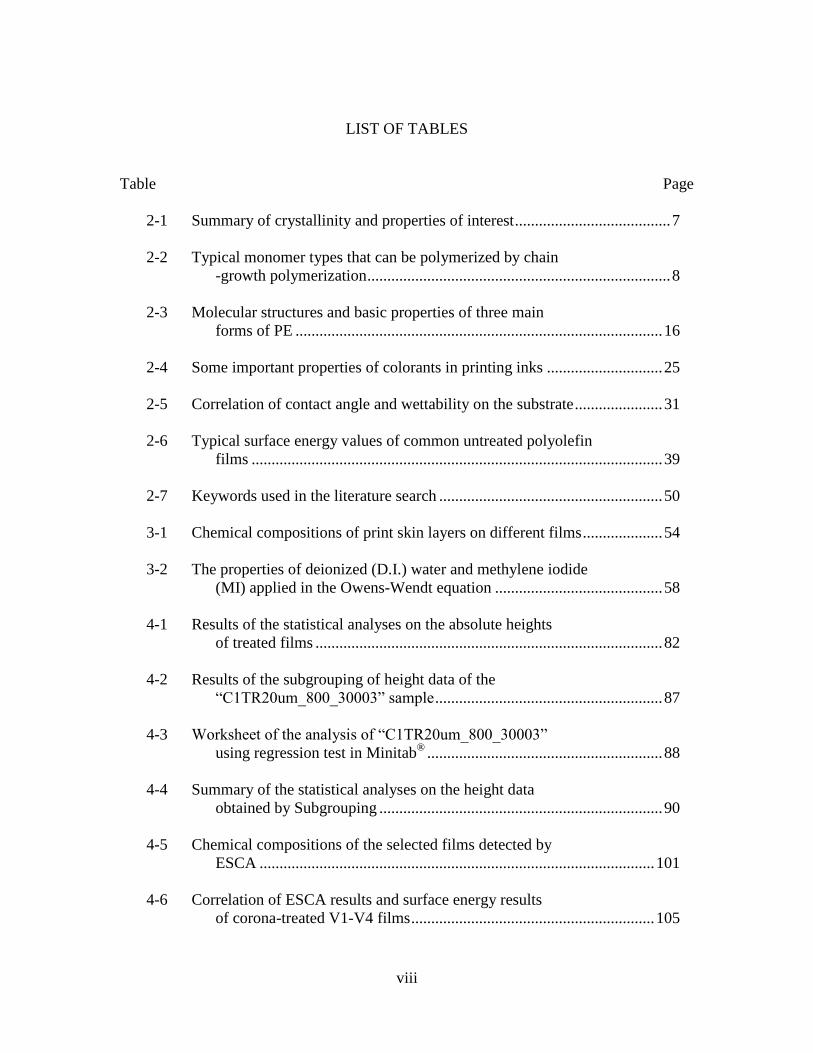
LIST OF TABLES
Table Page
2-1 Summary of crystallinity and properties of interest ....................................... 7
2-2 Typical monomer types that can be polymerized by chain
-growth polymerization ............................................................................ 8
2-3 Molecular structures and basic properties of three main
forms of PE ............................................................................................ 16
2-4 Some important properties of colorants in printing inks ............................. 25
2-5 Correlation of contact angle and wettability on the substrate ...................... 31
2-6 Typical surface energy values of common untreated polyolefin
films ....................................................................................................... 39
2-7 Keywords used in the literature search ........................................................ 50
3-1 Chemical compositions of print skin layers on different films .................... 54
3-2 The properties of deionized (D.I.) water and methylene iodide
(MI) applied in the Owens-Wendt equation .......................................... 58
4-1 Results of the statistical analyses on the absolute heights
of treated films ....................................................................................... 82
4-2 Results of the subgrouping of height data of the
“C1TR20um_800_30003” sample ......................................................... 87
4-3 Worksheet of the analysis of “C1TR20um_800_30003”
using regression test in Minitab® ........................................................... 88
4-4 Summary of the statistical analyses on the height data
obtained by Subgrouping ....................................................................... 90
4-5 Chemical compositions of the selected films detected by
ESCA ................................................................................................... 101
4-6 Correlation of ESCA results and surface energy results
of corona-treated V1-V4 films ............................................................. 105
ix
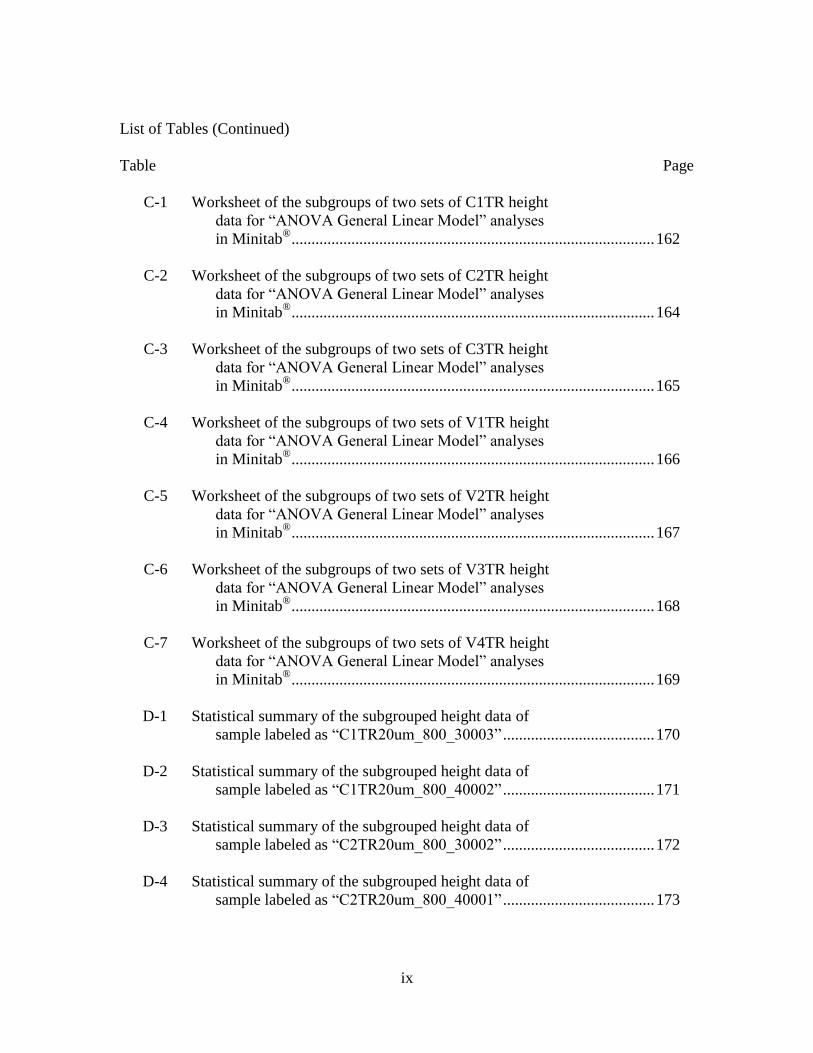
List of Tables (Continued)
Table Page
C-1 Worksheet of the subgroups of two sets of C1TR height
data for “ANOVA General Linear Model” analyses
in Minitab® ........................................................................................... 162
C-2 Worksheet of the subgroups of two sets of C2TR height
data for “ANOVA General Linear Model” analyses
in Minitab® ........................................................................................... 164
C-3 Worksheet of the subgroups of two sets of C3TR height
data for “ANOVA General Linear Model” analyses
in Minitab® ........................................................................................... 165
C-4 Worksheet of the subgroups of two sets of V1TR height
data for “ANOVA General Linear Model” analyses
in Minitab® ........................................................................................... 166
C-5 Worksheet of the subgroups of two sets of V2TR height
data for “ANOVA General Linear Model” analyses
in Minitab® ........................................................................................... 167
C-6 Worksheet of the subgroups of two sets of V3TR height
data for “ANOVA General Linear Model” analyses
in Minitab® ........................................................................................... 168
C-7 Worksheet of the subgroups of two sets of V4TR height
data for “ANOVA General Linear Model” analyses
in Minitab® ........................................................................................... 169
D-1 Statistical summary of the subgrouped height data of
sample labeled as “C1TR20um_800_30003” ...................................... 170
D-2 Statistical summary of the subgrouped height data of
sample labeled as “C1TR20um_800_40002” ...................................... 171
D-3 Statistical summary of the subgrouped height data of
sample labeled as “C2TR20um_800_30002” ...................................... 172
D-4 Statistical summary of the subgrouped height data of
sample labeled as “C2TR20um_800_40001” ...................................... 173
x
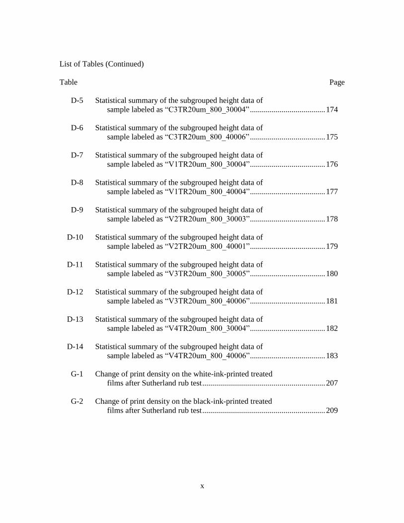
List of Tables (Continued)
Table Page
D-5 Statistical summary of the subgrouped height data of
sample labeled as “C3TR20um_800_30004” ...................................... 174
D-6 Statistical summary of the subgrouped height data of
sample labeled as “C3TR20um_800_40006” ...................................... 175
D-7 Statistical summary of the subgrouped height data of
sample labeled as “V1TR20um_800_30004” ...................................... 176
D-8 Statistical summary of the subgrouped height data of
sample labeled as “V1TR20um_800_40004” ...................................... 177
D-9 Statistical summary of the subgrouped height data of
sample labeled as “V2TR20um_800_30003” ...................................... 178
D-10 Statistical summary of the subgrouped height data of
sample labeled as “V2TR20um_800_40001” ...................................... 179
D-11 Statistical summary of the subgrouped height data of
sample labeled as “V3TR20um_800_30005” ...................................... 180
D-12 Statistical summary of the subgrouped height data of
sample labeled as “V3TR20um_800_40006” ...................................... 181
D-13 Statistical summary of the subgrouped height data of
sample labeled as “V4TR20um_800_30004” ...................................... 182
D-14 Statistical summary of the subgrouped height data of
sample labeled as “V4TR20um_800_40006” ...................................... 183
G-1 Change of print density on the white-ink-printed treated
films after Sutherland rub test .............................................................. 207
G-2 Change of print density on the black-ink-printed treated
films after Sutherland rub test .............................................................. 209
xi
LIST OF FIGURES
Figure Page
2-1 Simplified schematic of a homopolymer and different
copolymers ............................................................................................... 2
2-2 Simplified illustration of a linear polymer (HDPE), a branched
polymer (LDPE and LLDPE), and crosslinked network ......................... 3
2-3 Repeating subunits of polyolefins (a), polyethylene (b) and
polypropylene (c) ..................................................................................... 4
2-4 Examples of PP with different tacticities ....................................................... 5
2-5 Schematic of a semi-crystalline polymer structure ........................................ 6
2-6 Schematic of the formation of multimers in step-growth
polymerization ......................................................................................... 8
2-7 Schematic of the reactions in different stages of free radical
polymerization ....................................................................................... 10
2-8 Schematic of long-chain branching and short-chain branching
through back-biting ................................................................................ 11
2-9 Simplified mechanism of Z-N catalyzed polymerization ............................ 13
2-10 Molecular structure of metallocene ............................................................. 14
2-11 Polypropylene with different tacticities catalyzed with
different metallocene ligand structures .................................................. 15
2-12 Illustration of a typical flexo printing unit ................................................... 22
2-13 Configuration of a typical in-line flexo press .............................................. 23
2-14 Configuration of a typical stack flexo press ................................................ 23
2-15 Configuration of a typical central impression flexo press ........................... 23
2-16 General ink composition .............................................................................. 24
xii
List of Figures (Continued)
Figure Page
2-17 Diagram of the forces on molecules of liquid .............................................. 30
2-18 Schematic of a liquid drop showing the quantities in the
Young’s equation ................................................................................... 31
2-19 Schematic diagram of a corona discharge generator ................................... 40
2-20 Gas-phase reaction mechanism for air-corona discharges ........................... 40
2-21 Simplified schematic of the AFM device (MFP-3D, Asylum
Research) used in this study ................................................................... 44
2-22 Tip movement in contact mode.................................................................... 45
2-23 Tip movement in tapping mode ................................................................... 45
2-24 PRISMA flow diagram performed in the literature search
of this study ............................................................................................ 51
4-1 Topography of C1TR obtained from light tapping on a
20×20 µm2 area ...................................................................................... 64
4-2 Topography of C2TR obtained from light tapping on a
20×20 µm2 area ...................................................................................... 64
4-3 Topography of C3TR obtained from light tapping on a
20×20 µm2 area ...................................................................................... 65
4-4 Topography of V1TR obtained from light tapping on a
20×20 µm2 area ...................................................................................... 65
4-5 Topography of V2TR obtained from light tapping on a
20×20 µm2 area ...................................................................................... 66
4-6 Topography of V3TR obtained from light tapping on a
20×20 µm2 area ...................................................................................... 66
4-7 Topography of V4TR obtained from light tapping on a
20×20 µm2 area ...................................................................................... 67
xiii
List of Figures (Continued)
Figure Page
4-8 Topography (a) and phase angle image (b) obtained
simultaneously from hard tapping on 5×5 µm2 sample
of C1TR ................................................................................................. 72
4-9 Topography (a) and phase angle image (b) obtained
simultaneously from hard tapping on 5×5 µm2 sample
of C2TR ................................................................................................. 73
4-10 Topography (a) and phase angle image (b) obtained
simultaneously from hard tapping on 5×5 µm2 sample
of C3TR ................................................................................................. 73
4-11 Topography (a) and phase angle image (b) obtained
simultaneously from hard tapping on 5×5 µm2 sample
of V1TR ................................................................................................. 74
4-12 Topography (a) and phase angle image (b) obtained
simultaneously from hard tapping on 5×5 µm2 sample
of V2TR ................................................................................................. 74
4-13 Topography (a) and phase angle image (b) obtained
simultaneously from hard tapping on 5×5 µm2 sample
of V3TR ................................................................................................. 75
4-14 Topography (a) and phase angle image (b) obtained
simultaneously from hard tapping on the #1 5×5 µm2
area of the V4TR sample in Figure 4-17 ............................................... 75
4-15 Topography (a) and phase angle image (b) obtained
simultaneously from hard tapping on the #2 5×5 µm2
area of the V4TR sample in Figure 4-17 ............................................... 76
4-16 Phase angle image obtained from light tapping on 20×20 µm2
sample of V3TR ..................................................................................... 76
4-17 Phase angle image obtained from light tapping on 20×20 µm2
sample of V4TR ..................................................................................... 76
xiv
List of Figures (Continued)
Figure Page
4-18 Phase angle distribution obtained from hard tapping on
5×5 µm2 sample of C1TR, corresponding to Figure 4-8 ....................... 77
4-19 Phase angle distribution obtained from hard tapping on
5×5 µm2 sample of C2TR, corresponding to Figure 4-9 ....................... 77
4-20 Phase angle distribution obtained from hard tapping on
5×5 µm2sample of C3TR, corresponding to Figure 4-10 ...................... 78
4-21 Phase angle distribution obtained from hard tapping on
5×5 µm2sample of V1TR, corresponding to Figure 4-11 ...................... 78
4-22 Phase angle distribution obtained from hard tapping on
5×5 µm2 sample of V2TR, corresponding to Figure 4-12 ..................... 79
4-23 Phase angle distribution obtained from hard tapping on
5×5 µm2 sample of V3TR, corresponding to Figure 4-13 ..................... 79
4-24 Phase angle distribution obtained from hard tapping on #1
5×5 µm2 sample of V4TR, corresponding to Figure 4-17 ..................... 80
4-25 Phase angle distribution obtained from hard tapping on #2
5×5 µm2 sample of V4TR, corresponding to Figure 4-17 ..................... 80
4-26 Illustration of dividing each set of height data into sixteen
subgroups according to the coordinates of the data points .................... 85
4-27 Average roughness results of all treated films ............................................. 93
4-28 Change of water contact angles with time on the untreated
films ....................................................................................................... 95
4-29 Change of MI contact angles with time on the untreated
films ....................................................................................................... 95
4-30 Change of water contact angles with time on the corona
-treated films .......................................................................................... 96
4-31 Change of MI contact angles with time on the corona
-treated films .......................................................................................... 97
xv
List of Figures (Continued)
Figure Page
4-32 Surface energy of the corona-treated and untreated films
calculated using Owens-Wendt equation ............................................... 98
4-33 Polar components contributing to the surface energy of
the corona-treated and untreated films ................................................... 98
4-34 Dispersive components contributing to the surface energy
of the corona-treated and untreated films .............................................. 99
4-35 Increments in surface energy, polar component and dispersive
component after corona treatment ....................................................... 100
4-36 C1s spectrum of untreated V1 film ............................................................ 102
4-37 C1s spectrum of treated V1 film ................................................................ 102
4-38 Oxygen percent concentration of corona-treated V1-V4
films obtained from ESCA analysis ..................................................... 103
4-39 Correlation of surface energy and (oxygen)% of untreated
V1 film and corona-treated V1-V4 films ............................................. 105
4-40 Correlation of surface energy and oxygen/carbon ratio of
untreated V1 film and corona-treated V1-V4 films ............................. 105
4-41 Oxygen percent concentration of all corona-treated films ......................... 109
4-42 Percent peak areas of oxygen in the forms of “C-O” or
“C=O” bonds based on Figure 4-43 ...................................................... 109
4-43 Percent peak areas of the treated films V1-V4 resulted
from ESCA C1s peak decomposition .................................................. 110
4-44 Comparison of the 45° print gloss of the treated films
printed with black and white inks ........................................................ 110
4-45 Results of tape tests on all the corona-treated films printed
with white and black inks respectively ................................................ 115
xvi
List of Figures (Continued)
Figure Page
A-1 Original result report of AFM analysis on sample “C1TR
20um_800_30003” ............................................................................... 120
A-2 Original result report of AFM analysis on sample “C1TR
5um_500_30000” ................................................................................. 121
A-3 Original result report of AFM analysis on sample “C1TR
20um_800_40002” ............................................................................... 122
A-4 Original result report of AFM analysis on sample “C1TR
5um_500_40000” ................................................................................. 123
A-5 Original result report of AFM analysis on sample “C2TR
20um_800_30002” ............................................................................... 124
A-6 Original result report of AFM analysis on sample “C2TR
5um_500_30000” ................................................................................. 125
A-7 Original result report of AFM analysis on sample “C2TR
20um_800_40001” ............................................................................... 126
A-8 Original result report of AFM analysis on sample “C2TR
5um_500_40000” ................................................................................. 127
A-9 Original result report of AFM analysis on sample “C3TR
20um_800_30004” ............................................................................... 128
A-10 Original result report of AFM analysis on sample “C3TR
5um_500_30000” ................................................................................. 129
A-11 Original result report of AFM analysis on sample “C3TR
20um_800_40006” ............................................................................... 130
A-12 Original result report of AFM analysis on sample “C3TR
5um_500_40001” ................................................................................. 131
A-13 Original result report of AFM analysis on sample “V1TR
20um_800_30004” ............................................................................... 132
xvii
List of Figures (Continued)
Figure Page
A-14 Original result report of AFM analysis on sample “V1TR
5um_500_30000” ................................................................................. 133
A-15 Original result report of AFM analysis on sample “V1TR
5um_500_30001” ................................................................................. 134
A-16 Original result report of AFM analysis on sample “V1TR
20um_800_40004” ............................................................................... 135
A-17 Original result report of AFM analysis on sample “V1TR
5um_500_40000” ................................................................................. 136
A-18 Original result report of AFM analysis on sample “V2TR
20um_800_30003” ............................................................................... 137
A-19 Original result report of AFM analysis on sample “V2TR
5um_500_30000” ................................................................................. 138
A-20 Original result report of AFM analysis on sample “V2TR
20um_800_40001” ............................................................................... 139
A-21 Original result report of AFM analysis on sample “V2TR
5um_500_40000” ................................................................................. 140
A-22 Original result report of AFM analysis on sample “V3TR
20um_800_30005” ............................................................................... 141
A-23 Original result report of AFM analysis on sample “V3TR
5um_500_30000” ................................................................................. 142
A-24 Original result report of AFM analysis on sample “V3TR
20um_800_40006” ............................................................................... 143
A-25 Original result report of AFM analysis on sample “V3TR
5um_500_40000” ................................................................................. 144
A-26 Original result report of AFM analysis on sample “V3TR
5um_500_40001” ................................................................................. 145
xviii
List of Figures (Continued)
Figure Page
A-27 Original result report of AFM analysis on sample “V4TR
20um_800_30004” ............................................................................... 146
A-28 Original result report of AFM analysis on sample “V4TR
5um_500_30000” ................................................................................. 147
A-29 Original result report of AFM analysis on sample “V4TR
5um_500_30001” ................................................................................. 148
A-30 Original result report of AFM analysis on sample “V4TR
20um_800_40006” ............................................................................... 149
A-31 Original result report of AFM analysis on sample “V4TR
5um_500_40000” ................................................................................. 150
A-32 Original result report of AFM analysis on sample “V4TR
5um_500_40001” ................................................................................. 151
A-33 Original result report of AFM analysis on sample “V4TR
20um_800_30004” ............................................................................... 152
A-34 Original result report of AFM analysis on sample “V4TR
5um_500_30000” ................................................................................. 153
A-35 Original result report of AFM analysis on sample “V4TR
5um_500_30001” ................................................................................. 154
F-1 Curve fitting of the C1s spectra of treated V1 – replicate#1 ..................... 201
F-2 Curve fitting of the C1s spectra of treated V1 – replicate#2 ..................... 201
F-3 Curve fitting of the C1s spectra of treated V1 – replicate#3 ..................... 202
F-4 Curve fitting of the C1s spectra of treated V2 – replicate#1 ..................... 202
F-5 Curve fitting of the C1s spectra of treated V2 – replicate#2 ..................... 203
F-6 Curve fitting of the C1s spectra of treated V2 – replicate#3 ..................... 203
F-7 Curve fitting of the C1s spectra of treated V3 – replicate#1 ..................... 204
xix
List of Figures (Continued)
Figure Page
F-8 Curve fitting of the C1s spectra of treated V3 – replicate#2 ..................... 204
F-9 Curve fitting of the C1s spectra of treated V3 – replicate#3 ..................... 205
F-10 Curve fitting of the C1s spectra of treated V4 – replicate#1 ..................... 205
F-11 Curve fitting of the C1s spectra of treated V4 – replicate#2 ..................... 206
F-12 Curve fitting of the C1s spectra of treated V4 – replicate#3 ..................... 206
CHAPTER ONE
INTRODUCTION
A wide variety of polyolefins is used in the form of multilayer films in the
flexible packaging industry. The top two polyolefins in sales are polyethylene (PE) and
polypropylene (PP). To increase production efficiency, various catalyst systems have
been employed in the commercial synthesis of polyolefins from monomers. The
conventional Ziegler-Natta (Z-N) catalyst system is still dominant in commercial
production, while metallocene catalyst systems have drawn increased attention for their
better stereo-selectivity toward the final polymers. Because of this stereo-selectivity, the
polyolefins catalyzed with metallocene catalysts generally have more uniform molecular
weight distributions than their Z-N counterparts. This difference stimulates their broad
application potential in the industry. To better apply this technology, many studies have
been conducted in the past in terms of the extrusion processability, strength properties,
seal strength and hot tack, etc. of these polymers. Multiple patents also claim the
potential of metallocene catalyzed polyolefins used in multilayer plastic films as either
core layers or skin layers. However, no analytical study has been conducted to understand
the surface characteristics of such multilayer films and their effects on ink wetting and
adhesion. The work presented in this document is intended to fill this missing
information. The findings from this project are expected to guide the selection of
polyolefin blends containing metallocene catalyzed components for the print layers of
multilayer plastic films.
1
2
CHAPTER TWO
LITERATURE REVIEW
Polymers
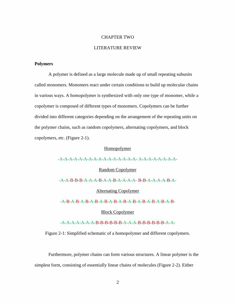
A polymer is defined as a large molecule made up of small repeating subunits
called monomers. Monomers react under certain conditions to build up molecular chains
in various ways. A homopolymer is synthesized with only one type of monomer, while a
copolymer is composed of different types of monomers. Copolymers can be further
divided into different categories depending on the arrangement of the repeating units on
the polymer chains, such as random copolymers, alternating copolymers, and block
copolymers, etc. (Figure 2-1).
Homopolymer
-A-A-A-A-A-A-A-A-A-A-A-A-A-A-A-A- A-A-A-A-A-A-A-A-
Random Copolymer
-A-A-B-B-B-A-A-A-B-A-A-B-A-A-A-A- B-B-A-A-A-A-B-A-
Alternating Copolymer
-A-B-A-B-A-B-A-B-A-B-A-B-A-B-A-B-A-B-A-B-A-B-A-B-
Block Copolymer
-A-A-A-A-A-A-A-B-B-B-B-B-B-A-A-A-B-B-B-B-B-B-A-A-
Figure 2-1: Simplified schematic of a homopolymer and different copolymers.
Furthermore, polymer chains can form various structures. A linear polymer is the
simplest form, consisting of essentially linear chains of molecules (Figure 2-2). Either
3
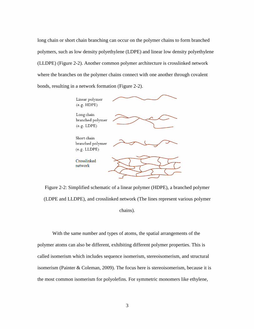
long chain or short chain branching can occur on the polymer chains to form branched
polymers, such as low density polyethylene (LDPE) and linear low density polyethylene
(LLDPE) (Figure 2-2). Another common polymer architecture is crosslinked network
where the branches on the polymer chains connect with one another through covalent
bonds, resulting in a network formation (Figure 2-2).
Figure 2-2: Simplified schematic of a linear polymer (HDPE), a branched polymer
(LDPE and LLDPE), and crosslinked network (The lines represent various polymer
chains).
With the same number and types of atoms, the spatial arrangements of the
polymer atoms can also be different, exhibiting different polymer properties. This is
called isomerism which includes sequence isomerism, stereoisomerism, and structural
isomerism (Painter & Coleman, 2009). The focus here is stereoisomerism, because it is
the most common isomerism for polyolefins. For symmetric monomers like ethylene,
4
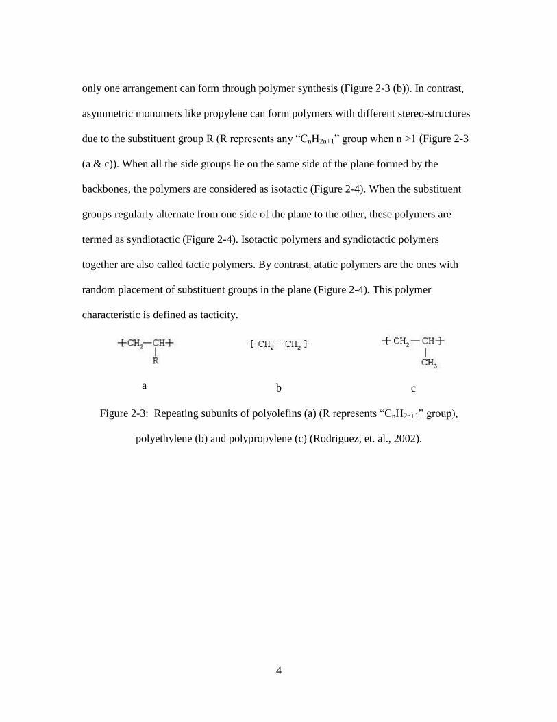
only one arrangement can form through polymer synthesis (Figure 2-3 (b)). In contrast,
asymmetric monomers like propylene can form polymers with different stereo-structures
due to the substituent group R (R represents any “CnH2n+1” group when n >1 (Figure 2-3
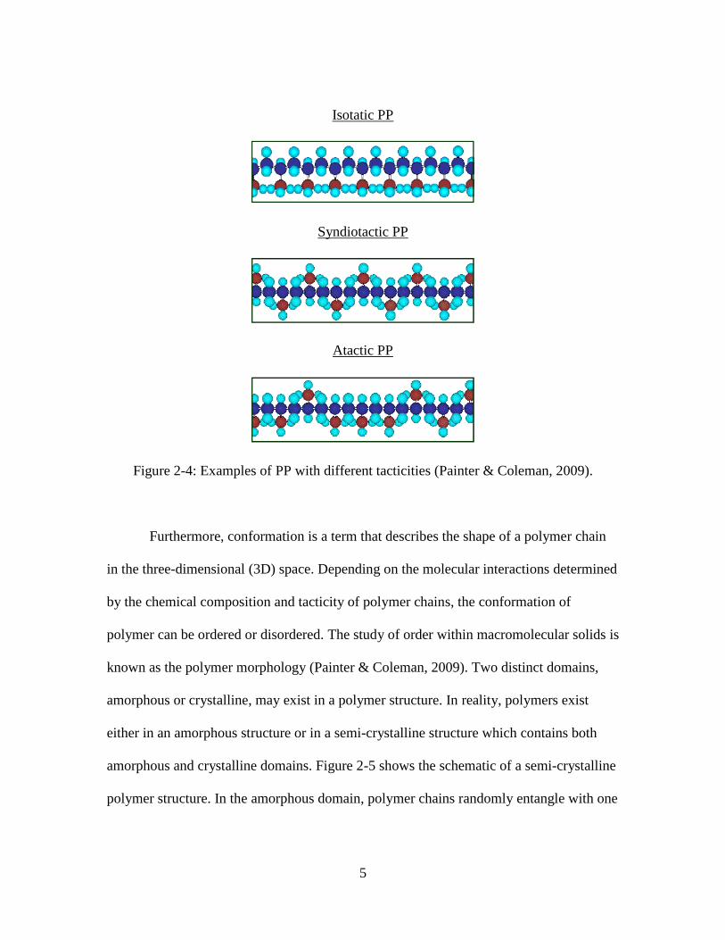
(a & c)). When all the side groups lie on the same side of the plane formed by the
backbones, the polymers are considered as isotactic (Figure 2-4). When the substituent
groups regularly alternate from one side of the plane to the other, these polymers are
termed as syndiotactic (Figure 2-4). Isotactic polymers and syndiotactic polymers
together are also called tactic polymers. By contrast, atatic polymers are the ones with
random placement of substituent groups in the plane (Figure 2-4). This polymer
characteristic is defined as tacticity.
a
b
c
Figure 2-3: Repeating subunits of polyolefins (a) (R represents “CnH2n+1” group),
polyethylene (b) and polypropylene (c) (Rodriguez, et. al., 2002).
5
Isotatic PP
Syndiotactic PP
Atactic PP
Figure 2-4: Examples of PP with different tacticities (Painter & Coleman, 2009).
Furthermore, conformation is a term that describes the shape of a polymer chain
in the three-dimensional (3D) space. Depending on the molecular interactions determined
by the chemical composition and tacticity of polymer chains, the conformation of
polymer can be ordered or disordered. The study of order within macromolecular solids is
known as the polymer morphology (Painter & Coleman, 2009). Two distinct domains,
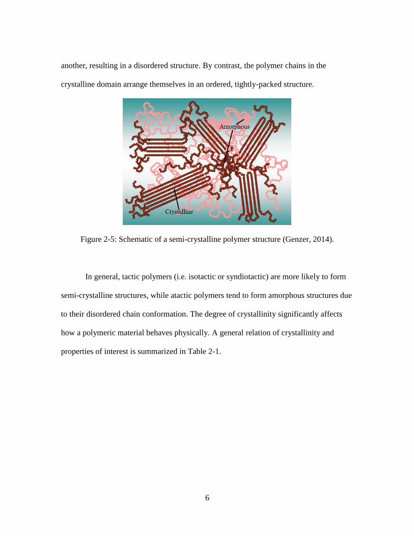
amorphous or crystalline, may exist in a polymer structure. In reality, polymers exist
either in an amorphous structure or in a semi-crystalline structure which contains both
amorphous and crystalline domains. Figure 2-5 shows the schematic of a semi-crystalline
polymer structure. In the amorphous domain, polymer chains randomly entangle with one
6
another, resulting in a disordered structure. By contrast, the polymer chains in the
crystalline domain arrange themselves in an ordered, tightly-packed structure.
Figure 2-5: Schematic of a semi-crystalline polymer structure (Genzer, 2014).
In general, tactic polymers (i.e. isotactic or syndiotactic) are more likely to form
semi-crystalline structures, while atactic polymers tend to form amorphous structures due
to their disordered chain conformation. The degree of crystallinity significantly affects
how a polymeric material behaves physically. A general relation of crystallinity and
properties of interest is summarized in Table 2-1.

7
Table 2-1: Summary of crystallinity and properties of interest (Painter & Coleman, 2009).
Property Change with Increasing Degree of Crystallinity
Strength Generally increases with degree of crystallinity
Stiffness Generally increases with degree of crystallinity
Toughness Generally decreases with degree of crystallinity
Optical Clarity Generally decreases with degree of crystallinity
Barrier Properties Generally increases with degree of crystallinity
Solubility Generally increases with degree of crystallinity
It is well accepted to classify polymerization reactions into two categories: step-
growth polymerization and chain-growth polymerization (Painter & Coleman, 2009).
Monomers containing functional groups, such as amine (-NH2), alcohol (-OH) or
carboxylic acid (-COOH), etc., go through stepwise reactions to form polymers. Figure 2-
6 illustrates the formation of multimers in step-growth polymerization. Monomers with
functional groups slowly react to form dimers, trimers, quadrimers and so on step by step
until all the functional groups react. This process depends on the probabilities of random
collisions between different oligomers and the resultant molecular weight and molecular
weight distribution can be predicted using statistical analysis. Some typical polymers
produced in this way are polyesters, polyamides, and polyurethanes. What’s more, when
the monomers have multifunctional groups, step-growth polymerization can even
generate complicated polymers with network formations.
8
Monomer + Monomer Dimer A-A + B-B A-AB-B
Dimer + Monomer Trimer A-AB-B + A-A A-AB-BA-A
Dimer + Dimer Quadrimer A-AB-B + A-AB-B A-AB-BA-AB-B
This process continues.
Figure 2-6: Schematic of the formation of multimers in step-growth polymerization.
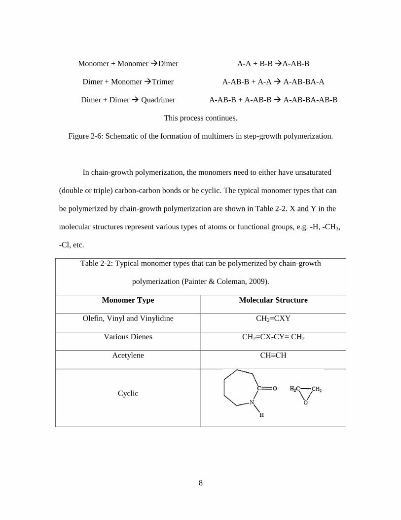
In chain-growth polymerization, the monomers need to either have unsaturated
(double or triple) carbon-carbon bonds or be cyclic. The typical monomer types that can
be polymerized by chain-growth polymerization are shown in Table 2-2. X and Y in the
molecular structures represent various types of atoms or functional groups, e.g. -H, -CH3,
-Cl, etc.
Table 2-2: Typical monomer types that can be polymerized by chain-growth
polymerization (Painter & Coleman, 2009).
Monomer Type Molecular Structure
Olefin, Vinyl and Vinylidine CH2=CXY
Various Dienes CH2=CX-CY= CH2
Acetylene CH≡CH
Cyclic
9
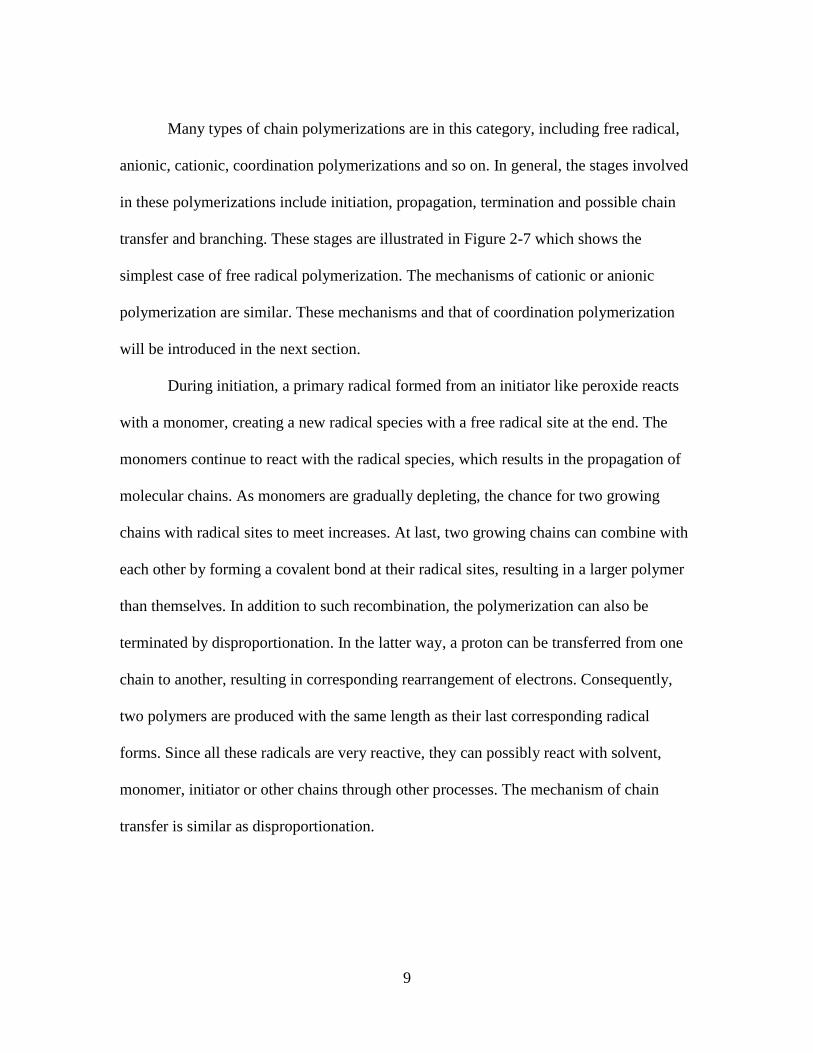
Many types of chain polymerizations are in this category, including free radical,
anionic, cationic, coordination polymerizations and so on. In general, the stages involved
in these polymerizations include initiation, propagation, termination and possible chain
transfer and branching. These stages are illustrated in Figure 2-7 which shows the
simplest case of free radical polymerization. The mechanisms of cationic or anionic
polymerization are similar. These mechanisms and that of coordination polymerization
will be introduced in the next section.
During initiation, a primary radical formed from an initiator like peroxide reacts
with a monomer, creating a new radical species with a free radical site at the end. The
monomers continue to react with the radical species, which results in the propagation of
molecular chains. As monomers are gradually depleting, the chance for two growing
chains with radical sites to meet increases. At last, two growing chains can combine with
each other by forming a covalent bond at their radical sites, resulting in a larger polymer
than themselves. In addition to such recombination, the polymerization can also be
terminated by disproportionation. In the latter way, a proton can be transferred from one
chain to another, resulting in corresponding rearrangement of electrons. Consequently,
two polymers are produced with the same length as their last corresponding radical
forms. Since all these radicals are very reactive, they can possibly react with solvent,
monomer, initiator or other chains through other processes. The mechanism of chain
transfer is similar as disproportionation.
10
Figure 2-7: Schematic of the reactions in different stages of free radical polymerization
(“●” represents an unshared electron.) (Genzer, 2014).
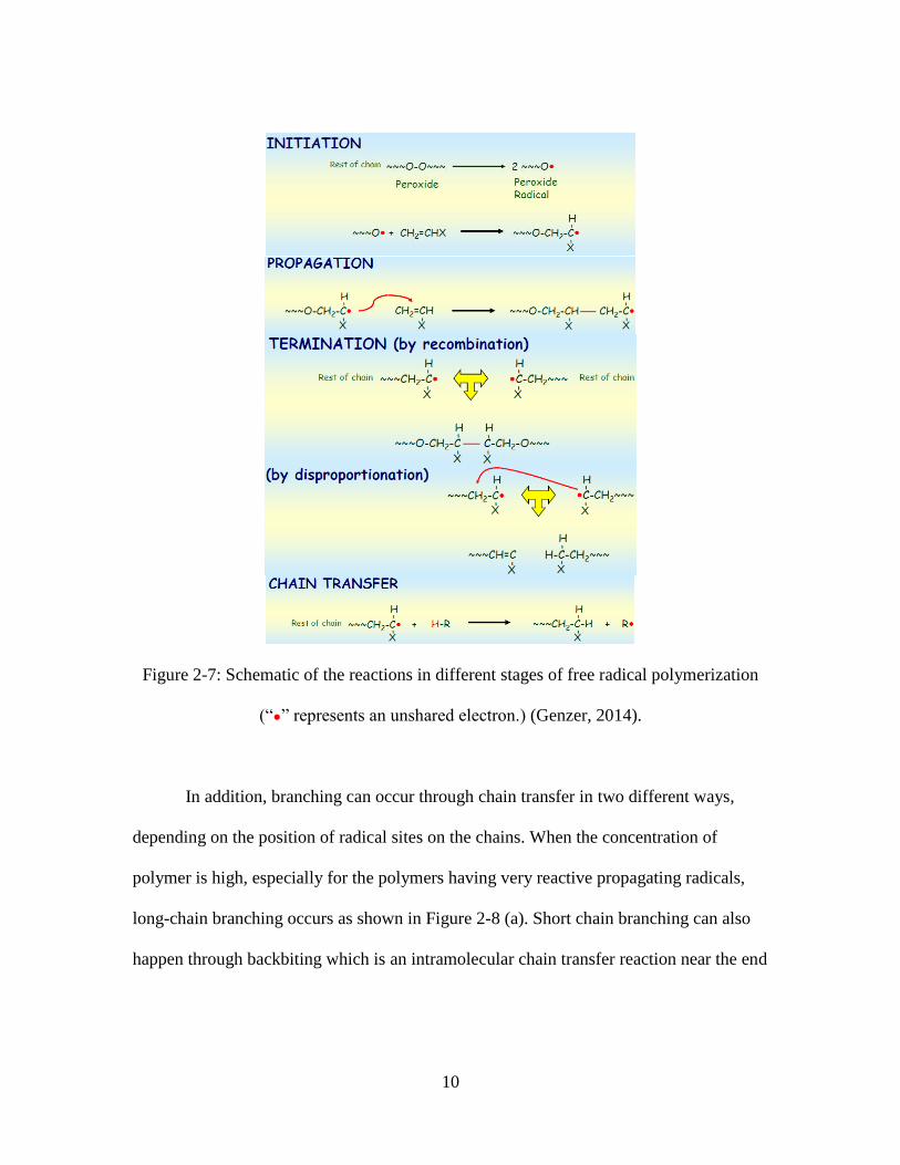
In addition, branching can occur through chain transfer in two different ways,
depending on the position of radical sites on the chains. When the concentration of
polymer is high, especially for the polymers having very reactive propagating radicals,
long-chain branching occurs as shown in Figure 2-8 (a). Short chain branching can also
happen through backbiting which is an intramolecular chain transfer reaction near the end
11
of the chains. Figure 2-8 (b) shows the mechanism of backbiting in short-chain
branching. This will be further discussed in the next section.
a
b
Figure 2-8: Schematic of long-chain branching and short-chain branching through
backbiting (Painter & Coleman, 2009).
Ziegler-Natta Catalysts vs. Metallocene Catalysts
Coordination polymerization is a type of polymerization that involves complexes
formed between a transition metal and the π electrons of monomer. A typical application
of this type of polymerization is in the production of polyolefins. To efficiently produce
polyolefins, various catalyst systems have been determined to the achieve properties
desired for different applications.
In the last century, one of the most important discoveries in the plastic industry
was the discovery of Ziegler-Natta catalysis for the polymerization of olefins. Karl
Ziegler first discovered the production of high density polyethylene (HDPE) using a
catalyst system based on titanium tetrachloride (α-TiCl3) and a co-catalyst

12
diethylaluminium chloride (Al(C2H5)2Cl) (Ziegler, Holzkamp, Breil & Martin, 1955).
This finding was soon utilized by Giulio Natta in the polymerization of propylene in a
stereo-regulated form (isotactic PP) (Natta, 1959). This polymerization process was
named the Ziegler-Natta process (Z-N process) and both of them were awarded the Nobel
Prize in Chemistry in 1963 for this invention (Claverie & Schaper, 2013). Since then,
various modifications of the Z-N catalyst system have been implemented leading it to
dominate the commercial production of polyolefins. For example, MgCl2 is added,
together with other additives, in this catalyst system to improve polyolefin productivity
(Kissin, 1985; Moore, 1996). Simply speaking, the MgCl2 crystal attracts TiCl4 onto its
surface, resulting in multi-site active centers to which the monomers can be attracted.
Such multi-site active centers allow the polymerization to happen at multiple locations,
resulting in a polyolefin with different tacticity, molecular weights and molecular weight
distributions. Consequently, Z-N catalyzed polyolefins often have relatively broad
molecular weight distributions and composition distributions.
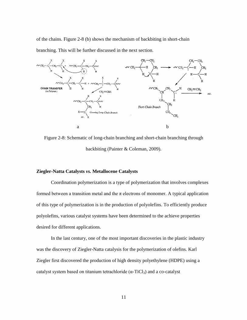
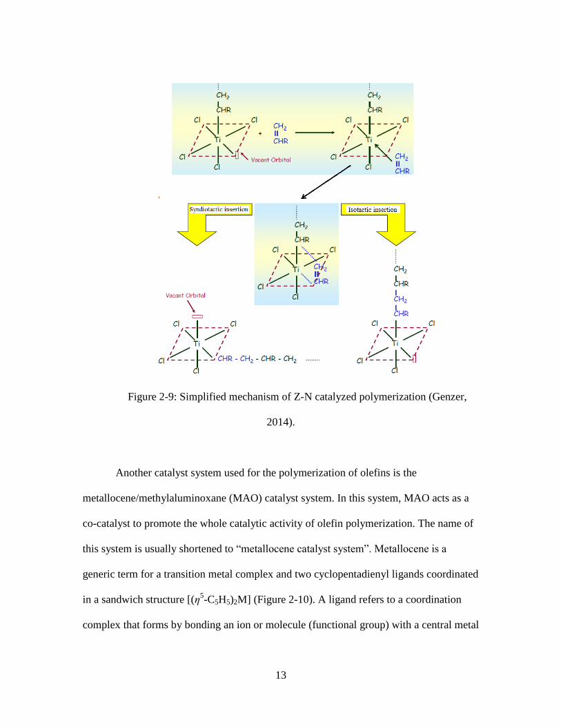
A well-known mechanism of olefin polymerization catalyzed by a Z-N catalyst
system is shown in Figure 2-9 (Cossee, 1964; Arlman, 1964; Arlman & Cossee, 1964). In
this mechanism, a transition metal-carbon bond is formed at the active center. Through
ethylene coordination, a new ethylene monomer is attached to the metal and is further
inserted into the polymer chain in different ways, generating polymers with different
tacticities. These molecular chains continue to propagate until the termination reaction
happens.
13
Figure 2-9: Simplified mechanism of Z-N catalyzed polymerization (Genzer,
2014).
Another catalyst system used for the polymerization of olefins is the
metallocene/methylaluminoxane (MAO) catalyst system. In this system, MAO acts as a
co-catalyst to promote the whole catalytic activity of olefin polymerization. The name of
this system is usually shortened to “metallocene catalyst system”. Metallocene is a
generic term for a transition metal complex and two cyclopentadienyl ligands coordinated
in a sandwich structure [(η5-C5H5)2M] (Figure 2-10). A ligand refers to a coordination
complex that forms by bonding an ion or molecule (functional group) with a central metal
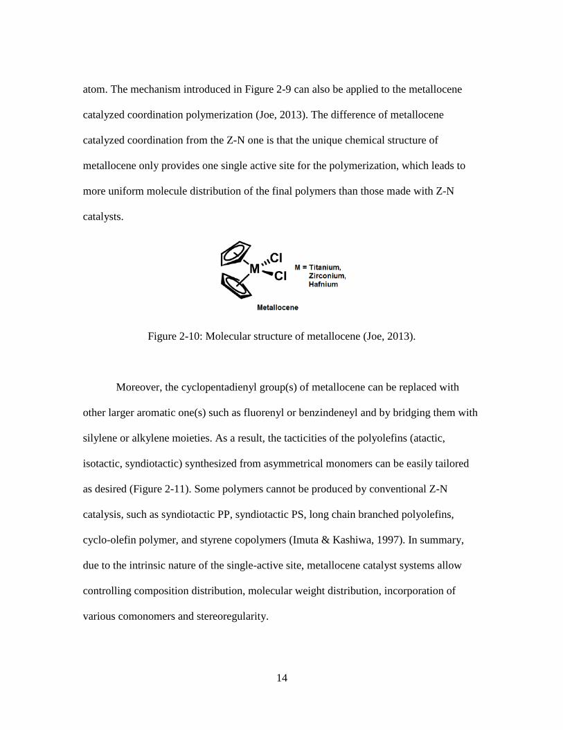
14
atom. The mechanism introduced in Figure 2-9 can also be applied to the metallocene
catalyzed coordination polymerization (Joe, 2013). The difference of metallocene
catalyzed coordination from the Z-N one is that the unique chemical structure of
metallocene only provides one single active site for the polymerization, which leads to
more uniform molecule distribution of the final polymers than those made with Z-N
catalysts.
Figure 2-10: Molecular structure of metallocene (Joe, 2013).
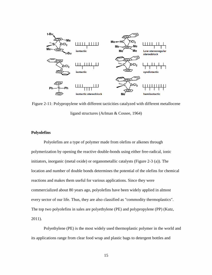
Moreover, the cyclopentadienyl group(s) of metallocene can be replaced with
other larger aromatic one(s) such as fluorenyl or benzindeneyl and by bridging them with
silylene or alkylene moieties. As a result, the tacticities of the polyolefins (atactic,
isotactic, syndiotactic) synthesized from asymmetrical monomers can be easily tailored
as desired (Figure 2-11). Some polymers cannot be produced by conventional Z-N
catalysis, such as syndiotactic PP, syndiotactic PS, long chain branched polyolefins,
cyclo-olefin polymer, and styrene copolymers (Imuta & Kashiwa, 1997). In summary,
due to the intrinsic nature of the single-active site, metallocene catalyst systems allow
controlling composition distribution, molecular weight distribution, incorporation of
various comonomers and stereoregularity.
15
Figure 2-11: Polypropylene with different tacticities catalyzed with different metallocene
ligand structures (Arlman & Cossee, 1964)
Polyolefins
Polyolefins are a type of polymer made from olefins or alkenes through
polymerization by opening the reactive double-bonds using either free-radical, ionic
initiators, inorganic (metal oxide) or organometallic catalysts (Figure 2-3 (a)). The
location and number of double bonds determines the potential of the olefins for chemical
reactions and makes them useful for various applications. Since they were
commercialized about 80 years ago, polyolefins have been widely applied in almost
every sector of our life. Thus, they are also classified as "commodity thermoplastics".
The top two polyolefins in sales are polyethylene (PE) and polypropylene (PP) (Kutz,
2011).
Polyethylene (PE) is the most widely used thermoplastic polymer in the world and
its applications range from clear food wrap and plastic bags to detergent bottles and
16
automobile fuel tanks (Kutz, 2011). It is formed by the polymerization of ethylene
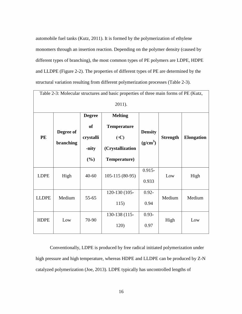
monomers through an insertion reaction. Depending on the polymer density (caused by
different types of branching), the most common types of PE polymers are LDPE, HDPE
and LLDPE (Figure 2-2). The properties of different types of PE are determined by the
structural variation resulting from different polymerization processes (Table 2-3).
Table 2-3: Molecular structures and basic properties of three main forms of PE (Kutz,
2011).
PE
Degree of
branching
Degree
of
crystalli
-nity
(%)
Melting
Temperature
(◦C)
(Crystallization
Temperature)
Density
(g/cm3)
Strength Elongation
LDPE High 40-60 105-115 (80-95)
0.915-
0.933
Low High
LLDPE Medium 55-65
120-130 (105-
115)
0.92-
0.94
Medium Medium
HDPE Low 70-90
130-138 (115-
120)
0.93-
0.97
High Low
Conventionally, LDPE is produced by free radical initiated polymerization under
high pressure and high temperature, whereas HDPE and LLDPE can be produced by Z-N
catalyzed polymerization (Joe, 2013). LDPE typically has uncontrolled lengths of
17
branches induced by side reactions, such as backbiting, and chain transfer of short chain
branches and long chain branches to polymer backbones respectively (Figure 2-8)
(Kaminsky & Piel, 2004; Janicek, Cermak, Obadal, Piel & Ponizil, 2011). This makes
LDPE more difficult to crystalize than HDPE which has more linear polymer chains with
less branching on the backbones. Due to its higher crystallinity, HDPE exhibits better
tensile strength, chemical resistance, and stiffness, but lower elongation and tendency to
crosslink than LDPE.
LLDPE is made by the copolymerization of ethylene and a comonomer, typically
1-butene (CH3CH2CH=CH2), 1-hexene (CH3CH2CH2CH2CH=CH2), or 1-octene
(CH3CH2CH2CH2CH2CH2CH=CH2) (Figure 2-3(b)). These comonomers form short side
chains linked to the main chains of PE. The length of the side chain is essentially
determined by the comonomer. This allows better control of the properties than LDPE
exhibits. Some properties of LLDPE are similar to those of LDPE, but some are not
because of its lack of long chain branching. LLDPE can be produced with coordination
catalysts, such as Z-N or metallocenes, but currently Z-N systems are still dominant for
the commercial production of LLDPE (Joe, 2013). In addition, it has been found that
LLDPE catalyzed via the metallocene process usually has more consistent comonomer
distribution. The reaction is also more efficient for the comonomer incorporation. This
requires a lower feeding ratio of comonomer, compared with that required for Z-N
catalysis (Hlatky, 1999; Razavi, 2000; Shamiri, et al., 2014).
18
Polypropylene (PP) is the second most consumed commercial polyolefin in the
market, following PE. It was first commercially produced in the 1950s after the discovery
of the Z-N catalyst system (Joe, 2013).
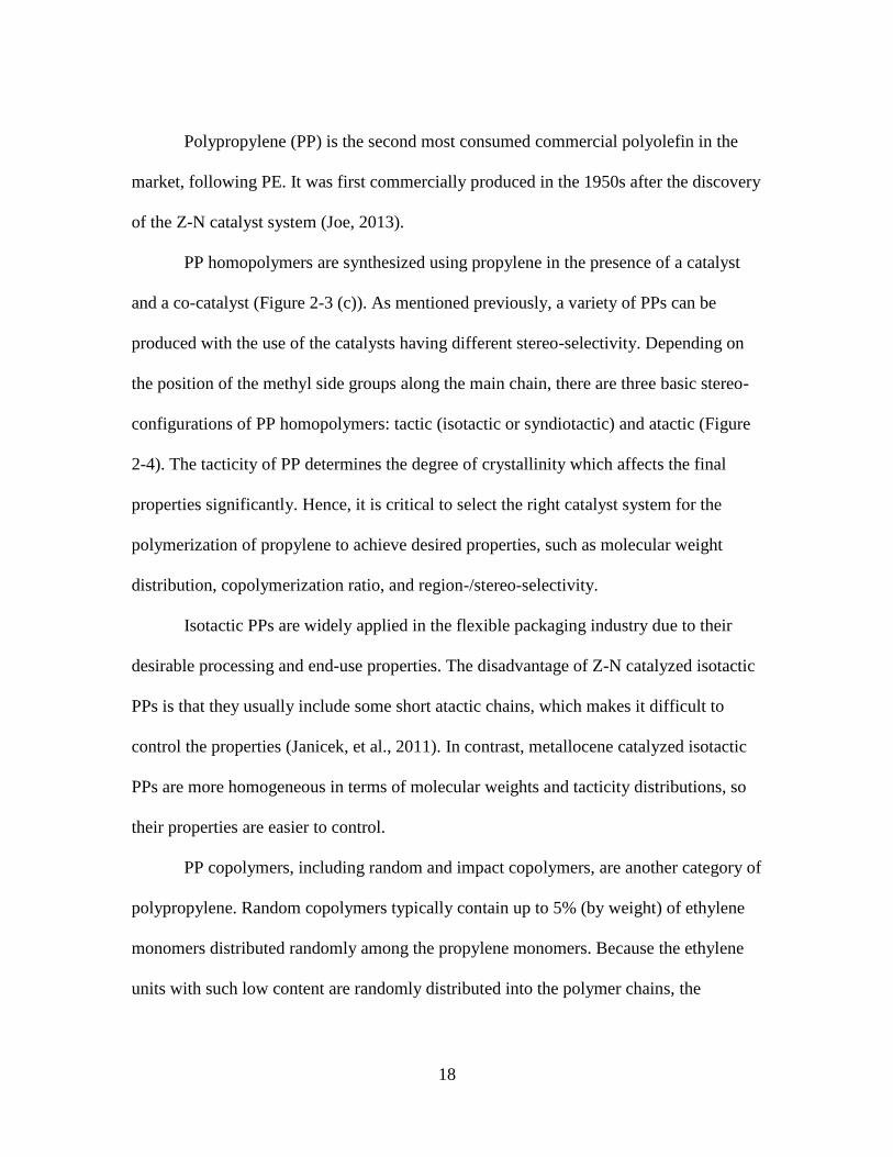
PP homopolymers are synthesized using propylene in the presence of a catalyst
and a co-catalyst (Figure 2-3 (c)). As mentioned previously, a variety of PPs can be
produced with the use of the catalysts having different stereo-selectivity. Depending on
the position of the methyl side groups along the main chain, there are three basic stereo-
configurations of PP homopolymers: tactic (isotactic or syndiotactic) and atactic (Figure
2-4). The tacticity of PP determines the degree of crystallinity which affects the final
properties significantly. Hence, it is critical to select the right catalyst system for the
polymerization of propylene to achieve desired properties, such as molecular weight
distribution, copolymerization ratio, and region-/stereo-selectivity.
Isotactic PPs are widely applied in the flexible packaging industry due to their
desirable processing and end-use properties. The disadvantage of Z-N catalyzed isotactic
PPs is that they usually include some short atactic chains, which makes it difficult to
control the properties (Janicek, et al., 2011). In contrast, metallocene catalyzed isotactic
PPs are more homogeneous in terms of molecular weights and tacticity distributions, so
their properties are easier to control.
PP copolymers, including random and impact copolymers, are another category of
polypropylene. Random copolymers typically contain up to 5% (by weight) of ethylene
monomers distributed randomly among the propylene monomers. Because the ethylene
units with such low content are randomly distributed into the polymer chains, the
19
polymer chains are essentially mainly composed of PP blocks with different lengths.
Therefore, these random PP copolymers still share some properties of PP homopolymers.
However, the introduction of comonomers into polymeric chains not only affects the
aforementioned structural parameters, but also the crystallization behavior of the resultant
copolymers. As a result, the crystallization slows down, resulting in lower total
crystallinity and a reduction of the melting temperature related to the less perfect
structure of the crystals (Kutz, 2011). Random PP copolymers are usually used where
clarity, lower melting point, or a lower modulus is desirable. Impact PP copolymers,
usually contain up to about 40% ethylene-propylene rubber (EPR), distributed inside the
semi-crystalline PP homopolymer matrix (Kutz, 2011). The purpose is to increase the
impact strength of PPs at low temperatures, so these products are typically used in low-
temperature applications.
In the global market, metallocene catalyzed PE, mainly metallocene catalyzed
HDPE and metallocene catalyzed LLDPE, accounted for the largest market share for
metallocene catalyzed polyolefins in 2015 and has been forecasted to have the most rapid
growth rate in the next six years (Market Research Report, 2016). Metallocene catalyzed
PP is another significant segment in the market. The market size of metallocene catalyzed
polyolefins has been forecasted to reach USD 14.05 billion by 2021 (Market Research
Report, 2016). The main applications of metallocene catalyzed polyolefins are film and
sheet, injection molding, and others (rotomolding, fiber, blow molding, raffia, wire &
cable, and pipes & panels). The application of these resins in film and sheet was
dominant in the global market in 2015 and has been forecasted to grow rapidly due to the
20
rise of the food and non-food packaging industries (Market Research Report, 2016).
Among all the applications, injection molding has been estimated to account for the
highest annual value and volume growth between 2016 and 2021 (Market Research
Report, 2016). The rising demand for metallocene catalyzed polyolefins is mainly due to
their superior properties over conventional polyolefins, which are the major driving force
in this market. However, the cost of metallocene catalyzed polyolefins is higher than that
of their Z-N counterparts, which is one of the main constraints hindering the further
growth in the market. In addition, the difficulty in processing on film extrusion and
manufacturing equipment also increases the cost, making them less attractive in some
applications.
Flexography
In the flexible packaging industry, printing on flexible packages not only provides
product information and/or instructions to the consumers but also allows the packages to
stand out on the shelf. The printing on the packages can contain brand communication
information, product information, pictures, usage instructions, nutrition facts, Universal
Product Code (UPC), and many other graphic images.
Primarily, printing is a method used to reproduce text or images from a pre-
designed template. Two different techniques are available to reproduce color text and
images through printing. One is process color printing and the other one is spot color (or
line color) printing. In process color printing, four process colors, cyan (C), magenta (M),
yellow (Y) and black (K), are printed in tiny dots with various sizes or spacing. Human
21
eyes perceive these dots as various solid colors accordingly. This process is also called
halftone printing. In contrast, spot color printing prints a full coverage of images on the
substrate with specific colored inks (called spot colors). The range of achievable colors,
defined as the color gamut, available to print can be further extended with the use of spot
colors in process printing.
Various printing processes, including lithography, gravure, flexography, screen
printing, and digital printing, have been used in various applications. Flexography is one
of the printing processes that are widely used in the packaging and labeling industry. It is
preferred over other printing methods for good print quality, flexibility, quick
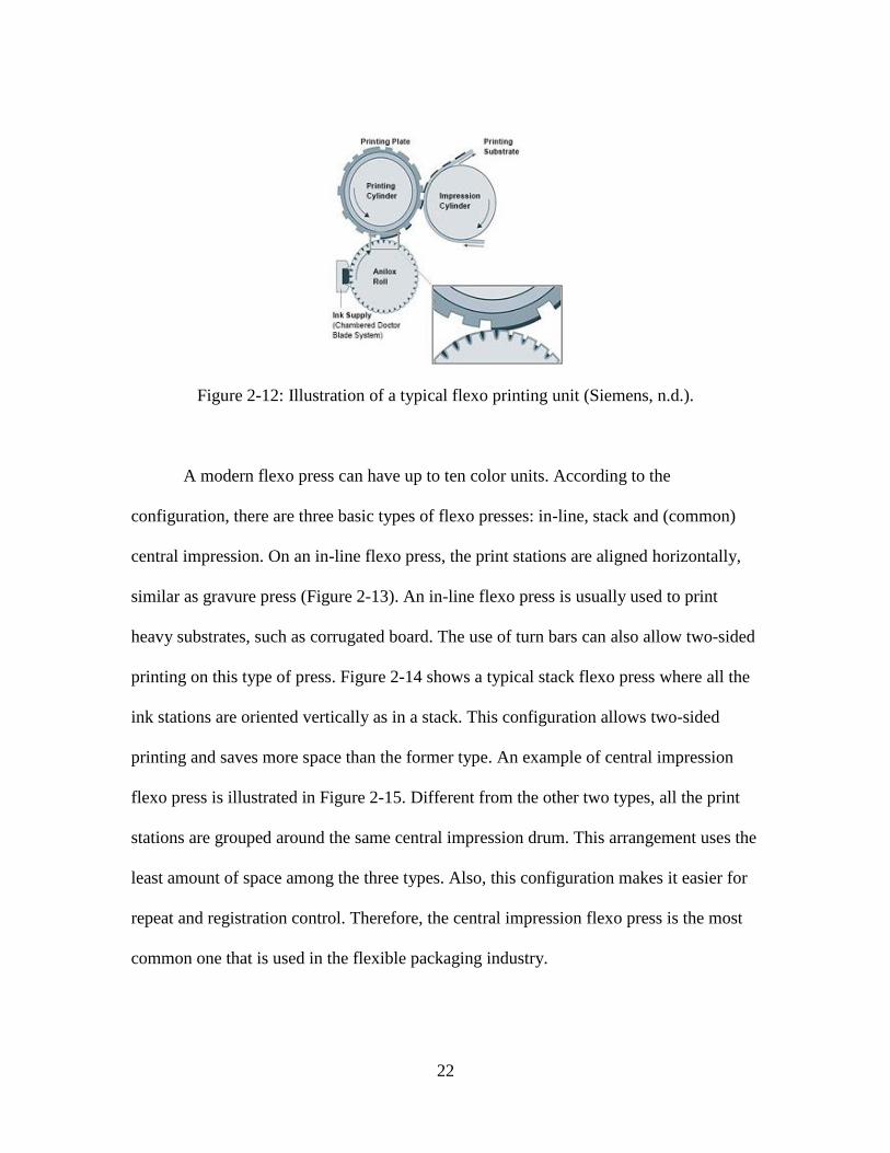
changeover, optional integration of processing units, and cost effectiveness. A typical
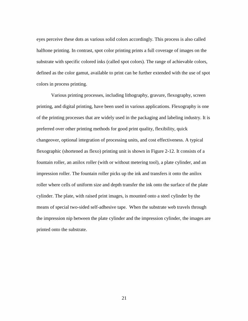
flexographic (shortened as flexo) printing unit is shown in Figure 2-12. It consists of a
fountain roller, an anilox roller (with or without metering tool), a plate cylinder, and an
impression roller. The fountain roller picks up the ink and transfers it onto the anilox
roller where cells of uniform size and depth transfer the ink onto the surface of the plate
cylinder. The plate, with raised print images, is mounted onto a steel cylinder by the
means of special two-sided self-adhesive tape. When the substrate web travels through
the impression nip between the plate cylinder and the impression cylinder, the images are
printed onto the substrate.
22
Figure 2-12: Illustration of a typical flexo printing unit (Siemens, n.d.).
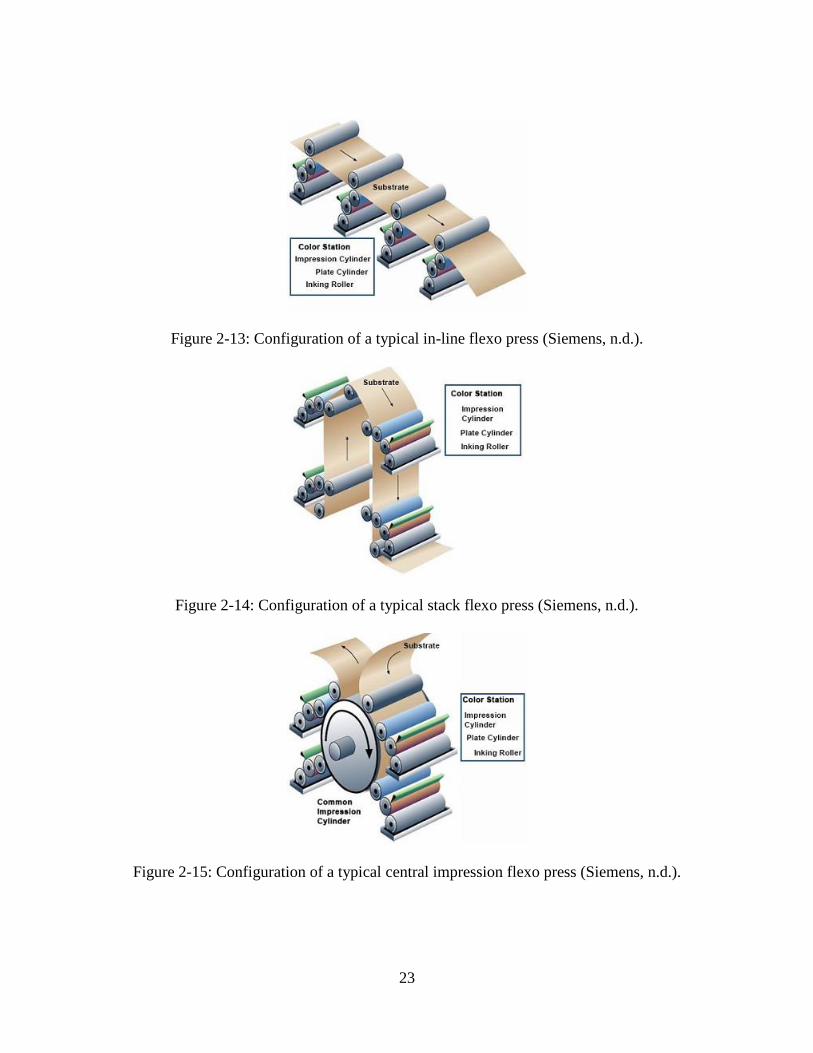
A modern flexo press can have up to ten color units. According to the
configuration, there are three basic types of flexo presses: in-line, stack and (common)
central impression. On an in-line flexo press, the print stations are aligned horizontally,
similar as gravure press (Figure 2-13). An in-line flexo press is usually used to print
heavy substrates, such as corrugated board. The use of turn bars can also allow two-sided
printing on this type of press. Figure 2-14 shows a typical stack flexo press where all the
ink stations are oriented vertically as in a stack. This configuration allows two-sided
printing and saves more space than the former type. An example of central impression
flexo press is illustrated in Figure 2-15. Different from the other two types, all the print
stations are grouped around the same central impression drum. This arrangement uses the
least amount of space among the three types. Also, this configuration makes it easier for
repeat and registration control. Therefore, the central impression flexo press is the most
common one that is used in the flexible packaging industry.
23
Figure 2-13: Configuration of a typical in-line flexo press (Siemens, n.d.).
Figure 2-14: Configuration of a typical stack flexo press (Siemens, n.d.).
Figure 2-15: Configuration of a typical central impression flexo press (Siemens, n.d.).
24
Ink Formulation
Ink formulation is mainly determined by substrate, printing method, substrate
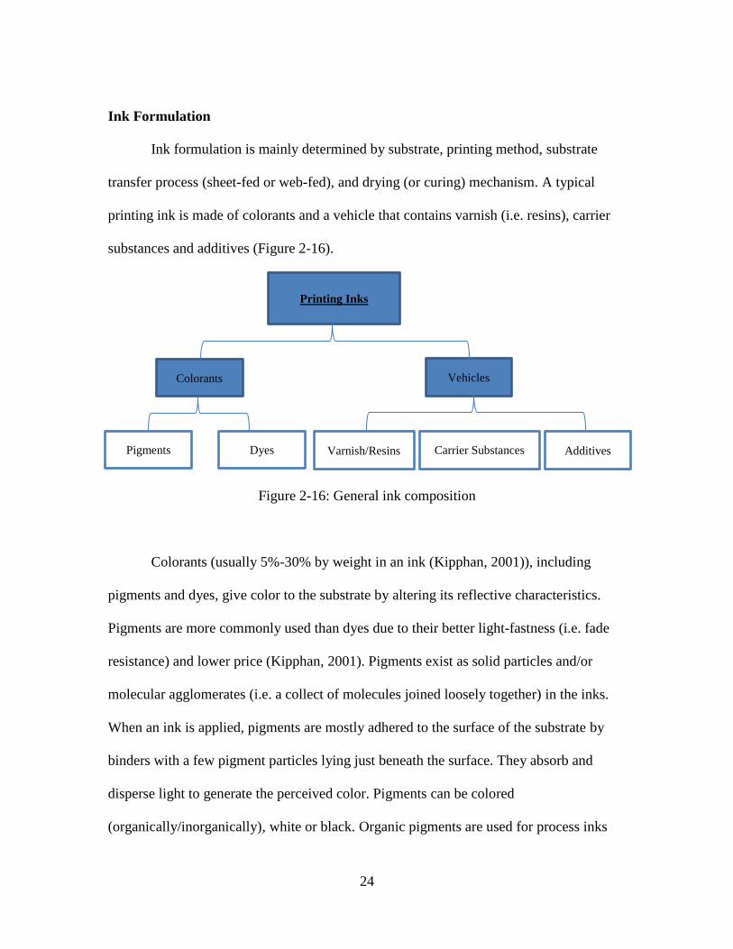
transfer process (sheet-fed or web-fed), and drying (or curing) mechanism. A typical
printing ink is made of colorants and a vehicle that contains varnish (i.e. resins), carrier
substances and additives (Figure 2-16).
Figure 2-16: General ink composition
Colorants (usually 5%-30% by weight in an ink (Kipphan, 2001)), including
pigments and dyes, give color to the substrate by altering its reflective characteristics.
Pigments are more commonly used than dyes due to their better light-fastness (i.e. fade
resistance) and lower price (Kipphan, 2001). Pigments exist as solid particles and/or
molecular agglomerates (i.e. a collect of molecules joined loosely together) in the inks.
When an ink is applied, pigments are mostly adhered to the surface of the substrate by
binders with a few pigment particles lying just beneath the surface. They absorb and
disperse light to generate the perceived color. Pigments can be colored
(organically/inorganically), white or black. Organic pigments are used for process inks
Additives Varnish/Resins Carrier Substances Pigments Dyes
Printing Inks
Colorants Vehicles
25
(CMYK) for their good transparency required by halftone process printing, while
inorganic pigments have better opacity than the organic ones (Chen, 2012). Dyes mostly
dissolve in the inks and generate a wider color gamut because of their higher efficiency
of selective absorption than pigments. However, they are not used in ink formulations as
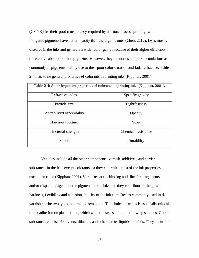
commonly as pigments mainly due to their poor color duration and fade resistance. Table
2-4 lists some general properties of colorants in printing inks (Kipphan, 2001).
Table 2-4: Some important properties of colorants in printing inks (Kipphan, 2001).
Refractive index Specific gravity
Particle size Lightfastness
Wettability/Dispersibility Opacity
Hardness/Texture Gloss
Tinctorial strength Chemical resistance
Shade Durability
Vehicles include all the other components: varnish, additives, and carrier
substances in the inks except colorants, so they determine most of the ink properties
except for color (Kipphan, 2001). Varnishes act as binding and film forming agents
and/or dispersing agents to the pigments in the inks and they contribute to the gloss,
hardness, flexibility and adhesion abilities of the ink film. Resins commonly used in the
varnish can be two types, natural and synthetic. The choice of resins is especially critical
to ink adhesion on plastic films, which will be discussed in the following sections. Carrier
substances consist of solvents, diluents, and other carrier liquids or solids. They allow the

26
ink to be transported from the ink fountain to the roller and mainly control the speed of
ink drying and/or curing, the mechanism of which varies with the ink system. They also
help to control the ink viscosity, which is one of the important factors in printing.
Various additives (typically 0-10% by weight in an ink (Kipphan, 2001)) are
available to further adjust the ink properties, such as ink tack, drying, flow behavior, and
end-use properties. For instance, anti-skinning agents or antioxidants are used to prevent
premature drying and skin formation on the surface, in the can or in the ink fountain.
Waxes are commonly used to improve the slip properties and rub resistance of the final
print. It is important to choose the additives that provide the desired ink properties and
are also compatible with the other components in the ink system.
Flexographic Inks
Flexographic (flexo) inks can be solvent-based, water-based or energy-cured
depending on the vehicles. To formulate an ink, the ink manufacturer needs to know what
properties are desired for both the specific printing process and the product application.
Desired color properties, ink adhesion and other end-use properties, such as slip, rub and
heat resistance, etc. are the basic requirements for flexo inks. Also, the inks also must
meet multiple requirements for proper processing on the flexo press. For instance, flexo
inks must be fluid enough, i.e. have relatively low viscosity. This allows inks to be
pumped and freely flow in the system, as well as to be transferred from roll to roll
relatively evenly. However, they cannot be too fluid to interfere with achieving the
desired thickness of ink film on the substrate. The selection of solvents in flexo inks is

27
another key which controls not only the ink viscosity but also the drying speed. Ideally,
the ink should not dry so fast that it dries into the cells of the anilox roller, yet it has to be
quickly dried and/or cured once being applied onto the substrate prior to the next printing
station.
As mentioned before, colorants are responsible for all the color-related properties
of the final print and vehicles take care of the rest. In flexo ink vehicles, resins, also
called varnish, are required to provide good solubility in the solvents, good adhesion to
substrates, good pigment-wetting, good solvent release, good film-forming properties,
low odor, and compatibility with other resins, etc. (Leach & Pierce, 1999). To meet these
requirements, a blend of resins is usually used in an ink system. The selection of resin
blends is determined by the substrate to be printed due to the different adhesion
mechanisms on different substrates. In this study, water-based flexo inks will be applied
on the polyolefin films.
When printing on polyolefins, the colorants used are similar to other conventional
water-based inks, but the compositions of ink vehicles, especially varnishes, are unique.
On polyolefin films, one of the keys to achieving good adhesion is to control the film
forming properties of the emulsion resins in the vehicle. Theoretically, the resins with
low Tg (i.e. “soft”) exhibit good ink adhesion, as well as offers a flexible ink film, on the
polyolefin substrates (Leach & Pierce, 1999). Emulsion resin does not dissolve in water
but forms an ink film as the hydroxide and amines are released from the ink during
drying through the evaporation of solvents. Acrylic emulsion resins can be used to obtain
good ink film formation, flexibility, hardness, water resistance, and high gloss, etc.
28
(Pekarovicova, 2013). Meanwhile, water-soluble resins need to be included in the
formulations to enhance the wetting of pigment particles, and improve ink drying and
resolubility. Water-soluble acrylic resins such as polyester-acrylics (PEA), styrene-
acrylics (SAA) and polyurethane acrylics (PUA) are often used to balance the ink
properties (Pekarovicova, 2013). To ensure good solubility, the pH value of the liquid ink
needs to be controlled in the range of 8.5-9.0 through the use of ammonia or amines
(Pekarovicova, 2013). Alternatively, other resin systems exhibiting good ink adhesion to
polyolefin films are also available, such as water-based polyurethanes, polyamides and
nitrocellulose (Leach & Pierce, 1999; Pekarovicova, 2013). These resin systems also
have to exhibit proper film forming properties and molecular affinity for the polyolefin
substrates.
Solvents can affect ink adhesion in three ways. First, solvents assist the wetting
and flow-out of ink to create a continuous ink film on the surface of the substrate.
Secondly, the evaporation rate of solvents affects the quality of ink film. Evaporating too
rapidly can result in a high surface energy gradient on the ink film during drying, which
leads to many print defects, such as craters (Sharma & Micale, 1991). Lastly, solvents
can penetrate into some substrates, such as paper and PVC, to cause softening of the
surface to assist physical and chemical bonding (Leach & Pierce, 1999). In water-based
flexo inks, solvents are often comprised of water and small amounts of alcohols to
increase the drying speed. It is also worth noting that water-based inks will not dissolve
the “boundary layer” (process additives, organic contaminations) on the polyolefin films
as readily as solvent-based inks, so they usually require the substrates to have higher
29
surface treatment levels (Leach & Pierce, 1999). Ammonia is often added to adjust the
pH to be in the range of 8.5-9.0.
Additives used in water-based flexo inks vary with the needs. In this study, it is
worth mentioning that adhesion promoters are often added to the inks to improve
adhesion to the polyolefin films. For example, Tyzor® titanates and zirconates are two
adhesion promoters commercially available to add into the ink formulation (Awaja, et al.,
2009). Their adhesion functions are achieved by bonding to the functional groups (e.g. -
OH, - COOH) of the ink resins and the substrates, so surface treatment (which will be
introduced later) is still required on the substrates in order to create functional groups.
Surface Tension/Surface Energy
Once an ink is applied onto the substrate, it must wet the surface sufficiently in
order to further adhere to the substrate as it dries and cures. The wettability of an ink on a
substrate is determined by the surface tension/surface energy compatibility of the two
materials.
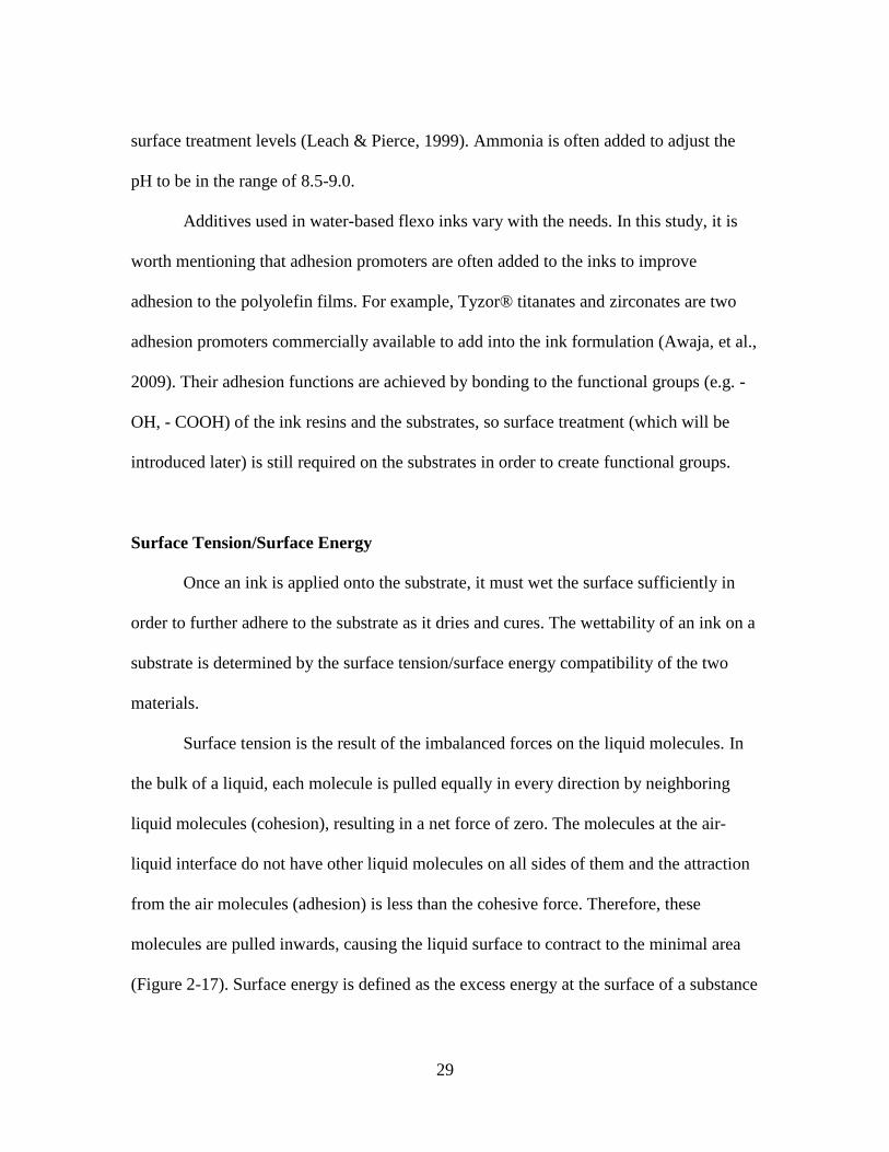
Surface tension is the result of the imbalanced forces on the liquid molecules. In
the bulk of a liquid, each molecule is pulled equally in every direction by neighboring
liquid molecules (cohesion), resulting in a net force of zero. The molecules at the air-
liquid interface do not have other liquid molecules on all sides of them and the attraction
from the air molecules (adhesion) is less than the cohesive force. Therefore, these
molecules are pulled inwards, causing the liquid surface to contract to the minimal area
(Figure 2-17). Surface energy is defined as the excess energy at the surface of a substance
30
compared to the bulk. Also called surface free energy, surface energy physically
quantifies the disruption of intermolecular bonds that occur when a surface is created.
Although surface tension is derived from force per unit length and surface energy is
defined by the work per unit area, they are essentially the same and both can be expressed
in the unit of dynes/cm or mN/m. In the industry, surface tension and surface energy are
used interchangeably. To reduce confusion, surface tension will be specified for liquids
and surface energy will be used for solids in this manuscript.
Figure 2-17: Diagram of the forces on molecules of liquid.
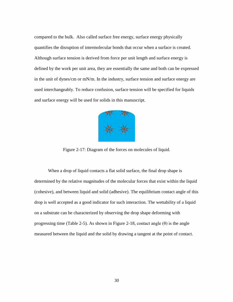
When a drop of liquid contacts a flat solid surface, the final drop shape is
determined by the relative magnitudes of the molecular forces that exist within the liquid
(cohesive), and between liquid and solid (adhesive). The equilibrium contact angle of this
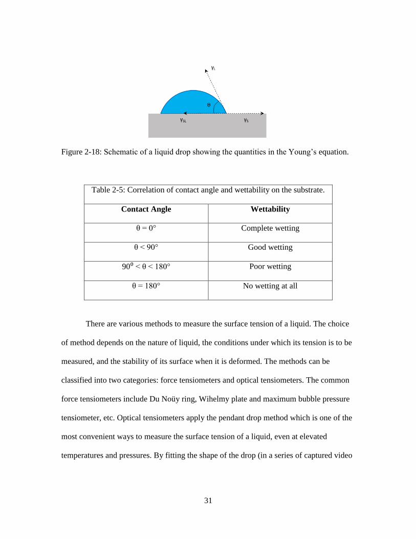
drop is well accepted as a good indicator for such interaction. The wettability of a liquid
on a substrate can be characterized by observing the drop shape deforming with
progressing time (Table 2-5). As shown in Figure 2-18, contact angle (θ) is the angle
measured between the liquid and the solid by drawing a tangent at the point of contact.
31
Figure 2-18: Schematic of a liquid drop showing the quantities in the Young’s equation.
Table 2-5: Correlation of contact angle and wettability on the substrate.
Contact Angle Wettability
θ = 0° Complete wetting
θ < 90° Good wetting
90⁰ < θ < 180° Poor wetting
θ = 180° No wetting at all
There are various methods to measure the surface tension of a liquid. The choice
of method depends on the nature of liquid, the conditions under which its tension is to be
measured, and the stability of its surface when it is deformed. The methods can be
classified into two categories: force tensiometers and optical tensiometers. The common
force tensiometers include Du Noüy ring, Wihelmy plate and maximum bubble pressure
tensiometer, etc. Optical tensiometers apply the pendant drop method which is one of the
most convenient ways to measure the surface tension of a liquid, even at elevated
temperatures and pressures. By fitting the shape of the drop (in a series of captured video

32
images) to the Young-Laplace equation, one can relate the drop shape parameters to the
interfacial tension.
It is relatively easy and straightforward to measure the surface tension of a liquid.
On the contrary, determining the surface energy of a solid is not nearly as simple. Dupré
presented the concepts of the work of adhesion and work of cohesion between two
substances in equations 1 and 2 (Jaycock & Parfitt, 1981).
For two immiscible substances, the energy per unit area necessary to achieve the
separation of the substances, i.e. work of adhesion, is
𝑊𝑎 = 𝛾1 + 𝛾2 − 𝛾12 Equation 1
For a single substance, the energy per unit area necessary to overcome the
intermolecular (cohesive) forces of molecules of the same species, i.e. work of cohesion,
is
𝑊𝑐 = 𝛾1 + 𝛾1 = 2 𝛾1 Equation 2
Where:
Wa: Work of adhesion;
Wc: Work of cohesion;
γ1: Surface tension/surface energy of substance 1;
γ2: Surface tension/surface energy of substance 2;
γ12: Interfacial energy between substances 1 and 2.
Another fundamental equation was derived to express the equilibrium of a liquid
drop wetting on an ideal solid surface that is smooth, rigid, chemically homogeneous, and
33
not soluble in the liquid phase (Figure 2-13) (Jaycock, et al., 1981). This is known as
Young’s equation.
𝛾𝑆 = 𝛾𝑆𝐿 + 𝛾𝐿 cos 𝜃𝑐 + 𝜋𝑒 Equation 3
Where:
θC: Contact angle;
γS: Solid surface energy;
γSL: Solid-liquid interfacial energy;
γL: Liquid surface tension;
πe: A factor that accounts for the equilibrium pressure of adsorbed vapor of the
liquid on the solid.
Equation 3 was applied in the Zisman method to approximate surface energy
where an empirical curve is plotted with cosθ of many liquids on the same surface against
the liquid surface tension (γL). The “critical surface tension” can then be obtained by
extrapolating to cosθ=1. It is found that this critical value is very close to the surface
energy of the solid, although it is strictly correct only when the interfacial energy (γLS)
and the equilibrium vapor pressure (πe) are negligible under the condition of cosθ=1
(Zisman, 1964). In reality, these conditions are often not met. However, this method has
been demonstrated to be useful for simple comparison of polymer surface energy,
especially in the industry when multiple dyne solutions are available (Sabbatini, 2014).
Assuming that the vapor pressure of the solid (πe) is negligible, Young’s equation
can be simplified in a more general form:

34
𝛾𝑆 = 𝛾𝑆𝐿 + 𝛾𝐿 cos 𝜃 Equation 4
Where
θ: Contact angle;
γS: Surface energy of the solid;
γSL: Solid-liquid interfacial energy;
γL: Surface tension of the liquid.
Combining equations 1 and 3, the work of adhesion between a drop of liquid and
a flat solid can be expressed in Young-Dupré equation (Jaycock, et al., 1981).
𝑊𝑎 = 𝛾𝐿 + 𝛾𝑆 − 𝛾𝐿𝑆 = 𝛾𝐿(1 + cos 𝜃) Equation 5
This equation states that adhesion is favored by low interfacial energy. The work
of adhesion has also been expressed by the geometric mean of the two substances in
Girifalco and Good equation (Good & Girifalco, 1956):
𝑊𝑎 = 2Φ√(𝛾1𝛾2 ) Equation 6
Where Φ is an interaction parameter for the correction of this equation. It is
related to the molar volumes (V) of these substances. Several methods have been
suggested to determine this parameter in different systems. For instance, one can
calculate empirical values for Φ by using the values of Φ measured by liquid/liquid
interactions in systems of similar polarity. Using an extensive amount of low energy
polymers, Kwok and Neumann proposed to use an analytical expression and equation of
state for Φ (Kwok and Neumann, 1999). In many papers, the interaction parameter Φ ≈ 1
is often used for the approximation of surface energy, especially for polymers (Equation
7) (Jaycock, et al., 1981; Agrawal, 2005). Thus,
35
𝑊𝑎 = 2√(𝛾1𝛾2 ) Equation 7
With this equation, the work of adhesion (or adhesion energy) between the
wetting liquid and the polyolefin film can be found, i.e.
𝑊𝑎 = 2√(𝛾𝑆𝛾𝐿 ) Equation 8
Combining the second part of equations 5 and equation 8, the surface energy of a
solid can be approximated by measuring the contact angle of a liquid with known surface
tension on its surface using equation 9.
𝛾𝑠 =𝛾𝐿(1+cos 𝜃)2
4 Equation 9
With the first part of equations 5 and equation 8, the interfacial energy between a
liquid and a solid can be obtained using the following equation.
𝛾𝐿𝑆 = 𝛾𝐿 + 𝛾𝑆 − 2√(𝛾𝐿𝛾𝑆 ) Equation 10
The Girifalco and Good theory was then applied by Fowkes for the approximation
of interfacial energy of two substances with only dispersive interactions (𝛾12 = 𝛾1 + 𝛾2 −
2√(𝛾1𝑑𝛾2
𝑑), Equation 11) (Fowkes, 1964). Combining with Young’s equation (Equation
4), the dispersive energy, i.e. surface energy in this case, can be obtained by measuring
the contact angle using a liquid with a known dispersive tension (surface tension in this
case). After Fowkes determined the interfacial energy of different substances resulting
from other molecular interactions, he suggested that the total work of adhesion should
account for all types of molecular interactions between the two surfaces (Fowkes, 1964;
Owens & Wendt, 1969). Fowkes’ theory was then extended and put into mathematical
expressions. Note that this theory and its extended theories all assume that the
36
equilibrium vapor pressure (πe) is negligible and the interaction parameter Φ ≈ 1
(Fowkes, 1964; Owens & Wendt, 1969; Jaycock, et al., 1981; Agrawal, 2005; Sabbatini
ed., 2014).
The Owens-Wendt method essentially can be considered as one of the extensions
of Fowkes’ theory where surface energy is attributed to dispersive and polar (hydrogen
bonding and dipole-dipole) interactions (Owens & Wendt, 1969). Thus, the interfacial
energy between a liquid and a solid can be expressed as
𝛾𝐿𝑆 = 𝛾𝐿 + 𝛾𝑆 − 2√(𝛾𝐿𝑑𝛾𝑆
𝑑) − 2√(𝛾𝐿𝑝𝛾𝑆
𝑝) Equation 12
Substituting the interfacial energy in the Young’s equation (Equation 4), one can
obtain the Owens-Wendt equation as follows (Owens & Wendt, 1969).
1 + cos 𝜃 = 2√𝛾𝑆𝑑(
√𝛾𝐿𝑑
𝛾𝐿+ 2√𝛾𝑆
𝑝(√𝛾𝐿
𝑝
𝛾𝐿) Equation 13
With this equation, the dispersive and polar components of surface energy can be
obtained by measuring the contact angles using two liquids with known dispersive and
polar components. Owens and Wendt (1969) recommended water (polar) and methylene
iodide (MI) (non-polar) as the testing liquids. In testing, the Owens-Wendt equation can
be written a linear form as Y=mX +b:
𝛾𝐿(cos 𝜃+1)
2 √𝛾𝐿𝑑
= √𝛾𝑆𝑝√
𝛾𝐿𝑝
𝛾𝐿𝑑 + √𝛾𝑆
𝑑 Equation 14
Where 𝑌 =𝛾𝐿(cos 𝜃+1)
2 √𝛾𝐿𝑑
, 𝑚 = √𝛾𝑆𝑝 , 𝑋 = √
𝛾𝐿𝑝
𝛾𝐿𝑑 and 𝑏 = √𝛾𝑆
𝑑
37
Hence, after measuring the contact angles on the testing substrate using a polar
liquid and a non-polar liquid respectively, one can plot a line with these two sets of data
which include the contact angles and the polar and dispersive components of the testing
liquids used. As in equation 14, the slope of the line gives the polar component of the
surface energy of the substrate (γSp) and the intercept gives the dispersive component
(γSd). This method is most applicable to surfaces that have low surface charge and are
moderately polar in nature. Polymers containing atoms other than carbons and hydrogens,
like polyvinyl chloride (PVC), polyurethanes, polyimides, polyesters (PET),
polyacrylates, polycarbonates are all good examples (Hansen, 2004; Krϋss, n.d.).
In principle, molecular interactions can be categorized into London dispersive
interaction and polar interactions including hydrogen bonding, dipole-to-dipole and
dipole-induced dipole interactions, etc. To extend Fowkes’ theory, the interactive forces
are additive in a general form as in equation 15.
𝛾 = 𝛾𝑑 + 𝛾𝑝 + 𝛾ℎ + 𝛾𝑎𝑏 + ⋯ Equation 15
Where the superscripts d= dispersion force, p= other polar force, h=hydrogen
bonding, ab=acid/base force, etc. The geometric mean is used to calculate the work of
adhesion for each type of force/energy:
𝑊12𝑑 = 2√(𝛾1
𝑑𝛾2𝑑) Equation 16
𝑊12𝑝 = 2√(𝛾1
𝑝𝛾2𝑝) Equation 17
𝑊12ℎ = 2√(𝛾1
ℎ𝛾2ℎ) Equation 18

38
Similarly to the Owens-Wendt method, one can obtain n different components of
surface energy by measuring the contact angles of n different liquids on the same solid
surface, as long as the corresponding n components of the liquids are known (Hansen,
2004; Kitazaki & Hata, 1972). This method is often referred to as the extended Fowkes’
method and it was first demonstrated by Kitazaki and Hata (1972) three years after the
publication of the Owens-Wendt method by studying the dispersive, hydrogen bonding,
and other polar components of the surface energy.
As multiple methods are available for the approximation of solid surface energy,
it is important to understand the specific molecular interactions of the substances prior to
the selection of method and testing liquid (s). As a rule of thumb, the methods that do not
emphasize specific molecular interactions should be used to characterize non-polar
surfaces (e.g. Zisman plot), while those that emphasize molecular interactions by
modeling the solid as having either two or three components to its surface energy should
be applied in the measurement of polar surfaces (Krϋss, n.d.). Moreover, it is meaningless
to compare any surface energy values (for the same sample or for two different samples)
that are not approximated using the same method.
Impacts of Corona Treatment on Ink Wetting and Adhesion
The surface tension of water-based flexo ink is typically around 35-40 dynes/cm
(Wolf, 2014). As a rule of thumb, good ink wettability requires the surface energy of the
substrate to be at least 10 dynes/cm higher than the surface tension of the ink (Leach &
Pierce, 1999; Wolf, 2014). However, the original surface energy of polyolefin films is
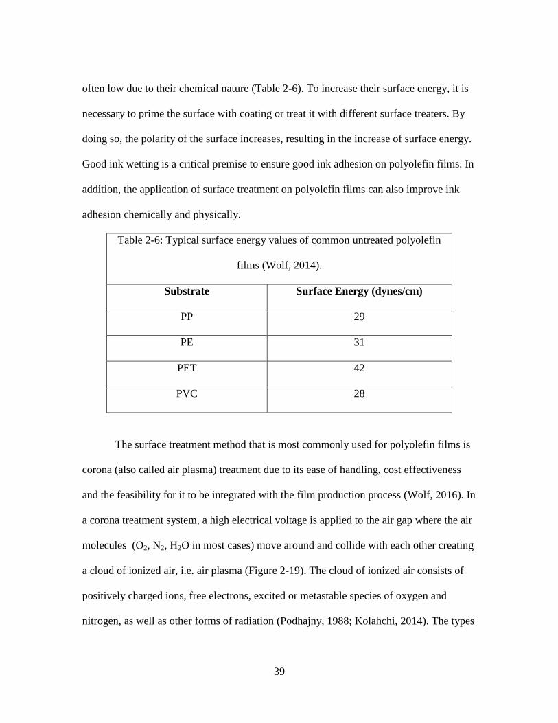
39
often low due to their chemical nature (Table 2-6). To increase their surface energy, it is
necessary to prime the surface with coating or treat it with different surface treaters. By
doing so, the polarity of the surface increases, resulting in the increase of surface energy.
Good ink wetting is a critical premise to ensure good ink adhesion on polyolefin films. In
addition, the application of surface treatment on polyolefin films can also improve ink
adhesion chemically and physically.
Table 2-6: Typical surface energy values of common untreated polyolefin
films (Wolf, 2014).
Substrate Surface Energy (dynes/cm)
PP 29
PE 31
PET 42
PVC 28
The surface treatment method that is most commonly used for polyolefin films is
corona (also called air plasma) treatment due to its ease of handling, cost effectiveness
and the feasibility for it to be integrated with the film production process (Wolf, 2016). In
a corona treatment system, a high electrical voltage is applied to the air gap where the air
molecules (O2, N2, H2O in most cases) move around and collide with each other creating
a cloud of ionized air, i.e. air plasma (Figure 2-19). The cloud of ionized air consists of
positively charged ions, free electrons, excited or metastable species of oxygen and
nitrogen, as well as other forms of radiation (Podhajny, 1988; Kolahchi, 2014). The types
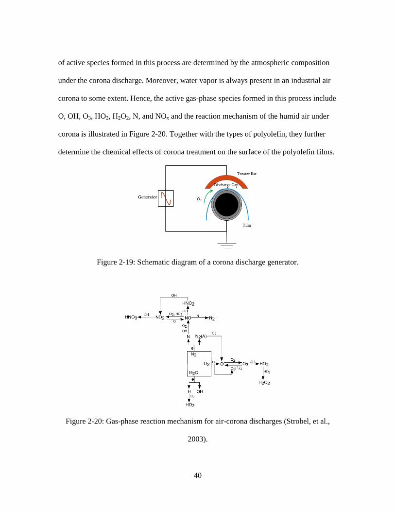
40
of active species formed in this process are determined by the atmospheric composition
under the corona discharge. Moreover, water vapor is always present in an industrial air
corona to some extent. Hence, the active gas-phase species formed in this process include
O, OH, O3, HO2, H2O2, N, and NOx and the reaction mechanism of the humid air under
corona is illustrated in Figure 2-20. Together with the types of polyolefin, they further
determine the chemical effects of corona treatment on the surface of the polyolefin films.
Figure 2-19: Schematic diagram of a corona discharge generator.
Figure 2-20: Gas-phase reaction mechanism for air-corona discharges (Strobel, et al.,
2003).
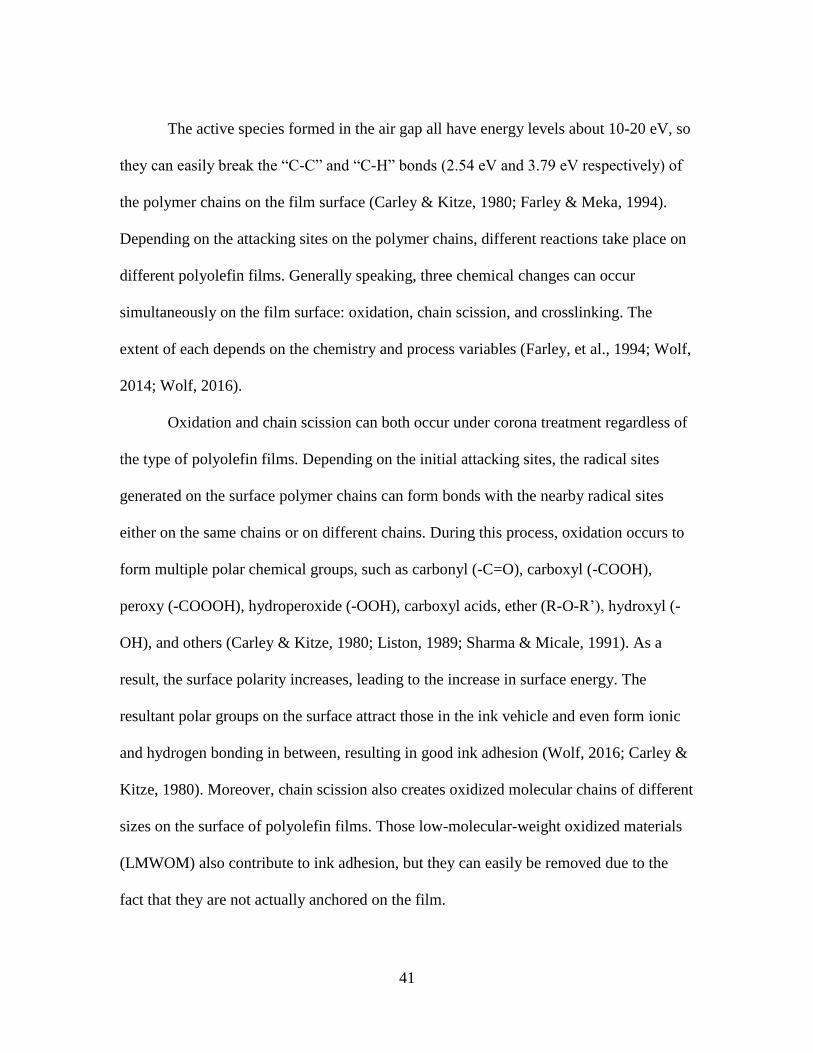
41
The active species formed in the air gap all have energy levels about 10-20 eV, so
they can easily break the “C-C” and “C-H” bonds (2.54 eV and 3.79 eV respectively) of
the polymer chains on the film surface (Carley & Kitze, 1980; Farley & Meka, 1994).
Depending on the attacking sites on the polymer chains, different reactions take place on
different polyolefin films. Generally speaking, three chemical changes can occur
simultaneously on the film surface: oxidation, chain scission, and crosslinking. The
extent of each depends on the chemistry and process variables (Farley, et al., 1994; Wolf,
2014; Wolf, 2016).
Oxidation and chain scission can both occur under corona treatment regardless of
the type of polyolefin films. Depending on the initial attacking sites, the radical sites
generated on the surface polymer chains can form bonds with the nearby radical sites
either on the same chains or on different chains. During this process, oxidation occurs to
form multiple polar chemical groups, such as carbonyl (-C=O), carboxyl (-COOH),
peroxy (-COOOH), hydroperoxide (-OOH), carboxyl acids, ether (R-O-R’), hydroxyl (-
OH), and others (Carley & Kitze, 1980; Liston, 1989; Sharma & Micale, 1991). As a
result, the surface polarity increases, leading to the increase in surface energy. The
resultant polar groups on the surface attract those in the ink vehicle and even form ionic
and hydrogen bonding in between, resulting in good ink adhesion (Wolf, 2016; Carley &
Kitze, 1980). Moreover, chain scission also creates oxidized molecular chains of different
sizes on the surface of polyolefin films. Those low-molecular-weight oxidized materials
(LMWOM) also contribute to ink adhesion, but they can easily be removed due to the
fact that they are not actually anchored on the film.
42
Therefore, surface molecular weight distribution plays another critical role in the
ink adhesion on the treated polyolefin films. It is considered to be comparable in
importance for determining the practical performance properties of the treated surface as
the extent of oxidation and the types of oxidized functionalities found on the modified
polymer (Földes, Tóth, Kálmán, Fekete, & Tomasovszky-Bobák, 2000).
In addition, previous studies also found that PP tends to undergo β-scission or
disproportion faster than combining with oxygen due to its unstable tertiary radicals
formed under corona discharging (Strobel, et al., 2003). By contrast, PE chains form
primary and secondary radicals, which more readily combine with oxygen to form polar
groups, such as alcohol (-OH), ketone (-C=O), or ester (-O-C=O) (Farley, et al., 1994;
Nihlstrand, Hjerberg & Johansson, 1997). In other words, PE tends to be oxidized more
easily resulting in higher polarity than PP under the same level of corona treatment, while
PP tends to undergo more chain scission than oxidation (Zenkiewicz, 2001; Strobel, et
al., 2003; Nuntapichedkula, Tantayanonb & Laohhasurayotinda, 2014). Moreover, the
polymer chains on the surface of PE films tend to crosslink to a higher degree than those
on the PP films due to the lack of side group (-CH3) hindrance. The formation of the
crosslinked structure hinders the mobility and rearrangements of polar functional groups
at the surface, which affects ink adhesion as well (Kwon, Tang, Myung, Lu & Choi,
2005).
As the high energy particles bombard the film surface, small micro-voids can also
form simultaneously. Such a “roughening” effect provides the ink with more sites and
larger surface area to “bite” onto the surface, allowing further mechanical interlocking
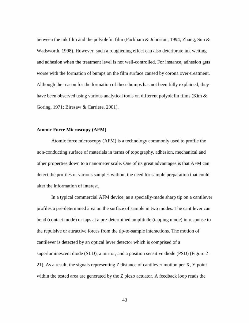
43
between the ink film and the polyolefin film (Packham & Johnston, 1994; Zhang, Sun &
Wadsworth, 1998). However, such a roughening effect can also deteriorate ink wetting
and adhesion when the treatment level is not well-controlled. For instance, adhesion gets
worse with the formation of bumps on the film surface caused by corona over-treatment.
Although the reason for the formation of these bumps has not been fully explained, they
have been observed using various analytical tools on different polyolefin films (Kim &
Goring, 1971; Biresaw & Carriere, 2001).
Atomic Force Microscopy (AFM)
Atomic force microscopy (AFM) is a technology commonly used to profile the
non-conducting surface of materials in terms of topography, adhesion, mechanical and
other properties down to a nanometer scale. One of its great advantages is that AFM can
detect the profiles of various samples without the need for sample preparation that could
alter the information of interest.
In a typical commercial AFM device, as a specially-made sharp tip on a cantilever
profiles a pre-determined area on the surface of sample in two modes. The cantilever can
bend (contact mode) or taps at a pre-determined amplitude (tapping mode) in response to
the repulsive or attractive forces from the tip-to-sample interactions. The motion of
cantilever is detected by an optical lever detector which is comprised of a
superluminescent diode (SLD), a mirror, and a position sensitive diode (PSD) (Figure 2-
21). As a result, the signals representing Z distance of cantilever motion per X, Y point
within the tested area are generated by the Z piezo actuator. A feedback loop reads the
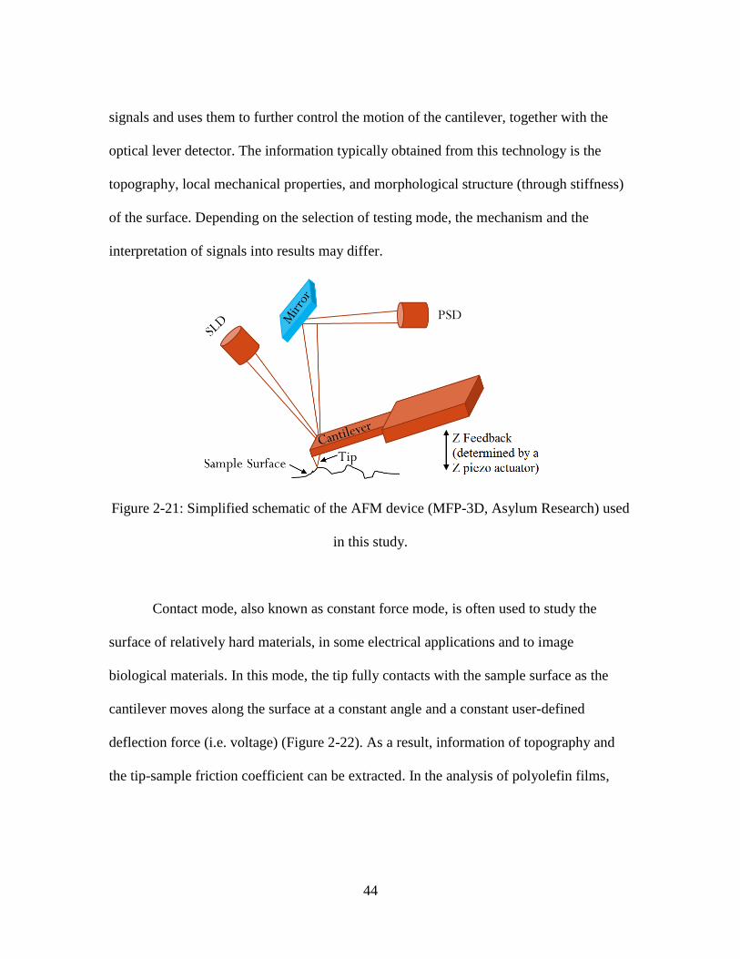
44
signals and uses them to further control the motion of the cantilever, together with the
optical lever detector. The information typically obtained from this technology is the
topography, local mechanical properties, and morphological structure (through stiffness)
of the surface. Depending on the selection of testing mode, the mechanism and the
interpretation of signals into results may differ.
Figure 2-21: Simplified schematic of the AFM device (MFP-3D, Asylum Research) used
in this study.
Contact mode, also known as constant force mode, is often used to study the
surface of relatively hard materials, in some electrical applications and to image
biological materials. In this mode, the tip fully contacts with the sample surface as the
cantilever moves along the surface at a constant angle and a constant user-defined
deflection force (i.e. voltage) (Figure 2-22). As a result, information of topography and
the tip-sample friction coefficient can be extracted. In the analysis of polyolefin films,
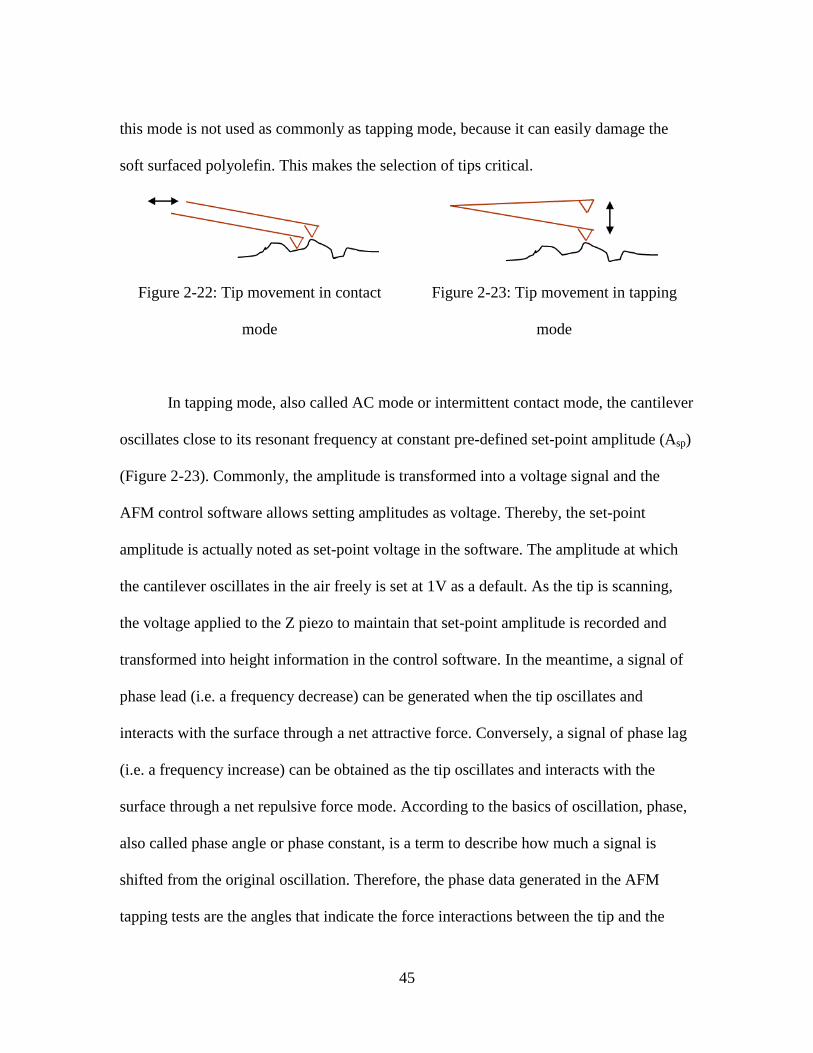
45
this mode is not used as commonly as tapping mode, because it can easily damage the
soft surfaced polyolefin. This makes the selection of tips critical.
Figure 2-22: Tip movement in contact
mode
Figure 2-23: Tip movement in tapping
mode
In tapping mode, also called AC mode or intermittent contact mode, the cantilever
oscillates close to its resonant frequency at constant pre-defined set-point amplitude (Asp)
(Figure 2-23). Commonly, the amplitude is transformed into a voltage signal and the
AFM control software allows setting amplitudes as voltage. Thereby, the set-point
amplitude is actually noted as set-point voltage in the software. The amplitude at which
the cantilever oscillates in the air freely is set at 1V as a default. As the tip is scanning,
the voltage applied to the Z piezo to maintain that set-point amplitude is recorded and
transformed into height information in the control software. In the meantime, a signal of
phase lead (i.e. a frequency decrease) can be generated when the tip oscillates and
interacts with the surface through a net attractive force. Conversely, a signal of phase lag
(i.e. a frequency increase) can be obtained as the tip oscillates and interacts with the
surface through a net repulsive force mode. According to the basics of oscillation, phase,
also called phase angle or phase constant, is a term to describe how much a signal is
shifted from the original oscillation. Therefore, the phase data generated in the AFM
tapping tests are the angles that indicate the force interactions between the tip and the
46
sample surface. Note that the term of “phase” in chemistry is defined as a distinct and
homogeneous state of a system that does not have a visible boundary to separate itself
into parts. To differentiate these two concepts of “phase” in this manuscript, the phase
data directly obtained from AFM measurements are referred to as “phase angle”. Other
than that, the “phase” refers to its definition in chemistry.
Typically, the height (i.e. roughness) and phase angle at each point scanned by the
cantilever are collected by the AFM software. In the results of topography, AFM
typically reports the descriptive statistics of the roughness data, including mean, standard
deviation, and median, etc. In addition, the root mean square (RMS) roughness is also
calculated using the following equation.
𝑅𝑀𝑆 = √(𝑍12+𝑍2
2+𝑍32…+𝑍𝑛
2
𝑛 Equation 19
When the tip surveys the surface, AFM control software automatically determines
a reference plane (assigned Z=0) based on the scanning data in order to produce a
topographic image with the best contrast. Accordingly, the height data generated in this
way can be either positive or negative. Thus, the regular average roughness sometimes
could be very close to zero which does not reflect the true roughness of the surface. In
this case, calculating the mean of the absolute heights or RMS becomes more helpful
since they represent the true surface roughness. In this study, the means and standard
deviations of roughness were all calculated using the absolute heights measured by AFM.
In the results of phase angle scan, a phase angle image constituted of all the phase
angles and their corresponding locations within the selected scan area can be obtained. A
distribution curve of all the phase angles can also be generated in the AFM software.
47
It has been demonstrated that the contrast of height and phase angle images are
highly dependent on experimental conditions, including the cantilever force constant, the
tip shape, the free-air vibration amplitude A0, and particularly the set-point amplitude
ratio (R = Asp/A0) (Brandsch, Bar & Whangbo,1997; Whangbo, Bar & Brandsch, 1998;
Bar, Brandsch & Whangbo, 1999; Magonov, 2000; Godehardt, et al., 2004). It has been
well accepted that the set-point amplitude ratio R ≈ 0.8 is considered as “light tapping”
and R ≈ 0.5 is “hard tapping” (Chang, et al., 2002; Fuierer, 2009; Rams, et al. 2012, etc.).
In other words, when the free-air amplitude is usually A0 = 1 V, the set-point amplitude in
light tapping mode should be Asp = 800 mV and the set-point amplitude in hard tapping
mode should be Asp = 500 mV. Many previous studies have demonstrated that the height
image obtained within a larger scan size (e.g. 20×20 µm2 or 10×10 µm
2) in the light
tapping mode presents the true topography of the sample. Moreover, the phase angle
image measured on a smaller scan size (e.g. 5×5 µm2 or 1×1 µm
2) in the hard tapping
mode has also been proven to accentuate the contrast of phase angle image which results
in the best morphological structure (Chang, et al., 2002; Fuierer, 2009; Rams, et al. 2012,
etc.). Thereby, not only force modulation mode (not used in this work) (Radmacher,
Tillmann & Gaub, 1991; Chen & Thomas, 1996; Galuska, Poulter & McElrath, 1997) but
also the phase angle mode with hard tapping can detect the interactions in polymer blends
by investigating the resultant morphological structure information (Chang, et al., 2002;
Godehardt, et al., 2004; Fuierer, 2009; Rams, et al., 2012). In the analysis of polyolefins,
the AFM hard tapping mode has proven to be efficient at differentiation of different
phases in polyolefin blends, as well as that of the amorphous and crystalline phases

48
within a semicrystalline polymer. Therefore, it is often used to study the impacts of
various processes, such as thermal treatment, film casting/extrusion/orientation, and
surface treatment by tracking the evolution of the surface characteristics of interest.
Electron Spectroscopy for Chemical Analysis (ESCA)
Electron spectroscopy for chemical analysis (ESCA), also called X-Ray
photoelectron spectroscopy (XPS), is a powerful tool to identify the atomic compositions,
the relative percentage of each component, atomic structure, and the oxidation state of a
surface layer that is a few nanometers thick. An ESCA mainly contains an X-ray source,
a sample holder, an analyzer, a detector, a signal processor and read-out, and a vacuum
chamber. An X-ray beam of known energy (hv) irradiates the sample surface and excites
an atom on the surface to emit electrons with energy (Ek). The emitted electrons are
collected and analyzed by the analyzer, which disperses these electrons according to their
kinetic energy. A term defined as binding energy can be calculated using the following
equation.
Eb = hv - Ek – w Equation 20
Where
Eb: Binding energy of an electron;
h: Planck’s constant, which is equal to 6.6254×10⁻³⁴
J/s;
v: Frequency of the incident photon;
Ek: Energy of the emitted electron;
w: a correction factor of the spectrometer.

49
A survey scan spectrum of intensity vs. binding energy, containing multiple peaks
corresponding to different atoms, is first generated for the qualitative determination of the
surface elemental composition. The peaks (i.e. atoms) of interest in the survey spectrum
can be further examined to provide more detailed information in terms of the number of
valence electrons and the type of bonds the corresponding atoms have. Such information
allows quantifying each type of bond that an atom has by using the percentage peak area
of that atom in each bonding status. In recent times, ESCA has been used most widely in
the identification of oxidation states of elements in various materials.
Literature Search Strategy
The purposes of literature search in this work are 1) To learn the current research
status of metallocene catalyzed polyolefin for film applications; 2) To find if the films
made of metallocene catalyzed polyolefins or polyolefin blends have been studied in
terms of ink wetting and adhesion properties.
Preferred Reporting Items for Systematic Reviews and Meta-Analyses (PRISMA)
principles were used to guide this literature search. The search was performed in the
following databases: Science Direct, Compendex, Inspec and Knovel using the keywords
listed in Table 2-7. The article types included journal articles and books all in English or
Chinese. No limit was set for “Published Date”.

50
Table 2-7: Keywords used in the literature search.
Term 1: Properties Term 2: Materials Term 3: Catalyst
“Ink Adhesion” OR
“Print Quality”
OR “Polyethylene ” OR
“Polypropylene ” OR
“Ethylene Propylene
Copolymer ” OR
“Polyolefin Blend”
AND “Metallocene
Catalyzed”
Figure 2-24 shows the procedures followed to conduct the literature search in the
databases. Initially 647 out of 805 records were found after removing the repeated
records. By screening all the titles and abstracts, 53 of them were saved for further
examination.
Among these 53 records, 15 were directly related to the process properties
required by film manufacturing. Although many records besides these 53 records were
about the melting behaviors or rheological studies of metallocene-catalyzed polyolefins,
which are critical for process properties, they were not included in these 15 records due to
the lack of application focus. 14 out of 53 records were about the studies of the physical
properties of films containing metallocene catalyzed polyolefins or polyolefin blends,
including heat sealing properties, tensile strength, haze and so on (e.g. Hanyu & Wheat,
1999; Viganò, 2007; Simanke, Lemos & Pires, 2012; Najarzadeh, 2014). In addition to
the aforementioned records directly related to film applications, another 15 out of 53
records about the morphology of polyolefins or polyolefin blends and 5 out of 53 records

51
about the overview of metallocene catalyst technologies and/or global market were
included as well. The findings in these literature references have been incorporated in the
previous text in this chapter. However, no article was found that studied the ink wetting
and adhesion on metallocene-catalyzed polyolefin films.
Figure 2-24: PRISMA flow diagram performed in the literature search of this study.
In addition, multiple patents were also found in Google Scholar, claiming the
application of metallocene catalyzed polyolefins in multilayer film structures as either
core layers or skin layers (e.g. Peet, 2001a; Peet, 2001b; Delisio & Peet, 2002; Delisio,
Harley, Keung & Peet, 2002; Cretekos & Amon, 2004). However, due to the nature of
patents, no detailed studies or data have been published. Therefore, PRISMA was not
performed in this database. Because deep analytical study on the root causes was not

52
included in the patents, the factors contributing to the comparable or better ink wetting
and adhesion on some metallocene catalyzed polyolefin films compared to their Z-N
counterparts still remain unknown.
Objectives
This study was conducted to determine what impacts of different metallocene
catalyzed polyolefins incorporated in the print layers produced on the surface
characteristics of biaxial oriented polypropylene (BOPP) multilayer films. By evaluating
the wettability and adhesion of water-based flexo inks on these films, the factors
determining the wettability and adhesion of this type of ink on these films were further
evaluated. It was expected that the findings from this project will guide the selection of
metallocene catalyzed polyolefin or polyolefin blends for the print layers of multilayer
BOPP films in the flexible packaging industry.
53
CHAPTER THREE
MATERIALS AND METHODS
Materials
Three commercial BOPP films (labeled C1-C3) with different uncoated skin
layers were chosen as the control films in this study. These films were made on the
commercial extrusion lines at Jindal Films in LaGrange, GA. The experimental films
(labeled V1-V4) were made on a pilot film extrusion line at Jindal Films in Luxembourg.
This pilot line simulated the whole production processes of the control films. The final
thickness of the skin layer on all the films was controlled to be 0.8 µm. The compositions
of the printable skin layers and the comparison of the raw materials in terms of their
degrees of crystallinity are shown in Table 3-1 (“Z-N”: Ziegler-Natta catalyzed, “m”:
Metallocene catalyzed). All the resins used in this project were semi-crystalline except m
EP. The EPs used in this study were both PP random copolymers with low but different
wt.% of ethylene. Compared with Z-N EP, the m EP contained higher wt.% of ethylene
content. Thus, it was essentially amorphous, while the Z-N EP was semi-crystalline. All
these resin grades are proprietary to Jindal Films. In Table 3-1, the skin layers of C1 and
C2 films are the most common compositions used for printing purposes, while that of C3
film acts commonly as a metal acceptance layer during metallization. No migratory
additives were added to these films. Both untreated and corona-treated (at commercial
treatment level) film samples were retained for analyses. In the rest of the manuscript,
samples labeled with “TR” means that they are corona-treated, while those labeled with
“UTR” means untreated. Two commercial water-based flexo inks provided by Press
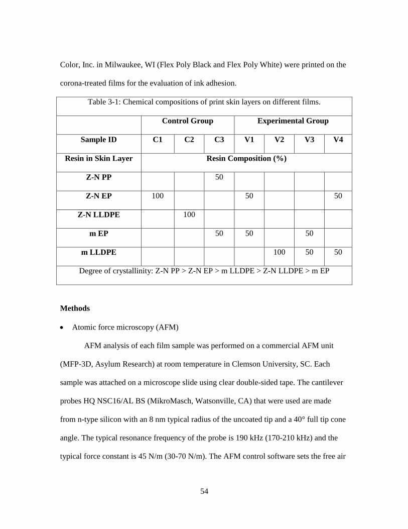
54
Color, Inc. in Milwaukee, WI (Flex Poly Black and Flex Poly White) were printed on the
corona-treated films for the evaluation of ink adhesion.
Table 3-1: Chemical compositions of print skin layers on different films.
Control Group Experimental Group
Sample ID C1 C2 C3 V1 V2 V3 V4
Resin in Skin Layer Resin Composition (%)
Z-N PP 50
Z-N EP 100
50 50
Z-N LLDPE
100
m EP
50 50 50
m LLDPE
100 50 50
Degree of crystallinity: Z-N PP > Z-N EP > m LLDPE > Z-N LLDPE > m EP
Methods
Atomic force microscopy (AFM)
AFM analysis of each film sample was performed on a commercial AFM unit
(MFP-3D, Asylum Research) at room temperature in Clemson University, SC. Each
sample was attached on a microscope slide using clear double-sided tape. The cantilever
probes HQ NSC16/AL BS (MikroMasch, Watsonville, CA) that were used are made
from n-type silicon with an 8 nm typical radius of the uncoated tip and a 40° full tip cone
angle. The typical resonance frequency of the probe is 190 kHz (170-210 kHz) and the
typical force constant is 45 N/m (30-70 N/m). The AFM control software sets the free air
55
amplitude of the cantilever at 1Volt and it can record both height and phase angle data
simultaneously with one measurement. However, to achieve optimal contrast, the
topography of each sample with a scan size of 20×20 µm2 was obtained in light tapping
mode (Set-point amplitude = 800 mV), while the phase angle image of each sample with
a scan size of 5×5 µm2 was obtained in hard tapping mode (Set-point amplitude = 500
mV). During testing, the scan rate was set at 1 Hz, the scan angle was 0°, and the point &
line resolution was 512. For each corona-treated film, two pieces of specimens were
analyzed for topography on AFM in light tapping mode (scan size = 20×20 µm2). Based
on the results, some surface areas of interest were then selected for the hard tapping
analyses (scan size = 5×5 µm2) in order to obtain the phase angle image with the optimal
contrast. The resultant topography and phase angle images were analyzed visually and
the height (i.e. roughness) data were also analyzed using the statistical methods below.
Statistical analyses
All the height (i.e. roughness) data obtained from AFM light tapping on the
20×20 µm2 areas were analyzed statistically in Minitab
® software. To determine the
repeatability of the roughness results of two replicates for each film type, a “2-Sample t-
test” was conducted with the means of the absolute heights and the corresponding
standard deviations. Before that, a “2-Variance test” was performed with the two standard
deviations in order to determine if the t-test for samples with equal variances or the t-test
for samples with unequal variances should be used in the second step.
The procedures performed in Minitab® for these analyses are as follows.

56
1. StatBasic Statistics2-VariancesEnter “Sample size” and “Standard
deviation” for each sampleOK;
2. Compare the P-value with α = 0.05. If P-value < α, it means that these two
variances are not equal, and vice versa.
3. Stat Basic Statistics2-Sample t-test Enter “Sample size” “Mean”
and “Standard deviation” for each sampleIf the variances are proven to
be equal by step 1, check the box “Assume equal variances”; If not, do not
check it. OK;
4. Compare the P-value with α = 0.05. If P-value < α, it means that these two
means are not equal, and vice versa.
After subgrouping the height data obtained from AFM light tapping on the 20×20
µm2 areas, regression tests were performed on the RMS roughness and mean of absolute
heights of sixteen subgroups. The purposes of these analyses and subgrouping method
will be introduced in details in Chapter Four. All the worksheets used in Minitab® are
included in Appendix C. After entering the data in the worksheets, the tests were
conducted as follows.
1. StatRegressionRegressionEnter “RMS” as the responseEnter
“Column” and “Row” as predictorsOK;
2. Repeat step 1 with “Mean” as the response.
3. Compare the P-values of each factor (i.e. Column and Row) with α = 0.05.
If P-value < α, it means that this factor affects the response significantly,
and vice versa.
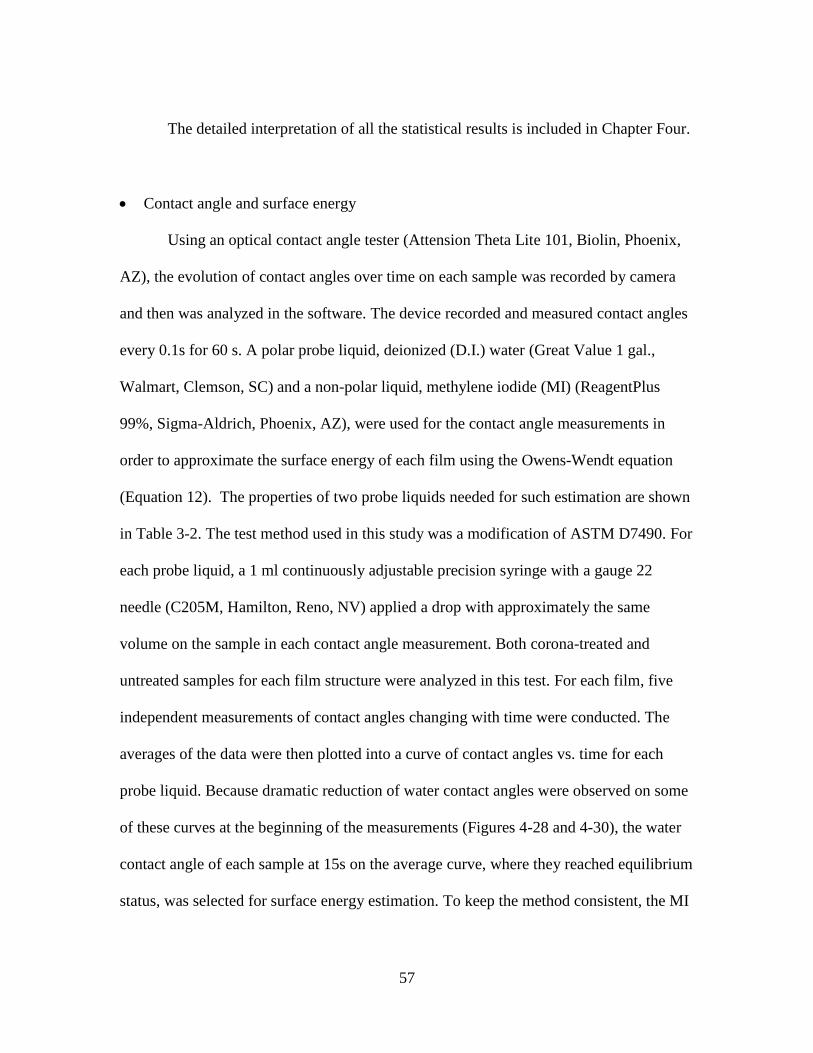
57
The detailed interpretation of all the statistical results is included in Chapter Four.
Contact angle and surface energy
Using an optical contact angle tester (Attension Theta Lite 101, Biolin, Phoenix,
AZ), the evolution of contact angles over time on each sample was recorded by camera
and then was analyzed in the software. The device recorded and measured contact angles
every 0.1s for 60 s. A polar probe liquid, deionized (D.I.) water (Great Value 1 gal.,
Walmart, Clemson, SC) and a non-polar liquid, methylene iodide (MI) (ReagentPlus
99%, Sigma-Aldrich, Phoenix, AZ), were used for the contact angle measurements in
order to approximate the surface energy of each film using the Owens-Wendt equation
(Equation 12). The properties of two probe liquids needed for such estimation are shown
in Table 3-2. The test method used in this study was a modification of ASTM D7490. For
each probe liquid, a 1 ml continuously adjustable precision syringe with a gauge 22
needle (C205M, Hamilton, Reno, NV) applied a drop with approximately the same
volume on the sample in each contact angle measurement. Both corona-treated and
untreated samples for each film structure were analyzed in this test. For each film, five
independent measurements of contact angles changing with time were conducted. The
averages of the data were then plotted into a curve of contact angles vs. time for each
probe liquid. Because dramatic reduction of water contact angles were observed on some
of these curves at the beginning of the measurements (Figures 4-28 and 4-30), the water
contact angle of each sample at 15s on the average curve, where they reached equilibrium
status, was selected for surface energy estimation. To keep the method consistent, the MI
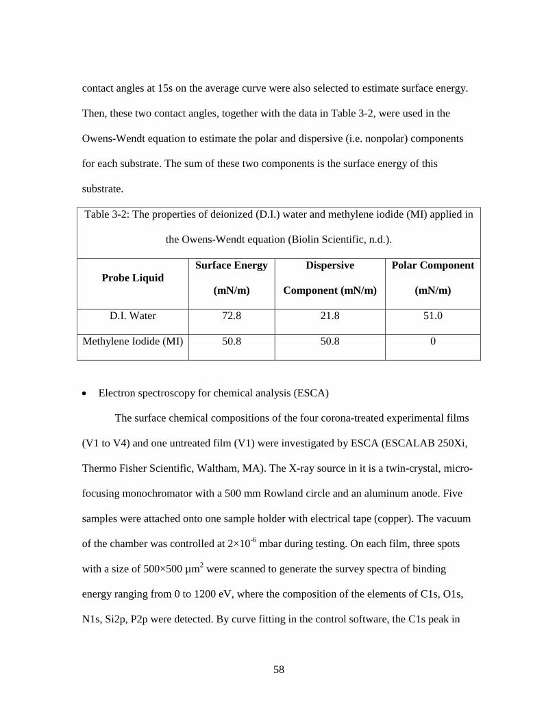
58
contact angles at 15s on the average curve were also selected to estimate surface energy.
Then, these two contact angles, together with the data in Table 3-2, were used in the
Owens-Wendt equation to estimate the polar and dispersive (i.e. nonpolar) components
for each substrate. The sum of these two components is the surface energy of this
substrate.
Table 3-2: The properties of deionized (D.I.) water and methylene iodide (MI) applied in
the Owens-Wendt equation (Biolin Scientific, n.d.).
Probe Liquid
Surface Energy
(mN/m)
Dispersive
Component (mN/m)
Polar Component
(mN/m)
D.I. Water 72.8 21.8 51.0
Methylene Iodide (MI) 50.8 50.8 0
Electron spectroscopy for chemical analysis (ESCA)
The surface chemical compositions of the four corona-treated experimental films
(V1 to V4) and one untreated film (V1) were investigated by ESCA (ESCALAB 250Xi,
Thermo Fisher Scientific, Waltham, MA). The X-ray source in it is a twin-crystal, micro-
focusing monochromator with a 500 mm Rowland circle and an aluminum anode. Five
samples were attached onto one sample holder with electrical tape (copper). The vacuum
of the chamber was controlled at 2×10⁻⁶
mbar during testing. On each film, three spots
with a size of 500×500 µm2 were scanned to generate the survey spectra of binding
energy ranging from 0 to 1200 eV, where the composition of the elements of C1s, O1s,
N1s, Si2p, P2p were detected. By curve fitting in the control software, the C1s peak in
59
the survey spectra was decomposed into three peaks representing C-C (284.75 eV), C-O
(286.50 eV) and C=O (288.9) respectively.
Ink adhesion analyses
Two inks, black and white, were drawn down on the corona-treated films using
rod #2 on a K Control Coater (RK PrintCoat Instruments, Litlington, UK). ASTM
D7305-08a was followed in these measurements. The printed samples were quickly dried
in the oven (GS Lindberg/Blue M, Thermo Fisher Scientific, Waltham, MA) at 54 °C for
35s. To achieve consistent ink weight for each ink on different films, the print density
(508 XRGA spectrodensiometer, X-Rite, Grand Rapids, MI) of the samples printed with
black and white inks was controlled in the ranges of 1.8 to 2.1 and 0.25 to 0.35
respectively. It was found that this did not require changing either rod or drawdown
speed.
A Sutherland rub tester (Brown Company, Kalamazoo, MI) was used to perform
the rub tests on the printed samples in both print-to-print and print-to-film modes
according to ASTM 5264-98. Three rubbing tests were conducted on each film in each
mode. In each test, the sample went through 50 rubbing cycles under a 4-lb weight.
Afterwards, the print density was measured on three different spots on the rubbed sample
again. The change of print density was considered as the rub resistance of that printed
film.
Three types of tape (Scotch® 600/610/810, 3M, St. Paul, MN) were used to check
the ink adhesion following procedures in ASTM F2252/F2252M. After peeling off the

60
tape from the surface, the amount of ink remaining on the sample, was visually
determined and reported as a percentage by the same technician. Five replicates were
conducted on each film using each type of tape.
In addition, the 45° print gloss of each printed film was also measured against a
black background using a gloss meter (Micro-Gloss 45°, BYK Gardener USA, Columbia,
MD) according to ASTM 2457-13. This test was repeated 5 times for each sample.
61
CHAPTER FOUR
RESULTS AND DISCUSSIONS
Hypothesis
As introduced in the literature review, the main effects of corona treatment on the
polyolefin films include oxidation, chain scission, crosslinking and roughening. Under
the same level of corona discharge, PE is easier to be oxidized than PP, while PP tends to
undergo more chain scission than oxidation. The PE polymer chains on the film surface
can crosslink in a higher degree than those on the PP films due to the lack of side group
hindrance (-CH3). Nevertheless, the crosslinking degree of LLDPE is limited to some
extent due to the existence of short side chains. Because the EPs used in this study were
PP random copolymers and contained very low amount of ethylene, they should still
exhibit similar features as PP. In other words, they should tend to get chain scission more
than oxidation during the corona treatment as well.
It was also stated earlier that the metallocene catalyzed polyolefins generally have
narrower molecular weight distributions and higher stereo-regularity than their Z-N
catalyzed counterparts. Therefore, it should be easier for them to form tightly-packed and
orderly crystalline structures than their Z-N catalyzed counterparts.
It is known that such crystalline structures hinder the mobility and re-
arrangements of polymer chains. Hence, it can be speculated that the corona effects
introduced above should have less influence on the surface of metallocene catalyzed
polyolefin film than that of their Z-N counterpart. Furthermore, depending on which
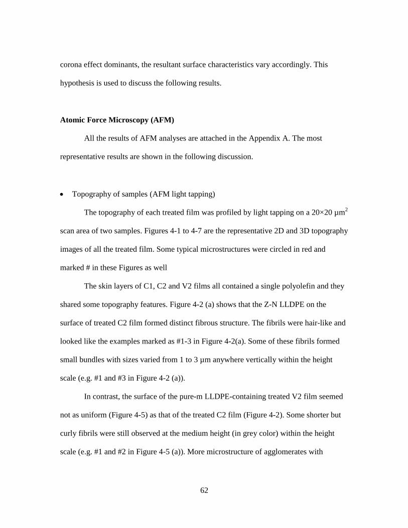
62
corona effect dominants, the resultant surface characteristics vary accordingly. This
hypothesis is used to discuss the following results.
Atomic Force Microscopy (AFM)
All the results of AFM analyses are attached in the Appendix A. The most
representative results are shown in the following discussion.
Topography of samples (AFM light tapping)
The topography of each treated film was profiled by light tapping on a 20×20 µm2
scan area of two samples. Figures 4-1 to 4-7 are the representative 2D and 3D topography
images of all the treated film. Some typical microstructures were circled in red and
marked # in these Figures as well
The skin layers of C1, C2 and V2 films all contained a single polyolefin and they
shared some topography features. Figure 4-2 (a) shows that the Z-N LLDPE on the
surface of treated C2 film formed distinct fibrous structure. The fibrils were hair-like and
looked like the examples marked as #1-3 in Figure 4-2(a). Some of these fibrils formed
small bundles with sizes varied from 1 to 3 µm anywhere vertically within the height
scale (e.g. #1 and #3 in Figure 4-2 (a)).
In contrast, the surface of the pure-m LLDPE-containing treated V2 film seemed
not as uniform (Figure 4-5) as that of the treated C2 film (Figure 4-2). Some shorter but
curly fibrils were still observed at the medium height (in grey color) within the height
scale (e.g. #1 and #2 in Figure 4-5 (a)). More microstructure of agglomerates with
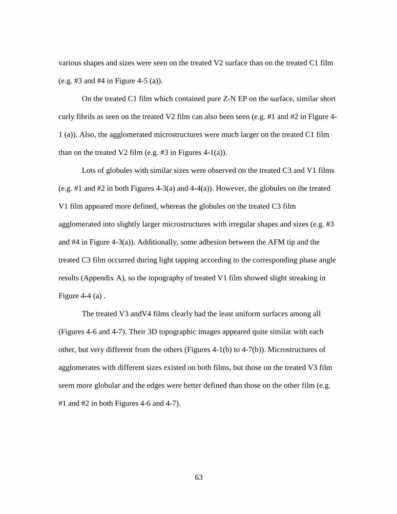
63
various shapes and sizes were seen on the treated V2 surface than on the treated C1 film
(e.g. #3 and #4 in Figure 4-5 (a)).
On the treated C1 film which contained pure Z-N EP on the surface, similar short
curly fibrils as seen on the treated V2 film can also been seen (e.g. #1 and #2 in Figure 4-
1 (a)). Also, the agglomerated microstructures were much larger on the treated C1 film
than on the treated V2 film (e.g. #3 in Figures 4-1(a)).
Lots of globules with similar sizes were observed on the treated C3 and V1 films
(e.g. #1 and #2 in both Figures 4-3(a) and 4-4(a)). However, the globules on the treated
V1 film appeared more defined, whereas the globules on the treated C3 film
agglomerated into slightly larger microstructures with irregular shapes and sizes (e.g. #3
and #4 in Figure 4-3(a)). Additionally, some adhesion between the AFM tip and the
treated C3 film occurred during light tapping according to the corresponding phase angle
results (Appendix A), so the topography of treated V1 film showed slight streaking in
Figure 4-4 (a) .
The treated V3 andV4 films clearly had the least uniform surfaces among all
(Figures 4-6 and 4-7). Their 3D topographic images appeared quite similar with each
other, but very different from the others (Figures 4-1(b) to 4-7(b)). Microstructures of
agglomerates with different sizes existed on both films, but those on the treated V3 film
seem more globular and the edges were better defined than those on the other film (e.g.
#1 and #2 in both Figures 4-6 and 4-7).
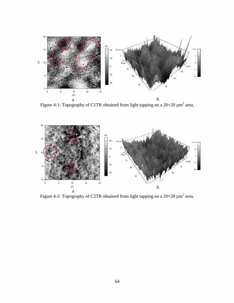
64
a
b
Figure 4-1: Topography of C1TR obtained from light tapping on a 20×20 µm2 area.
a
b
Figure 4-2: Topography of C2TR obtained from light tapping on a 20×20 µm2 area.
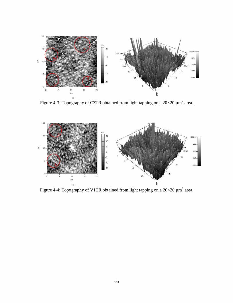
65
a
b
Figure 4-3: Topography of C3TR obtained from light tapping on a 20×20 µm2 area.
a
b
Figure 4-4: Topography of V1TR obtained from light tapping on a 20×20 µm2 area.
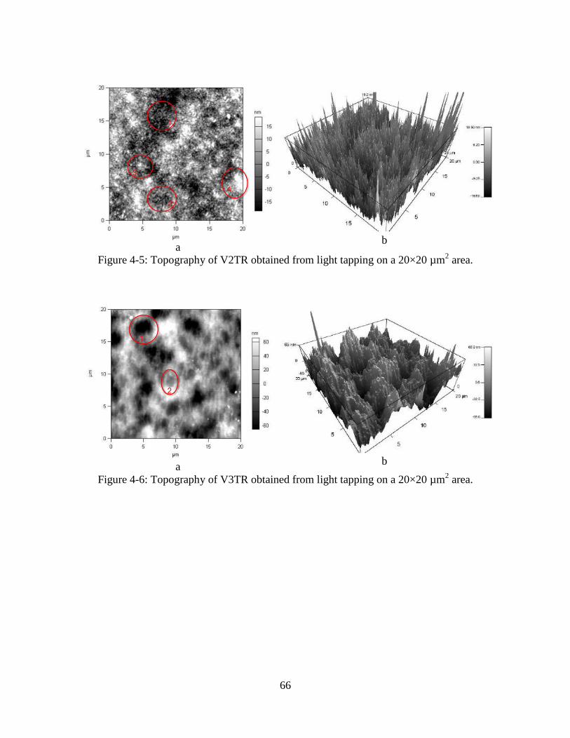
66
a
b
Figure 4-5: Topography of V2TR obtained from light tapping on a 20×20 µm2 area.
a
b
Figure 4-6: Topography of V3TR obtained from light tapping on a 20×20 µm2 area.
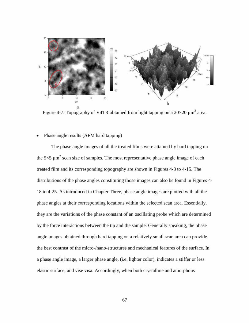
67
a
b
Figure 4-7: Topography of V4TR obtained from light tapping on a 20×20 µm2 area.
Phase angle results (AFM hard tapping)
The phase angle images of all the treated films were attained by hard tapping on
the 5×5 µm2 scan size of samples. The most representative phase angle image of each
treated film and its corresponding topography are shown in Figures 4-8 to 4-15. The
distributions of the phase angles constituting those images can also be found in Figures 4-
18 to 4-25. As introduced in Chapter Three, phase angle images are plotted with all the
phase angles at their corresponding locations within the selected scan area. Essentially,
they are the variations of the phase constant of an oscillating probe which are determined
by the force interactions between the tip and the sample. Generally speaking, the phase
angle images obtained through hard tapping on a relatively small scan area can provide
the best contrast of the micro-/nano-structures and mechanical features of the surface. In
a phase angle image, a larger phase angle, (i.e. lighter color), indicates a stiffer or less
elastic surface, and vise visa. Accordingly, when both crystalline and amorphous
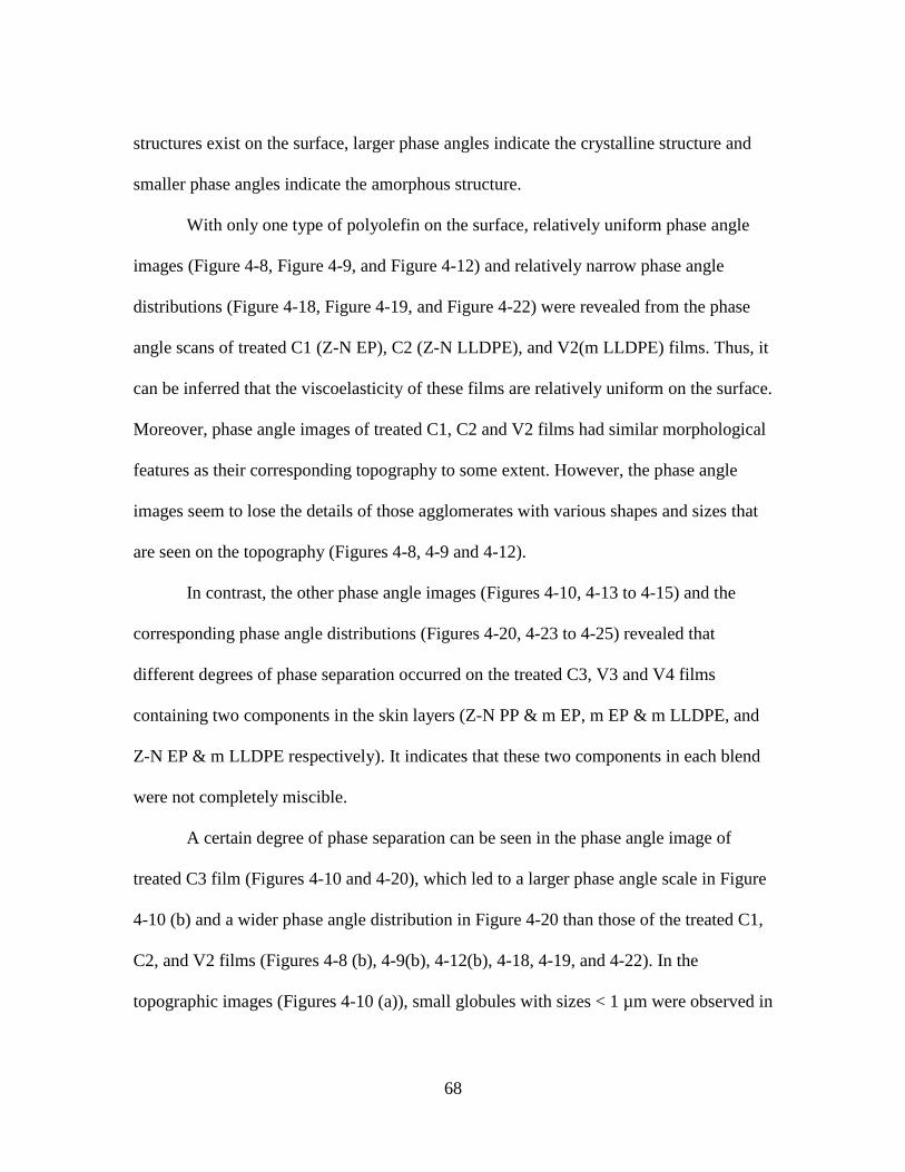
68
structures exist on the surface, larger phase angles indicate the crystalline structure and
smaller phase angles indicate the amorphous structure.
With only one type of polyolefin on the surface, relatively uniform phase angle
images (Figure 4-8, Figure 4-9, and Figure 4-12) and relatively narrow phase angle
distributions (Figure 4-18, Figure 4-19, and Figure 4-22) were revealed from the phase
angle scans of treated C1 (Z-N EP), C2 (Z-N LLDPE), and V2(m LLDPE) films. Thus, it
can be inferred that the viscoelasticity of these films are relatively uniform on the surface.
Moreover, phase angle images of treated C1, C2 and V2 films had similar morphological
features as their corresponding topography to some extent. However, the phase angle
images seem to lose the details of those agglomerates with various shapes and sizes that
are seen on the topography (Figures 4-8, 4-9 and 4-12).
In contrast, the other phase angle images (Figures 4-10, 4-13 to 4-15) and the
corresponding phase angle distributions (Figures 4-20, 4-23 to 4-25) revealed that
different degrees of phase separation occurred on the treated C3, V3 and V4 films
containing two components in the skin layers (Z-N PP & m EP, m EP & m LLDPE, and
Z-N EP & m LLDPE respectively). It indicates that these two components in each blend
were not completely miscible.
A certain degree of phase separation can be seen in the phase angle image of
treated C3 film (Figures 4-10 and 4-20), which led to a larger phase angle scale in Figure
4-10 (b) and a wider phase angle distribution in Figure 4-20 than those of the treated C1,
C2, and V2 films (Figures 4-8 (b), 4-9(b), 4-12(b), 4-18, 4-19, and 4-22). In the
topographic images (Figures 4-10 (a)), small globules with sizes < 1 µm were observed in
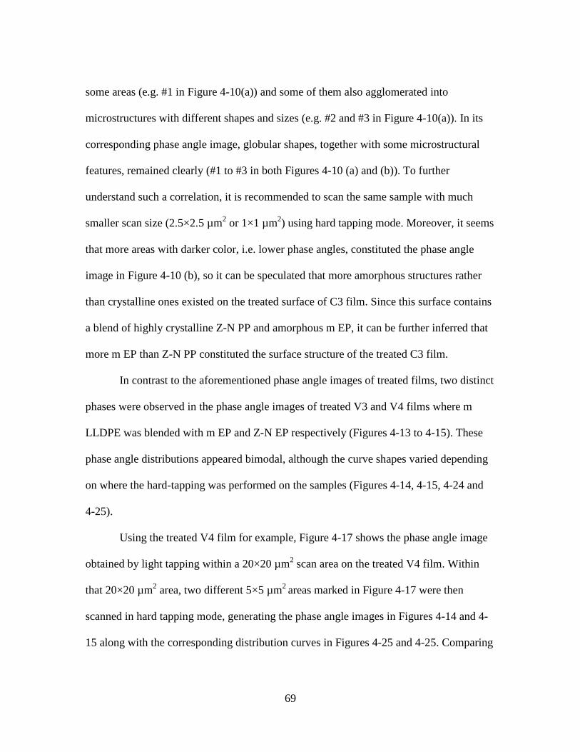
69
some areas (e.g. #1 in Figure 4-10(a)) and some of them also agglomerated into
microstructures with different shapes and sizes (e.g. #2 and #3 in Figure 4-10(a)). In its
corresponding phase angle image, globular shapes, together with some microstructural
features, remained clearly (#1 to #3 in both Figures 4-10 (a) and (b)). To further
understand such a correlation, it is recommended to scan the same sample with much
smaller scan size (2.5×2.5 µm2 or 1×1 µm
2) using hard tapping mode. Moreover, it seems
that more areas with darker color, i.e. lower phase angles, constituted the phase angle
image in Figure 4-10 (b), so it can be speculated that more amorphous structures rather
than crystalline ones existed on the treated surface of C3 film. Since this surface contains
a blend of highly crystalline Z-N PP and amorphous m EP, it can be further inferred that
more m EP than Z-N PP constituted the surface structure of the treated C3 film.
In contrast to the aforementioned phase angle images of treated films, two distinct
phases were observed in the phase angle images of treated V3 and V4 films where m
LLDPE was blended with m EP and Z-N EP respectively (Figures 4-13 to 4-15). These
phase angle distributions appeared bimodal, although the curve shapes varied depending
on where the hard-tapping was performed on the samples (Figures 4-14, 4-15, 4-24 and
4-25).
Using the treated V4 film for example, Figure 4-17 shows the phase angle image
obtained by light tapping within a 20×20 µm2 scan area on the treated V4 film. Within
that 20×20 µm2 area, two different 5×5 µm
2 areas marked in Figure 4-17 were then
scanned in hard tapping mode, generating the phase angle images in Figures 4-14 and 4-
15 along with the corresponding distribution curves in Figures 4-25 and 4-25. Comparing
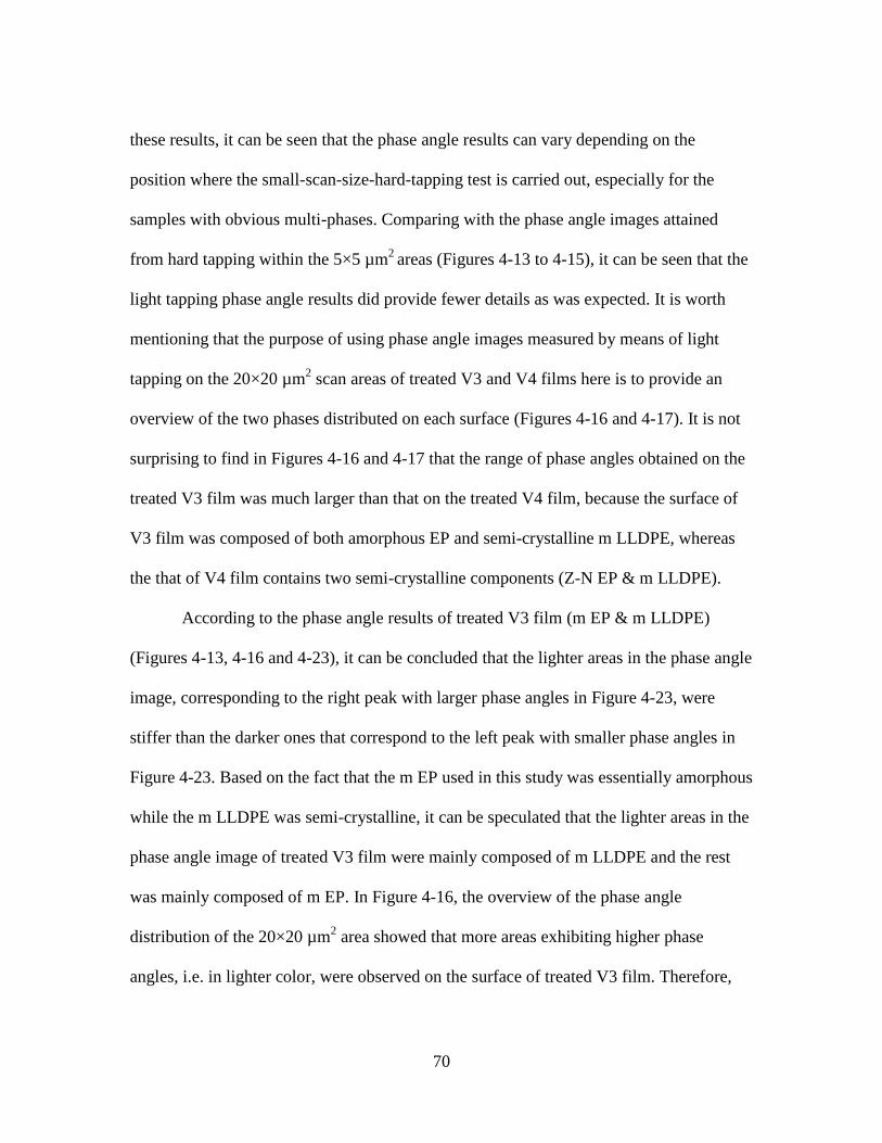
70
these results, it can be seen that the phase angle results can vary depending on the
position where the small-scan-size-hard-tapping test is carried out, especially for the
samples with obvious multi-phases. Comparing with the phase angle images attained
from hard tapping within the 5×5 µm2
areas (Figures 4-13 to 4-15), it can be seen that the
light tapping phase angle results did provide fewer details as was expected. It is worth
mentioning that the purpose of using phase angle images measured by means of light
tapping on the 20×20 µm2 scan areas of treated V3 and V4 films here is to provide an
overview of the two phases distributed on each surface (Figures 4-16 and 4-17). It is not
surprising to find in Figures 4-16 and 4-17 that the range of phase angles obtained on the
treated V3 film was much larger than that on the treated V4 film, because the surface of
V3 film was composed of both amorphous EP and semi-crystalline m LLDPE, whereas
the that of V4 film contains two semi-crystalline components (Z-N EP & m LLDPE).
According to the phase angle results of treated V3 film (m EP & m LLDPE)
(Figures 4-13, 4-16 and 4-23), it can be concluded that the lighter areas in the phase angle
image, corresponding to the right peak with larger phase angles in Figure 4-23, were
stiffer than the darker ones that correspond to the left peak with smaller phase angles in
Figure 4-23. Based on the fact that the m EP used in this study was essentially amorphous
while the m LLDPE was semi-crystalline, it can be speculated that the lighter areas in the
phase angle image of treated V3 film were mainly composed of m LLDPE and the rest
was mainly composed of m EP. In Figure 4-16, the overview of the phase angle
distribution of the 20×20 µm2 area showed that more areas exhibiting higher phase
angles, i.e. in lighter color, were observed on the surface of treated V3 film. Therefore,
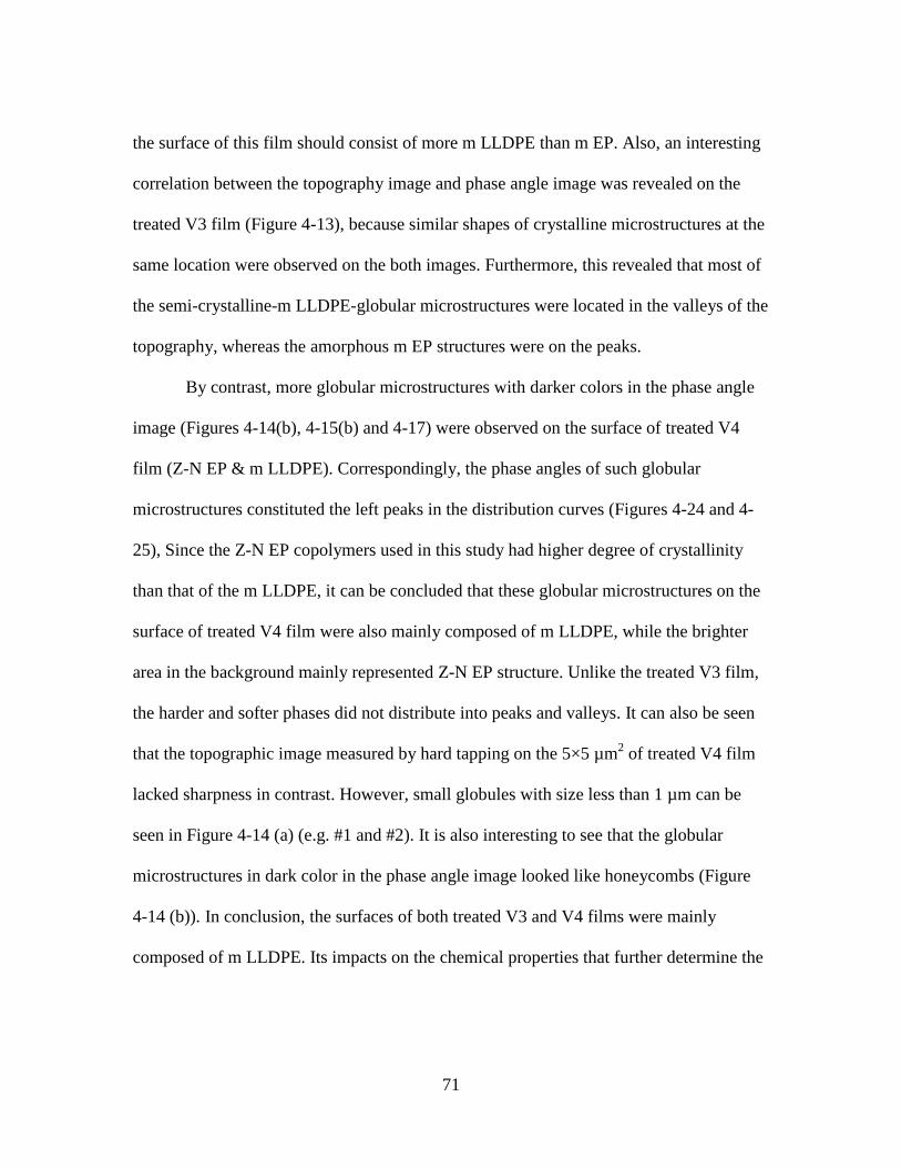
71
the surface of this film should consist of more m LLDPE than m EP. Also, an interesting
correlation between the topography image and phase angle image was revealed on the
treated V3 film (Figure 4-13), because similar shapes of crystalline microstructures at the
same location were observed on the both images. Furthermore, this revealed that most of
the semi-crystalline-m LLDPE-globular microstructures were located in the valleys of the
topography, whereas the amorphous m EP structures were on the peaks.
By contrast, more globular microstructures with darker colors in the phase angle
image (Figures 4-14(b), 4-15(b) and 4-17) were observed on the surface of treated V4
film (Z-N EP & m LLDPE). Correspondingly, the phase angles of such globular
microstructures constituted the left peaks in the distribution curves (Figures 4-24 and 4-
25), Since the Z-N EP copolymers used in this study had higher degree of crystallinity
than that of the m LLDPE, it can be concluded that these globular microstructures on the
surface of treated V4 film were also mainly composed of m LLDPE, while the brighter
area in the background mainly represented Z-N EP structure. Unlike the treated V3 film,
the harder and softer phases did not distribute into peaks and valleys. It can also be seen
that the topographic image measured by hard tapping on the 5×5 µm2 of treated V4 film
lacked sharpness in contrast. However, small globules with size less than 1 µm can be
seen in Figure 4-14 (a) (e.g. #1 and #2). It is also interesting to see that the globular
microstructures in dark color in the phase angle image looked like honeycombs (Figure
4-14 (b)). In conclusion, the surfaces of both treated V3 and V4 films were mainly
composed of m LLDPE. Its impacts on the chemical properties that further determine the
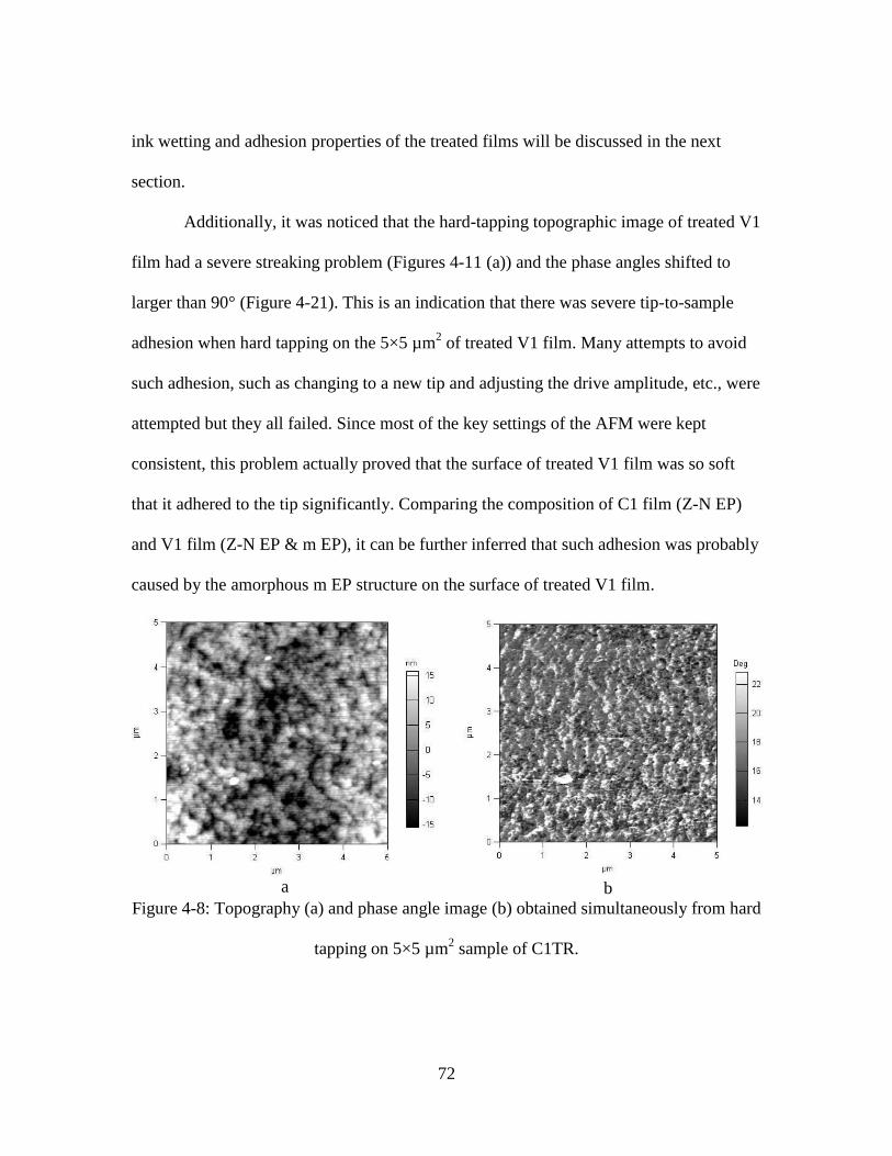
72
ink wetting and adhesion properties of the treated films will be discussed in the next
section.
Additionally, it was noticed that the hard-tapping topographic image of treated V1
film had a severe streaking problem (Figures 4-11 (a)) and the phase angles shifted to
larger than 90° (Figure 4-21). This is an indication that there was severe tip-to-sample
adhesion when hard tapping on the 5×5 µm2 of treated V1 film. Many attempts to avoid
such adhesion, such as changing to a new tip and adjusting the drive amplitude, etc., were
attempted but they all failed. Since most of the key settings of the AFM were kept
consistent, this problem actually proved that the surface of treated V1 film was so soft
that it adhered to the tip significantly. Comparing the composition of C1 film (Z-N EP)
and V1 film (Z-N EP & m EP), it can be further inferred that such adhesion was probably
caused by the amorphous m EP structure on the surface of treated V1 film.
a
b
Figure 4-8: Topography (a) and phase angle image (b) obtained simultaneously from hard
tapping on 5×5 µm2 sample of C1TR.
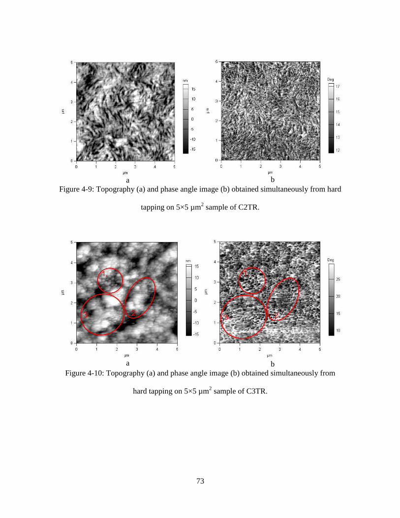
73
a
b
Figure 4-9: Topography (a) and phase angle image (b) obtained simultaneously from hard
tapping on 5×5 µm2 sample of C2TR.
a
b
Figure 4-10: Topography (a) and phase angle image (b) obtained simultaneously from
hard tapping on 5×5 µm2 sample of C3TR.

74
a
b
Figure 4-11: Topography (a) and phase angle image (b) obtained simultaneously from
hard tapping on 5×5 µm2 sample of V1TR.
a
b
Figure 4-12: Topography (a) and phase angle image (b) obtained simultaneously from
hard tapping on 5×5 µm2 sample of V2TR.
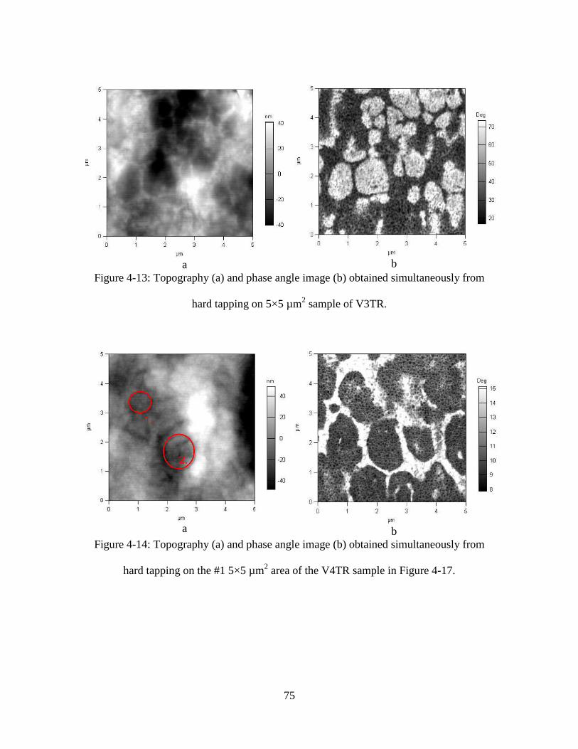
75
a
b
Figure 4-13: Topography (a) and phase angle image (b) obtained simultaneously from
hard tapping on 5×5 µm2 sample of V3TR.
a
b
Figure 4-14: Topography (a) and phase angle image (b) obtained simultaneously from
hard tapping on the #1 5×5 µm2 area of the V4TR sample in Figure 4-17.
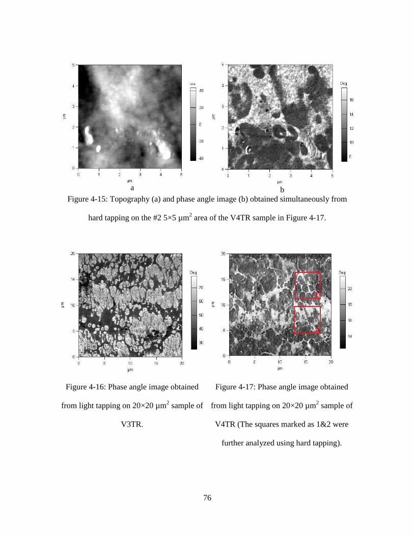
76
a
b
Figure 4-15: Topography (a) and phase angle image (b) obtained simultaneously from
hard tapping on the #2 5×5 µm2 area of the V4TR sample in Figure 4-17.
Figure 4-16: Phase angle image obtained
from light tapping on 20×20 µm2 sample of
V3TR.
Figure 4-17: Phase angle image obtained
from light tapping on 20×20 µm2 sample of
V4TR (The squares marked as 1&2 were
further analyzed using hard tapping).
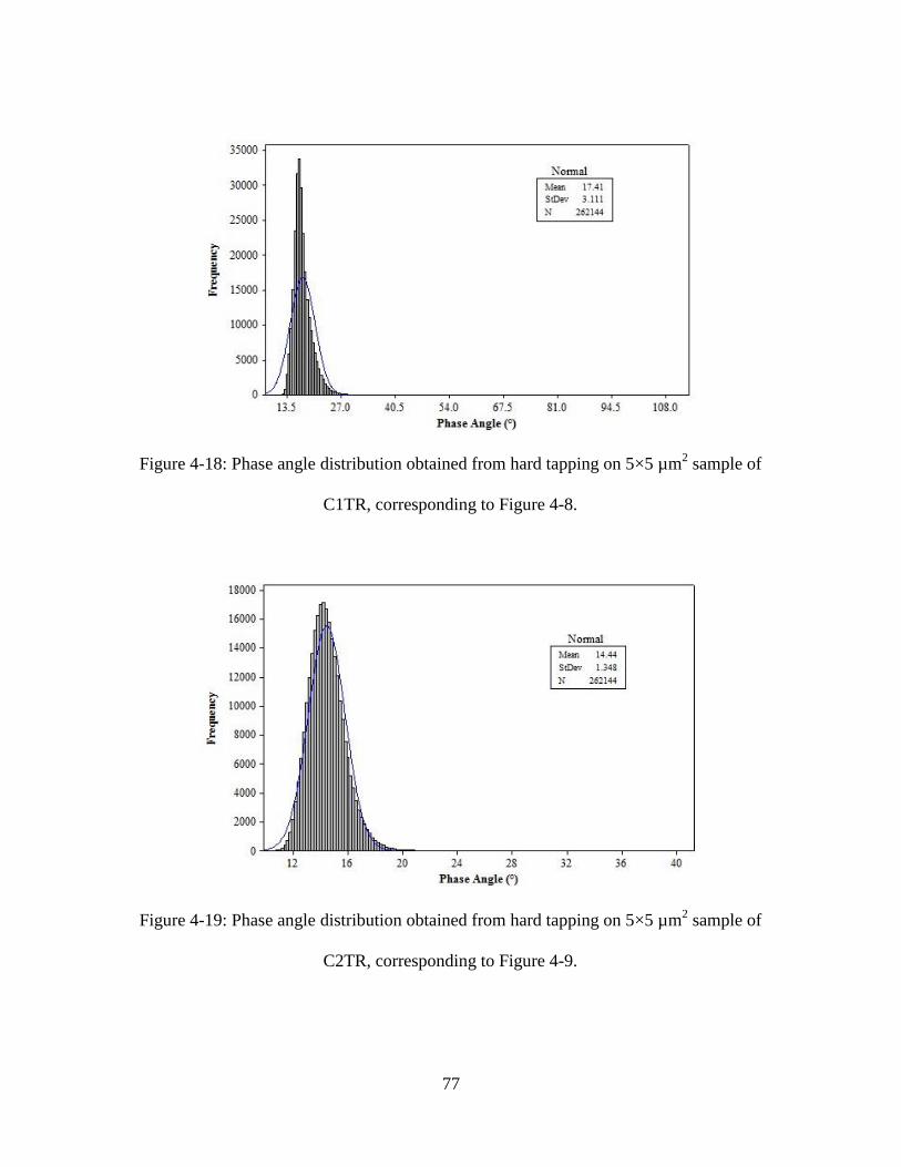
77
Figure 4-18: Phase angle distribution obtained from hard tapping on 5×5 µm2 sample of
C1TR, corresponding to Figure 4-8.
Figure 4-19: Phase angle distribution obtained from hard tapping on 5×5 µm2 sample of
C2TR, corresponding to Figure 4-9.
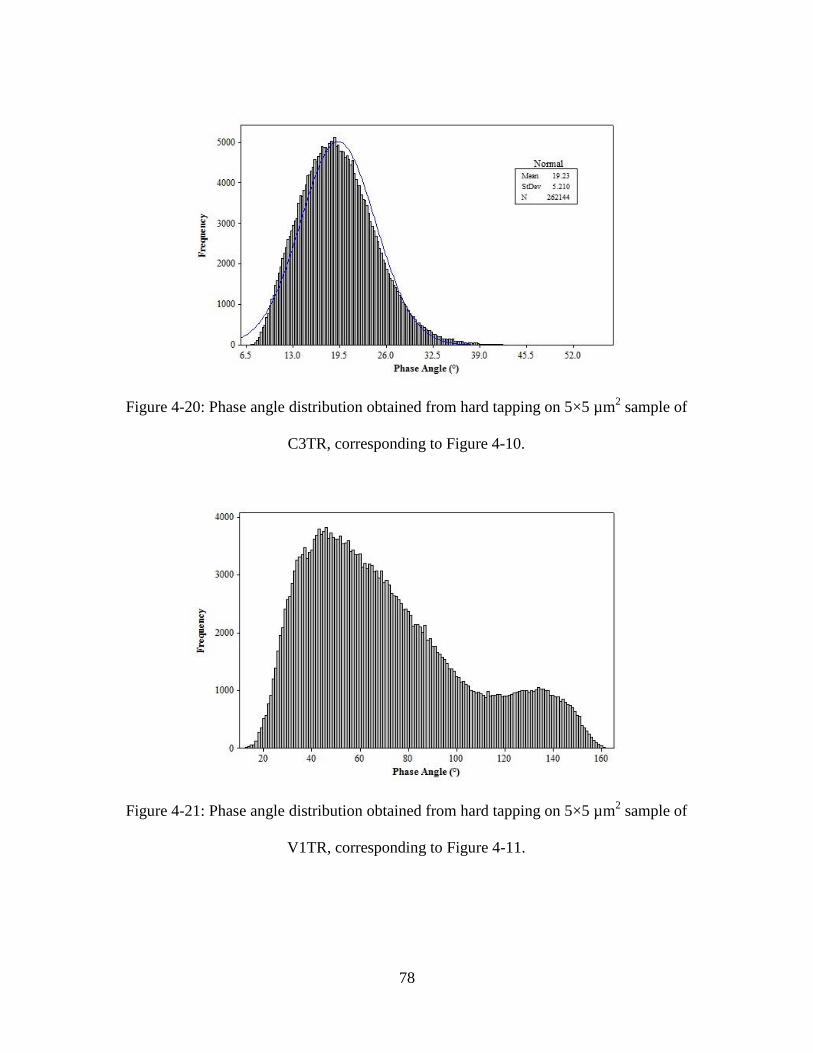
78
Figure 4-20: Phase angle distribution obtained from hard tapping on 5×5 µm2 sample of
C3TR, corresponding to Figure 4-10.
Figure 4-21: Phase angle distribution obtained from hard tapping on 5×5 µm2 sample of
V1TR, corresponding to Figure 4-11.
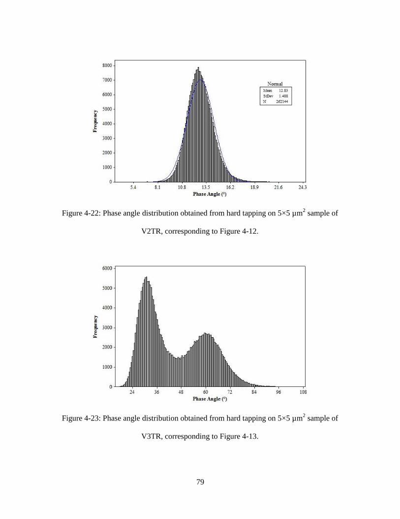
79
Figure 4-22: Phase angle distribution obtained from hard tapping on 5×5 µm2 sample of
V2TR, corresponding to Figure 4-12.
Figure 4-23: Phase angle distribution obtained from hard tapping on 5×5 µm2 sample of
V3TR, corresponding to Figure 4-13.
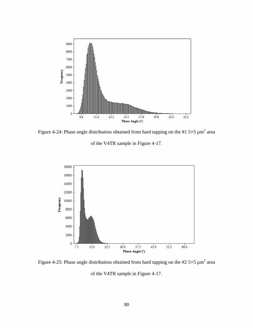
80
Figure 4-24: Phase angle distribution obtained from hard tapping on the #1 5×5 µm2 area
of the V4TR sample in Figure 4-17.
Figure 4-25: Phase angle distribution obtained from hard tapping on the #2 5×5 µm2 area
of the V4TR sample in Figure 4-17.
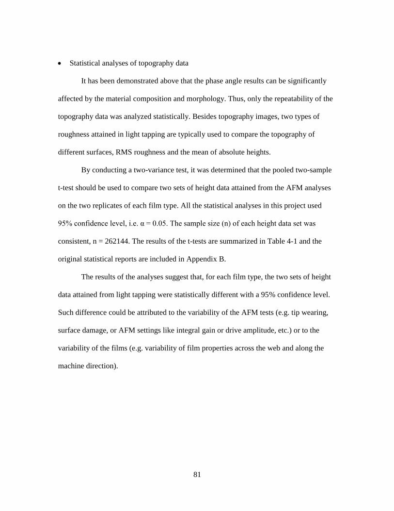
81
Statistical analyses of topography data
It has been demonstrated above that the phase angle results can be significantly
affected by the material composition and morphology. Thus, only the repeatability of the
topography data was analyzed statistically. Besides topography images, two types of
roughness attained in light tapping are typically used to compare the topography of
different surfaces, RMS roughness and the mean of absolute heights.
By conducting a two-variance test, it was determined that the pooled two-sample
t-test should be used to compare two sets of height data attained from the AFM analyses
on the two replicates of each film type. All the statistical analyses in this project used
95% confidence level, i.e. α = 0.05. The sample size (n) of each height data set was
consistent, n = 262144. The results of the t-tests are summarized in Table 4-1 and the
original statistical reports are included in Appendix B.
The results of the analyses suggest that, for each film type, the two sets of height
data attained from light tapping were statistically different with a 95% confidence level.
Such difference could be attributed to the variability of the AFM tests (e.g. tip wearing,
surface damage, or AFM settings like integral gain or drive amplitude, etc.) or to the
variability of the films (e.g. variability of film properties across the web and along the
machine direction).
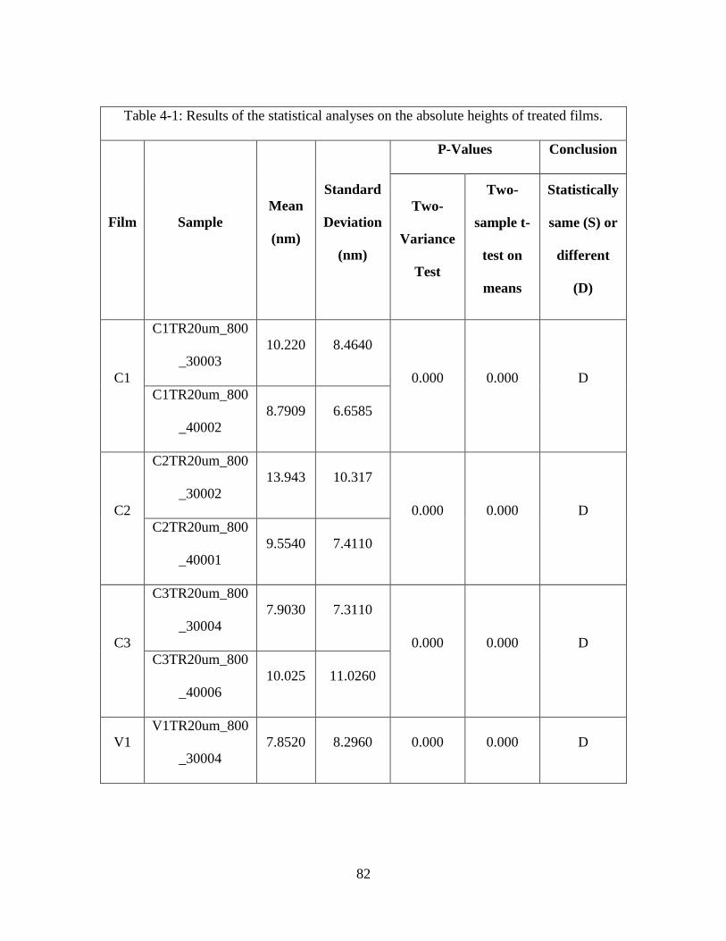
82
Table 4-1: Results of the statistical analyses on the absolute heights of treated films.
Film Sample
Mean
(nm)
Standard
Deviation
(nm)
P-Values Conclusion
Two-
Variance
Test
Two-
sample t-
test on
means
Statistically
same (S) or
different
(D)
C1
C1TR20um_800
_30003
10.220 8.4640
0.000 0.000 D
C1TR20um_800
_40002
8.7909 6.6585
C2
C2TR20um_800
_30002
13.943 10.317
0.000 0.000 D
C2TR20um_800
_40001
9.5540 7.4110
C3
C3TR20um_800
_30004
7.9030 7.3110
0.000 0.000 D
C3TR20um_800
_40006
10.025 11.0260
V1
V1TR20um_800
_30004
7.8520 8.2960 0.000 0.000 D
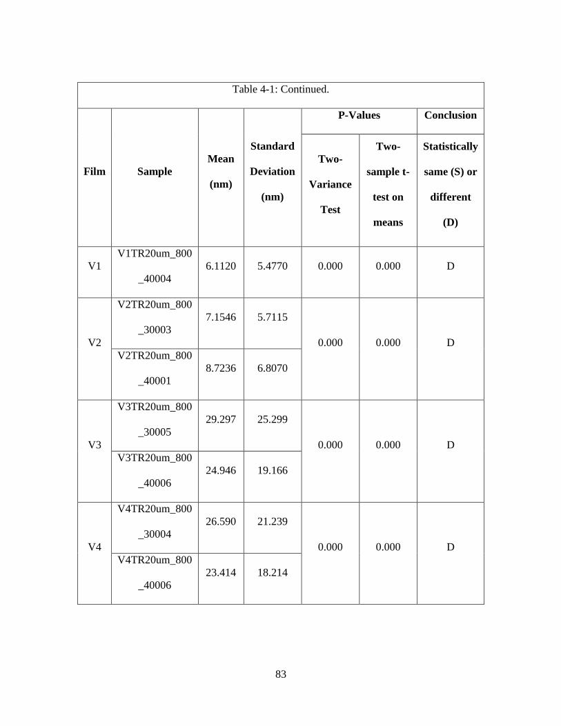
83
Table 4-1: Continued.
Film Sample
Mean
(nm)
Standard
Deviation
(nm)
P-Values Conclusion
Two-
Variance
Test
Two-
sample t-
test on
means
Statistically
same (S) or
different
(D)
V1
V1TR20um_800
_40004
6.1120 5.4770 0.000 0.000 D
V2
V2TR20um_800
_30003
7.1546 5.7115
0.000 0.000 D
V2TR20um_800
_40001
8.7236 6.8070
V3
V3TR20um_800
_30005
29.297 25.299
0.000 0.000 D
V3TR20um_800
_40006
24.946 19.166
V4
V4TR20um_800
_30004
26.590 21.239
0.000 0.000 D
V4TR20um_800
_40006
23.414 18.214
84
If the two replicates of roughness results remain statistically different after
minimizing the variability of the AFM tests, it can be speculated that the variability of
roughness results was mainly attributed to that of the films. With this purpose, each set of
the height data measured by light tapping on a 20×20 µm2 area was divided into sixteen
subgroups as shown in Figure 4-26. This method can avoid altering the surface by
tapping and minimize the variability caused by tip wearing, minimizing the variability of
the AFM tests. Hence, it was preferred over tapping on the same 20×20 µm2 area twice
under the same AFM settings.
In each AFM measurement, the tip surveys the sample surface in such an order
that each data point can be located with pre-defined X and Y coordinates within the scan
area. This means that each data point is also reported based on its X and Y coordinates
within the test area. As illustrated in Figure 4-26, a 20×20 µm2 scan area on a surface
tested in light tapping mode generated n = 262144 data points. These can be further
divided into sixteen 5×5 µm2 areas, Within each 5×5 µm
2 area, there are 16384 data
points, meaning the sample size of each subgroup is n’ = 16384. To locate each subgroup
on that 20×20 µm2 area, each 5×5 µm
2 area was also labeled as “xy” where x is the row#
and y is the column# after subgrouping. Then, the mean of absolute heights and RMS
roughness of each subgroup were calculated for the statistical comparison to the others.
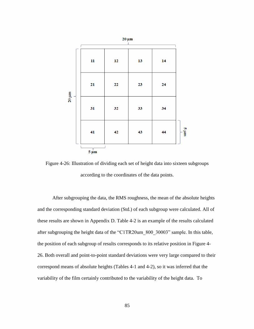
85
Figure 4-26: Illustration of dividing each set of height data into sixteen subgroups
according to the coordinates of the data points.
After subgrouping the data, the RMS roughness, the mean of the absolute heights
and the corresponding standard deviation (Std.) of each subgroup were calculated. All of
these results are shown in Appendix D. Table 4-2 is an example of the results calculated
after subgrouping the height data of the “C1TR20um_800_30003” sample. In this table,
the position of each subgroup of results corresponds to its relative position in Figure 4-
26. Both overall and point-to-point standard deviations were very large compared to their
correspond means of absolute heights (Tables 4-1 and 4-2), so it was inferred that the
variability of the film certainly contributed to the variability of the height data. To

86
further prove this, the data obtained from subgrouping were analyzed using the regression
test in Minitab®.
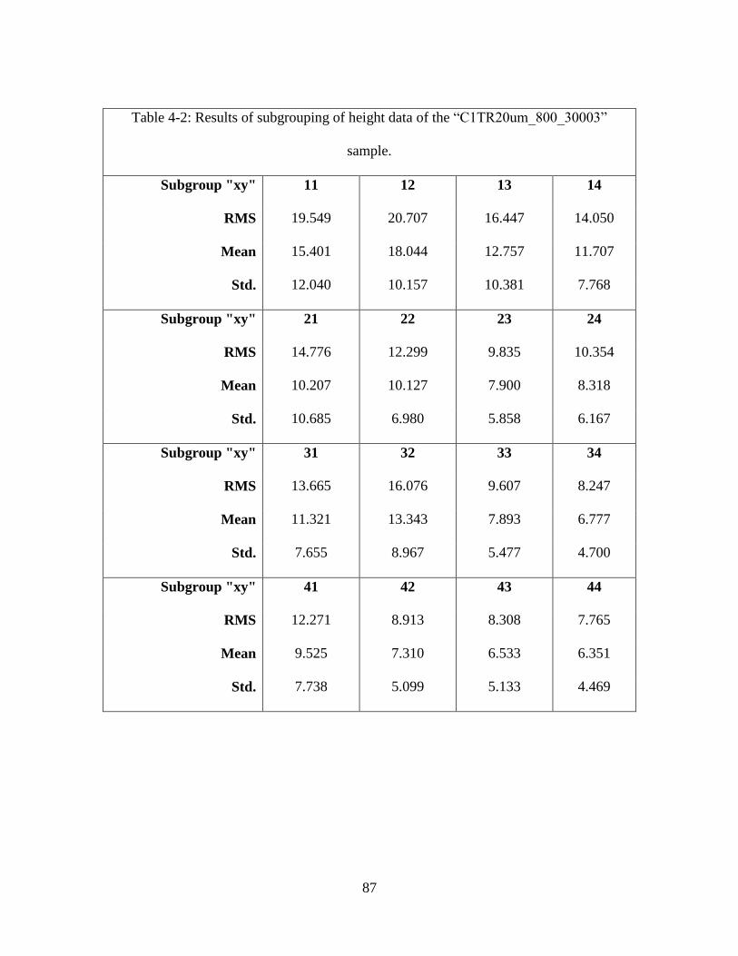
87
Table 4-2: Results of subgrouping of height data of the “C1TR20um_800_30003”
sample.
Subgroup "xy" 11 12 13 14
RMS 19.549 20.707 16.447 14.050
Mean 15.401 18.044 12.757 11.707
Std. 12.040 10.157 10.381 7.768
Subgroup "xy" 21 22 23 24
RMS 14.776 12.299 9.835 10.354
Mean 10.207 10.127 7.900 8.318
Std. 10.685 6.980 5.858 6.167
Subgroup "xy" 31 32 33 34
RMS 13.665 16.076 9.607 8.247
Mean 11.321 13.343 7.893 6.777
Std. 7.655 8.967 5.477 4.700
Subgroup "xy" 41 42 43 44
RMS 12.271 8.913 8.308 7.765
Mean 9.525 7.310 6.533 6.351
Std. 7.738 5.099 5.133 4.469

88
Table 4-3 is an example of the worksheet used in the regression test of sample
“C1TR20um_800_30003”. To determine the impacts of scan position (i.e. “Column” and
“Row”) on the roughness results (i.e. “RMS” or “Mean”), two rounds of regression tests
were conducted for each set of subgrouped data. One studied the impacts of the two
factors (“Column” and “Row”) on the RMS roughness and the other one studied the
impacts of two factors on the mean of absolute heights.
Table 4-3: Worksheet of the analysis of “C1TR20um_800_30003” using regression test
in Minitab®
.
Factors Responses
Column Row RMS Mean
1 1 19.55 15.40
1 2 20.71 18.04
1 3 16.45 12.76
1 4 14.05 11.71
2 1 14.78 10.21
2 2 12.30 10.13
2 3 9.83 7.90
2 4 10.35 8.32
3 1 13.67 11.32
3 2 16.08 13.34
3 3 9.61 7.89
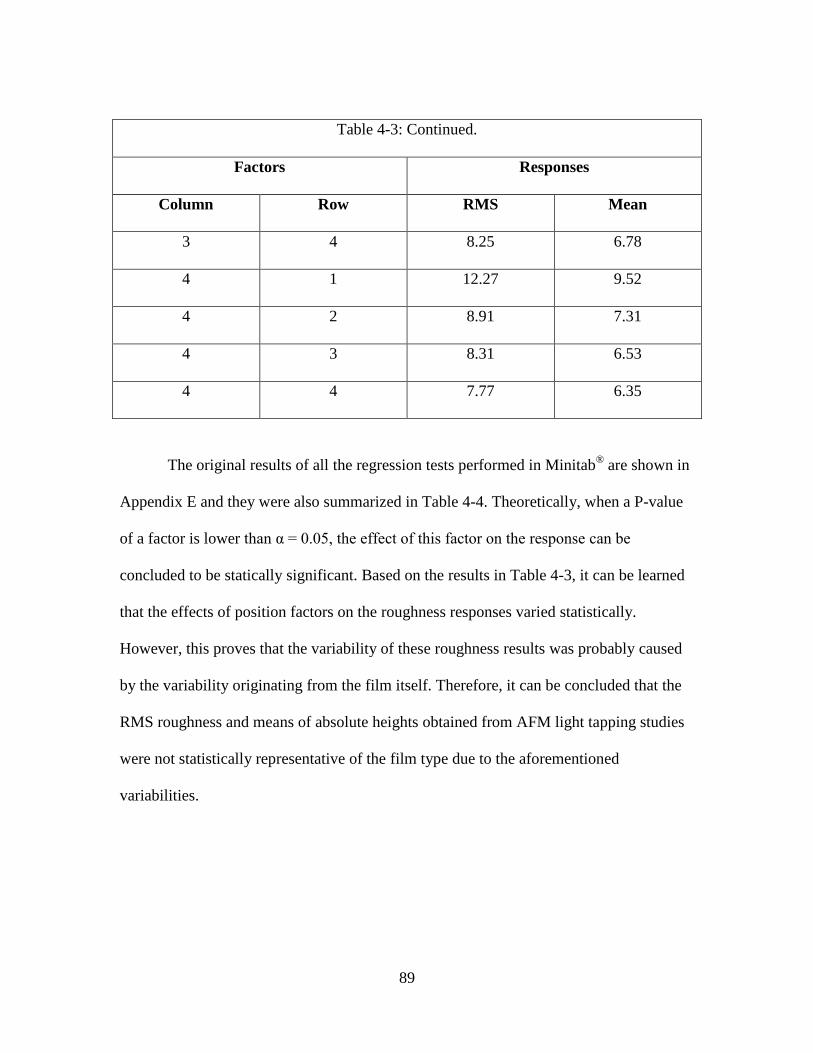
89
Table 4-3: Continued.
Factors Responses
Column Row RMS Mean
3 4 8.25 6.78
4 1 12.27 9.52
4 2 8.91 7.31
4 3 8.31 6.53
4 4 7.77 6.35
The original results of all the regression tests performed in Minitab® are shown in
Appendix E and they were also summarized in Table 4-4. Theoretically, when a P-value
of a factor is lower than α = 0.05, the effect of this factor on the response can be
concluded to be statically significant. Based on the results in Table 4-3, it can be learned
that the effects of position factors on the roughness responses varied statistically.
However, this proves that the variability of these roughness results was probably caused
by the variability originating from the film itself. Therefore, it can be concluded that the
RMS roughness and means of absolute heights obtained from AFM light tapping studies
were not statistically representative of the film type due to the aforementioned
variabilities.
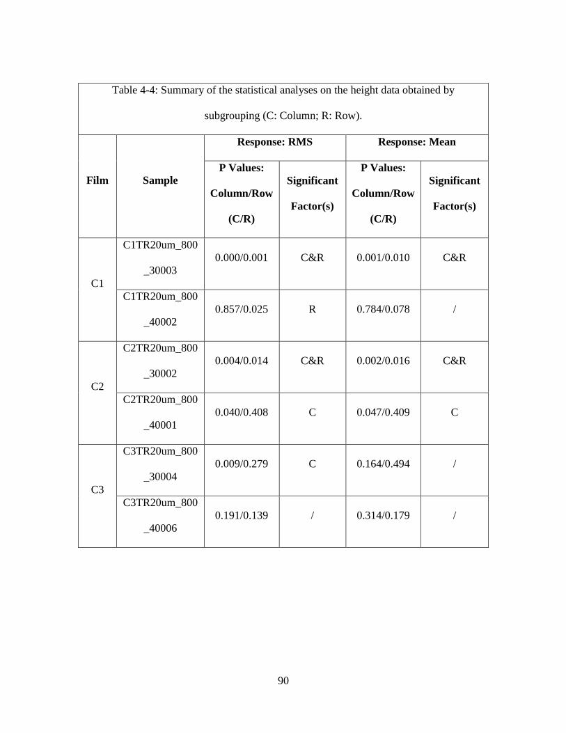
90
Table 4-4: Summary of the statistical analyses on the height data obtained by
subgrouping (C: Column; R: Row).
Film Sample
Response: RMS Response: Mean
P Values:
Column/Row
(C/R)
Significant
Factor(s)
P Values:
Column/Row
(C/R)
Significant
Factor(s)
C1
C1TR20um_800
_30003
0.000/0.001 C&R 0.001/0.010 C&R
C1TR20um_800
_40002
0.857/0.025 R 0.784/0.078 /
C2
C2TR20um_800
_30002
0.004/0.014 C&R 0.002/0.016 C&R
C2TR20um_800
_40001
0.040/0.408 C 0.047/0.409 C
C3
C3TR20um_800
_30004
0.009/0.279 C 0.164/0.494 /
C3TR20um_800
_40006
0.191/0.139 / 0.314/0.179 /
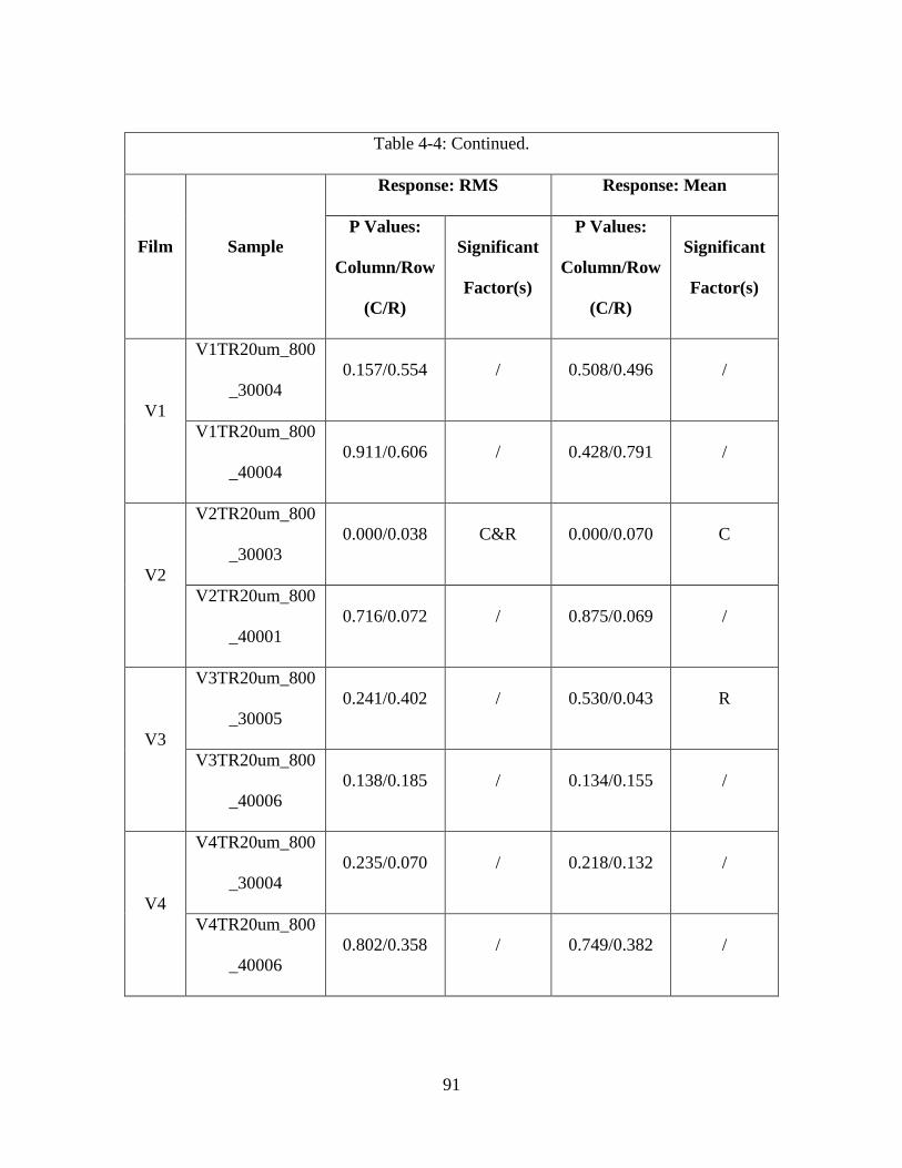
91
Table 4-4: Continued.
Film Sample
Response: RMS Response: Mean
P Values:
Column/Row
(C/R)
Significant
Factor(s)
P Values:
Column/Row
(C/R)
Significant
Factor(s)
V1
V1TR20um_800
_30004
0.157/0.554 / 0.508/0.496 /
V1TR20um_800
_40004
0.911/0.606 / 0.428/0.791 /
V2
V2TR20um_800
_30003
0.000/0.038 C&R 0.000/0.070 C
V2TR20um_800
_40001
0.716/0.072 / 0.875/0.069 /
V3
V3TR20um_800
_30005
0.241/0.402 / 0.530/0.043 R
V3TR20um_800
_40006
0.138/0.185 / 0.134/0.155 /
V4
V4TR20um_800
_30004
0.235/0.070 / 0.218/0.132 /
V4TR20um_800
_40006
0.802/0.358 / 0.749/0.382 /
92
It is worth noting that similar statistical analyses were not found in the research
studies previously conducted using AFM, particular in the studies of various substrates.
The AFM topography and phase angle images are often used for visual analyses (Strobel,
et al., 2003; Rams, et al., 2012; Nuntapichedkula, et. al., 2014). In the studies where the
roughness results (usually the RMS roughness) of the substrates play an important part,
researchers commonly use the average of the RMS roughness of three to five replicates in
their comparison (Guimond & Wertheimer, 2004; Nuntapichedkula, et. al., 2014).
However, the above statistical analyses of all the subgrouped data demonstrated that the
variability of the substrate may not be avoided even with sixteen replicates, regardless of
the impact of the variability of the AFM test on the roughness results. Thus, it should be
understood that the AFM test results can be affected by so many variables that they are
hard to maintain as statistically repeatable. However, these results have been proven to be
practically repeatable by many studies and increasing test replicates can increase the
practical (and statistical) repeatability.
In this study, good practical repeatability was seen between two replicates when
comparing the height and phase angle images visually (Appendix A). However, the
limited number of replicates did result in large variability in the roughness results, which
cannot be neglected. As shown in Figure 4-27, the RMS roughness and mean of absolute
heights of two replicates for each film type were averaged and plotted for comparison.
Note that all the error bars in the column graphs in this manuscript represent plus and
minus one standard deviation. Clearly, the average RMS values and average means of
the treated C1, C2, C3, V1 and V2 films were too close to differentiate from each other
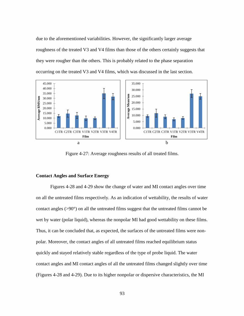
93
due to the aforementioned variabilities. However, the significantly larger average
roughness of the treated V3 and V4 films than those of the others certainly suggests that
they were rougher than the others. This is probably related to the phase separation
occurring on the treated V3 and V4 films, which was discussed in the last section.
a
b
Figure 4-27: Average roughness results of all treated films.
Contact Angles and Surface Energy
Figures 4-28 and 4-29 show the change of water and MI contact angles over time
on all the untreated films respectively. As an indication of wettability, the results of water
contact angles (>90°) on all the untreated films suggest that the untreated films cannot be
wet by water (polar liquid), whereas the nonpolar MI had good wettability on these films.
Thus, it can be concluded that, as expected, the surfaces of the untreated films were non-
polar. Moreover, the contact angles of all untreated films reached equilibrium status
quickly and stayed relatively stable regardless of the type of probe liquid. The water
contact angles and MI contact angles of all the untreated films changed slightly over time
(Figures 4-28 and 4-29). Due to its higher nonpolar or dispersive characteristics, the MI
0.000
5.000
10.000
15.000
20.000
25.000
30.000
35.000
40.000
45.000
C1TR C2TR C3TR V1TR V2TR V3TR V4TR
Avera
ge R
MS
/nm
Film
0.000
5.000
10.000
15.000
20.000
25.000
30.000
35.000
C1TR C2TR C3TR V1TR V2TR V3TR V4TR
Avera
ge M
ea
n/n
m
Film

94
contact angles of the untreated C2 film were at least 10° smaller than those of its
counterparts (Figure 4-29).
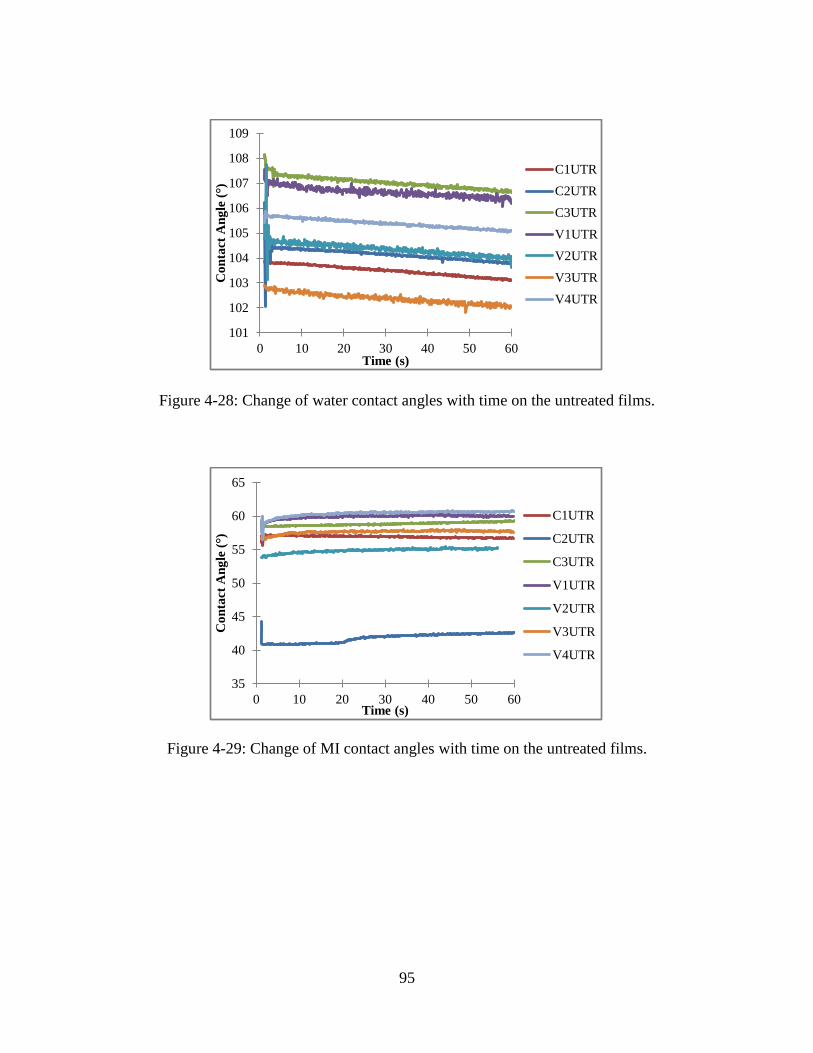
95
Figure 4-28: Change of water contact angles with time on the untreated films.
101
102
103
104
105
106
107
108
109
0 10 20 30 40 50 60
Co
nta
ct A
ng
le (
°)
Time (s)
C1UTR
C2UTR
C3UTR
V1UTR
V2UTR
V3UTR
V4UTR
Figure 4-29: Change of MI contact angles with time on the untreated films.
35
40
45
50
55
60
65
0 10 20 30 40 50 60
Co
nta
ct A
ng
le (
°)
Time (s)
C1UTR
C2UTR
C3UTR
V1UTR
V2UTR
V3UTR
V4UTR
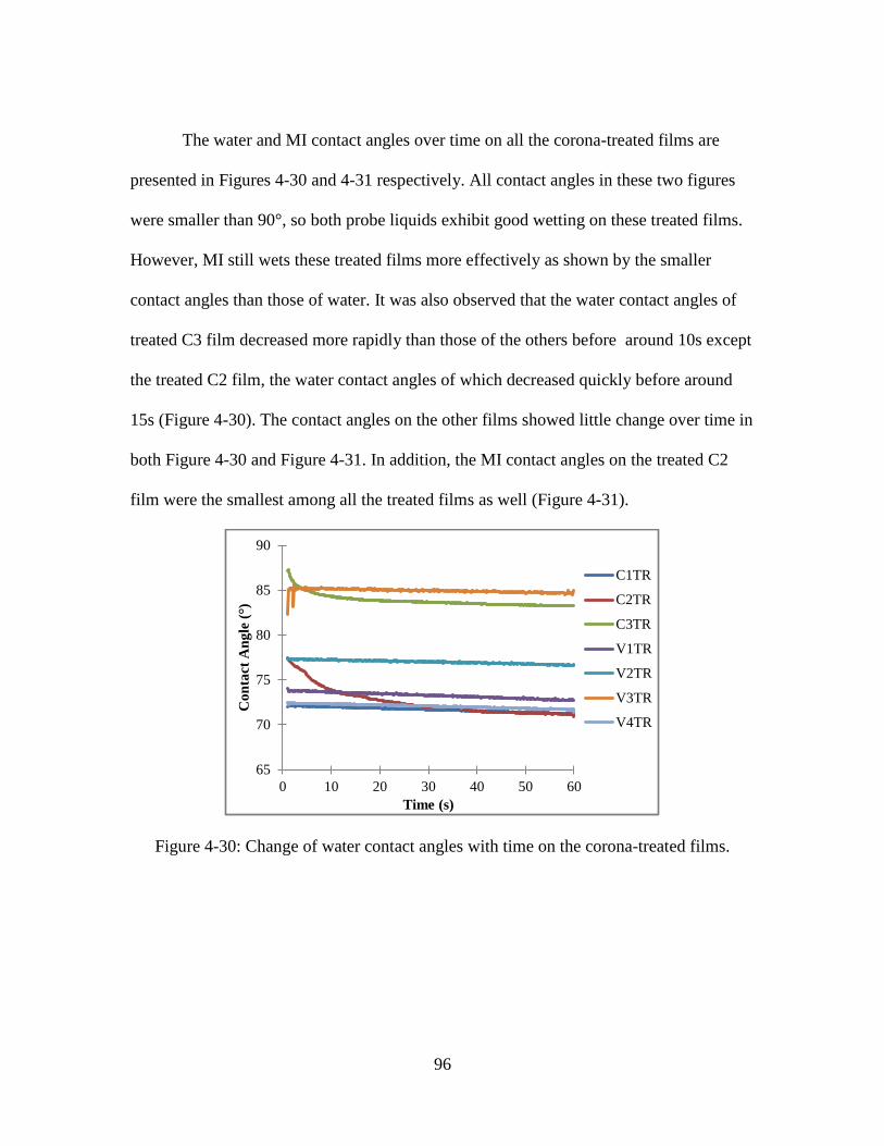
96
The water and MI contact angles over time on all the corona-treated films are
presented in Figures 4-30 and 4-31 respectively. All contact angles in these two figures
were smaller than 90°, so both probe liquids exhibit good wetting on these treated films.
However, MI still wets these treated films more effectively as shown by the smaller
contact angles than those of water. It was also observed that the water contact angles of
treated C3 film decreased more rapidly than those of the others before around 10s except
the treated C2 film, the water contact angles of which decreased quickly before around
15s (Figure 4-30). The contact angles on the other films showed little change over time in
both Figure 4-30 and Figure 4-31. In addition, the MI contact angles on the treated C2
film were the smallest among all the treated films as well (Figure 4-31).
Figure 4-30: Change of water contact angles with time on the corona-treated films.
65
70
75
80
85
90
0 10 20 30 40 50 60
Co
nta
ct A
ng
le (
°)
Time (s)
C1TR
C2TR
C3TR
V1TR
V2TR
V3TR
V4TR
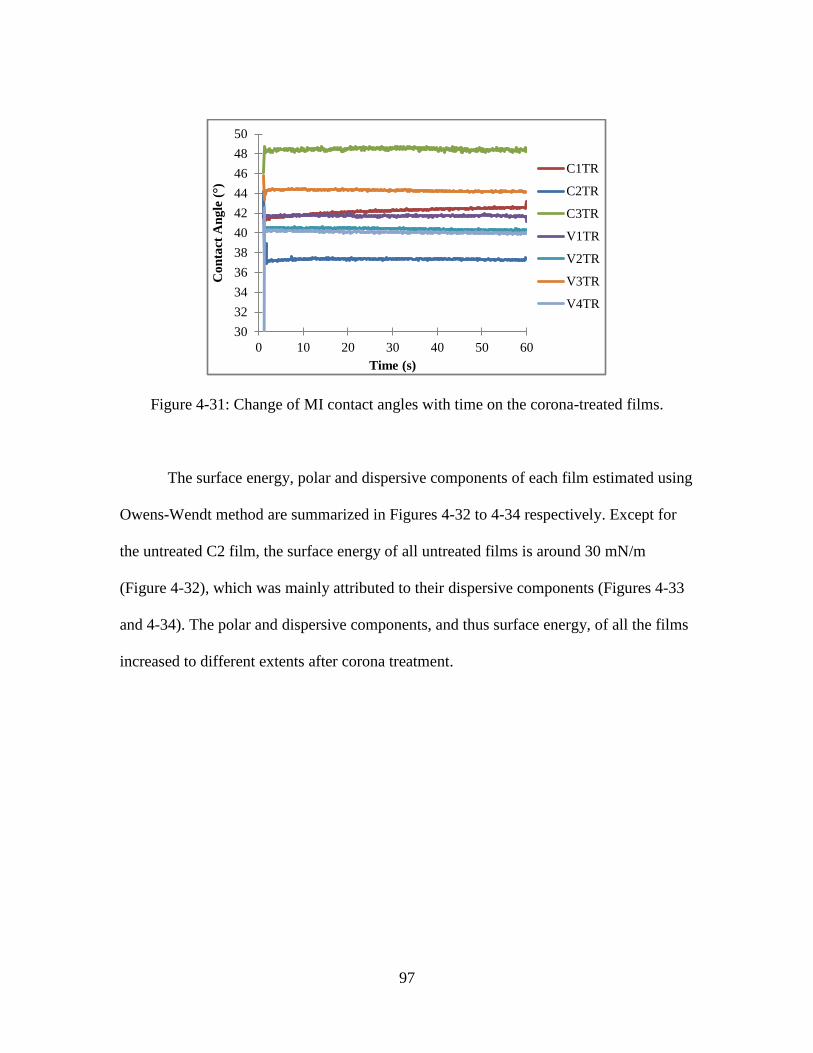
97
Figure 4-31: Change of MI contact angles with time on the corona-treated films.
The surface energy, polar and dispersive components of each film estimated using
Owens-Wendt method are summarized in Figures 4-32 to 4-34 respectively. Except for
the untreated C2 film, the surface energy of all untreated films is around 30 mN/m
(Figure 4-32), which was mainly attributed to their dispersive components (Figures 4-33
and 4-34). The polar and dispersive components, and thus surface energy, of all the films
increased to different extents after corona treatment.
30
32
34
36
38
40
42
44
46
48
50
0 10 20 30 40 50 60
Co
nta
ct A
ng
le (
°)
Time (s)
C1TR
C2TR
C3TR
V1TR
V2TR
V3TR
V4TR
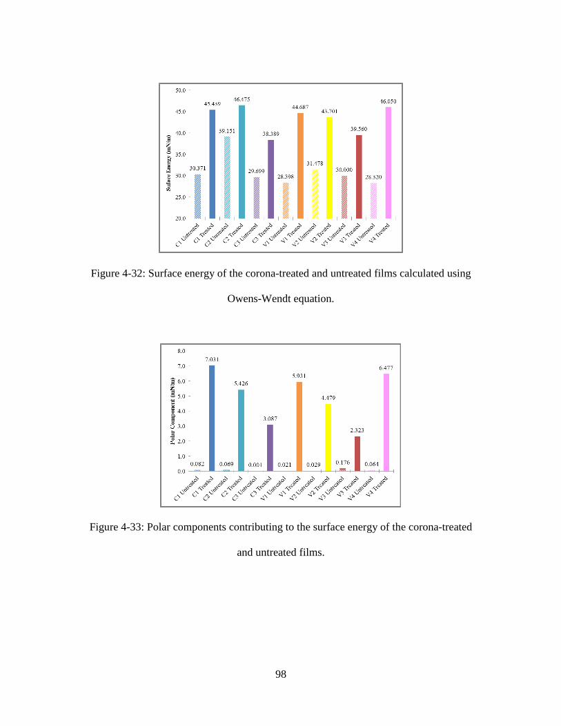
98
Figure 4-32: Surface energy of the corona-treated and untreated films calculated using
Owens-Wendt equation.
Figure 4-33: Polar components contributing to the surface energy of the corona-treated
and untreated films.
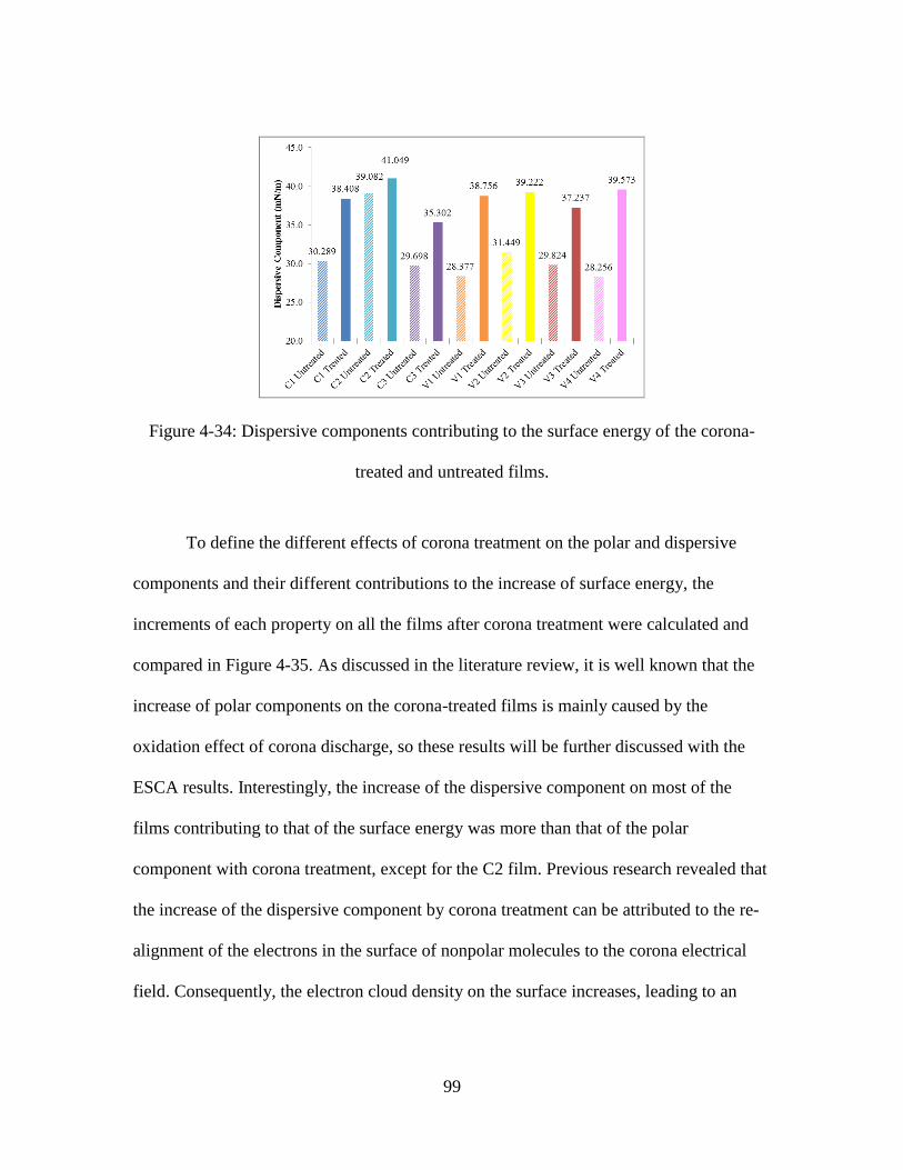
99
To define the different effects of corona treatment on the polar and dispersive
components and their different contributions to the increase of surface energy, the
increments of each property on all the films after corona treatment were calculated and
compared in Figure 4-35. As discussed in the literature review, it is well known that the
increase of polar components on the corona-treated films is mainly caused by the
oxidation effect of corona discharge, so these results will be further discussed with the
ESCA results. Interestingly, the increase of the dispersive component on most of the
films contributing to that of the surface energy was more than that of the polar
component with corona treatment, except for the C2 film. Previous research revealed that
the increase of the dispersive component by corona treatment can be attributed to the re-
alignment of the electrons in the surface of nonpolar molecules to the corona electrical
field. Consequently, the electron cloud density on the surface increases, leading to an
Figure 4-34: Dispersive components contributing to the surface energy of the corona-
treated and untreated films.
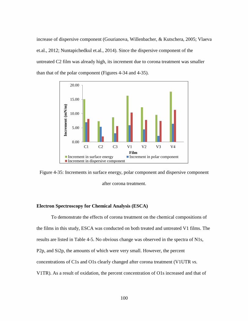
100
increase of dispersive component (Gourianova, Willenbacher, & Kutschera, 2005; Vlaeva
et.al., 2012; Nuntapichedkul et.al., 2014). Since the dispersive component of the
untreated C2 film was already high, its increment due to corona treatment was smaller
than that of the polar component (Figures 4-34 and 4-35).
Figure 4-35: Increments in surface energy, polar component and dispersive component
after corona treatment.
Electron Spectroscopy for Chemical Analysis (ESCA)
To demonstrate the effects of corona treatment on the chemical compositions of
the films in this study, ESCA was conducted on both treated and untreated V1 films. The
results are listed in Table 4-5. No obvious change was observed in the spectra of N1s,
P2p, and Si2p, the amounts of which were very small. However, the percent
concentrations of C1s and O1s clearly changed after corona treatment (V1UTR vs.
V1TR). As a result of oxidation, the percent concentration of O1s increased and that of
0.00
5.00
10.00
15.00
20.00
C1 C2 C3 V1 V2 V3 V4
Incr
em
ent
(mN
/m)
Film Increment in surface energy Increment in polar componentIncrement in dispersive component
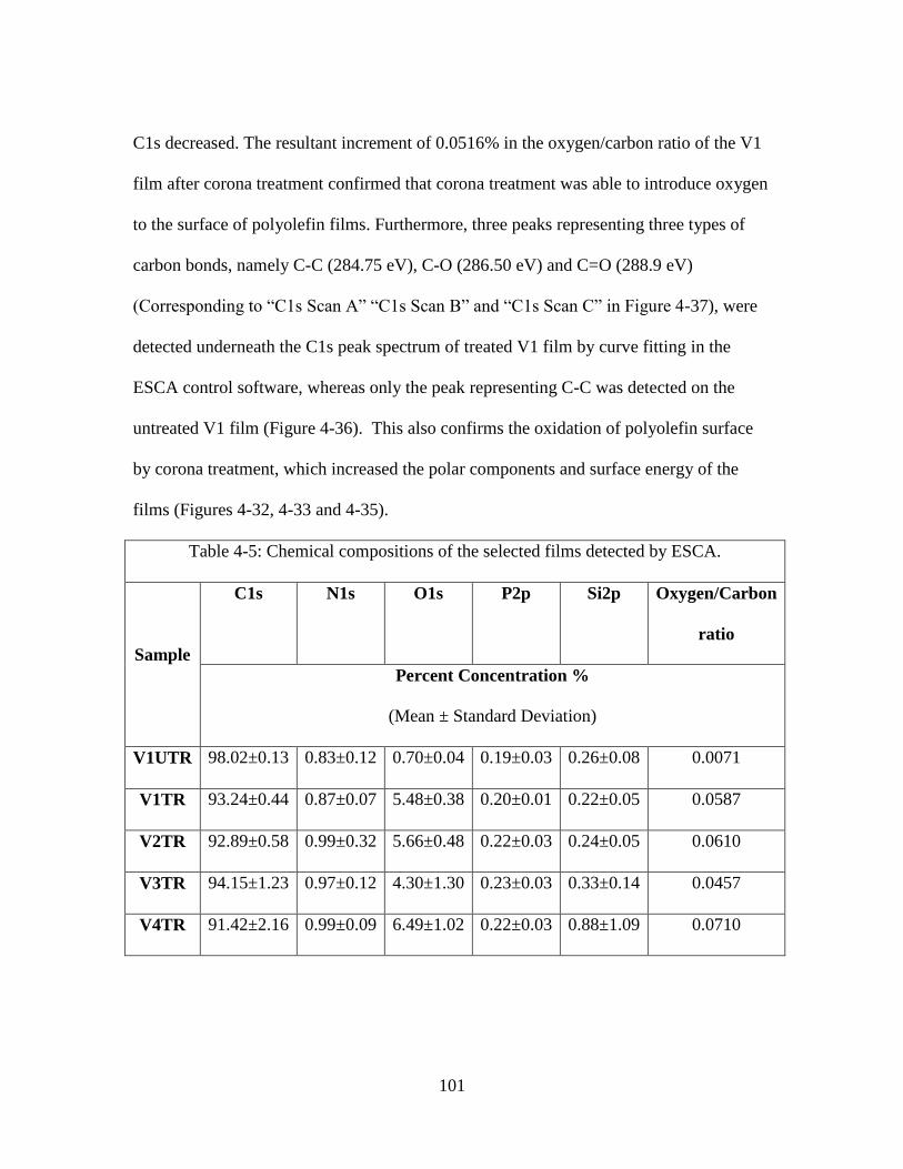
101
C1s decreased. The resultant increment of 0.0516% in the oxygen/carbon ratio of the V1
film after corona treatment confirmed that corona treatment was able to introduce oxygen
to the surface of polyolefin films. Furthermore, three peaks representing three types of
carbon bonds, namely C-C (284.75 eV), C-O (286.50 eV) and C=O (288.9 eV)
(Corresponding to “C1s Scan A” “C1s Scan B” and “C1s Scan C” in Figure 4-37), were
detected underneath the C1s peak spectrum of treated V1 film by curve fitting in the
ESCA control software, whereas only the peak representing C-C was detected on the
untreated V1 film (Figure 4-36). This also confirms the oxidation of polyolefin surface
by corona treatment, which increased the polar components and surface energy of the
films (Figures 4-32, 4-33 and 4-35).
Table 4-5: Chemical compositions of the selected films detected by ESCA.
Sample
C1s N1s O1s P2p Si2p Oxygen/Carbon
ratio
Percent Concentration %
(Mean ± Standard Deviation)
V1UTR 98.02±0.13 0.83±0.12 0.70±0.04 0.19±0.03 0.26±0.08 0.0071
V1TR 93.24±0.44 0.87±0.07 5.48±0.38 0.20±0.01 0.22±0.05 0.0587
V2TR 92.89±0.58 0.99±0.32 5.66±0.48 0.22±0.03 0.24±0.05 0.0610
V3TR 94.15±1.23 0.97±0.12 4.30±1.30 0.23±0.03 0.33±0.14 0.0457
V4TR 91.42±2.16 0.99±0.09 6.49±1.02 0.22±0.03 0.88±1.09 0.0710
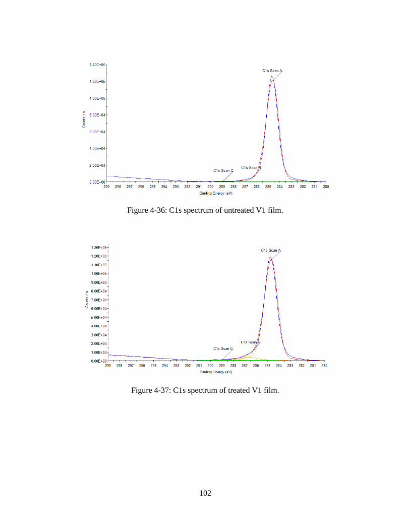
102
Figure 4-36: C1s spectrum of untreated V1 film.
Figure 4-37: C1s spectrum of treated V1 film.
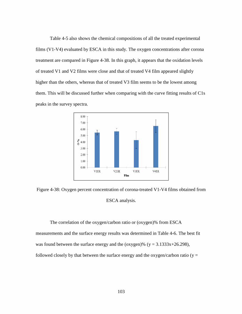
103
Table 4-5 also shows the chemical compositions of all the treated experimental
films (V1-V4) evaluated by ESCA in this study. The oxygen concentrations after corona
treatment are compared in Figure 4-38. In this graph, it appears that the oxidation levels
of treated V1 and V2 films were close and that of treated V4 film appeared slightly
higher than the others, whereas that of treated V3 film seems to be the lowest among
them. This will be discussed further when comparing with the curve fitting results of C1s
peaks in the survey spectra.
Figure 4-38: Oxygen percent concentration of corona-treated V1-V4 films obtained from
ESCA analysis.
The correlation of the oxygen/carbon ratio or (oxygen)% from ESCA
measurements and the surface energy results was determined in Table 4-6. The best fit
was found between the surface energy and the (oxygen)% (y = 3.1333x+26.298),
followed closely by that between the surface energy and the oxygen/carbon ratio (y =

104
285.95x+26.553) of these films. The fitting graphs resulting in R² = 0.9902 and R² =
0.9876 are shown in Figure 4-39 and Figure 4-40 respectively.
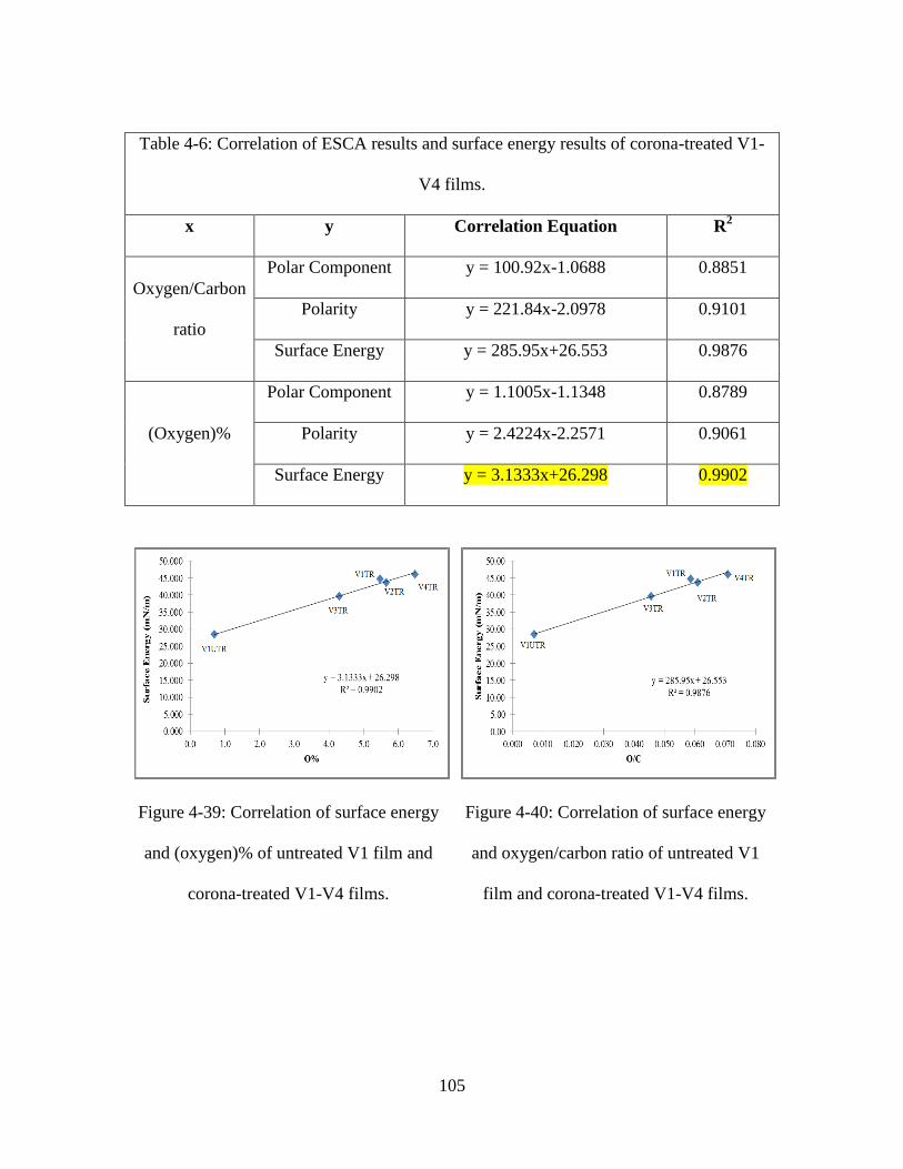
105
Table 4-6: Correlation of ESCA results and surface energy results of corona-treated V1-
V4 films.
x y Correlation Equation R2
Oxygen/Carbon
ratio
Polar Component y = 100.92x-1.0688 0.8851
Polarity y = 221.84x-2.0978 0.9101
Surface Energy y = 285.95x+26.553 0.9876
(Oxygen)%
Polar Component y = 1.1005x-1.1348 0.8789
Polarity y = 2.4224x-2.2571 0.9061
Surface Energy y = 3.1333x+26.298 0.9902
Figure 4-39: Correlation of surface energy
and (oxygen)% of untreated V1 film and
corona-treated V1-V4 films.
Figure 4-40: Correlation of surface energy
and oxygen/carbon ratio of untreated V1
film and corona-treated V1-V4 films.
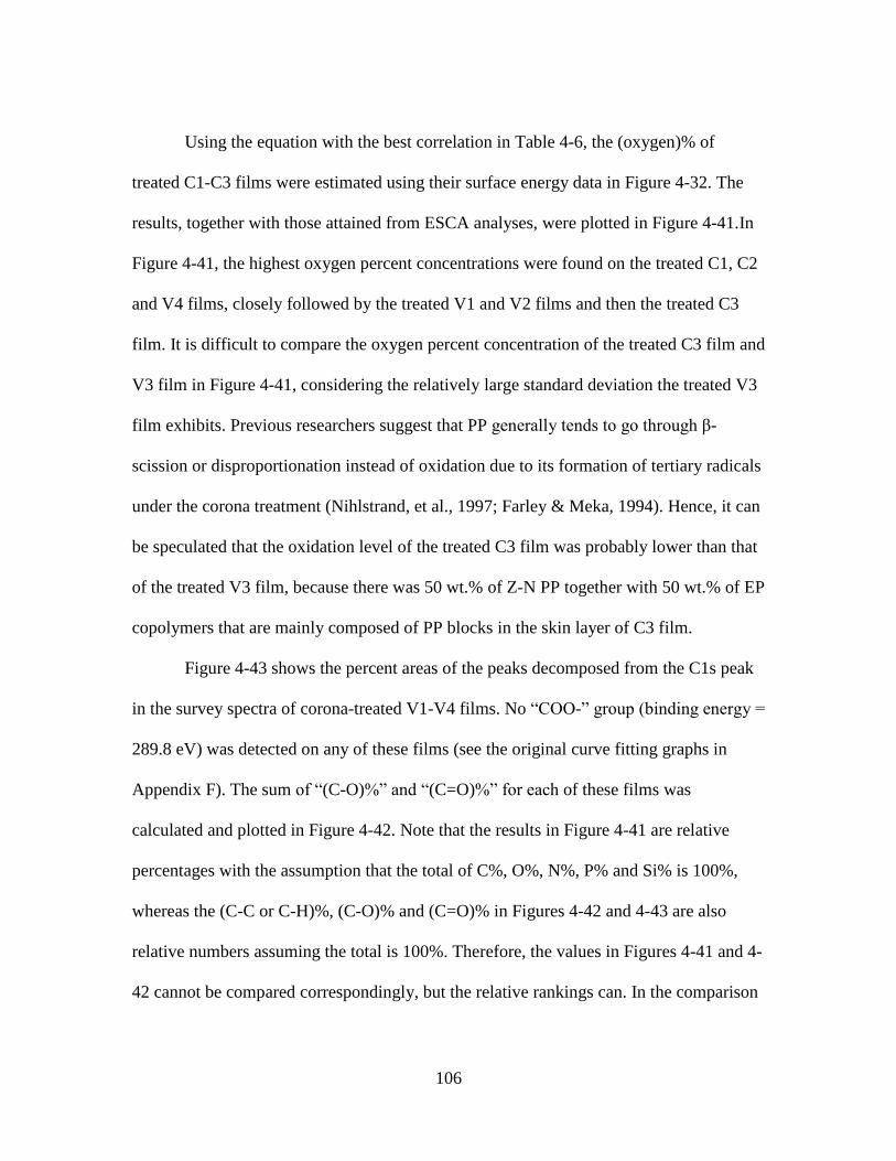
106
Using the equation with the best correlation in Table 4-6, the (oxygen)% of
treated C1-C3 films were estimated using their surface energy data in Figure 4-32. The
results, together with those attained from ESCA analyses, were plotted in Figure 4-41.In
Figure 4-41, the highest oxygen percent concentrations were found on the treated C1, C2
and V4 films, closely followed by the treated V1 and V2 films and then the treated C3
film. It is difficult to compare the oxygen percent concentration of the treated C3 film and
V3 film in Figure 4-41, considering the relatively large standard deviation the treated V3
film exhibits. Previous researchers suggest that PP generally tends to go through β-
scission or disproportionation instead of oxidation due to its formation of tertiary radicals
under the corona treatment (Nihlstrand, et al., 1997; Farley & Meka, 1994). Hence, it can
be speculated that the oxidation level of the treated C3 film was probably lower than that
of the treated V3 film, because there was 50 wt.% of Z-N PP together with 50 wt.% of EP
copolymers that are mainly composed of PP blocks in the skin layer of C3 film.
Figure 4-43 shows the percent areas of the peaks decomposed from the C1s peak
in the survey spectra of corona-treated V1-V4 films. No “COO-” group (binding energy =
289.8 eV) was detected on any of these films (see the original curve fitting graphs in
Appendix F). The sum of “(C-O)%” and “(C=O)%” for each of these films was
calculated and plotted in Figure 4-42. Note that the results in Figure 4-41 are relative
percentages with the assumption that the total of C%, O%, N%, P% and Si% is 100%,
whereas the (C-C or C-H)%, (C-O)% and (C=O)% in Figures 4-42 and 4-43 are also
relative numbers assuming the total is 100%. Therefore, the values in Figures 4-41 and 4-
42 cannot be compared correspondingly, but the relative rankings can. In the comparison
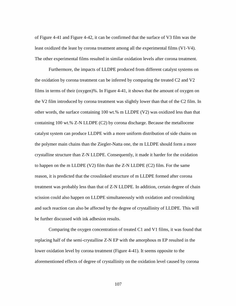
107
of Figure 4-41 and Figure 4-42, it can be confirmed that the surface of V3 film was the
least oxidized the least by corona treatment among all the experimental films (V1-V4).
The other experimental films resulted in similar oxidation levels after corona treatment.
Furthermore, the impacts of LLDPE produced from different catalyst systems on
the oxidation by corona treatment can be inferred by comparing the treated C2 and V2
films in terms of their (oxygen)%. In Figure 4-41, it shows that the amount of oxygen on
the V2 film introduced by corona treatment was slightly lower than that of the C2 film. In
other words, the surface containing 100 wt.% m LLDPE (V2) was oxidized less than that
containing 100 wt.% Z-N LLDPE (C2) by corona discharge. Because the metallocene
catalyst system can produce LLDPE with a more uniform distribution of side chains on
the polymer main chains than the Ziegler-Natta one, the m LLDPE should form a more
crystalline structure than Z-N LLDPE. Consequently, it made it harder for the oxidation
to happen on the m LLDPE (V2) film than the Z-N LLDPE (C2) film. For the same
reason, it is predicted that the crosslinked structure of m LLDPE formed after corona
treatment was probably less than that of Z-N LLDPE. In addition, certain degree of chain
scission could also happen on LLDPE simultaneously with oxidation and crosslinking
and such reaction can also be affected by the degree of crystallinity of LLDPE. This will
be further discussed with ink adhesion results.
Comparing the oxygen concentration of treated C1 and V1 films, it was found that
replacing half of the semi-crystalline Z-N EP with the amorphous m EP resulted in the
lower oxidation level by corona treatment (Figure 4-41). It seems opposite to the
aforementioned effects of degree of crystallinity on the oxidation level caused by corona
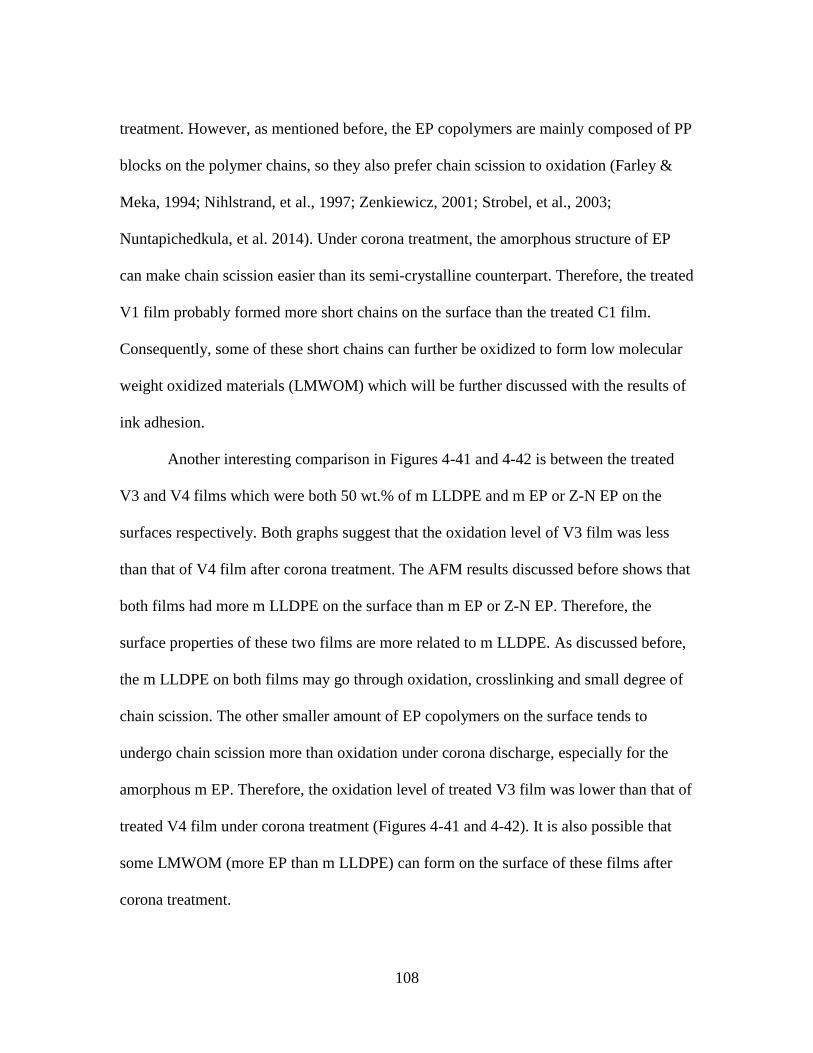
108
treatment. However, as mentioned before, the EP copolymers are mainly composed of PP
blocks on the polymer chains, so they also prefer chain scission to oxidation (Farley &
Meka, 1994; Nihlstrand, et al., 1997; Zenkiewicz, 2001; Strobel, et al., 2003;
Nuntapichedkula, et al. 2014). Under corona treatment, the amorphous structure of EP
can make chain scission easier than its semi-crystalline counterpart. Therefore, the treated
V1 film probably formed more short chains on the surface than the treated C1 film.
Consequently, some of these short chains can further be oxidized to form low molecular
weight oxidized materials (LMWOM) which will be further discussed with the results of
ink adhesion.
Another interesting comparison in Figures 4-41 and 4-42 is between the treated
V3 and V4 films which were both 50 wt.% of m LLDPE and m EP or Z-N EP on the
surfaces respectively. Both graphs suggest that the oxidation level of V3 film was less
than that of V4 film after corona treatment. The AFM results discussed before shows that
both films had more m LLDPE on the surface than m EP or Z-N EP. Therefore, the
surface properties of these two films are more related to m LLDPE. As discussed before,
the m LLDPE on both films may go through oxidation, crosslinking and small degree of
chain scission. The other smaller amount of EP copolymers on the surface tends to
undergo chain scission more than oxidation under corona discharge, especially for the
amorphous m EP. Therefore, the oxidation level of treated V3 film was lower than that of
treated V4 film under corona treatment (Figures 4-41 and 4-42). It is also possible that
some LMWOM (more EP than m LLDPE) can form on the surface of these films after
corona treatment.
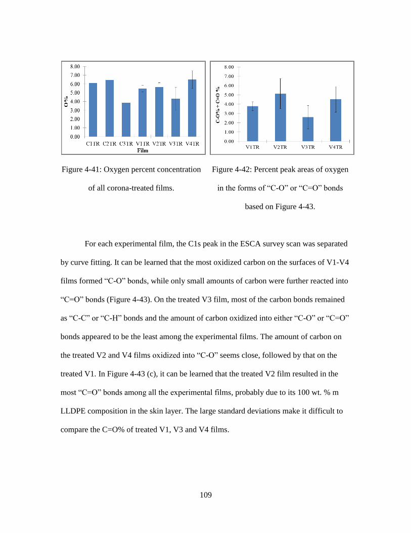
109
Figure 4-41: Oxygen percent concentration
of all corona-treated films.
Figure 4-42: Percent peak areas of oxygen
in the forms of “C-O” or “C=O” bonds
based on Figure 4-43.
For each experimental film, the C1s peak in the ESCA survey scan was separated
by curve fitting. It can be learned that the most oxidized carbon on the surfaces of V1-V4
films formed “C-O” bonds, while only small amounts of carbon were further reacted into
“C=O” bonds (Figure 4-43). On the treated V3 film, most of the carbon bonds remained
as “C-C” or “C-H” bonds and the amount of carbon oxidized into either “C-O” or “C=O”
bonds appeared to be the least among the experimental films. The amount of carbon on
the treated V2 and V4 films oxidized into “C-O” seems close, followed by that on the
treated V1. In Figure 4-43 (c), it can be learned that the treated V2 film resulted in the
most “C=O” bonds among all the experimental films, probably due to its 100 wt. % m
LLDPE composition in the skin layer. The large standard deviations make it difficult to
compare the C=O% of treated V1, V3 and V4 films.
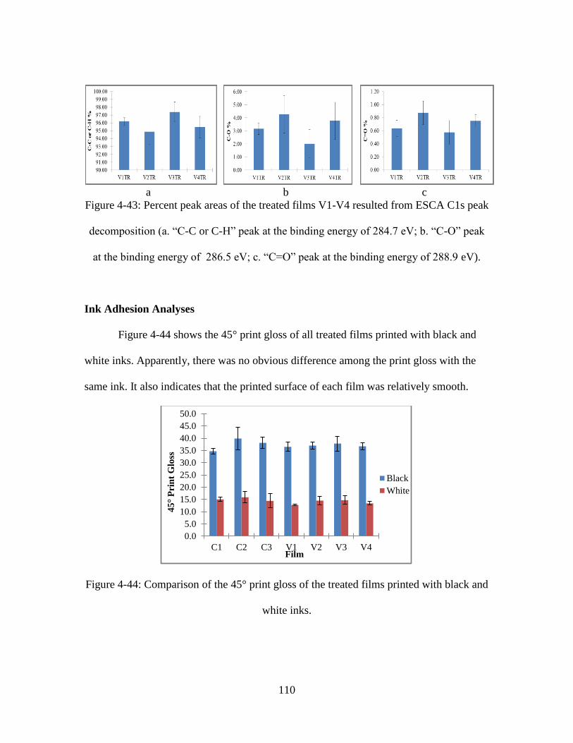
110
a
b
c
Figure 4-43: Percent peak areas of the treated films V1-V4 resulted from ESCA C1s peak
decomposition (a. “C-C or C-H” peak at the binding energy of 284.7 eV; b. “C-O” peak
at the binding energy of 286.5 eV; c. “C=O” peak at the binding energy of 288.9 eV).
Ink Adhesion Analyses
Figure 4-44 shows the 45° print gloss of all treated films printed with black and
white inks. Apparently, there was no obvious difference among the print gloss with the
same ink. It also indicates that the printed surface of each film was relatively smooth.
Figure 4-44: Comparison of the 45° print gloss of the treated films printed with black and
white inks.
0.0
5.0
10.0
15.0
20.0
25.0
30.0
35.0
40.0
45.0
50.0
C1 C2 C3 V1 V2 V3 V4
45
° P
rin
t G
loss
Film
Black
White
111
After Sutherland rub tests, damage on the printed films was barely seen, which
led to no change in the print density by rubbing tests (see results in Appendix G).
Rubbing the printed sample against either the printed sample or the unprinted film makes
no difference in the results. This can be explained by the relatively smooth printed
surfaces of all the treated films that were revealed in Figure 4-44.
The ink adhesion on each treated film was also tested using the tape test. Since the
treated C1 and C2 films are commercial grades, widely used in the flexible packaging
industry, their tape test results in this study were regarded as the target.
In Figure 4-45(a), the white ink adhesion on all the treated films using three
different tapes matched the target. When printing on the polyolefin clear films, white ink
is sometimes printed first or last as the background for text or image, so it is generally
formulated to provide strong ink adhesion. Therefore, it was not surprising that the white
ink adhesion on all the treated films was better than that of the black ink (Figures 4-45).
As is shown in Figure 4-45(b), the type of tape used in the test exhibits difference
in the results of black ink adhesion. With tape #810 and tape #610, the adhesion of black
ink on all the treated films achieved the target. Different tape test results were found
when using the strongest tape (#600). The treated V3 and V4 films resulted in ink
adhesion close to the target, while the treated C3, V1 and V2 films failed using tape
#600. The most common type used in industry is the #610 tape.
The poor ink adhesion on the treated C3 film can probably be attributed to the low
oxidation level it had after corona treatment (Figures 4-41 and 4-45 (b)) and the reason
for this has been discussed in Chapter Two. A certain amount of LMWOM could also
112
form during corona treatment since PP tends to go through more chain scission than
oxidation under the corona treatment. In Chapter Two, it was stated that LMWOM can
form on polyolefin films due to corona treatment and these species can attract the polar
groups in the ink to generate ink adhesion. However, these species do not anchor onto the
surface, so they can still be peeled off from the base film, leading to ink adhesion failure.
To prove the existence of LMWOM, it is recommended for future studies that the treated
film surface be washed with any polar liquid, such as water, and followed by conducting
the AFM, surface energy and ESCA analyses, as well as the tape tests, on the films again.
Surprisingly, the treated film V2 resulted in poor ink adhesion, even though it
showed high oxygen percent concentration in the ESCA analyses. As speculated before,
the m LLDPE containing V2 film possibly formed less crosslinked structure and more
chain scission than the Z-N LLDPE containing C2 film after corona treatment. Therefore,
any LMWOM formed due to corona treatment on the V2 film had more mobility to get to
the surface. From the results of AFM analyses, it was learned that the treated C2 film
formed a very uniform fibrous structure on the surface (Figures 4-4 and 4-11). The
surface of V2 film seemed more fragmented, including some microstructures with
various sizes that were formed on the top surface, together with some small curly fibrous
structure underneath (Figures 4-7 and 4-14). This could be an indication of the existence
of LMWOM on the surface of the treated V2 film. After adhering with the ink, these
unanchored LMWOM-ink structures could be peeled off easily by the tape, resulting in
what appears to be poor ink adhesion on the treated V2 film.
113
The same reason could also explain why the ink adhesion of treated V1 film did
not match the target, in spite of a high oxygen percent concentration detected by ESCA.
As explained before, EP mainly containing PP blocks on the polymer chains tends to
undergo chain scission rather than oxidation under corona treatment and the amorphous
structure of m EP makes it easier for chain scission than the semi-crystalline structure of
Z-N EP (Farley & Meka, 1994; Nihlstrand, et al., 1997; Zenkiewicz, 2001; Strobel, et al.,
2003; Nuntapichedkula, et al. 2014). Thus, lower oxygen content was detected by ESCA
on the treated V1 film than that of the treated C1 film. Also LMWOM were likely to exist
on the treated V1 film, which would lead to the apparently worse ink adhesion on the
treated V1 film than its counterpart. Again, further investigation is needed using the
washing method.
Another surprise in the black ink adhesion results tested using tape #600 was the
treated V3 film (Figure 4-45 (b)). The results of surface energy and ESCA analyses
suggest that the polarized or oxidation level of treated V3 film was lower than the target
(treated C1 or C2 film). Nevertheless, it actually exhibited very comparable black ink
adhesion to the target.
The good ink adhesion of both treated V3 and V4 films could be related to the
higher roughness compared to their counterparts (Figure 4-2). It is well known that the
“roughening” effects of corona treatment on the polyolefin film due to radical reaction
can possibly enhance the ink wettability and adhesion of the film surface to some extent
due to the increase of contact surface area (Packham & Johnston, 1994; Zhang, Sun &
Wadsworth, 1998). As stated earlier, more m LLDPE than m EP or Z-N EP existed on
114
the treated V3 and V4 films and this could have contributed more to the resultant ink
adhesion than the other EP components. Moreover, m LLDPE is easier to oxidize and it
also can form some degree of crosslinked structure on the surface of the films. As to the
smaller amount of EP on these two films, it has been discussed before that EP tends to
undergo chain scission more than oxidation and the amorphous structure of m EP can
make it easier to get scission than on the semi-crystalline Z-N EP structure. Thus, there
were probably more LMWOM on the treated V3 film leading to worse apparent ink
adhesion than on the treated V4 film, based on the hypothesis presented at the beginning
of this chapter.
However, the results in Figure 3-35 do not support this. Another unique factor
affecting the ink adhesion on the treated V3 film was missing in above discussion.
According to the AFM results, there was more m LLDPE formed on the top surface of
treated V3 film, while the amorphous m EP existed at the lower area. It is possible that,
because the m EP was beneath the level of the film-and-tape contact area, the low
molecular weight of m EP was difficult to pick up with the tape. In contrast, such vertical
distribution difference was not observed in the AFM results of treated V4 film. This is a
possible explanation of why the ink adhesion of treated V3 film was slightly better than
that of treated V4 film.
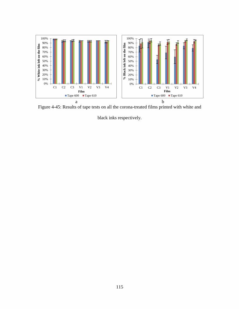
115
a
b
Figure 4-45: Results of tape tests on all the corona-treated films printed with white and
black inks respectively.
0%
10%
20%
30%
40%
50%
60%
70%
80%
90%
100%
C1 C2 C3 V1 V2 V3 V4
% W
hit
e i
nk
left
on
th
e f
ilm
Film
Tape 600 Tape 610
0%
10%
20%
30%
40%
50%
60%
70%
80%
90%
100%
C1 C2 C3 V1 V2 V3 V4
% B
lack
in
k l
eft
on
th
e f
ilm
Film
Tape 600 Tape 610
116
CHAPTER FIVE
CONCLUSIONS AND RECOMMENDATIONS
Conclusions
The use of AFM in different tapping modes was demonstrated to be very useful to
determine the topography, morphology, and viscoelasticity of the polyolefin films.
Furthermore, the phase angle results can be used to indicate the miscibility of the multi-
component polyolefin blend and also to study the distribution of amorphous and
crystalline structures on the surface. Based on the results of AFM, it was learned that the
film surfaces containing only one component generated relatively uniform topography
and morphology. In contrast, the topography and morphology of the film surface
composed of polyolefin blends was proven to be highly related to the miscibility and
distribution of different components in the blends.
It was learned that the same type of polyolefin, produced using different catalyst
systems, were still miscible (e.g. V1: m EP & Z-N EP), although they had very different
degrees of crystallinity. Metallocene catalyzed EP was semi-miscible with Ziegler-Natta
catalyzed PP probably because they both have long PP blocks (i.e. chains in PP). Either
metallocene or Ziegler-Natta catalyzed EP was not miscible with metallocene catalyzed
LLDPE (e.g. V3 and V4 films). Furthermore, when two components are not miscible in a
blend, they can result in uneven distributions of these components not only on the surface
but also vertically after corona treatment. Moreover, the phase separation in the blends
can also increase the roughness of the film, which to some extent can improve the ink

117
wetting and adhesion, possibly due to the increase in contact surface areas (e.g. treated
V3 film).
It was proposed as a hypothesis that the corona effects (including oxidation, chain
scission, crosslinking and roughening) have less influence on the surface of metallocene
catalyzed polyolefin film than on their Z-N counterpart and the surface characteristics
affecting ink wetting and adhesion vary depending on which corona effect dominants.
This hypothesis was found to be supported by the results obtained in this study.
Combining light tapping and hard tapping AFM, surface energy, and ESCA
analyses was proven to be a feasible method to study the effects of different surface
properties on the ink wetting and adhesion. However, the possible formation of LMWOM
under corona treatment on the polyolefin films also needs to be studied, because it may
affect good ink adhesion on the polyolefin films.
In addition, a correlation of surface energy and the oxidation level detected by
ESCA was revealed. It was used to estimate the oxygen content on the treated control
films in this study. It can be a useful tool to estimate the oxidation level of a polyolefin
film when an ESCA unit is not available.
Recommendations
Due the limited scope of this project, the untreated films were not analyzed using
AFM. It is highly recommended to do so in order to further understand the effects of
corona treatment on the topography and morphology of all the skin compositions in this
study. Due to the aforementioned variability of the AFM analyses of polyolefin films, it

118
is also advised to increase test replicates in the light tapping test in order to achieve good
repeatability and reproducibility of the roughness results. However, it is worth noting that
the variability caused by the film production processes, such as the variability across the
film web, is hard to avoid. A statistical analysis to study the variability of AFM test itself
also needs to be conducted with a proper method.
To better understand the factors influencing ink adhesion, it is recommended to
wash the surface of each treated film with a polar liquid in order to remove the possible
LMWOM from the surface. Then, the same series of tests should be conducted on the
washed samples. This could help to further understand the factors affecting the ink
wetting and adhesion on the polyolefin films.
In addition, more data should be obtained to further verify and/or modify the
correlation between the surface energy results and the ESCA results found in Table 4-5.
If it is proven to be feasible, it could allow for the understanding of the impact of corona
treatment on the oxidation of polyolefin films when an expensive and sophisticated
ESCA machine is not available.

119
APPENDICES
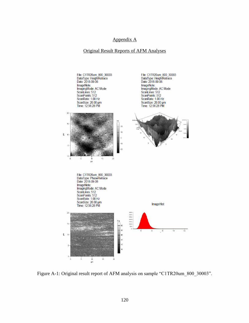
120
Appendix A
Original Result Reports of AFM Analyses
Figure A-1: Original result report of AFM analysis on sample “C1TR20um_800_30003”.
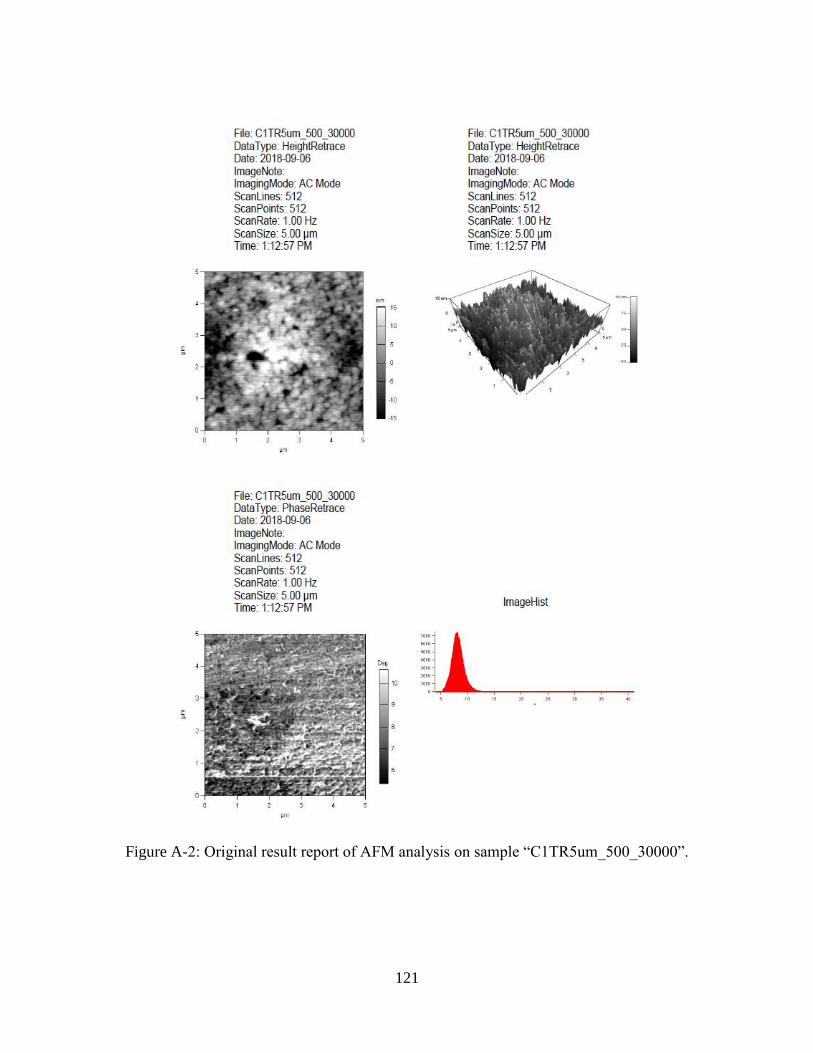
121
Figure A-2: Original result report of AFM analysis on sample “C1TR5um_500_30000”.

122
Figure A-3: Original result report of AFM analysis on sample “C1TR20um_800_40002”.
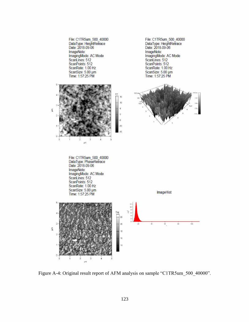
123
Figure A-4: Original result report of AFM analysis on sample “C1TR5um_500_40000”.
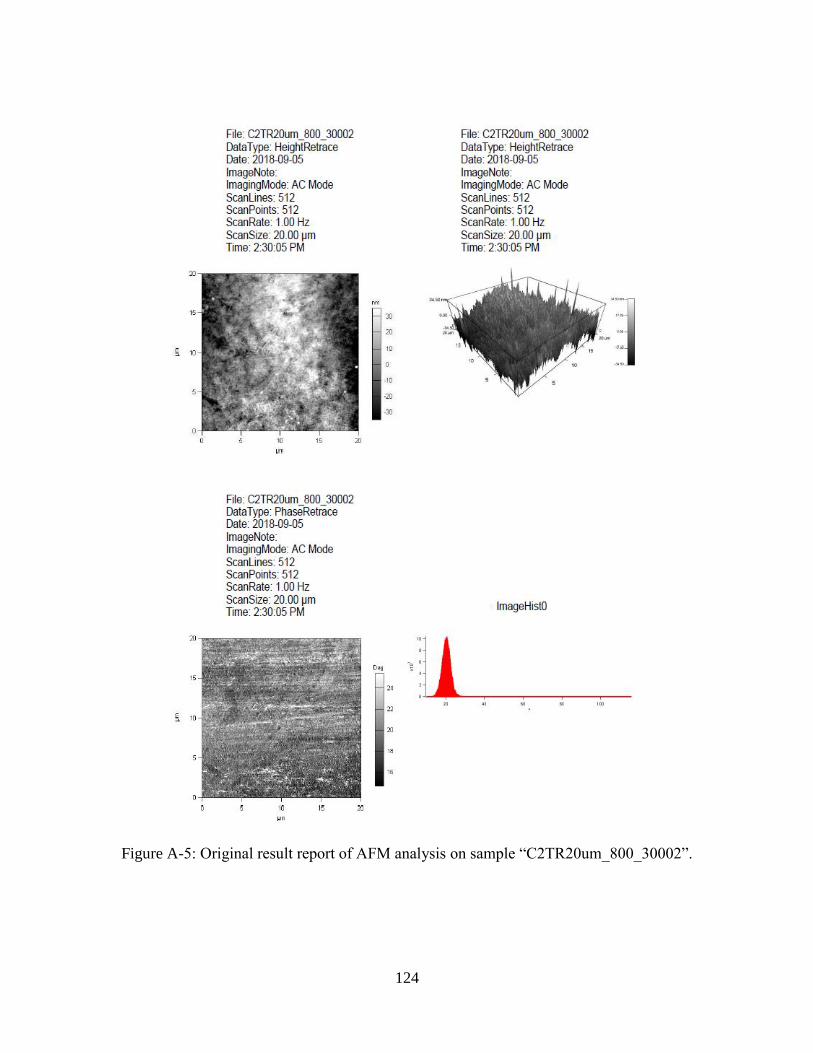
124
Figure A-5: Original result report of AFM analysis on sample “C2TR20um_800_30002”.
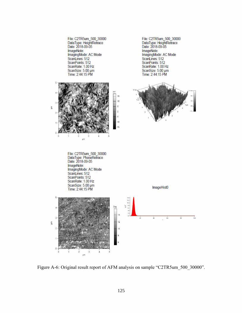
125
Figure A-6: Original result report of AFM analysis on sample “C2TR5um_500_30000”.

126
Figure A-7: Original result report of AFM analysis on sample “C2TR20um_800_40001”.
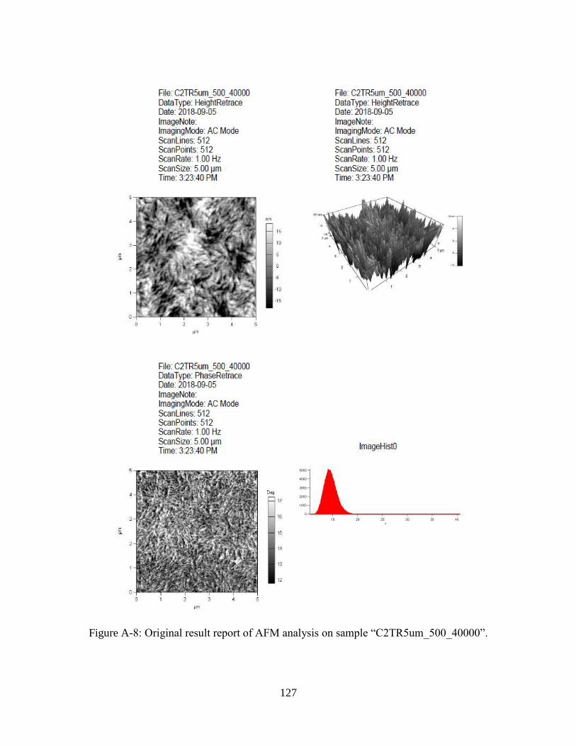
127
Figure A-8: Original result report of AFM analysis on sample “C2TR5um_500_40000”.
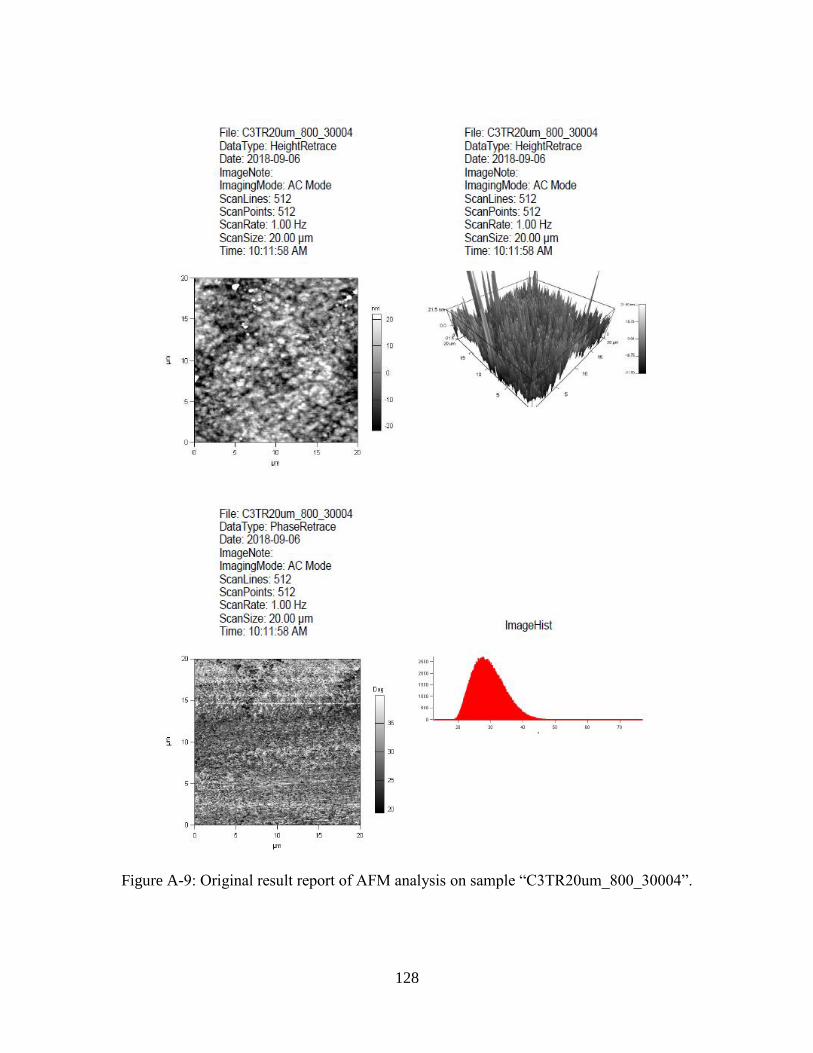
128
Figure A-9: Original result report of AFM analysis on sample “C3TR20um_800_30004”.

129
Figure A-10: Original result report of AFM analysis on sample “C3TR5um_500_30000”.
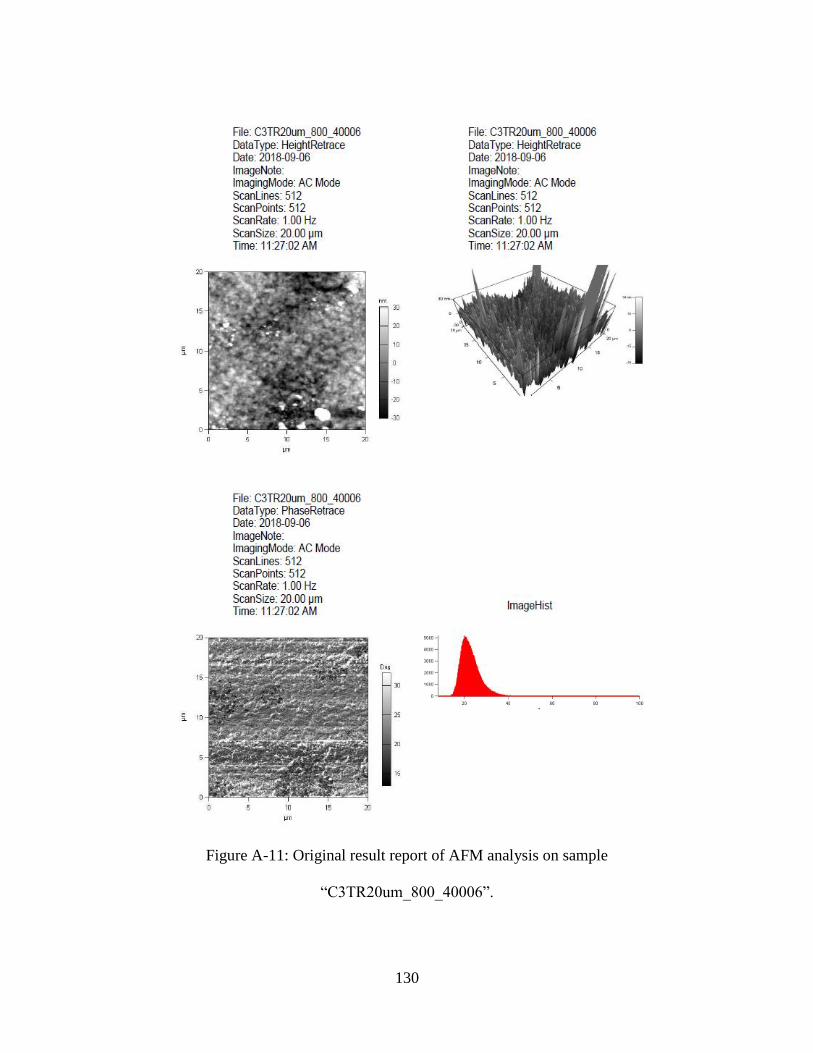
130
Figure A-11: Original result report of AFM analysis on sample
“C3TR20um_800_40006”.
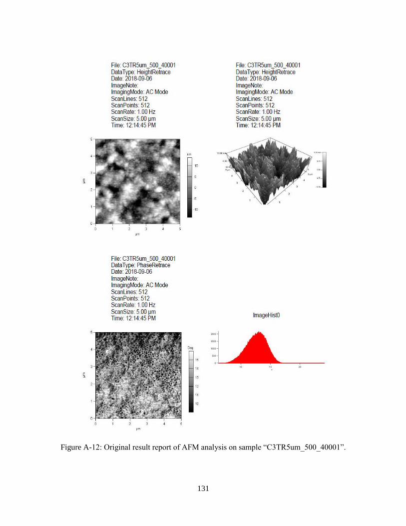
131
Figure A-12: Original result report of AFM analysis on sample “C3TR5um_500_40001”.
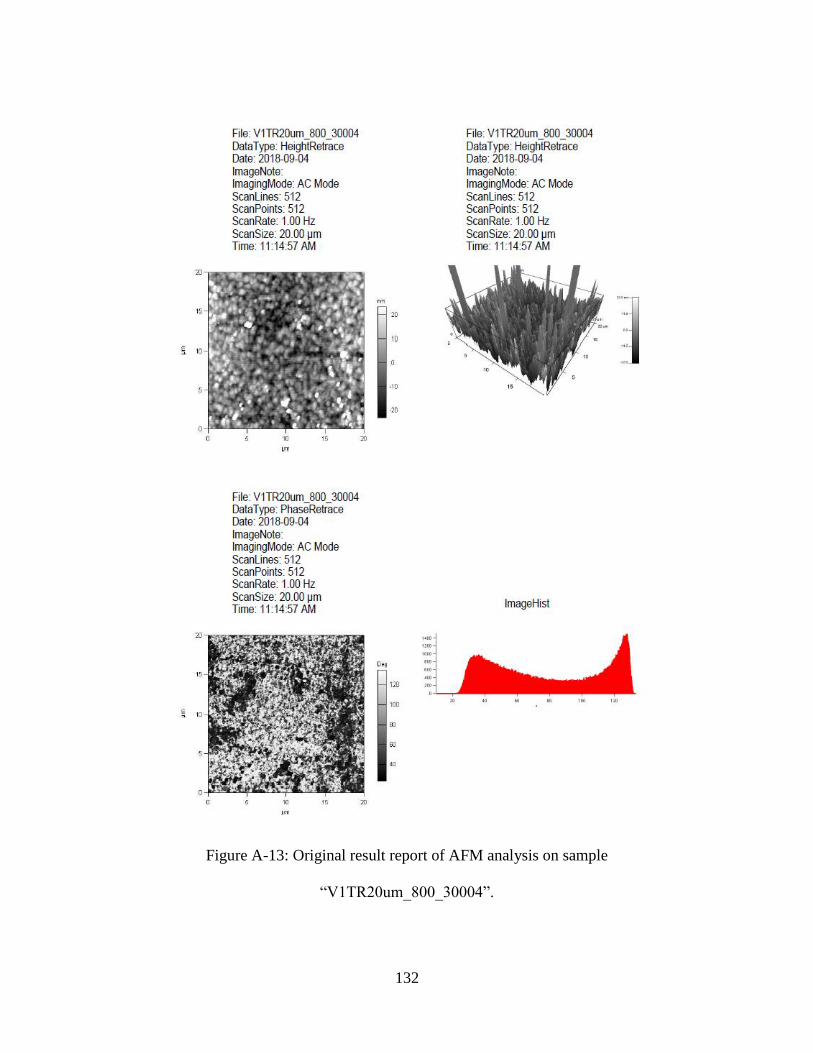
132
Figure A-13: Original result report of AFM analysis on sample
“V1TR20um_800_30004”.
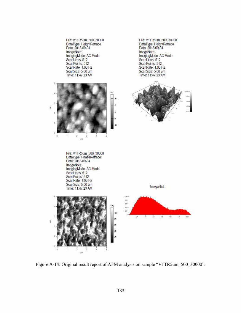
133
Figure A-14: Original result report of AFM analysis on sample “V1TR5um_500_30000”.
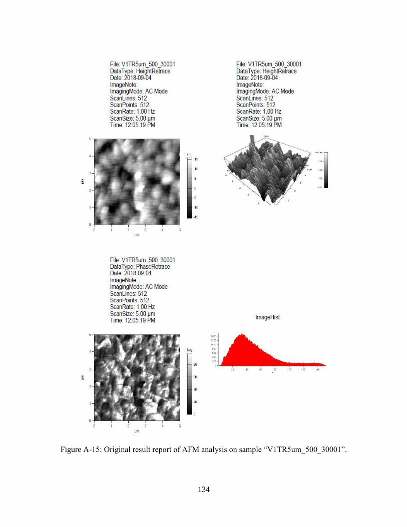
134
Figure A-15: Original result report of AFM analysis on sample “V1TR5um_500_30001”.
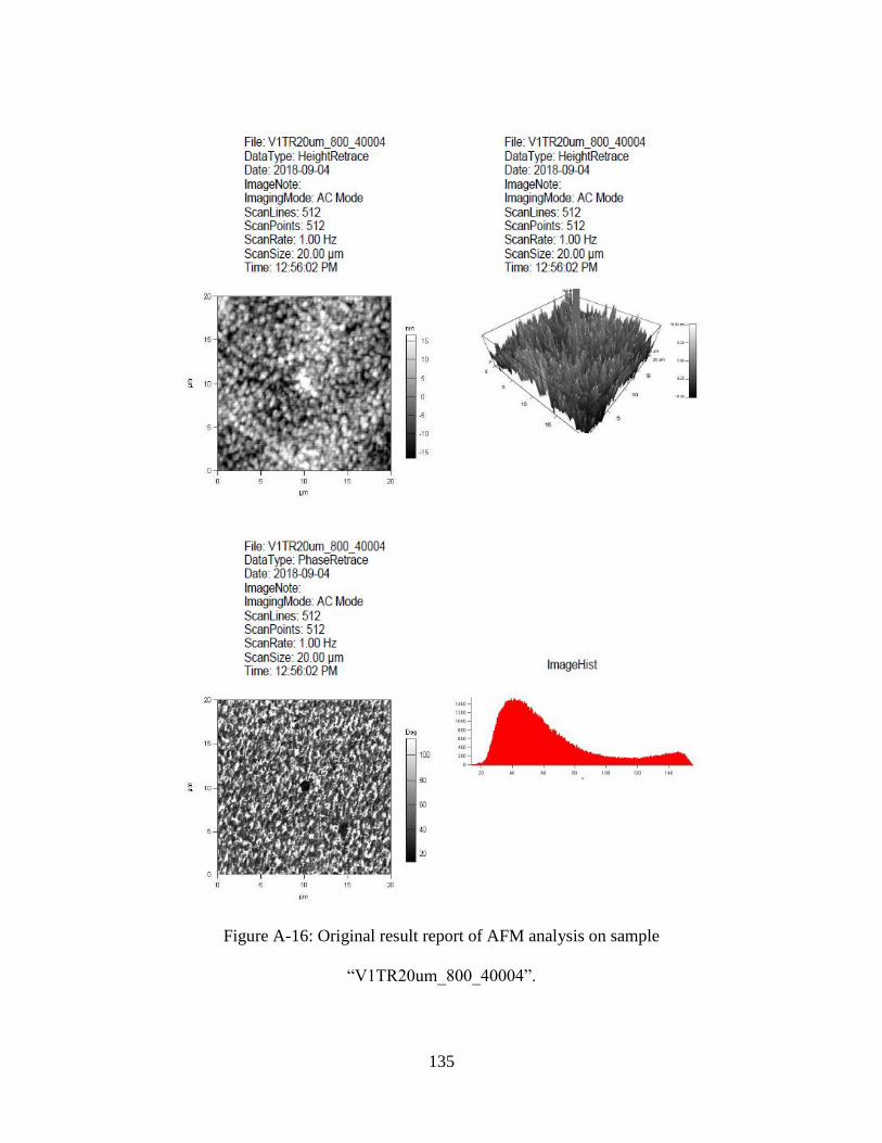
135
Figure A-16: Original result report of AFM analysis on sample
“V1TR20um_800_40004”.
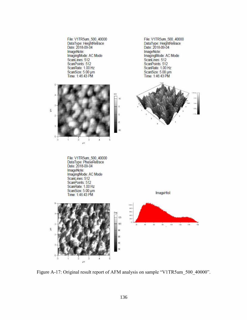
136
Figure A-17: Original result report of AFM analysis on sample “V1TR5um_500_40000”.
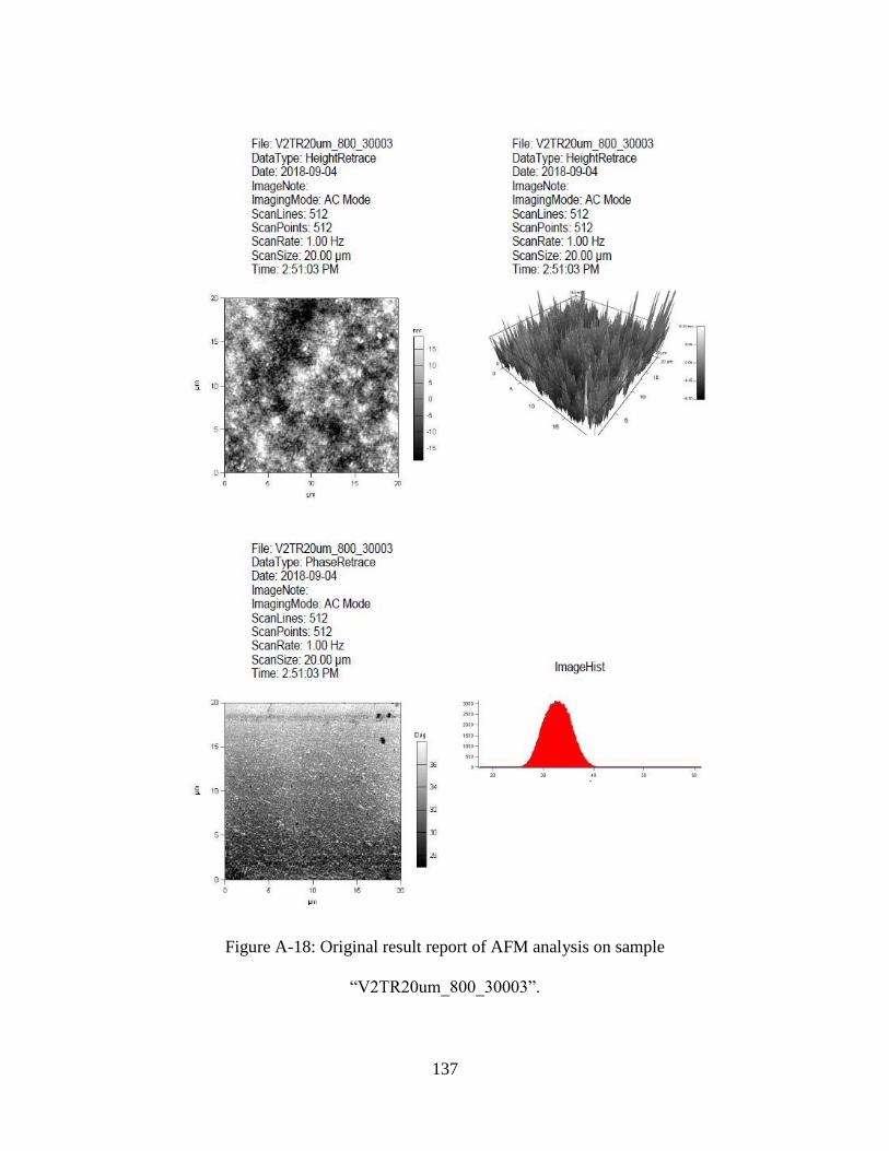
137
Figure A-18: Original result report of AFM analysis on sample
“V2TR20um_800_30003”.

138
Figure A-19: Original result report of AFM analysis on sample “V2TR5um_500_30000”.
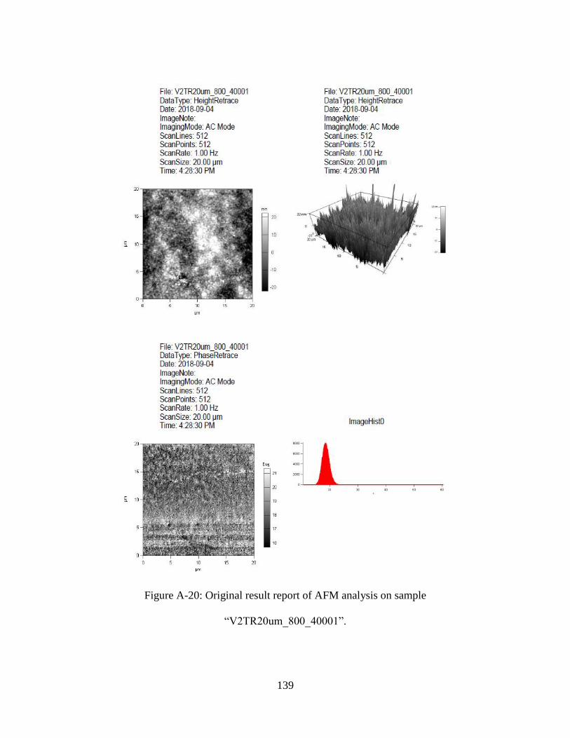
139
Figure A-20: Original result report of AFM analysis on sample
“V2TR20um_800_40001”.
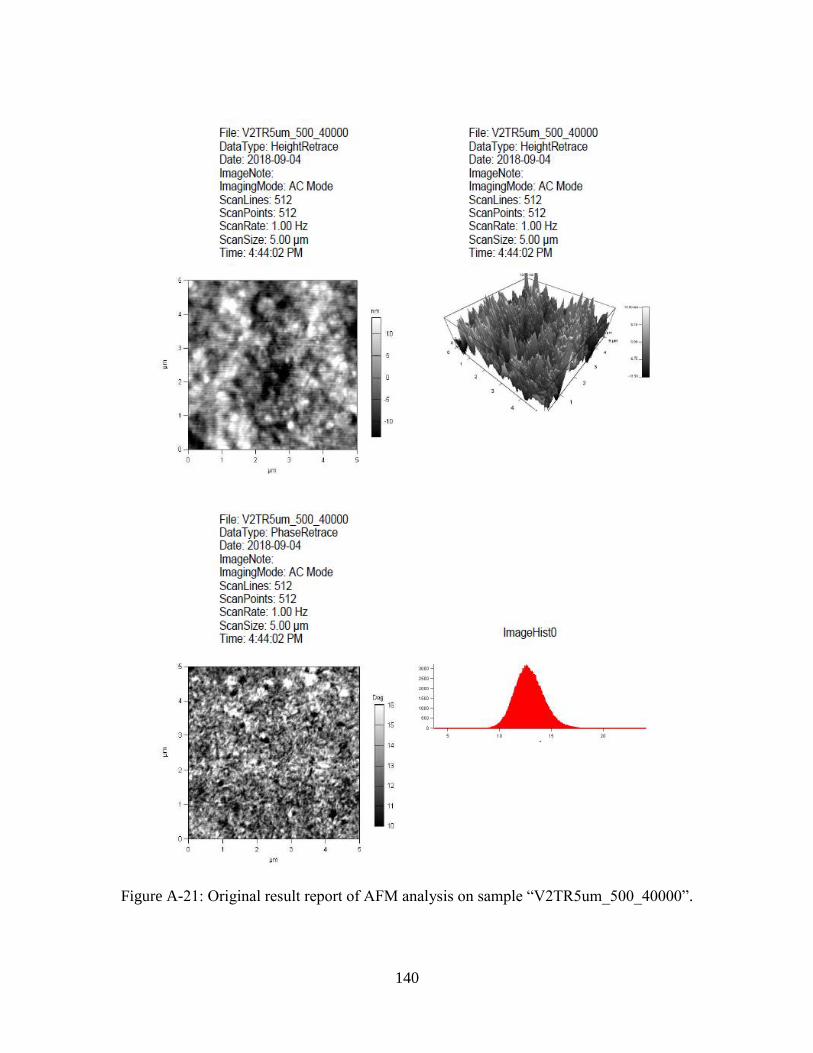
140
Figure A-21: Original result report of AFM analysis on sample “V2TR5um_500_40000”.
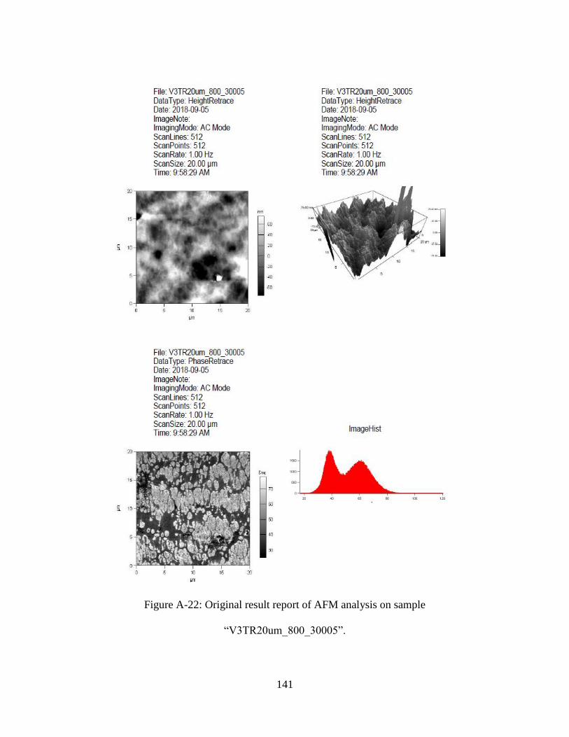
141
Figure A-22: Original result report of AFM analysis on sample
“V3TR20um_800_30005”.
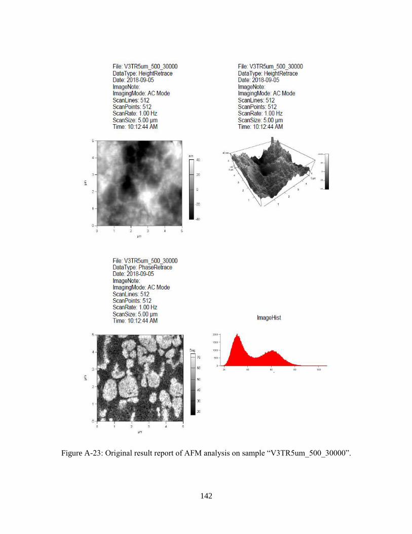
142
Figure A-23: Original result report of AFM analysis on sample “V3TR5um_500_30000”.
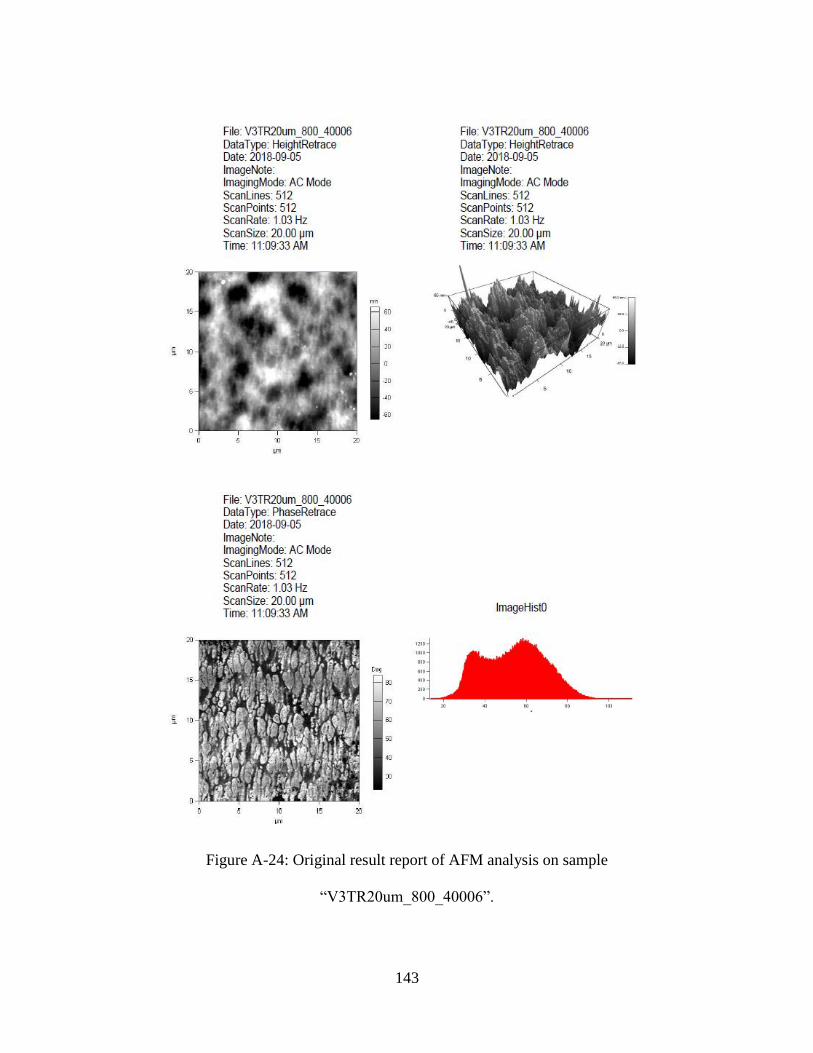
143
Figure A-24: Original result report of AFM analysis on sample
“V3TR20um_800_40006”.
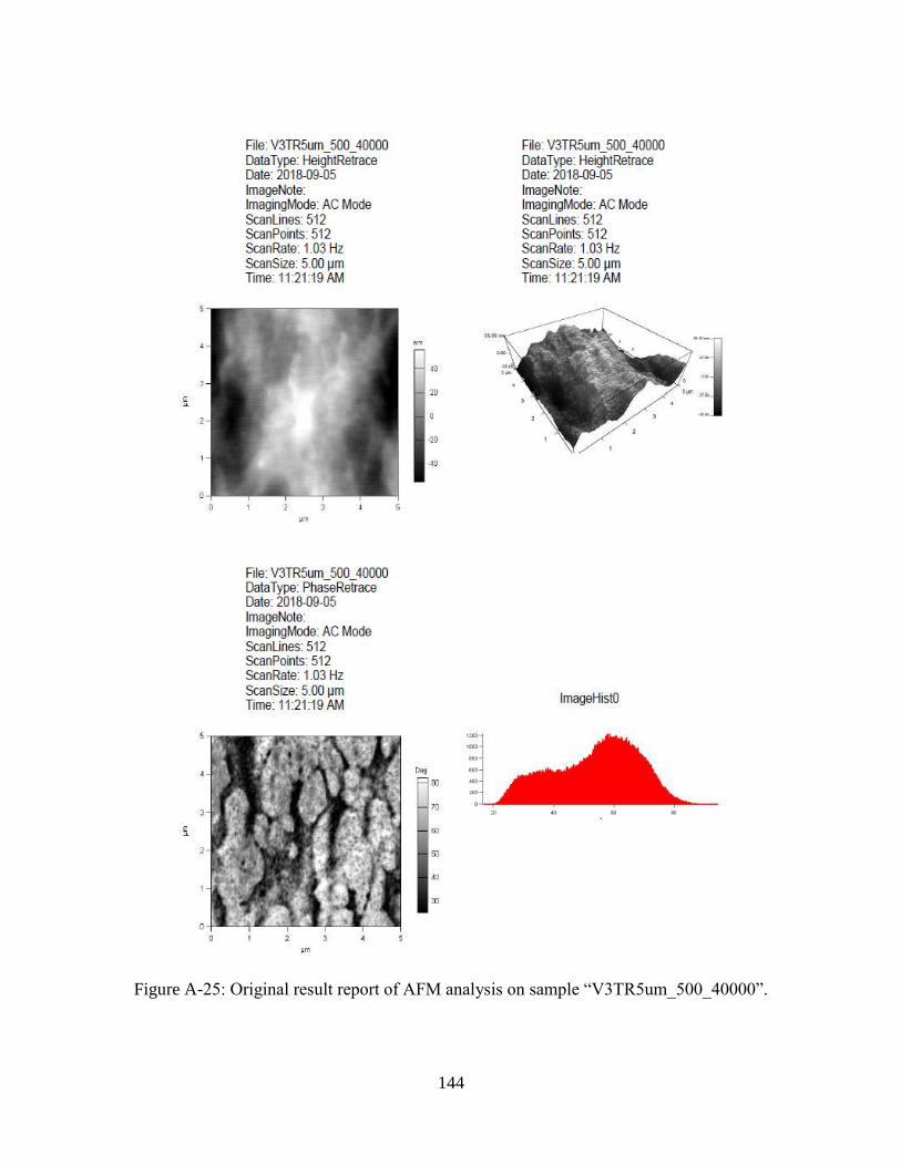
144
Figure A-25: Original result report of AFM analysis on sample “V3TR5um_500_40000”.
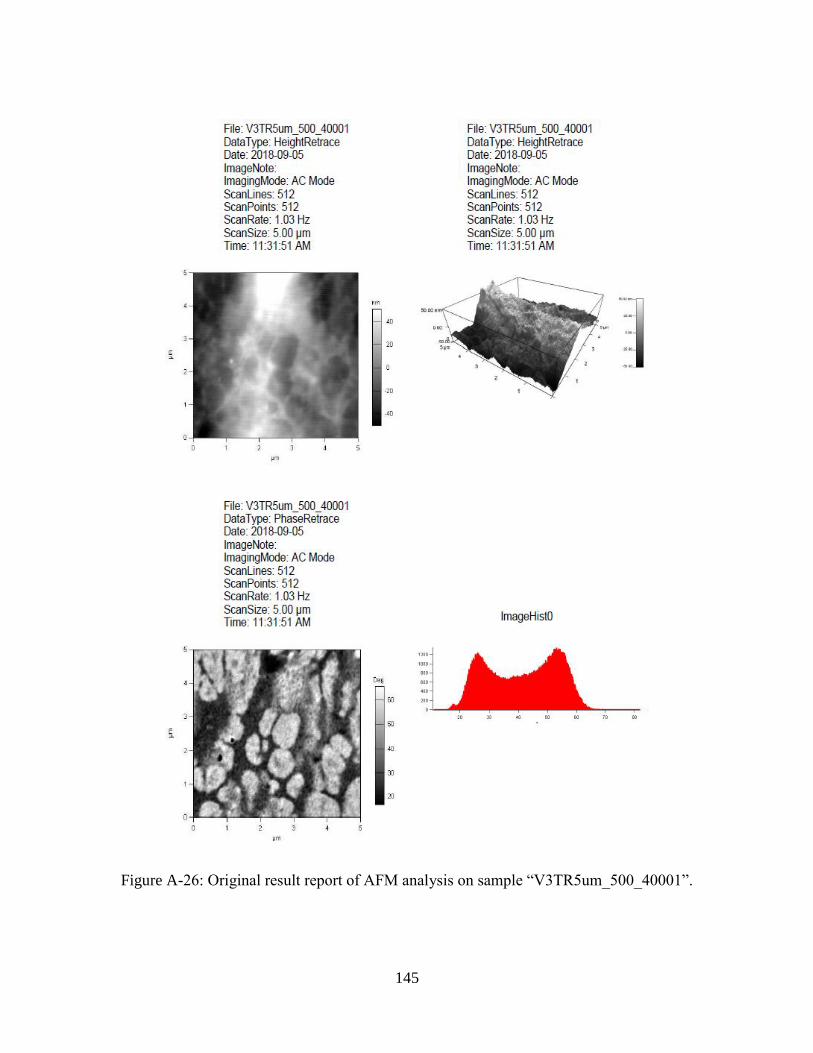
145
Figure A-26: Original result report of AFM analysis on sample “V3TR5um_500_40001”.

146
Figure A-27: Original result report of AFM analysis on sample
“V4TR20um_800_30004”.

147
Figure A-28: Original result report of AFM analysis on sample “V4TR5um_500_30000”.
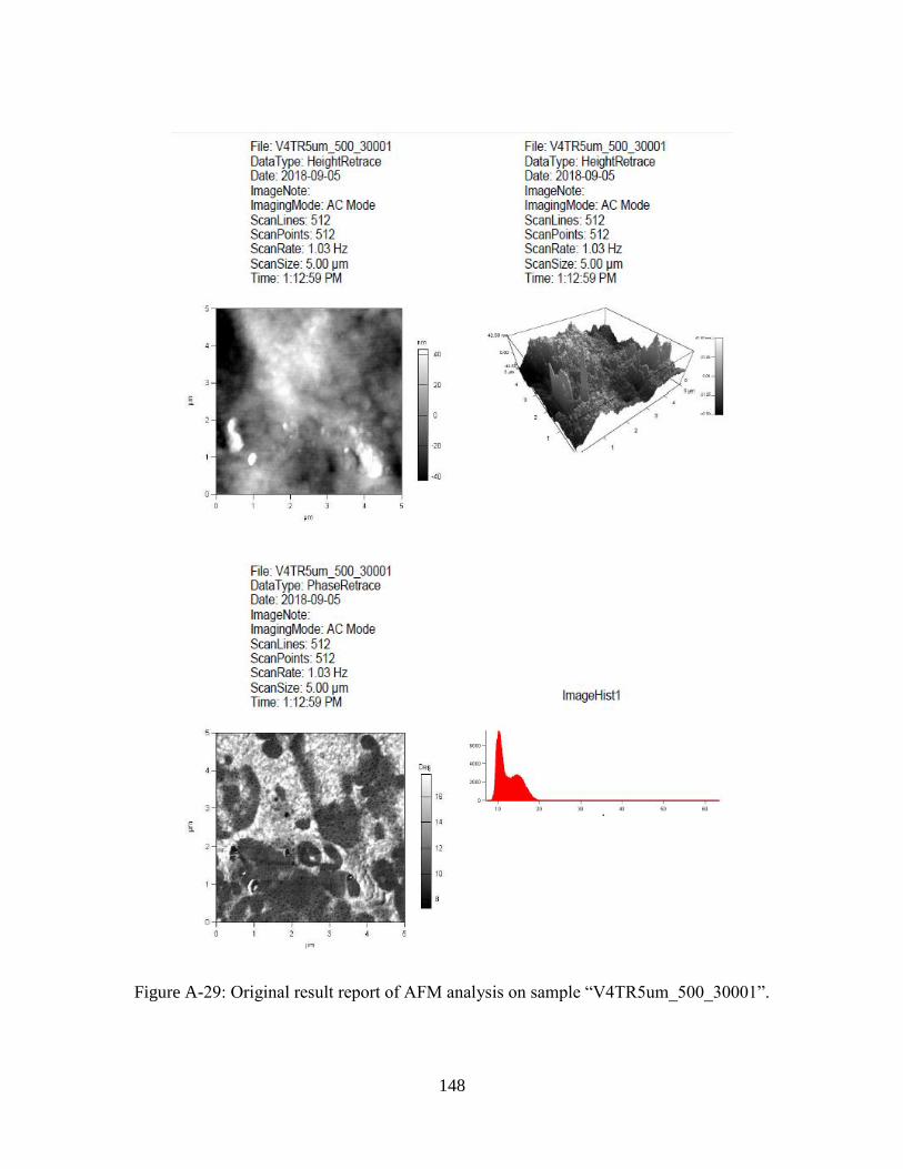
148
Figure A-29: Original result report of AFM analysis on sample “V4TR5um_500_30001”.
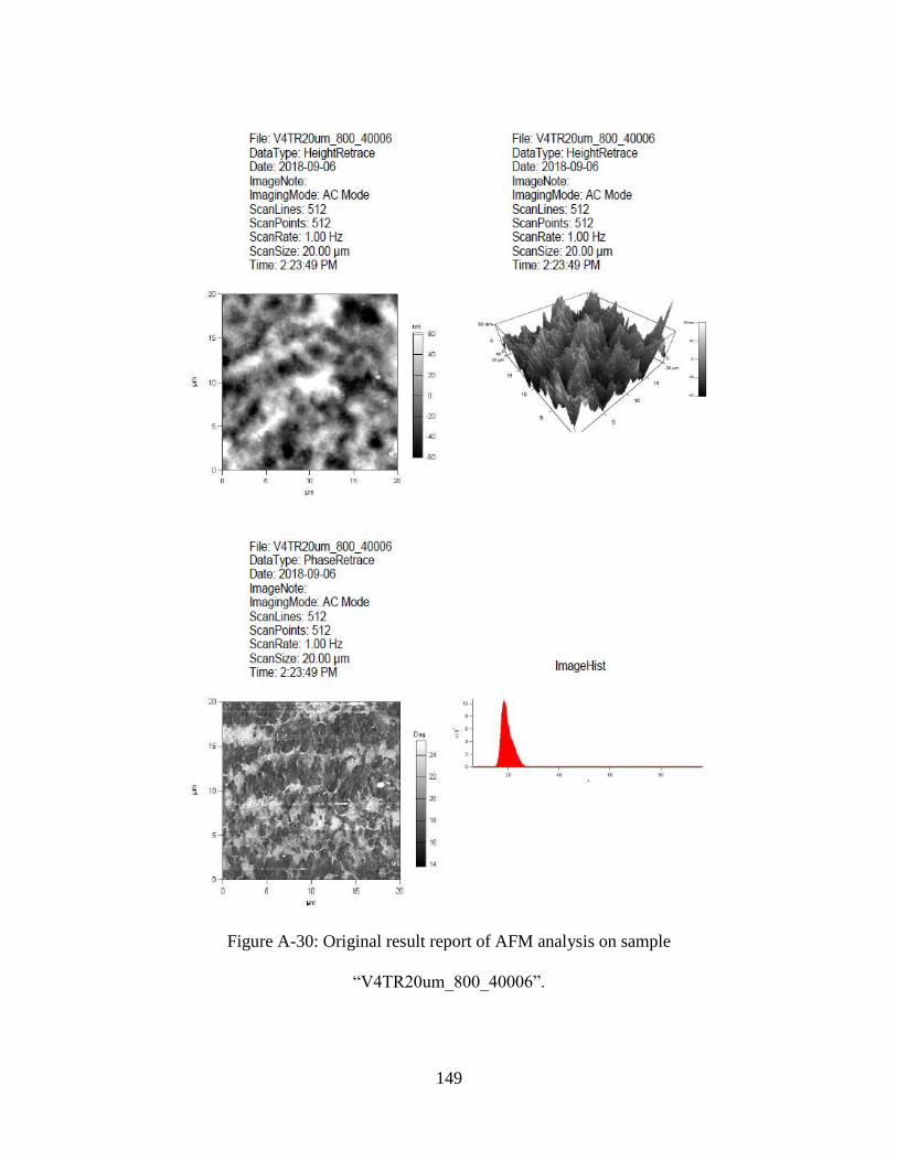
149
Figure A-30: Original result report of AFM analysis on sample
“V4TR20um_800_40006”.
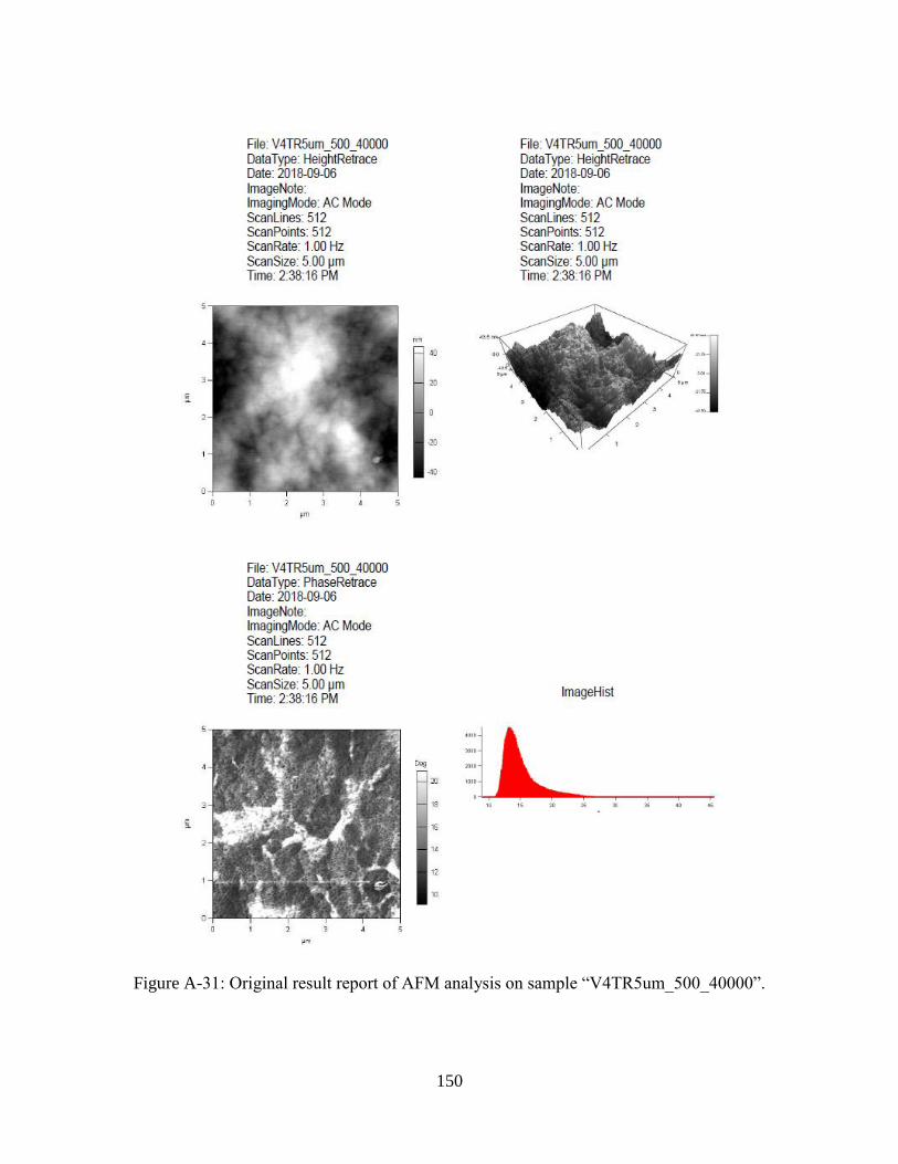
150
Figure A-31: Original result report of AFM analysis on sample “V4TR5um_500_40000”.
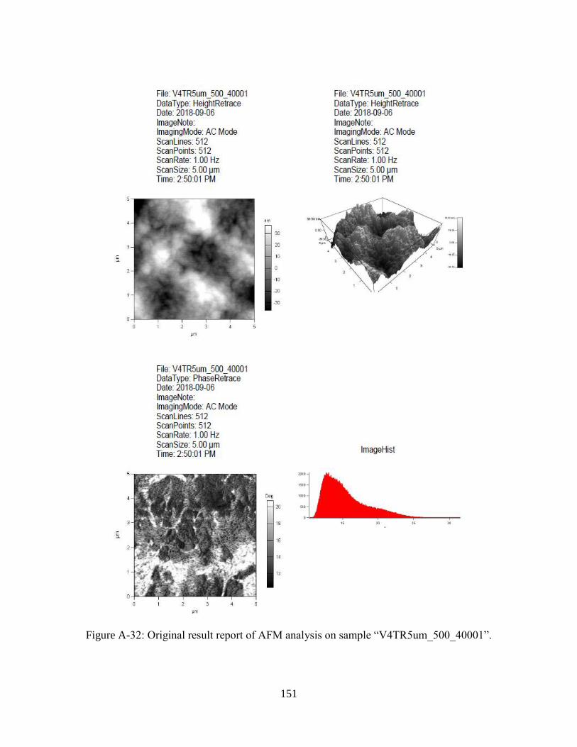
151
Figure A-32: Original result report of AFM analysis on sample “V4TR5um_500_40001”.
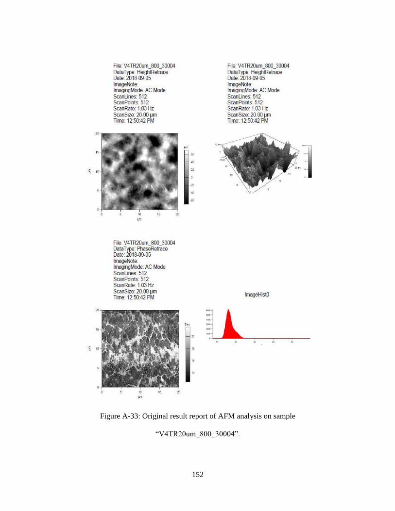
152
Figure A-33: Original result report of AFM analysis on sample
“V4TR20um_800_30004”.
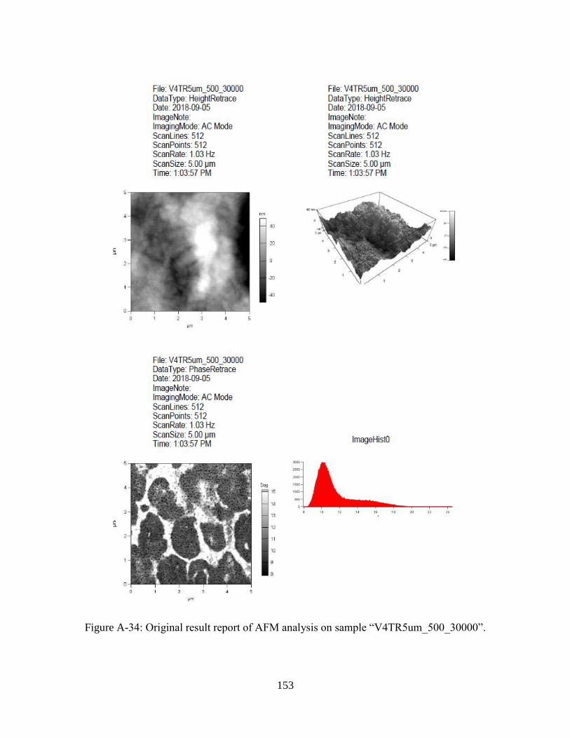
153
Figure A-34: Original result report of AFM analysis on sample “V4TR5um_500_30000”.

154
Figure A-35: Original result report of AFM analysis on sample “V4TR5um_500_30001”.
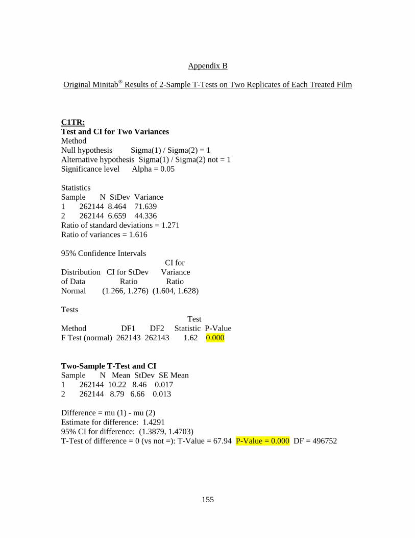
155
Appendix B
Original Minitab® Results of 2-Sample T-Tests on Two Replicates of Each Treated Film
C1TR:
Test and CI for Two Variances
Method
Null hypothesis Sigma(1) / Sigma(2) = 1
Alternative hypothesis Sigma(1) / Sigma(2) not = 1
Significance level Alpha = 0.05
Statistics
Sample N StDev Variance
1 262144 8.464 71.639
2 262144 6.659 44.336
Ratio of standard deviations = 1.271
Ratio of variances = 1.616
95% Confidence Intervals
CI for
Distribution CI for StDev Variance
of Data Ratio Ratio
Normal (1.266, 1.276) (1.604, 1.628)
Tests
Test
Method DF1 DF2 Statistic P-Value
F Test (normal) 262143 262143 1.62 0.000
Two-Sample T-Test and CI
Sample N Mean StDev SE Mean
1 262144 10.22 8.46 0.017
2 262144 8.79 6.66 0.013
Difference = mu (1) - mu (2)
Estimate for difference: 1.4291
95% CI for difference: (1.3879, 1.4703)
T-Test of difference = 0 (vs not =): T-Value = 67.94 P-Value = 0.000 DF = 496752
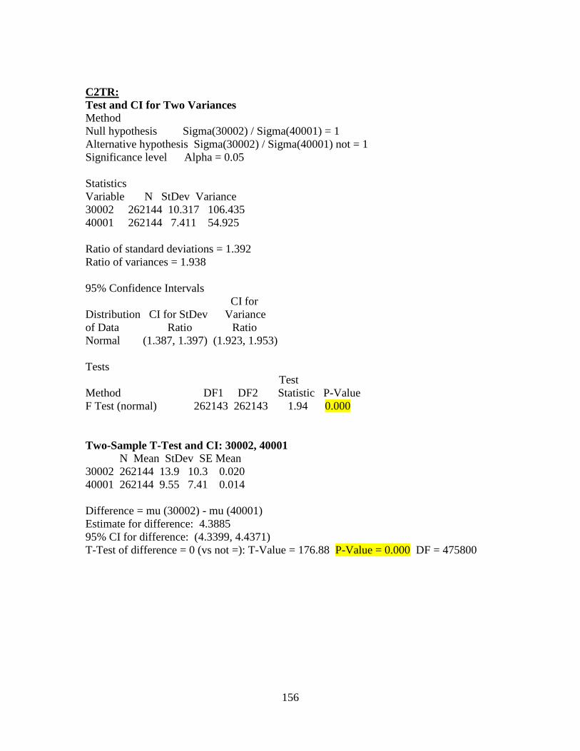
156
C2TR:
Test and CI for Two Variances
Method
Null hypothesis Sigma(30002) / Sigma(40001) = 1
Alternative hypothesis Sigma(30002) / Sigma(40001) not = 1
Significance level Alpha = 0.05
Statistics
Variable N StDev Variance
30002 262144 10.317 106.435
40001 262144 7.411 54.925
Ratio of standard deviations = 1.392
Ratio of variances = 1.938
95% Confidence Intervals
CI for
Distribution CI for StDev Variance
of Data Ratio Ratio
Normal (1.387, 1.397) (1.923, 1.953)
Tests
Test
Method DF1 DF2 Statistic P-Value
F Test (normal) 262143 262143 1.94 0.000
Two-Sample T-Test and CI: 30002, 40001
N Mean StDev SE Mean
30002 262144 13.9 10.3 0.020
40001 262144 9.55 7.41 0.014
Difference = mu (30002) - mu (40001)
Estimate for difference: 4.3885
95% CI for difference: (4.3399, 4.4371)
T-Test of difference = 0 (vs not =): T-Value = 176.88 P-Value = 0.000 DF = 475800
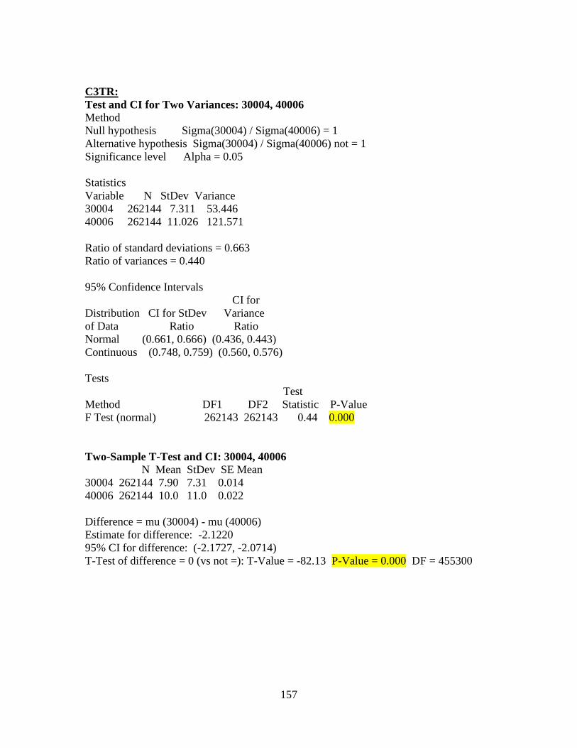
157
C3TR:
Test and CI for Two Variances: 30004, 40006
Method
Null hypothesis Sigma(30004) / Sigma(40006) = 1
Alternative hypothesis Sigma(30004) / Sigma(40006) not = 1
Significance level Alpha = 0.05
Statistics
Variable N StDev Variance
30004 262144 7.311 53.446
40006 262144 11.026 121.571
Ratio of standard deviations = 0.663
Ratio of variances = 0.440
95% Confidence Intervals
CI for
Distribution CI for StDev Variance
of Data Ratio Ratio
Normal (0.661, 0.666) (0.436, 0.443)
Continuous (0.748, 0.759) (0.560, 0.576)
Tests
Test
Method DF1 DF2 Statistic P-Value
F Test (normal) 262143 262143 0.44 0.000
Two-Sample T-Test and CI: 30004, 40006
N Mean StDev SE Mean
30004 262144 7.90 7.31 0.014
40006 262144 10.0 11.0 0.022
Difference = mu (30004) - mu (40006)
Estimate for difference: -2.1220
95% CI for difference: (-2.1727, -2.0714)
T-Test of difference = 0 (vs not =): T-Value = -82.13 P-Value = 0.000 DF = 455300
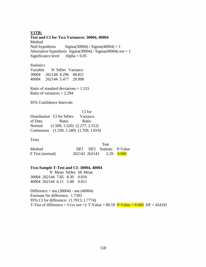
158
V1TR:
Test and CI for Two Variances: 30004, 40004
Method
Null hypothesis Sigma(30004) / Sigma(40004) = 1
Alternative hypothesis Sigma(30004) / Sigma(40004) not = 1
Significance level Alpha = 0.05
Statistics
Variable N StDev Variance
30004 262144 8.296 68.821
40004 262144 5.477 29.998
Ratio of standard deviations = 1.515
Ratio of variances = 2.294
95% Confidence Intervals
CI for
Distribution CI for StDev Variance
of Data Ratio Ratio
Normal (1.509, 1.520) (2.277, 2.312)
Continuous (1.330, 1.349) (1.769, 1.819)
Tests
Test
Method DF1 DF2 Statistic P-Value
F Test (normal) 262143 262143 2.29 0.000
Two-Sample T-Test and CI: 30004, 40004
N Mean StDev SE Mean
30004 262144 7.85 8.30 0.016
40004 262144 6.11 5.48 0.011
Difference = mu (30004) - mu (40004)
Estimate for difference: 1.7393
95% CI for difference: (1.7013, 1.7774)
T-Test of difference = 0 (vs not =): T-Value = 89.59 P-Value = 0.000 DF = 454181

159
V2TR:
Test and CI for Two Variances: 30003, 40001
Method
Null hypothesis Sigma(30003) / Sigma(40001) = 1
Alternative hypothesis Sigma(30003) / Sigma(40001) not = 1
Significance level Alpha = 0.05
Statistics
Variable N StDev Variance
30003 262144 5.711 32.621
40001 262144 6.807 46.335
Ratio of standard deviations = 0.839
Ratio of variances = 0.704
95% Confidence Intervals
CI for
Distribution CI for StDev Variance
of Data Ratio Ratio
Normal (0.836, 0.842) (0.699, 0.709)
Continuous (0.816, 0.823) (0.665, 0.678)
Tests
Test
Method DF1 DF2 Statistic P-Value
F Test (normal) 262143 262143 0.70 0.000
Two-Sample T-Test and CI: 30003, 40001
N Mean StDev SE Mean
30003 262144 7.15 5.71 0.011
40001 262144 8.72 6.81 0.013
Difference = mu (30003) - mu (40001)
Estimate for difference: -1.5690
95% CI for difference: (-1.6030, -1.5350)
T-Test of difference = 0 (vs not =): T-Value = -90.41 P-Value = 0.000 DF = 508931

160
V3TR:
Test and CI for Two Variances: 30005, 40006
Method
Null hypothesis Sigma(30005) / Sigma(40006) = 1
Alternative hypothesis Sigma(30005) / Sigma(40006) not = 1
Significance level Alpha = 0.05
Statistics
Variable N StDev Variance
30005 262144 25.299 640.039
40006 262144 19.166 367.343
Ratio of standard deviations = 1.320
Ratio of variances = 1.742
95% Confidence Intervals
CI for
Distribution CI for StDev Variance
of Data Ratio Ratio
Normal (1.315, 1.325) (1.729, 1.756)
Continuous (1.161, 1.174) (1.348, 1.377)
Tests
Test
Method DF1 DF2 Statistic P-Value
F Test (normal) 262143 262143 1.74 0.000
Two-Sample T-Test and CI: 30005, 40006
N Mean StDev SE Mean
30005 262144 29.3 25.3 0.049
40006 262144 24.9 19.2 0.037
Difference = mu (30005) - mu (40006)
Estimate for difference: 4.3509
95% CI for difference: (4.2294, 4.4724)
T-Test of difference = 0 (vs not =): T-Value = 70.19 P-Value = 0.000 DF = 488490

161
V4TR:
Test and CI for Two Variances: 30004, 40006
Method
Null hypothesis Sigma(30004) / Sigma(40006) = 1
Alternative hypothesis Sigma(30004) / Sigma(40006) not = 1
Significance level Alpha = 0.05
Statistics
Variable N StDev Variance
30004 262144 21.239 451.076
40006 262144 18.214 331.754
Ratio of standard deviations = 1.166
Ratio of variances = 1.360
95% Confidence Intervals
CI for
Distribution CI for StDev Variance
of Data Ratio Ratio
Normal (1.162, 1.171) (1.349, 1.370)
Continuous (1.156, 1.167) (1.337, 1.362)
Tests
Test
Method DF1 DF2 Statistic P-Value
F Test (normal) 262143 262143 1.36 0.000
Two-Sample T-Test and CI: 30004, 40006
N Mean StDev SE Mean
30004 262144 26.6 21.2 0.041
40006 262144 23.4 18.2 0.036
Difference = mu (30004) - mu (40006)
Estimate for difference: 3.1765
95% CI for difference: (3.0694, 3.2836)
T-Test of difference = 0 (vs not =): T-Value = 58.13 P-Value = 0.000 DF = 512381
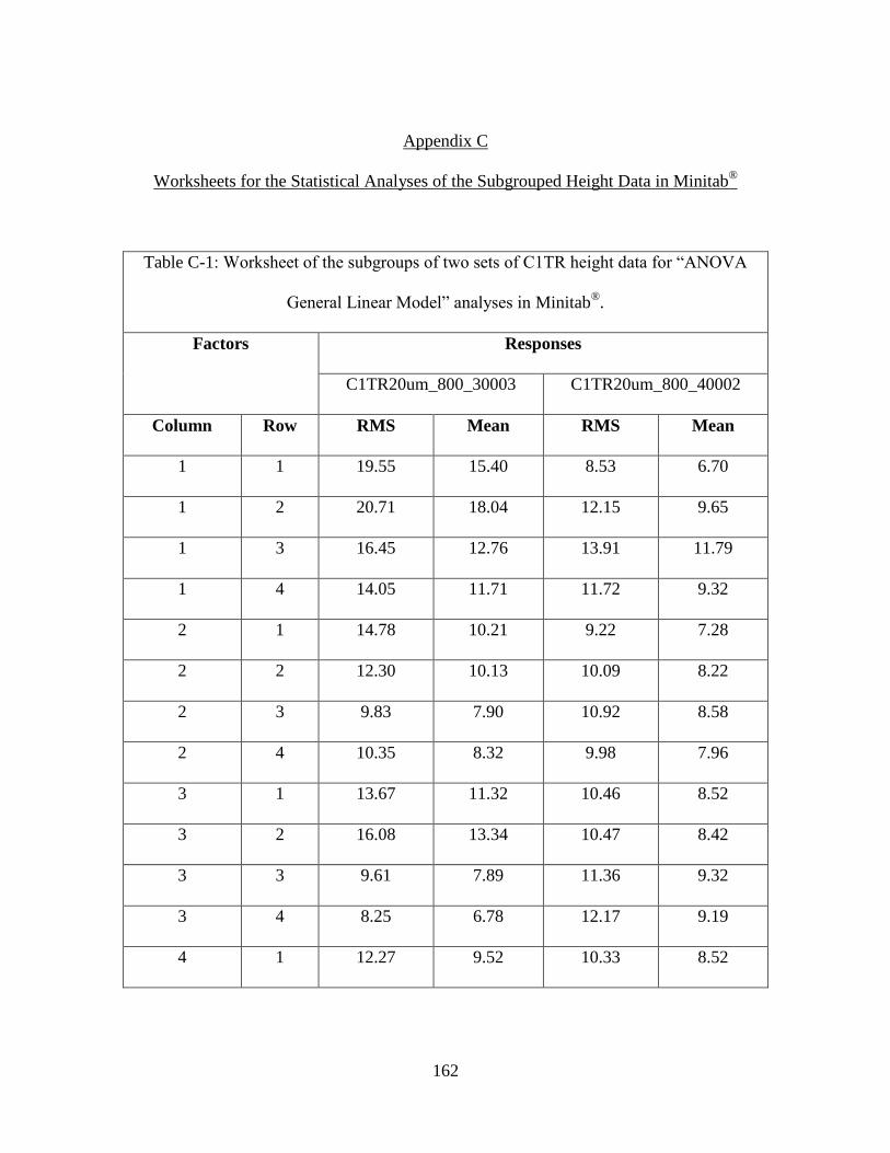
162
Appendix C
Worksheets for the Statistical Analyses of the Subgrouped Height Data in Minitab®
Table C-1: Worksheet of the subgroups of two sets of C1TR height data for “ANOVA
General Linear Model” analyses in Minitab®.
Factors Responses
C1TR20um_800_30003 C1TR20um_800_40002
Column Row RMS Mean RMS Mean
1 1 19.55 15.40 8.53 6.70
1 2 20.71 18.04 12.15 9.65
1 3 16.45 12.76 13.91 11.79
1 4 14.05 11.71 11.72 9.32
2 1 14.78 10.21 9.22 7.28
2 2 12.30 10.13 10.09 8.22
2 3 9.83 7.90 10.92 8.58
2 4 10.35 8.32 9.98 7.96
3 1 13.67 11.32 10.46 8.52
3 2 16.08 13.34 10.47 8.42
3 3 9.61 7.89 11.36 9.32
3 4 8.25 6.78 12.17 9.19
4 1 12.27 9.52 10.33 8.52
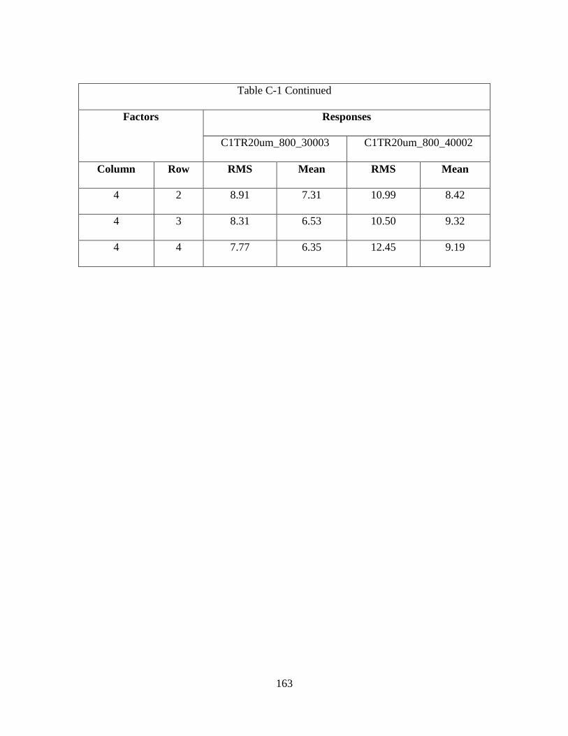
163
Table C-1 Continued
Factors Responses
C1TR20um_800_30003 C1TR20um_800_40002
Column Row RMS Mean RMS Mean
4 2 8.91 7.31 10.99 8.42
4 3 8.31 6.53 10.50 9.32
4 4 7.77 6.35 12.45 9.19
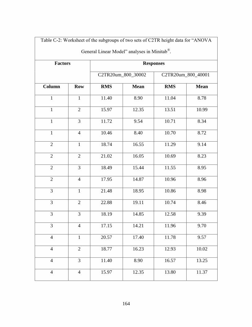
164
Table C-2: Worksheet of the subgroups of two sets of C2TR height data for “ANOVA
General Linear Model” analyses in Minitab®.
Factors Responses
C2TR20um_800_30002 C2TR20um_800_40001
Column Row RMS Mean RMS Mean
1 1 11.40 8.90 11.04 8.78
1 2 15.97 12.35 13.51 10.99
1 3 11.72 9.54 10.71 8.34
1 4 10.46 8.40 10.70 8.72
2 1 18.74 16.55 11.29 9.14
2 2 21.02 16.05 10.69 8.23
2 3 18.49 15.44 11.55 8.95
2 4 17.95 14.87 10.96 8.96
3 1 21.48 18.95 10.86 8.98
3 2 22.88 19.11 10.74 8.46
3 3 18.19 14.85 12.58 9.39
3 4 17.15 14.21 11.96 9.70
4 1 20.57 17.40 11.78 9.57
4 2 18.77 16.23 12.93 10.02
4 3 11.40 8.90 16.57 13.25
4 4 15.97 12.35 13.80 11.37

165
Table C-3: Worksheet of the subgroups of two sets of C3TR height data for “ANOVA
General Linear Model” analyses in Minitab®.
Factors Responses
C3TR20um_800_30004 C3TR20um_800_40006
Column Row RMS Mean RMS Mean
1 1 8.66 7.04 11.58 8.86
1 2 8.93 7.15 14.95 11.32
1 3 8.64 6.88 30.06 19.33
1 4 9.29 7.36 21.91 12.19
2 1 11.70 8.52 9.92 7.85
2 2 9.17 7.27 11.30 8.80
2 3 9.95 8.02 11.53 9.62
2 4 12.10 9.74 11.26 9.18
3 1 10.16 8.29 12.65 8.74
3 2 10.60 8.03 10.68 8.61
3 3 9.90 7.93 8.13 6.51
3 4 8.88 7.02 7.98 6.36
4 1 14.81 9.14 9.15 7.38
4 2 15.19 9.47 9.13 7.41
4 3 9.93 6.85 15.47 13.11
4 4 11.46 7.72 22.71 15.10
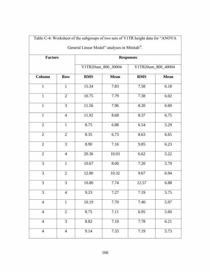
166
Table C-4: Worksheet of the subgroups of two sets of V1TR height data for “ANOVA
General Linear Model” analyses in Minitab®.
Factors Responses
V1TR20um_800_30004 V1TR20um_800_40004
Column Row RMS Mean RMS Mean
1 1 15.34 7.83 7.58 6.18
1 2 10.75 7.79 7.38 6.02
1 3 11.56 7.96 8.20 6.60
1 4 11.92 8.68 8.37 6.75
2 1 8.75 6.88 6.54 5.29
2 2 8.35 6.73 8.63 6.65
2 3 8.90 7.16 9.85 6.23
2 4 20.36 10.03 6.62 5.22
3 1 10.67 8.00 7.20 5.79
3 2 12.80 10.32 9.67 6.94
3 3 10.80 7.74 12.57 6.88
3 4 9.23 7.27 7.19 5.75
4 1 10.19 7.70 7.40 5.97
4 2 8.75 7.11 6.95 5.60
4 3 8.82 7.10 7.78 6.21
4 4 9.14 7.33 7.19 5.73
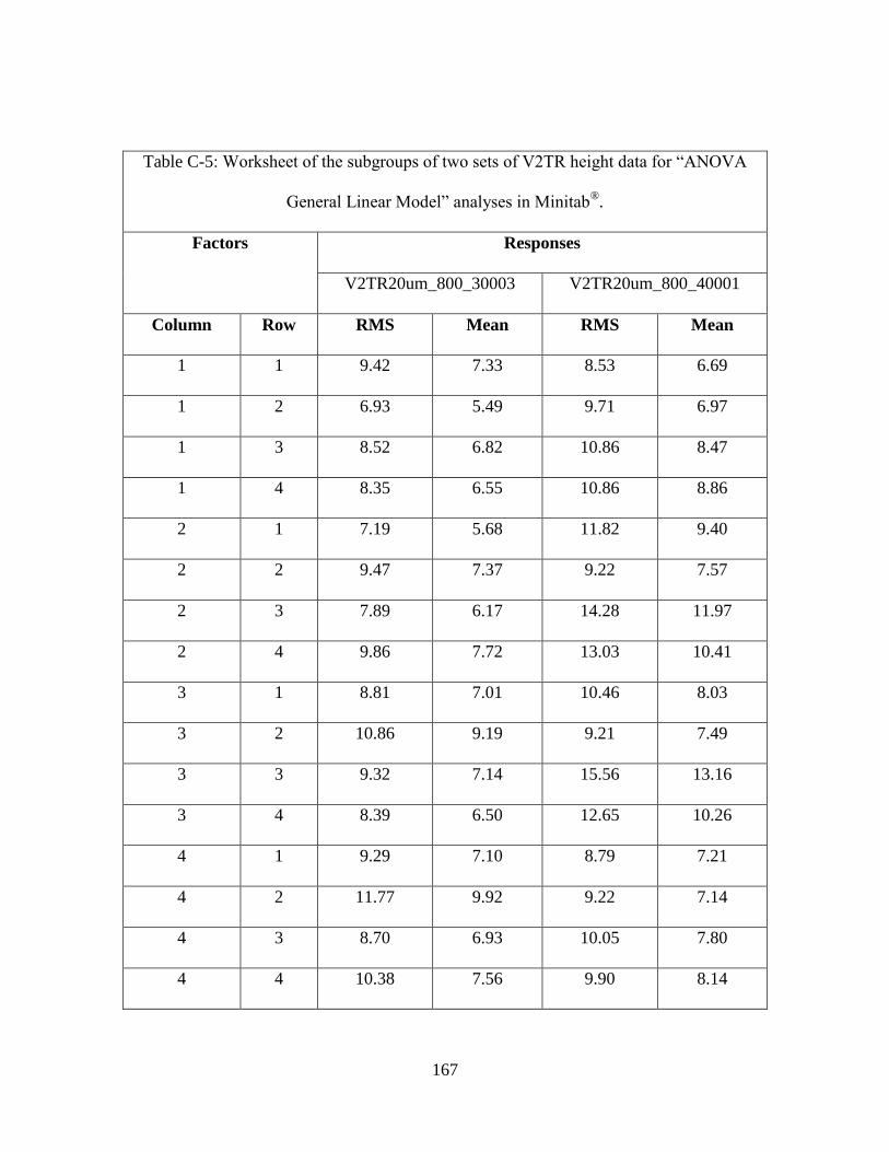
167
Table C-5: Worksheet of the subgroups of two sets of V2TR height data for “ANOVA
General Linear Model” analyses in Minitab®.
Factors Responses
V2TR20um_800_30003 V2TR20um_800_40001
Column Row RMS Mean RMS Mean
1 1 9.42 7.33 8.53 6.69
1 2 6.93 5.49 9.71 6.97
1 3 8.52 6.82 10.86 8.47
1 4 8.35 6.55 10.86 8.86
2 1 7.19 5.68 11.82 9.40
2 2 9.47 7.37 9.22 7.57
2 3 7.89 6.17 14.28 11.97
2 4 9.86 7.72 13.03 10.41
3 1 8.81 7.01 10.46 8.03
3 2 10.86 9.19 9.21 7.49
3 3 9.32 7.14 15.56 13.16
3 4 8.39 6.50 12.65 10.26
4 1 9.29 7.10 8.79 7.21
4 2 11.77 9.92 9.22 7.14
4 3 8.70 6.93 10.05 7.80
4 4 10.38 7.56 9.90 8.14

168
Table C-6: Worksheet of the subgroups of two sets of V3TR height data for “ANOVA
General Linear Model” analyses in Minitab®.
Factors Responses
V3TR20um_800_30005 V3TR20um_800_40006
Column Row RMS Mean RMS Mean
1 1 26.77 22.240 20.88 17.47
1 2 28.37 23.73 29.86 24.06
1 3 60.57 46.16 29.22 23.39
1 4 44.88 37.41 29.86 23.89
2 1 32.77 25.98 29.71 24.46
2 2 31.04 25.23 37.79 30.16
2 3 56.32 49.22 34.15 28.23
2 4 59.01 45.66 24.51 19.25
3 1 34.25 28.94 28.95 23.96
3 2 23.64 19.48 34.36 28.77
3 3 24.58 20.45 24.01 18.63
3 4 26.26 20.90 18.51 15.13
4 1 51.45 22.24 39.69 32.20
4 2 26.37 23.73 48.00 41.21
4 3 30.31 46.16 33.03 25.00
4 4 28.09 37.41 27.86 23.32

169
Table C-7: Worksheet of the subgroups of two sets of V4TR height data for “ANOVA
General Linear Model” analyses in Minitab®.
Factors Responses
V4TR20um_800_30004 V4TR20um_800_40006
Column Row RMS Mean RMS Mean
1 1 27.96 22.11 30.83 24.36
1 2 34.97 30.08 31.93 26.59
1 3 35.49 27.22 26.67 22.74
1 4 37.62 28.30 30.57 24.50
2 1 21.86 17.23 26.57 20.59
2 2 25.93 21.19 32.61 26.00
2 3 26.86 22.03 34.16 27.93
2 4 20.99 15.83 22.78 17.86
3 1 30.64 24.57 28.04 22.25
3 2 42.41 36.20 29.20 24.37
3 3 37.88 30.27 31.41 24.62
3 4 45.38 36.10 24.13 19.04
4 1 28.92 24.12 17.33 14.27
4 2 26.98 21.76 20.81 16.42
4 3 43.45 32.26 41.39 34.33
4 4 43.06 36.17 36.79 28.76
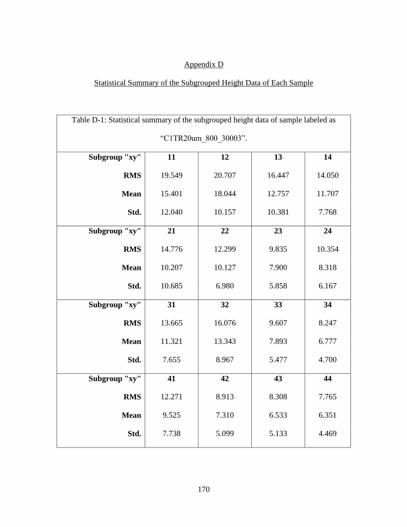
170
Appendix D
Statistical Summary of the Subgrouped Height Data of Each Sample
Table D-1: Statistical summary of the subgrouped height data of sample labeled as
“C1TR20um_800_30003”.
Subgroup "xy" 11 12 13 14
RMS 19.549 20.707 16.447 14.050
Mean 15.401 18.044 12.757 11.707
Std. 12.040 10.157 10.381 7.768
Subgroup "xy" 21 22 23 24
RMS 14.776 12.299 9.835 10.354
Mean 10.207 10.127 7.900 8.318
Std. 10.685 6.980 5.858 6.167
Subgroup "xy" 31 32 33 34
RMS 13.665 16.076 9.607 8.247
Mean 11.321 13.343 7.893 6.777
Std. 7.655 8.967 5.477 4.700
Subgroup "xy" 41 42 43 44
RMS 12.271 8.913 8.308 7.765
Mean 9.525 7.310 6.533 6.351
Std. 7.738 5.099 5.133 4.469
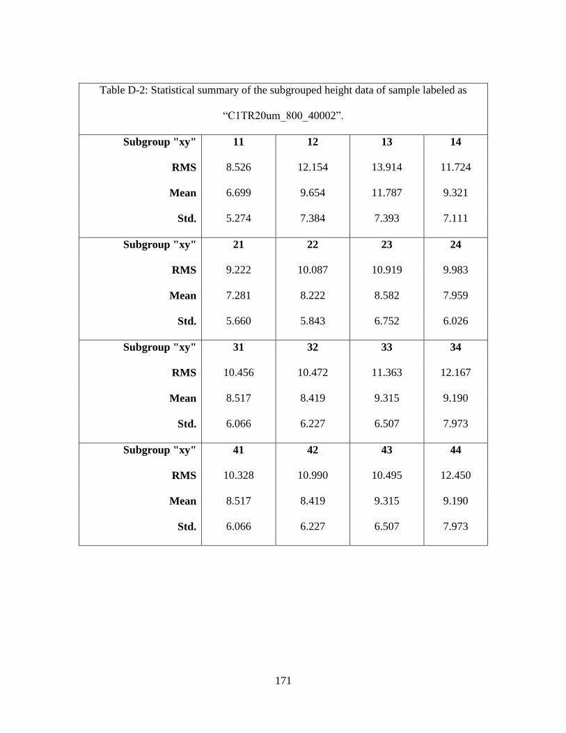
171
Table D-2: Statistical summary of the subgrouped height data of sample labeled as
“C1TR20um_800_40002”.
Subgroup "xy" 11 12 13 14
RMS 8.526 12.154 13.914 11.724
Mean 6.699 9.654 11.787 9.321
Std. 5.274 7.384 7.393 7.111
Subgroup "xy" 21 22 23 24
RMS 9.222 10.087 10.919 9.983
Mean 7.281 8.222 8.582 7.959
Std. 5.660 5.843 6.752 6.026
Subgroup "xy" 31 32 33 34
RMS 10.456 10.472 11.363 12.167
Mean 8.517 8.419 9.315 9.190
Std. 6.066 6.227 6.507 7.973
Subgroup "xy" 41 42 43 44
RMS 10.328 10.990 10.495 12.450
Mean 8.517 8.419 9.315 9.190
Std. 6.066 6.227 6.507 7.973

172
Table D-3: Statistical summary of the subgrouped height data of sample labeled as
“C2TR20um_800_30002”.
Subgroup "xy" 11 12 13 14
RMS 12.599 13.433 11.396 15.974
Mean 9.425 10.822 8.896 12.354
Std. 8.361 7.959 7.122 10.127
Subgroup "xy" 21 22 23 24
RMS 11.717 10.457 18.743 21.015
Mean 9.536 8.401 16.554 16.048
Std. 6.809 6.227 8.791 13.569
Subgroup "xy" 31 32 33 34
RMS 18.495 17.951 21.477 22.876
Mean 15.437 14.873 18.945 19.109
Std. 10.186 10.051 10.116 12.576
Subgroup "xy" 41 42 43 44
RMS 18.194 17.155 20.570 18.771
Mean 14.853 14.205 17.395 16.233
Std. 10.507 9.617 10.979 9.427
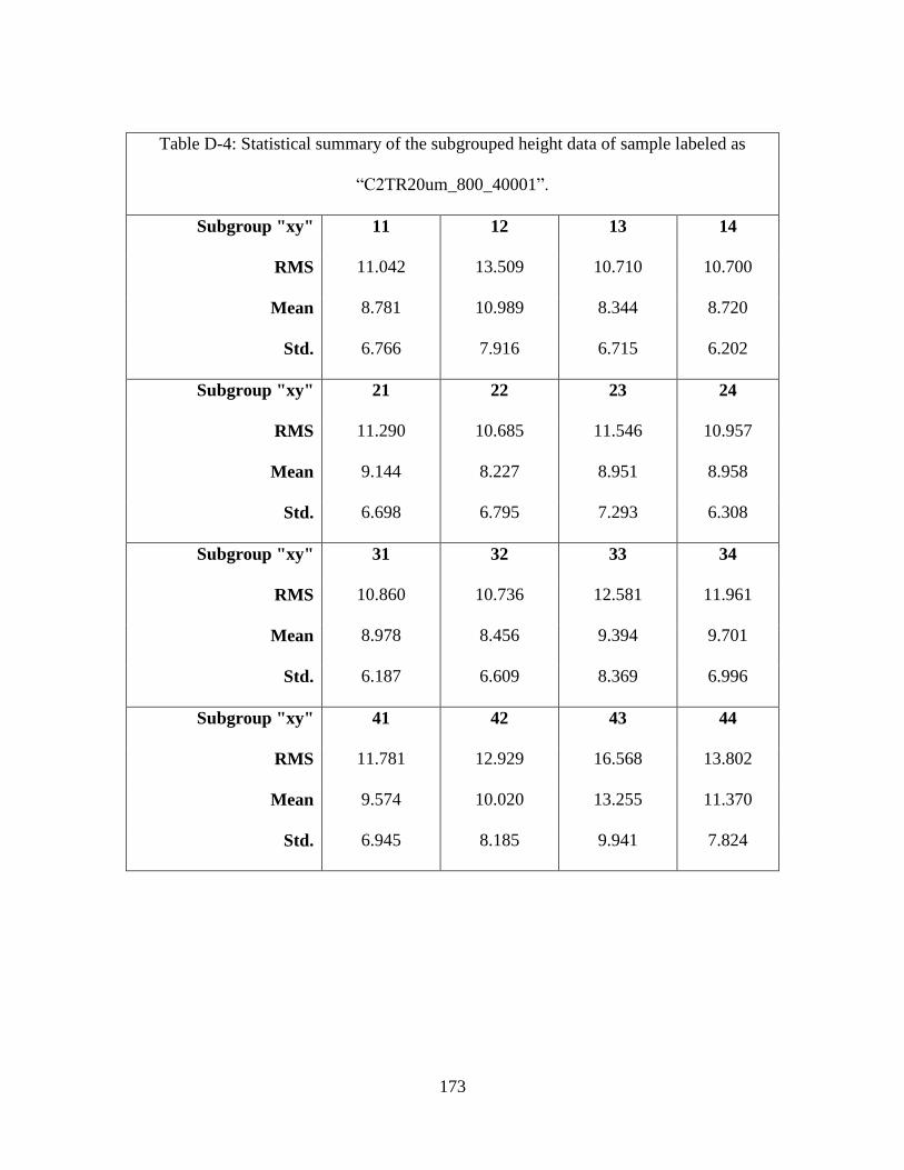
173
Table D-4: Statistical summary of the subgrouped height data of sample labeled as
“C2TR20um_800_40001”.
Subgroup "xy" 11 12 13 14
RMS 11.042 13.509 10.710 10.700
Mean 8.781 10.989 8.344 8.720
Std. 6.766 7.916 6.715 6.202
Subgroup "xy" 21 22 23 24
RMS 11.290 10.685 11.546 10.957
Mean 9.144 8.227 8.951 8.958
Std. 6.698 6.795 7.293 6.308
Subgroup "xy" 31 32 33 34
RMS 10.860 10.736 12.581 11.961
Mean 8.978 8.456 9.394 9.701
Std. 6.187 6.609 8.369 6.996
Subgroup "xy" 41 42 43 44
RMS 11.781 12.929 16.568 13.802
Mean 9.574 10.020 13.255 11.370
Std. 6.945 8.185 9.941 7.824

174
Table D-5: Statistical summary of the subgrouped height data of sample labeled as
“C3TR20um_800_30004”.
Subgroup "xy" 11 12 13 14
RMS 8.659 8.928 8.637 9.291
Mean 7.044 7.149 6.884 7.359
Std. 5.035 5.348 5.217 5.672
Subgroup "xy" 21 22 23 24
RMS 11.702 9.169 9.952 12.097
Mean 8.519 7.271 8.021 9.739
Std. 8.024 5.586 5.891 7.176
Subgroup "xy" 31 32 33 34
RMS 10.163 10.599 9.899 8.877
Mean 8.291 8.032 7.932 7.016
Std. 5.878 6.917 5.922 5.438
Subgroup "xy" 41 42 43 44
RMS 14.813 15.188 9.930 11.457
Mean 9.144 9.470 6.849 7.723
Std. 11.654 11.874 7.190 8.463
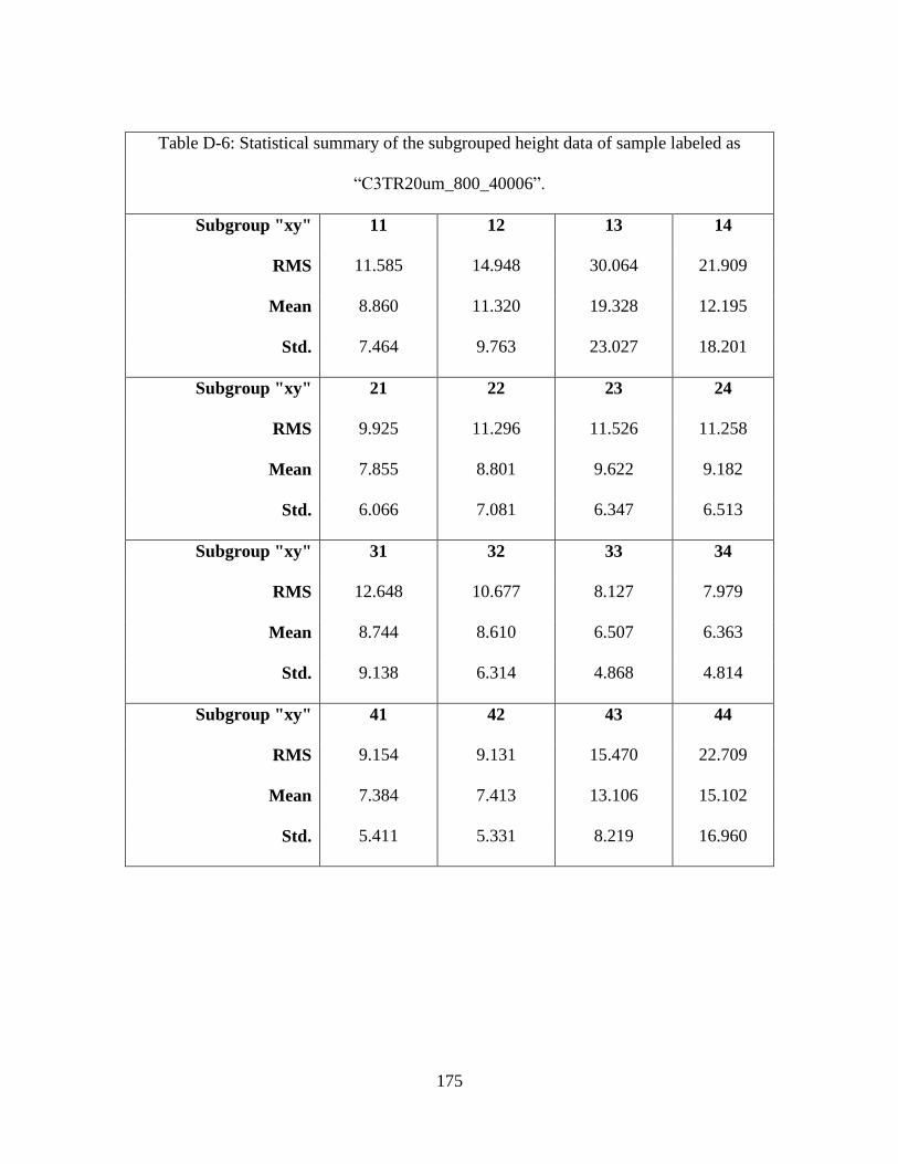
175
Table D-6: Statistical summary of the subgrouped height data of sample labeled as
“C3TR20um_800_40006”.
Subgroup "xy" 11 12 13 14
RMS 11.585 14.948 30.064 21.909
Mean 8.860 11.320 19.328 12.195
Std. 7.464 9.763 23.027 18.201
Subgroup "xy" 21 22 23 24
RMS 9.925 11.296 11.526 11.258
Mean 7.855 8.801 9.622 9.182
Std. 6.066 7.081 6.347 6.513
Subgroup "xy" 31 32 33 34
RMS 12.648 10.677 8.127 7.979
Mean 8.744 8.610 6.507 6.363
Std. 9.138 6.314 4.868 4.814
Subgroup "xy" 41 42 43 44
RMS 9.154 9.131 15.470 22.709
Mean 7.384 7.413 13.106 15.102
Std. 5.411 5.331 8.219 16.960
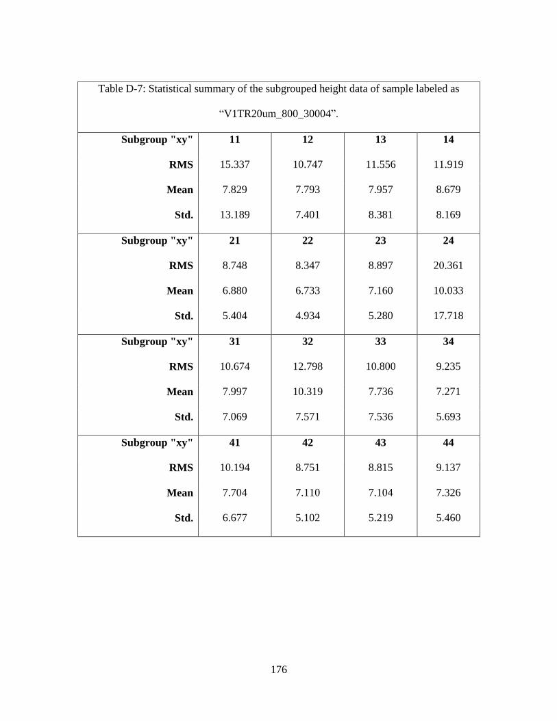
176
Table D-7: Statistical summary of the subgrouped height data of sample labeled as
“V1TR20um_800_30004”.
Subgroup "xy" 11 12 13 14
RMS 15.337 10.747 11.556 11.919
Mean 7.829 7.793 7.957 8.679
Std. 13.189 7.401 8.381 8.169
Subgroup "xy" 21 22 23 24
RMS 8.748 8.347 8.897 20.361
Mean 6.880 6.733 7.160 10.033
Std. 5.404 4.934 5.280 17.718
Subgroup "xy" 31 32 33 34
RMS 10.674 12.798 10.800 9.235
Mean 7.997 10.319 7.736 7.271
Std. 7.069 7.571 7.536 5.693
Subgroup "xy" 41 42 43 44
RMS 10.194 8.751 8.815 9.137
Mean 7.704 7.110 7.104 7.326
Std. 6.677 5.102 5.219 5.460

177
Table D-8: Statistical summary of the subgrouped height data of sample labeled as
“V1TR20um_800_40004”.
Subgroup "xy" 11 12 13 14
RMS 7.578 7.381 8.204 8.371
Mean 6.183 6.017 6.596 6.746
Std. 4.382 4.276 4.878 4.956
Subgroup "xy" 21 22 23 24
RMS 6.542 8.628 9.853 6.620
Mean 5.289 6.652 6.228 5.218
Std. 3.851 5.495 7.635 4.075
Subgroup "xy" 31 32 33 34
RMS 7.201 9.668 12.570 7.194
Mean 5.789 6.943 6.882 5.753
Std. 4.283 6.728 10.519 4.319
Subgroup "xy" 41 42 43 44
RMS 7.395 6.950 7.783 7.187
Mean 5.966 5.600 6.208 5.730
Std. 4.371 4.117 4.695 4.338
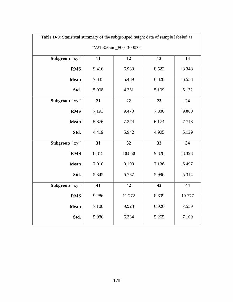
178
Table D-9: Statistical summary of the subgrouped height data of sample labeled as
“V2TR20um_800_30003”.
Subgroup "xy" 11 12 13 14
RMS 9.416 6.930 8.522 8.348
Mean 7.333 5.489 6.820 6.553
Std. 5.908 4.231 5.109 5.172
Subgroup "xy" 21 22 23 24
RMS 7.193 9.470 7.886 9.860
Mean 5.676 7.374 6.174 7.716
Std. 4.419 5.942 4.905 6.139
Subgroup "xy" 31 32 33 34
RMS 8.815 10.860 9.320 8.393
Mean 7.010 9.190 7.136 6.497
Std. 5.345 5.787 5.996 5.314
Subgroup "xy" 41 42 43 44
RMS 9.286 11.772 8.699 10.377
Mean 7.100 9.923 6.926 7.559
Std. 5.986 6.334 5.265 7.109
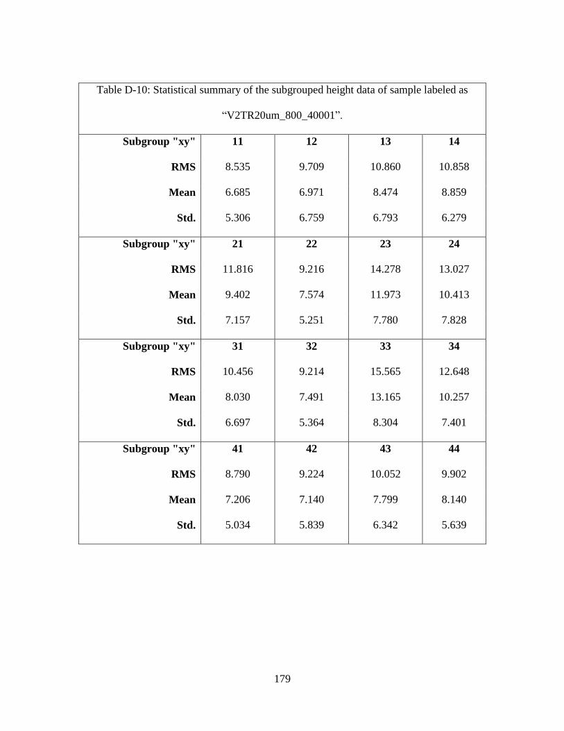
179
Table D-10: Statistical summary of the subgrouped height data of sample labeled as
“V2TR20um_800_40001”.
Subgroup "xy" 11 12 13 14
RMS 8.535 9.709 10.860 10.858
Mean 6.685 6.971 8.474 8.859
Std. 5.306 6.759 6.793 6.279
Subgroup "xy" 21 22 23 24
RMS 11.816 9.216 14.278 13.027
Mean 9.402 7.574 11.973 10.413
Std. 7.157 5.251 7.780 7.828
Subgroup "xy" 31 32 33 34
RMS 10.456 9.214 15.565 12.648
Mean 8.030 7.491 13.165 10.257
Std. 6.697 5.364 8.304 7.401
Subgroup "xy" 41 42 43 44
RMS 8.790 9.224 10.052 9.902
Mean 7.206 7.140 7.799 8.140
Std. 5.034 5.839 6.342 5.639
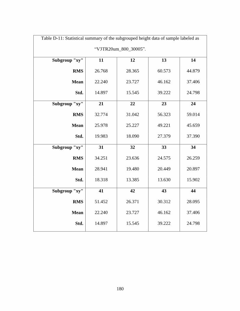
180
Table D-11: Statistical summary of the subgrouped height data of sample labeled as
“V3TR20um_800_30005”.
Subgroup "xy" 11 12 13 14
RMS 26.768 28.365 60.573 44.879
Mean 22.240 23.727 46.162 37.406
Std. 14.897 15.545 39.222 24.798
Subgroup "xy" 21 22 23 24
RMS 32.774 31.042 56.323 59.014
Mean 25.978 25.227 49.221 45.659
Std. 19.983 18.090 27.379 37.390
Subgroup "xy" 31 32 33 34
RMS 34.251 23.636 24.575 26.259
Mean 28.941 19.480 20.449 20.897
Std. 18.318 13.385 13.630 15.902
Subgroup "xy" 41 42 43 44
RMS 51.452 26.371 30.312 28.095
Mean 22.240 23.727 46.162 37.406
Std. 14.897 15.545 39.222 24.798
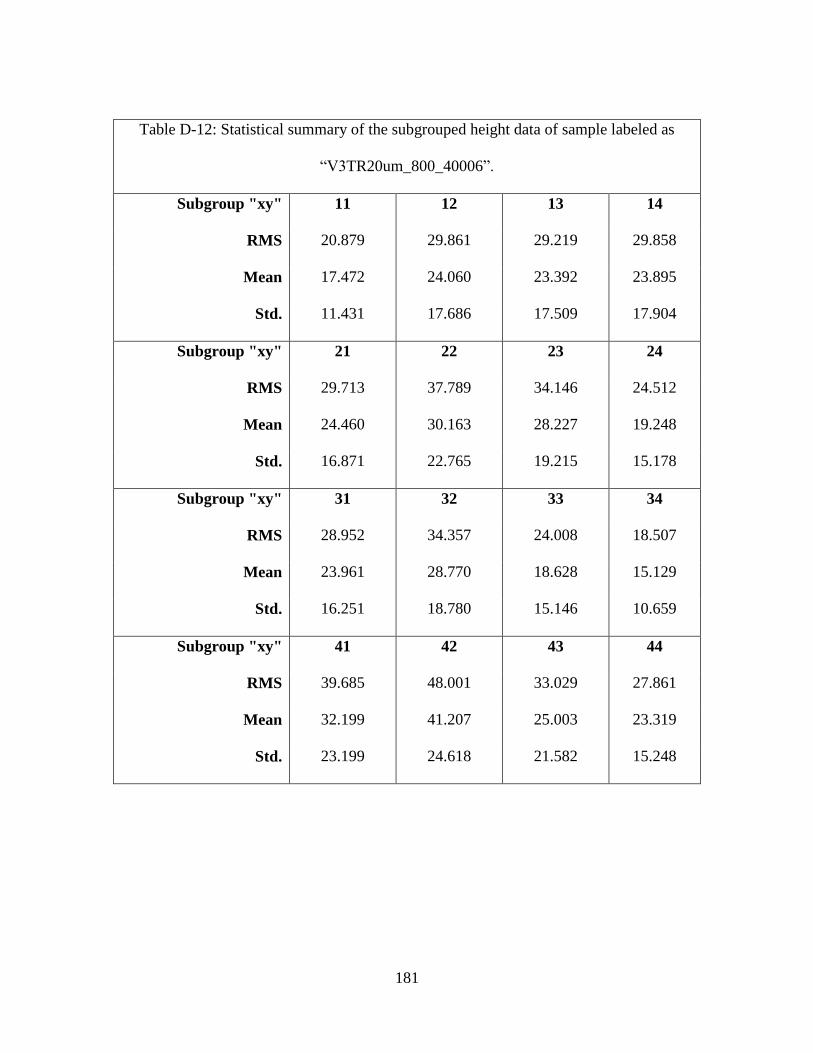
181
Table D-12: Statistical summary of the subgrouped height data of sample labeled as
“V3TR20um_800_40006”.
Subgroup "xy" 11 12 13 14
RMS 20.879 29.861 29.219 29.858
Mean 17.472 24.060 23.392 23.895
Std. 11.431 17.686 17.509 17.904
Subgroup "xy" 21 22 23 24
RMS 29.713 37.789 34.146 24.512
Mean 24.460 30.163 28.227 19.248
Std. 16.871 22.765 19.215 15.178
Subgroup "xy" 31 32 33 34
RMS 28.952 34.357 24.008 18.507
Mean 23.961 28.770 18.628 15.129
Std. 16.251 18.780 15.146 10.659
Subgroup "xy" 41 42 43 44
RMS 39.685 48.001 33.029 27.861
Mean 32.199 41.207 25.003 23.319
Std. 23.199 24.618 21.582 15.248
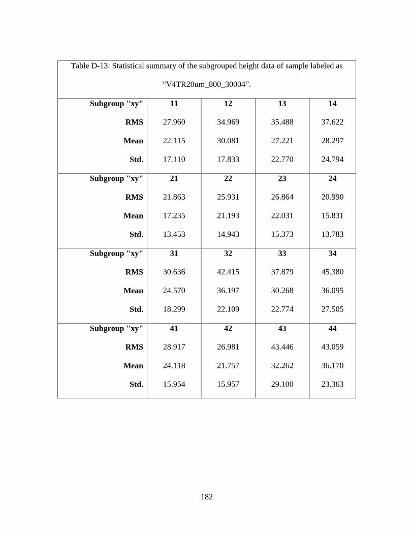
182
Table D-13: Statistical summary of the subgrouped height data of sample labeled as
“V4TR20um_800_30004”.
Subgroup "xy" 11 12 13 14
RMS 27.960 34.969 35.488 37.622
Mean 22.115 30.081 27.221 28.297
Std. 17.110 17.833 22.770 24.794
Subgroup "xy" 21 22 23 24
RMS 21.863 25.931 26.864 20.990
Mean 17.235 21.193 22.031 15.831
Std. 13.453 14.943 15.373 13.783
Subgroup "xy" 31 32 33 34
RMS 30.636 42.415 37.879 45.380
Mean 24.570 36.197 30.268 36.095
Std. 18.299 22.109 22.774 27.505
Subgroup "xy" 41 42 43 44
RMS 28.917 26.981 43.446 43.059
Mean 24.118 21.757 32.262 36.170
Std. 15.954 15.957 29.100 23.363
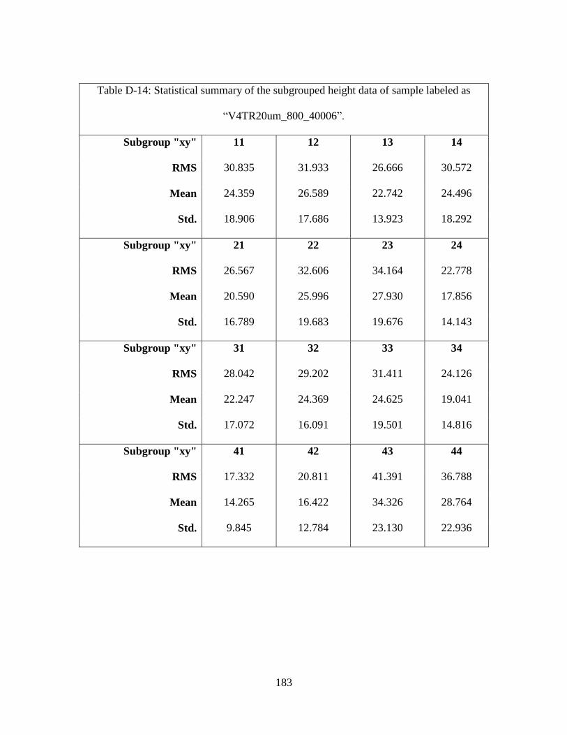
183
Table D-14: Statistical summary of the subgrouped height data of sample labeled as
“V4TR20um_800_40006”.
Subgroup "xy" 11 12 13 14
RMS 30.835 31.933 26.666 30.572
Mean 24.359 26.589 22.742 24.496
Std. 18.906 17.686 13.923 18.292
Subgroup "xy" 21 22 23 24
RMS 26.567 32.606 34.164 22.778
Mean 20.590 25.996 27.930 17.856
Std. 16.789 19.683 19.676 14.143
Subgroup "xy" 31 32 33 34
RMS 28.042 29.202 31.411 24.126
Mean 22.247 24.369 24.625 19.041
Std. 17.072 16.091 19.501 14.816
Subgroup "xy" 41 42 43 44
RMS 17.332 20.811 41.391 36.788
Mean 14.265 16.422 34.326 28.764
Std. 9.845 12.784 23.130 22.936
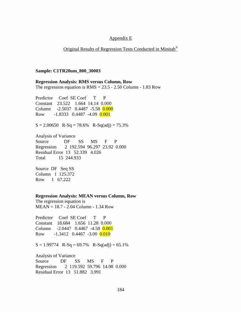
184
Appendix E
Original Results of Regression Tests Conducted in Minitab®
Sample: C1TR20um_800_30003
Regression Analysis: RMS versus Column, Row
The regression equation is RMS = 23.5 - 2.50 Column - 1.83 Row
Predictor Coef SE Coef T P
Constant 23.522 1.664 14.14 0.000
Column -2.5037 0.4487 -5.58 0.000
Row -1.8333 0.4487 -4.09 0.001
S = 2.00650 R-Sq = 78.6% R-Sq(adj) = 75.3%
Analysis of Variance
Source DF SS MS F P
Regression 2 192.594 96.297 23.92 0.000
Residual Error 13 52.339 4.026
Total 15 244.933
Source DF Seq SS
Column 1 125.372
Row 1 67.222
Regression Analysis: MEAN versus Column, Row
The regression equation is
MEAN = 18.7 - 2.04 Column - 1.34 Row
Predictor Coef SE Coef T P
Constant 18.684 1.656 11.28 0.000
Column -2.0447 0.4467 -4.58 0.001
Row -1.3412 0.4467 -3.00 0.010
S = 1.99774 R-Sq = 69.7% R-Sq(adj) = 65.1%
Analysis of Variance
Source DF SS MS F P
Regression 2 119.592 59.796 14.98 0.000
Residual Error 13 51.882 3.991
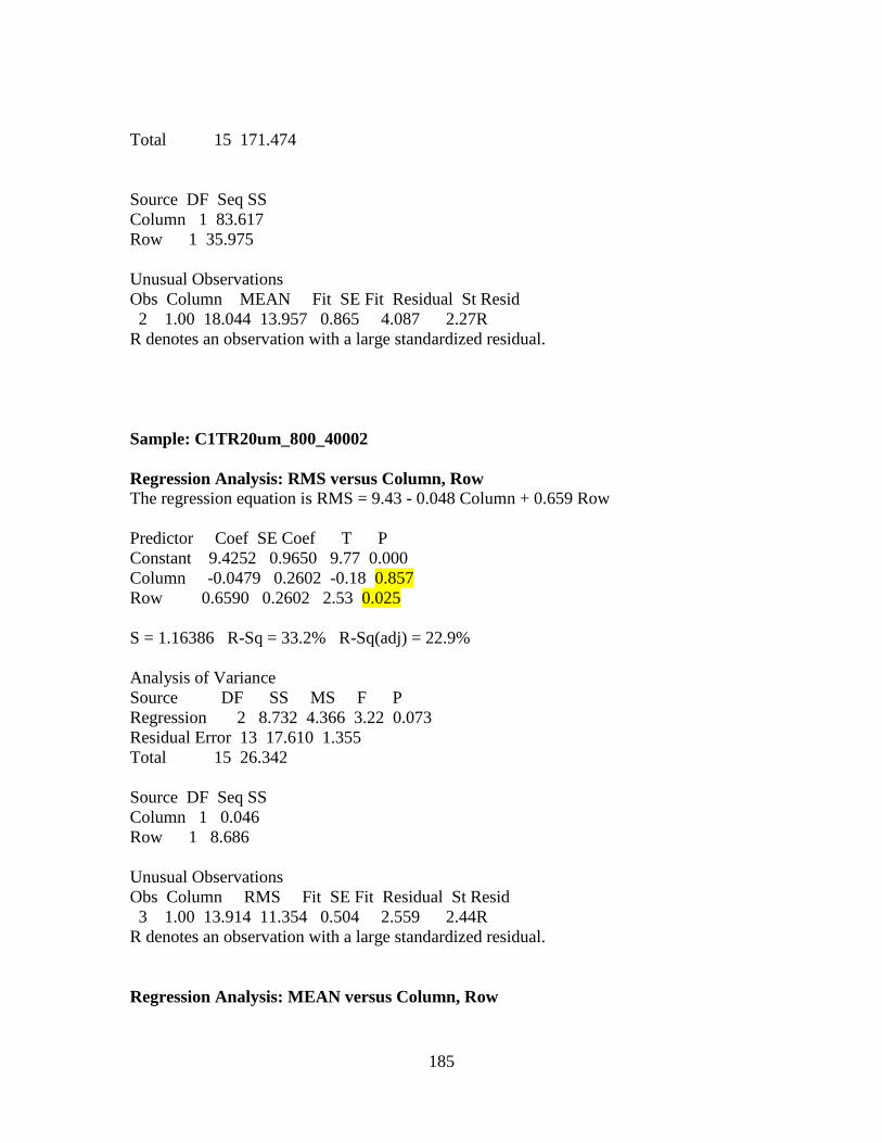
185
Total 15 171.474
Source DF Seq SS
Column 1 83.617
Row 1 35.975
Unusual Observations
Obs Column MEAN Fit SE Fit Residual St Resid
2 1.00 18.044 13.957 0.865 4.087 2.27R
R denotes an observation with a large standardized residual.
Sample: C1TR20um_800_40002
Regression Analysis: RMS versus Column, Row
The regression equation is RMS = 9.43 - 0.048 Column + 0.659 Row
Predictor Coef SE Coef T P
Constant 9.4252 0.9650 9.77 0.000
Column -0.0479 0.2602 -0.18 0.857
Row 0.6590 0.2602 2.53 0.025
S = 1.16386 R-Sq = 33.2% R-Sq(adj) = 22.9%
Analysis of Variance
Source DF SS MS F P
Regression 2 8.732 4.366 3.22 0.073
Residual Error 13 17.610 1.355
Total 15 26.342
Source DF Seq SS
Column 1 0.046
Row 1 8.686
Unusual Observations
Obs Column RMS Fit SE Fit Residual St Resid
3 1.00 13.914 11.354 0.504 2.559 2.44R
R denotes an observation with a large standardized residual.
Regression Analysis: MEAN versus Column, Row
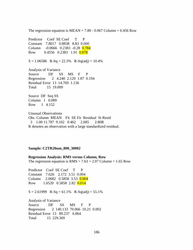
186
The regression equation is MEAN = 7.80 - 0.067 Column + 0.456 Row
Predictor Coef SE Coef T P
Constant 7.8017 0.8838 8.83 0.000
Column -0.0666 0.2383 -0.28 0.784
Row 0.4556 0.2383 1.91 0.078
S = 1.06586 R-Sq = 22.3% R-Sq(adj) = 10.4%
Analysis of Variance
Source DF SS MS F P
Regression 2 4.240 2.120 1.87 0.194
Residual Error 13 14.769 1.136
Total 15 19.009
Source DF Seq SS
Column 1 0.089
Row 1 4.152
Unusual Observations
Obs Column MEAN Fit SE Fit Residual St Resid
3 1.00 11.787 9.102 0.462 2.685 2.80R
R denotes an observation with a large standardized residual.
Sample: C2TR20um_800_30002
Regression Analysis: RMS versus Column, Row
The regression equation is RMS = 7.63 + 2.07 Column + 1.65 Row
Predictor Coef SE Coef T P
Constant 7.626 2.172 3.51 0.004
Column 2.0682 0.5858 3.53 0.004
Row 1.6520 0.5858 2.82 0.014
S = 2.61999 R-Sq = 61.1% R-Sq(adj) = 55.1%
Analysis of Variance
Source DF SS MS F P
Regression 2 140.133 70.066 10.21 0.002
Residual Error 13 89.237 6.864
Total 15 229.369
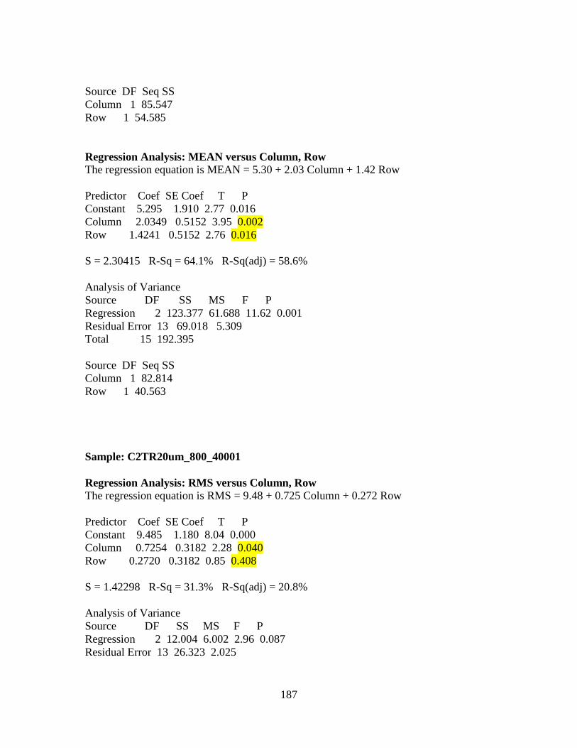
187
Source DF Seq SS
Column 1 85.547
Row 1 54.585
Regression Analysis: MEAN versus Column, Row
The regression equation is MEAN = 5.30 + 2.03 Column + 1.42 Row
Predictor Coef SE Coef T P
Constant 5.295 1.910 2.77 0.016
Column 2.0349 0.5152 3.95 0.002
Row 1.4241 0.5152 2.76 0.016
S = 2.30415 R-Sq = 64.1% R-Sq(adj) = 58.6%
Analysis of Variance
Source DF SS MS F P
Regression 2 123.377 61.688 11.62 0.001
Residual Error 13 69.018 5.309
Total 15 192.395
Source DF Seq SS
Column 1 82.814
Row 1 40.563
Sample: C2TR20um_800_40001
Regression Analysis: RMS versus Column, Row
The regression equation is RMS = 9.48 + 0.725 Column + 0.272 Row
Predictor Coef SE Coef T P
Constant 9.485 1.180 8.04 0.000
Column 0.7254 0.3182 2.28 0.040
Row 0.2720 0.3182 0.85 0.408
S = 1.42298 R-Sq = 31.3% R-Sq(adj) = 20.8%
Analysis of Variance
Source DF SS MS F P
Regression 2 12.004 6.002 2.96 0.087
Residual Error 13 26.323 2.025
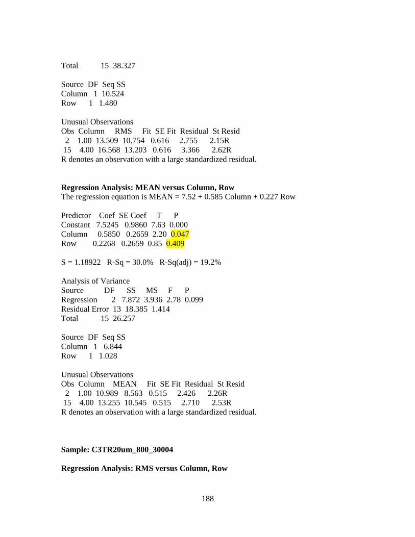
188
Total 15 38.327
Source DF Seq SS
Column 1 10.524
Row 1 1.480
Unusual Observations
Obs Column RMS Fit SE Fit Residual St Resid
2 1.00 13.509 10.754 0.616 2.755 2.15R
15 4.00 16.568 13.203 0.616 3.366 2.62R
R denotes an observation with a large standardized residual.
Regression Analysis: MEAN versus Column, Row
The regression equation is MEAN = 7.52 + 0.585 Column + 0.227 Row
Predictor Coef SE Coef T P
Constant 7.5245 0.9860 7.63 0.000
Column 0.5850 0.2659 2.20 0.047
Row 0.2268 0.2659 0.85 0.409
S = 1.18922 R-Sq = 30.0% R-Sq(adj) = 19.2%
Analysis of Variance
Source DF SS MS F P
Regression 2 7.872 3.936 2.78 0.099
Residual Error 13 18.385 1.414
Total 15 26.257
Source DF Seq SS
Column 1 6.844
Row 1 1.028
Unusual Observations
Obs Column MEAN Fit SE Fit Residual St Resid
2 1.00 10.989 8.563 0.515 2.426 2.26R
15 4.00 13.255 10.545 0.515 2.710 2.53R
R denotes an observation with a large standardized residual.
Sample: C3TR20um_800_30004
Regression Analysis: RMS versus Column, Row
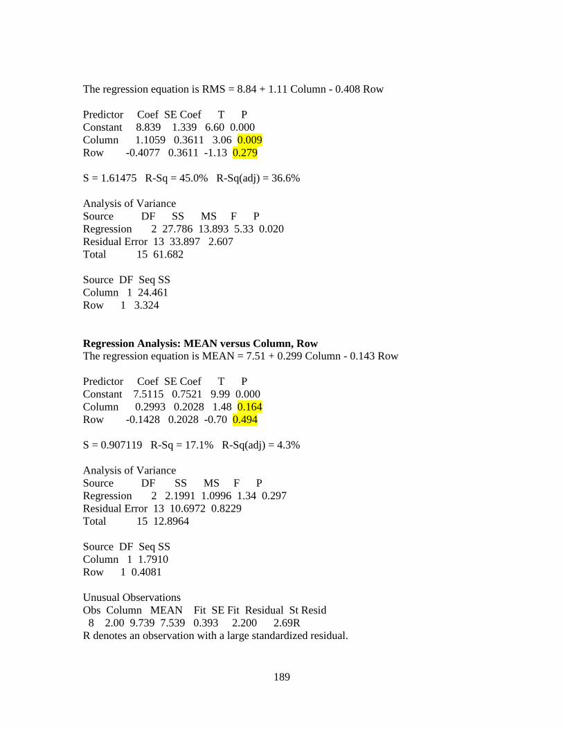
189
The regression equation is RMS = 8.84 + 1.11 Column - 0.408 Row
Predictor Coef SE Coef T P
Constant 8.839 1.339 6.60 0.000
Column 1.1059 0.3611 3.06 0.009
Row -0.4077 0.3611 -1.13 0.279
S = 1.61475 R-Sq = 45.0% R-Sq(adj) = 36.6%
Analysis of Variance
Source DF SS MS F P
Regression 2 27.786 13.893 5.33 0.020
Residual Error 13 33.897 2.607
Total 15 61.682
Source DF Seq SS
Column 1 24.461
Row 1 3.324
Regression Analysis: MEAN versus Column, Row
The regression equation is MEAN = 7.51 + 0.299 Column - 0.143 Row
Predictor Coef SE Coef T P
Constant 7.5115 0.7521 9.99 0.000
Column 0.2993 0.2028 1.48 0.164
Row -0.1428 0.2028 -0.70 0.494
S = 0.907119 R-Sq = 17.1% R-Sq(adj) = 4.3%
Analysis of Variance
Source DF SS MS F P
Regression 2 2.1991 1.0996 1.34 0.297
Residual Error 13 10.6972 0.8229
Total 15 12.8964
Source DF Seq SS
Column 1 1.7910
Row 1 0.4081
Unusual Observations
Obs Column MEAN Fit SE Fit Residual St Resid
8 2.00 9.739 7.539 0.393 2.200 2.69R
R denotes an observation with a large standardized residual.
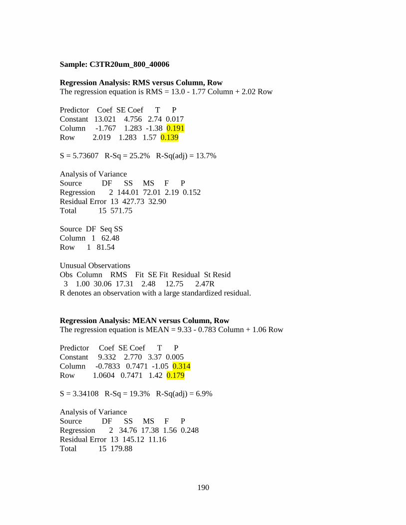
190
Sample: C3TR20um_800_40006
Regression Analysis: RMS versus Column, Row
The regression equation is RMS = 13.0 - 1.77 Column + 2.02 Row
Predictor Coef SE Coef T P
Constant 13.021 4.756 2.74 0.017
Column -1.767 1.283 -1.38 0.191
Row 2.019 1.283 1.57 0.139
S = 5.73607 R-Sq = 25.2% R-Sq(adj) = 13.7%
Analysis of Variance
Source DF SS MS F P
Regression 2 144.01 72.01 2.19 0.152
Residual Error 13 427.73 32.90
Total 15 571.75
Source DF Seq SS
Column 1 62.48
Row 1 81.54
Unusual Observations
Obs Column RMS Fit SE Fit Residual St Resid
3 1.00 30.06 17.31 2.48 12.75 2.47R
R denotes an observation with a large standardized residual.
Regression Analysis: MEAN versus Column, Row
The regression equation is MEAN = 9.33 - 0.783 Column + 1.06 Row
Predictor Coef SE Coef T P
Constant 9.332 2.770 3.37 0.005
Column -0.7833 0.7471 -1.05 0.314
Row 1.0604 0.7471 1.42 0.179
S = 3.34108 R-Sq = 19.3% R-Sq(adj) = 6.9%
Analysis of Variance
Source DF SS MS F P
Regression 2 34.76 17.38 1.56 0.248
Residual Error 13 145.12 11.16
Total 15 179.88
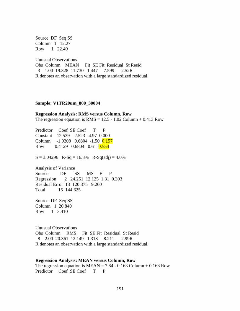
191
Source DF Seq SS
Column 1 12.27
Row 1 22.49
Unusual Observations
Obs Column MEAN Fit SE Fit Residual St Resid
3 1.00 19.328 11.730 1.447 7.599 2.52R
R denotes an observation with a large standardized residual.
Sample: V1TR20um_800_30004
Regression Analysis: RMS versus Column, Row
The regression equation is RMS = 12.5 - 1.02 Column + 0.413 Row
Predictor Coef SE Coef T P
Constant 12.539 2.523 4.97 0.000
Column -1.0208 0.6804 -1.50 0.157
Row 0.4129 0.6804 0.61 0.554
S = 3.04296 R-Sq = 16.8% R-Sq(adj) = 4.0%
Analysis of Variance
Source DF SS MS F P
Regression 2 24.251 12.125 1.31 0.303
Residual Error 13 120.375 9.260
Total 15 144.625
Source DF Seq SS
Column 1 20.840
Row 1 3.410
Unusual Observations
Obs Column RMS Fit SE Fit Residual St Resid
8 2.00 20.361 12.149 1.318 8.211 2.99R
R denotes an observation with a large standardized residual.
Regression Analysis: MEAN versus Column, Row
The regression equation is MEAN = 7.84 - 0.163 Column + 0.168 Row
Predictor Coef SE Coef T P
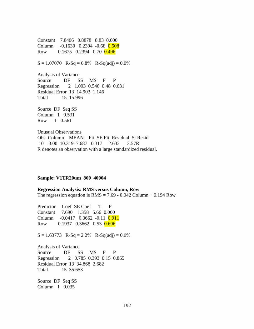
192
Constant 7.8406 0.8878 8.83 0.000
Column -0.1630 0.2394 -0.68 0.508
Row 0.1675 0.2394 0.70 0.496
S = 1.07070 R-Sq = 6.8% R-Sq(adj) = 0.0%
Analysis of Variance
Source DF SS MS F P
Regression 2 1.093 0.546 0.48 0.631
Residual Error 13 14.903 1.146
Total 15 15.996
Source DF Seq SS
Column 1 0.531
Row 1 0.561
Unusual Observations
Obs Column MEAN Fit SE Fit Residual St Resid
10 3.00 10.319 7.687 0.317 2.632 2.57R
R denotes an observation with a large standardized residual.
Sample: V1TR20um_800_40004
Regression Analysis: RMS versus Column, Row
The regression equation is RMS = 7.69 - 0.042 Column + 0.194 Row
Predictor Coef SE Coef T P
Constant 7.690 1.358 5.66 0.000
Column -0.0417 0.3662 -0.11 0.911
Row 0.1937 0.3662 0.53 0.606
S = 1.63773 R-Sq = 2.2% R-Sq(adj) = 0.0%
Analysis of Variance
Source DF SS MS F P
Regression 2 0.785 0.393 0.15 0.865
Residual Error 13 34.868 2.682
Total 15 35.653
Source DF Seq SS
Column 1 0.035

193
Row 1 0.750
Unusual Observations
Obs Column RMS Fit SE Fit Residual St Resid
11 3.00 12.570 8.146 0.484 4.424 2.83R
R denotes an observation with a large standardized residual.
Regression Analysis: MEAN versus Column, Row
The regression equation is MEAN = 6.29 - 0.103 Column + 0.034 Row
Predictor Coef SE Coef T P
Constant 6.2855 0.4687 13.41 0.000
Column -0.1034 0.1264 -0.82 0.428
Row 0.0342 0.1264 0.27 0.791
S = 0.565222 R-Sq = 5.4% R-Sq(adj) = 0.0%
Analysis of Variance
Source DF SS MS F P
Regression 2 0.2373 0.1186 0.37 0.697
Residual Error 13 4.1532 0.3195
Total 15 4.3905
Source DF Seq SS
Column 1 0.2139
Row 1 0.0234
Sample: V2TR20um_800_30003
Regression Analysis: RMS versus Column, Row
The regression equation is RMS = 7.45 + 0.593 Column + 0.055 Row
Predictor Coef SE Coef T P
Constant 7.4510 0.9513 7.83 0.000
Column 0.5934 0.2565 2.31 0.038
Row 0.0549 0.2565 0.21 0.834
S = 1.14731 R-Sq = 29.3% R-Sq(adj) = 18.5%
Analysis of Variance
Source DF SS MS F P
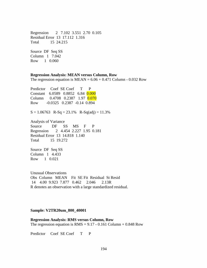
194
Regression 2 7.102 3.551 2.70 0.105
Residual Error 13 17.112 1.316
Total 15 24.215
Source DF Seq SS
Column 1 7.042
Row 1 0.060
Regression Analysis: MEAN versus Column, Row
The regression equation is MEAN = 6.06 + 0.471 Column - 0.032 Row
Predictor Coef SE Coef T P
Constant 6.0589 0.8852 6.84 0.000
Column 0.4708 0.2387 1.97 0.070
Row -0.0325 0.2387 -0.14 0.894
S = 1.06763 R-Sq = 23.1% R-Sq(adj) = 11.3%
Analysis of Variance
Source DF SS MS F P
Regression 2 4.454 2.227 1.95 0.181
Residual Error 13 14.818 1.140
Total 15 19.272
Source DF Seq SS
Column 1 4.433
Row 1 0.021
Unusual Observations
Obs Column MEAN Fit SE Fit Residual St Resid
14 4.00 9.923 7.877 0.462 2.046 2.13R
R denotes an observation with a large standardized residual.
Sample: V2TR20um_800_40001
Regression Analysis: RMS versus Column, Row
The regression equation is RMS = 9.17 - 0.161 Column + 0.848 Row
Predictor Coef SE Coef T P
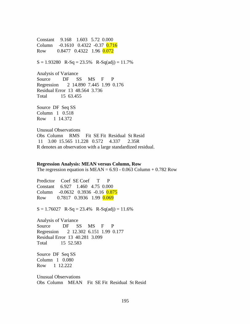
195
Constant 9.168 1.603 5.72 0.000
Column -0.1610 0.4322 -0.37 0.716
Row 0.8477 0.4322 1.96 0.072
S = 1.93280 R-Sq = 23.5% R-Sq(adj) = 11.7%
Analysis of Variance
Source DF SS MS F P
Regression 2 14.890 7.445 1.99 0.176
Residual Error 13 48.564 3.736
Total 15 63.455
Source DF Seq SS
Column 1 0.518
Row 1 14.372
Unusual Observations
Obs Column RMS Fit SE Fit Residual St Resid
11 3.00 15.565 11.228 0.572 4.337 2.35R
R denotes an observation with a large standardized residual.
Regression Analysis: MEAN versus Column, Row
The regression equation is MEAN = 6.93 - 0.063 Column + 0.782 Row
Predictor Coef SE Coef T P
Constant 6.927 1.460 4.75 0.000
Column -0.0632 0.3936 -0.16 0.875
Row 0.7817 0.3936 1.99 0.069
S = 1.76027 R-Sq = 23.4% R-Sq(adj) = 11.6%
Analysis of Variance
Source DF SS MS F P
Regression 2 12.302 6.151 1.99 0.177
Residual Error 13 40.281 3.099
Total 15 52.583
Source DF Seq SS
Column 1 0.080
Row 1 12.222
Unusual Observations
Obs Column MEAN Fit SE Fit Residual St Resid
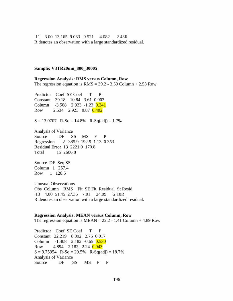
196
11 3.00 13.165 9.083 0.521 4.082 2.43R
R denotes an observation with a large standardized residual.
Sample: V3TR20um_800_30005
Regression Analysis: RMS versus Column, Row
The regression equation is RMS = 39.2 - 3.59 Column + 2.53 Row
Predictor Coef SE Coef T P
Constant 39.18 10.84 3.61 0.003
Column -3.588 2.923 -1.23 0.241
Row 2.534 2.923 0.87 0.402
S = 13.0707 R-Sq = 14.8% R-Sq(adj) = 1.7%
Analysis of Variance
Source DF SS MS F P
Regression 2 385.9 192.9 1.13 0.353
Residual Error 13 2221.0 170.8
Total 15 2606.8
Source DF Seq SS
Column 1 257.4
Row 1 128.5
Unusual Observations
Obs Column RMS Fit SE Fit Residual St Resid
13 4.00 51.45 27.36 7.01 24.09 2.18R
R denotes an observation with a large standardized residual.
Regression Analysis: MEAN versus Column, Row
The regression equation is MEAN = 22.2 - 1.41 Column + 4.89 Row
Predictor Coef SE Coef T P
Constant 22.219 8.092 2.75 0.017
Column -1.408 2.182 -0.65 0.530
Row 4.894 2.182 2.24 0.043
S = 9.75954 R-Sq = 29.5% R-Sq(adj) = 18.7%
Analysis of Variance
Source DF SS MS F P
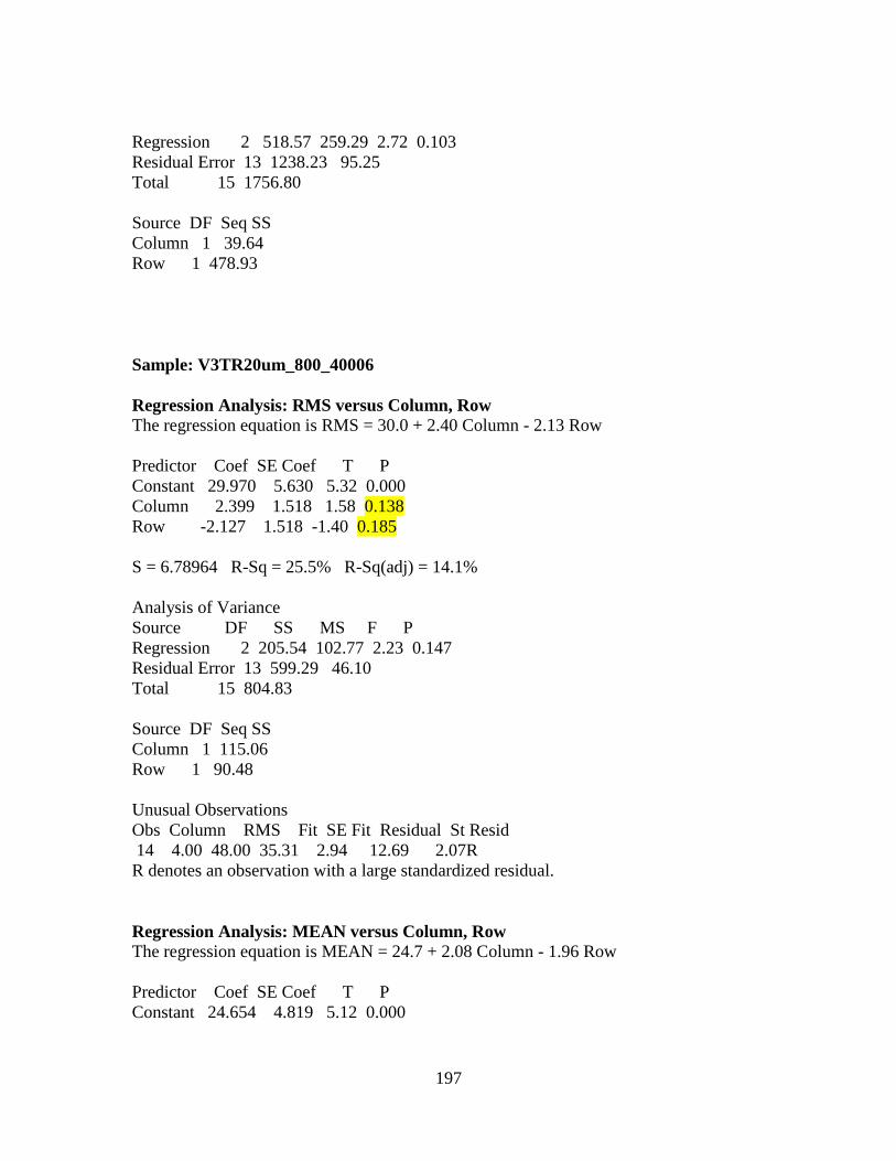
197
Regression 2 518.57 259.29 2.72 0.103
Residual Error 13 1238.23 95.25
Total 15 1756.80
Source DF Seq SS
Column 1 39.64
Row 1 478.93
Sample: V3TR20um_800_40006
Regression Analysis: RMS versus Column, Row
The regression equation is RMS = 30.0 + 2.40 Column - 2.13 Row
Predictor Coef SE Coef T P
Constant 29.970 5.630 5.32 0.000
Column 2.399 1.518 1.58 0.138
Row -2.127 1.518 -1.40 0.185
S = 6.78964 R-Sq = 25.5% R-Sq(adj) = 14.1%
Analysis of Variance
Source DF SS MS F P
Regression 2 205.54 102.77 2.23 0.147
Residual Error 13 599.29 46.10
Total 15 804.83
Source DF Seq SS
Column 1 115.06
Row 1 90.48
Unusual Observations
Obs Column RMS Fit SE Fit Residual St Resid
14 4.00 48.00 35.31 2.94 12.69 2.07R
R denotes an observation with a large standardized residual.
Regression Analysis: MEAN versus Column, Row
The regression equation is MEAN = 24.7 + 2.08 Column - 1.96 Row
Predictor Coef SE Coef T P
Constant 24.654 4.819 5.12 0.000

198
Column 2.078 1.300 1.60 0.134
Row -1.961 1.300 -1.51 0.155
S = 5.81199 R-Sq = 27.1% R-Sq(adj) = 15.9%
Analysis of Variance
Source DF SS MS F P
Regression 2 163.30 81.65 2.42 0.128
Residual Error 13 439.13 33.78
Total 15 602.43
Source DF Seq SS
Column 1 86.36
Row 1 76.94
Unusual Observations
Obs Column MEAN Fit SE Fit Residual St Resid
14 4.00 41.21 29.04 2.52 12.16 2.32R
R denotes an observation with a large standardized residual.
Sample: V4TR20um_800_30004
Regression Analysis: RMS versus Column, Row
The regression equation is RMS = 20.3 + 1.99 Column + 3.16 Row
Predictor Coef SE Coef T P
Constant 20.265 5.942 3.41 0.005
Column 1.994 1.602 1.24 0.235
Row 3.160 1.602 1.97 0.070
S = 7.16622 R-Sq = 29.5% R-Sq(adj) = 18.6%
Analysis of Variance
Source DF SS MS F P
Regression 2 279.24 139.62 2.72 0.103
Residual Error 13 667.61 51.35
Total 15 946.85
Source DF Seq SS
Column 1 79.51
Row 1 199.74
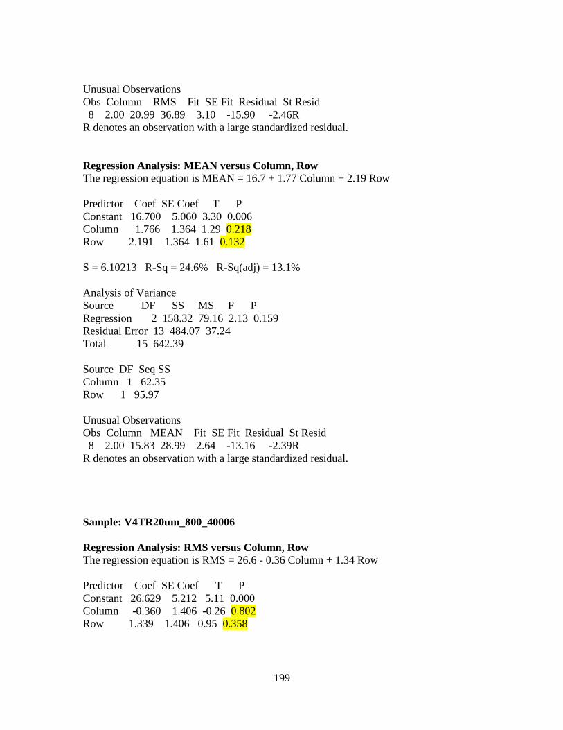
199
Unusual Observations
Obs Column RMS Fit SE Fit Residual St Resid
8 2.00 20.99 36.89 3.10 -15.90 -2.46R
R denotes an observation with a large standardized residual.
Regression Analysis: MEAN versus Column, Row
The regression equation is MEAN = 16.7 + 1.77 Column + 2.19 Row
Predictor Coef SE Coef T P
Constant 16.700 5.060 3.30 0.006
Column 1.766 1.364 1.29 0.218
Row 2.191 1.364 1.61 0.132
S = 6.10213 R-Sq = 24.6% R-Sq(adj) = 13.1%
Analysis of Variance
Source DF SS MS F P
Regression 2 158.32 79.16 2.13 0.159
Residual Error 13 484.07 37.24
Total 15 642.39
Source DF Seq SS
Column 1 62.35
Row 1 95.97
Unusual Observations
Obs Column MEAN Fit SE Fit Residual St Resid
8 2.00 15.83 28.99 2.64 -13.16 -2.39R
R denotes an observation with a large standardized residual.
Sample: V4TR20um_800_40006
Regression Analysis: RMS versus Column, Row
The regression equation is RMS = 26.6 - 0.36 Column + 1.34 Row
Predictor Coef SE Coef T P
Constant 26.629 5.212 5.11 0.000
Column -0.360 1.406 -0.26 0.802
Row 1.339 1.406 0.95 0.358
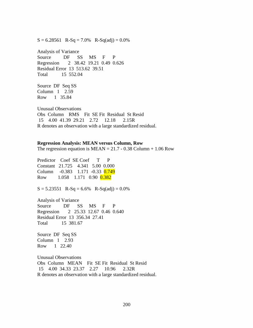
200
S = 6.28561 R-Sq = 7.0% R-Sq(adj) = 0.0%
Analysis of Variance
Source DF SS MS F P
Regression 2 38.42 19.21 0.49 0.626
Residual Error 13 513.62 39.51
Total 15 552.04
Source DF Seq SS
Column 1 2.59
Row 1 35.84
Unusual Observations
Obs Column RMS Fit SE Fit Residual St Resid
15 4.00 41.39 29.21 2.72 12.18 2.15R
R denotes an observation with a large standardized residual.
Regression Analysis: MEAN versus Column, Row
The regression equation is MEAN = 21.7 - 0.38 Column + 1.06 Row
Predictor Coef SE Coef T P
Constant 21.725 4.341 5.00 0.000
Column -0.383 1.171 -0.33 0.749
Row 1.058 1.171 0.90 0.382
S = 5.23551 R-Sq = 6.6% R-Sq(adj) = 0.0%
Analysis of Variance
Source DF SS MS F P
Regression 2 25.33 12.67 0.46 0.640
Residual Error 13 356.34 27.41
Total 15 381.67
Source DF Seq SS
Column 1 2.93
Row 1 22.40
Unusual Observations
Obs Column MEAN Fit SE Fit Residual St Resid
15 4.00 34.33 23.37 2.27 10.96 2.32R
R denotes an observation with a large standardized residual.
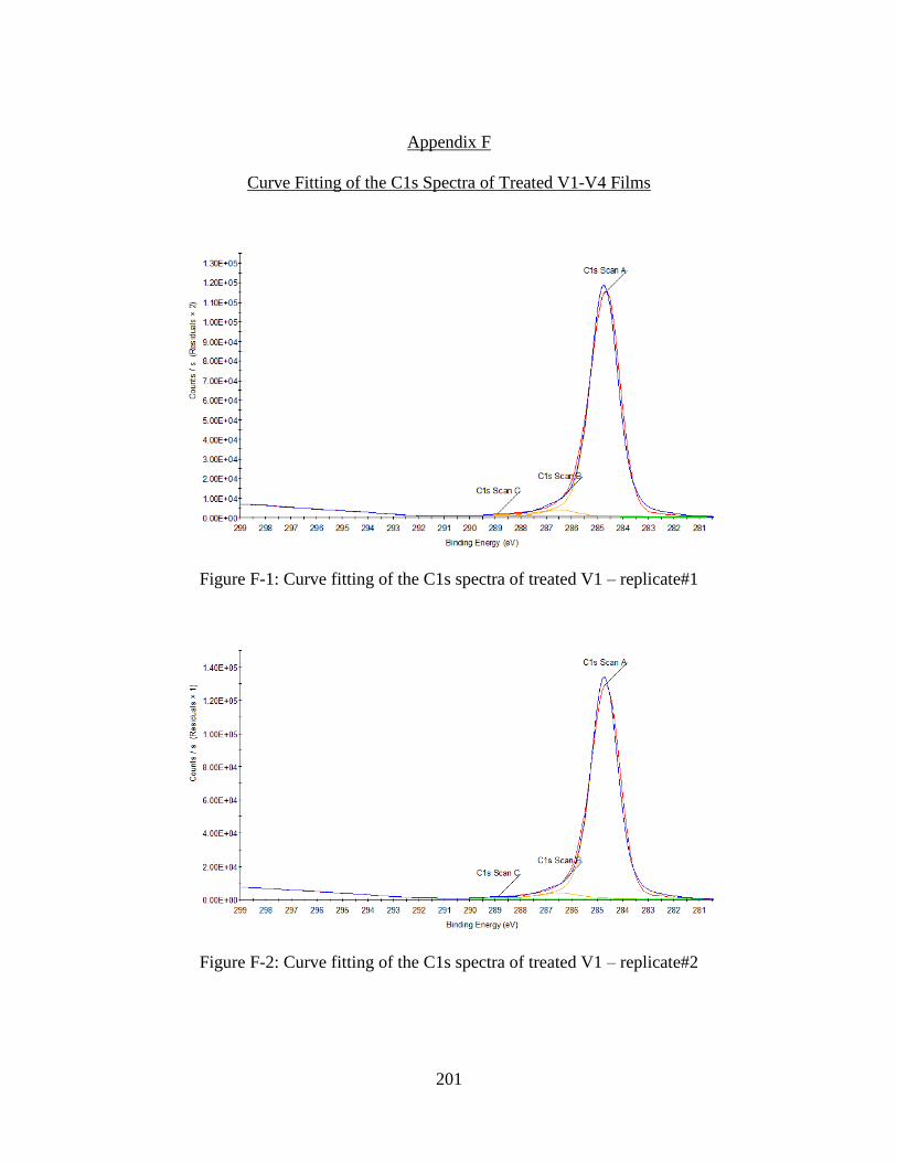
201
Appendix F
Curve Fitting of the C1s Spectra of Treated V1-V4 Films
Figure F-1: Curve fitting of the C1s spectra of treated V1 – replicate#1
Figure F-2: Curve fitting of the C1s spectra of treated V1 – replicate#2
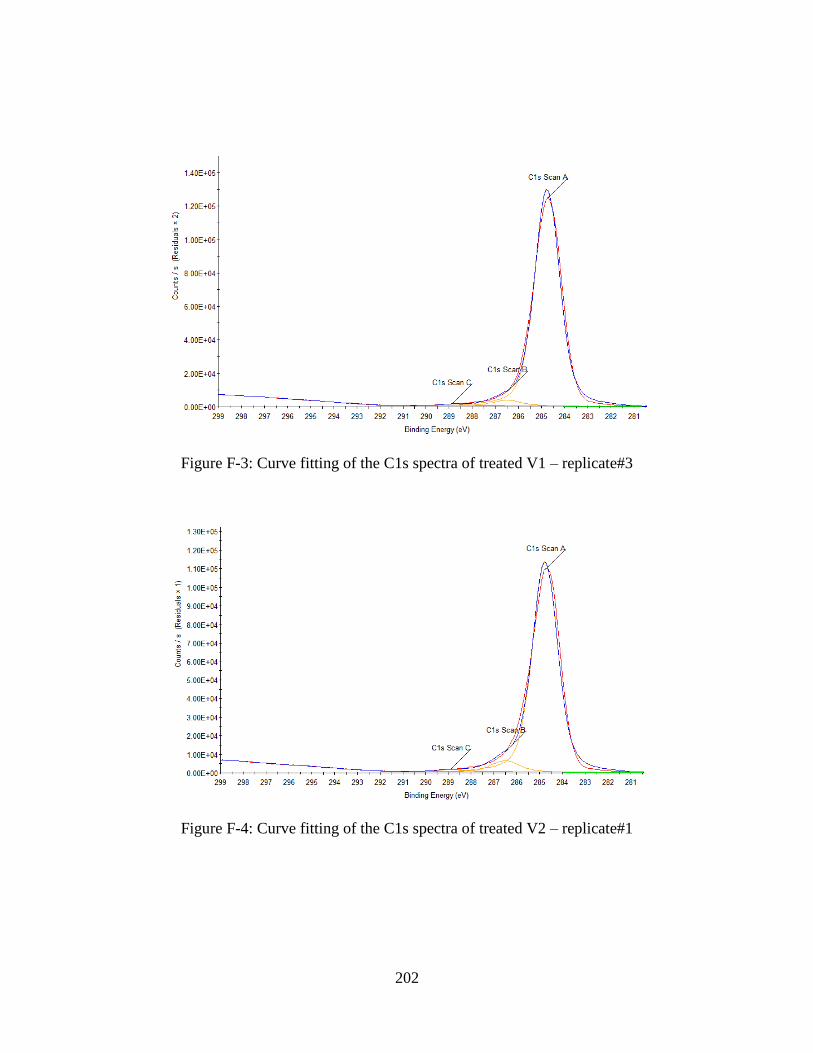
202
Figure F-3: Curve fitting of the C1s spectra of treated V1 – replicate#3
Figure F-4: Curve fitting of the C1s spectra of treated V2 – replicate#1
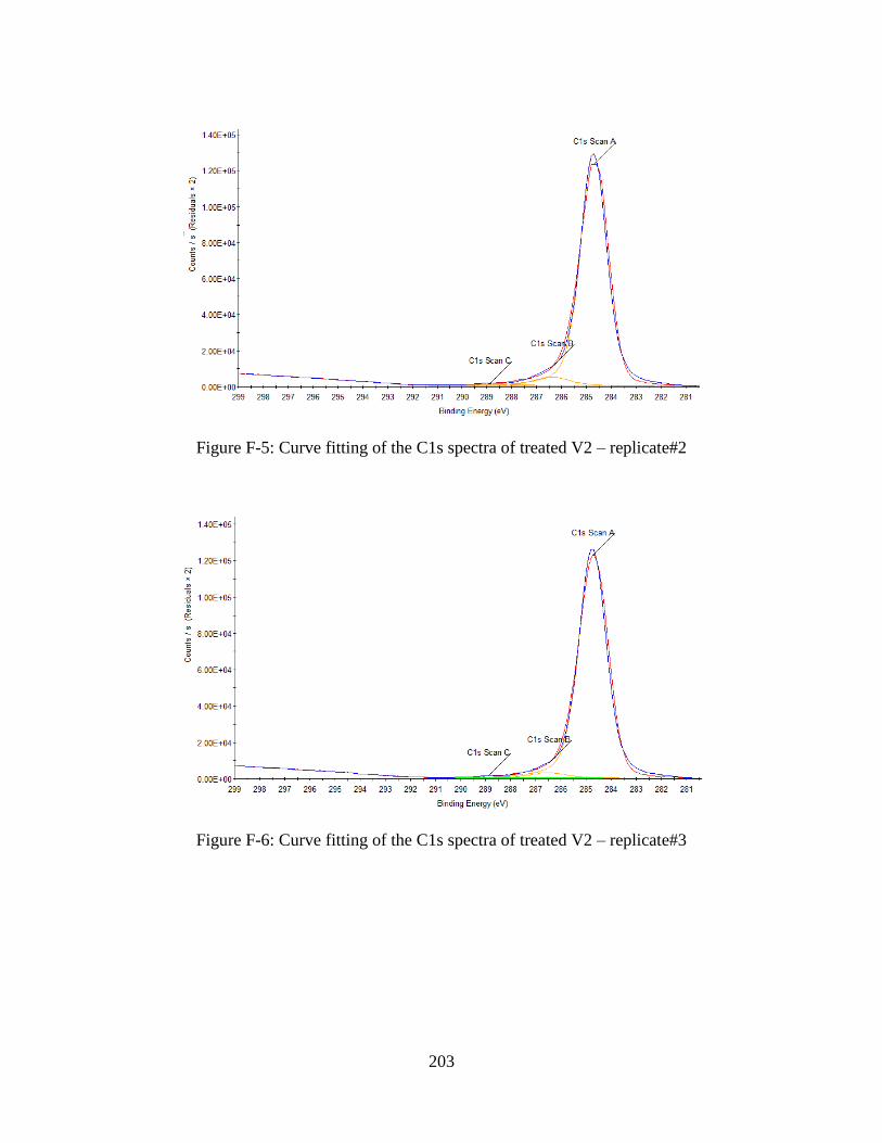
203
Figure F-5: Curve fitting of the C1s spectra of treated V2 – replicate#2
Figure F-6: Curve fitting of the C1s spectra of treated V2 – replicate#3
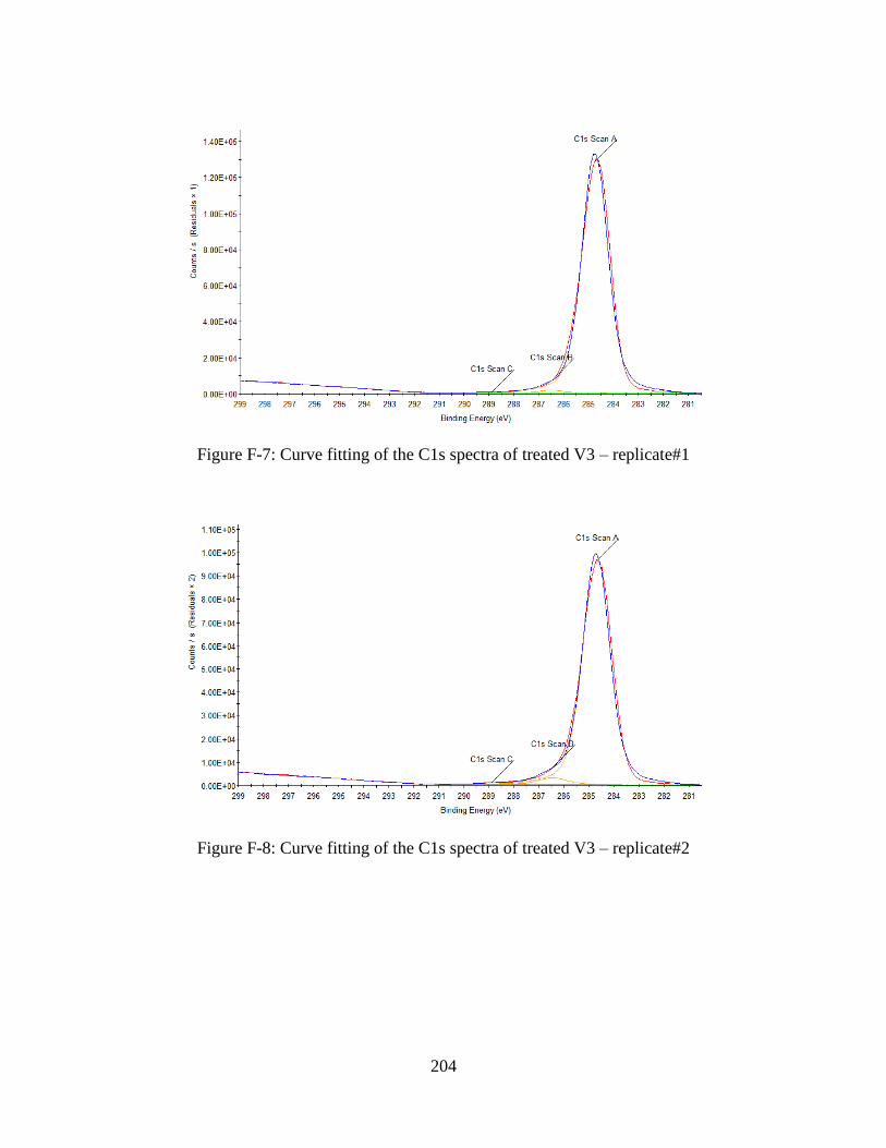
204
Figure F-7: Curve fitting of the C1s spectra of treated V3 – replicate#1
Figure F-8: Curve fitting of the C1s spectra of treated V3 – replicate#2
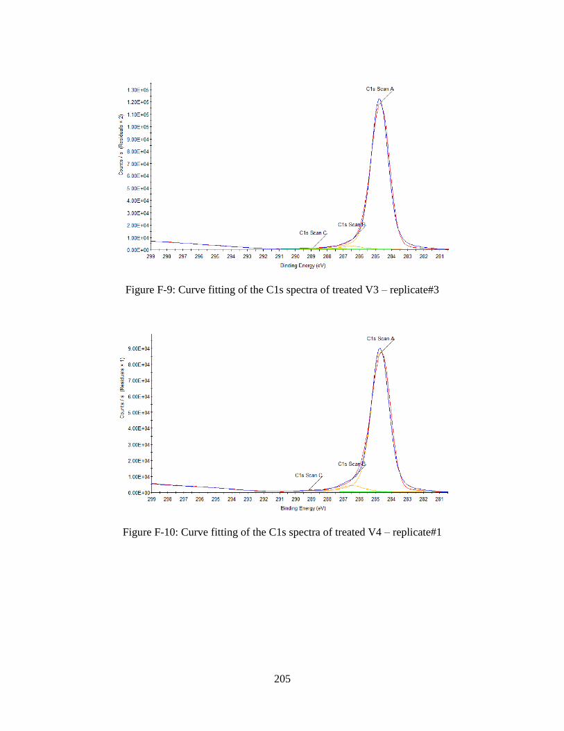
205
Figure F-9: Curve fitting of the C1s spectra of treated V3 – replicate#3
Figure F-10: Curve fitting of the C1s spectra of treated V4 – replicate#1
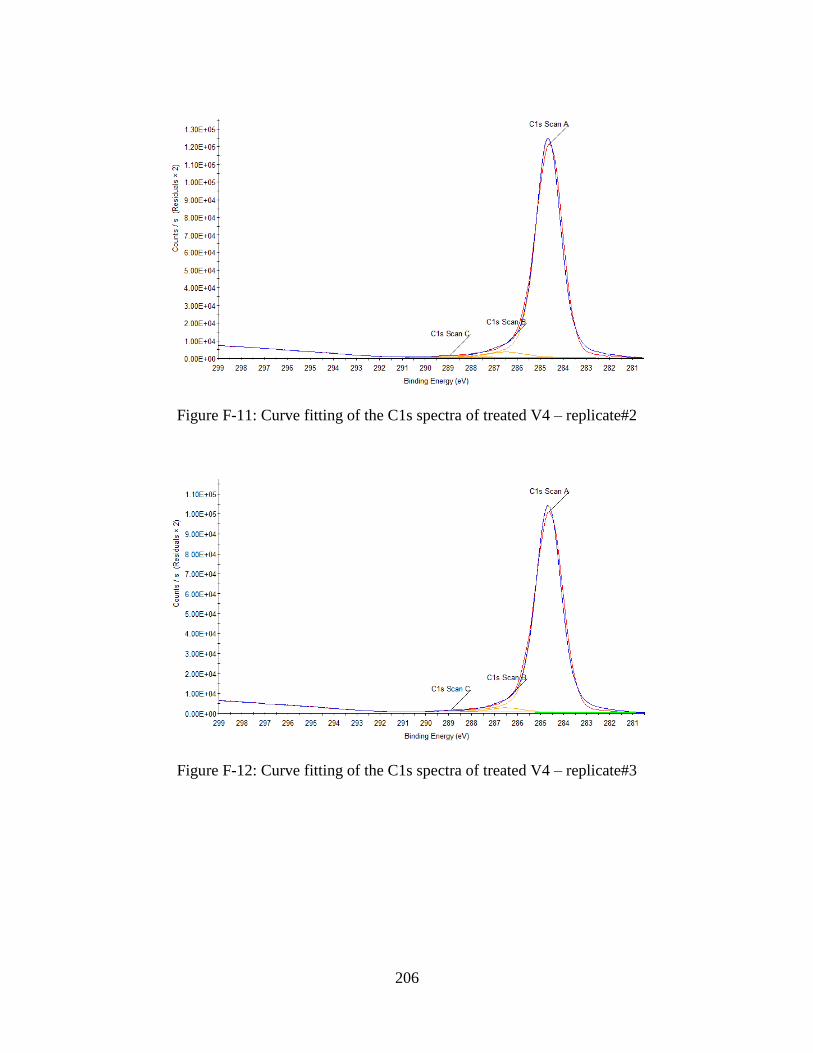
206
Figure F-11: Curve fitting of the C1s spectra of treated V4 – replicate#2
Figure F-12: Curve fitting of the C1s spectra of treated V4 – replicate#3
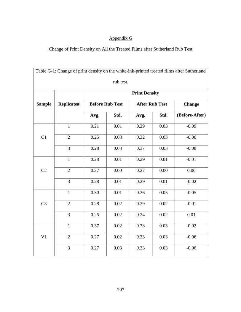
207
Appendix G
Change of Print Density on All the Treated Films after Sutherland Rub Test
Table G-1: Change of print density on the white-ink-printed treated films after Sutherland
rub test.
Sample Replicate#
Print Density
Before Rub Test After Rub Test Change
(Before-After) Avg. Std. Avg. Std.
C1
1 0.21 0.01 0.29 0.03 -0.09
2 0.25 0.03 0.32 0.03 -0.06
3 0.28 0.03 0.37 0.03 -0.08
C2
1 0.28 0.01 0.29 0.01 -0.01
2 0.27 0.00 0.27 0.00 0.00
3 0.28 0.01 0.29 0.01 -0.02
C3
1 0.30 0.01 0.36 0.05 -0.05
2 0.28 0.02 0.29 0.02 -0.01
3 0.25 0.02 0.24 0.02 0.01
V1
1 0.37 0.02 0.38 0.03 -0.02
2 0.27 0.02 0.33 0.03 -0.06
3 0.27 0.03 0.33 0.03 -0.06
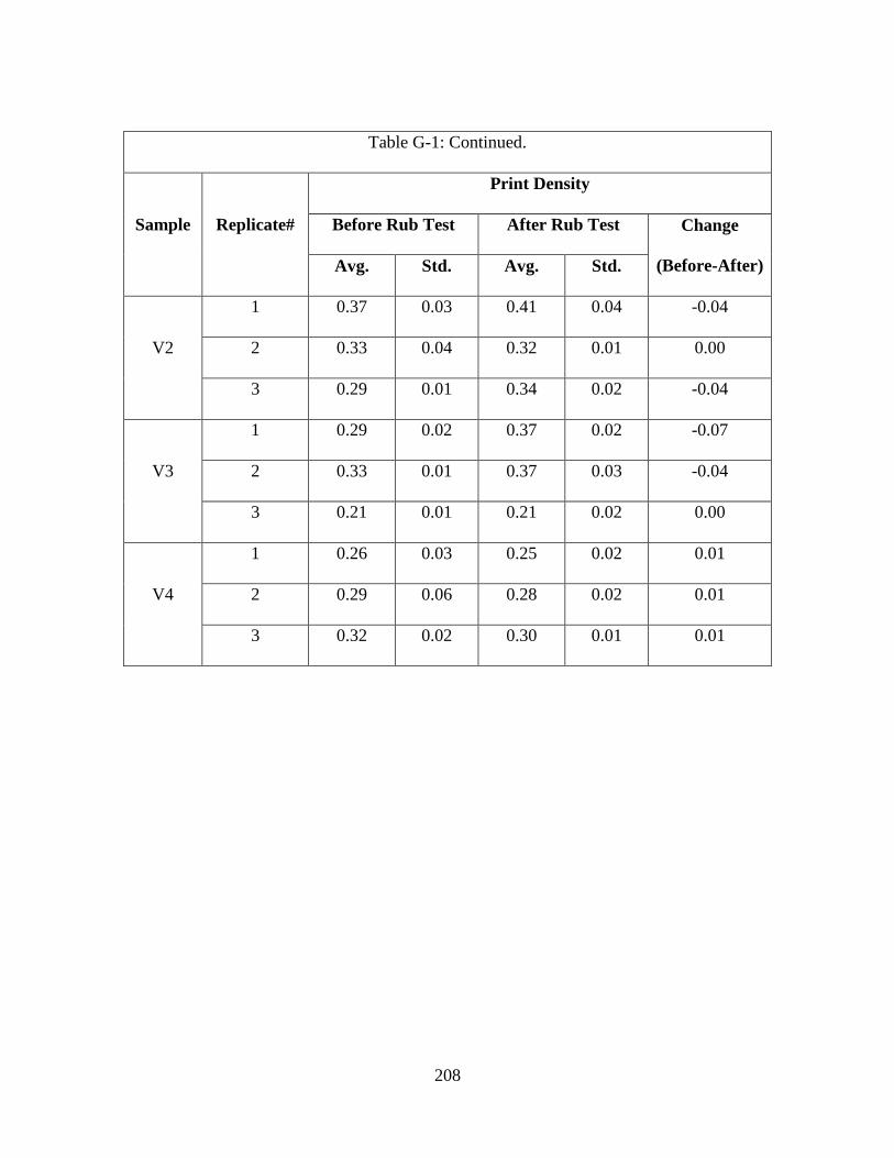
208
Table G-1: Continued.
Sample Replicate#
Print Density
Before Rub Test After Rub Test Change
(Before-After) Avg. Std. Avg. Std.
V2
1 0.37 0.03 0.41 0.04 -0.04
2 0.33 0.04 0.32 0.01 0.00
3 0.29 0.01 0.34 0.02 -0.04
V3
1 0.29 0.02 0.37 0.02 -0.07
2 0.33 0.01 0.37 0.03 -0.04
3 0.21 0.01 0.21 0.02 0.00
V4
1 0.26 0.03 0.25 0.02 0.01
2 0.29 0.06 0.28 0.02 0.01
3 0.32 0.02 0.30 0.01 0.01
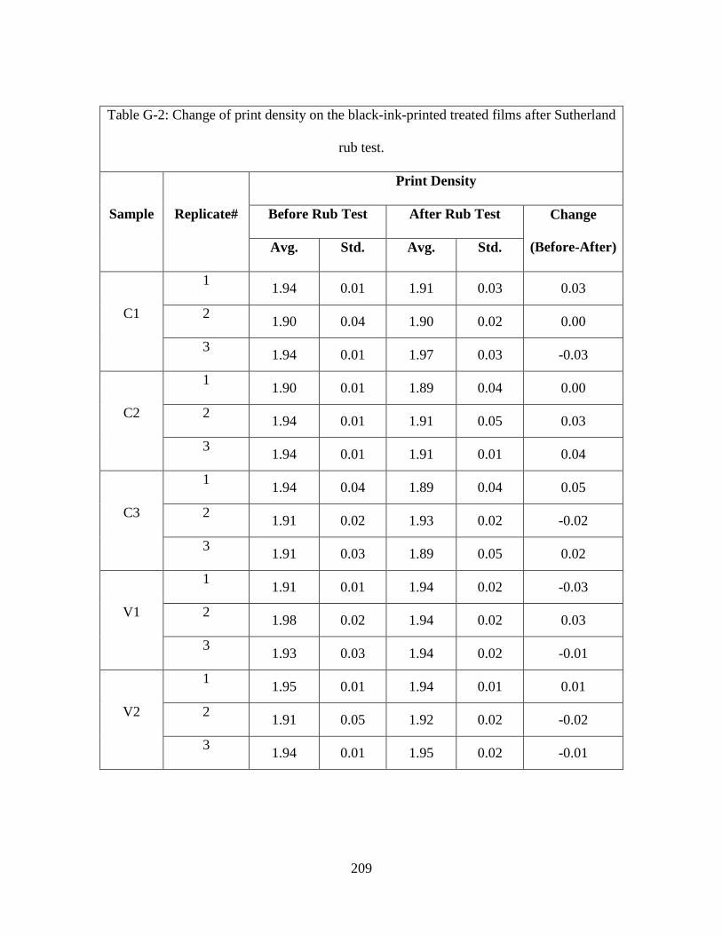
209
Table G-2: Change of print density on the black-ink-printed treated films after Sutherland
rub test.
Sample Replicate#
Print Density
Before Rub Test After Rub Test Change
(Before-After) Avg. Std. Avg. Std.
C1
1 1.94 0.01 1.91 0.03 0.03
2 1.90 0.04 1.90 0.02 0.00
3 1.94 0.01 1.97 0.03 -0.03
C2
1 1.90 0.01 1.89 0.04 0.00
2 1.94 0.01 1.91 0.05 0.03
3 1.94 0.01 1.91 0.01 0.04
C3
1 1.94 0.04 1.89 0.04 0.05
2 1.91 0.02 1.93 0.02 -0.02
3 1.91 0.03 1.89 0.05 0.02
V1
1 1.91 0.01 1.94 0.02 -0.03
2 1.98 0.02 1.94 0.02 0.03
3 1.93 0.03 1.94 0.02 -0.01
V2
1 1.95 0.01 1.94 0.01 0.01
2 1.91 0.05 1.92 0.02 -0.02
3 1.94 0.01 1.95 0.02 -0.01
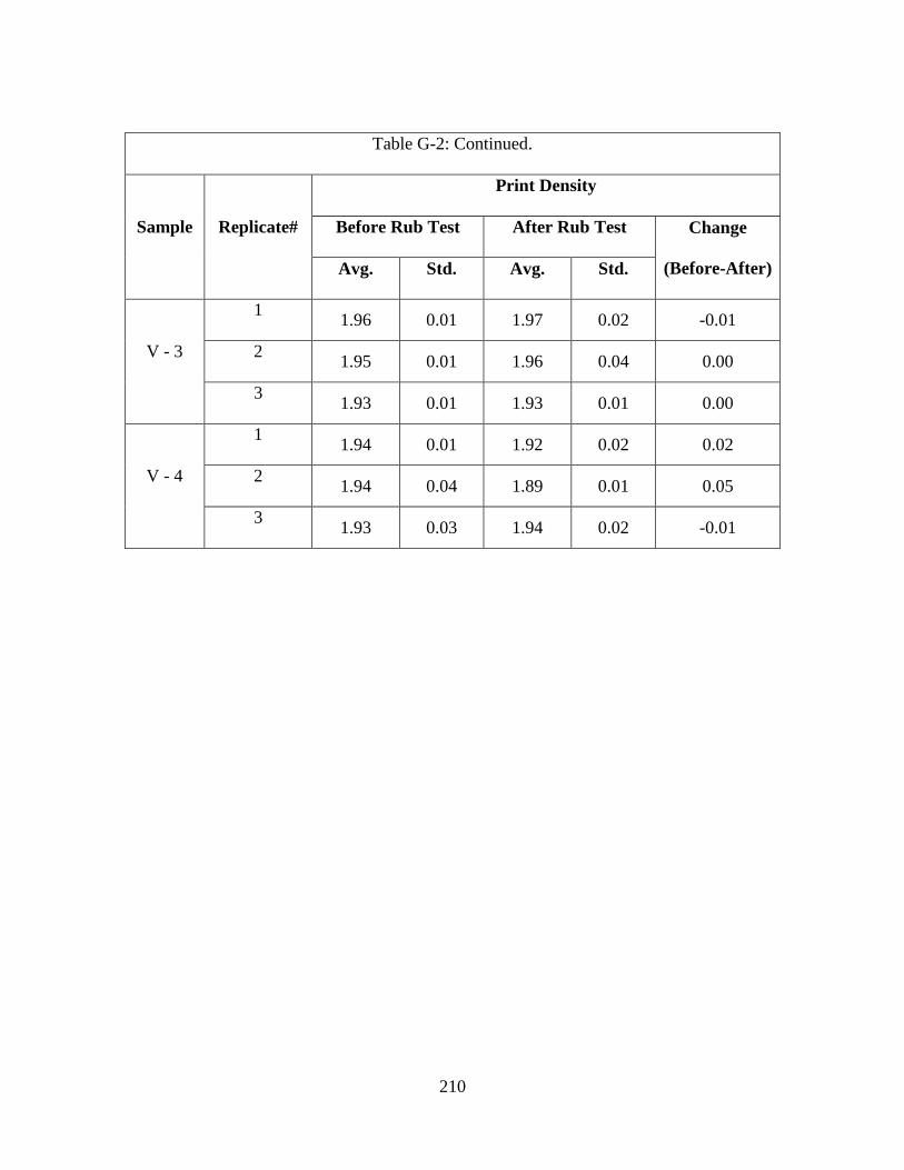
210
Table G-2: Continued.
Sample Replicate#
Print Density
Before Rub Test After Rub Test Change
(Before-After) Avg. Std. Avg. Std.
V - 3
1 1.96 0.01 1.97 0.02 -0.01
2 1.95 0.01 1.96 0.04 0.00
3 1.93 0.01 1.93 0.01 0.00
V - 4
1 1.94 0.01 1.92 0.02 0.02
2 1.94 0.04 1.89 0.01 0.05
3 1.93 0.03 1.94 0.02 -0.01
211
REFERENCES
Arlman, E. J. (1964). Ziegler-Natta catalysis II: surface structure of layer-lattice
transition metal chlorides. Journal of Catalysis, 3, 89-98.
Arlman, E. J., & Cossee, P. (1964). Ziegler-Natta catalysis III: stereospecific
polymerization of propene with the catalyst system TiCl3-AlEt3”, Journal of
Catalysis, 3, 99-104.
Agrawal, A. (2005). Surface tension of polymers. Retrieved June 2, 2018 from
http://web.mit.edu/nnf/education/wettability/summerreading-2005short.pdf
Biresaw, G., & Carriere, C. J. (2001). Correlation between mechanical adhesion and
interfacial properties of starch/biodegradable polyester blends. Journal of Polymer
Science Part B: Polymer Physics, 39(9), 920-930.
Bar, G., Brandsch, R., & Whangbo, M. H. (1999). Effect of tip sharpness on the relative
contributions of attractive and repulsive forces in the phase imaging of tapping
mode atomic force microscopy. Surface Science, 422(1-3), L192-L199.
Brandsch, R., Bar G, & Whangbo M. H. (1997). On the factors affecting the contrast of
height and phase images in tapping mode atomic force microscopy. Langmuir,
13(24), 6349-6353.
Biolin Scientific, Surface energy information of probe liquids. Retrieved June 15, 2018
from the database in the control software of Attension Theta Lite 101.
212
Claverie, J.P., & Schaper, F. (2013, March). Ziegler-Natta catalysis: 50 years after the
Nobel Prize. MRS Bulletin, 213-218.
Chen, J.T., & Thomas, E.L. (1996). The use of force modulation microscopy to
investigate block copolymer morphology. Journal of Material Science, 31, 2531-
2538.
Cossee, P. J. (1964). Ziegler-Natta catalysis I: mechanism of polymerization of α-olefins
with Ziegler-Natta catalysts. Journal of Catalysis, 3, 80-88.
Cretekos, G.F., & Amon, M. (2004). U.S. Patent 6,773,81. Retrieved from Google
Patents
Chen, T. (2012). The influence of coating structure on sheet-fed offset ink setting rates
(M.S. Thesis, Western Michigan University). Retrieved from
https://scholarworks.wmich.edu/masters_theses/22
Carley, J. F., & Kitze, P. T. (1980). Corona-discharge treatment of polymetric films II:
chemical studies. Polymer Engineering Science, 20, 330-338.
Delisio, J.P., & Peet, R.G. (2002). U.S. Patent 6,391,467 B1.Retrieved from Google
Patents.
Delisio, J.P., Harley, L.J., Keung, J.K., & Peet, R.G. (2002). U.S. Patent 6,458,469 B1.
Retrieved from Google Patents.
213
Farley, J. M. & Meka, P. (1994). Heat sealing of semicrystalline polymer films III: effect
of corona discharge treatment of LLDPE. Journal of Applied Polymer Science,
51, 121-131.
Fowkes, F.M. (1964). Attractive forces at interfaces. Industrial and Engineering
Chemistry, 56(12), 40-52.
Földes, E., Tóth, A., Kálmán, E., Fekete, E., & Tomasovszky-Bobák, Á. (2000). Surface
changes of corona-discharge-treated polyethylene films. Journal of Applied
Polymer Science, 76, 1529-1541.
Fuierer, R. (2009). AFM MFP-3D procedural operation ‘Manualette’ (10.5 ed.). Asylum
Research.
Genzer, J. (2014). Polymer synthesis-Part II. Course Materials, North Carolina State
University, Raleigh, NC.
Good, R.J. & Girifalco, L.A. (1956). A theory for the estimation of surface and interfacial
energies. I: derivation and application to interfacial tension. Journal of Physical
Chemistry, 61(7), 904-909.
Godehardt, R., Lebek, W., Adhikari, R., Rosenthal, M., Martin, C., Frangov, S., &
Michler, G.H. (2004). Optimum topographical and morphological information in
AFM tapping mode investigation of multicomponent polyethylene. European
Polymer Journal, 40, 917-926.
214
Galuska, A. A., Poulter, R.R., & McElrath, K. O. (1997). Force modulation AFM of
elastomer blends: morphology, fillers and cross-linking. Surf Interface Analysis,
25, 418-429.
Gourianova, S., Willenbacher, N., & Kutschera, M. (2005). Chemical force microscopy
study of adhesive properties of polypropylene films: influence of surface polarity
and medium, Langmuir, 21(2), 5429-5438.
Guimond, S., & Wertheimer, M.R. (2004). Surface degradation and hydrophobic
recovery of polyolefins treated by air corona and nitrogen atmospheric pressure
glow discharge. Journal of Applied Polymer Science, 94, 1291-1303.
Hlatky, G.G. (1999). Metallocene catalysts for olefin polymerization - annual review for
1996. Coordination Chemistry Reviews, 181, 243-296.
Hanyu, A. & Wheat, R. (1999). Properties and film applications of metallocene-based
isotactic polypropylenes. Journal of Plastic Film and Sheeting, 15(2), 109-119.
Hansen, F.K. (2004). The measurement of surface energy of polymers by means of
contact angles of liquids on solid surfaces. Retrieved June 15, 2018 from
http://www.ramehart.com/surface_energy_finn.pdf
Imuta, J., & Kashiwa, N. (1997). Recent progress on olefin polymerization catalysts.
Catalysis Surveys from Japan, 1(1), 125-142.
215
Janicek, M., Cermak, R., Obadal, M., Piel, C., & Ponizil, P. (2011). Ethylene copolymers
with crystallizable side chains. Macromolecules, 44, 6759-6766.
Jaycock, M.J., & Parfitt, G.D. (1981). Chemistry of interfaces. Chichester: Ellis Horwood
Ltd.
Kutz, M. (Ed.). (2011). Applied plastics engineering handbook: processing and materials.
Oxford: Elsevier Inc.
Kissin, Y. V. (1985). Isospecific polymerization of olefins with heterogeneous Ziegler-
Natta catalysts", New York: Springer-Verlag.
Kaminsky, W., & Piel, C. (2004). Tailoring polyolefins by metallocene catalysis: kinetic
and mechanistic aspects. Journal of Molecular Catalysis A: Chemical, 213, 15-19.
Kipphan, H. (Ed.) (2001). Handbook of print media. Berlin: Springer-Verlag.
Kwok, D.Y., & Neumann, A.W. (1999). Contact angle measurement and contact angle
interpretation. Advances in Colloid and Interface Science, 81, 167-249.
Krϋss GmbH. So You Want to Measure Surface Energy? Retrieved June 15, 2018 from
https://www.kruss-scientific.com/fileadmin/user_upload/website/literature/kruss-
tn306-en.pdf
Kitazaki, Y., & Hata, T. (1972). Surface-chemical criteria for optimum adhesion II: the
variability of critical surface tension (γc) and its choice. Journal of Adhesion, 4,
123-132.
216
Kolahchi, A. R. (2014). Polyethylene terephthalate (PET) films surface modification
through blending (Ph.D. Dissertation, Université de Montréal). Retrieved October
16, 2018 from
https://publications.polymtl.ca/1368/1/2014_AhamdRezaeiKolachi.pdf
Kim, C.Y., & Goring, D. A. J. (1971). Surface morphology of polyethylene after
treatment in a corona discharge. Journal of Applied Polymer Science, 15(6),
1357-1364.
Kwon, O. J., Tang, S., Myung, S. W., Lu, N., & Choi, H. S. (2005). Surface
characterization of polypropylene film treated by an atmospheric pressure plasma.
Surface and Coatings Technology, 192, 1-10.
Leach, R.H., & Pierce, R.J. (Eds.). (1999). The printing ink manual (5th
ed.). Dordrecht:
Kluwer Academic Publishers.
Liston, E. M. (1989). Plasma treatment for improved bonding: a review, Journal of
Adhesion, 30, 199-218.
Magonov, S. N. (2000). Atomic force microscopy in analysis of polymers. In Meyers, R.
A. (Ed.). Encyclopedia of analytical chemistry (pp. 7432-7491). Chichester: John
Wiley&Sons.
Moore, E.P. (1996). Polypropylene handbook. Munchen: Jr. Hanser Publishers.
217
Market Research Report. (2016). Metallocene polyolefin market - global industry
analysis, size, share, growth, trends, and forecast 2016-2024. Retrieved June 15,
2018 from https://www.marketsandmarkets.com/Market-Reports/metallocene-
polyolefin-market-199596649.html
Natta, G. (1959). Kinetic studies of α-olefin polymerization. Journal of Polymer Science,
34, 21-48.
Najarzadeh, Z. (2014). Control and optimization of sealing layer in films. (Ph.D.
Dissertation. Université de Montréal).
Nihlstrand, A., Hjertberg, T., & Johansson, K. (1997). Adhesion properties of oxygen
plasma-treated polypropylene-based copolymers. Polymer, 38, 1557-1563.
Nuntapichedkula, B., Tantayanonb, S., & Laohhasurayotinda, K. (2014). Practical
approach in surface modification of biaxially oriented polypropylene films for
gravure printability. Applied Surface Science, 314, 331-340.
Owens, D.K., & Wendt, R.C. (1969). Estimation of the surface free energy of polymers.
Journal of Applied Polymer Science, 13, 1741-1747.
Painter, P.C. & Coleman, M. (2009). Essentials of polymer science and engineering.
Pennsylvania: DEStech Publications, Inc.
Peet, R.G. (2001). U.S. Patent 6,270,912 B1. Retrieved from Google Patents.
Peet, R.G. (2001). U.S. Patent 6,242,084 B1. Retrieved from Google Patents.
218
Pekarovicova, A. (2013). Flexographic ink polymers. Course Materials, Western
Michigan University, Kalamazoo, MI.
Podhajny, R. M. (1988). Corona treatment of polymeric films. Journal of Plastic
Filmsheet, 4(3), 177-188.
Packham, D. E., & Johnston, C. (1994). Mechanical adhesion: Were McBain and
Hopkins right? An empirical study. International Journal of Adhesion and
Adhesives, 14(2), 131-135.
Rodriguez, F., Stevens, M. P., Preston, J., Kauffman, G. B., Bierwagen, G. P., & Gent, A.
N. (2002). Major industrial polymers. Encyclopedia Britannica. Retrieved
November 13, 2018 from https://www.britannica.com/topic/industrial-polymers-
468698#ref76434
Razavi, A. (2000). Metallocene catalysts technology and environment. Comptes Rendus
de l'Académie des Sciences - Series IIC - Chemistry, 3, 615-625.
Radmacher, M., Tillmann, R.W., & Gaub, H. E. (1991). Imaging viscoelasticity by force
modulation with the atomic force microscope. Biophysical Journal, 64, 735-742.
Rams, J., López, A.J., Sánchez, M., Ureňa, A., Leal, V., Sánchez-Mariscal, B., &
Lafuente, P. (2012). Application of atomic force microscopy to the study of
blown polyethylene films. Polymer Testing, 31, 136-148.
219
Shamiri, A., Chakrabarti, M. H., Jahan, S., Hussain, M. A., Kaminsky, W., Aravind, P. V.
& Yehye, W. A. (2014). The influence of Ziegler-Natta and metallocene catalysts
on polyolefin structure, properties, and processing ability. Materials, 7, 5069-
5108.
Sharma, M.K., & Micale, F.J. (Eds.) (1991). Surface phenomena and fine particles in
water-based coatings and printing technology. New York and London: Plenum
Press.
Simanke, A.G., Lemos, C.D., & Pires, M. (2012). Linear low density polyethylene:
microstructure and sealing properties correlation. Polymer Testing, 32, 279-290.
Siemens. Flexographic printing. Retrieved May 25, 2018 from
https://www.industry.usa.siemens.com/drives/us/en/motion-control-systems-and-
solutions/motion-control-industry-solutions/printing
systems/pages/flexographic.aspx
Sabbatini, L. (Ed.) (2014). Polymer surface characterization. Berlin and Boston: Walter
de Gruyter GmbH.
Strobel, M., Jones, V., Lyons, C. S., Ulsh, M., Kushner, M.J., Dorai,R., & Branch, M. C.
(2003). A comparison of corona-treated and flame-treated polypropylene films.
Plasmas and Polymers, 8(1), 61-95.
Viganò, S. (2007). The use of metallocene polyethylene in co-extruded lamination film.
11th
European PLACE Conference. Athens, Greece.
220
Vlaeva, I., Yovcheva, T., Viraneva, A., Kitova, S., Exner, G., & Guzhova A. (2012).
Contact angle analysis of corona treated polypropylene films. Journal of Physics:
Conference Series, 398, 012054.
Whangbo, M. H., Bar G, & Brandsch R. (1998). Qualitative relationships describing
height and phase images of tapping mode atomic force microscopy. An
application to micro-contact printed patterned self-assembled monolayers.
Applied Physics A, 66(S), 1267-1270.
Wolf, R.A. (2014). Adhering flexo inks to flexible packaging substrate-the surface
energy solution. Proceedings of SPE ANTEC FlexPackCon Conference, 1294-
1297.
Wolf, R.A. (2016). Plastic surface modification: surface treatment and adhesion (2nd
ed.).
Munich, German: Carl Hanser Verlag GmbH & Co. KG.
Zenkiewicz, M. (2001). Investigation on the oxidation of surface layers of polyolefins
treated with corona discharge. Journal of Adhesion Science and Technology, 15,
63-70.
Ziegler, K., Holzkamp, E., Breil, H., & Martin, H. (1955). Angewandte chemie. 67, 541.
Zisman, W.A. (1964). Relation of the equilibrium contact angle to liquid and solid
constitution. Advances in Chemistry, 43(1), 1-51.

221
Zhang, D., Sun Q., & Wadsworth, L. C. (1998). Mechanism of corona treatment on
polyolefin films. Polymer Engineering and Science, 38(6), 965-970.