Universidad de Concepción Dirección de Posgrado

Facultad de Ciencias Forestales PROGRAMA DE DOCTORADO EN CIENCIAS FORESTALES

Effects of forest fragmentation on biodiversity in the Andes region

Efectos de fragmentación de los bosques sobre la biodiversidad en la región de los andes

Tesis para optar al grado de Doctor en Ciencias Forestales

JIN KYOUNG NOH

Concepción-Chile

2019

Profesor Guía: Cristian Echeverría Leal, Ph.D.

Profesor Co-guía: Aníbal Pauchard, Ph.D.

Dpto. de Manejo de Bosques y Medioambiente

Facultad de Ciencias Forestales

Universidad de Concepción

ii

Effects of forest fragmentation on biodiversity in the Andes region

Comisión Evaluadora: Cristian Echeverría (Profesor guía) Ingeniero Forestal, Ph.D. Aníbal Pauchard (Profesor co-guía) Ingeniero Forestal, Ph.D. Francis Dube (Comisión Evaluador) Ingeniero Forestal, Doctor Horacio Samaniego (Comisión Evaluador) Ingeniero Forestal, Ph.D. Directora de Posgrado: Darcy Ríos Biologa, Ph.D. Decano Facultad de Ciencias Forestales: Jorge Cancino Ingeniero Forestal, Ph.D.

iii

DEDICATORIA 활짝 웃으며 내 손잡고, 길고 힘들었던 여정을 동행해 준 나의 사랑하는 남편 파블로,

바쁜 엄마를 이해하고 위로하고 사랑해주는 나의 소중한 두 꼬맹이 테오와 벤자민,

조건없는 사랑으로 믿고 이끌고 도와주신 존경하고 사랑하는 아빠 (노창균)와 엄마

(최문경)께

이 논문을 바칩니다.

Para mi esposo, Pablo Cuenca,

por su extraordinaria generosidad, fortaleza y dulzura.

Para mis hijos, Teo y Benjamin,

que son mi mayor fortaleza y motivación.

Para mis padres, Chang Gyun Noh y Moon Kyung Choi

quienes me brindaron su amor incondicional y me motivaron a seguir adelante.

iv

ACKNOWLEDGMENTS

I would like to acknowledge with great pleasure all people and organizations mention below for their assistance and support. My deepest appreciation to Dr. Cristian Echeverria, my tutor professor, for his patience and dedication while guiding and orienting my studies. To overcome my disadvantages and weakness and grow into a professional, he strongly supported me and took my hands all the time. Besides, I took unforgettable sharing memories with you, Fiesta Patria, Navidad, Cumpleaños, etc. Many thanks Professor. To Dr. Anibal Pauchard, my co-tutor, for helping me clear my doubts in many critical time. Special thanks to your wife, our psychologist Dr. Paula, for the concerns to my family. With my husband, we will never forget Wednesday therapies which saved us and our family, offered by Dr. Pauchard from when our second son’s born. To Dr. Francis Dube and Dr. Horacio Samaniego, my sincere recognition for your valuable guidance and contributions during all period of this thesis. To the university of Concepcion, faculty of Forest Science and their authorities, for your support and attention which made my stay in Concepcion and my study more pleasant. To my Latin friends, Paula, Karina, Leo, Samuel, Jocelyn, Cynthia, Pamela, Rodrigo, Felipe, Pablo, Claudio, Camilo, Margarita, Francisco, for your sincere friendship, especially for spending the most pleasant time with many constructive conversations and advices during my study. To my Korean friends, Dr. Joong Ku Lee, Dr. Park Gwang Wu, Dr. Sang Ho Choi, Dr. Mi Jung Yoon, M.D. So Hee Park, for your concerns and surprising long-distance emails, phone calls, visits during my study. This study was supported by The KOICA/WFK Scholarship funded by KOICA (Korea International Cooperation Agency), CONICYT (Comisión Nacional de Investigación Científica y Tecnológica), Korea Forest Service, and KNA (Korea National Arboretum).

v

TABLE OF CONTENTS DEDICATORIA ........................................................................................................... iii

ACKNOWLEDGMENTS ............................................................................................. iv

TABLE INDEX ........................................................................................................... vii

FIGURE INDEX ......................................................................................................... ix

ANNEX INDEX ........................................................................................................... xi

ABSTRACT ................................................................................................................ xii

CHAPTER 1 ................................................................................................................. 1

General introduction ........................................................................................................ 1 Aichi goals and international initiative ................................................................................................. 1 Biodiversity conservation and landscape ecology ............................................................................. 2 Spatial patterns and habitat fragmentation......................................................................................... 3 Island biogeography & metapopulation theory and fragmentation impacts................................... 6 Extinction debt ...................................................................................................................................... 11 Conservation status of territorial ecosystems .................................................................................. 13

Literature .......................................................................................................................... 19

CHAPTER 2 ............................................................................................................... 25

Extinction debt in a biodiversity hotspot: The case of the Chilean winter rainfall-valdivian forest ............................................................................................................... 25

Introduction ..................................................................................................................... 25

Materials and methods .................................................................................................. 29 Study site ............................................................................................................................................... 29 Forest cover data ................................................................................................................................. 31 Plant species richness ......................................................................................................................... 35 Analysis ................................................................................................................................................. 36

Results ............................................................................................................................. 38 Habitat fragmentation and actual plant richness ............................................................................. 38 Influence of past habitat on plant species richness ........................................................................ 40 Changes of the single long-lived species’ DPS ............................................................................... 42

DISCUSSION ................................................................................................................... 43 Detection of extinction debt ................................................................................................................ 43 Change of long-lived species’ DPS during 1979 - 2011 ................................................................ 47 Value of small size patches in rapidly changing landscape ........................................................... 48 Suggestions for preventing future biodiversity loss in the NMR .................................................... 50

Conclusion ...................................................................................................................... 51

Acknowledgements ........................................................................................................ 52

Literature ......................................................................................................................... 52

Annex ............................................................................................................................... 61

CHAPTER 3 ............................................................................................................... 65

vi

National assessment of forest ecosystem fragmentation in Ecuador: strong needs of landscape management in Tropical Andes ................................................. 65

Introduction ..................................................................................................................... 65

Materials and methods .................................................................................................. 70 GIS data................................................................................................................................................. 70 Deforestation rate, change rate of land cover types and forest fragmentation index ................ 76 Analysis ................................................................................................................................................. 78

Results ............................................................................................................................. 78 Land use change in forest ecosystems............................................................................................. 78 Forest fragmentation ............................................................................................................................ 82 Relationship between forest fragmentation and human land use ................................................. 83

Discussion ....................................................................................................................... 85

Conclusion ...................................................................................................................... 89

Literature ......................................................................................................................... 89

CHAPTER 4 ............................................................................................................... 94

Warning about conservation status of forest ecosystems in Tropical Andes: national assessment in Ecuador, based on IUCN criterion ...................................... 94

Introduction ..................................................................................................................... 94

Materials and methods .................................................................................................. 98 Study area ............................................................................................................................................. 98 Framework of assessment based on IUCN criteria ...................................................................... 100 Assessment of criterion B ................................................................................................................. 100 Evidences of ongoing decline of an ecosystem ............................................................................. 101 Decline of spatial extent (B1ai OR B2ai) ........................................................................................ 102 Decline of environmental quality to characteristic biota (B1aii OR B2aii) .................................. 103 Number of locations (B1c OR B2c) ................................................................................................. 104

Results ........................................................................................................................... 105

Identification of spatially restricted forest ecosystems .......................................... 105

Potential threats of forest ecosystem collapse ........................................................ 108 Current land use and forest fragmentation ..................................................................................... 108 Conversion to cultivated land ........................................................................................................... 109 Number of locations ........................................................................................................................... 110

Discussion ..................................................................................................................... 112

Conclusion .................................................................................................................... 115

Acknowledgements ...................................................................................................... 116

Literature ....................................................................................................................... 116

Annex ............................................................................................................................. 129

CHAPTER 5 ............................................................................................................. 132

General conclusion ...................................................................................................... 132

vii

TABLE INDEX Chap.2. Extinction debt in a biodiversity hotspot: The case of the Chilean winter rainfallvaldivian forest Table 1. Description of land cover types defined in the study area………..……....32

Table 2. Number of selected patches and sampling plots per patch size………...36

Table 3. Changes in landscape pattern indices for the native forests in 1979 and

2011…...........................................................................................................….....40

Table 4. (A) Current richness of different assemblage of plant species, n: species

number. (B) Linear regression testing the relationship between the current and past

patch size and current richness of plant species………………………..….…...…..40

Table 5. Multiple regression of the current and past connectivity relationship on the

current richness………….………………………………….……………..….……..…43

Chap.3. National assessment of forest ecosystem fragmentation in Ecuador: strong needs of landscape management in Tropical Andes Table 1. Description and source of land cover types defined in the study area....74

Table 2. Spatial scale (region-ecoregion-ecosystem), altitudinal range and Forest

Fragmentation Index (FFI: proportion of non-continuous forest in a given

ecosystem) of 64 natural forest ecosystems in the Ecuadorian continent.……..75

Table 3. Summary of FAD fragmentation class thresholds, names and color

assignment………………………………………………………………………...…..78

Table 4. Standard coefficients of multiple regressions testing the relationship

between forest fragmentation index (FFI) and human land use in 2014 in three

regions of Ecuador………………………………………………………………...…84

Table 5. Standard coefficients of multiple regressions testing the relationship

between forest fragmentation index (FFI) and human land use for 2014 in forest

ecosystems divided by FFI value (Low: FFI ≤10, Moderate: 10 <FFI ≤60, High: FFI

>60)………………………………………………………………………..…….…….85

Chap.4. Warning about conservation status of forest ecosystems in Tropical Andes: national assessment in Ecuador, based on IUCN criterion

viii

Table 1. Summary of IUCN Red list criteria B for ecosystems V. 2.0 and

Subcriterion applied for the present study……….………………………....….101

Table 2. Land use and cover types that may be found within the potential

distribution of forest ecosystem clases…………………………..…….….…...103

Table 3. Summary of data sources………………………………………..…....105

Table 4. List of 64 terrestrial forest ecosystems in Ecuador, assessed by IUCN

RLE criterion B………………………………………………………….………...106

ix

FIGURE INDEX Chap.1. General introduction Figure 1. Different classifications of habitat fragmentation…………….……….….5

Figure 2. Four approaches for evaluating extinction debt from Kuussaari et al.

(2009)…………………………………………………………………….………….….12

Figure 3. Structure of the IUCN Red List of Ecosystems Categories (IUCN,

2017)…………………………………………………………………….…………….…14

Chap.2. Extinction debt in a biodiversity hotspot: The case of the Chilean winter rainfallvaldivian forest

Figure 1. Map of study area including study ecosystem (Costal temperate

deciduous forest of N.nervosa & P.lingue) and the major land cover types in 1979

and 2011…………………………………………………………………..………….…35

Figure 2. Generalized linear model for current richness of long-lived specialist

plants and patch size in 1979 (solid line and symbols) and 2011(dotted line and

open symbols)...................................................................................................…42

Figure 3. Changes in dwelling patch size (size value at maximum probability of

presence) of single long-lived species (n = 27) for period 1979 and 2011.....…..45

Chap.3. National assessment of forest ecosystem fragmentation in Ecuador: strong needs of landscape management in Tropical Andes Figure 1. (A) Ecoregions of continental Ecuador. Elevation detail is shown. (B) The

major land cover types inside 64 forest ecosystems in 1990, 2000, 2008 and 2014.

(C) Distribution of each ecoregion’s elevation. Cutting section of a geological map

based on a red dotted line (A). (D) The major land cover types and changes of

ecoregions (n=7) in 1990, 2000, 2008 and 2014, (E) The major land cover types

that have replaced the original forest ecosystem of single ecosystems (n=64) in

x

2014. Ecosystems containing forest area <10 % (n=6) are marked with black

outline……………………………………………………………….…………….......72

Figure 2. Scatter diagrams of forest ecosystems annual deforestation rate for the

periods 1990-2000 and 2000-2014. (A) Changes in annual deforestation rate of

single forest ecosystem (n=64) for the periods 1990-2000 and 2000-2014. Each

point represents one forest ecosystem. Solid black outline is zoomed out (B). (B) Changes in annual deforestation rate of single forest ecosystem (n=59), excluding

extreme data (n=5) (Inset) The distribution of the ecosystem’s differences in

deforested area between 1990 and 2014. The vertical dotted line marks zero shifts,

and the vertical solid line marks the median shift. The arrow describes the direction

of the shift……………………………………………………………….……………..80

Figure 3. Net change (i.e. gains plus losses), gains and losses for each land cover

class as a percentage of three regions for the periods 1990-2000, 2000-2008 and

2008-2014……….............................................................................................…82

Figure 4. Temporal variation of number of different FAD (log) in three regions of

Ecuador…………………………………………………………………………………83

Chap.4. Warning about conservation status of forest ecosystems in Tropical Andes: national assessment in Ecuador, based on IUCN criterion Figure 1. (A) Ecoregions of continental Ecuador. Elevation detail is shown. (B) The

major land use and cover types inside the potential limits of 64 forest ecosystems

in 1990, 2000, 2008 and 2014……………………………………………………....100

Figure 2. The major land cover types of single ecosystems (n=64) in 2014.

Continuous and separated native forests were distinguished based on the Forest

Area Density (FAD) values calculated from GUIDOS. Human land use and cover

includes agricultural land, pasture, forest plantation and urban area. Ecosystems

containing either continuous native forests <30 % or human land use >40% (n=7)

are E 10, 17, 32, 33, 34, 35 and 44………………………………………..……….110

Figure 3. Map of 13 threatened forest ecosystems in mainland Ecuador, assessed

by IUCN RLE criteria B………………………………………………………………112

xi

ANNEX INDEX Chap.2. Extinction debt in a biodiversity hotspot: The case of the Chilean winter rainfallvaldivian forest

Annex 1. Confusion matrices for the two images…………………………………...62

Annex 2. List of long-lived species and their habitat specialization degree in

Nahuelbuta Mountain Range…………………………………………………………..62

Annex 3. List of long-lived species that were best described by unimodal bell-

shaped model (n=27) displaying a highly significant Gaussian logit model (at the

0.001 level) for both periods of 1979 and 2011. DPS: dwelling patch size, VU:

Vulnerable, NT: Near threatened……………………………………………………...64

Chap.4. Warning about conservation status of forest ecosystems in Tropical Andes: national assessment in Ecuador, based on IUCN criterion

Annex 1. Spatial scale (nation-region-ecoregion-ecosystem) of the system under

study and 64forest ecosystems of continental Ecuador………………………….130

xii

ABSTRACT

Since rapid economic development, natural system decline and fragmentation is one

of the core drivers of global change and has huge implications for ecosystem

functioning and conservation. The impacts of habitat fragmentation can arise in the

face of primarily biotic change, primarily abiotic change and a combination of both,

including extinction, disruption of trophic interactions and increased susceptibility to

disturbances (e.g. logging, fires and invasive species) (Holl and Aide 2011; Laurance

et al. 2002; Letcher and Chazdon 2009; Turner 2010a). Some changes result in

species extinction and system degradation retaining some original characteristics as

well as novel elements, whereas larger changes will result in system replacement or

collapse. Against this background, the present study aimed to analyze the effects of

habitat fragmentation on different levels of biodiversity including species, community

and ecosystems.

Previously the majority of efforts to conserve biodiversity have been focused on

species, communities or their habitat under forest fragmentation, as well as on

negative influences on species declines and extinctions. However, local extinction

of different types of biodiversity can occur with a temporal delay following habitat

fragmentation and such delay is called extinction debt. We assumed that the

distribution of many vascular plant species in the Coastal Range of south-central

Chile is not in equilibrium with the present habitat distribution. One of the aims of this

research was to quantify patterns of habitat loss and to detect extinction debt from

xiii

relationships between current richness of different assemblage of vascular plants

(considering longevity and habitat specialization) and both of past and current habitat

variables. Results showed that native forests have been fragmented and reduced by

53%, with annual deforestation rate of 1.99%, in the study area between 1979 and

2011. Current richness of plant species was mostly explained by past habitat area

and connectivity. Past habitat variables explained best for richness of long-lived

specialist plants, which are characterized by restricted habitat specialization and

slower population turnover. We also showed that habitat fragmentation has resulted

in a significant reduction in long-lived plant species’ Dwelling Patch Size (DPS)

between 1979 and 2011.

At ecosystem level, human have changed natural systems more rapidly and

extensively than in any comparable period time in human history over the past 50

years. Despite previous studies indicated highest rates of deforestation and forest

fragmentation in Ecuador, there was no clear relationship between the degree of

forest ecosystem fragmentation and human land use to better design conservation

strategies. We quantified and graphed forest fragmentation on different spatial

scales, according to the results using GUIDOS, which measures forest

fragmentation and classify forests into five main categories—intact, core, perforated,

edge, and patch—based on Forest Area Density (FAD) in a given forest pixels. Our

results showed that forest fragmentation in 64 forest ecosystems was mostly

explained by pasture between 2008 and 2014. Although forest fragmentation

became the dominant process in the Coast and Andes, rapid increase of number of

patchy and rare FAD was observed in the Amazon during 1990-2014.

xiv

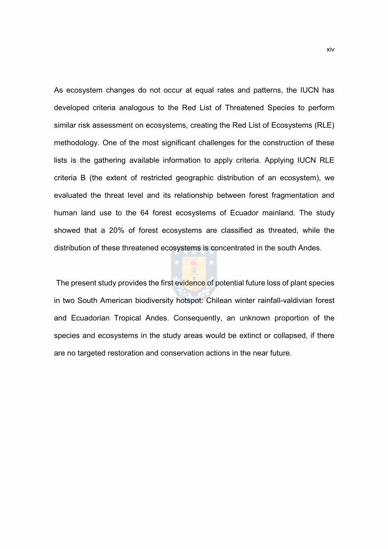
As ecosystem changes do not occur at equal rates and patterns, the IUCN has

developed criteria analogous to the Red List of Threatened Species to perform

similar risk assessment on ecosystems, creating the Red List of Ecosystems (RLE)

methodology. One of the most significant challenges for the construction of these

lists is the gathering available information to apply criteria. Applying IUCN RLE

criteria B (the extent of restricted geographic distribution of an ecosystem), we

evaluated the threat level and its relationship between forest fragmentation and

human land use to the 64 forest ecosystems of Ecuador mainland. The study

showed that a 20% of forest ecosystems are classified as threated, while the

distribution of these threatened ecosystems is concentrated in the south Andes.

The present study provides the first evidence of potential future loss of plant species

in two South American biodiversity hotspot: Chilean winter rainfall-valdivian forest

and Ecuadorian Tropical Andes. Consequently, an unknown proportion of the

species and ecosystems in the study areas would be extinct or collapsed, if there

are no targeted restoration and conservation actions in the near future.

1

CHAPTER 1

General introduction

Aichi goals and international initiative

The adaptation by the world’s governments, at the tenth conference of the Parties of

the Convention on Biological Diversity (CBD) in Nagoya in 2010, of the 2020

Strategic Plan for Biodiversity and its associated 20 Aichi Targets, marked a

watershed moment in the history of biodiversity conservation (Brooks et al., 2015).

Because the primary driver of biodiversity loss is habitat loss, one of the main

strategic goals of the Aichi Targets includes increasing the amount of protected

terrestrial habitat (excluding Antarctica) from the current 13% to 17% across the

globe by 2020 (Aichi Target 11). With nearly 200 nations agreeing to the principles

of the Aichi Targets, this could lead to the most rapid rate of land preservation in

history, even if the targets are not fully achieved. Another key goal is to prevent the

extinction of species already known to be threatened with future extinction and to

achieve improvement towards sustainability in their populations by 2020 (Aichi

Target 12). This ten-year framework for effective and urgent action by all countries

and stakeholders to save biodiversity and enhance its benefit for people is about to

be elevated to even greater prominence.

Fortunately, existing mechanisms provide a strong basis from which Aichi challenges

can be addressed. With the combination of different international initiatives for

biodiversity conservation (e.g. IUCN Red list of species and ecosystems, UN list of

2

protected areas, UN Sustainable Development Goals, Key Biodiversity Areas by

BirdLife International), key indicator towards the Aichi Targets are likely to product

comprises standards, governance and quality control, data sets, tools, capacity

building and ongoing processes for derivation of biodiversity conservation strategies.

Yet identifying tools that can be used to assess progress towards these ecosystem-

based conservation targets remains a fundamental challenge (Collen and Nicholson,

2014; Tittensor et al., 2014). The emergence of ecosystem risk assessment

protocols such as the IUCN Red List of Ecosystems (IUCN, 2018), which provide

decision rules for classifying ecosystems according to their risk of collapse, can help

address this challenge.

Biodiversity conservation and landscape ecology

Biodiversity has been defined as “the variety of living organisms considered at all

levels of organization, including the genetic, species, and higher taxonomic levels,

and the variety of habitats and ecosystems, as well as the processes occurring

therein” (Meffe and Carroll, 1997). Although the concept of genetic variation can be

specific to the level of genetic diversity within an individual, in terms of biodiversity

and landscapes, it is best viewed at a population level (Gutzwiller, 2002). On the

other hand, biodiversity at community and ecosystem level is often characterized by

a variety of species-diversity indices that quantify the number of species (richness)

and the relative abundance of those species (evenness) (Whittaker, R. H., & Likens,

1975). The objective of biodiversity conservation is the long-term maintenance of

populations or species or, more broadly, of ecosystems. As many of the threats are

3

related to human land use, virtually all conservation issues are ultimately land-use

issues (Gutzwiller, 2002).

Landscape ecology is an interdisciplinary field that studies landscape structure,

function, and change (Forman and Godron, 1986). Although landscape ecology

provides a spatial systems perspectives, its application in biodiversity conservation

and management has been lagging (Forman and Godron, 1986). Likewise,

biodiversity conservation actions have not been fully utilized for the advancement of

landscape ecology (Liu and Taylor, 2004). Given these needs and potential benefits,

key future studies may be to identify links and ways of bridging the gaps between

landscape ecology and biodiversity conservation.

Spatial patterns and habitat fragmentation

Basic knowledge of species richness patterns and species distributions within a

region is a necessary starting point to predict species extinction under habitat loss,

as well as to prioritize conservation efforts and designing conservation areas

(Margules and Pressey, 2000). Because organisms are distributed neither uniformly

nor at random in nature, ecologists have begun to realize the importance of not only

biotic response to species occurrences, but also the influence of spatial patterns and

relationship (Liebhold and Gurevitch, 2002). Therefore, spatial pattern is essential to

understanding the consequences of fragmentation and habitat loss for wildlife

understanding the response of a species to a spatial structure (Collinge, 2001).

Landscape spatial pattern is defined as the composition and configuration of spatial

elements in the landscape (Turner et al. 2003). In particular, habitat fragmentation

4

can be measured by quantifying changes in the spatial structure of the landscape,

which refers to the spatial relationship between patches or fragments (Turner et al.

2001). These measurements are made through spatial metrics or indices of

landscape, and its use is very useful, as they can provide information about the

occurrence of deforestation and fragmentation (Li and Wu 2004). These rates can

be applied to landscape thematic maps, which can be generated from satellite

images (Kerr and Ostrovsky 2003).

The changes produced by the fragmentation are reflected in the spatial structure of

the landscape as the size, shape or position of the fragments in the landscape

(Turner, Gardner and O’Neill, 2001). Some studies have applied levels of landscape

as the size of fragments suggest that high levels of fragmentation are associated

with predominance of smaller sized fragments (Fitzsimmons, 2003). Other indices

such as insulation and as fragments have also been applied to assess the degree of

fragmentation of ecosystems, reporting higher levels of fragmentation dominated by

fragments with greater isolation and regular shapes (Bustamante and Castor, 1998;

Echeverria et al., 2006).

Not all species depend on habitat area, isolation and landscape context equally

(Tscharntke et al., 2002). (1) Habitat specialists are more affected by habitat loss

than generalists, (Warren et al., 2001). (2) The surrounding landscape is inhabitable

for habitat specialists, but at least partly habitable for generalists, supporting the

prediction that habitat isolation affects habitat specialists more than generalists

(Jonsen and Fahrig, 1997). (3) High landscape diversity in the surrounding matrix

provides more different habitat types for generalists or species with other habitat

5

preferences, supporting the prediction that landscape diversity enhances the

number of generalists, especially at edges, but hardly specialists (Jonsen and Fahrig

1997).

Fragmentation and loss of natural habitats are of global concerns due to negative

implications on biodiversity conservation (Wiens and Moss, 2005; Fraterrigo,

Pearson and Turner, 2009). Anthropogenic activities have modified the natural

environment to the point that the most common landscape is a mosaic of human

settlements, farmlands and fragmented natural ecosystems surrounding protected

areas (Cox, Dickman and Hunter, 2004).

Figure 1. Different classifications of habitat fragmentation

Habitat fragmentation is an active and dynamic process resulting in the reduction in

size and isolation of natural systems over time (Cox et al. 2004). According to

Bennett and Saunders (2010), “fragmentation” is defined as the changes that occur

when contiguous natural habitats are broken into small and scattered remnants.

Different classifications of landscape change have been identified in terms of

structural thresholds (Forman and Godron, 1986; McIntyre and Hobbs, 1999) or the

prevalent land use (Hobbs and Hopkins, 1990). In addition to these classifications,

(Hobbs y Hopkins 1990) (Forman 1995b)

6

a model that synthesizes four landscape states (intact, variegated, fragmented and

relictual) was proposed by merging the previous classifications of landscape change

(McIntyre and Hobbs 1999) (Figure 2). According to Forman’s (1995) models, the

current classifications of landscape change are typically represented by a decrease

in connectivity and remaining cover, and an increase in edge effects. On the other

hand, Bennett et al. (2003) characterized fragmentation by: a) loss of natural habitat

in the landscape, b) natural habitat size reduction, c) isolation of habitat fragments

and, d) human use of the matrix surrounding isolated fragments increase and

intensified.

Island biogeography & metapopulation theory and fragmentation impacts

Island biogeography theory emphasizes the roles of area and geographical isolation

as the main determinants of species diversity. Based on the assumption that

colonization rates are determined by the degree of geographical isolation and

extinction rates are determined by the size (area) of the island, the theory predicts

that species richness should be positively correlated with island size and negatively

correlated with the degree of isolation (MacArthur and Wilson, 1967). This presents

a “nonequilibrial” view of ecological communities in the sense that species

composition is constantly changing over time (Chaves et al., 2002). According to this

view, species diversity in a local community reflects a dynamic balance between

colonization (arrival of new species) and extinction of species already present in the

community. Island biogeography theory ignores functional differences among

species and, in recent formulations (He et al., 2005), explicitly considers all species

to be ecologically equivalent.

7

Metapopulation theory is a popular basis for conserving species in patchy or

fragmented environments (McCullough, 1996). Most studies of metapopulations

consider the dynamics of populations divided into a number of subpopulations that

exchange migrants and that may be subject to local extinction and recolonization

(Hanski, 1997). Tilman et al., (1994) considered the order of extinctions in relation

to competitive dominance. This concept is specifying the number or proportion of

extant species predicted to become extinct as the species community reaches a new

equilibrium after habitat fragmentation. It can also be applied to single-species

metapopulations by estimating the number or proportion of local populations that are

predicted to become extinct (Bulman et al. 2007; Hanski et al. 1996).

Fragmentation is a dynamic process in which the habitat is progressively reduced

into smaller patches that become more isolated and increasingly affected by edge

effects (Forman and Godron, 1986; Turner, Gardner and O’Neill, 2003). And, it has

effects not only on almost all ecological patterns and processes, but also on species

extinction. The major impact of fragmentation is species loss due to habitat loss and

size reduction (Cox, Dickman and Hunter, 2004; Moser et al., 2007; Mapelli and

Kittlein, 2009; Fitz-Gibbon et al., 2013).

In general, larger patches of habitat contain more species and often a greater

number of individuals than smaller patches of the same habitat (Turner et al. 2003),

because many species cannot maintain viable populations in small habitat patches,

which lead to local extinction and loss of biodiversity (Forman and Godron, 1986).

Small habitat fragments contain small populations, which are more vulnerable to

extinction due to environmental and demographic stochasticity (Shaffer, 1981;

8

Lande, 1988). In addition, small populations may be more prone to extinction due to

the loss of genetic variation (Frankham, 1996). A decreasing population size may

result in erosion of genetic variation through the loss of alleles by random genetic

drift. In addition, increased selfing (in plants) and mating among closely related

individuals in small populations may result in inbreeding and a reduction of the

number of heterozygotes (Young, Boyle and Brown, 1996). Over the short term

decreasing heterozygosity and the expression of deleterious alleles may result in

reduced fitness (Keller LF and DM, 2002; Reed et al., 2002). In the long term lower

levels of genetic variation may limit a species’ ability to respond to changing

environmental conditions through adaptation and selection (Booy et al., 2000). Also,

patch size has effects on within-patch processes, such as nitrogen cycling and

recruitment, and processes that connect patches, such as dispersion and movement

(McIntyre and Hobbs, 1999).

Moreover, the degree of connectivity between patches of equally suitable habitat can

constrain the spatial distribution of a species by making some areas accessible and

others inaccessible. Once suitable habitat for a species of interest is characterized,

determining whether the habitat is or is not spatially connected is often of interest

(Turner, Gardner and O’Neill, 2003). Finally, edges provide both positive and

negative effects in movement, mortality, feeding or reproductive subsidies and

species interaction (Liu and Taylor, 2002). Fragmentation leads to the formation of

marked edges creating a distinctive contrast in the structural and floristic composition

between different patches (Kupfer, Malanson and Franklin, 2006) and they impact

negatively species movement patterns through the landscape affecting species

9

ability to colonize adequate habitats and by limiting their access to food (Alderman

et al., 2005).

When the amount of native vegetation in a region drops below about 20-30%,

fragmentation of the remaining vegetation may lead to disproportionate reductions

in populations (Radford, Bennett and Cheers, 2005). Individual remnants lose

species due to chance extinctions, the negative effects of habitat edges, the inability

or unwillingness to disperse among isolated remnants and loss of key resources.

These local species losses may accumulate until a species goes extinct locally and

even regionally (Saunders, 1989). And, if species become isolated in a fragment,

their survival depends on fragment size, quality and spatial configuration of remnants

(Brouwers and Newton, 2009), species’ dispersal ability and population dynamics

(Lauga and Joachim, 1992; Castelletta, Thiollay and Sodhi, 2005).

In order to link landscape matters and species ecology, one of the central themes of

landscape ecology is concerned with four features of spatial structure, such as (i)

patch quality, (ii) boundaries, (iii) patch context and (iv) connectivity (Liu and Taylor,

2002).

The difference in landscape elements are generally structural and organisms

translate into differences in threats and opportunities (Liu and Taylor, 2002). The

elements of landscape are bounded and these boundaries play a critical role in

determining the movement or flows of individuals, nutrients, materials or

disturbances across a landscape (Wiens, Crawford and Gosz, 1985; Holland and

Risser, 1991). A permeable boundary to flows contributes to the linkages among the

10

elements in a landscape, while an impermeable boundary relatively, on the other

hand, reflects movements back into the patch and internalizes dynamics within

landscape elements (Liu and Taylor, 2002). The surroundings of a patch in a

landscape influence both patch quality and boundary, creating differences in within-

and between-patch dynamics among neighboring landscape elements (Liu and

Taylor, 2002). Connectivity, the ability of organisms to move through a landscape, is

a function of a boundary permeability and patch contexts that characterize a given

mosaic (Taylor et al., 1993; Tischendorf and Fahrig, 2000).

Some studies have emphasized that connectivity is a priority attribute of the

landscape spatial configuration that has to be recovered in order to improve

biodiversity (Luque, Saura and Fortin, 2012; Tambosi and Metzger, 2013). This is

mainly due to the fact that a reduction in connectivity can lead to a decline in species

dispersal, gene flow and even local extinction (Bennett and Saunders, 2010). The

sharpness of habitat edges and contrast across habitat boundaries can directly affect

the connectivity, as they can determine the degree of movement of organisms across

the landscape (Stevens et al., 2006; Peyras et al., 2013). A marked contrast in the

community attributes at the interface (high-contrast forest edge) between natural

habitats and human-related land can inhibit many organisms from readily moving

across the edge (Wiens, Crawford and Gosz, 1985). Applying resistance estimates

of high-contrast edges to improve connectivity have been highlighted for the

implementation of wildlife corridors and biodiversity conservation (Zeller, McGarigal

and Whiteley, 2012; Cushman et al., 2013).

11

In many tropical countries, forest ecosystem fragmentation is occurring at an

alarming rate by changes in human land use activities (Laurance 1999; Rudel and

Roper 1997; Sanchez-Azofeifa, Harriss, and Skole 2001). The fragmentation of

tropical forests is considered highly relevant to changes of ecological function and

services and effect negatively on natural recovery after disturbances as catalysts of

rapid ecological change (Holl and Aide 2011; Letcher and Chazdon 2009; Turner

2010). To date, the relationship between land use change by human activities and

forest ecosystem fragmentation has been widely studied, described and interpreted

by using landscape metrics, (e.g. mean patch size, edge density, mean shape index:

O´Neil et al. 1999, Echeverria et al. 2006) or quantitative measurement (e.g.

Morphological spatial pattern analysis: Soille and Vogt 2009, Landscape mosaic

index: Ritters et al. 2009, and Forest connectivity index: Saura and Torné 2009). The

specific studies of forest ecosystem fragmentation carried out in Tropical Andes are

initiated in late 1980’s (D. Armenteras, Gast, and Villareal 2003; Dolors Armenteras

et al. 2006; Gómez, Anaya, and Alvarez 2005; Rodríguez Eraso, Armenteras-

Pascual, and Alumbreros 2013). In the eastern Andes of Colombia, Armenteras et

al. (2003) have incorporated the degree of fragmentation for ecosystem

conservation planning, using five landscape metrics; patch number, largest patch

index, mean patch size, mean nearest neighbor distance, and landscape shape

index.

Extinction debt

Species can initially survive habitat fragmentation but later become extinct without

any further habitat change, which has been known as delayed extinction, also called

12

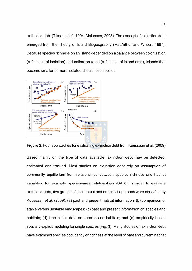
extinction debt (Tilman et al., 1994; Malanson, 2008). The concept of extinction debt

emerged from the Theory of Island Biogeography (MacArthur and Wilson, 1967).

Because species richness on an island depended on a balance between colonization

(a function of isolation) and extinction rates (a function of island area), islands that

become smaller or more isolated should lose species.

Figure 2. Four approaches for evaluating extinction debt from Kuussaari et al. (2009)

Based mainly on the type of data available, extinction debt may be detected,

estimated and tracked. Most studies on extinction debt rely on assumption of

community equilibrium from relationships between species richness and habitat

variables, for example species–area relationships (SAR). In order to evaluate

extinction debt, five groups of conceptual and empirical approach were classified by

Kuussaari et al. (2009): (a) past and present habitat information; (b) comparison of

stable versus unstable landscapes; (c) past and present information on species and

habitats; (d) time series data on species and habitats; and (e) empirically based

spatially explicit modeling for single species (Fig. 3). Many studies on extinction debt

have examined species occupancy or richness at the level of past and current habitat

13

patch, because these data are available generally. If current species richness is

better described by past than by present landscape variables, the presence of

extinction debt can be assumed, although the magnitude of the extinction debt can,

however, not be estimated using this approach (Kuussaari et al., 2009).

However, all empirical approaches have clear limitations. It is important to target the

habitat specialist species analyzing with appropriate habitat parameters and the

scale, because extinction debt depends on specialization and scale (Batáry et al.,

2007; Kuussaari et al., 2009; Cousins and Vanhoenacker, 2011). Moreover, high-

quality historical data and long-term monitoring of community equilibrium is a key

limiting factor for studying extinction debt (Lewis, 2006; Cousins, 2009).

Recent studies have revealed the importance of spatial configuration to detect

extinction debt on rapidly fragmented landscape. In comparison with a large number

of studies undertaken in fragmented grassland in Europe (Lindborg and Eriksson,

2004; Adriaens, Honnay and Hermy, 2006; Ranius, Eliasson and Johansson, 2008),

few researchers have explored the species’ responses to fragmentation in temperate

forest (Vellend et al., 2006; Noh et al., 2018) and very little work has been done in

Southern Hemisphere forests.

Conservation status of territorial ecosystems

Despite systematic methods for assessing the threat of extinction of individual

species were notably advanced in recent years, there is few widely accepted

scientific framework for tracking the status of Earth’s ecosystem and identifying

those with a high probability of loss or degradation (Nicholson, Keith and Wilcove,

14

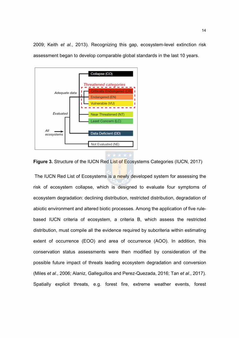
2009; Keith et al., 2013). Recognizing this gap, ecosystem-level extinction risk

assessment began to develop comparable global standards in the last 10 years.

Figure 3. Structure of the IUCN Red List of Ecosystems Categories (IUCN, 2017)

The IUCN Red List of Ecosystems is a newly developed system for assessing the

risk of ecosystem collapse, which is designed to evaluate four symptoms of

ecosystem degradation: declining distribution, restricted distribution, degradation of

abiotic environment and altered biotic processes. Among the application of five rule-

based IUCN criteria of ecosystem, a criteria B, which assess the restricted

distribution, must compile all the evidence required by subcriteria within estimating

extent of occurrence (EOO) and area of occurrence (AOO). In addition, this

conservation status assessments were then modified by consideration of the

possible future impact of threats leading ecosystem degradation and conversion

(Miles et al., 2006; Alaniz, Galleguillos and Perez-Quezada, 2016; Tan et al., 2017).

Spatially explicit threats, e.g. forest fire, extreme weather events, forest

15

fragmentation, land conversion, invasion, are commonly eligible as threats of

ecosystem distribution. In spite of quantification of actual EOO and AOO is

applicable to diverse ecosystem classification, direct standardized measurement of

the level of threat to ecosystem or species is relatively difficult because it depends

on biological, social and economic factors specifically tailored for each region (Mace

et al., 2008). Moreover, as many systems show multiple threatening process acting

together (Brook, Sodhi and Bradshaw, 2008), the combined negative effects and

their interaction must be assessed for future conservation action.

A series of global assessment was has been employed to provide an overview of

the conservation status and distribution of territorial tropical ecosystems based on

important determinates of ecosystem loss; land use, climate, atmospheric carbon

dioxide, vegetation, human population, oil /gas and other known sensitivity of

ecosystem to these change (Doumenge et al., 1995; Tilman et al., 2001; Miles et al.,

2006; Tarrasón et al., 2010). Regional studies demonstrate that for tropical forests

in Latin America, land-use change probably will have the largest effect, followed by

climate change (Sala et al., 2000; Salazar, Nobre and Oyama, 2007; Jarvis et al.,

2010). However, statements regarding the relative underlying drivers to area with

high-diverse ecosystem are difficult to make with precision (Rodríguez Eraso,

Armenteras-Pascual and Alumbreros, 2013). In many biodiversity hotspot regions

and nations associated with rapid global change, it is still unknown how much of

these endemic ecosystems are left, and how likely are they to disappear by

predicting combination of local-scale forcing drivers and threatening process.

Improved deforestation forecasting is necessary for implementing land management

16

strategies that target the development of local communities as well as future policy

decision making.

The tropical Andes range is classified as a center of biodiversity and endemism in

the world (Myers et al., 2000). The specific studies of ecosystem threats and risk

assessment carried out in Tropical Andes are initiated in late 1980’s (Armenteras,

Gast and Villareal, 2003; Armenteras et al., 2006; Rodríguez Eraso, Armenteras-

Pascual and Alumbreros, 2013; Cuenca, Arriagada and Echeverría, 2016). These

previous studies may suggest that two main threats of concern are human land use

and system fragmentation in the region. Despite ecological importance, highest

deforestation rate is occurred by human activities (logging, agriculture, grazing, etc.)

during last 30 years in this region (Sierra et al., 1999; Mena, 2008; Tapia-Armijos et

al., 2015; Cuenca and Echeverria, 2017). Recent studies are increasingly worrying

negative effects on biodiversity by forest fragmentation in the tropical Andes (Cuenca

and Echeverria, 2017; Cuesta et al., 2017). Notwithstanding the growing literature

on threats which drives ecosystem collapse under land use change by

anthropogenic disturbances, few studies have assessed simultaneously

conservation status at ecosystem level, based on IUCN criterion.

Research questions

1. How does a temporal delay of response to habitat fragmentation exhibit in a

rapidly changing landscape at the plant species and community level?

17

2. How did forest fragmentation change at the ecosystem level in Tropical Andes

during last decades? In particular, which human land uses drive the forest

ecosystem fragmentation in Tropical Andes?

3. How do forest fragmentation incorporate in the assessment of the potential

collapse of forest ecosystems?

Hypotheses

1. Current richness of vascular plant species is more related to patch size and

connectivity of past habitat than current habitat.

2. The richness of short-lived plants, as well as long-lived plants, exhibits a

temporal delay of response to habitat fragmentation in a rapidly changing

landscape.

3. Long-lived species´observations are more probable in smaller patch size in

2011 compared to in 1979 in a rapidly changing landscape.

4. It exists differences on human land use type associated to forest

fragmentation at ecosystem level among three regions of Ecuador mainland.

General objectives

18

1. To detect extinction debt from relationship between current richness of

vascular plants and habitat variables of 1979 and 2011 in fragmented

temperate forests of Chile.

2. To quantify forest fragmentation and analyze its relationship with with human

land use in Ecuador mainland.

3. To assess the conservation status of forest ecosystems in Ecuador mainland.

Specific objectives

1. To evaluate relationships between current richness of vascular plants (short-

lived plants, as well as long-lived plants) and spatial patterns (patch size and

connectivity) of both the past and the current habitat in fragmented temperate

forests of Chile.

2. To compare dwelling patch size of long-lived plants between 1979 and 2011

in fragmented temperate forests of Chile.

3. To quantify and graph forest change (deforestation, forest fragmentation) in

Ecuador mainland during 1990-2000-2008-2014.

4. To relate the degree of forest fragmentation for 2014 to human land use at

ecosystem level in Ecuador mainland.

5. To assess the conservation status of 64 forest ecosystems, using IUCN RLE

criteria, in Ecuador mainland.

19

Literature Adriaens, D., Honnay, O. and Hermy, M. (2006) ‘No evidence of a plant extinction

debt in highly fragmented calcareous grasslands in Belgium’, Biological Conservation, 133(2), pp. 212–224. doi: http://dx.doi.org/10.1016/j.biocon.2006.06.006.

Alaniz, A. J., Galleguillos, M. and Perez-Quezada, J. F. (2016) ‘Assessment of quality of input data used to classify ecosystems according to the IUCN Red List methodology: The case of the central Chile hotspot’, Biological Conservation. doi: 10.1016/j.biocon.2016.10.038.

Alderman, J. et al. (2005) ‘Modelling the Effects of Dispersal and Landscape Configuration on Population Distribution and Viability in Fragmented Habitat’, Landscape Ecology. Kluwer Academic Publishers, 20(7), pp. 857–870. doi: 10.1007/s10980-005-4135-5.

Batáry, P. et al. (2007) ‘Responses of grassland specialist and generalist beetles to management and landscape complexity: Biodiversity research’, Diversity and Distributions. doi: 10.1111/j.1472-4642.2006.00309.x.

Bennett, A. F. and Saunders, D. A. (2010) ‘Habitat Fragmentation and Landscape Change’, Conservation biology for all. doi: 10.1086/523187.

Booy, G. et al. (2000) ‘Genetic diversity and the survival of populations’, Plant Biology. doi: 10.1055/s-2000-5958.

Brook, B. W., Sodhi, N. S. and Bradshaw, C. J. A. (2008) ‘Synergies among extinction drivers under global change’, Trends in Ecology and Evolution. doi: 10.1016/j.tree.2008.03.011.

Brooks, T. M. et al. (2015) ‘Harnessing biodiversity and conservation knowledge products to track the Aichi Targets and Sustainable Development Goals’, Biodiversity. doi: 10.1080/14888386.2015.1075903.

Brouwers, N. C. and Newton, A. C. (2009) ‘Movement rates of woodland invertebrates: A systematic review of empirical evidence’, Insect Conservation and Diversity. doi: 10.1111/j.1752-4598.2008.00041.x.

Bulman, C. R. et al. (2007) ‘Minimum viable metapopulation size, extinction debt, and the conservation of a declining species’, Ecological Applications. doi: 10.1890/06-1032.1.

Bustamante, R. O. and Castor, C. (1998) ‘The decline of an endangered temperate ecosystem: The ruil (Nothofagus alessandrii) forest in central Chile’, Biodiversity and Conservation. doi: 10.1023/A:1008856912888.

Castelletta, M., Thiollay, J. M. and Sodhi, N. S. (2005) ‘The effects of extreme forest fragmentation on the bird community of Singapore Island’, Biological Conservation. doi: 10.1016/j.biocon.2004.03.033.

Chaves, M. M. et al. (2002) ‘How plants cope with water stress in the field. Photosynthesis and growth’, Annals of Botany. doi: 10.1093/aob/mcf105.

Collinge, S. K. (2001) ‘Spatial ecology and biological conservation’, Biological Conservation, 100(1), pp. 1–2.

Cousins, S. A. O. (2009) ‘Extinction debt in fragmented grasslands: paid or not?’, Journal of Vegetation Science. Blackwell Publishing Ltd, 20(1), pp. 3–7. doi: 10.1111/j.1654-1103.2009.05647.x.

20

Cousins, S. A. O. and Vanhoenacker, D. (2011) ‘Detection of extinction debt depends on scale and specialisation’, Biological Conservation, 144(2), pp. 782–787. doi: http://dx.doi.org/10.1016/j.biocon.2010.11.009.

Cox, M. P., Dickman, C. R. and Hunter, J. (2004) ‘Effects of rainforest fragmentation on non-flying mammals of the Eastern Dorrigo Plateau, Australia’, Biological Conservation. doi: 10.1016/S0006-3207(03)00105-8.

Cushman, S. A. et al. (2013) ‘Biological corridors and connectivity’, in Key Topics in Conservation Biology 2. doi: 10.1002/9781118520178.ch21.

Doumenge, C. et al. (1995) ‘Tropical Montane Cloud Forests : Conservation Status and Management Issues’, Tropical Montane Cloud Forests.

Echeverria, C. et al. (2006) ‘Rapid deforestation and fragmentation of Chilean Temperate Forests’, Biological Conservation. doi: 10.1016/j.biocon.2006.01.017.

Fitz-Gibbon, S. et al. (2013) ‘Propionibacterium acnes strain populations in the human skin microbiome associated with acne’, Journal of Investigative Dermatology. doi: 10.1038/jid.2013.21.

Fitzsimmons, M. (2003) ‘Effects of deforestation and reforestation on landscape spatial structure in boreal Saskatchewan, Canada’, Forest Ecology and Management. doi: 10.1016/S0378-1127(02)00067-1.

Forman, R. T. T. and Godron, M. (1986) ‘Landscape Ecology’, Landscape Ecology. doi: 10.2307/2402669.

Frankham, R. (1996) ‘Relationship of Genetic Variation to Population Size in Wildlife’, Conservation Biology. doi: 10.1046/j.1523-1739.1996.10061500.x.

Fraterrigo, J. M., Pearson, S. M. and Turner, M. G. (2009) ‘Joint effects of habitat configuration and temporal stochasticity on population dynamics’, Landscape Ecology. doi: 10.1007/s10980-009-9364-6.

Gutzwiller, K. J. (2002) ‘Applying Landscape Ecology in Biological Conservation: Principles, Constraints, and Prospects’, in Applying Landscape Ecology in Biological Conservation. doi: 10.1007/978-1-4613-0059-5_25.

Hanski, I. (1997) ‘Predictive and practical metapopulation models: The incidence function approach’, in Spatial Ecology: The role of space in population dynamics and interspecific interactions. Monographs in Population Biology (30).

Hanski, I., Kuussaari, M. and Nieminen, M. (1994) ‘Metapopulation structure and migration in the butterfly Melitaea cinxia’, Ecology. doi: 10.2307/1941732.

He, J. S. et al. (2005) ‘Density may alter diversity-productivity relationships in experimental plant communities’, Basic and Applied Ecology. doi: 10.1016/j.baae.2005.04.002.

Hobbs, R. J. and Hopkins, A. J. M. (1990) ‘From frontier to fragments: European impact on Australia’s vegetation.’, Proceedings of the Ecological Society of Australia. doi: 10.1017/CBO9781107415324.004.

Holland, M. M. and Risser, P. G. (1991) ‘The Role of Landscape Boundaries in the Management and Restoration of Changing Environments: Introduction’, in Ecotones. doi: 10.1007/978-1-4615-9686-8_1.

Jarvis, A. et al. (2010) ‘Assessment of threats to ecosystems in South America’, Journal for Nature Conservation. doi: 10.1016/j.jnc.2009.08.003.

Jonsen, I. D. and Fahrig, L. (1997) ‘Response of generalist and specialist insect

21

herbivores to landscape spatial structure’, Landscape Ecology. doi: 10.1023/A:1007961006232.

Keith, D. A. et al. (2013) ‘Scientific Foundations for an IUCN Red List of Ecosystems’, PLoS ONE. doi: 10.1371/journal.pone.0062111.

Keller LF and DM, W. (2002) ‘Inbreeding effects in wild populations’, Trends in Ecology & Evolution. doi: 10.1016/s0169-5347(02)02489-8.

Kupfer, J. A., Malanson, G. P. and Franklin, S. B. (2006) ‘Not seeing the ocean for the islands: The mediating influence of matrix-based processes on forest fragmentation effects’, Global Ecology and Biogeography. doi: 10.1111/j.1466-822X.2006.00204.x.

Kuussaari, M. et al. (2009) ‘Extinction debt: a challenge for biodiversity conservation’, Trends in Ecology & Evolution, 24(10), pp. 564–571. doi: http://dx.doi.org/10.1016/j.tree.2009.04.011.

Lande, R. (1988) ‘Genetics and demography in biological conservation’, Science. doi: 10.1126/science.3420403.

Lauga, J. and Joachim, J. (1992) ‘Modelling the effects of forest fragmentation on certain species of forest-breeding birds’, Landscape Ecology. doi: 10.1007/BF00130030.

Lewis, O. T. (2006) ‘Climate change, species–area curves and the extinction crisis’, Philosophical Transactions of the Royal Society of London B: Biological Sciences, 361(1465), pp. 163–171. Available at: http://rstb.royalsocietypublishing.org/content/361/1465/163.abstract.

Liebhold, A. M. and Gurevitch, J. (2002) ‘Integrating the statistical analysis of spatial data in ecology’, Ecography. doi: 10.1034/j.1600-0587.2002.250505.x.

Lindborg, R. and Eriksson, O. (2004) ‘Historical landscape connectivity affects present plant species diversity’, Ecology. doi: 10.1890/04-0367.

Liu, J. and Taylor, W. W. (2002) Integrating Landscape Ecology Into Natural Resource Management. Cambridge University Press. Available at: https://books.google.cl/books?id=tv0TUf0-pRoC.

Liu, J. and Taylor, W. W. (2004) ‘Integrating Lanscape Ecology into Natural Resource Management’, Cambridge University Press.

Luque, S., Saura, S. and Fortin, M.-J. (2012) ‘Landscape connectivity analysis for conservation: insights from combining new methods with ecological and genetic data’, Landscape Ecology. doi: 10.1007/s10980-011-9700-5.

MacArthur, R. H. and Wilson, E. O. (1967) The Theory of Island Biogeography. Princeton University Press. Available at: https://books.google.cl/books?id=a10cdkywhVgC.

Mace, G. M. et al. (2008) ‘Quantification of extinction risk: IUCN’s system for classifying threatened species’, Conservation Biology. doi: 10.1111/j.1523-1739.2008.01044.x.

Malanson, G. P. (2008) ‘Extinction debt: Origins, developments, and applications of a biogeographical trope’, Progress in Physical Geography. doi: 10.1177/0309133308096028.

Mapelli, F. J. and Kittlein, M. J. (2009) ‘Influence of patch and landscape characteristics on the distribution of the subterranean rodent Ctenomys porteousi’, Landscape Ecology. doi: 10.1007/s10980-009-9352-x.

22

Margules, C. R. and Pressey, R. L. (2000) ‘Systematic conservation planning’, Nature. doi: 10.1038/35012251.

McCullough, D. R. (1996) Metapopulations and wildlife conservation. Island press. McIntyre, S. and Hobbs, R. (1999) ‘A framework for conceptualizing human effects

on landscapes and its relevance to management and research models’, Conservation Biology. doi: 10.1046/j.1523-1739.1999.97509.x.

Meffe, G. K. and Carroll, C. R. (1997) ‘Genetics : conservation of diversity within species’, in Principles of conservation biology. doi: 10.1371/journal.pntd.0001726.

Miles, L. et al. (2006) ‘A global overview of the conservation status of tropical dry forests’, in Journal of Biogeography. doi: 10.1111/j.1365-2699.2005.01424.x.

Moser, B. et al. (2007) ‘Modification of the effective mesh size for measuring landscape fragmentation to solve the boundary problem’, Landscape Ecology. doi: 10.1007/s10980-006-9023-0.

Nicholson, E., Keith, D. A. and Wilcove, D. S. (2009) ‘Assessing the Threat Status of Ecological Communities’, Conservation Biology. doi: 10.1111/j.1523-1739.2008.01158.x.

Noh, J. kyoung et al. (2018) ‘Extinction debt in a biodiversity hotspot: the case of the Chilean Winter Rainfall-Valdivian Forests’, Landscape and Ecological Engineering. doi: 10.1007/s11355-018-0352-3.

Peyras, M. et al. (2013) ‘Quantifying edge effects: The role of habitat contrast and species specialization’, Journal of Insect Conservation. doi: 10.1007/s10841-013-9563-y.

Radford, J. Q., Bennett, A. F. and Cheers, G. J. (2005) ‘Landscape-level thresholds of habitat cover for woodland-dependent birds’, Biological Conservation. doi: 10.1016/j.biocon.2005.01.039.

Ranius, T., Eliasson, P. and Johansson, P. (2008) ‘Large-scale occurrence patterns of red-listed lichens and fungi on old oaks are influenced both by current and historical habitat density’, Biodiversity and Conservation. Springer Netherlands, 17(10), pp. 2371–2381. doi: 10.1007/s10531-008-9387-3.

Reed, D. H. et al. (2002) ‘Inbreeding and extinction: The effect of environmental stress and lineage’, Conservation Genetics. doi: 10.1023/A:1019948130263.

Rodríguez Eraso, N., Armenteras-Pascual, D. and Alumbreros, J. R. (2013) ‘Land use and land cover change in the Colombian Andes: Dynamics and future scenarios’, Journal of Land Use Science. doi: 10.1080/1747423X.2011.650228.

Sala, O. E. et al. (2000) ‘Global biodiversity scenarios for the year 2100’, Science. doi: 10.1126/science.287.5459.1770.

Salazar, L. F., Nobre, C. A. and Oyama, M. D. (2007) ‘Climate change consequences on the biome distribution in tropical South America’, Geophysical Research Letters. doi: 10.1029/2007GL029695.

Saunders, D. A. (1989) ‘Changes in the Avifauna of a region, district and remnant as a result of fragmentation of native vegetation: the wheatbelt of western Australia. A case study’, Biological Conservation. doi: 10.1016/0006-3207(89)90007-4.

23

Shaffer, M. L. (1981) ‘Minimum Population Sizes for Species Conservation’, BioScience. doi: 10.2307/1308256.

Stevens, V. M. et al. (2006) ‘Quantifying functional connectivity: Experimental assessment of boundary permeability for the natterjack toad (Bufo calamita)’, Oecologia. doi: 10.1007/s00442-006-0500-6.

Subcommittee, I. S. and P. (2017) ‘Guidelines for Using the IUCN Red List Categories and Criteria’, Geographical. doi: http://www.iucnredlist.org/documents/RedListGuidelines.pdf.

Tambosi, L. R. and Metzger, J. P. (2013) ‘A framework for setting local restoration priorities based on landscape context’, Natureza a Conservacao. doi: 10.4322/natcon.2013.024.

Tan, J. et al. (2017) ‘Preliminary assessment of ecosystem risk based on IUCN criteria in a hierarchy of spatial domains: A case study in Southwestern China’, Biological Conservation. doi: 10.1016/j.biocon.2017.09.011.

Tarrasón, D. et al. (2010) ‘Conservation status of tropical dry forest remnants in Nicaragua: Do ecological indicators and social perception tally?’, Biodiversity and Conservation. doi: 10.1007/s10531-009-9736-x.

Taylor, P. D. et al. (1993) ‘Connectivity Is a Vital Element of Landscape Structure’, Oikos. doi: 10.2307/3544927.

Tilman, D. et al. (1994) ‘Habitat destruction and the extinction debt’, Nature. doi: 10.1038/371065a0.

Tilman, D. et al. (2001) ‘Forecasting agriculturally driven global environmental change’, Science. doi: 10.1126/science.1057544.

Tischendorf, L. and Fahrig, L. (2000) ‘On the usage and measurement of landscape connectivity’, Oikos. doi: 10.1034/j.1600-0706.2000.900102.x.

Tscharntke, T. et al. (2002) ‘Characteristics of insect populations on habitat fragments: A mini review’, in Ecological Research. doi: 10.1046/j.1440-1703.2002.00482.x.

Turner, M. G., Gardner, R. H. and O’Neill, R. V. (2001) Landscape Ecology in Theory and Practice. Pattern and Process, National Geographic. doi: 10.1007/b97434.

Turner, M. G., Gardner, R. H. and O’Neill, R. V (2003) Landscape Ecology in Theory and Practice: Pattern and Process. Springer New York. Available at: https://books.google.cl/books?id=RENW9Nq6IDYC.

Vellend, M. et al. (2006) ‘Extinction debt of forest plants persists for more than a century following habitat fragmentation’, Ecology. doi: 10.1890/05-1182.

Warren, M. S. et al. (2001) ‘Rapid responses of British butterflies to opposing forces of climate and habitat change’, Nature. doi: 10.1038/35102054.

Whittaker, R. H., & Likens, G. E. (1975) ‘The biosphere and man’, in In Primary productivity of the biosphere. doi: https://dx.doi.org/10.1007/978-3-642-80913-2.

Wiens, J. A., Crawford, C. S. and Gosz, J. R. (1985) ‘Boundary Dynamics: A Conceptual Framework for Studying Landscape Ecosystems’, Oikos. doi: 10.2307/3565577.

Wiens, J. and Moss, M. (2005) Issues and perspectives in landscape ecology, North.

Young, A., Boyle, T. and Brown, T. (1996) ‘The population genetic consequences

24

of habitat fragmentation for plants’, Trends in Ecology & Evolution. doi: 10.1016/0169-5347(96)10045-8.

Zeller, K. A., McGarigal, K. and Whiteley, A. R. (2012) ‘Estimating landscape resistance to movement: A review’, Landscape Ecology. doi: 10.1007/s10980-012-9737-0.

25

CHAPTER 2

Extinction debt in a biodiversity hotspot: The case of the Chilean

winter rainfall-valdivian forest1

Introduction

Habitat fragmentation has become a major research theme in

conservation biology (Fazey et al. 2005; Haila 2002) as one of the main

threats to biodiversity (CBD Secretariat, 2001). Habitat fragmentation is

associated with reduction of habitat area and increased isolation of

remaining habitats (Laurance et al. 2002; Loreau et al. 2001), and leads

to species declines and extinctions (Lienert 2004; Ouborg et al. 2006;

Young et al. 1996; Young and Clarke 2000). Species extinction

associated with habitat fragmentation begins as a result of deterministic

and stochastic threatening processes which are exogenous (Bennett et

al. 2003; Fischer and Lindenmayer 2007). Although a large proportion of

exogenous extinctions typically occur almost immediately, endogenous

threatening processes can cause local extinction for many years due to

demographic, genetic or environmental variability in an isolated small-size

1 This chapter was published in the journal Landscape and Ecological Engineering as: Noh, J. K., Echeverría, C., Pauchard, A., & Cuenca, P. 2018. Extinction debt in a biodiversity hotspot: the case of the Chilean Winter Rainfall-Valdivian Forests, 1-12. https://doi.org/10.1007/s11355-018-0352-3

26

population (Lindenmayer and Fischer 2006). This means local extinction

of individual species is often characterized by considerable time-lags (=

relaxation time) following habitat fragmentation because species do not

always respond instantly to habitat changes (Dullinger et al. 2013; 2012;

Gilbert and Levine 2013; Kuussaari et al. 2009). This is known as

extinction debt (= time-delayed extinction), future extinction of species

due to events in the past (Tilman et al. 1994) Such extinction debt implies

that, although the species are still present, the conditions for species

persistence are no longer met (Hanski and Ovaskainen 2002; Tilman et

al. 1994).

Over the last two decades, many studies have attempted to understand

such extinction debt and predict the extinction proneness of species and

length of relaxation times. The following four factors about extinction debt

have been reliable to date (Kuussaari et al. 2009; Lindenmayer and

Fischer 2006). First, Lindborg (2007) showed that species vary in their

sensitivity to habitat fragmentation depending on life history traits. It has

been suggested that species with short generation and habitat

specialization might be the most sensitive to habitat changes, and thus

have shortest relaxation time, whereas these expectations remain largely

unconfirmed by empirical data. (Allendorf and Hard 2009; Koh et al. 2004;

Kuussaari et al. 2009). Secondly, the species response to habitat

fragmentation, in many cases, depends on the patch attributes (e.g.,

spatio-temporal configuration of habitat patches) (Lindborg and Eriksson

27

2004). In many studies on extinction debt, habitat patch size and

connectivity are considered as crucial spatial configuration (Cousins and

Vanhoenacker 2011; Helm et al. 2006; Kolk and Naaf 2015; Piqueray et

al. 2011). Thirdly, historical contingency can affect the results. For

example, the time since the habitat was altered is crucial because of the

possibility that extinction debt has already been paid via realized

extinctions (Hanski 2000). Finally, the nature of the alteration, which

refers to the spatial and temporal dynamics of landscape perturbation

(e.g., perturbation frequency, size, intensity and return interval), affects

the time of extinction after the metapopulation falls below an extinction

threshold (Ovaskainen and Hanski 2002, 2004; Turner 2010b).

As knowledge of species richness in the past is rarely available, past and

present habitat information can be mostly used to detect ongoing

extinction debt from the relationships between current species richness

and habitat variables (Lindborg and Eriksson 2004; Piessens and Hermy

2006; Ranius et al. 2008). Aside from the large number of studies

undertaken in European fragmented grasslands and temperate forests

(Adriaens et al. 2006; Cousins et al. 2007; Gustavsson et al. 2007;

Lindborg and Eriksson 2004; Öster et al. 2007), few researchers have

explored identifying the presence of extinction debt in the rest of the world

(Vellend et al. 2006) and very little work has been done in the Southern

Hemisphere’s temperate forests. While the presence of an extinction debt

has been largely tested in well-delimited areas, where natural cover

28

(forests or grassland) has been relatively stable over the last couple of

centuries (Lindborg 2007; Piqueray et al. 2011; Vellend et al. 2006),

extinction debt in rapidly changing landscapes has been little studied

(Piqueray et al. 2011). Thus, empirical studies that specifically examine

potential extinction debt have been focused on species occupancy or

richness at the community level (Cousins et al. 2007; Lindborg and

Eriksson 2004), whereas identifying individual species at increased risk

of extinction in the near future is rare (Piqueray et al. 2011). Because

response to habitat fragmentation is species-dependent (Lindborg 2007;

Mildén et al. 2007), identification of particular species at a high risk of

extinction among grouping species that share a common set of life history

traits is vital for developing appropriate conservation action.

The Chilean coastal range (CCR) is identified as a center of biodiversity

and endemism in the South American Temperate Rainforests (Armesto

et al. 1998). Because of their geographic isolation, these rainforests are

characterized by a highly endemic flora and fauna (Armesto et al. 1996),

and are considered to be globally threatened ecosystems (Armesto et al.

1998; Myers et al. 2000b). During the last few decades, native forests in

the CCR were rapidly destroyed, fragmented and associated with small

size patches (<100 ha) of native forest surrounded by exotic species

plantations (Aguayo et al. 2009; Echeverria et al. 2006a). Despite an

ongoing trend of forest fragmentation and decline, this area still contains

high species diversity and endemism among plants (Cavieres et al. 2005).

29

Therefore, we assumed that the distribution of many vascular plant

species in the CCR is in disequilibrium with the present habitat distribution

(Grez et al. 2005; Wolodarsky-Franke and Herrera 2011). The recent

deforestation and forest fragmentation of the CCR, with its dramatic

decline in patch area and connectivity could provide an excellent model

system to test for the presence of an extinction debt in a wide range of

ecological traits.

Our objective was to evaluate relationships between current richness of

vascular plant species and spatial patterns of both the past and the

current habitat in a rapidly changing biodiversity hotspot located in

Chilean temperate forests. We tested the following hypotheses: 1) current

richness of vascular plant species is more related to patch size and

connectivity of past habitat than current habitat; 2) the richness of short-

lived plants, as well as long-lived plants, exhibits a temporal delay of

response to habitat fragmentation in a rapidly changing landscape and 3)

long-lived species’ observations are more probable in smaller patch size

in 2011 compared to in 1979.

Materials and methods

Study site

The study was carried out in coastal temperate deciduous forest of

Nothofagus nervosa and Persea lingue, with elevations ranging between

600 and 1000 m.a.s.l. (Luebert and Pliscoff 2006) (Figure 1). It is one of

30

six vegetation formations (ecosystems) located in the Nahuelbuta

mountain range (NMR) of the CCR (37°11’-38°45’S, 73°13’O). The range

is located in a transition zone of two ecosystems: Mediterranean

vegetation and temperate rainforest. This feature of the study area allows

an increase in plant species richness over the rest of the Chilean

temperate forest (Hinojosa and Villagrán 1997). Native vascular plant

species dwelling in the range are 690, of which 265 are endemic

(Wolodarsky-Franke and Herrera 2011). However, recent data suggests

a pessimistic future for this globally important area. Many specialist plants

including nine representative trees (e.g. Myrceugenia pinifolia, Araucaria

araucana, Pitavia punctata, Gomortega keule and Prumnopytis andina)

have been evaluated as threatened species by IUCN (2017). The NMR’s

landscape structure over the past 40 years has been highly dynamic, with

reductions in native forest cover of 33.2 % (Otavo and Echeverría 2017).

Moreover, the high rate of native forest loss and turnover has been

continuing (31.5% of native forest loss in unprotected areas between

1999 and 2008) (Altamirano et al. 2013) in a landscape where only 1.8%

of the land is under protection (Wolodarsky-Franke and Herrera 2011). At

present, the landscape is dominated by massive commercial plantations

of exotic species of Pinus radiate and Eucalyptus spp. and large

plantation industrial companies own most of the remaining native forests

(Wolodarsky-Franke and Herrera 2011). Recognizing the continuing

threats in this area of biologically important value, the NMR has been

currently reported as a global conservation priority by The World Wildlife

31

Fund (WWF), The International Union for Conservation of Nature (IUCN),

The World Resources Institute and Birdlife International (Owen 2007).

Table. 1. Description of land cover types defined in the study area

Land cover type Description

Old-growth/secondary

forest

Vegetation with native tree species >2m height, >25%

canopy cover, including old growth forests with species

as Nothofagus nervosa, Araucaria araucana,

Cryptocarya alba, Persea lingue, Gevuina avellana and

secondary forest with mainly Nothofagus oblique as

dominant species.

Shrubland Vegetation with native species <2m height, tree cover

<25%, and shrubland cover of 10-75%.

Industrial plantation Vegetation with planted exotic species like Pinus radiate

and Eucalyptus sp. Including young and harvested

plantations.

Crop field Crops of wheat, maize and vegetables. Also including

annual and semi-annual pastures.

Urban areas Land occupied by cities, industry and other

anthropogenic surfaces.

Open water Land occupied by water bodies such as small lakes and

ponds.

Bare ground Cleared land, rocks and river beds.

Forest cover data

We obtained forest cover data from spring and summer Landsat satellite

scenes (<10% cloudcover) acquired from different sensors: 1979 (Multi

Spectral Scanner, MSS) and 2011 (Thematic Mapper, TM), which had

been pre-processed and classified by the Laboratory of Landscape

Ecology, University of Concepción through FONDECYT (Chilean National

32

Fond for Scientific and Technological Development) Research Project

1140531. Each image had been corrected geometrically, atmospherically,

and topographically (Chander et al. 2009), with shadow reduced hillshade

correction (Reese and Olsson 2011). Three resources were available to

aid the image classification: 1) “Catastro”, a GIS-based data set of

thematic maps derived from aerial photographs and satellite imagery

(CONAF 1999) which provide detailed information on land use and forest

types; 2) forest cover maps generated from aerial photograph between

1978 and 1987 (Lara et al. 1989) for the 1979 image classification and 3)

a set of 300 training sites used in the 2011 image classification. Owing to

the availability of ground-based data sets, we used a supervised

classification method (Echeverria et al. 2006a; Otavo and Echeverría

2017) and generated 30 x 30 m raster land cover maps using Arc-GIS

(ESRI). The statistical decision criterion of Maximum Likelihood was used

in the supervised classification to assist in the classification of overlapping

signatures, in which pixels were assigned to the class of highest

probability. A minimum mapping unit of greater than 5 pixels was used in

this study. This enabled differences in data quality produced by the

resampling of the MSS images to be minimized (Echeverria et al. 2006a).

To increase the accuracy of the land cover classifications, we added

calculated raster for the Normalized Difference Vegetation Index (NDVI),

Simple Ratio (SR), Soil-Adjusted Vegetation Index (SAVI) and Land

Surface Water Index (LSWI) (Huete 1988; Rouse Jr et al. 1974). In the

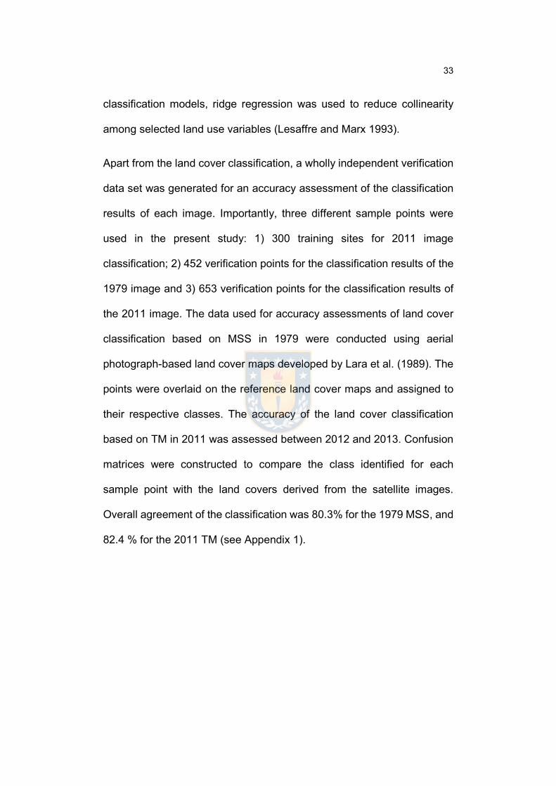
33

classification models, ridge regression was used to reduce collinearity

among selected land use variables (Lesaffre and Marx 1993).

Apart from the land cover classification, a wholly independent verification

data set was generated for an accuracy assessment of the classification

results of each image. Importantly, three different sample points were

used in the present study: 1) 300 training sites for 2011 image

classification; 2) 452 verification points for the classification results of the

1979 image and 3) 653 verification points for the classification results of

the 2011 image. The data used for accuracy assessments of land cover

classification based on MSS in 1979 were conducted using aerial

photograph-based land cover maps developed by Lara et al. (1989). The

points were overlaid on the reference land cover maps and assigned to

their respective classes. The accuracy of the land cover classification

based on TM in 2011 was assessed between 2012 and 2013. Confusion

matrices were constructed to compare the class identified for each

sample point with the land covers derived from the satellite images.

Overall agreement of the classification was 80.3% for the 1979 MSS, and

82.4 % for the 2011 TM (see Appendix 1).

34

Figure 1. Map of study area including study ecosystem (Costal temperate

deciduous forest of N.nervosa & P.lingue) and the major land cover types

in 1979 and 2011.

In the present study, the following land cover types were distinguished:

old-growth forest, secondary forest, shrubland, industrial plantation with

exotic species, crop field, urban areas, open water, bare ground and

others (Table 1). These categories were based on the land cover types

defined by Catastro (CONAF et al., 1999). Furthermore, habitat maps

were derived using two land cover types: secondary forest and old-growth

forest. Both of these forests are dominated by tree species of height

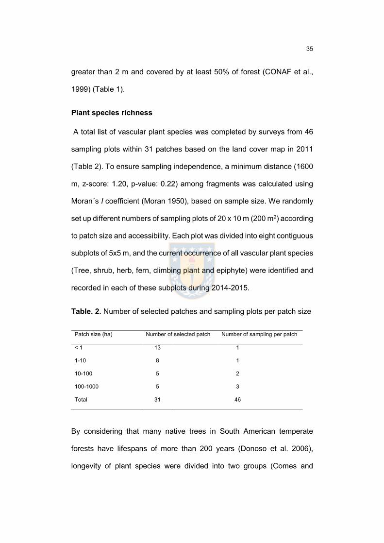
35

greater than 2 m and covered by at least 50% of forest (CONAF et al.,

1999) (Table 1).

Plant species richness

A total list of vascular plant species was completed by surveys from 46

sampling plots within 31 patches based on the land cover map in 2011

(Table 2). To ensure sampling independence, a minimum distance (1600

m, z-score: 1.20, p-value: 0.22) among fragments was calculated using

Moran´s I coefficient (Moran 1950), based on sample size. We randomly

set up different numbers of sampling plots of 20 x 10 m (200 m2) according

to patch size and accessibility. Each plot was divided into eight contiguous

subplots of 5x5 m, and the current occurrence of all vascular plant species

(Tree, shrub, herb, fern, climbing plant and epiphyte) were identified and

recorded in each of these subplots during 2014-2015.

Table. 2. Number of selected patches and sampling plots per patch size

Patch size (ha) Number of selected patch Number of sampling per patch

< 1 13 1

1-10 8 1

10-100 5 2

100-1000 5 3

Total 31 46

By considering that many native trees in South American temperate

forests have lifespans of more than 200 years (Donoso et al. 2006),

longevity of plant species were divided into two groups (Comes and

36

Kadereit 1998): 1) long-lived species referred to as trees and 2) short-

lived species to herbs, ferns and climbings. Habitat specialization for long-

lived species was classified by considering the following factors: 1) the

type of species considered (endemic plant as specialist; Harrison 1999) ;

2) the number of habitat classes (specialists as species occurring in few

habitat classes, while generalists in many habitat classes (Owens and

Bennett 2000) and 3) local expert knowledge (an ability to determine

which habitat is appropriate for which species; Gregory et al. 2005). The

degree of habitat specialization was quantified as high, medium and low

(see Appendix 2).

Analysis

The spatial patterns of habitat fragmentation were assessed using the

following indices of FRAGSTATS (Echeverría et al. 2012; McGarigal et

al. 2002; Nagendra et al. 2009): 1) patch density (number of habitat

patches per 100 ha); 2) largest patch index (% of the landscape

comprised by the largest habitat patch) and 3) total edge length (km).

These indices provide information about the patterns of subdivision of

forest patches, in which forest cover becomes disaggregated and isolated

across the landscape (Forman and Godron 1986). The annual

deforestation rate was calculated with the formula proposed by

Puyravaud (2003) :

P =

37

Where and are the forest cover at times and .

For 31 forest patches, the habitat patch size (ha) was measured in GIS.

In order to measure patch connectivity, we analyzed a simple proportional

index – the proportion of old-growth forest and secondary forest, within

different buffer distance around each patch. This index has been

implemented and recommended when habitat patches are oddly shaped

and relatively close together (Winfree et al. 2005). Buffer distances of 100,

500 and 1,500 m were chosen to reflect the potential dispersal rates of

different vascular plant species in temperate forests of South America

(Donoso et al. 2006; García et al. 2009).

The relationship between plant species richness and patch variables was

tested through regression analysis with Poisson error distribution and log

link function. The dependent variables were species richness of (i) all

vascular plants, (ii) long-lived plants (trees), (iii) long-lived specialist

plants (specialist trees) and (iv) short-lived plants (herbs, ferns and

climbings). The independent variables were: 1) current patch size; 2) past

patch size; 3) current connectivity and 4) past connectivity.

In order to compare the maximum probability of a single long-lived

species’ presence between 1979 and 2011, we also investigated changes

in patch size over the study area using Gaussian logit model (Lenoir et al.

2008; ter Braak and Looman 1986). Logistic regression is a generalized

linear modeling technique using a logit link function computed with the

38

log-likelihood expression of Bernoulli distribution (presence/absence).

We rewrote the model defined as a second-degree polynomial with

logarithmic link function (Jamil et al. 2014):

Logit (p) = + x +

where p is probability of presence, and x is patch size.

To track changes in species’ dwelling patch sizes, we compared the

dwelling information criterion between two periods. This parameter for

dwelling patch size (DPS) can be easily found by the following formula

(Ter Braak and Barendregt 1986; ter Braak and Looman 1986):

DPS = –

where and are the two coefficients of the Gaussian logit model using

maximum likelihood. The DPS represents the habitat patch size at which

the probability of presence reaches its maximum. All statistical analyses

were made with open source software R (version 3.2.2).

Results

Habitat fragmentation and actual plant richness

Between 1979 and 2011, native forests were reduced by 53% in the study

area (Figure 1). In 1979, there were 4,672 habitat patches covering an

area of 115,132 ha with a mean patch size of 24.64 ha. By 2011, the

mean patch size had declined to 1.44 ha, ranging from 0.09 to 5,731 ha.

39

During this period, habitat loss (old-growth forest plus secondary forest)

occurred at a rate of 1.99%yr-1 in the study area. The process of habitat

fragmentation was accompanied by the loss of the largest forest patch,

ranging from 43 % in 1979 to 9.42 % of the total area in 2011, while patch

density and total edge increased between 1979 and 2011 (Table 3).

Table. 3. Changes in landscape pattern indices for the native forests in

1979 and 2011

1979 2011

Total area (ha) 115,132 60,846

Number of patches 4,672 42,094

Mean patch area (ha) 24.64 1.44

(a) Patch desity 4.05 69.18

(b) Largest patch index (%) 43.72 9.42

(c) Total edge (km) 9,606 17,985

A total of 84 vascular plant species (36 trees, 17 shrubs, 19 herbs, 5 ferns,

6 climbing plants and 1 epiphyte) were identified in 31 habitat patches,

with a mean richness of 14.77 per patch (SD = 4.16; range 4-23) (Table

4. A). There were 36 long-lived species (7.97 per patch; SD =3.38), of

which 18 species were specialists (3.161 per patch; SD = 2.29). Mean

richness of short-lived plants was 3.19 per patch (SD = 1.76) (Table 4. A).

Table 4. (A) Current richness of different assemblage of plant species, n:

species number. (B) Linear regression testing the relationship between

40

the current and past patch size and current richness of plant species, F :

F -test value.

Plant assamblage (A) Richness (B) Patch size

n mean ± SD current F past F

All vascular plants 84 14.77 ± 4.16 0.051 2.371

Long-lived plants 36 7.97± 3.38 2.426 7.406 *

Long-lived specialists 18 3.16 ± 2.29 3.160 11.650 **

Short-lived plants 31 3.19 ± 1.75 1.505 1.786 * P <0.05

** P <0.01

Influence of past habitat on plant species richness

The study patch size ranged between 0.09 ha and 628.65 ha in 2011 and

between 1.8 ha and 15,077 ha in 1979. The linear regression models

revealed significant relationship between the past patch size and the

current richness of long-lived plants and long-lived specialist plants (Table

4. B). Among them, richness for long-lived specialist plants was best

explained by past patch size (Figure 2). The current richness of plant

assemblages could not be explained by the current patch size of the

native forest.

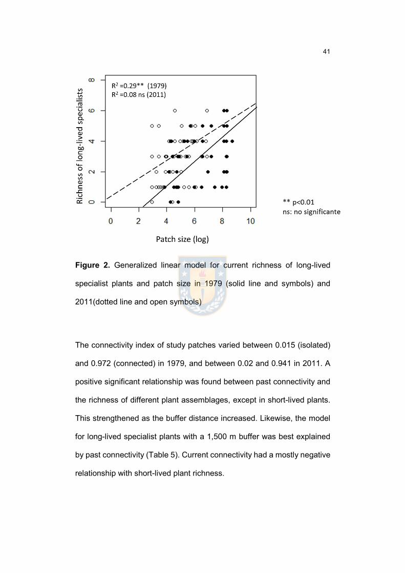
41

Figure 2. Generalized linear model for current richness of long-lived

specialist plants and patch size in 1979 (solid line and symbols) and

2011(dotted line and open symbols)

The connectivity index of study patches varied between 0.015 (isolated)

and 0.972 (connected) in 1979, and between 0.02 and 0.941 in 2011. A

positive significant relationship was found between past connectivity and

the richness of different plant assemblages, except in short-lived plants.

This strengthened as the buffer distance increased. Likewise, the model

for long-lived specialist plants with a 1,500 m buffer was best explained

by past connectivity (Table 5). Current connectivity had a mostly negative

relationship with short-lived plant richness.

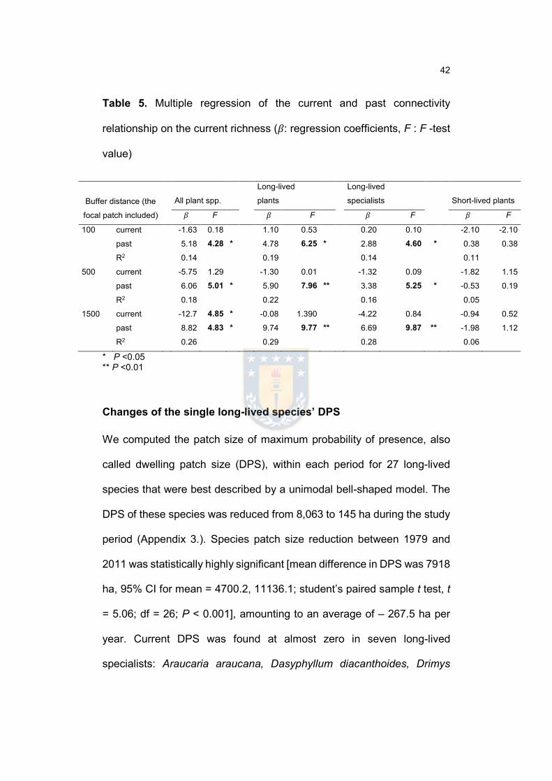
42

Table 5. Multiple regression of the current and past connectivity

relationship on the current richness (: regression coefficients, F : F -test

value)

Buffer distance (the

focal patch included)

All plant spp.

Long-lived

plants

Long-lived

specialists

Short-lived plants

F F F F

100 current -1.63 0.18 1.10 0.53 0.20 0.10 -2.10 -2.10

past 5.18 4.28 * 4.78 6.25 * 2.88 4.60 * 0.38 0.38

R2 0.14 0.19 0.14 0.11

500 current -5.75 1.29 -1.30 0.01 -1.32 0.09 -1.82 1.15

past 6.06 5.01 * 5.90 7.96 ** 3.38 5.25 * -0.53 0.19

R2 0.18 0.22 0.16 0.05

1500 current -12.7 4.85 * -0.08 1.390 -4.22 0.84 -0.94 0.52

past 8.82 4.83 * 9.74 9.77 ** 6.69 9.87 ** -1.98 1.12

R2 0.26 0.29 0.28 0.06

* P <0.05 ** P <0.01

Changes of the single long-lived species’ DPS

We computed the patch size of maximum probability of presence, also

called dwelling patch size (DPS), within each period for 27 long-lived

species that were best described by a unimodal bell-shaped model. The

DPS of these species was reduced from 8,063 to 145 ha during the study

period (Appendix 3.). Species patch size reduction between 1979 and

2011 was statistically highly significant [mean difference in DPS was 7918

ha, 95% CI for mean = 4700.2, 11136.1; student’s paired sample t test, t

= 5.06; df = 26; P < 0.001], amounting to an average of – 267.5 ha per

year. Current DPS was found at almost zero in seven long-lived

specialists: Araucaria araucana, Dasyphyllum diacanthoides, Drimys

43

winteri, Nothofagus nervosa, Prumnopitys andina, Saxegothaea

conspicua and Weinmannia trichosperma (Figure 3).

DISCUSSION

Detection of extinction debt

In this study, current species richness is generally better explained by

past patch size and connectivity than by current patch size and

connectivity, except in short-lived plants. If past landscape patterns

explain current species richness better than the current landscape pattern

(Kuussaari et al. 2009), this can be interpreted as evidence of an

extinction debt. Consequently, an unknown proportion of the current

vascular plants in the study area would be extinct.

Although the response to habitat fragmentation display different patterns

of distribution of a particular organism, species that share the same

ecological properties may show similar consistent patterns of changes

(Dambrine et al. 1995). Studying richness within species groups that differ

in their degree of habitat specialization may provide a more complete

picture of the community-level consequences of habitat fragmentation

than analyses focusing on total species richness (Brückmann et al. 2010;

Reitalu et al. 2012). Species that have restricted ecological preferences

(habitat specialists) are likely to be more strongly affected by habitat loss

and fragmentation than species that have broader ecological tolerances

and are able to occupy a wider range of habitats (generalists) (Devictor

44

et al. 2008; Polus et al. 2007). Additionally, the response to habitat

fragmentation in long-lived specialists is slower than in other species

groups in the same landscape (Krauss et al. 2010; Sang et al. 2010). Our

results showed that long-lived specialist plants are best explained by past

habitat area and connectivity (Table 4, Table 5) and confirmed that the

detection of extinction debt clearly depends on the longevity and habitat

specialization of study species (Cousins and Vanhoenacker 2011; Reitalu

et al. 2012).

Figure 3. Changes in dwelling patch size (size value at maximum

probability of presence) of single long-lived species (n = 27) for period

AH

AL

AN

ESEP

GA LA

LH

AM, EC LD

MB

ME

NT

PA

PL

PR

RSSM

AA

DD, DW, WT

NASC0

1

2

3

4

5

0 1 2 3 4 5

Spec

ies D

PS (L

og10

) 201

1

Species DPS(Log10) 1979

LF, LS

45

1979 and 2011. Each point represents one species: specialists are

displayed as dark gray ( ) and solid line (n = 14), whereas remnant

species are displayed as light gray ( ) and dotted line (n = 13). AA

Araucaria araucana, AH Aristotelia chilensis, AL Amomyrtus luma, AM

Acacia melanoxylon, AN Azara dentata, DD Dasyphyllum diacanthoides,

DW Drimys winteri, EC Eucryphia cordifolia, EP Escallonia pulverulenta,

ES Acacia caven, GA Gevuina avellana, LA Luma apiculata, LD Lomatia

dentata, LF Lomatia ferruginea, LH Lomatia hirsuta, LS Laurelia

sempervirens, NT Nothofagus antarctica, MB Maytenus boaria, ME

Myrceugenia exsucca, NA Nothofagus nervosa, PA Prumnopitys andina,

PL Persea lingue, PR Pinus radiate, RS Rhaphithamnus spinosus, SC

Sophora cassioides, SM Sophora cassioides, WT Weinmannia

trichosperma

In terms of relaxation time, a number of theoretical studies supported that

species richness in patches was negatively correlated with time since

fragmentation (Helm et al. 2006; Kuussaari et al. 2009; Saunders et al.

1991). Extinction debts are more likely in those landscapes where large-

scale habitat destruction has occurred recently (Cousins 2009). However,

field observations indicate the limited applicability of the relaxation time

for describing the effect of habitat fragmentation on risks of species

extinctions, varying in both space and time. In the temperate deciduous

forests of Europe, for example, the extinction debt of forest plant species

46

was found to persist for more than a couple of centuries (Kolb and

Diekmann 2005; Vellend et al. 2006), while other studies did not find any

extinction debts over a similar period of time (Adriaens et al. 2006;

Cousins et al. 2007). Likewise, studies from landscape with a large

amount of remaining natural area supported the concept of an extinction

debt, while highly fragmented landscapes did not provide any evidence of

an extinction debt (Adriaens et al. 2006; Cousins 2009). We assumed that

an extinction debt across a wider range of ecological traits may be

identified in a rapidly changing landscape with recent fragmentation

history and relatively large amounts of remnant forest area. Unlike our

expectations, we could not detect any statistically robust effect of habitat

configuration on the richness of short-lived plant species. This

unpredictability of extinction debt of short-lived plants in the NMR may be

explained as a combination of the following factors: 1) in southern Chile,

alien herbaceous species are widely introduced by anthropogenic

disturbances (logging and grazing) in understory layer (personal

observation, Bustamante and Castor, 1998 Pauchard and Alaback, 2004,

Braun and Vogt, 2014); 2) in the study area, secondary forest occupied

77% of native forest area. These secondary forests with relatively open

canopy may have changed microclimates (light, wind, soil moisture, etc.)

that have often been linked to the performance of native herb species

(Bierzychudek 1982; Matlack 1994; Tilman 1990) and 3) changes in plant

reproduction and recruitment (flowering, seed production, etc.) of

understory native species due to current abiotic and biotic alteration

47

(personal observation, McKinney and Goodell, 2010, Schemske et al.,

1978, Smith-Ramirez and Armesto, 1994).

Change of long-lived species’ DPS during 1979 - 2011

To identify species which their current occurrences are highly connected

to past habitat and have not yet paid an extinction debt, we investigated

changes in long-lived species’ dwelling patch size (DPS) over the study

periods. Our results provided strong evidence that 27 long-lived species

have already distributed in severely size-reduced patches in 2011

compared to 1979 (Figure 3, appendix 3).

We showed that many long-lived specialist plants have experienced

notable decline in DPS over about 30 years (Figure 3), and are more

affected and threatened by habitat fragmentation. Among them, A.

araucana and to the P. andina are vulnerable (VU), and S. conspicua is

near threatened (NT) according to the UICN red list of threatened species

(2015) (Appendix 2). Although these specialist trees associated with

small-size habitat patches seem to persist at present, their additional

biological attributes that are directly linked with key threatening processes

could act synergistically to elevate extinction risk and change this pattern

quickly (Davies et al. 2004; Gaston et al. 1997; Lindenmayer and Fischer

2013; Valiente-Banuet et al. 2015). Two additional attributes of concern

are population size and dispersal ability. Piqueray et al. (2011) showed

that it is likely that grassland specialist species which cannot maintain

relatively large populations in small habitat patches require larger habitat

48

patches. In the fragmented landscape of the CCR, several specialist trees

were shown to have reduced population density in small size habitat. For

example, W. trichosperma shows a reduced germination rate as well as

a lower seedling survival rate in small patches (Lusk and Pozo 2002).

Echeverria et al. (2007) observed that the seedling abundance of P.

andina was significantly related to only large-sized forest patches. Poor

dispersal ability might have another effect that increases the extinction

risk which disrupts metapopulation functioning (Honnay et al. 1999;

Jamoneau et al. 2011). Many previous studies suggested that specialist

trees in our study area have traits associated with short-distance dispersal.

For N. nerviosa, fruit dispersal only reaches between 50 and 100 m per

year (Donoso Zegers 1993) and the average distance of pollen dispersal

is also very short (<35m) (Marchelli et al. 2012). A. araucana is known as

a gravity-dispersed species with poor dispersal distance due to the seed

size (2-4 cm long, 1-2 cm wide) and heavy weight (3.5-5.0 g) (González

and Veblen 2006). Conversely, the population density and seed dispersal

of shade-intolerant generalist trees (e.g., P. lingue, G. avellana, El.

Cordifolia, L. dentate) are likely to benefit from forest edges in a

fragmented habitat surrounded by plantations of exotic species

(Bustamante and Simonetti 2005; Echeverría et al. 2007).

Value of small size patches in rapidly changing landscape

Despite strong evidence of the importance of large areas of native

vegetation (Gaston and Spicer 2013; Rosenzweig 1995) under

49

mechanisms underlying the species-area relationship (Arrhenius 1921),

extinction debt is proportionally higher in recently fragmented small size

patches than in historically fragmented large patches (Kuussaari et al.

2009). Patch-level extinction may occur faster in small patches than in

large patches due to differences in susceptibility to disturbance between

small and large patches (Sheil and Burslem 2003). Habitat fragmentation

of Chilean temperate forests is associated with a rapid decrease in patch

size (Echeverria et al. 2006a). A high number of plant species were

observed in small-sized patches in the present study, which typically had

shorter relaxation time. Although expanding the habitat area may be a

straightforward solution to prevent future extinction of specialist species

in the NMR, preserving or restoring large reserve areas is usually difficult

because of the high costs involved.

In the CCR, a positive relationship between patch quality/connectivity and

plant abundance/richness was reported in fragmented landscapes

dominated by small size patches (Robledo-Arnuncio et al. 2014; Vergara

et al. 2010). Similarly, Wulf and Kolk (2014) demonstrated that increasing

the quality of small patches reaps more benefits than increasing patch

area in the fragmented landscapes of Australia. Diamond (1975) found

that if small size patches of remnant habitats are widespread in the

landscape, they might be a contributing factor to a relatively lower

extinction debt or longer relaxation time by enhancing habitat connectivity.

Likewise, configuring the spatial arrangement to minimize isolation may

50

help to ensure that many of the species with extinction debts do not reach

their extinction threshold in the long term (Paltto et al. 2006).

With these considerations, specific recommendations for the

management of small-size habitat patches in the NMR should include 1)

maintaining current quality and quantity of old-growth forests, which are

at risk of rapid decline and degradation of their structure without active

management (15.5% of old-growth forest rate in 1979, declining to 8.2%

in 2011); 2) restoring habitat quality of secondary forests targeted for the

re-development of old-growth attributes (Bauhus et al. 2009); 3)

managing soften boundaries or creating buffers around ecologically

sensitive areas, in order to reduce edge effect and enhance landscape

connectivity (Lindenmayer and Fischer 2006; López-Barrera 2004) and 4)

identifying and designing adequate landscape configuration based on the

remnant small-size patches to enhance specialist species’ persistence

and resilience, because it is likely the current landscape configuration no

longer supports the species habitat requirements (Suding et al. 2004;

Tambosi and Metzger 2013).

Suggestions for preventing future biodiversity loss in the NMR

Early detection of an extinction debt of long-lived specialist plants can be

considered a benefit to begin habitat restoration and conservation actions

in an adequate time in the study area. However, as responses to habitat

fragmentation are species-dependent, conservation actions which target

species groups are inadequate. Future monitoring plans of extinction

51

dynamics must focus on single species of long-lived specialist plants

rather than focusing on species richness or a set of species. In the

fragmented landscapes of biodiversity hotspot, it may be crucial to identify

and prioritize the conservation of species with extinction proneness over

those that have no significant risk.

Finally, because a large portion of the study area is privately owned

(Carruthers and Rodriguez 2009), participation and cooperation of the

private sector is a key element to address biodiversity conservation goals

in the NMR. It will be necessary to create appropriate conditions for the

participation of all relevant stakeholders in the planning and

implementation of conservation initiatives.

Conclusion

Our analyses provide the first evidence of potential future loss of many

vascular plant species in South American temperate hotspot. However,

as long as a species that is predicted to become extinct still persists, we

believe that extinction debt provides new challenges and opportunities to

current biodiversity conservation. However, it depends on valid timing

because extinction debt payment is in progress and imposes an

undefined deadline. Instead of waiting to launch large-scale conservation

projects, we suggest immediate implementation of local or small-scale

restoration projects in order to mitigate the existing extinction debt.

52

Acknowledgements

This study was a part of Research project 1140531 of FONDECYT

(Chilean National Fond for Scientific and Technological Development).

This study was also supported by CONICYT (Chilean National

Commission for Scientific and Technological Research), KNA (Korea

National Arboretum) and KOICA (Korea International Cooperation

Agency). We are grateful to Roberto Rodriguez, Ph.D., for valuable

support on botanical information, Rodrigo Fuentes, M.Sc., and Dr.(c)

Samuel Otavo for Land cover classification and Felipe Sáez, M.Sc. for

field data collection. The experiments comply with the current laws of the

country in which they were performed.

Literature ADRIAENS, D., HONNAY, O. & HERMY, M. 2006. No evidence of a plant

extinction debt in highly fragmented calcareous grasslands in Belgium. Biological Conservation, 133, 212-224.

AGUAYO, M., PAUCHARD, A., AXOCAR, G. & PARRA, O. 2009. Cambio del uso del suelo en el centro sur de Chile a fines del siglo XX: Entendiendo la dinámica espacial y temporal del paisaje. Revista chilena de historia natural, 82, 361-374.

ALTAMIRANO, A., APLIN, P., MIRANDA, A., CAYUELA, L., ALGAR, A. C. & FIELD, R. 2013. High rates of forest loss and turnover obscured by classical landscape measures. Applied Geography, 40, 199-211.

ALLENDORF, F. W. & HARD, J. J. 2009. Human-induced evolution caused by unnatural selection through harvest of wild animals. Proceedings of the National Academy of Sciences, 106, 9987-9994.

ARMESTO, J., ROZZI, R., SMITH-RAMÍREZ, C. & ARROYO, M. 1998. Conservation targets in South American temperate forests. America, 5, 6.

ARMESTO, J. J., VILLAGRAN, C. & ARROYO, M. K. 1996. Ecología de los bosques nativos de Chile. Textos Universitarios/Monografias, Santiago, Universitaria,| c1996, edited by Armesto, Juan J.; Villagran, Carolina; Arroyo, Mary Kalin, 1.

53

ARRHENIUS, O. 1921. Species and area. Journal of Ecology, 9, 95-99. BAUHUS, J., PUETTMANN, K. & MESSIER, C. 2009. Silviculture for old-

growth attributes. Forest Ecology and Management, 258, 525-537. BENNETT, A. F., NATURE, I. U. F. C. O., RESOURCES, N. &

PROGRAMME, I. F. C. 2003. Linkages in the Landscape: The Role of Corridors and Connectivity in Wildlife Conservation, IUCN.

BIERZYCHUDEK, P. 1982. Life histories and demography of shade-tolerant temperate forest herbs: a review. New Phytologist, 90, 757-776.

BRÜCKMANN, S. V., KRAUSS, J. & STEFFAN-DEWENTER, I. 2010. Butterfly and plant specialists suffer from reduced connectivity in fragmented landscapes. Journal of Applied Ecology, 47, 799-809.

BUSTAMANTE, R. O. & SIMONETTI, J. A. 2005. Is Pinus radiata invading the native vegetation in central Chile? Demographic responses in a fragmented forest. Biological Invasions, 7, 243-249.

CARRUTHERS, D. & RODRIGUEZ, P. 2009. Mapuche protest, environmental conflict and social movement linkage in Chile. Third World Quarterly, 30, 743-760.

CAVIERES, L. A., MIHOC, M., MARTICORENA, A., MARTICORENA, C., MARY, C. M. B. Y. & ARROYO, K. 2005. 13. Flora vascular de la Cordillera de la Costa en la región del Biobío: riqueza de especies, géneros, familias y endemismos.

CBD 2001. Global biodiversity outlook. UNEP: Nairobi. COMES, H. P. & KADEREIT, J. W. 1998. The effect of Quaternary

climatic changes on plant distribution and evolution. Trends in plant science, 3, 432-438.

CONAF 1999. Catastro y evaluación de los recursos vegetacionales nativos de Chile. Informe Nacional con Variables Ambientales. Santiago, Chile.

COUSINS, S. A. O. 2009. Extinction debt in fragmented grasslands: paid or not? Journal of Vegetation Science, 20, 3-7.

COUSINS, S. A. O. & VANHOENACKER, D. 2011. Detection of extinction debt depends on scale and specialisation. Biological Conservation, 144, 782-787.

COUSINS, S. O., OHLSON, H. & ERIKSSON, O. 2007. Effects of historical and present fragmentation on plant species diversity in semi-natural grasslands in Swedish rural landscapes. Landscape Ecology, 22, 723-730.

CHANDER, G., MARKHAM, B. L. & HELDER, D. L. 2009. Summary of current radiometric calibration coefficients for Landsat MSS, TM, ETM+, and EO-1 ALI sensors. Remote sensing of environment, 113, 893-903.

DAMBRINE, E., ULRICH, E., CÉNAC, N., DURAND, P., GAUQUELIN, T., MIRABEL, P., NYS, C., PROBST, A., RANGER, J. & ZÉPHORIS, M. 1995. Atmospheric Deposition in France and Possible Relation with Forest Decline. In: LANDMANN, G., BONNEAU, M. & KAENNEL, M. (eds.) Forest Decline and

54

Atmospheric Deposition Effects in the French Mountains. Springer Berlin Heidelberg.

DAVIES, K. F., MARGULES, C. R. & LAWRENCE, J. F. 2004. A synergistic effect puts rare, specialized species at greater risk of extinction. Ecology, 85, 265-271.

DEVICTOR, V., JULLIARD, R. & JIGUET, F. 2008. Distribution of specialist and generalist species along spatial gradients of habitat disturbance and fragmentation. Oikos, 117, 507-514.

DIAMOND, J. M. 1975. The island dilemma: lessons of modern biogeographic studies for the design of natural reserves. Biological conservation, 7, 129-146.

DONOSO, C., SPURR, S., AMBASHT, R., DANSEREAU, P., SIERRA PINEDA, A., VÁZQUEZ SOTO, J. & RODRÍGUEZ TREJO, D. 2006. Las especies arbóreas de los bosques templados de Chile y Argentina autoecología. Cartilla-Servicio Autónomo Forestal Venezolano

DONOSO ZEGERS, C. 1993. Bosques templados de Chile y Argentina: variación, estructura y dinámica.

DULLINGER, S., ESSL, F., RABITSCH, W., ERB, K.-H., GINGRICH, S., HABERL, H., HÜLBER, K., JAROŠÍK, V., KRAUSMANN, F. & KÜHN, I. 2013. Europe’s other debt crisis caused by the long legacy of future extinctions. Proceedings of the National Academy of Sciences, 110, 7342-7347.

DULLINGER, S., GATTRINGER, A., THUILLER, W., MOSER, D., ZIMMERMANN, N. E., GUISAN, A., WILLNER, W., PLUTZAR, C., LEITNER, M. & MANG, T. 2012. Extinction debt of high-mountain plants under twenty-first-century climate change. Nature Climate Change, 2, 619-622.

ECHEVERRIA, C., COOMES, D., SALAS, J., REY-BENAYAS, J. M., LARA, A. & NEWTON, A. 2006. Rapid deforestation and fragmentation of Chilean Temperate Forests. Biological Conservation, 130, 481-494.

ECHEVERRÍA, C., NEWTON, A., NAHUELHUAL, L., COOMES, D. & REY-BENAYAS, J. M. 2012. How landscapes change: Integration of spatial patterns and human processes in temperate landscapes of southern Chile. Applied Geography, 32, 822-831.

ECHEVERRÍA, C., NEWTON, A. C., LARA, A., BENAYAS, J. M. R. & COOMES, D. A. 2007. Impacts of forest fragmentation on species composition and forest structure in the temperate landscape of southern Chile. Global Ecology and Biogeography, 16, 426-439.

FAZEY, I., FISCHER, J. & LINDENMAYER, D. B. 2005. What do conservation biologists publish? Biological conservation, 124, 63-73.

FISCHER, J. & LINDENMAYER, D. B. 2007. Landscape modification and habitat fragmentation: a synthesis. Global Ecology and Biogeography, 16, 265-280.

FORMAN, R. T. T. & GODRON, M. 1986. Landscape Ecology, Wiley.

55

GARCÍA, D., RODRÍGUEZ-CABAL, M. A. & AMICO, G. C. 2009. Seed dispersal by a frugivorous marsupial shapes the spatial scale of a mistletoe population. Journal of Ecology, 97, 217-229.

GASTON, K. J., BLACKBURN, T. M. & LAWTON, J. H. 1997. Interspecific abundance-range size relationships: an appraisal of mechanisms. Journal of Animal Ecology, 579-601.

GASTON, K. J. & SPICER, J. I. 2013. Biodiversity: an introduction, John Wiley & Sons.

GILBERT, B. & LEVINE, J. M. 2013. Plant invasions and extinction debts. Proceedings of the National Academy of Sciences, 110, 1744-1749.

GONZÁLEZ, M. E. & VEBLEN, T. T. 2006. Climatic influences on fire in Araucaria araucana-Nothofagus forests in the Andean cordillera of south-central Chile. Ecoscience, 13, 342-350.

GREGORY, R. D., VAN STRIEN, A., VORISEK, P., MEYLING, A. W. G., NOBLE, D. G., FOPPEN, R. P. & GIBBONS, D. W. 2005. Developing indicators for European birds. Philosophical Transactions of the Royal Society of London B: Biological Sciences, 360, 269-288.

GREZ, A. A., SMITH-RAMÍREZ, C., ARMESTO, J. & VALDOVINOS, C. 2005. El valor de los fragmentos pequeños de bosque maulino en la conservación de la fauna de coleópteros epigeos. Historia, biodiversidad y ecología de los bosques de la Cordillera de la Costa, 565-572.

GUSTAVSSON, E., LENNARTSSON, T. & EMANUELSSON, M. 2007. Land use more than 200years ago explains current grassland plant diversity in a Swedish agricultural landscape. Biological conservation, 138, 47-59.

HAILA, Y. 2002. A conceptual genealogy of fragmentation research: from island biogeography to landscape ecology*. Ecological applications, 12, 321-334.

HANSKI, I. Extinction debt and species credit in boreal forests: modelling the consequences of different approaches to biodiversity conservation. Annales Zoologici Fennici, 2000. JSTOR, 271-280.

HANSKI, I. & OVASKAINEN, O. 2002. Extinction Debt at Extinction Threshold. Conservation Biology, 16, 666-673.

HARRISON, S. 1999. Local and regional diversity in a patchy landscape: native, alien, and endemic herbs on serpentine. Ecology, 80, 70-80.

HELM, A., HANSKI, I. & PÄRTEL, M. 2006. Slow response of plant species richness to habitat loss and fragmentation. Ecology letters, 9, 72-77.

HINOJOSA, L. F. & VILLAGRÁN, C. 1997. Historia de los bosques del sur de Sudamérica, I: antecedentes paleobotánicos, geológicos y climáticos del Terciario del cono sur de América. Revista Chilena de Historia Natural, 70, 225-240.

HONNAY, O., HERMY, M. & COPPIN, P. 1999. Effects of area, age and

56

diversity of forest patches in Belgium on plant species richness, and implications for conservation and reforestation. Biological conservation, 87, 73-84.

HUETE, A. R. 1988. A soil-adjusted vegetation index (SAVI). Remote sensing of environment, 25, 295-309.

HUTH, N. & POSSINGHAM, H. P. 2011. Basic ecological theory can inform habitat restoration for woodland birds. Journal of Applied Ecology, 48, 293-300.

IUCN 2017. The IUCN Red List of Threatened Species. Version 2017-3. . 05 December 2017. http://www.iucnredlist.org.

JAMIL, T., KRUK, C. & TER BRAAK, C. J. 2014. A unimodal species response model relating traits to environment with application to phytoplankton communities.

JAMONEAU, A., SONNIER, G., CHABRERIE, O., CLOSSET-KOPP, D., SAGUEZ, R., GALLET-MORON, E. & DECOCQ, G. 2011. Drivers of plant species assemblages in forest patches among contrasted dynamic agricultural landscapes. Journal of Ecology, 99, 1152-1161.

KOH, L. P., SODHI, N. S. & BROOK, B. W. 2004. Ecological correlates of extinction proneness in tropical butterflies. Conservation Biology, 18, 1571-1578.

KOLB, A. & DIEKMANN, M. 2005. Effects of Life-History Traits on Responses of Plant Species to Forest Fragmentation

Efectos de las Características de la Historia de Vida Sobre las Respuestas de Especies de Plantas a la Fragmentación de Bosques. Conservation Biology, 19, 929-938.

KOLK, J. & NAAF, T. 2015. Herb layer extinction debt in highly fragmented temperate forests – Completely paid after 160 years? Biological Conservation, 182, 164-172.

KRAUSS, J., BOMMARCO, R., GUARDIOLA, M., HEIKKINEN, R. K., HELM, A., KUUSSAARI, M., LINDBORG, R., ÖCKINGER, E., PÄRTEL, M. & PINO, J. 2010. Habitat fragmentation causes immediate and time-delayed biodiversity loss at different trophic levels. Ecol. letters, 13, 597-605.

KUUSSAARI, M., BOMMARCO, R., HEIKKINEN, R. K., HELM, A., KRAUSS, J., LINDBORG, R., ÖCKINGER, E., PÄRTEL, M., PINO, J., RODÀ, F., STEFANESCU, C., TEDER, T., ZOBEL, M. & STEFFAN-DEWENTER, I. 2009. Extinction debt: a challenge for biodiversity conservation. Trends in Ecology & Evolution, 24, 564-571.

LARA, A., ARAYA, L., CAPELLA, J., FIERRO, M. & CAVIERES, A. 1989. Evaluación de la destrucción y disponibilidad de los recursos forestales nativos en la VII y VIII Región. Informe Técnico, Comité Pro Defensa Fauna y Flora, Santiago, Chile.

LAURANCE, W. F., LOVEJOY, T. E., VASCONCELOS, H. L., BRUNA, E. M., DIDHAM, R. K., STOUFFER, P. C., GASCON, C., BIERREGAARD, R. O., LAURANCE, S. G. & SAMPAIO, E. 2002.

57

Ecosystem decay of Amazonian forest fragments: a 22-year investigation. Conservation Biology, 16, 605-618.

LENOIR, J., GÉGOUT, J., MARQUET, P., DE RUFFRAY, P. & BRISSE, H. 2008. A significant upward shift in plant species optimum elevation during the 20th century. science, 320, 1768-1771.

LESAFFRE, E. & MARX, B. D. 1993. Collinearity in generalized linear regression. Communications in Statistics-Theory and Methods, 22, 1933-1952.

LIENERT, J. 2004. Habitat fragmentation effects on fitness of plant populations – a review. Journal for Nature Conservation, 12, 53-72.

LINDBORG, R. 2007. Evaluating the distribution of plant life-history traits in relation to current and historical landscape configurations. Journal of Ecology, 95, 555-564.

LINDBORG, R. & ERIKSSON, O. 2004. HISTORICAL LANDSCAPE CONNECTIVITY AFFECTS PRESENT PLANT SPECIES DIVERSITY. Ecology, 85, 1840-1845.

LINDENMAYER, D. B. & FISCHER, J. 2006. Habitat fragmentation and landscape change: an ecological and conservation synthesis, Island Press.

LINDENMAYER, D. B. & FISCHER, J. 2013. Habitat fragmentation and landscape change: an ecological and conservation synthesis, Island Press.

LÓPEZ-BARRERA, F. 2004. Estructura y función en bordes de bosques. Revista Ecosistemas, 13.

LOREAU, M., NAEEM, S., INCHAUSTI, P., BENGTSSON, J., GRIME, J., HECTOR, A., HOOPER, D., HUSTON, M., RAFFAELLI, D. & SCHMID, B. 2001. Biodiversity and ecosystem functioning: current knowledge and future challenges. science, 294, 804-808.

LUEBERT, F. & PLISCOFF, P. 2006. Sinopsis bioclimática y vegetacional de Chile, Editorial Universitaria.

LUSK, C. H. & POZO, A. D. 2002. Survival and growth of seedlings of 12 Chilean rainforest trees in two light environments: gas exchange and biomass distribution correlates. Austral Ecology, 27, 173-182.

MARCHELLI, P., SMOUSE, P. E. & GALLO, L. A. 2012. Short-distance pollen dispersal for an outcrossed, wind-pollinated southern beech (Nothofagus nervosa (Phil.) Dim. et Mil.). Tree genetics & genomes, 8, 1123-1134.

MATLACK, G. R. 1994. Vegetation dynamics of the forest edge--trends in space and successional time. Journal of Ecology, 113-123.

MCGARIGAL, K., CUSHMAN, S. A., NEEL, M. C. & ENE, E. 2002. FRAGSTATS: spatial pattern analysis program for categorical maps.

MILDÉN, M., COUSINS, S. A. & ERIKSSON, O. The distribution of four grassland plant species in relation to landscape history in a Swedish rural area. Annales Botanici Fennici, 2007. JSTOR, 416-426.

58

MORAN, P. A. 1950. Notes on continuous stochastic phenomena. Biometrika, 37, 17-23.

MYERS, N., MITTERMEIER, R. A., MITTERMEIER, C. G., DA FONSECA, G. A. B. & KENT, J. 2000. Biodiversity hotspots for conservation priorities. Nature, 403, 853-858.

NAGENDRA, H., PAUL, S., PAREETH, S. & DUTT, S. 2009. Landscapes of protection: forest change and fragmentation in Northern West Bengal, India. Environmental Management, 44, 853-864.

ÖSTER, M., COUSINS, S. A. & ERIKSSON, O. 2007. Size and heterogeneity rather than landscape context determine plant species richness in semi-natural grasslands. Journal of Vegetation Science, 18, 859-868.

OTAVO, S. & ECHEVERRÍA, C. 2017. Fragmentación progresiva y pérdida de hábitat de bosques naturales en uno de los hotspot mundiales de biodiversidad. Revista Mexicana de Biodiversidad, 88, 924-935.

OUBORG, N., VERGEER, P. & MIX, C. 2006. The rough edges of the conservation genetics paradigm for plants. Journal of Ecology, 94, 1233-1248.

OVASKAINEN, O. & HANSKI, I. 2002. Transient dynamics in metapopulation response to perturbation. Theoretical population biology, 61, 285-295.

OVASKAINEN, O. & HANSKI, I. 2004. From individual behavior to metapopulation dynamics: unifying the patchy population and classic metapopulation models. The American Naturalist, 164, 364-377.

OWEN, E. 2007. Informe final: Una evaluacion rapida de la biodiversidad de dos predios integrados a la Red Conservacionista del Patrimonio Natural de Contulmo.

OWENS, I. P. & BENNETT, P. M. 2000. Ecological basis of extinction risk in birds: habitat loss versus human persecution and introduced predators. Proceedings of the National Academy of Sciences, 97, 12144-12148.

PALTTO, H., NORDÉN, B., GÖTMARK, F. & FRANC, N. 2006. At which spatial and temporal scales does landscape context affect local density of Red Data Book and Indicator species? Biological Conservation, 133, 442-454.

PIESSENS, K. & HERMY, M. 2006. Does the heathland flora in north-western Belgium show an extinction debt? Biological Conservation, 132, 382-394.

PIQUERAY, J., BISTEAU, E., CRISTOFOLI, S., PALM, R., POSCHLOD, P. & MAHY, G. 2011. Plant species extinction debt in a temperate biodiversity hotspot: Community, species and functional traits approaches. Biological Conservation, 144, 1619-1629.

POLUS, E., VANDEWOESTIJNE, S., CHOUTT, J. & BAGUETTE, M. 2007. Tracking the effects of one century of habitat loss and fragmentation on calcareous grassland butterfly communities.

59

Biodiversity and Conservation, 16, 3423-3436. PUYRAVAUD, J.-P. 2003. Standardizing the calculation of the annual

rate of deforestation. Forest Ecology and Management, 177, 593-596.

RANIUS, T., ELIASSON, P. & JOHANSSON, P. 2008. Large-scale occurrence patterns of red-listed lichens and fungi on old oaks are influenced both by current and historical habitat density. Biodiversity and Conservation, 17, 2371-2381.

REESE, H. & OLSSON, H. 2011. C-correction of optical satellite data over alpine vegetation areas: A comparison of sampling strategies for determining the empirical c-parameter. Remote Sensing of Environment, 115, 1387-1400.

REITALU, T., PURSCHKE, O., JOHANSSON, L. J., HALL, K., SYKES, M. T. & PRENTICE, H. C. 2012. Responses of grassland species richness to local and landscape factors depend on spatial scale and habitat specialization. Journal of Vegetation Science, 23, 41-51.

ROBLEDO-ARNUNCIO, J. J., KLEIN, E. K., MULLER-LANDAU, H. C. & SANTAMARÍA, L. 2014. Space, time and complexity in plant dispersal ecology. Movement ecology, 2.

ROSENZWEIG, M. L. 1995. Species diversity in space and time, Cambridge University Press.

ROUSE JR, J. W., HAAS, R., SCHELL, J. & DEERING, D. 1974. Monitoring vegetation systems in the Great Plains with ERTS.

SANG, A., TEDER, T., HELM, A. & PÄRTEL, M. 2010. Indirect evidence for an extinction debt of grassland butterflies half century after habitat loss. Biological Conservation, 143, 1405-1413.

SAUNDERS, D. A., HOBBS, R. J. & MARGULES, C. R. 1991. Biological consequences of ecosystem fragmentation: a review. Conservation biology, 5, 18-32.

SCHEMSKE, D. W., WILLSON, M. F., MELAMPY, M. N., MILLER, L. J., VERNER, L., SCHEMSKE, K. M. & BEST, L. B. 1978. Flowering ecology of some spring woodland herbs. Ecology, 59, 351-366.

SHEIL, D. & BURSLEM, D. F. 2003. Disturbing hypotheses in tropical forests. Trends in Ecology & Evolution, 18, 18-26.

SUDING, K. N., GROSS, K. L. & HOUSEMAN, G. R. 2004. Alternative states and positive feedbacks in restoration ecology. Trends in ecology & evolution, 19, 46-53.

TAMBOSI, L. R. & METZGER, J. P. 2013. A framework for setting local restoration priorities based on landscape context. Natureza & Conservação. This issue.

TER BRAAK, C. J. & BARENDREGT, L. G. 1986. Weighted averaging of species indicator values: its efficiency in environmental calibration. Mathematical Biosciences, 78, 57-72.

TER BRAAK, C. J. & LOOMAN, C. W. 1986. Weighted averaging, logistic regression and the Gaussian response model. Vegetatio, 65, 3-11.

TILMAN, D., MAY, R. M., LEHMAN, C. L. & NOWAK, M. A. 1994. Habitat

60

destruction and the extinction debt. Nature, 371, 65-66. TILMAN, J. G. D. 1990. Perspectives on Plant Competition: Some

Introductory Remarks. Perspectives on plant competition, 3. TURNER, M. G. 2010. Disturbance and landscape dynamics in a

changing world. Ecology, 91, 2833-2849. VALIENTE-BANUET, A., AIZEN, M. A., ALCÁNTARA, J. M., ARROYO,

J., COCUCCI, A., GALETTI, M., GARCÍA, M. B., GARCÍA, D., GÓMEZ, J. M. & JORDANO, P. 2015. Beyond species loss: the extinction of ecological interactions in a changing world. Functional Ecology, 29, 299-307.

VELLEND, M., VERHEYEN, K., JACQUEMYN, H., KOLB, A., VAN CALSTER, H., PETERKEN, G. & HERMY, M. 2006. Extinction debt of forest plants persists for more than a century following habitat fragmentation. Ecology, 87, 542-548.

VERGARA, P. M., SMITH, C., DELPIANO, C. A., ORELLANA, I., GHO, D. & VAZQUEZ, I. 2010. Frugivory on Persea lingue in temperate Chilean forests: interactions between fruit availability and habitat fragmentation across multiple spatial scales. Oecologia, 164, 981-991.

WINFREE, R., DUSHOFF, J., CRONE, E. E., SCHULTZ, C. B., BUDNY, R. V., WILLIAMS, N. M. & KREMEN, C. 2005. Testing simple indices of habitat proximity. The American Naturalist, 165, 707-717.

WOLODARSKY-FRANKE, A. & HERRERA, S. D. 2011. Cordillera de Nahuelbuta. Reserva mundial de biodiversidad. Valdivia: WWF.

WULF, M. & KOLK, J. 2014. Plant species richness of very small forests related to patch configuration, quality, heterogeneity and history. Journal of vegetation science, 25, 1267-1277.

YOUNG, A., BOYLE, T. & BROWN, T. 1996. The population genetic consequences of habitat fragmentation for plants. Trends in Ecology & Evolution, 11, 413-418.

YOUNG, A. G. & CLARKE, G. M. 2000. Genetics, demography and viability of fragmented populations, Cambridge University Press.

61

Annex

A. 1. Confusion matrices for the two images

Classified data Reference data User's

accuracy (%)

Old-growth/

secondary

forest

Shrub

-land

Industrial

plantation Crop field

Urban

areas

Open

water

Bare

ground

A. 1979 image

Old-growth/secondary forest 69 5 12 0 0 0 0 80

Shrubland 5 55 1 1 0 0 0 89

Industrial plantation 14 7 53 0 0 0 0 72

Crop field 0 8 1 49 3 0 10 69

Urban areas 0 0 0 4 47 0 4 85

Open water 0 0 0 0 0 40 0 100

Bare ground 0 2 0 6 6 0 50 78

Total 88 77 67 60 56 40 64

Omission error (%) 22 29 21 18 16 0 22

Producer's accuracy (%) 78 71 79 82 84 100 78

Overall classification accuracy: 80.3

B. 2011 image

Old-growth/secondary forest 126 12 18 0 0 0 0 81

Shrubland 14 121 5 4 0 0 0 84

Industrial plantation 11 14 86 0 0 0 0 77

Crop field 0 8 1 60 5 0 5 76

Urban areas 0 0 0 4 50 0 0 93

Open water 0 0 0 0 0 40 0 100

Bare ground 0 2 0 8 4 0 55 80

Total 151 157 110 76 59 40 60

Omission error (%) 17 23 22 21 15 0 8

Producer's accuracy (%) 83 77 78 79 85 100 92

Overall classification accuracy: 82.4

A. 2. List of long-lived species and their habitat specialization degree in

Nahuelbuta Mountain Range

Family Scientific name Habitat

specialization*

Aextoxicaceae Aextoxicon punctatum Ruiz & Pav. M

62

Anacardiaceae Lithraea caustica (Molina) Hook. & Arn. G

Araliaceae Pseudopanax laetevirens (Gay) Franchet M

Araucariaceae Araucaria araucana (Molina) K. Koch S

Asteraceae Dasyphyllum diacanthoides(Less.) Cabrera S

Celastraceae Maytenus boaria Molina G

Cunoniaceae Weinmannia trichosperma Ruiz & Pav. S

Elaeocarpaceae Aristotelia chilensis (Molina) Stuntz G

Escalloniaceae Escallonia pulverulenta (Ruiz & Pav.) Pers. S

Eucryphiaceae Eucryphia cordifolia Cav. M

Fabaceae Acacia melanoxylon R. Br. G

Sophora cassioides (Phil.) Sparre S

Gomortegaceae Gomortega keule (Molina) Baill. S

Icacinaceae Citronella mucronata (Ruiz & Pav.)D. Don M

Lauraceae Cryptocarya alba (Molina) Looser G

Persea lingue (Miers ex Bertero) Nees G

Mimosaceae Acacia caven (Molina) Molina S

Laureliopsis philippiana (Looser) Schodde S

Laurelia sempervirens (Ruiz & Pav.) Tul. S

Peumus boldus Molina G

Myrtaceae Amomyrtus luma (Molina) Legrand & Kausel S

Luma apiculata (DC.) Burret S

Myrceugenia exsucca (DC.) Berg. M

Nothofagaceae Nothofagus nervosa (Poepp. & Endl.) Oerst. S

Nothofagus dombeyi (Mirb.) Oerst. G

Nothofagus obliqua (Mirb.) Oerst. G

Nothofagus pumilio (Poepp. & Endl.) Krasser M

Nothofagus antarctica (Forster) Oerst. M

Pinaceae Pinus radiata D. Don G

Podocarpaceae

Prumnopitys andina (Poepp. ex Endl.) de

Laub. S

Podocarpus saligna D. Don S

Saxegothaea conspicua Lindl. S

Proteaceae Embothrium coccineum J.R. & G. Forster G

Gevuina avellana Molina G

Lomatia dentata (Ruiz & Pav.) R. Br. S

Lomatia ferruginea (Cav.) R. Br. S

Lomatia hirsuta (Lam.) Diels ex J.F.Macbr. G

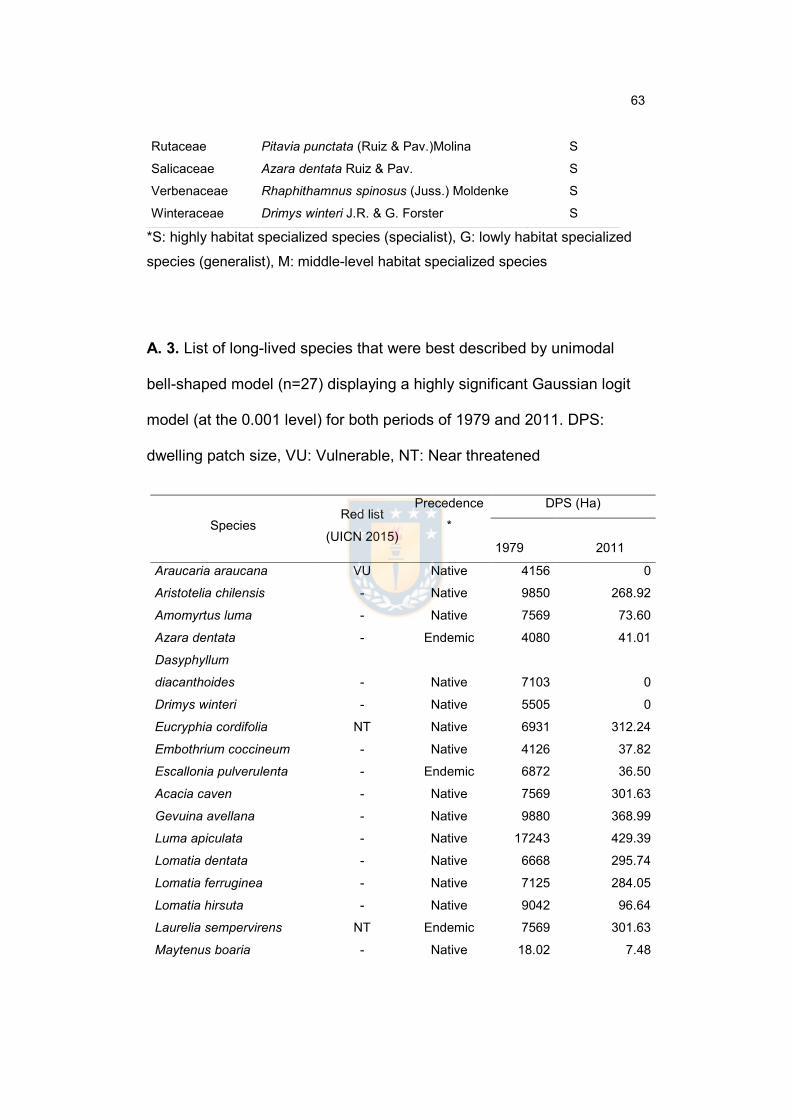
63

*S: highly habitat specialized species (specialist), G: lowly habitat specialized

species (generalist), M: middle-level habitat specialized species

A. 3. List of long-lived species that were best described by unimodal

bell-shaped model (n=27) displaying a highly significant Gaussian logit

model (at the 0.001 level) for both periods of 1979 and 2011. DPS:

dwelling patch size, VU: Vulnerable, NT: Near threatened

Species Red list

(UICN 2015)

Precedence

*

DPS (Ha)

1979 2011

Araucaria araucana VU Native 4156 0

Aristotelia chilensis - Native 9850 268.92

Amomyrtus luma - Native 7569 73.60

Azara dentata - Endemic 4080 41.01

Dasyphyllum

diacanthoides - Native 7103 0

Drimys winteri - Native 5505 0

Eucryphia cordifolia NT Native 6931 312.24

Embothrium coccineum - Native 4126 37.82

Escallonia pulverulenta - Endemic 6872 36.50

Acacia caven - Native 7569 301.63

Gevuina avellana - Native 9880 368.99

Luma apiculata - Native 17243 429.39

Lomatia dentata - Native 6668 295.74

Lomatia ferruginea - Native 7125 284.05

Lomatia hirsuta - Native 9042 96.64

Laurelia sempervirens NT Endemic 7569 301.63

Maytenus boaria - Native 18.02 7.48

Rutaceae Pitavia punctata (Ruiz & Pav.)Molina S

Salicaceae Azara dentata Ruiz & Pav. S

Verbenaceae Rhaphithamnus spinosus (Juss.) Moldenke S

Winteraceae Drimys winteri J.R. & G. Forster S

64

Myrceugenia exsucca - Native 6518 157.12

Nothofagus nervosa - Native 11189 0

Nothofagus antarctica - Native 144.9 12.12

Prumnopitys andina VU Native 991.3 1.50

Persea lingue NT Native 13836 621.24

Pinus radiata - Introduced 43934 12.74

Rhaphithamnus spinosus - Native 7281 147.90

Saxegothaea conspicua NT Native 49.57 0

Sophora cassioides - Endemic 6441 109.21

Weinmannia trichosperma - Native 6019 0

*Donoso et al. (2006)

65

CHAPTER 3

National assessment of forest ecosystem fragmentation in Ecuador: strong

needs of landscape management in Tropical Andes2

Introduction

Since rapid economic development, natural system decline and fragmentation is one

of the core drivers of global change and has huge implications for ecosystem

functioning and conservation (Fahrig 2003). The impacts of habitat fragmentation

can arise in the face of primarily biotic change, primarily abiotic change and a

combination of both, including extinction, disruption of trophic interactions and

increased susceptibility to disturbances (e.g. logging, fires and invasive species)

(Holl and Aide 2011; Laurance et al. 2002; Letcher and Chazdon 2009; Turner

2010a). Some changes result in system degradation retaining some original

characteristics as well as novel elements, whereas larger changes will result in

system replacement or collapse (Hobbs et al. 2009). Previously the majority of efforts

to conserve biodiversity have been focused on species, communities or their habitat

under forest fragmentation (Wiens and Moss 2005; Wu 2013a), although there is

clearly a need to more effective conservation policy focusing on ecosystems which

include fundamental biotic and abiotic components and ensure the protection of a

2 This chapter is in preparation in order to submit a journal as: Noh, J. K., Echeverría, C. & Cuenca, P. 2019. National assessment of forest ecosystem fragmentation in Ecuador: strong needs of landscape management in Tropical Andes

66

sufficient portion of all ecosystems in these regions (Bennett and Saunders 2010;

Hughes et al. 2000; Schmidt 1996; Sierra et al. 2002)

In many tropical countries, forest ecosystem fragmentation is occurring at an

alarming rate by changes in human land use activities (Laurance 1999; Rudel and

Roper 1997; Sanchez-Azofeifa, Harriss, and Skole 2001). The fragmentation of

tropical forests is considered highly relevant to changes of ecological function and

services and negative effects on natural recovery after disturbances as catalysts of

rapid ecological change (Holl and Aide 2011; Letcher and Chazdon 2009; Turner

2010). To date, the relationship between land use change by human activities and

forest ecosystem fragmentation has been widely studied, described and interpreted

by using landscape metrics: e.g. mean patch size, edge density, mean shape

index:(Echeverria et al. 2006b), O´Neil et al. 1999 or quantitative measurement (e.g.

Morphological spatial pattern analysis: (Soille and Vogt 2009), Landscape mosaic

index: (Riitters et al. 2009), and Forest connectivity index: (Saura and Torn 2009).

The specific studies of forest ecosystem fragmentation carried out in Tropical Andes

are initiated in late 1980’s (Armenteras et al. 2003; Armenteras et al. 2006; Gmez et

al. 2005; Gómez Mora et al. 2005; Rodríguez Eraso et al. 2013). In the eastern

Andes of Colombia, Armenteras et al. (2003) have incorporated the degree of

fragmentation for ecosystem conservation planning, using five landscape metrics;

patch number, largest patch index, mean patch size, mean nearest neighbor

distance, and landscape shape index.

Despite such studies are abundant and has received much attention in tropics, very

few studies showed the relationship between the degree of forest fragmentation and

67

human land use at the ecosystem level. Over the past 50 years, human have

changed ecosystems more rapidly and extensively than in any comparable period

time in human history, largely to meet rapidly growing demands for food, fresh water,

timber, fiber and fuel (Duraiappah and Naeem 2005). Thus, this ecosystem

degradation (e.g. fragmentation) by human activities is associated with a substantial

and largely irreversible loss in the diversity of life on Earth, and leads to the

degradation of many ecosystem services, increased risks of nonlinear changes and

the exacerbation of poverty for some groups of people (Duraiappah and Naeem

2005). The challenge of reversing the degradation of ecosystems while meeting

increasing demands may initiate to understand what changes happened in

ecosystems under interaction with human land use.

Nevertheless, one of the major reasons, why the relationship between forest

fragmentation and human land use at ecosystem level has been little studied, is that

there is no universally accepted global taxonomy of ecosystems (Keith et al. 2013)

to date. This means the classification and delimitation of ecosystems are rarely

studied and available in most countries. In addition, human-fragmentation study is

the lack of a commonly accepted method for quantifying fragmentation (Butler et al.

2004). As not all landscape metrics can capture the entire extent of forest

fragmentation in a particular landscape (Cain et al. 1997), most studies about forest

fragmentation have been described the relationship with human land use based on

landscape metrics. In many studies on ecosystem fragmentation, increase in number

of patches, decrease in patch size and increased patch isolation together address

the quantitative measures of fragmentation (Echeverria et al. 2006a; kyoung Noh et

68

al. 2018). Although these studies have often magnified the controversy because of

correlation among multiple landscape metrics (e.g. edge, isolation and area),

together with these correlative observation, Ibanez et al (2014) reveal that

fragmentation has multiple simultaneous effects that are interwoven in complex ways

and that operate over potentially long time scales. With these considerations, to date

few researchers have shown the relationship between human land use and forest

ecosystem fragmentation using an explicit single forest fragmentation index at

ecosystem level. For example, Butler et al. (2004) have produced a forest

fragmentation index for western Oregon and western Washington that combined

measures of forested are, percentage edge and interspersion. Likewise, Abdullah

and Nakagoshi (2007) developed a single forest fragmentation index based on a

combination of three landscape metrics: (i) non-forest area; (ii) forest edge, and (iii)

patch size coefficient of variation, in the state of Selangor, Malaysia. A central benefit

of quantifying forest fragmentation through a single index is feasible to be statistically

correlated to human land use. The impact of human land use on specific forest

ecosystem fragmentation can support political justification of sustainable landscape

planning and management based on contribution to human well-being (Wu 2013).

Ecuador is located in tropical Andes range and known as one of the most mega-

diverse worldwide per surface unit, with 1,250 species of plants belonging to 136

different families registered in 1 km2 (León et al. 2011; Valencia et al. 1994) and

also home of high-diverse terrestrial ecosystems that exhibits very high levels of

endemism (Olson and Dinerstein 2002). Despite its ecological importance, highest

rates of forest decline and fragmentation were reported last 30 years (Cuenca et al.

69

2016; Mena 2008a; Sierra and Stallings 1998; Tapia-Armijos et al. 2015). This

recognition is resulting in a collective shift in empirical studies on biodiversity and

biological conservation in the country (Cadilhac et al. 2017; Cuenca and Echeverria

2017b; Cuesta et al. 2017; Lessmann et al. 2014). In the conservation point of view,

one of the most remarkable achievements in Ecuador might be the establishment of

official identification, classification and delimitation of the national-wide ecosystems

(MAE, 2013), after initiative framework of the ecosystem classification by Sierra et

al. (1999) and Josse et al. (2003). Unfortunately, literature review reveals that this

baseline information has not fully exploited to generate a monitoring system of

national ecosystem changes. For example, Cuesta et al. (2017) used this ecosystem

maps and species distribution models to identify priority areas for biodiversity

conservation in mainland Ecuador. Likewise, MAE (2015) attempted to assess

ecosystem fragmentation and risk based on the ecosystem map (considered all land

cover type inside ecosystem), using patch numbers, mean patch size, and patch

size coefficient of variation. Their studies complement current conservation efforts,

but cannot provide relationship between the degree of forest ecosystem

fragmentation and human land use at ecosystem level to better design conservation

strategies integrated into land use planning and management in Ecuador.

Against this background, we aimed to (i) quantify and graph forest change

(deforestation, forest fragmentation) in Ecuador mainland during 1990-2000-2008-

2014 on different spatial scales, and (ii) relate the degree of forest fragmentation to

human land use at ecosystem level in 2014. The present study considered

‘ecosystem’ as standard reporting unit for national level assessment and have

70

utilized landscape metrics to analyze forest fragmentation. The present study is

allowing us to answer the following research question: 1) How did forest

fragmentation change in Tropical Andes during last decades? ; 2) Which human land

use drive the current forest ecosystem fragmentation in Tropical Andes?

This paper provides a broad review of how recent forest fragmentation at ecosystem

level has affected by practices in human land use. By illuminating the critical gaps

between forest conservation strategies and actual practices employed in human land

use, we suggest ecosystem-level conservation implementation based on a land-use-

related planning and sustainable development in Ecuador, which involve significant

changes in policies, institutions, and practices that are not currently under way.

Materials and methods

GIS data

The baseline information used consisted of satellite images (Landsat – 5 TM)

obtained in 1990, 2000, 2008 and 2014, which were classified by the Ecuadorian

Ministry of Agriculture (MAGAP) and Ministry of the Environment (MAE), using

LANDSAT 4 and 5 TM for 1990, LANDSAT ETM+ for 2000, LANDSAT ETM+ and

ASTER for 2008 (MAE 2012), and LANDSAT 8 OLI, LANDSAT ETM+ and Rapid

Eye satellite images for 2014 (MAE, 2015). Except the thematic map of the 2014,

which was classified by supervised classification using data from field surveys (at

least 30 sites were monitored for each land use type), the other three maps of

previous dates were generated by using unsupervised classification (MAE, 2015).

71

Figure 1. (A) Ecoregions of continental Ecuador. Elevation detail is shown. (B) The

major land cover types inside 64 forest ecosystems in 1990, 2000, 2008 and 2014.

(C) Distribution of each ecoregion’s elevation. Cutting section of a geological map

based on a red dotted line (A). (D) The major land cover types and changes of

72

ecoregions (n=7) in 1990, 2000, 2008 and 2014, (E) The major land cover types that

have replaced the original forest ecosystem of single ecosystems (n=64) in 2014.

Ecosystems containing forest area <10 % (n=6) are marked with black outline.

In the present study, seven land cover types were mainly considered for the land

use change analysis (Table 1). Furthermore, human land use was distinguished

using seven land cover types: industrial plantation (PLT), pasture (PST), annual

farming (AFM), permanent farming (PFM), semipermanent farming (SFR), inhabited

area (HBT) and infrastructure (IFR) (Table 1). To perform the analysis of ecosystem-

level deforestation and forest fragmentation, this study considered category of native

forest, which cover about 14 million hectares, as the following four forest types:

1) Higher mountain forest: trees reach 10-15 m of height with thick and

sometimes gnarled trunks, with adventitious roots occupying up to 70 m2

(Buytaert, Iñiguez, and Bièvre 2007; Sierra et al. 1999).

2) Cloud mountain forest: Trees reach a height of 15-25 m. The underwood is

very rich and epiphytes and mosses are very abundant. Persistent presence

of fog at the vegetation level, which significantly reduces incident solar

radiation and evapotranspiration (Célleri and Feyen 2009).

3) Lower mountain forest: The canopy height can reach 20-35 m tall with

sporadic trees of 40 m. Composed by different layers such as canopy, sub-

canopy, shrub and herbaceous species (Valencia, Balslev, and Paz Y Miño

C 1994).

4) Foothill forest: Forest transition between the foothills of Eastern and Western

ranges and Amazonian forest. Substrate mainly composed by volcanic rocks

73

and sediments of recent origins. The canopy height reaches 30 m and sub-

canopy and understory are very dense (Bendix et al. 2009).

Table 1. Description and source of land cover types defined in the study area

Main

land use

No. Land cover type Description Source

Forest 1 Native forest Vegetation with native tree species, including higher

mountain forest, cloud mountain forest, lower mountain

forest and foothill forest.

MAE (2016)

Shrub/Gr

assland

2 Shrubland Area with a substantial component of non-arboreal native

woody species. It includes degraded areas in transition to

dense canopy.

MAE (2011)

3 Grassland Native grassland with a spontaneous growth, which do

not receive special care, and use for sporadic grazing or

protection

MAGAP

(2012)

4 Paramo Typical ecosystem of tropical Andes, located above 3400

m.a.s.l. Vegetation can reach 50 cm height.

MAGAP

(2012)

Industrial

plantation

5 Industrial

plantation (PLT)

Vegetation with planted exotic species, including young

and harvested plantations.

MAE (2011)

Pasture 6 Pasture (PST) Cultivated grassland, dominated by introduced species of

gramineas and legunimosas, for feeding livestock

MAGAP

(2012)

Agricultu

re

7 Annual farming

(AFM)

Cultivated land for annual crops MAGAP

(2012)

8 Permanent

farming (PFM)

Mainly orchards and lands for permanent crops and

vegetables.

MAGAP

(2012)

9 Semipermanent

farming (SFM)

Cultivated land for 2 or 3-year-cycle crops MAGAP

(2012)

Urban 10 Inhabited area

(HBT)

Land mainly occupied by housing and buildings for

communities and public services

MAGAP

(2012)

11 Infrastructure

(IFR)

Land occupied by roads, industries and other

anthropogenic surfaces (e.g. shrimp fishery)

MAGAP

(2012)

Others 12 Natural water Land occupied by natural water bodies such as small

lakes and ponds.

MAGAP

(2012)

13 Artificial water Land or flowing water associated with anthropic activities

and water resource management

MAGAP

(2012)

14 Bare ground Cleared land, rocks and river beds. MAGAP-

IEE (2012)

15 Glacier Snow and ice MAGAP-

74

IEE (2012)

In Ecuador, the definition, classification and delimitation of total 91 national territorial

ecosystems (87 natural ecosystems with four other systems such as: area of human

intervention, water, other areas and no information) are established and completed

on the basis of the following factors: 1) physiognomy; 2) bioclimate; 3) biogeography;

4) geoform; 5) general flooding; 6) Phenology; 7) bioclimatic floor, and 8) substratum.

(MAE 2013). According to the vegetation physiognomic classification (forest,

shrubland and grassland), we selected 64 forest ecosystems including two

mangroves (Table 2), among 87 natural territorial ecosystems in whole Ecuador.

Table 2. Spatial scale (region-ecoregion-ecosystem), altitudinal range and Forest

Fragmentation Index (FFI: proportion of non-continuous forest in a given

ecosystem) of 64 natural forest ecosystems in the Ecuadorian continent

Region Ecoregion Cod

e Forest Ecosystems (forest vegetation type)

Altitudinal

range (m)

FFI

2014

COAST Equatorial

-Chocó

E1 Flood alluvial plain forest of the Equatorial Chocó 50-200 10.68

E2 Equatorial Chocó mangrove 0-20 32.20

E3 Evergreen forest of the Equatorial Chocó lowland 0-300 22.18

E4 Flood intertidal plain forest of the Equatorial Chocó 0-50 23.14

E5 Seasonal evergreen forest of Equatorial Chocó lowlands 0-300 41.70

E6 Piedmont seasonal evergreen forest of the Chocó coastal range 200-400 36.16

E7 Low montane evergreen forest of Chocó coastal range >400 25.81

Equatorial

-Pacific

E8 Semideciduous forest of the Jama-Zapotillo lowland 0-300 33.50

E9 Semideciduous forest of the Equatorial Pacific coastal range >200 19.29

E10 Low forest and deciduous shrubland of the Jama-Zapotillo

lowland 0-400

87.37

E11 Piedmont seasonal evergreen forest of the Equatorial Pacific

coastal range 200-400

54.04

E12 Low montane seasonal evergreen forest of the Equatorial

Pacific coastal range 400-860

31.64

E13 Seasonal evergreen forest of the Jama-Zapotillo lowland 0-400 65.46

75

E14 Deciduous forest of the Jama-Zapotillo lowland 0-400 21.09

E15 Deciduous forest of the Equatorial Pacific coastal range >200 23.95

E16 Jama-Zapotillo mangrove 0-10 30.11

E17 Seasonal flood alluvial plain evergreen forest of the Jama-

Zapotillo 0-300

98.62

ANDES Western-

range

E18 Piedmont evergreen forest of the western Andean range 300-1400 18.51

E19 Low montane evergreen forest of the western Andean range 1400-2000 23.58

E20 Montane evergreen forest of the western Andean range 2000-3100 23.16

E21 High montane evergreen forest of the western Andean range 3100-3600 39.45

E22 Piedmont seasonal evergreen forest of the western Andean

range 300-1400

35.28

E23 Piemontano seasonal evergreen forest of the Catamayo-Alamor 400-1600 63.45

E24 Low montane seasonal evergreen forest of the Catamayo-

Alamor 1600-2000

56.93

E25 Montane evergreen forest of the Catamayo-Alamor 2200-2900 58.11

E26 High montane evergreen forest of the Catamayo-Alamor 2900-3400 38.30

E27 Low montane evergreen forest of the Catamayo- Alamor 1600-2200 60.31

E28 Piedmont evergreen forest of the Catamayo-Alamor 400-1600 55.02

E29 Piedmont semideciduous forest of the Catamayo-Alamor 400-1600 38.20

E30 Low montane semideciduous forest of the Catamayo-Alamor 1600-2200 63.05

E31 Piedmont deciduous forest of the Catamayo-Alamor 400-1600 42.67

E32 Low montane deciduous forest of the Catamayo- Alamor 1600-2200 96.81

Valley,

Alpine

E33 Semideciduos forest and shrubland of the North Valleys 1200-2600 99.99

E34 Semideciduos forest and shrubland of the South Valleys 1200-2000 99.40

E35 Páramo evergreen forest 3200-4100 99.76

Eastern-

range E36

High montane evergreen forest of the north-eastern Andean

range 3000-3700

18.51

E37 Montane evergreen forest of the north-eastern Andean range 2000-3000 2.55

E38 Low montane evergreen forest of the north-eastern Andean

range 1200-2000

2.95

E39 Piedmont evergreen forest of the north-eastern Andean range 400-1200 8.73

E40 Low montane evergreen forest of the south-eastern Andean

range 1660-2200

13.97

E41 Montane evergreen forest of the south-eastern Andean range 2200-3000 7.59

E42 High montane evergreen forest of the south-eastern Andean

range 3000-3400

25.06

E43 Piedmont evergreen forest of the south-eastern Andean range 400-1650 42.54

E44 Piedmont semideciduous forest of the south-eastern Andean

range 500-1300

78.61

76

AMAZO

N

Range E45 Low montane evergreen forest of Galeras 1300-1700 0.00

E46 Piedmont evergreen forest of Galeras 600-1300 0.00

E47 Piedmont evergreen forest of the Cóndor-Kutukú range 350-1400 13.81

E48 Low montane evergreen forest of the Cóndor-Kutukú range 1400-1900 3.12

E49 Montane evergreen forest of the Cóndor-Kutukú range 1900-2400 1.42

E50 Piedmont evergreen forest on sandstone plateaus of the

Cóndor-Kutukú range 350-1400

4.89

E51 Montane evergreen forest on sandstone plateaus of the Cóndor

range 1900-2700

1.10

E52 Piedmont evergreen forest on limestone outcrops of the

Amazonian range 600-1400

6.08

E53 Low montane evergreen forest on sandstone plateaus of the

Cóndor-Kutukú range 1400-1900

0.62

E54 Evergreen forest on sandstone plateaus of the Cóndor range in

the lower Ecuadorian Amazon 243-550

0.02

Plain E55 Evergreen forest of the Aguarico-Putumayo-Caquetá lowland 168-350 8.24

E56 Flood alluvial plain palm forest of the Amazon 171-350 1.19

E57 Flood river (originated in the Andean and Amazonian ranges)

alluvial-plain forest 164-350

8.87

E58 Lowland evergreen forest of the Napo-Curaray 170-350 3.30

E59 Flood alluvial plain forest of the Amazon 158-350 1.41

E60 Flood forest and lacustrine-riparian vegetation of the

Amazonian black water 170-350

10.59

E61 Flood river (originated in the Amazon) alluvial plain forest 158-350 4.29

E62 Evergreen bamboo forest of the Amazonian lowland 196-500 0.00

E63 Evergreen forest of the Tigre-Pastaza lowland 166-350 0.48

E64 Evergreen forest of the Pastaza fan-shaped lowland 197-350 2.69

Deforestation rate, change rate of land cover types and forest fragmentation

index

The annual deforestation rate was calculated with the formula proposed by

Puyravaud (2003):

P =

77

Where and are the forest cover at time and .

In order to calculate change rate of land cover types, a cross-tabulation procedure

between the classifications was processed with ArcGIS 10.5; gains and losses were

calculated as proposed by Pontius et al. (2004). Fragmentation analyses were

performed using the approach by Forest Area Density (FAD), which is a simple

metric of fragmentation as a contextual variable associated with a given forest pixel

(Riitters and Wickham 2012). The result is a set of a map showing FAD values in [0,

100]% for neighborhood area over each forest pixel (Table 3). If forest is not

fragmented in the vicinity of a given forest pixel, then by definition FAD equals 1.0

for a neighborhood with contains that forest pixel. On the other hand, if forest is

fragmented in the vicinity, then the value of FAD is less than 1.0 in proportion to the

degree of fragmentation (i.g. number of non-forest pixels) within the neighborhood.

At the present study, we evaluated FAD with square neighborhood areas of length

27 pixels and the FAD values were classified into the following forest fragmentation

classes:

Table 3. Summary of FAD fragmentation class thresholds, names and color

assignment

FAD class Color FAD range

1 Rare FAD < 10 %

2 Patchy 10% ≤ FAD < 40%

3 Transitional 40% ≤ FAD < 60%

4 Dominant 60% ≤ FAD < 90%

5 Interior 90% ≤ FAD ≤ 100%

78

To characterize forest fragmentation in each forest ecosystem using a forest

fragmentation index (FFI), we first summed continuous forest using ratio between

the number of FAD ≥ 40% classified as “Interior”, “Dominant” and “Transitional”,

divided by the total number of pixels in that forest ecosystem (Vogt 2018). Then, FFI

was defined as a proportion of non-continuous forest in a given ecosystem.

Analysis

The relationship between FFI and current human land use was tested through

regression analysis with Poisson error distribution and log link function. The

independent variables were the percentage of human land uses in potential forest

ecosystems in 2014(Table 1). The dependent variables were FFI of grouping

ecosystems that share a common set of the following biogeographic characters and

forest fragmentation rate; (1) region; and (2) FFI degree in 2014. All statistical

analyses made with open source software R (version 3.2.2).

Results

Land use change in forest ecosystems

Between 1990 and 2014, native forests have been cleared approx. 454,000 ha in 64

forest ecosystems of Ecuador mainland, averaging 7100 ha per each ecosystem

(Figure 1.B, Figure 2.B). Deforestation rate of 64 forest ecosystems significantly

increased between 1990-2000 and 2000-2014 [mean difference in deforestation rate

was 0.6%, 95% CI for mean = -0.15, 0.45; student´s paired sample t test, t = 2.18,

df = 63, < 0.01].

79

Figure 2. Scatter diagrams of forest ecosystems annual deforestation rate for the

periods 1990-2000 and 2000-2014. (A) Changes in annual deforestation rate of

single forest ecosystem (n=64) for the periods 1990-2000 and 2000-2014. Each

point represents one forest ecosystem. Solid black outline is zoomed out (B). (B)

Changes in annual deforestation rate of single forest ecosystem (n=59), excluding

extreme data (n=5) (Inset) The distribution of the ecosystem’s differences in

deforested area between 1990 and 2014. The vertical dotted line marks zero shifts,

and the vertical solid line marks the median shift. The arrow describes the direction

of the shift.

In 64 forest ecosystems, E44 showed the highest deforestation rate of 3.95 % yr-1,

followed by 1.34 % yr-1 in E23 and 1.30 % yr-1 in E32. In 2014, percentage of forest

cover was under 10 % of spatial extent in six forest ecosystems: E33 (0.11 % of

forested area), E35 (1.7 %), E34 (3.44 %), E32 (5.65 %) and E17 (7.4 %) (Figure

1.E). During the whole study period, five forest ecosystems showed an increase in

80

area: E4 (8.3% of gain in forest area), E33 (1700%), E35 (29.69%), E56 (0.70%)

and E64 (0.03%).

In forest ecosystems, human land use (agriculture, industrial plantation, urban and

pasture) showed a rapid increase of 54% over 24 years (Figure 1.B). At national

level, agriculture was the major anthropogenic land use in 1990 (4.3 %), 2000 (5.4 %)

and 2008 (6.1 %), but declining to 2.6 % by 2014. In 2014, pasture, rising from 1.1 %

in 2008 to 5.4 % in 2014, became the largest single human land cover class. The

other notable features of the data are the relatively stable proportion of the natural

shrubland/grassland (≈ 2 %) during 1990 to 2008, and an increase (≈ 3 %) in 2014.

Industrial plantation and urban areas showed a slight increase in area across the

study period.

Land cover changes did not occur at equal rates during all time intervals in the three

regions (Figure 3). The most intensive change was located in the Coast, where

frequent exchanges between pasture and agriculture land as well as pasture,

shrubland and agriculture land (particularly rotations between pastures, herbaceous

crops and fallow cycles), were found. The most consistent trend of changes among

land uses between 2008-2014 was a progressive increase in pasture at the expense

of agriculture and native forest. Thus, a slight increase in urban area was observed

in all regions over the whole study period.

81

Figure 3. Net change (i.e. gains plus losses), gains and losses for each land cover

82

class as a percentage of three regions for the periods 1990-2000, 2000-2008 and

2008-2014

Forest fragmentation

By 2014, continuous fragmentation became the dominant process, owing to a

decline in number of interior and dominant FAD classes and a slight increase in

patchy and rare FAD in the Coast and Andes (Figure 4). In the Amazon, forest

fragmentation was accompanied by the rapid increase in the number of patchy and

rare FAD. The amount of interior FAD decreased following the introduction of these

disturbed fragments into the matrix.

Figure 4. Temporal variation of number of different FAD (log) in three regions of

Ecuador

The FFI varied between 0 (no fragmented) and 99.99 (highly fragmented) in 2014

(Table 2). The highest FFI was recorded for the semideciduos forest and shrubland

of the North Valleys (E33), while the lowest FFI (value=0) was observed in E45, E46

and E62.

83

Relationship between forest fragmentation and human land use

The increase in human land uses had a significantly positive relationship on forest

fragmentation in all forest ecosystems of Ecuador (Table 4). At national level,

positive significant relationship was constantly found between forest fragmentation

and two human land uses: pasture (PST) and habited area (HBT). Additional results

using regions were presented in more detail (Table 4). In the Andes, we detected

statistically robust relationships of pasture (PST) and habited area (HBT) on forest

fragmentation. Thus, regional regression model indicated that forest fragmentation

was mostly explained by permanent (PFM) and semi-permanent farming (SFM), and

habitat area (HBT) in the Andes, and pasture (PST) in the Amazon, respectly.

Table 4. Standard coefficients of multiple regressions testing the relationship

between forest fragmentation index (FFI) and human land use in 2014 in three

regions of Ecuador

PLT: industrial plantation; PST: pasture; AFM: annual farming; PFM: permanent

farming; SFM: semi-permanent farming; HBT: inhabited area; IFR: infrastructure . p < 0.1

* p < 0.05

** p < 0.01

Human Land Use Adj.R2 F PLT PST AFM PFM SFM HBT IFR All (n=64)

0.646 17.41 *** 2.52 1.30 *** 1.45 0.18 1.23 59.78 *** 6.57

Coast (n=17) 0.572 4.06 * 0.126 -0.47 -5.64 2.58 . 4.61 . 59.74 . 54.47 Andes (n=27) 0.854 4.89 ** 0.70 1.31 *** 0.44 -4.10 3.67 106.48 ** -358.21 Amazon(n=20) 0.003 5.31 ** - 1.08 ** -26.97 -9.53 16.00 -87.06 -98.74

84

*** p < 0.001

The regression models indicated that the forest fragmentation had mostly positive

relationship with pasture (PST) in ecosystems of low, moderate and high

fragmentation in 2014 (Table 5). In addition, forest fragmentation in ecosystems

associated to high FFI value was positively explained by semi-permanent farming

(SFM) and infrastructure (IFR), and negatively by permanent farming (PFM). Lowly

fragmented forest ecosystems also showed negative significant relationship

between forest fragmentation and industrial plantation (PLT).

Table 5. Standard coefficients of multiple regressions testing the relationship

between forest fragmentation index (FFI) and human land use for 2014 in forest

ecosystems divided by FFI value (Low: FFI ≤10, Moderate: 10 <FFI ≤60, High: FFI

>60)

PLT: industrial plantation; PST: pasture; AFM: annual farming; PFM: permanent

farming; SFM: semi-permanent farming; HBT: inhabited area; IFR: infrastructure . p < 0.1

* p < 0.05

** p < 0.01

*** p < 0.001

Human Land Use Adj.R2 F PLT PST AFM PFM SFM HBT IFR

Low (n=22) 0.936 45.39 *** -2.08 * 1.20 *** 46.67 *** -3.51 3.33 -63.78 0.88 Moderate (n=31) 0.302 2.61 * 1.90 0.63 * 1.55 . 0.43 0.34 4.92 1.2358.21

High (n=11) 0.995 232 ** 9.23 0.37 * 0.43 -0.61 * 1.28 . 10.30 93.33 *

85

Discussion

To understand how changes in forest structure interact with human land use, we

need information on what kind and magnitude of changes happen as a first step

(Lambin et al. 2003). This study aimed at providing some of this relevant information

based on comparative studies across different spatial scales of the forest

ecosystems in Ecuador.

Considering the three regions of continental Ecuador, the Coastal forest ecosystems

showed significant forest conversion by human land use (Figure 1). This region has

supported much of the country’s agriculture and has suffered from significant urban

development (Lessmann et al. 2016; Senz and Onofa 2005; Sierra 1999b).

Specifically, the equatorial pacific is under higher transformation trends from native

forest to human land use than equatorial Chocó (Figure 1.D). The Andes showed

the largest gap between human land use and conservation efforts. Even though

many studies set priorities for forest conservation efforts in the tropical Andes

(Mittermeier et al. 1998; Olson and Dinerstein 2002), we observed that forest

ecosystems in Andean valley have a very low proportion of original native forests

and are aware of the loss of defining features and replacement by a novel ecosystem

by transforming diagnostic component. On the other hand, as the western Andes

harbor less protected areas than the eastern Andes, human land use is more

proportioned and represented in western Andes than east Andes (MAE 2015).

Expansion of agropastoral land-use trends in Andes was recognized as the main

reason of deforestation and forest conversion (Brandt and Townsend 2006; Wunder

2000). As reporting recently higher rate of deforestation in Amazonian region (MAE,

86

2015) than in the Coast and Andes, we expected significant influence of human land

use on native forest ecosystems in this region. Unlike our expectation, human land

use is poorly observed in the Amazon region comparing the rests. This

unpredictability of human land use in forest ecosystems in Amazon may be

explained by their larger extension comparing with the rest. In contrast to the Coast

and Andes, forest ecosystems in Amazon are much more extensive. As the rate of

human land use in Amazon is relatively smaller than the rest of regions, it seems

that there is no urgent need to be assigned to initiatives within the priority areas of

biodiversity conservation at landscape level. Similarly, Sierra et al. (2002) mainly

prioritize conservation of natural ecosystems in the Coast and Andes based on

ecosystem-risk-representativeness approach, as the highest risk areas. However,

results using species as conservation targets may differ from the results using

ecosystem level approach. For example, from a species-based perspective,

Lessmann et al. (2014) suggest that more conservation efforts are needed in the

northern Amazon where the highest species richness can be found. It is noteworthy

that, ecosystem level conservation should be considered apart from species–only

approach (e.g. based on richness or endemism).

Our most remarkable finding was to identify the different degrees of forest changes

at the ecosystem level across Ecuador. Although overall forest loss and

fragmentation is slightly observed between 1990 and 2014 in 64 natural forest

ecosystems, we identified several seriously modified ecosystems. For example, the

2014 native forest proportion reached only 0.11% for Semideciduos forest and

shrubland of the North Valleys. Declining total forest area of spatial extent in an

87

ecosystem type, it seems that the forest ecosystem has undergone transformation

of identity. Importantly, Suding and Hobbs (2009) address such severe changes in

natural ecosystems could be mostly observed when human activities change

frequently (e.g. cultivation land rotation). As Ecuador is dominated by patterns of

small-holder land use that reflect fragmented and heterogeneous livelihood

strategies, our results seem to be explained by frequent land use change by human

activities. These severe changes in ecosystems can be characterized by pressure

on resource use and short fallow shifting cultivation as a type of rotational land use

(e.g. forest-pasture-shrubland or forest-shrubland-pasture-crop) (Brown and

Schreckenberg 1998). Forest conversion to pasture for cattle grazing has been one

of the main reasons for deforestation in tropical forests (Amelung and Diehl 1992;

Holl et al. 2000). In southern Ecuador, high deforestation rate is reported by

conversion to pastures, in spite of its high diversity of forest ecosystems (Potthast et

al. 2010). Although these cultivated or fallow lands are abandoned after several

years, the natural regeneration is detected by increasing forest fragmentation (e.g.

decline of mean patch area, increase of patch number in the study site) (Cubina and

Aide 2001; Myster 2004). Zahawi and Augspurger (1999) found that herbaceous

species are dominated in early plant succession of abandoned pastures in

Ecuadorian Andes, whereas a successional trajectory toward a forested condition

(secondary forests) was estimated between 20 and 30 years after land abandonment.

Therefore, in most Ecuadorian forest ecosystems, losses and gains of native forests

are treated as equal when calculating net change, but the loss of primary native

forest is qualitatively different from the gain of early-successional secondary forests

(Rudel et al. 2005).

88

Ecuadorian policies have been developed in response to the issue of forest loss and

change from the 2000s. Despite being a small country (284,000 km2), Ecuador has

44 state-protected areas that cover approximately 19% of its whole territory (Cuenca

et al. 2016) and is known as a leader in the debate to have avoided deforestation,

credits ‘recognized by international climate-change conventions (Cuenca et al. 2018).

In addition, the Ecuadorian government has invested around 56 million dollars in

direct payment program (Socio Bosque) to achieve native forest conservation.

Regarding the Government´s goal of avoiding deforestation, there are two important

lessons that can be learned from this study. First, it is important to optimize the

protection efficiency in forest ecosystems. We observed lack of protection in small-

sized and/or highly-fragmented forest ecosystems, which may result in conservation

gaps for species and ecosystems in the country (Lessmanneta 2014). Although

establishing new areas under protection is a long and difficult process due to

conflicts with relevant stakeholders (Redpath et al. 2013), it will be necessary to

create appropriate conditions for the active participation and cooperation of private

sector in planning and implementation of conservation initiatives in these forest

ecosystems. Secondly, the main conservation challenge in the highly-fragmented

forest ecosystems which has experienced extensive transformation of the original

ecosystems by human activities. However, small patches of native forest still remain

in these ecosystems. Therefore, forest structure in highly fragmented ecosystems

could improve by following landscape approaches: 1) creating buffers around native

forests to mitigate the trend toward a forest fragmentation; 2) connecting fragments

of native forests in order to enhance landscape connectivity and 3) identifying and

89

designing an adequate landscape configuration based on the remnant small-size

patches, to enhance ecosystem persistence and resilience (Suding et al. 2004).

Conclusion

Conservation of forest areas is contingent upon understanding of the anthropogenic

pressures on them. This study represents a baseline for understanding potential

ecological effects of fragmentation and deforestation on biodiversity and ecosystems

in Ecuador. Even though the present work has used analysis at the landscape scale,

more comprehensive local analyses will be necessary to recognize the underlying

factors that have resulted in the distinct trends observed in Ecuador’s forest

ecosystems.

Literature

ABDULLAH, S. A. & NAKAGOSHI, N. 2007. Forest fragmentation and its correlation

to human land use change in the state of Selangor, peninsular Malaysia. Forest ecology and Management, 241, 39-48.

AMELUNG, T. & DIEHL, M. 1992. Deforestation of tropical rainforests: economic causes and impact on development.

ARMENTERAS, D., GAST, F. & VILLAREAL, H. 2003. Andean forest fragmentation and the representativeness of protected natural areas in the eastern Andes, Colombia. Biological conservation, 113, 245-256.

ARMENTERAS, D., RUDAS, G., RODRIGUEZ, N., SUA, S. & ROMERO, M. 2006. Patterns and causes of deforestation in the Colombian Amazon. Ecological Indicators, 6, 353-368.

BALMFORD, A., MACE, G. M. & GINSBERG, J. R. 1998. The challenges to conservation in a changing world: putting processes on the map. Conservation in a Changing World: Integrating Processes into Priorities for Action.

BENNETT, A. F. & SAUNDERS, D. A. 2010. Habitat Fragmentation and Landscape Change. Conservation biology for all.

BRANDT, J. S. & TOWNSEND, P. A. 2006. Land use - Land cover conversion, regeneration and degradation in the high elevation Bolivian Andes.

90

Landscape Ecology. BROWN, D. & SCHRECKENBERG, K. 1998. Shifting Cultivators as Agents of

Deforestation: Assessing the Evidence. Overseas Development Institute. BUTLER, B. J., SWENSON, J. J. & ALIG, R. J. 2004. Forest fragmentation in the

Pacific Northwest: quantification and correlations. Forest Ecology and Management, 189, 363-373.

CADILHAC, L., TORRES, R., CALLES, J., VANACKER, V. & CALDERN, E. 2017. Desaf \' i os para la investigaci \' o n sobre el cambio clim \' a tico en Ecuador. Neotropical Biodiversity.

CAIN, D. H., RIITTERS, K. & ORVIS, K. 1997. A multi-scale analysis of landscape statistics. Landscape Ecology.

CUBINA, A. & AIDE, T. M. 2001. The Effect of Distance from Forest Edge on Seed Rain and Soil Seed Bank in a Tropical Pasture1. Biotropica.

CUENCA, P., ARRIAGADA, R. & ECHEVERRÍA, C. 2016. How much deforestation do protected areas avoid in tropical Andean landscapes? Environmental Science & Policy, 56, 56-66.

CUENCA, P. & ECHEVERRIA, C. 2017. How do protected landscapes associated with high biodiversity and population levels change? PLoS One, 12, e0180537.

CUENCA, P., ROBALINO, J., ARRIAGADA, R. & ECHEVERRA, C. 2018. Are government incentives effective for avoided deforestation in the tropical Andean forest? PLoS ONE.

CUESTA, F., PERALVO, M., MERINO-VITERI, A., BUSTAMANTE, M., BAQUERO, F., FREILE, J. F., MURIEL, P. & TORRES-CARVAJAL, O. 2017. Priority areas for biodiversity conservation in mainland Ecuador. Neotropical Biodiversity.

DURAIAPPAH, A. K. & NAEEM, S. 2005. Millennium Ecosystem Assessment, 2005. ECHEVERRIA, C., COOMES, D., SALAS, J., REY-BENAYAS, J. M., LARA, A. &

NEWTON, A. 2006a. Rapid deforestation and fragmentation of Chilean Temperate Forests. Biological Conservation.

ECHEVERRIA, C., COOMES, D., SALAS, J., REY-BENAYAS, J. M., LARA, A. & NEWTON, A. 2006b. Rapid deforestation and fragmentation of Chilean Temperate Forests. Biological Conservation, 130, 481-494.

ECUADOR, M. D. A. D. 2013. Sistema de Clasificación de los Ecosistemas del Ecuador Continental. Subsecretaría de Patrimonio Natural. Quito.

FAHRIG, L. 1998. When does fragmentation of breeding habitat affect population survival? Ecological modelling, 105, 273-292.

GMEZ, A., ANAYA, J. & ALVAREZ, E. 2005. An \' a lisis De Fragmentaci \' o n De Los Ecosistemas Boscosos En Una Regi \' o n De La Cordillera Central De Los Andes Colombianos. Revista ingenier \' i as Universidad de Medell \' i n.

GÓMEZ MORA, A. M., ANAYA, J. A. & ÁLVAREZ DÁVILA, E. 2005. Análisis de fragmentación de los ecosistemas boscosos en una región de la cordillera central de los andes colombianos. Revista Ingenierías Universidad de Medellín, 4.

HOBBS, R. J., HIGGS, E. & HARRIS, J. A. 2009. Novel ecosystems: implications for conservation and restoration. Trends in Ecology and Evolution.

HOLL, K. D. & AIDE, T. M. 2011. When and where to actively restore ecosystems?

91

Forest Ecology and Management, 261, 1558-1563. HOLL, K. D., LOIK, M. E., LIN, E. H. V. & SAMUELS, I. A. 2000. Tropical montane

forest restoration in Costa Rica: Overcoming barriers to dispersal and establishment. Restoration Ecology.

HUGHES, J. B., DAILY, G. C. & EHRLICH, P. R. 2000. Conservation of insect diversity: a habitat approach. Conservation Biology, 14, 1788-1797.

IBEZ, I., KATZ, D. S. W., PELTIER, D. & WOLF, S. M. A. 2014. Assessing the integrated effects of landscape fragmentation on plants and plant communities: The challenge of multiprocess-multiresponse dynamics. Journal of Ecology.

KEITH, D. A., RODRGUEZ, J. P., RODRGUEZ-CLARK, K. M., NICHOLSON, E., AAPALA, K., ALONSO, A., ASMUSSEN, M., BACHMAN, S., BASSET, A., BARROW, E. G., BENSON, J. S., BISHOP, M. J., BONIFACIO, R., BROOKS, T. M., BURGMAN, M. A., COMER, P., COMN, F. A., ESSL, F., FABER-LANGENDOEN, D., FAIRWEATHER, P. G., HOLDAWAY, R. J., JENNINGS, M., KINGSFORD, R. T., LESTER, R. E., NALLY, R. M., MCCARTHY, M. A., MOAT, J., OLIVEIRA-MIRANDA, M. A., PISANU, P., POULIN, B., REGAN, T. J., RIECKEN, U., SPALDING, M. D. & ZAMBRANO-MARTNEZ, S. 2013. Scientific Foundations for an IUCN Red List of Ecosystems. PLoS ONE.

KYOUNG NOH, J., ECHEVERRA, C., PAUCHARD, A. & CUENCA, P. 2018. Extinction debt in a biodiversity hotspot: the case of the Chilean Winter Rainfall-Valdivian Forests.

LAMBIN, E. F., GEIST, H. J. & LEPERS, E. 2003. Dynamics of land-use and land-cover change in tropical regions. Annual review of environment and resources, 28, 205-241.

LAURANCE, W. F., LOVEJOY, T. E., VASCONCELOS, H. L., BRUNA, E. M., DIDHAM, R. K., STOUFFER, P. C., GASCON, C., BIERREGAARD, R. O., LAURANCE, S. G. & SAMPAIO, E. 2002. Ecosystem decay of Amazonian forest fragments: a 22-year investigation. Conservation Biology, 16, 605-618.

LEÓN, S., VALENCIA, R., PITMAN, N., ENDARA, L., ULLOA, C. & NAVARRETE, H. 2011. Libro rojo de las plantas endémicas del Ecuador. Publicaciones del Herbario QCA, Pontificia Universidad Católica del Ecuador, Quito.

LESSMANN, J., FAJARDO, J., MU±OZ, J. & BONACCORSO, E. 2016. Large expansion of oil industry in the Ecuadorian Amazon: biodiversity vulnerability and conservation alternatives. Ecology and Evolution.

LESSMANN, J., MUOZ, J. & BONACCORSO, E. 2014. Maximizing species conservation in continental Ecuador: A case of systematic conservation planning for biodiverse regions. Ecology and Evolution.

LETCHER, S. G. & CHAZDON, R. L. 2009. Lianas and self-supporting plants during tropical forest succession. Forest Ecology and Management.

MENA, C. F. 2008. Trajectories of Land-use and Land-cover in the Northern Ecuadorian Amazon. Photogrammetric Engineering & Remote Sensing, 74, 737-751.

MITTERMEIER, R. A., MYERS, N., TLIOMSEN, J. B. & OLIVIERI, S. 1998. Biodiversity hotspots and major tropical wilderness areas: Approaches to setting conservation priorities.

MYSTER, R. W. 2004. Post-Agricultural Invasion, Establishment, and Growth of

92

Neotropical Trees. The Botanical Review. OLSON, D. M. & DINERSTEIN, E. 2002. The Global 200: Priority Ecoregions for

Global Conservation. Annals of the Missouri Botanical Garden. PONTIUS, R. G., SHUSAS, E. & MCEACHERN, M. 2004. Detecting important

categorical land changes while accounting for persistence. Agriculture, Ecosystems and Environment.

RIITTERS, K. H. & WICKHAM, J. D. 2012. Decline of forest interior conditions in the conterminous United States. Scientific Reports.

RIITTERS, K. H., WICKHAM, J. D. & WADE, T. G. 2009. An indicator of forest dynamics using a shifting landscape mosaic. Ecological Indicators.

RODRÍGUEZ ERASO, N., ARMENTERAS-PASCUAL, D. & ALUMBREROS, J. R. 2013. Land use and land cover change in the Colombian Andes: dynamics and future scenarios. Journal of Land Use Science, 8, 154-174.

SAURA, S. & TORN 2009. Conefor Sensinode 2.2: A software package for quantifying the importance of habitat patches for landscape connectivity. Environmental Modelling and Software.

SCHMIDT, K. 1996. Rare habitats vie for protection: a new approach to saving biological diversity focuses on beleaguered ecosystems even if they do not house an extraordinary number fo plant and animal species. Science, 274, 916-919.

SENZ, M. & ONOFA 2005. Reporte de los ecosistemas terrestres ecuatoriano, Indicadores de biodiversidad para su uso nacional. Ministerio de Ambiente de Ecuador y Ecociencia.

SIERRA, R. 1999. Vegetacion Remanente del Ecuador Continental. Scale 1: 1.000. 000. Proyecto INEFAN/GEF-BIRF, Wildlife Conservation Society and EcoCiencia, Quito.

SIERRA, R., CAMPOS, F. & CHAMBERLIN, J. 2002. Assessing biodiversity conservation priorities: ecosystem risk and representativeness in continental Ecuador. Landscape and Urban Planning, 59, 95-110.

SIERRA, R. & STALLINGS, J. 1998. The dynamics and social organization of tropical deforestation in Northwest Ecuador, 1983-1995. Human Ecology, 26, 135-161.

SOILLE, P. & VOGT, P. 2009. Morphological segmentation of binary patterns. Pattern Recognition Letters.

SUDING, K. N., GROSS, K. L. & HOUSEMAN, G. R. 2004. Alternative states and positive feedbacks in restoration ecology. Trends in ecology & evolution, 19, 46-53.

SUDING, K. N. & HOBBS, R. J. 2009. Threshold models in restoration and conservation: a developing framework. Trends in ecology & evolution, 24, 271-279.

TAPIA-ARMIJOS, M. F., HOMEIER, J., ESPINOSA, C. I., LEUSCHNER, C. & DE LA CRUZ, M. 2015. Deforestation and forest fragmentation in South Ecuador since the 1970s–losing a hotspot of biodiversity. PLoS one, 10, e0133701.

TURNER, B. L. 2010. Vulnerability and resilience: coalescing or paralleling approaches for sustainability science? Global Environmental Change, 20, 570-576.

VALENCIA, R., BALSLEV, H. & PAZ Y MIÑO C, G. 1994. High tree alpha-diversity

93

in Amazonian Ecuador. Biodiversity and conservation, 3, 21-28. VOGT, P. 2018. Measuring Forest Area Density to quantify Forest Fragmentation.

(Available in the free JRC software GuidosToolbox). European Commission, http //ies--ows.jrc.ec.europa.eu/gtb/GTB/psheets/GT.

WIENS, J. A. & MOSS, M. R. 2005. Issues and perspectives in landscape ecology, Cambridge University Press.

WU, J. 2013. Landscape sustainability science: ecosystem services and human well-being in changing landscapes. Landscape Ecology, 28, 999-1023.

WUNDER, S. 2000. Deforestation: the Poor Man's Lot? The Economics of Deforestation, 141--163.

ZAHAWI, R. A. & AUGSPURGER, C. K. 1999. Early plant succession in abandoned pastures in Ecuador. Biotropica.

94

CHAPTER 4 Warning about conservation status of forest ecosystems in Tropical Andes:

national assessment in Ecuador, based on IUCN criterion3

Introduction

Since development of agriculture, habitat fragmentation is one of the core drivers of

biodiversity loss at local, regional and global scales (Fahrig 2002). There is a clear

need to manage fragmented systems in order to maintain and conserve the diversity

of species or ecosystems (Dale et al. 2000; Saunders et al. 1991). Previously the

majority of efforts to conserve biodiversity have been focused on species,

communities or their habitat, but currently there has been an increasing awareness

of the importance of considering larger-scales such as entire ecosystems and

landscapes with the aim of benefiting both biodiversity and human well-being

(McIntyre and Wiens 1999; Wiens and Moss 2005; Wu 2013b). Likewise, the general

tendency in conservation planning is focused on ecosystem-level assessment,

which ensures not only the protection of a sufficient portion of all ecosystems in a

country, but also the persistence of lower-level of biodiversity (e.t. genetic diversity,

species, etc.) (Liebhold and Gurevitch 2002; Loreau et al. 2001; Sierra et al. 2002).

3 This chapter was submitted in the journal PLOS ONE as: Noh, J. K., Echeverría, C. & Cuenca, P. 2019. Warning about conservation status of forest ecosystems in Tropical Andes: national assessment in Ecuador, based on IUCN criterion

95

Despite systematic methods for assessing the threat of extinction of individual

species were notably advanced in recent years, there is few widely accepted

scientific framework for tracking the status of Earth’s ecosystem and identifying

those with a high probability of loss or degradation (Keith et al. 2015). Recognizing

this gap, ecosystem-level extinction risk assessment began to develop and

implement comparable global standards from IV World Conservation congress in

2008. The IUCN Red List of Ecosystems is a newly developed system for assessing

the risk of ecosystem collapse, which is designed to evaluate four symptoms of

ecosystem degradation: declining distribution, restricted distribution, degradation of

abiotic environment and altered biotic processes (2013).

An ecosystem is considered under collapse “when it is virtually certain that it defining

biotic or abiotic features are lost, and the characteristic native biota is no longer

sustained’ (Rodrguez et al. 2012). A key task is to identify transition between states

either as part of natural variability within an ecosystem type, or as a process of

collapse and replacement by different or novel ecosystem type (Rodrguez et al.

2012). As land use change is identified as the major driver for changes in terrestrial

ecosystems (Sala et al. 2000), this human process could cause some ecosystems

to be closer to collapse. The loss of plant cover has been considered one of the main

triggers of degradation, since the structure of the ecosystem is directly involved

(Crespin and Simonetti 2015). For example, Tozer et al. (2015) use a state-and-

transition framework to identify processes that drive transitions between different

state of a woodland ecosystem, and identify the states that represent ecosystem

collapse.

96

IUCN provide an effective assessment protocol for establishing a systematic Red

List of world’s ecosystems (Balmford et al. 1998). There are five criteria in the risk

assessment protocol (Keith et al. 2015): Criterion A refers to the reduction in the

distribution of the ecosystem over a certain period of time ( 50 years in the past, 50

years in the future, 50 years in any range and historical loss); B refers to ecosystems

with a limited geographic distribution; C refers to the degradation of the ecosystem´s

abiotic or environmental components over a certain period of time (same as Criterion

A); D refers to the disruption of biotic processes or interactions fundamental to the

ecosystem in certain period of time (same as Criterion A); and E refers to a

quantitative analysis that estimates the likelihood or an ecosystem’s collapse.

Among these five rule-based IUCN RLE criteria, criterion B must compile all the

evidence required by subcriteria to estimate extent of occurrence (EOO) and area of

occurrence (AOO). Spatially explicit threats, e.g. forest fire, extreme weather events,

forest fragmentation, land conversion, invasion, are commonly eligible as threats of

ecosystem distribution or process decline. In terrestrial ecosystems, literature review

reveals that temporal trends in the distribution of land uses have been proposed and

applied as threat for assessing the status of some types of ecosystems (Reyers et

al. 2007; Rodrguez et al. 2007). For example, Rodrguez et al. (2008) used land cover

loss and the rate of changes in land cover across multiple spatial scales for

ecosystem risk assessment. On the other hands, because threats may be assessed

in at least three dimensions: immediacy, scope and severity, forest loss represents

current forest ecosystems’ composition, structure and function. As many systems

show multiple threatening process acting together (Brook et al. 2008), the combined

97

negative effects and their interaction leading to ecosystem extinction must be tested

for future conservation action.

The tropical Andes range is classified as a center of biodiversity and endemism in

the world (Myers et al. 2000a). The specific studies of ecosystem threats and risk

assessment carried out in Tropical Andes are initiated in late 1980’s (Armenteras et

al. 2003; Armenteras et al. 2006; Cuenca et al. 2016; Rodríguez Eraso et al. 2013).

These previous studies may suggest that two main threats of concern are human

land use and forest fragmentation in the region. Despite ecological importance, the

highest deforestation rate has been related to human activities (logging, agriculture,

grazing, etc.) during last 30 years in this region (Cuenca and Echeverria 2017b;

Mena 2008a; Sierra 1999a; Tapia-Armijos et al. 2015). Recent studies are

increasingly worrying negative effects on biodiversity by forest fragmentation in the

tropical Andes (Cuenca and Echeverria 2017a; Cuesta et al. 2017). Notwithstanding

the growing literature reporting forest decline and land use change driving

ecosystem collapse, few studies have assessed conservation status at ecosystem

level based on IUCN criteria (Fajardo et al. 2005).

Ecuador is home to high-biodiversity terrestrial ecosystems that exhibit very high

levels of endemism in the tropics (Olson and Dinerstein 2002). The tropical Andes

of Ecuador is characterized by landscapes with peculiar climatic and topographic

conditions where human settlements both affect and depend on natural forest

ecosystems (Gaglio et al. 2017). During the last few decades, Ecuador’s native

forests have been destroyed, fragmented and associated with anthropogenic

disturbances such as agriculture, logging and grazing (Cuenca and Echeverria

98

2017b; Tapia-Armijos et al. 2015). Despite an ongoing trend of forest change (loss

and fragmentation), this area still contains high diversity of forest ecosystems

(Jimnez et al. 2017).

Against this background, we aimed to assess the conservation status of 64 forest

ecosystems in entire Ecuadorian mainland. Our analyses provide the first evidence

of potential risk of collapse of forest ecosystem in Ecuador. Considering that many

forest ecosystems of the present study are unique, their loss poses significant

impacts for biodiversity conservation across global level. From the conservation

point of view, urgent and effective conservation actions may allow the recovery of

threatened forest ecosystems located in this biodiversity hotspot.

Materials and methods

Study area

The study was carried out in 64 forest ecosystems equivalent to 54% of national

territory (≈ 135,936 km2) of whole Ecuadorian mainland with elevations ranging

between 0 and 6000 m a.s.l. (Figure 1, A1). Ecuador is located in a transition zone

of two biodiversity hotspots: 1) Choco/Darlen western Ecuador and 2) Tropical

Andes (Myers et al. 2000b). Likewise, Ecuadorian Amazon is known as one of the

most biodiverse places on Earth with apparent world species richness record,

including a considerable number of threatened species and regional endemics (Bass

et al. 2010; IUCN 2018). This feature of the study area allows an increase in endemic

species richness and conservation priority.

99

Figure 1. (A) Ecoregions of continental Ecuador. Elevation detail is shown. (B) The

major land use and cover types inside the potential limits of 64 forest ecosystems in

1990, 2000, 2008 and 2014.

Despites of its biological importance, recent data suggests a pessimistic future of

this globally important country. According to the Food and Agriculture Organization

of the United Nations (FAO 2014), Ecuador has maintained the highest deforestation

rates of South America at the country level during the last 20 years (annual rates of

1.5% and 1.8% for the 1990-2000 and 2000-2010 periods, respectively). To date,

agriculture expansion, wood extraction commercial logging, cacao and banana

plantations, mining and road construction are reported as main drivers of ongoing

land cover change in Ecuador (Cuenca and Echeverria 2017b; Mena 2008b).

Baseline information of ecosystem types at national scale for Ecuador was used in

this study. Definition, classification and delimitation of 91 terrestrial ecosystems were

100

established on the basis of the following factors: 1) physiognomy; 2) bioclimate; 3)

biogeography; 4) geoform; 5) general flooding; 6) phenology; 7) bioclimatic soil, and

8) substratum (MAE 2013). Among 91 terrestrial ecosystems in whole Ecuador, 89

correspond to natural ecosystems: 64 forests, 13 grasslands and 12 shrublands. In

the present study, we selected and analyzed the potential distribution of 64 forest

ecosystems including two mangroves (Table 2, A1). The potential distributions of

these forest ecosystems may include other types of land use and cover as a result

of human-induced changes (Ecuador 2013). To apply Criterion B, the map of native

forest in 2014 was used, identifying those ecosystems with a limited distribution.

Framework of assessment based on IUCN criteria

Due to the lack of available geospatial data across time for the application of criteria

A, C and D, we only applied criterion B in this study.

Assessment of criterion B

Current distribution of 64 forest ecosystems are quantified applying IUCN criterion

B: the extent of geographic distribution of an ecosystem influences its risk of collapse

when exposed to spatial threats (Keith et al. 2013). For each ecosystem we

calculated EOO and AOO using ArcGIS 10.2.2. (Table 1).

Table 1. Summary of IUCN Red list criteria B for ecosystems V. 2.0 and Subcriterion

applied for the present study

Criterion B: restricted geographic distribution

indicated by ANY of B1, B2 or B3 Critically

Endangered

(CR)

Endangered

(EN)

Vulnerable

(VU)

1 Extent of Occurrence (EOO) ≤2,000 km2 ≤20,000 km2 ≤50,000 km2

101

and observed or inferred continuing decline at least one of the following:

(a) i) a measure of spatial extent appropriate to

the ecosystem; OR ii) a measure of

environmental quality appropriate to

characteristic biota of the ecosystem; OR

iii) a measure of disruption to biotic

interactions appropriate to the

characteristic biota of the ecosystem.

(b) Observed or inferred threatening processes

that are likely to cause continuing declines

in geographic distribution, environmental

quality or biotic interactions within the next

20 years.

(c) Ecosystem exits at

1 location ≤ 5 locations ≤ 10 locations

2 Number of 10x10 km grid cell (AOO) ≤2 ≤20 ≤50

and observed or inferred continuing decline at least one of the following: (same as for B1)

3 Number of locations Very small (generally fewer than 5) AND prone to

the effects of human activities or stochastic events

within a very short time period in an uncertain future,

and thus capable of Collapse or becoming critically

Endangered within a very short time period (B3 can

only lead to a listing as VU)

Evidences of ongoing decline of an ecosystem

Spatial data describing current threats to forest loss were obtained from a number

of sources (Table 3). To capture threats, we decided to use a 30-m grid scale in the

map of ecosystem as well as forest. Analysis was carried out separately for each

ecosystem. Subcriteria B1a and B2a address continuing declines in ecosystem

distribution, abiotic environment or biotic processes.

102

Decline of spatial extent (B1ai OR B2ai)

As land use and cover have profoundly changed the natural habitats (Vanacker et

al. 2018), we analyzed the current land use inside potential distribution of each forest

ecosystem class, using five main land use types (Table 3) in 2014. Human-related

land use types were considered as agricultural land and urban areas. As a threat,

severe human land use was defined as a human land use > 40% of total ecosystem

area in 2014.

Also, the native forest conversion rate to agriculture, pasture and forest plantation

within each ecosystem class was assessed using land use maps of 1990 and 2014.

The agricultural land included: permanent, semi-permanent, annual and mixed

agriculture, industrial plantation and pasture (Table 3). ‘Severe forest conversion to

cultivated land’ was defined as at least 30% during 24 years.

Table 2. Land use and cover types that may be found within the potential distribution

of forest ecosystem classes

No. Main land cover No. Sub category

1 Native forest 1 Native forest

2 Grassland/shrubland 2 Grassland

3 Shrubland

4 Paramo

3 Agricultural land 5 Permanent

6 Semi-permanent

7 Annual

103

8 Mixed

9 Pasture

10 Industrial plantation

4 urban 11 Inhabited area

12 Infrastructure

5 Others 13 Natural water

14 Artificial water

15 Bare soil

16 Glacier

Decline of environmental quality to characteristic biota (B1aii OR B2aii)

As a measure of environmental quality to characteristic biota of an ecosystem, we

analyzed forest fragmentation in each ecosystem. As fragmentation is a summary

descriptor addressing a variety of spatial attribute of a forest, the analysis of forest

fragmentation assessment was conducted using GUIDOS (Vogt 2018) which

accounts for key aspects of fragmentation, such as the area and shape of continuous

forest, forest integrity (amount, shape and area of perforations inside intact forests),

and the spatial inter-patch distance distribution of forest patches separated by non-

forest lands (Soille and Vogt 2009). Vogt (2018) reports the methodology to describe

and quantify forest fragmentation and temporal change by measuring forest area

density (FAD). The FAD values at 27 pixels–length scale, are classified as two

classes: separated (FAD < 40%) and continuous (40% ≤ FAD ≤ 100). Ecosystems

with low values of continuous FAD are subject to high levels of fragmentation.

104

‘Severe fragmentation’ was defined as continuous native forests of ≤ 30% within an

ecosystem.

Number of locations (B1c OR B2c)

A location is defined as a geographically or ecologically distinct area in which a single

threatening event can rapidly affect all occurrences of an ecosystem types (IUCN

2017). As the most severe threat to the ecosystem in tropical landscape is land

transformation associated with agricultural expansion, the number of location

therefore determined using three jurisdictional zones with different regulatory control

on land use: i) county boundary, ii) public protected area, and iii) private protected

area (Keith et al. 2013). Data were derived from the National Parks and Reserves

Network (NPRN) and Socio Bosque Program (SBP), which are managed by the

Ministry of the Environment of Ecuador, and county map from the National Mapping

Agency (IGM) (Table 3). It was superimposed over the distribution map of forest

ecosystems to generate ecosystem extent incorporated within different land use

control.

Table 3. Summary of data sources

Name Resolution Source

Territorial Ecosystem map 30m MAE 2013

Land use thematic map 30m MAGAP 2018

County map 30m IGM 2018

NPRN 30m MAE 2015

Socio Bosque Program 30m MAE 2014

105

Results

Identification of spatially restricted forest ecosystems

We identified 60 ecosystems with restricted EOO (11 ecosystems of EOO ≤2,000

km2, 30 of > 2,000 and ≤20,000 km2 and 19 of > 20,000 and ≤50,000 km2 ) and 28

ecosystems with restricted AOO (4 ecosystems of AOO ≤2, 15 of >2 and ≤20, and 9

of > 20 and ≤50). A total of 28 ecosystems are classified as restricted geographic

distribution indicated by either EOO or AOO (Table 4).

Table 4. List of 64 terrestrial forest ecosystems in Ecuador, assessed by IUCN RLE

criterion B

Ecosystem

code

Criteria B Sub-criteria assessed (+: detected evidence) Criteria

determining

overall

status

IUCN

status EOO(km2) AOO (#

10 km x

10 km)

Current

human

LU

Conversion

to

Agriculture

Forest

fragmentation

No.

location

E01 3.32 1 2 B3 VU

E02 6,338.54 26 67 B1, B2 NT

E03 22,444.80 100 429 B2, B3 LC

E04 679.66 14 36 B1, B2 NT

E05 20,512.71 75 107 B2, B3 LC

E06 4,476.46 53 69 B1, B2 LC

E07 2,877.61 34 49 B1, B2 NT

E08 54,091.38 216 341 B1, B2 LC

E09 27,147.75 107 150 B1, B2 LC

E10 32,207.88 91 158 B1, B2 LC

E11 23,261.57 148 225 B1, B2 LC

106

E12 23,185.29 84 168 B1, B2 LC

E13 47,546.70 122 + + + 157 B1(a)i,ii VU

E14 45,460.15 153 306 B1, B2 LC

E15 10,183.20 40 93 B1, B2 NT

E16 22,742.13 79 45 B1, B2 LC

E17 193.53 4 + + + 8 B1(a)i,ii CR

E18 27,846.44 173 724 B1, B2 LC

E19 31,046.19 171 519 B1, B2 LC

E20 36,784.07 193 695 B1, B2 LC

E21 33,510.24 146 457 B1, B2 LC

E22 8,130.38 43 49 B1, B2 NT

E23 4,333.59 48 + + 192 B1(a)I,ii EN

E24 3,763.32 20 60 B1, B2 NT

E25 8,325.38 57 153 B1, B2, B3 LC

E26 4,087.80 20 121 B1, B2 NT

E27 547.67 10 + 54 B1(a)I,ii CR

E28 125.85 3 11 B1, B2, B3 NT

E29 6,123.16 65 155 B1 LC

E30 3,657.26 44 72 B1, B2 LC

E31 2,660.12 20 62 B1, B2 NT

E32 184.98 2 + + + 6 B1, B2(a)i,ii CR

E33 1,012.12 11 + + 81 B1(a)i,ii CR

E34 2,069.48 9 + + + 17 B1, B2(a)i,ii EN

E35 8,870.84 13 + + 164 B1, B2(a)i,ii EN

E36 20,023.85 139 382 B1, B2 LC

E37 21,641.19 152 391 B1, B2 LC

E38 15,052.86 130 527 B1, B2 LC

107

E39 18,298.44 158 657 B1, B2 LC

E40 15,732.84 127 286 B1, B2 LC

E41 18,133.01 165 305 B1, B2 LC

E42 14,426.60 125 136 B1, B2 LC

E43 12,877.16 89 221 B1, B2 LC

E44 193.80 4 + + + 5 B1(a)i,ii CR

E45 39.34 2 9 B3 VU

E46 135.55 3 16 B1,B2 NT

E47 17,786..25 152 280 B1, B2 LC

E48 13,552.64 121 195 B1, B2 LC

E49 10,581.21 73 144 B1, B2 LC

E50 8,094.90 26 22 B1, B2 LC

E51 4,297.49 20 47 B1, B2 NT

E52 6,523.91 23 37 B1, B2 NT

E53 5,837.63 35 99 B1, B2 LC

E54 18.79 1 2 B3 VU

E55 23,716.19 227 660 B1, B2 LC

E56 64,968.60 424 720 B1, B2 LC

E57 70,216.35 194 186 B1, B2 LC

E58 25,123.32 237 411 B1, B2 LC

E59 55,127.77 316 241 B1, B2 LC

E60 5,256.45 14 25 B1, B2 NT

E61 43,108.96 153 59 B1, B2 LC

E62 4,372.73 12 6 B3 VU

E63 26,774.64 289 1,320 B1, B2 LC

E64 8,822.89 98 40 B1, B2 LC

108

Potential threats of forest ecosystem collapse

Current land use and forest fragmentation

In 2014, many forest ecosystems located in Coast, western Andes and Valley were

affected from direct human activities (Figure 2). For example, native forest remained

only 7.6% in ‘Seasonal flood alluvial plain evergreen forest of the Jama-Zapotillo

(E17)’ in the landscape dominated by human land use. Across the entire country,

the primary form of land use change in forest system was the creation to pastures

(45.67% of converted area), followed by natural shrub/grassland (24.77%),

agricultural land (22.31%), others (5.48%), industrial plantation (1.18%) and urban

(0.60%) (Figure 1. B). Based on the definition of ‘severe human land use’, it was

found that six forest ecosystems have shown strong effects on human activities in

2014 (Figure 2).

As evidence of decline of environmental quality to characteristic biota, the analysis

of forest fragmentation showed the distribution of continuous forests across potential

limit of 64 forest ecosystem class (Figure 2). We mainly distinguished seven

ecosystems in severe forest fragmentation: E10, E17, E32, E33, E34, E35 and E44.

109

Figure 2. The major land cover types of single ecosystems (n=64) in 2014.

Continuous and separated native forests were distinguished based on the Forest

Area Density (FAD) values calculated from GUIDOS. Human land use and cover

includes agricultural land, pasture, forest plantation and urban area. Ecosystems

containing either continuous native forests <30 % or human land use >40% (n=7)

are E 10, 17, 32, 33, 34, 35 and 44.

Conversion to cultivated land

Forest conversion rate to cultivated land between 1990 and 2014 ranged from 0.5 %

to 98.9 % in ecosystems located in the Coast; between 0.7 % and 60 % in Andes,

and between 0 % to 4 % in Amazon. Forests were not converted to any type of

cultivated land in three forest ecosystems in Amazon: E52, E 55 and E64.

Conversely, six forest ecosystems classified as severe conversion to cultivated land:

E17 (98.8%), E44 (60.0%), E23 (36.8%), E34 (34.4%), E32 (33.4%) and E13(31.6%).

110

Number of locations

According to estimated number of locations that are occupied relative to the extent

of serious plausible threat of land use change, we identified seven ecosystems under

10 locations: E4 (2 locations), E17 (8), E32 (6), E44 (5), E45 (9), E54 (2) and E 62

(6).

In 2014, the percentage of protected land in each ecosystem varied (SD = 28.3,

Range 0-100). Only in the case of E24, entire land extent is under protection. A total

of 34 forest ecosystems (5 ecosystems in Coast, 16 in Andes and 13 in Amazon)

were identified fewer than 17 % of protected land. Among them, 15 ecosystems

where 0% of its land is under protection were: E18, E25, E28, E33, E34, E37, E39,

E41, E44, E46, E47, E50, E51, E52 and E54. Also, calculating the difference

between proportion of native forest and protected land in a given ecosystem,

deforestation within protected areas was observed in 4 forest systems: E11, E17,

E24 and E32 (A. 2). An example is the E17, which showed the only 7.4 % of native

forest in a landscape under 59.75% of land protection in 2014 (A. 3).

Our results revealed that 13 ecosystems are threatened: five were categorized as

CR (E17, E27, E32, E33, E44), three as EN (E23, E34, E35) and five as VU (E1,

E13, E45, E54, E62) (Table 4, Figure 3), which represent 20% of total forest

ecosystems and 2.2 % (≈ 2,996.28 km2) of total area of forest ecosystems.

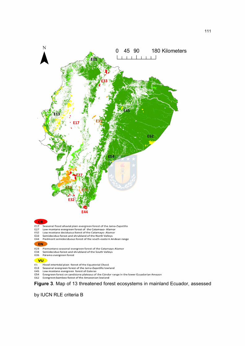
111

Figure 3. Map of 13 threatened forest ecosystems in mainland Ecuador, assessed

by IUCN RLE criteria B

112

Discussion

Many forest systems in Ecuador suffered from human activities and pressure,

particularly in the sub-montane area. However, it is difficult to assess precisely the

local extent of such pressures in terms of their effects on structure and composition

or disappearance of the systems. Our most important, but perhaps least surprising

result is that many tropical Andean forest systems are indeed faced extinction risk

at national and local scales in Ecuador. In the present study, we estimated that

several Tropical Andean forest systems are rapidly changing and probably

disappearing faster than other forest ecosystems. The results suggest that the

success of ecosystem conservation will increase when the merits of a conservation

prioritization system based on the ecological and biogeographic knowledge known

as ecosystem (Harris et al. 2008; Laumonier et al. 2010).

As knowledge of biogeographic zoning at national level is rarely available, previous

studies about RLE focusing on single territorial ecosystems, small areas or regions

reported and assessed a probability of loss or degradation. In northern Venezuela,

Rodrguez et al. (2008) assessed extinction risk categories of tropical dry forests

using historical and current dry forest cover. Likewise, conservation status of

temperate grasslands in southern Africa was estimated by combination of two

landscape-scaled factors: level of protection and degree of land transformation

(Carbutt et al. 2011). However, these results provide limited information to facilitate

identification of critical zones for shaping the national conservation policy. On the

other hands, methods for assessing the threat of extinction of individual ecosystems

113

were not systematized in many of the previous studies. For example, although Sierra

et al. (2002) identified the prioritization among 46 natural ecosystems for the

conservation of Ecuador´s biodiversity using a multi-criteria model, their criteria

(representativeness in the current reserve network, human pressure, habitat loss

and species-level value based on bird species data) associated with developed

model are not directly linked with key symptoms of ecosystem degradation.

Therefore, unlike the results of Sierra et al. (2002) which were found 26 critical

ecosystems, we identified 13 threatened ecosystems; three in the Coast, seven in

the Andes and three in the Amazon.

A central benefit of assessing conservation status of nationwide ecosystems from

systematic method is that policy-makers may become explicitly aware of the spatial

scale at which their policies are implemented or affected between conservation and

development of a given ecosystem. Forest system change is particularly severe in

tropical regions of developing countries under the pressure of strong socio-economic

changes (Geist and Lambin 2002; Lambin et al. 2003; Sanchez-Azofeifa et al. 2001).

To mitigate the dramatic deforestation rate of the country, Ecuadorian government

promoted incentive-based policies for the conservation of native forests, such as the

Socio Bosque program (Cuenca et al. 2018) as well as the establishment of several

protected areas (Cuenca et al. 2016). In the conservation point of view, there are

two concerns on existing forest protection policy. The first one is the NPRN in

Ecuador is not optimized the protection of natural forest ecosystems. For example,

because of higher poverty and a shortage of adult labor, the farms are characterized

by large pasture areas around dwellings, small areas used for subsistence

114

agriculture and forest patches (< 20km2) in South Ecuador. Although threatened or

near threatened forest ecosystems are concentrated in this area, we demonstrated

that the current NPRN coverage does not provide appropriate protection for these

critical ecosystems. Secondly, despite the protected areas seem to be effective for

avoiding or reducing deforestation in Ecuadorian Tropical Andean forests (Cuenca

et al. 2016), it was found that the passive landscape conservation focused on

biodiversity may not be sufficient to maintain forest ecosystems, as land protection

seems to be failed avoiding deforestation in several forest ecosystems (SI 2). Thus,

meanwhile private and community land owners can benefit from a financial incentive

in exchange for conservation of forests through the Socio Bosque Program,

stakeholders and funding agencies now raise the question to what are effective and

efficient for nationwide ecosystem conservation (Andam et al. 2010; Vanacker et al.

2018).

The main challenge to future forest ecosystem conservation is a paucity of explicit

policies for management and use. The role of specific forest ecosystems on

scientific-based ecosystem services can support political justification based on

contribution to human well-being (Wu 2013a). Recognizing provisional ecosystem

services’ supply and demand of a locally-threatened ecosystem may promote

informed decisions regarding investments in protection or restoration (Rodrguez et

al. 2008). Aiming to strengthen conservation, valorization and sustainable use of

natural resources, ecosystem services and biodiversity, ecosystem conservation

strategies may be designed to further achieve environmental sustainability and

territorial development. Thus, such targets, efforts and goals assigned to ecosystem

115

conservation should be updated considering the knowledge and experience gained

by stakeholders and associated institutions participating in management plans.

Our analyses provide the first potential evidence of future loss of tropical Andean

ecosystems in the tropical Andean biodiversity hotspot according to IUCN RLE

criterions. Specific recommendations and more detailed future field studies for the

management of these threatened or near-threatened ecosystems should include; (1)

restoring forest quality and mitigating the trend toward a loss and degradation of

ecosystem, (2) managing soften boundaries or creating buffers around remaining

surface of forests, in order to reduce edge effect and landscape connectivity, (3) one

of the limitations of this study is that mapping of intrinsic threats were restricted at

the scale used (30 m-resolution). With these consideration, we suggest future

research on adaptive capacity of the threatened ecosystems with regard to

anthropogenic (e.g. logging, agriculture, fragmentation) and intrinsic (e.g. forest fire,

flooring, climate change) threats and their synergy, (4) researches to determine the

threshold of resilience and vulnerability of the remaining forest patches in each

ecosystems, (5) promoting off-reserve conservation on privately or communally

owned lands, and (6) identifying and designing adequate landscape configuration

based on the remnant forests to enhance ecosystem persistence and resilience

(Suding et al. 2004; Tambosi and Metzger 2013).

Conclusion

The present analysis of conservation status of forest ecosystems in Ecuador drew

several conclusions: i) only small extent of forest patches remain in several forest

116

system; ii) these forest systems are in danger of complete elimination due to

pressure from human land use, and iii) the official management institutions are

limited with respect to protection of forest ecosystems. This study stands as baseline

for understanding and measuring forest ecosystem change, threats and potential

extinction risk at landscape scale. It complements current conservation efforts and

could contribute to guide land-use planning at local and national scales in mainland

Ecuador.

Acknowledgements

We would like to thank Ministry of Environment of Ecuador for providing a number

of data sources and Laboratorio de Cambio Global (LCG) of Universidad Regional

Amazónica Ikiam for their valuable assistance. J. Noh acknowledges financial

supports from CONICYT (Comisión Nacional de Investigación Científica y

Tecnológica) of Chile, KOICA (Korea International Cooperation Agency) and KNA

(Korea National Arboretum).

Literature

Abdullah, S.A., Nakagoshi, N., 2007. Forest fragmentation and its correlation to

human land use change in the state of Selangor, peninsular Malaysia. Forest Ecology and Management 241, 39-48. Adriaens, D., Honnay, O., Hermy, M., 2006. No evidence of a plant extinction

debt in highly fragmented calcareous grasslands in Belgium. Biological Conservation 133, 212-224.

Aguayo, M., Pauchard, A., Axocar, G., Parra, O., 2009. Cambio del uso del suelo en el centro sur de Chile a fines del siglo XX: Entendiendo la dinámica espacial y temporal del paisaje. Revista Chilena de Historia Natural 82, 361-374.

Allendorf, F.W., Hard, J.J., 2009. Human-induced evolution caused by unnatural selection through harvest of wild animals. Proceedings of the National Academy of Sciences 106, 9987-9994.

117

Altamirano, A., Aplin, P., Miranda, A., Cayuela, L., Algar, A.C., Field, R., 2013. High rates of forest loss and turnover obscured by classical landscape measures. Applied Geography 40, 199-211.

Amelung, T., Diehl, M., 1992. Deforestation of tropical rainforests: economic causes and impact on development.

Andam, K.S., Ferraro, P.J., Sims, K.R.E., Healy, A., Holland, M.B., 2010. Protected areas reduced poverty in Costa Rica and Thailand. Proceedings of the National Academy of Sciences.

Armenteras, D., Gast, F., Villareal, H., 2003. Andean forest fragmentation and the representativeness of protected natural areas in the eastern Andes, Colombia. Biological Conservation 113, 245-256.

Armenteras, D., Rudas, G., Rodriguez, N., Sua, S., Romero, M., 2006. Patterns and causes of deforestation in the Colombian Amazon. ecological indicators 6, 353-368.

Armesto, J., Rozzi, R., Smith-Ramírez, C., Arroyo, M., 1998. Conservation targets in South American temperate forests. America 5, 6.

Armesto, J.J., Villagran, C., Arroyo, M.K., 1996. Ecología de los bosques nativos de Chile. Textos Universitarios/Monografias, Santiago, Universitaria,| c1996, edited by Armesto, Juan J.; Villagran, Carolina; Arroyo, Mary Kalin 1.

Arrhenius, O., 1921. Species and area. Journal of Ecology 9, 95-99. Balmford, A., Mace, G.M., Ginsberg, J.R., 1998. The challenges to conservation in

a changing world: putting processes on the map. Conservation in a Changing World: Integrating Processes into Priorities for Action.

Bass, M.S., Finer, M., Jenkins, C.N., Kreft, H., Cisneros-Heredia, D.F., McCracken, S.F., Pitman, N.C.A., English, P.H., Swing, K., Villa, G.a., 2010. Global conservation significance of Ecuador's Yasun \' i National Park.

Bauhus, J., Puettmann, K., Messier, C., 2009. Silviculture for old-growth attributes. Forest Ecology and Management 258, 525-537.

Bennett, A.F., Nature, I.U.f.C.o., Resources, N., Programme, I.F.C., 2003. Linkages in the Landscape: The Role of Corridors and Connectivity in Wildlife Conservation. IUCN.

Bennett, A.F., Saunders, D.A., 2010. Habitat Fragmentation and Landscape Change. Conservation biology for all.

Bierzychudek, P., 1982. Life histories and demography of shade-tolerant temperate forest herbs: a review. New Phytologist 90, 757-776.

Brandt, J.S., Townsend, P.A., 2006. Land use - Land cover conversion, regeneration and degradation in the high elevation Bolivian Andes. Landscape Ecology.

Brook, B.W., Sodhi, N.S., Bradshaw, C.J.A., 2008. Synergies among extinction drivers under global change. Trends in Ecology & Evolution 23, 453-460.

Brown, D., Schreckenberg, K., 1998. Shifting Cultivators as Agents of Deforestation: Assessing the Evidence. Overseas Development Institute.

Brückmann, S.V., Krauss, J., Steffan-Dewenter, I., 2010. Butterfly and plant specialists suffer from reduced connectivity in fragmented landscapes. Journal of Applied Ecology 47, 799-809.

Bulman, C.R., Wilson, R.J., Holt, A.R., Bravo, L.G., Early, R.I., Warren, M.S., Thomas, C.D., 2007. Minimum viable metapopulation size, extinction debt, and the conservation of a declining species. Ecological Applications 17, 1460-

118

1473. Bustamante, R.O., Simonetti, J.A., 2005. Is Pinus radiata invading the native

vegetation in central Chile? Demographic responses in a fragmented forest. Biological Invasions 7, 243-249.

Butler, B.J., Swenson, J.J., Alig, R.J., 2004. Forest fragmentation in the Pacific Northwest: quantification and correlations. Forest Ecology and Management 189, 363-373.

Cadilhac, L., Torres, R., Calles, J., Vanacker, V., Caldern, E., 2017. Desaf \' i os para la investigaci \' o n sobre el cambio clim \' a tico en Ecuador. Neotropical Biodiversity.

Cain, D.H., Riitters, K., Orvis, K., 1997. A multi-scale analysis of landscape statistics. Landscape Ecology.

Carbutt, C., Tau, M., Stephens, A., Escott, B., 2011. The conservation status of temperate grasslands in southern Africa. Grassroots.

Carruthers, D., Rodriguez, P., 2009. Mapuche protest, environmental conflict and social movement linkage in Chile. Third World Quarterly 30, 743-760.

Cavieres, L.A., Mihoc, M., Marticorena, A., Marticorena, C., MARY, C.M.B.Y., ARROYO, K., 2005. 13. Flora vascular de la Cordillera de la Costa en la región del Biobío: riqueza de especies, géneros, familias y endemismos.

CBD, 2001. Global biodiversity outlook, In UNEP: Nairobi. Chander, G., Markham, B.L., Helder, D.L., 2009. Summary of current radiometric

calibration coefficients for Landsat MSS, TM, ETM+, and EO-1 ALI sensors. Remote sensing of environment 113, 893-903.

Comes, H.P., Kadereit, J.W., 1998. The effect of Quaternary climatic changes on plant distribution and evolution. Trends in plant science 3, 432-438.

CONAF, 1999. Catastro y evaluación de los recursos vegetacionales nativos de Chile, In Informe Nacional con Variables Ambientales. Santiago, Chile.

Cousins, S.A.O., 2009. Extinction debt in fragmented grasslands: paid or not? Journal of Vegetation Science 20, 3-7.

Cousins, S.A.O., Vanhoenacker, D., 2011. Detection of extinction debt depends on scale and specialisation. Biological Conservation 144, 782-787.

Cousins, S.O., Ohlson, H., Eriksson, O., 2007. Effects of historical and present fragmentation on plant species diversity in semi-natural grasslands in Swedish rural landscapes. Landscape Ecology 22, 723-730.

Cox, M.P., Dickman, C.R., Hunter, J., 2004. Effects of rainforest fragmentation on non-flying mammals of the Eastern Dorrigo Plateau, Australia. Biological Conservation 115, 175-189.

Crespin, S.J., Simonetti, J.A., 2015. Predicting ecosystem collapse: Spatial factors that influence risks to tropical ecosystems. Austral Ecology.

Cubina, A., Aide, T.M., 2001. The Effect of Distance from Forest Edge on Seed Rain and Soil Seed Bank in a Tropical Pasture1. Biotropica.

Cuenca, P., Arriagada, R., Echeverría, C., 2016. How much deforestation do protected areas avoid in tropical Andean landscapes? Environmental Science & Policy 56, 56-66.

Cuenca, P., Echeverria, C., 2017a. How do protected landscapes associated with high biodiversity and population levels change? PLoS one.

Cuenca, P., Echeverria, C., 2017b. How do protected landscapes associated with

119

high biodiversity and population levels change? PLoS one 12, e0180537. Cuenca, P., Robalino, J., Arriagada, R., Echeverra, C., 2018. Are government

incentives effective for avoided deforestation in the tropical Andean forest? PLoS one.

Cuesta, F., Peralvo, M., Merino-Viteri, A., Bustamante, M., Baquero, F., Freile, J.F., Muriel, P., Torres-Carvajal, O., 2017. Priority areas for biodiversity conservation in mainland Ecuador. Neotropical Biodiversity.

Dale, V.H., Brown, S., Haeuber, R., Hobbs, N., Huntly, N., Naiman, R., Riebsame, W., Turner, M., Valone, T., 2000. Ecological principles and guidelines for managing the use of land. Ecological Applications 10, 639-670.

Dambrine, E., Ulrich, E., Cénac, N., Durand, P., Gauquelin, T., Mirabel, P., Nys, C., Probst, A., Ranger, J., Zéphoris, M., 1995. Atmospheric Deposition in France and Possible Relation with Forest Decline, In Forest Decline and Atmospheric Deposition Effects in the French Mountains. eds G. Landmann, M. Bonneau, M. Kaennel, pp. 177-200. Springer Berlin Heidelberg.

Davies, K.F., Margules, C.R., Lawrence, J.F., 2004. A synergistic effect puts rare, specialized species at greater risk of extinction. Ecology 85, 265-271.

Devictor, V., Julliard, R., Jiguet, F., 2008. Distribution of specialist and generalist species along spatial gradients of habitat disturbance and fragmentation. Oikos 117, 507-514.

Diamond, J.M., 1975. The island dilemma: lessons of modern biogeographic studies for the design of natural reserves. Biological Conservation 7, 129-146.

Donoso, C., Spurr, S., Ambasht, R., Dansereau, P., Sierra Pineda, A., Vázquez Soto, J., Rodríguez Trejo, D., 2006. Las especies arbóreas de los bosques templados de Chile y Argentina autoecología. Cartilla-Servicio Autónomo Forestal Venezolano.

Donoso Zegers, C., 1993. Bosques templados de Chile y Argentina: variación, estructura y dinámica.

Dullinger, S., Essl, F., Rabitsch, W., Erb, K.-H., Gingrich, S., Haberl, H., Hülber, K., Jarošík, V., Krausmann, F., Kühn, I., 2013. Europe’s other debt crisis caused by the long legacy of future extinctions. Proceedings of the National Academy of Sciences 110, 7342-7347.

Dullinger, S., Gattringer, A., Thuiller, W., Moser, D., Zimmermann, N.E., Guisan, A., Willner, W., Plutzar, C., Leitner, M., Mang, T., 2012. Extinction debt of high-mountain plants under twenty-first-century climate change. Nature Climate Change 2, 619-622.

Duraiappah, A.K., Naeem, S., 2005. Millennium Ecosystem Assessment, 2005. Echeverria, C., Coomes, D., Salas, J., Rey-Benayas, J.M., Lara, A., Newton, A.,

2006a. Rapid deforestation and fragmentation of Chilean Temperate Forests. Biological Conservation 130, 481-494.

Echeverria, C., Coomes, D., Salas, J., Rey-Benayas, J.M., Lara, A., Newton, A., 2006b. Rapid deforestation and fragmentation of Chilean Temperate Forests. Biological Conservation.

Echeverría, C., Newton, A., Nahuelhual, L., Coomes, D., Rey-Benayas, J.M., 2012. How landscapes change: Integration of spatial patterns and human processes in temperate landscapes of southern Chile. Applied Geography 32, 822-831.

Echeverría, C., Newton, A.C., Lara, A., Benayas, J.M.R., Coomes, D.A., 2007.

120

Impacts of forest fragmentation on species composition and forest structure in the temperate landscape of southern Chile. Global Ecology and Biogeography 16, 426-439.

Ecuador, M.d.A.d., 2013. Sistema de Clasificación de los Ecosistemas del Ecuador Continental. Subsecretaría de Patrimonio Natural. Quito.

Fahrig, L., 1998. When does fragmentation of breeding habitat affect population survival? Ecological modelling 105, 273-292.

Fahrig, L., 2002. EFFECT OF HABITAT FRAGMENTATION ON THE EXTINCTION THRESHOLD: A SYNTHESIS. Ecological Applications 12, 346-353.

Fajardo, L., Gonzlez, V., Nassar, J.M., Lacabana, P.a., 2005. Tropical dry forests of Venezuela: Characterization and current conservation status. Biotropica.

Fao, 2014. State of the world's forests. Enhancing the socioeconomic benefits from forests.

Fazey, I., Fischer, J., Lindenmayer, D.B., 2005. What do conservation biologists publish? Biological Conservation 124, 63-73.

Fischer, J., Lindenmayer, D.B., 2007. Landscape modification and habitat fragmentation: a synthesis. Global Ecology and Biogeography 16, 265-280.

Forman, R.T.T., Godron, M., 1986. Landscape Ecology. Wiley. Gaglio, M., Aschonitis, V.G., Mancuso, M.M., Puig, J.P.R., Moscoso, F., Castaldelli,

G., Fano, E.A., 2017. Changes in land use and ecosystem services in tropical forest areas: A case study in Andes mountains of Ecuador. International Journal of Biodiversity Science, Ecosystem Services and Management.

García, D., Rodríguez-Cabal, M.A., Amico, G.C., 2009. Seed dispersal by a frugivorous marsupial shapes the spatial scale of a mistletoe population. Journal of Ecology 97, 217-229.

Gaston, K.J., Blackburn, T.M., Lawton, J.H., 1997. Interspecific abundance-range size relationships: an appraisal of mechanisms. Journal of Animal Ecology, 579-601.

Gaston, K.J., Spicer, J.I., 2013. Biodiversity: an introduction. John Wiley & Sons. Geist, H.J., Lambin, E.F., 2002. Proximate causes and underlying driving forces of

tropical deforestation: Tropical forests are disappearing as the result of many pressures, both local and regional, acting in various combinations in different geographical locations. BioScience 52, 143-150.

Gilbert, B., Levine, J.M., 2013. Plant invasions and extinction debts. Proceedings of the National Academy of Sciences 110, 1744-1749.

Gmez, A., Anaya, J., Alvarez, E., 2005. An \' a lisis De Fragmentaci \' o n De Los Ecosistemas Boscosos En Una Regi \' o n De La Cordillera Central De Los Andes Colombianos. Revista ingenier \' i as Universidad de Medell \' i n.

Gómez Mora, A.M., Anaya, J.A., Álvarez Dávila, E., 2005. Análisis de fragmentación de los ecosistemas boscosos en una región de la cordillera central de los andes colombianos. Revista Ingenierías Universidad de Medellín 4.

González, M.E., Veblen, T.T., 2006. Climatic influences on fire in Araucaria araucana-Nothofagus forests in the Andean cordillera of south-central Chile. Ecoscience 13, 342-350.

Gregory, R.D., Van Strien, A., Vorisek, P., Meyling, A.W.G., Noble, D.G., Foppen, R.P., Gibbons, D.W., 2005. Developing indicators for European birds. Philosophical Transactions of the Royal Society of London B: Biological

121

Sciences 360, 269-288. Grez, A.A., Smith-Ramírez, C., Armesto, J., Valdovinos, C., 2005. El valor de los

fragmentos pequeños de bosque maulino en la conservación de la fauna de coleópteros epigeos. Historia, biodiversidad y ecología de los bosques de la Cordillera de la Costa, 565-572.

Gustavsson, E., Lennartsson, T., Emanuelsson, M., 2007. Land use more than 200years ago explains current grassland plant diversity in a Swedish agricultural landscape. Biological Conservation 138, 47-59.

Haila, Y., 2002. A conceptual genealogy of fragmentation research: from island biogeography to landscape ecology*. Ecological Applications 12, 321-334.

Hanski, I., 2000. Extinction debt and species credit in boreal forests: modelling the consequences of different approaches to biodiversity conservation, In Annales Zoologici Fennici. pp. 271-280. JSTOR.

Hanski, I., Moilanen, A., Gyllenberg, M., 1996. Minimum viable metapopulation size. American Naturalist, 527-541.

Hanski, I., Ovaskainen, O., 2002. Extinction Debt at Extinction Threshold. Conservation Biology 16, 666-673.

Harris, N.L., Petrova, S., Stolle, F., Brown, S., 2008. Identifying optimal areas for REDD intervention: East Kalimantan, Indonesia as a case study. Environmental Research Letters.

Harrison, S., 1999. Local and regional diversity in a patchy landscape: native, alien, and endemic herbs on serpentine. Ecology 80, 70-80.

Helm, A., Hanski, I., Pärtel, M., 2006. Slow response of plant species richness to habitat loss and fragmentation. Ecology letters 9, 72-77.

Hinojosa, L.F., Villagrán, C., 1997. Historia de los bosques del sur de Sudamérica, I: antecedentes paleobotánicos, geológicos y climáticos del Terciario del cono sur de América. Revista Chilena de Historia Natural 70, 225-240.

Hobbs, R.J., Higgs, E., Harris, J.A., 2009. Novel ecosystems: implications for conservation and restoration. Trends in Ecology and Evolution.

Holl, K.D., Aide, T.M., 2011. When and where to actively restore ecosystems? Forest Ecology and Management 261, 1558-1563.

Holl, K.D., Loik, M.E., Lin, E.H.V., Samuels, I.A., 2000. Tropical montane forest restoration in Costa Rica: Overcoming barriers to dispersal and establishment. Restoration Ecology.

Honnay, O., Hermy, M., Coppin, P., 1999. Effects of area, age and diversity of forest patches in Belgium on plant species richness, and implications for conservation and reforestation. Biological Conservation 87, 73-84.

Huete, A.R., 1988. A soil-adjusted vegetation index (SAVI). Remote sensing of environment 25, 295-309.

Hughes, J.B., Daily, G.C., Ehrlich, P.R., 2000. Conservation of insect diversity: a habitat approach. Conservation Biology 14, 1788-1797.

Huth, N., Possingham, H.P., 2011. Basic ecological theory can inform habitat restoration for woodland birds. Journal of Applied Ecology 48, 293-300.

Ibez, I., Katz, D.S.W., Peltier, D., Wolf, S.M.a., 2014. Assessing the integrated effects of landscape fragmentation on plants and plant communities: The challenge of multiprocess-multiresponse dynamics. Journal of Ecology.

IUCN, 2017. The IUCN Red List of Threatened Species. Version 2017-3. , In 05

122

December 2017. http://www.iucnredlist.org. Iucn, 2018. the IUCN red list of threatened species. Jamil, T., Kruk, C., ter Braak, C.J., 2014. A unimodal species response model

relating traits to environment with application to phytoplankton communities. Jamoneau, A., Sonnier, G., Chabrerie, O., Closset-Kopp, D., Saguez, R., Gallet-

Moron, E., Decocq, G., 2011. Drivers of plant species assemblages in forest patches among contrasted dynamic agricultural landscapes. Journal of Ecology 99, 1152-1161.

Jimnez, L., Gusmn, J., Capa-Mora, D., Quichimbo, P., Mezquida, E., Benito, M., Rubio, A., 2017. Riqueza y diversidad vegetal en un bosque siempreverde piemontano en los Andes del sur del Ecuador. Bosques Latitud Cero 7.

Jonsen, I.D., Fahrig, L., 1997. Response of generalist and specialist insect herbivores to landscape spatial structure. Landscape Ecology 12, 185-197.

Keith, D.A., Rodrguez, J.P., Brooks, T.M., Burgman, M.A., Barrow, E.G., Bland, L., Comer, P.J., Franklin, J., Link, J., McCarthy, M.A., Miller, R.M., Murray, N.J., Nel, J., Nicholson, E., Oliveira-Miranda, M.A., Regan, T.J., Rodrguez-Clark, K.M., Rouget, M., Spalding, M.D., 2015. The IUCN red list of ecosystems: Motivations, challenges, and applications. Conservation Letters.

Keith, D.A., Rodrguez, J.P., Rodrguez-Clark, K.M., Nicholson, E., Aapala, K., Alonso, A., Asmussen, M., Bachman, S., Basset, A., Barrow, E.G., Benson, J.S., Bishop, M.J., Bonifacio, R., Brooks, T.M., Burgman, M.A., Comer, P., Comn, F.A., Essl, F., Faber-Langendoen, D., Fairweather, P.G., Holdaway, R.J., Jennings, M., Kingsford, R.T., Lester, R.E., Nally, R.M., McCarthy, M.A., Moat, J., Oliveira-Miranda, M.A., Pisanu, P., Poulin, B., Regan, T.J., Riecken, U., Spalding, M.D., Zambrano-Martnez, S., 2013. Scientific Foundations for an IUCN Red List of Ecosystems. PLoS one.

Kerr, J.T., Ostrovsky, M., 2003. From space to species: ecological applications for remote sensing. Trends in Ecology & Evolution 18, 299-305.

Koh, L.P., Sodhi, N.S., Brook, B.W., 2004. Ecological correlates of extinction proneness in tropical butterflies. Conservation Biology 18, 1571-1578.

Kolb, A., Diekmann, M., 2005. Effects of Life-History Traits on Responses of Plant Species to Forest Fragmentation

Efectos de las Características de la Historia de Vida Sobre las Respuestas de Especies de Plantas a la Fragmentación de Bosques. Conservation Biology 19, 929-938.

Kolk, J., Naaf, T., 2015. Herb layer extinction debt in highly fragmented temperate forests – Completely paid after 160 years? Biological Conservation 182, 164-172.

Krauss, J., Bommarco, R., Guardiola, M., Heikkinen, R.K., Helm, A., Kuussaari, M., Lindborg, R., Öckinger, E., Pärtel, M., Pino, J., 2010. Habitat fragmentation causes immediate and time-delayed biodiversity loss at different trophic levels. Ecology letters 13, 597-605.

Kuussaari, M., Bommarco, R., Heikkinen, R.K., Helm, A., Krauss, J., Lindborg, R., Öckinger, E., Pärtel, M., Pino, J., Rodà, F., Stefanescu, C., Teder, T., Zobel, M., Steffan-Dewenter, I., 2009. Extinction debt: a challenge for biodiversity conservation. Trends in Ecology & Evolution 24, 564-571.

kyoung Noh, J., Echeverra, C., Pauchard, A., Cuenca, P., 2018. Extinction debt in a

123

biodiversity hotspot: the case of the Chilean Winter Rainfall-Valdivian Forests. Lambin, E.F., Geist, H.J., Lepers, E., 2003. Dynamics of land-use and land-cover

change in tropical regions. Annual review of environment and resources 28, 205-241.

Lara, A., Araya, L., Capella, J., Fierro, M., Cavieres, A., 1989. Evaluación de la destrucción y disponibilidad de los recursos forestales nativos en la VII y VIII Región. Informe Técnico, Comité Pro Defensa Fauna y Flora, Santiago, Chile.

Laumonier, Y., Uryu, Y., Stwe, M., Budiman, A., Setiabudi, B., Hadian, O., 2010. Eco-floristic sectors and deforestation threats in Sumatra: Identifying new conservation area network priorities for ecosystem-based land use planning. Biodiversity and Conservation.

Laurance, W.F., Lovejoy, T.E., Vasconcelos, H.L., Bruna, E.M., Didham, R.K., Stouffer, P.C., Gascon, C., Bierregaard, R.O., Laurance, S.G., Sampaio, E., 2002. Ecosystem decay of Amazonian forest fragments: a 22-year investigation. Conservation Biology 16, 605-618.

Lenoir, J., Gégout, J., Marquet, P., De Ruffray, P., Brisse, H., 2008. A significant upward shift in plant species optimum elevation during the 20th century. Science 320, 1768-1771.

León, S., Valencia, R., Pitman, N., Endara, L., Ulloa, C., Navarrete, H., 2011. Libro rojo de las plantas endémicas del Ecuador. Publicaciones del Herbario QCA, Pontificia Universidad Católica del Ecuador, Quito.

Lesaffre, E., Marx, B.D., 1993. Collinearity in generalized linear regression. Communications in Statistics-Theory and Methods 22, 1933-1952.

Lessmann, J., Fajardo, J., Mu±oz, J., Bonaccorso, E., 2016. Large expansion of oil industry in the Ecuadorian Amazon: biodiversity vulnerability and conservation alternatives. Ecology and Evolution.

Lessmann, J., Muoz, J., Bonaccorso, E., 2014. Maximizing species conservation in continental Ecuador: A case of systematic conservation planning for biodiverse regions. Ecology and Evolution.

Letcher, S.G., Chazdon, R.L., 2009. Lianas and self-supporting plants during tropical forest succession. Forest Ecology and Management.

Li, H., Wu, J., 2004. Use and misuse of landscape indices. Landscape Ecology 19, 389-399.

Liebhold, A., Gurevitch, J., 2002. Integrating the statistical analysis of spatial data in ecology. Ecography 25, 553-557.

Lienert, J., 2004. Habitat fragmentation effects on fitness of plant populations – a review. Journal for Nature Conservation 12, 53-72.

Lindborg, R., 2007. Evaluating the distribution of plant life-history traits in relation to current and historical landscape configurations. Journal of Ecology 95, 555-564.

Lindborg, R., Eriksson, O., 2004. HISTORICAL LANDSCAPE CONNECTIVITY AFFECTS PRESENT PLANT SPECIES DIVERSITY. Ecology 85, 1840-1845.

Lindenmayer, D.B., Fischer, J., 2006. Habitat fragmentation and landscape change: an ecological and conservation synthesis. Island Press.

Lindenmayer, D.B., Fischer, J., 2013. Habitat fragmentation and landscape change: an ecological and conservation synthesis. Island Press.

López-Barrera, F., 2004. Estructura y función en bordes de bosques. Revista

124

Ecosistemas 13. Loreau, M., Naeem, S., Inchausti, P., Bengtsson, J., Grime, J., Hector, A., Hooper,

D., Huston, M., Raffaelli, D., Schmid, B., 2001. Biodiversity and ecosystem functioning: current knowledge and future challenges. Science 294, 804-808.

Luebert, F., Pliscoff, P., 2006. Sinopsis bioclimática y vegetacional de Chile. Editorial Universitaria.

Lusk, C.H., Pozo, A.D., 2002. Survival and growth of seedlings of 12 Chilean rainforest trees in two light environments: gas exchange and biomass distribution correlates. Austral Ecology 27, 173-182.

Marchelli, P., Smouse, P.E., Gallo, L.A., 2012. Short-distance pollen dispersal for an outcrossed, wind-pollinated southern beech (Nothofagus nervosa (Phil.) Dim. et Mil.). Tree genetics & genomes 8, 1123-1134.

Matlack, G.R., 1994. Vegetation dynamics of the forest edge--trends in space and successional time. Journal of Ecology, 113-123.

McGarigal, K., Cushman, S.A., Neel, M.C., Ene, E., 2002. FRAGSTATS: spatial pattern analysis program for categorical maps.

McIntyre, N., Wiens, J., 1999. Interactions between landscape structure and animal behavior: the roles of heterogeneously distributed resources and food deprivation on movement patterns. Landscape Ecology 14, 437-447.

McIntyre, S., Hobbs, R., 1999. A Framework for Conceptualizing Human Effects on Landscapes and Its Relevance to Management and Research Models

Marco para la Conceptualización de los Efectos Humanos en Paisajes y su Relevancia en Modelos de Manejo y Investigación. Conservation Biology 13, 1282-1292.

Mena, C.F., 2008a. Trajectories of Land-use and Land-cover in the Northern Ecuadorian Amazon. Photogrammetric Engineering & Remote Sensing 74, 737-751.

Mena, C.F., 2008b. Trajectories of Land-use and Land-cover in the Northern Ecuadorian Amazon: Temporal Composition, Spatial Configuration, and Probability of Change. Photogrammetric Engineering \& Remote Sensing.

Mildén, M., Cousins, S.A., Eriksson, O., 2007. The distribution of four grassland plant species in relation to landscape history in a Swedish rural area, In Annales Botanici Fennici. pp. 416-426. JSTOR.

Miles, L., Newton, A.C., DeFries, R.S., Ravilious, C., May, I., Blyth, S., Kapos, V., Gordon, J.E., 2006. A global overview of the conservation status of tropical dry forests. Journal of Biogeography 33, 491-505.

Mittermeier, R.A., Myers, N., Tliomsen, J.B., Olivieri, S., 1998. Biodiversity hotspots and major tropical wilderness areas: Approaches to setting conservation priorities.

Moran, P.A., 1950. Notes on continuous stochastic phenomena. Biometrika 37, 17-23.

Myers, N., Mittermeier, R.A., Mittermeier, C.G., Da Fonseca, G.A., Kent, J., 2000a. Biodiversity hotspots for conservation priorities. Nature 403, 853-858.

Myers, N., Mittermeier, R.A., Mittermeier, C.G., da Fonseca, G.A.B., Kent, J., 2000b. Biodiversity hotspots for conservation priorities. Nature 403, 853-858.

Myster, R.W., 2004. Post-Agricultural Invasion, Establishment, and Growth of Neotropical Trees. The Botanical Review.

125

Nagendra, H., Paul, S., Pareeth, S., Dutt, S., 2009. Landscapes of protection: forest change and fragmentation in Northern West Bengal, India. Environmental Management 44, 853-864.

Olson, D.M., Dinerstein, E., 2002. The Global 200: Priority Ecoregions for Global Conservation. Annals of the Missouri Botanical Garden.

Öster, M., Cousins, S.A., Eriksson, O., 2007. Size and heterogeneity rather than landscape context determine plant species richness in semi-natural grasslands. Journal of Vegetation Science 18, 859-868.

Otavo, S., Echeverría, C., 2017. Fragmentación progresiva y pérdida de hábitat de bosques naturales en uno de los hotspot mundiales de biodiversidad. Revista Mexicana de Biodiversidad 88, 924-935.

Ouborg, N., Vergeer, P., Mix, C., 2006. The rough edges of the conservation genetics paradigm for plants. Journal of Ecology 94, 1233-1248.

Ovaskainen, O., Hanski, I., 2002. Transient dynamics in metapopulation response to perturbation. Theoretical Population Biology 61, 285-295.

Ovaskainen, O., Hanski, I., 2004. From individual behavior to metapopulation dynamics: unifying the patchy population and classic metapopulation models. The American Naturalist 164, 364-377.

Owen, E., 2007. Informe final: Una evaluacion rapida de la biodiversidad de dos predios integrados a la Red Conservacionista del Patrimonio Natural de Contulmo.

Owens, I.P., Bennett, P.M., 2000. Ecological basis of extinction risk in birds: habitat loss versus human persecution and introduced predators. Proceedings of the National Academy of Sciences 97, 12144-12148.

Paltto, H., Nordén, B., Götmark, F., Franc, N., 2006. At which spatial and temporal scales does landscape context affect local density of Red Data Book and Indicator species? Biological Conservation 133, 442-454.

Piessens, K., Hermy, M., 2006. Does the heathland flora in north-western Belgium show an extinction debt? Biological Conservation 132, 382-394.

Piqueray, J., Bisteau, E., Cristofoli, S., Palm, R., Poschlod, P., Mahy, G., 2011. Plant species extinction debt in a temperate biodiversity hotspot: Community, species and functional traits approaches. Biological Conservation 144, 1619-1629.

Polus, E., Vandewoestijne, S., Choutt, J., Baguette, M., 2007. Tracking the effects of one century of habitat loss and fragmentation on calcareous grassland butterfly communities. Biodiversity and Conservation 16, 3423-3436.

Pontius, R.G., Shusas, E., McEachern, M., 2004. Detecting important categorical land changes while accounting for persistence. Agriculture, Ecosystems and Environment.

Potthast, K., Hamer, U., Makeschin, F.J.S.B., Biochemistry, 2010. Impact of litter quality on mineralization processes in managed and abandoned pasture soils in Southern Ecuador. 42, 56-64.

Puyravaud, J.-P., 2003. Standardizing the calculation of the annual rate of deforestation. Forest Ecology and Management 177, 593-596.

Ranius, T., Eliasson, P., Johansson, P., 2008. Large-scale occurrence patterns of red-listed lichens and fungi on old oaks are influenced both by current and historical habitat density. Biodiversity and Conservation 17, 2371-2381.

126

Redpath, S.M., Young, J., Evely, A., Adams, W.M., Sutherland, W.J., Whitehouse, A., Amar, A., Lambert, R.A., Linnell, J.D., Watt, A.J.T.i.e., evolution, 2013. Understanding and managing conservation conflicts. 28, 100-109.

Reese, H., Olsson, H., 2011. C-correction of optical satellite data over alpine vegetation areas: A comparison of sampling strategies for determining the empirical c-parameter. Remote sensing of environment 115, 1387-1400.

Reitalu, T., Purschke, O., Johansson, L.J., Hall, K., Sykes, M.T., Prentice, H.C., 2012. Responses of grassland species richness to local and landscape factors depend on spatial scale and habitat specialization. Journal of Vegetation Science 23, 41-51.

Reyers, B., Rouget, M., Jonas, Z., Cowling, R.M., Driver, A., Maze, K., Desmet, P., 2007. Developing products for conservation decision-making: Lessons from a spatial biodiversity assessment for South Africa. Diversity and Distributions.

Riitters, K.H., Wickham, J.D., 2012. Decline of forest interior conditions in the conterminous United States. Scientific Reports.

Riitters, K.H., Wickham, J.D., Wade, T.G., 2009. An indicator of forest dynamics using a shifting landscape mosaic. ecological indicators.

Robledo-Arnuncio, J.J., Klein, E.K., Muller-Landau, H.C., Santamaría, L., 2014. Space, time and complexity in plant dispersal ecology. Movement ecology 2.

Rodrguez, J.P., Nassar, J.M., Rodrguez-Clark, K.M., Zager, I., Portillo-Quintero, C.A., Carrasquel, F., Zambrano, S., 2008. Tropical dry forests in Venezuela: Assessing status, threats and future prospects. Environmental conservation.

Rodrguez, J.P., Rodrguez-Clark, K.M., Keith, D.A., Barrow, E.G., Benson, J.S., Nicholson, E., Wit, P., 2012. IUCN Red List of Ecosystems. Sapiens.

Rodrguez, J.P., Taber, A.B., Daszak, P., Sukumar, R., Valladares-Padua, C., Padua, S., Aguirre, L.F., Medelln, R.A., Acosta, M., Aguirre, A.A., Bonacic, C., Bordino, P., Bruschini, J., Buchori, D., Gonzlez, S., Mathew, T., Mndez, M., Mugica, L., Pacheco, L.F., Dobson, A.P., Pearl, M., 2007. Environment. Globalization of conservation: A view from the south.

Rodríguez Eraso, N., Armenteras-Pascual, D., Alumbreros, J.R., 2013. Land use and land cover change in the Colombian Andes: dynamics and future scenarios. Journal of Land Use Science 8, 154-174.

Rosenzweig, M.L., 1995. Species diversity in space and time. Cambridge University Press.

Rouse Jr, J.W., Haas, R., Schell, J., Deering, D., 1974. Monitoring vegetation systems in the Great Plains with ERTS.

Sala, O.E., Chapin, F.S., Armesto, J.J., Berlow, E., Bloomfield, J., Dirzo, R., Huber-Sanwald, E., Huenneke, L.F., Jackson, R.B., Kinzig, A., 2000. Global biodiversity scenarios for the year 2100. Science 287, 1770-1774.

Sanchez-Azofeifa, G., Harriss, R.C., Skole, D.L., 2001. Deforestation in Costa Rica: A quantitative analysis using remote sensing imagery. Biotropica.

Sang, A., Teder, T., Helm, A., Pärtel, M., 2010. Indirect evidence for an extinction debt of grassland butterflies half century after habitat loss. Biological Conservation 143, 1405-1413.

Saunders, D.A., Hobbs, R.J., Margules, C.R., 1991. Biological consequences of ecosystem fragmentation: a review. Conservation Biology 5, 18-32.

Saura, S., Torn, 2009. Conefor Sensinode 2.2: A software package for quantifying

127

the importance of habitat patches for landscape connectivity. Environmental Modelling and Software.

Schemske, D.W., Willson, M.F., Melampy, M.N., Miller, L.J., Verner, L., Schemske, K.M., Best, L.B., 1978. Flowering ecology of some spring woodland herbs. Ecology 59, 351-366.

Schmidt, K., 1996. Rare habitats vie for protection: a new approach to saving biological diversity focuses on beleaguered ecosystems even if they do not house an extraordinary number fo plant and animal species. Science 274, 916-919.

Senz, M., Onofa, 2005. Reporte de los ecosistemas terrestres ecuatoriano, Indicadores de biodiversidad para su uso nacional. Ministerio de Ambiente de Ecuador y Ecociencia.

Sheil, D., Burslem, D.F., 2003. Disturbing hypotheses in tropical forests. Trends in Ecology & Evolution 18, 18-26.

Sierra, R., 1999a. Vegetación Remanente del Ecuador Continental Scale: 1: 1,000,000 Proyecto 426 INEFAN/GEF-BIRF. Wildlife Conservation Society and EcoCiencia, Quito—Ecuador.

Sierra, R., 1999b. Vegetacion Remanente del Ecuador Continental. Scale 1: 1.000. 000. Proyecto INEFAN/GEF-BIRF, Wildlife Conservation Society and EcoCiencia, Quito.

Sierra, R., Campos, F., Chamberlin, J., 2002. Assessing biodiversity conservation priorities: ecosystem risk and representativeness in continental Ecuador. Landscape and Urban Planning 59, 95-110.

Sierra, R., Stallings, J., 1998. The dynamics and social organization of tropical deforestation in Northwest Ecuador, 1983-1995. Human Ecology 26, 135-161.

Soille, P., Vogt, P., 2009. Morphological segmentation of binary patterns. Pattern Recognition Letters.

Suding, K.N., Gross, K.L., Houseman, G.R., 2004. Alternative states and positive feedbacks in restoration ecology. Trends in Ecology & Evolution 19, 46-53.

Suding, K.N., Hobbs, R.J., 2009. Threshold models in restoration and conservation: a developing framework. Trends in Ecology & Evolution 24, 271-279.

Tambosi, L.R., Metzger, J.P., 2013. A framework for setting local restoration priorities based on landscape context. Natureza & Conservação. This issue.

Tapia-Armijos, M.F., Homeier, J., Espinosa, C.I., Leuschner, C., de la Cruz, M., 2015. Deforestation and forest fragmentation in South Ecuador since the 1970s–losing a hotspot of biodiversity. PLoS one 10, e0133701.

Ter Braak, C.J., Barendregt, L.G., 1986. Weighted averaging of species indicator values: its efficiency in environmental calibration. Mathematical Biosciences 78, 57-72.

ter Braak, C.J., Looman, C.W., 1986. Weighted averaging, logistic regression and the Gaussian response model. Vegetatio 65, 3-11.

Tilman, D., May, R.M., Lehman, C.L., Nowak, M.A., 1994. Habitat destruction and the extinction debt. Nature 371, 65-66.

Tilman, J.G.D., 1990. Perspectives on Plant Competition: Some Introductory Remarks. Perspectives on plant competition, 3.

Tozer, M.G., Leishman, M.R., Auld, T.D., 2015. Ecosystem risk assessment for C

128

umberland P lain W oodland, N ew S outh W ales, A ustralia. Austral Ecology 40, 400--410.

Turner, B.L., 2010a. Vulnerability and resilience: coalescing or paralleling approaches for sustainability science? Global Environmental Change 20, 570-576.

Turner, M.G., 2010b. Disturbance and landscape dynamics in a changing world. Ecology 91, 2833-2849.

Turner, M.G., Gardner, R.H., O'neill, R.V., 2001. Landscape ecology in theory and practice: pattern and process. Springer Science & Business Media.

Turner, M.G., Gardner, R.H., O'Neill, R.V., 2003. Landscape Ecology in Theory and Practice: Pattern and Process. Springer New York.

Valencia, R., Balslev, H., Paz Y Miño C, G., 1994. High tree alpha-diversity in Amazonian Ecuador. Biodiversity and Conservation 3, 21-28.

Valiente-Banuet, A., Aizen, M.A., Alcántara, J.M., Arroyo, J., Cocucci, A., Galetti, M., García, M.B., García, D., Gómez, J.M., Jordano, P., 2015. Beyond species loss: the extinction of ecological interactions in a changing world. Functional Ecology 29, 299-307.

Vanacker, V., Molina, A., Torres, R., Calderon, E., 2018. Challenges for research on global change in mainland Ecuador. Neotropical Biodiversity 4, 113--117.

Vellend, M., Verheyen, K., Jacquemyn, H., Kolb, A., Van Calster, H., Peterken, G., Hermy, M., 2006. Extinction debt of forest plants persists for more than a century following habitat fragmentation. Ecology 87, 542-548.

Vergara, P.M., Smith, C., Delpiano, C.A., Orellana, I., Gho, D., Vazquez, I., 2010. Frugivory on Persea lingue in temperate Chilean forests: interactions between fruit availability and habitat fragmentation across multiple spatial scales. Oecologia 164, 981-991.

Vogt, P., 2018. Measuring Forest Area Density to quantify Forest Fragmentation. (Available in the free JRC software GuidosToolbox). European Commission, http //ies--ows.jrc.ec.europa.eu/gtb/GTB/psheets/GT.

Warren, M., Hill, J., Thomas, J., Asher, J., Fox, R., Huntley, B., Roy, D., Telfer, M., Jeffcoate, S., Harding, P., 2001. Rapid responses of British butterflies to opposing forces of climate and habitat change. Nature 414, 65-69.

Wiens, J.A., Moss, M.R., 2005. Issues and perspectives in landscape ecology. Cambridge University Press.

Winfree, R., Dushoff, J., Crone, E.E., Schultz, C.B., Budny, R.V., Williams, N.M., Kremen, C., 2005. Testing simple indices of habitat proximity. The American Naturalist 165, 707-717.

Wolodarsky-Franke, A., Herrera, S.D., 2011. Cordillera de Nahuelbuta. Reserva mundial de biodiversidad. Valdivia: WWF.

Wu, J., 2013a. Landscape sustainability science: ecosystem services and human well-being in changing landscapes. Landscape Ecology 28, 999-1023.

Wu, J., 2013b. Landscape sustainability science: Ecosystem services and human well-being in changing landscapes. Landscape Ecology.

Wulf, M., Kolk, J., 2014. Plant species richness of very small forests related to patch configuration, quality, heterogeneity and history. Journal of Vegetation Science 25, 1267-1277.

Wunder, S., 2000. Deforestation: the Poor Man's Lot? The Economics of

129

Deforestation, 141--163. Young, A., Boyle, T., Brown, T., 1996. The population genetic consequences of

habitat fragmentation for plants. Trends in Ecology & Evolution 11, 413-418. Young, A.G., Clarke, G.M., 2000. Genetics, demography and viability of fragmented

populations. Cambridge University Press. Zahawi, R.A., Augspurger, C.K., 1999. Early plant succession in abandoned

pastures in Ecuador. Biotropica.

Annex

A1. Spatial scale (nation-region-ecoregion-ecosystem) of the system under study

and 64 forest ecosystems of continental Ecuador

Region Ecoregion Code Forest Ecosystems (forest vegetation type) Altitudinal

range (m)

COAST Equatorial-

Chocó

E1 Flood alluvial plain forest of the Equatorial Chocó 50-200

E2 Equatorial Chocó mangrove 0-20

E3 Evergreen forest of the Equatorial Chocó lowland 0-300

E4 Flood intertidal plain forest of the Equatorial Chocó 0-50

E5 Seasonal evergreen forest of Equatorial Chocó lowlands 0-300

E6 Piedmont seasonal evergreen forest of the Chocó coastal range 200-400

E7 Low montane evergreen forest of Chocó coastal range >400

Equatorial-

Pacific

E8 Semideciduous forest of the Jama-Zapotillo lowland 0-300

E9 Semideciduous forest of the Equatorial Pacific coastal range >200

E10 Low forest and deciduous shrubland of the Jama-Zapotillo lowland 0-400

E11 Piedmont seasonal evergreen forest of the Equatorial Pacific coastal

range 200-400

E12 Low montane seasonal evergreen forest of the Equatorial Pacific coastal

range 400-860

E13 Seasonal evergreen forest of the Jama-Zapotillo lowland 0-400

E14 Deciduous forest of the Jama-Zapotillo lowland 0-400

E15 Deciduous forest of the Equatorial Pacific coastal range >200

E16 Jama-Zapotillo mangrove 0-10

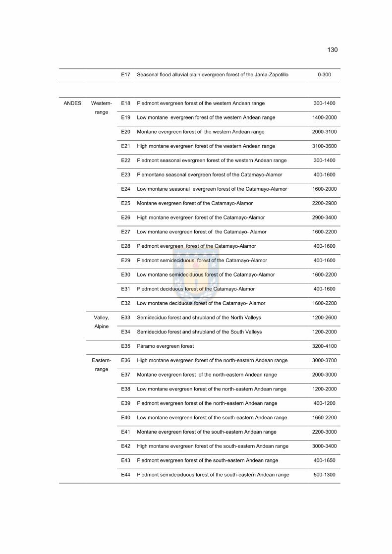
130

E17 Seasonal flood alluvial plain evergreen forest of the Jama-Zapotillo 0-300

ANDES Western-

range

E18 Piedmont evergreen forest of the western Andean range 300-1400

E19 Low montane evergreen forest of the western Andean range 1400-2000

E20 Montane evergreen forest of the western Andean range 2000-3100

E21 High montane evergreen forest of the western Andean range 3100-3600

E22 Piedmont seasonal evergreen forest of the western Andean range 300-1400

E23 Piemontano seasonal evergreen forest of the Catamayo-Alamor 400-1600

E24 Low montane seasonal evergreen forest of the Catamayo-Alamor 1600-2000

E25 Montane evergreen forest of the Catamayo-Alamor 2200-2900

E26 High montane evergreen forest of the Catamayo-Alamor 2900-3400

E27 Low montane evergreen forest of the Catamayo- Alamor 1600-2200

E28 Piedmont evergreen forest of the Catamayo-Alamor 400-1600

E29 Piedmont semideciduous forest of the Catamayo-Alamor 400-1600

E30 Low montane semideciduous forest of the Catamayo-Alamor 1600-2200

E31 Piedmont deciduous forest of the Catamayo-Alamor 400-1600

E32 Low montane deciduous forest of the Catamayo- Alamor 1600-2200

Valley,

Alpine

E33 Semideciduo forest and shrubland of the North Valleys 1200-2600

E34 Semideciduo forest and shrubland of the South Valleys 1200-2000

E35 Páramo evergreen forest 3200-4100

Eastern-

range

E36 High montane evergreen forest of the north-eastern Andean range 3000-3700

E37 Montane evergreen forest of the north-eastern Andean range 2000-3000

E38 Low montane evergreen forest of the north-eastern Andean range 1200-2000

E39 Piedmont evergreen forest of the north-eastern Andean range 400-1200

E40 Low montane evergreen forest of the south-eastern Andean range 1660-2200

E41 Montane evergreen forest of the south-eastern Andean range 2200-3000

E42 High montane evergreen forest of the south-eastern Andean range 3000-3400

E43 Piedmont evergreen forest of the south-eastern Andean range 400-1650

E44 Piedmont semideciduous forest of the south-eastern Andean range 500-1300

131

AMAZON Range E45 Low montane evergreen forest of Galeras 1300-1700

E46 Piedmont evergreen forest of Galeras 600-1300

E47 Piedmont evergreen forest of the Cóndor-Kutukú range 350-1400

E48 Low montane evergreen forest of the Cóndor-Kutukú range 1400-1900

E49 Montane evergreen forest of the Cóndor-Kutukú range 1900-2400

E50 Piedmont evergreen forest on sandstone plateaus of the Cóndor-Kutukú

range 350-1400

E51 Montane evergreen forest on sandstone plateaus of the Cóndor range 1900-2700

E52 Piedmont evergreen forest on limestone outcrops of the Amazonian range 600-1400

E53 Low montane evergreen forest on sandstone plateaus of the Cóndor-

Kutukú range 1400-1900

E54 Evergreen forest on sandstone plateaus of the Cóndor range in the lower

Ecuadorian Amazon 243-550

Plain E55 Evergreen forest of the Aguarico-Putumayo-Caquetá lowland 168-350

E56 Flood alluvial plain palm forest of the Amazon 171-350

E57 Flood river (originated in the Andean and Amazonian ranges) alluvial-plain

forest 164-350

E58 Lowland evergreen forest of the Napo-Curaray 170-350

E59 Flood alluvial plain forest of the Amazon 158-350

E60 Flood forest and lacustrine-riparian vegetation of the Amazonian black

water 170-350

E61 Flood river (originated in the Amazon) alluvial plain forest 158-350

E62 Evergreen bamboo forest of the Amazonian lowland 196-500

E63 Evergreen forest of the Tigre-Pastaza lowland 166-350

E64 Evergreen forest of the Pastaza fan-shaped lowland 197-350

132

CHAPTER 5

GENERAL CONCLUSION

Although highly fragmented landscapes may conserve high diversity of species and

ecosystems, a close look at their composition reveals a deterministic consequence

that the landscape has surpasses its essential threshold for the forest conservation.

However, as long as a different type of biodiversity (e.g. species, community and

ecosystem) that is predicted to become extinct still persists, we believe that they

provide new challenges and opportunities to current biodiversity conservation. It will

depend on valid timing because species extinction and ecosystem collapse are on-

going processes and imposes an undefined deadline. Instead of waiting to develop

large-scale conservation projects, we suggest the immediate implementation of local

or small-scale restoration projects in order to reduce the biodiversity loss.

This study provide evidence on the potential ecological effects of fragmentation on

biodiversity and measuring the vulnerability of forests due to forest fragmentation in

biodiversity hotspots. Even though the present investigation has analyzed forest

species and ecosystems at the landscape scale, more comprehensive local level

analyses will be necessary to recognize the underlying factors that have resulted in

the distinct changes observed in forests of the Andean region

We suggest the following recommendations for preventing future biodiversity

loss

133

i) Early detection of an extinction debt of long-lived specialist plants can be

considered a benefit to begin habitat restoration and conservation actions in

an adequate time in the study area. However, as responses to habitat

fragmentation are species-dependent, conservation actions which target

species groups are inadequate. Future monitoring plans of extinction

dynamics must focus on single species of long-lived specialist plants rather

than focusing on species richness or a set of species. In the fragmented

landscapes of biodiversity hotspot, it may be crucial to identify and prioritize

the conservation of species with extinction proneness over those that have

no significant risk.

ii) Specific recommendations and more detailed future field studies for the

management of these threatened or near-threatened ecosystems should

include; (1) restoring forest quality and mitigating the trend toward a loss and

degradation of ecosystem, (2) managing soften boundaries or creating

buffers around remaining surface of forests, in order to reduce edge effect

and landscape connectivity, (3) further researches to determine the threshold

of resilience and vulnerability of the remaining forest patches in each

ecosystems, (4) promoting off-reserve conservation like agroforestry

management on privately or communally owned lands, and (5) identifying and

designing adequate landscape configuration based on the remnant forests to

enhance ecosystem persistence and resilience.

134

iii) Because a large portion of the study area is privately owned in Chile and

Ecuador, participation and cooperation of the private sector is a key element

to address biodiversity conservation goals in the study area. It will be

necessary to create appropriate conditions for the participation of all relevant

stakeholders in the planning and implementation of conservation initiatives.