EFFECTS OF ENVIRONMENTAL CONDITIONS ON

ELECTRICAL CHARACTERISTICS OF

PHOTOVOLTAIC MODULES AT UH MANOA:

A MONITORING AND ASSESSMENT REPORT

A THESIS SUBMITTED TO THE GRADUATE DIVISION OF THE UNIVERSITY OF

HAWAI‘I AT MĀNOA IN PARTIAL FULFILLMENT OF THE REQUIREMENTS FOR THE

DEGREE OF

PROFESSIONAL MASTER OF GEOSCIENCE

IN

GEOLOGY AND GEOPHYSICS

JULY 2016

By

Ksenia Trifonova

Thesis Committee:

Janet Becker, Chairperson

Severine Busquet

Paul Wessel

Keywords: photovoltaic, monitoring, performance, weather

1

Abstract

This study comprises the monitoring and evaluation of the outdoor performance of two types of

commercial photovoltaic (PV) modules in Hawaii over the year 2015. The PV technologies studied here are

micromorph tandem (a-Si/µc-Si) and polycrystalline (c-Si) modules. The performance evaluation of the PV

modules is carried out for meteorological observations, and an algorithm is applied to several environmental

parameters related to the position of the sun compared to the PV module surface i.e. angle-of-incidence

(AOI) and air mass (AM). The results present an assessment of the main solar and meteorological parameters

and their impact on electrical PV performance as shown by empirical relationships. Spectral effects are

investigated using the average photon energy (APE) index. Both daily and seasonal variability of the module

performance is assessed. Daily changes are analyzed over a range of AOI. The environmental parameters

are evaluated by their impact on the current-voltage (IV) curves and subsequently PV system performance.

The key parameter to PV performance that is considered here is current performance (IP). The performance

of a-Si/µc-Si modules appears to show higher sensitivity to several environmental parameters compared to

c-Si.

2

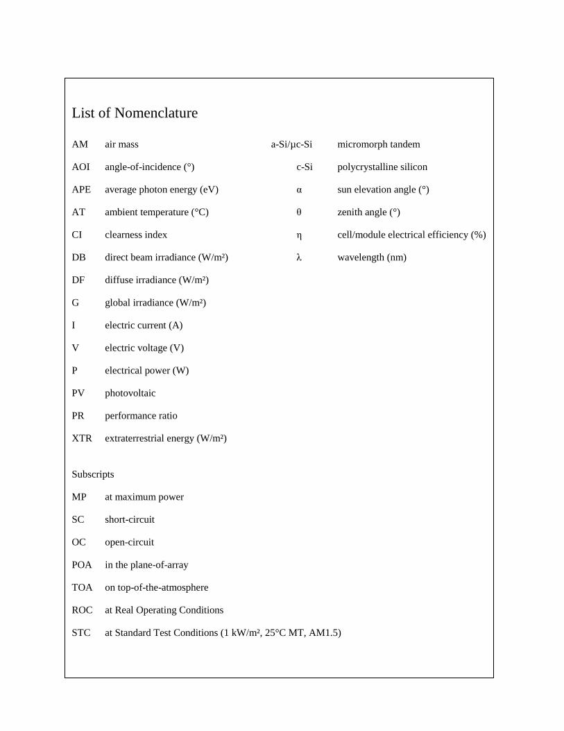
List of Nomenclature

AM air mass a-Si/µc-Si micromorph tandem

AOI angle-of-incidence (°) c-Si polycrystalline silicon

APE average photon energy (eV) α sun elevation angle (°)

AT ambient temperature (°C) θ zenith angle (°)

CI clearness index η cell/module electrical efficiency (%)

DB direct beam irradiance (W/m²) λ wavelength (nm)

DF diffuse irradiance (W/m²)

G global irradiance (W/m²)

I electric current (A)

V electric voltage (V)

P electrical power (W)

PV photovoltaic

PR performance ratio

XTR extraterrestrial energy (W/m²)

Subscripts

MP at maximum power

SC short-circuit

OC open-circuit

POA in the plane-of-array

TOA on top-of-the-atmosphere

ROC at Real Operating Conditions

STC at Standard Test Conditions (1 kW/m², 25°C MT, AM1.5)

3

Table of Contents

Abstract .................................................................................................................................................... 1

List of Figures .......................................................................................................................................... 4

1. Introduction ................................................................................................................................... 6

2. Hardware ....................................................................................................................................... 7

3. PV performance and parameters ................................................................................................. 10

3.1. Electrical characteristics .......................................................................................................... 10

3.2. Performance characterization under Standard Test Conditions............................................... 11

3.3. Performance criteria for outdoor testing .................................................................................. 12

3.4. Environmental parameters affecting PV performance ............................................................ 14

4. Methodology ............................................................................................................................... 19

5. Results ......................................................................................................................................... 20

5.1. Environmental conditions ........................................................................................................ 20

5.1.1. Solar resource ...................................................................................................................... 20

5.1.2. Atmospheric attenuation .......................................................................................................... 24

5.2. Evaluation of PV performance under ROC ............................................................................. 33

6. Discussion ................................................................................................................................... 47

7. Conclusion and Recommendations ............................................................................................. 50

References .............................................................................................................................................. 52

Appendix ................................................................................................................................................ 57

4

List of Figures Figure 1 – Rooftop installation of the two tested PV technologies, micromorph tandem MHI (front) and

polycrystalline KYO (back). .................................................................................................................... 8

Figure 2 – Parts of the weather station (top), thermopile pyranometer (middle), masked pyranometer (bottom

left), and spectroradiometer (bottom right). ............................................................................................. 9

Figure 3 – Typical I-V curve of a PV module. (Coelho and Martins, 2012). ............................................. 10

Figure 4 – Environmental parameters influencing solar yield in photovoltaic (PV) modules. ................... 14

Figure 5 – Annual variation (blue line) of XTRTOA for the coordinates of the UH Manoa test location. ... 15

Figure 6 – ASTM reference spectrum at AM1.5 received by a 37° tilted module surface and XTRTOA

(Andrews, 2011). .................................................................................................................................... 16

Figure 7 – Spectral energy density [W/m²×nm] (right y-axis) of the ASTM reference spectrum at AM1.5

and spectral response [A/W] (left y-axis) of different PV technologies (Silverman et al., 2014). ........ 17

Figure 8 – Environmental parameters under different atmospheric conditions (left: clear sky, right: overcast)

over the course of two days in February 2015. ...................................................................................... 18

Figure 9 – Daily average irradiation received in the POA at GHHI in 2015 per month. ............................ 21

Figure 10 – Annual variation of solar irradiance G received in the POA per angle-of-incidence (AOI) for

the year 2015 as measured by the solar cell (left) and by the pyranometer (right). ............................... 22

Figure 11 – Difference between solar energy received per AOI in mornings compared to afternoons and

cumulative solar energy (green line) from 0° AOI to 70° in percent from yearly global energy........... 22

Figure 12 – Impact of tilt (top) and azimuth (bottom) on XTRPOA (left) and minimum AOI (right) for the

test site location. ..................................................................................................................................... 23

Figure 13 – Air mass AM as a function of all AOI (left) and versus time for the year 2015 (right) per AOI.

................................................................................................................................................................ 25

Figure 14 – Clearness index CI versus time per AOI for the year 2015. .................................................... 26

Figure 15 – Clearness index CI as a function of AM (left) and versus time for AOI 70° (right)................ 26

Figure 16 – Ambient temperature AT versus time per AOI for the year 2015. .......................................... 27

Figure 17 – Diffuse DF versus AM (left) and direct beam DB versus CI (right) under different AOI. ...... 28

Figure 18 – Average photon energy APE [eV] per AOI versus time for the year 2015. ............................ 29

Figure 19 – APE for all AOI as a function of AM for the year 2015. ......................................................... 29

Figure 20 – Average photon energy APE as a function of CI for the full year with selected AOI included

(left) and at AOI between 0°-40° (right). ............................................................................................... 30

5

Figure 21 - APE per AOI as a function of DB irradiance for 2015. ............................................................ 31

Figure 22 – Average photon energy APE per AOI as a function of CI in June (left) and in November (right).

................................................................................................................................................................ 31

Figure 23 – Monthly average IPSC versus time for multiple PV modules tested in 2015, a-Si/µc-Si (dotted

line) and c-Si (continuous line). ............................................................................................................. 34

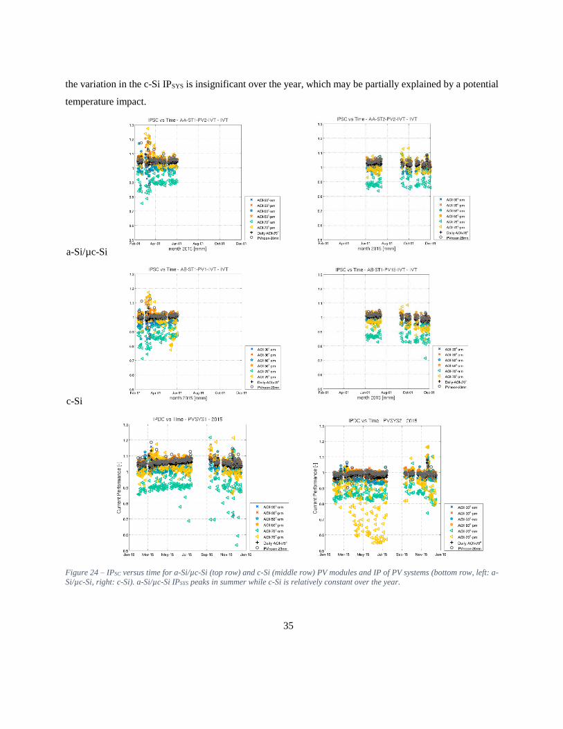
Figure 24 – IPSC versus time for a-Si/µc-Si (top row) and c-Si (middle row) PV modules and IP of PV

systems (bottom row, left: a-Si/µc-Si, right: c-Si). a-Si/µc-Si IPSYS peaks in summer while c-Si is

relatively constant over the year. ............................................................................................................ 35

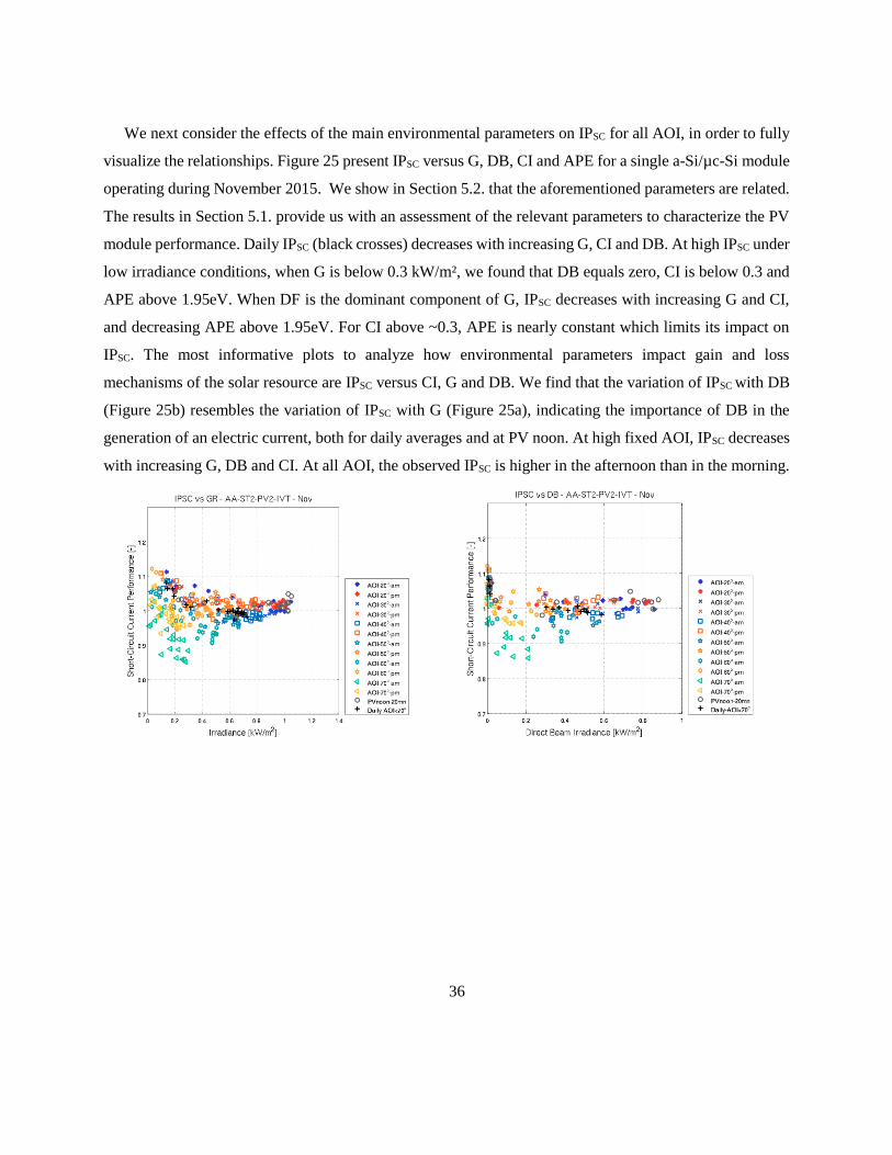
Figure 25 – IPSC versus G (top left), DB (top right), CI (bottom left) and APE (bottom right) for all AOI for

a single a-Si/µc-Si module operating over November 2015. ................................................................. 37

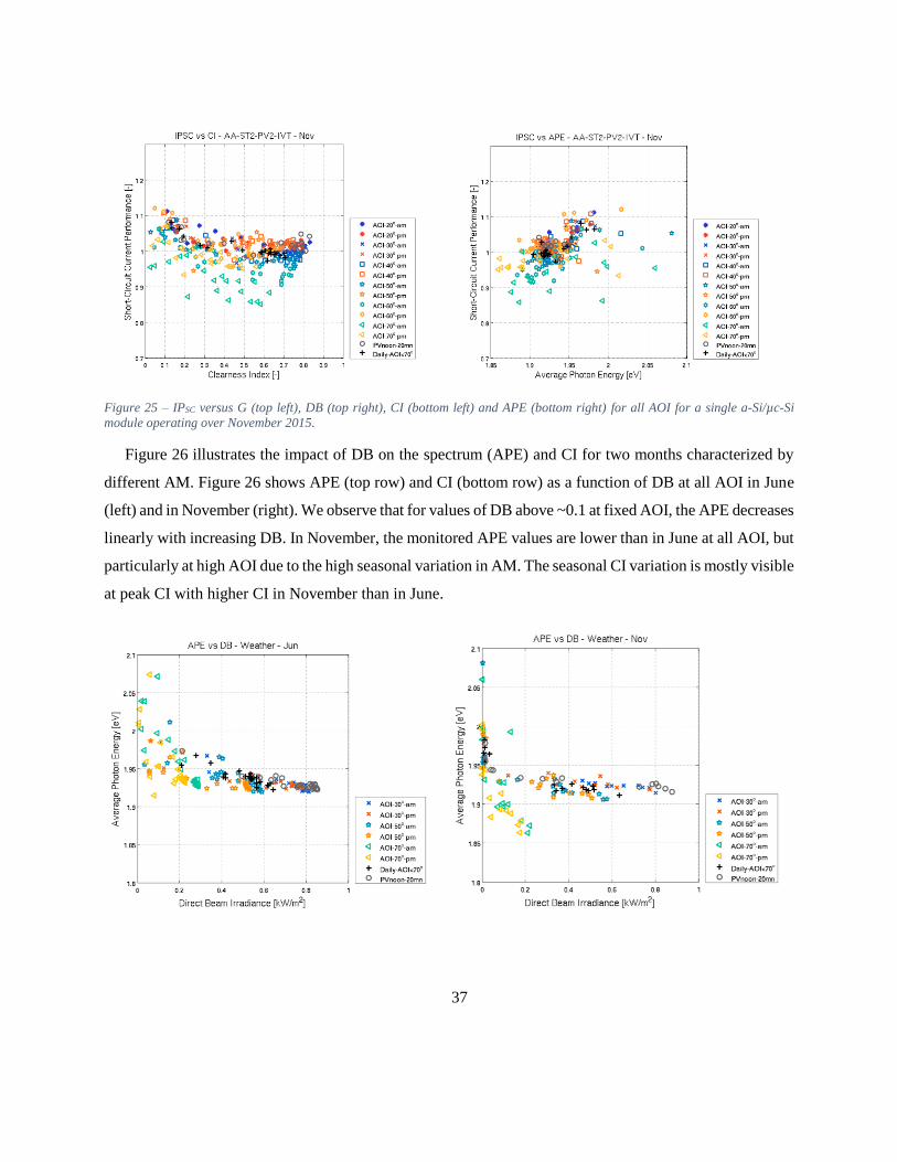
Figure 26 – APE (top row) and CI (bottom row) per AOI versus DB for the months of June (left) and

November (right) 2015. .......................................................................................................................... 38

Figure 27 – IPSC per AOI versus DB for a module of each technology (a-Si/µc-Si: top row; c-Si: middle

row) for the months of June (left) and November (right). IPSYS per AOI versus DB for both PV systems

(bottom row, a-Si/µc-Si: left; c-Si: right) for the year 2015. ................................................................. 39

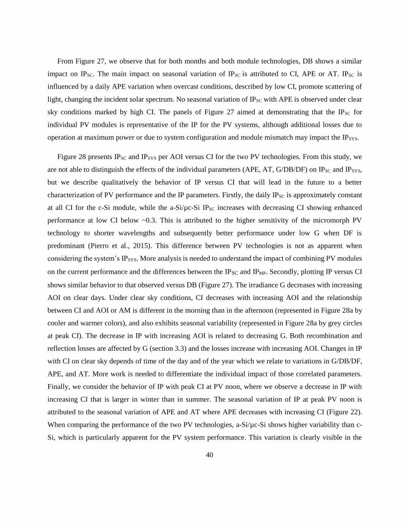
Figure 28 – IPSC per AOI versus CI for a module of each technology (left: a-Si/µc-Si, right: c-Si) for full

period of testing (June-November 2015) and IPSYS for year 2015 on the PV systems........................... 41

Figure 29 – IPSC per AOI versus G for a-Si/µc-Si (left) and c-Si (right) modules over the second testing

period (top) and PV systems (bottom). .................................................................................................. 43

Figure 30 – PR per AOI versus IP for the PV systems (left: a-Si/µc-Si, right: c-Si) showing the current

performance impact on the maximum power performance. ................................................................... 44

Figure 31 – Monthly PR, IP and VN versus time for both PV systems tested in 2015. .............................. 45

Table 1 – STC specifications indicated in the datasheet of the Kyocera c-Si PV module KD205GX-LP. . 11

Table 2 – Annual and monthly average values for AM, CI, APE and AT. ................................................. 24

Table 3 – Yearly average PR, IP and VN for both PV systems in 2015. .................................................... 46

Table 4 – Yearly average PR, and efficiencies at STC and ROC for both PV systems in 2015. ................ 47

6

1. Introduction

The Hawaii Clean Energy Initiative (HCEI) has set the goal to become fully dependent upon renewable

energy by 2045, proving the state’s commitment to green energy development. Hawaii’s abundant solar

resource favors the development of solar energy as a suitable means to help achieve the HCEI’s goal. The

Hawaii Natural Energy Institute (HNEI) is positioned to contribute to Hawaii’s renewable energy efforts.

Hence, research and development of solar photovoltaic energy is being pursued in accordance with the

commitments to the state’s renewable energy goals. As part of the Green Holmes Hall Initiative (GHHI), an

energy infrastructure project, HNEI is fostering the understanding of photovoltaic power deployment

through a research project on PV system performance on top of Holmes Hall at the University of Hawai’i

at Manoa, which was initiated in 2010. The PV energy exploration and testing for rooftop applications is

aimed at evaluating the performance of PV modules under a range of environmental conditions. The

assessment of environmental factors that reduce or enhance the amount of solar energy collected by a PV

module and subsequently converted into electricity, illustrates how PV systems perform under real operating

conditions (ROC) specific to Hawaii.

Commercial and residential use of solar photovoltaic technology has seen a steady increase in Hawaii,

motivating the development of a better understanding of how we can exploit different PV technologies to

optimize the energy yield. The way that PV modules function when they are tested in a laboratory

environment does not reflect the true performance of modules when exposed to the natural environment. In

addition, environmental conditions vary with location. This study focuses on characterizing two PV

technologies in the Hawaiian environment to assess how environmental parameters affect different module

technologies, primarily in terms of current performance. A comprehensive assessment of the basic solar

physics shall help to determine critical parameters influencing PV system performance.

The method for evaluating the performance of a photovoltaic (PV) module is to compare the module

performance against that provided by the manufacturer in the module’s specifications under Standard Test

Conditions (STC). This method uses the performance criteria called performance ratio (PR), which relates

the module’s operating efficiency (ηROC) under ROC to the theoretical output (ηSTC) indicated in the

manufacturer‘s specifications evaluated at STC, where PR = ηROC ÷ ηSTC (Pierro et al., 2015). The ratio of

actual to predicted power is estimated anywhere between 75% to 95% in the literature depending on PV

system technologies and locations and has grown from less than 70% in the nineties to an average range

7

between 80% and 90% observed in most PV systems today (Nordmann et al., 2014). These quoted PR values

include a conversion loss (~5%) from direct to alternating current due to wiring individual modules in the

PV system (AC PR), hence the DC PR values are nowadays around 84-95%. In the following, we focus on

DC PR. Under ROC, operating temperature, solar irradiance and the solar spectrum, for example, are subject

to natural fluctuations that are not accounted for by STC resulting in lower system performance under ROC.

The wide range of published PR values does not allow one to predict the actual performance of the PV

system. Hence, this study’s objective is to assess the weather conditions impacting the PR and to determine

the average PR for Hawaii.

This present study describes the applied methodology for monitoring and testing of the PV modules and

reports on their performance characteristics. The study begins with an assessment of the weather conditions

at UH Manoa, understanding the variation that occurs daily and seasonally. Then the impact of

environmental parameters on electrical PV performance is evaluated by assessing the current-voltage (IV)

curve characteristics and PR based on the demonstrated empirical relationships. The report presents results

that support empirical relationships between performance characteristics, while qualitatively assessing the

impact of each parameter on module efficiency. Finally, the relationships among parameters are used in

describing PV module efficiency under ROC for Hawaii.

2. Hardware

This study involves analyzing data to determine relationships among environmental parameters and PV

performance that were recorded under the GHHI project on the roof of Holmes Hall, where two PV systems

were commissioned at the end of 2010. This section introduces firstly the data acquisition system (DAS)

selected and installed by HNEI in order to assess PV performance under given environmental conditions.

8

2.1. The PV systems

Two PV systems using two

different PV technologies are operating

on the roof of Holmes Hall. Figure 1

shows the micromorph tandem (a-

Si/µc-Si) (Mitsubishi Heavy Industries

(MHI) MT130, 130W) in the front row

and the polycrystalline (c-Si) (Kyocera

(KYO) KD205, 205W) in the back

rows. The first PV system is

comprised of a 3kW system made of 24

micromorph PV modules (MHI),

which is a technology that combines a layer of amorphous silicon on top of a microcrystalline silicon cell

(Keppner et al., 1999). The second system is rated at 5kW consisting of 26 polycrystalline PV modules

(KYO). In both systems, the PV modules are connected in series and in parallel to a string inverter that

converts the DC power of the PV modules into AC power and feeds it safely into the electrical grid. The

PV modules are mounted on top of the flat roof and are tilted according to latitude with a 20° tilt to the

horizontal plane and a 180° orientation towards true South. The PV systems were instrumented to record

electrical performance and weather conditions. In 2015, a new instrumentation was used to investigate

further the PV performance through collecting the electrical characteristics of individual PV modules. The

following section describes the instrumentation used to monitor the weather conditions. The analysis uses

the data collected by the IV tracer that is described thereafter.

2.2. The monitoring equipment

The weather station system consists of different sensors that provide measurements of the solar resource

and of the environmental conditions such as the ambient temperature, relative humidity, barometric

pressure, wind speed and direction (Figure 2, top). A thermopile pyranometer (Hukseflux LP 02) (Figure 2,

bottom right) and a masked pyranometer (Delta-T SPN 1) (Figure 2, bottom left) were selected to collect

Figure 1 – Rooftop installation of the two tested PV technologies, micromorph

tandem MHI (front) and polycrystalline KYO (back).

9

information on the solar resource including global and diffuse irradiance, from

which we calculate the direct beam irradiance. There are also cheaper solar

sensors i.e. solar cell pyranometers surrounding the PV arrays also used in the

following analysis. The results vary depending on the measuring instrument,

with lower PR for data collected with the thermopile compared to the solar cell

pyranometer, which is consistent with the findings of Reich et al., 2011. For

this study, the analysis is based on data received by the thermopile pyranometer,

as this sensor collects data over a full spectral range, while the solar cell spectral

response is limited. All solar sensors are located in the plane-of-array (POA) to

record the solar input received by the PV modules. This includes a

spectroradiometer (Eko MS 700) that records spectral irradiance

measurements, which refers to the energy distribution as a function of

wavelength of emitted radiation from the light source. The spectroradiometer

records spectral solar irradiance in the range 350 to 1050 nm every 15 seconds

in the POA. The other analog instruments described above sample every

second.

Each instrument has its own limitations

in terms of accuracy and operating

conditions, including limited spectral and

directional ranges.

2.3. The IV tracer

Part of the following PV performance analysis is conducted on individual PV modules that were

extracted from the PV systems previously described. An IV-tracer (Daystar Multi-Tracer) is designed to

collect the electrical characteristics or current-voltage (IV) curves of the PV modules. IV curves were

recorded every minute. During the year 2015, two sets of PV modules were tested with the IV tracer. Four

micro-amorphous and two polycrystalline PV modules were tested from February to June and a second set

of modules was tested from June to November. This provides information on the temporal change of the PV

Figure 2 – Parts of the weather station (top), thermopile pyranometer

(middle), masked pyranometer (bottom left), and spectroradiometer

(bottom right).

10

module performance over a year of operation and gives information on the performance distribution of the

PV modules constituting the five-year old PV systems.

3. PV performance and parameters

The following sections describe the PV modules, their electric characteristics, the specifications provided

by the manufacturers in the datasheet, and the criteria used to characterize their performance. We end this

section by introducing the parameters found in the literature that influence the PV module performance.

3.1. Electrical characteristics

A photovoltaic module is composed of interconnected

photovoltaic cells that convert sunlight directly into

electricity. When a PV module receives solar radiation,

photons are absorbed as light enters the cells, thereby

freeing electrons and creating an electric current usable by

an external load. The operational characteristics of a PV

module, within an electrical circuit can be represented by a

current-voltage (IV) curve, as shown in Figure 3. The IV

curve shows the relationship between the current (I)

flowing through and the voltage (V) across the electronic

device. The operating point for a PV device varies from no

load or short circuit condition ISC to infinite load or open

circuit condition VOC. The product of current and voltage is

power (P). The maximum power point for a module is the

operating point of maximum power output (PMPP) that varies with environmental conditions. The current

and voltage at the maximum power point is represented by IMP and VMP, respectively.

Figure 3 – Typical I-V curve of a PV module. (Coelho

and Martins, 2012).

11

3.2. Performance characterization under Standard Test Conditions

Each PV cell and therefore each module is unique in terms of its electrical performance. Once assembled,

the PV modules are evaluated by the manufacturer under a specified set of conditions, so as to ensure that

each module is compliant within the specifications indicated in the datasheet. These so called flash tests are

conducted in an indoor controlled environment under standard test conditions (STC). STC are defined by

the ASTM standard G173-03, which includes a fixed cell temperature of 25°C and a solar irradiance in POA

of 1 kW/m², whose spectrum corresponds to AM1.5G, the characteristic solar spectrum received on the US

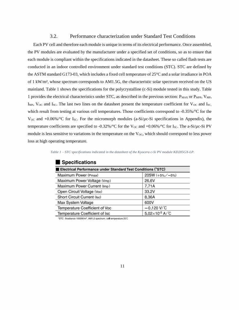
mainland. Table 1 shows the specifications for the polycrystalline (c-Si) module tested in this study. Table

1 provides the electrical characteristics under STC, as described in the previous section: PMAX or PMPP, VMP,

IMP, VOC and ISC. The last two lines on the datasheet present the temperature coefficient for VOC and ISC,

which result from testing at various cell temperatures. Those coefficients correspond to -0.35%/°C for the

VOC and +0.06%/°C for ISC. For the micromorph modules (a-Si/µc-Si specifications in Appendix), the

temperature coefficients are specified to -0.32%/°C for the VOC and +0.06%/°C for ISC. The a-Si/µc-Si PV

module is less sensitive to variations in the temperature on the VOC, which should correspond to less power

loss at high operating temperature.

Table 1 – STC specifications indicated in the datasheet of the Kyocera c-Si PV module KD205GX-LP.

12

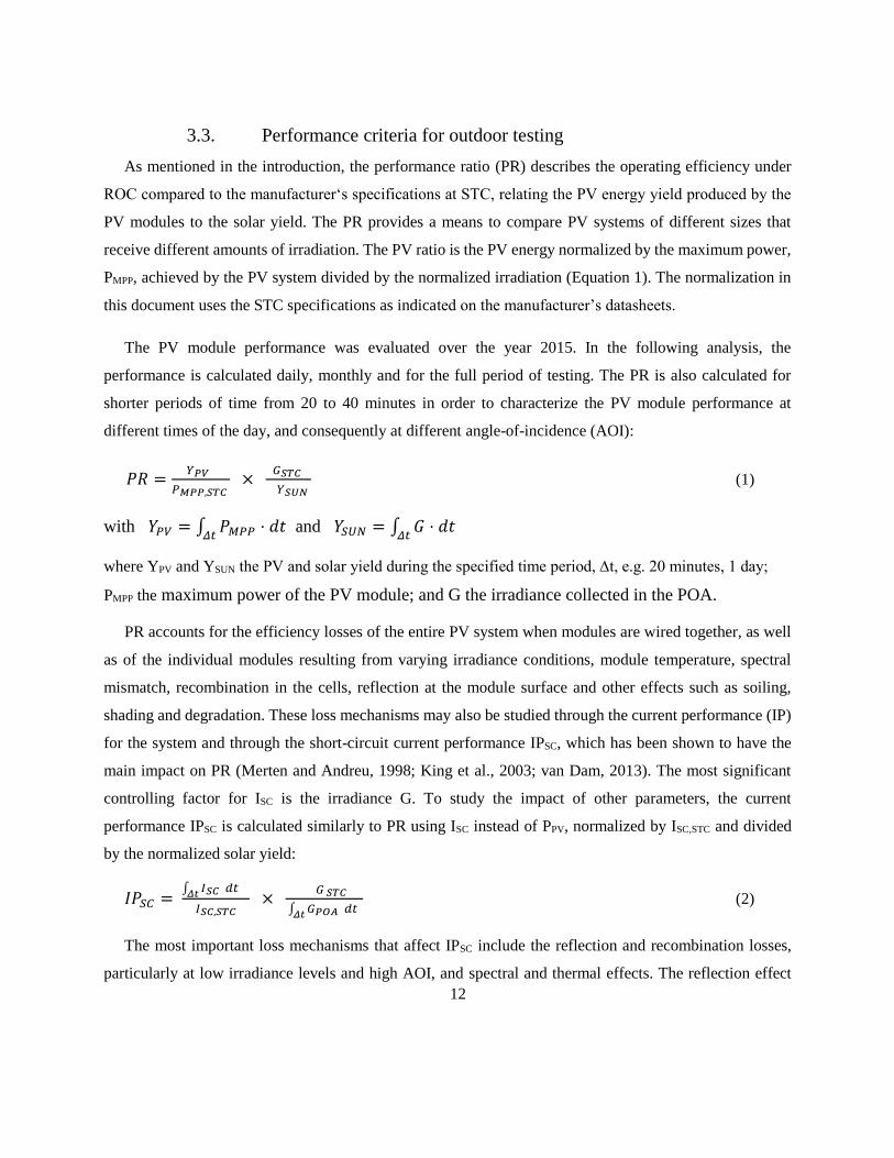
3.3. Performance criteria for outdoor testing

As mentioned in the introduction, the performance ratio (PR) describes the operating efficiency under

ROC compared to the manufacturer‘s specifications at STC, relating the PV energy yield produced by the

PV modules to the solar yield. The PR provides a means to compare PV systems of different sizes that

receive different amounts of irradiation. The PV ratio is the PV energy normalized by the maximum power,

PMPP, achieved by the PV system divided by the normalized irradiation (Equation 1). The normalization in

this document uses the STC specifications as indicated on the manufacturer’s datasheets.

The PV module performance was evaluated over the year 2015. In the following analysis, the

performance is calculated daily, monthly and for the full period of testing. The PR is also calculated for

shorter periods of time from 20 to 40 minutes in order to characterize the PV module performance at

different times of the day, and consequently at different angle-of-incidence (AOI):

𝑃𝑅 =𝑌𝑃𝑉

𝑃𝑀𝑃𝑃,𝑆𝑇𝐶 ×

𝐺𝑆𝑇𝐶

𝑌𝑆𝑈𝑁 (1)

with 𝑌𝑃𝑉 = ∫ 𝑃𝑀𝑃𝑃𝛥𝑡⋅ 𝑑𝑡 and 𝑌𝑆𝑈𝑁 = ∫ 𝐺

𝛥𝑡⋅ 𝑑𝑡

where YPV and YSUN the PV and solar yield during the specified time period, ∆t, e.g. 20 minutes, 1 day;

PMPP the maximum power of the PV module; and G the irradiance collected in the POA.

PR accounts for the efficiency losses of the entire PV system when modules are wired together, as well

as of the individual modules resulting from varying irradiance conditions, module temperature, spectral

mismatch, recombination in the cells, reflection at the module surface and other effects such as soiling,

shading and degradation. These loss mechanisms may also be studied through the current performance (IP)

for the system and through the short-circuit current performance IPSC, which has been shown to have the

main impact on PR (Merten and Andreu, 1998; King et al., 2003; van Dam, 2013). The most significant

controlling factor for ISC is the irradiance G. To study the impact of other parameters, the current

performance IPSC is calculated similarly to PR using ISC instead of PPV, normalized by ISC,STC and divided

by the normalized solar yield:

𝐼𝑃𝑆𝐶 = ∫ 𝐼𝑆𝐶𝛥𝑡 𝑑𝑡

𝐼𝑆𝐶,𝑆𝑇𝐶 ×

𝐺 𝑆𝑇𝐶

∫ 𝐺𝑃𝑂𝐴𝛥𝑡 𝑑𝑡

(2)

The most important loss mechanisms that affect IPSC include the reflection and recombination losses,

particularly at low irradiance levels and high AOI, and spectral and thermal effects. The reflection effect

13

describes the loss due to reflected light beams on top of the PV module surface, which increases with

increasing incidence angle AOI (Okada et al., 2003). The recombination loss relates to electrons that

recombine instead of creating a current, which is the dominant loss mechanism under low irradiance levels.

The thermal effect represents an increase in IP with increasing cell temperature as indicated by the

temperature coefficient (+0.06%/°C) mentioned previously in section 3.2. Finally, the spectral effect

describes the performance variation due to changes in the incident spectrum, leading to higher or lower

mismatch with the spectral response of the PV module, further discussed in the following subsection 3.4.

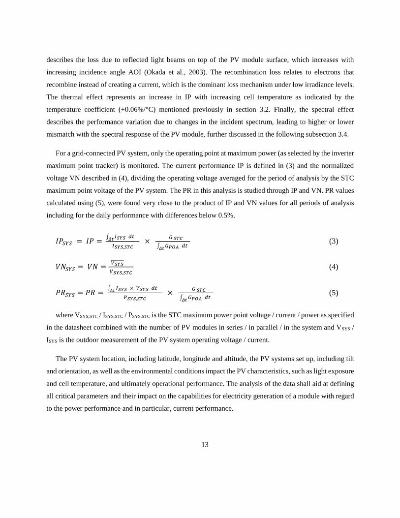
For a grid-connected PV system, only the operating point at maximum power (as selected by the inverter

maximum point tracker) is monitored. The current performance IP is defined in (3) and the normalized

voltage VN described in (4), dividing the operating voltage averaged for the period of analysis by the STC

maximum point voltage of the PV system. The PR in this analysis is studied through IP and VN. PR values

calculated using (5), were found very close to the product of IP and VN values for all periods of analysis

including for the daily performance with differences below 0.5%.

𝐼𝑃𝑆𝑌𝑆 = 𝐼𝑃 = ∫ 𝐼𝑆𝑌𝑆𝛥𝑡 𝑑𝑡

𝐼𝑆𝑌𝑆,𝑆𝑇𝐶 ×

𝐺 𝑆𝑇𝐶

∫ 𝐺𝑃𝑂𝐴𝛥𝑡 𝑑𝑡 (3)

𝑉𝑁𝑆𝑌𝑆 = 𝑉𝑁 =𝑉𝑆𝑌𝑆̅̅ ̅̅ ̅̅ ̅

𝑉𝑆𝑌𝑆,𝑆𝑇𝐶 (4)

𝑃𝑅𝑆𝑌𝑆 = 𝑃𝑅 = ∫ 𝐼𝑆𝑌𝑆𝛥𝑡 × 𝑉𝑆𝑌𝑆 𝑑𝑡

𝑃𝑆𝑌𝑆,𝑆𝑇𝐶 ×

𝐺 𝑆𝑇𝐶

∫ 𝐺𝑃𝑂𝐴𝛥𝑡 𝑑𝑡 (5)

where VSYS,STC / ISYS,STC / PSYS,STC is the STC maximum power point voltage / current / power as specified

in the datasheet combined with the number of PV modules in series / in parallel / in the system and VSYS /

ISYS is the outdoor measurement of the PV system operating voltage / current.

The PV system location, including latitude, longitude and altitude, the PV systems set up, including tilt

and orientation, as well as the environmental conditions impact the PV characteristics, such as light exposure

and cell temperature, and ultimately operational performance. The analysis of the data shall aid at defining

all critical parameters and their impact on the capabilities for electricity generation of a module with regard

to the power performance and in particular, current performance.

14

3.4. Environmental parameters affecting PV performance

This section presents the main environmental parameters influencing PV performance and gives a brief

literature review of each. The power of a PV module is proportional to the total irradiance received by a

module in the plane-of-array (POA), termed global irradiance (G). G may be decomposed into its

components, the direct beam (DB) and diffuse (DF) irradiance (Figure 4), which vary differently depending

on the environmental conditions. Direct beam is the irradiance travelling in a straight line to the receiving

surface of the module. Diffuse irradiance is the difference between global irradiance and direct beam

irradiance, which is scattered crossing the atmosphere or reflected on surfaces including ground. The

intensity of solar irradiance, its distribution between DB and DF, and the solar spectrum all are influenced

by the angle-of-incidence (AOI), air mass (AM) and extraterrestrial radiation (XTR), illustrated in Figure

4 and discussed further in the study results.

Figure 4 – Environmental parameters influencing solar yield in photovoltaic (PV) modules.

The solar irradiance received by the PV module surface, G or GPOA, depends on the solar irradiance

available on top-of-the-atmosphere (TOA), XTRTOA, minus the light absorbed by the atmosphere. The XTR

received in POA, XTRPOA, depends on XTRTOA and AOI, which is the angle between the direct Earth-Sun

vector and the perpendicular line of the module surface:

15

XTRPOA = XTRTOA × cos(AOI) (6)

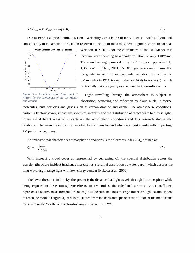
Due to Earth’s elliptical orbit, a seasonal variability exists in the distance between Earth and Sun and

consequently in the amount of radiation received at the top of the atmosphere. Figure 5 shows the annual

variation in XTRTOA for the coordinates of the UH Manoa test

location, corresponding to a yearly variation of only 100W/m².

The annual average power density for XTRTOA is approximately

1,366 kW/m² (Chen, 2011). As XTRTOA varies only minimally,

the greater impact on maximum solar radiation received by the

PV modules in POA is due to the cos(AOI) factor in (6), which

varies daily but also yearly as discussed in the results section.

Light travelling through the atmosphere is subject to

absorption, scattering and reflection by cloud nuclei, airborne

molecules, dust particles and gases such as carbon dioxide and ozone. The atmospheric conditions,

particularly cloud cover, impact the spectrum, intensity and the distribution of direct beam to diffuse light.

There are different ways to characterize the atmospheric conditions and this research studies the

relationship between the indicators described below to understand which are most significantly impacting

PV performance, if any.

An indicator that characterizes atmospheric conditions is the clearness index (CI), defined as:

𝐶𝐼 = 𝐺𝑃𝑂𝐴

𝑋𝑇𝑅𝑃𝑂𝐴 (7)

With increasing cloud cover as represented by decreasing CI, the spectral distribution across the

wavelengths of the incident irradiance increases as a result of absorption by water vapor, which absorbs the

long-wavelength range light with low energy content (Nakada et al., 2010).

The lower the sun is in the sky, the greater is the distance that light travels through the atmosphere while

being exposed to these atmospheric effects. In PV studies, the calculated air mass (AM) coefficient

represents a relative measurement for the length of the path that the sun’s rays travel through the atmosphere

to reach the module (Figure 4). AM is calculated from the horizontal plane at the altitude of the module and

the zenith angle θ or the sun’s elevation angle α, as θ + α = 90°:

Figure 5 – Annual variation (blue line) of

XTRTOA for the coordinates of the UH Manoa

test location.

16

𝐴𝑀 = 1

𝑐𝑜𝑠 (𝜃)=

1

𝑠𝑖𝑛 (𝛼) (8)

AM is an important parameter for PV performance, because the solar spectral irradiance varies with

different air mass conditions during the day and throughout the year (Nakada et al., 2010; Roumpakias et

al., 2015). AM0 spectrum refers to the solar radiation available outside the atmosphere XTRTOA. AM1

reflects the value for the thickness of the atmosphere that light needs to cross to reach a module at sea level

when the sun is directly overhead (King et al., 2004). The STC AM1.5 corresponds to an elevation of

arcsin(1/1.5) = 42°.

The solar spectrum describes the energy distribution of the incident light as a function of the wavelength.

About 19% of solar radiation travelling through the atmosphere is absorbed by atmospheric gases (Litjens,

2013), and the gases absorb differently in varying wavelength ranges. Figure 6 describes the specific energy

of the extraterrestrial irradiance (XTRTOA) at AM0

and of the STC reference energy spectrum (AM1.5)

for the irradiance received by a 37° tilted module

surface. Figure 6 also distinguishes between the

spectra of each irradiance component, the direct beam

(DB) and the diffuse (DF) irradiance. All spectra

show high energy content for wavelengths from 350

to 1050 nm, which is the STC wavelength range at

AM1.5. The extraterrestrial and global irradiances, as

well as DB are very similar in intensity and wavelength range. Global and direct irradiance are almost

identical in the atmospheric absorption bands at different wavelengths, which are wavelength ranges in

which radiation of certain frequencies is absorbed by different gases. The molecules with the highest

absorption rates throughout the spectrum are water vapor (Litjens, 2013). At 630, 690, and 760 nm the

absorption is mainly due to molecular oxygen, whereas at 1400 nm and higher carbon dioxide is the gas

with the highest absorption rates. The diffuse irradiance of AM1.5G has lower energy and is shifted towards

smaller average wavelengths.

The average photon energy (APE), measured in electron volts (eV), is related to the solar spectral content

and refers to the distribution of photons across the wavelengths of the solar spectrum (Cornaro and

Andreotti, 2013). This parameter indicates the energy content of light and influences electrical

Figure 6 – ASTM reference spectrum at AM1.5 received by

a 37° tilted module surface and XTRTOA (Andrews, 2011).

17

characteristics of module performance as is discussed further in the results section. APE is a calculated

value of the total energy in a spectrum divided by the number of photons, giving an average energy of all

photons in the irradiance spectrum (Minemoto, 2009). APE is calculated using data collected by a

spectroradiometer that measures the range of wavelengths across a spectrum. The spectroradiometer

records spectral solar irradiance in a specific range of wavelength. APE values are sensitive to the

wavelength range of the instrument. The APE of the STC spectrum using the spectroradiometer wavelength

range of our instrument (350-1050 nm) is 1.88 eV (Minemoto, 2009). We will see later in the document

that the APE can vary during the day and throughout the year, thereby giving us insights into the

characteristics of the atmospheric conditions. Higher values of APE are observed with increasing cloud

cover, while lower values of APE are observed with increasing AM, which has been found in other studies

(Cornaro and Andreotti, 2012; Nakada et al., 2010). CI impacts the solar irradiance intensity and

distribution between the DB and DF components, thereby affecting the solar spectrum due to scattering of

light as it crosses the atmosphere. The average photon energy (APE) has been used by multiple laboratories

since the nineties and was selected as an indicator for the solar spectral content to characterize the spectrum

and to assess the impact of the solar spectrum on PV module performance.

The portion of irradiance that a PV module can

actually convert into current, depends on the incident

spectrum of light and the spectral response of the PV

modules. Figure 7 shows the spectral response of three

PV technologies in comparison to the AM1.5G

spectrum (van Dam, 2013). Again, as each module has

its own performance, including spectral response, this

graph shows the characteristic spectral range for

different PV technologies. The polycrystalline c-Si PV

modules have a wide range of absorption from 350-

1050nm, whereby the amorphous a-Si PV modules

have an absorption range between 300 to 780 nm. The micromorph tandem (MHI) is a dual cell combining

the absorption range from two thin film cells. The top cell is an amorphous cell (a-Si) and the bottom cell

is a microcrystalline cell (µc-Si 500-1000nm) whose combined range covers 300 to 1000 nm (Yamauchi et

al., 2005). The last technology plotted in the graph is a thin film made of Copper indium gallium (di)selenide

Figure 7 – Spectral energy density [W/m²×nm] (right y-axis)

of the ASTM reference spectrum at AM1.5 and spectral

response [A/W] (left y-axis) of different PV technologies

(Silverman et al., 2014).

18

(CIGS) with an absorption range from 350 to 1100 nm. The mismatch between a given solar spectrum and

the spectrum at which a module operates results in a spectral loss. Although c-Si shows a wider wavelength

range for its spectral response, it is at wavelengths where the incident energy content is small compared to

a-Si, which operates in the most energy dense sections of the solar spectrum with higher photon flux density

in the short-wavelength region compared to the spectrum at long-wavelength regions, which has a lower

photon flux density (Nakada et al., 2010).

Figure 8 presents the variation of the main environmental parameters over the course of one day for two

days in February 2015. The plots show the raw 1-second data, applying coefficients as indicated in the

legend in order to visualize the parameters along the same range of values and to contrast the behavior for

a day with clear sky conditions (left) and a day with overcast conditions (right). For a clear day, G looks

like a bell curve and the DF component is minimal. APE spikes only at dawn and dusk, when the sun

comes/goes over the horizon. For an overcast day, relative humidity is higher due to cloud cover, influencing

solar intensity, distribution and spectrum, as more water vapor in the atmosphere causes more scattering of

light. G is mainly made up of DF, both of which follow the trajectory of the CI, which is highly variable,

thereby influencing the APE variability throughout the day and causing APE values to spike above values

under clear sky conditions. Overall, we observe a higher APE, lower CI and higher DF for times of the day

marked by overcast compared to clear sky conditions, indicating that cloud cover is a dominant factor

influencing various environmental parameters.

Figure 8 – Environmental parameters under different atmospheric conditions (left: clear sky, right: overcast) over the course of

two days in February 2015.

19

4. Methodology

The analysis described here utilizes both collected data and computed parameters. The collected solar

data consist of G and DF, from which DB is calculated. The weather conditions, including AT, and the IV-

curves are likewise collected data. From the IV-tracer, we obtain the electrical measurements for individual

module performance, including ISC, VOC and PMPP, and from the HNEI DAS the data for the PV system

performance, from which current performance (IP) and normalized voltage (VN) is calculated. In parallel

to the logged data, the developed methodology includes the calculation of the parameters AM, AOI, CI and

XTR. The SolPos algorithm developed at the National Renewable Energy Laboratory (NREL, Martin

Rymes, 2000) applies astronomical equations to evaluate the position of the sun compared to a given

location, date and time, and with the module setup, including orientation and tilt. APE is used as an indicator

of the solar spectrum.

Due to the large amount of collected data and computed parameters (as illustrated in Figure 8), the

analysis bins all data into angle-of-incidence ranges between 0° to 90° using 10°-bins, e.g. from 0° to 5°, 5°

to 15°, until 85° to 90°, to assess the variability of the solar irradiance and other parameters over a day. We

form 30 to 40 minute averages of the 1-second data and plot this data per AOI bin to visualize the daily

variation of the parameters and to identify relationships and correlations among parameters during the day

and throughout a year. To simplify the plots and whenever it helps visibility, we plot fewer AOI at 70°, 50°

and 30° bins, including the daily averages and data for PV noon (defined below).

It is important to define the PV performance over a complete day of operation. The parameters are

calculated per day as total daily average. The data used here is restricted to AOI below 70°, in order to limit

error due to directional response of the solar sensors as well as to omit possibly biased data, as for instance

the spikes in APE at dusk/dawn, mentioned in section 3.4.

The parameters are also estimated at PV noon, which represents a 20-minute interval around when the

sun is closest to the normal to the POA of the PV surface. This value is representative of a midday

performance when PV modules are expected to be most productive. Analyzing the time interval around

where AOI values are at minimum proved to be informative for evaluating PV performance at maximum

conditions in terms of irradiance and temperature. PV noon is equal to solar noon, when the azimuth equals

180°, or true South. In future work, the time interval of 20 minutes should be varied to consider the effects

of the interval choice.

20

The daily results are averaged per month and year for 2015. The results are presented per AOI either

versus time to visualize daily and seasonal variation or versus other parameters, to determine empirical

relationships, particularly investigating the module behavior as a function of irradiance GPOA. Finally, we

discuss the main parameters affecting IP (and thus PR) and their impact on PV performance.

5. Results

This section presents the study’s assessment of the impact of environmental conditions at UH Manoa

on PV performance. The first part on environmental conditions characterizes the local solar resource

received in POA in terms of irradiation (or energy [in Wh/m²]) and in terms of irradiance (or power [in

W/m²]), before studying the main indicators of atmospheric conditions. The second part of the results

determines the average PV performance under ROC at the test site and defines the parameters that influence

the daily and seasonal performance variation.

5.1. Environmental conditions

This section presents firstly, the local solar resource through irradiation and irradiance, GPOA, and

provides a short analysis of the impact of PV orientation on the solar resource (XTRPOA). Secondly, we

study the three indicators of the atmospheric conditions, namely CI, AM, and APE, and discuss the

empirical relationships between the parameters. In the next two subsections, we refer to monthly and yearly

values of the solar resource (Figure 9-12) and the environmental conditions included in Table 2.

5.1.1. Solar resource

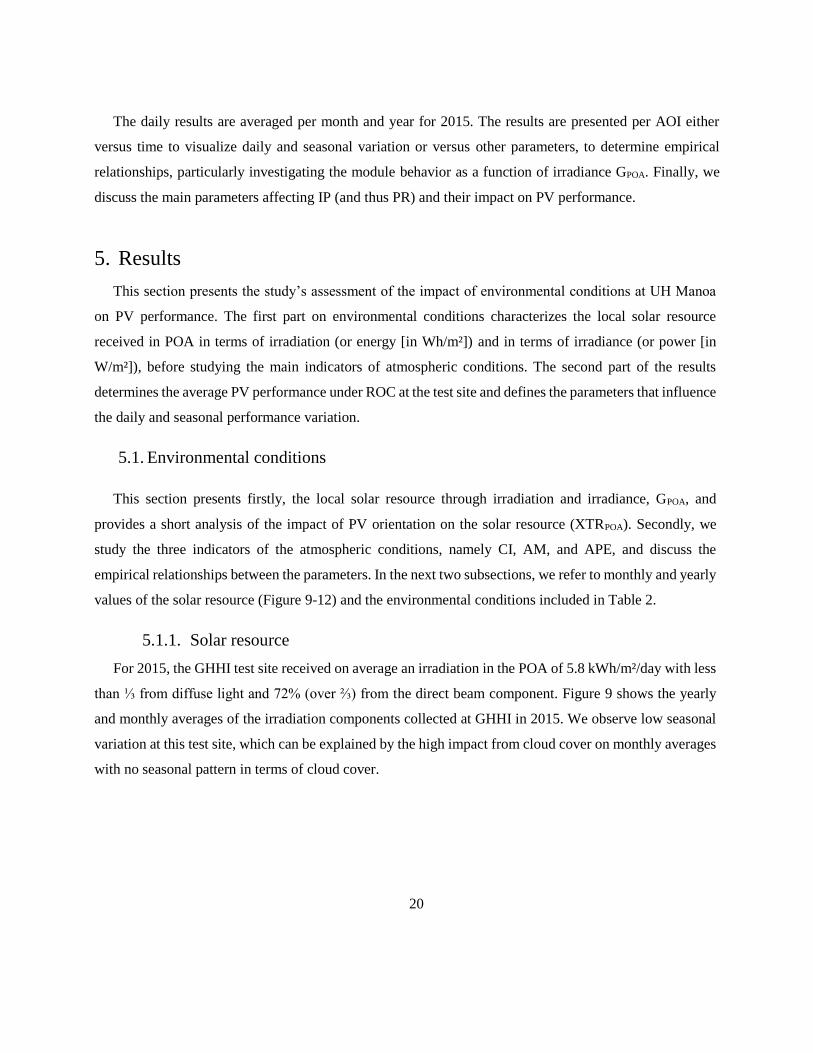
For 2015, the GHHI test site received on average an irradiation in the POA of 5.8 kWh/m²/day with less

than ⅓ from diffuse light and 72% (over ⅔) from the direct beam component. Figure 9 shows the yearly

and monthly averages of the irradiation components collected at GHHI in 2015. We observe low seasonal

variation at this test site, which can be explained by the high impact from cloud cover on monthly averages

with no seasonal pattern in terms of cloud cover.

21

Figure 9 – Daily average irradiation received in the POA at GHHI in 2015 per month.

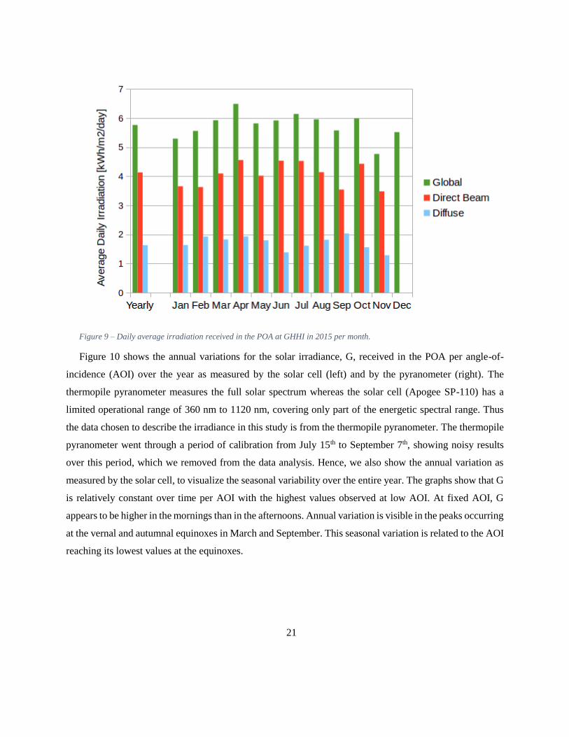
Figure 10 shows the annual variations for the solar irradiance, G, received in the POA per angle-of-

incidence (AOI) over the year as measured by the solar cell (left) and by the pyranometer (right). The

thermopile pyranometer measures the full solar spectrum whereas the solar cell (Apogee SP-110) has a

limited operational range of 360 nm to 1120 nm, covering only part of the energetic spectral range. Thus

the data chosen to describe the irradiance in this study is from the thermopile pyranometer. The thermopile

pyranometer went through a period of calibration from July 15th to September 7th, showing noisy results

over this period, which we removed from the data analysis. Hence, we also show the annual variation as

measured by the solar cell, to visualize the seasonal variability over the entire year. The graphs show that G

is relatively constant over time per AOI with the highest values observed at low AOI. At fixed AOI, G

appears to be higher in the mornings than in the afternoons. Annual variation is visible in the peaks occurring

at the vernal and autumnal equinoxes in March and September. This seasonal variation is related to the AOI

reaching its lowest values at the equinoxes.

22

Figure 10 – Annual variation of solar irradiance G received in the POA per angle-of-incidence (AOI) for the year 2015 as

measured by the solar cell (left) and by the pyranometer (right).

Another characteristic of the solar resource is a daily variation between the energy intensity in the

morning (am) compared to the afternoon (pm). Figure 11 shows the difference of the solar energy collected

per AOI in the morning compared to the afternoon, including the cumulative energy received from 0° AOI

to 70°. This confirms that global irradiance G and direct beam DB are stronger in the morning at all values

of AOI while more DF is collected in the afternoon. The cumulative energy (green line) indicates that most

energy is collected at low AOI, with 80% of the daily energy collected for AOI below 45°.

Figure 11 – Difference between solar energy received per AOI in mornings compared to afternoons and cumulative solar energy

(green line) from 0° AOI to 70° in percent from yearly global energy.

23

The AOI depends on the location, including latitude, longitude and altitude, and on the orientation of

the PV modules, including tilt and azimuth. Figure 12 illustrates the impact of the tilt (top) and azimuth

(bottom) on XTRPOA (left) and minimum AOI (right) using the coordinates for Holmes Hall, demonstrating

the variation in the availability of the solar resource on TOA received in the POA. XTRPOA varies with the

seasons under varying tilt and azimuth, whereby tilt most impacts on the seasonal variation of XTRPOA and

AOI at PV noon. For a 20° tilt as is the configuration for this study, solar radiation peaks during the vernal

and autumnal equinoxes as shown in Figure 10, which is when AOI is lowest during the year. With

decreasing tilt, the minimum AOI is lowest in summer, because the sun is the highest in the sky, leading to

higher energy collection in summer compared to winter. Increasing the tilt shifts the seasonal variation of

the solar energy yield and AOI leading to a higher solar energy yield in winter instead of summer for a tilt

higher than 20°. The bottom panels (Figure 12) show the low impact of azimuth on the annual energy

collection and AOI.

Figure 12 – Impact of tilt (top) and azimuth (bottom) on XTRPOA (left) and minimum AOI (right) for the test site location.

24

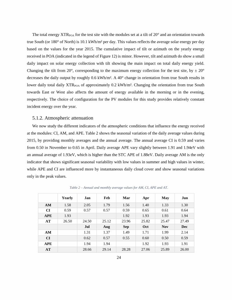
The total energy XTRPOA for the test site with the modules set at a tilt of 20° and an orientation towards

true South (or 180° of North) is 10.1 kWh/m² per day. This values reflects the average solar energy per day

based on the values for the year 2015. The cumulative impact of tilt or azimuth on the yearly energy

received in POA (indicated in the legend of Figure 12) is minor. However, tilt and azimuth do show a small

daily impact on solar energy collection with tilt showing the main impact on total daily energy yield.

Changing the tilt from 20°, corresponding to the maximum energy collection for the test site, by ± 20°

decreases the daily output by roughly 0.6 kWh/m². A 40° change in orientation from true South results in

lower daily total daily XTRPOA of approximately 0.2 kWh/m². Changing the orientation from true South

towards East or West also affects the amount of energy available in the morning or in the evening,

respectively. The choice of configuration for the PV modules for this study provides relatively constant

incident energy over the year.

5.1.2. Atmospheric attenuation

We now study the different indicators of the atmospheric conditions that influence the energy received

at the modules: CI, AM, and APE. Table 2 shows the seasonal variation of the daily average values during

2015, by providing monthly averages and the annual average. The annual average CI is 0.59 and varies

from 0.50 in November to 0.65 in April. Daily average APE vary slightly between 1.91 and 1.94eV with

an annual average of 1.93eV, which is higher than the STC APE of 1.88eV. Daily average AM is the only

indicator that shows significant seasonal variability with low values in summer and high values in winter,

while APE and CI are influenced more by instantaneous daily cloud cover and show seasonal variations

only in the peak values.

Table 2 – Annual and monthly average values for AM, CI, APE and AT.

Yearly Jan Feb Mar Apr May Jun

AM 1.58 2.05 1.79 1.56 1.40 1.33 1.30

CI 0.59 0.57 0.57 0.59 0.65 0.61 0.64

APE 1.93 1.92 1.93 1.93 1.94

AT 26.50 24.50 25.12 23.96 25.82 25.47 27.49

Jul Aug Sep Oct Nov Dec

AM 1.31 1.37 1.49 1.71 1.99 2.14

CI 0.62 0.57 0.55 0.60 0.50 0.59

APE 1.94 1.94 1.92 1.93 1.91

AT 28.66 29.14 28.28 27.06 25.89 26.00

25

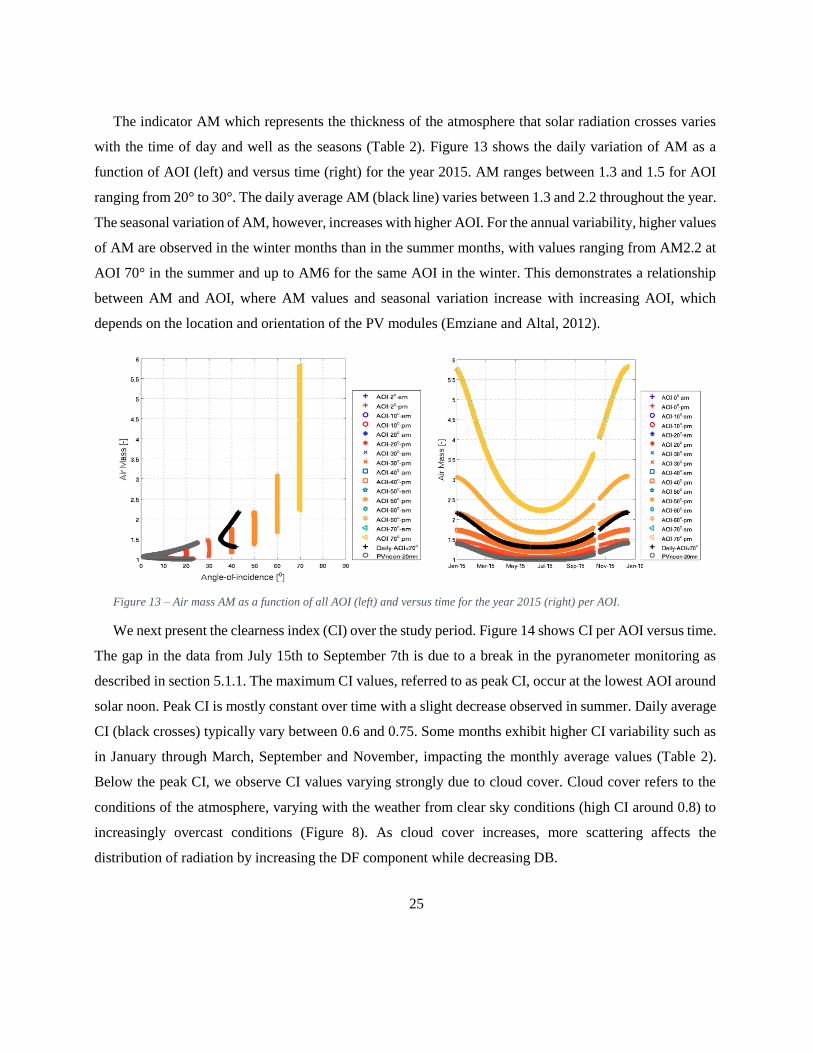
The indicator AM which represents the thickness of the atmosphere that solar radiation crosses varies

with the time of day and well as the seasons (Table 2). Figure 13 shows the daily variation of AM as a

function of AOI (left) and versus time (right) for the year 2015. AM ranges between 1.3 and 1.5 for AOI

ranging from 20° to 30°. The daily average AM (black line) varies between 1.3 and 2.2 throughout the year.

The seasonal variation of AM, however, increases with higher AOI. For the annual variability, higher values

of AM are observed in the winter months than in the summer months, with values ranging from AM2.2 at

AOI 70° in the summer and up to AM6 for the same AOI in the winter. This demonstrates a relationship

between AM and AOI, where AM values and seasonal variation increase with increasing AOI, which

depends on the location and orientation of the PV modules (Emziane and Altal, 2012).

Figure 13 – Air mass AM as a function of all AOI (left) and versus time for the year 2015 (right) per AOI.

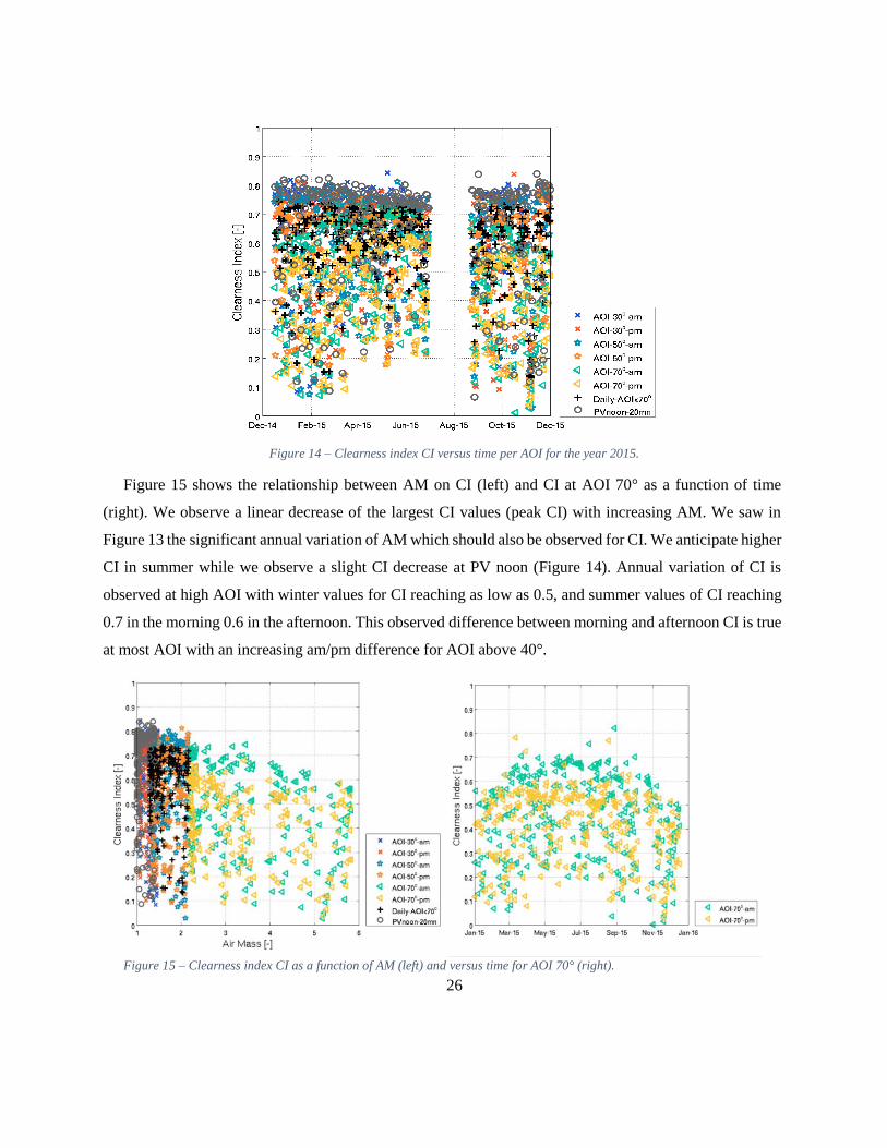
We next present the clearness index (CI) over the study period. Figure 14 shows CI per AOI versus time.

The gap in the data from July 15th to September 7th is due to a break in the pyranometer monitoring as

described in section 5.1.1. The maximum CI values, referred to as peak CI, occur at the lowest AOI around

solar noon. Peak CI is mostly constant over time with a slight decrease observed in summer. Daily average

CI (black crosses) typically vary between 0.6 and 0.75. Some months exhibit higher CI variability such as

in January through March, September and November, impacting the monthly average values (Table 2).

Below the peak CI, we observe CI values varying strongly due to cloud cover. Cloud cover refers to the

conditions of the atmosphere, varying with the weather from clear sky conditions (high CI around 0.8) to

increasingly overcast conditions (Figure 8). As cloud cover increases, more scattering affects the

distribution of radiation by increasing the DF component while decreasing DB.

26

Figure 14 – Clearness index CI versus time per AOI for the year 2015.

Figure 15 shows the relationship between AM on CI (left) and CI at AOI 70° as a function of time

(right). We observe a linear decrease of the largest CI values (peak CI) with increasing AM. We saw in

Figure 13 the significant annual variation of AM which should also be observed for CI. We anticipate higher

CI in summer while we observe a slight CI decrease at PV noon (Figure 14). Annual variation of CI is

observed at high AOI with winter values for CI reaching as low as 0.5, and summer values of CI reaching

0.7 in the morning 0.6 in the afternoon. This observed difference between morning and afternoon CI is true

at most AOI with an increasing am/pm difference for AOI above 40°.

Figure 15 – Clearness index CI as a function of AM (left) and versus time for AOI 70° (right).

27

Higher CI observed in the morning than in the afternoon at high AOI and higher CI in winter than in

summer could be related to the effects of ambient temperature (AT) on CI that show significant am/pm

differences at fixed AOI. Figure 16 presents AT versus time at all AOI. AT appears lower at high AOI,

particularly in the morning compared to the afternoon. We observe an increase in temperature from May to

September, and another increase end of October, while the rest of the year AT is mostly constant below

28°C. Monthly average AT varies between 24°C in March and 29°C in September (Table 2) with an average

of 26.5°C for the year 2015.

Figure 16 – Ambient temperature AT versus time per AOI for the year 2015.

Although the impact of AM on CI is apparent on both daily and seasonal time scales, the largest impact

is at high AOI with less impact on the CI, both daily and at PV noon, which we suspect may be related to

the AT. Cloud cover has a major effect on CI, which affects the distribution of DB and DF. As for the global

irradiance G, the ranges of the DB and DF components increase with increasing solar resource received in

the POA under decreasing AOI as shown in Figure 17, through plots of the DF irradiance as a function of

AM (left) and the DB component as a function of CI (right). At high AOI (70°), DB and DF contribute

approximately equal amounts to G, while DB becomes the main component of incident solar radiation

received by the PV modules at low AOI, where it contributes roughly twice as much to total irradiance as

DF. The right panel of Figure 17 shows that in the early morning for values of CI below ~0.3, the irradiance

is purely DF until the sun rises over the horizon and DB becomes measurable. Above a CI value of ~0.3, a

28

quadratic increase in DB with increasing CI is observed, with a stronger increase in DB for decreasing AOI.

DB is directly proportional to the extraterrestrial solar resource received in POA.

Figure 17 – Diffuse DF versus AM (left) and direct beam DB versus CI (right) under different AOI.

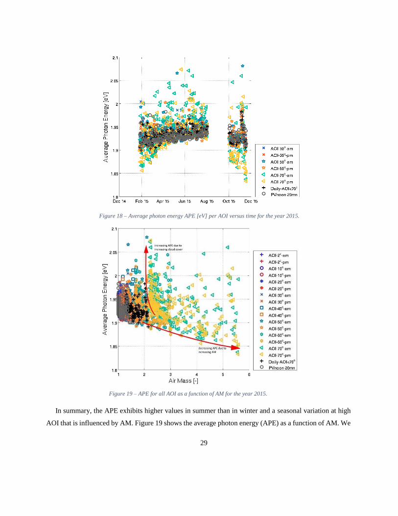
We next examine how the solar spectrum is described by the indicator APE. Figure 18 shows the annual

variation of the average photon energy APE per AOI for the year 2015. The spectroradiometer was not

operating continuously during the year due to updates that were conducted on the instrument. Therefore,

APE values are missing for January, September, October and December. Daily average and PV noon APE

vary over the year with highest values recorded in August and lowest in February. This tendency is not as

clear in the monthly averages in APE (Table 2). For example, daily average APE in November is higher

than in October. This is related to the cloud cover that significantly decreased the CI in November causing

high variability in the APE values during that month. At all AOI, the measurements of APE are above the

APESTC (1.88eV), with the only exception at high AOI during winter. APE exhibits high variability at high

AOI above 60° and seasonal variability with lower values in winter compared to summer.

29

Figure 18 – Average photon energy APE [eV] per AOI versus time for the year 2015.

In summary, the APE exhibits higher values in summer than in winter and a seasonal variation at high

AOI that is influenced by AM. Figure 19 shows the average photon energy (APE) as a function of AM. We

Figure - Average photon energy APE as a function of AM.

Figure 19 – APE for all AOI as a function of AM for the year 2015.

30

observe low values of APE decreasing with increasing AM. APE values are clustered in the range between

1.91eV and 1.96eV with scattered readings of higher values up to 2.08eV distributed at all AOI.

Figure 20 presents APE versus CI for the full year with all AOI included (left) and APE versus CI

exclusively for AOI between 0° to 40° (right), representing the time during which solar yield is the highest.

A large range of APE values is observed at high AOI. At low AOI, APE varies mostly between 1.91eV for

clear sky conditions (CI~0.8) and 1.96eV for overcast sky conditions (CI~0.3), indicating elevated APE

values at lower CI. At CI values under ~0.3 at dawn and dusk, or when highly overcast, DF is the major

component to irradiance. As DF is lies within the lower wavelength range in the spectrum, APE is higher

(Figure 6), hence, providing empirical evidence for somewhat higher APE values for DF compared to DB

irradiance. At peak CI at solar noon, APE decreases with increasing CI, which is consistent with the seasonal

variation of both CI and APE. Lower CI in summer is responsible for more scattering and thus higher APE

values (seasonal variation ~0.03-0.04eV), whereby APE increases by around 0.05-0.1eV with decreasing

CI due to increasing cloud cover.

Figure 20 – Average photon energy APE as a function of CI for the full year with selected AOI included (left) and at AOI between

0°-40° (right).

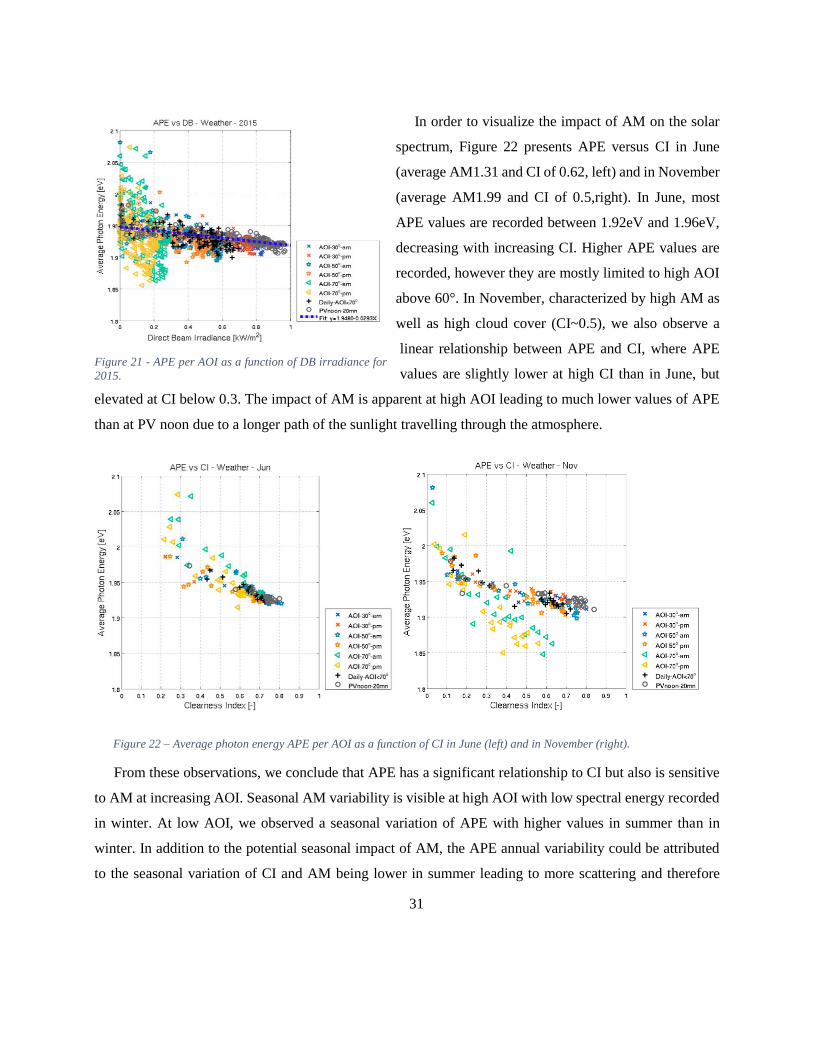
When plotting APE versus DB for 2015 (Figure 21), a linear relationship is visible at PV noon between

the two parameters. The plotted fitting curve (dashed blue line) is calculated using the least-squares method.

In the regression, we remove the bottom 10% of the DB data, below 0.1kW/m², as the data at low irradiance

is not representative of the linear trend. The impact of DB on APE at PV noon is estimated at -0.028eV per

kW/m² with APE at 1.92eV when DB is 1kW/m². This variability of APE at all AOI is due to the effects of

CI and AM.

31

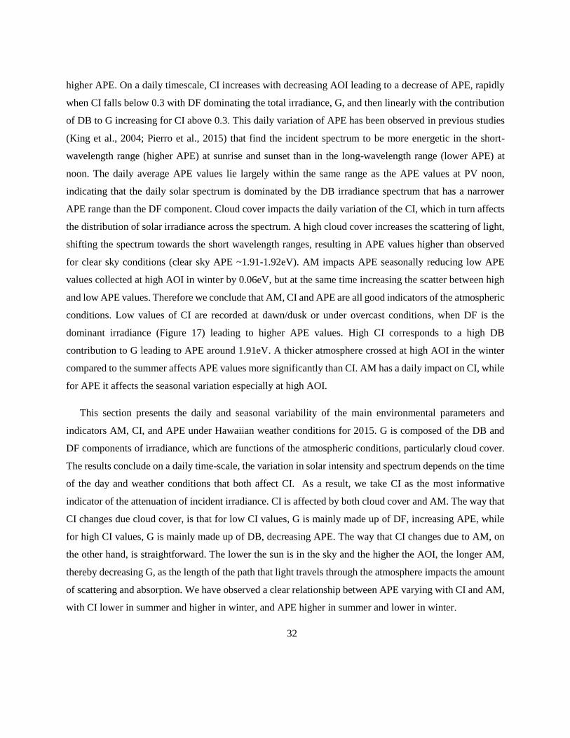
In order to visualize the impact of AM on the solar

spectrum, Figure 22 presents APE versus CI in June

(average AM1.31 and CI of 0.62, left) and in November

(average AM1.99 and CI of 0.5,right). In June, most

APE values are recorded between 1.92eV and 1.96eV,

decreasing with increasing CI. Higher APE values are

recorded, however they are mostly limited to high AOI

above 60°. In November, characterized by high AM as

well as high cloud cover (CI~0.5), we also observe a

linear relationship between APE and CI, where APE

values are slightly lower at high CI than in June, but

elevated at CI below 0.3. The impact of AM is apparent at high AOI leading to much lower values of APE

than at PV noon due to a longer path of the sunlight travelling through the atmosphere.

Figure 22 – Average photon energy APE per AOI as a function of CI in June (left) and in November (right).

From these observations, we conclude that APE has a significant relationship to CI but also is sensitive

to AM at increasing AOI. Seasonal AM variability is visible at high AOI with low spectral energy recorded

in winter. At low AOI, we observed a seasonal variation of APE with higher values in summer than in

winter. In addition to the potential seasonal impact of AM, the APE annual variability could be attributed

to the seasonal variation of CI and AM being lower in summer leading to more scattering and therefore

Figure 21 - APE per AOI as a function of DB irradiance for

2015.

32

higher APE. On a daily timescale, CI increases with decreasing AOI leading to a decrease of APE, rapidly

when CI falls below 0.3 with DF dominating the total irradiance, G, and then linearly with the contribution

of DB to G increasing for CI above 0.3. This daily variation of APE has been observed in previous studies

(King et al., 2004; Pierro et al., 2015) that find the incident spectrum to be more energetic in the short-

wavelength range (higher APE) at sunrise and sunset than in the long-wavelength range (lower APE) at

noon. The daily average APE values lie largely within the same range as the APE values at PV noon,

indicating that the daily solar spectrum is dominated by the DB irradiance spectrum that has a narrower

APE range than the DF component. Cloud cover impacts the daily variation of the CI, which in turn affects

the distribution of solar irradiance across the spectrum. A high cloud cover increases the scattering of light,

shifting the spectrum towards the short wavelength ranges, resulting in APE values higher than observed

for clear sky conditions (clear sky APE ~1.91-1.92eV). AM impacts APE seasonally reducing low APE

values collected at high AOI in winter by 0.06eV, but at the same time increasing the scatter between high

and low APE values. Therefore we conclude that AM, CI and APE are all good indicators of the atmospheric

conditions. Low values of CI are recorded at dawn/dusk or under overcast conditions, when DF is the

dominant irradiance (Figure 17) leading to higher APE values. High CI corresponds to a high DB

contribution to G leading to APE around 1.91eV. A thicker atmosphere crossed at high AOI in the winter

compared to the summer affects APE values more significantly than CI. AM has a daily impact on CI, while

for APE it affects the seasonal variation especially at high AOI.

This section presents the daily and seasonal variability of the main environmental parameters and

indicators AM, CI, and APE under Hawaiian weather conditions for 2015. G is composed of the DB and

DF components of irradiance, which are functions of the atmospheric conditions, particularly cloud cover.

The results conclude on a daily time-scale, the variation in solar intensity and spectrum depends on the time

of the day and weather conditions that both affect CI. As a result, we take CI as the most informative

indicator of the attenuation of incident irradiance. CI is affected by both cloud cover and AM. The way that

CI changes due cloud cover, is that for low CI values, G is mainly made up of DF, increasing APE, while

for high CI values, G is mainly made up of DB, decreasing APE. The way that CI changes due to AM, on

the other hand, is straightforward. The lower the sun is in the sky and the higher the AOI, the longer AM,

thereby decreasing G, as the length of the path that light travels through the atmosphere impacts the amount

of scattering and absorption. We have observed a clear relationship between APE varying with CI and AM,

with CI lower in summer and higher in winter, and APE higher in summer and lower in winter.

33

Low CI corresponds to dawn/dusk or overcast conditions when the DF component of G is predominant

leading to high spectral energy (APE). High CI is related to midday and clear sky conditions when DB is

predominant inducing lower APE values. We observe seasonal variations in AM, CI, APE and somewhat

AT and with the biannual cycle of the solar resources peaking at the two equinoxes and related to the PV

location and orientation. AM impacts all others parameters by decreasing CI and APE when a thicker

atmosphere is crossed during winter. The impact of AM on the parameters, however, occurs mostly at high

AOI where the solar energy collection is minimal. The seasonal impact observed at PV noon when most

solar energy is collected, is attributed to the lower observed values of CI and AM both leading to higher

spectral energy (APE) in summer than in winter. The solar resource at UH Manoa is consistently high in

intensity and energy all year.

5.2. Evaluation of PV performance under ROC

The PV module performance and parameters are described in section 3. Now, we examine how the

variability in the environmental parameters affects the performance of both the individual PV modules as

tested in the two PV sets over the first and second half of the year as well as the complete a-Si/µc-Si and c-

Si grid-connected PV systems that were in operation over the year 2015. The PR is a function of the energy

generated by the PV module or system divided by energy received by the PV module or system (EPV ÷ ESUN)

which we use as the performance criteria for outdoor testing of PV systems under ROC. In this approach,

the PR is considered as the product of the current performance (IP) of the system and the operating voltage

normalized to STC (VN). The main daily variation observed for the PR is due to the variation in IP, while

the impact of VN on the PR variation is considerably lower on a daily time-scale. In this study, we analyze

the individual modules’ short-circuit current performance IPSC, which is compared to the systems’ IP,

reflecting the system’s and module’s abilities to absorb the solar resource and changing spectrum under

ROC compared to STC.

The short-circuit current performance, IPSC, reflects the part of solar radiation that can be usefully

converted into an electric current (Pierro et al., 2015) and represents the main parameter of the PV module

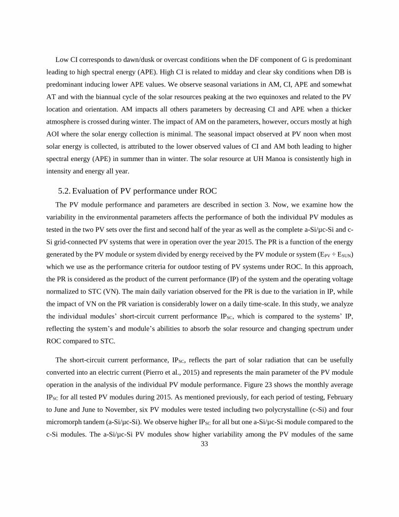
operation in the analysis of the individual PV module performance. Figure 23 shows the monthly average

IPSC for all tested PV modules during 2015. As mentioned previously, for each period of testing, February

to June and June to November, six PV modules were tested including two polycrystalline (c-Si) and four

micromorph tandem (a-Si/µc-Si). We observe higher IPSC for all but one a-Si/µc-Si module compared to the

c-Si modules. The a-Si/µc-Si PV modules show higher variability among the PV modules of the same

34

model, which is due to the performance distribution among newly installed modules and/or different

degradation among modules. The variation in performance also is evident in June where the tested PV

modules exhibit different performance. The IPSC shows minor variability over the year, with a tendency to

be slightly higher in summer than in December. When including all twelve tested modules, IPSC averages

102.5% for a-Si/µc-Si and 98.4% for c-Si.

Figure 23 – Monthly average IPSC versus time for multiple PV modules tested in 2015, a-Si/µc-Si (dotted line) and c-Si (continuous

line).

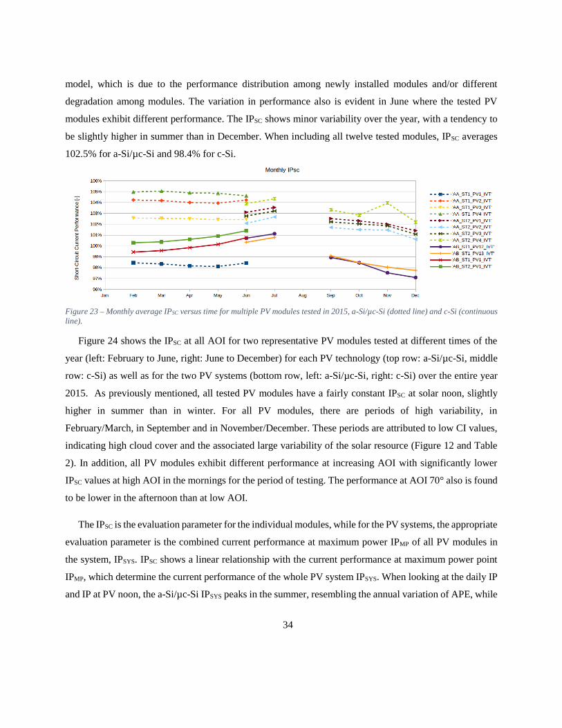
Figure 24 shows the IPSC at all AOI for two representative PV modules tested at different times of the

year (left: February to June, right: June to December) for each PV technology (top row: a-Si/µc-Si, middle

row: c-Si) as well as for the two PV systems (bottom row, left: a-Si/µc-Si, right: c-Si) over the entire year

2015. As previously mentioned, all tested PV modules have a fairly constant IPSC at solar noon, slightly

higher in summer than in winter. For all PV modules, there are periods of high variability, in

February/March, in September and in November/December. These periods are attributed to low CI values,

indicating high cloud cover and the associated large variability of the solar resource (Figure 12 and Table

2). In addition, all PV modules exhibit different performance at increasing AOI with significantly lower

IPSC values at high AOI in the mornings for the period of testing. The performance at AOI 70° also is found

to be lower in the afternoon than at low AOI.

The IPSC is the evaluation parameter for the individual modules, while for the PV systems, the appropriate

evaluation parameter is the combined current performance at maximum power IPMP of all PV modules in

the system, IPSYS. IPSC shows a linear relationship with the current performance at maximum power point

IPMP, which determine the current performance of the whole PV system IPSYS. When looking at the daily IP

and IP at PV noon, the a-Si/µc-Si IPSYS peaks in the summer, resembling the annual variation of APE, while

35

the variation in the c-Si IPSYS is insignificant over the year, which may be partially explained by a potential

temperature impact.

a-Si/µc-Si

c-Si

Figure 24 – IPSC versus time for a-Si/µc-Si (top row) and c-Si (middle row) PV modules and IP of PV systems (bottom row, left: a-

Si/µc-Si, right: c-Si). a-Si/µc-Si IPSYS peaks in summer while c-Si is relatively constant over the year.

36

We next consider the effects of the main environmental parameters on IPSC for all AOI, in order to fully

visualize the relationships. Figure 25 present IPSC versus G, DB, CI and APE for a single a-Si/µc-Si module

operating during November 2015. We show in Section 5.2. that the aforementioned parameters are related.

The results in Section 5.1. provide us with an assessment of the relevant parameters to characterize the PV

module performance. Daily IPSC (black crosses) decreases with increasing G, CI and DB. At high IPSC under

low irradiance conditions, when G is below 0.3 kW/m², we found that DB equals zero, CI is below 0.3 and

APE above 1.95eV. When DF is the dominant component of G, IPSC decreases with increasing G and CI,

and decreasing APE above 1.95eV. For CI above ~0.3, APE is nearly constant which limits its impact on

IPSC. The most informative plots to analyze how environmental parameters impact gain and loss

mechanisms of the solar resource are IPSC versus CI, G and DB. We find that the variation of IPSC with DB

(Figure 25b) resembles the variation of IPSC with G (Figure 25a), indicating the importance of DB in the

generation of an electric current, both for daily averages and at PV noon. At high fixed AOI, IPSC decreases

with increasing G, DB and CI. At all AOI, the observed IPSC is higher in the afternoon than in the morning.

37

.

Figure 25 – IPSC versus G (top left), DB (top right), CI (bottom left) and APE (bottom right) for all AOI for a single a-Si/µc-Si

module operating over November 2015.

Figure 26 illustrates the impact of DB on the spectrum (APE) and CI for two months characterized by

different AM. Figure 26 shows APE (top row) and CI (bottom row) as a function of DB at all AOI in June

(left) and in November (right). We observe that for values of DB above ~0.1 at fixed AOI, the APE decreases

linearly with increasing DB. In November, the monitored APE values are lower than in June at all AOI, but

particularly at high AOI due to the high seasonal variation in AM. The seasonal CI variation is mostly visible

at peak CI with higher CI in November than in June.

38

Figure 26 – APE (top row) and CI (bottom row) per AOI versus DB for the months of June (left) and November (right) 2015.

Figure 27 presents IPSC versus DB for June (left) when the AM is low, and November (right) when AM

is high. The top panel shows data for the a-Si/µc-Si module (MHI), the middle panels for the c-Si module

(KYO). The bottom panels present the results for the IP of the two PV systems a-Si/µc-Si (left) and c-Si

(right) versus DB for the complete year of operation.

For both PV module types, we observe higher performance in June than in November. This may be

related to lower APE, higher CI or lower AT in November compared to June. Despite that slight drop in

performance in November, the IPSC versus DB curves are very similar between the two months and even

between PV modules types. A slight difference exists at clear sky conditions (bottom data points with low

IP, high DB) which may be due to different relationships among CI/DB/AT/AM depending upon the month

of operation. For clear skies, IP increases with increasing DB and decreasing AOI. APE has a high seasonal

impact at high AOI under clear sky conditions, which is not apparent in IP due to the low impact of seasonal

APE on IPSC at high AOI. Clear sky IP would therefore be affected mostly by recombination and reflection

loss whose impacts increase at low G or high AOI. Morning performance is much lower than in the afternoon

at all AOI which we also attribute to different CI/DB/AT/AM relationships depending upon the time of day.

In the afternoons, IPSC has high constant values at high DB with AOI above 50°. Afternoon IPSC values

decrease with increasing AOI above 50°, which is due to the PV modules being particularly affected by

light reflection on the surface. For both PV systems, we plotted (not shown here) IPSYS versus DB for the 2

selected months, June and November, as with the PV modules and observed similar results for IP compared

to IPSC. The bottom panels of Figure 27 represent data for the complete year of operation, showing higher

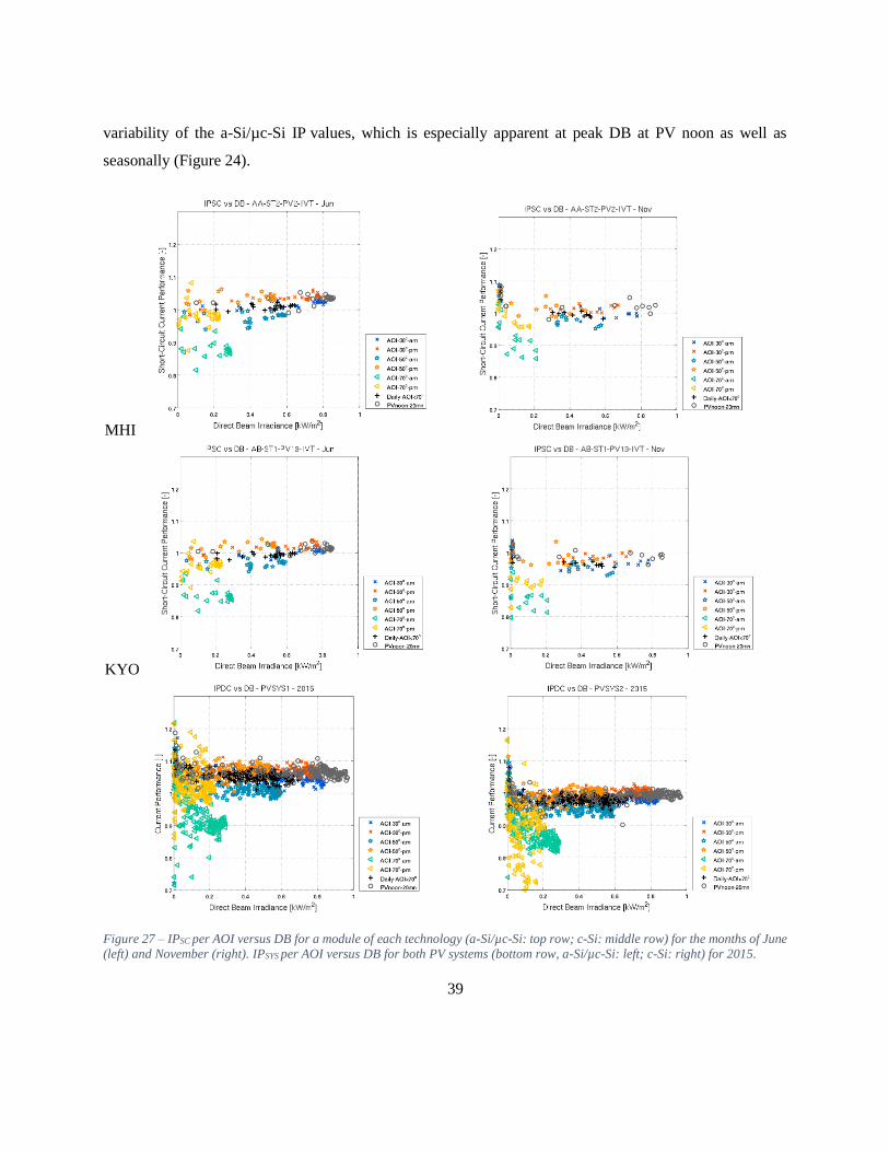
39

variability of the a-Si/µc-Si IP values, which is especially apparent at peak DB at PV noon as well as

seasonally (Figure 24).

MHI

KYO …

Figure 27 – IPSC per AOI versus DB for a module of each technology (a-Si/µc-Si: top row; c-Si: middle row) for the months of June

(left) and November (right). IPSYS per AOI versus DB for both PV systems (bottom row, a-Si/µc-Si: left; c-Si: right) for 2015.

40

From Figure 27, we observe that for both months and both module technologies, DB shows a similar

impact on IPSC. The main impact on seasonal variation of IPSC is attributed to CI, APE or AT. IPSC is

influenced by a daily APE variation when overcast conditions, described by low CI, promote scattering of

light, changing the incident solar spectrum. No seasonal variation of IPSC with APE is observed under clear

sky conditions marked by high CI. The panels of Figure 27 aimed at demonstrating that the IPSC for

individual PV modules is representative of the IP for the PV systems, although additional losses due to

operation at maximum power or due to system configuration and module mismatch may impact the IPSYS.

Figure 28 presents IPSC and IPSYS per AOI versus CI for the two PV technologies. From this study, we

are not able to distinguish the effects of the individual parameters (APE, AT, G/DB/DF) on IPSC and IPSYS,

but we describe qualitatively the behavior of IP versus CI that will lead in the future to a better

characterization of PV performance and the IP parameters. Firstly, the daily IPSC is approximately constant

at all CI for the c-Si module, while the a-Si/µc-Si IPSC increases with decreasing CI showing enhanced

performance at low CI below ~0.3. This is attributed to the higher sensitivity of the micromorph PV

technology to shorter wavelengths and subsequently better performance under low G when DF is

predominant (Pierro et al., 2015). This difference between PV technologies is not as apparent when

considering the system’s IPSYS. More analysis is needed to understand the impact of combining PV modules

on the current performance and the differences between the IPSC and IPMP. Secondly, plotting IP versus CI

shows similar behavior to that observed versus DB (Figure 27). The irradiance G decreases with increasing

AOI on clear days. Under clear sky conditions, CI decreases with increasing AOI and the relationship

between CI and AOI or AM is different in the morning than in the afternoon (represented in Figure 28a by

cooler and warmer colors), and also exhibits seasonal variability (represented in Figure 28a by grey circles

at peak CI). The decrease in IP with increasing AOI is related to decreasing G. Both recombination and

reflection losses are affected by G (section 3.3) and the losses increase with increasing AOI. Changes in IP

with CI on clear sky depends of time of the day and of the year which we relate to variations in G/DB/DF,

APE, and AT. More work is needed to differentiate the individual impact of those correlated parameters.

Finally, we consider the behavior of IP with peak CI at PV noon, where we observe a decrease in IP with

increasing CI that is larger in winter than in summer. The seasonal variation of IP at peak PV noon is

attributed to the seasonal variation of APE and AT where APE decreases with increasing CI (Figure 22).

When comparing the performance of the two PV technologies, a-Si/µc-Si shows higher variability than c-

Si, which is particularly apparent for the PV system performance. This variation is clearly visible in the

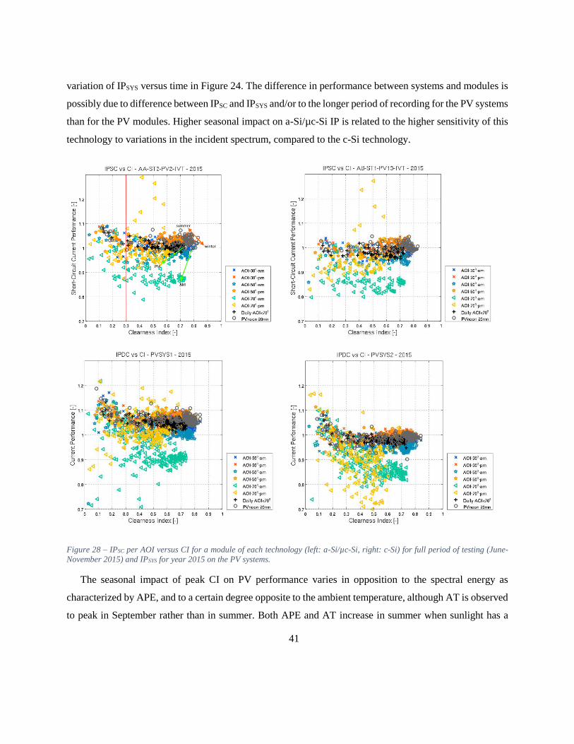
41

variation of IPSYS versus time in Figure 24. The difference in performance between systems and modules is

possibly due to difference between IPSC and IPSYS and/or to the longer period of recording for the PV systems

than for the PV modules. Higher seasonal impact on a-Si/µc-Si IP is related to the higher sensitivity of this

technology to variations in the incident spectrum, compared to the c-Si technology.

Figure 28 – IPSC per AOI versus CI for a module of each technology (left: a-Si/µc-Si, right: c-Si) for full period of testing (June-

November 2015) and IPSYS for year 2015 on the PV systems.

The seasonal impact of peak CI on PV performance varies in opposition to the spectral energy as

characterized by APE, and to a certain degree opposite to the ambient temperature, although AT is observed

to peak in September rather than in summer. Both APE and AT increase in summer when sunlight has a

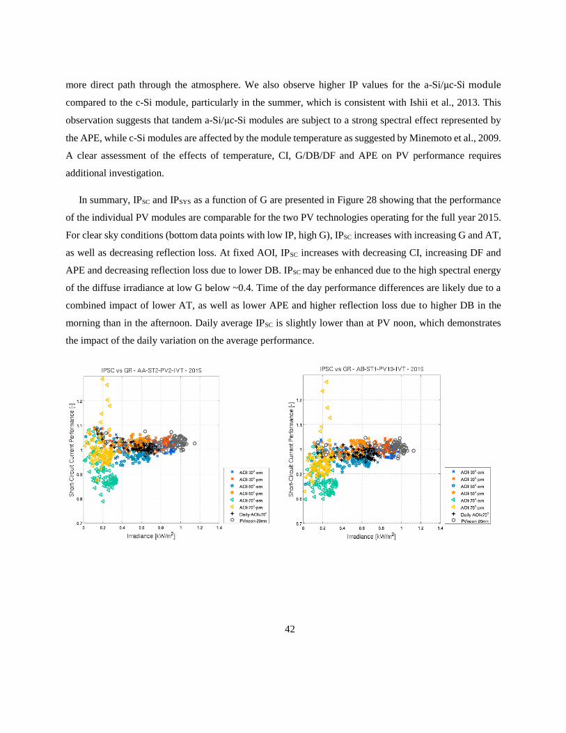
42

more direct path through the atmosphere. We also observe higher IP values for the a-Si/µc-Si module

compared to the c-Si module, particularly in the summer, which is consistent with Ishii et al., 2013. This

observation suggests that tandem a-Si/µc-Si modules are subject to a strong spectral effect represented by

the APE, while c-Si modules are affected by the module temperature as suggested by Minemoto et al., 2009.

A clear assessment of the effects of temperature, CI, G/DB/DF and APE on PV performance requires

additional investigation.

In summary, IPSC and IPSYS as a function of G are presented in Figure 28 showing that the performance

of the individual PV modules are comparable for the two PV technologies operating for the full year 2015.

For clear sky conditions (bottom data points with low IP, high G), IPSC increases with increasing G and AT,

as well as decreasing reflection loss. At fixed AOI, IPSC increases with decreasing CI, increasing DF and

APE and decreasing reflection loss due to lower DB. IPSC may be enhanced due to the high spectral energy

of the diffuse irradiance at low G below ~0.4. Time of the day performance differences are likely due to a

combined impact of lower AT, as well as lower APE and higher reflection loss due to higher DB in the

morning than in the afternoon. Daily average IPSC is slightly lower than at PV noon, which demonstrates

the impact of the daily variation on the average performance.

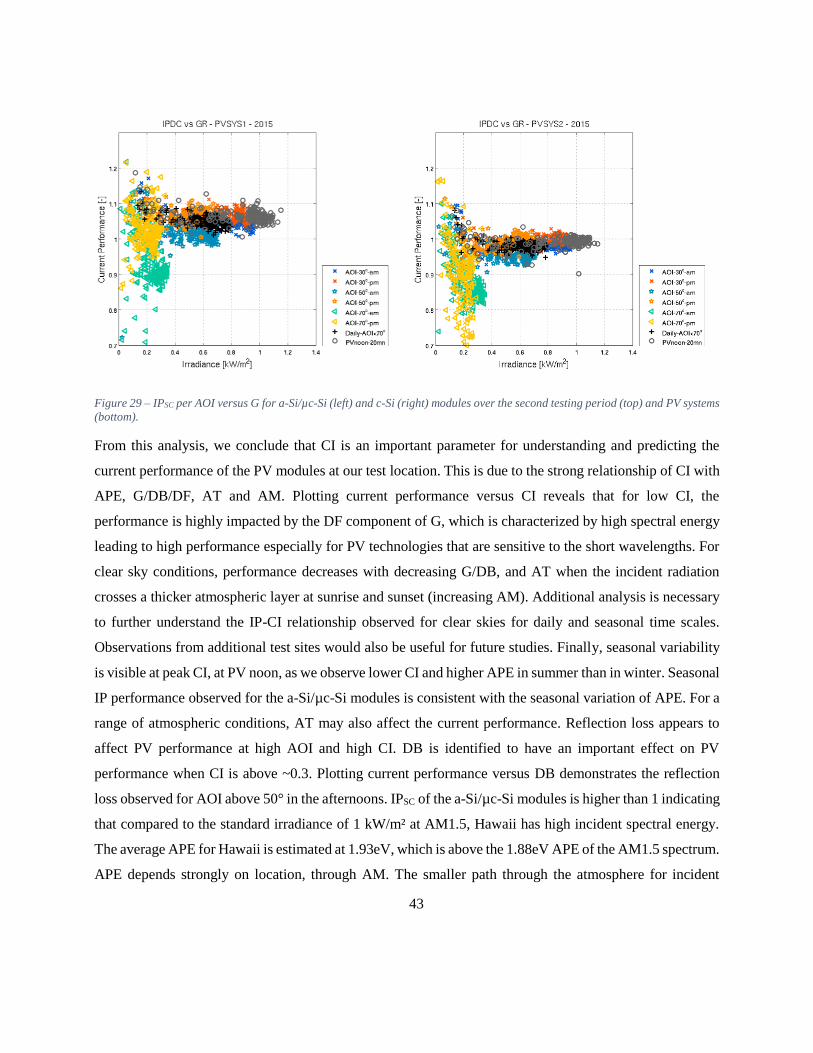
43

Figure 29 – IPSC per AOI versus G for a-Si/µc-Si (left) and c-Si (right) modules over the second testing period (top) and PV systems

(bottom).

From this analysis, we conclude that CI is an important parameter for understanding and predicting the

current performance of the PV modules at our test location. This is due to the strong relationship of CI with

APE, G/DB/DF, AT and AM. Plotting current performance versus CI reveals that for low CI, the

performance is highly impacted by the DF component of G, which is characterized by high spectral energy

leading to high performance especially for PV technologies that are sensitive to the short wavelengths. For

clear sky conditions, performance decreases with decreasing G/DB, and AT when the incident radiation

crosses a thicker atmospheric layer at sunrise and sunset (increasing AM). Additional analysis is necessary

to further understand the IP-CI relationship observed for clear skies for daily and seasonal time scales.

Observations from additional test sites would also be useful for future studies. Finally, seasonal variability

is visible at peak CI, at PV noon, as we observe lower CI and higher APE in summer than in winter. Seasonal

IP performance observed for the a-Si/µc-Si modules is consistent with the seasonal variation of APE. For a

range of atmospheric conditions, AT may also affect the current performance. Reflection loss appears to

affect PV performance at high AOI and high CI. DB is identified to have an important effect on PV

performance when CI is above ~0.3. Plotting current performance versus DB demonstrates the reflection

loss observed for AOI above 50° in the afternoons. IPSC of the a-Si/µc-Si modules is higher than 1 indicating

that compared to the standard irradiance of 1 kW/m² at AM1.5, Hawaii has high incident spectral energy.

The average APE for Hawaii is estimated at 1.93eV, which is above the 1.88eV APE of the AM1.5 spectrum.

APE depends strongly on location, through AM. The smaller path through the atmosphere for incident

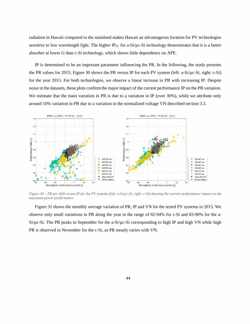
44

radiation in Hawaii compared to the mainland makes Hawaii an advantageous location for PV technologies

sensitive to low wavelength light. The higher IPSC for a-Si/µc-Si technology demonstrates that it is a better

absorber at lower G than c-Si technology, which shows little dependence on APE.

IP is determined to be an important parameter influencing the PR. In the following, the study presents

the PR values for 2015. Figure 30 shows the PR versus IP for each PV system (left: a-Si/µc-Si, right: c-Si)

for the year 2015. For both technologies, we observe a linear increase in PR with increasing IP. Despite

noise in the datasets, these plots confirm the major impact of the current performance IP on the PR variation.

We estimate that the main variation in PR is due to a variation in IP (over 30%), while we attribute only

around 10% variation in PR due to a variation in the normalized voltage VN described section 3.3.

Figure 30 – PR per AOI versus IP for the PV systems (left: a-Si/µc-Si, right: c-Si) showing the current performance impact on the

maximum power performance.

Figure 31 shows the monthly average variation of PR, IP and VN for the tested PV systems in 2015. We

observe only small variations in PR along the year in the range of 92-94% for c-Si and 83-90% for the a-

Si/µc-Si. The PR peaks in September for the a-Si/µc-Si corresponding to high IP and high VN while high

PR is observed in November for the c-Si, as PR mostly varies with VN.

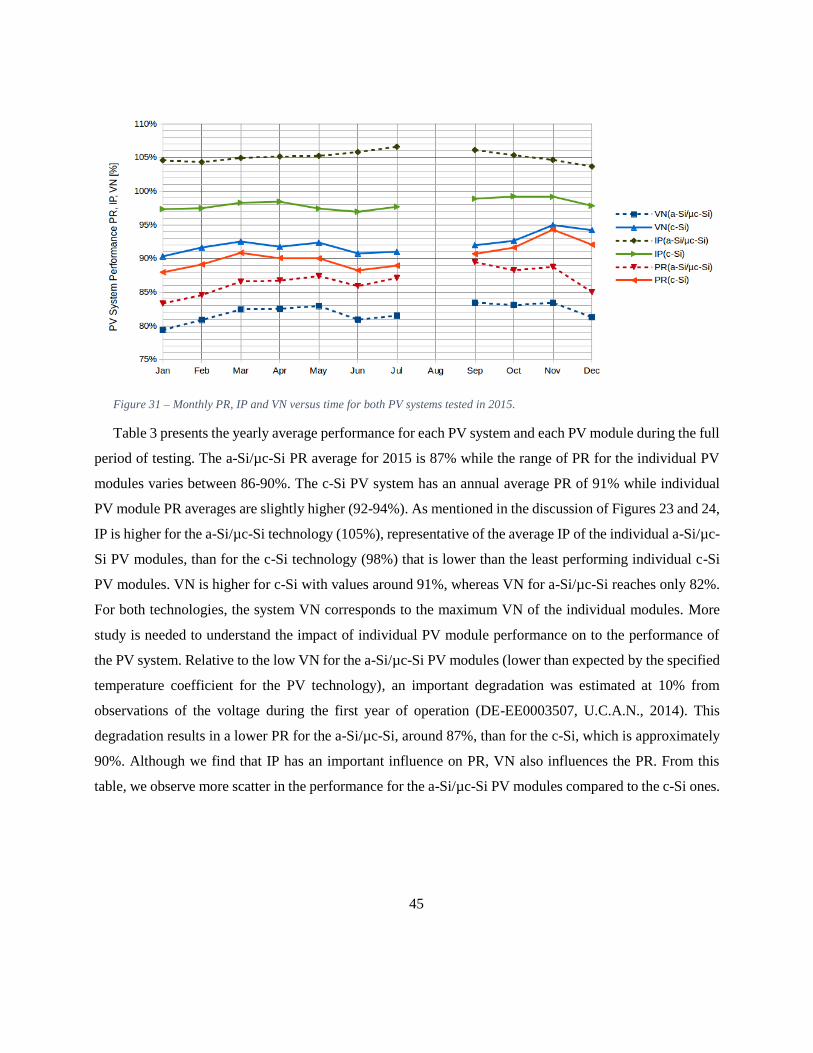
45

Figure 31 – Monthly PR, IP and VN versus time for both PV systems tested in 2015.

Table 3 presents the yearly average performance for each PV system and each PV module during the full

period of testing. The a-Si/µc-Si PR average for 2015 is 87% while the range of PR for the individual PV

modules varies between 86-90%. The c-Si PV system has an annual average PR of 91% while individual

PV module PR averages are slightly higher (92-94%). As mentioned in the discussion of Figures 23 and 24,

IP is higher for the a-Si/µc-Si technology (105%), representative of the average IP of the individual a-Si/µc-

Si PV modules, than for the c-Si technology (98%) that is lower than the least performing individual c-Si

PV modules. VN is higher for c-Si with values around 91%, whereas VN for a-Si/µc-Si reaches only 82%.

For both technologies, the system VN corresponds to the maximum VN of the individual modules. More

study is needed to understand the impact of individual PV module performance on to the performance of

the PV system. Relative to the low VN for the a-Si/µc-Si PV modules (lower than expected by the specified

temperature coefficient for the PV technology), an important degradation was estimated at 10% from

observations of the voltage during the first year of operation (DE-EE0003507, U.C.A.N., 2014). This

degradation results in a lower PR for the a-Si/µc-Si, around 87%, than for the c-Si, which is approximately

90%. Although we find that IP has an important influence on PR, VN also influences the PR. From this

table, we observe more scatter in the performance for the a-Si/µc-Si PV modules compared to the c-Si ones.

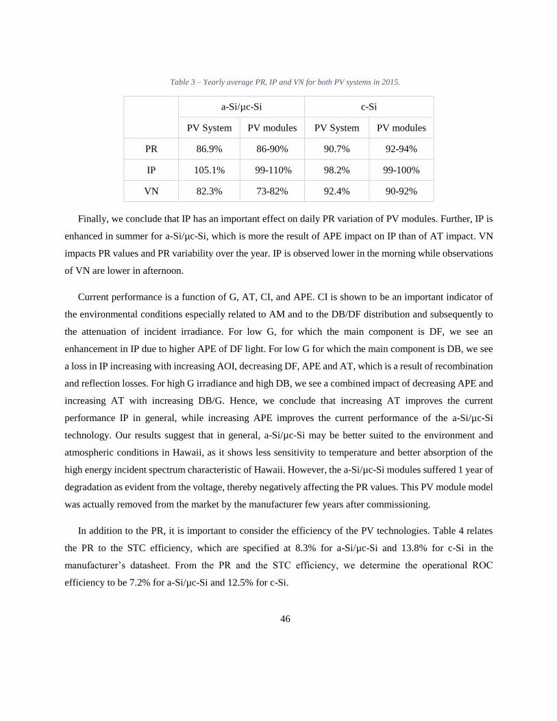
46

Table 3 – Yearly average PR, IP and VN for both PV systems in 2015.

a-Si/µc-Si c-Si

PV System PV modules PV System PV modules

PR 86.9% 86-90% 90.7% 92-94%

IP 105.1% 99-110% 98.2% 99-100%

VN 82.3% 73-82% 92.4% 90-92%

Finally, we conclude that IP has an important effect on daily PR variation of PV modules. Further, IP is

enhanced in summer for a-Si/µc-Si, which is more the result of APE impact on IP than of AT impact. VN

impacts PR values and PR variability over the year. IP is observed lower in the morning while observations

of VN are lower in afternoon.

Current performance is a function of G, AT, CI, and APE. CI is shown to be an important indicator of

the environmental conditions especially related to AM and to the DB/DF distribution and subsequently to

the attenuation of incident irradiance. For low G, for which the main component is DF, we see an

enhancement in IP due to higher APE of DF light. For low G for which the main component is DB, we see

a loss in IP increasing with increasing AOI, decreasing DF, APE and AT, which is a result of recombination

and reflection losses. For high G irradiance and high DB, we see a combined impact of decreasing APE and

increasing AT with increasing DB/G. Hence, we conclude that increasing AT improves the current

performance IP in general, while increasing APE improves the current performance of the a-Si/µc-Si

technology. Our results suggest that in general, a-Si/µc-Si may be better suited to the environment and

atmospheric conditions in Hawaii, as it shows less sensitivity to temperature and better absorption of the

high energy incident spectrum characteristic of Hawaii. However, the a-Si/µc-Si modules suffered 1 year of

degradation as evident from the voltage, thereby negatively affecting the PR values. This PV module model

was actually removed from the market by the manufacturer few years after commissioning.

In addition to the PR, it is important to consider the efficiency of the PV technologies. Table 4 relates

the PR to the STC efficiency, which are specified at 8.3% for a-Si/µc-Si and 13.8% for c-Si in the

manufacturer’s datasheet. From the PR and the STC efficiency, we determine the operational ROC

efficiency to be 7.2% for a-Si/µc-Si and 12.5% for c-Si.

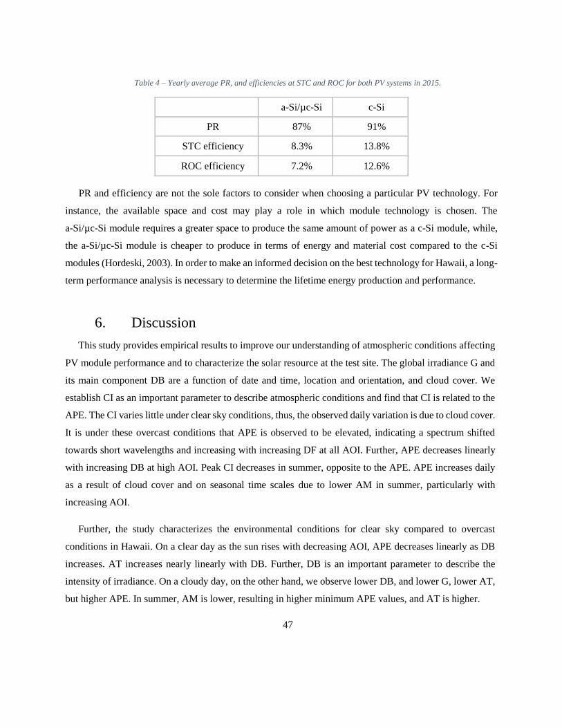
47

Table 4 – Yearly average PR, and efficiencies at STC and ROC for both PV systems in 2015.

a-Si/µc-Si c-Si

PR 87% 91%

STC efficiency 8.3% 13.8%

ROC efficiency 7.2% 12.6%

PR and efficiency are not the sole factors to consider when choosing a particular PV technology. For

instance, the available space and cost may play a role in which module technology is chosen. The

a-Si/µc-Si module requires a greater space to produce the same amount of power as a c-Si module, while,

the a-Si/µc-Si module is cheaper to produce in terms of energy and material cost compared to the c-Si

modules (Hordeski, 2003). In order to make an informed decision on the best technology for Hawaii, a long-

term performance analysis is necessary to determine the lifetime energy production and performance.

6. Discussion

This study provides empirical results to improve our understanding of atmospheric conditions affecting

PV module performance and to characterize the solar resource at the test site. The global irradiance G and

its main component DB are a function of date and time, location and orientation, and cloud cover. We

establish CI as an important parameter to describe atmospheric conditions and find that CI is related to the

APE. The CI varies little under clear sky conditions, thus, the observed daily variation is due to cloud cover.

It is under these overcast conditions that APE is observed to be elevated, indicating a spectrum shifted

towards short wavelengths and increasing with increasing DF at all AOI. Further, APE decreases linearly

with increasing DB at high AOI. Peak CI decreases in summer, opposite to the APE. APE increases daily

as a result of cloud cover and on seasonal time scales due to lower AM in summer, particularly with

increasing AOI.

Further, the study characterizes the environmental conditions for clear sky compared to overcast

conditions in Hawaii. On a clear day as the sun rises with decreasing AOI, APE decreases linearly as DB

increases. AT increases nearly linearly with DB. Further, DB is an important parameter to describe the

intensity of irradiance. On a cloudy day, on the other hand, we observe lower DB, and lower G, lower AT,

but higher APE. In summer, AM is lower, resulting in higher minimum APE values, and AT is higher.

48

We analyze the changes in PV module performance and efficiency, while demonstrating which

parameters appear to be responsible for the observed variations in IP and PR. The comparison of the two

technologies a-Si/µc-Si and c-Si for the year 2015 has shown a daily PR average of 87% and 91%,

respectively. The higher PR for c-Si is largely due to a higher voltage performance. The variation in

performance between tested PV modules is estimated to be higher for the a-Si/µc-Si modules than for the

c-Si modules. Performance variation among modules in a system may impact PV system performance,

limiting the current performance of a string of modules to the least performing module. For this study, the

module wiring of the PV systems was set to six parallel strings of four PV modules for the micromorph

system, which proved to be advantageous over the two parallel strings of 13 PV modules for the c-Si system.

Module wiring is related to the PV technologies due to the voltage level of the PV modules (100 VMP for a-

Si/µc-Si and 26.6 VMP for c-Si). The outdoor performance of the two PV module technologies differs also

in the way that current output is affected by the environmental parameters. The PR of c-Si modules is largely

impacted by temperature, with less impact from APE due to the wide spectral response of c-Si. In contrast,

a-Si/µc-Si modules operate in a spectral range that is shifted towards the short-wavelength higher energy-

density radiation, resulting in PR that mainly depends on the spectral irradiance distribution while being

less sensitive to temperature than c-Si. These results are consistent with other studies (Minemoto et al.,

2009; Cañete et al., 2014) that have shown better c-Si performance in winter while superior a-Si/µc-Si

performance in summer, for which the a-Si layer is the main factor of enhancement under such conditions.

Hawaii’s climatic conditions are comparable to a long summer, in which a-Si/µc-Si performance is favored

over much of the year. Hence, the APE dependency of a-Si/µc-Si results in higher current performance IP

compared to c-Si.

As the study has shown, most environmental parameters are related, making it is challenging to isolate

the impact of a single parameter. In this study, the assessment of environmental parameters has shown

different impacts on the IP and PR due to the intensity, distribution, and spectrum of solar radiation. The

analysis of the impact of environmental parameters on the intensity of solar irradiance suggests the following

conclusions:

1. The availability of the solar resource XTRPOA depends on the cosine of the incident angle cos(AOI).

The yearly minimum AOI is optimized at a 20° tilt for this test configuration, hence enabling the

maximum energy yield.

49

2. DB is the main component of G, in spite of showing lower spectral energy content (as shown by

APE) compared to DF.

3. The solar intensity is influenced by CI, which is impacted by cloud cover and slightly by AM.

APE proves to be a good indicator for atmospheric conditions. The range for APE for the test location is

between 1.91eV and 1.96eV, which is higher than the average spectrum at AM1.5 collected on the mainland,

whose energy is 1.88eV for the spectral response range of 350-1050 nm. This indicates that the solar

resource at UH Manoa is characterized by generally high energy levels in terms of XTRPOA as well as clear

sky conditions, as indicated by high CI. The analysis of the impact of environmental parameters on the solar

spectrum reveals the following:

1. APE is mainly influenced by cloud cover and AM, both controlling factors of CI, whereby APE

may increase with increasing cloud cover, but decreases with increasing AM.

2. At increasing AOI, seasonal variations between summer and winter become more apparent.

3. The solar spectrum is characterized by a wider range of APE at dawn/dusk due to higher DF,

whereas DB, which dominates at decreasing AOI, displays a narrower range of APE values.

This paper presents the characterization of PV performance parameters and compares PV module

characteristics by plotting performance characteristics (primarily IP) versus DB, CI and G. Analyzing the

data as a function of DB shows the impact of APE and AT on IP. Plotting IP versus CI, we were able to

distinguish several gain and loss mechanisms of the PV performance, including the daily impact of DF at

low CI with high APE, as well as a seasonal impact at clear sky conditions at PV noon. Moreover, relating

IP to CI shows the impact of recombination and reflection losses that vary primarily with the AOI, but also

with CI and AT. Finally, although a thermal effect cannot clearly be distinguished between AT and APE or

G, plotting the normalized voltage VN versus AT reveals the temperature impact on VN and thus on annual

PR.

This study focuses on establishing current performance (IP) as a valid parameter to characterize PV

performance. IP is a function of the irradiance GPOA that is largely described by DB. G and hence IP depend

on the DB to DF ratio, which varies as a function of cloud cover and AOI. Thus, an informative way to

study variations in IP is by plotting IP as a function of CI. When comparing both PV technologies, a-Si/µc-

Si shows higher IP than the c-Si and also increased sensitivity at low G, indicating that

a-Si/µc-Si are better able to absorb low wavelength light. The current performance of the a-Si/µc-Si PV

50

modules is enhanced by the high energy solar resource received at UH Manoa, showing better performance

at peak temperatures during the day compared to c-Si. The results are influenced by the setup of the PV

modules and the characteristics of the location in terms of the quality and quantity of the available solar

resource. Hawaii proves to be a location with an extensive solar resource with a strong DB component and

spectrum above STC, as indicated in the high APE values.

7. Conclusion and Recommendations

The solar resource received in POA depends on the available energy XTRPOA and cloud cover. XTRPOA

varies largely with AOI, which depends on the PV orientation, in terms of module tilt and azimuth, and the

location (latitude). For the location at UH Manoa, a high irradiation GPOA and high spectral energy

characterize enhanced solar capabilities. Further, a low temperature variation in Hawaii limits the extent of

a seasonal effect on thermal loss variation, leading to small seasonal variability in PV performance in the

island environment over the course of a year (see Appendix).

This study evaluates the environmental and electrical parameters in PV operation to develop a better

understanding of the performance characterization of two types of PV technologies (a-Si/µc-Si and c-Si).

The irradiation received in POA at the test site in 2015 amounts to a yearly average of 5.6 kWh/m²/day,

and a corresponding average CI of 0.59. DB is the main component of the irradiance, accounts for 71% of

the irradiation and varies in proportion to XTRPOA and CI, and thus to the total irradiance G. CI is marginally

impacted by AM on a daily basis due to higher absorption of light at high AOI. CI is mostly affected by

cloud cover, whereby the test site results did not show a particular seasonal pattern on cloud cover. The

annual average AT is 26.5°C with the highest monthly average values in September and lowest in winter.

The average AM at the testing location is 1.58 for the year 2015. AM exhibits the most seasonal variation

with low values in summer, e.g. AM1.31 in June, and higher AM in winter, e.g. AM2.14 in December. AM

impacts all parameters to some extent, including AT, CI, APE G, DF and DB on a daily time-scale, but

shows less impact on seasonal time-scales. Our results suggest that AT may explain the small seasonal

variation of CI as well as the higher CI observed in the morning compared to the afternoon at this location.

Finally, we concluded that APE is a very good indicator of the atmospheric conditions as it accounts for

the impact of AM and cloud cover. APE varies seasonally with AM, decreasing in winter as AM increases,

and is especially affected by high AOI. APE varies moreover daily with cloud cover, increasing with

decreasing CI and with elevated APE values when irradiance is only diffuse.

51

The data analysis per AOI proved to be an effective means of visualizing the daily impact of the sun’s

elevation in the sky and a valid averaging method for demonstrating empirical relationships between

environmental parameters and PV performance. Splitting PR into IP and VN was observed a reasonable

approximation leading to easily visualize spectral enhancement on the current performance and thermal

impact on the voltage. The data for PV noon, as used in this paper, is a representative part of the PV

performance analysis around solar noon, characterized by a low AOI impact and indicating a particularly

high DB component of irradiance under clear sky conditions. Further research may include investigating

the PR at PV noon by looking at IP and VN individually, as well as in considering the most characteristic

time interval over which to define PV noon. Studying clear sky performance during the full year will also

lead to essential results on recombination and reflection losses in relation with seasonal change in

atmospheric conditions. Additional analysis should also lead to a deeper understanding of the performance

differences between short-circuit current and current at maximum power, as well as to estimate the impact

of combining PV modules into a system.

The paper presents observations of local environmental conditions for ROC with a focus specifically on

Hawaii. Future research may include the comparison of the impacts of environmental parameters on PV

performance in different locations (particularly latitudes) of the world. The location and climatic conditions

may influence the PV systems setup, including tilt and orientation, the distribution of DB to DF, and

subsequently solar intensity, spectrum and energy yield. These parameters will affect the performance of

various technologies differently, offering the opportunity to compare technologies operating under a range

of environmental conditions.

52

References

Abood, A.A., 2015, A comprehensive solar angles simulation and calculation using matlab, International

Journal of Energy and Environment, v. 6, p. 367–376.

Andrews, R. W., 2011, Open Source Solar Spectrum Project, Appropedia: The Sustainability Wiki.

<http://www.appropedia.org/Open_source_solar_spectrum_project>.

ASTM G173-03, 2012, Standard Tables for Reference Solar Spectral Irradiances: Direct Normal and

Hemispherical on 37° Tilted Surface, ASTM International, West Conshohocken, PA,

doi:10.1520/G0173-03R12.

Bailey, D.A., 1999, HS440 Reading Assignment 4, University of Georgia, College of Agricultural and

Environmental Sciences, 3 Aug. 1999. Web. 28 May 2016.

<http://faculty.caes.uga.edu/pthomas/hort4050.web/Hort4050web/op/op4/angle.html#goback1>.

Cañete, C., Carretero, J., and Sidrach-de-Cardona, M., 2014, Energy performance of different photovoltaic

module technologies under outdoor conditions, Energy, v. 65, p. 295–302,

doi:0.1016/j.energy.2013.12.013.

Chen, C.J., 2011, Physics of solar energy, Print, Published by John Wiley & Sons, Inc., Hoboken, New

Jersey.

Coelho, R. F., and Martins, D. C., 2012, An Optimized Maximum Power Point Tracking Method Based

on PV Surface Temperature Measurement, Sustainable Energy - Recent Studies, Dr. Alemayehu

Gebremedhin (Ed.), doi:10.5772/51167.

Cornaro, C., and Andreotti, A., 2012, Influence of Average Photon Energy index on solar irradiance

characteristics and outdoor performance of photovoltaic modules, Progress in Photovoltaics: Research

and Applications, v. 21, p. 996–1003, doi:10.1002/pip.2194.

Diffey, B., 2015, Solar Spectral Irradiance and Summary Outputs Using Excel, Photochemistry and

Photobiology, v. 91, p. 553–557, doi:10.1111/php.12422.

Dubard, J., Filtz, J.-R., Cassagne, V., and Legrain, P., 2012, Solar metrology: Photovoltaic module

performance measurements, XX IMEKO World Congress Metrology for Green Growth, September 9-

14, 2012, Busan, Republic of Korea.

Emziane, M., and Altal, F., 2012, Orientation, air-mass and temperature effects on the optimal power

output of stationary photovoltaic modules in the GCC region, International Journal of Ambient Energy,

v. 33, p. 209–213, doi:10.1080/01430750.2012.711082.

53

Hassan, J., 2014, ARIMA and regression models for prediction of daily and monthly clearness index,

Renewable Energy, v. 68, p. 421–427, doi:10.1016/j.renene.2014.02.016.

Hawaii Clean Energy Initiative, 2015, Hawaii Clean Energy Initiative, Hawaii Is the Most Fossil Fuel

Dependent State in the Nation Comments. Web. <http://www.hawaiicleanenergyinitiative.org/>.

Hirata, Y., and Tani, T., 1995, Output variation of the photovoltaic modules with environmental factors. I:

The effect of spectral solar radiation on photovoltaic module output, Solar Energy, v. 55, p. 463–468.

Hordeski, M.F., 2003, New Technologies for Energy Efficiency, The Fairmont Press, p. 79.

Ishii, T., Otani, K., Itagaki, A., and Utsunomiya, K., 2013, A simplified methodology for estimating solar

spectral influence on photovoltaic energy yield using average photon energy, Energy Science and

Engineering, v. 1, p. 18–26, doi:10.1002/ese3.3.

Keppner, H., Meier, J., Torres, P., Fischer, D., and Shah, A., 1999, Microcrystalline silicon and

micromorph tandem solar cells, Applied Physics A, v. 69, p. 169–177, doi:10.1007/s003390050987.

King, D.L., 1997, Photovoltaic module and array performance characterization methods for all system

operating conditions, Proceeding of NREL/SNL Photovoltaics Program Review Meeting, November

18-22,1996, Lakewood, CO, AIP Press, New York, 1997.

King, D.L., Boyson, W.E., and Kratochvil, J.A., 2004, Photovoltaic array performance model. Report

SAND2004-3535. <http://www.sandia.gov/pv/docs/PDF/King%20SAND.pdf>.

Kurtz, S., Whitfield, K., Miller, D., Joyce, J., Wohlgemuth, J., Kempe, M, Dhere, N., Bosco, N., and

Zgonena, T., 2009, Evaulation of high-temperature exposure of photovoltaic modules, Conference

Paper NREL/CP-520-45986.

Kyocera Datasheet, Model KD205GX-LP.

Litjens, G., 2013, Investigation of spectral effects on photovoltaic technologies by modelling the solar

spectral distribution, University Utrecht, Faculty of Geosciences Theses, Master Thesis in Energy

Science.

Mitsubishi Heavy Industries Datasheet, Model MT130.

Merten, J., and Andreu, J., 1998, Clear separation of seasonal effects on the performance of amorphous

silicon solar modules by outdoor I/V-measurements, Solar Energy Materials and Solar Cells, v.52, p.

11–25, doi;10.1016/S0927-0248(97)00263-8.

Moreno, J.C., Serrano, M.A., Cañada, J., Gurrea G., Utrillas, M.P., and Solar Radiation Group, 2014,

Effect of the relative optical air mass and the clearness index on solar erythemal UV irradiance, Journal

54

of Photochemistry and Photobiology B: Biology, v. 138, p. 92–98,

doi:10.1016/j.jphotobiol.2014.05.005.

Minemoto, T., Nakada, Y., Takahashi, H., and Takakura, H., 2009, Uniqueness verification of solar

spectrum index of average photon energy for evaluating outdoor performance of photovoltaic modules,

Solar Energy, v. 83, p. 1294–1299, doi:10.1016/j.solener.2009.03.004.

Minemoto, T., Yamasaki, K., and Takakura, H., 2011, Relationship of spectral irradiance distribution and

average photon energy for analyzing the impact of solar spectrum on photovoltaic module

performance, 26th European Photovoltaic Solar Energy Conference, p. 3345–3348.

Moreno-Sáez, R., Sidrach-de Cardona, M., and Mora-López, L., 2013, Characterization of solar spectral

irradiance using the index of average photon energy for its use in the performance evaluation of PV

modules, 28th European Photovoltaic Solar Energy Conference and Exhibition, WIP Munich, p. 3200–

3202.

Moreno-Sáez, R., Sidrach-de-Cardona, M., and Mora-López, L., 2016, Analysis and characterization of

photovoltaic modules of three different thin-film technologies in outdoor conditions, Applied Energy,

v. 162, p.827-838, doi:10.1016/j.apenergy.2015.10.156.

Nakada, Y., Takahashi, H., Ichida, K., Minemoto, T., and Takakura, H., 2010, Influence of clearness

index and air mass on sunlight and outdoor performance of photovoltaic modules, Current Applied

Physics, v. 10, pp. 261–264, doi:10.1016/j.cap.2009.11.026.

National Renewable Energy Laboratory Martin Rymes, 2000, “Solar Position and Intensity 2.0”.

<http://rredc.nrel.gov/solar/codesandalgorithms/solpos/aboutsolpos.html#refs>.

Nordmann, T, Clavadetscher, L., van Sark, W.G.J.H.M., and Green, M., 2014, Analysis of Long-Term

Performance of PV Systems, IEA International Energy Agency Photovoltaic Power Systems

Programme, Report IEA-PVPS T13-05:2014, ISBN 978-3-906042-21-3.

Norton, M., Gracia Amillo, A.M., and Galleano R., 2015, Comparison of solar spectral irradiance

measurements using the average photon energy parameter, Solar Energy, v. 120, p. 337–344,

doi:10.1016/j.solener.2015.06.023.

Okada, N., Yamanaka, S., Kawamura, H., Ohno, H., and Kawamura, H., 2003, Energy loss of

photovoltaic system caused by irradiance and incident angle, 3rd World Conference on Photovoltaic

Energy Conversion, v. 2, pp. 2062–2065.

Ormachea, O., Abrahamse, A., Tolavi, N., Romero, F., Urquidi, O., Pearce, J. M., and Andrews R., 2013,

Installation of a variable-angle spectrometer system for monitoring diffuse and global solar radiation,

55

Proceedings of SPIE, v. 8785, 8th Iberoamerican Optics Meeting and 11th Latin American Meeting on

Optics, Lasers, and Applications, doi:10.1117/12.2025480.

Parretta, A., Sarno, A., and Vicari, L.R.M., 1998, Effects of solar irradiation conditions on the outdoor

performance of photovoltaic modules, Optics Communications, v. 153, p. 153–163,

doi:10.1016/S0030-4018(98)00192-8.

Pierro, M., Bucci, F., and Cornaro, C., 2014, Full characterization of photovoltaic modules in real

operating conditions: theoretical model, measurement method and results, Progress in Photovoltaics:

Research and Applications, v. 23, p. 443–461, doi:10.1002/pip.

Reynolds, S., and Smirnov, V., 2015, Modelling performance of two- and four-terminal thin-film silicon

tandem solar cells under varying spectral conditions, Energy Procedia, v. 84, p. 251–260, E-MRS

Spring Meeting 2015 Symposium C - Advanced inorganic materials and structures for photovoltaics,

doi: 10.1016/j.egypro.2015.12.321.

Roumpakias, E., Zogou, O., and Stamatelos A., 2015, Correlation of actual efficiency of photovoltaic

panels with air mass, Renewable energy, v. 74, p. 70–77, doi:10.1016/j.renene.2014.07.051.

Sandia National Laboratories, 2014, Extraterrestrial Radiation, PV Performance Modelling Collaborative,

Web. <https://pvpmc.sandia.gov/modeling-steps/1-weather-design-inputs/irradiance-and-insolation-

2/extraterrestrial-radiation/>.

Schimmrich, S., 2011, Vernal Equinox, Hudson Valley Geologist. N.p., 20 Mar. 2011. Web. 28 May

2016. <http://hudsonvalleygeologist.blogspot.com/2011_03_01_archive.html>.

Silverman, T.J., Jahn, U., Friesen, G., Pravettoni, M., Apolloni, M., Louwen, A., van Sark, W.G.J.H.M.,

Schweiger, M., Belluardo, G., Wagner, J. and Tetzlaff, A., 2014, Characterisation of Performance of

Thin-film Photovoltaic Technologies, IEA International Energy Agency Photovoltaic Power Systems

Programme, Report IEA-PVPS T13-02:2014, ISBN 978-3-906042-17-6.

Sirisamphanwong, C., Ketjoy, N., and Sirisamphanwong, C., The effect of average photon energy and

module temperature on performance of photovoltaic module under Thailand’s climate condition, 2014,

Energy Procedia, v. 56, p. 359–366, 11th Eco-Energy and Materials Science and Engineering (11th

EMSES), doi:10.1016/j.egypro.2014.07.168.

Sirisamphanwong, C., Ketjoy, N., Rakwichain, W., Vaivudh, S., 2011, Average photon energy under

Thailand’s climatic condition, International Journal of Renewable Energy, v. 6.

56

Skoplaki, E., and Palyvos, J.A., 2009, On the temperature dependence of photovoltaic module electrical

performance: A review of efficiency/power correlations, Solar Energy, v. 83, p. 614–624,

doi:10.1016/j.solener.2008.10.008.

Solar Energy Industries Association, 2015, 2014 Top 10 Solar States, Solar Energy Industries Association

(SEIA), Web. <http://www.seia.org/research-resources/2014-top-10-solar-states>.

Stein, J.S., Sutterlueti, J., Ransome, S., Hansen, C.W., and King, B. H., 2013, Outdoor PV performance

evaluation of three different models: Single-diode, SAPM and Loss Factor Model, in: 28th European

PV Solar Energy Conference, Paris, France, 2013.

Touati, F., Al-Hitmi, M.A. Chowdhury, N.A. Hamad, J.A., and San Pedro Gonzales, A.J.R., 2016,

Investigation of solar PV performance under Doha weather using a customized measurement and

monitoring system, Renewable Energy, v. 89, p. 564–577, doi:10.1016/j.renene.2015.12.046.

DE-EE0003507, U.C.A.N., 2014, Performance and Analysis of Different Photovoltaic Technologies at

Selected Sites.

van Dam, B., 2013, Accounting for variations in the spectral irradiance distribution in pv panel

performance model, University Utrecht, Faculty of Geosciences Theses, Master Thesis in Energy

Science.

Williams, S.R., Betts, T.R., Helf, T., Gottschalg, R., Beyer, H.G., and Infield, D.G., 2003, Modelling

long-term module performance based on realistic reporting conditions with consideration to spectral

effects, 3rd World Conference on Photovoltaic Energy Conversion, v. 2, pp. 1908–1911.

Williams, S.R., Gottschalg, R., and Infield, D.G., 2003, Performance of photovoltaic modules in a

temperate maritime climate, 3rd World Conference on Photovoltaic Energy Conversion, v. 2, pp.

2070–2073.

Wilson, A., and Ross, R., 1983, Angle-of-incidence effects on module power and energy performance,

Progress Report 21 and Proceedings of the 21st Project Integration Meeting, Jet Propulsion Laboratory,

Pasadena, CA, 1983, pp. 423-426.

Zdanowicz, T., Rodziewicz, T., and Waclawek, M.Z., 2003, Effect of air mass factor on the performance

of different type of PV modules, 3rd World Conference on Photovoltaic Energy Conversion, v. 2, pp.

2019–2022.

57

Appendix

i. Datasheet for MHI (a-Si/µc-Si)) PV modules.

ii. Datasheet for KYO (c-Si) PV modules.

iii. Monthly and yearly results for electrical performance.

i. Datasheet for MHI (a-Si/µc-Si) PV modules.

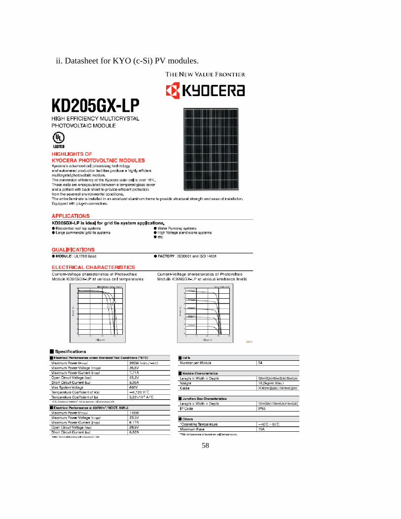
58

ii. Datasheet for KYO (c-Si) PV modules.

59

iii. Daily variation of electrical performance characteristics of the two PV systems

operating at GHHI for the year 2015.

Figure 32 – PR, VN and IP of the a-Si/µc-Si (left) and c-Si (right) PV systems (2015) for all AOI. Lower VN in summer (following

temperature) - higher AOI impact on VN (lower in the afternoon, negative temperature coefficient). PR combine with impact on IP

(lower during summer for a-Si/µc-Si favored by sensitivity to APE (bluer wavelength) and lower temperature impact on VN.