Effects of Covid-19 Related Government Response Strin ...

9116 2021

May 2021

Effects of Covid-19 Related Government Response Strin-gency and Support Policies: Evidence from European Firms Benedikt Janzen, Doina Radulescu

Impressum:

CESifo Working Papers ISSN 2364-1428 (electronic version) Publisher and distributor: Munich Society for the Promotion of Economic Research - CESifo GmbH The international platform of Ludwigs-Maximilians University’s Center for Economic Studies and the ifo Institute Poschingerstr. 5, 81679 Munich, Germany Telephone +49 (0)89 2180-2740, Telefax +49 (0)89 2180-17845, email [email protected] Editor: Clemens Fuest https://www.cesifo.org/en/wp An electronic version of the paper may be downloaded · from the SSRN website: www.SSRN.com · from the RePEc website: www.RePEc.org · from the CESifo website: https://www.cesifo.org/en/wp

mailto:[email protected]

https://www.cesifo.org/en/wp

http://www.ssrn.com/

http://www.repec.org/

https://www.cesifo.org/en/wp

CESifo Working Paper No. 9116

Effects of Covid-19 Related Government Response Stringency and Support Policies:

Evidence from European Firms

Abstract In this paper we employ survey information on more than 10,000 Southern and Eastern European firms and panel data methods to assess the effects of the COVID-19-related lockdown and government support policies on the business operations of enterprises. Our findings reveal considerable size- and sector-related effect heterogeneity, with small firms, exporting firms and firms operating in the facility sector experiencing the largest losses in terms of sales. A complete lockdown leads to an average decrease in sales by approximately 64%. We also document a disproportionate impact on female self-employed. Furthermore, state aid in the form of deferral of payments or wage subsidies were the most effective government support instruments. For instance, wage subsidies saved up to 2.7 employees per firm in the surveyed enterprises.

JEL-Codes: D220, H120, H320.

Keywords: Covid-19, firms, government support policies, panel data methods.

Benedikt Janzen

University of Bern KPM Center for Public Management

Schanzeneckstr. 1 Seitzerland – 3001 Bern

[email protected]

Doina Radulescu University of Bern

KPM Center for Public Management Schanzeneckstr. 1

Seitzerland – 3001 Bern [email protected]

May 25, 2021

1 Introduction

The year 2020 will be portrayed in history books as the year the COVID-19 pandemic

disrupted economies worldwide and individuals suddenly faced a drastic change of their

lives. The negative effects of this shock are looming large across countries and sectors of

the economy. Governments have undertaken tremendous efforts to contain the spread of

the virus, even if that meant lockdown of economic sectors for varying time periods and

thus drastic implications for businesses and the employed. At the same time, vast state

support funding has been deployed to sustain businesses in coping with the negative economic

consequences triggered by the pandemic.

In this paper we contribute to the nascent literature that addresses the effects of COVID-

19 related lockdown as well as government support policies on firms. Quantifying the magni-

tude and heterogeneity of the containment measures along different dimensions is paramount

to gain an accurate picture of the most hardly hit firms and sectors. This in turn assists

policymakers in designing the appropriate response policies and targeting those most in need.

The present crisis has revealed how vulnerable societies are to diseases that start in a

particular area of the world and then spread like wildfire over the globe, and highlighted the

risk of similar situations arising in the future. Thus, we also provide insights that can be

translated to future epidemics that require stringent government intervention and subsequent

support policies to cushion the negative impacts on people’s lives.

We employ information from the World Bank Enterprise Survey (WBES) and the first

wave of the World Bank Enterprise Follow-up Survey on COVID-19. While in the regular

WBES, business owners and top managers of firms of different sizes, active in different eco-

nomic sectors, are asked about the characteristics, climate, and constraints of their business

operations in the respective countries, the follow-up questionnaire aims at collecting timely

information on sales, liquidity, operations of the business, labor adjustments or expectations

about the future during the COVID-19 crisis. The data sample includes around 10,000 firms

of a rather homogeneous group of 23 Southern and Eastern European countries where we

1

have information on both, the business operations of the respondents before and during the

pandemic.

On average, we document that firm size, exporting status, female ownership, innovative

capabilities, as well as sectoral affiliation determine firm performance, as governments in-

crease their response stringency. As opposed to other types of shocks where one could argue

that exporting firms are in a better position to cushion the negative impact, the current

pandemic triggered a more pronounced decline in sales of those enterprises that depend on

exports. Furthermore, we also provide evidence of significant size- and sector-related effect

heterogeneity. The magnitude of the effect on year-on-year sales change is 0.14 percentage

points higher for small compared to large enterprises and the discrepancy is more pronounced

for higher values of the response stringency indicator. A similar picture emerges for firms in

the facility sector relative to other economic sector. Firms in the former experience larger

losses in terms of sales and the gap relative to firms operating in other sectors intensifies with

increasing lockdown strictness. Since the share of female owners is also higher in this sec-

tor, the pandemic disproportionately affected female self-employed compared to their male

counterparts.

We also scrutinize the effectiveness of different government support policies such as de-

ferral of payments, fiscal incentives or wage subsidies to alleviate the negative repercussions

of the lockdown. Firms that received wage subsidies recorded 33.8% fewer redundancies

compared to firms receiving other types of support. Assuming a firm in the dataset laid off

on average between 3.3 and 7.8 employees1, implies that wage subsidies saved between 1.1

and 2.7 employees per surveyed firm.

The remainder of this paper is structured as follows: Section 2 reviews the related lit-

erature, Section 3 provides an overview of the data and Section 4 addresses the correlation

between government response stringency and firm performance. The impact of government

support policies on financial and labor market and financial outcomes is analysed in Section

1The first number refers to the unrestricted sample including all 10,419 firms and the second to therestricted sample including only those 3,834 firms that received some kind of public support.

2

5 and finally Section 6 concludes.

2 Literature

The nascent literature on the pandemic and its devastating effects deals with several aspects

of the crisis. These range from the consequences for individuals and firms, health of the

population, spread of the disease, effects on the overall economy or the effects of different

forms of state aid. Our research contributes to this quickly evolving literature.

One strand of literature uses high-frequency data to assess the effect of the lockdown

in real time. These papers employ for instance transaction data from credit or debit card

purchases (Chetty et al., 2020), hourly electricity load (Janzen & Radulescu, 2020), text

data from earnings reports (Hassan et al., 2020). These studies find a pronounced negative

effect of the lockdown on economic activity.

A second strand of literature employs survey data to assess the impact of the pandemic

and the implemented measures on employment and business activities. Adams-Prassl et al.

(2020) use real time survey evidence from the UK, US and Germany and show that the

immediate labour market impacts of the pandemic differ substantially between countries,

with anglophone countries experiencing much more employment ties cut. Furthermore, they

find that employees on temporary contracts have been more likely to lose their jobs and

women and less educated workers are more affected by the crisis. Bartik et al. (2020)

conduct a survey on 5,800 small business in the US during the spring lockdown. Their

findings highlight the financial fragility of many small businesses, and how deeply affected

they are by the pandemic. They show that 43% of businesses were temporarily closed and

that employment had fallen by 40%. These results imply that many of these firms had

little cash on hand at the start of the pandemic, which means that they either had to

cut expenses, take on additional debt, or declare bankruptcy. This suggests that without

financial assistance, the firms are likely to fail. While the above mentioned papers analyse

3

the effects for developed countries and small businesses, Beck et al. (2020) focus on listed

firms in emerging economies,2 and find that these reacted by reducing investments rather

than payrolls.

A third strand of related papers scrutinize the effects of different government policies

to cushion the effects of the pandemic. These are mostly single country studies, using

information on countries such as the United States (Cororaton & Rosen, 2020), (Granja et

al., 2020), Italy (Core & De Marco, 2020), Portugal (Kozeniauskas et al., 2020) or Switzerland

(Brulhart et al., 2020). Financial support to US firms in the form of the Paycheck Protection

Program (PPP - a USD 349 bn fund aimed at keeping workers employed by providing

forgivable loans to businesses) does not seem to have achieved its scope since the short-

and medium-term employment effects of the program were small compared to the program’s

size. In addition, many firms used the loans to make non-payroll fixed payments and build

up savings buffers (Granja et al., 2020). Furthermore, 17.7% of borrowers chose to return

their loans after receiving public backlash and some firms who borrowed faced negative

stock returns upon PPP loan announcement (Cororaton & Rosen, 2020). The relatively low

success of Corona government-backed loans relative to labour-income support measures is

also documented by Brulhart et al. (2020) for Switzerland. They find a better performance

of labour-income support measures among small businesses and that recourse to government-

backed loans was driven to a large extent by firms’ prior history of indebtedness.

Compared to the above mentioned papers, our study includes enterprises of different sizes

from a large number of countries and also information of firms’ pre-crisis characteristics that

may also affect the results and are thus important to account for. In addition, we compare

the impact of different support instruments such as wage subsidies, cash transfers, payment

deferral or access to credit instead of assessing the effectiveness of one instrument only.

Recent working papers that also employ the COVID-19 Follow-Up Survey to assess the

short-term impact of the pandemic on businesses include Apedo-Amah et al. (2020), Cirera et

2These are Bangladesh, Indonesia, Malaysia, Pakistan, Philippines, Saudi Arabia, South Africa, Thai-land, Turkey and Vietnam

4

al. (2021), Bosio et al. (2020), Nelson (2021), and Grover & Karplus (2021). The first two fo-

cus on developing countries and report persistent negative impacts on sales and employment

adjustments mainly along reduction of hours worked and leave of absence (Apedo-Amah

et al., 2020) and identify mismatches between policies provided and policies most sought

(Cirera et al., 2021). Bosio et al. (2020) estimate the survival of 7,000 firms in high- and

middle-income countries and find that the median survival time ranges between 8 and 19

weeks. In addition, firms suffer from illiquidity regardless of productivity levels, age or size.

Singling out the labour market effect of each containment measure is at the heart of Nelson

(2021). His research paper looks at firms in 20 emerging countries3 and finds that whereas

containment and closure policies negatively affected permanent jobs and total hours worked

at the firm level, temporary employment was less affected. Furthermore, policies directed

at closure of public events had significant negative effects across all employment categories.

Grover & Karplus (2021) employ the World Bank Enterprise Survey to analyse the impact

of pre-crisis management practices on subsequent post-COVID-19 outcomes, such as firm’s

ability to adjust their products or shift sales online.

Whereas these studies mostly employ only data from the COVID-19 Follow Up Survey

and primarily show a number of correlations, we enrich our analysis with information from

the original World Bank Enterprise Surveys as well. This additional data allows us to

explicitly control for pre-crisis firm specific observable characteristics that may affect the

results. Furthermore, appropriate econometric approaches that account for the distributional

assumptions allow us to identify the underlying effects more accurately.

3 Data

We draw on two main data sources for this research project. First, data from the World

Bank Enterprise Survey (WBES) and the first wave of the World Bank Follow-up Survey

3These include 7 European and 13 non-European countries: Albania, Belarus, Bulgaria, Chad, Cyprus,El Salvador, Greece, Guatemala, Guinea, Honduras, Jordan, Mongolia, Morocco, Nicaragua, Niger, Poland,Slovenia, Togo, Zambia, Zimbabwe.

5

on COVID-194 and second, information from the Oxford COVID-19 Government Response

Tracker.

The regular WBES are establishment level surveys where business owners and top man-

agers are asked about the characteristics, climate and constraints of their business operations

in the respective countries. They are constructed on a stratified random sample of small (less

than 20 employees), medium (20-99 employees) and large establishments (over 100 employ-

ees). The COVID-19 follow-up surveys were conducted in countries with recent enterprise

surveys and measure the impact of the pandemic on businesses using the same methodology

as the WBES. The questionnaire collects information on sales, liquidity, operations of the

business, labor adjustments or expectations about the future5.

Overall, the follow-up study was implemented in 42 countries, where the original WBES

was conducted in 2019 or 2018. For the purpose of our study we focus on 23 European

countries including the Russian Federation. The countries we consider are Albania, Be-

larus, Bosnia and Herzegovina, Bulgaria, Croatia, Cyprus, Czech Republic, Estonia, Geor-

gia, Greece, Hungary, Italy, Latvia, Lithuania, Malta, Moldova, Poland, Portugal, Romania,

Russian Federation, Serbia, Slovak Republic, and Slovenia. Overall our sample covers 10,419

firms that answered both questionnaires, varying between 171 firms (Cyprus) to 1,191 firms

(Russian Federation) per country (see Table 1). The sample covers small, medium and large

formal businesses across the main sectors of the economy (D: manufacturing (ISIC 3.1 Rev.

15-37), F: construction (ISIC 3.1 Rev. 45), G: retail and wholesale trade (ISIC 3.1 Rev.

50-52), H: facility sector (ISIC 3.1 Rev. 55), I: transport, storage and communication (ISIC

3.1 Rev. 60-64), and one business division of sector K: computer related services (ISIC 3.1

Rev. 72)). Table 1 shows that the majority of the surveyed firms (55%) belong to the manu-

facturing sector, followed by the retail and wholesale trade sector (28% of firms). Hotels and

restaurants represent around 5% of enterprises. Information on the strictness of lockdown

measures in reaction to COVID-19 is retrieved from the Oxford COVID-19 Government

4https://www.enterprisesurveys.org/en/covid-19.5We provide examples of the most important questions for our analysis in Figure A1 in the Appendix.

6

Table 1

Country Year of Baseline SurveyMonth and Year of

Follow-up SurveyNo. of Obs. Business sector

D

(15-37)

F

(45)

G

(50-52)

H

(55)

I

(60-64)

K

(72)

Albania 2019 June 2020 347 132 27 123 43 19 3

Belarus 2018 August 2020 551 314 36 163 10 19 9

Bosnia and Herzegovina 2019 February - March 2021 241 86 23 104 11 13 4

Bulgaria 2019 July - September 2020 559 326 41 134 17 37 4

Croatia 2019 September 2020 351 133 35 129 27 21 6

Cyprus 2019 June 2020 171 65 24 63 13 6 0

Czech Republic 2019 September - October 2020 405 252 25 81 18 16 13

Estonia 2019 October 2020 272 100 51 80 19 20 2

Georgia 2019 June 2020 514 182 45 170 92 23 2

Greece 2018 June - July 2020 532 277 35 162 41 12 5

Hungary 2019 September 2020 630 378 37 164 23 21 7

Italy 2019 May - June 2020 453 277 23 108 28 9 8

Latvia 2019 October - November 2020 244 83 29 105 8 16 3

Lithuania 2019 October 2020 214 79 16 85 16 14 4

Malta 2019 September - October 2020 196 67 9 77 11 24 8

Moldova 2019 May 2020 286 110 34 121 3 14 4

Poland 2019 July - August 2020 1,005 738 70 143 18 22 14

Portugal 2019 September - October 2020 820 605 16 144 44 10 1

Romania 2019 August - September 2020 532 327 35 125 11 23 11

Russian Federation 2019 June 2020 1,191 815 42 283 10 23 18

Serbia 2019 February 2021 318 114 33 131 11 20 9

Slovak Republic 2019 September - October 2020 338 154 18 113 22 18 13

Slovenia 2019 July - August 2020 249 93 27 76 18 24 11

Total 10,419 5,707 731 2,884 514 424 159

Notes: classification of business sections according to ISIC Rev. 3.1. D: Manufacturing; F: Construction; G: Wholesale and

retail trade; H: Hotels and restaurants; I: Transport, storage and communications; K: Real estate, renting and business activities

(here: only computer and related activities, ISIC Rev. 3.1 72). Corresponding division codes reported in parentheses.

Response Tracker(Hale et al., 2021), which provides a systematic way to track government

responses to the pandemic and renders policy responses comparable across regions and ju-

risdictions. The project provides a total of 19 different indicators. In our analysis we only

consider nine indicators related to containment, closure and health system policies6. Each in-

dicator is ordinally scaled and scored based on the evaluation of publicly available data. For

example, the indicator on international travel controls can take on integer values from zero

to four, with zero representing no restrictions and a value of four being total border closure.

Hence, for the regressions, the stringency index is defined as an additive unweighted index

combining all aforementioned indicators capturing policies that were primarily designed to

restrict individuals’ behaviour7.

6These are: school closing, workplace closing, cancellation of public events, restrictions on gatherings,closure of public transport, stay-at-home orders, restrictions on internal movements, international travelcontrols, and public information campaigns.

7See https://www.bsg.ox.ac.uk/research/research-projects/covid-19-government-response-tracker formore information on the calculation of the stringency index.

7

Figure 1: Evolution of the Oxford COVID-19 Government Response Tracker StringencyIndex, 3/2020 - 2/2021

25

50

75

100

3/20 4/20 5/20 6/20 7/20 8/20 9/20 10/20 11/20 12/20 1/21 2/21

Time

OxCGRT

SI

Notes: Each coloured solid line refers to the average monthly stringency index in one of our sampled countries. The black dashed line shows the

pooled average monthly stringency index for all sampled countries.

Figure 1 plots the evolution of the monthly stringency index from March 2020 to Febru-

ary 2021. Most of the sampled countries exhibit the same time pattern, with very strict

lockdown policies at the beginning of the pandemic, that were relaxed during the summer,

and tightened again towards the end of the year 2020. The highest value during our obser-

vation period was reported in Georgia in April 2020, with an average monthly stringency

index of 99.51. Only in Belarus policy measures to restrict the outbreak of SARS-CoV-2

were relatively liberal throughout the year. Therefore, it is of no surprise that the lowest

average monthly stringency index during our observation period in all sampled countries was

reported in Belarus in March 2020, with a value of 4.8. The only curtailment measure that

8

Table 2: Summary Statistics

Obs. Mean Std. Dev. Median Min Max

OxCGRT SI 276 57.09 17.93 55.48 4.84 99.51

WBES Baseline

Age 10,359 21.05 16.06 19 1 205

OwnerFemaleShare 10,419 19.40 33.14 0 0 100

SalesExportShare 10,324 17.30 30.73 0 0 100

SupplyImportShare 10,020 34.87 36.29 20 0 100

Innovation (No = 1) 10,357 0.70 0.46 1 0 1

COVID-19 Follow-up ES

%∆sales 9,676 -22.31 31.40 -20 -100 300

Closure (No = 1) 10,419 0.71 0.45 1 0 1

SaleChange (No = 1) 10,021 0.80 0.4 1 0 1

Employees 9,747 88.72 350.79 23 1 20,000

LayoffShare 9,640 0.02 0.58 0 -32.33 1

Layoff 9,640 3.34 35.42 0 -630 1610

OverdueFinancial 9,538 0.10 0.30 0 0 1

OverdueOther 9,937 0.33 0.47 0 0 1

Insolvency 10,032 0.02 0.14 0 0 1

Notes: The variable OxCGRT SI refers to the average monthly value of the

stringency index.

was captured by the nine aforementioned indicators in Belarus during that month was a ban

on arrivals from certain regions.

Table 2 presents summary statistics for the independent variables as well as the main

dependent variables. The mean decrease in sales amounts to 22.3% but can even reach

100%. Firms laid off on average 3.34 employees, however some recorded even much larger

layoffs whereas others even increased their workforce. The stringency index varies between

a minimum of 4.84 and a maximum of 99.51 with a median of 55.48.

4 Response Stringency

4.1 Overall Impact on Firm Performance

One major objective of this study is to untangle the effects of COVID-19 related government

response strictness on firm performance. For this purpose, we resort to the WBES Follow-up

Survey’s questions on year-on-year sales growth, which we consider an appropriate measure

of firm performance (Figure A1 Panel (a) in the Appendix). In the questionnaire, firms

are explicitly asked for a relative comparison of sales in the last completed month before

9

Figure 2: Changes in sales relative to the same month in the previous year, by month

2/21

1/21

12/20

11/20

10/20

9/20

8/20

7/20

6/20

5/20

4/20

-100 0 100 200 300

%∆sales

Mon

th

the survey was conducted in 2020, with the same month in the previous year, therefore,

automatically negating the effect of seasonality. Two main assumptions are necessary to

ensure the validity of our estimates: (i) all changes in sales compared to the same month

in the previous year were caused by pandemic-related government policies only (i.e. no

year-on-year sales growth in the absence of COVID-19) and (ii) no systemic response bias

in the reported values. While the first assumption may not hold on a case-by-case basis, we

consider the endogenous sales growth of firms on average to be negligible given the short

time period of one year.8 We cannot rule out a systemic response bias which may impact the

validity of the estimates. This is however a well-known potential source of bias when working

with survey data in general. Figures 2 and 3 provide descriptive evidence of reported year-

on-year sales growth across months, countries and economic divisions. Figure 2 shows that

firms that were surveyed in May 2020, therefore providing information on sales in April 2020

relative to April 2019, report the steepest decline, with an average reduction in sales of 53.5

%. Reported mean year-on-year sales growth is considerably closer to zero if the COVID-19

follow-up survey was conducted during the later months of 2020 or earlier months of 2021.

8A close look at the unprocessed data shows it is safe to assume that most of the year-on-year saleschanges can be attributed to the pandemic. For example, five establishments in our sample more thantripled their sales compared to the same period in the previous year. All of these firms either manufactureor deal with pharmaceutical and/or medical products (i.e. ISIC 3.1 Rev. 2423, 3311, 5190, 5211).

10

Figure 3: Changes in sales relative to the same month in the previous year by (a) countryand (b) division

Slovenia

Slovak Republic

Serbia

Russian Federation

Romania

Portugal

Poland

Moldova

Malta

Lithuania

Latvia

Italy

Hungary

Greece

Georgia

Estonia

Czech Republic

Cyprus

Croatia

Bulgaria

Bosnia and Herzegovina

Belarus

Albania

-100 0 100 200 300

%∆sales

Cou

ntr

y(a)

72646362616055525150453736353433323130292827262524232221201918171615

-100 0 100 200 300

%∆sales

Busi

nes

sdiv

isio

n(I

SIC

Rev

.3.

1)

(b)

Notes: description of ISIC Codes can be found under https://unstats.un.org/unsd/classifications/Econ/ISIC.

11

Figure 4: Changes in sales relative to the same month in the previous year, by firm size

Large

Medium

Small

-100 0 100 200 300

%∆sales

Fir

mSiz

e

Notes: firm size classifications according to the World Bank Enterprise Survey. Small firms employ less than 20 people, medium sized firms have20-99 employees, and large firms have more than 100 full-time employees.

Figure 4 plots the reported year-on-year percentage changes in sales by company size.

We follow the classification of the World Bank Enterprise Survey, that distinguishes between

small (less than 20 employees), medium (20-99 employees) and large (over 100 employees)

establishments. Reported mean reductions range from 17.4% for large establishments to even

25.3% for small sized firms. Panel (a) in Figure 3 shows year-on-year growth rates of sales by

country. While Moldovan enterprises report an average reduction of 54.7%, firms in Latvia

are the least affected, with an average year-on-year sales change close to zero. However, since

the follow-up surveys were conducted at different points in time, and policy measures to cope

with the pandemic vary across countries, the comparability of these descriptive unconditional

differences in firm performance across jurisdictions is rather limited and calls for an in depth

empirical analysis. Panel (b) in Figure 3 plots growth rates by business division (2-Digit ISIC

Rev. 3.1). Air transport (62), hotels & restaurants (55), and supporting transport activities

(63) report the largest reductions in sales with an average negative year-on-year sales growth

of 60%, 55.5% and 44%, respectively. Descriptive statistics suggest that manufacturers of

chemical products (24), computing machinery (30), and plastic products (25) are the least

affected industry divisions in our sample.

While the temporal variation of the COVID-19 Follow-up Enterprise Survey may limit

the explanatory power of descriptive cross-country evidence, it offers the advantage of greater

variation in our data. We employ a fixed effects regression model to capture the impact of

12

the COVID-19 related lockdown policies on firms’ performance in terms of sales changes:

%∆salesict = α0 + α1OxCGRTSIct + X ′

iA2 + Y ′i A3 + θs + ζc + εict, (1)

where the dependent variable, %∆salesict, refers to the reported percentage change in sales

for company i in country c at time t relative to the same month in the previous year. The

main independent variable of interest OxCGRT SIct denotes the average stringency index in

country c at time t as communicated by the Oxford Covid-19 Government Response Tracker.

While the stringency index reports daily changes in lockdown measures, firms in the WBES

are asked to provide information on year-on-year sales growth for the last completed month.

We construct an average monthly stringency index for every country in our sample and

match it to the month that was referred to in the World Bank COVID-19 Follow-up Survey.

Therefore, the corresponding coefficient α1 measures the average percentage point change

in year-on-year sales growth induced by a marginal change in containment measures. As

a robustness check, we also employ the monthly maximum value of the stringency index

in the respective countries. The vector Y includes additional information retrieved from

the COVID-19 Follow-up Enterprise Survey, such as the number of full-time employees in

December 2019, information on temporary closure of the establishment during the pandemic,

and whether the firm adjusted its products, services or sales channels in reaction to COVID-

19. X includes a set of individual pre-pandemic firm characteristics, such as firm age, share

of sales that is exported directly or indirectly9, share of input supplies that are of foreign

origin, share of female ownership, and general innovative capabilities of the company10. We

also include a full set of sector dummies θs and country fixed effects ζc to account for the

heterogeneous impact of lockdown policies on industry sectors and unobservables across

countries that were not captured by the stringency index respectively.

9For some service establishments (i.e. hotels), direct sales to foreign customers are defined as directexport. Services sold to foreigners via intermediaries are defined as indirect exports.

10Innovative capability of the firm is indicated by a dummy variable that is equal to unity if the companyintroduced new or improved products or services in the three years prior to the baseline survey year.

13

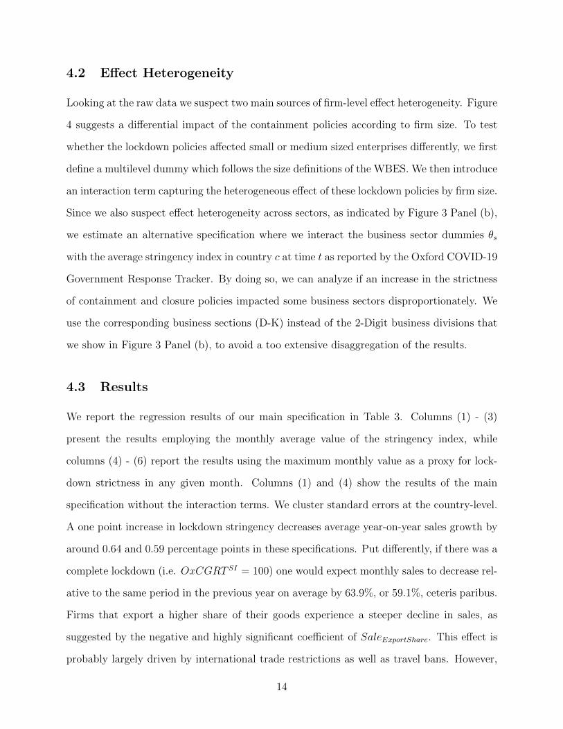
4.2 Effect Heterogeneity

Looking at the raw data we suspect two main sources of firm-level effect heterogeneity. Figure

4 suggests a differential impact of the containment policies according to firm size. To test

whether the lockdown policies affected small or medium sized enterprises differently, we first

define a multilevel dummy which follows the size definitions of the WBES. We then introduce

an interaction term capturing the heterogeneous effect of these lockdown policies by firm size.

Since we also suspect effect heterogeneity across sectors, as indicated by Figure 3 Panel (b),

we estimate an alternative specification where we interact the business sector dummies θs

with the average stringency index in country c at time t as reported by the Oxford COVID-19

Government Response Tracker. By doing so, we can analyze if an increase in the strictness

of containment and closure policies impacted some business sectors disproportionately. We

use the corresponding business sections (D-K) instead of the 2-Digit business divisions that

we show in Figure 3 Panel (b), to avoid a too extensive disaggregation of the results.

4.3 Results

We report the regression results of our main specification in Table 3. Columns (1) - (3)

present the results employing the monthly average value of the stringency index, while

columns (4) - (6) report the results using the maximum monthly value as a proxy for lock-

down strictness in any given month. Columns (1) and (4) show the results of the main

specification without the interaction terms. We cluster standard errors at the country-level.

A one point increase in lockdown stringency decreases average year-on-year sales growth by

around 0.64 and 0.59 percentage points in these specifications. Put differently, if there was a

complete lockdown (i.e. OxCGRT SI = 100) one would expect monthly sales to decrease rel-

ative to the same period in the previous year on average by 63.9%, or 59.1%, ceteris paribus.

Firms that export a higher share of their goods experience a steeper decline in sales, as

suggested by the negative and highly significant coefficient of SaleExportShare. This effect is

probably largely driven by international trade restrictions as well as travel bans. However,

14

Table 3: Regression Results: Response Stringency

Dependent variable:

%∆sales

(1) (2) (3) (4) (5) (6)

OxCGRT SI −0.639∗∗∗ −0.533∗∗∗ −0.621∗∗∗ −0.591∗∗∗ −0.499∗∗ −0.550∗∗∗

(−7.557) (−5.382) (−7.210) (−3.350) (−2.974) (−2.982)

FirmSizeM −0.773 −0.166

(−0.332) (−0.069)

FirmSizeS −1.323 −0.131

(−0.399) (−0.035)

SalesExportShare −0.048∗∗∗ −0.043∗∗∗ −0.044∗∗∗ −0.048∗∗∗ −0.043∗∗∗ −0.043∗∗∗

(−4.050) (−3.743) (−3.965) (−4.054) (−3.654) (−3.841)

SupplyImportShare −0.004 −0.005 −0.005 −0.004 −0.004 −0.004

(−0.445) (−0.493) (−0.501) (−0.384) (−0.463) (−0.414)

log(age) −0.316 −0.157 −0.384 −0.340 −0.183 −0.411

(−0.839) (−0.404) (−1.012) (−0.908) (−0.474) (−1.092)

log(employees) 2.616∗∗∗ 2.591∗∗∗ 2.637∗∗∗ 2.605∗∗∗

(6.119) (6.198) (6.041) (6.132)

OwnerFemaleShare −0.023∗∗ −0.025∗∗ −0.023∗∗ −0.023∗∗ −0.026∗∗ −0.023∗∗

(−1.979) (−2.115) (−2.000) (−1.998) (−2.125) (−1.990)

Innovation = No −1.523∗ −1.701∗∗ −1.478∗ −1.490∗ −1.691∗∗ −1.440∗

(−1.750) (−1.977) (−1.700) (−1.710) (−1.964) (−1.663)

Closure = No 13.802∗∗∗ 13.821∗∗∗ 14.229∗∗∗ 13.827∗∗∗ 13.837∗∗∗ 14.276∗∗∗

(9.906) (9.907) (10.758) (9.910) (9.957) (10.718)

SaleChange = No −6.657∗∗∗ −6.782∗∗∗ −6.492∗∗∗ −6.691∗∗∗ −6.834∗∗∗ −6.531∗∗∗

(−4.059) (−4.199) (−4.150) (−4.077) (−4.218) (−4.159)

ISICF 0.377 0.214 2.285 0.327 0.189 4.471

(0.223) (0.127) (0.581) (0.192) (0.113) (1.229)

ISICG 4.134∗∗∗ 3.905∗∗∗ 6.486∗∗∗ 4.146∗∗∗ 3.921∗∗∗ 6.824∗∗∗

(5.249) (4.796) (3.609) (5.278) (4.847) (3.987)

ISICH −25.974∗∗∗ −26.108∗∗∗ −1.800 −25.960∗∗∗ −26.073∗∗∗ −0.752

(−5.671) (−5.666) (−0.273) (−5.663) (−5.659) (−0.120)

ISICI −9.664∗∗∗ −9.843∗∗∗ −10.366∗∗ −9.647∗∗∗ −9.838∗∗∗ −10.025∗∗

(−4.369) (−4.514) (−2.036) (−4.363) (−4.507) (−1.966)

ISICK 0.711 0.439 −7.469∗ 0.568 0.283 −5.498

(0.281) (0.171) (−1.653) (0.224) (0.109) (−1.182)

OxCGRT SI :FirmSizeM −0.082∗∗ −0.088∗∗∗

(−2.382) (−2.681)

OxCGRT SI :FirmSizeS −0.135∗∗ −0.147∗∗∗

(−2.437) (−2.578)

OxCGRT SI :ISICF −0.035 −0.071

(−0.436) (−1.032)

OxCGRT SI :ISICG −0.042 −0.044∗

(−1.441) (−1.753)

OxCGRT SI :ISICH −0.411∗∗∗ −0.400∗∗∗

(−3.123) (−3.508)

OxCGRT SI :ISICI 0.016 0.010

0.137) (0.089)

OxCGRT SI :ISICK 0.168∗ 0.119

(1.790) (1.296)

Constant 4.695 12.192 4.740 1.880 10.569 −0.233

(0.582) (1.490) (0.604) (0.122) (0.728) (−0.015)

Country fixed effects Yes Yes Yes Yes Yes Yes

Observations 8,888 8,888 8,888 8,888 8,888 8,888

R2 0.240 0.240 0.244 0.239 0.239 0.243

Adjusted R2 0.237 0.237 0.240 0.236 0.236 0.240

Residual Std. Error 27.132 (df = 8851) 27.134 (df = 8848) 27.070 (df = 8846) 27.156 (df = 8851) 27.148 (df = 8848) 27.084 (df = 8846)

F Statistic 77.643∗∗∗ (df = 36; 8851) 71.704∗∗∗ (df = 39; 8848) 69.618∗∗∗ (df = 41; 8846) 77.073∗∗∗ (df = 36; 8851) 71.414∗∗∗ (df = 39; 8848) 69.309∗∗∗ (df = 41; 8846)

Notes: ∗p<0.1; ∗∗p<0.05; ∗∗∗p<0.01. All models are estimated using OLS. t-values reported in parentheses. Standard errors are clustered at the country-level.

15

we don’t find evidence for a supply shock induced by international restrictions. Having a

higher share of imported production inputs, does not significantly impact firm performance.

Our results indicate the existence of gender-based differences in economic consequences

of the pandemic. An increase in female ownership by one percentage point is associated

with an average decrease in sales by 0.02 percentage points. The coefficient is statistically

significant in all model specifications. Looking at an extreme case, if a firm is 100% female-

owned, the reduction in sales is 2.3 percentage points higher than for businesses that are

exclusively owned by men. This effect has also been documented by Graeber et al. (2021),

who find that self-employed women are 35% more likely to experience income losses than

their male counterparts in Germany due to the pandemic. This can be mainly explained by

the fact that women disproportionately work in industries that are more severely affected

by the pandemic. In our data, the share of female ownership is with 25.7% much higher in

the facility sector than in the construction sector (11.6%). Furthermore, the share of female

ownership amounts to 12.8% in large firms and reaches even 24.1% in small firms. Since our

findings reveal that small firms and firms belonging to the facility sector were most severely

hit, it is not surprising that female self-employed were disproportionately affected.

We document that general innovative abilities make firms more resilient to changes in

government response stringency to the pandemic. Establishments that reported product

or service innovation during the last three years before the baseline WBES was conducted,

display on average a 1.52 percentage point lower reduction in sales. Perhaps unsurprisingly,

establishments that were not permanently or temporarily closed due to COVID-19 report a

13.8 percentage point lower average decline in sales than firms that were shut down.

We find strong evidence for heterogeneous effects across firm size and business sectors.

Small sized establishments were disproportionately impacted by the containment and clo-

sure measures. While a one percentage point increase in the stringency index leads to a

sales decrease by 0.53 percentage points for large enterprises, it decreases sales of small sized

firms by 0.67 (= (-0.53) + (-0.14)) percentage points. Differences in sales changes between

16

large and medium sized firms are closer to zero but still statistically significant. Models

employing the maximum monthly value of the stringency index as a proxy for the strictness

of lockdown policies display similar effects. Columns (3) and (6) provide evidence of effect

heterogeneity across sectors. While, on average, businesses operating in the manufacturing

sector (ISICD) experience a decline in sales relative to the same period in the previous year

of 35.5 percent11, businesses operating in the facility sector experience a stronger reduction

of even 58.9 per cent12. Of course, due to effect heterogeneity, the absolute difference in

year-on-year sales decline between both business sectors is even more pronounced assuming

a full lockdown (i.e. OxCGRT SI = 100). The results seem plausible, because containment

and closure policies are mainly aimed at restricting mobility and social gatherings, both

of which the facility sector is highly dependent on. Differences between the decline in the

manufacturing sector and other business sectors are not statistically significant. Therefore,

our results indicate that these business sectors are impacted proportionally by an increase

in lockdown strictness.

In the following, we illustrate effect heterogeneity of government response stringency to

COVID-19. Figure 5 plots the previously estimated interaction effects of two of our mod-

els (Table 3, columns (2) and (3)). Each dot represents one of the firm-level observations,

grouped by firm size and business division, respectively. As shown in Table 3, the slope

coefficient between large and small enterprises is significantly different, as well as the dif-

ference in slopes between firms in the facility sector and firms in the manufacturing sector.

The effect heterogeneity results in an increasing discrepancy in the reaction of sales between

firms operating in the facility versus firms in other economic sectors with higher levels of

the stringency index. We provide additional model specifications and robustness checks in

Table A1 in the Appendix. First, instead of following the arbitrarily chosen WBES firm

size classifications, we interact a continuous measure of firm size (log(employees)) with our

independent variable of interest to validate our findings regarding size-related effect hetero-

1157.1*0.621 = 35.46; 57.1 corresponds to the average value of the stringency index.1257.1*(0.621+0.411) = 58.93.

17

Figure 5: Interaction Plot: Response Stringency

−100

−50

0

50

25 50 75

OxCGRTSI

%∆s

ales

<50 Size

L

M

S

−100

−50

0

50

25 50 75

OxCGRTSI

%∆s

ales

<50

ISIC

D

F

G

H

I

K

Notes: Figure plots predicted values of interaction effects using the average value of the stringency index (Table 2, columns (2) and (3)). Firm sizeclassifications according to the World Bank Enterprise Survey. Small firms employ less than 20 people, medium sized firms have 20-99 employees,and large firms have more than 100 full-time employees. Classification of business sections according to ISIC Rev. 3.1. D: Manufacturing; F:Construction; G: Wholesale and retail trade; H: Hotels and restaurants; I: Transport, storage and communications; K: Real estate, renting andbusiness activities, here: only computer and related activities, ISIC Rev. 3.1 72

geneity. Second, we construct a dummy variable that indicates if an establishment does not

export or import at all, to check for robustness of the impact on internationally operating

firms. The results confirm our findings that exporting firms report significantly higher de-

clines in sales than non-exporting companies. Third, we construct a dummy variable that

is equal to unity if the establishment has no female owners. The coefficient supports the

findings of a higher economic burden of the pandemic for female self-employed13. Another

13We also check for potential sources of effect heterogeneity other than sector affiliation and firm size,such as exporting status and female ownership, however, we don’t find any further significant interactionterms. Regression results are available upon request.

18

potential concern regarding our results is that they are driven by countries that followed a

different path in containing the spread of the pandemic. Looking at Figure 2 we identify

Belarus as a potential threat to the validity of our estimates. To address this concern we

re-estimate our main specification outlined in equation (1) excluding this country. The re-

sults of using this alternative sample are reported in Table A2 in the Appendix. We also

check if our results are biased by countries that were questioned in the earlier months of

2021, therefore reporting sales changes relative to the same month in 2020 (i.e. Bosnia and

Herzegovina and Serbia). The main coefficients retain their sign, magnitude and significance

even in these alternative specifications.

5 Government Support Policies

5.1 Policy Targeting

To cushion the negative repercussions documented above, many countries introduced a num-

ber of support policies. In the following, we assess the effectiveness of these measures along

a number of different dimensions. Overall 3,834 out of 10,419 firms in our sample received

public support, 623 firms expected to receive public support within the next three months,

5,542 firms did not get any public support, and 420 firms did not answer the respective

survey question. The COVID-19 Follow-up Enterprise Survey distinguishes between five dif-

ferent policy support schemes: direct cash transfers, deferral of payments, credit access, fiscal

exemptions and wage subsidies. We provide some descriptive evidence of targeting effective-

ness of government support policies, that aimed at relieving economic distress for companies

during the COVID-19 pandemic14. Figure 6 Panel (a) plots the correlation between reported

average percentage reduction in sales and the share of companies that received public sup-

port across sectors. Each dot in the scatterplot represents one business division covered by

14See Cirera et al. (2021) for a more detailed analysis of targeting effectiveness based on the COVID-19Follow-up World Bank Enterprise Survey.

19

Figure 6: Target effectiveness of public support by (a) division and (b) countries

R = - 0.59 , p = 0.00034

0.2

0.4

0.6

-60 -40 -20

%∆sales

Shar

eof

firm

sth

atre

ceiv

edpublic

supp

ort

(a)

R = 0.21 , p = 0.33

0.0

0.2

0.4

0.6

0.8

-60 -40 -20 0

%∆sales

Shar

eof

firm

sth

atre

ceiv

edpublic

supp

ort

(b)

the WBES. There is a strong and statistically significant correlation of -0.59 between receiv-

ing public support and operating in a specific division that was significantly impacted by

the containment and closure policies. 75% of firms operating in the air transport business

division (ISIC 3.1 Rev. 62), the most affected industry division in our sample with an av-

erage year-on-year sales growth of -60%, received public support. However, the descriptive

evidence also suggests that some business divisions, such as manufacturers of motor vehicles,

trailers and semi-trailers (ISIC 3.1 Rev. 34) may have been overcompensated. Companies

in these divisions experienced a decline in sales by only 20.1% on average, but 56% received

public support to cope with the negative economic consequences of the pandemic. Panel (b)

of Figure 6 shows that there is no significant correlation between the share of companies that

received public support in any given country and the average mean reduction in sales in the

same country. There is a huge discrepancy in public support schemes across countries. In

our sample only 1.7% of Moldovan firms received public support during the first months of

the pandemic, whereas 74% of Slovenian firms and 83% of Serbian firms received any form

20

of public support15.

5.2 Policy Outcomes

In this section we provide some preliminary evidence on the short-term outcomes of govern-

ment support schemes during the COVID-19 pandemic. We run the following regression on

a restricted sample of firms that received public support in order to assess which particular

public support scheme was the most effective in helping firms to cope with the negative

economic consequences of the lockdown :

Oic = β0 +5∑

k=1

βkSupportik + β6OxCGRTSIic + β7Daysi+

β8OxCGRTSIic ×Daysi + X ′

iB9 + Y ′i B10 + θs + ζc + εic, (2)

where Oic denotes the dependent variables of interest, that are either related to financial

outcomes (i.e. probability of filing bankruptcy, delaying payments due to COVID-19, or

defaulting on financial obligations) or labor outcomes (i.e. share of workers laid off or count

of workers laid off). The dummy variable Supportik is equal to unity if firm i reports

that it received a specific type of public support (such as possibility to defer payments,

cash transfers, fiscal exemptions, wage subsidies or access to credit) and thus captures the

effect of each specific government support instrument. Therefore, β1 − β5 denote our main

coefficients of interest. As opposed to the questions on year-on-year sales growth, survey

questions on labor, finance, and policies do not refer to a specific time period. Hence,

we estimate the average daily lockdown stringency for every company i, that is defined as

the average value of the Oxford COVID-19 Government Response Tracker stringency index

between the day the first measures in country c were introduced and the day the follow-up

15One could argue that these differences are mainly due to the different points in time the survey wasundertaken. However, if we compare countries where the survey was conducted during the same monthswe still find large discrepancies between countries (e.g. 60.8 % of Cypriot establishments received publicsupport, but only 30.7 % of Albanian companies in our sample. Both surveys were conducted in June 2020.)

21

interview was conducted. As an alternative we also use the maximum value of the stringency

index during that exact time period. In addition, we interact the number of days with our

stringency measure, since we assume that the negative economic consequences increase with

the number of days between the interview took place and the first lockdown measures were

introduced. The vectors X and Y include the same variables as introduced in the previous

sections. We again include full sets of fixed effects to control for unobserved differences in

policy schemes between countries and sectors.

5.2.1 Labor Market Outcomes

We employ two different measures to compare the effectiveness of the public support schemes

on labor market outcomes: (i) the share of employees laid off and (ii) the number of employees

laid off. First, we compute the share of employees a firm laid off by taking the difference

between the number of employees the company employed pre-pandemic and the number of

employees the firm reported in the Follow-up Survey (Figure A1 Panel (b) in the Appendix),

divided by the number of employees pre-pandemic. We exclude all establishments that

received public support and increased their workforce since the focus of our analysis lies on

the companies in need of public support16. We start our analysis with estimating a fixed-

effects linear regression model as laid out in equation (2). Since the dependent variable is

bounded between 0 and 1, we would impose arbitrary restrictions on the range of variation

in our exogenous variables by simply estimating a linear model. Furthermore, using a linear

specification for the conditional mean, may not capture non-linearities in a correct manner.

Therefore, we employ a quasi maximum likelihood estimator, as suggested by Papke &

16i.e. Layoffshare < 0. In total 431 companies receive public support and report an increase in the numberof employees.

22

Wooldridge (1996), to estimate the following fractional response model:

Layoffshare = Φ(β0 +5∑

k=1

βkSupportik + β6OxCGRTSIic + β7Daysi+

β8OxCGRTSIic ×Daysi + X ′

iB9 + Y ′i B10 + θs + ζc), (3)

where Φ is specified as a logistic function (i.e. Φ(x) = exp(x)1+exp(x)

).

We report the results of the model estimating the impact of public support policies on

one of our labour market outcomes of interest in Table 4. Columns (1) and (3) display

the results of a simple linear regression model. Columns (2) and (4) present the average

marginal effects of the logit quasi maximum likelihood model. Columns (1), (2) and (5) use

the average value of the stringency index, whereas in the remaining columns we report the

Table 4: Regression Results: Share of workers laid off

Dependent variable:

Layoffshare

(1) (2) (3) (4) (5) (6)

(OLS) (QMLE) (OLS) (QMLE) (OLS) (OLS)

Cash transfer = Yes −0.010 −0.010 −0.010 −0.009 0.013 0.009

(−1.378) (−1.248) (−1.435) (−1.301) (0.313) (0.219)

Deferral of payments = Yes −0.023∗∗∗ −0.022∗∗∗ −0.023∗∗∗ −0.022∗∗∗ −0.072∗ −0.073∗

(−2.609) (−3.180) (−2.607) (−3.179) (−1.759) (−1.755)

Credit access = Yes 0.004 0.005 0.004 0.005 0.003 0.003

(0.749) (1.012) (0.755) (1.026) (0.278) (0.229)

Fiscal exemptions = Yes −0.003 −0.005 −0.003 −0.005 −0.074 −0.075

(−0.364) (−0.570) (−0.383) (−0.588) (−1.075) (−1.086)

Wage subsidies = Yes −0.025∗∗ −0.023∗∗∗ −0.025∗∗ −0.023∗∗∗ 0.088 0.086

(−2.272) (−2.582) (−2.308) (−2.618) (0.893) (0.874)

Stringency controls Yes Yes Yes Yes Yes Yes

Baseline firm controls Yes Yes Yes Yes Yes Yes

Follow-up firm controls Yes Yes Yes Yes Yes Yes

Sector fixed effects Yes Yes Yes Yes Yes Yes


Observations 3,445 3,445 3,445 3,445 3,933 3,933

R2 0.172 0.221 0.172 0.222 0.022 0.022

Notes: ∗p<0.1; ∗∗p<0.05; ∗∗∗p<0.01. Columns (1), (3), and (5)-(6) are estimated using OLS.

Columns (2) and (4) are estimated using quasi maximum likelihood estimation. Columns (1)-(4)

employ the restricted sample, where Layoffshare ≥ 0. t-values reported in parentheses. Standard

errors are clustered at the country-level.

23

regression results using the maximum value.

Results indicate that the deferral of payments (i.e. credit, rent, mortgage, interest, and

rollover of debt) as well as wage subsidies were the most effective policies with respect to labor

market outcomes in terms of the share of laid off employees. The coefficients of payments

deferral are negative and highly significant in all model specifications, the coefficients of wage

subsidies are significant at the 1% level in the fractional logit model, and significant at the

5% level in the linear model specification. The share of laid of workers in total employees is

by 2.3 percentage points lower (Table 4, column (2)) in firms that received wage subsidies

compared to other forms of public support. A similar interpretation applies to the deferral

of payments.

As an additional robustness check we estimate a linear regression model using the unre-

stricted sample (i.e. including companies that increased their labor force and still received

public support). We present the results in columns (5) and (6) of Table 4. While the model

fit is significantly lower, the coefficient for the deferral of payments is still significant whereas

the coefficient pertaining to wage subsidies loses its significance.

We employ the count of workers laid off as an alternative dependent variable and report

the results of the corresponding regressions in Table 5. We estimate three different model

specifications: Linear regression17, Poisson model, and Negative Binomial model. The latter

are adequate to avoid estimation bias due to misspecification of the distributional assump-

tions. Columns (1)-(3) and column (7) report the results using the average stringency index,

the other columns show the estimates if we employ the maximum value of the stringency

index. The Poisson model assumes that the mean and the variance are equally distributed.

However, in case of overdispersed count data (conditional variance is greater than the con-

ditional mean), the Negative Binomial model may represent a suitable alternative. A simple

test for overdispersion (Cameron & Trivedi, 1990) provides evidence in favor of using a Neg-

17In the case of OLS estimation, we use a convenience function that provides a continuity correctedlogarithm. More specifically, we set Oic = log(layoff + 1 - min(layoff)).

24

Table 5: Regression Results: Number of workers laid off

Dependent variable:

Layoff

(1) (2) (3) (4) (5) (6) (7) (8)

(OLS) (P) (NB) (OLS) (P) (NB) (OLS) (OLS)

Cash transfer = Yes −0.087 −0.015 −0.233∗∗ −0.089 −0.049 −0.234∗∗ 0.001 0.001

(−1.337) (−0.074) (−2.276) (−1.379) (−0.235) (−2.310) (0.961) (0.939)

Deferral of payments = Yes −0.167∗∗∗ −0.242∗∗∗ −0.258∗∗∗ −0.168∗∗∗ −0.236∗∗∗ −0.260∗∗∗ 0.0001 0.0001

(−4.093) (−2.929) (−2.628) (−4.079) (−2.789) (−2.656) (0.428) (0.422)

Credit access = Yes −0.016 0.287∗∗ 0.067 −0.015 0.276∗∗ 0.068 0.001 0.001

(0.297) (2.035) (1.082) (0.295) (2.060) (1.010) (1.160) (1.154)

Fiscal exemptions = Yes −0.098∗∗ −0.162 −0.203∗∗ −0.099∗∗∗ −0.159 −0.203∗∗ −0.00002 −0.00002

(−2.573) (−1.361) (−2.526) (−2.634) (−1.251) (−2.549) (−0.176) (0.264)

Wage subsidies = Yes −0.178∗∗ −0.454∗ −0.413∗∗∗ −0.181∗∗ −0.462∗ −0.414∗∗∗ 0.001 0.001

(−2.066) (−1.674) (−3.849) (−2.098) (−1.703) (−3.888) (1.026) (1.007)

Stringency controls Yes Yes Yes Yes Yes Yes Yes Yes

Baseline firm controls Yes Yes Yes Yes Yes Yes Yes Yes

Follow-up firm controls Yes Yes Yes Yes Yes Yes Yes Yes

Sector fixed effects Yes Yes Yes Yes Yes Yes Yes Yes

Country fixed effects Yes Yes Yes Yes Yes Yes Yes Yes

Observations 3,445 3,445 3,445 3,445 3,445 3,445 3,933 3,933

R2 0.258 0.577 0.093 0.259 0.575 0.093 0.002 0.002

Notes: ∗p<0.1; ∗∗p<0.05; ∗∗∗p<0.01. Columns (1), (4), and (6)-(7) are estimated using OLS. Columns (2) and (5) are estimated

using Poisson regression. Columns (3) and (6) are estimated using Negative Binomial regression. Columns (1)-(6) employ the

restricted sample, where Layoffshare ≥ 0. t-values reported in parentheses. Standard errors are clustered at the country-level.

ative Binomial model to overcome the restrictions imposed by the Poisson model18. All

model specifications point to similar conclusions. The estimates support our previous re-

sults that the deferral of payment and wage subsidies were the most effective government

support schemes with respect to labor market outcomes. Firms that received wage subsidies

as compared to other forms of public support, laid off 33.8 percent fewer workers on average

(column (3))19. A back of the envelope calculation suggests that, in our restricted sample,

where the mean number of workers laid off per firm amounts to 7.84, wage subsidies can

save, on average, 2.65 employees per firm.

18We also use a likelihood ratio test to compare the Poisson model and the Negative Binomial model. Wefind strong evidence that Negative Binomial model is more appropriate in our case. Results of test statisticsare available upon request.

19[(e(−0.413) − 1) × 100 = −33.8]

25

Table 6: Regression Results: Finance

Dependent variable:

OverdueFinancial OverdueOther

(1) (2) (3) (4)

Cash transfer = Yes −0.030∗∗∗ -0.032∗∗∗ -0.048∗ −0.047∗

(−2.952) (−3.288) (−1.717) (−1.711)

Deferral of payments = Yes −0.095∗∗∗ −0.095∗∗∗ −0.198∗∗∗ −0.198∗∗∗

(−7.960) (−7.903) (−7.146) (−7.148)

Credit access = Yes −0.014 −0.014 −0.050∗ −0.050∗

(−0.963) (−1.002) (−1.781) (−1.780)

Fiscal exemptions = Yes −0.040∗∗∗ −0.040∗∗∗ −0.076∗∗∗ −0.076∗∗∗

(−3.465) (−3.457) (−4.080) (−4.079)

Wage Subsidies = Yes −0.042∗∗∗ −0.042∗∗∗ −0.050∗∗ −0.049∗∗

(−5.389) (−5.329) (−2.079) (−2.070)

Stringency controls Yes Yes Yes Yes

Baseline firm controls Yes Yes Yes Yes

Follow-up firm controls Yes Yes Yes Yes

Sector fixed effects Yes Yes Yes Yes

Country fixed effects Yes Yes Yes Yes

Observations 3,869 3,869 3,927 3,927

R2 0.106 0.108 0.098 0.098

Notes: ∗p<0.1; ∗∗p<0.05; ∗∗∗p<0.01. All models are estimated using Logistic

Regression. t-values reported in parentheses. Standard errors are clustered at

the country-level.

5.2.2 Financial Vulnerability

In this section we look at a different dimension of firms’ vulnerability, namely the probabil-

ity to delay payments. Hence, Table 6 displays the results of logistic regressions where the

dependent variables are binary indicators equal to unity if the firm delayed payments due

to the COVID-19 outbreak. The coefficients pertain to average marginal effects. We also

provide the results of an alternative linear model specification in Table A3 in the Appendix.

20 The follow-up questionnaire distinguishes between a delay in payments to financial insti-

tutions, suppliers, landlords and tax authorities (Figure A1 Panel (c) in the Appendix). We

construct two dummy variables, one that captures the delay in payment to financial institu-

20The logistic regression model does not converge when using the probability to declare bankruptcy dueto complete separation in some of our covariates (i.e. some of our variables perfectly predict the outcome),as well as a low prevalence of insolvency in our sample in general (n = 189). Therefore, we can only reportthe results for this dependent variable employing a linear probability model.

26

tions (OverdueFinancial) and another one that indicates if the establishment delayed any other

payments (OverdueOther). The coefficients for deferral of payments, fiscal exemptions and

wage subsidies are negative and significant in all model specifications. Receiving national or

local government support in the form of payment deferral has the strongest impact on firms’

ability to repay their financial obligations in time. It decreases the probability of a firm being

overdue on its obligations to any financial institution by 9.5% (Table 6 column (1)) and the

probability of delaying payments due to COVID-19 for more than one week to its suppliers,

landlords or the tax authorities by 19.8% (Table 6 column (3)). The results also show, that

receiving direct cash transfers and wage subsidies had a positive impact on firms’ financial

situation, decreasing the probability of being overdue on obligations to financial institutions

by 3% and 4.2%, respectively.

6 Conclusion

The COVID-19 pandemic represents an extraordinary challenge for societies worldwide.

Even though such a crisis has not been encountered during the more recent decades, the

globalized world we live in, characterized by a high mobility of goods and people has shown

that it can be easily susceptible to similar situations in the future. A disease that starts in

one area of the globe can spread fast to everywhere else paralyzing public life.

Our research contributes to understanding the effect of both government restrictions as

well as support policies that may be required during such a crisis. We provide insight into

what to expect if governments decide to implement drastic containment policies and what

type of enterprises are most likely to be hit.

We employ data on more than 10,000 firms from 23 Southern and Eastern European

countries. Our findings reveal that the containment measures badly affected especially small

enterprises, exporting firms of firms in the facility sector that recorded sales drops of up

to 100% with a complete lockdown. The gap between losses of firms operating in differ-

27

ent sectors widens with increasing stringency. In addition, firms with a higher share of

female owners experience larger sale reductions compared to firms with a higher share of

male owners, suggesting the existence of gender-based differences in the consequences of the

pandemic.

We also find that the different forms of government support helped firms in dealing with

the negative repercussions. Both financial as well as labour support policies decreased the

number of redundancies as well as the probability of delaying payment obligations. For

instance, assuming the mean number of laid off employees ranges between 3.3 and 7.8 in

the unrestricted and restricted sample respectively, a 33.8% reduction in layoffs due to wage

subsidies implies up to 2.7 jobs per firm were saved due to these support mechanisms.

28

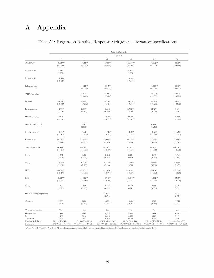
A Appendix

Table A1: Regression Results: Response Stringency, alternative specifications

Dependent variable:

%∆sales

(1) (2) (3) (4) (5) (6)

OxCGRT SI −0.637∗∗∗ −0.641∗∗∗ −0.763∗∗∗ −0.588∗∗∗ −0.592∗∗∗ −0.735∗∗∗

(−7.609) (−7.510) (−8.498) (−3.352) (−3.308) (−4.016)

Export = No 2.005∗ 2.007∗

(1.882) (1.886)

Import = No −0.469 −0.499

(−0.526) (−0.560)

SalesExportShare −0.047∗∗∗ −0.045∗∗∗ −0.048∗∗∗ −0.044∗∗∗

(−4.042) (−3.928) (−4.046) (−3.835)

SupplyImportShare −0.004 −0.005 −0.004 −0.005

(−0.460) (−0.553) (−0.398) (−0.529)

log(age) −0.267 −0.266 −0.265 −0.291 −0.289 −0.291

(−0.709) (−0.717) (−0.724) (−0.776) (−0.785) (−0.802)

log(employees) 2.486∗∗∗ 2.680∗∗∗ 0.342 2.506∗∗∗ 2.702∗∗∗ 0.081

(5.708) (6.365) (0.376) (5.644) (6.279) (0.080)

OwnerFemaleShare −0.023∗∗ −0.023∗ −0.023∗∗ −0.023∗

(−2.001) (−1.919) (−2.020) (−1.924)

FemaleOwner = No 0.986∗ 0.986∗

(1.832) (1.790)

Innovation = No −1.524∗ −1.541∗ −1.542∗ −1.493∗ −1.508∗ −1.526∗

(−1.872) (−1.775) (−1.751) (−1.831) (−1.735) (−1.733)

Closure = No 13.850∗∗∗ 13.835∗∗∗ 13.818∗∗∗ 13.874∗∗∗ 13.860∗∗∗ 13.832∗∗∗

(9.871) (9.927) (9.999) (9.879) (9.931) (10.055)

SaleChange = No −6.805∗∗∗ −6.633∗∗∗ −6.702∗∗∗ −6.840∗∗∗ −6.667∗∗∗ −6.751∗∗∗

(−4.113) (−4.026) (−4.159) (−4.131) (−4.044) (−4.172)

ISICF 0.761 0.465 0.340 0.711 0.416 0.324

(0.421) (0.272) (0.205) (0.392) (0.242) (0.195)

ISICG 4.366∗∗∗ 4.133∗∗∗ 4.144∗∗∗ 4.383∗∗∗ 4.145∗∗∗ 4.162∗∗∗

(5.468) (5.197) (5.290) (5.514) (5.226) (5.347)

ISICH −25.783∗∗∗ −26.029∗∗∗ −25.848∗∗∗ −25.775∗∗∗ −26.016∗∗∗ −25.805∗∗∗

(−5.478) (−5.690) (−5.674) (−5.472) (−5.683) (−5.665)

ISICI −9.637∗∗∗ −9.652∗∗∗ −9.740∗∗∗ −9.619∗∗∗ −9.634∗∗∗ −9.745∗∗∗

(−4.571) (−4.385) (−4.386) (−4.562) (−4.379) (−4.390)

ISICK 0.859 0.829 0.606 0.724 0.688 0.448

(0.335) (0.332) (0.234) (0.281) (0.274) (0.172)

OxCGRT SI :log(employees) 0.041∗∗∗ 0.043∗∗∗

(2.725) (2.779)

Constant 2.190 3.303 10.694 −0.686 0.389 10.052

(0.274) (0.407) (1.356) (−0.046) (0.025) (0.647)


Observations 8,888 8,888 8,888 8,888 8,888 8,888

R2 0.239 0.240 0.242 0.238 0.238 0.241

Adjusted R2 0.236 0.237 0.238 0.234 0.235 0.238




29

Table A2: Regression Results: Response Stringency, robustness checks

Dependent variable:

%∆sales

(1) (2) (3) (4)

OxCGRT SI −0.639∗∗∗ −0.590∗∗∗ −0.640∗∗∗ −0.593∗∗∗

(−7.581) (−3.352) (−7.580) (−3.352)

Baseline firm controls Yes Yes Yes Yes

Follow-up firm controls Yes Yes Yes Yes

Sector fixed effects Yes Yes Yes Yes

Country fixed effects Yes Yes Yes Yes

Observations 8,386 8,386 8,449 8,449

R2 0.245 0.244 0.241 0.240

Adjusted R2 0.242 0.241 0.238 0.237

Residual Std. Error 27.084 (df = 8350) 27.109 (df = 8350) 27.235 (df = 8414) 27.260 (df = 8414)

F Statistic 77.594∗∗∗ (df = 35; 8350) 76.999∗∗∗ (df = 35; 8350) 78.691∗∗∗ (df = 34; 8414) 78.089∗∗∗ (df = 34; 8414)

Notes: ∗p<0.1; ∗∗p<0.05; ∗∗∗p<0.01. All models are estimated using OLS. t-values reported in parentheses. Standard errorsare clustered

at the country-level. Column (1) and (3) employ the average stringency index. Column (2) and (4) employ the maximum value.

In column (1) and (2) we exclude all observations from Belarus. In column (3) and (4) we exclude all observations from Bosnia and

Herzegovina and Serbia.

Table A3: Regression Results: Finance, Linear Probability Model

Dependent variable:

OverdueFinancial OverdueOther Insolvency

(1) (2) (3) (4) (5) (6)

Cash transfer = Yes −0.040∗∗∗ −0.040∗∗∗ −0.049∗ −0.049 −0.019 −0.018

(−3.539) (−3.651) (−1.799) (−1.791) (−1.304) (−1.487)

Deferral of payments = Yes −0.115∗∗∗ −0.115∗∗∗ −0.212∗∗∗ −0.212∗∗∗ −0.011 −0.011∗

(−6.141) (−6.149) (−7.086) (−7.080) (−1.508) (−1.859)

Credit access = Yes −0.021 −0.021 −0.053∗ −0.053∗ −0.025∗ −0.025∗

(−1.234) (−1.254) (−1.783) (−1.784) (−1.861) (−1.700)

Fiscal exemptions = Yes −0.048∗∗∗ −0.048∗∗∗ −0.079∗∗∗ −0.079∗∗∗ −0.014∗ −0.014

(−2.976) (−2.990) (−3.938) (−3.938) (−1.703) (−1.458)

Wage Subsidies = Yes −0.053∗∗∗ −0.052∗∗∗ −0.053∗∗ −0.052∗∗ −0.015 −0.014∗

(−6.161) (−6.061) (−2.148) (−2.141) (−1.479) (−1.749)

Stringency controls Yes Yes Yes Yes Yes Yes

Baseline firm controls Yes Yes Yes Yes Yes Yes

Follow-up firm controls Yes Yes Yes Yes Yes Yes

Sector fixed effects Yes Yes Yes Yes Yes Yes


Observations 3,869 3,869 3,927 3,927 3,958 3,958

R2 0.083 0.083 0.124 0.124 0.079 0.079

Adjusted R2 0.073 0.073 0.115 0.115 0.069 0.069




30

Figure A1: COVID 19 Impact ES Follow-up Survey, selected questions

(a)

(b)

(c)

Notes: The complete questionnaire can be accessed under https://www.enterprisesurveys.org/en/covid-19. If the survey was conducted in 2021,

the question in Panel (a) refers to the same month in 2020 instead of the same month in 2019.

31

References

Adams-Prassl, A., Boneva, T., Golin, M., & Rauh, C. (2020). Inequality in the impact of

the coronavirus shock: Evidence from real time surveys. Journal of Public Economics ,

189 , 104245.

Apedo-Amah, M. C., Avdiu, B., Cirera, X., Cruz, M., Davies, E., Grover, A., . . . Maduko,

F. O. (2020). Unmasking the impact of COVID-19 on businesses: Firm level evidence

from across the world. World Bank Policy Research Working Paper No. 9434 .

Bartik, A. W., Bertrand, M., Cullen, Z., Glaeser, E. L., Luca, M., & Stanton, C. (2020).

The impact of COVID-19 on small business outcomes and expectations. Proceedings of

the National Academy of Sciences , 117 (30), 17656–17666.

Beck, T., Flynn, B., & Homanen, M. (2020). COVID-19 in emerging markets: Firm-survey

evidence. Covid Economics , 38 .

Bosio, E., Djankov, S., Jolevski, F., & Ramalho, R. (2020). Survival of firms during economic

crisis. World Bank Policy Research Working Paper No. 9239 .

Brulhart, M., Lalive, R., Lehmann, T., & Siegenthaler, M. (2020). COVID-19 financial

support to small businesses in Switzerland: Evaluation and outlook. Swiss Journal of

Economics and Statistics , 156 (1), 1–13.

Cameron, A. C., & Trivedi, P. K. (1990). Regression-based tests for overdispersion in the

poisson model. Journal of Econometrics , 46 (3), 347–364.

Chetty, R., Friedman, J., Hendren, N., Stepner, M., et al. (2020). How did COVID-19 and

stabilization policies affect spending and employment? A new real-time economic tracker

based on private sector data. National Bureau of Economic Research Working Paper No.

27431 .

Cirera, X., Cruz, M., Davies, E., Grover, A., Iacovone, L., Lopez, J. E., . . . Ortega, S. R.

(2021). Policies to support businesses through the COVID-19 shock: A firm-level perspec-

tive. Covid Economics , 42.

Core, F., & De Marco, F. (2020). Public guarantees for small businesses in Italy during

COVID-19. CEPR Discussion Paper No. DP15799 .

Cororaton, A., & Rosen, S. (2020). Public firm borrowers of the US Paycheck Protection

Program. Available at SSRN 3590913 .

32

Graeber, D., Kritikos, A. S., & Seebauer, J. (2021). COVID-19: A crisis of the female

self-employed. GLO Discussion Paper No. 788 .

Granja, J., Makridis, C., Yannelis, C., & Zwick, E. (2020). Did the paycheck protection

program hit the target? National Bureau of Economic Research Working Paper No.

27095 .

Grover, A., & Karplus, V. J. (2021). Coping with COVID-19: Does management make firms

more resilient? World Bank Policy Research Working Paper No. 9514 .

Hale, T., Angrist, N., Goldszmidt, R., Kira, B., Petherick, A., Phillips, T., . . . Majumdar,

S. (2021). A global panel database of pandemic policies (Oxford COVID-19 Government

Response Tracker). Nature Human Behaviour , 5 (4), 529–538.

Hassan, T. A., Hollander, S., Van Lent, L., & Tahoun, A. (2020). Firm-level exposure to

epidemic diseases: COVID-19, SARS, and H1N1. National Bureau of Economic Research

Working Paper No. 26971 .

Janzen, B., & Radulescu, D. (2020). Electricity use as a real-time indicator of the economic

burden of the COVID-19-related lockdown: Evidence from Switzerland. CESifo Economic

Studies , 66 (4), 303–321.

Kozeniauskas, N., Moreira, P., & Santos, C. (2020). COVID-19 and firms: Productivity and

government policies. CEPR Discussion Paper No. DP15156 .

Nelson, M. (2021). COVID-19 closure and containment policies: A first look at the labour

market effects in emerging nations. Covid Economics , 66 .

Papke, L. E., & Wooldridge, J. M. (1996). Econometric methods for fractional response

variables with an application to 401 (k) plan participation rates. Journal of Applied

Econometrics , 11 (6), 619–632.

33

Effects of Covid-19 Related Government Response Strin ...

Documents

Transcript of Effects of Covid-19 Related Government Response Strin ...