Fish

Effects of Channel Modification on Habitat in the Upper Yellowstone River

Final Report to the USACE, Omaha

Open File Report 03-476

U.S. Department of the Interior U.S. Geological Survey

U.S. Department of the Interior U.S. Geological Survey

Effects of Channel Modification on Fish Habitat in the Upper Yellowstone River

By

Zachary H. Bowen1

Ken D. Bovee1

and Terry J. Waddle1

Open-File Report 03-476

This report has not been reviewed for conformity with U.S. Geological Survey editorial standards. Any use of trade product or firm names is for descriptive purposes only and does not imply endorsement by the U.S. Government.

_________________________________________________ 1U.S. Geological Survey, Fort Collins Science Center, 2150 Centre Avenue, Building C, Fort Collins CO 80526-8118

ii

Contents

Page

Introduction ................................................................................................................................... 1 Research Questions ................................................................................................................... 2 Study Area................................................................................................................................. 3 Methods.......................................................................................................................................... 4 Study Approach......................................................................................................................... 4 Data Collection.......................................................................................................................... 4 Data Reduction .......................................................................................................................... 6 Hydrodynamic Simulation ........................................................................................................ 7 Habitat Mapping...................................................................................................................... 11 Results.......................................................................................................................................... 15 Channel Modification and SSCV Habitat Among Sites ......................................................... 15 Availability of SSCV Habitat Among Bank Types................................................................. 16 Accretions of SSCV from Large Woody Debris and Channel Modifications ........................ 18 Comparison of Main Channel and Off-Channel SSCV Habitats ............................................ 20 Discussion.................................................................................................................................... 22 Management Implications............................................................................................................ 24 Acknowledgments........................................................................................................................ 24 References.................................................................................................................................... 26 Relationships Among Metric and English Units ......................................................................... 29 Glossary ....................................................................................................................................... 29 Appendix A (Habitat Class Distribution Maps).........................................................OVERSIZED Appendix B (Bank Type Classification Maps)..........................................................OVERSIZED Appendix C (Stream Power Maps) ............................................................................OVERSIZED Appendix D (Simulation of Velocity Patterns and Habitat Conditions Near Barbs) Appendix E (Basic Equations Used in the River-2D Hydrodynamic Model) Appendix F (Water Surface Calibration Details) Appendix G (Hydrodynamic Modeling and Habitat Mapping Details)

iii

Effects of Channel Modification on Fish Habitat in the Upper Yellowstone River

By

Zachary H. Bowen, Ken D. Bovee, Terry J. Waddle

U.S. Geological Survey Fort Collins Science Center

2150 Centre Avenue, Building C Fort Collins, Colorado 80526-8118

Abstract: A two-dimensional hydrodynamic simulation model was coupled with a geographic information system (GIS) to produce a variety of habitat classification maps for three study reaches in the upper Yellowstone River basin in Montana. Data from these maps were used to examine potential effects of channel modification on shallow, slow current velocity (SSCV) habitats that are important refugia and nursery areas for young salmonids. At low flows, channel modifications were found to contribute additional SSCV habitat, but this contribution was negligible at higher discharges. During runoff, when young salmonids are most vulnerable to downstream displacement, the largest areas of SSCV habitat occurred in side channels, point bars, and overbank areas. Because of the diversity of elevations in the existing Yellowstone River, SSCV habitat tends to be available over a wide range of discharges. Based on simulations in modified and unmodified sub-reaches, channel simplification results in decreased availability of SSCV habitat, particularly during runoff. The combined results of the fish population and fish habitat studies present strong evidence that during runoff, SSCV habitat is most abundant in side channel and overbank areas and that juvenile salmonids use these habitats as refugia. Channel modifications that result in reduced availability of side channel and overbank habitats, particularly during runoff, will probably cause local reductions in juvenile abundances during the runoff period. Effects of reduced juvenile abundances during runoff on adult numbers later in the year will depend on (1) the extent of channel modification, (2) patterns of fish displacement and movement, (3) longitudinal connectivity between reaches that contain refugia and those that do not, and (4) the relative importance of other limiting factors.

Introduction During the last several decades, portions of the upper Yellowstone River in Montana

have been modified for flood control and erosion prevention. The U.S. Army Corps of Engineers (USACE) is responsible for administration of a permit program for evaluating construction activities affecting rivers, streams, and wetlands. Following two consecutive large floods during 1996 and 1997, the number of permit applications received by the USACE for channel modification structures increased. In response to concern regarding the potential environmental and ecological consequences of channel modification, the USACE and the Governor’s Upper Yellowstone River Task Force, in conjunction with state and local government agencies, initiated a cumulative effects investigation to better understand the effects of channel modification in the upper Yellowstone River. Results from the cumulative effects investigation will support more informed decisions about river management and serve as a

1

foundation for future monitoring and research. This report is a summary of research findings from the fish habitat study that was conducted as part of the cumulative effects investigation.

The goal of the fish habitat study was to evaluate the effects of channel modification on shallow depth, slow current velocity (SSCV) habitat. We focused on SSCV habitat because shallow and slow water habitats (with varying quantitative definitions in different studies) have been demonstrated repeatedly as important growth and survival factors for young fish (Welcomme 1979; Sedell et al. 1984; Kwak 1988; Nehring and Anderson 1993; Bovee et al. 1994; Scheidegger and Bain 1995; Copp 1997; Bowen et al. 1998; Freeman et al. 2001; Zale and Rider 2003). The larvae and early juvenile lifestages of virtually all species share the common characteristics of small size, poor swimming capability, and reliance on zooplankton, small insects, and detritus as primary food items (e.g., Chapman 1966; Hall et al. 1979; Papoulias and Minckley 1990, 1992; Muir et al. 2000). Shallow water, slow current velocity habitats found in backwaters and side channels provide refuge from high current velocities in main channel areas (Hjort et al. 1984) that can displace small fish downstream, particularly during periods of high discharge (Ottaway and Clarke 1981; Ottaway and Forest 1983). These SSCV habitat areas typically provide favorable feeding conditions and shallow water in combination with structural cover which can reduce the risk of predation for small fish (Schlosser 1991; Ward and Stanford 1995). Our study examined the effects of bank armoring and flow training structures on the availability of SSCV habitat. We mapped representative study reaches in the upper Yellowstone River and used hydrodynamic models and hydrograph data to describe the availability of SSCV habitat during different hydroperiods. We focused on availability of SSCV habitat because of its function as a refugium and nursery habitat for young fish.

Research Questions Our research was designed in conjunction with the concurrent fish population study

conducted by Zale and Rider (2003) to address important questions regarding channel modification and habitat for juvenile fish. Specifically, the research questions we addressed were:

1. Do different levels of channel modification change the amount or distribution of SSCV habitat at different sites?

2. Does availability of SSCV habitat vary among sections of river with different types of

modified and unmodified banks? 3. How important is large woody debris in creating SSCV habitat? 4. What is the relative importance of main channel SSCV habitats compared to SSCV

habitat available in side channels and other areas?

2

Study Area

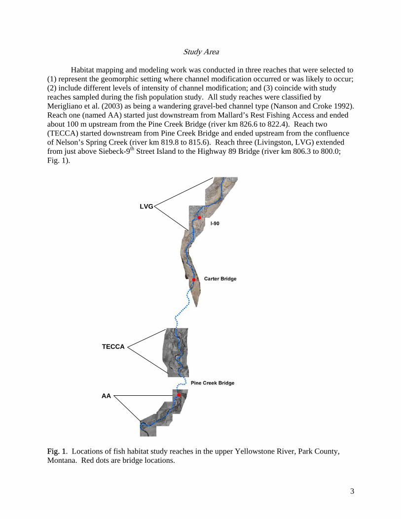
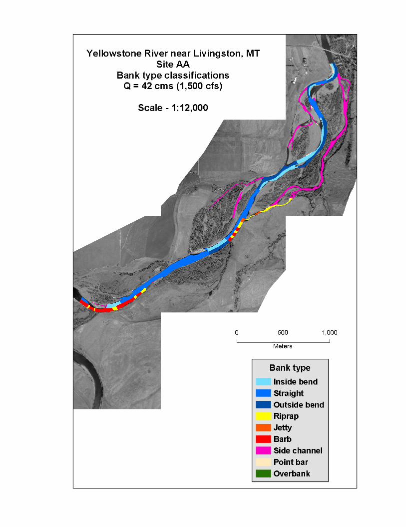
Habitat mapping and modeling work was conducted in three reaches that were selected to (1) represent the geomorphic setting where channel modification occurred or was likely to occur; (2) include different levels of intensity of channel modification; and (3) coincide with study reaches sampled during the fish population study. All study reaches were classified by Merigliano et al. (2003) as being a wandering gravel-bed channel type (Nanson and Croke 1992). Reach one (named AA) started just downstream from Mallard’s Rest Fishing Access and ended about 100 m upstream from the Pine Creek Bridge (river km 826.6 to 822.4). Reach two (TECCA) started downstream from Pine Creek Bridge and ended upstream from the confluence of Nelson’s Spring Creek (river km 819.8 to 815.6). Reach three (Livingston, LVG) extended from just above Siebeck-9th Street Island to the Highway 89 Bridge (river km 806.3 to 800.0; Fig. 1).

LVG

TECCA

AA

Fig. 1. Locations of fish habitat study reaches in the upper Yellowstone River, Park County, Montana. Red dots are bridge locations.

3

Methods

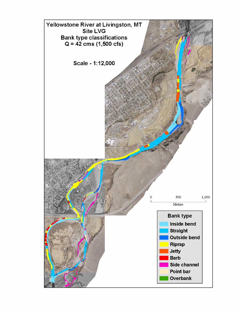
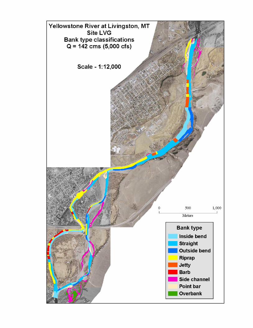
Study Approach As a general procedure, we used a two-dimensional hydrodynamic simulation model and a geographic information system (GIS) to generate habitat classification maps of each study reach for discharges typical during base flow (42 m3/s), snowmelt runoff (680 m3/s), and recession (142 m3/s). Names for flow rates associated with modeling work (base flow, runoff, and recession) were selected to orient the reader to the hydrologic cycle. Model results apply to flow rates regardless of their timing in the year. Each site was subdivided into bank types slightly modified from those used by Zale and Rider (2003): straight, outside bend, point bar, inside bend, overbank, side channel, riprap, barb, and jetty. We used output from the hydrodynamic model and the bank type map in a GIS to determine the amount and distribution of SSCV habitat (ca. < 90 cm deep, < 45 cm/s velocity; < 3.0 ft deep, < 1.5 ft/s) among modified and unmodified river sections. The definition for SSCV habitat used in this study was based on habitat data from recent fish collections in the upper Yellowstone River (Al Zale, personal communication).

Data Collection Input to the two-dimensional hydrodynamic model consisted of a topographic (x,y,z) description of the study reach, a roughness parameter for each x,y location, inflow discharge, and downstream (exiting cross-section) water surface elevation. Topographic data for floodplains, permanent islands, and other above-water features were obtained from aerial photogrammetry and global positioning system (GPS) ground surveys. Echosounding and ground surveys were used to obtain topographic data for the underwater channel bed. All data were projected as Montana State Plane coordinates, referenced to the National Geodetic Survey benchmark (designation AERO, PID QX0005) located at the Livingston Airport. Referencing study reach benchmarks to the benchmark at the airport provides a common reference for future surveys in the event that local benchmarks are lost.

Photogrammetric analyses on 1:6000- and 1:8000-scale photography (Surdex Corporation) were used to develop 0.61 m (2 ft.) contours in the region of the LVG study reach and 1.22 m (4 ft.) contours for the AA and TECCA reaches. Survey-grade GPS receivers were used to obtain calibration data for the photogrammetric analysis. In addition, we surveyed the tops and toes of banks and the perimeters and surfaces of islands, bars, and man-made structures to ground-truth and supplement the photogrammetry data. Care was taken to locate several ground-surveyed points on or near the elevation contours to allow for cross-validation of the aerial and ground survey data sets.

Bathymetric and current velocity data were collected using a boat-mounted echo sounder in conjunction with a survey-grade GPS receiver. The GPS equipment provided a three-dimensional position of the sonar transducer. Thus, the horizontal and vertical position of the sonar transducer is known for each sonar ping. Subtracting the depth from the transducer elevation for each ping gives an elevation of the river bottom. Because the GPS equipment provides x, y (horizontal) and z (elevation) data in real time, changes in water level due to standing waves, changes in discharge, and super elevation around sharp bends are accounted for. Using this equipment, channel features such as margins, bars, islands, and secondary channels were traced with the echo sounder. Additional data were collected longitudinally along

4

approximate streamlines spaced 10-20 m (30-60 ft.) apart between the channel feature traces. Where the water was too shallow for echosounding (< 0.3 m deep) and in areas that were inaccessible by boat, we collected ground survey data using GPS (Fig. 2). Water surface elevations and positions were measured at intervals of 180-300 m (~600-1000 ft.) along the channel to generate a longitudinal profile of the water surface throughout each study site. Discharge was obtained from USGS Gaging Station 06192500, Yellowstone River near Livingston, Montana. Aerial photography was flown during 1999 and other survey data were collected in a series of field trips during 2001-2002 (Table 1).

Contours

Ping points

Data fill

Structure

Fig. 2. Data sources for input to the digital elevation model describing the river corridor. Contours were derived from aerial photography, ping points were collected using a boat-mounted echosounder, and data fill points and structures were both surveyed using a GPS receiver (left panel).

5

Table 1. Dates of field data collection for the upper Yellowstone River fish habitat study.

Dates Mean discharge Data collected

April 11, 1999

41 m3/s Aerial photography used to generate orthophotos and topography for overbank areas (provided by the Governor’s Upper Yellowstone River Task Force and Park County, Montana, Conservation District)

June 4-8, 2001 153−195 m3/s Ground GPS survey of semi-permanent site benchmarks used for survey control

Sept. 3-10, 2001 37−41 m3/s Ground GPS survey of channel modification structures

May 31-June 7, 2002 453-680 m3/s Hydrographic survey by boat used to generate topography for main channel and side channel areas

July 6-13, 2002 153-215 m3/s Hydrographic survey by boat and ground GPS survey to fill in data gaps and provide additional ground control for merging data from different sources

Data Reduction

Data from digitized aerial photogrammetry, echosounding, and ground surveys were processed and combined to provide topographic input for the hydrodynamic model. Contour data from the aerial photogrammetry were converted into point elevations using ArcInfo®. Based on the scale and specified contour intervals for the photogrammetry, elevations derived from the contour data were approximately ± 30 cm (one foot) for the Livingston site and ± 61 cm (two feet) for the upstream sites. Echosounder data were processed to obtain depths and information on substrate roughness and hardness. An interpolation and filtering algorithm was used to calculate bed elevations based on echosounder data and concurrently collected GPS positions and elevations. This algorithm also eliminated duplicate points, filtered based on minimum distance between points, and flagged questionable GPS values. Based on previous experience, as well as equipment specifications for the echosounder and GPS equipment, we approximate the precision of echosounder-based elevations at ± 15 cm. Ground survey GPS data were collected using a real-time kinematic survey style that typically provides ±3 cm accuracy in three dimensions. In addition to surveying features and filling in gaps in topographic coverage, ground GPS was used to validate data from photogrammetry and echosounding. Data from all sources were combined to construct a digital elevation model of the river corridor (Fig. 3).

6

Fig. 3. Detail showing point data from multiple sources and color-filled elevation contours from the TECCA study reach on the upper Yellowstone River.

Hydrodynamic Simulation

The River2D two-dimensional (depth-averaged) model developed at the University of Alberta (Ghanem et al. 1995, 1996) was used to simulate depths and water velocities at unmeasured flows. We chose this model because it can predict regions of supercritical flow and associated transitions and can accommodate lateral wetting/drying boundaries of the surface flow without user intervention.

A two-dimensional, finite-element computational mesh consisting of linear triangular elements was generated for each site (Fig. 4). The mesh was created in an unstructured fashion with the primary criterion for refinement being topographic matching, assessed visually by overlaying contour maps in the mesh generation program. At each node, bed elevation and roughness height were specified and were assumed to vary linearly over each triangle. The computational domain was extended about 120 m in the upstream and downstream directions to minimize the effect of inflow and outflow boundary conditions on flow characteristics at the upstream and downstream limits of the study sites.

7

Fig. 4. Detail showing finite element computational mesh for a portion of the TECCA study reach on the upper Yellowstone River. Colors represent water depth. Warmer colors (red, yellow) are deep relative to cooler colors (blues). Flow is from southeast to northwest.

For calibration, we provided boundary conditions of inflow discharge and the measured water surface elevation at the outflow. Calibration was achieved by scaling the roughness values for different parts of each study site. Our primary criterion for calibration was matching of the predicted and measured water surface profiles for the site. In general, this criterion was satisfied if the predicted water surface elevations were within 10 cm/km of the measured values.

Simulation runs required boundary conditions (inflow discharge and outflow water surface elevation) from stage-discharge relations that were either developed on site or extrapolated from a nearby USGS stream gage. A file of node attributes was created at the completion of each simulation for input to habitat mapping and spatial analysis programs. These files contained information regarding location (coordinates), predicted depth, and predicted velocity at each node in the mesh (Fig. 5).

Flow fields generated by structures were investigated by developing a high-resolution model of a section of river containing barbs. To describe a typical barb placement area in detail, we selected the south bank at the upstream end of the AA study reach (Fig. 6) where a series of barbs approximately 15 m long project from the bank at roughly 50 m intervals. The extracted areas incorporated a region that projected approximately 15 m further into the channel than the

8

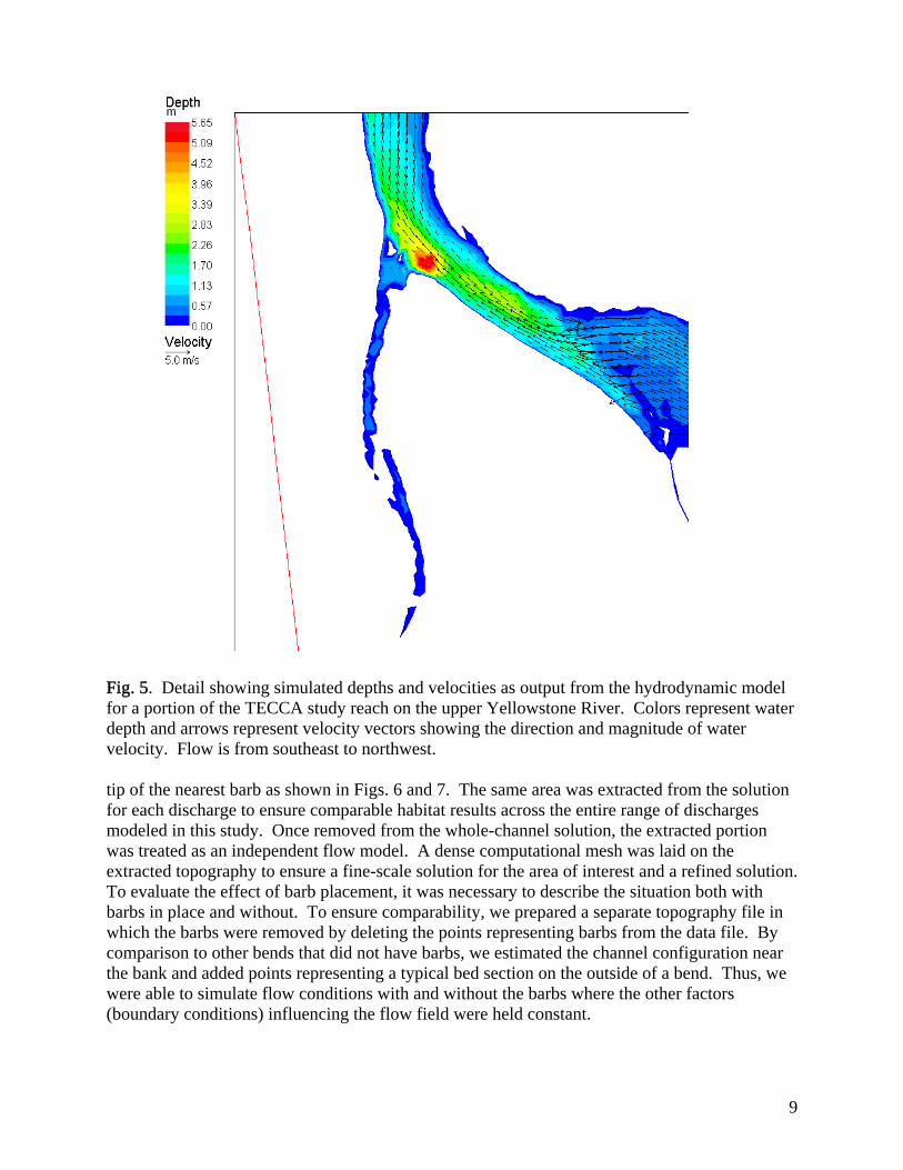
m Fig. 5. Detail showing simulated depths and velocities as output from the hydrodynamic model for a portion of the TECCA study reach on the upper Yellowstone River. Colors represent water depth and arrows represent velocity vectors showing the direction and magnitude of water velocity. Flow is from southeast to northwest.

tip of the nearest barb as shown in Figs. 6 and 7. The same area was extracted from the solution for each discharge to ensure comparable habitat results across the entire range of discharges modeled in this study. Once removed from the whole-channel solution, the extracted portion was treated as an independent flow model. A dense computational mesh was laid on the extracted topography to ensure a fine-scale solution for the area of interest and a refined solution. To evaluate the effect of barb placement, it was necessary to describe the situation both with barbs in place and without. To ensure comparability, we prepared a separate topography file in which the barbs were removed by deleting the points representing barbs from the data file. By comparison to other bends that did not have barbs, we estimated the channel configuration near the bank and added points representing a typical bed section on the outside of a bend. Thus, we were able to simulate flow conditions with and without the barbs where the other factors (boundary conditions) influencing the flow field were held constant.

9

Fig. 6. AA Study Reach: Location of extracted barb field; colors indicate depth.

Fig. 7. Topography of extracted barb field; colors indicate elevation, units are meters.

10

Habitat Mapping

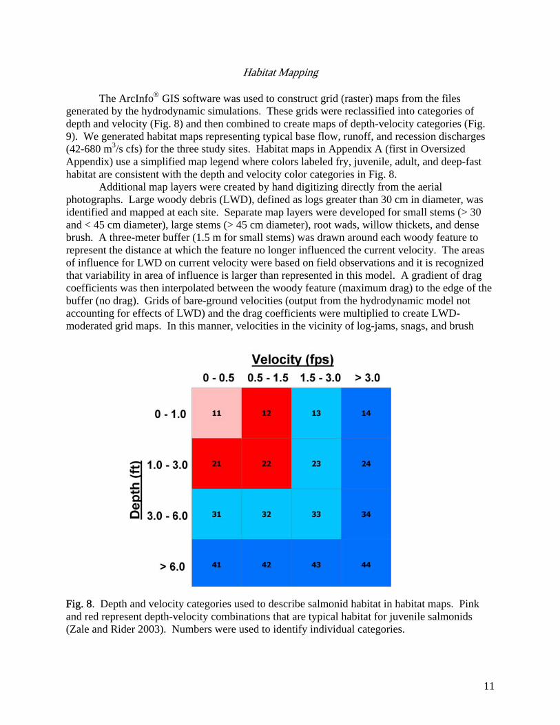
The ArcInfo® GIS software was used to construct grid (raster) maps from the files generated by the hydrodynamic simulations. These grids were reclassified into categories of depth and velocity (Fig. 8) and then combined to create maps of depth-velocity categories (Fig. 9). We generated habitat maps representing typical base flow, runoff, and recession discharges (42-680 m3/s cfs) for the three study sites. Habitat maps in Appendix A (first in Oversized Appendix) use a simplified map legend where colors labeled fry, juvenile, adult, and deep-fast habitat are consistent with the depth and velocity color categories in Fig. 8.

Additional map layers were created by hand digitizing directly from the aerial photographs. Large woody debris (LWD), defined as logs greater than 30 cm in diameter, was identified and mapped at each site. Separate map layers were developed for small stems (> 30 and < 45 cm diameter), large stems (> 45 cm diameter), root wads, willow thickets, and dense brush. A three-meter buffer (1.5 m for small stems) was drawn around each woody feature to represent the distance at which the feature no longer influenced the current velocity. The areas of influence for LWD on current velocity were based on field observations and it is recognized that variability in area of influence is larger than represented in this model. A gradient of drag coefficients was then interpolated between the woody feature (maximum drag) to the edge of the buffer (no drag). Grids of bare-ground velocities (output from the hydrodynamic model not accounting for effects of LWD) and the drag coefficients were multiplied to create LWD-moderated grid maps. In this manner, velocities in the vicinity of log-jams, snags, and brush

Fig. 8. Depth and velocity categories used to describe salmonid habitat in habitat maps. Pink and red represent depth-velocity combinations that are typical habitat for juvenile salmonids (Zale and Rider 2003). Numbers were used to identify individual categories.

11

Fig. 9. Output from the hydrodynamic model interpolated using a triangular irregular network (TIN) and converted to a grid (left) and then reclassified into velocity categories (right). Area represented is a detail of the AA study reach in the upper Yellowstone River. Flow is 680 m3/s from southwest to northeast. piles were reduced locally, whereas all other velocities were the same as in the bare-ground model (Fig. 10). By calculating the amount of SSCV habitat predicted for the LWD-moderated and bare-ground models, respectively, it was possible to estimate the contribution of LWD to the total amount of SSCV habitat. This approach provided a relatively simple and conservative estimate of the contribution of LWD to creation of SSCV habitat. Additional details regarding the GIS procedures used to estimate the effects of LWD on current velocity are provided in Appendix G. Each site was also divided into bank types that were based on the conventions used by Zale and Rider (2003; Fig. 11). Bank types were inside bend, straight, outside bend, riprap, jetty, barb, side channel, point bar, and overbank. The overbank type as used here included islands, benches, and floodplain areas. Channel modification structures were delineated based on data from the 1999 physical features inventory, the 2001-2002 fish population study (Zale and Rider 2003), and our survey of structures conducted during 2001. For main channel areas, a centerline was used to distinguish the features from the top of the bank to the middle of the channel. Although this convention tended to exaggerate the area of stream actually containing the physical material of riprap, jetties, or barbs, it was a consistent and objective method for classifying entire reaches of river. Additional details on bank-type classification methods are available in Appendix G, and bank type maps are in Appendix B (oversized).

12

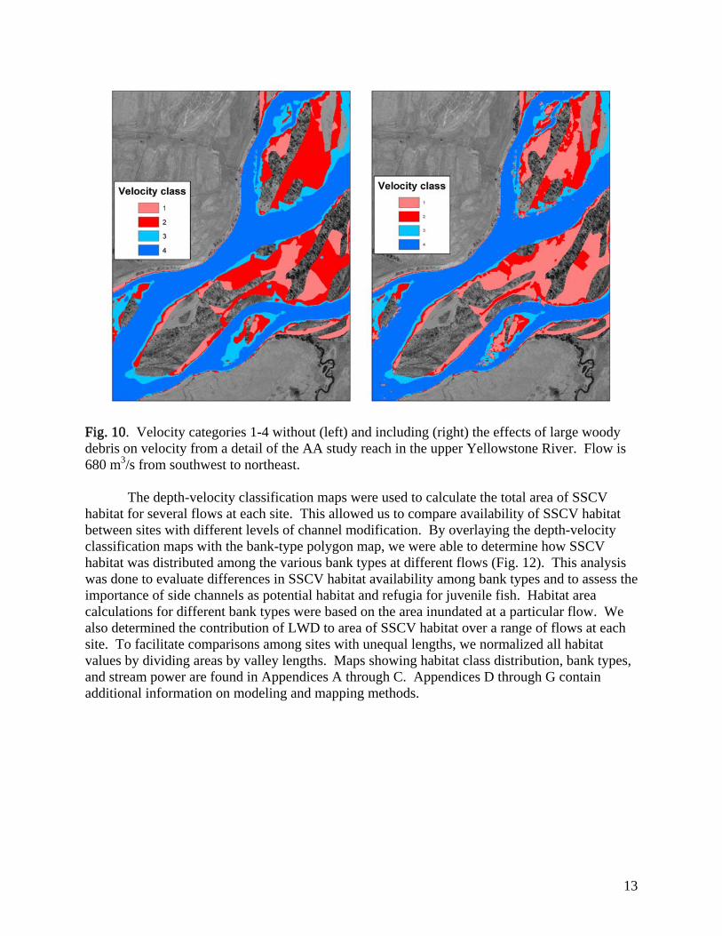
Fig. 10. Velocity categories 1-4 without (left) and including (right) the effects of large woody debris on velocity from a detail of the AA study reach in the upper Yellowstone River. Flow is 680 m3/s from southwest to northeast. The depth-velocity classification maps were used to calculate the total area of SSCV habitat for several flows at each site. This allowed us to compare availability of SSCV habitat between sites with different levels of channel modification. By overlaying the depth-velocity classification maps with the bank-type polygon map, we were able to determine how SSCV habitat was distributed among the various bank types at different flows (Fig. 12). This analysis was done to evaluate differences in SSCV habitat availability among bank types and to assess the importance of side channels as potential habitat and refugia for juvenile fish. Habitat area calculations for different bank types were based on the area inundated at a particular flow. We also determined the contribution of LWD to area of SSCV habitat over a range of flows at each site. To facilitate comparisons among sites with unequal lengths, we normalized all habitat values by dividing areas by valley lengths. Maps showing habitat class distribution, bank types, and stream power are found in Appendices A through C. Appendices D through G contain additional information on modeling and mapping methods.

13

Fig. 11. Detail from a bank type classification map of the AA study reach on the upper Yellowstone River. Flow is 680 m3/s from south to north.

Fig. 12. Detail from a map from of the AA study reach on the upper Yellowstone River showing bank type (pattern) overlaid with habitat categories (color). Flow is 680 m3/s from south to north.

14

Results

Channel Modification and SSCV Habitat Among Sites The relative proportions of SSCV habitat and modified bank-type area varied with the discharge at all three study reaches. Modified bank-type area in a study reach was the sum of areas for riprap, jetty, and barb bank types that were inundated at a given discharge. As discharge and water surface elevation increased, the total area inundated increased. Generally, with increasing discharge, the percent of the site classified as modified decreased and the amount of SSCV habitat increased (Figs. 13 and 14). Regardless of the discharge, however, the LVG reach had the highest proportion of modified bank type area, with roughly double the amount of modification of either the AA or TECCA reach. The area of SSCV habitat per km was about the same at all three sites at the two lower discharges, but differed considerably at bankfull flow. At base flow (~42 m3/s), normalized SSCV was highest at LVG, but was lowest there at bankfull flow (~680 m3/s). In addition, normalized SSCV was about the same for all discharges at LVG, varying by about 44% from smallest to largest area. In contrast, normalized SSCV varied by over 500% at TECCA and by 200% at AA for the same range of discharges. At bankfull flow, the amount of SSCV was highest at the two sites with the least amount of channel modification. Normalized SSCV at TECCA was 11.3 ha/km, compared to 5.91 ha/km at AA, and 4.21 ha/km at LVG.

0

2

4

6

8

10

12

0 100 200 300 400 500 600 700 800

Discharge (cms)

Nor

mal

ized

SSC

V (h

a/km

)

AA TECCA LVG

Fig. 13. Percent of modified bank type area at AA, TECCA, and LVG study reaches at discharges ranging from base flow (42 m3/s) to bankfull discharge(680 m3/s).

15

0%

5%

10%

15%

20%

25%

30%

0 100 200 300 400 500 600 700 800

Discharge (cms)

Inun

date

d ar

ea m

odifi

ed

AA TECCA LVG

Fig. 14. Normalized area of SSCV habitat at AA, TECCA, and LVG study reaches at discharges ranging from base flow (42 m3/s) to bankfull discharge (680 m3/s).

Availability of SSCV Habitat Among Bank Types

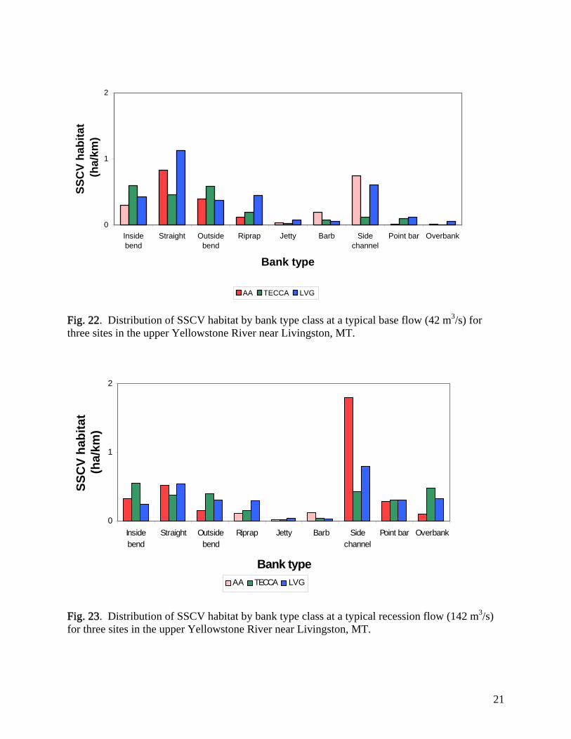
The proportional distribution of SSCV habitat varied among bank types at different discharges at all three sites. At base flow, SSCV habitat was predominantly associated with unmodified main channel locations at TECCA and LVG (78% and 58%, respectively) and in side channels at AA (50%, Fig. 15). At all three sites, the proportion of SSCV habitat associated with unmodified main channel areas exceeded the proportion associated with riprap, jetties, and barbs. For example, LVG had the highest proportion of SSCV habitat associated with modified banks of all the sites, at 19%. However, the proportion of SSCV associated with unmodified banks was nearly three times higher (58%). The discrepancy between modified and unmodified main channel locations was even more pronounced at TECCA and AA (Fig. 15). The basic pattern of SSCV distribution during recession was similar to that observed at base flow (Fig. 16). However, the proportion of SSCV occurring in main channel areas was smaller, and the amount associated with side channels, point bars, and overbank areas was greater at the recession flow than at base flow. As observed for base flow, the relative contribution of modified channel areas to the total area of SSCV habitat was small compared to unmodified areas. Unlike the base flow scenario, however, the distribution of SSCV habitat appeared to be divided nearly evenly between main channel (modified and unmodified) and off-channel areas. The distribution of SSCV habitat at bankfull discharge was substantially different from the two lower discharges (Fig. 17). At all three sites, nearly all the SSCV habitat occurred in locations other than the main channel. Slow, shallow habitat areas tended to be concentrated the most in overbank areas and side channels. Modified main channel areas appeared to be less significant contributors of SSCV habitat at bankfull discharge than at the lower flows.

16

Fig. 15. Distribution of SSCV habitat by bank type at a typical base flow discharge (42 m3/s) for three sites in the upper Yellowstone River near Livingston, MT.

Fig. 16. Distribution of SSCV habitat by bank type at a typical recession flow (142 m3/s) for three sites in the upper Yellowstone River near Livingston, MT.

Fig. 17. Distribution of SSCV habitat by bank type at bankfull discharge (680 m3/s) for three sites in the upper Yellowstone River near Livingston, MT.

17

Accretions of SSCV from Large Woody Debris and Channel Modifications Contribution of SSCV Attributable to Large Woody Debris

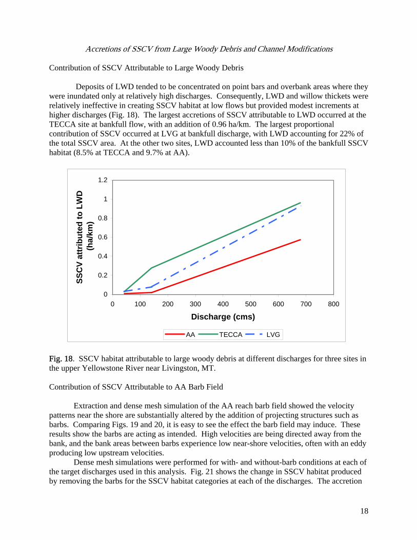
Deposits of LWD tended to be concentrated on point bars and overbank areas where they were inundated only at relatively high discharges. Consequently, LWD and willow thickets were relatively ineffective in creating SSCV habitat at low flows but provided modest increments at higher discharges (Fig. 18). The largest accretions of SSCV attributable to LWD occurred at the TECCA site at bankfull flow, with an addition of 0.96 ha/km. The largest proportional contribution of SSCV occurred at LVG at bankfull discharge, with LWD accounting for 22% of the total SSCV area. At the other two sites, LWD accounted less than 10% of the bankfull SSCV habitat (8.5% at TECCA and 9.7% at AA).

0

0.2

0.4

0.6

0.8

1

1.2

0 100 200 300 400 500 600 700 800

Discharge (cms)

SSC

V at

trib

uted

to L

WD

(ha/

km)

AA TECCA LVG

Fig. 18. SSCV habitat attributable to large woody debris at different discharges for three sites in the upper Yellowstone River near Livingston, MT.

Contribution of SSCV Attributable to AA Barb Field

Extraction and dense mesh simulation of the AA reach barb field showed the velocity

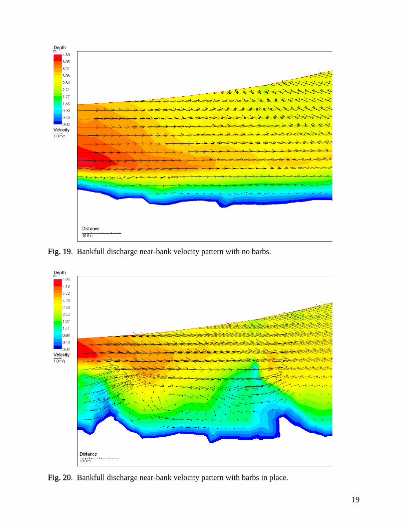
patterns near the shore are substantially altered by the addition of projecting structures such as barbs. Comparing Figs. 19 and 20, it is easy to see the effect the barb field may induce. These results show the barbs are acting as intended. High velocities are being directed away from the bank, and the bank areas between barbs experience low near-shore velocities, often with an eddy producing low upstream velocities.

Dense mesh simulations were performed for with- and without-barb conditions at each of the target discharges used in this analysis. Fig. 21 shows the change in SSCV habitat produced by removing the barbs for the SSCV habitat categories at each of the discharges. The accretion

18

m

Fig. 19. Bankfull discharge near-bank velocity pattern with no barbs.

m

Fig. 20. Bankfull discharge near-bank velocity pattern with barbs in place.

19

0.000

0.005

0.010

0.015

0.020

0.025

0.030

0 100 200 300 400 500 600 700 800

Discharge (cms)

Cha

nge

in S

SCV

(ha/

km)

Fig. 21. SSCV habitat attributable to the barb field in the AA study reach at different discharges. of SSCV habitat attributable to the barb field at AA was negligible at all simulated discharges. A quick comparison between Figs. 18 and 21 shows that the SSCV contribution by LWD in the AA site was more than an order of magnitude greater than the contribution from the barb field at bankfull flow. For this comparison, the contribution of LWD to SSCV habitat was normalized by study area valley length, and the contribution of the AA barb field was normalized by the length of bank associated with the barb field (0.57 km).

Comparison of Main Channel and Off-Channel SSCV Habitats

The most telling differences between main channel and off-channel locations of SSCV habitat are demonstrated by comparing Figs. 22 and 23 with Fig. 24. Consistent with the findings shown in Figs. 15-17, most of the SSCV habitat at all three sites occurred in main channel locations at low flows and in off-channel areas at bankfull flow. However, Figs. 22-24 demonstrate the magnitude of the differences in SSCV habitat from low to high flow. Compared to the area of SSCV habitat available at base flow, the area at bankfull flow was about 50% greater at LVG, twice as large at AA, and five times greater at TECCA. At bankfull discharge, main channel areas contributed negligible amounts of SSCV habitat at all three sites, compared to side channel and overbank areas. Side channels, point bars, and overbank areas accounted for 97% of the SSCV habitat at AA, 95% at TECCA, and 90% at LVG. During a typical runoff discharge, main channel areas were dominated by high water velocities and large depths compared to overbank and side channel areas. These results highlight the importance of side channels and overbank as areas of SSCV habitat, particularly at higher discharges when the probability of downstream displacement for juvenile fish in main channel habitats is highest.

20

0

1

2

Insidebend

Straight Outsidebend

Riprap Jetty Barb Sidechannel

Point bar Overbank

Bank type

SSC

V ha

bita

t (h

a/km

)

AA TECCA LVG

Fig. 22. Distribution of SSCV habitat by bank type class at a typical base flow (42 m3/s) for three sites in the upper Yellowstone River near Livingston, MT.

0

1

2

Insidebend

Straight Outsidebend

Riprap Jetty Barb Sidechannel

Point bar Overbank

Bank type

SSC

V ha

bita

t (h

a/km

)

AA TECCA LVG

Fig. 23. Distribution of SSCV habitat by bank type class at a typical recession flow (142 m3/s) for three sites in the upper Yellowstone River near Livingston, MT.

21

Fig. 24. Distribution of SSCV habitat by bank type class at bankfull discharge (680 m3/s) for three sites in the upper Yellowstone River near Livingston, MT.

0

1

2

3

4

5

6

Insidebend

Straight Outsidebend

Riprap Jetty Barb Sidechannel

Point bar Overbank

Bank type

SSC

V ha

bita

t (h

a/km

)

AA TECCA LVG

Discussion

Results from the fish population study showed equal or higher abundances of juvenile salmonids in modified main channel habitats compared to unmodified main channel habitats. One conclusion from the fish population study was that during base flow, river banks containing boulders were used by juvenile salmonids. Higher abundances of juvenile trout in modified areas, where overall availability of SSCV habitat was lower than in unmodified areas, suggest that visual isolation (e.g., predator avoidance) was more important than hydraulic shelter during late summer and at lower discharges. Our results, showing SSCV habitat availability at base flow, are consistent with conclusions from the fish population study that factors other than SSCV availability (e.g., habitat diversity and cover provided by boulder-sized elements of barbs and riprap) were causing juvenile trout to preferentially use modified banks.

Results from the fish population study showed equal or higher abundances of juvenile salmonids in modified main channel habitats compared to unmodified main channel habitats. One conclusion from the fish population study was that during base flow, river banks containing boulders were used by juvenile salmonids. Higher abundances of juvenile trout in modified areas, where overall availability of SSCV habitat was lower than in unmodified areas, suggest that visual isolation (e.g., predator avoidance) was more important than hydraulic shelter during late summer and at lower discharges. Our results, showing SSCV habitat availability at base flow, are consistent with conclusions from the fish population study that factors other than SSCV availability (e.g., habitat diversity and cover provided by boulder-sized elements of barbs and riprap) were causing juvenile trout to preferentially use modified banks.

Many studies have confirmed that a critical time period for young-of-year fish is from emergence through the runoff period (Welcomme 1979; Sedell et al. 1984; Kwak 1988; Nehring and Anderson 1993; Bovee et al. 1994; Scheidegger and Bain 1995; Copp 1997; Bowen et al. 1998; Freeman et al. 2001; Zale and Rider 2003). Because of their small size and poor swimming capability, fry and younger age classes of fish use SSCV habitats as refugia and nursery areas. This generalization is supported by studies in small, warmwater streams (Schlosser 1982), coldwater streams (Miller 1957; Horner and Bjornn 1976), and great floodplain rivers (Holland 1986). During runoff, we found the largest areas of SSCV habitat were available in side-channels and overbank locations. This result is consistent with results from the fish population study that showed juvenile fish occupied ephemeral side channels as soon as they became inundated and that juvenile abundances increased with duration of side channel inundation. Main channel locations (regardless of their state of modification) were substantially smaller sources of SSCV habitat during runoff, compared to off-channel areas.

Many studies have confirmed that a critical time period for young-of-year fish is from emergence through the runoff period (Welcomme 1979; Sedell et al. 1984; Kwak 1988; Nehring and Anderson 1993; Bovee et al. 1994; Scheidegger and Bain 1995; Copp 1997; Bowen et al. 1998; Freeman et al. 2001; Zale and Rider 2003). Because of their small size and poor swimming capability, fry and younger age classes of fish use SSCV habitats as refugia and nursery areas. This generalization is supported by studies in small, warmwater streams (Schlosser 1982), coldwater streams (Miller 1957; Horner and Bjornn 1976), and great floodplain rivers (Holland 1986). During runoff, we found the largest areas of SSCV habitat were available in side-channels and overbank locations. This result is consistent with results from the fish population study that showed juvenile fish occupied ephemeral side channels as soon as they became inundated and that juvenile abundances increased with duration of side channel inundation. Main channel locations (regardless of their state of modification) were substantially smaller sources of SSCV habitat during runoff, compared to off-channel areas.

22

SSCV habitat was more extensive at AA and TECCA than at LVG during runoff. The comparatively lower value for SSCV habitat at LVG is attributable to reduced SSCV habitat availability in side channels and overbank areas. Although the channel near Livingston is classified as wandering gravel bed, the channel is more confined than at the other two study reaches. On the east side of the valley near Livingston, flooding, channel migration, and side channel formation are constrained by a resistant high-elevation valley wall. To the west, riprap and levees installed to prevent erosion and flooding in the town of Livingston similarly reduce the area of overbank inundated and limit the availability of SSCV habitat in side channels. Areas with the least amount of SSCV habitat within the LVG site occurred where the channel was confined and energy was highest (e.g., from the 9th Street Bridge to Mayor’s Landing Fishing Access). In contrast, both AA and TECCA were characterized by vast areas of SSCV habitat occurring in off-channel locations, either in ephemeral side channels, over inundated islands, or on the floodplain. Examination of the habitat classification maps in Appendix A reveals that large amounts of SSCV habitat occurred in side channels and overbank areas at flows ranging from bankfull to as low as 142 m3/s. This finding suggests that the availability of SSCV habitat during runoff periods is persistent. That is, large, contiguous, and widely dispersed areas of SSCV habitat are likely to be available for colonization by young salmonids, regardless of the discharge during the critical runoff period. This persistence can be attributed in large measure to a diversity of elevations that is characteristic of the braided portion of the Yellowstone River. The section of river in our study area contains multiple channels, point bars, islands, and floodplains that lie at different elevations relative to one another. As the discharge increases, some areas of the channel become too fast or deep to be suitable for young salmonids. However, as one area of the channel becomes unusable, another appears at a higher elevation. Conversely, as the water level recedes after runoff, SSCV habitat appears to transition smoothly from overbank areas to side channels, and eventually to the main channel as discharge approaches base flow. Persistence of SSCV habitat does not occur as readily in confined channels. As flow and stage increase in a confined channel, the wetted perimeter associated with a river cross-section increases less than in an unconfined reach. Generally, in confined reaches as flow increases, shallow or slow water habitat is associated with the channel margins. Examination of some of the more confined reaches of the LVG (e.g., the lower half of the reach) reveals that SSCV habitat occurs mostly as a thin strip along the river margin at all but the lowest discharges. This characteristic makes the availability of SSCV habitat much more responsive to changes in discharge. At high flows, the marginal strip of SSCV is very narrow and at lower flows, it is broader.

The habitat dynamics associated with channel confinement can influence fish populations by affecting survival of early life stages. Studies of fish populations in confined rivers have revealed that (1) the adult fish population tends to be recruitment-driven, and (2) the number of recruits is highly correlated with the discharge and amount of available SSCV habitat during the runoff period (Nehring and Anderson 1993; Bovee et al. 1994; Bowen et al. 1998; Freeman et al. 2001). Thus, year class strength is typically very low in years of above-average runoff, but considerably larger during drought years when runoff is less (Nehring and Anderson 1993). Our study focused on availability of shallow, slow current velocity habitat because of its importance as a refugium and nursery for juvenile salmonids, particularly during periods of high discharge. Other habitat requirements include spawning habitat, adult habitat, and overwintering habitat. Populations of trout can be limited by a deficiency in any of these (Behnke 1992). Flow

23

regime, especially summer low flows, are important in determining trout biomass (Binns and Eiserman 1979). Low flows during summer that result in dewatering of important habitats, increased water temperature, or adverse affects on water quality could affect survival or limit carrying capacity. Similarly, the condition of fish at the beginning of winter and availability of overwintering habitat are very important in determining overwinter survival (Behnke 1992). Additional research and population monitoring should strive to determine which factors, including physical habitat, are most directly regulating numbers of adult salmonids.

Management Implications

The combined results from the fish population and fish habitat studies present strong evidence that during runoff, SSCV habitat is most abundant in side channel and overbank areas and that juvenile salmonids use these habitats as refugia. Channel modifications that result in reduced availability of side channel and overbank habitats, especially during runoff, will probably cause local reductions in juvenile abundances during the runoff period. The effect of local reductions during runoff on adult numbers later in the year will depend on the extent of channel modification, patterns of fish displacement and movement, longitudinal connectivity between reaches that contain refugia and those that do not, and the relative importance of other potential limiting factors. River confinement, in itself, will probably not result in elimination of the trout population of the upper Yellowstone River. As the amount of confinement increases, however, we expect a concomitant reduction in the area and persistence of SSCV habitat. As the availability of SSCV habitat becomes more and more responsive to changes in discharge, we postulate that salmonid population dynamics will become more variable over time. We would expect the trout populations of the upper Yellowstone to become more recruitment-driven and more responsive to conditions during runoff, as has been observed in other confined trout streams (e.g., Nehring and Anderson 1993). This study intensively examined SSCV habitat availability at three representative study reaches. Additional ongoing research is using coarser grain data to evaluate SSCV habitat availability over a range of flood discharges within the study corridor from Point of Rocks to Mission Creek. This ongoing second phase will help provide context for the intensive fish habitat study as well as provide a measure of habitat availability in different channel types over a large, continuous reach. The extensive SSCV habitat evaluation and habitat maps will also serve as a foundation for integrated analyses of results from other studies conducted as part of the overall cumulative effects investigation.

Acknowledgments This project was funded by the U. S. Army Corps of Engineers, Omaha District, and directed by Michael C. Gilbert. Eric Morrison, also with the USACE, provided outstanding technical assistance with data and GIS files from multiple sources that were used as part of this study. The Coordinator of the Governor’s Upper Yellowstone River Task Force, Liz Galli-Noble; Duncan Patten, Chair of the Technical Advisory Committee; and members of the Committee and Task Force provided valuable input and advice throughout the study. Brad Shepard and Adam Craig

24

kindly provided us with an initial orientation and tour of the study area. Professional surveyor Tom Hallin gave us a huge head start when he helped us locate benchmarks and gain access to the river by introducing us to local landowners. Landowners Charles Almond, John Tecca, and Park County graciously allowed us access to their property and let us install local benchmarks. Al Zale and Steve Rider with the Montana Cooperative Fishery Research Unit conducted the concurrent fish population study and consistently had good ideas and sage advice for our fish habitat work. The careful and thorough job they did in the fish population study made telling the habitat story an easier job for us. At the Fort Collins Science Center, Bob Waltermire was always willing to help with difficult GIS questions. Various versions of the content in this report were commented on by Al Zale, Brad Shepard, Chuck Dalby, and numerous others who remain anonymous (though we have some ideas). We sincerely appreciate the effort put into the reviews as they greatly improved the final report. Thanks to all who helped in making the project successful.

25

References Behnke, R.J. 1992. Native trout of western North America. American Fisheries Society

Monograph 6. Binns, N.A., and F.M. Eiserman. 1979. Quantification of fluvial trout habitat in Wyoming.

Transactions of the American Fisheries Society 108:215-228. Bovee, K.D., T.J. Newcomb, and T.G. Coon. 1994. Relations between habitat variability and

population dynamics of bass in the Huron River, Michigan. U.S. Department of the Interior, National Biological Survey Biological Report 21. 63 pp.

Bowen, Z.H., M.C. Freeman, and K.D. Bovee. 1998. Evaluation of generalized habitat criteria

for assessing impacts of altered flow regimes on warmwater fishes. Transactions of the American Fisheries Society 127:455-468.

Chapman, D.W. 1966. Food and space as regulators of salmonid populations in streams.

American Naturalist 100:35-37. Copp, G.H. 1997. Importance of marinas and off-channel water bodies as refuges for young

fishes in a regulated lowland river. Regulated Rivers: Research and Management 13:303-307.

Freeman, M.C., Z.H. Bowen, K.D. Bovee, and E.R. Irwin. 2001. Flow and habitat effects on

juvenile fish abundance in natural and altered flow regimes. Ecological Applications 11(1):179-190.

Ghanem, A., P. Steffler, F. Hicks, and C. Katopodis. 1995. Two-dimensional finite element

modeling of flow in aquatic habitats. Water Resources Engineering Report No. 95-S1. University of Alberta.

Ghanem, A., P. Steffler, F. Hicks, and C. Katopodis. 1996. Two-dimensional simulation of

physical habitat conditions in flowing streams. Regulated Rivers: Research and Management 12:185-200.

Hall, D.J., E.E. Werner, J.F. Gilliam, G.G. Mittelbach, D. Howard, C.G. Doner, J.A. Dickerman,

and A.J. Stewart. 1979. Diel foraging behavior and prey selection in the golden shiner (Notemigonus crysoleucas). Journal of the Fisheries Research Board of Canada 36:1029-1039.

Hjort, R.C., P.L. Hulett, L.D. Labolle, and H.W. Li. 1984. Fish and invertebrates of revetments

and other habitats in the Willamette River, Oregon. Technical Report E-84-9, U.S. Army Engineer Waterway Experiment Station, Vicksburg, Mississippi.

Holland, L.E. 1986. Distribution of early life history stages of fishes in selected pools of the

upper Mississippi River. Hydrobiologia 136:121-130.

26

Horner, N., and T.C. Bjornn. 1976. Survival, behavior, and density of trout and salmon fry in

streams. University of Idaho, Forestry and Wildlife Experiment Station. Contract 56, Progress Report. 38 pp.

Kwak, T.J. 1988. Lateral movement and use of floodplain habitat by fishes of the Kankakee

River, Illinois. American Midland Naturalist 120:241-249. Merigliano, M.F., and M.L. Polzin. Temporal patterns of channel migration, fluvial events, and

associated vegetation along the Yellowstone River, Montana. Project report to the U.S. Army Corps of Engineers, Omaha, NE. University of Montana, Missoula.

Miller, R.B. 1957. Permanence and size of home territory in stream-dwelling cutthroat trout.

Journal of the Fisheries Research Board of Canada 14:687-691. Muir, W.D., G.T. McCabe, Jr., M.J. Parsley, and S.A. Hinton. 2000. Diet of first-feeding and

young-of-the-year white sturgeon in the lower Columbia River. Northwest Science 74:25-33.

Nanson, G.C., and J.C. Croke. 1992. A genetic classification of floodplains. Geomorphology

4:459-486 Nehring, R.B., and R.M. Anderson. 1993. Determination of population-limiting critical

salmonid habitats in Colorado streams using the Physical Habitat Simulation System. Rivers 4(1):1-19.

Ottaway, E.M., and A. Clarke. 1981. A preliminary investigation in to the vulnerability of

young trout (Salmo trutta) and Atlantic salmon (Salmo salar) to downstream displacement by high water velocities. Journal of Fish Biology 19:135-145.

Ottaway, E.M., and D.R. Forest. 1983. The influence of water velocity on downstream

movement of alevins and fry of brown trout, Salmo trutta. Journal of Fish Biology 23:221-227.

Papoulias, D., and W.L. Minckley. 1990. Food limited survival of larval razorback sucker,

Xyrauchen texanus, in the laboratory. Environmental Biology of Fishes 29:73-78. Papoulias, D., and W.L. Minckley. 1992. Effects of food availability on survival and growth of

larval razorback suckers in ponds. Transactions of the American Fisheries Society 121:340-355.

Scheidegger, K.J., and M.B. Bain. 1995. Larval fish distribution and microhabitat use in free-

flowing and regulated rivers. Copeia 1995:125-135. Schlosser, I.J. 1982. Fish community structure and function along two habitat gradients in a

headwater stream. Ecological Monographs 52:395-414.

27

Schlosser, I.J. 1991. Stream fish ecology: a landscape perspective. Bioscience 41:704-712. Sedell, J.R., J.E. Yuska, and R.W. Speaker. 1984. Habitats and salmonid distribution in pristine,

sediment-rich valley systems: South Fork Hoh and Queets River, Olympic National Park. Pages 33-46 in W. R. Meehan, T. R. Merrel, and T. A. Hanley, editors. Fish and wildlife relationships in old-growth forests. American Institute of Fishery Research Biologists.

Ward, J.V., and J.A. Stanford. 1995. Ecological connectivity in alluvial river ecosystems and its

disruption by flow regulation. Regulated Rivers: Research and Management 11:105-119. Welcomme, R.L. 1979. Fisheries ecology of floodplain rivers. Longman Group Limited, New

York. Zale, A.V., and D. Rider. 2003. Comparative use of modified and natural habitats of the upper

Yellowstone River by juvenile salmonids. Final project report to the U.S. Army Corps of Engineers, Omaha, NE. Montana Cooperative Fishery Research Unit, Bozeman, MT.

28

Relationships Among Metric and English Units Length 1 inch = 2.54 centimeters (cm) 1 foot = 0.305 meters (m) 1 mile = 1.609 kilometers (km) Area 1 square foot = 0.0929 square meters (m2) 1 acre = 0.4047 hectares (ha) Flow rate

1 cubic foot per second (cfs) = 0.0283 cubic meters per second (cms or m3/s)

Glossary Bankfull discharge – discharge where the water surface elevation is nearly equal to the top of the main channel banks. In the reaches studied, bankfull discharge equals about 680 m3/s (24,000 cfs). Base flow – period of stable low flow after runoff and recession that usually occurs during late summer through winter. Calibration – process of adjusting parameters in a model until model-predicted values (in this case, water surface elevation and relative velocities) match or are close to measured values. Computational mesh – the aggregate of all nodes at which calculations of mass and momentum flux are performed. In the River2D model, the mesh is composed of triangular elements. Drag coefficient – a multiplier used to achieve a percentage reduction in velocity that varied linearly from the center of a large woody debris object (100% reduction) to the edge of the field of influence (0% reduction). Echosounder – a device that measures water depth from a boat using sound waves. The scientific echosounder used in this study is capable of ±1 inch precision. Geographic information system (GIS) – computer software used to create and analyze map-based data sets. Global positioning system (GPS) – system of satellites and ground control stations that allows precise determination of positions and elevations by receivers used in mapping and surveying. Grid maps – a type of data set where values (e.g., depths) are represented as individual squares (called cells) of fixed size that together make up a lattice representing the map area.

29

Hand digitizing – creation of a GIS map layer by tracing and identifying features from digital photographs (or other source data) on a computer screen. Hydrodynamic model – a model that calculates a balance of forces and mass flow to predict water surface elevations, depths, and velocities. Hydroperiod – a portion of the hydrograph characterized by the period of time the hydrograph reflects a particular pattern of precipitation and runoff. For example, base flow is primarily associated with groundwater, has little surface runoff component, and typically occurs from October to January in the Rocky Mountain region. Map layers – also called coverages. These are map-based data that contain information on a certain topic. For example, one map layer could show depths, while a second layer could show locations of large woody debris. Overbank – the area above the typical channel bank that is inundated by flows greater than the bankfull discharge. In this study, vegetated islands and bars were also classified as overbank, even though they might be inundated at bankfull discharge or somewhat less than that. Recession – period during which discharges decrease from peak flow during runoff to base flow during late summer or fall. Recruitment – the supply of fish that becomes available at a certain size or life stage. For example, a fish might be considered a recruit when it reaches catchable size or when it reaches sexual maturity. Roughness parameter – a value representing the average height of roughness elements, generally meaning the substrate on the river bottom, that is used to calibrate the hydrodynamic model. Runoff – In the western U.S. , the hydroperiod associated with snowmelt, resulting in the annual rise in discharge during May and June, followed by the recession from peak flow to base flow. Simulation – use of a calibrated model to predict depths and velocities at unmeasured discharges. Two-dimensional hydrodynamic model – a kind of open-channel flow model that solves the forces acting on a vertical column of water to produce maps of depth and velocity over a section of river. Triangulated Irregular Network (TIN) – an array of points connected in triangles where each triangle constitutes the set of nearest neighboring points.

30

Effects of Channel Modification on Fish Habitat in the Upper Yellowstone River

Oversized Appendixes

Zachary H. Bowen, Ken D. Bovee, and Terry J. Waddle

U.S. Geological Survey

Fort Collins Science Center 2150 Centre Avenue, Building C

Fort Collins, CO 80526-8118

March 31, 2003

U.S. Department of the InteriorU.S. Geological Survey

Appendix D

Simulation of Velocity Patterns and Habitat Conditions Near Barbs

A major question being asked about the Yellowstone River in the vicinity of Livingston is the habitat value of various bank stabilization devices. The current state of 2-dimensional hydrodynamic modeling allows investigation of some aspects of the hydraulics surrounding bank protection structures. While it is not possible to simulate the spaces between boulders used as rip rap or in barbs and jetties, it is possible to model the flow fields generated by structures such as barbs at different discharges.

The River2D model contains a feature that permits extracting a portion of a flow solution for closer examination. One can define four boundaries for an extraction as follows: lateral boundaries are taken along streamlines. Streamlines (potential flow lines) are identified using a right-to-left calculation of cumulative discharge. Upstream and downstream boundaries are identified by selecting two points across which the model constructs lines orthogonal to the streamlines. Careful placement of the lateral and longitudinal boundaries allows any area in a whole-channel solution to be extracted for further analysis. It is necessary to extract results from a solution for the whole channel as hydrodynamic effects across the entire channel influence the flow field along a bank.

To describe a typical barb placement area in detail we selected the south bank at the upstream end of the AA study site (Figure 6) where a series of barbs approximately 15 m long project from the bank at roughly 50 m intervals. Extraction areas were selected that incorporated an area approximately 15 m further into the channel than the tip of the barbs as shown in Figure 7. The same area was extracted from the solution for each discharge to ensure comparable habitat results across the entire range of discharges modeled in this study.

Once removed from the whole-channel solution, the extracted portion can be treated as an independent flow model. A dense computational mesh can be laid on the extracted topography to ensure a fine-scale solution for the area of interest and a refined solution can be obtained.

To evaluate the effect of barb placement, it was necessary to describe both the situation with barbs in place and without. To ensure comparability, we prepared a separate topography file in which the barbs were removed by deleting the points representing barbs from the data file. By comparison to other bends that did not have barbs we estimated the channel configuration near the bank and added points representing a typical bed section on the outside of a bend. Thus, we were able to simulate flow conditions with and without the barbs where the other factors (boundary conditions) influencing the flow field were held constant. The velocity patterns near the shore are substantially altered by addition of projecting structures such as barbs. Comparing Figures 19 and 20, it is easy to see the substantial effect the barb field may induce.

The model results show the barbs are acting as intended. High velocities are being directed away from the bank and the bank areas between barbs experience low near-shore velocities often with an eddy producing low upstream velocities. The results shown in these figures are time-averaged and are sensitive to the full channel discharge and depth of flow.

i

It is important to note that the near-shore depth for the no-barb case (Figure 19) is

estimated. Further studies would be needed to quantitatively describe the likely future bankline configuration and near-bank erosion pattern at this site. Because we did not collect extensive velocity data near the barbs, the results are an illustration of the flow field generated by barbs that is based on the physical representation given in equations 1-3 (Appendix E). While we believe the simulated velocity patterns are in good agreement with actual conditions, they are not a verified quantitative prediction. Thus, the exact SSCV habitat numbers also cannot be taken as a verified prediction, but the patterns and trends are reasonable given the nature of the simulated with- and without-barb velocity and depth patterns.

ii

Appendix E

Basic Equations used in the River2D Hydrodynamic Model The following description, adapted from Steffler and Blackburn (2002), describes the basic hydrodynamic equations and their implementation in River2D. Conservation of Mass

0=∂

∂+

∂∂

+∂

∂y

qx

qt

H yx (1)

Conservation of x-direction momentum:

( ) ( )

( ) ( ) ( )⎟⎟⎠

⎞⎜⎜⎝

⎛∂∂

+⎟⎠⎞

⎜⎝⎛

∂∂

+−=

∂∂

+∂∂

+∂∂

+∂

∂

xyxxfxx

xxx

Hy

Hx

SSgH

Hx

gVqy

Uqxt

q

τρ

τρ

11

2

0

2

(2)

Conservation of y-direction momentum:

( ) ( )

( ) ( ) ( )⎟⎟⎠

⎞⎜⎜⎝

⎛∂∂

+⎟⎠⎞

⎜⎝⎛

∂∂

+−=

∂∂

+∂∂

+∂∂

+∂

∂

yyyxfyy

yyy

Hy

Hx

SSgH

Hy

gVqy

Uqxt

q

τρ

τρ

11

2

0

2

(3)

where:

H is the depth of flow; U and V are the depth-averaged velocities in the x and y coordinate directions respectively; qx and qy are the respective discharge intensities, which are related to the velocity components through

HUqx = (4) and

HVq y = ; (5) g is the acceleration due to gravity; ρ is the density of water; S0x and S0y are the bed slopes in the x and y directions; Sfx and Sfy are the corresponding friction slopes; and τxx, τxy, τyx, and τyy are the components of the horizontal turbulent stress tensor.

i

Bed Resistance Model

The friction slope terms depend on the bed shear stresses; which are assumed to be related to the magnitude and direction of the depth- averaged velocity. In the x direction for example,

UgHC

VUgH

Ss

bxfx 2

22 +==

ρτ

, (6)

where τbx is the bed shear stress in the x direction and Cs is a non- dimensional Chezy coefficient. This coefficient is related to the effective roughness height, ks, of the boundary, and the depth of flow through

⎟⎟⎠

⎞⎜⎜⎝

⎛=

ss k

HC 12log75.5 . (7)

For a given flow depth, H, Manning's n and ks are related by

ms eHk 12

= (8)

where m is

gnHm5.2

61

= (9)

The effective roughness height was chosen as the resistance parameter because it tends to remain constant over a wider range of depth than does Manning's n.

For very small depth to roughness ratios (12

2ekH

s

< ), Equation 7 is replaced by

⎟⎟⎠

⎞⎜⎜⎝

⎛+=

ss k

He

C 2

305.2 (10)

which gives a smooth, continuous, non-negative relation for any depth of flow. There is no physical basis for this formula. The effective roughness height (in meters) is specified

ii

at every mesh node in the input files. This value becomes the major calibration parameter in an application of River2D.

Transverse Shear Model

Depth-averaged transverse turbulent shear stresses are modeled with a Boussinesq type eddy viscosity formulation. For example:

⎟⎟⎠

⎞⎜⎜⎝

⎛∂∂

+∂∂

ν=τxV

yU

txy (11)

where νt is the eddy viscosity coefficient. Assuming that the dominant turbulence generation mechanism is bed shear, the eddy viscosity coefficient is assumed to depend on the depth and bed shear stress. Thus,

st C

VUH 22

21+

+= εεν (12)

where ε1 and ε2 are user definable coefficients. The default value for ε2 is 0.5. The default value for ε1 is 0. In deep lakes, or with high velocity outlets, transverse shear may be the dominant turbulence generation mechanism and the above model is invalid.

Wet/Dry Area Treatment

In performing a two-dimensional flow calculation, the depth of flow is a dependent variable and, thus, is not known in advance. The horizontal extent of the water coverage is therefore unknown. Significant computational difficulties are encountered when the depth is very shallow or there is no water at all over a part of the modeled area. Various methods have been proposed to deal with this “edge wetting” problem. The River2D model handles these occurrences by changing the surface flow equations to groundwater flow equations in these areas. Specifically, the water mass conservation equation is replaced by:

( ) ⎟⎟⎠

⎞⎜⎜⎝

⎛+

∂

∂++

∂

∂=

∂∂ )(2

2

2

2

bb zHy

zHxS

Tt

H (13)

where T is the transmissivity, S is the storativity of the artificial aquifer and zb is the ground surface elevation.

This allows a mesh element to have some nodes that are under water using equation (1) and some that are under the land surface using equation (13) for mass conservation. A

iii

continuous free surface with positive (above ground) and negative (below ground) depths is calculated. The default storativity is arbitrarily taken as unity. This approach allows calculations to carry on without changing or updating the boundary conditions as water levels fluctuate.

iv

Appendix F

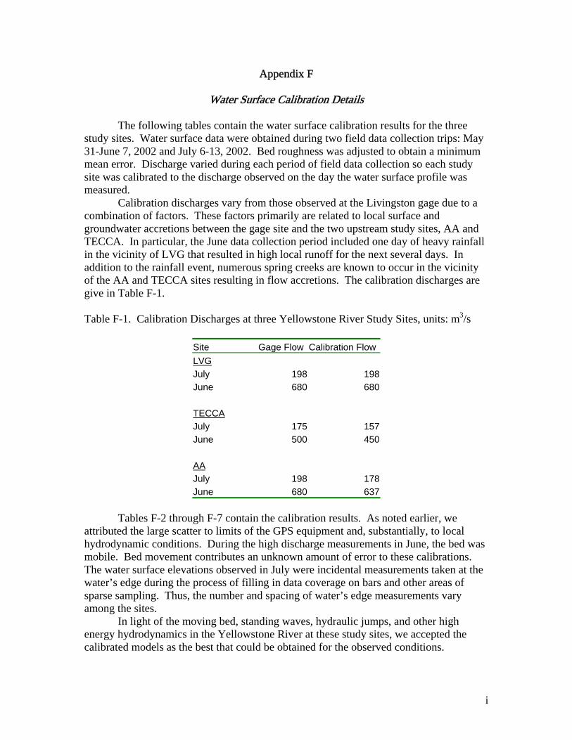
Water Surface Calibration Details The following tables contain the water surface calibration results for the three study sites. Water surface data were obtained during two field data collection trips: May 31-June 7, 2002 and July 6-13, 2002. Bed roughness was adjusted to obtain a minimum mean error. Discharge varied during each period of field data collection so each study site was calibrated to the discharge observed on the day the water surface profile was measured.

Calibration discharges vary from those observed at the Livingston gage due to a combination of factors. These factors primarily are related to local surface and groundwater accretions between the gage site and the two upstream study sites, AA and TECCA. In particular, the June data collection period included one day of heavy rainfall in the vicinity of LVG that resulted in high local runoff for the next several days. In addition to the rainfall event, numerous spring creeks are known to occur in the vicinity of the AA and TECCA sites resulting in flow accretions. The calibration discharges are give in Table F-1. Table F-1. Calibration Discharges at three Yellowstone River Study Sites, units: m3/s

Site Gage Flow Calibration FlowLVG July 198 198June 680 680 TECCA July 175 157June 500 450 AA July 198 178June 680 637

Tables F-2 through F-7 contain the calibration results. As noted earlier, we

attributed the large scatter to limits of the GPS equipment and, substantially, to local hydrodynamic conditions. During the high discharge measurements in June, the bed was mobile. Bed movement contributes an unknown amount of error to these calibrations. The water surface elevations observed in July were incidental measurements taken at the water’s edge during the process of filling in data coverage on bars and other areas of sparse sampling. Thus, the number and spacing of water’s edge measurements vary among the sites.

In light of the moving bed, standing waves, hydraulic jumps, and other high energy hydrodynamics in the Yellowstone River at these study sites, we accepted the calibrated models as the best that could be obtained for the observed conditions.

i

Table F-2. Livingston (LVG) Study Site Water Surface Elevation Calibration June 2002 Nr. X Y Longitudinal Distance Observed WSL Simulated WSL Residual

1 519096.6 158766.2 82 1360.245 1360.162 -0.08262 519013.6 158546.6 440 1360.442 1360.414 -0.02843 519021.6 158222.8 630 1361.232 1361.044 -0.18854 519030.6 157889.1 990 1361.84 1361.937 0.0975 519048 157484.8 1380 1363.146 1363.208 0.06186 518860.3 157108 1825 1364.738 1364.706 -0.03227 518374.6 156812.2 2410 1366.394 1366.394 08 518107.6 156539.8 2760 1367.658 1367.693 0.03499 517621 156398.7 3295 1368.962 1368.921 -0.0408

10 517579.6 155956.5 3755 1370.102 1370.195 0.09311 517362.5 155724.5 4135 1371.091 1371.323 0.232212 517435.1 155242.2 4620 1372.938 1373.054 0.116213 517205.6 154587.1 5340 1375.101 1375.3 0.19914 516879.4 154435.1 5700 1376.366 1376.197 -0.16915 516746.8 154272.4 5855 1376.996 1376.97 -0.026

mean error 0.017773 Table F-3. Livingston (LVG) Study Site Water Surface Elevation Calibration July 2002 Nr. X Y Longitudinal Distance Observed WSL Simulated WSL Residual

1 519107.9 158716.6 165 1358.512 1358.883 0.3707122 519066.7 158470.1 400 1359.617 1359.8 0.1832073 519129.5 158327.1 540 1359.815 1359.914 0.0985874 519122.8 158074 780 1360.441 1360.154 -0.287375 519080.9 157339.5 1505 1362.517 1362.349 -0.168666 519070.7 157298.1 1560 1362.715 1362.645 -0.070387 518996.6 157075.6 1760 1363.601 1363.846 0.2448718 517601.8 156422.8 3275 1367.813 1367.748 -0.065679 517573.4 156008 3720 1368.569 1368.635 0.066236

10 517585.5 155935.3 3755 1369.345 1369.592 0.24761511 517532.2 155817.1 3850 1369.971 1370.176 0.20474612 517335 155696 4140 1370.285 1370.4 0.11551213 517415.2 155641.7 4215 1370.407 1370.765 0.357282

mean error 0.099745

ii

Table F-4. AA Ranch Study Site Water Surface Elevation Calibration June 2002 Nr. X Y Longitudinal Distance Observed WSL Simulated WSL Residual

1 515491.9 140662.4 100 1424.421 1424.385 -0.0362 515640 140475.4 305 1424.707 1424.664 -0.0433 515276.3 140294.4 680 1426.035 1426.258 0.2234 515490.9 139979.1 1035 1426.922 1427.014 0.0925 515061.2 139424.8 1830 1428.626 1428.742 0.1166 514606.9 138896.9 2580 1430.266 1430.301 0.0357 513887 138481.4 3420 1432.128 1432.086 -0.0428 513504.2 138113.6 3950 1432.965 1433.037 0.0729 513197 137929.4 4295 1434.214 1434.297 0.083

10 512822 138022.6 4635 1435.177 1435.067 -0.110 mean error 0.039 Table F-5. AA Ranch Study Site Water Surface Elevation Calibration July 2002 Nr. X Y Longitudinal Distance Observed WSL Simulated WSL Residual

1 515408.1 140359 565 1424.356 1424.26 -0.0962 515392.3 140352.7 580 1424.42 1424.401 -0.0203 515380.4 140346.7 595 1424.498 1424.544 0.0464 515406 139989.8 1035 1426.207 1426.179 -0.0285 515396.4 139881.9 1050 1426.593 1426.575 -0.0187 514653 138956.8 2530 1429.895 1429.898 0.0038 514642.4 138946.1 2550 1429.964 1429.904 -0.0619 514637.6 138941.5 2555 1430.005 1429.93 -0.075

10 513625.9 138221.1 3800 1431.567 1431.739 0.17212 513511.3 138124.8 3945 1432.188 1432.3 0.11213 513497.1 138111.4 3965 1432.428 1432.318 -0.11015 513423.6 138047.5 4063 1432.739 1432.786 0.04716 513423.7 138047.1 4065 1432.739 1432.811 0.07218 513276.9 137965.8 4233 1433.364 1433.388 0.02419 513201.5 137938.9 4313 1433.563 1433.628 0.06521 513160.5 137924.2 4358 1433.636 1433.736 0.10024 513093.8 137920 4225 1433.753 1433.743 -0.010

mean error 0.013

iii

Table F-6. TECCA Study Site Water Surface Elevation Calibration June 2002 Nr. X Y Longitudinal Distance Observed WSL Simulated WSL Residual

1 515229.9 145938.5 74 1402.538 1402.52 -0.01792 515240.1 145532.7 526 1403.844 1403.713 -0.13083 515631.5 145403.7 937 1405.299 1405.367 0.06824 515648.9 145019.1 1293 1406.045 1405.837 -0.20835 515460.9 144914.4 1575.5 1406.828 1406.809 -0.01946 515553.2 144460.3 1922.5 1407.846 1407.93 0.08377 515803.6 144245.7 2290 1408.762 1408.701 -0.06148 515849 143917.1 2575 1409.918 1409.789 -0.12889 515585.2 143971.7 2845 1410.285 1410.165 -0.1205

10 515225.5 143686.1 3303 1411.79 1411.705 -0.085411 515752.8 143276.3 4014 1413.41 1413.541 0.131212 515877.6 142884.3 4286 1414.676 1414.709 0.032913 515684.3 142928.2 4475 1414.929 1414.916 -0.013114 515486.1 142645.2 4793 1415.991 1415.945 -0.045815 515565.7 142529.4 4929 1416.1 1416.047 -0.0527

mean error -0.03787 Table F-7. TECCA Study Site Water Surface Elevation Calibration July 2002 Nr. X Y Longitudinal Distance Observed WSL Simulated WSL Residual

1 515648 144591.7 2020 1406.782 1406.864 0.081962 515659.7 144556.6 2045 1407.017 1407.317 0.2992453 515684.9 142815.2 4485 1414.381 1414.256 -0.124914 515624 142750 4575 1414.786 1414.722 -0.063795 515612.8 142737.4 4590 1414.832 1414.7 -0.13162

mean error 0.012178

iv

Appendix G

Hydrodynamic Modeling and Habitat Mapping Details

Hydrodynamic Model Inputs

Data Requirements

Two-dimensional hydrodynamic models require channel bed topography, roughness and transverse eddy viscosity distributions, boundary conditions, and initial flow conditions to be supplied as input data. The field data consists of bed topography, discharge and initial downstream water surface elevation values. Bed topography is supplied as a series of three-dimensional or “x, y, z” values distributed over the study area and arranged to capture the major topographic features.

Bed roughness was estimated based on approximate average particle size and then adjusted as part of the calibration process. Default transverse shear values (eddy viscosity) were used for this study, as we did not need to capture sudden (shock) changes in discharge.

Discharge boundary conditions were obtained by developing a stage-discharge relation for the downstream boundary of each study site. The stage-discharge relations were derived from conditions observed during two field data collection efforts in June and July 2002. The computational boundary for each study site was determined from the topography data and established high enough in the flood plain to accommodate the highest flows to be simulated. Mesh Design

Two-dimensional finite element models operate on a set of computational node points arranged in an irregular mesh that must be supplied as input to the model. “Mesh or grid design is the black art of 2D modeling.” (Steffler and Blackburn, 2002). The number of computational nodes is limited by the computer speed and memory, and by time available. For one-to-three day calculation time-to-convergence for a single discharge on current generation personal computers, a computational mesh of approximately 100,000 nodes is feasible (Steffler and Blackburn, 2002).

There is a significant trade-off between accuracy of representation (dense node spacing), computer capacity, and time to arrive at a solution. Even the fastest currently available microcomputers may require several days to arrive at an accurate solution for a single discharge using a very large (therefore dense) computational mesh. The challenge is to distribute mesh nodes so the most accurate solution is obtained for a particular purpose. For habitat studies, a higher density of computational nodes is required in side channels and other areas of low hydraulic conveyance than might be used in other applications such as flood studies. Computational meshes used for the three study sites in this investigation ranged from about 25000 to 90000 nodes.

i

The River2D Model

Two-dimensional flow models typically describe flow dynamics in the two horizontal directions. There is no calculation of vertical differences in flow conditions, e.g. the flows described are depth-averaged. River2D, as other 2-D hydrodynamic models, incorporates three governing equations that are solved for three unknowns; depth and mass flux in the x and y directions. (See Appendix E for a complete development of these governing equations.) Basic Assumptions in River2D 1. The vertical pressure distribution is hydrostatic. Generally, this limits accuracy in

areas of steep slopes and rapid changes of bed slopes. In general, bed features of horizontal size less than about 10 depths (typically dune bedforms) will not be modeled accurately.

2. The distributions of horizontal velocities over the depth are essentially constant (depth-averaged). An assumed vertical velocity distribution may be used in the interpretation of the simulated depth-average velocity, but velocity is treated as a single constant value by the internal calculations. This means that information on secondary flows and circulations is not available.

3. Coriolis and wind forces are assumed negligible. For very large water bodies, particularly for large lakes and estuaries, these forces may be significant.

Basic Concepts

Conservation of Mass. Mass conservation is the principle that the inflow of fluid to any point in the model matches the outflow. This is represented by summing the mass flux in the x and y directions and setting the total mass flux equal to the change in depth over a small time increment. So, if inflow is greater than outflow over a small time increment, the depth increases; if inflow equals outflow, the depth is unchanged; and so on. This approach is used in hydrodynamic models to allow simulation of unsteady flow conditions based on varying inflow and outflow.

Conservation of x- and y-direction momentum. A major contribution of 2-D flow models is the ability to represent forces acting on the fluid. In River2D (and other 2-D hydrodynamic models) changes in momentum are represented as a sum of forces. These forces include shear stresses, gravitational force and friction forces. The great advantage of this representation for ecological modeling of rivers lies in improved representation of divided flow situations when compared to 1-D or transect-based models. Stated simply, the model includes the physical processes that result in the respective flow volumes that occur on each side of an island. Previous methods required numerous measurements and empirical fitting of flow-splitting relations.

Friction Forces. In River2D friction is represented as a surface or “skin” friction and are related to an effective roughness height. Effective roughness height is used because it tends to remain constant over a wider range than other roughness measures such as Manning’s n. It is similar to n in the sense that it is used as a major calibration parameter in River2D. Effective roughness height has the advantage that it is a linear

ii

distance (given in meters) that can be approximately related to dominant bed material size. Supercritical Flow and Edge Wetting Conditions occurring in the Yellowstone River near Livingston, MT led us to select the River2D model for this study for two reasons. The study sites are very steep and numerous local occurrences of supercritical flow can be observed. Thus, the model needed to have the capacity to accurately represent this phenomenon. (Supercritical flow is a condition where the water level is determined by conditions upstream of a point rather than the more common situation where downstream conditions determine the water surface elevation, known as subcritical flow.) The study sites also have numerous areas of side channels that are wet only at certain discharges. Therefore, the model needed to be able to accurately calculate the inundation and drying of those areas as different flows were simulated. As noted below wetting and drying of computational elements at the edge of the flowing channel is a difficult process for numerical models. River2D has a unique and robust method of handling this process that was suited to the Yellowstone River study sites. Supercritical Flow. River2D uses a conservative Petrov-Galerkin upwinding formulation to solve the flow field. Because of this feature, the model is able to represent situations where upstream flow conditions limit the water surface at a downstream point. This allows supercritical flow to be calculated over sills, steep bars and other conditions common to the areas of the Yellowstone River that are the focus of this study.

Wet/Dry Area Treatment. When performing a two-dimensional flow calculation, the depth of flow is a dependent variable and is not known in advance. The horizontal extent of the water coverage is therefore unknown. Significant computational difficulties are encountered when the depth is very shallow or there is no water at all over a part of the modeled area. Various methods have been proposed to deal with this “edge wetting” problem. For example, some models simply neglect or drop out partially wet edge elements, others declare edge elements to be porous. The River2D model handles these occurrences by coupling a very simplified ground water model with the surface water model. This approach changes the surface flow equations to groundwater flow equations in these areas. This allows a mesh element to have some nodes that are under water using the open-channel equation of mass conservation and some that are under the land surface a sub-surface representation for mass conservation. A continuous free surface with positive (above ground) and negative (below ground) depths is calculated. This approach allows calculations to carry on without changing or updating the boundary conditions as water levels fluctuate.

Hydrodynamic Simulation Steps

Typical applications of simulation models of natural phenomena require the basic

steps of field data acquisition, conversion of data into the form used by the model, calibration of the model to observed conditions, and simulation of conditions for which data were not collected due to considerations of fiscal efficiency or safety. Application

iii

of River2D to the Yellowstone River in the vicinity of Livingston, MT involved the following steps.

Develop Digital Terrain Model

Once x, y, z data from photogrammetry, ground surveys, and echosounding has been checked for quality and translated into metric units we combine all the terrain data into one file and import that file to the River2D digital terrain model R2D_Bed.

In R2D_Bed, the x, y, z data are arranged (triangulated) to produce a “triangulated irregular network” (TIN) and elevation contours are displayed. This process often yields interpolation irregularities in areas where the data is not of uniform density. These irregularities usually consist of TIN edges that do not conform to the known or apparent local topography. They occur because the TIN algorithm simply builds triangles based on the nearest neighbor without considering the topographic relevance of those neighbors. The R2D_Bed module is used to remove such irregularities by a combination of adding (by interpolation) and, in some cases, moving or copying x, y, z points. Elevation contours are generated in the R2D_Bed program and compared with the original aerial photographs for consistency of representation of the river system. This process produces a digital topographical map of the study site including the riverbed. Develop the Computational Mesh

As noted above, there is a trade-off between the density of nodes in the computational mesh, the required accuracy of representing the study site, and the time required to arrive at a solution for a single discharge. The following general criteria were used when creating computational meshes for the three study sites in this investigation.

To obtain the best fit to the main channel and significant habitat areas the mesh density may vary among locations and channel configurations. In general it is desirable to have a minimum of 8 to 10 nodes across channels carrying significant amounts of water to ensure the model can adequately convey flow downstream without calculating too much of the flow at any one node. Inflow and outflow boundaries usually need to be subdivided into 20 or more nodes to again ensure that no node carries too much of the computational burden. This also ensures that the mass balance for the entire site can converge properly.

In single-thread channels, a mesh with adequate density to satisfy these criteria can be constructed as a uniform fill of equally spaced nodes. The study sites in this application had numerous side cannels that were of major significance to the overall study objectives. Thus, it was necessary to use much smaller mesh elements (denser node spacing) in those areas than the main channel.

Additional nodes are required to describe channel features that vary from simple cross sections. For example, irregular channel edges, bars, bedrock sills and other features produce complex flow patterns and require higher node density to achieve adequate representation in the model. Such areas were identified by examination of the aerial photographs and searching the results of intermediate model runs for hydraulic anomalies. In general, habitat studies require higher mesh density in backwater areas

iv

than do other hydrodynamic model applications. Node density in those areas was adjusted to ensure such areas were adequately represented.

Finally, the finite element numerical solution method works best if the elements are of regular shape and the sizes of adjacent mesh elements change gradually, rather than abruptly. Thus, some additional nodes are needed to attain gradual size and shape changes. The mesh building program, R2D_Mesh, provides tools for creating an initial mesh for a study site that attempts to satisfy these criteria.

The mesh program also generates a starting data file for the River2D model that consists of the boundary conditions of inflow discharge (m3/sec), outflow elevation (m) and an initial estimate of the depth (m) for all nodes. Thus, the initial condition file is rather like a river full of water but with no initial velocity. The velocities are to be calculated by the model.

It is difficult to anticipate all possible flow complexities when building the initial computational mesh. Thus, the last step of mesh building is to refine the mesh within the River2D model itself by iteratively simulating a particular discharge, and altering the mesh as conditions indicate. The initial mesh is run (usually for the calibration discharge conditions) and the mesh is refined to dampen oscillations and produce more realistic results in areas where flow anomalies are found. Refinement usually consists of increasing node density in areas that do not perform according to reasonable hydraulic behavior. Considerable judgment is required at this stage. Calibrate the Flow Model

The River2D hydrodynamic model is designed for use in both a “dynamic” and a “steady state” mode. The solution algorithm proceeds as if all conditions are time varying – e.g. dynamic – so the solution appears to be carried out over an advancing time scale. If the inflow and outflow boundary conditions vary with time, one is performing a dynamic simulation and the objective of the analysis is related to the way flow conditions change over time. Additional data is required for this application.

Steady state simulations consist of using fixed boundary conditions that represent desired flow conditions. In this situation, the initial condition file created by the R2D_Mesh program contains the desired simulation discharge and initial boundary conditions. For each discharge to be simulated, the model is run to steady state convergence. That is, for a constant input discharge, the model runs until there is a constant output discharge and those discharges are nominally the same. Typical convergence tolerance is 1% of inflow.

For each study site in this application we calibrated the River2D model to the flow conditions observed during the June 2002 data collection effort. The model was run to steady state convergence and the bed roughness was adjusted until we achieved the best match between observed and simulated water surface profile for each site. Figures G1, G2 and G3 show the observed and simulated water surface profile and the residual calibration error.

v

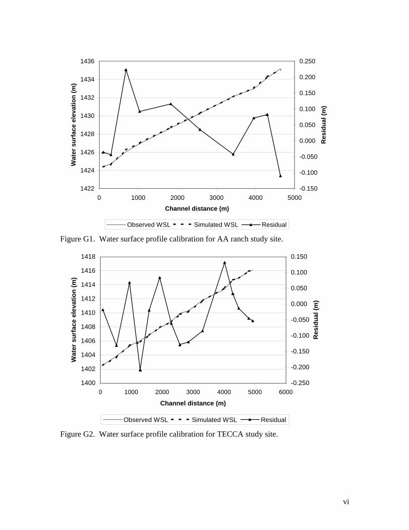
1422

1424

1426

1428

1430

1432

1434

1436

0 1000 2000 3000 4000 5000

Channel distance (m)

Wat

er s

urfa

ce e

leva

tion

(m)

-0.150

-0.100

-0.050

0.000

0.050

0.100

0.150

0.200

0.250

Res

idua

l (m

)

Observed WSL Simulated WSL Residual

Figure G1. Water surface profile calibration for AA ranch study site.

1400

1402

1404

1406

1408

1410

1412

1414

1416

1418

0 1000 2000 3000 4000 5000 6000

Channel distance (m)

Wat

er s

urfa

ce e

leva

tion

(m)

-0.250

-0.200

-0.150

-0.100

-0.050

0.000

0.050

0.100

0.150

Res

idua

l (m

)

Observed WSL Simulated WSL Residual

Figure G2. Water surface profile calibration for TECCA study site.

vi

1358

1360

1362

1364

1366

1368

1370

1372

1374

1376

1378

0 1000 2000 3000 4000 5000 6000 7000

Channel distance (m)

Wat

er s

urfa

ce e

leva

tion

(m)

-0.250

-0.200

-0.150

-0.100

-0.050

0.000

0.050

0.100

0.150

0.200

0.250

0.300

Res

idua

l (m

)

Observed WSL Simulated WSL Residual

Figure G3. Water surface profile calibration for LVG study site. In Figures G1-G3 the residual represents the difference between measured and

observed water surface elevation at the measured location. When calibrating a flow simulation model to water surface elevation, the goal is to attempt to obtain a residual of zero at all measured locations. These figures show that at all three sites the residuals exhibit a wide scatter. The range of residual scatter can be explained by three phenomena.

First, our survey-grade global positioning system unit is capable of a ±2 cm (0.8 inch) vertical resolution under ideal conditions. Our experience suggests that we obtain ± 3 cm vertical accuracy when used for ground surveying under the conditions typically encountered in river surveys. That is, at least 3 cm and up to 6 cm of each residual is due to the available precision of the instrument.

Second, the flow conditions we measured were highly variable. The calibration discharge measurements were obtained at or near bankfull discharge for all three sites. During the observed flow event, we encountered standing waves with amplitude on the order of 1 m (3 ft) and frequent waves near the bank with amplitude of 30 cm (1 ft). We were able to locate some water surface measurements in areas that were protected from these effects, but to provide approximately equal longitudinal coverage it was necessary to measure the water surface at several areas subject to strong wave action and local water surface elevation or depression caused by nearby standing waves.

Third, at each study site we did find protected areas that were not subject to strong wave action. We located staff gages in some of these areas to check for unsteady flow conditions during the period of measurement for each site. In general, the protected areas showed the smallest residuals. For example, the second, ninth and fifteenth points at the

vii

Livingston site have residuals less than 4 cm. Staff gages were located at points 9 and 15 and point 2 was located in a quiet area protected from wave action by a mid-channel bar.

When each site had been calibrated to produce the best fit of simulated to observed water surface profile for the calibration discharge, the roughness values thus obtained were used to simulate the discharges observed during the July field data collection effort. Comparison of observed and simulated water surface profiles for July showed similar agreement as the June values. See Appendix E for calibration details. Simulate Unmeasured Flows

To satisfy the model boundary conditions, we developed a stage-Q relation using water surface data obtained for the June and July field measurements at the downstream end of each site. A log-log relation was fit to each set of measurements and used to determine the downstream water surface elevation for each simulated discharge.

During the process of simulating flow at the three study sites, the water surface changes for each discharge. These changes can result in computational difficulties as certain areas of the channel become shallow. As such problems were encountered, nodes were added to the computational mesh to improve the discretization in shallow areas as needed to ensure hydraulically reasonable results.

To encompass the range of habitat conditions of interest in this study we simulated the discharges (values for the Yellowstone River near Livingston gage) given in Table G-1.

Table G-1. Categories of Discharge simulated for Yellowstone River Habitat Study

Flow Category Simulated Discharge 2000 low flow 15.5 m3/s (550 ft3/s) typical base flow 42.47 m3/s (1500 ft3/s) recession flow 141.6 m3/s (5000 ft3/s) bank full = 2001 peak flow 680 m3/s (24000 ft3/s) 1997 flood flow 1019 m3/s (36000 ft3/s)

As a final step, velocity and depth values were extracted from simulation results, converted from metric to State Plane Feet units to match the aerial photogrammetry and reformatted for input to ArcInfo where habitat calculations were performed.

GIS Habitat Mapping

Products from GIS habitat mapping included a variety of statistics describing

compositional and distribution characteristics of trout habitats in each study site at different discharges. Compositional characteristics included total class area for different types of trout habitat, mean patch size of each type, and patch density (number of individual patches per mile of stream). The spatial distribution of class types was analyzed by determining the association of different habitat classes with the bank types defined by Zale and Rider (2003) as fish-sampling stratifications. In order to derive these habitat-related statistics, a variety of coverage types were constructed. They are roughly divisible into five map types or layers, as illustrated in Figure G4.

viii

Figure G4. Flow chart of intermediate map layers created to derive analysis products for the upper Yellowstone River fish habitat study. Bare-ground Depth and Velocity Grids

The first type of map layer we developed consisted of individual grids for depth and velocity, respectively, for each site and simulated discharge. Input for this layer originated as output from the hydraulic simulation model, specifically in the form of spatial (x, y) coordinates and the attributes of depth and velocity. These data were imported into ArcInfo to generate a point coverage of the same values. Two Triangulated Irregular Networks, or TINs, were developed from each point coverage - one for depth and one for velocity. The purpose of the TIN is to allow interpolation of depths or velocities between data points (for example, to draw contour lines). Each TIN was converted to a floating-point (real number) grid of 1.5 m x 1.5 m cells by linear interpolation.

Large Woody Debris (LWD) Zone-of-influence Map Layer

Accumulations of woody debris, dense brush, and thickets of willow can affect hydraulics in two notable ways. First, these features tend to increase the overall resistance to flow, resulting in an elevation of the water surface. The second effect is a localized retardation of current velocity in the vicinity of the object. Large-scale effects, such as increased water surface elevations, can easily be incorporated into the hydraulic simulation model. In contrast, localized adjustments to velocity cannot be handled as cleanly, owing to limitations on the mesh density needed to describe individual woody features. Rather than attempt to incorporate these effects in the hydraulic model, we used a GIS map layer to simulate the same phenomenon.

We defined large woody debris (LWD) as downed logs, branches, and associated root wads larger than 30 cm in diameter. Large stems, having a diameter greater than 45 cm, were delineated from small stems. Individual stems and root wads were digitized from 1:6000 or 1:8000 digital aerial photos for each site. Root wads were marked with one or more points, whereas stems were digitized by hand as lines. We used the extent of

ix

the simulated 1997 flood (~680 m3/s) from the bare-ground model to limit our accounting of LWD to areas likely to be inundated at the highest simulated discharges. Points were added at 60-cm intervals along the lines for the stems, and buffered to create a polygon representing the zone of influence for an individual log, branch, or root wad. Large stems and root wads were buffered 3 m, and small stems, 1.5 m from each of the points, resulting in a polygon representing the zone of influence around each stem or debris pile. Similarly, the perimeters willow thickets and areas of dense brush were digitized and zones of influenced were established by buffering the willow/brush polygons 3 m. A point coverage of velocity adjustment factors (VAFs) was created by adding nodes to all of the polygons and combining with the points associated with stems and root wads (Figure G5). At the surface of a hard object, such as a log, it was assumed that the velocity was zero, and at the edge of the zone of influence, the velocity was the same as the bare-ground model. Consequently, points along stems and root wads were assigned a velocity adjustment factor of 0.0, whereas points representing the buffered zones of influence were assigned a value of 1.0. Interiors of willow thickets and brush were assigned a VAF of 0.25. VAF points within the zones of influence were then interpolated in a TIN and converted to a grid of the same size as the bare-ground velocity grid from the previous step (Figure G6). The VAF and bare-ground velocity grids were then multiplied to create a modified velocity grid incorporating the localized effects of LWD.

Figure G5. Point coverage of LWD Figure G6. Velocity adjustment factor grid polygons used to adjust velocities from resulting from interpolation of point VAFs the bare-ground hydraulic simulation in Figure G5. model.

x

Composite Habitat Classification Maps Each of the floating-point grids prepared in the previous two steps were reclassified according to the categories illustrated in Table G-2, and combined to create a grid of composite habitat classes (Figure 8). For example, a grid cell having a depth of 36 cm and a velocity of 12 cm/s would be classified as “2” for depth and “1” for velocity. The two individual class codes were then combined, with the depth code in the 10’s place and the velocity code in the 1’s place, to produce a composite class code of 21. Table G-2. Depth and velocity reclassification tables used to create composite habitat classes for the upper Yellowstone River.

Depth interval (cm)

Depth class Velocity interval (cm/s)

Velocity class

0 - 30 1 0 - 15 1 30 - 90 2 15 - 45 2 90 - 180 3 45 - 60 3

>180 4 > 60 4

The reclassified, combined habitat maps representing both the bare-ground velocity model and the LWD-moderated model were converted to polygons, and the attributes of area, perimeter, and class type exported to a spreadsheet. The total area of SSCV habitat was found by summing class areas 11, 12, 21, and 22 for the bare-ground and LWD-moderated models, respectively. The difference in SSCV area between the two models was the amount attributable to LWD.

Bank-Type Classification Maps Bank-type classification maps were digitized by hand from 1:6000 and 1:8000 aerial photographs, generally following the protocols set forth by Zale and Rider (2003). Our classification differed slightly from theirs in two aspects. First, Zale and Rider classified lengths of shoreline as bank-types. We applied the same bank-type definition to areas extending from the 2002 high-water line to the centerline of the main channel (Figure 11). This procedure allowed us to use the same bank classification consistently without having to re-digitize for other flows or re-define the center of the channel as a bank type. Second, we added three types of habitat that were not included in the original (main channel) classification system: point bars, side channels, and overbank areas. Point bars were defined as areas between inside bends and vegetated shorelines that were exposed during the 2002 runoff, but inundated at higher flows. Side channels were defined as secondary waterways that had surface-water connections to the main channel at one or more discharges (either flowing or backwater). Overbank areas were all other locations having surface water connections with the main channel at one or more discharges. Typically, floodplains and vegetated islands were included in the overbank category. Some low areas on floodplains were flooded by groundwater and were removed from further analysis if a surface connection with the river was not apparent.

xi

Distribution of Habitat Classes by Bank Type

The distribution of habitat classes by bank type was determined by overlaying the habitat class polygons for a particular discharge and the bank-type polygons described above. This process resulted in a mosaic of polygons having unique combinations of habitat class and bank type. The attributes of area, perimeter, class, and bank type were exported from the aggregated coverage into a spreadsheet, where the areas of SSCV (and other habitat types) were summed for each category of bank type. Stream Power Although not central to our investigation of salmonid habitat, we developed a series of maps showing unit stream power at bankfull discharge (Appendix C). These maps may provide useful information for the analysis of geomorphology and channel migration phenomenon, as well as insights into the large-scale hydraulic effects of channel modifications.

Stream power is a measure of the amount of energy expended per unit time at the channel bed in overcoming friction and transporting sediment. Unit stream power(w), is expressed as watts per square meter of bed, by

w = rgDvS where r is the water density, g is the force of gravity, D and v are the water depth and mean column velocity, respectively, at a point, and S is the slope of the energy grade line. Water density and the force of gravity are (essentially) constants, and depths and velocities for a discharge are contained in the base point coverage from which the habitat classification maps were constructed. These terms were multiplied together in the original point coverage and converted to a 30 cm x 30 cm grid (henceforth, the CDV grid). We used the SLOPE algorithm in ArcInfo to create a 15 m x 15m grid of localized slopes, as a surrogate for energy slope, (henceforth, the Slope grid) based on the simulated water surface elevations generated at each of the sites for bankfull discharge. Stream power was calculated by multiplying the CDV grid by the Slope grid, to create a grid of calculated stream power at each node in the original depth and velocity base coverage. The power grid was then converted back into points and triangulated.

xii