EFFECT OF BETA RADIATION DOSE DISTRIBUTION ON THE EXPRESSION OF

EPIDERMAL NECROSIS AND RADIATION-INDUCED VASCULATURE

CHANGES

BY

OLGA V. PEN

A Dissertation Submitted to the Graduate Faculty of

WAKE FOREST UNIVERSITY GRADUATE SCHOOL OF ARTS AND SCIENCES

in Partial Fulfillment of the Requirements

for the Degree of

DOCTOR OF PHILOSOPHY

Biomedical engineering

May 2019

Winston-Salem, North Carolina

Approved By:

J. Daniel Bourland, PhD, Advisor

William A. Dezarn, PhD

Michael T. Munley, PhD

Surendra Prajapati, PhD

Mac B. Robinson, PhD

Jeffrey S. Willey, PhD

ACKNOWLEDGEMENTS

The author expresses deep gratitude to my advisor, Dr. J. Daniel Bourland, for his

guidance and unwavering support throughout my graduate studies, in both research and

professional development. I would also like to extend my gratitude to the members of the

PhD defense committee: Dr. Michael Munley, Dr. William Dezarn, Dr. Jeffrey Willey,

Dr. Surendra Prajapati and Dr. Mac Robinson, for agreeing to serve on my committee

and providing their time and expertise, as well as their help in the course in this study. I

also would like to acknowledge Dr. Nancy Kock for the special contribution to this study.

Special thanks go to all past and present medical physicists, radiation oncologists and all

of the staff in the Department of Radiation Oncology for their clinical expertise and

guidance throughout these years, as well as the members of the School of Biomedical

Engineering and Sciences for the provided training and support, in academic field as well

as overall graduate school experience. I would also like to thank all of the current and

former Wake Forest and Virginia Tech graduate students, including Dr. Jennifer Dorand,

Dr. Inna McGowin, Dr. Hao Gong, Dr. Catherine Okoukoni, Dr. Callistus Nguyen, Xu

Dong, Tong Ren, Briana Thompson, Alexander Borg, Manal Ahmidouch, and many

other of my peers who were immense help and support during these years.

I would especially like to thank Dr. Vladimir Pen and Dr. Svetlana Levchenko for their

unwavering love and support, scientific advice and life guidance throughout this journey.

I would also like to acknowledge my funding agency. This project has been funded in

whole or in part with Federal funds from the Biomedical Advanced Research and

Development Authority, ASPR, DHHS, under Contract Nos. HHSO100201200007C and

HHS010020130DD18

Table of contents

ACKNOLEDGEMENTS ................................................................................................................. ii

LIST OF FIGURES AND TABLES ............................................................................................... iii

LIST OF ABBREVIATIONS ......................................................................................................... ix

ABSTRACT .................................................................................................................................... xi

STUDY SUMMARY....................................................................................................................... 1

INTRODUCTION ........................................................................................................................... 3

RADIATION DERMATITIS AND CUTANEOUS RADIATON INJURY .............................. 4

MICRODOSIMETRY AT THE EPIDERMAL LAYER DEPTH ............................................ 15

EXPERIMENTAL SET-UP ...................................................................................................... 27

SPECIFIC AIMS ....................................................................................................................... 38

CHAPTER 1: Quantitative analysis of the epidermal necrosis in cutaneous radiation injuries and

radiation dermatitis ........................................................................................................................ 39

MATERIALS AND METHODS ............................................................................................... 39

Necrotic cell detection ........................................................................................................... 39

NDPI processing .................................................................................................................... 47

Feature separation .................................................................................................................. 50

Particle analysis ..................................................................................................................... 53

Statistical analysis .................................................................................................................. 56

RESULTS .................................................................................................................................. 58

DISCUSSION ............................................................................................................................ 67

CHAPTER 2: Monte Carlo simulation of the beta source irradiation device ................................ 69

MATERIALS AND METHODS ............................................................................................... 69

Monte Carlo simulation basics ............................................................................................... 69

MCNP6 functionality ............................................................................................................. 76

MCNP6 simulation run output ............................................................................................... 95

RESULTS ................................................................................................................................ 103

DISCUSSION .......................................................................................................................... 119

CHAPTER 3: Monte Carlo modeling of the skin features .......................................................... 122

MATERIALS AND METHODS ............................................................................................. 122

Correlation between the epidermal necrosis expression and blood vasculature changes in

skin ....................................................................................................................................... 122

Monte Carlo modeling of the skin features .......................................................................... 124

RESULTS ................................................................................................................................ 132

DISCUSSION .......................................................................................................................... 138

CONCLUSION AND FUTURE DIRECTION ........................................................................... 140

LIST OF REFERENCES ............................................................................................................. 143

Appendix 1 ................................................................................................................................... 153

Appendix 2 ................................................................................................................................... 166

CURRICULUM VITAE ............................................................................................................. 176

LIST OF FIGURES AND TABLES

LIST OF FIGURES Page

Figure 1 – Skin structure depicting different layers of dermis and epidermis,

including the basal layer

6

Figure 2 – Representation of the radiation-induced skin injuries of the varying

degree of severity graded in accordance with the RTOG scoring system

12

Figure 3 – Sr-90 decay scheme 16

Figure 4 – Sr-90 and Y-90 activity equilibrium as denoted over time for the

100mCi source

18

Figure 5 – Nuclear drip line. Sr-90 and Y-90. Both Sr-90 and Y-90 fall within

the blue region of β- decay

19

Figure 6 – Collisional vs radiative stopping power for varying energies in

water and lead media

22

Figure 7 – β-particle interactions 25

Figure 8 – Percent depth dose curves for various energies of megavoltage

electron

26

Figure 9 – Diagram of Sr-90 source encapsulation 28

Figure 10 – Sr-90 sources configuration 29

Figure 11 – Schematic view of the source 31

Figure 12 – The beta radiation device 32

Figure 13 – Diagram of the β-particle path in the beta radiation device 33

Figure 14 – Beta radiation device attached to: a) three-legged stand; b) wall-

mount arm.

34

Figure 15 – Pig with tattooed areas of irradiation and application of the device

to the pig skin

34

Figure 16 – Cell undergoing apoptosis via pyknosis 40

Figure 17 – Histological sample with heavy epidermal necrosis expression 41

Figure 18 – Wound map for histology 43

Figure 19 – Histological samples with different degrees of epidermal necrosis 45

Figure 20 – Magnified view of the dead cells 46

Figure 21 – Program flow of automated analysis of the epidermal necrosis

expression

47

Figure 22 – Mosaic representation of digitalized histological slide 49

Figure 23 – Epidermal layer selection 51

Figure 24 – Epidermal layer selection 52

Figure 25 – Region of interest selection 53

Figure 26 – Pixel-march algorithm depicting a particle analysis 55

Figure 27 – CRI analysis 59

Figure 28 – Distribution of the samples within a group based on the number of

the pyknotic nuclei detected

62

Figure 29 – Distribution of the samples within a group based on the number of

the percentage of the area of the lesion in comparison to the overall area of the

epidermis

63

Figure 30 – Monte Carlo simulation run 72

Figure 31 – Example MCNP 6 history 74

Figure 32 – MCNP6 simulation range in terms pf particle types and energies 75

Figure 33 – Cell representation in MCNP6 77

Figure 34 – Representation of the beta radiation device in MCNP6 package 80

Figure 35 – Source modeling. Upper: diagram of the source encapsulation in

the beta radiation device; lower: MCNP6 model of the source

83

Figure 36 – Source inhomogeneity measured for Sr-90 sources utilized in the

beta radiation device

86

Figure 37 – Strontium-90 and Yttrium-90 spectra for beta decay 87

Figure 38 – PDD curve obtained from MCNP simulation run with 125 µm

resolution

106

Figure 39 – PDD overlay comparison 107

Figure 40 – Detector array across the radiation field 109

Figure 41 – Absorbed dose profile comparison at 0 and 90 degrees angle

detector array positioning

110

Figure 42 – 1 mm resolution dose distribution curve 111

Figure 43 – Pie chart geometrical configuration 112

Figure 44 – Pie chart dose comparison 113

Figure 45 – Standard and combined dose source configuration 114

Figure 46 – Standard and combined dose absorption curve 115

Figure 47 – 3D dose profile of the irradiated area 116

Figure 48 – Dose distribution measure with radiochromic film 117

Figure 49 – Skin curvature variation 125

Figure 50 – Blood vessel thickening 127

Figure 51 – Blood vessel histological cross-section: A) normal; B) thickened 128

Figure 52 – Blood vessel modeling: left: blood vessel cross-section; right:

blood vessel passing through the length of the irradiated area

130

Figure 53 – Curved skin model and blood vessels positioning 131

Figure 54 – Dose distribution for various configurations of skin curvature 132

Figure 55 – NCC vs dose profile comparison 133

Figure 56 – Dose rate to the blood vessels across the length of the irradiated

area, Gy/min

136

LIST OF TABLES Page

Table I: Radiation-induced lesions of the skin with respect to dose and time of

onset

8

Table II – Number and spread of the necrotic cells in samples vs the assigned

RTOG grade

60

Table III – P-values for the comparison between the mean number of dead

cells

61

Table IV – P-values for the comparison between the mean lesion spread

proportional percentage of the overall area of the sample

61

Table V – Probabilities of the features of the samples belonging to a class to

take a certain range of values

64

Table VI – MCNP input mnemonics 78

Table VII – MCNP macrobodies 79

Table VIII – Elemental weight concentration 82

Table IX – Source variables defined by the user 84

Table X – Beta particle energy spectrum 88

Table XI – Type of tallies available in MCNP6 90

Table XII – First 50 particles simulated at the source: 96

Table XIII – Photon interactions 97

Table XIV – Electron interactions: 97

Table XV – Photon activity in each cell 98

Table XVI – Electron activity in each cell 99

Table XVII – Tally fluctuation charts for cell 12 – F6, F4 photons, F4

electrons

102

Table XVIII – Dose rate comparison – surface 103

Table XIX – Surface dose measurement statistical error 104

Table XX – Statistical error margin at different depths for 2 mm3

measurement volumes

119

Table XXI – Elemental weight concentrations of the tissues present in skin

model

129

Table XXII – Dose rate at the blood vessels throughout the skin, Gy/min 134

Table XXIII – Doses delivered to the blood vessels located throughout the

skin, 16 Gy dose

134

Table XXIV – Doses delivered to the blood vessels located throughout the

skin, 32 Gy dose

135

Table XXV – Doses delivered to the blood vessels located throughout the

skin, 37 Gy dose

135

Table XXVI – Doses delivered to the blood vessels located throughout the

skin, 37 Gy dose

136

LIST OF ABBREVIATIONS

2D Two dimensional

3D Three dimensional

β Beta

BARDA Biomedical Advanced Research and

Development Authority

C Coulomb

cGy Centigray

cm Centimeter

CRI Cutaneous Radiation Injury

CSDA Continuous slowing down approximation

CTCAE Common toxicity criteria-adverse event

d Depth

𝐸𝛽 Beta particle energy

ft Foot

g Gram

γ Gamma

Gy Gray

H&E Hematoxylin and eosin

kg Kilogram

m Meter

mBq Megabecquerel

mCi Millicurie

MCNP Monte Carlo N-Particle

min Minute

MeV Megaelectronvolt

mm Millimeter

µm Micrometer

NCC Necrotic cell count

NDPI Nanoscale Digital Processing Image

PDD Percent Depth Dose

PMMA Poly(methyl methacrylate)

RD Radiation dermatitis

RTOG Radiation therapy oncology group

s Second

Sr-90 Strontium-90

t1/2 Half-life

Y-90 Yttrium-90

yr Year

Zr-90 Zirconium-90

ABSTRACT

Pen, Olga V.

EFFECT OF BETA RADIATION DOSE DISTRIBUTION ON THE EXPRESSION OF

EPIDERMAL NECROSIS AND RADIATION-INDUCED VASCULATURE

CHANGES

Dissertation under the direction of

J. Daniel Bourland, Ph.D., Professor of Radiation Oncology, Biomedical Engineering,

and Physics

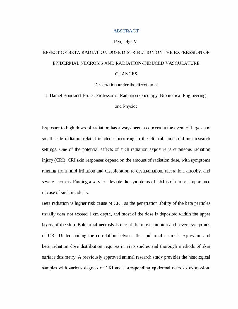
Exposure to high doses of radiation has always been a concern in the event of large- and

small-scale radiation-related incidents occurring in the clinical, industrial and research

settings. One of the potential effects of such radiation exposure is cutaneous radiation

injury (CRI). CRI skin responses depend on the amount of radiation dose, with symptoms

ranging from mild irritation and discoloration to desquamation, ulceration, atrophy, and

severe necrosis. Finding a way to alleviate the symptoms of CRI is of utmost importance

in case of such incidents.

Beta radiation is higher risk cause of CRI, as the penetration ability of the beta particles

usually does not exceed 1 cm depth, and most of the dose is deposited within the upper

layers of the skin. Epidermal necrosis is one of the most common and severe symptoms

of CRI. Understanding the correlation between the epidermal necrosis expression and

beta radiation dose distribution requires in vivo studies and thorough methods of skin

surface dosimetry. A previously approved animal research study provides the histological

samples with various degrees of CRI and corresponding epidermal necrosis expression.

Digitized slides of the histological samples are quantitatively analyzed through automated

processing for the severity of CRI, with comparison to histopathologist scores. Monte-

Carlo modeling is then used to calculate the dose distribution in the upper layers of the

skin, modeling the beta radiation device design and Strontium-90 physical parameters.

The model of dose delivery is then applied to certain morphological features of the skin.

The resulting correlation of the skin dose distribution with epidermal cell death

expression and vasculature changes in the upper skin layers is presented at the end of the

study.

1

STUDY SUMMARY

Background, hypothesis and significance of the proposed research

Exposure to high doses of radiation is a concern in the event of large– and small-scale

radiation-related incidents that may occur in the clinical, industrial and research settings.

One of the potential effects of such radiation exposure is cutaneous radiation injury

(CRI). CRI skin responses depend on the amount of radiation dose, with symptoms

ranging from mild irritation and discoloration to desquamation, ulceration, atrophy and

severe necrosis. Finding a way to alleviate the symptoms of CRI is of utmost importance

in case of such incidents.

Beta radiation is higher risk cause of CRI, as the penetration ability of the beta particles

usually doesn’t exceed 1 cm depth, and most of the dose is deposited within the upper

layers of the skin. Epidermal cell death is one of the most common and severe symptoms

of the CRI. Understanding the correlation between the epidermal necrosis expression and

dose delivery from the beta irradiation is important for development of techniques to

alleviate the symptoms, however, in vivo studies and complex and thorough methods of

skin surface dosimetry are required for the most accurate representation of the CRI

progression and potential effects of beta radiation on skin. Porcine models are

acknowledged as an accurate representation of human skin. Irradiating pig skin with the

radiation from a beta-particle source with a well-established dose distribution allows us to

harvest the histological samples with various degrees of the epidermal necrosis

expression. Monte-Carlo modeling is then used to reconstruct the precise dose

2

distribution in the upper layers of the skin based on the beta source device design and

physical parameters combined with skin layer modeling. The goal of the study is to

assess the influence of the dose variation at the skin surface layers on the epidermal

necrosis expression – a type of microdosimetry study. The underlying hypothesis is

that a certain correlation exists between the dose variation due to morphological

features in skin and with correlation of the severity of epidermal necrosis

expression. Three aims are pursued in the study:

1) Development of an automatic histological assessment tool for the epidermal necrosis

expression evaluation – completed in part

2) Development of the precise Monte-Carlo model of the beta irradiation device and skin

layers for the purposes of dose distribution profiling

3) Establishment of the possible correlation between the dose distribution and epidermal

necrosis expression and radiation-induced vasculature changes is dermal layer

The proposed study is innovative, as to the author’s best knowledge there have been no

attempts to establish the dose distribution from beta irradiation in the upper layers of

skin. The study is impactful due to contributions to the overall understanding of the

effects of beta-radiation on CRI, as well as providing the first Monte Carlo simulation

reference for the dose distribution from the custom beta radiation device. The study is

translatable to other types of radiation injuries, including a milder form of CRI, called

Radiation Dermatitis (RD), which commonly occurs for radiation treatment patients, and

the developed automatic necrosis assessment algorithm may have applications in

histological clinical practice.

3

INTRODUCTION

Exposure of skin to high doses of ionizing radiation has always been a great concern in

the event of radiation-related incidents, such as the Fukushima Daiichi nuclear accident

of 2011 or the earlier Chernobyl accident of 1986, as well as smaller-scale exposure

accidents that could occur at industrial, research and clinical facilities across the world. A

potential result of the radiation exposure in these cases is cutaneous radiation injury

(CRI). Beta radiation is of particular concern for CRI manifestation, with symptoms

ranging from mild irritation, discoloration and hair loss up to severe atrophy and

ulceration that can have long-lasting consequences and keep reoccurring months and

years after the initial exposure [1]. Understanding the mechanisms of radiation injury

occurrence is of importance in order to alleviate CRI symptoms and promote skin

healing, and this complicated process benefits from in vivo studies of the CRI

progression.

In similar fashion, one important side effect of radiation treatment, observed in cancer

patients, is radiation-induced skin injury, manifesting in a condition called radiation

dermatitis (RD) [1]. While CRI occurs from single acute dose delivery and RD – from

fractionated doses, both CRI and RD share the same clinical progression and are regarded

as interchangeable in their respective treatment approach. The methods of the radiation

skin injury diagnosis, evaluation, prevention and treatment being investigated in the

following work can be applied to both.

Skin irradiation is difficult to characterize both in the measurement of the skin dose

delivered [2] and the evaluation of the skin injury severity and underlying biological

mechanisms [3]. The following research project is aimed to clarify the matter of radiation

4

skin injury, quantifying biological expression and providing correlation with the skin

dose distribution at the relevant depths. The research performed in this particular project

is a continuation of a previous CRI studies at this institution. The aforementioned study

was performed on the porcine animal model with the utilization of Strontium-90 β-

sources enclosed in a specifically developed beta radiation device. Porcine models are

acknowledged as an accurate representation of human skin [2]. Expanding on the

previous studies, we have been able to analyze digitized histological data from one

particular animal study and continued the project towards the research aims described in

this study.

RADIATION DERMATITIS AND CUTANEOUS RADIATON INJURY

In order to understand how RD and CRI occur and progress, it is important to understand

in general how the dose deposited at the skin level might affect its biological function,

lead to physiological and morphological changes, and what separates healthy skin from

affected skin. As all mammalian skin follows the same morphological pattern, general

human physiology will be explained in the following chapter and then extrapolated on the

porcine model for the animal studies.

Skin is the outer covering of the body and the largest organ in the human organism. Skin

by itself fulfills three biological functions: protection of the underlying layers, regulation

of the body temperature and secretion, and sensation of temperature and pressure

changes. All three of the skin functions can become compromised as a result of the

radiation-induced injury.

Overall, skin can be subdivided into three main layers: epidermis, derma and subcutis,

also known as hypodermis. Epidermis, usually only 0.7 mm in thickness, is the most

5

outer layer of skin whose primary function is the protection of the inner layers against

infection. Epidermis by itself has no blood vessels flowing through it and relies on the

oxygen diffusion from the surrounding area for its metabolic needs [4]. Epidermis can be

further subdivided into the outer strata layers and the underlying basal layer containing

the dividing basal stem cells that guarantee epithelium regeneration. Derma is a thicker

skin layer containing the epithelial tissue with nerve endings, hair follicles, blood vessels

and sweat glands, as well as other structures. Being tightly connected to epidermis by the

basement membrane, dermal blood vessels also provide nourishment to the basal layer of

the epidermis. Derma can be further subdivided into the outer papillary region and deeper

reticular region which have several morphological differences. Generally, thickness of

derma lies within 1-3 mm range. The papillary region of the derma contains

morphological protrusion deep into the epidermal layer, making the distinction between

different layers of skin less clear in certain regions. The blood vessels penetrating the

papillary layer are generally thin. In contrast, the reticular layer of skin contains thicker

cutaneous vessels and contains higher concentration of the collagenous, elastic and

reticular fibers, allowing skin to maintain its shape [5]. Underneath the dermal layer lies

the connective subcutis layer that provides the attachment of skin to the inner structures

of the body. It contains a large number of fibroblasts, macrophages and adipocytes – fat

cells that provide cushioning and insulation to the body.

Overall, the structural composition of the skin can be presented in the following figure

(figure 1):

6

Figure 1 – Skin structure depicting different layers of dermis and epidermis, including the

basal layer [6] Image is in the public domain.

The skin injuries induced by radiation can be subdivided into acute and long-term effects.

Generally, the timeframe of the injury occurrence after the initial exposure ranges from

minutes or hours up to several years [7][8]. Thus, an important distinction is made

between the acute radiation injuries (ARI), typically occurring within less than two

weeks, and chronic radiation injury of skin (CRIS). According to the literature, the most

common symptom of the ARI is erythema, which can manifest after exposure to the

7

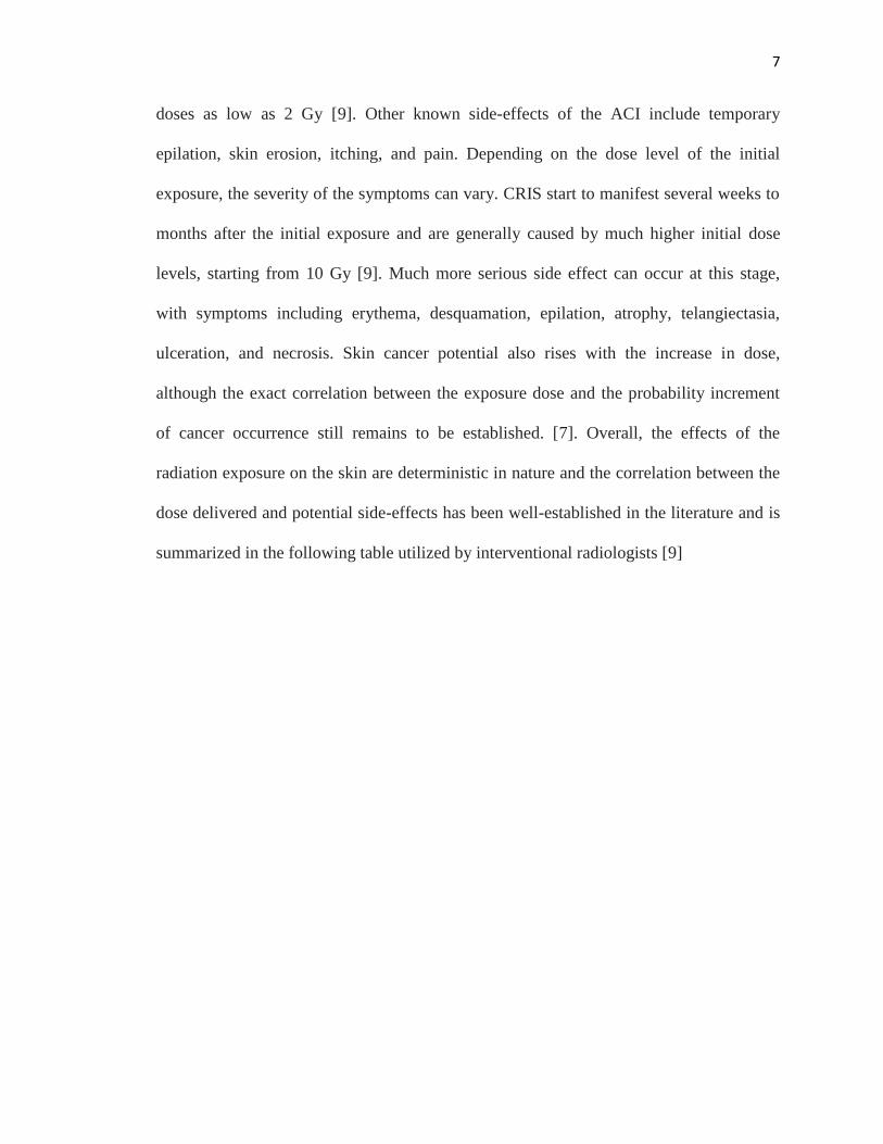
doses as low as 2 Gy [9]. Other known side-effects of the ACI include temporary

epilation, skin erosion, itching, and pain. Depending on the dose level of the initial

exposure, the severity of the symptoms can vary. CRIS start to manifest several weeks to

months after the initial exposure and are generally caused by much higher initial dose

levels, starting from 10 Gy [9]. Much more serious side effect can occur at this stage,

with symptoms including erythema, desquamation, epilation, atrophy, telangiectasia,

ulceration, and necrosis. Skin cancer potential also rises with the increase in dose,

although the exact correlation between the exposure dose and the probability increment

of cancer occurrence still remains to be established. [7]. Overall, the effects of the

radiation exposure on the skin are deterministic in nature and the correlation between the

dose delivered and potential side-effects has been well-established in the literature and is

summarized in the following table utilized by interventional radiologists [9]

8

Table I: Radiation-induced lesions of the skin with respect to dose and time of onset.

Adapted from ICRP publication 85/2000 [7] and summarized by Jaschke et al [9]

Effect

Approximate Threshold Dose,

Gy

Time of onset

Early transient erythema 2 2-24 hours

Main erythema reaction 6 ~ 1.5 weeks

Temporary epilation 3 ~ 3 weeks

Permanent epilation 7 ~ 3 weeks

Dry desquamation 14 ~ 4 weeks

Moist desquamation 18 ~ 4 weeks

Secondary ulceration 24 > 6 weeks

Late erythema 15 8-10 weeks

Ischemic dermal necrosis 18 > 10 weeks

Dermal atrophy 10 > 52 weeks

Telangiectasia 10 > 52 weeks

Dermal necrosis >12 > 52 weeks

Skin cancer Unknown > 15 years

9

It should be noted, that in clinical practice physicians separate several stages of CRI and

RD based on the time that passed since the initial radiation exposure. The earliest stage –

prodromal – lasts for the first 1-2 days from the exposure and might include the first

wave of erythema, as well as sensations of pain and heat in the affected area. After the

first couple of days, the erythema disappears and the exposed body part enters the latent

stage, at which no injury is evident. This stage significantly shortens as the initial

exposure dose increases. After the latent state, the stage of the illness manifestation

follows for the next days to weeks post-exposure. As the affected cells of the basal layer

of the epidermis start to repopulate the affected skin layer, a new wave of erythema, skin

tone changes and, depending on the severity of the injury, dry and moist desquamation,

epilation and ulceration can manifest. At 10 to 16 weeks post exposure, especially in the

cases of β-radiation, the third wave of erythema manifests with the new ulcerations and

dermal alterations, including blood vessel damage, not being uncommon. With the dose

exceeding the threshold of 10 Gy, late effects observed after several months up to years

and even decades can emerge. The irregularities in the blood supply, lymphatic network,

as well as dermal necrosis occurring at this stage can lead to permanent telangiectasia,

atrophy, the formation of the fibrotic scar tissue. Constant ulcer recurrence and soreness

in the general area of the injury might manifest. Skin cancer possibility might become

concern following decades after exposure [10]. Other effects of chronic CRI and RD can

include xerosis, hyperkeratosis, dyspigmentation, alopecia, decreased or absent sweating

due to the damage to sweat glands in the dermal layer, friable nails, longitudinal

striations, necrosis of the soft tissues, cartilage and bones, as well as general painful

sensations and limited pain of motions [12]. It should be noted that unlike acute radiation

10

injury, chronic radiation dermatitis symptoms are unlikely to be self-repaired and might

become permanent, thus significantly affecting the patient’s quality of life [1].

The extensive summary of the radiation injury effects in comparison to the dose of the

exposure, with the corresponding timeline, recovery dynamics, and potential late side

effects, has been summarized as CRI: Fact Sheet for Physicians [10].

Evaluating the severity of the radiation injury is one of the basic steps in establishing the

course of treatment for CRI and RD and predicting all possible complications that might

occur. However, as practice shows, it is not such an easy task. Usually, physicians have

to rely on the visual analysis of the skin condition in order to evaluate the severity of the

radiation-induced injury. Several clinical scoring scales exist that enable the evaluation of

the severity of the radiation skin injury in clinical setting.

The National Cancer Institute has developed a certain classification scheme, called the

Common Toxicity Criteria for Adverse Effects (CTCAE) scale with grade 1 through 4

being assigned to the injury site depending on symptoms expressed [11]. Grade 1 usually

corresponds to faint erythema and dry desquamation. As the erythema expression

becomes more pronounced and desquamation might become moist, the injury slides into

grade 2 category. Grade 3 is associated with even more pronounced moist desquamation,

edema, and bleeding in cases of slight trauma. In cases of more serious injuries,

ulceration and even skin necrosis can occur, thus earning the wound grade 4. [11].

One of the most common scales used for the long-term radiation injury evaluation is

Radiation Therapy Oncology Group (RTOG) grading scale [12]. The RTOG scale ranges

from grade 0, associated with the normal skin, where none of the symptoms are present,

to grade 5, associated with death directly related to the late-onset effects of the radiation.

11

Similarly to the acute effect scaling, grade 4 is diagnosed when the active ulceration

process is present. Grades 1 through 3 demonstrate a varying degree of atrophy,

pigmentation change, hair loss severity and, in case of grade 3, gross telangiectasia [12].

Moist and dry desquamation, erythema and edema expression are also used to

differentiate between the grades. It should be noted that this type of grading system

remains highly subjective and depends strongly on physician’s opinion, as many samples

can present as borderline cases and, as such, might be graded differently by the different

specialists.

The images of the injuries of the varying severity were retrieved at this research facility

and graded in accordance with the RTOG scale based on the symptoms exhibited. The

representation of the radiation-induced skin injuries in the porcine model developed at

this institution, graded in accordance with the RTOG criteria can be found in figure 2,

presenting a browser-based quick diagnosis tool developed by the author along with

collegues.

12

Figure 2 – Representation of the radiation-induced skin injuries of the varying degree of

severity graded in accordance with the RTOG scoring system. Table on the bottom

represents the symptoms used for the degree of differentiation. Image by Pen, Antinozzi,

2016

The details of the study evaluating the concordance between the scores given by different

physicians for the same injury sites will be explained further on.

CTCAE and RTOG are not the only existing grading scales that have been proposed over

the course of years of clinical practice. Though less commonly used, several more refined

grading systems have been proposed, such as the Oncology Nursing Society scale [13]

and the Douglas and Fowler [13] and Radiation Dermatitis Society scales [3].

13

Visual assessment usually allows the physicians to successfully identify the extent of the

radiation injury and make a treatment plan for this unfortunate side effect. However, a

deeper understanding of the causes and effects of the radiation-induced skin injury

require more precise analysis. Many different techniques are used to investigate the

injury process in more details, and correlating the results achieved by the researchers with

the relevant scaling system used by a physician in practice is of importance. One of the

techniques widely used in the biological research that produces the results that can be

easily matched with the aforementioned grading systems is histological analysis.

Histology is a branch of science that studies the microscopic anatomy of cells and tissues.

The tissues are usually taken from the living organism via biopsy, preserved on a glass

microscopic slide and then evaluated under a microscope. While light microscopy has

been widely used in the past, the electron microscope has become a popular choice,

allowing for the digitalization of the slides with a use of specialized scanner. In order to

highlight certain morphological structures in the tissues, histological stains are frequently

used. One of the more commonly used stains, hematoxylin and eosin (H&E), is

particularly useful, as it allows to easily separate the cell nuclei, that tend to accumulate

hemalum, from the protein-rich eosinophilic structures. Using the H&E on the tissue

from the radiation skin injury site allows the pathologist to see the effects of the radiation

on the cellular level, as well as observe certain morphological changes in a dermal layer

of the skin. Several important tissue characteristics exhibited with CRI include epidermal

necrosis, epidermal inflammation, the progress of the re-epithelialization, the dermal

stromal fibroplasia (scarification), degree of dermal edema and necrosis, change in the

epidermal and dermal vasculature, subcutaneous inflammation, and other morphological

14

changes in the subcutaneous layer, including, but not limited to, subcutaneous stromal

fibroplasia, edema, inflammation, necrosis, and collagen lysis. The evaluation of the

extent of the aforementioned characteristics follows the general criteria of the RTOG

grading criteria [12] and corresponds to the 0-5 RTOG grading scale utilized by the

clinicians in medical practice. As the symptoms most easily observed in the patients

suffering from RD and CRI are concentrated on the outer layer of the skin, epidermal cell

death has been deemed to be one of the most easily distinguishable characteristic that

allows for the investigation of the causes and effects of the radiation-induced skin injuries

both at the cellular level provided by the detailed histological analysis and correlation of

the study results with the clinically observed expressions of CRI and RD.

The evaluation of the expression of certain features and tissue characteristic in

histopathology is qualitative in nature and, having no exact numerical description, relies

on the histopathologist’s expertise and judgement. Potentially, over and underestimation

of the feature expression severity can occur (observer bias). In the course of this project,

we have developed a quantitative approach to the epidermal necrosis evaluation that

would allow for a consistent approach to the evaluation of the tissue affected by beta

radiation. Such a quantitative approach would allow us to numerically express the

severity of the damage across the wound site based on the amount of epidermal necrosis

expressed. One of the observations introduced during the course of the study was the

microdifferences in the dose distribution at the skin surface level (0.07 mm) that

correspond to the depth of the epidermal layer of the skin. Microdosimetry measurements

and accurate modeling of the dose distribution became paramount in understanding the

15

mechanisms of epidermal necrosis expression and development of techniques aimed at

mitigating it.

MICRODOSIMETRY AT THE EPIDERMAL LAYER DEPTH

While not detected through the typical means, as actual skin dose measurement is very

difficult [2], the minuscule changes in the dose profile may have a significant effect on

the epidermal necrosis. Microdosimetry, thus, becomes a necessity. The empirical

calculation and measurement of the skin surface dose had been proposed and performed

in previous work with beta radiation device [14]. Several varying methods exist, allowing

to estimate the dose at the surface, including, but not limited to, radiochromic films,

extrapolation chambers, parallel-plate ionization chambers, optical and

thermoluminiscent dosimeters [15][16][17][18][19][20]. In the course of the previous

study, GafchromicTM

EBT3 radiochromic film and Markus© ion chamber type 23343

have been used to evaluate the dose deposited on the skin surface. Several analytical

models can be utilized in order to estimate the dose at the skin surface deposited in the

architecture corresponding to the experimental conditions. The Loevinger point-source

dose function [21], Vynckier-Wambersie [22] and Cross functions [23] were investigated

previously by Dr. Dorand [14], but provided insufficient agreement between the

predicted and measured surface dose profiles. Monte Carlo simulation, on the other hand,

has consistently proven to provide an accurate estimation of the radiation dose under

certain conditions [24].

The source of the radiation utilized in this particular study is an isotope of Strontium, Sr-

90, radioactive in nature and prone to beta-particles emission. Sr-90 decays by β-emission

(Eβ = 0.55 MeVmax) to Yttrium-90 (Y-90), another unstable radioactive isotope that then

16

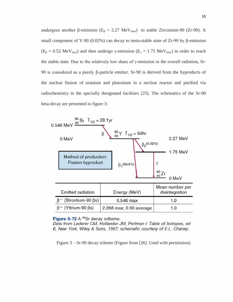
undergoes another β-emission (Eβ = 2.27 MeVmax) to stable Zirconium-90 (Zr-90). A

small component of Y-90 (0.02%) can decay to meta-stable state of Zr-90 by β-emission

(Eβ = 0.52 MeVmax) and then undergo γ-emission (Eγ = 1.75 MeVmax) in order to reach

the stable state. Due to the relatively low share of γ-emission in the overall radiation, Sr-

90 is considered as a purely β-particle emitter. Sr-90 is derived from the byproducts of

the nuclear fission of uranium and plutonium in a nuclear reactor and purified via

radiochemistry in the specially designated facilities [25]. The schematics of the Sr-90

beta-decay are presented in figure 3:

Figure 3 – Sr-90 decay scheme (Figure from [26]. Used with permission)

17

The half-life of Sr-90 is 28.1 yr, while Y-90 has a half-life λ = 64 hours. Due to such a

big difference in their respective half-lives, the aforementioned isotopes exist in the

secular equilibrium with the average energy of the β-particle being 0.9 MeV, with isotope

quantity correlations described as:

𝜆2𝑁2

𝜆1𝑁1=

𝜆2

𝜆2 − 𝜆1 (1)

Here, λ represents the total radioactive decay constant, with 𝜆 = ln (2)

𝑇1/2, and 𝑇1/2 is the

half-life of the isotope, N is the number of atoms, and λN is the activity of the isotope.

The “child” isotope Y-90 is denoted by “1”, and “parent” isotope Sr-90 is denoted by

“2”. The secular equilibrium with the ratio of activity ~1 is achieved 31.8 days after the

production of Sr.90, as denoted in Attix, 2004 [27] and illustrated by figure 4:

18

Figure 4 – Sr-90 and Y-90 activity equilibrium as denoted over time for the 100mCi

source [27]. Image used with permission.

Out of the two isotopes, Y-90 with its higher particle energy presents more of a risk, yet

for the purpose of simplification the term “Sr-90” has been used for the combined Sr-

90/Y-90 energy spectrum once the equilibrium has been achieved. In the Monte Carlo

simulation study performed in the course of this work, a special provision is made to

account for Y-90 presence and corresponding energy levels of the emitted particles.

19

The main process of radioactivity occurring in the study is beta decay. In beta decay, a

beta ray (electron or positron) and neutrino or antineutrino are emitted. The propensity of

the isotope to a particular type of decay is defined by the nuclear drip line and can be

estimated based on the number of protons and neutrons in the nucleus of the isotope

(figure 5).

Figure 5 – Nuclear drip line for Sr-90 and Y-90. Both Sr-90 and Y-90 fall within the blue

region of β–

decay [28] Image is in the public domain

20

In this particular case, the β-particles emitted by Sr-90 source come from the β–

radioactive decay. In such a process, an unstable atomic nucleus loses the excessive

energy by emitting radiation in the form of an electron, accompanied by the release of

energy. The Sr-90 isotope is characterized by the excess of neutrons, and as the electrons

are emitted, a neutron then converts to a proton, increasing the effective atomic number

of the particle. As have been mentioned previously, Sr-90 is then converted to Y-90,

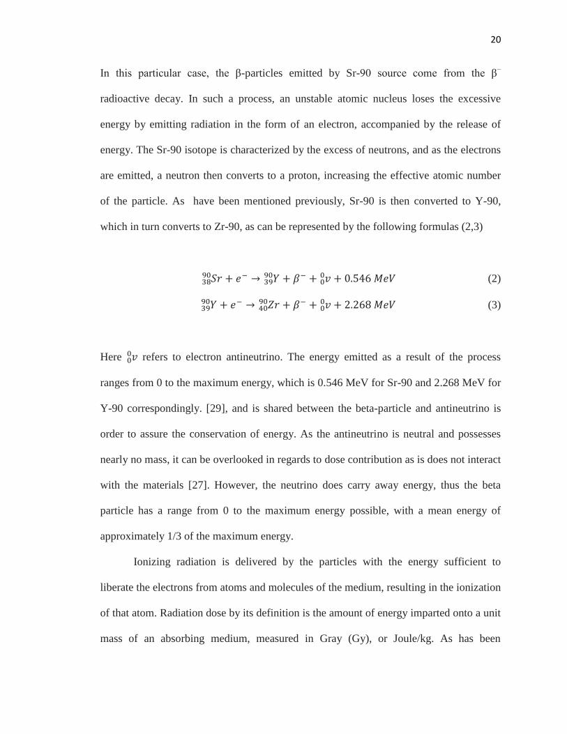
which in turn converts to Zr-90, as can be represented by the following formulas (2,3)

𝑆𝑟3890 + 𝑒− → 𝑌39

90 + 𝛽− + 𝑣00 + 0.546 𝑀𝑒𝑉 (2)

𝑌3990 + 𝑒− → 𝑍𝑟40

90 + 𝛽− + 𝑣00 + 2.268 𝑀𝑒𝑉 (3)

Here 𝑣00 refers to electron antineutrino. The energy emitted as a result of the process

ranges from 0 to the maximum energy, which is 0.546 MeV for Sr-90 and 2.268 MeV for

Y-90 correspondingly. [29], and is shared between the beta-particle and antineutrino is

order to assure the conservation of energy. As the antineutrino is neutral and possesses

nearly no mass, it can be overlooked in regards to dose contribution as is does not interact

with the materials [27]. However, the neutrino does carry away energy, thus the beta

particle has a range from 0 to the maximum energy possible, with a mean energy of

approximately 1/3 of the maximum energy.

Ionizing radiation is delivered by the particles with the energy sufficient to

liberate the electrons from atoms and molecules of the medium, resulting in the ionization

of that atom. Radiation dose by its definition is the amount of energy imparted onto a unit

mass of an absorbing medium, measured in Gray (Gy), or Joule/kg. As has been

21

mentioned before, in case of Sr-90/Y-90 almost the entire dose comes from the emitted β-

particles, as γ component of the emission is negligible. The number of particles given by

the emitting isotope is referred to as the source’s activity (A) and is measured in Curies

(Ci), with one Curie being equal to 3.7x10^10 disintegrations per second. As the secular

equilibrium of the parent and child isotope is achieved, the probability of either Sr-90 or

Y-90 emitting a β-particle becomes equal, which introduces an additional complexity is

calculating the average energy of the emitted spectrum, with its peak generally falling

within 1/3 of the maximum energy of the β-particle. Both the activity rate and energy of

the particle being emitted affect the magnitude of the dose imparted to the medium.

In order to understand how exactly the dose is delivered to the skin surface in the event of

the β-radiation, the interactions of the atoms of the medium with the charged particles –

the source of ionizing radiation – have to be considered. Whenever charged particle

interacts with the atoms it encounters in the medium, some amount of energy is lost, with

the expected value of the rate of energy loss per unit of path length x being expressed as

𝑑𝑇

𝑑𝑥, or stopping power, where T is the energy. As the density of the material is taken into

account, mass stopping power can be expressed as 𝑑𝑇

𝜌𝑑𝑥 . It is typically measured in MeV

cm2/g. As the particle continues to lose its energy as it progresses through the medium,

the “continuous slowing down approximation” (CSDA) is used as a description of the

rate of energy loss and the average range of particle travel path within the medium. In

order to consider the different possible outcomes of the energy loss experienced by the

charged particle and consequent manner in which this energy is imparted onto the

medium, a further subdivision of the mass stopping power into collision stopping power

and radiative stopping power is introduced.

22

Collision stopping power describes the energy loss occurring as the result of hard and soft

collisions. Radiative stopping power occurs as the result of the radiative interactions and,

for the purposes of this study, is considered to mainly consist of the bremsstrahlung

production. A comparative chart of the proportions of collision vs radiative stopping

power in a different medium under the influence of different energies is introduced in

figure 6:

Figure 6 – Collisional vs radiative stopping power for varying energies in water and lead

media (Figure from Bourland, 2012 [26]. Used with permission.)

23

The overall dose absorbed by the medium can be determined as the mass stopping power

of the particle integrated over the energy spectrum of the particles multiplied by the

number of particles at each energy within the spectrum (equation 4):

𝐷𝑤 = 1.602𝑥10−10 ∫ Ф𝑥𝑇 (𝑑𝑇

𝜌𝑑𝑥)

𝑐,𝑤

𝑇𝑚𝑎𝑥

0𝑑𝑇 (4)

Here 𝐷𝑤 is the absorbed dose in the medium 𝑤, 1.602x10-10

is the conversion term for Gy

(1.602x10-10

Gy = 1 MeV/g), Ф𝑥𝑇 is the differential charged particle fluence spectrum.

All collisions the β-particles experience can be further subdivided into elastic (where

small or no significant kinetic energy loss occurs) and inelastic (where the energy is lost

as a result of other non-elastic interactions). Furthermore, a particle may interact with

either electrons of the atom or its nucleus. Thus, different forms of interaction of the β-

particle with the medium can be observed.

When the inelastic collision of the β-particle with the atomic nucleus occurs,

bremsstrahlung effect can be observed. The Coulomb force field of the nucleus interacts

with the passing β-particle and slows it down. The energy released as the results of this

loss transforms into x-ray photon, which is then emitted from the nucleus. Depending on

the magnitude of energy loss, the initial β-particle might be stopped completely and all of

the energy might be transferred to the photon (low probability). It should be noted that

inelastic radiative interaction occurs only in 2-3% of cases of the electron passing near

the nucleus [30].

24

Inelastic collisions with the atomic electrons occur when the distance between the passing

particle and the nucleus is relatively big, yet the Coulomb force field of the passing

particle is great enough to possibly excite the atom to higher state and potentially create

a vacancy in the higher electron shells by ejecting the atom’s electron from its orbit. The

particle itself can experience very insignificant loss of energy (around a few eV) and

suffer no changes in trajectory [30]. Under very specific conditions, this energy can be

emitted by the absorbing medium as Cherenkov radiation. For the energy range of β-

particles produced by Sr-90/Y-90 source, the fraction of Cherenkov photons is negligibly

small.

Elastic collision of the β-electron with the electrons of the atom results in the ejection of

the atomic electron from its shell in the form of delta ray. Both electrons then

significantly change their trajectory and are further scattered in the medium, losing

kinetic energy with each interaction. If the ejected delta-ray electron was originally

positioned at the inner shell, an electron from the outer shell might fill the vacancy, with

the difference in energy between inner and outer shell being emitted as a characteristic x-

ray. Alternatively, this energy may be transferred to the electron in the outer shell. In

order to account for the differences in binding energy, this electron is then emitted from

the atom in the form of Auger electron.

Overall, the aforementioned interactions of the β-particles can be summarized by the

following figure (figure 7):

25

Figure 7 – β-particle interactions in: a) inelastic collision with the electron, b) elastic

collision with the outer shell electron, c) elastic collision with the inner shell electron, d)

inelastic collision with the atomic nucleus. Image from [14], used with permission.

Elastic collisions of the electron with the nucleus of the atom occur when the energy

imparted by the electron to the nucleus is not great enough to excite the nucleus. Yet

these interactions are incredibly important in the case of surface skin dose, as the low-Z

elements comprising the soft tissue are much more prone to these types of interactions

and introduce the highest percent of scattering events. Due to the relatively high density

of the atoms in the medium, an electron can undergo several elastic collisions before

losing a significant amount of energy, resulting in a tortuous path. The extensive Monte-

Carlo simulation is required in order to estimate the possible trajectories of the β-

particles, and will be presented in the corresponding chapter along with the detailed

explanation of the possible interactions.

26

Due to the highly unpredictable nature of this path, the mean energy of the β-particles

undergoing elastic collisions is evaluated as the linear decrease over depth. For instance,

for 6 to 20 MeV electrons, having higher energy than the beta particles emitted from Sr-

90 and typically used clinically in radiation treatment, percent depth dose curves can be

used to estimate the depth in water at which most of the particles come to a stop, as

illustrated in figure 8:

Figure 8 – Percent depth dose curves for various energies of megavoltage electron.

(Figure from Bourland, 2012 [26]. Used with permission.)

27

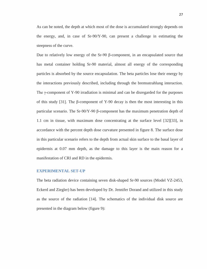
As can be noted, the depth at which most of the dose is accumulated strongly depends on

the energy, and, in case of Sr-90/Y-90, can present a challenge in estimating the

steepness of the curve.

Due to relatively low energy of the Sr-90 β-component, in an encapsulated source that

has metal container holding Sr-90 material, almost all energy of the corresponding

particles is absorbed by the source encapsulation. The beta particles lose their energy by

the interactions previously described, including through the bremsstrahlung interaction.

The γ-component of Y-90 irradiation is minimal and can be disregarded for the purposes

of this study [31]. The β-component of Y-90 decay is then the most interesting in this

particular scenario. The Sr-90/Y-90 β-component has the maximum penetration depth of

1.1 cm in tissue, with maximum dose concentrating at the surface level [32][33], in

accordance with the percent depth dose curvature presented in figure 8. The surface dose

in this particular scenario refers to the depth from actual skin surface to the basal layer of

epidermis at 0.07 mm depth, as the damage to this layer is the main reason for a

manifestation of CRI and RD in the epidermis.

EXPERIMENTAL SET-UP

The beta radiation device containing seven disk-shaped Sr-90 sources (Model VZ-2453,

Eckerd and Ziegler) has been developed by Dr. Jennifer Dorand and utilized in this study

as the source of the radiation [14]. The schematics of the individual disk source are

presented in the diagram below (figure 9):

28

Figure 9 – Diagram of Ar-90 source encapsulation (in mm): a) angled, b) cross-section

view (Schematic courtesy of Eckert & Ziegler, Nuclitec GmbH, Braunschweig, Germany,

© 2009)

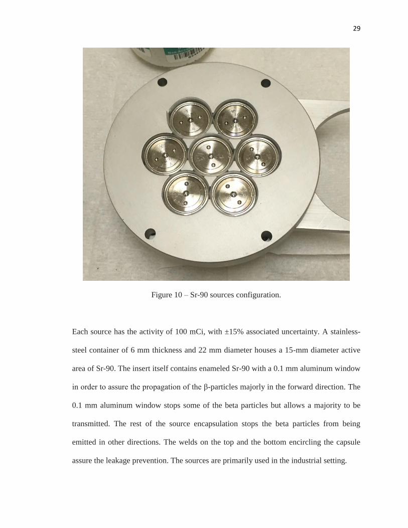
Overall, 7 sources, each with diameter of 22 mm, were employed and positioned into a

semi-circle with one source in the center and six others surrounding it (figure 10):

29

Figure 10 – Sr-90 sources configuration.

Each source has the activity of 100 mCi, with ±15% associated uncertainty. A stainless-

steel container of 6 mm thickness and 22 mm diameter houses a 15-mm diameter active

area of Sr-90. The insert itself contains enameled Sr-90 with a 0.1 mm aluminum window

in order to assure the propagation of the β-particles majorly in the forward direction. The

0.1 mm aluminum window stops some of the beta particles but allows a majority to be

transmitted. The rest of the source encapsulation stops the beta particles from being

emitted in other directions. The welds on the top and the bottom encircling the capsule

assure the leakage prevention. The sources are primarily used in the industrial setting.

30

An extensive series of test was performed in order to establish the relative dose

distribution of each of the seven sources used in the device. Radiochromic film

positioned on top of solid phantom has been utilized. Dose rate has also been measured

by Markus ® parallel-plate ionization chamber. As the measurements have been

performed and data obtained, it was determined that additional distance from the surface

to the source would be required in order to make the dose uniform across the surface.

Thus, an additional series of experiments have been performed in order to establish the

most efficient experimental set-up.

The study performed was intended to investigate the progression of RD and CRI in vivo

and thus had to adhere to CDC definition of CRI in 10 cm2 region of injury. Additional

safety installation features such as remote on/off control, additional shielding cassette and

long handles were introduced.

Due to the large inhomogeneity found between the seven Sr-90 sources, specific

alignment of each individual source within the configuration and increase in SSD from

the device to the skin surface have become a necessity. A plastic cone has been

introduced in order to collimate the circular radiation field. A detailed report of the

device configuration process and the established of the surface dose heterogeneity can be

found in Dr. Dorand’s dissertation [14]. Despite the best attempts to homogenize the

dose distribution, some effects still lingered and might have become a reason of the

variation in the epidermal necrosis expression observed upon the extensive analysis of the

digital histological slides harvested at the injury sites.

Schematic view of the cassette is presented in figure 11:

31

Figure 11 – Schematic view of the source: a) from the top, with white disks representing

the Sr-90/Y-90 source active area (15 mm in diameter), blue disks representing the

overall inactive area, including stainless steel shielding (22 mm diameter) and red

representing the cassette area; b) Positioning of the cassette upon the application cone.

Images used with permission (Dorand, 2014 [14])

The detailed description of the inhomogeneity of the source activity and corresponding

surface dose distribution can be found in chapter 2.

The final device developed by Dr. Dorand had a long detachable handle, the 5-mm thick

aluminum shatters that switched the device into an on-position when opened and

prevented the radiation leakage when closed, the aluminum cassette containing all seven

radiation sources, and Lucite (Polymethylmethacrylate, PMMA) collimator cone. The

final device is presented in figure 12:

32

Figure 12 – The beta radiation device; a) in the off position; b) in the on position; c) from

the side, illustrating the source cassette and additional applicator cone. Image used with

permission (Dorand, 2014 [14])

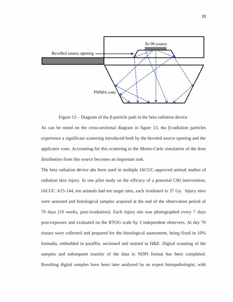
The simplified model of the particles propagation in the source of aforementioned

configuration is presented in the figure 13:

33

Figure 13 – Diagram of the β-particle path in the beta radiation device.

As can be noted on the cross-sectional diagram in figure 13, the β-radiation particles

experience a significant scattering introduced both by the beveled source opening and the

applicator cone. Accounting for this scattering in the Monte-Carlo simulation of the dose

distribution from this source becomes an important task.

The beta radiation device ahs been used in multiple IACUC-approved animal studies of

radiation skin injury. In one pilot study on the efficacy of a potential CRI intervention,

IACUC A15-144, ten animals had ten target sites, each irradiated to 37 Gy. Injury sites

were assessed and histological samples acquired at the end of the observation period of

70 days (10 weeks, post-irradiation). Each injury site was photographed every 7 days

post-exposure and evaluated on the RTOG scale by 3 independent observers. At day 70

tissues were collected and prepared for the histological assessment, being fixed in 10%

formalin, embedded in paraffin, sectioned and stained in H&E. Digital scanning of the

samples and subsequent transfer of the data in NDPI format has been completed.

Resulting digital samples have been later analyzed by an expert histopathologist, with

34

results of her analysis being recorded in the separate report that has been later utilized as

the ground truth for the automated analytical system development.

The experimental set-up can be presented by the following figures (figure 14 and figure

15):

Figure 14 – Beta radiation device attached to: a) three-legged stand; b) wall-mount arm.

Image used with permission (Dorand, 2014 [14])

Figure 15 – Pig with tattooed areas of irradiation and application of the device to the pig

skin (Dorand, 2014 [14], image used with permission)

35

Calculating the skin equivalent dose is not an easy task and several different approaches

have been developed according to different publications. A first approach to describe the

radiation biophysics of the skin and develop a reliable method of skin surface dosimetry

was published in 1983 [34][35]. The first attempts at microdosimetry in case of beta-

radiation and its effects on the basal layer of the epidermis were also undertaken at the

same time [36]. The next approach attempted by Schultz and Zoetelief [37] calculates the

equivalent dose as the average between the doses at 0.07 mm and 2 mm in tissue. This

approach has become the basis for Publication 74 of the ICRP [38]. Six years later,

another approach has been presented in Norm ISO 15382 [39]. New protocols have been

established in 2010 to account for the weakly penetrating particles, such as positrons and

electrons, defining a new protection quantity: the “Local Skin Absorbed Dose” (LSD)

[40]. The LSD conversion coefficients have been defined for electrons [40] and positrons

[41] for MCNP6 Monte Caro simulation of the general water phantom.

Experiments on the porcine model as the most accurate representation of the human skin

tissue continued [42]. However, accurate microdosimetry in the basal layer of the

epidermis still remains challenging to the researchers.

In order to estimate the dose delivered to the skin surface of the pigs, a series of the

dosimetry experiments conducted previously in the study have been compared to the

analytically estimated dose values. Beta-ray point source function, namely, Loevinger

point-source dose function [21], has been integrated for a particular geometrical set-up.

Cross [43] additions to the initial function further increased the veracity of the model.

The dose rate calculated by this model could be calculated as:

36

𝐷 = 2𝜋𝛼𝑠𝑣∗0.046∗⟨𝐸𝛽⟩

3𝑐2−(𝑐2−1) exp(1)((𝑐 − 𝜌𝑣 ∗ 𝑅 ∗ exp(1 − 𝜌𝑣𝑅))𝑙𝑛

𝑦

𝑥+ 𝑐 (exp (1 −

𝜌𝑣𝑦

𝑐) −

exp (1 −𝜌𝑣𝑥

𝑐)) − exp(1 − 𝜌𝑣𝑦) + (1 − 𝜌𝑣𝑥) (5)

Where for the Sr-90/Y-90 source [44]:

⟨𝐸𝛽⟩ = 0.933 MeV

𝑐 = 1.09

𝑣 = 5.45 cm2/g

𝜌 = 1 g/cm3 for water

R = 0.87 cm

𝛼𝑠 = 100 mCi = 3700 mBq for one source

𝑦 = √𝑥2 + 𝑎2

𝑎 = 0.75

𝑥 – distance from the source in cm

Due to some of the limitations of the initial model, the alternative model based on the

Vynckier-Wambersie function have also been implemented [45]. In this model:

𝐷 = 2𝜋𝛼𝑠𝑣∗0.046∗⟨𝐸𝛽⟩

3𝑐2−(𝑐2−1) exp(1)+(3+𝑓) exp(1−𝑓)−4 exp(1−𝑓

2)

(𝑐 ∗ 𝑙𝑛𝑦

𝑥+ 𝑐 ∗ exp (1 −

𝜌𝑣𝑦

𝑐) − 𝑐 ∗

exp (1 −𝜌𝑣𝑥

𝑐) − exp(1 − 𝜌𝑣𝑦) + exp(1 − 𝜌𝑣𝑥) + 2 ∗ exp (1 −

𝜌𝑣𝑦

2−

𝑓

2) (6)

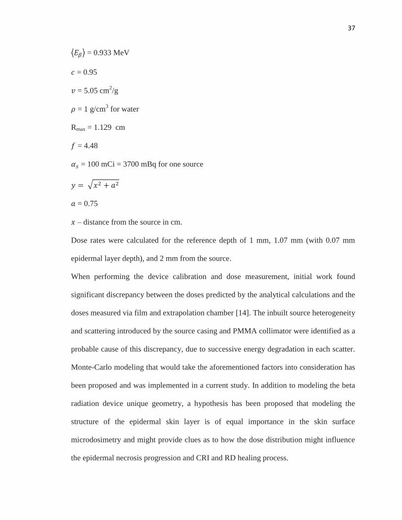
With the parameters used to calculated the dose for the Sr-90/Y-90 source being [44]:

37

⟨𝐸𝛽⟩ = 0.933 MeV

𝑐 = 0.95

𝑣 = 5.05 cm2/g

𝜌 = 1 g/cm3 for water

Rmax = 1.129 cm

𝑓 = 4.48

𝛼𝑠 = 100 mCi = 3700 mBq for one source

𝑦 = √𝑥2 + 𝑎2

𝑎 = 0.75

𝑥 – distance from the source in cm.

Dose rates were calculated for the reference depth of 1 mm, 1.07 mm (with 0.07 mm

epidermal layer depth), and 2 mm from the source.

When performing the device calibration and dose measurement, initial work found

significant discrepancy between the doses predicted by the analytical calculations and the

doses measured via film and extrapolation chamber [14]. The inbuilt source heterogeneity

and scattering introduced by the source casing and PMMA collimator were identified as a

probable cause of this discrepancy, due to successive energy degradation in each scatter.

Monte-Carlo modeling that would take the aforementioned factors into consideration has

been proposed and was implemented in a current study. In addition to modeling the beta

radiation device unique geometry, a hypothesis has been proposed that modeling the

structure of the epidermal skin layer is of equal importance in the skin surface

microdosimetry and might provide clues as to how the dose distribution might influence

the epidermal necrosis progression and CRI and RD healing process.

38

Keeping this in mind, several aims have been identified in the course of this study as

necessary for the thorough investigation of the correlation between the dose variations at

the skin surface level and the epidermal necrosis expression characteristic in the CRI and

RD injuries.

SPECIFIC AIMS

1) Quantification of the epidermal necrosis expression in the skin affected by the

beta radiation

2) Monte-Carlo modeling of the beta radiation for the surface dose delivered under

the conditions specified for the particular experimental geometry of unique beta

radiation device.

3) Analysis of the surface dose distribution profiles acquired with the Monte Carlo

model and epidermal expression profiled acquired through the automated

quantification algorithm applied to the histological slides with the experimentally

acquired data.

39

CHAPTER 1: Quantitative analysis of the epidermal necrosis in cutaneous

radiation injuries and radiation dermatitis

MATERIALS AND METHODS

Necrotic cell detection

Evaluation of the severity of radiation-induced skin injury is not a trivial task. A

thorough study of the effects of radiation on cellular and tissue level is required and is

usually performed via analysis of the histological samples of the tissues exposed to

radiation. Evaluation of the histopathological features of radiation-induced injury is often

qualitative in nature and relies on the histologist’s expertise and judgement. Over– and

under-estimation of the expressed features can occur. Developing an unbiased, automatic,

quantitative approach to the histopathological feature evaluation is the focus of this

chapter.

In the course of analysis of the histological features most characteristic of CRI and RD,

epidermal necrosis is often one of the most noticeable and commonly occurring [1]. It

mostly affects the keratinocytes, a type of cells that make up 90% of the epidermal skin

layer. [2]. Under the influence of the radiation, keratinocytes undergo a series of

molecular biological changes, which, in case of radiation exposure, leads to pyknotic

nucleus formation. [46] Pyknosis is the irreversible concentration of chromatin in the

nucleus of the cell undergoing necrosis or apoptosis [47]. It is followed by the

fragmentation of the nucleus (karyorrhexis) and subsequent cell nucleus dissolution.

While the exact mechanisms of the trigger of epidermal necrosis and apoptosis in the

keratinocytes are still under investigation, the prevalence of the cells with a pyknotic

40

nucleus in the histological samples of the biopsy tissue is well-documented [48][49][50].

The schematic progression of cell death is depicted in figure 16:

Figure 16 – Cell undergoing apoptosis. Image is in a public domain [50]

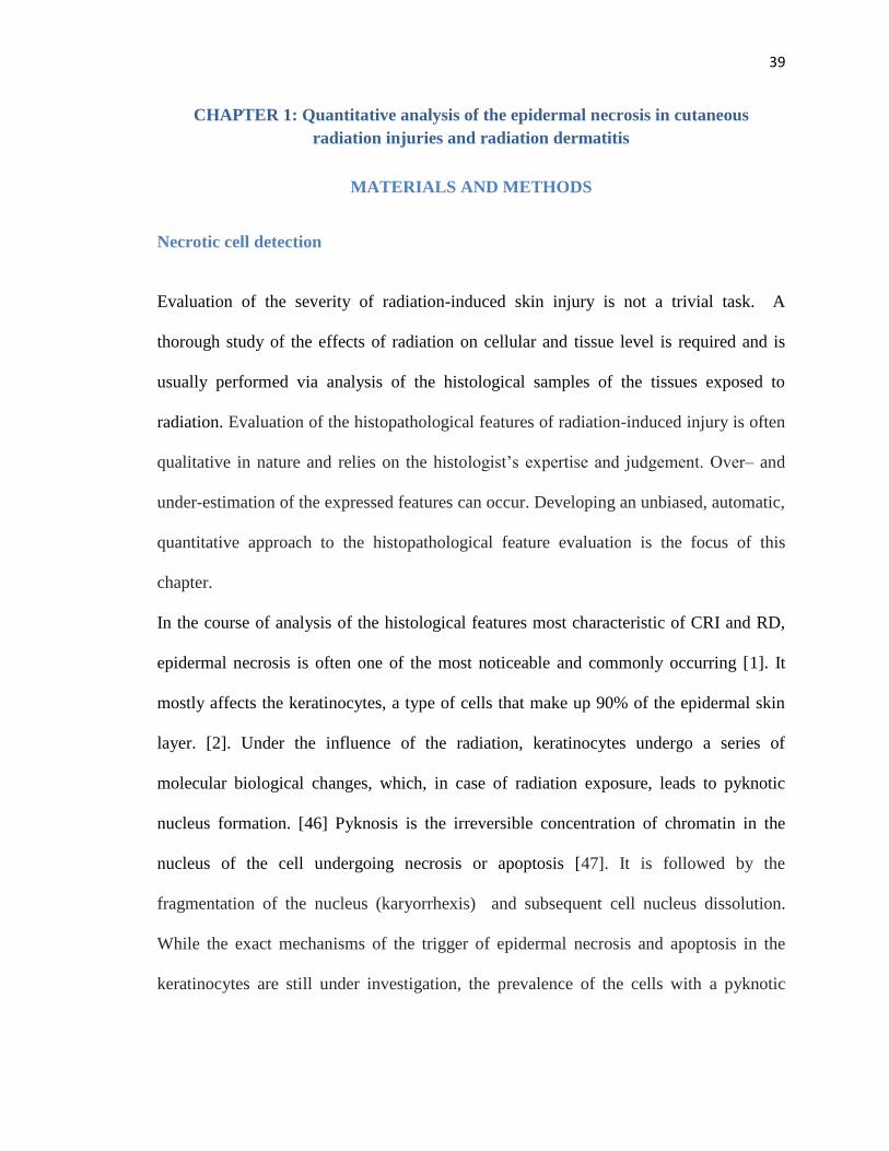
The pyknotic nucleus can be characterized on the histological samples stained with H&E

as a condensed, circular dark-violet spot with the area of 10-12 microns [51]. Dead

keratinocytes in the epidermis are easily identified on the histological slides:

41

Figure 17 – Histological sample with heavy epidermal cell death expression. The arrows

highlight the pyknotic nucleus.

Histological samples used in this study were obtained as part of a completed,

institutionally-approved animal research study on beta radiation effects on porcine skin.

The experimental beta radiation device containing seven disk-shaped Sr-90 sources for

beta exposure has previously been described [14]. Beta-source irradiation was utilized in

the study in order to assure a high skin surface dose with little internal dose deposition,

providing controlled experimental conditions with no morbidity to internal structures, as

well as to model the principal component of beta radiation that can induce skin injury, as

found in nuclear fallout. The beta device was used to uniformly irradiate a one-time dose

of 37 Gy to a defined 40 mm circular region of skin of the Yorkshire White pig (5

42

locations on each side of an animal, 10 targets total per animal, 10 animals, all female, 6

months old at the beginning of the study). The pigs were sedated by the injection of

acepromazine and ketamine into animal’s clavotrapezius or gluteus maximus, with

further sedation being induced by vaporized isoflurane being delivered through a

breathing mask positioned over the snout of the pig, and anesthesia being maintained

through isoflurane inhalation. The duration of the whole procedure including anesthesia

and irradiation is 2.5 hours.

Previous studies performed on this particular animal model allowed for the establishment

of the dose being necessary to evoke the variety of the skin responses at the irradiation

site. The dose of 37 Gy was chosen to evoke the medium-level response that would

demonstrate the severity of CRI without causing the excessive burns that would prevent

any healing from occurring at the irradiation site. After irradiation, animals were

observed for the duration of 70 days to allow the skin go through the singular cycle of

healing, as the cycle of healing for radiation-induced injuries tends to follow sinusoidal

healing curve based on the rate of proliferation for the basal layer of the epidermal cells.

During the duration of the observation period, the irradiated sites were photographed to

track the wound healing progression with pigs being awake at the time of the pictures of

the wound sites being taken. The photographs of the wound sites taken at 7-day period

over the course of 70 days were collected for all 10 wound sites for 10 animals, and at the

conclusion of the 70 days period were subjected for RTOG grading by seven independent

experts. The scores obtained from the experts were then averaged to provide a mean

score for 100 samples that have undergone irradiation.

43

In this particular experimental set-up, the samples were collected over the whole

irradiation area (4 cm in diameter) plus the 2 cm on the sides in order to account for the

cases where the test subject might have moved during irradiation and the lesion might

have formed outside of the tattoo area. The schematic depiction of the histological slide

acquisition is presented in figure 18:

Figure 18 – Wound map for histology (Dorand, 2014) [14], image used with permission

At the conclusion of the 70-day period, the pigs were euthanized and whole-skin

histological strip samples were collected from the test subjects and appropriately

prepared for H&E staining. The strips were collected at the center of the irradiation field

in order to ensure the good representation of the radiation-induced wound across the

whole span of the irradiated area, as demonstrated in Figure 18. Mounted samples were

then digitally scanned at high resolution for data archiving as well as to enable digital

analysis of the extent and progression of CRI. In the course of the algorithm development

study, 120 histology samples were analyzed (n = 12 per pig; 10 receiving 37 Gy and 2

receiving no radiation and being used as a control).

At day 70, strip biopsies across each target were obtained and the tissues were prepared

for the histological assessment, being fixed in 10% formalin, embedded in paraffin,

sectioned and stained with H&E. Digital scanning of the samples was performed by a

44

Hamamatsu C9600-12 scanner, with the digitalized slides being saved in the NDPI

(Nanoscale Digital Processing Images) format. The resulting image size of the digitalized

samples is 86400 x 52736 pixels, with 453 nm/pixel resolution (56070 DPI), obtained

with a 20X source lens. These scanned images were evaluated by a board certified

veterinary pathologist (American College of Veterinary Pathologists), and qualitatively

graded as to epidermal necrosis severity as a basis for the development of the automated

analytical method.

For the analysis of the epidermal necrosis, the number of pyknotic nuclei and the area of

their concentration in relation to the overall area of the epidermis were taken into account

and served as defining parameters for the RTOG grading. The spread of the pyknotic

cells was defined as the distance between the starting points where H&E stain starts to

accumulate on both ends of the sample and was used in order to estimate the length of the

lesion in comparison to the overall length of the sample. By analyzing the spread and

density of the dead keratinocytes, the histopathologist graded the 120 samples on a 0-4

scale corresponding to the RTOG grading scale. The range of injury is demonstrated in

Figure 19:

45

Figure 19 – Histological samples with different degrees of epidermal necrosis. Arrows

point to the lesion site. Corresponding RTOG scale degrees: A) 0; B) 1; C) 2) D) 3; E) 4

As can be noted, the degrees very both in the concentration of the number of the dead

cells and spread of the area of the lesion in comparison to the total length of the slide. At

the sight of the lesion itself, though, the difference between different grades is less

pronounced (figure 20):

46

Figure 20 – Magnified view of the dead cells (grade 4 (A) vs grade 1 (B))

Therefore, a single algorithm can be applied to automatize the search for the pyknotic

nuclei and evaluation of their spread across the length of the histological sample.

The report based on the findings of histopathologist has served as the ground truth for

the training of the algorithm developed to automatically quantify the epidermal necrosis

expression in CRI and RD.

In order to automatize and quantify the evaluation of the epidermal necrosis expression,

several steps had to be performed. Due to the large size (>500 Mb/sample) of the initial

NDPI files and the necessity to evaluate the spread of the epidermal necrosis across the

length of the sample, the histological samples were presented in the form of mosaic that

cut the initial sample into the pieces of equal area size, thus making them available for

evaluation and allowing the algorithm to track the spread of the necrotic tissue across the

uniform length segments. After the segmentation of the sample into mosaic pieces was

performed, each piece further underwent feature analysis that allowed the selection of the

epidermal layer exclusively for further evaluation. This selected region, in turn, was

subjected to thresholding and particle analysis in order to establish the number of the

47

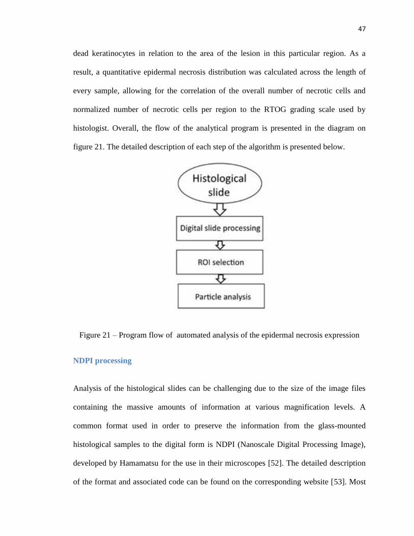
dead keratinocytes in relation to the area of the lesion in this particular region. As a

result, a quantitative epidermal necrosis distribution was calculated across the length of

every sample, allowing for the correlation of the overall number of necrotic cells and

normalized number of necrotic cells per region to the RTOG grading scale used by

histologist. Overall, the flow of the analytical program is presented in the diagram on

figure 21. The detailed description of each step of the algorithm is presented below.

Figure 21 – Program flow of automated analysis of the epidermal necrosis expression

NDPI processing

Analysis of the histological slides can be challenging due to the size of the image files

containing the massive amounts of information at various magnification levels. A

common format used in order to preserve the information from the glass-mounted

histological samples to the digital form is NDPI (Nanoscale Digital Processing Image),

developed by Hamamatsu for the use in their microscopes [52]. The detailed description

of the format and associated code can be found on the corresponding website [53]. Most

48

of the images taken for the variety of resolutions starting from 0.25X magnification up to

40X magnification can take up to several gigabytes of memory. Hamamatsu managed to

develop the tool, NDPI viewer, that allows for the rapid access to the image itself,

making it available for the histologist’s assessment even on the machines with relatively

low RAM memory, however, this application doesn’t allow for any meaningful

quantitative analysis and lacks the programming capabilities. Several attempts have been

made by Hamamatsu and affiliated parties in order to rectify the problem, however, all of

them have certain limitations such as the size of the image that can be opened [54],

inability to transform the NDPI format [55] or the reliability on the singular platform and

lack of the open source code [56]. However, in recent years, an attempt has been made to

incorporate the NDPI reader function to the open-source software tools commonly used

in the scientific community. One of the other tools that could be potentially used in order

to open the files with NDPI format is ImageJ, a public domain software platform

developed for the scientific purposes and geared towards image analysis [57]. An add-on

to the ImageJ that would allow for easy manipulation has been developed [58] and is

utilized in the course of this work. This software tool is capable of reading the NDPI-

formatted files and transforming them into a TIFF format, as well as splitting them into

“tiles”, or mosaic pieces, that can be processed on the individual basis without

overloading the RAM capacity of the machine. A mosaic in this scenario is the series of

images that reassembled together would form an original file; however, this mosaic tiles

are of manageable size and are thus available for analysis. The mosaic tiles are of an

equal length that can be adjusted by the user and may be optimized to overlap in case of

the pyknotic nuclei being located on the boundaries of the tile. The detailed description of

49

the program functionality can be found in the original paper by Deroulers et al.[58]. The

examples of the mosaic tiles in case of Windows interface are provided in figure 22:

Figure 22 – Mosaic representation of digitalized histological slide: a) mosaic tiles, b)

original slide

Each individual tile metadata includes the information about the tile size both in terms of

memory taken and the physical size of the sample depicted in this tile, the resolution of

the image both in pixels and in physical terms (inches per cm2), as well as correlated

technical information. The detailed areal description and correlation between the pixel

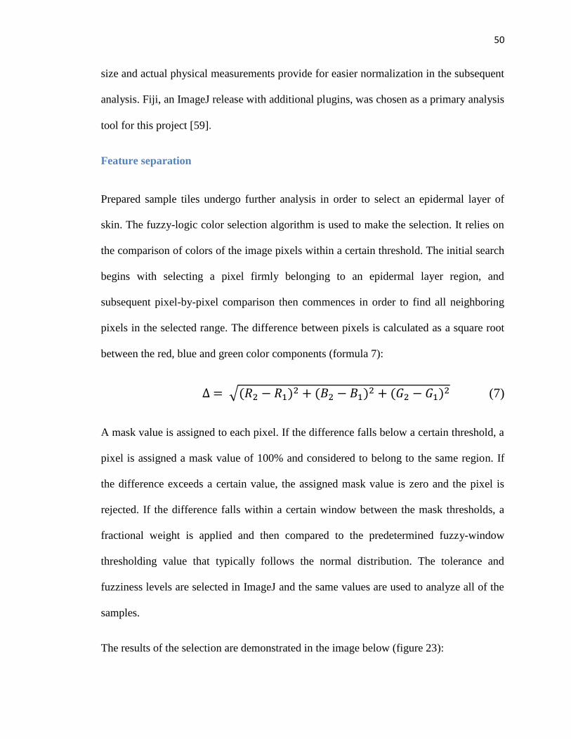
50

size and actual physical measurements provide for easier normalization in the subsequent

analysis. Fiji, an ImageJ release with additional plugins, was chosen as a primary analysis

tool for this project [59].

Feature separation

Prepared sample tiles undergo further analysis in order to select an epidermal layer of

skin. The fuzzy-logic color selection algorithm is used to make the selection. It relies on

the comparison of colors of the image pixels within a certain threshold. The initial search

begins with selecting a pixel firmly belonging to an epidermal layer region, and

subsequent pixel-by-pixel comparison then commences in order to find all neighboring

pixels in the selected range. The difference between pixels is calculated as a square root

between the red, blue and green color components (formula 7):

∆ = √(𝑅2 − 𝑅1)2 + (𝐵2 − 𝐵1)2 + (𝐺2 − 𝐺1)2 (7)

A mask value is assigned to each pixel. If the difference falls below a certain threshold, a

pixel is assigned a mask value of 100% and considered to belong to the same region. If

the difference exceeds a certain value, the assigned mask value is zero and the pixel is

rejected. If the difference falls within a certain window between the mask thresholds, a

fractional weight is applied and then compared to the predetermined fuzzy-window

thresholding value that typically follows the normal distribution. The tolerance and

fuzziness levels are selected in ImageJ and the same values are used to analyze all of the

samples.

The results of the selection are demonstrated in the image below (figure 23):

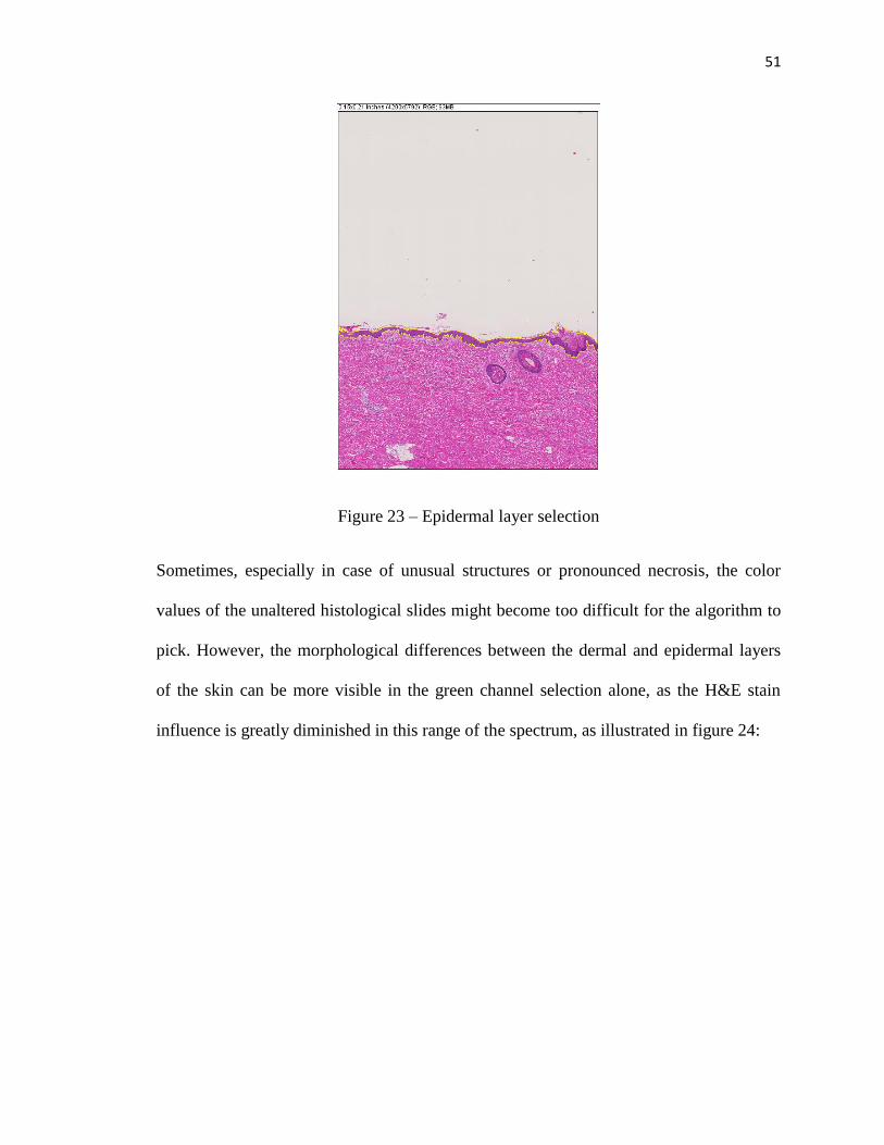
51

Figure 23 – Epidermal layer selection

Sometimes, especially in case of unusual structures or pronounced necrosis, the color

values of the unaltered histological slides might become too difficult for the algorithm to

pick. However, the morphological differences between the dermal and epidermal layers

of the skin can be more visible in the green channel selection alone, as the H&E stain

influence is greatly diminished in this range of the spectrum, as illustrated in figure 24:

52

Figure 24 – Epidermal layer selection: A) original slide; B) Green channel selection only

As can be seen from figure 24, while selection at the original slide image proves to be

difficult for the algorithm, the selection applied to the green channel layer only can help

depict subtle morphological structures between the epidermal and dermal layer even with

a high degree on necrosis present.

The selected region can then be applied to the combination of the red and blue channels

containing the information pertaining to the spread of the H&E stain [60]. By adding the

information from blue and red channels, we can highlight the pyknotic nuclei of the

keratinocytes specifically, as they accumulate the majority of the stain. The binary mask

is then applied to the selected epidermal layer (figure 25):

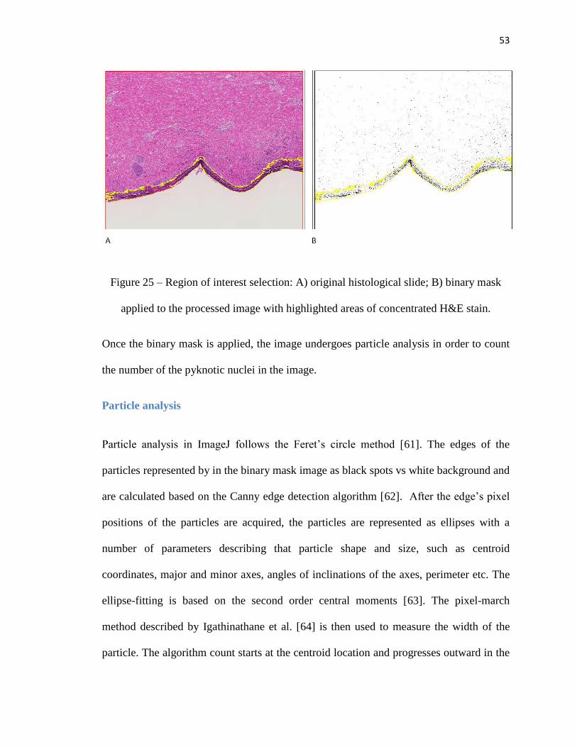
53

Figure 25 – Region of interest selection: A) original histological slide; B) binary mask

applied to the processed image with highlighted areas of concentrated H&E stain.

Once the binary mask is applied, the image undergoes particle analysis in order to count

the number of the pyknotic nuclei in the image.

Particle analysis

Particle analysis in ImageJ follows the Feret’s circle method [61]. The edges of the

particles represented by in the binary mask image as black spots vs white background and

are calculated based on the Canny edge detection algorithm [62]. After the edge’s pixel

positions of the particles are acquired, the particles are represented as ellipses with a

number of parameters describing that particle shape and size, such as centroid

coordinates, major and minor axes, angles of inclinations of the axes, perimeter etc. The

ellipse-fitting is based on the second order central moments [63]. The pixel-march

method described by Igathinathane et al. [64] is then used to measure the width of the

particle. The algorithm count starts at the centroid location and progresses outward in the

54

search direction by differentiating between the pixel colors (white and black in binary

mask scenario). The slope of the search line comes from the minor axis ellipse-fitting

parameters calculated beforehand [63] The minor axis boundary is determined once the

pixel values switch from black to white. The length of the particle is determined through

the Feret’s diameter or the distance between two parallel tangents on the opposite sides of

the image of a randomly oriented particle. The pixel-marched method only works for the

convex-shaped particles. The roundness of the particle is estimated as:

𝑅𝑜𝑢𝑛𝑑𝑛𝑒𝑠𝑠 =4∗𝐴𝑟𝑒𝑎

𝜋∗𝐹𝑒𝑟𝑒𝑡′𝑠 𝑑𝑖𝑎𝑚𝑒𝑡𝑒𝑟2 (8)

As the non-circle shaped particles are unlikely to be pyknotic cell nuclei, once the

roundness parameter falls below the certain threshold, they are automatically discarded

from the analysis and pixel-marched method’s limitations become irrelevant to the

purpose of this research. The overall representation of the particle in the course of

particle analysis is provided in figure 26:

55

Figure 26 – Pixel-march algorithm depicting a particle analysis

In figure 26, 𝐿𝑊̅̅̅̅̅ corresponds to the length of the particle calculated as Feret’s diameter

of the smallest enclosing circle, and 𝑁𝑆̅̅ ̅̅ is its width. The fitted ellipse helps estimate the

size of the particle and its roundness by taking into account the ratio between the major

and minor axes.

Particle analysis is performed via the “Analyze particles” plug-in in the ImageJ. The

menu allows to specifically choose the size of the particles of interest in square microns

as well as pixels, circularity, and summarizes the results with the overall particle count,

area covered by the counted particles (in square microns) and the average size of

particles. It should be noted that while the average healthy cell nuclei is usually 10

microns in diameter, the pyknotic nucleus tends to be smaller in size due to the chromatin

56

condensation, a fact established in the previous studies [65]. Thus the boundaries of

search have to be expanded. The results of the morphological changes in the cell nuclei

structure, in particular nuclei diameter, will be presented below.

The accuracy of the particle counting algorithm has been confirmed by comparing the

count results with the manual counting analysis, and the difference doesn’t exceed 0.5%.

Statistical analysis

In order to estimate the mean and variance of the samples belonging to a separate RTOG

grade, all samples were assigned a group in accordance with histopathologist’s

assessment and mean and variance were calculated as:

𝑚𝑒𝑎𝑛𝑔𝑟𝑎𝑑𝑒 = ∑ 𝑥𝑖

𝑁𝑖=1

𝑁 (9)

𝑆𝑇𝐷𝑔𝑟𝑎𝑑𝑒 = √∑ (𝑥𝑖−𝑚𝑒𝑎𝑛)2𝑁

𝑖=1

𝑁−1 (10)

Where N – number of samples assigned to a particular RTOG grade, 𝑥𝑖 – particular

sample in that the data sample pool.

As the number of samples available in the data sample pool was small, central limit

theorem might have not been sufficient to determine the type of distribution of the

samples in each grade. In order to rectify the problem, kernel density estimation, a non-

parametric method to estimate the probability density function, has been utilized. The

estimation of the probability density function in this scenario can then be presented as:

𝑓ℎ̂(𝑥) = 1

𝑛ℎ∑ 𝐾(

𝑥−𝑥𝑖

ℎ)𝑛

𝑖=1 (11)

57

Where K is the kernel and ℎ > 0 is the smoothing parameter called bandwidth that is

chosen in accordance with the mean integrated square error. The Epanechnikov

(parabolic) kernel is chosen in this scenario as being optimal [66]. The kernel is then

calculated as:

𝐾(𝑢) = 3

4(1 − 𝑢2) (12)

As the kernel density estimation established the normal distribution of the samples within

the grade group, Student’s two-tail t-test could then be utilized in order to establish the

significant difference between the associated grades’ means and variances. In order to

determine whether or not the variances of the groups are different and which statistical

test should be utilized, Bartlett’s test is used. A Welch’s variation of the Student’s t-test is

particularly useful in this scenario as the groups have an unequal number of samples and

unequal variances [67]. The ratio of the difference between the two groups and the

difference within the group, also known as t-score, is estimated as:

𝑡 = 𝑀1−𝑀2

√𝑠1

2

𝑁1+

𝑠22

𝑁2

(13)

In order to determine the sample’s grade automatically, a naive Bayesian classifier is

utilized. The idea of classification in this particular scenario follows the probability

model presented as:

𝑝(𝐶|𝑥1, 𝑥2, … , 𝑥𝑛) = 𝑝(𝐶)𝑝(𝑥1,𝑥1,…,𝑥𝑛|𝐶)

𝑝(𝑥1,𝑥2,…,𝐹𝑥𝑛) (14)

58

Here 𝑥1, 𝑥1, … , 𝑥𝑛 are independent features (such as the number of dead cells and the

spread of the lesions) of the particular class (RTOG grades 0-4). An assumption is made

that the characteristics are independent of each other. As has already been established, the

probabilities of the particular sample belonging to a particular RTOG grade follow the

normal distribution. As we do not know the probabilities of the particular sample to

belong to a certain grade, these probabilities are established based on the graded samples

as:

𝑝�̂� = 𝑛𝑖

𝑛 (15)

Where i = 0,…, 4 in accordance with RTOG grade assigned by the histopathologist, n =

95 (number of irradiated samples demonstrating good central positioning of the resulting

wound). The class (RTOG grade) is then assigned to a particular sample is

𝑐𝑙𝑎𝑠𝑠(0, … ,4) = argmax𝑐 𝑝(𝐶 = 𝑐) ∏ 𝑝(𝐹𝑖 = 𝑓𝑖|𝐶 = 𝑐)4𝑖=0 (16)

Which is an estimation by the maximum likelihood method. It is a special case of a

maximum a posteriori estimation.

RESULTS

In the course of the study 120 samples have been analyzed, with the rated RTOG levels

of CRI and RD ranging from zero (no symptoms) to four (severe necrosis and ulceration).

The number of the dead cells in the epidermal layer of skin has been recorded across the

spread of the sample and correlated with the visible injuries. The results of the analysis of

a single sample are presented in figure 27:

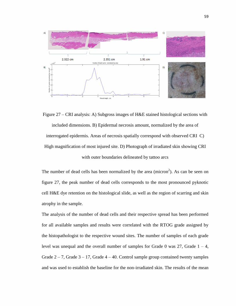
59

Figure 27 – CRI analysis: A) Subgross images of H&E stained histological sections with

included dimensions. B) Epidermal necrosis amount, normalized by the area of

interrogated epidermis. Areas of necrosis spatially correspond with observed CRI C)

High magnification of most injured site. D) Photograph of irradiated skin showing CRI

with outer boundaries delineated by tattoo arcs

The number of dead cells has been normalized by the area (micron2). As can be seen on

figure 27, the peak number of dead cells corresponds to the most pronounced pyknotic

cell H&E dye retention on the histological slide, as well as the region of scarring and skin

atrophy in the sample.

The analysis of the number of dead cells and their respective spread has been performed

for all available samples and results were correlated with the RTOG grade assigned by

the histopathologist to the respective wound sites. The number of samples of each grade

level was unequal and the overall number of samples for Grade 0 was 27, Grade 1 – 4,

Grade 2 – 7, Grade 3 – 17, Grade 4 – 40. Control sample group contained twenty samples

and was used to establish the baseline for the non-irradiated skin. The results of the mean

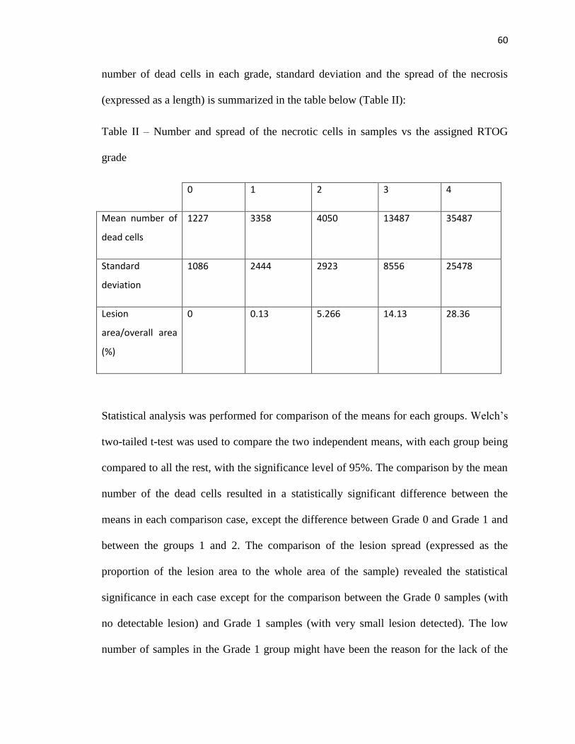
60

number of dead cells in each grade, standard deviation and the spread of the necrosis

(expressed as a length) is summarized in the table below (Table II):

Table II – Number and spread of the necrotic cells in samples vs the assigned RTOG

grade

0 1 2 3 4

Mean number of

dead cells

1227 3358 4050 13487 35487

Standard

deviation

1086 2444 2923 8556 25478

Lesion

area/overall area

(%)

0 0.13 5.266 14.13 28.36

Statistical analysis was performed for comparison of the means for each groups. Welch’s

two-tailed t-test was used to compare the two independent means, with each group being

compared to all the rest, with the significance level of 95%. The comparison by the mean

number of the dead cells resulted in a statistically significant difference between the

means in each comparison case, except the difference between Grade 0 and Grade 1 and

between the groups 1 and 2. The comparison of the lesion spread (expressed as the

proportion of the lesion area to the whole area of the sample) revealed the statistical

significance in each case except for the comparison between the Grade 0 samples (with

no detectable lesion) and Grade 1 samples (with very small lesion detected). The low

number of samples in the Grade 1 group might have been the reason for the lack of the

61

distinction between the grades in this particular case, as the application of the central

limit theorem becomes somewhat limited.

The summary of the statistical comparisons between the means of different groups is

summarized below:

Table III – P-values for the comparison between the mean number of dead cells

0 1 2 3 4

0 X 0.17 0.047 <0.0001 <0.0001

1 0.17 X 0.7 <0.0001 <0.0001

2 0.047 0.7 X 0.0008 <0.0001

3 <0.0001 <0.0001 0.0008 X <0.0001

4 <0.0001 <0.0001 <0.0001 <0.0001 X

Table IV – P-values for the comparison between the mean lesion spread proportional

percentage of the overall area of the sample

0 1 2 3 4

0 X 0.18 0.006 <0.0001 <0.0001

1 0.18 X 0.03 0.004 0.000061

2 0.006 0.03 X 0.001 <0.0001

3 <0.00001 0.004 0.001 X <0.0001

4 <0.00001 0.000061 <0.0001 <0.0001 X

The spread of the values of dead cells belonging to each class within the class and in

comparison to each other is presented on the diagram below:

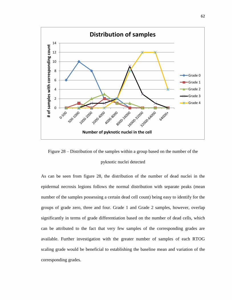
62

Figure 28 – Distribution of the samples within a group based on the number of the

pyknotic nuclei detected

As can be seen from figure 28, the distribution of the number of dead nuclei in the

epidermal necrosis legions follows the normal distribution with separate peaks (mean

number of the samples possessing a certain dead cell count) being easy to identify for the

groups of grade zero, three and four. Grade 1 and Grade 2 samples, however, overlap

significantly in terms of grade differentiation based on the number of dead cells, which

can be attributed to the fact that very few samples of the corresponding grades are

available. Further investigation with the greater number of samples of each RTOG

scaling grade would be beneficial to establishing the baseline mean and variation of the

corresponding grades.

0

2

4

6

8

10

12

14

# o

f sa

mp

les

wit

h c

orr

esp

on

din

g co

un

t

Number of pyknotic nuclei in the cell

Distribution of samples

Grade 0

Grade 1

Grade 2

Grade 3

Grade 4

63

The distribution of the samples in accordance to the percentage of the area of the lesion in

comparison with the overall area of the epidermis is depicted in figure 29:

Figure 29 – Distribution of the samples within a group based on the number of the

percentage of the area of the lesion in comparison to the overall area of the epidermis

As can be observed from figure 29, while less obvious, the ratios of the lesion area vs the

overall area of the sample still follow the normal distribution. Grade 4, possessing the

highest amount of samples within the group, presents the clearest normal distribution

pattern with the mean ratio of the lesion area to the overall area of the sample at around

30. Grade 0 samples are omitted from this graph as not lesion is discernable and the

percent ratio is always zero. Probabilities of a particular sample belonging to each class

in the provided 120 samples set are:

0

2

4

6

8

10

12

14

0-0.5 0.5-1 1-2 2-4 4-8 8-12 12-1818-2626-3434-4242-50 50+

# o

f sa

mp

les

Percent ratio of lesion area/overall area

Distribution of samples

Grade 1

Grade 2

Grade 3

Grade 4

64

𝑝0 = 0.28

𝑝1 = 0.04

𝑝2 = 0.07

𝑝3 = 0.18

𝑝4 = 0.42

The probabilities of the particular samples within a class to have a certain range of

features are presented in Table V:

Table V – Probabilities of the features of the samples belonging to a class to take a

certain range of values

Length \NCC 0-500

500-1000 1k-2k 2k-4k 4k-8k 8k-16k

16k-32k

32k-64k 64+

0-0.5 0 0 0 0 0 0 0 0 0

0 0.0625 0 0.125 0.0625 0 0 0 0

0 0 0 0 0 0 0 0 0

0 0 0 0 0 0 0 0 0

0 0 0 0 0 0 0 0 0

0.5-1 0 0 0 0 0 0 0 0 0

0 0.125 0 0.25 0.125 0 0 0 0

0 0 0.0407 0.0605 0.0204 0.0204 0 0 0

0 0 0 0 0 0 0 0 0

0 0 0 0 0 0 0 0 0

1-2 0 0 0 0 0 0 0 0 0

0 0 0 0 0 0 0 0 0

0 0 0.0407 0.0605 0.0204 0.0204 0 0 0

0 0 0 0 0 0 0 0 0

0 0 0 0 0 0 0 0 0

2-4 0 0 0 0 0 0 0 0 0

0 0.0625 0 0.125 0.0625 0 0 0 0

65

0 0 0 0 0 0 0 0 0

0 0 0.0035 0.0035 0.007 0.0311 0.0103 0.0035 0

0 0 0 0 0 0 0 0 0

4-8 0 0 0 0 0 0 0 0 0

0 0 0 0 0 0 0 0 0

0 0 0.16245 0.24111 0.08151 0.0815 0 0 0

0 0 0.0138 0.0138 0.0276 0.124 0.04136 0.0138 0

0 0 0 0 0.00125 0.005 0.0075 0.0075 0.0038

8-12 0 0 0 0 0 0 0 0 0

0 0 0 0 0 0 0 0 0

0 0 0.0407 0.0605 0.0204 0.0204 0 0 0

0 0 0.0173 0.0173 0.034 0.156 0.052 0.0173 0

0 0 0 0 0.00375 0.015 0.0225 0.0225 0.0113

12-18 0 0 0 0 0 0 0 0 0

0 0 0 0 0 0 0 0 0

0 0 0 0 0 0 0 0 0

0 0 0.0035 0.0035 0.007 0.0311 0.0103 0.0035 0

0 0 0 0 0.0075 0.03 0.045 0.045 0.0225

18-26 0 0 0 0 0 0 0 0 0

0 0 0 0 0 0 0 0 0

0 0 0 0 0 0 0 0 0

0 0 0.0173 0.0173 0.034 0.156 0.052 0.0173

0 0 0 0 0.0075 0.03 0.045 0.045 0.0225

26-34 0 0 0 0 0 0 0 0 0

0 0 0 0 0 0 0 0 0

0 0 0 0 0 0 0 0 0

0 0 0.0069 0.0069 0.0137 0.062 0.0206 0.0069 0

0 0 0 0 0.015 0.06 0.09 0.09 0.045

34-42 0 0 0 0 0 0 0 0 0

0 0 0 0 0 0 0 0 0

0 0 0 0 0 0 0 0 0

0 0 0 0 0 0 0 0 0

0 0 0 0 0.00875 0.035 0.0525 0.0525 0.02625

42-50 0 0 0 0 0 0 0 0 0

0 0 0 0 0 0 0 0 0

0 0 0 0 0 0 0 0 0

0 0 0 0 0 0 0 0 0

0 0 0 0 0.005 0.02 0.03 0.03 0.015

50+ 0 0 0 0 0 0 0 0 0

0 0 0 0 0 0 0 0 0

66

0 0 0 0 0 0 0 0 0

0 0 0 0 0 0 0 0 0

0 0 0 0 0.00125 0.005 0.0075 0.0075 0.00375

In Table V, Grade 0 is highlighted by green, Grade 1 – by yellow, Grade 2 – by orange,

Grade 3 – by pink, Grade 4 – by red. The values utilized to calculate the overall

probability of the correct grade identification are highlighted by blue and then multiplied

by the corresponding probability of the sample belonging to a particular class. Overall,

the probability of the successful identification is 0.57, or 57%, with the probability of an

error being 43%. Unfortunately, the use of a naïve Bayesian classifier showed that the

classification between the neighboring grades (0 and 1, 1 and 2, 2 and 3, 3 and 4) is often

prone to errors and would require more samples in the training set before a precise

classifier could be developed. Better results are achieved in classifying between the

grades with higher differential, with the probability of correct grade identification rising

to 70% when Grades 1 and 2 are combined into a single class.

67

DISCUSSION

The semi-automated, quantitative analysis of epidermal necrosis performed in this study

provides an objective assessment of the severity of CRI that is rapid and free of bias. The

approach represents a viable tool for evaluating the degree of injury when digitized

images of biopsy samples are available, such as for the purposes of CRI research. The

quantified number of pyknotic cells and the spread of damaged cells across the lesion

correlate with the grade of damage as determined by a pathologist. The image-based

analysis was automated using a novel ImageJ plugin designed specifically for detection

of epidermal necrosis.

This study presents proof of feasibility for the proposed algorithm for automated

assessment of the epidermal necrosis in the case of radiation-induced injury. At the

present, some uncertainty about the feasibility of using the algorithm to differentiate

between grades in the borderline cases remains, as was evidenced by the high overlap

between different grades in figure 6, however, further refinement to the algorithm can be

made provided a larger teaching set and overall principle should be applicable between

all grades once the algorithm is further trained. Further studies with expanded sample sets

are required in order to establish the definite distinctions between the various grades of

the severity of epidermal necrosis based on the RTOG or other scales used in a clinical

setting. An extended study with a higher number of test samples over all grades of injury

is a future direction.

The correlation of the areal distribution of epidermal necrosis across the irradiated area,

requiring serial biopsy samples to be taken over the observation period, e.g., seventy

days, and the microdosimetry characteristics of the radiation dose delivered, might

68

provide important insights into the healing process. The automated grading algorithm

based on the dead cell count and areal spread of the lesion area could potentially be a

valuable research tool, improving efficiency of histological analysis, consistent and

measurable quality, and eliminating potential observer bias of the human-based

evaluation. A more thorough study with the expanded number of samples in each grading

group will be beneficial for the establishment of the complete set of the training

examples.

This particular study introduces an innovative method aimed at reducing costs and

increasing efficiency of preclinical research studies by providing a rapid, automated and

unbiased approach to quantify the extent of cellular and tissue level damage, while still

measuring a response that correlates well with histopathologic grading. Given digitized

histology images of biopsy samples, this technique will permit the rapid, independent

assessment of CRI, or perhaps radiation injury in other organ systems, when introduced

as a part of the overall research strategy. However, further refinements based on the

larger training dataset are still required and will be implemented in order to provide better

specificity of the method.

69

CHAPTER 2: Monte Carlo simulation of the beta source irradiation device

MATERIALS AND METHODS

Monte Carlo simulation basics

The approximation function used in analytical calculation of dose is usually a linear

approximation of Lambert-Beer’s law extrapolated over the whole multitude of particles

released due to the radioactive source activity, and as such the particles are usually

treated as a single entity during the dose calculation. In contrast, Monte Carlo simulation

is based on tracking the histories of individual particles and simulating the statistical

processes theoretically through an extensive system of equations describing the potential

interactions of electron and proton particles. The Monte Carlo method solves an integral

form of the Boltzmann equation through a notion of random sampling. The individual

probabilistic events that comprised a process are simulated sequentially, and with enough

particle histories being traced it becomes possible to predict the overall behavior of the

radiation originating at the source location and its interaction with the different media in

the outer world. The Boltzmann transport equation underlying the principle of radiation

transport can be presented as [68]:

𝛹(𝑟, 𝑣) = ∫[∫ 𝛹(𝑟′, 𝑣′)𝐶(𝑣′ → 𝑣, 𝑟′)𝑑𝑣′ + 𝑄(𝑟′, 𝑣′)]𝑇(𝑟′ → 𝑟, 𝑣)𝑑𝑟′ (17)

Where

𝛹(𝑟, 𝑣) = particle collision density

𝑄(𝑟′, 𝑣′) = source term

𝐶(𝑣′ → 𝑣, 𝑟′) = collision kernel, change velocity at fixed position

𝑇(𝑟′ → 𝑟, 𝑣) = transport kernel, change position at fixed velocity

70

Within a certain volume the particle is passing through, the following assumptions are

made to ensure the fidelity of the Monte Carlo approach for radiation transport:

- Static, homogeneous medium

- Time-independence

- Markovian – next event depends only on current (r,v,E), not on previous events

- Particles tracked as parts of different history runs don’t interact with each other

- Neglect relativistic effects

- Material properties are not affected by particle reactions

The basis for Monte Carlo solution method lies in the following:

1) Let 𝑝 = (𝑟, �⃗�) and 𝑅(𝑝′ → 𝑝) = 𝐶(𝑣′ → 𝑣, 𝑟′) ∗ 𝑇(𝑟′ → 𝑟, 𝑣)

2) Expand 𝛹 into having k collisions

𝛹(𝑝) = ∑ 𝛹𝑘(𝑝)∞𝑘=0 with 𝛹0(𝑝) = ∫ 𝑄(𝑟′, 𝑣)𝑇(𝑟′ → 𝑟, 𝑣)𝑑𝑟′

3) By definition

𝛹𝑘(𝑝) = ∫ 𝛹𝑘−1 (𝑝′) ∗ 𝑅(𝑝′ → 𝑝)𝑑𝑝′

4) After repeated substitution for 𝛹𝑘

𝛹𝑘(𝑝) = ∫ 𝛹𝑘−1 (𝑝′) ∗ 𝑅(𝑝′ → 𝑝)𝑑𝑝′ = ∫ … ∫ 𝛹0 (𝑝0) ∗ 𝑅(𝑝0 → 𝑝1) ∗

𝑅(𝑝1 → 𝑝2) … ∗ 𝑅(𝑝𝑘−1 → 𝑝 ) ∗ 𝑑𝑝0 … 𝑑𝑝𝑘−1 (18)

With this approach, a “history” becomes a sequence of states (p0, p1, p2…,pk) and a

“tally” marks the occurrences for each collision of each history within a region.

With these criteria the Monte Carlo approach is then implemented by:

71

1) Generating a sequence of states (p0, p1, p2…,pk), or a history, by:

- Randomly sampling for source 𝛹0(𝑝0)

- Randomly sampling for kth

transition 𝑅(𝑝𝑘−1 → 𝑝𝑘)

2) Generating estimates of results by averaging over states for M histories:

𝐴 = ∫ 𝐴(𝑝) ∗ 𝛹(𝑝)𝑑𝑝 ≈1

𝑀∗ ∑ (∑ 𝐴(𝑝𝑘,𝑚

∞𝑘=1

𝑀𝑚=1 )) (19)

Collisions are modeled analytically using physics equations and with validated cross-

section data retrieved from the internal databases. Collisional physics modeling involves

determining, which isotope the interaction is with and the interaction type for that

isotope, energy, and direction of exiting particle, as well as any secondary particles that

might have been produced during this interaction. For the electrons, the collisional

stopping power and radiative stopping powers are considered to determine the energy of

the electron, and angular deflection is considered in accordance with Goudsmit-

Saunderson theory for the probability distribution of angular deflections [69]. For

photons, coherent (Raleigh) and incoherent (Compton) scattering are considered, as well

as photoelectric effect and pair production, cross-sections for which are derived from

tabulated values [70][71]. Tallying of the quantities of interest, such as energy deposited,

also occurs at this step. Free flight between collisions is modeled using computational

geometry based on the user’s input. For the charged particles that experience continuous

slowing down and are characterized by an extremely torturous path, delta tracking (also

called Woodcock tracking, fast tracking, or hole tracking) is often implemented to cut

down on the calculation time. It utilizes a fictitious cross-section to process the number of

particles experiencing similar interactions in “batches” and lower the number of steps

charged particles will go through the matter before finally stopping [72]. The occurrences

72

of events in each region are tallied as specified. All secondary particles generated along

the path are also modeled within this history run. Tallies are then averaged depending on

the number of the runs. The validity of the tally statistics is supported by Central Limit

Theorem. As the Monte Carlo runs tend to require a lot of computational power and

significant time, several variance reduction techniques exist, allowing to run a fewer

number of histories without affecting the statistical significance of the tallies. Some of the

most popular variance reduction techniques include truncation method, population

control method, sampling modification method, partially deterministic method, as well as

energy cut-off, time cut-off and geometry splitting with Russian roulette [72]. The

underlying principles behind the MCNP run are presented in the following diagram:

Figure 30 – Monte Carlo simulation run

73

Monte Carlo simulation has long been proven to be an accurate and relevant model of the

dose deposition and as thus has been utilized in research and clinical practice for decades.

Multiple bench tests have been implemented to rigorously test the accuracy of the various

Monte Carlo packages currently in use, and experimental confirmation remains an

important part of testing the validity of the Monte Carlo models of a particular system.

The systems currently on the market and used in the clinical setting include, but are not

limited to: CARMEN (EGSnrc based), CERR, Corvus (PEREGRINE-based), Eclipse

(MMC based), eIMRT (EGSnrc based), iPlan RT Dose, MCDE (EGSnrc based),

MCDOSE (EGS4 based), MCVS (EGSnrc based), MMCTP (EGSnrc based), Monaco,

MSKCC (EGS4 based), Oncentra, Pinnacle, PLanUNC (EGSnrc based), PRIMO

(PENEPOLE based), RTGrid (EGSnrc based), SMCP (EGSnrc based), VIMC (EGSnrc

based), XiO (EGSnrc based) [73]. Research-based code packages available for free

distribution and code modification include EGSnrc, MCNP, GEANT4 and EGS4.

However, one of the most exciting possibilities of using Monte Carlo model for dose

deposition prediction lies in the fact that it is possible to use Monte Carlo modeling in the

conditions where normal experimental measurement might not be feasible, such as

surface dosimetry. The problem of skin surface dosimetry has long been gathering the

attention of researches around the globe and Monte Carlo modeling has proved to be an

excellent solution [2][74]. Modeling skin surface interface with surrounding area allows

for extremely precise dosimetry at the epidermal layer of the skin, normally unachievable

due to ion chamber volumetric constraints. For this purposes, Monte Carlo simulation of

the beta radiation device and the upper skin layers is developed.

74

The MCNP6 package is used for this particular research study. MCNP is a general

purpose Monte Carlo N-Particle code that can be used for neutron, photon, electron and

coupled neutron/photon/electron particles problem. It’s a successor of its predecessor,

MCNP5 code, which in turn has been a result of long development conducted by Los

Alamos National Lab dating back to the Manhattan Project. The timeline of MCNP6

development is presented below:

Figure 31 – MCNP 6 history [75], image is in the public domain

MNCP6 release package includes codes for MCNP6.1, MCNP5-1.60, MCNPX2.7,

nuclear data libraries, and MCNP reference collection. The overall number of the particle

types available for simulation is 37. The range of simulated particle transports at different

energy ranges covered by MCNP6 simulation is presented in figure 32:

75

Figure 32 – MCNP6 simulation range in terms of particle types and energies [72]

The MNCP6 package is widely used in the research for solving the problems of radiation

dosimetry, detection, shielding, nuclear reactor modeling, radiography, and other related

fields. It has flexible tally structures, including several energy deposition tally options for

different types of particles, making it particularly suited towards dose measurement. The

cross-section data included with MCNP6 package is one of the most extensive in the field

[76]. ETRAN-integrated TIGER electron/photon transport implemented in MCNP6

package is one of the most accurate and updated electron transport mechanism currently

available. [77]. The MCNP6 code provides for geometry and tally plotting via UNIX-

based X-Windows interfaces. MCNP6 package can be configured for multiprocessing

mode to drastically cut on the calculation time. In this particular research project, an

agreement with Los Alamos National Laboratory (LANL) provided use of MCNP6 and

allowed for a use of 64-core supercomputer for increase performance. MNCP6 code

undergoes extensive testing and has continued user support and patch upgrades issued by

LANL in conjunction with the Radiation Safety Information Computational Center

76

(RSICC), which makes it more reliable than GEANT4 and EGSnrc, two other packages

commonly used in research. With this in mind, MCNP6 package was chosen for this

research project.

MCNP6 functionality

The MCNP6 package allows for input customization through the scripted input files.

Structure of the input file for MCNP includes:

- File Title

- Cell cards

- Surface cards

- Data cards

Card entry begins in the first 5 columns and can contain a maximum of 80 columns

(symbols including blanks). In case more than 80 symbols are required, special syntax

rules exist to allow linking between different lines into a single entry. Both upper and

lower case can be used.

The geometry of the radiation problem is specified by cell cards. A cell is an enclosed

volume filled with a material of a certain density and composition that has boundaries

specified by surfaces. While radiation dose “at a point” may be of interest, MCNP6 is a

statistical program that can only calculate dose within a volume for the electron particles.

Cells contain homogeneous materials and as such have a constant cross-section. Cells are

usually the volumetric units for which tallies are defined, though certain exemptions can

exist for surfaces tallies (defined by a certain surface, an area through which radiation

propagates) or mesh tallies that create a mesh of measuring points throughout the cell.

Sometimes cells can be subdivided for variance reduction. Each region of the simulation

77

needs to be defined as belonging to a certain cell. The importance of a certain type of

particles being traced in the particular cell can be assigned. All problems defined in

MCNP should have an “outside cell” filled with vacuum in which particle tracking stops

and the importance of all particles is zero. Cell assignment follows a certain format

illustrated in figure 33:

Figure 33 – Cell representation in MCNP6

As can be seen in figure 33, all cells are assigned their unique ID numbers by which they

are defined in the simulation. Cells cannot overlap and clear distinction between the

surfaces defining each cell has to be made.

Surfaces defining the cell boundaries are usually designated by the mnemonics. Typically

cells are defined by infinite planes, cylinders, and cones. All coordinates for the surface

definition are given in a Cartesian three-dimensional coordinate system. However, in

MCNP6, commonly used macrobodies also exist to provide surface definition for

common repetitive shapes such as a finite cylinder, box and sphere. All dimensions of the

surface positioning are expressed in centimeters. The list of mnemonics for the basic

planes is presented in Table VI [72]. The list of macrobodies available in MCNP in

presented in Table VII [72].

78

Table VI – MCNP input mneumonics

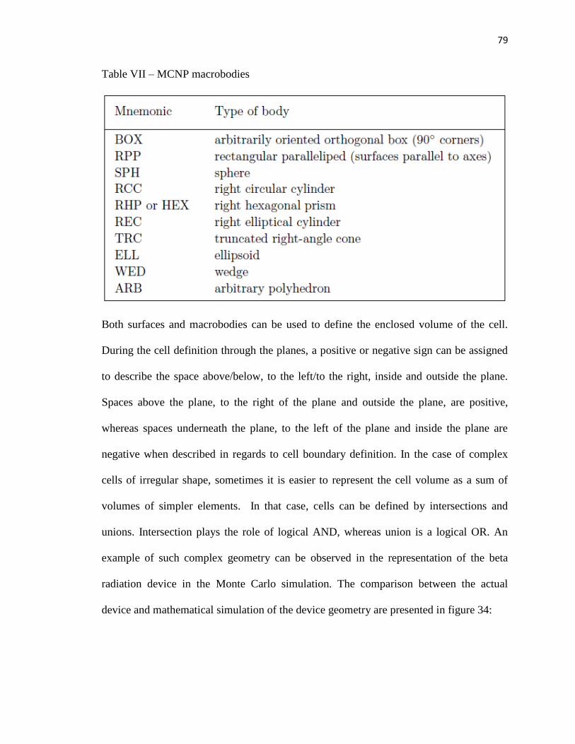
79

Table VII – MCNP macrobodies

Both surfaces and macrobodies can be used to define the enclosed volume of the cell.

During the cell definition through the planes, a positive or negative sign can be assigned

to describe the space above/below, to the left/to the right, inside and outside the plane.

Spaces above the plane, to the right of the plane and outside the plane, are positive,

whereas spaces underneath the plane, to the left of the plane and inside the plane are

negative when described in regards to cell boundary definition. In the case of complex

cells of irregular shape, sometimes it is easier to represent the cell volume as a sum of

volumes of simpler elements. In that case, cells can be defined by intersections and

unions. Intersection plays the role of logical AND, whereas union is a logical OR. An

example of such complex geometry can be observed in the representation of the beta

radiation device in the Monte Carlo simulation. The comparison between the actual

device and mathematical simulation of the device geometry are presented in figure 34:

80

Figure 34 – Representation of the beta radiation device in MCNP6 package. Upper: beta-

radiation device, including PMMA cone collimator; lower: MCNP6 representation of the

beta radiation device.

As can be observed, the air-filled region forms a complex shape comprised of a number

of cones and cylinders. These shapes are all combined to form a united volume for a

single air-filled cell. This cell can be represented by the following code:

81

2 2 -0.001225 (-11 18 -16):-19:-20:-21:-40:-41:-42:-43:-46:-47&

:-44:-45:-48:-49:-491:-492:-493:-494 60 70 IMP:P=1 IMP:E=1

It should be noted that both intersection and union operators can be used simultaneously.

The dimensions of the simulated beta radiation device cassette and PMMA cone

correspond to the dimensions of the real-life device. The material composition of the

aluminum cassette, steel holders, PMMA cone, air and basic skin model used in the

simulation are encoded via material description datacard. MCNP6 allows one to input

any material composition of the cell as long as the material in question is described as a

proportional sum of elements present in the composition compound. For example, air,

containing 78.09% nitrogen, 20.95% oxygen, 0.93% argon and 0.04% carbon dioxide, is

described as:

M2 007014 -0.780804

008016 -0.209764

018040 -0.0093

006012 -0.000132

Here M2 denotes the material ID number that has been used to assign this material to a

certain cell, first three numbers (007) note the element number in the periodic table

(oxygen has the atomic number 7), and the last three numbers (014) note the atomic

weight of the comprising elements in case of the isotope use. The element contribution to

the overall compound composition is noted in proportion to one, and minus sign notes

that the composition of the compound is encoded in proportions.

The materials used in modeling of the beta radiation device include an aluminum holder,

steel source cassettes, PMMA collimator cone, air filler, and basic skin layer. The

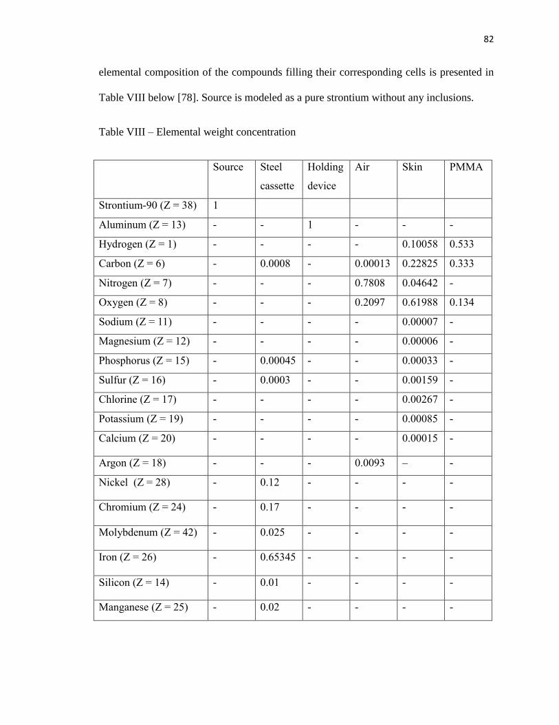
82

elemental composition of the compounds filling their corresponding cells is presented in

Table VIII below [78]. Source is modeled as a pure strontium without any inclusions.

Table VIII – Elemental weight concentration

Source Steel

cassette

Holding

device

Air Skin PMMA

Strontium-90 (Z = 38) 1 - - - - -

Aluminum (Z = 13) - - 1 - - -

Hydrogen (Z = 1) - - - - 0.10058 0.533

Carbon (Z = 6) - 0.0008 - 0.00013 0.22825 0.333

Nitrogen (Z = 7) - - - 0.7808 0.04642 -

Oxygen (Z = 8) - - - 0.2097 0.61988 0.134

Sodium (Z = 11) - - - - 0.00007 -

Magnesium (Z = 12) - - - - 0.00006 -

Phosphorus (Z = 15) - 0.00045 - - 0.00033 -

Sulfur (Z = 16) - 0.0003 - - 0.00159 -

Chlorine (Z = 17) - - - - 0.00267 -

Potassium (Z = 19) - - - - 0.00085 -

Calcium (Z = 20) - - - - 0.00015 -

Argon (Z = 18) - - - 0.0093 – -

Nickel (Z = 28) - 0.12 - - - -

Chromium (Z = 24) - 0.17 - - - -

Molybdenum (Z = 42) - 0.025 - - - -

Iron (Z = 26) - 0.65345 - - - -

Silicon (Z = 14) - 0.01 - - - -

Manganese (Z = 25) - 0.02 - - - -

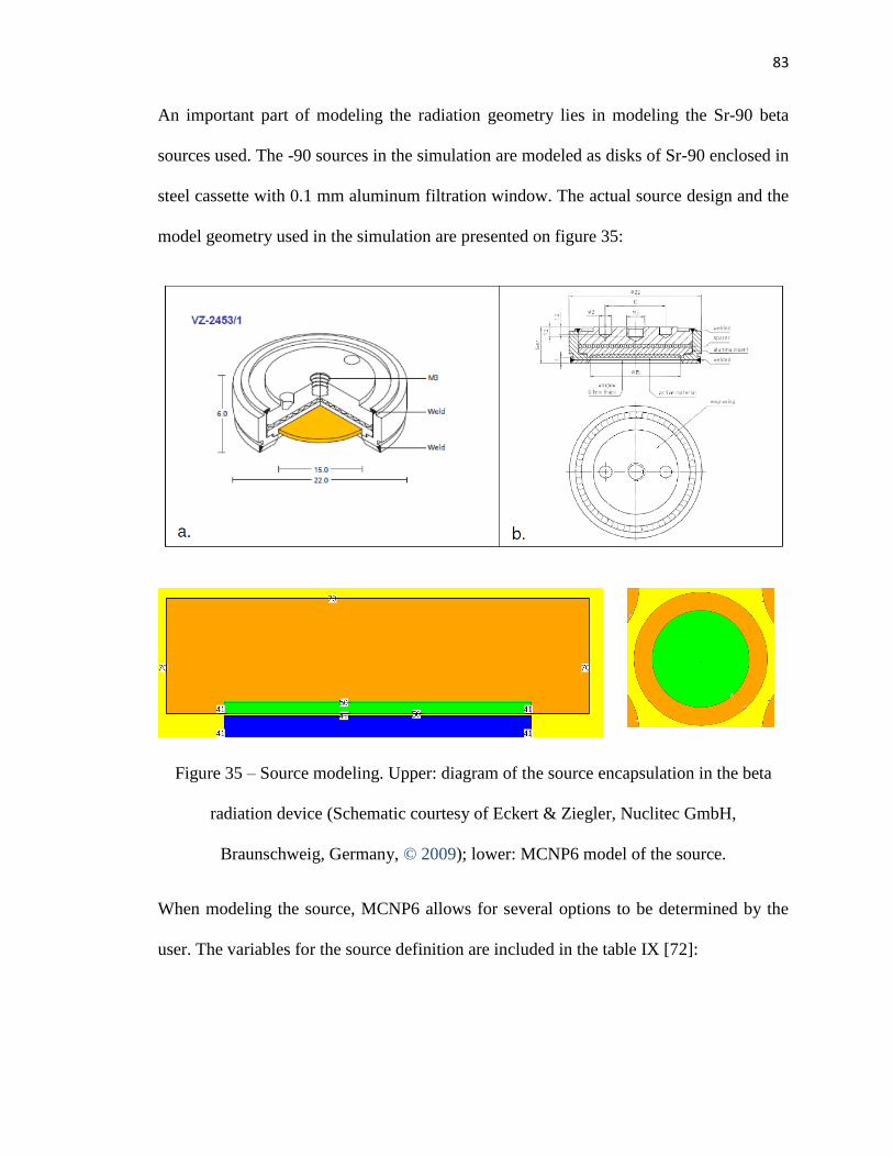
83

An important part of modeling the radiation geometry lies in modeling the Sr-90 beta

sources used. The -90 sources in the simulation are modeled as disks of Sr-90 enclosed in

steel cassette with 0.1 mm aluminum filtration window. The actual source design and the

model geometry used in the simulation are presented on figure 35:

Figure 35 – Source modeling. Upper: diagram of the source encapsulation in the beta

radiation device (Schematic courtesy of Eckert & Ziegler, Nuclitec GmbH,

Braunschweig, Germany, © 2009); lower: MCNP6 model of the source.

When modeling the source, MCNP6 allows for several options to be determined by the

user. The variables for the source definition are included in the table IX [72]:

84

Table IX – Source variables defined by the user

Several options for the variety of sources exist, and in this particular study, seven

cylindrical sources with isotropic distribution have been chosen to represent the

respective Sr-90 sources used in the device. It should be noted that the sources created by

the MCNP6 simulation have an equal probability of the source particle to be generated at

85

any point within the source cylinder volume. However, as has been observed previously,

the original Sr-90 sources have manufacturing processes that make the probabilities of

source particle generation unequal throughout the volume of seven sources. The

illustration of the source inhomogeneity can be found in figure 36:

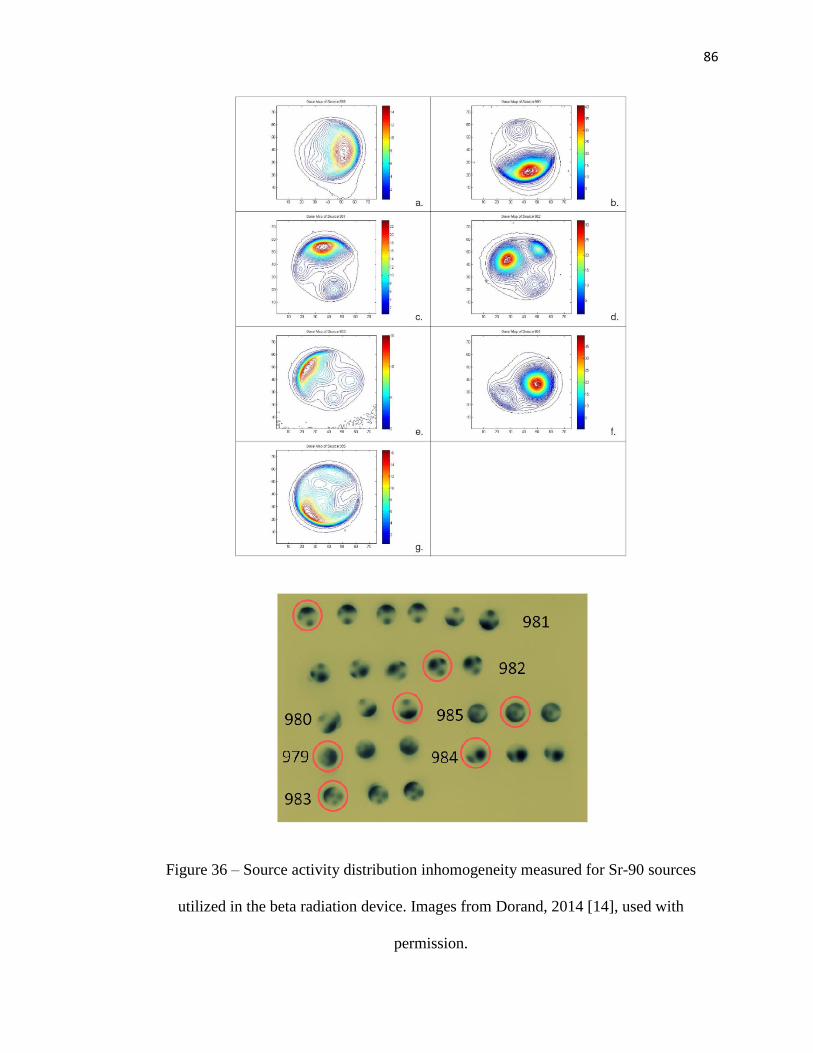
86

Figure 36 – Source activity distribution inhomogeneity measured for Sr-90 sources

utilized in the beta radiation device. Images from Dorand, 2014 [14], used with

permission.

87

This creates additional uncertainty in terms of model validity and should be taken into

account when comparing the percent depth dose curve and the dose profile curves

generated by the Monte Carlo simulation and the ones derived from previous

experimental measurements [14].

The sources described in the MCNP setup are set to generate electron particles of a

particular energy spectrum. The energy spectrum comes from a combined spectrum for

Sr-90 and Y-90 beta particles emitted. As Sr-90 and Y-90 exist in equilibrium and

contribute to the beta emission in 1:1 proportion, the averaged energy over a certain

probabilistic range has been simulated in the model. The corresponding spectra have been

derived from [79] and are presented in figure 37:

Figure 37 – Strontium-90 and Yttrium-90 spectra for beta decay [79]

For the purposes of energy distribution, 20 bins with different energies have been utilized

in this simulation. Corresponding Sr-90, Y-90 and combined spectrum data, including

energy binning and probability distribution, is included in table X [79]:

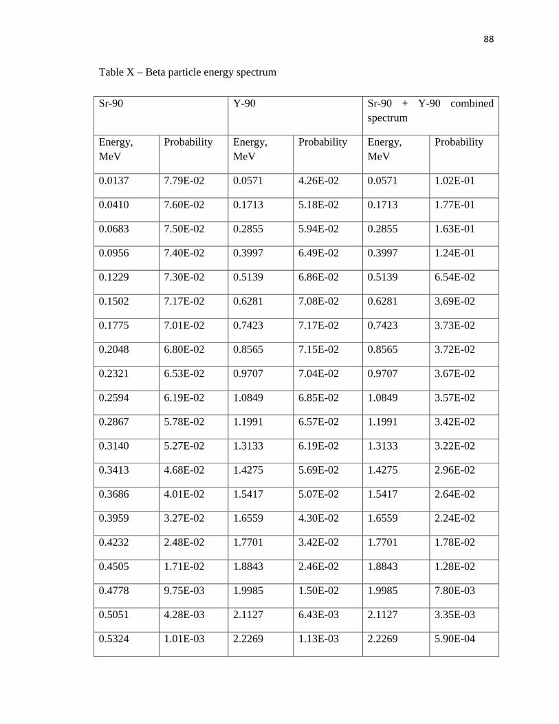
88

Table X – Beta particle energy spectrum

Sr-90 Y-90 Sr-90 + Y-90 combined

spectrum

Energy,

MeV

Probability Energy,

MeV

Probability Energy,

MeV

Probability

0.0137 7.79E-02 0.0571 4.26E-02 0.0571 1.02E-01

0.0410 7.60E-02 0.1713 5.18E-02 0.1713 1.77E-01

0.0683 7.50E-02 0.2855 5.94E-02 0.2855 1.63E-01

0.0956 7.40E-02 0.3997 6.49E-02 0.3997 1.24E-01

0.1229 7.30E-02 0.5139 6.86E-02 0.5139 6.54E-02

0.1502 7.17E-02 0.6281 7.08E-02 0.6281 3.69E-02

0.1775 7.01E-02 0.7423 7.17E-02 0.7423 3.73E-02

0.2048 6.80E-02 0.8565 7.15E-02 0.8565 3.72E-02

0.2321 6.53E-02 0.9707 7.04E-02 0.9707 3.67E-02

0.2594 6.19E-02 1.0849 6.85E-02 1.0849 3.57E-02

0.2867 5.78E-02 1.1991 6.57E-02 1.1991 3.42E-02

0.3140 5.27E-02 1.3133 6.19E-02 1.3133 3.22E-02

0.3413 4.68E-02 1.4275 5.69E-02 1.4275 2.96E-02

0.3686 4.01E-02 1.5417 5.07E-02 1.5417 2.64E-02

0.3959 3.27E-02 1.6559 4.30E-02 1.6559 2.24E-02

0.4232 2.48E-02 1.7701 3.42E-02 1.7701 1.78E-02

0.4505 1.71E-02 1.8843 2.46E-02 1.8843 1.28E-02

0.4778 9.75E-03 1.9985 1.50E-02 1.9985 7.80E-03

0.5051 4.28E-03 2.1127 6.43E-03 2.1127 3.35E-03

0.5324 1.01E-03 2.2269 1.13E-03 2.2269 5.90E-04

89

The overall code for the source description is included below:

SDEF CEL=d1 POS=0 0 3.95999 AXS=0 0 1 EXT=d2 RAD=d3 PAR=3 ERG=d4

SI1 L 4 5 6 7 8 9 10

SP1 0.142857 0.142857 0.142857 0.142847 0.142857 0.142857

0.142857

SI2 H 0 0.0601

SP2 -21 0

SI3 H 0 3.3

SP3 -21 1

SI4 L 0.035375 0.106125 0.176875 0.247625 0.318375 0.389125&

0.459875 0.530625 0.601375 0.672125 0.742875 0.813625 0.884375&

0.955125 1.025875 1.096625 1.167375 1.288125 1.308875 1.379625

SP4 D 0.060206 0.063908 0.067176 0.069487 0.070822 0.071433&

0.070892 0.069763 0.067874 0.065218 0.061719 0.057289 0.05183&

0.045359 0.037843 0.02954 0.020849 0.012366 0.005356 0.00107

Here SDEF denotes that the following lines of code refer to the source, CEL=d1 refers to

the cells included in the geometrical description of the source, where only the points

contained within the cells are treated as valid geometrical starting points for the source

particle, POS, AXS, EXT and RAD further define the geometrical boundaries of the

source, PAR=3 denotes that electron particles are generated at the source, and ERG=d4

denotes the spectrum of the generated particles. SI and SP commands denote the binning

and probabilities for the values that might have probabilistic distribution,

correspondingly.

In order to specify, what results are needed to be given at the end of the simulation,

several tally specifications exist. A list of tallies available for the MCNP6 simulation is

presented in Table XI [72]:

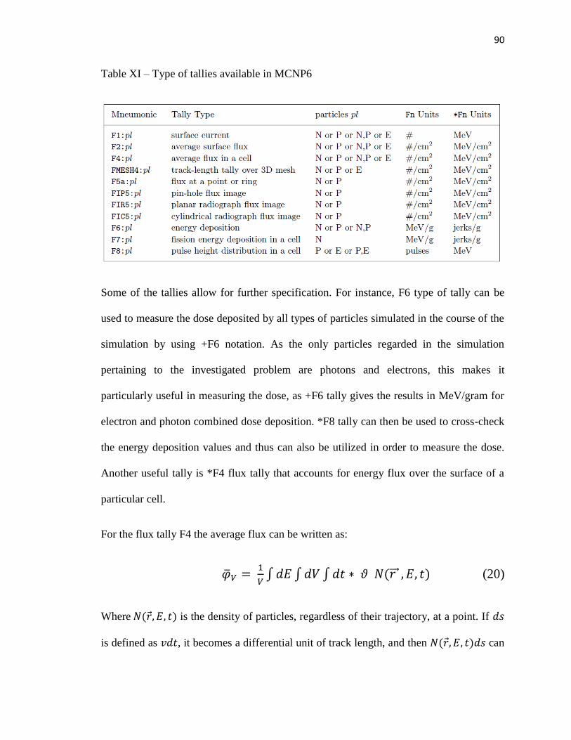
90

Table XI – Type of tallies available in MCNP6

Some of the tallies allow for further specification. For instance, F6 type of tally can be

used to measure the dose deposited by all types of particles simulated in the course of the

simulation by using +F6 notation. As the only particles regarded in the simulation

pertaining to the investigated problem are photons and electrons, this makes it

particularly useful in measuring the dose, as +F6 tally gives the results in MeV/gram for

electron and photon combined dose deposition. *F8 tally can then be used to cross-check

the energy deposition values and thus can also be utilized in order to measure the dose.

Another useful tally is *F4 flux tally that accounts for energy flux over the surface of a

particular cell.

For the flux tally F4 the average flux can be written as:

�̅�𝑉 = 1

𝑉∫ 𝑑𝐸 ∫ 𝑑𝑉 ∫ 𝑑𝑡 ∗ 𝜗 𝑁(𝑟 ⃗⃗⃗ , 𝐸, 𝑡) (20)

Where 𝑁(𝑟, 𝐸, 𝑡) is the density of particles, regardless of their trajectory, at a point. If 𝑑𝑠

is defined as 𝑣𝑑𝑡, it becomes a differential unit of track length, and then 𝑁(𝑟, 𝐸, 𝑡)𝑑𝑠 can

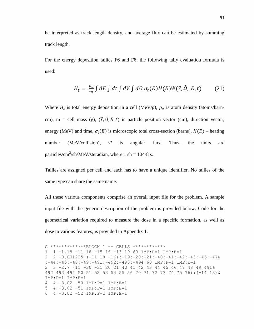
91

be interpreted as track length density, and average flux can be estimated by summing

track length.

For the energy deposition tallies F6 and F8, the following tally evaluation formula is

used:

𝐻𝑡 = 𝜌𝑎

𝑚∫ 𝑑𝐸 ∫ 𝑑𝑡 ∫ 𝑑𝑉 ∫ 𝑑𝛺 𝜎𝑡(𝐸)𝐻(𝐸)𝛹(𝑟, �̂�, 𝐸, 𝑡) (21)

Where 𝐻𝑡 is total energy deposition in a cell (MeV/g), 𝜌𝑎 is atom density (atoms/barn-

cm), m = cell mass (g), (𝑟, �̂�, 𝐸, 𝑡) is particle position vector (cm), direction vector,

energy (MeV) and time, 𝜎𝑡(𝐸) is microscopic total cross-section (barns), 𝐻(𝐸) – heating

number (MeV/collision), 𝛹 is angular flux. Thus, the units are

particles/cm2/sh/MeV/steradian, where 1 sh = 10^-8 s.

Tallies are assigned per cell and each has to have a unique identifier. No tallies of the

same type can share the same name.

All these various components comprise an overall input file for the problem. A sample

input file with the generic description of the problem is provided below. Code for the

geometrical variation required to measure the dose in a specific formation, as well as

dose to various features, is provided in Appendix 1.

C *************BLOCK 1 -– CELLS ************

1 1 -1.18 -11 18 -15 16 -13 19 60 IMP:P=1 IMP:E=1

2 2 -0.001225 (-11 18 -16):-19:-20:-21:-40:-41:-42:-43:-46:-47&

:-44:-45:-48:-49:-491:-492:-493:-494 60 IMP:P=1 IMP:E=1

3 3 -2.7 (11 -30 -31 20 21 40 41 42 43 44 45 46 47 48 49 491&

492 493 494 50 51 52 53 54 55 56 70 71 72 73 74 75 76):(-14 13)&

IMP:P=1 IMP:E=1

4 4 -3.02 -50 IMP:P=1 IMP:E=1

5 4 -3.02 -51 IMP:P=1 IMP:E=1

6 4 -3.02 -52 IMP:P=1 IMP:E=1

92

7 4 -3.02 -53 IMP:P=1 IMP:E=1

8 4 -3.02 -54 IMP:P=1 IMP:E=1

9 4 -3.02 -55 IMP:P=1 IMP:E=1

10 4 -3.02 -56 IMP:P=1 IMP:E=1

11 5 -1.1 -60 61 62 83 84 85 86 IMP:P=1 IMP:E=1

12 5 -1.1 -61 IMP:P=1 IMP:E=1

13 6 -7.87 -70 50 IMP:P=1 IMP:E=1

14 6 -7.87 -71 51 IMP:P=1 IMP:E=1

15 6 -7.87 -72 52 IMP:P=1 IMP:E=1

16 6 -7.87 -73 53 IMP:P=1 IMP:E=1

17 6 -7.87 -74 54 IMP:P=1 IMP:E=1

18 6 -7.87 -75 55 IMP:P=1 IMP:E=1

19 6 -7.87 -76 56 IMP:P=1 IMP:E=1

20 5 -1.1 -62 IMP:P=1 IMP:E=1

21 5 -1.1 -83 IMP:P=1 IMP:E=1

22 5 -1.1 -84 IMP:P=1 IMP:E=1

23 5 -1.1 -85 IMP:P=1 IMP:E=1

24 5 -1.1 -86 IMP:P=1 IMP:E=1

44 0 (-18 60):(-11 15 18 14):(11 -30 31):30 IMP:P=0 IMP:E=0

C *************BLOCK 2 -– SURFACES *********

11 PZ 2.7

13 CZ 4.5

14 RCC 0 0 2.4 0 0 0.3 5

15 KZ -2.1 1 1

16 KZ -1.3 1 1

18 PZ 0

19 RCC 0 0 0 0 0 0.6 1.8

20 TRC 0 0 2.7 0 0 0.4 3.84 3.44

21 RCC 0 0 3.1 0 0 0.5 3.44

30 PZ 6.1

31 CZ 5

40 TRC 0 0 3.6 0 0 0.2 1 0.8

41 RCC 0 0 3.8 0 0 0.15 0.8

42 TRC 0 2.4445 3.6 0 0 0.2 1 0.8

43 RCC 0 2.4445 3.8 0 0 0.15 0.8

44 TRC 0 -2.4445 3.6 0 0 0.2 1 0.8

45 RCC 0 -2.4445 3.8 0 0 0.15 0.8

46 TRC 2.11 1.22 3.6 0 0 0.2 1 0.8

47 RCC 2.11 1.22 3.8 0 0 0.15 0.8

48 TRC -2.11 1.22 3.6 0 0 0.2 1 0.8

49 RCC -2.11 1.22 3.8 0 0 0.15 0.8

491 TRC 2.11 -1.22 3.6 0 0 0.2 1 0.8

492 RCC 2.11 -1.22 3.8 0 0 0.15 0.8

493 TRC -2.11 -1.22 3.6 0 0 0.2 1 0.8

494 RCC -2.11 -1.22 3.8 0 0 0.15 0.8

50 RCC 0 0 3.96 0 0 0.06 0.8

51 RCC 0 2.4445 3.96 0 0 0.06 0.8

52 RCC 0 -2.4445 3.96 0 0 0.06 0.8

53 RCC 2.11 1.22 3.96 0 0 0.06 0.8

54 RCC -2.11 1.22 3.96 0 0 0.06 0.8

55 RCC 2.11 -1.22 3.96 0 0 0.06 0.8

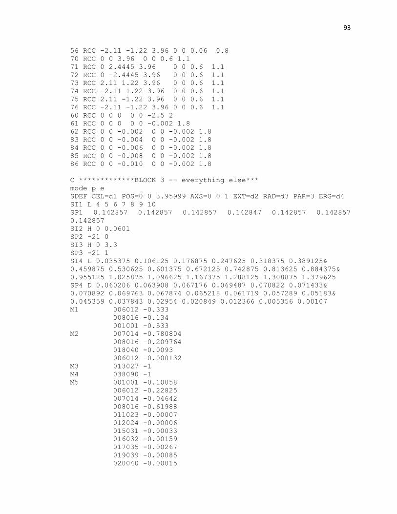
93

56 RCC -2.11 -1.22 3.96 0 0 0.06 0.8

70 RCC 0 0 3.96 0 0 0.6 1.1

71 RCC 0 2.4445 3.96 0 0 0.6 1.1

72 RCC 0 -2.4445 3.96 0 0 0.6 1.1

73 RCC 2.11 1.22 3.96 0 0 0.6 1.1

74 RCC -2.11 1.22 3.96 0 0 0.6 1.1

75 RCC 2.11 -1.22 3.96 0 0 0.6 1.1

76 RCC -2.11 -1.22 3.96 0 0 0.6 1.1

60 RCC 0 0 0 0 0 -2.5 2

61 RCC 0 0 0 0 0 -0.002 1.8

62 RCC 0 0 -0.002 0 0 -0.002 1.8

83 RCC 0 0 -0.004 0 0 -0.002 1.8

84 RCC 0 0 -0.006 0 0 -0.002 1.8

85 RCC 0 0 -0.008 0 0 -0.002 1.8

86 RCC 0 0 -0.010 0 0 -0.002 1.8

C *************BLOCK 3 -– everything else***

mode p e

SDEF CEL=d1 POS=0 0 3.95999 AXS=0 0 1 EXT=d2 RAD=d3 PAR=3 ERG=d4

SI1 L 4 5 6 7 8 9 10

SP1 0.142857 0.142857 0.142857 0.142847 0.142857 0.142857

0.142857

SI2 H 0 0.0601

SP2 -21 0

SI3 H 0 3.3

SP3 -21 1

SI4 L 0.035375 0.106125 0.176875 0.247625 0.318375 0.389125&

0.459875 0.530625 0.601375 0.672125 0.742875 0.813625 0.884375&

0.955125 1.025875 1.096625 1.167375 1.288125 1.308875 1.379625

SP4 D 0.060206 0.063908 0.067176 0.069487 0.070822 0.071433&

0.070892 0.069763 0.067874 0.065218 0.061719 0.057289 0.05183&

0.045359 0.037843 0.02954 0.020849 0.012366 0.005356 0.00107

M1 006012 -0.333

008016 -0.134

001001 -0.533

M2 007014 -0.780804

008016 -0.209764

018040 -0.0093

006012 -0.000132

M3 013027 -1

M4 038090 -1

M5 001001 -0.10058

006012 -0.22825

007014 -0.04642

008016 -0.61988

011023 -0.00007

012024 -0.00006

015031 -0.00033

016032 -0.00159

017035 -0.00267

019039 -0.00085

020040 -0.00015

94

M6 028059 -0.12

024052 -0.17

042096 -0.025

014028 -0.01

025055 -0.02

006012 -0.0008

015031 -0.00045

016032 -0.0003

026056 -0.65345

NPS 1000000000

PRINT 110

+F16 12

+F26 20

+F36 21

+F46 22

+F56 23

+F66 24

*F14:P 12

*F24:P 20

*F34:P 21

*F44:P 22

*F54:P 23

*F64:P 24

*F214:E 12

*F224:E 20

*F234:E 21

*F244:E 22

*F254:E 23

*F264:E 24

After the code is loaded into the computer system, it is executed by performing the start

command. For the Los Alamos National Lab supercomputer, the process is initiated

within a remote controlled Linux server control window by entering the command line:

mcnp filename.inp

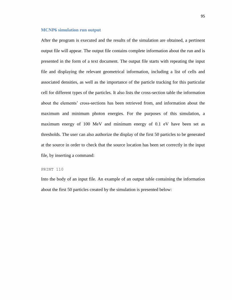
95

MCNP6 simulation run output

After the program is executed and the results of the simulation are obtained, a pertinent

output file will appear. The output file contains complete information about the run and is

presented in the form of a text document. The output file starts with repeating the input

file and displaying the relevant geometrical information, including a list of cells and

associated densities, as well as the importance of the particle tracking for this particular

cell for different types of the particles. It also lists the cross-section table the information

about the elements’ cross-sections has been retrieved from, and information about the

maximum and minimum photon energies. For the purposes of this simulation, a

maximum energy of 100 MeV and minimum energy of 0.1 eV have been set as

thresholds. The user can also authorize the display of the first 50 particles to be generated

at the source in order to check that the source location has been set correctly in the input

file, by inserting a command:

PRINT 110

Into the body of an input file. An example of an output table containing the information

about the first 50 particles created by the simulation is presented below:

96

Table XII – First 50 particles simulated at the source

The output file will contain the information about the photon and electron creation

statistics and tracking, and will present the information about the types of interactions

particles might undergo while simulated. The information about the photon interaction

statistics is presented in table XIII:

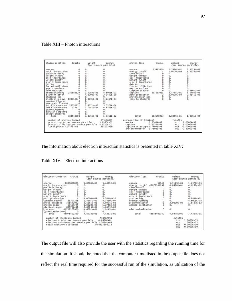
97

Table XIII – Photon interactions

The information about electron interaction statistics is presented in table XIV:

Table XIV – Electron interactions

The output file will also provide the user with the statistics regarding the running time for

the simulation. It should be noted that the computer time listed in the output file does not

reflect the real time required for the successful run of the simulation, as utilization of the

98

supercomputer significantly reduces the time necessary for a successful simulation run.

An example of the running time statistics is presented below:

The output file presents the information about the source efficiency, number of histories

processed by each processor, and the number of statistical information dumps performed

in the course of the simulation.

The output file also contains information about the photon and electron activity in each

cell. This information includes the number of tracks entering the cell, the number of the

collisions, number and flux weighted energy and the average length of the particle track

in that particular cell. The tables for the photon and electron activity are presented below:

Table XV – Photon activity in each cell

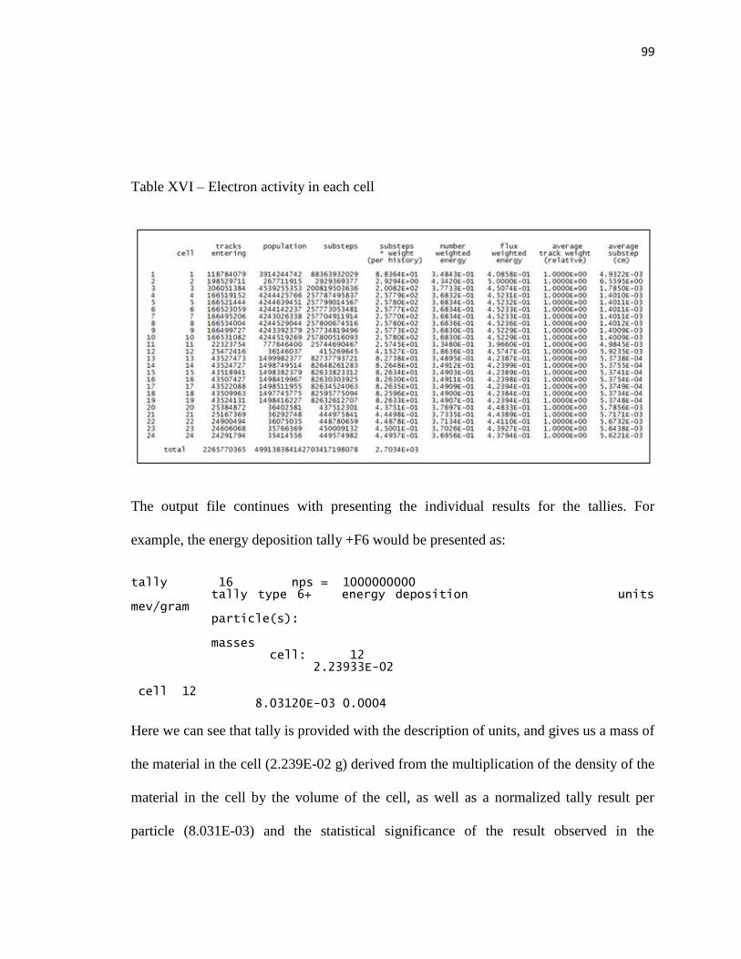
99

Table XVI – Electron activity in each cell

The output file continues with presenting the individual results for the tallies. For

example, the energy deposition tally +F6 would be presented as:

tally 16 nps = 1000000000 tally type 6+ energy deposition units mev/gram particle(s): masses cell: 12 2.23933E-02 cell 12 8.03120E-03 0.0004

Here we can see that tally is provided with the description of units, and gives us a mass of

the material in the cell (2.239E-02 g) derived from the multiplication of the density of the

material in the cell by the volume of the cell, as well as a normalized tally result per

particle (8.031E-03) and the statistical significance of the result observed in the

100

simulation run (error = 0.0004 or 0.04%). For the tally results to be statistically

significant, the margin of the error should not exceed 5 %.

In order to convert the tally results calculated as MeV/g per one disintegration, we have

to convert tally results from MeV/g to Joules/kg (definition of a Gy unit), and then

multiply the resultant value by the number of disintegrations happening as a result of beta

decay in all of the sources over the course of one minute, accounting for the stated

activity of 100 mCi/source and seven sources being utilized at the same time. Overall the

dose conversion from the tally result to dose can be summarized as:

𝐷𝑜𝑠𝑒 = 𝑇𝑎𝑙𝑙𝑦 ∗ 𝑐𝑜𝑛𝑣𝑒𝑟𝑠𝑖𝑜𝑛 𝑓𝑎𝑐𝑡𝑜𝑟 ∗ 𝑆𝑜𝑢𝑟𝑐𝑒 𝐴𝑐𝑡𝑖𝑣𝑖𝑡𝑦 (22)

Likewise, for the F4 tally for the same cell results are represented in the following

format:

tally 14 nps = 1000000000 tally type 4* track length estimate of energy flux. units mev/cm**2 particle(s): photons volumes cell: 12 2.03575E-02 cell 12 3.20688E-05 0.0012

Here particle type is specified to refer to a specific type of particles being accounted for

in the course of simulation. The results for the same cell for the electrons would look

like:

tally 214 nps = 1000000000 tally type 4* track length estimate of energy flux. units mev/cm**2 particle(s): electrons

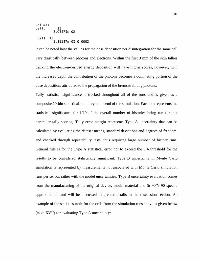
101

volumes cell: 12 2.03575E-02 cell 12 1.51157E-03 0.0002

It can be noted how the values for the dose deposition per disintegration for the same cell

vary drastically between photons and electrons. Within the first 3 mm of the skin tallies

tracking the electron-derived energy deposition will have higher scores, however, with

the increased depth the contribution of the photons becomes a dominating portion of the

dose deposition, attributed to the propagation of the bremsstrahlung photons.

Tally statistical significance is tracked throughout all of the runs and is given as a

composite 10-bin statistical summary at the end of the simulation. Each bin represents the

statistical significance for 1/10 of the overall number of histories being run for that

particular tally scoring. Tally error margin represents Type A uncertainty that can be

calculated by evaluating the dataset means, standard deviations and degrees of freedom,

and checked through repeatability tests, thus requiring large number of history runs.

General rule is for the Type A statistical error not to exceed the 5% threshold for the

results to be considered statistically significant. Type B uncertainty in Monte Carlo

simulation is represented by measurements not associated with Monte Carlo simulation

runs per se, but rather with the model uncertainties. Type B uncertainty evaluation comes

from the manufacturing of the original device, model material and Sr-90/Y-90 spectra

approximation and will be discussed in greater details in the discussion section. An

example of the statistics table for the cells from the simulation runs above is given below

(table XVII) for evaluating Type A uncertainty:

102

Table XVII – Tally fluctuation charts for cell 12 – F6, F4 photons, F4 electrons.

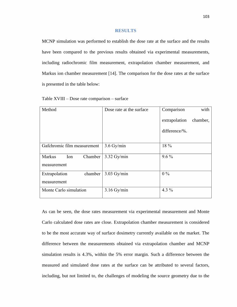
103

RESULTS

MCNP simulation was performed to establish the dose rate at the surface and the results

have been compared to the previous results obtained via experimental measurements,

including radiochromic film measurement, extrapolation chamber measurement, and

Markus ion chamber measurement [14]. The comparison for the dose rates at the surface

is presented in the table below:

Table XVIII – Dose rate comparison – surface

Method Dose rate at the surface Comparison with

extrapolation chamber,

difference/%.

Gafchromic film measurement 3.6 Gy/min 18 %

Markus Ion Chamber

measurement

3.32 Gy/min 9.6 %

Extrapolation chamber

measurement

3.03 Gy/min 0 %

Monte Carlo simulation 3.16 Gy/min 4.3 %

As can be seen, the dose rates measurement via experimental measurement and Monte

Carlo calculated dose rates are close. Extrapolation chamber measurement is considered

to be the most accurate way of surface dosimetry currently available on the market. The

difference between the measurements obtained via extrapolation chamber and MCNP

simulation results is 4.3%, within the 5% error margin. Such a difference between the

measured and simulated dose rates at the surface can be attributed to several factors,

including, but not limited to, the challenges of modeling the source geometry due to the

104

inherent activity inhomogeneity of the manufactured sources versus the perfect

cylindrical model of the source present in the simulation, as well as spectral binning

approximation used to generate the spectrum of Sr-90 and Y-90 beta particles energies.

Also, the individual Sr-90 source activity has a potential variance of +/- 15% from 100

mCi for each of the actual Sr-90 sources.

The statistical information about the simulation run that provided the dose rate results is

presented in Table XIX:

Table XIX – Surface dose measurement statistical error

105

In Table XIX, tally 16 presents the statistical error for the dose deposition estimation,

while tallies 14 and 914 reflect the surface flux estimation accuracy for photon and

electron correspondingly. It should be noted that for the surface dose estimation, the

percent error never exceeds 0.35%, well below the 5% statistical significance cutoff, thus

providing statistically significant results.

Percent depth dose (PDD) measurements have also been previously performed for the

various skin depths using carefully obtained radiochromic film measurements [14]. A

125-micrometer depth increment was utilized to establish the PDD curve of the dose as a

function of penetration depth. The resulting PDD is presented in figure 38:

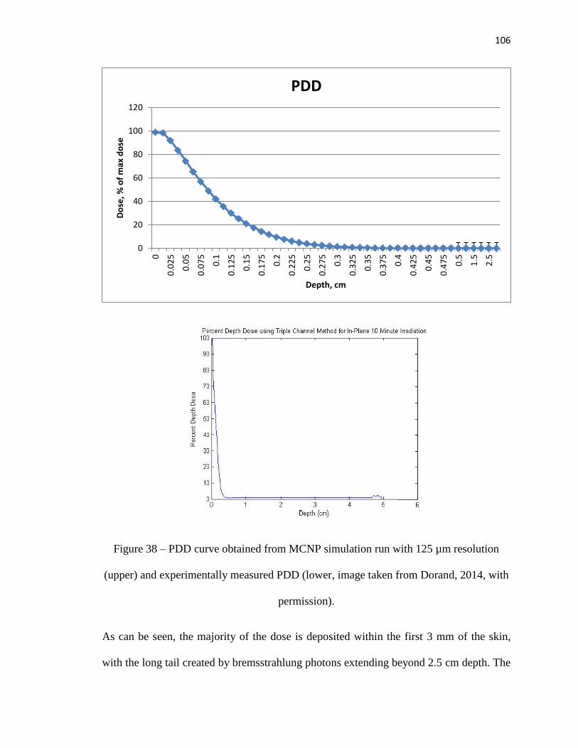
106

Figure 38 – PDD curve obtained from MCNP simulation run with 125 µm resolution

(upper) and experimentally measured PDD (lower, image taken from Dorand, 2014, with

permission).

As can be seen, the majority of the dose is deposited within the first 3 mm of the skin,

with the long tail created by bremsstrahlung photons extending beyond 2.5 cm depth. The

0

20

40

60

80

100

120

0

0.0

25

0.0

5

0.0

75

0.1

0.1

25

0.1

5

0.1

75

0.2

0.2

25

0.2

5

0.2

75

0.3

0.3

25

0.3

5

0.3

75

0.4

0.4

25

0.4

5

0.4

75

0.5

1.5

2.5

Do

se, %

of

max

do

se

Depth, cm

PDD

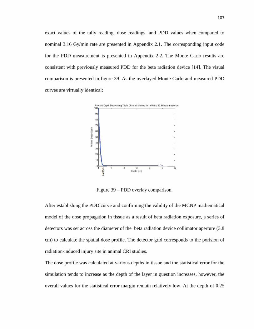
107

exact values of the tally reading, dose readings, and PDD values when compared to

nominal 3.16 Gy/min rate are presented in Appendix 2.1. The corresponding input code

for the PDD measurement is presented in Appendix 2.2. The Monte Carlo results are

consistent with previously measured PDD for the beta radiation device [14]. The visual

comparison is presented in figure 39. As the overlayed Monte Carlo and measured PDD

curves are virtually identical:

Figure 39 – PDD overlay comparison.

After establishing the PDD curve and confirming the validity of the MCNP mathematical

model of the dose propagation in tissue as a result of beta radiation exposure, a series of

detectors was set across the diameter of the beta radiation device collimator aperture (3.8

cm) to calculate the spatial dose profile. The detector grid corresponds to the porision of

radiation-induced injury site in animal CRI studies.

The dose profile was calculated at various depths in tissue and the statistical error for the

simulation tends to increase as the depth of the layer in question increases, however, the

overall values for the statistical error margin remain relatively low. At the depth of 0.25

108

cm below the skin surface, the error rises to 0.41%, at the depth of 0.3 cm – 0.64%, at the

depth of 0.4 cm – 1.92%, at the depth of 0.5 cm – 4.67%. The increase to the percent

error is attributed to the fact that fewer and fewer particles reach the depth of interest,

thus presenting fewer histories available for statistical analysis and increasing the margin

of error. However, as Sr-90 and Y-90 beta particles do not penetrate beyond the first 5

mm of the skin surface, this increase in the error values can be disregarded as the depth of

interest still falls within the 5% statistical error margin. It should be of interest to note

that while the statistical error margins for the electron flux reflect the same increase of

the statistical error with the increased depth, the values for the statistical errors for the

tallies recording photon flux are almost unaffected, which agrees with the assumption

that the photon penetration depth is much deeper than that of the electrons and the

majority of the bremsstrahlung photons pass through the first 0.5 cm of the skin and only

deposit dose at the deeper subcutaneous fat layers.

A series of tests have been conducted in order to establish the symmetry of the dose

distribution curve along the surface of the wound. First, a series of 2-mm detector

simulations recording the energy deposition with the length and depth of 1 mm were

positioned across the length of the wound, so that the absorbed dose measured within the

detectors would correspond to the average dose measured at 0.05 cm depth. The detectors

were positioned both along the x-axis (zero degrees position) and y-axis (90 degrees

position), with the underlying assumption that the difference between the dose

distribution curve should be minimal due to the symmetry of the system across the x and

y axis. The volume of the voxel was constant at 1 mm3. The formation of the detectors

across the skin surface is presented in figure 40:

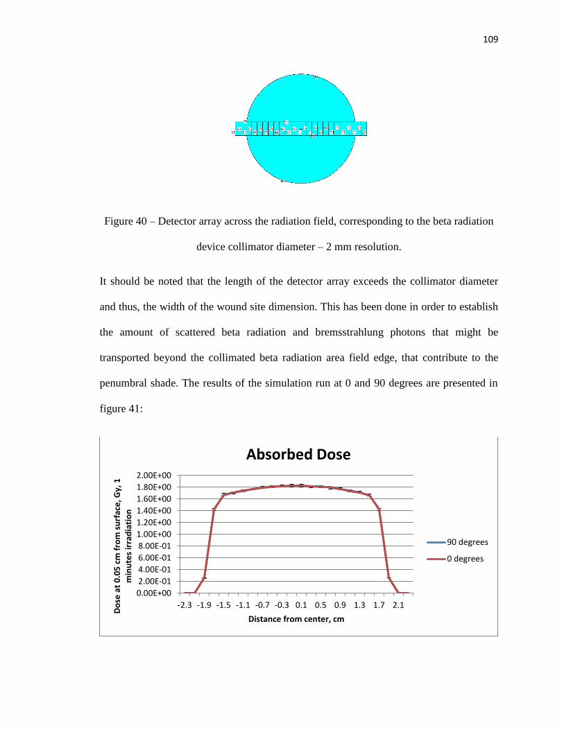
109

Figure 40 – Detector array across the radiation field, corresponding to the beta radiation

device collimator diameter – 2 mm resolution.

It should be noted that the length of the detector array exceeds the collimator diameter

and thus, the width of the wound site dimension. This has been done in order to establish

the amount of scattered beta radiation and bremsstrahlung photons that might be

transported beyond the collimated beta radiation area field edge, that contribute to the

penumbral shade. The results of the simulation run at 0 and 90 degrees are presented in

figure 41:

0.00E+00

2.00E-01

4.00E-01

6.00E-01

8.00E-01

1.00E+00

1.20E+00

1.40E+00

1.60E+00

1.80E+00

2.00E+00

-2.3 -1.9 -1.5 -1.1 -0.7 -0.3 0.1 0.5 0.9 1.3 1.7 2.1

Do

se a

t 0

.05

cm

fro

m s

urf

ace

, Gy,

1

min

ute

s ir

rad

iati

on

Distance from center, cm

Absorbed Dose

90 degrees

0 degrees

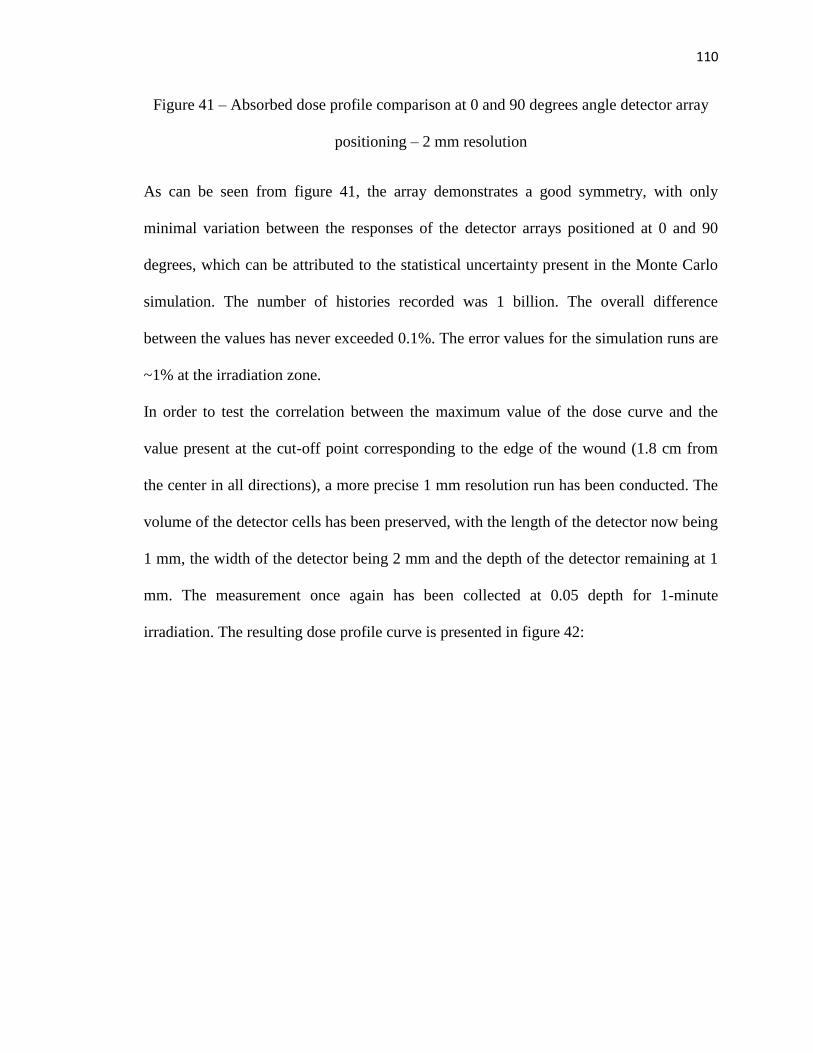
110

Figure 41 – Absorbed dose profile comparison at 0 and 90 degrees angle detector array

positioning – 2 mm resolution

As can be seen from figure 41, the array demonstrates a good symmetry, with only

minimal variation between the responses of the detector arrays positioned at 0 and 90

degrees, which can be attributed to the statistical uncertainty present in the Monte Carlo

simulation. The number of histories recorded was 1 billion. The overall difference

between the values has never exceeded 0.1%. The error values for the simulation runs are

~1% at the irradiation zone.

In order to test the correlation between the maximum value of the dose curve and the

value present at the cut-off point corresponding to the edge of the wound (1.8 cm from

the center in all directions), a more precise 1 mm resolution run has been conducted. The

volume of the detector cells has been preserved, with the length of the detector now being

1 mm, the width of the detector being 2 mm and the depth of the detector remaining at 1

mm. The measurement once again has been collected at 0.05 depth for 1-minute

irradiation. The resulting dose profile curve is presented in figure 42:

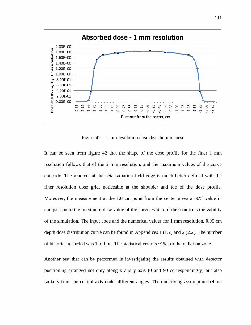
111

Figure 42 – 1 mm resolution dose distribution curve

It can be seen from figure 42 that the shape of the dose profile for the finer 1 mm

resolution follows that of the 2 mm resolution, and the maximum values of the curve

coincide. The gradient at the beta radiation field edge is much better defined with the

finer resolution dose grid, noticeable at the shoulder and toe of the dose profile.

Moreover, the measurement at the 1.8 cm point from the center gives a 50% value in

comparison to the maximum dose value of the curve, which further confirms the validity

of the simulation. The input code and the numerical values for 1 mm resolution, 0.05 cm

depth dose distribution curve can be found in Appendices 1 (1.2) and 2 (2.2). The number

of histories recorded was 1 billion. The statistical error is ~1% for the radiation zone.

Another test that can be performed is investigating the results obtained with detector

positioning arranged not only along x and y axis (0 and 90 correspondingly) but also

radially from the central axis under different angles. The underlying assumption behind

0.00E+00

2.00E-01

4.00E-01

6.00E-01

8.00E-01

1.00E+00

1.20E+00

1.40E+00

1.60E+00

1.80E+00

2.00E+00

2.3

5

2.1

5

1.9

5

1.7

5

1.5

5

1.3

5

1.1

5

0.9

5

0.7

5

0.5

5

0.3

5

0.1

5

-0.0

5

-0.2

5

-0.4

5

-0.6

5

-0.8

5

-1.0

5

-1.2

5

-1.4

5

-1.6

5

-1.8

5

-2.0

5

-2.2

5

Do

se a

t 0

.05

cm

, G

y, 1

min

irra

dia

tio

n

Distance from the center, cm

Absorbed dose - 1 mm resolution

112

such an arrangement is that the dose measured at the points equally distant from the

center should be the same throughout the entire cylinder forming the skin slab. In order to

test that assumption, a so-called pie chart geometrical configuration was created and is

presented in figure 43:

Figure 43 – Pie chart geometrical configuration.

Slices of the “pie” have 8 basic orientations – upper right slice aligned with x axis, lower

right slice aligned with x axes, upper left slice aligned with x axis, lower left slice aligned

with x axis, upper right slice aligned with y axis, lower right slice aligned with y axes,

upper left slice aligned with y axis, lower left slice aligned with y axis. The “pieces”

located at the same distance from the center of the cylinder are equal among slices. The

resulting dose profile curves are presented in figure 44:

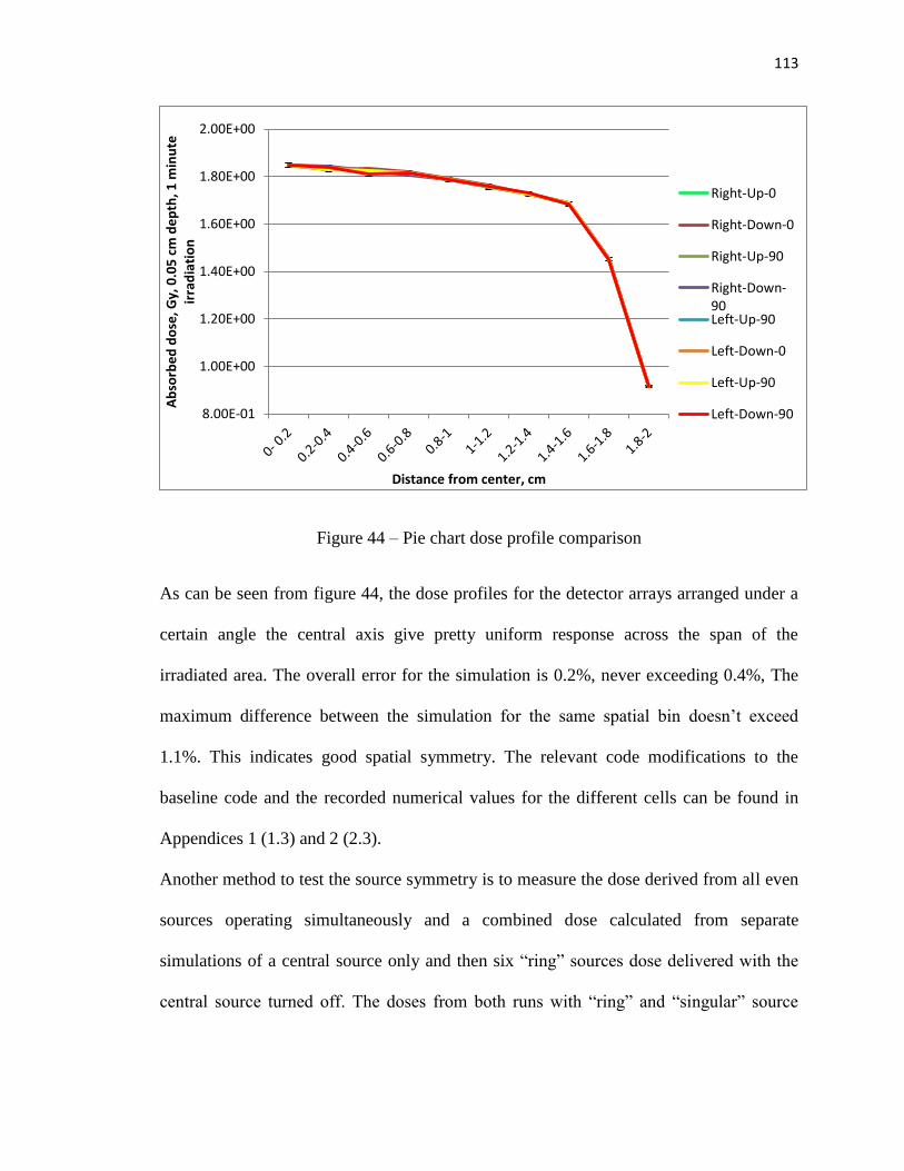
113

Figure 44 – Pie chart dose profile comparison

As can be seen from figure 44, the dose profiles for the detector arrays arranged under a

certain angle the central axis give pretty uniform response across the span of the

irradiated area. The overall error for the simulation is 0.2%, never exceeding 0.4%, The

maximum difference between the simulation for the same spatial bin doesn’t exceed

1.1%. This indicates good spatial symmetry. The relevant code modifications to the

baseline code and the recorded numerical values for the different cells can be found in

Appendices 1 (1.3) and 2 (2.3).

Another method to test the source symmetry is to measure the dose derived from all even

sources operating simultaneously and a combined dose calculated from separate

simulations of a central source only and then six “ring” sources dose delivered with the

central source turned off. The doses from both runs with “ring” and “singular” source

8.00E-01

1.00E+00

1.20E+00

1.40E+00

1.60E+00

1.80E+00

2.00E+00

Ab

sorb

ed

do

se, G

y, 0

.05

cm

de

pth

, 1 m

inu

te

irra

dia

tio

n

Distance from center, cm

Right-Up-0

Right-Down-0

Right-Up-90

Right-Down-90Left-Up-90

Left-Down-0

Left-Up-90

Left-Down-90

114

configurations are then summed to create a single cumulative dose profile. A schematic

for such configuration is presented in figure 45:

Figure 45 – Standard and combined dose source configuration

The resulting dose curve for the simulated standard and combined doses are presented in

figure 46:

115

Figure 46 – Standard and combined dose absorption curve

As can be seen from figure 46, the simulated doses for standard and combined

configurations do not significantly differ from one another. At any point the difference

between the measurements of the standard and combined simulation runs does not exceed

0.5%. This is an important observation as it allows us to use the developed Monte Carlo

model for testing different source configurations, including the use of the sources of

different activities in various geometrical formations.

After the validity of the created model has been tested by the surface dose rate

comparison, PDD comparison, and rigorous symmetry response testing, the dose profiles

for different depths can be derived from a series of simulation runs. The three-

dimensional dose distributions across the length of the wound are presented in figure 47:

0

0.2

0.4

0.6

0.8

1

1.2

1.4

1.6

1.8

2

2.3

52

.15

1.9

51

.75

1.5

51

.35

1.1

50

.95

0.7

50

.55

0.3

50

.15

-0.0

5-0

.25

-0.4

5-0

.65

-0.8

5-1

.05

-1.2

5-1

.45

-1.6

5-1

.85

-2.0

5-2

.25

Do

se, G

y/m

in, 0

.05

cm

de

pth

.

Distance from center, cm

Dose -standard

Dose -combined

Dose - nocentralsource

Dose -centralsource only

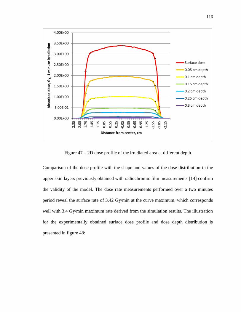
116

Figure 47 – 2D dose profile of the irradiated area at different depth

Comparison of the dose profile with the shape and values of the dose distribution in the

upper skin layers previously obtained with radiochromic film measurements [14] confirm

the validity of the model. The dose rate measurements performed over a two minutes

period reveal the surface rate of 3.42 Gy/min at the curve maximum, which corresponds

well with 3.4 Gy/min maximum rate derived from the simulation results. The illustration

for the experimentally obtained surface dose profile and dose depth distribution is

presented in figure 48:

0.00E+00

5.00E-01

1.00E+00

1.50E+00

2.00E+00

2.50E+00

3.00E+00

3.50E+00

4.00E+00

2.3

5

2.0

5

1.7

5

1.4

5

1.1

5

0.8

5

0.5

5

0.2

5

-0.0

5

-0.3

5

-0.6

5

-0.9

5

-1.2

5

-1.5

5

-1.8

5

-2.1

5

Ab

sorb

ed

do

se, G

y, 1

min

ute

irra

dia

tio

n

Distance from center, cm

Surface dose

0.05 cm depth

0.1 cm depth

0.15 cm depth

0.2 cm depth

0.25 cm depth

0.3 cm depth

117

Figure 48 – Dose distribution measure with radiochromic film. Upper: central dose

profiles, horizontal and vertical, measured over 2 minutes. Lower: 3D distribution of the

dose in-depth, measured over 10 minutes. Images from Dorand, 2014 [14], used with

permission.

As can be seen, both the shape of the individual dose profiles and 3D dose distribution

derived from the simulation runs follow the experimental results closely. The maximum

rate at the surface is 3.4 Gy/minute, the average rate is 3.2 Gy/min for the experimental

measurements and 3.16 Gy/minute for the Monte Carlo simulation measurements. It

should be noted that the dose rate obtained from the radiochromic film measurement

taken over longer periods of time is lower than the dose rate obtained from 1-minute

exposures, which may be attributed to the uncertainties in radiochromic film calibration,

which is very difficult to perform for lower energy electrons such as beta particles. The

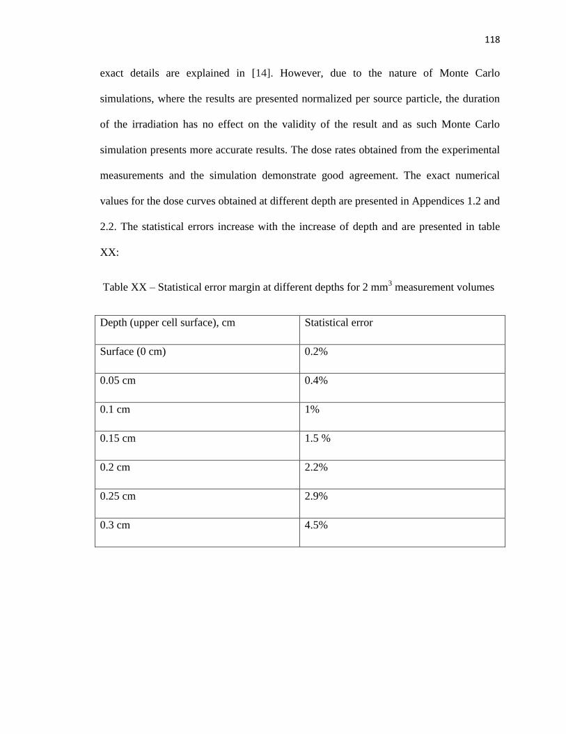
118

exact details are explained in [14]. However, due to the nature of Monte Carlo

simulations, where the results are presented normalized per source particle, the duration

of the irradiation has no effect on the validity of the result and as such Monte Carlo

simulation presents more accurate results. The dose rates obtained from the experimental

measurements and the simulation demonstrate good agreement. The exact numerical

values for the dose curves obtained at different depth are presented in Appendices 1.2 and

2.2. The statistical errors increase with the increase of depth and are presented in table

XX:

Table XX – Statistical error margin at different depths for 2 mm3 measurement volumes

Depth (upper cell surface), cm Statistical error

Surface (0 cm) 0.2%

0.05 cm 0.4%

0.1 cm 1%

0.15 cm 1.5 %

0.2 cm 2.2%

0.25 cm 2.9%

0.3 cm 4.5%

119

DISCUSSION

Skin surface and upper skin layers present a certain dosimetry challenge and establishing

a percent depth dose curve and surface dose rate is difficult to achieve via experimental

means. While using an extrapolation chamber allows for a very accurate estimation of the

surface dose rate and dose for particular uniform geometries, it requires considerable

resources and to perform point dose measurements at multiple depths underneath the skin

layer surface. Dose measurement of the doses delivered to the specific morphological

structures of the skin is essentially impossible with the use of conventional dosimetry

instrumentation.

Analytical calculations of the dose based on the mathematical model of the physical

processes occurring during the beta decay and subsequent deposition of the dose in the

upper skin layers prove to be inaccurate and typically cannot be used for dose estimation.

However, Monte Carlo modeling of the radiation processes has long been proved to

provide highly accurate dose deposition estimations and as such is utilized in the course

of this study to obtain the dose profiles in the upper layers of the skin and measure the

dose delivered to the specific morphological structures of the skin. An extensive series of

tests to confirm the validity of the model is conducted. The symmetry of the model is

tested through a series of tests meant to confirm the shape of the dose distribution curve,

and the dosimetric values recorded at various depths under the skin surface are compared

to physical measurements obtained in the previous set of experiments. The results of the

simulation compare favorably to the measurements made by the use of radiochromic

film, Markus Ion Chamber and extrapolation chamber, with the overall difference in dose

rate not exceeding the 5% error margin. Thus a conclusion can be made that Monte Carlo

120

model of the unique Sr-90 beta radiation device is valid and can be used for the

estimation of the dose delivered to the epidermal skin layer and various other structures,

including dermal layer vasculature.

An additional test is performed in order to ensure the model’s suitability for the use as

dose rate estimator for various source configurations and cone size variations. The results

obtained by comparing the dose delivered by a standard configuration versus the dose

delivered by consecutive irradiation by a single central source and then a ring of six

sources confirm that the model can be used to predict the behavior of the source

comprising of several individual sources with varying activity and even energy spectrum

values. This makes the developed model particularly useful as an engineering tool for

developing the plans for future beta radiation device variations.

Differences in the model response in comparison to the experimentally obtained

measurements can be explained by the source activity distribution variations in

comparison to the manufactured Sr-90 sources, representing the Type B uncertainty. The

model operated on the assumption of the ideally circular isotropic cylindrical sources,

whereas the manufactured sources have irregular deposition of Sr-90 radioactive

material, thus the activity is not as uniform as in Monte Carlo model. This assumption

might lead to the dose rate estimations from the model being slightly different than the

experimentally measured values. Another reason for the difference in the responses might

lie in the difference between the stated and actual activity of the sources. According to

the manufacture manifest, the activity of the sources can vary within ±15% of the stated

100 mCi activity. The variability between the experimentally measured values obtained

via different dose measurement methods (film vs ion chamber) adds another layer of

121

uncertainty and might contribute to the differences between the measured and modeled

dose distribution. One more reason of such uncertainty of the results might lie in the

approximate nature of the spectra for Sr-90 and Y-90 with 10-bins mode of spectra

representation introducing additional error margin to the model’s validity evaluation. All

of these Type B uncertainty considerations relate to the representation of the real-life

device in the form of a mathematical model that relies on the manufacture manifests and

additional information retrieved from the literature and might not be the most accurate

representation of the exact sources and devices used for the experimental measurements.

The future direction of the model development involves more precise modeling of the

different features of the skin and is detailed in Chapter 3.

122

CHAPTER 3: Monte Carlo modeling of skin features

MATERIALS AND METHODS

Correlation between the epidermal necrosis expression and blood vasculature

changes in skin

The radiobiological basis for cell response to the ionizing radiation can be described by

two concepts: dose-response curve and clonogenic cell survival fraction. In most

biological tissues, the relationship between the dose delivered to the tissue and its

response can be described by a sigmoid function. After a certain threshold is reached, the

tissue cells are destroyed without the possibility of recovery and significant injury to the

tissue can occur. Meanwhile, the clonogenic cell survival graph represents the fraction or

proportion of the cells surviving irradiation. On a semilog plot, after an initial “shoulder”

region, it follows the steep slope, with further increase in dose leading to a decrease in the

surviving cells fraction exponentially. Typically, dose delivered via a single irradiation

event causes more cell death than the same dose delivered via several fractions. Higher

doses delivered over a short period of time, or in a single fraction, as is the case with

radiation-related incidents, tend to lead to more rapid onset of tissue necrosis. It should be

noted, however, that this necrotic process can be triggered by two independent biological

mechanisms – the destruction of the cellular compartments in the tissue in question,

leading to the necrosis of the tissue cells due to the cells’ inability to properly function,

and the occlusion of the microvasculature leading to the interruptions in the blood

circulation which leads to cell death due to lack of oxygen and malnutrition [80]. Damage

to the endothelial wall of the blood vessels is a particular cause of concern. In case of the

skin tissue, the main effect the radiation has on epidermis is in the destruction of the

123

epidermal basal layer cell structure, which leads to the epidermis’ inability to properly

regenerate, and the interruption of the dermal blood supply via blood vessel thickening,

leading to the vessels occlusion.

It should also be noted that due to the selected tattooed area geometry, circular

configuration of the dose distribution on the skin surface the blood vessels penetrating the

skin beneath the irradiated area received different doses of radiation even though they

might have been located at the same distance from the surface and might have had the

same dose delivered at the particular point of the diameter cross-section. An assumption

of the equivalent uniform dose calculation applicability and the estimation of the overall

dose delivered to the vessels following the integrated geometrical distribution have been

investigated for their potential application [83][84].

Investigating the effects of the irradiation on the epidermis is impossible without the

study of the dose deposition in the upper layers of the skin and to the different

morphological structures of the skin, in particular, vasculature. With the development of

the Monte Carlo model discussed in Chapter 2, it became possible to establish a direct

correlation between the dose delivered to the basal skin layer and the blood vessels

permitting the dermal skin layer at various depths. This chapter concentrates on studying

the effects of the dose delivered by the beta radiation device and the epidermal necrosis

expression observed in the Yorkshire pig test subjects 70 days post-irradiation, as

determined by the histological analysis.

124

Monte Carlo modeling of the skin features

During the Monte Carlo model testing phase, the assumption has been made that the

irradiated surface is perfectly flat, as the dose comparison has been made against the

experimental measurements obtained via use of the flat-surfaced radiochromic film and

parallel-plate extrapolation chamber. However, this assumption might be flawed when

the irradiation device is applied for research purposes to the skin surface. Due to the

relative softness of the skin and underlying subcutaneous fat layer, a curvature might

form at the place of the PMMA cone application to the skin. This curvature in the skin

surface, a gentle arc into the collimator aperture with the skin surface closer to the beta

sources than for a flat surface, might affect the dose distribution in the epidermal and

upper dermal layers of the skin, in particular affecting the dose distribution to the

epidermal basal cell layers and the microvessels closest to the skin surface. The skin

geometry variation due to “bulging” has been estimated based on the skin elasticity and

evaluated for 1 and 2 mm rises. The illustration of the geometry reflecting the changes in

the vasculature is demonstrated in figure 49:

125

Figure 49 – Skin curvature variation. Top: flat skin surface. Middle: Curved skin surface

as a result of the PMMA cone application to the living skin, 1 mm rise at the collimator

central axis. Bottom: Curved skin surface as a result of the PMMA cone application to

the living skin, 2 mm rise at the collimator central axis.

The figure above demonstrates the skin curvature with the highest point of the curve

rising 1 mm above the base skin level at the edges of the PMMA cone. Likewise, a

126

simulation of the skin curvature with the highest point rising 2 mm above the base skin

level has been made. Relevant code modifications are presented in Appendix 1 (1.4).

In order to compare the dose distribution in the upper skin layers to the epidermal

necrosis expression, a comparison is made between the dose delivered to the skin surface

and the amount of the necrotic keratinocytes found in the epidermis of the 120 analyzed

histological samples. The spatial distribution of the necrotic cell count (NCC) is

compared to the dose profile across the wound length. The NCC profile is obtained by

averaging the 120 NCC profiles over the same spatial points across the wound regions.

Both dose and NCC are normalized for comparison.

Once the results for the necrotic cell distribution are obtained, the dose rate to the

underlying vasculature of the dermal layer supplying epidermis is investigated. To

demonstrate the effect of different radiation doses on the skin, a separate IACUC-

approved experiment with 2 Yorkshire pigs was previously conducted. Each pig had 10

tattooed sites, with 2 being used for control, and eight others irradiated with the doses of

16 Gy, 32 Gy, 37 Gy, and 42 Gy. Overall, each dose had 4 samples in a group. Test

subjects were euthanized and histological samples were collected following the procedure

described in Chapter 1. The expression of the blood vessel thickening has been analyzed

by a trained histopathologist. The comparison of the blood vessel thickening and

morphological abnormalities versus the position of the blood vessel cross-sections along

the length of the histological samples can be found in figure 50:

127

Figure 50 – Blood vessel thickening (Unpublished data, image used with permission of M

Robinson and JD Bourland)

As can be seen on figure 50, blood vessels demonstrate a tendency to thicken more as the

dose increases, and thickening effect can most often be observed at the center of the

irradiated sample, which corresponds well with the epidermal necrosis expression peak as

well as the radiation dose profile shape. The histological comparison between the normal

and affected “thickened” vessel is presented in figure 51:

128

A) B)

Figure 51 – Blood vessel histological cross-section: A) normal; B) thickened

As can be observed in figure 51, the morphological structures of the normal and

thickened vessels vary, with the thickened vessels demonstrating thicker walls with an

abundance of necrotic endothelial cells and pronounced scarification, leading to

significant narrowing of the lumen of the vessels, thus significantly reducing blood

supply to the surrounding tissue. The expression of the blood vessel thickening, however,

is not homogeneous and varies significantly with the depth of the vessel within the

dermal layer and its relative position to the center of the irradiated area. In order to

investigate what exact dose has been delivered to the blood vessels in order to induce

vessel thickening, a Monte Carlo simulation model of the blood vessels within the dermal

layer of the skin has been assembled. The resulting model contains three skin layers –

epidermis (0 – 0.007 cm depth), a dermal layer rich in collagen (0.007 – 0.2 cm depth)

and subcutaneous fat layer (0.2 – 2 cm depth). The blood vessels are modeled as a

cylinder made of muscle wall (0.01 cm in diameter) and a lumen of the vessel filled with

blood (0.006 cm). The average size of the blood vessels permitting skin is derived from

the literature [81]. The elemental weight concentration of the investigated tissues can be

summarized by the following table:

129

Table XXI – Elemental weight concentrations of the tissues present in skin model [78]

Elemental

Concentration

Adipose

tissue (d =

0.92 g/cm3)

Blood (d =

1.069

g/cm3)

Muscle (d =

1.04 g/cm3)

Epidermal

Skin (d =

1.1 g/cm3)

Dermal skin

(d = 1.1

g/cm3)

H 0.11947 0.10186 0.10063 0.10058 0.411603

C 0.63724 0.10002 0.10783 0.22825 0.29805

N 0.00797 0.02964 0.02768 0.04642 0.079186

O 0.23233 0.75941 0.75477 0.619 0.205354

Na 0.0005 0.00185 0.00075 0.00007 0.00007

Mg 0.00002 0.00004 0.00019 0.00006 0.00006

Si N/A 0.00003 N/A N/A N/A

P N/A 0.00035 0.00018 0.00033 0.00033

S 0.00016 0.00185 0.00241 0.00159 0.00159

Cl 0.00119 0.00278 N/A 0.00267 0.00267

K N/A 0.00163 N/A 0.00085 0.00085

Ca N/A 0.00006 N/A 0.00015 0.00015

Fe N/A 0.000045 N/A 0.00001 0.00001

Zn N/A 0.00001 N/A 0.00001 0.00001

The model of the blood vessel in the MCNP program can be represented by the diagram

in figure 52 (not to scale):

130

Figure 52 – Blood vessel modeling: left: blood vessel cross-section; right: blood vessel

passing through the length of the irradiated area

Relevant code modifications are presented in Appendix 1 (1.5). The cutaneous

microcirculation is organized at two horizontal plexuses – 1-1.5 mm below the skin

surface and at dermal-subcutaneous junction [82]. The majority of the arterioles and

venules affected by the beta irradiation are thus going to be located within the first 2 mm

of the skin depth. In order to calculate the dose delivered to blood vessels at different

anatomical positions, the vessels have been modeled at the depth of 0.05 mm, 1 mm, 1.5

mm and 2 mm below the skin surface to predict for anatomical variations. The vessels

have been positioned symmetrically along the irradiated area, with the central position

being denoted as 0, and a series of vessels being positioned at 0.5 cm, 1 cm, 1.5 cm and 2

cm away from the center of the irradiated area, providing the coverage of the whole

irradiated area in terms of the dose to the individual blood vessels.

131

An alternative “curved” arrangement of the skin and blood vessels positioning can be

made to imitate the skin curve formed by the PMMA cone application. A schematic for

such simulation is presented in the figure below:

Figure 53 – Curved skin model and blood vessels positioning

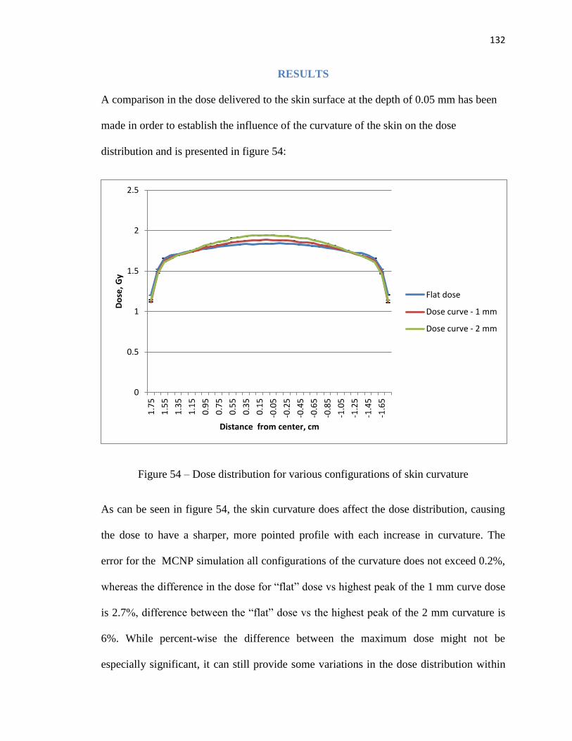
132

RESULTS

A comparison in the dose delivered to the skin surface at the depth of 0.05 mm has been

made in order to establish the influence of the curvature of the skin on the dose

distribution and is presented in figure 54:

Figure 54 – Dose distribution for various configurations of skin curvature

As can be seen in figure 54, the skin curvature does affect the dose distribution, causing

the dose to have a sharper, more pointed profile with each increase in curvature. The

error for the MCNP simulation all configurations of the curvature does not exceed 0.2%,

whereas the difference in the dose for “flat” dose vs highest peak of the 1 mm curve dose

is 2.7%, difference between the “flat” dose vs the highest peak of the 2 mm curvature is

6%. While percent-wise the difference between the maximum dose might not be

especially significant, it can still provide some variations in the dose distribution within

0

0.5

1

1.5

2

2.5

1.7

5

1.5

5

1.3

5

1.1

5

0.9

5

0.7

5

0.5

5

0.3

5

0.1

5

-0.0

5

-0.2

5

-0.4

5

-0.6

5

-0.8

5

-1.0

5

-1.2

5

-1.4

5

-1.6

5

Do

se, G

y

Distance from center, cm

Flat dose

Dose curve - 1 mm

Dose curve - 2 mm

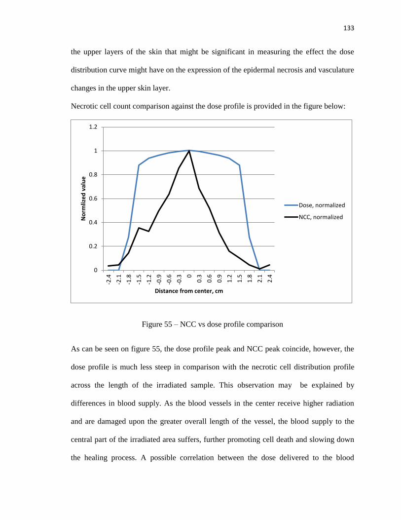
133

the upper layers of the skin that might be significant in measuring the effect the dose

distribution curve might have on the expression of the epidermal necrosis and vasculature

changes in the upper skin layer.

Necrotic cell count comparison against the dose profile is provided in the figure below:

Figure 55 – NCC vs dose profile comparison

As can be seen on figure 55, the dose profile peak and NCC peak coincide, however, the

dose profile is much less steep in comparison with the necrotic cell distribution profile

across the length of the irradiated sample. This observation may be explained by

differences in blood supply. As the blood vessels in the center receive higher radiation

and are damaged upon the greater overall length of the vessel, the blood supply to the

central part of the irradiated area suffers, further promoting cell death and slowing down

the healing process. A possible correlation between the dose delivered to the blood

0

0.2

0.4

0.6

0.8

1

1.2

-2.4

-2.1

-1.8

-1.5

-1.2

-0.9

-0.6

-0.3 0

0.3

0.6

0.9

1.2

1.5

1.8

2.1

2.4

No

rmliz

ed

val

ue

Distance from center, cm

Dose, normalized

NCC, normalized

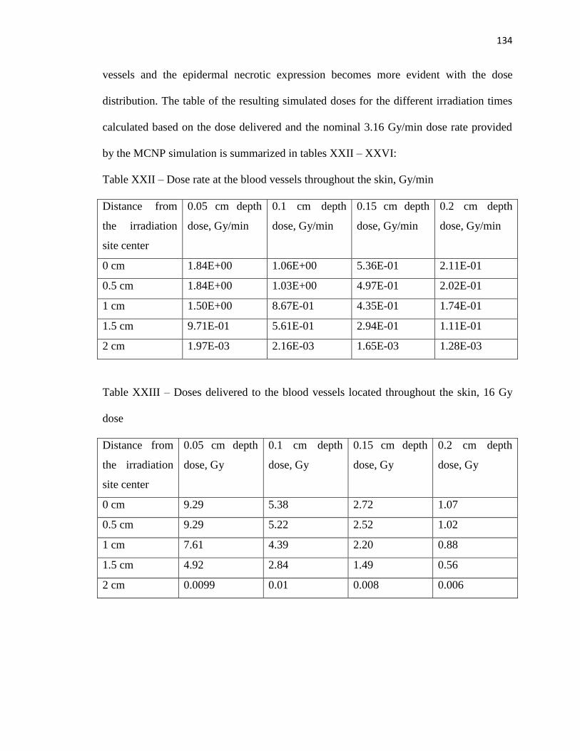
134

vessels and the epidermal necrotic expression becomes more evident with the dose

distribution. The table of the resulting simulated doses for the different irradiation times

calculated based on the dose delivered and the nominal 3.16 Gy/min dose rate provided

by the MCNP simulation is summarized in tables XXII – XXVI:

Table XXII – Dose rate at the blood vessels throughout the skin, Gy/min

Distance from

the irradiation

site center

0.05 cm depth

dose, Gy/min

0.1 cm depth

dose, Gy/min

0.15 cm depth

dose, Gy/min

0.2 cm depth

dose, Gy/min

0 cm 1.84E+00 1.06E+00 5.36E-01 2.11E-01

0.5 cm 1.84E+00 1.03E+00 4.97E-01 2.02E-01

1 cm 1.50E+00 8.67E-01 4.35E-01 1.74E-01

1.5 cm 9.71E-01 5.61E-01 2.94E-01 1.11E-01

2 cm 1.97E-03 2.16E-03 1.65E-03 1.28E-03

Table XXIII – Doses delivered to the blood vessels located throughout the skin, 16 Gy

dose

Distance from

the irradiation

site center

0.05 cm depth

dose, Gy

0.1 cm depth

dose, Gy

0.15 cm depth

dose, Gy

0.2 cm depth

dose, Gy

0 cm 9.29 5.38 2.72 1.07

0.5 cm 9.29 5.22 2.52 1.02

1 cm 7.61 4.39 2.20 0.88

1.5 cm 4.92 2.84 1.49 0.56

2 cm 0.0099 0.01 0.008 0.006

135

Table XXIV – Doses delivered to the blood vessels located throughout the skin, 32 Gy

dose

Distance from

the irradiation

site center

0.05 cm depth

dose, Gy

0.1 cm depth

dose, Gy

0.15 cm depth

dose, Gy

0.2 cm depth

dose, Gy

0 cm 18.58 10.77 5.43 2.14

0.5 cm 18.59 10.43 5.03 2.05

1 cm 15.23 8.78 4.40 1.76

1.5 cm 9.83 5.68 2.99 1.12

2 cm 0.02 0.02 0.02 0.013

Table XXV – Doses delivered to the blood vessels located throughout the skin, 37 Gy

dose

Distance from

the irradiation

site center

0.05 cm depth

dose, Gy

0.1 cm depth

dose, Gy

0.15 cm depth

dose, Gy

0.2 cm depth

dose, Gy

0 cm 21.49 12.45 6.28 2.47

0.5 cm 21.499 10.43 5.81 2.37

1 cm 17.609 10.15 5.09 2.03

1.5 cm 11.37 6.57 3.44 1.30

2 cm 0.023 0.03 0.02 0.01

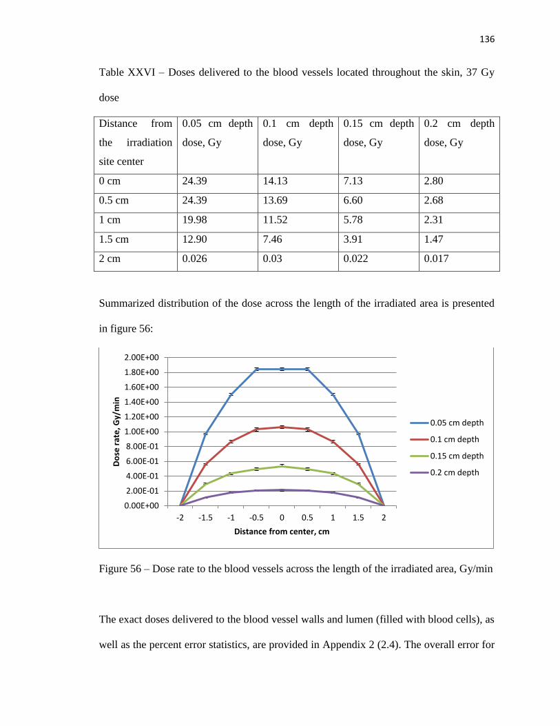
136

Table XXVI – Doses delivered to the blood vessels located throughout the skin, 37 Gy

dose

Distance from

the irradiation

site center

0.05 cm depth

dose, Gy

0.1 cm depth

dose, Gy

0.15 cm depth

dose, Gy

0.2 cm depth

dose, Gy

0 cm 24.39 14.13 7.13 2.80

0.5 cm 24.39 13.69 6.60 2.68

1 cm 19.98 11.52 5.78 2.31

1.5 cm 12.90 7.46 3.91 1.47

2 cm 0.026 0.03 0.022 0.017

Summarized distribution of the dose across the length of the irradiated area is presented

in figure 56:

Figure 56 – Dose rate to the blood vessels across the length of the irradiated area, Gy/min

The exact doses delivered to the blood vessel walls and lumen (filled with blood cells), as

well as the percent error statistics, are provided in Appendix 2 (2.4). The overall error for

0.00E+00

2.00E-01

4.00E-01

6.00E-01

8.00E-01

1.00E+00

1.20E+00

1.40E+00

1.60E+00

1.80E+00

2.00E+00

-2 -1.5 -1 -0.5 0 0.5 1 1.5 2

Do

se r

ate

, Gy/

min

Distance from center, cm

0.05 cm depth

0.1 cm depth

0.15 cm depth

0.2 cm depth

137

the dose measurement does not exceed the accepted threshold of 5% except in the cases

of the region located 2 cm away from the irradiation center that come outside of the

collimator edge area and was included for comparison purposes.

The comparison between the doses delivered to the blood vessels positioned in the “flat”

skin and “curved” skin model reveals a maximum difference of 3.2% and can be

attributed to the error margin of the simulation, thus not contributing significantly to the

results.

138

DISCUSSION

It is interesting to see that the shape of the curve of the dose rate profile across the length

of the wound strongly resembles the shape of the blood vessel thickening observed by the

histopathologist during the examination of the biological samples, confirming the close

correlation between the dose delivered to the vessels and the probability of the vessel

thickening to occur. As the blood vessel thickening is more likely to occur in the center

of the irradiated area, a cause might be established for a close correlation between the

differences in the blood supply in the center and on the edges of the irradiated area and

the epidermal necrosis expression.

It should also be noted that while the dose profile for the overall dose distribution across

the span of the wound is relatively flat and the difference between the dose profile in the

center of the irradiated area and at 1.5 cm away from the center of the irradiation is

within 10%, the same is not true for the dose delivered to the vessel located at the center

of the irradiated area and the blood vessel located 1.5 cm away from the center of the

irradiated area, with the difference in the doses delivered reaching 47%. This difference

might be a contributing factor in the dynamics of the blood vessel thickening. Such a big

difference in the dose profile comparisons vs the doses delivered to the blood vessel can

be attributed to the fact that while the dose distribution profile is collected in a relatively

small volumes mimicking ion chambers, the dose delivered to the blood vessel is

measured over the whole length of the vessel (6 cm length covering the span of the

histological samples collected) and the dose is distributed over the whole length of the

vessel within that region. This design of the investigated volume gives an approximation

of the actual positioning of the blood vessels traversing the irradiated area and as such

139

containing different partitioned volumes that would receive higher radiation doses

depending on the location of the vessel relative to the beta radiation device central axis

even for vessels of equal length. The application of the tubular structure equivalent dose

uniformity considerations seem to support this observation, even though additional

research is required in order to translate the models typically used for bigger structures

(like spinal cord or big vessels) to the microvessels found in the upper skin layers.

The natural curving of the skin during the application of the PMMA cone can introduce

some uncertainty to the results, however, during the analysis of the influence of the

curvature on the dose delivered to the skin morphological structures lying deeper into the

skin, proves to be insignificant.

Overall, a conclusion can be made that a spatial variation in the dose distribution over the

span of the irradiated area plays an important role in the epidermal necrosis expression

and blood vessel thickening. The spatial difference in the position of the blood vessels of

similar size is directly linked to the doses they receive, and there seems to be a direct

correlation between the dose the vessel received and its propensity to thicken and express

wall formation abnormalities even at the blood vessel cross section taken directly at the

center of the irradiated area. This raises an interesting question about the healing

properties of the cells forming blood vessel walls and the threshold value of the length of

the portion of the vessel, which is a serial structure, being directly affected by the

radiation that is required for the blood vessel thickening to manifest.

140

CONCLUSION AND FUTURE DIRECTION

A study of the correlation between the dose delivered by beta radiation resulting from a

one-fraction exposure and the necrosis in the upper skin layers is paramount in

understanding the mechanisms behind the cutaneous radiation injuries and developing

strategies of alleviating, and in cases of radiation dermatitis occurring as a result of

planned radiation treatment, preventing the skin reaction to radiation exposure. The

overall principals applied to the portions of this study make it applicable not only to beta

radiation, but also other types of radiation resulting in epidermal necrosis expression.

This makes the study conducted innovative, impactful and translatable.

In the course of the study, an automated tool for the epidermal necrosis assessment in the

histological samples has been developed based on the number of the dead keratinocytes

present in the epidermal layer on the skin and spread of the radiation injury. The

assessment is based on the RTOG scale used in clinical practice and utilizes a trainable

naïve Bayesian classifier in order to determine the RTOG grade of the epidermal necrosis

expression present in the histological sample. The results showed that even a small

training set is sufficient to train the classifier and provide a degree of fidelity within 70%.

However, the classifier becomes less reliable when the number of samples belonging to a

particular class are not enough to satisfy the Central Limit Theorem, making the

differentiation between grades 1 and 2 somewhat compromised and making the fidelity of

the classifier to drop to 53%. Currently, a new study is being proposed that will

significantly broaden the number of samples in the study, thus increasing the overall

number of the samples in the training set, and the number of samples within each grade.

It could be highly beneficial for future research to consider irradiating test subjects with

141

lower doses of single fraction radiation in order to invoke more responses that could be

categorized as Grades 1 and 2 on the RTOG grading scale. Another possible application

of the developed algorithm would be in adapting it to trace other features besides

epidermal necrosis, both at the irradiated skin site and other anatomical structures within

the organism.

The study provides not only the assessment of the epidermal necrosis, but also an

accurate mathematical model of the custom beta radiation device developed at Wake

Forest University. Monte Carlo simulation is confirmed as an accurate model of the

electron and photon transport and dose deposition, and as such can be used to evaluate

the dose delivered to the different skin layers. A series of tests are conducted in order to

confirm the validity of the created model of the beta radiation device. The results of the

Monte Carlo simulation are compared against the experimentally obtained surface dose

rate, cross-sectional dose profiles and percent depth dose and confirm the fidelity of the

created model. In the future, the underlying model can be then used to assess the dose

distribution from various engineering solutions for the beta radiation device,

complementing and reducing the need from laboratory experiments with different source

geometry and parameters in order to achieve desired dosimetric character, as physical

experiments can be both expensive and time consuming, and expose the beta radiation

device operator to unnecessary dose. Also the creation of an accurate model of the source

allows for an investigation of the dose delivered to the particular morphological features

of the skin.

Different skin formations found during the in vivo experiments are considered in order to

establish the possible variation between the dose rate calculated based on flat surface

142

measurements and the actual dose rate delivered to the slightly curved skin surface. The

differences in the dose rate as predicted by the Monte Carlo simulation are found to be

negligible. A comparison between the dose profile across the span of the irradiated area

and the averaged epidermal necrosis expression presented as a number of necrotic cells

present in the epidermal layer reveals a certain correlation. The peak dose location

coincides with the peak NCC expression; however, the slope of the curve describing the

NCC presence is much steeper. This fact can be explained by the further modeling of the

vasculature of the upper dermal layers responsible for supplying the epidermis. The

decrease of the dose delivered to the blood vessels located at a certain distance from a

center correlates well with the blood vessel walls’ thickening observed in the histological

samples of the irradiated tissue. That allows us to connect the shape of the dose profile

from the dose delivered to the skin surface, epidermal necrosis expression across the

wound site and the deeper morphological changes in the skin vasculature. Further

modeling of other skin components, such as nerves, hair follicles, and sweat glands

would allow us an even better understanding of the dose distribution in the upper layers

of the skin and the response of the corresponding skin features. In addition, this aspect

would also benefit from an extended study proposed on the higher number of test subjects

over the longer period of time, and with a variety of doses. This would allow for an even

better understanding of the exact mechanisms of the effect of the dose on different

components of the skin.

143

LIST OF REFERENCES

1) Hymes SR, Strom EA, Fife C. Radiation dermatitis: Clinical presentation,

pathophysiology and treatment 2006. J Am Acad Dermatol 2006; 54:28-46.

2) Bourgois, L., S. Ménard, and N. Comte. "Calculation of skin dose due to beta

contamination using the new quantity of the ICRP 116: the ‘local skin

dose’." Radiation protection dosimetry 176.4 (2017): 365-379.

3) Ryan, Julie L. "Ionizing radiation: the good, the bad, and the ugly." Journal of

Investigative Dermatology 132.3 (2012): 985-993.

4) Stücker, M.; A. Struk; P. Altmeyer; M. Herde; H. Baumgärtl; D. W. Lübbers

(2002). "The cutaneous uptake of atmospheric oxygen contributes significantly to

the oxygen supply of human dermis and epidermis". The Journal of Physiology.

538 (3): 985–994

5) Maton, Anthea; Jean Hopkins; Charles William McLaughlin; Susan Johnson;

Maryanna Quon Warner; David LaHart; Jill D. Wright (1893). Human Biology

and Health. Englewood Cliffs, New Jersey, USA: Prentice Hall. ISBN 0-13-

981176-1.

6) http://training.seer.cancer.gov/ss_module14_melanoma/images/illu_skin01.jpg

7) Valentin J. ICRP publication 85: avoidance of radiation injuries from medical

interventional procedures. Ann ICRP. 2000;30(2):7–67

8) Balter S, Hopewell JW, Miller DL, Wagner LK, Zelefsky MJ. Fluoroscopically

guided interventional procedures: a review of radiation effects on patients’ skin

and hair. Radiology. 2010;254(2):326–41

144

9) Jaschke, Werner, et al. "Radiation-Induced Skin Injuries to Patients: What the

Interventional Radiologist Needs to Know." CardioVascular and Interventional

Radiology (2017): 1-10.

10) Centers for Disease Control and Prevention. "Cutaneous radiation injury: fact

sheet for physicians." (2008).

11) Bray, Fleta N., et al. "Acute and chronic cutaneous reactions to ionizing radiation

therapy." Dermatology and therapy 6.2 (2016): 185-206.

12) https://www.rtog.org/ResearchAssociates/AdverseEventReporting/RTOGEORTC

LateRadiationMorbidityScoringSchema.aspx

13) Douglas BG, Fowler JF. The effect of multiple small doses of x rays on skin

reactions in the mouse and the basic interpretation. Radiat Res 1976; 66: 401-426

scale

14) Dorand, Jennifer Elisabeth. A f Irradiation Device for the Study of Cutaneous

Radiation Injury from a Radiological Incident. Diss. Wake Forest University,

2014.

15) E. O’Shea and P. McCavana, “Review of surface dose detectors in radiotherapy,”

J. Radiother. Pract. 3, 69-76 (2003)

16) S. C. Klevenhagen, D. D’Souza, and I. Bonnefoux, “Complications in low energy

x-ray dosimetry caused by electron contamination,” Phys. Med. Biol. 36, 1111-

1116 (1991)

17) A. Vaananen, “Theoretical and experimental study on transition zone dosimetry

with special reference to skin dose measurement with low megavoltage beams,”

Ph. D. thesis, University of Kuopio, 2002.

145

18) S. Devic, J. Seuntjens, W. Abdel-Rahman, M. Evans, M. Olivares, E. B.

Podgorsak, T. Vuong, and C. G. Soares, “Accurate skin dose measurements using

radiochromic film in clinical applications,” Med. Phys. 33, 1116-1124 (2006).

19) C. G. Soares, “Radiochromic film dosimetry,” Radiat. Meas. 41, S100-S116

(2007).

20) B. E. Bassey and N. P. S. Sidhu, “Comparison of surface dose measurements

using Attix parallel-plate ionization chamber and GafChromic EBT 2 film for 6

MV photon beam,” Powerpoint presentation, University of Saskatchewan, 2011.

21) Murthy, M. S. S., G. Venkataraman, and Shiv Datta. Revised parameters for use

in Loevinger's beta point-source dose-distribution function. Bhabha Atomic

Research Centre, Trombay, India, 1973.

22) Vynckier, Stefaan, and André Wambersie. "Dosimetry of beta sources in

radiotherapy. I. The beta point source dose function." Physics in Medicine &

Biology 27.11 (1982): 1339.

23) Cross, W. G., and L. Tommasino. "Dosimetry of high energy neutrons and

protons by 209Bi fission." Radiation protection dosimetry 70.1-4 (1997): 419-

424.

24) T. P. Selvam, P.R. B. Saull, D. W. O. Rogers, “Monte Carlo modeling of the

response of NRC’s 90Sr/90Y primary beta standard,” Med. Phys. 32, 3084-3094

(2005).

25) “Strontium,” (U.S. Environmental Protection Agency, 2012), URL:

http://www.epa.gov/radiation/radionuclides/strontium.html#wheredoes

146

26) J. D. Bourland, “Radiation Oncology Physics,” in Clinical Radiation Oncology

(eds. L. L. Gunderson and J. E. Tepper) (W. B. Saunders Company, Philadelphia,

2012).

27) F.H. Attix, Introduction to Radiological Physics and Radiation Dosimetry (Wiley-

VCH Verlag GmbH & Co. KGaA, Weinheim, Germany, 2004).

28) "Interactive Chart of Nuclides". National Nuclear Data Center, Brookhaven

National Laboratory. Retrieved 2014-09-18.

29) W. G. Cross, H. Ing, and N. Freedman, “A short atlas of beta-ray spectra,” Phys.

Med. Biol. 28, 1251-1260 (1983).

30) Attix, Frank Herbert. Introduction to radiological physics and radiation dosimetry.

John Wiley & Sons, 2008.

31) Bureau of Radiological Health and Training Institute Environmental Control

Administration, Radiological Health Handbook, (U.S. Department of Health,

Education, and Welfare: Public Health Service, Rockville, Md., 1970).

32) S. J. Goetsch and K. S. Sunderland, “Surface dose rate calibration of Sr-90 plane

ophthalmic applicators,” Med. Phys. 18, 161-165 (1991).

33) C. S. Reft, F. T. Kuchnir, I. Rosenberg, and L. C. Myrianthopoulos, “Dosimetry

of Sr-90 ophthalmic applicators,” Med. Phys. 17, 641-646 (1990).

34) Osanov, D. P. Dosimetry and radiation biophysics of the skin/D. P. Osanov,

Moscow; “Energoatomizdat” publishing house, 1983

35) Osanov, D. P., Kinetics of the dose deposition in the skin with radiation pollution/

D. P. Osanov, E. B. Ershov et al/Medical Radiology, issue # 5, 1971, p. 44-50.

147

36) Osanov, D. P. Microdosimetry deposition in skin with alpha and beta radiation/D.

P. Osanov, E. B. Ershov et al., /”Radiation Medicine”, Moscow, “Atomizdat”

publishing house, 1972, p. 239-246

37) Schultz, F. W. and Zoetelief, J. Organ and effective doses in the male phantom

Adam exposed in AP direction to broad unidirectional beams of monoenergetic

electrons. Health Phys. 70(4), 498–504 (1996).

38) International Commission on Radiological Protection. Coefficients for use in

radiological protection against external radiation. ICRP Publication 74. Ann.

26(3/4) (1996)

39) Norme ISO 15382 Procédure de surveillance dosimétrique de radioprotection

dans les installations nucléaires pour l’exposition externe aux rayonnements

faiblement pénétrants, en particulier au rayonnement bêta (2002)

40) International Commission on Radiological Protection. Conversion coefficients for

radiological protection quantities for external radiation exposures. ICRP

Publication 116. Ann. ICRP 40(2–5) (2010)

41) Bourgois, L. and Antoni, R. Fluence to local skin absorbed dose and dose

equivalent conversion coefficients for monoenergetic positrons using Monte-

Carlo code MCNP6. Appl. Radiat. Isot. 107(2016), 372–376 (2016)

42) Ershov, E. B., Osanov, D. P., “Skin dosimetry with constant pollution by

plutonium-239 and americium-241 solutions”, Radiation hygiene, issue 5.4, 2015,

p. 36-39

43) Cross, W. G. “Empirical expressions for beta ray point source dose distributions.”

Radiation protection dosimetry 69.2 (1997): 85-96.

148

44) “Dosimetry of beta rays and low-energy photons for brachytherapy with sealed

sources (Report 72),” J. ICRU. 4, 17-163 (2004).

45) S Vynckier and A Wambersie 1982 Phys. Med. Biol. 27 1339

46) Young AR (June 1987). "The sunburn cell". Photodermatology. 4 (3): 127–134.

PMID 3317295.

47) Kumar V, Abbas A, Nelson F, Mitchell R (2007). "Robbins Basic

Pathology". Robbins Basic Pathology (8th ed.): 6, 9–10 (table 1–1).

48) Kolm, I., et al. "Subacute cutaneous lupus erythematosus triggered by

radiotherapy." Case reports in dermatology 5.2 (2013): 232-235

49) Meyn, Raymond E. "Apoptosis and response to radiation: implications for

radiation therapy." Oncology (Williston Park, NY) 11.3 (1997): 349-56.

50) Hymes SR, Strom EA, Fife C. Radiation dermatitis: clinical presentation,

pathophysiology, and treatment 2006. J Am Acad Dermatol. 2010

51) Biswas, Asok. Pearls and Pitfalls in Inflammatory Dermatopathology.

Cambridge University Press, 2017.

52) http://openslide.org/formats/hamamatsu/

53) http://openslide.cs.cmu.edu/download/openslide-testdata/Hamamatsu/

54) Linkert M, Rueden CT, Allan C, Burel JM, Moore W, Patterson A, Loranger B,

Moore J, Neves C, MacDonald D, Tarkowska A, Sticco C, Hill E, Rossner M,

Eliceiri KW, Swedlow JR: Metadata matters: access to im– age data in the real

world. Journal of Cell Biology 2010, 198(5):777{782}

149

55) Goode A, Satyanarayanan M: A Vendor-Neutral Library and Viewer for Whole-

Slide Images. Tech. Rep. Technical Report CMU-CS-08-136, Computer Science

Department, Carnegie Mellon University 2008

56) Khushi M, Edwards G, de Marcos DA, Carpenter JE, Graham JD, Clarke CL:

Open source tools for man– agement and archiving of digital microscopy data to

allow integration with patient pathology and treatment information. Diagnostic

pathology 2013, 8:22

57) https://imagej.net/Welcome

58) Deroulers, Christophe, et al. "Analyzing huge pathology images with open source

software." Diagnostic pathology 8.1 (2013): 92.

59) Schindelin, Johannes, et al. "Fiji: an open-source platform for biological-image

analysis." Nature methods 9.7 (2012): 676-682

60) Kuru, Kaya. "Optimization and enhancement of H&E stained microscopical

images by applying bilinear interpolation method on lab color mode." Theoretical

Biology and Medical Modelling 11.1 (2014)

61) Walton, W. H. "Feret’s statistical diameter as a measure of particle size." Nature

162.4113 (1948): 329-330.

62) Canny, John. "A computational approach to edge detection." IEEE Transactions

on pattern analysis and machine intelligence 6 (1986): 679-698.

63) Rodieck, B. (2008).

http://rsb.info.nih.gov/ij/developer/source/ij/process/EllipseFitter.java.html

150

64) Igathinathane, C., L. O. Pordesimo, and W. D. Batchelor. "Major orthogonal

dimensions measurement of food grains by machine vision using ImageJ." Food

Research International 42.1 (2009): 76-84.

65) Eidet, Jon R., et al. "Objective assessment of changes in nuclear morphology and

cell distribution following induction of apoptosis." Diagnostic pathology 9.1

(2014): 92.

66) Epanechnikov, V.A. (1969). "Non-parametric estimation of a multivariate

probability density". Theory of Probability and its Applications. 14: 153–158.

doi:10.1137/1114019

67) Welch, B. L. (1947). "The generalization of "Student's" problem when several

different population variances are involved". Biometrika. 34 (1–2): 28–35.

doi:10.1093/biomet/34.1-2.28. MR 0019277

68) Brown, Forrest B. "Fundamentals of Monte Carlo particle transport." Los Alamos

National Laboratory, LA-UR-05-4983(2005).

69) S. Goudsmit and J. L. Saunderson, “Multiple Scattering of Electrons,” Phys. Rev.

57 (1940)24.

70) R. N. Blomquist and E. M. Gelbard, “An Assessment of Existing Klein-Nishina

Monte Carlo Sampling Methods,” Nucl. Sci. Eng., 83, 380 (1983)

71) G. W. Grodstein, “X-Ray Attenuation Coefficients from 10 keV to 100 MeV,”

National Bureau of Standards, Circular No. 583 (1957).

72) Goorley, Tim. Monte Carlo N Particle Transport Code System Including MCNP6.

1, MCNP5-1.60, MCNPX-2.7. 0 and Data Libraries. No. MCNP6.

151

1/MCNP5/MCNPX-EXE; 004380MLTPL00. Oak Ridge National Laboratory

(ORNL), Oak Ridge, TN (United States), 2013.

73) Brualla, Lorenzo, Miguel Rodriguez, and Antonio M. Lallena. "Monte Carlo

systems used for treatment planning and dose verification." Strahlentherapie und

Onkologie 193.4 (2017): 243-259.

74) Afzalifar, Azam, et al. "Monte Carlo based determination of dose distribution for

some patch sources employed for radionuclide skin therapy." Australasian

physical & engineering sciences in medicine 41.4 (2018): 853-860.

75) 1-1 MCNP6 , mcnp5, mcnpx, mcnp6 Monte Carlo Codes XCP – 3 & NEN – 5

Los Alamos National Laboratory/ MCNP6 Class Alabama Agricultural and

Mechanical University March 3 7, 2014 Presented by H. Grady Hughes and

Michael R. James Los Alamos National Laboratory

76) L. J. Lorence, Jr., J. E. Morel, G. D. Valdez, “Physics Guide to CEPXS: A

Multigroup Coupled Electron–Photon Cross–Section Generating Code, Version

1.0,” SAND89–1685 (1989)

77) Stephen M. Seltzer, “An Overview of ETRAN Monte Carlo Methods,” in Monte

Carlo Transport of Electrons and Photons, edited by Theodore M. Jenkins, Walter

R. Nelson, and Alessandro Rindi, (Plenum Press, New York, 1988) 153.

78) Tekin, Huseyin Ozan, et al. "Mass attenuation coefficients of human body organs

using MCNPX Monte Carlo code." Iranian Journal of Medical Physics 14.4

(2017): 229-240.

152

79) K. F. Eckerman, R. J. Westfall, J. C. Ryman, and M. Cristy, "Availability of

Nuclear Decay Data in Electronic Form, Including Beta Spectra not Previously

Published," Health Phys. 67(4):338-345 (1994).

80) Rubin P, Nelson DF. Late effects of cancer treatments:radiation and drug toxicity.

Clinical Oncology. Rochester: W.B. Saunders Co., 1999; 735-760.

81) Braverman, Irwin M. "The cutaneous microcirculation." Journal of Investigative

Dermatology Symposium Proceedings. Vol. 5. No. 1. Elsevier, 2000.

82) Braverman, Irwin M. "The cutaneous microcirculation." Journal of Investigative

Dermatology Symposium Proceedings. Vol. 5. No. 1. Elsevier, 2000.

83) Niemierko, Andrzej. "Reporting and analyzing dose distributions: a concept of

equivalent uniform dose." Medical physics 24.1 (1997): 103-110.

84) Li, X. Allen, et al. "The use and QA of biologically related models for treatment

planning: Short report of the TG‐166 of the therapy physics committee of the

AAPM." Medical Physics39.3 (2012): 1386-1409.

153

Appendix 1

1.1 Percent depth dose measurement - MCNP6 code

Input code for the measurement of the dose at the depths of 0 cm to 0.25 cm

Source model correct C *************BLOCK 1 -- CELLS ************ 1 1 -1.18 -11 18 -15 16 -13 19 60 IMP:P=1 IMP:E=1 2 2 -0.001225 (-11 18 -16):-19:-20:-21:-40:-41:-42:-43:-46:-47& :-44:-45:-48:-49:-491:-492:-493:-494 60 IMP:P=1 IMP:E=1 3 3 -2.7 (11 -30 -31 20 21 40 41 42 43 44 45 46 47 48 49 491& 492 493 494 50 51 52 53 54 55 56 70 71 72 73 74 75 76):(-14 13)& IMP:P=1 IMP:E=1 4 4 -3.02 -50 IMP:P=1 IMP:E=1 5 4 -3.02 -51 IMP:P=1 IMP:E=1 6 4 -3.02 -52 IMP:P=1 IMP:E=1 7 4 -3.02 -53 IMP:P=1 IMP:E=1 8 4 -3.02 -54 IMP:P=1 IMP:E=1 9 4 -3.02 -55 IMP:P=1 IMP:E=1 10 4 -3.02 -56 IMP:P=1 IMP:E=1 11 5 -1.1 -60 61 62 83 84 85 86 87 88 89 90 91 92& 93 94 95 96 97 98 99 100 101 IMP:P=1 IMP:E=1 12 5 -1.1 -61 IMP:P=1 IMP:E=1 13 6 -7.87 -70 50 IMP:P=1 IMP:E=1 14 6 -7.87 -71 51 IMP:P=1 IMP:E=1 15 6 -7.87 -72 52 IMP:P=1 IMP:E=1 16 6 -7.87 -73 53 IMP:P=1 IMP:E=1 17 6 -7.87 -74 54 IMP:P=1 IMP:E=1 18 6 -7.87 -75 55 IMP:P=1 IMP:E=1 19 6 -7.87 -76 56 IMP:P=1 IMP:E=1 20 5 -1.1 -62 IMP:P=1 IMP:E=1 21 5 -1.1 -83 IMP:P=1 IMP:E=1 22 5 -1.1 -84 IMP:P=1 IMP:E=1 23 5 -1.1 -85 IMP:P=1 IMP:E=1 24 5 -1.1 -86 IMP:P=1 IMP:E=1 25 5 -1.1 -87 IMP:P=1 IMP:E=1 26 5 -1.1 -88 IMP:P=1 IMP:E=1 27 5 -1.1 -89 IMP:P=1 IMP:E=1 28 5 -1.1 -90 IMP:P=1 IMP:E=1 29 5 -1.1 -91 IMP:P=1 IMP:E=1 30 5 -1.1 -92 IMP:P=1 IMP:E=1 31 5 -1.1 -93 IMP:P=1 IMP:E=1 32 5 -1.1 -94 IMP:P=1 IMP:E=1 33 5 -1.1 -95 IMP:P=1 IMP:E=1 34 5 -1.1 -96 IMP:P=1 IMP:E=1 35 5 -1.1 -97 IMP:P=1 IMP:E=1 36 5 -1.1 -98 IMP:P=1 IMP:E=1 37 5 -1.1 -99 IMP:P=1 IMP:E=1 38 5 -1.1 -100 IMP:P=1 IMP:E=1 39 5 -1.1 -101 IMP:P=1 IMP:E=1 44 0 (-18 60):(-11 15 18 14):(11 -30 31):30 IMP:P=0 IMP:E=0 C *************BLOCK 2 -- SURFACES ********* 11 PZ 2.7 13 CZ 4.5 14 RCC 0 0 2.4 0 0 0.3 5 15 KZ -2.1 1 1 16 KZ -1.3 1 1

154

18 PZ 0 19 RCC 0 0 0 0 0 0.6 1.8 20 TRC 0 0 2.7 0 0 0.4 3.84 3.44 21 RCC 0 0 3.1 0 0 0.5 3.44 30 PZ 6.1 31 CZ 5 40 TRC 0 0 3.6 0 0 0.2 1 0.8 41 RCC 0 0 3.8 0 0 0.15 0.8 42 TRC 0 2.4445 3.6 0 0 0.2 1 0.8 43 RCC 0 2.4445 3.8 0 0 0.15 0.8 44 TRC 0 -2.4445 3.6 0 0 0.2 1 0.8 45 RCC 0 -2.4445 3.8 0 0 0.15 0.8 46 TRC 2.11 1.22 3.6 0 0 0.2 1 0.8 47 RCC 2.11 1.22 3.8 0 0 0.15 0.8 48 TRC -2.11 1.22 3.6 0 0 0.2 1 0.8 49 RCC -2.11 1.22 3.8 0 0 0.15 0.8 491 TRC 2.11 -1.22 3.6 0 0 0.2 1 0.8 492 RCC 2.11 -1.22 3.8 0 0 0.15 0.8 493 TRC -2.11 -1.22 3.6 0 0 0.2 1 0.8 494 RCC -2.11 -1.22 3.8 0 0 0.15 0.8 50 RCC 0 0 3.96 0 0 0.06 0.8 51 RCC 0 2.4445 3.96 0 0 0.06 0.8 52 RCC 0 -2.4445 3.96 0 0 0.06 0.8 53 RCC 2.11 1.22 3.96 0 0 0.06 0.8 54 RCC -2.11 1.22 3.96 0 0 0.06 0.8 55 RCC 2.11 -1.22 3.96 0 0 0.06 0.8 56 RCC -2.11 -1.22 3.96 0 0 0.06 0.8 70 RCC 0 0 3.96 0 0 0.6 1.1 71 RCC 0 2.4445 3.96 0 0 0.6 1.1 72 RCC 0 -2.4445 3.96 0 0 0.6 1.1 73 RCC 2.11 1.22 3.96 0 0 0.6 1.1 74 RCC -2.11 1.22 3.96 0 0 0.6 1.1 75 RCC 2.11 -1.22 3.96 0 0 0.6 1.1 76 RCC -2.11 -1.22 3.96 0 0 0.6 1.1 60 RCC 0 0 0 0 0 -2.5 2 61 RCC 0 0 0 0 0 -0.0125 1.8 62 RCC 0 0 -0.0125 0 0 -0.0125 1.8 83 RCC 0 0 -0.025 0 0 -0.0125 1.8 84 RCC 0 0 -0.0375 0 0 -0.0125 1.8 85 RCC 0 0 -0.05 0 0 -0.0125 1.8 86 RCC 0 0 -0.0625 0 0 -0.0125 1.8 87 RCC 0 0 -0.075 0 0 -0.0125 1.8 88 RCC 0 0 -0.0875 0 0 -0.0125 1.8 89 RCC 0 0 -0.1 0 0 -0.0125 1.8 90 RCC 0 0 -0.1125 0 0 -0.0125 1.8 91 RCC 0 0 -0.125 0 0 -0.0125 1.8 92 RCC 0 0 -0.1375 0 0 -0.0125 1.8 93 RCC 0 0 -0.15 0 0 -0.0125 1.8 94 RCC 0 0 -0.1625 0 0 -0.0125 1.8 95 RCC 0 0 -0.175 0 0 -0.0125 1.8 96 RCC 0 0 -0.1875 0 0 -0.0125 1.8 97 RCC 0 0 -0.2 0 0 -0.0125 1.8 98 RCC 0 0 -0.2125 0 0 -0.0125 1.8 99 RCC 0 0 -0.225 0 0 -0.0125 1.8 100 RCC 0 0 -0.2375 0 0 -0.0125 1.8 101 RCC 0 0 -0.25 0 0 -0.0125 1.8 C *************BLOCK 3 -- everything else*** mode p e SDEF CEL=d1 POS=0 0 3.95999 AXS=0 0 1 EXT=d2 RAD=d3 PAR=3 ERG=d4 SI1 L 4 5 6 7 8 9 10 SP1 0.142857 0.142857 0.142857 0.142847 0.142857 0.142857 0.142857 SI2 H 0 0.0601 SP2 -21 0

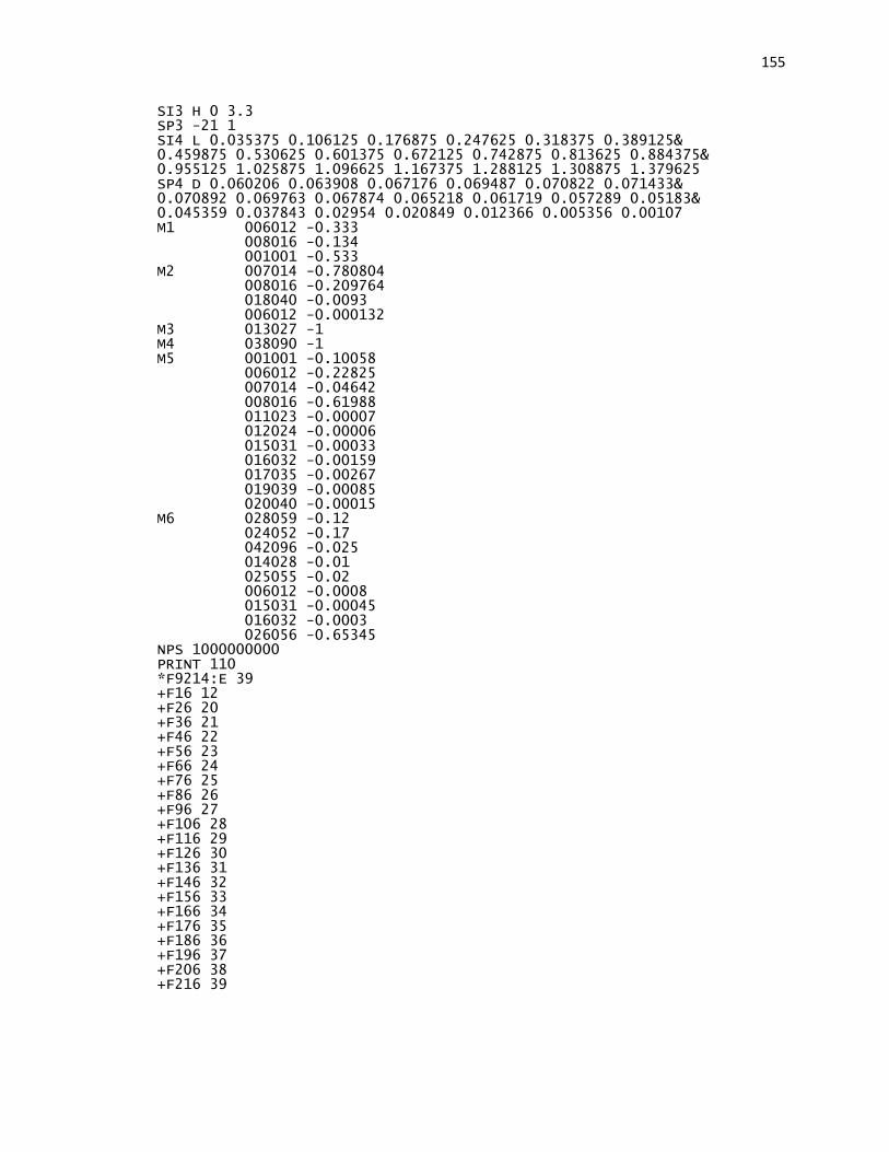
155

SI3 H 0 3.3 SP3 -21 1 SI4 L 0.035375 0.106125 0.176875 0.247625 0.318375 0.389125& 0.459875 0.530625 0.601375 0.672125 0.742875 0.813625 0.884375& 0.955125 1.025875 1.096625 1.167375 1.288125 1.308875 1.379625 SP4 D 0.060206 0.063908 0.067176 0.069487 0.070822 0.071433& 0.070892 0.069763 0.067874 0.065218 0.061719 0.057289 0.05183& 0.045359 0.037843 0.02954 0.020849 0.012366 0.005356 0.00107 M1 006012 -0.333 008016 -0.134 001001 -0.533 M2 007014 -0.780804 008016 -0.209764 018040 -0.0093 006012 -0.000132 M3 013027 -1 M4 038090 -1 M5 001001 -0.10058 006012 -0.22825 007014 -0.04642 008016 -0.61988 011023 -0.00007 012024 -0.00006 015031 -0.00033 016032 -0.00159 017035 -0.00267 019039 -0.00085 020040 -0.00015 M6 028059 -0.12 024052 -0.17 042096 -0.025 014028 -0.01 025055 -0.02 006012 -0.0008 015031 -0.00045 016032 -0.0003 026056 -0.65345 NPS 1000000000 PRINT 110 *F9214:E 39 +F16 12 +F26 20 +F36 21 +F46 22 +F56 23 +F66 24 +F76 25 +F86 26 +F96 27 +F106 28 +F116 29 +F126 30 +F136 31 +F146 32 +F156 33 +F166 34 +F176 35 +F186 36 +F196 37 +F206 38 +F216 39

156

Input code for the measurement of the dose at the depths of 0.25 cm to 0.5 cm – code

variation only:

61 RCC 0 0 -0.25 0 0 -0.0125 1.8 62 RCC 0 0 -0.2625 0 0 -0.0125 1.8 83 RCC 0 0 -0.275 0 0 -0.0125 1.8 84 RCC 0 0 -0.2875 0 0 -0.0125 1.8 85 RCC 0 0 -0.3 0 0 -0.0125 1.8 86 RCC 0 0 -0.3125 0 0 -0.0125 1.8 87 RCC 0 0 -0.325 0 0 -0.0125 1.8 88 RCC 0 0 -0.3375 0 0 -0.0125 1.8 89 RCC 0 0 -0.35 0 0 -0.0125 1.8 90 RCC 0 0 -0.3625 0 0 -0.0125 1.8 91 RCC 0 0 -0.375 0 0 -0.0125 1.8 92 RCC 0 0 -0.3875 0 0 -0.0125 1.8 93 RCC 0 0 -0.4 0 0 -0.0125 1.8 94 RCC 0 0 -0.4125 0 0 -0.0125 1.8 95 RCC 0 0 -0.425 0 0 -0.0125 1.8 96 RCC 0 0 -0.4375 0 0 -0.0125 1.8 97 RCC 0 0 -0.45 0 0 -0.0125 1.8 98 RCC 0 0 -0.4625 0 0 -0.0125 1.8 99 RCC 0 0 -0.475 0 0 -0.0125 1.8 100 RCC 0 0 -0.4875 0 0 -0.0125 1.8 101 RCC 0 0 -0.5 0 0 -0.0125 1.8

1.2 Absorbed dose profile measurement – MCNP6 code

Input code for the 1 mm measurement

C *************BLOCK 1 -- CELLS ************ 1 1 -1.18 -11 18 -15 16 -13 19 60 IMP:P=1 IMP:E=1 2 2 -0.001225 (-11 18 -16):-19:-20:-21:-40:-41:-42:-43:-46:-47& :-44:-45:-48:-49:-491:-492:-493:-494 60 IMP:P=1 IMP:E=1 3 3 -2.7 (11 -30 -31 20 21 40 41 42 43 44 45 46 47 48 49 491& 492 493 494 50 51 52 53 54 55 56 190 191 192 193 194 195 196):(-14 13)& IMP:P=1 IMP:E=1 4 4 -3.02 -50 IMP:P=1 IMP:E=1 5 4 -3.02 -51 IMP:P=1 IMP:E=1 6 4 -3.02 -52 IMP:P=1 IMP:E=1 7 4 -3.02 -53 IMP:P=1 IMP:E=1 8 4 -3.02 -54 IMP:P=1 IMP:E=1 9 4 -3.02 -55 IMP:P=1 IMP:E=1 10 4 -3.02 -56 IMP:P=1 IMP:E=1 11 5 -1.1 -60 61 62 63 64 65 66 67 68 69 70 71 72 73 74 75& 76 77 78 79 80 81 82 83 84 161 162 163 164 165 166 167 168& 169 170 171 172 173 174 175 176 177 178 179 180 181 182& 183 184 IMP:P=1 IMP:E=1 13 6 -7.87 -190 50 IMP:P=1 IMP:E=1 14 6 -7.87 -191 51 IMP:P=1 IMP:E=1 15 6 -7.87 -192 52 IMP:P=1 IMP:E=1 16 6 -7.87 -193 53 IMP:P=1 IMP:E=1 17 6 -7.87 -194 54 IMP:P=1 IMP:E=1 18 6 -7.87 -195 55 IMP:P=1 IMP:E=1 19 6 -7.87 -196 56 IMP:P=1 IMP:E=1 22 5 -1.1 -61 IMP:P=1 IMP:E=1 23 5 -1.1 -62 IMP:P=1 IMP:E=1

157

24 5 -1.1 -63 IMP:P=1 IMP:E=1 25 5 -1.1 -64 IMP:P=1 IMP:E=1 26 5 -1.1 -65 IMP:P=1 IMP:E=1 27 5 -1.1 -66 IMP:P=1 IMP:E=1 28 5 -1.1 -67 IMP:P=1 IMP:E=1 29 5 -1.1 -68 IMP:P=1 IMP:E=1 30 5 -1.1 -69 IMP:P=1 IMP:E=1 31 5 -1.1 -70 IMP:P=1 IMP:E=1 32 5 -1.1 -71 IMP:P=1 IMP:E=1 33 5 -1.1 -72 IMP:P=1 IMP:E=1 34 5 -1.1 -73 IMP:P=1 IMP:E=1 35 5 -1.1 -74 IMP:P=1 IMP:E=1 36 5 -1.1 -75 IMP:P=1 IMP:E=1 37 5 -1.1 -76 IMP:P=1 IMP:E=1 38 5 -1.1 -77 IMP:P=1 IMP:E=1 39 5 -1.1 -78 IMP:P=1 IMP:E=1 40 5 -1.1 -79 IMP:P=1 IMP:E=1 41 5 -1.1 -80 IMP:P=1 IMP:E=1 42 5 -1.1 -81 IMP:P=1 IMP:E=1 43 5 -1.1 -82 IMP:P=1 IMP:E=1 44 5 -1.1 -83 IMP:P=1 IMP:E=1 45 5 -1.1 -84 IMP:P=1 IMP:E=1 122 5 -1.1 -161 IMP:P=1 IMP:E=1 123 5 -1.1 -162 IMP:P=1 IMP:E=1 124 5 -1.1 -163 IMP:P=1 IMP:E=1 125 5 -1.1 -164 IMP:P=1 IMP:E=1 126 5 -1.1 -165 IMP:P=1 IMP:E=1 127 5 -1.1 -166 IMP:P=1 IMP:E=1 128 5 -1.1 -167 IMP:P=1 IMP:E=1 129 5 -1.1 -168 IMP:P=1 IMP:E=1 130 5 -1.1 -169 IMP:P=1 IMP:E=1 131 5 -1.1 -170 IMP:P=1 IMP:E=1 132 5 -1.1 -171 IMP:P=1 IMP:E=1 133 5 -1.1 -172 IMP:P=1 IMP:E=1 134 5 -1.1 -173 IMP:P=1 IMP:E=1 135 5 -1.1 -174 IMP:P=1 IMP:E=1 136 5 -1.1 -175 IMP:P=1 IMP:E=1 137 5 -1.1 -176 IMP:P=1 IMP:E=1 138 5 -1.1 -177 IMP:P=1 IMP:E=1 139 5 -1.1 -178 IMP:P=1 IMP:E=1 140 5 -1.1 -179 IMP:P=1 IMP:E=1 141 5 -1.1 -180 IMP:P=1 IMP:E=1 142 5 -1.1 -181 IMP:P=1 IMP:E=1 143 5 -1.1 -182 IMP:P=1 IMP:E=1 144 5 -1.1 -183 IMP:P=1 IMP:E=1 145 5 -1.1 -184 IMP:P=1 IMP:E=1 53 0 (-18 60 161 76 176 77 177 78 178 82 182 83 183 84 184)& :(-11 15 18 14):(11 -30 31):30 IMP:P=0 IMP:E=0 C *************BLOCK 2 -- SURFACES ********* 11 PZ 2.7 13 CZ 4.5 14 RCC 0 0 2.4 0 0 0.3 5 15 KZ -2.1 1 1 16 KZ -1.3 1 1 18 PZ 0 19 RCC 0 0 0 0 0 0.6 1.8 20 TRC 0 0 2.7 0 0 0.4 3.84 3.44 21 RCC 0 0 3.1 0 0 0.5 3.44 30 PZ 6.1 31 CZ 5 40 TRC 0 0 3.6 0 0 0.2 1 0.8 41 RCC 0 0 3.8 0 0 0.15 0.8 42 TRC 0 2.4445 3.6 0 0 0.2 1 0.8

158

43 RCC 0 2.4445 3.8 0 0 0.15 0.8 44 TRC 0 -2.4445 3.6 0 0 0.2 1 0.8 45 RCC 0 -2.4445 3.8 0 0 0.15 0.8 46 TRC 2.11 1.22 3.6 0 0 0.2 1 0.8 47 RCC 2.11 1.22 3.8 0 0 0.15 0.8 48 TRC -2.11 1.22 3.6 0 0 0.2 1 0.8 49 RCC -2.11 1.22 3.8 0 0 0.15 0.8 491 TRC 2.11 -1.22 3.6 0 0 0.2 1 0.8 492 RCC 2.11 -1.22 3.8 0 0 0.15 0.8 493 TRC -2.11 -1.22 3.6 0 0 0.2 1 0.8 494 RCC -2.11 -1.22 3.8 0 0 0.15 0.8 50 RCC 0 0 3.96 0 0 0.06 0.8 51 RCC 0 2.4445 3.96 0 0 0.06 0.8 52 RCC 0 -2.4445 3.96 0 0 0.06 0.8 53 RCC 2.11 1.22 3.96 0 0 0.06 0.8 54 RCC -2.11 1.22 3.96 0 0 0.06 0.8 55 RCC 2.11 -1.22 3.96 0 0 0.06 0.8 56 RCC -2.11 -1.22 3.96 0 0 0.06 0.8 190 RCC 0 0 3.96 0 0 0.6 1.1 191 RCC 0 2.4445 3.96 0 0 0.6 1.1 192 RCC 0 -2.4445 3.96 0 0 0.6 1.1 193 RCC 2.11 1.22 3.96 0 0 0.6 1.1 194 RCC -2.11 1.22 3.96 0 0 0.6 1.1 195 RCC 2.11 -1.22 3.96 0 0 0.6 1.1 196 RCC -2.11 -1.22 3.96 0 0 0.6 1.1 60 RCC 0 0 0 0 0 -2 2 61 BOX -0.5 0 -0.1 1 0 0 0 0.1 0 0 0 -0.1 161 BOX -0.5 0.1 -0.1 1 0 0 0 0.1 0 0 0 -0.1 62 BOX -0.5 0.2 -0.1 1 0 0 0 0.1 0 0 0 -0.1 162 BOX -0.5 0.3 -0.1 1 0 0 0 0.1 0 0 0 -0.1 63 BOX -0.5 0.4 -0.1 1 0 0 0 0.1 0 0 0 -0.1 163 BOX -0.5 0.5 -0.1 1 0 0 0 0.1 0 0 0 -0.1 64 BOX -0.5 0.6 -0.1 1 0 0 0 0.1 0 0 0 -0.1 164 BOX -0.5 0.7 -0.1 1 0 0 0 0.1 0 0 0 -0.1 65 BOX -0.5 0 -0.1 1 0 0 0 -0.1 0 0 0 -0.1 165 BOX -0.5 -0.1 -0.1 1 0 0 0 -0.1 0 0 0 -0.1 66 BOX -0.5 -0.2 -0.1 1 0 0 0 -0.1 0 0 0 -0.1 166 BOX -0.5 -0.3 -0.1 1 0 0 0 -0.1 0 0 0 -0.1 67 BOX -0.5 -0.4 -0.1 1 0 0 0 -0.1 0 0 0 -0.1 167 BOX -0.5 -0.5 -0.1 1 0 0 0 -0.1 0 0 0 -0.1 68 BOX -0.5 -0.6 -0.1 1 0 0 0 -0.1 0 0 0 -0.1 168 BOX -0.5 -0.7 -0.1 1 0 0 0 -0.1 0 0 0 -0.1 69 BOX -0.5 0.8 -0.1 1 0 0 0 0.1 0 0 0 -0.1 169 BOX -0.5 0.9 -0.1 1 0 0 0 0.1 0 0 0 -0.1 70 BOX -0.5 -0.8 -0.1 1 0 0 0 -0.1 0 0 0 -0.1 170 BOX -0.5 -0.9 -0.1 1 0 0 0 -0.1 0 0 0 -0.1 71 BOX -0.5 1 -0.1 1 0 0 0 0.1 0 0 0 -0.1 171 BOX -0.5 1.1 -0.1 1 0 0 0 0.1 0 0 0 -0.1 72 BOX -0.5 -1 -0.1 1 0 0 0 -0.1 0 0 0 -0.1 172 BOX -0.5 -1.1 -0.1 1 0 0 0 -0.1 0 0 0 -0.1 73 BOX -0.5 1.2 -0.1 1 0 0 0 0.1 0 0 0 -0.1 173 BOX -0.5 1.3 -0.1 1 0 0 0 0.1 0 0 0 -0.1 74 BOX -0.5 1.4 -0.1 1 0 0 0 0.1 0 0 0 -0.1 174 BOX -0.5 1.5 -0.1 1 0 0 0 0.1 0 0 0 -0.1 75 BOX -0.5 1.6 -0.1 1 0 0 0 0.1 0 0 0 -0.1 175 BOX -0.5 1.7 -0.1 1 0 0 0 0.1 0 0 0 -0.1 76 BOX -0.5 1.8 -0.1 1 0 0 0 0.1 0 0 0 -0.1 176 BOX -0.5 1.9 -0.1 1 0 0 0 0.1 0 0 0 -0.1 77 BOX -0.5 2 -0.1 1 0 0 0 0.1 0 0 0 -0.1 177 BOX -0.5 2.1 -0.1 1 0 0 0 0.1 0 0 0 -0.1 78 BOX -0.5 2.2 -0.1 1 0 0 0 0.1 0 0 0 -0.1 178 BOX -0.5 2.3 -0.1 1 0 0 0 0.1 0 0 0 -0.1 79 BOX -0.5 -1.2 -0.1 1 0 0 0 -0.1 0 0 0 -0.1 179 BOX -0.5 -1.3 -0.1 1 0 0 0 -0.1 0 0 0 -0.1

159

80 BOX -0.5 -1.4 -0.1 1 0 0 0 -0.1 0 0 0 -0.1 180 BOX -0.5 -1.5 -0.1 1 0 0 0 -0.1 0 0 0 -0.1 81 BOX -0.5 -1.6 -0.1 1 0 0 0 -0.1 0 0 0 -0.1 181 BOX -0.5 -1.7 -0.1 1 0 0 0 -0.1 0 0 0 -0.1 82 BOX -0.5 -1.8 -0.1 1 0 0 0 -0.1 0 0 0 -0.1 182 BOX -0.5 -1.9 -0.1 1 0 0 0 -0.1 0 0 0 -0.1 83 BOX -0.5 -2 -0.1 1 0 0 0 -0.1 0 0 0 -0.1 183 BOX -0.5 -2.1 -0.1 1 0 0 0 -0.1 0 0 0 -0.1 84 BOX -0.5 -2.2 -0.1 1 0 0 0 -0.1 0 0 0 -0.1 184 BOX -0.5 -2.3 -0.1 1 0 0 0 -0.1 0 0 0 -0.1

1.3 Pie cell formation simulation – MCNP6 code

Input for the geometrical arrangement of symmetrical circular sectors:

C *************BLOCK 1 -- CELLS ************ 1 1 -1.18 -11 18 -15 16 -13 19 60 IMP:P=1 IMP:E=1 2 2 -0.001225 (-11 18 -16):-19:-20:-21:-40:-41:-42:-43:-46:-47& :-44:-45:-48:-49:-491:-492:-493:-494 60 70 IMP:P=1 IMP:E=1 3 3 -2.7 (11 -30 -31 20 21 40 41 42 43 44 45 46 47 48 49 491& 492 493 494 50 51 52 53 54 55 56 90 91 92 93 94 95 96):(-14 13) IMP:P=1 IMP:E=1 4 4 -3.02 -50 IMP:P=1 IMP:E=1 5 4 -3.02 -51 IMP:P=1 IMP:E=1 6 4 -3.02 -52 IMP:P=1 IMP:E=1 7 4 -3.02 -53 IMP:P=1 IMP:E=1 8 4 -3.02 -54 IMP:P=1 IMP:E=1 9 4 -3.02 -55 IMP:P=1 IMP:E=1 10 4 -3.02 -56 IMP:P=1 IMP:E=1 11 5 -1.1 -60 IMP:P=1 IMP:E=1 12 5 -1.1 -61 62 (70:-71:-72:-73:74) (70:-71:72:-73:74)& (70:71:-72:73:-74) (70:71:72:73:-74) (70:-71:-72:-75:-76)& (70:71:-72:-75:-76) (70:-71:72:75:76) (70:71:72:75:76)& (69:-71:-72:-73:74) (68:-71:-72:-73:74) (67:-71:-72:-73:74)& (66:-71:-72:-73:74) (65:-71:-72:-73:74) (64:-71:-72:-73:74)& (63:-71:-72:-73:74) (69:-71:72:-73:74)& (68:-71:72:-73:74) (67:-71:72:-73:74) (66:-71:72:-73:74)& (65:-71:72:-73:74) (64:-71:72:-73:74) (63:-71:72:-73:74)& (69:71:-72:73:-74)(68:71:-72:73:-74)& (67:71:-72:73:-74) (66:71:-72:73:-74) (65:71:-72:73:-74)& (64:71:-72:73:-74) (63:71:-72:73:-74)& (69:71:72:73:-74) (68:71:72:73:-74) (67:71:72:73:-74)& (66:71:72:73:-74) (65:71:72:73:-74) (64:71:72:73:-74)& (63:71:72:73:-74) (69:-71:-72:-75:-76)& (68:-71:-72:-75:-76) (67:-71:-72:-75:-76) (66:-71:-72:-75:-76)& (65:-71:-72:-75:-76) (64:-71:-72:-75:-76) (63:-71:-72:-75:-76)& (69:71:-72:-75:-76) (68:71:-72:-75:-76)& (67:71:-72:-75:-76) (66:71:-72:-75:-76) (65:71:-72:-75:-76)& (64:71:-72:-75:-76) (63:71:-72:-75:-76)& (69:-71:72:75:76) (68:-71:72:75:76)(67:-71:72:75:76)& (66:-71:72:75:76) (65:-71:72:75:76) (64:-71:72:75:76)& (63:-71:72:75:76) (69:71:72:75:76)& (68:71:72:75:76) (67:71:72:75:76) (66:71:72:75:76)& (65:71:72:75:76) (64:71:72:75:76) (63:71:72:75:76)& IMP:P=1 IMP:E=1 13 5 -1.1 -70 71 72 73 -74 69 VOL=0.0178 IMP:P=1 IMP:E=1 14 5 -1.1 -70 71 -72 73 -74 69 VOL=0.0178 IMP:P=1 IMP:E=1 15 5 -1.1 -70 -71 72 -73 74 69 VOL=0.0178 IMP:P=1 IMP:E=1

160

16 5 -1.1 -70 -71 -72 -73 74 69 VOL=0.0178 IMP:P=1 IMP:E=1 17 5 -1.1 -70 71 72 75 76 69 VOL=0.0178 IMP:P=1 IMP:E=1 18 5 -1.1 -70 -71 72 75 76 69 VOL=0.0178 IMP:P=1 IMP:E=1 19 5 -1.1 -70 71 -72 -75 -76 69 VOL=0.0178 IMP:P=1 IMP:E=1 20 5 -1.1 -70 -71 -72 -75 -76 69 VOL=0.0178 IMP:P=1 IMP:E=1 21 5 -1.1 -69 71 72 73 -74 68 VOL=0.0157 IMP:P=1 IMP:E=1 22 5 -1.1 -68 71 72 73 -74 67 VOL=0.01361 IMP:P=1 IMP:E=1 23 5 -1.1 -67 71 72 73 -74 66 VOL=0.01152 IMP:P=1 IMP:E=1 24 5 -1.1 -66 71 72 73 -74 65 VOL=0.00942 IMP:P=1 IMP:E=1 25 5 -1.1 -65 71 72 73 -74 64 VOL=0.00733 IMP:P=1 IMP:E=1 26 5 -1.1 -64 71 72 73 -74 63 VOL=0.00524 IMP:P=1 IMP:E=1 27 5 -1.1 -63 71 72 73 -74 62 VOL=0.00314 IMP:P=1 IMP:E=1 29 5 -1.1 -69 71 -72 73 -74 68 VOL=0.0157 IMP:P=1 IMP:E=1 30 5 -1.1 -68 71 -72 73 -74 67 VOL=0.01361 IMP:P=1 IMP:E=1 31 5 -1.1 -67 71 -72 73 -74 66 VOL=0.01152 IMP:P=1 IMP:E=1 32 5 -1.1 -66 71 -72 73 -74 65 VOL=0.00942 IMP:P=1 IMP:E=1 33 5 -1.1 -65 71 -72 73 -74 64 VOL=0.00733 IMP:P=1 IMP:E=1 34 5 -1.1 -64 71 -72 73 -74 63 VOL=0.00524 IMP:P=1 IMP:E=1 35 5 -1.1 -63 71 -72 73 -74 62 VOL=0.00314 IMP:P=1 IMP:E=1 37 5 -1.1 -69 -71 72 -73 74 68 VOL=0.0157 IMP:P=1 IMP:E=1 38 5 -1.1 -68 -71 72 -73 74 67 VOL=0.01361 IMP:P=1 IMP:E=1 39 5 -1.1 -67 -71 72 -73 74 66 VOL=0.01152 IMP:P=1 IMP:E=1 40 5 -1.1 -66 -71 72 -73 74 65 VOL=0.00942 IMP:P=1 IMP:E=1 41 5 -1.1 -65 -71 72 -73 74 64 VOL=0.00733 IMP:P=1 IMP:E=1 42 5 -1.1 -64 -71 72 -73 74 63 VOL=0.00524 IMP:P=1 IMP:E=1 43 5 -1.1 -63 -71 72 -73 74 62 VOL=0.00314 IMP:P=1 IMP:E=1 45 5 -1.1 -69 -71 -72 -73 74 68 VOL=0.0157 IMP:P=1 IMP:E=1 46 5 -1.1 -68 -71 -72 -73 74 67 VOL=0.01361 IMP:P=1 IMP:E=1 47 5 -1.1 -67 -71 -72 -73 74 66 VOL=0.01152 IMP:P=1 IMP:E=1 48 5 -1.1 -66 -71 -72 -73 74 65 VOL=0.00942 IMP:P=1 IMP:E=1 49 5 -1.1 -65 -71 -72 -73 74 64 VOL=0.00733 IMP:P=1 IMP:E=1 50 5 -1.1 -64 -71 -72 -73 74 63 VOL=0.00524 IMP:P=1 IMP:E=1 51 5 -1.1 -63 -71 -72 -73 74 62 VOL=0.00314 IMP:P=1 IMP:E=1 53 5 -1.1 -69 71 72 75 76 68 VOL=0.0157 IMP:P=1 IMP:E=1 54 5 -1.1 -68 71 72 75 76 67 VOL=0.01361 IMP:P=1 IMP:E=1 55 5 -1.1 -67 71 72 75 76 66 VOL=0.01152 IMP:P=1 IMP:E=1 56 5 -1.1 -66 71 72 75 76 65 VOL=0.00942 IMP:P=1 IMP:E=1 57 5 -1.1 -65 71 72 75 76 64 VOL=0.00733 IMP:P=1 IMP:E=1 58 5 -1.1 -64 71 72 75 76 63 VOL=0.00524 IMP:P=1 IMP:E=1 59 5 -1.1 -63 71 72 75 76 62 VOL=0.00314 IMP:P=1 IMP:E=1 61 5 -1.1 -69 -71 72 75 76 68 VOL=0.0157 IMP:P=1 IMP:E=1 62 5 -1.1 -68 -71 72 75 76 67 VOL=0.01361 IMP:P=1 IMP:E=1 63 5 -1.1 -67 -71 72 75 76 66 VOL=0.01152 IMP:P=1 IMP:E=1 64 5 -1.1 -66 -71 72 75 76 65 VOL=0.00942 IMP:P=1 IMP:E=1 65 5 -1.1 -65 -71 72 75 76 64 VOL=0.00733 IMP:P=1 IMP:E=1 66 5 -1.1 -64 -71 72 75 76 63 VOL=0.00524 IMP:P=1 IMP:E=1 67 5 -1.1 -63 -71 72 75 76 62 VOL=0.00314 IMP:P=1 IMP:E=1 69 5 -1.1 -69 71 -72 -75 -76 68 VOL=0.0157 IMP:P=1 IMP:E=1 70 5 -1.1 -68 71 -72 -75 -76 67 VOL=0.01361 IMP:P=1 IMP:E=1 71 5 -1.1 -67 71 -72 -75 -76 66 VOL=0.01152 IMP:P=1 IMP:E=1 72 5 -1.1 -66 71 -72 -75 -76 65 VOL=0.00942 IMP:P=1 IMP:E=1 73 5 -1.1 -65 71 -72 -75 -76 64 VOL=0.00733 IMP:P=1 IMP:E=1 74 5 -1.1 -64 71 -72 -75 -76 63 VOL=0.00524 IMP:P=1 IMP:E=1 75 5 -1.1 -63 71 -72 -75 -76 62 VOL=0.00314 IMP:P=1 IMP:E=1 77 5 -1.1 -69 -71 -72 -75 -76 68 VOL=0.0157 IMP:P=1 IMP:E=1 78 5 -1.1 -68 -71 -72 -75 -76 67 VOL=0.01361 IMP:P=1 IMP:E=1 79 5 -1.1 -67 -71 -72 -75 -76 66 VOL=0.01152 IMP:P=1 IMP:E=1 80 5 -1.1 -66 -71 -72 -75 -76 65 VOL=0.00942 IMP:P=1 IMP:E=1 81 5 -1.1 -65 -71 -72 -75 -76 64 VOL=0.00733 IMP:P=1 IMP:E=1 82 5 -1.1 -64 -71 -72 -75 -76 63 VOL=0.00524 IMP:P=1 IMP:E=1 83 5 -1.1 -63 -71 -72 -75 -76 62 VOL=0.00314 IMP:P=1 IMP:E=1 84 5 -1.1 -62 IMP:P=1 IMP:E=1 90 6 -7.87 -90 50 IMP:P=1 IMP:E=1 91 6 -7.87 -91 51 IMP:P=1 IMP:E=1

161

92 6 -7.87 -92 52 IMP:P=1 IMP:E=1 93 6 -7.87 -93 53 IMP:P=1 IMP:E=1 94 6 -7.87 -94 54 IMP:P=1 IMP:E=1 95 6 -7.87 -95 55 IMP:P=1 IMP:E=1 96 6 -7.87 -96 56 IMP:P=1 IMP:E=1 100 0 (-18 60 61):(-11 15 18 14):(11 -30 31):30 IMP:P=0 IMP:E=0 C *************BLOCK 2 -- SURFACES ********* 11 PZ 2.7 13 CZ 4.5 14 RCC 0 0 2.4 0 0 0.3 5 15 KZ -2.1 1 1 16 KZ -1.3 1 1 18 PZ 0 19 RCC 0 0 0 0 0 0.6 1.8 20 TRC 0 0 2.7 0 0 0.4 3.84 3.44 21 RCC 0 0 3.1 0 0 0.5 3.44 30 PZ 6.1 31 CZ 5 40 TRC 0 0 3.6 0 0 0.2 1 0.8 41 RCC 0 0 3.8 0 0 0.15 0.8 42 TRC 0 2.4445 3.6 0 0 0.2 1 0.8 43 RCC 0 2.4445 3.8 0 0 0.15 0.8 44 TRC 0 -2.4445 3.6 0 0 0.2 1 0.8 45 RCC 0 -2.4445 3.8 0 0 0.15 0.8 46 TRC 2.11 1.22 3.6 0 0 0.2 1 0.8 47 RCC 2.11 1.22 3.8 0 0 0.15 0.8 48 TRC -2.11 1.22 3.6 0 0 0.2 1 0.8 49 RCC -2.11 1.22 3.8 0 0 0.15 0.8 491 TRC 2.11 -1.22 3.6 0 0 0.2 1 0.8 492 RCC 2.11 -1.22 3.8 0 0 0.15 0.8 493 TRC -2.11 -1.22 3.6 0 0 0.2 1 0.8 494 RCC -2.11 -1.22 3.8 0 0 0.15 0.8 50 RCC 0 0 3.96 0 0 0.06 0.8 51 RCC 0 2.4445 3.96 0 0 0.06 0.8 52 RCC 0 -2.4445 3.96 0 0 0.06 0.8 53 RCC 2.11 1.22 3.96 0 0 0.06 0.8 54 RCC -2.11 1.22 3.96 0 0 0.06 0.8 55 RCC 2.11 -1.22 3.96 0 0 0.06 0.8 56 RCC -2.11 -1.22 3.96 0 0 0.06 0.8 60 RCC 0 0 -0.1 0 0 -2 2 61 RCC 0 0 0 0 0 -0.1 2 62 RCC 0 0 0 0 0 -0.1 0.2 63 RCC 0 0 0 0 0 -0.1 0.4 64 RCC 0 0 0 0 0 -0.1 0.6 65 RCC 0 0 0 0 0 -0.1 0.8 66 RCC 0 0 0 0 0 -0.1 1 67 RCC 0 0 0 0 0 -0.1 1.2 68 RCC 0 0 0 0 0 -0.1 1.4 69 RCC 0 0 0 0 0 -0.1 1.6 70 RCC 0 0 0 0 0 -0.1 1.8 71 PX 0 72 PY 0 73 P 1 1.7321 0 0 74 P -1 1.7321 0 0 75 P 1.7321 1 0 0 76 P -1.7321 1 0 0 90 RCC 0 0 3.96 0 0 0.6 1.1 91 RCC 0 2.4445 3.96 0 0 0.6 1.1 92 RCC 0 -2.4445 3.96 0 0 0.6 1.1 93 RCC 2.11 1.22 3.96 0 0 0.6 1.1 94 RCC -2.11 1.22 3.96 0 0 0.6 1.1 95 RCC 2.11 -1.22 3.96 0 0 0.6 1.1 96 RCC -2.11 -1.22 3.96 0 0 0.6 1.1

162

1.4 “Curved” skin geometry modification code

Modified input for the curved skin detector arrangement

C *************BLOCK 1 -- CELLS ************ 1 1 -1.18 -11 18 -15 16 -13 19 60 IMP:P=1 IMP:E=1 2 2 -0.001225 (-11 18 -16 185):(-19 185):-20:-21:-40:-41:-42:-43:-46:-47& :-44:-45:-48:-49:-491:-492:-493:-494 IMP:P=1 IMP:E=1 3 3 -2.7 (11 -30 -31 20 21 40 41 42 43 44 45 46 47 48 49 491& 492 493 494 50 51 52 53 54 55 56 190 191 192 193 194 195 196)& :(-14 13) IMP:P=1 IMP:E=1 4 4 -3.02 -50 IMP:P=1 IMP:E=1 5 4 -3.02 -51 IMP:P=1 IMP:E=1 6 4 -3.02 -52 IMP:P=1 IMP:E=1 7 4 -3.02 -53 IMP:P=1 IMP:E=1 8 4 -3.02 -54 IMP:P=1 IMP:E=1 9 4 -3.02 -55 IMP:P=1 IMP:E=1 10 4 -3.02 -56 IMP:P=1 IMP:E=1 11 5 -1.1 -185 186 (-64:-65:62:-63:-61) IMP:P=1 IMP:E=1 13 6 -7.87 -190 50 IMP:P=1 IMP:E=1 14 6 -7.87 -191 51 IMP:P=1 IMP:E=1 15 6 -7.87 -192 52 IMP:P=1 IMP:E=1 16 6 -7.87 -193 53 IMP:P=1 IMP:E=1 17 6 -7.87 -194 54 IMP:P=1 IMP:E=1 18 6 -7.87 -195 55 IMP:P=1 IMP:E=1 19 6 -7.87 -196 56 IMP:P=1 IMP:E=1 20 5 -1.1 -186 IMP:P=1 IMP:E=1 21 5 -1.1 -185 186 64 65 66 67 68 69 70 71 72 73 74 75& 76 77 78 79 80 81 82 83 84 85 86 87 88 89 90 91 92 93 94 95& 96 97 98 99 100 -62 63 61 VOL=0.01005 IMP:P=1 IMP:E=1 22 5 -1.1 -185 186 64 -66 -62 63 61 VOL=0.01005 IMP:P=1 IMP:E=1 23 5 -1.1 -185 186 64 65 -67 -62 63 61 VOL=0.01005 IMP:P=1 IMP:E=1 24 5 -1.1 -185 186 66 67 -68 -62 63 61 VOL=0.01005 IMP:P=1 IMP:E=1 25 5 -1.1 -185 186 67 68 -69 -62 63 61 VOL=0.01005 IMP:P=1 IMP:E=1 26 5 -1.1 -185 186 68 69 -70 -62 63 61 VOL=0.01005 IMP:P=1 IMP:E=1 27 5 -1.1 -185 186 69 70 -71 -62 63 61 VOL=0.01005 IMP:P=1 IMP:E=1 28 5 -1.1 -185 186 70 71 -72 -62 63 61 VOL=0.01005 IMP:P=1 IMP:E=1 29 5 -1.1 -185 186 71 72 -73 -62 63 61 VOL=0.01005 IMP:P=1 IMP:E=1 30 5 -1.1 -185 186 72 73 -74 -62 63 61 VOL=0.01005 IMP:P=1 IMP:E=1 31 5 -1.1 -185 186 73 74 -75 -62 63 61 VOL=0.01005 IMP:P=1 IMP:E=1 32 5 -1.1 -185 186 74 75 -76 -62 63 61 VOL=0.01005 IMP:P=1 IMP:E=1 33 5 -1.1 -185 186 75 76 -77 -62 63 61 VOL=0.01005 IMP:P=1 IMP:E=1 34 5 -1.1 -185 186 76 77 -78 -62 63 61 VOL=0.01005 IMP:P=1 IMP:E=1 35 5 -1.1 -185 186 77 78 -79 -62 63 61 VOL=0.01005 IMP:P=1 IMP:E=1 36 5 -1.1 -185 186 78 79 -80 -62 63 61 VOL=0.01005 IMP:P=1 IMP:E=1 37 5 -1.1 -185 186 79 80 -81 -62 63 61 VOL=0.01005 IMP:P=1 IMP:E=1 38 5 -1.1 -185 186 80 81 -82 -62 63 61 VOL=0.01005 IMP:P=1 IMP:E=1 39 5 -1.1 -185 186 81 82 -83 -62 63 61 VOL=0.01005 IMP:P=1 IMP:E=1 40 5 -1.1 -185 186 82 83 -84 -62 63 61 VOL=0.01005 IMP:P=1 IMP:E=1 41 5 -1.1 -185 186 83 84 -85 -62 63 61 VOL=0.01005 IMP:P=1 IMP:E=1 42 5 -1.1 -185 186 84 85 -86 -62 63 61 VOL=0.01005 IMP:P=1 IMP:E=1 43 5 -1.1 -185 186 85 86 -87 -62 63 61 VOL=0.01005 IMP:P=1 IMP:E=1 44 5 -1.1 -185 186 86 87 -88 -62 63 61 VOL=0.01005 IMP:P=1 IMP:E=1 45 5 -1.1 -185 186 87 88 -89 -62 63 61 VOL=0.01005 IMP:P=1 IMP:E=1 46 5 -1.1 -185 186 88 89 -90 -62 63 61 VOL=0.01005 IMP:P=1 IMP:E=1 47 5 -1.1 -185 186 89 90 -91 -62 63 61 VOL=0.01005 IMP:P=1 IMP:E=1 48 5 -1.1 -185 186 90 91 -92 -62 63 61 VOL=0.01005 IMP:P=1 IMP:E=1 49 5 -1.1 -185 186 91 92 -93 -62 63 61 VOL=0.01005 IMP:P=1 IMP:E=1 50 5 -1.1 -185 186 92 93 -94 -62 63 61 VOL=0.01005 IMP:P=1 IMP:E=1

163

51 5 -1.1 -185 186 93 94 -95 -62 63 61 VOL=0.01005 IMP:P=1 IMP:E=1 52 5 -1.1 -185 186 94 95 -96 -62 63 61 VOL=0.01005 IMP:P=1 IMP:E=1 53 5 -1.1 -185 186 95 96 -97 -62 63 61 VOL=0.01005 IMP:P=1 IMP:E=1 54 5 -1.1 -185 186 96 97 -98 -62 63 61 VOL=0.01005 IMP:P=1 IMP:E=1 55 5 -1.1 -185 186 97 98 -99 -62 63 61 VOL=0.01005 IMP:P=1 IMP:E=1 56 5 -1.1 -185 186 98 99 -100 -62 63 61 VOL=0.01005 IMP:P=1 IMP:E=1 63 0 (-18 185):(-11 15 18 14):(11 -30 31):30 IMP:P=0 IMP:E=0 C *************BLOCK 2 -- SURFACES ********* 11 PZ 2.7 13 CZ 4.5 14 RCC 0 0 2.4 0 0 0.3 5 15 KZ -2.1 1 1 16 KZ -1.3 1 1 18 PZ 0 19 RCC 0 0 0 0 0 0.6 1.8 20 TRC 0 0 2.7 0 0 0.4 3.84 3.44 21 RCC 0 0 3.1 0 0 0.5 3.44 30 PZ 6.1 31 CZ 5 40 TRC 0 0 3.6 0 0 0.2 1 0.8 41 RCC 0 0 3.8 0 0 0.15 0.8 42 TRC 0 2.4445 3.6 0 0 0.2 1 0.8 43 RCC 0 2.4445 3.8 0 0 0.15 0.8 44 TRC 0 -2.4445 3.6 0 0 0.2 1 0.8 45 RCC 0 -2.4445 3.8 0 0 0.15 0.8 46 TRC 2.11 1.22 3.6 0 0 0.2 1 0.8 47 RCC 2.11 1.22 3.8 0 0 0.15 0.8 48 TRC -2.11 1.22 3.6 0 0 0.2 1 0.8 49 RCC -2.11 1.22 3.8 0 0 0.15 0.8 491 TRC 2.11 -1.22 3.6 0 0 0.2 1 0.8 492 RCC 2.11 -1.22 3.8 0 0 0.15 0.8 493 TRC -2.11 -1.22 3.6 0 0 0.2 1 0.8 494 RCC -2.11 -1.22 3.8 0 0 0.15 0.8 50 RCC 0 0 3.96 0 0 0.06 0.8 51 RCC 0 2.4445 3.96 0 0 0.06 0.8 52 RCC 0 -2.4445 3.96 0 0 0.06 0.8 53 RCC 2.11 1.22 3.96 0 0 0.06 0.8 54 RCC -2.11 1.22 3.96 0 0 0.06 0.8 55 RCC 2.11 -1.22 3.96 0 0 0.06 0.8 56 RCC -2.11 -1.22 3.96 0 0 0.06 0.8 190 RCC 0 0 3.96 0 0 0.6 1.1 191 RCC 0 2.4445 3.96 0 0 0.6 1.1 192 RCC 0 -2.4445 3.96 0 0 0.6 1.1 193 RCC 2.11 1.22 3.96 0 0 0.6 1.1 194 RCC -2.11 1.22 3.96 0 0 0.6 1.1 195 RCC 2.11 -1.22 3.96 0 0 0.6 1.1 196 RCC -2.11 -1.22 3.96 0 0 0.6 1.1 60 RCC 0 0 0 0 0 -2 2 61 PZ -0.5 62 PX 0.5 63 PX -0.5 64 P 0 8.9722 1 -16.15 65 P 0 -8.9722 1 -16.15 66 P 0 9.5 1 -16.15 67 P 0 -9.5 1 -16.15 68 P 0 10.0935 1 -16.15 69 P 0 -10.0925 1 -16.15 70 P 0 10.766667 1 -16.15 71 P 0 -10.766667 1 -16.15 72 P 0 11.53571 1 -16.15 73 P 0 -11.53571 1 -16.15 74 P 0 12.4231 1 -16.15 75 P 0 -12.4231 1 -16.15

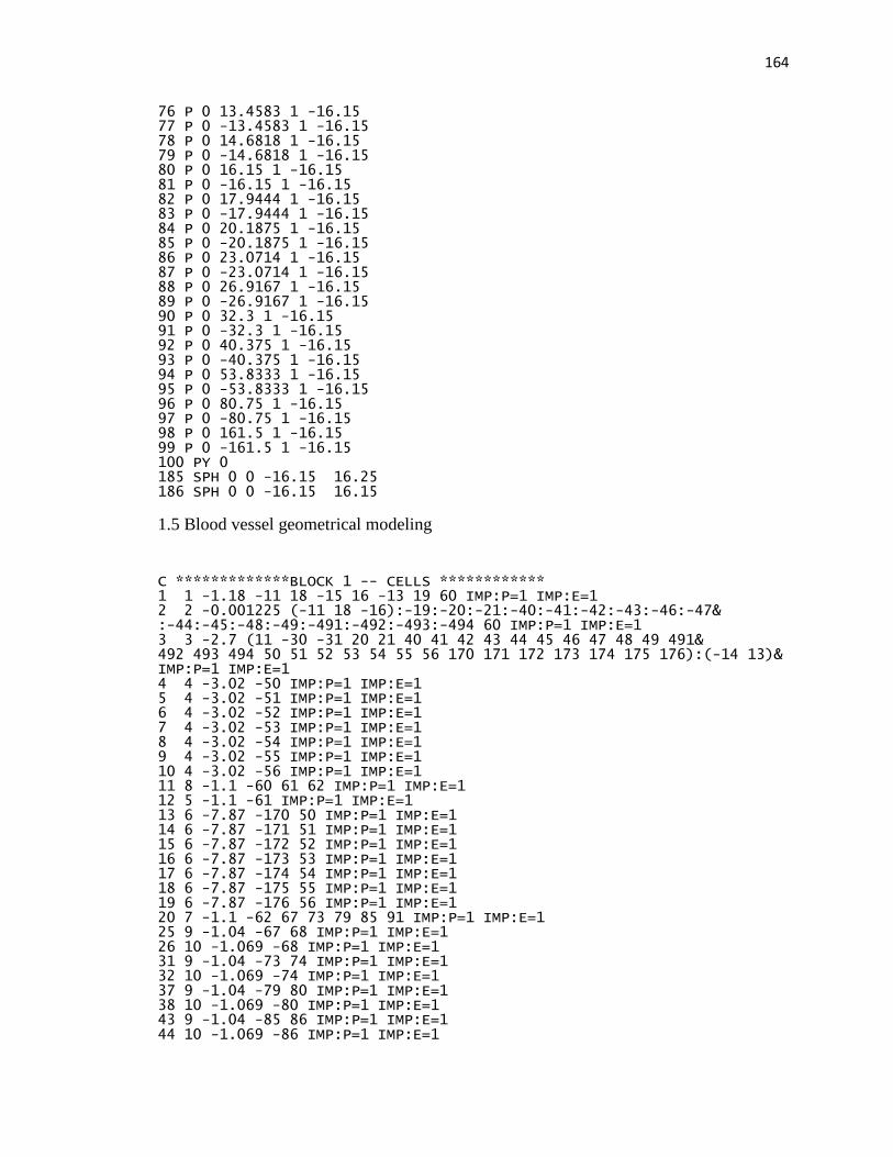
164

76 P 0 13.4583 1 -16.15 77 P 0 -13.4583 1 -16.15 78 P 0 14.6818 1 -16.15 79 P 0 -14.6818 1 -16.15 80 P 0 16.15 1 -16.15 81 P 0 -16.15 1 -16.15 82 P 0 17.9444 1 -16.15 83 P 0 -17.9444 1 -16.15 84 P 0 20.1875 1 -16.15 85 P 0 -20.1875 1 -16.15 86 P 0 23.0714 1 -16.15 87 P 0 -23.0714 1 -16.15 88 P 0 26.9167 1 -16.15 89 P 0 -26.9167 1 -16.15 90 P 0 32.3 1 -16.15 91 P 0 -32.3 1 -16.15 92 P 0 40.375 1 -16.15 93 P 0 -40.375 1 -16.15 94 P 0 53.8333 1 -16.15 95 P 0 -53.8333 1 -16.15 96 P 0 80.75 1 -16.15 97 P 0 -80.75 1 -16.15 98 P 0 161.5 1 -16.15 99 P 0 -161.5 1 -16.15 100 PY 0 185 SPH 0 0 -16.15 16.25 186 SPH 0 0 -16.15 16.15

1.5 Blood vessel geometrical modeling

C *************BLOCK 1 -- CELLS ************ 1 1 -1.18 -11 18 -15 16 -13 19 60 IMP:P=1 IMP:E=1 2 2 -0.001225 (-11 18 -16):-19:-20:-21:-40:-41:-42:-43:-46:-47& :-44:-45:-48:-49:-491:-492:-493:-494 60 IMP:P=1 IMP:E=1 3 3 -2.7 (11 -30 -31 20 21 40 41 42 43 44 45 46 47 48 49 491& 492 493 494 50 51 52 53 54 55 56 170 171 172 173 174 175 176):(-14 13)& IMP:P=1 IMP:E=1 4 4 -3.02 -50 IMP:P=1 IMP:E=1 5 4 -3.02 -51 IMP:P=1 IMP:E=1 6 4 -3.02 -52 IMP:P=1 IMP:E=1 7 4 -3.02 -53 IMP:P=1 IMP:E=1 8 4 -3.02 -54 IMP:P=1 IMP:E=1 9 4 -3.02 -55 IMP:P=1 IMP:E=1 10 4 -3.02 -56 IMP:P=1 IMP:E=1 11 8 -1.1 -60 61 62 IMP:P=1 IMP:E=1 12 5 -1.1 -61 IMP:P=1 IMP:E=1 13 6 -7.87 -170 50 IMP:P=1 IMP:E=1 14 6 -7.87 -171 51 IMP:P=1 IMP:E=1 15 6 -7.87 -172 52 IMP:P=1 IMP:E=1 16 6 -7.87 -173 53 IMP:P=1 IMP:E=1 17 6 -7.87 -174 54 IMP:P=1 IMP:E=1 18 6 -7.87 -175 55 IMP:P=1 IMP:E=1 19 6 -7.87 -176 56 IMP:P=1 IMP:E=1 20 7 -1.1 -62 67 73 79 85 91 IMP:P=1 IMP:E=1 25 9 -1.04 -67 68 IMP:P=1 IMP:E=1 26 10 -1.069 -68 IMP:P=1 IMP:E=1 31 9 -1.04 -73 74 IMP:P=1 IMP:E=1 32 10 -1.069 -74 IMP:P=1 IMP:E=1 37 9 -1.04 -79 80 IMP:P=1 IMP:E=1 38 10 -1.069 -80 IMP:P=1 IMP:E=1 43 9 -1.04 -85 86 IMP:P=1 IMP:E=1 44 10 -1.069 -86 IMP:P=1 IMP:E=1

165

49 9 -1.04 -91 92 IMP:P=1 IMP:E=1 50 10 -1.069 -92 IMP:P=1 IMP:E=1 53 0 (-18 60):(-11 15 18 14):(11 -30& 31):30 IMP:P=0 IMP:E=0 C *************BLOCK 2 -- SURFACES ********* 11 PZ 2.7 13 CZ 4.5 14 RCC 0 0 2.4 0 0 0.3 5 15 KZ -2.1 1 1 16 KZ -1.3 1 1 18 PZ 0 19 RCC 0 0 0 0 0 0.6 1.8 20 TRC 0 0 2.7 0 0 0.4 3.84 3.44 21 RCC 0 0 3.1 0 0 0.5 3.44 30 PZ 6.1 31 CZ 5 40 TRC 0 0 3.6 0 0 0.2 1 0.8 41 RCC 0 0 3.8 0 0 0.15 0.8 42 TRC 0 2.4445 3.6 0 0 0.2 1 0.8 43 RCC 0 2.4445 3.8 0 0 0.15 0.8 44 TRC 0 -2.4445 3.6 0 0 0.2 1 0.8 45 RCC 0 -2.4445 3.8 0 0 0.15 0.8 46 TRC 2.11 1.22 3.6 0 0 0.2 1 0.8 47 RCC 2.11 1.22 3.8 0 0 0.15 0.8 48 TRC -2.11 1.22 3.6 0 0 0.2 1 0.8 49 RCC -2.11 1.22 3.8 0 0 0.15 0.8 491 TRC 2.11 -1.22 3.6 0 0 0.2 1 0.8 492 RCC 2.11 -1.22 3.8 0 0 0.15 0.8 493 TRC -2.11 -1.22 3.6 0 0 0.2 1 0.8 494 RCC -2.11 -1.22 3.8 0 0 0.15 0.8 50 RCC 0 0 3.96 0 0 0.06 0.8 51 RCC 0 2.4445 3.96 0 0 0.06 0.8 52 RCC 0 -2.4445 3.96 0 0 0.06 0.8 53 RCC 2.11 1.22 3.96 0 0 0.06 0.8 54 RCC -2.11 1.22 3.96 0 0 0.06 0.8 55 RCC 2.11 -1.22 3.96 0 0 0.06 0.8 56 RCC -2.11 -1.22 3.96 0 0 0.06 0.8 170 RCC 0 0 3.96 0 0 0.6 1.1 171 RCC 0 2.4445 3.96 0 0 0.6 1.1 172 RCC 0 -2.4445 3.96 0 0 0.6 1.1 173 RCC 2.11 1.22 3.96 0 0 0.6 1.1 174 RCC -2.11 1.22 3.96 0 0 0.6 1.1 175 RCC 2.11 -1.22 3.96 0 0 0.6 1.1 176 RCC -2.11 -1.22 3.96 0 0 0.6 1.1 60 BOX -3 -3 0 6 0 0 0 6 0 0 0 -3 61 BOX -3 -3 0 6 0 0 0 6 0 0 0 -0.007 62 BOX -3 -3 -0.007 6 0 0 0 6 0 0 0 -0.207 67 RCC -3 0 -0.2 6 0 0 0.01 68 RCC -3 0 -0.2 6 0 0 0.006 73 RCC -3 -0.5 -0.2 6 0 0 0.01 74 RCC -3 -0.5 -0.2 6 0 0 0.006 79 RCC -3 -1 -0.2 6 0 0 0.01 80 RCC -3 -1 -0.2 6 0 0 0.006 85 RCC -3 -1.5 -0.2 6 0 0 0.01 86 RCC -3 -1.5 -0.2 6 0 0 0.006 91 RCC -3 -2 -0.2 6 0 0 0.01 92 RCC -3 -2 -0.2 6 0 0 0.006

166

Appendix 2

2.1 Percent depth dose measurements

Depth, cm Cell Tally, MeV/g Dose, Gy/min PDD, %

0 12 1.25E-03 3.124 98.862

0.0125 20 1.25E-03 3.107 98.322

0.025 21 1.17E-03 2.904 91.885

0.0375 22 1.06E-03 2.635 83.389

0.05 23 9.43E-04 2.347 74.273

0.0625 24 8.28E-04 2.062 65.256

0.075 25 7.20E-04 1.793 56.729

0.0875 26 6.21E-04 1.546 48.924

0.1 27 5.32E-04 1.323 41.874

0.1125 28 4.52E-04 1.124 35.578

0.125 29 3.81E-04 0.949 30.028

0.1375 30 3.20E-04 0.796 25.198

0.15 31 2.67E-04 0.664 21.006

0.1625 32 2.21E-04 0.549 17.390

0.175 33 1.82E-04 0.452 14.303

0.1875 34 1.48E-04 0.369 11.687

0.2 35 1.20E-04 0.299 9.479

0.2125 36 9.69E-05 0.24 7.636

0.225 37 7.74E-05 0.19 6.099

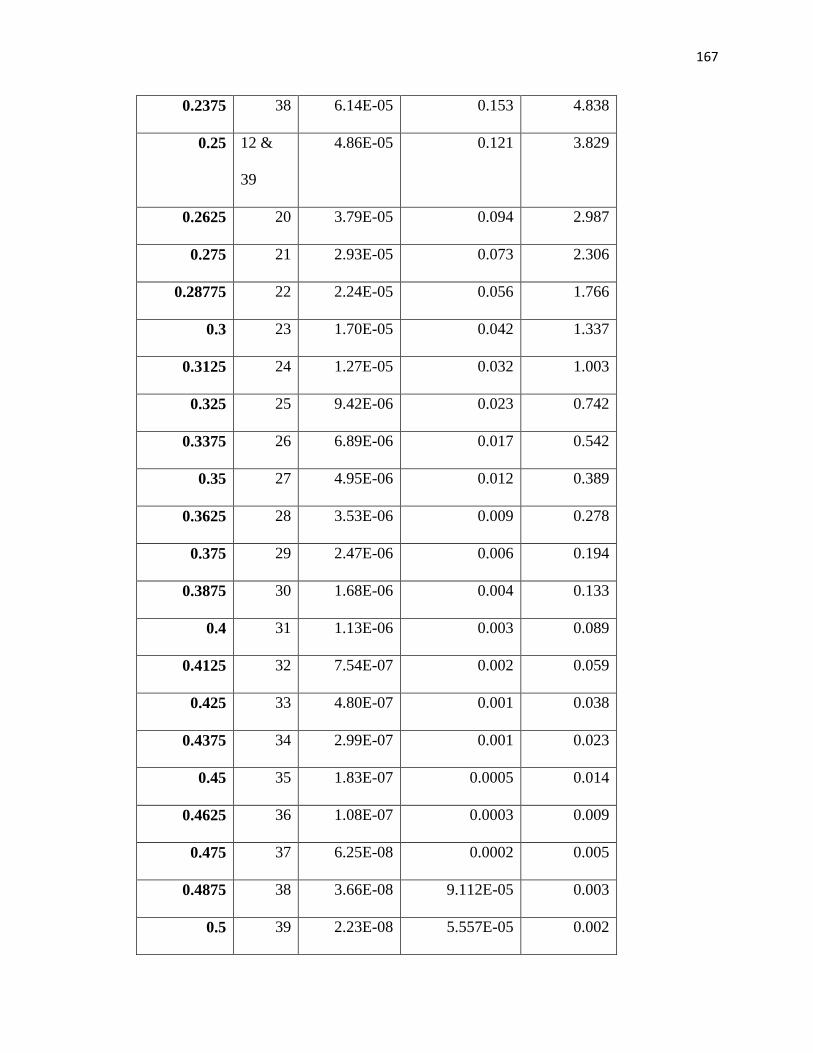
167

0.2375 38 6.14E-05 0.153 4.838

0.25 12 &

39

4.86E-05 0.121 3.829

0.2625 20 3.79E-05 0.094 2.987

0.275 21 2.93E-05 0.073 2.306

0.28775 22 2.24E-05 0.056 1.766

0.3 23 1.70E-05 0.042 1.337

0.3125 24 1.27E-05 0.032 1.003

0.325 25 9.42E-06 0.023 0.742

0.3375 26 6.89E-06 0.017 0.542

0.35 27 4.95E-06 0.012 0.389

0.3625 28 3.53E-06 0.009 0.278

0.375 29 2.47E-06 0.006 0.194

0.3875 30 1.68E-06 0.004 0.133

0.4 31 1.13E-06 0.003 0.089

0.4125 32 7.54E-07 0.002 0.059

0.425 33 4.80E-07 0.001 0.038

0.4375 34 2.99E-07 0.001 0.023

0.45 35 1.83E-07 0.0005 0.014

0.4625 36 1.08E-07 0.0003 0.009

0.475 37 6.25E-08 0.0002 0.005

0.4875 38 3.66E-08 9.112E-05 0.003

0.5 39 2.23E-08 5.557E-05 0.002

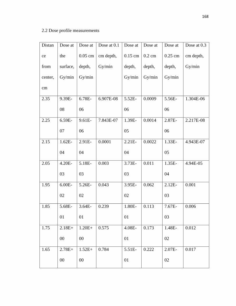
168

2.2 Dose profile measurements

Distan

ce

from

center,

cm

Dose at

the

surface,

Gy/min

Dose at

0.05 cm

depth,

Gy/min

Dose at 0.1

cm depth,

Gy/min

Dose at

0.15 cm

depth,

Gy/min

Dose at

0.2 cm

depth,

Gy/min

Dose at

0.25 cm

depth,

Gy/min

Dose at 0.3

cm depth,

Gy/min

2.35 9.39E-

08

6.78E-

06

6.907E-08 5.52E-

06

0.0009 5.56E-

06

1.304E-06

2.25 6.59E-

07

9.61E-

06

7.843E-07 1.39E-

05

0.0014 2.87E-

06

2.217E-08

2.15 1.62E-

04

2.91E-

04

0.0001 2.21E-

04

0.0022 1.33E-

05

4.943E-07

2.05 4.20E-

03

5.18E-

03

0.003 3.73E-

03

0.011 1.35E-

04

4.94E-05

1.95 6.00E-

02

5.26E-

02

0.043 3.95E-

02

0.062 2.12E-

03

0.001

1.85 5.68E-

01

3.64E-

01

0.239 1.80E-

01

0.113 7.67E-

03

0.006

1.75 2.18E+

00

1.20E+

00

0.575 4.08E-

01

0.173 1.48E-

02

0.012

1.65 2.78E+

00

1.52E+

00

0.784 5.51E-

01

0.222 2.07E-

02

0.017

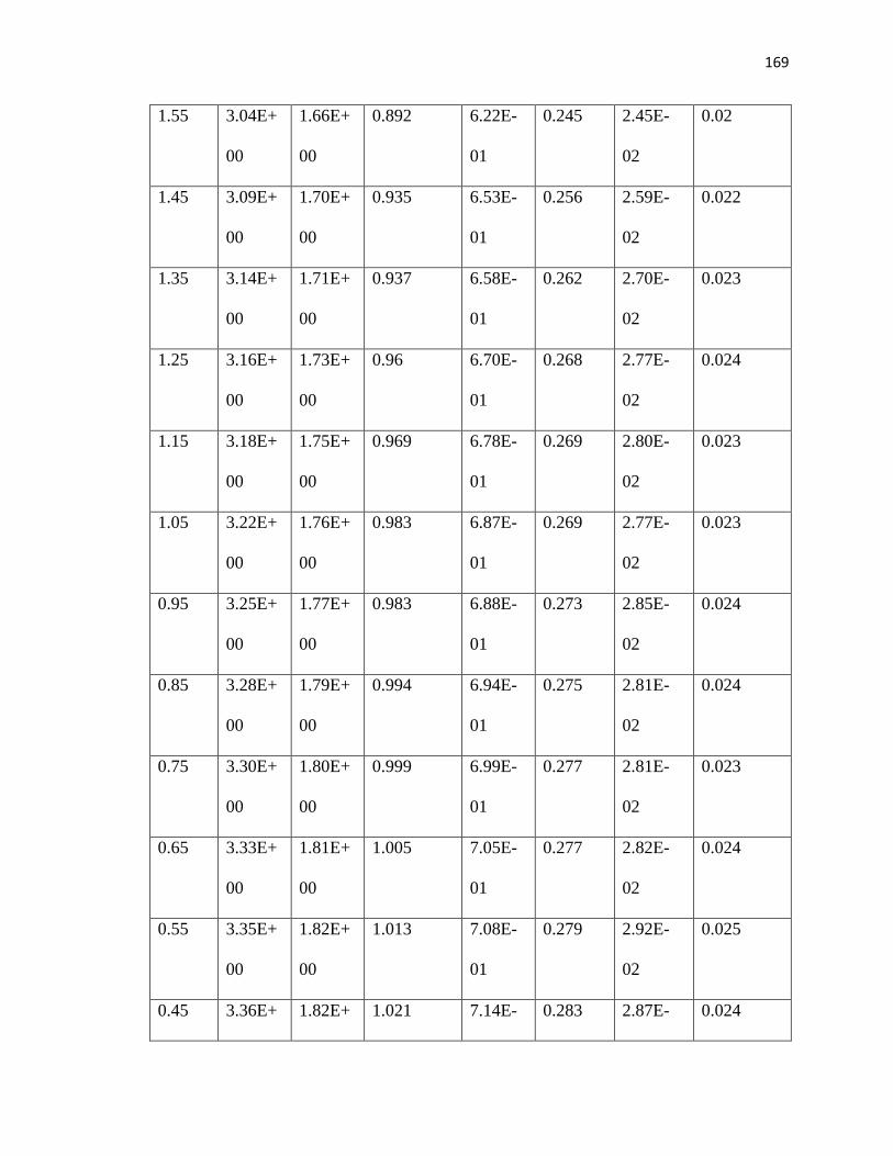
169

1.55 3.04E+

00

1.66E+

00

0.892 6.22E-

01

0.245 2.45E-

02

0.02

1.45 3.09E+

00

1.70E+

00

0.935 6.53E-

01

0.256 2.59E-

02

0.022

1.35 3.14E+

00

1.71E+

00

0.937 6.58E-

01

0.262 2.70E-

02

0.023

1.25 3.16E+

00

1.73E+

00

0.96 6.70E-

01

0.268 2.77E-

02

0.024

1.15 3.18E+

00

1.75E+

00

0.969 6.78E-

01

0.269 2.80E-

02

0.023

1.05 3.22E+

00

1.76E+

00

0.983 6.87E-

01

0.269 2.77E-

02

0.023

0.95 3.25E+

00

1.77E+

00

0.983 6.88E-

01

0.273 2.85E-

02

0.024

0.85 3.28E+

00

1.79E+

00

0.994 6.94E-

01

0.275 2.81E-

02

0.024

0.75 3.30E+

00

1.80E+

00

0.999 6.99E-

01

0.277 2.81E-

02

0.023

0.65 3.33E+

00

1.81E+

00

1.005 7.05E-

01

0.277 2.82E-

02

0.024

0.55 3.35E+

00

1.82E+

00

1.013 7.08E-

01

0.279 2.92E-

02

0.025

0.45 3.36E+ 1.82E+ 1.021 7.14E- 0.283 2.87E- 0.024

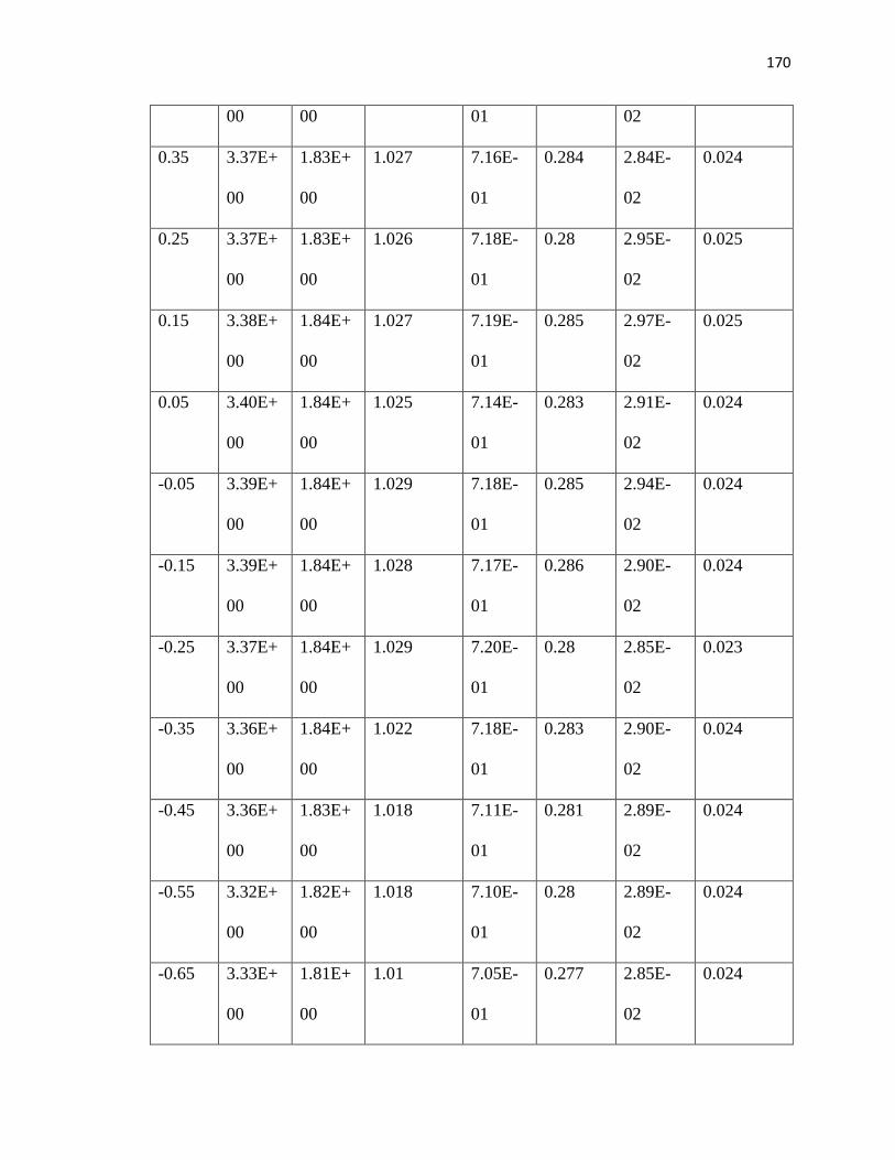
170

00 00 01 02

0.35 3.37E+

00

1.83E+

00

1.027 7.16E-

01

0.284 2.84E-

02

0.024

0.25 3.37E+

00

1.83E+

00

1.026 7.18E-

01

0.28 2.95E-

02

0.025

0.15 3.38E+

00

1.84E+

00

1.027 7.19E-

01

0.285 2.97E-

02

0.025

0.05 3.40E+

00

1.84E+

00

1.025 7.14E-

01

0.283 2.91E-

02

0.024

-0.05 3.39E+

00

1.84E+

00

1.029 7.18E-

01

0.285 2.94E-

02

0.024

-0.15 3.39E+

00

1.84E+

00

1.028 7.17E-

01

0.286 2.90E-

02

0.024

-0.25 3.37E+

00

1.84E+

00

1.029 7.20E-

01

0.28 2.85E-

02

0.023

-0.35 3.36E+

00

1.84E+

00

1.022 7.18E-

01

0.283 2.90E-

02

0.024

-0.45 3.36E+

00

1.83E+

00

1.018 7.11E-

01

0.281 2.89E-

02

0.024

-0.55 3.32E+

00

1.82E+

00

1.018 7.10E-

01

0.28 2.89E-

02

0.024

-0.65 3.33E+

00

1.81E+

00

1.01 7.05E-

01

0.277 2.85E-

02

0.024

171

-0.75 3.29E+

00

1.80E+

00

1.007 7.04E-

01

0.279 2.89E-

02

0.024

-0.85 3.28E+

00

1.79E+

00

1 6.98E-

01

0.278 2.86E-

02

0.024

-0.95 3.25E+

00

1.78E+

00

0.991 6.90E-

01

0.275 2.77E-

02

0.023

-1.05 3.22E+

00

1.76E+

00

0.973 6.81E-

01

0.271 2.78E-

02

0.024

-1.15 3.21E+

00

1.74E+

00

0.964 6.74E-

01

0.268 2.74E-

02

0.023

-1.25 3.17E+

00

1.73E+

00

0.949 6.64E-

01

0.266 2.67E-

02

0.022

-1.35 3.14E+

00

1.72E+

00

0.948 6.63E-

01

0.263 2.73E-

02

0.023

-1.45 3.10E+

00

1.70E+

00

0.93 6.52E-

01

0.258 2.72E-

02

0.023

-1.55 3.04E+

00

1.66E+

00

0.887 6.20E-

01

0.247 2.46E-

02

0.0212

-1.65 2.78E+

00

1.52E+

00

0.785 5.49E-

01

0.22 2.09E-

02

0.017

-1.75 2.17E+

00

1.21E+

00

0.577 4.08E-

01

0.173 1.47E-

02

0.012

-1.85 5.60E- 3.65E- 0.24281 1.82E- 0.113 7.47E- 0.006

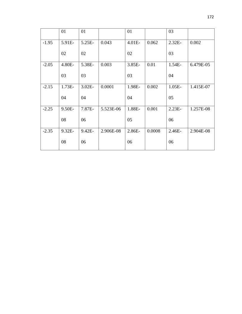
172

01 01 01 03

-1.95 5.91E-

02

5.25E-

02

0.043 4.01E-

02

0.062 2.32E-

03

0.002

-2.05 4.80E-

03

5.38E-

03

0.003 3.85E-

03

0.01 1.54E-

04

6.479E-05

-2.15 1.73E-

04

3.02E-

04

0.0001 1.98E-

04

0.002 1.05E-

05

1.415E-07

-2.25 9.50E-

08

7.87E-

06

5.523E-06 1.88E-

05

0.001 2.23E-

06

1.257E-08

-2.35 9.32E-

08

9.42E-

06

2.906E-08 2.86E-

06

0.0008 2.46E-

06

2.904E-08

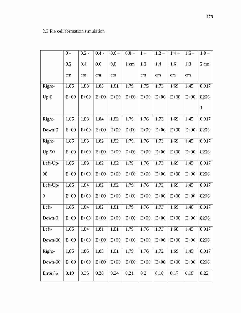
173

2.3 Pie cell formation simulation

0 -

0.2

cm

0.2 -

0.4

cm

0.4 -

0.6

cm

0.6 –

0.8

cm

0.8 –

1 cm

1 –

1.2

cm

1.2 –

1.4

cm

1.4 –

1.6

cm

1.6 –

1.8

cm

1.8 –

2 cm

Right-

Up-0

1.85

E+00

1.83

E+00

1.83

E+00

1.81

E+00

1.79

E+00

1.75

E+00

1.73

E+00

1.69

E+00

1.45

E+00

0.917

8206

1

Right-

Down-0

1.85

E+00

1.83

E+00

1.84

E+00

1.82

E+00

1.79

E+00

1.76

E+00

1.73

E+00

1.69

E+00

1.45

E+00

0.917

8206

Right-

Up-90

1.85

E+00

1.83

E+00

1.82

E+00

1.82

E+00

1.79

E+00

1.76

E+00

1.73

E+00

1.69

E+00

1.45

E+00

0.917

8206

Left-Up-

90

1.85

E+00

1.83

E+00

1.82

E+00

1.82

E+00

1.79

E+00

1.76

E+00

1.73

E+00

1.69

E+00

1.45

E+00

0.917

8206

Left-Up-

0

1.85

E+00

1.84

E+00

1.82

E+00

1.82

E+00

1.79

E+00

1.76

E+00

1.72

E+00

1.69

E+00

1.45

E+00

0.917

8206

Left-

Down-0

1.85

E+00

1.84

E+00

1.82

E+00

1.81

E+00

1.79

E+00

1.76

E+00

1.73

E+00

1.69

E+00

1.46

E+00

0.917

8206

Left-

Down-90

1.85

E+00

1.84

E+00

1.81

E+00

1.81

E+00

1.79

E+00

1.76

E+00

1.73

E+00

1.68

E+00

1.45

E+00

0.917

8206

Right-

Down-90

1.85

E+00

1.85

E+00

1.83

E+00

1.81

E+00

1.79

E+00

1.76

E+00

1.72

E+00

1.69

E+00

1.45

E+00

0.917

8206

Error,% 0.19 0.35 0.28 0.24 0.21 0.2 0.18 0.17 0.18 0.22

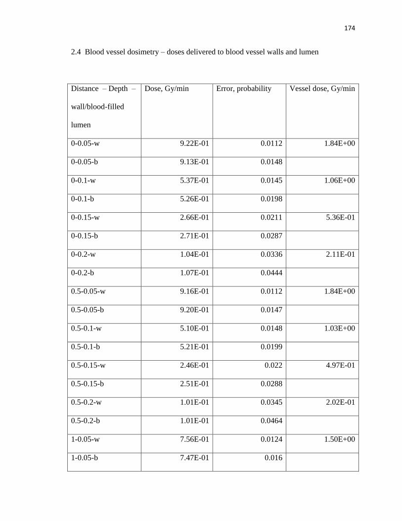
174

2.4 Blood vessel dosimetry – doses delivered to blood vessel walls and lumen

Distance – Depth –

wall/blood-filled

lumen

Dose, Gy/min Error, probability Vessel dose, Gy/min

0-0.05-w 9.22E-01 0.0112 1.84E+00

0-0.05-b 9.13E-01 0.0148

0-0.1-w 5.37E-01 0.0145 1.06E+00

0-0.1-b 5.26E-01 0.0198

0-0.15-w 2.66E-01 0.0211 5.36E-01

0-0.15-b 2.71E-01 0.0287

0-0.2-w 1.04E-01 0.0336 2.11E-01

0-0.2-b 1.07E-01 0.0444

0.5-0.05-w 9.16E-01 0.0112 1.84E+00

0.5-0.05-b 9.20E-01 0.0147

0.5-0.1-w 5.10E-01 0.0148 1.03E+00

0.5-0.1-b 5.21E-01 0.0199

0.5-0.15-w 2.46E-01 0.022 4.97E-01

0.5-0.15-b 2.51E-01 0.0288

0.5-0.2-w 1.01E-01 0.0345 2.02E-01

0.5-0.2-b 1.01E-01 0.0464

1-0.05-w 7.56E-01 0.0124 1.50E+00

1-0.05-b 7.47E-01 0.016

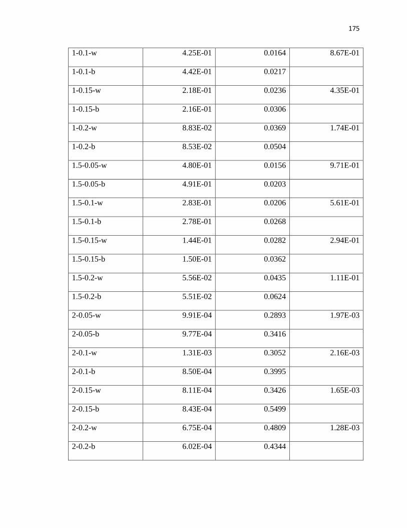
175

1-0.1-w 4.25E-01 0.0164 8.67E-01

1-0.1-b 4.42E-01 0.0217

1-0.15-w 2.18E-01 0.0236 4.35E-01

1-0.15-b 2.16E-01 0.0306

1-0.2-w 8.83E-02 0.0369 1.74E-01

1-0.2-b 8.53E-02 0.0504

1.5-0.05-w 4.80E-01 0.0156 9.71E-01

1.5-0.05-b 4.91E-01 0.0203

1.5-0.1-w 2.83E-01 0.0206 5.61E-01

1.5-0.1-b 2.78E-01 0.0268

1.5-0.15-w 1.44E-01 0.0282 2.94E-01

1.5-0.15-b 1.50E-01 0.0362

1.5-0.2-w 5.56E-02 0.0435 1.11E-01

1.5-0.2-b 5.51E-02 0.0624

2-0.05-w 9.91E-04 0.2893 1.97E-03

2-0.05-b 9.77E-04 0.3416

2-0.1-w 1.31E-03 0.3052 2.16E-03

2-0.1-b 8.50E-04 0.3995

2-0.15-w 8.11E-04 0.3426 1.65E-03

2-0.15-b 8.43E-04 0.5499

2-0.2-w 6.75E-04 0.4809 1.28E-03

2-0.2-b 6.02E-04 0.4344

176

CURRICULUM VITAE

Name: Olga V. Pen

Current position: Research Assistant

Address: Department of Radiation Oncology

Wake Forest Baptist Health Cancer Center

1, Medical Boulevard

Winston-Salem, NC, 27103, USA

(336)713-6626 (office)

e-mail: olgapen@vt.edu

Education:

2016-Present

2014-2016

Virginia Tech-Wake Forest School of Biomedical Engineering and

Sciences, Wake Forest University

Ph.D. in Biomedical Engineering (Medical Physics track)

Advisor: Dr. J. Daniel Bourland, Ph.D.

Project: Effect of beta radiation dose distribution on the expression

of epidermal necrosis

Virginia Tech-Wake Forest School of Biomedical Engineering and

177

2009-2014

Sciences, Virginia Polytechnic Institute and State University

M.S. in Biomedical Engineering (Medical Imaging track)

Advisor: Dr. Guohua Cao, Ph.D.

Thesis: Calculation of the effective atomic numbers for the iodine-

based contrast agent solution of different concentrations

Siberian Federal University, Institute of Space and Information

Technology

B.S. in Computer Engineering (Automated data processing and

management track)

Advisor: Dr. Sergei Videnin, Ph.D.

Thesis: Automated EEG processing for the epilepsy diagnostics

Additional training:

January-March,

2016

August, 2013

National Instruments Company representative, Virginia Polytechnic

Institute and State University

Labview Associate Developer Workshop

Moscow State University – Saint Petersburg University, University

of California in Los Angeles

Summer School of Bioinformatics

178

January-May,

2014

Krasnoyarsk State Medical University

Internship in Medical Imaging and Data Processing

Advisor: Dr. Natalia Schnaider, M.D.

Work Experience:

2016-present

2014-

2016

Research Assistant at Wake Forest Cancer Center:

- Multidisciplinary research project participation with the

emphasis on the medical imaging data processing and

Monte-Carlo modeling of the dose distribution

- IMRT QA and LINAC machine QA assistance

- IMRT QA workshop instructor

Research Assistant at the X-ray laboratory at Virginia Polytechnic

Institute and State University

- Computer modeling of the nuclear physics processes

- Computer Tomography acquisition, reconstruction and

processing

Publications:

1) “Sensory-Predominant chronic inflammatory demyelinating polyneuropathy in a

patient with a parainfectious limbic encephalitis”/T.E. Popova, T.Y.Nikolaeva,

N.A. Schneider, M.M. Petrova, A.A. Semenov, O.V. Pen, J.S. Panina, A.V.

Muraveva/ Yakut Medical Journal, December, 2014, ISBN 1813-1905

2) Dong, X., Pen, O. V., Zhang, Z., & Cao, G. (2019). An improved physics model

for multi-material identification in photon counting CT/SPIE proceedings,

179

2019/ arXiv preprint arXiv:1902.03360.

3) "Automated, Quantitative Assessment of Epidermal Necrosis Expression Resulting

from Skin Exposure to Beta Radiation"/Olga V. Pen, Peter A. Antinozzi, Nancy D.

Kock, Mac B. Robinson, Jeffrey S. Willey, J. Daniel Bourland /International

Journal of Radiation Biology (submitted)

Scientific presentations and abstracts:

1) BMES 2016 Annual Meeting, Minneapolis, MN: “Improving Iodine Contrast

Agent Sensitivity in Spectral Computed Tomography via Rho-Z Mapping”, Olga

V. Pen, Guohua Cao, October, 5-8, 2016

2) BMES 2017 Annual Meeting, Phoenix, AZ: “Quantitative analysis of the

epidermal necrosis in CRI and RD induced by beta-source irradiation”, Olga V.

Pen, Peter A. Antinozzi, Nancy D. Kock, J. Daniel Bourland, October, 11-14,

2017

3) BMES 2017 Annual Meeting, Phoenix, AZ: “Quantitative Imaging of Electron

Density and Effective Atomic Number Using Spectral CT”, Xu Dong, Olga V.

Pen, Guohua Cao, October, 11-14, 2017

4) SEAAPM Regional Meeting, Greenville, NC: “Initial Considerations for

Analytical and Monte-Carlo Modeling of a Unique Beta-Source”, Olga V. Pen,

Peter A. Antinozzi, J. Daniel Bourland, February, 23-26, 2018

5) AAPM 2018 Annual Meeting, Nashville, TN: “Analytical and Monte-Carlo

Modeling of a Unique Beta-Source in Relation to Skin Surface Dosimetry”, Olga

V. Pen, Peter A. Antinozzi, J. Daniel Bourland, July, 29 – August, 2, 2018

180

6) BMES 2018 Annual Meeting, Atlanta, GA: “Monte Carlo modeling of the effects

of beta radiation from a unique beta source on the skin surface”, Olga V. Pen,

Peter A. Antinozzi, J. Daniel Bourland, October 17-20, 2018

Special awards:

2012-2014

2009-2014

Presidential Scholarship for the outstanding academic and

scientific achievements

Graduated from Siberian Federal University with honors

Professional affiliations:

2014-Present

2016-Present

2018-Present

Biomedical Engineering Society membership (Active)

Association of Physicists in Medicine membership (Active)

Radiation Research Society Membership (Active)

Languages:

Russian:

English:

Native

Fluent