Econometrics I
29
Part 22: Semi- and Nonparametric Estimation 2-1/29 Econometrics I Professor William Greene Stern School of Business Department of Economics
-
Upload
rahim-hunt -
Category
Documents
-
view
32 -
download
0
description
Econometrics I. Professor William Greene Stern School of Business Department of Economics. Econometrics I. Part 22 – Semi- and Nonparametric Estimation. Cornwell and Rupert Data. Cornwell and Rupert Returns to Schooling Data, 595 Individuals, 7 Years Variables in the file are - PowerPoint PPT Presentation
Transcript of Econometrics I

Part 22: Semi- and Nonparametric Estimation22-1/29
Econometrics IProfessor William Greene
Stern School of Business
Department of Economics

Part 22: Semi- and Nonparametric Estimation22-2/29
Econometrics I
Part 22 – Semi- and Nonparametric Estimation
Part 22: Semi- and Nonparametric Estimation22-3/29
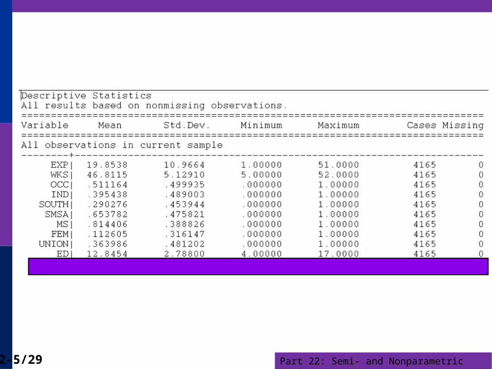
Cornwell and Rupert DataCornwell and Rupert Returns to Schooling Data, 595 Individuals, 7 YearsVariables in the file are
EXP = work experienceWKS = weeks workedOCC = occupation, 1 if blue collar, IND = 1 if manufacturing industrySOUTH = 1 if resides in southSMSA = 1 if resides in a city (SMSA)MS = 1 if marriedFEM = 1 if femaleUNION = 1 if wage set by union contractED = years of educationLWAGE = log of wage = dependent variable in regressions
These data were analyzed in Cornwell, C. and Rupert, P., "Efficient Estimation with Panel Data: An Empirical Comparison of Instrumental Variable Estimators," Journal of Applied Econometrics, 3, 1988, pp. 149-155. See Baltagi, page 122 for further analysis. The data were downloaded from the website for Baltagi's text.
Part 22: Semi- and Nonparametric Estimation22-4/29
A First Look at the DataDescriptive Statistics
Basic Measures of Location and Dispersion Graphical Devices
Histogram Kernel Density Estimator
Part 22: Semi- and Nonparametric Estimation22-5/29

Part 22: Semi- and Nonparametric Estimation22-6/29
Histogram for LWAGE
Part 22: Semi- and Nonparametric Estimation22-7/29
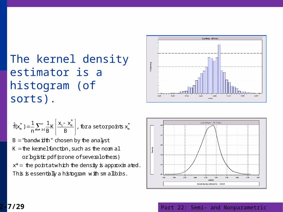
The kernel density estimator is ahistogram (of sorts).
n i mm mi 1
** *x x1 1
f̂(x ) K , for a set or points xn B B
B "bandwidth" chosen by the analyst
K the kernel function, such as the normal
or logistic pdf (or one of several others)
x* the point at which the density is approximated.
This is essentially a histogram with small bins.
Part 22: Semi- and Nonparametric Estimation22-8/29
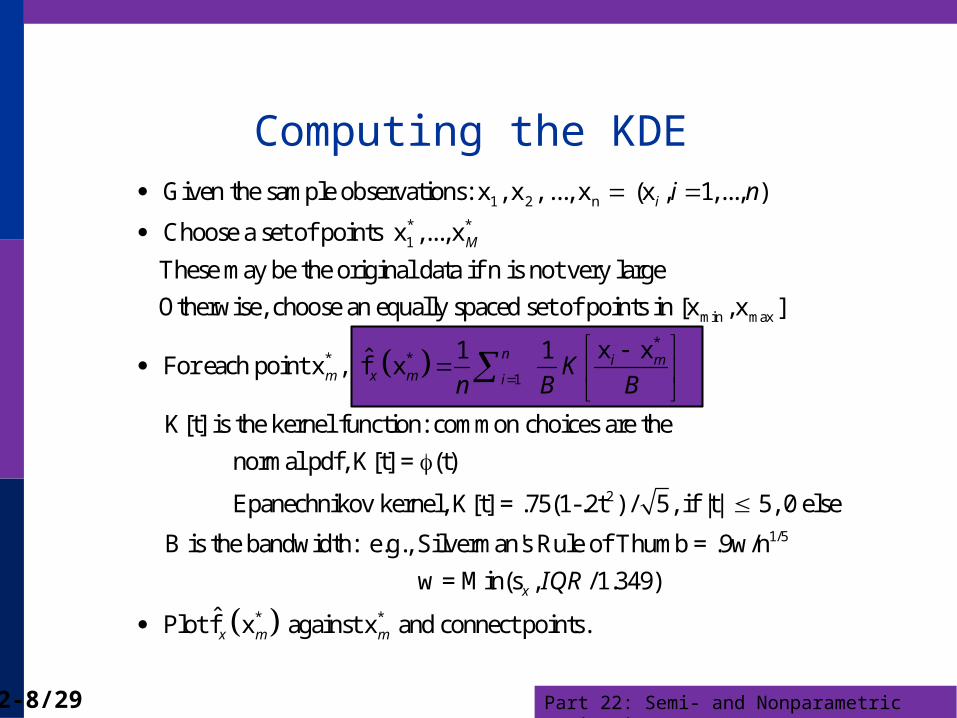
Computing the KDE
1 2 n
* *1
Given the sample observations: x , x , ..., x (x , 1,..., )
Choose a set of points x ,..., x
These may be the original data if n is not very large
Otherwise, choose an equally spaced se
i
M
i n
min max
** *
1
t of points in [x , x ]
x x1 1ˆ For each point x , f x
K[t] is the kernel function: common choices are the
normal pdf, K[t] = (t)
Epanechniko
n i mm x m i
Kn B B
2
1/5
*
v kernel, K[t] = .75(1-.2t ) / 5, if |t| 5, 0 else
B is the bandwidth: e.g., Silverman's Rule of Thumb = .9w/n
w = Min(s , /1.349)
ˆ Plot f x ag
x
x m
IQR
*ainst x and connect points.m
Part 22: Semi- and Nonparametric Estimation22-9/29
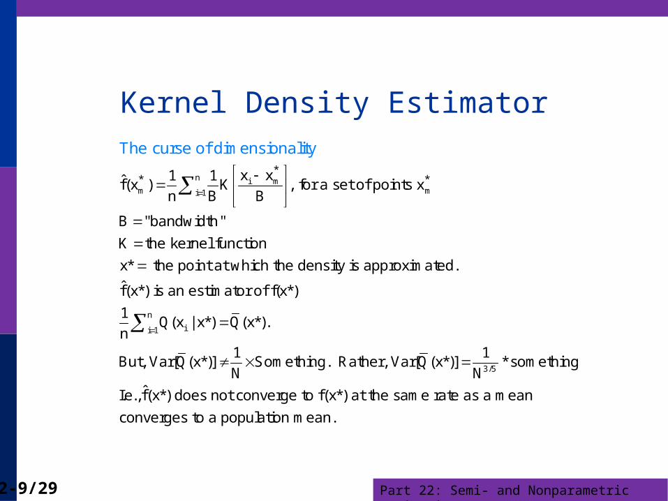
Kernel Density Estimator
n i mm mi 1
** *x x1 1
f̂(x ) K , for a set of points xn B B
B "bandwidth"
K the kernel function
x* the point at which the density is approximated.
f̂(x*) is an estimator of f(x*)
1
The curse of dimensionality
n
ii 1
3/5
Q(x | x*) Q(x*). n
1 1But, Var[Q(x*)] Something. Rather, Var[Q(x*)] * something
N NˆI.e.,f(x*) does not converge to f(x*) at the same rate as a mean
converges to a population mean.
Part 22: Semi- and Nonparametric Estimation22-10/29
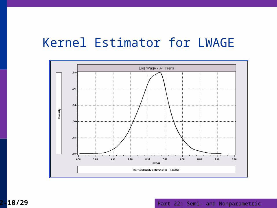
Kernel Estimator for LWAGE

Part 22: Semi- and Nonparametric Estimation22-11/29
Application: Stochastic Frontier Model
Production Function Regression: logY = b’x + v - u
where u is “inefficiency.” u > 0. v is normally distributed.
Save for the constant term, the model is consistently estimated by OLS.
If the theory is right, the OLS residuals will be skewed to the left, rather than symmetrically distributed if they were normally distributed.
Application: Spanish dairy data used in Assignment 2
yit = log of milk productionx1 = log cows, x2 = log land, x3 = log feed, x4 = log labor

Part 22: Semi- and Nonparametric Estimation22-12/29
Regression Results

Part 22: Semi- and Nonparametric Estimation22-13/29
Distribution of OLS Residuals
Part 22: Semi- and Nonparametric Estimation22-14/29
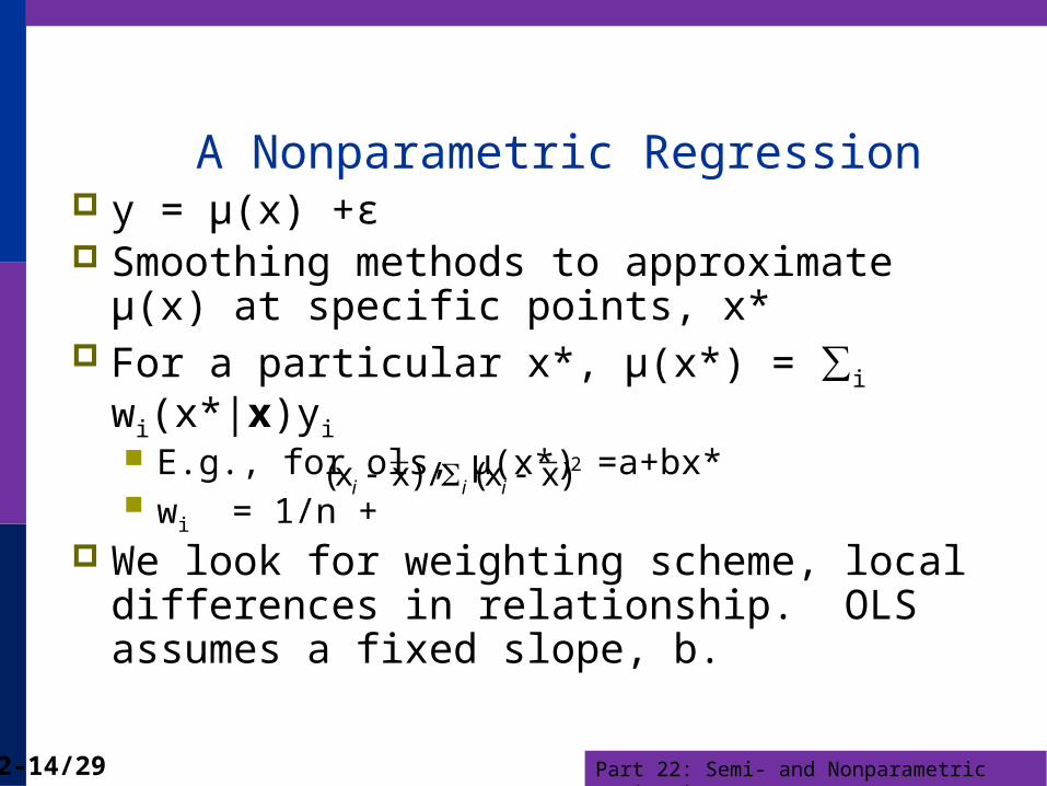
A Nonparametric Regression y = µ(x) +ε Smoothing methods to approximate µ(x) at
specific points, x* For a particular x*, µ(x*) = ∑i wi(x*|x)yi
E.g., for ols, µ(x*) =a+bx* wi = 1/n +
We look for weighting scheme, local differences in relationship. OLS assumes a fixed slope, b.
2( ) / ( )i i i x x x x

Part 22: Semi- and Nonparametric Estimation22-15/29
Nearest Neighbor Approach
Define a neighborhood of x*. Points near get high weight, points far away get a small or zero weight
Bandwidth, h defines the neighborhood:e.g., Silverman h =.9Min[s,(IQR/1.349)]/n.2
Neighborhood is + or – h/2 LOWESS weighting function: (tricube)
Ti = [1 – [Abs(xi – x*)/h]3]3.
Weight is wi = 1[Abs(xi – x*)/h < .5] * Ti .

Part 22: Semi- and Nonparametric Estimation22-16/29
LOWESS Regression
Part 22: Semi- and Nonparametric Estimation22-17/29
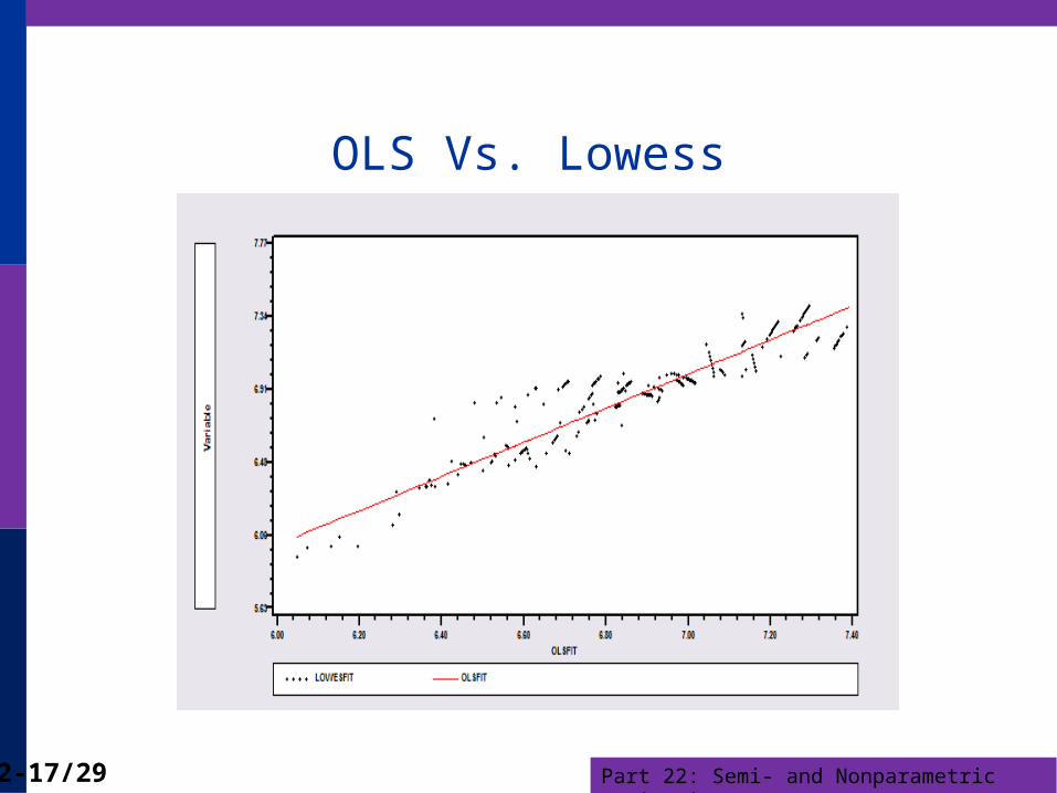
OLS Vs. Lowess
Part 22: Semi- and Nonparametric Estimation22-18/29
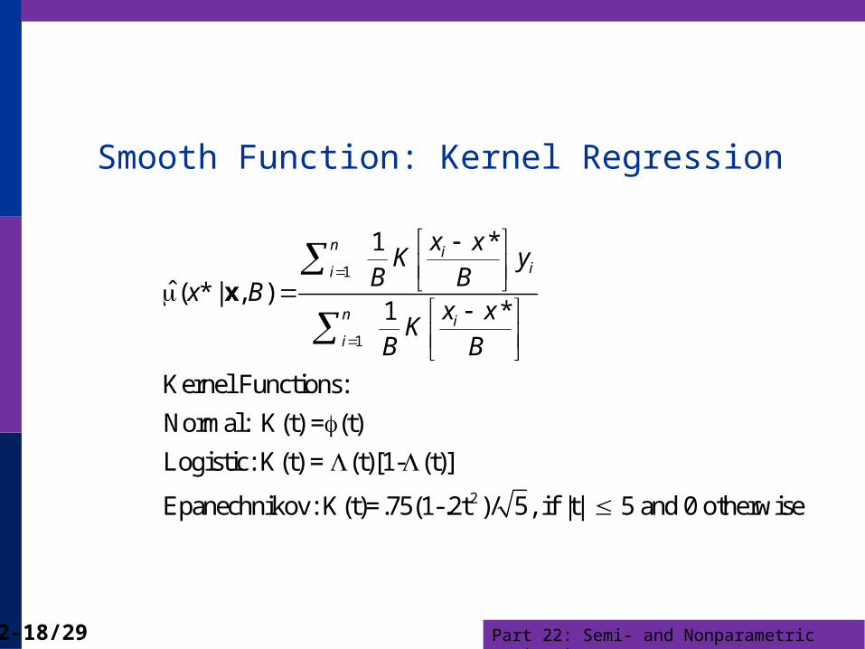
Smooth Function: Kernel Regression
1
1
2
*1
ˆ ( * | , )*1
Kernel Functions:
Normal: K(t) = (t)
Logistic: K(t) = (t)[1- (t)]
Epanechnikov: K(t)=.75(1-.2t )/ 5, if |t| 5 and 0 otherwise
n iii
n ii
x xK y
B Bx B
x xK
B B
x
Part 22: Semi- and Nonparametric Estimation22-19/29
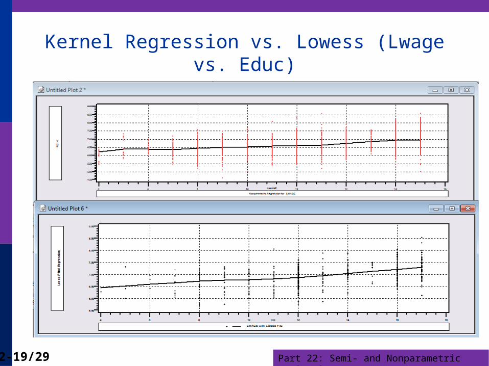
Kernel Regression vs. Lowess (Lwage vs. Educ)

Part 22: Semi- and Nonparametric Estimation22-20/29
Locally Linear Regression
1
1 1
( *) ( *) ' *.
( *) ( *, ) ( *, ) y
( *, ) [( * ) ( * ), ]
n n
i i i i i i i ii i
i i i i
w w
w K h
x x x
x x x x x x x x
x x x x x x

Part 22: Semi- and Nonparametric Estimation22-21/29
OLS vs. LOWESS
Part 22: Semi- and Nonparametric Estimation22-22/29
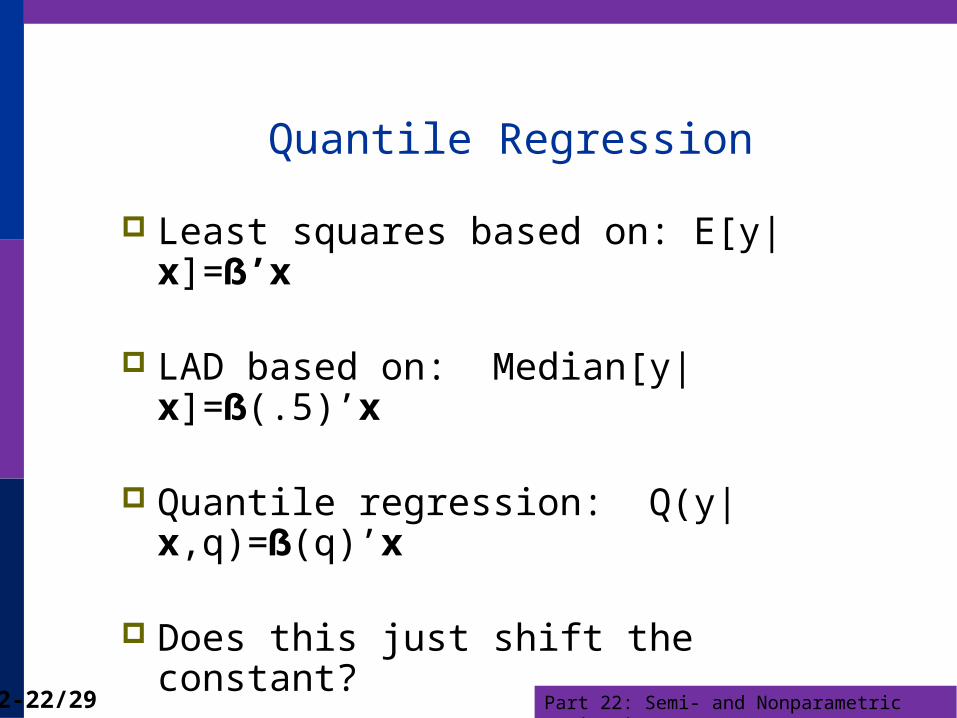
Quantile Regression
Least squares based on: E[y|x]=ẞ’x
LAD based on: Median[y|x]=ẞ(.5)’x
Quantile regression: Q(y|x,q)=ẞ(q)’x
Does this just shift the constant?

Part 22: Semi- and Nonparametric Estimation22-23/29
OLS vs. Least Absolute Deviations----------------------------------------------------------------------Least absolute deviations estimator...............Residuals Sum of squares = 1537.58603 Standard error of e = 6.82594Fit R-squared = .98284 Adjusted R-squared = .98180Sum of absolute deviations = 189.3973484--------+-------------------------------------------------------------Variable| Coefficient Standard Error b/St.Er. P[|Z|>z] Mean of X--------+------------------------------------------------------------- |Covariance matrix based on 50 replications.Constant| -84.0258*** 16.08614 -5.223 .0000 Y| .03784*** .00271 13.952 .0000 9232.86 PG| -17.0990*** 4.37160 -3.911 .0001 2.31661--------+-------------------------------------------------------------Ordinary least squares regression ............Residuals Sum of squares = 1472.79834 Standard error of e = 6.68059 Standard errors are based onFit R-squared = .98356 50 bootstrap replications Adjusted R-squared = .98256--------+-------------------------------------------------------------Variable| Coefficient Standard Error t-ratio P[|T|>t] Mean of X--------+-------------------------------------------------------------Constant| -79.7535*** 8.67255 -9.196 .0000 Y| .03692*** .00132 28.022 .0000 9232.86 PG| -15.1224*** 1.88034 -8.042 .0000 2.31661--------+-------------------------------------------------------------

Part 22: Semi- and Nonparametric Estimation22-24/29
Quantile Regression
Q(y|x,) = x, = quantile Estimated by linear programming Q(y|x,.50) = x, .50 median regression Median regression estimated by LAD (estimates
same parameters as mean regression if symmetric conditional distribution)
Why use quantile (median) regression? Semiparametric Robust to some extensions (heteroscedasticity?) Complete characterization of conditional distribution

Part 22: Semi- and Nonparametric Estimation22-25/29
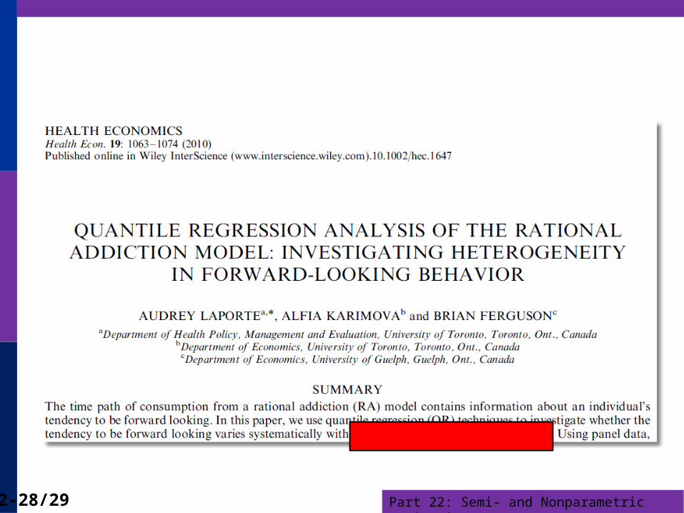
Quantile Regression
Part 22: Semi- and Nonparametric Estimation22-26/29
1 1
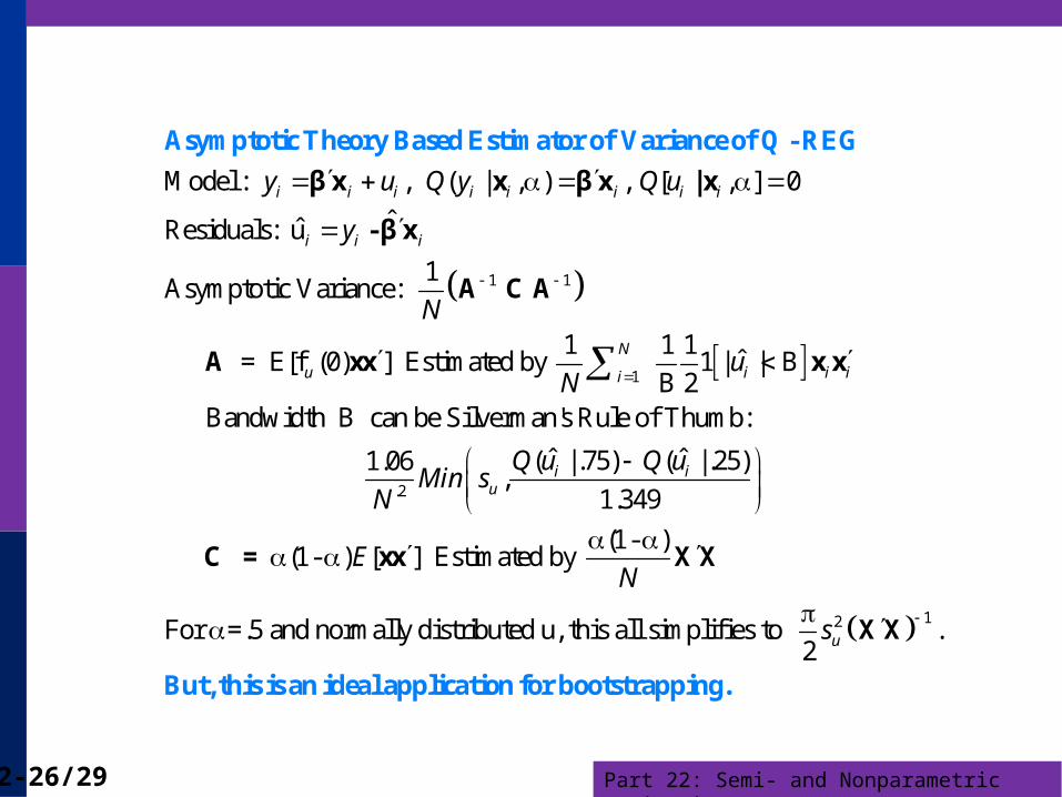
Model : , ( | , ) , [ , ] 0
ˆˆResiduals: u
1Asymptotic Variance:
= E[f (0) ] Estimated by
Asymptotic Theory Based Estimator of Variance of Q - REG
x | x
A C A
A xx
i i i i i i i i
i i i
u
y u Q y Q u
y
N
βx βx
-βx
1
.2
1 1 1ˆ1 | | B
B 2 Bandwidth B can be Silverman's Rule of Thumb:
ˆ ˆ( | .75) ( | .25)1.06 ,
1.349
(1- )(1- ) [ ] Estimated by
x x
C = xx
N
i i ii
i iu
uN
Q u Q uMin s
N
EN
12For =.5 and normally distributed u, this all simplifies to .2
But, this is an ideal application for bootstrapping
X
X
.
X
Xus
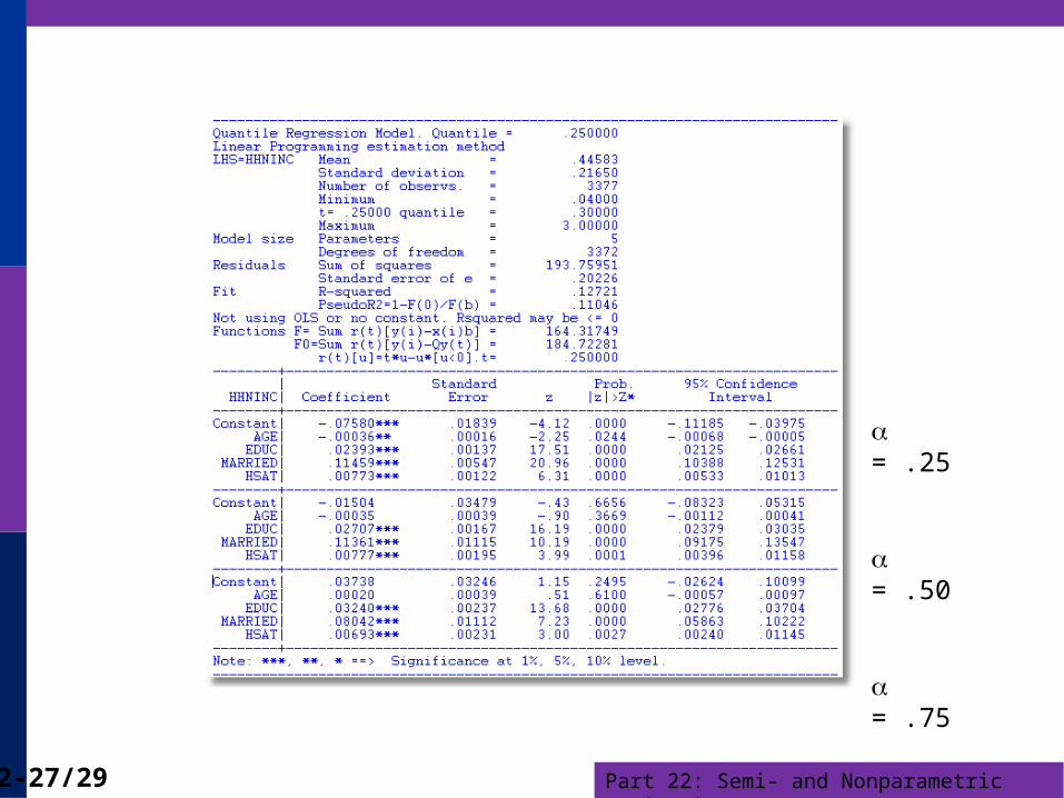
Part 22: Semi- and Nonparametric Estimation22-27/29
= .25
= .50
= .75
Part 22: Semi- and Nonparametric Estimation22-28/29

Part 22: Semi- and Nonparametric Estimation22-29/29