Econ 551 Government Finance: Revenues Winter,...

ECON 551: Lecture 5a 1 of 41

Econ 551

Government Finance: Revenues

Winter, 2018

Given by Kevin Milligan

Vancouver School of Economics

University of British Columbia

Lecture 5a: Optimal Income Taxation, Part I


Agenda:

1. The Mirrlees approach to optimal income taxation

2. Setting up the Mirrlees problem

3. ‘Zero at the top’

4. The full Mirrlees problem

5. The Piketty perturbation derivation of a Mirrlees result


Optimal Income Taxation Overview

Through the 1960s, the economics of income taxation was filled with ‘rules of thumb’, partial

equilibrium analyses, and other things that didn’t look like the rest of then-modern economics.

• Paper by Mirrlees (1971) was a big departure.

Good references for this are Myles chapter 5, the Handbook chapter by Auerbach and Hines (ch.

21), and Atkinson and Stiglitz ch. 13.

Really nice treatment in the Salanié textbook.


The Mirrlees Contribution

The paper “An Exploration in the Theory of Optimum Income Taxation”

(1971 REStud) by James Mirrlees took the tools of modern micro-economic

theory to the question of income taxation.

While progress has continued in the study of taxation, most of it builds on

Mirrlees; it remains at the foundation.

The framework is one of mechanism design: designing institutions to maximize some objective

when the agents might have different information and incentives.

The key tension is to get high ability people to continue to work hard and earn high incomes, rather

than ‘mimic’ low ability types. Incentive compatibility lies at the heart of the analysis.


Planet Mirrlees

The Mirrlees analysis takes place in a specific context. This is a set of assumptions used to define

the ‘playground’ used for optimal income tax discussions. Subsequent research might play with,

relax, or change some of these to test how the results change.


Planet Mirrlees

• Many households, differing in ability to earn

• Ability to earn determined by endowment of skill—no human

capital.

• Skill not observable to tax authority; earnings are.

• Firms are competitive price takers; no excess profits (CRTS)

• Static framework; no dynamics.

• Planner’s problem: maximize social welfare subject to a revenue

constraint.

• Utilitarian social welfare function—we trade off the welfare of one person for another.

• Planner’s tool: a tax function. Could think of it directly choosing pre- and post-tax incomes.

• Tax function T(*) assumed to be smooth and differentiable

• Preferences assumed to satisfy a single-crossing condition.

Q: what would be optimal tax scheme if planner could observe ability?


Agenda:







Setup for Mirrlees approach:

• Consumption is c.

• labour is l.

• Type is w, which is also the wage rate.

• Gross income is therefore: 𝑧 = 𝑤𝑙. o Note that gov’t observes z, not w or l independently.

o This assumption drives everything. How realistic is it? Can the tax authority observe w or

l?

• Tax function looks like this: 𝑦 = 𝑧 − 𝑇(𝑧), so y is after-tax income.

• Since there is no saving, c=y. You consume your after-tax income.


Setup for Mirrlees approach:

Utility looks like this:

𝑈(𝑦, 𝑧, 𝑤) = 𝑉 (𝑦,𝑧

𝑤) = 𝑉(𝑦, 𝑙)

Consumer maximizes utility subject to the tax function:

max𝑧

𝑈 = 𝑈(𝑦, 𝑧, 𝑤) 𝑠. 𝑡. 𝑦 = 𝑧 − 𝑇(𝑧)

FOC:

0 = 𝑈𝑦

𝜕𝑦

𝜕𝑧+ 𝑈𝑧

We can see that 𝜕𝑦

𝜕𝑧= (1 − 𝑇′), so the optimal choice is where

(1 − 𝑇′) = −𝑈𝑧

𝑈𝑦≡ 𝜎(𝑦, 𝑧, 𝑤).


Some structure on preferences:

To make the model work well, we need to restrict preferences a bit.

Truth versus reporting:

𝜙(𝑤, 𝑠) = 𝑈(𝑦(𝑠), 𝑧(𝑠), 𝑤): utility of someone of type w who reports wage of s.

Incentive compatibility: A tax function if incentive compatible if:

𝜙(𝑤, 𝑤) ≥ 𝜙(𝑤, 𝑠) ∀𝑤, 𝑠

Single-crossing:

𝜎(𝑦, 𝑧, 𝑤) is the MRS between y and z for a guy of type w.

If 𝜕𝜎

𝜕𝑤≤ 0 ∀𝑦, 𝑧, 𝑤 , then preferences satisfy single-crossing.


Why single-crossing?

If 𝜕𝜎

𝜕𝑤≤ 0 ∀𝑦, 𝑧, 𝑤 , then preferences satisfy single-crossing.

• This means that as you move to higher ability guys, their indifference curves get flatter; and

the curves of any two guys only cross once.

• This also implies that there will be no backward bending labour supply curve, as gross

incomes will grow with wages

• This is a restriction on preferences that is necessary to get some results.

• This is important. Why? Because single-crossing is a necessary condition for a separating

equilibrium. If we don’t have a separating equilibrium, then someone will not be reporting

truthfully. That is not desirable.


Agenda:







Zero at the top

This is a famous result, but somewhat of a ‘toy’ result. Not too be taken too seriously (for reasons

we shall discuss), but useful to test our understanding of what is going on in the model.

Let’s take a simplified situation to highlight what goes on at the top of the income distribution.

• Take two people H and H-1.

• Assume for now that government’s goal is to maximize revenue.

Goal: offer ‘contracts’𝛼 to these two people, where a contract specifies how much of their z they

get to keep as y.

Graph this in y-z space.


Government iso-revenue curves

Every point on one of these iso-revenue lines raises the same revenue. All parallel to 45° line

through origin.

y

y = z

45°

z = 100 z z = 200

y = z-100 y = z-200


Separating equilibrium

If we offer 𝛼𝐻−1 to type H-1, we can offer any 𝛼𝐻 to type H that is in the shaded region and get a

separating equilibrium. Which of these points should we choose?

y

z

𝛼𝐻−1

𝛼𝐻

𝑢𝐻−1

𝑢𝐻


Revenue-maximizing separating equilibrium

Which 𝛼𝐻? How about the one that raises the most revenue—touches the furthest out iso-revenue

curve:

z

𝛼𝐻−1

y

𝛼𝐻

𝑢𝐻

What is slope at this

point? What is

marginal tax rate?

(1 − 𝑇′) = −𝑈𝑧

𝑈𝑦


Some comments on ‘zero at the top’

• What is the intuition? Imagine he faced a positive tax rate. He would choose to stop working

at some point. Now imagine we moved the tax rate to be 0 for his next dollar earned. He

would then choose to work a bit more, but we would raise no more revenue. However, his

extra work increases social welfare. So, it doesn’t cost us anything to get some more work out

of him. Equivalently, a positive MTR distorts his decision but doesn’t raise revenue.

• This doesn’t mean that the highest guy pays no taxes. He will face positive MTRs on his

dollars earned up to the point of the 2nd highest guy’s contract. It’s just zero from then on.

• Note that this result holds only at the very top; for the highest ability individual. The 2nd

highest guy will face a positive MTR. So, we shouldn’t get carried away with this result.

That is, we shouldn’t take it as a serious policy prescription.

• The result does not hold asymptotically. So, if the distribution of w is unbounded, then MTR

does not approach zero as w goes to infinity.

• Substantively, this result suggests that MTRs might not optimally be progressive.


Agenda:







The full Mirrlees problem

We will now write out the full Mirrlees optimization problem that could be solved to deliver the

optimal tax schedule.

As it turns out, we’re not actually going to solve it though.

• We will use a much simpler solution approach.


Define some terms:

𝑤 is the lowest level of ability.

𝑤 is the highest level of ability.

s a particular level of w. Will be used as an index for integration.

𝐹(𝑠) CDF for abilities s.

𝑓(𝑠) PDF for abilities s.


Define some more terms:

Ψ(𝑈(𝑦, 𝑧, 𝑤)) Social welfare just from the individual with ability w and incomes y and z. This

is kind of like an ‘instantaneous’ utility.

η The marginal effect on gross income as we move to a higher w type: 𝜂 ≡𝜕𝑧

𝜕𝑤.

𝑅(𝑤) = ∫ (𝑧 − 𝑦)𝑑𝐹(𝑠)𝑤

𝑤 Government revenue up to skill level w.

𝑅 ≡ 𝑅(𝑤) Government Budget Constraint. Also, 𝑅(𝑤) = 0


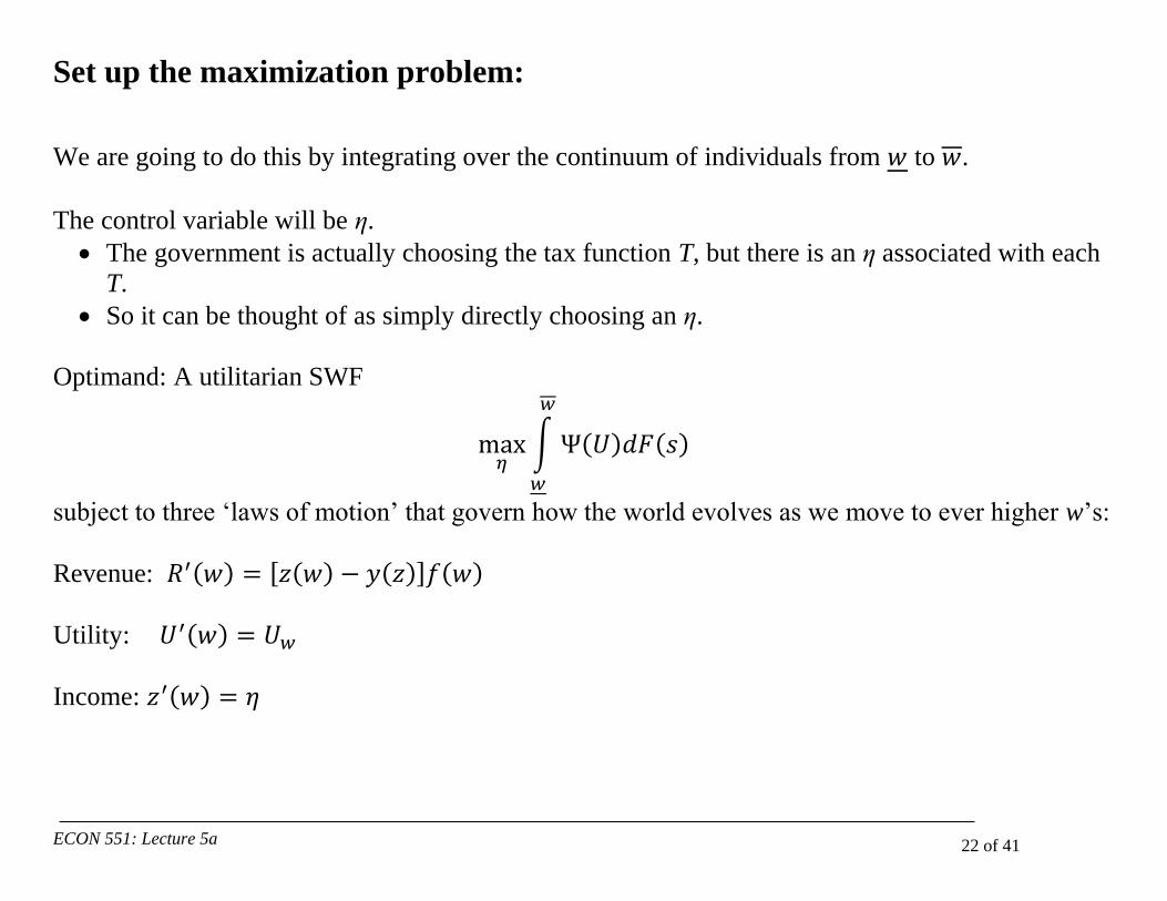
Set up the maximization problem:

We are going to do this by integrating over the continuum of individuals from 𝑤 to 𝑤.

The control variable will be η.

• The government is actually choosing the tax function T, but there is an η associated with each

T.

• So it can be thought of as simply directly choosing an η.

Optimand: A utilitarian SWF

max𝜂

∫ Ψ(𝑈)𝑑𝐹(𝑠)

𝑤

𝑤

subject to three ‘laws of motion’ that govern how the world evolves as we move to ever higher w’s:

Revenue: 𝑅′(𝑤) = [𝑧(𝑤) − 𝑦(𝑧)]𝑓(𝑤)

Utility: 𝑈′(𝑤) = 𝑈𝑤

Income: 𝑧′(𝑤) = 𝜂


Agenda:







The Piketty differential perturbation approach

• Mirrlees solved the problem using a Hamiltonian / ‘dynamic’

programming approach.

• Salanié (2003) argues that the Mirrlees approach is “tedious”;

141 numbered equations. Amen, brother.

• Salanié presents an approach first developed by Piketty (1997) that is much more intuitive.

• Piketty’s approach starts with a graph and presents a simple perturbation that generates

intuitive and informative optimal tax formulae.


Notation and setup:

Consumption is c.

labour is l.

Type is w, which is also the wage rate. CDF 𝐹(𝑤); PDF 𝑓(𝑤)

Gross income is therefore: 𝑧 = 𝑤𝑙 • Note that gov’t observes z, not w or l independently.

• This assumption drives everything. How realistic is it? Can the tax authority observe w or l?

Labour elasticity: 𝜀 =𝑑𝑙

𝑑𝑤

𝑤

𝑙

Tax function looks like this: 𝑦 = 𝑧 − 𝑇(𝑧), so y is after-tax income.

Since there is no saving, c=y. You consume your after-tax income.


Key Assumption:

Key assumption: Government is maximizing revenue for interior taxpayers.

Why is this useful?

• Means we can use a ‘zero marginal revenue’ condition to derive optimal tax rates.

What is meant by ‘interior’ taxpayers?

• We don’t assume this result holds for the bottom taxpayer.

Why do we isolate the bottom taxpayer?

• We’re assuming Rawlsian preferences in order to get us to the ‘revenue maximizing’ position.

• If there are other ways to get to ‘revenue maximizing’ objective function for government, that

would work too.


The tax function and perturbation:

Tax function maps z into y.

Perturb the marginal tax rate by 𝑑𝑇′ over range 𝑑𝑧 at point 𝑧0:

Before Tax Income

𝑧 = 𝑤𝑙 z0 z0+dz

After

Tax

Income

(y)

𝑦 = 𝑇(𝑧)

Slope is 𝑑𝑦

𝑑𝑧=

𝑇′


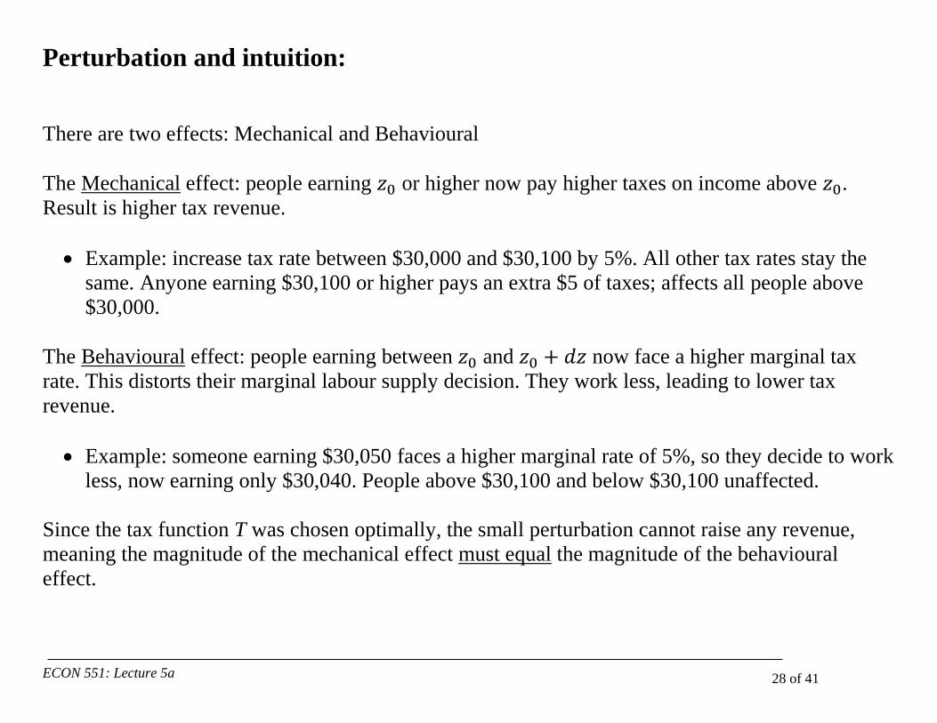
Perturbation and intuition:

There are two effects: Mechanical and Behavioural

The Mechanical effect: people earning 𝑧0 or higher now pay higher taxes on income above 𝑧0.

Result is higher tax revenue.

• Example: increase tax rate between $30,000 and $30,100 by 5%. All other tax rates stay the

same. Anyone earning $30,100 or higher pays an extra $5 of taxes; affects all people above

$30,000.

The Behavioural effect: people earning between 𝑧0 and 𝑧0 + 𝑑𝑧 now face a higher marginal tax

rate. This distorts their marginal labour supply decision. They work less, leading to lower tax

revenue.

• Example: someone earning $30,050 faces a higher marginal rate of 5%, so they decide to work

less, now earning only $30,040. People above $30,100 and below $30,100 unaffected.

Since the tax function T was chosen optimally, the small perturbation cannot raise any revenue,

meaning the magnitude of the mechanical effect must equal the magnitude of the behavioural

effect.


Expression for mechanical effect:

Multiply the number of people affected by the amount of increase paid by each.

Proportion of people affected: (1 − 𝐹(𝑤0))

Tax increase per person: 𝑑𝑇′𝑑𝑧

(In the example, this is 5% times $100 = $5)

So, the total mechanical effect is 𝑑𝑇′𝑑𝑧(1 − 𝐹(𝑤0))


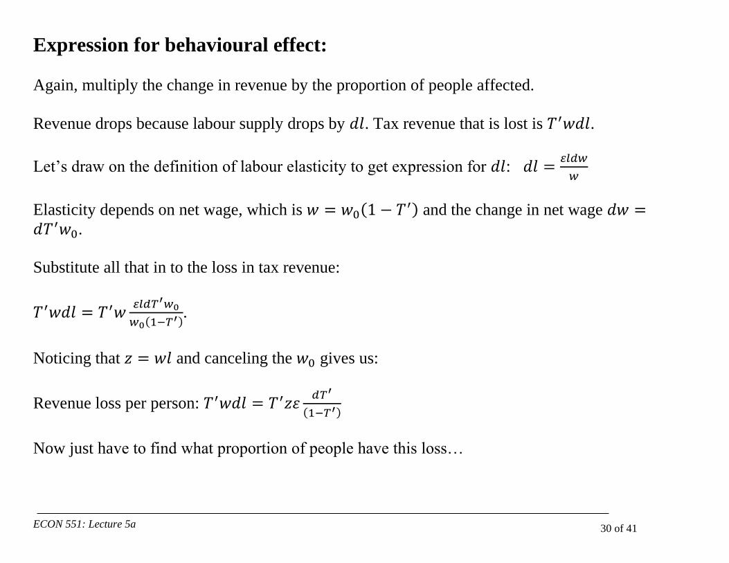
Expression for behavioural effect:

Again, multiply the change in revenue by the proportion of people affected.

Revenue drops because labour supply drops by 𝑑𝑙. Tax revenue that is lost is 𝑇′𝑤𝑑𝑙.

Let’s draw on the definition of labour elasticity to get expression for 𝑑𝑙: 𝑑𝑙 =𝜀𝑙𝑑𝑤

𝑤

Elasticity depends on net wage, which is 𝑤 = 𝑤0(1 − 𝑇′) and the change in net wage 𝑑𝑤 =𝑑𝑇′𝑤0.

Substitute all that in to the loss in tax revenue:

𝑇′𝑤𝑑𝑙 = 𝑇′𝑤𝜀𝑙𝑑𝑇′𝑤0

𝑤0(1−𝑇′).

Noticing that 𝑧 = 𝑤𝑙 and canceling the 𝑤0 gives us:

Revenue loss per person: 𝑇′𝑤𝑑𝑙 = 𝑇′𝑧𝜀𝑑𝑇′

(1−𝑇′)

Now just have to find what proportion of people have this loss…


Expression for behavioural effect:

In the range of the behavioural effect, the number affected is:

𝑓(𝑤0)𝑑𝑤0.

Let’s play with 𝑑𝑤0 to get an expression we can work with:

𝑑𝑧

𝑑𝑤0=

𝑑𝑧

𝑑𝑤=

𝑑(𝑤𝑙)

𝑑𝑤= 𝑙 + 𝑤

𝑑𝑙

𝑑𝑤= 𝑙 + 𝑤 (

𝜀𝑙

𝑤) = 𝑙(1 + 𝜀), implying 𝑑𝑤0 =

𝑑𝑧

𝑙(1+𝜀).

Now multiply together the change in revenue per person with the proportion of people in this range:

𝑇′𝑧𝜀𝑑𝑇′

(1 − 𝑇′)𝑓(𝑤0)

𝑑𝑧

𝑙(1 + 𝜀)


Put it all together:

Mechanical Effect = Behavioural Effect

𝑑𝑇′𝑑𝑧(1 − 𝐹(𝑤0)) = 𝑇′𝑧𝜀𝑑𝑇′

(1 − 𝑇′)𝑓(𝑤0)

𝑑𝑧

𝑙(1 + 𝜀)

Which reduces to:

𝑇′

(1 − 𝑇′)= (1 +

1

𝜀)

(1 − 𝐹(𝑤0))

𝑤0𝑓(𝑤0)


Poking the result a bit:

1. What is the marginal tax rate for a person who earns at the very top of the income distribution?

Why?

2. All else equal, what happens at thin parts of the income distribution (where there aren’t many

people)? Why?

3. What happens to the tax rate when you’re looking at a higher value of 𝑤0? Why?

4. All else equal, what pushes up the tax rates at the bottom of the income distribution?

5. What impact does a higher labour supply elasticity have on optimal tax rates? Does this make

sense?


How to enrich this:

• Allow for ‘bunching’: extensive margin decision to join labour market at bottom.

• Consider joint taxation of family income.

• Consider different income distributions at the top.

• Consider elasticities other than labour supply (e.g. mobility; tax avoidance)


Some simulated MTR schedules from Saez 2001:


Notes on simulated MTR schedules from Saez 2001:

• Utility type 1 has no income effects; type 2 has income effects.

• Why no ‘zero at the top’? He uses unbounded ability distribution.

• Why no ‘zero at the bottom’? Because labour supply is going to zero near the bottom.

• Why such high tax rates on the low ability guys? The model assumes a flat transfer to

everybody—a guaranteed income level. So, the high tax rate at the bottom just means that we

are taxing this guaranteed income level away very quickly with higher earned income. This

ensures that the guaranteed income amount is targeted at the poorest. Also note that high tax

rate at low income levels raises a lot of revenue!

• Why does the tax rate start to swing up around 70k? This just reflects the shape of the income

distribution used in the simulations. There are fewer people up at those levels so the

productivity cost of taxing them more isn’t as high.

• Note that the higher wage elasticity (=0.5) simulations show lower tax schedules.

• Rawlsian schedules feature higher tax rates. Why? Because more redistribution toward the

very poor; the next-to-poor are not as well off under Rawlsian.


Actual Y vs Z in 2010 SLID


Actual MTR schedules for some provinces, 2008

Married couple, two children.


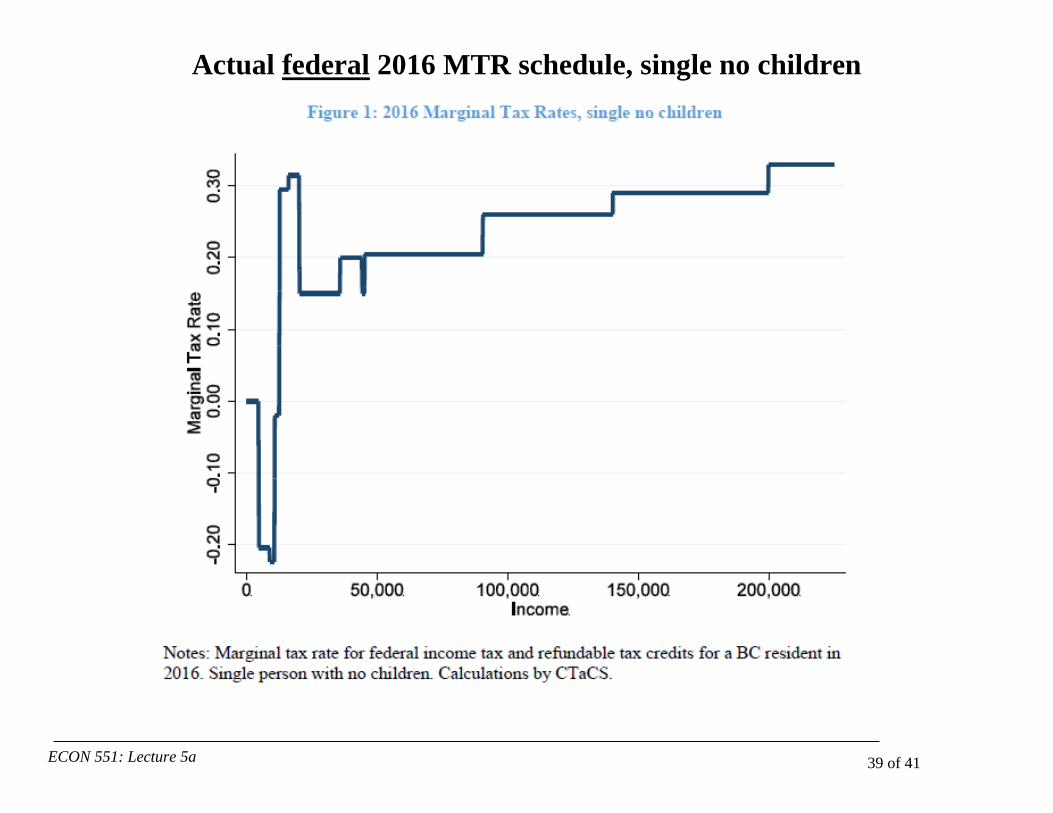
Actual federal 2016 MTR schedule, single no children


Actual federal 2016 MTR schedule, single two children


For next class:

Have a look at:

“Myth and Reality of Flat Tax Reform: Micro Estimates of Tax Evasion Response and Welfare

Effects in Russia”

Yuriy Gorodnichenko, Jorge Martinez-Vazquez, and Klara Sabirianova Peter

Journal of Political Economy, Vol. 117, No. 3, pp. 504-554. (June 2009)

…and

Boadway, Robin and Pierre Pestieau (2003), “Indirect Taxation and Redistribution: The Scope of

the Atkinson-Stiglitz Theorem,” in Richard Arnott, Bruce Greenwald, Ravi Kanbur and Barry

Nalebuff (eds.), Economics for an Imperfect World: Essays in Honor of Joseph E. Stiglitz.

Cambridge, Mass: MIT Press, pp. 387-403.

Econ 551 Government Finance: Revenues Winter,...

Documents

Transcript of Econ 551 Government Finance: Revenues Winter,...