Econ 219A Psychology and Economics: Foundations (Lecture 2)
84
Econ 219A Psychology and Economics: Foundations (Lecture 2) Stefano DellaVigna November 18, 2009
Transcript of Econ 219A Psychology and Economics: Foundations (Lecture 2)

Econ 219A
Psychology and Economics: Foundations
(Lecture 2)
Stefano DellaVigna
November 18, 2009

Outline
1. Reference Dependence: Housing
2. Reference Dependence: Mergers
3. Reference Dependence: Insurance
4. Reference Dependence: Employment and Effort
5. Reference Dependence: Disposition Effect I

1 Reference Dependence: Housing
• Genesove-Mayer (QJE, 2001)— For houses sales, natural reference point is previous purchase price
— Loss Aversion —> Unwilling to sell house at a loss
• Formalize intuition.— Seller chooses price P at sale
— Higher Price P
∗ lowers probability of sale p (P ) (hence p0 (P ) < 0)
∗ increases utility of sale U (P )— If no sale, utility is U < U (P ) (for all relevant P )

• Maximization problem:maxP
p(P )U (P ) + (1− p (P ))U
• F.o.c. impliesMG = p(P ∗)U 0 (P ∗) = −p0(P ∗)(U (P ∗)− U) =MC
• Interpretation: Marginal Gain of increasing price equals Marginal Cost
• S.o.c are2p0(P ∗)U 0 (P ∗) + p(P ∗)U 00 (P ∗) + p00(P ∗)(U (P ∗)− U) < 0
• Need p00(P ∗)(U (P ∗)− U) < 0 or not too positive

• Reference-dependent preferences with reference price P0:
v (P |P0) =(
P − P0 if P ≥ P0;λ (P − P0) if P < P0,
— Can write as
p(P ) = −p0(P )(P − P0 − U) if P ≥ P0
p(P )λ = −p0(P )(λ (P − P0)− U) if P < P0
— Plot Effect on MG and MC of loss aversion
• Compare P ∗λ=1 (equilibrium with no loss aversion) and P ∗λ>1 (equilibriumwith loss aversion)

• Case 1. Loss Aversion λ increase price (P ∗λ=1 < P0)
• Case 2. Loss Aversion λ induces bunching at P = P0 (P ∗λ=1 < P0)

• Case 3. Loss Aversion has no effect (P ∗λ=1 > P0)
• General predictions. When aggregate prices are low:— High prices P relative to fundamentals
— Bunching at purchase price P0
— Lower probability of sale p (P )
— Longer waiting on market

• Evidence: Data on Boston Condominiums, 1990-1997
• Substantial market fluctuations of price
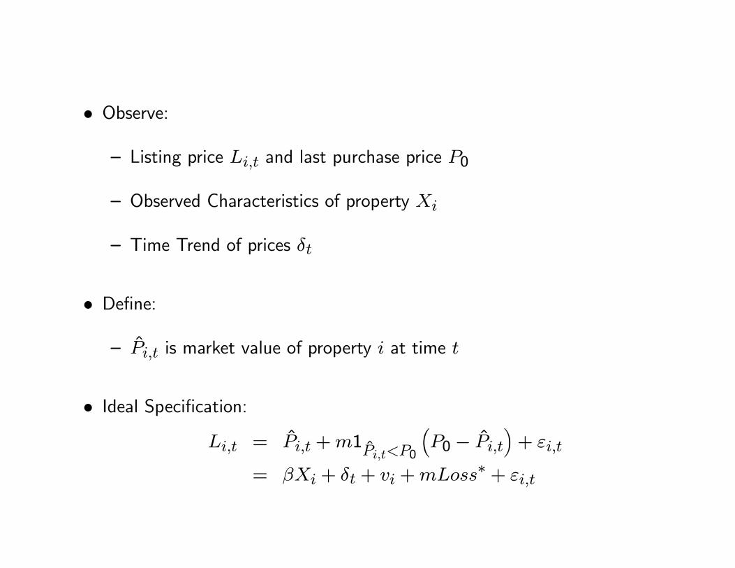
• Observe:
— Listing price Li,t and last purchase price P0
— Observed Characteristics of property Xi
— Time Trend of prices δt
• Define:
— Pi,t is market value of property i at time t
• Ideal Specification:Li,t = Pi,t +m1
Pi,t<P0
³P0 − Pi,t
´+ εi,t
= βXi + δt + vi +mLoss∗ + εi,t

• However:— Do not observe Pi,t, given vi (unobserved quality)— Hence do not observe Loss∗
• Two estimation strategies to bound estimates. Model 1:Li,t = βXi + δt +m1
Pi,t<P0(P0 − βXi − δt) + εi,t
— This model overstate the loss for high unobservable homes (high vi)— Bias upwards in m, since high unobservable homes should have highLi,i
• Model 2:Li,t = βXi+δt+α (P0 − βXi − δt)+m1Pi,t<P0
(P0 − βXi − δt)+εi,t
• Estimates of impact on sale price


• Effect of experience: Larger effect for owner-occupied

• Some effect also on final transaction price

• Lowers the exit rate (lengthens time on the market)
• — Overall, plausible set of results that show impact of reference point
— Would have been nice to tie better to model
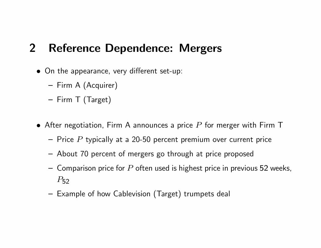
2 Reference Dependence: Mergers
• On the appearance, very different set-up:— Firm A (Acquirer)
— Firm T (Target)
• After negotiation, Firm A announces a price P for merger with Firm T
— Price P typically at a 20-50 percent premium over current price
— About 70 percent of mergers go through at price proposed
— Comparison price for P often used is highest price in previous 52 weeks,P52
— Example of how Cablevision (Target) trumpets deal


• Assume that Firm T chooses price P , and A decides accept reject
• As a function of price P, probability p(P ) that deal is accepted (dependson perception of values of synergy of A)
• If deal rejected, go back to outside value U
• Then maximization problem is same as for housing sale:maxP
p(P )U (P ) + (1− p (P ))U
• Can assume T reference-dependent with respect to
v (P |P0) =(
P − P52 if P ≥ P52;λ (P − P52) if P < P52,

• Obtain same predictions as in housing market
• (This neglects possible reference dependence of A)
• Baker, Pan, and Wurgler (2009): Test reference dependence in mergers
— Test 1: Is there bunching around P52? (GM did not do this)
— Test 2: Is there effect of P52 on price offered?
— Test 3: Is there effect on probability of acceptance?
— Test 4: What do investors think? Use returns at announcement

• Test 1: Offer price P around P52
— Some bunching, missing left tail of distribution

• Notice that this does not tell us how the missing left tail occurs:
— Firms in left tail raise price to P52?
— Firms in left tail wait for merger until 12 months after past peak, soP52 is higher?
— Preliminary negotiations break down for firms in left tail
• Would be useful to compare characteristics of firms to right and left ofP52
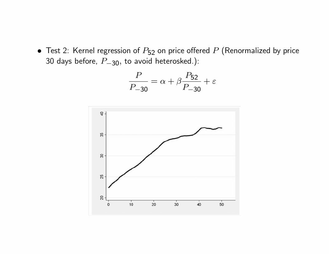
• Test 2: Kernel regression of P52 on price offered P (Renormalized by price30 days before, P−30, to avoid heterosked.):
P
P−30= α+ β
P52P−30
+ ε

• Test 3: Probability of final acquisition is higher when offer price is aboveP52 (Skip)
• Test 4: What do investors think of the effect of P52?
— Holding constant current price, investors should think that the higherP52, the more expensive the Target is to acquire
— Standard methodology to examine this:
∗ 3-day stock returns around merger announcement: CARt−1,t+1
∗ This assumes investor rationality
∗ Notice that merger announcements are typically kept top secret untillast minute —> On announcement day, often big impact

• Regression (Columns 3 and 5):
CARt−1,t+1 = α+ βP
P−30+ ε
where P/P−30 is instrumented with P52/P−30
• Results very supportive of reference dependence hypothesis — Also alter-native anchoring story

3 Reference Dependence: Insurance
• Much of the laboratory evidence on prospect theory is on risk taking
• Field evidence considered so far (mostly) does not involve risk:— Trading behavior — Endowment Effect— Daily Labor Supply
• Field evidence on risk taking?
• Sydnor (2006) on deductible choice in the life insurance industry
• Uses Menu Choice as identification strategy as in DellaVigna and Mal-mendier (2006)
• Slides courtesy of Justin Sydnor

Dataset50,000 Homeowners-Insurance Policies
12% were new customers Single western stateOne recent year (post 2000)Observe
Policy characteristics including deductible1000, 500, 250, 100
Full available deductible-premium menuClaims filed and payouts by company

Features of ContractsStandard homeowners-insurance policies (no renters, condominiums)Contracts differ only by deductibleDeductible is per claimNo experience rating
Though underwriting practices not clearSold through agents
Paid commissionNo “default” deductible
Regulated state

Summary Statistics
VariableFull
Sample 1000 500 250 100
Insured home value 206,917 266,461 205,026 180,895 164,485(91,178) (127,773) (81,834) (65,089) (53,808)
8.4 5.1 5.8 13.5 12.8(7.1) (5.6) (5.2) (7.0) (6.7)
53.7 50.1 50.5 59.8 66.6(15.8) (14.5) (14.9) (15.9) (15.5)
0.042 0.025 0.043 0.049 0.047(0.22) (0.17) (0.22) (0.23) (0.21)
Yearly premium paid 719.80 798.60 715.60 687.19 709.78(312.76) (405.78) (300.39) (267.82) (269.34)
N 49,992 8,525 23,782 17,536 149Percent of sample 100% 17.05% 47.57% 35.08% 0.30%
Chosen Deductible
Number of years insured by the company
Average age of H.H. members
Number of paid claims in sample year (claim rate)
* Means with standard errors in parentheses.

Deductible PricingXi = matrix of policy characteristicsf(Xi) = “base premium”
Approx. linear in home valuePremium for deductible D
PiD = δD f(Xi)
Premium differencesΔPi = Δδ f(Xi)
⇒Premium differences depend on base premiums (insured home value).

Premium-Deductible Menu
Available Deductible
Full Sample 1000 500 250 100
1000 $615.82 $798.63 $615.78 $528.26 $467.38(292.59) (405.78) (262.78) (214.40) (191.51)
500 +99.91 +130.89 +99.85 +85.14 +75.75(45.82) (64.85) (40.65) (31.71) (25.80)
250 +86.59 +113.44 +86.54 +73.79 +65.65(39.71) (56.20) (35.23) (27.48) (22.36)
100 +133.22 +174.53 +133.14 +113.52 +101.00(61.09) (86.47) (54.20) (42.28) (82.57)
Chosen Deductible
Risk Neutral Claim Rates?
100/500 = 20%
87/250 = 35%
133/150 = 89%
* Means with standard deviations in parentheses

The curves in the upper graphs are fan locally-weighted kernel regressions using a quartic kernel.
The dashed lines give 95% confidence intervales calculated using a bootstrap procedure with 200 repititions.
The range for additional premium covers 98% of the available data
The graph in the upper left gives the fraction that chose either the $250 or $500 deductibles versus theadditional premium an individual faced to move from a $1000 to the $500 deductible.
The graph in the upper right represents the average expected savings from switching to the $1000deductible for customers facing a given premium difference. The potential savings is calculated at theindividual level and then the kernel regressions are run. Because they filed no claims, for mostcustomers this measure is simply the premium reductions they would have seen with the $1000deductible. For the roughly 4% of customers who filed claims the potential savings is typicallynegative.
0.1
.2.3
.4.5
.6.7
.8.9
1F
ract
ion
50 100 150 200 250 300Additional Premium for $500 Deductible
Full Sample
0.0
05.0
1.0
15
De
nsi
ty
50 100 150 200 250 300Additional Premium for $500 Deductible
Full Sample
Kernel Density of Additional Premium
Fraction Choosing $500 or Lower Deductible
Epanechnikov kernel, bw = 10
Quartic kernel, bw = 10
05
010
01
50
20
02
50
30
0P
ote
ntia
l Sa
vin
gs
$
50 100 150 200 250 300Additional Premium for $500 Deductible
Low Deductible CustomersQuartic kernel, bw = 20
Potential Savings with the Alternative $1000 Deductible
What if the x-axis were insured home value?

The graph in the upper left gives the fraction that chose either the $250 or $500 deductibles as afunciton of the insured home value.
The graph in the upper right represents the average expected savings from switching to the $1000deductible for customers who chose one of the lower deductibles. The potential savings iscalculated at the individual level and then the kernel regressions are run. Because they filed noclaims, for most customers this measure is simply the premium reductions they would have seenwith the $1000 deductible. For the roughly 4% of customers who filed claims the potential savings istypically negative.
The curves in the upper graphs are fan locally-weighted kernel regressions using a quartic kernel.
The dashed lines give 95% confidence intervales calculated using a bootstrap procedure with 200 repititions.
The range for insured home value covers 99% of the available data
050
10
01
50
200
250
Pot
en
tial S
avi
ngs
$
100 150 200 250 300 350 400 450 500 550Insured Home Value ($000)
Low Deductible Customers
0.1
.2.3
.4.5
.6.7
.8.9
1F
ract
ion
100 150 200 250 300 350 400 450 500 550Insured Home Value ($000)
Full Sample
0.0
02
.00
4.0
06.0
08D
ensi
ty
100 150 200 250 300 350 400 450 500 550Insured Home Value ($000)
Full Sample
Kernel Density of Insured Home Value
Quartic kernel, bw = 25
Epanechnikov kernel, bw = 25
Quartic kernel, bw = 50
Fraction Choosing $500 or Lower Deductible Potential Savings with the Alternative $1000 Deductible

Potential Savings with 1000 Ded
Chosen DeductibleNumber of claims
per policy
Increase in out-of-pocket payments per claim with a
$1000 deductible
Increase in out-of-pocket payments per policy with a
$1000 deductible
Reduction in yearly premium per policy with
$1000 deductible
Savings per policy with $1000 deductible
$500 0.043 469.86 19.93 99.85 79.93 N=23,782 (47.6%) (.0014) (2.91) (0.67) (0.26) (0.71)
$250 0.049 651.61 31.98 158.93 126.95 N=17,536 (35.1%) (.0018) (6.59) (1.20) (0.45) (1.28)
Average forgone expected savings for all low-deductible customers: $99.88
Claim rate?Value of lower deductible? Additional
premium? Potential savings?
* Means with standard errors in parentheses

Back of the Envelope
BOE 1: Buy house at 30, retire at 65, 3% interest rate ⇒ $6,300 expected
With 5% Poisson claim rate, only 0.06% chance of losing money
BOE 2: (Very partial equilibrium) 80% of 60 million homeowners could expect to save $100 a year with “high” deductibles ⇒ $4.8 billion per year

Consumer Inertia?Percent of Customers Holding each Deductible Level
0
10
20
30
40
50
60
70
80
90
0-3 3-7 7-11 11-15 15+
Number of Years Insured with Company
%
1000
500
250100

Chosen DeductibleNumber of claims
per policy
Increase in out-of-pocket payments per claim with a $1000 deductible
Increase in out-of-pocket payments per policy with a $1000 deductible
Reduction in yearly premium per policy with
$1000 deductible
Savings per policy with $1000 deductible
$500 0.037 475.05 17.16 94.53 77.37 N = 3,424 (54.6%) (.0035) (7.96) (1.66) (0.55) (1.74)
$250 0.057 641.20 35.68 154.90 119.21 N = 367 (5.9%) (.0127) (43.78) (8.05) (2.73) (8.43)
Average forgone expected savings for all low-deductible customers: $81.42
Look Only at New Customers

Risk Aversion?
Simple Standard ModelExpected utility of wealth maximizationFree borrowing and savingsRational expectationsStatic, single-period insurance decisionNo other variation in lifetime wealth

What level of wealth?
Consumption maximization:
(Indirect) utility of wealth maximization
.........
),,...,,(max
2121
21
TT
Tc
yyycccts
cccUt
++=+++
),(max wuw
),,...,,(max)( 21 TccccUwu
t
=
wyyycccts TT =+++=+++ ........ 2121
where
⇒ w is lifetime wealth
Chetty (2005)

Model of Deductible Choice
Choice between (PL,DL) and (PH,DH)π = probability of loss
Simple case: only one loss
EU of contract:U(P,D,π) = πu(w-P-D) + (1- π)u(w-P)

Bounding Risk Aversion
1)ln()(,1)1(
)()1(
==≠−
=−
ρρρ
ρ
forxxuandforxxu
Assume CRRA form for u :
)1()(
)1()1(
)()1(
)()1(
)1()( )1()1()1()1(
ρπ
ρπ
ρπ
ρπ
ρρρρ
−−
−+−−−
=−
−−+
−−− −−−−
HHHLLL PwDPwPwDPw
Indifferent between contracts iff:

Getting the bounds
Search algorithm at individual levelNew customers
Claim rates: Poisson regressionsCap at 5 possible claims for the year
Lifetime wealth:Conservative: $1 million (40 years at $25k)More conservative: Insured Home Value

CRRA Bounds
Chosen Deductible W min ρ max ρ
$1,000 256,900 - infinity 794 N = 2,474 (39.5%) {113,565} (9.242)
$500 190,317 397 1,055 N = 3,424 (54.6%) {64,634} (3.679) (8.794)
$250 166,007 780 2,467 N = 367 (5.9%) {57,613} (20.380) (59.130)
Measure of Lifetime Wealth (W): (Insured Home Value)

Interpreting Magnitude
50-50 gamble: Lose $1,000/ Gain $10 million
99.8% of low-ded customers would rejectRabin (2000), Rabin & Thaler (2001)
Labor-supply calibrations, consumption-savings behavior ⇒ ρ < 10
Gourinchas and Parker (2002) -- 0.5 to 1.4Chetty (2005) -- < 2

Wrong level of wealth?
Lifetime wealth inappropriate if borrowing constraints.$94 for $500 insurance, 4% claim rate
W = $1 million ⇒ ρ = 2,013W = $100k ⇒ ρ = 199W = $25k ⇒ ρ = 48

Prospect Theory
Kahneman & Tversky (1979, 1992)Reference dependence
Not final wealth states
Value functionLoss AversionConcave over gains, convex over losses
Non-linear probability weighting

Model of Deductible Choice
Choice between (PL,DL) and (PH,DH)π = probability of loss EU of contract:
U(P,D,π) = πu(w-P-D) + (1- π)u(w-P)
PT value:V(P,D,π) = v(-P) + w(π)v(-D)
Prefer (PL,DL) to (PH,DH)v(-PL) – v(-PH) < w(π)[v(- DH) – v(- DL)]

Loss Aversion and Insurance
Slovic et al (1982)Choice A
25% chance of $200 lossSure loss of $50
Choice B25% chance of $200 lossInsurance costing $50
[80%][20%]
[35%][65%]
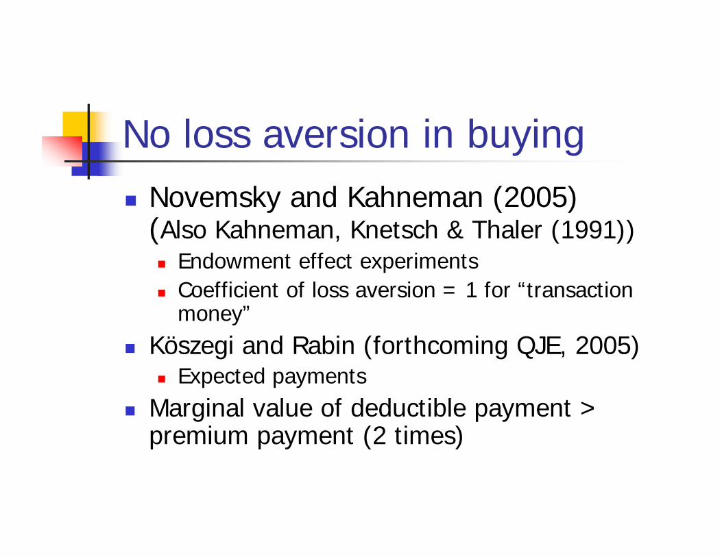
No loss aversion in buyingNovemsky and Kahneman (2005) (Also Kahneman, Knetsch & Thaler (1991))
Endowment effect experimentsCoefficient of loss aversion = 1 for “transaction money”
Köszegi and Rabin (forthcoming QJE, 2005)Expected payments
Marginal value of deductible payment > premium payment (2 times)

So we have:
Prefer (PL,DL) to (PH,DH):
Which leads to:
Linear value function:
)]()()[()()( LHHL DvDvwPvPv −−−<−−− π
][)( ββββ λπ LHHL DDwPP −<−
DwPWTP Δ=Δ= λπ )(
= 4 to 6 times EV

Parameter values
Kahneman and Tversky (1992)λ = 2.25β = 0.88
Weighting function
γ = 0.69
γγγ
γ
ππππ 1
))1(()(
−+=w

WTP from Model
Typical new customer with $500 dedPremium with $1000 ded = $572Premium with $500 ded = +$94.534% claim rate
Model predicts WTP = $107Would model predict $250 instead?
WTP = $166. Cost = $177, so no.

Choices: Observed vs. Model
Chosen Deductible 1000 500 250 100 1000 500 250 100
$1,000 87.39% 11.88% 0.73% 0.00% 100.00% 0.00% 0.00% 0.00% N = 2,474 (39.5%)
$500 18.78% 59.43% 21.79% 0.00% 100.00% 0.00% 0.00% 0.00% N = 3,424 (54.6%)
$250 3.00% 44.41% 52.59% 0.00% 100.00% 0.00% 0.00% 0.00% N = 367 (5.9%)
$100 33.33% 66.67% 0.00% 0.00% 100.00% 0.00% 0.00% 0.00% N = 3 (0.1%)
Predicted Deductible Choice from Prospect Theory NLIB Specification:
λ = 2.25, γ = 0.69, β = 0.88
Predicted Deductible Choice from EU(W) CRRA Utility:
ρ = 10, W = Insured Home Value

Conclusions(Extreme) aversion to moderate risks is an empirical reality in an important marketSeemingly anomalous in Standard Model where risk aversion = DMUFits with existing parameter estimates of leading psychology-based alternative model of decision makingMehra & Prescott (1985), Benartzi & Thaler(1995)

Alternative ExplanationsMisestimated probabilities
≈ 20% for single-digit CRRAOlder (age) new customers just as likely
Liquidity constraintsSales agent effects
Hard sell?Not giving menu? ($500?, data patterns)Misleading about claim rates?
Menu effects

4 Reference Dependence: Employment and Ef-fort
• Back to labor markets: Do reference points affect performance?
• Mas (2006) examines police performance
• Exploits quasi-random variation in pay due to arbitration
• Background
— 60 days for negotiation of police contract —> If undecided, arbitration
— 9 percent of police labor contracts decided with final offer arbitration
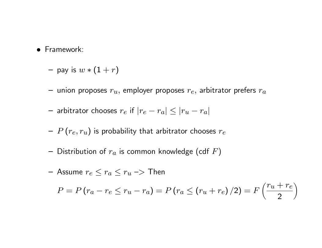
• Framework:
— pay is w ∗ (1 + r)
— union proposes ru, employer proposes re, arbitrator prefers ra
— arbitrator chooses re if |re − ra| ≤ |ru − ra|
— P (re, ru) is probability that arbitrator chooses re
— Distribution of ra is common knowledge (cdf F )
— Assume re ≤ ra ≤ ru —> Then
P = P (ra − re ≤ ru − ra) = P (ra ≤ (ru + re) /2) = Fµru + re
2
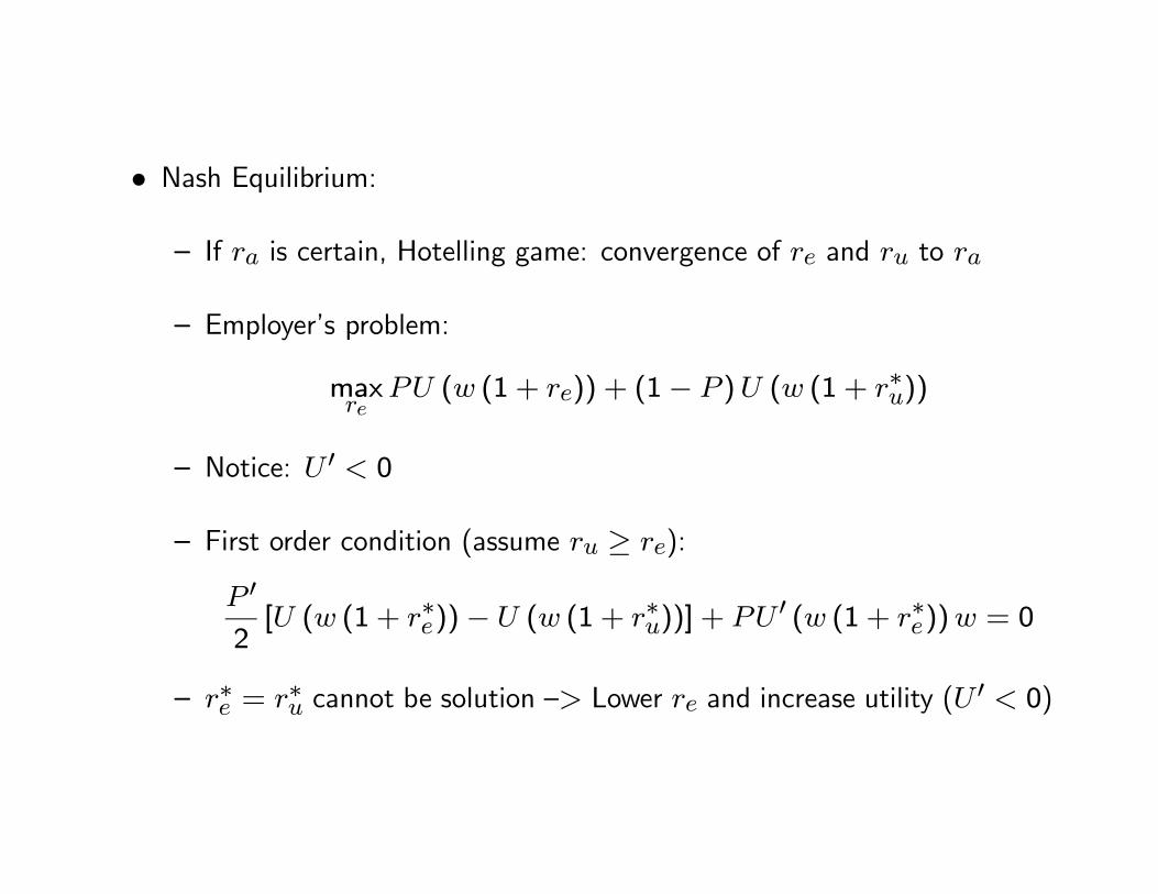
• Nash Equilibrium:
— If ra is certain, Hotelling game: convergence of re and ru to ra
— Employer’s problem:
maxre
PU (w (1 + re)) + (1− P )U (w (1 + r∗u))
— Notice: U 0 < 0
— First order condition (assume ru ≥ re):
P 02[U (w (1 + r∗e))− U (w (1 + r∗u))] + PU 0 (w (1 + r∗e))w = 0
— r∗e = r∗u cannot be solution —> Lower re and increase utility (U 0 < 0)

— Union’s problem: maximizes
maxru
PV (w (1 + r∗e)) + (1− P )V (w (1 + ru))
— Notice: V 0 > 0
— First order condition for union:
P 02[V (w (1 + r∗e))− V (w (1 + r∗u))]+(1− P )V 0 (w (1 + r∗e))w = 0
— To simplify, assume U (x) = −bx and V (x) = bx
— This implies V (w (1 + r∗e))− V (w (1 + r∗u)) = −U (w (1 + r∗e))−U (w (1 + r∗u)) —>
−bP ∗w = − (1− P ∗) bw

— Result: P ∗ = 1/2
• Prediction (i) in Mas (2006): “If disputing parties are equally risk-averse,the winner in arbitration is determined by a coin toss.”
• Therefore, as-if random assignment of winner
• Use to study impact of pay on police effort
• Data:— 383 arbitration cases in New Jersey, 1978-1995
— Observe offers submitted re, ru, and ruling ra
— Match to UCR crime clearance data (=number of crimes solved byarrest)

• Compare summary statistics of cases when employer and when police wins• Estimated P = .344 6= 1/2 —>Unions more risk-averse than employers• No systematic difference between Union and Employer cases except for re
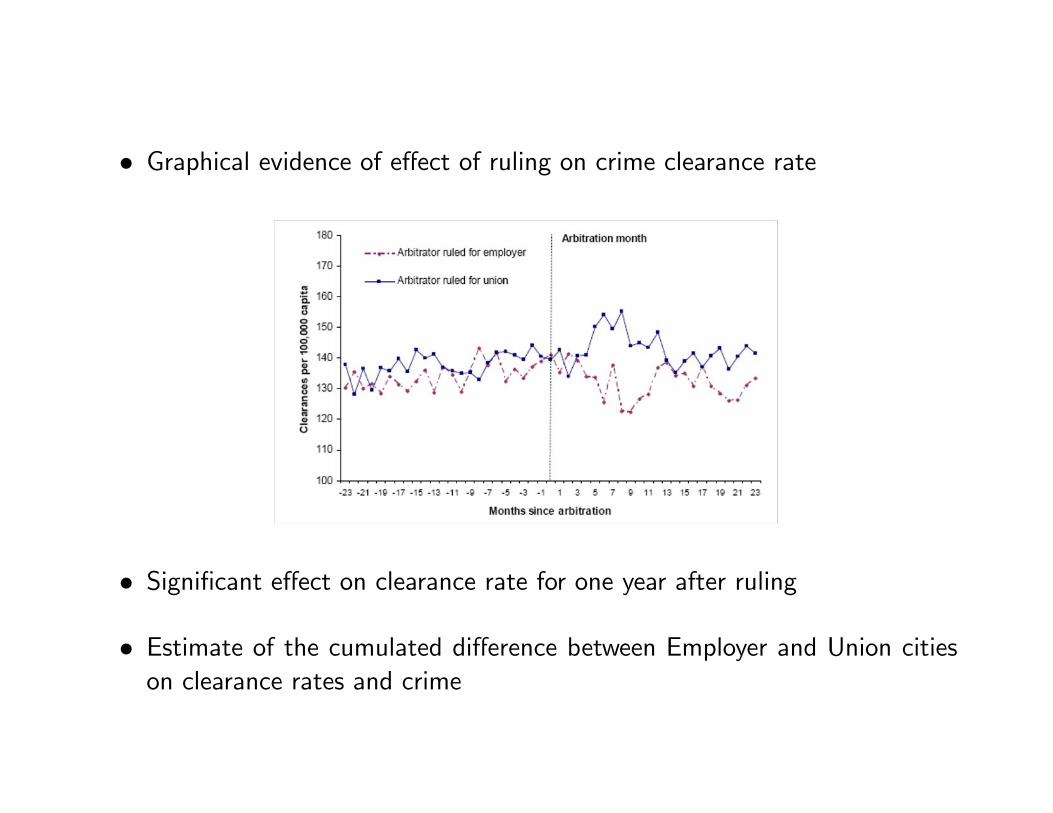
• Graphical evidence of effect of ruling on crime clearance rate
• Significant effect on clearance rate for one year after ruling
• Estimate of the cumulated difference between Employer and Union citieson clearance rates and crime
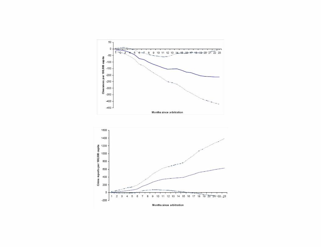

• Arbitration leads to an average increase of 15 clearances out of 100,000each month

• Effects on crime rate more imprecise

• Do reference points matter?• Plot impact on clearances rates (12,-12) as a function of ra− (re+ ru)/2

• Effect of loss is larger than effect of gain

• Column (3): Effect of a gain relative to (re + ru)/2 is not significant;effect of a loss is
• Columns (5) and (6): Predict expected award ra using covariates, thencompute ra − ra
— ra − ra does not matter if union wins
— ra − ra matters a lot if union loses
• Assume policeman maximizes
maxe
hU + U (w)
ie− θ
e2
2

where
U (w) =
(w − w if w ≥ w
λ (w − w) if w < w
• F.o.c.:U + U (w)− θe = 0
Then
e∗ (w) = U
θ+1
θU (w)
• It implies that we would estimateClearances = α+ β (ra − ra) + γ (ra − ra) 1 (ra − ra < 0) + ε
with β > 0 (also in standard model) and γ > 0 (not in standard model)
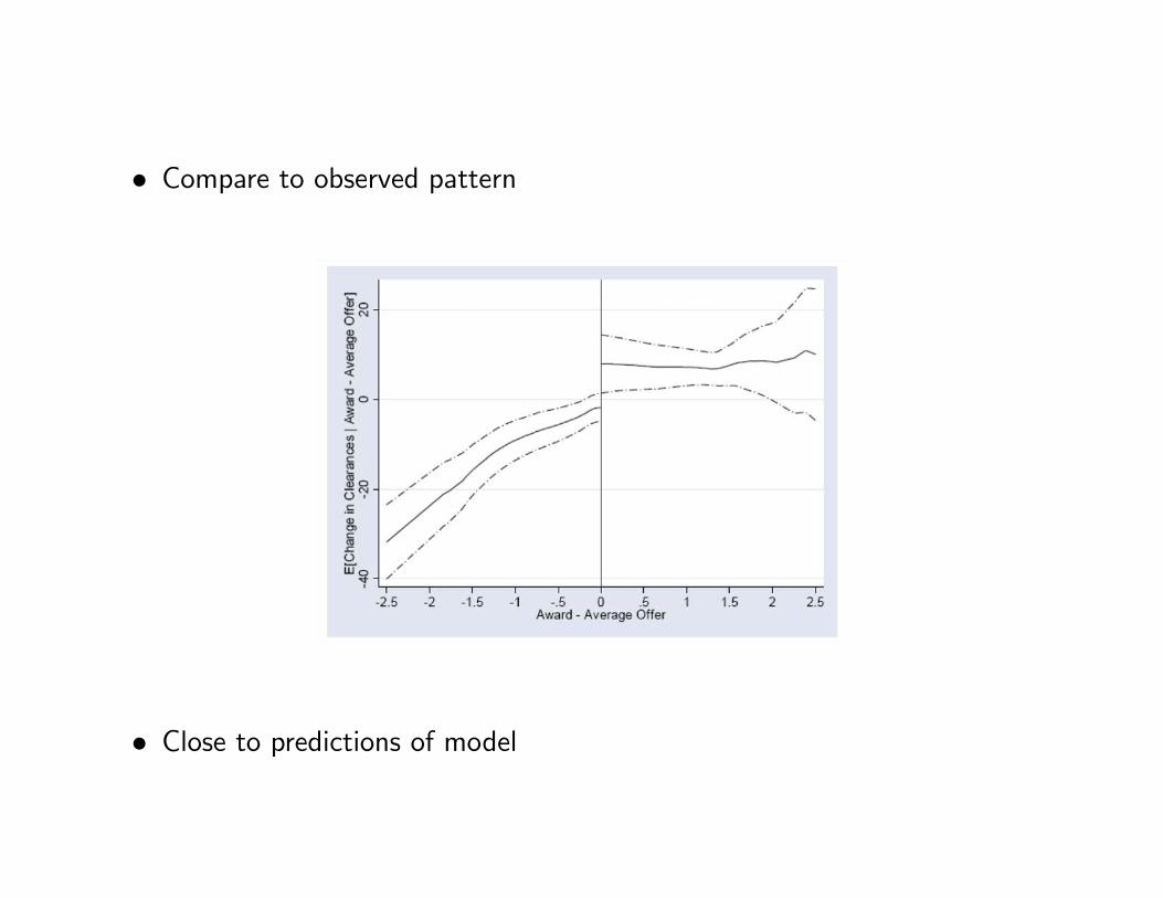
• Compare to observed pattern
• Close to predictions of model

5 Reference Dependence: Disposition Effect
• Odean (JF, 1998)
• Do investors sell winning stocks more than losing stocks?
• Tax advantage to sell losers
— Can post a deduction to capital gains taxation
— Stronger incentives to do so in December, so can post for current taxyear

• Prospect theory intuition:— Evaluate stocks regularly
— Reference point: price of purchase
— Convexity over losses –> gamble, hold on stock
— Concavity over gains –> risk aversion, sell stock

• Individual trade data from Discount brokerage house (1987-1993)
• Rare data set —>Most financial data sets carry only aggregate information
• Share of realized gains:
PGR =Realized Gains
Realized Gains+Paper Gains
• Share of realized losses:PLR =
Realized LossesRealized Losses+Paper Losses
• These measures control for the availability of shares at a gain or at a loss

• Notes on construction of measure:
— Use only stocks purchased after 1987
— Observations are counted on all days in which a sale or purchase occurs
— On those days the paper gains and losses are counted
— Reference point is average purchase price
— PGR and PLR ratios are computed using data over all observations.
— Example:
PGR =13, 883
13, 883 + 79, 658
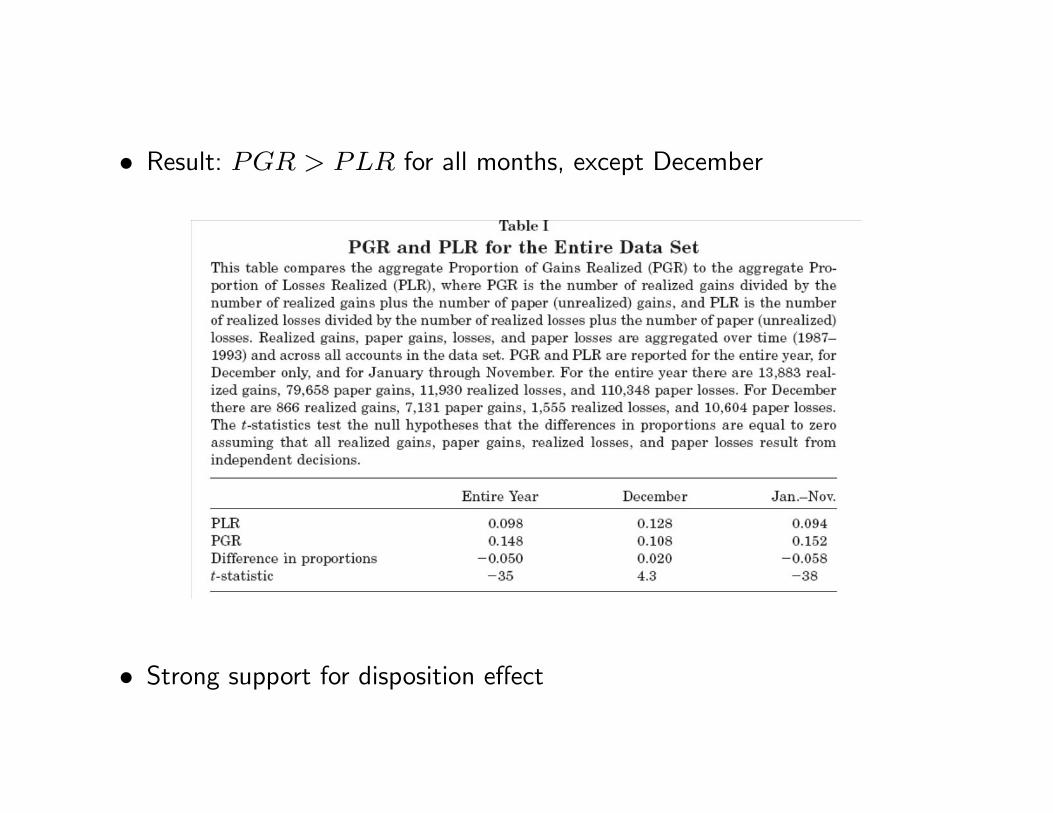
• Result: PGR > PLR for all months, except December
• Strong support for disposition effect

• Effect monotonically decreasing across the year
• Tax reasons are also at play

• Robustness: Across years and across types of investors
• Alternative Explanation 1: Rebalancing —> Sell winners that appreciated
— Remove partial sales

• Alternative Explanation 2: Ex-Post Return —> Losers outperform winnersex post
— Table VI: Winners sold outperform losers that could have been sold

• Alternative Explanation 3: Transaction costs —> Losers more costly totrade (lower prices)
— Compute equivalent of PGR and PLR for additional purchases ofstock
— This story implies PGP > PLP
— Prospect Theory implies PGP < PLP (invest in losses)
• Evidence:PGP =
Gains Purchased
Gains Purchased+ Paper Gains= .094
< PLP =Losses Purchased
Losses Purchased+ Paper Losses= .135.
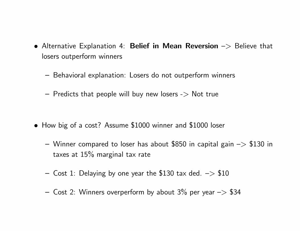
• Alternative Explanation 4: Belief in Mean Reversion —> Believe thatlosers outperform winners
— Behavioral explanation: Losers do not outperform winners
— Predicts that people will buy new losers -> Not true
• How big of a cost? Assume $1000 winner and $1000 loser
— Winner compared to loser has about $850 in capital gain —> $130 intaxes at 15% marginal tax rate
— Cost 1: Delaying by one year the $130 tax ded. —> $10
— Cost 2: Winners overperform by about 3% per year —> $34

• Are results robust to time period and methodology?
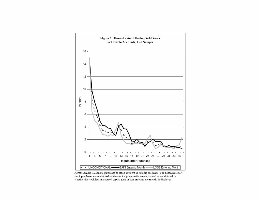
• Ivkovich, Poterba, and Weissbenner (2006)
• Data
— 78,000 individual investors in Large discount brokerage, 1991-1996
— Compare taxable accounts and tax-deferred plans (IRAs)
— Disposition effect should be stronger for tax-deferred plans

• Methodology: Do hazard regressions of probability of buying an sellingmonthly, instead of PGR and PLR
• For each month t, estimate linear probability model:SELLi,t = αt + β1,tI(Gain)i,t−1 + β2,tI(Loss)i,t−1 + εi,t
• Regression only applies to shares not already sold
• αt is baseline hazard at month t
• Pattern of βs always consistent with disposition effect, except in December
• Difference is small for tax-deferred accounts

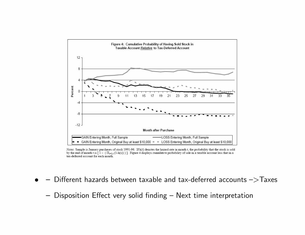
• — Different hazards between taxable and tax-deferred accounts —>Taxes
— Disposition Effect very solid finding — Next time interpretation

6 Next Lecture
• Reference Dependence
— More Disposition Effect
— Labor Supply
• Social Preferences
— Gift Exchange
— Workplace
— From Lab to Field