Ecology and Development Series No. 33, 2005 - zef.de · La actividad agrícola de los últimos 100...
168
Ecology and Development Series No. 33, 2005 Editor-in-Chief: Paul L.G.Vlek Editors: Manfred Denich Christopher Martius Charles Rodgers Nick van de Giesen Carlos Javier Puig Carbon sequestration potential of land-cover types in the agricultural landscape of eastern Amazonia, Brazil Cuvillier Verlag Göttingen
Transcript of Ecology and Development Series No. 33, 2005 - zef.de · La actividad agrícola de los últimos 100...

Ecology and Development Series No. 33, 2005
Editor-in-Chief: Paul L.G.Vlek
Editors:
Manfred Denich Christopher Martius
Charles Rodgers Nick van de Giesen
Carlos Javier Puig
Carbon sequestration potential of land-cover types in the agricultural landscape of eastern Amazonia, Brazil
Cuvillier Verlag Göttingen

Carbon sequestration potential of land-cover types in the agricultural landscape of eastern Amazonia, Brazil
ABSTRACT
After more than 100 years of agriculture, the moist tropical primary forest in the Bragantina region, eastern Amazonia, Brazil, has been almost completely replaced by a mosaic of crops and secondary forest of different ages. Primary forest is only to be found in flooded areas. The area of secondary forest declines and the traditional slash and burn system has led to a decrease in productivity and species richness. The present study explores the potential of secondary forest to sequester atmospheric carbon as an environmental service that could be an incentive for the farmers to conserve these forests. Carbon stocks of the forest stands were estimated based on the respective aboveground biomass using the average height of the highest canopy strata in 35 secondary forest stands between 2 and 20 m height. The relationship between average stand height (AHH) and total aboveground biomass (TAGB; including litter and dead trees) is represented by AHHTAGB ln9428.04143.2ln += (R2 = 0.84) and AHHTTABAHH ln1793.16614.1ln += (R2 = 0.85) for trees only (TTAB). Tree biomass was adjusted by the correction factors for height, volume, wood density and bark. Carbon stocks reach 17, 40, 64 and 90 t C ha-1 when the average height of the highest canopy strata is 5, 10, 15 and 20 m, respectively. The potential carbon stock in secondary forest and other land covers was calculated combining biomass and carbon stocks with spatial information derived from Ikonos images; the results were extrapolated to the municipality of Igarapé Açu and the Bragantina region. Secondary forest higher than 2 m covers 37 % in the region, initial secondary succession 8 %, grassland 21 %, oil palm plantations 1 % and semi-permanent and annual crops 9 %. These land covers store 7.9, 0.2, 0.7, 0.15 and 0.2 Mt C, respectively. The carbon stock in secondary forest represents 5 % of the carbon released by the replacement of the original forest. Secondary forest sequesters carbon more effectively than oil palm plantations only after the first decade of growth. If carbon sequestration projects consider secondary forest as a carbon sink, the expected benefit within 10 years is 10,814 US$ (41 %) in addition to the average farm income from agricultural products (26,065 US$ within 10 years) when the current price per t CO2 within the framework of CDM projects is considered (5.63 US$) or even more than 100 % when the price reaches 13.6 US$.

Das Potential zur Kohlenstoffspeicherung verschiedener Landbedeckungssysteme in der Agrarlandschaft Ostamazoniens, Brasilien KURZFASSUNG
Der Regenwald in der Region Bragantina, Ostamazonien, Brasilien, ist nach mehr als 100 Jahren landwirtschaftlicher Aktivitäten fast vollkommen durch ein Mosaik von Anbauflächen und Sekundärwald unterschiedlichen Alters ersetzt worden. Reste von Primärwald kommen nur noch in Überschwemmungsgebieten vor und die traditionelle Brandrodung hat zur Abnahme von Produktivität und Artenvielfalt geführt. Die vorliegende Studie untersucht das Potenzial der Sekundärwälder, atmosphärischen Kohlenstoff zu speichern. Diese Umweltserviceleistung kann als Anreiz für Bauern dienen, die Wälder zu erhalten und dadurch ein zusätzliches Einkommen zu erwirtschaften. Zur Berechnung der oberirdischen Biomasse der Bestände wurde die durchschnittliche Höhe der höchsten Kronenschicht von 35 Sekundärwaldbeständen mit Höhen von 2 bis 20 m benutzt. Die Beziehung zwischen durchschnittlicher Bestandeshöhe (AHH) und oberirdischer Biomasse (einschl. Streu und Totholz) wird dargestellt durch AHHTAGB ln9428.04143.2ln += (R2 = 0.84) bzw.
AHHTTABAHH ln1793.16614.1ln += (R2 = 0.85), wenn nur Bäume berücksichtigt werden. Bei der Berechnung der Baumbiomasse wurden Korrekturfaktoren für Höhe, Volumen, Holzdichte und Baumrinde verwendet. Die Kohlenstoffvorräte betragen 17, 40, 64 bzw. 90 t C ha-1 für durchschnittliche Kronenschichthöhen von 5, 10, 15 bzw. 20 m. Die potenzielle Kohlenstoffspeicherung durch Sekundärwälder und andere Pflanzendecken wurde über die Kombination von Biomasse bzw. Kohlenstoffvorräte mit räumlichen Daten aus Ikonos-Satellitenbildern errechnet; die Ergebnisse wurden auf die Fläche des Verwaltungsbezirks Igarapé Açu bzw. der Region Bragantina extrapoliert. Sekundärwald höher als 2 m bedeckt 37 % der Region, junge Sekundärvegetation 8 %, Grasland 21 %, Ölpalmen 1 % und landwirtschaftliche Anbauflächen 9 %. Diese Flächen speichern 7.9, 0.2, 0.7, 0.15 bzw. 0.2 Mt C. Die Studie ergab, dass der gespeicherte Kohlenstoff im Sekundärwald 5 % des durch die Umwandlung des Primärwaldes freigesetzten Kohlenstoffs darstellt. Des weiteren zeigte sich, dass der Sekundärwald erst nach zehn Jahren eine effektivere Kohlenstoffaufnahme pro Hektar hat als Ölpalmenplantagen. Wenn Projekte zur Kohlenstoffbindung Sekundärwälder als Kohlenstoffsenke berücksichtigen, kann das in einem Zeitraum von 10 Jahren zu erwartende Durchschnittseinkommen einer Farm (26,065 US$) aus landwirtschaftlichen Produkten um 10,814 US$ (41 %) steigen wenn der aktuelle Preis pro t CO2 in CDM-Projekten (5.63 US$) zugrunde gelegt wird. Das Einkommen kann sich verdoppeln, wenn der Preis innerhalb von 10 Jahren 13.6 US$ erreicht.

Potencial de seqüestro de carbono em diferentes tipos de cobertura vegetal na paisagem agrícola da Amazônia Oriental
RESUMO
A floresta primária tropical úmida da região Bragantina, Amazônia, Brasil com mais de 100 anos de atividade agrícola, foi substituída em sua maioria por um mosaico de culturas agrícolas e por florestas secundárias de diferentes idades. Atualmente florestas primárias são encontradas somente em áreas de várzeas. A área de floresta secundária diminuiu e o sistema tradicional de corte-e-queima conduziram a uma diminuição da produtividade e da biodiversidade de espécies. O presente estudo aborda o potencial da floresta secundária em seqüestrar o carbono atmosférico como um serviço ambiental que poderia ser um incentivo para que os agricultores conservassem estas florestas. Estoque de carbono foram estimados em 35 florestas secundárias entre 2 e 20 m de altura, através da biomassa aérea usando a altura média da camada mais alta do dossel. A correlação entre a altura média da parcela (AHH) e a biomassa total aérea TAGB; ncluindo a liteira e árvores mortas) é representado por ln TAGB = 2,4143 + 0,9428 ln AHH (R2 = 0,84) e ln TTABAHH = 1,6614 + 1,1793 ln AHH (R2 = 0,85) somente para árvores (TTAB). A biomassa da árvore foi ajustado pelos fatores de correção para altura, volume, densidade e casca da madeira. O estoque de carbono chega a 17, 40, 64 e 90 t C ha-1 quando a altura média da camada mais altas do dossel é 5, 10, 15 e 20 m, respectivamente. O potencial de estoque de carbono em floresta secundária e em outras coberturas vegetais foi calculado combinando a biomassa com o estoque de carbono e com a informação espacial derivada de imagens do Ikonos; os resultados foram extrapolados para o município de Igarapé-Açú e para a região Bragantina. Florestas secundárias com mais de 2 m de altura cobrem 37 % da região, a sucessão secundária inicial cerca de 8 %, capim 21 %, plantação de palma oleaginosa 1 % e culturas anuais e semi-permanentes 9 %. Estas coberturas vegetais armazenam 7,9, 0,2, 0,7, 0,15 e 0,2 Mt C, respectivamente. O estoque de carbono na floresta secundária representa 5 % do carbono liberado pela reposição da floresta original. Somente após 10 anos de crescimento, a floresta secundária seqüestra carbono da atmosfera mais eficiente do que a plantação de óleo de palma. Se os projetos de seqüestro de carbono considerarem a floresta secundária como um sumidouro de carbono, o benefício previsto dentro de 10 anos é 10.814 US$ (41 %) adicional à renda média das propriedades rurais, obtida com os produtos agriculturais (25.065 US$ dentro de 10 anos). Está se considerando o preço atual por t CO2 dentro da estrutura dos projetos de CDM (5,63 US$) ou mais de 100 % se o preço aumentase para 13,6 US$.

Secuestro potencial de carbono por diferentes tipos de coberturas vegetales, en el paisaje agrícola de Amazonía oriental, Brasil
RESUMEN
La actividad agrícola de los últimos 100 años ha reemplazado casi en su totalidad el bosque tropical de la región Bragantina, localizada en el este de la región Amazónica en Brasil por un mosaico de cultivos y bosques secundarios de diferentes edades. Actualmente, los remanentes del bosque primario solo se encuentran en las áreas inundadas. La extensión de bosques secundario se reduce con el tiempo y el sistema agrícola tradicional de corte y quema decrece en productividad y riqueza de especies. El presente estudio explora el potencial del bosque secundario para asimilar carbono atmosférico como un servicio ambiental que puede ser usado para incentivar la conservación de las áreas con bosques por parte de los agricultores. La cantidad de carbono en los rodales de bosques secundarios fue calculada en base a la biomasa, esta última fue estimada usando el promedio de altura de los árboles del estrato más alto en el dosel de 35 bosques secundarios con alturas entre 2 a 20 m. La relación entre el promedio de altura (AHH) y la biomasa total de la parte aérea (TAGB; incluido residuos de hojarascas y árboles muertos) es expresada por AHHTAGB ln9428.04143.2ln += (R2 = 0.84) y AHHTTABAHH ln1793.16614.1ln += (R2 = 0.85) solamente para los árboles vivos (TTAB). La biomasa de los árboles fue ajustada con factores de corrección por altura, volumen, densidad de la madera y de la corteza. Cuando el promedio de altura de los árboles del dosel superior alcanza los 5, 10, 15 y 20 m la cantidad accumulada de carbono es 17, 40, 64 y 90 t C ha-1 respectivamente. El potencial de almacenamiento de carbono por parte de los bosques secundarios y otros tipos de cobertura vegetal fue calculado combinando información de biomasa y cantidad de carbono con información espacial generada de análisis de imágenes Ikonos. Los resultados fueron extrapolados a toda la municipalidad de Igarapé Açu y a la región Bragantina. El bosque secundario mayor a 2 m de altura se extiende en el 37 % del área de la región, sucesión secundaria inicial en el 8 %, pastos en el 21 %, plantaciones de palma aceitera en el 1 % y cultivos semipermanentes y anuales en el 9 %. Estos tipos de cobertura acumulan 7.9, 0.2, 0.7, 0.15 y 0.2 Mt C respectivamente. El carbón almacenado en el bosque secundario representa solamente el 5 % del carbono emitido por la eliminación del bosque original. El bosque secundario es más eficiente para secuestrar carbono comparado con plantaciones de palma aceitera, solamente después de primera década crecimiento. En el caso de que nuevos proyectos consideren el bosque secundario como un sumidero de carbono, los beneficios esperados en un plazo de 10 años es 10814 US$ (41 %) adicional al promedio de renta neta que los agricultores reciben por la venta de productos agrícolas (26065 US$ ha-1 en un plazo de 10 años), cuando es considerado el precio actual de la t CO2 en el marco de proyectos de MDL (5.63 US$) o más del 100 % si el precio incrementase a 13.6 US$.

TABLE OF CONTENTS
1 INTRODUCTION................................................................................................... 1
2 TROPICAL RAIN FOREST AND GLOBAL CLIMATE CHANGE.................... 2
2.1 Global climate change ................................................................................. 2 2.1.1 The role of forest in the global climate change......................................... 4
2.2 Tropical rain forest ...................................................................................... 6 2.3 Secondary forest .......................................................................................... 7 2.4 Bragantina region ........................................................................................ 8
3 STRUCTURE AND FLORISTIC COMPOSITION OF SECONDARY FOREST ................................................................................................................ 10
3.1 Introduction ............................................................................................... 10 3.1.1 Regeneration process in fallow vegetation ............................................. 11 3.1.2 Development stages in secondary succession......................................... 12 3.1.3 Diversity of secondary forest .................................................................. 13 3.1.4 Structural characteristics of secondary forest ......................................... 14 3.1.5 Age estimation ........................................................................................ 15
3.2 Objectives .................................................................................................. 16 3.3 Methodology.............................................................................................. 16
3.3.1 Study site................................................................................................. 16 3.3.2 Fieldwork activities................................................................................. 17 3.3.3 Analysis process...................................................................................... 22
3.4 Results ....................................................................................................... 23 3.4.1 Canopy strata .......................................................................................... 23 3.4.2 Age estimation ........................................................................................ 24 3.4.3 Stem density............................................................................................ 29 3.4.4 Floristic composition .............................................................................. 32 3.4.5 Stand structure characteristics................................................................. 44 3.4.6 Crown position and shape....................................................................... 51 3.4.7 Uncontrolled fire..................................................................................... 52
3.5 Conclusions ............................................................................................... 53
4 SECONDARY FOREST BIOMASS .................................................................... 55
4.1 Introduction ............................................................................................... 55 4.2 Forest biomass ........................................................................................... 56
4.2.1 Methods for predicting forest biomass ................................................... 56 4.2.2 Forest biomass prediction ....................................................................... 59 4.2.3 Biomass prediction by remote sensing ................................................... 60 4.2.4 Biomass of secondary forest ................................................................... 61 4.2.5 Litter biomass.......................................................................................... 64 4.2.6 Wood density .......................................................................................... 65
4.3 Objectives .................................................................................................. 66 4.4 Methodology.............................................................................................. 67
4.4.1 Study site................................................................................................. 67 4.4.2 Fieldwork activities................................................................................. 68

4.4.3 Tree aboveground biomass ..................................................................... 74 4.4.4 Total live tree aboveground biomass ...................................................... 79 4.4.5 Biomass of standing dead trees............................................................... 79 4.4.6 Litter biomass.......................................................................................... 80 4.4.7 Total stand aboveground biomass........................................................... 80 4.4.8 Forest growth models.............................................................................. 81
4.5 Results ....................................................................................................... 81 4.5.1 Average wood density............................................................................. 81 4.5.2 Litter biomass.......................................................................................... 84 4.5.3 Total standing dead tree biomass............................................................ 86 4.5.4 Stand biomass ......................................................................................... 88 4.5.5 Tree height ............................................................................................ 101 4.5.6 Tree aboveground biomass ................................................................... 101
4.6 Conclusions ............................................................................................. 102
5 CARBON STOCK IN DIFFERENT LAND COVERS IN THE AGRICULTURAL LANDSCAPE OF EASTERN AMAZONIA...................... 104
5.1 Introduction ............................................................................................. 104 5.1.1 Carbon stock in different land covers ................................................... 105 5.1.2 Municipality of Igarapé Açu................................................................. 107
5.2 Objectives ................................................................................................ 112 5.3 Methodology............................................................................................ 112
5.3.1 Study sites ............................................................................................. 112 5.3.2 Remote sensing ..................................................................................... 114 5.3.3 Biomass and carbon stock in land covers ............................................. 117 5.3.4 Biomass and carbon stock in farms ...................................................... 119 5.3.5 Carbon sequestration project................................................................. 120
5.4 Results ..................................................................................................... 121 5.4.1 Land-cover classification ...................................................................... 121 5.4.2 Land covers on farms............................................................................ 124 5.4.3 Carbon sequestration potential.............................................................. 127 5.4.4 Economic benefits from the sequestration of carbon............................ 132
5.5 Conclusions ............................................................................................. 133
6 FINAL CONCLUSIONS .................................................................................... 135
7 REFERENCES .................................................................................................... 137
8 GLOSSARY ........................................................................................................ 150
9 APPENDICES..................................................................................................... 152
ACKNOWLEDGEMENTS

LIST OF ABBREVIATIONS
AHH Average height of the highest canopy stratum (m)
BA Basal area (m2 ha-1)
C Carbon
CDM Clean Development Mechanism
CO2 Carbon dioxide
DBH Diameter measured at breast height (1.30 m; cm)
DWCi Dry weight of tree components (leaves, branches, trunk; kg)
GHG Greenhouse gas
HCF Height correction factor
SD Standard deviation
SDTB Total standing dead tree biomass (t ha-1)
SE Standard error
TAB Tree aboveground biomass (kg)
TAGB Total aboveground biomass (t ha-1)
TBEF Tree biomass expansion factor
TBRF Tree biomass reduction factor
TDWL Total dry weight of litter (t ha-1)
TTAB Total live tree aboveground biomass (t ha-1)
VCF Volume correction factor
WCF Weight correction factor
WD Wood density (g cm-3)

Introduction
1
1 INTRODUCTION
The Bragantina region is located in eastern Amazonia, Northern Brazil, covering around
9000 km2 and with a long history of agricultural activities. For over 150 years, human
activities have modified the landscape and reduced the primary forest area to less than
5 % of the original cover (Hedden-Dunkhorst et al., 2004). Land use consists mainly of
livestock grazing and cultivation of annual and perennial crops mixed with spontaneous
forest vegetation in the fallow areas. During the past 40 years, the population has
rapidly increased and the road network expanded, which has led to increasing pressure
on the land resources. As the smallholders have to produce increasing amounts of food
supplies for the neighboring cities, fallow periods are shortened, and soils and fallow
vegetation have become degraded. Although the Bragantina region is an old colonized
region, other tropical areas along the Amazonian basin have been recently deforested
and 30 % of these areas are covered by secondary forests (Fearnside and Guimarães,
1996; Houghton et al., 2000). Alternatives uses for secondary forest must be developed
in order to avoid the degradation of further areas. Forest management and atmospheric
carbon sequestration of secondary forest are alternatives to be explored.
The present study comprises four main chapters that aim to:
• explain the importance of tropical rain forest as a regulator of the global
climate and producer of goods and services,
• describe the florisitic composition and structural characteristics of
secondary forest in the Bragantina region,
• provide new equations to estimate the carbon assimilation potential of
secondary forest using height as a predictive variable, and
• estimate the carbon sequestration potential on farms and in the landscape of
the municipality of Igarapé Açu and the Bragantina region combining
different sources of data and methodologies.
Finally, conclusions with respect to the potential carbon sequestration in the
study area and the forest stand characteristics will be provided.

Tropical rain forest and global climate change
2
2 TROPICAL RAIN FOREST AND GLOBAL CLIMATE CHANGE
2.1 Global climate change
Carbon dioxide (CO2) is one of the main gases in the atmosphere. Since the Industrial
Revolution (mid 19th century), CO2 concentration in the atmosphere has increased from
285 to 366 parts per million by volume (ppmv), which is about 28 % higher than the
pre-industrial level. The main factors responsible for this increase are fuel combustion
and the reduction of forest areas due to land-use changes. During the 20th century, the
CO2 concentration remained high as a result of emissions following land-use change
and deforestation in the tropics and was responsible for 60 % of the carbon (C)
emissions by land-use changes and management, with average fluxes of 2.2 gigatons
(Gt) of carbon per year during the 1990s (Houghton, 2003). The average global
temperature increased by 0.6 ºC and is expected to increase from 1.4 to 5.8 oC by the
year 2100 through the increase in the concentration of atmospheric gases with a
greenhouse effect (GHG). Variation in the atmospheric concentration of some GHGs
has important consequences for the warming effect. Carbon dioxide is the gas with the
lowest global warming potential (GWP) among the GHGs, but the increase in
concentration and the long lifetime time in the atmosphere make it responsible for about
70 % of the warming. Small changes in the global atmospheric temperature are expected
to modify rainfall patterns, raise the sea level and increase the frequency of extreme
weather events, with subsequent economic and social impacts. A synthesis of the
different indicators of global climate change and its effects during the twentieth century
are summarized in Table 1.1.
With the creation of the United Nation Framework Convention on Climate
Change (UNFCCC) after the 1992 Earth Summit in Rio de Janeiro, countries began to
look for appropriate measures to reduce the emission of GHGs and to take action.
During the Third Conference of Parties of the Convention (COP 3) in Japan in 1997,
the attending countries adopted the Kyoto Protocol, where industrialized nations agreed
to reduce their overall GHGs emissions by 2008-2012 by at least 5 % compared to 1990
levels (UNFCCC, 1998). The protocol entered into force on 16 February, 2005.
In the protocol, several mechanisms were proposed to reduce GHG emissions and to
increase GHG removals by sinks. One is the Clean Developement Mechanism (CDM)

Tropical rain forest and global climate change
3
(Article 12), by which industrialized countries can assist developing countries in
achieving sustainable development, at the same time reducing their emissions and fulfill
their commitments (UNFCCC, 1998). Several GHG trading systems have emerged
during the past years, e.g., for certificates for emission reduction (Lecocq and
Capoor, 2005).
Table 2.1 Main indicators of global changes in atmosphere, climate and biophysical system in the 20th century
Indicator Observed Changes Concentration indicators Atmospheric concentration of CO2
Terrestrial biospheric CO2 exchange Atmospheric concentration of CH4 Atmospheric concentration of N2O Tropospheric concentration of O3
Stratospheric concentration of O3 Atmospheric concentrations of HFCs, PFCs, and SF6
280 ppmv for the period 1000–1750 to 368 ppmv in year 2000 (31±4 % increase). Cumulative source of about 30 giga tons (Gt) of C between the years 1800 and 2000; but during the 1990s, a net sinkof about 14±7 Gt C. 700 parts per billon (ppb) for the period 1000–1750 to 1,750 ppb in year 2000 (151±25 % increase). 270 ppb for the period 1000–1750 to 316 ppb in year 2000 (17±5 % increase). Increased by 35±15 % from the years 1750 to 2000, varieswith region. Decreased over the years 1970 to 2000, varies with altitudeand latitude. Increased globally over the last 50 years.
Weather indicators Global mean surface temperature Northern Hemisphere surface temperature Diurnal surface temperature range Hot days / heat index Cold / frost days Continental precipitation Heavy precipitation events Frequency and severity of drought
Increased by 0.6±0.2°C over the 20th century; land areas warmed more than the oceans (very likely). Increase over the 20th century greater than during any other century in the last 1000 years; 1990s warmest decade ofthe millennium (likely). Decreased over the years 1950 to 2000 over land:nighttime minimum temperatures increased at twice the rate of daytime maximum temperatures (likely). Increased (likely). Decreased for nearly all land areas during the 20th century (very likely). Increased by 5–10 % over the 20th century in the Northern Hemisphere (very likely), although decreased in some regions (e.g., north and west Africa and parts of theMediterranean). Increased at mid- and high northern latitudes (likely). Increased summer drying and associated incidence ofdrought in a few areas (likely). In some regions, such as parts of Asia and Africa, the frequency and intensity ofdroughts have been observed to increase in recentdecades.

Tropical rain forest and global climate change
4
Table 2.1 continued Biological and physical indicators Global mean sea level Duration of ice cover of rivers and lakes Arctic sea-ice extent and thickness Non polar glacier Snow cover Permafrost El Niño events Growing season Plant and animal ranges Breeding, flowering, and migration Coral reef bleaching
Increased at an average annual rate of 1 to 2 mm during the 20th century. Decreased by about 2 weeks over the 20th century in mid-and high latitudes of the Northern hemisphere (very likely). Thinned by 40 % in recent decades in late summer to early autumn (likely) and decreased in extent by 10-15% since the 1950s in spring and summer. Widespread retreat during the 20th century. Decreased in area by 10 % since global observations became available from satellites in the 1960s (very likely). Thawed, warmed, and degraded in parts of the polar, sub-polar, and mountainous regions. Became more frequent, persistent, and intense during the last 20 to 30 years compared to the previous 100 years. Lengthened by about 1 to 4 days per decade during the last 40 years in the Northern hemisphere, especially at higher latitudes. Shifted pole ward and up in elevation for plants, insects, birds, and fish. Earlier plant flowering, earlier bird arrival, earlier dates of breeding season, and earlier emergence of insects in the Northern Hemisphere. Increased frequency, especially during El Niño events.
(Source: Watson et al., 2001)
2.1.1 The role of forest in the global climate change
The original world forest area (around 8000 years ago), before conversion by human
activities, was estimated to be 6.22 x 10⁹ ha, but only 54 % of this forest area has
remained (Bryant et al., 1997). Around 750 Mha (million hectares) have been
transformed into different agricultural uses, and since the industrial revolution,
136±55 Gt C have been emitted to the atmosphere by the transformation of forest
ecosystems (Lal et al., 1998 cited by WBGU 1998; IPCC, 2000). Conversion of forest
to agriculture and to other land use during the 20th century was responsible for 33 % of
the 28 % increase in the atmospheric CO2 concentration (IPCC, 2000).
Destructive activities in the forest have a direct influence on the atmospheric
carbon concentration as 50 % of the dry wood material consists of carbon
(Brown, 1997). Deforestation affects the soil-carbon stock, modifying any previous
equilibrium in the system, and dying roots and decomposition processes release more
carbon to the atmosphere. In addition, residuals of wood and leaf material on the surface

Tropical rain forest and global climate change
5
decompose and release the carbon accumulated in the forest biomass to the atmosphere.
Not all wood materials are burned during the first fire, i.e., the efficiency of burning
(carbon released as gas) averages 39.4 % of the original material. Some parts are
converted to charcoal (2.2 %) or to small amounts of graphitic particles, which are burnt
again during subsequent fires releasing further carbon (Fearnside, 2000).
Pristine forest is considered to have a neutral carbon-balance system, i.e.,
emissions and removals of carbon are in equilibrium, although recent research shows
that the net productivity of primary forest is increasing and is related to weather
variation (IPCC, 2000; Phillips et al., 1998). Extraction of wood without appropriate
management could convert the forest stand into a source of atmospheric carbon through
the decomposition of litter material and damaged trees. Appropriate forest management
reduces emissions through the accumulation of carbon in the remaining trees after
selective logging leading to a positive carbon balance. On the other hand, the harvested
materials store the carbon for a long period of time until they decay or are burnt.
Carbon fixation can be enhanced by improving the growth rates through thinning,
weeding or fertilization (Hoen and Solberg, 1994). In the context of the Kyoto Protocol,
forest management in tropical countries constitutes an alternative to ensure the
continuity of forests, providing a choice of income to farmers and ensuring the uptake
of atmospheric carbon in highly valuable wood tree species. In the case of afforestation
or reforestation (when forest develops in areas previously not covered by forest or
where a new forest develops in previously forested areas), they represent net sinks,
where carbon is assimilated during the photosynthesis process as a component of the
cellular structure of different vegetable tissues until tree maturity when the positive rate
ends and then declines.
Information about changes in forest covers and land use is essential to
understand their contribution to the emission or reduction of GHGs and their effect on
climate change. Precise estimations of these changes and the ability of forest and land
covers to assimilate carbon would help to build good predictive models to apply
strategies to mitigate and to adapt to global climate changes.

Tropical rain forest and global climate change
6
2.2 Tropical rain forest
Per definition tropical forests are forests growing between the two tropic parallels lines
and those forests that extend outside these limits to areas with tropical weather
influence. Tropical forest extends on rain and moist to semi-arid regions
(Holdridge, 1967). Tropical rain forest with its two types, rain forest (real rainforest)
and moist forest (monsoon forest and montane/cloud forest), play an important role in
the global weather regulation and account for more than 50 % of all living species,
hosting some of the biologically most diverse areas on the planet (Dupuy et al., 1999).
The most biodiverse forests occur in west Amazonia, in Yanamono, Peru, and in the
Cuyabeno Reserve, Ecuador with more than 300 trees species ha-1 with a diameter
larger than 10 cm at breast height (Mori, 1994; Richards, 1996).
Tropical rain forest represents around 7 % of the world's total land area and
stores 46 % of the living terrestrial carbon pools (Brown and Lugo, 1982). Estimations
report that when tropical rain forest is burned or removed, sequestration of the released
carbon in trees would require between 50 years to centuries under secondary succession
(Houghton et al., 2000; Koskela et al., 2000; Lucas, et al., 1996; Saldarriaga et al.,
1988). However, not all stands accumulates carbon at the same rate; the rate depends on
species composition, site condition and previous land use (Brown and Lugo, 1990;
Fearnside and Guimarães, 1996; Moran et al., 2000a; Moran et al., 2000b;
Hondermann, 1995; Uhl et al., 1988).
The area occupied by tropical rain forest around the world amounts to
1.17x10⁹ ha (Groombridge and Jenkins, 2002) and is the target of extensive pressure
through the demand for wood products, expansion of agricultural land and population
increase.
Tropical deforestation started more than a century ago, but the process has
accelerated during the last 30 years, with a forest loss of 13 Mha yr-1 (WBGU, 1998).
The original area of tropical forests has shrank to less than half, and the tropical forests
have been replaced mainly by agriculture and secondary vegetation (vegetation growing
in secondary succession over a long and short periods of time), the latter currently
covering more than 30 % of the tropical rain forest area (Brown and Lugo, 1990;
FAO, 2000). The Amazonian primary forest used to cover an area of about
7.6 million km2, extending over nine countries (INPA, 2005) but has been reduced in

Tropical rain forest and global climate change
7
many areas. In Brazil, the National Institute for Spatial Research (INPE) estimated that
more than 630,000 km2, which is around 13 % of the Brazilian Amazon rain forest,
were deforested until 2003, and the rate from 2002 to 2003 reached 24,600 km2 year-1
(INPE, 2005). In Amazon region the major causes of deforestation is caused by increase
in the size of settlements, advance of agricultural frontiers (Nascimento, 2003),
expansion of areas for cattle production (Fearnside and Guimarães, 1996) and the
demand for products, infrastructure and land by the growing population.
2.3 Secondary forest
The forests generated from secondary succession are termed secondary forest and are
the result of natural or human disturbance of previous natural forest areas (Dupuy et al.,
1999). Due to the dynamic process of use and abandonment of land through shifting
cultivation, cattle production, permanent agriculture, fuel-wood extraction, harvesting or
burning (Brown and Lugo, 1990), secondary forest in tropical areas consists of a mosaic
of stands with mixed-age and structure. Currently, secondary forest covers more than
350 Mha around the world, where 50 % is to be found in tropical South and Central
America. In the Brazilian Amazon 30 % of the deforested area contains young
secondary forest (Fearnside and Guimarães, 1996; Houghton et al., 2000).
The importance of secondary forest is due to the fact that it can provide
valuable benefits when long-term growth is allowed. These new forest areas protect the
soil against erosion, restore soil productivity, provide new wildlife habitats, and wood
and non-wood products for farmers, and regulate water streams among others.
Secondary forests show a rapid increase in biomass, accumulating atmospheric carbon
in wood, leaves and roots, soil surface and underground, with a productivity of almost
double that of primary forest (Smith et al., 2000; Brown and Lugo, 1990). It could save
more than 90 t ha-1 to 120 t ha-1 in stands between 20 years old to 30 years old in
Amazon basin (Honzák et al., 1996; Lucas et al., 1996; Steininger, 2000).
In agricultural system of cycles of slash and burn, vegetation develops during
fallows. Using this practice, common in tropical areas, farmers cut and burn the
secondary vegetation to cultivate the area for a short period. After yields decline, the
land is abandoned for several years and the subsequent spontaneous vegetation grows
again and restores soil nutrients. After slashing with the application of fire, nutrients are

Tropical rain forest and global climate change
8
liberated and easily let them available for following crops. Nevertheless, most of the
carbon that was assimilated in the different compartments of the growing vegetation is
released to the atmosphere, and the positive contribution to carbon sequestration by
assimilation during the growing period is lost.
2.4 Bragantina region
The Bragantina region is located in Pará state in the east of the Amazonian basin,
Brazil, and covers an area of approximately 8700 km2 and includes 13 municipalities
(IBGE, 2005a). A long agricultural tradition and old landscape types characterize the
region. Construction of the railway that connected the city of Belém with the town of
Bragança began in 1883 and numerous settlements developed near the railway line.
Due to the creation of the highway to Brasilia and the economic uncompetitiveness of
the railway, this closed in 1966 (Denich and Kanashiro, 1993, Kemmer, 1999).
Despite this, the population grew and the land was almost completely deforested
(> 90 %) and replaced by agriculture and cattle farms. Salomão (1994) estimated that
around 180 Mt (million tons) C were emitted to the atmosphere by the conversion of
0.95 Mha of forest to other land covers. Today the landscape consists of a complex
mosaic of different farm sizes and areas assigned to production of commercial and
subsistence crops (Sousa Filho et al., 1999a), mixed with patches of secondary forest.
Primary forest only occurring along river banks and small creeks.
Slash and burn practices are practiced in the region because of low fertility of
soil. During fallow period, fallow vegetation recover soil productivity; nevertheless,
fallow periods in the region are being reduced to satisfy market demands and the
growing population pressure (Denich and Kanashiro, 1995; Metzger, 2002;
Metzger, 2003). Furthermore, the area of cropped land has increased in order to
compensate the reduction of soil fertility. In addition, land use has been intensively
mechanized and the production of crops, as in many cases, changed from subsistence
production to the monoculture of cash crops (Denich and Kanashiro, 1995).
The short fallow period and high fire frequency are not favorable for the recovery of
nutrients lost during the land preparation and cropping phases (Hölscher, 1997;
Mackensen et al., 1996). The agricultural system, which has been in operation for over
150 years, is now collapsing due to the decrease in soil productivity and vitality of the

Tropical rain forest and global climate change
9
fallow vegetation. Secondary forest management or implementation of carbon
sequestration projects are alternatives to the current agricultural activities, which can
contribute to an increased uptake of atmospheric carbon and provide additional
economic benefits to farmers. According to the study by Salomão (1994), only in the
Bragantina region there is a total potential carbon uptake of 1.7 Mt yr-1 by secondary
forest at a rate of 2 t C ha-1 yr-1.

Structure and floristic composition of secondary forest
10
3 STRUCTURE AND FLORISTIC COMPOSITION OF SECONDARY
FOREST
3.1 Introduction
Secondary forest includes forest formed as a consequence of human impact on
forestlands (Brown and Lugo, 1990) and of natural disturbances. To date, more than
13 % of the tropical rain forest in Brazil has been deforested (INPE, 2005) and been
replaced by at least on 30 % by secondary forest, mainly as a result of cattle production
activities (Fearnside and Guimarães, 1996; Fearnside, 1996), but also to a great part as a
result of agricultural slash-and-burn practices in the Amazon region. Secondary forest
normally grows after cropping or cattle grazing during a fallow period, and the
frequency of fallows is strongly related to the rotation of land use on the farms.
Fallow vegetation (vegetation cover growing for a certain period in areas occupied
previously by agriculture or other land use or by forest) develops into a forest fallow
when the fallow period is long enough to allow the trees to grow and build up
a forest stand. The benefits of fallow vegetation are the same as those provided by
secondary forest (Chapter 2), but most important for the farmers is the restoration of
soil productivity to ensure continuity of the different agricultural activities.
The landscape in the Bragantina region in east Amazonia, Brazil, has been
modifed during the last 150 years by slash-and-burn agriculture with crop rotation in the
same productive units, and fallow vegetation plays an important role in local
agricultural production, alternating in space and time with crops and pastures.
The increase in population in the neighboring cities is leading to an increased demand
for food, in turn leading to shortened fallow periods to increase the frequency of crops
and to apply unsustainable land preparation. As a result, the time for the soil to
accumulate nutrients to ensure sustainability of the slash-and-burn system
(Hölscher, 1997; Mackensen et al., 1996) and to maintain crop yields (Smith et al.,
2000) is inadequate.
Old secondary forest stands are rare in the Bragantina region.
However, high and medium-hight stands are allow to further develop, since farmers
concentrate work mainly on young fallow areas where the land preparation is easier
(Denich and Kato, 1995; Smith et al., 2000).

Structure and floristic composition of secondary forest
11
In the Bragantina region, the continuity of fallow vegetation in areas
previously occupied by agriculture or other land use is threatened. Alternatives to the
current cropping system should be consider to prevent degradation of soils and
vegetation. Management of secondary forest can provide wood products and
environmental services such as carbon sequestration. Understanding of
floristic composition, arrangement in the structure and species dynamics in these
forests will facilitate conservation and forest management practices.
3.1.1 Regeneration process in fallow vegetation
Fallow vegetation in Bragantina regenerates in two ways, i.e., by seeds or by vegetative
resprouting. Seed production varies between species, and regeneration through seeding
is possible in young secondary forest. However, Denich (1986a) found that after a short
period of 6 months only few seeds germinated, showing the low capacity of plants to
produce viable seeds that can survive the high rate of attack by fungus and bacteria.
Futhermore, the slash-and-burn practice also contributes to the destruction of seed banks
and new seedlings (Denich and Kanashiro, 1995; Smith et al., 2000; Vieira, 1996).
The high fragmentation of the landscape is threatening the existence of species
that depend exclusively on animals to pollinate flowers and disperse seeds (Vieira et al.,
1996). Seeds do not disperse far from the producer trees and new seeds from adjacent
older vegetation are rare (Stevens and Gottberger, 1995). Vieira et al. (1996) studying
differences between primary forest and fallow vegetation in the Bragantina region
observed that 34.5 % of the species of the original forest could still find favorable
conditions in the neighboring areas for reproducing after the land was not longer used
for agricultural purposes. The regeneration strategy of fallow vegetation after the
cropping period changed from seeding to resprouting after at least 3 slash-and-burn
cycles. In fallow stands of more than 30 years and 4 cycles of slash and burn
approximately 60 % of the plants regenerated by sprouting (Stevens and Tillery-
Stevens, 1995).
The shortening of fallow periods limits plant reproduction and trees do not
have enough time to reach maturity to produce viable seeds. On the other hand,
mechanized agriculture reduces the ability of the root systems to survive and maintain
the vitality of the fallow vegetation (Denich and Kanashiro, 1995). Permanent and

Structure and floristic composition of secondary forest
12
semi-permanent crops like oil palm, black pepper and passion fruit are common in the
Bragantina region. These crops require land preparation that usually includes stump
removal, plowing and harrowing. Furthermore, they strongly modify soil structure and
vegetation type, and negatively influence the regeneration of fallow vegetation during
the subsequent fallow period (Pereira and Vieira, 2001). After abandonment of the these
cropped lands, the fallow vegetation takes over the area again, but with important
irregularity in structure and species composition (Denich and Kanashiro, 1995;
Hondermann, 1995). The survival and maintenance of healthy secondary forest as
fallow vegetation is guaranteed only with the manual land preparation in traditional
agriculture with short cropping periods and long fallows (SHIFT-Capoeira, 2003)
3.1.2 Development stages in secondary succession
Secondary succession is defined as the sequential changes in tree species composition
while forest stands grow in areas previously covered by primary forest. Clear stages are
characterized by the presence of species better adapted to the new site conditions
(Finegan, 1992; Peña-Claros, 2001). However, the course of the succession and the
floristic variability will be controlled by the phenology stage of species at the time of
land abandonment, the colonization strategy of species (seeds or sprouts), the presence
of remaining trees in the area, soil fertility and the previous land-use practices
(Smith et al., 1997; Finegan, 1997).
During the secondary succession, the stand changes both in species
composition and structure. These changes are recognized by farmers in the Bragantina
region, who define three main stages of stand development based on tree height and
dimension, and vegetation type:
“juquira” grass and shrubs
“capoeira fina” thin and small trees
“capoeira grossa” thick and tall trees
The time that the vegetation requires to reach each of the size categories
depends on species composition, previous land-use practices and site characteristics.
According to Denich and Kanashiro (1995), in lands that are not degraded, trees in

Structure and floristic composition of secondary forest
13
stands require more than 3 to 7 years to exceed 5 m in height and more than 20 years to
reach diameter larger than 10 cm (diameter at breast height 1.30 m - DBH), and heights
more than 10 m (Salomão, 1994; Vieira, 1996).
3.1.3 Diversity of secondary forest
The floristic composition of secondary forest in the Bragantina region is the result of
many years of human influence and changes in the forest cover. Denich (1986a) defined
the vegetation community in the municipality of Igarapé Açu, Bragantina region as
a product of anthropogenic substitution. This human-induced vegetation is characterized
by a varied number of plant communities. In 4- and 5-year old secondary forest stands,
Denich (1986b) found a total of 173 species of plants arranged in 50 families,
which included trees, vines/lianas and shrubs. In another study in the same municipality,
Magalhães and Gonçalves (1998) found 99 species and 46 families of trees with a DBH
larger than 5 cm as well as herbs and vines in an area of 1.2 ha in a more than
13-year-old secondary forest.
Vieira et al. (1996) compared the species diversity of primary forest with that
of secondary forest in the Bragantina region. They found that species richness in the
primary forest was always higher than in any secondary forest stand. In the primary
forest, they counted 268 species with a DBH larger than 5 cm, while in secondary
forests of 5, 10, 20 and 40 years these values were 62, 84, 108 and 112, respectively.
In similar research, in stands of 3, 6, 10, 20, 40 and 70 years in the municipality of
São Francisco do Pará in the same region, Almeida (2000) found a total 195 species
with 18, 15, 32, 53 and 54 species, respectively, when the trees had a DBH larger than
2 cm in the 3-year-old stands and larger than 5 cm in the others. The differences in
species richness according to Almeida (2000) could be attributed to intensive previous
use of the land and the number of agricultural cycles. In the 70-year-old stand,
the species composition and richness did not correspond to that in the primary forests
(Shannon-Wiener Diversity Index gave values of 3.46 and 3.93 respectively).
She affirmed that in order to reach the diversity of primary forest, secondary forest
stands require seed deposition from neighboring primary forest stands.

Structure and floristic composition of secondary forest
14
3.1.4 Structural characteristics of secondary forest
A common view of secondary forest is that its structure is simple and characterized by
a high density of individuals of small diameter (Brown and Lugo, 1990). However,
stands in secondary forests can differ in structures according to their origin, i.e.,
differences are the result of previous land use, soil type, agricultural land preparation
and species composition (Baar, 1997; Hondermann, 1995). The structural characteristics
of secondary forest stands change with age, while the change rate is controlled by site
and weather conditions. While the forest grows, the canopy structure and floristic
composition change (Vieira, 1996), stem density decreases and the individual tree
diameter, stand height, stand basal area (BA = sum of tree section areas per ha) and
stand volume (sum of stem volumes) increases (Brown and Lugo, 1990; Fearnside and
Guimarães, 1996). As secondary forests develop and get older, they become similar to
primary forests (Budowski, 1961 cited by Brown and Lugo, 1990; DeWalt et al., 2003).
Nevertheless, specific structural characteristics and species composition make it
possible to distinguish between old secondary forest stands and primary forest
(Moran et al., 2000a; Moran et al., 2000b).
Studies focusing on secondary forest as complex strata systems are rare.
Most of the studies consider stands as the organization of trees and saplings (small trees
higher than 2 meters and smaller than 5 cm in diameter) in one single stratum,
and forest parameters are based on the information provided by trees bigger than a
minimum diameter. In most cases, the sapling component is not considered although it
represents an important part of the basal area (Moran et al., 2000a; Moran et al., 2000b)
and species richness of the stand. In the Amazon region, there are few studies that show
the forest as a multi-strata system and describe growth phases. Moran et al. (2000a,
2000b) observed in 5 sites along the Amazon region that secondary forest was arranged
in 3 main groups characterized by floristic composition, age and structure. Height and
basal area were the main parameters used to differentiate classes. Watrin (1994) also
used the same approach, but the age classes differed in range, while Peña-Claros (2001)
studied the forest as an arrangement of trees in 3 main strata, i.e., understory, subcanopy
and canopy.

Structure and floristic composition of secondary forest
15
3.1.5 Age estimation
The age of a secondary forest is a useful parameter to estimate the rate of growth and
the recovery rate of the stand and to compare growth among stands. When floristic
composition, soil and climate conditions are alike, secondary forest stands can be
similar using the parameter age, but land-use history and land-preparation practices for
different land uses are modifier factors that cause difficulties in the comparison process.
Tucker et al. (1998) suggested the use of structural criteria rather than age to compare
and aggregate data sets. Finegan (1997) came to the same conclusion and suggested that
age does not characterize forest appropriately.
It is not always easy to obtain precise information on stand age of secondary
forest from the farmers. Ferreira et al. (2000) stated that 50 % of the farmers that they
interviewed in the municipality of Igarapé Açu had lived in the area for more than
20 years and the others for a shorter period, while some were relatively new in the area.
A large proportion of the farmers was not able to give precise information on the age of
the forest stands, although they had been in the area for long time. This situation was
also experienced by Hondermann (1995) when he needed information on the age
of secondary forests in the same municipality. Sometimes, external data such as
sequential satellite images can provide the required information (Honzák et al., 1996;
Lucas, et al., 1996; Metzger, 2003), but these may not always be available due to
temporal, spatial, weather and cost limitations.
Some researchers explored age estimation by counting wood rings in wood
samples from selected trees. This procedure provides precise values in temperate
forests, where the conditions of seasonality produce visible changes in the structure of
wood cells. In the case of tropical rain forest, this application is limited as the trees have
a relatively constant growth rate over all the year. In tropical areas with a marked
seasonality, however, rain patterns can affect the growth of many species, and age
estimation by interpretation of wood rings is possible (Mattos et al., 1999;
Pumijumnong, 1999; Tomazello and Cardoso, 1999).

Structure and floristic composition of secondary forest
16
3.2 Objectives
In this chapter, species richness, species dynamics and stand characteristics of
35 secondary forest stands in the municipality of Igarapé Açu considering horizontal
and vertical structure are described.
3.3 Methodology
3.3.1 Study site
The study area covers approximately 100 km2 in the municipality of Igarapé Açu,
Bragantina region, Brazil, and is located between the coordinates -1° 8' 51.1800" south /
-47° 38' 22.7040" west and -1° 13' 34.4280" south / -47° 32' 12.3719" west (Figure 3.1).
In this area all development phases of secondary forest in the municipality and those
forests most frequent in the Bragantina region are represented.
Figure 3.1 Study area (100 km2) in the municipality of Igarapé Açu, Bragantina
region, Brazil
The climate in the region is humid tropical with high relative air humidity
varying between 80 and 89 % (Bastos and Pacheco, 1999; Sá, 1986);
annual precipitation is between 2300 and 3000 mm (Bastos and Pacheco, 1999;
Brasil_SUDAM, 1984, cited by Sá, 1986) with rain falling mainly between December

Structure and floristic composition of secondary forest
17
and June. Annual frequency of days with precipitation varies from 180 to 240 days
(Brasil SUDAM 1984, cited by Sá, 1986). In the dry season, there can be no rainfall for
several days to weeks. In the dryest month, rainfall amounts to 60 mm. Depending on
the data source, average maximum temperatures range between 30 and 33.8 °C and
minimum temperatures between 20 and 22.6 °C (Bastos and Pacheco, 1999;
Denich and Kanashiro, 1998; Sá, 1986).
Uplands and floodplains dominate the landscape of the Bragantina region.
The soil is loamy to sandy (Silva and Carvalho, 1986), represented by Oxisols and
Ultisols (USDA Soil Taxonomy) (Denich and Kanashiro, 1998). Under the Brazilian
soil classification, the Latossolo amarelo soil type prevails in the region (IBGE/CNPS-
EMBRAPA, 2001), but the traslocation of clay and organic matter particles to the
topsoil by erosion processes causes the evolution of soil to a new type classified as
Podzólico amarelo (Denich and Kanashiro, 1998). Soils are poor in organic matter and
macronutrients and have a low effective cation exchange capacity (SHIFT-Capoeira,
2003), low pH and high aluminum content (Denich and Kanashiro, 1995;
Hölscher, 1997).
The area was colonized around 150 years ago, and since then intensive
land use has transformed the landscape into an agricultural land-use type typical for the
region. In the municipality of Igarapé Açu the remaining primary forest is concentrated
alongside rivers and small creeks and is very fragmented due to fires, wood extraction
and agricultural activities. The remaining land is covered by a mosaic of agriculture and
cattle grassland mixed with secondary forest in different development stages.
In 1991, secondary forest covered 73 % of the area (Watrin, 1994) and has been
replaced by agriculture at the rate of 3 % yr-1 (Metzger, 2002).
3.3.2 Fieldwork activities
Data were collected during two field surveys: the first at the end of the dry season
2003-2004 (November-January) and the second 6 months later between the next
rainy season and dry season 2004-2005 (July). The activities concentrated on
measurements of tree dimension, classification of tree species and stratification
of the canopy.

Structure and floristic composition of secondary forest
18
Selection of study plots
Due to the fact that secondary forest growth is strongly influenced by previous land
management and species composition (Vanclay, 1994; Hondermann, 1995), the sample
plots were selected in order to include all possible variations in structure and
floristic composition of secondary forest stands under traditional slash-and-burn
activities while looking for the maximum potential growth of the forest stands.
Thirty five plots were selected from different forest stands avoiding differences due to
previous management. The plots fulfilled the following conditions:
• the study plot must be included in a secondary forest stand and should not
be a small isolated plot,
• the forest stand should not show evidence of wood extraction
or uncontrolled fire since abandonment,
• the forest stand should have maximum tree density indicative of maximum
capacity to sustain trees,
• the forest stand should look healthy; stands with Cecropia sp. were not
included in the study, since this species is indicator of land degradation in a
very modified agricultural landscape (Denich, 1986; Rull, 1999),
• the stands cover all ranges of height in the secondary forests in the region,
• the plots are evenly distributed over the study region,
• authorization from the landowners is available.
Potential areas were first located in satellite images of Ikonos sensor from
October 22, 2002 and November 27, 2003 and ground truthed. If the areas fulfilled
all requirements, they were selected for installation of the plots. In the field,
an initial random point was located in the forest stand from where the boundaries
of the study plot were determined. Each plot was geo-located with a GPS device.

Structure and floristic composition of secondary forest
19
Study plot design
The variation in height and growth of secondary forest was considered using different
plot sizes. Plot size was based on a previous visual estimation or by use of a clinometer
to determine the average height of selected trees from the highest stratum of crowns in
the canopy. In total, 7 plot sizes were defined; stands with an average height lower than
2 m were not included (Table 3.1). The size and shape of the study plots was defined
following the recommendation of Alder and Synnott (1992).
Table 3.1 Size of study plots related to average height of trees in highest canopy stratum
Plot type 1 2 3 4 5 6 7
Height range (m) 2 -<4 4 - <6 6 - <8 8 - <10 10 - <15
15 - <20 >20
Area (m2) 4 25 100 100 200 400 625
On each plot, two lines with 3 equidistant points were determined from which
the information on the stand was collected. The distance between lines and points varied
according to the dimension of the plot (Table 3.2).
Table 3.2 Plot dimension and distance between sample lines and sample points Plot type 1 2 3 and 4 5 6 7 Plot dimension (m) 2x2 5x5 10x10 10x20 20x20 25x25
Lines Not applicable 2 4 4 8 10
Equidistance Points Not
applicable 1.5 2.5 5 5 6
Distance from plot corner Lines Not
applicable 1.5 3 3 6 7.5
Distance from plot border
First point
Not applicable 1 2.5 5 5 6
In plot size type 1, no lines and points were marked, but instead, all trees
in the area were sampled.

Structure and floristic composition of secondary forest
20
Canopy stratification
The canopy of secondary forest can be stratified in several strata. While the forest grows
in height, the stand changes from a simple and single stratum to 2 to 3 strata in the
canopy. In order to include these variations in the survey, trees in the plots were
classified in strata according to the relative location in the canopy compared to the
neighboring trees.
Measurement of trees
All living and dead trees with a DBH larger than 1 cm were measured with
forest calipers or diameter bands (mm graduation) and classified per stratum position
and tree condition. In plot types 1 and 2, measurements were taken at ground level.
All dead trees were classified as belonging to the lowest stratum.
Trees in secondary forest stands do not show a substantial increase in the
trunk buttress, but when there were anomalies in the trunk such as bifurcation or
increase in diameter through wood wounds, the DBH was measured above
the wood expansion or division, and two or more individuals were accounted for
the cases where the trunk was subdivided in several stems.
Closest to each of the six sample points, representative live trees were selected
in each canopy stratum. In the case of the highest stratum, the selected trees were those
that reached the upper surface of the canopy (top canopy trees). However, this does not
mean that the highest trees were always chosen, sometimes small trees located in
depressions of the canopy that had reached the top surface of the canopy were also
selected. This approach guaranteed the approximation to the average height of the
highest canopy stratum using top heights (Loetsch et al., 1973) with a sampling density
of more than 96 height measurements per hectare when the average height was near to
20 m. In stands with a multi-strata organization, 12 to 18 trees were chosen among all
canopy strata, each tree was identified taxonomically, and the DBH again measured.
In the case of plot type 1, all woody plants located in the area were measured (total plant
height, trunk height and DBH) and identified.
Dawkins (1958 cited by Alder and Synnott, 1992) proposed classification of
crown position and form for high trees in the forest. In the present study,
this classification was adapted to the secondary forest as a function of the dominance

Structure and floristic composition of secondary forest
21
and crown shape of trees in the highest canopy stratum. The selected trees were
classified into 4 categories of crown position and 5 of crown shape (Table 3.3). This
classification was not performed for plot type 1, as the trees in this plot type were
mostly small and had the same type of crown position and shape.
Table 3.3 Classification of trees of highest canopy stratum of secondary forest according to relative crown position and crown shape
Tree crown position
Type Description Tree crown shape
Type Description
1
Dominant
1
Well developed and
wide
2
Co-dominant
2
Straight and small
3
Non-dominant 1
3
Skewed to one side
4
Skewed and small
4 Non-dominant 2
5 One main branch,
other branches dead
Most of the selected trees per canopy stratum were cut for fresh biomass
determination (see Chapter 4, sections 4.4.2, 4.4.3 and 4.5.4), and total tree length and
trunk length measured. Total length was used as an estimator of the total height.
In some plots, trees were not cut but their height was measured by telescope pole (cm)
until 15 m or by electronic clinometer when higher measurements were necessary.
Trunk height was the distance between the trunk bottom to the first branch forming the
top of the crown (this height is sometimes higher than the distance to the first branch)
and total height the distance from the bottom of the trunk to the top of the crown.
Average tree and trunk height for each canopy stratum in the plot were estimated using
the corresponding measurements of 6 sample trees.
Age estimation
The seasonality of the rain in the study region suggests that some tropical trees could
show changes in their wood structure. Using the cut trees from the 30 plots surveyed in

Structure and floristic composition of secondary forest
22
the first fieldwork season, a section piece of trunk wood was extracted from the first
50 cm of the stem above the soil surface (Figure 3.2).
These pieces were used to estimate the age of each tree and using the highest
average age of the tree samples by canopy strata, the age of the tree stand was
calculated. Interpretation of the wood rings also was useful to discover previous
disturbances in the forest stands. The pieces of wood were polished and, using a
magnifying glass (10+), the wood rings were counted in four directions. Counting in
sections with very highly compressed rings was avoided to reduce errors and avoid
underestimation of age.
Figure 3.2 Example of trunk section of Banara guianensis used to count wood rings
and estimate tree age 3.3.3 Analysis process
Based on the information collected from field, canopy structure, variation of tree density
along the growth of secondary forest, species composition and distribution in the
canopy, stand parameters and tree crown conditions were analysed. Horizontal and
vertical distribution and dynamics of trees and species were analyzed based on graphs,
regression equations and multivariate analyses. Stand age was estimated by counting
wood rings and by regression models and the results related to farmers descriptions.

Structure and floristic composition of secondary forest
23
3.4 Results
3.4.1 Canopy strata
Secondary forest varies in structure while it increases in height and age. It changes from
a simple stand structure characterized by a high density of individuals with small
crowns, to a multi-strata arrangement, where new trees take advantage of space and
resources and develop underneath the main crown layer. In the secondary forest stands
in the study area, the trees were arranged up to three main strata (Figure 3.3)
(Table 3.4). The highest stratum was composed mainly of dominant and
codominant trees; stunted trees with crowns located in this stratum were also considered
as belonging to this level. This highest stratum was found both in stands with
a single simple stratum and in stands with a complex arrangement of several strata.
This level can comprise trees with heights from 2 m to more than 23 m.
The intermediate level was presented in stands with three main canopy strata. The trees
in this layer extended on average from 8.1 m to 11.7 m height and grew under the shade
of the highest stratum. The crowns in this stratum were separate from the upper and
lower strata. The existence of this stratum expressed the most advanced
canopy arrangement. The lowest stratum was present in stands with two or three
main canopy strata and trees developed between an average minimum
and maximum height of 4.2 m and 8.4 m, respectively.
Figure 3.3 Multi-stratified secondary forest stand arranged in two main strata

Structure and floristic composition of secondary forest
24
Table 3.4. Location of different canopy strata in the canopy of secondary forest stands in the municipality of Igarapé Açu, Bragantina region, Brazil
Highest stratum (1)
Intermediate stratum (2)
Lowest stratum (2) (3)
One canopy stratum Two canopy strata Three canopy strata
Canopy structure
11 1 1 11 1
11
1 111
2 22 2
22
2 2
22
3 3
33
3 3
Highest stratum (1)
Intermediate stratum (2)
Lowest stratum (2) (3)
One canopy stratum Two canopy strata Three canopy strata
Canopy structure
11 1 1 11 1
11
1 111
2 22 2
22
2 2
22
3 3
33
3 3
3.4.2 Age estimation
The estimations of age for some stands are coincident or very close using the methods
based on wood ring counting and the parameter age provided by the farmers; while for
other stands, the age is over- or underestimated (Figure 3.4.a). The accuracy of the age
given by the farmers shows considerable variation. Some farmers were not old enough
or had not been living on the farm long enough to provide a precise estimation, they just
approximated the age based on their knowledge of occupation time and height of the
forest.
On average, farmers' estimations differed by an average of 4 years among the
24 plots compared to the corresponding calculated values using wood rings, with
a maximum of 16 years (Plot 17, Figure 3.4.a). When stands were stratified according to
height, i.e., lower and higher than 10 m, groups of data showed average differences
of 3.8±4.3 (mean±SD) and 2.6±1.8 years, respectively. Age estimation based on
both methodologies shows low correlation for the set of data from the 25 stands
(Figure 3.4.b).

Structure and floristic composition of secondary forest
25
a)
0
5
10
15
20
25
30
35
28 26 29 27 14 21 19 9 2 8 5 7 3 17 10 6 20 11 22 4 13 12 1 23
Plot No.
Age
(yea
rs)
Age by wood ringsAge by farmers
b)
Age_farmers = 3.4975 + 0.8122 Age_wood ringsR sq. 0.49N 24SE 5.49
0 5 10 15 20 25 30Age by counting wood rings (years)
0
5
10
15
20
25
30
35
Age
by fa
rmer
s (y
ears
)
95 % Conf. Interv.
Figure 3.4 a) Stand age estimation by farmers and by counting wood rings;
b) Correlation between estimation of age by farmers and age by counting wood rings in secondary forest stands in the municipality of Igarapé Açu, Bragantina region, Brazil

Structure and floristic composition of secondary forest
26
For some forest stands, no trunk-wood samples were taken and thus no direct
estimation of the age of the highest stratum by counting wood rings was performed.
Here, age was calculated using an allometric equation based on the age and the average
total height of the cut trees of the uppermost canopy stratum from other stands
(Figure 3.5).
Age = 2.0111 + 1.3623 AHHR sq. 0.85N 24SE 2.53
0 5 10 15 20Average height of the highest canopy stratum (m)
0
5
10
15
20
25
30
Age
(yea
rs)
95 % Conf. Interv.
Figure 3.5 Stand age estimation based on average height of highest canopy stratum
(AHH) of secondary forest stands in the of municipality of Igarapé Açu, Bragantina region, Brazil
Table 3.5 shows the stand age based on farmers' estimations, wood rings and
the equation of Figure 3.5, which is based on the average height of the highest canopy
stratum. The age of young stands, which should be well known by the farmers,
differs from the estimations through wood ring counting; a possible explanation is that
farmers take the beginning of the fallow period just after the last harvest. However,
trees begin to resprout earlier, i.e., after the last weeding. These trees will have
competitive advantages and will occupy the higher part of the canopy during
early stages.

Structure and floristic composition of secondary forest
27
Table 3.5 Estimation of age of secondary forest stands in the municipality of Igarapé Açu, Bragantina region, Brazil, using counting of wood rings, farmers' estimations and regression model based on average height of highest canopy stratum (AHH)
Plot AHH (m)
Average age based on wood rings (years)
Average age based on farmers estimation (years)
Highest stratum
Intermediate stratum
Lowest stratum
25 2.1 5.5 ? 28 2.2 5.3 6 27 3.6 6.9 9 26 3.7 6.3 3-4 19 3.9 9.5 20 24 4.2 7.8 ? 14 4.9 7.5 10 29 4.9 6.7 5 21 5.4 8.7 18
9 6.2 9.8 7 2 7.1 10.8 10-15 7 7.4 12.8 >20
11 7.4 17.2 10 10 7.8 14.0 10
6 8.1 14.2 12 17 8.5 13.7 30
8 8.9 11.3 7 5 9.2 11.6 15 3 9.3 13.7 10-15
20 10.4 15.0 12.7 7.0 18 30 10.7 *16.6 ? 13 10.9 20.2 9.5 17 12 12.3 22.3 16.0 16 31 12.5 *18.9 ? 32 13.9 *21.0 ? 34 14.4 *21.6 16 22 14.8 18.0 12.8 7.7 18-20
4 15.2 19.0 13.5 15-20 33 15.7 *23.4 >33 16 16.4 *24.4 16.0 12.7 >30 35 16.4 *24.3 30 23 17.7 31.0 16.5 11.0 33
1 18.4 26.4 14.0 >25 18 18.6 27.2 20.7 8.3 30 15 19.1 *28.1 25.0 11.2 30
* Age (years) calculated by equation; Age = 2.0111 + 1.3625 AHH, R2 = 0.85
In the study area only a few of the sample sites were covered by forest stands
as high as 20 m; the age of these stands estimated by counting wood rings was between
20 and 30 years. In the study region, Vieira (1996) recorded 21 and 25 m for the

Structure and floristic composition of secondary forest
28
highest trees in 40- and 20-year-old stands, respectively, while Almeida (2000) and
Tucker et al. (1998) found that 20-year-old stands reached almost 20 m. On the other
hand, Watrin (1994) observed an average height of only 12 m in an 18-year-old stand in
Igarapé Açu. These values do not make clear how tree age can explain height as
a function. Furthermore, although the stands were of the same height, ages varied by
as much as factor 2 among the sites of the same region. However, in the present study,
the data of age estimated by counting wood rings and stand height of 24 plots correlated
significantly (p=0.0001) with time (Figure 3.6).
AHH = -0.0007 + 0.6274 AgeR sq. 0.85N 24SE 2.54
0 5 10 15 20 25 30 35Age (years)
0
5
10
15
20
Ave
rage
hei
ght o
f the
hig
hest
can
opy
stra
tum
(m)
95 % Conf. Interv.
Figure 3.6 Relation of average height of highest canopy stratum (AHH) and age of
secondary forest in the municipality of Igarapé Açu, Bragantina region, Brazil
In contrast, differences in ages among trees in the same stand and among plots
with similar forest structures were observed. Trees such as Tapirira guianensis and
Croton matouriensis, when dominant in the stands, showed marked age differences
compared with neighboring trees, and always had the highest number of wood rings.
This could be due to the fact that these trees can produce more than one ring during a

Structure and floristic composition of secondary forest
29
year or that these trees had remained in the area during the previous cropping period,
providing the seeds for new individuals. Consequently, the estimated age differed
considerably from that of the other trees in the stand. On the other hand, under favorable
conditions, new successional tree species could rapidly reach the highest stratum,
generating a mixture of older and younger individuals. In this case, the real age of the
stand could be underestimated.
3.4.3 Stem density
The selection process during 150 years of slash-and-burn activities in the study region
only allowed the reproduction of tree and shrub species that are capable of resprouting,
tolerate felling, produce viable seeds in a short growth time and survive frequent fires
and land preparation. Most of the trees growing in the fallow period have several stems,
they resprout from the same stump or root system and thus, several stems in fact
represent an individual tree (Figure 3.7).
Figure 3.7 Example of a single tree composed of several stems sharing the same
root system in a slashed-and-burned area in the agricultural landscape of the municipality of Igarapé Açu, Bragantina region, Brazil
The unit "trees per hectare" when describing secondary forest stands in the
Bragantina region is not always appropriate. More adequate would be use of the unit

Structure and floristic composition of secondary forest
30
"stems per hectare" besides other variables such as species composition, structure
and biomass.
The number of stems in the highest stratum in the canopy varies with the
increase in stand height. There is a tendency for stem density to decrease from more
than 60,000 small stems ha-1 in a low stand to around 3,100 stems ha-1 in
a medium-height stand (10 m) and to around 700 stems ha-1 when the stand reaches
18 m (Table 9.1 in Appendix 1). This reduction can be explained by a negative
exponential model with a coefficient of determination (R2) of 0.9 (Figure 3.8)
No. live stems_highest stratum = 71569 e-0.2688 AHH
R sq. 0.9N 35
0
10000
20000
30000
40000
50000
60000
2.1
2.2
3.6
3.7
3.9
4.2
4.9
4.9
5.4
6.2
7.1
7.4
7.4
7.8
8.1
8.5
8.9
9.2
9.3
10.4
10.7
10.9
12.3
12.5
13.9
14.4
14.8
15.2
15.7
16.4
16.4
17.7
18.4
18.6
19.1
Average height of the highest canopy stratum(m)
No s
tem
s ha
-1
Highest Intermediate Lowest Dead trees Total live trees
Figure 3.8 Variation of stem density along canopy strata and stand height, and
relation between number of stems per ha-1 and the average height of the highest canopy stratum (AHH) in secondary forest in the municipality of Igarapé Açu, Bragantina region, Brazil
The intermediate and lowest canopy strata varied in stem density when the
stands got older, and they start to be present in a multi-strata structure just after the
uppermost canopy stratum had reached 10 m height (Figure 3.8). They were
characterized by variations in stem density along growth, showing distinct peaks that
sometimes reached more than 4,900 and 5,300 small stems ha-1 in the intermediate and

Structure and floristic composition of secondary forest
31
in the lowest stratum respectively. During the initial growth phase, where only one
stratum was observed, the stands had on average more than 20,000 stems ha-1, reaching
peaks of 30,000-65,000 stems ha-1 until 5.5 m height.
Dead trees were present in all development stages, with peaks that sometimes
correlated with stem density; however, there was not clear relation between
tree mortality and stand density. The maximum number of dead trees (5,150 stems ha-1)
was observed in stands between 10 and 11 m height, when a multi-strata began
to develop. The number of dead trees declined to an average of 862 stems ha-1
around 15 m height. In stands of 19 m height, the mortality rate decreased by 86 %
compared to the 18 m height and does not overpass the 90 stems ha-1. The data reflect
the importance of a high stem density for stand growth and the resulting mortality of
trees with low competitiveness, allowing the development of a multi-strata structure in
the canopy. In the higher stands, the number of living stems in the uppermost canopy
stratum tended to stabilize, and the mortality rate slowly decreased with increasing
stand height.
When stem density is expressed as a function of average age, the trend
changed somewhat (Figure 3.9), i.e., the multi-strata structure appeared after the stand
had reached an age of 15 years. This confirms observations by Moran et al. (2000a,
2000b) and Watrin (1994). In this study, in older stands, stem density in the highest
stratum decreased to 786 stems ha-1 after 25 years.
Lowest stratum presented the maximum number of trees among the strata in
the plots, this high density is important to ensure an adequate tree stand density for
future stand growth.

Structure and floristic composition of secondary forest
32
No. live stems_highest stratum = 84028 e-0.1822 Age
R sq. 0.81N 35
0
10000
20000
30000
40000
50000
600005.
35.
56.
36.
76.
97.
57.
88.
79.
59.
811
.311
.311
.612
.813
.713
.714
.014
.215
.016
.617
.218
.018
.919
.020
.220
.921
.522
.323
.324
.224
.326
.427
.227
.931
.0
Age (years)
No
stem
s ha
-1
Highest Intermediate Lowest Dead trees Total live trees
Figure 3.9 Variation of stem density along canopy strata and stand age, and relation
between number of stems per ha-1 and age of stand in secondary forest in the municipality of Igarapé Açu, Bragantina region, Brazil
3.4.4 Floristic composition
In highly modified landscapes such as the study region, secondary succession is mainly
generated by resprouting from remaining stumps and root systems of previous trees.
However, during the development of stands in the study area, an interchange of species
among the strata in the canopy indicates replacement and dynamic adaptation of species
to new conditions. In total, 81 species from 34 families were identified in the different
canopy strata in the secondary forest stands (Table 3.6). These values are not
representative of the total species richness in the secondary forest in the study area,
since the sampling was designed to obtain information on the structural characteristics
of the different stands based on the selected trees and not on canopy species richness.
In the region, Vieira (1996) found 81 species in a 20-year-old plot with an area of
250 m2; this value is similar to the total number of species surveyed in this research for
a total area of 8137 m2.

Structure and floristic composition of secondary forest
33
Table 3.6 Species of selected trees in 35 plots of secondary forest in the municipality of Igarapé Açu, Bragantina region, Brazil
Species Family Abarema cochleata (Wild.) Barnaby & Grimmes Fabaceae Abarema jupunba (Willd.) Britton & Killip. Var. jupunba Fabaceae Allophylus edulis (A. St.-Hil.) Radlk. var. edulis Sapindaceae Ambelania acida Aubl. Apocynaceae Annona montana MacFad. Annonaceae Annona paludosa Aubl. Annonaceae Aspindosperma excelsum Benth. A. Apocynaceae Balizia elegans (Ducke) Barneby & J.W. Grimes Fabaceae Banara guianensis Aubl. Flacourtiaceae Byrsonima aerugo Sagot Malpighiaceae Byrsonima amazonica Griseb. Malpighiaceae Byrsonima densa (Poiret) A.P. De Candolle Malpighiaceae Casearia arborea (Rich.) Urb. Flacourtiaceae Casearia decandra Jacg. Flacourtiaceae Casearia javitensis H.B.K. Flacourtiaceae Chamaecrista apoucouita (Aubl.) H.S. Irwin & Barneby Fabaceae Connarus perrotettii (DC.) Planch (var. angustifolius Radlk) Connaraceae Cordia exaltata Lam. Borraginaceae Croton matourensis Aubl Euphorbiaceae Cupania diphylla Valh. Sapindaceae Cupania scrobiculata Rich. Sapindaceae Cybianthus sp. Mart. Myrsinaceae Derris spruceanum Benth. Fabaceae Emmotum fagifolium Desv. Icacinaceae Eschweilera coriacea (DC.) Mart. ex Berg. Lecythidaceae Eschweilera ovata (Cambess.) Miers Lecythidaceae Eschweilera sp. Lecythidaceae Eugenia biflora (L.) DC. Myrtaceae Eugenia coffeifolia DC. Myrtaceae Eugenia flavescens DC. Myrtaceae Eugenia guianensis Aubl. Myrtaceae Guatteria poeppigiana Mart. Annonaceae Guatteria schomburgkiana Mart. Annonaceae Heisteria densifrons Engl. Olacaceae Hirtella racemosa Lamarck Chrysobalanaceae Inga fragelliformis (Vell.) Mart. Fabaceae Inga heterophylla Willd. Fabaceae Inga thibaudiana DC. Fabaceae Lacistema pubescens Mart. Lacistemataceae Lacunaria crenata (Tulasne) A.C. Smith Quiinaceae Lecythis lurida (Miers) S. A. Mori Lecythidaceae Licania canescens Benoist Chrysobalanaceae Licania kunthiana Hook. f. Chrysobalanaceae Maprounea guianensis Aubl. Euphorbiaceae

Structure and floristic composition of secondary forest
34
Table 3.6 continued Species Family Margaritaria nobilis L.f. Euphorbiaceae Maytenus myrsinoides Reisse K. 1861 Celastraceae Miconia guianensis(Aubl.) Cogn. Melastomataceae Miconia minutiflora (Bonpl.) DC. Melastomataceae Myrcia cuprea (O. Berg) Kiaersk. Myrtaceae Myrcia deflexa (Poir.) DC. Myrtaceae Myrcia fallax (Rich.) DC. Myrtaceae Myrcia sylvatica (G. Mey.) DC. Myrtaceae Myrciaria tenella (DC.) O. Berg Myrtaceae Nectandra cuspidata Nees Laureaceae Neea floribunda P.& E. Nyctaginaceae Neea oppositifolia Ruiz. & Pav. Nyctaginaceae Ocotea opifera Mart. Lauraceae Ormosia paraensis Ducke Fabaceae Ouratea cataneaeformis Engl. Ochnaceae Palicourea guianensis Aubl. Rubiaceae Platonia insignis Mart. Clusiaceae Poecilanthe effusa (Huber.) Ducke Fabaceae Pogonophora schomburgkiana Miers ex Benth. . Euphorbiaceae Pouteria macrophylla (Lam.) Eyma Sapotaceae Rollinia exsucca (Dun.) DC. Annonaceae Saccoglottis guianensis Benth. Humiriaceae Simaba cedron Planch. Simaroubaceae Siparuna amazonica (Martius) A.L. De Candolle Monimiaceae Siparuna guianensis Aubl. Monimiaceae Swartzia brachyrachis Harms Swartzieae Tabernaemontana angulata Mart Apocynaceae Tabernaemontana heterophylla (Vahl.) Muell. Apocynaceae Talisia carinata Raldlk. Sapindaceae Talisia megaphylla Sagot ex LAT Radlkofer Sapindaceae Talisia retusa R.S. Cowan Sapindaceae Tapirira guianensis Aubl. Anacardiaceae Tapura amazonica Poepp. & Endl. Dichapetalaceae Terminalia amazonica (Gmell.) Exell Combretaceae Thyrsodium paraense Hub. Anacardiaceae Virola calophylla Warb. Myristicaceae Vismia guianensis (Aubl.) Choisy Clusiaceae
The similarity among species was studied by means of cluster analysis using
as grouping variables the maximum height among trees of the same species, the canopy
stratum that contains the maximum height for the species and in which strata the species
occurs. Data were standardized to range from 0 to 1. The analysis (Figure 3.10)
produced two main groups of species at level 22 of the rescaled distance and six groups
at level 12.5.

Structure and floristic composition of secondary forest
35
Rescaled Distance Cluster CombineCASE 0 5 10 15 20 25 Specie +---------+---------+---------+---------+---------+ Lacunaria crenata ─┐ Poecilanthe effusa ─┼─┐ Casearia decandra ─┤ │ Guatteria schomburgkiana ─┘ ├─┐ Inga fragelliformis ─┐ │ │ Siparuna amazonica ─┼─┘ │ Ouratea cataneaeformis ─┘ ├─────┐ Myrcia falax ─┐ │ │ Palicourea guianensis ─┼─┐ │ │ Swartzia brachyrachis ─┘ ├─┘ │ Abarema cocheorta ─┬─┘ │ Heisteria densifrons ─┘ ├───┐ Eugenia flavescens ─┐ │ │ Neea floribunda ─┼─┐ │ │ Tabernaemontana heterophylla ─┤ │ │ │ Talisia carinata ─┤ │ │ │ Thyrsodium paraense ─┘ ├───────┘ │ Aspidosperma excelsum ─┐ │ ├─────────────┐ Tapura amazonica ─┼─┤ │ │ Eugenia coffeifolia ─┘ │ │ │ Cupania scrobiculata ─┐ │ │ │ Myrcia deflexa ─┤ │ │ │ Siparuna guianensis ─┼─┘ │ │ Talisia megaphylla ─┘ │ │ Cordia exaltata ─────┬─────────┘ │ Maprounea guianensis ─────┘ ├───────┐ Inga thibaudiana ─┬───┐ │ │ Virola calophylla ─┘ ├─────────┐ │ │ Maytenus myrsinoides ─────┘ │ │ │ Ambelania acida ─┬─┐ ├───────┐ │ │ Eugenia guianensis ─┘ ├─┐ │ │ │ │ Allophylus edulis ─┐ │ │ │ │ │ │ Eschweilera ovata ─┼─┘ ├─────────┘ │ │ │ Licania canescens ─┘ │ ├─────┘ │ Byrsonima amazonica ─────┘ │ │ Myrcia sylvatica ─┬─────────────┐ │ ├───────────┐ Myrciaria tenella ─┘ ├─┐ │ │ │ Lacistema pubescens ───┬─────┐ │ │ │ │ │ Myrcia cuprea ───┘ ├─────┘ ├─────┘ │ │ Banara guianensis ───────┬─┘ │ │ │ Vismia guianensis ───────┘ │ │ │ Neea oppositifolia ─────────────────┘ │ │ Casearia javitensis ─┬─┐ │ │ Simaba cedron ─┘ ├─────┐ │ │ Annona montana ───┘ ├───────┐ │ │ Tabernaemontana angulata ─────────┘ ├───────────────────┘ │ Connarus perrotettii ─────────────────┘ │ Margaritaria nobilis ─────┬───┐ │ Ormosia paraensis ─────┘ ├─────┐ │ Eschweilera coriacea ─────────┘ ├───────┐ │ Byrsonima aerugo ───────────────┘ │ │ Lecythis lurida ───┬───────┐ ├───────────────┐ │ Pogonophora schomburgkiana ───┘ ├─────┐ │ │ │ Licania kunthiania ───┬───────┘ │ │ │ │ Platonia insignis ───┘ ├─────┘ │ │ Chamaecrista apoucouita ───┬─────────┐ │ │ │ Inga heterophylla ───┘ ├───┘ │ │ Croton matourensis ─┬───────┐ │ │ │ Guatteria poeppigiana ─┘ ├───┘ │ │ Casearia arborea ─┬─────┐ │ │ │ Saccoglottis guianensis ─┘ ├─┘ ├─────────┘ Abarema jupunba ───┬───┘ │ Ocotea opifera ───┘ │ Balizia elegans ─┐ │ Terminalia amazonica ─┼─┐ │ Emmotum fagifolium ─┘ ├─┐ │ Nectandra cuspidata ───┘ ├─────────────────────────┐ │ Tapirira guianensis ─────┘ │ │ Derris spruceanum ─┬─────┐ │ │ Miconia minutiflora ─┘ │ ├───────┘ Eschweilera sp. ─┐ ├───────────┐ │ Hirtella racemosa ─┤ │ │ │ Cupania diphylla ─┼─┐ │ │ │ Eugenia biflora ─┤ ├───┘ ├───────────┘ Cybianthus sp. ─┘ │ │ Pouteria macrophylla ───┘ │ Miconia guianensis ───┬─────────┐ │ Rollinia exsucca ───┘ ├─────┘ Byrsonima densa ─────┬─┐ │ Talisia retusa ─────┘ ├─────┘ Annona paludosa ───────┘
Figure 3.10 Hierarchical cluster analysis of 81 tree species from 35 plots of secondary forest in the municipality of Igarapé Açu, Bragantina region, Brazil, using average groups linkage and Euclidean distance as similarity measurement. The tested variables were maximum species height, canopy strata where the species was present and canopy stratum that contained the maximum height of the species

Structure and floristic composition of secondary forest
36
When species were plotted by their presence and maximum height per
canopy stratum, several groups were distinguished, which reflect the arrangement of the
species in the canopy (Figure 3.11). These groups are characterized as follows:
• Species always grow in the highest canopy stratum when the stand
consists of a single or a multi-strata organization.
• Species are present in stands with three strata in the canopy, but they
are only found in the intermediate stratum.
• Species are present in stands with two or three strata in the canopy,
but they are only found in the lowest stratum.
• Species are present in the three strata of the canopy, but reach
the maximum height either when they form part of the highest
stratum.
• Species are present in the three strata of the canopy, but reach
the maximum height when they form part of the intermediate
stratum.
• Species grow only in the highest and intermediate stratum.
The maximum height can be reached by trees growing in any of
these strata..
• Species grow only in the highest and lowest stratum. The maximum
height can be reached by trees growing in any of these strata.
• Species grow only in the intermediate and lowest stratum.
The maximum height is reached by trees growing in the
intermediate stratum.

Structure and floristic composition of secondary forest
37
0
5
10
15
20
25
Der
ris s
pruc
eanu
mM
icon
ia m
inut
iflor
aP
oute
ria m
acro
phyl
laC
ybia
nthu
s sp
.C
upan
ia d
iphy
llaE
ugen
ia b
iflor
aE
schw
eile
ra s
p.H
irtel
la ra
cem
osa
Byr
soni
ma
dens
aTa
lisia
retu
saA
nnon
a pa
ludo
saR
ollin
ia e
xsuc
caM
icon
ia g
uian
ensi
sN
ecta
ndra
cus
pida
taTe
rmin
alia
am
azon
ica
Bal
izia
ele
gans
Em
mot
um fa
gifo
lium
Tapi
rira
guia
nens
isE
ugen
ia g
uian
ensi
sA
mbe
lani
a ac
ida
Allo
phyl
us e
dulis
Esc
hwei
lera
ova
taLi
cani
a ca
nesc
ens
Byr
soni
ma
amaz
onic
aM
ayte
nus
myr
sino
ides
Viro
la c
alop
hylla
Inga
thib
audi
ana
Nee
a flo
ribun
daE
ugen
ia fl
aves
cens
Thyr
sodi
um p
arae
nse
Tabe
rnae
mon
tana
het
erop
hylla
Talis
ia c
arin
ata
Asp
idos
perm
a ex
cels
umTa
pura
am
azon
ica
Eug
enia
cof
feifo
liaS
ipar
una
guia
nens
isC
upan
ia s
crob
icul
ata
Myr
cia
defle
xaTa
lisia
meg
aphy
llaH
eist
eria
den
sifro
nsA
bare
ma
coch
eorta
Myr
cia
fala
xP
alic
oure
a gu
iane
nsis
Sw
artz
ia b
rach
yrac
his
Lacu
naria
cre
nata
Poe
cila
nthe
effu
saG
uatte
ria s
chom
burg
kian
aC
asea
ria d
ecan
dra
Sip
arun
a am
azon
ica
Inga
frag
ellif
orm
isO
urat
ea c
atan
eaef
orm
isLi
cani
a ku
nthi
ania
Pla
toni
a in
sign
isB
anar
a gu
iane
nsis
Sac
cogl
ottis
gui
anen
sis
Vis
mia
gui
anen
sis
Cas
earia
arb
orea
Oco
tea
opife
raA
bare
ma
jupu
nba
Nee
a op
posi
tifol
iaB
yrso
nim
a ae
rugo
Con
naru
s pe
rrote
ttii
Mar
garit
aria
nob
ilis
Orm
osia
par
aens
isE
schw
eile
ra c
oria
cea
Tabe
rnae
mon
tana
ang
ulat
aA
nnon
a m
onta
naC
asea
ria ja
vite
nsis
Sim
aba
cedr
onC
ordi
a ex
alta
taP
ogon
opho
ra s
chom
burg
kian
aLe
cyth
is lu
rida
Cro
ton
mat
oure
nsis
Gua
tteria
poe
ppig
iana
Inga
het
erop
hylla
Cha
mae
cris
ta a
pouc
ouita
Myr
ciar
ia te
nella
Myr
cia
sylv
atic
aM
apro
unea
gui
anen
sis
Laci
stem
a pu
besc
ens
Myr
cia
cupr
ea
Species
Hei
ght (
m)
Intermediate stratum Lowest stratum Highest stratum
Figure 3.11 Distribution of species by height and arrangement in the canopy strata in 35 plots of secondary forest in the municipality of
Igarapé Açu, Bragantina region, Brazil

Structure and floristic composition of secondary forest
38
The upper canopy stratum of high secondary forest stands is constitued of
species of late succession, as well as by species from lower levels. Species like
Inga heterophylla, Ocotea opifera, Casearia arborea and Rollinia exsucca, common in
small secondary forest areas, were also present in the highest stratum of some stands,
dominating the canopy at a height of 15-20 m. Other species such as
Tapirira guianensis and Abarema jupunba were only present in medium to
high secondary forests. Dominant species in the low fallow stands,
like Lacistema pubescens, survived in higher secondary forest as very thin trees with
small crowns in the intermediate level, receiving sunlight through very small gaps
between the crowns. This species was also observed with a relative abundance of almost
10 % by Almeida (2000) in a 40-year-old secondary forest of 35 m height.
Species frequently growing higher than 10 m in the lowest stratum were
Siparuna amazonica and Inga fragelliformis and those reaching higher than 15 m in the
intermediate stratum were Virola calophylla and Inga thibaudiana. Only 6 species
found in the highest canopy stratum were higher than 20 m, i.e., Balizia elegans,
Chamaescrista apoucouita, Emmotum fagifolium, Inga heterophylla, Tapirira
guianensis and Terminalia amazonica. Seven species in the lowest stratum
(Chamaescrista apoucouita, Croton matourensis, Eschweilera coriacea,
Guatteria poeppigiana, Inga heterophylla, Ocotea opifera and Ormosia paraensis) had
increased in height and become dominant in forest stands higher than 15 m.
Four species (Abarema jupunba, Casearia arborea, Margaritaria nobilis and
Saccoglottis guianensis) specific of the intermediate and highest stratum became
dominant in heights when they reach 15 m.
The location of these species in these groups gives an idea of their adaptability
to the site conditions and their competitiviness. Unfortunately, some of these species
where only found once and it is difficult to compare them with others that had
high occurrence (i.e., Lacistema pubescens, Inga heterophylla, Myrcia cuprea,
Vismia guianensis, Ocotea opifera and Rollinia exsucca). The 10 most frequent species
accounted for 54% of identified individuals and 36 species from the total 81 species
were only observed and measured once (Table 3.7). To better understand species
dynamics and organization, a larger number of individuals per representative species is
necessary.

Structure and floristic composition of secondary forest
39
Table 3.7 Frequency and percentage of occurrence of tree species in 35 sample plots of secondary forest in the municipality of Igarapé Açu, Bragantina region, Brazil
Species Frequency per stratum Total % Highest Inter-
mediate.Lowest Frequency
Lacistema pubescens 31 12 20 63 15.4 Inga heterophylla 21 3 3 27 6.6 Myrcia cuprea 12 6 6 24 5.9 Vismia guianensis 20 1 21 5.1 Ocotea opifera 16 2 18 4.4 Rollinia exsucca 18 18 4.4 Pogonophora schomburgkiana 6 4 5 15 3.7 Chamaecrista apoucouita 5 5 2 12 2.9 Myrciaria tenella 3 1 7 11 2.7 Tapirira guianensis 11 11 2.7 Croton matourensis 7 2 1 10 2.5 Abarema jupunba 6 3 9 2.2 Casearia arborea 7 2 9 2.2 Casearia javitensis 5 4 9 2.2 Guatteria poeppigiana 4 4 1 9 2.2 Myrcia sylvatica 5 1 1 7 1.7 Banara guianensis 5 1 6 1.5 Lecythis lurida 2 2 2 6 1.5 Ormosia paraensis 3 2 5 1.2 Cordia exaltata 2 1 1 4 1.0 Maprounea guianensis 1 2 1 4 1.0 Neea oppositifolia 1 3 4 1.0 Palicourea guianensis 4 4 1.0 Platonia insignis 3 1 4 1.0 Annona montana 2 1 3 0.7 Annona paludosa 3 3 0.7 Byrsonima aerugo 2 1 3 0.7 Casearia decandra 3 3 0.7 Eschweilera coriacea 1 2 3 0.7 Hirtella racemosa 3 3 0.7 Margaritaria nobilis 2 1 3 0.7 Poecilanthe effusa 3 3 0.7 Byrsonima densa 2 2 0.5 Connarus perrotettii 1 1 2 0.5 Derris spruceanum 2 2 0.5 Heisteria densifrons 2 2 0.5 Inga fragelliformis 2 2 0.5 Licania canescens 2 2 0.5 Licania kunthiania 1 1 2 0.5 Myrcia deflexa 2 2 0.5 Neea floribunda 2 2 0.5 Sacoglottis guianensis 1 1 2 0.5 Simaba cedron 1 1 2 0.5 Tabernaemontana angulata 1 1 2 0.5 Talisia retusa 2 2 0.5

Structure and floristic composition of secondary forest
40
Table 3.7 continued Species Frequency per stratum Total % Highest Inter-
mediate.Lowest Frequency
Abarema cocheorta 1 1 0.2 Allophylus edulis 1 1 0.2 Ambelania acida 1 1 0.2 Aspidosperma excelsum 1 1 0.2 Balizia elegans 1 1 0.2 Byrsonima amazonica 1 1 0.2 Cupania diphylla 1 1 0.2 Cupania scrobiculata 1 1 0.2 Cybianthus sp. 1 1 0.2 Emmotum fagifolium 1 1 0.2 Eschweilera ovata 1 1 0.2 Eschweilera sp. 1 1 0.2 Eugenia biflora 1 1 0.2 Eugenia coffeifolia 1 1 0.2 Eugenia flavescens 1 1 0.2 Eugenia guianensis 1 1 0.2 Guatteria schomburgkiana 1 1 0.2 Inga thibaudiana 1 1 0.2 Lacunaria crenata 1 1 0.2 Maytenus myrsinoides 1 1 0.2 Miconia guianensis 1 1 0.2 Miconia minutiflora 1 1 0.2 Myrcia falax 1 1 0.2 Nectandra cuspidata 1 1 0.2 Ouratea cataneaeformis 1 1 0.2 Pouteria macrophylla 1 1 0.2 Siparuna amazonica 1 1 0.2 Siparuna guianensis 1 1 0.2 Swartzia brachyrachis 1 1 0.2 Tabernaemontana heterophylla 1 1 0.2 Talisia carinata 1 1 0.2 Talisia megaphylla 1 1 0.2 Tapura amazonica 1 1 0.2 Terminalia amazonica 1 1 0.2 Thyrsodium paraense 1 1 0.2 Virola calophylla 1 1 0.2 Total 228 66 102 396 100
The presence of the 10 most frequent species in all strata varies according to
the development of the stands. Lacistema pubescens, Myrciaria tenella and
Pogonophora schomburgkiana were present mainly in the low (2-6 m height) and
medium (5-15 m height) secondary forest. Rollinia exucca, Myrcia cuprea,
Vismia guianensis and Ocotea opifera occurred in medium secondary forest while
Tapirira guianensis and Chamaecrista apocouita were observed in medium to high
(> 15 m height) secondary forest. Inga heterophylla was found along all the
development stages of secondary forest.

Structure and floristic composition of secondary forest
41
Species diversity in the stands was estimated using the Shannon-Wiener
Diversity Index (Shannon, 1948) that combines the information of species richness and
abundance. The equation of the Shannon-Wiener Diversity Index (SDI) is:
∑=
=−=
si
iii ppSDI
1ln
pi the number of individuals of species “i” over the total number of
individuals in the plot.
s total number of species in the plot.
The SDI values in the present study are lower for young fallow vegetation than
those reported by Vieira (1996) and Almeida (2000) for their study sites in the
Bragantina region. However, after the stands reached 15 m height, values increased and
were higher than some estimations. The maximum SDI determined for the study area
equals 4.33 in Plot 18; this is very close to the value obtained by Vieira (1996) in a
primary forest stand and higher than the values reported by Almeida (2000). The values
are in all cases lower than the range reported by Saldarriaga et al. (1988) for
secondary forest stands of the same age in the north-western Amazon basin.
Figures 3.12.a and 3.12.b show the relation between the SDI and age and
height of the stand respectively. The predictive quadratic equations explain the data
variation with a significant relation (p=0.0001) and R2 of 0.49 and 0.57, respectively.

Structure and floristic composition of secondary forest
42
a) SDI = 1.0156 + 0.0089 Age + 0.0023 Age2
R sq. 0.49N 35
0
1
2
3
4
0 5 10 15 20 25 30
Age (years)
Sha
nnon
-Wie
ner D
iver
sity
Inde
x
b)
SDI = 1.1741- 0.0245 AHH + 0.0073 AHH2
R sq. 0.57N 35
0
1
2
3
4
0 5 10 15 20
Average height of the highest canopy stratum (m)
Shan
non-
Wie
ner D
iver
sity
Inde
x
Figure 3.12 Relation between Shannon-Wiener Diversity Index (SDI) and stand age
(a) and average height of the highest canopy stratum (AHH) (b) of 35 secondary forest stands in the municipality of Igarapé Açu, Bragantina region, Brazil

Structure and floristic composition of secondary forest
43
The distribution of the SDI values against age and height shows that diversity
in young stages is irregular, depending on how well the plants are able to colonize the
area by resprouting or seeds. Increased competition leads to a reduction in
species richness. Competition also leads to high mortality when the stands are around
14 to 15 years old or have reached 10 m height; here niches are created, i.e., space and
resources, that are filled by new species. Later, diversity increases with stand age and
reaches values close to those of primary forest (Saldarriaga et al. 1988),
as a consequence of the reduction of a number of pioneer trees in the canopy which
are replaced by long-lived and shade tolerant pioneer species (Peña-Claros, 2001).
Moran et al. (2000a, 2000b) observed that secondary forests of about 15 years old go
through changes in floristic composition, which mark the transition from “intermediate”
secondary succession classes to “advanced”. The increase in diversity is also directly
related to the number of strata in the canopy (Figure 3.13).
1 2 3No. of strata in the canopy
1
2
3
4
Sha
nnon
-Wie
ner D
iver
sity
Inde
x
SDI = 0.3675 + 0.8243 No_strata R sq. 0.71 N 35 SE 0.50
95 % Conf. Interv.
Figure 3.13 Increment of Shannon-Wiener Diversity Index (SDI) according to
number of canopy strata in 35 plots of secondary forest in the municipality of Igarapé Açu, Bragantina region, Brazil

Structure and floristic composition of secondary forest
44
To obtain comparable values among stands with multi-strata or single-strata
tree organization, the Shannon Evenness Index (Shannon, 1948) was calculated.
This index expresses the grade of similarities when the maximum diversity in the
samples is considered. The Shannon Evenness Index (SEI) is calculated as:
maxSDISDISEI =
SDI Shannon-Wiener Diversity Index
SDImax diversity under conditions of maximal equitability
The SEI does not always increase with the number of strata in the canopy.
In the study plots, single-stratified stands reached the lowest (0.30) and highest values
(1.00) in SEI among all stands (Table 3.8). These extremes are associated to the
variation in the number of pionneer species in early stages. This floristic variation
depends on the origin and course of the succession in the stands.
3.4.5 Stand structure characteristics
Similarity among forest stands was tested using variables that describe growth, diversity
and structure. The cluster analysis classified stands in three groups based on the
variables total trunk volume, basal area, number of canopy strata, average height of the
highest canopy stratum, Shannon-Wiener Diversity Index (Shannon, 1948) and
Shannon Evenness Index (Shannon, 1948); the agglomerative method was
average group linkage and the similarity measurement was Euclidean distance
(Figure 3.14 and Table 3.8).

Structure and floristic composition of secondary forest
45
1 2 3
1a 1b 2b 3a 3b3c2a1c
Rescaled Distance Cluster Combine
CASE 0 5 10 15 20 25
Plot +---------+---------+---------+---------+---------+
2 ─┐
10 ─┤
11 ─┤
3 ─┼─┐
6 ─┤ ├───┐
27 ─┘ │ │
9 ───┘ ├───┐
5 ─┬─┐ │ │
17 ─┘ ├───┘ │
8 ───┘ │
14 ─┐ ├───────────┐
24 ─┤ │ │
19 ─┼───┐ │ │
25 ─┤ │ │ │
28 ─┘ ├─────┘ │
21 ─┐ │ │
29 ─┼─┐ │ ├─────────────────────────┐
7 ─┘ ├─┘ │ │
26 ───┘ │ │
13 ─┐ │ │
20 ─┼─┐ │ │
4 ─┘ ├─────┐ │ │
31 ─┬─┤ │ │ │
32 ─┘ │ ├─────────────┘ │
12 ───┘ │ │
22 ─┬─┐ │ │
34 ─┘ ├─────┘ │
30 ───┘ │
18 ─┬───┐ │
23 ─┘ ├─────┐ │
15 ─┬─┐ │ │ │
35 ─┘ ├─┘ ├───┐ │
16 ───┘ │ ├─────────────────────────────────┘
1 ───────────┘ │
33 ───────────────┘
Figure 3.14 Hierarchical cluster analysis of 35 plots of secondary forest in the
municipality of Igarapé Açu, Bragantina region, Brazil, using average groups linkage and Euclidean distance as similarity measurement. The selected variables were total trunk volume per ha-1, basal area, number of canopy strata, average height of highest canopy stratum, Shannon-Wiener Diversity Index and Shannon Evenness Index
The cluster analysis produced three main groups of plots at level 9
of the rescaled distance and eight groups at level 5. Clusters differ in the combination of
some stand characteristics. Cluster 1 comprises stands lower than 10 m with only one
stratum and a trunk volume lower than 71 m3 ha-1. This cluster can be subdivided
in three subgroups according to the trunk volume, first subgroup (1a) has volume higher
than 38 m3 ha-1 and lower than 52 m3 ha-1, subgroup "1b" ranges from 60 m3 ha-1
to 71 m3 ha-1 and subgroup "1c" from 10 m3 ha-1 to 31 m3 ha-1. Plots in Cluster 2 extend
in the average height of the highest stratum from higher than 10 m to lower 15.2 m and
the trunk volume from higher than 86 m3 ha-1 and lower than 121 m3 ha-1. The number
of strata in the canopy varies from 2 to 3. Cluster 3 includes high values of volume and
height. In this cluster, Plot 1 and 33 can be classified in two new subgroups

Structure and floristic composition of secondary forest
46
Table 3.8 Forest stand characteristics based on the groups identified from cluster analysis of 35 plots of secondary forest in the municipality of Igarapé Açu, Bragantina region, Brazil
Plot Cluster group
Height highest stratum
(m)
Basal area (m2 ha-1)
Total trunk volume (m3 ha-1)
No. strata in canopy
Shannon Diversity
Index
Shannon Eveness
Index
Stems highest stratum
(No ha-1)
Stems inter-mediate stratum (No ha-1)
Stems lowest stratum
(No ha-1)
Dead stems (No ha-1)
27 1a 3.55 15.69 44.10 1 1.23 0.79 65000 0 0 0 9 1a 6.19 12.22 38.40 1 1.21 0.78 12000 0 0 0 2 1a 7.12 10.89 46.40 1 1.39 0.89 6200 0 0 100
11 1a 7.43 13.88 47.30 1 0.87 0.56 9800 0 0 200 10 1a 7.79 13.54 46.10 1 1.21 0.78 5000 0 0 0 6 1a 8.07 17.12 49.70 1 1.39 0.89 7200 0 0 200 3 1a 9.32 12.91 51.90 1 0.55 0.36 6550 0 0 225
17 1b 8.48 14.64 70.60 1 1.39 0.89 8200 0 0 300 8 1b 8.93 15.67 60.40 1 1.56 1.00 9800 0 0 400 5 1b 9.24 15.65 67.00 1 0.87 0.56 6300 0 0 300
25 1c 2.06 7.65 11.90 1 1.85 1.19 35000 0 0 0 28 1c 2.15 6.00 9.80 1 0.98 0.54 32500 0 0 0 26 1c 3.71 12.42 23.20 1 1.21 0.31 45200 0 0 3600 19 1c 3.88 9.86 14.10 1 0.87 0.56 26000 0 0 400 24 1c 4.22 9.45 16.70 1 1.39 0.30 28400 0 0 2000 14 1c 4.90 5.29 15.60 1 1.21 0.78 12800 0 0 1200 29 1c 4.92 17.82 29.40 1 1.39 0.41 36800 0 0 0 21 1c 5.38 18.13 31.40 1 1.15 0.74 30400 0 0 400 7 1c 7.35 11.09 30.40 1 0.97 0.62 6800 0 0 0
20 2a 10.43 16.54 87.30 3 3.29 0.70 2700 2400 4800 900 13 2a 10.85 19.48 86.20 2 1.93 0.57 3750 5250 2400 31 2a 12.47 16.31 96.20 3 2.82 0.60 752 1632 5312 832 32 2a 13.92 19.47 94.50 3 2.47 0.53 1650 2500 2600 1050 4 2a 15.21 16.75 87.30 2 2.01 0.65 416 1536 288
30 2b 10.74 20.33 109.50 3 2.63 1.69 3100 4900 4350 5150 12 2b 12.32 18.96 101.80 2 1.60 0.51 2300 4850 950 34 2b 14.35 20.19 120.60 3 1.63 0.35 1400 2700 3950 1200 22 2b 14.84 18.55 119.40 3 2.50 0.53 1100 2100 3000 1550 35 3a 16.37 25.97 191.10 3 1.80 0.38 1550 1450 4725 775 16 3a 16.43 25.72 183.90 3 3.81 0.81 752 1664 2192 336 23 3a 17.74 24.88 205.30 3 2.88 0.92 1000 1425 3850 525 18 3a 18.60 26.14 204.50 3 4.33 0.93 512 1056 2672 352 15 3a 19.13 23.80 195.70 3 2.74 0.59 608 464 3328 48 1 3b 18.41 27.63 166.70 2 2.43 0.78 1024 2752 448
33 3c 15.72 31.69 234.20 3 3.23 0.69 1425 2175 2625 750

Structure and floristic composition of secondary forest
47
characterized also by high values of BA and SDI. The height of plots in this cluster are
higher than 15.7 m. Plot 33 shows the highest basal area in the study area, exceeding
31 m2 ha-1 and the second highest stand trunk volume even though the height of this plot
was the lowest in Cluster 3. This extraordinary growth could be related to good site
conditions. All plots in this cluster are formed by three strata with the exception of
Plot 1 that had two strata. Height and basal area in Cluster 2 and 3 are higher than those
proposed by Moran et al. (2000a, 2000b) for their class “advanced regrowth stage”,
(height 13 to 17 m; basal area 10-15 m2 ha-1).
The observed clusters well describe the organization of secondary forest stands
from 2 m to almost 20 m height. Until the 10 m height, stands consisted of a
single stratum in the canopy, while between 15 m and 20 m, most of the forest stands
consisted of 3 main strata. The wide range classes of the secondary forest, i.e., lower
(2-10 m), intermediate (10-15 m) and high (>15 m) correspond well with the structure
and species composition of the stands.
Table 3.8 shows also that stands with a variable stem density have the same
volume: Stands with few stems have a similar volume to very dense stands
(i.e., plots 10-11, plots 4-13, plots 14-24, plots 22-34 and plots 23-18). However,
with the same number of stems, the variation of basal area and stand height result in
substantial differences in total volume (i.e., plots 2-5, 9-14, 16-31, and 22-23).
The same average height of the highest canopy stratum is reached by both less dense
and dense stands, by stands with lower density but with more strata in the canopy,
and by variable stem density in the strata.
The increment in basal area tends to decline in advanced stages of the
secondary succession, caused by a transitional period to mature forest (Moran et al.,
2000a; Moran et al., 2000b). This situation was observed in the study plots,
but the regression model that related the rate of increment in the basal area to age of the
secondary forest can only explain 34 % of the data variability (R2 = 0.34,
p=0.0001; Figure 3.15).
Tucker et al. (1998) expressed that basal area is a poor indicator of
successional development in stands between 7 and 20 years old. Several combinations
of stem densities for well developed trunks and saplings could exhibit similar basal area.
They observed that in the Bragantina region the regeneration strategy is based on

Structure and floristic composition of secondary forest
48
a large number of saplings until the stand is around 20 years old, and these contribute
most to the basal area.
0.0
0.5
1.0
1.5
2.0
2.5
3.0
0 5 10 15 20 25 30Age (years)
Annual incr. BA = 0.7083 + 5.7779/Age R sq. 0.34
N 35
Ann
ual i
ncre
men
t in
BA (m
2ha
-1)
Figure 3.15 Annual increment in basal area (BA) in 35 plots of secondary forest in
the municipality of Igarapé Açu, Bragantina region, Brazil
The basal area in well defined multi-strata stands in the study area reached
values similar to those in some primary forests in the region (Mackensen et al., 2000;
Salomão, 1994; Vieira, 1996). These estimations lie between the values found by
Almeida (2000), Salomão (1994) and Vieira (1996), who worked in forest stands in the
Bragantina region, and those in other studies in the Amazon region (Alves et al., 1997;
Moran et al., 1996; Saldarriaga et al., 1988; Steininger, 2000; Tucker et al., 1998).
In this study, trees with a minimum diameter of 1 cm and higher than 2 m
were included in the measurements. In contrast, other studies limited the measurement
to trees with a minimum DBH of 5 cm (Almeida, 2000; Salomão, 1994; Vieira, 1996)
or higher. Small trees are very important components in secondary forest (Moran et al.,
2000a; Moran et al., 2000b; Tucker et al., 1998) and constituted up to 42 % of the
basal area in the study plots. When the average height of the highest canopy stratum was

Structure and floristic composition of secondary forest
49
around 10 m, saplings still constituted an important fraction of the stand basal area with
around 30 %, this value declined to 10 % when stands reached 15 m height (Table 3.9).
At this height, the basal area of plot 33 consisted of only 7 % saplings; this stand
was located on a site with extraordinary good conditions that allowed significant
tree growth, specially of the basal area.
Table 3.9 Percentage of saplings in total basal area in 35 plots of secondary forest in the municipality of Igarapé Açu, Bragantina region, Brazil
Plot Saplings (No. ha-1)
Trees (No. ha-1)
Total basal area
(m2)
Saplings (%)
Trees (%)
AHH (m)
24 28400 0 9 100 0 4.22 25 35000 0 8 100 0 2.06 27 65000 0 16 100 0 3.55 28 32500 0 6 100 0 2.15 26 44800 400 12 94 6 3.71 19 25600 400 9 90 10 3.88 29 36000 800 16 90 10 4.92 14 12400 400 5 85 15 4.90
9 10800 1200 9 76 24 6.19 21 28800 1600 14 75 25 5.38
8 7600 2200 8 50 50 8.93 11 8000 1800 7 47 53 7.43
7 5600 1200 5 44 56 7.35 2 4300 1900 4 34 66 7.12 3 4350 2200 4 31 69 9.32
13 6650 2350 6 30 70 10.85 20 7750 2150 5 30 70 10.43 17 5800 2400 4 27 73 8.48
6 4000 3200 5 27 73 8.07 10 3200 1800 4 26 74 7.79 30 9750 2600 5 26 74 10.74
5 3700 2600 4 25 75 9.24 12 4750 2400 4 22 78 12.32 31 6000 1696 3 21 79 12.47 34 6200 1850 4 19 81 14.35 22 4100 2100 3 14 86 14.84 32 4300 2450 2 12 88 13.92
4 1056 896 2 10 90 15.21 15 2928 1472 2 10 90 19.13 16 2656 1952 2 9 91 16.43 35 5300 2425 2 9 91 16.37 23 4275 2000 2 8 92 17.74 33 3525 2700 2 7 93 15.72 18 2848 1392 2 7 93 18.60
1 1616 2160 2 7 93 18.41 Average 42

Structure and floristic composition of secondary forest
50
During the first years of succession in the secondary forest, stems diameter
was not larger than 5 cm, they gradually increasing with stand growth. When the stands
exceeded 15 m height, they had on average around 2000 stems ha-1 with a DBH
larger than 5 cm. The increase in the number of stems with a larger diameter when
the stand is around 10 m is closely related to mortality and stratification. The stands
reach a critical point when they are around 14 years old or 10 m high, and only because
many trees die can the remaining trees continue to grow. While the trees increase
in size, the number of saplings declines, but the sapling-tree ratio remains high.
The declining percentage of saplings is explained by an exponential equation that
adjusts to the data with a R2 of 0.93 (p=0.0001) (Figure 3.16).
0
20
40
60
80
100
0 5 10 15 20
Average height of the highest canopy stratum (m)
Sap
ling
(%)
Sapling_% = 162.73 e(-0.1714 AHH)
R sq. 0.93N 35
Figure 3.16 Percentage of saplings in relation to average height of highest canopy
stratum (AHH) in 35 plots of secondary forest in the municipality of Igarapé Açu, Bragantina region, Brazil
From the above-described analyses it can be seen that during the development
of secondary forest, species composition, tree density and structure vary. Stands develop
from a single stratum of shrubs and heliophyte tree species into a secondary forest stand

Structure and floristic composition of secondary forest
51
with a multi-strata structure, with variable stem densities per stratum and a medium
level of species richness. New strata develop under the protection of and in the space
underneath the crowns of higher trees and in the niches left by dead trees in the canopy.
In the study sites, forest stands of similar average heights were organized as follows:
• One to two strata with few trees, large basal area per stem.
• One to two strata with many trees, small basal area per stem.
• Several strata with many trees, small diameter and small basal area
per stem.
• Several strata with few trees in the upper stratum contributing most of
the basal area, and many trees in the lower strata.
• In good-condition sites, several strata with many stems, large diameter and
basal area per stem.
3.4.6 Crown position and shape
Trees in the highest canopy stratum compete with each other for light, nutrients and
space. In the maturity process, some trees acquire a well organized crown shape making
maximum use of the resources. In contrast, other trees grow where resources are
limited, expressing reduced crown size and sometimes unhealthy appearance. When the
information of crown position in relation to neighboring crowns and crown shape is
analyzed, it can be seen that the canopy of the highest stratum consists of 50 % of
codominant trees, while only 14 % of the trees are dominant and 36 % are dominated by
the neighboring trees, even though all of them are able to reach the top and receive
direct sunlight (Table 3.10).
Only 13.5 % of the trees that reached the highest stratum in the canopy
presented well organized, open and balanced crowns; in most cases, these correspond to
the dominant trees. The most frequent crown shapes among trees in the highest stratum
were found on straight-upright trees with small crowns (36 %) and skewed trees with
two crown shapes (crown skewed, and crown skewed and small) (46 %). Small crowns
expressed the competition among the trees in the stand as a result of tree density.
The skewed shape of some trees is the response to strategies for capturing more sunlight
from small gaps in the canopy or to competition with other tree species. The crowns of

Structure and floristic composition of secondary forest
52
5 % of the trees were almost completely dead; however, at least one branch had
live leaves. This amount give an idea of how much the highest canopy stratum will
contribute to total tree mortality in the near future.
Table 3.10 Frequency of crown position and crown shape from selected trees in the highest stratum in the canopy of 32 plots of secondary forest (higher than 4 m) in the municipality of Igarapé Açu, Bragantina region, Brazil
Plot AHH (m)
Crown position Crown shape Total Freq.
Tree crown position
1 2 3 4 1 2 3 4 5 1 18.4 2 2 2 2 1 3 6 1 Dominant 2 7.1 3 1 2 1 2 1 2 6 2 Co-dominant 3 9.3 3 2 1 3 2 1 6 3 Non-dominant 1 4 15.2 1 4 1 1 2 2 1 6 4 Non-dominant 2 5 9.2 1 4 1 1 3 1 1 6 6 8.1 3 3 1 4 1 6 Tree crown shape 7 7.3 1 3 2 1 2 2 1 6 8 8.9 5 1 2 3 1 6 9 6.2 5 1 3 1 1 1 6 1 Well developed and
10 7.8 3 2 1 1 1 3 1 6 wide 11 7.4 4 2 2 4 6 2 Straight and small 12 12.3 1 2 2 1 1 1 2 2 6 3 Skewed to one side 13 10.8 2 3 1 4 1 1 6 4 Skewed and small 14 4.9 1 3 2 3 1 2 6 5 One main branch, 15 19.1 3 3 4 1 1 6 others dead 16 16.4 3 1 1 1 2 2 2 6 17 8.5 3 1 2 3 1 2 6 18 18.6 2 3 1 2 1 1 1 1 6 19 3.9 2 1 3 2 2 1 1 6 20 10.4 4 2 1 2 3 6 21 5.4 2 2 2 3 2 1 6 22 14.8 1 2 2 1 1 3 1 1 6 23 17.7 5 1 4 2 6 24 4.2 3 2 1 1 1 2 2 6 26 3.7 1 2 3 2 1 1 2 6 29 4.9 2 2 1 1 1 2 3 6 30 10.7 4 2 1 3 2 6 31 12.5 3 2 1 2 1 2 1 6 32 13.9 2 4 3 2 1 6 33 15.7 1 4 1 2 1 2 1 6 34 14.3 4 1 1 4 1 1 6 35 16.4 1 2 2 1 2 4 6
Total 27 96 40 29 26 69 54 34 9 192 % 14.1 50.0 20.8 15.1 13.5 35.9 28.1 17.7 4.7
3.4.7 Uncontrolled fire
High mortality can be observed in dense stands where debris provided by the uppermost
canopy and lower strata accumulate as litter material, which increases toward the end of
the dry season. Slash activities allow more air to circulate in the understory of

Structure and floristic composition of secondary forest
53
neighboring stands and the material accumulated on the soil surface during the
dry period rapidly dries. Uncontrolled fires thus find favorable conditions and burn
the litter layer, small trees, bark, and the lower part of the main canopy of
neighboring stands or even, in the worse case, the complete stand. In the study area,
uncontrolled fires are common during the dry period and were observed in many
high secondary forest stands during fieldwork activities (see also section 5.4.2).
Past uncontrolled fire events could be recognized by the irregular structure of
the canopy, presence of gaps and mixed-age tree composition. When trees in the
upper canopy are not damaged too seriously and survive, the forest stand recovers
its vitality and develops into a less dense stand with a closed canopy. A number of
uncontrolled fires was discovered during the counting of wood rings in some plots, i.e.,
some samples showed charcoal residuals between rings, which indicated
past disturbance events that affected the normal development of the stand.
Sample plots 7, 18, 20, 21, and 23 contained trees with signs of previous
uncontrolled fires.
3.5 Conclusions
Secondary forest as fallow vegetation in the Bragantina region is an important
component in the agricultural cycle of many small farmers, and during the fallow
periods after cropping, vegetation covers the area and restores soil properties.
While secondary forest grows, it varies both in floristic composition and structure,
i.e., from simple dense groups of small trees, the stands develop into tall and
stratified forests.
Competition was present during the whole growth period, increasing in
importance to an age of 15 years, when many trees died and space became available to
new plants. These new trees organized in new canopy strata and under favorable
conditions, they grew and reached the upper canopy in the following years. While the
stand grew in height, new space was created under the strata, and new site conditions
developed resulting in the establishment of new groups of tree species. Around 15 years
after the fallow period started or when the forest stands were higher than 10 m,
the stands were composed of 2 to 3 clearly distinguished strata, and around 30-year-old
stands reached a height of 20 m.

Structure and floristic composition of secondary forest
54
Forest diversity was variable and affected by the growth of the trees in the
stand, site conditions and previous land use. In general, diversity increased with height
and age of the stand. The diversity of species in high stands approximated those found
in primary forests in the region.
This study shows the importance of including all trees in the estimation of
basal area and volume, i.e., trees with a DBH larger than 5 or 10 cm as well as the
small trees, since more than 8.4 % of the basal area is attributed to saplings in stands
higher than 15 m and more than one third in stands between 5 and 15 m.
Secondary forest stands were not characterized by a simple structure,
but consisted of a varying combination of tree density, height, basal area distribution
and number of canopy strata. The same stand wood volume can be reached by
few well developed trees, by many small trees in dense stands or by multi-strata stands.
Variation in tree density controlled the size of tree diameters, but did not much
affect height.
Disturbances during the growth of the forest stands, such as uncontrolled fire
can affect the age structure and the development of the stand.
Estimation of the age of forest stands based on counting wood rings was
proven to be consistent and practicable for the tropical tree species in the region.
Information provided by the farmers on the age of secondary forest stands should be
viewed with caution, since considerable errors can be expected.

Secondary forest biomass
55
4 SECONDARY FOREST BIOMASS
4.1 Introduction
Thirteen percent of the Brazilian Amazon region is deforested (INPE, 2005) and more
than 30 % is covered by secondary forest (forest growing in a secondary succession as a
consequence of natural or human impacts on forest land) originating after 1970
(Fearnside and Guimarães, 1996). Many of these forest stands are incorporated in the
agricultural production system, which is based on slash-and-burn practices.
The conservation and management of the secondary forest ensures, among others,
continued goods supply, maintains and recovers soil fertility, avoids deforestation
pressure on nearby primary forest and forms a carbon sink. Not all secondary forests
produce the same amount of woody biomass, which is defined as the quantity of dry
vegetal material per unit of area (Brown, 1997). Inter- and intra-regional differences in
growth rate can be associated with different impacts through land-use history and their
effect on forest recovery (Moran et al., 2000a; Moran et al., 2000b).
During the secondary succession the vegetation system evolves with time from
an association of shrubs, herbs and grasses to a well formed forest with a structure and
species richness similar to that of primary forest. In the process, the amount of
wood material in the stand increases rapidly a with rate sometimes similar to that
in primary forest (Brown and Lugo, 1990).
Understanding the increment in wood and organic matter in the stand provides
information for management practices and for assessing the contribution of
secondary forest to the assimilation and emission of carbon dioxide during growth or
deforestation processes, since half of the dry material consists of carbon (Brown, 1997),
and its emission through decay and fire or its uptake by regrowth will have a direct
effect on the global carbon balance.
Forest biomass can be assessed by different methods, but precise and practical
procedures for estimating biomass will ensure the availability of carbon data along
secondary forest growth. Allometric equations based on height as the predictive variable
can provide representative values. Average stand height is controlled by soil fertility
and is the parameter that best indicates differences in stand structure (Moran et al.,
2000a; Moran et al., 2000b).

Secondary forest biomass
56
In this chapter, the biomass of secondary forest stands in the municipality of
Igarapé Açu, Bragantina region, eastern Amazonia, will be assessed and the
accumulation of biomass along the growth in height will be modeled.
4.2 Forest biomass
The forest biomass can be organized in several pools,, i.e., living biomass, dead biomass
and soil. The living biomass consists of aboveground and belowground biomass and
the dead biomass of dead wood and litter (small fragments of dead material on the
ground surface). Living aboveground biomass includes live standing trees and
undergrowth components, and the belowground biomass the live roots. Dead wood
comprises standing and lying dead trees or any woody debris on the ground larger than
10 cm in diameter (IPCC, 2003; Araújo et al., 1999).
4.2.1 Methods for predicting forest biomass
Forest biomass can be predicted by direct or indirect methods. With direct methods,
all trees over a defined area are cut down, and by determining the total dry weight of the
material, the biomass per unit area can be calculated. A simple option is to cut down
representative trees of each diametric class or select trees by a stratification method,
convert all components of the trees to dry weight and then determine the biomass of the
remaining trees based on the values of the selected trees. The total live tree
aboveground biomass (TTAB) will be the sum of all estimations per category.
Indirect methods involve the use of mathematic models generated by previous
destructive or non-destructive methods that relate variables such as diameter, basal area
(BA - sum of tree sections and expressed as m2 ha-1), tree height and wood density to
the aboveground biomass or dry weight (Araújo et al., 1999). Indirect methods have the
advantage of reducing the time for obtaining a good approximation of the real biomass
of the forest and avoiding destruction or modification of the stand. These predictive
equations can be extrapolated to other regions with similar climatic conditions,
stand structures and floristic composition, thus avoiding repetitive work.
Numerous methods exist, but the predictions suggest that no method is optimal, as they
all depend on the selected function relationship and the type of independent variable
(Alves et al., 1997; Chave et al., 2004; Honzák et al., 1996; Overman et al., 1994).

Secondary forest biomass
57
Predictions also vary with the representativity of the data set (trees) used to develop the
models (Araujo et al., 1999; Chave et al., 2004; Nelson et al., 1999); sometimes data
used to generate the models come from different forest inventories and regions and do
not match with the site-specific conditions. Local-specific models for predicting
biomass have been shown to be more precise with respect to the specific
plant community and site conditions (Chambers et al., 2001; Nelson et al., 1999).
Equations for predicting biomass should not be applied in other areas without previous
comparative analysis of the site conditions. In most cases, a high variability exists
among the forest regions, and the use of an inappropriate model could lead to inaccurate
biomass values. There are no equations that cover all types of forests due to the
variability in the site quality and representativity of the forest types, i.e., high secondary
forests are not always represented in predictive equations.
Honzák et al. (1996) suggested that allometric equations should be generated
and applied to stands with similar characteristics and similar species composition rather
than using information from large data sets, which themselves show large variations.
Chave et al. (2004) recommend the use of models based on at least 100 weighted trees
to avoid errors associated with the representativity of the data. They also suggested that
models based on regional and pantropical data compilation should be preferred, since
this reduces the heterogeneity among sites. On the other hand, Brown et al. (1989)
pointed out that prediction of biomass considering growth stages and site quality will
improve estimation of the potential carbon sequestration by forests.
The productivity in biomass of forests varies according to spatial distribution
of forest stands (Baker et al., 2004; Houghton et al., 2001; Moran et al., 2000a;
Moran et al., 2000b), site quality, type and structure of the forest, degree of disturbance
by previous land-use practices (Fearnside and Guimarães, 1996; Hondermann, 1995)
and climate conditions. Trees with a given diameter are taller and more productive in
tropical moist zones than in tropical wet zones due to the favorable water balance and
declines when the moisture either increases or decreases (Brown and Lugo, 1982;
Brown et al, 1989). Biomass also varies when the size of the sample area changes
(Chave et al., 2004; Saldarriaga et al., 1988); an adequately representative plot size
should therefore be chosen.

Secondary forest biomass
58
Diameter, height and basal area are variables directly affected by the
site quality (Baker, 1950 cited by Brown et al., 1989; Moran et al., 2000a). Prediction of
biomass improves when models combine information of diameter (at breast height -
DBH) with tree height to reduce the variability of data (Brown et al., 1989; Overman
et al., 1994) or with height and wood density (Brown et al., 1989; Chave et al., 2004;
Nelson et al., 1999; Saldarriaga et al., 1988; Uhl et al., 1988). Age is another common
variable, which, when used alone, can give good correlation (Alves et al., 1997;
Fearnside and Guimarães, 1996; Hondermann, 1995).
The type of variables selected to predict biomass can be a source of error.
Brown et al. (1989) and Overman et al. (1994) observed that the variance of
tree biomass is higher when the diameter of the trunks increases. To solve this problem
and to reduce the data variability, they suggested the use of logarithmic transformation
in the biomass prediction models. On the other hand, when the variable “age” is used,
the land-use history is usually known and biomass can be easily predicted.
However, especially in very old secondary forest stands, the precise age of the stands
based on the information provided by the local people is not easy to determine
(Hondermann, 1995; chapter 3, section 3.4.2). Even when the stand age is well known,
predictions on the productivity of the trees can be strongly influenced by type and
extent of previous land-use practices (Brown et al., 1989; Moran et al., 1996;
Steininger, 2000).
Biomass equations that use height as a predictor of biomass are not frequently
used due to time-intensive data collection, especially when there is a closed canopy
condition as in tropical rain forest. Another reason is the lack of information
on tree height compared to other variables such as trunk diameter or volume in many
forest inventories (Brown, 2002).
The average height of a forest stand is a parameter that provides information
on the conditions and potentialities of the site to maintain a specific tree species
composition. Forest site productivity can be based on a site index, which expresses the
productivity using the average height of the dominant and co-dominant trees for a
specified age (Vanclay, 1994). Site index productivity is strongly influenced by
soil type and local climatic conditions. After the stand reaches a maximum height,
the trees continue to increase in diameter and crown size (Brown et al., 1989) and the

Secondary forest biomass
59
competition for nutrients and energy continues, concentrating the biomass in some few
developed high trees. Taking into consideration the previous remarks, the average
height of the dominant and co-dominant trees will represent the conditions and
productivity of an even-aged forest stand for a specific site (Alder and Synnott, 1992;
Vanclay, 1994). The growth of secondary forest will be conditioned by site quality,
which includes factors such as soil type, species composition, previous land-use
practices and nutrient availability.
Research carried out in the Amazonian region shows that the best prediction of
biomass for secondary forest was obtained when the total height instead of basal area or
age was used as a predictive variable (Moran and Randolph, 1998; Santos et al., 2004;
Schmitt, 1997; Tippman, 2000). Height is directly related with site productivity
and under conditions of low nutrient availability or high modification of soil structure,
the same vegetation type will grow slowly and reduce the average height of the stand
for the same period compared with areas with only few changes. The average height of
secondary vegetation is also a common indicator used by farmers in the Bragantina
region, Pará state, Brazil, as a way to estimate the recovery of soil productivity
(Smith et al., 2000).
4.2.2 Forest biomass prediction
The use of appropriate models for predicting biomass and a better understanding of the
distribution pattern of forest biomass will help to obtain better estimations of its
influence within the global carbon cycle (Baker et al, 2004; Chave et al., 2004;
Houghton et al., 2001). Considering the extent of the Amazonian forest and the
species diversity, differences in biomass values are to be expected. Some research
has been performed to obtain regional predictions of forest biomass (Brown et al., 1989;
Houghton et al., 2001) and the potential contribution of tropical rain forest to the
emission and uptake of atmospheric carbon dioxide (Brown and Lugo, 1982;
Fearnside and Guimarães, 1996; Fearnside, 1996). Not all research includes the
contribution of each forest stand component such as dead trees, litter and
small-diameter trees (saplings) to the total biomass value, and a comparison of
different studies is thus difficult. Uncertainties regarding the predicted values of the
total aboveground biomass can be observed in many publications (Araújo et al., 1999;

Secondary forest biomass
60
Brown et al., 1995; Keller et al., 2001; Honzák et al., 1996). The main reasons are the
incomplete measurements of all trees in a single plot, lack of specification about the
inclusion or not of dead biomass, selection of wood density values, and the inclusion of
root biomass and biomass of non-tree vegetation in the estimation (Houghton et al.,
2001; Brown et al., 1995).
Small trees constitute a small fraction of biomass, but when forest stands have
a biomass lower than 50 t ha-1, small trees with a DBH smaller than 10 cm can represent
about 75 % of the aboveground biomass. Ignoring these trees would underestimate
considerably the stand biomass (Brown, 2002).
The proportion of biomass in the various components of the forest differs.
In two primary forests studied by Mackensen et al. (2000) in eastern Amazonia by the
destructive weighing approach, they found that trees larger than 10 cm DBH
represented 64.5 % - 70 % of the total live tree aboveground biomass. The rest consists
of vines/lianas (6.2 %-13.8 %), epiphytes (0.3%), undergrowth (7 %-7.4 %),
organic litter (4.5 %) and dead wood (10.3 %-17.7 %).
Primary forest in the Brazilian Amazon averages 463 t ha-1 total biomass
(aboveground + belowground biomass) and 354 t ha-1 aboveground biomass according
to an estimation performed over 2954 ha of forest distributed throughout the region
(Fearnside, 2000).
4.2.3 Biomass prediction by remote sensing
Remote sensing data can be used as an alternative to obtain predictions of biomass,
as it is a very cost-efficient method for covering large areas of forest and facilitates the
application of repetitive analysis over the same area. For many remote areas,
satellite images are the only choice to obtain forest data or to monitor areas
with rapid changes in land use (Lucas et al., 1996). The repetition of images ensures the
assessment of changes in biomass and carbon stock by growing forest or
land-cover changes.
New technologies such as high resolution satellites, hyper-spectral sensors and
laser scanners have created new methods for analyzing remote sensing data and
obtaining detailed information of heterogeneous landscapes. High resolution satellites
provide images of less than 1 m pixel resolution, which facilitates the discrimination

Secondary forest biomass
61
and analysis of individual trees, selective logging and the distinction of small crops
in tropical regions. Laser scanners (Lidar) are capable of registering the height of trees
and allow prediction of forest biomass (Brown, 2002; Drake et al., 2002a; Drake et al.,
2002b; Drake et al., 2003; Houghton et al., 2001; Nelson et al., 1988). The difference
between the first and last pulse in the scanned forest area can be interpreted as the total
height of the tree and can be used as a predictive variable of biomass. Application of
laser scanning sensors is a potential technology for estimating biomass and carbon
sstocks in different land covers in tropical ecosystems.
4.2.4 Biomass of secondary forest
The accumulation of biomass can differ in even-age secondary forests within the
same region. Almeida (2000) and Salomão (1994), who worked in the Bragantina
region and used the same predictive model, estimated biomass with marked differences.
The dissimilarity seem to be related to previous land use and the heterogeneity of the
tree composition in the stands.
Salomão (1994) observed that the range of variation among plots of the same
age differed by the factors 3 to 9 between stands of secondary forest with the lowest
biomass and those with the highest biomass. Productivity of secondary forest is strongly
affected by previous land-use practices (Brown and Lugo, 1990; Alegre et al, 2001;
Hondermann, 1995), i.e. stands growing in areas of previous shifting cultivation show
much faster growth than those used for ranching (Fearnside and Guimarães, 1996).
Table 4.1 provides some examples of different biomass values obtained by different
studies in secondary forest in the Bragantina region.
There are only few biomass estimations for old secondary forest stands in the
Bragantina region (Salomão, 1994; Almeida, 2000; Johnson et al.; 2001). In the
Amazon region, Lucas et al. (1996) and Steininger (2000) determined between
175 t ha-1 and 200 t ha-1 total live tree aboveground biomass for 20- and 30-year-old
regrowth respectively, near to Manaus. In contrast, Honzák et al. (1996) obtained
257 t ha-1 for a secondary forest of the same age and in the same region.
In Bolivian Amazon, 170 t ha-1 were estimated for a 25-year-old secondary forest
(Steininger, 2000). Outside of the Amazonian basin on the Pacific coast of Ecuador,

Secondary forest biomass
62
a secondary forest was able to accumulate to 223 t ha-1 in the live tree aboveground
biomass during the first 30 years after land abandonment (López et al., 2002).
Table 4.1 Estimated aboveground biomass of live trees (TTAB) and litter for secondary forest stands in the Bragantina region, Pará State, Brazil
Authors Place Age (yr)
TTAB (t ha-1)
Litter (t ha-1)
Comments
Denich (1986a) Igarapé Açu 4 20±9 7.8 Denich et al. (1998) Igarapé Açu 4 – 5 16 – 32 7 36 – 66 10 - 12 68 – 82 Mackensen et al. (1996)
East of Belém, Pará
7 31.2
Kato et al. (1999) Igarapé Açu 4 20 4 10 52 7 Teixeira and Oliveira (1999)
Bragantina region 14 67.02 66.22
3.3 3.8
1 previous agricultural cycle
Salomão (1994) Peixe Boi 5 13.1±3.1 DBH ≥ 5 cm 10 43.9±4.4 DBH ≥ 5 cm 20 80.5±8.6 DBH ≥ 5 cm Almeida (2000) São Francisco do
Pará 3 2.1 DBH ≥ 5 cm
6 10.2 DBH ≥ 5 cm 10 5.8 DBH ≥ 5 cm 20 51.9 DBH ≥ 5 cm 40 112.1 DBH ≥ 5 cm 70 141.4 DBH ≥ 5 cm Johnson et al. (2001) Peixe Boi and
Nova 10 54.9 DBH ≥ 5 cm
Timboteua, Bragantina
20 65.5 DBH ≥ 5 cm
region 40 128.8 DBH ≥ 5 cm Hondermann (1995) Igarapé Açu and
São 1 6.9 2.1
Francisco do Pará 4 19.9 7.7 7 37.7 8.8 10 77.4 12.9

Secondary forest biomass
63
The allocation of the biomass in the structural parts of secondary forest stands
was studied by Kato et al. (1999), Mackensen et al. (1996), Hondermann (1995) and
Teixeira and Oliveira (1999) in the Bragantina region. They observed that the biomass
in the different structural components (leaves, branches, trunk and litter) varies
according to the age of the forest stand (Table 4.2). These values show that in
young secondary forest an important part of the biomass is made up by the
leaf component, and as the stand develops, woody material such as trunks and branches
become more important.
Table 4.2 Biomass allocation by different tree components as a percentage of total aboveground biomass in secondary forest in the Bragantina region, Pará State, Brazil
Authors Age (yr)
Leaves (%)
Woody material
(%)
Litter (%)
Kato et al. (1999) 4 21 63 16 10 14 74 12 Mackensen et al. (1996) 7 11 Hondermann (1995) 1 55.2 44.8 4 23.1 76.9 7 17.4 82.6 10 11.7 88.3 Teixeira and Oliveira (1999) 14 9 91 14 16 84
The biomass of non-trees such as vines/lianas (cipos) also is high in small
secondary forest but declines with time (Denich, 1986a; Restom 1996; Gehring et al.,
2004; Gehring et al., 2005). After the first crop cycle under slash-and-burn agriculture,
the biomass of these plants in 2- to 3-year-old stands represents 5 % of the
stand biomass and reduces to 1.9 % in old regrowths in central Amazonia
(Gehring et al., 2005). In the same study, regrowth following long-term land use had
higher proportions of vines/lianas biomass. However, the values did not exceed 6 %.
The belowground biomass in secondary forest in slash-and-burn systems is
proportionally much higher than the aboveground and is similar that of primary forest
(Denich et al., 1998). The reasons are that secondary forest sometimes uses the
root system of original trees to resprout; this root system continues to expand during the

Secondary forest biomass
64
following growth cycles, while the aboveground biomass is merely made up of the
accumulation during the last fallow period. The productivity of secondary forest is
related to the extent of the root system left after clearing (Wiesenmüller et al., 2002).
The ratio of belowground to aboveground biomass decreases with the time since the
abandom. Hondermann (1995) observed that the root fraction in relation to the total
aboveground biomass, including litter and dead trees, reduces from 57 %, 38 %, 24 % to
19 % in 1-, 4-, 7- and 10-year-old secondary forest respectively. On the other hand,
the relation of root biomass to total live tree aboveground biomass in 5- and 80-year-old
secondary forests was 0.2 and 0.42, respectively (Fearnside and Guimarães, 1996).
The recovery of biomass in secondary forest to the levels of former
primary forests varies according to different researchers. Lucas et al. (1996) estimated
50 years, while 75, 90 and at least 190 years were estimated by Houghton et al. (2000),
Salomão (1994) and Saldarriaga et al. (1988), respectively. Koskela et al. (2000) was of
the opinion that secondary forests would require more than 100 years or even centuries
to reach the biomass and carbon stock level of primary forest.
4.2.5 Litter biomass
Litter consists of dead material such as leaves, twigs and small branches
(less than 10 cm diameter), fruits, flowers and bark lying on the soil (IPCC, 2003).
During forest regrowth, the litter layer accumulates rapidly. Its amount is related to the
magnitude of structural development and destruction that occurs in the stand during the
first 20 years, and it constitutes an important fraction of the aboveground biomass
(Brown and Lugo, 1990). Litter accumulation is affected by the season; litter fall is
maximum in the dry season and more marked in secondary forest than in primary forest
(Dantas, 1991).
Litter is an important component of the stand biomass in low secondary forest,
sometimes reaching 12 to 13 t ha-1 (Diekmann, 1997; Brown and Lugo, 1990;
Hedden-Dunkhorst et al., 2003; Hondermann, 1995) and constitutes the higher fraction
of net primary productivity for stands less than 20 years old (Brown and Lugo, 1990).

Secondary forest biomass
65
4.2.6 Wood density
Wood density, also termed wood specific gravity, is defined as the oven-dry weight
divided by the fresh volume of a wood sample (Brown, 1997; Muller-Landau, 2004).
The wood density value per tree species is required for calculation of tree stem biomass.
Wood density is based on 0 % moisture or other specified moisture content values and
applied as a factor to the wood volume to obtain its dry weight or biomass.
Wood density varies among trees species, among trees of the same species,
tree parts, among the forest stands, geographic location and successional stage
(Brown and Lugo, 1990; Baker et al., 2004; Fearnside, 1997; Johnson et al., 2001;
Woodcock and Shier, 2003). Furthermore, wood density varies inversely with
soil fertility and is independent of rainfall seasonality and temperature
(Muller-Landau, 2004). Variation in wood density among individuals of the
same species may be due to variation in structural matter generated under
different circumstances (Fearnside, 1997). A reduction in wood density can also be
observed in trees in small to high diameter classes (Chave et al., 2004).
Average wood density values for tropical rain forest are a source of
controversy among researchers (Fearnside, 1997; Baker et al., 2004) due to high
diversity of tree species in tropical rain forest, low frequency of individuals per species
and unknown specific wood density values per species.
The average wood density of the tree species in primary tropical rain forest in
Amazonia ranged from 0.60-0.73 g cm-3 according to different references (Baker et al.,
2004; Brown et al., 1995; Brown, 1997; Brown and Lugo, 1992; Fearnside, 1997;
Houghton et al., 2001; Reyes et al., 1992; Salomão, 1994; Uhl et al., 1988).
Fearnside (1997) analyzed the different publications and wood density databases
available for the Amazonian forest and expressed concern about the bias occurring
through the data collection of mainly tree species with medium wood density, which
had been selected to satisfy commercial interests. These trees later served as input of
databases used by other researchers for calculation of average wood density.
Young vegetation in secondary succession grows fast during the initial period
and while it has maximum availability of sunlight. Wood should thus be lighter than in
primary forest or in very old successional stands (Denslow, 1980;
Rueda and Williamson, 1992 cited by Fearnside, 1997). This assumption contradicts the

Secondary forest biomass
66
observation of Chave et al. (2004) who observed a reduction in wood density when
diameter increases.
As in primary forest, wood density values for secondary forest species are rare,
and those studies that make use of published wood density values sometimes only apply
to well developed trees of primary forest, and any estimation using these values could
overestimate tree biomass of secondary forest.
Specific wood density values for secondary forest vary by location and species
included in the sample. Alves et al. (1997) estimated around 0.53 g cm-3 for a stand in
Rondônia, Brazil; Nelson et al. (1999) calculated 0.52 g cm-3 in a stand near Manaus.
In Pará state, eastern Amazon the average wood density is close to and also overpasses
0.7 g cm-3 (Baker et al., 2004; Uhl et al., 1988). Withelm (unpublished data) studied
125 woody species in a secondary forest in Igarapé Açu, northeastern Pará and found
density values ranging from 0.24 g cm-3 to 0.99 g cm-3, with an average of 0.69 g cm-3
(standard deviation 0.18).
4.3 Objectives
The analyses in this chapter will test the premise that the biomass of secondary forest
stands with a regular canopy should be similar to that of other stands of similar
total height, independently of the stand structure. The potential biomass along the
growth of secondary forest in the municipality of Igarapé Açu, Pará State will be
estimated with the aim to:
• establish a sampling method to stratify and obtain information of the stand
based on the height of secondary forest,
• generate a new method to predict biomass based on the height of the
highest stratum in the canopy of secondary forest,
• determine parameters to estimate the biomass of trees in secondary forest
based on total tree height or trunk height, and
• determine new stand parameters of secondary forest.

Secondary forest biomass
67
4.4 Methodology
4.4.1 Study site
The study was carried out in an area of approximately 100 km2 in the municipality of
Igarapé Açu, Bragantina region, Brazil, localized between the coordinates
- 1° 8' 51.1800" south / -47° 38' 22.7040" west and -1° 13' 34.4280" south /
-47° 32' 12.3719" west (Figure 4.1). This area covers 12.6 % of the municipality and all
development phases of secondary forest in the municipality and those forests
most frequent in the Bragantina region are represented.
Figure 4.1 Study area (100 km2) in the municipality of Igarapé Açu, Bragantina
region, Brazil
The climate in the region is humid tropical with high relative air humidity
varying between 80 and 89 % (Bastos and Pacheco, 1999; Sá, 1986);
annual precipitation is between 2300 and 3000 mm (Bastos and Pacheco, 1999;
Brasil_SUDAM, 1984, cited by Sá, 1986) with rain falling mainly between December
and June. Annual frequency of days with precipitation varies from 180 to 240 days
(Brasil SUDAM 1984, cited by Sá, 1986). In the dry season, there can be no rainfall for
several days to weeks. In the dryest month, rainfall amounts to 60 mm. Depending on
the data source, average maximum temperatures range between 30 and 33.8 °C and

Secondary forest biomass
68
minimum temperatures between 20 and 22.6 °C (Bastos and Pacheco, 1999;
Denich and Kanashiro, 1998; Sá, 1986).
Uplands and floodplains dominate the landscape of the Bragantina region.
The soil is loamy to sandy (Silva and Carvalho, 1986), represented by Oxisols and
Ultisols (USDA Soil Taxonomy) (Denich and Kanashiro, 1998). Under the Brazilian
soil classification, the Latossolo amarelo soil type prevails in the region (IBGE/CNPS-
EMBRAPA, 2001), but the traslocation of clay and organic matter particles to the
topsoil by erosion processes causes the evolution of soil to a new type classified
as Podzólico amarelo (Denich and Kanashiro, 1998). Soils are poor in organic matter
and macronutrients and have a low effective cation exchange capacity
(SHIFT-Capoeira, 2003), low pH and high aluminum content (Denich and Kanashiro,
1995; Hölscher, 1997).
The area was colonized around 150 years ago, and since then intensive
land use has transformed the landscape into an agricultural land-use type typical for the
region. In the municipality of Igarapé Açu the remaining primary forest is concentrated
alongside rivers and small creeks and is very fragmented due to fires, wood extraction
and agricultural activities. The remaining land is covered by a mosaic of agriculture and
cattle grassland mixed with secondary forest in different development stages.
In 1991, secondary forest covered 73 % of the area (Watrin, 1994) and has been
replaced by agriculture at the rate of 3 % yr-1 (Metzger, 2002).
4.4.2 Fieldwork activities
Data were collected during two field surveys: the first at the end of the dry season
2003-2004 (November-January) and the second 6 months later in between the next rainy
season and dry season 2004-2005 (July). The same data were collected in both surveys.
Activities concentrated on measurements of tree dimension (trunk diameter,
trunk height and total height), collection of litter biomass data, identification of
tree species, and the fresh and dry weight of representative trees. In the second survey,
the latter activity was not performed.

Secondary forest biomass
69
Selection of study plots
As secondary forest growth is strongly influenced by previous land management and
species composition (Vanclay, 1994; Hondermann, 1995), the sample plots were
selected such that all possible variations in structure and floristic composition of
secondary forest stands under traditional slash and burn activities were included while
looking for the maximum potential growth of the forest stands. Thirty-five plots were
selected from different forest stands avoiding differences due to previous management.
The plots fulfilled the following conditions:
• the study plot must be included in a secondary forest stand and should not be
a small isolated plot,
• the forest stand should not show evidence of wood extraction or uncontrolled
fire since abandonment,
• the forest stand should have maximum tree density indicative of maximum
capacity to sustain trees,
• the forest stand should look healthy; stands with Cecropia sp. were not
included in the study, since they are indicator of land degradation in a very
modified agricultural landscape (Denich, 1986a; Rull, 1999),
• the stands cover all ranges of height in the secondary forests in the region,
• the plots are evenly distributed over the study region,
• authorization from the landowners is available.
Potential areas were first located in satellite images of Ikonos sensor from the
dates 22/10/2002 and 27/11/2003 and ground truthed. If the areas fulfilled all
requirements, they were selected for installation of the plots. In the field, an initial
random point was located in the forest stand from where the boundaries of the
study plot were determined. Each plot was located with a GPS device.

Secondary forest biomass
70
Study plot design
The variation in height and growth of secondary forest was considered using different
plot sizes. Plot size was based on a previous visual estimation or by use of a clinometer
to determine the average height of selected trees from the highest stratum of crowns in
the canopy. In total, 7 plot sizes were defined; stands with an average height lower than
2 m were not included (Table 4.3). The size and shape of the study plots was defined
following the recommendation of Alder and Synnott (1992).
Table 4.3 Size of study plots related to average height of trees in highest canopy stratum
Plot type 1 2 3 4 5 6 7 Height range (m) 2 -<4 4 - <6 6 - <8 8 - <10 10 - <15 15 - <20 >20 Area (m2) 4 25 100 100 200 400 625
On each plot, two lines with 3 equidistant points were determined from which
the information on the stand was collected. The distance between lines and points varied
according to the dimension of the plot (Table 4.4).
Table 4.4 Relation between plot dimension and distance between sample lines and sample points
Plot type 1 2 3 and 4 5 6 7 Plot dimension (m) 2x2 5x5 10x10 10x20 20x20 25x25
Lines Not applicable 2 4 4 8 10
Equidistance Points Not
applicable 1.5 2.5 5 5 6
Distance from plot corner Lines Not
applicable 1.5 3 3 6 7.5
Distance from plot border
First point
Not applicable 1 2.5 5 5 6
In plot size type 1, no lines and points were marked, but instead, all trees in the
area were sampled.

Secondary forest biomass
71
Litter sample collection
After demarcation of the plots, litter material was collected in those places where the six
points were located. The material on the soil surface was enclosed by a metal frame
(1 m2), collected, sieved to remove sand particles (mesh 1 mm2) and weighed
(IPCC, 2003). In the case of plot type 1, only one sample from 1 m2 was collected in
each plot. In the case of plot type 2, the frame square measured 0.25 m2. The material
was fresh weighed (mechanical precision scales OHausTM, of maximum tare 2610 g and
precision 0.1g) and later a small subsample was collected from each sample, deposited
in a paper bag and also fresh weighed. In total, six subsamples were collected from each
plot. All material longer than 1 mm and smaller than 10 cm in diameter was included in
the samples and subsamples.
A group of subsamples was used to estimate remaining sand or clay particles
in the litter samples after sieving. The material was sieved in the field and then after
oven-drying (105 °C) in order to calculate the weight in percentage of these particles.
This value was then subtracted from the estimated litter value in all samples and
subsamples.
Canopy stratification
As explained in Chapter 3, in the canopy of secondary forest, several strata can develop
while the stand grows, and the structure of the canopy changes from a simple and dense
main stratum to a multi-strata structure when the stand exceeds 10 m height. In order to
include these variations in the survey, the trees in the plots were classified in strata
according to their relative location in the canopy in comparison with the neighboring
trees.
Tree measurement
All living trees and standing dead trees larger than 1 cm DBH were measured with
forest calipers or diameter bands (mm graduation). In plot types 1 and 2, tree diameters
were measured at ground level. All standing dead trees were classified as belonging to
the lowest stratum in the plot.
Trees in secondary forest stands do not show a substantial increase in the trunk
buttress, but when there were anomalies in the trunk such as bifurcation or increase in

Secondary forest biomass
72
diameter through wood wounds, the DBH was measured above the wood expansion or
division, and two or more individuals were counted in the cases where the trunk was
subdivided in several stems.
Close to each of the six sample points, representative live trees were selected
in each canopy stratum. In the case of the highest stratum, the selected trees were those
that reached the upper surface of the canopy (top canopy trees). However, this does not
mean that the highest trees were always chosen; sometimes small trees located in
depressions of the canopy that had reached the top surface of the canopy were also
selected. This approach guarranteed the approximation to the average height of the
highest canopy stratum using top heights (Loetsch et al., 1973) with a sampling density
of more than 96 height measurements per hectare when high stands were near to 20 m.
In stands with a multi-strata organization, 12 to 18 trees were chosen among all canopy
strata, each tree was identified taxonomically and the DBH again measured. In the case
of plot type 1, all woody plants located in the area were measured (total plant height,
trunk height and DBH) and identified.
Most of the selected trees per canopy stratum were cut for fresh biomass
determination, and total tree length and trunk length measured. Total length was used as
an estimator of the total height. In some plots, trees were not cut and their height was
measured by telescope pole (cm) until 15 m or by electronic clinometer when higher
measurements were necessary. Trunk height was the distance between the trunk bottom
to the first branch forming the top of the crown in the tree (this height is sometimes
higher to than the first branch) and total height as the distance from the bottom of the
trunk to the top of the crown. Average tree and trunk height for each canopy stratum in
the plot were estimated using the corresponding measurements of 6 sample trees.
Fresh weight of tree components and litter
The cut trees were divided into the main tree parts or aboveground components,
i.e., leaves, branches and trunk. The material was placed on a canvas and immediately
weighed in order to minimize the loss of moisture through evaporation (Zerbini, 1992).
The material was weighed using a mechanical precision scales for small samples
(OHausTM maximum tare 2610 g and precision 0.1g) and two balances for heavier

Secondary forest biomass
73
samples (mechanical balance, maximum tare 300 kg, precision 100 g, and a nails clock
balance, 200 g precision).
Since vines/lianas and herbaceous plants can constitute an important part of
the biomass of young secondary vegetation, in plot size type 1 all trees, vines/lianas and
non-woody plants were also cut and weighed. The vines/lianas were differentiated in
leaves and stems.
A representative subsample was collected from each tree component
(trunk, branches and leaves) of each cut tree and fresh weighed. A total of 6 subsamples
was collected from each tree section for each canopy stratum in the study plots.
Subsamples (litter, leaves, branches and trunks) were oven-dried at 105 °C
until constant weight. The dry subsamples were weighed using the electronic precision
scale KERN EW1500–2m (precision 0.01 g and maximum tare 1500 g).
During weighing, the weights increased, as the samples rapidly absorbed moisture from
the air. In order to minimize errors in the estimation of dry weight, the weights were
adjusted by subtracting a quantity equalivalent to the average percentage of
weight increase obtained from a group of subsamples for each tree component.
During each weighing session, 10 or more subsamples per tree component and litter
were separated randomly and weighed immediately after being taken out of the oven
and after two hours; this time was long enough for the material to cool down to
ambient temperature. The remaining samples were measured also after two hours.
In total, 72 subsamples for trunks, 73 for leaves and branches and 115 for litter material
were collected to estimate the weight increment. These numbers exceed the minimum
required for each tree component and litter, allowing an error of 0.5-0.6 g with
a confidence interval of 99 %. Table 4.5 shows the weight increment in percentage of
each subsample type, the minimum calculated sample size and total collected samples.
Table 4.5 Percentage of average weight increment in oven dried subsamples after 2 hours outside the oven, minimum subsample size, and total number of weighed subsamples
Leaves Litter Branches Trunk Average weight variation (%) 4.24 2.91 1.13 0.70 Minimum sample size 71 92 16 71 Total subsamples weighed 73 115 73 72

Secondary forest biomass
74
4.4.3 Tree aboveground biomass
The estimation of individual tree aboveground biomass requires knowing the biomass of
each tree component (leaves, branches and trunk). The calculation of biomass can be
estimated in two ways: by summing up the dry weight of each tree component or by
multiplying stand parameters with biomass correction/expansion factors. These two
approaches were applied for estimation of tree aboveground biomass.
The dry weight of each tree component was calculated using the product of
total fresh weight of the tree component per ratio of dry weight over fresh weight
determined from the subsamples. The tree aboveground biomass is the sum of
the dry weight of each component:
csi
sic FWC
FWDWDWC ∗=
DWCc total dry weight of the component c
DWsi dry weight of the subsample i
FWsi fresh weight of the subsample i
FWCc fresh weight of the component c
c trunk, branches or leaves component
∑= cDWCTAB
DWCc total dry weight of the component c
TAB tree aboveground biomass
c trunk, branches or leaves component
On the other hand, the estimation of aboveground biomass using the
parameters trunk volume and wood density required adjustment by several
correction factors. These factors approximate the calculations to the real value of the
tree aboveground biomass and facilitate estimations by different approaches
(source of data). The correction factors and equations are provided in Table 4.6.

Secondary forest biomass
75
Table 4.6 Correction factors used to calculate tree aboveground biomass Correction factor
Calculation Variable Description
Wood density t
p
t VolWDDWC
≤ • DWCt: dry weight of
trunk • WDp: published wood
density for species i • Volt: trunk volume
calculated by DBH and trunk height
When the first part of this ratio is bigger, the wood density of the specific tree was higher than the published value, and the wood density for this tree was corrected and approximated to the relation between the dry weight (calculated from field data) over the volume of a cylinder (calculated by DBH and trunk height).
Bark 9861.0=BCF • BCF: bark correction
factor Bark density is around 80 % of that of wood density (Fearnside, 1997). The average percentage of bark of the total aboveground biomass taken from reference studies is 6.95 % (Jordan and Uhl, 1978; Mackensen et al., 2000). The BCF was applied to the DWCt to correct the estimation of biomass caused by bark density.
Height
HHHCF t=
• HCF: height correction factor
• Ht: trunk height • H: total height
This factor when is applied to the total height adjusts the height of the tree to the length of the trunk until the first branch that reaches the top of the crown.
Volume
2
4DBHH
WDDWC
VCF
t
t
∗∗
=
π
• VCF: volume correction factor
• DWCt: dry weight of trunk
• WD: wood density • π: the number Pi
(3.14159) • Ht: trunk height • DBH: diameter at
breast height or in some plots diameter at ground level
Also called form factor (López et al., 2002), this is the relation of the real volume of the trunk to the volume of a hypothetic cylinder of a diameter equal to the DBH and height equal to Ht. Real volume is calculated as the relation of DWCt over WD. This factor adjusts the volume from a cylinder to the real volume of the trunk.

Secondary forest biomass
76
Table 4.6 continued Correction factor
Calculation Variable Description
Weight
TABDWCWCF t=
• WCF: weight correction factor
• DWCt: dry weight of trunk
• TAB: total dry weight of the tree (aboveground biomass
This factor relates the tree trunk dry weight to the total dry weight of the aerial part of the tree (including branches and leaves). The weight correction factor adjusts the biomass of the trunk to the total aboveground biomass.
Tree biomass reduction factor
TBRF =HCF*VCF*WCF
• TBRF: tree biomass reduction factor
• HCF: height correction factor
• VCF: volume correction factor
• WCF: weight correction factor
This factor transforms the biomass of a hypothetic cylinder of diameter equal to the DBH and height equal to the total tree height to the approximated biomass of the tree, which has a specific trunk length with a volume smaller than the cylinder, where total weight includes branches, leaves and trunk.
Tree biomass expansion factor
WCFVCFTBEF ∗= • TBEF: tree biomass expansion factor
• VCF: volume correction factor
• WCF: weight correction factor
When only the trunk height is known, the application of this factor to the biomass of a cylinder of equal to the DBH and height to the trunk height gives the total dry weight of the whole tree.
Weight correction factor of dead trees
bt
td DWC
DWCWCF+
= • WCFd: weight
correction factor of dead trees
• DWCt: dry weight of trunk
• DWCt+b:dry weight of trunk and branches
This correction factor adjusts the biomass to the dry weight of the trunk and branches. Values were approximated using data from trees in the lowest canopy layer.
Reference wood density values per species were obtained from research
performed in the same or in nearby study areas (Block, 2004; Salomão, 1994;
Withelm, 1993), from similar studies in the Amazonian region (Steege and Hammond,
2001; Hoheisel, 1988) and from other studies (Brown, 1997; Chudnoff, 1980;
Fearnside, 1997; IPCC, 2003; Reyes et al, 1992; Simpson, 1996). Wood densities with

Secondary forest biomass
77
a 12 % moisture content were transformed to 0 % using the equation published
by Reyes et al. (1992). Wood density for the respective genus or the approximation
between the total trunk dry weight over trunk volume was used when no data from
publications or databases for specific tree species were available. Unusual approximated
wood density values higher than 1.25 g cm-3 were eliminated from the analysis to avoid
possible errors in the measurement procedure. Only 4 species showed a higher value:
Pogonophora schomburgkiana (2 individuals), Eschweilera coriacea (1 individual) and
Maprounea guianensis (1 individual).
Correction factors for volumes and weight of those trees remaining in the
stand (plots 15, 16, 18, 23, 30-35) were calculated using the average values calculated
for the other trees of the same species and stratum type from the other plots, or the
average of values of trees of the same species and different stratum type from the other
plots when only one tree of the specific species and strata was uncut, or the averages of
the other trees in the same canopy stratum in the plot when different tree species were
concerned.
The averages of the height, volume and weight correction factors, as well as of
the wood density and biomass reduction factor were calculated per canopy stratum and
per plot site. These averages were used to predict the total aboveground biomass in each
plot.
Tree biomass reduction and biomass expansion factors can be used to correct
biomass according to the approach selected for collecting data in the field.
When only the total height is known, the reduction factor should be applied, and when
only the trunk height is known, the expansion factor should be applied. Figure 4.2
illustrates the use of these factors.
Athough hollow in trees in primary moist tropical forest can reduce the
biomass by 9.2 % (Fearnside, 1997), this anomaly was not present in any of the cut trees
in the study stands.

Secondary forest biomass
78
a)
Tree vol.(total height & diameter)
Trunk vol.(trunk height & diameter)
Real trunk vol. (weight & WD)
Tree dry weight
(-)
(+)
WD
Wood density
HCF VCF WCF
Tree biomass reduction factor (TBRF)
Measurements
Trunk Trunk Trunk
Trunk dry
weight
Crown dry weight
Total height
Trunk height
b)
(-)
Real trunk vol. (weight & WD)
Total height
WD
Wood density
VCF WCF
Trunk TrunkTrunk vol.
(trunk height & diameter)
Tree dry weight
Trunk dry
weight
Trunk height
(+)
Crown dry weight
Measurements
Tree biomass expansion factor (TBEF)
HCF height correction factor VCF volume correction factor WCF weight correction factor WD wood density
Figure 4.2 Two approaches for estimating tree aboveground biomass, using tree biomass reduction (a) and biomass expansion factors (b)

Secondary forest biomass
79
4.4.4 Total live tree aboveground biomass
The total live tree aboveground biomass of the stands was calculated as the sum
of the tree biomass in each canopy stratum. Each tree was associated with a
basal area (m2 ha-1) and canopy stratum. Trees were grouped by canopy strata,
and the sum of the basal area of the trees in each stratum was multiplied by the
corresponding average height of 6 selected trees, average wood density and
average tree biomass reduction factor.
( )∑=
=∗∗∗=
ni
iSiSiSiSi ATBRFAWDAHBATTAB
1
TTAB total live tree aboveground biomass
BASi basal area of canopy stratum i
AHSi average height of 6 trees in canopy stratum i
AWDSi average wood density of 6 trees in canopy stratum i
ATBRFSi average tree biomass reduction factor of 6 trees in canopy
stratum i
n number of canopy stratum
4.4.5 Biomass of standing dead trees
It is assumed that dead trees in secondary forest are normally small dead trees located in
the lowest part of the canopy when the stand is compound of 2 or 3 layers (lowest
canopy stratum, see Chapter 3, section 3.4.1), as well as confined dead trees that used to
be located in the lowest stratum, and broken-dead stems. The biomass of standing dead
trees was calculated according to the following equation:
dSLSLSLSLSLd AWCFAVCFAHCFAWDAHBASDTB ∗∗∗∗= *
SDTB total standing dead tree biomass
BAd total basal area of dead trees
AHSL average height of trees in lowest canopy stratum
AWDSL average wood density of trees in lowest canopy stratum

Secondary forest biomass
80
AHCFSL average height correction factor of trees in lowest canopy stratum
AVCFSL average volume correction factor of trees in lowest canopy
stratum
AWCFdSL average weight correction factor of dead trees in lowest canopy
stratum
4.4.6 Litter biomass
Litter biomass was calculated applying the ratio dry weight/fresh weight from
subsample material to the total dead material collected aboveground in the sample,
adding up all litter biomass samples and expressing the result in tons per hectare:
isi
sii FWL
FWLDWLDWL ∗=
areaDWLTLB
ni
ii
10000
1×= ∑
=
=
TLB total litter biomass
DWLi dry weight of litter in sample i
DWLsi dry weight of litter in subsample i
FWLsi fresh weight of litter in subsample i
FWLi fresh weight of the litter in sample i
area total area of samples in the plot in hectares unit
4.4.7 Total stand aboveground biomass
Total aboveground biomass is the sum of the three main components, TTAB, SDTB and
TDWL and expressed in tons per hectare for each stand:
( )∑ ++= TLBSDTBTTABTAGB
TAGB total aboveground biomass
TTAB total live tree aboveground biomass
SDTB total standing dead tree biomass
TLB total litter biomass

Secondary forest biomass
81
4.4.8 Forest growth models
The variation in biomass of secondary forest during height growth was modeled
with cohort allometric equations based on the average height of 6 trees in the
highest canopy stratum. The sum of the dry weight values of trees in the plot was used
as a reference of the total live tree aboveground biomass of the stand.
The statistical differences between both approaches were assessed by a T test of the
means. Data were also compared with other predictive models proposed by
Brown (1997), Nelson et al. (1999), Overman et al. (1994) and Uhl et al. (1988).
4.5 Results
4.5.1 Average wood density
In total, 359 wood density values, corresponding to 81 species of 34 families were
analyzed for 35 stands of secondary forest. The average wood density was 0.7 g cm-3
with a standard error of 0.015 (Table 4.7). This value is similar to those estimated by
Baker et al. (2004), Fearnside (1997), Uhl et al. (1988) and Withelm (unpublished data)
in Pará State (0.69 to 0.72 g cm-3), but higher that the average proposed by
Brown (1997), Chudnoff (1980) and Reyes et al. (1992) for tropical moist forest.
The value is in agreement with the suggestion of Fearnside (1997), who stated that the
average wood density for tropical rain forest in Amazonia could be higher than
0.69 g cm-3 if better botanical identification is perform. According to Muller-Landau
(2004), variation of wood densities is mainly inversely related to soil richness;
in the Bragantina region, soils are poor and degraded, which could be a reason for the
high value in this study compared with other regions in Amazonia and other
tropical rain forest stands.
The calculated average wood density value was higher than the 0.65 g cm-3 for
low young secondary forest estimated by Block (2004) in the same region.
In contrast, in this research, stands of different tree sizes and ages up to more than
30 years old were studied.
The differences between wood density corrected by the wood density factor
and the wood density from reference publications could be attributed to the variation of
wood density due to specific site conditions and intra-species and intra-wood variations
(Fearnside, 1997; Woodcock and Shier, 2003).

Secondary forest biomass
82
Table 4.7 Trunk wood density (WD) values classified by canopy stratum of 82 species of secondary forest in the municipality of Igarapé Açu, Bragantina region, Brazil
Tree species WD canopy stratum (g cm-3) WD per Highest Inter-
mediateLowest species
<10 m >10 m Mean (g cm-3)Abarema cochleata 0.566 0.566 Abarema jupunba 0.629 0.629 0.629 0.629 Allophylus edulis 0.421 0.421 Ambelania acida 0.540 0.540 Annona montana 0.441 0.441 0.518 0.479 Annona paludosa 0.579 0.496 0.552 0.552 Aspidosperma excelsum 0.749 0.749 Balizia elegans 0.701 0.701 0.701 Banara guianensis 0.686 0.600 0.669 0.600 0.635 Byrsonima aerugo 0.593 0.593 0.593 0.593 0.593 Byrsonima amazonica 0.610 0.610 Byrsonima densa 0.618 0.618 0.618 Casearia arborea 0.760 0.760 0.760 0.760 0.760 Casearia decandra 0.780 0.780 Casearia javitensis 0.742 0.742 0.616 0.679 Chamaecrista apoucouita 0.893 0.893 0.893 0.893 0.893 0.893 Connarus perrotettii 0.830 0.830 0.830 0.830 Cordia exaltata 0.580 0.580 0.580 0.580 0.580 Croton matourensis 0.490 0.490 0.469 0.469 0.476 Cupania diphylla 0.791 0.791 0.791 Cupania scrobiculata 0.779 0.779 Cybianthus sp. 0.851 0.851 0.851 Derris spruceanum 0.667 0.667 0.667 Emmotum fagifolium 0.830 0.830 0.830 Eschweilera coriacea 0.724 0.724 0.724 1.247 0.898 Eschweilera ovata 0.623 0.623 Eschweilera sp. 0.710 0.710 0.710 Eugenia biflora 0.820 0.820 0.820 Eugenia coffeifolia 0.787 0.787 Eugenia flavescens 0.829 0.829 Eugenia guianensis 0.749 0.749 Guatteria poeppigiana 0.854 0.562 0.708 0.479 0.479 0.555 Guatteria schomburgkiana 0.496 0.496 Heisteria densifrons 0.679 0.679 Hirtella racemosa 0.791 0.791 0.791 Inga fragelliformis 0.722 0.722 Inga heterophylla 0.800 0.800 0.800 0.800 0.800 0.800 Inga thibaudiana 0.816 0.816 Lacistema pubescens 0.620 0.610 0.620 0.638 0.610 0.623 Lacunaria crenata 0.621 0.621 Lecythis lurida 0.880 0.880 0.880 0.880 0.880 0.880 Licania canescens 0.880 0.880 Licania kunthiana 0.749 0.749 0.749 0.749

Secondary forest biomass
83
Table 4.7 continued Tree species WD canopy stratum (g cm-3) WD per
Highest Inter-mediate
Lowest species
<10 m >10 m Mean (g cm-3)Maprounea guianensis 0.670 0.670 0.670 0.670 Margaritaria nobilis 0.571 0.571 0.571 0.571 0.571 Maytenus myrsinoides 0.760 0.760 Miconia guianensis 0.606 0.606 0.606 Miconia minutiflora 0.740 0.740 0.740 Myrcia cuprea 0.843 0.820 0.840 0.807 0.826 0.824 Myrcia deflexa 0.793 0.793 Myrcia fallax 0.850 0.850 Myrcia sylvatica 0.880 0.880 0.880 0.880 0.880 Myrciaria tenella 0.950 0.950 0.950 Nectandra cuspidata 0.526 0.526 0.526 Neea floribunda 0.560 0.560 Neea oppositifolia 0.466 0.517 0.491 Ocotea opifera 0.572 0.560 0.564 0.560 0.562 Ormosia paraensis 0.670 0.670 0.670 0.670 Ouratea cataneaeformis 0.694 0.694 Palicourea guianensis 0.576 0.576 Platonia insignis 0.679 0.679 0.679 0.679 Poecilanthe effusa 0.940 0.940 Pogonophora schomburgkiana 1.051 0.970 1.019 0.970 0.970 0.986 Pouteria macrophylla 0.680 0.680 0.680 Rollinia exsucca 0.590 0.590 0.590 0.590 Simaba cedron 0.502 0.502 0.820 0.661 Siparuna amazonica 0.677 0.677 Siparuna guianensis 0.733 0.733 Swartzia brachyrachis 0.730 0.730 Tabernaemontana angulata 0.358 0.358 Tabernaemontana heterophylla 0.478 0.478 Talisia carinata 0.862 0.862 Talisia megaphylla 0.840 0.840 Talisia retusa 0.742 0.779 0.760 0.760 Tapirira guianensis 0.612 0.612 0.612 0.612 Tapura amazonica 0.749 0.749 Terminalia amazonica 0.750 0.750 0.750 Thyrsodium paraense 0.623 0.623 Virola calophylla 0.640 0.640 Vismia guianensis 0.754 0.720 0.745 0.720 0.733 Saccoglottis guianensis 0.870 0.870 0.870 0.870 Average trunk WD among species (g cm-3) 0.719 0.692 0.705 0.693 0.724 0.700 Standard error (SE) 0.024 0.023 0.019 0.026 0.026 0.015 Number of species 31 31 45 34 42 81

Secondary forest biomass
84
Steininger (2000) observed that wood density varied along tree development.
To test this hypothesis, the wood density data of each species was divided into the
observable canopy strata; the differences among means between strata with the T test
were not statistically significative (p=0.001), neither in high nor in low- to
medium-vegetation (vegetation height based on when canopy structure showed
stratification, lower or higher than 10 m; see Chapter 3, section 3.4.1).
4.5.2 Litter biomass
The total litter biomass values per plot are almost 3 to 4 times higher than those stated
in numerous studies for the Bragantina region. The highest average of total litter
biomass was 22.9 t ha-1 (plot 20; Table 4.8). This value was close to that observed by
Martius et al. (2004) in an 8-year-old plot of secondary forest in central Amazonia
(24.7±3.03 t ha-1). In another study, Hondermann (1995) estimated 19 t ha-1 after
10 years of fallow in a neighboring municipality in the Bragantina region.
Variation among biomass samples was observed in the plots. This was also
experienced by Martius et al. (2004), who related the disparity to changes in micro-sites
(Table 4.8). Litter also expresses changes in the dynamics of species in the forest stand
(Martius et al., 2004). In this study, no clear relationship between age, height,
stand dead trees, tree density, diversity (Shannon-Wiener Diversity Index) and
litter biomass was observed. Among all samples of all plots, average litter biomass was
12.4 t ha-1 and standard error 0.7. This average was also quite high when compared with
other studies (Denich, 1986a; Luizão and Luizão, 1991; Texeira and Oliveira, 1999),
but similar to the biomass accumulated in forest stands in 10 years according to
Hedden-Dunkhorst et al. (2003). They also showed that litter in stands between 5 and
10 years old could reach a stock of 14 t ha-1. All their values were registered in the
middle of the dry season.
The selection of stands based on high tree density, canopy closure and
not visible perturbation, among others criteria, can contribute significantly to high
biomass values in the litter layer. High tree density implies early closure of the canopy,
competition for resources, higher number of dead trees, thus higher accumulation of
material in the litter layer. Litter biomass represented up to 49 % of the stand biomass of
young secondary forest and dropped to 4 % in the highest forest stand (Table 4.8).

Secondary forest biomass
85
Table 4.8 Average and standard deviation (SD) of total litter biomass (TLB), and percentage of litter biomass of total aboveground biomass (TAGB) in relation to season, average height of the highest canopy stratum (AHH) and age in 35 secondary forest stands in the municipality of Igarapé Açu, Bragantina region, Brazil
Plot AHH (m)
Age (years)
Average TLB (t ha-1)
SD TLB (t ha-1)
% of TAGB Season
1 18.41 26.40 14.1 1.43 7.8 2 7.12 11.33 13.7 2.47 18.5 3 9.32 13.67 22.9 3.16 26.6 4 15.21 19.00 13.0 5.65 12.4 5 9.24 11.60 13.1 5.34 16.0 6 8.07 14.20 12.6 2.02 12.9 7 7.35 12.83 9.0 1.42 17.7 8 8.93 11.25 11.8 1.83 14.0 9 6.19 9.83 12.6 1.57 18.6
10 7.79 14.00 9.3 2.42 10.4 11 7.43 17.17 9.8 1.46 10.6 12 12.32 22.33 9.5 1.29 10.2 13 10.85 20.17 10.7 3.88 10.8 14 4.90 7.50 11.7 2.75 36.2 15 19.13 27.87 9.5 1.92 4.2 16 16.43 27.16 7.8 1.36 4.1 17 8.48 13.67 10.9 2.05 17.4 18 18.60 24.00 13.2 4.25 7.8 19 3.88 9.50 10.3 3.48 39.8 20 10.43 15.00 22.7 3.29 21.8 21 5.38 8.67 2.6 0.44 5.2 22 14.84 18.00 17.0 3.01 13.9 23 17.74 31.00 20.3 4.92 10.9 24 4.22 7.83 11.0 3.43 38.6 25 2.06 5.50 13.5 43.0 26 3.71 6.33 20.6 2.87 41.3 27 3.55 6.90 12.9 29.2 28 2.15 5.33 15.1 48.6 29 4.92 6.67 10.5 4.11 20.7
End
of d
ry s
easo
n (N
ovem
ber 2
003-
Janu
ary
2004
)
30 10.73 16.61 13.0 2.06 8.6 31 12.47 18.93 10.7 2.36 10.0 32 13.92 20.87 7.9 1.65 8.4 33 15.72 23.29 11.8 4.26 5.4 34 14.35 21.45 11.6 1.75 7.4 35 16.37 24.16 8.0 2.81 3.6
End
of r
ainy
se
ason
(J
uly
2004
)
Mean among plots 12.4 17.5 Standard error (SE) among plots 0.7
The influence of the dry season in the first survey was very strong, as many
trees were without leaves and litter accumulation was very high. This situation was also
observed by Dantas, (1991), Luizão and Luizão (1991) and Martius et al. (2004).
On the other hand, Silva and Lobo, (1982) observed that short dry periods have

Secondary forest biomass
86
no significant effect on litter accumulation. Litter is known to decompose more rapidly
in conditions of high humidity and temperatures than in drier conditions, and thus the
accumulated amount of litter should be different according to season. This hypothesis
was tested using the average values of litter samples obtained at the end of dry season
2003-2004 (29 plots) and the estimation of litter from 6 plots following the next
rainy season. Comparison of the means of both groups with the T test did not show
a significative difference (p=0.001) (Table 4.9).
Table 4.9 Statistical differences between average values of total litter biomass calculated for two different seasons in secondary forest stands in the municipality of Igarapé Açu, Bragantina region, Brazil
Season No. of plots Mean SE of mean End of dry season 29 12.81 0.82 End of rain season 6 10.50 0.86
T test for equality of means (equal variances assumed) T df Sig.
(2-tailed) Mean Diff. SE of Diff. 95 % Conf. Int. of Diff.
Lower Upper 1.23 33 0.22 2.32 1.87 -1.36 6.13
SE Standard error
It was calculated that after sieving, on average, the samples still contain
around 5 % of adhered sand particles. In the samples from the plot with clay soil
(plot 32), clay represented 25 % of the dry weight.
4.5.3 Total standing dead tree biomass
The methodology applied here to estimate the biomass of standing dead trees combines
the guidelines provided by IPCC (2003) with some simplifications. The assumption that
dead trees belong to the lowest stratum is due to the fact that most of the dead trees are
found in the lower level, where mortality is high due to lack of incoming light and the
high tree density. The few bigger dead trees in the study plots were considered to have
the same height as the lower stratum of the canopy. This assumption underestimates
the biomass of this component. On the other hand, the assumption that the wood
condition of the dead trees is the same as that of live trees greatly overestimates
the biomass. Under the circumstances that not more information was collected from

Secondary forest biomass
87
the field, for the purpose of this research it was assumed that over- and under-estimation
would be balanced.
No clear relationship was found between total standing dead tree biomass and
average height of the highest canopy stratum. However, total standing dead tree biomass
increased when the stand was around 10-m high, becoming variable in the following
height classes (Figure 4.3). This increase in mortality can also be associated with the
competition originating from the high tree density and the beginning of multi-strata
organization in the canopy (Chapter 3, section 3.4.3).
0
2
4
6
8
10
0 5 10 15 20
Average height of the highest canopy stratum (m)
Tota
l sta
ndin
g de
ad tr
ee b
iom
ass
(t ha
-1)
SDTB = 0.0586 AHH1.4895
R sq. 0.42N 28
Figure 4.3 Total standing dead tree biomass (SDTB) estimated as function of
average height of highest canopy stratum (AHH) in 28 secondary forest stands in the municipality of Igarapé Açu, Bragantina region, Brazil
Total standing dead tree biomass depends on the number and volume of
dead trees and the wood density of the lower stratum. The combination of these
variables leads to high variation in the estimations. Maximum values were observed
when the stands were around 15-16 m high or 22-23 years after abandonment according
to the age model (Chapter 3, section 3.4.2, Figure 3.5).

Secondary forest biomass
88
In 28 plots dead trees were found. Total standing dead tree biomass averaged
3.1±0.6 t ha-1 and represented on average 2.9±0.5 % of the total aboveground biomass,
but could reach to 10.2 % (Table 4.10).
Table 4.10 Total standing dead tree biomass (STDB) and relation to the measured total aboveground biomass (TAGB) in 28 secondary forest stands in the municipality of Igarapé Açu, Bragantina region, Brazil
Plot TAGB (t ha -1)
SDTB (t ha-1)
% SDTB in TAGB
19 25.8 0.1 0.4 24 28.5 1.0 3.5 14 32.4 1.3 4.2 21 49.8 0.4 0.8 26 50.0 2.6 5.2 17 62.9 1.4 2.2
2 73.8 0.2 0.3 5 81.6 1.0 1.2 8 83.7 1.0 1.2 3 85.9 0.8 0.9
11 92.1 0.6 0.7 12 93.3 3.7 3.9 32 93.9 3.6 3.9
6 97.2 0.8 0.8 13 98.3 8.0 8.2 20 104.0 1.3 1.3
4 104.3 10.6 10.2 31 107.3 6.6 6.2 22 122.7 10.2 8.3 30 150.9 4.7 3.1 34 155.6 1.5 1.0 18 169.2 4.3 2.5
1 180.9 4.7 2.6 23 186.9 6.4 3.4 16 190.1 2.7 1.4 33 219.2 1.6 0.7 35 225.4 4.3 1.9 15 225.6 1.4 0.6
Mean 3.1 2.9 SE 0.6 0.5
4.5.4 Stand biomass
The biomass of secondary forest depends on the combination of several stand variables
such as basal area, stand height and average wood density. The final predictive equation
of total aboveground biomass was generated by data from 35 plots using the average
height of 6 selected trees from the highest canopy stratum as the independent variable.
In this study, all sites are considered as having the same site conditions except for
plot 32, which has a high proportion of clay soil.

Secondary forest biomass
89
Data of total aboveground biomass of the secondary forest stands increased
in variability when the height of the stand increases. Stand biomass of plot 33, 35, 4
and 30 behaved as extreme values in the data distribution. To reduce this effect a
logarithmic transformation was applied to both set of data, the average height of the
highest canopy stratum and the total aboveground biomass.
The accumulated biomass of all living trees, dead trees and litter components
responded to growth in height according to the linear equation 4.5.4.a. Figure 4.4
illustrates the data distribution and the fitting model.
AHHTAGB ln9428.04143.2ln += (4.5.4.a)
R2 0.84
TAGB total aboveground biomass (t ha-1), including litter and dead trees
AHH average height of the highest canopy stratum (m)
0.5 1.0 1.5 2.0 2.5 3.0ln (Average height of the highest canopy stratum (m))
3.0
3.5
4.0
4.5
5.0
5.5
ln (T
otal
abo
vegr
ound
bio
mas
s (t
ha-1
))
ln TAGB = 2.4143 + 0.9428 ln AHH R sq. 0.84 N 35 SE 0.25
95 % Conf. Interv.
Figure 4.4 Relation of natural logarithm of total aboveground biomass (ln TAGB -
includes litter and dead trees) to natural logarithm of average height of the highest canopy stratum (ln AHH) in 35 secondary forest stands in the municipality of Igarapé Açu, Bragantina region, Brazil

Secondary forest biomass
90
The total live tree aboveground biomass accounted on average for 79.5±2.2 %
(mean±SE) of the total aboveground biomass in the selected plots and accumulation
also responded to the linear model represented by equation 4.5.4.b (Figure 4.5).
AHHTTABAHH ln1793.16614.1ln += (4.5.4.b)
R2 0.85
TTABAHH total live tree aboveground biomass (t ha-1)
AHH average height of the highest canopy stratum (m)
0.5 1.0 1.5 2.0 2.5 3.0ln (average height of the highest canopy stratum (m))
2.5
3.0
3.5
4.0
4.5
5.0
5.5
ln (t
otal
live
tree
abo
vegr
ound
bio
mas
s (t
ha-1
))
ln TTAB_AHH = 1.6614 + 1.1793 ln AHH R sq. 0.85 N 35 SE 0.30
95 % Conf. Interv.
Figure 4.5 Relation of natural logarithm of total live tree aboveground biomass
(ln TTABAHH) to natural logarithm of average height of the highest canopy stratum (ln AHH) in 35 secondary forest stands in the municipality of Igarapé Açu, Bragantina region, Brazil

Secondary forest biomass
91
The prediction of stand biomass obtained from live trees in each plot and
based on the average height of the highest canopy layer (equation based on height)
was cross-checked with the prediction based on the sum of the dry weight of the trees
as a function of the tree diameter (equation based on diameter).
The aboveground dry weight (tree aboveground biomass) increases in
variability when trunk diameter increases (Figure 4.6.a). As it was explained before,
this dispersion also was reduced applying a logarithmic transformation to the square
diameter and to the aboveground biomass of each tree (Brown et al., 1989; Nelson et al.,
1999; Overman et al., 1994). A lineal regression model was fitted with
359 measurements of tree diameter and weight (Figure 4.6.b).
The total biomass of the stand was calculated as the sum of tree aboveground
biomass per plot expressed in tons per hectare (Eq. 4.5.4.c and Eq. 4.5.4.d).
⎟⎠⎞⎜
⎝⎛ +−
=2ln2341194571 DBH..
eTAB (4.5.4.c)
TAB tree aboveground biomass (kg)
DBH diameter at breast height (cm)
10001
_10000)(
1××= ∑
=
= plotareaTABTTAB
ni
iiDBH (4.5.4.d)
TTABDBH total live tree aboveground biomass (t ha-1) based on diameter
TABi aboveground biomass of tree i (kg)
area_plot area of study plot (m2)
n number of trees in plot

Secondary forest biomass
92
a)
0 10 20 30 40Diameter (cm)
0
250
500
750
1000
1250
Tree
abo
vegr
ound
bio
mas
s (k
g)
b)
0 2 4 6 8ln (square diameter (cm))
-4
-2
0
2
4
6
8
ln (t
ree
abov
egro
und
biom
ass
(kg)
) 95 % Conf. Interv.
ln TAB = -1.9457 + 1.2341 ln diam^2 R sq. 0.94 N 359 SE 0.46
Figure 4.6 a) Scatterplot of the increment of variability of tree aboveground biomass
with tree diameter b) Logarithmic transformation of tree aboveground biomass (ln TAB)
and square diameter (ln diam^2) of 359 trees of secondary forest stands in the municipality of Igarapé Açu, Bragantina region, Brazil

Secondary forest biomass
93
The predictions of total live tree aboveground biomass obtained with the
two calculations (Eq. 4.5.4.b and 4.5.4.d) were compared to the values provided by the
equations of Brown (1997), Nelson et al. (1999), Overman et al. (1994) and Uhl et al.
(1988). The equation proposed by Brown (1997) applies to moist tropical forests with
DBH ranging from 5 to 135 cm. Overman et al. (1994) built an equation for trees in
moist tropical forest based on their study in primary forest in Colombia for trees with a
DBH from 8 cm to more than 100 cm. As aforementioned in this study (section 4.2.6),
wood density values differ according to the region. In secondary forest in the south of
Pará State, Uhl et al. (1988) used a similar wood density (0.71 g cm-3) to the one
calculated for the trees in this study area (section 3.6.1), while Nelson et al. (1999) in
a secondary forest near Manaus worked with a wood density about 23 % lower
(0.54 g cm-3). In order to approximate the stand data in this study to the conditions
of the latter site, the predictions of biomass provided by the equations derived from
height and diameter were reduced by 23 %. Furthermore, the prediction based on the
average height of the trees in the highest canopy stratum was also reduced by a
correction factor (height factor) that relates the average height of all trees in the
highest canopy stratum, calculated from the equation between diameter and height
of 392 trees (Eq. 4.5.4.e; Figure 4.7), to the average height of the 6 selected trees in the
highest canopy stratum.
DBHH ln3253.52265.0 += (4.5.4.e)
R2 0.85
H total tree height (m)
DBH diameter at breast height (cm)

Secondary forest biomass
94
0
5
10
15
20
0 10 20 30 40
Diameter (cm)
Tota
l tre
e he
ight
(m)
Total tree height = 0.2265 + 5.3253 ln diamR sq. 0.85N 392
Figure 4.7 Logarithmic relationship between tree diameter (DBH in most cases) and
total height of trees in secondary forest stands in the municipality of Igarapé Açu, Bragantina region, Brazil
Comparing the values generated by all the above equations, 5 pairs of
equations show significant differences; these include differences between the tested
equations (using diameter and height) and the predictions generated with Uhl et al.
(1988) and Nelson et al. (1999) equations. Only the equation based on diameter also
differs from the Brown (1997) model (Table 4.11).

Secondary forest biomass
95
Table 4.11 Statistical differences among means of total live tree aboveground biomass predicted by different equations in 35 secondary forest stands in the municipality of Igarapé Açu, Bragantina region, Brazil
Pair No. Method Paired differences t df Sig (2-tailed) Mean SE 95% Conf. Int. of Diff. of diff. of Mean Lower Upper Pair 1 Biomass based on diameter
Biomass based on AHH
3.950 3.657 -3.481 11.381 1.080 34 0.288
Pair 2 Biomass based on diameter Biomass based on AHH with reduction by height factor
4.571 4.183 -3.930 13.071 1.093 34 0.282
Pair 3 Biomass based on diameter with reduction of 23 % of biomass Biomass based on AHH with reduction of 23 % of biomass
-3.048 2.821 -8.780 2.685 -1.080 34 0.288
Pair 4 Biomass based on diameter Biomass by Brown (1997) equation
3.745 0.303 3.130 4.361 12.370 34 0.000
Pair 5 Biomass based on diameter Biomass by Overman et al. (1994) equation
0.991 0.337 0.307 1.676 2.942 34 0.006
Pair 6 Biomass based on diameter Biomass by Uhl et al. (1988) equation
18.733 3.469 11.684 25.782 5.401 34 0.000
Pair 7 Biomass based on diameter with reduction of 23 % of biomass Biomass by Nelson et al. (1999) equation
-8.878 0.728 -10.356 -7.399 -12.202 34 0.000
Pair 8 Biomass based on AHH Biomass based on AHH with reduction by height factor
0.621 1.918 -3.276 4.518 0.324 34 0.748
Pair 9 Biomass based on AHH Biomass by Brown (1997) equation
-0.204 3.595 -7.511 7.102 -0.057 34 0.955
Pair 10 Biomass based on AHH Biomass by Overman et al. (1994) equation
-2.958 3.681 -10.439 4.523 -0.804 34 0.427
Pair 11 Biomass based on AHH Biomass by Uhl et al. (1988) equation
14.783 4.291 6.063 23.503 3.445 34 0.002
Pair 12 Biomass based on AHH with reduction of 23 % of biomass Biomass by Nelson et al. (1999) equation
-11.925 3.193 -18.415 -5.436 -3.735 34 0.001

Secondary forest biomass
96
Mean values of biomass calculated from predictions by equations using either
diameter or average height of trees in the highest stratum both show values that are
statistically similar. Furthermore, the equations show no statistical differences to the
results given by Overman et al. (1994), although the equations were generated with
different sets of tree data from opposite ends of the Amazonian forest and from different
growth conditions (secondary and primary forest). Even so, especially when the
diameter approach is used, the approximations in the results are very close in all stands
(Table 4.12).
The stand biomass calculated by the average height of six trees in the
uppermost canopy stratum is not statistically different to the biomass predicted from the
average height of all trees of the same canopy stratum.
The prediction of total live tree aboveground biomass along the growth varies
according to the applied equation, i.e., the Brown (1997) model underestimates
compared to the estimation based on diameter; the predictions performed with
Nelson et al. (1999) equation were higher than the estimations corrected due to lower
wood density, while the equation of Uhl et al. (1988) always gave lowest values,
except when stands were lower than 5 m (Figure 4.8). Since the different models were
developed with different representative groups of trees from different places with
diverse species composition, stand structure, tree density and different land-use history,
the differences in values are feasible and can be related to the combination
of all these variables. The equation of total live tree aboveground biomass using height
of the highest canopy stratum predicts on average, lower values along the height range
of 2 to 20 m height in secondary forest stands in comparison to predictions
based on diameter.

Secondary forest biomass
97
0
20
40
60
80
100
120
140
160
180
0 2 4 6 8 10 12 14 16 18
Average height of the highest canopy stratum (m)
Bio
mas
s (t
ha-1
)Biomass_DBHBiomass_AHHOverman et al. (1994)Brown (1997)Uhl et al. (1988)Nelson et al. (1999)Biomass_DBH -23%
Figure 4.8 Comparison of behaviour of different biomass equations based on lineal
regression of the predicted values in 35 secondary forest stands in the municipality of Igarapé Açu, Bragantina region, Brazil. Predictions of total live tree aboveground biomass provided by equations Biomass_DBH, Overman et al. (1994), Brown (1997), Uhl et al. (1988), Nelson et al. (1999) and Biomass_DBH-23% are obtained as the sum of individual tree biomass predicted using trunk diameter at the breast height (DBH). The predictions of Biomass_AHH are based on average height of the highest canopy stratum (AHH)
When the estimation of stand biomass using the diameter of trees is taken as
the nearest approximation to the real biomass value, it can be assumed that forest stands
in the municipality of Igarapé Açu, with heights of 2 m, 5 m, 10 m, 15 m and 19 m,
can accumulate in the total live tree aboveground biomass around 35 t ha-1, 58 t ha-1,
85 t ha-1, 125 t ha-1 and 178 t ha-1, respectively. In contrast, for the same height ranges,
12 t ha-1, 35 t ha-1, 80 t ha-1, 128 t ha-1 and 170 t ha-1 are predicted using the equation
derived from the average height of the highest canopy stratum, respectively
(Table 4.12).

Secondary forest biomass
98
Table 4.12 Prediction of total live tree aboveground biomass (TTAB) based on equations of tree diameter (DBH), average height of the highest canopy stratum (AHH) and Overman et al. (1994) and estimation of variation (CV - coefficient of variation) among 35 secondary forest stands in the municipality of Igarapé Açu, Bragantina region, Brazil
Plot AHH (m)
Predicted TTABDBH
(t ha-1)
Predicted TTABAHH
(t ha-1)
Predicted TTAB based on
Overman et al. (1994) eq. (t ha-1)
CV among the predictions
25 2.06 42.99 12.34 39.52 0.53 28 2.15 27.00 12.99 24.65 0.35 27 3.55 65.60 23.49 61.12 0.46 26 3.71 34.37 24.69 32.00 0.17 19 3.88 28.79 26.03 26.92 0.05 24 4.22 27.39 28.76 25.60 0.06 14 4.90 15.37 34.29 14.36 0.53 29 4.92 55.08 34.49 51.77 0.23 21 5.38 60.56 38.31 57.37 0.23
9 6.19 42.70 45.19 40.57 0.05 2 7.12 46.20 53.29 44.76 0.09 7 7.35 47.78 55.37 46.40 0.10
11 7.43 55.62 56.02 53.58 0.02 10 7.79 64.91 59.31 63.63 0.05
6 8.07 75.05 61.77 72.87 0.10 17 8.48 65.44 65.54 63.73 0.02
8 8.93 62.95 69.67 60.64 0.07 5 9.24 78.43 72.53 77.41 0.04 3 9.32 55.69 73.21 54.02 0.17
20 10.43 75.04 83.59 73.19 0.07 30 10.73 95.29 86.43 93.27 0.05 13 10.85 91.54 87.65 89.59 0.02 12 12.32 99.25 101.80 98.34 0.02 31 12.47 87.19 103.22 86.50 0.10 32 13.92 103.23 117.52 102.14 0.08 34 14.35 108.18 121.85 107.20 0.07 22 14.84 103.31 126.75 102.84 0.12
4 15.21 75.80 130.52 77.33 0.33 33 15.72 196.94 135.65 197.80 0.20 35 16.37 153.36 142.29 153.32 0.04 16 16.43 180.69 142.97 184.19 0.14 23 17.74 151.83 156.47 152.22 0.02
1 18.41 192.59 163.44 195.93 0.10 18 18.60 194.32 165.45 198.75 0.10 15 19.13 161.71 171.06 163.96 0.03
Average 86.35 82.40 85.36 0.14 CV 0.60 0.59 0.62
The average differences in the biomass predictions for all stands are
subestimated by 4.6 % when the method derived from height is compared to the
diameter method. The mean of the coefficient of variation among the stands using
height or diameter is similar to that obtained using the Overman et al. (1994) equation.
Among the predicted values for each plots with the different equations, the coefficient

Secondary forest biomass
99
of variation was on average not higher than 14 %. Maximal variation concentrates
mainly in stands lower than 5 m high.
In case it should be necessary to relate total aboveground biomass based on
average height of highest canopy stratum to that based on diameter, Eq. 4.5.4.f
(Figure 4.9) can be applied.
AHHDBH TTABTTAB 9716.02894.6 += (4.5.4.f)
R2 0.82
TTABDBH total live tree aboveground biomass (t ha-1) using diameter
TTABAHH total live tree aboveground biomass (t ha-1) using average height
of trees in highest canopy stratum (AHH)
0 50 100 150Predicted TTAB using AHH (t ha-1)
0
50
100
150
200
Pred
icte
d TT
AB
usin
g di
amet
ers
(t ha
-1)
TTAB_DBH = 6.2894 + 0.9716 TTAB_AHH R sq. 0.82 N 35 SE 21.91
95 % Conf. Interv.
Figure 4.9 Relation of total live tree aboveground biomass between equations using
diameter of trees (TTAB_DBH) and equation using average height of the highest canopy stratum (TTAB_AHH) based on 35 secondary forest stands in the municipality of Igarapé Açu, Bragantina region, Brazil

Secondary forest biomass
100
The prediction of total live tree aboveground biomass corresponds to the
values published by different researchers for tropical moist forest, even when the
average height of trees in the highest canopy stratum is applied. For stands lower than
12-m height, the calculated values are congruent with those obtained by
destructive measurements by Tippmann (2000) in Igarapé Açu. Biomass of
medium-aged stands was in the range of values observed by Saldarriaga et al. (1989) for
secondary forest stands in northwest Amazonia. However, for older stands,
their estimations are far lower than those calculated using the equations derived from
diameter and height, even when the predictions are reduced by 16 % due to differences
in wood densities (0.59 g cm-3). Similar results were achieved by López et al. (2002)
when they compared their own measurements with the results of the
allometric equations of Saldarriaga et al. (1988) and Nelson et al. (1999).
The total live tree aboveground biomass of high stands are in the range of the
biomass estimated by Honzák et al. (1996), López et al. (2002), Lucas et al. (1996) and
Steiniger (2000) There is not enough information on high and old secondary forest
exists in the Bragantina region for comparison with the values of total live tree
aboveground biomass calculated in this study. Almeida (2000), Johnson et al. (2001),
Salomão (1994) and Vieira et al. (2003) studied the biomass of young to old stands in
the Bragantina; their predictions are lower than those calculated with the two equations
used in this study when the same basal area in the stand is taken as reference.
These authors used the equation developed by Uhl et al. (1988) to predict tree biomass.
This equation also gave the lowest predictions when applied to all diameters in
the stands. The equation was developed for secondary forest of the municipality of
Paragomina, where the weather conditions are drier than in Igarapé Açu.
The equation based on average height of the highest canopy stratum predicts
that an old stand with an average height of around 19 m could accumulate a biomass of
170 t ha-1, this value is 64 % of the biomass predicted by Salomão (1994) for primary
forest stands in the municipality of Peixe Boi (266 t ha-1) or 67 % when the prediction
based on diameter is used.

Secondary forest biomass
101
4.5.5 Tree height
The total height of individual trees can be approximated using the trunk height and
applying the inverse of the height correction factor (HCF-1) (section 4.5.4, Table 4.6).
Trees in the upper canopy stratum have an average HCF-1 of 0.66. The means of the
heights of 32 plots calculated with this factor show no significant differences when
compared with the mean of measured height (Table 4.13). These values can be used to
approximate to the average height of the highest canopy stratum and to predict the
total live tree aboveground biomass in the stand using Eq. 4.5.4.b or the
total aboveground biomass using Eq. 4.5.4.a.
Table 4.13 Statistical differences among the mean values of tree height calculated using the inverse of the height correction factor (HCF-1) and height measurements of trees in 32 plots of secondary forest in the municipality of Igarapé Açu, Bragantina region, Brazil Method No. of plots Mean SE of mean Measured height 32 10.6 0.875 Calculated height by HCF-1 32 10.7 0.851
T test for paired samples Paired Sample
Method Mean No. of plots
SE of mean
T df Sig. (2-tailed)
Pair 1 Measured height Calculated height by HCF-1 -0.143 32 0.259 -0.551 31 0.585
SE Standard error
4.5.6 Tree aboveground biomass
Based on the available information, three main alternatives are proposed to estimate the
individual tree aboveground biomass. As explained in section 4.4.3 and Figure 4.2,
biomass can be estimated using the “tree biomass reduction factor” calculated from the
selected trees per stratum. This factor is on average 0.73 for trees in the highest canopy
stratum, 0.72 for trees in the intermediate level and 0.77 for those in lowest.
Furthermore, tree aboveground biomass can be estimated applying the “tree biomass
expansion factor” to the trunk height, which is on average 1.21 for the highest, 1.01 for
the intermediate and 1.09 for the lowest canopy stratum (Table 4.14).
The third alternative is using the Eq. 4.5.4.c derived from diameter.

Secondary forest biomass
102
Table 4.14 Alternatives for estimating aboveground biomass of individual trees of the different canopy layers based on total height or trunk height and tree biomass reduction factor (BRF) or tree biomass expansion factor (BEF) in secondary forest in the municipality of Igarapé Açu, Bragantina region, Brazil
Total height Trunk height Stratum TBRF TBEF Highest 0.73 1.21 Intermediate 0.72 1.01 Lowest 0.77 1.09
4.6 Conclusions
Two main equations were proposed in this chapter to predict biomass in
secondary forest stands. The first is based on the sum of individual tree biomass
calculated from the tree diameters, and the second on the average height of the highest
canopy stratum.
The methodology developed in this research to calculate aboveground biomass
based on height is simple and quick and can be applied with the information on the
total height of only six trees selected from the highest canopy stratum.
The methodology allows assessment of the stand aboveground biomass using
two different options. When the condition of the canopy closure is such that it is almost
impossible to estimate the top canopy height, these values can be estimated based on
trunk height multiplied by the inverse of the height correction factor. The average height
of the 6 trees in the highest canopy stratum can be used to predict the total aboveground
biomass. This flexibility can help to develop own surveys and to obtain the required
information independent of the canopy closure condition. The methodology for tree
selection applied in this study also takes into account possible irregularities of the
surface of the highest canopy stratum independent of the arrangement of trees in the
stand.
It must be borne in mind that the prediction of live aboveground biomass using
average height of the highest canopy stratum can result in an average subestimation of
4.6 % along the growth compared with the prediction based on the diameter of
individual trees.
In ideal conditions, the variation in average height of dominant and
codominant trees will represent the productivity of the stand at several growth stages;
however, this assumption is skewed when the site has been changed by

Secondary forest biomass
103
land preparation, thus reducing the growth potential of trees. Under these conditions,
even-aged stands in the same region could give different biomass values, and removing
the predictive variable “age” from the biomass prediction is recommended.
Although height is also affected by previous land-use practices, a reduction in
total height would give the stand a structure and accumulated biomass amount similar to
younger stands, so two stands with different ages but similar average height can have
similar biomass values.
The combination of site quality and anthropogenic management results in
forest stands with particular species composition and structure development.
New “height-biomass” relationships must be found for other sites. The model proposed
in this study can be applied to the secondary forest in the municipality of Igarapé Açu,
to sites in the Bragantina region with similar soil, vegetation type and height range
(2-20 m) or to other stands of moist tropical secondary forest which have similar
stand structure and average wood density placed in regions with comparable weather
and soil conditions to those in the present study.
Although signs of reduced site productivity were observed in the municipality
of Igarapé Açu, the accumulation of biomass in secondary forest under the
old traditional slash-and-burn system is still similar to that in other areas in
the Amazon region due to the high wood density values of the trees.
High values of litter accumulation was observed. The amount was enhanced
by tree stand density and not affectedof seasonality.
Although competition among trees and tree mortality are high in
secondary forest, the average standing dead trees biomass represents in average only
the 3 % of the total aboveground biomass.

Carbon stock in different land covers in the agricultural landscape of eastern Amazonia
104
5 CARBON STOCK IN DIFFERENT LAND COVERS IN THE
AGRICULTURAL LANDSCAPE OF EASTERN AMAZONIA
5.1 Introduction
Deforestation in the tropics, e.g., through the conversion of forest to grassland and
agriculture land, contributes to the emission of greenhouse gases. In the 1980’s, this was
responsible for 90 % of the net released carbon dioxide (CO2) by the replacement of
forests to agriculture (IPCC, 2000).
As a result of the abandonment or fallowing of productive lands, 30 % of the
tropical forest worldwide (Brown and Lugo, 1990) and 13 % in Brazilian Amazon
region (INPE, 2005) is currently covered by secondary forest (spontaneous forest
growing in a secondary succession as a consequence of natural or human impacts on
forest lands). Over a long period, this forest has a high potential for uptake of the
carbon (C) emitted by the previous deforestation. Secondary forest can absorb carbon
with a rate of 1 to 4.5 t ha-1 yr-1, accumulating more than 100 t C ha-1 during the first
15 years (Brown and Lugo, 1990). In the Bragantina region, Pará state, Brazil,
nearly 1 million ha of tropical moist forest have beeen slashed and converted to
agriculture land, releasing more than 180 Mt (million tons) C (Salomão, 1994).
The traditional agriculture activities rotate in time and space with secondary forest,
but intense land use has led to reduced fallow periods of only 3 to 7 years
(Denich and Kanashiro, 1995; Metzger, 2002; Metzger, 2003), and intensive
modification by mechanization of land preparation impairs the sustainability of the
agricultural systems (Hölscher, 1997; Hölscher et al., 1997). To stop this trend,
management practices such as enrichment of fallows with fast growing
leguminous trees and mulching technology have been tested to increase biomass and
nutrients in short period for future crops (Brienza Jr., 1999; Hedden-Dunkhorst et al.,
2004; SHIFT-Capoeira, 2003). On the other hand, alternative as mechanisms that
support the commmercialzation of carbon rights for secondary forest will increase
the incomes of the local farmers and at the same time incentive forest conservation and
obatin important ecological benefits.

Carbon stock in different land covers in the agricultural landscape of eastern Amazonia
105
In this chapter, the carbon stock of secondary vegetation (vegetation growing
in secondary succession over a long and short periods of time) and representative
land covers in three study areas will be assessed, i.e., in a study area of 100 km2,
in the municipality of Igarapé Açu and in the Bragantina region. These areas share
similar land-cover types, land-use practices, history and weather and site conditions.
In addition, using a map of farm properties, the contribution of each land-cover type to
the carbon stock at the farm level will be estimated.
5.1.1 Carbon stock in different land covers
Carbon is considered as a fraction of the biomass, and its potential assimilation is
determined by the type of cover, and its area and permanence in time. In the Bragantina
region, several land-covers types of both natural and agriculture origin extend over
the area, and their importance has been studied by several researchers (Almeida, 2000;
IBGE, 2005b; Lu et al., 2002; Metzger, 2002; Salomão, 1994; Vieira et al., 2003;
Watrin, 1994); among them, only Salomão (1994) estimated the carbon stock of
secondary forest, while the other studies focused mainly on land-cover area distribution.
For the Amazonian basin and tropical regions around the world, some studies
exist that estimated the carbon stock of different agricultural land covers or provide data
on the carbon factor of the respective biomass. Alegre et al. (2001) assessed the
carbon content of several land-cover types in Peruvian Amazon in areas with
Ultisol soils with low fertility and high aluminum saturation. Denich et al. (2000)
estimated that passion fruit (Passiflora edulis) and cassava (Manihot esculenta)
in Igarapé Açu sequestered 2.6 t C ha-1 in 1-year-old plantations and black pepper
(Piper nigrum) 5.3 t ha-1 in 2.5-year-old plantations. Rodrigues et al. (2000) estimated
41.8 t ha-1 of biomass for a 12-year-old oil palm (Elais guineensis) plantation
in west Amazonia, while Viegas (1993) obtained similar values in a plantation of
around 7 years old in east Amazonia. Table 5.1 shows the carbon and biomass stock of
some typical agricultural land covers in Amazonia and tropical regions.

Carbon stock in different land covers in the agricultural landscape of eastern Amazonia
106
Table 5.1 Estimation of carbon storage and aboveground biomass of different agricultural land-cover types in some tropical regions
Land-use type Site Carbon (t ha-1) Biomass (t ha-1) Comments Reference
Rice (Oryza sativa) Yurimaguas, Peru 16.8 (carbon) carbon factor 0.45 Alegre et al. (2001) Corn (Zea mays) NE Pará, Brazil 2.1 (carbon) 4 to 5 months old Denich et al. (2000) Cassava (Manihot esculenta) Pucallpa, Peru 3.4 (carbon) carbon factor 0.45 Alegre et al. (2001) Cassava (Manihot esculenta)* Igarapé Açu, Brazil 2.6 (carbon) after 1 yr Denich et al. (1998)
Denich et al. (2000) Cowpea (Vigna unguiculata) NE Pará, Brazil 1.6 (carbon) 3 to 4 months old Denich et al. (2000) Passion fruit (Passiflora edulis)* Igarapé Açu, Brazil 2.6 (carbon) after 1 yr Denich et al. (2000) Black pepper (Piper nigrum)* Igarapé Açu, Brazil 5.3 (carbon) after 2 ½ years Denich et al. (2000) Hevea braziliensis plantation Pucallpa, Peru 74 (carbon) carbon factor 0.45 Alegre et al. (2001) Mix agro-forestry system Yurimaguas, Peru 58.6 (carbon) carbon factor 0.45 Alegre et al. (2001) Degraded grass by annual fire Yurimaguas, Peru 1.8 (carbon) carbon factor 0.45 Alegre et al. (2001) Degraded grass* Pucallpa, Peru 3.1 (carbon) carbon factor 0.45 Alegre et al. (2001) Improved grass (Brachiaria decumbes)* Yurimaguas, Peru 4.8 (carbon) carbon factor 0.45 Alegre et al. (2001) Oil palm (Elais guineensis) plantation* NE Pará, Brazil 2.30 (biomass) after 2 years, included fruits Viégas (1993) Oil palm (Elais guineensis) plantation* NE Pará, Brazil 5.30 (biomass) after 3 years, included fruits Viégas (1993) Oil palm (Elais guineensis) plantation* NE Pará, Brazil 12.70 (biomass) after 4 years, included fruits Viégas (1993) Oil palm (Elais guineensis) plantation* NE Pará, Brazil 19.90 (biomass) after 5 years, included fruits Viégas (1993) Oil palm (Elais guineensis) plantation* NE Pará, Brazil 32.10 (biomass) after 6 years, included fruits Viégas (1993) Oil palm (Elais guineensis) plantation* NE Pará, Brazil 43.60 (biomass) after 7 years, included fruits Viégas (1993) Oil palm (Elais guineensis) plantation* NE Pará, Brazil 56.70 (biomass) after 8 years, included fruits Viégas (1993) Oil palm (Elais guineensis) plantation Pucallpa, Peru 41.4 (carbon) ~20 years; carbon factor 0.45 Alegre et al. (2001) Oil palm (Elais guineensis) plantation* Western Amazonia 41.8 (biomass) after 12 years, carbon factor 0.43 Rodrigues et al. (2000) Oil palm (Elais guineensis) plantation* Malasyia 85 (biomass) after 23 years Khalid et al. (1999) Oil palm (Elais guineensis) plantation* Malasyia 86 (biomass) after 25 years Nordin (2002) Oil palm (Elais guineensis) plantation Benin 14.75-14.94 (carbon) 1-5 years; West African savannas Thenkabail et al. (2002) * Information used for calculation in section 4.3.3

Carbon stock in different land covers in the agricultural landscape of eastern Amazonia
107
In the Bragantina region, those studies that focused on the biomass and
carbon stock of natural land covers were mainly carried out in secondary forests
(Almeida, 2000; Denich et al., 2000; Salamão, 1994; Hondermann, 1995). According to
estimations for the eastern Amazonia region, secondary forest assimilates atmospheric
carbon in the aboveground biomass at a rate of 2 t C ha-1yr-1 (Salomão, 1994;
Teixeira and Oliveira, 1999; Vieira et al., 1996), however carbon values differ due to
different site conditions and applied methodologies or models. Denich et al. (2000)
collected the results of many studies in the region and summarized that secondary
vegetation growing in fallow periods can accumulate after:
• 1 year between 3 and 5 t C ha-1
• 4 years between 8 and 16 t C ha-1
• 7 years between 18 and 33 t C ha-1
• 10 years between 34 and 41 t C ha-1
In Chapter 4 of this research, it was shown that the best estimation of biomass
and consequently for carbon is obtained when the estimation does not consider age.
The variation in site conditions caused by previous land use and land preparation
modify the predictions among sites (Hondermann, 1995). As an alternative, stand height
can be used to compare and express the biomass and carbon stock in forest stands
(Chapter 4, section 4.5.4). Secondary forest of around 5, 10, 15, and 20 m height can
store 17, 40, 64 and 90 t C ha-1 respectively, in the avobeground biomass of live trees.
5.1.2 Municipality of Igarapé Açu
Igarapé Açu is one of the 13 municipalities in the Bragantina region, and covers
786 km2. The municipality is located at 1o 07’ 33” south latitude and 47o 37’ 27”
west longitude, around 100 km east of the city of Belém. According to the population
census, in 2000 the municipality had 32,400 inhabitants, with 60 % concentrated in
the urban areas and 40 % living in the rural areas; while average population density
was 40.7 inhabitants per km2 (IBGE, 2001). In the year 2004, the population increased
to 44.7 inhabitants per km2 (IBGE, 2005a). The main productive activity in the
municipality is agriculture.

Carbon stock in different land covers in the agricultural landscape of eastern Amazonia
108
The history of the municipality goes back 110 years ago, when the settlement
Jambu Açu was established in 1895. In 1901, the area was crossed by the railway
Belém-Bragança from west to east (Kemmer, 1999; Silva et al., 1998), which helped to
strengthen the agricultural activities in the region. Since then, the traditional
slash-and-burn system and new mechanized land preparation have deforested and
transformed more than 95 % of the area (Watrin, 1994).
Farm characterization
The rural area of Igarapé Açu presents a mixed pattern of farm types. A few farmers
cultivate mainly oil palm and practice cattle farming. On the other hand, a large group
of farmers works on small farms producing basic food for their own consumption and
for commercial purposes; their income is low and they generally do not use
high technology to work the land (Ferreira et al., 2000; Hedden-Dunkhorst et al., 2004).
The average farm size is the result of different grades of aggregation based on
the original property distribution (25 ha) (Ferreira et al., 2000). This aggregation is
identified by Smith et al. (2000) as a consequence of the so-called “fallow crisis”.
Here, the farmers sell their farms when soil productivity declines due to degradation of
the land, and in many cases, neighboring farmers or outsider producers buy the land,
creating large homogeneous and productive pasture areas (Metzger, 2003) or land for
permanent and semipermanent crops (i.e., black pepper, oil palm, coconut palm).
In contrast, Sousa Filho et al. (1999b) assessed that 59 % of the farmers held properties
smaller than 25 ha (original size), and Hedden-Dunkhorst et al. (2003, 2004) found
holdings as small as 21 ha. Mendoza-Escalante (2005) observed that from the
82 surveyed farms smaller than 100 ha, 26 % housed more than one family.
The average area per family was 13.8 ha, representing 2.5 households per farm.
In another survey, Ferreira et al. (2000) observed that only 47 % of the farmers
possessed a land ownership title and another 47 % just occupied the land; of the people
with title, 56 % had bought and 44 % inherited the land.

Carbon stock in different land covers in the agricultural landscape of eastern Amazonia
109
Productive system
Originally, rubber, rice and cotton production played and important role in the
local economy (Sousa Filho et al., 2000). However, agricultural activities in the
municipality today mainly consist of cattle ranching and production of annual,
semi-permanent and permanent crops (Ferreira et al., 2000).
The main agricultural products of the municipality are: black pepper,
passion fruit, beans and cassava (Guimarães, 2002). Cultivation is based on the
slash-and-burn system, where farmers apply land rotation, allowing land productivity to
recover during a fallow period. In the cropping phase, farmers obtain up to 2 or 3 crops
in 1 to 1.5 years. The main annual crops are rice, corn, cassava and beans, and the most
frequent semi-permanent and permanent crops are oil palm, black pepper and
passion fruit. The main processed product is toasted cassava meal (farinha).
Black pepper and passion fruit plantations and pastures have been established by
43, 35, and 37 %, respectively, of the farmers (Hedden-Dunkhorst et al., 2003).
According to some surveys among farms, permanent and semi-permanent crops covered
15 %-16 % of properties area in 1997 and 1998 respectively (Ferreira et al., 2000;
Silva et al., 1998; Smith et al., 2000).
The main income among the small farmers is obtained from annual crops,
cassava toast meal (fahrina), muruci fruits (Byrsonima crassifolia (L) Kunth), beans and
firewood, and to a small part from corn, black pepper, coconut and charcoal
(Ferreira et al., 2000).
Although the utilization of forest products is not a priority of the farmers in the
municipality (Ferreira et al., 2000), these can contribute up to 21 % of the total income
(Ferreira et al., 2000; Smith et al., 2000), however, 70 % of the income produced from
wood and non-wood products is consumed by the farmers themselves (Ferreira et al.,
2000).
Sousa Filho et al. (1999b) identified 15 types of productive units in the
municipality of Igarapé Açu, concentrated in 4 size levels (micro, small, medium and
large) and 6 productive systems (agriculture, agro-silviculture, agro-extractive,
cattle farming, agro-cattle farming). According to farm size, farmers are specialized in
different activities; 59 % of the farms are smaller than 26 ha and activities here are
mainly subsistence agriculture. Other farms are 25 to 100 ha in size and cover 37.4 %

Carbon stock in different land covers in the agricultural landscape of eastern Amazonia
110
of the municipality; here the farmers practice subsistence agriculture, agro-extractive,
agro-silviculture, agro-cattle farming, cattle farming. Most of the commercial crops can
be found in these units. The remaining farms are bigger than 100 ha (3.6 %) and
specialized in mechanized agriculture, agro-cattle farming, agro-silviculture and
cattle farming.
Secondary vegetation
Secondary vegetation has developed alternating with cropping period since the
beginning of settlement in the area. the current species composition of secondary
vegetation is the result of human-induced selection over a long period (Denich, 1986a),
where only those tolerant to frequent disturbances of the environment and capable of
revegetating during the fallow periods survived.
Farmers allow secondary vegetation to grow in order to recover
soil productivity. The length of the fallow period varies among farmers depending on
land use, farm size and external market demands. Fallow periods have been reduced to
3-7 years (Denich and Kanashiro, 1995; Metzger, 2000; Metzger, 2003) or increased in
area in order to compensate the declining of productivity (Denich and Kanashiro, 1995).
Secondary vegetation, mainly consists of young forest fallows, which are cyclically
slashed and burned. The selection of secondary forest for clearing depends on several
factors, like proximity of roads, houses, and size of the trees (Denich and Kato, 1995).
According to Watrin (1994), most of the old secondary forests are localized in areas
with difficult access, far from main roads and with low population density. Even though
old forest stands can provide wood products from big trees, farmers avoid cutting these
during clearing activities as this (the cutting of the big trees) is very labor intensive. In
contrast, lower and younger fallows are in areas where intensive agriculture is practiced.
The permanence of secondary forest in the rural area is influenced by the
number of inhabitants and is threatened when population density exceeds
40 inhabitants/km2 and the demand for food and wood products is high
(Smith et al., 2000). In the Bragantina region, the municipalities of Bragança and
Igarapé Açu have densities higher or close to this value; however, there has been
considerable out migration to larger urban areas, with the result that permanent
secondary vegetation in the rural areas is possible.

Carbon stock in different land covers in the agricultural landscape of eastern Amazonia
111
Land-use/land-cover distribution
Currently, more than 90 % of the original vegetation of the Bragantina region,
eastern Amazonia, Brazil, has been replaced. After 4 to 6 cropping rotations following
the first settlers (Hölscher 1997; Hölscher et al., 1997), the region was converted to
a landscape of mixed-age secondary forest and initial secondary succession
interchanged with different agricultural land covers (Figure 5.1). The original forest
remains as highly exploited patches and along riverbanks and in flooded areas
(Denich and Kanashiro, 1995; Watrin, 1994).
Figure 5.1 Frequent land cover types in the Bragantina region: a) secondary forest,
b) cassava, c) beans, d) grassland, e) oil palm plantation, f) forest plantation, g) coconut palm plantation , h) passion fruit, i) plack pepper
The municipality of Igarapé Açu suffered the same deforestation and land
occupation process as the whole Bragantina region. Using remote sensing data,
it was estimated that in 1991 secondary vegetation covered 73.2 % of the municipality
(Watrin, 1994). In the same study, land covers in the municipality was classified as
follows:

Carbon stock in different land covers in the agricultural landscape of eastern Amazonia
112
• Young secondary vegetation 23.9 %
• Intermediate secondary vegetation 31.5 %
• Old secondary vegetation 17.8 %
• Remaining primary forest (igapó) 5.3 %
• Other land covers 21.5 %.
Of the 21.5 % of the area not covered by forest or secondary vegetation,
10.9 % was occupied by clean grass, 63.6 % by weed- and shrub-infested grass, 6.4 %
by bare soils, 15.4 % by annual and semipermanent crops (passion fruit and
black pepper) and 3.8 % by permanent crops (oil palm) (Watrin, 1994).
According to Metzger (2002), the secondary vegetation areas decrease at a rate
of 3 % yr-1 due to advancing agriculture.
Grassland for cattle farming has increased and in 1985 covered over 13 % of
the municipality area (IBGE, 1985 cited by Denich and Kanashiro, 1995), while in 1991
this area increased to 16 % (Watrin, 1994) and in 1997 reached 21.6 % (IBGE, 1997).
5.2 Objectives
In this chapter, the carbon sequestration potential of different land covers in the
landscape of a study area of 100 km2, in the municipality of Igarapé Açu,
in the Bragantina region and at the farm scale is estimated, as well as the economic
contribution to the farm income by the sequestration of carbon in secondary vegetation.
5.3 Methodology
5.3.1 Study sites
The study was performed in the Bragantina region, the municipality of Igarapé Açu and
a study area of approximately 100 km2. The latter is located between the coordinates
-1° 8' 51.1800" south / -47° 38' 22.7040" west and -1° 13' 34.4280" south /
-47º 32' 12.3719" west (Figure 5.2). This area represents 12.7 % of the municipality
and includes all land covers in the municipality and in most of the Bragantina region.
The three study areas share similar characteristics in soil, climate, land use, land cover,
history and type of productive units. The Bragantina region covers 8710 km2 and the
municipality 786 km2.

Carbon stock in different land covers in the agricultural landscape of eastern Amazonia
113
Figure 5.2 Location of study areas in eastern Amazonia, Brazil: study area
of 100 km2, municipality of Igarapé Açu and Bragantina region
The climate in the region is humid tropical with high relative air humidity
varying between 80 and 89 % (Bastos and Pacheco, 1999; Sá, 1986);
annual precipitation is between 2300 and 3000 mm (Bastos and Pacheco, 1999;
Brasil_SUDAM, 1984, cited by Sá, 1986) with rain falling mainly between December
and June. Annual frequency of days with precipitation varies from 180 to 240 days
(Brasil SUDAM 1984, cited by Sá, 1986). In the dry season, there can be no rainfall for
several days to weeks. In the dryest month, rainfall amounts to 60 mm. Depending on
the data source, average maximum temperatures range between 30 and 33.8 °C and
minimum temperatures between 20 and 22.6 °C (Bastos and Pacheco, 1999;
Denich and Kanashiro, 1998; Sá, 1986).
Uplands and floodplains dominate the landscape of the Bragantina region.
The soil is loamy to sandy (Silva and Carvalho, 1986), represented by Oxisols and
Ultisols (USDA Soil Taxonomy) (Denich and Kanashiro, 1998). Under the Brazilian
soil classification, the Latossolo amarelo soil type prevails in the region (IBGE/CNPS-
EMBRAPA, 2001), but the traslocation of clay and organic matter particles to the
topsoil by erosion processes causes the evolution of soil to a new type classified as
Podzólico amarelo (Denich and Kanashiro, 1998). Soils are poor in organic matter and
macronutrients and have a low effective cation exchange capacity (SHIFT-Capoeira,

Carbon stock in different land covers in the agricultural landscape of eastern Amazonia
114
2003), low pH and high aluminum content (Denich and Kanashiro, 1995;
Hölscher, 1997).
According to the vegetation map of Brazil, in the Bragantina region the
predominant vegetation type is secondary vegetation (IBGE-MMA, 2004). In contrast,
the potential vegetation type in the region is evergreen moist tropical forest
(Holdrige, 1967).
5.3.2 Remote sensing
Remote sensing processes were used to generate two main products, i.e.,
the classification of land covers and the interpretation of farm units based on the
digitizing of farmlands in the study area of 100 km2. Three satellite images were used,
i.e., two Ikonos images approximately one year apart (October 22, 2002 and November
27, 2003) and one Landsat 7 ETM+ image (path 223, Row 061) of September 7, 2002.
The first two images were used to classify land covers and delineate farm borders and
the third to complete the extraction of land-cover classes to combine with the
Ikonos images classification. All images are from the dry season and free of clouds,
except the Ikonos image from 2003 that shows almost 20 % of cloud cover.
Image preprocessing
Ikonos images were radiometrically corrected, first by sun position, since they had
differences in sun elevation angles between both dates (69º in image 2002 and
63.8º in image 2003) using the ratio between the digital pixel values and the sine of
sun elevation angle (Littesand and Kiefer, 2000; Subedi, 2002) and later by atmospheric
distortion. In the second case, bands in the Ikonos image 2002 were standardized to the
bands of the 2003 image by subtracting the most frequent value (mode) of each
histogram in the 2003 image from the histograms of the 2002 image. The mode was the
only comparable parameter in both images that represented the atmospheric effect in the
response of the land-cover types. After rectification, the final histograms presented
a similar distribution and the same mode value. Other correction methods did not work
well due to the highly variable conditions of surface reflectance and stability between
both dates. Land-cover types in the area were the same in both images, but most of them
showed changes with respect to vegetation growth and space arrangement.

Carbon stock in different land covers in the agricultural landscape of eastern Amazonia
115
The atmospheric effect in the Landsat image of 2002 was reduced using the correction
method based on dark pixel subtraction, where the reflectance value of the darkest pixel
in clean deep water for each band was subtracted from each pixel in the image bands
(Hadjimitsis et al., 2004). No large and clean water bodies were present in the 100 km2
study area, so that the correction was performed in a larger area with the presence of
larger water bodies, and a final subset of the image was then cut according to the
boundaries of this study area.
The geometric correction was performed in the Ikonos image 2003 and
Landsat image 2002 using the Ikonos image 2002 as reference data. The latter showed
the smallest and most regular displacement compared to the location of the GPS points
(GPS device Garmin VentureTM), without differential correction. The average
displacement error for the Ikonos image 2003 was 2.525 m (RMS 0.631, RMSx 0.477,
RMSy 0.412) with seven ground control points (GCP) and a polynomial transformation
of order 1; as the area is mainly flat, no correction by terrain relief was performed.
The geocorrection of the Landsat image showed an overall error of 1.877 pixels
(RMSx 1.093 and RMSy 1.529) using eight ground control points and a polynomial
transformation of order 1. All images were geolocated using the reference system
UTM WGS 84, Zone 23, south and the space unit was meter.
After the images were coincident in location, a common area covering almost
100 km2 (9903.5 ha), .i.e., the product of the intersection of the Ikonos images 2002
and 2003, was defined as the study area, and all Ikonos and Landsat images were cut
using the boundaries of this new area.
Land-cover classification
The Ikonos image 2003 was acquired during the first fieldwork activities,
but unfortunately it showed a cloud cover of around 20 % and a similar area with
cloud shadows. In order to obtain information from under the clouds and
cloud shadows, a mask of clouds and their shadows was segmented with the
eCognition professional 4.0 package and reclassified by visual edition with Arcview 3.2
software. The mask was increased by a buffer area of 50 m to avoid the effect of
cloud edges or light cloud shadows. This mask was applied to the Ikonos image 2003 to
obtain an image without data for the area under the clouds and shadow and then

Carbon stock in different land covers in the agricultural landscape of eastern Amazonia
116
inversed to the Ikonos image 2002 to extract data from those areas. The final image
resulted from the combination of both images and contained information of data outside
the cloud shadows provided by the Ikonos image 2003 and data from underneath the
clouds and shadows by the Ikonos image 2002.
The compound image was segmented in three hierarchy levels using
eCognition. The intermediate segmentation level was chosen as the one to contain the
final classification classes. The classes in Level 3 were simply classified by the
nearest neighboring classification; misclassified polygons were assigned manually
using the support information from fieldwork experience and GPS points from different
land covers. The classes included all possible land covers, and forest. The secondary
vegetation was represented by three classes only. Using membership functions and
class-related features for Level 1, the secondary vegetation classes were classified in
20 new classes and the grass covers in 4 additional classes. Ranges in the
Normalized Difference Vegetation Index (NDVI) of bands 3 and 4 using membership
functions were the main classification parameters in Level 2; this level synthesized the
secondary vegetation in 7 classes and recognized 22 more land-covers types in the
study area (Table 5.2).
Table 5.2 Segmentation and classification parameters of the compound Ikonos images of years 2002/2003 using eCognition 4.0
Level 3 Level 2 Level 1 Scale parameter 20 10 10 Shape factor 0.2 0 0 Compactness 0.9 0 0 Smoothness 0.1 0 0 No classes 40 29 27 Classification type Nearest neighbor Membership
functions of “class-related features”
Membership functions of “object- and class-related
features”
It was not possible to separate the class corresponding to “riparian forest”, i.e.,
vegetation confined to the sides of streams, using the same methodology that was used
for classifying the other classes. It is important to differentiate, this vegetation type,
since in most of the cases it represents the remaining areas of primary forest and it
provides numerous ecological benefits. According to Watrin (1994), this class is highly
irregular in structure, the height of the trees differs considerably and it can develop over

Carbon stock in different land covers in the agricultural landscape of eastern Amazonia
117
small patches. Species composition differs from that of forest stands growing in soil
without flood influence. The area covered by riparian forest in the Landsat image was
classified with a nearest neighbor algorithm and the result vectorized; the errors were
corrected by manual editing in Arcview 3.2, and the resulting vector was added to the
land-cover classification generated with eCognition. In this research,
the “riparian forest” class included forest as well as secondary succession stands
growing in flooded areas along streams or rivers.
The final classification resulted in 30 classes, which included riparian forest
class, 7 secondary vegetation classes, 2 grass classes, 9 classes of forest plantations and
permanent and semi-permanent crops, 1 annual crop class, 4 impacted cover classes,
2 aquatic ecosystem classes, 1 residential-industrial class, 1 miscellaneous class and
2 classes with no data (Table 5.3). Six of the secondary vegetation classes are grouped
in three main classes with two subdivisions each class. They represent differences in
growth stages and average stand height of the highest canopy stratum (see Chapter 3,
section 3.4.5).
5.3.3 Biomass and carbon stock in land covers
Land-cover classification was associated with the dry aboveground biomass and
carbon content values. Carbon was calculated as a ratio 0.5 of the biomass
(Brown, 1997) or according to other values specified in Table 5.1. The land covers
listed in this table and marked with “*”, the prediction of total live tree aboveground
biomass of secondary forest categories calculated using Equation 4.5.4.b in Chapter 4
for the average height values of the height classes of secondary forest (Table 5.3), and
the estimation of 3 t C ha-1 after the first year of fallow for the initial secondary
succession class (Denich et al., 2000) were used to create a database of dry aboveground
biomass and carbon content of the most representative covers. The carbon stock per
each oil palm class (low, medium and high) was approximated by a S-curve model
based on the data of biomass reported by Viegas (1993), Khalid et al. (1999) and Nordin
(2002), and the carbon fraction of 0.43 calculated from data of Rodrigues et al. (2000)
and Syahrinundin (2005) to the average height value of each height class. Growth in
height was based on the increment of 0.7 m yr-1 described by van Gelder (2004).

Carbon stock in different land covers in the agricultural landscape of eastern Amazonia
118
Table 5.3 Land-cover classes from Ikonos and Landsat images classification in the study area (100 km2), municipality of Igarapé Açu, Bragantina region, Brazil
Class name Class No.
Description
Riparian forest 1 Primary, intervened and secondary forest of variable height located beside streams in soils flooded most of the time or during rainy season
High secondary forest >20 m 2 Secondary forest higher than 20 m High secondary forest 15-20 m 3 Secondary forest between 15 m and 20 m height Medium secondary forest 10-15 m 4 Secondary forest between 10 m and 15 m height Medium secondary forest 6-10 m 5 Secondary forest between 6 m and 10 m height Low secondary forest 4-6 m 6 Fallow and degraded secondary forest between
4 m and 6 m height Low secondary forest 2-4 m 7 Fallow and degraded secondary forest between
2 m and 4 m height Initial secondary succession 8 Vegetation that grows spontaneously in areas
previously cleared or under some land use. This class includes vegetation lower than 2 m height mixed with grass or dead residual material.
Burned forest 9 Forest burned by uncontrolled fires Grass irregular 10 Natural or planted grass with irregular structure,
sometimes infested by undesired plants Grass regular 11 Natural or planted grass with regular structure and
homogeneous Forest plantation 12 Tree forest plantations for different purposes High oil palm plantation 13 Oil palm (Elais guineensis) plantation between 7 m
and 12 m height (average 9.5 m) Medium oil palm plantation 14 Oil palm (Elais guineensis) plantation between 4 m
and 7 m height (midpoint height class 5.5 m) Low oil palm plantation 15 Oil palm (Elais guineensis) plantation between
1 m and 4 m height (average 2 m) Coconut palm 16 Coconut palm (Cocos nucifera) plantation Pupunha plantation 17 Palm (Bactris gasipaes) plantation Citrus plantation 18 Citrus (Citrus sp.) plantation Black pepper plantation 19 Black pepper (Pipper nigrum) plantation Passion fruit plantation 20 Passion fruit (Passiflora edulis) plantation Annual crop 21 Areas with annual crops: cassava
(Manihot sculenta), maize (Zea mays), rice (Oryza sativa), beans (Vigna unguiculata)
Miscellaneous 22 Combination of soil, trees, constructions and homegarden; these areas are mainly located near to the farmhouses.
Land preparation 23 New cleared area where trees still remain on the soil surface drying (no burning)
Burned area 24 Area recently burned in grassland areas or in previously slashed fallows
Bare soil 25 Area exposed without vegetation cover; this class includes roads, land preparation, mine areas and bare soil near to houses
Large shed 26 Large building, e.g, shed or important house, which can be easily discriminated from miscellaneous and bare soil classes
Swamp cover 27 Swamp area or water pool covered by aquatic vegetation
Water body 28 Free water lakes, pools and streams Shadow 29 Cloud shadow Cloud 30 Cloud
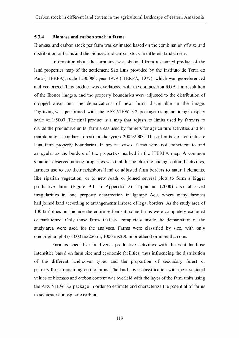
Carbon stock in different land covers in the agricultural landscape of eastern Amazonia
119
5.3.4 Biomass and carbon stock in farms
Biomass and carbon stock per farm was estimated based on the combination of size and
distribution of farms and the biomass and carbon stock in different land covers.
Information about the farm size was obtained from a scanned product of the
land properties map of the settlement São Luis provided by the Instituto de Terra do
Pará (ITERPA), scale 1:50,000, year 1979 (ITERPA, 1979), which was georeferenced
and vectorized. This product was overlapped with the composition RGB 1 m resolution
of the Ikonos images, and the property boundaries were adjusted to the distribution of
cropped areas and the demarcations of new farms discernable in the image.
Digitizing was performed with the ARCVIEW 3.2 package using an image-display
scale of 1:5000. The final product is a map that adjusts to limits used by farmers to
divide the productive units (farm areas used by farmers for agriculture activities and for
maintaining secondary forest) in the years 2002/2003. These limits do not indicate
legal farm property boundaries. In several cases, farms were not coincident to and
as regular as the borders of the properties marked in the ITERPA map. A common
situation observed among properties was that during clearing and agricultural activities,
farmers use to use their neighbors’ land or adjusted farm borders to natural elements,
like riparian vegetation, or to new roads or joined several plots to form a bigger
productive farm (Figure 9.1 in Appendix 2). Tippmann (2000) also observed
irregularities in land property demarcation in Igarapé Açu, where many farmers
had joined land according to arrangements instead of legal borders. As the study area of
100 km2 does not include the entire settlement, some farms were completely excluded
or partitioned. Only those farms that are completely inside the demarcation of the
study area were used for the analyses. Farms were classified by size, with only
one original plot (~1000 mx250 m, 1000 mx200 m or others) or more than one.
Farmers specialize in diverse productive activities with different land-use
intensities based on farm size and economic facilities, thus influencing the distribution
of the different land-cover types and the proportion of secondary forest or
primary forest remaining on the farms. The land-cover classification with the associated
values of biomass and carbon content was overlaid with the layer of the farm units using
the ARCVIEW 3.2 package in order to estimate and characterize the potential of farms
to sequester atmospheric carbon.

Carbon stock in different land covers in the agricultural landscape of eastern Amazonia
120
5.3.5 Carbon sequestration project
In the present study, an economic calculation was performed regarding to the success of
carbon sequestration projects in the study area if secondary vegetation resulting from
revegetation and cropland management activities is assumed as a sink under the
CDM framework.
During the Seventh Conference of Parties (COP 7) to the United Nations
Framework Convention on Climate Change (UNFCCC), the Marrakesh Accord was
signed. Here, activities such afforestation, reforestation, deforestation, revegetation,
forest management, crop management and grazing land management were identified
under the land-use, land-use change and forestry sector as mechanisms for the removal
of greenhouse gases (GHG). In the first commitment period agreed in the
Kyoto Protocol (UNFCCC, 1998), activities other than afforestation and reforestation
do not classify as removals units for sinking GHG under the Clean Development
Mechanism (CDM). The inclusion of the rest of activities in future commitment periods
shall be decided as part of the negotiations on the second commitment period
(UNFCCC, 2001).
According to the Decision 19/CP.9 of the COP to the UNFCCC
(UNFCCC, 2004), two kinds of certificates of certified emission reduction (CER) in
afforestation and reforestation projects under the CDM are possible: temporary CERs
(tCERs), and long-term CERs (lCERs). The first will be issued to projects with a
maximum crediting period of 20 years, which may only be renewed twice. The second
corresponds to a single period of up to 30 years. In both cases, the emission of
certificates will be in 5-year intervals until the end of the crediting period.
The tCER corresponds to the net antropogenic greenhouse gasses removed by the sinks
in the project since the start of the project, while a lCER refers to the increase in the
carbon stocks between two consecutive certification periods.
The economic calculation compared the current annual income per farm from
agricultural product with the amount to be received through the sale of carbon credits
as lCERs. The analysis was performed in 2 main scenarios based on different carbon
credit prices and on the following assumptions:

Carbon stock in different land covers in the agricultural landscape of eastern Amazonia
121
• the proportion in area assigned to the project corresponds to the
average extension of secondary vegetation stands in the average farm area,
• the farm area used in agricultural production is the area no covered with
secondary vegetation,
• carbon uptake rates were calculated based on information provided by
Denich et al. (2000) and the average of annual carbon uptakes rates.
The latter were calculated from the differences in predicted carbon stock
values per hectare per year. These predictions were obtained from the
application of equation 4.5.4.b from section 4.5.4, and ages were calculated
using the equation Age = 2.0111 + 1.3623 AHH (section 3.4.2, Figure 3.5),
• the project costs is assumed to be equal to 0 US$, the interest rate equals to
Prime (May 31, 2005) and the issuance of carbon credit every 5 years.
In both scenarios, the economic benefit through certification of CO2 uptake
was tested at 10, 20 and 30 years after the project started compared to the opportunity
costs that farmers will have if the land is used in the traditional agriculture system.
In addition to the previous assumptions, it is important to be aware that the
economic analyses of both scenarios are not conform to the calculation procedures
necessary for presentation of an afforestation/reforestation CDM project activity and
that investor companies/entities need to be found that are willing to pay the high prices
for the carbon credits.
5.4 Results
5.4.1 Land-cover classification
The 30 land-cover classes identified in the images of the 100 km2 study area varied
from some few hectares to more than 1700 ha. Secondary vegetation covered 51.4 % of
the study area, showing all stages of secondary succession. This value is almost
coincident to the prediction of the fallow-cover reduction by 3 % yr-1 by
Metzger (2002), and to the area of secondary vegetation estimated by Watrin (1994) for
the year 1991 and by Sampaio et al. (1998) for the year 1995 using of satellite images.
In the studa area, “Low secondary forest from 2-4 m” represented 34 % of the
secondary vegetation area, pastures covered 19.4 %, permanent and semi-permanent

Carbon stock in different land covers in the agricultural landscape of eastern Amazonia
122
crops 8.2 %, annual crops 5.3 % and bare soil in burned and land preparation areas
6.5 %. The 5 largest land-cover classes were “Low secondary forest 2-4 m” (17.5 %),
“Grass irregular” (13.0 %), “Low secondary forest 4-6 m” (9.7 %), “Initial secondary
succession” (9.2 %) and “Medium secondary forest 6-10 m” (7.5 %) (Table 5.4).
High, medium and low secondary forest higher than 2 m covered 42 % of the
study area.
Table 5.4 Land-cover types, area and representativeness in study area (100 km2), municipality of Igarapé Açu, Bragantina region, Brazil
Class No Class name Area (ha) Area (%) 1 Remaining riparian forest 720.2 7.3 2 High secondary forest >20 m 38.5 0.4 3 High secondary forest 15-20 m 108.7 1.1 4 Medium secondary forest 10-15 m 594.2 6.0 5 Medium secondary forest 6-10 m 742.1 7.5 6 Low secondary forest 4-6 m 962.8 9.7 7 Low secondary forest 2-4 m 1731.0 17.5 8 Initial secondary succession 915.2 9.2 9 Burned forest 83.3 0.8
10 Grass irregular 1290.1 13.0 11 Grass regular 631.5 6.4 12 Forest plantation 24.9 0.3 13 High oil palm plantation 72.1 0.7 14 Medium oil palm plantation 250.2 2.5 15 Low oil palm plantation 183.3 1.9 16 Coconut palm plantation 23.8 0.2 17 Pupunha plantation 11.0 0.1 18 Citrus plantation 23.9 0.2 19 Black pepper plantation 221.2 2.2 20 Passion fruit plantation 25.3 0.3 21 Annual crop 525.1 5.3 22 Miscellaneous 41.2 0.4 23 Land preparation 140.7 1.4 24 Burned area 194.8 2.0 25 Bare soil 309.1 3.1 26 Large shed 1.2 0.0 27 Swamp cover 6.6 0.1 28 Water body 1.5 0.0 29 Shadow 11.4 0.1 30 Cloud 18.8 0.2
Total 9903.5 100.0
Riparian forest covered 7.3 %. This value is coincident with the estimation did
by Sampaio et al. (1998) in an area larger than that of the present study; however,
it is higher than the estimation of Watrin (1994) for the entire municipality, and lower

Carbon stock in different land covers in the agricultural landscape of eastern Amazonia
123
than the value (13 %) calculated by Wickel (2004) for an area larger than the present
study area, the main differences being size and location of the study areas.
The proportion of riparian forest decreases to 7.1 % when the area studied
by Wickel (2004) is adjusted to the present study area. Watrin (1994) and
Wickel (2004) used Landsat images with 30 m resolution and both produced results
with misclassification; the classification of Watrin (1994) did not include small forest
stands along small creeks as riparian forest, while in Wickel’s classification
secondary forest and riparian forest were confused.
The agricultural area (including pasture, permanent, semipermanent and
annual crops, and areas with land preparation or burned) covered 36.6 % of the
study area. This estimation is coincident with IBGE (2005b) statistics and close to that
of Wickel (2004) for his classification performed with a Landsat image year 2001,
when the 3 % yr-1 increase in agriculture area (Metzger, 2002) is added. On the other
hand, the area is 35 % larger than that calculated by Watrin (1994) in the assessment for
1991, even when reducing the estimation by 3 % yr-1. Among the agricultural covers,
pasture covers almost 53.1 % of the agricultural area followed by annual crops
with 14.5 %, oil palm plantations with 14 %, black pepper with 6.1 %, passion fruit
0.7 %, citrus 0.7 %, coconut palm 0.7 % and pupunha 0.3 %. Wickel (2004) did not
distinguished annual crops, and it seems they were included in one of the
pasture classes; when both classes are summed, the estimation corresponds to the area
occupied by the pasture and crop classes identified in the present research.
Semipermanent and permanent crops according to Hedden-Dunkhorst et al.
(2003) and Watrin (1994) have increased in area during the last years. In this research,
oil palm plantations covered 5.1 %, while semipermanent crops of passion fruit and
black pepper, and associated plantations-crops with coconut palm, citrus and pupunha
cover 3.1 % of the study area of 100 km2. The percentage of annual and semipermanent
crops sampled in this study covers an area 5 % larger than the estimation by
Watrin (1994), and initial secondary succession is 14.7 % lower than in his assessment.
Two possible answers to these differences can be found in the increase of area under
agriculture in areas previously occupied by initial secondary vegetation or in a
misclassification of annual crops such as cassava or corn, mistaking these for initial
secondary succession when the satellite image of 1991 was used.

Carbon stock in different land covers in the agricultural landscape of eastern Amazonia
124
Figure 9.2 in Appendix 2 contains the land-cover map generated with
eCognition 4.0 and Arcview 3.2. The classification accuracy was tested by means of a
mask of land covers generated from GPS points. The overall accuracy as well as the
Kappa value (Congalton et al., 1983) were higher than 0.91; this value shows the
consistence of the classification in the study area. The main confusions were among the
secondary vegetation classes. “Low secondary forest 4-6 m” (Class 6) showed
the lowest precision per class (0.62) and “Medium secondary forest 10-15 m” (Class 4)
the highest (0.91). “Remaining riparian forest” and “High secondary forest >20 m” were
excluded from the precision analysis due to the use of different recognition methods and
the lack of GPS points from fieldwork, respectively (Table 5.5).
5.4.2 Land covers on farms
The settlement Jambú Açu was originally demarked in lots of 25 ha; many of the
farm divisions had changed with time due to the creation of new roads, boundaries or
the merging of neighboring lots to form large farms.
The average size of the 241 selected farms (those that are fully included in the
study area was 35.8±32.8 ha (mean±SD). The main changes observed in farm sizes are
due to the combination of lots to create larger productive units; almost 20 % of the
farms are made up of such aggregated lots and covered 45.2 % of the total area cover by
farms full included in the 100 km2 study area (86.2 km2), the largest farm covering
253.4 ha, averaging 82.9±51.4 ha. The largest farms were dedicated mainly to cattle
farming and oil palm plantations. Farms with a single lot covered 54.8 % of the study
area with an averaged size of 24.3±5.9 ha. This is on average 3 ha smaller than the size
estimated by Ferreira et al. (2000) for smallholders in the municipality of Igarapé Açu.
On the other hand, Hedden-Dunkhorst et al. (2003 and 2004) indicated that smallholders
reduced the farm size by continued splitting of land among different descendants. This
situation was also observed by Mendoza-Escalante (2005) but it was not possible to
detect this in the present research, since the new families mainly share the land with
relatives, and there were not clear divisions that could be identified in the
satellite images.

Carbon stock in different land covers in the agricultural landscape of eastern Amazonia
125
Table 5.5 Classification accuracy for 28 land-cover classes using a combination of Ikonos images (22/10/2002 - 27/11/2003) and a mask of GPS points of different land covers in a study area of 100 km2 in the municipality of Igarapé Açu, Bragantina region, Brazil
User\Reference Class No. 3 4 5 6 7 8 9 10 11 12 13 14 15 16 17 18 19 20 21 22 23 24 25 26 27 28 29 30 Sum
3 57 6 634 24 322 34 3805 22 231 8 2616 72 170 31 2737 7 76 344 4278 10 25 116 4 1 1569 3 84 8710 20 219 71 1 31111 193 19312 130 13013 415 41514 258 25815 230 23016 93 9317 60 6018 91 9119 134 13420 126 12621 249 24922 104 10423 93 9324 130 13025 72 7226 15 1527 24 2428 18 1829 411 41130 142 142
Unclassified 81 350 310 264 400 139 84 223 264 130 415 258 230 93 60 91 134 126 249 104 93 130 72 16 24 19 445 142 Producer accuracy
0.70 0.92 0.75 0.64 0.86 0.83 1 0.98 0.73 1 1 1 1 1 1 1 1 1 1 1 1 1 1 0.94 1 0.95 0.92 1
User accuracy 0.90 0.85 0.89 0.62 0.81 0.74 0.97 0.70 1 1 1 1 1 1 1 1 1 1 1 1 1 1 1 1 1 1 1 1 KHAT per class 0.70 0.91 0.73 0.62 0.85 0.83 1 0.98 0.72 1 1 1 1 1 1 1 1 1 1 1 1 1 1 0.94 1 0.95 0.92 1 Overall accuracy 0.91 KHAT (Kappa analysis)
0.91

Carbon stock in different land covers in the agricultural landscape of eastern Amazonia
126
In the study area, 42.32 %, 52.7 % and 4.98 % of the farms were smaller than
25 ha, between 25 and 100 ha and bigger than 100 ha, respectively. These values differ
from the estimation of Sousa Filho et al. (1999b), who estimated 59 % in the first size
category, 37.4 % for intermediate farm sizes and 3.6 % for the largest farms.
The differences express the increase in aggregation of lots on the farms.
Not all land covers are present on all farms, some gaining importance in a
specific farm size. The extension of patches of different land covers also varies from
farm to farm and according to the productive system of the farm.
Secondary vegetation higher than 2 m covered in average 47 % of the farm
areas and 52.2 % when initial-secondary-succession vegetation was included. The latter
value is 6 % lower than the estimation obtained by Hedden-Dunkhorst et al. (2004) in
three municipalities in the Bragantina region, and 12 % less than that calculated for
Igarapé Açu based on interviews. Agriculture cover extended to 32.9 % of the
farm area, unprotected soil areas (bared soil, land preparation and burned areas)
covered 5.9 % and uncontrolled burned forest as much as 0.9 % of the farm area.
The values change when the presence or not of lot aggregation in the organization of the
farm is considered. While agricultural area reduced to 25 %, secondary vegetation,
bare soil area and uncontrolled burned forest increased to 60.8 %, 7.1 % and 1 %,
respectively, on farms with unaggregated lots. On the other hand, on farms with
aggregated lots, these land covers covered 42 %, 41.7 %, 4.5 % and 0.8 % of the
farm area, respectively (Table 5.6).
Table 5.6 Variation of percentage of land covers according to size of productive units in the study area of 100 km2 in the municipality of Igarapé Açu, Bragantina region, Brazil
Land cover All farms Farms with unaggregated lots
Farms with aggregated lots
Secondary forest + initial secondary succession
52.2 60.8 41.7
Agriculture 32.9 25.0 42.6 Bare soil 5.9 7.1 4.5 Uncontrolled burned forest 0.9 1.0 0.8 Other land covers 8.1 6.2 10.4
The areas with long fallow periods that corresponded to secondary
forest stands higher than 10 m increased from 1.9±2.8 ha on farms with
unaggregated lots to 6.3±11.1 ha on farms with aggregated lots. Among farms with

Carbon stock in different land covers in the agricultural landscape of eastern Amazonia
127
long fallows of the three higher secondary forest classes (high secondary forest >20 m,
high secondary forest 15-20 m and medium secondary forest 10-15 m), were found in
42.6 %, 57.4 % and 95.7 %, respectively, of the aggregated farms. In contrast,
20.1 %, 45.4 % and 90.2 %, respectively, were calculated for farms with unaggregated
lots. These values indicate that long fallow periods and very high stands are more
frequent on large farms as already observed by Metzger (2003), nevertheless patches
represent in proportion the same area of the farm area, i.e., 7.6 % and 7.7 % for
aggregated and unaggregated farms, respectively. On the other hand, the vegetation type
of “Initial secondary succession” varied with farm size, being 9.2 %, 9.5 % and 8.9 %
for all farm sizes, farms with aggregated lots and unaggregated lots, respectively.
These values indicate that this vegetation type is intensively slashed, burned and
cropped on small farms, where thus more of the secondary vegetation as
low secondary forest is concentrated, while on aggregated farms, after several years
of intense use the land becomes degraded. The area is then abandoned and
secondary vegetation invades the land (Hohnwald et al., 2000).
5.4.3 Carbon sequestration potential
Landscape level
In the study area of 100 km2, 5092 ha (51 %) were covered by secondary forest
higher than 2 m and initial secondary succession, which accumulated a
dry aboveground biomass of 203,228 t and had a carbon stock of 101,614 t.
Land covers such as grass, oil palm and semipermanent and annual crops accumulated
7030, 7183 and 2603 t C, respectively. In total, for the dates 2002/2003 these
land covers assimilated 118,431 t C.
The estimation of carbon sequestration in the municipality gaves a
carbon stock of 765,086 t for secondary vegetation and 808,818 t C together with
some agricultural land covers (grass, black pepper, passion fruit, annual crops and
oil palm). Total sequestration in the region amounted to 8.17 Mt C for
secondary vegetation and more than 9.3 Mt C for all land covers (Table 5.7).

Carbon stock in different land covers in the agricultural landscape of eastern Amazonia
128
Table 5.7 Biomass and carbon stock in the aboveground biomass of the most common land covers in three study areas: 100 km2 area, the municipality of Igarapé Açu and the Bragantina region, Brazil, for the years 2002/2003
Study area Land cover Area (ha)
% of area
Biomass (t)
Carbon (t)
Secondary vegetation 5092 50.9 203228 101614 High secondary forest 147 1.5 23680 11840 Medium secondary forest 1336 13.4 106916 53458 Low secondary forest 2694 26.9 67141 33571 Initial secondary succession 915 9.2 5491 2746
Grass 1922 19.2 15623 7030 Oil palm 506 5.1 14366 7183
High oil palm 72 0.7 4169 2084 Medium oil palm 250 2.5 9182 4591 Low oil palm 183 1.8 1016 508
Semipermanent and annual crops 772 7.7 5510 2603 Black pepper 221 2.2 2344 1172 Passion fruit 25 0.3 132 66 Annual crops 525 5.3 3034 1365
Stu
dy a
rea
(100
km
2 )
Total 8292 82.9 238727 118431 Secondary vegetation 37761 48.0 1530171 765086
High secondary forest 978 1.2 155719 77859 Medium secondary forest 8879 11.3 748516 374258 Low secondary forest 21822 27.8 589449 294724 Initial secondary succession 6081 7.7 36488 18244
Grass 16961 21.6 22230 10004 Oil palm 1400 1.8 39779 19889
High oil palm 200 0.3 11543 5772 Medium oil palm 693 0.9 25423 12712 Low oil palm 508 0.6 2812 1406
Semipermanent and annual crops 5320 6.8 30718 13839 Black pepper 3 0.0 32 16 Passion fruit 54 0.1 282 141 Annual crops 5262 6.7 30404 13682
Igar
apé
Açu
(786
km
2 )
Total 61441 78.2 1622899 808818 Secondary vegetation 388503 44.6 16351396 8175698
High secondary forest 11231 1.3 1787773 893887 Medium secondary forest 101941 11.7 8593548 4296774 Low secondary forest 205512 23.6 5551162 2775581 Initial secondary succession 69819 8.0 418913 209456
Grass 185257 21.3 1730250 778613 Oil palm 10808 1.2 307109 153555
High oil palm 1540 0.2 89118 44559 Medium oil palm 5348 0.6 196279 98140 Low oil palm 3919 0.4 21712 10856
Semipermanent and annual crops 77149 8.9 445946 200959 Black pepper 138 0.0 1462 731 Passion fruit 808 0.1 4201 2101 Annual crops 76203 8.7 440283 198127
Bra
gant
ina
(871
0.7
km2 )
Total 661717 76.0 18834701 9308824

Carbon stock in different land covers in the agricultural landscape of eastern Amazonia
129
The amount of carbon accumulated by aboveground biomass of
secondary vegetation in the Bragantina region is equivalent to only 5.6 % of the
total carbon liberated by substitution of the original primary forest (Salomão, 1994).
Secondary vegetation cover increased from 45 % to 50 % when the size of the
study area decreased. Nevertheless, base on the current extension and proportion of
secondary forests and initial secondary succession, the storage of carbon per unit in
the aboveground biomass of the stands in the landscape of the three studies areas
was similar, with values between 9.3 and 10.1 t C ha-1.
Farm level
The capacity of farms to serve as sinks of atmospheric carbon depends on the types and
areas of land cover present on the farms and the life cycle of the covers. Among farms
that had covers of secondary forest, initial secondary succession, pasture, oil palm,
semi-permanent crops of pepper or passion fruit or annual crops, the average size of
patches of the land-cover classes varied from more than 0.6 ha for “High secondary
forest >20 m” to almost 14.7 ha for “Medium oil palm” (Table 5.8). Secondary forests
lower than 4 m showed the highest value after oil palm in area per farm followed by
grass. These values express the dominance of low secondary forest in productive units
(Metzger 2003); however as was previously observed for aggregated farms, the increase
in agricultural activities is based mainly on cattle farming and oil palm plantations
(section 5.4.2), which require large areas of farm land.
The estimation of patch sizes for secondary forest are higher than those
calculated by Metzger (2003) in the same region using Landsat TM images for young
and old fallow (younger and older than 6-years old, respectively): as much as 4-fold
when stands are lower than 4 m and 2- fold in stands > 4m. Height ranges were
calculated based on height provided by the equation AHH = -0.0007 + 0.6274 Age
(Chapter 3, section 3.4.2, Figure 3.6).

Carbon stock in different land covers in the agricultural landscape of eastern Amazonia
130
Table 5.8 Estimated biomass and carbon storage of different land covers in the average area of patches on farms in a study area of 100 km2, municipality of Igarapé Açu, Bragantina region, Brazil
Land cover Average area (ha)
SD Potential C uptake (t ha-1)
Aboveground biomass per
average patch size (t)
Aboveground carbon per
average patch size (t)
High secondary forest >20 m 0.6 1.3 90.1 110.4 55.2 High secondary forest 15-20 m 0.8 1.8 77.0 126.0 63.0 Medium secondary forest 10-15 m 2.4 4.2 51.8 249.3 124.7 Medium secondary forest 6-10 m 2.8 3.7 30.6 171.1 85.6 Low secondary forest 4-6 m 3.5 4.5 17.6 124.1 62.0 Low secondary forest 2-4 m 6.4 6.0 9.6 123.4 61.7 Initial secondary succession 3.3 4.7 3.0 19.8 9.9 Grass irregular 4.8 11.6 3.1 33.1 14.9 Grass regular 3.0 8.0 4.8 32.3 14.5 High oil palm plantation 5.9 10.8 28.9 340.4 170.2 Medium oil palm plantation 14.7 22.9 18.3 537.2 268.6 Low oil palm plantation 7.3 17.5 2.8 40.6 20.3 Black pepper plantation 2.7 6.2 5.3 28.1 14.1 Passion fruit plantation 0.8 1.1 2.6 4.1 2.1 Annual crops 2.5 3.2 2.6 14.4 6.5
Table 4.8 also shows the contribution to the carbon sequestration by each
land cover using their average extension in the farms: “Medium secondary forest
10-15 m” can accumulate the highest amount of carbon (124.7 t C) among
secondary forest classes on the farms. “Medium oil palm” shows the maximum
carbon accumulation (268.6 t C), however in an area 6.1 times larger, followed by
“High oil palm” (170.2 t C), “Medium secondary forest 10-15 m” (124.7 t C), and
“Medium secondary forest 6-10 m” (85.6 t C). For the same unit area,
the “High secondary forest >20 m” can accumulate 9.4 times more carbon than
the “Low secondary forest 2-4 m” and 1.2, 3.1, and 34.7 times more than
“High secondary forest 15-20 m”, “High oil palm” and “Annual crop”, respectively.
A hypothetic farm of average size (35.8 ha) and land-cover distribution equals
to the proportions and types found for all farms can assimilate 433.8 t C among most of
the most common land covers and 374 t C in the biomass of secondary vegetation
(Table 5.9).

Carbon stock in different land covers in the agricultural landscape of eastern Amazonia
131
Table 5.9 Estimated carbon (C) storage in different land covers in a hypothetic farm of average size from a study area of 100 km2, municipality of Igarapé Açu, Bragantina region, Brazil
Land cover % of farm area
Area (ha)
Potential C uptake (t ha-1)
Total C uptaked (t)
High secondary forest >20 m 0.4 0.2 90.1 13.5 High secondary forest 15-20 m 1.1 0.4 77.0 30.1 Medium secondary forest 10-15 m 6.1 2.2 51.8 113.9 Medium secondary forest 6-10 m 7.6 2.7 30.6 83.5 Low secondary forest 4-6 m 9.8 3.5 17.6 61.6 Low secondary forest 2-4 m 17.9 6.4 9.6 61.8 Initial secondary succession 9.2 3.3 3.0 9.9 Grass irregular 13.1 4.7 3.1 14.5 Grass regular 5.7 2.1 4.8 9.8 High oil palm plantation 0.8 0.3 28.9 7.8 Medium oil palm plantation 2.4 0.9 18.3 15.6 Low oil palm plantation 2.0 0.7 2.8 1.9 Black pepper plantation 2.4 0.9 5.3 4.6 Passion fruit plantation 0.2 0.1 2.6 0.2 Annual crop 5.6 2.0 2.6 5.2 Others 15.7 5.6 Total 100 35.8 432.1
Secondary vegetation on average extends over 52.2 % of the average farm area
which represents about 18.6 ha and the farm can potentially accumulate 10.5 t C ha-1
in secondary forest only. This value is higher than the value calculated by
Tippmann (2000) (7 t C ha-1) for secondary vegetation on a farm of 56 ha in the
municipality of Igarapé Açu.
Among land-cover types, the major potential to store carbon on the
average-sized farm is secondary vegetation followed by oil palm plantations. On the
average farm, the latter accumulate more than 25.3 t C. Oil palm plantations showed a
higher rate of carbon accumulation during at least the first decade after plantation
compared to secondary forest when prediction models for age and biomass of secondary
forest are used; nevertheless, the values reported by Denich (2000) for carbon stock in
secondary forest arranged close and higher than predictions in oil palm (Figure 5.3).
Using the predictive equation of carbon sequestration in oil palm plantations
developed for Indonesia sites (Syahrinundin, 2005), the calculations suggest that
secondary forest will requires up to 15 years to reach the carbon uptake of
oil palm stands. However, after 11 years, carbon sequestration by secondary forest

Carbon stock in different land covers in the agricultural landscape of eastern Amazonia
132
exceeded that of oil palm, as the life-time of this land cover is longer, leading to
assimilation of a larger amount of carbon over time.
0
20
40
60
80
100
0 5 10 15 20 25 30
Age (years)
Tota
l abo
vegr
ound
car
bon
cont
ent (
t ha-1
)
Estimated C in oil palm plantationPredicted C in oil palm plantationEstimated C in SF (Denich, 2000)Predicted C in SF (i) (ii)
C oil palm = exp(3.9906 - (84936/Age))(iii)R sq. 0.97
N 9where age > 2 years
(i) Carbon uptake of secondary forest calculated as a fraction of 0.5 of total live tree
aboveground biomass predicted with Equation 4.5.4.b from Chapter 4, section 4.5.4. (ii) Age of secondary forest predicted with equation Age = 2.0111 + 1.3623 AHH from Chapter 3, section 3.4.2, Figure 3.5. (iii) Growth model of oil palm plantations based on data from Khalid et al. (1999),
Nordin (2002), Rodrigues et al. (2000), Syahrinundin (2005) and Viegas (1993). Figure 5.3 Relation of carbon (C) stock in the aboveground biomass of oil palm
plantation and secondary forest along the time in northeast Pará state, Brazil
5.4.4 Economic benefits from the sequestration of carbon
The results of the economic analysis from the sequestration of carbon show that when
52 % of the farm area (current percentage of area in the average farm covered by
secondary vegetation) is allocated to a CDM project, this can provide the same income
as that the obtained from agricultural products by 48 % of the farm area (~ US$ 163 ha-1
yr-1) in the municipality of Igarapé Açu (Mendoza-Escalante, 2005); income excludes
the contribution of fallow products. This can be achieved only when the price per ton
CO2 within the framework of CDM projects for reforestation and afforestation project is

Carbon stock in different land covers in the agricultural landscape of eastern Amazonia
133
higher than US$ 13.6 for the three study periods (Table 9.2a in Appendix 2). In the
second scenario, the price per ton CO2 was US$ 5.63. This price corresponds to that of
the first quarter of 2005 for CDM projects (Lecocq and Capoor, 2005). The benefits of
the project at 10, 20 and 30 years can represent up to 41 %, 42 % and 42 %,
respectively, of the farm income from agricultural products (Table 9.2b in Appendix 2).
Even though these exercices show that the economic benefits by fixation of
CO2 can add important surplus to current annual income on the average farm,
the situation in reality is different, the prices for lCER are expected to be lower than the
prices of CER of other CDM activities as the carbon in afforestation/reforestation
projects is not permanentally stored (Subak, 2003) and carbon credits have to be replace
after they expire. The project has operative costs, which were not included in the
analysis. Furthermore, many of the assumptions may not remain the same over time.
On the other hand, the success of the returns through revegetation/cropland management
projects will also depend on the capacities of farmers to leave the vegetation untouched
during each certification period.
5.5 Conclusions
The land partitioning designed 100 years ago was not longer valid on the dates of the
applied satellite images, and the farm borders had adjusted to new roads, water sources
and new productive units. On average, farm size had increased by 10 ha as
a consequence of the merging of plots.
In the study area of 100 km2 vegetation from secondary succession covered
more than 50 %, but only 42 % was covered by secondary forest higher than 2 m.
Most of the agricultural land was occupied by pasture. Secondary vegetation reduced
with increasing study area size. This indicate that the intensification of land use based
on extensive farming practices such as cattle grazing are more common in the
Bragantina region than in the study area of 100 km2. Although secondary vegetation
covered a considerable part of the agricultural landscape, the current distribution of
secondary vegetation can only accumulate a small fraction of the carbon emitted by
deforestation of the original forest. Its contribution to sequestration of
atmospheric carbon is low, due to the large proportion of low secondary forest and
initial secondary succession on areas that are intensely slashed and burned.

Carbon stock in different land covers in the agricultural landscape of eastern Amazonia
134
Conservation and enhancement of areas with medium and old secondary forest
will substantially increase the accumulation of carbon in the vegetation.
Under the assumption that half of the average farm area is assigned to a project
of carbon sequestration by secondary vegetation for at least a period of 10 years,
a farmer could expect additional income per farm similar to that achieved by
agricultural activities (crops, cattle). However, the price per ton CO2 within the
framework of CDM projects needs to remain on the current level or increase in order to
provide an incentive to farmers to preserve secondary forest. The protection of
secondary vegetation for at least two certification periods will replenish the nutrients in
soil and vegetation and at the same time provide benefits through CO2 sequestration.
On the other hand, diversification of farm products and avoidance of intensive
agriculture will reduce pressure on land and guarantee farm income while achieving
additional benefits resulting from the conservation of secondary forest areas.
Among the land covers, oil palm plantations showed the highest efficiency in
the accumulation of carbon during at least the first 11 years after plantation
establishment compared to secondary forest. The advantage of secondary forest as an
atmospheric carbon sink can only be achieved under longer fallow periods.

Final conclusions
135
6 FINAL CONCLUSIONS
Secondary vegetation in the municipality of Igarapé Açu as well as in other areas in the
Bragantina region, state of Pará, Brazil, is decreasing in area due to continued
intensification of land use. The shorter fallow periods have been shown to be
insufficient to recover losses in productivity caused by slash-and-burn and agricultural
activities. Improved management of secondary vegetation to gain the benefits associated
with carbon sequestration is, therefore, called for.
Only a small fraction of carbon released by substitution of the primary forest
cover was stored in the aboveground biomass of the different land covers of the region.
Carbon sequestration can be enhanced in the landscape and on the farms if the
proportion of long fallows increases.
Projects that include secondary vegetation as a sink of greenhause gases are a
promising alternative for farmers to increase their farm income, ensure conservation
of soil and plant communities, and carbon sequestration. However, activities which
manage revegetation and cropland in old agriculture systems, as the one in the
Bragantina region, should be included in the next commitment period after 2012 within
the framework of CDM projects to allow secondary vegetation to count as removal units
for sinking carbon. To ensure successful carbon sequestration, future projects should
also provide incentives to farmers to diversify farm income through the introduction of
new production activities that avoid removal of secondary vegetation.
Permanent cash crops such as oil palm can accumulate the same and even
higher carbon amounts per unit area than secondary forest in the first 11 years, but after
this secondary forest has a comparative advantage as sequestration becomes
more efficient.
Since the average wood density of the tree species in the region is higher than
the average value for many other areas in the Amazon region, the prediction of biomass
using models generated with information on the average wood density of moist tropical
forest without any differentiation of variation of wood density by regions will,
without doubt, underestimate the biomass and carbon sequestration potential of
secondary forest stands in Eastern Amazonia.

Final conclusions
136
In the present study, 30 years after land abandonment the secondary forest had
developed a multi-strata structure of around 20 m total average height and accumulated
94 t ha-1 of carbon in the dry biomass in live and standing dead trees and litter layer.
Secondary forest is not just organized as a group of fast growing trees of
small diameter and small individual volume, but is a complex system that includes a
wide spectrum of tree arrangements, where big and small trees compete for space and
resources and where an important species replacement dynamics is present along
forest growth.
The methodology used in the present research shows that the biomass and
the carbon stock of the entire stand could be estimated by the average height of
selected trees in the highest canopy stratum. Repetitive measurements of tree height
over time should be useful to determine differences in height and thus to estimate the
increment in biomass and carbon of secondary forest.
Considering the diversity of the study areas and stands of secondary forest
surveyed in the region in previous studies, the estimation of biomass by average height
of the highest canopy stratum showed values close to those determined in many studies.
Nevertheless, an average subestimation of 4.6 % compared with the method based on
the diameter of trees could be observed.
Many municipalities in the Bragantina region have similar climatic conditions,
soil properties, trees species, land-use history and practices to those of the municipality
of Igarapé Açu. Other regions in moist tropical forest should verify site conditions,
average wood density and history of land-use practices to apply the equations proposed
in Chapters 3 and 4. The equations should be applied within the range of the heights,
diameters and ages studied here.

References
137
7 REFERENCES
Alder, D. and Synnott, T.J. 1992. Permanent sample pot techniques for mixed tropical
forest. Tropical Forestry Papers No. 25. Oxford Forestry Institute, University of Oxford, UK.
Alegre, J., Arevalo, L., Ricse, A., Barbaran, J. and Palm, Ch. 2001. Reservas de carbono y emisión de gases de diferentes sistemas de uso de la tierra en dos sitios de Amazonia Peruana. In: Palestras III Congreso Brasileiro de Sistemas Agroflorestais. Embrapa, Manaus, AM, 2000, pp. 60-68.
Almeida, A.S. de. 2000. Dinâmica da paisagem e ecologia de florestas primárias remanescentes e sucessionais do municipio de São Francisco do Pará. Master thesis, Faculdade de Ciências Agrárias do Pará, Belém, Brasil, 100 pp.
Alves, D.S., Vianei, J.S., Amaral, S., Mello, E:M.K., Almeida, S.A.S., Fernandes, O. da S. et al. 1997. Biomass of primary and secondary vegetation in Rondônia, Western Brazilian Amazon. Global Change Biology, 3:451-461.
Araújo, T.M., Higuchi, N. and Carvalho Jr., J.A. 1999. Comparison of formulae for biomass content determination in a tropical rain forest site in the state of Pará, Brazil. Forest Ecology and Management, 117:43-52.
Baar, R. 1997. Vegetationskundliche und oekologische Untersuchungen der Buschbrache in der Feldumlagewirtschaft im oestlichen Amazonasgebiet. Doktorarbeit, Georg-August-Universität Göttingen, Deutschland.
Baker, F.S. 1950. Principles of silviculture. McGraw-Hill, New York, 414 pp. Baker, T.R., Phillips, O.L., Malhi,Y., Almeida, S., Arroyo, L., DiFiore, A. et al. 2004.
Variation in wood density determines spatial patterns in Amazonian forest biomass. Global Change Biology, 10:1-18.
Bastos, T.X. and Pacheco, N.A. 1999. Características agroclimatológicas de Igarapé-Açu, PA e suas implicações para as culturas anuais: feijão caupi, milho, arroz e mandioca. Embrapa Amazônia Oriental, Belém. Boletim de Pesquisa No. 25, 30 pp.
Block. A. 2004. Göttinger Mähhäcksler Tritucap und Forstmulcher – Nicht Brennende Flächenvorbereitung am Beispiel der Zona Bragantina, Nord-Ost-Amazonien, Brasilien. Doktorarbeit. Georg-August-Universität Göttingen, Deutschland, 174 pp.
Brasil_SUDAM. 1984. Projeto de hidrologia e climatologia da Amazônia, Belém, Pará. Superintendencia do desenvolvimiento da Amazônia, Belém. Atlas climatológico da Amazônia brasileira, 125 pp.
Brienza Jr., S. 1999. Biomass dynamics of fallow vegetation enriched with leguminous trees in the eastern Amazon of Brazil. Ph.D. thesis. Göettinger Beiträge zur Land und Forstwirtschaft in den Tropen und Subtropen. Georg August University of Göettingen. Heft 134, 134 pp.
Brown, F., Martinelli, L.A., Wayt Thomas, W., Moreira, M.Z., Cid Ferreira, C.A. and Victoria, R.A. 1995. Uncertainty in the biomass of Amazonian forest: an example from Rondônia, Brazil. Forest Ecology and Management, 75:175-189.
Brown, S. 1997. Estimating biomass and biomass change of tropical forests: a primer. UN-FAO Forestry Paper 134. Rome, Italy.
Brown, S. 2002. Measuring carbon in forests: current status and future challenges. Environmental Pollution, 116:363-372.

References
138
Brown, S. and Lugo, A.E. 1982. The storage and production of organic matter in tropical forests and their role in the global carbon cycle. Biotropica, 14(3):161-187.
Brown, S. and Lugo, A.E. 1990. Tropical secondary forest. Journal of Tropical Ecology, 6:1-32.
Brown, S. and Lugo, AE. 1992. Aboveground biomass estimates for tropical moist forests of the Brazilian Amazon. Interciencia, 17:8-18.
Brown, S, Gillespie, A.J.R. and Lugo, A. 1989. Biomass estimation methods for tropical forests with applications to forest inventory data. Forest Science, 35(4):881-902.
Bryant, D., Nielsen, D., and Tangley, L., 1997. The last frontier forests: Ecosystems and economies on the edge. World Resources Institute, Washington, D.C., 42 pp.
Budowski, G. 1961. Studies on forest succession in Costa Rica and Panama. Ph.D. thesis, University, New Haven, CT., 189 pp.
Chambers, J.Q., Santos, J. dos, Ribeiro, R. and Higuchi, N. 2001. Tree damage, allometric relationships and above-ground net primary production in central Amazon forest. Forest Ecology and Management, 152:73-84.
Chave, J., Condit, R., Aguilar, S., Hernandez, A., Lao, S. and Perez, R. 2004. Error propagation and scaling for tropical forest biomass estimates. Philosophical Transactions: Biological Sciences, The Royal Society, 359(1443):409-420(12).
Chudnoff, M. 1980. Tropical timbers of the world. Agriculture Handbook #607. Madison, WI. U.S. Dept. of Agriculture, Forest Service, Forest Products Laboratory, 464 pp.
Congalton, R.G., Oderwald, R.G. and Mead, R.A. 1983. Assessing Landsat classification accuracy using discrete multivariate statistical techniques. Photogrammetric Engineering and Remote Sensing, 49(12):1671-1678.
Dantas, M. 1991. The production of litter and its nutrient content in primary forest and "capoeira" of the eastern Amazon Region. In: Studies on the utilization and conservation of soil in the eastern Amazon region. Eschborn, Germany. Embrapa/ CPATU/GTZ, pp. 141-155.
Dawkins, H.C. 1958. The management of natural tropical high forest with special reference to Uganda. Imperial Forest Institute, University of Oxford, Institute paper, No. 34, 155 pp.
Denich, M. 1986a. A vegetação da Amazônia Oriental com enfase na vegetação antrópica. In: Pesquisas sobre utilização e conservação do solo na Amazônia Oriental. Relatorio Final do Convenio Embrapa-CPATU-GTZ. Belém, PA, Brasil, pp. 43-69.
Denich, M. 1986b. Composição florística de capoeiras baixas no municipio de Igarapé-Açu no Estado do Pará. Embrapa -CPATU. Belém, PA, Brasil. Embrapa-CPATU, Documentos No 39, 16 pp.
Denich, M. and Kanashiro, M. 1993. Secondary forest and fallow vegetation in the eastern Amazon region: Function and management (ENV-25). In: SHIFT (Studies on Human Impact on Forest and Floodplains in the Tropics). Summaries of 1st SHIFT-Workshop, Belém, Brazil, 8-13 March 1993. CNPq-IBAMA-BMFT, pp. 145-151.

References
139
Denich, M. and Kanashiro, M. 1995. Secondary vegetation in the agricultural landscape of northeast Pará, Brazil. In: Management and rehabilitation of degraded lands and secondary forests in Amazonia. Proceedings of an International Symposium/Workshop. Santarém, Pará, Brazil, 12-21 April 1993. International Institute of Tropical Forestry, USDA-Forest Service, Puerto Rico, USA, pp.12-21.
Denich, M. and Kanashiro, M. 1998. Potential land-use and management of altered and abandoned areas in the Brazilian Amazon region. Studies of Human Impact on Forests and Floodplains in the Tropics – SHIFT. MCT/CNPq, Brasília, Brasil, 153 pp.
Denich, M. and Kato, M.S. 1995. Capoeira: secondary vegetation as an integral part of the agricultural production system (ENV-25/1). In: SHIFT (Studies on Human Impact on Forest and Floodplains in the Tropics), Summaries of 1st SHIFT-Workshop, Belém, Brazil, 8-13 March 1993. CNPq-IBAMA-BMFT, pp. 152-153.
Denich, M; Sommer, R. and Vlek, P.L.G.. 1998. Soil carbon stocks in small holder land-use systems of the Northeast of Pará state, Brazil. Mitt. Ges. Pflanzenbauwiss, 11:211-212.
Denich, M., Kanashiro, M. and Vlek, P.L.G. 2000. The potential and dynamics of carbon sequestration in traditional and modified fallow systems of the eastern Amazon region, Brazil. In: Lal, R., Kimble, J.M. and Stewart, B.A. (eds). Global climate change and tropical ecosystems. Advances in Soil Science, CRC Press LLC, Boca Raton, Unites States of America, pp. 213-229.
Denslow, J.S. 1980. Gap partitioning among tropical rainforest trees. Biotropica, 12 (Suppl.):23-30.
DeWalt, S.J., Maliakal, S.K. and Denslow, J.S. 2003. Changes in vegetation structure and composition along a tropical forest chronosequence: implications for wildlife. Forest Ecology and Management, 182:139-151.
Diekmann, U. 1997. Biologische und chemische Bodencharakteristika zur Beurteilung der nachhaltigen Produktivität von Landnutzungssystemen in der Zona Bragantina, Ost-Amazonien. Doktorarbeit, Fakultät für Agrawissenchaften.Georg-August-Universität Göttingen, Deutschland,189 pp.
Drake, J.B., Dubayah, R.O., Clark, D.B., Knox, R.G., Blair, J.B., Hofton, M.A. et al. 2002a. Estimation of tropical forest structural characteristics using large-footprint lidar. Remote Sensing of Environment, 79:305-319.
Drake, J.B., Dubayah, R.O., Clark, D.B., Knox, R.G., Clark, D.B. and Blair, J.B. 2002b. Sensitivity of large-footprint lidar to canopy structure and biomass in a neotropical rainforest. Remote Sensing of Environment, 81:378-392.
Drake, J.B., Knox, R.G., Dubayah, R.O., Clark, D.B., Condit, R., Blair, J.B. et al. 2003. Above-ground biomass estimation in closed canopy Neotropical forest using lidar remote sensing: factors affecting the generality of relationships. Global Ecology &Biogeography, 12:147-159.

References
140
Dupuy, B., Maître, H. F. and Amsallem, I. 1999. Tropical forest management techniques: a review of the sustainability of forest management practices in tropical countries. Working Paper: FAO/FPIRS/04 prepared for the World Bank Forest Policy Implementation Review and Strategy. CIRAD - FAO Forestry Policy and Planning Division, Rome. (http://www.fao.org/ documents/show_cdr.asp?url_file=/DOCREP/003/X4110e/X4110E00.htm).
EMBRAPA (Empresa Brasileira de Pesquisa Agropecuária). 1999. Sistema brasileiro de clasificação de solos. Embrapa, Brasilia, Brasil.
FAO (Food and Agriculture Organization). 2000. Global Forest Resources Assessment 2000. Main report, Rome. Food and Agriculture Organization. (http://www.fao.org/forestry/foris/webview/forestry2/index.jsp?siteId=2921&sitetreeId=7947&langId=1&geoId=0).
Fearnside, P.M. 1996. Amazonian deforestation and global warming: carbon stocks in vegetation replacing Brazil’s Amazon forest. Forest Ecology and Management, 80:21-34.
Fearnside, P.M. 1997. Wood density for estimating forest biomass in Brazilian Amazonia. Forest Ecology and Management, 90:59-87.
Fearnside, P.M. 2000. Greenhouse gas emissions from land-use change in Brazil’s Amazon region. In: Lal, R., Kimble, J.M. and Stewart, B.A. (eds). Global climate change and tropical ecosystems. Advances in Soil Science, CRC Press LLC, Boca Raton, Unites States of America, pp. 231-249.
Fearnside, P.M. and Guimarães, W.M. 1996. Carbon uptake by secondary forests in Brazilian Amazonia. Forest Ecology and Management, 80:35-46.
Ferreira, C.A.P., Carvalho, R. de A., Ferreira, M. do S.G., Smith, J., Van de Kopp, P.. 2000. Caracterização socieconômica dos pequenos produtores rurais do nordeste paraense. Embrapa. Documentos No. 39, 21 pp.
Finegan, B. 1992. El potencial de manejo de los bosques húmedos secundarios neotropicales de las tierras bajas. CATIE-COSUDE, Costa Rica. CATIE No. 188, 28 pp.
Finegan, B. 1997. Bases ecológicas para el manejo de bosques secundarios de las zonas húmedas del trópico americano, recuperación de la biodiversidad y producción sostenible de maderas. In: Memorias del taller internacional sobre el estado actual y potencial de manejo y desarrollo del bosque secundario tropical en América Latina. Pucallpa-Perú, 2-6 June, 1997, pp. 106-119.
Gehring, C.; Park, S. and Denich, M. 2004. Liana allometric biomass equations for Amazonian primary and secondary forest. Forest Ecology and Management, 195:69-83.
Gehring, C.; Denich, M. and Vlek, P.L.G. 2005. Resilience of secondary forest regrowth after slash-and-burn agriculture in central Amazonia. Journal of Tropical Ecology, 21:1-9.
Groombridge, B. and Jenkins, M.D. 2002. World atlas of diversity. Prepared by the UNEP World Conservation Monitoring Centre. University of California Press, Berkeley, USA, 340 pp.
Guimarães, L.A.C. 2002. Structure and dynamic of the market for the Igarapé-Açú´s agriculture. In: Lieberei, R., Bianchi, H-K., Boehm, V. and Reisdorff, C. (eds.). Proceedings of Neotropical Ecosystems, German-Brazilian Workshop, Hamburg, Germany, 6-8 September 2000. GKSS-Geesthacht. Germany, p. 198.

References
141
Hadjimitsis, D.G., Clayton, C.R.I. and Hope, V.S. 2004. An assessment of the effectiveness of atmospheric correction algorithms through the remote sensing of some reservoirs. International Journal of Remote Sensing, 25(18):3651-3674.
Hedden-Dunkhorst, B., Denich, M., Vielhauer, K., Mendoza, A. E., Börner, J., Hurtiene, T. et al. 2003. Forest-based fallow systems: A safety net for smallholders in the eastern Amazon?. The international conference on “Rural livelihoods, forest and biodiversity”, 19-13 May 2003, Bonn, Germany, 25 pp.
Hedden-Dunkhorst, B., Börner, J., Mendoza-Escalante, A., Mburu, J., Vosti., S. and Frohberg, K. 2004. Smallholders in the Amazon: interactions between ecosystem and social system in the use and protection of tropical rain forests. Abschlussbericht Phase III (1.2.2001-31.7.2004). Studies on Human Impact on Forests and Floodplains in the Tropics SHIFT ENV 44. ZEF-NAEA. Bonn, November 2004, 209 pp.
Hoen, F.H. and Solberg, B. 1994. Potential and economic efficiency of carbon sequestration in forest biomass through silvicultural management. Forest Science, 40:429-451.
Holdridge, L.S. 1967. Ecología basada en zonas de vida. San José, Costa Rica, Editorial IICA, 206 pp.
Hoheisel, H. 1988. Manual del grupo andino para preservación de madera. Junta de acuerdo de Cartagena. Lima, Perú.
Hohnwald, S., Rischkowsky, B., Camarão, A. P., Rodrigues Filho, J. A., Vielhauer, K., Schultze-Kraft, R. et al. 2000. From Monotonous to Enriched Bushy Pastures to Replace the Traditional Smallholder Management in North-Eastern Pará, Brazil. In: Lieberei, R., Bianchi, H-K., Boehm, V., Reisdorff, C., (eds.). Proceedings of Neotropical Ecosystems, German-Brazilian Workshop, 6-8 September 2000, Hamburg, Germany. GKSS-Geesthacht, Germany, pp. 971-973.
Hölscher, D. 1997. Shifting cultivation in eastern Amazonia: A case on the water and nutrient balance. Institute for Scientific Co-operation, Tübingen, Germany. Plant Research and Development, Vol 46:68-87.
Hölscher, D., Möller, R.M.F., Denich, M. and Fölster, H. 1997. Nutrient input-output budget of shifting cultivation in eastern Amazonia. Nutrient Cycling in Agroecosystems, 47:49-57.
Hondermann, J.B.N. 1995. Fitomasa e estoque de biolementos das diversas fases de vegetação secundária, proveneintes de diferentes sistemas de uso da terra no Nordeste Paraense, Brasil. Master thesis. Universidad Federal do Pará, Belém, Pará, 185 pp.
Honzák, M., Lucas, R.M., Amaral, I. do, Curran, P.J., Floody, G.M. and Amaral, S. 1996. Estimation of the leaf area index and total biomass of tropical regenerating forests: comparison of methodologies. In: Cash, J.H.C., Nobre, C.A., Roberts, J.M. and Victoria, R.L. Amazonian deforestation and climate. Wiley, pp. 365-381.
Houghton, R.A. 2003. Revised estimates of the annual net flux of carbon to the atmosphere from changes in land use and land management 1850-2000. Tellus B, 55(2):378-390.

References
142
Houghton, R.A., Skole, D.L., Nobre, C.A., Hackler, J.L., Lawrence, K.T. and Chomentowski. 2000. Annual fluxes of carbon from the deforestation and regrowth in the Brazilian Amazon. Nature, 403:301-304.
Houghton, R.A., Lawrence, K.T., Hackler, J.L. and Brown, S. 2001. The spatial distribution of forest biomass in the Brazilian Amazon: a comparison of estimates. Global Change Biology, 7:731-746.
IBGE (Instituto Brasileiro de Geografia e Estatística). 1985. Censo agropecuário, número 6, Pará, IBGE, Río de Janeiro, Brasil.
IBGE (Instituto Brasileiro de Geografia e Estatística). 1997. Censo agropecuário 1995-1996, número 5 Pará, IBGE, Río de Janeiro, Brasil.
IBGE (Instituto Brasileiro de Geografia e Estatística). 2001. Censo demográfico 2000. Rio de Janeiro, Brasil.
IBGE (Instituto Brasileiro de Geografia e Estatística). 2005a. Estimativas populacionais para os municípios brasileiros em 01/07/2004. (http://www.ibge.gov.br).
IBGE (Instituto Brasileiro de Geografia e Estatística). 2005b. Banco de dados agregados - Sistema IBGE de Recuperação Automática (SIDRA). (http://www.sidra.ibge. gov.br/bda/).
IBGE-MMA (Instituto Brasileiro de Geografia e Estatística - Ministério do Meio Ambiente). 2004. Mapa de Biomas e de Vegetação. (http://www.ibge.gov.br/home/presidencia/noticias/noticia_visualiza.php?id_noticia=169&id_pagina=1).
IBGE/CNPS-EMBRAPA. 2001. Mapa de Solos do Brasil; 1:5.000.000. Mapa e legenda. Rio de Janeiro.
INPA (Instituto Nacional de Pesquisas da Amazônia). 2005. Amazônia, Informações Científicas. Manaus, Brasil. (http://www.inpa.gov.br/amazonia.html).
INPE (Instituto Nacional de Pesquisas Espaciais). 2005. Monitoramento da floresta amazônica brasileira por satélite, Projeto PRODES. São José dos Campos, Brasil. (http://www.obt.inpe.br/prodes/index.html; http://www.obt.inpe.br/ prodes/prodes_analogico.htm).
IPCC (Intergovernmental Panel on Climate Change). 2000. Watson, R.T., Noble, I.R., Bolin, B., Ravindranath, N.H., Verardo, D.J. and Kokken, D.J. (eds.). Land use, land-use change and forestry. A special report of the IPCC. Intergovernmental Panel on Climate Change. Cambridge University Press, 377 pp.
IPCC (Intergovernmental Panel on Climate Change). 2003. Penman, J., Gytarsky, M., Hiraishi, T., Krug, T., Kruger, D., Pipatti, R., Buendia, L., Miwa, K., Ngara, T., Tanabe, K. and Wagner, F. (eds). Good practice guidance for land use, land-use change and forestry. IPCC/OECD/IEA/IGES, Hayama, Japan. (http://www.ipcc-nggip.iges.or.jp/public/gp/english/).
ITERPA (Instituto de Tierra do Pará). 1979. Plantas de localização da colônia São Luiz baseada na planta fornecida per la Sectretaria de Agricultura (SAGRI), escala 1:50000.
Johnson, Ch.M., Vieira, I.C.G., Zarin, D.J., Frizano, J. and Johnson, A.H. 2001. Carbon and nutrient storage in primary and secondary forests in eastern Amazônia. Forest Ecology and Management, 147:245-252.
Jordan, C.F. and Uhl, C. 1978. Biomass of a terra firme forest in the Amazon basin. Oecologia Plantarum, 13(4):387-400.

References
143
Khalid, H, Zin, Z.Z.and Anderson, J.M. 1999. Quantification of oil palm biomass and nutrient value in a mature plantation. I. above-ground biomass. Journal of Oil Palm Research, 11(1):1:23-32.
Kato, M.S.A., Kato, O.R., Denich, M. and Vlek, P.L.G. 1999. Fire –free alternatives to slash-and-burn for shifting cultivation in the eastern Amazon region: the role of fertilizers. Field crops research, 62:225-237.
Keller, M., Palace, M. and Hurtt, G. 2001. Biomass estimation in the Tapajos National Forest, Brazil. Examination of sampling and allometric uncertainties. Forest Ecology and Management, 154:371-382.
Kemmer, S. 1999. Peasants’ youths between tradition and modernity. Perspectives of youths in peasant communities, the education system and migration motives of rural youths in eastern Amazon. Master thesis. Georg August University Göttingen.
Koskela, J., Nygren, P., Berninger, F. and Luukkanen, O. 2000. Implications of the Kyoto Protocol for tropical forest management and land use: prospects and pitfalls. Tropical Forestry Reports 22. University of Helsinki, Department of Forest Ecology. Helsinki, Finland.
Lal, R., Kimble, J. and Follett, R. 1998. Land use and soil C pools in terrestrial ecosystems. In: Lal, R., Kimble, J., Follett, R. und Stewart, B. A. (Hrsg.): Management of carbon sequestration in soil. Boca Raton: CRC Press, pp. 1-10.
Lecocq, F. and Capoor, K.. 2005. State and trends of the carbon market 2005. World Bank - International Emissions Trading Association. Washington DC, 44 pp. (http://carbonfinance.org/docs/CarbonMarketStudy2005.pdf).
Littesand, T.M. and Kiefer, R.W. 2000. Remote sensing and image interpretation. Fourth edition, John Wiley & Sons, Inc., United States of America, 724 pp.
Loetsch, F., Zöhrer, F. and Haller, K.E.1973. Forest inventory. BLV Verlagsgesellchaft mbH, München, Germany, Vol II, 469 pp.
López, M., Koning, F. de, Paredes, H. and Benítez, P. 2002. Estimación de carbono en biomasa de bosques secundarios y plantaciones forestales en el Noroccidente de ecuador. Investigación de Bosques tropicales. Begleitprogramm Tropenökologie (TÖB), Deutsche Gesellschaft für Technische Zusammenarbeit (GTZ) GmbH, 34 pp.
Lu, D., Mausel, P., Brondizio, E. and Moran E. 2002. Aboveground biomass estimation of successional and mature forests using TM images in the Amazon basin. In: Richardson, E. and van Oosteron, P. (eds). Advances in spatial data handling, 10th International Symposium on Spatial Data Handling, Springer, pp. 183-196.
Lucas, R.M., Curran, P.J., Honzák, M., Floody, G.M., Amaral, I. do and Amaral, S. 1996. Disturbance and recovery of tropical forests: balancing the carbon account. In: Cash, J.H.C., Nobre, C.A., Roberts, J.M. and Victoria, R.L. Amazonian deforestation and climate. Wiley, pp. 383-398.
Luizão, R.C.C. and Luizão, F.J. 1991. Liteira e biomass microbiana do solo no ciclo da matéria orgânica e nutrientes em terra firme na Amazônia central. In: Val, L., Figliuolo, R. and Feldberg, E. (eds). Bases científicas para estratégias de preservação e desenvolvimento da Amazônia: fatos e perspectivas. Vol I, Manaus, Amazonas, Brasil, pp. 65-75.

References
144
Mackensen, J., Hölscher, D., Klinge, R. and Fölster, H. 1996. Nutrient transfer to the atmosphere by burning of debris in eastern Amazonia. Forest Ecology and Management, 86:121-128.
Mackensen, J., Tillery-Stevens, M., Klinge, R. and Fölster, H. 2000. Site parameters, species composition, phytomass structure and element stores of a terra firme forest in East-Amazonia, Brazil. Plant Ecology, 151:101-119.
Magalhães, F.P.O. and Gonçalves, M.A.J. 1998. Composição florística de ua floresta secundária no município de Igarapé-Açu, estado do Pará, Brasil. Botânica, Museu Parense Emílio Goeldi, 14(2):127-143.
Martius, Ch., Höfer, H., Garcia, M.V.B., Römbke, J. And Hanagarth W. 2004. Litter fall, litter stocks and decomposition rates in rainforest and agroforestry sites in central Amazonia. Nutrient Cycling in Agroecosystems, 68:137-154.
Mattos, P.P. de, Seitz, R.A. and Bolzon, G.I. de M. 1999. Identification of annual growth rings based on periodical shoot growth. In: Wimmer, R. and Vetter, R.E. (eds). Tree-ring analysis. CAB International, pp. 139-145.
Mendoza-Escalante, A. 2005. Analysis of smallholder agricultural production in the eastern Amazon: Empirical evidence and policy perspectives for the Bragantina region. Ph,D. Thesis. University of Bonn. Cuvillier Verlag, Göttingen, Germany. 222 pp.
Metzger, J.P. 2002. Landscape dynamics and equilibrium in areas of slash and burn agriculture with short and long fallow period (Bragantina region, NE Brazilian Amazon). Landscape Ecology, 17:419-431.
Metzger, J.P. 2003. Effects of slash-and-burn fallow periods on landscape structure. Environmental Conservation, 30(4):325-333.
Moran, E.F., Packer, A., Brondizio, E. and Tucker J. 1996. Restoration of vegetation cover in the eastern Amazon. Ecological Economics, 18:41-54.
Moran, E. and J.C. Randolph. 1998. Contrasting successional rates and carbon cycling in eutrophic and oligotrophic ecosystems of Amazonia. Annual Progress Report for FY 97/98. National Institute for Global Environmental Change, Indiana University. (http://nigec.ucdavis.edu/publications/annual97/ midwestern/project68.html).
Moran, E.F., Brondizio, E., Tucker J., Silva-Forsberg, M.C., Falesi, I.C. and McCracken, S. 2000a. Strategies for Amazonian forest restoration: evidence for afforestation in five regions of the Brazilian Amazon. In: Hall, A. (ed.). Amazonia at the crossroads: the challenge of sustainable development. Institute of Latin American Studies, London, pp. 129-149.
Moran, E.F., Brondizio, E., Tucker J., Silva-Forsberg, M.C., McCracken, S. and Falesi, I. and 2000b. Effects of soil fertility and land-use on forest succession in Amazônia. Forest Ecology and Management, 139:93-108.
Mori, S.A. 1994. The rain forests of Latin America: Is there hope for the future?. Lecture essay: 11th Annual Ellsworth Lecture al Johnson State College. The New York Botanical Garden (http://www.nybg.org/bsci/staf/ellslec.html).
Muller-Landau, H.C. 2004. Interspecific and intersite variation in wood specific gravity of tropical trees. Patterns, causes, and consequences. Biotropica, 36(1): 20-32.
Nascimento, D.T. do. 2003. Monthly environmental report. Summary paper. JICA Brazil Office. 20 pp. (http://www.jica.org.br/ein/downloads/ Monthly%20Paper_AUGUST_2003.doc).

References
145
Nelson, B.W, Mesquita, R., Pereira, J.L.G., Garcia, S.A.de S., Teixeira, G.B. and Bovino, L.C. 1999. Allometric regressions for improved estimate of secondary forest biomass in the central Amazon. Forest Ecology and Management, 117:149-167.
Nelson, R., Kabill, W. And Tonelli, J. 1988. Estimating forest biomass and volume using airborne laser. Remote Sensing of Environment, 24:247-267.
Nordin, L. 2002. Application of Airsar data to oil palm tree characterization. 23rd Asian Conference on Remote Sensing. 25-29 November, 2002. Kathmandu, Nepal. Asian Association on Remote Sensing (AARS). Gisdevelopment. 7 pp. (http://www.gisdevelopment.net/aars/acrs/2002/sar/038.pdf).
Overman, J.P.M., Witte, H.J.L. and Saldarriaga, J.G. 1994. Evaluation of regression models for above-ground biomass determination in Amazon rainforest. Journal of Tropical Ecology, 10:207-218.
Peña-Claros, M. 2001. Secondary forest succession. Processes affecting the regeneration of Bolivian trees species. Programa de Manejo de Bosques de la Amazonía Boliviana. PROMAB Scientific Series 3. Riberalta, Bolivia, 169 pp.
Pereira, C.A. and Vieira, C.G. 2001. A importância das florestas secundárias e os impactos de sua substituição por plantios mecanizados de grãos na Amazônia. Interciencia, 26(8):1-5.
Phillips, O.L., Malhi, Y., Higuchi, N., Laurance, W.F., Nuñez, P.V., Vásquez, R.M. et al. 1998. Changes in the carbon balance of tropical forests: evidence from long-term plots. Science, 282:439-442.
Pumijumnong. 1999. Climate-growth relationships of Teak (Tectona grandis L.) from Northern Thailand. In: Wimmer, R. and Vetter, R.E. (eds). Tree-ring analysis. CAB International, pp. 155-168.
Restom, T.G. 1996. Contibução dos cipós à evapotranspiração de floresta secundária na Amazônia Oriental. Master thesis, Universidade Federal do Pará, Belém, Brasil. 117 pp.
Reyes, G., Brown, S., Chapman, J. and Lugo A.E. 1992. Wood densities of tropical trees species. United Staes Department of Agriculture, Forest Service, General technical report New Orleans, LA, S0-88, 15 pp.
Richards, P.W. 1996. The tropical rain forest. Second edition, Cambridge University Press, 575 pp.
Rodrigues, M. do R.L.; Santos, J. de A. Dos and Barcelos, E. 2000. Carbono e nitrogênio na biomassa aérea de cultivo do dendê em Latossolo Amarelo da Amazônia Ocidental. In: Congresso Brasileiro de sistemas agroflorestais: Manejando a biodiversidade e compondo a paisagem rural, Manaus, AM. Resumos expandidos. Manaus, Embrapa Amazônia Ocidental. Documentos 7, pp. 82-84.
Rueda, R. and Williamson, G.B. 1992. Radial and vertical wood specific gravity in Ochroma pyramidale (Cav. Ex Lam.) Urb. (Bombacaceae). Biotropica, 24(4):512-518.
Rull, V. 1999. A palynological record of a secondary succession after fire in the Gran Sabana, Venezuela. Journal of Quatenary Science, 14(2):137–152.
Sá, T.D.A. 1986. Caracterização climatica da Amazônia Oriental. In: Pesquisas sobre utilização e conservação do solo na Amazônia Oriental. Relatorio Final do Convenio EMBRAPA-CPATU-GTZ. Belém, PA, Brasil, pp. 3-13.

References
146
Saldarriaga, J.G., West, D.C., Tharp, M.L. and Uhl, C. 1988. Long-term chronosequence of forest succession in the upper Rio Negro of Colombia and Venezuela. Journal of Ecology, 76:938-958.
Salomão, R. de P. 1994. Estimativas de biomassa e avaliação do estoque de carbono da vegetação de florestas primárias e secundárias de diversas idades (fallow vegetation) na Amazônia Oriental, município de Peixe-Boi, Pará. Master thesis. Universidades Federal do Pará-Museu Paraense Emílio Goeldi. Belém, Pará, Brasil, 53 pp.
Sampaio, S.M.N., Watrin, O.dos S. and Venturieri, A. 1998. Characterization of vegetation and land use in rural communities of the Bragantina micro-region, Pará-Brazil. In: Proceedings of the Third SHIFT-Workshop Manaus, 15-19 March, 1998, pp. 83-93.
Santos, J.R., Neeff, T., Dutra, L.V., Araujo, L.S., Gama, F.F. and Elmiro, M.A.T. 2004. Tropical forest biomass mapping from dual frequency SAR interferometry (X and P-Bands). In: Twentieth International Society for Photogrametry and Remote Sensing (ISPRS) Congress: GeoImagery Bridging Continents, Istanbul, v.XXXV, pp. 1133-1136.
Schmitt, D. 1997. Untersuchungen über nichtdestruktive Methoden zur Bestimmung von Biomasse junger Sekundärvegetation in östlichen Amazonien. Magisterarbeit. Institut für Pflanzenbau and Tierproduktion in den Tropen und Subtropen, Universität Göttingen, 87 pp.
Shannon, C.E. 1948. A mathematical theory of communication. Bell System Technical Journal, vol. 27:379-423 and 623-656, July and October, 1948.
SHIFT-Capoeira (Studies on Human Impact on Forests and Floodplains in the Tropics). 2003. Secondary forests and fallow vegetation in the eastern Amazon region - Function and management. Center for Development Research (ZEF), University of Bonn, Germany – Embrapa Amazônia Oriental, Brazil. (http://www.shift-capoeira.uni-bonn.de/).
Silva, M.F.F.da and Lobo,M. da G.A. 1982. Nota sobre deposição de materia orgânica em floresta de terra firme, várzea e igapó. Boletim do Museu Paraense Emílio Goeldi, Botânica, No 58. 13 pp.
Silva, B.N.R. da and Carvalho, J.dos S. 1986. Os solos da Amazônia oriental. In: Pesquisas sobre utilização e conservação do solo na Amazônia Oriental. Relatorio Final do Convenio Embrapa-CPATU-GTZ. Belém, PA, Brasil, pp. 14-41.
Silva, A.A. da, Sousa Filho, F.R. de, Corteletti, J., Pinto, W. da S., Silveira, J.L. da, Silva, S.R.M. da et al. 1998. Historical dynamics of reproduction of agriculture in Igarapé Açu (Northeast of the State of Pará): A study focusing on agrarian systems. In: Proceedings of the Third SHIFT-Workshop Manaus, 15-19 March, 1998, pp. 67-83.
Simpson, W.T. 1996. Method to estimate dry-kiln schedules and species groupings: Tropical and temperate hardwoods. Res. Pap. FPL–RP–548. Madison, WI: U.S. Department of Agriculture, Forest Service, Forest Products Laboratory, 57 pp.

References
147
Smith, J., Sabogal, C., Jong, W. de and Kaimowitz, D. 1997. Bosques secundarios como recurso para el desarrollo rural y la conservación ambiental en los trópicos de América Latina. In: Memorias del taller internacional sobre el estado actual y potencial de manejo y desarrollo del bosque secundario tropical en América Latina. Pucallpa-Perú, 2-6 June, 1997, pp. 79-106.
Smith, J., Ferreira, M. do S.G., Van de Kop, P., Ferreira, C.A.P. and Sabogal, C. 2000, Cobertura florestal secundária em pequenas propiedades rurais na Amazônia: implicações para a agricultura de corte e queima. Embrapa. Doc. No 51, 43 pp.
Sousa Filho, F.R. de., Silva, A.A. da, Marques, U.M.F., Cahete, F.L.S., Pinto, W.da S., Silveira, J.L. da et al. 1999a. Dinâmica histórica da reprodução em Igarapé Açu (região Bragantina do Estado do Pará): I conformação do espaço agrário e dinámica dos sistemas agrários. In: Anais “Seminário sobre manejo de vegetação secundaría para a sustentabilidade da agricultura familiar da Amazônia Oriental, Belém, Setembro 8-9, 1999, pp. 59-62.
Sousa Filho, F.R. de., Silva, A.A. da, Marques, U.M.F., Cahete, F.L.S., Pinto, W.da S., Silveira, J.L. da et al. 1999b. Dinâmica histórica da reprodução em Igarapé Açu (região Bragantina do Estado do Pará): II tipologia e situação atual das unidades de produção. In: Anais “Seminário sobre manejo de vegetação secundaría para a sustentabilidade da agricultura familiar da Amazônia Oriental, Belém, Setembro 8-9, 1999, pp. 63-65.
Sousa Filho, F.R. de., Arapiraca da Silva, A., Marques, U.M., Cahete, D.L.S., Pinto, W. da S., Silveira, J.L. da et al. 2000. A dinâmica histórica da reprodução da agricultura em área de fronteira na Amazônia Oriental: O exemplo de Igarapé-Açu, no Pará. Grupo de Interesse em Pesquisa para Agricultura Familiar, Embrapa, 11 pp. (http://gipaf.cnptia.embrapa.br/itens/publ/artigos_ trabalhos.html).
Steege, H. ter and Hammond, D. 2001. Character convergence, diversity, and disturbance in tropical rain forest in Guyana. Ecology, 82(11):2197-3212.
Steininger, M.K. 2000. Secondary forest structure and biomass following short and extended land-use in central and southern Amazonia. Journal of Tropical Ecology, 16:689-708.
Stevens, A.D. and Gottberger, G. 1995 (ENV-24/11). In: SHIFT (Studies on Human Impact on Forest and Floodplains in the Tropics). Summaries of 1st SHIFT-Workshop, Belém, Brazil, 8-13 March 1993. CNPq-IBAMA-BMFT, pp. 168-171.
Stevens, A.D. and Tillery-Stevens, M. 1995. Species composition and modes of regeneration in treefall-gaps and young slash-und-burn sites. In: Summaries of the Second SHIFT-Workshop, Cuiabá, 10-14 July, 1995. ENV 25-22.
Subak, S. 2003. Replacing carbon lost from forest: an assessment of insurance, reserves, and expiring credits. Climate Policy, 3:107-122.

References
148
Subedi, N.R. 2002. Updating geographic information using high resolution remote sensing optical imagery. Twenty third Asian Conference on Remote Sensing, Nov. 25 - 29, 2002, Kathmandu, Nepal. Asian Conference on Remote Sensing. Procedding online, 9 pp. (http://www.gisdevelopment.net/aars/acrs/2002/vhr/ 112.pdf).
Syahrinundin. 2005. The potential of oil palm and forest plantations for carbon sequestration on degraded land in Indonesia. Doctoral thesis. Center for Development Research, University of Bonn, Germany, 110 pp.
Teixeira, L.B. and Oliveira, R.F.de. 1999. Biomassa vegetal e carbono orgânico em fallow vegetation e agroecossistemas no nordeste do Pará. Embrapa. Boletim de Pesquisa No 6, 21 pp.
Thenkabail, P.S., Stucky, N., Griscom, B.W., Ashton, M.S., Enclona. E., Diels, J. et al. 2002. Biomass estimations and carbon stock calculations in the oil palm plantations of African derived savannas using Ikonos data. Pecora 15/Land Satellite Information IV/ISPRS Commission I/FIEOS 2002, Conference Proceedings.
Tippmann, R. 2000. Assessment of carbon sequestration in landscape under the Clean Development Mechanism of the Kyoto Protocol. Diploma thesis, University of Bonn, Germany, 121 pp.
Tomazello, M and Cardoso, N.da S. 1999. Seasonal variations of the vascular cambium of Teak (Tectona grandis L.) in Brazil. In: Wimmer, R. and Vetter, R.E. (eds). Tree-Ring Analysis. CAB International, pp. 147-154.
Tucker, J.M., Brondizio, E.S. and Morán, E.F. 1998. Rates of forest regrowth in Eastern Amazônia: a comparison of Altamira and Bragantina regions, Pará State, Brazil. Interciencia, 23(2):64-73.
Uhl, C., Buschbacker, R. and Serrão, E.A.S. 1988. Abandoned pastures in eastern Amazonia. I. Patterns of plant succession. Journal of Ecology, 76:663-681.
UNFCCC. 1998. The Kyoto Protocol to the Convention on Climate Change. United Nations Framework Convention on Climate Change (UNFCCC) – United Nations Environments Programme (UNEP), 34 pp.
UNFCCC. 2001. Decision 11/CP7 Land use, land-use change and forestry, Marrakesh Accords & the Marrakesh Declaration. Report of the Conference of the Parties on its seventh session, held at Marrakesh, Morocco from 29 October to 10 November, 2001, pp. 54-63 (http://unfccc.int/resource/docs/cop7/13a01.pdf# page=54)
UNFCCC. 2004. ‘Decision 19/CP9’, in: Report of the Conference of the Parties on its nineth session, held at Milan from 1/12 to 12/12/2003. Addendum. Part two: Action taken by the Conference of the Parties at its ninth session, Bonn, pp. 13-31 (http://unfccc.int/resource/docs/cop9/06a02.pdf).
van Gelder, J.W. 2004. Greasy Palms: European buyers of Indonesian palm oil. Friends of the Earth, London, UK, 64 pp.
Vanclay, J.K. 1994. Modelling forest growth and yield, applications to mixed tropical forests. CAB International, 312 pp.
Viégas, I. de J.M. 1993. Crescimento do dendezeiro (Elaeis guineensis Jacq.), concentração, conteúdo e exportação de nutrientes nas diferentes partes das plantas com 2 a 8 anos de idade, cultivadas em latossolo amarelo distrófico, Tailândia, Pará. Ph.D. thesis, Escola Superior de Agronomia “Luís de Queiroz” (ESALQ) Piracicaba –SP, Brazil, 217 pp.

References
149
Vieira, I.C.G. 1996. Forest succession after shifting cultivation in Eastern Amazonia. Doctoral thesis. University of Stirling, Scotland, UK, 99 pp.
Vieira, I.C.G., Salomão, R.de P., Rosa, N.de A.A., Nepstad, D.C. and Roma, J.C. 1996. O renascimento da floresta no rastro da agricultura: como a floresta amazônica sobrevive ao desmatamento e às queimadas. Ciéncia Hoje, 20(119):38-44.
Vieira, I.C.G., Almeida, A.S.de, Davidson, E.A., Stone, T.A., Carvalho, C.J.R. de and Guerrero, J.B. 2003. Classifying successional forests using Landsat spectral properties and ecological characteristics in eastern Amazônia. Remote Sensing of Environment, 87:470-481.
Watrin, O. dos S. 1994. Estudo da dinâmica na paisagem da Amazonia Oriental atraves de tecnicas de geoprocessamento, Master thesis, INPE, São Jose dos Campos, São Paulo, Brazil.
Watson, R.T, Albritton, D.L., Barker, T., Bashmakov, I.A., Canziani, O., Christ, R. et al. 2001. Climate Change 2001: Synthesis Report . Contribution of Working Clusters I, II, and III to the Third Assessment Report of the Intergovernmental Panel on Climate Change. Intergovernmental Panel on Climate Change. Cambridge University Press, 397 pp.
WBGU (Wissenschaftlicher Beirat der Bundesregierung Globale Umweltveränderungen). 1998. The accounting of biological sinks and sources under the Kyoto Protocol – A step forwards or backwards for global environmental protection?. Special Report 1998, Bremerhaven, Germany, 74 pp.
Wickel, B. 2004. Water and nutrient dynamics of a humid tropical agricultural watershed in Eastern Amazonia. Ecology and Development Series, Center for Development Research, University of Bonn, No. 21, 122 pp.
Wiesenmüller, J., Denich, M. and Vlek, P.L.G. 2002. Secondary vegetation re-growth in the eastern Amazon region is directly linked to subterranean root biomass. In: Lieberei, R., Bianchi, H-K., Boehm, V., Reisdorff, C., (eds.). Proceedings of Neotropical Ecosystems, German-Brazilian Workshop, 6-8 September 2000, Hamburg, Germany. GKSS-Geesthacht, Germany, 309 pp.
Withelm, D. 1993. Die Nutzung der Sekundärvegetation in der Region Igarapé-Açu (Bundesstaat Pará, Brasilien) durch die lokale Bevölkerung. Diplomarbeit, Universität Hamburg, Hamburg, Deutschland, pp. 106-111.
Woodcock, D.W. and Shier, A.D. 2003. Does canopy position affect wood specific gravity in temperate forest trees?. Annals of Botany, 91(5):529-537.
Zerbini, N.J. 1992. Estimativa de fitomassa aérea em região de floresta tropical com uso de dados TM-Landsat 5 e HRV-SPOT 1. Master thesis, INPE, São José dos Campos, Brasil, 127 pp.

Glossary
150
8 GLOSSARY
Biomass Total amount of aboveground living organic matter of
trees and undergrowth expressed as oven-dry tons per
unit area (Brown, 1997)
Canopy Group of crowns of a forest stand organized as a single
stratum or multiple strata
Dead wood Includes all dead woody biomass not contained in the
litter, either standing or lying on the soil surface,
dead roots and stumps larger than or equal to 10 cm in
diameter or any other predefined diameter (IPCC 2003)
Fallow period Rest period on land without agricultural activities
Fallow vegetation Spontaneous vegetation that grows in areas during the
fallow period
Litter Includes all dead biomass with a diameter less than a
predefined minimum diameter lying on the ground in
various states of decomposition above the mineral or
organic soil level expressed as weight per unit area
(IPCC, 2003)
Live tree aboveground biomass Dry biomass provided by the aerial part of live trees and
expressed as weight per unit area
Plot Corresponds to the area where a forest stand develops
and where samples and measurements are collected
Sapling Small trees higher than 2 m and with a diameter smaller
than 5 cm in at breast height (1.30 m)
Secondary forest Forest generated in secondary succession after changes
caused by natural events or human activities in areas
originally covered by primary forest
Secondary succession Sequential changes in the tree species composition
during growth of vegetation after colonization of a
perturbed area previously covered by primary forest

Glossary
151
Secondary vegetation Vegetation types growing in secondary succession over
long or short periods of time
Top height Total height of those trees in the uppermost stratum in
the canopy. These trees have crowns totally or partially
exposed to sunlight
Total aboveground biomass Dry biomass comprising aerial part of live and dead
trees, undergrowth, and litter expressed weight per unit
area

Appendices
152
9 APPENDICES
Appendix 1:
Table 9.1 Forest stand characteristics based on the average height of selected trees in the different strata (AH), basal area per strata (BA), number of stems per strata and frequency of species per strata in 35 plots of secondary forest in the municipality of Igarapé Açu, Bragantina region, Brazil
Plot Canopy stratum
AH (m)
BA (m2)
Stems (No. ha-1)
Species and frequency
15 Highest 19.13 17.37 608 Eschweilera coriacea (1), Inga heterophylla (2), Tapirira guianensis (2), Terminalia amazonica (1)
15 Intermediate 11.88 2.37 464 Maprounea guianensis (2), Myrcia cuprea (4) 15 Lowest 7.55 4.06 3328 Byearsonima aerugo (1), Myrcia cuprea (1),
Palicourea guianensis (3), Swartzia brachyrachis (1)
15 Dead trees 0.37 48 18 Highest 18.60 19.38 512 Abarema jupunba (2), Emmotum fagifolium (1),
Miconia guianensis (1), Nectandra cuspidata (1), Tapirira guianensis (1)
18 Intermediate 13.80 5.15 1056 Inga thibaudiana (1), Lacistema pubescens (2), Maytenus myearsinoides (1), Pogonophora schomburgkiana (1), Virola calophylla (1)
18 Lowest 6.80 1.62 2672 Aspidosperma excelsum (1), Guatteria poeppigiana (1), Lacunaria crenata (1), Neea oppositifolia (1), Siparuna amazonica (1), Siparuna guianensis (1)
18 Dead trees 1.29 352 1 Highest 18.41 21.18 1024 Abarema jupunba (1), Chamaecrista apoucouita
(1), Inga heterophylla (2), Tapirira guianensis (2) 1 Intermediate 8.85 6.46 2752 Cordia exaltata (1), Lacistema pubescens (2),
Lecythis lurida (2), Palicourea guianensis (1) 1 Dead trees 1.48 448
23 Highest 17.74 18.18 1000 Guatteria poeppigiana (1), Ocotea opifera (4), Ormosia paraensis (1)
23 Intermediate 9.22 5.09 1425 Eugenia guianensis (1), Guatteria poeppigiana (2), Lecythis lurida (1), Myrciaria tenella (1), Pogonophora schomburgkiana (1)
23 Lowest 4.61 1.61 3850 Casearia javitensis (1), Eugenia coffeifolia (1), Eugenia flavescens (1), Myrciaria tenella (3)
23 Dead trees 1.78 525 16 Highest 16.43 14.95 752 Balizia elegans (1), Byearsonima aerugo (1), Inga
heterophylla (1), Myrcia cuprea (1), Tapirira guianensis (2)
16 Intermediate 11.06 8.79 1664 Eschweilera coriacea (1), Guatteria schomburgkiana (1), Maprounea guianensis (1), Margaritaria nobilis (1), Myrcia cuprea (1), Ouratea cataneaeformis (1)
16 Lowest 7.66 1.97 2192 Annona montana (1), Heisteria densifrons (1), Inga fragelliformis (1), Myrcia cuprea (2), Myrcia falax (1)
16 Dead trees 0.70 336

Appendices
153
Table 9.1 continued Plot Canopy
stratum AH (m)
BA (m2)
Stems (No. ha-1)
Species and frequency
35 Highest 16.37 20.72 1550 Abarema jupunba (1), Chamaecrista apoucouita (3), Lecythis lurida (1), Margaritaria nobilis (1)
35 Intermediate 9.57 3.57 1450 Chamaecrista apoucouita (5), Cordia exaltata (1) 35 Lowest 4.42 1.69 4725 Abarema cocheorta (1), Chamaecrista apoucouita
(2), Myrciaria tenella (1), Neea floribunda (1), Neea oppositifolia (1)
35 Dead trees 1.44 775 33 Highest 15.72 24.71 1425 Casearia arborea (1), Ocotea opifera (2), Ormosia
paraensis (2), Saccoglottis guianensis (1) 33 Intermediate 9.50 5.74 2175 Ambelania acida (1), Byearsonima amazonica (1),
Lacistema pubescens (1), Licania canescens (1), Ocotea opifera (1), Saccoglottis guianensis (1)
33 Lowest 4.17 1.24 2625 Casearia javitensis (1), Lacistema pubescens (1), Ormosia paraensis (2), Tabernaemontana angulata (1), Thyearsodium paraense (1)
33 Dead trees 0.97 750 4 Highest 15.21 12.38 416 Banara guianensis (1), Croton matourensis (4),
Vismia guianensis (1) 4 Intermediate 7.27 4.36 1536 Eschweilera coriacea (1), Inga fragelliformis (1),
Poecilanthe effusa (3), Talisia megaphylla (1) 4 Dead trees 2.02 288
22 Highest 14.84 12.43 1100 Abarema jupunba (2), Casearia arborea (1), Ocotea opifera (3)
22 Intermediate 9.96 4.84 2100 Abarema jupunba (3), Allophylus edulis (1), Casearia arborea (1), Myrcia cuprea (1)
22 Lowest 4.79 1.27 3000 Casearia javitensis (1), Myrcia cuprea (2), Myrcia deflexa (2), Tapura amazonica (1)
22 Dead trees 3.54 1550 34 Highest 14.35 15.08 1400 Annona paludosa (1), Inga heterophylla (4), Vismia
guianensis (1) 34 Intermediate 9.03 3.85 2700 Guatteria poeppigiana (1), Inga heterophylla (2),
Lacistema pubescens (3) 34 Lowest 4.69 1.26 3950 Casearia javitensis (1), Inga heterophylla (1),
Lacistema pubescens (3), Tabernaemontana heterophylla (1)
34 Dead trees 0.70 1200 32 Highest 13.92 14.71 1650 Rollinia exsucca (6) 32 Intermediate 8.33 4.09 2500 Casearia arborea (1), Lacistema pubescens (2),
Lecythis lurida (1), Myrcia sylvatica (1), Pogonophora schomburgkiana (1)
32 Lowest 4.33 0.67 2600 Neea floribunda (1), Neea oppositifolia (1), Pogonophora schomburgkiana (3), Talisia carinata (1)
32 Dead trees 1.23 1050 31 Highest 12.47 9.01 752 Cordia exaltata (1), Croton matourensis (3),
Tapirira guianensis (2) 31 Intermediate 9.72 4.25 1632 Banara guianensis (1), Croton matourensis (2),
Inga heterophylla (1), Lacistema pubescens (1), Ocotea opifera (1)
31 Lowest 5.22 3.06 5312 Casearia decandra (2), Croton matourensis (1), Lacistema pubescens (1), Myrciaria tenella (1), Pogonophora schomburgkiana (1)
31 Dead trees 2.05 832

Appendices
154
Table 9.1 continued Plot Canopy
stratum AH (m)
BA (m2)
Stems (No. ha-1)
Species and frequency
12 Highest 12.32 13.65 2300 Lacistema pubescens (1), Pogonophora schomburgkiana (2), Rollinia exsucca (1), Tapirira guianensis (1), Vismia guianensis (1)
12 Intermediate 9.03 5.31 4850 Casearia decandra (1), Lacistema pubescens (5) 12 Dead trees 1.11 950 13 Highest 10.85 14.66 3750 Connarus perrotettii (1), Inga heterophylla (2),
Rollinia exsucca (3), Talisia retusa (1) 13 Intermediate 7.95 4.82 5250 Connarus perrotettii (1), Inga heterophylla (2),
Lacistema pubescens (2), Simaba cedron (1) 13 Dead trees 1.89 2400 30 Highest 10.74 15.49 3100 Inga heterophylla (2), Platonia insignis (3), Vismia
guianensis (1) 30 Intermediate 8.74 3.82 4900 Eschweilera ovata (1), Lacistema pubescens (1),
Licania canescens (1), Neea oppositifolia (1), Platonia insignis (1), Vismia guianensis (1)
30 Lowest 4.82 1.02 4350 Lacistema pubescens (4), Myrcia sylvatica (1), Pogonophora schomburgkiana (1)
30 Dead trees 2.23 5150 20 Highest 10.43 11.37 2700 Casearia arborea (1), Cordia exaltata (1),
Guatteria poeppigiana (1), Licania kunthiania (1), Myrcia cuprea (1), Ocotea opifera (1)
20 Intermediate 7.50 3.23 2400 Guatteria poeppigiana (1), Lacistema pubescens (2), Licania kunthiania (1), Myrcia cuprea (1), Pogonophora schomburgkiana (1)
20 Lowest 4.96 1.95 4800 Cupania scrobiculata (1), Heisteria densifrons (1), Lacistema pubescens (2), Myrciaria tenella (2)
20 Dead trees 0.66 900 3 Highest 9.32 12.91 6550 Inga heterophylla (5), Tapirira guianensis (1) 3 Dead trees 0.19 225 5 Highest 9.24 15.65 6300 Guatteria poeppigiana (1), Lacistema
pubescens (4), Ocotea opifera (1) 5 Dead trees 0.24 300 8 Highest 8.93 15.67 9800 Annona paludosa (1), Casearia arborea (1),
Chamaecrista apoucouita (1), Lacistema pubescens (1), Pogonophora schomburgkiana (1), Vismia guianensis (1)
8 Dead trees 0.24 400 17 Highest 8.48 14.64 8200 Byearsonima aerugo (1), Byearsonima densa (2),
Guatteria poeppigiana (1), Maprounea guianensis (1), Margaritaria nobilis (1)
17 Dead trees 0.34 300 6 Highest 8.07 17.12 7200 Casearia arborea (1), Lacistema pubescens (1),
Myrcia cuprea (2), Rollinia exsucca (1), Vismia guianensis (1)
6 Dead trees 0.18 200 10 Highest 7.79 13.54 5000 Lacistema pubescens (1), Myrcia cuprea (2),
Simaba cedron (1), Vismia guianensis (2) 11 Highest 7.43 13.88 9800 Banara guianensis (1), Myrcia cuprea (4), Rollinia
exsucca (1) 11 Dead trees 0.11 200
7 Highest 7.35 11.09 6800 Lacistema pubescens (2), Lecythis lurida (1), Vismia guianensis (3)

Appendices
155
Table 9.1 continued Plot Canopy
stratum AH (m)
BA (m2)
Stems (No. ha-1)
Species and frequency
2 Highest 7.12 10.89 6200 Annona paludosa (1), Casearia javitensis (1), Ocotea opifera (1), Pogonophora schomburgkiana (2), Vismia guianensis (1)
2 Dead trees 0.05 100 9 Highest 6.19 12.22 12000 Casearia arborea (1), Cybianthus sp. (1), Myrcia
cuprea (2), Vismia guianensis (2) 21 Highest 5.38 18.13 30400 Eugenia biflora (1), Hirtella racemosa (3), Talisia
retusa (1), Vismia guianensis (1) 21 Dead trees 0.17 400 29 Highest 4.92 17.82 36800 Cupania diphylla (1), Inga heterophylla (2),
Lacistema pubescens (1), Rollinia exsucca (1), Vismia guianensis (1)
14 Highest 4.90 5.29 12800 Banara guianensis (1), Lacistema pubescens (2), Pogonophora schomburgkiana (1), Vismia guianensis (2)
14 Dead trees 0.39 1200 24 Highest 4.22 9.45 28400 Casearia javitensis (1), Eschweilera sp. (1), Inga
heterophylla (1), Lacistema pubescens (2), Pouteria macrophylla (1)
24 Dead trees 0.64 2000 19 Highest 3.88 9.86 26000 Myrcia sylvatica (1), Ocotea opifera (4), Rollinia
exsucca (1) 19 Dead trees 0.07 400 26 Highest 3.71 13.64 45200 Annona montana (1), Banara guianensis (2),
Casearia arborea (1), Lacistema pubescens (2) 26 Dead trees 1.56 3600 27 Highest 3.55 15.69 65000 Myrciaria tenella (3), Lacistema pubescens (2),
Vismia guianensis (1), Annona montana (1) 28 Highest 2.15 6.00 32500 Myrcia sylvatica (4), Lacistema pubescens (7),
Casearia javitensis (1), Miconia minutiflora (1) 25 Highest 2.06 7.65 35000 Lacistema pubescens (5), Vismia guianensis (1),
Rollinia exsucca (4), Casearia javitensis (2), Derris spruceanum (2), Tabernaemontana angulata (1)

Appendices
156
Appendix 2:
Figure 9.1 Delineation of farm areas in 100 km2 study area in the municipality of Igarapé Açu, Bragantina region, Brazil, based on map
of properties units and interpretation of mosaic of images Ikonos images of years 2002 and 2003

Appendices
157
Figure 9.2 Classification of land covers in 100 km2 study area in the municipality of Igarapé Açu, Bragantina region, Brazil, using a
mosaic of Ikonos images of years 2002 and 2003

Appendices
158
Table 9.2 Evaluation of economic viability of two scenarios of carbon sequestration project managing secondary vegetation in the average farm area in the municipality of Igarapé Açu, Bragantina region, Brazil. Scenarios a) 52 % of farm allocated to the project during 10, 20 and 30 years, carbon credit price US$ 13.6 and b) 52 % of farm allocated to the project during 10, 20 and 30 years, carbon credit price US$ 5.63
a) Assumptions
Year Carbon stock
(t ha-1)
Uptake (t CO2 yr-1)
Issuance of carbon
credits
Net Revenue
(US$)
NPV (US$)
Net revenue with farm products
(US$)
NPV (US$)
Farm area (ha) 35.8 0 0.0 204.8 2802.7 2802.7% farm area use for agricultural 1 3.0 204.8 2802.7 2706.9production 48 2 3.0 204.8 2802.7 2614.3% farm area allocated in the project 52 3 3.0 232.1 2802.7 2525.0Uptake rate (t C ha-1) 4 4.2 232.1 2802.7 2438.6
until 6 years 3 5 6.0 232.1 1 17823.7 14978.1 2802.7 2355.3after 7 years 3.4 6 9.6 232.1 2802.7 2274.7
Project costs (US$) 0 7 11.5 232.1 2802.7 2197.0Interest rate (Prime 31/05/05 - %) 3.5 8 13.5 232.1 2802.7 2121.8Issuance of carbon credit (years) 5 9 15.5 232.1 2802.7 2049.3Carbon credit price (US$ t CO2) 13.6 10 17.6 232.1 2 15781.4 11144.6 2802.7 1979.2Farm income (US$ ha-1) 163 11 21.8 232.1 2802.7 1911.6
12 23.9 232.1 2802.7 1846.213 26.1 232.1 2802.7 1783.114 30.6 232.1 2802.7 1722.115 35.1 232.1 3 15781.4 9365.33 2802.7 1663.2
Decisions 16 37.5 232.1 2802.7 1606.417 39.8 232.1 2802.7 1551.5
at 30 years project time 18 44.5 232.1 2802.7 1498.4NPV_benefit / NPV_Cost 1.02 19 49.3 232.1 2802.7 1447.2Do project? yes 20 51.8 232.1 4 15781.4 7870.14 2802.7 1397.7
21 54.2 232.1 2802.7 1349.9at 20 years project time 22 59.2 232.1 2802.7 1303.8NPV_benefit / NPV_Cost 1.02 23 64.2 232.1 2802.7 1259.2Do project? yes 24 66.7 232.1 5 2802.7 1216.1
25 69.3 232.1 15781.4 6613.66 2802.7 1174.6at 10 years project time 26 74.4 232.1 2802.7 1134.4NPV_benefit / NPV_Cost 1.00 27 79.6 232.1 2802.7 1095.6Do project? yes 28 84.8 232.1 2802.7 1058.2
29 90.1 232.1 2802.7 1022.030 92.8 232.1 6 15781.4 5557.77 2802.7 987.0
Sum at 30 years 96730.7 55529.6 54092.9Sum at 20 years 65167.9 43358.2 42492.2Sum at 10 years 33605.1 26122.7 26064.8
NPV Net present value
With project scenario
Benefits
Without project scenario
Opportunity Costs

Appendices
159
Table 9.2 continued b) Assumptions
Year Carbon stock (t ha-1)
Uptake (t CO2 yr-1)
Issuance of carbon
credits
Net Revenue
(US$)
NPV (US$)
Net revenue with farm products
(US$)
NPV (US$)
Farm area (ha) 35.8 0 0.0 204.8 2802.7 2802.7% farm area use for agricultural 1 3.0 204.8 2802.7 2706.9production 48 2 3.0 204.8 2802.7 2614.3% farm area allocated in the project 52 3 3.0 232.1 2802.7 2525.0Uptake rate (t C ha-1) 4 4.2 232.1 2802.7 2438.6
until 6 years 3 5 6.0 232.1 1 7378.5 6200.5 2802.7 2355.3after 7 years 3.7 6 9.6 232.1 2802.7 2274.7
Project costs (US$) 0 7 11.5 232.1 2802.7 2197.0Interest rate (Prime 31/05/05 - %) 3.5 8 13.5 232.1 2802.7 2121.8Issuance of carbon credit (years) 5 9 15.5 232.1 2802.7 2049.3Carbon credit price (US$ t CO2) 5.63 10 17.6 232.1 2 6533.0 4613.5 2802.7 1979.2Farm income (US$ ha-1) 163 11 21.8 232.1 2802.7 1911.6
12 23.9 232.1 2802.7 1846.213 26.1 232.1 2802.7 1783.114 30.6 232.1 2802.7 1722.115 35.1 232.1 3 6533.0 3877.0 2802.7 1663.2
Decisions 16 37.5 232.1 2802.7 1606.417 39.8 232.1 2802.7 1551.5
at 30 years project time 18 44.5 232.1 2802.7 1498.4NPV_benefit / NPV_Cost 0.42 19 49.3 232.1 2802.7 1447.2Do project? no 20 51.8 232.1 4 6533.0 3258.0 2802.7 1397.7
21 54.2 232.1 2802.7 1349.922 59.2 232.1 2802.7 1303.8
at 20 years project time 23 64.2 232.1 2802.7 1259.2NPV_benefit / NPV_Cost 0.40 24 66.7 232.1 5 2802.7 1216.1Do project? no 25 69.3 232.1 6533.0 2737.9 2802.7 1174.6
26 74.4 232.1 2802.7 1134.427 79.6 232.1 2802.7 1095.6
at 10 years project time 28 84.8 232.1 2802.7 1058.2NPV_benefit / NPV_Cost 0.41 29 90.1 232.1 2802.7 1022.0Do project? no 30 92.8 232.1 6 6533.0 2300.8 2802.7 987.0
Sum at 30 years 40043.7 22987.6 54092.9Sum at 20 years 26977.6 17949.0 42492.2Sum at 10 years 13911.5 10814.0 26064.8
NPV Net present value
With project scenario Without project scenario
Benefits Opportunity Costs

ACKNOWLEDGEMENTS
This study was developed within the framework of the SHIFT program (Studies on
Human Impact on Forests and Floodplains in the Tropics), a bilateral governmental
German-Brazilian research program, auspiced by the German Ministry of Education and
Research (BMBF) and the Brazilian National Research Council (CNPq). One of the
components of the program was “Secondary Forests and Fallow Vegetation in the
Eastern Amazon Region - Function and Management” from 1989 to July 2004 in the
Bragantina region. Several research institutions collaborated to investigate the
ecological and environmental dimensions of the local land covers, to search for a
sustainable land use and to assist in achieving better social conditions for the local
population.
My sincere thanks to Dr. Tatiana Sá, Dr. Osvaldo Kato and Dr. Maria do
Soccoro Andrade Kato, who coordinated the component of the program in
Embrapa Belém, Brazil, and supported my work there and also made my time
enjoyable. Special thanks to the group of people who worked hard during all
fieldwork activities, to Manoel dos Reis Cordeiro and Ednaldo Pinheiro for their help in
plant identification, to all farmers who made the data collection from their fallow stands
possible and to Dr. Manfred Denich for his constant supervision and advice.


![FACULTAD DE INGENIERÍA GEOLÓGICA, MINERA Y METALÚRGICA · reemplazado por la covelita. Esta en un porcentaje menor del 1%. Esfalerita [ZnS].- Se presenta como cristales de formas](https://static.fdocuments.us/doc/165x107/5e74d96b7728fc541b0ff65d/facultad-de-ingeniera-geolgica-minera-y-metalrgica-reemplazado-por-la-covelita.jpg)