ECE 225 Experiments

1 | P a g e

A semester of Experiments for ECE 225

Contents

General Lab Instructions ................................................................................................................. 3

Notes on Experiment #1 .................................................................................................................. 4

ECE 225 Experiment #1

Introduction to the function generator and the oscilloscope .................................................... 5

Notes on Experiment #2 ................................................................................................................ 14


Practice in DC and AC measurements using the oscilloscope .................................................. 16



Voltage, current, and resistance measurement ....................................................................... 21



Power, Voltage, Current, and Resistance Measurement .......................................................... 28



Using The Scope To Graph Current-Voltage (i-v) Characteristics ............................................. 31



Analog Meters ........................................................................................................................... 39



Kirchoff's current and voltage laws .......................................................................................... 43

2 | P a g e

Notes on Experiment #8 ............................................................................................................... 55


Theorems of Linear Networks ................................................................................................... 52

Notes on Experiment #9 ............................................................................................................... 55


Thevenin's Theorem ................................................................................................................. 57

Notes on Experiment #10 .............................................................................................................. 55

Operational Amplifier Tutorial ...................................................................................................... 61


Operational Amplifiers .............................................................................................................. 70



RC Circuits ................................................................................................................................. 79



Phasors and Sinusoidal Analysis ............................................................................................... 86

3 | P a g e

General Lab Instructions

The Lab Policy is here just to remind you of your responsibilities.

Lab meets in room 3250 SEL. Be sure to find that room BEFORE your first lab meeting.

You don't want to be late for your first (or any) lab session do you? Arrive on time for all

lab sessions.

You must attend the lab section in which you are registered. You can not make up a

missed lab session! So, be sure to attend each lab session.

REMEMBER: You must get a score of 60% or greater to pass lab.

It is very important that you prepare in advance for every experiment. The Title page and

the first four parts of your report (Purpose, Theory, Circuit Analysis, and Procedure)

should be written up BEFORE you arrive to your lab session. You should also prepare

data tables and bring graph paper when necessary. To insure that you get into the habit of

doing the above, your lab instructor MAY be collecting your preliminary work at the

beginning of your lab session. Up to four points will be deducted if this work is not

prepared or is prepared poorly. This work will be returned to you while you are setting up

the experiment.

NOTE: No report writing (other than data recording) will be allowed until after you

have completed the experiment. This will insure that you will have enough time to

complete the experiment. If your preliminary work has also been done then you should

easily finish your report before the lab session ends. Lab reports must be submitted by the

end of the lab session. (DEFINE END OF LAB SESSION = XX:50, where XX:50 is the

time your lab session officially ends according to the UIC SCHEDULE OF CLASSES.)

If your report is not complete then you must submit your incomplete report. If you

prepare in advance you should always have enough time to complete your experiment

and report by the end of the lab session.

4 | P a g e

Notes on Experiment #1

Bring graph paper (cm cm is best)

From this week on, be sure to print a copy of each experiment and bring it with you to lab.

There will not be any experiment copies available in the lab.

The purpose of this experiment is to get familiar with the function generator and the

oscilloscope.

During your lab session read very carefully and do everything just as described in the text.

For each question that you encounter in the text, write down the question and then answer

the question. There is very little calculation required. Please do draw the sketches

required at the end of Section III.

Experiment1 is a bit long and so you may not finish. That's OK. There will be no penalty

if you do not finish. But do as much as you can. It will make the next experiment go

easier for you.

To prepare for this experiment:

1. Read the entire experiment.

2. Write down all the questions that are asked in the text of the experiment.

3. Prepare a title page, purpose paragraph (no theory or circuit analysis), and the

questions (with space for the answers) in advance to coming to lab.

Your report, which is due at the end of the lab session, will include the material above,

the answers to the questions (which you will determine from performing the experiment),

and a conclusion paragraph.

Note: Taking pictures of the waveforms is also acceptable (instead of plotting on graph

paper). In either case, the X and Y axes should be clearly labeled, and the divisions also

must be labeled.

5 | P a g e


Introduction to the function generator and the oscilloscope

Purpose: To familiarize yourself with the laboratory equipment

Equipment: Agilent 54622A Oscilloscope, Agilent 33120A 15MHz Function/Arbitrary

Waveform generator

I. General Introduction

1. The function generator is a voltage source. It is most generally set so that

the voltage at the output terminal is

v(t) = B + Asinwt volts where

a. B is the DC component of v(t) called the DC offset or just the

offset b. Asinwt is the AC component of v(t). Note that the AC component

is a periodic function of time. There are other periodic waveform

shapes available from the function generator.

The AC component has three parts: Shape (sin implies a

sinusoidal shape); Amplitude (A is the zero-to-peak amplitude);

Frequency (in this example the frequency would be radian

frequency. But note that the function generator frequency must be

set in Hertz (Hz))

Here are some useful terms:

Radian frequency w = 2pif where f is frequency in Hertz (i.e.

cycles/second)

Period T = 1/f = 2pi /w

Zero-to-Peak Amplitude = A for a sinusoidal function

Peak-to-Peak Amplitude = 2A for a sinusoidal function

RMS Amplitude = A /(2)1/2

= 0.707A for a sinusoidal function

There are controls on the function generator that allow you to set

each of the parts of v(t) (B, A, shape, frequency) very accurately.

6 | P a g e

2. The oscilloscope is a voltmeter. You measure the voltage by observing the

graphical image on the display. The parts of the voltage v(t) (B, A, shape,

frequency) above can be determined very easily on the "scope."

The scopes in your lab are digital "dual trace" oscilloscopes. They are

capable of measuring two voltages simultaneously. Note that the scope has

two sets of input terminals. Each input is called a channel. More about this

later in the experiment.

II. Learning to use the function generator

1. The function generator controls

Take a look at the Agilent 33120A 15MHz Function/Arbitrary Waveform

generator. Locate the sync and output terminals on the right hand side of

the front panel. Note the special "Pomona plug" connector attached to

each terminal. The function v(t) would be available at the output terminal.

The voltage at the sync terminal is a special waveform that we will take a

look at later in this experiment.

Just to the left of the terminals are four arrow buttons. These are used to

select menu options and to make incremental changes in various numerical

quantities (frequency, amplitude, offset, etc.) So the arrow buttons are

multi-purpose in nature. Which arrow button do think is used to select a

peak-to-peak voltage setting? Which arrow button do you think is used to

select mega-Hertz frequency setting? Which button selects an RMS

voltage setting.

Just above the arrow button is a large dial knob. This dial knob can be

used to set numerical quantities for frequency, amplitude, offset, etc. You

can also use this dial knob to "fine tune" any quantity.

Locate the three buttons under the Function/Modulation heading on the

left side of the front panel with the sine wave, square wave, and triangle

wave shapes. These buttons allow you to select the wave shape of the AC

part of v(t). Just below these three buttons are buttons used to set the

frequency, amplitude, and DC offset of v(t)

The buttons described above are the features most frequently used for the

experiments in this lab.

Press the power button. Observe the display. Record what is written to the

display exactly as you see it. Press the button with the triangle waveform.

How does the display change. Press the square waveform button. How

does the display change? Press the sine waveform button.

2. Setting the frequency

7 | P a g e

Press the frequency button labeled Freq

There are three methods to set numerical values. These methods

apply to all function settings.

i. Using the dial knob and left - right arrow buttons.

Turn the dial and observe how the display changes. Note also that

one of the digits is blinking off and on. Press the left arrow button.

What happens? Press the right arrow button. What happens? Use

the left and right arrow buttons to select the left most (most

significant) digit as the blinking digit. Now turn the dial knob and

set this digit to 7. Now press the right arrow key once to select the

digit to the right. Again use the dial knob to set this digit to 7.

Repeat this for the next two digits to the right. What is the value of

the frequency displayed?

ii. Using the arrow buttons

The up and down arrow buttons can be used to increment and

decrement digits in the display. Use the left and right arrow buttons

to select the left most digit. Press the down arrow button. What

happens? Press the up arrow button what happens? Use the up and

down arrow keys to set this digit to 3. Use this method to set the

three digits to the right to value 3. What is the value of the

frequency now?

iii. Using the Enter Number button

Note that the twelve keys on the left and center of the panel have

green numbers printed to the left of each key. Which key has the

number 7? Which key has the +- symbol? Which key has the

decimal point?

You can use these keys for numerical input if you press the Enter

Number key. Press the Enter Number key. Now enter the

following key sequence: 6, . , 3, 2, 4 Now press the ENTER button.

What is the frequency displayed?

You may change the units to MHz by pressing the MHz (up arrow

button) instead of the ENTER button. Set the frequency to 2.701

MHz

iv. Practice

Use each of the above methods to set these frequencies:

8 | P a g e

27.3 KHz

351 Hz

11.77 MHz

73.26 KHz

What happens when you try to set the frequency to 20 MHz?

Set the frequency back to 1 kHz and go on to the next section

3. Setting the AC magnitude

Press the Amplitude key Ampl and record exactly what appears on the

display.

To set the amplitude to 2 volts peak-to-peak

. Press Enter Number

a. Press 2

b. Press Vpp (the up arrow button)

Note that you have created the pure sinusoidal voltage

v(t) = 1sin2000pit volts

This has an RMS value of 1/(2)1/2

= 0.707 volts. We can set this

value directly.

c. Press Enter Number

d. Press 0.707

e. Press Vrms (the down arrow button)

Record exactly what appears in the display.

What happens when you try to set the voltage to 12 volts peak-to-peak?

What happens when you try to set the voltage to 0.03 volts peak-to-peak?

Set the amplitude to 1 volt peak-to-peak and go on to the next section.

4. Setting the DC offset

Press the offset button and record exactly what you see in the display.

Now let's set the DC offset to 1.2 volts.

. Press Enter Number

a. Press 1.2

9 | P a g e

b. Press ENTER

Reset the DC offset to zero.

5. Putting it altogether

Note that the frequency given below in the argument of the sine function

is in radians. You must convert the radian frequency to hertz (Hz, KHz, or

MHz) to set the function generator properly. (Recall that w = 2pif so f =

w/2pi) Note also that it is best to set the AC magnitude before setting the

offset. (Recall that Vpp = 2*A where A is the coefficient of the sine wave

signal Asinwt volts.)

Set the output voltage v(t) to:

. 1 + 2sin2000pit volts

a. -0.5 + 0.7sin500pit volts

b. 2 + 0.5sin7000pit volts

6. Learning to use the oscilloscope

0. The oscilloscope controls

Take a look at the Agilent 54622A 100MHz Oscilloscope. Locate

the two input terminals labeled 1 and 2. Note the special "Pomona

plug" connector attached to each terminal. Just above these

terminals are the "vertical" presentation controls. The small dial

knobs with the up-down arrows along side them are the vertical

position controls which allow you to move the image on the

display up and down. The soft buttons labeled 1 and 2 allow you to

access display menus for each channel. The larger dial knobs

above the soft buttons are the vertical scale controls.

The horizontal scale and position controls are at the very top of the

front panel. The small dial knob with the left-right arrows below it

is the horizontal position control which allow you to move the

image on the display left and right. Locate the controls labeled

Quick Meas and Auto scale. These are the buttons you will use

most often when measuring voltages with the scope. Locate the

Run/Stop and Single controls. They are used to control the digital

"sampling" of the voltages being measured. They will help you to

get a stable image on the display. Whenever the image that appears

on the display is unstable, just press Run/Stop to stabilize the

image.

10 | P a g e

1. Measuring voltages with the scope

Connect the function generator terminal labeled output to the

channel 1 input terminal using the red and black cables available in

the lab. Now press the power button (at the lower right corner of

the display) to turn on the scope. An information page is displayed

on the screen for about 15 seconds. Set the function generator to

the following voltage:

1 + 2sin2000pit volts (Be sure to set the AC part first.)

Press Auto scale

There should be a sinusoidal image in the center of the display.

Take a look along the edges of the display. Information about the

location of the horizontal and vertical axis (small black arrows

with right angle shafts), the vertical scale (in the upper left corner)

as well as other values has been displayed along the edges of the

display. Of course you also see the voltage image at the center of

the display. To what value has the vertical scale been set? Use the

vertical scale to determine the peak-to-peak voltage of the sine

wave image that appears in the display. Is the value of the peak-to-

peak voltage what you expected?

If the value is not what you expect, don't worry, we will learn to

fix this a bit later in the experiment.

Play with the small dial knobs with the up-down arrows along side

them (the vertical position controls) to move the image on the

display up and down.

Play with the small dial knob with the left-right arrows below it

(the horizontal position control) to move the image on the display

left and right. You can use the position controls to move an image

to a location on the display that may make it easier for you to make

more accurate visual measurements.

2. The channel 1 menu

i. Press the soft 1 button one time.

Notice the menu options at the bottom of the display.

ii. Select the probe option by pressing the key below the word

probe. Now turn the dial knob next to the circular arrow.

What happens? Set the probe setting to 1.0:1 This will

insure that the scope is correctly calibrated for the probes

(which in this case are just the wire cables.)

11 | P a g e

You should try to remember to set the probe option to

1.0:1 every time you use the scope in this lab.

iii. Note that the coupling option is set to DC. This means the

image on the display contains both the DC and AC

components of the voltage signal. Select this option and

change the coupling to AC. How has the image on the

display changed? In this setting only the AC component of

the signal is displayed. The DC has been removed. Change

the coupling back to DC.

iv. Select the invert option. This changes the sign of the signal.

What happened to the image on the display? To get the

signal back on the display use the position control dial knob

just below the soft 1 button Adjust this control until the

horizontal axis is at the second grid line from the top of the

display. You may now need to press Run/Stop a couple of

times to get a "clean" image. Select the invert option again

and reposition the image so that the horizontal axis is at the

second grid line from the bottom.

v. Turn the vertical scale dial knob (just above the soft 1

button) Note that the scale value is changing (upper left

corner edge of the display) Set the scale to 1.0V/ How does

the image in the display change? Now set the scale to 2.0V/

and then to 200mV/ Note how the image changes as the

scale changes. Remember, if the image is unstable press the

Run/Stopbutton a few times. Note that the "best" scale is

the scale that makes the image as large as possible but no

part of the image goes beyond the top and bottom of the

display. Find the "best" scale for the image. What is the

scale setting for the "best" image?

vi. Press the Quick Measure button

The scope will now do all of your measurement for you!

Press each of the following menu options and

record the values given on the display: (Use the

arrow option to access more options)

1. Frequency

2. Peak-Peak

3. RMS

4. Maximum

5. Minimum

6. Average (is the DC value of the signal)

Have you noticed that the image on the display is twice as

big as it should be. Have you noticed that the measured

12 | P a g e

values of the peak-to-peak voltage and the average value

are twice as big as they should be?

The problem is in the function generator. Here is the

fix. On the function generator:

7. Press Shift (the blue button)

8. Press Menu

9. Repeatedly press Right Arrow until the display

shows

D: SYS MENU

10. Press Down Arrow two times so that the display

shows

50 Ohms

11. Press Right Arrow one time so that the display

shows

High Z

12. Press Enter

Now reset the function generator for 1 + 2sin2000pit

Go back to the scope and measure the peak-to-peak and

average values. They should now be correct.

Please note: The scope will always give the correct

measurement. When in doubt, use the scope measurement

and not the function generator display to determine the

actual voltage at the output of the function generator.

vii. Measuring two signals at one time.

Here will will be displaying two very different images ( a

sine wave from the output connection of the function

generator and the SYNC signal - a pulse wave from the

SYNC connection of the function generator) at the same

time.

Set the function generator to: 0 + 2sin4000pit

With the output terminal of the function generator still

connected to the channel 1 input of the scope, connect a set

of cables from the SYNC terminal to the channel 2 input of

the scope. Now press Auto scale. There should be two

images on the scope. Make a sketch of all that is on the

scope display. You can turn off either channel by pressing

the channel soft button two times. Turn off channel 1 now.

13 | P a g e

Use the channel 2 vertical position control knob to adjust

the position of the channel 2 horizontal axis (remember the

black arrow with the right angle shaft?) so that it is at the

center of the display. Turn on channel 1 and turn off

channel 2. Move the channel one axis to the center of the

display. Turn channel 2 back on. The two images overlap.

Sketch what is on the display. Let's do some math! Press

the math soft button and select the menu option 1-2. There

are three images on the display now. Turn off channels 1

and 2 The remaining image is the difference between the

voltages input to the two channel. To set the vertical scale

of the math mode image press the settings option (accessed

by pressing the math soft button once) and then turn the

indicted control knob so that the vertical scale is 2.00V/

Sketch this image. Repeat the above procedures using the

triangle waveform and then the square waveform from the

function generator.

You should now be familiar with the operation of the

function generator and the oscilloscope.

Bring this experiment with you each time you come to the

lab. It will be a useful reference for future experiments.

14 | P a g e


The purpose of this experiment is to get some practice measuring voltage using the

oscilloscope. You will be practicing direct and differential measuring techniques. You

will also learn that under certain conditions the scope can give what appears to be wrong

values if connected to the circuit incorrectly.

You will also learn how to construct a circuit on the "breadboard" and how to set the DC

and AC power supplies.

Your circuit analysis will lead you to the expected values of the various voltages

indicated in the circuit diagram. You will then measure the voltages and compare that

data to your calculated values from your circuit analysis. (i.e. do some error analysis) To

find a voltage in this circuit first use Ohm's law to find the total current. Then find the

individual voltages using Ohm's law again.

So,

I = Vs/(R1 + R2 + R3)

V1 = I*R1

V2 = I*R2

V3 = I*R3

V4 = I*(R1 + R2)

V5 = I*(R2 + R3)

Note if Vs is a pure DC voltage then all of the above voltages will also be pure DC (i.e.

constant values.) If Vs is an AC voltage then all of the voltages will also be AC.

DC + AC Example (NOTE: THESE ARE NOT THE VALUES FROM THE

EXPERIMENT)

Vs = 10 + 25sin(100t) volts

R1 = 10K

R2 = 15K

R3 = 25K

I = (10 + 25sin(100t))/(10K + 15K + 25K)

= 0.2 + 0.5sin(100t) mA.

So,

V2 = 0.2 + 0.5sin(100t) mA.*15K

= 3 + 7.5sin(100t) volts

15 | P a g e

Hope this helps you with your preparation for experiment #2. Please note that

calculations like the above are the work that you must do (for each section of the

experiment) as your preliminary work. Also, make a list all of the questions you find in

the text of the experiment. These questions will require answers that must be included in

your write-up. Experiment 2 takes a lot of time. Prepare as much of your report as

possible BEFORE going to lab.

16 | P a g e


Practice in DC and AC measurements using the oscilloscope

Be sure to bring a copy of this experiment and a copy of experiment 1 (as a reference for

equipment operation) to the lab this week.

Purpose: To familiarize yourself with the DC voltage supply, and to practice using the

oscilloscope DC and AC measurements.


Waveform Generator, Agilent E3631A Triple Output DC Power Supply,

Universal Breadbox

I. The Agilent E3631A Triple Output DC Power Supply

The Agilent E3631A has three power supplies, a +6 V supply capable of

delivering 5A, and two supplies of +25 and -25 V capable of delivering 1A each.

The (ground) output is the reference ground and is connected to the ground of

the building. Under normal use (for safety reasons) it is important to connect the

COM (common) terminal of the +25 V supplies, and the (-) terminal of the +6 V

supply to the (ground) reference.

1. Looking now at the control keys:

The Output ON/OFF key turns the output ON or OFF.

2. To Set the Output Voltage:

a. Press the +6, +25, -25 keys to select the power supply to be set.

b. Press Voltage/Current key so that the Volt Display is active.

c. Use the circular control knob to set the output voltage. Use the

arrow keys for selecting the resolution.

3. To Set the Maximum Output Current:

a. The Display Limit key lets you select the maximum current that

the power supply can deliver (up to 5A for the 6V and 1A for the

+25V supplies). This is basically your current protection feature.

b. Press Voltage/Current the key so that the Current Display is

active.

c. Use the circular control knob and the resolution keys to set this

limit (if needed).

d. Practice. Set each output to 3.7 volts with current limit at 0.100

amps.

17 | P a g e

4. To Read the Output Voltage or Output Current:

a. The Voltage/Current key also shows the output voltage and the

output current of the power supply.

b. To measure the output current of the supply, make sure that the

Display Limit key is not active.

II. The Oscilloscope As A DC Voltmeter: Direct Measurement

Warm up the oscilloscope, function generator, and the DC supply.

Set up the circuit in Figure 1 below using the + and COM terminal of the +25 volt

output terminal of the DC supply for VS. So, the + side of VS is the + side of the

+25 terminals and the - side of VS is the COM side of the +25 terminals. Set VS

to 8 Volts. Set the current limit to 0.100 Amps.

Figure 1.

Let

R1 = 20K

R2 = 33K

R3 = 47K

Calculate V1, V2, V3, V4, and V5. Measure each of the voltages using channel 1 of

the oscilloscope. (Press Auto Scale for easy scope measurements.) Note that these

voltages are all DC values. So, be sure that the channel 1 coupling is set to DC.

You should see only a straight horizontal line on the display of the scope. This

line will be above the horizontal axis for channel 1. The distance above the axis

times the vertical scale is the DC value of the voltage. If the image is very "fuzzy"

try setting the channel 1 vertical scale (dial just above the 1 button) to a larger

value like 2.00V/ or press the Single button. Record your measurements. Repeat

these measurements using channel 2. Record these measurements. Do channels 1

and 2 give exactly the same measurements? Note that you could very accurately

18 | P a g e

measure the voltages using Quick Measure and the average value measurement

option. Compare your measured values to your calculated values from your

preliminary report and determine the percent error using:

%ERR = [(measured value - calculate value)/(calculated value)] X 100

III. The Oscilloscope As A DC Voltmeter: Differential Measurement

Next we will be measure two voltages simultaneously and have the math mode

feature of the scope display their difference. Connect the negative (black)

terminals of both channel 1 and 2 to the COM terminal of the DC supply. (Note

that COM is NOT the ground ( ) terminal.) To measure V3 connect the positive

(red) terminal of channel 1 to the + polarity node of V3 and connect the positive

(red) terminal of channel 2 to the - polarity node of V3. Now press the Math

button and select option 1 - 2. Turn off channels 1 and 2 (press the channel 1 and

2 buttons twice each.) The image on the display is now V3. Prove that this must be

true using Kirchoff's voltage law. Remember that you are able to adjust the

vertical scale of the math mode image. (See experiment 1.) Adjust the math mode

vertical scale so that you may get an accurate measurement. You will notice that

there is no horizontal axis marker at the left edge of the display. You can create a

horizontal axis using the cursor option. Press the cursor button. Now choose the

X Y button to get the Y (horizontal) cursors. Select the Y1 button and then turn

the indicated dial knob to set the Y1 cursor to read 0.00 volts. The position of this

cursor is now the location of the horizontal axis. You can now measure the value

of the voltage with respect to the location of the Y1 cursor. To reposition the

horizontal axis press the math button one time and select the settings option. Now

select the offset option and then turn the indicated dial. Adjusting the offset will

allow you to position the horizontal axis (the Y1 cursor.) Use this method to move

the axis down to the first line above the bottom of the display. Now select the

scale option and adjust the scale to 2.00V/. You may need to reposition the axis

again as explained above. You should now be able to get a very accurate

measurement. Use the differential measuring method to measure all of the

voltages in Figure 1 including VS. Record your measurement. Compare these

measurements to your calculated values.

The following section was omitted from experiment 2. This should

explain your data.

IV. The Problem With Ground

Leave the circuit set up as it is. Get another black cable and use it to connect the

ground terminal ( ) of the DC supply to the COM terminal of the +25 volt output

of the DC supply. Doing this will have no effect on the circuit. However, this will

cause a problem when measuring voltages with the scope. Repeat all of the

measurements of the previous two sections. How has the accuracy of your

measurements been affected.

19 | P a g e

The negative side of the scope is connected to earth ground through the chassis

of the scope. So whenever a voltage measurement is made with the scope, the

measurement is being made with respect to earth ground. There is no getting

around that fact! Therefore if a circuit under investigation has a node connected to

earth ground, then the negative side of the scope (the BLACK lead) must be

connected to that node. If the negative side of the scope is connected elsewhere, a

"short circuit" will be created and all voltage (and current) values in the circuit

will change!

A source, instrument, or circuit that has no connection to earth ground is said to

be "floating." When the ground terminal of the DC supply is not being used, the

supply is floating, as it was in the initial part of this experiment. For a circuit that

is floating the negative side of the scope may be connected to any node of the

circuit without upsetting any voltage or current values. A short circuit can cause a

disaster to a circuit and its components. So, if you are not sure about the ground

situation for a circuit then use the differential measuring technique when

measuring voltages with the scope.

V. Using The Scope For Direct And Differential AC Measurement

Remove the Agilent DC supply from the circuit and replace it with the Agilent

function generator as the voltage source VS. Be sure to use the black terminal of

the function generator as the - side of VS.

Set VS = 5 cos(3000pit) volts. (Don't forget to set the function generator into the

HIGH Z output mode. (See experiment 1.) Be sure that the DC offset is set to

zero. Calculate V1 through V5. Using the differential measurement technique,

measure and record Vpeak-to-peak for all of the voltages. Repeat all of the

measurements using the direct measurement technique Calculate the %ERR of

each of the measured voltages with respect to the calculated values.

20 | P a g e


This week you learn to measure voltage, current, and resistance with the digital multi-

meter (DMM) You must practice measuring each of these quantities (especially current)

as much as you can.

Be sure to calculate all of the expected voltages and currents of each circuit BEFORE

you come to lab.

21 | P a g e


Voltage, current, and resistance measurement

Purpose: To measure V, I, and R with a Digital Multimeter (DMM.) We also verify

Kirchoff's Laws.

Equipment: Agilent 34401A Digital Multimeter (DMM), Agilent 33120A 15MHz

Function/Arbitrary Waveform Generator, Agilent E3631A Triple Output DC

Power Supply, Universal Breadbox

I. General Introduction to the DMM

1. Voltage and Current

The voltages and currents measured in this lab generally take on the form

v(t) = B + Asinwt volts where

a. B is the DC component of v(t) called the DC offset or just offset

b. Asinwt is the AC component of v(t). Note that the AC component

is a periodic function of time. The AC component has three parts:

Shape (sin implies a sinusoidal shape); Amplitude (A is the zero-

to-peak amplitude); Frequency (in this example the frequency

would be radian frequency.

Recall these useful terms:

Radian frequency w = 2pif where f is frequency in Hertz (i.e.

cycles/second)

Period T = 1/f = 2pi /w

Zero-to-Peak Amplitude = A for a sinusoidal function

Peak-to-Peak Amplitude = 2A for a sinusoidal function

RMS Amplitude = A /21/2

for a sinusoidal function

22 | P a g e

There are controls on the DMM that allow you to measure each of the

parts of v(t) (B, A RMS, and frequency) very accurately. Note that each

key has two (or more) options. To select the function printed on a key just

press the key. To select the function printed just above the key you must

first press the blue Shift key and then the function key. For example, if

you wish to measure DC current then you must press the Shift key and

then the DC V key to put the DMM into DC I (DC current) measuring

mode. Note that you may only measure one quantity at a time. You must

select either the DC V or AC V key to measure DC or AC voltages

respectively.

2. Range Setting

The are two range modes: Auto ranging (the default mode) and Manual

ranging. You may toggle between the two ranges by pressing the

Auto/Man key. Pressing an arrow key puts the DMM into manual ranging

mode and allows you to select a higher (arrow up) or lower (arrow down)

range. If a range is to low for a value being measured then the meter goes

into an overload condition indicated by OVLD printed to the display. To

get out of overload simple select a higher range or select auto ranging. The

most accurate rage is the lowest possible range that does not put the meter

into an overload state.

3. Terminals

For voltage and resistance measurements use the two upper right hand

terminals just below the Omega V diode symbols. HI is the positive (+)

terminal and LO is the negative (-) terminal for the voltage measurement.

Use the two lower right hand terminals I and LO for current measurement.

The I terminal is the positive terminal for the current measurement. The

most common mistake made in the lab will be forgetting to move the

positive connection from HI to I when going from a voltage measurement

to a current measurement.

4. How to measure current, voltage, and resistance

Your Teaching Assistant will explain to you how to use DMM to measure

currents, voltages, and resistances. However, note the following:

a. To measure voltages, you only need to attach the leads of the

DMM to two points of the circuit, select the DC V or AC V

function, and select a meter range. The meter reading gives the

voltage of the point connected to the HI terminal (use a red cable)

with respect to the point connected to the LO terminal (use a black

cable.) Voltage readings are the easiest type to take.

23 | P a g e

b. To measure currents, you must break the circuit at the point where

the unknown current flows, and re-route the current through the

meter, entering at the I terminal (use a red cable) and leaving at the

LO terminal (use a black cable.) Then you must select the DC I or

AC I function, and select the appropriate range.

c. To measure resistance, you must disconnect at least one side of the

resistor from the circuit before attaching it to the DMM terminals

or leads. If you leave the resistor in the circuit and try to measure it

in place, you are likely to get bizarre results. This is because the

DMM sends current through the resistor to perform the

measurement, and it assumes that the current flows only through

that single resistor. If the resistor is still connected to the circuit,

the current from the DMM might go through other paths, with

unpredictable results. Press the key labeled Omega 2W. 2W stands

for the "two wire" measurement. Now select a range.

II. Current, Voltage, and Resistance

Set up the circuit in Figure 1 using the DC supply for VS and a 3.3K resistor for R.

Adjust the DC voltage supply until the DMM, used as an ammeter, shows that the

current is 1.00 mA. Then remove the DMM from the circuit (don't forget to re-

connect the bottom of R to VS) and use it, now as a voltmeter, to measure the

voltage across the resistor. Last, disconnect the resistor from the circuit and use

the DMM to measure its resistance. Do the three readings verify Ohm's Law?

Record the measurements and the percent error observed between R measured

directly, and R calculated by R = V/I. Compare both of these values with the

value of the resistor read from its color code (the so-called "nominal" value) and

see whether or not the value is within the stated percentage tolerance.

Figure 1.

24 | P a g e

III. Measuring Voltage

Set up the circuit in Figure 2 with

R1 = 20K

R2 = 33K

R3 = 47K

V6 = 8 Volts (use the +25 - COM terminals of the DC supply with the current

limit set to 100mA. Remember that you are setting the maximum current that the

generator will be able to deliver and not the actual value that is being delivered -

you will measure that value.)

Figure 2.

Measure all six voltages with the voltmeter (the DMM set on the DC voltage

setting.) Using your DATA, make a table indicating the percent inaccuracy,

according to your measurements (i.e. your DATA), in these three Kirchoff voltage

law relationships:

V1 + V2 = V4

V2 + V3 = V5

V1 + V2 + V3 = V6

Do the data values on the left sum to the data on the right? That is the inaccuracy

error that you are checking.

Measure the three resistors with the DMM and make a table indicating the percent

inaccuracy, according to your measurements, in the relationships

V3 /R3 = V2 /R2 = V1 /R1 = I

25 | P a g e

We have not measured I yet. But each of the above ratios should equal the same

value of I since the same I is flowing in all three resistors. Are the currents the

same?

Now remove the DC supply from the circuit and insert the function generator as

VS. Set VS = 4sin(3000pit) volts. The DC offset should be set to zero. Now repeat

the above experiment making AC voltage measurements.

IV. Measuring Currents

There are two ways to measure currents: (1) directly, using an ammeter, and (2)

indirectly, using a voltmeter (or a scope) to measure the voltage across a resistor

and then calculating the current by use of Ohm's Law. The second method, of

course, is only accurate if you have an accurate value for the resistor.

Set up the circuit in Figure 3 with

R1 = 20K

R2 = 33K

R3 = 47K

VS = 8 Volts (use the +25 - COM terminals of the DC supply with the current

limit set to 100mA.)

Figure 3.

Measure the indicated currents directly by inserting the ammeter (the DMM set on

the DC I setting) into the circuit at the locations indicated by "I1", "I2", etc.

Record your observations in a table and indicate the percent inaccuracy, according

to your measurements, in the Kirchoff's current law relationships

I1 + I2 = I4

I3 + I4 = I5

26 | P a g e

Now measure the indicated currents indirectly (by measuring the voltages,

measuring the resistances, and using Ohm's law) and repeat the above calculations

of inaccuracy.

We will not do AC current measurements in this experiment.

27 | P a g e


Use only Ohm's Law, Voltage Division, Current Division and the Power equation to do

your circuit analysis.

Do part I as is.

In part II you will be measuring and recording the voltages with both the DMM and the

scope. So set up your data tables accordingly.

For the circuit analysis in part I you MUST USE VOLTAGE DIVISION to find every

voltage value. For the voltage Vi across a single resistor Ri we have:

Vi = [Ri/(R1 + R2 + R3 +R4)]*Vs

If you need the voltage across two adjacent resistors, say R1 and R2, then let

Ri = R1 + R2 in the above formula and you have it!

For the circuit analysis in part III you MUST USE CURRENT DIVISION to find every

current value. In this case you MUST find Is first.

Is = Vs*(1/R1 + 1/R2 + 1/R3 + 1/R4) = Vs/Req, Where Req = R1||R2||R3||R4

then For the current Ii in a single resistor Ri we have:

Ii = [Gi/(G1 + G2 + G3 + G4)]*Is, Where G = 1/R (conductance)

For the current in two resistors, say R1 and R2, then Gi = G1 + G2

28 | P a g e


Power, Voltage, Current, and Resistance Measurement

Purpose: To measure V, I, and R with a Digital Multimeter (DMM) and the V with the

oscilloscope; verify voltage and current division rules; investigate the effect

of power dissipated by a resistor

Equipment: Agilent 54622A Oscilloscope, Agilent 34401A Digital Multimeter (DMM),

Agilent 33120A 15MHz Function/Arbitrary Waveform Generator, Agilent

E3631A Triple Output DC Power Supply, Universal Breadbox

I. Power

Accurately measure the resistance of a 27-ohm, 1/4 watt resistor. If the value is

more than 5% in error ask your lab instructor for a replacement resistor. Calculate

the DC voltage which results in 1/2 watt of power dissipation in the resistor, and

set the DC supply to that value. Use the + and - terminals of the 6 volt output. Set

the current limit to 200 mA. Attach cables from breadbox directly to the + and -

terminals of the DC voltage supply. Use hookup wire to connect the resistor to the

cables. Wait a few minutes and feel the resistor. Comment. Disconnect the

resistor from the DC supply and measure the resistor's value and see if the value

has changed as a result of the abuse. Now repeat the experiment with the DC

supply set for a power dissipation of 1 watt (four times the rated amount). Don't

burn yourself! Be sure to measure the resistor again before you start the 1 watt

trial.

II. Voltage Division

For the next two parts you will need accurate values of the resistors in order to

verify the voltage division and current division shortcuts. Measure these values

accurately if you have not already done so. Set up the circuit in Figure 1. using the

DC supply as VS. Set VS to 10 volts. Then by measuring V1, V2, V3, V4, V12, V123,

and VS with the DMM , verify the voltage division rule for each of these voltages.

Present your results (measured values vs. values calculated on the basis of the

voltage division rule, using the accurately measured R values) in the form of a

table. Next, replace the DC supply with the function generator, set it for a

waveform 4sin(4000pit) volts (be sure the DC offset is zero), and repeat.

Next, repeat all of the above measuring the voltages with the oscilloscope.

29 | P a g e

R1 = 1.0K

R2 = 3.3K

R3 = 2.0K

R4 = 4.7K

Figure 1.

III. Current Division

Verify the current division rule, in a manner similar to your verification of the

voltage division rule above, for the circuit in Figure 2. Let VS be 10 volts DC.

Measure the currents using the DMM. No need to use the scope. The scope is a

voltmeter.

NOTE: WE WILL NOT DO AC CURRENT MEASUREMENT. THE AC

CURRENTS ARE TOO SMALL TO BE MEASURED BY THE DMM IN

THIS LAB.

R1 = 1.0K

R2 = 3.3K

R1 = 2.0K

R1 = 4.7K

Figure 2.

30 | P a g e


This week we will do experiment 5 AS IS. Your data will be the graphical images on the

display of the scope. So, BRING GRAPH PAPER! cm X cm is best since that is the

actual scale of the scope display. You will be sketching the current/voltage characteristics

of several elements and simple networks. Since many of these i/v curves are non-linear

the term NL is used as the test element (or network) general name. When NL = a resistor

then of course the i/v curves follow the linear relation of Ohm's law.

So,

i = (1/R)v The equation of a line!

So you should see a line on the display that has a slope = 1/R and a i-intercept at (0,0)

When NL is a series combination of a battery Vb and a resistor R then it is easy to show

that:

i = (1/R)v - (1/R)Vb A line again!

The slope is still 1/R but the i-intercept is -(1/R)Vb

Show that this is true by doing the circuit analysis. No other circuit analysis is required.

Read and know the setup of this experiment and

Have fun!

31 | P a g e


Using The Scope To Graph Current-Voltage (i-v) Characteristics

Purpose: to become skilled at obtaining v-i characteristics of circuits and devices.


Waveform Generator, Universal Breadbox

I. Introduction

One way to measure the i-v characteristic of a device is to attach a DC voltage

source to it, measure the voltage and current, thus obtaining one i-v combination

(one point on a graph), and then repeat for many combinations. It is much more

efficient to get the scope and the function generator to display the i-v

characteristic directly on the screen of the scope. To do so the technique is as

follows:

a. Press the Main/Delayed key and then choose the XY option. This puts the

scope into XY mode.

b. Apply the voltage "v" to the CH1 or "X" input terminals of the scope, so

that the horizontal axis of the scope can be interpreted as "v";

c. Apply a voltage proportional to "i" to the CH2 or "Y" input terminals of

the scope, so that the vertical beam deflection is proportional to "i". This

sets up an "i" vertical axis on the scope;

d. Use an external time-varying source to cause "v" and "i" to change

through a whole range of values, thus tracing out the i-v curve, and record

the trace on the scope.

This is exactly what will be done in this experiment. The circuit is shown below.

Note that the voltage across the 1K resistor is proportional to the current "i"

through the device in question, and its resistance is chosen to be 1K so that this

voltage will be 1 volt when the device current is 1 mA, making the conversion to

current units easy.

It is also important that both CH1 and CH2 be set to DC. Explain why.

32 | P a g e

The Circuit Setup

Recall that the black terminal of the scope is the "ground" connection on the

scope.

In this technique the voltage applied to the vertical input is -Ri, so that the display

will be the shape of the i-v characteristic, but upside down. Fortunately by using

the invert option for CH2, the vertical ("-Ri") component can be inverted so as to

be correctly oriented. Then vertical deflection = i in mA, and horizontal deflection

= v in volts.

To cause the device to experience a variety of i-v combinations, so as to trace out

the characteristic curve, it is convenient to use the signal generator set to a

triangle function. Different sections of the i-v curve can be viewed by changing

the DC offset and the amplitude of the triangle.

II. i-v Curve Of A Resistor

Set up the circuit with NL = a 2.7K resistor, which is of course a linear device and

should result in a linear i-v characteristic curve, through the origin and with a

slope equal to 1/R. Position the appropriate axis of both CH1 and CH2 to the

center of the scope, which becomes the origin of the i-v graph. Set the frequency

of the signal generator to 60Hz. Display and record the i-v curve (as much of it as

you can get with maximum signal amplitude and maximal variations of the DC

offset). Be sure to record this graph in units of Volts (horizontally) and milliamps

(vertically). All graphs in this course should be labeled in electrical units such as

33 | P a g e

these. Compare the measured i-v graph with the theoretical expectation. If the 1 K

resistor in the circuit is significantly different from 1000 ohms you may have to

insert a correction factor for that, or you might try "building" a resistor which

measures exactly 1000 ohms.

Turn down the generator frequency to 1 Hz so you can see just what is happening

here - a tracing out of a lot of individual i-v combinations, so fast at 60Hz that

they blend into an apparently solid curve. Incidentally you can do a little

experiment here about human perception. Experiment to determine the lowest

frequency (in the neighborhood of 20-30 Hz) where the scope trace appears to

you to stop flickering and look "solid." Movies and TV must refresh their images

at this frequency or faster in order to convey the impression of smooth movement.

III. i-v Curves Of Other Elements

Once you understand part II, go on to record the characteristics of other devices,

as given in the figures below. The first one is of course a linear circuit and should

give a linear i-v curve. It is constructed from the DC voltage source in series with

a plain resistor. The other devices are not covered in this course but they have

interesting i-v curves. You don't need to know anything about the diodes in order

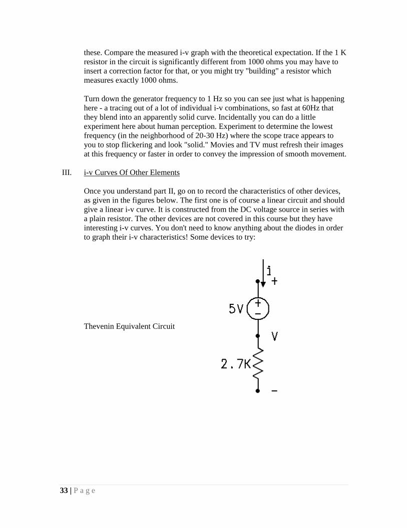
to graph their i-v characteristics! Some devices to try:

Thevenin Equivalent Circuit

34 | P a g e

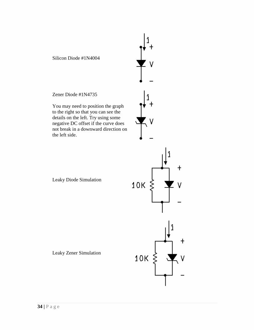
Silicon Diode #1N4004

Zener Diode #1N4735

You may need to position the graph

to the right so that you can see the

details on the left. Try using some

negative DC offset if the curve does

not break in a downward direction on

the left side.

Leaky Diode Simulation

Leaky Zener Simulation

35 | P a g e

Note: diode polarity (direction) is indicated by a ring, as follows:

36 | P a g e


We will do experiment #6 AS IS. Follow the instructions as given.

Analog Meters

When attaching a meter to a circuit to make a measurement we would hope that the

presence of the meter does not cause voltage and current values in the circuit to change.

Analog meters, in order to operate, generally borrow energy from the circuit to which

they are attached. This is called "loading the circuit." If the meter uses a very small

amount of energy and does not cause voltages or currents to change then we say the

meter is a "light load." If the meter draws a great deal of energy and current and voltage

values in the circuit change dramatically then then meter is "loading down the circuit" or

is "a heavy load."

The Simpson multi-meter is an analog meter and will load a circuit when making a

measurement. The DMM is almost an "ideal meter" and as such will be an extremely

light load on a circuit. (There are cases when the DMM could load down a circuit

however.) We will be using the DMM to observe the loading effect of the Simpson meter

on a circuit.

Current Meters

All current meters can be modeled as a resistor Rm. An ideal current meter has Rm=0. A

practical current meter has Rm equal to "a very small resistance." The circuit in Figure_1

has a current meter in series with a voltage source and a resistor. The current in the circuit

without the meter is

I = VS /R

If the meter is "in circuit" then the current becomes

I = VS /(R + Rm )

which is clearly a lower value than the original current. You will notice that this new

current will actually be the current that the meter displays!

37 | P a g e

Figure_1

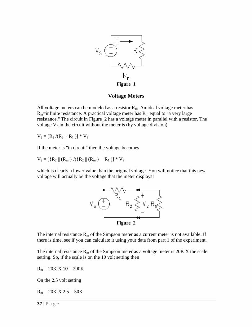
Voltage Meters

All voltage meters can be modeled as a resistor Rm. An ideal voltage meter has

Rm=infinite resistance. A practical voltage meter has Rm equal to "a very large

resistance." The circuit in Figure_2 has a voltage meter in parallel with a resistor. The

voltage V2 in the circuit without the meter is (by voltage division)

V2 = [R2 /(R2 + R1 )] * VS

If the meter is "in circuit" then the voltage becomes

V2 = [{R2 || (Rm } /({R2 || (Rm } + R1 )] * VS

which is clearly a lower value than the original voltage. You will notice that this new

voltage will actually be the voltage that the meter displays!

Figure_2

The internal resistance Rm of the Simpson meter as a current meter is not available. If

there is time, see if you can calculate it using your data from part 1 of the experiment.

The internal resistance Rm of the Simpson meter as a voltage meter is 20K X the scale

setting. So, if the scale is on the 10 volt setting then

Rm = 20K X 10 = 200K

On the 2.5 volt setting

Rm = 20K X 2.5 = 50K

38 | P a g e

Note that this is the scale setting used here and not the voltage value measured at this

setting.

For your circuit analysis in part 2. Calculate V1 and V2 with no meter and then again with

the meter attached appropriately. Consult your lab manual for available voltage scales on

the Simpson meter. Choose an appropriate scale for each measurement.

Have fun.

39 | P a g e


Analog Meters

Purpose: To illustrate use and pitfalls of analog meters

Equipment: Agilent 34401A Digital Multimeter (DMM), Agilent E3631A Triple Output

DC Power Supply, Universal Breadbox, Simpson Multipurpose Analog

Meter

I. Using an analog meter to measure current, voltage, and resistance

CAUTION: with the Simpson meter, as with all analog meters, care must be taken

to put the meter in the circuit with the proper polarity and on the proper range, or

the meter can easily be damaged. Current must flow into the meter terminal which

on analog meters such as this is usually labeled "+" or "V-A" or some such thing

and is often colored red, and out of the terminal which is usually labeled "COM"

or "GROUND" or "-", etc. and is often colored black. Ammeters should always be

set initially to the least sensitive scale (labeled with the largest values of current)

and then turned to more sensitive ranges until a good needle deflection is obtained.

Similar precautions hold when using the Simpson as a voltmeter; polarity must be

observed and you should start on the least sensitive scale, then switch to more

sensitive ranges to get a good reading. These precautions are largely unnecessary

for our digital meters multimeter (DMM), which if used wrong merely announces

that fact by an overload indication.

Taking these precautions, set up the circuit below. Throughout this part, leave the

DMM in the circuit, operating as a current meter.

Figure 1.

40 | P a g e

Put the Simpson in the circuit as a current meter (in series with the DMM) and

adjust the DC voltage supply until the current is 1 mA. Do the DMM and the

Simpson agree? Then remove the Simpson from the circuit. Does the current (as

measured by the DMM) change as a result of removing the Simpson? Now use

the Simpson as a voltmeter to measure the voltage across the resistor. Pay close

attention to the current (measured on the DMM): does the current change when

the Simpson is attached to measure the voltage? Last, disconnect the resistor from

the circuit and use the Simpson to measure its resistance. Do the readings of V, I,

and R verify Ohm's Law? Record the measurements and the percent error

observed in V = I R, with readings taken on the Simpson. Measure the same three

quantities with the DMM and calculate the error in V = I*R again. Comment on

your observations.

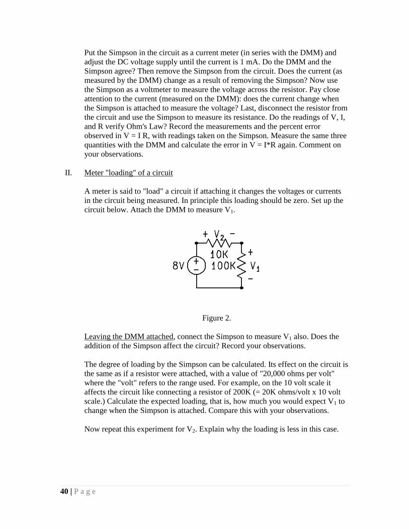
II. Meter "loading" of a circuit

A meter is said to "load" a circuit if attaching it changes the voltages or currents

in the circuit being measured. In principle this loading should be zero. Set up the

circuit below. Attach the DMM to measure V1.

Figure 2.

Leaving the DMM attached, connect the Simpson to measure V1 also. Does the

addition of the Simpson affect the circuit? Record your observations.

The degree of loading by the Simpson can be calculated. Its effect on the circuit is

the same as if a resistor were attached, with a value of "20,000 ohms per volt"

where the "volt" refers to the range used. For example, on the 10 volt scale it

affects the circuit like connecting a resistor of 200K (= 20K ohms/volt x 10 volt

scale.) Calculate the expected loading, that is, how much you would expect V1 to

change when the Simpson is attached. Compare this with your observations.

Now repeat this experiment for V2. Explain why the loading is less in this case.

41 | P a g e


Prepare for this experiment!

During this experiment you will be building the most elaborate circuit of the term. (See

Figure 1. below for circuit diagram and values.) You will also be measuring voltages and

currents using all of the techniques we've learned this term. If you come to lab prepared

you will finish early. If you do not prepare for this experiment you will not finish on time.

Measure the Resistors First!

The resistors must be accurate in this experiment. Discard any with an error greater than

5%. Ask your lab instructor for a replacement.

Procedure

We will do this experiment twice. The first time through we will use two pure DC

sources. The second time through we will use one pure DC source and the function

generator set to have pure DC.

For each case above we will measure and record all voltages using:

The DMM and

The Oscilloscope.

We will also directly measure and record the current in each element using the DMM.

(That means each resistor and each source.)

Set up appropriate data tables for the expected data.

You will then compare this data to the calculated values from your circuit analysis and do

error analysis.

Circuit Analysis

Use mesh analysis to determine the mesh currents. Then calculate each element current

(including resistors and sources.) Now use Ohm's law to calculate each resistor voltage.

You will be doing this twice!.

First time: Use the dual DC supply for the two pure DC sources.

RS = 0 Ohms,

VS1 = 10 Volts DC, and

42 | P a g e

VS2 = 6 Volts DC.

Second time: Use the function generator for VS1 and one side of the dual DC supply for

VS2. YOU MUST SET THE SOURCES BEFORE YOU CONNECT THEM TO THE

CIRCUIT. WHY?

RS = 50 Ohms (NOT K OHMS),

VS1 = 10cos(2000(pi)t) Volts (AC), and

VS2 = 6 Volts DC.

Figure 1.

Have fun.

100

1K

470

680

43 | P a g e


Kirchoff's current and voltage laws

Purpose: To verify Kirchoff's laws experimentally


DC Power Supply, Universal Breadbox

I. Introduction

If a branch of a circuit contains a resistor, the best way to measure the current in

that branch is to measure the voltage across the resistor and divide by R. However

this gives a value which is only as accurate as the value of R. Consequently, start

this investigation by accurately measuring the values of all resistors which will be

used.

Of course if a branch of a circuit contains no resistors, the current in that branch

must be measured directly with a milliammeter (or else deduced by Kirchoff's

current law from other known currents.)

II. Verifying KCL, KVL, and power balance for a linear circuit (DC)

Set up the circuit in Figure 1. Use the +25 volt output for VS1 (set to 10 volts) and

the 6 volt output for VS2 (set to 6 volts.) Set the current limits to 100mA. Use the

DMM for measurements.

44 | P a g e

Figure 1.

Make the appropriate measurements to verify KVL around loops 1, 2, and 3, and

the perimeter of the circuit. (You will find that you must understand the sign

convention for voltages, and you must understand what the DMM tells you about

the sign of a measured voltage, in order to do this.) Record the measurements and

comment on the accuracy with which KVL is verified for these four loops.

Make the appropriate measurements to verify KCL at nodes A, B, C, and D. (As

before, you must understand signs! The DMM counts current as positive if it

enters the mA terminal and leaves the COMMON terminal.) Record and comment

as for the KVL experiment.

Calculate the power absorbed by all elements in the circuit, including the sources.

Add these up and comment on the degree to which your measurements confirm

the fact that the total power absorbed in the circuit is zero.

III. Verifying KCL, KVL, and power balance for a linear circuit (AC)

Repeat part II, but replace VS1 with the function generator, set for 10cos(2000pit).

Make the voltage measurements with the DMM and with the scope. Make the

current measurements with the DMM. Skip the power calculations.

100

1K

470

680

45 | P a g e


Theorems of Linear Networks


If you prepare, you can finish in 90 minutes. If you do not prepare, you will not finish

even half of this experiment. So, do your preliminary work. Set up data tables and graphs

before you come to lab.

Bring cm cm graph paper




The resistor values should be:

Part 1:

RS = 3.3K (DC case); RS will be determined experimentally (AC case)

Parts 2 and 3:

R1 = 3.3K; R2 = 6.8K; R3 = 4.7K; R4 = 10K

Procedure

We will do the experiment almost "as is" in the experiment. The discussion below gives a

bit more detail about the procedures of this experiment.

46 | P a g e

Part 1: Maximum Power Transfer Theorem

We will do this part twice. The first time through we will use a pure DC source. See

Figure 1. The second time through we will use a pure AC source. See Figure 2.

For each case above we will measure and record VL for ten different test values of RL in

the range 0.1RS to 10RS. This, of course, will require you to know the value of RS. It is

very important to include RL = RS as the center test value of set of RL. So use this set of

RL:

RL = {.1RS, .3RS, .5RS, .7RS, .9RS, RS, 2RS, 5RS, 8RS, and 10RS}

You will then calculate the power absorbed by RL:

PABS_RL = (VRL)2/RL for each value of RL. Use your data to plot PABS_RL as a function of

RL.

To begin each case you will measure VOC, the "open-circuit" voltage. See Figure 3. This

is the case when RL = infinity. i.e. there is no RL connected. Note that VOC = VS. Then

connect a variable resistor as RL and adjust RL until the voltage VL becomes exactly

0.5VOC. When VL = 0.5VOC then we know that RL is exactly equal to RS. (See circuit

analysis below.) So, we have just experimentally found RS! Use this value of RS to

determine the test values required as explained above and measure the voltages VL as

explained above.

Part 1A: DC Case

Build the circuit using these discreet values:

VS = 8 volts DC. (Use one side on the dual DC supply)

RS = 3.3K (So we know RS in advance. However use the above technique to

verify that RL = RS when VL = 0.5VOC)

Now get the data for the various RL and plot the power curve.

Part 1B: AC Case

The circuit is the Function Generator! RS and VS are inside the function generator. DO

NOT INCLUDE AN EXTERNAL RS!!!

Set VS = 5 Volts RMS (Pure AC. The DC = 0.) To set this just use the DMM to measure

the AC voltage at the terminals of the function generator and adjust the amplitude control

until the AC (RMS) meter reads 5.00 Volts. Now connect the resistor decade box as RL

and follow the above procedures to determine the value of the internal RS of the function

generator. Now get the data for the various RL and plot the power curve.

Answer these questions:

47 | P a g e

1. Does RL = RS when VL = 0.5VOC?

2. Does RL = RS when the maximum power is being delivered to RL?

Part 2: Linearity

Part 2A: DC Point by Point Plot (The hard way)

1. Set up the circuit in Figure 4. Use a DC supply for VS.

2. Measure VO for these values of VS:

VS = { -4, -2, -1, 0, 1, 2, and 4} Volts.

3. Plot VO as a function of VS. Connect the points to get a continuous relation. Is the

relation linear?

4. Verify that the slope VO /VS is the same value as calculated in your circuit

analysis.

Part 2B: Automatic Plotting (The easy way)

1. Set up the circuit in Figure 5. Use the function generator for VS.

2. Connect the scope as indicated in Figure 5.

3. Scope Setup

a. Put the scope in "X-Y" mode.

b. Set both channels to GND and position the "dot" to center screen.

c. Now set both channels to 1 Volt/DIV

4. Function Generator Setup:

a. Turn DC to Off

b. Use a sinusoidal waveform

c. Set AC amplitude to maximum

d. Set frequency to a "low" value ~60 to 120 Hz (whatever frequency give

the best or "cleanest" image)

5. You should now see a continuous plot of VO as a function of VS. Sketch it. Is the

relation linear?

6. Verify that the slope VO /VS is the same value as calculated in your circuit

analysis.

Are the plots from the above two methods the same? Which method was easier?

Part 3: Superposition

1. Set up the circuit in Figure 6.

2. Use the DMM to accurately set:

a. VS1 = 5.00 Volts.

b. VS2 = 4.00 Volts.

3. Now verify that superposition holds for V1 and I2. This requires that you show

that:

a. V1|(VS1 = 5, VS2 = 0) + V1|(VS1 = 0, VS2 = 4) = V1|(VS1 = 5, VS2 = 4)

48 | P a g e

and

b. I2|(VS1 = 5, VS2 = 0) + I2|(VS1 = 0, VS2 = 4) = I2|(VS1 = 5, VS2 = 4)

4. HINT:After setting the sources, the best way to go back to Zero Volts (as is

needed during data taking) is to remove the cables from a voltage source

terminals and connect the cables together. You will have the Zero Volts required.

Then, when you need the non-zero value again, just plug the cables back into the

source. That way you do not waste time re-setting the source voltages.

5. So, fill in a data table like the one below and verify that the addition of rows one

and two is equivalent to row three for each column.

Superposition Data Table

Set up appropriate data tables and plots for all the expected data for each part.

You will then compare this data to the calculated values from your circuit analysis and do

error analysis for each part.

Circuit Analysis

Note: An arrow through a resister is the circuit symbol for a variable resister. Your Lab

instructor will show you how to use the POWER RESISTOR DECADE BOX as a

variable resistor.

Part 1A: DC Case

RS = 3.3K, and

VS = 8 Volts DC

Figure 1.

49 | P a g e

Part 1B: AC Case

RS = 50 Ohms, and

VS = 5 Volts AC (RMS)

Figure 2.

For each circuit above the "open circuit voltage" VOC is the value of VL when RL is

infinite. Note that in that case

VOC = VS. See Figure 3.

Figure 3.

Note that in Figures 1 and 2 if RL = RS then

VL = 0.5VS = 0.5VOC.

Which can be found easily by voltage division.

Also, when we have the above conditions, RL is absorbing the maximum power that the

circuit is able to deliver. See pages 143-145 in your text for a proof.

Part 2: DC Point-by-Point Plot

For the circuit in Figure 4. find the ratio of VO /VS. You can do this using by successive

voltage division of VS. Note that this ratio is a constant now matter what the value of VS.

Show all of your work.

50 | P a g e

Part 2 Elements:

R1 = 3.3K

R2 = 6.8K

R3 = 4.7K

R4 = 10K

Figure 4.

VS = { -4, -2, -1, 0, 1, 2, and 4 volts}

Part 2: AC Continuous Plot

The circuit in Figure 5. shows how to connect the oscilloscope to easily verify linearity.

Figure 5.

Part 3: Superposition

Use the principle of superposition to find V1 and I2 for the circuit in Figure 6. Show all of

your work.

Part 3 Elements:

R1 = 3.3K

R2 = 6.8K

R3 = 4.7K

R4 = 10K

Figure 6.

51 | P a g e

VS1 = 5 volts.

VS2 = 4 volts.

Have fun.

52 | P a g e


Theorems of Linear Networks

Purpose: To illustrate linearity, superposition, and the maximum power transfer

theorem.


Agilent E3631A Triple Output DC Power Supply, Universal Breadbox

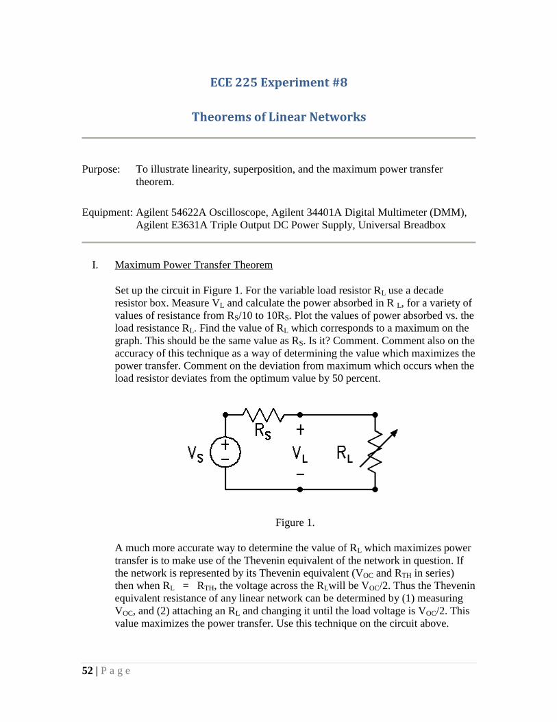
I. Maximum Power Transfer Theorem

Set up the circuit in Figure 1. For the variable load resistor RL use a decade

resistor box. Measure VL and calculate the power absorbed in R L, for a variety of

values of resistance from RS/10 to 10RS. Plot the values of power absorbed vs. the

load resistance RL. Find the value of RL which corresponds to a maximum on the

graph. This should be the same value as RS. Is it? Comment. Comment also on the

accuracy of this technique as a way of determining the value which maximizes the

power transfer. Comment on the deviation from maximum which occurs when the

load resistor deviates from the optimum value by 50 percent.

Figure 1.

A much more accurate way to determine the value of RL which maximizes power

transfer is to make use of the Thevenin equivalent of the network in question. If

the network is represented by its Thevenin equivalent (VOC and RTH in series)

then when RL = RTH, the voltage across the RLwill be VOC/2. Thus the Thevenin

equivalent resistance of any linear network can be determined by (1) measuring

VOC, and (2) attaching an RL and changing it until the load voltage is VOC/2. This

value maximizes the power transfer. Use this technique on the circuit above.

53 | P a g e

This technique also works if the sources in the network are sinusoidal, the

difference being that RMS measurements are made rather than DC measurements.

Adjust the function generator for zero DC offset and a frequency of 1 KHz. Then

using the method of the previous paragraph, determine the RTH of the function

generator (which, although shown as an ideal source in the circuit, actually has a

nonzero internal resistance), and using the less accurate graphical method find the

value of RL which maximizes the power transfer from the generator to its load.

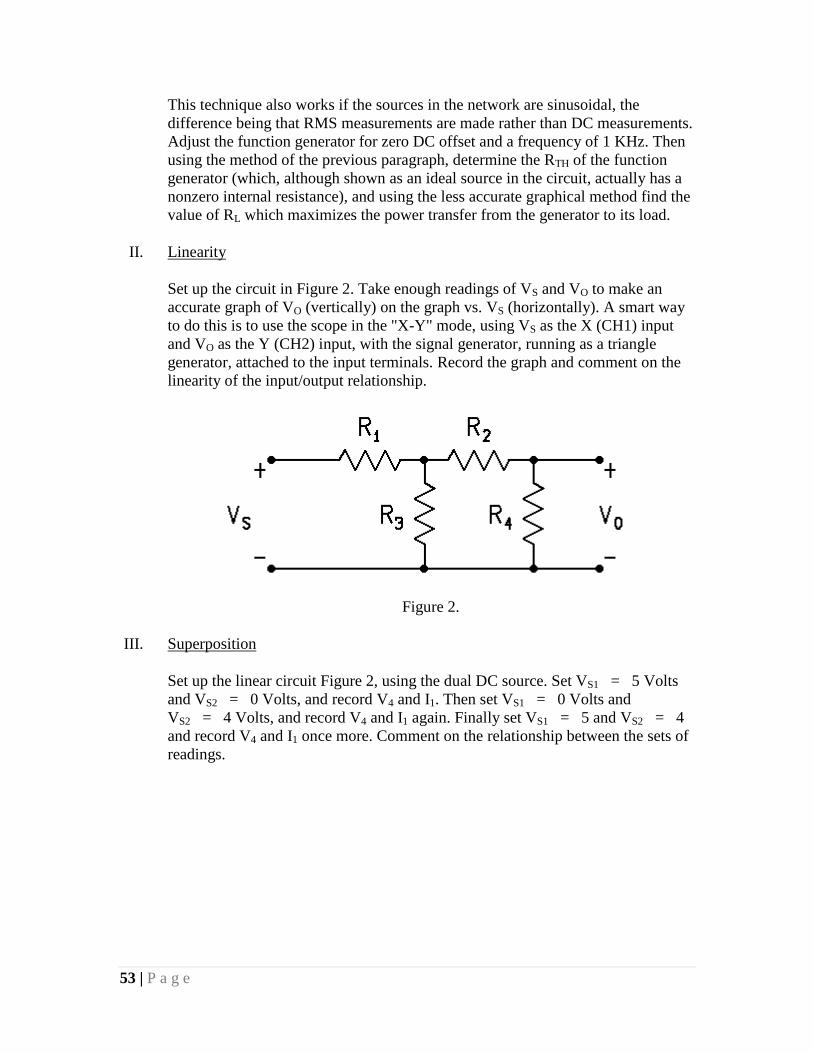
II. Linearity

Set up the circuit in Figure 2. Take enough readings of VS and VO to make an

accurate graph of VO (vertically) on the graph vs. VS (horizontally). A smart way

to do this is to use the scope in the "X-Y" mode, using VS as the X (CH1) input

and VO as the Y (CH2) input, with the signal generator, running as a triangle

generator, attached to the input terminals. Record the graph and comment on the

linearity of the input/output relationship.

Figure 2.

III. Superposition

Set up the linear circuit Figure 2, using the dual DC source. Set VS1 = 5 Volts

and VS2 = 0 Volts, and record V4 and I1. Then set VS1 = 0 Volts and

VS2 = 4 Volts, and record V4 and I1 again. Finally set VS1 = 5 and VS2 = 4

and record V4 and I1 once more. Comment on the relationship between the sets of

readings.

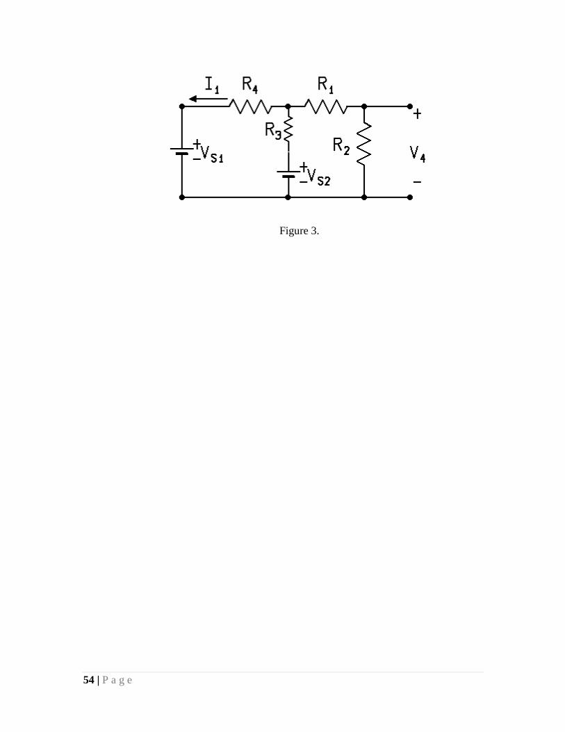
54 | P a g e

Figure 3.

55 | P a g e


Thevenin's Theorem




The element values are:

Part 1:

R1 = 10K; R2 = 6.8K; R3 = 10K; R4 = 3.3K, and R5 = 2.7K

V1 = 10 Volts and V2 = 6 Volts.

Procedure

Use a DC source for V1 and V2.

Procedure

1. Build the circuit but do not connect a load resistor.

2. Measure VOC.

3. Measure ISC.

4. Compare these values to the values from your circuit analysis. There should be

almost no error. If there is error then:

a. you did not build the circuit correctly or

b. you did not measure correctly.

5. If the data is OK then use the above data values of VOC and ISC to calculate RTH.

6. Now measure RTH! Just set the voltage sources to zero and use an Ohm meter to

measure the resistance at the output terminals. PLEASE NOTE: Normally you

can not and should not measure RTH in the above manner. Usually we can't turn

of the the internal sources in a circuit. Try measuring RTH while the sources are

connected. You should get a very large error.

7. Does the calculated RTH equal the measured RTH? It should!

8. DO NOT GO ON. show your data to your lab instructor. If all the data is OK then

you may go on.

9. Connect the following load resistors RL (one at a time) and measure and record:

a. VL and

b. IL

56 | P a g e

RL = {100 Ohms, 470 Ohms, 1K, 4.7K, 10K, 20K}

IMPORTANT: Do not use the power resistor decade box for RL. Use the extra

resistors supplied in your kit.

10. DO NOT GO ON. show your data to your lab instructor. If all the data is OK then

you may go on. DO NOT DISMANTLE THE CIRCUIT.

11. Now build the Thevenin Equivalent Circuit (TEC) of the elaborate circuit you just

worked on.

a. Set the voltage source VOC equal to the open circuit voltage VOC YOU

measured and

b. Use the power resistor decade box as RTH. Do not trust the dials. Measure

the resistance on the decade box so that you know that it is set correctly.

c. Now repeat steps 2 to 10 above. Be sure to use exactly the same load

resistors.

12. Compare the data from the original circuit and the TEC. Do error analysis.

13. Plot the suggested graph using the values of RL from above.

14. You're done. Dismantle the circuits, put the parts away, and turn in your report.

Circuit Analysis

Calculate the values for VOC, ISC, and RTH using any method you like. Use the values

given at the top of this page. You do not need to calculate the load resistor voltages and

currents. That's all.

Have fun.

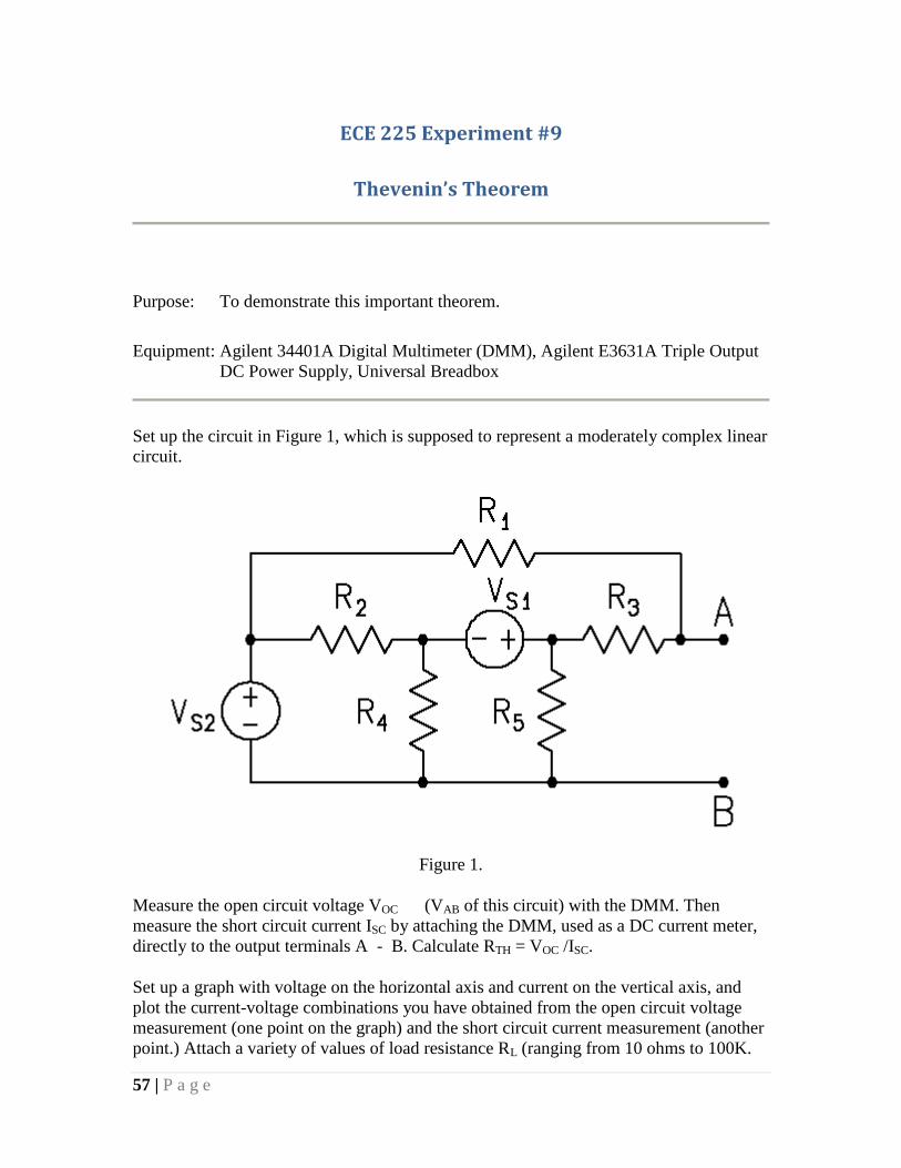
57 | P a g e


Thevenin’s Theorem

Purpose: To demonstrate this important theorem.


DC Power Supply, Universal Breadbox

Set up the circuit in Figure 1, which is supposed to represent a moderately complex linear

circuit.

Figure 1.

Measure the open circuit voltage VOC (VAB of this circuit) with the DMM. Then

measure the short circuit current ISC by attaching the DMM, used as a DC current meter,

directly to the output terminals A - B. Calculate RTH = VOC /ISC.

Set up a graph with voltage on the horizontal axis and current on the vertical axis, and

plot the current-voltage combinations you have obtained from the open circuit voltage

measurement (one point on the graph) and the short circuit current measurement (another

point.) Attach a variety of values of load resistance RL (ranging from 10 ohms to 100K.

58 | P a g e

See Figure 2.) to the output terminals; for each value of RL, first determine the load

voltage and load current which result and then plot the combination as a point on the

graph. Comment on the nature of the graph.

Figure 2.

Now construct the Thevenin equivalent of this circuit, using a DC source set equal to the

measured VOCmeasured above, and a resistance equal to RTH calculated above. See

Figure 3.

Attach the same set of RL values you used earlier, and record the load voltages and

currents which result. See Figure 4. If this simplified circuit is in fact equivalent to the

original more complex circuit, these values should be the same as before. Are they?

Comment.

Figure 3.

Figure 4.

59 | P a g e



Read the OP-Amp Tutorial before going on with this experiment.

For any Ideal Op Amp with negative feedback you may assume:

V- = V

+ (But not necessarily 0)

I- = I

+ = 0

Now write KCL equations everywhere except at V-sources and the Op-Amp

output.

Do some algebra to find your answer

Part 2: Op Amp as a Linear Amplifier

Since the circuit has negative feedback the above assumptions are true.

Let's find VO = f(VS)

KCL at V-:

(V- - VS)/1K + (V

- - VO)/10K = 0

But V- = V

+ = 0 So,

VO = -(10K/1K)VS = -10VS

Let VS = 1cos(2000(pi)t) volts. Then,

VO = -10(1cos(2000(pi)t)) = -10cos(2000(pi)t) volts.

Let VS = 2cos(2000(pi)t) volts. Then,

VO = -10(2cos(2000(pi)t)) = -20cos(2000(pi)t) volts.

http://www.uic.edu/classes/ece/ece225/exams/opamps/opamps.html

60 | P a g e

But in this case the output voltage exceeds the supply voltage of the op amp. So the amp

goes into "saturation" for |VO| > 15 volts. The result of this is that the peaks of the -

20cos(2000(pi)t) are "clipped off" at +15 and -15 volts.

Part 3: Op Amp as a Linear Adder


Let's find VO = f(Va, Vb)

KCL at V- :

(V- - Va)/10K + (V

- - Vb)/20K + (V

- - VO)/10K = 0

But V- = V

+ = 0 So,

VO = -(10K/10K)Va -(10K/20K)Vb = -1(Va + 1/2Vb)

Part 4: Op Amp as an Integrator



KCL at V-:

(V- - VS)/R + iC + i100K = 0

But V- = V

+ = 0 , assume i100K = 0 and

iC = Cd(vC)/dt = Cd(0 - VO)/dt So,

-VS/R - Cd(VO)/dt = 0

d(VO) = (-1/RC)VSdt So,

VO = (-1/RC)I[VS;(-infinity, t)] where,

I[VS;(-infinity, t)] is " the integral of VS from -infinity to t"

Let R = 10K, C= 0.02uF and VS = 4cos(10000(pi)t) volts. Then,

VO = (-1/10000x0.02E-6)[(-4/10000(pi))sin(10000(pi)t)] Or,

VO = 0.637sin(10000(pi)t)

61 | P a g e

Operational Amplifier Tutorial

The Basic Ideal Op-Amp Analysis Strategy

For any Ideal Op-Amp with negative feedback you may assume:

V- = V

+ (But not necessarily 0)

I- = I

+ = 0

Now write KCL equations everywhere except at V-sources and the Op-Amp

output.

Do some algebra to find your answer

Since the output voltage can not exceed the power supplies, check to see that

VPS- < VO < VPS+

The Inverting Amplifier Configuration

Figure 1.

62 | P a g e

Since the circuit in Figure 1. has negative feedback the above assumptions are true.


KCL at V-:

(V- - VS) /R1 + (V

- - VO) /RF = 0

Note that in this case V+ = 0! So,

V- = V

+ = 0. So,

VO = -(RF /R1)VS. Note that the value of RL does not matter!

Let VS be a triangle wave with peaks at +2 and -2. See Figure 2. Let

RF = 6K and

RF = 2K. So,

VO = -(6K / 2K)VS is an "upside down" triangle 3 times taller than VS. So, the peaks of

VO are at +6 and -6. See Figure 2.

If VPS- = -10 Volts and VPS+ = +10 Volts then the output voltage VO is well within the

power supply limits and linear amplification does indeed take place as seen in Figure 2.

Figure 2.

Now let VS be a triangle wave with peaks at +2 and -2. See Figure 3. Let

RF = 12K and

RF = 2K. So,

63 | P a g e

VO = -(12K / 2K)VS is an "upside down" triangle 6 times taller than VS. So, the peaks of

VO should be at +12 and -12.

But If VPS- = -10 Volts and VPS+ = +10 Volts then the output voltage VO tries to exceed

the power supply limits. When the output tries to go beyond the power supply limits we

say that the op-amp is "in saturation." Linear amplification does not take place when the

op-amp is in saturation. Output values are "clipped" at the supply values as seen in Figure

3.

Figure 3.

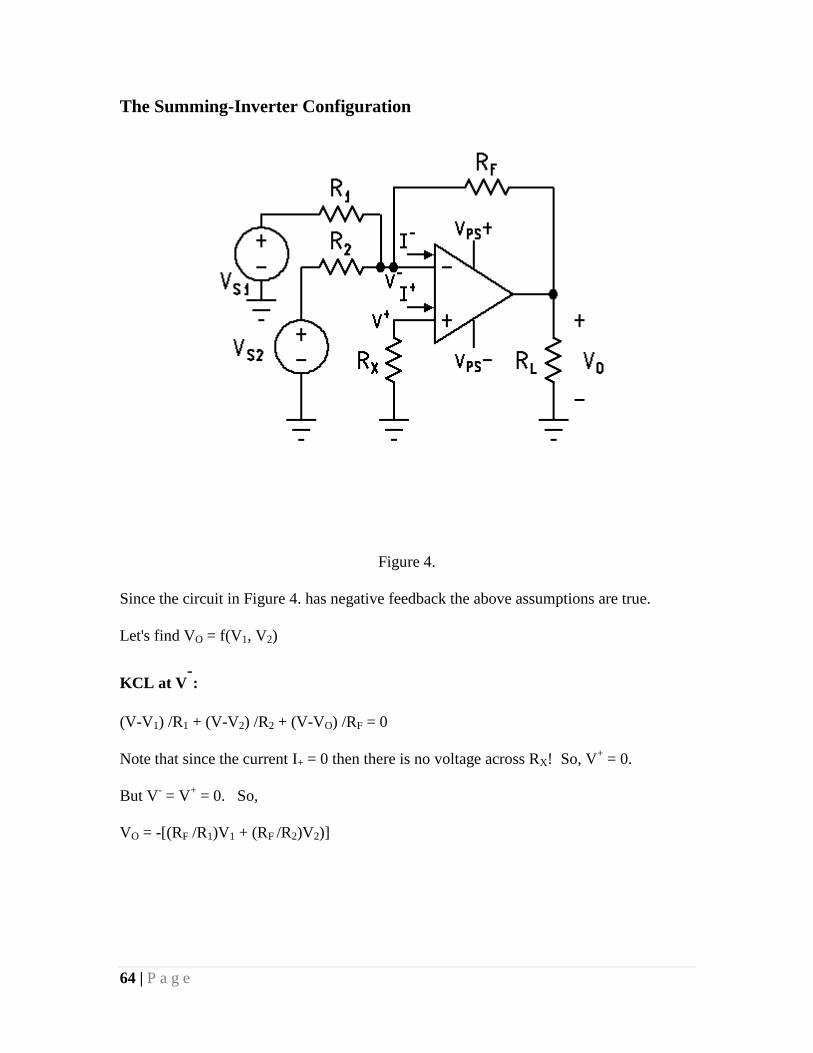
64 | P a g e

The Summing-Inverter Configuration

Figure 4.


Let's find VO = f(V1, V2)

KCL at V-:

(V-V1) /R1 + (V-V2) /R2 + (V-VO) /RF = 0

Note that since the current I+ = 0 then there is no voltage across RX! So, V+ = 0.

But V- = V

+ = 0. So,

VO = -[(RF /R1)V1 + (RF /R2)V2)]

65 | P a g e

The Non-Inverting Configuration

Figure 5.

Since the circuit in Figure 5 has negative feedback the above assumptions are true.

(V-0) /R1 + (V-VO) /RF = 0

But V- = V

+ = VS. So,

VO = (RF /R1 + 1)VS

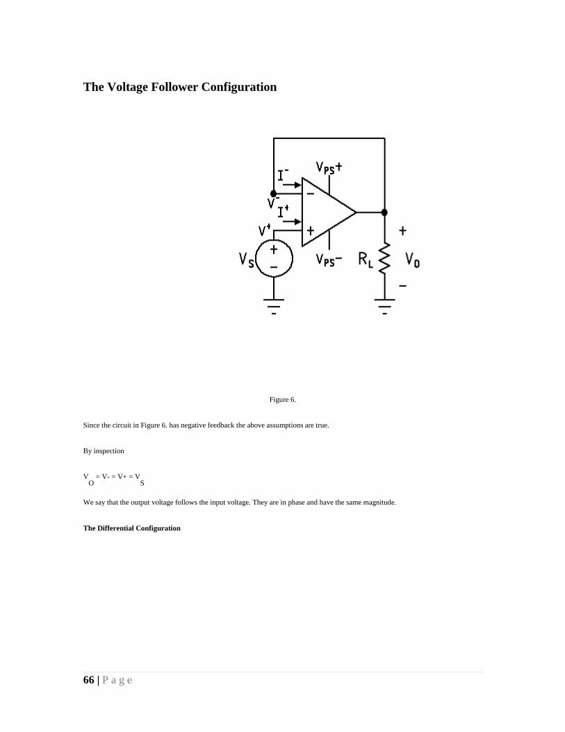
66 | P a g e

The Voltage Follower Configuration

Figure 6.


By inspection

VO

= V- = V+ = VS

We say that the output voltage follows the input voltage. They are in phase and have the same magnitude.

The Differential Configuration

67 | P a g e

Figure 7.

Can you show that

VO

= [(RF

/R1

) + 1)*(RX

/(RX

+ RY

))]VS2

- [RF

/R1

]VS1

??

Note that if all the resistors are the same value then

VO

= VS2

- VS1

!

Finding the Output Current IO

68 | P a g e

Figure 8.


Find VO

first using the same procedures as in the inverting amplifier configuration. Then find IO

by writing a KCL equation at VO

using the KNOWN VALUE of VO

and V- that you just calculated.

KCL at VO

:

IO

= (VO

- V-) /RF

+ VO

/RL

Note that since the current I+ = 0 then there is no voltage across R2

! So, V+ = 0

Practice Problem

Can you find VO

= f(VS

) for the circuit in Figure 9?

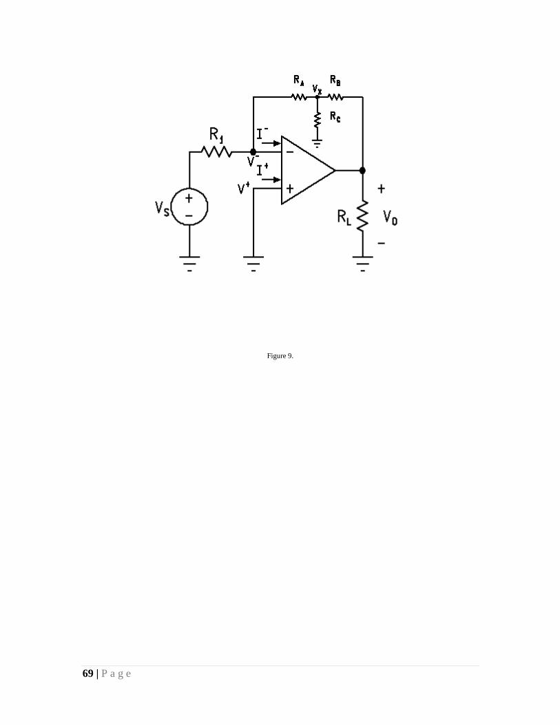
69 | P a g e

Figure 9.

70 | P a g e


Operational Amplifiers

Purpose: To illustrate a few of the uses of op amps.


Agilent E3631A Triple Output DC Power Supply, Universal Breadbox,

LM741 Linear Amplifier.

I. Introduction

a. Op Amp Pin Conventions are as Follows:

Figure 1.

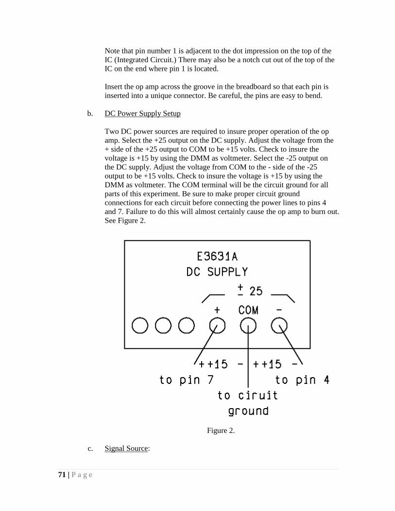
71 | P a g e

Note that pin number 1 is adjacent to the dot impression on the top of the

IC (Integrated Circuit.) There may also be a notch cut out of the top of the

IC on the end where pin 1 is located.

Insert the op amp across the groove in the breadboard so that each pin is

inserted into a unique connector. Be careful, the pins are easy to bend.

b. DC Power Supply Setup

Two DC power sources are required to insure proper operation of the op

amp. Select the +25 output on the DC supply. Adjust the voltage from the

+ side of the +25 output to COM to be +15 volts. Check to insure the

voltage is +15 by using the DMM as voltmeter. Select the -25 output on

the DC supply. Adjust the voltage from COM to the - side of the -25

output to be +15 volts. Check to insure the voltage is +15 by using the

DMM as voltmeter. The COM terminal will be the circuit ground for all

parts of this experiment. Be sure to make proper circuit ground

connections for each circuit before connecting the power lines to pins 4

and 7. Failure to do this will almost certainly cause the op amp to burn out.

See Figure 2.

Figure 2.

c. Signal Source:

72 | P a g e

Turn on the signal generator, and adjust its AC output to minimum with

the output amplitude knob. Adjust the DC offset of the signal generator to

zero. Check to insure the DC offset is zero by using the DMM as a DC

voltmeter for accuracy.

II. Op Amps as Linear Amplifiers

In this part you will set up an op amp as a linear amplifier with a gain of 10, and

inspect the input and output to see how well or poorly it behaves as such a device.

Operational amplifiers must be treated with care; they are powerful but can be

destroyed by abuse. In particular it is very abusive to apply voltages to the input

terminals before fully powering up the opamp, or to exceed certain maximum

limits. Therefore, you will (a) set up the signal source but with zero output; (b) set

up the rest of the circuit; (c) have your instructor check the circuit; and THEN (d)

power the circuit up for the experiment.

Inverting Amplifier Circuit: wire up the circuit in Figure 3 below, checking

carefully to see that it is correct, but with ALL POWER OFF (no connection to

pins 4 and 7 yet) and the signal generator disconnected from the rest of the circuit.

Connect VS1 to CH1 and VO to CH2 of the scope. Set the scope to display both of

them simultaneously.

Note: Set the scope to trigger off of CH1 for all parts of this experiment. Your

instructor will show you how to do this.

Figure 3.

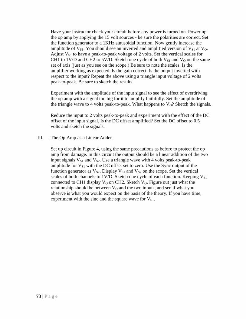
73 | P a g e

Have your instructor check your circuit before any power is turned on. Power up

the op amp by applying the 15 volt sources - be sure the polarities are correct. Set

the function generator to a 1KHz sinusoidal function. Now gently increase the

amplitude of VS1. You should see an inverted and amplified version of VS1 at VO.

Adjust VS1 to have a peak-to-peak voltage of 2 volts. Set the vertical scales for

CH1 to 1V/D and CH2 to 5V/D. Sketch one cycle of both VS1 and VO on the same

set of axis (just as you see on the scope.) Be sure to note the scales. Is the

amplifier working as expected. Is the gain correct. Is the output inverted with

respect to the input? Repeat the above using a triangle input voltage of 2 volts

peak-to-peak. Be sure to sketch the results.

Experiment with the amplitude of the input signal to see the effect of overdriving

the op amp with a signal too big for it to amplify faithfully. Set the amplitude of

the triangle wave to 4 volts peak-to-peak. What happens to VO? Sketch the signals.

Reduce the input to 2 volts peak-to-peak and experiment with the effect of the DC

offset of the input signal. Is the DC offset amplified? Set the DC offset to 0.5

volts and sketch the signals.

III. The Op Amp as a Linear Adder

Set up circuit in Figure 4, using the same precautions as before to protect the op

amp from damage. In this circuit the output should be a linear addition of the two

input signals VS1 and VS2. Use a triangle wave with 4 volts peak-to-peak

amplitude for VS1 with the DC offset set to zero. Use the Sync output of the

function generator as VS2. Display VS1 and VS2 on the scope. Set the vertical

scales of both channels to 1V/D. Sketch one cycle of each function. Keeping VS1

connected to CH1 display VO on CH2. Sketch VO. Figure out just what the

relationship should be between VO and the two inputs, and see if what you

observe is what you would expect on the basis of the theory. If you have time,

experiment with the sine and the square wave for VS1.

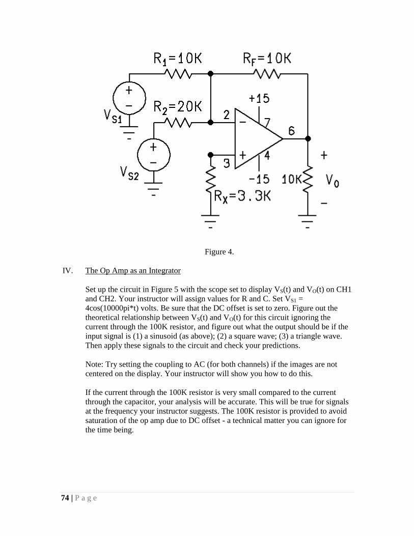
74 | P a g e

Figure 4.

IV. The Op Amp as an Integrator

Set up the circuit in Figure 5 with the scope set to display VS(t) and VO(t) on CH1

and CH2. Your instructor will assign values for R and C. Set VS1 =

4cos(10000pi*t) volts. Be sure that the DC offset is set to zero. Figure out the

theoretical relationship between VS(t) and VO(t) for this circuit ignoring the

current through the 100K resistor, and figure out what the output should be if the

input signal is (1) a sinusoid (as above); (2) a square wave; (3) a triangle wave.

Then apply these signals to the circuit and check your predictions.

Note: Try setting the coupling to AC (for both channels) if the images are not

centered on the display. Your instructor will show you how to do this.

If the current through the 100K resistor is very small compared to the current

through the capacitor, your analysis will be accurate. This will be true for signals

at the frequency your instructor suggests. The 100K resistor is provided to avoid

saturation of the op amp due to DC offset - a technical matter you can ignore for

the time being.

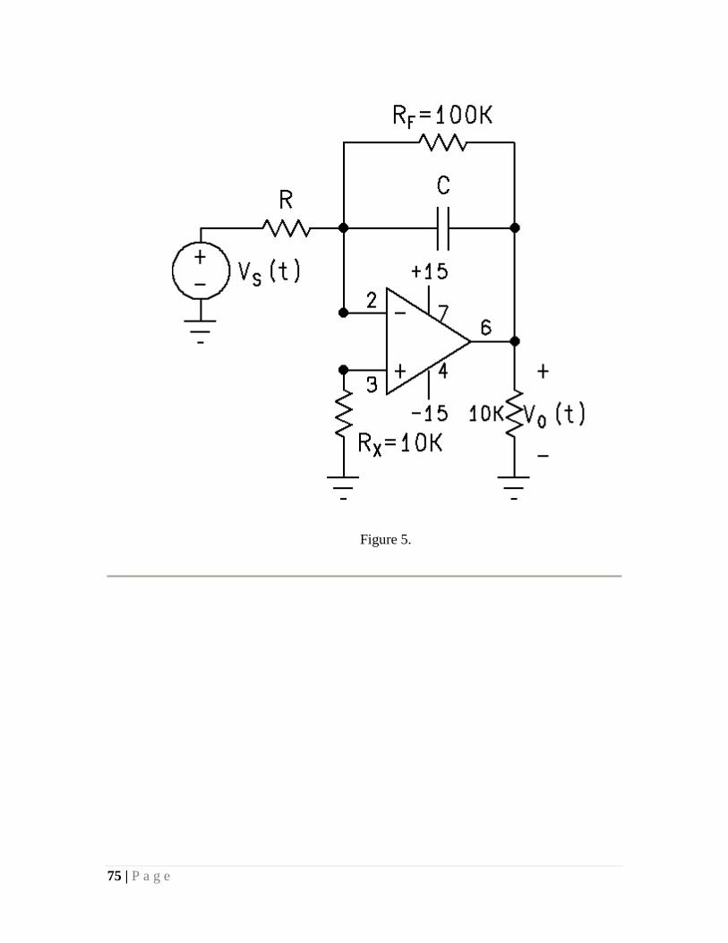
75 | P a g e

Figure 5.

76 | P a g e


You should be able to finish this experiment very quickly.

This week we will do experiment 11 almost AS IS. Your data will be the graphical

images on the display of the scope. So, BRING GRAPH PAPER! cm X cm is best since

that is the actual scale of the scope display. You will be sketching the transient response

of a RC circuit. We will also take a look at the capacitor as an integrating device.

Procedure

Part 1

Set up the circuit as shown in the lab manual with C = 0.01uF and R =27K. Set the

amplitude of the square wave to 6 volts peak-to-peak (NOT the 20 volts indicated in the

lab manual.). It is important that the frequency of the 6 volt (peak-to-peak) be exactly 200

Hz. Do not trust the scales on the function generator. The scope scales are much more

accurate. So, do this:

1. Set the time base to 0.5msec/DIV.

2. Adjust the frequency control dial on the function gen. so that there is one

complete cycle of the input and output in exactly the 10 horizontal divisions. (i.e.

one cycle is 5msec and therefore f = 200Hz.)

3. Draw a large (half page at least) accurate sketch of the input VS(t) and output VC(t)

(on the same sketch) just as you see it on the scope.

4. Repeat steps 1 to 3 with C = 0.02uF and C = 0.068uF.

Now we will be making an estimation of the values of the RC time constants (tau) for

each sketch of VC(t). To understand how to do this consider the following explanation.

For the part of VC(t) that starts up at t = 0:

VC(t) = VCSS(t) + [VC(0) - VCSS(0) ]e-t/RC

where VCSS(t) = -3 Volts (a constant for all time).

The slope of the tangent line to VC(t) can be found by taking the derivative of VC(t)

d{VC(t)}/dt = (-1/RC)[VC(0) - VCSS(0) ]e-t/RC

At t = 0 this becomes

d{VC(t)}/dt|t=0 = (1/RC)[ VCSS(0) - VC(0)]

So, for a vertical change of VCSS(0) - VC(0) the horizontal change is RC which is tau.

77 | P a g e

Note if VCSS(t) is constant then VCSS(0) = VCSS(infinity) = VC(infinity).

If you sketch the tangent line of VC(t) from the point t = 0 to the -3 Volt line the the

amount of horizontal change must be tau. Project that amount of change up to the t axis

and you have graphically found the value of tau. See Figure 1.

Figure 1.

Part 2

Let R = 100K and C = 1uF.

At 200 Hz VC will be very small compared to VS as required. Use only one trial of VS(t)

for this part:

VS(t) = 3cos(400(pi)t)

Is VC(t) approximately 1/RC times the integral of 3cos(400(pi)t)?

Verify this by checking the amplitude and phase of VC(t).

Do not use the square wave and triangle wave for input as suggested in the lab manual.

Circuit Analysis

Part 1

78 | P a g e

Use the model in the lab manual (with voltage sources at 3 volts and not 10 volts) to find

the general expression for VC(t). Calculate the expected value of tau for each capacitor.

Part 2

Show that if VC(t) is very tiny compared to VS(t) then VC(t) approximately 1/RC times

the integral of VS(t). (Hint: if VC(t) is very small then iC(t) is approximately VS(t) /R )

Read and know the setup of this experiment and have fun!

79 | P a g e


RC Circuits

Purpose: To illustrate properties of capacitors and their operation in R-C circuits

Equipment: Agilent 54622A Oscilloscope, Agilent function generator, Universal

Breadbox.

I. R-C step response

Set up the circuit in Figure 1 below. Adjust the function generator to provide a

200 Hz square wave, with zero DC offset, and 6 volts peak- to-peak. After these

adjustments you can visualize the generator as the switching circuit shown

illustrated below the circuit.

Figure 1.

Connect the scope to display VC(t) on CH1 and VS(t) on CH2. Ground both

displays (with the GND selection) to set the traces at the center of the display;

then select the DC presentation, and display VC(t) and VS(t) simultaneously and

with the same vertical sensitivity (VOLTS/DIV) for each channel. Record the

input and output time functions. Measure the time constant by the method

discussed in the notes, and compare it with the value calculated from the values of

R and C. In order to measure the time constant accurately, you may have to alter

the function generator's frequency. Record and comment upon your observations.

Repeat the experiment with all values of C provided by your instructor.

Notice that VS(t) at the output terminals of the function generator is not a perfect

square wave. Why? Record the waveforms accurately, especially the

"imperfection" in VS(t).

II. An RC circuit as an integrator

80 | P a g e

Using the same circuit from part I, if VC(t) is much less than then VR(t) is almost

equal to VS(t) and therefore iC(t) is almost equal to Vs(t)/R. Under this condition,

VC(t) = 1/RC times the integral of VS(t), and thus the system with can be viewed

as an integrator.

Use a square wave of frequency 200 Hz and amplitude 4 V peak-to-peak, and use

C = 1 uF. Are the approximations mentioned above valid under these conditions?

Display VS(t) and VC(t) simultaneously on the scope as in part 1, except that since

VC(t) is much smaller than VC(t) you will have to use different vertical

sensitivities (VOLTS/DIV) for the two channels. Try the sinusoidal and triangle

waveforms. Record your observations.

Comment on the quality of this circuit as an integrator.

What is the integral of a square wave? Of a sinusoidal wave? Of a triangle wave?

(Hints: the square wave is a succession of constants; what function g(t) is the

integral of the constant function f(t) = +3? f(t) = -3? The sinusoid is easy, from a

basic calculus course. The triangle wave resembles the function f(t) = K1*t + K2;

what function g(t) is the integral of that?)

81 | P a g e


Phasors and Sinusoidal Analysis

We will do experiment #12 AS IS. Follow the instructions in the experiment as given.

The value of R in the circuit setup will be 100 Ohms and not the 1K shown in the

experiment. Also, NL is the imdedance Z. This is the only change for this experiment.

PREPARE FOR THIS EXPERIMENT!

You will take 75 data values during this experiment! That takes time! So, you must come

to the lab prepared! Read about and know about the setup and measuring techniques for

this experiment. If you are not prepared you will not finish this experiment. But, as with

all the other experiment, if you prepare in advance you will finish early.

There is no circuit analysis for this experiment so nothing to do there. Prepare the

purpose, theory, and procedure as usual.

You _must_ set up three separate data tables using the headings given in the lab manual.

The first two tables will have the following frequencies (in Hz) down the first column:

100, 200, 400, 600, 800, 1000, 1500, 2000, 2500, 3000. The frequencies for the third

table will be found experimentally so you cannot list them until you get some data. The

right most column will have the heading "C" for table 1 and "L" for table 2. Table 3 does

not need that last column.

All of the above preparation must be submitted to your lab instructor at the beginning of

the lab session for scoring and will be returned to you after you set up the first circuit.

The lab report will not be due at the end of the lab session. It will be collected at the

_beginning_ of your next lab session. This is because the data evaluation and plotting

will need more time then we have during the lab session. So, you have an extra week to

write up this report. Given that much time your reports are expected to be perfect! ;)

What You Will Do in Lab

For this experiment you will be solving the mystery of the unknown elements. You will

be given a capacitor and inductor of unknown values. By indirectly measuring the

current-voltage characteristics you will determine the element values. Since the

measuring techniques used are not very accurate (due to visual estimations) we will take

many data samples and get an average value of the data. In the past the average values of

the data have given elements values within 3-5% accuracy!

During the lab session for each impedance you will measure:

82 | P a g e

Voltage |VZ|;

Voltage |VR|; and

Phase Angle ØZ.

This will done at each frequency in the tables for each impedance.

What You Will Do at Home

After completing the experiment you will take your data home and:

Fill in the remaining columns of the table;

Calculate the average value of C and L from data of tables 1 and 2 respectively:

Calculate FO_Calc and compare it to FO_Exp (See How it works below);

Plot data:

For each table, plot at each frequency:

o The complex impedance vector in the complex plane; and

o |Z| = F(w) (Connect the points to get an estimated continuous function.)

Write your conclusion.

How it works

We know that the complex impedance is defined by:

|Z| / ØZ = |VZ| / ØV / |IZ| / ØI

The Magnitude of Z

At each frequency in the table you will be directly measuring the RMS magnitude of the

voltage across your elements and indirectly measuring the RMS magnitude of the current

through your elements using the DMM. The ratio of these magnitudes gives the

magnitude of the Complex Impedance of your element. SO,

|Z| = |VZ| / |IZ|

You will use a 100 Ohm resistor (NOTE CHANGE FROM LAB MANUAL 1K) in

series with Z to indirectly measure the magnitude of IZ. Since R is in series with Z they

have the same current. If we measure |VR| then:

|IZ| = |VR| / R [Be sure you measure R so you know its exact value.]

The Phase Angle of Z

Also at each frequency, you will directly measure the Phase Angle difference between the

sinusoidal voltage and current using the oscilloscope (scaled to degrees using the

83 | P a g e

technique explained in your lab manual. READ IT! KNOW IT!) This phase angle

difference is the phase angle of the complex impedance of your element since:

ØZ = ØV - ØI

On the scope we will position IZ so that ØI = 0. That way ØZ = ØV.

The Sign of the Angle

Lead: If the voltage "leads" the current (voltage has a t-axis cross over point to

the left of the current t-axis cross over point) then the angle is the distance in

degrees between the two signals and has a positive sign.

Lag: If the voltage "lags" the current (voltage has a t-axis cross over point to the

right of the current t-axis cross over point) then the angle is the distance in

degrees between the two signals and has a negative sign.

Evaluating Z

Once you have the magnitude and phase angle of Z you have its polar form as a complex

number. Convert this to rectangular form and enter the value in the table. You will have:

Z = a ± Jb

The value of b will be used to determine the value of the unknown element.

Table 1 - The Capacitor

Start with the capacitor. We know that for a capacitor that:

ZC = 0 - J/wC

So from your data:

b = 1/wC so,

C = 1/wb

Calculate the value of C using the value of b at each frequency in table 1. Then get the

average value of the ten values of C. Call it CAVG.

Table 2 - The Inductor

Warning: Handle the inductors with care. The fine inductor wire breaks easily. If you

break your inductor you will be required to repeat parts 2 and 3 of this experiment!

Bummer!

The inductor you will be given is made of very long piece (10 yds?) of very fine wire

wrapped around a metal core. This wire will have a resistance RL of about 40 to 80 Ohms

84 | P a g e

depending on your actual inductor. We cannot remove that resistance. So your actual

"practical" inductor will behave like a resister in series with an ideal inductor so:

ZL_prac = RL + JwL

So from your data:

a = RL and

b = wL so,

L = b/w

Calculate the value of L using the value of b at each frequency in table 2. Then get the

average value of the ten values of L. Call it LAVG. Note that the average value of data a is

the average value of RL.

Please Note: In the drawing of the practical inductor in your lab manual the ideal R is RL

and NOT the 100 Ohm resister in the circuit setup used to find |IZ|.

Table 3 - The Capacitor and Inductor in Series

For the series combination of the capacitor and inductor the total impedance will be:

ZLC = ZC + ZL_prac = 1/JwC + ( RL + JwL). So,

ZLC = RL + J(wL - 1/wC)

Notice that at just the right frequency wo (called the resonant frequency):

woL - 1/woC = 0

At wo ZLC = RL + J0 is a pure Real number. So the phase angle is zero. It is easy to show

that:

wo = 1/[(LC)1/2

]

Define: FO_Calc = 1/{2(pi)[(LAVG *CAVG)1/2

]} as the calculated resonant frequency in Hertz.

You will find the experimental resonant frequency FO_Exp by adjusting the frequency

control dial on the function generator until the voltage and current images on the scope

display cross the t-axis together everywhere. This means the phase angle is zero. Note

that for your L-C combinations FO_Exp will be in the range of 1000 to 6500 Hz. For table

3 use frequencies based on FO_Exp as follows:

FO_Exp - 1000 Hz

FO_Exp - 500 Hz

85 | P a g e

FO_Exp

FO_Exp + 500 Hz

FO_Exp + 1000 Hz

You must fill in table 3. So, you will need the voltage and phase angles for each of the

above calculated frequencies. Don't forget to get that data.

Setup Tips

Run the function gen. amplitude at max output.

Ch 2 must be set negative. (Pull Invert)

The taller the images on the scope the more easily the angles can be measured.

The images do not need to be the same height.

You must alway reset the 7.2/cycle each time you change the frequency.

Check that the baseline (line you see in GND mode) for both channels on the

scope are in the same position - dead center on the screen - before each

measurement.

All of the phase angles for the capacitor should be -90 degrees. The cap. behaves

in an ideal manner. For some of you the angle may drop a few degrees at

frequencies above 1500 Hz. i.e you may get -87 or -82 but never -91 or higher(in

magnitude.)

The phase angle for the practical inductor at 100Hz is NOT zero. It is a very small

angle in the range of about 2 to 12 degrees. Zero degrees will skew your data.

OK. That was a lot. But once you get into performing the experiment it will go quickly

since it is so repetitive in nature.

Its my favorite experiment and quite instructive.

Have fun.

86 | P a g e


Phasors and Sinusoidal Analysis

Purpose: measure phasors and impedance; study a series resonant circuit.

Equipment: Agilent 54622A Oscilloscope, Agilent function generator, Universal

Breadbox.

I. Introduction

A phasor is a complex number having a magnitude and a phase angle. The

magnitude of phasor voltages and currents can be measured directly with the

DMM. However the phase angle of a phasor is always taken relative to some

standard; it represents the phase shift of the sinusoidal current or voltage in

question, with respect to some reference sinusoidal current or voltage. In the

circuit below we will take the reference quantity to be the current, and we will

measure the phase shift of various voltages with respect to this current. Actually,

since voltages are more convenient to deal with than currents we will use the

voltage -VR/R, which is equal to i.

87 | P a g e

Figure 1

Measuring the magnitude and relative phase shift of some voltage V with respect

to the reference current i involves an initial setup and a somewhat tricky

measurement, detailed on the following pages.

Initial Setup

a. Measure R accurately so that from VR, you can calculate i accurately.

b. Connect VR as the CH2 input and V as the CH1 input.

c. Set the SOURCE mode to CH1 (or CH2 - whichever provides the most

stable display.)

d. Use the INVERT option for the CH2 display. The reason for this is that

VR = -Ri, so that reversing the polarity of VR results in a signal which is Ri,

i.e. has the same polarity as i. If R = 1000 ohms then the signal being

displayed is i in milliamp units.

e. Set the function generator's DC OFFSET to zero and the function type to

sinusoid.

f. Adjust the vertical positions of the traces for CH1 and CH2 so that they

are accurately centered on the scope face, with the coupling mode set to

GND. This step is important, and you might want to check the centering

from time to time, for example if you change the vertical sensitivity, since

an error in vertical position will result in an error in the phase

measurement. During all measurements in this experiment, the coupling

should be set to their AC positions for both channels.

88 | P a g e

g. Select the frequency of interest. Display CH2 only. Uncalibrate the time

axis (by the TIME/DIV dial), and adjust it, the horizontal position knob,

and the CH2 sensitivity until you get a single sinusoid covering 7.2

centimeters per cycle. Adjust the horizontal position until this sinusoid

starts at a convenient position. At this point the horizontal axis of the

scope face is calibrated, at 360 degrees per 7.2 cm, or 50 degrees per

centimeter, or 10 degrees per small division on the time axis; zero degrees

corresponds to the position[s] at which the sinusoid crosses the axis going

positive.

Measuring the phase angle and magnitude of v

h. Apply v to the CH1 input and VR to CH2. Adjust the controls until you get

a good picture. Be sure (by momentarily GND-ing CH1) that the CH1

trace is vertically centered.

i. Read off the phase angle of V with respect to VR from the horizontal scale

which has been calibrated above at 50 degrees/cm.

j. Obtain the magnitude of v with the DMM. Together with the phase angle

from VR, this determines the phasor V.

When the frequency of the sinusoid is changed you must return to step g

and start over, recalibrating the horizontal scale.

II. Measuring phasor voltages and impedances

For Z (NL in the Figure), use the capacitor provided by your instructor, and let V

be the voltage VZ across Z. Measure the magnitude and phase angle. Repeat the

measurement at 10 frequencies provided by your instructor.

Present your results in three forms:

1. as a table;

2. as a graph of Z in the complex plane showing the points Z(w) for 10

different values of w, each point labeled with the value of w; and

3. as a graph of |Z(w)| vs w. Estimate the value of C from the theoretical

|Z(w)| = 1/wC and put it in the table. Expect some deviation from

theoretical since capacitors also involve inherent resistance, primarily

leakage resistance in parallel with the C. Calculate the average value of C

from the 10 estimates. This value will be used in a later section.

Next repeat the investigation of the last paragraph, this time using an

inductor provided by your instructor. (In the tabular representation, the last

column will be "L".) Your results will reflect the fact that practical

inductors really consist of a resistor and an inductor in series; the RL is

inherent resistance of the wire from which the inductor is wound.

89 | P a g e

From your investigation, deduce the values of RL and L for each of the 10

trials, and average them. These values will be used later.

III. A series resonant circuit

This part investigates an impedance which exhibits series resonance. The

impedance consists of the capacitor you measured earlier, in series with the

practical inductor you measured earlier.

Display VR on CH2 and V on CH1 as you have done before. Adjust the frequency

of the signal generator until you find the frequency at which V has a zero phase

angle, i.e. the impedance Z(w) is purely real. This is the observed series resonant

frequency of the circuit. Call it wo. Now calculate the resonant frequency, using

the theoretical formula wo = 1/(LC)1/2

and using the values of L and C which you

determined earlier in part II above. Compare with the observed value.

Investigate the magnitude and phase angle of vZ, with respect to i, at frequencies

in the vicinity of wo. On the scope you should be able to see a very dramatic

change of magnitude and angle of vZ in this vicinity. Observe and record your

results in the same 3 forms explained earlier, but without the last column (C or L)

of the earlier tables. Take sufficient data in the vicinity of the resonant frequency

to allow you to draw a good graph of |Z(w)|; draw the graph as you take the data.

Then on the same axes with your experimentally derived plot of Z(w), draw the

plot which would be expected on a theoretical basis, and comment.

ECE 225 Experiments

Documents

Transcript of ECE 225 Experiments