ECE 429

Control Systems LabLaboratory and Experiment Guide

George Mason UniversitySchool of Information Technology and Engineering

Department of Electrical and Computer Engineering

ECE 429 Control Systems Laboratory

PREREQUISITES: ECE 421 or POI.

HONOR CODE POLICY:All students are expected to abide by the George Mason University Honor Code. Although students will

work in teams to carry out the experiments, each student is required to submit his/her own lab report. Labreports MUST be done individually. It is an honor code violation to submit another person’s work as yourown OR to allow your work to be submitted as another person’s work. Any reasonable suspicion of an honorviolation will be reported.

OBJECTIVES:The objective of this laboratory is to enable the students to strengthen their understanding of the design

and analysis of control systems through practical exercises. This will be accomplished by using modernsoftware resources to analyze and simulate the performance of realistic system models and to design controlsystems to satisfy various performance specifications.

Students will learn how to implement various types of compensators and control algorithms using MAT-LAB and Simulink. In addition to using ‘theoretical’ systems and simulations, students will also be requiredto work on a torsional plant system, ball and beam controller and an inverted pendulum setup. They willdesign and implement controllers to ensure the stability of the system, and produce the desired results. Thiswill give them a feel for the ‘real world’ systems, and how to use theoretical knowledge on practical systems.

OVERVIEW:The control systems laboratory consists of four separate units. Each unit consists of one or more ex-

periments. Unit A is a review programming in MATLAB (with emphasis on control system commands)and basic compensator design techniques. Unit B involves compensator design for systems with realisticparameters involving practical specifications, uncertainty, and nonlinearities. Students are also introducedto Simulink models. Units C, D and E involve designing and testing controllers for real systems such as atorsional plant, inverted pendulum and a ball-beam setup.

Students in the lab will work individually on Units A and B. The pre-lab work for all units must bedone independently but the students can form groups of 2-3 while working on the hardware (Units C, D, E).The instructor should make sure that there are no more than 8 groups in total. The size of each group willbe determined accordingly. Students will document each experiment with a description of their procedures,results of their analysis or design, and plots as appropriate. The reports for the various experiments mustbe written according to the sample report provided. At the end of each experiment a comprehensive report,along with a working code and required figures should be submitted to the instructor.

Unit A – 3 weeks :This set of experiments is intended to provide students with a review of standard control system design

techniques for a fairly simple single-block system. Gain compensation is used initially, and then dynamiccompensators, such as phase lead or phase lag, are used to satisfy certain performance requirements. Re-quirements are given in both the time domain and frequency. domain.

Unit B – 3 weeks :The transfer functions to be used in this set of experiments represent a practical system such as the

relationship between the heading angle of a ship and the angle of the rudder used for controlling heading.A compensator will be designed for the nominal linear system model, and the performance of the closed-loop system will be evaluated. Following that, nonlinearities and changes to the model will be introduced,and their effects on performance and stability will be investigated. Simulation of the system will be done

1

in SIMULINK. The Proportional-Derivative (PD) controller is also introduced as an alternative to leadcompensators.

Unit C – 2 weeks :The system to be controlled is a torsional plant with only one disk attached. It is a rigid body, with

frictional damping. The moment of inertia of the plant can be changed by the weights added on the disk.First, the concepts of proportional-derivative controller design for such a plant is to be studied through atheoretical pre-lab exercise. The system is then identified by looking at the step response curve. Finally, aPD controller (for the given transient response specifications) is designed and tested on the plant.

Unit D – 2 weeks :The objective of this experiment is to balance a ball on a beam. The beam is attached to a servo motor

and the angle of the beam can be changed by changing the servo position. The position of the ball on thebeam is measured through a potentiometer and can be read in MATLAB Simulink via a data acquisitiondevice (Q2-USB). A second software, QUARC, needs to be installed in order for Simulink to communicatewith the Q2-USB. The voltage to the motor is the control variable which is input through the amplifier. Thecontroller is built in Simulink and the position of the ball is controlled in real time.

Unit E – 2 weeks :In this experiment the objective is to balance an inverted pendulum using a servo motor. The pendulum

angle and servo angle are outputs of the system and the input is the voltage to the servo motor. Thesoftware-hardware interface is the same as Unit D. A double PD controller is used to control the pendulum.

References[1] J. D’Azzo and C. Houpis, Linear Control System Analysis and Design. New York : McGraw-Hill, 4th

ed., 1995.

[2] R. C. Dorf and R. H. Bishop, Modern Control Systems. Upper Saddle River, NJ : Prentice Hall, 10thed., 2005.

[3] G. C. Goodwin, S. F. Graebe and M. E. Salgado, Control System Design. Upper Saddle River, NJ :Prentice Hall, 2001.

[4] B. C. Kuo, Automatic Control Systems. Englewood Cliffs, NJ : Prentice Hall, 7th ed., 1995.

[5] N. S. Nise, Control Systems Engineering. New York : John Wiley & Sons, 3rd ed., 2000.

[6] K. Ogata, Modern Control Engineering. Upper Saddle River, NJ : Prentice Hall, 4th ed., 2002.

In addition to the list of reference texts listed above, students are referred to the various examples anddesign procedures available on Dr. Beale’s website at:

http://ece.gmu.edu/˜gbeale/ece 421/examples 421.html.

2

SAMPLE LAB REPORT

ECE 429 - Control Systems LabUnit ***

Name : Date of Experiment :Semester : Date Report submitted :

The lab report for each experiment should contain the sections as mentioned below. In addition to the codes,simulink diagrams and plots, the report should describe to the reader the experiment and its objective. Thereport should explain the methodology as well.

Introduction

The experiment and the motivation behind it should be explained.

Problem Statement

Describe the problem. The system and required specifications should be mentioned.

Methods

Explain the methodology used. The type of compensator design should be described. Also, if there areany new MATLAB commands used, then a detailed description of the command with the syntax should beincluded.

Results and Figures

The final results of compensator design, as well as achieved specifications should be listed. The requiredplots should be included here.

Discussion

Write a summary of the experiment. What were the problems encountered? Mention any MATLAB issues.

3

CONTROL SYSTEMS LAB – UNIT A.1Review of Computer-Aided Control System

Analysis and Design Software1 Week

• OBJECTIVE:To provide a review for students to the basics of using MATLAB for control system applications andfor analyzing system performance requirements and designing compensators.

• TASKS:

1. Using references for MATLAB, review the capabilities of MATLAB as a design and analysis tool.In particular, examine the capabilities for control system analysis and design. Specifically, look atthe capabilities of the MATLAB functions: bode, margin, rlocus, rlocfind, series, parallel, feedback,tf, tfdata, logspace, semilogx, step, lsim, roots, pole, tzero, damp, angle, abs, poly, polyval, pzmap,find, unwrap, linspace, conv, size, length, real, imag, sum, prod, eval.

2. Assume that the following transfer function models a system to be controlled which is used in aunity feedback configuration. Using the specification that the steady-state error for a ramp inputshould be 0.001, find the value of the gain K to achieve this. Use MATLAB to find the closed-looppoles with that K. Is the closed-loop system stable?

Gp(s) = K (s+ 20)s (s+ 0.4) (s+ 5) (1)

3. Using the gain found in step 2, generate Bode plots for magnitude and phase of the open-loopsystem. Find the gain and phase margins. Are your results consistent with your analysis onsystem stability? Plot the closed-loop step response.

4. Plot the root locus for this system. Determine the value of the gain K at the point where theroot locus branches cross the imaginary axis, and the frequency value at the crossing.

5. Approximating Gp(s) as the 2nd-order system 4K/[s(s + 0.4)], select K such that the dampingratio is ζ = 0.707. Determine the closed-loop stability and the gain and phase margins withthe new value of K (applied to the complete Gp(s) transfer function). Plot the step and rampresponses. What is the steady-state error for a ramp input? Use MATLAB to find the maximumovershoot.

• REPORT:Write a report including the plots that you made, your procedures for selecting the values of K, youranalyses of system stability and performance, and a discussion of the capabilities and ease of use ofMATLAB in performing this work.

4

CONTROL SYSTEMS LAB – PreLab for UNIT A.2Time Domain Analysis and Design

Of Control Systems

• OBJECTIVE :To review the mathematical techniques and formulae of root locus compensator design for a given planttransfer function and response specifications.

• TASKS :

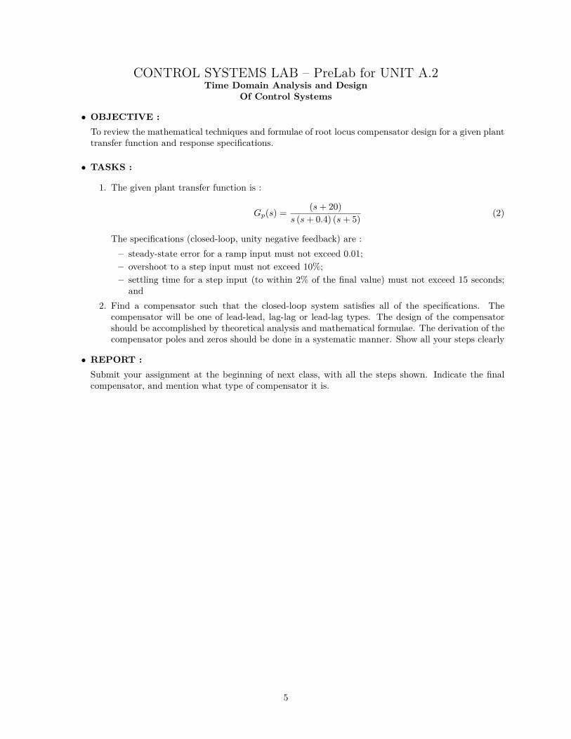
1. The given plant transfer function is :

Gp(s) = (s+ 20)s (s+ 0.4) (s+ 5) (2)

The specifications (closed-loop, unity negative feedback) are :– steady-state error for a ramp input must not exceed 0.01;– overshoot to a step input must not exceed 10%;– settling time for a step input (to within 2% of the final value) must not exceed 15 seconds;

and2. Find a compensator such that the closed-loop system satisfies all of the specifications. The

compensator will be one of lead-lead, lag-lag or lead-lag types. The design of the compensatorshould be accomplished by theoretical analysis and mathematical formulae. The derivation of thecompensator poles and zeros should be done in a systematic manner. Show all your steps clearly

• REPORT :Submit your assignment at the beginning of next class, with all the steps shown. Indicate the finalcompensator, and mention what type of compensator it is.

5

CONTROL SYSTEMS LAB – UNIT A.2Time Domain Analysis and Design

Of Control Systems1 Week

• OBJECTIVE:To use MATLAB to analyze the time domain response of a third-order dynamic system, and to designclosed-loop feedback control systems using cascade compensation in order to satisfy desired time domainspecifications.

• TASKS:

1. The plant transfer function is the one given in experiment A.1 (with K = 1). The followingspecifications are imposed on the closed-loop system:

– steady-state error for a ramp input must not exceed 0.01;– overshoot to a step input must not exceed 10%;– settling time for a step input (to within 2% of the final value) must not exceed 15 seconds;

and– ratios of compensator zero to pole must satisfy αlead = zcd/pcd > 0.05 and αlag = zcg/pcg < 20

for any single stage of compensation.2. Design a compensator such that the closed-loop system satisfies all of the specifications. Possible

compensator types might include phase lead, phase lag, lag-lead, PID, PD, or PI. More thanone section of compensator can be used if necessary. The design of the compensator should beaccomplished by theoretical analysis aided by the time-domain response capabilities of MATLAB.Random trial and error will not be acceptable.

3. Verify that the final closed-loop system satisfies the requirements. Time domain plots of the stepand ramp responses are required for this. Make sure that “steady-state” can be easily identifiedin each of the plots.

• REPORT:Write a report containing a description of the design problem and your approach to designing a com-pensator. Include your reasons for choosing the particular compensator type and how the compensatorparameter values were obtained. Include all plots necessary to verify that the specifications have beensatisfied.

6

CONTROL SYSTEMS LAB – PreLab for UNIT A.3Frequency Domain Analysis and Design

Of Control Systems

• OBJECTIVE :To review the mathematical techniques and formulae of bode analysis and compensator design for agiven plant transfer function and frequency domain specifications.

• TASKS :

1. The given plant transfer function is :

Gp(s) = (s+ 20)s (s+ 0.4) (s+ 5) (3)

The specifications (closed-loop, unity negative feedback) are :– steady-state error for a ramp input must not exceed 0.01;– phase margin for the compensated system must be at least 40o;– compensated gain crossover frequency must be in the range 1–2 r/s;

2. Find a compensator such that the closed-loop system satisfies all of the specifications. Thecompensator will be one of lead-lead, lag-lag or lead-lag types. The design of the compensatorshould be accomplished by theoretical analysis and mathematical formulae. The derivation of thecompensator poles and zeros should be done in a systematic manner. Show all your steps clearly

• REPORT :Submit your assignment at the beginning of next class, with all the steps shown. Indicate the finalcompensator, and mention what type of compensator it is.

7

CONTROL SYSTEMS LAB – UNIT A.3Frequency Domain Analysis and Design

Of Control Systems1 Week

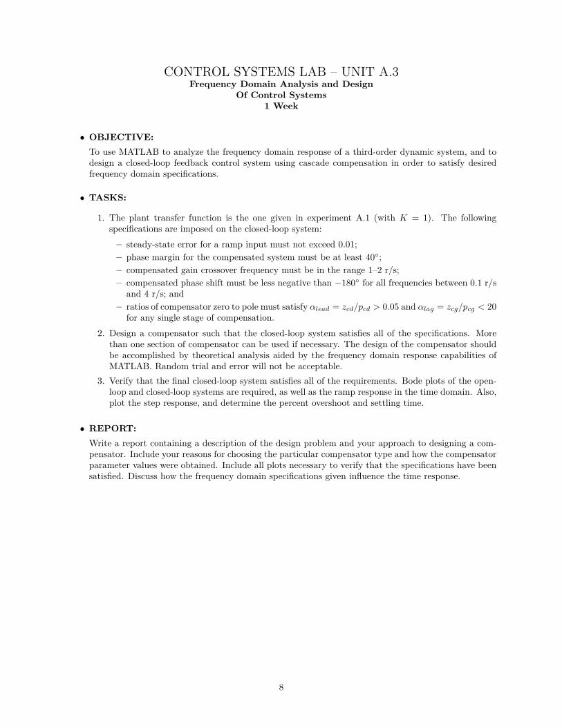
• OBJECTIVE:To use MATLAB to analyze the frequency domain response of a third-order dynamic system, and todesign a closed-loop feedback control system using cascade compensation in order to satisfy desiredfrequency domain specifications.

• TASKS:

1. The plant transfer function is the one given in experiment A.1 (with K = 1). The followingspecifications are imposed on the closed-loop system:

– steady-state error for a ramp input must not exceed 0.01;– phase margin for the compensated system must be at least 40◦;– compensated gain crossover frequency must be in the range 1–2 r/s;– compensated phase shift must be less negative than −180◦ for all frequencies between 0.1 r/s

and 4 r/s; and– ratios of compensator zero to pole must satisfy αlead = zcd/pcd > 0.05 and αlag = zcg/pcg < 20

for any single stage of compensation.2. Design a compensator such that the closed-loop system satisfies all of the specifications. More

than one section of compensator can be used if necessary. The design of the compensator shouldbe accomplished by theoretical analysis aided by the frequency domain response capabilities ofMATLAB. Random trial and error will not be acceptable.

3. Verify that the final closed-loop system satisfies all of the requirements. Bode plots of the open-loop and closed-loop systems are required, as well as the ramp response in the time domain. Also,plot the step response, and determine the percent overshoot and settling time.

• REPORT:Write a report containing a description of the design problem and your approach to designing a com-pensator. Include your reasons for choosing the particular compensator type and how the compensatorparameter values were obtained. Include all plots necessary to verify that the specifications have beensatisfied. Discuss how the frequency domain specifications given influence the time response.

8

CONTROL SYSTEMS LAB – PreLab for UNIT B.1Implementation of Contol Systems

using Simulink

• OBJECTIVE:To become familiar with the Simulink toolbox in MATLAB and the functions of different blocks availalein the library.

• TASKS:

1. Generate the plant transfer function given below :

Gp(s) = 10(s+ 5)s(s+ 1)(s+ 10)

– The plant is used with unity negative feedback. Calculate the closed loop system.– Plot the step response of the closed loop system.

2. Open the simulink ‘Library Browser’ by clicking on Start → Simulink. Open a new model file(.mdl). Build a model of the above closed loop system by using the following blocks.

– Continuous → Transfer Fcn– Commonly Used Blocks → Sum– Sources → Step– Sinks → Scope

You will need to ‘drag and drop’ each block in your model file. Double-click on the blocks to openit’s property editor. This will give you options of changing the parameters of the blocks. Connectthe Scope to the output.

Transfer Fcn

10s+50

den(s)

Step Scope

3. Arrange the blocks in the proper order, and connect them.4. Go to Simulation→ Configuration Parameters. Set the Stop Time as 10. Simulate the model and

look at the output by double-clicking on the Scope. Compare this output to the step responsewhich you generated earlier.

5. Generate a plot of the error (input to the plant) by connecting another Scope at the appropriatelocation.

• REPORT:Upload the model file on Blackboard. This PreLab won’t be graded, but it is recommended that youfamiliarize yourself with Simulink before Lab B.1

9

CONTROL SYSTEMS LAB – UNIT B.1Introduction to Simulink

(implementing PD control)1 Week

• OBJECTIVES:

1. To create Simulink models of physical systems.2. To become familiar with PD control.

• OVERVIEW:The system to be controlled is a mechanical mass-spring-damper system (see figure below). The input isa force, u and the output is the displacement of the first mass, y. The open-loop system is representedby the blocks connected with dampers only and no springs. The spring (connected to the first block)provides the feedback in the model. The damping factors are b and the spring constant is k.

The open loop model (without spring) is defined by the following differential equations :

my = −b(y − x) + u (4)

mx = −bx+ b(y − x) (5)

Feedback is provided by attaching a spring to the first block (as shown in figure). For the closed loopsystem, equation (4) changes to

my = −b(y − x)− ky + u

• TASKS (by hand) :

1. Compute the open loop transfer function of the model. Use equations (4) and (5). y is the output,and u is the input. Show that the transfer function is

Gp(s) =mb s+ 2

m2

b s3 + 3ms2 + bs

2. Compute the closed loop transfer function by using the modified equation (4). Verify that thefeedback function, H(s), is equal to k.

• TASKS (using MATLAB) :

Use the following data for the tasks : m = 1, b = 0.1, k = 0.5. Use 0.1 as the step size for allsimulations.

10

1. Develop a Simulink model (using the differential equations) for the open loop system. Simulateit for a step input of 1 for 50s. Is the system stable? (OpenLoop.mdl)

2. Develop a Simulink model for the closed loop system. (Again, by using the differential equationsand not the transfer function). Simulate it for 50s. Is the system stable? What is the approximatesteady state error and peak oversoot? (ClosedLoop.mdl )

3. Implement the PD controller with the closed loop model. Adjust the controller gains such thatthere is negligible overshoot, and a settling time of about 10s. Will you be able to remove thesteady state error with this controller? If yes, how? If no, why? ( PDcontrol.mdl )

• REPORT:Write a report which documents your design process. Include the tasks to be done by hand in yourreport. All steps should be clearly mentioned. Include all plots and results. Discuss the process ofimplementing the PD controller, and how you selected the gains. Did the final closed loop step resonsemeet the design specifications? Also upload the 3 simulink model files along with the report.

11

CONTROL SYSTEMS LAB – UNIT B.2Compensator Design and Evaluation

for Ship Heading Angle1 Week

• OBJECTIVES:

1. To design a compensator to control the heading angle of a ship such that it satisfies a set oftime-domain performance objectives.

2. To test the robustness of the compensator designed using Simulink.

• OVERVIEW:The system to be controlled is the heading angle of a ship. The input to the system is the rudder angle,and the output is the heading angle. The transfer function for a linear model of the Mariner-class cargoship with nominal parameter values is shown below.

Gp−nom(s) =3.7424 · 10−3 ·

(s+ 5.3879 · 10−2)

s (s+ 8.4688 · 10−3) (s+ 1.2870 · 10−1) (6)

• TASKS:

1. Compensator Design :

The closed-loop response for a unit step input must satisfy the following specifications:– the settling time (2%) must be less than 125 seconds;– the overshoot must be less than 25%; and– the maximum absolute value of the rudder angle must be less than 3.

Design a compensator which accomplishes this. Does the overshoot match exactly the desiredspecification? Explain.

2. Results of compensated system :

Develop a SIMULINK model for the closed-loop system (unity negative feedback). The for-ward path should consist of one transfer function block for your compensator and one transferfunction block for the ship model. The reference input (ordered heading angle) should be a stepof amplitude 10, beginning at time t = 5s.The simulation should be run for 300 seconds. A variable-step integration time should be used.Choose a numerical integration method such as the ode23s (stiff/Mod. Rosenbrock) method. Thefollowing variables should plotted (using the scope) and returned to the MATLAB workspace bythe simulation (a time vector tout is automatically returned):

– reference input (ordered heading angle);– commanded rudder angle (output of your compensator).– actual heading angle;

3. Testing robustness of compensator - introduce nonlinear effects :

Often, while designing compensators, there are assumptions made about the physical system.In the above design we have assumed that the output of the compensator is the ‘commanded

12

rudder angle’ which is used to steer the ship. However, in reality the ‘actual rudder angle’ isa nonlinear transformation of the ‘commanded rudder angle’ (due to effects such as saturation,deadzone, hysterisis and rate limiting). Using SIMULINK we test the compensator when thecommanded input is transformed to the actual input.Insert the ‘Nonlinear steering mechanism’ block between the compensator and the plant transferfunction. The simulation should be run for 1200 seconds. The following variables should plotted(using the scope) and returned to the MATLAB workspace by the simulation :

– reference input (ordered heading angle);– commanded rudder angle;– actual rudder angle;– actual heading angle;

Compare the results of this simulation with that of Task 2. How does the change in the steeringmechanism affect the output of the system?

4. Testing robustness of compensator - introduce perturbations in the system

(a) Repeat Task 3 (with the nonlinear steering mechanism) using the system transfer function as

Gp−min(s) =1.4970 · 10−2 ·

(s+ 2.6940 · 10−2)

s (s+ 1.6938 · 10−2) (s+ 1.2870 · 10−1)

(b) Repeat Task 3 using the system transfer function as

Gp−max(s) =9.3560 · 10−4 ·

(s+ 1.0776 · 10−1)

s (s+ 4.2344 · 10−3) (s+ 1.2870 · 10−1)

Compare the results of (a) and (b) with that of Task 3. Is the compensator still able to controlthe heading angle of the ship. Does the change in the ship parameters affect the overshootand settling time?

• REPORT:Write a report which documents your design process as well as your analysis of the designed compen-sator. Discuss how satisfying the performance specifications is related to the locations of the closed-looppoles. Include time domain plots, and other plots if appropriate (such as root locus), to illustrate andjustify your work.Also show the robustness of your compensator. Illustrate (using appropriate plots and arguments) howthe compensator work/does not work after taking the inaccuracies into account.Discuss the ease or difficulty of developing a SIMULINK model for evaluating the response relative towriting code directly in MATLAB.

13

CONTROL SYSTEMS LAB – UNIT B.3Compensator Design and Evaluation

for Depth Rate Control1 Week

• OBJECTIVES:

1. To design a compensator for a given system such that the compensated system satisfies a set offrequency-domain performance objectives.

2. To analyze the effects of implementing the compensator in different configurations.

• OVERVIEW:The system to be controlled (plant) represents the dynamics relating rate of change of applied forceto rate of change of vertical position for an underwater vehicle having zero forward speed. The inputto the plant is the flow rate of water into or out of depth control tanks in the vehicle (lbs/sec), andthe output is the vehicle’s depth rate, that is, its vertical velocity (ft/sec). The transfer function for alinearized model of the system to be used in this experiment is shown below.

Gp(s) = 5 · 10−7

s2 (s+ 0.75) (7)

The reference signal for the closed-loop system is the desired depth rate. The system has unity feedback.

The compensator can be implemented in multiple configurations : as a Proportional-Derivative (PD)controller or as Proportional-Derivative-on-output-only (PD-DOO) controller.

• TASKS:

1. Compensator Design :

The compensated system must satisfy the following specifications.– the compensated phase margin must be in the range of 45 to 50 degrees;– the compensated gain crossover frequency must be in the range of 0.045 to 0.055 rad/sec.– note that there is no steady state error requirement.

2. Results of compensated system :

Verify that the compensator you design satisfies the specifications by producing Bode plots ofthe compensated system. Use the margin function in MATLAB to determine the actual values ofphase margin and gain crossover frequency. Also, plot the compensated closed-loop step response,and determine the overshoot and settling time.

3. Implementation of compensator as a PD controller :

Use the values of compensator gain, pole and zero (from Task 1) to determine the values forthe PD controller gains (Kp,Kd, τ). Implement this PD controller in simulink with a unit stepinput and unity negative feedback. Compare the output of the closed loop system in this config-uration to the output from Task 2.

4. Implementation of compensator as a PD-DOO controller

In simulink, implement the controller from Task 3 in PD-DOO form (discussed in class notes).Compare the output to the outputs from Tasks 2 and 3.

14

• REPORT:Write a report which documents your design process. Include Bode plots for the compensated anduncompensated systems, and the compensated step response plot. Discuss why the time-domain per-formance for the compensated closed-loop system will be better than the closed-loop performance ofthe uncompensated system (plant model with unity feedback). Give your opinion on the overshoot inthe step response, taking into consideration what the system model actually represents.

Include the step response of the closed loop system for each implementation of the compensator.Discuss the differences seen in the different implementations. Which do you think is the better config-uration. Why?

15

CONTROL SYSTEMS LAB – PreLab for UNIT CPosition Control for a servo motor

• OBJECTIVES:

1. To identify a type-1 system from closed loop step response measurements.2. To design a compensator (in PD-DOO configuration) for the system such that a given set of

transient response specifications is met.3. To become familiar with the Torsional Plant (205a) and the Educational Control Products (ECP)

software.

• OVERVIEW:

1. The system to be identified and controlled is a rigid body system with input from a DC motor.

Figure 1: From the ECP manual, for Torsional Plant 205

J is the moment of inertia of the disc, θ(t) is the angular position of the disc (output) and T (t)is the torque applied by the motor (input). In an ideal case this would be an undamped system.However, due to the effect of friction there will be a damping constant, c. The equation for thissystem becomes

T (t) = J θ(t) + c θ(t) (8)

2. The torsional plant is interfaced to the computer through a data board and can be controlledusing the ECP software. The software allows you to implement different types of controllers withuser-defined parameters. The input to the system, in terms of degrees, can be generated. Theposition, velocity and acceleration of the discs can be measured and plotted. Ask the instructorto give a demonstration of the different functionalities of the software. More information aboutthe hardware and software can be found at http://www.ecpsystems.com/.

• TASKS:

1. Derive the open loop plant transfer function, Gp(s), from equation (7). The input is the torque -T (t) and the output is the position of the disc, θ(t).

2. Use closed loop step response measurements to identify the parameters, J and c of the system.– A unity feedback is applied to the plant with a gain, Kp = 0.1. (Fig. 2)– Derive the closed loop transfer function, Gc1(s).– Assume that from the step response of the closed loop system the time-to-peak, tp = 0.5s,

and overshoot, Mp = 30% is determined.– Compute ωn and ζ for the closed loop system.

16

Figure 2: Proportional closed loop control

– In this configuration, Kp, ωn and ζ are now known. The unknown parameters are J andc. Compute the unkown parameters .by comparing Gc1(s) to a general second order system,

ω2n

s2+2ζωns+ω2n

.

3. Design the proportional (Kp) and derivative (Kd) coefficients for a controller in Propotional-Derivative with Derivative on Output Only (PD-DOO) form. (Fig. 3)

Figure 3: Proportional-Derivative closed loop control with Derivative-on-Output-Only

– Derive the closed loop transfer function, Gc2(s).– Let the desired specifications of the compensated, closed loop system be ωn = 12 and ζ = 0.6.– In this configuration the known parameters are J , c, ωn and ζ. Determine the unknown

coefficients, Kp and Kd by again comparing Gc2(s) to a general second order system.4. Learn to operate the hardware and software for the Torsional Plant, model 205a. You can perform

this task with a group partner. Follow the steps to construct a rigid body setup (as shown in Fig.1.) and take closed loop step response measurements. The hardware is shown in Fig. 4.

– Switch on the computer. Do NOT turn on the hardware.– Attach a single disc in the lower most position of the torsional spring. Attach 2 masses on

either end of a diameter of the disc. Do not attach anything in the other two positions.– Turn on the hardware. Start the ECP software on the computer.– Go to Setup - User Units and select Degrees– Go to Setup - Setup Control Algorithm∗ Select Continuous Time∗ Select PI with Velocity Feedback and click on Setup Algorithm∗ Enter 0 for Kd and Ki. Feedback should be from Encoder 1.∗ Choose a value between 0.02 and 0.3 for Kp. Click OK.∗ Click on Implement Algorithm first, and then on OK to return to the main screen.

– Select Command and then Trajectory Configuration.∗ Select Step and click on Setup.∗ Select Closed Loop Step with a Step Size of 25 degrees, Dwell Time of 5000ms and

Number of Reps as 1.∗ Click OK and return to main screen.

– Select Command and then Execute

17

∗ Choose Normal Data Sampling and click OK– Select Plotting and then Setup Plot∗ Add Commanded Position and Encoder 1 Position on the Left Axis. Do not add

anything to the Right Axis.∗ Click OK. Then select Plotting and click on Plot Data.

– The plot shows the closed loop step response of the system. Experiment with different valuesof Kp.

Figure 4: From http : //www.ecpsystems.com/docs/ECP Torsion Model 205.pdf

• REPORT:Solve the problems outlined in tasks 1, 2 and 3. The derivations and equations should be shown clearly.Also mention what you observed by changing the value of Kp in task 4. Is this what you expected?Explain with the help of the system defined in task 2. You do not need to include plots in your report.

18

CONTROL SYSTEMS LAB – UNIT C.1Position Control for a servo motor

System Identification1 week

• OBJECTIVES:

1. To generate the closed loop step response of the rigid body system, and compute overshoot andtime-to-peak.

2. To calculate the moment of inertia and frictional damping coefficient of the rigid body system.

• OVERVIEW:The system to be identified is the Gp(s) derived in Unit C.1 from equation (7). J is the moment ofinertia and c is the coefficient of damping. The overshoot and time-to-peak should be computed fromthe closed loop step response curve. These values can be used to compute J and c as derived in thePreLab for Unit C.

• TASKS:

1. Set up the Torsional plant in the rigid body system setup (illustrated in PreLab for Unit C).2. Put two weights on the ends of a diameter of the disc. The other two weights are to be put at

approximately a distance of n cms from the center on the other diameter of the disc, on oppositesides. Here, n is the last non-zero digit of your G number. For example, if your G number isG12450230, then n = 3. The concentric circles on the disc correspond to 1 cm each. The radiusof the disc is 9 cms.

3. Set the input to a 25 degrees step. Set up the controller in PI with Velocity Feedback form.Set Kp and Kd to zero. Experiment with the value of Kp such that you get a ‘nice’ and stablestep response curve. Choose 3 such Kp.

4. For each value of Kp, run the simulation 3 times, and take the average of the time-to-peak, tpand percent overshoot, Mp. Use these average value to compute J and c.

5. Report the 3 different J and c corresponding to the 3 Kp. Are they the same? Why?

• REPORT:Submit a report which contains all the details of the experiment you have performed. Mention the stepsin setting up the system, executing and generating the step response curve, and measuring the values.All the data collected should be put in a table. Report the result of system identification. Also mentionany particular difficulty you faced while performing the experiment or taking the measurements.

19

CONTROL SYSTEMS LAB – UNIT C.2Position Control for a servo motor

Designing Controller1 week

• OBJECTIVES:To design a Proportional-Derivative (with Derivative on Output Only), PD-DOO, controller for thesystem identified in Unit C.1

• OVERVIEW:The system identified in Unit C.1 needs to be controlled. Using the plant transfer function, andspecifying a desired zeta and ωn, a controller is to be designed. The controller will be in the PD-DOOform (with Ki = 0), and the Kp and Kd parameters are to be found out. The controller should first betested by simulation of the closed loop system in MATLAB, and then finally tested on the hardware.

• TASKS:

1. Find the closed loop system for the system defined in PreLab for Unit C, task 3 (Fig. 3).2. Decide a suitable response. You will have to choose a desired peak overshoot (Mp), and either a

desired time-to-peak (tp) or a desired settling time (ts).3. Compute the desired ζ and ωn using the specifications.4. Compare the closed loop system with the general 2nd order system to find the coefficients Kp andKd.

5. Simulate the compensated system in MATLAB (m-file or Simulink) and check if you are satisfyingthe specifications set in task 2.

6. Set up the torsional plant with the corresponding Kp, Kd and Ki = 0 values, and generate thestep response. Does your controlled system meet the specifications you desired?

7. If there is a large error in your achieved and desired values (Mp, tp and ts) in experimentation,try to perform the system identification again and re-design your controller. Remember to keepthe same value for the input (25 degrees step function) in all cases. Again, it would be helpful ifyou write an m-file so that you can enter the number from your step response measurements (inUnit C.1) and your specifications - and the code will output the values for Kp and Kd. Rememberto run the system 3 times for all cases, and report the results in each of the 3 runs.

8. Once you are able to achieve the desired response on the torsional plant (with reasonable errortolerance), change the position of the weights.

– Change the position of the 2 weights which are on the end, and bring them in by 2-3 cms.Execute with the same input, and measure the percent overshoot and time to peak. Havethey changed? Is it what you expected? Explain in a short paragraph why this happens.

– Put the 2 weights back on the edge of the disc. Now change the position of the other 2 weights(the ones which you placed according to your G-number), and move them out by 2-3 cms.Again execute with the same input and measure the results. Do it 3 times to ensure thatthere is no error. Explain what you see.

• REPORT:Submit a report which contains all the details of the design steps and experiments you have performed.Clearly mention the specifications you chose. Also, compare the results obtained via simulation andvia experimentation. The report should give the reader a good idea of what was the objective of theentire project and how you solved the problem.

20

CONTROL SYSTEMS LAB – PreLab for UNIT DBall and Beam Experiment

• OBJECTIVES:

1. Modeling dynamics of the ball from first principles.2. Obtaining transfer function representation of the system.

• OVERVIEW:The system to be controlled (plant) represents the dynamics of a ball balancing on a beam. The angleof the beam is controlled by a servo motor. In this assignment, you are required to compute the relationbetween the angular position of the servo motor and the linear position of the ball on the beam. Thevariables used in the derivation are :

x(t) Linear position of ball on beamα(t) Angle of beamθ(t) Angular position of servo motorγb(t) Angle of ballrb Radius of ballJb Moment of inertia of ballmb Mass of ball

The time varying parameters - x(t), α(t), θ(t), γb(t) are abbreviated as - x, α, θ, γb.

Figure 5: Completed ball and beam free body diagram

Use the following relations to find the transfer function between θ(t) (input) and x(t) (output).

Fx,t = mbg sin(α), Fx,r = τbrb, τb = Jbγb, Jb = mbr

2b

mx = Fx,t − Fx,r

x = γbrb, sin(α) = h

Lbeam, sin(θ) = h

rarm

You will also need to use the following assumption : sin(θ) ∼ θ

• TASKS:

1. Compute the differential equation relating the ball position to the angular position of the servomotor.

2. Write down the transfer function (in terms of variables defined) :

Pbb(s) = Θ(s)X(s)

21

CONTROL SYSTEMS LAB – UNIT D.1Ball and Beam Experiment

Design and Test Controller using MATLAB/Simulink1 week

• OBJECTIVES:

1. Understanding the system of servo motor and ball balancer.2. Designing an accurate PD-DOO controller for the position control of the servo motor.3. Designing a PD-DOO controller, with filtering, to balance the ball on the beam.4. Testing the entire system using Simulink (physical limits of the system to be incorporated).

• OVERVIEW:

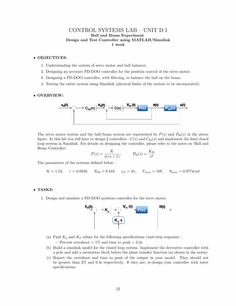
The servo motor system and the ball/beam system are represented by P (s) and Pbb(s) in the abovefigure. In this lab you will have to design 2 controllers - C(s) and Cbb(s) and implement the final closedloop system in Simulink. For details on designing the controller, please refer to the notes on ‘Ball andBeam Controller’.

P (s) = K

s(τs+ 1) , Pbb(s) = Kbb

s2

The parameters of the systems defined below :

K = 1.53, τ = 0.0248, Kbb = 0.419, ωf = 2π, Vmax = 10V, θmax = 0.9774rad

• TASKS:

1. Design and simulate a PD-DOO position controller for the servo motor.

(a) Find Kp and Kd values for the following specifications (unit-step response) :– Percent overshoot = 1% and time to peak = 0.2s

(b) Build a simulink model for the closed loop system. Implement the derivative controller witha pole and add a saturation block before the plant transfer function (as shown in the notes).

(c) Report the overshoot and time to peak of the output in your model. They should notbe greater than 2% and 0.4s respectively. If they are, re-design your controller with lowerspecifications.

22

2. Design and simulate a PD-DOO (with filtering) controller for the ball balancing model (ignoreservo dynamics).

(a) Find Kp,bb and Kd,bb values for the following specifications (unit-step response) :i. Percent overshoot = 15% and settling time = 5sii. Percent overshoot = 1% and settling time = 3s

(b) Build a simulink model (for both cases) of the closed loop system (without the servo transferfunction). Verify that the output, x(t) satisfies the specifications.

3. Solve the following tasks for both cases (using the appropriate controller as designed earlier).

(a) Build the complete system in Simulink (including the saturation blocks).(b) Simulate the model to balance the ball at 2 cm.(c) Include the following plots in your report

– Desired and actual ball position.– Desired and actual servo angle position.– Input voltage to the servo motor.

(d) Analyzing the plots, explain why the response (overshoot and settling time) is not the sameas that in Task 2. What can be done to reduce the difference?

• REPORTWrite a report indicating the problem that you have solved in this lab. Mention clearly the systems,and the type of controllers you have designed. Include all the plots generated. Explain the differenceyou see in Task 2 and Task 3.

23

CONTROL SYSTEMS LAB – UNIT D.2Ball and Beam Experiment

Implement controller using Simulink and QUARC1 week

• OBJECTIVES:To implement the controller designed in Unit D.1 in real-time using MATLAB Simulink and QUARC.

• OVERVIEW:Using the PD controller designed in the last lab, the ball will be balanced on the beam at a desiredposition. It is important to note how the theoretical design translates to real results.

• TASKS:

1. Implement and check results of the servo motor controller from D.1.– Start MATLAB. Run the file BallBeam Parameters.m.– Load and run the code you wrote in the previous lab to generate the controller parameters

for the position control of the servo motor (Task 1, Unit D.1).– Open the simulink model ControlServo Incomplete.slx. Save the file as ControlServo YourName.slx– Complete the model using the PD-DOO controller. The input block and open loop plant are

already built in the model.– Remember that the servo motor angle is measured in radians. You will need to convert the

input (desired angle, θd) to radians and similarily the output (actual angle, θ) to degrees.– The saturation blocks have already been added at the appropriate places.– Switch on the amplifier, and connect the data acquisition device to the system via the USB

port.– Choose a simulation time of 10s. The solver should be a fixed step solver (ODE 8) and the

step size should be 0.002s.– You will first need to ‘build’ your model, and then ‘Connect to Target’. After this, run your

model. You should see the servo motor changing position.– Plot the desired servo angle and the actual servo angle. Also plot the voltage input to the

plant.– Is the result what you expected to see, based on what you designed for?

2. Implement and check results of the ball and beam controller from D.1 (for both cases)– Start MATLAB. Run the file BallBeam Parameters.m.– Load and run the codes you wrote in the previous lab to generate the controller parameters

for the servo motor as well as the ball balancing model (Task 1 and 2, Unit D.1).– Open the simulink model ControlBallBeam Incomplete.slx. Save the file as

ControlBallBeam YourName.slx– Complete the model. The closed loop servo motor is built as a subsystem. Double click the

block to open it. Complete the subsystem first (similar to Task 1 in this lab). Next, completebuilding the controller for the ball and beam plant.

– Remember that the servo motor angle is measured in radians and the ball position is measuredin m (not cm). You will need to convert the input (desired ball position, xd) to m andsimilarily the output (actual position, x) to cms before plotting. Also, convert the angles(θ, θd) to degrees before plotting.

– The saturation blocks have already been added at the appropriate places.– Switch on the amplifier, and connect the data acquisition device to the system via the USB

port.

24

– Choose a simulation time of 10s. The solver should be a fixed step solver (ODE 8) and thestep size should be 0.002s.

– You will first need to ‘build’ your model, and then ‘Connect to Target’. After this, run yourmodel. You should see the servo motor changing position.

– Plot the desired ball position and the actual ball position (in cms). Also plot the desiredservo angle and actual servo angle (in degrees).

– Do you see any correlation between your simulated results from D.1 and the results of theactual system? Are the results identical? Explain.

• REPORT:Submit a report which contains all the details of the design steps and experiments you have performed.Mention how simulation helped you test the controller, and whether the results of the actual systemwere similar. Also, explain the plots in terms the real system and what you actually observed.

25

CONTROL SYSTEMS LAB – UNIT EInverted Pendulum Experiment

Controller Design and Implementation3 weeks

• OBJECTIVES:

1. Obtaining transfer function representation of the inverted pendulum setup.2. Designing a PD controller using feedback from measured angles.3. Testing the PD controller using Simulink.4. Implementing the PD controller in real time using Simulink and QUARC.

• OVERVIEW:The system to be controlled (plant) represents the dynamics an inverted pendulum. The aim is tokeep the pendulum upright (at a desired pendulum angle of zero) by varying the motor angle. The

Figure 6: Inverted Pendulum Setup

measured variables (to be used as feedback for closed loop control) are the pendulum angle, α(t),and the servo motor angle, θ(t). Following are the differential equations which establish the dynamicrelation between α(t), θ(t) and the control input, u(t).

θ(t) = 80.3α(t)− 10.2θ(t)− 0.93α(t) + 83.2u(t)α(t) = 122α(t)− 10.3θ(t)− 1.4α(t) + 80.1u(t)

The open loop transfer functions needed to design the controller are :

Pθ(s) = Θ(s)U(s) , Pα(s) = α(s)

U(s)

26

• TASKS:

1. Derive the transfer functions, Pθ(s) and Pα(s) from the differential equations described above.Assume all initial conditions to be zero. [15]

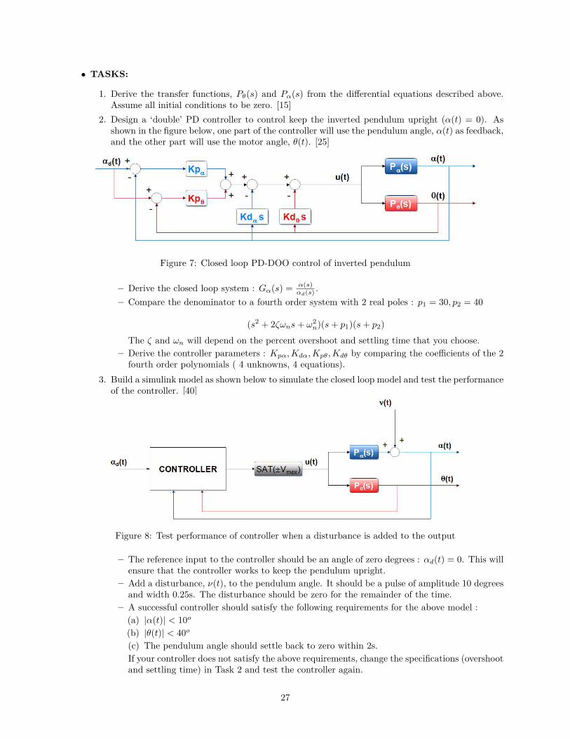
2. Design a ‘double’ PD controller to control keep the inverted pendulum upright (α(t) = 0). Asshown in the figure below, one part of the controller will use the pendulum angle, α(t) as feedback,and the other part will use the motor angle, θ(t). [25]

Figure 7: Closed loop PD-DOO control of inverted pendulum

– Derive the closed loop system : Gα(s) = α(s)αd(s) .

– Compare the denominator to a fourth order system with 2 real poles : p1 = 30, p2 = 40

(s2 + 2ζωns+ ω2n)(s+ p1)(s+ p2)

The ζ and ωn will depend on the percent overshoot and settling time that you choose.– Derive the controller parameters : Kpα,Kdα,Kpθ,Kdθ by comparing the coefficients of the 2

fourth order polynomials ( 4 unknowns, 4 equations).3. Build a simulink model as shown below to simulate the closed loop model and test the performance

of the controller. [40]

Figure 8: Test performance of controller when a disturbance is added to the output

– The reference input to the controller should be an angle of zero degrees : αd(t) = 0. This willensure that the controller works to keep the pendulum upright.

– Add a disturbance, ν(t), to the pendulum angle. It should be a pulse of amplitude 10 degreesand width 0.25s. The disturbance should be zero for the remainder of the time.

– A successful controller should satisfy the following requirements for the above model :(a) |α(t)| < 10o

(b) |θ(t)| < 40o

(c) The pendulum angle should settle back to zero within 2s.If your controller does not satisfy the above requirements, change the specifications (overshootand settling time) in Task 2 and test the controller again.

27

4. Implement your controller on the real system and measure the duration for which it keeps theinverted pendulum upright. [20]

– Start MATLAB. Run the file InvertedPendulum Parameters.m.– Load and run your code to generate the controller parameters (Kpθ,Kdθ,Kpα,Kdα).– Open the simulink model ControlPendulum Incomplete.slx. Save the file as ControlPendu-

lum YourName.slx– Complete the model using the PD-DOO controller. The input block and open loop plant are

already built in the model. There won’t be any disturbance added to the model.– Build the model and Connect-to-target. Start the simulation and slowly move the pendulum

to the upright position. You will feel the controller turn on as it reaches the zero degreeangle. Leave the pendulum and let the controller maintain it in its upright position. Whenthe pendulum falls down, stop the simulation.

• REPORT:Submit a report which contains all the details of the design steps and experiments you have performed.The report should contain steps of the controller design, results of simulation and finally the perfor-mance while implementing it on the actual system. The content of the report as well as the resultswill be graded. Make sure that your report has the proper plots and discussions.

28