Earnings management and the underperformance...

Journal of Financial Economics 50 (1998) 63—99

Earnings management and the underperformance ofseasoned equity offerings1

Siew Hong Teoh!,*, Ivo Welch", T.J. Wong#

! University of Michigan Business School, Ann Arbor, MI 48109, USA" Anderson Graduate School of Management, UCLA, Los Angeles, CA 90095, USA# Hong Kong University of Science and Technology, Clearwater Bay, Hong Kong

Received 28 March 1995; received in revised form 26 June 1997

Abstract

Seasoned equity issuers can raise reported earnings by altering discretionary ac-counting accruals. We find that issuers who adjust discretionary current accruals toreport higher net income prior to the offering have lower post-issue long-run abnormalstock returns and net income. Interestingly, the relation between discretionary currentaccruals and future returns (adjusted for firm size and book-to-market ratio) is strongerand more persistent for seasoned equity issuers than for non-issuers. The evidence isconsistent with investors naively extrapolating pre-issue earnings without fully adjustingfor the potential manipulation of reported earnings. ( 1998 Elsevier Science S.A. Allrights reserved.

JEL classification: G14; G24; G32; M41

Keywords: Corporate finance; Seasoned equity offerings; Earnings management;Accounting accruals; Anomalies; Market efficiency

*Corresponding author. Tel.: 313/763-1264; fax: 313/764-2557; e-mail: [email protected].

1We thank Brad Barber (the referee), Randy Beatty, Vic Bernard, K.C. Chan, Kent Daniel, MarkDeFond, Laura Field, David Heike, Chuan Yang Hwang, Jonathan Karpoff, S.P. Kothari, CharlesLee, Wayne Mikkelson (the editor), Tim Opler, Krishna Palepu, K. Ramesh, Jay Ritter, TerryShevlin, Doug Skinner, Sheridan Titman, Ross Watts, Jerry Zimmerman, and seminar participantsat the University of California Finance and Accounting Conference (Davis, March 1995), the NBERCorporate Finance Conference (Boston, August 1995), the Center for Research in Security PricesSeminar (Chicago, October 1995), the American Finance Association Conference (San Francisco,1996), the American Accounting Association Conference (Chicago, August 1996), the University ofMichigan, and the University of Rochester for helpful comments and discussions.

0304-405X/98/$19.00 ( 1998 Elsevier Science S.A. All rights reservedPII S 0 3 0 4 - 4 0 5 X ( 9 8 ) 0 0 0 3 2 - 4

1. Introduction

Loughran and Ritter (1995) and Spiess and Affleck-Graves (1995) documentthat firms underperform the stock market in the five years after a seasonedequity issue. For example, Loughran and Ritter report average returns ofonly 7% per year, while comparable non-issuing firms average 15% per year.The return differentials are so large that one wonders why investors buy theseissues.

In this paper, we examine whether unusually aggressive management ofearnings through income-increasing accounting adjustments leads investors tobe overly optimistic about the issuer’s prospects. That is, investors may misinter-pret high earnings reported at the time of the offering, and consequentlyovervalue the new issues. When high pre-issue earnings are not sustained,disappointed investors subsequently revalue the firm down to a level justifiedby fundamentals. This earnings management hypothesis predicts that issuershave unusually high income-increasing accounting adjustments pre-issue andunusually poor earnings and stock return performance post-issue. Further,the hypothesis predicts worse performance for issuers with unusually largeincome-increasing accounting adjustments prior to the offering.

We report evidence consistent with the earnings management hypothesis. Fora sample of seasoned equity issuers from 1976 to 1989, Table 2 documentshigher net income growth in the issue year for issuers than for performance-matched non-issuing industry peers. Post-issue, however, issuers significantlyunderperform their matches. For example, the annual growth in the issuers’asset-scaled net income significantly exceeds that of the matched non-issuers bya median of 1.69% in the issue year, but is significantly less than that of thematched non-issuers by a median of 1.60% and 0.32% in the two sub-sequent years. Decomposing net income into cash flow from operations andaccounting adjustments (hereafter referred to as accruals), we find that it is theaccruals that cause the at-issue peak and post-issue underperformance in netincome. In contrast, cash flow from operations exhibit an opposite profile.Table 2 reports that asset-scaled cash flow from operations are 3.8% below theindustry median in the issue year, remain below the industry median for the nexttwo years, and only rise to 1% above the industry median three years after theissue.

We decompose accruals into four categories jointly by time period (currentand long-term) and manager control (discretionary and nondiscretionary).Table 3 reports that of the four categories, discretionary current accruals (thecomponent most subject to managerial manipulation) drive the post-issueearnings underperformance. In the offering year, the asset-scaled discretionarycurrent accruals of issuers exceed their pre-issue performance-matched industrypeers by 2.9%. For each of the three subsequent years, the issuers’ discre-tionary current accruals decline by more than those of their matches. Ranking

64 S.H. Teoh, et al. /Journal of Financial Economics 50 (1998) 63—99

issuers by discretionary current accruals, Table 4 reports that issuers in the mostaggressive quartile (i.e. with the largest discretionary current accruals in thepre-issue year) underperform their matched non-issuers by 7.50% in asset-scalednet income in the three years after the issue year. In contrast, issuers in theconservative quartile outperform their matches by 0.99%. Table 5 reports thatthe Spearman rank correlations between pre-issue discretionary current ac-cruals and post-issue net income changes (all asset-scaled) are approximately!20% and statistically significant in all three post-issue years. In sum, theevidence suggests that discretionary current accruals predict post-issue earningsunderperformance.

Most interestingly, we find evidence that discretionary current accruals alsopredict underperformance in post-issue stock returns. For 48 months after theoffering, issuers in the aggressive quartile underperform conservative issuers bya raw return differential of about 40%, a market-adjusted return differential ofabout 25%, and a Fama—French adjusted return differential of about 35% (seeTable 6). These differences are remarkable considering that the earnings man-agement proxy is based on public information available four to 16 monthsbefore the period over which returns are measured. Finally, in Table 7, we usea Fama—Macbeth type procedure in a sample containing issuing and non-issuing firms. We test whether post-issue abnormal stock returns are negativelyrelated to lagged accruals, and whether this relation is stronger for pre-issueaccruals. The results indicate that discretionary current accruals have a strongerand more persistent influence on subsequent returns for seasoned equity issuers.Therefore, consistent with earnings management, we find evidence that highdiscretionary current accruals predict post-issue long-run earnings and stockreturn underperformance.

2. Accruals-based earnings management proxies

To evaluate the role of earnings management, we construct a proxy for theamount of accounting adjustments undertaken by management. Reported earn-ings in the financial statement consist of cash flow from operations plus totalaccruals:

Net Income"Total Accruals#Cash Flow from Operations. (1)

The accrual adjustments reflect business transactions that affect future cashflows even though cash has not currently changed hands. Under generallyaccepted accounting principles (GAAP), firms have discretion to recognize thesetransactions as economic events, so that reported earnings reflect the trueunderlying business conditions of the firm more accurately. With the accrualsystem of accounting, reported earnings are supposed to be invariant to thetiming of cash receipts and payments. However, managerial flexibility in the

S.H. Teoh, et al. /Journal of Financial Economics 50 (1998) 63—99 65

accruals system also opens opportunities for earnings management.2 By takingincome-increasing accrual adjustments now, managers can raise current re-ported earnings, but future reported earnings will be lower. However, ac-counting regulations, such as the requirement of an independent audit, limit themanager’s discretion over the timing and magnitude of accruals.

Accruals can be classified into categories based on time period and manageri-al control. Current accruals are adjustments involving short-term assets andliabilities that support the day-to-day operations of the firm. For example,managers can alter current accruals by advancing recognition of revenues withcredit sales (before cash is received), by delaying recognition of expenses aftercash is advanced to suppliers, and by assuming a low provision for bad debts. Incontrast, long-term accruals are adjustments involving long-term net assets.These accruals can be altered by decelerating depreciation, decreasing deferredtaxes (the difference between tax expense recognized for financial reporting andactual taxes paid), and realizing unusual gains. We consider current accruals andlong-term accruals separately because accounting researchers (e.g., Guenther,1994) have argued that managers have greater discretion over current accrualsthan over long-term accruals.

Although investors can observe accruals, they cannot infer perfectly whatportion of accruals is discretionary, i.e., ‘managed’. Given industry-related andfirm-specific business conditions, some accrual adjustments are necessary, andindeed expected by investors; for example, asset-intensive firms have highdepreciation, and rapidly growing firms have revenues that exceed cash sales.

To extract these nondiscretionary accruals that are dictated by firm condi-tions and independent of managerial manipulation, we use a cross-sectionaladaptation Teoh et al. (forthcoming b) of the modified Jones (1991) model. Thedetails of the procedure are described in the Appendix. In essence, current

2For specific examples of how earnings can be managed in an accrual accounting system, seeDavidson et al. (1986), Teoh et al. (forthcoming b), Appendix B in Teoh et al. (forthcoming a),Kellogg and Kellogg’s Financial Statement Alert, which is an investor newsletter devoted toferreting out suspicious accounting adjustments, and media articles such as ‘The Sherlock Holmes ofAccounting’, (Business Week, pp. 48—52; September 5, 1994), and the series of articles in Forbes inthe section ‘Numbers Game’, such as ‘Lies of the Bottom Line’ (November 12, 1990), ‘SillyPussyfooting’ (August 21, 1989), ‘Numbers Pumpers’ (November 11, 1991), and ‘Mystery Profits’(April 20, 1987). These articles detail earnings management within generally accepted accountingprinciples and not necessarily fraudulent reporting.

We do not consider fraudulent reporting behavior specifically, because the majority of theseasoned equity issuers in our sample appears to comply with generally accepted accountingprinciples (GAAP). Relatively few firms in the general population are caught not complying withGAAP, and of these, few are seasoned equity issuers. Mike Maher generously provided us the namesof 159 SEC-reporting violators from January 1980 to December 1985, and only seven of our SEOfirms overlapped with his sample of violators.


accruals are regressed on the change in sales in a cross-sectional regression usingall firms in the same two-digit SIC code as the issuer (but excluding the issuer).The cross-sectional regression is performed for each fiscal year, and all variablesare scaled by beginning-year firm assets. After adjusting sales growth for theincrease in accounts receivable, the issuer’s fitted current accruals level, termednondiscretionary current accruals (NDCA

~1), is considered typical in the indus-

try for the level of sales growth. Since the remaining current accruals are notdictated by firm condition, but are managed, they are termed discretion-ary current accruals (DCA

~1).

To decompose long-term accruals, we apply an equivalent procedure. We firstdecompose total accruals into a discretionary and a nondiscretionary compon-ent based on sales growth and property, plant, and equipment (to adjust fordepreciation). The difference between discretionary total accruals and dis-cretionary current accruals is termed discretionary long-term accruals (D¸A

~1);

the difference between nondiscretionary total accruals and nondiscretionarycurrent accruals is termed nondiscretionary long-term accruals (ND¸A

~1).

The cross-sectional approach automatically adjusts for changing indus-trywide economic conditions which influence accruals independently ofearnings management. Using industry benchmarks to measure discretionaryaccruals is suggested by the common practice of underwriters, who price newequity issues by comparing market prices and accounting variables of similarfirms.

To summarize, accruals are decomposed into four components: discretionaryand nondiscretionary current accruals, and discretionary and nondiscretionarylong-term accruals. The nondiscretionary accruals are proxies for accrual recog-nition outside the control of management and the discretionary accruals areproxies for earnings management.3

3. Sample selection and sample characteristics

Our initial sample consists of 6386 seasoned equity issues between January1970 and September 1989 from the Securities Data Corporation. Of these, only3032 issues are available on the primary, full coverage, and research Compustat1993 tapes and on the Center for Research in Security Prices (CRSP) 1993 tapes.For inclusion in the final sample, we require available stock returns data and

3The robustness of models of earnings management measures has been discussed by Dechowet al. (1995), Guay et al. (1996), and Healy (1996). Dechow, Sloan, and Sweeney conclude superiorityof the modified Jones model over all other currently available models, though the Jones modelremains imperfect.


sufficient data to compute discretionary accounting accruals for the year priorto the offering. To avoid survivorship bias, we do not require that firms haveaccruals data for the entire period of three years before to three years after theissue year. Because banking and utilities industries have unique disclosurerequirements, we eliminate firms in these industries from our sample. If a firmhas multiple issues, we include only the earliest issue to avoid using overlappingdata to estimate the returns-accruals relation.

Of the 3032 issuers available on CRSP and Compustat, 2645 have sufficientdata to compute accruals in at least one year between the 1974—1993 periodcovered by Compustat 1993 tapes. Of these, 1285 have at least ten other firms inthe same two-digit SIC code industry group to allow estimation of the intra-industry regression to calculate expected accruals. The final sample consists of1265 issuers with available accruals data in the fiscal year prior to the fiscal yearof the new issue. The actual sample size varies depending on the test proceduresand accruals measures used. Only 1248 firms have available returns during theissue month.

Table 1 reports the sample statistics and data characteristics for our firms.The earliest data available on Compustat 1993 are for fiscal year 1973. Becausewe examine the accruals behavior of seasoned issuers from fiscal year !3 to#3 relative to the fiscal year of the offering, our sample begins in 1976.Seasoned equity issues are clustered by industries and time periods. Four of thesample years (1980, 1982, 1983 and 1986) are very active and contain more than10% of the sample, with 1983 carrying 22% of the issues. Furthermore, thecomputer and electronics industries account for a large fraction of the issueswith approximately 31% of the sample. Earnings management may be prevalentin these relatively new industries because high information asymmetry andlimited past history make it difficult to judge the appropriateness of theaccounting choices.

Panel C of Table 1 reports size statistics for the sample in the fiscal year priorto the issue. The mean and median of total book value of assets are $625 millionand $40 million. The mean and median of market capitalization of equity are$284 million and $52 million. Asset size varies considerably in the sample asevidenced by the large standard deviations. The mean and median of salesgrowth scaled by assets, an explanatory variable in the Jones (1991) model foraccruals, are 54% and 28%. Loughran and Ritter (1995) also report high salesgrowth for new issuers.

4. Post-issue predictability of earnings

In this section, we first examine if there is earnings underperformance aftera seasoned equity issue. We then examine the time profile of the accrual and cashflow components of net income around the time of the issue to evaluate the


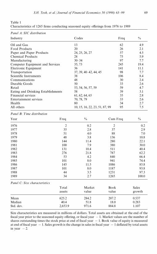
Table 1Characteristics of 1265 firms conducting seasoned equity offerings from 1976 to 1989

Panel A: SIC distribution

Industry Codes Freq %

Oil and Gas 13 62 4.9Food Products 20 26 2.1Paper and Paper Products 24, 25, 26, 27 57 4.5Chemical Products 28 75 5.9Manufacturing 30—34 97 7.7Computer Equipment and Services 35, 73 245 19.4Electronic Equipment 36 141 11.1Transportation 37, 39, 40—42, 44, 45 98 7.7Scientific Instruments 38 106 8.4Communications 48 30 2.4Durable Goods 50 33 2.6Retail 53, 54, 56, 57, 59 59 4.7Eating and Drinking Establishments 58 39 3.1Financial services 61, 62, 64, 65 35 2.8Entertainment services 70, 78, 79 33 2.6Health 80 34 2.7All others 10, 15, 16, 22, 23, 51, 87, 99 95 7.5

Panel B: ¹ime distribution

Year Freq % Cum Freq %

1976 2 0.2 2 0.21977 35 2.8 37 2.91978 51 4.0 88 7.01979 48 3.8 136 10.81980 144 11.4 280 22.11981 100 7.9 380 30.01982 131 10.4 511 40.41983 276 21.8 787 62.21984 53 4.2 840 66.41985 101 8.0 941 74.41986 145 11.5 1086 85.81987 101 8.0 1187 93.81988 44 3.5 1231 97.31989 34 2.7 1265 100.0

Panel C: Size characteristics

Totalassets

Marketvalue

Bookvalue

Salesgrowth

Mean 625.2 284.2 207.2 0.537Median 40.4 51.8 18.0 0.283Std. dev. 2,653.9 971.6 884.8 1.107

Size characteristics are measured in millions of dollars. Total assets are obtained at the end of thefiscal year prior to the seasoned equity offering, or fiscal year !1. Market values are the number ofshares outstanding times the stock price at end of fiscal year !1. Book value of equity is measuredat end of fiscal year !1. Sales growth is the change in sales in fiscal year !1 deflated by total assetsin year !2.


relative contribution of cash flows and accruals to the post-issue net incomeperformance. For evidence on the relative magnitude of the earnings underper-formance, we compare the post-issue earnings performance of issuers ranked bytheir discretionary current accruals in the pre-issue year. Finally, we examine theSpearman rank order correlation between pre-issue accruals and post-issueearnings underperformance to test whether pre-issue accruals explain the cross-sectional variation in post-issue earnings underperformance.

4.1. Post-Issue earnings underperformance in time series

Table 2 reports three measures of net income performance in the six yearssurrounding the issue year: net income as a percentage of prior year total assets,asset-scaled net income minus the industry median asset-scaled net income, andthe annual change in asset-scaled net income of the issuer minus the change fora pre-issue performance-matched non-issuer. Net income is Compustat item172, which is the number reported in an earnings announcement in the WallStreet Journal and which captures more fully the effects of discretionary report-ing choices, such as extraordinary items, on the earnings performance. Theresults using earnings before interest and taxes (item 18) are qualitatively similar,and are not reported here. The second measure adjusts for changing businessconditions in the industry. This adjustment could be important given theevidence in Ritter (1991) that some industries experienced significant declines inoperating performance in the 1980s. The third measure is recommended byBarber and Lyon (1997) for removing normal mean reversion in net income. Thestatistical means are obtained after winsorizing the data at the 1% and 99%level to reduce the effect of a few large values. The means without winsorizingare similar, but less statistically significant.

The pattern of unadjusted asset-scaled net income indicates improving pre-issue performance but deteriorating post-issue performance. The median growsfrom 6.50% in year !3 to a peak of 9.00% in year 0, then declines to 3.80% byyear #3. The equivalent means are 6.33% in year !3, 6.63% in year 0, and0.71% in year #3. The industry-adjusted performance measures indicatea similar profile of pre-issue improvement and post-issue decline. The medianindustry-adjusted asset-scaled net income grows from 1.40% in year !3 to5.00% in year 0, and declines to 1.40% by year #3. The equivalent means are1.23% in year !3, 3.01% in year 0, and !1.42% in year #3.

To match each issuer with a non-issuer of comparable pre-issue performancefor the third measure, we first select the non-issuer from the same industry withasset-scaled net income closest to that of the issuer in year !1. We begin withthe four-digit SIC code; if no match is available, we search among three-digitSIC codes, then two-digit, and finally one-digit. Although we require theasset-scaled net income of the non-issuer to be at least 80% of the asset-scalednet income of the issuer, we do not impose an upper bound. The majority of the


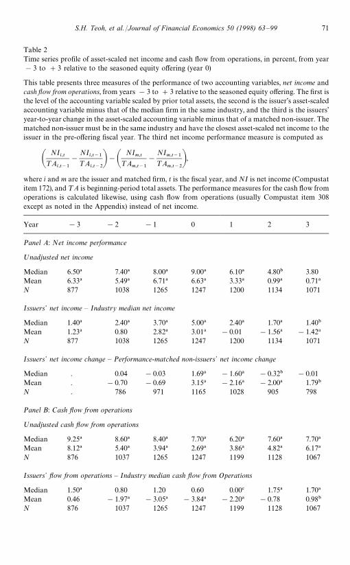
Table 2Time series profile of asset-scaled net income and cash flow from operations, in percent, from year!3 to #3 relative to the seasoned equity offering (year 0)

This table presents three measures of the performance of two accounting variables, net income andcash flow from operations, from years !3 to #3 relative to the seasoned equity offering. The first isthe level of the accounting variable scaled by prior total assets, the second is the issuer’s asset-scaledaccounting variable minus that of the median firm in the same industry, and the third is the issuers’year-to-year change in the asset-scaled accounting variable minus that of a matched non-issuer. Thematched non-issuer must be in the same industry and have the closest asset-scaled net income to theissuer in the pre-offering fiscal year. The third net income performance measure is computed as

ANI

i,t¹A

i,t~1

!

NIi,t~1

¹Ai,t~2B!A

NIm,t

¹Am,t~1

!

NIm,t~1

¹Am,t~2

B,where i and m are the issuer and matched firm, t is the fiscal year, and NI is net income (Compustatitem 172), and ¹A is beginning-period total assets. The performance measures for the cash flow fromoperations is calculated likewise, using cash flow from operations (usually Compustat item 308except as noted in the Appendix) instead of net income.

Year !3 !2 !1 0 1 2 3

Panel A: Net income performance

ºnadjusted net income

Median 6.50! 7.40! 8.00! 9.00! 6.10! 4.80" 3.80Mean 6.33! 5.49! 6.71! 6.63! 3.33! 0.99! 0.71!N 877 1038 1265 1247 1200 1134 1071

Issuers+ net income — Industry median net income

Median 1.40! 2.40! 3.70! 5.00! 2.40! 1.70! 1.40"Mean 1.23! 0.80 2.82! 3.01! !0.01 !1.56! !1.42!

N 877 1038 1265 1247 1200 1134 1071

Issuers+ net income change — Performance-matched non-issuers+ net income change

Median . 0.04 !0.03 1.69! !1.60! !0.32" !0.01Mean . !0.70 !0.69 3.15! !2.16! !2.00! 1.79"N . 786 971 1165 1028 905 798

Panel B: Cash flow from operations

ºnadjusted cash flow from operations

Median 9.25! 8.60! 8.40! 7.70! 6.20! 7.60! 7.70!Mean 8.12! 5.40! 3.94! 2.69! 3.86! 4.82! 6.17!N 876 1037 1265 1247 1199 1128 1067

Issuers+ flow from operations — Industry median cash flow from Operations

Median 1.50! 0.80 1.20 0.60 0.00# 1.75! 1.70!Mean 0.46 !1.97! !3.05! !3.84! !2.20! !0.78 0.98"

N 876 1037 1265 1247 1199 1128 1067


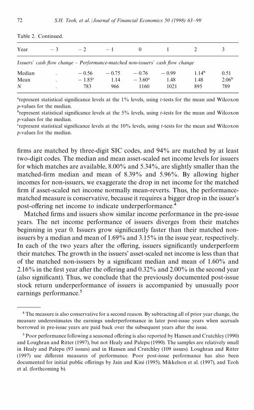
Table 2. Continued.

Year !3 !2 !1 0 1 2 3

Issuers+ cash flow change — Performance-matched non-issuers+ cash flow change

Median . !0.56 !0.75 !0.76 !0.99 1.14" 0.51Mean . !1.85# 1.14 !3.60! 1.48 1.48 2.06"N . 783 966 1160 1021 895 789

!represent statistical significance levels at the 1% levels, using t-tests for the mean and Wilcoxonp-values for the median."represent statistical significance levels at the 5% levels, using t-tests for the mean and Wilcoxonp-values for the median.#represent statistical significance levels at the 10% levels, using t-tests for the mean and Wilcoxonp-values for the median.

firms are matched by three-digit SIC codes, and 94% are matched by at leasttwo-digit codes. The median and mean asset-scaled net income levels for issuersfor which matches are available, 8.00% and 5.34%, are slightly smaller than thematched-firm median and mean of 8.39% and 5.96%. By allowing higherincomes for non-issuers, we exaggerate the drop in net income for the matchedfirm if asset-scaled net income normally mean-reverts. Thus, the performance-matched measure is conservative, because it requires a bigger drop in the issuer’spost-offering net income to indicate underperformance.4

Matched firms and issuers show similar income performance in the pre-issueyears. The net income performance of issuers diverges from their matchesbeginning in year 0. Issuers grow significantly faster than their matched non-issuers by a median and mean of 1.69% and 3.15% in the issue year, respectively.In each of the two years after the offering, issuers significantly underperformtheir matches. The growth in the issuers’ asset-scaled net income is less than thatof the matched non-issuers by a significant median and mean of 1.60% and2.16% in the first year after the offering and 0.32% and 2.00% in the second year(also significant). Thus, we conclude that the previously documented post-issuestock return underperformance of issuers is accompanied by unusually poorearnings performance.5

4The measure is also conservative for a second reason. By subtracting all of prior year change, themeasure underestimates the earnings underperformance in later post-issue years when accrualsborrowed in pre-issue years are paid back over the subsequent years after the issue.

5Poor performance following a seasoned offering is also reported by Hansen and Crutchley (1990)and Loughran and Ritter (1997), but not Healy and Palepu (1990). The samples are relatively smallin Healy and Palepu (93 issues) and in Hansen and Crutchley (109 issues). Loughran and Ritter(1997) use different measures of performance. Poor post-issue performance has also beendocumented for initial public offerings by Jain and Kini (1995), Mikkelson et al. (1997), and Teohet al. (forthcoming b).


Next, we examine which of the two components, cash flow from operations oraccruals, induces the observed net income pattern. The results in Panel B ofTable 2 indicate that the net income profile is not mirrored by cash flow fromoperations. The medians of all three measures of asset-scaled cash flows (unad-justed, industry-adjusted, and performance-matched) show a monotonic declinefrom pre-issue periods to the lowest levels in the issue year before improving inyears #2 and #3. The means also show similar patterns, with low levels inyears 0 and #1. Therefore, new issues occur when cash flows from operationsare declining, not when they are at a peak. Consequently, as the remainingcomponent of earnings, accruals must be driving the observed net income profilefor new issues.

We now evaluate which of the four accrual measures is the primary con-tributor to the net income profile. Table 3 presents the profiles of the fouraccrual measures, with levels of asset-scaled accruals shown in Panel A andyear-to-year changes in Panel B. The profile of discretionary current accrualsshows the most dramatic change, suggesting manipulation of current accrualsduring a new issue. Discretionary current accruals are significantly positive,monotonically rising to a peak in the offering year before decreasing signifi-cantly in years #2 and #3. (The year-to-year changes cannot be derived fromthe mean levels in Panel A because the number of issuers varies in our sampleeach year.) The year 0 peak in asset-scaled discretionary current accruals isstatistically significant at a mean and median of 5.59% and 2.50%.6 In post-issue years #1 through #3, the discretionary accruals decline monotonicallyuntil year #3, when they are no longer statistically significantly different fromzero.

The nondiscretionary current accruals show a somewhat similar profile. Thenondiscretionary current accruals peak in the issue year and decline significantlyin year #1. Nondiscretionary current accruals are a positive linear function ofsales growth (see the Appendix), so the evidence is consistent with new issuerstiming offerings for when sales growth peaks. The pre-issue mean and medianchanges in Panel B, however, are usually negative, and so do not suggesta monotonic improvement prior to the offering. As reported later in Table 7,pre-issue nondiscretionary current accruals do not predict post-issue underper-formance.

6The level of accruals do not turn negative immediately after the offering, suggesting that issuersavoid immediate reversals in accruals. A similar peak in year 0 was reported for initial publicofferings by Teoh et al. (forthcoming b). They suggest institutional explanations such as the threat oflawsuits if reversals occur immediately, commitment by underwriters to stabilize price near theoffering price, and the existence of lock-up periods when insiders commit not to sell. Interestingly,Loughran and Ritter (1995) and Section 5 of this paper document that the decline in stock returnperformance also does not occur immediately after the offering.


Table 3Time-series profile of asset-scaled accruals, in percent, from year !3 to #3 relative to the seasonalequity offering (year 0).

This table presents the discretionary and nondiscretionary current and long-term accruals of firmsoffering seasoned equity offerings from the three years before to three years after the offering. Thenondiscretionary accruals reflect accruals choices largely dictated by economic conditions, whereasthe discretionary accruals are designed to pick up reporting choices that are largely controlled(‘managed’) by the firm. The accruals measures are scaled by beginning-period total assets, andreported in percent. In the last three rows of Panels A and B, an alternative matched-pair method isused. The discretionary current accruals are calculated as the modified Jones model discretionarycurrent accruals of the issuer minus the modified Jones model discretionary current accruals of thematched non-issuing industry peer. The matched non-issuer has similar net income performance asthe issuer in year !1 and is selected using the matching procedure as described for the third netincome performance measure in Table 2. See the Appendix for details of the model to decomposeaccruals into discretionary and non-discretionary components.

Fiscal Year !3 !2 !1 0 #1 #2 #3

Panel A: Accruals (levels)

Discretionary current accruals (DCA)Median 0.90! 1.30! 2.05! 2.50! 2.20! 0.70! 0.10Mean 2.21" 3.32! 5.37! 5.59! 4.18! 1.59# !0.24N 863 1020 1248 1234 1183 1122 1064

Discretionary long-term accruals (D¸A)Median !1.10! !1.00! !1.00" !1.20! !1.00! !1.30! !1.50!

Mean !1.00 !1.70! !0.83 !1.33! !1.51! !3.33! !1.86!

N 857 1012 1241 1218 1175 1103 1054

Nondiscretionary current accruals (NDCA)Median 0.90! 1.40! 1.50! 2.20! 1.20! 0.70! 0.80!Mean 2.59! 3.80! 4.95! 5.98! 2.24! 1.76! 2.06!N 863 1020 1248 1234 1183 1122 1064

Nondiscretionary long-term accruals (ND¸A)Median !3.70! !4.20! !4.70! !4.60! !4.30! !4.20! !4.10!

Mean !4.49! !5.15! !6.80! !6.32! !5.54! !4.52! !5.24!

N 857 1012 1241 1218 1175 1103 1054

Discretionary current accruals (DCA) of Issuer — DCA of matched non-issuerMedian 0.41 0.86" 1.64" 2.85" 1.42 0.18 0.26Mean 0.60 1.83# 3.90" 4.90" 2.01" !0.61 !0.89N 773 954 1248 1154 1017 900 797

Panel B: Accruals (changes)

Fiscal Year !2 !1 0 #1 #2 #3

Discretionary current accruals (DCA)Median 0.25 0.40 0.70 !0.45# !1.20! !1.10!

Mean 0.89 0.62 0.30 !1.37 !2.62! !1.98"

N 862 1017 1228 1176 1111 1057


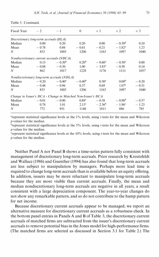
Table 3. Continued.

Fiscal Year !2 !1 0 #1 #2 #3

Discretionary long-term accruals (D¸A)Median 0.00 0.20 0.20 0.00 !0.30" 0.10Mean !0.78 0.86 !0.61 !0.21 !1.82! 1.23N 853 1005 1206 1163 1097 1040

Nondiscretionary current accruals (NDCA)Median 0.15 !0.30" 0.20" !0.60! !0.50! 0.00Mean !0.08 !0.30 1.00 !3.85! !0.50 0.14N 862 1017 1228 1176 1111 1057

Nondiscretionary long-term accruals (ND¸A)Median !0.20 !0.40! !0.40" 0.30! 0.00" !0.20Mean !0.48 !0.96 0.37 0.69 1.07! !0.51N 853 1005 1206 1163 1097 1040

Change in Issuer+s DCA - Change in Matched Non-Issuer+s DCAMedian !0.01 !0.00 0.89# !0.58 !0.98" !0.57Mean 0.78 1.01 2.13# !2.36" !1.96# !1.23N 772 951 1148 1011 886 785

!represent statistical significance levels at the 1% levels, using t-tests for the mean and Wilcoxonp-values for the median."represent statistical significance levels at the 5% levels, using t-tests for the mean and Wilcoxonp-values for the median.#represent statistical significance levels at the 10% levels, using t-tests for the mean and Wilcoxonp-values for the median.

Neither Panel A nor Panel B shows a time-series pattern fully consistent withmanagement of discretionary long-term accruals. Prior research by Kreutzfeldtand Wallace (1986) and Guenther (1994) has also found that long-term accrualsare less subject to manipulation by managers. Perhaps more lead time isrequired to change long-term accruals than is available before an equity offering.In addition, issuers may be more reluctant to manipulate long-term accrualsbecause they are more visible than current accruals. Finally, the mean andmedian nondiscretionary long-term accruals are negative in all years, a resultconsistent with a large depreciation component. The year-to-year changes donot show any remarkable pattern, and so do not contribute to the hump patternfor net income.

Because discretionary current accruals appear to be managed, we report analternative measure for discretionary current accruals as a robustness check. Inthe bottom panel entries in Panels A and B of Table 3, the discretionary currentaccruals of matched firms are subtracted from the issuer’s discretionary currentaccruals to remove potential bias in the Jones model for high-performance firms.(The matched firms are selected as discussed in Section 3.1 for Table 2.) The


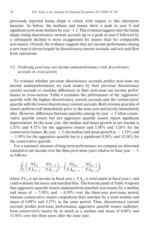
previously reported hump shape is robust with respect to this alternativemeasure. As before, the medians and means show a peak in year 0 andsignificant post-issue declines by year #2. This evidence suggests that the humpshape (rising discretionary current accruals up to a peak in year 0 followed bya subsequent decline) is more exaggerated for issuers than for comparablenon-issuers. Overall, the evidence suggests that net income performance duringa new issue is driven largely by discretionary current accruals, and not cash flowfrom operations.

4.2. Predicting post-issue net income underperformance with discretionaryaccruals in cross-section

To evaluate whether pre-issue discretionary accruals predict post-issue netincome underperformance, we rank issuers by their pre-issue discretionarycurrent accruals to examine differences in their post-issue net income perfor-mance in cross-section. Table 4 examines the performance of the ‘aggressive’quartile with the highest discretionary current accruals and the ‘conservative’quartile with the lowest discretionary current accruals. Both extreme quartiles ofissuers perform well immediately prior to the issue year and poorly immediatelyafter. However, differences between quartiles emerge by year #3 when conser-vative quartile issuers but not aggressive quartile issuers report significantimprovement. In the issue year, the median and mean growth in net income is1.53% and 4.72% for the aggressive issuers and 1.56% and 3.26% for theconservative issuers. By year #3, the median and mean growth is !1.52% and!1.39% for the aggressive quartile but is a significant 0.50% and 13.24% forthe conservative quartile.

For a summary measure of long-term performance, we compute an abnormalcumulative net income over the three post-issue years relative to base year !1,as follows:

3+t/1A

NIi,t

¹Ai,t~1

!

NIi,~1

¹Ai,~2B!A

NIm,t

¹Am,t~1

!

NIm,~1

¹Am,~2

B,where NI

i,tis net income in fiscal year t, ¹A

i,tis total assets in fiscal year t, and

i and m denote the issuer and matched firm. The bottom panel of Table 4 reportsthat aggressive quartile issuers underperform matched non-issuers by a medianand mean of !7.50% and !6.29% over the three-year post-issue period,whereas conservative issuers outperform their matches by a total median andmean of 0.99% and 5.27% in the same period. Thus, discretionary currentaccruals predict post-issue performance; aggressive quartile issuers underper-form conservative issuers by as much as a median and mean of 8.49% and11.56% over the three years after the issue year.


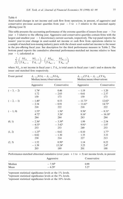
Table 4Asset-scaled changes in net income and cash flow from operations, in percent, of aggressive andconservative pre-issue accruer quartiles from year !3 to #3 relative to the seasoned equityoffering (year 0)

This table presents the accounting performance of the extreme quartiles of issuers from year !3 toyear #3 relative to the offering year. Aggressive and conservative quartiles contain firms with thelargest and smallest year !1 discretionary current accruals, respectively. The top panel reports theissuers’ year-to-year change in asset-scaled net income or cash flow from operations relative toa sample of matched non-issuing industry peers with the closest asset-scaled net income to the issuerin the pre-offering fiscal year. See description for the third performance measure in Table 2. Thebottom panel reports the cumulative abnormal performance-matched net income relative to baseyear !1, calculated as

3+t/1A

NIi,t

¹Ai,t~1

!

NIi,~1

¹Ai,~2B!A

NIm,t

¹Am,t~1

!

NIm,~1

¹Am,~2B,

where NIi,t

is net income in fiscal year t, ¹Ai,t

is total assets in fiscal year t and i and m denote theissuer and matched firm respectively.

Event period Dt~1,t

NIAi!D

t~1,tNIA

mDt~1,t

CFAi!D

t~1,tCFA

mMedian/mean/observations Median/mean/observations

Aggressive Conservative Aggressive Conservative

(!3,!2) 1.74# 0.46 !1.19 !1.201.72 !2.03 !0.61 !2.37159 173 159 173

(!2,!1) !1.40# 0.53 !11.73! 12.02!!2.34 !0.91 !11.61! 14.73!

218 222 218 222

(!1, 0) 1.53! 1.56! 9.56! !8.31!

4.72! 3.26# 8.16# !16.18!

284 284 283 284

(0, 1) !2.36! !3.39" 1.99 !2.54!4.53! !3.42! 9.91! !1.07

253 253 249 253

(1, 2) !1.25" !0.62 !0.10 1.77#

!0.82 !1.30 1.35 3.33230 214 227 213

(2, 3) !1.52 0.50! 1.14 0.22!1.39 13.24! 3.25 2.47

203 189 201 188

Performance-matched abnormal cumulative (over years #1 to #3) net income levels, in percent

Aggressive Conservative

Median !7.50" 0.99Mean !6.29# 5.27

!represent statistical significance levels at the 1% levels."represent statistical significance levels at the 5% levels.#represent statistical significance levels at the 10% levels.


As before, we evaluate the contribution of cash flow changes to the net incomeunderperformance. The evidence suggests that cash flows are not responsible forthe poorer post-issue net income performance of aggressive quartiles. In fact,aggressive quartile issuers experience greater cash flow improvement beginningin year !1 through year #3. Perhaps aggressive pre-issue accrual manipula-tors also manipulate cash flow from operations through real changes in opera-tions.

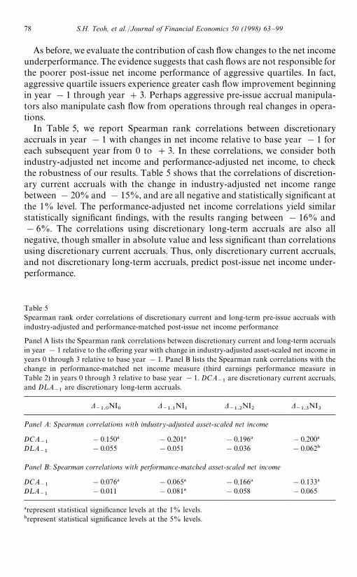
In Table 5, we report Spearman rank correlations between discretionaryaccruals in year !1 with changes in net income relative to base year !1 foreach subsequent year from 0 to #3. In these correlations, we consider bothindustry-adjusted net income and performance-adjusted net income, to checkthe robustness of our results. Table 5 shows that the correlations of discretion-ary current accruals with the change in industry-adjusted net income rangebetween !20% and !15%, and are all negative and statistically significant atthe 1% level. The performance-adjusted net income correlations yield similarstatistically significant findings, with the results ranging between !16% and!6%. The correlations using discretionary long-term accruals are also allnegative, though smaller in absolute value and less significant than correlationsusing discretionary current accruals. Thus, only discretionary current accruals,and not discretionary long-term accruals, predict post-issue net income under-performance.

Table 5Spearman rank order correlations of discretionary current and long-term pre-issue accruals withindustry-adjusted and performance-matched post-issue net income performance

Panel A lists the Spearman rank correlations between discretionary current and long-term accrualsin year !1 relative to the offering year with change in industry-adjusted asset-scaled net income inyears 0 through 3 relative to base year !1. Panel B lists the Spearman rank correlations with thechange in performance-matched net income measure (third earnings performance measure inTable 2) in years 0 through 3 relative to base year !1. DCA

~1are discretionary current accruals,

and D¸A~1

are discretionary long-term accruals.

D~1,0

NI0

D~1,1

NI1

D~1,2

NI2

D~1,3

NI3

Panel A: Spearman correlations with industry-adjusted asset-scaled net income

DCA~1

!0.150! !0.201! !0.196! !0.200!

D¸A~1

!0.055 !0.051 !0.036 !0.062"

Panel B: Spearman correlations with performance-matched asset-scaled net income

DCA~1

!0.076! !0.065! !0.166! !0.133!

D¸A~1

!0.011 !0.081! !0.058 !0.065

!represent statistical significance levels at the 1% levels."represent statistical significance levels at the 5% levels.


Overall, our results are consistent with the following scenario. Although cashflows from operations are declining prior to the offering, managers of issuingfirms report high and improving earnings by managing discretionary currentaccruals. In the year of the offering, reported earnings peak despite relativelyweak cash flow from operations because managers continue to take largepositive discretionary current accruals. Post-offering, high net income cannot besustained because cash flows from operations do not improve sufficiently andissuers can no longer continue to take large discretionary accruals. Issuers withthe highest discretionary current accruals in year !1 experience the largestdrop in net income after the issue.

5. Predicting post-issue stock returns with pre-issue accruals

We next examine whether pre-issue discretionary accruals predict post-issuestock return underperformance. Addressing this topic requires an appropriatemeasure for expected long-run returns, an issue that is debated in the assetpricing literature. We use three long-run return measures: raw returns, returnsnet of the returns to the value-weighted market portfolio, and returns net of theFama and French (1997) three-factor model for expected returns (described inthe Appendix).

5.1. Post-issue returns by pre-issue accrual quartiles

We study the relation between pre-issue accruals and post-issue returns byfirst examining differences in stock return performance among four quartileportfolios grouped by levels of pre-issue discretionary current accruals. Eachquartile portfolio contains about 200 firms. We then track each portfolio’sreturn performance relative to month 0, which is either the month of the issue orfour months after the previous fiscal year end, whichever is later. The four-monthlag represents a tradeoff: using accounting information with shorter lags mightmean that financial statements are not yet available to investors, while longerlags might not capture the period when investors react to the report containingmanipulated earnings. To check the robustness of our results, the panel regres-sions in Section 6 extend the waiting period to six months.

The long-run return performance reported in Table 6 is measured in thefollowing way. For each firm and year, we first compound monthly returns intoan annual return. We then average these returns across all sample firms in theportfolio to compute the overall annual raw returns. For the adjusted returns,we subtract the compound annual return on a benchmark portfolio (either themarket portfolio or a Fama and French equivalent portfolio, described in theAppendix) from the compound annual raw return for each firm. When a samplefirm disappears during the year, the remaining monthly raw or adjusted returns


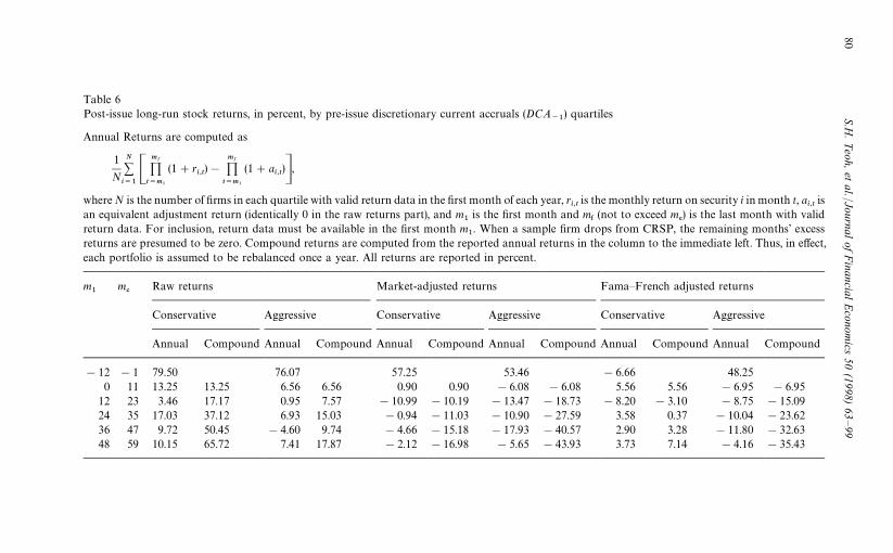
Table 6Post-issue long-run stock returns, in percent, by pre-issue discretionary current accruals (DCA

~1) quartiles

Annual Returns are computed as

1

N

N+i/1C

mf

<t/m1

(1#ri,t)!

mf

<t/m1

(1#ai,t)D,

where N is the number of firms in each quartile with valid return data in the first month of each year, ri,t

is the monthly return on security i in month t, ai,t

isan equivalent adjustment return (identically 0 in the raw returns part), and m

1is the first month and m

&(not to exceed m

%) is the last month with valid

return data. For inclusion, return data must be available in the first month m1. When a sample firm drops from CRSP, the remaining months’ excess

returns are presumed to be zero. Compound returns are computed from the reported annual returns in the column to the immediate left. Thus, in effect,each portfolio is assumed to be rebalanced once a year. All returns are reported in percent.

m1

m%

Raw returns Market-adjusted returns Fama—French adjusted returns

Conservative Aggressive Conservative Aggressive Conservative Aggressive

Annual Compound Annual Compound Annual Compound Annual Compound Annual Compound Annual Compound

!12 !1 79.50 76.07 57.25 53.46 !6.66 48.250 11 13.25 13.25 6.56 6.56 0.90 0.90 !6.08 !6.08 5.56 5.56 !6.95 !6.95

12 23 3.46 17.17 0.95 7.57 !10.99 !10.19 !13.47 !18.73 !8.20 !3.10 !8.75 !15.0924 35 17.03 37.12 6.93 15.03 !0.94 !11.03 !10.90 !27.59 3.58 0.37 !10.04 !23.6236 47 9.72 50.45 !4.60 9.74 !4.66 !15.18 !17.93 !40.57 2.90 3.28 !11.80 !32.6348 59 10.15 65.72 7.41 17.87 !2.12 !16.98 !5.65 !43.93 3.73 7.14 !4.16 !35.43

80S.H

.T

eoh,et

al./Journalof

Financial

Econom

ics50

(1998)63

—99

are assumed to be zero until the end of the year. (Such firms drop from ourportfolio in the following year.) Finally, we compound the annual raw andadjusted return averages into five-year cumulative returns. This proceduremimicks a trading strategy that rebalances the portfolio annually, assigningequal weight to those stocks still in existence.

Table 6 shows that our strategy nets about a 66% raw return over five yearsfor firms in the conservative earnings management quartile, and 18% for firmsin the aggressive quartile. When the equivalent market-returns are subtracted,the conservative quartile portfolio earns !17% excess returns and the aggres-sive quartile portfolio earns !44%. Among firms with sufficient pre-issuereturn data to compute Fama—French exposures, the conservative quartileportfolio earns a #7% Fama—French adjusted return and the aggressivequartile portfolio earns !35%.

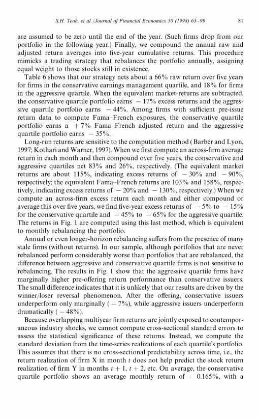
Long-run returns are sensitive to the computation method ( Barber and Lyon,1997; Kothari and Warner, 1997). When we first compute an across-firm averagereturn in each month and then compound over five years, the conservative andaggressive quartiles net 83% and 26%, respectively. (The equivalent marketreturns are about 115%, indicating excess returns of !30% and !90%,respectively; the equivalent Fama—French returns are 103% and 158%, respec-tively, indicating excess returns of !20% and !130%, respectively.) When wecompute an across-firm excess return each month and either compound oraverage this over five years, we find five-year excess returns of !5% to !15%for the conservative quartile and !45% to !65% for the aggressive quartile.The returns in Fig. 1 are computed using this last method, which is equivalentto monthly rebalancing the portfolio.

Annual or even longer-horizon rebalancing suffers from the presence of manystale firms (without returns). In our sample, although portfolios that are neverrebalanced perform considerably worse than portfolios that are rebalanced, thedifference between aggressive and conservative quartile firms is not sensitive torebalancing. The results in Fig. 1 show that the aggressive quartile firms havemarginally higher pre-offering return performance than conservative issuers.The small difference indicates that it is unlikely that our results are driven by thewinner/loser reversal phenomenon. After the offering, conservative issuersunderperform only marginally (!7%), while aggressive issuers underperformdramatically (!48%).

Because overlapping multiyear firm returns are jointly exposed to contempor-aneous industry shocks, we cannot compute cross-sectional standard errors toassess the statistical significance of these returns. Instead, we compute thestandard deviation from the time-series realizations of each quartile’s portfolio.This assumes that there is no cross-sectional predictability across time, i.e., thereturn realization of firm X in month t does not help predict the stock returnrealization of firm Y in months t#1, t#2, etc. On average, the conservativequartile portfolio shows an average monthly return of !0.165%, with a


Fig. 1. Time-series graph of Fama—French adjusted returns classified by pre-issue discretionarycurrent accruals (DCA

~1) quartiles. An average monthly excess return is constructed by first

subtracting an equivalent Fama—French benchmark return from each issuer’s monthly return andthen averaging these individual firm excess returns across all firms in the portfolio. The graphedreturns are the logged cumulative sum of these monthly portfolio excess returns. The returns arenormalized so that the event-month return is zero. Firms are classified into the four quartileportfolios using DCA

~1, the discretionary current accruals in the fiscal year prior to the seasoned

equity offering. Time is measured from the date of the seasoned equity offering or four months afterthe prior fiscal yearend (where DCA

~1was reported), whichever comes later.

t-statistic of !0.96. The aggressive quartile portfolio shows an averagemonthly return of !1.346%, with a t-statistic of !7.00. The averagereturn difference of 1.18% per month has a t-statistic of 4.60, indicatingthat more aggressive earnings management predicts poorer post-issue returnperformance.

In sum, the partitioned univariate evidence suggests a large long-run returndifference between conservative and aggressive firms. It thus appears that poorpost-issue performance can be explained partially by the pre-issue earningsmanagement of seasoned new issuers. By choosing firms with negative or lowdiscretionary current accruals, investors can avoid investing in issuers thatdramatically underperform their non-issuing peers.


5.2. Regressions of post-issue returns on pre-issue accruals

Table 7 displays the results from ordinary least squares regressions ofpost-issue firm stock price performance on pre-issue accounting accruals. Thedependent variable is the log of the four-year compounded stock return (orcompounded excess stock return), beginning either from the issue date or fourmonths after the previous fiscal year, whichever comes later. To avoid influentialeccentric observations, we winsorize accruals at the 1% and 99% percentiles. Ingeneral, our results are robust to winsorization.

The discretionary accruals components are the key explanatory variables ofinterest. We include the nondiscretionary accruals components in the regressionto evaluate the relative information content for returns between the discretion-ary and nondiscretionary components. We also include a set of industry andyear control dummies (coefficients are not reported). The industry dummies, asoutlined in Table 1, account for post-issue performance variance across indus-tries. Intercept dummies for individual years 1978 through 1989 account forbusiness cycle effects and capture contemporaneous cross-sectional correlationbetween four-year returns. Log equity-size and log book-to-market variablescontrol for firm characteristics. Multi-year returns of different stocks overlapacross firms. (We do not have duplicate returns.) Contemporaneous cross-sectional returns can contain spurious residual correlation, which does not biascoefficient estimates but could bias coefficient standard errors if the inducednonzero off-diagonal covariances correlate with our measure of discretionarycurrent accruals. Section 6 implements a more complex panel data test proced-ure that takes the cross-sectional correlations in the residuals into account.Finally, we do not report results for Fama—French adjusted returns, becausethey are similar to the two reported regressions.

We also include a variant of Cheng (1995) measure of use of proceeds. Chengfinds that equity issuers that do not invest underperform after the issue, whereasissuers that invest do not underperform. We use Cheng’s measure to examinewhether the earnings management proxy in this paper has an incremental effecton returns over the Cheng effect. The capital expenditure growth between pre-and post-issue periods is calculated as

DCAPEXPt`1

"

(CAPEXPt#CAPEXP

t`1)!(CAPEXP

t~1#CAPEXP

t~2)

2TAt~1

, (2)

where CAPEXPtis the issuer’s capital expenditure (Compustat item 128) and

TAt

is the firm’s total assets in year t. Year 0 data are from the financialstatements following the issue. Consequently, DCAPEXP

t`1incorporates two

numbers not available at the time of the seasoned offering, and so has a two-yeartiming advantage over our accruals measures.


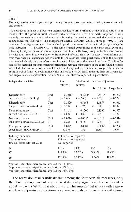
Table 7Ordinary least-squares regressions predicting four-year post-issue returns with pre-issue accrualsand controls

The dependent variable is a four-year aftermarket log return, beginning at the offering date or fourmonths after the previous fiscal year-end, whichever comes later. For market-adjusted returns,monthly raw returns are first adjusted by subtracting the market return, and then continuouslycompounded for four years. The independent accrual variables (DCA

~1through ND¸A

~1) are

computed from regressions (described in the Appendix) and measured in the fiscal year preceding theissue (subscript !1). DCAPEXP

t`1is the sum of capital expenditures in the (post-issue) event and

following fiscal year minus the sum of capital expenditures in the two years prior to the event, dividedby twice total assets in the year prior to the seasoned offering. Thus, DCAPEXP

t`1uses information

from two financial statements not available to the seasoned issue purchasers, unlike the accrualsmeasures which rely only on information known to investors at the time of the issue. To adjust forsome cross-sectional contemporaneous correlations between components of the compounded returns,we include but do not report a complete set of industry and year dummies (two year dummies for1983), as well as firms’ log book-market value and log equity size. Small and large firms are the smallestand largest market capitalization tertials. White-t statistics are reported in parentheses.

Independent variable Raw Market-adj. Market-adj. returnsreturns returns

Small firms Large firms

Discretionary Coef !0.3818! !0.3954! !0.5413! !0.1962current accruals (DCA

~1) (t) (!2.61) (!2.68) (!2.51) (!0.92)

Discretionary Coef !0.3620 !0.3665 !1.485! !0.1962long-term accruals (D¸A

~1) (t) (!1.28) (!1.26) (!3.20) (!0.33)

Nondiscretionary Coef !0.1141 !0.1200 !0.1390 !0.1377!

current accruals (NDCA~1

) (t) (!0.88) (!0.89) (!0.39) (!3.49)

Nondiscretionary Coef !0.0714 !0.0652 !0.0516 !0.7914long-term accruals (ND¸A

~1) (t) (!0.20) (!0.18) (!0.09) (!1.30)

Change in capital Coef 0.0829 0.0801 0.3034! !0.1206#

expenditures (DCAPEXPt`1

) (t) (1.59) (1.53) (3.30) (!1.65)

Industry dummies Full set — not reportedYear dummies Full set — not reportedBook/Market, Market value Not reported

N 1,035 1,035 332 355

R2 15.89% 13.73% 27.45% 20.47%

R2 12.59% 10.35% 17.76% 10.62%

!represent statistical significance levels at the 1% level."represent statistical significance levels at the 5% level.#represent statistical significance levels at the 10% level.

The regression results indicate that among the four accruals measures, onlythe discretionary current accrual is statistically significant. Its coefficient isabout !0.4, its t-statistic is about !2.6. This implies that issuers with aggres-sive levels of pre-issue discretionary current accruals perform significantly worse


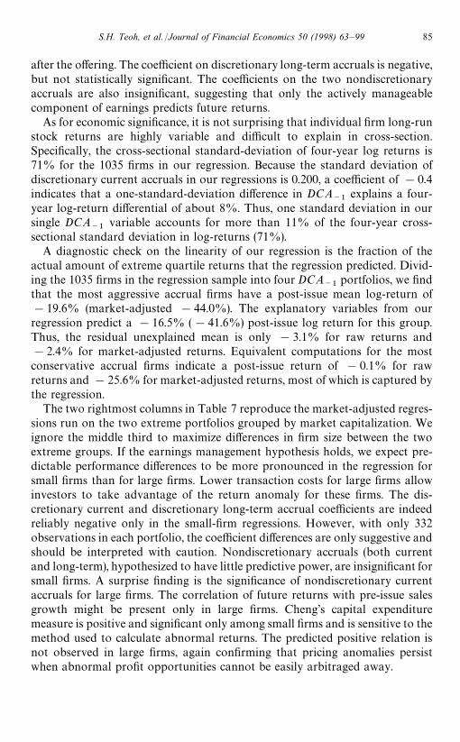
after the offering. The coefficient on discretionary long-term accruals is negative,but not statistically significant. The coefficients on the two nondiscretionaryaccruals are also insignificant, suggesting that only the actively manageablecomponent of earnings predicts future returns.

As for economic significance, it is not surprising that individual firm long-runstock returns are highly variable and difficult to explain in cross-section.Specifically, the cross-sectional standard-deviation of four-year log returns is71% for the 1035 firms in our regression. Because the standard deviation ofdiscretionary current accruals in our regressions is 0.200, a coefficient of !0.4indicates that a one-standard-deviation difference in DCA

~1explains a four-

year log-return differential of about 8%. Thus, one standard deviation in oursingle DCA

~1variable accounts for more than 11% of the four-year cross-

sectional standard deviation in log-returns (71%).A diagnostic check on the linearity of our regression is the fraction of the

actual amount of extreme quartile returns that the regression predicted. Divid-ing the 1035 firms in the regression sample into four DCA

~1portfolios, we find

that the most aggressive accrual firms have a post-issue mean log-return of!19.6% (market-adjusted !44.0%). The explanatory variables from ourregression predict a !16.5% (!41.6%) post-issue log return for this group.Thus, the residual unexplained mean is only !3.1% for raw returns and!2.4% for market-adjusted returns. Equivalent computations for the mostconservative accrual firms indicate a post-issue return of !0.1% for rawreturns and !25.6% for market-adjusted returns, most of which is captured bythe regression.

The two rightmost columns in Table 7 reproduce the market-adjusted regres-sions run on the two extreme portfolios grouped by market capitalization. Weignore the middle third to maximize differences in firm size between the twoextreme groups. If the earnings management hypothesis holds, we expect pre-dictable performance differences to be more pronounced in the regression forsmall firms than for large firms. Lower transaction costs for large firms allowinvestors to take advantage of the return anomaly for these firms. The dis-cretionary current and discretionary long-term accrual coefficients are indeedreliably negative only in the small-firm regressions. However, with only 332observations in each portfolio, the coefficient differences are only suggestive andshould be interpreted with caution. Nondiscretionary accruals (both currentand long-term), hypothesized to have little predictive power, are insignificant forsmall firms. A surprise finding is the significance of nondiscretionary currentaccruals for large firms. The correlation of future returns with pre-issue salesgrowth might be present only in large firms. Cheng’s capital expendituremeasure is positive and significant only among small firms and is sensitive to themethod used to calculate abnormal returns. The predicted positive relation isnot observed in large firms, again confirming that pricing anomalies persistwhen abnormal profit opportunities cannot be easily arbitraged away.


In sum, our evidence of post-issue return differences in cross-section isconsistent with an earnings management scenario. Rangan (1997) confirms thisfinding using quarterly accruals. Among our four accrual measures, discretion-ary (i.e., managed) current accruals predict subsequent poor stock price perfor-mance the best. The fact that discretionary current accruals are a good predictoris especially surprising in light of the fact that they are an imperfect measure ofearnings management and calculated from information available as early as fourto sixteen months before the issue.

6. A Fama–MacBeth panel procedure

6.1. Methodology

In this section, we outline a procedure that addresses two previouslyneglected issues. First, since the previous regressions use overlapping multiyearreturns, the regression errors could be correlated if all risk factors have notbeen properly accounted for. (The appropriate risk-factor adjustments for ex-pected returns are currently still debated in the asset-pricing literature, anda consensus has yet to emerge.) Second, the significance of the accrual variablesin the previous regressions may have been due to the ability of discretionaryaccruals to explain subsequent returns in all firms, not just in periods when thereare new issues. Thus, we want to measure the incremental predictive power ofpost-issue returns by pre-issue accruals pertaining to periods of seasoned equityofferings.

To address the above issues, we run cross-sectional regressions explainingmonthly returns from July 1975 through December 1994 with the followinglagged variables: (a) the log of the firm’s book-to-market value, (b) the logof the firm’s market value of equity, (c) the four accrual measures describedearlier, and (d) four interaction variables, accrual*SEO dummy, which are thepre-issue accrual measure during seasoned equity offering-related periods, andzero otherwise. All independent variables are from the same fiscal year and lagthe LHS returns they seek to explain. Following the tradition of using logar-ithms for the Fama—French variables, the book-to-market and size variables aretruncated at 0.0001. Accrual measures are winsorized at the 5% and 95%percentiles to avoid undue influence of outliers. The results are robust towinsorizing at more extreme percentiles.

Fig. 2 illustrates the time line, the lag structure for the independent variables,and the algorithm for when the new issue dummy is set to one. We now assumean even more conservative reporting lag of six months (instead of the four-month lag in the previous section). Thus, the regressions relate returns toaccruals and controls from fiscal years ending at least six months prior to the


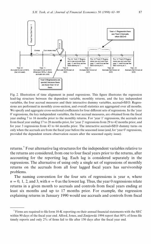
Fig. 2. Illustration of time alignment in panel regressions. This figure illustrates the regressionlead-lag structure between the dependent variable, monthly returns, and the key independentvariables, the four accrual measures and their interactive dummy variables, accrual*SEO. Regres-sions are performed in monthly cross-section, and overall statistics are aggregated over all months.We specify and aggregate cross-sectional coefficients for four different sets of regressions. In the ‘year0’ regressions, the key independent variables, the four accrual measures, are obtained from the fiscalyear ending 7 to 16 months prior to the monthly returns. For ‘year 1’ regressions, the accruals arefrom fiscal year ending 17 to 28 months prior, for ‘year 2’ regressions from 29 to 42 months prior, andfor year 3 regressions from 43 to 64 months prior. The interactive accrual*SEO dummy turns ononly when the accruals are from the fiscal year before the seasoned issue (and, for ‘year 0’ regressions,provided the dependent return observation occurs after the seasoned equity issue).

returns.7 Four alternative lag structures for the independent variables relative tothe returns are considered, from one to four fiscal years prior to the returns, afteraccounting for the reporting lag. Each lag is considered separately in theregressions. The alternative of using only a single set of regressions of monthlyreturns on the accruals from all four lagged fiscal years has survivorshipproblems.

The naming convention for the four sets of regressions is year n, wheren"0, 1, 2, and 3, with n"0 as the lowest lag. Thus, the year 0 regressions relatereturns in a given month to accruals and controls from fiscal years ending atleast six months and up to 17 months prior. For example, the regressionexplaining returns in January 1990 would use accruals and controls from fiscal

7Firms are required to file form 10-K reporting on their annual financial statements with the SECwithin 90 days of the fiscal year end. Alford, Jones, and Zmijewski 1994 report that 80% of firms filetimely reports and only 2% of firms fail to file after 150 days after the fiscal year end.


years ending no later than June 1989. Equivalently, accruals and controls datedJune 1989 would be used to explain returns in each month from January 1990 toDecember 1990. Year 1 regressions relate returns to accruals and controls fromfiscal years ending 18 to 29 months earlier, year 2 regressions relate returns toaccruals and controls 30 to 41 months earlier, and year 3 regressions relatereturns to accruals and controls 42 to 53 months earlier. Thus, we have a total offour regression sets of about 180 monthly regressions each, with each setexplaining the predictive power of accruals and controls for various lead-periodreturns. The year 0 set of regressions predicts returns from July 1975 throughMay 1991; the year 1 set predicts returns from June 1976 through May 1992, andso on. In each of the 180 regressions, the typical number of firms ranges between2700 to 3200 observations.

The interaction dummy for the presence of a seasoned equity offering equalsone only for the fiscal year data immediately preceding the offering in allregression sets. Consequently, the coefficients on the interaction variable,accrual*SEO dummy, measure the marginal predictive ability of pre-issueaccruals for returns between zero and three years after the issue.

The interaction dummy is set to one only after the offering for the year0 regression set. Suppose, for example, the new issue occurs in February 1990and the fiscal year ends in June. The issue dummy is set to one in monthlyreturn regressions from March 1990 to December 1990 on June 1989 accrualsand other control variables for the year 0 set of regressions. The issue dummyis one also in the other three sets of regressions whenever June 1989 accrualsare used. Thus, the issue dummy is one for the following regressions: Jan-uary 1991 to December 1991 monthly return regressions on June 1989accruals and controls for the year 1 set, January 1992 to December 1992monthly return regressions on June 1989 accruals and controls for the year 2 set,and so on. We exclude months in the period from four months after the fiscalyear end to the offering date from the regressions. It would be misleading toattribute explanatory power in these months as a ‘non-issue’ effect, just as itwould be misleading to call it ‘post-issue’ return predictability when the equityoffering has not yet occurred. The results are robust to omitting or includingthese months.

The time series of the estimated coefficients on each independent variable areaveraged across the 180 monthly regressions in each set, and an overallt-statistic is calculated assuming serial independence. Finally, a grand mean anda grand t-statistic are computed across all four sets of regressions to estimate therelation between accruals and four-year returns. Attributing Gaussian unit-normality to the aggregated four-year t-statistics in effect assumes zero correla-tion in the time series of the accruals for the issuers. The observed correlationsare of the order of 5—10%, and thus the assumption of uncorrelated accountingvariables is unlikely to be problematic. But, to warn the reader, we havebracketed the significance level indicators in the table.


Unlike the approach in the previous section, in which multimonth returns arecompounded into long-term holding periods, the cross-sectional regressions areperformed monthly, so no overlapping periods exist to induce cross-sectionalcorrelations. Instead of the Fama—French factor coefficients, we now use thefirm’s own book-to-market and firm size measures to control for cross-sectionalvariation in expected returns.8 Because the explanatory variables are knownwhen returns are measured, there is no need to run pre-test-period regressions toestimate ex ante (beta) coefficients or group firms into portfolios to reduce theerrors-in-variables problem (as in Fama and MacBeth, 1973). By using thisvariation of the Fama—French model, we can evaluate the robustness of therelation between accruals and future returns with respect to alternativemodels of expected returns. Finally, by performing the cross-sectional regres-sion on all firms, with accruals*SEO dummy variables as regressors, we canestimate the incremental predictability of post-issue returns by pre-issue ac-cruals beyond any average predictability of accruals for future returns. Thisallows us to extend Sloan’s (1996) research relating total accruals to futurereturns to evaluate the relative importance of discretionary versus nondis-cretionary accruals and pre-issue period versus non-issue period accruals inpredicting future returns.

6.2. Results

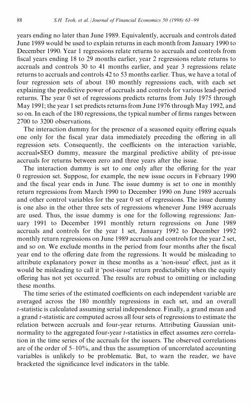
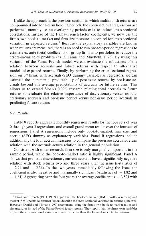
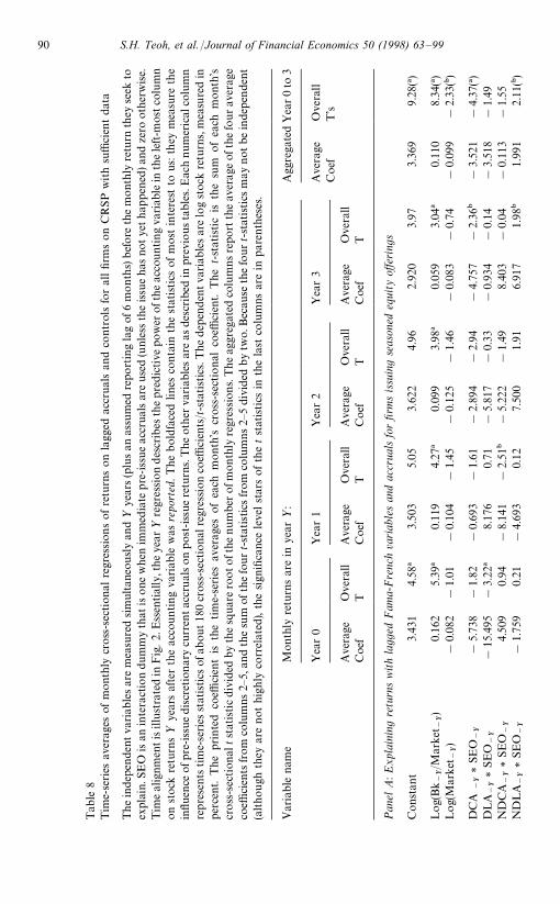
Table 8 reports aggregate monthly regression results for the four sets of year0 through year 3 regressions, and overall grand mean results over the four sets ofregressions. Panel A regressions include only book-to-market, firm size, andaccrual*SEO dummy as explanatory variables. Panel B regressions includeadditionally the four accrual measures to compare the pre-issue accruals-returnrelation with the accruals-return relation in the general population.

Consistent with other research, firm size is only marginally important in thesample period, while the book-to-market ratio is highly significant. Panel Ashows that pre-issue discretionary current accruals have a significantly negativerelation with stock returns two and three years after the issue (t-statistics of!2.94 and !2.36). In the two years immediately following the issue, thecoefficient is also negative and marginally significant(t-statistics of !1.82 and!1.61). Aggregating over the four years, the average coefficient is !3.521 with

8Fama and French (1993, 1997) argue that the book-to-market (HML portfolio returns) andmarket (SMB portfolio returns) factors describe the cross-sectional variation in returns quite well.However, Daniel and Titman (1997) recommend using the firm’s own book-to-market ratios andsize measures instead of the Fama—French factor returns. They report that the firm’s own variablesexplain the cross-sectional variation in returns better than the Fama—French factor returns.


Tab

le8

Tim

e-se

ries

aver

ages

ofm

ont

hly

cross

-sec

tiona

lre

gres

sion

sofre

turn

son

lagg

edac

crua

lsan

dco

ntro

lsfo

ral

lfirm

son

CR

SPw

ith

suffi

cien

tda

ta

The

inde

pende

ntva

riab

lesar

em

easu

red

sim

ultan

eously

and½

year

s(p

lusan

assu

med

repo

rtin

gla

gof

6m

ont

hs)

bef

ore

the

mon

thly

retu

rnth

eyse

ekto

expl

ain.S

EO

isan

inte

ract

ion

dum

my

that

isone

when

imm

edia

tepre

-iss

ue

accr

uals

are

used

(unl

essth

eissu

ehas

notye

thap

pen

ed)a

ndze

root

her

wise.

Tim

eal

ignm

entis

illu

stra

ted

inF

ig.2.

Ess

ential

ly,t

he

year

½re

gres

sion

des

crib

esth

epre

dic

tive

pow

eroft

he

acco

unting

variab

lein

the

left-m

ostco

lum

non

stock

retu

rns½

year

saf

ter

the

acco

unting

variab

lew

asre

port

ed.T

he

bol

dfa

ced

line

sco

nta

inth

est

atistics

ofm

ostin

tere

stto

us:t

hey

mea

sure

the

influen

ceof

pre-

issu

ediscr

etio

nar

ycu

rren

tac

crual

son

pos

t-issu

ere

turn

s.T

heot

her

variab

lesar

eas

desc

ribe

din

prev

ious

table

s.E

ach

num

eric

alco

lum

nre

pre

sent

stim

e-se

ries

stat

istics

ofab

out18

0cr

oss-

sect

ional

regr

ession

coeffi

cien

ts/t

-sta

tist

ics.

The

dep

enden

tva

riab

lesar

elo

gst

ock

retu

rns,

mea

sure

din

perc

ent.

The

prin

ted

coeffi

cien

tis

the

tim

e-se

ries

aver

ages

of

each

mon

th’s

cros

s-se

ctio

nal

coeffi

cien

t.T

het-st

atistic

isth

esu

mof

each

mont

h’s

cross

-sec

tion

altst

atistic

divi

ded

byth

esq

uare

rootoft

henum

berofm

onth

lyre

gres

sion

s.The

aggr

egat

edco

lum

nsre

port

the

aver

age

ofth

efo

urav

erag

eco

effici

ents

from

colu

mns

2—5,

and

the

sum

ofth

efo

urt-st

atistics

from

colu

mns2—

5di

vided

by

two.B

ecau

seth

efo

urt-

stat

istics

may

notbe

inde

pen

dent

(althou

ghth

eyar

enot

high

lyco

rrel

ated

),th

esign

ifica

nce

leve

lst

ars

ofth

et

stat

istics

inth

ela

stco

lum

nsar

ein

par

enth

eses

.

Var

iabl

ena

me

Mon

thly

retu

rns

are

inye

ar½

:A

ggre

gate

dY

ear0

to3

Yea

r0

Yea

r1

Yea

r2

Yea

r3

Ave

rage

Ove

rall

Coe

fT’s

Ave

rage

Ove

rall

Ave

rage

Ove

rall

Ave

rage

Ove

rall

Ave

rage

Ove

rall

Coe

fT

Coef

TC

oef

TC

oef

T

Pan

elA

:Exp

lain

ing

retu

rns

with

lagg

edFam

a-Fre

nch

variab

les

and

accr

uals

for

firm

sissu

ing

seas

oned

equi

tyoff

erin

gs

Con

stan

t3.

431

4.58

!3.

503

5.05

3.62

24.

962.

920

3.97

3.36

99.

28(!)

Log(

Bk ~

Y/Mar

ket ~

Y)0.

162

5.39

!0.

119

4.27

!0.

099

3.98

!0.

059

3.04

!0.

110

8.34

(!)

Log(

Mar

ket

~Y)

!0.

082

!1.

01!

0.10

4!

1.45

!0.

125

!1.

46!

0.08

3!

0.74

!0.

099

!2.

33(")

DC

A~Y

*SE

O~Y

!5.

738

!1.

82!

0.69

3!

1.61

!2.

894

!2.

94!

4.75

7!

2.36

"!

3.52

1!

4.37

(!)

DL

A~

Y*

SEO

~Y

!15

.495

!3.

22!

8.17

60.

71!

5.81

7!

0.33

!0.

934

!0.

14!

3.51

8!

1.49

ND

CA

~Y

*SEO

~Y

4.50

90.

94!

8.14

1!

2.51

"!

5.22

2!

1.49

8.40

3!

0.04

!0.

113

!1.

55N

DL

A~Y

*SEO

~Y

!1.

759

0.21

!4.

693

0.12

7.50

01.

916.

917

1.98

"1.

991

2.11

(")


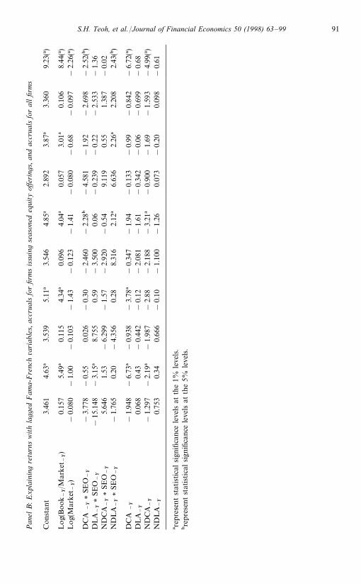
Pan

elB

:Exp

lain

ing

retu

rns

with

lagg

edF

ama-

Fre

nch

variab

les,

accr

uals

for

firm

sissu

ing

seas

oned

equi

tyoff

erin

gs,an

dac

crua

lsfo

ral

lfirm

s

Con

stan

t3.

461

4.63

!3.

539

5.11

!3.

546

4.85

!2.

892

3.87

!3.

360

9.23

(!)

Log(

Book

~Y/M

arket

~Y)

0.15

75.

49!

0.11

54.

34!

0.09

64.

04!

0.05

73.

01!

0.10

68.

44(!)

Log(

Mar

ket

~Y)

!0.

080

!1.

00!

0.10

3!

1.43

!0.

123

!1.

41!

0.08

0!

0.68

!0.

097

!2.

26(!)

DC

A~Y

*SE

O~Y

!3.

778

!0.

550.

026

!0.

30!

2.46

0!

2.28

"!

4.58

1!

1.92

!2.

698

!2.

52(")

DL

A~

Y*

SEO

~Y

!15

.148

!3.

15!

8.75

50.

59!

3.50

00.

06!

0.23

9!

0.22

!2.

533

!1.

36N

DC

A~

Y*

SEO

~Y

5.64

61.

53!

6.29

9!

1.57

!2.

920

!0.

549.

119

0.55

1.38

7!

0.02

ND

LA

~Y

*SEO

~Y

!1.

765

0.20

!4.

356

0.28

8.31

62.

12!

6.63

62.

26!

2.20

82.

43(")

DC

A~Y

!1.

948

!6.

73!

!0.

938

!3.

78!

!0.

347

!1.

94!

0.13

3!

0.99

!0.

842

!6.

72(!)

DL

A~

Y0.

068

0.43

!0.

442

!0.

12!

2.08

1!

1.61

!0.

342

!0.

06!

0.69

9!

0.68

ND

CA

~Y

!1.

297

!2.

19!

!1.

987

!2.

88!

2.18

8!

3.21

!!

0.90

0!

1.69

!1.

593

!4.

99(!)

ND

LA

~Y

0.75

30.

340.

666

!0.

10!

1.10

0!

1.26

0.07

3!

0.20

0.09

8!

0.61

!rep

rese

ntst

atistica

lsign

ifica

nce

leve

lsat

the

1%le

vels.

"rep

rese

ntst

atistica

lsign

ifica

nce

leve

lsat

the

5%le

vels.


a t-statistic of !4.37, indicating that high pre-issue discretionary currentaccruals predict poor stock returns during the four-year period after the issue.The significance of discretionary current accruals is similar to that of thebook-market ratio, and considerably higher than the significance of firm size. Incontrast, pre-issue nondiscretionary current accruals are generally not a signifi-cant predictor of stock returns, except in year 1. As Panel B below shows, thisexplanatory power of pre-issue nondiscretionary current accruals is generic toall firms, and not specifically related to seasoned new issues.

For the pre-issue long-term accruals, the coefficient for discretionary long-term accruals is negative and statistically significant at the 1% level only in themonths immediately after issue. This coefficient is neither negative nor signifi-cant in the remaining three years. On the other hand, nondiscretionary long-term accruals have a more delayed impact on returns; the coefficients for theyear 2 and year 3 regressions are actually positive and significant at about the5% level. These results suggest that firms with positive pre-issue nondiscretion-ary long-term accruals actually outperform the market after the issue.

Panel B compares the difference in explanatory power of the accrual variablesbetween issue periods and non-issue periods. The coefficients on the four accrualvariables without the interactive dummies are for non-issuers in all months andissuers in non-issue months. The coefficients on the four interactive dummyvariables now measure the incremental explanatory power of pre-issue accrualsabove and beyond the explanatory power of accruals in the general population.

Discretionary current accruals appear to predict returns for the generalpopulation of firms in the short term. The t-statistics for the year 0 and year1 regressions are highly significant at !6.73 and !3.78, respectively. Ofsignificance to the earnings management hypothesis, the interaction pre-issuediscretionary current accrual variable has a significant additional effect in years2 and 3. The coefficients for the DCA

~1*SEO variables are one order of

magnitude larger than the coefficients of the DCA~1

variables (!2.46 and!4.58, as compared with !0.35 and !0.13, respectively), and the t-statistic(!2.28) for the year 2 lagged discretionary current accruals for issuers isstatistically significant at the 5% level.

In economic terms, the !2.5 to !4.6 magnitude of the coefficients ondiscretionary accruals suggests that a one-standard-deviation difference in dis-cretionary current accruals between two issuers (about 0.2) can explaina 0.5—0.9% monthly return differential. Aggregating over the four-year period,the DCA

~1*SEO variable is statistically significant at about the 1% level. Thus,

the evidence indicates that the negative relation between discretionary currentaccruals and subsequent long-term stock returns is stronger during issue-relatedperiods.

As for the other three accrual variables, discretionary long-term accruals donot predict future stock returns in either new issuers or in the general populationof firms. Nondiscretionary current accruals predict negative subsequent returns


in the general population, perhaps from contamination of the variable by thediscretionary component that is left in the variable. Nondiscretionary long-term accruals, on the other hand, predict incrementally positive futurereturns for issuers but are unrelated to stock returns for the general populationof firms.

In sum, the simple cross-sectional regressions in the previous section and thepanel regressions here document a strong ability of pre-issue discretionarycurrent accruals to predict multiyear post-issue abnormal returns. We alsodocument that discretionary current accruals have a (time-diminishing) abilityto predict subsequent returns for all firms, although this predictive ability issignificantly greater for issuers. In contrast, discretionary long-term accrualspredict returns only in the year immediately following the issue (which results ina lower significance in the simple cross-sectional regressions). Finally, nondis-cretionary pre-issue accruals have no reliable predictive ability on post-issuestock market performance.

7. Summary and conclusion

This paper examines whether pre-issue earnings management, as reflectedin discretionary accruals, explains the long-term underperformance of sea-soned equity issuers. We document that discretionary current accruals growbefore the offering, peak in the offering year, and decline thereafter. Thisaccruals pattern causes net income to grow before, peak in, and decline afterthe offering year, despite low pre-issue and improved post-issue cash flowfrom operations. The post-issue net income decline is especially pronouncedfor issuers that aggressively manage discretionary current accruals before theissue.

Most importantly, we document a negative relation between pre-issue dis-cretionary current accruals and post-issue earnings and stock returns. Thenegative relation with stock returns remains after controlling for firm size,book-to-market ratio, and post-issue capital expenditures. The negative relationbetween discretionary current accruals and subsequent returns is common to allfirms during the 1976 to 1990 test period. These results extend prior research intwo ways. First, we show that the discretionary component of current accrualsexplains future returns as well as the book-to-market ratio does and consider-ably better than firm size. Second, we show that the negative relation betweendiscretionary current accruals and future returns is stronger and more persistentamong firms engaging in new equity offerings.

The relation between discretionary current accruals and post-issue underper-formance in stock returns has also been documented by Teoh et al. (forthcomingb) and Teoh et al. (forthcoming a) for initial public offerings. Because seasonedequity issuers are already followed by analysts, offer more public and audited


information, have greater market capitalization, and are easier to sell short, itwould seem plausible that incentives and opportunities for deceiving investorsby managing earnings are more limited for seasoned equity issues than for initialpublic offerings. Thus, the evidence here of predictable post-issue returns forseasoned issuers based on available discretionary accrual information poses aneven stronger challenge to the efficient markets theory than the evidence oninitial public offerings.

In sum, the evidence is consistent with the hypothesis that investorsnaively extrapolate pre-issue earnings, and ignore relevant information con-tained in pre-issue discretionary current accruals. In this interpretation, aninformationally imperfect market is too optimistic when a seasoned equityissue is offered and later on becomes disappointed when the high earningscannot be sustained. These findings have implications for investors, firms,and accounting standard setters. Investors can use information containedin the pre-offering accounting accruals to discriminate among issuers. Man-agers can consider permissible accounting choices to reduce the firm’s costof capital or increase their own welfare. And accounting standard setters maywant to consider the costs of discretion in accrual choices, especially wheninvestors have considerably less information than do the managers of issuingfirms.9

Appendix A.

A.1. Computation of the accruals measures

This appendix explains the estimation of the four accrual measures. Numbersin parentheses are Compustat item numbers. Total accruals (¹AC) consist ofcurrent accruals (CA) or working capital accruals, and long-term accruals (¸A).¹AC is calculated as

¹AC"CA#¸A

"Net Income (172)!Cash Flow from Operations (308). (A.1)

Prior to 1987, cash flow from operations is not available as item (308) so it iscalculated as the funds flow from operations (item 110) minus current accruals

9A current proposal at the Financial Accounting Standards Board (FASB) suggests requiringonly a short-form report. Our evidence suggests that this may have adverse consequences forinvestors. The elimination of price-relevant accounting items (such as items necessary to computeaccruals) may result in investors trading in an even less informationally efficient market.


as defined below (see page 111 of the Compustat 1994 manual for furtherdetails).10

Current accruals are the change in noncash current assets minus the change inoperating current liabilities:

CA"D[current assets (4)!cash (1)]!D[current liabilities (5)

!current maturity of long!term debt (44)]. (A.2)

To obtain the discretionary and nondiscretionary accruals for a given year,we use the cross-sectional adaptation of the modified Jones (1991) model as inTeoh et al. (forthcoming b). An ordinary least squares regression of currentaccruals for a given year is regressed on the change in sales for that year using allfirms in the same two-digit SIC code as the seasoned new issuer, but excludingthe issuer. This intra-industry cross-sectional regression is reestimated for eachyear in the test period (from years !3 to #3 relative to the fiscal year of theissue). Consistent with the use of the model in the accounting literature, allvariables including the intercept term in the cross-sectional regression aredeflated by beginning total assets to reduce heteroskedasticity:

CAjt

¹Aj,t~1

"a0A

1

¹Aj,t~1

B#a1A

DSA¸ESjt

¹Aj,t~1

B#ejt, (A.3)

where j firms belong in the same two-digit SIC code as the issuing firm butexcluding the issuer, ¹A

j,t~1is total assets in year t!1, and DSA¸ES

j,tis the

change in sales in year t for firm j.The nondiscretionary current accruals (scaled by beginning assets), NDCA

~1,

represent the portion of current accruals dictated by firm sales growth, and isviewed as independent of managerial control. It is computed as

NDCAit"aL

0A1

¹Ai,t~1

B#aL1A

DSA¸ESit!DA/R

it¹A

i,t~1B, (A.4)

where DA/Rit

is the change in trade receivables in year t for issuer i. We subtractthe increase in accounts receivable from sales growth to allow for the possibilityof credit sales manipulation by the issuer, who might allow generous creditpolicies to obtain high sales prior to the offering (see Dechow et al., 1995). Themain results of our paper are robust to omitting this adjustment.

10 Item (110) is used as the cash flow from operations in cases when Compustat already excludescurrent accruals from item (110). This occurs when funds from operations are reported either as onetotal or grouped together in the funds flow statement (format code for item 318 is 2) or in the cash byactivity statement (format code for item 318 is 3).


The remaining current accruals are the scaled discretionary current accruals(DCA

~1) and are the portion of current accruals subject to manipulation by

management:

DCAit"

CAit

¹Ai,t~1

!NDCAit. (A.5)

For long-term accruals, we first estimate total accruals by using a regressionsimilar to Eq. (A.3). The dependent variable is total accruals. We includeproperty, plant, and equipment as an additional regressor because long-termaccruals (e.g. depreciation levels) are affected by the amount of long-term assetsas in Jones (1991):

¹ACjt

¹Aj,t~1

"b0A

1

¹Aj,t~1

B#b1A

DSA¸ESjt

¹Aj,t~1

B#b2A

PPEjt

¹Aj,t~1

B#ejt, (A.6)

where j firms belong in the same two-digit SIC code as the issuer (excluding theissuer), ¹AC

jtis total accruals, and PPE

jtis gross property, plant, and equip-

ment for firm j in year t.The nondiscretionary total accruals scaled by assets (ND¹AC) and the

discretionary total accruals scaled by assets (D¹AC) are computed as

ND¹ACit"bK

0A1

¹Ai,t~1

B#bK1A

DSA¸ESit!DA/R

it¹A

i,t~1B#bK

2APPE

it¹A

i,t~1B,(A.7)

and

D¹ACit"A

¹ACit

¹AitB!ND¹AC

it. (A.8)

As in Eq. (A.4), the increase in accounts receivable is subtracted from salesgrowth to allow for the manipulation of credit sales.

Long-term accruals are total accruals net of current accruals. Thus, non-discretionary long-term accruals scaled by assets (ND¸A

~1) will be the differ-

ence between ND¹AC and NDCA~1

. Discretionary long-term accruals scaledby assets (D¸A

~1) will be the difference between long-term accruals and

ND¸A~1

.To summarize, the four accruals measures are discretionary current accruals

(DCA~1

), discretionary long-term accruals (D¸A~1

), nondiscretionary currentaccruals (NDCA

~1) and nondiscretionary long-term accruals (ND¸A

~1). The

two discretionary accrual measures are proxies for earnings management where-as the two nondiscretionary accrual measures are proxies for accrual recogni-tion outside the control of management.


Table 9 provides some descriptive statistics on the properties of the estimatedregressions (coefficients, t-statistics, regression fits, and numbers of observations)from Eqs. (A.3) and (A.6). In general, the regression statistics are comparablewith those reported in previous studies (see Perry and Williams, 1994). Themedian adjusted R2 for the regression for current accruals is 20% and for totalaccruals is 32%, which is encouraging as an indicator of the explanatory powerof the cross-sectional Jones model.

A.2. Fama—French returns11

To extract individual firm factor loadings (c) on the three Fama—French(1993) factors, we run a time series regression for each firm of the monthly excessreturn over the risk-free rate on the three Fama—French factors from month!36 to month !12 relative to the filing date of the offering:

Ri,t!r

f,t"c

1(R

m,t!r

f,t)#c

2R

4.",t#c

3R

).-,t#e

i,t, (A.9)

where t is a month index, R4.",t

is the return on a small-capitalization portfoliominus a large-capitalization portfolio, R

).-,tis the return on a high book-to-

market portfolio minus a low book-to-market portfolio, Rm,t

is the return ona value-weighted market index, r

f,tis the one-month Treasury bill (risk-free) rate

of return, and Ri,t

is the return for each issuer. A minimum of 12 availablemonths is required to estimate each regression.

The expected return for each month is computed from month !11 to #60,using the estimated coefficients from the factor regression, the relevant monthfactor returns, and replacing the intercept with the risk-free rate of return:

ERi,t"r

f,t#cL

1(R

m,t!r

f,t)#cL

2R

4.",t#cL

3R

).-,t. (A.10)

The abnormal return is the realized return minus the Fama—French expectedreturn. In our sample, the coefficients indicate that the Fama—French variablesare unlikely to explain differences in observed returns between the two extremeaccrual quartiles. The betas for the market premium and firm equity size differby 0.06 and 0.03, respectively. The betas for the book-to-market variable differby a modest 0.35. Furthermore, Table 6 indicates that the two quartiles havesimilar pre-issue return performance, making it unlikely that our results aredriven by the winner/loser reversal phenomenon.

11There is some argument as to whether the Fama—French model explains systematic risk(covariance). However, it is known to explain the cross-sectional variation in average returns in theCRSP data set quite well. By including abnormal returns relative to the Fama—French factors forexpected returns, we show that the accruals’ influence on returns is distinct from that exerted by themarket-return, the firm’s book-to-market ratio and the firm’s size. Loughran and Ritter (1995)follow the same strategy.


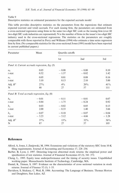
Table 9Descriptive statistics on estimated parameters for the expected accruals model

This table provides descriptive statistics on the parameters from the regressions that estimateexpected (current and total) accruals. For each issuing firm, the parameters are estimated froma cross-sectional regression using firms in the same two-digit SIC code as the issuing firm (over 60two-digit SIC code industries are represented). N is the number of firms in the issuer’s two-digit SICindustry used in the cross-sectional regressions. The statistics on the parameters are roughlycomparable with those reported in Perry and Williams (1994) who estimate a time series regressionfirm by firm. (No comparable statistics for the cross-sectional Jones (1991) model have been reportedin current published papers.)

Parameter Mean Quartile cutoffs

1st 2nd 3rd

Panel A: Current accruals regression, Eq. (5)

a0

0.05 !0.08 !0.00 0.10t-stat 0.52 !1.37 !0.02 1.42

a1

0.05 0.01 0.08 0.16t-stat 3.10 0.13 2.10 5.00

Adj. R2 27% 4% 20% 41%N 88 27 57 111

Panel B: ¹otal accruals regression, Eq. (8)

b0

!0.01 !0.11 !0.01 0.07t-stat !0.84 !1.75 !0.24 0.92

b1

0.03 !0.02 0.05 0.13t-stat 2.00 !0.33 1.40 3.66

b2

!0.07 !0.10 !0.07 !0.04t-stat !3.23 !5.12 !4.66 !1.28

Adj. R2 37% 15% 32% 56%N 87 27 57 105

References

Alford, A, Jones, J, Zmijewski, M, 1994. Extensions and violations of the statutory SEC form 10-Kfiling requirements. Journal of Accounting and Economics 17, 228—254.

Barber, B, Lyon, J, 1997. Detecting long-run abnormal stock returns: the empirical power andspecification of test statistics. Journal of Financial Economics 43 (3), 341—372.

Cheng, L., 1995. Equity issue underperformance and the timing of security issues. Unpublishedworking paper. Massachusetts Institute of Technology, Cambridge, MA.

Daniel, K, Titman, S, 1997. Evidence on the characteristics of cross sectional variation in stockreturns. Journal of Finance 52 (1), 1—33.

Davidson, S, Stickney, C, Weil, R, 1986. Accounting: The Language of Business. Thomas Hortonand Daughters, Sun Lakes, AZ.


Dechow, P, Sloan, R, Sweeney, A, 1995. Detecting earnings management. Accounting Review 70 (2),193—225.

DeFond, M, Jiambalvo, J, 1994. Debt covenant violation and manipulation of accruals. Journal ofAccounting and Economics 18 (2), 145—176.

Fama, E, French, K, 1993. Common risk factors in the returns on stocks and bonds. Journal ofFinancial Economics 33, 3—56.

Fama, E, French, K, 1997. Industry costs of equity. Journal of Financial Economics 43 (2), 153—194.Fama, E, MacBeth, J, 1973. Risk, return and equilibrium: empirical tests. Journal of Political

Economy 81, 607—636.Guay, W, Kothari, S, Watts, R, 1996. A market-based evaluation of discretionary accrual models.

Journal of Accounting Research Supplement 34, 83—105.Guenther, D, 1994. Measuring earnings management in response to corporate tax rate changes:

evidence from the 1986 tax reform act. Accounting Review 69, 230—243.Hansen, R, Crutchley, C, 1990. Corporate earnings and financing: an empirical analysis. Journal of

Business 63, 349—371.Healy, P, 1996. Discussion of a market-based evaluation of discretionary accrual models. Journal of

Accounting Research Supplement 34, 107—115.Healy, P, Palepu, K, 1990. Earnings and risk changes surrounding primary stock offers. Journal of

Accounting Research 28, 25—48.Jain, B, Kini, O, 1995. The post-issue operating performance of ipo firms. The Journal of Finance 49

(2), 1699—1726.Jones, J, 1991. Earnings management during import relief investigation. Journal of Accounting

Research 29 (2), 193—228.Kothari, S, Warner, J, 1997. Measuring long-horizon security price performance. Journal of

Financial Economics 43 (4), 301—340.Kreutzfeldt, R, Wallace, W, 1986. Error characteristics in audit populations: their profile and

relationship to environmental factors. Auditing: A Journal of Practice and Theory 6, 20—43.Loughran, T, Ritter, J, 1995. The new issues puzzle. Journal of Finance 50 (1), 23—51.Loughran T., Ritter, J., 1997. The operating performance of firms conducting seasoned equity

offerings. Journal of Finance 52, forthcoming.Mikkelson, W, Partch, M, Shah, K, 1997. Ownership and operating performance of companies that

go public. Journal of Financial Economics 44, 281—307.Perry, S, Williams, T, 1994. Earnings management preceding management buyout offers. Journal of

Accounting and Economics 18, 157—179.Rangan, S., 1997. Earnings Around Seasoned Equity Offerings: Are they overstated? Journal of

Financial Economics, forthcoming.Ritter, J, 1991. The long-run performance of initial public offerings. Journal of Finance 66, 3—27.Spiess, K, Affleck-Graves, J, 1995. Underperformance in long-run stock returns following seasoned

equity offerings. Journal of Financial Economics 38, 243—267.Sloan, R, 1996. Do stock prices fully impound information in accruals about future earnings?

Accounting Review 71, 289—315.Teoh, S.H, Welch, I, Wong, T.J, forthcoming a. Earnings management and the long-term market

performance of initial public offerings. Journal of Finance.Teoh S.H., Wong, T.J., Rao, G., forthcoming b. Are accruals during initial public offerings opportun-

istic? Review of Accounting Studies.


Earnings management and the underperformance...

Documents

Transcript of Earnings management and the underperformance...