Imperial College London

Department of Mathematics

Effective topological bounds and

semiampleness questions

Diletta Martinelli

October 25, 2016

Supervised by Dr. Paolo Cascini

Report submitted in partial fulfilment of the requirements

of the degree of PhD of Imperial College London

1

Abstract

In this thesis we address several questions related to important conjectures in bi-

rational geometry. In the first two chapters we prove that it is possible to bound

the number of minimal models of a smooth threefold of general type depending on

the topology of the underlying complex manifold. Moreover, under some technical

assumptions, we provide some explicit bounds and we explain the relationship with

the effective version of the finite generation of the canonical ring. Then we prove

the existence of rational curves on certain type of fibered Calabi–Yau manifolds.

Finally, in the last chapter we move to birational geometry in positive characteristic

and we prove the Base point free Theorem for a three dimensional log canonical pair

over the algebraic closure of a finite field.

2

Un piccolo passo alla volta.

3

Declaration of originality

I hereby declare that this thesis was entirely my own work and that any additional

sources of information have been duly cited.

Declaration of copyright

The copyright of this thesis rests with the author and is made available under a Cre-

ative Commons Attribution Non-Commercial No Derivatives licence. Researchers

are free to copy, distribute or transmit the thesis on the condition that they at-

tribute it, that they do not use it for commercial purposes and that they do not

alter, transform or build upon it. For any reuse or redistribution, researchers must

make clear to others the licence terms of this work.

4

Contents

Introduction and summary of results 6

2 Preliminary Results 20

2.1 The minimal model program for threefolds . . . . . . . . . . . . . . . 23

2.2 Descending Sections . . . . . . . . . . . . . . . . . . . . . . . . . . . 29

2.3 Some properties of varieties over Fp . . . . . . . . . . . . . . . . . . . 31

3 On the number of minimal models 34

3.1 Introduction . . . . . . . . . . . . . . . . . . . . . . . . . . . . . . . . 34

3.2 The main technical result . . . . . . . . . . . . . . . . . . . . . . . . 35

3.3 Proof of Theorem 3.2 . . . . . . . . . . . . . . . . . . . . . . . . . . . 39

4 Effective topological bounds for threefolds 41

4.1 Introduction . . . . . . . . . . . . . . . . . . . . . . . . . . . . . . . . 41

4.2 On the number of minimal models . . . . . . . . . . . . . . . . . . . . 42

4.2.1 Bounds for low Picard number . . . . . . . . . . . . . . . . . . 48

4.3 On the degree of the generators and the weight of the relations of the

canonical ring . . . . . . . . . . . . . . . . . . . . . . . . . . . . . . . 50

4.3.1 A Vanishing Theorem for Koszul Cohomology . . . . . . . . . 50

4.3.2 Proof of Theorem 4.3 . . . . . . . . . . . . . . . . . . . . . . . 52

5 Rational curves on Calabi-Yau manifolds 56

5.1 Introduction . . . . . . . . . . . . . . . . . . . . . . . . . . . . . . . . 56

5.2 Proof of Theorem 5.1 . . . . . . . . . . . . . . . . . . . . . . . . . . . 56

5.3 Proof of Theorem 5.2 . . . . . . . . . . . . . . . . . . . . . . . . . . . 59

6 The Base point free Theorem in positive characteristic 64

6.1 Introduction . . . . . . . . . . . . . . . . . . . . . . . . . . . . . . . . 64

6.2 Base point free theorem for normal surfaces . . . . . . . . . . . . . . 65

6.3 Reduction to surfaces . . . . . . . . . . . . . . . . . . . . . . . . . . . 73

6.4 Semiampleness on non irreducible surfaces . . . . . . . . . . . . . . . 75

5

6.5 Proof of Theorem 6.1 . . . . . . . . . . . . . . . . . . . . . . . . . . . 80

6.6 Examples . . . . . . . . . . . . . . . . . . . . . . . . . . . . . . . . . 80

Acknowledgements 83

References 88

6

Introduction and summary of

results

As in many other branches of mathematics, one of the main guiding problem in

algebraic geometry is the classification problem. The objects that we want to study

are the solutions of systems of polynomial equations in the projective space, that

we call algebraic varieties.

Problem 1.1. Classify algebraic varieties up to isomorphisms.

Except where explicitly stated, we work over the complex number.

The slogan that is going to guide us is that a lot of the geometry of an algebraic

variety X is determined by the behaviour of the canonical bundle ωX := ∧dimXΩX .

We will denote with KX any Cartier divisor satisfying OX(KX) ' ωX . In particular

the classification will depend on the positivity of KX . The first example is the well

known classification of curves. Let C be a smooth projective curve and let KC

its canonical bundle. The central feature of a curve is its genus gC = h0(C,KC).

Thanks to Riemann–Roch Theorem we have that deg(KC) = 2gC − 2, and then it

follows that

1. gC = 0 if and only if degKC < 0;

2. gC = 1 if and only if degKC = 0;

3. gC ≥ 2 if and only if degKC > 0.

The natural generalization of positive degrees line bundle on curves in higher dimen-

sion is the notion of ample line bundles. Therefore, given X an algebraic variety of

arbitrary dimension, the previous trichotomy can be generalized as follows.

1. Fano varieties: −KX is ample;

2. Calabi–Yau type varieties: KX is torsion;

3. Varieties of “general type”: KX is ample.

7

It is no longer true, as it was for curves, that given any smooth variety X, then it

belongs to one of these three main types. For instance, we can consider the product

of a Fano variety and a variety of general type or the blow up of a pure type variety.

However, the Minimal Model Program (MMP) permits to relate any variety X with

one of these families. Let us enter a litte bit more into the details of the Minimal

Model Program, the situation becomes more complicated with the increasing of the

dimension.

Surfaces

Starting from a smooth projective surface S, it is always possible to blow up a

point p ∈ S and produce another smooth surface S ′ that is strictly related to S

even though they are not isomorphic. It arises the necessity of a new equivalence

relation that identifies S and S ′. The solution is to classify algebraic varieties up to

birational equivalence.

Definition 1.2. Two varieties X and Y are birationally equivalent if there exist

open subsets U ⊆ X and V ⊆ Y such that U and V are isomorphic.

So clearly S and S ′ are birationally equivalent. Now the first natural step in the

classification problem becomes finding a good representative inside the birational

equivalence class of a smooth surface. By good representative we mean a surface

that is simpler than all other surfaces birational to it. Since we can birationally

modify a variety via blow ups it is natural to require that the simplest surface in

the birational equivalence class is a surface that cannot be obtained from another

smooth surface via a blow up. We say that such a surface is minimal.

A blow up of a point on a surface leaves a trace: an exceptional divisor E that

be characterised as follows: E ' P1 and E2 = (−1). We call E a (-1)-curve. We

arrive, therefore, to the following definition.

Definition 1.3. A smooth surface is minimal if it does not contained any (-1)-

curves. Let S be a smooth surface, the minimal surface inside the birational equiv-

alence class of S is called a minimal model of S.

Now, starting from a smooth surface S it is natural to ask how can we reach its

minimal model? If S does not contained any (-1)-curves, we are done. If there is a

(-1)-curve, then we can contract it thanks to the following theorem.

Theorem 1.4 (Castelnuovo Theorem). [KM98, Theorem 1.2] If a smooth surface

S contains a (−1)-curve, we can contract it via a birational morphism φ : S → T to

obtain another smooth surface T .

8

Then we can replace S with T and start again the algorithm. Does the process

stop? To answer this question we first need to consider an important parameter:

the Picard number ρ(S). We will be precise in Definition 2.4, but for now we can

think that the Picard number “counts the curves on S”.

So, if φ : S → T is a contraction of a (-1)-curve, ρ(T ) = ρ(S) − 1. Therefore,

starting form a smooth surface S after a finite number of steps it is always possible

to reach its minimal model.

Now that we have reached a minimal surface we can study its property and ar-

rive to an actual classification. Again, the division into classes is governed by the

behaviour of the canonical bundle of the surface. In particular by a fundamental

birational invariant, the Kodaira dimension.

Definition 1.5 (Kodaira dimension). If dimH0(X,mKX) = 0 for every m, then

we define the Kodaira dimension of X as K(X,KX) := −∞. Otherwise, we look at

the pluricanonical maps

φm : X 99K P(H0(X,mKX))

and define K(X,KX) := maxmdim Im(φm). Hence, in this second case 0 ≤K(X,KX) ≤ dimX and if K(X,KX) = dimX, then we say that X is of general

type and that KX is big.

We recall now the famous Enriques and Kodaira classification of surfaces, see

[Mat92, Theorem 1-7-1]. Let S be a minimal surface.

• If K(S,KS) = −∞, then S is either P2 or a P1-bundle over a curve;

• If K(S,KS) = 0, then S is either abelian, K3, Enriques or an hyperelliptic

surface, so that KS is a torsion divisor;

• If K(S,KS) = 1, then S is an elliptic surface, i.e. φm, for m 0, induces a

morphism S → C whose fibers are elliptic curves;

• If K(S,KS) = 2, then S is of general type and φm, for m 0, induces a

birational morphism S → S ′ such that KS′ is ample.

We can now explain the abuse of terminology for varieties of general type: the

canonical bundle of a minimal surface S of general type a priori is only big, but S

admits a birational morphism onto another surface with ample canonical bundle.

We can observe that if a minimal surface does not belong to one of the three pure

9

types (KS ample, KS torsion and KS antiample), it admits a fibration onto a curve

whose fibers belong to one of these families or a birational morphism onto a variety

that belongs to the first type.

Higher dimensional varieties

For varieties of dimension higher than two the situation is much more complicated.

First of all we need to find the right notion of minimal model.

We have to consider two different generalization depending on the Kodaira di-

mension. The first is the following notion of Mori fiber space that generalizes the

concept of P1-bundle.

Definition 1.6. An algebraic variety Z that admits a morphism Z → S whose

fibers are Fano varieties and such that dimS < dimZ is called a Mori fiber space.

Morover, it holds that ρ(Z) = ρ(S)− 1.

Otherwise, we define a minimal model in the following way.

Definition 1.7. Let X be a variety with non-negative Kodaira dimension. We say

that a minimal model of X is a variety X ′ that is birational to X such that KX′ is

nef, i.e. KX′ · C ≥ 0 for any curve C in X ′.

Another important difference with the surfaces case is that, even if we start with a

smooth variety X, where dimX ≥ 3, and we run an MMP, we end up with singular

varieties. Therefore, it is necessary to understand the singularities that might arise,

see Definition 2.6.

The main guiding conjecture of the MMP predicts the following.

Conjecture 1.8. Let X be a smooth projective variety.

1. If K(X,KX) = −∞, then X is birational to a Mori Fiber Space.

2. If 0 ≤ K(X,KX) ≤ dimX − 1, then X admits a birational model X ′ and

a fibration X ′ → Z into a variety of smaller dimension whose fibers are of

Calabi–Yau type;

3. If K(X,KX) = dimX, then X admits a birational model X ′ and a birational

morphism X ′ → Z such that KZ is ample.

Remark 1.9. In the general type case, the variety Z is called a canonical model

of X, see [KM98, Definition 3.50]. The canonical model is always unique, [KM98,

Theorem 3.52 (1)].

10

The following is the crucial definition of semiampleness of line bundles.

Definition 1.10. We say that a line bundle L on Y is semiample when the linear

system |mL| is base point free for a sufficiently large and divisible positive integer

m.

We can, therefore, reformulate Conjecture 1.8 saying that if K(X,KX) ≥ 0, then

X is birational to the variety X ′ such that K ′X is semiample and that the map

φm, for m 0, induces a fibration onto a lower dimensional variety in the case of

intermediate Kodaira dimension, or a birational morphism onto a variety Z such

that KZ is ample in the general type case.

The property of semiampless plays a crucial role in birational geometry. There-

fore, it is fundamental to look for sufficient and necessary conditions for a line bundle

to be semiample.

Conjecture 1.8 can be split into two parts: first we have to find the minimal

model, then it comes the so called Abundance Conjecture [KM98, Conjecture 3.12]

that predict that if KX′ is nef, then it is semiample. Minimal models for varieties of

general type do exist thanks to the groundbreaking result in [BCHM10]. Abundance

is known only up to dimension three (see for instance [Kol92]) or when KX′ is also

big, the so called Base point free Theorem [KM98, Theorem 3.3] in the other cases

is much open and it is one of the most important conjecture in birational geometry.

After this overview of the the main guiding conjectures of the Minimal Model

Program, we would like to move to the problems that are adressed in this thesis.

Chapter 3

We saw that the first step in the classification problem is finding a minimal model.

Starting from a smooth projective variety X, it is natural to ask whether it admits

a unique minimal model and if not how many minimal models does X have and how

different models are related to each others.

Definition 1.11. A marked minimal model of a projective variety X is a pair (Y, φ),

where φ : X 99K Y is a birational map and Y is a minimal model.

Remark 1.12. In Chapter 4, we also require that φ is an MMP for X, that means in

particular that it is a series of birational contractions of KX-negative extremal rays.

See Section 2.1 for a precise description of what we mean by counting the number

of minimal models.

11

If X is of general type, the number of marked minimal models is finite, see

[BCHM10], [KM87].

Otherwise, it is possible to construct examples where there exists an infinite num-

ber [Rei83]. However, it is an important and long-standing conjecture that the

number of minimal models of a smooth projective variety is finite up to isomor-

phisms. The conjecture has been proved only in the the case of threefold of positive

Kodaira dimension [Kaw97].

In [CL14], Cascini and Lazic proved that the number of minimal models of a

certain class of three-dimensional log smooth pairs (X,∆) of log general type can be

bounded by a constant that depends only on the homeomorphism type of the pair

(X,∆). This has its roots in earlier results that show that the topology governs the

birational geometry to some extent, see for instance [Kol86] and [CZ14]. Motivated

by these results, Cascini and Lazic [CL14] conjectured that for a smooth complex

projective threefold of general type, the number of minimal models is bounded in

terms of the topology of the underlying complex manifold.

In Chapter 3, we prove this conjecture.

Theorem 1.13. Let c be a positive real number. Then there is a positive constant

N(c), such that for any smooth complex projective threefold X of general type, whose

Betti numbers are bounded by c, i.e. bi(X) ≤ c for all i, the number of marked

minimal models of X is at most N(c).

The work of Chapter 3 is part of a joint project with Stefan Schreieder and Luca

Tasin.

Chapter 4

After proving in Chapter 3 that is possible to bound the number of marked minimal

models of a smooth projective threefold of general type depending on the topology

of the underlying complex manifold, it is now natural to ask if it possible to obtain

some explicit bounds for this number using some topological invariant such as the

Picard number ρ(X). In Chapter 4 we present some partial results in this direction

and some strategies for what we plan to do in the future.

We recall that along Chapter 4, a marked minimal model for X is a pair (Y, φ),

where Y is a minimal model and φ is a birational map that is an MMP for X, see

Definition 1.11 and Remark 1.12. In particular, φ can be decomposed in two types

of birational operations: divisorial contractions and flips, see Section 2.1 for the

precise definitions. We prove the following.

12

Theorem 1.14. Let X be a smooth projective threefold of general type. Then the

number of marked minimal models of X that can be reach with a series of divisorial

contractions followed by a series of flips is at most max1, 3 (ρ(X)−2)[(ρ(X)− 2)!]2.

Theorem 1.14 reduces quickly to find a bound for the number of possible flipping

curves passing through a terminal singularity, see Definition 2.6. Note that in the

case of a smooth surface S of general type, the minimal model is unique, [KM98,

Definition 1.30], and we cannot have two (-1)-curves E1 and E2 passing through the

same point, because they both should be contracted before reaching the minimal

model of S, but the contraction of C1 transforms C2 in a curve with non-negative

selfintersection, and so impossible to contract.

Theorem 1.14 is a technical theorem, in the sense that in general we cannot

impose geometric condition on X so that the hypothesis is satisfied. However, using

Theorem 1.14 we can obtain some effective bounds in the case of Picard number

equal to three.

Theorem 1.15. Let X be a smooth projective threefold of general type of Picard

number ρ(X) = 3. Then the number of marked minimal models of X is at most 3.

Moreover, we will explain a possible strategy for the case of Picard number equal

to four that we hope will lead in the future to an explicit bound also in that case.

Towards an effective version of finite generation

In Section 4.3 we deal with the search of an effective bound for the degree of the

generators of the canonical ring and for the weights of the relations among these

generators. This would provide a step towards an effective version of the finite gen-

eration of the canonical ring. This kind of problems are related with the finiteness

of minimal models, see for instance [BCHM10] and [KKL12].

In the case of curves Noether’s theorem [SD73] and the work of Enriques and

Petri [SD73] cover both the bounds for generators and relations.

Theorem 1.16. Let C be a smooth complex projective curve, and let R := R(C,KC)

be the canonical ring of C. Then

• R is generated in degree d ≤ 3;

• R is related in weight w ≤ 4.

13

The surfaces case was considered first by Ciliberto [Cil83] that proved that the

canonical ring of a surface S of general type is generated in degree d ≤ 5, as soon

as pg(S) > 0. Then Reid [Rei90] proved that R(S,KS) is generated in degree d ≤ 3

and related in weight w ≤ 6, when pg(S) ≥ 2, q(S) = 2, K2S ≤ 3 and the canonical

model has an irreducible canonical curve. Mendes Lopes [ML97] generalized Cilib-

erto’s theorem using Reider’s results [Rei88] and proved that R(S,KS) is generated

in degree 4, when pg(S) = 0 and |2KS| is free, (see also [Kon08]).

In an article dated 1982 [Gre82] Green gave a generalization of these results for a

smooth variety of general type of dimension n under the assumption of |KX | being

base point free, [Gre82, Theorem 3.9, Theorem 3.11]. He also found a bound for

the degree of the generators in the slightly more general assumption of KX being

semiample [Gre82, Theorem 3.15]. The canonical bundle of a minimal model of a

variety of general type is semiample, thanks to the Base point free Theorem, but

the minimal model is not going to be smooth in general. However, thanks to the

huge development in birational geometry of the last decades, it is now possible to

reformulate Green’s results in terms of terminal varieties, see Definition 2.6.

Theorem 1.17. Let X be a Gorenstein minimal terminal variety of general type of

dimension n. Let R(X,KX) be the canonical ring of X. Then

(1) R(X,KX) is generated in degree d ≤ (n+ 1)mn + 1;

(2) R(X,KX) is related in weight w ≤ 2(n+ 1)mn + 2;

where mn is the multiple of KX such that |mnKX | is free.

Remark 1.18. We recall that thanks to Kollar’s Effective base point freeness (see

Theorem 2.2), mn ≤ 2(n+ 2)!(2 + n).

Let S be a complex projective surface, then its minimal model S ′ is smooth, so

that, in particular, KS is Cartier. Then we obtain the following corollary.

Corollary 1.19. Let S be a smooth complex projective surface. Assume that S is

minimal and of general type. Let R(S,KS) be the canonical ring of S. Then

(1) R(S,KS) is generated in degree d ≤ 577;

(2) R(S,KS) is related in weight w ≤ 1154;

In the future we plan to use Theorem 1.17 to obtain a bound for the Veronese

subring R(d) where d is the Cartier index of the canonical divisor, i.e. the smallest

14

index m such that mKX is Cartier. Such a bound would give interesting geometrical

information, because Proj(R) = Proj(R(d)), see [Rei02, Proposition 3.3].

Indeed, we consider Y := Proj(R) = Proj(R(d)) ⊆ P[d0, . . . , dn]. Having a bound

on the degree di would make possible to explicitly compute an integer N such that

P[d0, . . . , dn] embedds into PN , using some standard tools in toric geometry, see

[Rei02, Proposition 3.6] and [CLS11, Theorem 2.2.12]: we can assume that the

degrees d0, . . . , dn are well-formed, that means that no n of d0, . . . , dn have a common

factor. Let M be the lowest common multiple of the di’s, then OX(kM) is a very

ample line bundle for any k ≥ n− 1. Then Y ⊆ P(H0(X,OX(kM))).

In dimension three, moreover, thanks to results of Cascini and Zhang [CZ14], it

is possible to bound the Cartier index d depending on the topology of the variety

X, making all the construction explicit.

Chapter 5

In Chapter 5, we investigate some properties of Calabi–Yau varieties. For us a

Calabi–Yau variety X is a smooth complex projective variety with trivial founda-

mental group and such that KX is trivial.

Calabi–Yau manifolds are of interest in both algebraic geometry and theoretical

physics. In particular, the problem of determining whether they do contain rational

curves is important in string theory (see for instance [Wit86, DSWW86], where the

physical relevance of rational curves on Calabi–Yau manifolds is discussed).

Another important motivation for this problem comes from Kobayashi hyperbol-

icity. Indeed, in 1970, Kobayashi conjectured that if a compact Kahler manifold

X is Kobayashi hyperbolic (i.e. there are no non-constant maps f : C → X), then

its canonical bundle KX should be ample. An important step to prove this conjec-

ture is to show that compact Kahler manifolds X with trivial first Chern class are

not hyperbolic (see [DF14, Section 4] for more details on this and the very recent

breakthrough [Ver15] for a proof in the case where X is holomorphic symplectic).

Showing that a variety contains a rational curve represents a very strong (algebraic)

way to prove its non-hyperbolicity.

Moreover, a folklore conjecture in algebraic geometry predicts the existence of ra-

tional curves on every Calabi–Yau manifold, see for instance [Miy94, Question 1.6],

and [MP97, Problem 10.2]. Calabi–Yau manifolds in dimension two are just K3

surfaces that are known to contain rational curves thanks to Bogomolov–Mumford

Theorem [MM83]. However, already in dimension three, the conjecture is open.

There are results for high Picard rank (see [Wil89] and [HBW92]) and in the case

of existence of a non-zero, effective, non-ample divisor (see [Pet91] and [Ogu93]).

15

Almost nothing is known in higher dimension.

The existence of rational curves on Calabi–Yau varieties appear to be a very

difficult problem, we can start considering the following weaker question that was

formulated in dimension three by Oguiso.

Conjecture 1.20. [Ogu93, Three dimensional case, Conjecture p.456] Let X be a

Calabi–Yau variety that admits a nef non-zero non-ample divisor D. Then X does

contain a rational curve.

Conjecture 1.20 has been proven provided that b2(X) ≥ 5, see [DF14, Theorem

1.2]. This kind of questions are strictly related to the generalized version of Abun-

dance Conjecture for Calabi–Yau varieties, as we explain below.

Conjecture 1.21 (Generalized Abundance Conjecture). [Kol15, Conjecture 51]

Let X be a Calabi–Yau variety, then any nef Q-Cartier divisor on X is semiample.

Let us consider Conjecture 1.20 (note that this forces b2(X) ≥ 2) under the as-

sumption that Conjecture 1.21 holds. Let φ := X → Y be the morphism induced by

a sufficiently high multiple of D. Then if D is big, φ is a birational morphism, but

not an isomorphism because D is not ample. Then we can find rational curves in the

exceptional locus of φ, see Theorem 5.4. If K(X,D) = 0 instead, Conjecture 1.21

implies that D is torsion, and then trivial since X has trivial fundamental group.

Then we reduced ourselves to consider the cases where φ is a fibration onto a lower

dimensional variety Y .

In Chapter 5, we prove the first results about existence of rational curves in fibered

Calabi–Yau manifolds in higher dimension. In particular we proved the following

result in the slightly more general assumption of elliptically fibered manifolds (with

some restriction on their fundamental group). We always assume that the dimension

of X is greater than two, since, as we already mentioned, this is the first non-trivial

case thanks to Bogomolov–Mumford Theorem.

Theorem 1.22. Let X be a smooth projective manifold with finite fundamental

group. Suppose there exists a projective variety B and a morphism f : X → B such

that the general fiber has dimension one. Suppose, moreover, that there exists a

Cartier divisor L on B such that KX ' f ∗L. Then X does contain a rational curve.

An elliptic fiber space is a projective variety endowed with a fibration of relative

dimension one such that its general fiber is an elliptic curve. The assumption on the

16

canonical bundle in the statement readily implies, by adjunction, that the manifold

X in the statement is indeed an elliptic fiber space.

As an immediate corollary of Theorem 1.22, we obtain that on an elliptic Calabi–

Yau manifolds, i.e. a Calabi–Yau manifold which is also an elliptic fiber space, there

is always at least one rational curve. It is a generalization of [Ogu93, Theorem 3.1,

Case ν(X,L) = 2], who treated therein the three dimensional case.

Corollary 1.23. Let X be an elliptic Calabi–Yau manifold. Then X always contains

a rational curve.

Thanks to Conjecture 1.21, a Calabi–Yau manifold X is elliptic if and only if there

exists a nef Q-Cartier divisor D on X of numerical dimension ν(D) = dimX − 1.

We recall that the numerical dimension of a nef divisor D is the biggest integer m

such that self-intersection Dm is non-zero. This conjecture is known to hold, under

the further assumption that DdimX−2 · c2(X) 6= 0, for threefolds by the work of

[Wil94, Ogu93] and in all dimensions by [Kol15, Corollary 11]. We can thus state

the following numerical sufficient criterion for the existence of rational curves on

Calabi–Yau manifolds.

Corollary 1.24. Let X be a Calabi–Yau manifold. Suppose that X possesses a nef

Q-Cartier divisor D such that

• the numerical dimension ν(D) of D is dimX − 1,

• the intersection product DdimX−2 · c2(X) is non-zero.

Then X is elliptic and therefore it contains a rational curve.

In order to discuss another corollary, let us recall the following. Suppose that X

is a projective manifold with semi-ample canonical bundle, then there exists on X

an algebraic fiber space structure φ : X → B, called the semi-ample Iitaka fibration.

This algebraic fiber space has the property that dimB = κ(X) and that there exists

an ample line bundle A over B such that K⊗`X ' φ∗A (see [Laz04, Theorem 2.1.27]).

Here, ` is the exponent of the sub-semigroup of natural numbers m such that K⊗mXis globally generated. In particular, if every sufficiently large power of KX is free,

then m = 1.

Corollary 1.25. Let X be a smooth projective manifold with finite fundamental

group and Kodaira dimension κ(X) = dimX − 1. Suppose that KX is semiample

and of exponent ` = 1. Then X contains a rational curve.

17

Observe that the hypothesis of semi-ampleness of KX can actually be weakened

to KX nef. This is because the numerical dimension of a nef line bundle is always

greater than or equal to its Kodaira dimension, so that ν(KX) ≥ dimX − 1. Now,

if ν(KX) = dimX then KX would be big and thus X of general type, contradicting

κ(X) = dimX − 1. Thus, we necessarily have ν(X) = κ(X) = dimX − 1, and

so KX is semi-ample by [Kaw85, Theorem 1.1]. On the other hand, the hypothesis

on the exponent ` = 1 of KX cannot be dropped, since in general it is not automatic.

Then we prove an application of Theorem 1.22, where we deal with Calabi–Yau

manifolds endowed with a fibration onto a curve whose fibers are abelian varieties.

Theorem 1.26. Let X be a Calabi–Yau manifold that admits a fibration onto a

curve whose general fibers are abelian varieties. Then X does contain a rational

curve.

For explicit examples of fibrations as in Theorem 1.26 we refer to [Ogu93, Theo-

rem 4.9] and to [GP01].

The work of Chapter 5 is part of a joint project with Simone Diverio and Claudio

Fontanari [DFM16] (see the appendix by Roberto Svaldi for a more detailed picture

on the three dimensional case).

Chapter 6

In Chapter 6 we move to positive characteristic. Recently birational geometry in

postive characteristic has been a very active field of research. Reducing varieties

modulo p one would hope to get some more insights on some open problems even

on the complex numbers.

The Base point free Theorem is a fundamental result and over the complex num-

bers the proof is due to Kawamata and Shokurov. Again, for the definition of

singularities in birational geometry, see Definition 2.6.

Theorem 1.27. [KM98, Theorem 3.3] Let (X,∆) be a proper klt pair defined over

C, with ∆ effective. Let D be a nef Cartier divisor such that aD −KX −∆ is nef

and big for some a > 0. Then |bD| has no base points for all b 0.

In positive characteristic, questions regarding semiampleness are more difficult,

due to the absence of a proof of the resolution of singularities for varieties of di-

mension greater than three and the failure of the Kawamata–Viehweg vanishing

18

Theorem. As such, the Base point free Theorem remains still unsolved in general.

However, many partial results for threefolds may be obtained by reductions to the

two-dimensional cases.

The Base point free Theorem in positive characteristic is known for big line bun-

dles L when (X,∆) is a three-dimensional Kawamata log terminal projective pair

defined over an algebraically closed field of characteristic larger than five (see [Bir13]

and [Xu13]). Over Fp, the algebraic closure of a finite field, a stronger result is due

to Keel [Kee99] who proved the Base point free Theorem for big line bundles L

when (X,∆) is a three-dimensional projective log pair defined over Fp with all the

coefficients of ∆ less than one.

In Chapter 6, we generalize Keel’s result to the cases when the coefficients of ∆

may be equal to one. Our main theorem is the following.

Theorem 1.28. Let X be a three-dimensional projective variety defined over Fp and

let ∆ be an effective Q-divisor on X, so that (X,∆) is a log pair. Assume that one

of the following conditions holds:

(1) (X,∆) is log canonical, or

(2) all the coefficients of ∆ are at most one and each irreducible component of

Supp(b∆c) is normal.

Let L be a nef and big line bundle on X. If L− (KX + ∆) is also nef and big, then

L is semiample.

The next corollary follows easily from Theorem 1.28.

Corollary 1.29. Let (X,∆) be a three-dimensional log canonical projective pair

defined over Fp. Then the following hold:

(1) If KX + ∆ is nef and big, then KX + ∆ is semiample.

(2) If −(KX + ∆) is nef and big, then −(KX + ∆) is semiample.

We also prove the Base point free Theorem for normal surfaces defined over Fpwithout assuming bigness.

Theorem 1.30. Let X be a normal projective surface defined over Fp and let ∆ be

an effective Q-divisor. Assume that we have a nef line bundle L on X such that

L− (KX + ∆) is also nef. Then L is semiample.

Remark 1.31. Note that it is not true in general that nef line bundles on smooth

surfaces over Fp are semiample (see Totaro’s example in [Tot09]).

The work of Chapter 6 is part of a joint project with Jakub Witaszek and Yusuke

Nakamura [MNW15].

19

2 Preliminary Results

In this chapter we would like to recall all the notations and preliminary results

necessary to understand the following chapters. We start with some remarks and

recalling some definitions.

• In Chapters 3, 4 and 5 we work over the complex number, whereas in Chapter

6 we work over Fp, the algebraic closure of a finite field.

• Schemes are assumed to be separated; varieties are reduced schemes of finite

type over the base field.

• We say that a projective variety X is Q-factorial when every Weil divisor D

is Q-Cartier, i.e. there exist an integer m such that mD is Cartier.

• The index of a point p ∈ X is the smallest integer r such that rKX is Cartier

at p. If KX has index one, then we say that X is Gorenstein.

• When we work over a normal variety X, we often identify a line bundle L with

any divisor corresponding to L. For example, we use the additive notation

L+ A for a line bundle L and a divisor A.

• We recall the definition of volume that we will use in Chapter 3.

Definition 2.1. [Laz04, Definition 2.2.31] Let X be an irreducible projective

variety of dimension n and let L be a line bundle on X. The volume of L is

defined in the following way

volX(L) = lim supm→∞

h0(X,L⊗m)

mn/n!.

Note that volX(L) > 0 if and only if L is big, see [Laz04, Lemma 2.2.3].

• Let f : X 99K Y be a birational map, we recall that the exceptional locus of f ,

that we denote with Exc(f), is the locus of X where f is not an isomorphism.

20

• Given a holomorphic (proper) surjective map f : X → Y of smooth complex

manifolds, we say that y ∈ Y is a regular value for f if for all x ∈ f−1(y)

the differential df(x) : TX,x → TY,y is surjective; the set of singular values for

f , i.e. the complement of the set of regular values for f , is a proper closed

analytic subset of Y .

Remarks on Semiampleness

We already emphasized in the Introduction that the property of semiampleness is

crucial. When we consider a semiample line bundle L, it is natural to look for an

explicit expression for the multiple of L that is base point free.

Theorem 2.2 (Effective base point freeness). [Kol93, Theorem 1.1] Let X be a

projective variety with terminal singularities of dimension n. Let L be a nef Cartier

divisor on X. Assume that aL −KX is big and nef for some non-negative integer

a. Then

|2(n+ 2)!(a+ n)L|

is base point free.

Definition 2.3. A semiample line bundle L produces an algebraic fiber space, i.e.

a surjective proper mapping of projective varieties f : Y → Z, defined by |mL|,such that f∗OY = OZ for a sufficiently large and divisible positive integer m; in

particular it has connected fibers and if Y is normal, so is Z. We refer to f as the

map associated to L.

The Picard number

Let X be a proper scheme. Two Cartier divisors D1 and D1 on X are numerically

equivalent, D1 ≡ D2, if they have the same degree on every curve on X, i.e. if

D1 ·C = D2 ·C for each curve C in X. The quotient of the group of Cartier divisors

modulo this equivalence relation is denoted by N1(X).

We can also define N1(X) as the subspace of cohomology H2(X,Z) spanned by

divisors. Indeed, let us consider the exponential sequence

0→ Z→ OX → O∗X → 0

and the associated long exact sequence in cohomology

· · · → H1(X,OX)→ H1(X,O∗X)c→ H2(X,Z)→ . . .

21

where c is the Chern map that associates to any line bundle its first Chern class. The

image via c of H1(X,O∗X) ' Pic(X) coincides with N1(X). We write N1(X)Q :=

N1(X)⊗Z Q. N1(X)Q is a finite dimensional vector space.

Definition 2.4. We define ρ(X) := dimQ N1(X)Q and we call it the Picard number

of X.

For what we have shown, ρ(X) ≤ b2, the second Betti number of X that depends

only on topological information of X.

The dual vector space, via the intersection pairing, is N1(X), the space of 1-cycles

modulo numerical equivalence. We can also see N1(X) as the subspace of homology

H2(X,Z) spanned by algebraic curves.

In Chapter 4 we will also use the following defintion.

Definition 2.5. Let E be an irreducible divisor contained in a projective variety

X. We consider the following map

ψ : N1(E) // N1(X)

and we denote with N1(E|X) := ψ(N1(E)) ⊆ N1(X), and ρ(E|X) := dimψ(N1(E)).

Note that kerψ might be not empty.

Singularities in the MMP

A log pair (X,∆) is a normal variety X and an effective Q-divisor ∆, possibly zero,

such that KX + ∆ is Q-Cartier.

Definition 2.6. For a proper birational morphism f : X ′ → X from a normal

variety X ′, we write

KX′ = f ∗(KX + ∆) +∑i

a(X,∆, Ei)Ei,

where Ei is a prime divisor and a(X,∆, Ei) is a rational number called the discrep-

ancy of Ei with respect to (X,∆). The discrepancy of (X,∆) is given by

discrep(X,∆) := infEa(X,∆, Ei)|E prime divisor over X.

We say that the pair (X,∆) is respectively log canonical, Kawamata log terminal,

canonical and terminal if discrep(X,∆) > −1, discrep(X,∆) ≥ −1, discrep(X,∆) ≥0, and discrep(X,∆) > 0 respectively, for any proper birational morphism f .

22

The canonical ring

Let X be a smooth projective variety of general type. An important object that

determines a lot of the geometry of X is the canonical ring.

R(X,KX) :=∞⊕d=0

H0(X, dKX)

In the seminal paper [BCHM10], Birkar, Cascini, Hacon and McKernan proved that

R(X,KX) is globally generated.

We recall that if g1, . . . , gk are generators for R(X,KX) with degree deg(gi) = di,

a relation is said to be of weight w if it is a linear combination of monomials

ge11 ge22 . . . gekk , with

∑ki+1 eidi = w.

To understand the canonical ring of a variety of general type, in Chapter 4 we are

going to compute Koszul cohomology groups, using some techniques introduced by

Green in [G+84]. We recall the definition.

Definition 2.7. Let V be a finite dimensional complex vector space and S(V ) the

symmetric algebra over V . Let B =⊕

q∈ZBq a graded S(V )-module. Then we have

the Koszul complex

· · · → ∧p+1V ⊗Bq−1

dp+1,q−1

−−−−→ ∧pV ⊗Bq

dp,q

−→ ∧p−1V ⊗Bq+1 → . . . .

The Koszul cohomology groups are defined by

Kp,q(B, V ) =ker dp,q

im dp+1,q−1

.

In our context,

X a complex projective variety

L a line bundle on X

Q∗0 a vector bundle on X

V = H0(X,L)

B =⊕

q∈ZH0(X,Q∗0 ⊗ qL).

2.1 The minimal model program for threefolds

In Chapters 3 and 4, we focus on a smooth complex projective threefold X of general

type. In the three dimensional case the MMP works succesfully, thanks to the work

of Mori and many other people such as Kawamata, Kollar, Reid and Shokurov.

23

Let Y be a minimal model for X. The map f : X 99K Y is a birational contraction,

this means that its inverse f−1 does not contract any divisors. Let us recall also that

f can be decomposed in two types of birational operations: divisorial contractions

and flips. Indeed, Mori Cone Theorem [KM98, Theorem 3.7] tells us that we can

contract all the curves that prevents KX from being nef, i.e. the curves C such that

KX · C. Let g be the contraction of C. There are two cases:

• If the exceptional locus of g, Exc(g) has codimension one in X, then g is called

divisorial contraction and X ′ might be singular, but it has only mild singu-

larities that we call terminal, see Definition 2.6. Note that with a divisorial

contraction the Picard number drops by one, i.e ρ(X ′) = ρ(X)− 1.

• If the exceptional locus of g, Exc(g) has codimension two instead, then g is

called small contraction and K ′X is no longer Q-Cartier. This is a major prob-

lem because we can no longer use intersection theory and check the condition

of nefness for the canonical bundle. The solution is to take a step back and

construct a variety X+ where we replace the curve C with a curve C+ such

that KX+ ·C+ > 0. Note that C and C+ might be reducible curves. We obtain

the following diagram

X h //

X ′

X ′

The map h is an isomorphism in codimension one, that we call flip. We call

C and C+ the flipping and flipped curve respectively. Note that under a flip

the Picard number is stable, i.e. ρ(X+) = ρ(X).

The difficulty

In dimension three, the existence and termination of flips was proved by Mori and

Shokurov. A key ingredient for the proof of termination is the so called difficulty of

X, introduced by Shokurov.

Definition 2.8. [Sho86, Definition 2.15], [KM98, Definition 6.20] Let X be a pro-

jective threefold, then the difficulty of X

d(X) := #E prime divisor | a(E,X) < 1, E is exceptional over X,

where the ai(E,X) is the discrepancy of E with respect of X.

24

Remark 2.9. Note that the difficulty always goes down under a flip, and if X is

smooth, then d(X) = 0 and we cannot have any flips. See [? , Lemma 3.6], [KM98,

Lemma 3.38].

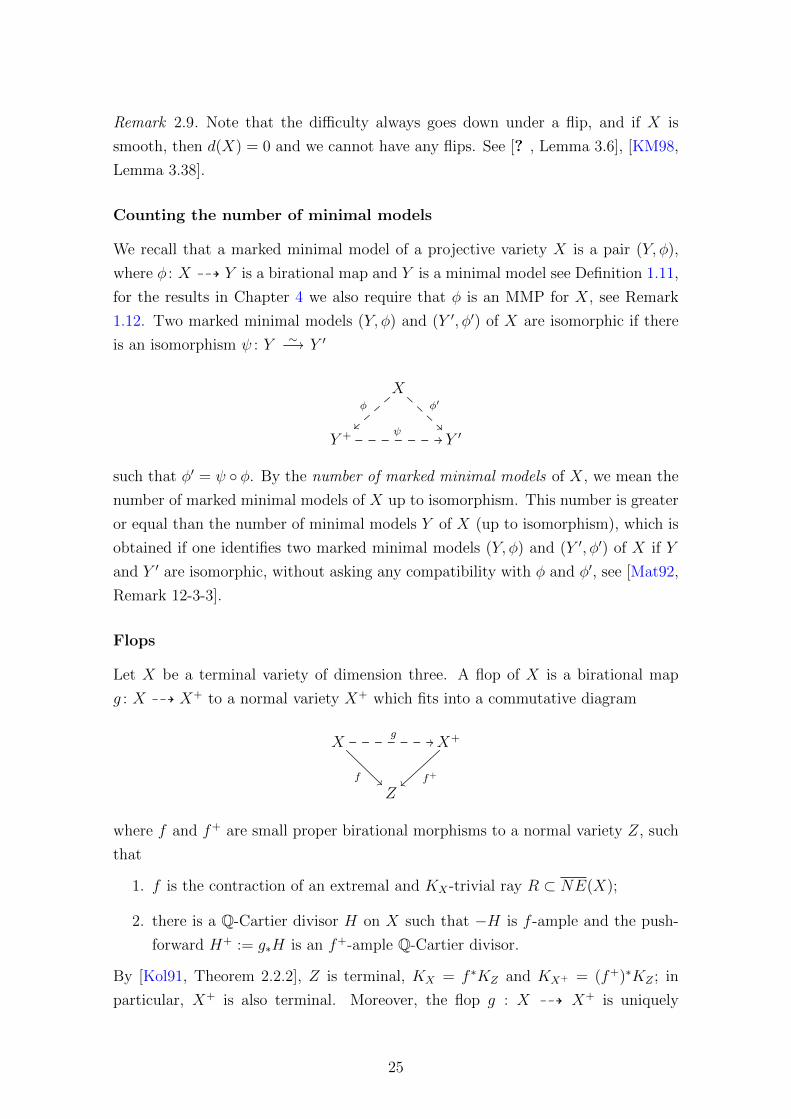
Counting the number of minimal models

We recall that a marked minimal model of a projective variety X is a pair (Y, φ),

where φ : X 99K Y is a birational map and Y is a minimal model see Definition 1.11,

for the results in Chapter 4 we also require that φ is an MMP for X, see Remark

1.12. Two marked minimal models (Y, φ) and (Y ′, φ′) of X are isomorphic if there

is an isomorphism ψ : Y ∼ // Y ′

Xφ′

φ

Y + ψ// Y ′

such that φ′ = ψ φ. By the number of marked minimal models of X, we mean the

number of marked minimal models of X up to isomorphism. This number is greater

or equal than the number of minimal models Y of X (up to isomorphism), which is

obtained if one identifies two marked minimal models (Y, φ) and (Y ′, φ′) of X if Y

and Y ′ are isomorphic, without asking any compatibility with φ and φ′, see [Mat92,

Remark 12-3-3].

Flops

Let X be a terminal variety of dimension three. A flop of X is a birational map

g : X 99K X+ to a normal variety X+ which fits into a commutative diagram

Xg

//

f

X+

f+

Z

where f and f+ are small proper birational morphisms to a normal variety Z, such

that

1. f is the contraction of an extremal and KX-trivial ray R ⊂ NE(X);

2. there is a Q-Cartier divisor H on X such that −H is f -ample and the push-

forward H+ := g∗H is an f+-ample Q-Cartier divisor.

By [Kol91, Theorem 2.2.2], Z is terminal, KX = f ∗KZ and KX+ = (f+)∗KZ ; in

particular, X+ is also terminal. Moreover, the flop g : X 99K X+ is uniquely

25

determined by the extremal ray R ⊂ NE(X) contracted by f , see [KM98, Corollary

6.4].

If X is a threefold, then f and f+ contract (possibly reducible) curves C and C+,

respectively; we call C the curve we are flopping and C+ the flopped curve.

Remark 2.10. Assume in addition that X is projective, Q-factorial and of general

type. Then, by the contraction theorem, for any KX-trivial extremal ray R ⊂NE(X), the contraction of R exists and is given by a linear series. Since Z in

the above diagram is normal, f has to coincide with that contraction and so Z is

projective. Moreover, X+ is projective and Q-factorial [KM98, Proposition 3.37].

In particular, if X is a minimal model, then so is X+.

Lemma 2.11. Let f : X //Z a small contraction such that all the contracted curves

are numerically proportional. Assume moreover that Z is (quasi-)projective. Then

f is the contraction of an extremal ray.

Proof. Let as assume that there exist two distinct numerically equivalent curves C

and D such that only C is contracted by f . Let H be an ample divisor on the base,

then C · f ∗H = 0 whereas D · f ∗H > 0 contradicting the fact that C and D are

numerically equivalent.

A sequence of flops is a finite composition of flops; we allow also the empty

sequence, by which we mean the identity. We will use the following versions for

families.

Definition 2.12. A flop (resp. sequence of flops) of a family π : X //B is a rational

map G : X 99K X+ over B

X G //

π

X+

π+

B

which restricts to a flop (resp. sequence of flops) on each geometric fibre.

Minimal models are connected by a sequence of flops.

Theorem 2.13. [Kol89, Theorem 4.9] If (Y, φ) and (Y ′, φ′) are two marked minimal

models of a projective variety X, then φ′ φ−1 : Y 99K Y ′ is a sequence of flops.

Boundedness of canonical models

A variety X is canonical if it is normal, KX is Q-Cartier and the discrepancy of X

is non-negative, see Definition 2.6. We recall that a canonical model is a projective

canonical variety X such that KX is ample.

26

Complex projective varieties of general type and bounded volume are birationally

bounded by [HM06, Tak06, Tsu06]. Together with the existence of canonical models

[BCHM10], this can be used to show that the canonical models of varieties of general

type with bounded volume have a parameter space. The precise statement is the

following, see [HK11, Corollary 13.9].

Theorem 2.14. Let n be a positive integer and c be a positive constant. Then there

is a projective morphism of normal quasi-projective varieties p : Y //S, such that

any canonical model of general type of dimension n whose volume is bounded by c is

isomorphic to a fibre of p. Moreover, each fibre of p is a canonical model of general

type of dimension n.

Families of minimal models

In Chapter 3 we deal with families of minimal models. A family is a proper flat

morphism with connected fibres π : X //B of reduced finite type schemes over k.

If not specified otherwise, a fibre of a family is a fibre over a closed point. A family

of minimal models is a family such that all its geometric fibres are minimal models,

see [KM92, Section 12.4].

A geometric point b of a scheme B is a morphism b : Spec(F ) //B where F is an

algebraically closed field; if B is irreducible, then η denotes the geometric generic

point, given by the natural morphism Spec(k(B)) //B.

Remark 2.15 (Specialization of the general fiber). Let R be a discrete valuation

ring with fraction field K and residue field k. Let X // Spec(R) be a proper flat

morphism, then we say that a fiber over k is a specialization of the general fiber

over K.

Classification of flips of Kollar and Mori

In this subsection we list some results from [KM92] that we are extensively going to

use in Chapter 3.

Theorem 2.16. [KM92, Corollary 11.11] Let f0 : X0 → Y0 be a proper morphism

between normal threefolds. Assume that X0 has only normal terminal singularities.

Moreover, assume that f0 contracts a curve C0 ⊂ X0 to a point Q0 ∈ Y0 and that KX0

has zero intersection with any components of C0. Let XS → S be a flat deformation

of X0 over the germ of a complex space 0 ∈ S. Let Sgen be a generic point of S and

let Xgen be the fiber of XS over Sgen. Then for any irreducible component Ci0 of C0

there is a curve Cigen ⊂ Xgen such that Ci

gen specializes to a multiple of Ci0.

27

Theorem 2.17. [KM92, Theorem 12.2.6] Let X and S be irreducible analytic spaces

of finite type and let X/S be a proper and flat relative algebraic space, i.e. it is

bimeromorphic to a projective fiberspace. We assume that X/S satisfies the following

property: let p : ∆ → S be a morphism and let X∆/∆ be the pull-back family. We

assume that if D ⊂ ∆ is a Weil divisor proper over ∆ such that D is Cartier outside

finitely many fibers then D is Q-Cartier. Assume that for some 0 ∈ S the fiber X0

is projective, then there is a Zariski open neighbourhood 0 ∈ U ⊂ S, such that for

each s ∈ U the fiber Xs is projective.

Proposition 2.18. [KM92, Proposition 12.2.6] Let X/S be as in Theorem 2.17.

Let C/S ⊂ X/S be a family of 1-cycles. If C0 ⊂ X0 is numerically equivalent to

zero for some 0 ∈ S, then Cs ⊂ Xs is numerically equivalent to zero for every s ∈ S.

Proposition 2.19 (MMP in families). [KM92, Proposition 12.4.2] Let S be a con-

nected normal quasi-projective variety and let X/S be a flat, projective family of

threefolds such that every fiber has only Q-factorial terminal singularities. Then

there is a finite etale and Galois base change p : S ′ → S, a flat projective fam-

ily Y ′/S ′, and a rational map f ′ : p∗(X)/S ′ 99K Y ′/S ′ such that on each fiber f ′

induces a birational map, each fiber of Y ′/S ′ has only Q-factorial terminal singular-

ities and KY ′/S′ is either relatively nef or Y ′/S ′ admits a relative Mori Fiber Space

structure.

Remark 2.20. In order to ensure that the fibres of a smooth family X //B stay

Q-factorial after running a relative MMP, it is necessary to perform a base change

which trivializes the monodromy on N1(Xt) for very general t ∈ B (or equivalently,

such that N1(X ) //N1(Xt) is onto, see [KM92, Remark 12.4.3] and the following

lemma for an explicit construction.

Lemma 2.21. Let B be a complex variety and let π : X //B be a family of complex

projective varieties. After replacing B by a finite covering of some Zariski open and

dense subset of B, the restriction map N1(X ) //N1(Xt) is onto for any very general

t ∈ B.

Proof. In order to prove surjectivity of N1(X ) //N1(Xt), we pick a basis e1, . . . , em

of the vector space N1(Xη). Each ei can be represented by a line bundle Li on

Xη. Moreover, each Li can be defined over some finite extension of the function

field C(B). After replacing B by a finite covering, we may thus assume that Li can

be defined over C(B), and hence after shrinking B, Li extends to a line bundle Lion the total space X . This shows that N1(X ) //N1(Xt) is onto, because for very

general t ∈ B, Xt and Xη are isomorphic as schemes over Z and so the restrictions

of L1, . . . ,Lm to Xt induce a basis of N1(Xt). This concludes the lemma.

28

2.2 Descending Sections

All the following results are going to be used in Chapter 6 and hold over an arbitrary

algebraically closed field of characteristic p. Following the notation of [Kee99], for a

morphism f : X → Y , a line bundle L on Y , and a section s ∈ H0(Y, L), we denote

by L|X and s|X the pullbacks f ∗L and f ∗s, respectively.

We say that a section t ∈ H0(X,L|X) descends to Y if there exists a section

s ∈ H0(Y, L) such that f ∗s = t.

Let X be a scheme and F ⊂ X a closed subscheme. Let L be a line bundle on X

and s ∈ H0(X,L) its section. We say that s is nowhere vanishing on F if s|x is

not zero as an element in the one-dimensional vector space H0(x, L|x) for any

closed point x ∈ F .

The conductor scheme

Let X be a reduced scheme of finite type over a field, X =⋃Xi the decomposition

into irreducible components, and Xi → Xi the normalizations. Then we define the

normalization of X as the composition⊔Xi →

⊔Xi → X.

Definition 2.22. The conductor scheme: X be a reduced scheme of finite type

over a field and X → X its normalization. We identify the sheaf of rings OX as the

subring of OX . Let I ⊂ OX be the ideal sheaf satisfying IOX ⊂ OX , so that I is

maximal by inclusion. The conductor of X is the subscheme D ⊂ X defined by I.

By abuse of notation, the subscheme C ⊂ X defined by IOX will also be called the

conductor.

The notion of conductor is important, because of the following lemma.

Lemma 2.23. Let C ⊂ X, D ⊂ X be the conductors and let L be a line bundle on

X.

C

// X

D // X

Then, a section s ∈ H0(X,L|X) descends to X if and only if s|C descends to D.

Proof. By definition of the conductor, we have the following exact sequence

0 //H0(X,L) //H0(X,L|X)⊕H0(D, L|D) //H0(C, L|C),

where the second map is defined by t // (t|X , t|D), and the third map is defined by

29

(t, u) // t|C − u|C. Therefore, a section s ∈ H0(X,L|X) descends to X if and only if

s|C descends to D.

Adjunction formula

Let (X,∆) be a log pair and S the union of the supports of some of the divisors with

coefficient one in ∆. Let p : S → S be the normalization of S. Then there exists an

effective Q-divisor ∆S on S such that

KS + ∆S = (KX + ∆)|S

holds at the level of rational equivalence (see for instance [Kol13, Definition 4.2]).

Note that the choice of ∆S is not unique.

We denote by C the possibly non-reduced divisor on S corresponding to the

codimension one part of C, where C ⊂ S is the conductor of S.

When X is Q-factorial, it follows that C ≤ ∆S by [Kee99, Theorem 5.3]. In

Chapter 6, we will use the following proposition, which only states Supp(C) ⊂Supp(b∆Sc), but is valid even for a non-Q-factorial variety X.

Proposition 2.24. Let (X,∆) be a log pair, and let S be the union of the supports

of some of the divisors with coefficient one in ∆. Let p : S → S be the normalization

of S, and let ∆S be an effective Q-divisor on S defined by the adjunction as above.

Further, we denote by C the (possibly non-reduced) divisor on S corresponding to the

codimension one part of C, where C ⊂ S is the conductor of S. Then the following

hold:

1. Supp(C) ⊂ Supp(b∆Sc).

2. Let D1, . . . , Dc be prime divisors with coefficient greater than or equal to one in

b∆c, and let T =⋃

1≤i≤c Supp(Di). Assume that each Di satisfies Supp(Di) 6⊂S. Then, the codimension one part of p−1(S ∩T ) is contained in Supp(b∆Sc).

Proof. First, we prove (1). Let V ⊂ S be a codimension one subvariety such that

V ⊂ C. It is sufficient to show coeffV ∆S ≥ 1. When (X,∆) is not log canonical

at the generic point ηp(V ) of p(V ), we have coeffV ∆S > 1 (see [Kol13, Proposition

4.5 (2)]). Hence, we may assume that (X,∆) is log canonical at ηp(V ). In this case,

S has a node at ηp(V ) and coeffV ∆S = 1 (see [Kol13, Proposition 4.5 (6), Theorem

2.31]).

Next, we prove (2). Let V ⊂ S be a codimension one subvariety such that

V ⊂ p−1(S ∩ T ). It is sufficient to show coeffV ∆S ≥ 1. Since the problem is local

30

around V , we may assume that p(V ) ⊂ Supp(Di) for all i. If coeffDi ∆ > 1 for some

i, then (X,∆) is not log canonical at the generic point ηp(V ) of p(V ). In this case,

we have coeffV ∆S > 1 as above. Hence, we may assume that coeffDi ∆ = 1 for all

i. Note that S ∩ T is contained in the conductor of the normalization of S ∪ T .

Therefore, we conclude the proof by applying (1) to S ∪ T .

2.3 Some properties of varieties over FpIn Chapter 6, we work over the algebraic closure of a finite field, Fp. In this section

we collect the following facts and properties that distinguish Fp from other fields of

positive characteristic.

Proposition 2.25. The Picard scheme Pic0X is a torsion group when X is a

projective scheme defined over Fp. In particular, any numerically trivial Cartier

divisor is Q-linearly trivial.

For the proof, see for instance [Kee99, Lemma 2.16].

We need the following lemmas in Section 6.4.

Lemma 2.26. Let X be a proper scheme over Fp. Let s1, s2 ∈ H0(X,OX) be

sections of the structure sheaf. Assume that s1 and s2 are nowhere vanishing on X.

Then there exists n ≥ 1 such that sn1 = sn2 in H0(X,OX).

Proof. Without loss of generality we may assume that X is connected. Set A :=

H0(X,OX). It is a finite-dimensional vector space over Fp, because X is proper.

Since X is connected, A has the unique maximal ideal m, and it follows that A/m 'H0(Xred,OXred) ' Fp.

Let ai be the element of A corresponding to si and ai the image of ai in Fp. Since

si is nowhere vanishing on X, the element ai ∈ Fp is not zero. Hence, there exists

e ≥ 1 for which a1pe−1 = a2

pe−1 = 1. Take r ≥ 1 such that mpr = 0. Then we have

apr(pe−1)1 − ap

r(pe−1)2 =

(ap

e−11 − ap

e−12

)pr ∈ mpr = 0.

Therefore, it is sufficient to set n = pr(pe − 1).

Lemma 2.27. Let X be a one-dimensional reduced scheme of finite type over Fp,L a line bundle on X, and p : X → X the normalization of X. Let C ⊂ X be the

conductor of X, and s ∈ H0(X,L|X) be a section nowhere vanishing on C. Then sn

descends to X for some n ≥ 1.

31

Proof. Let D ⊂ X be the conductor. Note that C and D are either empty or have

dimension zero. By Lemma 2.23, it is sufficient to prove that sn|C descends to D for

some n ≥ 1. Let t ∈ H0(D, L|D) be a section nowhere vanishing on D. Then t|C is

nowhere vanishing on C. Any line bundle is trivial on a zero-dimensional scheme,

and so by Lemma 2.26, we get sn|C = tn|C for some n ≥ 1. In particular, sn|Cdescends to D.

Lemma 2.28. Let C be a smooth proper connected curve over Fp. Then, a finitely

generated subgroup of Aut(C) is finite.

Proof. If g(C) ≥ 2, then Aut(C) is finite and the statement is trivial. If C = P1,

then Aut(C) ' PGL(2,Fp). A finitely generated subgroup G of PGL(2,Fp) is always

finite, because G is contained in PGL(2,Fpe) for some e ≥ 1. If C is an elliptic curve,

then we get Aut(C) ' T oF , where T is the group of translations and F is a finite

group (see for instance [Sil09, Section X.5]). Note that each element of T has finite

order, because C is defined over Fp. Hence, a finitely generated subgroup of the

abelian group T is always finite, and so a finitely generated subgroup of Aut(C) is

also finite.

For completeness, we note a general fact in group theory: any finitely generated

subgroup of G1 o G2 is finite, if we assume that for each i, any finitely generated

subgroup of Gi is finite.

Keel’s theorems

In this subsection, we list some theorems from Keel [Kee99]. The following theorem

is crucial in reducing problems from threefolds to surfaces.

Theorem 2.29 ([Kee99, Proposition 1.6]). Let X be a projective scheme over a field

of positive characteristic. Let L be a nef line bundle on X, and let E be an effective

Cartier divisor on X such that L−E is ample. Then L is semiample if and only if

L|Eredis semiample.

We note that Cascini, McKernan, and Mustata gave a different proof of Theo-

rem 2.29 [CMM14, Theorem 3.2].

Theorem 2.30 ([Art62, Theorem 2.9], [Kee99, Corollary 0.3]). Let X be a projective

surface over Fp and let L be a nef and big line bundle on X. Then L is semiample.

Proof. Since by Proposition 2.25 nef line bundles on curves over Fp are semiample,

the claim follows from Theorem 2.29.

32

We say that a map f : X → Y is a finite universal homeomorphism if it is a finite

homeomorphism under any base change. In this case, we have a correspondence, up

to taking powers, between the set of sections of a line bundle L on Y and the set of

sections of L|X .

Theorem 2.31 ([Kee99, Lemma 1.4]). Let f : X → Y be a finite universal homeo-

morphism between varieties defined over a field of characteristic p > 0 and let L be

a line bundle on Y . Then the following hold.

(1) For s ∈ H0(X,L|X), the section spe ∈ H0(X,L⊗p

e|X) descends to Y for a

sufficiently large integer e ≥ 1.

(2) If t ∈ H0(Y, L) satisfies t|X = 0, then tpe

= 0 holds for a sufficiently large

integer e ≥ 1.

In Chapter 6, we frequently use the following theorems.

Theorem 2.32 ([Kee99, Corollary 2.12]). Let X = X1 ∪X2 be a projective scheme

over Fp, where Xi are closed subsets. Let L be a nef line bundle on X such that L|Xiare semiample. Let gi : Xi → Zi be the map associated to L|Xi. Assume that all but

finitely many fibers of g2|X1∩X2 are geometrically connected. Then L is semiample.

Theorem 2.33 ([Kee99, Corollary 2.14]). Let X be a reduced projective scheme

over Fp. Let p : X → X be the normalization of X. Let D ⊂ X and C ⊂ X be the

reductions of the conductors. Let L be a nef line bundle on X such that L|X and

L|D are semiample. Let g : X → Z be the map associated to L|X . Assume that all

but finitely many fibers of g|C are geometrically connected. Then L is semiample.

33

3 On the number of minimal

models

3.1 Introduction

As we already recall in Introduction, starting from dimension three, minimal models

of a smooth complex projective variety X are in general not unique. Nevertheless,

if X is of general type, even the number of marked minimal models of X is finite

[BCHM10], [KM87], that is, up to isomorphism, there are only finitely many pairs

(Y, φ), where φ : X 99K Y is a birational map and Y is a minimal model, see Section

2.1.

In this chapter we prove that it is possible to bound the number of minimal

models of a smooth projective threefold of general type in terms of the topology of

the underlying complex manifold, solving a conjecture of Cascini and Lazic [CL14].

Theorem 3.1. Let c be a positive real number. Then there is a positive constant

N(c), such that for any smooth complex projective threefold X of general type, whose

Betti numbers are bounded by c, i.e. bi(X) ≤ c for all i, the number of marked

minimal models of X is at most N(c).

The proof of Theorem 3.1 is not constructive, so that N(c) cannot be estimated.

For some effective results, under further assumption see Chapter 4.

By [CT14, Theorem 4.1], the volume of a smooth complex projective threefold

of general type is bounded by the Betti numbers. Therefore, Theorem 3.1 is a

consequence of the following, which is the main result of this chapter.

Theorem 3.2. Let c be a positive real number. Then there is a positive constant

N ′(c), such that for any smooth complex projective threefold X of general type and

of volume vol(X) ≤ c, the number of marked minimal models of X is at most N ′(c).

The proof of Theorem 3.2 is based on the birational boundedness result for three-

folds of general type, due to Hacon and McKernan [HM06], Takayama [Tak06] and

Tsuji [Tsu06], together with results on deformations of flops in dimension three,

34

due to Kollar and Mori [KM92]; our proof uses and generalizes ideas from [ST16,

Theorem 13].

3.2 The main technical result

Before we state the main technical result (Proposition 3.5 below), we need some

auxiliary lemmas.

Lemma 3.3. Let π : X //B be a family over an irreducible base B, such that Xη is

normal and KXη is Q-Cartier. Then there is a dense open subset U ⊂ B such that

the base change XU //U has only normal geometric fibres, normal total space XUand KXU/U is Q-Cartier.

Proof. Since the geometric generic fibre of π is normal, the normalization of the total

space X is an isomorphism over the generic point of B. After shrinking B, we may

thus assume that X is normal. Since (geometric) normality is an open condition in

families [Gro64, Theorem 12.2.4], we may also assume that all geometric fibres of π

are normal.

By assumptions, there is some positive integer a, such that aKXη is Cartier. This

Cartier divisor is defined over some finite extension of the function field k(B). There-

fore, there is a dominant morphism p : B′ //B, finite onto its image, such that the

base change π′ : X ′ //B′ carries a Cartier divisor L which restricts to aKX ′η on the

geometric generic fibre. After shrinking B and B′, we may assume that B and B′

are smooth and p : B′ //B is proper and etale. It follows that KX ′/B′ is Q-Cartier

if and only if KX/B is, see for instance proof of [KM98, Lemma 5.16]. This proves

the lemma, because L = aKX ′/B′ after shrinking B′.

Lemma 3.4. Let π : X //B be a family of minimal complex projective threefolds of

general type over an irreducible base B. Let Xη be the geometric generic fibre of π,

and let g : Xη 99K X+η be a flop. Then there is a generically finite morphism B′ //B,

such that the base change π′ : X ′ //B′ admits a flop of families G : X ′ 99K (X ′)+

over B′ which restricts to the given flop g of the geometric generic fibre X ′η = Xη.

Proof. Recall from Section 2.1 that the flop g consists of a diagram of terminal

varieties

Xηg

//

f

X+η

f+~~

Z

35

where f and f+ are small contractions. Here, f contracts an extremal ray and

there is a Q-Cartier divisor Hη on Xη which intersects negatively the curves that are

contracted by f and H+η = g∗Hη intersects positively the curves contracted by f+.

The above diagram as well as the Cartier divisor Hη are defined over some finite

extension of C(B). Thus, after a suitable base change, these are defined over C(B).

Then, after shrinking B, we can spread the above diagram over B and obtain a

diagram

X G //

F

X+

F+

Zof families over B and there is a Cartier divisor H on X that restricts to Hη on Xη.By Lemma 3.3, we may after shrinking B assume that X+ is normal, all geometric

fibres of π+ : X+ //B are normal and KX+/B is Q-Cartier. Since g∗Hη is Q-Cartier,

we may after base change also assume that H+ := G∗H is Q-Cartier on X+. We

want to show that, possibly after a base change, G : X 99K X+ restricts to a flop on

each geometric fibre of π : X //B, i.e. G is a flop of the family π.

Let C ⊂ X and C+ ⊂ X+ be the exceptional locus of F and F+, respectively.

After a base change, if necessary, we may assume that all components of C and C+

dominate B, and that all components of the geometric generic fibres of C and C+

are defined over B. That is, C = C1 ∪ · · · ∪ Cm and C+ = C+1 ∪ · · · ∪ C+

m+ such that

the geometric generic fibres of Ci and C+j are irreducible for all i and j. By generic

flatness, after shrinking B, we may assume that Ci and C+j are flat over B, and, after

shrinking further, we may assume that all fibres of Ci and C+j over B are irreducible.

Since Xη is projective and of general type, Z and X+η are projective, see Remark

2.10. Up to shrinking B, we may therefore assume that X , X+ and Z are projective

over B, and all fibres are normal, because the latter is an open condition [Gro64,

Theorem 12.2.4]. Let b be a geometric point of B. The morphism F : X //Zrestricts then to a contraction Fb : Xb

//Zb of the curve Cb = C|Xb . By Proposition

2.18, two flat families of curves over B are fibrewise numerically proportional, if

this is true for the restriction to one fibre. This implies that all the components

of Cb are numerically proportional because they are proportional on the geometric

generic fibre. This implies that Fb is the contraction of an extremal ray, because Zb

is projective, see Lemma 2.11.

We need to prove that the induced birational map Gb : Xb 99K X+b is a flop. Since

each component Ci of C is flat over B, and since KXb = KX/B|Xb is the restriction

of a Q-Cartier divisor on X , for any component Cb,i of Cb the intersection number

KXb · Cb,i does not depend on b; hence it is zero because this is true for b = η. For

36

the same reason, H|Xb .Cb,i < 0 for all i. Similarly, we conclude H+|X+b.C+

b,j > 0,

where H+|X+b

= Gb∗H|Xb and C+b,j is any component of C+

b = C+|X+b

. This proves

that Gb is a flop, as we want.

Proposition 3.5. Let p : Y //S be a family of minimal complex projective threefolds

of general type. Then there is a family π : X //B of minimal complex projective

threefolds of general type, such that each fibre of p is isomorphic to a fibre of π,

and the following holds for each component Bi of B, where πi : Xi //Bi denotes the

restriction of π to Xi = π−1(Bi).

There are finitely many families πki : X ki

//Bi of minimal models over Bi, k =

1, . . . , r(i), such that π1i coincides with πi : Xi //Bi, and such that for all k:

(i) there is a sequence of flops of families φki : Xi 99K X ki ;

(ii) if X is the fibre of πki above any b0 ∈ Bi, then for any flop g : X 99K X+, there

is some j, such that φji (φki )−1 : X k

i 99K X ji restricts to the given flop of X.

Proof. We proceed in several steps.

Step 1. There is a family π : X //B with the same fibres as p, such that for

each component Bi of B, any sequence of flops of the geometric generic fibre of

Xi = π−1(Bi) extends to a sequence of flops of families of πi : Xi //Bi.

Proof. The construction of π : X //B proceeds by induction on n = dim(S). If

n = 0, then the assertion follows from the finiteness of minimal models. If n > 0,

then we construct the family π as base change of p via some surjective morphism

B //S. By induction, we may assume that S is pure dimensional of dimension

n. For the same reason, we may replace S by some Zariski open and dense subset

because the complement has lower dimension and so we know how to construct the

desired family there by induction. Step 1 is therefore an immediate consequence of

Lemma 3.4.

By [KM87], Xi,η has only finitely many minimal models, say r(i)-many. We denote

them by (X ki,η, φ

ki,η), where k = 1, . . . , r(i) and

φki,η : Xi,η 99K X ki,η

is a birational map. By Theorem 2.13, each φki,η is a (possibly trivial) sequence of

flops, because Xi,η is minimal. Without loss of generality, we assume that Xi,η = X 1i,η

and φ11,η = id. By Step 1, for k = 1, . . . , r(i), we obtain families

πki : X ki

//Bi,

37

with X 1i = Xi and sequences of flops of families

φki : Xi 99K X ki ,

whose restriction to the geometric generic point of Bi coincides with (X ki,η, φ

ki,η) from

above. We may in particular assume φ1i = id, which proves item (i) of the proposi-

tion and it remains to prove item (ii). We first note the following.

Step 2. For any flop ξ : X ki,η 99K (X k

i,η)+ of the geometric generic fibre of πki , there

is some j such that φji (φki )−1 : X k

i 99K X ji is a flop of families which restricts to

the given flop of X ki,η.

Proof. In order to prove the assertion in Step 2, it suffices to note that ((X ki,η)

+, ξ φki,η) is a minimal model of Xi,η and so it is isomorphic to some (X j

i,η, φji,η); in par-

ticular, φji (φki )−1 restricts to the given flop ξ of X k

i,η, as we want.

In order to prove item (ii), let X = Xb0 be the fibre of πki over some point b0 ∈ Bi,

and let g : X 99K X+ be a flop.

Let ∆ ⊂ Bi be an analytic disc, centered at b0 and with the property that any

very general point of ∆ is a very general point of Bi. By [KM92, Theorem 11.10],

after possibly shrinking ∆, the flop g : X 99K X+ extends to a flop of the analytic

family X ki |∆ //∆,

X ki |∆

G∆ //

F∆ ""

(Xki )+|∆

F+∆zz

Z∆ .

(3.1)

Step 3. After shrinking ∆, (3.1) restricts fibrewise to a flop in the sense of Section

2.1.

Proof. In [KM92], a slightly weaker definition of flops is used; it is only required

that fibrewise, the curves contracted by F∆ are KX-trivial, but it is not asked that

they form an extremal ray. In order to see that after shrinking ∆, (3.1) restricts

for all t ∈ ∆ to a flop in the sense of Section 2.1, we therefore need to prove that

Ft contracts an extremal ray. Note that it suffices to prove this after a finite base

change ∆′ //∆ of the disc (we do not perform any base change of Bi here).

By Theorem 2.17, we may, after shrinking ∆, assume that any fibre of Z∆//∆

is projective. Let C∆ ⊂ Xi|∆ be the exceptional locus of F∆. Let C0 ⊂ X be the

fibre of C∆ above b0, i.e. the flopping curve of g : X 99K X+. By Theorem 2.16, each

38

component of C0 is (up to a multiple) a specialization of a curve on the general fibre

of X|∆ //∆. In particular, after shrinking ∆, we may assume that each component

of C∆ dominates ∆ and so C∆ is flat over ∆. After a finite base change ∆′ //∆

and possibly shrinking further, we may assume that any component C ′∆ of C∆ has

irreducible fibres above any point of the punctured disc ∆ \ b0. It then follows

from [KM92, Proposition 12.2.6] that the components of any fibre of C∆//∆ are

numerically proportional. Since Z∆//∆ has projective fibres, it follows that F∆

restricts for any t ∈ ∆ to a contraction of a KXt-trivial ray, see Lemma 2.11. This

proves that (3.1) restricts fibrewise to a flop in the sense of Section 2.1.

Let bg be a very general point of ∆. By construction of ∆, bg is a very general point

of Bi and so the fibre Xbg of X ki |∆ //∆ is abstractly isomorphic to the geometric

generic fibre of πki . That is, there is an isomorphism of schemes over Z, σ : Xbg∼ //

X ki,η, because we can choose an isomorphism of fields C ∼ // C(Bi). The flop of the

family in (3.1) restricts to a flop Xbg 99K X+bg

of Xbg and hence induces via σ a flop

of X ki,η. It therefore follows from Step 2 that there is some j ∈ 1, . . . , r(i) such

that

φji (φki )−1 : X k

i 99K X ji (3.2)

is a flop of families which restricts to the given flop of X ki,η.

Step 4. For any t ∈ ∆, restricting (3.1) and (3.2) to the fibre above t yields the

same flop of Xt.

Proof. In order to see this, we need to prove that the flopping curves are the same

(see Section 2.1) and for this it suffices to prove that they are numerically propor-

tional. The latter follows from Proposition 2.18, and the fact that the flopping curves

are flat over ∆ and coincide in the fibre above bg by construction. This concludes

Step 4.

By Step 4, (3.2) restricts to the given flop g : X 99K X+ of the special fibre

X = Xb0 , as we want in item (ii). This finishes the proof of the proposition.

3.3 Proof of Theorem 3.2

Proof of Theorem 3.2. Let c be a positive constant. By Theorem 2.14, there exists

a quasi-projective scheme S, hence of finite type over C and a projective family

pcan : Ycan //S such that any canonical models of threefolds of general type whose

39

volume is bounded by c is isomorphic to a fiber of pcan. By Noetherian induction,

replacing S by a disjoint union of locally closed subsets and resolving Ycan, we get

a smooth family psm : Ysm //S. We now run the relative minimal model program

for this family, see Proposition 2.19; note that this operation requires a base change

in order to trivialize the monodromy of the very general fiber, see Remark 2.20 and

Lemma 2.21. In this way we obtain a family pmin : Ymin //S of minimal threefolds

of general type.

By Proposition 3.5, the family pmin gives rise to a family π : X //B of minimal

models of general type such that any minimal threefold of general type and with

volume bounded by c is birational to a fibre of π. Let B1, . . . , Bs denote the compo-

nents of B. Since minimal models are connected by sequences of flops (see Theorem

2.13), it follows from item (ii) that each fibre of π above a point of Bi has, in the

notation of Proposition 3.5, at most r(i) many minimal models. It follows that

any smooth complex projective threefold of general type and with volume bounded

by c has at most N ′(c) := maxr(i) | i = 1, . . . , s many minimal models, as we

want.

By Theorem 2.14, canonical models of general type and bounded volume are

bounded. The following immediate corollary of the proof of Theorem 3.2 proves the

same for minimal threefolds of general type.

Corollary 3.6. Let c ∈ R+. Then there is a family of minimal models π : X //B,

such that any minimal model of a smooth complex projective threefold of general type

and volume bounded by c is isomorphic to at least one fibre of π.

40

4 Effective topological bounds for

threefolds

4.1 Introduction

In this chapter we find an explicit bound for the number of minimal models of a

smooth threefold of general type, under some technical assumptions. We recall that

in this chapter we define a marked minimal model for a projective variety X as a

pair (Y, φ), where Y is a minimal model for X and the birational map φ is a MMP

for X, it means in particular that φ is a series of KX-negative extremal rays. see

Definition 1.11 and Remark 1.12.

Theorem 4.1. Let X be a smooth projective threefold of general type. Then the

number of marked minimal models of X that can be reached with a series of divisorial

contractions followed by a series of flips is at most max1, 3 (ρ(X)−2)[(ρ(X)− 2)!]2.

Using Theorem 4.1 we can obtain an effective bound in the case of Picard number

equal to three.

Theorem 4.2. Let X be a smooth projective threefold of general type of Picard

number ρ(X) = 3, then the number of marked minimal models of X is at most 3.

In Section 4.3 we found some effective bounds for the degree of the generators and

for the weight of the relations of the canonical ring. The bounds are obtained as a

straightforward generalization of some techniques introduced by Green [Gre82].

Theorem 4.3. Let X be a Gorenstein minimal variety of general type of dimension

n (i.e. X has terminal singularities and KX is Cartier, big and nef). Let R(X,KX)

be the canonical ring of X. Then

(1) R(X,KX) is generated in degree d ≤ (n+ 1)mn + 1;

(2) R(X,KX) is related in weight w ≤ 2(n+ 1)mn + 2;

where mn is a multiple of KX such that |mnKX | is free.

Remark 4.4. We recall that thanks to Kollar’s Effective base point freeness (see

Theorem 2.2), mn ≤ 2(n+ 2)!(2 + n).

41

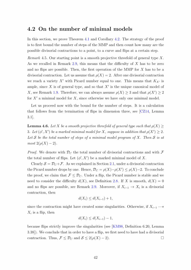
4.2 On the number of minimal models

In this section, we prove Theorem 4.1 and Corollary 4.2. The strategy of the proof

is to first bound the number of steps of the MMP and then count how many are the

possible divisorial contractions to a point, to a curve and flips at a certain step.

Remark 4.5. Our starting point is a smooth projective threefold of general type X.

As we recalled in Remark 2.9, this means that the difficulty of X has to be zero

and no flips are possible. Then, the first operation of the MMP for X has to be a

divisorial contraction. Let us assume that ρ(X) = 2. After one divisorial contraction

we reach a variety X ′ with Picard number equal to one. This means that KX′ is

ample, since X is of general type, and so that X ′ is the unique canonical model of

X, see Remark 1.9. Therefore, we can always assume ρ(X) ≥ 3 and that ρ(X ′) ≥ 2

for X ′ a minimal model for X, since otherwise we have only one minimal model.

Let us proceed now with the bound for the number of steps. It is a calculation

that follows from the termination of flips in dimension three, see [CZ14, Lemma

3.1].

Lemma 4.6. Let X be a smooth projective threefold of general type such that ρ(X) ≥3. Let (φ′, X ′) be a marked minimal model for X, suppose in addition that ρ(X ′) ≥ 2.

Let S be the total number of steps of a minimal model program of X. Then S is at

most 2(ρ(X)− 2).

Proof. We denote with DC the total number of divisorial contractions and with Fthe total number of flips. Let (φ′, X ′) be a marked minimal model of X.

Clearly S = DC+F . As we explained in Section 2.1, under a divisorial contraction

the Picard number drops by one. Hence, DC = ρ(X)−ρ(X ′) ≤ ρ(X)−2. To conclude

the proof, we claim that F ≤ DC . Under a flip, the Picard number is stable and we

need to consider the difficulty d(X), see Definition 2.8. If X is smooth, d(X) = 0

and no flips are possible, see Remark 2.9. Moreover, if Xi−1 → Xi is a divisorial

contraction, then

d(Xi) ≤ d(Xi−1) + 1,

since the contraction might have created some singularities. Otherwise, if Xi−1 99K

Xi is a flip, then

d(Xi) ≤ d(Xi−1)− 1,

because flips strictly improve the singularities (see [KM98, Definition 6.20, Lemma

3.38]). We conclude that in order to have a flip, we first need to have had a divisorial

contraction. Thus, F ≤ DC and S ≤ 2(ρ(X)− 2).

42

Let X be a smooth threefold of general type, satisfying all the assumption of

Theorem 4.1 and Lemma 4.6. Let (φ′, X ′) be a marked minimal models for X that

can be reached by a series of divisorial contractions and then by a series of flip.

Then we can represent φ′ in the following way.

φ′ : X = X0 → X1 → · · · → Xi︸ ︷︷ ︸divisorial contractions

= X0 99K X1 99K · · · 99K Xj︸ ︷︷ ︸flips

= X ′.

We will always indicate with Xi, 0 ≤ i ≤ ρ(X) − 2, a step in the minimal model

program for X that can be reached from X with a series of divisorial contractions;

with Xj, 0 ≤ j ≤ ρ(X)− 2, a step in the minimal model program for X from which

we can reach the minimal model X ′, with a series of flips.

We now proceed to bound the number of divisorial contractions to a point.

Lemma 4.7. Let X = X0 be a smooth projective threefold of general type satisfying

the assumptions of Lemma 4.6 and Theorem 4.1. Let Xi be a step in the minimal

model program for X, 1 ≤ i ≤ ρ(X)− 2. The number of ways to go from Xi to the

following step with a divisorial contraction to a point is at most ρ(X)− 2− i.

Proof. We divide the proof into steps.

Step 1. We consider the last divisorial contraction.

ψ : Xi−1 → Xi = X0

and we claim that there is a unique choice of divisor E that can be contracted to a

point by ψ.

Proof of Step 1. Let us assume by contradiction that there are two distinct divisors

E1 and E2 contained in Xi−1 and that they can be both contracted to a point.

Xi−1

ψ2

''

ψ1// X ′i

X ′′i

We denote with ψ1 the contraction of E1 and with ψ2 the contraction of E2. But

then, X ′i contains ψ1(E2) and X ′′i contains ψ2(E1). Since X ′i and X ′′i are followed

only by flips, ψ1(E2) and ψ2(E1) are not contracted and survive until the minimal

models.

43

Xi−1

ψ2

''

ψ1// X ′i // X ′

η12

X ′′i // X ′′

We have that X ′ ⊇ ψ1(E2) and X ′′ ⊇ ψ2(E1), (where by abuse of notation with

still indicate with ψ1(E2) and ψ2(E1) the images of the divisors through the series

of flips). However, X ′ and X ′′ are minimal models and are, therefore, connected by

a flop η12, i.e. an isomorphism in codimension one, see Theorem 2.13. We reach a

contradiction.

Step 2.

Let us now consider the preceding step. In this case we have at least two divisors

E1 and E2 that can be contracted to a point.

Xi−2

ψ′′i−1 ''

ψ′i−1// X ′i−1

ψ′i // X ′i

X ′′i−1 ψ′′i

// X ′′i

We can choose to first contract E1 with ψ′i−1 and then E2 with ψ′i or we can invert

the order and contract first E2 with ψ′′i−1 and then E1 with ψ′′i . We claim that there

are no more possible divisors that can be contracted into a point.

Proof of Step 2. Let us assume by contradiction that there exists an other divisor

E3, such that E3 is distinct from E1 and E2 and that can be contracted into a

point by a divisorial contraction that we call ψ′′′i−1 : Xi−2 → X ′′′i−1. Since E3 is

not contracted by ψ′i−1 and ψ′i, ψ′i(ψ′i−1(E3)) is contained in X ′i and so also in the

minimal model X ′ because X ′i is followed just by flips. If we consider instead the

minimal model X ′′′ that follows X ′′′i−1, in particular this means that X ′′′ is obtained

contracting KX′′′i−1-negative extremal rays, X ′′′ is not going to contain the image of

E3. But since X ′ and X ′′′ are minimal models and so connected by an isomorphism

in codimension one, we reach a contradiction.

Step 3. At the step Xi, for 0 ≤ i ≤ ρ(X)− 2, the number of ways to go from Xi

to the following step with a divisorial contraction to a point is at most ρ(X)− 2− i.

Proof of Step 3. We can iterate the argument of Step 2 in the case of a series of

divisorial contractions. Let Xi be a step of the minimal model for X, there are at

least ρ(X)− 2− i choices for a divisor to be contracted to a point. If there were at

least ρ(X) − 1 − i choices, there would be a divisor E that survives until we reach

44

the minimal model X ′. But since at the step Xi the divisor E can be contracted,

there exists another marked minimal model (φ′′, X ′′) such that E is contracted and

again we reach a contradiction since minimal models are isomorphic in codimension

one. We conclude that the number of possible contractions to a point at the step

Xi is at most ρ(X)− 2− i.

This conclude the proof of the lemma.

We want now to count how many are the possible choices for a divisorial contrac-

tion to a curve.

Lemma 4.8. Let X = X0 be a smooth projective threefold of general type satisfying

the assumptions of Lemma 4.6 and Theorem 4.1. Let Xi be one step in the minimal

model program for X, 0 ≤ i ≤ ρ(X)− 2. The number of ways to go from Xi to the

following step with a divisorial contraction to a curve is at most 2(ρ(X)− 2− i).

Proof. Again we divide the proof into steps.

Step 1. We consider the last divisorial contraction.

ψ : Xi−1 → Xi = X0

and we claim that there are at most two divisorial contractions to a curve.

Proof of Step 1. Proceeding as we did in Step 1 of Lemma 4.7, we can prove that

there is a unique choice for a divisor E to be contracted. Then we need to understand

in how many ways the divisor E can be contracted into a curve C. We know that

ρ(C) = 1 because two divisors on a curve are numerically equivalent if they have

the same degree, then we obtain that ρ(E|X) = 2, see Definition 2.5, because

ρ(Xi−1) − ρ(Xi) = 1, since ψi is a divisorial contraction. We then obtain two

possible contractions: ψ1 that contracts E into a curve C1 and ψ2 that contracts E

into a curve C2. The simplest example of this situation is the case of Atiyah’s flop,

see for instance [HM10, Example 1.16], where E ' P1×P1 and the map η12 between

X ′i and X ′′i is the flop that sends C1 into C2.

Xi−1

ψ2

''

ψ1// X ′i

η12

X ′′i

45

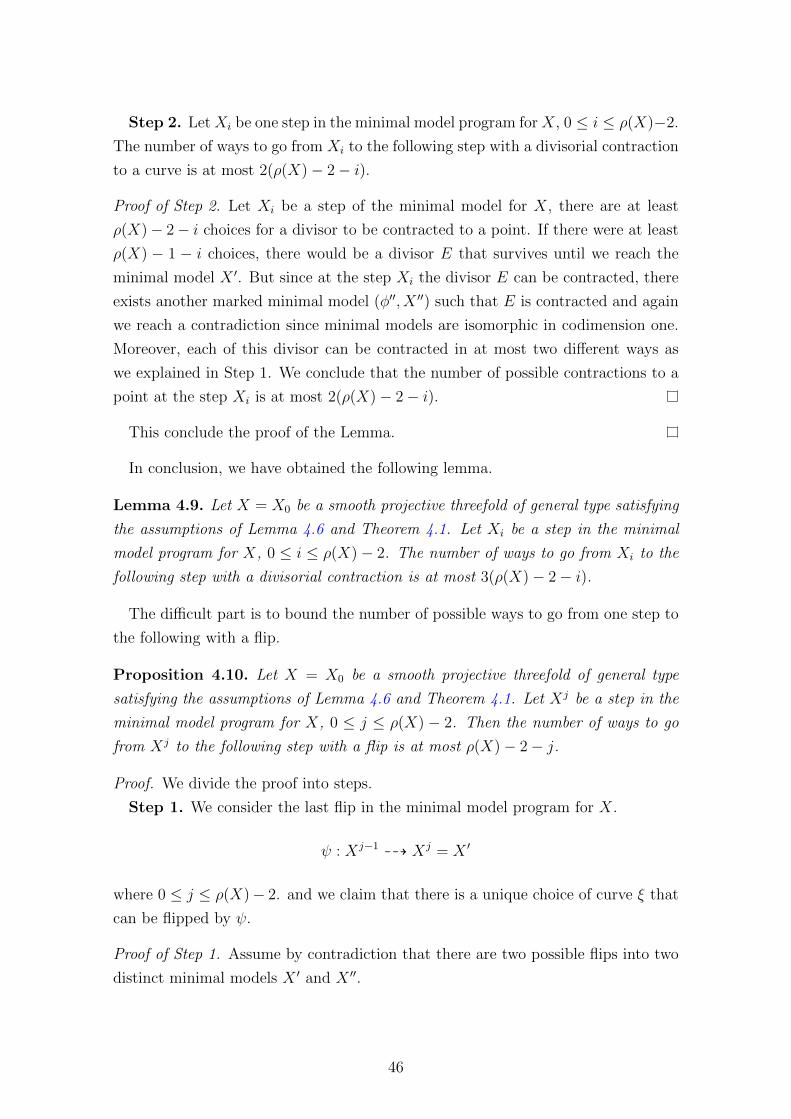
Step 2. LetXi be one step in the minimal model program forX, 0 ≤ i ≤ ρ(X)−2.

The number of ways to go from Xi to the following step with a divisorial contraction

to a curve is at most 2(ρ(X)− 2− i).

Proof of Step 2. Let Xi be a step of the minimal model for X, there are at least

ρ(X)− 2− i choices for a divisor to be contracted to a point. If there were at least

ρ(X) − 1 − i choices, there would be a divisor E that survives until we reach the

minimal model X ′. But since at the step Xi the divisor E can be contracted, there

exists another marked minimal model (φ′′, X ′′) such that E is contracted and again

we reach a contradiction since minimal models are isomorphic in codimension one.

Moreover, each of this divisor can be contracted in at most two different ways as

we explained in Step 1. We conclude that the number of possible contractions to a

point at the step Xi is at most 2(ρ(X)− 2− i).

This conclude the proof of the Lemma.

In conclusion, we have obtained the following lemma.

Lemma 4.9. Let X = X0 be a smooth projective threefold of general type satisfying

the assumptions of Lemma 4.6 and Theorem 4.1. Let Xi be a step in the minimal

model program for X, 0 ≤ i ≤ ρ(X)− 2. The number of ways to go from Xi to the

following step with a divisorial contraction is at most 3(ρ(X)− 2− i).

The difficult part is to bound the number of possible ways to go from one step to

the following with a flip.

Proposition 4.10. Let X = X0 be a smooth projective threefold of general type

satisfying the assumptions of Lemma 4.6 and Theorem 4.1. Let Xj be a step in the

minimal model program for X, 0 ≤ j ≤ ρ(X) − 2. Then the number of ways to go

from Xj to the following step with a flip is at most ρ(X)− 2− j.

Proof. We divide the proof into steps.

Step 1. We consider the last flip in the minimal model program for X.

ψ : Xj−1 99K Xj = X ′

where 0 ≤ j ≤ ρ(X)− 2. and we claim that there is a unique choice of curve ξ that

can be flipped by ψ.

Proof of Step 1. Assume by contradiction that there are two possible flips into two

distinct minimal models X ′ and X ′′.

46

Xj−1

ψ2

((

ψ1// X ′

η12

X ′′

Where we denoted by η12 the flop connecting the two minimal models X ′ and X ′′

(see Theorem 2.13) and by ξ2 the curve that is flipped by ψ2. Now, thanks to the

Base point free Theorem [KM98, Theorem 3.3], there exists an integer m such that

|mKX′| is free. Therefore, we can choose a general surface

S ∈ |mKX′| (4.1)

such that it does not contain any irreducible components of Exc(η12). Then let

S0 := (ψ−11 )∗(S) be the strict transform of S, since flips do not change divisors,

S0 ∈ |mKXj−1 |. We are assuming that there exists another flipping curve ξ2 such

that ξ1 6= ξ2 and so ξ2 * Exc(ψ1). Since ξ2 is a flipping curve, KXj−1 · ξ2 < 0, and

so ξ2 ⊆ S0. Now we consider the restriction of ψ1 to S0

g := ψ1|S0

: S0 99K S

and since Exc(g) ⊆ Exc(ψ1) ∩ S0, we obtain that ξ2 * Exc(g) and so ψ1(ξ2) ⊆ S.

This is a contradiction, because ψ1(ξ2) is flopped by η12 into ψ2(ξ1) but S was chosen

in such a way that it does not contain any irreducible components of Exc(η12).

Step 2. Let Xj be a step in the minimal model program for X, 0 ≤ j ≤ ρ(X)−2.

Then the number of ways to go from Xj to the following step with a flip is at most

ρ(X)− 2− j.

Proof. We can iterate the argument of Step 1 in the case of a series of flips. Let

Xi be a step of the minimal model for X, there are at least ρ(X) − 2 − i choices

for possible flipping curves. If there were at least ρ(X)− 1− i choices, there would

be a curve ξ that survives until we reach the minimal model X ′ and so is contained

in the surface S chosen in (4.1). But since at the step Xi the curve ξ is a flipping

curve, there exists another marked minimal model (φ′′, X ′′) that flips ξ and again

we reach a contradiction because ξ would be contained in Exc(η12). We conclude

that the number of possible flips at the step Xi is at most ρ(X)− 2− i.

This conclude the proof of the lemma.

Now we have all the ingredients to prove Theorem 4.1.

47

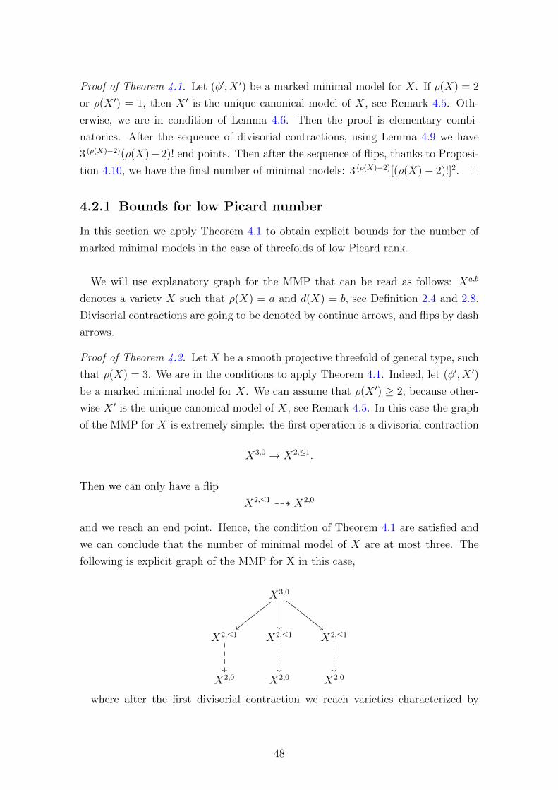
Proof of Theorem 4.1. Let (φ′, X ′) be a marked minimal model for X. If ρ(X) = 2

or ρ(X ′) = 1, then X ′ is the unique canonical model of X, see Remark 4.5. Oth-

erwise, we are in condition of Lemma 4.6. Then the proof is elementary combi-

natorics. After the sequence of divisorial contractions, using Lemma 4.9 we have

3 (ρ(X)−2)(ρ(X)−2)! end points. Then after the sequence of flips, thanks to Proposi-

tion 4.10, we have the final number of minimal models: 3 (ρ(X)−2)[(ρ(X)− 2)!]2.

4.2.1 Bounds for low Picard number

In this section we apply Theorem 4.1 to obtain explicit bounds for the number of

marked minimal models in the case of threefolds of low Picard rank.

We will use explanatory graph for the MMP that can be read as follows: Xa,b

denotes a variety X such that ρ(X) = a and d(X) = b, see Definition 2.4 and 2.8.

Divisorial contractions are going to be denoted by continue arrows, and flips by dash

arrows.

Proof of Theorem 4.2. Let X be a smooth projective threefold of general type, such

that ρ(X) = 3. We are in the conditions to apply Theorem 4.1. Indeed, let (φ′, X ′)

be a marked minimal model for X. We can assume that ρ(X ′) ≥ 2, because other-

wise X ′ is the unique canonical model of X, see Remark 4.5. In this case the graph

of the MMP for X is extremely simple: the first operation is a divisorial contraction

X3,0 → X2,≤1.

Then we can only have a flip

X2,≤1 99K X2,0

and we reach an end point. Hence, the condition of Theorem 4.1 are satisfied and

we can conclude that the number of minimal model of X are at most three. The

following is explicit graph of the MMP for X in this case,

X3,0

##

X2,≤1

X2,≤1

X2,≤1

X2,0 X2,0 X2,0

where after the first divisorial contraction we reach varieties characterized by

48

Picard number equal to two and difficulty less or equal one, and then after the flip

we stopped having reached varieties with difficulty equal to zero and Picard number

equal to two.

Strategy for ρ(X) = 4

In this last section we present a strategy to find an explicit bound in the case of

Picard number equal to four and we highlight the main difficulties. Let X be a

smooth projective threefold of general type such that ρ(X) = 4. Again we assume

that if (φ′, X ′) is a marked minimal model for X, then ρ(X ′) ≥ 2. The situation is

more complicated. The graph of the MMP for X, in this case can be described in

the following way

X4,0

6

X3,≤1

3

?

##

X2,≤2

2

X3,0

3

X2,≤1

1

X2,≤1

1

X2,0 X2,0

The numbers at the right of the arrows represent the valence of the arrow in the

graph, i.e. in how many ways can be realized the operation corresponding to that

arrow. The valence is computed applying all the results of the previous section. In

order to count the number of end points, we need to compute the valence of the

missing arrow that corresponds to a flip followed by a divisorial contraction, and so

we can not conclude using Proposition 4.10.

Let us fix some notation

X3,≤1 φ199K X3,0 φ2→ X2,≤1

where φ1 is a flip and φ2 is a divisorial contractions.

• Let ξ ⊆ X3,≤1 be the flipping curve.

• Let ξ+ ⊆ X3,0 be the flipped curve.

49

• Let E ⊆ X3,≤1 be the divisor that is contracted by φ2.

• Let E+ ⊆ X3,0 be the image of the divisor through the flip φ1.

Lemma 4.11. If ξ * E, then the flip can be realized in at most two ways.

Proof. We consider the surface S ∈ |mKX2,0 |, for m > 0 as defined in (4.1), and its

strict transform S ′ ⊆ X2,≤1, since flips do not change divisors S ′ ∈ |mKX2,≤1|. Since

mKX3,≤1 = mKX2,≤1 + βE, where β > 0, because X2,≤1 is terminal, if we choose

S1 a general element in |mKX3,≤1|, then S1 = (φ−11 )∗S

′ + βE. Since ξ ·KX3,≤1 < 0,

because ξ is a flipping curve, ξ ⊆ S1. But we are assuming that ξ * E, so this forces

ξ ∈ (φ−11 )∗S

′, but then we can conclude thanks to the same proof of Proposition

4.10.

The major problem if ξ ⊆ E is that E is not normal. Indeed, since the discrepan-

cies are increasing under a flip, thanks to [KM98, Proposition 6.21] the multiplicity

of E along ξ is greater than one. Then E is singular along ξ and so not normal,

since E is a surface.

4.3 On the degree of the generators and the

weight of the relations of the canonical ring

4.3.1 A Vanishing Theorem for Koszul Cohomology

In this section we prove an analogue of [Gre82, Theorem 2.8] in the context of ter-

minal varieties.

Let X be a terminal variety of dimension n and let L be a nef and big line

bundle on X such that there exists an integer m so that |mL| is free. Therefore, the

evaluation map

H0(X,mL)⊗OX → mL,

defined as

s⊗ f // f · s,

is surjective. Let Qm0∗ be the kernel of the evaluation map. We have the following

exact sequence

0→ Qm0∗ → H0(X,mL)⊗OX → mL→ 0. (4.2)

Remark 4.12. Note that Qm0∗ is an actual vector bundle. Indeed, since mL is globally

generated, it induces a morphism i : X → PN . Let us consider the Euler sequence

50

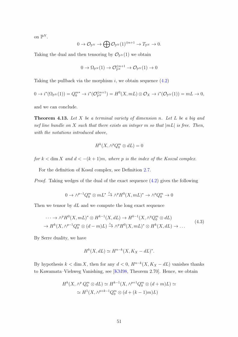
on PN .

0→ OPN →⊕OPN (1)⊕n+1 → TPN → 0.

Taking the dual and then tensoring by OPN (1) we obtain

0→ ΩPN (1)→ O⊕n+1PN → OPN (1)→ 0

Taking the pullback via the morphism i, we obtain sequence (4.2)

0→ i∗(ΩPN (1)) = Qm0∗ → i∗(O⊕n+1

PN ) = H0(X,mL)⊗OX → i∗(OPN (1)) = mL→ 0,

and we can conclude.

Theorem 4.13. Let X be a terminal variety of dimension n. Let L be a big and

nef line bundle on X such that there exists an integer m so that |mL| is free. Then,

with the notations introduced above,

Hk(X,∧pQm0 ⊗ dL) = 0

for k < dimX and d < −(k + 1)m, where p is the index of the Koszul complex.

For the definition of Kosul complex, see Definition 2.7.

Proof. Taking wedges of the dual of the exact sequence (4.2) gives the following

0→ ∧p−1Qm0 ⊗mL∗

∧s→ ∧pH0(X,mL)∗ → ∧pQm0 → 0

Then we tensor by dL and we compute the long exact sequence

· · · → ∧pH0(X,mL)∗ ⊗Hk−1(X, dL)→ Hk−1(X,∧pQm0 ⊗ dL)

→ Hk(X,∧p−1Qm0 ⊗ (d−m)L)

∧s→ ∧pH0(X,mL)∗ ⊗Hk(X, dL)→ . . .(4.3)

By Serre duality, we have

Hk(X, dL) ' Hn−k(X,KX − dL)∗.

By hypothesis k < dimX, then for any d < 0, Hn−k(X,KX − dL) vanishes thanks

to Kawamata–Viehweg Vanishing, see [KM98, Theorem 2.70]. Hence, we obtain

Hk(X, ∧p Qm0 ⊗ dL) ' Hk−1(X,∧p+1Qm

0 ⊗ (d+m)L) '

' H1(X,∧p+k−1Qm0 ⊗ (d+ (k − 1)m)L)

51

for d < −(k − 1)m. Moreover, for d < −(k − 1)m

H0(X,∧p+kQm0 ⊗ (d+ km)L)→ H1(X,∧p+k−1Qm

0 ⊗ (d+ (k − 1)m)L)→ 0 (4.4)

is surjective. From (4.3) with k = 0 we get

0→ H0(X,∧p+kQm0 ⊗ (d+ km)L)

∧s→ ∧p+k+1H0(X,mL)⊗H0(X, (d+ (k + 1)m)L),

and for d < −(k + 1)m,

H0(X, (d+ (k + 1)m)L) = 0,

hence

H0(X,∧p+kQm0 ⊗ (d+ km)L) = 0.

Then from (4.4) we obtain

H1(X,∧p+k−1Qm0 ⊗ (d+ (k − 1)m)L) = 0

and finally from (4.3.1),

Hk(X,∧pQm0 ⊗ dL) = 0

for d < −(k + 1)m.

4.3.2 Proof of Theorem 4.3

In this section we prove Theorem 4.3. We first deal we the bound for the degree of

the generators.

Proof of Theorem 4.3 (1). Let X be a Gorestein minimal variety of general type

of dimension n. The canonical divisor KX is a Cartier, big and nef divisor, then

KX is semiample, thanks to the Base point free Theorem, [KM98, Theorem 3.3].

Then, according to Theorem 2.2, there exist an integer mn depending only on the

dimension n, such that |mnKX | is free, i.e. the evaluation map

H0(X,mnKX)⊗OX → mnKX

is surjective. Again, we define Qmn0 as the dual of the kernel of the exact sequence

0→ (Qmn0 )∗ → H0(X,mnKX)→ mnKX → 0. (4.5)

52

We tensor by (d−mn)KX and we take the long exact sequence

0→ H0(X, (Qmn0 )∗ ⊗ (d−mn)KX)→ H0(X,mnKX)⊗H0(X, (d−mn)KX)

µ→

→ H0(X, dKX)→ H1(X, (Qmn0 )∗ ⊗ (d−mn)KX)→

→ H0(X,mnKX)⊗H1(X, (d−mn)KX)→ . . .

(4.6)

where µ is the multiplication map. In order to find a bound for the degree of the

generators of R(m) we need to understand when µ is surjective. This happens, in

particular, when H1(X, (Qmn0 )∗ ⊗ (d−mn)KX) = 0.

By Serre duality

H1(X, (Qmn0 )∗ ⊗ (d−mn)KX) ' Hn−1(X,Qmn

0 ⊗ (mn + 1− d)KX)∗.

Thanks to vanishing Theorem 4.13 in the case of p = 1, Hn−1(X,Qmn0 ⊗ (mn + 1−

d)KX) = 0 for d > (n + 1)mn + 1. Therefore, R(KX , X) is generated in degree

d ≤ (n+ 1)mn + 1.

Before proving the second part of Theorem 4.3 regarding the bound for the weight

of the relations we first need to recall some notation introduced by Green, slightly

generalized to this contest (see [Gre82, Section 3]).

We define Rdmn and Cdmn via the following exact sequence

0→ Rdmn → H0(X,mnKX)⊗H0(X, (d−mn)KX)µ→ H0(X, dKX)→ Cdmn → 0.

From (4.6), we get

Rdmn ' H0(X, (Qmn0 )∗ ⊗ (d−mn)KX).

Among the relations Rdmn , there are certain trivial ones, that we denote with

RKozdmn

:= Im(νdmn), where

∧2H0(X,mnKX)⊗H0(X, (d− 2mn)KX)νdmn→ H0(X, (Qmn

0 )∗ ⊗ (d−mn)KX)

((ωi ∧ ωj)⊗ φ) //ωi ⊗ ωjφ− ωj ⊗ ωiφ

Now we take the second wedge of (4.5)

0→ ∧2(Qmn0 )∗ → ∧2H0(X,mnKX)→ (Qmn

0 )∗ ⊗mnKX → 0

and then we tensor by (d− 2mn)KX and take the long exact sequence

53

. . .→ ∧2H0(X,mnKX)⊗H0(X, (d− 2mn)KX)νdmn→

→ H0(X, (Qmn0 )∗ ⊗ (d−mn)KX)

φdmn→

→ H1(X,∧2(Qmn0 )∗ ⊗ (d− 2mn)KX)

ψdmn→

→ ∧2H0(X,mnKX)⊗H1(X, (d− 2mn)KX)→ . . .

Then we can compute Rdmn/RKozdmn

.

Rdmn/RKozdmn '

H0(X, (Qmn0 )∗ ⊗ (d−mn)KX)

Im(νdmn)' H0(X, (Qmn

0 )∗ ⊗ (d−mn)KX)

ker(φdmn)'

' Im(φdmn) ' ker(ψdmn).

We define

• a := maxd |Cdmn 6= 0;

• b := degree of the highest-degree generator of the canonical ring of X, (note

that b ≤ a, see [Gre82, Example 4.5]);

• c := maxd |Rdmn/RKozdmn6= 0 or 0 if the set is empty.

Theorem 4.14. Let X be a threefold of general type satisfing the assumption of

Theorem 4.3.The relations among the generators of the canonical ring of X are

generated in weight w ≤ maxa+ b, c.

Proof. We can follow verbatim the proof in [Gre82, Theorem 3.11].

Proof of Theorem 4.3 (2)

Thanks to Theorem 4.3 (1), the worst case scenario in Theorem 4.14 is when a =

b = (n+ 1)mn + 1. Hence, prove Theorem 4.3 (2) it is enough to prove the following

claim.

Claim 4.15. c ≤ (n+ 2)mn + 1.

Proof of the Claim. Taking the dual, we have

(Rdmn/RKozdmn)∗ =

H1(X,∧2(Qmn0 )∗ ⊗ (d− 2mn)KX)∗

Im(φdmn)∗.

By Serre duality,

H1(X,∧2(Qmn0 )∗ ⊗ (d− 2mn)KX)∗ ' Hn−1(X,∧2Qmn

0 ⊗ (2mn + 1− d)KX)

54

Thanks to the Vanishing Theorem 4.13, for d > (n+ 2)mn + 1

Hn−1(X,∧2Qmn0 ⊗ (2mn + 1− d)KX) = 0.

So we can conclude that c ≤ (n+ 2)mn + 1.

Finally, the canonical ring of X is related in weight w ≤ 2(n+ 2)mn + 2.

55

5 Rational curves on Calabi-Yau

manifolds

5.1 Introduction

The purpose of this chapter is to prove the following result about the existence of

rational curves on an elliptically fibered projective manifold X with some restriction

on its fundamental group. We always assume that the dimension of X is greater

than two.

Theorem 5.1. Let X be a smooth projective manifold of dimension greater than

two with finite fundamental group. Suppose there exists a projective variety B and

a morphism f : X → B such that the general fiber has dimension one. Suppose,

moreover, that there exists a Cartier divisor L on B such that KX ' f ∗L. Then X

does contain a rational curve.

In the second part of this chapter we prove an application of Theorem 5.1, where

we deal with Calabi–Yau manifolds endowed with a fibration onto a curve whose

fibers are abelian varieties.

Theorem 5.2. Let X be a Calabi–Yau manifold of dimension greater than two that

admits a fibration onto a curve whose general fibers are abelian varieties. Then X

does contain a rational curve.

5.2 Proof of Theorem 5.1

In this section we prove the following result, which will readily imply Theorem 5.1.

Theorem 5.3. Let X be a smooth projective n dimensional manifold, n > 2. Sup-

pose that X is simply connected and that it is endowed with an elliptic fiber space

structure φ : X → B. Suppose moreover that there exist a Cartier divisor L on B

such that KX ' φ∗L. Then X does contain a rational curve.

Let us first show how Theorem 5.3 implies Theorem 5.1.

56

Proof of Theorem 5.1. Let f : X → B as in Theorem 5.1 and consider the universal

cover π : X → X of X. It is of course smooth and projective. Next, consider the

Stein factorization of f πX

φ//

fπ33B′

ν // B,

so that φ has connected fibers, and B′ is a normal projective variety. Since KX 'π∗KX , we obtain that KX ' (f π)∗L = (ν φ)∗L = φ∗L′, where L′ is the Cartier

divisor on B′ given by ν∗L. Moreover, φ : X → B′ is an elliptic fiber space since by

construction it is a fiber space whose general fiber has dimension one and, moreover,

has trivial canonical bundle. Indeed, let B0 ⊂ B′ the non-empty Zariski open set

of regular point of B′ which are also regular values for φ, so that φ0 = φ|φ−1(B0) is

a proper holomorphic submersion. Then over X0 = φ−1(B0), the relative tangent

bundle sequence

0→ TX0/B0 → TX0 → (φ0)∗TB0 → 0 (5.1)

is a short exact sequence of vector bundles. Restricting to one fiber E and taking

the determinant of the dual sequence gives a (non canonical) isomorphism

KE ' KX0|E = KX |E ' φ∗L|E ' OE,

and thus E is an elliptic curve. Therefore, Theorem 5.3 applies to φ : X → B′ and

we deduce that X contains a rational curve R ⊂ X. But then R = π(R) ⊂ X is a

rational curve in X.

We now start the proof of Theorem 5.3. We first observe that thanks to the

following result of Kawamata, which we state in a slightly simplified version, one

can suppose that the fibers of φ are all one dimensional.

Theorem 5.4. (Simplified version of [Kaw91, Theorem 2]) Let f : X → Y be a

surjective projective morphism, where X is smooth and −KX is f -nef (that is, it

intersects non negatively the curves which are contracted by f). Then any irreducible

component of Exc(f) = x ∈ X | dim f−1(f(x)) > dimX − dimY is uniruled.

Notice that, if the exceptional set Exc(φ) is not empty, then we obtain at once

infinitely many rational curves.

Next, we look at the proper subvariety Z ⊂ B consisting of all the singular points

of B and all the singular values of φ. We also call B0 the Zariski open set complement

of Z in B, and X0 = φ−1(B0). Thus, the restriction φ0 = φ|X0 : X0 → B0 is a proper

surjective submersion.

57

Lemma 5.5. The subvariety Z has at least one irreducible component of codimen-

sion one in B.

Proof. Consider the holomorphic function J : B0 → C given by the j-invariant of the

(elliptic) fibers. Since we suppose that B0 has at least codimension two complement

in B and B is normal, J extends to a holomorphic function B → C, which must

be constant. Thus, all fibers over B0 are isomorphic and by the Grauert–Fischer

theorem, [FG65], the family φ0 : X0 → B0 is locally holomorphically trivial. We

are thus in position to apply [KL09, Lemma 17] which gives, since B0 is moreover

simply connected because X0 is and we are in the conditions to apply the long

exact sequence for homotopy groups, that φ0 : X0 → B0 is globally holomorphically

trivial. In particular X0 ' E ×B0 and thus X0 cannot be simply connected.

Following [Ogu93], we shall reduce our situation to the surface case by picking a

general curve in B and use Kodaira’s canonical bundle formula to study singular

fibers. So, let H be a very ample line bundle over B, positive enough in order to

ensure that H⊗(n−2) ⊗ OB(L) is generated by global sections. Observe that, since

φ : X → B is an algebraic fiber space, then H0(X,φ∗H) ' H0(B, φ∗(φ∗H)) '

H0(B,H ⊗φ∗OX) ' H0(B,H). In particular, general elements in the linear system

|H| are also general members of |φ∗H|. Now, take a curve C ⊂ B which is a general

complete intersection of divisors in |H|, and the surface S ⊂ X cut out by the pull-

back of such divisors to X. By Bertini’s theorem, C is normal, hence smooth, and

S is smooth, too. Let us still call, by abuse of notation, φ : S → C the restriction of

φ to S. The surface S is an elliptic surface, which we can suppose to be relatively

minimal (otherwise we would have found a rational curve on S and hence on X).

Since C is general, and the singular locus Bsing of B is of codimension two, we

can suppose that C ∩ Bsing = ∅. Next, pick a divisorial irreducible component Z0

of Z, which always exists thanks to Lemma 5.5. Then C must necessarily intersect

Z0, since C · Z0 = Hn−2 · Z0 > 0. This means that φ : S → C must always have at

least one singular fiber. Our goal is now to show that such a fiber can never be a

multiple fiber and that a singular (non multiple) fiber must necessarily contain an

irreducible component which is rational.

Let us start with the following.

Lemma 5.6. The canonical bundle KS of S is globally generated.

Proof. Let H1, . . . , Hn−2 ∈ |φ∗H| be the smooth divisors in general position which

cut out S. Then by iterating the adjunction formula we find

KS '(KX ⊗ φ∗H⊗(n−2)

)|S ' φ∗

(OB(L)⊗H⊗(n−2)

)|S. (5.2)

58

Thus, KS, as a restriction of a pull-back of a globally generated line bundle, is

globally generated itself.

Now, recall the (weaker form of the) canonical bundle formula for relatively mini-

mal elliptic fibrations such that its multiple fibers are Sc1 = m1F1, . . . , Sck = mkFk,

which reads (see [BHPVdV15, Corollary V.12.3]):

KS ' φ∗G⊗OS( k∑i=1

(mi − 1)Fi

), (5.3)

where G is some line bundle over C.

Proposition 5.7. The elliptic surface S does not have any multiple fiber.

Proof. Indeed, on the one hand the restriction to KS to any subscheme of S is

globally generated, since KS is globally generated itself. On the other hand, the

canonical bundle formula (5.3) together with [BHPVdV15, Lemma III.8.3] tell us

that the restrictionOFi((mi−1)Fi

)of KS to Fi would have no sections, sinceOFi(Fi)

is torsion of order mi.

To conclude the proof, we now have to examine singular but not multiple fibers,

following Kodaira’s table [BHPVdV15, Section V.7]. So, let F be such a fiber.

(i) If F is irreducible, then it is necessarily rational with a node, or rational with

a cusp. In both cases we find a (singular) rational curve on S, and hence on

X.

(ii) If F is reducible, then it is of the form F =∑miFi, with Fi irreducible and

reduced, and gcdmi = 1. Since F 2 =∑mimjFi · Fj = 0 and we have

at least two components, it follows that there exists at least one irreducible

component, say F1, with negative self-intersection. But since KS is a pull-

back by (5.2) and F1 is contained in a fiber, then KS · F1 = 0. It follows by

adjunction that F1 is a smooth rational (−2)-curve.

5.3 Proof of Theorem 5.2

In this section, after collecting all the essential ingredients, we prove Theorem 5.2.

In the following lemma, vaguely inspired by the key lemma in [Wil89, Key Lemma,

page 142], we combine some standard tools to produce rational curves on a smooth

projective variety such as the logarithmic version of the Cone Theorem (see for

instance [Mat92, Theorem 7-2-2]).

59

Lemma 5.8. Let X be a Calabi–Yau manifold such that there exists D a non-ample

divisor on X satisfying Dn > 0. Assume that hi(X,mD) = 0 for i > 1 and for m

large enough. Then X does contain a rational curve.

Proof. We first observe that we may assume D non-nef: otherwise D nef and Dn >

0 implies that D is big (see for instance [Laz04, Theorem 2.2.16]). Then D is

semiample by the Base point free Theorem (see for instance [KM98, Theorem 3.3]).

So there exists a multiple of D that defines a surjective generically 1-1 morphism

g : X → Z; since D is non-ample, the exceptional locus of g is non-empty, so we can

conclude thanks to Kawamata’s Theorem 5.4 that Exc(g) is uniruled.

Now we prove that it is possible to choose m > 0 such that mD is effective.

Indeed, by the Hirzebruch–Riemann–Roch Theorem, we have

χ(OX(mD)) = deg (ch(mD) · td(TX))n.

Since ch(mD) =∑∞

k=0mkDk

k!because mD is a line bundle, we obtain for m suffi-

ciently large

χ(OX(mD)) ∼ mnDn

n!> 0.

By assumption,

χ(OX(mD)) = h0(OX(mD))− h1(OX(mD)) ≤ h0(OX(mD)).

Then h0(OX(mD)) > 0 and mD is effective. Since mD is not nef, then we can

conclude thanks to the logarithmic version of the Cone Theorem, because we find a

rational curve in the extremal ray that intersect negatively the canonical divisor.

We are going to apply Lemma 5.8 to Da,b := aH − bF , where H is an ample

divisor on X and F is the generic fiber of a fibration of X onto a curve. The point

is to obtain an asymptotic vanishing of the higher cohomology of D for some a, b

fixed. Indeed, we are able to prove a slightly stronger statement, where we obtain a

uniform vanishing for every b.

Lemma 5.9. Let X be an n-dimensional projective manifold that admits a fibration

onto a curve, let H ′ be an ample divisor on X and let F be the generic fiber of the

fibration. Let m0 ∈ N such that

• hi(X,OX(mH ′)) = 0, i > 0,

• hi(F,OF (mH ′)) = 0, i > 0,

60

for all m ≥ m0. Then hi(X,mH ′ − kF ) = 0, i > 1, for all m ≥ m0 and for all

k ∈ N.

Let H := m0H′. Then, for any positive integer a, b, the divisor Da,b = aH − bF

satisfies the hypothesis of Lemma 5.8.

It is of course always possible to choose m0 satisfying the hypothesis of Lemma

5.9 thanks to Serre vanishing.

Proof. Given the standard exact sequence

0→ OX(mH ′ − kF )→ OX(mH ′)→ OkF (mH ′)→ 0,

it is enough to show that for every i > 1 we have

hi−1(kF,OkF (mH ′)) = 0.

Indeed, let D be an effective Cartier divisor on X and let I be the ideal sheaf of

D in X, i.e. I = OX(−D). Then for any k ∈ N, we have O(k+1)D = OX/Ik+1 and

OkD = OX/Ik. Let K be defined by the short exact sequence

0→ K → O(k+1)D → OkD → 0.

There is a natural sheaf isomorphism

K = Ik/Ik+1 = Ik ⊗OXOX/I = OX(−kD) ⊗

OXOD = OD(−kD).

Hence we obtain the exact sequence

0→ OD(−kD)→ O(k+1)D → OkD → 0

and tensoring by OX(mH ′) we get

0→ OD(mH ′ − kD)→ O(k+1)D(mH ′)→ OkD(mH ′)→ 0.

Now, if we set D = F , since F is a fiber we have

OF (mH ′ − kF ) = OF (mH ′),

so we can easily conclude by induction on k. Indeed, for k = 1 hi−1(F,OF (mH ′)) = 0

for i > 1 by hypothesis. Then, we can assume the thesis for k − 1 so that using the

61

following sequence

. . .→ H i−1(F,OF (mH ′))→ H i−1(kF,OkF (mH ′))

→ H i−1((k − 1)F,O(k−1)F (mH ′))→ . . .

we obtain that hi−1(kF,OkF (mH ′)) = 0 for i > 1, as we wanted.

We also need the following remark.

Remark 5.10. We recall that the Beauville–Bogomolov decomposition theorem states

that if X is a compact Kahler manifold such that c1(X) = 0, then up to finite un-

ramified quotient X is a product of Calabi–Yau manifolds, tori and hyperkahler

manifodls, see [B+83, Theorem 1]. Then, in our case, c2(X) is not-zero, otherwise

X would be a finite unramified quotient of a torus and its fundamental group would

contain a free abelian group of rank 2n, contradicting our assumption of simply con-

nectedness. Given the fibration f : X → C, thanks to the relative tangent sequence

(5.1) we get

0→ TF → TX|F → OF → 0

where F is the generic fiber of the fibration. Hence we deduce

c2(X) · F = c2(TX|F ) = c2(TF ) = c2(F ).

Since F is an abelian variety, we have c2(X) · F = c2(F ) = 0 as a cycle.

Finally we prove Theorem 5.2.

Let F be the generic fiber of the fibration and let H ′ be an ample divisor on X

and H := m0H′ where m0 is as in Lemma 5.9. We consider the affine line of divisors

(with rational slope) Nt = H − tF for t ∈ Q≥0. If we let

t0 =Hn

nHn−1 · F∈ Q≥0,

then we have (Nt)n > 0 for each t < t0 and (Nt0)n = 0. Now there are two possible

cases:

(I) Nt is nef for each t < t0.

(II) There exists a t < t0 such that Nt is non-nef.

Let us focus on case (I) first. Since being nef is a closed condition, Nt0 is also nef.

Next, it is easy to verify that (Nt0)n−1 · H = (1 − n−1n

)Hn > 0. Finally, according

62

to Remark 5.10, c2(X) · F = 0, hence we can conlcude that c2(X) · (Nt0)n−2 =

c2(X)·Hn−2 > 0, thanks to [Miy87, Theorem 1.1] because H is ample and c2(X) 6= 0,

see Remark 5.10. Hence from [Kol15, Corollary 11], it follows that Nt0 is semiample

and since we have ν(Nt0) = n− 1 we can conclude thanks to Corollary 1.23.

Let us consider now case (II). Let a and b positive natural numbers such that

t = ba. Then we have that Nt = aH − bF = Da,b is as in Lemma 5.9 and since

(aNt)n = an(Nt)

n > 0 we can conclude thanks to Lemma 5.8.

63

6 The Base point free Theorem in

positive characteristic

6.1 Introduction

In this chapter, we prove the Base point free Theorem over Fp, the algebraic closure

of a finite field, for a three-dimensional log canonical pair.

Theorem 6.1. Let (X,∆) be a three-dimensional projective log pair defined over

Fp. Assume that one of the following conditions holds:

(1) (X,∆) is log canonical, or

(2) all the coefficients of ∆ are at most one and each irreducible component of

Supp(b∆c) is normal.

Let L be a nef and big line bundle on X. If L− (KX + ∆) is also nef and big, then

L is semiample.

The next corollary follows from Theorem 6.1 in the case of L = 2(KX + ∆) in (1)

and L = −(KX + ∆) in (2).

Corollary 6.2. Let (X,∆) be a three-dimensional log canonical projective pair de-

fined over Fp. Then the following hold:

(1) If KX + ∆ is nef and big, then KX + ∆ is semiample.

(2) If −(KX + ∆) is nef and big, then −(KX + ∆) is semiample.

Remark 6.3. Theorem 6.1 does not hold over fields k 6= Fp even in the two-dimensional

case (Example 6.31). Corollary 6.2 (2) also does not hold over algebraically closed

fields k 6= Fp (Example 6.32).

In Example 6.30, we give a counterexample to Theorem 6.1 if one does not impose

any conditions on the effective Q-divisor ∆. It is not clear whether the theorem

remains true if we only assume that all the coefficients of ∆ are at most one.

64

We also prove the base point free theorem for normal surfaces defined over Fpwithout assuming bigness.

Theorem 6.4. Let X be a normal projective surface defined over Fp and let ∆ be

an effective Q-divisor. Assume that we have a nef line bundle L on X such that

L− (KX + ∆) is also nef. Then L is semiample.

Remark 6.5. Theorem 6.1 and Theorem 6.4 hold if we assume that L is only a

Q-Cartier Q-divisor. Note, that if L and L− (KX + ∆) are big and nef, then also

nL− (KX + ∆) = (n− 1)L+ (L− (KX + ∆))

is big and nef for any integer n ≥ 1.

In Section 6.2, we prove the base point free theorem for surfaces under weaker as-

sumptions (Theorem 6.4). In Section 6.3, generalizing the proof of [Kee99, Theorem

0.5], we reduce Theorem 6.1 to showing that the line bundle L|Suppb∆c is semiample

(Theorem 6.20). If Suppb∆c is irreducible, we know that L|Suppb∆c is semiample

by Theorem 6.4. The non-irreducible case is treated in Section 6.4. In order to

generalize Theorem 6.4 to the non-irreducible surfaces, we combine an idea from

Fujino [Fuj00] and Tanaka [Tan13], together with special properties of varieties de-

fined over Fp, which are proved in Section 2.3. In Section 6.5, we complete the proof

of Theorem 6.1 and of Corollary 1.29. In Section 6.6, we give counterexamples as it

was stated in Remark 6.3.

6.2 Base point free theorem for normal surfaces

In this section, we prove Theorem 6.4. The key tool is the following theorem of

Tanaka. We say that a Q-divisor B on a variety X is Q-effective if h0(X,mB) 6= 0

for some m ≥ 1. Note that a normal surface over Fp is always Q-factorial (see

[Tan14, Theorem 11.1]).

Theorem 6.6. [Tan14, Theorem 12.6] Let X be a projective normal surface over

Fp and let D be a nef Q-divisor. If qD−KX is Q-effective for some positive rational

number q ∈ Q, then D is semiample.

We will use the following proposition.

Proposition 6.7. [Kee99, Lemma 2.10] Let p : Y → X be a proper surjection be-

tween varieties defined over an algebraically closed field and let L be a line bundle

on X. Assume that X is normal. Then L is semiample if and only if p∗(L) is

semiample.

65

Proof of Theorem 6.4. Recall that we have the nef line bundle L and the Q-divisor

D := L− (KX + ∆) on the normal surface X over Fp.

Claim 6.8. We can assume that X is smooth.

Proof. Let f : Y → X be the minimal resolution of singularities of X. Define ∆Y

so that KY + ∆Y = f ∗(KX + ∆). The divisor ∆Y is an effective Q-divisor by

the negativity lemma (cf. [KM98, Corollary 4.3]). Note that f ∗L and f ∗D =

f ∗L− (KY + ∆Y ) are nef. By Proposition 6.7 we know that L is semiample if and

only if f ∗L is semiample. Thus, by replacing X by Y , we may assume that the

surface is smooth.

We extensively use the following lemma.

Lemma 6.9. If D is Q-effective, then L is semiample.

Proof. As D is Q-effective, then also L −KX = D + ∆ is Q-effective, and so L is

semiample by Theorem 6.6.

Claim 6.10. We can assume that all the following statements are true.

(1) L 6≡ 0 and D 6≡ 0, (2) L2 = 0, (3) D2 = 0,

(4) L ·∆ = 0, (5) L ·KX = 0, (6) (KX + ∆) ·∆ = 0,

(7) (KX + ∆) ·KX = 0, (8) χ(OX) ≤ 0.

Proof. If L ≡ 0, then L ∼Q OX by Proposition 2.25, so L is semiample. Thus, we

may assume that L 6≡ 0. Analogously and thanks to Lemma 6.9, we may assume

that D 6≡ 0.

As L and D are nef, we get L2 ≥ 0 and D2 ≥ 0. If L2 > 0, then, by Theorem

2.30, the line bundle L is semiample. Thus, we may assume that L2 = 0. If D2 > 0,

then D is big, and so Q-effective. In this case L is semiample by Lemma 6.9. Hence,

we may assume D2 = 0.

Since L 6≡ 0, we know that there exists a curve C on X satisfying L ·C > 0. Take

an ample divisor A such that A−C is effective. Then L ·A = L ·C+L · (A−C) > 0.

If m is sufficiently large so that it satisfies (KX −mL) · A < 0, then h2(X,mL) =

h0(X,KX −mL) = 0. The Riemann–Roch theorem gives

h0(X,mL) = h1(X,mL) +1

2mL · (mL−KX) + χ(OX)

= h1(X,mL)− 1

2mL ·KX + χ(OX).

As L and D are nef, it follows that

0 ≤ L ·D = −L ·KX − L ·∆.

66

Since ∆ is effective and L is nef, we find 0 ≤ L · D ≤ −L · KX . If −L · KX > 0,

then κ(X,L) = 1 by the calculation of h0(X,mL) above. A nef line bundle L with

κ(X,L) = 1 is always semiample (see for instance [Kol92, Theorem 11.3.1]). Thus,

we may assume that L ·∆ = 0 and L ·KX = 0.

As above, h2(X,mD) = 0 holds for sufficiently large m, and so the Riemann–Roch

theorem gives

h0(X,mD) = h1(X,mD)− 1

2mD ·KX + χ(OX)

= h1(X,mD) +1

2mD · (D − L+ ∆) + χ(OX)

= h1(X,mD) +1

2mD ·∆ + χ(OX)

= h1(X,mD)− 1

2m(KX + ∆) ·∆ + χ(OX).

If −(KX + ∆) · ∆ > 0, then D is Q-effective and by Lemma 6.9 the line bundle

L is semiample. Since 0 ≤ D · ∆ = −(KX + ∆) · ∆ holds by the nefness of D,

we may assume (KX + ∆) · ∆ = 0. Given D2 = L2 = D · L = 0, it follows that

(KX + ∆) ·KX = 0.

By the Riemann–Roch theorem, we get h0(X,mD) = h1(X,mD) + χ(OX). If

χ(OX) > 0, then D is Q-effective and by Lemma 6.9 the line bundle L is semiample.

Hence, we may assume that χ(OX) ≤ 0.

We divide the proof into cases depending on the Kodaira dimension.

Case 1. Assume κ(X) ≥ 0.

Claim 6.11. We may assume that KX is nef.

Proof. Let π : X → Xmin be the minimal model of X. By π∗L we denote the

pushforward of L as a divisor.

By the assumption κ(X) ≥ 0, we have that KX is Q-linearly equivalent to an

effective Q-divisor containing every π-exceptional curve in its support. Since L ·KX = 0 thanks to Claim 6.10 and L is nef, it follows that L · E = 0 for every π-

exceptional curve E. Hence, we get L = π∗π∗L, by the negativity of the intersection

form on the exceptional locus (cf. [KM98, Lemma 3.40]).

Since L = π∗π∗L, it is sufficient to show the semiampleness of π∗L. Note that

π∗L and π∗D are nef, because L and D are nef. Further, we have π∗D = π∗L −(KXmin

+ π∗∆). Therefore, we can reduce the problem to the case of the minimal

model Xmin.

67

In what follows, we assume that X is minimal. We use the classification of minimal

surfaces in positive characteristic (see for instance [Lie13]).

Case 1.1. Assume κ(X) = 2.

We can write KX ∼Q A+ E for an ample Q-divisor A and an effective Q-divisor

E, because KX is big. Since L, D are nef and L ·KX = D ·KX = 0, it follows that

L · A = D · A = 0. Thus, (L−D) · A = (KX + ∆) · A = 0. We get a contradiction

0 < A2 ≤ (KX + ∆) · A = 0.

Hence, there are no line bundles L satisfying the assumptions in Claim 6.10.

Case 1.2. Assume κ(X) = 1.

In our case, KX is semiample and it gives an elliptic or quasi-elliptic fibration

f : X → B. Let F be its general fiber. Then KX ≡ aF holds for some positive

rational number a.

Since D·KX = 0, it follows that D·F = 0. Therefore, D is f -numerically trivial by

the nefness of D, becasue it has intersection zero with any components of F . Since

D is nef and f -numerically trivial, it satisfies D ≡ bF for some b ≥ 0, by Lemma

6.12. Hence, D is Q-effective by Proposition 2.25. Therefore, L is semiample by

Lemma 6.9.

Lemma 6.12. Let f : X → B be a surjective morphism satisfying f∗(OX) = OBfrom a smooth projective surface X to a smooth projective curve B. Suppose that L

is an f -numerically trivial nef Q-Cartier Q-divisor. Then L ≡ bF for some b ≥ 0,

where F denotes a general fiber of f .

Proof. See for instance [Leh15, Lemma 2.4].

Case 1.3. Assume κ(X) = 0.

By the classification of minimal surfaces, there are five possibilities: a K3 sur-

face, an Enriques surface, an abelian surface, a hyperelliptic surface, or a quasi-

hyperelliptic surface.

If X is a K3 surface or an Enriques surface, then χ(OX) = 2 or χ(OX) = 1,

respectively, which contradicts Claim 6.10.

If X is an abelian surface, then every nef divisor is numerically equivalent to a

semiample divisor (see Proposition 6.15). Therefore, L is semiample by Proposition

2.25.

If X is a hyperelliptic surface, then X is a finite quotient of an abelian surface by

a finite group. Therefore, we have a surjective morphism A → X from an abelian

68

surface A. Since L|A is a nef line bundle on an abelian surface, it is semiample (see

Proposition 6.15). Hence, L is also semiample by Proposition 6.7.

If X is a quasi-hyperelliptic surface, then X can be written as a finite quotient

E × C → X, where E is an elliptic curve and C is a rational curve with a cusp.

Therefore, we have a surjective morphism X ′ := E × P1 → X. Any divisor on X ′

is numerically equivalent to aF1 + bF2 with a, b ∈ Q, where F1 is the fiber class

of X ′ → E and F2 is the fiber class of X ′ → P1. Hence, any nef divisor on X ′

is numerically equivalent to a semiample divisor. Thus, we can conclude that L is

semiample by Proposition 2.25 and Proposition 6.7.

Case 2. Assume κ(X) = −∞.

By χ(OX) ≤ 0, the surface X is irrational. Thus, we can assume that f : X → B

is a birationally ruled surface, where B is a curve with g(B) ≥ 1.

We need the following lemma, which can be found in the proof of [Tan14, Theorem

12.4]. We remind that f-horizontal means that every component surjects onto the

base.

Lemma 6.13. Let C be an f -horizontal curve on X such that D · C = 0. Then D

is Q-effective.

Proof. Since C is a f-horizontal curve, it holds that g(B) ≤ h1(C,OC) by Riemann–

Hurwitz theorem, since h1(C,OC) is the arithmetic genus of C. By the Riemann–

Roch theorem, we get

h0(X,mD) = h1(X,mD) + χ(OX) = h1(X,mD) + 1− g(B),

so it is sufficient to show h1(X,mD) ≥ h1(C,OC) for some m > 0.

Since D · C = 0, we have D|C ≡ 0. Hence, by Proposition 2.25 we can conclude

that mD|C is trivial for sufficiently divisible m > 0. Therefore, we get an exact

sequence

0 //OX(mD − C) //OX(mD) //OC // 0.

By the same reason as before, h2(X,mD − C) = 0 holds for sufficiently large m.

Hence, we get h1(X,mD) ≥ h1(C,OC).

For any irreducible component C of ∆, it follows that D ·C = 0, because D is nef

and D ·∆ = 0. In particular, if ∆ has an f -horizontal component, then the lemma

above implies that D is Q-effective, and hence L is semiample by Lemma 6.9. Thus,

in what follows, we may assume that ∆ has only f -vertical components.

69

Claim 6.14. Under these assumptions, it follows that ∆ = 0, g(B) = 1, and X is

a minimal ruled surface.

Proof. Let π : X → Xmin be a minimal model of X. We have KX ∼ π∗KXmin+ E,

where E is an exceptional divisor. We refer the reader to [Har77, Ch V, Section 2]

for the properties of ruled surfaces. It holds that

KXmin≡ −2C0 + (2g(B)− 2− e)F

for C0 a normalized section, e = −C20 , and F a general fiber of Xmin → B. Note

that K2Xmin

= 8(1− g(B)).

Since (KX + ∆) ·∆ = 0 and (KX + ∆) ·KX = 0, we get

∆2 = −KX ·∆ = K2X .

As ∆ has only f -vertical components, we have π∗F ·∆ = 0, and so

0 = (KX + ∆) ·∆ = −2π∗C0 ·∆ + (E + ∆) ·∆.

Since π∗C0 ·∆ ≥ 0, it follows that E ·∆ ≥ −∆2. Therefore,

(E + ∆)2 = E2 + 2E ·∆ + ∆2 ≥ E2 −∆2

= E2 −K2X = −K2

Xmin= 8(g(B)− 1) ≥ 0.

By the Zariski Lemma (see Theorem 1.23 in [Liu02, Section 9]), the intersection

form on f -vertical fibers is seminegative definite with one-dimensional radical equal

to the span of a general fiber, so (E + ∆)2 = 0 and E + ∆ ≡ π∗pF for some p ∈ Q.

Since all the inequalities must be equalities, it follows that E · ∆ = −∆2 and

g(B) = 1. Furthermore, we have 2π∗C0 ·∆ = (E + ∆) ·∆, and thus

0 = π∗C0 ·∆ = π∗C0 · (E + ∆) = p.

It implies that E + ∆ = 0. Since ∆ and E are both effective divisors, we get ∆ = 0

and E = 0. Hence, X is minimal.

By this claim, we can assume that X is a minimal ruled surface over an elliptic

curve. In this case, it is well-known that NEF(X) ⊂ NE(X) holds (see Proposition

6.18). We can conclude that the nef divisor D is Q-effective and L is semiample by

Lemma 6.9.

For completeness, we prove two propositions which were used in the above proof.

70

Proposition 6.15. Let A be an abelian variety defined over an algebraically closed

field. Then, any nef line bundle on A is numerically equivalent to a semiample line

bundle.

Remark 6.16. Note that any effective divisor on an abelian variety is always semi-

ample (see the proof of Application 1 ((i)⇒(iii)) in [Mum08, Section 6]).

Proof. Let L be a nef line bundle on A. Define K(L) to be the maximal subscheme

of A such that

(m∗L− p∗1L− p∗2L)|K(L)×A = OK(L)×A

as in [Mum08, Section 13], where m : A× A→ A is the multiplication map, and pi

are the first and second projections.

By the above remark, we may assume that L is not big, so that Lg = 0 where

g = dimA. By the Riemann–Roch theorem [Mum08, Section 16], we have χ(L) = 0.

Hence, it follows that dimK(L) > 0 by the vanishing theorem [Mum08, Section 16].

Set X := K(L)0red. This is a subabelian variety of A. Thus, there exists a

subabelian variety Y ⊂ A such that the morphism m : X × Y → A; (x, y) //x+ y

defined by the group law on A is an isogeny (see Theorem 1 in [Mum08, Section

19]). Note that, L|X ∈ Pic0(X), because it is invariant under translations by any

element of X (see Remark 6.17).

First, we prove m∗L ≡ p∗Y (L|Y ), where pY : X × Y → Y is the second projection.

By definition of K(L), we get m∗L = p∗X(L|X) + p∗Y (L|Y ). Since L|X ∈ Pic0(X), we

have L|X ≡ 0, which proves m∗L ≡ p∗Y (L|Y ).

Since dimY < dimA, we may assume that L|Y is numerically equivalent to a

semiample line bundle by induction on dimA. By Proposition 6.7, in order to

complete the proof, it is sufficient to show that p∗Y (L|Y ) descends to A. This is true,

because Pic0(A) → Pic0(X × Y ) is surjective (see Theorem 1 in [Mum08, Section

15]).

Remark 6.17. Mumford in [Mum08, Section 8] defines Pic0(X), for an abelian va-

riety X, to be the subgroup of Pic(X) consisting of line bundles invariant under

translations by any element of X. The existence of the dual abelian variety and the

Poincare line bundle (see [Mum08, Section 13]) shows that this definition is equiva-

lent to the standard definition of Pic0(X) as the identity component of the Picard

functor.

Proposition 6.18. Let X be a minimal ruled surface over an elliptic curve B.

Then, it follows that NEF(X) ⊂ NE(X).

71

Proof. We refer the reader to [Har77, Ch V, Section 2] for the properties of ruled

surfaces. Let C0 ⊂ X be a normalized section and F a fiber of X → B. Set

e := −C20 . When e ≥ 0, we get

NEF(X) = Cone(F,C0 + eF ),

by [Har77, Ch V, Proposition 2.21] and the fact that the Nef Cone is the closure of

the Ample Cone. So nef line bundles are effective.

In what follows, we may assume e = −1 by [Har77, Ch V, Theorem 2.15]. We

know that

NEF(X) = NE(X) = Cone(F, 2C0 − F )

by [Har77, Ch V, Proposition 2.21] and the fact that the Nef Cone is the closure of

the Ample Cone. Further, there exists a rank two indecomposable vector bundle E

of degree one on C such that X ' PC(E) holds. We denote by p : PC(E) → C the

projection. It is sufficient to show that H0(X,OX(2C0 − p∗Q)) 6= 0 for some point

Q ∈ C, because then NE(X) = NE(X). Note that

H0(X,OX(2C0 − p∗Q)) ' H0(C, S2(E)⊗OC(−Q))

and S2(E) has both rank and degree equal to three (cf. [Har77, Ch II, Ex 5.16] and

the proof of [Har77, Ch V, Theorem 2.15]). When S2(E) is indecomposable, we can

complete the proof by using the following proposition from Atiyah.

Proposition 6.19 (Atiyah, [Ati57, Lemma 11]). Let F be an indecomposable vector

bundle of rank r and degree d on an elliptic curve. If r = d, then F contains a

degree one line bundle as a subbundle.

When S2(E) is decomposable, it can be written as S2(E) ' E1 ⊕E2, where E1 is a

line bundle and E2 is a vector bundle of rank two. If degE1 ≥ 1, then

H0(C, S2(E)⊗OC(−Q)) ⊃ H0(C,E1 ⊗OC(−Q)) 6= 0

for some point Q ∈ C, which finishes the proof in this case. If degE1 < 1, then

degE2 ≥ 3, and so deg(E2 ⊗OC(−Q)) ≥ 1 for any point Q ∈ C. Therefore,

H0(C, S2(E)⊗OC(−Q)) ⊃ H0(C,E2 ⊗OC(−Q)) 6= 0

by the Riemann–Roch theorem.

72

6.3 Reduction to surfaces

The first step in the proof of Theorem 6.1 is to reduce the problem to the case of

surfaces.

Theorem 6.20. Let (X,∆) be a three-dimensional projective log pair defined over

Fp, and L a line bundle on X. If we assume that

• L and L− (KX + ∆) are nef and big,

• L|Suppb∆c is semiample,

then L is semiample.

Here, we adopt the convention that, when b∆c = 0, then L|Suppb∆c is automatically

semiample.

Remark 6.21. Under the assumption b∆c = 0, Theorem 6.20 was proved by Keel

[Kee99, Theorem 0.5].

Proof of Theorem 6.1. Set S := b∆c. Since L is a big line bundle, we can decompose

it as L ∼Q A + E, where A is an ample and E is an effective Q-Cartier Q-divisor.

By Theorem 2.29 it is enough to show that L|Eredis semiample.

We write Ered = T +∑m

i=1 Ei, where Supp(T ) ⊂ Supp(S) and Ei are prime

divisors not contained in Supp(S). Define λi ∈ Q so that ∆ + λiE contains Ei with

coefficient one. Then by definition of λi, there exists an effective Q-divisor Γi such

that

∆ + λiE = Ei + Γi

and Ei 6⊂ Supp(Γi). Since Ei 6⊂ Supp(S), it follows that λi > 0. By rearranging

indices, we may assume without loss of generality that

λ1 ≤ λ2 ≤ . . . ≤ λm,

so we have

T +∑

1≤j≤i−1

Ej ≤ Γi

for each i.

We define U0 := Supp(T ) and Ui := Ui−1∪Ei for i > 0. Recall that it is sufficient

to show that L restricted to Um = Supp(Ered) is semiample. We prove it by induction

on i.

73

Observe that L|U0 is semiample, because U0 = Supp(T ) ⊂ Supp(S) and L|S is

semiample by hypothesis. Let us assume that L|Ui−1is semiample. In order to prove

the semiampleness of L|Ui , we first prove the semiampleness of L|Ei .We consider the normalization pi : Ei → Ei. By adjunction (see Subsection 2.2),

there exists an effective Q-divisor ∆Eisuch that

(KX + Ei + Γi)|Ei ∼ KEi+ ∆Ei

holds.

Lemma 6.22. L|Ei is semiample.

Proof. We define auxiliary divisors Di as follows:

Di := (1 + λi)L− (KX + ∆ + λiE).

Observe that

Di = L− (KX + ∆) + λi(L− E)

∼Q (L− (KX + ∆)) + λiA,

and so Di is ample, because L− (KX + ∆) is nef and λiA is ample. Hence,

Di|Ei = (1 + λi)L|Ei − (KEi+ ∆Ei

)

is nef. Since (1+λi)L|Ei is also nef, the semiampleness of L|Ei follows from Theorem

6.4 and Remark 6.5.

Assume κ(L|Ei) is equal to 0 or 2. Then the assumptions of Theorem 2.33 are

satisfied, and so L|Ei is semiample. Using Theorem 2.32 for X1 = Ui−1 and X2 = Ei,

we get that L|Ui is semiample.

In what follows, we assume κ(L|Ei) = 1.

Lemma 6.23. Let πi : Ei → Zi be the map associated to the semiample line bundle

L|Ei and let F be a general fiber of πi. Further, let Ci ⊂ Ei be the the reduction

of the conductor of the normalization pi : Ei → Ei. Then F and Ci intersect in at

most one point.

Proof. Let Di be the Q-divisor on Ei as in the proof of Lemma 6.22. Then, Di is

ample, so we have F ·Di|Ei > 0. Since F · L|Ei = 0, we get

F ·KEi+ F ·∆Ei

< 0.

74

Hence,

F ·∆Ei< −F ·KEi

= 2− 2h1(F,OF ) ≤ 2

holds.

By the adjunction formula (Proposition 2.24), the one-dimensional part of Ci is

contained in Supp(b∆Eic). Hence, we get #(F ∩ Ci) ≤ F ·∆Ei

< 2.

By Lemma 6.23, the assumptions of Theorem 2.33 are satisfied, and so L|Ei is

semiample. Let ρi : Ei → Z ′i be the map associated to L|Ei and let G be a general

fiber of ρi. Since πi is the Stein factorization of ρi pi, there exists a finite map

Zi → Z ′i such that the following diagram commutes (cf. [Kee99, Definition-Lemma

1.0 (4)]).

Ei

πi

pi // Ei

ρi

Zi // Z ′i

We want to apply Theorem 2.32 to X1 = Ui−1 and X2 = Ei to show that L|Ui is

semiample. It is sufficient to prove that G intersects Ui−1 ∩Ei in at most one point.

Recall that

T +∑

1≤j≤i−1

Ej ≤ Γi, Ui−1 = Supp(T +

∑1≤j≤i−1

Ej

).

Hence, the one-dimensional part of p−1i (Ui−1 ∩ Ei) is contained in Supp(b∆Ei

c) by

the adjunction formula (Proposition 2.24). By the proof of Lemma 6.23, we can

conclude

#((Ui−1 ∩ Ei) ∩G

)= #

(pi(p−1i (Ui−1 ∩ Ei) ∩ F

))≤ #

(p−1i (Ui−1 ∩ Ei) ∩ F

)≤ F ·∆Ei

< 2,

which completes the proof.

6.4 Semiampleness on non irreducible surfaces

In this section, we prove Theorem 6.25. Before stating it, we need to introduce

some notation. Let S be a pure two-dimensional reduced projective scheme over Fpand let S =

⋃ni=1 Si be its irreducible decomposition, and let ν : S :=

⊔Si → S

its normalization. Let D ⊂ S and C ⊂ S be the conductors of S. Let Cnorm.−−−→

75

Cred// C and D

norm.−−−→ Dred//D be the compositions of the reduction map and the

normalization. Then we have a natural morphism f : C → D such that the following

diagram commutes.

C

f

norm. // Cred// C //

S

Dnorm. // Dred

// D // S

Consider the one-dimensional part C(1)

of C and the restriction f : C(1) → D. We

say that S satisfies the condition (?) when the restriction of f to any one-dimensional

connected component of C is an isomorphism onto its image. Further, we say that S

satisfies the condition (??) when any fiber of the restriction f : C(1) → D has length

at most two.

Remark 6.24. If each Si is normal, then S satisfies the condition (?). If S is regular

or nodal in codimension one, then S satisfies the condition (??). See the proof of

Theorem 6.1.

Theorem 6.25. Let S be a pure two-dimensional reduced projective scheme over Fpand let S =

⋃ni=1 Si be its irreducible decomposition. Let L be a nef line bundle on

S. Suppose that S satisfies the condition (?) or (??) defined above and that there

exists an effective Q-divisor ∆S on the normalization S of S such that

• L|S − (KS + ∆S) is nef, and

• Supp(C(1)) is contained in Supp(b∆Sc), where C(1) ⊂ S is the one-dimensional

part of the conductor scheme of the normalization of S.

Then L is semiample.

Proof. We use the same notation as above. Let ν : S :=⊔Si → S be the normaliza-

tion of S. Set ∆Si:= ∆S|Si . We know that L|Si are semiample from Theorem 6.4.

Let gi : Si → Zi be the map associated to L|Si . Set g : S → Z, where g := tgi and

Z :=⊔Zi. If dimZi 6= 1, then gi satisfies the conditions of Theorem 2.32. Hence,

we may assume that dimZi = 1 for any i by the inductive argument as in the proof

of Theorem 6.20.

C

f2

))

f1

norm.// Cred

// C //

S g//

ν

Z

Dnorm. // Dred

// D // S

76

By Lemma 2.23, it is sufficient to show that for any point p ∈ S, there exist m ≥ 1

and a section s ∈ H0(S, L⊗m|S) such that s|C descends to D and s|p 6= 0. To obtain

this, we prove the following claim.

Claim 6.26. For any finite set F ⊂ S of closed points of S, we can find m ≥ 1 and

a section s ∈ H0(S, L⊗m|S) such that s|C descends to D and s is nowhere vanishing

on F .

First, we assume this claim and complete the proof of Theorem 6.25. Let F ′ ⊂ Dred

be the conductor corresponding to the normalization D → Dred. Let F ′′ be the image

of F ′ in S. Set F := ν−1(F ′′) ∪ p. Then F is a finite set.

By Claim 6.26, we can take s ∈ H0(S, L⊗m|S) and sD ∈ H0(D,L⊗m|D) such that

s|C = sD|C and that s is nowhere vanishing on F . By Lemma 2.27, if we replace sDby some power of it, then sD descends to a section sDred

on Dred. Since Dred → D is

a universal homeomorphism, sDreddescends to a section sD on D, if we replace sD

by some power of it (cf. Theorem 2.31).

It is sufficient to show that s|C = sD|C. By construction, (s|C)|C = (sD|C)|Cholds. Since C → Cred is surjective, we get (s|C)|Cred

= (sD|C)|Cred. As Cred → C

is a universal homeomorphism, if we replace s by some power of it, then we get

s|C = sD|C (cf. Theorem 2.31). This completes the proof of Theorem 6.25.

Proof of Claim 6.26. Let f1 and f2 be as in the above diagram. For a one-dimensional

scheme X, we write X = X(0) tX(1), where X(i) is the i-dimensional part. Further,

we write C(1)

= Ch t Cv

, where Ch

is the f2-horizontal part, that means the every

components surjects from the base and it is empty if f2 is birational, and Cv

is the

f2-vertical part.

First, we claim that for any closed point p ∈ Z the inverse image of p by Ch → Z

has length at most two. This can be proved as follows: by the nefness of L− (KSi+

∆Si), we have

0 ≤ Gi · (L− (KSi+ ∆Si

)) = −Gi · (KSi+ ∆Si

) ≤ 2−Gi ·∆Si,

where Gi is a general fiber of gi : Si → Zi. Since the one-dimensional part of C|Si is

contained in Supp(b∆Sic), we have

#(Gi ∩ C|Si) ≤ Gi ·∆Si≤ 2.

Hence, f2 : Ch → Z satisfies the assumption of Lemma 6.27. Further, by the

condition (?) and (??), f1 : Ch → D′ also satisfies the assumption of Lemma 6.27,

77

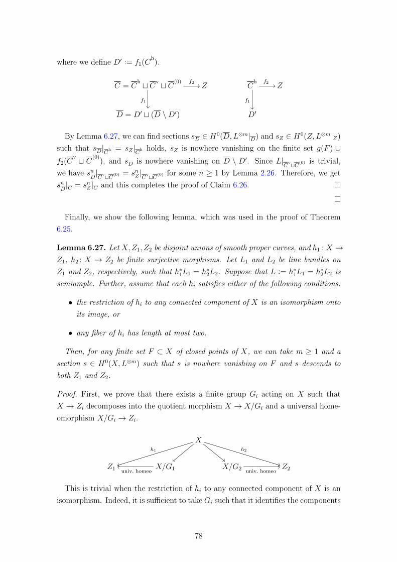
where we define D′ := f1(Ch).

C = Ch t Cv t C(0)

f1

f2// Z C

h

f1

f2// Z

D = D′ t (D \D′) D′

By Lemma 6.27, we can find sections sD ∈ H0(D,L⊗m|D) and sZ ∈ H0(Z,L⊗m|Z)

such that sD|Ch = sZ |Ch holds, sZ is nowhere vanishing on the finite set g(F ) ∪f2(C

v t C(0)), and sD is nowhere vanishing on D \ D′. Since L|

CvtC(0) is trivial,

we have snD|C

vtC(0) = snZ |CvtC(0) for some n ≥ 1 by Lemma 2.26. Therefore, we get

snD|C = snZ |C and this completes the proof of Claim 6.26.

Finally, we show the following lemma, which was used in the proof of Theorem

6.25.

Lemma 6.27. Let X,Z1, Z2 be disjoint unions of smooth proper curves, and h1 : X →Z1, h2 : X → Z2 be finite surjective morphisms. Let L1 and L2 be line bundles on

Z1 and Z2, respectively, such that h∗1L1 = h∗2L2. Suppose that L := h∗1L1 = h∗2L2 is

semiample. Further, assume that each hi satisfies either of the following conditions:

• the restriction of hi to any connected component of X is an isomorphism onto

its image, or

• any fiber of hi has length at most two.

Then, for any finite set F ⊂ X of closed points of X, we can take m ≥ 1 and a

section s ∈ H0(X,L⊗m) such that s is nowhere vanishing on F and s descends to

both Z1 and Z2.

Proof. First, we prove that there exists a finite group Gi acting on X such that

X → Zi decomposes into the quotient morphism X → X/Gi and a universal home-

omorphism X/Gi → Zi.

X

||

h1

tt""

h2

**Z1 X/G1univ. homeooo X/G2 univ. homeo

// Z2

This is trivial when the restriction of hi to any connected component of X is an

isomorphism. Indeed, it is sufficient to take Gi such that it identifies the components

78

with the same image under hi. Then X → Zi is isomorphic to the quotient morphism

X → X/Gi.

For the second case, assume that any fiber of hi has length at most two. Let Z ′i

be a connected component of Zi. Set X ′ = h−1i (Z ′i). There are four possibilities:

(1) X ′ is connected and X ′ → Z ′i is an isomorphism.

(2) X ′ is connected and X ′ → Z ′i is the Frobenius map (this case may only occur

for characteristic p = 2).

(3) X ′ is connected and every fiber of X ′ → Z ′i has length two. There exists an

involution ι : X ′ → X ′ such that X ′ → Z ′i is the quotient by ι.

(4) X ′ has two connected components X ′1 and X ′2. Further, X ′1 → Z ′i and X ′2 → Z ′i

are isomorphisms. In this case, we have X ′1 ' X ′2.

In the cases (3) and (4), we have a finite group G′ acting on X ′ such that the

morphism X ′ → Z ′i is isomorphic to the quotient morphism X ′ → X ′/G′.

Hence, we have a finite group Gi acting on X such that the morphism X → Zi

decomposes in the following way X → X/Gi → Zi, where X → X/Gi is the quotient

morphism and X/Gi → Zi is a universal homeomorphism (actually, if we restrict it

to a connected component, it is either an isomorphism or the Frobenius map).

Note that L = g∗L for any g ∈ Gi. We claim that if s ∈ H0(X,L⊗m) is Gi-

equivariant, then spe

descends to Zi for sufficiently large e. This is because s descends

to X/Gi and X/Gi → Zi is a universal homeomorphism (cf. Theorem 2.31).

Let G := G1G2 ⊂ Aut(X) be a composition of the groups and let S ⊂ X be the

G-orbit of the set F . By Lemma 2.28, G is a finite group, and therefore S is a finite

set.

Take m ≥ 1 and a section s ∈ H0(X,L⊗m) such that s is nowhere vanishing on

S. Set

sG :=∏σ∈G

σ∗s ∈ H0(X,L⊗m|G|).

The section sG is Gi-invariant for each i and nowhere vanishing on F . Hence, (sG)pe

satisfies the statement of the lemma for sufficiently large e ≥ 1.

Remark 6.28. The main issue of this section is related to the following question

discussed by Keel in [Kee03].

Question 6.29. Let L be a line bundle on a variety X and let p : X → X be the

normalization of X. Assume that p∗L is semiample. What additional assumptions

are necessary for L to be semiample?

79

6.5 Proof of Theorem 6.1

In this section, we prove Theorem 6.1 using Theorem 6.20 and Theorem 6.25.

Proof of Theorem 6.1. Let S := b∆c. By Theorem 6.20, it is sufficient to show that

L|Supp(S) is semiample. Note that in both case (1) and case (2), all the coefficients

of ∆ are at most one.

By the adjunction formula (Proposition 2.24), if we define ∆S on S so that (KX +

∆)|S = KS +∆S, then ∆S satisfies the conditions in the statement of Theorem 6.25.

In the case (2), that is, the case when each component Si of S is normal, S

clearly satisfies the condition (?), because on each component the normalization is

an isomorphism. In the case (1), that is, the case when (X,∆) is log canonical, the

surface S is regular or nodal in codimension one (see [Kol13, Corollary 2.32]), and

so S satisfies the condition (??) (see [Kol13, Claim 1.41.1] or [Tan13, Lemma 3.4,

3.5]).

Thus, we can complete the proof by using Theorem 6.25.

We easily deduce Corollary 1.29.

Proof of Corollary 1.29. It is enough to take L = 2(KX + ∆) and L = −(KX + ∆),

respectively.

6.6 Examples

Theorem 6.1 does not hold if we do not impose any conditions on ∆. It is in fact

possible to construct a nef and big line bundle L on a smooth threefold X such that

L− (KX + ∆) is nef and big for ∆ ≥ 0, but L is not semiample. We construct such

L and ∆ in the following way.

Example 6.30. Let L be a nef and big line bundle on a smooth threefold, which

is not semiample (see an example of Totaro in [Tot09, Theorem 7.1]). Since L is

big, we can write L = A + E for an ample Q-Cartier Q-divisor A and an effective

Q-Cartier Q-divisor E. Take ∆ = mE for m ∈ N big enough. Then mL− (KX +∆)

is an ample Cartier divisor, and so the pair L′ := mL and ∆ is an example, which

we were looking for.

Theorem 6.1 does not hold over algebraically closed fields k 6= Fp even in the

two-dimensional case.

Example 6.31 (Tanaka [Tan14, Example 19.3]). Let C0 ⊂ P2 be an elliptic curve in

P2, and let p1, . . . , p10 ∈ C0 be ten general points on C0. Let X be the blowup of P2

80

along these ten points, and C the proper transform of C0. Note that KX + C ∼ 0

and C2 = −1.

Take an ample divisor H on X, and set L := H+aC, where a := H ·C > 0. Note

that L is a nef and big divisor. Further, (X,C) is log canonical, and L− (KX +C)

is also nef and big. Nevertheless, L is not semiample if the base field is not Fp. This

is because L · C = 0, but L|C = (H + aC)|C is not torsion.

Corollary 1.29 (2) also does not hold over algebraically closed fields k 6= Fp.

Example 6.32 (Gongyo [Gon12, Example 5.2]). Let S be the blowup of P2 along

nine general points. Note that −KS is nef but not semiample if the base field is not

Fp. Take a very ample divisor H on S, and set X := PS(OS ⊕OS(−H)). Let E be

the tautological section of OS ⊕OS(−H). Since E ' S, it follows that −KE is not

semiample.

Then, (X,E) is log canonical, and L := −(KX +E) is nef and big by the nefness

of −KS (for details, see [Gon12, Example 5.2]). Nevertheless, L is not semiample,

because L|E = −KE is not semiample.

81

Acknowledgements

First of all I would like to thank my supervisor Paolo Cascini, for the invaluable

help, encouragement and support. I also thank the entire Imperial geometry group,

professors, postdocs and students. It has been a privilege to be part of such a stim-

ulating working environment.

In this last year I also had the lucky chance to work with other amazing people

outside of London.

Thanks to Simone Diverio, for the great hospitality in Paris, his fondness and

charisma, all the advices in terms of maths, career, restaurants and parisian treats.

Then I moved again to Trento, and also there I met very nice people and an excel-

lent working environment. A special thanks to Claudio Fontanari and his wonderful

family for their incredible kindness and hosplitality.

I learned as much from my professors as from my peers. Thanks to Jakub, a

great collaborator, always a source of inspiration and a very dear friend. Thanks

to Roberto and Luca (le mie montagne trentine), and thanks to Yusuke and Stefan.

Special thanks to my office mates of 526 and to my amazing flatmates Giovanni and

Dave.

There is not enough space to name all the great people that I met in these four

years, mathematicians and friends from all over the world. And we should’t forget

the physicists: Antony, Kamil, Viggy and all Cohort 4. Thanks to all the members

of the Jep Book Club. Thanks to Liana, my favourite conference roommate, and

to Eleonora, friend, colleague and fundraising partner. Thanks to Daniele Agostini

for the syzygies consulting. I also cannot forget all the old friends from Ferrara

and Pavia that are still a constant support and became a permanent and important

presence in my life: special thanks to March, Denver, Kinder, Andres, Agne, Ceci

and Michele: almost family.

And now let me thank some very special people. Without them this thesis would

82

not have been written and I would be a very different person now.

Thanks to the other members of the powerful tetrad DAJE. In order of appear-

ance. I genuinely believe that one the best think that can happen to you if you

are doing a PhD in algebraic geometry is having an accademic brother as Andrea

Fanelli. I met him on my first day at Imperial, and I quickly understood that my

PhD was going to be a lot of fun. It was, and it is mainly thanks to Fano. Then

came Enrica. She is my canonical bundle formula guru, one of the first person that

I turn to for advice and encouragement, an example for the kind of mathematician

that I want to become and most of all a great friend. Last but not least, Andrea

Petracci. We shared travels, anxieties for the future, gossips, laughs and disappoint-

ments, he has been really a daily support in these last years. He is also my first aid

for my many and frequent algebraic emergencies. And you know what is the funny

thing? Il jazz!

Since a while ago home has stop to be a geographical place. It doesn’t matter

where I am, it matters who I am with. My parents are home and they will always

be no matter where we are. Having Alessio and Nilla as parents and examples has

been one of the greatest blessing of my life. Sara and Nicola are home. My sister is

not only my best friend and my doctor, she is really the person that can understand

and heal my body and my mind. Thank you for all you have done for me. A special

thanks to Mira, she probably did not realize how much joy she gave me with her

black humid nose and her wagging tail.

Un piccolo passo alla volta. A little step at the time. This is what I said to my

self all the time that I though I couldn’t make it. This thesis and these four years of

PhD have been a long series of little steps, some of them harder than others. None

of them would have been possible if Teo would not have been on my side along all

the way. I can not wait to see what are the challenges that are waiting for us in the

future and I am serene because I know I will face them with you.

83

References

[Art62] M. Artin. Some numerical criteria for contractability of curves onalgebraic surfaces. American Journal of Mathematics, 84(3):485–496,1962.

[Ati57] M. Atiyah. Vector bundles over an elliptic curve. Proc. London Math.Soc, 7(3):415–452, 1957.

[B+83] A. Beauville et al. Varietes kahleriennes dont la premiere classe dechern est nulle. J. Differential Geom, 18(4):755–782, 1983.

[BCHM10] C. Birkar, P. Cascini, C. Hacon, and J. McKernan. Existence ofminimal models for varieties of log general type. J. Amer. Math. Soc,23(2):405–468, 2010.

[BHPVdV15] W. Barth, K. Hulek, C. Peters, and A. Van de Ven. Compact complexsurfaces, volume 4. Springer, 2015.

[Bir13] C. Birkar. Existence of flips and minimal models for 3-folds in charp. arXiv preprint arXiv:1311.3098, 2013.

[Cil83] C. Ciliberto. Sul grado dei generatori dell anello canonico di unasuperficie di tipo generale. Rend. Sem. Mat. Univ. Pol. Torino,41(3):83–111, 1983.

[CL14] P. Cascini and V. Lazic. On the number of a log smooth threefold.Journal de Mathematiques Pures et Appliquees, 102(3):597–616, 2014.

[CLS11] D. A Cox, J. Little, and H. Schenck. Toric varieties. AmericanMathematical Soc., 2011.

[CMM14] P. Cascini, J. McKernan, and M. Mustata. The augmented base locusin positive characteristic. Proceedings of the Edinburgh MathematicalSociety (Series 2), 57(01):79–87, 2014.

[CT14] P. Cascini and L. Tasin. On the Chern numbers of a smooth threefold.arXiv preprint arXiv:1412.1686, 2014.

[CZ14] P. Cascini and D. Zhang. Effective finite generation for adjoint rings.Annales de l’Institut Fourier, 64(1):127–144, 2014.

[DF14] S. Diverio and A. Ferretti. On a conjecture of Oguiso about rationalcurves on Calabi-Yau threefolds. Comment. Math. Helv., 89(1):157–172, 2014.

84

[DFM16] S. Diverio, C. Fontanari, and D. Martinelli. Rational curves on fiberedCalabi-Yau manifolds (with an appendix by Roberto Svaldi). arXivpreprint arXiv:1607.01561, 2016.

[DSWW86] M. Dine, N. Seiberg, X. Wen, and E. Witten. Nonperturbative effectson the string world sheet. Nuclear Phys. B, 278(4):769–789, 1986.

[FG65] W. Fischer and H. Grauert. Lokaltriviale Familien kompakter kom-plexer Mannigfaltigkeiten. Vandenhoeck & Ruprecht, 1965.

[Fuj00] O. Fujino. Abundance theorem for semi log canonical threefolds. DukeMath. J., 102(3):513–532, 2000.

[G+84] M. Green et al. Koszul cohomology and the geometry of projectivevarieties. Journal of Differential Geometry, 19(1):125–171, 1984.

[Gon12] Y. Gongyo. On weak fano varieties with log canonical singularities.J. Reine Angew. Math., 665:237–252, 2012.

[GP01] M. Gross and S. Popescu. Calabi–Yau threefolds and moduli ofabelian surfaces I. Compositio Mathematica, 127(2):169–228, 2001.

[Gre82] M. Green. The canonical ring of a variety of general type. Duke Math.J, 49(4):1087–1113, 1982.

[Gro64] A. Grothendieck. Elements de geometrie algebrique iv. Publ. Math.IHES, 20(24):1965, 1964.

[Har77] R. Hartshorne. Algebraic geometry. Springer-Verlag, New York-Heidelberg, 1977. Graduate Texts in Mathematics, No. 52.

[HBW92] D. Heath-Brown and P. Wilson. Calabi–Yau threefolds with ρ > 13.Mathematische Annalen, 294(1):49–57, 1992.

[HK11] C. Hacon and S. Kovacs. Classification of higher dimensional algebraicvarieties, volume 41. Springer Science & Business Media, 2011.

[HM06] C. Hacon and J. McKernan. Boundedness of pluricanonical mapsof varieties of general type. Inventiones mathematicae, 166(1):1–25,2006.

[HM10] C. Hacon and J. McKernan. Flips and flops. Proceedings of the In-ternational Congress of Mathematicians Hyderabad, India, 2010.

[Kaw85] Y. Kawamata. Pluricanonical systems on minimal algebraic varieties.Invent. Math., 79(3):567–588, 1985.

[Kaw91] Y. Kawamata. On the length of an extremal rational curve. Invent.Math., 105(3):609–611, 1991.

[Kaw97] Y. Kawamata. On the cone of divisors of calabi–Yau fiber spaces.International Journal of Mathematics, 8(05):665–687, 1997.

85

[Kee99] S. Keel. Basepoint freeness for nef and big line bundles in positivecharacteristic. Annals of Mathematics, 149:253–286, 1999.

[Kee03] S. Keel. Polarized pushouts over finite fields. Communications inAlgebra, 31(8):3955–3982, 2003.

[KKL12] A.S. Kaloghiros, A. Kuronya, and V. Lazic. Finite generation andgeography of models. arXiv preprint arXiv:1202.1164, 2012.

[KL09] J. Kollar and M. Larsen. Quotients of calabi–Yau varieties. In Algebra,Arithmetic, and Geometry, pages 179–211. Springer, 2009.

[KM87] Y. Kawamata and K. Matsuki. The number of the minimal models fora 3-fold of general type is finite. Mathematische Annalen, 276(4):595–598, 1987.

[KM92] J. Kollar and S. Mori. Classification of three-dimensional flips. Jour-nal of the American Mathematical Society, 5(3):533–703, 1992.

[KM98] J. Kollar and S. Mori. Birational geometry of algebraic varieties,volume 134. Cambridge University Press, 1998.

[Kol86] J. Kollar. Higher direct images of dualizing sheaves I. Annals ofMathematics, 123(1):11–42, 1986.

[Kol89] J. Kollar. Flops. Nagoya Mathematical Journal, 113:15–36, 1989.

[Kol91] J. Kollar. Flips, flops, minimal models, etc. Surveys in Differen-tial Geometry (Cambridge, MA, 1990), J. Differential Geom. Suppl,1:113–199, 1991.

[Kol92] J. Kollar. Flips and abundance for algebraic threefolds. Asterisque,211, 1992.

[Kol93] J. Kollar. Effective base point freeness. Mathematische Annalen,296(1):595–605, 1993.

[Kol13] J. Kollar. Singularities of the minimal model program, volume 200 ofCambridge Tracts in Mathematics. 2013.

[Kol15] J. Kollar. Deformations of elliptic calabi–yau manifolds. Recent Ad-vances in Algebraic Geometry: A Volume in Honor of Rob Lazarsfelds60th Birthday, 417:254, 2015.

[Kon08] K. Konno. Relations in the canonical algebras on surfaces. Rendicontidel Seminario Matematico della Universita di Padova, 120:227–261,2008.

[Laz04] R. Lazarsfeld. Positivity in algebraic geometry I: Classical setting:line bundles and linear series, volume 48. Springer Science & BusinessMedia, 2004.

86

[Leh15] B. Lehmann. Numerical triviality and pullbacks. Journal of Pure andApplied Algebra, 219(12):5637–5649, 2015.

[Lie13] C. Liedtke. Algebraic surfaces in positive characteristic. In Birationalgeometry, rational curves, and arithmetic, pages 229–292. Springer,2013.

[Liu02] Q. Liu. Algebraic geometry and arithmetic curves, volume 6 of OxfordGraduate Texts in Mathematics. Oxford University Press, Oxford,2002.

[Mat92] K. Matsuki. Introduction to the Mori program. Springer–Verlag, 1992.

[Miy87] Y. Miyaoka. The Chern classes and Kodaira dimension of a minimalvariety. In Algebraic geometry, Sendai, 1985, volume 10 of Adv. Stud.Pure Math., pages 449–476. North-Holland, Amsterdam, 1987.

[Miy94] Y. Miyaoka. Rational curves on algebraic varieties. Proceeding of theInternational Congress of Mathematicians, 1,2, 1994.

[ML97] M. Mendes Lopes. The degree of the generators of the canonicalring of surfaces of general type with pg= 0. Archiv der Mathematik,69(5):435–440, 1997.

[MM83] S. Mori and S. Mukai. The uniruledness of the moduli space of curvesof genus 11. In Algebraic geometry, pages 334–353. Springer, 1983.

[MNW15] D. Martinelli, Y. Nakamura, and J. Witaszek. On the basepoint-freetheorem for log canonical threefolds over the algebraic closure of afinite field. Algebra & Number Theory, 9(3):725–747, 2015.

[MP97] Y. Miyaoka and T. Peternell. Geometry of higher dimensional alge-braic varieties, volume 26. Birkhauser, 1997.

[Mum08] D. Mumford. Abelian varieties, volume 5 of Tata Institute of Funda-mental Research Studies in Mathematics. 2008.

[Ogu93] K. Oguiso. On algebraic fiber space structures on a Calabi-Yau 3-fold.Internat. J. Math., 4(3):439–465, 1993. With an appendix by NoboruNakayama.

[Pet91] T. Peternell. Calabi–Yau manifolds and a conjecture of Kobayashi.Mathematische Zeitschrift, 207(1):305–318, 1991.

[Rei83] M. Reid. Minimal models of canonical 3-folds. Adv. Stud. Pure Math,1:131–180, 1983.

[Rei88] I. Reider. Vector bundles of rank 2 and linear systems on algebraicsurfaces. Annals of Mathematics, 127(2):309–316, 1988.

87

[Rei90] M. Reid. Infinitesimal view of extending a hyperplane section-deformation theory and computer algebra. In Algebraic geometry,pages 214–286. Springer, 1990.

[Rei02] M. Reid. Graded rings and varieties in weighted projective space.Manuscript, M. Reids Web page Available at www. maths. warwick.ac. uk/ miles/ surf/ more/ grad. pdf , 2002.

[SD73] B. Saint-Donat. On Petri’s analysis of the linear system of quadricsthrough a canonical curve. Mathematische Annalen, 206(2):157–175,1973.

[Sho86] V. Shokurov. The nonvanishing theorem. Mathematics of the USSR-Izvestiya, 26(3):591, 1986.

[Sil09] J. Silverman. The arithmetic of elliptic curves, volume 106 of Grad-uate Texts in Mathematics. Springer, Dordrecht, 2 edition, 2009.

[ST16] S. Schreieder and L. Tasin. Kaehler structures on spin 6-manifolds.arXiv preprint arXiv:1606.09237, 2016.

[Tak06] S. Takayama. Pluricanonical systems on algebraic varieties of generaltype. Inventiones mathematicae, 165(3):551–587, 2006.

[Tan13] H. Tanaka. Abundance theorem for semi log canonical surfaces inpositive characteristic. arXiv preprint arXiv:1301.6889, 2013.

[Tan14] H. Tanaka. Minimal models and abundance for positive characteristiclog surfaces. Nagoya Mathematical Journal, 216:1–70, 2014.

[Tot09] B. Totaro. Moving codimension-one subvarieties over finite fields.Amer. J. Math., 131(6):1815–1833, 2009.

[Tsu06] H. Tsuji. Pluricanonical systems of projective varieties of general typei. Osaka Journal of Mathematics, 43(4):967–995, 2006.

[Ver15] M. Verbitsky. Ergodic complex structures on hyperkahler manifolds.Acta Math., 215(1):161–182, 2015.

[Wil89] P. Wilson. Calabi-Yau manifolds with large Picard number. Inven-tiones mathematicae, 98(1):139–155, 1989.

[Wil94] P. Wilson. The existence of elliptic fibre space structures on Calabi-Yau threefolds. Math. Ann., 300(4):693–703, 1994.

[Wit86] E. Witten. Holomorphic curves on manifolds of SU(3) holonomy.Conf. Proc., C8607214:145–149, 1986.

[Xu13] C. Xu. On base point free theorem of threefolds in positive charac-teristic. arXiv preprint arXiv:1311.3819, 2013.

88