Dynamics of Planetary Rings - Observatoire de Paris
18
Dynamics of Planetary Rings Bruno Sicardy 1, 2 1 Observatoire de Paris, LESIA, 92195 Meudon C´ edex, France [email protected] 2 Universit´ e Pierre et Marie Curie, 75252 Paris C´ edex 05, France Abstract. Planetary rings are found around all four giant planets of our solar sys- tem. These collisional and highly flattened disks exhibit a whole wealth of physical processes involving microscopic dust grains, as well as meter-sized boulders. These processes, together with ring composition, can help to understand better the for- mation and evolution of proto-satellite and proto-planetary disks in the early solar system. The present chapter reviews some fundamental aspects of ring dynamics, namely their flattening, their stability against proper modes, their particle sizes, and their responses to resonance forcing by satellites. These concepts will be used and tested during the forthcoming exploration of the Saturn system by the Cassini mission. 1 Introduction Planetary rings consist in thin disks of innumerable colliding particles revolv- ing around a central planet. They are found around all the four giant planets of our solar system, Jupiter, Saturn, Uranus and Neptune. Meanwhile, they exhibit a wide variety of sizes, masses and physical properties. Also, they in- volve many different physical processes, ranging from large spiral waves akin to galactic structures, down to microscopic electromagnetic forces on charged dust grains. All these effects have a profound influence on the long term evolution of rings. As such, they can teach us something about the origin of rings, i.e. whether they are cogenetic to the central planet, or the result of a more recent breakup of a comet or satellite. These processes are also linked to disk dynamics in general, either in proto-planetary circumstellar disks or in galaxies. A complete review of all these processes remains out of the scope of this short chapter. Instead, we would like to address here a few basic issues related to planetary rings, by asking the following questions: • Why are planetary rings so flat? B. Sicardy: Dynamics of Planetary Rings, Lect. Notes Phys. 682, 183–200 (2006) www.springerlink.com c Springer-Verlag Berlin Heidelberg 2006
Transcript of Dynamics of Planetary Rings - Observatoire de Paris

Dynamics of Planetary Rings
Bruno Sicardy1,2
1 Observatoire de Paris, LESIA, 92195 Meudon Cedex, [email protected]
2 Universite Pierre et Marie Curie, 75252 Paris Cedex 05, France
Abstract. Planetary rings are found around all four giant planets of our solar sys-tem. These collisional and highly flattened disks exhibit a whole wealth of physicalprocesses involving microscopic dust grains, as well as meter-sized boulders. Theseprocesses, together with ring composition, can help to understand better the for-mation and evolution of proto-satellite and proto-planetary disks in the early solarsystem. The present chapter reviews some fundamental aspects of ring dynamics,namely their flattening, their stability against proper modes, their particle sizes,and their responses to resonance forcing by satellites. These concepts will be usedand tested during the forthcoming exploration of the Saturn system by the Cassinimission.
1 Introduction
Planetary rings consist in thin disks of innumerable colliding particles revolv-ing around a central planet. They are found around all the four giant planetsof our solar system, Jupiter, Saturn, Uranus and Neptune. Meanwhile, theyexhibit a wide variety of sizes, masses and physical properties. Also, they in-volve many different physical processes, ranging from large spiral waves akinto galactic structures, down to microscopic electromagnetic forces on chargeddust grains.
All these effects have a profound influence on the long term evolution ofrings. As such, they can teach us something about the origin of rings, i.e.whether they are cogenetic to the central planet, or the result of a morerecent breakup of a comet or satellite. These processes are also linked todisk dynamics in general, either in proto-planetary circumstellar disks or ingalaxies.
A complete review of all these processes remains out of the scope of thisshort chapter. Instead, we would like to address here a few basic issues relatedto planetary rings, by asking the following questions:
• Why are planetary rings so flat?
B. Sicardy: Dynamics of Planetary Rings, Lect. Notes Phys. 682, 183–200 (2006)www.springerlink.com c© Springer-Verlag Berlin Heidelberg 2006

184 B. Sicardy
• How thin and dynamically stable are they?• How do they respond to resonant forcing from satellites?
Answering these questions may help to understand the connection betweenrings global properties (mass, optical depth, etc. . . ) and their local character-istics (particle size and distribution, velocity dispersion, etc. . . ).
Extensive descriptions and studies of the issues presented in this chapterare available in the literature. Detailed reviews (and related references) on ringstructures, ring dynamics and open issues are presented in [1–6], while ringorigin and evolution are discussed in [7] and [8]. Stability issues are discussedin classical papers like [9], and in very much details in reference text bookslike [10]. Collisional processes are reviewed for instance in [11]. Finally, thevarious possible responses of disks to resonances and their applications areexposed in [1, 12–14].
2 Planetary Rings and the Roche Zone
Generally speaking, planetary rings reside inside a limit loosely referred to asthe ‘Roche zone’ of the central planet. Inside this limit, the tidal stress fromthe central body tends to disrupt satellites into smaller bodies. Outside thislimit, accretion tends to sweep dispersed particles into larger lumps.
Reality is not so sharply defined, though. For instance, the tidal disruptionlimit for a given body depends not only on the bulk density of that body, whichmay differ significantly from one body to the other, but also on the tensilestrength of that body, another parameter which may vary by several ordersof magnitude. Thus, due to these uncertainties, the Roche zone depicted inFig. 1 remains rather blurred.
In spite of these difficulties, it is instructive to plot the sizes of, say,Saturn’s satellites as a function of their distances to the center of the planet(Fig. 1). Interestingly, one notes that the sizes of the satellites decrease asone approaches the Roche zone, as expected from a simple modelling of tidalstress.
Figure 1 also plots the sizes of satellites that could be formed by lumpingtogether the material of Saturn’s A, B and C rings, as well as of CassiniDivision. This figure supports the general idea that the Roche Limit delineatesthe region inside which tides disrupt solid satellites into a fluid-like ring disk.
Note finally that in the Roche zone, rings and satellites can co-exist, asit is the case for instance for Pan, which orbits inside the Encke Division ofSaturn’s A ring. An interesting question is then to know whether satellitesand rings can influence each other gravitationally, or even if they can betransformed into each other on long (billions of years) or short (a few years)time scales.
Although Jupiter’s, Uranus’ and Neptune’s rings are much less massivethat Saturn’s, they exhibit the same general behavior: smaller and smaller
Dynamics of Planetary Rings 185
Fig. 1. The relative sizes of Saturn’s inner satellites as a function of their distanceto the planet center, in units of the planet radius. The “sizes” of the rings have beencalculated by lumping all the material of A, B, C rings and Cassini Division intosingle bodies. All the sizes have been plotted so that to respect the relative masses ofthe various bodies involved. For comparison, Mimas has a diameter of about 500 km
satellites are encountered as one approches the planet Roche zone, then amixture of rings and satellites is observed, and then only rings are found.
3 Flattening of Rings
Planetary rings flatten because of collisions between particles. This processdissipates mechanical energy, while conserving angular momentum of the en-semble.
Consider a swarm of particles labelled 1, . . . , i, . . . , with total initialangular momentum H orbiting a spherical planet centered on O. Let us call theOz axis directed along H the “vertical” axis, and the plane Oxy perpendicularto Oz the “horizontal plane”. The orthogonal unit vectors along Ox, Oy andOz will be denoted x, y and z, respectively.
Each particle of mass mi, position ri and velocity vi has an angular mo-mentum Hi = miri × vi, so that:
H =∑
i
miri × vi =∑
i
miri × viz +∑
i
miri × vih ,
where viz and vih are the vertical and horizontal contributions of the ve-locities, respectively. The vector vih can furthermore be decomposed into a

186 B. Sicardy
tangential component, viθ and a radial one, vir. Projecting H along the unitvector z along Oz, one gets:
H = H · z =∑
i
mi(ri × viz) · z +∑
i
mi(ri × vih) · z =∑
i
miriviθ .
The equality above holds because the first sum vanishes altogether since viz
and z are parallel, and also because only the tangential velocity survives inthe second sum, due to the presence of ri in the mixed product (ri × vih) · z.
On the other hand, the mechanical energy of the ring is given by:
E =∑
i
miΦP (ri) +∑
i
miv2iθ/2 +
∑i
miv2ir/2 +
∑i
miv2iz/2 ,
where ΦP (ri) is the planetary potential well per unit mass felt by the particlei.
Comparing the expressions of H and E, one sees that it is possible to min-imize the energy E of the ring while conserving the angular momentum H, bysimply zeroing vir and viz. In other words, the collisions, by dissipating energywhile conserving angular momentum, tend to flatten the disk perpendicularto its total angular momentum, and to circularize the particles orbits.
If the planet is not spherically symmetric, as it is the case for all theoblate giant planets, then only the projection of H along the planet spin axis(say, Hspin) is conserved. The same reasoning as above then shows that theconfiguration of least energy which conserves Hspin is a flat, but now equatorialring.
4 Stability of Flat Disks
The considerations presented above lead to the conclusion that a dissipativering will eventually collapse to an infinitely thin disk with perfectly circularorbits.
In reality, this is not quite true, as some physics is still missing in the des-crition of the rings. For instance, the differential Keplerian motion, combinedwith the finite size of the particles and the mutual gravitational stirring ofthe larger particles will maintain a small residual velocity dispersion in thesystem (i.e. a pressure).
This dispersion induces a small but non-zero thickness of the disk, and isactually necessary to ensure the dynamical stability of the disk versus anotherdestabilizing effect, namely self-gravity.
To quantify this effect, let us describe a planetary ring as a very thin diskwhere the surface density, velocity and pressure at a given point r and a giventime t will be denoted respectively Σ, v and p. Furthermore, let ΦD be thegravitational potential (per unit mass) created by the disk and cs the speedof sound in the ring, corresponding to the typical velocity dispersion of theparticles.
Dynamics of Planetary Rings 187
A detailed account of the calculations derived below and their physicalinterpretations can be found in [10]. In a first step, one can use a toy modelwhere the disk is in uniform rotation with constant angular velocity vector Ωdirected along the vertical axis Oz. This will highlight the role of rotation inthe stability of the ring, while simplifying the equations of motion. In reality, adisk around a planet exhibits a roughly Keplerian shear (Ω ∝ r−3/2), but theconclusions concerning the role of rotation will not be altered in the present,simplified, approach.
The eulerian equations describing the dynamics of the disk are then, in aframe rotating at angular velocity Ω:
∂v∂t
+ (v · ∇)v = −∇p
Σ−∇(ΦP + ΦD) − 2Ω × v + Ω2r
∂Σ
∂t+ ∇ · (Σv) = 0
∇2ΦD = 4πGΣδ(z)
p = Σc2s
(1)
The first line is Euler’s equation, where the acceleration on the fluid isexpressed in terms of the pressure p, the potentials of the planet and the disk,ΦP and ΦD, respectively, the Coriolis term and the centrifugal acceleration.The second line the continuity equation, expressing the conservation of mass.The next line is Poisson’s equation, relating the potential ΦD of an infinitivelythin disk to the surface density Σ, the gravitational constant G and the Diracfunction δ(z), where z is the elevation perpendicular to the ring plane. Finally,the last line is the simplest equation of state, that of an isothermal disk,relating the pressure p to the surface density Σ through the speed of soundcs.
A classical approach is to consider what happens to the disk when smallperturbations are applied. For small enough disturbances, the equations abovecan be linearized, assuming that the unperturbed disk has uniform density.Then the various quantities involved can decomposed into an unperturbedbackground value (with index 0) and a small perturbed value (with index 1):Φ = ΦP + ΦD0 + ΦD1, Σ = Σ0 + Σ1, v = 0 + v1, Σ = Σ0 + Σ1.
This leads, after linearization of (1):
∂Σ1
∂t+ Σ0 (∇ · v1) = 0
∂v1
∂t= − c2
s
Σ0∇Σ1 −∇ΦD1 − 2Ω × v1
∇2ΦD1 = 4πGΣ1δ(z)
(2)
188 B. Sicardy
One can seek how a given disturbance, for instance Σ1 = Σ1 exp[i(k · r −ωt)], propagates in the disk, where Σ is the amplitude, k is the wavevector andω is the frequency of the disturbance (with similar notations for the pressureand velocity). With no loss of generality we can assume that the disturbancepropagates in the disk along the horizontal axis Ox, i.e. k = kx.
Partial derivatives with respect to x and t are then equivalent to multipli-cations by ik and −iω, respectively. Also, Poisson’s equation in the system 2can be integrated as |k|ΦD1 = −2πGΣ1. This provides the algebraic system:
ikΣ0v1x −iωΣ1 = 0
iωv1x +2Ωv1y +(
2πG
|k| − c2s
Σ0
)ikΣ1 = 0
2Ωv1x −iωv1y = 0
This system has non trivial solutions only if its determinant is non zero,thus providing the dispersion relation for propagating modes in a uniformlyrotating disk:
ω2 = k2c2s − 2πGΣ0|k| + 4Ω2 (3)
Modes with ω2 < O will be unstable, so that the dispersion relation tellsus which wavenumbers are unstable in the disk.
It is instructive to vary the values of cs and Ω to see the respective effectsof pressure and rotation on the stability of a thin (i.e. 2-D) disk. Various casescan be considered:
• Cold and motionless disk: cs = 0 and Ω = 0. Then ω2 = −2πGΣ0|k|, seeFig. 2(a), and all the modes are unstable, as expected, since nothing canstop the gravitational collapse of any disturbance. Note that the free fallcollapse time, tcolla ∼ 1/
√GΣ0|k| depends on the wavenumber k of the
disturbance, the smaller structures collapsing faster than the larger ones.This contrasts with the 3-D case, where the free fall time scale depends onlyupon the unperturbed density ρ0: tcolla ∼ 1/
√Gρ0.
• Hot and motionless disk: cs = 0 and Ω = 0. Now ω2 = k2c2s − 2πGΣ0|k|, so
that the disk is unstable for disturbances with |k| < kJ , where
kJ = 2πGΣ0/c2s
is the Jeans wavenumber, see Fig. 2(b). The relation |k| < kJ is actuallythe Jeans criterium for a 2-D disk. It can be compared to its 3-D classicalcounterpart |k| < kJ =
√4πGρ0/c2
s. This criterium indicates how small thewavenumber must be (i.e. how large and massive the disturbance must be)in order to overcome the pressure associated with cs.
• Cold rotating disk: cs = 0 and Ω = 0. This yields ω2 = −2πGΣ0|k| + 4Ω2,which shows that now the large disturbances (with small k) are stabilizedby rotation, while the small structures (|k| > kR = 2Ω2/πGΣ0) remain

Dynamics of Planetary Rings 189
Fig. 2. Various cases of relation dispersions of free modes in rotating disks (3).In all panels, the grey intervals denote unstable mode regions. (a): motionless colddisk, (b): motionless hot disk, (c): rotating cold disk and (d): rotating hot disk. Seetext for details
unstable, see Fig. 2(c). This can be understood as large structures have adifferential velocity in the disk due to the angular velocity Ω of the latter.As a consequence, a large structure which attempts to collapse under itsown gravity will be stopped by the rotational barrier, when the centrifugalacceleration at its periphery balances its self gravity.
Note in passing that rotation does not stabilize the disk against alldisturbances, as the smallest of them are still subject to gravitational col-lapses.
• Hot rotating disk: cs = 0 and Ω = 0. The dispersion relation ω2 = k2c2s −
2πGΣ0|k| + 4Ω2 shows that ω2 is minimum for |k| = kJ/2 = πGΩ0/c2s,
and that the minimum value is ω2min = 4Ω2 − π2G2Σ2
0/c2s, as illustrated in
Fig. 2(d).
It is convenient to define a dimensionless parameter, called the Toomreparameter ([9]):
Q =csΩ
πGΣ0,
so that ω2min = (4Ω2/Q2) · [Q2−1/4]. Thus, if Q < 1/2, then ω2
min < 0 and thedisk remains unstable for an interval of wavenumbers (kmin,kmax) centered onkJ/2, see Fig. 2(d). Large structures (with small |k|) are then stabilized byrotation, while small structure (with large |k|) are stabilized by pressure. For
Q =csΩ
πGΣ0>
12
,
the disk is stable to any disturbances. The above condition is called theToomre criterium. Note that it is derived for a uniformly rotating disk. A

190 B. Sicardy
differentially rotating disk will also yield a similar criterium, except for thethe numerical coefficient in the right-hand side of the inequality.
Now, if a disk is rotating around a planet with potential ΦP , then theequations of motion read (in a fixed frame this time):
(∂
∂t+ v · ∇
)v = −∇ (ΦP + ΦD) − ∇ · p
Σ
∂Σ
∂t+ ∇(Σv) = 0
∇2ΦD = 4πΣGδ(z)
p = Σc2s
(4)
It is then more convenient to work with the radial and tangential compo-nents of the velocity, vr and vθ, respectively, instead of vx and vy. The price topay is that vr and vθ now depend on θ, and this must be accounted for whenapplying the nabla operator ∇. The linearization of the (4) then proceeds asbefore, and the new dispersion relation is:
ω2 = k2c2s − 2πGΣ0|k| + κ2 , (5)
where κ = r−3∂[r3∂ΦP /∂r
]/∂r is the so-called epicyclic frequency, basically
the frequency at which a particle oscillates horizontally around its averageposition (note that κ coincides with the mean motion n in the special case ofa Keplerian potential ΦP ∝ −1/r).
Equation (5) shows that the disk is stable against any disturbances if:
Q =csκ
πGΣ0> 1 , (6)
which constitutes a more general version of the Toomre criterium. It illustratesquantitatively how pressure (cs) and rotation (κ) tend to stabilize the diskagainst self-gravity (Σ0).
5 Particle Size and Ring Thickness
In planetary rings, inelastic collisions tend to reduce the velocity dispersioncs. This in turn decreases the value of Q below unity, leading to gravitationalinstabilities at some point, according to (6), and see Fig. 3. This causes thering to collapse into small lumps. At that point, the finite mass and size ofthe lumps will maintain a small but non-zero velocity dispersion, of the orderof the escape velocity at the surface of the largest particles,
cs ∼√
Gmmax/Rmax ,
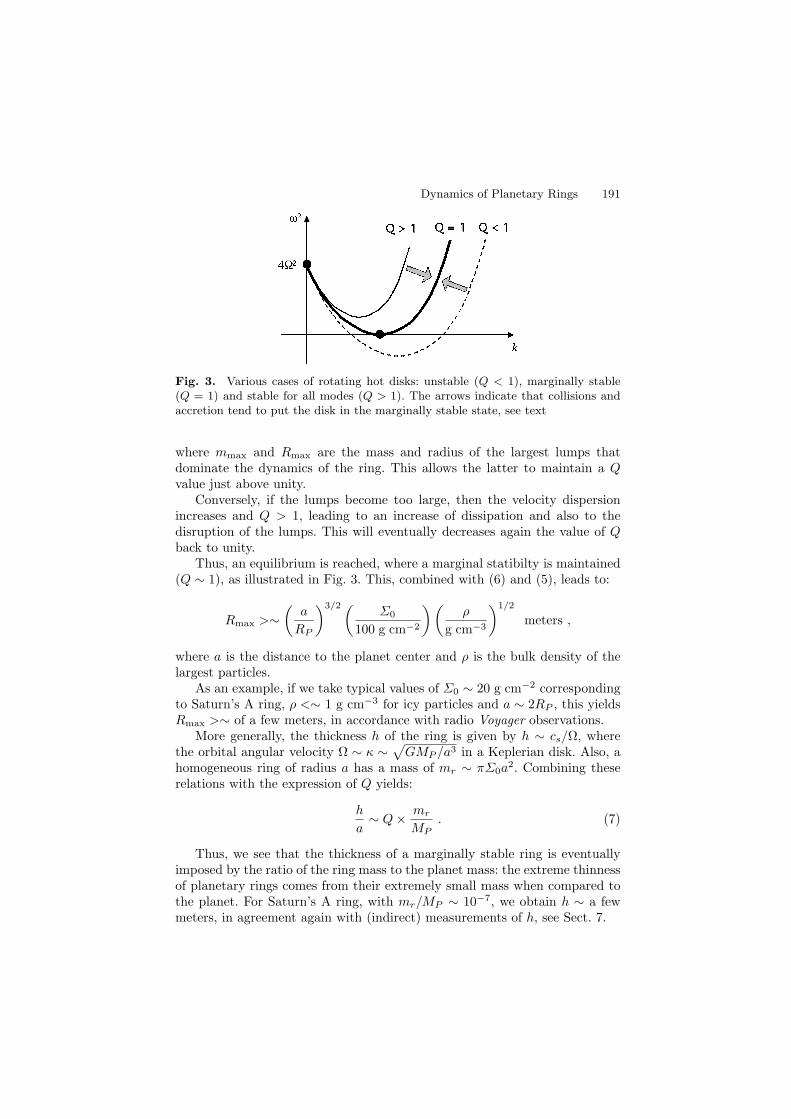
Dynamics of Planetary Rings 191
Fig. 3. Various cases of rotating hot disks: unstable (Q < 1), marginally stable(Q = 1) and stable for all modes (Q > 1). The arrows indicate that collisions andaccretion tend to put the disk in the marginally stable state, see text
where mmax and Rmax are the mass and radius of the largest lumps thatdominate the dynamics of the ring. This allows the latter to maintain a Qvalue just above unity.
Conversely, if the lumps become too large, then the velocity dispersionincreases and Q > 1, leading to an increase of dissipation and also to thedisruption of the lumps. This will eventually decreases again the value of Qback to unity.
Thus, an equilibrium is reached, where a marginal statibilty is maintained(Q ∼ 1), as illustrated in Fig. 3. This, combined with (6) and (5), leads to:
Rmax >∼(
a
RP
)3/2(Σ0
100 g cm−2
)(ρ
g cm−3
)1/2
meters ,
where a is the distance to the planet center and ρ is the bulk density of thelargest particles.
As an example, if we take typical values of Σ0 ∼ 20 g cm−2 correspondingto Saturn’s A ring, ρ <∼ 1 g cm−3 for icy particles and a ∼ 2RP , this yieldsRmax >∼ of a few meters, in accordance with radio Voyager observations.
More generally, the thickness h of the ring is given by h ∼ cs/Ω, wherethe orbital angular velocity Ω ∼ κ ∼
√GMP /a3 in a Keplerian disk. Also, a
homogeneous ring of radius a has a mass of mr ∼ πΣ0a2. Combining these
relations with the expression of Q yields:
h
a∼ Q × mr
MP. (7)
Thus, we see that the thickness of a marginally stable ring is eventuallyimposed by the ratio of the ring mass to the planet mass: the extreme thinnessof planetary rings comes from their extremely small mass when compared tothe planet. For Saturn’s A ring, with mr/MP ∼ 10−7, we obtain h ∼ a fewmeters, in agreement again with (indirect) measurements of h, see Sect. 7.

192 B. Sicardy
Note for closing this section that the first marginally unstable modes,appearing when Q ∼ 1, corresponds to the minimal value of ω2 in (5). Theyhave wavenumbers kunst ∼ kJ/2 ∼ Ω/cs, i.e. wavelengths:
λunst ∼ 2πh ,
or a few tens of meters. These marginal instabilities are probably the expla-nation for the quadrant asymmetries observed in Saturn’s A ring.
6 Resonances in Planetary Rings
So far, we have been considering free modes propagating in rings. We nowturn to the case where modes are forced by a satellite near a resonance.
Considering the very small masses of the satellites relative to the giantplanets, these forced modes are in general “microscopic”, in the sense thatthey induce deviations of a few meters on the particles orbits. However, nearresonances, a satellite can excite macroscopic responses in the disk, whichexhibit large collective disturbances over tens of kilometers, i.e. on scales ob-servable by spacecraft imagers.
As explained later, this collective response allows an secular exchange ofangular momentum and energy between the ring and the satellite, very muchlike tides allow secular exchanges between a planet and its satellites.
The equations of motion are the same as in (4), except that the firstequation (Euler’s) must now accounts for the forcing of the satellite throughits disturbing potential ΦS :
(∂
∂t+ v · ∇
)v = −∇ (ΦP + ΦD + ΦS) − ∇ · P
Σ
∂Σ
∂t+ ∇(Σv) = 0
∇2ΦD = 4πΣGδ(z)
p = Σc2s ,
(8)
Note in passing that we have replaced the (scalar) isotropic pressure p by apressure tensor, P. This allows us to take into account in a general way morecomplicated effects like viscosity or non-isotropic pressure terms.
The simplest case we can think of is the forcing of a homogeneous disk bya small satellite of mass ms MP with a circular orbit of radius as and meanmotion nS around a point-like planet with potential ΦP (r) = −GMP /r. Thisis the Keplerian approximation. In reality, the oblateness of the planet intro-duces extra terms causing a slow precession of the apse and node of the orbit.These subtleties will not be taken into account here since they obscure our
Dynamics of Planetary Rings 193
main point (the study of a simple isolated resonance) without changing ourmain conclusions. These effects would become important, however, if the or-bital eccentricity and inclination of the satellite were to come into play.
With these assumptions, the satellite potential is periodic in θ − nSt, sothat it can be Fourier expanded as:
ΦS(r, θ, t) =+∞∑
m=−∞ΦSm(r) · exp [im (θ − nSt)] , (9)
where m is an integer, ΦSm(r) = −(GmS/2aS) · bm1/2(r/aS) and bm
1/2 is theclassical Laplace coefficient (see [12] for a review of the properties of thesecoefficients). We note that Φm(r) = Φ−m(r), since Φs is real.
Equations (8) are then linearized, and we assume that the free modesof the disk are damped by collisions, or are at least negligible with respectto the forced modes, especially near the resonances. Then all the perturbedquantities, for instance the radial velocity vr, take the same form as the forcing(9), i.e. vr(r, θ, t) =
∑vrm(r) · exp[jm(θ − nSt)], etc. . .
Each term ΦSm(r) · exp[jm(θ − nSt)] of the satellite potential then forcesa mode in the ring, and if equations (8) remain linear, then it is enoughto study the reaction of the disk to each mode separately. As already notedbefore, this replaces the differential operators by mere multiplications, namely∂/∂t = −jmns and ∂/∂θ = jm.
This approach is especially useful near resonances, where one mode dom-inates over all the other ones, and can thus be “clipped off” from the rest.Consider a particle with mean motion n, so that it longitude writes θ = nt(plus an arbitrary constant). This particle thus feels a forcing potentialΦSm(r) ·exp[jm(θ−nSt)] = ΦSm exp[jm(n−nS)t], i.e. a term with frequencym(n − nS).
A so-called (“Excentric Lindblad Resonance”) (ELR) occurs when thisfrequency matches the horizontal epicyclic frequency κ of the particle, i.e.when:
κ = ±m(n − nS) . (10)
In this case, and for small horizontal displacements of the particle, the lat-ter behaves very much like a harmonic oscillator (i.e. a linear system) near aclassical resonance. This simple model predicts that the horizontal displace-ment of the particle increases as it approaches the resonance, and becomessingular at exact resonance1. In reality, non-linear terms come into play inthe disk and eventually prevent the singularity. In counterpart, this compli-cates significantly the equations of motion, and renders the system 8 ratheruntractable.
Fortunately, for sufficiently dense planetary rings perturbed by very smallsatellites, collisions, pressure and self-gravity prevent a wild behavior for
1This horizontal displacement is proportional to the orbital eccentricity of theparticle, hence the nomenclature “Excentric Lindblad Resonance”

194 B. Sicardy
nearby streamlines, thus keeping the perturbed motion small, and eventuallyensuring that the system 8 remains linear.
Note that for a Keplerian disk κ = n, so that the condition κ = ±m(n−nS)is equivalent to
n =m
m ∓ 1· nS , (11)
corresponding to mean motion resonances 2:1, 3:2, 4:3, etc. . . , also calledfirst order resonances. Other resonances, e.g. second order resonances 3:1, 4:2,5:3 (i.e. of the form m : m − 2) can also come into play when the smallersecond order terms in the particle orbital eccentricity are considered. Stillother resonances (referred to as “corotation resonances”) can also arise whenthe satellite orbital eccentricity is accounted for. These kinds of resonancesfall outside the main topic of this chapter and will not be considered here.
Another important simplification comes from the fact that in planetaryrings, the perturbed quantities vary much more rapidly radially than az-imuthally. Physically, this means that the spiral structures resonantly forcedare tightly wound, like the grooves of a music disk. More precisely, the lowerorder radial derivatives can be neglected with respect to higher orders:
m2
r2 m
r· d
dr d2
dr2. (12)
This is the WKB approximation2, which greatly simplifies the system 8, lead-ing to (see [13]):
jm(n − ns)vrm − 2nvθm = −ΦSm − ΦDm − c2sσm
Σ0+(
µ +4ν
3
)vrm
n
2vrm + jm(n − ns)vθm = −jm
ΦSm + ΦDm
r− jm
c2sσm
rΣ0+ νvθm
σm = − Σ0vrm
jm(n − ns)
ΦDm = −2πGjsσm
pm = c2sσm .
(13)The quantities µ and ν are the bulk and shear kinematic viscosities, respec-tively, coming from the pressure tensor P. The dot stands for the space (nottime) derivative d/dr. The Poisson equation has been solved using the resultsof [12], where s = ±1 is chosen in such a way that the disk potential out ofthe disk plane tends to zero:
ΦDm(r + is|z|) → 0 , (14)2Developed by Wentzel-Kramer-Brilloin in the field of quantum mechanics.

Dynamics of Planetary Rings 195
as |z| goes to infinity. We will see that boundary conditions actually imposes = +1.
If we forget for the moment the terms ΦDm, σm, µ and ν, i.e. if we considera test disk with no self-gravity, no pressure nor viscosity, then we get:
vrm(r) = −jm
[(n − ns)r
d
dr+ 2n
]· ΦSm(r)
1rD
vθm(r) =[nr
d
dr+ 2m2(n − ns)
]· ΦSm(r)
12rD
,
(15)
where D(r) = n2 − m2(n − ns)2 is a measure of the distance to exact res-onance. The velocity is singular when D= 0, i.e. when n = m/(m ∓ 1)ns,corresponding to the condition (11). Thus the dependence in 1/D is just theexpected response of a linear oscillator near a resonance.
The result obtained above does not strike by its simplicity: complicatedequations and tedious calculations have just shown that a harmonic oscillatorbehaves as derived in basic text books. However, we have gained with theseequations some important insights into more subtle effects associated withviscosity, pressure and self-gravity. More generally, these equations show howcollective effects modify the simple harmonic oscillator paradigm into morecomplicated behaviors.
Near the resonance, D = 0, the system 13 is almost degenerate, and (15)yield uθm ∼ ±(j/2)urm. To solve for urm, one uses this degeneracy, plus thetightly wound wave condition (12). We note x the relative distance to theresonance radius am, x = (a−am)/am, and we expand (13) near x = 0, whichyields:
− α3v
d2
dx2(urm) + α2
G
d
dx(urm) − jxurm = Cm , (16)
where:
α3v = jα3
P + α3ν
α3P = ∓ c2
s/n
3ma2mns
α3ν =
µ + 7ν/33ma2
mns
α2G = ± 2πsGΣ0
3mamnns,
(17)
and Cm is a factor which weakly depends on m ([13]). For purposes of numeri-cal applications, Cm ∼ ±0.27an(ms/M) as m tends to infinity. The coefficientCm ∝ ms in (16) is the forcing term due to the satellite. The coefficients αP ,αν and αG encapsulate the effects of pressure, viscosity and self-gravitation,respectively. In the absence of all the α’s, the response of the disk is indeed

196 B. Sicardy
singular at the resonance x=0: urm ∝ 1/x, as expected in a test disk in thelinear regime. The extra terms with the α’s in (16) prevent such an outcome,and forces the solution to remain finite at x = 0. If oscillations are present inthe solution, then waves are launched.
Equation (16) can be solved by defining the Fourier transform of urm:
urm(k) =∫ +∞
−∞exp(−jkx)urm(x)dx ,
assuming that urm(x) is square integrable. Then we take the Fourier transformof (16):
d
dk(urm) + (α3
vk2 + jα2Gk)urm = 2πCmδ(k) , (18)
where δ is the Dirac function. This first-order equation is solved with theboundary condition urm → 0 as k → ∞, since urm is a Fourier transform.Then:
urm(k) = 2πCmH(k) exp[−(α3vk3/3 + jα2
Gk2/2)] ,
where H is the unit-step function (=0 for k < 0 and =1 for k > 0). Thiseventually provides the solution we are looking for:
urm(x) = Cm
∫ +∞
0
exp[j(kx − α2Gk2/2 − α3
P k3/3) − α3νk3/3]dk . (19)
Note that the boundary condition (14) also requires urm(x+ is|z|) → 0 as|z| → +∞, i.e. s = +1 since k > 0 in the integral above.
The qualitative behavior of urm(x) can be estimated from the behavior ofthe argument in the exponential, j(kx − α2
Gk2/2 − α3P k3/3) − α3
νk3/3. Thisargument has an imaginary part, j(kx− α2
Gk2/2− α3P k3/3), which causes an
oscillation of the function in the integral, and a real part, −α3νk3/3, which
causes a damping of that function.The integral in (19) is significant only when the phase kx − α2
Gk2/2 −α3
P k3/3 is stationary, i.e. near the wave number kstat such that:
α2Gkstat + α3
P k2stat = x (20)
somewhere in the domain of integration (k > 0).For instance, if the disk is dominated by self-gravity, i.e. α2
G α3P , then
the condition (20) reduces to x = α2Gkstat. Thus, the integral in (19) is signifi-
cant only on that side of the resonance where x and α2G have the same sign. In
that case, the solution of 19 oscillates near x with a local radial wave numberkstat ≈ x/α2
G. The local radial wavelength of the wave is thus ∝ 1/x. Conse-quently, the wave oscillates more and more and more rapidly as it propagatesaway from the resonance, see Fig. 4(a). On the other side of the resonance(where x and α2
G have opposite signs), the argument of the exponential in(19) is never stationary, and the integral damps to zero. This means that the
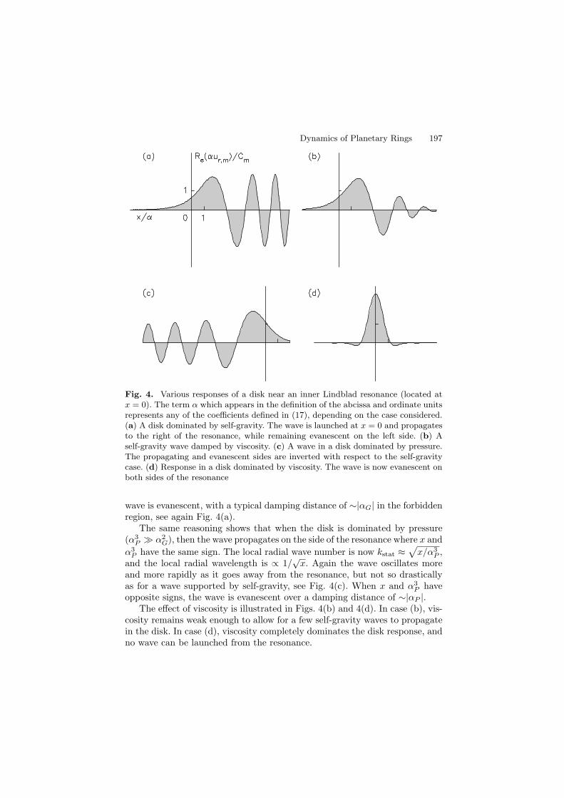
Dynamics of Planetary Rings 197
Fig. 4. Various responses of a disk near an inner Lindblad resonance (located atx = 0). The term α which appears in the definition of the abcissa and ordinate unitsrepresents any of the coefficients defined in (17), depending on the case considered.(a) A disk dominated by self-gravity. The wave is launched at x = 0 and propagatesto the right of the resonance, while remaining evanescent on the left side. (b) Aself-gravity wave damped by viscosity. (c) A wave in a disk dominated by pressure.The propagating and evanescent sides are inverted with respect to the self-gravitycase. (d) Response in a disk dominated by viscosity. The wave is now evanescent onboth sides of the resonance
wave is evanescent, with a typical damping distance of ∼|αG| in the forbiddenregion, see again Fig. 4(a).
The same reasoning shows that when the disk is dominated by pressure(α3
P α2G), then the wave propagates on the side of the resonance where x and
α3P have the same sign. The local radial wave number is now kstat ≈
√x/α3
P ,and the local radial wavelength is ∝ 1/
√x. Again the wave oscillates more
and more rapidly as it goes away from the resonance, but not so drasticallyas for a wave supported by self-gravity, see Fig. 4(c). When x and α3
P haveopposite signs, the wave is evanescent over a damping distance of ∼|αP |.
The effect of viscosity is illustrated in Figs. 4(b) and 4(d). In case (b), vis-cosity remains weak enough to allow for a few self-gravity waves to propagatein the disk. In case (d), viscosity completely dominates the disk response, andno wave can be launched from the resonance.

198 B. Sicardy
7 Waves as Probes of the Rings
It is interesting to compare the numerical values of the coefficients αG and αP
for planetary rings. The larger of the two coefficients tells us which process(self-gravity or pressure) dominates in the wave propagation. According tothe expressions given in (17), using the definition of Toomre’s parameter,Q = csn/πGΣ0, and remembering that the thickness of the ring is given byh ∼ cs/n, we obtain:
∣∣∣∣αP
αG
∣∣∣∣ ∼√
2Q
(3m
h
a
)1/6
.
As we saw before, h/a ∼ 10−7 is very small and Q ∼ 1, while m is typicallya few times unity. Thus, the ratio αP /αG ∼ 0.1 − 0.2 is small, but not by anoverwhelming margin, because of the exponent 1/6 in the expression above.
The same is true with the ratio αν/αG since αν ∼ αP . This is becausethe kinematic viscosities µ and ν are both of the order of c2
s/n is moderatelythick planetary rings ([2]).
Consequently, self-gravity is the dominant process governing the propa-gation of density waves in planetary rings, but viscosity is efficient enoughto damp the wave after a few wavelengths, see for instance the panel (b) inFig. 4.
Note that self-gravity waves are macroscopic features which can be used asa probe to determine microscopic parameters such as the local surface densityΣ0 of the ring, or its kinematic viscosities µ or ν. This method has been usedwith bending waves in Saturn’s A ring and is the only way so far to derive Σ0
or ν in these regions ([5]).The determination of ν has an important consequence, namely the esti-
mation of the local thickness h of the ring, since ν ∼ c2s/n. Typical values
obtained for Saturn’s A ring indicate that h ∼ 10−50 meters, a value alreadyconsistent with stability considerations, see for instance the discussion afterEq. (7).
8 Torque at Resonances
A remarkable property of the function urm(x) defined in (19) is that the realpart of its integral, [
∫ +∞−∞ urm(x)dx], is independent of the values of the coeffi-
cients α’s. For instance, all the areas under the curves of Fig. 4 (i.e. the shadedregions) are equal, including in the cases (c) and (d), where dissipation playsan important role.
This can be shown by using an integral representation of the step function([13]),
H(k) = (j/2π)∫ +∞
−∞[exp(−jku)/(u + jε)]

Dynamics of Planetary Rings 199
in (19), where ε is an arbitrarily small number. Equation (19) may then bethen integrated in x, which yields δ(k), then in k, and finally in u:
(∫ +∞
−∞urmdx
)=
(jCm
∫ +∞
−∞
du
u + jε
)= πCm . (21)
Now, the complex number urm(x) describes how the disk responds tothe resonant excitation of the satellite at the distance x from the resonance.More precisely, the modulus |urm(x)| is a measure of the amplitude of theperturbation at x, and is thus directly proportional to the eccentricity of thestreamlines around x. The argument φ = arg[urm(x)] is on the other handdirectly connected to the phase lag Ψ of the perturbation with respect to thesatellite potential. It can be shown easily that φ = Ψ ∓ π/2, see [13].
Consequently, the satellite torque acting on a given streamline is pro-portional to its eccentricity ∝ |urm(x)| and to sin(Ψ) ± cos(φ), a classicalproperties of linear oscillators. Consequently the total torque exerted at theresonance is proportional to [
∫ +∞−∞ urm(x)dx].
More precisely, the torque exerted by the satellite on the disk is by def-inition Γ =
∫ ∫(r × ∇ΦS)Σd2r, where ΦS and Σ may be Fourier expanded
according to (9) when the stationary regime is reached. After linearization,one gets the torque exerted at the resonance:
Γm = ∓12πm2Σ0a2sCm
(∫ +∞
−∞urm(x)dx
), (22)
where the upper (resp. lower) sign applies to a resonance inside (resp. outside)the satellite orbit.
This is the so-called “standard torque” ([1]), originally derived for a self-gravity wave launched at an isolated resonance. The calculations made aboveshow that this torque is actually independent of the physical process at workin the disk, as long as the response of the latter remains linear. In particular,dissipative processes such as viscous friction do not modify the torque value.
This torque allows a secular exchange of angular momentum between thedisk and the satellite. Note that the sign of this exchange is such that thetorque always tends to push the satellite away from the disk.
This torque have a wide range of applications that we will not reviewhere. We will just note here that it may lead to the confinement of a ringwhen two satellites lie on each side of the latter (the so-called “shepherdingmechanism”). This could explain for instance the confinement of some of thenarrow Uranus’ rings.
Another consequence of such a torque is that Saturn’s rings and the innersatellites are constinuously pushed away from each other. The time scalesassociated with such interactions (of the order of 108 years) tend to be shorterthan the age of the solar system ([2]). This suggests that planetary rings areeither rather young, or, if primordial, have continuously evolved and livedseveral cycles since their formation.

200 B. Sicardy
9 Concluding Remarks
We have considered in this chapter some fundamental concepts associatedwith rings: their flattening, their thickness and their resonant interactions withsatellites. Note that these processes are mainly linked to the larger particlesof the rings. Furthermore, they make a useful bridge between the microscopicand macroscopic properties of circumplanetary disks.
Meanwhile, many other processes have not been discussed here, such asthe effect of electromagnetic forces on dust particles, the detailed nature ofcollisions between the larger particles, the accretion and tidal disruption ofloose aggregates of particles, the origin of sharp edges in some rings, theirnormal modes of oscillation, etc. . .
These issues, and others, are addressed in some of the references givenin the bibliography below. All the processes involved clearly show that ringsare by no means the simple and everlasting objects they seem to be whenobserved from far away.
References
1. P. Goldreich, S. Tremaine: Ann. Rev. Astron. Astrophys. 20, 249 (1982)2. N. Borderies, P. Goldreich, S. Tremaine: unsolved problems in planetary ring
dynamics. In: Planetary rings, ed by R. Greenberg, A. Brahic (Univ. Of ArizonaPress 1984) pp 713–734
3. P.D. Nicholson, L. Dones: Rev. Geophys. 29, 313 (1991)4. P. Goldreich: puzzles and prospects in planetary ring dynamics. In: Chaos, reso-
nance and collective dynamical phenomena in the solar system, ed by S. Ferraz-Mello (Kluwer Academic Publishers, Dordrecht Boston London 1992) pp 65–73
5. L.W. Esposito: Annu. Rev. Earth Planet. Sci. 21, 487 (1993)6. J.N. Cuzzi: Earth, Moon, and Planets 67, 179 (1995)7. A.W. Harris: the origin and evolution of planetary rings. In: Planetary rings, ed
by R. Greenberg, A. Brahic (Univ. Of Arizona Press 1984) pp 641–6598. W. Ward: the solar nebula and the planetesimal disk. In: Planetary rings, ed by
R. Greenberg, A. Brahic (Univ. Of Arizona Press 1984) pp 660–6849. A. Toomre: ApJ. 139, 1217 (1964)
10. J. Binney, S. Tremaine: Galactic Dynamics (Princeton University Press 1988)11. P.Y. Longaretti: Planetary ring dynamics: from Boltzmann’s equation to celes-
tial dynamics. In: Interrelations between physics and dynamics for minor bodiesin the solar system, ed by D. Benest, C. Froeschle (Editions Frontieres, Gif-sur-Yvette 1992) pp 453–586
12. F.H. Shu: waves in planetary rings. In: Planetary rings, ed by R. Greenberg, A.Brahic (Univ. of Arizona Press 1984) pp 513–561
13. N. Meyer-Vernet, B. Sicardy: Icarus 69, 157 (1987)14. B. Sicardy: Planetary ring dynamics: Secular exchange of angular momentum
and energy with a satellite. In: Interrelations between physics and dynamicsfor minor bodies in the solar system, ed by D. Benest, C. Froeschle (EditionsFrontieres, Gif-sur-Yvette 1992) pp 631–651