Dynamics of machines and mechanisms
306
-
Upload
nguyen-hoai-nam -
Category
Documents
-
view
1.517 -
download
27
Transcript of Dynamics of machines and mechanisms

DYNAMICS ofMACHINES andMECHANISMS
FUNDAMENTALSof KINEMATICS
and

0257/FM/Frame Page 2 Friday, June 2, 2000 6:38 PM

Oleg Vinogradov
DYNAMICS ofMACHINES andMECHANISMS
FUNDAMENTALSof KINEMATICS
and
Boca Raton London New York Washington, D.C.CRC Press

This book contains information obtained from authentic and highly regarded sources. Reprintedmaterial is quoted with permission, and sources are indicated. A wide variety of references arelisted. Reasonable efforts have been made to publish reliable data and information, but theauthor and the publisher cannot assume responsibility for the validity of all materials or forthe consequences of their use.
Neither this book nor any part may be reproduced or transmitted in any form or by any means,electronic or mechanical, including photocopying, microfilming, and recording, or by anyinformation storage or retrieval system, without prior permission in writing from the publisher.
The consent of CRC Press LLC does not extend to copying for general distribution, for promo-tion, for creating new works, or for resale. Specific permission must be obtained in writingfrom CRC Press LLC for such copying.
Direct all inquiries to CRC Press LLC, 2000 N.W. Corporate Blvd., Boca Raton, Florida 33431.
Trademark Notice:
Product or corporate names may be trademarks or registered trademarks,and are used only for identification and explanation, without intent to infringe.
© 2000 by CRC Press LLC
No claim to original U.S. Government worksInternational Standard Book Number 0-8493-0257-9
Library of Congress Card Number 00-025151Printed in the United States of America 1 2 3 4 5 6 7 8 9 0
Printed on acid-free paper
Library of Congress Cataloging-in-Publication Data
Vinogradov, Oleg (Oleg G.)Fundamentals of kinematics and dynamic of machines and mechanisms /by Oleg Vinogradov.
p. cm.Includes bibliographical references and index.ISBN 0-8493-0257-9 (alk. paper)1. Machinery, Kinematics of. 2. Machinery, Dynamics of. I. Title.
TJ175.V56 2000621.8
′
11—dc21 00-025151 CIP
0257/FM/Frame Page 4 Friday, June 2, 2000 6:38 PM

Preface
The topic of
Kinematics and Dynamics of Machines and Mechanisms
is one of thecore subjects in the Mechanical Engineering curriculum, as well as one of thetraditional subjects, dating back to the last century. The teaching of this subject has,until recently, followed the well-established topics, which, in a nutshell, were somegeneral properties, and then analytical and graphical methods of position, velocity,and acceleration analysis of simple mechanisms. In the last decade, computer tech-nology and new software tools have started making an impact on how the subjectof
kinematics and dynamics of machines and mechanisms
can be taught. I have taught
kinematics and dynamics of machines and mechanisms
for manyyears and have always felt that concepts and numerical examples illustrating them didnot allow students to develop a perception of a mechanism as a whole and an under-standing of it as an integral part of the design process. A laboratory with a variety ofmechanisms might have alleviated some of my concerns. However, such a laboratory,besides being limited to a few mechanisms, mainly serves as a demonstration toolrather than as a design tool, since it would be very time-consuming to measure suchfundamental properties as position, velocity, and acceleration at any point of themechanism. It would be even more difficult to measure forces, internal and external.There is yet one more consideration. With class sizes as they are, the experience of astudent becomes a group experience, limited in scope and lacking in the excitementof an individual “discovery.”
A few years ago I started using Mathematica in my research, and it became clearto me that this software can be used as a tool to study mechanisms. It gives a studenta chance to perform symbolic analysis, to plot the results, and, what is most impor-tant, to animate the motion. The student thus is able to “play” with the mechanismparameters and see their effect immediately. The idea was not only to develop anunderstanding of basic principles and techniques but, more importantly, to open anew dimension in this understanding by appealing to the student’s visual perceptionand intuition. I noticed also that it gives students a sense of pride to be able to dosomething on their own and have it “work.” I have seen many times how their eyesbrighten when they see their mechanism in motion for the first time. In general, suchsoftware as Mathematica allows students to study complex mechanisms without thelimitations imposed by either a physical laboratory or a calculator. All of thisprompted me to write this book.
The subject of this book is kinematics and dynamics of machines and mechanisms,and Mathematica is used only as a tool. In my view it would be detrimental to thesubject of the book if too much attention were placed on a tool that is incidental to thesubject itself. So in the book the two, the subject and the tool, are presented separately.Specifically, the Appendix shows how Mathematica can be used to illuminate thesubject of each chapter. All the material in the Appendix is available on CD-ROM in
0257/FM/Frame Page 5 Friday, June 2, 2000 6:38 PM

the form of interactive Mathematica notebooks. The Problems and Exercises at theend of each chapter are also split into two types: Problems, that do not require the useof Mathematica and emphasize understanding concepts, and Exercises, based on Math-ematica, that require students to perform analysis of mechanisms. The second typeI call projects, since they require homework and a report.
In my opinion, the use of a symbolic language such as Mathematica shouldnot prevent a student from developing analytical skills in the subject. With this inmind, I provide a consistent analytical approach to the study of simple and complex(chain-type) mechanisms. The student should be able to derive solutions in a closedform for positions, velocities, accelerations, and forces. Mathematica
allows oneto input these results for plotting and animation. As an option, students can performcalculations for a specific mechanism position using analytical solutions.
In my class, the numerical part of the course is moved to the computer laboratory.It is done in the form of projects and assumes complete analysis, parametric study,and animation. There are two to three projects during the term, which gives studentssufficient exposure to numerical aspects of mechanism analysis and design. Thisprocedure then allows the instructor to concentrate in quizzes and exams on under-standing of the subject by asking students to answer conceptual-type questionswithout the students’ spending time on calculations. Thus, instructors can cover morematerial in their tests.
A few basic Mathematica files (programs) are available on the CD-ROM. Theintention is to provide students with the foundation needed to solve other problemswithout spending too much time studying the tool itself. For example, the programsfor simple slider-crank and four-bar mechanisms allow students to study a complexmechanism combining them. I must emphasize, however, that the available programscannot substitute for the Mathematica book by S. Wolfram (see Bibliography).
Specifically, the following programs written in Mathematica
are on CD-ROM:
• introduction.nb outlines basic features of Mathematica with examples ofnumerical calculations, symbolic solutions, plotting, and animation.
• howTo.nb gives a set of Mathematica answers to specific questions arisingin solutions of kinematics and dynamics problems, such as, for example,how to write an ordinary differential equation, how to solve it in symbols,how to plot the results, how to draw a line, etc.
• sliderCrank.nb provides a complete solution of the kinematics and dynamicsof the offset slider-crank mechanism, with plots and animation.
• fourBar.nb provides a complete solution of the kinematics and dynamicsof the four-bar mechanism, with plots and animation.
• CamHarmonic.nb provides analysis of a harmonic cam with oscillatingand offset followers.
• 2DOFfree.nb provides analysis of the free vibrations of a two-degree-of-freedom system with damping.
• 2DOFforced.nb provides analysis of the forced vibrations of a two-degree-of-freedom system with damping.
0257/FM/Frame Page 6 Friday, June 2, 2000 6:38 PM

All the above programs contain textual explanations and executable commands(Mathematica allows mingling of text and executable commands in one file).
An inevitable question arises when any software tool is introduced: How dostudents learn Mathematica? Knowing Mathematica to a sufficient degree is, of course,prerequisite to this course. Some universities introduce students to Mathematica intheir calculus courses. In my third-year course in kinematics I introduce Mathematicain the first few weeks in the computer laboratory by giving students the interactiveprograms Introduction to Mathematica
and How-To in
Mathematica
.
The latter answersspecific questions relevant to the course material. In addition, I make programs dealingwith two basic mechanisms,
slider-crank mechanism
and
four-bar linkage
, availableto students. Students use these two programs as starting points for studying morecomplex mechanisms.
All of the problems listed in this book as assignments were assigned to studentsas projects over the last 3 years since I began teaching this course in a new format.The students’ reaction to this new learning environment helped me design this book.And for that I am thankful to all of them. My specific thanks go to my former third-year student Mr. Yannai Romer Segal who developed all of the graphics for this book.I also appreciate the support provided by the technical personnel in our department,Mr. B. Ferguson, Mr. D. Forre, and Mr. N. Vogt, at various stages of this project.My sincere thanks to the Killam Foundation for awarding me a fellowship to writethis book.
Oleg Vinogradov
Calgary, 2000
0257/FM/Frame Page 7 Friday, June 2, 2000 6:38 PM

0257/FM/Frame Page 8 Friday, June 2, 2000 6:38 PM

About the Author
Oleg Vinogradov,
Professor of Mechanical Engineering at the University of Calgary,has been involved in the design and analysis of machines in industrial, researchinstitute, and university settings for more then 35 years. He has B.Sc. degrees inMechanical Engineering and Applied Mechanics and a Ph.D. in MechanicalEngineering. Dr. Vinogradov has published
Introduction to Mechanical Reliability:A Designer’s Approach
(Hemisphere), and has written more than 100 papers on arange of topics, including structural and rotor dynamics, vibrations, and machinecomponents design.
0257/FM/Frame Page 9 Friday, June 2, 2000 6:38 PM

0257/FM/Frame Page 10 Friday, June 2, 2000 6:38 PM

Table of Contents
Chapter 1
Introduction1.1 The Subject of Kinematics and Dynamics of Machines ................................. 11.2 Kinematics and Dynamics as Part of the Design Process............................... 11.3 Is It a Machine, a Mechanism, or a Structure? ............................................... 31.4 Examples of Mechanisms; Terminology.......................................................... 41.5 Mobility of Mechanisms .................................................................................. 61.6 Kinematic Inversion........................................................................................ 101.7 Grashof’s Law for a Four-Bar Linkage ......................................................... 10Problems .................................................................................................................. 12
Chapter 2
Kinematic Analysis of Mechanisms2.1 Introduction..................................................................................................... 152.2 Vector Algebra and Analysis .......................................................................... 162.3 Position Analysis ............................................................................................ 18
2.3.1 Kinematic Requirements in Design ................................................... 182.3.2 The Process of Kinematic Analysis ................................................... 192.3.3 Kinematic Analysis of the Slider-Crank Mechanism ........................ 202.3.4 Solutions of Loop-Closure Equations ................................................ 222.3.5 Applications to Simple Mechanisms.................................................. 282.3.6 Applications to Compound Mechanisms ........................................... 362.3.7 Trajectory of a Point on a Mechanism .............................................. 39
2.4 Velocity Analysis ............................................................................................ 412.4.1 Velocity Vector.................................................................................... 412.4.2 Equations for Velocities...................................................................... 422.4.3 Applications to Simple Mechanisms.................................................. 452.4.4 Applications to Compound Mechanisms ........................................... 49
2.5 Acceleration Analysis ..................................................................................... 512.5.1 Acceleration Vector ............................................................................ 512.5.2 Equations for Accelerations ............................................................... 522.5.3 Applications to Simple Mechanisms.................................................. 55
2.6 Intermittent-Motion Mechanisms: Geneva Wheel ......................................... 60Problems and Exercises........................................................................................... 64
Chapter 3
Force Analysis of Mechanisms3.1 Introduction..................................................................................................... 73
0257/FM/Frame Page 11 Friday, June 2, 2000 6:38 PM

3.2 Force and Moment Vectors............................................................................. 743.3 Free-Body Diagram for a Link ...................................................................... 753.4 Inertial Forces ................................................................................................. 793.5 Application to Simple Mechanisms ............................................................... 80
3.5.1 Slider-Crank Mechanism: The Case of Negligibly SmallInertial Forces ..................................................................................... 80
3.5.2 Slider-Crank Mechanism: The Case of Significant Inertial Forces... 823.5.3 Four-Bar Mechanism: The Case of Significant Inertial Forces......... 883.5.4 Five-Bar Mechanism: The Case of Significant Inertial Forces ......... 903.5.5 Scotch Yoke Mechanism: The Case of Significant Inertial Forces ... 95
Problems and Exercises........................................................................................... 99
Chapter 4
Cams4.1 Introduction................................................................................................... 1034.2 Circular Cam Profile..................................................................................... 1044.3 Displacement Diagram ................................................................................. 1094.4 Cycloid, Harmonic, and Four-Spline Cams................................................. 110
4.4.1 Cycloid Cams ................................................................................... 1104.4.2 Harmonic Cams ................................................................................ 1154.4.3 Comparison of Two Cams: Cycloid vs. Harmonic.......................... 1174.4.4 Cubic Spline Cams........................................................................... 1184.4.5 Comparison of Two Cams: Cycloid vs. Four-Spline....................... 124
4.5 Effect of Base Circle .................................................................................... 1274.6 Pressure Angle .............................................................................................. 127Problems and Exercises......................................................................................... 132
Chapter 5
Gears5.1 Introduction................................................................................................... 1355.2 Kennedy’s Theorem...................................................................................... 1355.3 Involute Profile ............................................................................................. 1375.4 Transmission Ratio ....................................................................................... 1385.5 Pressure Angle .............................................................................................. 1395.6 Involutometry................................................................................................ 1405.7 Gear Standardization .................................................................................... 1435.8 Types of Involute Gears ............................................................................... 148
5.8.1 Spur Gears ........................................................................................ 1485.8.2 Helical Gears .................................................................................... 1505.8.3 Bevel Gears....................................................................................... 1535.8.4 Worm Gears...................................................................................... 157
5.9 Parallel-Axis Gear Trains ............................................................................. 1605.9.1 Train Transmission Ratio ................................................................. 1605.9.2 Design Considerations...................................................................... 161
0257/FM/Frame Page 12 Friday, June 2, 2000 6:38 PM

5.10 Planetary Gear Trains ................................................................................... 1625.10.1 Transmission Ratio in Planetary Trains ........................................... 1635.10.2 Example of a More Complex Planetary Train................................. 1655.10.3 Differential........................................................................................ 166
Problems ................................................................................................................ 167
Chapter 6
Introduction to Linear Vibrations6.1 Introduction................................................................................................... 1716.2 Solution of Second-Order Nonhomogeneous Equations with
Constant Coefficients.................................................................................... 1756.2.1 Solution of the Homogenous Equation............................................ 1756.2.2 Particular Solution of the Nonhomogeneous Equation ................... 1776.2.3 Complete Solution of the Nonhomogeneous Equation ................... 179
6.3 Free Vibrations of an SDOF System with No Damping............................. 1816.4 Forced Vibrations of an SDOF System with No Damping......................... 1826.5 Steady-State Forced Vibrations of an SDOF System with No Damping ... 1846.6 Free Vibrations of an SDOF System with Damping ................................... 1856.7 Forced Vibrations of a Damped (
ξ
< 1) SDOF System withInitial Conditions .......................................................................................... 188
6.8 Forced Vibrations of an SDOF System with Damping (
ξ
< 1)as a Steady-State Process ............................................................................. 190
6.9 Coefficient of Damping, Logarithmic Decrement, and Energy Losses ...... 1946.10 Kinematic Excitation .................................................................................... 1966.11 General Periodic Excitation.......................................................................... 1976.12 Torsional Vibrations...................................................................................... 1996.13 Multidegree-of-Freedom Systems ................................................................ 200
6.13.1 Free Vibrations of a 2DOF System without Damping .................... 2026.13.2 Free Vibrations of a 2DOF System with Damping ......................... 2086.13.3 Forced Vibrations of a 2DOF System with Damping ..................... 212
6.14 Rotordynamics .............................................................................................. 2156.14.1 Rigid Rotor on Flexible Supports .................................................... 2156.14.2 Flexible Rotor on Rigid Supports .................................................... 2196.14.3 Flexible Rotor with Damping on Rigid Supports............................ 2206.14.4 Two-Disk Flexible Rotor with Damping ......................................... 224
Problems and Exercises......................................................................................... 229
Bibliography .......................................................................................................... 233
Appendix — Use of Mathematica as a Tool ........................................................ 235A.1 Introduction to Mathematica ........................................................................ 240A.2 Vector Algebra .............................................................................................. 242A.3 Vector Analysis ............................................................................................. 242
0257/FM/Frame Page 13 Friday, June 2, 2000 6:38 PM

A.4 Kinematic and Force Analysis of Mechanisms ........................................... 242A.4.1 Slider-Crank Mechanism.................................................................. 242A.4.2 Four-Bar Linkage.............................................................................. 254
A.5 Harmonic Cam with Offset Radial and Oscillatory Roller Followers ........ 263A.6 Vibrations...................................................................................................... 274
A.6.1 Free Vibrations of a 2DOF System.................................................. 275A.6.2 Forced Vibrations of a 2DOF System.............................................. 283
Index ...................................................................................................................... 289
0257/FM/Frame Page 14 Friday, June 2, 2000 6:38 PM

1
1
Introduction
1.1 THE SUBJECT OF KINEMATICS AND DYNAMICS OF MACHINES
This subject is a continuation of statics and dynamics, which is taken by studentsin their freshman or sophomore years. In kinematics and dynamics of machines andmechanisms, however, the emphasis shifts from studying general concepts withillustrative examples to developing methods and performing analyses of real designs.This shift in emphasis is important, since it entails dealing with complex objectsand utilizing different tools to analyze these objects.
The objective of
kinematics
is to develop
various means of transforming motion
to achieve a specific kind needed in applications. For example, an object is to bemoved from point
A
to point
B
along some path. The first question in solving thisproblem is usually: What kind of a mechanism (if any) can be used to perform thisfunction? And the second question is: How does one design such a mechanism?
The objective of
dynamics
is analysis of the behavior of a given machine ormechanism when subjected to dynamic forces. For the above example, when themechanism is already known, then external forces are applied and its motion isstudied. The determination of forces induced in machine components by the motionis part of this analysis.
As a subject, the kinematics and dynamics of machines and mechanisms isdisconnected from other subjects (except statics and dynamics) in the MechanicalEngineering curriculum. This absence of links to other subjects may create the falseimpression that there are no constraints, apart from the kinematic ones, imposed onthe design of mechanisms. Look again at the problem of moving an object from
A
to
B
. In designing a mechanism, the size, shape, and weight of the object all constituteinput into the design process. All of these will affect the size of the mechanism.There are other considerations as well, such as, for example, what the allowablespeed of approaching point
B
should be. The outcome of this inquiry may affecteither the configuration or the type of the mechanism. Within the subject of kine-matics and dynamics of machines and mechanisms such requirements cannot bejustifiably formulated; they can, however, be posed as a learning exercise.
1.2 KINEMATICS AND DYNAMICS AS PART OF THE DESIGN PROCESS
The role of kinematics is to ensure the functionality of the mechanism, while therole of dynamics is to verify the acceptability of induced forces in parts. Thefunctionality and induced forces are subject to various constraints (specifications)imposed on the design. Look at the example of a cam operating a valve (Figure 1.1).
Ch1Frame Page 1 Friday, June 2, 2000 6:39 PM

2
Fundamentals of Kinematics and Dynamics of Machines and Mechanisms
The
design process
starts with meeting the
functional requirements
of the prod-uct. The basic one in this case is the proper
opening, dwelling,
and
closing
of thevalve
as a function of
time
. To achieve this objective, a corresponding cam profileproducing the needed follower motion should be found. The rocker arm, being alever, serves as a displacement amplifier/reducer. The timing of opening, dwelling,and closing is controlled by the speed of the camshaft. The function of the springis to keep the roller always in contact with the cam. To meet this requirement theinertial forces developed during the follower–valve system motion should be known,since the spring force must be larger than these forces at any time. Thus, it followsthat the determination of component accelerations needed to find inertial forces isimportant for the choice of the proper spring stiffness.
Kinematical analysis allows one to satisfy the functional requirements for valvedisplacements. Dynamic analysis allows one to find forces in the system as a functionof time. These forces are needed to continue the design process. The
design process
continues with meeting the
constraints requirements
, which in this case are:
1. Sizes of all parts;
2. Sealing between the valve and its seat;
3. Lubrication;
4. Selection of materials;
5. Manufacturing and maintenance;
6. Safety;
7. Assembly, etc.
The forces transmitted through the system during cam rotation allow one todetermine the proper sizes of components, and thus to find the overall assemblydimension. The spring force affects the reliability of the valve sealing. If any of therequirements cannot be met with the given assembly design, then another set of
FIGURE 1.1
A schematic diagram of cam operating a valve.
Ch1Frame Page 2 Friday, June 2, 2000 6:39 PM

Introduction
3
parameters should be chosen, and the kinematic and dynamic analysis repeated forthe new version.
Thus, kinematic and dynamic analysis is an
integral part
of the machine designprocess, which means it
uses input
from this process and
produces output
for itscontinuation.
1.3 IS IT A MACHINE, A MECHANISM, OR A STRUCTURE?
The term
machine
is usually applied to a complete product. A
car
is a machine, asis a
tractor
, a
combine
, an
earthmoving machine,
etc. At the same time, each of thesemachines may have some devices performing specific functions, like a windshieldwiper in a car, which are called
mechanisms
. The schematic diagram of the assemblyshown in Figure 1.1 is another example of a mechanism. In Figure 1.2 a punchmechanism is shown. In spite of the fact that it shows a complete product, it,nevertheless, is called a mechanism. An internal combustion engine is called neithera machine nor a mechanism. It is clear that there is a historically establishedterminology and it may not be consistent. What is important, as far as the subjectof kinematics and dynamics is concerned, is that the identification of something asa machine or a mechanism has no bearing on the analysis to be done. And thus inthe following, the term
machine
or
mechanism
in application to a specific devicewill be used according to the established custom.
The distinction between the
machine/mechanism
and the
structure
is more fun-damental. The former must have moving parts, since it transforms motion, produceswork, or transforms energy. The latter does not have moving parts; its function ispurely structural, i.e., to maintain its form and shape under given external loads,like a bridge, a building, or an antenna mast. However, an example of a folding
FIGURE 1.2
Punch mechanism.
Ch1Frame Page 3 Friday, June 2, 2000 6:39 PM

4
Fundamentals of Kinematics and Dynamics of Machines and Mechanisms
chair, or a solar antenna, may be confusing. Before the folding chair can be used asa chair, it must be
unfolded
. The transformation from a folded to an unfolded stateis the transformation of motion. Thus, the folding chair meets two definitions: it isa
mechanism
during unfolding and a
structure
when unfolding is completed. Again,the terminology should not affect the understanding of the substance of the matter.
1.4 EXAMPLES OF MECHANISMS; TERMINOLOGY
The punch mechanism shown in Figure 1.2 is a schematic representation of a deviceto punch holes in a workpiece when the oscillating
crank
through the
coupler
movesthe punch up and down. The function of this mechanism is to transform a smallforce/torque applied to the crank into a large punching force. The specific shape ofthe crank, the coupler, and the punch does not affect this function. This functiondepends only on locations of points
O
,
A
, and
B
. If this is the case, then the linesconnecting these points can represent this mechanism. Such a representation, shownin Figure 1.3, is called a
skeleton
representation of the mechanism. The power issupplied to crank 2, while punch 4 is performing the needed function.
In Figure 1.3, the lines connecting points
O
,
A
, and
B
are called
links
and theyare connected to each other by
joints
. Links are assumed to be rigid. Revolute jointsconnect link 2 to link 3 and to the frame (at point
O
)
.
A revolute joint is a pin, andit allows rotation in a plane of one link with respect to another. A revolute joint alsoconnects the two links 3 and 4. Link 4 is allowed to slide with respect to the frame,and this connection between the frame and the link is called a
prismatic joint.
Themotion is transferred from link 2, which is called the
input link,
to link 4, which iscalled the
output link.
Sometimes the input link is called a
driver
, and the outputlink the
follower.
Another example of a mechanism is the windshield wiper mechanism shown inFigure 1.4. The motion is transferred from the crank driven by a motor through the
FIGURE 1.3
A skeleton representing the punch mechanism.
Ch1Frame Page 4 Friday, June 2, 2000 6:39 PM

Introduction
5
coupler
to the left rocker. The two rockers, left and right, are connected by the rockercoupler, which synchronizes their motion. The mechanism comprising links 1(frame), 2 (crank), 3 (coupler), and 4 (rocker) is called a
four-bar mechanism
. Inthis example, revolute joints connect all links.
A
kinematic chain
is an interconnected system of links in which not a single linkis
fixed
. Such a chain becomes a
mechanism
when one of the links in the chain isfixed. The fixed link is called a
frame
or, sometimes, a
base link
. In Figure 1.3 link1 is a frame. A
planar mechanism
is one in which all points move in parallel planes.A joint between two links restricts the
relative motion
between these links, thusimposing a
constraining condition
on the mechanism motion. The type of constrainingcondition determines the number of degrees of freedom (DOF) a mechanism has. Ifthe constraining condition allows only one DOF between the two links, the corre-sponding joint is called a lower-pair joint. The examples are a revolute joint betweenlinks 2 and 3 and a prismatic joint between links 4 and 1 in Figure 1.3. If the constraintallows two DOF between the two links, the corresponding joint is called a high-pairjoint. An example of a high-pair joint is a connection between the cam and the rollerin Figure 1.1, if, in addition to rolling, sliding between the two links takes place.
A dump truck mechanism is shown in Figure 1.5, and its skeleton diagram inFigure 1.6. This is an example of a
compound mechanism
comprising two simpleones: the first, links 1–2–3, is called the
slider-crank mechanism
and the second,links 1–3–5–6, is called the
four-bar linkage.
The two mechanisms work in sequence(or they are
functionally in series
): the input is the displacement of the piston in thehydraulic cylinder, and the output is the tipping of the dump bed.
All the previous examples involved only links with two connections to other links.Such links are called
binary links
. In the example of Figure 1.6, in addition to binarylinks, there is link 2, which is connected to three links: 1 (frame), 3, and 5. Such a linkis called a
ternary link
. It is possible to have links with more than three connections.
FIGURE 1.4
A windshield wiper mechanism.
Ch1Frame Page 5 Friday, June 2, 2000 6:39 PM

6
Fundamentals of Kinematics and Dynamics of Machines and Mechanisms
1.5 MOBILITY OF MECHANISMS
The
mobility
of a mechanism is its
number of degrees of freedom
. This translatesinto a number of independent input motions leading to a single follower motion.
A single unconstrained link (Figure 1.7a) has three DOF in planar motion: twotranslational and one rotational. Thus, two disconnected links (Figure 1.7b) will havesix DOF. If the two links are welded together (Figure 1.7c), they form a single linkhaving three DOF. A revolute joint in place of welding (Figure 1.7d) allows a motionof one link relative to another, which means that this joint introduces an additional(to the case of welded links) DOF. Thus, the two links connected by a revolute jointhave four DOF. One can say that by connecting the two previously disconnectedlinks by a revolute joint, two DOF are eliminated. Similar considerations are validfor a prismatic joint.
FIGURE 1.5
Dump truck mechanism.
FIGURE 1.6
Skeleton of the dump truck mechanism.
Ch1Frame Page 6 Friday, June 2, 2000 6:39 PM

Introduction
7
Since the revolute and prismatic joints make up all low-pair joints in planarmechanisms, the above results can be expressed as a rule:
a low-pair joint reducesthe mobility of a mechanism by two DOF.
For a high-pair joint the situation is different. In Figure 1.8 a roller and a camare shown in various configurations. If the two are not in contact (Figure 1.8a), thesystem has six DOF. If the two are welded (Figure 1.8b), the system has three DOF.If the roller is not welded, then two relative motions between the cam and the rollerare possible: rolling and sliding. Thus, in addition to the three DOF for a weldedsystem, another two are added if a relative motion becomes possible. In other words,if disconnected, the system will have six DOF; if connected by a high-pair joint, itwill have five DOF. This can be stated as a rule:
a high-pair joint reduces the mobilityof a mechanism by one DOF.
These results are generalized in the following formula, which is called
Kutz-bach
’
s criterion
of mobility
m
= 3(
n
– 1) – 2
j
1
–
j
2
(1.1)
where
n
is the number of links,
j
1
is the number of low-pair joints, and
j
2
is thenumber of high-pair joints. Note that 1 is subtracted from
n
in the above equationto take into account that the mobility of the frame is zero.
FIGURE 1.7
Various configurations of links with two revolute joints.
FIGURE 1.8
Various configurations of two links with a high-pair joint.
Ch1Frame Page 7 Friday, June 2, 2000 6:39 PM

8
Fundamentals of Kinematics and Dynamics of Machines and Mechanisms
In Figure 1.9 the mobility of various configurations of connected links is calcu-lated. All joints are low-pair ones. Note that the mobility of the links in Figure 1.9ais zero, which means that this system of links is not a mechanism, but a structure.At the same time, the system of interconnected links in Figure 1.9d has mobility 2,which means that any two links can be used as input links (drivers) in this mechanism.
Look at the effect of an additional link on the mobility. This is shown in Figure1.10, where a four-bar mechanism (Figure 1.10a) is transformed into a structurehaving zero mobility (Figure 1.10b) by adding one link, and then into a structurehaving negative mobility (Figure 1.10c) by adding one more link. The latter is calledan
overconstrained
structure.In Figure 1.11 two simple mechanisms are shown. Since slippage is the only
relative motion between the cam and the follower in Figure 1.11a, then this interfaceis equivalent to a prismatic low-pair joint, so that this mechanism has mobility 1.
FIGURE 1.9
Mobility of various configurations of connected links: (a)
n
= 3,
j
1
= 3,
j
2
= 0,
m
= 0; (b)
n
= 4,
j
1
= 4,
j
2
= 0,
m
= 1; (c)
n = 4, j1 = 4, j2 = 0, m = 1; (d) n = 5, j1 = 5, j2 = 0, m = 2.
FIGURE 1.10 Effect of additional links on mobility: (a) m = 1, (b) m = 0, (c) m = -1.
Ch1Frame Page 8 Friday, June 2, 2000 6:39 PM

Introduction 9
On the other hand, if both slippage and rolling are taking place between the rollerand the frame in Figure 1.11b, then this interface is equivalent to a high-pair joint.Then the corresponding mobility of this mechanism is 2.
Kutzbach’s formula for mechanism mobility does not take into account thespecific geometry of the mechanism, only the connectivity of links and the type ofconnections (constraints). The following examples show that Kutzbach’s criterioncan be violated due to the nonuniqueness of geometry for a given connectivity oflinks (Figure 1.12). If links 2, 5, and 4 are as shown in Figure 1.12a, the mobilityis zero. If, however, the above links are parallel, then according to Kutzbach’scriterion the mobility is still zero, whereas motion is now possible.
It has been shown that in compound mechanisms (see Figure 1.6) there are linkswith more than two joints. Kutzbach’s criterion is applicable to such mechanismsprovided that a proper account of links and joints is made. Consider a simplecompound mechanism shown in Figure 1.13, which is a sequence of two four-bar
FIGURE 1.11 Mechanisms involving slippage only (a), and slippage and rolling (b).
FIGURE 1.12 Example of violation of Kutzbach's criterion: (a) n = 5, j1 = 6, j2 = 0, m = 0;(b) n = 5, j1 = 6, j2 = 0, m = 0.
Ch1Frame Page 9 Friday, June 2, 2000 6:39 PM

10 Fundamentals of Kinematics and Dynamics of Machines and Mechanisms
mechanisms. In this mechanism, joint B represents two connections between threelinks. A system of three links rigidly coupled at B would have three DOF. If oneconnection were made revolute, the system would have four DOF. If another onewere made revolute, it would have five DOF. Thus, if the system of three discon-nected links has nine DOF, their connection by two revolute joints reduces it to fiveDOF. According to Kutzbach’s formula m = 3 × 3 – 2 × 2 = 5. In other words, itshould be taken into account that there are, in fact, two revolute joints at B. Theaxes of these two joints may not necessarily coincide, as in the example of Figure 1.6.
1.6 KINEMATIC INVERSION
Recall that a kinematic chain becomes a mechanism when one of the links in thechain becomes a frame. The process of choosing different links in the chain as framesis known as kinematic inversion. In this way, for an n-link chain n different mecha-nisms can be obtained. An example of a four-link slider-crank chain (Figure 1.14)shows how different mechanisms are obtained by fixing different links functionally.By fixing the cylinder (link 1) and joint A of the crank (link 2), an internal combustionengine is obtained (Figure 1.14a). By fixing link 2 and by pivoting link 1 at point A,a rotary engine used in early aircraft or a quick-return mechanism is obtained(Figure 1.14b). By fixing revolute joint C on the piston (link 4) and joint B of link2, a steam engine or a crank-shaper mechanism is obtained (Figure 1.14c). By fixingthe piston (link 4), a farm hand pump is obtained (Figure 1.14d).
1.7 GRASHOF’S LAW FOR A FOUR-BAR LINKAGE
As is clear, the motion of links in a system must satisfy the constraints imposed bytheir connections. However, even for the same chain, and thus the same constraints,different motion transformations can be obtained. This is demonstrated in Figure 1.15,where the motions in the inversions of the four-bar linkage are shown. In Figure 1.15,s identifies the smallest link, l is the longest link, and p, q are two other links.
From a practical point of view, it is of interest to know if for a given chain at leastone of the links will be able to make a complete revolution. In this case, a motor candrive such a link. The answer to this question is given by Grashof’s law, which states
FIGURE 1.13 An example of a compound mechanism with coaxial joints at B.
Ch1Frame Page 10 Friday, June 2, 2000 6:39 PM

Introduction 11
that for a four-bar linkage, if the sum of the shortest and longest links is not greaterthan the sum of the remaining two links, at least one of the links will be revolving.For the notations in Figure 1.15 Grashof’s law (condition) is expressed in the form:
s + l ≤ p + q (1.2)
Since in Figure 1.15 Grashof’s law is satisfied, in each of the inversions thereis at least one revolving link: in Figure 1.15a and b it is the shortest link s; in Figure1.15c there are two revolving links, l and q; and in Figure 1.15d the revolving linkis again the shortest link s.
FIGURE 1.14 Four inversions of the slider-crank chain: (a) an internal combustion engine,(b) rotary engine used in early aircraft, quick-return mechanism, (c) steam engine, crank-shaper mechanism, (d) farm hand pump.
FIGURE 1.15 Inversions of the four-bar linkage: (a) and (b) crank-rocker mechanisms, (c)double-crank mechanism, (d) double-rocker mechanism.
Ch1Frame Page 11 Friday, June 2, 2000 6:39 PM

12 Fundamentals of Kinematics and Dynamics of Machines and Mechanisms
PROBLEMS
1. What is the difference between a linkage and a mechanism?
2. What is the difference between a mechanism and a structure?
3. Assume that a linkage has N DOF. If one of the links is made a frame, how willit affect the number of DOF of the mechanism?
4. How many DOF would three links connected by revolute joints at point B(Figure P1.1) have? Prove.
5. A fork joint connects two links (Figure P1.2). What is the number of DOF ofthis system? Prove.
6. An adjustable slider drive mechanism consists of a crank-slider with an adjust-able pivot, which can be moved up and down (see Figure P1.3).
a. How many bodies (links) can be identified in this mechanism?b. Identify the type (and corresponding number) of all kinematic joints.c. What is the function of this mechanism and how will it be affected by
moving the pivot point up and down?
FIGURE P1.1
FIGURE P1.2
Ch1Frame Page 12 Friday, June 2, 2000 6:39 PM

Introduction 13
7. In Figure P.1.4 a pair of locking toggle pliers is shown.
a. Identify the type of linkage (four-bar, slider-crank, etc.).b. What link is used as a driving link?c. What is the function of this mechanism? d. How does the adjusting screw affect this function?
8. A constant velocity four-bar slider mechanism is shown in Figure P1.5.
a. How many bodies (links) can be identified in this mechanism?b. Identify the type (and corresponding number) of all kinematic joints.c. Identify the frame and the number of joints on it.
FIGURE P1.3
FIGURE P1.4
Ch1Frame Page 13 Friday, June 2, 2000 6:39 PM

14 Fundamentals of Kinematics and Dynamics of Machines and Mechanisms
9. How many driving links are in the dump truck mechanism shown in Figure P1.6?
10. What are the mobilities of mechanisms shown in Figures P1.3 through P1.5?
11. What are the mobilities of mechanisms shown in Figures P1.6 and P1.7?
12. Identify the motion transformation taking place in a windshield wiper mecha-nism (Figure 1.4). What must the relationship between the links in this mech-anism be to perform its function?
FIGURE P1.5 Constant-velocity mechanism.
FIGURE P1.6 Double-toggle puncher mechanism.
FIGURE P1.7 Variable-stroke drive.
Ch1Frame Page 14 Friday, June 2, 2000 6:39 PM

15
2
Kinematic Analysis of Mechanisms
2.1 INTRODUCTION
There are various methods of performing kinematic analysis of mechanisms, includ-ing
graphical, analytical,
and
numerical
. The choice of a method depends on theproblem at hand and on available computational means. A Bibliography given at theend of this book provides references to textbooks in which various methods ofanalysis are discussed. In this book the emphasis is placed on studying mechanismsrather than methods of analysis. Thus, the presentation is limited to one method,which is sufficient for simple and for many compound mechanisms. This method isknown as the
loop-closure equation
method
.
It is presented here in vector notation.
Coordinate Systems
One should differentiate between the
global (inertial, absolute)
and
local (moving)
coordinate systems. Figure 2.1 shows a point
P
on a body referenced in global (
x,y
)and local (
x
1
,y
1
) coordinate systems. The local coordinate system is embedded inthe body and thus moves with it in a global system. For consistency, the
right-handcoordinate system
is used throughout this book for both local and global coordinatesystems. Recall that the coordinate system is called
right-hand
if the rotation of the
x-
axis toward the
y-
axis is counterclockwise when viewed from the tip of the
z
-axis.Thus, in Figure 2.1 the
z
-axis is directed toward the reader.A vector
r
has two components in the (
x,y
) plane:
r
x
and
r
y
(Figure 2.2). Notethat the bold font identifies vectors. The following two notations for a vector in acomponent form will be used:
FIGURE 2.1
Global (
x
,
y
) and local (
x
1
,
y
1
) coordinate systems.
Ch2Frame Page 15 Friday, June 2, 2000 6:39 PM

16
Fundamentals of Kinematics and Dynamics of Machines and Mechanisms
(2.1)
or
(2.2)
where
r
x
,
r
y
are
x-
and
y-
components of the vector, |
r
| is the vector magnitude andis equal to |
r
| = (
r
x
2
+
r
y
2
)
1/2
, cos
α
=
r
x
/ |
r
|, sin
α
=
r
y
/|
r
|, and
T
is the transpositionsign. Denote in the following |
r
| =
r
. A unit vector
u
=
r
/
r
= (cos
α,
sin
α)
Τ
givesthe direction of
r
.It is important for the sake of consistency and to formalize the analysis to adopt
a convention for the positive angles characterizing vector directions. It is taken thatthe positive angle
α
is always directed
counterclockwise
and is measured from thepositive direction of the
x-
axis (see Figure 2.2).
2.2 VECTOR ALGEBRA AND ANALYSIS
An addition/subtraction of two (or more) vectors is a vector whose elements arefound by addition/subtraction of the corresponding
x-
and
y-
components of theoriginal vectors. If
a
= (
a
x
,
a
y
)
T
and
b
= (
b
x
,
b
y
)
T
, then
(2.3)
The scalar (or dot) product of two vectors is a scalar, which is found by multi-plication of the corresponding
x-
and
y-
components of two vectors and then thesummation of results. For the two vectors
a
and
b
, their scalar product is
(2.4)
FIGURE 2.2
A vector in a plane.
r r x
r y
r x r y,( )T= =
r r αcos
αsinr α αsin,cos( )T==
a b ax bx ay by+,+( )T=+
d aTb ax ay,( ) bx
by
axbx ayby+= = =
Ch2Frame Page 16 Friday, June 2, 2000 6:39 PM

Kinematic Analysis of Mechanisms
17
If vectors
a
and
b
are given in the form
a
=
a
(cos
α
, sin
α
)
T
and
b
=
b
(cos
β
,sin
β
)
T
, then the result of their scalar product takes the form
(2.5)
Note that
a
T
b
=
b
T
a. This property of the scalar multiplication is called the commu-tative law.
The result of the cross-product of two vectors is a vector perpendicular to theplane in which the original two vectors are lying. Thus, if the two vectors are lyingin the (x,y) plane, then their product will have a z-direction. To find this product thetwo vectors must be described as three-dimensional objects. Thus, for the two vectorsa = (ax,ay, 0)T and b = (bx,by,0)T their cross-product u = aT × b can be found byfinding the three determinants of the matrix associated with the three componentsof the vector u.
(2.6)
In Equation 2.6 i, j , and k are the unit vectors directed along the x-, y-, and z-axis,respectively. The components of the vector u are the second-order determinantsassociated with the unit vectors. Thus, the vector u is equal to
u = (ay0 – by0) i – (ax0 – bx0) j + (axby – bxay) k = (axby – bxay) k (2.7)
It is seen that the magnitude of the vector |u| is
|u| = u = (axby – bxay) (2.8)
and it is directed along the z-axis. Note that the cross-product is not commutative,i.e., aT × b = –bT × a.
If vectors a and b are given in the form of Equation 2.2, then in Equation 2.8ax = a cos α, ay = a sin α, bx = b cos β, and by = b sin β, and the expression for themagnitude of u is reduced to
u = ab (cos α sin β – cos β sin α) = ab sin(β – α) (2.9)
If vectors a and b are normal, then their scalar product is zero. It follows fromEquation 2.5, since in this case α – β = π/2, 3π/2. If vectors a and b are collinear,then their scalar product is ±ab, since in this case α – β = 0, π.
Vector differentiation is accomplished by differentiating each vector component.For example, if a = a(t) [cos α(t), sin α(t)]T, then
(2.10)
d aTb ab α βcoscos α βsinsin+( )= ab α β–( )cos= =
ui j kax ay 0
bx by 0
=
da t( )dt
------------- da t( )
dt------------- α t( ) α t( )sin,cos[ ] T a t( ) αsin t( ) αcos t( ),–[ ] Tdα t( )
dt--------------+=
Ch2Frame Page 17 Friday, June 2, 2000 6:39 PM

18 Fundamentals of Kinematics and Dynamics of Machines and Mechanisms
Note that the latter equation can be written in the form
(2.11)
One can see that the differentiated vector comprises two components: the first hasthe direction of the original vector, while the second component is being rotatedwith respect to the first by π/2 in the positive direction.
2.3 POSITION ANALYSIS
2.3.1 KINEMATIC REQUIREMENTS IN DESIGN
Kinematic considerations are part of machine design specifications. Although the twoexamples discussed here do not adequately represent the thousands of mechanisms inapplications, they should help to develop a general perception of such requirements.
Figure 2.3 shows an earthmoving machine, which has a front-mounted bucketand a linkage that loads material into the bucket through forward motion of themachine and then lifts, transports, and discharges this material. Hydraulic cylinder5 lifts arm 4, while hydraulic cylinder 6 controls, through links 10 (bellcrank) and7, the position of the bucket. Thus, the final displacement of the bucket is controlledby two mechanisms: one is the mechanism for lifting the arm, and the other is forthe rotation of the bucket. The first is an inversion of the slider-crank mechanism(see Figure 1.14b). The second is a four-bar linkage, in which link 10 is a crank,link 7 is a coupler, and the bucket is a follower link. In designing this machine, ifthe positions of the bucket are given, then the designer has to find such dimensionsof the links that allow attaining the given positions of the bucket. Since the hydrauliccylinders have a limited stroke, the rotations of both the arm and the bucket arelimited to some specific angles. Thus, in order for a bucket to be in a needed position,the two motions, of arm 4 and of crank 10, must be synchronized.
The process of finding the mechanism parameters given the needed output iscalled kinematic synthesis. If, however, the mechanism parameters are known, thenthe objective is to find the motion of the output link. This process of finding theoutput motion given the mechanism parameters is called kinematic analysis. In thecase of the example in Figure 2.3, if the dimensions of all links were known, thenthe objective would be to find the displacements of the hydraulic cylinders such thatthe bucket is in proper position. In other words, by performing kinematic analysisthe relationship between the displacements of the pistons in cylinders and the positionof the bucket will be established.
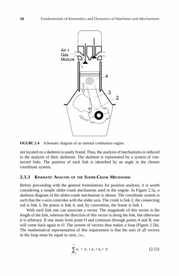
Another example is an application of a slider-crank mechanism in an internalcombustion engine (Figure 2.4). The motion from piston 4 is transferred throughconnecting rod 3 to crank 2, which rotates the crankshaft. This is a diesel engine,which means that one cycle, combustion–exhaust–intake–compression, comprisestwo complete crank revolutions. If all components of the cycle are equal in duration,then each will take 180°. In other words, the stroke of the engine, the piston motion
da t( )dt
------------- da t( )
dt------------- α t( ) α t( )sin,cos[ ] T a t( ) α t( ) π
2---+
α t( ) π2---+
sin,cosTdα t( )
dt--------------+=
Ch2Frame Page 18 Friday, June 2, 2000 6:39 PM

Kinematic Analysis of Mechanisms 19
from its maximum upper position to its lowest position, should correspond to 180°
of the crank rotation. This is a kinematic requirement of the mechanism. Anotherkinematic requirement is that the swing of the connecting rod be such that it doesnot interfere with the walls of the cylinder. There are other design requirementsaffecting kinematic and dynamic analysis: link dimensions and shape.
2.3.2 THE PROCESS OF KINEMATIC ANALYSIS
Kinematics is the study of motion without consideration of what causes the motion.In other words, the input motion is assumed to be known and the objective is to findthe transformation of this motion. Kinematic analysis comprises the following steps:
• Make a skeletal representation of the real mechanism.• Find its mobility.• Choose a coordinate system.• Identify all links by numbers.• Identify all angles characterizing link positions.• Write a loop-closure equation.• Identify input and output variables.• Solve the loop-closure equation.• Check the results by numerical analysis.
A skeletal representation completely describes the kinematics of the mechanism;i.e., it allows one to find the trajectories, velocities, and accelerations of any pointon a skeleton. As long as this information is available, the trajectory of any point
FIGURE 2.3 A loader.
Ch2Frame Page 19 Friday, June 2, 2000 6:39 PM
20 Fundamentals of Kinematics and Dynamics of Machines and Mechanisms
not located on a skeleton is easily found. Thus, the analysis of mechanisms is reducedto the analysis of their skeletons. The skeleton is represented by a system of con-nected links. The position of each link is identified by an angle in the chosencoordinate system.
2.3.3 KINEMATIC ANALYSIS OF THE SLIDER-CRANK MECHANISM
Before proceeding with the general formulations for position analysis, it is worthconsidering a simple slider-crank mechanism used in the engine. In Figure 2.5a, askeleton diagram of the slider-crank mechanism is shown. The coordinate system issuch that the x-axis coincides with the slider axis. The crank is link 2, the connectingrod is link 3, the piston is link 4, and, by convention, the frame is link 1.
With each link one can associate a vector. The magnitude of this vector is thelength of the link, whereas the direction of this vector is along the link, but otherwiseit is arbitrary. If one starts from point O and continues through points A and B, onewill come back again to O. The system of vectors thus makes a loop (Figure 2.5b).The mathematical representation of this requirement is that the sum of all vectorsin the loop must be equal to zero, i.e.,
(2.12)
FIGURE 2.4 Schematic diagram of an internal combustion engine.
r i
i 1=
3
∑ r 1 r 2 r 3 0=+ +=
Ch2Frame Page 20 Friday, June 2, 2000 6:39 PM

Kinematic Analysis of Mechanisms 21
Recall that the connection between any two links imposes a constraint on linksmotion. The fundamental property of the loop-closure equation is that it takes intoaccount all the constraints imposed on links motion.
Since each vector can be represented in the form:
(2.13)
Equation 2.12 becomes
(2.14)
Now the problem is reduced to solving Equation 2.14. There are many ways tosolve this equation (the reader should consult the books listed in the Bibliography).Presented here is only one approach, which can be applied to any planar mechanismand allows obtaining symbolic solutions in the simplest form. It is important to solvethe equations in symbols because the symbolic form of the solution gives explicitrelationships between the variables, which, in turn, enhances understanding of theproblem and the subject matter. It should be noted that Mathematica could solveEquation 2.14 in symbols. Although the result it gives is not in the simplest form,it can be used for numerical analysis.
Equation 2.14 is a vector equation comprising two scalar ones, which meansthat it can be solved for only two unknowns. Since the number of parameters in
FIGURE 2.5 Skeleton of slider-crank mechanism (a) and its vector representation (b).
r i r i θi θisin,cos( )T=
r 1 θ1 θ1sin,cos( )T r 2 θ2 θ2sin,cos( )T r 3 θ3 θ3sin,cos( )T 0=++
Ch2Frame Page 21 Friday, June 2, 2000 6:39 PM

22 Fundamentals of Kinematics and Dynamics of Machines and Mechanisms
Equation 2.14 (vector magnitudes and their corresponding direction angles) exceedstwo, it is necessary to identify what is given, and what is to be found.
If the mechanism shown in Figure 2.5 is an engine, then it can be assumed thatthe motion of the piston is given, that is, r1 = r1(t) is known at any moment in time.The magnitudes of vectors r2 and r3 are also given, as well as the direction of thevector r1. Thus, one is left with two unknowns: angles θ2 and θ3.
If, on the other hand, the mechanism in Figure 2.5 is a compressor, then therotation of the crankshaft is known, that is, θ2 = θ2 (t) is given as a function of time.Since the magnitudes of the vectors r 2 and r 3 are known, as well as the direction ofthe vector r1, then the two unknowns are r1 and θ3.
The following considers some generic loop-closure equations and their symbolicsolutions. Five various cases are presented, which should be sufficient to analyzeany simple planar mechanism.
2.3.4 SOLUTIONS OF LOOP-CLOSURE EQUATIONS
Since any simple (as opposed to compound) planar mechanism can be described bya loop-closure equation, then a generic equation can be solved for various possiblecombinations of known parameters and unknown variables. For a mechanism withN links, such an equation has the form:
(2.15)
There are only a few possible cases arising from this loop-closure equation indifferent applications.
First Case
A vector is the unknown; i.e., its magnitude and its direction are to be found. If onemoves all the known vectors in Equation 2.15 to the right-hand side, then thisequation takes the form:
(2.16)
where b is the vector equal to the sum of all vectors except the unknown vector r j
(2.17)
In Equation 2.17
(2.18)
r i θi θisin,cos( )T 0=i 1=
N
∑
r j θ j θ jsin,cos( )T b α αsin,cos( )T=
b bx by,( )T r i θi θisin,cos( )T
i 1 i j≠,=
N
∑–==
bx r i θicosi 1 i j≠,=
N
∑–=
Ch2Frame Page 22 Friday, June 2, 2000 6:39 PM

Kinematic Analysis of Mechanisms 23
and
(2.19)
Thus b, cos α, and sin α in Equation 2.16 are equal to
(2.20)
(2.21)
and
(2.22)
The angle α must be known explicitly to solve for rj and θj in Equation 2.16.Denote the principal solution belonging to the x > 0 and y > 0 quadrant as
(2.23)
Then the solution for α depends on the signs of cos α and sin α in Equations 2.21and 2.22.
(2.24)
Note, that in Mathematica the ArcTan[cos α, sin α] function finds the properquadrant.
Now, from the vector Equation 2.16 two scalar equations follow:
(2.25)
and
(2.26)
by r i θisini 1 i j≠,=
N
∑–=
b bx2 by
2+ 0>=
αcosbx
b-----=
αsinby
b----=
α∗ arc by
b----sin=
α
α∗ if α 0>cos and α 0>sin
π α– ∗ if α 0<cos and α 0>sin
π α+ ∗ if α 0<cos and α 0<sin
2π α– ∗ if α 0>cos and α 0<sin
=
r j θ j b αcos=cos
r j θ j sin b sinα=
Ch2Frame Page 23 Friday, June 2, 2000 6:39 PM

24 Fundamentals of Kinematics and Dynamics of Machines and Mechanisms
Since rj and b are both positive, it follows from the above equations that the anglesα and θj must be equal. Thus, the solution in this case is
rj = b, θj = α (2.27)
Second Case
In this case the magnitude of one vector and the direction of another vector are tobe found. Again all the known vectors are moved to the right-hand side, so that thevector equation (Equation 2.15) takes the form:
(2.28)
Assume that the two unknowns are ri and θj. First, premultiply Equation 2.28from the left by a unit vector perpendicular to the vector r i, namely, by the vectoru1 = (–sin θi, cos θi)T, and then by a unit vector parallel to r i, namely, by the vectoru2 = (cos θi, sin θi)T. The result of the first operation is
(2.29)
and the result of the second operation is
ri + rj cos(θj – θi) = b cos(α – θi) (2.30)
The system of Equation 2.28 has been transformed into a new system of Equa-tions 2.29 and 2.30 having a new variable (θj – θi). Now this new system can befurther simplified by moving ri in Equation 2.30 to the right-hand side, squaringboth Equation 2.29 and the transformed Equation 2.30, and then adding them. Theresult is a quadratic equation for the ri, the solution of which is
(2.31)
If both signs in the above equation give positive values for ri , then it means thatthere are two physically admissible mechanism configurations.
As soon as ri is known, the signs of sin(θj – θi) and cos (θj – θi) are found fromEquations 2.29 and 2.30. Again, this allows one to find the unique solution for theangle θj
(2.32)
r i θi θisin,cos( )T r j θ j θ jsin,cos( )T b α sinα,cos( )T=+
r j θ j θi–( ) b α θi–( )sin=sin
r i b α θi–( )cos= r j2 b2– 2 α θ i – ( ) sin ±
θ j
θ j∗ if θ j θi–( ) 0>cos and θ j θi–( )sin 0≥
π θ j– ∗ if θ j θi–( ) 0<cos and θ j θi–( )sin 0≥
π θ j+ ∗ if θ j θi–( ) 0<cos and θ j θi–( )sin 0≤
2π θ j– ∗ if θ j θi–( ) 0>cos and θ j θi–( )sin 0≤
=
Ch2Frame Page 24 Friday, June 2, 2000 6:39 PM

Kinematic Analysis of Mechanisms
25
where the angle
θ
j*
in this case is equal to the principal value given by
θ
j*
=
θ
i
+ arcsin|
b
sin(
α
–
θ
i
)/
r
j
| (2.33)
Third Case
In this case the magnitudes of two vectors are to be found. As before, all the knownvectors are moved to the right-hand side, and the vector equation has the form ofEquation 2.28, except that in this case ri and rj are the two unknowns. The solutionis unique because the inverse trigonometric functions are not involved in this case.As before, eliminate one of the unknowns by premultiplying Equation 2.28 fromthe left by a unit vector perpendicular to the vector r i, and then eliminating thesecond unknown by premultiplying Equation 2.28 by a unit vector perpendicular tothe vector r j. The first result gives Equation 2.29, from which a formula for rj follows:
(2.34)
Similarly, the formula for ri is
(2.35)
Fourth Case
This case involves two unknown angles in Equation 2.28, namely, θi and θj. Thesolution strategy in this case must be different from the previous cases because inthis case multiplying Equation 2.28 by the corresponding unit vectors cannot elim-inate the two unknown angles. Instead, a new unit vector ub = (cosα, sinα)T is usedto transform the variables θi and θj into new variables α – θi and α – θj. This isachieved by premultiplying Equation 2.28 first by the unit vector perpendicular tovector b, and then by a unit vector parallel to vector b. The result is the followingtwo equations, respectively:
ri sin (α – θi) + rj sin (α – θj) = 0 (2.36)
and
ri cos (α – θi) + rj cos (α – θj) = b (2.37)
There are still two unknowns in Equations 2.36 and 2.37, namely, α – θi and α – θj.However, this system is solvable. First, one can find sin(α – θi) from Equation 2.36,and then, by using the trigonometric identity (sin2 (α – θi) + cos2 (α – θi) = 1), reducethe second equation (Equation 2.37) to the following:
(2.38)
r j bα θ i–( )sinθ j θi–( )sin
----------------------------=
r i bα θ j–( )sinθi θ j–( )sin
----------------------------=
r i 1r j
r i
----
2
α θ j–( )2sin– r j α θ j–( ) b+cos–=
Ch2Frame Page 25 Friday, June 2, 2000 6:39 PM
26 Fundamentals of Kinematics and Dynamics of Machines and Mechanisms
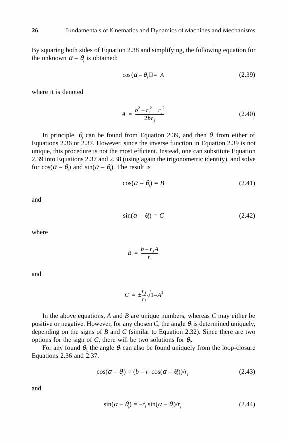
By squaring both sides of Equation 2.38 and simplifying, the following equation forthe unknown α – θj is obtained:
(2.39)
where it is denoted
(2.40)
In principle, θj can be found from Equation 2.39, and then θi from either ofEquations 2.36 or 2.37. However, since the inverse function in Equation 2.39 is notunique, this procedure is not the most efficient. Instead, one can substitute Equation2.39 into Equations 2.37 and 2.38 (using again the trigonometric identity), and solvefor cos(α – θi) and sin(α – θi). The result is
cos(α – θi) = B (2.41)
and
sin(α – θi) = C (2.42)
where
and
In the above equations, A and B are unique numbers, whereas C may either bepositive or negative. However, for any chosen C, the angle θi is determined uniquely,depending on the signs of B and C (similar to Equation 2.32). Since there are twooptions for the sign of C, there will be two solutions for θi.
For any found θi, the angle θj can also be found uniquely from the loop-closureEquations 2.36 and 2.37.
cos(α – θj) = (b – ri cos(α – θi))/rj (2.43)
and
sin(α – θj) = –ri sin(α – θi)/rj (2.44)
α θ j–( )cos A=
Ab2 r i
2 r j2+–
2br j
-----------------------------=
Bb r j A–
r i
-----------------=
Cr j
r i
---- 1 A2–±=
Ch2Frame Page 26 Friday, June 2, 2000 6:39 PM

Kinematic Analysis of Mechanisms 27
In summary, for a + C a set of solution angles (θi ,θj)1 is found, and for a – C anotherset of solutions (θi ,θj)2 is found. Since both sets are based on the solution of theloop-closure equation, they are physically admissible. In practical terms it meansthat a mechanism with given links allows two physical configurations.
Fifth Case
In this case the magnitude of one vector, the direction of another vector, and thedirections of two other vectors, functionally related to the direction of the secondvector, are to be found. The loop-closure equation, after the known vectors are movedto the right-hand side, has the form:
ri (cos θi, sin θi)T+ r j (cos(θi – γ), sin(θi – γ))T
+r k(cos (θi – β), sin(θi – β))T = b (cos α, sin α)T (2.45)
where θi and rj are the two unknowns, and it is seen that θj = θi – γ and θk = θi – β.Premultiply Equation 2.45 from the left by a unit vector perpendicular to the
vector r j, namely, by the vector u1 = (–sin(θi – γ), cos(θi – γ))T. The result is
ri sin γ + rk sin(γ – β) = b sin(α – θi +γ) (2.46)
Now premultiply Equation 2.45 from the left by a unit vector parallel to thevector r j, namely, by the vector u2 = (cos(θi – γ), sin(θi – γ))T. The result is
ri cos γ + r j + rk cos(γ – β) = b cos(α – θi + γ) (2.47)
The strategy is to find rj first. To achieve this, square both sides in Equations 2.46and 2.47 and add the two. The result is
ri2 + r j
2 + rk2 + 2 ri rk cos β + 2 rj ri cos γ
+ 2 rj rk cos(γ – β) + 2 ri rk cos γ cos(γ – β) = b2 (2.48)
The latter equation is a quadratic one with respect to rj
rj2 + crj + d = 0 (2.49)
where c = 2ri cos γ + 2 rk cos(γ – β) and d = ri2 + rk
2 +2ri rk cos β – b2.
Equation 2.49 has two roots:
(2.50)
It is seen that for the solution of the original system Equation 2.45 to exist theremust be a positive root in Equation 2.50. If such a root does exist, it defines the
r j1 2,
c2---– c2
4---- d–±=
Ch2Frame Page 27 Friday, June 2, 2000 6:39 PM

28 Fundamentals of Kinematics and Dynamics of Machines and Mechanisms
unknown magnitude rj. The other unknown, angle θi, is found from the system ofEquations 2.46 and 2.47, which has multiple solutions. However, in this case a uniquesolution can be found. Denote ζ = α – θi +γ, and ζ* = |α – θi +γ|. From Equations2.46 and 2.47 it follows that
sin ζ = (ri sin γ +r k sin(γ – β))/b = A (2.51)
and
cos ζ = (ri cos γ + r j + rk cos(γ – β))/b = B (2.52)
Since A and B are known constants for the already-found rj, then angle ζ is uniquelyfound from the following conditions:
(2.53)
Having found ζ, the unknown angle θi = α – ζ +γ can be determined.
2.3.5 APPLICATIONS TO SIMPLE MECHANISMS
Slider-Crank Inversions
One can apply the solutions found in Section 2.3.4 to some inversions of the slider-crank mechanism shown in Figure 1.14.
• Case of Figure 1.14aAssuming that the crank 2 is the driver, the loop-closure equation is
r1 (cos θ1 , sin θ1)T + r3 (cos θ3 , sin θ3)T = –r2 (cos θ2 , sin θ2)T (2.54)
where r1 and θ3 are the unknowns, and thus the equation falls into the second casecategory. Note that r1 is given by Equation 2.31, and θ3 by Equation 2.32.
A position analysis of this mechanism was done using Mathematica. Snapshotsof the motion at four positions are shown in Figure 2.6 for the following input data:
The change of the angle of rotation of the connecting rod (link 3) during onecycle of crank rotation is shown in Figure 2.7. Note that when θ2 = 0, π, 2π, theconnecting rod coincides with the x-axis. The maximum of the angle θ3 allows oneto check for possible interference with the cylinder walls.
ζ
ζ∗ if A 0> and B 0>π ζ– ∗ if A 0> and B 0<π ζ+ ∗ if A 0< and B 0<2π ζ– ∗ if A 0< and B 0>
=
r 3
r 1---- 4 θ 1 , = π =
Ch2Frame Page 28 Friday, June 2, 2000 6:39 PM

Kinematic Analysis of Mechanisms
29
• Case of Figure 1.14aAssuming that piston 4 is the driver, the loop-closure equation is
r
2
(cos
θ
2
,
sin
θ
2
)
T
+ r
3
(cos
θ
3
,
sin
θ
3
)
T
= –r
1
(cos
θ
1
,
sin
θ
1
)
T
(2.55)
where
θ
2
and
θ
3
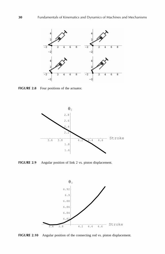
are unknowns, and thus the equation falls into the fourth casecategory. This case represents the actuator mechanism. The stroke of the piston islimited to a less-than-half-circle rotation of link 2. Snapshots of this system in fourpositions are shown in Figure 2.8 in which the following data were used:
The angular position of link 2 as a function of piston displacement is shown inFigure 2.9, and the angular position of the connecting rod as a function of pistondisplacement is shown in Figure 2.10.
• Case of Figure 1.14bAssuming that link 3 is the driver, the loop-closure equation is
r
1
(cos
θ
1
,
sin
θ
1
)
T
= –r
2
(cos
θ
2
,
sin
θ
2
)
T
–r
3
(cos
θ
3
,
sin
θ
3
)
T
(2.56)
where
r
1
and
θ
1
are unknowns, and thus the equation falls into the first case category.
FIGURE 2.6
A slider-crank mechanism in four positions during crank rotation.
FIGURE 2.7
Angle
θ
3
as a function of crank angle
θ
2
.
1 2 3 4 5 6θ2
-0.2
-0.1
0.1
0.2
θ3
r 3
r 1---- 4 θ 1 , 5 π
4------= =
Ch2Frame Page 29 Friday, June 2, 2000 6:39 PM
30
Fundamentals of Kinematics and Dynamics of Machines and Mechanisms
FIGURE 2.8
Four positions of the actuator.
FIGURE 2.9
Angular position of link 2 vs. piston displacement.
FIGURE 2.10
Angular position of the connecting rod vs. piston displacement.
3.6 3.8 4.2 4.4 4.6Stroke
1.6
1.8
2.2
2.4
2.6
2.8
θ2
3.6 3.8 4.2 4.4 4.6Stroke
6.82
6.84
6.86
6.88
6.9
6.92
θ3
Ch2Frame Page 30 Friday, June 2, 2000 6:39 PM

Kinematic Analysis of Mechanisms
31
Four-Bar Mechanism
For the case of Figure 1.4, crank 2 is the driver, and the loop-closure equation is
r
3
(cos
θ
3
,
sin
θ
3
)
T
+ r
4
(cos
θ
4
,
sin
θ
4
)
T
= –r
1
(cos
θ
1
,
sin
θ
1
)
T
–
r
2
(cos
θ
2
,
sin
θ
2
)
T
(2.57)
where
θ
3
and
θ
4
are unknowns, and thus this equation falls into the fourth casecategory. In this case the vector
b
= (
b
x
, b
y
)
T
=
b
(cos
α,
sin
α
)
T
is defined by
(2.58)
(2.59)
and angle
α
by
(2.60)
The following data were used to simulate the four-bar linkage:
In Figure 2.11 a four-bar mechanism is shown in six positions during crank
r
2
rotation. As is seen, the crank does not make full circle; it rotates from
π
/2 to 3
π
/2.Thus, this four-bar linkage is a triple rocker. This is confirmed by plotting the anglesof rotation for the coupler (link 3) (Figure 2.12) and follower (link 4) (Figure 2.13).
In the example shown in Figure 2.11 the driving link 2, as well as two otherlinks, was rocking. What if one wants to make this link revolving, i.e., to be a crank?This can be achieved if the relationships between the links in this mechanism arechanged in such a way that they satisfy Grashof’s criteria for having at least onerevolving link.
Five-Bar Mechanism
An example of a five-bar linkage is shown in Figure 2.14a and the correspondingloop of vectors in Figure 2.14b. It is given that vectors
r
3
and
r
5
are perpendicularto the vector
r
4
, i.e.,
θ
4
=
θ
3
–
π
/2 and
θ
5
=
θ
3
–
π
. Assuming that crank 2 is the input link, then there are two unknowns in this
system:
θ
3
and
r4. The loop-closure equation is
r3(cos θ3, sin θ3)T + r4(cos θ4, sin θ4)T + r5(cos θ5, sin θ5)T = b (2.61)
bx r– 1 θ1 r 2– θ2 and bycoscos r 1 θ1 r 2– θ2sinsin–= =
b bx2 by
2+=
αcosbx
b----- and αsin
by
b----= =
r 1
r 2---- 4
r 3
r 2----, 7
r 4
r 2---- 3 and θ1,=, π= = =
Ch2Frame Page 31 Friday, June 2, 2000 6:39 PM

32 Fundamentals of Kinematics and Dynamics of Machines and Mechanisms
FIGURE 2.11 A four-bar linkage in six positions during link 2 rocking.
FIGURE 2.12 Angular positions of the coupler during link 2 rocking.
FIGURE 2.13 Angular positions of the follower during link 2 rocking.
1 2 3 4 5 6
0.8
0.9
1
1.1
1.2
θ2
θ2
1 2 3 4 5 6θ2
1.7
1.6
1.5
1.4
1.3
θ41.2
Ch2Frame Page 32 Friday, June 2, 2000 6:39 PM

Kinematic Analysis of Mechanisms 33
where
b = –r1(cos θ1, sin θ1)T – r2(cos θ2, sin θ2)T (2.62)
Taking into account that θ4 and θ5 are functions of θ3, Equation 2.61 becomes
r3(cos θ3, sin θ3)T + r4(sin θ3, –cos θ3)T + r5(–cos θ3, –sin θ3)T = b (2.63)
The vectors r 3 and r 5 can be summed so that Equation 2.63 takes the form
r4(sin θ3, –cos θ3)T + (r3 – r5)(cos θ3, sin θ3)T = b (2.64)
Thus it is seen that this equation falls into the fifth case category. In Figure 2.15,snapshots of the animation are shown, where the following data were used:
FIGURE 2.14 Five-bar mechanism (a) and corresponding vector diagram (b).
FIGURE 2.15 Five-bar mechanism in six positions during crank rotation.
r 1
r 2---- 5
r 3
r 2----,
r 5
r 2---- 1.5= θ1 π= γ π
2------= and β, , , π= = =
Ch2Frame Page 33 Friday, June 2, 2000 6:39 PM
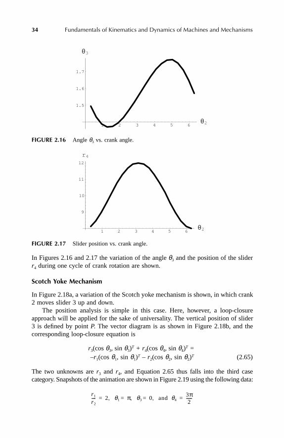
34 Fundamentals of Kinematics and Dynamics of Machines and Mechanisms
In Figures 2.16 and 2.17 the variation of the angle θ3 and the position of the sliderr4 during one cycle of crank rotation are shown.
Scotch Yoke Mechanism
In Figure 2.18a, a variation of the Scotch yoke mechanism is shown, in which crank2 moves slider 3 up and down.
The position analysis is simple in this case. Here, however, a loop-closureapproach will be applied for the sake of universality. The vertical position of slider3 is defined by point P. The vector diagram is as shown in Figure 2.18b, and thecorresponding loop-closure equation is
r3(cos θ3, sin θ3)T + r4(cos θ4, sin θ4)T = –r1(cos θ1, sin θ1)T – r2(cos θ2, sin θ2)T (2.65)
The two unknowns are r3 and r4, and Equation 2.65 thus falls into the third casecategory. Snapshots of the animation are shown in Figure 2.19 using the following data:
FIGURE 2.16 Angle θ3 vs. crank angle.
FIGURE 2.17 Slider position vs. crank angle.
1 2 3 4 5 6θ2
1.5
1.6
1.7
θ3
1 2 3 4 5 6θ2
9
10
11
12
r4
r 1
r 2---- 2, θ1 π= θ3 0= and θ4, , 3π
2------= =
Ch2Frame Page 34 Friday, June 2, 2000 6:39 PM

Kinematic Analysis of Mechanisms 35
In Figure 2.20 the displacements of two sliders are shown during one cycle. It isseen that r3 has the frequency of the crank, while r4 is double the crank’s frequency.The maximums are defined by the geometry of the mechanism.
FIGURE 2.18 An offset Scotch yoke mechanism (a) and corresponding vector diagram (b).
FIGURE 2.19 Six snapshots of the Scotch yoke mechanism.
FIGURE 2.20 Displacements r3 and r4 vs. crank angle θ2.
Ch2Frame Page 35 Friday, June 2, 2000 6:39 PM

36 Fundamentals of Kinematics and Dynamics of Machines and Mechanisms
2.3.6 APPLICATIONS TO COMPOUND MECHANISMS
Loader
For the loader shown in Figure 2.3, the motion of the bucket is the result of twoinputs: cylinder (actuator) 5 rotating lift arm 4, and cylinder 6 rotating the bucketthrough bellcrank 10. This compound mechanism comprises three simple onesrepresented by the links (1, 2, 3), (11, 8, 9, 10), and (12, 13, 14, 15). These threemechanisms form three loops: loop 1, loop 2, loop 3, respectively. The mechanismsand the vector loops are shown in Figures 2.21 through 2.23.
For each mechanism a loop-closure equation can be written:
Loop 1
r2(cos θ2, sin θ2)T + r3(cos θ3, sin θ3)T = –r1(cos θ1, sin θ1)T (2.66)
Loop 2
r8(cos θ8, sin θ8)T + r9(cos θ9, sin θ9)T = –r11(cos θ11, sin θ11)T + r10(cos θ2, sin θ2)T (2.67)
Loop 3
r13(cos θ13, sin θ13)T + r14(cos θ14, sin θ14)T = –r12(cos θ9, sin θ9)T + r 15(cos θ2, sin θ2)T (2.68)
In Equation 2.66 there are two unknowns: θ2 and θ3, which means that this equationcan be solved and thus it is independent of other equations (see graph in Figure 2.24).One of the solutions of Equation 2.66, namely θ2, becomes an input into loop 2, whilethe unknowns in loop 2 are angles θ8 and θ9. In loop 3, solutions from the two previousloops, θ2 and θ9, are used as inputs, while the unknowns are θ13 and θ14.
Equations 2.66 though 2.68 all belong to the fourth case of equations consideredabove. Indeed, in all of them the unknowns are two angles: θ2 and θ3 in Equation2.66, θ8 and θ9 in Equation 2.67, and θ13 and θ14 in Equation 2.68.
A graph in Figure 2.24 shows the functional connectivity between the loops.Such a graph is called a tree because it does not have any connections between thebranches. In this graph a node represents a mechanism loop, and a vertex representsa common link between the loops. The node corresponding to the bucket is calledthe root node. It is seen that the motion of the bucket is the result of two independentinputs (prove that the mobility of this mechanism is 2).
The following data were used to simulate this compound mechanism:
Loop 1
where v3 is the piston velocity and t is time.
r 1
r 2---- 0.6, θ1
π2---=
v3
r 2---- 1= and
r 3
r 2---- 0.76
v3
r 2----t+=, ,=
Ch2Frame Page 36 Friday, June 2, 2000 6:39 PM

Kinematic Analysis of Mechanisms 37
FIGURE 2.21 First mechanism (a) and corresponding vector diagram (b).
FIGURE 2.22 Second mechanism (a) and corresponding vector diagram (b).
FIGURE 2.23 Third mechanism (a) and corresponding vector diagram (b).
Ch2Frame Page 37 Friday, June 2, 2000 6:39 PM

38 Fundamentals of Kinematics and Dynamics of Machines and Mechanisms
Loop 2
Loop 3
In Figure 2.25 the change of the bucket orientation in time is shown. The smallestangle corresponds to the bucket in the low position.
In general, any mechanism the functionality of which is represented by a treegraph can be analyzed starting from loops containing input links, then solvingequations associated with each branch, and eventually finding the motion of the rootnote, i.e., the output link. Note that the number of inputs in mechanisms representedfunctionally as trees equals the number of branches in a tree.
FIGURE 2.24 A graph representing functional connectivity in a loader as a compoundmechanism.
FIGURE 2.25 Change of bucket orientation in time.
0.1 0.2 0.3 0.4 0.5 0.6 0.7Time , sec
0.25
0.5
0.75
1
1.25
1.5
1.75
Bucket angle
r 9
r 2---- 0.8
r 10
r 2------, 1.6=
r 11
r 2------ 0.14 θ11,=, 0
v8
r 2---- 1 and,
r 8
r 2---- 0.76
v8
r 2----+ t==,= =
r 12
r 2------ 0.4
r 13
r 2------, 1.1=
r 14
r 2------ 0.8,=,
r15
r 2----- 1.2==
Ch2Frame Page 38 Friday, June 2, 2000 6:39 PM

Kinematic Analysis of Mechanisms 39
2.3.7 TRAJECTORY OF A POINT ON A MECHANISM
In many applications the function of the mechanism is associated with the motionof a specific point on this mechanism. In Figure 2.26 a material-handling mechanismis shown. The function of the mechanism is to transfer the load from one conveyorbelt to another. There are position, velocity, and acceleration requirements to be metby the designers of this mechanism. The position requirements are to have the lineAB on a coupler horizontal to accept the load from the right belt in one position andthe line AC parallel to the left belt for proper unloading in another position. Thevelocity requirements to be met by the mechanism are that at the two extremepositions (loading/unloading) the velocities be minimal (or zero) to allow sufficienttime for load transfer. At the same time, the average velocity between the two extremepositions must be synchronized with the belt velocities to maintain constant loadflow rate. The acceleration requirements are to prevent jerks (sudden changes ininertial forces) in the system during the load transfer process to ensure the reliabilityof this operation. To meet these objectives a proper mechanism skeleton should befound first, and then a proper shape of the coupler.
A proper mechanism skeleton requirement may be to have a rocker-crank mech-anism subject to size constraints. This can be achieved by satisfying Grashof’s criteria(see Equation 1.2) for a rocker-crank. The needed shape of the coupler is the subjectof this section. For the example shown in Figure 2.28 this problem is reduced tofinding the trajectories of points identified on a coupler.
Consider the trajectory of any point P on a coupler (Figure 2.27). The positionof the point P in the global coordinate system is given by the vector RP which canbe found either as
(2.69)
or
(2.70)
FIGURE 2.26 Material-handling mechanism.
RP r 2 r P+ r 2 θ2 θ2sin,cos( )T r P+ θ3 α+( )cos θ3 α+( )sin,[ ] T= =
RP r 2 r D r DP r 2=+ + θ2 θ2sin,cos( )T
r D+ θ3 θ3sin,cos( )T r DP θ3π2---+
cos θ3π2---+
sin,T
+
=
Ch2Frame Page 39 Friday, June 2, 2000 6:39 PM

40 Fundamentals of Kinematics and Dynamics of Machines and Mechanisms
When the position analysis of the skeleton of the mechanism is done, then for anypair of angles θ2 and θ3 the vector RP can be found for either of the above equations.The important point is that there is an infinite number of possible trajectories andidentification of the needed one is done by trial and error.
In Figure 2.28 an example of a four-bar linkage with a coupler having anotherbar attached to it in the middle is shown. Three points are identified on this bar andtheir trajectories are shown. The mechanism is of the rocker-crank type with thefollowing nondimensional units:
FIGURE 2.27 Point P on a coupler.
FIGURE 2.28 Trajectories of three points on a coupler.
r 1
r 2---- 4
r 3
r 2----, 6=
r 4
r 2---- 5=,=
Ch2Frame Page 40 Friday, June 2, 2000 6:39 PM

Kinematic Analysis of Mechanisms 41
By choosing different points, different trajectories can be obtained: from thecircle for the crank–coupler joint to the chord for the follower–coupler joint.
2.4 VELOCITY ANALYSIS
2.4.1 VELOCITY VECTOR
For any vector the magnitude and the direction of which are functions of time, t,
(2.71)
the time derivative represents the velocity vector:
(2.72)
One can see that the velocity vector comprises two components. The first hasthe same direction as the original vector Equation 2.71, and it is called the transla-tional (or linear) velocity vector, Vt
(2.73)
The magnitude of the translational velocity vector represents the rate of changeof the vector length r. The second component is perpendicular to the direction ofthe original vector ([–sinθ(t), cos θ(t)]Τ = [cos(θ(t) + π/2), sin(θ(t) + π/2)]T) and itis rotated by π/2 in a counterclockwise direction. This component represents therotational (or angular) velocity vector:
(2.74)
The magnitude of the rotational velocity is proportional to the angular velocityω(t) = (t).
In Figure 2.29 the two components of the velocity vector are shown. Thesecomponents can also be viewed as characterizing the velocity of the point at the tip
FIGURE 2.29 Two components of the velocity vector.
r t( ) r t( ) θ t( ) θ t( )sin,cos[ ] T=
drdt------ r r t( ) θ t( ) θ t( )sin,cos[ ] T r t( ) θsin t( ) θcos t( ),–[ ] Tθ t( )+= =
V t r t( ) θ t( ) θ t( )sin,cos[ ] T=
V r r t( )θ t( ) θsin–( ) t( ) θcos t( ),[ ] T=
θ
Ch2Frame Page 41 Friday, June 2, 2000 6:39 PM

42 Fundamentals of Kinematics and Dynamics of Machines and Mechanisms
of vector r. One should also note that the translational and rotational velocitycomponents are independent components.
2.4.2 EQUATIONS FOR VELOCITIES
The equations for velocities follow from the loop-closure equation for positions,Equation 2.15. Indeed, if in Equation 2.15 ri = r i (t) and θi = θi(t), then differentiatingit with respect to t and using Equation 2.72 the following vector equation is obtained:
(2.75)
where ωi(t) = i(t) is the angular velocity.In Equation 2.75 the unknowns can be any two velocity components: two
translational, two rotational, or a combination of rotational and translational. Theimportant point is that Equation 2.75 is a linear function of velocities, and thus forany unknown velocities they are found from a system of two linear algebraic equa-tions. How to find symbolic solutions for a linear system of algebraic equations isshown in the Appendix. These solutions, as is shown below, are also easy to derivemanually. A symbolic solution allows a better understanding of position–velocitydependency in some mechanisms.
First Case
In this case (see Equation 2.16), all vectors except vector r j are moved to the right-hand side. Correspondingly, Equation 2.75 will take the form (note that all variablesare assumed to be time dependent):
(2.76)
Note that in the velocity analysis it is more convenient to take vector b in the formshown in Equation 2.76, since this equation is linear with respect to the twounknowns, j (t) and ωj (t).
One can find ωj (t) by multiplying Equation 2.76 from the left by a unit vectorperpendicular to the first vector on the left-hand side, i.e., by the vector u1 = [–sinθj,cosθj]. The result is
(2.77)
The latter explicitly defines ωj (t) as a function of variables found in positionanalysis. Similarly, if one multiplies Equation 2.76 from the left by a unit vectorperpendicular to the second vector on the left-hand side of Equation 2.76, i.e. bythe vector u2 = [cosθj, sinθj], the other unknown will be found:
(2.78)
r i
i 1=
N
∑ t( ) θi t( ) θi t( )sin,cos[ ] T r i t( ) θisin t( ) θicos t( ),–[ ] Tωi t( ) 0=+
θ
r j θ j θ jsin,( )cos[ ] T r j θ jsin , θ jcos( )–[ ] Tωj bx by,[ ] T=+
r
r jωj bx θ j by θ jcos+sin–=
r j t( ) bx θ j by θ jsin+cos=
Ch2Frame Page 42 Friday, June 2, 2000 6:39 PM

Kinematic Analysis of Mechanisms 43
Second Case
In this case the magnitude ri (t) and the angle θj (t) were the two unknowns in Equation2.28. Then Equation 2.75 takes the form
(2.79)
In Equation 2.79 the unknowns are i (t) and ωj (t). As before, by premultiplyingEquation 2.79 by unit vectors perpendicular to the first and fourth vectors on theleft-hand side of this equation, the explicit expressions for the two unknowns areobtained in the form:
(2.80)
and
(2.81)
Third Case
Since in this case the magnitudes of two vectors, ri and rj were the unknowns inEquation 2.28, the corresponding velocity unknowns in Equation 2.79 are i(t) and
j(t). These two unknowns can be found using the same procedure as above, andthe corresponding expressions are
(2.82)
and
(2.83)
Note that the last equation is obtained from the previous one by interchanging indicesi and j. An alternative way to derive the expressions for velocities in this case is todifferentiate Equations 2.34 and 2.35.
Fourth Case
In this case the two unknown angular velocities i(t) and j(t) are found fromEquation 2.79. The corresponding expressions are as follows:
(2.84)
r i θi θ jsin,cos[ ] T r i θisin , θicos–[ ] Tωi
r j θ j θ jsin,cos[ ] T r j θ jsin , θ jcos–[ ] Tωj bx by,[ ] T=
+ +
+
r
r jωj cos θ j θi–( ) r– iωi r j– θ j θi–( ) bx– θi by θicos+sinsin=
r i cos θ j θi–( ) r– iωi θ j θi–( ) r j b+ x– θ j by θ jsin+cossin=
rr
r i sin θi θ j–( ) r i– ωi θi θ j–( ) r jωj b– x–cos θ j by θ jcos+sin=
r j sin θ j θi–( ) r j– ωj θ j θi–( ) r iωi b– x–cos θi by θicos+sin=
θ θ
ωi r i θ j θi–( ) r i θ j θi–( ) r j bx θ jcos b+ + y θ jsin–cos–=sin
Ch2Frame Page 43 Friday, June 2, 2000 6:39 PM

44 Fundamentals of Kinematics and Dynamics of Machines and Mechanisms
and
(2.85)
Fifth Case
The loop-closure Equation 2.45 is differentiated under the assumption that all param-eters, except γ and β, are time dependent.
[cosθi, sinθi]T+ r i[–sinθi , cosθi]T ωi
+ [cos (θi – γ), sin(θi – γ)]T +r j[– sin(θi – γ), cos(θi – γ)]T ωι (2.86)
+ [cos (θi – β), sin(θi – β)]T +r k[– sin(θi – β), cos(θi – β)]T ωι = [ x, y]T
Recall that the unknowns in this case are ωi(t) and j(t). Collect similar terms in thelatter equation.
(2.87)
where it is denoted
(2.88)
and
(2.89)
Now the two unknowns can be found in the usual way by identifying the unit vectorsperpendicular to the vectors [cos(θi –γ), sin (θi –γ)]T and [dx,dy]T, and premultiplyingEquation 2.87 by these vectors (note that the vector perpendicular to the latter vectoris [–d4444, dx]T). As a result, the following expressions are obtained:
(2.90)
and
(2.91)
ωj r j θi θ j–( ) r j θi θ j–( ) r i bx θicos b+ + y θisin–cos–=sin
r i
r j
r k b b
r
r i θi θi ]sin, T dx dy,[ ] Tωi r j θi γ–( ) θi γ–( )sin,cos[ ] T+ +cos[
+r k θi β–( ) θi β–( )sin,cos[ ] T bx by,[ ] T=
dx r i θi r j θ( i γ ) r k θ( isin–– β)–sin–sin–=
dy r i θi r j θ( i γ ) r k θ( icos+– β)–cos+cos=
d– x θ( i γ )+dy θ( icos– γ )–sin( )ωi r i γ r k γ( β)–sin–sin–=
bx θ( isin γ )– by θ( icos γ )–+–
d– y θ( i γ )+dx θ( isin– γ )–cos( ) r j r i dy θi dx+ θisincos–( )+–=
–r k dy θi β–( ) dx θi β)–( ) dybx– dxby+( )+sin+cos–(
Ch2Frame Page 44 Friday, June 2, 2000 6:39 PM

Kinematic Analysis of Mechanisms 45
2.4.3 APPLICATIONS TO SIMPLE MECHANISMS
Slider-Crank Inversions (Figure 1.14)
• Figure 1.14a with the driving crank
The inversion in Figure 1.14a falls into the second case if the crank is the driver(see Equation 2.54 for the case when a crank is the driver). The correspondingvelocity equations are found from Equation 2.79 by taking that i = 1, j = 3,bx = –r2cosθ2, and by = –r2sinθ2 (see Equation 2.54). Now one can use the generalsolutions given by Equations 2.80 and 2.81 for this specific case, taking into accountthat x = r2ω2 sinθ2, y = –r2ω2 cosθ2, r2 = const., r3 = const. and θ1 = π.
(2.92)
Thus, the angular velocity of the connecting rod is
(2.93)
Similarly, for the slider velocity ,
(2.94)
As one can see, even if the crank angular velocity is constant, the velocities ofthe piston and the connecting rod are periodic functions which, in turn, depend onthe crank and connecting rod lengths. Note also that when θ2 – θ3 = 0, π, 2π thepiston velocity becomes zero. These extreme piston positions are called dead points.
In Figures 2.30 and 2.31 the variations of the angular velocity of the connectingrod and the translational velocity of the piston during one cycle of crank rotationare shown. As one can see from Figure 2.31 the extreme positions of the piston areat θ2 = 0, π, 2π, while the corresponding angles θ3 are 0, 0, 0 (see Figure 2.7). Notethat, since ω3 is a derivative of θ3, the maximums of the former are at the crankpositions corresponding to the minimums of the latter.
• Figure 1.14a with the driving piston
If in the inversion shown in Figure 1.14a the piston is the driver, then, as isknown, this situation belongs to the fourth case category. In this case i = 2, j = 3,
x = 1, y = 0, and θ1 = π. The equations for the unknown angular velocities and follow from Equations 2.84 and 2.85.
(2.95)
and
(2.96)
b b
r 3ω3 θ3cos– r 2ω2 θ2cos=
ω3 ω– 2
r 2 θ2cosr 3 θ3cos-------------------=
r 1 t( )
r 1 t( ) r 2ω– 2
θ2 θ3–( )sinθ3cos
-----------------------------=
b r bω2 θ2= ω3 θ3=
ω2r 1 θ3cos
r 2 θ3 θ2–( )sin----------------------------------=
ω3r 1 θ2cos
r 3 θ2 θ3–( )sin----------------------------------=
Ch2Frame Page 45 Friday, June 2, 2000 6:39 PM

46 Fundamentals of Kinematics and Dynamics of Machines and Mechanisms
It is seen from the two equations that when θ2 – θ3 = 0 or θ2 – θ3 = π thedenominators in both equations become zero. However, at these dead points thepiston velocity is also zero. Thus, the velocities become undetermined. The uncer-tainty can be resolved if the function r1(t) is at least twice differentiable so thatL’Hopital’s rule for resolving the 0/0-uncertainty can be used.
In Figures 2.32 and 2.33 the angular velocities of the crank and connecting rodare shown as functions of the piston stroke. As one can see, both angular velocitiesare finite at the dead points. The velocity of the piston is taken as being constantduring one stroke. Note that the velocity of the crank is not constant when the pistonis the driver.
• Figure 1.14b with link 3 as a driver
This inversion falls into the first case category and the equations for velocitiesare given by Equations 2.77 and 2.78. The specific equations are obtained by takingj = 1, θ2 = π/2, and b = (bx, by)T, where bx= –r3 cosθ3(t) and by = –r2 –r3 sinθ3(t).Thus, Equations 2.77 and 2.78 are reduced to
(2.97)
FIGURE 2.30 Angular velocity of the connecting rod during one cycle of crank rotation.
467FIGURE 2.31 Slider velocity during one cycle of crank rotation.
1 2 3 4 5 6θ2
-2
-1
1
2
ω3
1 2 3 4 5 6θ2
-10
-5
5
10
Slider Velocity
ω1
r 3
r 1----ω3 θ3 θ1–( )cos–=
Ch2Frame Page 46 Friday, June 2, 2000 6:39 PM

Kinematic Analysis of Mechanisms 47
and
(2.98)
Four-Bar Mechanism (Figure 1.4)
The solutions are given by Equations 2.84 and 2.85. If crank 2 is the driver, theni = 3, j = 4, bx= r 1 – r2 cosθ2, by = –r2 sinθ2 (assuming that θ1 = π), and the equationsfor angular velocities are
(2.99)
(2.100)
The angular velocities ω3 and ω4 as functions of the crank angle are shown inFigures 2.34 and 2.35 for the same dimensions as in the position analysis.
FIGURE 2.32 Angular velocity of link 2 vs. piston stroke.
FIGURE 2.33 Angular velocity of the hydraulic rod vs. piston stroke.
3.6 3.8 4 4.2 4.4 4.6stroke
-11
-10.5
-10
-9.5
-9
-8.5
ω2
3.6 3.8 4 4.2 4.4 4.6stroke
-3
-2.5
-2
-1.5
-1
-0.5
ω3
r 1 t( ) r 3ω3 θ3 θ1–( )sin=
ω3 ω2
r 2 θ2 θ4–( )sinr 3 θ4 θ3–( )sin----------------------------------=
ω4 ω2
r 2 θ2 θ3–( )sinr 4 θ3 θ4–( )sin----------------------------------=
Ch2Frame Page 47 Friday, June 2, 2000 6:39 PM

48 Fundamentals of Kinematics and Dynamics of Machines and Mechanisms
Five-Bar Mechanism (Figure 2.14a)
The solutions are given by Equations 2.90 and 2.91. If crank 2 is the driver, then inthese solutions i = 3, j = 4, k = 5, γ = π/2, and β = π. In this case (see Equation2.62) bx = r 1 – r2 cosθ2, by = –r2 sinθ2, and (see Equations 2.88 and 2.89) dx = (r5 – r3)sinθ3 + r4 cosθ3, dy = –(r5 – r3) cosθ3 + r4 sinθ3, where it was taken that θ1 = π. Recallalso that r2, r3, and r5 are all constant. Thus, for the case of Figure 2.14a the angularvelocity of link 3 and the sliding velocity of link 4 are, respectively,
(2.101)
(2.102)
In Figures 2.36 and 2.37 the angular velocity of link 3 and the translationalvelocity of the slider are shown during one cycle of crank rotation. The numerical
FIGURE 2.34 Angular velocity of the coupler vs. crank angle.
FIGURE 2.35 Angular velocity of the follower vs. crank angle.
1 2 3 4 5 6θ2
-4
-3
-2
-1
1
2
ω4
θ3 ω3 = ω2
r 2 θ2 θ3–( )sinr 4
----------------------------------=
r 4 r 2ω2 θ3 θ2–( )r 5 r 3–
r 4---------------+ θ3 θ2–( )sincos=
Ch2Frame Page 48 Friday, June 2, 2000 6:39 PM

Kinematic Analysis of Mechanisms 49
data were the same as in the position analysis, while the angular velocity wastaken to be ω2 = 5r2 rad/s.
Scotch Yoke Mechanism (Figure 2.18a)
The solution is given by Equations 2.82 and 2.83 in which i = 3, j = 4, θ1 = π,θ3 = 0, θ4 = π/2, bx = r 1 – r2 cosθ2, and by = –r2 sinθ2. After substitution,
(2.103)
(2.104)
In Figure 2.38 the velocities of sliders are shown during one cycle of crank rotationfor the crank angular velocity ω2 = 5r2 rad/s.
2.4.4 APPLICATIONS TO COMPOUND MECHANISMS
For a compound mechanism in which each loop is either in series or in parallel toother loops, the velocity equations are reduced to those for simple mechanisms.Below an example of a loader is considered.
FIGURE 2.36 Angular velocity of link 3 in a five-bar mechanism.
FIGURE 2.37 Translational velocity of the slider in a five-bar mechanism.
1 2 3 4 5 6θ2
-2
-1
1
ω3
1 2 3 4 5 6θ2
-20
-10
10
20
Slider velocity
r 3 r– 2ω2 θ2sin=
r 4 r– 2ω2 θ2cos=
Ch2Frame Page 49 Friday, June 2, 2000 6:39 PM

50 Fundamentals of Kinematics and Dynamics of Machines and Mechanisms
Loader
The loader comprises three mechanisms the loop-closure equations for which weregiven in Equations 2.66 to 2.68. They all fall into the fourth case category, so thatthe angular velocities are given by Equations 2.84 and 2.85.
Loop 1
In this case i = 2, j = 3, and . The corresponding angular velocities are
(2.105)
and
(2.106)
Loop 2
In this case i = 8, j = 9, , and . The correspond-ing angular velocities are
(2.107)
and
(2.108)
FIGURE 2.38 Velocities of two sliders during one cycle.
1 2 3 4 5 6θ2
-20
-10
10
20
Velocityslider4 slider3
bx by 0= =
ω2 –r 3
r 2 θ3 θ2–( )sin----------------------------------=
ω3
r 3
r 3---- θ3 θ2–( )cot=
bx r– 10ω2 θ2sin= by r 10ω2 θ2cos=
ω8 –r 8 θ9 θ8–( ) r 10ω2 θ2 θ9–( )sin+cos
r 8 θ8 θ9–( )sin------------------------------------------------------------------------------------=
ω9 –r 8 r 10ω2 θ2 θ8–( )sin+
r 9 θ8 θ9–( )sin-----------------------------------------------------=
Ch2Frame Page 50 Friday, June 2, 2000 6:39 PM

Kinematic Analysis of Mechanisms 51
Loop 3
In this case i = 13, j = 14, , and = –r12ω9cosθ9 +r15ω2cosθ2. The corresponding angular velocities are
(2.109)
and
(2.110)
In Figure 2.39 the angular velocity of the bucket (ω14 = ωb) vs. time is shown.
2.5 ACCELERATION ANALYSIS
2.5.1 ACCELERATION VECTOR
The acceleration vector is the time derivative of the velocity vector given byEquation 2.72
(2.111)
The following notations are used: for the angular velocity, and for theangular acceleration, . With these notations Equation 2.111 has the form
(2.112)
FIGURE 2.39 Angular velocity of the bucket vs. time.
0.1 0.2 0.3 0.4 0.5 0.6 0.7Time , sec
2.4
ω b
3
2.6
2.8
bx r 12ω9 θ9 r 15ω2 θ2sin–sin= by
ω13
r 12ω9 θ9 θ14–( ) r 15ω2 θ2 θ14–( )sin–sinr 13 θ14 θ13–( )sin
-----------------------------------------------------------------------------------------------=
ω14
r 12ω9 θ9 θ13–( ) r 15ω2 θ2 θ13–( )sin–sinr 14 θ13 θ14–( )sin
-----------------------------------------------------------------------------------------------=
d2r
dt2-------- r= r θcos θsin,[ ] T 2r θsin– θcos,[ ] Tdθ
dt------
r θcos[ θ ]sin T dθdt------
2
r θsin–[ θ ]cos T d2θdt2--------,+,–
+=
ω dθ dt⁄=α d2θ dt⁄ 2
=
r r θcos[ θ ]sin T, 2r θsin–[ θ ]cos Tω–r θcos[ θ ]sin Tω2 r θsin–[ θ ]cos T α,+,
,+=
Ch2Frame Page 51 Friday, June 2, 2000 6:39 PM

52 Fundamentals of Kinematics and Dynamics of Machines and Mechanisms
One can rewrite the above equation in such a way that the directions of all vectors arereferenced with respect to the direction of vector r. Then Equation 2.112 takes the form
(2.113)
The directions of four vectors and their magnitudes are shown in Figure 2.40,where one can see that the direction of first vector coincides with the direction ofvector r ; the direction of third vector is opposite to that of vector r, and the twoother vectors are perpendicular to vector r whereas their directions are found byrotating vector r counterclockwise by π/2. The first vector in Equation 2.113 is calledthe translational component of acceleration, the third is called the centripetal com-ponent of acceleration, the fourth is called the angular component of acceleration,and the second is called the coriolis component of acceleration.
Note that centripetal acceleration is caused by the rotation of the vector (irre-spective of whether this rotation is time dependent or time independent), whereascoriolis acceleration is caused by the rotation of a translationary moving vector. Bothof these components are functions of velocities only, and thus can be found basedon the velocity analysis. The other two components of acceleration, translationaland angular, are found as a result of acceleration analysis.
2.5.2 EQUATIONS FOR ACCELERATIONS
The equations for accelerations follow from the loop-closure equation for positions,Equation 2.15, if the equation is differentiated twice with respect to time. As a result,the loop-closure equation for accelerations is obtained. Note that it is assumed thatall parameters are time–dependent variables.
(2.114)
FIGURE 2.40 Components of acceleration vector.
r r θcos[ θ ]sin T, 2r θ π2---+
cos θ π2---+
T
sin ω
r θ π+( )cos θ π+( )sin,[ ] Tω2 r θ π2---+
θ π2---+
sin,cosT
α+–
,+=
r i θicos[ θi ]sin T, 2r i θisin–[ θi ]Tcos ωi
–r i θicos[ θi ]sin Tωi2 r i θisin– θicos,[ ] Tα i+,
,+i 1=
N
∑
0=
Ch2Frame Page 52 Friday, June 2, 2000 6:39 PM

Kinematic Analysis of Mechanisms 53
In Equation 2.114 the unknowns are and α i, and the system defining them islinear. As before, the loop-closure equation for accelerations can have only twounknowns. This again entails five possible combinations of these unknowns. In thiscase the solutions for each can be found from the solutions for velocities in astraightforward manner.
First Case
The unknowns, and , are found by differentiating Equations 2.77 and 2.78 withrespect to time assuming that all the variables are time dependent. The results, takinginto account Equations 2.77 and 2.78, are
(2.115)
and
(2.116)
Second Case
In this case the two unknowns, and , are found by differentiating Equations2.80 and 2.81, respectively.
(2.117)
and
(2.118)
Third Case
The unknowns in this case are the translational accelerations, and . The expres-sions for them are found by differentiating Equations 2.82 and 2.83.
(2.119)
and the equation for is obtained by interchanging indices i and j in the above.
(2.120)
r i
θ j r j
α j1r j
---- bx θ j by˙ θ j 2r jωj–cos+sin–[ ]=
r j bx θ j by˙ θ j r jωj
2+sin+cos=
θ j r i
α j1
r j θ j θi–( )cos---------------------------------
[ ω( j ωi–( )r jωj r j ) θ j θi–( ) 2ωj ωi–( ) r j θ j θi–( )cos–sin–
ω( i by bx ) θi ω–( i bx by ) θi ωi r i– r iα i ]–cos+ +sin+–=
r i1θ j θi–( )cos
-----------------------------[ r i ω( j 2ωi–( ) r– iα i ) θ j θi–( ) r iωi ωj ωi–( ) θ j θi–( ) r j–cos–sin
+ b( x byωj ) θ j by bxωj–( ) θ j ]sin+cos+=
r i r j
r i1
θi θ j–( )sin----------------------------
–[ r i 2ωi ωj–( )+r iα i( ) θi θ j–( )+r iωi ωi ωj–( ) θi θ j–( )sincos
–r jωj r jα j b(–– x byωj ) θ j by bxωj–( ) θ j ]cos+sin+=
r j
r j1
θ j θi–( )sin----------------------------
–[ r j 2ωj ωi–( )( r jα j ) θ j θi–( )+r jωj ωj ωi–( ) θ j θi–( )sincos+
–r iωi r iα i b(–– x byωi ) θi by bxωi–( ) θi ]cos+sin+=
Ch2Frame Page 53 Friday, June 2, 2000 6:39 PM
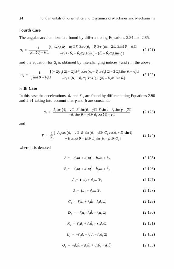
54 Fundamentals of Kinematics and Dynamics of Machines and Mechanisms
Fourth Case
The angular accelerations are found by differentiating Equations 2.84 and 2.85.
(2.121)
and the equation for α j is obtained by interchanging indices i and j in the above.
(2.122)
Fifth Case
In this case the accelerations, and , are found by differentiating Equations 2.90and 2.91 taking into account that γ and β are constants.
(2.123)
and
(2.124)
where it is denoted
(2.125)
(2.126)
(2.127)
(2.128)
(2.129)
(2.130)
(2.131)
(2.132)
(2.133)
α i1
r i θ j θi–( )sin--------------------------------
–([ ωi r i ωj ωi–( )–r i ) θ j θi–( )+r i ωj 2ωi–( ) θ j θi–( )sincos
–r j b(+ x byωj ) θ j by bxωj–( ) θ j ]sin+cos+=
α j1
r j θi θ j–( )sin--------------------------------
–([ ωj r j ωi ωj–( )–r j ) θi θ j–( )+r j ωi 2ωj–( ) θi θ j–( )sincos
–r i b(+ x byωj ) θi by bxωi–( ) θi ]sin+cos+=
θi r j
α i
Ai θi γ–( ) Bi θi γ–( ) r i γ r k γ(sin β)––sin–sin–cosdx– θi γ–( ) dy θi γ–( )cos+sin
-------------------------------------------------------------------------------------------------------------------------------=
r j1T j
-----A–[ j θi γ–( ) Bj θi γ–( ) Cj+sin–cos θi D j θisin+cos
+ K j θi β–( ) L j θi β–( ) Qj+sin+ ]cos=
Ai d– yωi dxωi2 bxωi by+–+=
Bi d– xωi dyωi2 byωi bx+–+=
Aj d– y dxωi+( ) r j=
Bj dx d+ yωi( ) r j=
Cj r idy r i di r idxωi–+=
D j r– idx r i dx r idyωi––=
K j r kdy r kdy r kdxωi–+=
L j r– kdx r kdx r kdyωi––=
Qj dy– bx dybx dxby dxby++–=
Ch2Frame Page 54 Friday, June 2, 2000 6:39 PM

Kinematic Analysis of Mechanisms 55
(2.134)
where bx, by are given by Equation 2.45, and dx, dy are defined by Equations 2.88and 2.89, respectively.
2.5.3 APPLICATIONS TO SIMPLE MECHANISMS
Slider-Crank Inversions (Figure 1.14)
• Figure 1.14a with the driving crank
This mechanism falls into the second case category. The solutions are given byEquations 2.117 and 2.118. In this case i = 1, j = 3, bx = –r2 cosθ2, by = –r2 sinθ2,
, , r2 = const., r3 = const., and θ1 = π. Assume alsothat the crank rotates with constant angular velocity, i.e., ω2 = const. Then,
, and . Taking all this into account, the general for-mulas, Equations 2.117 and 2.118, are reduced to
(2.135)
and
(2.136)
The above equations can also be obtained by differentiating the expressions for thecorresponding velocities (Equations 2.93 and 2.94).
A plot of the change of the angular acceleration of the connecting rod with thecrank angle is shown in Figure 2.41. A change of the slider acceleration with thecrank angle is shown in Figure 2.42.
FIGURE 2.41 Angular acceleration of the connecting rod vs. crank angle.
1 2 3 4 5 6θ2
-20
-10
10
20
α3
T j dy θi γ–( ) dy θi γ–( )sin+cos–=
bx r2θ2 θ2sin= by r 2θ2 θ2cos–=
bx r 2ω22 θ2cos= by r 2ω2
2 θ2sin=
α3r 2ω2
2 θ2 r 3ω32 θ3sin+sin
r 3 θ3cos-------------------------------------------------------=
r11
θ3cos-------------- r 1ω3 θ3 r 2– ω2 ω2 ω3–( ) θ2 θ3–( ) ]cossin[=
Ch2Frame Page 55 Friday, June 2, 2000 6:39 PM

56 Fundamentals of Kinematics and Dynamics of Machines and Mechanisms
• Figure 1.14a with the driving piston
The angular acceleration of link 2 is obtained by differentiating Equations 2.95and 2.96, taking into account that θ3 is time dependent,
(2.137)
and
(2.138)
The angular accelerations of links 2 and 3 are shown in Figures 2.43 and 2.44.
• Figure 1.14b with link 3 as a driver
The angular acceleration of the cylinder and the translational acceleration of thepiston are obtained by differentiating Equations 2.97 and 2.98, respectively, takinginto account that θ3 and ω3 are time dependent,
(2.139)
and
(2.140)
FIGURE 2.42 Slider acceleration vs. crank angle.
1 2 3 4 5 6θ2
-120
-110
-100
-80
Slider acceleration
α2
r 2ω2– ω3 ω2–( ) θ3 θ2–( ) r 1 θ3 r 1ω3 θ3sin–cos+cosr 2 θ3 θ2–( )sin
----------------------------------------------------------------------------------------------------------------------------=
α3
r 3ω3– ω2 ω3–( ) θ2 θ3–( ) r 1 θ2 r 1ω2 θ2sin–cos+cosr 3 θ2 θ3–( )sin
----------------------------------------------------------------------------------------------------------------------------=
α1
r 1– ω1 r 3ω3 ω3 ω1–( )+ θ3 θ1–( ) r 3– α3 θ3 θ1–( )cossinr 1
-------------------------------------------------------------------------------------------------------------------------------=
r 1 r3α3 θ3 θ1–( ) r 3ω3 ω3 ω1–( ) θ3 θ1–( )cos+sin=
Ch2Frame Page 56 Friday, June 2, 2000 6:39 PM
Kinematic Analysis of Mechanisms 57
Four-Bar Mechanism (Figure 1.4)
The angular accelerations of the coupler and the follower are obtained by differen-tiating Equations 2.99 and 2.100, respectively, taking into account that ω2 is timedependent,
(2.141)
and
(2.142)
The angular accelerations of the coupler and the follower are shown in Figures 2.45and 2.46.
FIGURE 2.43 Angular acceleration of link 2 vs. piston stroke.
FIGURE 2.44 Angular acceleration of the hydraulic rod vs. piston stroke.
3.6 3.8 4.2 4.4 4.6stroke
-100
-75
-50
-25
25
50
75
α2
3.6 3.8 4.2 4.4 4.6stroke
-50
-25
25
50
75
100
α3
α3
r 3– ω3 ω4 ω3–( ) θ4 θ3–( )cos +r 2α2 θ2 θ4–( )+ r 2ω2 ω2 ω4–( )sin θ2 θ4–( )cosr 3 θ4 θ3–( )sin
-----------------------------------------------------------------------------------------------------------------------------------------------------------------------------------=
α4
r 4– ω4 ω3 ω4–( ) θ3 θ4–( )cos +r 2α2 θ2 θ3–( )+ r 2ω2 ω2 ω3–( )sin θ2 θ3–( )cosr 4 θ3 θ4–( )sin
-----------------------------------------------------------------------------------------------------------------------------------------------------------------------------------=
Ch2Frame Page 57 Friday, June 2, 2000 6:39 PM

58 Fundamentals of Kinematics and Dynamics of Machines and Mechanisms
Five-Bar Mechanism (Figure 2.14a)
The angular acceleration of link 3 and the translational acceleration of the slider areobtained by differentiating Equations 2.101 and 2.102, taking into account that ω2is time dependent,
(2.143)
and
(2.144)
FIGURE 2.45 Angular acceleration of the coupler in a four-bar linkage.
5FIGURE 2.46 Angular acceleration of the follower in a four-bar linkage.
α31r 4---- ω3r– 4 r 2α2 θ2 θ3–( ) r 2ω2+sin ω2 ω3–( ) θ2 θ3–( )cos+[ ]=
r 4 r= 2α2 θ3 θ2–( )r 5 r 3–
r 4--------------- θ3 θ2–( )sin+cos
+ r 2ω2 ω3 ω2–( ) θ3 θ2–( )r 5 r 3–
r 4--------------- θ3 θ2–( )cos+sin–
Ch2Frame Page 58 Friday, June 2, 2000 6:39 PM

Kinematic Analysis of Mechanisms 59
The angular acceleration of the link 3 and the translational acceleration of the sliderare shown in Figures 2.47 and 2.48.
Scotch Yoke Mechanism (Figure 2.18a)
One can use Equations 2.119 and 2.120, in which i = 3, j = 4, θ3 = 0, θ4 = 3π/2,and bx, by are defined by Equation 2.65, to find the two unknown accelerations.
(2.145)
and
(2.146)
Note that the above equations can be obtained by differentiating expressions forvelocities, Equations 2.103 and 2.104. The translational accelerations of sliders 3and 4 are shown in Figure 2.49.
FIGURE 2.47 Angular acceleration of link 3 in a five-bar linkage.
FIGURE 2.48 Slider acceleration in a five-bar linkage.
1 2 3 4 5 6θ2
-20
-10
10
20
α3
1 2 3 4 5 6θ2
-20
-10
10
20
Slider acceleration
r 3 r– 2α2 θ2 r 2– ω22sin θ2cos=
r 4 r– 2α2 θ2cos r 2+ ω22 θ2sin=
Ch2Frame Page 59 Friday, June 2, 2000 6:39 PM

60 Fundamentals of Kinematics and Dynamics of Machines and Mechanisms
2.6 INTERMITTENT-MOTION MECHANISMS:GENEVA WHEEL
Very often there is a need to transform a continuous rotation of the driver into anintermittent motion of the follower, for example, in such applications as filmadvances, indexing, motion along the production line, etc. One of the mechanismsable to accomplish such a transformation is called the Geneva wheel. In Figures 2.50and 2.51 sketches of the mechanism are shown in two positions. The driver is wheel 2with a pin P, and the driven element is slotted wheel 3. The rotation of the lattertakes place only when the pin is engaged with the slot. In Figure 2.50 the mechanismis shown in a locked position; i.e., wheel 3 is not rotated while the driver is. Toprevent wheel 3 from any rotation (to lock it into position), the convex surface ofplate 2 matches the concave surface of wheel 3 until pin P becomes engaged. Atthis moment wheel 3 starts rotating (Figure 2.51).
From the point of view of motion transfer during the engagement, the Genevamechanism can be reduced to a slider-crank mechanism in which the rotation of thecrank is limited to some specified angle. The skeleton of the equivalent slider-crankmechanism is shown in Figure 2.52 in two extreme positions of engagement anddisengagement.
As opposed to the conventional slider-crank mechanisms discussed earlier, themechanism shown in Figure 2.52 must meet some constraints on the dimension oflinks, and also must relate these dimensions to the number of slots in wheel 3. Tomake the engagement and disengagement as smooth as possible, the angle betweenthe crank r2 and the slot must be 90° at these positions. This is the first requirementto be met by the mechanism design, which leads to a relationship between the crankand slotted wheel radii, and the center distance r1.
The second requirement concerns the kinematics, relating the crank and wheelrotations. The problem of designing a Geneva wheel is as follows. Given the crankspeed of rotation ω2, how many slots are needed to accomplish a single intermittentmotion in time τ? If the number of slots is N, then the angle γ, corresponding to thewheel rotation, equals
FIGURE 2.49 Accelerations of two sliders during one cycle.
1 2 3 4 5 6θ2
-200
-100
100
200
Accelerationslider4 slider3
Ch2Frame Page 60 Friday, June 2, 2000 6:39 PM
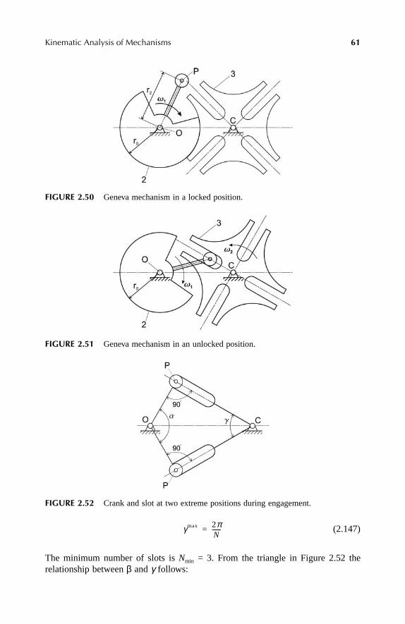
Kinematic Analysis of Mechanisms 61
(2.147)
The minimum number of slots is Nmin = 3. From the triangle in Figure 2.52 therelationship between β and γ follows:
FIGURE 2.50 Geneva mechanism in a locked position.
FIGURE 2.51 Geneva mechanism in an unlocked position.
FIGURE 2.52 Crank and slot at two extreme positions during engagement.
γmax 2πN------=
Ch2Frame Page 61 Friday, June 2, 2000 6:39 PM

62 Fundamentals of Kinematics and Dynamics of Machines and Mechanisms
(2.148)
Since the rotations through the angles βmax and γmax are accomplished during thesame time τ, from the relationship βmax = ω2τ it follows, using Equations 2.147and 2.148,
(2.149)
Note that the above equation makes clear why the number of slots must be not lessthan three.
Analysis of Geneva Wheel Motion
Since the Geneva wheel is an inversion of the slider-crank mechanism, Figure 1.14b,in which the crank is the driver, the loop-closure equation is given by Equation 2.16and the solution by Equation 2.27, in which j = 3,
(2.150)
and
(2.151)
In Equations 2.150 and 2.151, one should take into account that
and
In Figure 2.53 the angle of rotation of a four-slotted Geneva wheel as a function ofangle β for the case of
is shown. The latter relationship follows from the right triangle in Figure 2.52. Notealso that for the four-slotted wheel .
In Figures 2.54 and 2.55 the angular velocity and acceleration of the Genevawheel are shown during the driver rotation through angle β.
βmax π γmax–=
τ πN 2–Nω2-------------=
r 3 b r12 r 2
2 2–+ r 1r 2 θ2cos= =
αcos θ3cosr 2 θ2 r 1–cos
b----------------------------- αsin,– θ3sin
r 2 θ2sinb
------------------–= = = =
βmax
2---------- θ2
βmax
2----------≤ ≤– θ3 2π γ–=
r 2
r 1----
βmax
2----------cos 1
2-------= =
βmax γmax π= =
Ch2Frame Page 62 Friday, June 2, 2000 6:39 PM

Kinematic Analysis of Mechanisms 63
FIGURE 2.53 Angle of rotation of four-slotted Geneva wheel.
FIGURE 2.54 Angular velocity of four-slotted Geneva wheel.
FIGURE 2.55 Angular acceleration of four-slotted Geneva wheel.
-0.75 -0.5 -0.25 0.25 0.5 0.75β
-0.75
-0.5
-0.25
0.25
0.5
0.75
γ
-0.75 -0.5 -0.25 0.25 0.5 0.75β
-2
-1.5
-1
-0.5
ω3
-0.75 -0.5 -0.25 0.25 0.5 0.75β
-4
-2
2
4
α3
Ch2Frame Page 63 Friday, June 2, 2000 6:39 PM

64 Fundamentals of Kinematics and Dynamics of Machines and Mechanisms
PROBLEMS AND EXERCISES
PROBLEMS
1. In Figure 1.14c an inverted slider-crank mechanism is shown.
a. Write a loop-closure equation for this mechanism.b. If the input is the displacement of the cylinder, what are the unknowns? c. Solve the equation for the unknowns.
2. In Figure 1.14d an inverted slider-crank mechanism is shown.
a. Write a loop-closure equation for this mechanism.b. If the input is the displacement of the cylinder, what are the unknowns? c. Solve the equation for the unknowns.
3. In Figure P2.1 an inverted slider-crank mechanism is shown.
a. Write a loop-closure equation for this mechanism.b. If the input is the crank angle, what are the unknowns? c. Solve the equation for the unknowns. d. Express the position of point P in terms of the input angle.
4. In Figure P.2.2 a five-bar linkage is shown, in which AB is parallel and equalto O2C.
a. Write a loop-closure equation for this mechanism.b. If the input is the crank angle, what are the unknowns? c. Solve the equation for the unknowns.d. Express the position of point P in terms of the input angle.
5. In Figure P2.3 a slider-crank mechanism is shown.
a. Write a loop-closure equation for this mechanism.b. If the input is the crank angle, what are the unknowns? c. Solve the equation for the unknowns.d. Express the position of point P in terms of the input angle.
FIGURE P2.1
Ch2Frame Page 64 Friday, June 2, 2000 6:39 PM
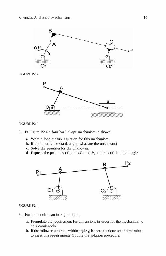
Kinematic Analysis of Mechanisms 65
6. In Figure P2.4 a four-bar linkage mechanism is shown.
a. Write a loop-closure equation for this mechanism.b. If the input is the crank angle, what are the unknowns? c. Solve the equation for the unknowns.d. Express the positions of points P1 and P2 in terms of the input angle.
7. For the mechanism in Figure P2.4,
a. Formulate the requirement for dimensions in order for the mechanism tobe a crank-rocker.
b. If the follower is to rock within angle γ, is there a unique set of dimensionsto meet this requirement? Outline the solution procedure.
FIGURE P2.2
FIGURE P2.3
FIGURE P2.4
Ch2Frame Page 65 Friday, June 2, 2000 6:39 PM

66 Fundamentals of Kinematics and Dynamics of Machines and Mechanisms
8. In Figure 2.4 find the maximum angle of rocking of the connecting rod, if r2
and r3 are given.
9. For a variable-stroke drive mechanism in Figure P1.7,
a. Identify two loops.b. For a coordinate system such that axis x is directed from the center of
the driving shaft to the center of the output shaft, outline the solutionprocedure using solutions in the book for a four-bar linkage.
10. For the double-toggle mechanism in Figure P1.6,
a. Identify two loops.b. For a coordinate system such that the x-axis passes through the center of
the crankshaft and is directed to the right, outline the solution procedureusing solutions in the book for a four-bar linkage and a slider-crankmechanism.
11. For the constant velocity mechanism shown in Figure P1.5,
a. Identify two loops.b. For a coordinate system such that the x-axis is directed along the cylinder
to the right, outline the solution procedure using solutions in the bookfor a four-bar linkage and a slider-crank mechanism.
12. A quick-return mechanism, shown in Figure P2.5, is used in machine tools. Fora constant angular velocity of the driving crank, it produces slow velocity duringthe cutting phase and then fast return.
a. Identify two loops.b. Define a coordinate system.
FIGURE P2.5
Ch2Frame Page 66 Friday, June 2, 2000 6:39 PM

Kinematic Analysis of Mechanisms 67
c. For a coordinate system such that the y-axis is going through the pointsO1 and O2 upwards, outline the solution procedure using solutions in thebook for a slider-crank mechanism.
d. Define the time ratio (time of cutting stroke to the time of return stroke)in terms of the distances O1O2 and O2A.
13. For the mechanism in Figure P2.1, find
a. the velocities.b. the accelerations of point P.
Assume that the position, velocity, and acceleration analyses of the skeletonhave been done.
14. For the mechanism in Figure P2.2, find
a. the velocities.b. the accelerations of point P.
Assume that the position, velocity, and acceleration analyses of the skeletonhave been done.
15. For the mechanism in Figure P2.3, find
a. the velocities.b. the accelerations of point P.
Assume that the position, velocity, and acceleration analyses of the skeletonhave been done.
16. Assume that dimensions of all links in Figure P1.4 are known.
a. What would be the configuration of the links when the pliers are closest?b. Assume that the coupler link is parallel to the frame link, and that the
frame link is 10 cm, the coupler link is 7 cm, the link connecting the twojaws is 2 cm, and the fourth link is 3 cm. What is the angle by which thecoupler link rotates from the initial to the extreme position?
17. Consider the double-rocker mechanism in Figure P2.6.
a. What should the relationship between the links dimensions be in orderfor the connecting link to make a complete rotation while the arms arerocking?
b. Assume 2a = 1 cm, h = 0.5 cm, 2d = 10 cm, and that the arms have equallength 7 cm. What is the angle of arm 1 rocking?
18. For an eight-slot Geneva mechanism
a. Find the distance between the centers of rotation, r1, given the radius ofthe crank r2 (distance from the center of the driving plate to the centerof the pin) and assuming that the pin enters and leaves the slot smoothly.
b. Find the length of the slot.
Ch2Frame Page 67 Friday, June 2, 2000 6:39 PM

68 Fundamentals of Kinematics and Dynamics of Machines and Mechanisms
19. In Figure P2.7 a linear intermittent motion mechanism is shown. Given theangular velocity of the crank and its radius, r2, how would velocity and accel-eration of the slider change during the cycle of the crank?
EXERCISES (PROJECTS) WITH MATHEMATICA
1. A motor drives a film-advancing mechanism with constant velocity ω(Figure P2.8) Link 2 is the driver. The path of point C should be as indicated,so that during the engagement with the film point C moves along a straight line.
a. Find (by trial and error) such dimensions of the mechanism that theneeded trajectory of point C is achieved.
b. Animate the motion.c. Plot the velocity and acceleration of point C over the cycle. Find the
velocities and accelerations during engagement and disengagement withthe film. Does the velocity remain constant during the engagement?
FIGURE P2.6
FIGURE P2.7
Ch2Frame Page 68 Friday, June 2, 2000 6:39 PM

Kinematic Analysis of Mechanisms 69
2. A motor drives a carrier mechanism with constant velocity ω (see Figure 2.26).The path of point A should be such that at the lowest position the line AB isparallel to the horizontal conveyor, and at the highest position the line AC shouldbe parallel to the inclined conveyor (so that the load can be transferred fromone conveyor to another).
a. Find (by trial and error) such dimensions of the mechanism (for theassumed positions of the conveyor belts) that the needed trajectory ofpoint A is achieved. (Hint: At extreme positions the motion of point A isreversed, which means that at these positions the links DC and CB arecollinear.)
b. Animate the motion.c. Plot the velocity and acceleration of point A over the cycle. What are the
velocities and accelerations at the points of load transfer?
3. For the dimensions of the double-rocker given in problem 17:
a. Animate the motion.b. Plot the trajectory, velocity, and acceleration of the tracing point over the
cycle.
4. The oscillating drive-arm in Figure P2.9 has the maximum operating angle π/6.For a relatively short guideway, the reciprocating output stroke is large and itfollows a straight line.
a. Find (by trial and error) such dimensions of the mechanism that theneeded trajectory of the tracing point is achieved.
b. Animate the motion.c. Plot the velocity and acceleration of point P over the cycle. What are the
velocities and accelerations at the end points of the stroke?
FIGURE P2.8
Ch2Frame Page 69 Friday, June 2, 2000 6:39 PM
70 Fundamentals of Kinematics and Dynamics of Machines and Mechanisms
5. For a complex mechanism operating a dump truck in Figure 1.6 assume that thebed moves from a horizontal to a π/3 position.
a. Find (by trial and error) such dimensions of the mechanism that theneeded trajectory of the bed is achieved.
b. Animate the motion.
6. In Figure P1.6 a double-toggle puncher is shown. When the drive crank rotatesclockwise, the second toggle begins to straighten to create a strong punching force.
a. Find link dimensions such that the desired motion is achieved.b. Animate the motion.c. Plot velocities and accelerations of the point P over the cycle.
7. In Figure P1.7 a variable-stroke drive, which is a combination of two four-barlinkages, is shown. The driving member rotates the eccentric, which, throughthe linkage, causes the output link to rotate a fixed amount. The ratchet on theoutput shaft transfers motion in one direction only. Thus, on the return stroke,the output link overrides the output shaft. As a result, a pulsating motion istransmitted to the output shaft, which is needed in many applications, such asfeeders and mixers. A smoother drive can be produced by mounting on the sameshaft the same device but with some shift in phase with respect to the first one.A continuously variable drive can be designed by mounting a few of such deviceson the same shaft and using the control link to change the position of theadjustable pivot.
a. Perform a complete kinematic analysis for one position of the adjustablepivot. Plot velocities and accelerations of the output link over the cycle.
b. Animate the motion.
FIGURE P2.9
Ch2Frame Page 70 Friday, June 2, 2000 6:39 PM
Kinematic Analysis of Mechanisms 71
8. In Figure P1.3 an adjustable stroke mechanism is shown. The output link slidesalong the horizontal line, and the stroke is controlled by the position of the pivotpoint.
a. Perform complete kinematic analysis for one position of the adjustablepivot. Plot velocities and accelerations of the output link over the cycle.
b. Animate the motion.
9. For the loader shown in Figure 2.3, assume that rods 5 and 6 move during thesame time interval (synchronized motion), but their velocities may be different.
a. Find by trial and error such dimensions that the bucket rotates over theπ/2 range from the lowest to the highest position.
b. Perform a complete kinematic analysis. Plot angular velocity and accel-eration of the bucket when it moves from the lowest to the highestposition.
c. Animate the motion.
Ch2Frame Page 71 Friday, June 2, 2000 6:39 PM

Ch2Frame Page 72 Friday, June 2, 2000 6:39 PM

73
3
Force Analysis of Mechanisms
3.1 INTRODUCTION
The design of mechanisms and their components requires information about forcesacting on these components. Some mechanisms are designed to perform a specifickinematic function (like the windshield wiper mechanism, Figure 1.4), others totransfer energy (like the internal combustion engine). However, in any mechanism,identification of forces is needed to determine the proper dimensions of components.
The power supplied to the input link flows through the mechanism to the outputlink. Associated with this power flow is a force flow. The objective of the forceanalysis of mechanisms is to find the
transformation of forces
from the input to theoutput links. This transformation of forces depends on the position of the mechanism;in other words, it is a function of time. Thus, it is important to find out how theseforces change during one cycle in order to find their maxima.
One should differentiate between two types of forces:
external
and
internal
. Theformer are forces that are applied to the links from external (with respect to themechanism) sources — driving forces, resistance forces — whereas the latter areforces acting between the joints (they are called
constraint
or
reaction
forces).The motion of a mechanism is caused by the known external forces, and can be
found by formulating and solving the differential equation describing the dynamicequilibrium of the mechanism at any moment in time. This approach to motionanalysis is called
direct dynamics
. An alternative approach is to assume that themotion is known (in other words, the motion of the input link is given as a functionof time). Then, as a result of kinematic analysis, the accelerations of all links areknown, and thus the inertial forces associated with these links. These inertial forcescan be treated as known external forces, and the force analysis is then reduced tosolving equilibrium equations for the mechanism at any given position. Thisapproach to force analysis is called
inverse dynamics
. It is important to keep in mindthat inverse dynamics is based on the assumption of known motion, whereas in factsuch motion can be found only from direct dynamics analysis. However, in manysituations the much simpler inverse dynamics approach is sufficient as a first approx-imation. This approach is considered in this book.
To summarize, it is assumed here that the forces acting on the input link aregiven as a function of time (or link position) and the inertial (dynamic) forces arealso known as a result of kinematic analysis of motion. The objective of force analysisthen is to find the internal and resistance forces. The method of solution is to performstatic analysis of a mechanism in a number of fixed positions over the region ofinput link motion.
Ch3Frame Page 73 Friday, June 2, 2000 6:40 PM

74
Fundamentals of Kinematics and Dynamics of Machines and Mechanisms
3.2 FORCE AND MOMENT VECTORS
A force is characterized by its magnitude and direction, and thus is a vector. In an(
x
,
y
)-plane the force vector,
F
, can be represented in different forms
F
= [
F
x
, F
y
] =
F
[cos
α
, sin
α
]
T
=
F
(
i
cos
α
+
j
sin
α
) (3.1)
where
F
x
,
F
y
are the
x
- and
y
-components of the vector (Figure 3.1),
α
indicatesforce direction (positive
α
is measured counterclockwise), and
i
and
j
are the unitvectors directed along the
x
- and
y
-axis, correspondingly.A moment of the force
F
with respect to a point
A
(Figure 3.2) is a vector foundas a cross-product of two vectors:
M
=
r
A
×
F
(3.2)
This vector is directed along the line perpendicular to the plane made by vectors
r
A
and
F
, which in this case is the (
x,y
)-plane. In Equation 3.2
r
A
is a vector associated
FIGURE 3.1
Force vector.
FIGURE 3.2
Illustration of the force moment.
Ch3Frame Page 74 Friday, June 2, 2000 6:40 PM

Force Analysis of Mechanisms
75
with point
A
and can be represented as a sum of two vectors: one collinear with
F
(
r
F
) and another perpendicular to it (
h
) (Figure 3.2). Then Equation 3.2 is reducedto
(3.3)
since the moment of the collinear component is zero (see Equation 2.9). The magni-tude of vector
h
is the distance from point
A
to the line of force
F
, whereas itsdirection is toward point
A
. Thus, vector
h
has the following forms:
(3.4)
Substituting Equations 3.1 and 3.4 into Equation 3.3, one obtains (see Equation 2.7)
(3.5)
Thus, the moment vector is directed along the
z
-axis in such a way that for anobserver on the tip of vector
M
the rotation from
h
to
F
is counterclockwise. It isimportant to note that its sign is determined by the convention for measuring thedirection of vectors (or by choosing the right-hand coordinate system).
3.3 FREE-BODY DIAGRAM FOR A LINK
A diagram of a link with all forces (external and internal) applied to it is called a
free-body diagram
. Under the action of all forces (static and inertial), the link mustbe in equilibrium. This requirement results in relationships between the known andunknown forces for a single link.
The internal forces originate in joints since joints constrain the relative motionbetween the connected links. In the case of a revolute joint, in general, both themagnitude and the direction of the constraint force are unknown, whereas in thecase of a prismatic joint only the magnitude of the constraint force is unknown. Thisis because the latter force is always directed along the normal to the axis of theslider (note that if the friction forces are taken into account, then their magnitudesand directions are assumed to be known functions of normal forces).
For each link, the vector equilibrium equations (for a planar problem) can bewritten:
(3.6)
where
n
is the number of forces and
m
is the number of moments.In global coordinates the system of equations (Equation 3.6) written for each link
is coupled, which means that the constraint forces for each link are interdependent
M h F¥=
h h α π2---+
cos α π2---+
sin,T
h α αcos,sin–[ ] T= h i α j αcos+sin–( )= =
M hF α π 2⁄+( ) α α π 2⁄+( ) αcossin–sincos( )k hFk–= =
Fi
i 1=
n
∑ 0 and M j
j 1=
m
∑ 0==
Ch3Frame Page 75 Friday, June 2, 2000 6:40 PM
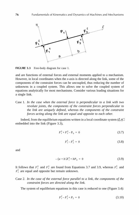
76
Fundamentals of Kinematics and Dynamics of Machines and Mechanisms
and are functions of external forces and external moments applied to a mechanism.However, in local coordinates when the
x
-axis is directed along the link, some of thecomponents of the constraint forces can be uncoupled, thus reducing the number ofunknowns in a coupled system. This allows one to solve the coupled system ofequations analytically for most mechanisms. Consider various loading situations fora single link.
Case 1.
In the case when the external force is perpendicular to a link with tworevolute joints, the components of the constraint forces perpendicular to
t
he link are uniquely defined, whereas the components of the constraintforces acting along the link are equal and opposite to each other
.
Indeed, from the equilibrium equations written in a local coordinate system (
ξ
,
η
)
embedded into the link (Figure 3.3),
(3.7)
(3.8)
and
(3.9)
It follows that and are found from Equations 3.7 and 3.9, whereas and are equal and opposite but remain unknown.
Case 2.
In the case of
the external force parallel to a link, the components of theconstraint forces are directed along the link.
The system of equilibrium equations in this case is reduced to one (Figure 3.4):
(3.10)
FIGURE 3.3
Free-body diagram for case 1.
F1η F2
η Pη–+ 0=
F1ξ F2
ξ– 0=
a(– b)F1η bPη++ 0=
F1η F2
η F1ξ
F2ξ
F1ξ F2
ξ Pξ+– 0=
Ch3Frame Page 76 Friday, June 2, 2000 6:40 PM

Force Analysis of Mechanisms 77
Case 3.In the case when only an external moment is applied to a link with tworevolute joints, the constraint forces form a couple.
The equilibrium equations in this case are (Figure 3.5)
(3.11)
and
(3.12)
If each of the constraint forces is resolved into two components, parallel and per-pendicular to the link (see Figure 3.5), then the magnitudes of the perpendicular tothe link components are completely defined by the acting moment:
(3.13)
while the components parallel to the link are equal but remain unknown:
(3.14)
FIGURE 3.4 Free-body diagram for case 2.
FIGURE 3.5 Free-body diagram for case 3.
F1 F2+ 0=
r F 1 M–× 0=
F1η– F2
η Mr-----= =
F1ξ F2
ξ=
Ch3Frame Page 77 Friday, June 2, 2000 6:40 PM

78 Fundamentals of Kinematics and Dynamics of Machines and Mechanisms
Case 4.In the case when there are no external forces acting on a link with tworevolute joints, the constraint forces act along the link and are equal andopposite to each other.
This is a particular situation of case 1. Indeed, if , then and (see Equations 3.7 and 3.9).
Case 5.In the case of a link with one revolute joint and another sliding joint whoseaxis is perpendicular to the link, the constraint forces act along the linkand are equal and opposite to each other.
This is clear from Figure 3.6a in the case when the friction forces in the slidingjoint are neglected.
Case 6. In the case of a link with one revolute joint and another sliding joint whoseaxis coincides with the link axis the constraint forces act normally to the link.
This is clear from Figure 3.6b in the case when the friction forces in the slidingjoint are neglected. The constraint forces are determined by Equations 3.11 and 3.12.
What follows from all of the above cases is that for a link with two revolute joints:
• For any external load acting on a link there is only one unknown associatedwith this link.
• The unknown is the component of the constraint force directed along thelink.
• The two components of the constraint force directed along the link arealways equal and opposite to each other.
Now one can split the unknown constraint forces for each link into two compo-nents: one parallel and the other perpendicular to the link. As a result, the system
FIGURE 3.6 Free-body diagrams for cases 5 and 6.
Pη 0= F1η 0=
F2η 0=
Ch3Frame Page 78 Friday, June 2, 2000 6:40 PM

Force Analysis of Mechanisms 79
of equilibrium equations for each link, Equation 3.6, will be split into two systems:one, independent from the equations for other links, and the other, coupled with theequations for other links. The order of the coupled system is equal to the number oflinks in the mechanism, and thus constitutes the minimum system of equations.
3.4 INERTIAL FORCES
The inertial forces are generated by nonzero translational and angular accelerations.If the mass center for each link j is identified, then the motion equations for thislink as a free body are
(3.15)
and
(3.16)
where is the position vector of the mass center of link j in the global coordinatesystem, θj is the angular coordinate of the link, mj is the mass of the link, Ij is themoment of inertia of the link, and and are the external forces and moments,respectively. Note that and include constraint forces applied to the joints.
If one assumes that the accelerations are known from the kinematic analysis,the inertial forces can be considered as known external forces so that Equations 3.15and 3.16 can be written in a standard form:
(3.17)
and
(3.18)
where
(3.19)
The problem of finding the unknown constraint forces in a moving mechanism isthus reduced to a problem of static equilibrium with the additional inertial forces givenby Equation 3.19 treated as known external forces. This is known as D’Alembert’sprinciple.
In the following, if the direction of the internal force is known, then it isconvenient to represent this force in a directional form ;otherwise a component form will be used.
mj r cj Fext∑=
I j q j M ext∑=
r cj
Fext M ext
Fext M ext
Fext Finert+∑ 0=
M ext M inert+∑ 0=
Finert m– j r cj and M inert I j q j–= =
Fij Fij α i j α i jsin,cos[ ] T=Fij Fij
x Fijy,[ ] T
=
Ch3Frame Page 79 Friday, June 2, 2000 6:40 PM

80 Fundamentals of Kinematics and Dynamics of Machines and Mechanisms
3.5 APPLICATION TO SIMPLE MECHANISMS
Here a few examples of simple mechanisms will be considered: the slider-crankmechanism, the four-bar linkage, the five-bar mechanism, and the Scotch yokemechanism.
3.5.1 SLIDER-CRANK MECHANISM: THE CASE OF NEGLIGIBLY SMALL INERTIAL FORCES
The skeleton of the mechanism and its vector representation are shown in Figure 3.7aand b, and the free-body diagrams of links are shown in Figure 3.8.
Assume that M2 is the known external moment, is the unknown resistanceforce, and the inertial forces can be neglected. All other forces shown in Figure 3.8are internal (constraint) forces. Each internal force is identified by two indices: the
FIGURE 3.7 Slider-crank mechanism driven by moment M 2.
FIGURE 3.8 Free-body diagrams of links for the slider-crank mechanism with negligibleinertial forces.
P4ξ
Ch3Frame Page 80 Friday, June 2, 2000 6:40 PM
Force Analysis of Mechanisms 81
first one indicates the adjoining link, and the second one the link to which the forceis applied. It follows from the equilibrium of forces applied to a joint that
(3.20)
Link 3 is the only one to which external forces are not applied. It follows thenthat for this link the internal forces are directed along the link and they are equal inmagnitude ( ) and opposite to each other. This reduces the system ofequations and simplifies the solution. Thus, the forces in the joints of link 3 containonly the unknown magnitude, since the directions of these forces are known. Assumethat the direction of vector F23 coincides with that of vector r 3 (if the assumption iswrong, the solution will have the opposite sign for this force).
(3.21)
Then all other unknown vectors are as follows:
(3.22)
where it was taken into account that forces F32 and F12 form a couple.Thus, there are three unknowns in this problem, which are the magnitudes of
three vectors: F23, F14, and P4. The first one is found from the moment equation forlink 2, and the other two from the equilibrium equation for link 4.
Link 2 Use the vector form of the moment equation, taking into account that theexternal moment is negative
(3.23)
If one substitutes in the above , M2 = –M2 k, and takesinto account Equations 2.9 and 3.21, one obtains a scalar equation for the unknownF32:
(3.24)
Thus, the unknown force magnitude is equal to
(3.25)
Note that the force magnitude is supposed to be positive by definition. If it becomesnegative, then it means that all forces in Equation 3.24 change directions.
Fij Fji+ 0=
F23ξ F43
ξ=
F23 F23ξ θcos 3 θ3sin,[ ] T=
F43 F32 F34– F12– F23–= = = =
r 2 F32 M 2–× 0=
r 2 r 2 θcos 2 θ2sin,[ ] T=
r 2F32 θ3 θ2–( ) M2–sin 0=
F32M2
r 2 θ3 θ2–( )sin----------------------------------=
Ch3Frame Page 81 Friday, June 2, 2000 6:40 PM

82 Fundamentals of Kinematics and Dynamics of Machines and Mechanisms
Link 4
(3.26)
In Equation 3.26 the forces are as follows:
(3.27)
(3.28)
and
(3.29)
After substituting the above forces into Equation 3.26 and equating the x- andy-components of the vector equation to zero, the expressions for the two unknownsare obtained:
(3.30)
and
(3.31)
3.5.2 SLIDER-CRANK MECHANISM: THE CASE OF SIGNIFICANT INERTIAL FORCES
The skeleton of the mechanism is shown in Figure 3.9a, where the inertial forcesare identified with the superscript i. In Figure 3.9b the free-body diagrams of linksare shown, where C2 and C3 are the centers of gravity of links 2 and 3.
Assume, as in the previous case, that M2 is an applied moment, and P4 is anunknown resistance force. One can see from Figure 3.9b that there are eightunknowns in this problem: (remember that the direction ofthe last two forces is known), and thus eight scalar equations are needed to find theunknowns. However, as is known, only the components of constraint forces collinearwith the links are coupled. One can then resolve each inertial force into two com-ponents: one parallel and the other perpendicular to the corresponding link. Thenthe free-body diagrams for links 2 and 3 in Figure 3.9b can be seen as the super-position of free-body diagrams in Figures 3.3 through 3.5, where the superscripts ξand η identify force components that are collinear and normal to the correspondinglinks. It should be pointed out that the direction of forces and moments can beconsidered with respect to the direction of the vector identifying the link (in otherwords, in a local coordinate system). Then, since all forces normal to the link and
F34 F14 P4+ + 0=
F14 F14π2--- π
2---sin,cos
T
F14 0 1,[ ] T= =
P4 P4 π πsin,cos[ ] T P4 1– 0,[ ] T= =
F34 F32 θ3 θ3sin,cos( )T=
P4 F32 θ3cos=
F14 F– 32 θ3sin=
F12 F32 F43 F14 andP4, , , ,
Ch3Frame Page 82 Friday, June 2, 2000 6:40 PM

Force Analysis of Mechanisms 83
all forces parallel to the link are collinear, the positive directions of forces can bechosen arbitrarily. In addition, in the local coordinate system one can treat theseforces as scalars since their directions are known. Later on, when all the unknownsare found, they can be transformed into a global coordinate system.
First consider the case of normal forces in links shown in Figure 3.9b.
Link 2 The two equilibrium equations are
(3.32)
and
FIGURE 3.9 (a) Slider-crank mechanism with inertial forces. (b) Free-body diagrams forlinks in a slider-crank mechanism with significant inertial forces.
F– 12η P2
iη F– 32η+ 0=
Ch3Frame Page 83 Friday, June 2, 2000 6:40 PM

84 Fundamentals of Kinematics and Dynamics of Machines and Mechanisms
(3.33)
where r2 and rC2 are the length of link 2 and the distance C2A (see Figure 3.9a). Itfollows from Equation 3.33 that
(3.34)
and from Equation 3.32 that
(3.35)
Equations 3.34 and 3.35 define the normal components of joint forces in link 2explicitly.
Link 3 The equilibrium equations are
(3.36)
and
(3.37)
where r3 and rC3 are the length of link 3 and the distance C3B (see Figure 3.9a). Itfollows from Equation 3.37 that
(3.38)
and from Equation 3.36 that
(3.39)
Equations 3.38 and 3.39 define the normal components of joint forces in link 3.Now consider forces acting along the link (see Figure 3.9b). For these forces
there is only one equilibrium equation per link.
Link 2
(3.40)
r 2F12η r C2P2
iη M2 M2i+–– 0=
F12η M2 M2
i r C2P2iη+–
r 2------------------------------------------=
F32η F– 12
η P2iη+=
F23η P3
iη F43η–+ 0=
r 3F23η r C3P3
iη M3i––– 0=
F23η M3
i r C3– P3iη–
r 3-----------------------------=
F43η F23
η P3iη+=
F12ξ P2
iξ F32ξ–+ 0=
Ch3Frame Page 84 Friday, June 2, 2000 6:40 PM
Force Analysis of Mechanisms 85
Link 3
(3.41)
As far as link 4 is concerned, the two equilibrium equations for both the x- andy-components of the forces contain three unknown constraint forces and oneunknown resistance force (see Figure 3.9b). Since none of the unknowns can befound explicitly from these equations, they must be solved together with Equations3.40 and 3.41.
Link 4
(3.42)
and
(3.43)
Recall that Equations 3.40 through 3.43 are written in local coordinate systems sothat, for example, . Because of this, the number of unknowns in the fourequations (Equations 3.40 through 3.43) is eight. Thus, it is necessary to supplementEquations 3.40 through 3.43 with four more equations. These come from the require-ment that the sum of constraint forces in a joint must be zero. Thus, there are twomore vector equations for the joints connecting links 2 and 3, and links 3 and 4.
(3.44)
and
(3.45)
All forces in Equations 3.44 and 3.45 are expressed in the global coordinatesystem. Now it is necessary to express these vector forces through the componentsof these forces in local coordinate systems. Such a transformation is easily per-formed. Consider, for example, vector F12 comprising two components and
in the global coordinate system. In the local coordinate system (ξ,η), isdirected along link 2 and thus has the same direction as vector r 2, whereas vector
is normal to vector r 2 and is being rotated by the angle –π/2 in the negative(counterclockwise) direction. Thus, vector F12 is equal to
(3.46)
F23ξ P3
iξ F43ξ––– 0=
P4i P4 F34
ξ+–– 0=
F34η F14
η+ 0=
F32ξ F23
ξ≠
F32 F23+ 0=
F43 F34+ 0=
F12x
F12y F12
ξ
F12η
F12 F12ξ θ2 θ2sin,cos[ ] T= F12
η θ2π2---–
θ2π2---–
sin,cosT
+
Ch3Frame Page 85 Friday, June 2, 2000 6:40 PM

86 Fundamentals of Kinematics and Dynamics of Machines and Mechanisms
or
(3.47)
Similarly,
(3.48)
(3.49)
(3.50)
(3.51)
Now, substitute vectors given by Equations 3.48 through 3.51 into Equations 3.44and 3.45:
(3.52)
and
(3.53)
The system of six equations (Equations 3.40 through 3.43 and Equations 3.52 and3.53) defines eight unknowns: . From the firstfour equations (Equations 3.40 through 3.43) some of the unknowns are easilyexpressed through others:
(3.54)
(3.55)
(3.56)
(3.57)
After the above expressions are substituted into Equations 3.52 and 3.53, the lattersystem of four equations will have only four unknowns: :
F12 F12ξ θ2 θ2sin,cos[ ] T= F12
η θ2 θ2cos–,sin[ ] T+
F32 F– 32ξ θ2 θ2sin,cos[ ] T= F32
η θ2 θ2cos–,sin[ ] T+
F23 F– 23ξ θ3 θ3sin,cos[ ] T= F23
η θ3 θ3cos,sin–[ ] T+
F43 F– 43ξ θ3 θ3sin,cos[ ] T= F43
η θ3 θ3cos–,sin[ ] T+
F34 F34ξ 0 0sin,cos[ ] T= F34
η π2--- π
2---sin,cos
T
+ F34ξ 1 0,[ ] T F34
η 0 1,[ ] T+=
F– 32ξ θ2 θ2sin,cos[ ] T F32
η θ2 θ2cos–,sin[ ] T+
F– 23ξ θ3 θ3sin,cos[ ] T F23
η θ3 θ3cos,sin–[ ] T+ 0=
F– 43ξ θ3 θ3sin,cos[ ] T F43
η θ3 θ3cos–,sin[ ] T F34ξ 1 0,[ ] T F34
η 0 1,[ ] T+ + + 0=
F12ξ F32
ξ F23ξ F, 43
ξ F34ξ F, 34
η F14η andP4, , , , ,
F32ξ F12
ξ P2iξ+=
F23ξ P3
iξ F–– 43ξ
=
F34ξ P4
iξ P4+=
F14η F34
η–=
F12ξ F43
ξ F34η andP4, , ,
Ch3Frame Page 86 Friday, June 2, 2000 6:40 PM
Force Analysis of Mechanisms 87
(3.58)
and
(3.59)
In Equation 3.58 the two unknowns, and , are uncoupled from otherunknowns, and thus they can be found by solving this equation. By multiplyingEquation 3.58 from the left by the unit vector this equation isreduced to
(3.60)
From the above equation the unknown is found to be
(3.61)
Now, premultiply Equation 3.58 by the unit vector . The result is
(3.62)
From the above equation the unknown is found to be
(3.63)
Now, since is given by Equation 3.61, the remaining unknowns, and ,can be found from Equation 3.59. First consider the ξ-components in Equation 3.59.As a result, the unknown is found:
(3.64)
Similarly, by considering the η-components in Equation 3.59, the unknown isfound
(3.65)
F12ξ P2
iξ+( ) θ2 θ2sin,cos[ ] T F32η θ2 θ2cos–,sin[ ] T+
F43ξ P3
iξ+( ) θ3 θ3sin,cos[ ] T F23η θ3 θ3cos,sin–[ ] T+ + 0=
F– 43ξ θ3 θ3sin,cos[ ] T F43
η θ3 θ3cos–,sin[ ] T+
+ P4i P4+( ) 1 0,[ ] T F34
η 0 1,[ ] T+ 0=
F12ξ F43
ξ
u1 θ2 θ2cos,sin–[ ]=
F32η F43
ξ P3iξ+( ) θ3 θ2–( ) F23
η θ3 θ2–( )cos–sin+– 0=
F43ξ
F43ξ P– 3
iξ F23η θ3 θ2–( ) F32
η–cosθ3 θ2–( )sin
----------------------------------------------------–=
u2 θ3 θ3cos,sin–[ ]=
F12ξ P2
iξ+( ) θ2 θ3–( ) F32η θ2 θ3–( ) F23
η+cos–sin 0=
F12ξ
F12ξ P– 2
iξ F32η θ2 θ3–( ) F23
η–cosθ2 θ3–( )sin
----------------------------------------------------+=
F43ξ F34
η P4
P4
P4 P4iξ– F43
ξ θ3 F43η θ3sin–cos+=
F34η
F34η F43
ξ θ3 F43η θ3cos+sin=
Ch3Frame Page 87 Friday, June 2, 2000 6:40 PM

88 Fundamentals of Kinematics and Dynamics of Machines and Mechanisms
Thus, the unknown joint forces and the external resistance force are found forany crank position and any moment applied to it. The explicit formulas for all12 unknowns are given in Equations 3.34, 3.35, 3.38, 3.39, 3.54 through 3.57, 3.61,and 3.63 through 3.65.
In conclusion, note that by representing the constraint forces in joints in localcoordinate systems the number of unknowns in these joints doubled, so that insteadof a total of eight unknowns in a global coordinate system one solved for 12 unknowns.However, the above representation of joint forces allowed one to decouple the equationsand thus to simplify the solution.
3.5.3 FOUR-BAR MECHANISM: THE CASE OF SIGNIFICANT INERTIAL FORCES
The mechanism is shown in Figure 3.10a, its vector representation in Figure 3.10b,and the free-body diagrams in Figure 3.11, where the inertial forces and momentsare identified by the superscript i.
One can see that the free-body diagrams for links 2 and 3 are identical, in termsof loading, to those for the slider-crank mechanism, Figure 3.9b. The only link thatis different is link 4, which means that Equations 3.44 and 3.45 for the joints arevalid for this mechanism. However, vector F34 is different in this case. Namely, it isequal to
(3.66)
FIGURE 3.10 Four-bar linkage driven by the moment M 2.
F34 F– 34ξ θ4 θ4sin,cos[ ] T F34
η θ4 θ4cos,sin–[ ] T+=
Ch3Frame Page 88 Friday, June 2, 2000 6:40 PM

Force Analysis of Mechanisms 89
The vector F14 is also different
(3.67)
The free-body diagrams for the normal and along the link forces in link 4 areshown in Figure 3.12. The corresponding scalar equilibrium equations are
FIGURE 3.11 Free-body diagrams of links for a four-bar linkage.
FIGURE 3.12 Free-body diagram for the link 4 in a four-bar linkage.
F14 F– 14ξ θ4 θ4sin,cos[ ] T F14
η θ4 θ4cos,sin–[ ] T+=
Ch3Frame Page 89 Friday, June 2, 2000 6:40 PM
90 Fundamentals of Kinematics and Dynamics of Machines and Mechanisms
(3.68)
(3.69)
and
(3.70)
There are three unknowns in Equations 3.68 and 3.69: . Thus, onecan express the internal forces through the unknown external force:
(3.71)
and
(3.72)
There are a total of seven remaining unknowns: .These unknowns are defined by the following system of equations: Equations 3.40and 3.41 for links 2 and 3, Equation 3.70 for link 4, and Equations 3.44 and 3.45 inwhich vector F34 is as defined by Equation 3.66. The two expressions (Equations 3.54and 3.55) are valid in this case as well. Another relationship between the unknownscomes from Equation 3.70:
(3.73)
If Equations 3.54 and 3.55 and Equation 3.73 are now substituted into Equations 3.44and 3.45, one will obtain two vector equations. The first one, corresponding toEquation 3.44, is Equation 3.58 and thus will have the same solutions: Equations 3.61and 3.63. The second vector equation is different, and it is as follows:
(3.74)
There are two unknowns in Equation 3.74, and , which can be easily found.Premultiply Equation 3.74 by a unit vector . As a result, theunknown is found
(3.75)
Now premultiply Equation 3.74 by a unit vector . As a result,the unknown is found:
F34η– F14
η P4iη– P4–+ 0=
r 4F14η– M4
i r C4P4iη– r D4P4–+ 0=
F14ξ F34
ξ– P4iξ–– 0=
F34η F14
η , and P4,
F14η M4
i r C4P4iη– r D4P4–
r 4------------------------------------------------=
F34η F14
η= P4iη– P4–
F12ξ F32
ξ F23ξ F, 43
ξ F34ξ F14
ξ andP4, , , , ,
F34ξ F– 14
ξ= P4iξ–
F– 43ξ θ3 θ3sin,cos[ ] T F43
η θ3 θ3cos–,sin[ ] T+
–F34ξ θ4 θ4sin,cos[ ] T F34
η θ4 θ4cos,sin–[ ] T+ 0=
F34ξ F34
η
u1 θ4 θ4cos,sin–[ ]=F34
η
F34η F43
ξ θ3 θ4–( ) F43η θ3 θ4–( )cos+sin=
u2 θ4cos θ4sin,[ ]=F34
ξ
Ch3Frame Page 90 Friday, June 2, 2000 6:40 PM

Force Analysis of Mechanisms 91
(3.76)
Now, substitute Equations 3.71 and 3.75 into Equation 3.72 and solve for P4. Theresult is
(3.77)
Thus, the explicit formulas for all 13 unknowns — , — expressed in local coordinate systems are given by Equa-
tions 3.34, 3.35, 3.38, 3.39, 3.54, 3.55, 3.61, 3.63, 3.71, 3.73, and 3.75 through 3.77.Note that, if the inertial forces can be neglected, then the corresponding expres-
sions for the forces are obtained as a particular case of the above solution.
3.5.4 FIVE-BAR MECHANISM: THE CASE OF SIGNIFICANT INERTIAL FORCES
The linkage with applied external moment M2 and inertial forces is shown in Figure 3.13.The resistance force P4 is assumed to be normal to link 4 during the motion. Note thatlinks 4 and 5 are treated as different bodies for the sake of convenience, but in factthey constitute one mechanism element. The external and constraint forces directedalong the links are shown in Figure 3.14a, and those normal to the links in Figure 3.14b.Note that because links 4 and 5 are rigidly connected, there is a constraint moment
FIGURE 3.13 Five-bar mechanism driven by moment M 2.
F34ξ F43
ξ θ4 θ3–( ) F43η θ4 θ3–( )sin+cos=
P4
r 4F43ξ θ3 θ4–( ) r 4F43
η– θ3 θ4–( ) M4i r( 4– r C4 )P4
iη+ +cossin–r 4 r D4+
------------------------------------------------------------------------------------------------------------------------------------------------=
F12ξ
F12η F, 32
ξF32
η F, 23ξ
F23η F, , 43
ξF43
η, , ,F34
ξ F34η F14
ξ F, , 14η andP4, ,
Ch3Frame Page 91 Friday, June 2, 2000 6:40 PM

92 Fundamentals of Kinematics and Dynamics of Machines and Mechanisms
FIGURE 3.14 (a) Free-body diagrams for links subjected to along-the-link forces in a five-bar mechanism. (b) Free-body diagrams for links subjected to normal to the link forces in afive-bar mechanism.
Ch3Frame Page 92 Friday, June 2, 2000 6:40 PM

Force Analysis of Mechanisms 93
at this interface, . Also assume an ideal sliding joint, i.e., friction forcesare zero.
First, consider the equilibrium of links subjected to normal forces.
Link 2
(3.78)
and
(3.79)
From the above equation,
(3.80)
and from Equation 3.78,
(3.81)
Link 3If the friction forces are neglected, then, as was found above, this link cannot
have any normal reaction forces.
Link 4
(3.82)
and
(3.83)
From the above equation,
(3.84)
and from Equation 3.82,
(3.85)
Note that the unknown internal moment and the external resistance force cannot be found from the equilibrium requirements for this link.
M54 M45=
F12η F32
η P2iη+ + 0=
r 2F12η– M2– M2
i r C2P2iη–+ 0=
F12η M2– M2
i r C2P2iη–+
r 2--------------------------------------------=
F32η P– 2
iη F12η–=
F34η F54
η P4iη P4–+– 0=
r 4F34η– M4
i r C4P4iη– M54 r D4P4+ + + 0=
F34η M54 M4
i r C4P4iη r D4P4+–+
r 4--------------------------------------------------------------=
F54η P4
iη F34η P4–+=
M54 P4
Ch3Frame Page 93 Friday, June 2, 2000 6:40 PM

94 Fundamentals of Kinematics and Dynamics of Machines and Mechanisms
Link 5
(3.86)
and
(3.87)
From the latter equation,
(3.88)
and from Equation 3.86
(3.89)
Thus, the only unknown left from the analysis of normal forces is the externalresistance force .
Now, consider the equilibrium of links subjected to along-the-link forces.
Link 2
(3.90)
Link 3
(3.91)
Link 4This link is not subjected to any longitudinal forces, if the friction forces are
neglected.
Link 5
(3.92)
As can be seen, Equations 3.90 through 3.92 contain six unknowns: ,. Recall that the external resistance force is another unknown.
Thus, in addition to three equations (Equations 3.90 through 3.92) four more equa-tions are needed to find the above unknowns. These come from the requirements ofjoints equilibrium.
Joint 2–3
(3.93)
F15η– P5
iη+ 0=
M5i r C5P5
iη– M45– 0=
M45 M5i r C5P5
iη–=
F15η P5
iη=
P4
F12ξ– F32
ξ+ 0=
F23ξ– F43
ξ P3iξ–+ 0=
F45ξ F15
ξ– P5iξ– 0=
F12ξ F32
ξ F23ξ, ,
F43ξ F45
ξ andF15ξ, , P4
F32ξ θ2 θ2sin,cos[ ] T F32
η θ2 θ2cos,sin–[ ] T F23ξ θ3 θ3sin,cos[ ] T–+ 0=
Ch3Frame Page 94 Friday, June 2, 2000 6:40 PM

Force Analysis of Mechanisms 95
Joint 3–4Since link 3 is normal to link 4, it follows that the corresponding magnitudes
of internal forces are equal:
(3.94)
Joint 4–5Since links 4 and 5 are perpendicular to each other, the following magnitudes
of forces are equal:
(3.95)
From the last two equations and Equations 3.84 and 3.85 it follows that and are functions of the external force .
(3.96)
and
(3.97)
From Equation 3.93 the two unknowns and are found by first premultiplyingit by the unit vector to obtain
(3.98)
and then by premultiplying it by the unit vector to obtain
(3.99)
With and given by the last two equations, and are found fromEquations 3.90 and 3.91. Recall that is given by Equations 3.80 and 3.81. Nowby substituting and from Equations 3.99 and 3.96 into Equation 3.91, theunknown external force is found:
(3.100)
The internal force can now be found from Equation 3.97, and then fromEquation 3.92.
F43ξ F34
η=
F45ξ F54
η=
F43ξ F45
ξ
P4
F43ξ M54 M4
i r C4P4iη r D4P4+–+
r 4--------------------------------------------------------------=
F45ξ M54 M4
i r 4 r– C4( )P4iη r(– 4 r– D4 )P4+ +
r 4-------------------------------------------------------------------------------------------=
F32ξ F23
ξ
u1 θ3 θ3cos,sin–[ ]=
F32ξ F– 32
η θ2 θ3–( )cot=
u2 θ2 θ2cos,sin–[ ]=
F23ξ F32
η
θ3 θ2–( )sin-----------------------------=
F32ξ F23
ξ F12ξ F43
ξ
F32η
F23ξ F43
ξ
P4
P4
r 4
r D4-------
M– 54 M4i– r C4P4
iη+r 4
----------------------------------------------- P3iξ F32
η
θ3 θ2–( )sin-----------------------------+ +
=
F45ξ F15
ξ
Ch3Frame Page 95 Friday, June 2, 2000 6:40 PM

96 Fundamentals of Kinematics and Dynamics of Machines and Mechanisms
Now, transform the internal forces from the local to the global coordinate systemtaking into account the directions of local forces in the global coordinate system.For example, for the force F12,
(3.101)
3.5.5 SCOTCH YOKE MECHANISM: THE CASE OF SIGNIFICANT INERTIAL FORCES
The mechanism with the driving moment M2 and resistance force P4 is shown inFigure 3.15. Note that links 3 and 4 constitute one mechanism element. However,it is convenient, as was done earlier in the five-bar linkage analysis, to represent itas comprising two perpendicular links.
In Figures 3.16a and b the free-body diagrams of links under the action of forcesparallel and normal to links are shown. First, one notices that link 3 does notexperience any along-the-link forces (Figure 3.16a), if friction forces in the sliderare neglected. Second, since a moment is transferred through a rigid joint connectinglinks 3 and 4, this moment is counterbalanced by a couple in the sliding support oflink 4. The distance d4 is assumed to be the length of the support. And, finally, ifthe friction forces are neglected, then no such couple is generated between link 3and the slider because the slider is connected to link 2 by a revolute joint.
The equilibrium equations for the along-the-link forces are as follows:
Link 2
(3.102)
Link 4
(3.103)
FIGURE 3.15 Scotch yoke mechanism driven by moment M2.
F12 F– 12ξ θ2 θ2sin,cos[ ] T F12
η θ2 θ2cos,sin–[ ] T+=
F12ξ F32
ξ P2iξ+– 0=
F– 34ξ P4
iξ P4+– 0=
Ch3Frame Page 96 Friday, June 2, 2000 6:40 PM

Force Analysis of Mechanisms 97
The equilibrium equations for the forces normal to the link are as follows:
Link 2
(3.104)
and
FIGURE 3.16 (a) Free-body diagrams for links subjected to along-the-link forces in aScotch yoke mechanism. (b) Free-body diagrams for links subjected to forces normal to thelink in a Scotch yoke mechanism.
F12η P2
iη F32η–+ 0=
Ch3Frame Page 97 Friday, June 2, 2000 6:40 PM

98 Fundamentals of Kinematics and Dynamics of Machines and Mechanisms
(3.105)
Link 3
(3.106)
and
(3.107)
Link 4
(3.108)
In seven equations (Equations 3.102 through 3.108) there are 10 unknowns. Thusthree more conditions are needed to obtain a complete system of equations. Thesecome from the balance of internal forces and moments in joints. The directions offorces and moments are according to those shown in Figure 3.16a and b.
Revolute joint 2–3
(3.109)
Rigid joint 3–4
(3.110)
and
(3.111)
From Equation 3.109 the two unknowns, and , are found by premulti-plying it first by a unit vector , and then by a unit vector
, taking into account that θ3 = 0.
(3.112)
and
(3.113)
r 2F12η M2
i+– M2– r C2P2iη– 0=
F23η P3
iη F43η–+ 0=
r 3F23η– r C3P3
iη– M43+ 0=
d4F14η– M34– 0=
F32ξ θ2 θ2sin,cos[ ] T F32
η θ2 θ2cos–,sin[ ] T F23η θ3 θ3cos,sin–[ ] T+ +– 0=
F43η π
2---–
π2---–
sin,cosT
F34ξ π
2---
π2---
sin,cosT
+ 0=
M43 M34– 0=
F32ξ F23
η
u1 θ3 θ3sin,cos[ ]=u2 θ2 θ2cos,sin–[ ]=
F32ξ F32
η θ2tan=
F23η F32
η
θ2cos--------------=
Ch3Frame Page 98 Friday, June 2, 2000 6:40 PM
Force Analysis of Mechanisms 99
From Equation 3.107,
(3.114)
and then from the above and Equation 3.106,
(3.115)
Equation 3.110 confirms that . Then by substituting into the above thecorresponding expressions for these forces, Equations 3.103 and 3.115, the followingrelationship between the two unknowns, and , is obtained:
(3.116)
By solving Equations 3.104 and 3.105 for and ,
(3.117)
and
(3.118)
And, finally, is found from Equation 3.113 by substituting corresponding forcesfrom Equations 3.114 and 3.118:
(3.119)
The unknown force can now be found from Equation 3.116.
PROBLEMS AND EXERCISES
PROBLEMS
1. Prove that if the external force is perpendicular to a link, the constraint forcesperpendicular to a link are uniquely defined.
2. Prove that if the external moment is applied to a link, the constraint forces forma couple.
3. Prove that if there are no external forces applied to a link, the constraint forcesact along the link and are equal and opposite to each other.
F23η r C3P3
iη– M43+r 3
-----------------------------------=
F43η r( 3 r C3 )P3
iη– M43+r 3
--------------------------------------------=
F34ξ F43
η=
P4 M43
P4 P4iξ M43 r(+ 3 r C3 )P3
iη–r 3
--------------------------------------------+=
F12η F32
η
F12η M2
i M2– r C2P2iη–
r 2---------------------------------------=
F32η M2
i M2– r(+ 2 r C2 )P2iη–
r 2-------------------------------------------------------=
M43
M43 r 3F32η cosecθ2 r C3P3
iη+=
P4
Ch3Frame Page 99 Friday, June 2, 2000 6:40 PM

100 Fundamentals of Kinematics and Dynamics of Machines and Mechanisms
4. Prove that in the case of a link with one revolute joint and another one slidingwhose axis is perpendicular to the link, the constraint forces act along the linkand are equal and opposite to each other.
5. Prove that in the case of a link with one revolute joint and another one slidingwhose axis is parallel to the link, the constraint forces are perpendicular to thelink.
6. Explain D’Alembert’s principle and how it is used in dynamic analysis of mech-anisms.
7. Consider a punch mechanism in Figure 1.3. Neglect inertial forces and drawfree-body diagrams of links 3 and 4, taking into account that a resistance forceacts along link 4. Is there a constraint force perpendicular to link 4? Explain.
8. Consider a windshield wiper mechanism in Figure 1.4. Neglect inertial forcesand draw a free-body diagram of the link DBE, taking into account a resistanceforce acting on the wiper. Identify on the diagram the directions of the rockerand crank couplers.
9. Consider a dump truck mechanism in Figure 1.6. Neglect inertial forces anddraw a free-body diagram of link 4. Identify on the diagram the directions oflinks 3 and 5.
10. For the slider-crank mechanism of the internal combustion engine shown inFigure 2.4, assume that the external force is applied to the piston and that inertialforces are significant. Then,
a. Draw free-body diagrams for all links.b. Write equilibrium equations.c. Identify the number of unknown forces and relate it to the number of
equations.
11. For the Scotch yoke mechanism shown in Figure 2.18a assume that the externalforce is applied to the vertical part of link 3 (along the vector r 4 in Figure 2.18b)and that inertial forces are significant. Then,
a. Draw free-body diagrams for all links.b. Write equilibrium equations.c. Identify the number of unknown forces and relate it to the number of
equations.
12. For the material-handling mechanism in Figure 2.26 assume that the inertialforces are insignificant. Then,
a. Draw free-body diagrams for all links.b. Write equilibrium equations.c. Identify the number of unknown forces and relate it to the number of
equations.
Ch3Frame Page 100 Friday, June 2, 2000 6:40 PM

Force Analysis of Mechanisms 101
EXERCISES (PROJECTS) WITH MATHEMATICA
The following projects are a continuation of those outlined in Chapter 2.
1. A motor drives a film-advancing mechanism with constant velocity (Figure P2.8).Assume that a constant resistance force is applied to the coupler only during itsengagement with the film. Neglect inertial forces and plot the external momentrequired to rotate the crank with constant speed vs. angle of rotation.
2. A motor drives a material-handling mechanism with constant velocity ω(Figure 2.26). Assume the mass of the load and take into account the corre-sponding inertial force associated with this mass. Neglect inertial forces asso-ciated with links. Plot the external moment required to rotate the crank withconstant speed vs. angle of rotation.
3. Do the force analysis for the double-rocker mechanism described in exercise 3in Chapter 2. Assume that a constant horizontal force, encountered only whenthe tracing point moves from left to right, is given, and also that the couplerrotates with a constant angular velocity. Neglect inertial forces associated withlinks and plot the external moment applied to the arm 1 needed to rotate thecoupler as a function of the coupler angle of rotation.
4. For the complex mechanism operating a dump truck in Figure 1.6, where thebed moves from a horizontal to a π/4 position, assume some load in the truckbed and plot the force needed to lift the bed. Neglect inertial forces.
5. For a double-toggle puncher shown in Figure P1.6, assume that a constantresistance force acts at point P only during the downward part of the cyclingmotion. Neglect inertial forces associated with links and plot the externalmoment required to rotate the crank with constant speed vs. angle of rotation.
6. For a variable-stroke drive in Figure P1.7, assume that a constant resistancemoment acts on the output link only when the latter rotates clockwise. Neglectinertial forces associated with links and plot the external moment required torotate the crank with constant speed vs. angle of rotation.
7. For an adjustable-stroke mechanism shown in Figure P1.3, assume that a con-stant resistance force acts on the slider only during one half of the cycle. Neglectinertial forces associated with links and plot the external moment required torotate the crank with constant speed vs. angle of rotation.
Ch3Frame Page 101 Friday, June 2, 2000 6:40 PM

Ch3Frame Page 102 Friday, June 2, 2000 6:40 PM

103
4
Cams
4.1 INTRODUCTION
A cam mechanism is a two-link system in which the cam is always a driving link.This mechanism transforms a rotational or translational motion of the cam into aprescribed translational or angular motion of the follower. An example of a cammechanism is shown in Figure 4.1 where 1 is the cam, 2 is the follower, 3 is thespring, and 4 is the camshaft. In Figure 4.1 the cam is a plate and the follower is apin. The transfer of motion is achieved through the contact between the cam and thefollower. As is clear, this contact exists only if there is a compressive force betweenthe cam and the follower. The function of the prestressed spring in this respect is toensure that this contact is maintained during the cycle of cam rotation. The motionof the follower reflects the shape of the cam profile, and thus
the main objective ofcam design is to find a cam profile needed to obtain a desired follower motion
.The follower in Figure 4.1 is called the
knife-edge follower
. The specific featureof this mechanism is that at the cam–follower interface a relative motion (sliding)takes place. Since the transfer of motion involves transfer of forces through thecam–follower interface, the contact stresses at this interface in the presence of slidingmay be unacceptable from the point of view of wear. Given that the contact stressesvary during the rotation, the wear is not uniform along the profile, thus leading toa deviation from the designed follower motion. Such potential for the deteriorationof motion transformation in systems with knife-edge followers has led to cammechanisms with
flat-faced
(Figure 4.2) or
roller
(Figure 4.3) followers. With theflat-faced follower, the contact stresses are lower while the sliding takes place. Withthe roller follower the sliding is eliminated at the expense of a more complex design.Note that the axis of the follower may pass through the camshaft center (Figure 4.1)or be at some distance from this center (Figure 4.3).
In all cases shown in Figures 4.1 through 4.3 the rotational motion of the camis transformed into the reciprocating (oscillating) follower motion. In Figure 4.4another transformation of motion, namely, from rotational to angular oscillation, isshown. Instead of the roller follower shown in Figure 4.4, a flat-faced follower canbe used. Another type of cam mechanism is shown in Figures 4.5 and 4.6, where areciprocating motion of the cam is transformed into either an angular oscillation(Figure 4.5) or translational oscillation (Figure 4.6).
The functional role of the spring in the above cam designs is to ensure a constantcontact between the cam and the follower. The presence of the spring complicatesthe design and results in increased contact stresses. An alternative design solutionis to insert the roller inside a groove, Figure 4.7. The outside and inside profiles ofthis groove are in fact the profiles of cams, one moving the follower up and anotherdown. Since clearance between the roller and the groove is needed to allow for freeroller rotation, the transition from up to down motion of the follower may beassociated with discontinuity in motion, additional parasitic forces, and noise.
Ch4Frame Page 103 Friday, June 2, 2000 6:41 PM

104
Fundamentals of Kinematics and Dynamics of Machines and Mechanisms
4.2 CIRCULAR CAM PROFILE
A
circular cam
is made by mounting a circular plate on a camshaft at some distance
d
away from the circle center (Figure 4.8). This gives the simplest cam profile. Theeccentric attachment of the circular plate produces a reciprocating motion of thefollower. The problem of direct analysis is to find the follower displacement giventhe rotation of a cam with known radius
R
and eccentricity
d
.Place the origin of the global coordinate system in the camshaft center. Then,
the distance
D
from this center (Figure 4.9) characterizes the follower position. Thetip of the follower can also be reached following the vectors
d
and
R
. The three
FIGURE 4.1
Cam with a knife-edge follower.
FIGURE 4.2
Cam with a flat-faced follower.
Ch4Frame Page 104 Friday, June 2, 2000 6:41 PM

Cams
105
vectors,
d
,
R
, and
D
, form a loop at any cam position. This loop is identical to aloop for a slider-crank mechanism, in which
d
plays the role of a crank,
R
of aconnecting rod, and
D
characterizes the slider position. This analogy means that theanalysis of this cam mechanism is identical to that of the slider-crank mechanism.Indeed, the loop-closure equation in this case is
(4.1)
where the angles
θ
and
γ
are shown in Figure 4.9. In the above equation the unknownsare the distance
D
and the angle
γ
. Thus, this equation falls into the second casecategory according to the analysis of various cases in Chapter 2. From the equiva-lency of Equations 2.28 and 4.1, it follows that the corresponding solutions for theformer, namely, Equations 2.31 and 2.32, can be used in this case. It is necessary
FIGURE 4.3
Cam with a roller follower.
FIGURE 4.4
Cam with a rocking follower.
d γ γsin,cos[ ] T R θ θsin,cos[ ] T D3π2
------ 3π
2------
sin,cosT
+ + 0=
Ch4Frame Page 105 Friday, June 2, 2000 6:41 PM

106
Fundamentals of Kinematics and Dynamics of Machines and Mechanisms
to substitute in these solutions
r
i
by
D
,
θ
j
by
θ
,
θ
i
by 3
π
/2,
α
by
γ
,
r
j
by
R
, and
b
by –
d
. As a result, the solution for the follower displacement is
(4.2)
and the angle
θ
is
(4.3)
FIGURE 4.5
Reciprocating cam with a flat follower.
FIGURE 4.6
Reciprocating cam with a knife follower.
FIGURE 4.7
Cam with a roller inside a groove.
D d γ R2 d2 γ2cos–±sin=
θ
θ∗ if θ 0>sin– and θ 0<cos
π θ– ∗ if θ 0<sin– and θ 0<cos
π θ+ ∗ if θ 0<sin– and θ 0>cos
2π θ– ∗ if θ 0>sin– and θ 0>cos
=
Ch4Frame Page 106 Friday, June 2, 2000 6:41 PM
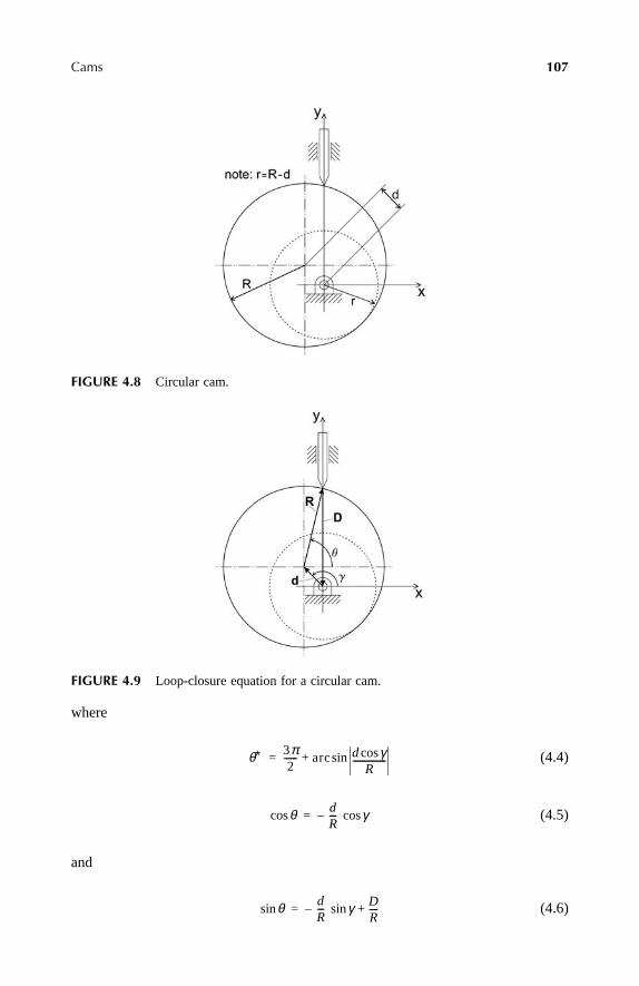
Cams
107
where
(4.4)
(4.5)
and
(4.6)
FIGURE 4.8
Circular cam.
FIGURE 4.9
Loop-closure equation for a circular cam.
θ∗ 3π2
------ arc d γcosR
---------------sin+=
θcos dR--- γcos–=
θsin dR--- γ D
R----+sin–=
Ch4Frame Page 107 Friday, June 2, 2000 6:41 PM

108
Fundamentals of Kinematics and Dynamics of Machines and Mechanisms
If, at the extreme,
d = R
, then Equation 4.2 gives . It followsfrom the above that the correct sign in Equation 4.2 must be plus for this case. Atthe other extreme, if
d << R
, then the second term under the square root can beneglected and the result is . Again, the correct sign must be plus for
D
to be positive. Thus, one can assume that the sign in Equation 4.2 must be plusfor any value of
d
.
(4.7)
In Figure 4.10 the position of the follower,
D
, is shown for one cycle of camrotation for the case of
d
= 1 cm and
R
= 4 cm. The difference between the maximumfollower displacement and its minimum is called the
lift
. If the minimum followercoordinate (position) is subtracted from its current position, the resulting diagram
FIGURE 4.10
Position of the follower during one cycle of circular cam rotation.
FIGURE 4.11
Displacement diagram for a circular cam.
1 2 3 4 5 6γ
1
2
3
4
5D
1 2 3 4 5 6γ
1
2
3
4
5u
D R θ R θsin±sin=
D d γ R±sin=
D d γ R2 d2 γ2cos–+sin=
Ch4Frame Page 108 Friday, June 2, 2000 6:41 PM

Cams 109
is called the displacement diagram. Such a diagram for a circular cam is shown inFigure 4.11.
A minimum follower position constitutes a reference level for the followerdisplacement. This reference level is a circle with a constant radius ,which is called the base radius. Thus, a cam profile can be viewed as a displacementdiagram wrapped around the base circle.
4.3 DISPLACEMENT DIAGRAM
The displacement diagram serves as an input into the cam mechanism design.Consider the cam mechanism in Figure 1.1. The function of the cam might be, asis the case in the internal combustion engine, to open the valve, to keep it openduring some part of the cycle (this is called dwell), and then to close it and to keepit closed for some time (to dwell again). A generic displacement diagram may lookas shown in Figure 4.12. The requirements of how long it should take to rise, todwell, to return, and to dwell again, and also of what the lift should be define thesize and the shape of the cam. The function depicted in Figure 4.12 is a piecewisefunction, which means that special attention should be paid to transition from onecontinuous function to another, for example, from rise to dwell. This representsanother objective of cam design, to ensure a smooth transition of the follower fromone part of the displacement diagram to another.
Consider, for example, a transition from rise to dwell in Figure 4.12. The risecurve is described by some function , while the dwell is described by anotherfunction . For a smooth transition from the rise to dwell, it is neededthat at ,
(4.8)
Since θ = ωt (where ω is the angular velocity of the cam, and t is the time),the requirements for the equality of first and second derivatives is equivalent to therequirements that the velocity and acceleration of the follower does not experiencejumps at the point of transition. The same requirement should be met at the othertransitional points in Figure 4.12: , , and . These latterrequirements put limitations on what type of functions can be used to generate the
FIGURE 4.12 Typical displacement diagram.
r b D= Dmin–
u1 θ( )u2 θ( ) const=
θ θA=
u1 θA( ) u2 θA( )du1 θ( )
dθ----------------, 0 and
d2u1 θ( )dθ2
-------------------, 0= = =
θ 0= θ θB= θ θC=
Ch4Frame Page 109 Friday, June 2, 2000 6:41 PM

110 Fundamentals of Kinematics and Dynamics of Machines and Mechanisms
cam profile for a given displacement diagram. The requirements (Equation 4.8) arecalled smoothness requirements.
4.4 CYCLOID, HARMONIC, AND FOUR-SPLINE CAMS
Any function that meets the type of requirements given in Equation 4.8 is a suitablecam profile function. For example, the suitable function for the rising part of thediagram must be tangential to the θ-axis at point 0 and at point A (Figure 4.13). Itmeans that it must change the curvature from concave to convex, and thus it musthave an inflection point. A few analytical functions are used to describe the rise andreturn parts of the displacement diagram while meeting the above smoothness con-ditions. These are cycloid, harmonic, and polynomial functions. In the following anapplication of all these functions to the displacement diagram design is considered.
A cycloid is a curve traced by a point on a circle rolling along a straight line.In Figure 4.14 an example of a cycloid function is shown, where point A is embeddedinto the circle, and angle α corresponds to arc αr, which is the distance traveled bythe circle. The x- and y-coordinates of the cycloid are parametric functions of angle α
(4.9)
and
(4.10)
Both functions can be used in cam profile design. A cam in which the first function,Equation 4.9, is used is called the cycloid cam, while a cam in which the secondfunction, Equation 4.10, is used is called the harmonic cam.
4.4.1 CYCLOID CAMS
The Rise Part of the Displacement Diagram
One can utilize the function given by Equation 4.9 to describe the rise of the followerfrom 0 to point A in Figure 4.13. Note that Equation 4.9 comprises two components:rα and –r sinα. Thus, it is a superposition of a straight line and a sinusoidal function.
FIGURE 4.13 Inflection points on the displacement diagram.
x r α αsin–( )=
y r 1 αcos–( )=
Ch4Frame Page 110 Friday, June 2, 2000 6:41 PM
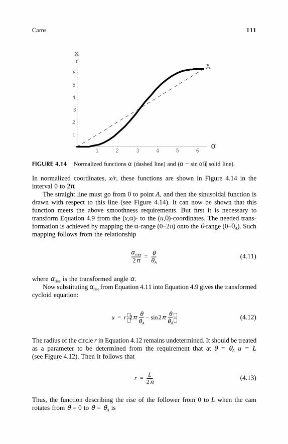
Cams 111
In normalized coordinates, x/r, these functions are shown in Figure 4.14 in theinterval 0 to 2π.
The straight line must go from 0 to point A, and then the sinusoidal function isdrawn with respect to this line (see Figure 4.14). It can now be shown that thisfunction meets the above smoothness requirements. But first it is necessary totransform Equation 4.9 from the (x,α)- to the (u,θ)-coordinates. The needed trans-formation is achieved by mapping the α-range (0–2π) onto the θ-range (0–θA). Suchmapping follows from the relationship
(4.11)
where αrise is the transformed angle α.Now substituting αrise from Equation 4.11 into Equation 4.9 gives the transformed
cycloid equation:
(4.12)
The radius of the circle r in Equation 4.12 remains undetermined. It should be treatedas a parameter to be determined from the requirement that at θ = θA u = L(see Figure 4.12). Then it follows that
(4.13)
Thus, the function describing the rise of the follower from 0 to L when the camrotates from θ = 0 to θ = θA is
FIGURE 4.14 Normalized functions α (dashed line) and (α − sin α) (solid line).
1 2 3 4 5 6α
1
2
3
4
5
6
xr—
A
α rise
2π---------- θ
θA
-----=
u r 2π θθA
----- 2π θθA
-----sin– =
rL
2π------=
Ch4Frame Page 111 Friday, June 2, 2000 6:41 PM

112 Fundamentals of Kinematics and Dynamics of Machines and Mechanisms
(4.14)
Now, check that the requirements given by Equation 4.8 are met. The first and secondderivatives of the function Equation 4.14 are
(4.15)
and
(4.16)
It is easy to see that both derivatives are equal to zero at θ = 0 and θ = θA.
The Return Part of the Displacement Diagram
Now, one can utilize the same function given by Equation 4.9 to describe the returnof the follower from θB to θC in Figure 4.13. The procedure is the same. One mapsthe α-range (0 to 2π) onto the θ-range (θB to θC). The coordinate transformation inthis case is
(4.17)
where αreturn is the transformed angle α.Since the expression for r is known (see Equation 4.13), the return part of the
displacement diagram is described by Equation 4.12, where angle α is, accordingto Equation 4.17,
(4.18)
The first and second derivatives in this case are as follows:
(4.19)
and
(4.20)
u1L
2π------ 2π θ
θA
----- 2π θθA
-----sin– =
du1
dθ--------
LθA
----- 1 cos 2π θθA
-----– =
d2u1
dθ2----------
2πL
θA2
---------- 2π θθA
-----sin=
α return
2π--------------
θ θC–θB θC–-----------------=
u3L
2π------ 2π
θ θC–θB θC–----------------- 2π
θ θC–θB θC–-----------------sin–
=
du3
dθ--------
LθB θC–----------------- 1 cos 2π
θ θC–θB θC–-----------------–
=
d2u3
dθ2----------
2πL
θB θC–( )2------------------------ 2π
θ θC–θB θC–-----------------sin=
Ch4Frame Page 112 Friday, June 2, 2000 6:41 PM

Cams 113
It is easy to check that at θ = θC and θ = θB both derivatives are equal to zero.Thus, the cycloid function can be used to describe the cam profile and satisfy thesmoothness requirements. An example of the normalized displacement diagram forθA = π/2, θB = 5π/4, and θC = 7π/4 is shown in Figure 4.15. In Figures 4.16 and 4.17the corresponding normalized velocity and acceleration diagrams are shown. Thenormalized displacements, velocities, and accelerations are, respectively, as follows:
On the rise part:
(4.21)
(4.22)
(4.23)
On the return part:
(4.24)
(4.25)
(4.26)
FIGURE 4.15 Normalized displacement diagram for a cycloid cam.
1 2 3 4 5 6θ
0.2
0.4
0.6
0.8
1
uL—
u1uL---=
u1˙ uθA
L---------=
u1˙ uθA
2
L---------=
u3uL---=
u3˙ u θB θC–( )
L-------------------------=
u3˙ u θB θC–( )2
L---------------------------=
Ch4Frame Page 113 Friday, June 2, 2000 6:41 PM

114 Fundamentals of Kinematics and Dynamics of Machines and Mechanisms
It is denoted above:
and
The displacement, velocity, and acceleration of the follower, shown in Figures 4.15through 4.17, are functions of the angle of rotation of the cam, and thus they do notdepend on the angular speed of rotation. The displacement as a function of the angleof rotation allowed one to find a proper cam profile. It does not, however, answerthe question of what is the real acceleration of the follower, which one has to knowto choose the proper spring stiffness (see Figure 4.1). If one substitutes the angle ofrotation into Equations 4.14 and 4.18, one will have displacements asfunctions of time and angular velocity ω.
(4.27)
FIGURE 4.16 Normalized velocity diagram for a cycloid cam.
FIGURE 4.17 Normalized acceleration diagram for a cycloid cam.
1 2 3 4 5 6θ
0.5
1
1.5
2
Velocity
1 2 3 4 5 6θ
-6
-4
-2
2
4
6
Acceleration
udu θ( )
dθ--------------= u
d2u θ( )dθ2
----------------=
θ ωt=
u1L
2π------ 2π ωt
θA
------ 2π ωtθA
------sin– =
Ch4Frame Page 114 Friday, June 2, 2000 6:41 PM

Cams 115
and
(4.28)
where for a single cycle the time t changes from 0 to T, and T = 2π/ω is the periodof the cycle.
It is clear from Equations 4.17 through 4.28 that the displacement of the followerdoes not depend on the angular velocity of the cam. However, the velocity andacceleration of the follower do depend on it. Indeed, the velocity of the follower asa function of time is proportional to ω, since
(4.29)
and is the velocity as the function of the angle of rotation. Similarly,assuming that the angular velocity is constant, the acceleration of the follower isproportional to the square of angular velocity, since
(4.30)
Because the angular velocity of the cam is a scaling factor in both velocity andacceleration of the follower, the solutions given by Equations 4.12 through 4.20 aregeneral solutions of the kinematics of the cycloid cam. In this respect, the plots ofthe follower displacement (Figure 4.15), velocity (Figure 4.16), and acceleration(Figure 4.17), except for the specific values of the angles θA, θB, and θC mentionedabove, are generic plots characterizing the cycloid cam.
4.4.2 HARMONIC CAMS
Now it will be shown that Equation 4.10 can also be used to describe the cam profileand it meets the requirement of smoothness. The plot of the function given byEquation 4.10 in normalized, y/r, coordinates over the interval 0 to 2π is shown inFigure 4.18.
As can be seen, a part of this function within the interval 0 to π can be used forthe rise part of the displacement diagram, whereas the second part, within the intervalπ to 2π for the return part of the diagram.
Again, points θA, θB, and θC (see Figure 4.12) will be used as transition pointsfrom one continuous function to another on a cam displacement diagram. However,in this case the 0 to θA interval will be mapped on 0 to π and θB to θC on π to 2πof the harmonic function. The corresponding mapping relationships are similar toEquations 4.11 and 4.17 except, instead of 2π, a π is used in both. Thus, thedisplacements of the follower during the rise and return parts of the cycle are obtainedfrom Equation 4.10 by substituting corresponding expressions for α
u3L
2π------ 2π
ωt θC–θB θC–------------------ 2π
ωt θC–θB θC–------------------sin–
=
du θ t( )[ ]dt
---------------------du θ t( )[ ]
dθ----------------------- dθ t( )
dt------------- du θ[ ]
dθ--------------ω= =
du θ[ ] dθ( )⁄
d2u θ t( )[ ]dt2
----------------------- ω ddt----- du θ t( )[ ]
dθ-----------------------
ω2d2u θ[ ]dθ2
----------------= =
Ch4Frame Page 115 Friday, June 2, 2000 6:41 PM

116 Fundamentals of Kinematics and Dynamics of Machines and Mechanisms
(4.31)
and
(4.32)
Now the corresponding displacement formulas are as follows:
(4.33)
and
(4.34)
It is easy to check that at θ = θA and θ = θB, u = L, whereas at θ = θC, u = 0. Thenormalized displacement diagram is shown in Figure 4.19.
Now, one can check whether the smoothness requirements are satisfied. The firstand the second derivatives of the function Equation 4.10 are r sin α and r cos α,respectively. For the rise part, α from Equation 4.31 is substituted, and for the returnone, α from Equation 4.32 is substituted for both derivatives. One can see that atboth points A and B (see Figure 4.12) the velocities are equal to zero, while accel-erations are not. Thus, the harmonic cam does not satisfy all the smoothness require-ments. The jump in acceleration while passing through these points means a jumpin inertial forces. For high-speed cams when there are design constraints on forcesor noise, this cam may not be acceptable.
FIGURE 4.18 Function 1 – cos α.
1 2 3 4 5 6α
0.5
1
1.5
2
yr—
α rise π θθA
-----=
α return πθ θC–θB θC–-----------------=
u1L2--- 1 cosπ θ
θA
-----– =
u3L2--- 1 cosπ
θ θC–θB θC–-----------------–
=
Ch4Frame Page 116 Friday, June 2, 2000 6:41 PM

Cams 117
In Figure 4.20 the normalized velocity and in Figure 4.21 the normalized accel-eration plots are shown. These plots confirm that there is a jump in accelerations atthe end of the rise and the beginning of the return. One can also see the amount ofthis jump in normalized coordinates. The normalization of displacements, velocities,and accelerations in this case is as for a cycloid cam (Equations 4.21 through 4.26).
4.4.3 COMPARISON OF TWO CAMS: CYCLOID VS. HARMONIC
Here the kinematic properties of two cams are compared: displacements, velocities,and accelerations in the same normalized coordinates. The displacements are shownin Figure 4.22. One can see that the displacement curves in Figure 4.22 looksufficiently close. However, the differences at specific angles may be significant.One can check the displacements, for example, at θ = θA/4. They are 0.0908451 and0.146447 for the cycloid and harmonic cams, respectively; i.e., the difference is 38%.
FIGURE 4.19 Normalized displacement diagram for a harmonic cam.
FIGURE 4.20 Normalized velocity plot for a harmonic cam.
1 2 3 4 5 6θ
0.2
0.4
0.6
0.8
1
uL—
1 2 3 4 5 6θ
0.25
0.5
0.75
1
1.25
1.5
Velocity
Ch4Frame Page 117 Friday, June 2, 2000 6:41 PM

118 Fundamentals of Kinematics and Dynamics of Machines and Mechanisms
It is also of interest to compare the accelerations of two cams at this point. They are6.28319 and 3.48943 for the cycloid and harmonic cams, respectively; i.e., thedifference is 45%. The velocities differ most significantly at the inflection pointθ = θA/2. They are 2 and 1.57 for the cycloid and harmonic cams, respectively.
The comparison of normalized velocities and accelerations for the cycloid andharmonic cams are shown in Figures 4.23 and 4.24.
4.4.4 CUBIC SPLINE CAMS
The cubic spline method of designing cams is based on using cubic polynomials tofit a given displacement diagram at a predetermined number of points. This methodis used for designing nonstandard cams. In general, the design of cams based on thisapproach requires a numerical solution of a system of linear algebraic equations. Thisbook will limit itself to a simplified version of the method, which retains all theconceptual elements of it but is more manageable from the analytical point of view.
FIGURE 4.21 Normalized acceleration plot for a harmonic cam.
FIGURE 4.22 Comparison of normalized displacement diagrams for two cams: cycloid(solid line) and harmonic (dashed line).
1 2 3 4 5 6θ
-4
-2
2
4
Acceleration
1 2 3 4 5 6θ
0.2
0.4
0.6
0.8
1
uL—
Ch4Frame Page 118 Friday, June 2, 2000 6:41 PM

Cams 119
One can design a displacement diagram comprising six piecewise continuousfunctions, which are identified in Figure 4.25 by numbers. The first two, 1 and 2, arecubic splines describing the rise, the constant function 3 describes the dwell, the nexttwo, 4 and 5, describe the return, and 6 is again a constant describing the dwell. It isnecessary to find such cubic polynomials that meet the smoothness criteria for the cam.
The general form of the cubic polynomial is
(4.35)
where ai, bi, ci, and hi are constants to be determined for each spline. In total, forfour splines there are 16 unknown constants. For each spline, one may request thatit meet the displacement, velocity, and acceleration requirements at its boundaries(in this case at points: 0, 0.5θA, θA, θB, and 0.5 (θB+ θC)). For each boundary (interfaceof two piecewise functions), one will have three equations defining the smoothness
FIGURE 4.23 Comparison of normalized velocity diagrams for two cams: cycloid (solidline) and harmonic (dashed line).
FIGURE 4.24 Comparison of normalized acceleration diagrams for two cams: cycloid(solid line) and harmonic (dashed line).
1 2 3 4 5 6θ
0.5
1
1.5
2
Velocity
1 2 3 4 5 6θ
-6
-4
-2
2
4
6
Acceleration
ui aiθi3 biθi
2 ciθi hi i =1, 2, 4, 5 + + +=
Ch4Frame Page 119 Friday, June 2, 2000 6:41 PM

120 Fundamentals of Kinematics and Dynamics of Machines and Mechanisms
requirements. In total, for six boundaries, there will be 18 requirements. For 16unknown constants there is need for only 16 equations, which means that not allsmoothness requirements will be satisfied. Thus, there is a freedom to choose whichsmoothness requirements to satisfy when using the cubic polynomial splines.
First, write down the first and second derivatives for the polynomial given byEquation 4.35. As before, they represent the velocity and acceleration of the followerin normalized (with respect to the angular velocity) coordinates.
(4.36)
and
(4.37)
Now, consider spline 1 in Figure 4.25, and assume that at θ = 0, the displacement,velocity, and acceleration are zeros.
(4.38)
and that at θ = 0.5θA the displacement is equal to 0.5L:
(4.39)
This gives four equations, which is sufficient to find four constants for the first spline.Similarly, for the second spline, if one declares that at θ = θA the displacement,
velocity, and acceleration are, respectively,
(4.40)
FIGURE 4.25 Piecewise continuous functions describing a displacement diagram.
ui 3aiθi2 2biθi ci i =1, 2, 4, 5 + +=
ui 6aiθi 2bi i =1, 2, 4, 5 +=
u1 0( ) 0du1 θ( )
dθ------------------ 0 and,=
d2u1 θ( )
dθ2---------------------- = 0 ,=
u1 θ( ) L2---=
u2 θ( ) Ldu2 θ( )
dθ------------------ 0 and,=
d2u2 θ( )
dθ2---------------------- = 0 ,=
Ch4Frame Page 120 Friday, June 2, 2000 6:41 PM

Cams 121
and that at θ = 0.5θA the displacement is equal to 0.5L:
(4.41)
there will be four equations needed to find four constants for the second spline.Before finding the spline constants, it is worth making two comments. First, at
the inflection point θ = 0.5θA the requirement of equal displacements only is satisfied;the equality of velocities and accelerations is not guaranteed. The second point ismore technical. Namely, if the rise part of the displacement diagram is approximatedwith two splines only, the system of equations defining constants can be decoupled.In other words, one can find these constants for each spline independently. Thedecoupling is achieved by specifying the boundary conditions for the splines asabove. If, however, one requested that at θ = 0, u1 = 0 and at θ = θA, u2 = L, and atθ = 0.5θA
(4.42)
and
(4.43)
then the equations for two splines would be coupled. Moreover, now the smoothnessrequirements would be met at the inflection point, and not guaranteed at θ = 0 andat θ = θA.
Only the first case, when the smoothness is satisfied at θ = 0, θ = θA, θ = θB,and θ = θC, will be discussed.
From Equations 4.38 it follows that b1 = c1 = h1 = 0, and from Equation 4.39,the last unknown is found:
(4.44)
Thus, the first spline is described by the formula:
(4.45)
For the second spline from Equations 4.40, it follows that
(4.46)
u2 θ( ) L2---=
du1 θ( )dθ
------------------du2 θ( )
dθ------------------=
d2u1 θ( )dθ2
--------------------d2u2 θ( )
dθ2--------------------=
a14L
θA3
------=
u1 4Lθ3
θA3
-----=
b2 3a2θA c2,– 3a2θA2 and h2, L a2θA
3–= = =
Ch4Frame Page 121 Friday, June 2, 2000 6:41 PM

122 Fundamentals of Kinematics and Dynamics of Machines and Mechanisms
and from Equation 4.41,
(4.47)
Thus, the second spline is described by the formula:
(4.48)
The boundary conditions for the fourth spline at θ = θB are
(4.49)
and at is
(4.50)
Satisfying the first set of boundary conditions, Equations 4.49 gives the expressionsfor the three constants:
(4.51)
Satisfying the fourth boundary condition, Equation 4.50 gives the expression for a4:
(4.52)
Thus the formula for the fourth spline is
(4.53)
The boundary conditions for the fifth spline at θ = θC are
(4.54)
and at is
(4.55)
a24L
θA3
------=
u2 4LθθA
----- 3
3θθA
----- 2
3θθA
----- +– 3L–=
u4 θ( ) L ,du4 θ( )
dθ------------------ 0 and,=
d2u4 θ( )
dθ2---------------------- = 0 =
θ θB θC+( ) 2⁄=
u4 θ( ) L2---=
b4 3a4θB c4,– 3a4θB2 and h4, L a4θB
3–= = =
a44L
θB θC–( )3------------------------=
u4 L4Lθ3
θB θC–( )3------------------------ –
12LθBθ2
θB θC–( )3------------------------ +
12LθB2θ
θB θC–( )3------------------------ –
4LθB3
θB θC–( )3------------------------+=
u5 θ( ) = 0, du5 θ( )
dθ------------------ 0 and
d2u5 θ( )dθ2
--------------------, 0= =
θ θB θ+ C( ) 2⁄=
u5 θ( ) L2---=
Ch4Frame Page 122 Friday, June 2, 2000 6:41 PM

Cams 123
Satisfying the first set of boundary conditions, Equation 4.54 gives the expressionsfor the three constants:
(4.56)
Satisfying the fourth boundary condition, Equation 4.55 gives the expression for a5:
(4.57)
As a result, the formula for the fifth spline is
(4.58)
The displacement diagram thus is described by the following piecewise function:
(4.59)
The velocities and acceleration functions are obtained by differentiating u(θ). Thus,
(4.60)
and, correspondingly,
(4.61)
b5 3a5θC c5,– 3a5θC2 and h5, a5θC
3–= = =
a54L
θB θC–( )3------------------------=
u5 4Lθ3
θB θC–( )3------------------------ –
3θCθ2
θB θC–( )3------------------------ +
3θC2 θ
θB θC–( )3------------------------ –
θC3
θB θC–( )3------------------------=
u θ( )
u1 if 0 θ 0.5θA<≤u2 if 0.5θA θ θA<≤L if θA θ θB<≤u4 if θB θ 0.5 θB θC+( )<≤u5 if 0.5 θB θC+( ) θ θC<≤0 if θC θ 2π<≤
=
du θ( )dθ
----------------
u1 if 0 θ 0.5θA<≤u2 if 0.5θA θ θA<≤0 if θA θ θB<≤u4 if θB θ 0.5 θB θC+( )<≤u5 if 0.5 θB θC+( ) θ θC<≤0 if θC θ 2π<≤
=
d2u θ( )dθ2
------------------
u1 if 0 θ 0.5θA<≤u2 if 0.5θA θ θA<≤0 if θA θ θB<≤u4 if θB θ 0.5 θB θC+( )<≤u5 if 0.5 θB θC+( ) θ θC<≤0 if θC θ 2π<≤
=
Ch4Frame Page 123 Friday, June 2, 2000 6:41 PM

124 Fundamentals of Kinematics and Dynamics of Machines and Mechanisms
The normalized displacements for a spline cam are the same as given by Equation4.21. The normalized velocities and accelerations for a spline cam are, respectively,as follows:
On the rise part:
(4.62)
(4.63)
On the return part:
(4.64)
(4.65)
In Figure 4.26 the normalized displacement diagram of a four-spline cam is shown,in Figure 4.27 the normalized velocity diagram of a four-spline cam is shown, andin Figure 4.28 the normalized acceleration diagram of a four-spline cam is shown.
One can see that if the displacements are described by the cubic polynomials(Equation 4.27), the velocities are quadratic functions and accelerations are straightlines (Figure 4.28). The jump in acceleration at the two inflection points is seen inFigure 4.28.
4.4.5 COMPARISON OF TWO CAMS: CYCLOID VS. FOUR-SPLINE
Here the kinematic properties of displacement diagrams for two cams in normalizedcoordinates will be compared. The comparison is shown in Figures 4.29 through 4.31for the displacement, velocity, and acceleration diagrams.
One can see that the normalized displacement curves in Figure 4.29 look suffi-ciently close. However, the displacements, for example, at θ = π/4 are 0.0908451and 0.0625 for the cycloid and spline cams, respectively; i.e., the difference is 31%.It is of interest to compare the velocities and accelerations for two cams at theinflection point θ = θA/4. The normalized velocities are 2 and 1.5, and the acceler-ations are 0 and 6, for the cycloid and four-spline cams, respectively.
There are two lessons one should learn from the comparison of cams: first, thatthe displacement diagram is not sufficient to assess the cam performance and, second,that relatively small errors in the displacement diagram might result in significantmisjudgment of velocities and accelerations.
u1˙ u2
˙=uθA
2L---------=
u1˙ u2
˙=uθA
2
4L---------=
u4˙ u5
˙=u θB θC–( )
2L-------------------------=
u4˙ u5
˙=u θB θC–( )2
4L---------------------------=
Ch4Frame Page 124 Friday, June 2, 2000 6:41 PM

Cams 125
FIGURE 4.26 Normalized displacement diagram for a four-spline cam.
FIGURE 4.27 Normalized velocity diagram for a four-spline cam.
FIGURE 4.28 Normalized acceleration diagram for a four-spline cam.
1 2 3 4 5 6θ
0.2
0.4
0.6
0.8
1
uL—
1 2 3 4 5 6θ
0.25
0.5
0.75
1
1.25
1.5
1.75
2Velocity
1 2 3 4 5 6θ
-3
-2
-1
1
2
3
Acceleration
Ch4Frame Page 125 Friday, June 2, 2000 6:41 PM

126 Fundamentals of Kinematics and Dynamics of Machines and Mechanisms
FIGURE 4.29 Comparison of normalized displacement diagrams for two cams: cycloid(solid line) and four-spline (dashed line).
FIGURE 4.30 Comparison of normalized velocity diagrams for two cams: cycloid (solid line)and four-spline (dashed line).
FIGURE 4.31 Comparison of normalized acceleration diagrams for two cams: cycloid(solid line) and four-spline (dashed line).
1 2 3 4 5 6θ
0.2
0.4
0.6
0.8
1
uL—
1 2 3 4 5 6θ
-6
-4
-2
2
4
6
Acceleration
Ch4Frame Page 126 Friday, June 2, 2000 6:41 PM

Cams 127
4.5 EFFECT OF BASE CIRCLE
The expression for the position of the follower:
(4.66)
shows that its velocity and acceleration do not depend on the base radius rb. However,a corresponding point on the cam does depend on this radius. Indeed, a point on thecam profile is characterized by the vector:
(4.67)
and the corresponding velocity vector is (see Chapter 2)
(4.68)
The first term in Equation 4.68 represents the translational component of thevelocity vector, and it is equal to the follower velocity. The second term representsthe angular (tangential with respect to the follower) component of the cam velocityvector. The follower does not have this component. It means that the tangentialvelocity is associated with the velocity of sliding of the follower along the cam profile.Although it does not affect the kinematics of motion transfer, it is important in thewear analysis of cams with knife or flat-faced followers since wear is proportionalto the coefficient of friction, the normal contact force, and the velocity of sliding.
So, as far as the kinematics is concerned, the base circle is not important. It isimportant, however, from the geometric point of view, namely, to allow a properinteraction between the cam and the follower, especially a flat-faced one. Look at theprofiles of two cams having identical harmonic displacement diagrams wrappedaround different base circles: one with rb = 0.5L (Figure 4.32), and another withrb = 2L (Figure 4.33). One can see that in Figure 4.32 the curvature of the cam profileat θ = 0 and θ = θC (see Figure 4.12) is concave, and thus the flat-faced follower, andeven the roller follower, may not be able to follow the profile around these points(the follower will ride over the “ditch”). The situation can be improved by increasingthe base circle, as shown in Figure 4.33. However, the base circle increase, as isknown, leads to the increase of the sliding velocity. In addition, the cam size mustconform to dimensional constraints of the design. Thus, a compromise between thekinematic requirements and overall design considerations must be reached.
4.6 PRESSURE ANGLE
The angle between the normal to the cam profile and the axis of the follower is calledthe pressure angle (Figure 4.34). This angle affects the transverse force Ft, creatinga bending moment on the follower (note that in Figure 4.34 forces shown are actingon the cam). Thus, it is desirable to keep this angle within an acceptable minimum.The point is that the pressure angle is a function of θ, and so this function should beinvestigated for its maximum. But, first, the function itself should be derived.
D θ( ) r b u θ( )+=
r D D θ( ) θ θsin,cos[ ] T=
rD D θ( ) θ θsin,cos[ ] T D θ( ) θ π 2⁄+( ) θ π 2⁄+( )sin,cos[ ] T+=
Ch4Frame Page 127 Friday, June 2, 2000 6:41 PM
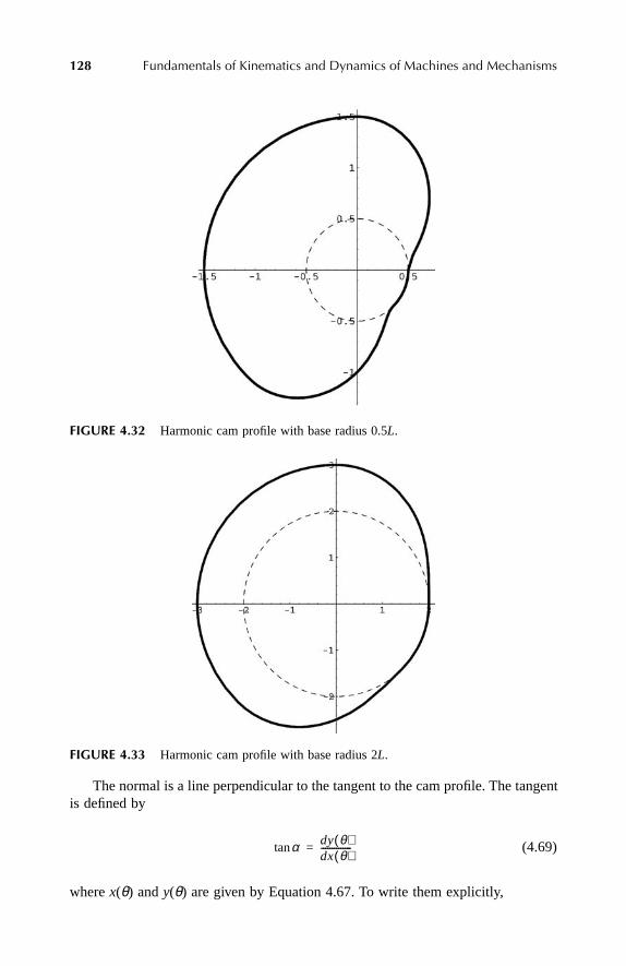
128 Fundamentals of Kinematics and Dynamics of Machines and Mechanisms
The normal is a line perpendicular to the tangent to the cam profile. The tangentis defined by
(4.69)
where x(θ) and y(θ) are given by Equation 4.67. To write them explicitly,
FIGURE 4.32 Harmonic cam profile with base radius 0.5L.
FIGURE 4.33 Harmonic cam profile with base radius 2L.
αtan dy θ( )dx θ( )--------------=
Ch4Frame Page 128 Friday, June 2, 2000 6:41 PM

Cams 129
(4.70)
and
(4.71)
By differentiating both x(θ) and y(θ) with respect to θ, an explicit expression fortan α is obtained:
(4.72)
The angle α is measured from the positive direction of the x-axis to the positivedirection of the tangent vector. The positive direction of the latter is counterclockwise(see Figure 4.35) in accordance with the right-hand coordinate system. The correct
FIGURE 4.34 Pressure angle and forces acting on the cam.
FIGURE 4.35 Tangential and normal to the cam profile.
x θ( ) D θ( ) θcos=
y θ( ) D θ( ) θsin=
αtan D θ( ) θsin D θ( ) θcos+
D θ( ) θcos D– θ( ) θsin---------------------------------------------------------=
Ch4Frame Page 129 Friday, June 2, 2000 6:41 PM

130 Fundamentals of Kinematics and Dynamics of Machines and Mechanisms
angle α is chosen based on the signs of sin α and cos α which are proportional tody and dx, respectively; see Equation 4.69. Thus, the expressions for dy and dx aredefined by Equation 4.72.
Defining the principal angle α as
(4.73)
the correct angle is subject to the signs of sin α and cos α,
(4.74)
The positive direction of the normal vector is then as indicated in Figure 4.35; i.e.,the tangent is rotated counterclockwise by π/2. Thus,
(4.75)
The pressure angle ϕ, as is clear from Figure 4.35, is equal to
(4.76)
Thus, for every angle θ the angle α is found from Equation 4.72 subject to Equation 4.74,and then the pressure angle ϕ from Equation 4.76.
Consider now how the pressure angle changes over the cycle of rotation for thecycloid, harmonic, and four-spline cams. The corresponding plots are shown inFigures 4.36 through 4.38 for the case when rb/L = 10, and θA = π/2, θB = 5π/4, andθC = 7π/4 (see Figure 4.13). As can be seen, the pressure angle reaches maximumat the inflection point for all three cams. Also, the maximums of the pressure anglesare sufficiently close for the three types of cams designed to the same specifications.
An important point is the effect of the base circle radius on the pressure angle.As is seen from Equations 4.66 and 4.73, the pressure angle depends nonlinearly onthis radius. Thus, in each particular case the relationship between the two must beinvestigated to optimize the design. In Figure 4.39 a comparison of two pressureangle plots is shown for two cases: rb/L = 10 and rb/L = 2. One can see that theeffect of the base radius is profound.
In summarizing the effect of the base circle radius on the cam mechanism design,it should be stated that
1. It does not affect the kinematics of motion transfer as long as the cam profileremains convex.
α∗ arc AbsD θ( ) θsin D θ( ) θcos+
D θ( ) θcos D– θ( ) θsin---------------------------------------------------------
tan=
α
α∗ if dx 0> and dy 0>π α– ∗ if dx 0< and dy 0>π α+ ∗ if dx 0< and dy 0<2π α– ∗ if dx 0> and dy 0<
=
β α π 2⁄+=
ϕ θ( ) β θ( ) θ π+( )– α θ( ) θ– π 2⁄–= =
Ch4Frame Page 130 Friday, June 2, 2000 6:41 PM

Cams 131
FIGURE 4.36 Variation of the pressure angle ϕ during the cycle of cycloid cam rotation.
FIGURE 4.37 Variation of the pressure angle ϕ during the cycle of harmonic cam rotation.
FIGURE 4.38 Variation of the pressure angle ϕ during the cycle of four-spline cam rotation.
1 2 3 4 5 6θ
-0.15
-0.1
-0.05
0.05
0.1
0.15
ϕ
1 2 3 4 5 6θ
-0.15
-0.1
-0.05
0.05
0.1
0.15
ϕ
1 2 3 4 5 6θ
-0.1
-0.05
0.05
0.1
ϕ
Ch4Frame Page 131 Friday, June 2, 2000 6:41 PM

132 Fundamentals of Kinematics and Dynamics of Machines and Mechanisms
2. Its increase leads to the reduction of the parasitic transverse force on the recip-rocating follower, and has no effect on the oscillating one.
3. Its increase leads to the increase of sliding velocity between the cam and knife-edge or flat-faced followers, and to the increase of the angular rotation of theroller in roller-type followers.
As can be seen, the base radius must be optimized based on various design consider-ations, including size constraints.
PROBLEMS AND EXERCISES
PROBLEMS
1. For a given cam, will the choice of the type of follower (knife-edge, flat-faced,roller) affect the displacement diagram?
2. For a circular cam with parameters R and d (Figure 4.8), what are the minimumand maximum displacements of the follower?
3. If in Figure 4.8, instead of a knife-edge follower, a flat-faced follower is to beused, would the displacement diagrams for both designs be identical? And, ifnot, what would be the difference?
4. Solve Equation 4.1
for the two unknowns: θ and D.
FIGURE 4.39 Variation of the pressure angle ϕ during the cycle of cycloid cam rotationfor two normalized base radii: rb/L = 10 (solid line) and rb/L = 2 (dashed line).
1 2 3 4 5 6θ
-0.6
-0.4
-0.2
0.2
0.4
0.6
ϕ
d γ γsin,cos[ ] T R θ θsin,cos[ ] T D3π2
------ 3π
2------
sin,cosT
+ + 0=
Ch4Frame Page 132 Friday, June 2, 2000 6:41 PM

Cams 133
5. The displacement diagram for a cam comprises rise, dwell, and return parts ofthe cycle. If the transition from one part to another is not smooth (while thecontinuity of displacements is guaranteed, the continuity of accelerations is not),will it make this cam unacceptable from a functional point of view? Explain.
6. Take a function describing the cycloidal cam, and construct adisplacement diagram with rise from 0 to π/2, dwell from π/2 to π, and returnfrom π to 2π. Take that the lift L = 1 cm. Find the maximum accelerations.
7. Take a function describing the harmonic cam and construct adisplacement diagram with rise from 0 to π/2, dwell from π/2 to π, and returnfrom π to 2π. Assume lift L = 1 cm. Find the maximum accelerations and atthe transitions from one part to another: π/2, π, and 2π.
8. The displacement diagram comprises rise, dwell, and return parts. Assumingthat the rise and return parts are to be approximated by cubic spline functions,write the smoothness requirements for the transition from one cubic splinefunction to another. If the number of cubic spline functions to approximate therise part of the diagram is 2N, how many equations of smoothness can beformulated?
9. Use two cubic splines to describe the rising part of the displacement diagram(from 0 to π/2). Find all constants by satisfying smoothness requirements at 0(transition from dwell) and π/2 (transition to dwell), and the equality of dis-placements at the inflection point π/4.
10. A circular cam in Figure 4.9 rotates with the angular velocity ω.
a. What is the velocity of the follower for an arbitrary position of the cam?b. What is the velocity of a point on the cam interfacing the follower?
11. For the cams in Figures 4.1 and 4.2 show forces acting on cams from the follower,and also the pressure angles.
12. For a circular cam in Figure 4.9 find the expression for the pressure angle.
EXERCISES (PROJECTS) WITH MATHEMATICA
1. A circular cam has the d/R ratio 0.2 and rotates with 10 rad/s. Plot the displace-ment, velocity, and acceleration diagrams of the points on the cam and a knife-edge follower. Assume zero offset.
2. For a cycloidal cam described in Problem 4.6, plot the displacement, velocity,and acceleration diagrams of the points on the knife-edge follower.
3. For a harmonic cam described in Problem 4.7, plot the displacement, velocity,and acceleration diagrams of the points on the knife-edge follower.
4. Construct a displacement diagram, with rise from 0 to π/2, dwell from π/2 to π,and return from π to 2π, using two cubic splines to describe each, rise and return,parts of the diagram. Assume lift L = 1 cm. Satisfy the smoothness requirements
x r α αsin–( )=
x r 1 αcos–( )=
Ch4Frame Page 133 Friday, June 2, 2000 6:41 PM

134 Fundamentals of Kinematics and Dynamics of Machines and Mechanisms
at the transition points (boundaries), and the equality of displacements at theinflection points. Plot the displacement, velocity, and acceleration diagrams ofthe points on the knife-edge follower.
5. For the data in Problem 4.6, investigate the effect of the base radius on thepressure angle. Choose two to three values of the base radius.
6. For the data in Problem 4.7, investigate the effect of the base radius on thepressure angle. Choose two to three values of the base radius.
Ch4Frame Page 134 Friday, June 2, 2000 6:41 PM

135
5
Gears
5.1 INTRODUCTION
The kinematic function of gears is to transfer rotational motion from one shaft toanother. Since these shafts may be parallel, perpendicular, or at any other angle withrespect to each other, gears designed for any of these cases take different forms andhave different names
: spur, helical, bevel, worm
, etc
.
The fundamental requirement in most applications is that the coefficient ofmotion transformation (called the gear ratio) remains constant. What is needed tomeet this requirement follows from Kennedy’s theorem. The important point is thatthis requirement imposes a constraint on the suitable geometry of gear teeth profiles.Herein only one such profile is considered, called the
involute
profile.
5.2 KENNEDY’S THEOREM
The transformation of motion from one shaft to another involves three bodies: aframe (the position of each shaft is fixed in the frame) and two gears. Consider ageneral case when two disks with arbitrary profiles (Figure 5.1) represent gears 2and 3. Also assume that disk 2 rotates with the constant angular velocity
ω
2
. Themotion is transferred through the direct contact at point
P
(note that
P
2
and
P
3
arethe same point
P
, but the first is associated with disk 2 whereas the second isassociated with disk 3). The question is whether or not the angular velocity
ω
3
ofdisk 3 will also be constant, and, if not, what is needed to make it constant. Theanswer is given by Kennedy’s theorem.
Kennedy’s theorem identifies the fundamental property of three rigid bodies inmotion.
The three instantaneous centers shared by three rigid bodies in relative motionto one another all lie on the same straight line.
First, recall that the
instantaneous center of velocity
is defined as the instanta-neous location of a pair of coincident points of two different rigid bodies for whichthe absolute velocities of two points are equal. If one considers body 2 and the frame(represented by point
O
2
) in Figure 5.1, then the instantaneous center of these twobodies is point
O
2
, which belongs to the frame and to disk 2. The absolute velocitiesof both bodies at point
O
2
are zero. The same is valid for disk 3 and the framerepresented by point
O
3
. For the three bodies in motion there are three instantaneouscenters: for all combinations of pairs. Thus, there is an instantaneous center betweenthe two disks.
Look at Figure 5.1 again. Since point
P
is a common point for two disks, foreach disk the velocity component at this point directed along the common normalis the same and equal to
V
p
. One can move this velocity vector along the common
Ch5Frame Page 135 Friday, June 2, 2000 8:43 PM

136
Fundamentals of Kinematics and Dynamics of Machines and Mechanisms
normal until it intersects the line connecting the two instantaneous centers
O
2
and
O
3
at point
C
. According to Kennedy’s theorem, this point is the instantaneous centerof velocity for the two disks. Indeed, the velocity
V
p
, the only instantaneous commonvelocity for the two disks, is equal to
(5.1)
From the similarity of the triangles
AO
2
C
and
BO
3
C
it follows that
(5.2)
By using the above relationship, the ratio of angular velocities in Equation 5.1 isequal to
(5.3)
where
l
2
and
l
3
denote
O
2
C
and
O
3
C
, respectively (see Figure 5.1).Thus, velocity
V
c
in Figure 5.1 is a common velocity for the two disks since
(5.4)
FIGURE 5.1
Illustration of Kennedy’s theorem.
Vp ω2AO2 ω3BO3= =
AO2
BO3----------
CO2
CO3----------=
ω2
ω3------
l3
l2---=
Vc ω2l2 ω3l3= =
Ch5Frame Page 136 Friday, June 2, 2000 8:43 PM

Gears
137
Velocity
V
c
is also the absolute velocity of each body at this point because therecannot be another velocity component along the line
O
2
O
3
(since the distancebetween the frame points
O
2
and
O
3
is not changing, and bodies 2 and 3 are assumedto be rigid).
Note that the relative velocity of two disks at point
C
is zero, whereas at point
P
it is not.Equation 5.3 gives the transformation of angular velocities from disk 2 to disk 3.
As can be seen, in order for the kinematic ratio
ω
2
/ω
3
to remain constant distances
l
2
and
l
3
must not change. It is clear from Figure 5.1, however, that for arbitraryprofile shapes the common normal changes its direction during the motion, and thuspoint
C
moves along line
O
2
O
3
. Thus, the problem of meeting the constant ratiorequirement is to find such disk profiles that the kinematic ratio remains constant.It will be shown in the following that if the disk profile is described by the
involutefunction
, the common normal does not change its direction.
5.3 INVOLUTE PROFILE
An involute is generated by a tracing point on a cord as it is unwrapped from a circle(called a
base circle
) starting at
T
0
and ending at
T
1
(Figure 5.2). It is seen that points
A
and
B
are the instantaneous centers of rotation of the cord. It follows that the cordis normal to the involute at each point. This property is fundamental for the involuteprofiles to be used in gears. Indeed, consider two circular disks with centers at
O
2
and
O
3
(Figure 5.3). To each disk a plate with an involute profile is attached. The involuteson these plates are different since they are generated for different base circles, startingat points
D
2
and
D
3
. The two plates have a common point
C
and a common normal
AB
. This common normal is tangential to both base circles at any moment duringthe rotation while the two involutes are engaged. Line
AB
intersects the line ofcenters
O
2
O
3
at point
P
. It then follows from Kennedy’s theorem that this point isthe instantaneous center for the two circular disks. And since this point remains thesame while the disks rotate, it follows also that the kinematic ratio (called the
transmission ratio
)
ω
2
/ω
3
remains constant. Note that the common normal
AB
iscalled the
line of action
because the force is transmitted from one disk to anotheralong this line.
FIGURE 5.2
Illustration of the involute profile generation.
Ch5Frame Page 137 Friday, June 2, 2000 8:43 PM

138
Fundamentals of Kinematics and Dynamics of Machines and Mechanisms
5.4 TRANSMISSION RATIO
The transmission ratio is given by Equation 5.3 (recall that
l
2
and
l
3
are the distancesfrom the centers of rotation of each body to the instantaneous center for the twobodies). In the case of two gears, the instantaneous center for the two bodies is theintersection of the line of action with the line of centers
O
2
O
3
(Figure 5.4). Thisinstantaneous center is called the
pitch point
. The corresponding distances from thegear centers to this point are called the
pitch radii
(the corresponding diameters arethe
pitch diameters
). Thus, Equation 5.3 in the case of gears is
(5.5)
where
r
2
p
,
r
3
p
, and
d
2
p
, d
3
p
are the pitch radii and pitch diameters, respectively.
FIGURE 5.3
Illustration of the involute profiles interaction.
FIGURE 5.4
Illustration of the transmission ratio.
ω2
ω3------
r 3p
r 2p
-------d3p
d2p
-------= =
Ch5Frame Page 138 Friday, June 2, 2000 8:43 PM

Gears 139
The distance between any two similar points on the adjacent teeth along thepitch circle is called the circular pitch, and it is equal to
(5.6)
where N is the number of teeth. Substituting pitch diameters into Equation 5.5 usingEquation 5.6, and taking into account that the circular pitch is equal for the twomeshing gears, one finds that the transmission ratio can be expressed through theratio of teeth numbers:
(5.7)
It is seen from Equation 5.5 that the transmission ratio of two gears is equivalentto the transmission ratio of two cylindrical disks having a contact at one point, P,and rotating without sliding. Note that the smallest of two intermeshing gears iscalled a pinion.
5.5 PRESSURE ANGLE
The force generated between the two gears acts along the normal to the involuteprofile, i.e., along the line of action AB in Figure 5.4. This force is called the normalforce, Fn, and it can be resolved in two components (Figure 5.5): along the line ofcenters, O2O3, and perpendicular to it. The first component is called the radial force,Fr, and the second is called the tangential force, Ft. The two components of thenormal force are
(5.8)
FIGURE 5.5 Illustration of forces at the involute interface.
pπdp
N---------=
ω2
ω3------
N3
N2------=
Ft Fn φcos=
Ch5Frame Page 139 Friday, June 2, 2000 8:43 PM

140 Fundamentals of Kinematics and Dynamics of Machines and Mechanisms
and
(5.9)
In Equations 5.8 and 5.9 the angle φ is called the pressure angle, since it characterizesthe direction of the normal force between the conjugate teeth at the pitch point P.As follows from the similar triangles, O3BP and O2AP, in Figure 5.4, this angle isthe same for both gears since
(5.10)
The radial forces at the gear interface are parasitic forces since they are notassociated with energy transfer, whereas the tangential forces create the transmissiontorques, T2p and T3p
(5.11)
and
(5.12)
Since the normal force of interaction is the same for both gears and the angle φis also the same, the radial and tangential forces acting on two meshing gears arethe same. The torques, however, as can be seen from Equations 5.11 and 5.12, arenot equal. In fact, their ratio equals the transmission ratio:
(5.13)
The latter equation shows that the energy is conserved during the motion transmissionthrough the gears, since
(5.14)
In reality the energy is not conserved due to friction losses at the involute interface.It will be seen later that, except at the pitch point, the relative motion of two involutesinvolves rolling and sliding. The latter results in friction losses.
5.6 INVOLUTOMETRY
A gear can be seen as a disk of radius rb with teeth attached to it (Figure 5.6). Theinvolute curve for each tooth starts at the base circle with radius rb and ends on theaddendum circle with radius ra. It is clear that the number of teeth must be an integer.
Fr Fn φsin=
r 3
r 3p
-------r 2
r 2p
------- φcos= =
T2p Ftr 2p=
T3p Ftr 3p=
T3p
T2p
--------r 3p
r 2p
-------ω2
ω3------= =
Energy T3pω3 T2pω2= =
Ch5Frame Page 140 Friday, June 2, 2000 8:43 PM

Gears 141
If this number is chosen, then it defines the circular pitch, i.e., the distance betweenthe two similar points on two successive teeth along the pitch circle (see Figure 5.6and Equation 5.6). Some of this circular distance occupied by the tooth is called thetooth thickness, while the rest of it is called the width of space. Ideally, the widthof space should be equal to the tooth thickness of the engaging gear. Since thecircular pitch for the engaging gear must be the same, then the width of space ofone gear must be equal to the tooth thickness of another. In other words, the tooththickness equals half of the circular pitch.
An involute profile can be described analytically. Consider an involute that startsfrom point A on a base circle (Figure 5.7). Any point C on the involute is describedby the radius r and an angle measured from the vertical axis, which is conventionallydenoted by inv ψ, and it is equal to ϕ – ψ. Since the distance ρ is equal to the arc AB,the angle ϕ can be expressed through this distance, namely, ρ = rbϕ. At the same time,from the rectangular triangle OBC it is seen that ρ = rb tanψ. Thus, rb tanψ = rbϕ, ortanψ = ϕ. As a result, the involute angle inv ψ is equal to
inv ψ = tanψ – ψ (5.15)
FIGURE 5.6 Teeth geometry.
FIGURE 5.7 Involute description.
Ch5Frame Page 141 Friday, June 2, 2000 8:43 PM

142 Fundamentals of Kinematics and Dynamics of Machines and Mechanisms
The radius r can also be expressed through the angle ψ from the triangle OBC.
(5.16)
Having found r and ψ, one can now describe the tooth profile by its x- andy-coordinates. In Figure 5.8 a tooth is shown in the global coordinate system (x,y).Involute 2 is a mirror image of involute 1 with respect to the symmetry line OC.The x- and y-coordinates of the point on involute 1 are given by
(5.17)
and
(5.18)
where ϕ0 is the angular position of the line of symmetry OC, and the angle ∆ϕ i isequal to
(5.19)
where γα is the angle corresponding to arc AB on the addendum circle, and inv ψαis the involute angle associated with point A on the addendum circle.
FIGURE 5.8 Description of tooth geometry.
rr b
ψcos-------------=
xi1 r i ϕ0 ∆ϕ i+( )cos=
yi1 r i ϕ0 ∆ϕ i+( )sin=
∆ϕ i
γa
2----- invψa invψi–+=
Ch5Frame Page 142 Friday, June 2, 2000 8:43 PM

Gears 143
Angle ψα is found from Equation 5.16 for r = ra.
(5.20)
It is seen from Figure 5.8 that the involute angle γa is equal to
(5.21)
where γp is the circular pitch angle, and the involute angle ψp is given by Equation 5.16for r = r p.
For involute 2 in Figure 5.8 the x- and y-coordinates are
(5.22)
(5.23)
To construct a gear with all teeth, an arbitrary angle ϕ0 is chosen, then the aboveformulas are used in which ϕ0 is substituted by ϕ0 + jγp (j = 1, N), where N is thenumber of teeth.
5.7 GEAR STANDARDIZATION
The kinematic properties of motion transformation by gears are uniquely determinedby the relationships in Equation 5.5, i.e., by the pitch diameters of two meshinggears. However, the ratio given by Equation 5.5 does not uniquely define the gearteeth. Indeed, if the pitch radii expressed through the base radii (see Equation 5.6)are substituted in Equation 5.5, then the transmission ratio becomes
(5.24)
What follows from Equation 5.24 is that the same transmission ratio can beachieved for various pressure angles given the pitch radii. The moment the pressureangle is chosen, however, it uniquely defines the base circles. Thus, for the giventransmission ratio and center distance O2O3, the pitch radii are uniquely defined,whereas the base radii remain uncertain. To determine the latter, some other designrequirements should be formulated. These are concerned with gear interchangeability,with the tooth strength, and with teeth interference during rotation (undercutting),which are maintainability, design, and assembly considerations.
ψacosr b
r a
----=
γa
2-----
γp
2----- invψp invψa–+=
xi2 r i ϕ0 ∆ϕ i–( )cos=
yi2 r i ϕ0 ∆ϕ i–( )sin=
ω2
ω3------
r 3 φcosr 2 φcos-----------------=
Ch5Frame Page 143 Friday, June 2, 2000 8:43 PM

144 Fundamentals of Kinematics and Dynamics of Machines and Mechanisms
Recall that the circular pitch is equal to
(5.25)
The two gears are kinematically compatible only if they have the same circular pitch.Thus, to meet the requirement of interchangeability of gears produced by differentmanufacturers they should agree on a specific set of numbers for the circular pitches.In other words, the circular pitch should be standardized. In practice, instead of circularpitch, the ratio D/N is standardized. This ratio is called the module in the metric system.
(5.26)
Since m defines the tooth thickness, it can be used as a normalizing parameter forthe tooth height. In other words, the tooth height is made proportional to m. Invarious countries these coefficients of proportionality, however, might be different.
In the United States the inverse of m is used for standardization purposes, andit is called the diametral pitch.
(5.27)
The basic elements of gear geometry are shown in Figure 5.9, where the addendumand dedendum are the radial distances from the pitch circle to the addendum circleand dedendum circles, respectively. These parameters are standardized in terms ofthe module or the diametrical pitch. For example, the British metric standard givesthe following relationships:
Addendum (a) 1.000mDedendum (b) 1.250mPressure angle (φ) 20°
FIGURE 5.9 Teeth terminology.
pπDN
-------=
mDN----=
PdND----=
Ch5Frame Page 144 Friday, June 2, 2000 8:43 PM
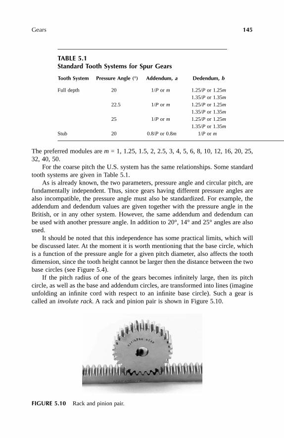
Gears 145
The preferred modules are m = 1, 1.25, 1.5, 2, 2.5, 3, 4, 5, 6, 8, 10, 12, 16, 20, 25,32, 40, 50.
For the coarse pitch the U.S. system has the same relationships. Some standardtooth systems are given in Table 5.1.
As is already known, the two parameters, pressure angle and circular pitch, arefundamentally independent. Thus, since gears having different pressure angles arealso incompatible, the pressure angle must also be standardized. For example, theaddendum and dedendum values are given together with the pressure angle in theBritish, or in any other system. However, the same addendum and dedendum canbe used with another pressure angle. In addition to 20°, 14° and 25° angles are alsoused.
It should be noted that this independence has some practical limits, which willbe discussed later. At the moment it is worth mentioning that the base circle, whichis a function of the pressure angle for a given pitch diameter, also affects the toothdimension, since the tooth height cannot be larger then the distance between the twobase circles (see Figure 5.4).
If the pitch radius of one of the gears becomes infinitely large, then its pitchcircle, as well as the base and addendum circles, are transformed into lines (imagineunfolding an infinite cord with respect to an infinite base circle). Such a gear iscalled an involute rack. A rack and pinion pair is shown in Figure 5.10.
TABLE 5.1Standard Tooth Systems for Spur Gears
Tooth System Pressure Angle (°) Addendum, a Dedendum, b
Full depth 20 1/P or m 1.25/P or 1.25m1.35/P or 1.35m
22.5 1/P or m 1.25/P or 1.25m1.35/P or 1.35m
25 1/P or m 1.25/P or 1.25m1.35/P or 1.35m
Stub 20 0.8/P or 0.8m 1/P or m
FIGURE 5.10 Rack and pinion pair.
Ch5Frame Page 145 Friday, June 2, 2000 8:43 PM

146 Fundamentals of Kinematics and Dynamics of Machines and Mechanisms
The involute profiles of the teeth in the rack become straight lines inclined withrespect to the vertical in Figure 5.11 by the angle φ. The line of action in the pinion–rackpair is a line tangential to the base circle of the pinion at the point E1 in Figure 5.11.
Recall that the line of action traces points of interaction between the two gears.Thus, if the addendum line of the rack passes through point E1, the two profiles willinteract only along the involutes. If, however, the addendum of the rack, ar, isincreased (as shown by broken lines in Figure 5.12), then its addendum line willcross the line of action at point E2. This means that some of the interaction betweenthe gears will take place outside of the pinion involute, namely, with a radial toothprofile inside the base disk. The interaction of an involute profile with the noninvoluteone violates the constant transmission ratio condition and leads to high contactstresses and, eventually, to wear of the teeth of the pinion inside the base circle. Thelatter phenomenon is called undercutting and is shown in Figure 5.12 by the darkenedareas on the pinion tooth profile. The undercutting weakens the tooth against bendingforces and may result in tooth failure.
To avoid undercutting, the geometry of the two mating teeth should be compat-ible; i.e., the addendum line of the rack should not intersect the base circle of the
FIGURE 5.11 Illustration of pinion and rack interaction.
FIGURE 5.12 Illustration of undercutting (the gray lines show the case of interaction withthe increased rack addendum).
Ch5Frame Page 146 Friday, June 2, 2000 8:43 PM

Gears 147
pinion above point E1. One can use this as a condition for the prevention of under-cutting. From Figure 5.11 it is seen that
(5.28)
Taking into account that , Equation 5.28 is reduced to
(5.29)
The pitch radius can be expressed through module m using Equation 5.26, that is,. The addendum can also be expressed through m in the form ,
where k is some constant. Then Equation 5.29 can be solved for the minimum numberof teeth for the addendum of the given rack.
(5.30)
Indeed, if the number of pinion teeth is larger then , then the pinion pitch andbase radii will be larger. The point E1 will now be below the addendum line andthus there will be no undercutting. On the other hand, if the number of teeth issmaller than the minimum, then undercutting will take place.
The constant k in Equation 5.30 is standardized. If k = 1, then the tooth is saidto have full depth; if k = 0.8, the depth is called shortened. In the case of φ = 20°,the minimum number of teeth is 18 for k = 1, and 14 for k = 0.8.
Another important point is that the minimum number of teeth determined forthe pinion–rack transmission is the smallest number. Indeed, if instead of the racka gear is used with the same addendum, then the point on the line of action wherethe engagement starts can only be below E1 in Figure 5.12.
Thus, the standardization of gears allows their interchangeability and guaranteesthe uniformity of kinematic performance. In this respect, it is important to understandthat the kinematic performance of a pair of gears does not depend on small variationsof the center distance between the shaft axes. Such a situation is shown in Figure 5.13,where in Figure 5.13a and b the same pair is mounted on shafts with different centerdistances. It follows from the similarity of the triangles that for both situations thekinematic ratio remains the same, i.e.,
(5.31)
However, aside from the kinematic performance, the change in the center distancemay affect the reliability of the gear set. Shortening of this distance may result injamming of the teeth, while increasing it leads to a clearance between the teeth,which is called backlash. The latter may cause knocks, vibrations, and noise.
r b φ ar+cos r p=
r b r p φcos=
ar r p φ2sin=
r p mN 2⁄= ar km=
Nmin2k
φ2sin------------=
Nmin
O3PO2P----------
ω2
ω3------
r 3b
r 2b
------= =
Ch5Frame Page 147 Friday, June 2, 2000 8:43 PM

148 Fundamentals of Kinematics and Dynamics of Machines and Mechanisms
5.8 TYPES OF INVOLUTE GEARS
The concept of an involute profile is used to design various types of gears havingdifferent functional and performance properties. Here, spur, helical, bevel, and wormgears will be briefly discussed.
5.8.1 SPUR GEARS
This is the most common and most fundamental type of gear. A pair of gears is shownin Figure 5.14. The involute surface of the gear tooth is a cylindrical surface. Tovisualize it, imagine that one is unwrapping a piece of paper from the base cylinder(Figure 5.15). Thus, in each cross section perpendicular to the cylinder axis theinvolute profile is identical. The resulting teeth and the corresponding terminologyare shown in Figure 5.9. The geometry of spur gears is standardized (see Table 5.1).
FIGURE 5.13 The effect of center distance on kinematic ratio.
FIGURE 5.14 Spur gears.
Ch5Frame Page 148 Friday, June 2, 2000 8:43 PM
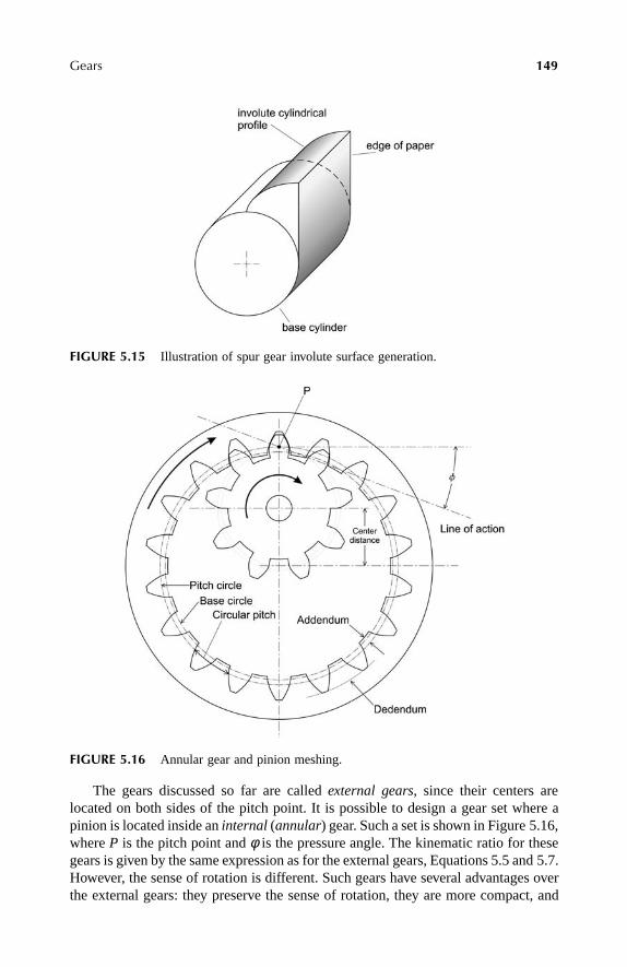
Gears 149
The gears discussed so far are called external gears, since their centers arelocated on both sides of the pitch point. It is possible to design a gear set where apinion is located inside an internal (annular) gear. Such a set is shown in Figure 5.16,where P is the pitch point and φ is the pressure angle. The kinematic ratio for thesegears is given by the same expression as for the external gears, Equations 5.5 and 5.7.However, the sense of rotation is different. Such gears have several advantages overthe external gears: they preserve the sense of rotation, they are more compact, and
FIGURE 5.15 Illustration of spur gear involute surface generation.
FIGURE 5.16 Annular gear and pinion meshing.
Ch5Frame Page 149 Friday, June 2, 2000 8:43 PM

150 Fundamentals of Kinematics and Dynamics of Machines and Mechanisms
their teeth are subjected to lower contact stresses because the curvature of the involutesurfaces is the same. These gears find applications in planetary gear systems (seeSection 5.10), and whenever compactness is a critical requirement.
5.8.2 HELICAL GEARS
A pair of helical gears is shown in Figure 5.17. The helical gear is an extension ofa spur gear to a more complex involute surface geometry. To understand this exten-sion, one can do a simple physical or imaginary experiment. Take a piece of paperand wrap it around the circular cylinder similar to the way that was done for a spurgear. However, in this case, cut the edge of the paper so that instead of it beingparallel to the cylinder axis it will now be inclined to this axis, thus becoming partof a helix line on the cylindrical surface. When the paper is unwrapped, each pointon the helix line (on the edge of the paper) will have a trajectory of an involute.Since the generating lines for each point on a helix line are different, they will resultin different involutes. The involutes all lie on a surface, which is called an involutehelicoid (Figure 5.18).
Since the involute helicoid is generated from the base cylinder, the two meshinghelical gears will have the transmission ratio defined by the radii of these cylinders,and, correspondingly, by the radii of the pitch cylindrical surfaces, exactly in thesame way as in the case of spur gears (see Equations 5.5 and 5.7). Thus, kinemat-ically, from the point of view of motion transfer, helical gears are not different fromspur gears. They have, however, other properties that make them attractive. The basicone is the increase in the so-called contact ratio. In Figure 5.19a contact lines duringthe motion of the spur gear are compared with the contact lines in Figure 5.19b ofthe helical gear. If, in the extreme case, the spur gear has only one tooth in contactat a time, then a comparable helical gear will have, not only more than one tooth incontact, but also a longer contact line. Benefits of this are smaller contact stressesand smoother motion transfer. Also, a helical gear, due to its geometry, is strongerin withstanding bending forces. This leads to one of the drawbacks of helical gears,the generation of parasitic axial forces.
The force generated at the interface of the helical involute surfaces acts along thenormal to this surface (assuming that friction forces are ignored). This normal force,
FIGURE 5.17 Helical gears.
Ch5Frame Page 150 Friday, June 2, 2000 8:43 PM

Gears 151
Fn, can be resolved into three components, Fr, Fa, and Ft, acting in radial, axial, andtangential (with respect to the surface of the base cylinder) directions, respectively.These forces are shown in Figure 5.20a, where Fn and Fr are lying in the plane normalto the helix line (plane ABC). The helix line is shown in Figure 5.20b, where it formsan angle ψ with the gear axis. The force Fn can be resolved in the normal planeABC into two components: Fr and Fnt, where the latter is a component of the normalforce lying in the tangential plane ACE. The angle φn between the forces Fn and Fnt
is the pressure angle defined in the same way as for spur gears. Thus, from theresolution of the forces in the normal plane one has the following relationshipsbetween the magnitudes of these forces:
(5.32)
and
(5.33)
FIGURE 5.18 Illustration of generation of a helical involute surface.
FIGURE 5.19 Comparison of contact lines for spur (a) and helical (b) gears.
Fr Fn φnsin=
Fnt Fn φncos=
Ch5Frame Page 151 Friday, June 2, 2000 8:43 PM

152 Fundamentals of Kinematics and Dynamics of Machines and Mechanisms
The force Fnt , in turn, can be resolved (see Figure 5.20b) into an axial force Fa anda tangential force Ft acting in the plane of rotation ADE. Thus, the components ofthe force Fnt are
(5.34)
and
(5.35)
FIGURE 5.20 (a) Forces acting on a helical tooth. (b) Forces acting on a helical tooth intangential plane.
Ft Fnt ψcos=
Fa Fnt ψsin=
Ch5Frame Page 152 Friday, June 2, 2000 8:43 PM

Gears 153
The tangential force is the only useful force, since it is the force transmitted by thegear. This force is known from the transmitted torque:
(5.36)
where rp is the pitch radius.Thus, for a given tooth geometry, φn and ψ, and given torque, T, the three
components of the normal force can be found from the above equations.
5.8.3 BEVEL GEARS
The spur gears transmit motion only between the parallel shafts, so that the gearplanes of rotation are parallel. The helical gears can be used to transmit motionbetween the shafts that can be either parallel or crossed, and thus the gear planes ofrotation can vary from being parallel to perpendicular, but their axes do not intersect.The bevel gears transmit motion between the shafts whose axes intersect while theirplanes of rotation may vary. In Figure 5.21 a pair of straight-tooth bevel gears withperpendicular shafts is shown.
Instead of a cylindrical surface, as in the case of spur and helical gears, servingas a base for an involute surface, in this case the base surface is conical. Thecorresponding pitch surface is also conical and is called the pitch cone. An involuteon a cone can be obtained by unfolding a piece of paper from the conical surfacewhile the edge of the paper follows the cone generating line and one point of thisedge is attached to the cone apex (Figure 5.22). Each involute ToT generated in thisway is called a spherical involute because it lies on a spherical surface. It is importantto understand that involutes are obtained in planes perpendicular to the cone surface.Thus, if one takes an infinitesimally thin slice of the involute surface, one can viewthis slice as if it had been obtained by unfolding a cord from the circle whose planeis perpendicular to the cone surface. Such a slice is shown in Figure 5.23 for a bevelgear. Thus, a very thin bevel gear will have practically the same properties as a spurgear with the equivalent base and pitch circles.
FIGURE 5.21 Straight-tooth bevel gears.
FtTr p
----=
Ch5Frame Page 153 Friday, June 2, 2000 8:43 PM
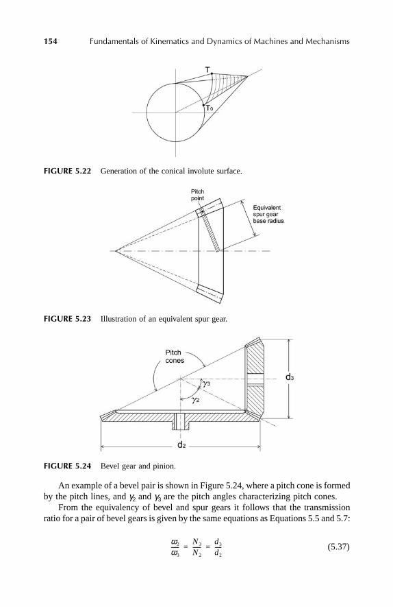
154 Fundamentals of Kinematics and Dynamics of Machines and Mechanisms
An example of a bevel pair is shown in Figure 5.24, where a pitch cone is formedby the pitch lines, and γ2 and γ3 are the pitch angles characterizing pitch cones.
From the equivalency of bevel and spur gears it follows that the transmissionratio for a pair of bevel gears is given by the same equations as Equations 5.5 and 5.7:
(5.37)
FIGURE 5.22 Generation of the conical involute surface.
FIGURE 5.23 Illustration of an equivalent spur gear.
FIGURE 5.24 Bevel gear and pinion.
ω2
ω3------
N3
N2------
d3
d2-----= =
Ch5Frame Page 154 Friday, June 2, 2000 8:43 PM

Gears 155
where d is the pitch diameter defined on the large end of the tooth (see Figure 5.24).In Figure 5.25 the forces acting at the interface of a pair of straight-tooth bevel
gears are shown. Note that in reality the forces are distributed along the tooth length,so those shown in Figure 5.25 should be considered as resultant forces applied inthe middle of the tooth, the latter being a simplification. The resultant force is anormal force Fn, shown in the A–A cross section, and it is directed along the line ofaction, i.e., at angle φ with respect to the tangential line. Thus, the resultant normalforce has two components in the plane perpendicular to the cone surface: normal(FnA) and tangential (FtA), which are found from the right-angled triangle to be(Figure 5.25)
(5.38)
and
(5.39)
The normal component acting in the plane A–A can, in turn, be resolved into twocomponents: one perpendicular to the axis of rotation of the gear (Fr) and anotherparallel to it (Fa). The former is called the radial force, while the latter the axial force.These forces are found from the right-angled triangle in Figure 5.25 to be
(5.40)
and
(5.41)
FIGURE 5.25 Forces acting on a tooth of a bevel gear.
FtA Fn φcos=
FnA Fn φsin=
Fr FnA γcos=
Fa FnA γsin=
Ch5Frame Page 155 Friday, June 2, 2000 8:43 PM

156 Fundamentals of Kinematics and Dynamics of Machines and Mechanisms
As is true for all gears, the tangential force is the only useful force and it is foundfrom the known transmitted torque T
(5.42)
where rap is the average pitch radius.As long as the tangential force is known, the normal resultant force can be
found from Equation 5.38, and then the radial and axial forces from Equations 5.39through 5.41.
In Equations 5.38 and 5.39 the pressure angle φ has not been defined. Thisangle is easier to understand using the concept of equivalent spur gears defined forthe large ends of teeth. This concept is illustrated in Figure 5.26, where a normalline to the common pitch cone line CP at point P is shown intersecting the gearsaxes at points O2 and O3. The distances O2P and O3P can be viewed as the pitchradii of equivalent spur gears, re2 and re3. Then the angle φ is defined by therelationship between the base radius and pitch radius for the spur gears. Forexample, for pinion 3,
FIGURE 5.26 Illustration of equivalent spur gears.
Ft FtATr ap
------= =
Ch5Frame Page 156 Friday, June 2, 2000 8:43 PM

Gears 157
(5.43)
where reb3 is the base radius of an equivalent spur gear 3 in the plane O2O3.It is easy to show from the similarity of triangles that the above relationship is
valid for any equivalent spur pair along the tooth length on the pitch cone line CPin Figure 5.26. In other words, the angle φ is a constant parameter of bevel gears inthe same sense as it is in the case of spur gears.
5.8.4 WORM GEARS
A worm–worm gear pair is shown in Figure 5.27. Worm gears are usually used whenthere is a need to transfer motion between perpendicular shafts and a large transmissionratio, from 10:1 to 15:1, is required. The worm has a screwlike thread (Figure 5.28)and is always a driver. The schematic representation of the worm–worm gear pair isshown in Figure 5.29. The teeth profiles are not involutes (since an involute profile fora tooth gives a point contact with the gear). To ensure a line contact of the interfacingteeth, they are cut using the same hob.
FIGURE 5.27 Worm gears.
FIGURE 5.28 Worm geometry.
φcosr b3
r 3------
r eb3
r e3--------= =
Ch5Frame Page 157 Friday, June 2, 2000 8:43 PM

158 Fundamentals of Kinematics and Dynamics of Machines and Mechanisms
From the kinematic point of view it is important to establish the relationshipbetween the pair geometric parameters and the transmission ratio. The wormgeometry is illustrated in Figure 5.30a, where ψ is the helix angle, while thecomplementary-to-90° angle λ is called the lead angle (see also Figure 5.28). Notethat the helix angle of the worm gear equals the lead angle of the worm. If acomplete revolution of a thread on a worm is unwrapped, a triangle is obtained(Figure 5.30b). It follows from this triangle that
(5.44)
where l is called the lead, and it is equal to the axial distance that a point on thehelix will move in one revolution of the worm, and d2 is the worm pitch diameter.
For a single-threaded worm, the lead is equal to its axial pitch px (Figure 5.30a).For a multithreaded worm the lead is equal to
(5.45)
where N2 is the number of threads (teeth) on the worm.Taking into account that for the shafts at 90° the axial pitch for the worm is
equal to the circular pitch for the gear:
(5.46)
FIGURE 5.29 Worm–worm gear meshing.
λtan 1πd2--------=
l pxN2=
px p=
Ch5Frame Page 158 Friday, June 2, 2000 8:43 PM

Gears 159
and that the circular pitch for the gear is , then from the equality(Equation 5.46 and Equation 5.45) it follows that
(5.47)
For one revolution of a worm with N2 threads a point on a worm tooth will moveby a distance l. Thus, for the angular velocity of the worm ω2 the axial velocity Va
of the point on a worm tooth is defined by the ratio
(5.48)
The axial velocity Va must be equal to the tangential velocity of the gear:
(5.49)
From the equality Va = Vt it follows that
(5.50)
and then from the latter and Equation 5.47 that
(5.51)
As seen from Equation 5.51, the transmission ratio for the worm–worm gearpair is defined in the same way as for the all other gears, namely, as a ratio betweenthe number of the corresponding teeth. One should recall that the number of teethfor the worm is its number of threads.
FIGURE 5.30 Illustration of worm geometry.
p πd3 N3⁄=
N3
N2------
πd3
l--------=
2πl
------ω2
Va
------=
Vt
d3ω3
2-----------=
πd3
l--------
ω2
ω3------=
N3
N2------
ω2
ω3------=
Ch5Frame Page 159 Friday, June 2, 2000 8:43 PM

160 Fundamentals of Kinematics and Dynamics of Machines and Mechanisms
5.9 PARALLEL-AXIS GEAR TRAINS
Very often a single gear pair transferring motion between two parallel shafts cannotmeet the needed transmission ratio requirement. For example, if this requirement is10:1, then the diameter of the gear must be 10 times larger then the diameter of thepinion. This is usually unacceptable from the design specifications concerning prod-uct size. The solution is achieved by arranging a series of gear pairs. Such series iscalled a gear train. A train may comprise different type of gears: spur, helical, bevel,and worm. The gears in a train are functionally in series with each other. If a systemcomprises a few trains, they are functionally in parallel with each other. Usually asystem of gears arranged physically in one case (box), whether in series or in parallel,is called a transmission box.
An example of a transmission box with parallel gear trains is shown in Figure 5.31.This transmission comprises three trains. The input into the box comes from shaft 10,the output shaft is 11, and the auxiliary shaft is 12. To achieve three different pathsof motion transmission from the input to the output shafts, the design allows therearranging of connections (meshing) between the gears by shifting some of themalong the shaft axis. In Figure 5.31 gears 3 and 4 can be shifted along the shaft sothat the following trains are obtained:
First: 2–5–7–4Second: 2–5–6–3Third: 2–5–8–9–4
One should note that there is a fourth mode of motion transmission in this example,when a clutch is engaged and the power is transmitted through the shaft directlyfrom the input to the output without any gears involved.
5.9.1 TRAIN TRANSMISSION RATIO
It is customary to define the transmission ratio of a pair as the ratio of driven todriving angular velocities. It is known that if the gears have external meshing, the
FIGURE 5.31 Automotive transmission.
Ch5Frame Page 160 Friday, June 2, 2000 8:43 PM

Gears 161
sense of rotation changes to the opposite, while for gears with internal meshing itremains the same. Thus, for any pair in the train with external meshing the trans-mission ratio is
(5.52)
And thus the train transmission ratio is
(5.53)
where K is the number of pairs. It is clear that for gears with external meshing, ifK is even, the sense of the rotation of the output is the same as that of the input,and, if K is odd, the sense of rotation changes to the opposite.
If Equation 5.52 is substituted into Equation 5.53, the train transmission ratiois obtained as a ratio of angular velocities of last and first gears in the train, i.e.,
(5.54)
Consider the transmission ratio of the first train in Figure 5.31. Recalling thatthe transmission ratio of a gear pair can be expressed through the ratio of gear teethnumbers, one can write, using Equation 5.53,
(5.55)
Similarly, the transmission ratios of the second and third trains are
(5.56)
(5.57)
One can see that in the third transmission ratio the ninth gear does not affect themagnitude of the output angular velocity, but it changes its sign (the sense ofrotation). The ninth gear in Figure 5.31 is called the idler gear, whose function isto reverse the rotation. The transmission box shown in Figure 5.31 is an example ofan automotive transmission with three forward speeds and one reverse.
5.9.2 DESIGN CONSIDERATIONS
In designing a gear box (such as, for example, that shown in Figure 5.31), the inputinformation is the required transmission ratios for each speed. Thus, the problem is,
eω– driven
ωdriving------------------=
etrain e1e2…eK=
etrainωLast
ωFirst------------=
eI 1–( )2N2
N5------
N7
N4------=
eII 1–( )2N2
N5------
N6
N3------=
eIII 1–( )3N2
N5------
N8
N9------
N9
N4------=
Ch5Frame Page 161 Friday, June 2, 2000 8:43 PM

162 Fundamentals of Kinematics and Dynamics of Machines and Mechanisms
given eI, eII, and eIII , find gears with teeth numbers that will meet other transmissionbox design requirements, such as, for example, specific center distances betweenthe shafts and the teeth strength, among others. The fact that gear pairs 2–5, 3–6,and 4–7 are mounted on two parallel shafts gives additional equations in the formof the requirement that the center distance for each pair be the same. The centerdistance equals the sum of two pitch radii, i.e.,
(5.58)
Taking into account that r = 0.5Nm, the above equation becomes
(5.59)
where the tooth module m is another parameter. Thus, for the case of Figure 5.31three equations of the above type can be written, bringing the total number ofequations to six. Since the total number of equations is smaller than the number ofunknowns, the solution is not unique. Since the transmission ratio of a train is aproduct of transmission ratios of gear pairs, there is a freedom of choosing the latterto obtain the same total transmission ratio. In addition, the solution, i.e., the numberof teeth for each gear, must be an integer; the type of the gear itself may be different(spur or helical) for each pair. Considering all of the above, the process of gear train(box) design is an iterative one, in which kinematic requirements must be satisfiedsubject to meeting other (space, strength, etc.) requirements.
5.10 PLANETARY GEAR TRAINS
An elementary planetary gear train is shown in Figure 5.32. It comprises two gears,2 and 4, each mounted on its own shaft. The new element here is the link 3 connectingthese shafts and able to rotate around the fixed axis O1. This system has two degreesof freedom, which means that if only the input velocity ωin = ω2 is given, the motionof the two other elements cannot be determined. Input gear 2 is called the sun
FIGURE 5.32 Planetary gear train.
C rdriven r driving+=
C 0.5m Ndriven Ndriving+( )=
Ch5Frame Page 162 Friday, June 2, 2000 8:43 PM

Gears 163
(or central) gear, gear 4 is called the planetary (or epicyclic) gear, and link 3 iscalled the planet carrier (or crank arm).
Planetary gear trains allow obtaining high transmission ratios in a compactdesign, which makes them suitable for applications in, for example, machine tools,hoists, and automatic transmissions. An example of a simple planetary gear box isshown in Figure 5.33, where in addition to the elements in Figure 5.32 an additionalannular gear 5 is added, so that the planetary gear 4 is now interfacing both the sunand the annular gears. Note that the annular gear is fixed. The number of degreesof freedom of this system is 1, which means that for a given input ωin = ω2 there isa unique output ωout = ω3.
5.10.1 TRANSMISSION RATIO IN PLANETARY TRAINS
One can determine the transmission ratio for a planetary train in Figure 5.32. Supposethat arm 3 rotates with angular velocity ω3. Then, if an observer is sitting on thisarm, for this observer the rotation of gears 2 and 4 will not be different from thatfor a parallel fixed-shaft system, and the corresponding transmission ratio will beω4/ω2. One realizes that an observer on the arm sees rotation in a moving (rotating)coordinate system. Now if the observer is standing on the frame, then the observerwill see that the arm rotates with ω3. The question is what will be the angularvelocities of gears 2 and 4 with respect to the observer on a frame.
The answer is given by a general rule for summation of angular velocities in thecase when a body rotates with respect to its own axis with velocity ω1, while theaxis itself rotates with respect to another axis with the velocity ω. In the case whenthe two axes are parallel, the total angular velocity equals the algebraic sum ofvelocities of two rotations. Thus, the total angular velocity will be
(5.60)
FIGURE 5.33 Planetary gear train with annular gear.
ωtotal ω ω1+=
Ch5Frame Page 163 Friday, June 2, 2000 8:43 PM

164 Fundamentals of Kinematics and Dynamics of Machines and Mechanisms
The above rule is directly applicable to the planetary gear trains. Indeed, the axesof gears 2 and 4 are parallel and one of them rotates with respect to the other withω3. Now, the transmission ratio in a coordinate system rotating with ω3 is known. Itis equal to e42 = –N2/N4. Thus, if one applies a counterrotation with –ω3 to the entiresystem, then the gear velocities (according to the rule of summation) will be and , and link 3 becomes fixed. Thus, the transmission ratio is given by
(5.61)
The above equation confirms that the system shown in Figure 5.32 has two degreesof freedom. Indeed, if only ω2 is given, two unknown velocities remain, ω3 and ω4,while the gears are defined.
The example of Figure 5.32 described by Equation 5.61 is equivalent to a one-pair system in conventional gear trains. In this respect, the system in Figure 5.33is equivalent to a two-pair system where the pairs are functionally in series witheach other. Thus, in this case there are two transmission ratios: first, from the sungear 2 to the planetary gear 4, which is described by Equation 5.61, and, second,from the planetary gear 4 to the annular gear 5. The latter is equal to (in a rotatingcoordinate system)
(5.62)
Note that the plus sign on the right-hand side in Equation 5.62 is due to internalgear meshing. If ω5 = 0 (annular gear is fixed) and ω2 is known, then ω3 and ω4 arefound from Equations 5.61 and 5.62.
And, finally, it should be noted that the planetary gear plays the role of an idlegear in Figure 5.33. Indeed, the total transmission ratio for a system in series isequal to the product of transmission ratios of its subsystems (see Equation 5.53). Inthe case of Figure 5.33 the total transmission ratio is the product of Equations 5.61and 5.62. The result is
(5.63)
As one can see, the angular velocity ω4 of the planetary gear does not affect thetransmission ratio.
Given that ω5 = 0 and ω2 is known, the unknown output velocity can be imme-diately found from Equation 5.63:
(5.64)
where it is denoted .
ω4 ω3–ω2 ω3–
e42ω4 ω3–ω2 ω3–------------------
N2
N4------–= =
ω5 ω3–ω4 ω3–------------------
N4
N5------=
eω5 ω3–ω2 ω3–------------------
N2
N5------–= =
ω3 ω2
n25
1 n25+----------------=
n25 N2 N5⁄=
Ch5Frame Page 164 Friday, June 2, 2000 8:43 PM

Gears 165
5.10.2 EXAMPLE OF A MORE COMPLEX PLANETARY TRAIN
Consider the example shown in Figure 5.34. The sun gear 2 is driven by shaft A andthe output shaft is B, which is driven by the planet carrier 7. The two gears, 4 and 5,are mounted on the same shaft, which means that their angular velocities must beequal. Notice also that gear 6 is fixed. Given all this information, and assuming thatthe teeth numbers of all gears are known, the problem is to find the velocity of theoutput shaft given the input velocity ω2.
The strategy is to follow the chain of gear interfaces 2–3, 3–4, and 5–6, and towrite for each interface the equation of the Equation 5.61 type. To shorten this proce-dure, one can take into account that the planetary gear does not change the kinematics(see Equation 5.63) and thus write a relationship between gears 2 and 4 directly.
(5.65)
and for gears 5 and 6,
(5.66)
Note that in Equation 5.65 the sign is positive because there is an even number ofinterfaces from gear 2 to gear 4. The system of equations above should be supple-mented by the requirement that
(5.67)
Given the latter condition and that ω6 = 0 and ω2 is known, the two equations (5.65and 5.66) allow one to find ω4 and ω7. The result is
(5.68)
FIGURE 5.34 Skeleton of a complex gear train.
ω4 ω7–ω2 ω7–------------------
N2
N4------=
ω6 ω7–ω5 ω7–------------------
N5
N6------–=
ω4 ω5=
ω7 ω2
n24n56
1 n24n56+-----------------------=
Ch5Frame Page 165 Friday, June 2, 2000 8:43 PM

166 Fundamentals of Kinematics and Dynamics of Machines and Mechanisms
and
(5.69)
where it is denoted
and
5.10.3 DIFFERENTIAL
Differentials are planetary trains made out of bevel gears and having two degreesof freedom. An example of an automotive differential is shown in Figure 5.35. Therotation from the engine is transferred through bevel gears 2 and 3 to the system ofbevel gears 4, 5, and 6. Gears 4 are mounted on the carrier and are the planetarygears, whereas gears 5 and 6 are two independent sun gears. The transmission ratiofrom 2 to 3 is independent from the rest of the system (in fact, gear 3 could beconsidered an input gear with known angular velocity). Thus, the transmissionthrough system 3–4–5–6 will be considered.
The important distinction of the bevel planetary mechanism is that the rule ofsummation of velocities for the planetary and sun gears is not applicable in the sensediscussed above since in this case the axes of gears 5 and 4 and gears 6 and 4 are notparallel. Thus, if gear 5 rotates clockwise, when viewed along its axis from the right,gear 6 will be rotating counterclockwise from the same point of view (Figure 5.36).However, the rotation of the gears 3 and 5 and gears 3 and 6 is around parallel axes,and so the rule of summation discussed for planar trains is applicable. Thus, if oneapplies a counterrotation –ω3 to the entire system, one will have the system shown in
FIGURE 5.35 Automotive differential.
ω4 ω2
n24 1 n56+( )1 n24n56+
----------------------------=
N2
N4------ n24=
N5
N6------ n56=
Ch5Frame Page 166 Friday, June 2, 2000 8:43 PM
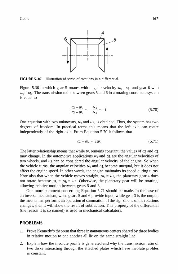
Gears 167
Figure 5.36 in which gear 5 rotates with angular velocity and gear 6 with. The transmission ratio between gears 5 and 6 in a rotating coordinate system
is equal to
(5.70)
One equation with two unknowns, ω5 and ω6, is obtained. Thus, the system has twodegrees of freedom. In practical terms this means that the left axle can rotateindependently of the right axle. From Equation 5.70 it follows that
(5.71)
The latter relationship means that while ω3 remains constant, the values of ω5 and ω6
may change. In the automotive applications ω5 and ω6 are the angular velocities oftwo wheels, and ω3 can be considered the angular velocity of the engine. So whenthe vehicle turns, the angular velocities ω5 and ω6 become unequal, but it does notaffect the engine speed. In other words, the engine maintains its speed during turns.Note also that when the vehicle moves straight, ω5 = ω6, the planetary gear 4 doesnot rotate because ω5 = ω6 = ω3. Otherwise, the planetary gear will be rotating,allowing relative motion between gears 5 and 6.
One more comment concerning Equation 5.71 should be made. In the case ofan inverse mechanism, when gears 5 and 6 provide input, while gear 3 is the output,the mechanism performs an operation of summation. If the sign of one of the rotationschanges, then it will show the result of subtraction. This property of the differential(the reason it is so named) is used in mechanical calculators.
PROBLEMS
1. Prove Kennedy’s theorem that three instantaneous centers shared by three bodiesin relative motion to one another all lie on the same straight line.
2. Explain how the involute profile is generated and why the transmission ratio oftwo disks interacting through the attached plates which have involute profilesis constant.
FIGURE 5.36 Illustration of sense of rotations in a differential.
ω5 ω3–ω6 ω3–
ω6 ω3–ω5 ω3–------------------
N5
N6------– 1–= =
ω5 ω6+ 2ω3=
Ch5Frame Page 167 Friday, June 2, 2000 8:43 PM

168 Fundamentals of Kinematics and Dynamics of Machines and Mechanisms
3. Prove that the transmission ratio of two involute gears does not depend on thecenter distance between them.
4. Explain why a straight line describes the tooth profile of the rack.
5. For a spur gear,
a. What is the direction of the force generated at the interface of two meshingteeth?
b. Is it true that , where T2 and T3 are the torques appliedto the corresponding gears? Prove.
6. Spur gears with a module m = 4 mm transmit motion between two shafts withcenter distance C = 136 mm. For the given transmission ratio 3:1 find the numberof teeth for each gear.
7. Sketch the axial, radial, and tangential components of the force acting on a toothof a helical gear. How does one find these forces given the torque T transmittedby the gear?
8. What is the involute surface for a straight teeth bevel gear? Draw a sketchexplaining how to generate this surface.
9. Explain, using the equivalency of spur and straight teeth bevel gears, that forthe latter the transmission ratio is given by .
10. Prove that the transmission ratio for the worm gears set is ,where d3 is the gear pitch diameter and l is the lead of the worm.
11. Prove that the transmission ratio between the sun 2 and the planet gear 4 inFigure 5.32 is
where ω3 is the angular velocity of arm 3.
12. Derive the transmission ratio for the planetary train in Figure 5.33.
13. Derive the transmission ratio for the planetary train in Figure 5.34.
14. Explain why in an automotive transmission the differential allows two wheelsto rotate with different angular velocities while the speed of the engine remainsthe same.
15. A worm has a double thread with a 10° lead angle and 20-mm pitch diameter.It meshes with a worm gear with a 90° angle between the shafts. For a speedreduction 15:1, determine:
a. The pitch diameter and the number of teeth of the gear.b. The helix angle of the gear.c. The center distance.
ω2 ω3⁄ T3 T2⁄=
ω2 ω3⁄ N3 N2⁄ d3 d2⁄= =
ω2 ω3⁄ πd3 l⁄=
e42ω4 ω3–ω2 ω3–------------------
N2
N4------–= =
ω3 ω2⁄
ω7 ω2⁄
Ch5Frame Page 168 Friday, June 2, 2000 8:43 PM

Gears 169
16. An 18-tooth spur pinion has module m = 2 mm. For the transmission ratio 1:2,find:
a. The number of teeth on the gear.b. The center distance.c. The pressure angle (take that the base diameter equals pitch diameter
minus 2.2m).
Ch5Frame Page 169 Friday, June 2, 2000 8:43 PM

Ch5Frame Page 170 Friday, June 2, 2000 8:43 PM

171
6
Introduction toLinear Vibrations
6.1 INTRODUCTION
A question one may ask is “Why do bodies vibrate?” The explanation is rooted inthe
energy conservation principle.
Consider as an example a mass
m
suspended ona spring having stiffness
k
(Figure 6.1) and assume that this mass is pushed up(or down) from its static equilibrium position by the amount
y
max
and then released.By deforming the spring some energy is stored in it, which will be denoted by
V
max
. This energy is called the
potential energy
, and
V
max
represents the maximumenergy transferred to the spring by deforming it by
y
max
. After releasing the mass, itwill start moving back to its original position. The motion of the mass means thatit acquires some
kinetic energy
, which is equal to
(6.1)
where is the time derivative of mass displacement, i.e., its velocity. At anyintermediate position the potential energy of the deformed spring is equal to
(6.2)
If one assumes that the spring is ideal, i.e., its deformation does not lead to anyenergy losses, then according to the energy conservation principle the sum of thekinetic energy of the mass and the potential energy in the spring must be equal tothe original energy introduced into this system,
V
max
. Thus,
. (6.3)
The above equation shows that in a spring–mass system an energy transformationtakes place, from potential to kinetic and back. More than that, one can see that thisprocess is periodic. Indeed, when then and it follows that atthese extreme positions . Thus, there are two extreme positions of the massand they are equal in magnitude, but at the opposite sides of the static equilibriumposition. On the other hand, when
y =
0
(or, more correctly, a static displacement),. This process of a mass moving between two extreme positions in a periodic
fashion is called
oscillation
. It is characterized by two parameters: the
amplitude
ofoscillation and the
period
of oscillation. The former is the maximum mass displace-
T12--- my2=
yy
V12--- ky2=
12--- my2 1
2--- ky2+ Vmax const= =
y ymax±= V Vmax=y 0=
y ymax=
Ch6Frame Page 171 Friday, June 2, 2000 6:43 PM

172
Fundamentals of Kinematics and Dynamics of Machines and Mechanisms
ment from the position of static equilibrium,
y
max
, whereas the latter is the timebetween two consecutive maximum displacements.
The relationship given by Equation 6.3 is a differential one. Since it is knownthat the motion of the mass is periodic with the amplitude
y
max
, one can assume itto be described by a function:
(6.4)
where
t
is the time,
T
is the period of oscillation, and
α
is some constant which isdefined by the requirement that at
t
= 0,
y = y
max
.In Equation 6.4 the maximum displacement
y
max
is known, and
T
is the onlyunknown (besides
α
) to be found in order to describe the motion of the mass in time.The expression for
T
follows from the requirement that the function (Equation 6.4)must satisfy Equation 6.3. Substitute and into Equation 6.3. After simplederivations, the differential Equation 6.3 is reduced to an algebraic relationship:
(6.5)
For the above equality to be true at any time, the term in the brackets must be equalto zero, i.e.,
(6.6)
The latter equation defines the period of oscillation as a function of mass and springstiffness:
(6.7)
FIGURE 6.1
Spring–mass system.
y ymax 2π tT--- α+
sin=
y y
m 2π( )2
T2------------------ k– ymax
2 cos2 2π tT--- α+
0=
m 2π( )2
T2------------------ k–
0=
T 2π mk----=
Ch6Frame Page 172 Friday, June 2, 2000 6:43 PM

Introduction to Linear Vibrations
173
The important point is that the period of oscillation is an intrinsic property ofthe mass–spring system and does not depend on the initial disturbance (or on theinitial energy pumped into the system). The inverse of
T
gives the number ofoscillations per unit time and it is called the
frequency
of oscillation,
f
. If the timeis measured in seconds, then one oscillation per second is called a
hertz
.
(6.8)
In Equation 6.4 2
π
/T
gives the angular displacement per unit time; i.e., it gives theangular velocity. This angular velocity is called the
circular frequency
of oscillation,
ω
, and it is equal to
(6.9)
The mass–spring system shown in Figure 6.1 represents a single-degree-of-freedom(SDOF) system. The motion of the mass discussed above was caused by its initialdisplacement and Equation 6.3 describes this motion. One can simplify this equationby differentiating both sides of it with respect to time. The result is
(6.10)
Since at
all
times, Equation 6.10 can be satisfied only if the first term equalszero, i.e.,
(6.11)
Now it can be seen that the obtained equation expresses Newton’s second law,where
ky
is the external spring force acting on the mass treated as a free body. Ingeneral, if a periodic force acts upon the mass, then its motionequation can be obtained by considering the equilibrium of forces, including inertialforce, acting on this mass (Figure 6.2). Taking into account that forces
ky
and
P(t)
are opposite, the motion equation becomes
(6.12)
Equations 6.11 and 6.12 have been derived assuming that the system is not experi-encing any energy losses during oscillations. If this assumption cannot be made, thena force associated with the energy losses should be added to the resultant force actingon the mass in Figure 6.2. The causes of energy losses may be many, such as frictionbetween the moving parts, oil or air resistance, internal losses in materials. Thesedifferent causes may entail different mathematical models to describe them. Ingeneral, unless there is a dominating factor, all of them contribute to the total energyloss. The most convenient way to model energy losses is to assume that they are
f1T---
12π------ k
m----= =
ω 2πT------ k
m----= =
my ky+( ) y 0=
y 0≠
my ky+ 0=
P t( ) P0 ωt( )sin=
my ky+ P0 ωt( )sin=
Ch6Frame Page 173 Friday, June 2, 2000 6:43 PM

174
Fundamentals of Kinematics and Dynamics of Machines and Mechanisms
caused by forces proportional to the body velocity, similar to the resistance experi-enced by a body moving through a viscous liquid. Accordingly, these forces arecalled
viscous forces
and are taken in the form:
(6.13)
where
c
is called the
damping coefficient
.In Figure 6.3a in addition to the spring a
damping element
is shown, which isconventionally used to identify the presence of viscous resistance force having damp-ing coefficient
c
. This additional force acts in the same direction as the spring resistanceforce (Figure 6.3b). The dynamic equilibrium of forces shown in Figure 6.3b givesthe following differential equation:
(6.14)
Equations 6.11, 6.12, and 6.14 have one important property; they are
linear
differential equations. Their linearity is due to the assumptions that resistance forces
FIGURE 6.2
External force applied to a mass–spring system (a), and a free-body diagramof the mass (b).
FIGURE 6.3
Mass–spring–damper system (a), and free-body diagram of mass (b).
Fr t( ) cy=
my cy ky+ + P0 ωt( )sin=
Ch6Frame Page 174 Friday, June 2, 2000 6:43 PM

Introduction to Linear Vibrations 175
are proportional to either displacement or velocity. If any of these assumptions isnot adequate, then the equation becomes nonlinear. There are well-developed math-ematical techniques for solving linear equations, whereas nonlinear equations veryoften require an individual analytical approach or a numerical solution. This bookwill be limited to linear equations.
Equation 6.14 is a second-order nonhomogeneous linear equation with constantcoefficients. The next section considers solutions of Equation 6.14.
6.2 SOLUTION OF SECOND-ORDER NONHOMOGENEOUS EQUATIONS WITH CONSTANT COEFFICIENTS
Linear equations have a very important property; they allow linear combination ofsolutions to form new solutions. Namely, if and are two solutions, thentheir combination with some constant coefficients, , is alsoa solution of this equation. This is called the superposition principle. The followingwill use this principle in various situations, but its first application is to split thesolution of Equation 6.14 into two parts: one describing the behavior of the systemwithout the external forces (the corresponding differential equation is called homo-geneous and its solution the general solution) and the other describing the behaviorof the system subjected to external forces (the corresponding differential equationis called nonhomogeneous and its solution the particular solution). The solution ofthe homogeneous equation will first be considered.
6.2.1 SOLUTION OF THE HOMOGENEOUS EQUATION
The homogeneous equation to be solved is
(6.15)
It is more convenient for the following to transform this equation into one withnondimensional constants by dividing each term by m. The transformed equation isas follows:
(6.16)
where it is denoted
(6.17)
In Equation 6.17 ξ is called the nondimensional damping coefficient, and ωn is calledthe natural frequency (see Section 6.3).
It is known that an exponential function
(6.18)
f 1 t( ) f 2 t( )f t( ) a1 f 1 t( ) a2 f 2 t( )+=
my cy ky+ + 0=
y 2ξωny ωn2y+ + 0=
ξ c2mωn
-------------- and ωn2 k
m----= =
y t( ) eλ t=
Ch6Frame Page 175 Friday, June 2, 2000 6:43 PM

176 Fundamentals of Kinematics and Dynamics of Machines and Mechanisms
is a possible solution of this equation, where λ is some constant. If this function issubstituted into Equation 6.16, the following algebraic equation is obtained:
(6.19)
Since in the above equation cannot be equal to zero, the nontrivial solution ofEquation 6.19 exists only if the quadratic polynomial equals zero:
(6.20)
The above equation is called the characteristic equation, since it defines two uniqueroots and thus two possible solutions of the differential equation. The two roots are
(6.21)
If λ1 and λ2 are two distinct roots, then it means that there are two possible solutionsof Equation 6.16. The general solution is a combination (again, the principle ofsuperposition is used) of these two solutions with some constants:
(6.22)
The specific form of the solution given by Equation 6.22 depends on the type ofroots in Equation 6.21: real and distinct, complex, or real and equal. Each of thesecases will be considered separately since, as will be seen later, the type of rootsreflects the type of system behavior.
• Roots are real and distinct
This is possible if in Equation 6.21; then the solution given by Equation 6.22is an exponentially decreasing in time function since both roots are negative.
• Roots are complex
This is possible if in Equation 6.21; then they can be written in the form, where and are real numbers and i is the
imaginary unit (square root of –1). Now the solution Equation 6.22 takes the followingform:
(6.23)
By using the Euler formula
(6.24)
λ2 2ξωnλ ωn2++( )eλ t 0=
eλ t
λ2 2ξωnλ ωn2+ + 0=
λ 1 2, ξ– ξ2 1–±( )ωn=
y t( ) c1eλ1t
c2eλ2t
+=
ξ 1>
ξ 1<λ1 2, α iβ±= α ξ– ωn= β 1 ξ2– ωn=
y t( ) c1eα iβ+( )t c2e
α iβ–( )t+=
e iβ± t βt i βtsin±cos=
Ch6Frame Page 176 Friday, June 2, 2000 6:43 PM

Introduction to Linear Vibrations 177
the solution Equation 6.23 can be transformed to
(6.25)
where a1 = c1 + c2 and a2 = i(c1 – c2) are two new arbitrary constants.
• Roots are real and equal
This is possible if in Equation 6.21 so that . In this case,in addition to the solution given by Equation 6.18, there is another one given by thefunction , and thus, the general solution becomes
(6.26)
6.2.2 PARTICULAR SOLUTION OF THE NONHOMOGENEOUS EQUATION
The nonhomogeneous equation with nondimensional coefficients is
(6.27)
where po = Po/m. The particular solution caused by the harmonic forcing functionis also harmonic and can be taken in either of the following two forms:
(6.28)
where d1, d2, D, and φ are constants.Taking the second form of the solution in Equation 6.28 and substituting it into
Equation 6.27 obtains
(6.29)
By using the trigonometric relations
(6.30)
and
(6.31)
y t( ) c1eα t βtcos i βtsin+( ) c2eα t βtcos i βtsin–( )+=
eα t c1 c2+( ) βt i c1 c2–( ) βtsin+cos[ ]=
e= α t a1 βt a2 βtsin+cos[ ]
ξ 1= λ1 2, λ ξ– ωn= =
teλ t
y t( ) c1eλ t c2te
λ t+=
y 2ξωny ωn2y+ + po ωtsin=
yp t( ) d1 ωt d2 ωtsin+cos D ωt φ–( )sin= =
D ωn2 ω2–( ) ωt φ–( ) 2+ ξωnω ωt φ–( )cossin[ ] po ωtsin=
ωt φ–( )cos ωt φ ωsin t φsin+coscos=
ωt φ–( )sin ωsin t φ ωcos– t φsincos=
Ch6Frame Page 177 Friday, June 2, 2000 6:43 PM

178 Fundamentals of Kinematics and Dynamics of Machines and Mechanisms
Equation 6.29 is transformed into the following:
(6.32)
The above equation can be satisfied at any moment in time if the harmonic functionson the left and on the right have equal amplitudes. This requirement leads to twoequations:
(6.33)
and
(6.34)
To solve the above system for the unknowns D and φ, transform it into a simplersystem. This is done by first multiplying Equation 6.33 by –sin φ and Equation 6.34by cos φ and adding them. The result is
(6.35)
Now, multiply Equation 6.33 by cos φ and Equation 6.34 by sin φ and add them.The result is
(6.36)
The new system, Equations 6.35 and 6.36, can be easily solved. Square both sidesin Equations 6.35 and 6.36 and add the equations. This gives the expression for theunknown D
(6.37)
Now if Equation 6.36 is divided by Equation 6.35, the expression for the angle φ isobtained:
(6.38)
Note that the constants d1, d2 in Equation 6.28 are equal to
(6.39)
D ωn2 ω2–( )– φ 2+ ξωnω φcossin[ ] ωcos t
+ D ωn2 ω2–( ) φ 2+cos ξωnω φsin[ ] ωsin t po ωtsin=
D ωn2 ω2–( )– φ 2+ ξωnω φcossin[ ] 0=
D ωn2 ω2–( ) φ 2+cos ξωnω φsin[ ] po=
D ωn2 ω2–( ) po φcos=
D2ξωnω po φsin=
Dpo
ωn2 ω2–( )2
2ξωnω( )2+------------------------------------------------------------=
φ arc2ξωnωωn
2 ω2–------------------
tan=
d1 D φ and d2 D φcos=sin–=
Ch6Frame Page 178 Friday, June 2, 2000 6:43 PM

Introduction to Linear Vibrations 179
Using Equations 6.35 and 6.36 to express sin φ and cos φ through D gives thefollowing expressions for these coefficients:
(6.40)
and
(6.41)
where D is given by Equation 6.37.It is of interest to consider the case when, instead of forcing function p0 sin ωt,
a function p0 cos ωt is used in Equation 6.27. It can be checked that the solutionsfor the amplitude, Equation 6.37, and for the phase angle, Equation 6.38, remainthe same.
6.2.3 COMPLETE SOLUTION OF THE NONHOMOGENEOUS EQUATION
The complete solution is a superposition of the general solution of the homogeneousequation (Equation 6.22) and the particular solution of the nonhomogeneous equation(Equation 6.28). Thus,
(6.42)
where c1 and c2 are unknown constants, and d1 and d2 are given by Equations 6.40and 6.41.
As was discussed in Section 6.1, the vibration of the mass on a spring is causedby the initial displacement of this mass. By displacing and releasing the mass, oneintroduces into the mass–spring system some initial potential energy. It was tacitlyassumed that this initial displacement was slow enough so that the correspondingkinetic energy of motion could be ignored. However, if this is not the case, then thetotal energy transferred to the system is a sum of both potential and kinetic energies.The former is associated with the initial displacement of the mass, while the secondis associated with its initial velocity. Thus, in general, the motion of a body fromthe undisturbed position starts with some initial displacement and with some initialvelocity. These are called initial conditions. For a single body in a uniaxial motion,there are two initial conditions, which are stated as follows
(6.43)
These two initial conditions define the constants c1 and c2 in Equation 6.42. Satisfyingthe initial displacement condition gives
d1
2D2ξωnωpo
------------------------–=
d2D2 ωn
2 ω2–( )po
------------------------------=
yc t( ) yg t( ) yp t( ) c=+ 1eλ1t
c2eλ2t
d1 ωcos t d2 ωsin t+ + +=
yc 0( ) Y0 and dyctdt
----------t 0=
V0==
Ch6Frame Page 179 Friday, June 2, 2000 6:43 PM
180 Fundamentals of Kinematics and Dynamics of Machines and Mechanisms
(6.44)
Then taking the derivative of yc(t) and then satisfying the initial velocity requirementgives
(6.45)
Solving Equations 6.44 and 6.45 for the unknowns c1 and c2 gives
(6.46)
and
(6.47)
where λ1 and λ2 are given by Equation 6.21.The type of roots (real or complex) in Equation 6.21 leads to different forms of
complete solution. Each case will be looked into separately.
• Roots are real and distinct ( )
In this case the complete solution is
(6.48)
One can see that the first two terms in Equation 6.48, associated with the initialdisturbance, tend to zero exponentially and so after some time, practically, only theperiodic terms caused by the external load will remain. A system in which thenondimensional damping coefficient ξ > 1 is said to be overdamped.
• Roots are complex ( )
In this case the complete solution is (see Equation 6.25 for the general part ofthe solution)
(6.49)
One can see that in this case the amplitude of the initial disturbance is also decreasingexponentially while oscillating. A system in which the nondimensional dampingcoefficient ξ < 1 is said to be underdamped. However, in this case, like in the previousone, the effect of initial disturbance disappears after some time and only the periodicoscillation remains.
c1 c2 d1+ + Y0=
c1λ1 c2λ2 d2ω+ + V0=
c1Y0 d1–( )λ2 V0– d2ω+
λ2 λ1–--------------------------------------------------------=
c2Y0 d1–( )λ1 V0– d2ω+
λ1 λ2–--------------------------------------------------------=
ξ 1>
yc t( ) c1eλ1 t–
c2eλ2 t–
d1 ωt d2 ωsin t+cos+ +=
ξ 1<
yc t( ) eξωnt–
a1 βt a2 βtsin+cos( ) d1 ωt d2 ωsin t+cos+=
Ch6Frame Page 180 Friday, June 2, 2000 6:43 PM

Introduction to Linear Vibrations 181
• Roots are real and equal (ξ = 1)
In this case the complete solution is
(6.50)
One can see that the initial disturbance tends to zero and after some time only theoscillation caused by the periodic external force remain. This is the boundary casebetween the oscillating and nonoscillating initial disturbance, and the correspondingdamping is called critical damping.
The next section considers various applications of the above solution to an SDOFsystem.
6.3 FREE VIBRATIONS OF AN SDOF SYSTEM WITH NO DAMPING ( )
The characteristic equation, Equation 6.20, in this case has imaginary roots (seeEquation 6.21) . This is a particular case of the complete solutionobtained in Section 6.2.3 and the corresponding solution can be obtained fromEquation 6.49 by taking, . As a result, oneobtains
(6.51)
where a1 and a2 are constants defined by the initial conditions:
(6.52)
and
(6.53)
Thus, the final form of the solution for an SDOF system without damping is
(6.54)
This equation once more shows that any disturbance causes the system tooscillate with the circular frequency ωn, which is defined by the system properties.This frequency is called the natural frequency of the system. One can also see thatthe effects of initial displacement and initial velocity are uncoupled, which is anothermanifestation of the principle of superposition in linear systems. In other words,one can solve first for initial displacement, second for initial velocity, and thencombine the results.
yc t( ) eξωnt–
c1 c2t+( ) d1 ωt d2 ωsin t+cos+=
ξ 0 po, 0= =
λ1 2, i ωn( )±=
ξ 0 d1, 0 d2, 0 and β, ωn= = = =
yg t( ) a1 ωnt a2 ωntsin+cos=
yg 0( ) a1 Y0= =
yg 0( ) a2ωn V0= =
yg t( ) Y0 ωntV0
ωn
------ ωntsin+cos=
Ch6Frame Page 181 Friday, June 2, 2000 6:43 PM

182 Fundamentals of Kinematics and Dynamics of Machines and Mechanisms
In Figure 6.4 oscillations of an SDOF system are shown for the case of initialdisplacement only, initial velocity only, and for both, displacement and velocity,conditions. The time between two consecutive peaks is the period of oscillation.One can see that the period is the same for any type of initial disturbance. Recallthat this period is equal to T = 2π/ωn and ωn does not depend on the type ofdisturbance.
6.4 FORCED VIBRATIONS OF AN SDOF SYSTEM WITH NO DAMPING ( )
It is assumed that forced vibrations start at time zero from the undisturbed state ofthe system. Thus, the initial conditions are Y0 = 0 and V0 = 0 at t = 0. The forcingfunction is p0 sin(ωt). The complete solution is given by Equation 6.49 in which thefirst two terms on the right describing the vibrations caused by the initial conditionscontain two unknown (a1 and a2) constants, whereas the constants in the last twoterms (d1 and d2) are given by Equations 6.40 and 6.41 and Equation 6.37. Takinginto account that, for the case of , and d1 = 0, the complete solution is
(6.55)
where the constants a1 and a2 are found by satisfying the initial conditions
(6.56)
and
(6.57)
FIGURE 6.4 Normalized amplitude of free vibrations of an SDOF system without damping(yst is the static displacement). Dashed line = initial velocity; solid thin line = initial displace-ment; solid thick line = both.
1 2 3 4 5 6Time
-7.5
-5
-2.5
2.5
5
7.5
yg(t)yst
ξ 0=
ξ 0= β ωn=
yc t( ) a1 ωnt a2 ωnt d2 ωtsin+sin+cos=
yc 0( ) a1 0= =
dyc t( )dt
--------------t 0=
a2ωn d2ω+ 0= =
Ch6Frame Page 182 Friday, June 2, 2000 6:43 PM

Introduction to Linear Vibrations 183
It follows from the latter equation that
(6.58)
Substituting the above constants into Equation 6.55 yields
(6.59)
where (see Equation 6.41)
(6.60)
and (see Equation 6.37)
(6.61)
Thus, the final form of the solution of forced vibrations starting from zero initialconditions is
(6.62)
The obtained result shows that the forced vibration in this case is a superpositionof two motions: one with the frequency of the external force ω and the other withthe natural frequency ωn. The resultant amplitude of vibrations is a function of thefrequency ω, and at ω = ωn it becomes undetermined since both numerator anddenominator equal zero at this frequency. One can use L’Hopital’s rule to resolvethe uncertainty by taking the ratio of derivatives of the numerator and denominatorwith respect to ω and then setting ω = ωn. The result is
(6.63)
One can see that the amplitude of vibrations in this case is proportional to the time tand thus grows to infinity. This phenomenon of unlimited amplitude growth is calledresonance, and the corresponding frequency is called the resonance frequency.As is clear, the resonance frequency is the natural frequency of the system. Itwill be seen later that in real systems with damping these frequencies are closebut not equal.
a2 d2ωωn
------–=
yc t( ) d2 ωtsinωωn
------ ωntsin– =
d2D2 ωn
2 ω2–( )p0
------------------------------=
Dp0
ωn2 ω2–
------------------=
yc t( )p0
ωn2 ω2–
------------------ ωtsinωωn
------ ωntsin– =
yc ω ωn=( )ωnt ωnt ωntcos+sin–
2ωn–---------------------------------------------------=
Ch6Frame Page 183 Friday, June 2, 2000 6:43 PM

184 Fundamentals of Kinematics and Dynamics of Machines and Mechanisms
In Figure 6.5 the displacement of the mass in a system without damping is shownat different frequencies of external force. One can see that at the resonance frequencythe amplitude of displacement grows linearly with time.
6.5 STEADY-STATE FORCED VIBRATIONS OF AN SDOF SYSTEM WITH NO DAMPING ( )
In this case the effect of the initial conditions is neglected and thus only the particularsolution is considered. The latter is given by Equation 6.55 in which both a1 and a2
equal zero. Thus, Equation 6.62 in which the second term in the parentheses is absentgives the solution
(6.64)
This solution shows that the frequency of vibrations in this case is equal to thefrequency of the forcing function, and the amplitude is a function of this frequency.One can see now that when ω = ωn the amplitude becomes infinite. Now look moreclosely at the amplitude as a function of forcing frequency ω.
(6.65)
From the latter equation it follows that, when ω = 0, then
FIGURE 6.5 Dynamic response in time of an SDOF system without damping (yst is thestatic displacement). Dashed line = ω/ωn = 0.5; solid thin line = ω/ωn = 0.75; solid thick line= ω/ωn = 1.
2 4 6 8 10Time
-40
-20
20
40
yc(t)
yst
ξ 0=
yc t( )p0
ωn2 ω2–
------------------ ωtsin=
Dp0
ωn2 ω2–
------------------=
Dp0
ωn2
------p0mmk----------
p0
k----- Dst= = = =
Ch6Frame Page 184 Friday, June 2, 2000 6:43 PM

Introduction to Linear Vibrations 185
where Dst is the static displacement of the mass caused by the force P0. Furthermore,when ω approaches ωn from the left (ω < ωn), then the amplitude tends to infinitywhile remaining positive, whereas when ω approaches ωn from the right (ω > ωn),then the amplitude tends to infinity while remaining negative. Also, when ω tendsto infinity, then the amplitude tends to zero while being negative. This dependenceof the amplitude on the frequency is shown in the diagram of Figure 6.6 in normalizedcoordinates. This diagram is called the amplitude–frequency diagram.
The function in the diagram depicted in Figure 6.6 comprises two continuousfunctions. Such a function is called a piecewise continuous function and can bedescribed as follows:
(6.66)
In Equation 6.66 the amplitude is now always positive, whereas the sign changeafter the resonance is controlled by the shift in the angle by π. This angle π is calledthe phase angle. Thus, up to the resonance frequency the phase angle is equal to 0,and after the resonance frequency it becomes –π. Below it will be seen that forsystems with damping this change in the phase angle is continuous.
6.6 FREE VIBRATIONS OF AN SDOF SYSTEM WITH DAMPING ( )
As was discussed in Section 6.2.1, the form of the general part of the solutiondepends on the degree of damping. Consider each case separately.
FIGURE 6.6 Amplitude–frequency diagram of an SDOF system without damping (yst isthe static displacement).
4 6 8 10 ωωn
-20
-10
10
20
ycyst
2
yc t( )
p0
ωn2 ω2–
------------------ ωt( )sin if ω ωn<
p0
ωn2 ω2–
------------------ ωt π–( )sin if ω ωn>
=
ξ 0 p0,≠ 0=
Ch6Frame Page 185 Friday, June 2, 2000 6:43 PM

186 Fundamentals of Kinematics and Dynamics of Machines and Mechanisms
• Overdamped system ( )
In this case Equation 6.42, in which d1 and d2 equal zero, gives the completesolution:
(6.67)
and c1 and c2 are determined by the initial conditions:
(6.68)
and
(6.69)
Taking into account that , (see Equa-tion 6.21), the expressions for the constants c1 and c2 become
(6.70)
and
(6.71)
One can see that the two initial conditions are independent of each other. In Figure 6.7the response of the overdamped system to initial conditions is shown for the caseof , , , and .
• Underdamped system ( )
In this case the complete solution is given by Equation 6.49 in which d1 and d2
equal zero.
(6.72)
where a1 and a2 are obtained from the initial conditions requirements
(6.73)
ξ 1>
yc t( ) c1eλ1t
c2eλ2t
+=
yc 0( ) c= 1 c2+ Y0=
yc 0( ) c= 1λ1 c2λ2+ V0=
λ1 ξ– ξ2 1–+( )ωn= λ2 ξ– ξ2 1––( )ωn=
c1
Y0λ2 V0–
2 ξ2 1– ωn
----------------------------–=
c2
Y0λ1 V0–
2 ξ2 1– ωn
----------------------------=
ξ 1.2= ωn 10 rad/s= Y0 1 cm= V0 5 cm/s=
ξ 1<
yc t( ) eξωnt–
a1 βt a2 βtsin+cos( )=
yc 0( ) a= 1 Y0=
Ch6Frame Page 186 Friday, June 2, 2000 6:43 PM

Introduction to Linear Vibrations 187
and
(6.74)
Taking into account Equation 6.73, the second constant is
(6.75)
where (see Section 6.2.1).Recall that the undamped system oscillates with natural frequency ωn when
subjected to initial disturbance. In the case of a damped system, the frequency ofoscillation becomes
(6.76)
One can see that this frequency of free damped vibrations is always smaller than thenatural frequency, .
The displacement of the mass in time is shown in Figure 6.8. As is seen fromEquation 6.72 the amplitude of the oscillating motion is decreasing exponentially.This property of the declining amplitude is used to determine the damping coefficientexperimentally. This will be discussed in Section 6.8.
It is important to point out that the coefficient of damping is not the property ofthe material only, since it depends also on the system mass and stiffness. Note thatthe material properties are not present explicitly in motion equations. It was onlyassumed in Section 6.2 that the material possesses some damping properties repre-sented by the damping coefficient.
FIGURE 6.7 Response of the overdamped (ξ = 1.2) SDOF system to initial conditions.
2 4 6 8 10Time
1
2
3
4
5
6
ycyst
dyc t( )dt
--------------t 0=
ξ– ωna1 a2β+ V0= =
a2V0 ξωnY0+
β----------------------------=
β 1 ξ2– ωn=
β ωd 1 ξ2– ωn= =
ωd ωn<
Ch6Frame Page 187 Friday, June 2, 2000 6:43 PM

188 Fundamentals of Kinematics and Dynamics of Machines and Mechanisms
• Critical damping ( )
The solution is given by Equation 6.50 in which d1 and d2 equal zero.
(6.77)
Satisfying the initial conditions yields
(6.78)
and
(6.79)
From Equations 6.78 and 6.79 the coefficient c2 follows
(6.80)
In Figure 6.9 the system response to initial conditions in the case of criticaldamping is shown. In Figure 6.10 the graphs from Figures 6.7 through 6.9 are showntogether for the sake of comparison.
6.7 FORCED VIBRATIONS OF A DAMPED (ξ < 1) SDOF SYSTEM WITH INITIAL CONDITIONS
Equation 6.49, repeated here for the sake of convenience, gives the complete solution:
(6.81)
FIGURE 6.8 Response of the underdamped (ξ = 0.2) SDOF system to initial conditions.
2 4 6 8 10Time
-4
-2
2
4
6
ycyst
ξ 1=
yc t( ) eωnt–
c1 c2t+( )=
yc 0( ) c1 Y0= =
dyc t( )dt
--------------t 0=
ωnc1 c2+– V0= =
c2 V0 ωnY0+=
yc t( ) eξωnt–
a1 βt a2 βtsin+cos( ) d1 ωt d2 ωsin t+cos+=
Ch6Frame Page 188 Friday, June 2, 2000 6:43 PM

Introduction to Linear Vibrations 189
Take the same initial conditions as in the case of no damping in Section 6.4,namely, that Y0 = 0 and V0 = 0 at t = 0, and the forcing function is also the same,p0 sin(ωt). The equations defining constants are given by Equations 6.46 and 6.47:
(6.82)
and
(6.83)
FIGURE 6.9 Response of the critically damped (ξ = 1) SDOF system to initial conditions.
FIGURE 6.10 Comparison of an SDOF system response to initial conditions. Dashed line =overdamping (ξ = 1.2); solid thin line = underdamping (ξ = 0.2); solid thick line = criticaldamping (ξ = 1).
2 4 6 8 10Time
1
2
3
4
5
6
ycyst
2 4 6 8 10Time
-4
-2
2
4
6
8
ycyst
c1d1λ2– d2ω+λ2 λ1–
-------------------------------=
c2d1λ1– d2ω+λ1 λ2–
-------------------------------=
Ch6Frame Page 189 Friday, June 2, 2000 6:43 PM

190 Fundamentals of Kinematics and Dynamics of Machines and Mechanisms
where λ terms are given by Equation 6.21, , and d1 and d2
by Equations 6.40 and 6.41, and . One cantake into account that the roots of the characteristic equation in this case are complexand use simplified expressions for the λ, λ1,2 = α ± iβ, where and
. Then, the constants c1 and c2 become complex conjugate numbers:
(6.84)
and
(6.85)
Thus, the constants a1 and a2 in Equation 6.81 become [recall that a1 = c1 + c2 anda2 = i(c1 – c2)]
(6.86)
and
(6.87)
In Figures 6.11 and 6.12 the vibrations of an SDOF initially undisturbed systemare shown for two forcing frequencies and ξ = 0.4, p0 = 1. It is seen that for afrequency close enough to the resonance frequency, ω = 0.75ωn, the effect of initialconditions is visible only for the first cycle of motion (Figure 6.11), while for afrequency far enough from the resonance frequency, ω = 0.25ωn, the effect of initialconditions is not visible at all (Figure 6.12).
In general, the effect of initial conditions diminishes very quickly. This allowsone to neglect it all together in applications and thus to consider forced vibrationsof systems with damping as a steady-state process.
6.8 FORCED VIBRATIONS OF AN SDOF SYSTEM WITH DAMPING (ξ < 1) AS A STEADY-STATE PROCESS
In this case the coefficients a1 and a2 in Equation 6.81 are set to zero. Thus, themotion is described by the particular solution of the nonhomogeneous equation,Equation 6.28:
(6.88)
λ1 2, ξ– ξ2 1–±( )ωn=d1 2D2ξωnω p0⁄–= d2 D2 ωn
2 ω2–( ) p0⁄=
α ξωn–=β 1 ξ2– ωn=
c1 0.5 d1 i– d1αβ---– d2
ωβ----+
–=
c2 0.5 d1 i d1αβ---– d2
ωβ----+
+–=
a1 c1 c2+ d1–= =
a2 i c1 c2–( ) d1αβ--- d2
ωβ----–= =
yp t( ) D ωt φ–( )sin=
Ch6Frame Page 190 Friday, June 2, 2000 6:43 PM

Introduction to Linear Vibrations 191
where
(6.89)
and the angle φ
(6.90)
The maximum amplitude is achieved when and it is equal to
FIGURE 6.11 Forced vibrations of an SDOF system with damping from undisturbed state(ω = 0.75ωn).
FIGURE 6.12 Forced vibrations of an SDOF system with damping from undisturbed state(ω = 0.25ωn).
5 10 15 20Time
-1
-0.5
0.5
1
yc (t)yst
5 10 15 20Time
-1
-0.5
0.5
1
yc(t)yst
Dp0
ωn2 ω2–( )2
2ξωnω( )2+------------------------------------------------------------=
φ arc2ξωnωωn
2 ω2–------------------
tan=
ω ωn 1 2ξ2–=
Ch6Frame Page 191 Friday, June 2, 2000 6:43 PM

192 Fundamentals of Kinematics and Dynamics of Machines and Mechanisms
(6.91)
where and .Equation 6.91 can be used to measure damping properties experimentally by
finding the amplitude of vibrations at the resonance for the given amplitude of theforcing function.
In Figure 6.13 the normalized (with respect to the static displacement) amplitude–frequency diagram for a system with damping are shown for two damping properties.One can see that the maximum amplitude takes place at ω < ωn.
In Figure 6.14 the change of the phase angle with frequency is shown. Forcomparison, a phase angle in the system without damping is also given. One cansee that the higher the damping, the more it affects the phase angle. The change insign of the phase angle means that below the resonance frequency the response lagsbehind the forcing function, whereas above the resonance frequency it forestalls thisfunction.
It was assumed above that the forcing function has the form . Assume amore general complex forcing function, . Then Equation 6.27 becomes
(6.92)
Here a particular solution of Equation 6.92 is of interest. One can see that the solutionwill be a complex number as well. By separating it into real and imaginary parts,one can find solutions to periodic excitations by and . The particularsolution of Equation 6.92 has the form:
(6.93)
FIGURE 6.13 Amplitude–frequency diagrams for an SDOF system with damping; ξ = 0.1(solid line), ξ = 0.15 (dashed line).
0.2 0.4 0.6 0.8 1 1.2 1.4
ωωn
1
2
3
4
5
DDst
Dmaxp0
2ξωn2 1 2ξ2–
----------------------------------=
p0 P0 m⁄= ξ c 2mωn⁄=
p0 ωtsinP t( ) P0e
iωt=
y 2ξωny ωn2y+ + P0e
iωt=
p0 ωtsin p0 ωcos t
y t( ) Deiωt=
Ch6Frame Page 192 Friday, June 2, 2000 6:43 PM

Introduction to Linear Vibrations 193
After substitution of the above form of the solution into Equation 6.92 and canceling, one obtains
(6.94)
The latter can be transformed into a conventional complex number by multiplyingthe numerator and denominator by . As a result,
(6.95)
Any complex number can be represented as , where
, and . Applying this to Equation 6.95 yields
(6.96)
and
(6.97)
The results are the same as in Equations 6.89 and 6.90, except for the sign of thephase angle. Now one can present the particular solution with complex forcingfunction in the form:
(6.98)
FIGURE 6.14 Phase angle vs. normalized frequency for an SDOF system: ξ = 0.1 (solidthick line), ξ = 0.15 (dashed line), ξ = 0 (solid thin line).
0.2 0.4 0.6 0.8 1 1.2 1.4
ωωn
-3
-2.5
-2
-1
-0.5
0
Phase angle, φ
eiωt D D iω( )=
D iω( )p0
ωn2 ω2– i2ξωnω+
--------------------------------------------=
ωn2 ω2– i2ξωnω–
D iω( ) p0
ωn2 ω2–
ωn2 ω2–( )2
2ξωnω( )2+-------------------------------------------------------- i
2ξωnω
ωn2 ω2–( )2
2ξωnω( )2+--------------------------------------------------------–=
a ib+ a ib+ eiφ= a ib+ =
a2 b2+ φ arc b a⁄( )tan=
D iω( )p0
ωn2 ω2–( )2
2ξωnω( )2+------------------------------------------------------------=
φ a– rc2ξωnωωn
2 ω2–------------------tan=
yp t( ) p0 H iω( ) ei ωt φ–( )=
Ch6Frame Page 193 Friday, June 2, 2000 6:43 PM

194 Fundamentals of Kinematics and Dynamics of Machines and Mechanisms
where , and is called the complex frequency responsefunction, which does not depend on the external force but only on the properties ofthe system. From Equation 6.98, it can be seen that
(6.99)
The frequency response function is a convenient way to describe the dynamicproperties of systems and it will be considered again later for the case of a 2DOFsystem.
6.9 COEFFICIENT OF DAMPING, LOGARITHMIC DECREMENT, AND ENERGY LOSSES
In the previous section it was indicated that the coefficient of damping c can bedetermined from vibration tests at resonance frequency (Equation 6.91). At the sametime, Figure 6.8 showed that in a free vibrating system the amplitude decreasesexponentially according to Equation 6.72. If the curve shown in Figure 6.8 is foundexperimentally, then it provides enough information to find the damping propertiesof the system. Identify two consecutive maximums on a curve in Figure 6.8. Appar-ently, the time difference between these two points is the period of free dampedoscillation Td. Now, consider the ratio of these two amplitudes:
(6.100)
In the above equation, the second ratio on the right-hand side is equal to 1, since Td
is the period of the trigonometric functions. Thus, the above ratio is reduced to
(6.101)
The logarithm of this ratio is called the logarithmic decrement, δ, and it is equal to
(6.102)
Taking into account that
(6.103)
the nondimensional damping coefficient can be expressed through the logarithmicdecrement:
H iω( ) D iω( ) p0⁄= H iω( )
H iω( ) H iω( ) e iφ–=
yc t( )yc t Td+( )------------------------
eξωnt–
eξωn– t T+ d( )-----------------------
a1 βt a2 βtsin+cosa1 β t T+ d( ) a2 β t T+ d( )sin+cos-------------------------------------------------------------------------------=
yc t( )yc t Td+( )------------------------ e
ξωnTd=
δ yc t( )yc t Td+( )------------------------ln ξωnTd= =
Td2πβ
------ 2π
ωn 1 ξ2–------------------------= =
Ch6Frame Page 194 Friday, June 2, 2000 6:43 PM

Introduction to Linear Vibrations 195
(6.104)
By recalling that , the damping coefficient c can be found for a givenlogarithmic decrement:
(6.105)
If δ2/4π2 << 1, then the above relationships can be simplified:
(6.106)
and
(6.107)
Once again it is worth noting that δ found experimentally reflects the properties ofa system tested, and so does the coefficient of damping c.
The presence of damping, and associated viscous forces, results in energy lossesduring vibrations. In Section 6.1 the case of energy conservation in a mass–springsystem was considered. In general, systems in which there are no losses are calledconservative, whereas systems with losses are nonconservative. Since mechanicallosses are transformed into thermal energy, it is important to know how much energyis lost during one cycle (or the dissipation energy of the system).
The lost energy is equal to the product of the viscous force , and thevelocity of moving mass,
(6.108)
Here, a case of forced vibrations of a system with damping in a steady-state regimeis of interest. As is known (see Section 6.8), the motion is described by Equation 6.88.Assume that the forcing frequency is equal to the frequency of free vibrations of a
damped system, i.e., .
(6.109)
The work done by the viscous force during one cycle is equal to
(6.110)
ξ δ
4π2 δ2–------------------------=
ξ c 2mωn( )⁄=
c2mωnδ
4π2 δ2–------------------------=
ξ δ2π------=
cmωnδ
π--------------=
Fd cy=y
Vd cy2=
ω ωd 1 ξ2– ωn= =
yp t( ) D ωdt φ–( )sin=
∆Wd cyp2 td
0
Td∫ cD2ωd2 ωdt φ–( )2cos td
0
Td∫= =
Ch6Frame Page 195 Friday, June 2, 2000 6:43 PM

196 Fundamentals of Kinematics and Dynamics of Machines and Mechanisms
Using the trigonometric identity and then taking intoaccount that the integral from a periodic function within the limits0 to Td is zero, the above expression after integration becomes
(6.111)
It is of interest to know the ratio of the energy dissipated during one cycle tothe maximum energy in the system during this cycle. The latter is equal to eithermaximum kinetic energy or maximum potential energy
. The ratio then is equal to
(6.112)
The latter, taking into account Equation 6.107 and that , is reduced to
(6.113)
In the case of ξ << 1, the above ratio can be simplified:
(6.114)
The ratio characterizes the damping capacity of the system.
6.10 KINEMATIC EXCITATION
Thus far, energy transferred to the system was either by initial disturbance or by externalforce. An alternative way is to shake the frame on which the mass–spring–dashpotsystem is mounted, in the same way a building is shaken by an earthquake or a car isshaken when going over a bump. This type of excitation is called kinematic excitation.
Consider an SDOF system, as shown in Figure 6.15, in which the base oscillateswith some frequency ω. The absolute displacement of the mass is equal to the sumof the displacement of the base, , and the displacement of the mass with respectto the base, :
(6.115)
The forces in the spring and the dashpot depend on the differences of displacements,, and velocities, (see Figure 6.15b), whereas the inertial force depends
on the absolute acceleration of the mass. Thus, the following motion equation exists:
(6.116)
γ2cos 1 2 1 2γcos+( )⁄=2 ωdt φ–( )cos
∆Wd12---cD2ωd
2Td πcD2ωd= =
Wmax 1 2⁄( )mD2ωd2=( )
Wmax 1 2⁄( )kD2=( )
∆WWmax------------
2πωdck
----------------=
ωd 1 ξ2– ωn=
∆WWmax------------ 2δ 1 ξ2–=
∆WWmax------------ 2δ=
∆W Wmax⁄
yb t( )y1 t( )
y t( ) yb t( ) y1 t( )+=
y yb– y yb–
my cy1 ky1+ + 0=
Ch6Frame Page 196 Friday, June 2, 2000 6:43 PM

Introduction to Linear Vibrations 197
Considering the periodic motion of the base,
(6.117)
Equation 6.116 is reduced to
(6.118)
Thus, the problem of kinematic excitation of a damped SDOF system is reduced tothe problem of forced excitation of this system. The force in this case is the inertialforce of the mass created by a moving frame. This equation can be rewritten withnondimensional coefficients:
(6.119)
which is the same as Equation 6.27, except in this case . Thus, the resultsgiven in Sections 6.2.1 through 6.2.3 can be used in this case.
6.11 GENERAL PERIODIC EXCITATION
There are many situations when the forcing function is a sum of a few periodicfunctions. For example, a gear generates a periodic force with the so-called teethfrequency. Thus, if two or more gears are mounted on the same shaft, the shaft willbe subjected to periodic forces with different frequencies. Since the sum of twoperiodic functions is also a periodic function, this case can be analyzed using all theprevious results.
In general, if the external force F(t) has a period T, then this function can berepresented as a Fourier series:
(6.120)
FIGURE 6.15 Kinematic excitation of an SDOF system.
yb t( ) Yb ωtsin=
my1 cy1 ky1+ + mYb– ω2 ωtsin=
y1 2ξωncy1 ωn2y1+ + p0 ωtsin=
p0 Ybω2=
F t( )a0
2----- aj jωt bj jωtsin
j 1=
∞
∑+cosj 1=
∞
∑+=
Ch6Frame Page 197 Friday, June 2, 2000 6:43 PM

198 Fundamentals of Kinematics and Dynamics of Machines and Mechanisms
where
(6.121)
and
(6.122)
The equation of motion of an SDOF system subjected to force F(t) is
(6.123)
The forcing function on the right-hand side is a sum of periodic functions. One canuse the principle of superposition to find the solution as a sum of solutions for eachperiodic function. Then the problem is reduced to finding the solution for the firstterm on the right and then for the terms with the index j.
(6.124)
(6.125)
(6.126)
The particular solution of the first equation (Equation 6.124) is a constant:
(6.127)
The particular solutions of the next two equations (Equations 6.125 and 6.126) aregiven in Section 6.2, where it was indicated that the solutions for both cosine andsine functions remain the same. However, in this case the value of p0 is differentand it should be taken into account in expressions for the amplitudes. Thus,
(6.128)
and
(6.129)
aj2T--- F t( ) jωtcos t j,d
0
T∫ 0 1 2…, ,= =
bj2T--- F t( ) jsin ωt t j,d
0
T∫ 0 1 2…, ,= =
y 2ξωny ωn2y+ +
a0
2m-------
1m---- aj jωt
1m---- bj jωtsin
j 1=
∞
∑+cosj 1=
∞
∑+=
y0 2ξωny0 ωn2y0+ +
a0
2m-------=
y j1 2ξωnyj1 ωn2yj1+ +
1m----aj jωtcos=
y j2 2ξωnyj2 ωn2yj2+ +
1m----bj jωtsin=
y0a0
2mωn2
--------------a0
2k------= =
yj1 t( ) D j1 ωt φj1–( )sin=
yj2 t( ) D j2 ωt φj2–( )sin=
Ch6Frame Page 198 Friday, June 2, 2000 6:43 PM

Introduction to Linear Vibrations 199
where
(6.130)
(6.131)
(6.132)
Thus, the solution of Equation 6.123 is
(6.133)
6.12 TORSIONAL VIBRATIONS
Vibrations of a mass on a spring take place along the axis (axis y in Figure 6.1). InFigure 6.16 a system is shown in which one end of the shaft with a diameter d isattached to a frame, while at the other end a disk is mounted on it. If the disk istwisted and then released, the disk will be oscillating by rotating around the shaftaxis in a periodic fashion. By twisting the shaft, some resistance moment, , isgenerated, caused by the angular stiffness of the shaft, . If the shaft material hassome damping properties, then another resistance moment, , will be generatedproportional to the angular velocity of the disk, . Taking into account that theinertial moment is equal to , the equilibrium of the disk subjected to all theseforces (Figure 6.1b) is
(6.134)
where J is the moment of inertia of the disk, ct is the torsional damping coefficient,and kt is the torsional stiffness.
If an external periodic moment is applied to the disk, then the disk oscillationsare described by a nonhomogeneous equation:
(6.135)
One can transform this equation into one with nondimensional coefficients, similarto the transformation in Section 6.2.1. As a result,
(6.136)
D j1aj
m ωn2 ω2–( )2
2ξωnω( )2+-----------------------------------------------------------------=
D j2bj
m ωn2 ω2–( )2
2ξωnω( )2+-----------------------------------------------------------------=
φj1 φj2 arc2ξωnωωn
2 ω2–------------------
tan= =
y t( )a0
2k------ D j1 ωt φj1–( ) D j2 ωt φj2–( )sin
j2 1=
∞
∑+sinj1 1=
∞
∑+=
ktθkt
ctθθ
Jθ
Jθ ctθ ktθ+ + 0=
Jθ ctθ ktθ+ + M 0 ωtsin=
θ 2ξ tωnθ ωn2θ+ + m0 ωtsin=
Ch6Frame Page 199 Friday, June 2, 2000 6:43 PM

200 Fundamentals of Kinematics and Dynamics of Machines and Mechanisms
where it is denoted
and (6.137)
One can see that Equation 6.136 differs from Equation 6.27 only in notations, andthus, all solutions developed for the latter equation are applicable to the former.
6.13 MULTIDEGREE-OF-FREEDOM SYSTEMS
An N-degree-of-freedom system is shown in Figure 6.17a. One can write the equationof motion for an intermediate mass mj. Forces acting on this mass depend on thedifference in displacement and velocities of this mass and its neighbors (Figure 6.17b).Thus, Newton’s law written for this mass gives the system of equations for all masses:
(6.138)
where it should be taken into account that
.
If there are no external forces, then Equation 6.138 describes free vibrations ofan N-degree-of-freedom system. Since Equation 6.138 comprises second-order dif-ferential equations, it will have 2N integration constants. To determine these constants,2N initial conditions, two for each mass, must be specified. For example, one maydisplace the Nth mass only, while assigning zero initial conditions for all other masses.
It is more convenient to present Equation 6.138 in a matrix form:
(6.139)
FIGURE 6.16 Torsional vibrations of a disk (a), and free-body diagram of the disk (b).
ξ t
ct
2Jωn
------------= ωn2 k
J--=
mj yj cj 1+ yj yj 1+–( ) cj yj yj 1––( )+ +
+ kj 1+ yj yj 1+–( ) k j yj yj 1––( )+ 0 j, 1,2,…N= =
y0 y0 yN 1+ yN 1+ cN 1+ kN 1+ 0= = = = = =
My Cy Ky+ + 0=
Ch6Frame Page 200 Friday, June 2, 2000 6:43 PM
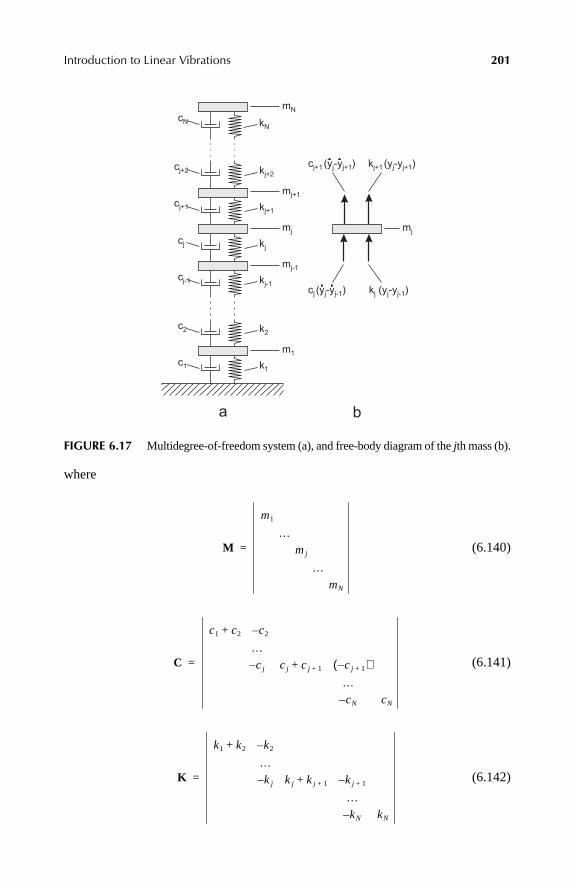
Introduction to Linear Vibrations 201
where
(6.140)
(6.141)
(6.142)
FIGURE 6.17 Multidegree-of-freedom system (a), and free-body diagram of the jth mass (b).
M
m1
…mj
…mN
=
C
c1 c2+ c2–
…cj– cj cj 1++ cj 1+–( )
…cN– cN
=
K
k1 k2 + k2–
…kj– kj kj 1+ + kj 1+–
…kN– kN
=
Ch6Frame Page 201 Friday, June 2, 2000 6:43 PM

202 Fundamentals of Kinematics and Dynamics of Machines and Mechanisms
and
(6.143)
In the case the external forces are applied to masses, the force vector is
(6.144)
and Equation 6.139 then becomes
(6.145)
6.13.1 FREE VIBRATIONS OF A 2DOF SYSTEM WITHOUT DAMPING
Consider free oscillations of an undamped system having two masses, Figure 6.18a.The equations of motion are a particular case of the system Equation 6.139:
(6.146)
Since the above is the system of linear equations with constant coefficients, the solutionis an amplitude vector multiplied by an exponential function (see Equation 6.18):
or (6.147)
If this form of the solution is substituted into Equation 6.146, then
(6.148)
Since , the latter equation is reduced to a requirement:
(6.149)
Since the amplitude vector is arbitrary, the matrix–vector product isequal to zero only if the determinant of the matrix is equal to zero. For a matrix ofrank 2 the second-order determinant is defined as follows:
Y y1 … yj … yN, , , ,( )T=
P P1 … Pj … PN, , , ,( )T=
My Cy Ky+ + P=
m1
m2
y1
y2
k1 k2+
k2–
k2–
k2
y1
y2
+ 0
0=
Y A eλ t=y1
y2
D1
D2
eλ t=
m1
m2
λ2 k1 k2+
k2–
k2–
k2
+D1
D2
eλ t 0
0=
eλ t 0≠
m1
m2
λ2 k1 k2+
k2–
k2–
k2
+D1
D2
0
0=
D D1 D2,( )T=
Ch6Frame Page 202 Friday, June 2, 2000 6:43 PM

Introduction to Linear Vibrations 203
(6.150)
Using the above definition, one can write the determinant of the matrix in Equation6.149:
(6.151)
The latter equation is a fourth-order polynomial with respect to λ:
(6.152)
The above equation is called the characteristic equation (see Equation 6.20) andit defines such values of λ that the nontrivial solutions of Equation 6.146 exist.These values of λ are called eigenvalues. Thus, the eigenvalues are the roots ofEquation 6.152. Solving Equation 6.152 for λ2 yields
(6.153)
If the parameters of the system are such that the expression under the square rootis positive, then the two roots are negative, which means that in this case λ is animaginary number. The two imaginary numbers are
and (6.154)
FIGURE 6.18 A 2DOF system (a), first mode of oscillation (b), and second mode ofoscillation (c).
detb1 d1
b2 d2
b1d2 b2d1–=
detm1λ
2 k1 k2+ + k2–
k2– m2λ2 k2+
m1λ2 k1 k2+ +( ) m2λ
2 k2+( ) k22–= 0=
m1m2λ4 m2 k1 k2+( ) m1k2+[ ] λ2 k1k2+ + 0=
λ1 2,2 1
2---
k1 k2+m1
----------------k2
m2------+
–14---
k1 k2+m1
----------------k2
m2------+
2 k1
m1------
k2
m2------–±=
λ1 iω1= λ2 iω2=
Ch6Frame Page 203 Friday, June 2, 2000 6:43 PM

204 Fundamentals of Kinematics and Dynamics of Machines and Mechanisms
The circular frequencies and are the natural frequencies of a two-masssystem. For each natural frequency the amplitudes D1 and D2 remain undeterminedsince the determinant of the matrix in Equation 6.149 is equal to zero. However, theratio of these amplitudes can be found from any of the two scalar equations for eachnatural frequency. For example, for ,
(6.155)
or
(6.156)
Thus, the ratio between the amplitudes for the first natural frequency is
(6.157)
Similarly, for the second natural frequency,
(6.158)
Thus, for each natural frequency there is an amplitude vector D (see Equation 6.147)
and (6.159)
Vectors D1 and D2 characterize the mode of vibrations. The vector corresponding tothe lowest natural frequency characterizes the first mode, and then the other char-acterizes the second mode. The meaning of modes will be made clear in the examplebelow.
It is very important to underscore that neither the natural frequencies nor themodes of oscillation depend on the initial conditions. As was the case in SDOFsystems, both reflect the properties of the system: masses and stiffnesses.
Recalling again Euler’s formula, , the solution entails twofunctions as possible solutions: and . Take, for example, the first root,
, and substitute it in Equation 6.147. Then,
(6.160)
ω1 ω2
λ1 iω1=
m1ω12– k1 k2+( )+[ ] D1
1 k2D21– 0=
k2D11 m2ω1
2– k2+( )D21+– 0=
r 1D2
1
D11
------m1ω1
2– k1 k2+( )+k2
--------------------------------------------k2
m2ω12– k2+
----------------------------= = =
r 2D2
2
D12
------m1ω2
2– k1 k2+( )+k2
--------------------------------------------k2
m2ω22– k2+
----------------------------= = =
D1 D11
r 1D11
= D2 D12
r 2D12
=
eiω ω i ωsin+cos= eiλ t
ωtcos ωsin tλ1 iω1=
y11
y21
D11
D21
ω1t i ω1tsin+cos( ) D11
r 1D11
ω1t iD1
1
r 1D11
ω1tsin+cos= =
Ch6Frame Page 204 Friday, June 2, 2000 6:43 PM

Introduction to Linear Vibrations 205
Similarly, for the second root ,
(6.161)
The latter expressions mean that any constant vector multiplied by either cosω1t,sinω1t, cosω2t, or sinω2t is a solution of Equation 6.146. These functions, cosω1t,sinω1t, cosω2t, and sinω2t are called fundamental solutions.
The general solution of the homogeneous equation Equation 6.146 is a combi-nation of two solutions corresponding to two roots (again, the superposition principleis used)
(6.162)
where b1 and b2 are arbitrary constants.For the two roots in Equation 6.154 one thus has four functions, cosω1t,
sinω1t, cosω2t, and sinω2t, as possible solutions. It means that the general solutionis a combination of these four fundamental solutions. From Equation 6.162 andEquations 6.160 and 6.161,
(6.163)
and
(6.164)
where , and are constants, and r1, r2 are given by Equations 6.157 and6.158.
Alternatively, Equations 6.163 and 6.164 can be written in the form:
(6.165)
and
(6.166)
where D1 and D2 are the amplitudes of displacement of mass 1 and 2, and φ1 and φ2are the corresponding phase angles.
Define the initial conditions, namely, that at t = 0
(6.167)
λ2 iω2=
y12
y22
D12
D22
ω2t i ω2tsin+cos( ) D12
r 2D12
ω2t iD1
2
r 2D12
ω2tsin+cos= =
Y b1Y1 b2Y
2+=
y1 t( ) c111 ω1t c12
1 ω1t c112 ω2t c12
2 ω2tsin+cos+sin+cos=
y2 t( ) r 1c111 ω1t r 1 c12
1 ω1t r 2c112 ω2t r 2c12
2 ω2tsin+cos+sin+cos=
c111 c12
1 c112, , c12
2
y1 t( ) D1 ω1t φ1+( ) D2 ω2t φ2+( )cos+cos=
y2 t( ) r 1D1 ω1t φ1+( ) r 2D2 ω2t φ2+( )cos+cos=
y1 0( ) D10 y1 0( ), V10 y2 0( ), D20 and y2, 0( ) V20= = = =
Ch6Frame Page 205 Friday, June 2, 2000 6:43 PM

206 Fundamentals of Kinematics and Dynamics of Machines and Mechanisms
Subjecting the solutions (Equations 6.165 and 6.166) to the above initial conditions,one obtains four equations for four unknowns:
(6.168)
(6.169)
(6.170)
(6.171)
This system of four equations can be solved for four unknowns: ,, and . Notice that this system is uncoupled, namely, Equations 6.168
and 6.170 form one independent subsystem, whereas Equations 6.169 and 6.171form another. These smaller systems can be easily solved, and, as a result,
(6.172)
(6.173)
(6.174)
(6.175)
Now, from Equations 6.172 and 6.174, D1 and φ1 are found:
(6.176)
(6.177)
And, similarly, from Equations 6.173 and 6.175, D2 and φ2 are found:
y1 0( ) D1 φ1 D2 φ2cos+cos D10= =
y1 0( ) ω1D– 1 φ1 ω2D2– φ2sinsin V10= =
y2 0( ) r 1D1 φ1 r 2D2 φ2cos+cos D20= =
y2 0( ) ω1r 1D– 1 φ1 ω2r 2D2– φ2sinsin V20= =
D1 φ1 D2 φ2cos,cosD1 φ1sin D2 φ2sin
D1 φ1cosr 2D10 D20–
r 2 r 1–---------------------------=
D2 φ2cosr 1D10 D20–
r 1 r 2–---------------------------=
D1 φ1sinr– 2V10 V20+ω1 r 2 r 1–( )
------------------------------=
D2 φ2sinr– 1V10 V20+ω2 r 1 r 2–( )
------------------------------=
D11
r 2 r 1–--------------- r 2D10 D20–( )2 r– 2V10 V20+( )2
ω12
-------------------------------------+=
φ1 arcr– 2V10 V20+
ω1 r 2D10 D20–( )---------------------------------------tan=
Ch6Frame Page 206 Friday, June 2, 2000 6:43 PM

Introduction to Linear Vibrations 207
(6.178)
(6.179)
Thus, Equations 6.165 and 6.166 together with Equations 6.176 through 6.179give the general solution of vibrations of a 2DOF system without damping subjectedto the initial disturbance.
Consider a numerical example for the case when m1 = m2 = m and k1 = k2 = k.Then Equation 6.153 becomes
(6.180)
and the natural frequencies and in Equation 6.154 are
and (6.181)
The ratio between the amplitudes for the first natural frequency, Equation 6.157, is
(6.182)
and for the second frequency, Equation 6.158, is
(6.183)
Recall that the amplitude ratio reflects the mode of vibrations, Equation 6.159.Now the meaning of the mode becomes clear from Equations 6.182 and 6.183. Inthe first mode, when the system oscillates with the low frequency ω1, the ratio ofamplitudes is positive, which means that the two masses move synchronously. Inthe second mode, when the system oscillates with the high frequency ω2, the ratioof amplitudes is negative, which means that the two masses move asynchronously.Note also that in the first mode the absolute value of the ratio of amplitude is larger.
In Figure 6.19 vibrations of the first mass are shown, caused by its initialdisplacement. One can see that it oscillates with two frequencies, low frequency ω1,and high frequency ω2. The resulting motion is the superposition of motions withthese two frequencies. In Figure 6.20 the motions of the first and second masses aresuperimposed. One can see that the two masses move synchronously at low frequency
D21
r 1 r 2–--------------- r 1D10 D20–( )2 r– 1V10 V20+( )2
ω22
-------------------------------------+=
φ2 arcr– 1V10 V20+
ω2 r 1D10 D20–( )---------------------------------------tan=
λ1 2,2 3
2--- k
m---- 1–
53
-------± =
ω1 ω2
ω12 k
m----
3 5–2
---------------- = ω2
2 km----
3 5+2
---------------- =
r 1a2
1
a11
-----mω1
2– 2k+k
---------------------------3 5–
2----------------– 2+ 1 5+
2----------------= = = =
r 2a2
2
a12
-----mω2
2– 2k+k
---------------------------3 5+
2----------------– 2+ 1 5–
2----------------= = = =
Ch6Frame Page 207 Friday, June 2, 2000 6:43 PM

208 Fundamentals of Kinematics and Dynamics of Machines and Mechanisms
and asynchronously (in other words, either apart or toward each other) at the highfrequency.
These two modes of vibrations are shown schematically in Figure 6.18b and c.
6.13.2 FREE VIBRATIONS OF A 2DOF SYSTEM WITH DAMPING
Equation 6.145 adds viscous forces defined by the matrix C (Equation 6.141)
(6.184)
The general solution of Equation 6.184 has the form:
(6.185)
FIGURE 6.19 Vibrations of the first mass.
FIGURE 6.20 Vibrations of a two-mass system. Solid line = mass 1; dashed line = mass 2.
2 4 6 8 10 12Time
-4
-2
2
4
y1yst
2 4 6 8 10 12Time
-4
-2
2
4
y1yst
y2yst
,
m1
m2
y1
y2
c1 c2+
c2–
c2–
c2
y1
y2
+ +k1 k2+
k2–
k2–
k2
y1
y2
0
0=
Y D1
D2
eλ t=
Ch6Frame Page 208 Friday, June 2, 2000 6:43 PM

Introduction to Linear Vibrations 209
Substituting the latter into Equation 6.184 yields an algebraic equation similar toEquation 6.149:
(6.186)
The determinant of the matrix must equal zero in order for the nontrivial solutionto exist. This requirement gives the equation to determine λ:
(6.187)
The above is a characteristic equation (polynomial) with respect to λ:
(6.188)
The solution of the above equation can be obtained with the help of Mathematica,but the expressions are complicated. Instead, consider a simplified case whenm1 = m2 = m, k1 = k2 = k, and c1 = c2 = c. In this case Equation 6.188 becomes
(6.189)
The roots of this equation are
(6.190)
and
(6.191)
To introduce the same notations as for an SDOF system, Equation 6.17,
(6.192)
Then, Equations 6.190 and 6.191 become
(6.193)
m1
m2
λ2 c1 c2+
c2–
c2–
c2
λ +k1 k2+
k2–
k2–
k2
+D1
D2
0
0=
detm1λ
2 c1 c2+( )λ k1 k2+ + +
c2λ– k2–
c2λ– k2–
m2λ2 c2λ k2+ +
m1λ2 c1 c2+( )λ k1 k2++ +( ) m2λ
2 c2λ k2+ +( ) c2λ k2+( )2–= 0=
m1m2λ4 m1c2 m+ 2 c1 c2+( )[ ] λ3 m1k2 m2 k1 k2+( ) c1c2+ +[ ] λ2++
+ c1k2 c2k1+( )λ k1k2+ 0=
m2λ4 3mcλ3 3mk c2+( )λ2 2ckλ k2+ + + + 0=
λ1 2,3 5+( )c
4m------------------------
24
------- c2
m2------ 7 3 5–( ) 4
km---- 3 5+–( )+±=
λ3 4,3 5+( )– c
4m---------------------------
24
------- c2
m2------ 7 3 5+( ) 4–
km---- 3 5+( )±=
ξ c2mωn
-------------- and ωn2 k
m----= =
λ1 2,3 5+( )
2---------------------ξ 2
4-------± 4ξ2 7 3 5–( ) 12 4 5–( )+
ωn=
Ch6Frame Page 209 Friday, June 2, 2000 6:43 PM

210 Fundamentals of Kinematics and Dynamics of Machines and Mechanisms
and
(6.194)
Similar to the case of the system without damping, for each root the amplitudes inEquation 6.186 are undetermined, but their ratio can be found from Equation 6.186.For any root λ i one has, taking, for example, the first scalar equation in Equation 6.186,
(6.195)
and
(6.196)
The general solution is a superposition of four fundamental solutions of the Equation6.185 type
(6.197)
and
(6.198)
As in the case of an SDOF system, the type of response depends on the amount ofdamping the system has, in other words, on the type of roots given by Equations 6.193and 6.194. The damping is determined by the coefficient c or a nondimensionalcoefficient ξ. In the case of an 2DOF system there are more combinations of responsessince there are more combinations of roots. First of all, find the critical values of ξthat identify the boundary between complex and real roots in Equations 6.193 and6.194. These values are found by equating the expressions under the radical to zero.From Equation 6.193,
(6.199)
and
(6.200)
λ3 4,3 5+( )–
2------------------------ξ 2
4-------± 4ξ2 7 3 5+( ) 12 4 5+( )–
ωn=
m1λ i2 c1 c2+( )λ i k1 k2++ +[ ] D1
i c2λ i k2––[ ] D2i+ 0=
r i
D2i
D1i
------m1λ i
2 c1 c2+( )λ i k1 k2+ + +c2λ i k2+
------------------------------------------------------------------mλ i
2 2cλ i 2k+ +cλ i k+
---------------------------------------= = =
y1 t( ) D11e
λ1tD1
2eλ2t
D13e
λ3tD1
4eλ4t
+ + +=
y2 t( ) r 1D11e
λ1tr 2D1
2eλ2t
r 3D13e
λ3tr 4D1
4eλ4t
+ + +=
ξ1cr 3 5–
7 3 5–------------------- 1.61803= =
ξ2cr 3 5+
7 3 5+------------------- 0.618034= =
Ch6Frame Page 210 Friday, June 2, 2000 6:43 PM

Introduction to Linear Vibrations 211
One can now see various possibilities:
• If , then both roots are real and it means that both masses are over-damped. There are no vibrations in this case due to initial disturbance.
• If , then roots in Equation 6.194 are real, while in Equation 6.193they are complex. In this case both masses will oscillate with one frequency(Equations 6.197 and 6.198).
• If , then roots in both Equations 6.194 and 6.195 are complex, andthe system will oscillate with two frequencies.
Consider now each case, taking, for example, that .
1. . The displacements of both bodies in time, caused by the initialdisplacement of the second body, are shown in Figure 6.21. It is seen that afterthe second body is released the two of them move to the position of staticequilibrium exponentially. Note that the first body slightly overshoots the posi-tion of static equilibrium (which is zero).
2. . The displacements of both bodies in time, caused by the initialdisplacement of the second body, are shown in Figure 6.22. It is seen that afterthe second body is released, the two of them cross the position of static equi-librium and then move to this position exponentially. There is a periodic termin the solutions, the amplitude of which becomes very small after the first half-cycle that it is not seen on the graph.
3. . The displacements of both bodies in time, caused by the initialdisplacement of the second body, are shown in Figure 6.23. It is seen that afterthe second body is released, the two of them move synchronously (first mode)while their amplitudes are decreasing exponentially. The fact that only the lowfrequency is visible indicates that the high frequency (second mode) is dampedout. This is a general feature of vibrating systems, namely, that high frequencycomponents decline faster.
FIGURE 6.21 Normalized displacements of m2 (solid line) and m1 (dashed line) caused byinitial displacement y2(0)/yst =5 of the second mass ( ).
1 2 3 4 5 6Time
1
2
3
4
5
y (t)yst
ξ 1.7 ξ1cr>=
ξ ξ 1cr>
ξ2cr ξ ξ 1
cr< <
ξ ξ 2cr<
ωn2 10=
ξ 1.7 ξ1cr>=
ξ2cr ξ 1.0 ξ1
cr<=<
ξ 0.2 ξ2cr<=
Ch6Frame Page 211 Friday, June 2, 2000 6:43 PM

212 Fundamentals of Kinematics and Dynamics of Machines and Mechanisms
6.13.3 FORCED VIBRATIONS OF A 2DOF SYSTEM WITH DAMPING
The matrix form of the equation is
(6.201)
where for a 2DOF system shown in Figure 6.18, the matrices M , C, and K are thesame as in Equation 6.186, and the vector P is as follows
(6.202)
FIGURE 6.22 Normalized displacements of m2 (solid line) and m1 (dashed line) caused byinitial displacement y2(0)/yst = 5 of the second mass ( ).
FIGURE 6.23 Normalized displacements of m2 (solid line) and m1 (dashed line) caused byinitial displacement y2(0)/yst = 5 of the second mass ( ).
1 2 3 4 5 6Time
-1
1
2
3
4
5
y (t)yst
ξ2cr ξ 1.0 ξ1
cr<=<
2 4 6 8Time
y (t)yst
-2
-4
4
2
ξ 0.2 ξ2cr<=
My Cy Ky+ + P=
P p1
p2
eiωt=
Ch6Frame Page 212 Friday, June 2, 2000 6:43 PM

Introduction to Linear Vibrations 213
The steady-state (particular) solutions are of the form (see Section 6.8)
(6.203)
After substitution of Equation 6.203 into Equation 6.201, and taking into accountEquation 6.202, one obtains
(6.204)
or, after summing up matrices on the left,
(6.205)
The matrix on the left is a complex dynamic stiffness matrix, which is also calledan impedance matrix. Denote the elements of the latter as zks(iω), k,s = 1,2. Thenthe impedance matrix has the form
(6.206)
where
(6.207)
(6.208)
(6.209)
The solution of Equation 6.205 is
(6.210)
where
(6.211)
where it was taken into account that z12(iω) = z21(iω).
Y D1
D2
eiωt=
m1
m2
– ω2 ic1 c2+
c2–
c2–
c2
ω+k1 k2+
k2–
k2–
k2
+D1
D2
p1
p2
=
k1 k2 m1ω2– iω c1 c2+( )++ k2– iωc2–
k2– iωc2– k2 m2ω2– iωc2+
D1
D2
p1
p2
=
Z iω( ) z11 iω( ) z12 iω( )z21 iω( ) z22 iω( )
=
z11 iω( ) k1 k2 m1ω2 iω c1 c2+( )+–+=
z12 iω( ) z21 iω( ) k2– iωc2–= =
z22 iω( ) k2 m2ω2 iωc2+–=
D1
D2
Z 1– iω( ) p1
p2
=
Z 1– iω( ) 1
z11 iω( )z22 iω( ) z– 12 iω( )2----------------------------------------------------------- z22 iω( ) z– 12 iω( )
z– 12 iω( ) z11 iω( )=
Ch6Frame Page 213 Friday, June 2, 2000 6:43 PM

214 Fundamentals of Kinematics and Dynamics of Machines and Mechanisms
Thus, the inverse of the impedance matrix is the dynamic frequency responsematrix. The expressions for dynamic responses of individual masses in Figure 6.18afollow from Equations 6.210 and 6.211
(6.212)
and
(6.213)
Consider the same numerical example as in Section 6.13.2, namely, whenm1 = m2 = m and k1 = k2 = k. In addition, assume that c1 = c2 = c and p2 = 0. Thenthe vibrations amplitudes are as follows:
(6.214)
and
(6.215)
where
(6.216)
(6.217)
(6.218)
The expressions for the amplitudes and phase angles, obtained with the help ofMathematica, are as follows:
(6.219)
(6.220)
D1z22 iω( )p1 z– 12 iω( )p2
z11 iω( )z22 iω( ) z– 12 iω( )2-----------------------------------------------------------=
D2
z– 12 iω( )p1 z+ 11 iω( )p2
z11 iω( )z22 iω( ) z– 12 iω( )2-----------------------------------------------------------=
D1z– 12 iω( )p2
z11 iω( )z22 iω( ) z– 12 iω( )2-----------------------------------------------------------=
D2z11 iω( )p2
z11 iω( )z22 iω( ) z– 12 iω( )2-----------------------------------------------------------=
z11 iω( ) 2k mω2– 2iωc+=
z12 iω( ) z21 iω( ) k iωc––= =
z22 iω( ) k mω2– iωc+=
D1
k2 c2ω2+
k4 6k3mω2– 6kmω4 c2 m2ω2+( )– k2 2c2ω2 11m2ω4+( )+--------------------------------------------------------------------------------------------------------------------------------------------
+ ω4 c4 7c2m2ω2 m4ω4+ +( )--------------------------------------------------------------------
1 2⁄=
D2
4c2 2k mω2+–( )2+
k4 6k3mω2– 6kmω4 c2 m2ω2+( )– k2 2c2ω2 11m2ω4+( )+--------------------------------------------------------------------------------------------------------------------------------------------
+ ω4 c4 7c2m2ω2 m4ω4+ +( )--------------------------------------------------------------------
1 2⁄=
Ch6Frame Page 214 Friday, June 2, 2000 6:43 PM

Introduction to Linear Vibrations 215
(6.221)
and
(6.222)
In Figures 6.24 through 6.26 the amplitude–frequency and phase angle dia-grams for the first and second bodies are shown in the case when k/m = 10/sec2
and ξ = 0.05 (so that c/m = 0.0316/sec).One can see from Figures 6.24 and 6.25 that in the case of damping almost
10 times smaller than the lowest critical, the second resonance cannot be practicallyexcited. This is also seen in Figure 6.23 in the case of free vibrations, whereas whenthe damping is absent then both frequencies are present (see Figures 6.19 and 6.20).The comparison of phase angles in Figure 6.26 shows that damping does not changequalitatively the phase angle function, except that it varies more smoothly nearresonances. One should recall that the phase angle characterizes the shift in timebetween the maximum of the force and that of the displacement.
6.14 ROTORDYNAMICS
Rotating machine components (shafts, rotors) are not perfectly manufactured andassembled and this causes machine vibrations. The result of a nonideal manufactur-ing of, for example, a rotor with a disk mounted on it, is that the center mass of thedisk may not lie on the axis of rotor rotation. This, in turn, leads to unbalancedforces during rotation and, thus, to vibrations. There may also be other causes ofvibrations, such as a nonideal geometry of supports and bearings, misalignment ofmultistage rotors, periodic forces generated by the meshing gears.
The common factor for all of the above dynamic forces is that their periodicityis proportional to the speed of rotation. If the periodicity of the dynamic forces isthat of the speed of rotation and they cause the system to resonate, then this speedof rotation is called the critical speed. Below, some simple examples of rotors withone mounted disk illustrating the dynamic phenomena in rotating machinery arepresented.
6.14.1 RIGID ROTOR ON FLEXIBLE SUPPORTS
The rotor is considered to be rigid if its critical speed is higher than its operatingspeed of rotation. However, such a system may still vibrate due to the flexibilityof the supports (journal or roller bearings). A schematic diagram of such a systemis shown in Figure 6.27, where e is the eccentricity of the mass center of the disk,k is the support stiffness, and m is the mass of the disk (it is assumed that the massof the rotor is small compared with that of the disk).
φ1tan kω 2ck 3cmω2–( )– cω k2 c2ω2– 3kmω2– m2ω4+( )+
cω2 2ck 3cmω2–( ) k k2 c2ω2– 3kmω2– m2ω4+( )+-------------------------------------------------------------------------------------------------------------------------------------=
φ2tan 2k mω2+–( )ω 2ck 3cmω2–( )– 2c k2 c2ω2– 3kmω2– m2ω4+( )–
2c– ω 2ck 3cmω2–( ) 2k mω2+–( ) k2 c2ω2– 3kmω2– m2ω4+( )+----------------------------------------------------------------------------------------------------------------------------------------------------------------=
Ch6Frame Page 215 Friday, June 2, 2000 6:43 PM

216 Fundamentals of Kinematics and Dynamics of Machines and Mechanisms
FIGURE 6.24 Normalized amplitude of the first body vs. frequency. Solid line = ξ = 0.05;dashed line = ξ = 0.
FIGURE 6.25 Normalized amplitude of the second body vs. frequency. Solid line = ξ = 0.05;dashed line = ξ = 0.
FIGURE 6.26 Phase angle of the first body vs. frequency. Solid line = ξ = 0.05; dashedline = ξ = 0.
1 2 3 4 5 6ω
5
10
15
20
Amplitude
1 2 3 4 5 6ω
5
10
15
20
25
30
35
Amplitude
2 3 4 5 6ω
0
0.5
1
1.5
2
2.5
3
Phase angle
1
Ch6Frame Page 216 Friday, June 2, 2000 6:43 PM

Introduction to Linear Vibrations 217
If the angular speed of the rotor is ω, then an eccentrically located (with respectto the rotor axis) mass will generate a centrifugal force:
(6.223)
This force rotates with the angular velocity ω in the (x,y)-coordinate system. Thus,at any angle θ the x- and y-projections of this force are
and (6.224)
Taking into account that the angle of rotation is , the latter expressions canbe written in terms of the rotor angular velocity and time, t.
and (6.225)
As one can see, the centrifugal force, Equation 6.223, is not periodic, whereas itsx- and y-components are. The centrifugal force is in fact a vector and can be written as
(6.226)
where i and j are the unit vectors directed along the x- and y-coordinates, respectively.Now one can use the superposition principle and consider the effect of each
force component separately and then sum up the results to obtain the effect of thecentrifugal force on the rotor dynamics. If the lateral deflections of the springs aresmall so that their lateral stiffness can be neglected, then the x- and y-motions ofthe rotor are uncoupled. In this case the corresponding motion equations for eachdirection are similar to those of the mass on a spring under the action of a periodicforce (see Equation 6.12). Namely,
(6.227)
FIGURE 6.27 Rigid rotor on flexible supports.
Fc meω2=
Fcx Fc θcos= Fcy Fc θsin=
θ ωt=
Fcx Fc ωtcos= Fcy Fc ωtsin=
Fc iFcx j Fcy+=
mx kx+ meω2 ω tcos=
Ch6Frame Page 217 Friday, June 2, 2000 6:43 PM

218 Fundamentals of Kinematics and Dynamics of Machines and Mechanisms
and
(6.228)
The solutions for the steady-state vibrations are given by Equation 6.64, in whichit should be taken that p0 = eω2. Thus, the solutions are
(6.229)
and
(6.230)
The axis of the rotor is displaced from the static position of equilibrium by the radialdistance r, which is equal to
(6.231)
As one can see from the latter formula, for any given frequency ω the rotor axisdisplacement remains constant. The rotor axis moves along the constant radius orbit.Such motion is called whirling. If the x- and y-springs have the same stiffness, thenthe orbit is circular (as is the case considered above); otherwise, the orbit becomeselliptical.
From Equation 6.231 it is seen that when the speed of rotation ω equals that ofnatural frequency ωn, then the displacement of the rotor is infinite; i.e., it is inresonance. The speed ωn is called the critical speed. In Figure 6.28 the rotor dis-placement normalized with respect to the eccentricity e is shown as a function of anondimensional frequency. It is seen from Equation 6.231 that when , then
(in Figure 6.28 this limit is equal to 1 and it is shown by a dashed line).The position of the mass center during the rotation is the sum of the rotor axis
displacement and the eccentricity (Figure 6.29)
(6.232)
The latter, using Equation 6.231 for r, is equal to
(6.233)
my ky+ meω2 ω tsin=
x t( ) eω2
ωn2 ω2–
------------------ ω tcos=
y t( ) eω2
ωn2 ω2–
------------------ ω tsin=
r x2 t( ) y2 t( )+ eω2
ωn2 ω2–
------------------= =
ω ∞→r e→
r c r e+=
r ceω2
ωn2 ω2–
------------------ e+=
Ch6Frame Page 218 Friday, June 2, 2000 6:43 PM

Introduction to Linear Vibrations 219
One can see that if the speed of the rotor is less than critical, ω < ωn, then rc > e,if ω > ωn, then rc < e, and when , then . In other words, in unbalancedrotors the mass center changes its position with respect to a whirling rotor axis atthe critical speed, and then with the increase in speed this mass center tends to theaxis of the undisturbed rotor.
It is important to understand that the rotation of the mass center is the result ofsummation of two rotations: one is the rotation of the rotor itself with respect to itscenter (the latter coincides with the tip of the vector r in Figure 6.29), and the otheris the rotation of the rotor axis (rotation of the vector r ) around the coordinate center.Since both these angular velocities are equal to ω, the whirl in this case is calledsynchronous. The two vectors, r and e, are always collinear.
6.14.2 FLEXIBLE ROTOR ON RIGID SUPPORTS
Such a system is shown in Figure 6.30, where for simplicity the disk is placed inthe middle of the shaft (rotor). The rotating unbalanced disk generates the centrifugalforces given by Equation 6.223. Then, the motion equations are the same as in the
FIGURE 6.28 Normalized radius of rotor whirling vs. nondimensional angular velocity.
FIGURE 6.29 Position of mass center of a disk on a rigid rotor when ω < ωn.
1 2 3 4 5
ωωn
2
4
6
8
10
re—
ω ∞→ r c 0→
Ch6Frame Page 219 Friday, June 2, 2000 6:43 PM

220 Fundamentals of Kinematics and Dynamics of Machines and Mechanisms
case of a rigid rotor (Equations 6.227 and 6.228), except that instead of springstiffness the shaft stiffness at the disk location should be used. Thus, all the resultsobtained in Section 6.14.1 are applicable in this case as well.
6.14.3 FLEXIBLE ROTOR WITH DAMPING ON RIGID SUPPORTS
The damping in the disk–rotor system may be caused by the material damping prop-erties of the rotor itself, by the friction at rotor supports (bearings), or by the airresistance to a rotor motion. The effect of damping is that the vectors r and e inFigure 6.29 are no longer collinear, because e is associated with the direction of theexternal force meω2 and r with the reaction of the system to this force. The angle φbetween the vectors r and e is the phase angle (Figure 6.31). When the angular velocityω of the rotor is constant, the angle φ also remains constant. Thus, the rotor imbalancevector e leads (or lags behind) the rotor whirl vector r by a constant phase angle φ. If
, then the corresponding whirl having constant velocity is called synchronous.In the case of a nonsynchronous whirl the time rate of change of the angle φ is
the spin velocity of the rotor relative to the rotating whirl vector r. Thus, the rotor
FIGURE 6.30 Unbalanced disk on a flexible shaft.
FIGURE 6.31 Positions of mass center of a disk on a flexible rotor with damping.
ω θ= θ
Ch6Frame Page 220 Friday, June 2, 2000 6:43 PM

Introduction to Linear Vibrations 221
angular velocity in this case is . The synchronous whirl takes place duringa steady-state rotation, while nonsteady rotation leads to a nonsynchronous whirl.
The case of a synchronous whirl ( ) will be considered. The equations ofmotion in this case are the same as Equations 6.227 and 6.228, but, in addition, theycontain terms associated with the damping forces. Thus,
(6.234)
and
(6.235)
where, as before in Equations 6.227 and 6.228, x and y are the coordinates of therotor axis, so that the coordinates of the center mass are
and (6.236)
Note that in Equations 6.234 and 6.235 the damping coefficient has a subscript e.It indicates that in the case of a synchronous whirl the rotation of a bent rotor doesnot cause internal damping forces, and so the damping may be only of externalnature (bearings, air).
Instead of solving Equations 6.234 and 6.235 for x and y, one can transformthis system into a single equation with respect to a complex variable z = x + iy,which is another form of the vector r. To achieve such transformation, multiplyEquation 6.235 by an imaginary unit i, add the two equations together, and takeinto account Euler’s formula ( ). The result is
(6.237)
For a steady-state regime, the solution of the above equation has the form:
(6.238)
By substituting the latter into Equation 6.237 and canceling the exponential terms,the following expression for the complex amplitude of rotor axis displacement isobtained:
(6.239)
By denoting, as before (see Section 6.14.1), the critical speed of the undampedsystem by , and expressing the coefficient of damping as
ω θ φ+=
φ 0=
mx cex kx++ meω2 ω tcos=
my cey ky++ meω2 ω tsin=
xm x e θ φ+( )cos+= ym y e θ φ+( )sin+=
eiωt ω t i ω tsin+cos=
mz cez kz+ meω2eiωt= =
z z0eiωt=
z0meω2
k mω2–( ) iceω+------------------------------------------=
ωn k m⁄( )0.5= ce 2mωnξe=
Ch6Frame Page 221 Friday, June 2, 2000 6:43 PM

222 Fundamentals of Kinematics and Dynamics of Machines and Mechanisms
(see Equation 6.17), Equation 6.239 can be written in nondimensional parametersas follows:
(6.240)
By multiplying the denominator in the latter by a complex conjugate number, it istransformed into the following form:
(6.241)
Thus, the complex amplitude of the axis position of the rotor has the form:
(6.242)
where x0 and y0 are the amplitudes associated with solutions of Equations 6.234 and6.235.
The complex number in Equation 6.242 can also be written in the form:
(6.243)
where |z0| is the absolute value of the amplitude and φ is the argument of the complexnumber, which in this case is the phase angle.
The expressions for the amplitude |z0| and the phase angle φ are as follows
(6.244)
and
(6.245)
It is seen that the above equations are identical to Equations 6.89 and 6.90, if it istaken into account that in this case p0 = eω2. In this case, however, the critical speed is
(6.246)
and the corresponding maximum amplitude is
(6.247)
z0eω2
ωn2 ω2–( ) 2iωωnξe+
---------------------------------------------------=
z0eω2 ωn
2 ω2–( ) 2– iωωnξe[ ]
ωn2 ω2–( )2
2ωωnξe( )2+------------------------------------------------------------=
z0 x0 iy0+=
z0 z0 eiφ x02 y0
2+ eiφ= =
z0eω2
ωn2 ω2–( )2
2ωωnξe( )2+--------------------------------------------------------------=
φ arc2ωωnξe
ωn2 ω2–
-------------------tan=
ωc
ωn
1 2ξe2–
---------------------=
z0 maxe
2ξe 1 ξe2–
--------------------------=
Ch6Frame Page 222 Friday, June 2, 2000 6:43 PM

Introduction to Linear Vibrations 223
In Figure 6.32 the normalized radius vs. the normalized angular speed is shownwhen the nondimensional coefficient of damping equals ξe = 0.1. The effect ofdamping on the system dynamics is a limiting of the maximum amplitude at thecritical speed (compare with Figure 6.28). For the chosen value of ξe the maximumnormalized amplitude is 5.025. Note that if ξe << 1, then the amplitude can beestimated by the formula:
(6.248)
The above formula gives the value of the normalized amplitude equal to 5.The change of the phase angle as a function of normalized rotor speed is shown
in Figure 6.33. First of all, it is seen that the phase angle changes with the speed ofrotation and, second, since this angle is negative the vector r lags behind the vectore (see Figure 6.32). Recall that the phase angle is the angle between the direction
FIGURE 6.32 Normalized radius of rotor whirling vs. nondimensional angular velocity.
FIGURE 6.33 Phase angle vs. normalized angular rotor speed.
1 2 3 4 5
1
2
3
4
5
re—
ωωn
1 2 3 4 5
ωωn
-3
-2.5
-2
-1.5
-1
-0.5
Phase angle—
z0 maxe
2ξe
--------=
Ch6Frame Page 223 Friday, June 2, 2000 6:43 PM
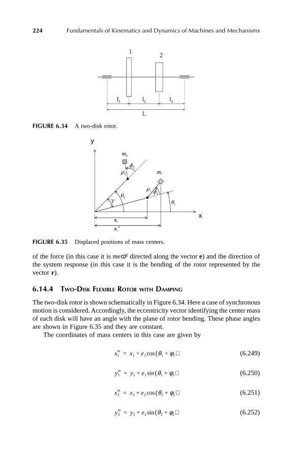
224 Fundamentals of Kinematics and Dynamics of Machines and Mechanisms
of the force (in this case it is meω2 directed along the vector e) and the direction ofthe system response (in this case it is the bending of the rotor represented by thevector r ).
6.14.4 TWO-DISK FLEXIBLE ROTOR WITH DAMPING
The two-disk rotor is shown schematically in Figure 6.34. Here a case of synchronousmotion is considered. Accordingly, the eccentricity vector identifying the center massof each disk will have an angle with the plane of rotor bending. These phase anglesare shown in Figure 6.35 and they are constant.
The coordinates of mass centers in this case are given by
(6.249)
(6.250)
(6.251)
(6.252)
FIGURE 6.34 A two-disk rotor.
FIGURE 6.35 Displaced positions of mass centers.
x1m x1 e1 θ1 φ1+( )cos+=
y1m y1 e1 θ1 φ1+( )sin+=
x2m x2 e2 θ2 φ2+( )cos+=
y2m y2 e2 θ2 φ2+( )sin+=
Ch6Frame Page 224 Friday, June 2, 2000 6:43 PM

Introduction to Linear Vibrations 225
where xi = xi(t), yi = yi(t) (i = 1,2) are the displacements of the rotor at disk locations,and θi = θi(t) (i = 1,2) identifies a plane in which the bent rotor lies in the vicinityof the disk i.
The planes in which the bending of rotors at each disk location takes placedepend on the direction of unbalanced forces. Denote the angle between the latterby γ (see Figure 6.35), and assume that this angle is known. Thus, θ2 = θ1 + γ. Fora constant angular velocity of the rotor ω, θ1 = ω t, and one can take that φ1 = φ2 = 0.
The motion equation in a matrix form in, for example, the x-plane is
(6.253)
where the mass matrix M , the damping matrix C, and the stiffness matrix K are equal to
(6.254)
(6.255)
(6.256)
(6.257)
and
(6.258)
In Equation 6.255, cij (i,j = 1,2) are the damping coefficients with the followingmeaning: c11 is the force at position 1 corresponding to a unit velocity at this position
, c12 is the force at position 1 corresponding to a unit velocity at position 2, c21 is the force at position 2 corresponding to a unit velocity at position 1, c22 is the force at position 2 corresponding to a unit velocity at this position. Note that c12 = c21.
In Equation 6.256, kij (i,j = 1,2) are the stiffness coefficients with the followingmeaning: k11 is the force at position 1 corresponding to a unit displacement at thisposition x1 = 1, k12 is the force at position 1 corresponding to a unit displacementat position 2 x2 = 1, k21 is the force at position 2 corresponding to a unit displacement
Mx m Cx Kx+ + 0=
M m1
m2
=
C c11 c12
c21 c22
=
K k11 k12
k21 k22
=
xm x1m
x2m
=
x x1
x2
=
x1 1=x2 1=x1 1=x2 1=
Ch6Frame Page 225 Friday, June 2, 2000 6:43 PM

226 Fundamentals of Kinematics and Dynamics of Machines and Mechanisms
at position 1 x1 = 1, k22 is the force at position 2 corresponding to a unit displacementat this position x2 = 1. Note that k12 = k21.
Substituting , , , and into Equation 6.253 yields the followingdifferential equation:
(6.259)
where
(6.260)
The term on the right in Equation 6.259 after differentiation of e becomes
(6.261)
where
(6.262)
Recall that the cosine functions can be represented as the real parts of a complexexponential function:
(6.263)
and
(6.264)
Now one can represent the force on the right-hand side P = P* cos ωt as a real partof a vector P* eiωt, where P* is equal to
(6.265)
Instead of solving Equation 6.261, one can solve the following equation:
(6.266)
x1m x2
m x1 x2
Mx Cx Kx+ + Me–=
e e1 ωt( )cos
e2 ωt γ+( )cos=
Mx Cx Kx+ + P=
Pm1e1ω
2 ωt( )cos
m2e2ω2 ωt γ+( )cos
=
eiωt ω tcos i ω tsin+=
ei ωt γ+( ) eiωteiγ eiγ ω tcos i ω tsin+( )= =
P*m1e1ω
2
m2e2ω2eiγ
=
Mx Cx Kx+ + P* eiωt=
Ch6Frame Page 226 Friday, June 2, 2000 6:43 PM

Introduction to Linear Vibrations 227
The advantage of this substitution of the original equation by Equation 6.266 is thatone can use already derived solutions for Equation 6.201, in which one has to takeinto account that the damping and stiffness matrices and the force vector are differentin this case. As a result, instead of Equations 6.207 through 6.209, one has the following:
(6.267)
(6.268)
(6.269)
In Equations 6.212 and 6.213 take into account that
(6.270)
and
(6.271)
The stiffness matrix K can be found as an inverse of the flexibility matrix A
(6.272)
The elements of the flexibility matrix are called the influence coefficients. Theirmeaning is as follows: α ij is the displacement at the position i from the unit forceapplied at the position j. The influence coefficients can thus be found by analyzingthe displacements in a beam. For the case of a beam on simple supports shown inFigure 6.34 the influence coefficients are as follows
(6.273)
(6.274)
(6.275)
where E is the modulus of elasticity of the rotor material, and I = πd4/64 is themoment of inertia of the cross section of the rotor.
z11 iω( ) k11 m1ω2 iωc11+–=
z12 iω( ) z21 iω( ) k12 iωc12+= =
z22 iω( ) k22 m2ω2 iωc22+–=
p1 m1e1ω2=
p2 m2e2ω2eiγ=
A α11 α12
α21 α22
=
α11l12 l2 l3+( )2
3EIL-------------------------=
α22l32 l1 l2+( )2
3EIL-------------------------=
α12 α21
l1l3
6EIL------------- L2 l1
2 l32––( )= =
Ch6Frame Page 227 Friday, June 2, 2000 6:43 PM

228 Fundamentals of Kinematics and Dynamics of Machines and Mechanisms
The corresponding stiffness coefficients are
, , , where . (6.276)
The characteristic equation in this case is found as the determinant of thefollowing matrix:
(6.277)
By using Equations 6.254 and 6.256,
(6.278)
The above equation is quadratic with respect to ω2.Consider a specific example: l1 = 0.325 m, l2 = 0.35 m, l3 = 0.525 m, D1 = D2
= 0.25 m (disk diameters), b = 0.05 m (disk thickness), E = 200 109 Pa, ρ = 7860 kg/m3,e1 = 0.035 10–3 (first disk eccentricity), e2 = 0.046 10–3 (second disk eccentricity),d = 0.05 m (rotor diameter). For the given system the critical speeds (naturalfrequencies) are ω1 = 241.533 rad/s and ω2 = 1061.81 rad/s.
The determination of the damping coefficients is not straightforward becausethey depend on the masses and natural frequencies of the system. Use a simplifiedassumption that all damping coefficients are equal, and that their value is δ m1ω1/π,where δ is the logarithmic decrement, and ω1 is the first natural frequency. Take thatδ = 0.02 (steel).
The amplitude–angular velocity diagram for the first disk for the given data isshown in Figure 6.36.
FIGURE 6.36 Amplitude–angular velocity diagram.
200 400 600 800 1000 1200w
0.0001
0.0002
0.0003
0.0004
x1
k11α22
∆-------= k22
α11
∆-------= k12 k21
α12
∆-------–= = ∆ α11α22 α12
2–=
detK ω2M– 0=
m1m2ω4 m1k22 m2k11+( )ω2– k11k22 k12
2–+ 0=
Ch6Frame Page 228 Friday, June 2, 2000 6:43 PM

Introduction to Linear Vibrations 229
PROBLEMS AND EXERCISES
PROBLEMS
1. Show that a mass on an ideal spring will have a periodic motion if subjected toinitial displacement.
2. Show that a mass on an ideal spring will have a periodic motion if subjected toinitial velocity.
3. For an SDOF, what is the effect of (a) mass and (b) spring stiffness on theresonance frequency?
4. If the SDOF system is not ideal, i.e., its damping properties are taken into account,would it affect the period of response when subjected to initial disturbance?
5. What is critical damping for an SDOF?
6. Why in systems with damping subjected to periodic forces can the initial con-ditions be neglected when finding the system response?
7. Find the solution of the equation in a steady-stateregime. What are the effects of damping on an SDOF system in terms of itsresponse to a periodic force?
8. Show that if in the equation the forcing function issubstituted by , the expressions for the amplitude and phase angleremain the same.
9. State the initial conditions and find the two constants in the following generalsolution of a motion equation for an SDOF system:
10. What is the definition of a logarithmic decrement? How it is related to thecoefficient of damping for an SDOF system?
11. What is called the kinematic excitation? Write the motion equation for an SDOFsystem. How does it differ from the case of forced excitation?
12. What is the principle of superposition? Explain, using the example of a polyhar-monic force acting on an SDOF system.
13. What causes torsional vibrations? Write the motion equation for an SDOFsystem and compare it with the equation for the mass–spring system. Is thereany similarity between the two in terms of the system response to a periodicexcitation?
14. How many natural frequencies characterize a 2DOF system without damping?What is called a mode of vibration? Explain.
15. Derive the characteristic equation for a 2DOF system without damping.
y 2ξωny ωn2y++ p0 ω t( )sin=
y 2ξωny ωn2y++ p0 ω tsin=
p0 ω tcos
yc t( ) yg t( ) yp t( ) c=+ 1eλ1t
c2eλ2t
d1 ωcos t d2 ωsin t+ + +=
Ch6Frame Page 229 Friday, June 2, 2000 6:43 PM
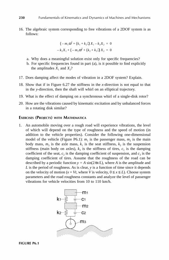
230 Fundamentals of Kinematics and Dynamics of Machines and Mechanisms
16. The algebraic system corresponding to free vibrations of a 2DOF system is asfollows:
a. Why does a meaningful solution exist only for specific frequencies?b. For specific frequencies found in part (a), is it possible to find explicitly
the amplitudes X1 and X2?
17. Does damping affect the modes of vibration in a 2DOF system? Explain.
18. Show that if in Figure 6.27 the stiffness in the x-direction is not equal to thatin the y-direction, then the shaft will whirl on an elliptical trajectory.
19. What is the effect of damping on a synchronous whirl of a single-disk rotor?
20. How are the vibrations caused by kinematic excitation and by unbalanced forcesin a rotating disk similar?
EXERCISES (PROJECTS) WITH MATHEMATICA
1. An automobile moving over a rough road will experience vibrations, the levelof which will depend on the type of roughness and the speed of motion (inaddition to the vehicle properties). Consider the following one-dimensionalmodel of the vehicle (Figure P6.1): m1 is the passenger mass, m2 is the mainbody mass, m3 is the axle mass, k1 is the seat stiffness, k2 is the suspensionstiffness (main body on axles), k3 is the stiffness of tires, c1 is the dampingcoefficient of the seat, c2 is the damping coefficient of suspension, and c3 is thedamping coefficient of tires. Assume that the roughness of the road can bedescribed by a periodic function y = A sin(2πx/L), where A is the amplitude andL is the period of roughness. As is clear, y is a function of time since it dependson the velocity of motion (x = Vt, where V is velocity, 0 ≤ x ≤ L). Choose systemparameters and the road roughness constants and analyze the level of passengervibrations for vehicle velocities from 10 to 110 km/h.
FIGURE P6.1
m1ω2– k1 k2+( )+{ } X1 k2X2– 0=
k2X1– m2ω2– k2 k3+( )+{ } X2+ 0=
Ch6Frame Page 230 Friday, June 2, 2000 6:43 PM

Introduction to Linear Vibrations 231
2. A steel shaft on two supports carries two spur gears (Figure P6.2). One of thecauses of shaft vibrations is the impact of teeth, which, in turn, is due to theimperfection of gear geometry. The frequency of these vibrations is called thetooth frequency, and it is equal to the product of the rotational frequency andthe number of teeth. For the following data, l = 165 mm, a = 40 mm, b = 130 mm,N1 = 25, N2 = 30, m1 = 1.3 kg, m2 = 0.7 kg, find the diameter of the shaft d suchthat there will be no resonances within the speed range of 2000 to 3000 rpm ofthe given shaft. Note, N1 and N2 are the teeth numbers of gears 1 and 2,respectively.
FIGURE P6.2
Ch6Frame Page 231 Friday, June 2, 2000 6:43 PM

Ch6Frame Page 232 Friday, June 2, 2000 6:43 PM

233
Bibliography
Chironis, N.P.,
Mechanisms and Mechanical Devices Sourcebook
, McGraw-Hill, New York,1991.
Erdman, A.G. and Sandor, G.N.,
Mechanical Design: Analysis and Synthesis
, Vol. 1,Prentice-Hall, Englewood Cliffs, NJ, 1991.
Kimbrell, J.T.,
Kinematic Analysis and Synthesis
, McGraw-Hill, New York, 1991.Mabie, H.H. and Reinholtz, C.F.,
Mechanisms and Dynamics of Machinery
, John Wiley& Sons, New York, 1987.
Malik, A.K., Ghosh, A., and Dittrich, G.,
Kinematic Analysis and Synthesis of Mechanisms
,CRC Press, Boca Raton, FL, 1994.
Martin, G.H.,
Kinematics and Dynamics of Machines
, McGraw-Hill, New York, 1982.Myszka, D.H.,
Machines and Mechanisms: Applied Kinematic Analysis
, Prentice-Hall,Englewood Cliffs, NJ, 1999.
Nikravesh, P.E.,
Computer-Aided Analysis of Mechanical System
s, Prentice-Hall, EnglewoodCliffs, NJ, 1988.
Norton, R.L.,
Design of Machinery: An Introduction to the Synthesis and Analysis of Mechanismsand Machines
, McGraw-Hill, New York, 1992.Rao, S.S.,
Mechanical Vibrations
, Addison-Wesley, Reading, MA, 1990.Shigley, J.E. and Uicker, J.J., Jr.,
Theory of Machines and Mechanisms
, McGraw-Hill,New York, 1995.
Waldron, K.J. and Kinzel, G.L.,
Kinematics, Dynamics, and Design of Machiner
y, John Wiley& Sons, New York, 1999.
Wolfram, S.,
Mathematica
, Cambridge University, Cambridge, U.K., 1999.
Bibliography/Frame Page 233 Friday, June 2, 2000 6:44 PM

Bibliography/Frame Page 234 Friday, June 2, 2000 6:44 PM

235
Appendix: Use of Mathematica as a Tool
A.1 INTRODUCTION TO MATHEMATICA
To start Mathematica, double-click the Mathematica icon and wait until an emptynotebook appears. Type a command, e.g., a numerical command; then pressSHIFT + ENTER and wait until the kernel is loaded (since this is the first evaluation).
In[1]:=
2 + 3
Out[1]:=
5
To the left of the command, 2 + 3, a label In[1] appears, and the result ofevaluation is labeled as Out[1]. Both input and output are identified on the right bybrackets, which are called
cells
. By moving the cursor below the Out[1] cell andthen clicking, a straight line appears, which opens a new cell ready for an input.Thus, the
notebook
consists of a series of cells.
N
UMERICAL
C
ALCULATIONS
Mathematica can be used as a calculator, in which case numbers and correspondingarithmetic operators are typed in and then executed by pressing SHIFT + ENTER,as in the example above. Mathematica has many built-in functions (see
Built-inFunctions
in
Help
), the numerical values of which can be found for any givenargument (1) by placing the argument in square brackets, (2) then by placing thefunction itself in square brackets, (3) then by preceding the latter with capital N,and (4) then by executing the hierarchy of two commands.
In[2]:=
N[Cos[
π
/3]]
Out[2]:=
0.5
In the above input In[2], N[ ] is a function that gives a numerical approximation ofa real number. Note also that all commands and all built-in functions are writtenwith the first letter capitalized.
Appendix Page 235 Friday, June 2, 2000 8:49 PM

236
Fundamentals of Kinematics and Dynamics of Machines and Mechanisms
S
YMBOLIC
C
ALCULATIONS
Consider a quadratic equation
ax
2
+
bx
+
c
= 0. We find the roots by using thecommand Solve[ ].
In[3]:=
quadraticEq = ax
2
+ bx + c == 0
Out[3]:=
c + bx + ax
2
== 0
In[4]:=
solution = Solve [quadraticEq, x]
Out[4]:=
The quadratic equation is defined by the user-defined name
quadraticEq
. If we type
quadraticEq
and execute, the equation will be the output.
In[5]:=
quadraticEq
Out[5]:=
c + bx +ax
2
== 0
The solution of the equation is given as a
List of Replacement Rules
, whichmeans that the expressions for the roots cannot be used explicitly in any othersymbolic or numerical operation. We can obtain explicit expressions for the rootsby extracting corresponding information and assigning it to specific names.
In[6]:=
rootOne = x/. solution[[1]]
Out[6]:=
The meaning of the above is “replace
x
by the expression in the first braces in thelist
solution
(/. denotes a
Replacement Rule
) and give it the name
rootOne
.” Now,rootOne can be used in any numerical or symbolic operation. Consider, for example,rootOne squared:
In[7]:=
rootOne
2
Out[7]:=
In[8]:=
rootOneSpecific = rootOne /. {a
→
2, b
→
5, c
→
10}
xb– b2 4ac––
2a-------------------------------------→
xb– b2 4ac–+
2a--------------------------------------→
,
b– b2 4ac––2a
-------------------------------------
b– b2 4ac––( )2
4a2--------------------------------------------
Appendix Page 236 Friday, June 2, 2000 8:49 PM

Appendix: Use of Mathematica as a Tool
237
Out[8]:=
We found a specific value of the root rootOne by replacing symbols with numbers.It turns out that for these numbers the root is a complex number (I denotes animaginary unit).
P
LOTTING
R
ESULTS
To plot a two-dimensional function, use the command
Plot
. Let us say that thefunction to be plotted is
x
– Sin[
x
] and it is to be plotted from
x
= 0 to
x
= 2
π
. Wename this plot
plotOne
.
In[9]:=
plotOne = Plot[
x
– Sin[
x
], {
x
, 0, 2 Pi}]
Out[9]:=
A
NIMATION
We would like to animate the motion of a wheel moving forth along a straight line.Mathematica has a
Circle
primitive, which is a command.
In[10]:=
circl = Circle[{0, rad}, rad]
Out[10]:=
Circle[{0, rad}, rad]
In the brackets 0,rad gives the coordinates of the circle center, and rad is its radius.This circle can be plotted with the Show and Graphics commands. Let us assign aspecific value to the radius:
In[11]:=
rad = 1.
Out[11]:=
1.
14--- 5– I 55–( )
Appendix Page 237 Friday, June 2, 2000 8:49 PM

238
Fundamentals of Kinematics and Dynamics of Machines and Mechanisms
In[12]:=
circleGraphics = Show[Graphics[circl], AspectRatio
→
Automatic,Axes
→
True]
Out[12]:=
The option in Graphics AspectRatio
→
Automatic gives the same scale for
x
- and
y
-coordinates. Now we can use another Mathematica primitive graphics,
Line
, todraw a line passing through the circle center.
In[13]:=
diameterY = Line[{{0, 0}, {0, 2 rad}}]
Out[13]:=
Line[{{0, 0}, {0, 2.}}]
The two primitives, Circle and Line, can be shown together as one object, wheelGraphics.
In[14]:=
wheelGraphics = Show[Graphics[circl], Graphics[diameterY], AspectRatio
→
Automatic]
Out[14]:=
Appendix Page 238 Friday, June 2, 2000 8:49 PM

Appendix: Use of Mathematica as a Tool
239
Now we introduce a function that describes the circle and the diameter at any positionalong the line in terms of the rotation
angle
and the number
j
characterizing itsdiscrete position.
In[15]:=
wheelFunction[angle_, j_] :=(
xCentre = rad angle[[j]]; yCentre = rad;xOne = rad(angle[[j]] – Sin[angle[[j]]]); yOne = rad (1 – Cos[angle[[j]]]);xTwo = rad(angle[[j]] + Sin[angle[[j]]]); yTwo = rad (1 + Cos[angle[[j]]]);{Thickness[0.01],{
{RGBColor[0, 0, 1], Circle[{xCentre, yCentre}, rad]},{RGBColor[1, 0, 0], Line[{{xOne, yOne}, {xTwo, yTwo}}]}
}}
)Clear[j]
The angle angle is expressed in radians; xCentre and yCentre are the coordinatesof the circle center;
xOne
,
yOne
and
xTwo
,
yTwo
are the coordinates of two pointson the circle through which the line passes; RGBColor[0, 0, 1] is an option for thecolor of the circle; and RGBColor[1, 0, 0] for the color of the line (these colors arenot shown).
Animation is achieved by displaying the wheel at various positions sequentially.The positions are given as functions of the angle of wheel rotation, i.e.,
angle
in ournotation. The discrete set of values for the variable angle is introduced in the formof an array, and this array is generated with the help of the
Table
command.
In[16]
:= angleDiscrete = Table[t, {t, 0., N[2 Pi], N[Pi/10]}]
Out[16]:=
{0., 0.314159, 0.628319, 0.942478, 1.25664, 1.5708, 1.88496, 2.19911,2.51327, 2.82743, 3.14159, 3.45575, 3.76991, 4.08407, 4.39823,4.71239, 5.02655, 5.34071, 5.65487, 5.96903, 6.28319}
Let us find the number of elements in the array angleDiscrete:
In[17]:=
nPositions = Length[angleDiscrete]
Out[17]:=
21
Now we create an array of all wheel positions by again using the command Table:
In[18]:=
plots = Table[Graphics[wheelFunction[angleDiscrete, j],AspectRatio
→
Automatic,Axes
→
True, PlotRange
→
{{–rad, N[2 Pi rad]}, {0, 2 rad}}],{j, 1, nPositions}
]
Appendix Page 239 Friday, June 2, 2000 8:49 PM

240
Fundamentals of Kinematics and Dynamics of Machines and Mechanisms
Out[18]:=
{– Graphics –, – Graphics –, – Graphics –, – Graphics –, – Graphics –, – Graphics –,– Graphics –, – Graphics –, – Graphics –, – Graphics –, – Graphics –, – Graphics –,– Graphics –, – Graphics –, – Graphics –, – Graphics –, – Graphics –, – Graphics –,– Graphics –, – Graphics –, – Graphics –}
Now we can plot the wheel at all nPositions positions:
In[19]:=
Show[plots]
Out[19]:=
To animate the sequence of wheel positions Mathematica uses a special code, i.e.,a standard package. The animation package can be loaded by the following command:
In[20]:=
Needs[“Graphics Animation ”]
The following command displays all wheel positions. To animate the motion, double-click on any of the positions. To stop animation, click anywhere within the cell once.Of course, the animation cannot be shown here.
In[21]:=
ShowAnimation[plots]
A.2 VECTOR ALGEBRA
A vector is represented as a
list
.
In[1]:=
vectorA = {ax, ay}
Out[1]:=
{ax, ay}
In[2]:=
vectorB = {bx, by}
Out[2]:=
{bx, by}
The sum of two vectors
vectorA
and vectorB is vectorC.
In[3]:= vectorC = vectorA + vectorB
Out[3]:= {ax + bx, ay + by}
Appendix Page 240 Friday, June 2, 2000 8:49 PM
Appendix: Use of Mathematica as a Tool 241
The scalar product of two vectors is obtained by placing a dot between the vectors:
In[4]:= vectorD = vectorA . vectorB
Out[4]:= ax bx + ay by
To obtain a cross-product, vectorA and vectorB should be represented as three-dimensional (3D) vectors:
In[5]:= vectorA3D = {ax, ay, 0}
Out[5]:= {ax, ay, 0}
In[6]:= vectorB3D = {bx, by, 0}
Out[6]:= {bx, by, 0}
The cross-product of two vectors is obtained by using a Cross command:
In[7]:= vectorU3D = Cross[vectorA3D, vector B3D]
Out[7]:= {0, 0, –ay bx + ax by}
Now we will extract the nonzero component and call it zComponent:
In[8]:= zComponent = vectorU3D[[3]]
Out[8]:= –ay bx + ax by
We will repeat it for the vectors with the trigonometric representation of coordinates:
In[9]:= vectorAtrig = a{Cos[α], Sin[α]}
Out[9]:= {a Cos[α], a Sin[α]}
In[10]:= vectorBtrig = b{Cos[β], Sin[β]}
Out[10]:= {b Cos[β], b Sin[β]}
In[11]:= vectorDtrig = vectorAtrig . vectorBtrig
Out[11]:= ab Cos[α] Cos[β] + ab Sin[α] Sin[β]
This expression can be simplified by using a TrigReduce command:
In[12]:= vectorDsimplified = TrigReduce[vectorDtrig]
Out[12]:= ab Cos[α – β]
Appendix Page 241 Friday, June 2, 2000 8:49 PM
242 Fundamentals of Kinematics and Dynamics of Machines and Mechanisms
A.3 VECTOR ANALYSIS
If vector parameters are functions of time t, then a vector is written as follows:
In[13]:= vectorFunction = am[t]{Cos[γ[t]], Sin[γ[t]]}
Out[13]:= {am[t] Cos[γ[t]], am[t] Sin[γ[t]]}
The time-derivative is
In[14]:= vectorDerivative = D[vectorFunction, t]
Out[14]:= {Cos[γ[t]] am′[t] – am[t] Sin[γ[t]] γ′[t],Sin[γ[t]] am′[t] + am[t] Cos[γ[t]] γ′[t]}
The second time-derivative is
In[15]:= vectorDerivativeSec = D[vectorFunction, {t, 2}]
Out[15]:= {–2 Sin[γ[t]] am′[t]γ′[t] – am[t] Cos[γ[t]] γ′[t] 2 +Cos[γ[t]] am″[t] – am[t] Sin[γ[t]] γ″[t],
2 Cos[γ[t]] am′[t]γ′[t] – am[t] Sin[γ[t]] γ′[t] 2 +Sin[γ[t]] am″[t] + am[t] Cos[γ[t]] γ″[t]}
A.4 KINEMATIC AND FORCE ANALYSIS OF MECHANISMS
A.4.1 SLIDER-CRANK MECHANISM
Position Analysis
Let us consider the case when the crank is the driver. Then, the distance from thepiston to the crankshaft center (r1) and the position of the connecting rod (θ3) arethe two unknowns. This case falls into the second category (see text). In this caseα = θ2 – π, θ1 = π, b = r2, and r2 and r3 are constants.
We put a semicolon at the end of the input if we do not want the output to bedisplayed.
In[1]:= α = θ2 + π;
In[2]:= b = r2;
In[3]:= θ1 = π;
In[4]:= r1 = r2 Cos[α – θ1] + Sqrt[r32 – r22 Sin[α – θ1]2]
Out[4]:= r2 Cos[θ2] + r32 r2
2Sin θ2[ ] 2–
Appendix Page 242 Friday, June 2, 2000 8:49 PM

Appendix: Use of Mathematica as a Tool 243
Now we find Sin[θ3 – θ1] and Cos[θ3 – θ1] from Equations 2.29 and 2.30:
In[5]:=
Out[5]:=
In[6]:=
Out[6]:=
The correct angle θ3 – θ1 = θ3 – π is found using the command ArcTan[Cosθ3θ1,Sinθ3θ1] :
In[7]:=
Out[7]:=
At this point, we should assign some values to r2 and r3:
In[8]:= r2 = 1.; r3 = 4.;
In[9]:= θ3Specific = θ3
Out[9]:=
In[10]:= r1Specific = rl
Out[10]:=
Now we can plot both functions.
In[11]:= Plot[θ3Specific, {θ2, 0, 2π}]
Out[11]:= – Graphics –
Sinθ3θ1bSin α θ1–[ ]
r3--------------------------------=
r2Sin θ2[ ]r3
-----------------------
Cosθ3θ1bCos α θ1–[ ] r1–
r3-------------------------------------------=
r32 r2
2Sin θ2[ ] 2–r3
--------------------------------------–
θ3 π ArcTan Cosθ3θ1 Sinθ3θ1,[ ]+=
π ArcTanr3
2 r22Sin θ2[ ] 2–r3
--------------------------------------r2Sin θ2[ ]
r3-----------------------,–+
π ArcTan 0.25– 16. 1.Sinθ2[ ] 2– 0.25Sinθ2[ ],[ ]+
1.Cos θ2[ ] 16. 1.Sinθ2[ ] 2–+
Appendix Page 243 Friday, June 2, 2000 8:49 PM

244 Fundamentals of Kinematics and Dynamics of Machines and Mechanisms
We can see that θ3 is described by the positive values of the angle. It is moreconvenient to look at this angle as being within ±θ3. We can transform the abovefunction:
In[12]:= θ3Transformed = If[θ2 ≤ π, θ3Specific – 2π, θ3Specific]
Out[12]:= If[ θ2 ≤ π, θ3Specific – 2π, θ3Specific]
In[13]:= Plot[θ3Transformed, {θ2, 0, 2π},AxesLabel → {“ θ2”, “ θ3”}, PlotStyle → {AbsoluteThickness[2.4]}]
Out[13]:= – Graphics –
In[14]:= Plot[r1Specific, {θ2, 0, 2π},AxesLabel → {“ θ2”, “r 1”}, PlotStyle → {AbsoluteThickness[2.4]}]
Out[14]:= – Graphics –
To animate the mechanism, we discretize the input angle θ2:
Appendix Page 244 Friday, June 2, 2000 8:49 PM

Appendix: Use of Mathematica as a Tool 245
In[15]:= theta2 = Table[iπ/10, {i, 0, 20}]
Out[15]:=
By replacing the symbolic variable θ2 by its numerical counterpart theta2 in allexpressions we automatically discretize these functions:
In[16]:= r1Discr = r1 /. θ2 → theta2
Out[16]:= {5., 4.9391, 4.76559, 4.50512, 4.19431, 3.87298, 3.57627, 3.32955, 3.14756, 3.03699, 3., 3.03699, 3.14756, 3.32955, 3.57627, 3.87298, 4.19431, 4.50512, 4.76559, 4.9391, 5.}
In[17]:= θ3Discr = θ3 /. θ2 → theta2
Out[17]:= {2π, 6.20585, 6.1357, 6.07953, 6.04312, 6.03051, 6.04312, 6.07953, 6.1357, 6.20585, 2π, 0.0773313, 0.14748, 0.203659, 0.240063, 0.25268, 0.240063, 0.203659, 0.14748, 0.0773313, 2π}
Animation is achieved by drawing the mechanism in Length[theta2] positions, andthen displaying them in sequence. To accomplish this, we have to create discretedata for all variables (which we already did), and then make the drawings as functionsof these variables. We define a function that describes the mechanism geometry atany angle θ2:
In[18]:= mechanismLines[theta2_, θ3Discr_, j_] :=(
x2 = r2 Cos[theta2[[j]]]; y2 = r2 Sin[theta2[[j]]];x3 = x2 + r3 Cos[θ3Discr[[j]]]; y 3 = y2 + r3 Sin[θ3Discr[[j]]];r1Mag = Sqrt[x32 + y3
2];(*Coordinates of the piston in the global system*)
;
;
;
;
0π10------ π
5--- 3π
10------ 2π
5------ π
2--- 3π
5------ 7π
10------ 4π
5------ 9π
10------ π, , , , , , , , , , ,
11π10
--------- 6π5
------ 13π10
--------- 7π5
------ 3π2
------ 8π5
------ 17π10
--------- 9π5
------ 19π10
--------- 2π, , , , , , , , ,
x1P r1Mag 18---– r2
Cos π θ1–[ ] 14---r2Sin π θ1–[ ]–=
y1P r1Mag 18---– r2
– Sin π θ1–[ ] 14---r2Cos π θ1–[ ]–=
x2P r1Mag 18---– r2
Cos π θ1–[ ] 14---r2Sin π θ1–[ ]+=
y2P r1Mag 18---– r2
– Sin π θ1–[ ] 14---r2Cos π θ1–[ ]+=
Appendix Page 245 Friday, June 2, 2000 8:49 PM

246 Fundamentals of Kinematics and Dynamics of Machines and Mechanisms
;
;
;
;
(*Coordinates of the cylinder in the global system*)
;
;
;
;
;
;
;
;
{Thickness[0.015],{
{RGBColor[1, 0, 0], Line[{{0, 0}, {x2, y2}}]},{RGBColor[0, 1, 0], Line[{{x2, y2}, {x 3, y3}}]},(*Drawing piston*)
{RGBColor[0, 0, 1], Line[{{x1P, y1P}, {x 2P, y2P}}]},{RGBColor[0, 0, 1], Line[{{x2P, y2P}, {x 3P, y3P}}]},{RGBColor[0, 0, 1], Line[{{x3P, y3P}, {x 4P, y4P}}]},{RGBColor[0, 0, 1], Line[{{x1P, y1P}, {x 4P, y4P}}]},
(*Drawing cylinder*){RGBColor[1, 0, 1], Line[{{x2C, y2C}, {x 3C, y3C}}]},{RGBColor[1, 0, 1], Line[{{x3C, y3C}, {x 4C, y4C}}]},{RGBColor[1, 0, 1], Line[{{x4C, y4C}, {x 1C, y1C}}]},
x3P r1Mag18---r2+
Cos π θ1–[ ] 14---r2Sin π θ1–[ ]+=
y3P r1Mag18---r2+
– Sin π θ1–[ ] 14---r2Cos π θ1–[ ]+=
x4P r1Mag18---r2+
Cos π θ1–[ ] 14---r2Sin π θ1–[ ]–=
y4P r1Mag18---r2+
– Sin π θ1–[ ] 14---r2Cos π θ1–[ ]–=
x1C r2 r316---r2–+–
Cos π θ1–[ ] 14--- 1
10------+
r2Sin π θ1–[ ]–=
y1C r2 r316---r2–+–
– Sin π θ1–[ ] 14--- 1
10------+
r2Cos π θ1–[ ]–=
x2C r2 r316---r2–+–
Cos π θ1–[ ] 14--- 1
10------+
r2Sin π θ1–[ ]+=
y2C r2 r316---r2–+–
– Sin π θ1–[ ] 14--- 1
10------+
r2Cos π θ1–[ ]+=
x3C r2 r316---r2+ +
Cos π θ1–[ ] 14--- 1
10------+
r2Sin π θ1–[ ]+=
y3C r2 r316---r2+ +
– Sin π θ1–[ ] 14--- 1
10------+
r2Cos π θ1–[ ]+=
x4C r2 r316---r2+ +
Cos π θ1–[ ] 14--- 1
10------+
r2Sin π θ1–[ ]–=
y4C r2 r316---r2+ +
– Sin π θ1–[ ] 14--- 1
10------+
r2Cos π θ1–[ ]–=
Appendix Page 246 Friday, June 2, 2000 8:49 PM

Appendix: Use of Mathematica as a Tool 247
(*Drawing joints*)
{RGBColor[0, 0, 1], Circle[{0, 0}, r2]},
{RGBColor[1, 0, 0], Circle[{x3, y3}, r2]},
{RGBColor[0, 0, 1], Circle[{x2, y2}, r2]}
}}
)In[19]:= Clear[j]
Now we plot the mechanism at Length[theta2] positions:
In[20]:= Mechplots = Table[Graphics[mechanismLines[theta2, θ3Discr, j],AspectRatio → Automatic, Axes → True,PlotRange → {{–2, 6}, {–2., 2.}}], {j, 1, Length[theta2]}
]
Out[20]:= {– Graphics –, – Graphics –, – Graphics –, – Graphics –,– Graphics –, – Graphics –, – Graphics –, – Graphics –,– Graphics –, – Graphics –, – Graphics –, – Graphics –,– Graphics –, – Graphics –, – Graphics –, – Graphics –,– Graphics –, – Graphics –, – Graphics –, – Graphics –, – Graphics –}
To animate the Length[theta2] plots we call upon a special package Graphics\Animation\:
In[21]:= Needs[“Graphics Animation ”]
Instead of ShowAnimation[Mechplots], below we use the GraphicsArray commandto show the slider-crank mechanism in the first four positions:
In[22]:= Show[GraphicsArray[{{Mechplots[[1]], Mechplots[[2]]},{Mechplots[[3]], Mechplots[[4]]}}, AspectRatio → Automatic]]
Out[22]:= – GraphicsArray –
110------
120------
120------
Appendix Page 247 Friday, June 2, 2000 8:49 PM

248 Fundamentals of Kinematics and Dynamics of Machines and Mechanisms
Velocity Analysis
We use the solutions given in the text for the angular velocity of the connecting rodand for the translational velocity of the slider:
In[22]:=
Out[22]:=
In[23]:=
Out[23]:=
Let us asume that the input angular velocity is constant and give it a value:
In[24]:=
Out[24]:= 10
In[25]:= plotω3 = Plot[omega3, {θ2, 0, 2π}, AxesLabel → {“ θ2”, “ ω3”},PlotStyle → (AbsoluteThickness[2.4]}]
Out[25]:= – Graphics –
In[26]:= plotSliderVel = Plot[sliderVel, {θ2, 0, 2π},AxesLabel → {“ θ2”, “Slider Velocity”},
PlotStyle → {AbsoluteThickness[2.4]}]
omega3 omega2r2Cos θ2[ ]r3Cos θ3[ ]------------------------–=
0.25omega2 Cosθ2[ ] Sec ArcTan[ 0.25 16. 1.Sin θ2[ ] 2– 0.25Sinθ2[ ],– ][ ]( )
sliderVel r2omega2Sin θ2 θ3–[ ]
Cos θ3[ ]------------------------------–=
1.– omega2 SecArcTan 0.25 16. 1.Sin θ2[ ] 2– 0.25Sinθ2[ ],–[ ][ ]Sin θ2 ArcTan 0.25 16. 1.Sin θ2[ ] 2– 0.25Sinθ2[ ],–[ ]–[ ]
()
omega2 10=
1 2 3 4 5 6θ2
-2
-1
1
2
ω \3
Appendix Page 248 Friday, June 2, 2000 8:49 PM

Appendix: Use of Mathematica as a Tool 249
Out[26]:= – Graphics –
Acceleration Analysis
We use the solutions given in the text for the angular acceleration of the connectingrod and for the translational acceleration of the slider:
In[27]:=
Out[27]:=
In[28]:=
Out[28]:= –Sec[ArcTan[–0.25 , 0.25 Sin[θ2]]]
(–10.(10 – 2.5Cos[θ2]Sec [ArcTan[–0.25 , 0.25Sin[θ2]])+
25.Cos[θ2]Sec[ArcTan[–0.25 , 0.25 Sin[θ2]]]
Sin[θ2 – ArcTan[–0.25 , 0.25 Sin[θ2]]]
Tan[ArcTan[–0.25 , 0.25 Sin[θ2]]])
In[29]:= plotAngularAccel3 = Plot[angularAccel3, {θ2, 0, 2π},AxesLabel → {“ θ2”, “ α3”}, PlotStyle → (AbsoluteThickness[2.4]}]
1 2 3 4 5 6θ2
-10
-5
5
10
Slider Velocity
angularAccel3r2omega22Sin θ2[ ] r3omega32Sin θ3[ ]+
r3Cos θ3[ ]-------------------------------------------------------------------------------------------------=
0.25 SecArcTan 0.25 16. 1.Sin θ2[ ] 2–– 0.25Sinθ2[ ],[ ][ ]100.Sin θ2[ ] 25. Cosθ2[ ] 2 Sec ArcTan 0.25 16. 1.Sin θ2[ ] 2–– 0.25Sinθ2[ ],[ ][ ]
Tan ArcTan 0.25 16. 1.Sin θ2[ ] 2–– 0.25Sinθ2[ ],[ ][ ](
)(
)–(
)
(
)
–
sliderAccelsliderVel omega3Sin θ3[ ] r2omega2 omega2 omega3–( )–
Cos θ3[ ]---------------------------------------------------------------------------------------------------------------------------------------------=
16. 1.Sinθ2[ ] 2–
16. 1.Sinθ2[ ] 2–
16. 1.Sinθ2[ ] 2–
16. 1.Sinθ2[ ] 2–
16. 1.Sinθ2[ ] 2–
Appendix Page 249 Friday, June 2, 2000 8:49 PM

250 Fundamentals of Kinematics and Dynamics of Machines and Mechanisms
Out[29]:= – Graphics –
In[30]:= plotSliderAccel = Plot[sliderAccel, {θ2, 0, 2π},AxesLabel → {“ θ2”, “Slider acceleration”},
PlotStyle → {AbsoluteThickness[2.4]}]
Out[30]:= – Graphics –
Force Analysis
We assume that the moment moment2 is applied to the crank, and the resistanceforce P4 is applied to the piston. We also assume that there are two concentratedmasses: one at point A, which is the revolute joint connecting the crank and theconnecting rod, and the other at point B, identifying the revolute joint on the slider.Note that we have to express all vectors as 3D objects.
In[31]:= r2IN3D = r2{Cos[θ2], Sin[θ2], 0}
Out[31]:= {1.Cos[θ2], 1.Sin[θ2], 0}
In[32]:= r3IN3D = r3{Cos[θ3], Sin[θ3], 0}
Out[32]:= {–4.Cos[ArcTan[–0.25 , 0.25 Sin[θ2]]],
–4.Sin[ArcTan[–0.25 , 0.25 Sin[θ2]]], 0}
1 2 3 4 5 6θ2
-120
-110
-100
-80
Slider acceleration
16. 1.Sinθ2[ ] 2–
16. 1.Sinθ2[ ] 2–
Appendix Page 250 Friday, June 2, 2000 8:49 PM

Appendix: Use of Mathematica as a Tool 251
Forces and moments as 3D vectors:
In[33]:= sliderForce = P4{–1, 0, 0};
In[34]:= crankMoment = moment2{0, 0, 1};
Force in the crank-connecting rod joint acting on the crank:
In[35]:= jointForce32 = {f32x, f32y, 0};
Force in the connecting rod–slider joint acting on the rod:
In[36]:= jointForce13 = f13{0, 1, 0};
Force in the crank–frame joint acting on the crank:
In[37]:= jointForce12 = {f12x, f12y, 0};
Inertial forcesAcceleration of point A:
In[38]:= accelA = r2 D[{Cos[θ2[t]], Sin[θ2[t]], 0}, {t, 2}]
Out[38]:= {1.(–Cos[θ2[t]] θ2′[t] 2 – Sin[θ2[t]] θ2″[t]),1.(–Sin[θ2[t]] θ2′[t] 2 + Cos[θ2[t]] θ2″[t]), 0}
Assume that omega2 is constant. Also, let us replace θ2[t] by θ2, the notation usedabove.
In[39]:= accelAMod = accelA /. {θ2[t] → θ2, θ2′[t] → omega2, θ2″[t] → 0}
Out[39]:= {–100.Cos[θ2], –100.Sin[θ2], 0}
Inertial force at joint A:
In[40]:= inertForceA = –massA accelAMod;
Acceleration of point B. But first we have to replace θ2 by θ2[t] in the expressionfor θ3.
In[41]:= θ3T = θ3 /. θ2 → θ2[t]
Out[41]:= π + ArcTan[–0.25 , 0.25 Sin[θ2[t]]]
In[42]:= accelB = D[r2{Cos[θ2[t]], Sin[θ2[t]], 0} + r3{Cos[θ3T], Sin[θ3T], 0}, {t, 2}];
16. 1.Sinθ2 t[ ][ ] 2–
Appendix Page 251 Friday, June 2, 2000 8:49 PM

252 Fundamentals of Kinematics and Dynamics of Machines and Mechanisms
Again, we take into account that omega2 is constant, and also replace θ2[t] with θ2.
In[43]:= accelBMod = accelB /. {θ2[t] → θ2, θ2′[t] → omega2, θ2″[t] → 0};
Equilibrium equationsForces in link 2, crank:
In[44]:= eqOne = jointForce12 + jointForce32 – inertForceA == 0
Out[44]:= {f12x + f32x – 100.massACos[θ2], f12y + f32y – 100.massASin[θ2], 0} == 0
Moments in link 2 about point 0:
In[45]:= eqTwo = Cross[jointForce32 – inertForceA, r2IN3D] – crankMoment == 0
Out[45]:= {0, 0, –moment2 – 1.f32yCos[θ2] + 1.f32x Sin[θ2] +0.massACos[θ2]Sin[θ2]} == 0
Forces in link 3, connecting rod:
In[46]:= eqThree = –jointForce32 + jointForce13 +sliderForce – massB accelBMod == 0;
Moments in link 3 about point B:
In[47]:= eqFour = Cross[r3IN3D, –jointForce32] == 0
Out[47]:= {0, 0, 4.f32yCos[ArcTan[–0.25 , 0.25 Sin[θ2]]] –
4.f32x Sin[ArcTan[–0.25 , 0.25 Sin[θ2]]]} == 0
Solution of equationsThere are six scalar equations with six unknowns: f12x, f12y, f32x, f32y, f13, and P4. Wedo not display the solutions since they are long. At this point, we assign specificinput data:
In[48]:= massA = 5; massB = 20; moment2 = 10;
In[49]:= solution = Solve[{eqOne, eqTwo, eqThree, eqFour},{f12x, f12y, f32x, f32y, f13, P4}];
The solutions are given in the form of the replacement rules. We transform replace-ment rules into explicit functions:
In[50]:= f12xFunct = f12x /. solution
16. 1.Sinθ2[ ] 2–
16. 1.Sinθ2[ ] 2–
Appendix Page 252 Friday, June 2, 2000 8:49 PM

Appendix: Use of Mathematica as a Tool 253
Out[50]:= {0. + 500. Cos[θ2] + 1. (0. + (1. Cot[ArcTan[–0.25 , 0.25Sin[θ2]]](0. Sin[θ2] – 4. (–10. + 0. Cos[θ2]Sin[θ2])
Sin[ArcTan[–0.25 , 0.25 Sin[θ2]]])) /
(–4. Cos[ArcTan[–0.25 , 0.25 Sin[θ2]]] Sin[θ2] +
4. Cos[θ2]Sin[ArcTan[–0.25 , 0.25 Sin[θ2]]]))}
In[51]:= f12yFunct = f12y /. solution
Out[51]:= {0. + 500. Sin[θ2] + (1. (0. Sin[θ2] – 4. (–10. + 0. Cos[θ2]Sin[θ2])
Sin[ArcTan[–0.25 , 0.25 Sin[θ2]]])) /
(–4. Cos[ArcTan[–0.25 , 0.25 Sin[θ2]]] Sin[θ2] +
4. Cos[θ2]Sin[ArcTan[–0.25 , 0.25 Sin[θ2]]])}
In[52]:= f32xFunct = f32x /. solution
Out[52]:= {0. – (1. Cot[ArcTan[–0.25 , 0.25 Sin[θ2]]](0. Sin[θ2] – 4. (–10. + 0. Cos[θ2]Sin[θ2])
Sin[ArcTan[–0.25 , 0.25 Sin[θ2]]])) /
(–4. Cos[ArcTan[–0.25 , 0.25 Sin[θ2]]] Sin[θ2] +
4. Cos[θ2]Sin[ArcTan[–0.25 , 0.25 Sin[θ2]]])}
In[53]:= f32yFunct = f32y /. solution
Out[53]:= {–(1. (0. Sin[θ2] – 4. (–10. + 0. Cos[θ2]Sin[θ2])
Sin[ArcTan[–0.25 , 0.25 Sin[θ2]]])) /
(–4. Cos[ArcTan[–0.25 , 0.25 Sin[θ2]]] Sin[θ2] +
4. Cos[θ2]Sin[ArcTan[–0.25 , 0.25 Sin[θ2]]])}
In[57]:= f13Funct = f13 /. solution;
In[58]:= P4Funct = P4 /. solution;
All of the above expressions are functions of the independent variable θ2. Now wecan plot any of these functions. For example, we plot P4:
In[59]:= Plot[P4Funct, {θ2, 0, 2π}, AxesLabel → {“ θ2”, “Slider force”},PlotStyle → (AbsoluteThickness[2.4]}]
16. 1.Sinθ2[ ] 2–
16. 1.Sinθ2[ ] 2–
16. 1.Sinθ2[ ] 2–
16. 1.Sinθ2[ ] 2–
16. 1.Sinθ2[ ] 2–
16. 1.Sinθ2[ ] 2–
16. 1.Sinθ2[ ] 2–
16. 1.Sinθ2[ ] 2–
16. 1.Sinθ2[ ] 2–
16. 1.Sinθ2[ ] 2–
16. 1.Sinθ2[ ] 2–
16. 1.Sinθ2[ ] 2–
16. 1.Sinθ2[ ] 2–
16. 1.Sinθ2[ ] 2–
Appendix Page 253 Friday, June 2, 2000 8:49 PM

254 Fundamentals of Kinematics and Dynamics of Machines and Mechanisms
Out[59]:= – Graphics –
As we can see, there are three spikes in the resistance force at the 0, π, and 2πpositions of the crank. These spikes correspond to the dead point positions of theslider (piston), since at these positions an infinite force is needed to maintain theequilibrium. In other words, the system becomes singular.
A.4.2 FOUR-BAR LINKAGE
The r 1 vector describes the distance between the support joints, and then r 2, r 3, andr 4 follow r 1 in a clockwise direction. If θ2 is an independent variable, then the twovectors, r 1 and r 2, are known. In this case b = –(r 1 + r 2).
In[1]:= b = –(r1{Cos[θ1], Sin[θ1]} + r 2{Cos[θ2], Sin[θ2]})
Out[1]:= {–r1Cos[θ1] – r2Cos[θ2], –r1Sin[θ1] – r2Sin[θ2]}
The magnitude of vector b is
In[2]:= bMagn = Sqrt[b[[1]]2 + b[[2]]2]
Out[2]:=
The Sin α and Cos α components of the vector b are
In[3]:= SinAlpha = b[[2]] / bMagn
Out[3]:=
In[4]:= CosAlpha = b[[1]] / bMagn
r– 1Cos θ1[ ] r2Cos θ2[ ]–( )2 r– 1Sin θ1[ ] r2Sin θ2[ ]–( )2+
r1Sin θ1[ ]– r2Sin θ2[ ]–
r– 1Cos θ1[ ] r2Cos θ2[ ]–( )2 r– 1Sin θ1[ ] r2Sin θ2[ ]–( )2+--------------------------------------------------------------------------------------------------------------------------------------------
Appendix Page 254 Friday, June 2, 2000 8:49 PM

Appendix: Use of Mathematica as a Tool 255
Out[4]:=
At this point we should assign some values to r 1, r 2, r 3, r 4, and θ1. Assume in thisexample such values that r 2 is a crank.
In[5]:= r 1 = 4.; r 2 = 1.; r 3 = 6.; r 4 = 5.; θ1 = π;
The angle α is determined explicitly using the ArcTan command
In[6]:= α = ArcTan[CosAlpha, SinAlpha]
Out[6]:=
In[7]:= Plot[α, {θ2, 0, 2π}]
Out[7]:= – Graphics –
Solution of Loop-Closure Equation
From the formulas in the text, in this case i = 3, j = 4, we have
In[8]:=
Out[8]:=
r1Cos θ1[ ]– r2Cos θ2[ ]–
r– 1Cos θ1[ ] r2Cos θ2[ ]–( )2 r– 1Sin θ1[ ] r2Sin θ2[ ]–( )2+--------------------------------------------------------------------------------------------------------------------------------------------
arc4. 1.Cosθ2[ ]–
4. 1.Cosθ2[ ]–( )2 1.Sin θ2[ ] 2+-------------------------------------------------------------------------------
1.Sin θ2[ ]
4. 1.Cosθ2[ ]–( )2 1.Sin θ2[ ] 2+-------------------------------------------------------------------------------–,tan
AbMagn2 r3
2– r42+
2bMagn r4--------------------------------------------=
0.1 11.– 4. 1.Cosθ2[ ]–( )2 1.Sin θ2[ ] 2+ +( )
4. 1.Cosθ2[ ]–( )2 1.Sin θ2[ ] 2+----------------------------------------------------------------------------------------------------------
Appendix Page 255 Friday, June 2, 2000 8:49 PM

256 Fundamentals of Kinematics and Dynamics of Machines and Mechanisms
In[9]:=
Out[9]:=
The sign of C is either positive or negative. This corresponds to two possiblesolutions, which is to say, to two possible configurations. Let us take a positive sign:
In[10]:=
Out[10]:=
Now we can find α – θ3, since Sin(α – θ3) = C and Cos(α – θ3) = B.
In[11]:= αθ3 = ArcTan[B, Cconst]
Out[11]:=
In[19]:= Plot[αθ3, {θ2, 0, 2π}]
BbMagn r4 A–
r3----------------------------------=
0.1666670.5 11.– 4. 1.Cosθ2[ ]–( )2 1.Sin θ2[ ] 2+ +( )
4. 1.Cosθ2[ ]–( )2 1.Sin θ2[ ] 2+----------------------------------------------------------------------------------------------------------–
4. 1.Cosθ2[ ]–( )2 1.Sin θ2[ ] 2+
+
Cconstr4 1 A2–
r3------------------------=
0.833333 10.01 11.– 4. 1.Cosθ2[ ]–( )2 1.Sin θ2[ ] 2+ +( )2
4. 1.Cosθ2[ ]–( )2 1.Sin θ2[ ] 2+---------------------------------------------------------------------------------------------------------------–
ArcTan 0.1666670.5 11.– 4. 1.Cosθ2[ ]–( )2 1.Sin θ2[ ] 2+ +( )
4. 1.Cosθ2[ ]–( )2 1.Sin θ2[ ] 2+----------------------------------------------------------------------------------------------------------–
4. 1.Cosθ2[ ]–( )2 1.Sin θ2[ ] 2+
+
0.833333 10.01 11.– 4. 1.Cosθ2[ ]–( )2 1.Sin θ2[ ] 2+ +( )2
4. 1.Cosθ2[ ]–( )2 1.Sin θ2[ ] 2+---------------------------------------------------------------------------------------------------------------–
,
Appendix Page 256 Friday, June 2, 2000 8:49 PM

Appendix: Use of Mathematica as a Tool 257
Out[19]:= – Graphics –
If the above attempt to plot gives an error message indicating that it encounterscomplex numbers, then link 2 is not a crank; i.e., θ2 varies within limits smaller than0 to 2π. Let us denote these limits: min θ2 and max θ2. These limits can be foundby using the FindRoot command, and the starting values for finding the root can beapproximately taken from the above plot.
If the above attempt to plot does not give error messages, then min θ2 = 0 andmax θ2 = 2π. We assume below that link 2 is a revolving link. However, we describethe case of a nonrevolving link 2 in the form of comments (* … *).
(*minθ2 = Chop[FindRoot[αθ3 == 0, {θ2, minθ2Appr}]]*)In[21]:= (*minθ2Expl = θ2 /. minθ2*)
In[22]:= (*maxθ2 = Chop[FindRoot[αθ3 == 0, {θ2, maxθ2Appr}]]*)
In[23]:= (*maxθ2Expl = θ2 /. maxθ2*)
In[24]:= (*Plot[αθ3, {θ2, minθ2Expl, maxθ2Expl}]*)
Now we can find θ3 as a function of θ2:
In[25]:= θ3 = α – αθ3;
In[26]:= Plot[θ3, {θ2, 0, 2π},AxesLabel → {“ θ2”, “ θ3”},
PlotStyle → {AbsoluteThickness[2.4]}]
Out[26]:= – Graphics –
Recall that Cos(α – θ4) = A and Sin(α – θ4) = –r3C/r4. Thus, we can find α – θ4:
1 2 3 4 5 6θ2
-1.2
-1.1
-0.9
-0.8
θ3
Appendix Page 257 Friday, June 2, 2000 8:49 PM

258 Fundamentals of Kinematics and Dynamics of Machines and Mechanisms
In[27]:= αθ4 = ArcTan[A, –r3 Cconst / r4];
In[28]:= θ4 = α – αθ4;
In[29]:= Plot[θ4, {θ2, 0, 2π},AxesLabel → {“ θ2”, “ θ4”}, PlotStyle → {AbsoluteThickness[2.4]}]
Out[29]:= – Graphics –
Let us now discretize the input angle θ2, needed for animation, within the limitsmin θ2÷max θ2.
In[30]:= θ2Interval = 2π;
In[32]:= theta2 = Table[i θ2Interval/20, {i, 0, 19}]
Out[32]:=
We discretize all found functions by replacing θ2 → theta2.
In[33]:= θ3Discr = θ3 /. θ2 → theta2
Out[33]:= {–0.981765, –1.08404, –1.16711, –1.21687, –1.23086, –1.21423,–1.17486, –1.12048, –1.05771, –0.991906, –0.927295, –0.867239,–0.814469, –0.771389, –0.7404, –0.724273, –0.726486, –0.751283,–0.802791, –0.882029}
In[34]:= θ4Discr = θ4 /. θ2 → theta2
1 2 3 4 5 6θ2
1.3
1.4
1.5
1.6
1.7
θ4
0π10------ π
5--- 3π
10------ 2π
5------ π
2--- 3π
5------ 7π
10------ 4π
5------ 9π
10------, , , , , , , , , ,
π 11π10
--------- 6π5
------ 13π10
--------- 7π5
------ 3π2
------ 8π5
------ 17π10
--------- 9π5
------ 19π10
---------, , , , , , , , ,
Appendix Page 258 Friday, June 2, 2000 8:49 PM
Appendix: Use of Mathematica as a Tool 259
Out[34]:= {1.63751, 1.5223, 1.40319, 1.30099, 1.22592, 1.17978,1.16037, 1.16445, 1.18881, 1.23057, 1.287, 1.35524, 1.43205,1.51354, 1.59483, 1.66974, 1.73029, 1.76658, 1.76751, 1.72431}
Animation
Now we introduce a function that will draw the mechanism for any set of anglesθ2(j), θ3(j), θ4(j), where j identifies the position number.
In[35]:= mechanismLines[θ2_, θ3_, θ4_, j_] :=(
x2 = r2 Cos[θ2[[j]]];y2 = r2 Sin[θ2[[j]]];x3 = x2 + r3 Cos[θ3[[j]]];y3 = y2 + r3 Sin[θ3[[j]]];x4 = x3 + r4 Cos[θ4[[j]]];y4 = y3 + r4 Sin[θ4[[j]]];{
Thickness[0.02],{
{RGBColor[1, 0, 0], Line[{{0, 0}, {x2, y2}}]},{RGBColor[0, 1, 0], Line[{{x2, y2}, {x 3, y3}}]},{RGBColor[0, 1, 0], Line[{{x3, y3}, {x 4, y4}}]},
{RGBColor[0, 0, 1], Circle[{0, 0}, r2]},
{RGBColor[0, 0, 1], Circle[{x2, y2}, r2]},
{RGBColor[0, 0, 1], Circle[{x3, y3}, r2]},
{RGBColor[0, 0, 1], Circle[{x4, y4}, r2]}
}}
)In[36]:= Clear[j]
Now we store all plots under the name plotsOne.
In[37]:= plotsOne = Table[Graphics[mechanismLines[theta2, θ3Discr, θ4Discr, j],AspectRatio → Automatic,Axes → True, PlotRange → {{–r 4, r2 + r3}, {–r 4, r4}}], {j, Length[theta2]}]
Out[37]:= {– Graphics –, – Graphics –, – Graphics –, – Graphics –, – Graphics –,– Graphics –, – Graphics –, – Graphics –, – Graphics –, – Graphics –,– Graphics –, – Graphics –, – Graphics –, – Graphics –, – Graphics –,– Graphics –, – Graphics –, – Graphics –, – Graphics –, – Graphics –}
15---
110------
110------
15---
Appendix Page 259 Friday, June 2, 2000 8:49 PM

260 Fundamentals of Kinematics and Dynamics of Machines and Mechanisms
Below we show an array of positions:
In[39]:= Show[GraphicsArray[{{plotsOne[[1]], plotsOne[[3]]},{plotsOne[[5]], plotsOne[[7]]}, {plotsOne[[9]], plotsOne[[11]]}},AspectRatio → Automatic]]
Out[39]:= – GraphicsArray –
Now we can see that by choosing a plus sign for C, we have chosen the cross-configuration for the four-bar linkage.
Velocity Analysis
We use formulas derived in the text. Denote: dθ3/dt = omega3, and dθ4/dt = omega4.
In[76]:= ;omega3 omega2r2Sin θ2 θ4–[ ]r3Sin θ4 θ3–[ ]----------------------------------=
Appendix Page 260 Friday, June 2, 2000 8:49 PM

Appendix: Use of Mathematica as a Tool 261
In[77]:= ;
Now we assign a specific value to omega2:
In[78]:= omega2 = 10;
In[79]:= omega3Specific = omega3;
In[80]:= Plot[omega3, {θ2, 0, 2π},AxesLabel → {“ θ2”, “ ω3”}, PlotStyle → {AbsoluteThickness[2.4]}]
Out[80]:= – Graphics –
In[81]:= omega4Specific == omega4;
In[82]:= Plot[omega4, {θ2, 0, 2π},AxesLabel → {“ θ2”, “ ω4”}, PlotStyle → {AbsoluteThickness[2.4]}]
Out[82]:= – Graphics –
omega4 omega2r2Sin θ2 θ3–[ ]r4Sin θ3 θ4–[ ]----------------------------------=
1 2 3 4 5 6θ2
-3
-2
-1
1
2
ω3
1 2 3 4 5 6θ2
-4
-3
-2
-1
1
2
ω4
Appendix Page 261 Friday, June 2, 2000 8:49 PM
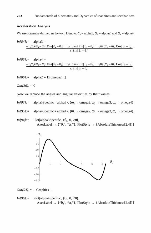
262 Fundamentals of Kinematics and Dynamics of Machines and Mechanisms
Acceleration Analysis
We use formulas derived in the text. Denote: α3 = alpha3, α2 = alpha2, and α4 = alpha4.
In[84]:= alpha3 =
;
In[85]:= alpha4 =
;
In[86]:= alpha2 = D[omega2, t]
Out[86]:= 0
Now we replace the angles and angular velocities by their values:
In[93]:= alpha3Specific = alpha3 /. {ω2 → omega2, ω3 → omega3, ω4 → omega4};
In[95]:= alpha4Specific = alpha4 /. {ω2 → omega2, ω3 → omega3, ω4 → omega4};
In[94]:= Plot[alpha3Specific, {θ2, 0, 2π},AxesLabel → {“ θ2”, “ α3”}, PlotStyle → {AbsoluteThickness[2.4]}]
Out[94]:= – Graphics –
In[96]:= Plot[alpha4Specific, {θ2, 0, 2π},AxesLabel → {“ θ2”, “ α4”}, PlotStyle → {AbsoluteThickness[2.4]}]
r3ω3 ω4 ω3–( )Cos θ4 θ3–[ ]– r2alpha2Sinθ2 θ4–[ ] r2ω2 ω2 ω4–( )Cos θ2 θ4–[ ]+ +r3Sin θ4 θ3–[ ]
-----------------------------------------------------------------------------------------------------------------------------------------------------------------------------------------------------------
r4ω4 ω3 ω4–( )Cos θ3 θ4–[ ]– r2alpha2Sinθ2 θ3–[ ] r2ω2 ω2 ω3–( )Cos θ2 θ3–[ ]+ +r4Sin θ3 θ4–[ ]
-----------------------------------------------------------------------------------------------------------------------------------------------------------------------------------------------------------
1 2 3 4 5 6θ2
-30
-20
-10
10
20
30
α3
Appendix Page 262 Friday, June 2, 2000 8:49 PM

Appendix: Use of Mathematica as a Tool 263
Out[96]:= – Graphics –
A.5 HARMONIC CAM WITH OFFSET RADIAL AND OSCILLATING ROLLER FOLLOWERS
A cam is designed to rise during 0 ≤ θ ≤ θOne to a level cLift, to dwell during θOne≤ θ ≤ θTwo on this level, to return during θTwo ≤ θ ≤ θThree to the zero level, andto dwell at the zero level during θThree ≤ θ ≤ 2π. Two types of followers areconsidered: an offset roller follower with the distance fOffset from the cam centerof rotation and an oscillating roller follower.
The harmonic function describing the follower motion is Sh = cLift (1 – Cos[α]),where 0 ≤ α ≤ π/2. Since the boundaries for the angle θ are arbitrary, in order tosatisfy the boundary conditions for the harmonic function the ranges 0÷One andθTwo÷θThree must be mapped on the α-range 0 to π/2. The corresponding trans-formations of angles for the rise and return parts of the cycle are
In the following, we first introduce the harmonic functions, then describe thecam profile, and, finally, analyze and animate a cam with a radial roller followerand a cam with an oscillating follower. We plot the translational and angular veloc-ities and accelerations of the two followers during one cycle of rotation.
HARMONIC FUNCTIONS
The two functions for the rise and return of the follower are, respectively,
In[1]:= harmonicOne[θ_] :=
1 2 3 4 5 6θ2
-40
-20
20
α4
αOne πθ2θOne-----------------= αThree π θThree θ–( )
2 θThree θTwo–( )----------------------------------------------=,
cLift 1 Cosπθ
2θOne----------------–
Appendix Page 263 Friday, June 2, 2000 8:49 PM

264 Fundamentals of Kinematics and Dynamics of Machines and Mechanisms
In[2]:= harmonicThree[θ_] :=
These two functions in the case when the angle θ exceeds 2π become
In[3]:= harmonicOneOver2π[θ_] :=
In[4]:= harmonicThreeOver2π[θ_] :=
CAM PROFILE
The cam profile is made of four functions corresponding to the four regions on thecam displacement diagram. A point on the cam is characterized by the vector rCam(Cos[θ], Sin[θ]), where rCam is a variable for the rising and returning parts andconstant for the dwelling parts of the cycle. We denote the base circle radius rBase.For animation purposes, we introduce another angle, ϕ, characterizing the camrotation (the angle ϕ is, in fact, a coordinate transformation angle). Thus, we describethe cam profile coordinates as functions of the angles θ and ϕ:
In[5]:= xOneAnim[ϕ_] := (rBase + harmonicOne[θ]) Cos[θ + ϕ]
In[6]:= yOneAnim[ϕ_] := (rBase + harmonicOne[θ]) Sin[θ + ϕ]
In[7]:= xTwoAnim[ϕ_] := (rBase + cLift) Cos[θ + ϕ]
In[8]:= yTwoAnim[ϕ_] := (rBase + cLift) Sin[θ + ϕ]
In[9]:= xThreeAnim[ϕ_] := (rBase + harmonicThree[θ]) Cos[θ + ϕ]
In[10]:= yThreeAnim[ϕ_] := (rBase + harmonicThree[θ]) Sin[θ + ϕ]
In[11]:= xFourAnim[ϕ_] := rBase Cos[θ + ϕ]
In[12]:= yFourAnim[ϕ_] := rBase Sin[θ + ϕ]
To display the profile we need to assign specific values to rBase, cLift, θOne, θTwo,θThree, and angular velocity ω.
In[13]:= rBase = 2.; cLift = 0.4; θOne = π/3; θTwo = 2π/3; θThree = 3π/2;θFour = 2π; ω = 10;
cLift 1 Cosπ θThree θ–( )θThree θTwo–( )
------------------------------------------–
cLift 1 Cosπ θ 2π–( )
2θOne------------------------–
cLift 1 Cosπ θThree θ 2π–( )–( )2 θThree θTwo–( )
----------------------------------------------------–
Appendix Page 264 Friday, June 2, 2000 8:49 PM

Appendix: Use of Mathematica as a Tool 265
Let us plot the displacement diagram first:
In[14]:= followerDisplFun[θ_] := Which[0 ≤ θ ≤ θOne, harmonicOne[θ],θOne < θ ≤ θTwo, cLift,θTwo < θ ≤ θThree, harmonicThree[θ],θThree < θ ≤ 2π, 0 ]
In[15]:= displDiagram = Plot[followerDisplFun[θ], { θ, 0, 2π},AspectRatio → Automatic]
Out[15]:= – Graphics –
In[16]:= velOne = D[harmonicOne[ωt], t]
Out[16]:= 6. Sin[15t]
In[17]:= velThree = D[harmonicThree[ωt], t]
Out[17]:=
In[18]:= angleθ = ωt
Out[18]:= 10 t
In[19]:= followerVel = Which[0 ≤ ωt ≤ θOne, velOne,θOne < ωt ≤ θTwo, 0,θTwo < ωt ≤ θThree, velThree,θThree < ωt ≤ 2π, 0 ]
Out[19]:= Which[0 ≤ 10t ≤ , velOne, θOne < ωt ≤ θTwo,
0, θTwo < ωt ≤ θThree, velThree, θThree < ωt ≤ 2π, 0]
2.4Sin35--- 3π
2------ 10t–
–
π3---
Appendix Page 265 Friday, June 2, 2000 8:49 PM

266 Fundamentals of Kinematics and Dynamics of Machines and Mechanisms
In[20]:= period = 2π / ω
Out[20]:=
In[21]:= ParametricPlot[{angleθ, followerVel}, {t, 0, period}]
Out[21]:= – Graphics –
In[22]:= accelOne = D[harmonicOne[ωt], {t, 2}]
Out[22]:= 90. Cos[15t]
In[23]:= accelThree = D[harmonicThree[ωt], {t, 2}]
Out[23]:=
In[24]:= followerAccel = Which[0 ≤ ωt ≤ θOne, accelOne,θOne < ωt ≤ θTwo, 0,θTwo < ωt ≤ θThree, accelThree,θThree < ωt ≤ 2π, 0 ]
Out[24]:= Which[0 ≤ 10t ≤ , accelOne, θOne < ωt ≤ θTwo,
0, θTwo < ωt ≤ θThree, accelThree, θThree < ωt ≤ 2π, 0]
In[25]:= ParametricPlot[{angleθ, followerAccel}, {t, 0, period}]
π5---
14.4Cos35--- 3π
2------ 10t–
π3---
Appendix Page 266 Friday, June 2, 2000 8:49 PM

Appendix: Use of Mathematica as a Tool 267
Out[25]:= – Graphics –
Now we introduce a function that will draw the cam profile for any position ϕ. Wedescribe the profile in a polar coordinate system.
In[26]:= camProfile[ϕ_] := ({ Graphics[Circle[{0, 0}, rBase]],ParametricPlot[{xOneAnim[ϕ], yOneAnim[ϕ]}, { θ, 0, θOne},DisplayFunction → Identity, PlotStyle → {AbsoluteThickness[2]}],ParametricPlot[{xTwoAnim[ϕ], yTwoAnim[ϕ]}, { θ, θOne, θTwo},DisplayFunction → Identity, PlotStyle → {AbsoluteThickness[2]}],ParametricPlot[{xThreeAnim[ϕ], yThreeAnim[ϕ]}, { θ, θTwo, θThree},DisplayFunction → Identity, PlotStyle → {AbsoluteThickness[2]}],ParametricPlot[{xFourAnim[ϕ], yFourAnim[ϕ]}, { θ, θThree, θFour},DisplayFunction → Identity, PlotStyle → {AbsoluteThickness[2]}]})
We denote the number of frames in animation by framesN:
In[27]:= framesN = 20;
The rotation of the cam is characterized by the angle ϕ. We introduce a discrete setof the variables ϕ corresponding to the number framesN. Note, that the negativesign of the angles means that the rotation will be in a clockwise direction in ourright coordinate system.
In[28]:= ϕDiscr = –Table[i 2π / framesN, {i, 0, framesN – 1}]
Out[28]:= 0 π10------– π
5---– 3π
10------– 2π
5------– π
2---– 3π
5------– 7π
10------– 4π
5------– 9π
10------–, , , , , , , , , ,
π 11π10
---------–,– 6π5
------– 13π10
---------– 7π5
------– 3π2
------– 8π5
------– 17π10
---------– 9π5
------– 19π10
---------–, , , , , , , ,
Appendix Page 267 Friday, June 2, 2000 8:49 PM

268 Fundamentals of Kinematics and Dynamics of Machines and Mechanisms
Now we store the five plots given by the function camProfile in framesN positions.
In[29]:= camPlots = Table[camProfile[ϕDiscr[[j]]], {j, Length[ϕDiscr]}]
Out[29]:= {{– Graphics –, – Graphics –, – Graphics –, – Graphics –, – Graphics –},{– Graphics –, – Graphics –, – Graphics –, – Graphics –, – Graphics –},{– Graphics –, – Graphics –, – Graphics –, – Graphics –, – Graphics –},{– Graphics –, – Graphics –, – Graphics –, – Graphics –, – Graphics –},{– Graphics –, – Graphics –, – Graphics –, – Graphics –, – Graphics –},{– Graphics –, – Graphics –, – Graphics –, – Graphics –, – Graphics –},{– Graphics –, – Graphics –, – Graphics –, – Graphics –, – Graphics –},{– Graphics –, – Graphics –, – Graphics –, – Graphics –, – Graphics –},{– Graphics –, – Graphics –, – Graphics –, – Graphics –, – Graphics –},{– Graphics –, – Graphics –, – Graphics –, – Graphics –, – Graphics –},{– Graphics –, – Graphics –, – Graphics –, – Graphics –, – Graphics –},{– Graphics –, – Graphics –, – Graphics –, – Graphics –, – Graphics –},{– Graphics –, – Graphics –, – Graphics –, – Graphics –, – Graphics –},{– Graphics –, – Graphics –, – Graphics –, – Graphics –, – Graphics –},{– Graphics –, – Graphics –, – Graphics –, – Graphics –, – Graphics –},{– Graphics –, – Graphics –, – Graphics –, – Graphics –, – Graphics –},{– Graphics –, – Graphics –, – Graphics –, – Graphics –, – Graphics –},{– Graphics –, – Graphics –, – Graphics –, – Graphics –, – Graphics –},{– Graphics –, – Graphics –, – Graphics –, – Graphics –, – Graphics –},{– Graphics –, – Graphics –, – Graphics –, – Graphics –, – Graphics –}}
In[30]:= plotSizeX = rBase + 1.2 cLift;
The following command displays the cam in all ϕDiscr positions. Here, we showonly one position.
In[31]:= Needs[“Graphics Animation ”]
In[32]:= ShowAnimation[camPlotsDispl]
CAM WITH RADIAL ROLLER FOLLOWER
Let us consider a roller follower, with the roller having the radius rRoller. Then thecenter of the roller is located on a curve equidistant from the cam curve. Thex-coordinate of the roller center is equal to the fOffset, whereas the y-coordinate isequal to the y-coordinate of the roller center on the equidistant cam profile. Let usdefine the latter:
In[34]:= rRoller = 0.1 rBase
Out[34]:= 0.2
Appendix Page 268 Friday, June 2, 2000 8:49 PM

Appendix: Use of Mathematica as a Tool 269
In[35]:= fOffset = 0.2 rBase
Out[35]:= 0.4
We introduce discrete θ- angles corresponding to the number of animation positions.But first we have to find the angle θ corresponding to the intersection of the linex=fOffset at the initial cam position. We will denote this angle θInitial.
In[36]:= eqθInitial = xTwoAnim[0] – fOffset == 0
Out[36]:= –0.4 + 2.4 Cos[θ] == 0
In[37]:= soleqθInitial = Solve[eqθInitial, θ]
Out[37]:= {{ θ → –1.40335}, {θ → 1.40335}}
If the follower is placed above the cam, the second solution is correct for the rightcoordinate system.
In[38]:= θInitial = θ /. soleqθInitial[[2]]
Out[38]:= 1.40335
In[39]:= θDiscrete = –ϕDiscr + θInitial
Out[39]:= {1.40335, 1.71751, 2.03167, 2.34583, 2.65999, 2.97414, 3.2883,3.60246, 3.91662, 4.23078, 4.54494, 4.8591, 5.17326, 5.48742,5.80158, 6.11574, 6.4299, 6.74406, 7.05822, 7.37237}
Appendix Page 269 Friday, June 2, 2000 8:49 PM

270 Fundamentals of Kinematics and Dynamics of Machines and Mechanisms
In[40]:= followerFunctionY[θ_] := Which[0 ≤ θ ≤ θOne, harmonicOne[θ],θOne < θ ≤ θTwo, cLift,θTwo < θ ≤ θThree, harmonicThree[θ],θThree < θ ≤ 2π, 0,2π < θ ≤ 2π + θOne, harmonicOneOver2π[θ],2π + θOne < θ ≤ 2π + θTwo, cLift,2π + θTwo < θ ≤ 2π + θThree, harmonicThreeOver2π[θ]
]
The follower displacements at framesN positions:
In[41]:= followerDispl = Table[followerFunctionY[θDiscrete[[j]]],{j, Length[θDiscrete]}]
Out[41]:= {0.4, 0.4, 0.4, 0.339885, 0.266849, 0.198529, 0.137347, 0.0854693,0.044734, 0.0165842, 0.0020171, 0, 0, 0, 0, 0, 0.00964685,0.0918343, 0.241198, 0.4}
We can plot the above displacements to see how closely we approximate the dis-placement diagram:
In[42]:= discrDisplacements = MapThread[List, {θDiscrete, followerDispl}]
Out[42]:= {{1.40335, 0.4}, {1.71751, 0.4}, {2.03167, 0.4}, {2.34583, 0.339885},{2.65999, 0.266849}, {2.97414, 0.198529}, {3.2883, 0.137347},{3.60246, 0.0854693}, {3.91662, 0.044734}, {4.23078, 0.0165842},{4.54494, 0.0020171}, {4.8591, 0}, {5.17326, 0}, {5.48742, 0},{5.80158, 0}, {6.11574, 0}, {6.4299, 0.00964685}, {6.74406, 0.0918343},{7.05822, 0.241198}, {7.37237, 0.4}}
Now we introduce a function describing the follower at any position, which issynchronized with the cam position:
In[43]:= followerLine[followerDispl_, j_] :=(xLower = fOffset; (*x-coordinate of the follower*)yLower = rBase + rRoller + followerDispl[[j]];
(*y-coordinate of the follower at the lower end*)yUpper = yLower + 2 rBase; (*y-coordinate of the follower at the upper end*)
(*Below are the coordinates of the frame supporting the follower*)xLeftSup = xLower – 0.3 fOffset;xRightSup = xLower + 0.3 fOffset;yLowerSup = 1.5 rBase;yUpperSup = 3.0 rBase;
Appendix Page 270 Friday, June 2, 2000 8:49 PM

Appendix: Use of Mathematica as a Tool 271
{Thickness[0.015], {RGBColor[0, 0, 1], Line[{{xLeftSup, yLowerSup},
{xLeftSup, yUpperSup}}]},{RGBColor[0, 0, 1], Line[{{xRightSup, yLowerSup},
{xRightSup, yUpperSup}}]},{RGBColor[1, 0, 0], Line[{{xLower, yLower}, {xLower, yUpper}}]},{RGBColor[1, 0, 0], Circle[{xLower, yLower}, rRoller]}
})
In[44]:= followerPositions = Table[Graphics[followerLine[followerDispl, j],DisplayFunction → Identity], {j, Length[ϕDiscr]}]
Out[44]:= {– Graphics –, – Graphics –, – Graphics –, – Graphics –, – Graphics –, – Graphics –,– Graphics –, – Graphics –, – Graphics –, – Graphics –, – Graphics –, – Graphics –,– Graphics –, – Graphics –, – Graphics –, – Graphics –, – Graphics –, – Graphics –,– Graphics –, – Graphics –}
In[45]:= followerPlots = Table[Show[followerPositions[[j]],AspectRatio → Automatic, Axes → True,Plot Range → {{–plotSizeX, plotSizeX}, {–plotSizeX, 3 rBase}}],{j, Length[ϕDiscr]}]
Out[45]:= {– Graphics –, – Graphics –, – Graphics –, – Graphics –, – Graphics –, – Graphics –,– Graphics –, – Graphics –, – Graphics –, – Graphics –, – Graphics –, – Graphics –,– Graphics –, – Graphics –, – Graphics –, – Graphics –, – Graphics –, – Graphics –,– Graphics –, – Graphics –}
In[46]:= camSet = MapThread[List, {camPlotsDispl, followerPlots}]
Out[46]:= {{– Graphics –, – Graphics –}, {– Graphics –, – Graphics –}, {– Graphics –, – Graphics –},{– Graphics –, – Graphics –}, {– Graphics –, – Graphics –}, {– Graphics –, – Graphics –},{– Graphics –, – Graphics –}, {– Graphics –, – Graphics –}, {– Graphics –, – Graphics –},{– Graphics –, – Graphics –}, {– Graphics –, – Graphics –}, {– Graphics –, – Graphics –},{– Graphics –, – Graphics –}, {– Graphics –, – Graphics –}, {– Graphics –, – Graphics –},{– Graphics –, – Graphics –}, {– Graphics –, – Graphics –}, {– Graphics –, – Graphics –},{– Graphics –, – Graphics –}, {– Graphics –, – Graphics –}}
We show only one position here:
In[47]:= ShowAnimation[camSet]
Appendix Page 271 Friday, June 2, 2000 8:49 PM

272 Fundamentals of Kinematics and Dynamics of Machines and Mechanisms
CAM WITH OSCILLATING ROLLER FOLLOWER
In[48]:= ϕDiscr = –ϕDiscr
Out[48]:=
In[49]:= camProfileDiscr = Table[followerDisplFun[θDiscr[[j]]], {j, Length[θDiscr]}]
Out[49]:= {0, 0.0435974, 0.164886, 0.337426, 0.4, 0.4, 0.4, 0.374884, 0.300524,0.229688, 0.164886, 0.108413, 0.0622688, 0.0280894, 0.0070851,0, 0, 0, 0, 0}
In[50]:= followerLength = 2 rBase
Out[50]:= 4.
In[51]:= followerCenterPos = (camProfileDiscr[[1]] + rBase) {Cos[θDiscr[[1]]],Sin[θDiscr[[1]]]} + followerLength{Cos[θDiscr[[1]] – π/2],Sin[θDiscr[[1]] – π/2]}
Out[51]:= {2., –4.}
0π10------ π
5--- 3π
10------ 2π
5------ π
2--- 3π
5------ 7π
10------ 4π
5------, , , , , , , , ,
9π10------ π 11π
10---------, 6π
5------ 13π
10--------- 7π
5------ 3π
2------ 8π
5------ 17π
10--------- 9π
5------ 19π
10---------, , , , , , , , ,
Appendix Page 272 Friday, June 2, 2000 8:49 PM
Appendix: Use of Mathematica as a Tool 273
In[52]:= camPoints = Table[(camProfileDiscr[[j]] + rBase + rRoller){Cos[θDiscr[[j]]], Sin[θDiscr[[j]]]}, {j, 1, Length[ θDiscr]}]
Out[52]:= {{2.2, 0}, {2.2436, 0}, {2.36489, 0}, {2.53743, 0}, {2.6, 0}, {2.6, 0},{2.6, 0}, {2.57488, 0}, {2.50052, 0}, {2.42969, 0}, {2.36489, 0},{2.30841, 0}, {2.26227, 0}, {2.22809, 0}, {2.20709, 0}, {2.2, 0}, {2.2, 0},{2.2, 0}, {2.2, 0}, {2.2, 0}}
In[53]:= followerGraphics[camPoints_, j_] :=(xCam = camPoints[[j, 1]]; yCam = camPoints[[j, 2]];
xCent = followerCenterPos[[1]]; yCent = followerCenterPos[[2]];xCentLeft = xCent – 0.2 rBase; xCentRight = xCent + 0.2 rBase;yCentLow = yCent – 0.2 rBase; yCentHigh = yCent +0.2 rBase;
{Thickness[0.008],{RGBColor[1, 0, 0], Line[{{xCam, yCam}, {xCent, yCent}}]},{RGBColor[0, 0, 1], Circle[{xCent, yCent}, 0.1 rBase]},{RGBColor[1, 0, 0], Circle[{xCam, yCam}, rRoller]},
{ AbsoluteThickness[1],Line[{{xCentLeft, yCent}, {xCentRight, yCent}}]},
{ AbsoluteThickness[1],Line[{{xCent, yCentLow}, {xCent, yCentHigh}}]}
})
In[54]:= flatFolPositions = Table[Graphics[followerGraphics[camPoints, j],DisplayFunction → Identity], {j, Length[θDiscr]}
]
Out[54]:= {– Graphics –, – Graphics –, – Graphics –, – Graphics –, – Graphics –, – Graphics –,– Graphics –, – Graphics –, – Graphics –, – Graphics –, – Graphics –, – Graphics –,– Graphics –, – Graphics –, – Graphics –, – Graphics –, – Graphics –, – Graphics –,– Graphics –, – Graphics –}
In[55]:= camFol = Table[Show[flatFolPositions[[j]], AspectRatio → Automatic,Axes → True, PlotRange → {{–2 plotSizeX, 2 plotSizeX},{–3 plotSizeX, 2 rBase}}], {j, Length[θDiscr]}]
Out[55]:= {– Graphics –, – Graphics –, – Graphics –, – Graphics –, – Graphics –, – Graphics –,– Graphics –, – Graphics –, – Graphics –, – Graphics –, – Graphics –, – Graphics –,– Graphics –, – Graphics –, – Graphics –, – Graphics –, – Graphics –, – Graphics –,– Graphics –, – Graphics –}
In[56]:= camSetFlat = MapThread[List, {camFol, camPlots}]
Appendix Page 273 Friday, June 2, 2000 8:49 PM

274 Fundamentals of Kinematics and Dynamics of Machines and Mechanisms
Out[56]:= {{– Graphics –, {– Graphics –, – Graphics –, – Graphics –, – Graphics –, – Graphics –}},{– Graphics –, {– Graphics –, – Graphics –, – Graphics –, – Graphics –, – Graphics –}},{– Graphics –, {– Graphics –, – Graphics –, – Graphics –, – Graphics –, – Graphics –}},{– Graphics –, {– Graphics –, – Graphics –, – Graphics –, – Graphics –, – Graphics –}},{– Graphics –, {– Graphics –, – Graphics –, – Graphics –, – Graphics –, – Graphics –}},{– Graphics –, {– Graphics –, – Graphics –, – Graphics –, – Graphics –, – Graphics –}},{– Graphics –, {– Graphics –, – Graphics –, – Graphics –, – Graphics –, – Graphics –}},{– Graphics –, {– Graphics –, – Graphics –, – Graphics –, – Graphics –, – Graphics –}},{– Graphics –, {– Graphics –, – Graphics –, – Graphics –, – Graphics –, – Graphics –}},{– Graphics –, {– Graphics –, – Graphics –, – Graphics –, – Graphics –, – Graphics –}},{– Graphics –, {– Graphics –, – Graphics –, – Graphics –, – Graphics –, – Graphics –}},{– Graphics –, {– Graphics –, – Graphics –, – Graphics –, – Graphics –, – Graphics –}},{– Graphics –, {– Graphics –, – Graphics –, – Graphics –, – Graphics –, – Graphics –}},{– Graphics –, {– Graphics –, – Graphics –, – Graphics –, – Graphics –, – Graphics –}},{– Graphics –, {– Graphics –, – Graphics –, – Graphics –, – Graphics –, – Graphics –}},{– Graphics –, {– Graphics –, – Graphics –, – Graphics –, – Graphics –, – Graphics –}},{– Graphics –, {– Graphics –, – Graphics –, – Graphics –, – Graphics –, – Graphics –}},{– Graphics –, {– Graphics –, – Graphics –, – Graphics –, – Graphics –, – Graphics –}},{– Graphics –, {– Graphics –, – Graphics –, – Graphics –, – Graphics –, – Graphics –}},{– Graphics –, {– Graphics –, – Graphics –, – Graphics –, – Graphics –, – Graphics –}}}
We show here only one position in animation:
In[57]:= ShowAnimation[camSetFlat]
A.6 VIBRATIONS
Free and forced vibrations of a two-degree-of-freedom (2DOF) system are consid-ered below as examples.
Appendix Page 274 Friday, June 2, 2000 8:49 PM

Appendix: Use of Mathematica as a Tool 275
A.6.1 FREE VIBRATIONS OF A 2DOF SYSTEM
The two-mass system has the following configuration: the m1-mass is connected tothe foundation; the m2-mass is connected to the mass m1. The stiffness and dampingcoefficients of springs and dashpots between the m1 and the foundation and betweenthe m1 and m2 are, correspondingly, k1, k2, c1, c2. We use the following notations:u1[t] is the displacement of m1 and u2[t] is the displacement of m2; t is the time.
Dynamic Equations
In[1]:= eqOne = m1u1″[t] + k1u1[t] + clu1′[t] + k2(u1[t] – u2[t]) + c2(u1′[t] – u2′[t]) == 0
Out[1]:= k1u1[t] + k2(u1[t] – u2[t]) + c1u1′[t] + c2(u1′[t] – u2′[t]) + m1u1″[t] == 0
In[2]:= eqTwo = m2u2″[t] + k2(u2[t] – u1[t]) + c2(u2′[t] – u1′[t]) == 0
Out[2]:= k2(–u1[t] + u2[t]) + c2(–u1′[t] + u2′[t]) + m2u2″[t] == 0
Let us substitute solutions in the form: u1[t] = d1 e(λt), u2[t] = d2 e(λt).
In[3]:= subst = {u1[t] → d1E(λ t), u2[t] → d2E(λ t), u1′[t] → D[d1E(λ t), t],u1″[t] → D[d1E(λ t), {t, 2}], u2′[t] → D[d2E(λ t), t], u2″[t] → D[d2E(λ t), {t, 2}]}
Out[3]:= {u1[t] → d1et λ, u2[t] → d2et λ, u1′[t] → d1et λλ, u1″[t] → d1et λλ2,u2′[t] → d2et λλ, u2″[t] → d2et λλ2}
In[4]:= eqOneSub = eqOne /. subst
Out[4]:= d1etλk1 + (d1etλ – d2etλ)k2 + c1d1etλλ + d1etλm1λ2 + c2(d1etλλ – d2etλλ) == 0
In[5]:= eqTwoSub = eqTwo /. subst
Out[5]:= (–d1et λ + d2et λ) k2 + d2et λm2λ2 + c2(–d1et λλ + d2et λλ) == 0
Now let us cancel E(λt) simply by replacing it with 1.
In[6]:= eqOneAlgebr = Simplify[eqOneSub /. E(λ t) → 1]
Out[6]:= d1(k1 + k2 + λ(c1 + c2 + m1λ)) == d2(k2 + c2λ)
In[7]:= eqTwoAlgebr = Simplify[eqTwoSub /. E(λ t) → 1]
Out[7]:= d2(k2 + λ(c2 + m2λ)) == d1(k2 + c2λ)
Appendix Page 275 Friday, June 2, 2000 8:49 PM

276 Fundamentals of Kinematics and Dynamics of Machines and Mechanisms
Solve eqOneAlgebr for d1:
In[8]:= sol = Solve[eqOneAlgebr, d1]
Out[8]:=
Make this solution explicit:
In[9]:= d1Expl = d1 /. sol[[1]]
Out[9]:=
Let us define the relationship r1 = d1/d2, which we will need later,
In[10]:= r1 = d1Expl /. d2 → 1
Out[10]:=
Substitute d1Expl into eqTwoAlgebr and replace d2 with 1 to obtain the characteristicequation:
In[11]:= charactEq = (eqTwoAlgebr /. d1 → d1Expl) /. d2 → 1
Out[11]:= k2 + λ(c2 + m2λ) ==
At this point let us choose specific data: m1=20 kg, m2 = 10 kg, k1 = 2000 N/m,k2 = 3000 N/m, c1 = 50 N/(m s), c2 = 50 N/(m s).
In[12]:= m1 = 20; m2 = 10; k1 = 2000; k2 = 3000; c1 = 50; c2 = 50;
Now we solve the characteristic equation to find the four roots:
In[13]:= solForλ = Solve[charactEq, λ];
Now we extract each root in an explicit form. We use the command N[ ] to reduceit to a number.
In[14]:= λOne = N[λ /. solForλ[[1]]]
Out[14]:= –4.25552 + 21.6862 i
d1
d2 k2 c2λ+( )k1 k2 c1λ c2λ m1λ
2+ + + +-----------------------------------------------------------------→
d2 k2 c2λ+( )k1 k2 c1λ c2λ m1λ
2+ + + +-----------------------------------------------------------------
k2 c2λ+
k1 k2 c1λ c2λ m1λ2+ + + +
-----------------------------------------------------------------
k2 c2λ+( )2
k1 k2 c1λ c2λ m1λ2+ + + +
-----------------------------------------------------------------
Appendix Page 276 Friday, June 2, 2000 8:49 PM

Appendix: Use of Mathematica as a Tool 277
In[15]:= λTwo = N[λ /. solForλ[[2]]]
Out[15]:= –4.25552 – 21.6862 i
In[16]:= λThree = N[λ /. solForλ[[3]]]
Out[16]:= –0.74448 – 7.80195 i
In[17]:= λFour = N[λ /. solForλ[[4]]]
Out[17]:= –0.74448 + 7.80195 i
The ratio of amplitudes for each of the roots is
In[18]:= r1One = N[r1 /. λ → λOne]
Out[18]:= –0.632843 – 0.0269852 i
We can represent this complex number in the form Abs[r1One] Exp[i Arg[r1One]],where i is the imaginary unit.
In[19]:= Abs[r1One]
Out[19]:= 0.633418
In[20]:= Arg[r1One]
Out[20]:= –3.09898
Similarly, for r1Two, r1Three, and r1Four,
In[21]:= r1Two = N[r1 /. λ → λTwo]
Out[21]:= –0.632843 + 0.0269852 i
In[22]:= r1Three = N[r1 /. λ → λThree]
Out[22]:= 0.794814 + 0.0121931 i
In[23]:= r1Four = N[r1 /. λ → λFour]
Out[23]:= 0.794814 – 0.0121931 i
Appendix Page 277 Friday, June 2, 2000 8:49 PM

278 Fundamentals of Kinematics and Dynamics of Machines and Mechanisms
General solutions with eight undetermined coefficients (a11, a12, b11, b12, a21, a22, b21, b22)have the following form:
In[24]:= uOne = a11E(Re[λOne]t)Cos[Im[λOne]t] + a12E(Re[λOne]t)Sin[Im[λOne]t] +b11E(Re[λThree]t)Cos[Im[λThree]t] + b12E(Re[λThree]t)Sin[Im[λThree]t]
Out[24]:= b11e–0.74448tCos[7.80195t] + a11e–4.25552tCos[21.6862t] –b12e–0.74448tSin[7.80195t] + a12e–4.25552tSin[21.6862t]
Now we take into account that a21 = r1One a11 = a11 Abs[r1One] Exp[i Arg[r1One]],a22 = r1Two a12, and so on.
In[25]:= uTwo = a11Abs[r1One]E(Re[λOne]t)Cos[Im[λOne]t + Arg[r1One]] +a12Abs[r1Two]E(Re[λTwo]t)Sin[Im[λTwo]t + Arg[r1One]] +b11Abs[r1Three]E(Re[λThree]t)Cos[Im[λThree]t + Arg[r1Three]] +b12Abs[r1Three]E(Re[λThree]t)Sin[Im[λThree]t + Arg[r1Three]]
Out[25]:= 0.633418 a11e–4.25552tCos[3.09898 – 21.6862t] +0.794908 b11e–0.74448tCos[0.0153396 – 7.80195t] +0.794908 b12e–0.74448tSin[0.0153396 – 7.80195t] –0.633418 a12e–4.25552tSin[3.09898 + 21.6862t]
Initial conditions: u1[0] = 0, u2[0] = 0, u1′ [0] = 1 m/s, u2′ [0] = 0. Now satisfyingthe first two initial conditions for displacements, we have
In[26]:= eqConOne = uOne == 0 /. t → 0
Out[26]:= a11 + b11 == 0
In[27]:= eqConTwo = uTwo == 0 /. t → 0
Out[27]:= –0.632843 a11 – 0.0269852 a12 + 0.794814 b11 + 0.0121931 b12 == 0
Finding the velocities, we have
In[28]:= uOneVel = D[uOne, t]
Out[28]:= –0.74448 b11e–0.74448tCos[7.80195t] – 7.80195 b12e–0.74448tCos[7.80195t] –4.25552 a11e–4.25552tCos[21.6862t] + 21.6862 a12e–4.25552tCos[21.6862t] –7.80195 b11e–0.74448tSin[7.80195t] + 0.74448 b12e–0.74448tSin[7.80195t] –21.6862 a11e–4.25552tSin[21.6862t] – 4.25552 a12e–4.25552tSin[21.6862t]
Appendix Page 278 Friday, June 2, 2000 8:49 PM

Appendix: Use of Mathematica as a Tool 279
In[29]:= uTwoVel = D[uTwo, t]
Out[29]:= –2.69552 a11e–4.25552tCos[3.09898 – 21.6862t] –0.591793 b11e–0.74448tCos[0.0153396 – 7.80195t] –6.20184 b12e–0.74448tCos[0.0153396 – 7.80195t] –13.7365 a12e–4.25552tCos[3.09898 + 21.6862t] +13.7365 a11e–4.25552tSin[3.09898 – 21.6862t] +6.20184 b11e–0.74448tSin[0.0153396 – 7.80195t] –0.591793 b12e–0.74448tSin[0.0153396 – 7.80195t] +2.69552 a12e–4.25552tSin[3.09898 + 21.6862t]
Satisfying the initial conditions for the velocities, we have
In[30]:= eqConThree = uOneVel – 1 == 0 /. t → 0
Out[30]:= –1 – 4.25552 a11 + 21.6862 a12 – 0.74448 b11 – 7.80195 b12 == 0
In[31]:= eqConFour = uTwoVel == 0 /. t → 0
Out[31]:= 3.27828 a11 + 13.8388 a12 – 0.496593 b11 – 6.21018 b12 == 0
Solving the four equations for constants a11, a12, b11, and b12, we have
In[32]:= solConst = Solve[{eqConOne, eqConTwo, eqConThree, eqConFour},{a11, a12, b11, b12}]
Out[32]:= {{a 11 → 0.0000304662, a12 → 0.2326,b11 → –0.0000304662, b12 → 0.518345}}
The explicit form of the solutions is
In[33]:= a11Expl = a11 /. solConst[[1]]
Out[33]:= 0.0000304662
In[34]:= a12Expl = al2 /. solConst[[1]]
Out[34]:= 0.2326
In[35]:= b11Expl = b11 /. solConst[[1]]
Out[35]:= –0.0000304662
Appendix Page 279 Friday, June 2, 2000 8:49 PM

280 Fundamentals of Kinematics and Dynamics of Machines and Mechanisms
In[36]:= b12Expl = b12 /. solConst[[1]]
Out[36]:= 0.518345
Substituting the constants into the motion equations, we have
In[37]:= motionOne = uOne /. {a11 → a11Expl, a12 → a12Expl, b11 → b11Expl,b12 → b12Expl}
Out[37]:= –0.0000304662 e–0.74448tCos[7.80195t] +0.0000304662 e–4.25552tCos[21.6862t] –0.518345 e–0.74448tSin[7.80195t] + 0.2326 e–4.25552tSin[21.6862t]
In[38]:= motionTwo = uTwo /. {a11 → a11Expl, a12 → a12Expl, b11 → b11Expl,b12 → b12Expl}
Out[38]:= 0.0000192978 e–4.25552tCos[3.09898 – 21.6862t] –0.0000242178 e–0.74448tCos[0.0153396 – 7.80195t] +0.412037 e–0.74448tSin[0.0153396 – 7.80195t] –0.147333 e–4.25552tSin[3.09898 + 21.6862t]
Plots of Displacements
In[39]:= p1One = Plot[motionOne, {t, 0, 5},PlotStyle → {AbsoluteThickness[2.4]}]
Out[39]:= – Graphics –
Appendix Page 280 Friday, June 2, 2000 8:49 PM

Appendix: Use of Mathematica as a Tool 281
In[40]:= plTwo = Plot[motionTwo, {t, 0, 5}, PlotStyle → {Dashing[{0.02}]}]
Out[40]:= – Graphics –
In[41]:= Show[plOne, plTwo]
Out[41]:= – Graphics –
Evaluations and Plots of Velocities
In[42]:= velOne = D[motionOne, t]
Out[42]:= –4.04408 e–0.74448tCos[7.80195t] + 5.04408 e–4.25552tCos[21.6862t] +0.386135 e–0.74448tSin[7.80195t] – 0.990493 e–4.25552tSin[21.6862t]
In[43]:= velTwo = D[motionTwo, t]
Out[43]:= –0.0000821223 e–4.25552tCos[3.09898 – 21.6862 t] –3.21467 e–0.74448tCos[0.0153396 – 7.80195t] –3.19509 e–4.25552tCos[3.09898 + 21.6862t] +0.000418497 e–4.25552tSin[3.09898 – 21.6862t] –0.306942 e–0.74448tSin[0.0153396 – 7.80195t] +0.626977 e–4.25552tSin[3.09898 + 21.6862t]
Appendix Page 281 Friday, June 2, 2000 8:49 PM

282 Fundamentals of Kinematics and Dynamics of Machines and Mechanisms
In[44]:= plThree = Plot[velOne, {t, 0, 5}, PlotStyle → {AbsoluteThickness[2.4]}]
Out[44]:= – Graphics –
In[45]:= plFour = Plot[velTwo, {t, 0, 5}, PlotStyle → {Dashing[{0.02}]}]
Out[45]:= – Graphics –
In[46]:= Show[plThree, plFour]
Out[46]:= – Graphics –
Appendix Page 282 Friday, June 2, 2000 8:49 PM

Appendix: Use of Mathematica as a Tool 283
A.6.2 FORCED VIBRATIONS OF A 2DOF SYSTEM
The system is the same as in the case of free vibrations. In this case, however, aperiodic force p2 Exp[iωt] is applied to the second mass.
Dynamic Equations
In[1]:= eqOne = m1u1″[t] + k1u1[t] + clu1′[t] + k2(u1[t] – u2[t]) + c2(u1′[t] – u2′[t]) == 0
Out[1]:= k1u1[t] + k2(u1[t] – u2[t]) + c1u1′[t] + c2(u1′[t] – u2′[t]) + m1u1″[t] == 0
In[2]:= eqTwo = m2u2″[t] + k2(u2[t] – u1[t]) + c2(u2′[t] – u1′[t]) == p2E(I omega t)
Out[2]:= k2(–u1[t] + u2[t]) + c2(–u1′[t] + u2′[t]) + m2u2″[t] == ei omega tp2
Substitute solutions in the form: u1[t] = d1 e(I omega t) and u2[t] = d2 e(I omega t).
In[3]:= substOne = {u1[t] → d1E(I omega t), u2[t] → d2E(I omega t),u1′[t] → D[d1E(I omega t), t], u1″[t] → D[d1E(I omega t), {t, 2}],u2′[t] → D[d2E(I omega t), t]};
In[4]:= substTwo = {u1[t] → d1E(I omega t), u2[t] → d2E(I omega t),u1′[t] → D[d1E(I omega t), t], u2′[t] → D[d2E(I omega t), t],u2″[t] → D[d2E(I omega t), {t, 2}]};
In[5]:= eqOneSub = eqOne /. substOne
Out[5]:= d1 ei omega tk1 + (d1 ei omega t – d2 ei omega t)k2 + i c1 d1 ei omega tomega –d1 ei omega tm1omega2 + c2(i d1 ei omega tomega – i d2 ei omega tomega) == 0
In[6]:= eqTwoSub = eqTwo /. substTwo
Out[6]:= (–d1 ei omega t + d2 ei omega t)k2 – d2 ei omega tm2omega2 +c2(–i d1 ei omega tomega + i d2 ei omega tomega) == ei omega tp2
Cancel E(I omega t) by replacing it with 1.
In[7]:= eqOneSub = eqOneSub /. E(I omega t) → 1
Out[7]:= d1k1 + (d1 – d2)k2 + i c1 d1 omega – d1 m1 omega2 +c2(i d1 omega – i d2 omega) == 0
In[8]:= eqTwoSub = eqTwoSub /. E(I omega t) → 1
Out[8]:= (–d1 + d2)k2 – d2 m2 omega2 + c2(–i d1 omega + i d2 omega) == p2
Appendix Page 283 Friday, June 2, 2000 8:49 PM

284 Fundamentals of Kinematics and Dynamics of Machines and Mechanisms
Solve the above equations for d1 and d2:
In[9]:= sol = Solve[{eqOneSub, eqTwoSub}, {d1, d2}]
Out[9]:= {{d 1 → –((k2 + i c2 omega) p2) /(–k1k2 – i c2 k1 omega – i c1 k2 omega + c1 c2 omega2 + k2 m1 omega2 +k1 m2 omega2 + k2 m2 omega2 + i c2 m1 omega3 + i c1 m2 omega3 +i c2 m2 omega3 – m1m2 omega4),
d2 → –((k1 + k2 + i c1 omega + i c2 omega – m1 omega2)p2) /((–k2 – i c2 omega)2 – (k1 + k2 + i c1 omega + i c2 omega – m1 omega2)(k2 + i c2 omega – m2 omega2))}}
At this point let us choose specific data: m1 = 20 kg, m2 = 10 kg, k1 = 2000 N/m,k2 = 3000 N/m, c1 = 50 N/(m s), c2 = 50 N/(m s):
In[10]:= m1 = 20; m2 = 10; k1 = 2000; k2 = 3000; c1 = 50; c2 = 50;
Find explicitly the amplitudes d1 and d2 of the first and second masses, respectively:
In[11]:= displOne = Simplify[d1 /. sol[[1,1]]]
Out[11]:=
In[12]:= displTwo = Simplify[d2 /. sol[[1,2]]]
Out[12]:= –
In[13]:= amplOne = Abs[displOne] /. p2 → 1
Out[13]:=
In[14]:= amplOneplot = Plot[amplOne, {omega, 0, 50},PlotStyle → {AbsoluteThickness[2.4]}]
Out[14]:= – Graphics –
60 i omega+( )p2
120000 5000 i omega 2250 omega2– 40 i omega3– 4 omega4+ +----------------------------------------------------------------------------------------------------------------------------------------------------------------
250– 5 i omega omega2+ +( )p2
5 60000 2500 i omega 1125 omega2– 20 i omega3– 2 omega4+ +( )---------------------------------------------------------------------------------------------------------------------------------------------------------------------
Abs60 i omega+
120000 5000 i omega 2250 omega2– 40 i omega3– 4 omega4+ +----------------------------------------------------------------------------------------------------------------------------------------------------------------
Appendix Page 284 Friday, June 2, 2000 8:49 PM

Appendix: Use of Mathematica as a Tool 285
In[15]:= amplTwo = Abs[displTwo] /. p2 → 1
Out[15]:=
In[16]:= amplTwoplot = Plot[amplTwo, {omega, 0, 50},PlotStyle → {Dashing[{0.02}]}]
Out[16]:= – Graphics –
In[17]:= Show[amplOneplot, amplTwoplot]
Out[17]:= – Graphics –
In[18]:= phaseAngle = Arg[displOne] /. p2 → 1
Out[18]:=
15---Abs
250– 5 i omega omega2+–
60000 2500 i omega 1125 omega2– 20 i omega3– 2 omega4+ +-------------------------------------------------------------------------------------------------------------------------------------------------------------
10 20 30 40 50
0.001
0.002
0.003
Arg60 i omega+
120000 5000 i omega 2250 omega2– 40 i omega3– 4 omega4+ +----------------------------------------------------------------------------------------------------------------------------------------------------------------
Appendix Page 285 Friday, June 2, 2000 8:49 PM

286 Fundamentals of Kinematics and Dynamics of Machines and Mechanisms
In[19]:= phaseOneplot = Plot[phaseAngle, {omega, 0, 50}]
Out[19]:= – Graphics –
We can see that the phase angle makes a 2π jump. Let us adjust it:
In[20]:= phaseOne = If[phaseAngle > 0, phaseAngle – 2π, phaseAngle]
Out[20]:=
In[21]:= phaseOneplot = Plot[phaseOne, {omega, 0, 50},PlotStyle → {AbsoluteThickness[2.4]}]
Out[21]:= – Graphics –
10 20 30 40 50
-3
-2
-1
1
2
3
If Arg60 i omega+
120000 5000 i omega 2250 omega2– 40 i omega3– 4 omega4+ +---------------------------------------------------------------------------------------------------------------------------------------------------------------- 0>
phaseAngle 2π– phaseAngle
,
,
Appendix Page 286 Friday, June 2, 2000 8:49 PM

Appendix: Use of Mathematica as a Tool 287
In[22]:= phaseTwo = Arg[displTwo] /. p2 → 1
Out[22]:=
In[23]:= phaseTwoplot = Plot[phaseTwo, {omega, 0, 50},PlotStyle → {Dashing[{0.02}]}]
Out[23]:= – Graphics –
In[24]:= Show[phaseOneplot, phaseTwoplot]
Out[24]:= – Graphics –
We can see that up to the first resonance frequency, 7.8 rad/s, the two masses movein the first mode; i.e., the phase angle is close to 0. Then the phase angle between thetwo masses increases until it becomes π; i.e., the two masses are in the second mode.
Arg 250– 5 i omega omega2+–
60000 2500 i omega 1125 omega2– 20 i omega3– 2 omega4+ +-------------------------------------------------------------------------------------------------------------------------------------------------------------–
10 20 30 40 50
-5
-4
-3
-2
-1
Appendix Page 287 Friday, June 2, 2000 8:49 PM

Appendix Page 288 Friday, June 2, 2000 8:49 PM

289
Index
A
Addendum circle, 140Addendum, dedendum, 144Amplitude and period of oscillations, 171, 182Amplitude–frequency diagram, 185
B
Backlash, 147Base circle in gears, 137Bevel gears, 153Binary link, 5
C
Cam base radius, 109Cam displacement diagram, 109Cam dwell, 109Cam lift, 108Characteristic equation, 176, 203, 228Circular
cam, 104frequency of oscillations, 173pitch, 139, 141
Commutative law, 17Complex dynamic stiffness matrix, 213Compound mechanism, 5Constraint forces, 73Critical
damping, 181, 188speed, 215, 218
Cubic spline cams, 118Cycloid cam, 110
D
Damping coefficient, 174Dead points, 45Dedendum, 144Diametral pitch, 144Differential, 166Direct dynamics, 73Dissipation energy, 195Dynamic frequency response matrix, 214
E
Eigenvalues, 203
F
Five-bar mechanism, 31, 48, 58Flat-faced follower, 103Forces
in bevel gears, 155in helical gears, 151
Four-barlinkage, 5mechanism, 5, 31, 47, 57mechanism, forces, 88
Free-body diagram, 75Frequency of oscillations, 173Fundamental solutions, 205
G
Gear interchangeability, 143Geneva wheel, 60Grashof’s law, 11
H
Harmonic cam, 110, 115Helical gears, 150Helix and lead angle in worm gears, 158High-pair joint, 5
I
Initial conditions, 179Instantaneous center of velocity, 135Inverse dynamics, 73Involute, 137, 141
rack, 145
J
Joint, 4
Index/Frame Page 289 Friday, June 2, 2000 6:46 PM

290
Fundamentals of Kinematics and Dynamics of Machines and Mechanisms
K
Kennedy’s theorem, 135Kinematic
analysis, 18, 19chain, 5excitation, 196inversion, 10synthesis, 18
Knife-edge follower, 103Kutzbach’s criterion, 7
L
Line of action in gears, 137Link, 4, 20Loader, 18, 36, 50Logarithmic decrement, 194Loop-closure equation, 15, 22Lower-pair joint, 5
M
Minimum teeth number, 147Mobility, 6Module, 144Motion constraints, 21
N
Natural frequency, 175, 181, 204Nondimensional damping coefficient, 175Normal, radial, tangential forces in gears, 139
P
Pitchdiameter, 138point, 138
Planar mechanism, 5Pressure angle
in cams, 127in gears, 139
Prismatic joint, 4
R
Resonance and resonance frequency, 183Right-hand coordinate system, 15Roller follower, 103
S
Scotch yoke mechanism, 34, 49, 59Skeleton, 4, 19Slider-crank
inversions, 28, 45, 55mechanism, 5, 20mechanism, forces, 80, 82
Smoothness requirements, 109Spur gears, 148Superposition principle, 175, 198, 217
T
Ternary link, 5Transmission
box, 160ratio, 137, 161ratio in planetary trains, 163
U
Undercutting, 143, 146
V
Vibration modes, 204
W
Whirlnonsynchronous, 220synchronous, 219
Whirling, 218Worm gears, 157
Index/Frame Page 290 Friday, June 2, 2000 6:46 PM