Dynamic Sensor Networksfor

Environmental Monitoring

Paul Flikkema

Northern Arizona University

20 June 2006

Acknowledgements

CollaboratorsJim ClarkBiology/Center on Global Change, Duke UniversityBruce HungateBiological Sciences, NAUGeorge KochBiological Sciences, NAUMario Montes-HeluBiological Sciences, NAUSteve SillettBiological Sciences, Humboldt State UniversityAmy WhippleMerriam-Powell Center for Environmental Research, NAUZijiang YangElectrical Engineering, NAU

Current StudentsMark Boissevain Rob ConantMichelle Hersh Ola Iranloye Dan Johnson Alan McBride Bill Ruggeri Nathan Welch Kun Xia

Former StudentsAnna Deem Curtis Fisher Myron Lee James Brandon Short Brent West Michael Wright

Thanks toNAU Merriam-Power Center

for Environmental ResearchUS National Science FoundationUS National Park ServiceThe Arboretum at Flagstaff

Overview

Wireless sensor netsevolution toward diverse, application-dependent deployment densities and node capabilitiesa new technology for measuring environmentsmotivating application: revolutionize understanding of environmental change

Project aimforecast how altered climate and CO2 will impact biodiversity and carbon storage in the biosphere

Approach: dynamic sensor networksDeeply embedded distributed intelligence for model inference and prediction

Outline

Sensor net design and implementationNode and software design

Dynamic sensor networksAlgorithms and software

Data service layerModel-driven controlResearch challenges

Concluding remarks

Requirements –Environmental Sensing

Minimal invasivenessLong battery life

Aggressive energy managementTarget: > 12 months

Scientific accuracySupport of a broad spectrum of probesSupport transparent incremental deployment

Scalable in network size and densityEase of installation and maintenanceSupport of internet connectivity via

Terrestrial (cellular)Satellite

Rugged, weatherproof packagingLow life cycle cost

Concept

Gateway(NetworkInterface)

UserCommunity

SatelliteLink

Multi-hopNetworking

Dense array of energy-efficient

sensors

Modular hardware designDual-processor architectureThree-board stack

Gateway nodes will use memory/time board in place of sensor data acquisition board

Brain

Probe dataacquistion

Radio

2nd Generation WiSARD

G2 WiSARDNet DesignCommunication and Networking

902 – 928 MHz ISM bandNon-Coherent Binary FSK (NC-BFSK) modulationSlow time/frequency hopping spread spectrum via pseudo-random number generatorCRMA radio channel sharing algorithm

Distributed controlLocal informationScalable

Power ManagementMonitor power statusReport battery voltageAdjustable radio transmit power (under development)

SchedulerDynamic scheduling of communicationOnline-configurable sample rate (under development)

User InterfaceCommand line from PCUser selection of ID, sample ratesOn-line diagnostics

Self OrganizationPeriodic search for new nodesOn-demand search for lost nodes (under development)Can add, move, or delete nodes

G2 WiSARD Capabilities

Built-in probe interfaces12-bit A/D conversion4 temperature channels

thermocouple4 light (PAR) channels

photodiode2 general purpose probe channels, two power outputs and two CCP modules (Capture/Compare/PWM)

Soil moistureDecagon Ech2oprobe

Serial communication withintelligent probesSap flow (future)

Interface for multiple additional intelligent probesOne-wire bus

Provision for external energy suppliesSupports autonomous switching between internal and external energy sourcesBattery-backed solar

Micro-Controller

PIC18F8720

PowerMgmt

MemorySRAMFLASH/FRAM

SPI+

SystemTime

BrainsBoard

Trans-ceiver Micro-

ControllerPIC18F452

RadioBoard Sensor

Board

AnalogI/O

1-W

ire

Tem

p(4)

Gen

eral

Purp

ose(

2)

Ligh

t(4)

PWM(2)

Pwr(2)

G2 WiSARD Functional H/W Design

Ext Power

Int Power Enclosure

MAC Algorithms for Wireless Sensor Nets

Wireless ad-hoc networks are unique:Global information is expensive

Algorithms should be distributed

Nodes have limited energy suppliesUnreliable links & shared, distributed channelsTopologies may be dynamic (e.g., mobile nodes)

Go after the biggest problem first

Energy is very limitedSolar too expensive and unreliable

Where is the most energy consumed?Transmission and reception of one bitconsumes approx. 6x104 times the energy required for execution of one microcontroller instructionDon’t communicate unless you really need to

MAC Layer Characteristics

Handling contention/collisions:Avoidance: deterministic algorithms, assign resourcesResolution: random algorithms, recovery strategies

Key tradeoff: proactive vs. reactive coordinationProactive coordination implies less contention, better energy efficiency (e.g. reservation TDMA)

But efficiency drops when topology is dynamicMay not scale well

Reactive mechanisms offer simplicity and poor energy efficiency (e.g., ALOHA)

Energy vs. Bandwidth Efficiency

Each application has unique set of characteristics that drive the MAC designIn general, in wireless sensor networks with low information rates, we aggressively trade bandwidth for energy efficiencyLarge amount of excess bandwidth allows randomized accessLow topology dynamics allows for energy efficiency via proactive coordination

Why Use a (Pseudo) Randomized Access Algorithm?

Allows local (one-hop) proactive coordination where contention/interference are criticalInterference from the rest of the net is made noise-like; implies good scalabilityAdmits exploitation of node’s communication resourcesProvides robustness to external interference and channel fading

CRMA Protocol

Time slotted into frames; frames divided into slotsProactive coordination:

Node cycles through cliquesNode contacts members of the clique; they cooperate to share a common package of information:

1) A pseudo-random number generator (PRNG)2) A seed3) A start-of-first-frame time

Operation: clique members update their common PRNG’s each frame, agreeing on future frame slot allocations

CRMA FeaturesCliques – a node’s cliques are subsets of its sets of one-hop neighbors

Includes unicast and multicast subsetsGeneralizes notion of links

Cleanly exploits multiple and multi-channel radiosLocally deterministic/globally random hopping among a set of orthogonal time/frequency/code channels

Predictive conflict resolutionNodes can predict and resolve collisions between cliques they belong to

Trial Deployment, April 2005: Grasslands site,C. Hart Merriam Elevational Gradient

Microburst andbrief cloud cover

Data from One Site

Data from All Sites

A few lessons learned so far…

Packaging is a challengeWeatherproofing vs. probe interfaces

Probe costs are significantProbeset costs will exceed sensor node costs

Deployment is time-consuming3D spaceTruly “embedded” probes

Requirements for deployment will vary by siteData correlation radii vs. transmission rangeMaintenance and QA

Probe models in non-stationary environments

Dynamic Sensing of Ecosystem Processes

motivating application: revolutionize understanding of environmental change

forecast how altered climate and CO2 will impact biodiversity and carbon storage in the biosphere

challenge: endow network with sufficient explanatory power under significant energy consumption constraintstight coupling between the sensed and the sensors

sensors are even more deeply embedded in their environmentsonly sense and communicate when you need to

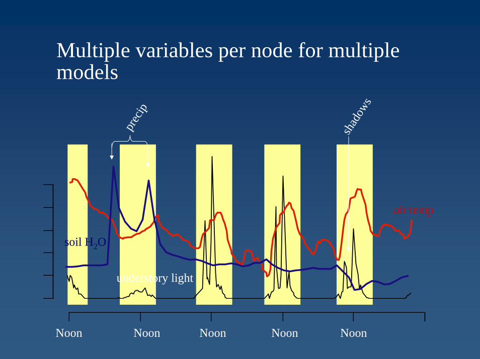
shad

ows

Noon Noon Noon Noon Noon

air temp

soil H2O

understory light

prec

ip

Multiple variables per node for multiple models

Application Properties

data is highly heterogeneous: natural scales range frommeters to landscapesseconds to years

systems are strongly non-linear and non-stationarymotivates dynamic model-driven control of

samplingcommunicationestimation and predictionmodel inference

according to their relative values and costs:

integrate spatio-temporal sensing with modeling and prediction in an adaptive framework

Architectural Properties1. limited in-network resources2. complementary out-of-network capability

relaxed energy constraintsmassive processing powerlatency

approachadaptive in-network joint estimation and coding(inner, fast control loop)supervisory out-of-network processing(outer, slow control loop) – model inference

Dynamic Sensor Networks: Components of Control

models and decisions

out-of-network

in-network

SLIP: scalable

landscape inference

and prediction

DONC: dynamic

out-of-network

control

Dynamic sampling

and reporting

DINC: dynamic

in-network

control

NIP: network

inference and

predictionscheduling

data

data, real-time

estimates,

uncertainty

pre-

dictions

data

Model-driven sensor network activity

Modeling effortModel, measure, and control uncertainty as a function of cost

Hierarchical BayesMCMC

Data service component implementationcoordinates the execution and adaptation of sub-plans and their interaction with WiSARDNet sensors and communication layertags data with meta-data about sampling and measurement conditionsprovides multi-resolution data storage within the network

Energy

Fide

lity

Model-driven measures

Easy

Where to be

Goal: maximum predictive power at ecological model level for a given energy cost

Model-DrivenDynamic Optimization:In- and Out-of-Network

Control of Sampling and Reporting

Precision and Energy Cost of Snapshot Estimates

Objectives:What are the performance and energy cost of samplingand estimating a correlated random field with a sensornetwork as a function of spatial resolution?If subsampling, does a hierarchical strategy for reportingdata pay off?Are there reasonably good distributed strategies forsubsampling and reporting?

Plan:Subsampled instantaneous snapshot of second-orderrandom fieldNoisy measurementsMinimum-variance estimateAssume communication is dominant cost

Central Issues and Related Work

Coding

Slepian-WolfJoint source-channel codingCoding, routing, and rate allocation

Field Models: random or deterministicSpatial approaches

Multi-resolution models

Communication channel models

Field Model

Collection of sensors i , i = 1, . . . , N; samples of a spatialprocess {xi}N

i=1 ∼ Σx

Snapshot {xi : i ∈ A} sent to central server......according to A → A = diag(a), where

ai =

{1, sample xi is reported;0, otherwise.

measurement noise ni ∼ Σ

Snapshot iss = Ax + n

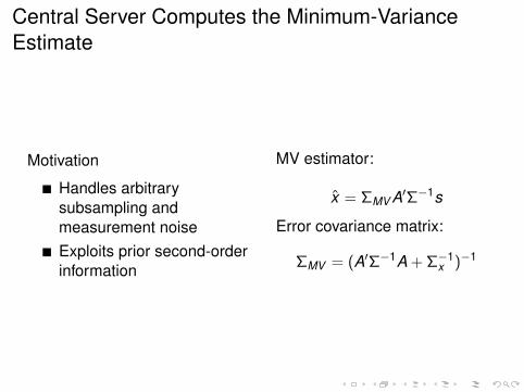
Central Server Computes the Minimum-VarianceEstimate

Motivation

Handles arbitrarysubsampling andmeasurement noiseExploits prior second-orderinformation

MV estimator:

x̂ = ΣMV A′Σ−1s

Error covariance matrix:

ΣMV = (A′Σ−1A + Σ−1x )−1

Use a Uniform Grid for Convenience

N sensors in√

N ×√

Ngridinter-sensor distance don each axisN = 4L

sample at 4l sensorswhere log resolutionis l = 0, . . . , LBase log resolution(no subsampling) isl = L

Precision Improves with Resolution and/or Correlation

100

101

102

103

0

510

1520

0

5

10

15

# of reporting sensorscorrelation radius

prior datauncertainty:

Σx(i , j) = e−d(i,j)

α

correlationradius: minimumcorrelation of 0.1measurementnoise σ2 = 1/4

Multi-resolution Sampling: Maximum-Sleep ReportingRouting follows Sampling Hierarchy.

Only the sensors that sample communicate.Each sensor at level l sends its information to the nearestsensor at level l − 1.If sampling is performed at level l , 0 ≤ l < log4 N, theincremental reporting cost is

γl = 4l

(√N

2l+1

√2d

)β

; γL =

(N −

L−1∑l=1

4l

)dβ

Total reporting cost for sampling at level l :

Γl =l∑

m=1

γm

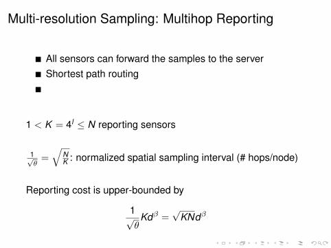
Multi-resolution Sampling: Multihop Reporting

All sensors can forward the samples to the serverShortest path routing

1 < K = 4l ≤ N reporting sensors

1√θ

=√

NK : normalized spatial sampling interval (# hops/node)

Reporting cost is upper-bounded by

1√θ

Kdβ =√

KNdβ

Propagation Loss has Critical Effect on Reporting Cost

0 50 100 150 200 2500

500

1000

1500

# of reporting sensors

repo

rtin

g co

st

β = propagation lossexponent

O β = 3� β = 2+ β = 1

A Note on EfficiencyRatio of Precision to Reporting Cost.

Per-sensor energy usage is√

KN/N =√

θ.

When data is uncorrelated and σ2x � σ2, per-sensor precision is

(σ̄MV )−1 ≈ 1(1− θ)σ2

x

. . .maximum efficiency as θ → 1.

PROSEProtocol for Randomized Opportunistic Sampling and Estimation

Motivation

Desire a simple, scalable, and robust algorithm forsampling and reportingCase where sampling is inexpensive relative to reporting

Core Ideas

Sensors make independent random two-step decisions:

1 To sample and originate a report to the central server2 If not an originator, whether to sample in hopes of being on

the route to the server for opportunistic aggregation

Centralized oracle propagates decision parameters tosensorsAt each node, next edge is chosen randomly from edgeson shortest-path routes

Sensor nodes make independent, random decisions

λ: probability that a sensorwill sample and originate areport to the central server

sets an averageminimum number ofsamples for the estimate

µ: probability that a sensorwill be opportunistic giventhat it decides not tosample and originate

select to balance benefitand cost of providingadditional samples forthe estimate

λ

µ Sample andoriginate

Sample andopportunisticallyaggregate

Forward

0

0

1

1

PROSE Exploits Low-Cost SamplesMonte-Carlo simulation: sensors select next destination randomly from those onshortest paths to central server.

0 50 100 150 200 2501

2

3

4

5

6

7

# of originating sensors

prec

isio

n

� PROSE µ = 1× PROSE µ = 0

MR sampling shownas a solid line

Correlation radius = 5(for a minimumcorrelation of 0.1)

Summary

Framework admits comparison of subsamplingapproaches in realistic scenariosRealistic cost models are essentialReasonable distributed algorithms for sampling andreporting seem attainable

OutlookRole of randomized algorithms and inter-sensorcollaborationSpatio-temporal modelsModel inference

Working at the right level…Example: multi-sensor time series of temperature.

Can view asstreams of numbers

use general-purpose source codes (e.g., delta modulation) correlated spatio-temporal process

use a parameterized statistical model to drive adaptive space-time sampling and reporting

high-level model inputsampling driven by the needs of, e.g., leaf efficiency/tree growth model; sampling rate may be high because of sensitivity of high-level model, even when dynamics appear slow

energy-constrained inference in sensor nets

fidel

ity

power consumption density (W/m2)

spatial granularity limit

slope = pwr densityefficiency limit

Effect ofscalability req’t?

Algorithmic Challenges

Finding good models totrade fidelity (including latency) and costExplore power of dynamic algorithms

Cross-layer run-time optimization frameworkMultiple applicationsData services

Multi-resolution storage and communicationOSNetworking

ConclusionCan a dynamic sensor network deliver better results than fixed sampling and out-of-network modeling in the context of changing real-world environmental conditions?

Understanding the biodiversity and carbon consequences of environmental change is a problem broad enough to encompass many of the types of challenges faced by DDDA systems.

Results from these experiments will inform the design of accurate and energy-efficient production networks tailored to specific applications.

Micrometeorological sensing and nowcasting, pollution monitoring and environmental remediation, and public security/safety.

Questionsand

Discussion…