Dynamic Network Flow Optimization for Real-time Evacuation ...
28
Accepted for publication, Reliability Engineering and System Safety, March 2021 1 Dynamic Network Flow Optimization for Real-time Evacuation Reroute Planning under Multiple Road Disruptions Ayda Darvishan; Gino J. Lim 1 Department of Industrial Engineering University of Houston, Houston, TX, USA Abstract During the course of an evacuation, evacuees often encounter unexpected incidents interrupting their plans for evacuation. Roads may not be accessible due to flooding, wild-fire propagation, accidents, the collapse of highway structures, and various other reasons. The evolving disturbances to the evacuation plan due to road disruptions may prolong the evacuation process and lead to chaos, injuries, and loss of life unless a quick, efficient recovery plan is implemented. In this work, we aim to provide a rerouting approach for an evacuation network that undergoes road disruptions. Unlike previous studies, it is assumed that incidents can occur on multiple roads and that the time of each occurrence can differ from the time of other occurrences. Flow optimization techniques are used to represent evacuation traffic flow on the transportation network. A dynamic traffic flow rate is considered in which the evacuation flow rate can change over time during the planning horizon. The variation in the flow rates enables a better projection of the traffic dynamics and consequences caused by disturbances. Furthermore, a path-based dynamic network flow optimization formulation is proposed to make the model scalable for large evacuation networks. Two preprocessing algorithms are introduced to calculate specific parameters associated with road disruptions and topology of the evacuation network. The use of these parameters enables us to transform the original optimization model into a linear model to reduce the computational burden. Numerical experiments are made to show the performance of the proposed model. Furthermore, the effects of specific features such as disruption time, disturbance location, and the plan updating time on the evacuation process are investigated. Results indicate that when more incidents occur later or when incident information is received earlier, the magnitude of the rerouting completion time is lessened. Keywords: Short-notice evacuation, dynamic network flow problem, network disruption. 1 Introduction Every year, numerous hazardous incidents have affected millions of people worldwide (see Figure 1). Natural hazards are the common concern for many communities, including Geo-physical (Geological) incidents, such as earthquakes, volcanic disruptions, and tsunamis, or weather-related events, such as storms, hurricanes, droughts, and tornados. Various case-scenarios regarding technological failures and intentional malevolence, such as nuclear meltdowns, hazardous material spills, and terrorist attacks, can also wreak havoc on communities. One of the most critical elements in response to a major disaster is the evacuation of people in the affected area, as it is directly associated with protecting human lives. An evacuation refers to the mass physical movement of people from endangered areas to safe shelters prior to the onset of, during, or after a hazardous event. According to a 2005 report by the Nuclear Regulatory Commission (2005), the need for evacuation of 1,000 or more Americans rises about every three weeks. In another report, FEMA (2008) 1 Corresponding author: Gino J. Lim, Department of Industrial Engineering, Univ. of Houston, Email: [email protected]
Transcript of Dynamic Network Flow Optimization for Real-time Evacuation ...

Accepted for publication, Reliability Engineering and System Safety, March 2021
1
Dynamic Network Flow Optimization for Real-time Evacuation Reroute Planning under Multiple Road Disruptions
Ayda Darvishan; Gino J. Lim1 Department of Industrial Engineering
University of Houston, Houston, TX, USA
Abstract
During the course of an evacuation, evacuees often encounter unexpected incidents interrupting their plans for evacuation. Roads may not be accessible due to flooding, wild-fire propagation, accidents, the collapse of highway structures, and various other reasons. The evolving disturbances to the evacuation plan due to road disruptions may prolong the evacuation process and lead to chaos, injuries, and loss of life unless a quick, efficient recovery plan is implemented. In this work, we aim to provide a rerouting approach for an evacuation network that undergoes road disruptions. Unlike previous studies, it is assumed that incidents can occur on multiple roads and that the time of each occurrence can differ from the time of other occurrences. Flow optimization techniques are used to represent evacuation traffic flow on the transportation network. A dynamic traffic flow rate is considered in which the evacuation flow rate can change over time during the planning horizon. The variation in the flow rates enables a better projection of the traffic dynamics and consequences caused by disturbances. Furthermore, a path-based dynamic network flow optimization formulation is proposed to make the model scalable for large evacuation networks. Two preprocessing algorithms are introduced to calculate specific parameters associated with road disruptions and topology of the evacuation network. The use of these parameters enables us to transform the original optimization model into a linear model to reduce the computational burden. Numerical experiments are made to show the performance of the proposed model. Furthermore, the effects of specific features such as disruption time, disturbance location, and the plan updating time on the evacuation process are investigated. Results indicate that when more incidents occur later or when incident information is received earlier, the magnitude of the rerouting completion time is lessened.
Keywords: Short-notice evacuation, dynamic network flow problem, network disruption.
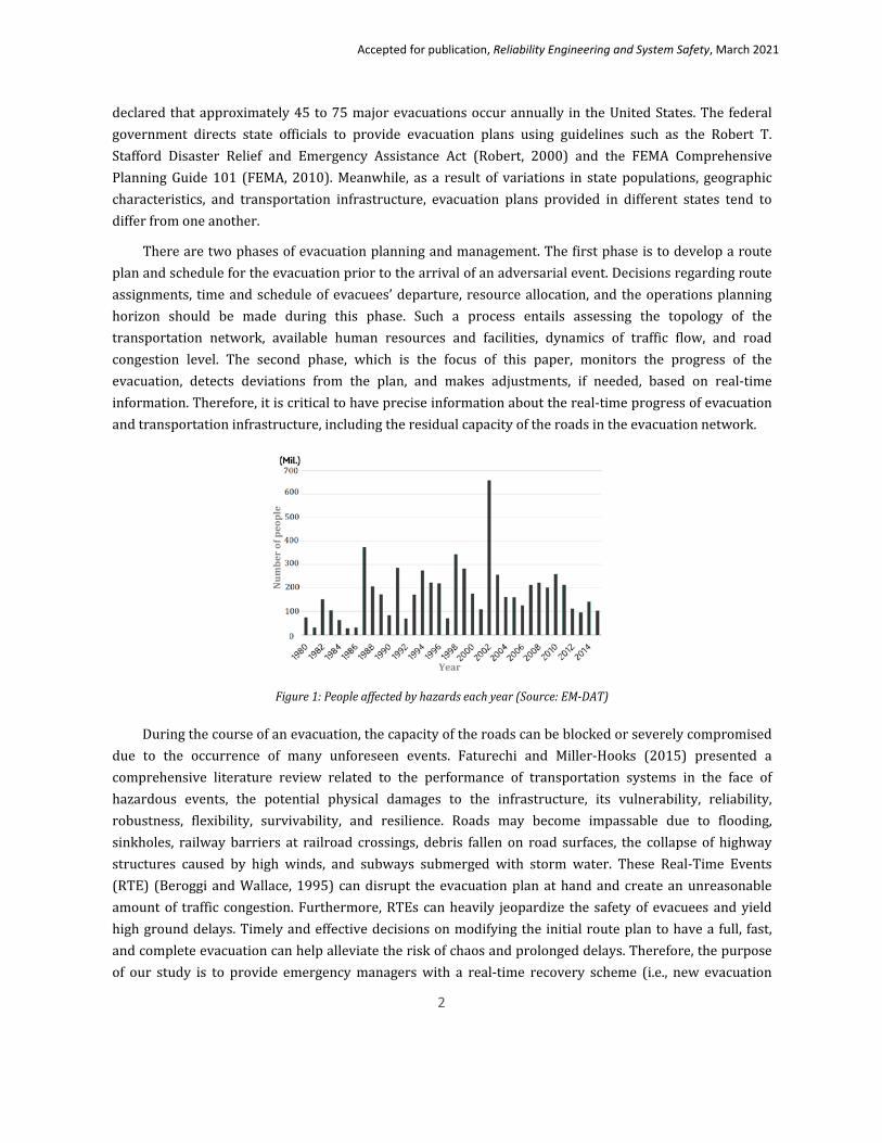
1 Introduction Every year, numerous hazardous incidents have affected millions of people worldwide (see Figure 1). Natural hazards are the common concern for many communities, including Geo-physical (Geological) incidents, such as earthquakes, volcanic disruptions, and tsunamis, or weather-related events, such as storms, hurricanes, droughts, and tornados. Various case-scenarios regarding technological failures and intentional malevolence, such as nuclear meltdowns, hazardous material spills, and terrorist attacks, can also wreak havoc on communities.
One of the most critical elements in response to a major disaster is the evacuation of people in the affected area, as it is directly associated with protecting human lives. An evacuation refers to the mass physical movement of people from endangered areas to safe shelters prior to the onset of, during, or after a hazardous event. According to a 2005 report by the Nuclear Regulatory Commission (2005), the need for evacuation of 1,000 or more Americans rises about every three weeks. In another report, FEMA (2008)
1 Corresponding author: Gino J. Lim, Department of Industrial Engineering, Univ. of Houston, Email: [email protected]
Accepted for publication, Reliability Engineering and System Safety, March 2021
2
declared that approximately 45 to 75 major evacuations occur annually in the United States. The federal government directs state officials to provide evacuation plans using guidelines such as the Robert T. Stafford Disaster Relief and Emergency Assistance Act (Robert, 2000) and the FEMA Comprehensive Planning Guide 101 (FEMA, 2010). Meanwhile, as a result of variations in state populations, geographic characteristics, and transportation infrastructure, evacuation plans provided in different states tend to differ from one another.
There are two phases of evacuation planning and management. The first phase is to develop a route plan and schedule for the evacuation prior to the arrival of an adversarial event. Decisions regarding route assignments, time and schedule of evacuees’ departure, resource allocation, and the operations planning horizon should be made during this phase. Such a process entails assessing the topology of the transportation network, available human resources and facilities, dynamics of traffic flow, and road congestion level. The second phase, which is the focus of this paper, monitors the progress of the evacuation, detects deviations from the plan, and makes adjustments, if needed, based on real-time information. Therefore, it is critical to have precise information about the real-time progress of evacuation and transportation infrastructure, including the residual capacity of the roads in the evacuation network.
Figure 1: People affected by hazards each year (Source: EM-DAT)
During the course of an evacuation, the capacity of the roads can be blocked or severely compromised due to the occurrence of many unforeseen events. Faturechi and Miller-Hooks (2015) presented a comprehensive literature review related to the performance of transportation systems in the face of hazardous events, the potential physical damages to the infrastructure, its vulnerability, reliability, robustness, flexibility, survivability, and resilience. Roads may become impassable due to flooding, sinkholes, railway barriers at railroad crossings, debris fallen on road surfaces, the collapse of highway structures caused by high winds, and subways submerged with storm water. These Real-Time Events (RTE) (Beroggi and Wallace, 1995) can disrupt the evacuation plan at hand and create an unreasonable amount of traffic congestion. Furthermore, RTEs can heavily jeopardize the safety of evacuees and yield high ground delays. Timely and effective decisions on modifying the initial route plan to have a full, fast, and complete evacuation can help alleviate the risk of chaos and prolonged delays. Therefore, the purpose of our study is to provide emergency managers with a real-time recovery scheme (i.e., new evacuation
Num
ber
of p
eopl
e
Year
Accepted for publication, Reliability Engineering and System Safety, March 2021
3
routes and schedule) in the case of a transportation network road disruption. We propose to develop such plans in a way that the total time required to clear the network is minimized.
To date, various strategies and methods have been proposed to develop efficient evacuation plans. Both simulation methods (Sheffi et al. 1981, Pidd et al. 1996, De Silva and Eglese 2000) and optimization techniques (Kim et al. 2008, Rungta et al. 2012, Lim et al. 2016, and Lim et al. 2019) have been widely used to study and improve evacuation decisions along with predictions pertaining to the minimum amount of evacuation completion time. Investigating a transportation network performance in the face of disastrous events has been studied by several authors. Lin et al. (2012) analyzed the performance of a stochastic-flow network under multiple correlated failures of physical lines and routers. Chen and Miller-Hooks (2012) introduced a network resilience metric to measure recovery capability of a freight transportation network under the possibility of disruptions. Bier and Hausken (2013) investigated the impact of blockage of specific roads of transportation networks due to intentional attacks. Faturechi and Miller-Hooks (2014) provided a bi-level three-stage stochastic program in which response strategies are defined in the upper level to enhance the network resilience and the affected users choose best possible routes for themselves in the lower level based on the upper-level decisions.
Our literature review reveals that the problem of the real-time plan adjustment for evacuation has received significantly less scholarly attention. Lim et al. (2016) provided a preprocessing algorithm that utilizes a path-based network flow optimization approach to reassign paths for evacuees affected by an incident, assuming the availability of real-time traffic information. However, there are two limitations on their work. First, their model is limited to a single road incident. Second, evacuation vehicles are assumed to join the evacuation routes at a constant flow rate. Both assumptions are less realistic because multiple road disruptions can occur at any time, and the vehicle flow rate joining major evacuation routes can vary over the evacuation planning horizon. Therefore, the purpose of this paper is to provide an approach to relax both of the assumptions within the context of a dynamic network flow optimization, in which a variable vehicle flow rate is assigned to each time interval of the planning horizon, and disruptions can occur on multiple roads of the network. The number of evacuees leaving the intermediate nodes into new pathways in the network can vary in each time interval, which results in a more realistic representation of evacuation flow dynamics and congestion.
The paper is organized as follows. Section 2 provides a detailed description of the problem assumptions and the developed dynamic network flow optimization model formulation. Section 3 introduces preprocessing algorithms to calculate specific parameter values and a bi-section algorithm to calculate the evacuation completion time. In Section 4, different disruption scenarios are discussed, and the performance of the proposed approach is investigated both on a sample network and on a real, large-scale metropolitan evacuation network. The same section discusses computational results to examine the effects of the incident time and incident location along with the plan updating time. Section 5 concludes the paper with a short summary and a future research direction.
2 Problem Statement
Traffic flow and congestion on the evacuation network are represented through a dynamic network
Accepted for publication, Reliability Engineering and System Safety, March 2021
4
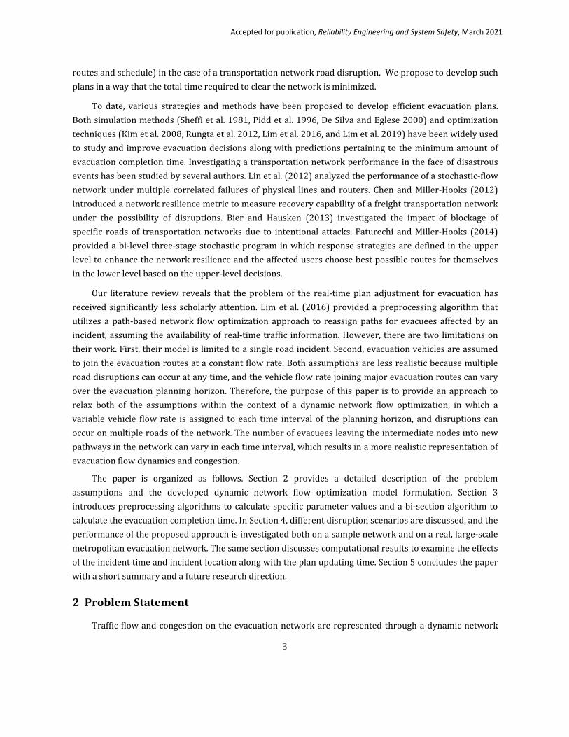
flow problem. A dynamic network is composed of multiple static networks in which each static network depicts the status of the network at a specific time (Ford Jr and Fulkerson, 2015). Let us consider a directed network 𝒢𝒢 = (𝒩𝒩,𝒜𝒜) consisting of a set of nodes 𝒩𝒩 and a set of arcs 𝒜𝒜 (see Figure 2). The nodes are categorized as origin nodes (𝒩𝒩𝑜𝑜), intermediate nodes, and destination nodes (𝒩𝒩𝑑𝑑). Intermediate nodes typically represent intersections of roads in the evacuation network. The planning horizon is divided into discrete time intervals represented by set 𝕋𝕋 = {0, 1, … , T}. A traffic assignment on this network relies upon a representation of traffic as a series of vehicle flows at each time interval as per topology of the network. The transit time of arc 𝑎𝑎 ∈ 𝒜𝒜 is shown by τa, and the time it takes to reach arc 𝑎𝑎 ∈ 𝒜𝒜 from the origin of path 𝑝𝑝 ∈ 𝓅𝓅 is denoted by 𝜃𝜃𝑝𝑝𝑝𝑝.
Figure 2: A directed graph representing an evacuation network
Our approach is based on a path-based approach (see Appendix A) to expedite solving the evacuation rerouting problem. In a path-based approach, all possible paths between each origin-destination (O-D) of the evacuation network are generated and enumerated a priori, and candidate paths are selected and defined as an input (i.e., set 𝓅𝓅) to the optimization model. Consequently, it reduces the number of variables and constraints in the optimization model and reduces the computational complexity of optimizing evacuation planning models. of the model. This is an advantage over other well-known methods such as a Cell Transmission Model (CTM) in simulating traffic speed and congestion (Lim et al. 2019).
Parameter 𝐷𝐷𝑇𝑇𝑝𝑝 is used to denote the disruption time on each arc 𝑎𝑎 ∈ 𝒜𝒜. The aim of the rerouting path-based model (𝑅𝑅𝑅𝑅𝑅𝑅𝑅𝑅) is to optimally utilize the residual capacity of the road networks to reassign the disturbed evacuees to new paths such that the overall evacuation reroute completion time is minimized.
The 𝑅𝑅𝑅𝑅𝑅𝑅𝑅𝑅 assigns the disturbed flow to both unaffected paths as well as partially damaged paths, or called affected paths. An affected path is a path involving one or more disrupted arcs. Although a path can be interrupted, the residual capacity of its intact arcs can still be used to reroute the flow and push it forward through the evacuation network. When the reassigned flow reaches a damaged arc of an affected path, it will gather and wait behind the associated node and can be sequentially rerouted to a path at another time (see Figure 3).
Source node Intermediate node Destination node

Accepted for publication, Reliability Engineering and System Safety, March 2021
5
Figure 3. Rerouting in 𝑅𝑅𝑅𝑅𝑅𝑅𝑅𝑅
For developing the mathematical formulation, the following notation is used:
Sets: 𝒩𝒩 Set of all nodes 𝕋𝕋 Set of all time slots 𝓅𝓅 Set of all paths
Decision Variables:
𝑟𝑟𝑝𝑝𝑝𝑝𝑝𝑝 Disturbed flow of node 𝑛𝑛 ∈ 𝒩𝒩 that is rerouted and assigned to alternate route 𝑝𝑝 at time 𝑡𝑡 ∈𝕋𝕋
ℎ𝑐𝑐𝑝𝑝𝑝𝑝 Remaining disrupted flow on node 𝑛𝑛 ∈ 𝒩𝒩 at time 𝑡𝑡 ∈ 𝕋𝕋
Parameters: 𝑓𝑓𝑝𝑝𝑝𝑝 Flow that starts on path 𝑝𝑝 ∈ 𝓅𝓅 at time 𝑡𝑡 ∈ 𝕋𝕋 (pre-disruption plan) 𝐻𝐻𝑝𝑝𝑝𝑝𝑝𝑝 Disturbed flow on node 𝑛𝑛 ∈ 𝒩𝒩 of path 𝑝𝑝 ∈ 𝓅𝓅 at time 𝑡𝑡 ∈ 𝕋𝕋 𝜃𝜃𝑝𝑝𝑝𝑝 Transit time from the origin of path 𝑝𝑝 ∈ 𝓅𝓅 to arc 𝑎𝑎 ∈ 𝒜𝒜 𝐶𝐶𝑝𝑝 Capacity of arc 𝑎𝑎 ∈ 𝒜𝒜 𝐷𝐷𝑝𝑝 Demand of source node 𝑛𝑛 ∈ 𝒩𝒩 ℓ𝑝𝑝 Capacity of destination node 𝑛𝑛 ∈ 𝒩𝒩 𝜏𝜏𝑝𝑝 Transit time on arc 𝑎𝑎 ∈ 𝒜𝒜 𝐿𝐿𝑝𝑝𝑝𝑝 Takes value 1 if node 𝑛𝑛 ∈ 𝒩𝒩 is the source node of path 𝑝𝑝 ∈ 𝓅𝓅, and otherwise 0 𝐾𝐾𝑝𝑝𝑝𝑝 Takes value 1 if node 𝑛𝑛 ∈ 𝒩𝒩 is the destination node of path 𝑝𝑝 ∈ 𝓅𝓅, and otherwise 0 ��𝜃𝑝𝑝𝑝𝑝 Transit time from the origin of path 𝑝𝑝 ∈ 𝓅𝓅 to node 𝑛𝑛 ∈ 𝒩𝒩 𝛿𝛿𝑝𝑝𝑝𝑝 Takes value 1 if arc 𝑎𝑎 ∈ 𝒜𝒜 belongs to path 𝑝𝑝 ∈ 𝓅𝓅, and otherwise 0 𝛾𝛾𝑝𝑝𝑝𝑝 Takes value 1 if node 𝑛𝑛 ∈ 𝒩𝒩 is the upstream (origin) node of arc 𝑎𝑎 ∈ 𝒜𝒜, and otherwise 0 𝜑𝜑𝑝𝑝𝑝𝑝𝑝𝑝 Takes value 1 if node 𝑛𝑛 ∈ 𝒩𝒩 is not behind node 𝑚𝑚 ∈ 𝒩𝒩 on path 𝑝𝑝 ∈ 𝓅𝓅, and otherwise 0
𝑊𝑊𝑝𝑝𝑝𝑝𝑝𝑝 Takes value 1 if the flow on path 𝑝𝑝 ∈ 𝓅𝓅 starting at time 𝑡𝑡 ∈ 𝕋𝕋 reaches the merging arc from node 𝑛𝑛 ∈ 𝒩𝒩 before the disruption time of the arc
𝒇𝒇𝒑𝒑𝒑𝒑𝒑𝒑
𝑛𝑛
𝒓𝒓��𝒑𝒑𝒑𝒑𝒑
𝑛𝑛
Path 𝒑𝒑
Path ��𝒑
Disturbed arc
Arc not used for flow transition
Arc used for flow transition
𝒓𝒓 Rerouting flow
𝒇𝒇 Initial flow

Accepted for publication, Reliability Engineering and System Safety, March 2021
6
𝑉𝑉𝑝𝑝𝑝𝑝𝑝𝑝 Takes value 1 if the flow on path 𝑝𝑝 ∈ 𝓅𝓅 starting at time 𝑡𝑡 ∈ 𝕋𝕋 is disturbed and stuck behind node 𝑛𝑛 ∈ 𝒩𝒩, and otherwise 0
𝜂𝜂𝑝𝑝𝑝𝑝𝑝𝑝𝑝𝑝 Takes value 1 if the flow on path 𝑝𝑝 ∈ 𝓅𝓅 starting at time 𝑡𝑡 ∈ 𝕋𝕋 is not affected through node 𝑚𝑚 ∈ 𝒩𝒩 and also is not disturbed between node 𝑚𝑚 ∈ 𝒩𝒩 and node 𝑛𝑛 ∈ 𝒩𝒩 (𝑚𝑚 is behind 𝑛𝑛), and otherwise 0
𝜕𝜕𝑝𝑝𝑝𝑝 Takes value 1 if there is no disturbed arcs on path 𝑝𝑝 ∈ 𝓅𝓅 after node 𝑛𝑛 ∈ 𝒩𝒩, and otherwise 0
Mathematical properties of the PBM model do not allow direct representation of flow departing from intermediate nodes. Variables denoting the flow are always related to the evacuees leaving the source node of a path rather than the intermediate node. However, a method is needed for rerouting the flow in order to reflect the flow departing from an intermediate node (see Figure 4). To resolve the issue in the optimization model formulation, the rerouting variable 𝑟𝑟𝑝𝑝𝑝𝑝𝑝𝑝 is introduced to denote the amount of flow departing from the origin of path 𝑝𝑝 ∈ 𝓅𝓅 at time 𝑡𝑡 ∈ 𝕋𝕋. Nevertheless, in our constraints, we ignore the values of 𝑟𝑟𝑝𝑝𝑝𝑝𝑝𝑝 associated with preceding nodes (or arcs) to node 𝑛𝑛 ∈ 𝒩𝒩. In this case, the preceding arcs are considered dummy arcs. This is done by introducing three sets of parameters 𝑊𝑊𝑝𝑝𝑝𝑝𝑝𝑝 , 𝑉𝑉𝑝𝑝𝑝𝑝𝑝𝑝, and 𝜂𝜂𝑝𝑝𝑝𝑝𝑝𝑝𝑝𝑝 which reflect the effect of disruptions on the evacuation flow with respect to the arc incident times, sequence of arcs in the set of paths as well as topology of the network. Using these parameter a mathematical model with a linear structure can be developed. Note that a flow departing at time 𝑡𝑡 ∈ 𝕋𝕋 takes 𝜃𝜃𝑝𝑝𝑝𝑝 time units to reach node 𝑛𝑛 ∈ 𝒩𝒩. Hence, based on the disturbed flow information 𝑟𝑟𝑝𝑝𝑝𝑝�𝑝𝑝−𝜃𝜃𝑝𝑝𝑝𝑝�, we can address the flow
reassignment from node 𝑛𝑛 ∈ 𝒩𝒩 onto route 𝑝𝑝 ∈ 𝓅𝓅 during time interval 𝑡𝑡 − 𝜃𝜃𝑝𝑝𝑝𝑝 + 𝜃𝜃𝑝𝑝𝑝𝑝 = 𝑡𝑡.
Figure 4. Representation of rerouting variable 𝑟𝑟𝑝𝑝𝑝𝑝𝑝𝑝
𝑅𝑅𝑅𝑅𝑅𝑅𝑅𝑅 (Rerouting Path-Based Model) formulation:
We now describe the proposed dynamic network flow optimization model formulation. When an arc disruption occurs, disturbed evacuees are assumed to be accumulated on the tail of the affected arc (i.e., a node behind the affected road in the evacuation network) for the purpose of rerouting them to alternative paths. The objective function of 𝑅𝑅𝑅𝑅𝑅𝑅𝑅𝑅 aims to minimize the total number of disturbed evacuees remaining in the evacuation network by the end of the planning horizon 𝑇𝑇.
min � ℎ𝑐𝑐𝑝𝑝𝑇𝑇𝑝𝑝∈𝒩𝒩
Constraints are explained as follows. The planning horizon set 𝕋𝕋 = {0, 1, … ,𝑇𝑇} covers both the pre-
Arc not used for flow transition
Arc used for flow transition
𝒓𝒓𝒑𝒑𝒑𝒑𝒑𝒑
𝒓𝒓 Rerouting flow

Accepted for publication, Reliability Engineering and System Safety, March 2021
7
disruption schedule (𝑓𝑓𝑝𝑝𝑝𝑝) as well as the post-disruption schedule (ℛ𝑝𝑝𝑝𝑝𝑝𝑝). The time periods at which the previous plan is updated are shown by set 𝕋𝕋𝑢𝑢𝑝𝑝𝑑𝑑𝑝𝑝𝑝𝑝𝑢𝑢𝑑𝑑 = �𝑡𝑡𝑢𝑢𝑝𝑝𝑢𝑢𝑎𝑎𝑡𝑡𝑢𝑢𝑛𝑛𝑢𝑢, … ,𝑇𝑇�. At time 𝑡𝑡 = 0, there are no disturbed evacuees in the system. Hence, the total amount of associated flow on all nodes is set to zero as in Constraint (1).
ℎ𝑐𝑐𝑝𝑝(𝑝𝑝=0) = 0, ∀ 𝑛𝑛 ∈ 𝒩𝒩. (1)
The process of a plan revision can only take place during the updating time interval (𝕋𝕋𝑢𝑢𝑝𝑝𝑑𝑑𝑝𝑝𝑝𝑝𝑢𝑢𝑑𝑑). The flow-route assignments before 𝑡𝑡𝑢𝑢𝑝𝑝𝑑𝑑𝑝𝑝𝑝𝑝𝑢𝑢𝑝𝑝𝑢𝑢 are equal to zero as in Constraint (2).
𝑟𝑟𝑝𝑝𝑝𝑝�𝑝𝑝−��𝜃𝑝𝑝𝑝𝑝� = 0, ∀𝑝𝑝 ∈ 𝓅𝓅, ∀𝑎𝑎 ∈ 𝒜𝒜,𝑛𝑛 ∈ 𝒩𝒩, 𝑡𝑡 ∈ 𝕋𝕋/𝕋𝕋𝑢𝑢𝑝𝑝𝑑𝑑𝑝𝑝𝑝𝑝𝑢𝑢𝑑𝑑. (2)
When calculating the amount of disturbed flow on node 𝑛𝑛 ∈ 𝒩𝒩 at time 𝑡𝑡 ∈ 𝕋𝕋, we take into account both the amount of the disturbed flow from the original plan (denoted by 𝐻𝐻𝑝𝑝𝑝𝑝𝑝𝑝) and the amount of the rerouted flow from nodes (𝑚𝑚 ∈ 𝒩𝒩) that were disturbed while passing through the alternative pathway (𝑊𝑊𝑝𝑝𝑝𝑝𝑝𝑝 ∑ 𝜂𝜂𝑝𝑝𝑝𝑝𝑝𝑝𝑝𝑝𝑟𝑟𝑝𝑝𝑝𝑝𝑝𝑝𝑝𝑝∈𝒩𝒩 ). This is stated in Constraint (3).
𝐻𝐻𝐶𝐶𝑝𝑝𝑝𝑝�𝑝𝑝+��𝜃𝑝𝑝𝑝𝑝� = 𝐻𝐻𝑝𝑝𝑝𝑝�𝑝𝑝+��𝜃𝑝𝑝𝑝𝑝� +𝑊𝑊𝑝𝑝𝑝𝑝𝑝𝑝 � 𝜂𝜂𝑝𝑝𝑝𝑝𝑝𝑝𝑝𝑝𝑟𝑟𝑝𝑝𝑝𝑝𝑝𝑝𝑝𝑝∈𝒩𝒩
, ∀𝑝𝑝 ∈ 𝓅𝓅, 𝑛𝑛 ∈ 𝒩𝒩, 𝑡𝑡 ∈ 𝕋𝕋. (3)
Parameter 𝐻𝐻𝑝𝑝𝑝𝑝𝑝𝑝 used in Constraint (3) can be calculated as follows:
𝐻𝐻𝑝𝑝𝑝𝑝�𝑝𝑝+��𝜃𝑝𝑝𝑝𝑝� = V𝑝𝑝𝑝𝑝𝑝𝑝𝑓𝑓𝑝𝑝𝑝𝑝, ∀𝑝𝑝 ∈ 𝓅𝓅, 𝑛𝑛 ∈ 𝒩𝒩, 𝑡𝑡 ∈ 𝕋𝕋.
When flow 𝑓𝑓𝑝𝑝𝑝𝑝 is blocked on node 𝑛𝑛 ∈ 𝒩𝒩 (denoted by 𝑉𝑉𝑝𝑝𝑝𝑝𝑝𝑝 = 1), and since the flow has started from the origin of the path at time 𝑡𝑡 ∈ 𝕋𝕋, the time at which it reaches and accumulates on node 𝑛𝑛 ∈ 𝒩𝒩 is 𝑡𝑡 + ��𝜃𝑝𝑝𝑝𝑝. Note that ��𝜃𝑝𝑝𝑝𝑝 is the transit time from the origin of path 𝑝𝑝 ∈ 𝓅𝓅 to node 𝑛𝑛 ∈ 𝒩𝒩. Accordingly, 𝐻𝐻𝑝𝑝𝑝𝑝�𝑝𝑝+��𝜃𝑝𝑝𝑝𝑝� represents the
number of evacuees disturbed on 𝑛𝑛 ∈ 𝒩𝒩 at time �𝑡𝑡 + ��𝜃𝑝𝑝𝑝𝑝�.
The total number of remaining interrupted evacuees at time (𝑡𝑡 + 1) equals its previous amount at time 𝑡𝑡 ∈ 𝕋𝕋, plus the newly interrupted evacuees (∑ 𝐻𝐻𝐶𝐶𝑝𝑝𝑝𝑝(𝑝𝑝+1)𝑝𝑝∈𝓅𝓅 ), minus the amount of rerouted evacuees at time 𝑡𝑡, as expressed in the following equation.
ℎ𝑐𝑐𝑝𝑝(𝑝𝑝+1) = ℎ𝑐𝑐nt + �𝐻𝐻𝐶𝐶𝑝𝑝𝑝𝑝(𝑝𝑝+1)𝑝𝑝∈𝓅𝓅
− ��ℑ𝑝𝑝𝑛𝑛𝑎𝑎 �1 −𝑊𝑊𝑝𝑝𝑝𝑝�𝑝𝑝−𝜃𝜃𝑝𝑝𝑝𝑝�� 𝑟𝑟𝑝𝑝𝑝𝑝�𝑝𝑝−𝜃𝜃𝑝𝑝𝑝𝑝�𝑝𝑝∈𝓅𝓅𝑝𝑝∈𝒜𝒜
∀ 𝑛𝑛 ∈ 𝒩𝒩, 𝑡𝑡 ∈ 𝕋𝕋. (4)
Parameter ℑ𝑝𝑝𝑝𝑝𝑝𝑝 in Constraint (4) reflects the topology of the network and can be calculated as:
ℑ𝑝𝑝𝑝𝑝𝑝𝑝 = 𝛿𝛿𝑝𝑝𝑝𝑝𝛾𝛾𝑝𝑝𝑝𝑝 ∀𝑝𝑝 ∈ 𝓅𝓅, 𝑎𝑎 ∈ 𝒜𝒜, 𝑛𝑛 ∈ 𝒩𝒩.
Considering constraints (2), (3), and (4), before the updating time, ℎ𝑐𝑐𝑝𝑝(𝑝𝑝+1) only equals the previous amount of the remaining flow plus the newly interrupted flow (i.e. ℎ𝑐𝑐𝑝𝑝(𝑝𝑝+1) = ℎ𝑐𝑐𝑝𝑝𝑝𝑝 + ∑ 𝐻𝐻𝐶𝐶𝑝𝑝𝑝𝑝(𝑝𝑝+1)𝑝𝑝∈𝓅𝓅 ). However, when the rerouting of the disturbed flow begins, the assigned disturbed flow 𝑟𝑟𝑝𝑝𝑝𝑝�𝑝𝑝−𝜃𝜃𝑝𝑝𝑝𝑝� at time 𝑡𝑡 ∈
𝕋𝕋 to alternate paths is no longer stalled behind node 𝑛𝑛 ∈ 𝒩𝒩 and is subtracted from the remaining disturbed flow of the next time interval ℎ𝑐𝑐𝑝𝑝(𝑝𝑝+1). We use ℎ𝑐𝑐𝑝𝑝𝑝𝑝 as a measure to be used to later study the performance of

Accepted for publication, Reliability Engineering and System Safety, March 2021
8
our MIP model.
� � � 𝜂𝜂𝑝𝑝�𝑝𝑝−𝜃𝜃𝑝𝑝𝑝𝑝�𝑝𝑝𝑝𝑝𝛿𝛿𝑝𝑝𝑝𝑝𝛾𝛾𝑝𝑝𝑝𝑝𝑝𝑝∈𝒩𝒩
��1 − 𝑉𝑉𝑝𝑝𝑝𝑝�𝑝𝑝−𝜃𝜃𝑝𝑝𝑝𝑝�� 𝐿𝐿𝑝𝑝𝑝𝑝𝑓𝑓𝑝𝑝�𝑝𝑝−𝜃𝜃𝑝𝑝𝑝𝑝�𝑝𝑝∈𝒩𝒩𝑝𝑝∈𝓅𝓅
+ �1 −𝑊𝑊𝑝𝑝𝑝𝑝�𝑝𝑝−𝜃𝜃𝑝𝑝𝑝𝑝�� ∅𝑝𝑝𝑝𝑝𝑝𝑝𝑟𝑟𝑝𝑝𝑝𝑝�𝑝𝑝−𝜃𝜃𝑝𝑝𝑝𝑝�� ≤ 𝐶𝐶𝑝𝑝,
∀𝑎𝑎 ∈ 𝒜𝒜, 𝑡𝑡 ∈ 𝕋𝕋. (5)
Constraint (5) ensures that the total flow from different paths reaching a shared arc does not exceed the capacity of the arc (𝐶𝐶𝑝𝑝). This flow includes (i) the pre-disruption flow schedule 𝑓𝑓𝑝𝑝𝑝𝑝, and (ii) the post-disruption flow schedule 𝑟𝑟𝑝𝑝𝑝𝑝𝑝𝑝. Let us consider flow 𝑓𝑓𝑝𝑝�𝑝𝑝−𝜃𝜃𝑝𝑝𝑝𝑝� departing from the origin of the path at time 𝑡𝑡 −
𝜃𝜃𝑝𝑝𝑝𝑝. Two cases can occur regarding the share of this flow in the capacity usage of arc 𝑎𝑎 ∈ 𝒜𝒜 (see Figure 5).
Case 1: Flow is disturbed before reaching arc 𝑎𝑎 ∈ 𝒜𝒜
Case 1 occurs when there is at least one disruption on the preceding arcs before reaching arc 𝑎𝑎 ∈ 𝒜𝒜 and when the disruption time of an associated arc is less than the time required for the flow to reach and pass through the arc. Hence, if there is at least one arc ��𝑎 ∈ 𝒜𝒜 in which the following condition holds true,
�𝑡𝑡 − 𝜃𝜃𝑝𝑝��𝑝� + 𝜃𝜃𝑝𝑝��𝑝 + 𝜏𝜏��𝑝 > 𝐷𝐷𝑇𝑇��𝑝 ∃��𝑎 ∈ 𝒜𝒜 preceding to 𝑎𝑎 ∈ 𝒜𝒜 on 𝑝𝑝 ∈ 𝓅𝓅
then, parameter 𝜂𝜂𝑝𝑝�𝑝𝑝−𝜃𝜃𝑝𝑝𝑝𝑝�𝑝𝑝𝑝𝑝 equals zero and 𝑓𝑓𝑝𝑝�𝑝𝑝−𝜃𝜃𝑝𝑝𝑝𝑝� is not considered in the capacity Constraint (5). Note that
𝑚𝑚 ∈ 𝒩𝒩 represents the origin node of the path if 𝐿𝐿𝑝𝑝𝑝𝑝 = 1. Also, 𝑛𝑛 ∈ 𝒩𝒩 represents the head of arc 𝑎𝑎 ∈ 𝒜𝒜 if 𝛾𝛾𝑝𝑝𝑝𝑝 = 1. Note that the details of calculating the amount of parameter 𝜂𝜂𝑝𝑝�𝑝𝑝−𝜃𝜃𝑝𝑝𝑝𝑝�𝑝𝑝𝑝𝑝 using an algorithm is explained in
Section 3.
Case 2: Flow can pass through arc 𝑎𝑎 ∈ 𝒜𝒜
When the flow is not disturbed on preceding arcs to arc 𝑎𝑎 ∈ 𝒜𝒜 and reaches and passes through arc 𝑎𝑎 ∈ 𝒜𝒜,
it occupies the capacity of arc 𝑎𝑎 ∈ 𝒜𝒜 until it completely passes through the arc. This occurs when the following condition holds:
�𝑡𝑡 − 𝜃𝜃𝑝𝑝��𝑝� + 𝜃𝜃𝑝𝑝��𝑝 + 𝜏𝜏��𝑝 ≤ 𝐷𝐷𝑇𝑇��𝑝
& 𝑉𝑉𝑝𝑝𝑝𝑝�𝑝𝑝−𝜃𝜃𝑝𝑝𝑝𝑝� = 0 ∀��𝑎 ∈ 𝒜𝒜 preceding to 𝑎𝑎 ∈ 𝒜𝒜 on 𝑝𝑝 ∈ 𝓅𝓅
When the value of �𝑡𝑡 − 𝜃𝜃𝑝𝑝��𝑝� + 𝜃𝜃𝑝𝑝��𝑝 + 𝜏𝜏��𝑝 is less than the disruption time (𝐷𝐷𝑇𝑇��𝑝) of a preceding arc ��𝑎 ∈ 𝒜𝒜, the flow can reach arc 𝑎𝑎 ∈ 𝒜𝒜, i.e., 𝜂𝜂𝑝𝑝�𝑝𝑝−𝜃𝜃𝑝𝑝𝑝𝑝�𝑝𝑝𝑝𝑝 = 1. At this point, if the flow is not disturbed on arc 𝑎𝑎 ∈ 𝒜𝒜 (i.e. 𝑉𝑉𝑝𝑝𝑝𝑝�𝑝𝑝−𝜃𝜃𝑝𝑝𝑝𝑝� =
0), it can flow through the arc, and the arc capacity is reduced accordingly. Note that Algorithm 2 explained in Section 3 is used to calculate the amount of parameter 𝜂𝜂𝑝𝑝�𝑝𝑝−𝜃𝜃𝑝𝑝𝑝𝑝�𝑝𝑝𝑝𝑝 to be used in the optimization model.
Accepted for publication, Reliability Engineering and System Safety, March 2021
9
Figure 5. Case 1 and Case 2 presentation for flow 𝒇𝒇𝒑𝒑�𝒑𝒑−𝜽𝜽𝒑𝒑𝒑𝒑�
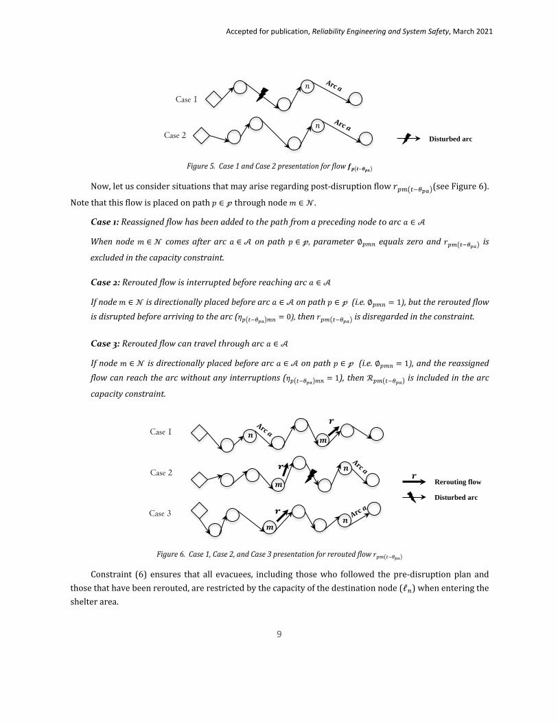
Now, let us consider situations that may arise regarding post-disruption flow 𝑟𝑟𝑝𝑝𝑝𝑝�𝑝𝑝−𝜃𝜃𝑝𝑝𝑝𝑝�(see Figure 6).
Note that this flow is placed on path 𝑝𝑝 ∈ 𝓅𝓅 through node 𝑚𝑚 ∈ 𝒩𝒩.
Case 1: Reassigned flow has been added to the path from a preceding node to arc 𝑎𝑎 ∈ 𝒜𝒜
When node 𝑚𝑚 ∈ 𝒩𝒩 comes after arc 𝑎𝑎 ∈ 𝒜𝒜 on path 𝑝𝑝 ∈ 𝓅𝓅, parameter ∅𝑝𝑝𝑝𝑝𝑝𝑝 equals zero and 𝑟𝑟𝑝𝑝𝑝𝑝�𝑝𝑝−𝜃𝜃𝑝𝑝𝑝𝑝� is
excluded in the capacity constraint.
Case 2: Rerouted flow is interrupted before reaching arc 𝑎𝑎 ∈ 𝒜𝒜
If node 𝑚𝑚 ∈ 𝒩𝒩 is directionally placed before arc 𝑎𝑎 ∈ 𝒜𝒜 on path 𝑝𝑝 ∈ 𝓅𝓅 (i.e. ∅𝑝𝑝𝑝𝑝𝑝𝑝 = 1), but the rerouted flow is disrupted before arriving to the arc (𝜂𝜂𝑝𝑝�𝑝𝑝−𝜃𝜃𝑝𝑝𝑝𝑝�𝑝𝑝𝑝𝑝 = 0), then 𝑟𝑟𝑝𝑝𝑝𝑝�𝑝𝑝−𝜃𝜃𝑝𝑝𝑝𝑝� is disregarded in the constraint.
Case 3: Rerouted flow can travel through arc 𝑎𝑎 ∈ 𝒜𝒜
If node 𝑚𝑚 ∈ 𝒩𝒩 is directionally placed before arc 𝑎𝑎 ∈ 𝒜𝒜 on path 𝑝𝑝 ∈ 𝓅𝓅 (i.e. ∅𝑝𝑝𝑝𝑝𝑝𝑝 = 1), and the reassigned flow can reach the arc without any interruptions (𝜂𝜂𝑝𝑝�𝑝𝑝−𝜃𝜃𝑝𝑝𝑝𝑝�𝑝𝑝𝑝𝑝 = 1), then ℛ𝑝𝑝𝑝𝑝�𝑝𝑝−𝜃𝜃𝑝𝑝𝑝𝑝� is included in the arc
capacity constraint.
Figure 6. Case 1, Case 2, and Case 3 presentation for rerouted flow 𝑟𝑟𝑝𝑝𝑝𝑝�𝑝𝑝−𝜃𝜃𝑝𝑝𝑝𝑝�
Constraint (6) ensures that all evacuees, including those who followed the pre-disruption plan and those that have been rerouted, are restricted by the capacity of the destination node (ℓ𝑝𝑝) when entering the shelter area.
𝑛𝑛
𝑛𝑛
Case 1
Case 2 Disturbed arc
𝒓𝒓 Case 1
Case 2
𝒑𝒑 𝒎𝒎
𝒓𝒓 𝒑𝒑 𝒎𝒎
𝒓𝒓 𝒑𝒑
𝒎𝒎 Case 3
Disturbed arc
𝒓𝒓 Rerouting flow

Accepted for publication, Reliability Engineering and System Safety, March 2021
10
��𝐾𝐾𝑝𝑝𝑝𝑝𝑝𝑝∈𝕋𝕋
� � 𝜂𝜂𝑝𝑝𝑝𝑝𝑝𝑝𝑝𝑝 𝐿𝐿𝑝𝑝𝑝𝑝 𝑓𝑓𝑝𝑝𝑝𝑝𝑝𝑝∈𝒩𝒩o
+ � 𝜂𝜂𝑝𝑝𝑝𝑝𝑝𝑝𝑝𝑝𝑝𝑝∈𝒩𝒩
𝑟𝑟𝑝𝑝𝑝𝑝𝑝𝑝�𝑝𝑝∈𝓅𝓅
≤ ℓ𝑝𝑝 ∀𝑛𝑛 ∈ 𝒩𝒩𝑑𝑑 . (6)
Evacuation flow 𝑓𝑓𝑝𝑝𝑝𝑝 is considered in Constraint (6) only if the following condition holds:
�𝑡𝑡 − 𝜃𝜃𝑝𝑝��𝑝� + 𝜃𝜃𝑝𝑝��𝑝 + 𝜏𝜏��𝑝 ≤ 𝐷𝐷𝑇𝑇��𝑝 ∀��𝑎 ∈ 𝒜𝒜 between the source node and
destination node of path 𝑝𝑝 ∈ 𝓅𝓅
Hence, starting from the origin and moving towards the destination, if the flow of an evacuee is not interrupted (𝜂𝜂𝑝𝑝𝑝𝑝𝑝𝑝𝑝𝑝 = 1 where 𝑚𝑚 ∈ 𝒩𝒩𝑜𝑜 and 𝑛𝑛 ∈ 𝒩𝒩𝑑𝑑), it is counted in Constraint (6). Similarly, the rerouted flow 𝑟𝑟𝑝𝑝𝑝𝑝𝑝𝑝 is considered to use the capacity of the destination node only if no incident affects the flow from node m ∈ 𝒩𝒩 (the point it had been inserted on the path) to the destination node 𝑛𝑛 ∈ 𝒩𝒩𝑑𝑑 (𝜂𝜂𝑝𝑝𝑝𝑝𝑝𝑝𝑝𝑝 = 1).
Finally, Constraints (7) reflects the non-negativity and integrality of decision variables, respectively.
𝑟𝑟𝑝𝑝𝑝𝑝𝑝𝑝 ∈ ℤ+, ℎ𝑐𝑐𝑝𝑝𝑝𝑝 ∈ ℤ+, ∀𝑝𝑝 ∈ 𝓅𝓅, 𝑛𝑛 ∈ 𝒩𝒩, 𝑡𝑡 ∈ 𝕋𝕋. (7)
3 Algorithms to Calculate Key Model Parameters and Network Clearance Time As explained in Appendix B, developing an optimization model for the problem that can be solved in a
timely manner was challenging. However, upon examining the problem characteristics, we realized that a mixed integer linear program can be developed if some key parameter values are determined a priori. Hence, this section introduces two preprocessing algorithms to calculate the parameter values, which makes it possible to solve the proposed 𝑅𝑅𝑅𝑅𝑅𝑅𝑅𝑅 model.
3.1 Methodology to Calculate Parameters Associated with Disruptions
Parameter 𝑉𝑉𝑝𝑝𝑝𝑝𝑝𝑝 indicates whether or not flow 𝑓𝑓𝑝𝑝𝑝𝑝 on path 𝑝𝑝 ∈ 𝓅𝓅 departing at time 𝑡𝑡 ∈ 𝕋𝕋 would be stalled on node 𝑛𝑛 ∈ 𝒩𝒩. Algorithm 1 is developed to calculate the value of 𝑉𝑉𝑝𝑝𝑝𝑝𝑝𝑝 . First, we calculate 𝑊𝑊𝑝𝑝𝑝𝑝𝑝𝑝 to define whether 𝑓𝑓𝑝𝑝𝑝𝑝 is stopped on node 𝑛𝑛 ∈ 𝒩𝒩 regardless of any possible disturbances that may have surfaced during the flow passage up to node 𝑛𝑛 ∈ 𝒩𝒩. Accordingly, we initialize disruption times of preceding arcs to node 𝑛𝑛 ∈ 𝒩𝒩 to be infinity. We disregard disturbances of the preceding arcs and only take into account the time of incident (𝐷𝐷𝑇𝑇𝑝𝑝) of the arc that emerges from node 𝑛𝑛 ∈ 𝒩𝒩, arc transit time (𝜏𝜏𝑝𝑝), and the time to transport from the origin of the route to arc 𝑎𝑎 ∈ 𝒜𝒜 (𝜃𝜃𝑝𝑝𝑝𝑝). If a flow departs on path 𝑝𝑝 ∈ 𝓅𝓅 at time 𝑡𝑡 ∈ 𝕋𝕋, it reaches arc 𝑎𝑎 ∈ 𝒜𝒜 at time 𝑡𝑡 + 𝜃𝜃𝑝𝑝𝑝𝑝. Also, it takes 𝜏𝜏𝑝𝑝 unit of time for the flow to completely pass through the arc. Therefore, if 𝑡𝑡 + 𝜃𝜃𝑝𝑝𝑝𝑝 + 𝜏𝜏𝑝𝑝 is greater than the disruption time of the arc (𝐷𝐷𝑇𝑇𝑝𝑝), the flow is interrupted, and 𝑊𝑊𝑝𝑝𝑝𝑝𝑝𝑝 takes value 1.

Accepted for publication, Reliability Engineering and System Safety, March 2021
11
Figure 7: Assumptions used to define parameters 𝑊𝑊𝑝𝑝𝑝𝑝𝑝𝑝 and 𝑣𝑣𝑝𝑝𝑝𝑝𝑝𝑝
Next, we calculate the value of 𝑉𝑉𝑝𝑝𝑝𝑝𝑝𝑝 and subsequently take into account incident times of preceding arcs to arc 𝑎𝑎 ∈ 𝒜𝒜. The value of 𝑉𝑉𝑝𝑝𝑝𝑝𝑝𝑝 equals 1 only if the flow 𝑓𝑓𝑝𝑝𝑝𝑝 experiences no interruption while moving toward node 𝑛𝑛 ∈ 𝒩𝒩 (i.e., ∑ 𝑊𝑊𝑝𝑝𝑝𝑝𝑝𝑝𝑝𝑝∈𝒩𝒩 = 0) and is disturbed on node 𝑛𝑛 ∈ 𝒩𝒩 of path 𝑝𝑝 ∈ 𝓅𝓅 (i.e., 𝑊𝑊𝑝𝑝𝑝𝑝𝑝𝑝 = 1). Else 𝑉𝑉𝑝𝑝𝑝𝑝𝑝𝑝 = 0.
Algorithm 1 Inputs:
An evacuation network 𝒢𝒢 consisting of a set of nodes 𝒩𝒩 and a set of arcs 𝒜𝒜. Disruption Time of Arcs
Calculating 𝑽𝑽𝒑𝒑𝒑𝒑𝒑𝒑: for all paths 𝑝𝑝 ∈ 𝓅𝓅 do
for all time slots 𝑡𝑡 ∈ 𝕋𝕋 do for all arcs that belong to path 𝑝𝑝 ∈ 𝓅𝓅 do
if 𝑡𝑡 + 𝜃𝜃𝑝𝑝𝑎𝑎 + 𝜏𝜏𝑎𝑎 − 𝐷𝐷𝑇𝑇𝑎𝑎 > 0 then 𝑊𝑊𝑝𝑝𝑝𝑝𝑝𝑝 = 1 (𝑛𝑛 is upstream node of arc 𝑎𝑎)
else if 𝑡𝑡 + 𝜃𝜃𝑝𝑝𝑎𝑎 + 𝜏𝜏𝑎𝑎 − 𝐷𝐷𝑇𝑇𝑎𝑎 ≤ 0 then 𝑾𝑾𝒑𝒑𝒑𝒑𝒑𝒑 = 𝟎𝟎
end if for all preceding nodes 𝒎𝒎 ∈ 𝓝𝓝 to arc 𝒑𝒑 on path 𝒑𝒑 do
if ∑ 𝑊𝑊𝑝𝑝𝑝𝑝𝑝𝑝𝑝𝑝∈𝒩𝒩 = 0 and 𝑊𝑊𝑝𝑝𝑝𝑝𝑝𝑝 = 1 then 𝑉𝑉𝑝𝑝𝑝𝑝𝑝𝑝 = 1 (𝑛𝑛 is upstream node of arc 𝑎𝑎)
else then 𝑽𝑽𝒑𝒑𝒑𝒑𝒑𝒑 = 𝟎𝟎
end if end for
end for end for
end for
A numerical example for calculating the value of 𝑉𝑉𝑝𝑝𝑝𝑝𝑝𝑝:
The following example is used to illustrate the calculation of parameter 𝑉𝑉𝑝𝑝𝑝𝑝𝑝𝑝. Consider the path, disruption times, and arc transit times shown in Figure 8. When an evacuee departs from node 𝑢𝑢 at time 𝑡𝑡 =1, the evacuee can pass through arc (𝑢𝑢, 𝑗𝑗) because the disruption on arc 𝐷𝐷𝑇𝑇(𝑢𝑢,𝑗𝑗) = 4 occurs after the flow has reached node 𝑗𝑗 (i.e., time 𝑡𝑡 = 2). This evacuee can also pass through arc (𝑗𝑗, 𝑘𝑘) with no interruption, as the time it arrives at node 𝑘𝑘 (i.e., time 𝑡𝑡 = 2 + 5 = 7) is earlier than the time of the incident on arc 𝐷𝐷𝑇𝑇(𝑗𝑗,𝑘𝑘) = 8. Accordingly, this flow is not disturbed on either of the arcs (𝑢𝑢, 𝑗𝑗) or (𝑗𝑗, 𝑘𝑘) and 𝑉𝑉𝑝𝑝𝑢𝑢(𝑝𝑝=1) = 𝑉𝑉𝑝𝑝𝑗𝑗(𝑝𝑝=1) = 0. Now, let
parameter 𝑾𝑾𝒑𝒑𝒑𝒑𝒑𝒑:
parameter 𝑽𝑽𝒑𝒑𝒑𝒑𝒑𝒑:

Accepted for publication, Reliability Engineering and System Safety, March 2021
12
us consider a flow starting on the path at time 𝑡𝑡 = 3. It will arrive at the origin of the arc (𝑗𝑗, 𝑘𝑘) at time 𝑡𝑡 = 4 with no disturbance. The arc transit time for arc (𝑗𝑗, 𝑘𝑘) is 5 units of time. Thus, it cannot pass through the arc because the incident occurred prior to the projected arrival to the location, i.e., 4 + 5 > 8. Associated values of 𝑉𝑉𝑝𝑝𝑝𝑝𝑝𝑝 will be 𝑉𝑉𝑝𝑝𝑢𝑢(𝑝𝑝=3) = 0 and 𝑉𝑉𝑝𝑝𝑗𝑗(𝑝𝑝=3) = 1, as the disturbed flow is only affected on node 𝑗𝑗. Similarly, for the departure time 𝑡𝑡 = 5, we would have 𝑉𝑉𝑝𝑝𝑢𝑢(𝑝𝑝=5) = 1 because the flow was not affected as the incident occurred prior to the departure time.
Figure 8: Example for parameter 𝑣𝑣𝑝𝑝𝑝𝑝𝑝𝑝
Next, Algorithm 2 is developed to determine whether a flow can pass through a specific location in the network and can reach another location without any interruptions. For any path 𝑝𝑝 ∈ 𝓅𝓅, we first derive the sequence of nodes composing the path called 𝜑𝜑𝑝𝑝. Then, for any combination of node 𝑚𝑚 ∈ 𝒩𝒩 and 𝑛𝑛 ∈ 𝒩𝒩 in the set 𝜑𝜑𝑝𝑝 (when 𝑚𝑚 is a precedence to node 𝑛𝑛), we calculate the summation of ∑ 𝑉𝑉𝑝𝑝𝑘𝑘𝑝𝑝𝑝𝑝−1
𝑘𝑘=𝑝𝑝 . If ∑ 𝑉𝑉𝑝𝑝𝑘𝑘𝑝𝑝𝑝𝑝−1𝑘𝑘=𝑝𝑝 = 0, we can
conclude that the flow on path 𝑝𝑝 ∈ 𝓅𝓅 at time 𝑡𝑡 ∈ 𝕋𝕋 is neither interrupted on node 𝑚𝑚 ∈ 𝒩𝒩 nor is disturbed between node 𝑚𝑚 ∈ 𝒩𝒩 and node 𝑛𝑛 ∈ 𝒩𝒩. If this condition holds, then 𝜂𝜂𝑝𝑝𝑝𝑝𝑝𝑝𝑝𝑝 = 1. Otherwise, 𝜂𝜂𝑝𝑝𝑝𝑝𝑝𝑝𝑝𝑝 = 0.
Algorithm 2 Inputs:
An evacuation network 𝒢𝒢 consisting of a set of nodes 𝒩𝒩 and a set of arcs 𝒜𝒜, and 𝑣𝑣𝑝𝑝𝑝𝑝𝑝𝑝 . Calculating 𝜼𝜼𝒑𝒑𝒑𝒑𝒎𝒎𝒑𝒑:
for all paths 𝑝𝑝 ∈ 𝓅𝓅 do determine set 𝜑𝜑𝑝𝑝 as sequence of nodes of path 𝑝𝑝
for all time slots 𝑡𝑡 ∈ 𝕋𝕋 do for all preceding nodes 𝑚𝑚 ∈ 𝜑𝜑𝑝𝑝 to node 𝑛𝑛 ∈ 𝜑𝜑𝑝𝑝 do
if ∑ 𝑣𝑣𝑝𝑝𝑘𝑘𝑝𝑝𝑝𝑝−1𝑘𝑘=𝑝𝑝 = 0 then
𝜂𝜂𝑝𝑝𝑝𝑝𝑝𝑝𝑝𝑝 = 1 else then
𝜼𝜼𝒑𝒑𝒑𝒑𝒎𝒎𝒑𝒑 = 𝟎𝟎 end if
end for end for
end for
3.2 Rerouted Clearance Time Calculation This section explains the procedure to calculate a performance measure rerouted clearance time
j m i 𝐷𝐷𝑇𝑇(𝑢𝑢,𝑗𝑗) = 4
𝐷𝐷𝑇𝑇(𝑗𝑗,𝑘𝑘) = 8 𝜏𝜏(𝑗𝑗,𝑘𝑘) = 5
k 𝜏𝜏(𝑢𝑢,𝑗𝑗) = 1
𝑡𝑡 = 1 𝑡𝑡 = 3 𝑡𝑡 = 5 > 4
𝑡𝑡 = 2 𝑡𝑡 = 4
𝑡𝑡 = 7 < 8 4 + 5 > 8
flow
star
t tim
e
Accepted for publication, Reliability Engineering and System Safety, March 2021
13
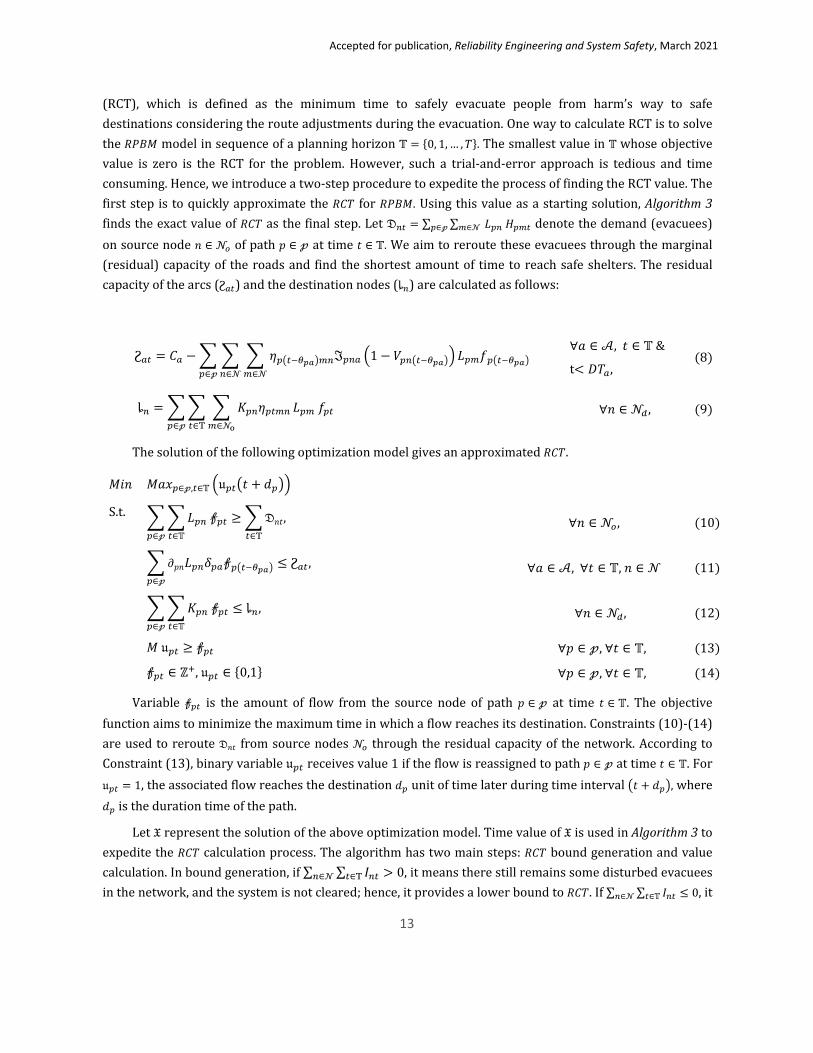
(RCT), which is defined as the minimum time to safely evacuate people from harm’s way to safe destinations considering the route adjustments during the evacuation. One way to calculate RCT is to solve the 𝑅𝑅𝑅𝑅𝑅𝑅𝑅𝑅 model in sequence of a planning horizon 𝕋𝕋 = {0, 1, … ,𝑇𝑇}. The smallest value in 𝕋𝕋 whose objective value is zero is the RCT for the problem. However, such a trial-and-error approach is tedious and time consuming. Hence, we introduce a two-step procedure to expedite the process of finding the RCT value. The first step is to quickly approximate the 𝑅𝑅𝐶𝐶𝑇𝑇 for 𝑅𝑅𝑅𝑅𝑅𝑅𝑅𝑅. Using this value as a starting solution, Algorithm 3 finds the exact value of 𝑅𝑅𝐶𝐶𝑇𝑇 as the final step. Let 𝔇𝔇𝑝𝑝𝑝𝑝 = ∑ ∑ 𝐿𝐿𝑝𝑝𝑝𝑝 𝐻𝐻𝑝𝑝𝑝𝑝𝑝𝑝𝑝𝑝∈𝒩𝒩 𝑝𝑝∈𝓅𝓅 denote the demand (evacuees) on source node 𝑛𝑛 ∈ 𝒩𝒩𝑜𝑜 of path 𝑝𝑝 ∈ 𝓅𝓅 at time 𝑡𝑡 ∈ 𝕋𝕋. We aim to reroute these evacuees through the marginal (residual) capacity of the roads and find the shortest amount of time to reach safe shelters. The residual capacity of the arcs (Ϩ𝑝𝑝𝑝𝑝) and the destination nodes (ȴ𝑝𝑝) are calculated as follows:
Ϩ𝑝𝑝𝑝𝑝 = 𝐶𝐶𝑝𝑝 −� � � 𝜂𝜂𝑝𝑝�𝑝𝑝−𝜃𝜃𝑝𝑝𝑝𝑝�𝑝𝑝𝑝𝑝ℑ𝑝𝑝𝑝𝑝𝑝𝑝𝑝𝑝∈𝒩𝒩
�1 − 𝑉𝑉𝑝𝑝𝑝𝑝�𝑝𝑝−𝜃𝜃𝑝𝑝𝑝𝑝�� 𝐿𝐿𝑝𝑝𝑝𝑝𝑓𝑓𝑝𝑝�𝑝𝑝−𝜃𝜃𝑝𝑝𝑝𝑝�𝑝𝑝∈𝒩𝒩𝑝𝑝∈𝓅𝓅
∀𝑎𝑎 ∈ 𝒜𝒜, 𝑡𝑡 ∈ 𝕋𝕋 &
t< 𝐷𝐷𝑇𝑇𝑝𝑝, (8)
ȴ𝑝𝑝 = �� � 𝐾𝐾𝑝𝑝𝑝𝑝𝜂𝜂𝑝𝑝𝑝𝑝𝑝𝑝𝑝𝑝 𝐿𝐿𝑝𝑝𝑝𝑝 𝑓𝑓𝑝𝑝𝑝𝑝𝑝𝑝∈𝒩𝒩o𝑝𝑝∈𝕋𝕋𝑝𝑝∈𝓅𝓅
∀𝑛𝑛 ∈ 𝒩𝒩𝑑𝑑 , (9)
The solution of the following optimization model gives an approximated 𝑅𝑅𝐶𝐶𝑇𝑇.
𝑅𝑅𝑢𝑢𝑛𝑛 𝑅𝑅𝑎𝑎𝑀𝑀𝑝𝑝∈𝓅𝓅,𝑝𝑝∈𝕋𝕋 �𝔲𝔲𝑝𝑝𝑝𝑝�𝑡𝑡 + 𝑢𝑢𝑝𝑝��
S.t. ��𝐿𝐿𝑝𝑝𝑝𝑝 𝒻𝒻𝑝𝑝𝑝𝑝𝑝𝑝∈𝕋𝕋𝑝𝑝∈𝓅𝓅
≥�𝔇𝔇𝑛𝑛𝑡𝑡𝑝𝑝∈𝕋𝕋
, ∀𝑛𝑛 ∈ 𝒩𝒩𝑜𝑜, (10)
�𝜕𝜕𝑝𝑝𝑛𝑛𝐿𝐿𝑝𝑝𝑝𝑝𝛿𝛿𝑝𝑝𝑝𝑝𝒻𝒻𝑝𝑝�𝑝𝑝−𝜃𝜃𝑝𝑝𝑝𝑝�𝑝𝑝∈𝓅𝓅
≤ Ϩ𝑝𝑝𝑝𝑝 , ∀𝑎𝑎 ∈ 𝒜𝒜, ∀𝑡𝑡 ∈ 𝕋𝕋, 𝑛𝑛 ∈ 𝒩𝒩 (11)
��𝐾𝐾𝑝𝑝𝑝𝑝 𝒻𝒻𝑝𝑝𝑝𝑝𝑝𝑝∈𝕋𝕋𝑝𝑝∈𝓅𝓅
≤ ȴ𝑝𝑝, ∀𝑛𝑛 ∈ 𝒩𝒩𝑑𝑑, (12)
𝑅𝑅 𝔲𝔲𝑝𝑝𝑝𝑝 ≥ 𝒻𝒻𝑝𝑝𝑝𝑝 ∀𝑝𝑝 ∈ 𝓅𝓅, ∀𝑡𝑡 ∈ 𝕋𝕋, (13)
𝒻𝒻𝑝𝑝𝑝𝑝 ∈ ℤ+, 𝔲𝔲𝑝𝑝𝑝𝑝 ∈ {0,1} ∀𝑝𝑝 ∈ 𝓅𝓅, ∀𝑡𝑡 ∈ 𝕋𝕋, (14)
Variable 𝒻𝒻𝑝𝑝𝑝𝑝 is the amount of flow from the source node of path 𝑝𝑝 ∈ 𝓅𝓅 at time 𝑡𝑡 ∈ 𝕋𝕋. The objective function aims to minimize the maximum time in which a flow reaches its destination. Constraints (10)-(14) are used to reroute 𝔇𝔇𝑝𝑝𝑝𝑝 from source nodes 𝒩𝒩𝑜𝑜 through the residual capacity of the network. According to Constraint (13), binary variable 𝔲𝔲𝑝𝑝𝑝𝑝 receives value 1 if the flow is reassigned to path 𝑝𝑝 ∈ 𝓅𝓅 at time 𝑡𝑡 ∈ 𝕋𝕋. For 𝔲𝔲𝑝𝑝𝑝𝑝 = 1, the associated flow reaches the destination 𝑢𝑢𝑝𝑝 unit of time later during time interval �𝑡𝑡 + 𝑢𝑢𝑝𝑝�, where 𝑢𝑢𝑝𝑝 is the duration time of the path.
Let 𝔛𝔛 represent the solution of the above optimization model. Time value of 𝔛𝔛 is used in Algorithm 3 to expedite the 𝑅𝑅𝐶𝐶𝑇𝑇 calculation process. The algorithm has two main steps: 𝑅𝑅𝐶𝐶𝑇𝑇 bound generation and value calculation. In bound generation, if ∑ ∑ 𝐼𝐼𝑝𝑝𝑝𝑝𝑝𝑝∈𝕋𝕋𝑝𝑝∈𝒩𝒩 > 0, it means there still remains some disturbed evacuees in the network, and the system is not cleared; hence, it provides a lower bound to 𝑅𝑅𝐶𝐶𝑇𝑇. If ∑ ∑ 𝐼𝐼𝑝𝑝𝑝𝑝𝑝𝑝∈𝕋𝕋𝑝𝑝∈𝒩𝒩 ≤ 0, it

Accepted for publication, Reliability Engineering and System Safety, March 2021
14
means the system has been cleared. However, we are aiming to find the minimum amount of time required to clear the system; hence, we consider 𝔛𝔛 as a lower bound to RCT. In the second part of the algorithm to calculate RCT, the RPBM is solved considering 𝑇𝑇 and 𝑇𝑇 − 1 as the planning horizon, where 𝑇𝑇 =(LBRCT + UBRCT) 2⁄ . If the objective value at T − 1 is positive (i.e., the system is not cleared) and becomes zero at time T (i.e., the system is cleared), the minimum time to clear the network is achieved at T; 𝑅𝑅𝐶𝐶𝑇𝑇 = 𝑇𝑇. If both objective values are positive, the system cannot be cleared at time 𝑇𝑇. Hence, we update the lower bound of 𝑅𝑅𝐶𝐶𝑇𝑇 to 𝐿𝐿𝑅𝑅𝑅𝑅𝑅𝑅𝑇𝑇 = 𝑇𝑇 if 𝑇𝑇 > 𝐿𝐿𝑅𝑅𝑅𝑅𝑅𝑅𝑇𝑇 . If both objective values equal zero, it means that the system has been cleared at T − 1. This triggers updating the upper bound to 𝑈𝑈𝑅𝑅𝑅𝑅𝑅𝑅𝑇𝑇 = 𝑇𝑇 − 1 if 𝑇𝑇 − 1 < 𝑈𝑈𝑅𝑅𝑅𝑅𝑅𝑅𝑇𝑇 . The algorithm continues until 𝑅𝑅𝐶𝐶𝑇𝑇 value is found.
Algorithm 3: Calculating Clearance time of the reroute plan Inputs: 𝑅𝑅𝑅𝑅𝑅𝑅𝑅𝑅 and 𝔛𝔛. put 𝐶𝐶𝑇𝑇 of the evacuation network with no disruption as 𝐿𝐿𝑅𝑅𝑅𝑅𝑅𝑅𝑇𝑇 put 𝑈𝑈𝑅𝑅𝑅𝑅𝑅𝑅𝑇𝑇 = 2 𝐿𝐿𝑅𝑅𝑅𝑅𝑅𝑅𝑇𝑇
Calculating a tight bound for RC𝑻𝑻: put 𝕋𝕋 = {0, 1, … ,𝔛𝔛} as the planning horizon solve 𝑅𝑅𝑅𝑅𝑅𝑅𝑅𝑅 if ∑ ∑ 𝐼𝐼𝑝𝑝𝑝𝑝𝑡𝑡∈𝕋𝕋𝑛𝑛∈𝒩𝒩 > 0 then
𝐿𝐿𝑅𝑅𝑅𝑅𝑅𝑅𝑇𝑇 = 𝔛𝔛 else then
𝑈𝑈𝑅𝑅𝑅𝑅𝑅𝑅𝑇𝑇 = 𝔛𝔛 end if
Calculating RC𝑻𝑻 Value: put 𝕋𝕋 = {0, 1, … ,𝑇𝑇} as the planning horizon While 𝜓𝜓 ≠ 1 do
put 𝑇𝑇 = (𝐿𝐿𝑅𝑅𝑅𝑅𝑅𝑅𝑇𝑇 + 𝑈𝑈𝑅𝑅𝑅𝑅𝑅𝑅𝑇𝑇) 2⁄ Solve 𝑅𝑅𝑅𝑅𝑅𝑅𝑅𝑅 for 𝕋𝕋 = {0, 1, … ,𝑇𝑇} and 𝕋𝕋 = {0, 1, … ,𝑇𝑇 − 1}
if one objective value is a positive value and the other is equal to zero then put 𝑅𝑅𝐶𝐶𝑇𝑇 = 𝑇𝑇 and 𝜓𝜓 = 1
else if both objective values are positive and 𝑇𝑇 > 𝐿𝐿𝑅𝑅𝑅𝑅𝑅𝑅𝑇𝑇 then put 𝐿𝐿𝑅𝑅𝑅𝑅𝑅𝑅𝑇𝑇 = 𝑇𝑇
else if both objective values are equal to zero and 𝑇𝑇 − 1 < 𝑈𝑈𝑅𝑅𝑅𝑅𝑅𝑅𝑇𝑇 then put 𝑈𝑈𝑅𝑅𝑅𝑅𝑅𝑅𝑇𝑇 = 𝑇𝑇 − 1
end if end while
4 Computational Results The computational experiments presented in this study focus on the impact of network arc
disruptions on evacuation plans and the performance of the proposed recovery strategy. First, the performance of 𝑅𝑅𝑅𝑅𝑅𝑅𝑅𝑅 is investigated on a small sample network in generating alternative routes. Then, the same experiment is conducted on a real evacuation network involving a large metropolitan area. The optimization models are solved using CPLEX 12.5.1, while experiments are performed on a PC with a 3.07 GHz Intel Core i7 processor having 24GB RAM and running Ubuntu 10.04.3.
Accepted for publication, Reliability Engineering and System Safety, March 2021
15
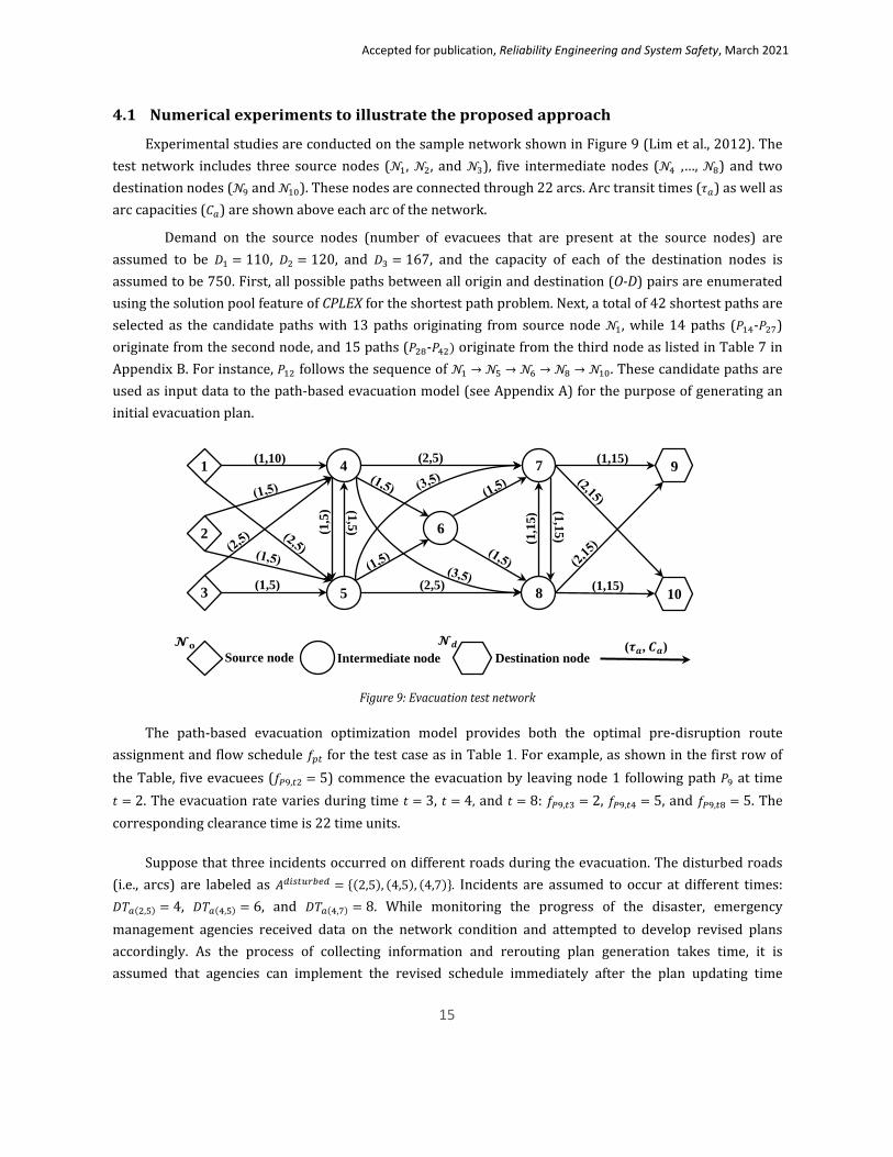
4.1 Numerical experiments to illustrate the proposed approach
Experimental studies are conducted on the sample network shown in Figure 9 (Lim et al., 2012). The test network includes three source nodes (𝒩𝒩1, 𝒩𝒩2, and 𝒩𝒩3), five intermediate nodes (𝒩𝒩4 ,…, 𝒩𝒩8) and two destination nodes (𝒩𝒩9 and 𝒩𝒩10). These nodes are connected through 22 arcs. Arc transit times (𝜏𝜏𝑝𝑝) as well as arc capacities (𝐶𝐶𝑝𝑝) are shown above each arc of the network.
Demand on the source nodes (number of evacuees that are present at the source nodes) are assumed to be 𝐷𝐷1 = 110, 𝐷𝐷2 = 120, and 𝐷𝐷3 = 167, and the capacity of each of the destination nodes is assumed to be 750. First, all possible paths between all origin and destination (O-D) pairs are enumerated using the solution pool feature of CPLEX for the shortest path problem. Next, a total of 42 shortest paths are selected as the candidate paths with 13 paths originating from source node 𝒩𝒩1, while 14 paths (𝑅𝑅14-𝑅𝑅27) originate from the second node, and 15 paths (𝑅𝑅28-𝑅𝑅42) originate from the third node as listed in Table 7 in Appendix B. For instance, 𝑅𝑅12 follows the sequence of 𝒩𝒩1 → 𝒩𝒩5 → 𝒩𝒩6 → 𝒩𝒩8 → 𝒩𝒩10. These candidate paths are used as input data to the path-based evacuation model (see Appendix A) for the purpose of generating an initial evacuation plan.
Figure 9: Evacuation test network
The path-based evacuation optimization model provides both the optimal pre-disruption route assignment and flow schedule 𝑓𝑓𝑝𝑝𝑝𝑝 for the test case as in Table 1. For example, as shown in the first row of the Table, five evacuees (𝑓𝑓𝑃𝑃9,𝑝𝑝2 = 5) commence the evacuation by leaving node 1 following path 𝑅𝑅9 at time 𝑡𝑡 = 2. The evacuation rate varies during time 𝑡𝑡 = 3, 𝑡𝑡 = 4, and 𝑡𝑡 = 8: 𝑓𝑓𝑃𝑃9,𝑝𝑝3 = 2, 𝑓𝑓𝑃𝑃9,𝑝𝑝4 = 5, and 𝑓𝑓𝑃𝑃9,𝑝𝑝8 = 5. The corresponding clearance time is 22 time units.
Suppose that three incidents occurred on different roads during the evacuation. The disturbed roads (i.e., arcs) are labeled as 𝐴𝐴𝑑𝑑𝑢𝑢𝑑𝑑𝑝𝑝𝑢𝑢𝑑𝑑𝑑𝑑𝑢𝑢𝑑𝑑 = {(2,5), (4,5), (4,7)}. Incidents are assumed to occur at different times: 𝐷𝐷𝑇𝑇𝑝𝑝(2,5) = 4, 𝐷𝐷𝑇𝑇𝑝𝑝(4,5) = 6, and 𝐷𝐷𝑇𝑇𝑝𝑝(4,7) = 8. While monitoring the progress of the disaster, emergency management agencies received data on the network condition and attempted to develop revised plans accordingly. As the process of collecting information and rerouting plan generation takes time, it is assumed that agencies can implement the revised schedule immediately after the plan updating time
(1,10)
4
5
6
7
8
9
10
1
2
3
Source node Intermediate node Destination node (𝝉𝝉𝒑𝒑, 𝑪𝑪𝒑𝒑) 𝓝𝓝𝒅𝒅
(1,5)
(1,15)
(1,
5) (1,5)
(1,15) (1,1
5)
(2,5) (1,15)
(2,5)

Accepted for publication, Reliability Engineering and System Safety, March 2021
16
𝑡𝑡𝑢𝑢𝑝𝑝𝑑𝑑𝑝𝑝𝑝𝑝𝑢𝑢𝑝𝑝𝑢𝑢 = 10. Hence, before 𝑡𝑡 = 10, no rerouting itinerary is planned and the corresponding variable (ℛ𝑝𝑝𝑝𝑝𝑝𝑝) remains at zero.
Table 1. An initial evacuation plan for the sample network (𝑓𝑓𝑝𝑝𝑝𝑝)
Time Slots 1 2 3 4 5 6 7 8 9 10 11 12 13 14 15 16 17 18
Path
s
P9 5 2 5 5 P10 5 5 5 5 5 5 5 5 5 5 5 5 5 P11 5 5 3 5 5 5 P16 5 P17 5 5 P18 5 P19 2 5 5 P21 3 P22 5 5 5 5 5 5 5 P23 2 2 5 5 5 5 5 5 P24 5 3 5 P27 3 P28 5 P30 3 P31 3 5 5 5 5 5 P33 5 5 5 P35 5 P36 5 5 5 5 5 5 5 P37 2 5 5 5 5 5 5 P39 5 P40 5 P41 2 5 5 5 2 5 5 P42 5
Disruptions on arcs (2,5), (4,5), and (4,7) partially affect several paths {𝑅𝑅17, 𝑅𝑅18,𝑅𝑅19,𝑅𝑅21,𝑅𝑅22,𝑅𝑅23,𝑅𝑅27,𝑅𝑅31,𝑅𝑅41,𝑅𝑅42}. For example, flow 𝑓𝑓𝑝𝑝23,𝑝𝑝2 = 2 was scheduled to arrive at arc (4,7) at time 𝑡𝑡 + 𝜃𝜃𝑝𝑝23,𝑝𝑝(4,7) = 2 + 1 = 3. It takes 𝜏𝜏𝑝𝑝(4,7) = 2 time units for the flow to pass through this arc. Since the arc is supposed to fail at time 𝐷𝐷𝑇𝑇𝑝𝑝(4,7) = 8, the flow 𝑓𝑓𝑝𝑝23,𝑝𝑝2 = 2 is not affected. Now, flow 𝑓𝑓𝑝𝑝23,𝑝𝑝9 = 5 is scheduled to reach arc (4,7) at time 𝑡𝑡 + 𝜃𝜃𝑝𝑝23,𝑝𝑝(4,7) = 9 + 1 = 10, but the arc is already blocked at time 𝑡𝑡 = 8. So, there will be a flow accumulation on node 2 at time 𝑡𝑡 = 10, and it is denoted by 𝐻𝐻𝑝𝑝23,𝑝𝑝4,𝑝𝑝10 = 5. The magnitude, location, and interruption time of the disturbed flow 𝐻𝐻𝑝𝑝𝑝𝑝𝑝𝑝 are demonstrated in Table 2.
Table 2. Disturbed flow (𝐻𝐻𝑝𝑝𝑝𝑝𝑝𝑝)
Time Slots 4 6 7 8 9 10 11 12 13 14 15 16 17 18 19 Total
Path
s
P17 n2 5 5 25 P18 n2 5
P19 n2 5 5 P22 n4 5 5 5 5 5 5 5
107 P23 n4 5 5 5 5 5 P31 n4 5 5 5 5 5 P41 n4 5 2 5 5 P42 n4 5
According to Table 2, 132 evacuees out of 392 are constrained at different locations of the transportation network between time periods 𝑡𝑡 = 4 and 𝑡𝑡 = 19. Hence, the proposed RPBM model is used to generate new paths to accommodate the disturbed flow.
Table 3 shows the rerouting schedule for the disturbed flow 𝑟𝑟𝑝𝑝𝑝𝑝𝑝𝑝 provided by 𝑅𝑅𝑅𝑅𝑅𝑅𝑅𝑅. The first row of
Accepted for publication, Reliability Engineering and System Safety, March 2021
17
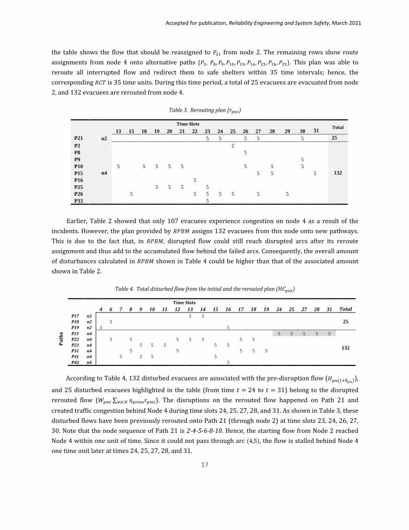
the table shows the flow that should be reassigned to 𝑅𝑅21 from node 2. The remaining rows show route assignments from node 4 onto alternative paths {𝑅𝑅2, 𝑅𝑅8,𝑅𝑅9,𝑅𝑅10,𝑅𝑅15,𝑅𝑅16,𝑅𝑅25,𝑅𝑅26,𝑅𝑅33}. This plan was able to reroute all interrupted flow and redirect them to safe shelters within 35 time intervals; hence, the corresponding 𝑅𝑅𝐶𝐶𝑇𝑇 is 35 time units. During this time period, a total of 25 evacuees are evacuated from node 2, and 132 evacuees are rerouted from node 4.
Table 3. Rerouting plan (𝑟𝑟𝑝𝑝𝑝𝑝𝑝𝑝)
Time Slots Total 13 15 18 19 20 21 22 23 24 25 26 27 28 29 30 31
P21 n2 5 5 5 5 5 25 P2
n4
2
132
P8 5 P9 5 P10 5 5 5 5 5 5 5 5 P15 5 5 5 P16 5 P25 5 5 5 5 P26 5 5 5 5 5 5 5 P33 5
Earlier, Table 2 showed that only 107 evacuees experience congestion on node 4 as a result of the incidents. However, the plan provided by 𝑅𝑅𝑅𝑅𝑅𝑅𝑅𝑅 assigns 132 evacuees from this node onto new pathways. This is due to the fact that, in 𝑅𝑅𝑅𝑅𝑅𝑅𝑅𝑅, disrupted flow could still reach disrupted arcs after its reroute assignment and thus add to the accumulated flow behind the failed arcs. Consequently, the overall amount of disturbances calculated in 𝑅𝑅𝑅𝑅𝑅𝑅𝑅𝑅 shown in Table 4 could be higher than that of the associated amount shown in Table 2.
Table 4. Total disturbed flow from the initial and the rerouted plan (𝐻𝐻𝐶𝐶𝑝𝑝𝑝𝑝𝑝𝑝)
Time Slots 4 6 7 8 9 10 11 12 13 14 15 16 17 18 19 24 25 27 28 31 Total
Path
s
P17 n2 5 5 25 P18 n2 5
P19 n2 5 5 P21 n4 5 5 5 5 5
132 P22 n4 5 5 5 5 5 5 5 P23 n4 5 5 5 5 5 P31 n4 5 5 5 5 5 P41 n4 5 2 5 5 P42 n4 5
According to Table 4, 132 disturbed evacuees are associated with the pre-disruption flow (𝐻𝐻𝑝𝑝𝑝𝑝�𝑝𝑝+��𝜃𝑝𝑝𝑝𝑝�),
and 25 disturbed evacuees highlighted in the table (from time 𝑡𝑡 = 24 to 𝑡𝑡 = 31) belong to the disrupted rerouted flow (𝑊𝑊𝑝𝑝𝑝𝑝𝑝𝑝 ∑ 𝜂𝜂𝑝𝑝𝑝𝑝𝑝𝑝𝑝𝑝𝑟𝑟𝑝𝑝𝑝𝑝𝑝𝑝𝑝𝑝∈𝒩𝒩 ). The disruptions on the rerouted flow happened on Path 21 and created traffic congestion behind Node 4 during time slots 24, 25, 27, 28, and 31. As shown in Table 3, these disturbed flows have been previously rerouted onto Path 21 (through node 2) at time slots 23, 24, 26, 27, 30. Note that the node sequence of Path 21 is 2-4-5-6-8-10. Hence, the starting flow from Node 2 reached Node 4 within one unit of time. Since it could not pass through arc (4,5), the flow is stalled behind Node 4 one time unit later at times 24, 25, 27, 28, and 31.

Accepted for publication, Reliability Engineering and System Safety, March 2021
18
The performance of the proposed model is further investigated using four different test instances. Table 5 shows the input data for these instances and includes information regarding the set of disrupted arcs, corresponding disruption times, and updating times for the rerouting strategy.
Table 5. Test problems C1 C2 C3 C4
Disrupted arcs (2,5),(4,5), (4,7),(6,7)
(5,4),(5,7), (6,8),(7,10)
(2,5),(4,5), (5,7),(8,7)
(2,5),(4,5),(4,6), (5,6),(8,7),(7,10)
Disruption time {9,16,14,8} {17,8,10,19} {12,15,14,7} {15,6,8,10,9,12}
Updating time 16 19 15 15
Figures 10 highlights the amount of remaining disturbed flow (hcnt) in the system as the evacuation progresses. The remaining disturbed flow gradually increased at early stages of the planning horizon. When the rerouting process began, hcnt gradually decreased until there remains no disturbed flow to be rerouted. The system was cleared when all evacuees reached the destination nodes. In test problem C1, the remaining disturbed flow was zero at time 𝑡𝑡 = 32. But, it took additional 2 units of time for the last rerouted flow to reach the destination via the assigned alternative path. Hence, the system was cleared at time 34, i.e., RCT=34. Similarly, the RCT for test problems C2 , C3, and C4 are 32, 25, and 29, respectively.
Figure 10. Accumulated remaining flow (ℎ𝑐𝑐𝑝𝑝𝑝𝑝𝑝𝑝) under different sample problems
0
20
40
60
80
100
hc
time
C1
0
20
40
60
80
100
hc
time
C2
0
50
100
hc
time
C3
Accumulated Remaining Flow
020406080
100
hc
time
C4
Accumulated Remaining Flow
Accumulated Remaining Flow Accumulated Remaining Flow
Accepted for publication, Reliability Engineering and System Safety, March 2021
19
The rerouted clearance times are different for each problem instance because the input data for the four cases are different in terms of the disrupted arcs, the arc disruption times, and the updating times. All of these factors have influence on the amount of clearance time of the network. In the following, we provide a sensitivity analysis on the evacuation plans under different problem settings for these factors.
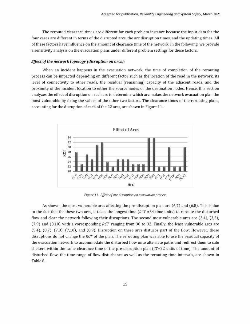
Effect of the network topology (disruption on arcs):
When an incident happens in the evacuation network, the time of completion of the rerouting process can be impacted depending on different factor such as the location of the road in the network, its level of connectivity to other roads, the residual (remaining) capacity of the adjacent roads, and the proximity of the incident location to either the source nodes or the destination nodes. Hence, this section analyzes the effect of disruption on each arc to determine which arc makes the network evacuation plan the most vulnerable by fixing the values of the other two factors. The clearance times of the rerouting plans, accounting for the disruption of each of the 22 arcs, are shown in Figure 11.
Figure 11. Effect of arc disruption on evacuation process
As shown, the most vulnerable arcs affecting the pre-disruption plan are (6,7) and (6,8). This is due to the fact that for these two arcs, it takes the longest time (𝑅𝑅𝐶𝐶𝑇𝑇 =34 time units) to reroute the disturbed flow and clear the network following their disruptions. The second most vulnerable arcs are (3,4), (3,5), (7,9) and (8,10) with a corresponding 𝑅𝑅𝐶𝐶𝑇𝑇 ranging from 30 to 32. Finally, the least vulnerable arcs are (5,4), (8,7), (7,8), (7,10), and (8,9). Disruption on these arcs disturbs part of the flow; However, these disruptions do not change the 𝑅𝑅𝐶𝐶𝑇𝑇 of the plan. The rerouting plan was able to use the residual capacity of the evacuation network to accommodate the disturbed flow onto alternate paths and redirect them to safe shelters within the same clearance time of the pre-disruption plan (𝐶𝐶𝑇𝑇=22 units of time). The amount of disturbed flow, the time range of flow disturbance as well as the rerouting time intervals, are shown in Table 6.
2022242628303234
RCT
Arc
Effect of Arcs

Accepted for publication, Reliability Engineering and System Safety, March 2021
20
Table 6. Analysis of Less Vulnerable Arcs
Arc (5,4) (8,7) (7,8) (7,10) (8,9) Total disrupted 35 10 30 0 0 Flow disruption time [9,17] [11,14] [9,18] 0 0 Arc capacity 5 15 15 15 15 Rerouting node n5 n8 n7 - - Rerouting time [11,17] [11,17] [11,20] 0 0
Note that the amount of disrupted flow is equal to the amount of rerouted flow. The rerouting node represents the upstream node of the disrupted arc from which the disturbed flow is rerouted. When arc (5,4) experiences a disturbance at time 9, it causes the disruption of 35 evacuees during the time intervals between 9 and 17. This amount of flow is gathered behind Node 5 and, consequently, is rerouted from the same node between time 11 and 17. Hence, the rerouting process ends before time 22, which also happens to be the 𝐶𝐶𝑇𝑇 of the pre-disruption plan. Cases for arcs (8,7) and (7,8) are similar. However, disruptions of arc (7,10) and (8,9) have no effect on the pre-disruption plan and no evacuees are disturbed. This is because the affected arcs are not associated with the paths used in the pre-disruption plan.
Effect of disruption times:
The occurrence time of an incident can be an important factor influencing the rerouted clearance time. For instance, if an incident occurs on an arc, it will create a disruption only to evacuees who have not yet passed the incident location in the route. Hence, this section studies the effect of arc disruption times on the evacuation and rerouting process. For this purpose, a set of disturbed arcs are chosen as 𝐴𝐴𝑑𝑑𝑢𝑢𝑑𝑑𝑝𝑝𝑢𝑢𝑑𝑑𝑑𝑑𝑢𝑢𝑑𝑑 ={(2,4), (4,8)}. The disruption times of the arcs are changed in the interval [1, 21], and an update will be triggered one unit after arc disruption times. Figure 12 (a) shows the 𝑅𝑅𝐶𝐶𝑇𝑇s when the disruption time of the arcs changes between time 1 and time 21. As can be seen, the rerouting CT is higher when the disruption time occurs earlier in the planning horizon. This is not surprising because as a disruption happens earlier on the road, more evacuees are affected, and more time is required to reroute them and clear the system.
Figure 12. Effect of disruption time and updating time on evacuation process
20
22
24
26
28
30
32
34
1 2 3 4 5 6 7 8 9 10 11 12 13 14 15 16 17 18 19 20 21
RCT
Disruption Time
Effect of Disruption Time
(a)
20
22
24
26
28
30
32
34
36
38
40
4 5 6 7 8 9 10 11 12 13 14 15 16 17 18 19 20 21
RCT
Updating Time
Effect of Updating Time
(b)

Accepted for publication, Reliability Engineering and System Safety, March 2021
21
Effect of information (updating time):
Shortly after an incident occurs within the network, it starts to disrupt the evacuation flow. It takes time for the planners to (1) understand and analyze the situation, (2) make an appropriate decision on the rerouting strategy, and (3) execute the reroute plan accordingly. To account for this delay in reroute planning, we introduce an updating time 𝑡𝑡𝑢𝑢𝑝𝑝𝑑𝑑𝑝𝑝𝑝𝑝𝑢𝑢𝑝𝑝𝑢𝑢 to capture the total time it took from the incidence analysis until the new plan is ordered to be executed. The effect of 𝑡𝑡𝑢𝑢𝑝𝑝𝑑𝑑𝑝𝑝𝑝𝑝𝑢𝑢𝑝𝑝𝑢𝑢 on the evacuation process is studied and is shown in Figure 12 (b). The more delay there is in receiving update information on the network situation, the longer the clearance time of the network after disturbed flow reassignments. Note that it took less than a second for running each preprocessing algorithm as well as the MIP model on the small network of Figure 8.
4.2 Numerical Experiments on a Large-Scale Network
We continue the experiments on an evacuation network of the Greater Houston area (Lim et al., 2012). Houston, Texas, the fourth largest city in the U.S., is known to be one of the most vulnerable metropolitan cities situated on the Gulf Coast, and has been severely affected by hurricanes and floods for the several decades. The Houston network (Figure 13) comprises of a total of 42 nodes and 107 arcs. The first thirteen nodes represent source nodes (𝒩𝒩1 -𝒩𝒩13), and the last four nodes (𝒩𝒩39 -𝒩𝒩42) represent safe destination nodes.

Accepted for publication, Reliability Engineering and System Safety, March 2021
22
Figure 13. City of Houston transportation network
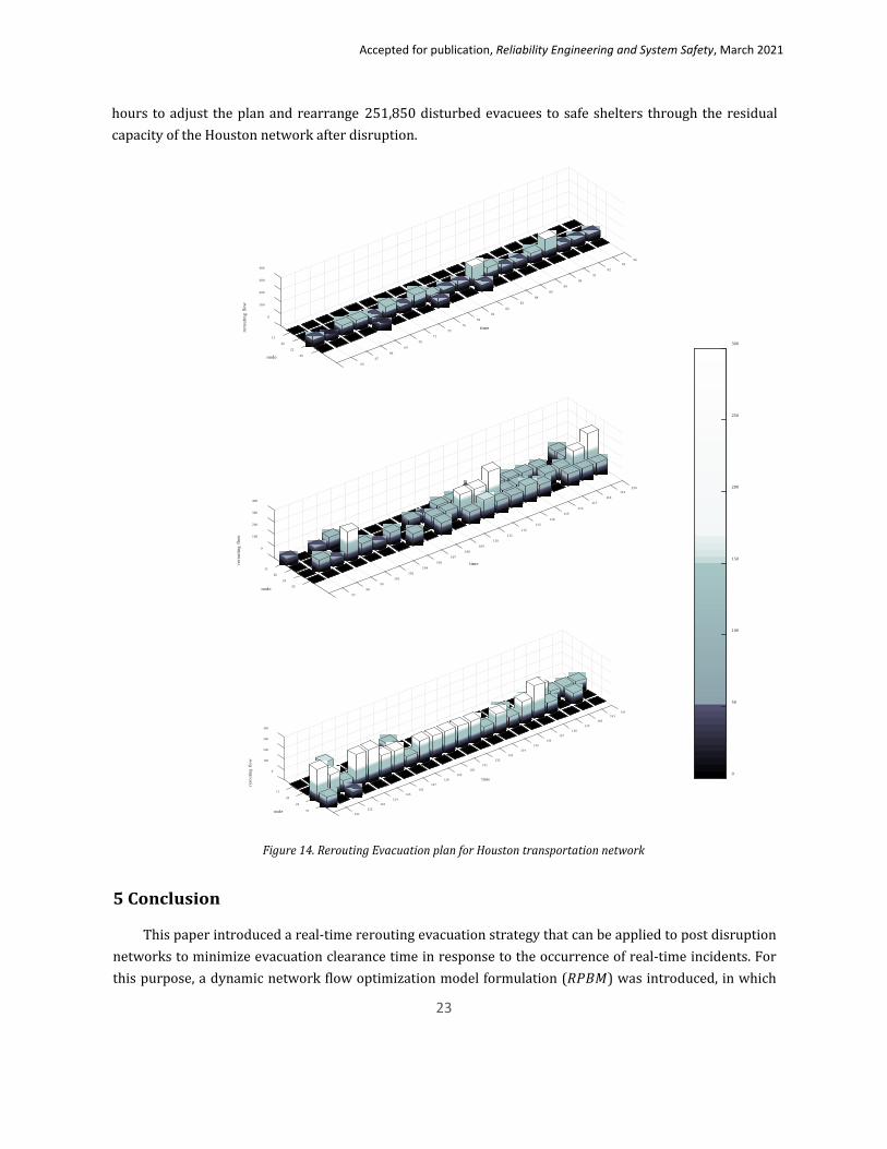
For the purpose of demonstrating our proposed evacuation rerouting approach, we used the same input data for this network as it was reported in Lim et al., 2012. Hence, the total number of evacuees (i.e., evacuation vehicles) on the source nodes are assumed to be 56,600, in which each of source nodes 1-6 has 100 evacuees, 3,500 for each of nodes 7-10, and 14,000 evacuees each for nodes 11-13. The transit times are defined to be multiplies of 𝜏𝜏 = 30 minute intervals. Using the PBM model in Appendix A, we first generate the pre-disruption evacuation plan using 140 candidate paths to be selected in the optimization model. The resulting pre-disruption plan distributed the evacuation flow over 52 selected paths, and it took 129τ to clear the network. Disruptions are triggered on arcs (22,42), (20,32), (11,27), and (35,34) at times 56, 69, 67 and 48, respectively. These road disruptions affect flows on 11 paths and result in 10,966 evacuees being stranded behind nodes 11, 20, 22, and 35. Among these evacuees, 600 are on node 11, 1,675 on node 20, 7,331 on node 22, and 1,360 on node 35. The 𝑅𝑅𝑅𝑅𝑅𝑅𝑅𝑅 is used to provide a reroute plan for the disturbed flow. The total combined computation time of running both Algorithm 1 and Algorithm 2 was 67.91 seconds, while it took 203.60 seconds to run Algorithm 3 to calculate 𝑅𝑅𝐶𝐶𝑇𝑇. It took 52.41 seconds to solve the 𝑅𝑅𝑅𝑅𝑅𝑅𝑅𝑅 based on the RCT value. The corresponding reroute plan is shown in Figure 14. In the figure, the amount of rerouted flow from each node during different time intervals are illustrated. The total time taken to move all disturbed flow to safe shelters was 162τ. This means that our model required approximately 16
Accepted for publication, Reliability Engineering and System Safety, March 2021
23
hours to adjust the plan and rearrange 251,850 disturbed evacuees to safe shelters through the residual capacity of the Houston network after disruption.
Figure 14. Rerouting Evacuation plan for Houston transportation network
5 Conclusion
This paper introduced a real-time rerouting evacuation strategy that can be applied to post disruption networks to minimize evacuation clearance time in response to the occurrence of real-time incidents. For this purpose, a dynamic network flow optimization model formulation (𝑅𝑅𝑅𝑅𝑅𝑅𝑅𝑅) was introduced, in which
9694
92
91
90
89
85
84
time
83
82
8178
0
76
100
200
75
300
71
rero
utin
g fl
ow
11
400
70
node
206922
6835
67
65
120119
118117
116115
114113
112
time
111110
109108
0
107
100
200
106
300
rero
utin
g fl
ow
10411
400
102
node
2010122
9935
9897
142141
140139
138137
136135
134133
time
132131
130129
0
100
128
200
127
300
rero
utin
g fl
ow
126
400
11125
node
20 12422 123
12235121
0
50
100
150
200
250
300
Accepted for publication, Reliability Engineering and System Safety, March 2021
24
variable evacuation flow rates are considered to develop alternative paths to achieve more practical and effective evacuation plans. Due to very high-level complexity for developing a practically useful optimization model, computational algorithms have been developed to calculate a few key values for specific parameters related to road disruption. As a result, it enabled us to develop a simple and computational efficient MIP model for the evacuation problem. A rerouting clearance time calculation algorithm is introduced to efficiently calculate the minimum amount of time required to mobilize disturbed evacuees to the safe shelters. Numerical experiments were thoroughly conducted to study the performance of the proposed 𝑅𝑅𝑅𝑅𝑅𝑅𝑅𝑅 under different problem configurations. Computational experiments were made to test computational efficient in solving the proposed approach. The impact of three incident-related factors have been investigated to better understand their effects on the rerouting process, including the location of the disruption, the time of disruption occurrence, and the plan updating time. The results showed that more flow was disturbed if an incident occurs earlier during the evacuation, which leads to a greater amount of time to reroute the affected flow and clear the system. When the time for plan updates was delayed (i.e., the rerouting process takes place later), the clearance time of the network increased accordingly. This emphasizes the importance of making timely decisions for fast response to incidents as it is crucial in an efficient evacuation rerouting plan. The proposed approach has also been tested on a large-scale evacuation network, and the results support that the proposed approach can handle in evacuating large metropolitan areas in a timely manner.
The proposed approach is limited to deterministic problem settings. As a future work, one can extend this paper by considering various uncertainties such as variations in the number of would-be evacuees, alternative road capacities, or evacuees’ behavior. Another venue for an extension is to extend the proposed approach to make it as a basis for vulnerabilities analysis through developing a probabilistic mechanism that accounts for factors including simultaneous multiple occurrences.
References
Beroggi, G.E., and Wallace, W.A. (1995). Operational control of the transportation of hazardous materials: An assessment of alternative decision models. Management Science. 41(12), 1962–1977.
Bier, V. M., and Hausken, K. (2013). Defending and attacking a network of two arcs subject to traffic congestion. Reliability Engineering & System Safety. 112, 214–224.
Chen, L., and Miller-Hooks, E. (2012). Resilience: an indicator of recovery capability in intermodal freight transport. Transportation Science. 46(1), 109–123.
De Silva, F.N., and Eglese, R.W. (2000). Integrating simulation modelling and GIS: spatial decision support systems for evacuation planning. Journal of the Operational Research Society. 51(4), 423–430.
Faturechi, R., and Miller-Hooks, E. (2014). Travel time resilience of roadway networks under disaster. Transportation research part B: methodological. 70, 47–64.
Faturechi, R., and Miller-Hooks, E. (2015). Measuring the performance of transportation infrastructure systems in disasters: A comprehensive review. Journal of infrastructure systems. 21(1), 04014025.

Accepted for publication, Reliability Engineering and System Safety, March 2021
25
FEMA, D. (2010). Developing and Maintaining Emergency Operations Plans, 1-124.
FEMA (2008). Producing Emergency Plans: A Guide for All-Hazard Emergency Operations Planning.
Ford Jr, L.R., and Fulkerson, D.R. (2015). Flows in networks. Princeton university press.
Kim, S., Shekhar, S., and Min, M. (2008). Contraflow transportation network reconfiguration for evacuation route planning. IEEE Transactions on Knowledge and Data Engineering. 20(8), 1115–1129.
Lim, G.J., Zangeneh, S., Baharnemati, M.R., and Assavapokee, T. (2012). A capacitated network flow optimization approach for short notice evacuation planning. European Journal of Operational Research. 223(1), 234–245.
Lim, G.J., Baharnemati, M.R., and Kim, S.J. (2016). An optimization approach for real time evacuation reroute planning. Annals of Operations Research. 238(1-2), 375–388.
Lim, G.J., Rungta, M., and Davishan, A. (2019). A Robust Chance Constraint Programming Approach for Evacuation Planning under Uncertain Demand Distribution. IISE Transactions. 51(6), 589-604.
Lim, G. J., Zangeneh, S., & Kim, S. J. (2016). Clustering approach for defining hurricane evacuation zones. Journal of Urban Planning and Development. 142(4), 04016008.
Lin, Y. K., Chang, P. C., and Fiondella, L. (2012). Quantifying the impact of correlated failures on stochastic flow network reliability. IEEE Transactions on Reliability. 61(3), 692–701.
Pidd, M., De Silva, F.N., and Eglese, R.W. (1996). A simulation model for emergency evacuation. European Journal of Operational Research. 90(3), 413–419.
Robert, T. (2000). Stafford disaster relief and emergency assistance act. Public Law 10, 106–390.
Rungta, M., Lim, G.J., and Baharnemati, M. (2012). Optimal egress time calculation and path generation for large evacuation networks. Annals of Operations Research. 201(1), 403–421.
Sheffi, Y., Mahmassani, H., and Powell, W.B. (1981). Evacuation studies for nuclear power plant sites: A new challenge for transportation engineers. ITE Journal. 51(6), 25–28.
Accepted for publication, Reliability Engineering and System Safety, March 2021
26
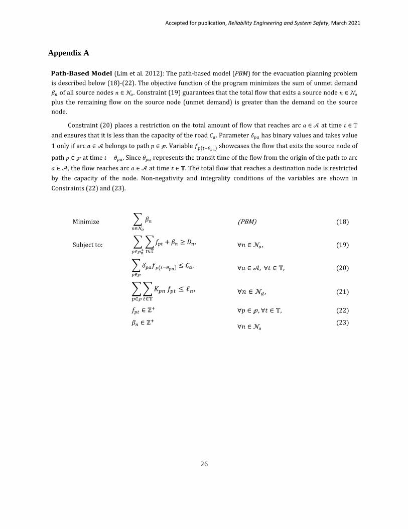
Appendix A
Path-Based Model (Lim et al. 2012): The path-based model (PBM) for the evacuation planning problem is described below (18)-(22). The objective function of the program minimizes the sum of unmet demand 𝛽𝛽𝑝𝑝 of all source nodes 𝑛𝑛 ∈ 𝒩𝒩𝑜𝑜. Constraint (19) guarantees that the total flow that exits a source node 𝑛𝑛 ∈ 𝒩𝒩𝑜𝑜 plus the remaining flow on the source node (unmet demand) is greater than the demand on the source node.
Constraint (20) places a restriction on the total amount of flow that reaches arc 𝑎𝑎 ∈ 𝒜𝒜 at time 𝑡𝑡 ∈ 𝕋𝕋 and ensures that it is less than the capacity of the road 𝐶𝐶𝑝𝑝. Parameter 𝛿𝛿𝑝𝑝𝑝𝑝 has binary values and takes value 1 only if arc 𝑎𝑎 ∈ 𝒜𝒜 belongs to path 𝑝𝑝 ∈ 𝓅𝓅. Variable 𝑓𝑓𝑝𝑝�𝑝𝑝−𝜃𝜃𝑝𝑝𝑝𝑝� showcases the flow that exits the source node of
path 𝑝𝑝 ∈ 𝓅𝓅 at time 𝑡𝑡 − 𝜃𝜃𝑝𝑝𝑝𝑝. Since 𝜃𝜃𝑝𝑝𝑝𝑝 represents the transit time of the flow from the origin of the path to arc 𝑎𝑎 ∈ 𝒜𝒜, the flow reaches arc 𝑎𝑎 ∈ 𝒜𝒜 at time 𝑡𝑡 ∈ 𝕋𝕋. The total flow that reaches a destination node is restricted by the capacity of the node. Non-negativity and integrality conditions of the variables are shown in Constraints (22) and (23).
Minimize � 𝛽𝛽𝑝𝑝𝑝𝑝∈𝒩𝒩𝑜𝑜
(PBM) (18)
Subject to: � �𝑓𝑓𝑝𝑝𝑝𝑝𝑝𝑝∈𝕋𝕋𝑝𝑝∈𝓅𝓅𝑝𝑝+
+ 𝛽𝛽𝑝𝑝 ≥ 𝐷𝐷𝑝𝑝, ∀𝑛𝑛 ∈ 𝒩𝒩𝑜𝑜, (19)
�𝛿𝛿𝑝𝑝𝑝𝑝𝑓𝑓𝑝𝑝�𝑝𝑝−𝜃𝜃𝑝𝑝𝑝𝑝�𝑝𝑝∈𝓅𝓅
≤ 𝐶𝐶𝑝𝑝, ∀𝑎𝑎 ∈ 𝒜𝒜, ∀𝑡𝑡 ∈ 𝕋𝕋, (20)
��𝐾𝐾𝑝𝑝𝑝𝑝 𝑓𝑓𝑝𝑝𝑝𝑝𝑝𝑝∈𝕋𝕋𝑝𝑝∈𝓅𝓅
≤ ℓ𝑝𝑝, ∀𝑛𝑛 ∈ 𝒩𝒩𝑑𝑑 , (21)
𝑓𝑓𝑝𝑝𝑝𝑝 ∈ ℤ+ ∀𝑝𝑝 ∈ 𝓅𝓅, ∀𝑡𝑡 ∈ 𝕋𝕋, (22)
𝛽𝛽𝑝𝑝 ∈ ℤ+ ∀𝑛𝑛 ∈ 𝒩𝒩𝑜𝑜 (23)

Accepted for publication, Reliability Engineering and System Safety, March 2021
27
Appendix B
This section is to explain our motivation for the proposed evacuation reroute planning model formulation. The pre-processing algorithms help us to develop a less complex optimization model which can be solved in a timely manner for the application discussed in this paper. Let us explain what happens if we were going to solve the optimization without the pre-processing algorithms. The main challenge lies in calculating the amount of disturbed flow (Hpnt). If the proposed pre-processing algorithms are not used, the following constraint should be included in the optimization framework to calculate the amount of disturbed flow (𝐻𝐻𝑝𝑝𝑝𝑝t) on node 𝑛𝑛 ∈ 𝒩𝒩 of path 𝑝𝑝 ∈ 𝓅𝓅 at time 𝑡𝑡 ∈ 𝕋𝕋.
𝐻𝐻𝑝𝑝𝑝𝑝�𝑝𝑝+��𝜃𝑝𝑝𝑝𝑝� ≥ 𝑓𝑓𝑝𝑝𝑝𝑝𝛾𝛾𝑝𝑝𝑝𝑝𝛿𝛿𝑝𝑝𝑝𝑝�𝑡𝑡 + 𝜃𝜃𝑝𝑝𝑝𝑝 + 𝜏𝜏𝑝𝑝 − 𝐷𝐷𝑇𝑇𝑝𝑝�𝑡𝑡 + 𝜃𝜃𝑝𝑝𝑝𝑝 + 𝜏𝜏𝑝𝑝 − 𝐷𝐷𝑇𝑇𝑝𝑝
− � � 𝛾𝛾𝑝𝑝��𝑝𝛿𝛿𝑝𝑝��𝑝�𝑡𝑡 + 𝜃𝜃𝑝𝑝��𝑝 + 𝜏𝜏��𝑝 − 𝐷𝐷𝑇𝑇��𝑝�𝑡𝑡 + 𝜃𝜃𝑝𝑝��𝑝 + 𝜏𝜏��𝑝 − 𝐷𝐷𝑇𝑇��𝑝��𝑝∈𝑁𝑁𝑝𝑝𝑝𝑝
+ �𝑁𝑁𝑝𝑝𝑝𝑝��𝑅𝑅
∀𝑝𝑝 ∈ 𝓅𝓅, 𝑛𝑛 ∈ 𝒩𝒩, 𝑡𝑡 ∈ 𝕋𝕋,
where 𝑅𝑅 is an arbitrarily large number and 𝑁𝑁𝑝𝑝𝑝𝑝 is the set of all preceding nodes to node 𝑛𝑛 ∈ 𝒩𝒩 of path 𝑝𝑝 ∈ 𝓅𝓅. Parameters 𝛾𝛾𝑝𝑝𝑝𝑝 and 𝛿𝛿𝑝𝑝𝑝𝑝 are used to represent the topology of the network (see the notation in p. 5). Flow fpt departs from the origin of path p ∈ 𝓅𝓅 at time t ∈ 𝕋𝕋 and reaches the end of arc a ∈ 𝒜𝒜 at time t +
θpa + τa. The term �t + θpa + τa − DTa� t + θpa + τa − DTa� is used to monitor arc disruption time DTa on the flow, fpt. If a disruption on the arc occurs after the flow has passed the incident arc, then t + θpa + τa <
DTa; hence, �t + θpa + τa − DTa� t + θpa + τa − DTa� = −1. If the disruption happens before the flow arrives
at the end of the arc, then we will have �t + θpa + τa − DTa� t + θpa + τa − DTa� = 1. To indicate whether flow fpt is disturbed by arc a ∈ 𝒜𝒜, we also need to take into account the effect of disruption times of the preceding arcs to arc a ∈ 𝒜𝒜. If the flow is not interrupted by any preceding arcs to the incident arc, we will have ∑ γnaδpa �t + θpa + τa − DTa� t + θpa + τa − DTa�n∈Npn = −�Npn�. Hence, if flow fpt is stopped due to
the disruption on arc a ∈ 𝒜𝒜 (which emerges from node n ∈ 𝒩𝒩) and not any other preceding arcs, the following equations hold:
�𝑡𝑡 + 𝜃𝜃𝑝𝑝𝑝𝑝 + 𝜏𝜏𝑝𝑝 − 𝐷𝐷𝑇𝑇𝑝𝑝� 𝑡𝑡 + 𝜃𝜃𝑝𝑝𝑝𝑝 + 𝜏𝜏𝑝𝑝 − 𝐷𝐷𝑇𝑇𝑝𝑝� = 1
� 𝛾𝛾𝑝𝑝��𝑝𝛿𝛿𝑝𝑝��𝑝 �𝑡𝑡 + 𝜃𝜃𝑝𝑝��𝑝 + 𝜏𝜏��𝑝 − 𝐷𝐷𝑇𝑇��𝑝� 𝑡𝑡 + 𝜃𝜃𝑝𝑝��𝑝 + 𝜏𝜏��𝑝 − 𝐷𝐷𝑇𝑇��𝑝���𝑝∈𝑁𝑁𝑝𝑝𝑝𝑝
= −�𝑁𝑁𝑝𝑝𝑝𝑝�
This leads to 𝐻𝐻𝑝𝑝𝑝𝑝(𝑝𝑝+��𝜃𝑝𝑝𝑝𝑝) = 𝑓𝑓𝑝𝑝𝑝𝑝 if the objective function is minimized, i.e., the amount of disturbed flow
is minimized. For any other scenarios, the constraint can be relaxed with an exception when the disruption occurrence time equals the time that the flow arrives at the end of the arc (𝐷𝐷𝑇𝑇𝑝𝑝 = t + θpa + τa). In this case,
we will have the following expression 00 in the constraint, which cannot be not defined.
To overcome this modeling complexity, we proposed to calculate the values of parameter V𝑝𝑝𝑝𝑝𝑝𝑝 a priori using the pre-processing algorithms. As a result, it simplifies the equation 𝐻𝐻𝑝𝑝𝑝𝑝�𝑝𝑝+��𝜃𝑝𝑝𝑝𝑝� = V𝑝𝑝𝑝𝑝𝑝𝑝𝑓𝑓𝑝𝑝𝑝𝑝 in the RPBM
as V𝑝𝑝𝑝𝑝𝑝𝑝 is not an unknown variable, but a parameter.

Accepted for publication, Reliability Engineering and System Safety, March 2021
28
Appendix C
Table 7: Node sequence of candidate paths
Sequences Sequences
Path
s
P1 1-4-7-9
Path
s
P22 2-4-5-8-10 P2 1-4-6-7-9 P23 2-4-7-8-10 P3 1-4-6-8-10 P24 2-4-6-7-8-10 P4 1-4-5-6-7-9 P25 2-4-6-8-7-9 P5 1-4-5-6-8-10 P26 2-4-8-10 P6 1-4-5-8-10 P27 2-5-4-7-9 P7 1-4-7-8-10 P28 3-5-6-7-9 P8 1-4-6-7-8-10 P29 3-5-6-8-10 P9 1-4-6-8-7-9 P30 3-5-8-10 P10 1-4-8-10 P31 3-4-7-9 P11 1-5-6-7-9 P32 3-4-6-7-9 P12 1-5-6-8-10 P33 3-4-6-8-10 P13 1-5-8-10 P34 3-5-4-7-9 P14 2-4-7-9 P35 3-5-4-6-7-9 P15 2-4-6-7-9 P36 3-5-4-6-8-10 P16 2-4-6-8-10 P37 3-5-7-9 P17 2-5-6-7-9 P38 3-5-6-7-8-10 P18 2-5-6-8-10 P39 3-5-6-8-7-9 P19 2-5-8-10 P40 3-5-8-7-9 P20 2-4-5-6-7-9 P41 3-4-5-6-7-9 P21 2-4-5-6-8-10 P42 3-4-5-6-8-10