
Dynamic Optimization Models for Ridesharing and … · Dynamic Optimization Models for Ridesharing...
74
Dynamic Optimization Models for Ridesharing and Carsharing by Mehdi Nourinejad A thesis submitted in conformity with the requirements for the degree of Master of Applied Science Department of Civil Engineering University of Toronto © Copyright by Mehdi Nourinejad 2014
Transcript of Dynamic Optimization Models for Ridesharing and … · Dynamic Optimization Models for Ridesharing...

Dynamic Optimization Models for Ridesharing and Carsharing
by
Mehdi Nourinejad
A thesis submitted in conformity with the requirements for the degree of Master of Applied Science
Department of Civil Engineering University of Toronto
© Copyright by Mehdi Nourinejad 2014

ii
Dynamic Optimization Models for Ridesharing and Carsharing
Mehdi Nourinejad
Master of Applied Science
Department of Civil Engineering
University of Toronto
2014
Abstract
Collaborative consumption is the culture of sharing instead of ownership in consumer
behaviours. Transportation services such as ridesharing, carsharing, and bikesharing have
recently adopted collaborative business models. Such services require real-time management of
the available fleets to increase revenues and reduce costs. This thesis proposes two dynamic
models for real-time management of carsharing and ridesharing services. In ridesharing, an
assignment problem is solved to match drivers with passengers. The model is expanded to
include multi-passenger and multi-driver matches. In carsharing, vehicles are relocated between
parking stations to service the users. Results of the two models are compared to benchmark
models which provide lower-bound solutions.

iii
Acknowledgments
It took me 17 emails, 2 phone calls, and 3 personal visits to get accepted at University of
Toronto. For some time I had lost all hope because I was rejected at every other university. It
was around April of 2012 that I was preparing myself to look for a job even though that was my
last priority. When I received my acceptance letter I knew it was a chance that not a lot of people
get. For that I would like to thank my supervisor Professor Matthew Roorda. Matt: Thanks for
believing in me and taking a chance in me. To me you are both a mentor and a role model.
iv
Table of Contents
Acknowledgments .......................................................................................................................... iii
Table of Contents ........................................................................................................................... iv
List of Tables ................................................................................................................................. vi
List of Figures ............................................................................................................................... vii
Chapter 1 Introduction .................................................................................................................... 1
1.1 Collaborative Consumption ................................................................................................ 1
1.2 Dynamic Optimization ........................................................................................................ 3
1.3 Thesis Structure .................................................................................................................. 5
Chapter 2 Ridesharing ..................................................................................................................... 6
2 Agent Based Model for Dynamic Ridesharing .......................................................................... 6
2.1 Introduction ......................................................................................................................... 6
2.2 Literature Review ................................................................................................................ 8
2.2.1 Centralized System Optimization ........................................................................... 8
2.2.2 Decentralized Agent Based Optimization ............................................................... 9
2.3 Dynamic Ridesharing Setting ........................................................................................... 10
2.3.1 Time Feasibility .................................................................................................... 10
2.3.2 Cost Feasibility ..................................................................................................... 12
2.3.3 Binary Integer Programming for the One Driver One Passenger Case ................ 13
2.4 Agent Based Model ........................................................................................................... 14
2.4.1 Auction Based Multi-Agent Optimization ............................................................ 15
2.5 Model Evaluation and Case Study .................................................................................... 19
2.5.1 Single Driver, Single Passenger ............................................................................ 19
2.5.2 Single Driver, Multiple Passengers ....................................................................... 22
2.5.3 Multiple Drivers Single Passenger ........................................................................ 25

v
2.6 Cost-Revenue Analysis and Survival of Service Providers .............................................. 30
2.7 Summary of Key Findings ................................................................................................ 32
Chapter 3 Carsharing .................................................................................................................... 33
3 A Dynamic Carsharing Decision Support System ................................................................... 33
3.1 Introduction ....................................................................................................................... 33
3.2 Literature Review .............................................................................................................. 34
3.3 Carsharing Problem Setting .............................................................................................. 37
3.3.1 User Schedules ...................................................................................................... 37
3.3.2 Fleet Size and Vehicle Relocation ........................................................................ 37
3.4 Benchmark Model ............................................................................................................. 38
3.5 Dynamic Relocation Model .............................................................................................. 42
3.5.1 Optimization: Vehicle Relocation and Parking Inventory .................................... 43
3.5.2 Simulation ............................................................................................................. 48
3.5.3 Measures of Effectiveness (MOE) ........................................................................ 50
3.6 Example Problem: The Case of Autoshare ....................................................................... 51
3.6.1 Benchmark Model Analysis .................................................................................. 51
3.6.2 Dynamic Model Analysis ..................................................................................... 54
3.7 Summary of Key Findings ................................................................................................ 56
Chapter 4 Conclusion .................................................................................................................... 58
4 Collaborative Consumption ..................................................................................................... 58
4.1 On Dynamic Ridesharing .................................................................................................. 58
4.2 On Dynamic Carsharing ................................................................................................... 59
4.3 Recommendations for Future Work .................................................................................. 60
References ..................................................................................................................................... 62

vi
List of Tables
Table 2-1: Six different driving patterns when one driver is considering two passengers ........... 24
Table 2-2: Reliability (first number in each cell), VKTS (in parenthesis), and number of transfers
(last number in each cell) for 3 different market penetration values (0.2%, 0.5%, and 1%) and 3
potential hub scenarios .................................................................................................................. 30
Table 3-1: Classification of previous work on operational models of carsharing ........................ 36
Table 3-2: Benchmark model fleet size for four demand scenarios ............................................. 53
Table 3-3: Measures of effectiveness at various ratios of Pr to Cr=1 where demand is 200
users/day ....................................................................................................................................... 55
Table 3-4: Relocation hours of the benchmark model (left) and the dynamic model with Pr=3,
Cr=1 (right) .................................................................................................................................. 56
Table 4-1: Effectiveness of different modules for three different market penetration rates.
Numbers outside parenthesis present the system reliability and number inside parenthesis
present VKTS (Vehicle Kilometers) ........................................................................................... 58

vii
List of Figures
Figure 2-1: Time feasibility for one driver and one passenger ................................................ 11
Figure 2-2: Vicinity approach ...................................................................................................... 15
Figure 2-3: Auction based optimization ....................................................................................... 16
Figure 2-4: (Left) Flowchart of the optimization setting, (Right) Flowchart of the auction ........ 18
Figure 2-5: The Sioux Falls network ............................................................................................ 19
Figure 2-6: Reliability of the the agent based model (white) and the benchmark model
(black) .......................................................................................................................................... 20
Figure 2-7: VKTS of the the agent based model (white) and the benchmark model (black) 21
Figure 2-8: Calculation time in minutes for the agent based model and the benchmark
model ............................................................................................................................................ 21
Figure 2-9: Link notations when one driver is considering two distinct passengers .................... 22
Figure 2-10: (a) driver d1 bidding simultaneously bidding on two passenger p1 and p2 (b) driver
d1 bidding only on passenger p1 .................................................................................................... 25
Figure 2-11: Original and new cost for members when multi-passenger matching is not enables
(top) and enabled (bottom) ............................................................................................................ 26
Figure 2-12: Schematic of the case where one passenger transfers between two vehicles .......... 27
Figure 2-13: Revenue ratio (obtained Revenue / maximum Revenue) with respect to the
commission rate ............................................................................................................................ 31
Figure 2-14: System reliability with respect to commission rate ................................................. 31
Figure 3-1: Time schedule of users ............................................................................................... 37

viii
Figure 3-2: Relocation of the single vehicle in the fleet to serve both users (b) Provision of an
additional vehicle to the fleet ........................................................................................................ 38
Figure 3-3: Normal parking rate and increased parking rate when vehicles surpass capacity ..... 45
Figure 3-4: Flowchart of the simulation model ............................................................................ 50
Figure 3-5: Parking locations of Autoshare (Toronto, Ontario) ................................................... 51
Figure 3-6: Benchmark model fleet size and relocation time for four demand scenarios (200
runs/scenario) ................................................................................................................................ 52
Figure 3-7: Benchmark model mean fleet size and relocation time for different reservation time
policies with a demand of 200 users/day ...................................................................................... 54
1
Chapter 1 Introduction
1.1 Collaborative Consumption
The last decade has witnessed an emergence of a new culture called “What’s mine is yours”. Be
it in an office, a school, or a social networking website, people are sharing more than ever with
their communities. Websites such as Craigslist, eBay, Swaptree, and Ourswaps are marketing
platforms where individuals buy, sell, and trade their belongings. Unwanted items are given
away on Freecycle, and ReUseIt to friends and strangers. Zilok, E-loue, and good-lok are peer-
to-peer sharing companies which connect lenders and borrowers to lease and lend any object
online. The number of users in Community Supported Agriculture (CSA) is increasing where
growers and consumers share the risks and benefits of food production. CouchSurfing, the most
visited “hospitality service” on the Internet, connects locals and travelers in an attempt to give
travelers a couch where they could “crash”. Cloud computing is extensively used for businesses
to share computing power through servers. Finally, Airbnb, operating in 30,000 cities and 192
countries, introduces hosts to guests looking for renting unoccupied residences.
Examination of such collaborative trends in behaviors and business examples points to an
emerging socioeconomic groundswell which is referred to as “Collaborative Consumption” by
Rachel Botsman, the author of What’s Mine is Yours: The Rise of Collaborative Consumption.
Collaborative consumption of the twenty-first century defines consumers by reputation, by
community, and by what we can share (Botsman, 2010). This collaboration can be local (face-to-
face), Internet-based, or many-to-many (peer-to-peer) and is often successful with critical mass
and social networking. Critical mass is achieved when the service is able to attract enough
participants to generate acceptable revenues. This is particularly important in sharing-based
services where a high number of both lenders and borrower is crucial in the survival of the
company. Social networking enhances communication between users and can be used to
increase trust in the service through web-based platforms such as user rating systems.
Application of collaborative consumption is not limited to product-based businesses and is
becoming more ubiquitous in service-based businesses in various sectors including
transportation.

2
Emerging transportation services, in the last decade, have also adopted collaborative
consumption in their business models. Examples of such services are bikesharing, carsharing,
ridesharing, personal vehicle sharing, carpooling, slugging, and taxi-sharing. Bikesharing and
carsharing allow individuals to have access to a fleet of bikes and vehicles, respectively, without
the costs and responsibilities of ownership. Personal vehicle sharing provides short-term access
to privately-owned vehicles. Ridesharing allows commuters to share a ride on demand (through
web-based systems) and split the costs. Carpooling is sharing a vehicle for specific daily
commutes such as the work-home trip. Slugging, a variation of ridesharing and hitchhiking, is
the practice of informal carpooling to benefit from HOV lanes and toll reductions. These services
are effective on an individual basis but also have a positive impact on the environment by
reducing our carbon footprint.
Collaborative consumption services have proven to be successful and are growing at a fast pace.
The total number of bikesharing services has grown from 7 in 2002 to 497 in 2012 (Kurtzleben,
2013). In U.S., during the financial crisis when the federal government was bailing out the three
major car companies, carsharing memberships increased by 51.5 percent (Pisani, 2009). Zipsters
(Zipcar users) are estimated to grow up to 4.4 million in North America and 5.5 million in
Europe by 2015 (Zhao, 2010). The impact of ridesharing providers is commonly mentioned in
media; The New York Times reported that the Carticipate smartphone application had more than
10,000 downloads in the first two months of its release (Eisenberg, 2008).
Toronto, located in Ontario, Canada with a population of 2.6 million residents, has been home to
some of collaborative consumption’s new transportation startups. Bixi, a bikesharing system
operating in Toronto among other cities, is made up of bike stations. Each station has a pay
booth, bikes, and bike docks. The bikes in the system are monitored by a real-time management
system for billing and other purposes such as management of bike relocations between stations.
ZipCar, Car2Go, and AuthoShare are the main three carsharing organizations (CSO) in Toronto.
While AutoShare’s fleet is positioned only in Toronto, ZipCar and Car2Go have stations in many
other North American cities. Ridesharing, despite expectations, has not yet boomed in Toronto
but is becoming very popular in other North American Cities such as New York and San
Francisco through companies such as SideCar, Avego, and ZimRide. A new carpooling program
called Smart Commute, on the other hand, was recently initiated by Metrolix which is a crown

3
agency integrating road and public transportation in the Greater Toronto Area and Hamilton
(GTHA). Smart Commute helps employers and commuters explore carpooling opportunities with
the aim of easing gridlock, improving air quality, and reducing greenhouse gas emission. More
than 305 workplaces are now registered in the Smart Commute program. Such cases show
Toronto’s potential for new collaborative services.
Collaborative consumption in transportation requires real time management of assets (be it
vehicles, bikes, etc.) through GPS navigation devices, smartphones, and social networks. GPS
navigation devices help track the location of company assets in an effort to better serve new user
request in service. Smartphones are the common means through which customers (users) can
request service from wherever they happen to be. Social networks help establish trust and
accountability between the users and the service providers. Despite the importance of real-time
management of such collaborative transportation services, little research is done.
1.2 Dynamic Optimization
In the last decade, ridesharing and carsharing services have gained much attention in
metropolitan cities. Both services rely on a high number of users to increase service viability.
Each day, users enter ridesharing services to request or offer a ride. In carsharing services, users
enter the system with a request for a vehicle. Users of both services have trip preferences such as
pickup and drop off time and location. Ridesharing services are responsible for matching drivers
with passengers and carsharing services are responsible for matching a user to a vehicle in their
fleet. In order to reduce costs and make the systems more attractive, both services seek matches
which are optimal (or near-optimal if optimality is hard to reach). Optimization objectives can be
defined as reduction in total costs of the service (reducing costs and increasing revenues) or
reduction in the user fees (making the service more attractive).
There are two types of decision support systems for reaching optimality: static and dynamic.
Static models hold one major assumption which makes them impractical in real life scenarios.
They assume that the service has complete information of all user requests at the start of the each
decision-making run. In a ridesharing company, for example, the static model takes the
preferences of all the passengers and drivers and matches then accordingly. This defies reality
where users of ridesharing services request/offer rides during the course of the day. Static models

4
are therefore more appropriate for services where user requests are known in advance. In that
essence, one can compare ridesharing to carpooling and carsharing to car-renting. Carpooling is
made of a number of users who share recurring trips with the similar preferences (on a daily
basis) and car-renting, usually, requires users to book a vehicle one or a few days in advance.
Therefore, both car-renting and carpooling services can obtain optimal results from static models
because all (or most) of the requests are known during each day’s sole model run. Ridesharing
can be referred to as carpooling on demand and carsharing can be referred to as car-renting on
demand.
Dynamic models, on the other hand, are run multiple times during a day (or the planning period)
instead of only once which was the case in static models. Each run considers only those users
who have entered the system so far and are still waiting for a match. Unmatched users would
eventually leave the system unsatisfied after a certain period of time. In a ridesharing service, for
example, a driver may offer a ride and only be willing to wait 30 minutes to be matched with a
passenger. After 30 minutes, the driver leaves the system. At every run of the dynamic model,
therefore, there are new users who have entered the system and there are users who have left the
system unsatisfied.
Comparison of static and dynamic models is insightful. Although static models are impractical in
“on-demand” based systems, they could be used as a lower bound (if minimizing costs) model to
assess the merits of proposed dynamic models.
The basic ridesharing problem where every driver can only be matched with one passenger and
vice versa is an assignment problem which is described in Chapter 2. The carsharing problem
where every vehicle is assigned to a list of drivers is a vehicle routing problem and is described
in Chapter 3. Both the assignment problem and the vehicle routing problem are NP-hard and
cannot be solved within acceptable computation time. Computation time in “on demand”
services such as ridesharing and carsharing is critical because the models need to run multiple
times in one day (e.g., every 10 minutes in the case of ridesharing). Acceptable computation time
is therefore one which is shorter than model run interval duration. Another objective of this
thesis is to build local search optimality algorithms to cut down computation times.

5
Although there is abundant literature on static models for the assignment (carpooling) and the
vehicle routing problem (car-renting), little research is devoted to dynamic models. Dynamic
models can be useful in practice to reach optimal matches and increase service viability. The
objectives of this research are therefore as follows:
Develop a dynamic model for both the carsharing and the ridesharing problem
Develop a static model for carsharing and ridesharing to use as a lower bound in the
assessment of the dynamic model
Contradictory to static models, dynamic models are run consecutively at various run
intervals. We therefore develop a simulation platform (continuous simulation for
ridesharing and discrete event simulation for carsharing) where the dynamic models can
run multiple times. A case study is presented for each problem.
This thesis uses the dynamic and the static models to assess various policies for
ridesharing and carsharing. For example, in ridesharing, what pricing strategy should the
service provider use to increase profits and what are the implications of such polices.
1.3 Thesis Structure
This thesis is prepared to propose two real-time management models for the cases of ridesharing
and carsharing and compare the results to the more common static models. In Chapter 2, a static
and a dynamic model are proposed for the case of ridesharing. The static model is also used as a
benchmark to evaluate the performance of the more practical dynamic model. The same
procedure is followed in Chapter 3 for the case of carsharing. Conclusions and future research
directions are provided in Chapter 4.

6
Chapter 2 Ridesharing
2 Agent Based Model for Dynamic Ridesharing
2.1 Introduction
Dynamic ridesharing is an automated process in which a service provider matches travelers with
similar itineraries and time schedules allowing them to travel together and share the costs. These
services are dynamic in nature since the users announce their participation at specific times
requesting or offering a ride. Advantages of ridesharing for commuters, employers, and
governments include travel time and cost savings, increased mode choice options, reduced
parking costs, GHG emission reduction, lower traffic congestion (Amey, 2011) , and lower fuel
costs (Kocur, 1983).
Private vehicle occupancy rates are relatively low in North America. In the United States, the
average number of vehicle occupants per vehicle mile was recorded as 1.67 in 2009 (Santos et al,
2011). In Canada, the average occupancy rate for light vehicles is 1.62 persons per trip; the
average occupancy rate for the jurisdiction of Ontario is 1.6 (Canadian Vehicle Survey, 2009).
The high travel demand of low occupancy vehicles during peak-hours contributes to severely
congested network routes. While low occupancy commutes are neither economical nor
ecological, the situation could be improved by increasing vehicle occupancy through effective
ridesharing programs.
State of the art technological advancements such as GPS-enabled (location aware) smart phones,
social networking, data repositories and the internet are key enablers in building successful
ridesharing systems (Chan and Shaheen, 2011). Recent ridesharing service providers which bring
together drivers and riders are Flinc [Germany, 2011], Avego [Ireland, United States, and China,
2007], Ville Fluide [France, 2011], Carticipate [United States, 2008], Car2gether [Germany,
2010], Carriva [Germany, 2009], and Nuride [United States, 2003]. Although similar in concept,
these startups differ in details such as financial transaction methodologies, route generation and
provision, social network connections (such as Facebook and Twitter), and subsidy plans. For
7
example, Avego provides monthly subsidies of $30 to both drivers and passengers whereas
Nuride offers incentives such as gift cards, grand prizes and coupons.
Ridesharing has recently gained attention in multidisciplinary areas such as transportation,
economics, and social sciences (Kleiner et al., 2011). Any system that aims to popularize
ridesharing must provide flexibility, convenience, reliability, and motivation. Flexibility is the
system’s ability to adapt to changes in itineraries and time schedules. Convenience is allowing
users to state their preferences, such as choice of music and sex of driver/rider. Reliability is
achieved through a system with a high matching rate. Finally, motivation can be provided
through financial and environmental incentives such as parking discounts and gift certificates in
addition to the cost savings by sharing a ride. With these characteristics, a ridesharing service has
the potential to compete with the convenience of private door-to-door transportation and low
travelling costs of public transportation.
Despite the available technology and numerous organized ridesharing project attempts, there are
few successful programs. Although there are many factors involved in the success of ridesharing
services, optimization of matches is at their heart. It is therefore critical to investigate
shortcomings of former optimization methods and propose more robust systems of ride-
matching. Agatz et al. (2012) present a systematic overview of the relevant optimization models
that support online dynamic ridesharing. They note that centralized ridesharing optimization
methods are not fast enough in realistic-size instances and lack flexibility in devising multi-
passenger or multi-hop trips. They also emphasize the significance of introducing novel
decentralized rideshare matching and effective decomposition approaches in terms of geographic
partitioning based on origins/destinations of participants.
In this chapter, we propose a decentralized rideshare system in which driver/passenger agents
evaluate potential pairing options compared to their cost to alone. The objectives of this chapter
are as follows:
Identify the strengths and weaknesses of centralized and agent-based ridesharing systems.
Develop a mechanism that overcomes some of the shortcomings of the two systems. We
compare our model’s performance with a centralized optimization binary integer
program.

8
Incorporate a multi passenger and a multi driver matching system in the model to increase
users’ chances of pairing up.
Investigate the efficiency of various service provider pricing schemes and the potential
impact of each on system reliability and VKT savings.
The remainder of this chapter is structured as follows. In Section 2.2, we describe the literature
review of centralized system based optimization and agent-based decentralized optimization
mechanisms. In Section 2.3, we present model variables, introduce the various matching
constraints, and propose a centralized binary integer program model as a benchmark to evaluate
the efficiency of our proposed agent-based model. In Section 2.4, we present our approach to the
dynamic ridesharing problem. In Section 2.5, we propose the multi-passenger multi-driver
modules of the model. In Section 2.6, we analyze the impact of pricing schemes.
2.2 Literature Review
There are two distinct solution algorithms for the dynamic ridesharing problem – the centralized
optimization approach and the de-centralized agent-based solution approach. The fundamental
differentiating features of the two approaches lie within the level control in each method. The
former uses a single system-wide objective function with all decisions made centrally. This
objective function can maximize either the total VKT savings or the number of matched
participants (Agatz et al., 2011, Ghoseiri et al., 2011, Amey, 2011). In comparison, the
decentralized system is composed of autonomous agents optimizing individual objectives using
the available local information perceived from the system.
While centralized optimization techniques provide better quality results they can be
computationally infeasible in realistic-size instances of metropolitan areas where thousands of
participants join the system hoping to be matched within minutes. Decentralized optimization
agents (Kleiner et al., 2011, Winter and Nittel, 2006, Xing et al. 2009), on the other hand, are of
interest because they reduce computation time extensively and provide near optimal results.
2.2.1 Centralized System Optimization
Among previous research on centralized system optimization mechanisms, Ghoseiri et al. (2011)
propose a dynamic rideshare matching optimization model where multiple/single passengers are

9
matched with multiple/single drivers based on their proximity to the driver’s route and
compatibility of preferences such as pet restrictions. A passenger is considered a valid match for
a driver if within walking vicinity of one of the nodes in the driver’s route. The proposed binary
integer programming model maximizes the total number of assignments (here referred to as
reliability).
Agatz et al. (2011) develop a dynamic ridesharing optimization system where available (online)
passengers and drivers are positioned at two sides of a bi-partite graph at every time-step. The
weight of the edges that link each driver and passenger are computed based on the total VKT
savings in case the match (between the driver and the passenger node). The bipartite graph is
solved by binary integer programming in a rolling horizon format where confirmation of matches
is delayed until the last minute and in a greedy format where matches are confirmed as soon as
they are found. The authors analyze the optimization frequency and conclude that the greedy
algorithm, which is less efficient than rolling horizon, should be optimized less often to allow for
accumulation of potential participants.
Amey (2011) considers the case of matching one driver with one passenger but allows users to
be either a driver or a passenger. The proposed solution algorithm for this problem is a CPLEX
approach which solves a general network flow problem with side constraints. Furthermore, a
heuristic solution is given by the author where feasible pairs are ranked based on potential VMT
savings. The algorithm then selects the top best match, discards the two selected users from the
rest of the list, and moves on to the next pair until the list is empty.
2.2.2 Decentralized Agent Based Optimization
Xing et al. (2009) introduce a spontaneous ridesharing system where passenger agents seek
potential drivers in the network every two minutes in order to find a ride. The authors show that
ridesharing can provide a lower travel time for one passenger in comparison to public transit
when enough drivers are available. Winter and Nittel (2006) study the impact of short-range
communication devices on disseminating users' information and propose heuristic routing to
guide drivers. Similar to Xing et al. (2009), they conclude that increasing the number of “hosts”
(drivers) can significantly decrease the average user travel times. However, one of the drawbacks
of both models, emphasized by Xing et al. (2009), is that there is no attempt to optimize.

10
In an attempt to incorporate user utility (trip cost) Kleiner et al. (2011) present an auction-based
dynamic ridesharing system where passengers bid on potential rides from available drivers. In
this model, a driver values a passenger based on the difference between the cost of his original
route and the detour he has to make plus the money he is compensated for by the passenger. The
authors then simulate a bid for each passenger. This proposed environment promises a higher
number of matches when passengers’ willingness to pay is higher than base costs. The research
assumes complete information about time schedules of all users whereas in real life users enter
the system at specific times.
In addition to the previous research on decentralized ridesharing, a few studies have utilized the
power of nature-inspired meta-heuristic algorithms to solve the problem. In multi-hop
ridesharing, Herbawi and Weber (2011) are the only researchers who propose an Ant Colony
solution approach to the multi-objective (cost, time, and number of drivers) route planning.
Furthermore, Teodorovic and Dell’ Orco (2006) propose a meta-heuristic Bee Colony
Optimization approach to match multiple passengers with one driver. However, there is a large
dimension in the search space of such meta-heuristics due to the large number of routing
combinations which may lead to local optima. The results are also not compared to the optimal
solutions for small problem sets for better validation.
2.3 Dynamic Ridesharing Setting
To model the dynamic ridesharing problem, we present a set of drivers (denoted by D) and a set
of passengers (denoted by P), each of whom have an origin (denoted by M(.)) and a
destination(denoted by N(.)). The two imposed constraints are time and cost. A match is
considered infeasible if it violates any constraints of the users.
2.3.1 Time Feasibility
Although there may be several passengers on a driver’s route, not all are feasible matches. One
of the fundamental criteria for feasibility is time. We present time feasibility based on that trips
have an earliest departure time (from origin)E(.), latest arrival time (to destination) L(.), and trip
time flexibility. We assume that latest arrival time is equal to the sum of the earliest departure
time, trip travel time, and time flexibility (Emmerink and VanBeek, 1997, Baldacci et al., 2004,
Kleiner et al., 2011, Amey, 2011). Trip flexibility is the extra time that the users have to meet

11
their time constaints. For example, if a driver’s travel time is t minutes her trip flexibility would
be ( ) ( ) . Announcement time A(.) is the point in time when
drivers(passengers) post their ride offer (ride request) online (Agatz et al. 2011). Figure 2-1
illustrates the annoucement time, earliest departure time, and lastest arrival time for two
participants (passenger p1 and driver d1).
Figure 2-1: Time feasibility for one driver and one passenger
For the match to be feasible, certain constraints have to be met. We first introduce the assigned
time of a trip as the time that the driver has to depart from his origin to pick up the passenger(s)
and denote it by H(Si ) where Si is the set of participants in car i. To clarify H(Si ), we consider a
simple example where one driver d1 is matched up with one passenger p1. In this example driver
d1 drives from her origin M(d1) to passenger p1’s origin M(p1), picks him up and drops him off at
his destination N(p1), then drives to her destination N(d1). The assigned time is set so that neither
the driver nor the passenger arrive to their destination after their latest arrival time. We assume
that users who still have not found a match stay in the system until they reach their flexibility
threshold. As an example, passenger p1, who is still not paired, leaves the system at E(p1)+fp1 (fp1
denotes flexibility time of passenger p1) to reach his destination at his latest arrival time L(p1).
Unmatched users are assumed to reach their destinations throught their private vehicles or public
transportation.
By denoting the travel time between zones a and b as T(a,b), the assigned departure time for the
simple example is:
( ) [ ( ) ( ( ) ( )) ( ( ) ( )) ( ) ( ( ) ( ))
( ( ) ( )) ( ( ) ( ))](1)
To ensure feasibility, the assigned time also needs to be higher than the earliest departure time of
both users ((1a) and (1b)). Furthermore, in (1c) the assigned time has to be higher than the clock

12
time denoted by t. In Section 2.5.2, H(Si ) is extended to check time feasibility for multiple
passengers.
( ) ( ) (1a)
( ) ( ( ) ( )) ( ) (1b)
( ) (1c)
2.3.2 Cost Feasibility
In this proposed dynamic ridesharing setting, a cost is incurred by both the driver(s) and the
passenger(s) who are matched. This cost is based on the notion that each participant pays based
on the proportion of his initial cost to the total cost of the trip. A simpler version of this cost
function is proposed by Agatz et al. (2012). We extend the cost function to include more than
one passenger and one driver. We measure trip cost as the total kilometers travelled which could
be transformed to monetary units by multiplying the cost by a dollars per kilometer conversion
rate. Here, we denote the shortest path distance between zones a and b by Le(a,b) and present
the cost of participant in vehicle i as:
( ) ( ( ( ) ( ))
∑ ( ( ) ( )) [ ]) ( ) (2)
where is the jth
participant in the match , and c is the cost that the service provider charges
the participants based on a certain pricing policy for using the service. The total cost is the new
cost of the trip which is the total distance travelled by the driver. This total cost can in some
instances also include parking cost. To clarify Equation (2), we consider the simple example of
one driver and one passenger from Section 2.3.1. The total cost in this example is the summation
of three distinct distances presented in the second term of Equation (3). Equation (3) is the cost
for the driver. The passenger’s cost is obtained by replacing the numerator by of the first term by
Le(M(p1),N(p1). Hence, assuming that the service provider isn’t charging the participants, the
summation of the two costs (for d1 and p1) is equal to the total cost shown in brackets.
( ) ( ( ) ( ))
( ( ) ( )) ( ( ) ( )) [ ( ( ) ( )) ( ( ) ( ))
( ( ) ( )] (3)

13
It is clear from Equation (2) that increasing the number of passengers in a vehicle can divide the
cost between more members, potentially resulting in lower cost for each member if the total cost
of the trip does not increase too much. We assume that service users will only accept a match if
the new cost of their trip is lower than their original trips cost ( ( ) ( ( ) ( )).
2.3.3 Binary Integer Programming for the One Driver One Passenger Case
We present a simple binary integer programming model which can be used as a benchmark
solution to evaluate the performance of the proposed agent based model presented in Section 2.4.
In this model the first objective is to maximize the total VKT savings (VKTS, presented in
Equation 4). However, another important objective to be considered is the matching success rate
of the service which is referred to as reliability (Rel, presented in Equation 5). Reliability is the
ratio of the matched users to total users. To solve this problem we use the bipartite graph
approach similar to the models proposed by Kleiner et al. (2011) and Agatz et al. (2011) where
is a binary variable specifying whether driver i is matched with passenger j; is 1 if a match
is made. The following problem can be solved by a modified version of the Hungarian algorithm
(Kuhn, 1995).
∑ (4)
∑ (5)
( ( ) ( )) ( ( ) ( )) ( ( ) ( )) ( ( ) ( )) ( ( ) ( ))
(6)
( ) ( ) (7)
( ) ( ( ) ( )) ( ) (8)
( ( ) ( ) ) (9)
( ( ) ( ) ) (10)
∑ (11)
∑ (12)
(13)
In Equation (4), the total VKTS is for all matched drivers i and passengers j. This is captured by
the difference between the sum of the original route distances of the two users and the distance of
the newly assigned route (Equation 6). Constraints (7) and (8) are set to ensure that neither of
the matched users leave their origin before their designated earliest departure time. Contraints (9)

14
and (10) confirm that both ride offer/request windows of the passenger and the driver overlap. A
match is infeasible if, for example, the driver announces a ride offer after the passenger has left
the system. Constraints (11) and (12) ensure that every driver(passenger) is matched with no
more than one passenger (driver). Finally contraint (13) ensures a binary decision variable.
Despite the presence of two objective functions ((4) and (5)), we solve the benchmark problem
for VKTS since the agents consider trip cost as the objective to accept a match. For a thorough
review of the difference between the two objectives we refer the readers to Agatz et al. (2012)
who evaluate the efficinecy and importance of each of each objective fucntion.
2.4 Agent Based Model
In the proposed agent based model, a decomposition strategy is deployed to partition participants
based on their geographic positions. In Tsao and Lin (1999), and Sarraino et al. (2008)
participants were chosen to share a ride only if they lived within two miles, or three kilometers of
each other, respectively. Although this assumption omits the geographically infeasible matches,
it limits the pairing possibility of the passengers who could be picked up on the route of the
driver (Amey, 2011). To reduce the loss of potential driver/passenger matches, an efficient
geographic partitioning system is introduced which allows passengers to be matched with drivers
who could pick them up en-route. In this research drivers consider passengers whose zone of
origin or destination is in the vicinity of one of the zones on the driver’s route. To illustrate this
notion, Figure 2-2 depicts a driver d1 who takes the shortest route from origin M(d1) to
destination N(d1) and a passenger p1 who plans to commute from origin M(p1) to destination
N(p1). The origin and the destination of the passenger, M(p1) and N(p1), are in the vicinity of
certain zones. This vicinity is defined based on a threshold of distance between zone centroids
and is presented in the figure by solid arrows. Driver d1 considers passenger p1 as a potential
match because p1’s destination is in the vicinity of the driver’s route; the solid arrow points to a
zone in d1’s path. For the convenience of passengers, it is assumed that drivers deviate from their
shortest path to pick up passengers from their origins and drop them off at their destination.

15
Figure 2-2: Vicinity approach
Decentralized optimization allows agents to independently select the lowest cost alternative in
order to obtain near optimal system objectives. Based on users’ itineraries, roles
(passenger/driver), and the vicinity approach, the system introduces potential passengers who are
good candidates for every driver. The driver agents then decide how much they would ask from
each passenger and how much their own costs would be reduced by matching with that
passenger. Rational drivers and passengers each seek a match that would minimize their costs.
This interaction between passenger and driver agents is presented as follows in an auction based
setting.
2.4.1 Auction Based Multi-Agent Optimization
Having found the potential passengers for every driver based on the vicinity approach, drivers
bid a price (calculated from Section 2.3.2) on each potential passenger. This price is
implemented through a single-shot first-price (a.k.a Vickrey) auction (Hoen and Poutre, 2003).
This auction is suitable for this problem because a single cost (single-shot) is calculated from the
given cost function and the lowest cost is accepted by the passenger.
The auction has three distinct phases: bid, accept, and confirm. Figure 2-3 illustrates the concept
of the auction where every driver agent possesses a list of potential passengers (obtained from
the vicinity approach) which is sorted from the lowest to the highest cost borne by the driver (as
per Equation 2). In the bidding phase, driver agents place a bid on the first passenger agent on
their list. Then, a list is created for passenger agents composed of all the driver agents who

16
placed a bid on them. Passenger agents accept the bid with the lowest passenger cost (as per
Equation 2). Following the acceptance phase, drivers review the feedback from passengers and
confirm the match. The confirmation phase is critical in multi-passenger cases where the driver
bids a price on a ride offered to more than one passenger to lower the total cost by dividing it
between more members. Clearly, the driver can only confirm a two passenger ride if both
passengers accept the offer. Similarly, the acceptance phase is critical when more than two
drivers are involved in offering a ride where the passenger has to transfer between cars. The
passenger can then only accept a transfer ride if two drivers bid on the two separate legs of the
ride. Finally, confirmed matches are terminated from the auction and the remaining drivers place
a bid on the second passenger on their list.
One important factor in the agent based model is the presence of Price Of Anarchy (POA)
(Roughgarden, 2005) which happens due to the selfish behavior of individual agents which
degrades the efficiency of the system. In the first iteration of the example in Figure 2-3 D1, D2,
and D3 place a bid on the first passengers on their list; this is presented by the black arrows in the
Figure. While D1 and D2 place a bid on the same passenger (P1), D1 fails to find a match because
D2 offers a lower cost to P1. Hence, in the second iteration D1 has to find the next best passenger.
In doing so, D1 cannot choose P3 (the second item on D1’s list) because P3 was already matched
with D3 in the first iteration. Therefore D1 has to move to the third item on her list to place her
second bid. It is clear that prohibiting D1 from choosing P3 may degrade the system performance
and introduce price of anarchy in certain circumstances.
Figure 2-3: Auction based optimization
In the dynamic ridesharing problem, users announce their participation at different times.
Therefore finalizing matches in the auction may not be optimal since better options may become

17
available with the arrival of more users. In other words, a match is not permanently terminated
from the system and no commitment is made unless time reaches a value close to the assigned
departure time of the matched driver. The use of a rolling horizon approach can be used to
address this, resulting in the dynamic ridesharing problem (Kleiner et al. (2011); Agatz et al.
(2011)) to delay commitment as much as possible in order to find better matches. The flowchart
in Figure 2-4 illustrates the concept of the rolling horizon approach along with the auction based
optimization mechanism. In this flow chart a fixed-increment time advance approach is used
instead of a next-event time advance approach to avoid processing exhaustion when multiple
users enter the system in small time intervals. The flowchart is interpreted in the following steps:
1- The proposed algorithm in the flowchart is initiated by setting time t to t0 which is the
start of the run time.
2- At time t, new users enter the system with announcement time of A(p) and A(d), for
passengers and drivers, respectively. .
3- The new users enter a user pool where every driver agent selects its potential passenger
agents based on the vicinity approach. The user pool includes new users, matched and
unmatched users who still have not reached their departure time.
4- The driver and passenger agents enter the auction where some users are matched and the
rest are unmatched.
5- Matched users who would reach their assigned time in the next time interval are
terminated from the system. They are then notified of the match to prepare for the ride.
The unmatched users who reach their latest arrival time (plus flexibility time) are also
terminated because staying any longer would violate their latest arrival time.
6- The matched and unmatched users who still have time are sent back to the user pool (step
3). This allows for better matches in the next time interval, considering that new users
will be joining the pool.
7- Time is advanced by and the new users who have requested/offered a ride are
identified and presented to the user pool.
The auction flowchart presented in Figure 2-4 is comprised of the following steps:
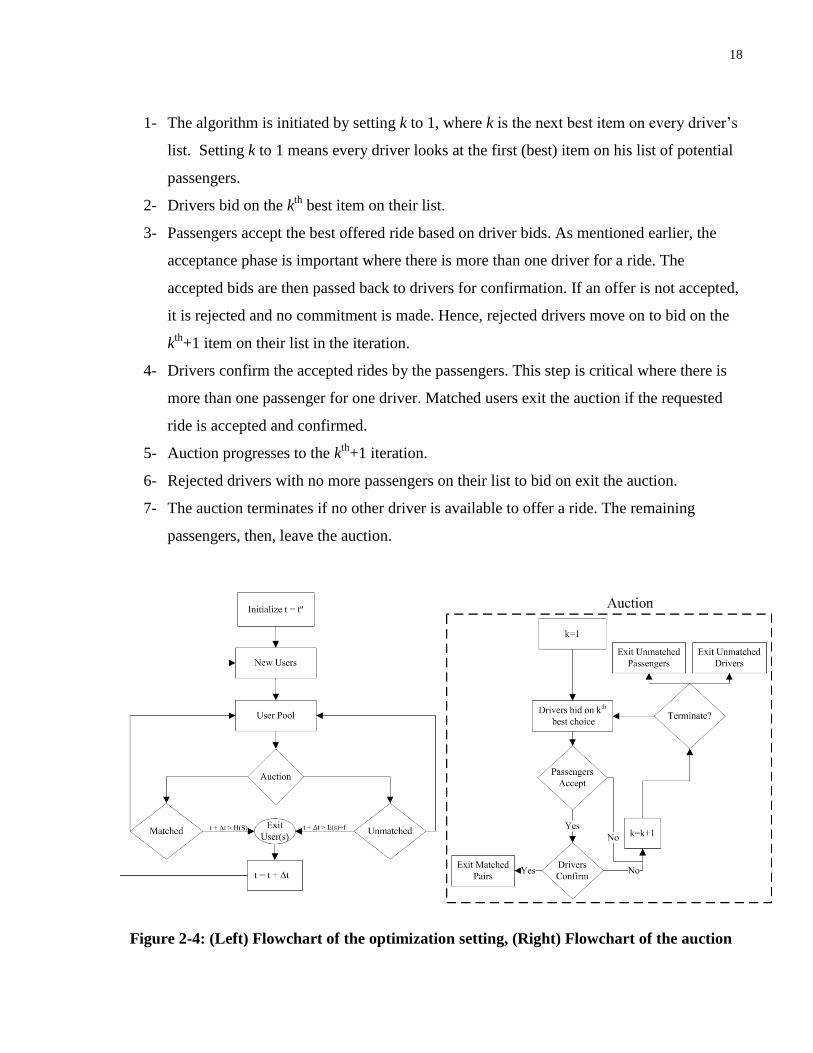
18
1- The algorithm is initiated by setting k to 1, where k is the next best item on every driver’s
list. Setting k to 1 means every driver looks at the first (best) item on his list of potential
passengers.
2- Drivers bid on the kth
best item on their list.
3- Passengers accept the best offered ride based on driver bids. As mentioned earlier, the
acceptance phase is important where there is more than one driver for a ride. The
accepted bids are then passed back to drivers for confirmation. If an offer is not accepted,
it is rejected and no commitment is made. Hence, rejected drivers move on to bid on the
kth
+1 item on their list in the iteration.
4- Drivers confirm the accepted rides by the passengers. This step is critical where there is
more than one passenger for one driver. Matched users exit the auction if the requested
ride is accepted and confirmed.
5- Auction progresses to the kth
+1 iteration.
6- Rejected drivers with no more passengers on their list to bid on exit the auction.
7- The auction terminates if no other driver is available to offer a ride. The remaining
passengers, then, leave the auction.
Figure 2-4: (Left) Flowchart of the optimization setting, (Right) Flowchart of the auction

19
2.5 Model Evaluation and Case Study
The case study uses the Sioux Falls network which is composed of 24 nodes, 76 transportation
links and 1.96 million individuals (Figure 2-5). We consider only the work trips where earliest
departure time of individuals is obtained from a normal distribution function with an average of
7:00 AM and a variance of 1 hour. The travel time flexibilities are assumed to be 20 minutes and
the simulation time increment is 5 minutes.
Figure 2-5: The Sioux Falls network
2.5.1 Single Driver, Single Passenger
The simplest form of a ridesharing matches one driver with one passenger. In order to assess the
efficiency of the agent based model we compare it with the optimal binary integer programming
model presented in Section 2.3.3.
We define market penetration as the ratio of the number of ridesharing members over the total
number of commuters. For the given example, we select 19 market penetration values ranging
from 0 (no active users) to 0.002 (193 active users). Higher market penetration values increase
computation time of the benchmark model (above 3 hours) and make comparison with the

20
dynamic model harder. We execute 10 runs of the proposed agent based model by varying users’
time preferences randomly for every market penetration value. We then compare the obtained
reliability and VKTS measures with those of the optimal benchmark. Figures 2-6 and 2-7 present
system reliability and VKTS for the centralized benchmark and the agent based model.
The numbers on top of each bar in Figure 2-6 are the ratio of the reliability of the agent-based
model over the reliability of the benchmark model (Equation 14). The POA values given in (14)
are similar in concept to price of anarchy in non-cooperative game theory.
( )
Our analysis confirms that the agent based model gives close to optimal solutions and shows
much lower computation times for market penetration values of above 0.0012 (Figure 2-8). The
proposed model is able to run for higher market penetration values whereas the benchmark
model fails to do so. The computation times given in Figure 2-8 are obtained from the solution
algorithm which is coded in Matlab 7.12 running on a dual-core 2.40 GHz desktop computer
with 6 GB RAM.
Figure 2-6: Reliability of the the agent based model (white) and the benchmark
model (black)

21
Figure 2-7: VKTS of the the agent based model (white) and the benchmark model
(black)
Figure 2-8: Calculation time in minutes for the agent based model and the benchmark
model

22
2.5.2 Single Driver, Multiple Passengers
If time limits do not constraint drivers, they may be able provide rides to several passengers on a
single trip. The main incentive for accommodating multiple passengers is to distribute the total
cost of the trip between more participants. However, increasing the number of participants only
makes economic sense when the new trip cost of each entity is lower than their original trip
costs. We only consider the case where a driver can offer a ride to a maximum of two
passengers. The same principles can be used in cases with more passengers.
Figure 2-9 presents a simple case where one driver is considering two separate passengers. The
links between every two nodes in the figure are labeled with the number on the associated edge
of the graph. Clearly there are multiple configurations that can be adopted to pick up and drop
off passengers. For example, the driver can pick up the passengers consecutively or
simultaneously. Table 2.1 presents all the possible driving configurations where xi denotes travel
time and yi denotes distance of route i. The dashed arrows in the table present original routes and
the black solid arrows present the assigned routes. For the case of two passengers, the associated
driver cost is C(d) and the passenger costs are C(p1) and C(p2) for the first and the second
passenger, respectively. These costs are computed as the product of the total cost (TC) and the
cost ratio ( , , and ) obtained from the first term in Equation 2. The trip initiation time is
also provided in the table to meet the latest arrival constraints of all users in the vehicle.
Intuitively, a match is possible only when every user in the vehicle is set to be picked up at a
time after their earliest arrival time.
Figure 2-9: Link notations when one driver is considering two distinct passengers

23
One of the advantages of the proposed agent based model is its flexibility in expansion. The
model is able to incorporate multi-passenger settings by adding a module to the auction stage. In
this module, drivers bid on both individual passengers and pairs of passengers. Figure 2-10a
presents an example of the first stage of an auction of Section 2.4.1 where driver d1 calculates the
costs of offering a ride to passengers p1 and p2 simultaneously and individually. The driver first
places a bid on both passengers simultaneously because this strategy incurs a lower cost on him.
However, the ride can only be finalized if both passengers accept the offer. After acceptance, the
driver can confirm the match and finalize his request. On the other hand, considering the scenario
where one passenger (p2) rejects the offer (Figure 2-10b), the driver moves on to the next item in
its list (p1).
One of the objectives of ridesharing users is to cut down their commuting costs. An analysis of
the ratio of the new cost to the original cost can indicate how well the system performs in
satisfying customers’ needs. To evaluate the performance of the multi-passenger module, we
compare it with the original (single driver, single passenger) model when market penetration is
1%. Figure 2-11a is a scatter plot of original costs (for commuting alone) against the assigned
costs (for using the ridesharing system) for the single driver single passenger arrangement. It is
clear that no participant uses the system if he has to pay more than the cost of commuting alone.
This is presented by the upper boundary line shown in the Figure. Similarly, the minimum cost
that a user can be charged in the system is half of its original cost. This happens when both
paired participants (the driver and the passenger) commute from the same origin to the same
destination.
Figure 2-11b presents the original and new user costs when multi-passenger matching is enabled.
In this Figure, users that were grouped in a vehicle of three members (1 driver, 2 passengers) are
presented by gray stars. Similar to Figure 2-11a, an upper boundary also exists for this
arrangement by the same logic. However, the lower cost limit here is one third of the original
user cost. This means, in the best case scenario, two passengers are matched with a driver all of
whom commute from the same origin to the same destination. Hence, the total trip cost is divided
between the three users. In general, the maximum price saving ratio when a maximum of m
members can be grouped together is equal to 1/m of the total trip cost. To elaborate, the
flexibility of considering multiple passenger matches opens new matching opportunities with

24
lower costs for the users. Addition of the multi-passenger module also changes the desired
objective function values. The single model (one driver, one passenger) has a reliability of 0.71
and VKTS of 0.29 whereas the multi-passenger model has a reliability of 0.77 and VKTS of
0.36.
Table 2-1: Six different driving patterns when one driver is considering two passengers

25
Figure 2-10: (a) driver d1 bidding simultaneously bidding on two passenger p1 and p2 (b)
driver d1 bidding only on passenger p1
2.5.3 Multiple Drivers Single Passenger
The arrangement where a passenger is able to transfer between potential driver vehicles that
make up portions of its path is called the multi-hop rideshare setting. Passengers who do not find
single rides can move closer to their destination one hop at a time. Incorporating such system
into the ridesharing company policy has been emphasized by researchers (Gruebele, 2008, Agatz
et al., 2012), yet seldom explored. Cortes et al. (2010) are among the few who present a
generalized classic pickup and delivery problem that encompasses the flexibility of allowing
passengers to transfer between vehicles at specific locations called transfer points. One major
component in Cortes’s model and in all transfer related research is the presence of hubs where
objects (passengers, goods, etc.) can relocate to another unit of transportation. Shahin and Nickel
(2011) provide a thorough review of the hub location problem in transportation networks and
propose a heuristic model which cuts down the computation time of the conventional MIP
models when solving the hub location problem. In this section, we propose a simple fixed hub
location methodology and present the details of how passenger agents can use such hubs to
request two individual rides instead of one.
We assume that the location of the hub(s) is exogenous to the model and is set at the zone(s) with
highest volume of traffic which enhances connectivity between vehicles. Figure 2-12 presents a
simple case where one passenger transfers between two distinct drivers to reach his destination.
In this situation, the passenger first hops off the first driver’s vehicle to reach the designated hub.
Then he transfers to another vehicle to reach his destination. In order for this match to be
successful both cost and time constraints need to be met. The passenger (p) accepts this match

26
only if it costs him less money than taking the original direct route to his destination. Moreover,
the passenger will not leave his origin before his earliest departure time and cannot get to his
destination after his latest arrival time. Similarly, the two drivers (d1 and d2) would confirm to
offer segments of this ride if their individual costs are cut down.
Figure 2-11: Original and new cost for members when multi-passenger matching is not
enables (top) and enabled (bottom)

27
For better presentation of the required constraints, we define time and distance of path i by yi and
xi, respectively. We use the route identification numbers given in Figure 2-12 where the hub in
Figure 2-12 is denoted by h.
Figure 2-12: Schematic of the case where one passenger transfers between two vehicles
2.5.3.1 Cost Constraints
The passenger accepts to make a transfer if its total ridesharing cost is lower than its original
cost. The cost of the passenger, however, is divided between the two drivers who are offering the
ride. We denote the fee that the passenger pays to drivers d1 and d2 by c1 and c2, respectively.
These costs are computed from Equation 2:
( ) (15-1)
( ) (15-2)
The sum of these two individual costs ( ) must therefore be lower than the passenger’s
original cost ( )
Similarly, the cost borne by the two drivers must be lower than their original cost. This can be
easily calculated from Equation 2.
2.5.3.2 Time Constraints
In order for the multi-hop ride to be accepted, time constraints of all individuals in a car must be
met. Hence, the two drivers and the passenger must leave their destination at some time after

28
their earliest departure time and reach their destination before their latest arrival time. To obtain
such constraints we begin from the end of the second trip where driver d2 drops off the passenger
at his destination. We present the trip initiation time of the second leg of the trip as:
( ) ( ( ) ( ) ) (16-1)
where ( ) denotes the departure time of the second driver from her origin (initiation time).
The calculated ( ) ensures that neither the second driver nor the passenger reach their
destination after their latest arrival time. From the given departure time of the second driver, we
compute the initiation time of the first leg of the trip as:
( ) ( ( ) ( ) ) (16-2)
Equation (16-2) confirms that the first driver reaches her destination before her latest arrival time
and that the passenger reaches the hub before the designated time to transfer to the second
vehicle ( ( ) ). In other words, if the second driver leaves her origin at ( ), she would
be at the hub at ( ) . Hence the passenger needs to find a ride to the hub before this time.
Furthermore, passengers are not inclined to wait at the hub for long times. Hence, the following
constraint confirms that the waiting time of the passenger at the hub is lower than a maximum
predefined waiting time ( )which we, for this study, set to 10 minutes.
( ( ) ) ( ( ) ) (16-3)
The final time constraints that need to be checked are that the initiation time is after the earliest
departure time of both drivers and that the passenger is picked up by the first driver after his
earliest departure time.
Similar to Section 2.5.2 a new module is added to the core of the algorithm to accommodate
multi driver matching. The main input to this module is the index of the hub zones. The
algorithm then starts by finding potential passengers who could use each hub as a transfer point
to relocate to another vehicle. This is done by considering the best transferring scenarios at each
hub with the following features:
The passenger and the first driver’s origin is the same zone (x1=0 )

29
The first driver’s destination and the second driver’s origin are both located at the hub
zone (x3=0, x4=0). This condition makes the original path of the first driver and the
passenger the same (x2=x7)
The second driver and the passenger’s destination are located in the same zone (x6=0,
x5=x9).
Choosing such scenarios makes the passengers consider the furthest hubs as a transfer point. In
other words, passengers choose hubs far enough from their origin and destination as long as
which is obtained from the cost constraint.
The passengers, hence, request two more rides from their origin to the hub and the hub to their
destination in addition to their original request which asked for a straight ride from their origin to
their destination. The transfer rides are accepted only if two drivers bid on the two legs of the trip
and the constraints (time and cost) are met.
Table 2-2 presents the two system outcomes (Reliability and VKTS) and the number of transfers
made for 3 different hub scenarios and 3 market penetration rates. It is clear that as the market
penetration rate increases there are more opportunities to transfer between drivers. This is shown
in the table for the case of 1 hub where increasing market penetration raises the number of
transfers from 0 to 196.
The second important conclusion of Table 2-2 is that increasing the number of hubs for higher
market penetration rates has a more significant impact. For example, increasing the number of
hubs from 1 to 3 for 0.2% market penetration raises the number of transfers by only 1, whereas
for a 1% market penetration rate, the number of transfers is increased by 106. This happens
because in higher market penetration rates there are more passengers scattered in the network
which could benefit from more hubs.

30
Table 2-2: Reliability (first number in each cell), VKTS (in parenthesis), and number of
transfers (last number in each cell) for 3 different market penetration values (0.2%, 0.5%,
and 1%) and 3 potential hub scenarios
Market Penetration Rate
Hub Scenario 0.20% 0.50% 1.00%*
1 Hub 0.56 (0.19) 0 0.68 (0.26) 98 0.72 (0.30) 196
2 Hubs 0.56 (0.19) 1 0.68 (0.26) 116 0.72 (0.31) 234
3 Hubs 0.56 (0.19) 1 0.68 (0.27) 141 0.72 (0.31) 302
* 1% penetration rate is equivalent to 19,600 agents
2.6 Cost-Revenue Analysis and Survival of Service Providers
A variety of pricing schemes can be administered by rideshare service providers to produce
profits. Prices should be low enough to attract potential users and high enough to compensate
the costs of the provider. The viability of a rideshare service depends on what price to charge the
service users.
Figure 2-13 presents the collected revenue by the service provider when different pricing
schemes are administered. The paired users in the system are charged (by the system provider) a
certain ratio of the total cost of their entire trip called the commission rate. Assuming that the
provider incurs no expenses, the revenue increases with the compensation rate until it reaches its
maximum value at the compensation rate of 0.5, then it drops. This drop in revenue happens
because higher commission rates increase the last term in Equation (2) making the trip more
expensive for the users than travelling alone. The second peak in the revenue is for those users
sharing the same origin and destination where each user pays half of the total cost. These users
accept their assigned matches to the point where they have to pay the service provider the cost of
their entire trip (commission rate of 1).
The increasing revenue in Figure 2-13 does not necessarily indicate that service providers can
increase their commission rates to 50% to maximize their revenue. Although this may work for
one day, it leads to lower reliability for the upcoming days because users who were denied

31
service due to high costs may not return. Figure 2-14 illustrates the reliability measure for
different commission rates. It is clear in the Figure 2-14 that system reliability decreases as the
service provider decides to charge more.
Figure 2-13: Revenue ratio (obtained Revenue / maximum Revenue) with respect to the
commission rate
Figure 2-14: System reliability with respect to commission rate

32
2.7 Summary of Key Findings
A new agent based model is introduced in this chapter for the dynamic ridesharing problem. This
agent based model uses a vicinity approach which reduces the choice set made of the passengers
that could be matched with each driver. Drivers and their choice sets (composed of passenger)
are engaged in an auction algorithm where drivers bid based on costs, passengers accept bids,
and finally drivers confirm the bids.
The results of the agent based model are compared to a static centralized assignment model. Two
measures of effectiveness are introduced to assess the performance of the agent based model
when compared to the static model. The measures (Reliability and vehicle kilometers travelled)
are very close in the two models.
The agent based model is then expanded to allow for multi-passenger single-driver and multi-
driver single passenger matches. Results show higher VKT savings for the multi-passenger
single driver case compared to other cases.
It is assumed in this chapter that the ridesharing company charges each matched driver and
passenger a percentage the new cost of their trip. A sensitivity analysis is performed on the
revenue of the ridesharing company with respect to the charged percentage. Initially, as this
percentage increases, the company obtains higher revenues. However, as this percentage further
increases, less users are willing to use the system due to increased costs (paid to the service
provider). Results show that revenue is maximized when this percentage is set at 50%. However,
system reliability is always reduced when this percentage is increased.

33
Chapter 3 Carsharing
3 A Dynamic Carsharing Decision Support System
3.1 Introduction
Urban carsharing services provide individuals with access to a fleet of shared-use vehicles
without the costs and responsibilities of private vehicle ownership. Members of these services
typically pay for subscription-access plans and are charged through hourly rates. Further benefits
of carsharing are reduced parking costs, mitigated environmental impact, and availability of an
alternative transportation mode (Katzev, 2003). City Carshare in San Francisco, the largest non-
profit carsharing organization in North America, released an environmental report in 2013
outlining its role in reducing a total of 25 million vehicle miles, 85 million pounds of CO2
emissions, and 4.3 million gallons of gasoline (City Carshare 2013).
CarSharing organizations (CSO) are commonly classified based on configuration into one-way
and two-way systems. Two-way systems (e.g., Zipcar and Autoshare) restrict vehicles to be
picked up from and returned to the same station. One-way carsharing systems (e.g., ICVS and
Praxitele), on the other hand, permit users to return the vehicle to a location of choice as long as
the drop-off station and time is indicated in advance. While two-way systems are far more
common and account for 94% of all North American carsharing memberships (Shaheen et al.,
2006), one-way systems are less adopted. This is mainly due to the issue of vehicle imbalance
which happens when cars shift towards certain destinations in the network. Some CSOs such as
Car2Go address vehicle imbalance by employing drivers to relocate the vehicles to high demand
locations. Such relocation operations increase costs for the CSOs.
Despite high relocation costs, the number of one-way systems is rising. Communauto, a privately
owned carsharing organization founded in city of Québec in 1994, has inaugurated the first
electric one-way carsharing service in Canada (Communauto, 2013). This pilot project aimed to
evaluate the benefits of one-way systems and was initiated due to public consultations that
showed the demand for such systems. To complement such pilot projects, better dynamic vehicle
relocation decision support tools need to be designed which consider dynamically the location of

34
all vehicles in the fleet and locations of new user requests. Accounting for these two, the
objective is to minimize total vehicle relocation costs. This tactical model differs from higher
level decision making models which mainly focus on where to locate carsharing parking stations
and what fleet size to use based on aggregate demand values.
The main objectives of this chapter are as follows:
Present a benchmark that considers simultaneously the complete set of all user requests
received in a particular day assuming user requests are known in advance
Propose a dynamic integrated simulation-optimization model which takes online user
requests and acts as a decision support tool for CSOs to maximize system profit
Perform sensitivity analysis on the fleet size of each system configuration and highlight
the important factors and policies which impact both the fleet size and vehicle relocation
costs
This chapter is structured as follows. In Section 3.2, we describe the literature review of previous
operational models on carsharing systems. In Section 3.3, we explain the user preferences,
constraints, and problem assumptions. Sections 3.4 and 3.5 present the benchmark model and the
dynamic model, respectively. In Section 3.6, we analyze both models for the case of Autoshare
in Toronto. Finally, in Section 3.7, we highlight the major findings of the article.
3.2 Literature Review
Previous research on carsharing mainly focuses on its environmental impacts (Steininger et al.,
1996, Cervero et al., 2007, Firnkorn and Muller, 2011), market dynamics (Shaheen and Cohen,
2007, Shaheen et al., 2006, Vine et al., 2013), users’ behavior (Celsor and Millar-ball, 2007,
Morency et al. 2010, Habib et al., 2009, Habib et al., 2012), and relationship with public transit
(Stillwater et al., 2009). The core of CSO operations, however, has received less attention. Table
3-1 presents previous operations models of CSOs.
Barth and Todd (1999) develop a simulation model of carshare operations with inputs and
measures of effectiveness that allow for scenario analysis. They conclude that a sufficient fleet
size for satisfying customers is 3-6 vehicles for every 100 trips but that 18-24 vehicles per 100
trips are required to minimize relocation costs. Fan et al. (2008) propose a multi-stage stochastic

35
linear integer model which attempts to capture system uncertainties such as carsharing demand
variation. The objective function of their model maximizes the revenue obtained from servicing
customers while minimizing the cost of vehicle relocation.
More recently, Kek et al. (2009) and Correia and Antunes (2012) propose two distinct mixed
integer programming models (MIP) that aim at optimizing specific features of CSO operations.
Kek et al. design a novel three phase optimization-trend-simulation (OTS) decision support
system for CSOs to indicate a set of near-optimal manpower and operating parameters for the
vehicle relocation problem. For a carsharing company in Singapore, they conclude that
optimization of manpower can reduce staff expenses by up to 50% and zero vehicle time
(duration of vehicle shortage at parking facilities) by up to 13%.
Correia and Anutues (2012), on the other hand, focus on the fleet size, number of vehicle
relocations, depot size, and location of potential parking facilities. Considering all these decision
variables, the authors present a mixed integer optimization MIP approach to maximize CSO
revenues while minimizing costs such as vehicle maintenance, parking provision, vehicle
depreciation, and vehicle relocation. The study concludes that a vehicle to trip ratio of 22.7 per
100 trips is the optimal fleet composition which confirms the finding of Barth and Todd (1999).
Correia and Antues and Kek et al. both verify the importance of system optimization in reducing
the expenses of one-way carsharing systems. Both, however, consider temporally aggregated
demands which result in static models. The results can therefore be biased since trip
specifications such as user request time are neglected. Realizing this drawback, Jorge et al.
(2012) apply the Correia and Antunes model in a simulation platform to capture the impact of
demand variability on on model results. They use the traditional minimum cost flow algorithm to
setup the relocation problem and set the fleet size to the maximum number of required vehicles
during the simulation. The model, while acknowledging the importance of user request patterns,
does not capture trade-offs between CSO features such as fleet size and vehicle relocations.
More recently, El Fassi et al. (2012) propose a more holistic discrete event simulation that assists
decision makers in selecting the best system improvement strategies. The model considers the
demand growth of the system while maximizing members’ satisfaction and minimizing the fleet
size.

36
Table 3-1: Classification of previous work on operational models of carsharing
Authors
(year)
Objective Function Main Decision
Variables
Solution
Methodology
System
Configuration
Study area
Barth and
Todd
(1999)
Minimize average
wait time, number of
customers waiting,
number of
relocations
Effective fleet
size
Simulation One-way Coachella
Valley
Fan et al.
(2008)
Maximize revenue,
minimize vehicle
relocations
Vehicle usage,
fleet size
Stochastic
programming
One-way _
Kek et al.
(2009)
Minimize vehicle
relocation, minimize
staff utilization cost,
minimize demand
rejection penalty
Crew size,
staff waiting
time, vehicle
relocation
Mixed
Integer
Programming
(MIP)
One-way Singapore
El Fassi et
al. (2012)
Maximize member
satisfaction,
minimize fleet size
Parking
capacity,
station
locations
Discrete
event
simulation
_ Montreal
Correia and
Antunes
(2012)
Maximize revenue,
minimize vehicle
maintenance,
relocation, and
depreciation
Depot size,
depot location,
fleet size,
vehicle
relocations
Mixed
Integer
Programming
(MIP)
One-way Lisbon
Jorge et al.
(2012)
Maximize revenue,
minimize vehicle
maintenance,
relocation, and
depreciation
Depot size,
depot location,
fleet size,
vehicle
relocations
Simulation –
Mixed
Integer
Programming
(MIP)
One-way Lisbon

37
3.3 Carsharing Problem Setting
3.3.1 User Schedules
Carsharing members’ needs can be accommodated if certain constraints are observed. Time is
one important concern. Users who wish to leave their origin and arrive at their destination at a
specific time commonly provide information on their time schedule preferences. We assume that
trips have certain attributes such as a desired departure time (from origin parking facility), arrival
time (to destination parking facility), and reservation time. Trip reservation time is defined here
as the time between the user’s announcement time and the departure time, where the
announcement time is the time when a user requests a vehicle. A minimum reservation time can
be imposed by CSOs. Figure 3-1 shows a generic illustration of user time schedules.
Figure 3-1: Time schedule of users
3.3.2 Fleet Size and Vehicle Relocation
CSOs make decisions about fleet size and vehicle relocation policy. A CSO can reduce its fleet
size by increasing vehicle relocations. Furthermore, increasing the required reservation time in
the system allows more time to relocate the vehicles. Figure 3-2 illustrates the trade-off between
fleet size and vehicle relocation where user u2 can be serviced by either relocating a vehicle from
user u1’s destination to u2’s origin (Figure 3-2a, dotted arrow) or positioning an extra vehicle at
u2’s origin (Figure 3-2b). Vehicle relocation requires that the time between u1’s arrival and u2’s
departure is longer than the travel time between u1’s destination and u2’s origin. The relocation
travel time must also be less than the reservation time for passenger u2.

38
Figure 3-2: Relocation of the single vehicle in the fleet to serve both users (b) Provision of
an additional vehicle to the fleet
3.4 Benchmark Model
The objective of the benchmark model is twofold. First, the model is a tool to assess policies
assuming that the CSO has advance information about users’ itineraries. Second, the benchmark
is designed to be compared to a more realistic dynamic model where users enter the system at at
their announcement times. The benchmark model, therefore, has advantages over reality since
the announcement times of the users are known in advance. The solutions obtained from this
benchmark act as a lower bound for the dynamic model presented in Section 3.5.
The following assumptions are made for the benchmark model:
1- Total demand is satisfied. This assumption is presented as one of the constraints in the
problem formulation but can be relaxed in the dynamic model.
2- The capital cost of purchasing a vehicle for the system is much higher than any value of
vehicle-km relocation. A new vehicle is added to the fleet only if a user cannot be
serviced by any of the existing available vehicles. Similarly, the cost of vehicle relocation
is much higher than parking costs.
3- Parking facility locations are known in advance and parking spaces are abundant in all
the designated facilities. However, the variable cost for parking (measured in dollars per
hour) in each facility can vary.
4- Vehicles can be relocated between parking lots.

39
5- Reservation time is a policy imposed by the CSO which all users follow exactly. We
assume that all user announcement times are their departure times less reservation time.
Setting reservation time to zero implies that all users request a car with no prior notice.
6- We consider only trips where the vehicle is booked and returned on the same day.
7- CSOs charge users by minutes travelled.
The following are the notations of the sets, decision variables, and parameters used to represent
the one-way system configurations. These definitions introduce the preferences of users, CSO
features, and the transportation network characteristics:
Users:
: set of members who wish to use the service during study time
: origin parking lot of
: destination parking lot of
: departure time of user from his/her origin
: arrival time of user at his/her destination
: trip announcement time of user
: activity duration time of user
CSO operations:
: set of all vehicles
: set of all reserved parking facilities of the CSO
: unit cost of parking at parking facility p [dollars per minute] paid by the CSO
: time when a vehicle leaves the destination of user i to relocate to the origin of user j
Pr : price rate based on minutes travelled by users [dollars per minute]
unit cost of relocation based on time [dollars per minute]
system reservation time [minutes]
initial location of vehicle k. This initial location can change in each iteration of the
dynamic model.
: availability time of vehicle k; time when vehicle k becomes available. Availability
time of each vehicle can change in each iteration of the dynamic model.

40
: 1 if a vehicle is relocated from the destination of user i to the origin of user j
: 1 if a vehicle is relocated from the origin of user j
: a hypothetical depot
Transportation network:
( ): travel time of a trip originating at parking facility a and terminating at parking
facility b [minutes]
Using the above notations, the one-way system configuration model is formulated similar to the
multiple travelling salesman problems (mTSP) with differences in time window constraints and
sub-tour elimination constraints (Kara and Bektas, 2005). The formulation is presented as
follows :
[ | |] ∑ ∑ [ ( )] ∑ ∑ [ ( )
( ( ))] (1a)
∑ (1b)
∑ ∑ (1c)
( ) (1d)
( ( ) ) (1e)
( ( )) (1f)
(1g)
( ) (1h)
∑ | | (1i)
(1j)
The objective function (1a) is composed of three terms that minimize the fleet size, relocation
operations, and parking costs, respectively. The first term is the product of a large number Z and
the fleet size which complies with Assumption 2. The second term is self-explanatory and the

41
third term is composed of two different costs which are the costs of parking at user i’s destination
( ( )) and user’s j’s origin (
( ( ) )), respectively. Once
the constants in the third term of (1a) are eliminated, it can be converted to (
) .
This objective function is designed in a way such that which implies that the
marginal rates of substitution between the three components can be neglected. In (1a), we neglect
the price rate (Pr) of the system because all demand is served which makes the monetary revenue
of the system constant and equal to∑ ( )
Constraints (1b) ensure that every user is served. Constraints (1c) are flow balancing constraints.
In (1b) and (1c), is a hypothetical depot that is common in the conventional mTSP. The cost
of travelling from to every user’s origin is equal to Z and the cost of travelling from every
user’s destination to is zero. The high Z value ensures that vehicles are not added to the fleet
unless they are needed. The zero cost of every user destination to ensures tour continuity.
Constraints (1d) and (1e) act as sub-tour elimination constraints (Proposition 1). The purpose of
(1e) is to ensure time feasibility between user i and j’s itineraries. Constraints (1f) and (1g)
ensure that the relocation time between users i and j is within the allowable time threshold. This
threshold is between and ( ( )). In (1f), a vehicle travels ( ) minutes and
has to arrive to before to serve user j. In (1g), a vehicle can leave for only after user i
arrives which is at . These constraints along with the third term in the objective function
((
) ) indicate three different possibilities for :
1- is equal to 0 whenever is 0
2- is equal to whenever is 1 and (
)
3- is equal to ( ( )) whenever is 1 and (
)
Constraints (1h) ensures that relocating a vehicle between Ni and Mj is only possible when the
travel time ( ) is below the reservation time. Constraints (1i) and (1j) are self-
explanatory.
Proposition 1. Constraints (1e) act as Sub-tour Elimination Constraints (SEC).

42
Proof. We define relation R for which the domain is the 2 dimensional set of all i’s and j’s and
the range is {0,1} depending on whether a match between users i and j is possible. Therefore if
has the potential to be 1, then . Conversely, if does not have the potential to be 1,
then .
By showing that relation R is asymmetric, we prove that no sub-tour can be made between two
users. Similarly, by showing that relation R is intransitive, we prove that no tour can be made
between three or more users.
Asymmetric Relation: According to (1e) can be equal to 1 (iRj=1) if (I). Given the
continuous and unidirectional nature of the time continuum, we know (II) and
(III). Considering (I), (II), and (III) we conclude that which contradicts constraint (1e)
and leads to jRi=0.
Intransitivity Relation: We show the intransitivity relation for the case of 3 users i, j, and k which
can be easily extended to any higher number of users. Assuming that iRj=1 and jRk=1, we show
that kRi=0. From iRj=1 we know (I’), and from jRk=1 we know
(II’). Given (I’) and (II’), we conclude that which contradicts constraint (1e) and leads
to kRi=0.
This completes the proof.
Given the asymmetric relation presented in Proposition 1, the maximum number of solutions that
can be considered for the benchmark is the number of edges in a complete graph with r (number
of users) nodes which is ( ). Many of these potential matches are not feasible due to
constraint (1e). We identify such infeasible matches to reduce computation time before running
the model to decrease variables and computational burden.
3.5 Dynamic Relocation Model
In reality, carsharing companies have a fixed fleet size which is not subject to immediate
changes. The dynamic relocation model takes the fleet size as an input and relocates the available
vehicles between the users. Contrary to the benchmark model, the constant fleet size in the
dynamic model implies that not all users will necessarily be serviced unless the maximum

43
number of needed vehicles (calculated from the benchmark model) is obtained. In other words,
any fleet size lower than the maximum fleet size calculated in the benchmark model leads to
some unserviced demand. This motivates CSOs to relocate their vehicles with the incentive of
maximizing profit. Profit is commonly generated through either travel time or travel distance of
the users. Therefore vehicles are most beneficial when assigned to users who travel longer and
require less relocation to be accommodated.
We present the the dynamic relocation model through an integrated optimization-simulation
platform. The optimization stage is composed of two phases: Vehicle Relocation Optimization
(VRO) and Parking Inventory Optimization (PIO). In Section 3.5.1, we present the the two
optimization phases and explain the simulation platform in Section 3.5.2.
3.5.1 Optimization: Vehicle Relocation and Parking Inventory
3.5.1.1 Vehicle Relocation Optimization (VRO)
The VRO phase functions similar to the benchmark with the following exceptions:
1- The price rate is added to the objective function
2- The fleet size is constant and initial vehicle locations are inputs to the model
3- Time of relocation (third term of (1a)) is eliminated from the objective function
4- Some demand is left unserviced
The VRO problem is formulated as follows:
∑ ∑ [ [ ( ) ( ) ]] ∑ ∑ [ [ ( )
( ) ]] (2a)
∑ ∑ | | (2b)
∑ ∑ | | ∑ (2c)
∑ (2d)
( ( ) ) (2e)

44
( ( ) ) (2f)
(2g)
(2h)
The objective function in (2a) maximizes the total profit of the system by considering the
generated revenue from user j ( ( ) ) when he/she travels from to and the cost
of relocation when a vehicle is transferred from user i’s destination to user j’s origin or when
vehicle k is transferred from its initial location to user j’s origin. Constraints (2b) ensure that
no user is served more than once. Constraints (2c) are flow balancing constraints with as a
dummy node where the cost of relocating a vehicle from every user’s destination to is zero.
is added to ensure constraints (2c). Constraints (2d) ensure that no vehicle is assigned to two
users. Constraints (2e) guarantee that there is enough time between the availability time of
vehicle k and the departure time of user j if the vehicle is to be assigned to that user. Availability
time of vehicle k ( ) is the point in time when vehicle k is free to be assigned to any user.
Availability of vehicles changes every time the model is run and depends on which users are
confirmed. This is further elaborated in Section 3.5.2. Constraints (2f) are similar to (1e) except
that is replaced with . This happens because the dynamic model has no a priori knowledge
of all users and only considers users who have already announced their requests. Constraints (2g)
and (2h) are self-explanatory.
3.5.1.2 Parking Inventory Optimization (PIO)
The objective of Parking Inventory Optimization (PIO) is to take and values of the VRO
phase as an input and find the optimal relocation times ( ). In this section, we relax the
simplified assumption of Section 3.4 that parking facilities do not have capacities and present a
more realistic assumption. Carsharing organizations, in reality, have a predefined number of
reserved parking spots at designated parking facilities. There is a higher incurred cost of storing
any additional number of vehicles that surpasses the original number of reserved spots (Figure 3-
3). The normal parking rate increases to when the number of occupied spots are beyond
reserved capacity.

45
Figure 3-3: Normal parking rate and increased parking rate when vehicles surpass
capacity
The following constants and sets are used to formulate the PIO problem:
Wp : set of every user where a vehicle is relocated from that user’s destination to parking
facility p
: set of every user where a vehicle is relocated from parking facility p to that user’s
origin
Sp : set of all vehicles that are relocated from parking facility p
Hp : set of all vehicles that are relocated to parking facility p
Ip : total initial number of vehicles located at p
: the number of users who arrive to parking facility p before time t
: the number of users who depart from parking facility p before time t
: reserved capacity of parking facility p
Both and
are easily obtained from the accepted set of users from the VRO phase. We
denote total occupancy of parking facility p at time t by (
) where is
occupancy below capacity capp (allowable capacity of parking facility p) and is any
additional parking volume that violates the reserved capacity. Hence, can only be above zero
when .
To formulate the PIO problem, we discretize time and transform and of the VRO phase
into and
where and . Decision variable is a binary

46
variable and is equal to 1 when a vehicle is relocated from ( ) to ( ) at time t. Decision
variable is a binary variable and is equal to 1 when a vehicle is relocated from ( ) to
( ) at time t.
We discretize time into T different segments of size µ where µT is the simulation duration and
formulate the problem using the concept of time-space networks as:
∑ ∑ (
) (3a)
(3b)
(3c)
∑ ∑ [ ] ( )
∑ ∑ [ ]
∑ ∑ [ ] ( )
∑ ∑ [ ]
(3d)
∑
(3e)
∑ ( )
(3f)
∑
(3g)
∑ ( )
(3h)
∑
(3i)
∑
(3j)
(3k)
(3l)

47
The presented model is a binary integer programming model with a piecewise convex objective
function (with the marginal costs shown in Figure 3-3) which attempts to minimize the total cost
of parking. Constraints (3b) and (3c) ensure that qpt values are within the correct boundaries.
Constraints (3d) have seven terms on their left side. The first two terms present initial vehicle
movements between a vehicle depot and a user and the second two terms present vehicle
relocation movements between users. The first term is the total number of vehicles that are
located from their initial location (p1) to p, and the second term is the total number of vehicles
that are relocated from their original location p to any other location (p2). The third term is the
total number of vehicles relocated from user i’s destination (Ni) to parking p to serve user j
(p=Mj) and the fourth term is the number of vehicles relocated from parking p where p=Ni to
user j’s origin (Nj). The first and the third term in (3d) sum over the first to the ( ( ))th
and ( ( ))th
time increments, respectively, because that is how long it takes a vehicle
to reach Mj. The next three terms in (3d) are self-explanatory. Constraints (3e) to (3h) check for
relocation time boundary violations which correspond to constraints (1f) and (1g). Constraints
(3i) and (3j) ensure that every relocation process is initiated only once and constraints (3k) and
(3l) are binary variable declarations.
One major factor in the discretization of the PIO model is the value of µ. A low value of µ would
increase the number of nodes in the time-space diagram which leads to high computation times.
On the other hand, high values of µ can make the problem infeasible in cases where µ is higher
than the relocation time window of at least one relocation process ( ( )- ).
In such a case, no suitable time can be obtained for relocating a vehicle from Ni to Mj. High µ
values can also lead to inefficient answers since some potential relocation start times will be
neglected. We, therefore, present a meta-heuristic Particle Swarm Optimization (PSO) algorithm
which treats relocation start times as continuous variables within allowable constraints ((3e) to
(3h)), calculates and
for different time segments, and obtains the objective function in
(3a). The st values are then altered in future iterations of PSO to find better values of (3a).
Particle Swarm Optimization (PSO), a population based stochastic optimization technique,
shares many similarities with evolutionary computation techniques such as Genetic Algorithm
(Eberhart and Kennedy, 1995). Analogous to GA, PSO initiates with a population of random

48
solutions and evolves the position of the particles based on the location of current optimal
particles, until a desirable one is found. Considering a Nx-dimensional problem (Nx vehicles are
awaiting their relocation operation), the position of the th particle is represented by
( ), where is the th
dimension of the th particle. In other words, every particle
is made of relocation times (st). In every iteration, each particle seeks solutions by moving in the
problem space with a velocity vector presented as ( ), where is the
velocity of the th particle in the th
dimension. In the search process, each particle keeps track of
its own best solution Glocal along with its location ( ) , and the best solution of the
entire swarm Gglobal accompanied by its location ( ) . The velocity of every particle
is updated in iteration z+1, (where z denotes the iteration counter) based on Glocal and Gglobal:
( ) ( ) ( ( ) ( )) ( ( ) ( )) (4)
where w is the inertia weight, c1 and c2 are constant values set to 2 (Eberhart and Kennedy,
1995), while r1 and r2 are random numbers uniformly distributed in the interval [0,1] (Abraham
et al., 2006). For the purpose of guiding the particles effectively, the velocity in any iteration
must be held within the interval [-Vmax , Vmax] (Abraham et al., 2006). The inertia weight,
developed to better balance explorations and exploitation, affects the convergence speed of the
PSO through controlling the impact of the history of velocities on the current velocity (Abraham
et al., 2006). Eberhart and Shi (2000) emphasize that initially setting the inertia weight to a large
value and linearly decreasing it with time has a better performance than using a fixed value.
After updating the velocity values, the new particle locations are computed as:
( ) ( ) ( ) (5)
which need to be within the constraints ((3e) to (3h)).
3.5.2 Simulation
The two presented optimization models run consecutively in a discrete event simulation
environment where an event is defined as the arrival of a user. We choose a discrete event model
instead of a continuous simulation model because the user announcements are situated fairly
apart. Therefore a continuous model would lead to extra unnecessary runs. However, the

49
optimization formulations (VRO and PIO) can be easily embedded in a continuous simulation
framework as well.
At every event (user arrival), the VRO and PIO models are executed which determine the
accepted users, vehicle relocations, and start time of vehicle relocation operations to serve those
users. A greedy approach would be to finalize requests (accept or reject them) as soon as they are
placed. Therefore, those rejected will not be reconsidered even if later on they become beneficial.
The appointed vehicles to accepted users would become unavailable until they reach the end of
their tours. The presented simulation model, however, follows a rolling horizon approach which
does not finalize any requests until the simulation time passes each assigned vehicle’s relocation
time (st). This strategy keeps the vehicles unassigned in case a more profitable user request
arrives. The flowchart in Figure 3-4 illustrates the rolling horizon approach and is interpreted in
the following steps:
1- The algorithm is initiated by setting time t to which is the request time of the first user.
Set availability time of every vehicle k (Avk) to .
2- A pool of the user requests is passed on to the VRO model and the PIO model. At the
first iteration, V1 is the only user in the pool.
3- The VRO finds the most beneficial user requests and relocates the vehicles to serve them.
4- The PIO model takes the results of the VRO and finds the optimal starting time for each
relocation operation to minimize parking costs.
5- The next event is defined at the arrival time of the next user q ( ).
6- Every user j for whom stij is smaller than t is eliminated from the user pool and the
corresponding vehicle for that user is relocated to its origin location Mj . This is presented
in Figure 3-4 at the “Exit Users” step. The users who reach their departure time before t
(Dj<t) and have not been assigned a vehicle are also terminated from the model and are
considered unanswered demand.
7- Availability and location of relocated vehicles is updated. Available vehicles are then
passed on to the vehicle pool along with their information such as location (nk) and
availability time (Avk). To find the new the Avk and nk , the tour itinerary of vehicle k is
checked to find the last user g where stig < t. Then, Avk = Ag and nk = Ng so that vehicle k
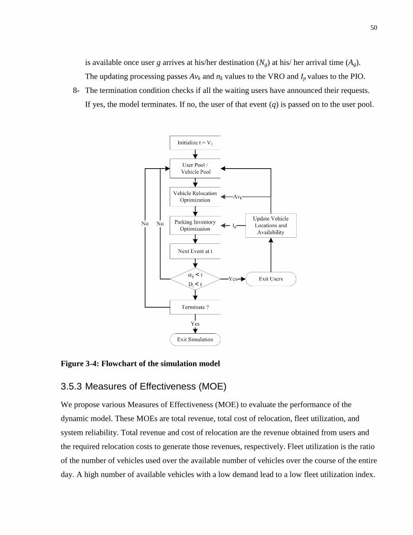
50
is available once user g arrives at his/her destination (Ng) at his/ her arrival time (Ag).
The updating processing passes Avk and nk values to the VRO and Ip values to the PIO.
8- The termination condition checks if all the waiting users have announced their requests.
If yes, the model terminates. If no, the user of that event (q) is passed on to the user pool.
Figure 3-4: Flowchart of the simulation model
3.5.3 Measures of Effectiveness (MOE)
We propose various Measures of Effectiveness (MOE) to evaluate the performance of the
dynamic model. These MOEs are total revenue, total cost of relocation, fleet utilization, and
system reliability. Total revenue and cost of relocation are the revenue obtained from users and
the required relocation costs to generate those revenues, respectively. Fleet utilization is the ratio
of the number of vehicles used over the available number of vehicles over the course of the entire
day. A high number of available vehicles with a low demand lead to a low fleet utilization index.

51
System reliability is the total number of accepted users over total demand. This index is between
0 (no user is served) and 1 (all users are served).
3.6 Example Problem: The Case of Autoshare
Autoshare, founded in 1998, is a Toronto based carsharing company with 209 parking locations
across the city (Figure 3-5), more than 10,000 users, and an average of 200 vehicle requests a
day (Costain et al. 2012). Autoshare has a flexible policy on vehicle reservation where users can
book a vehicle on the spur-of-the-moment or up to a year in advance. The service has no
restrictions on how far a vehicle can be driven from the origin parking facility but requires that
the users return the vehicle to its original location. In this section, we use the case of Autoshare
to evaluate the performance of the benchmark model presented in Section 3.3. Autoshare is a
potential candidate for a one-way system since its parking facilities are fairly closely spaced with
a mean distance of 5.48 km which we expect would lead to reasonable vehicle relocation cost.
Figure 3-5: Parking locations of Autoshare (Toronto, Ontario)
3.6.1 Benchmark Model Analysis
To evaluate the benchmark model we execute it 200 times for each of four different demand
scenarios (50, 100, 150, and 200 users/day). Every model run is executed using a different set of

52
user departure times obtained randomly from a curve fit to the observed data within the range of
12:00 PM to 9:00 PM (peak hours of the service) for a typical weekday. The origin/destination of
the users is obtained randomly from choice probabilities calculated from the observed data. The
probability of a parking facility p being chosen as an origin (destination) is the number of times it
was chosen as an origin (destination) over the total number of requests in a day. The arrival time
at the destination is calculated as departure time plus the travel time from origin to destination.
Travel times are computed by dividing an average velocity of 20 km/h by Manhattan distances
between the parking facilities. We assume a request time threshold (reservation time) of
30minutes. Figure 3-6 illustrates the results of the simulation showing a trade-off between the
hours of relocation and fleet size. The model runs with a lower fleet size are accompanied with
higher hours of vehicle relocation and vice versa. Both fleet size and relocation hours increase
with higher demands.
Figure 3-6: Benchmark model fleet size and relocation time for four demand scenarios (200
runs/scenario)
A common notion in the carsharing literature, which stems from static and aggregate treatment of
demand, is that a specific fleet size is needed to answer all or a portion of the demand (Kek et al.
2009, Correia and Antunes, 2012). Figure 3-6 and Table 3-2 show that the required fleet size is a

53
function of demand. Larger fleets are generally needed in cases of higher demand, where user
announcements are more closely spaced and vehicle relocation is challenging. On the contrary, in
cases of lower demand the system can relocate a smaller fleet to serve all users. Suitable fleet
size for every scenario, therefore, varies depending on the announcement patterns of the users.
The decreasing ratio of vehicles per user in the last row of Table 3-2 shows increasing economies
of scale as the demand increases.
Table 3-2: Benchmark model fleet size for four demand scenarios
Demand (users/day)
50 100 150 200
Maximum fleet size 18 29 34 43
Mean fleet size 12.08 20.24 26.79 33.36
Minimum fleet size 9 15 22 28
Variance of fleet size 2.97 4.95 5.42 8.41
Mean fleet size / Demand 0.24 0.20 0.18 0.16
Longer reservation time policies give CSOs more time to relocate the vehicles between the
parking facilities but make the system inconvenient for users who need immediate access. To
assess the importance of this component, we run the benchmark model 30 times for different
reservation time policies with the demand of 200 users/day. Figure 3-7 depicts the impact of
reservation time on the average fleet size size and total relocation time where the fleet size
decreases and relocation time increase with higher reservation time values. The figure illustrates
that fleet size stays roughly the same above 30 minutes of reservation time. This is dependent on
the proximity and locations of the parking facilities. In 30 minutes of reservation time, vehicles
can be easily transferred between any two parking facilities.

54
Figure 3-7: Benchmark model mean fleet size and relocation time for different reservation
time policies with a demand of 200 users/day
3.6.2 Dynamic Model Analysis
In this section, we assess the dynamic model and emphasize the importance of the price rate for
users (Pr) and the cost rate for relocations (Cr) parameters. The dynamic model is set up using
the same parameters from the benchmark model with the following exceptions and additions.
The initial location of each vehicle is randomly chosen from the 209 parking facilities. No two
vehicles are initially located at the same parking facility. The parking capacity of each parking
facility is set to 1 with . The population size of the PSO for solving the PIO is set to 10,
the number of iterations to 8, the initial inertia weight to 1.2, the final inertia weight to 0.4, and
C1 and C2 values to 2.
Pr and Cr highly impact the results of the dynamic model. If Cr is noticeably higher than Pr, the
CSO is not willing to relocate its vehicles. Conversely, with low Cr values, the CSO is
indifferent to any number of relocation operations. Table 3-3 presents various measures of
effectiveness at different Pr values with a demand of 200 users/day when Cr=1. We only
consider the ratio of Pr to Cr in the analysis because in objective function (2a) the least common
multiples can be removed. Each scenario is run 30 times. Results show that hours of relocation,

55
revenue, and reliability increase with higher Pr values. Revenue hours in Table 3-3 is the sum of
total travel time of the users without multiplying by Pr. All three mentioned measures of
effectiveness grow faster at lower Pr values and reach relatively constant values at higher Pr
values. This shows that higher Pr values lead to serving users who require high relocation costs
but offer less revenue to the system. The fairly constant Fleet Utilization index shows that all
vehicles are used at every Pr Scenario.
Table 3-3: Measures of effectiveness at various ratios of Pr to Cr=1 where demand is 200
users/day
Pr/Cr Relocation hours Revenue hours Reliability
Fleet
Utilization
0.5 3.42 9.46 0.80 0.94
1.0 7.53 11.29 0.86 0.98
1.5 9.89 14.04 0.93 1.00
2.0 11.34 15.49 0.95 1.00
2.5 12.57 16.23 0.96 1.00
3.0 13.39 16.75 0.97 1.00
Table 3-4 compares the relocation hours in the benchmark model and the dynamic model for a
Pr value of 3 and a demand of 200 users/day. We choose this ratio because the dynamic model
becomes more like the benchmark model at higher Pr to Cr ratios where Fleet Utilization
becomes 1 and Reliability gets closer to 1. The number of vehicles in the dynamic model is set to
the average number of vehicles in the benchmark model shown in Table 3-2 for each demand
scenario. Table 3-4 shows that the relocation hours for the benchmark model are lower than
those of the dynamic model for all levels of user demand. The better performance of the
benchmark model is expected due to the availability of complete information in the model.
However, the differences are not significantly different with 90% confidence.

56
The dynamic model has higher variances because many relocation decisions are made iteratively
whereas the benchmark model makes relocation decisions in only one iteration. The larger
number of iterations makes the dynamic model more dependent on the user request patterns.
Finally, Table 3-4 shows a lower percentage difference in the mean of the hours of relocation as
demand increases because there are better relocation opportunities within higher demands.
Table 3-4: Relocation hours of the benchmark model (left) and the dynamic model with
Pr=3, Cr=1 (right)
Benchmark model Dynamic model
Demand (users/day)
Demand (users/day)
50 100 150 200
50 100 150 200
Maximum 6.89 11.59 15.28 17.51
7.21 12.35 16.11 18.62
Mean 4.45 7.45 10.33 12.78
4.78 8.01 10.91 13.39
Minimum 2.58 4.56 6.99 8.46
2.82 4.69 7.31 9.14
Variance 0.70 1.39 2.12 3.05
1.04 2.03 2.82 3.34
Test of hypothesis do not imply that benchmark and the dynamic models are significantly
different with 90% level of confidence
The benchmark and the dynamic model can easily be operationalized with low computation
times. The models were coded in CPLEX using Matlab 7.12 running on a dual core 2.40 GHz
laptop computer with 8 GB RAM. The benchmark model with a demand of 200 users/day runs in
12 seconds. The dynamic model, with the same demand, runs in 34 seconds. The dynamic one-
way system with 400 users, however, runs in 3.41 minutes. Therefore, although the model
performs efficiently for the proposed case study, meta-heuristics can be used to reduce the
computational burden for larger problems.
3.7 Summary of Key Findings
In this chapter, a dynamic vehicle relocation and parking management model is proposed for
CSOs. The model is run in a discrete event simulation where at every event one user requests a

57
vehicle with specific preferences such as pick up time, drop off time, pick up location, and drop
off location.
The dynamic model is compared to a static model which assumes perfect information of all
users. The static model is run only once compared to the dynamic model which is run at every
event. Results of the two models are very close which validates the performance of the dynamic
model.
Analysis of the static benchmark of this chapter shows variability in the required fleet size which
is dependent on the user request patterns. This shows that unless the CSO acquires a fleet size
equal to or larger than the maximum number of vehicles calculated in the model, there will be
some unanswered demand in certain days (with certain user request patterns). Therefore
choosing an appropriate fleet size is a critical decision of the CSO.
This chapter also assesses the impact of various policies such as the required reservation time.
Results show that higher reservation times allow the CSO to relocate vehicles between parking
stations and therefore reduce the required fleet size. This impact diminishes when the reservation
time is further increased when there is no more potential for vehicle relocation.

58
Chapter 4 Conclusion
4 Collaborative Consumption
Collaborative consumption in transportation has been emerging in some of the new startups in
the last decade. Examples of such services include ridesharing, bikesharing, and carsharing.
Ridesharing and carsharing are the focus of this thesis. Dynamic models are proposed for both
services which are applicable in real life. Results of the dynamic models were satisfactorily
compared to static models for both services.
4.1 On Dynamic Ridesharing
Chapter 2 introduces an agent based model to solve the dynamic ridesharing problem. The model
is flexible to solve ridesharing schemes that allow single or multiple drivers to be matched with
single or multiple passengers. The new modules, in some cases, promise better system outcomes.
For example, the multi-passenger matching approach offers much lower costs to the users of the
system because it allows the trip cost to be distributed between a greater number of users. The
proposed agent based model is also much faster than the conventional centralized optimization
methods while providing the similar system objectives. We summarize the findings of Chapter 2
in Table 4-1:
Table 4-1: Effectiveness of different modules for three different market penetration
rates. Numbers outside parenthesis present the system reliability and number inside
parenthesis present VKTS (Vehicle Kilometers)
Market Penetration Rate
0.20% 0.50% 1.00%
Single driver, single passenger 0.56 (0.19) 0.67 (0.26) 0.71 (0.29)
Single driver, two passengers 0.59 (0.27) 0.71 (0.33) 0.77 (0.36)
Two drivers, single passenger 0.56 (0.19) 0.68 (0.26) 0.72 (0.30)

59
The agent based model exhibits the necessary features of successful dynamic ridesharing systems
such as flexibility, convenience, reliability, and motivation. The system is flexible in that it
allows users to announce their trip at any time up to the latest departure time. It also allows
matches to be updated as new users enter the system. The system is convenient because it can
limit the choice sets of users in the vicinity approach based on preferences specified in the
subscription process. For example, a driver bids only on passengers who are in the vicinity of the
driver’s path. The method could easily be extended to constrain matches on the basis of user
preferences (gender, non-smoking, etc.) Reliability is achieved with higher market penetrations
and is increased through the multi-passenger single driver composition. Finally, motivation can
be achieved by lowering the service provider’s charging rate to create incentives for the users. Of
course motivation can be reduced if the commission rates of the service provider are too high.
Other forms of motivation can be introduced by public sector subsidization which would reduce
user costs even more.
4.2 On Dynamic Carsharing
Chapter 3 presents a benchmark and a dynamic model for the carsharing operations problem and
evaluates the performance of the one-way system through various measures of effectiveness. The
benchmark model is set up with complete knowledge of user requests whereas the more realistic
dynamic model receives user information only when they make a request. The dynamic model
performs satisfactorily when compared to the benchmark model. The presented dynamic model
can benefit CSOs in building robust decision support systems and can lead to more successful
one-way carsharing systems. Furthermore, the dynamic model is more practical than the
conventional static models in the literature because it is flexible with different demand scenarios
(request patterns) and it can adapt to daily circumstances such as absence of a vehicle due to
maintenance.
This study also shows the importance of various policies such as extension of the required
reservation time on reducing the fleet size of the one-way carsharing systems. Increasing the
reservation time from zero (open-ended system) to 30 minutes can reduce the fleet size by 86%.
Results show a tradeoff between vehicle relocation hours and fleet size. A higher fleet size
requires less total relocation hours and vice versa. Both relocation hours and fleet size, however,

60
increase with higher demands. In addition to the value of demand, both the fleet size and
relocation hours also depend on the schedules of the users (request patterns). Fleet size decreases
when requests are spread out in time.
The benefit of the dynamic model depends on the ratio of price charged per unit time (Pr) and
cost of relocation per unit time (Cr). In cases where Pr is relatively higher than Cr, it is more
beneficial to service more customers. This leads to higher reliability of the system which leads to
customer satisfaction. Therefore, it is critical to cut down unit relocation costs as much as
possible.
4.3 Recommendations for Future Work
The following are some areas which require further research:
1- Chan and Shaheen (2012) consider multimodal integration as the future of ridesharing.
To provide this service, Zimride and Zipcar have launched an integrated partnership in
2009 to link their program with public transportation systems (Reidy, 2009).
Unfortunately, however, this idea has not be studied in the the academic literature. The
proposed model in Chapter 2 can be extended to accommodate multimodal integration
where the connections are allowed to be made with other transportation modes such as
public transit and Carsharing. A simple methodology for this is to set hub locations at
intermodal transfer nodes. The new cost function for users would then include the
additional cost of the alternatives modes of transportation.
2- There is no research available in the ridesharing literature that studies the differences
between en-route matching (where a driver can still pick up a passenger even though he
has departed from his origin) and pre-planned matching (studied in Chapter 2). This
comparison can be done by adding a module to the algorithm that would order drivers to
leave their origin before reaching their flexibility time. The module would then set a new
earliest departure time and origin zone for the driver depending on new locations of the
driver in the network. The auction mechanism would then treat en-route drivers as normal
drivers by with updated characteristics.

61
3- Some users enter the ridesharing system with no preference in being a driver or a
passenger. This can be incorporated in the model by a module that changes the role of a
user after a few iterations to see if a lower cost is found. Our research showed that
maximum network reliability occurs with the ratio of drivers to passengers is 0.5. Hence,
the module would be more efficient if it produces this ratio.
4- The hub location problem is an entirely new research area. The proposed ridesharing
agent based model can be extended to include dynamic hub locations instead of fixed
ones as was the assumption in Chapter 2. The location of the hubs can therefore change
dynamically at each time step.
5- There are two types of users in CSOs: one-way and two-way users. One-way users
require only one trip whereas two-way users require a return trip. Similarly, there are two
types of CSOs: one-way and two-way organizations. Two-way CSO require users to
return the vehicle to its original location whereas one-way systems have no such
restrictions. The models in Chapter 3 can be modified to presents both types of CSOs to
capture the impact of various market segmentations (selection of one-way and two-way
users) on the system as a whole.
6- A major assumption made in Chapter 3 is that staff members are always available to
relocate vehicles from each parking facility to every other parking facility. In reality,
however, this is not the case. There are limited staff members who are available at
specific times and locations. Staff members change their locations as they relocate
vehicles between parking facilities. This leads to the imbalance of staff members in
addition to the imbalance of cars between stations. A next step in CSO decision support
systems is to build a dynamic model which also considers flow of staff between parking
facilities.

62
References
Abraham, A., Guo, H., Lio, H. (2006). Swarm intelligence: foundations, perspectives and
applications. In: Nedjah, N., Mourelle, L.M. (Eds.), Swarm Intelligent Systems.
Springer, Netherlands, 18–25.
Agatz, N.A.H., Erera, A., Savelsbergh, M.W.P., Wang, X. (2011). Dynamic ride-sharing: a
simulation study in metro Atlanta. Transportation Reserch Part B, Methodological 45
(9), 1450–1464.
Agatz, N.A.H., Erera, A., Savelsbergh, M.W.P., Wang, X. (2012). Optimization for dynamic
ride-sharing: A review. European Journal of Operational Research, 223 (2), 29-303.
Amey, A. (2011). Proposed Methodology for Estimating Rideshare Viability Within an
Organization: Application to the MIT Community, Transportation Research Board
Annual Meeting 2011, Paper 11-2585.
Baldacci, R., Maniezzo, V., Mingozzi, A. ( 2004). An exact method for the car pooling
problem based on lagrangean column generation. Operations Research, 52 (3), 422–
439.
Barth, M., Todd, M. (1999). Simulation model performance analysis of a multiple station
shared vehicle system. Transportation Research Part C: Emerging Technologies, 7
(4), 237–259.
Botsman, R. (2010). What's Mine is Yours: The Rise of Collaborative Consumption.
HarperBusiness.
Canadian Vehicle Survey (2009). Summary Report; Natural Resources Canada’s Office of
Energy Efficiency.
Celsor, C., Millard-Ball, A. (2007). Where Does Carsharing Work? Using Geographic
Information Systems to Assess Market Potential. Transportation Research Record:
Journal of the Transportation Research Board, 1992.
Cervero, R., Golob, A., Nee, B. (2007). City CarShare: longer term travel demand and car
ownership impact. Transportation Research Record 1992, 70–80.
Chan, N., D. & Shaheen, S., A. (2012). Ridesharing in North America: Past, Present, and
Future. Transport Reviews, 32(1), 93-112.
City Carshare (2013). City Carshare 2013 fact sheet. < https://www.citycarshare.org/wp-
content/uploads/2013/04/1071_CCS_Fact_Sheet_v2-1.pdf> (Accessed 10.05. 13).
Communauto (2013). Communauto launches Auto-mobile : first 100% electric one-way
carsharing pilot project in Canada.

63
<http://actualites.communauto.com/en/2013/06/16/communauto-launches-auto-
mobile/> (Accessed 10.05.13).
Costain, C., Ardon, C., Habib, K. N. (2012). Synopsis of users’ behavior of a carsharing
program: A case study in Toronto. Transportation Research Part A: Policy and
Practice, 46 (3), 421-434.
Correia, G., H., Antunes, A., P. (2012). Optimization approach to depot location and trip
selection in one-way carsharing systems. Transportation Research Part E: Logistics
and Transportation Reviews, 48 (1), 233-247.
Cortes, C.E., Matamala, M., Contardo, C. (2010). The pickup and delivery problem with
transfers: formulation and a branch-and-cut solution method. European Journal of
Operational Research, 200 (3), 711–724.
Eberhart, R.C., Kennedy, J. (1995). A new optimizer using particle swarm theory. In:
Proceedings of the Sixth International Symposium on Micro Machine and Human
Science. IEEE Press, Piscataway, NJ, 39–43.
Eisenberg, A. (2008). Need a ride? Check you iPhone. NYTimes.com.
http://www.nytimes.com/2008/12/21/business/21novelties.html. (Accessed 8.2.2013).
El Fassi, A., Awasthi, A., Viviani, M. (2012). Evaluaction of carsharing network’s growth
strategies through discrete event simulation. Expert Systems with Applications, 39 (8),
6692-6705.
Emmerink, R.H.M., vanBeek, P. (1997). Empirical analysis of work schedule flexibility:
implications for road pricing and driver information systems. Urban Studies 34 (2),
217–234.
Fan, W., Machemehl, R.B., Lownes, N.E. (2008). Carsharing dynamic decision-making
problem for vehicle allocation. Transportation Research Record (2063), 97–104.
Firnkorn, J., Muller, M. (2011). What will be the environmental effects of new free-floating
car-sharing systems? The case of car2go in Ulm. Ecological Economy 70, 1519–
1528.
Ghoseiri, K., Haghani, A., Hamedi, M. (2011). Real-time rideshare matching problem.
University of Maryland, Department of Civil and Environmental Engineering, UMD-
2009-05.
Gruebele, P.A. (2008). Interactive system for real time dynamic multi-hop carpooling. Hall,
R.W., Qureshi, A., 1997. Dynamic ride-sharing: theory and practice. Journal of
Transportation Engineering 123 (4), 308–315.
Habib, K.M.N., Morency, C., Islam, T., Grasset, V. (2009). Modelling user’s behaviour of a
carsharing program in Montreal: application of zero inflated dynamic ordered probit

64
model. Presented at 12th International Association of Travel Behaviour Research
(IATBR) Conference, Jaipur, India.
Habib, K.M.N., Morency, C., Islam, T., Grasset, V. (2012). Modelling user’s behaviour of a
carsharing program in Montreal: application of zero inflated dynamic ordered probit
model. Transportation Research Part A 46, 241–254.
Herbawi, W., Weber, M. (2011). Ant Colony vs. Genetic Multiobjective Route Planning in
Dynamic Multi-hop Ridesharing, ictai, pp.282-288, 2011 IEEE 23rd International
Conference on Tools with Artificial Intelligence.
Hoen, P.J., Poutre, J.A.L (2003). A decommitment strategy in a competitive multi-agent
transportation setting. In: Proceedings of 2nd International Joint Conference on
Autonomous Agents and Multiagent Systems (AAMAS 2003). ACM Press, pp.
1010–1011.
Jorge, D., Correia, G., Barnhart, C. 2012. Testing the validity of MIP approach for locating
carsharing stations in one-way systems. Procedia – Social and Behavioral Sciences
(54), 138-148.
Kamar, E. & Horvitz, E (2009). Collaboration and shared plans in the open world: studies of
ridesharing. In Proceedings of the 21st international jont conference on Artifical
intelligence, pages 187–194, San Francisco, CA, USA, 2009. Morgan Kaufmann
Publishers Inc.
Kara, I., Bektas, T. (2006). Integer linear programming formulations of multiple salesman
problems and its variantions. European Journal of Operational Research, 174 (3),
1449-1458.
Katzev, R. (2003). Car Sharing: A New Approach to Urban Transportation Problems.
Analysis of Social Issues and Public Policy, 3(1), 65–86.
Kek, A.G.H., Cheu, R.L., Meng, Q., Fung, C.H. (2009). A decision support system for
vehicle relocation operations in carsharing systems. Transportation Research Part E:
Logistics and Transportation Review, 45 (1), 149–158.
Kleiner, A., Nebel, B., Ziparo, V. (2011). A mechanism for dynamic ride sharing based on
parallel auctions. In: Proc. of the 22th International Joint Conference on Artificial
Intelligence (IJCAI), Barcelona, Spain, pp. 266–272. ISBN 978-1-57735- 516-8.
Kocur, G., (1983). A model to assess cost and fuel savings from ride sharing. Transportation
Research Part B: Methodological 17 (4), 305-318.
Kuhn., H. W. (1995). The hungarian method for the assignment problem. Naval Research
Logistics Quarterly, (2), 83–97.

65
Kurtzleben (2013). “CHARTS: The exploding growth of bikesharing”.
http://www.usnews.com/news/articles/2013/06/05/the-exploding-growth-of-
bikesharing. (Accessed 4.6.2013)
Morency, C., Habib, K.M.N., Grasset, V., Islam, T. (2010). Understanding members’
carsharing (activity) persistency by using econometric model. Journal of Advanced
Transportation 46(1), 26-38.
Pisani, J. (2009). “Car Sharing Takes Off”.
http://76.12.4.249/artman2/uploads/1/Car_Sharing_Takes_Off_-_CNBC.pdf.
(Accessed 4.1.2013).
Reidy, C. (2009). Zipcar partners with ride sharing community. Boston.com.
http://www.boston.com/business/ticker/2009/04/zipcar_partners_2.html. (Accessed
8.2. 2013).
Roughgarden, T. (2005). Selfish Routing and the Price of Anarchy. MIT Press.
Santos, A., McGuckin, N., Nakamoto, H.Y., Gray, D., Liss, S. (2011). Summary of travel
trends: 2009 national household travel survey. Technical Report, US Department of
Transportation Federal Highway Administration.
Sarraino, J. (2008). Spatial Analysis of Commuting Patterns at the University of Toronto's St.
George Campus: Identifying Ridesharing and Public Transportation Potential.
University of Toronto Sustainability Office, University of Toronto.
Shaheen, S.A., Cohen, A.P. (2007). Growth in worldwide carsharing – an international
comparison. Transportation Research Record (1992), 81–89.
Shaheen, S.A., Cohen, A.P., Roberts, J.D. (2006). Carsharing in North America – market
growth, current developments, and future potential. Transportation Research Record
(1986), 116–124.
Shahin, G. & Nickel, S. (2011). Hub location problems in transportation networks,
Transportation Research Part E: Logistics and Transportation Review 47(6), 1092-
1111.
Steininger, K., Vogl, C., Zettl, R. (1996). Car-sharing organizations: the size of the market
segment and revealed change in mobility behavior. Transport Policy 3 (4), 177–185.
Stillwater, T., Mokhtarian, P.L., Shaheen, S.A. (2009). Carsharing and the built environment:
geographic information system-based study on one US operator. Transportation
Research Record 2110, 27–34.
Teodorovic, D. & Dell’ Orco, M. (2006). Mitigating traffic congestion: solving the ride-
matching problem by Bee Colony Optimization. Transportation Planning and
Technology 31 (2), 135-152.

66
Tsao, H. J. & Lin, D. J, (1999). Spatial and Temporal Factors in Estimating the Potential of
500 Ridesharing for Demand Reduction. Institute of Transportation Studies, UC
Berkeley.
Vine, S., Sivakumar, A., Polak, J., Lee-Gosselin, M. (2013). The market and impacts of new
types of carsharing systems: case study of Greater London. Transportation Research
Board Annual Meeting 2013, Paper.
Winter, S., Nittel, S. (2006). Ad-hoc shared-ride trip planning by mobile geo-sensor
networks. International Journal of Geographic Information Science 00 (00), 1– 21.
Xing, X., Warden, T., Nicolai, T., Herzog, O. (2009). Smize: a spontaneous ride-sharing
system for individual urban transit. In: Proceedings of the 7th German Conference on
Multiagent System Technologies, MATES’09. Springer-Verlag, Berlin Heidelberg,
165–176.
Zhao, D. (2010) “Carsharing: A Sustainable and Innovative Personal Transport Solution”.
www.frost.com/prod/servlet/market-insight-top.pag?Src=RSS&docid=190795176.
(Accessed 4.1.2013).