Dynamic Agency and Real Options∗

Sebastian Gryglewicz†

and Barney Hartman-Glaser‡

January 27, 2014

Abstract

We present a model integrating dynamic moral hazard and real options. A risk-averse manager can exert costly hidden effort to increase the productivity growth ofa firm. The risk-neutral owners of the firm can irreversibly increase the firm’s capitalstock. In contrast to the literature, we show that moral hazard can accelerate or delayinvestment relative to the first-best. When the agency problem is more severe, thefirm will invest earlier than in the first best case because investment acts as substitutefor effort. This mechanism provides an explanation for over-investment that does notrely on “empire-building” preferences. When the growth option is large, the firm willinvest later than in the first-best. We also discuss the implications of the presence ofreal options for the manager’s pay-performance sensitivity.

JEL classification: G31, D92, D86.

Keywords : Moral Hazard, Dynamic Contracting, Real Options, Pay-Performance Sensitivity.

∗We wish to thank Hengjie Ai, Jonathan Berk, Antonio Bernardo, Bruce Carlin, Mark Garmaise, SimonGervais, Zhiguo He, Dmitry Livdan, Semyon Malamud, Erwan Morellec, Norman Schurhoff, Alexei Tchistyi,Vish Vishwanathan, Nancy Wallace, and Gijsbert Zwart, as well as seminar and conference participants atUC Berkeley Haas (Real Estate), Duke Finance Brownbag, CPB Netherlands Bureau for Economic PolicyAnalysis, University of Lausanne-EPFL, the Revelstoke Finance Summit, VU University Amsterdam, Stan-ford Institute for Theoretical Economics Summer Institute, Erasmus School of Economics, the MinnesotaJunior Finance Conference, and the UCLA Finance brownbag for useful comments and suggestion.†Erasmus School of Economics, Erasmus University Rotterdam. Email: gryglewicz@ese.eur.nl.‡Anderson School of Management, UCLA. Email: bhglaser@anderson.ucla.edu.

1 Introduction

How firms make real investment decisions is a central topic in the study of corporate finance.

As the investments of individual firms are typically lumpy and (partially) irreversible, they

are well described as real options. In the standard real options model, cash flows of a firm are

generated without any agency conflicts. In reality, cash flow growth often requires managerial

effort and when this effort is costly and unobservable, a moral hazard problem arises. We

investigate how this moral hazard problem affects investment timing decisions.

The optimal time to invest equates the benefit of investment with the direct cost plus

the opportunity cost of investment. On the one hand, moral hazard will decrease the benefit

causing a delay in investment. On the other hand, moral hazard will decrease the opportunity

cost of investing and will thus accelerate investment. We show that when the moral hazard

problem is severe or the size of the investment option is small, the agency conflict decreases

the opportunity cost more than the benefit and hence accelerates investment. In contrast,

when the moral hazard problem is moderate or the size of the investment option is large,

the opposite is true and the agency problem delays investment.

Empirical evidence indicates that firms may either over- or under-invest relative to some

first-best benchmark. For example, Bertrand and Mullainathan (2003) find that when exter-

nal governance becomes weaker due to the passage of anti-takeover legislation, firms invest

less in new plants. In contrast, Morck et al. (1990) document that negative price reac-

tions to acquisitions are greater when the managers of bidding firms perform poorly before

acquisitions, indicating that these managers are pursuing their own objectives. In theoreti-

cal literature on firm investment under agency conflicts, two main themes have developed.

Grenadier and Wang (2005), DeMarzo and Fishman (2007), and DeMarzo et al. (2012) argue

that moral hazard in effort induces firms to curtail investment and not to over-invest. While

Jensen (1986), Stulz (1990), Harris and Raviv (1990), Hart and Moore (1995), and Zwiebel

(1996) posit firms over-invest because managers have a preference for “empire-building.”

Along similar lines, Roll (1986) and Bernardo and Welch (2001)) show that over-investment

1

may occur because managers are over-confident. We show that moral hazard in effort can

also cause a form of over-investment; a firm plagued with a severe problem of incentivizing

a manager to work will exercise investment options sooner than identical firms without a

moral hazard problem.

To arrive at this result, we construct a continuous-time dynamic moral hazard model in

which an investor contracts a manager to run a firm. The firm produces cash flow according

to a linear production technology. The manager of the firm can exert effort to increase the

expected growth rate of productivity. For example, the manager might need to work to

increase market share or improve operational efficiency to increase productivity. This effort

is costly to the manager and hidden to the investors so that the manager can potentially gain

utility by exerting less effort than would be optimal from the perspective of the investor. In

order to incentivize the manager to exert effort, the optimal contract will expose her to firm

performance. This exposure is costly because it reduces risk sharing between the manager

and the investor. In addition to increasing productivity by contracting with the manager,

the investor has an option to irreversibly increase the firm’s capital.

An important feature of our model is that capital and managerial effort are complements

in the firm’s production function. When the manager exerts more effort, productivity in-

creases at a faster rate, and capital becomes more productive. Similarly, when the firm has

more capital, managerial effort leads to more growth in cash flow. However, the complemen-

tarity of managerial effort and capital in the firm’s production function does not necessarily

mean the firm will invest less when the price of managerial effort rises. Indeed, if the price

of managerial effort rises due to an increase in the cost of incentives, the firm may accel-

erate investment and decrease incentives. In this sense, investment serves as a substitute

for managerial effort as a means of increasing cash flow. It is important to note that this

substitution effect is not driven by the manager’s preferences for investment. In fact, the

manager in our model is indifferent between any particular investment policy.

In addition to implications for the investment behavior of firms, our model also generates

2

results for the manager’s compensation and incentives. The power of incentives and pay-

performance sensitivity are closely related to the size of the growth opportunity. All else

equal, the productivity of managerial effort is increasing in the size of the growth option, and

hence so is the power of incentives as measured by the sensitivity of the manager’s wealth to

firm output. However, increasing the size of the growth option also changes the sensitivity of

firm value to output. Consequently, there is a wedge between pay-performance sensitivity and

incentives. If the manager’s cost of effort is increasingly convex, pay-performance sensitivity

may actually decrease with the size of the growth option. This result is a caveat for empirical

work on the power of incentives. In the presence of growth opportunities, there could be a

negative relationship between actual incentives and the sensitivity of the manager’s wealth

to firm value (rather than output).

Our model further predicts that the manager’s pay-performance sensitivity may increase

or decrease at investment depending on the agency conflicts. When the moral hazard problem

is less severe, the optimal contract will call for the manager to exert maximal effort before

and after investment. As a result, pay-performance sensitivity, as measured by the sensitivity

of the manager’s wealth to firm value, will actually increase after investment. If, however,

the moral hazard problem is more severe, the optimal contract will call for the manager to

significantly decrease effort after investment, which causes a decrease in pay-performance

sensitivity. An interesting feature of the results of our model is that the effect of investment

on pay-performance sensitivity and investment timing are closely linked. On the one hand,

when investment leads to an increase in pay-performance sensitivity, it must also be the

case that investment is delayed relative to the first-best case. On the other hand, when

investment leads to a decrease in pay-performance sensitivity, as is often empirically the

case (e.g., Murphy (1999)), investment must be accelerated relative to the first-best case.

It is useful to illustrate the model in terms of some real world examples. First, consider

a startup firm choosing the optimal time to raise its first round of venture capital. In this

case, the initial capital stock of the firm is small and, as a consequence, managerial effort

3

is relatively cheap. In other words, the start-up manager’s moral hazard problem prior

to raising the first round of capital is relatively mild or perhaps even non-existent. After

raising venture capital, the manager’s moral hazard becomes more pronounced. As a result,

increasing the cost of incentives decreases the present value of the added cash flow from the

additional capital more than the value of the small firm, resulting in a delay in investment.

Thus, our model predicts that startup firms with more severe moral hazard problems receive

venture financing later than others.1 A similar prediction applies to later stages of venture

funding and initial public offerings.

In the preceding example, the size of the investment option is large relative to the initial

capital stock of the firm, thus moral hazard delays investment timing. In the next example,

the investment opportunity is small relative to the capital stock of the firm. For instance,

consider a large mature firm choosing the optimal time to make an acquisition of a small tar-

get. In this setting, the acquisition allows the large firm to grow cash flows without providing

costly incentives for additional managerial effort. This in turn implies that increasing the

cost of incentives has a larger negative effect on the acquiring firm prior to the acquisition

than on the merged firm and thus accelerates the acquisition. A prediction of the model is

then that acquiring firms with more severe agency problems undertake acquisitions sooner

and at lower levels of productivity than otherwise.

To gain a greater understanding of the forces at work in generating both accelerated and

delayed investment, we generalize the model to allow for many different types of investment.

The existing models of moral hazard and investment largely consider contracts that imple-

ment effort at the first-best level and show that moral hazard decreases or delays investment

(e.g., Grenadier and Wang (2005); DeMarzo and Fishman (2007); Biais et al. (2010); De-

Marzo et al. (2012)). So as a first step, we consider a model in the spirit of DeMarzo et al.

(2012), i.e., a neoclassical model of investment, in which we allow optimal effort to deviate

1Of course, other aspects of the agency problem may change as a result of the venture financing. Indeed,Gompers (1995) finds evidence that venture capitalists act as monitors since firms with more agency problemsreceive more frequent rounds of venture financing. However, this finding does not preclude our prediction.

4

from the first best. In this case, the marginal value of capital is a sufficient statistic for

investment and always decreases with agency problems. Thus, investment decreases with

the severity of the moral hazard problem even when effort is flexible. A similar argument

applies to a setting with partially irreversible but perfectly divisible investment. However,

when the investment technology implies lumpiness, as is often inherently the case with firm

level investment as argued by Doms and Dunne (1998), Caballero and Engel (1999), and

Cooper et al. (1999) among others, optimal investment is determined by the average value of

new capital. Unlike the marginal value of capital, the average value of capital, and hence the

effect of moral hazard on investment, increases or decreases with the severity of the agency

problem depending on parameters.

This paper contributes to the growing literature on the intersection of dynamic agency

conflicts and investment under uncertainty. On the dynamic contracting side, Holmstrom and

Milgrom (1987) and Spear and Srivastava (1987) introduced the notion that providing agents

with incentives may take place over many periods. More recently, a number of papers have

built on the continuous time approach of Sannikov (2008) to characterize optimal dynamic

contracts in a variety of settings. For example, DeMarzo and Sannikov (2006) consider the

design of corporate securities when the manager may divert cash. Piskorski and Tchistyi

(2010, 2011) consider the optimal design of mortgages when lenders face stochastic interest

rates or house prices are stochastic. He (2009) considers optimal executive compensation

when firm size follows a geometric Brownian motion. Most closely related to our model of

the dynamic agency problem is the capital structure model of He (2011), which allows for a

risk-averse agent.

On the investment side, DeMarzo and Fishman (2007), Biais et al. (2010), and DeMarzo

et al. (2012) consider dynamic moral hazard with investment. One important distinction

between our paper and both Biais et al. (2010) and DeMarzo et al. (2012) is that their setups

yield first-best effort even under moral hazard, and as such the substitutability of effort and

investment is not present in their models. The investment technology we consider is based

5

on the classic real options models of Brennan and Schwartz (1985) and McDonald and Siegel

(1986). Dixit and Pindyck (1994) offer a comprehensive guide to the real options literature.

Two papers that use a similar model to ours to evaluate the effects of agency problems on

real options investment are Grenadier and Wang (2005) and Philippon and Sannikov (2007).

Grenadier and Wang consider a real option exercise problem in the presence of a static moral

hazard and find that when there is an additional adverse selection over managerial ability,

real option exercise is delayed. We consider a dynamic moral hazard problem and find that

real option exercise may be either delayed or accelerated. Philippon and Sannikov consider

real options in a dynamic moral hazard setting similar to ours. In their model, the first-best

effort level is always optimal because cash flows follow an i.i.d process. As a result, they find

that moral hazard can only delay investment. In contrast, we model cash flows that grow

in expectation and as a consequence optimal managerial effort depends on the level of cash

flows and may be lower than first best. This difference means that in our model, unlike in

that of Philippon and Sannikov, moral hazard can accelerate investment.

The rest of the paper proceeds as follows. Section 2 introduces our model of moral hazard

and real options. Section 3 provides the optimal contract and investment policy. Section

4 discusses the implications of the moral hazard problem for investment, compensation,

and incentives. Section 5 considers a generalization of our basic model to build are greater

understanding of the source of the effect of moral hazard on investment. Section 6 concludes.

2 The Model

In this section we present our model of dynamic moral hazard and real options. It resembles

that of He (2011) in that we consider an agent (the firm’s manager) with constant absolute

risk-averse (CARA) preferences who can affect the productivity growth of the firm by ex-

erting costly hidden effort. In addition, we endow the firm with an irreversible investment

opportunity.

6

2.1 Technology and Preferences

Time is continuous, infinite, and indexed by t. The risk-free rate is r. A risk-neutral investor

employs a risk-averse manager to operate a firm. Firm cash flows are XtKtdt, where Kt is

the level of capital at time t and Xt is a productivity shock with dynamics given by:

dXt = atµXtdt+ σXtdZt,

where at ∈ [0, 1] is the manager’s effort and Zt is a standard Brownian motion. Constants µ

and σ represent the (net of effort) drift and volatility of the productivity process. Managerial

effort here corresponds to any action that increases the growth rate — not the current level

— of productivity. For example, the manager may have to exert effort to increase market

share or the operational efficiency of the firm. The firm starts with capital K0 = k > 0

and has a one time expansion option to increase capital to k at cost p. In the notation that

follows, a hat indicates a post investment quantity.

The manager has CARA preferences over consumption. She values a stream of consump-

tion ct and effort at as:

E

[∫ ∞0

e−rtu(ct, at)dt|a],

where u(c, a) = −e−γ(c−XKg(a))/γ is the manager’s instantaneous utility for consumption and

effort and XKg(a) is the manager’s cost of effort in units of consumption. This specification

captures the notion that the manager’s effort costs are increasing in both capital employed

by the firm, as well as in productivity. In other words, it is more costly for the manager to

increase productivity when the firm is larger or more productive. We assume the manager’s

normalized cost of effort g(a) is continuously differentiable, increasing, and convex, g(a) ∈

C1([0, 1]), g′(a) ≥ 0, g′′(a) > 0, and g′(0) = 0. When we consider specific parameterizations

of the model, we assume a simple quadratic functional for g(a). In addition to facing a cost

7

of effort, the manager may save at the risk-free rate r. We assume that the manager begins

with zero savings. The manager’s savings and effort are unobservable to the investor.

2.2 Contracts

A contract consists of a compensation rule, a recommended effort level, and an investment

policy denoted Π = (ct, att≥0, τ). The compensation rule ct and recommended effort at

are stochastic processes adapted to the filtration of public information, Ft. For simplicity, we

drop the subscript t whenever we are referring to the entire process of either consumption or

effort. The investment policy τ is Ft-stopping time, which dictates when the firm exercises

the option to increase capital. We assume that the investors can directly control investment

and will pay the cost of investment. Note that the time t cash flow to the investor under a

contract Π is given by:

dDt = XtKtdt− ctdt− I(t = τ)p,

where Dt denotes cumulative cash flow to the investor.

Since the agent can privately save, the compensation, ct, specified by the contract need

not be equal to the manager’s time t consumption. Denote the manager’s accumulated

savings by St and her actual time t consumption and effort by ct and at, respectively. Given

a contract Π, the manager chooses a consumption and effort plan to maximize her utility

from the contract:

W (Π) = maxc,a

E

[∫ ∞0

−1

γe−γ(ct−XtKtg(at))−rtdt

](1)

such that dSt = rStdt+ (ct − ct)dt, S0 = 0

dXt = atµXtdt+ σXtdZt

Kt = k + (k − k)I(t ≥ τ).

The dynamics of savings St reflect that the difference between compensation ct and con-

8

sumption ct goes to increase (or decrease) savings while the balance grows at the risk-free

rate r. In addition to the dynamics for St given above, we impose the standard transver-

sality condition on the consumption process. The dynamics of productivity, Xt, reflect that

the expected growth rate of productivity depends on the actual effort, at, of the manager.

Finally, the time t capital stock of the firm depends on the investment policy set forth in

the contract.

Given an initial outside option of the manager w0, the investor then solves the problem:

B(X0, w0) = maxc,a,τ

E

[∫ ∞0

e−rtdDt

](2)

such that dXt = atµXtdt+ σXtdZt

Kt = k + (k − k)I(t ≥ τ)

w0 ≤ E(c,a,τ)[∫ ∞

0

−1

γe−γ(ct−XtKtg(at)−rtdt

],

where c, a solves problem (1).

We call a contract Π incentive compatible and zero savings if the solutions ct and at

to Problem (1) are equal to the payment rule and recommended effort plan given in the

contract. As is standard in the literature, we focus on contracts in which the solution to

problem (1) is to follow the recommended action level and maintain zero savings by virtue

of the following revelation-principle result.

Lemma 1. For an arbitrary contract Π, there is an incentive compatible and zero savings

contract Π that delivers at least as much value to the investor.

3 Solution

The solution follows the now standard martingale representation approach developed by

Sannikov (2008). The first step is to give a necessary and sufficient condition for a contract

to implement zero savings. We then represent the dynamics of the manager’s continuation

9

utility (the expected present value of her entire path of consumption) as the sum of a deter-

ministic drift component and some exposure to the unexpected part of productivity growth

shocks via the martingale representation theorem. With these dynamics in hand, we charac-

terize the incentive compatibility condition as a restriction on the dynamics of continuation

utility. Given the dynamics of continuation utility and productivity implied by incentive

compatibility, we can represent the investor’s optimal contracting problem as a dynamic

program resulting in a system of ordinary differential equations (ODEs) for investor value

together with boundary conditions that determine the investment policy. In the Appendix,

we provide verification that the solution to this system of ODEs indeed achieves the optimum

investor value.

3.1 The No-savings Condition

In this subsection, we follow He (2011) to characterize a necessary and sufficient condition

for the manager to choose consumption equal to her compensation and thus maintain zero

savings. In words, the condition states that the manager’s marginal utility for consumption

is equal to her marginal utility for savings. To determine the manager’s marginal utility for

an additional unit of savings, we first consider the impact of an increase in savings on her

optimal consumption and effort plan going forward. Suppose c, a solves problem (1) for

a given contract that implements zero savings. Now suppose we simply endow the manager

with savings S > 0 at some time t > 0. How would her consumption and effort plan

respond? Due to the absence of wealth affects implied by the manager’s CARA preferences,

the optimal consumption plan for s ≥ t would be just cs + rS, while the effort plan would

remain unchanged. Thus, an increase in savings from zero to S increases the manager’s

utility flow by a factor of e−γrS forever.2 To make this intuition formal, it is useful to define

the manager’s continuation utility for a given contract when following the recommended

2Since utility is always negative, the factor e−γrS < 1 represents an increase in utility.

10

effort policy and accumulating savings S up to time t,

Wt(Π, Xs, Kss≤t;S) = maxct,at

E

[∫ ∞t

−1

γe−γ(cs−XsKsg(at))−r(s−t)ds|Xs, Ks

](3)

such that dSs = rSsds+ (cs − cs)ds St = S

dXs = asµXsds+ σXsdZs

Ks = k + (k − k)I(s ≥ τ).

The definition of continuation utility and the intuition given above lead to Lemma 2.

Lemma 2 (He (2011)). Let Wt(Π, Xs, Kss≤t;S) be the solution to problem (3), then:

Wt(Π, Xs, Kss≤t;S) = e−γrSWt(Π, Xs, Kss≤t; 0). (4)

Equation (4) allows us to determine the manager’s marginal utility for savings under a

contract that implements zero savings:

∂

∂SWt(Π, Xs, Kss≤t;S)

∣∣S=0

= −γrWt(Π, Xs, Kss≤t; 0). (5)

Since we are focused on zero savings contracts, we now drop the arguments and refer simply

to continuation utility Wt. For the manager to maintain zero savings, her marginal utility

of consumption must be equal to her marginal utility of savings:

uc(ct, at) = −γrWt

which, together with the CARA form of the utility function, implies the convenient no-

savings condition:

u(ct, at) = rWt. (6)

Thus, for a contract to implement zero savings, the manager’s flow of utility from the contract

11

must be equal to the risk-free rate r times her continuation utility. This is intuitive; in order

for the manager to have no incentive to save, the contrast must deliver the risk-free yield

of her continuation utility in units of utility flow. For the remainder of the paper, we only

consider contracts that satisfy the no-savings condition given by Equation (6).

3.2 Incentive Compatibility

Now that we have characterized a necessary and sufficient condition for a contract to imple-

ment zero savings, we turn our attention to the incentive compatibility condition. For an

arbitrary incentive compatible and zero savings contract, consider the following process:

Ft = Et

[∫ ∞0

e−rsu(cs, as)ds

].

This process is clearly a martingale with respect to the filtration of public information

Ft, thus the martingale representation theorem implies that there exists a progressively

measurable process βt such that:

dFt = βt(−γrWt)e−rt (dXt − atµXtdt) . (7)

Now note that that Ft is related to the manager’s continuation utility Wt (under the recom-

mended consumption and effort plan) by:

dWt = (rWt − u(ct, at))dt+ ertdFt. (8)

Combining the no-savings condition (6) with Equations (7) and (8) gives the following dy-

namics for the manager’s continuation utility:

dWt = βt(−γrWt) (dXt − atµXtdt) . (9)

12

The process βt is the sensitivity of the manager’s continuation utility to unexpected shocks

to the firm’s productivity. Since a deviation from the recommended effort policy results

in an unexpected (from the investor’s perspective) shock to productivity, βt measures the

manager’s incentives to deviate from the contract’s recommended effort policy.

For a given contract, Problem (1) implies that the manager chooses her current effort

to maximize the sum of her instantaneous utility, u(ct, at)dt, and the expected change in

her continuation utility, Wt. The manager’s expected change in continuation utility from

deviating from the recommended effort policy at to at is:

E[dWt|a] = βt(−γrWt)(a− at)µXtdt.

Thus, incentive compatibility requires that:

at = arg maxa

u(ct, a) + βt(−γrWt)(a− at)µXt . (10)

Taking a first order condition for Problem (10) yields:

ua(ct, at) + βt(−γrWt)µXt = 0.

It is straightforward to show that this is a necessary and sufficient condition for the manager’s

optimal effort plan. Note that ua(ct, at) = −uc(ct, at)XtKtg′(a) and recall that the no-savings

condition is uc(ct, at) = (−γrWt), so that we can solve the first order condition above to

find:

βt =1

µKtg

′(at). (11)

Intuitively, the sensitivity, βt, that is required for incentive compatibility is the agent’s

marginal cost of effort, XtKtg′(at), scaled by the marginal impact of effort on output, µXt.

Lemma 3 characterizes incentive-compatible no-savings contracts.

Lemma 3. A contract is incentive compatible and has no savings if and only if the solution

13

Wt to Problem (3) has dynamics given by Equation (9), where βt is defined by Equation (11).

It is useful to represent the agent’s continuation utility, Wt, in terms of its certainty

equivalent, Vt = −1/(γr) ln(−γrWt). Applying Ito’s lemma to (9) and combining it with

Lemma 3 yields that the dynamics of Vt under an incentive-compatible no-savings contract

are given by:

dVt =1

2γr

(σ

µXtKtg

′(at)

)2

dt+σ

µXtKtg

′(at)dZt. (12)

The drift term in Equation (12) comes from the difference in risk aversion between the

investor and the manager. Since the manager is risk averse, the certainty equivalent of W

must have additional drift for each additional unit of volatility. Since W is a martingale, the

drift term in V is entirely due to this effect. This positive drift will show up in the investor’s

Hamilton-Jacobi-Bellman (HJB) equation as the cost of providing incentives.

3.3 First Best

As a benchmark, we first solve the model assuming effort is observable so that there are

no agency conflicts. In this case, the investor simply pays the manager her cost of effort.

Additionally, if the agent’s promised utility is W , its certainty equivalent, V , can be paid

out immediately. Thus, the investor’s first-best value function, BFB, depends linearly on

the certainly equivalent of W , or BFB(X, V ) = bFB(X)− V , for some function bFB(X). We

refer to this function as the investor’s gross value to indicate that it is equal to the investor’s

value gross of the certainty equivalent owed to the manager. To solve the for the investor’s

first-best value function, we simply maximize the value of cash flows from the firm less the

(direct) cost of effort. The investor’s post-investment gross value function, bFB, then solves

the following HJB equation:

rbFB = maxa∈[0,1]

Xk(1− g(a)) + aµXb′FB +

1

2σ2X2b′′FB

. (13)

14

Recall that a hat refers to a post-investment quantity. The first two terms in the brackets in

Equation (13) are instantaneous cash flows and the cost of effort, respectively, and the other

two terms reflect the impact of the dynamics of X on the value function. As all flows are

proportional to X, the solution is also expected to be linear in X and as a result the optimal

effort level given will be constant in X. We can solve Equation (13) to find the investor’s

first-best gross value function:

bFB(X) =1− g(aFB)

r − aFBµXk.

Before investment, the firm’s cash flows and the cost of effort are proportional to the

lower level of capital, k. The HJB equation for the pre-investment gross firm value, bFB(X),

is thus:

rbFB = maxa∈[0,1]

Xk(1− g(a)) + aµXb′FB +

1

2σ2X2b′′FB

. (14)

Note that b′FB is not constant due to the curvature implied by the option to invest. Conse-

quently, optimal effort prior to investment, aFB, will not necessarily be constant in X. To

solve the first-best gross firm value prior to investment, we must identify a set of boundary

conditions in addition to the HJB equation. At a sufficiently high level of X, denoted by

XFB, the firm pays the investment cost p to increase the capital to k. The firm value at

XFB must satisfy the usual value-matching and smooth-pasting conditions:

bFB(XFB) = bFB(XFB)− p,

b′FB(XFB) = b′FB(XFB).

Additionally, the firm value is equal to zero as X reaches its absorbing state of zero:

bFB(0) = 0.

15

3.4 Optimal Contracting and Investment

We now present a heuristic derivation of the optimal contract in the full moral hazard case.

First we characterize the payment rule to the manager. Recall that the no-savings condition

in Equation (6) provides a link between instantaneous utility and continuation utility. This

allows us to express the manager’s compensation as a function of the current state of the firm

(Xt, Kt), the recommended effort level at, and the certainty equivalent of her continuation

utility Wt as follows:

ct = XtKtg(at) + rVt. (15)

The first term in Equation (15) is the manager’s cost of effort in consumption units, while the

second is the risk-free rate times the certainty equivalent of her continuation utility. In other

words, the contract pays the manager her cost of effort plus the yield on her continuation

utility.

The next task is to calculate the value of the firm to the investor before and after the

investment. This amounts to expressing the investor’s optimization problem given in (2) as

a system of HJB equations. First, we consider the investor’s problem post investment. An

application of Ito’s formula plus the dynamics of Xt and Vt yields the following HJB equation

for the value function B post investment:

rB = maxa∈[0,1]

Xk(1− g(a))− rV + aµXBX +

1

2σ2X2BXX

+1

2γr

(σ

µXtkg

′(a)

)2

BV +σ2

µX2kg′(a)BXV +

1

2

(σ

µXkg′(a)

)2

BV V

. (16)

We guess that B(X, V ) = b(X)−V . Again, we refer to b(X) as the investor’s gross firm value

as it measures the investor’s valuation of the firm gross of the certainty equivalent promised

to the manager. Then BV = −1, BXV = 0, and BV V = 0. This leaves the following HJB

16

equation for b(X):

rb = maxa∈[0,1]

h(X, a) + aµXb′ +

1

2σ2X2b′′

, (17)

where:

h(X, a) = Xk(1− g(a))− 1

2γr

(σ

µXkg′(a)

)2

(18)

is the total cash flow to the firm net of effort and incentive costs. It is instructive to note

the difference between Equations (13) and (17). In the first-best case, the investor only

needs to compensate the manager for her cost of effort, while in the moral hazard case, the

investor must also bear incentive costs given by the second term in h. These are costs for

the risk-neutral investor of providing incentives to a risk-averse agent. The incentive cost of

effort is proportional to the square of the level of cash flows, Xk, and thus the value function

b(X) is no longer linear in X as in the first-best case. It is left to specify the boundary

conditions that determine a solution to ODE (17). The first boundary condition is that the

firm, gross of the consumption claim to the agent, must be valueless when productivity is

zero as this is an absorbing state:

b(0) = 0. (19)

The second boundary condition obtains by noting that the cost of positive effort goes to

infinity as X goes to infinity, and as a result the optimal effort goes to zero. Thus, the value

function must approach a linear function consistent with zero effort as X goes to infinity:

limX→∞

∣∣∣∣∣b′(X)− k

r

∣∣∣∣∣ = 0. (20)

We now turn to the pre-investment firm value B. We again guess that B(X, V ) =

b(X)− V , where b is the investor’s firm value gross of the certainty equivalent promised to

17

the manager. A similar argument to the above leads to the HJB equation for b:

rb = maxa∈[0,1]

h(X, a) + aµXb′ +

1

2σ2X2b′′

, (21)

where h(X, a) is as h(X, a) in Equation (18) with k replaced by k. Equation (21) is similar

to the post-investment ODE given by Equation (17) but for the level of employed capital.

A solution to ODE (21) is determined by investment-specific boundary conditions. As in

the first-best case, the optimal investment policy will be a threshold X in productivity

at which the investor will increase the capital of the firm. Again the value-matching and

smooth-pasting conditions apply3:

b(X) = b(X)− p (22)

b′(X) = b′(X). (23)

Additionally, as X reaches zero, the gross firm value is zero:

b(0) = 0. (24)

We collect our results on the optimal contract in Proposition refoptimal.

Proposition 1. The optimal contract is given by the payment rule (15) and investment time

τ = mint : Xt ≥ X such that the investor’s gross firm value before and after investment,

b and b, solve (21)-(24) and (17)-(20).

Note that our choice to endow the manager with CARA preferences and the ability to

privately save allows us to additively separate the dependence of the investor’s value on

productivity Xt and the certainty equivalent of the manager’s continuation utility Vt. As a

result, the investment problem reduces to the ODE in (21)-(24). If we had considered a risk-

3These conditions derive from the usual value-matching and smooth-pasting conditions on the investor’svalue function B: B(X,V ) = B(X,V )− p and BX(X,V ) = BX(X,V ).

18

neutral manager, the resulting investment problem would be substantially more complex,

with two state variables and the optimal investment threshold as a curve in (Xt,Wt) space.

4 Implications for Investment, Compensation, and In-

centives

In this section, we discuss the implications of the optimal contract characterized in Propo-

sition 1 for investment, compensation, and incentives. In numerical illustrations of these

implications, we use particular parameterizations of our model and the following function

form for the normalized cost of effort:

g(a) =1

2θa2. (25)

Following He (2011), we use a risk-free rate of r = 5% and a standard deviation of produc-

tivity growth of σ = 0.25. We choose a slightly lower upper bound on the growth rate of

productivity of µ = 4%, which reflects the that in our model the growth rate of productivity

is bounded below by 0 due to the non-negativity of effort and the multiplicative specification

for the effect of effort on productivity, while some calibrations (e.g., Goldstein et al. (2001))

find negative average growth rates. The parameter of risk aversion γ is set equal to 1. In-

vestment increases capital from k = 0.5 to k = 1 at cost 1 per unit of new capital. The cost

of effort parameter is θ = 1. We choose parameters for the cost of effort and investment so

that the two are close substitutes.

4.1 Investment and Moral Hazard

Previous models of investment with moral hazard have largely agreed upon a central result:

agency conflicts delay or curb firm investment. For example, DeMarzo and Fishman (2007)

and DeMarzo et al. (2012) find that dynamic moral hazard problems decrease the rate of firm

19

investment, while Grenadier and Wang (2005) find that moral hazard combined with adverse

selection delays the exercise of real options. In contrast to the extant literature, we find that

agency conflicts can also accelerate investment relative to first best. This result is driven

by the fact that although moral hazard decreases the value of the firm after investment,

it also decreases the value of not investing. Moreover, the investment decision is driven

by the difference between firm value with and without increased capital. Under conditions

discussed below, increasing moral hazard increases this difference, and as a result, decreases

the investment threshold.

The key intuition is that effort and investment are (imperfect) substitutes.4 One period

of high effort leads to one period of high expected cash flows growth. In a similar way, an

investment in additional capital increases cash flows. A key difference between these methods

of increasing cash flow growth is that effort is unobservable while investment is contractable.

Thus, the relative cost of these two technologies depends on the severity of the moral hazard

problem. Intuitively, when the moral hazard problem is severe, investment is a relatively

cheap way of growing cash flows. Figures 1-3 show the investment threshold for the moral

hazard and first-best cases over a range of parameter values. When the cost of effort θ, the

manager’s risk aversion γ, or the volatility of growth σ are low, the moral hazard problem

is less severe. In this case, higher effort is not too costly to implement and the investment

threshold is higher for the moral hazard case than for the first best. In contrast, when any

of these parameters are high, implementing high effort is costly relative to investment and

the investment threshold for the moral hazard case is below that of the first-best case.

In order to make this intuition precise, we examine the comparative static properties of

firm value before and after investment. Specifically, we consider the following comparative

static:

∂

∂γ

[b(X)− b(X)

]for X close to X. If this comparative static is negative, then an increase in γ decreases the

4The substitutability of effort and investment was first emphasized in Holmstrom and Weiss (1985).

20

difference between the firm’s value before and after investment. In other words, investment

is less attractive and will be delayed. However, when this comparative static is positive,

an increase in γ increases the profitability of investment and investment accelerates. To

compute the derivative above, we apply the method of comparative statics developed by

DeMarzo and Sannikov (2006). The details of this derivation are given in the Appendix.

The main intuition is that for X very close to the investment boundary, the difference

between the pre- and post-investment firm net of the cost of new capital is essentially just

the difference between cash flows over the final instant before investment. We can then

differentiate cash flow with respect to γ to get:

∂

∂γ

[b(X)− b(X)

]≈ 1

2r

(σ

µθX

)2

((kg′(a∗))2 − (kg′(a∗))2). (26)

When the right-hand side of Equation (26) is positive, a small increase in the manager’s

risk aversion γ leads to an increase in the difference between b(X) and b(X). By the value-

matching condition, this means that the investment threshold must decrease. We formally

state this result in Proposition 2.

Proposition 2. An increase in γ decreases the investment threshold X if and only if the

marginal cost of effort at the optimum drops by a sufficiently large amount at investment,

i.e., if and only if:

g′(a∗(X))

g′(a∗(X))≤ k

k. (27)

Proposition 2 highlights one of our main findings: increased moral hazed problems do

not necessarily lead to delayed or decreased investment. In fact, in our model, an increase

in managerial risk aversion can lead to a decrease in the investment threshold. Much of the

literature on agency conflicts and investment following Jensen (1986) has focused on problems

of free cash flow, in which managers may invest funds in pet projects that are not beneficial

to shareholders. This view posits that a central conflict between managers and shareholders

is that a manager may want to invest even when it does not benefit shareholders to do so, i.e.,

21

manager’s wish to “empire-build.” At the same time, another strand of the literature (e.g.,

DeMarzo and Fishman (2007) and DeMarzo et al. (2012)) has focused on the assumption that

motivating managers to apply effort is more costly for larger firms. This view implies that

managers either have no preferences over investment or prefer less investment. Consequently,

moral hazard in effort models typically predict that investment is curtailed or delayed. As

such, it seems hard to reconcile this type of moral hazard with empirical evidence that firms

sometimes over-invest. Proposition 2 demonstrates that over-investment can be perfectly

natural in a standard moral hazard setting without empire-building preferences if we allow

for flexible effort.

In Proposition 2, we posit that it is possible for moral hazard to accelerate real option ex-

ercise; we also provide some guidance for when such acceleration may take place. Specifically,

an increase in the manager’s risk aversion γ, which in turn makes incentive provision more

costly, accelerates investment when the marginal cost of effort at the optimum is greater

before investment than after it. Thus, the effect of γ on investment timing depends on how

the optimal effort changes when the firm invests. To investigate this effect further, it use-

ful to consider the quadratic effort cost given by Equation (25). For this special case, we

characterize the optimal effort policy by a simple first-order condition:

a∗(X) = min

µ3b′(x)

θk(µ2 + γrσ2Xk), 1

,

a∗(X) = min

µ3b′(x)

θk(µ2 + γrσ2Xk), 1

.

When optimal effort is interior both before and after investment, i.e., when α∗(X), α∗(X) <

1, Inequality (27) simplifies to:

µ2 + γrσ2θXk

µ2 + γrσ2θXk≤ 1,

which is always satisfied. When a∗(X) = 1, i.e., when the optimal contract calls for the

22

manager to exert full effort before investment, inequality (27) simplifies to:

a∗(X) =µ3b′(X)

kθ(µ2 + γrσ2θXk)≤ k

k.

This condition states that if optimal managerial effort drops immediately after investment

by a sufficiently large (small) amount, then increasing (decreasing) agency costs decreases

(increases) the investment threshold.

We now return to the examples we discuss in the introduction. Consider a startup firm

with no (or a very small amount of) initial capital choosing the optimal time to increase its

capital stock to start producing. In this case, the capital stock after investment is much larger

than before investment, k k, so that the right-hand side of Inequality (27) is essentially

zero. Note that in the left-hand side of the inequality, the ratio of the manager’s marginal

cost of effort before and after investment is always strictly positive. Thus the inequality

is violated and an increase in the severity of the moral hazard problem delays investment.

Intuitively, if the startup firm is not subject to a moral hazard problem prior to investment,

then a relatively large post-investment moral hazard problem will delay investment.

Now consider the example of a large firm considering the acquisition of a relatively

small target. In this case, the capital stock after investment is not much larger than before

investment, k − k k, so that the right-hand side of inequality (27) is close to one. The

HJB equations together with the smooth-pasting condition imply that optimal effort always

decreases at investment, so that the left-hand side of Inequality (27) is always strictly below

one. Thus the inequality is satisfied and an increase in the severity of the moral hazard

problem accelerates the acquisition. The intuition here is that the acquisition allows the

firm to grow its cash flows without requiring its manager to work more. This in turn allows

the firm to save on incentive costs, so that when incentive costs are larger, the acquisition is

accelerated.

Although Proposition 2 gives a condition to determine the sign of the effect of the agency

23

problem on investment, it does so in terms of the endogenously chosen effort levels before

and after investment. This evokes the following question: Under what circumstances would

optimal effort decrease after investment by a sufficiently large amount such that increasing

the agency problem accelerates investment? Consider the optimal effort choice under first

best (γ = 0). Intuitively, when the cost of effort θ is high, optimal effort will be interior both

before and after investment. Using a similar technique to compute comparative statics to

the one employed above, it is possible to show that effort weakly decreases with the severity

of the agency problem:

∂a∗

∂γ,∂a∗

∂γ≤ 0,

which implies that if optimal effort is interior in the first best, it will be interior in the presence

of agency conflicts as well. Thus, when the cost of effort is high, an increase in the severity

of the agency problem decreases the investment threshold and accelerates investment. When

the cost of effort θ is small, first-best effort prior to investment will be high, i.e., full effort

will be employed. In this case, an increase in the severity of the agency problem from γ = 0

will accelerate investment if and only if:

µb′FB(X) ≤ θk. (28)

Moreover, we have seen that in the first-best case, b(X) takes a simple linear form. We can

then state Proposition 3:

Proposition 3. Suppose the cost of effort is quadratic and given by Equation (25). If the

cost of effort θ is small, specifically when:

θ <2µk2

k(2rk − µk),

an increase in γ will delay investment when γ is small and accelerate investment when γ is

large. Moreover, the investment threshold X will be above the first best threshold XFB when

24

γ is small and below when γ is large. When the cost of effort is θ is large, an increase in

γ will always accelerate investment. Moreover, the investment threshold X will always be

below the first-best threshold, XFB

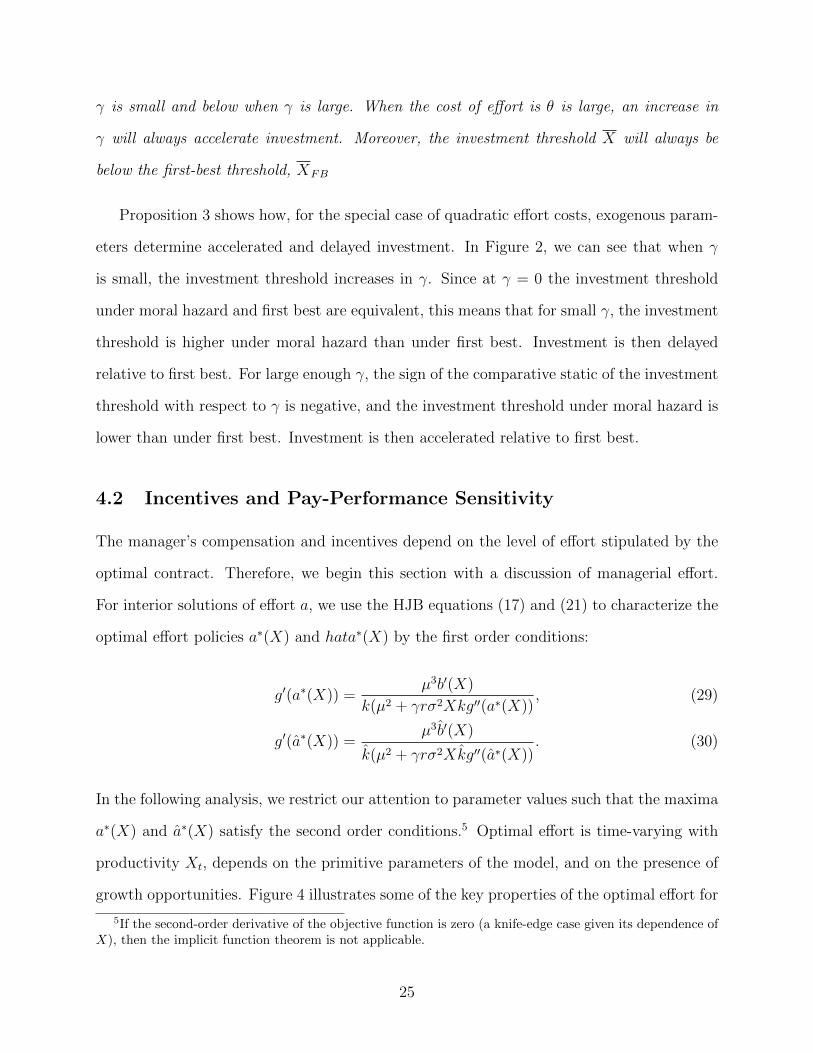
Proposition 3 shows how, for the special case of quadratic effort costs, exogenous param-

eters determine accelerated and delayed investment. In Figure 2, we can see that when γ

is small, the investment threshold increases in γ. Since at γ = 0 the investment threshold

under moral hazard and first best are equivalent, this means that for small γ, the investment

threshold is higher under moral hazard than under first best. Investment is then delayed

relative to first best. For large enough γ, the sign of the comparative static of the investment

threshold with respect to γ is negative, and the investment threshold under moral hazard is

lower than under first best. Investment is then accelerated relative to first best.

4.2 Incentives and Pay-Performance Sensitivity

The manager’s compensation and incentives depend on the level of effort stipulated by the

optimal contract. Therefore, we begin this section with a discussion of managerial effort.

For interior solutions of effort a, we use the HJB equations (17) and (21) to characterize the

optimal effort policies a∗(X) and hata∗(X) by the first order conditions:

g′(a∗(X)) =µ3b′(X)

k(µ2 + γrσ2Xkg′′(a∗(X)), (29)

g′(a∗(X)) =µ3b′(X)

k(µ2 + γrσ2Xkg′′(a∗(X)). (30)

In the following analysis, we restrict our attention to parameter values such that the maxima

a∗(X) and a∗(X) satisfy the second order conditions.5 Optimal effort is time-varying with

productivity Xt, depends on the primitive parameters of the model, and on the presence of

growth opportunities. Figure 4 illustrates some of the key properties of the optimal effort for

5If the second-order derivative of the objective function is zero (a knife-edge case given its dependence ofX), then the implicit function theorem is not applicable.

25

our baseline parameter values. Efforts in young (pre-investment), mature (post-investment),

and small no-growth (permanently small) firms are plotted at two levels of the cost of effort,

θ. Effort implemented in the mature and no-growth firms decreases and goes to zero as X

approaches infinity. This is because the cost of providing incentives grows more in X than

does the benefit of effort. A related effect makes effort decrease in response to exogenous

changes in capital (that is, abstracting from growth options; to see this, compare the efforts

of the no-growth and mature firms).

Effort implemented in the young firm is above that of the mature firm due to two reasons.

First, the young firm employs a low level of capital. This property also manifests itself in

the fact that effort (weakly) decreases at the moment of investment. The second reason for

high effort in young firms is due to the presence of growth options. As is standard in real

options models, growth options increase the sensitivity of firm value to productivity shocks

as the firm approaches the investment threshold. As the optimal effort increases in b′(X) (see

Equation (29)), this indicates that effort may increase in X in the young firm. Intuitively,

the prospect of capital investment makes contracting high effort additionally attractive from

the investor’s point of view.

To implement any of the optimal effort levels under moral hazard, the manager needs to

be appropriately incentivized. Our main interest is how investment and investment oppor-

tunities affect the power of incentives. We look at two alternative measures of incentives:

one implied by our model and another commonly used in practice. A direct measure of

a manager’s incentives in our model is βt. To see this, note that the certainty equivalent

of a manager’s promised continuation utility, Vt with the dynamics given in (12), can be

interpreted as her financial wealth. Its sensitivity to output surprises (unexpected changes

in Xt) divided by the volatility of output, σXt, is exactly equal to βt. In other words, βt

is an output-based pay-performance sensitivity (PPS) that measures the sensitivity of the

manager’s wealth to changes in output affected by the manager.

A standard approach to the measurement of PPS is to compute the sensitivity of the

26

manager’s wealth to changes in firm value. This approach is particularly convenient from

an empirical point of view as it is based on firm value changes, which are easy to measure.

In contrast, an output-based PPS measure must isolate that output process, which is most

directly attributable to the manager. In cases in which firm value is linear in output Xt, this

simplification would be inconsequential as value-based PPS would be equivalent to direct,

output-based PPS, such as β. However, growth options are known to generate a non-linear

relationship between firm value and output. Thus firms with growth opportunities may have

a wedge between output-based and value-based PPS.

In our model, the manager’s dollar value-based PPS is measured by the sensitivity of the

manager’s dollar value, Vt, to changes in firm value, b(Xt). Looking at the nondeterministic

components of the two values (that is, the volatility terms), pre-investment value-based PPS,

denoted by φ, is given by:

φt =βt

b′(Xt)=g′(a∗(Xt))k

µb′(Xt). (31)

Post-investment φt is characterized by a similar equation substituting appropriately k, a∗,

and b. As expected, φ is closely related to β. However, it is scaled by the slope of the value

function in output X. The presence of investment opportunities affects φ by changing β and

by changing the slope of b in output X.

In the next proposition, we posit that growth options can impact the two pay-performance

sensitivity measures, β and φ, differently.

Proposition 4. By increasing investment opportunities, the manager’s value-based PPS, φ,

changes in the opposite direction than the output-based PPS, β, if the convexity of the cost

of effort increases in effort, g′′′(a) > 0, and effort is interior.

To provide the intuition for this result, suppose for concreteness that optimal effort

increases in the size of investment opportunities. Incentives measured by β increase in the

size of investment opportunities because the marginal value of effort for the investor increases

and thus a higher optimal effort is contracted. However, in the case of φ, scaling by b′(X)

27

may change the relation. Indeed, φ decreases in the size of the investment opportunity when

the growth option creates a large sensitivity of the pre-investment firm value to productivity

shocks for which the manager does not have to be compensated. In such risky firms, it is then

optimal to set output-based PPS to a relatively low level. Thus, a low φ does not necessarily

mean that the manager’s incentives are low-powered but that a strong response of firm value

to output allows the principal to set a low value-based PPS. The condition g′′′(a) > 0 means

that the cost function of the manager’s effort is strongly convex (increasingly convex) and

additional effort is costly.

Another important observation is that the power of incentives may either increase or

decrease at investment. This is despite the fact that optimal effort never increases at invest-

ment. Proposition 5 give the precise conditions under which incentives increase or decrease

at investment.

Proposition 5. The manager’s power of incentives, measured by either β or φ, increases at

investment if:

g′(a∗(X))

g′(a∗(X))>k

k

and decreases otherwise.

Proposition 5 states that incentives increase at investment when the drop of the imple-

mented effort at investment is sufficiently small relative to the inverse of the size of the

growth option. This is the case for firms with low costs of effort (low agency conflicts) and

large growth opportunities.

It is interesting to note that the condition in Proposition 5 is closely related to the one

given in Proposition 2 for the negative sign of the effect of risk aversion on the investment

threshold. This means that the response of the manager’s incentives to investment can

be linked to the distortion in investment timing due to agency conflicts. Specifically, our

model predicts that the power of incentives decreases at investment if moral hazard conflicts

accelerate investment and increases at investment if moral hazard conflicts delay investment.

28

This does not depend on whether or not the manager’s incentives are measured by output-

or value-based metrics.

5 A Generalized Model of Investment

In this section we extend our basic real options model to consider other specifications of the

investment problem. The main goal of this exercise is to determine under what conditions

an increase in the severity of the moral hazard problem as measured by the manager’s

risk aversion, γ, leads to increases in investment. To that end, we make the following

modifications to the model of the previous sections. First, productivity now follows a general

diffusion of the form:

dXt = atµ(Xt)dt+ σ(Xt)dZt,

where the drift and volatility terms, µ and σ, are continuously differentiable functions of

productivity X. We maintain our restriction that effort must fall in the interval at ∈ [0, 1];

however, the cost of effort is now given by the general function G(Xt, Kt, at) such that G is

twice continuously differentiable in it arguments and convex in effort at. Next, the firm’s cash

flows are given by a general function π(Xt, Kt), which may exhibit increasing or decreasing

returns to scale, and may depend on either the increment or the level of productivity as well.

Finally, capital accumulates according to:

dKt = (It − δKt)dt,

where δ is capital depreciation and investment It is at the cost C(Xt, Kt, It)dt that may

feature convex adjustment cost, partial reversibility, and stock fixed costs. A contract in

this more general setting is then a triple (at, ct, It) consisting of a recommended effort level

at, a compensation plan ct, and an investment rule It. In the following subsections we give

a heuristic analysis of the generalized investment model, with formal proofs provided in the

29

Appendix.

Note that the arguments leading to a characterization of the no-savings condition and

incentive-compatibility conditions did not depend on a specification of the investment tech-

nology. Consequently, continuation utility arising from a contract without savings under this

more general model must be a martingale and satisfy uc(ct, at) = −γrWt. The incentive-

compatibility condition is then:

at = arg maxa

u(ct, a) + βt(−γrWt)(a− at)µ(X) , (32)

which implies that:

βt =1

µ(X)Ga(Xt, Kt, at)

and

dWt =σ(Xt)

µ(Xt)(−γrWt)Ga(Xt, Kt, at)dZt.

The characterization of incentive compatibility given above allows us to proceed to analyze

the effect moral hazard on investment in this more general setting.

5.1 Tobin’s q

For many of the models subsumed by our general setup, the optimal investment policy is

an increasing function of the investor’s marginal value of capital, commonly referred to as

Tobin’s q. For this class of models, including the neoclassical and capacity choice models,

the effect of the agency problem on optimal investment operates entirely through q. Thus,

to determine the effect of the moral hazard problem on optimal investment in these models,

it is sufficient to determine its effect on the marginal value of capital. We now show that

increasing the severity of the moral hazard problem decreases the marginal value of capital

and hence curtails investment.

To determine the effect of the moral hazard problem on the investor’s marginal value

30

of capital, we again apply the method of comparative statics developed in DeMarzo and

Sannikov (2006). Since the dynamics of continuation utility remain essentially unchanged

from the previous sections, the investor’s value function is still additively separable as

B(X,K, V ) = b(X,K) − V . Taking as given the optimal investment and effort policies

I∗ and a∗, an application of Ito’s formula, the envelope theorem, and the Feynman-Kac

formula detailed in the Appendix yields the following expression for the derivative of the

marginal value of capital, bk, with respect to the manager’s risk aversion γ:

bKγ = E

[∫ ∞0

e−(r+δ)hKγ(Xt, Kt, a∗(Xt, Kt))dt

∣∣X0, K0

], (33)

where h(X,K, a) is defined as in Equation (18) and represents the total cash flow to the firm

net of effort and incentive costs. Equation (33) states that the derivative of the marginal

value of capital with respect to γ is just the expected present value of all future derivatives

of the marginal products of capital with respect to γ. For any given point (X,K, a), it is

straightforward to compute the derivative of the marginal product of capital with respect to

γ to find:

hKγ(X,K, a) = −r(σ(X)

µ(X)

)2

Ga(X,K, a)GaK(X,K, a) ≤ 0. (34)

Equations (33) and (34) together imply the following proposition.

Proposition 6. The investor’s marginal value of capital bK is decreasing in the manager’s

risk aversion γ.

Proposition 6 confirms the intuition of the previous literature (e.g., DeMarzo et al. (2012)

and DeMarzo and Fishman (2007)) that the moral hazard problem decreases the marginal

value capital. This in turn implies that if the optimal investment policy can be expressed

as an increasing function of the marginal value of capital otherwise independent of the

severity of the moral hazard problem, then optimal investment decreases the severity of the

moral hazard problem. For example, in the neoclassical model with convex adjustment costs

(CII(X,K, I) > 0), the optimal investment rate equates the marginal value of capital with

31

the marginal cost of capital:

bK(X,K, a∗) = CI(X,K, I∗). (35)

Since investment costs are independent of the manager’s risk aversion, we can differentiate

both sides of Equation (35) to find:

I∗γ =bKγ(X,K, a

∗)

CII(X,K, I∗)≤ 0,

so that investment decreases with the severity of the moral hazard problem. Similarly, in a

capacity choice model with partial reversibility, as in Abel and Eberly (1996), the optimal

investment policy is to invest (divest) only when the marginal value of capital is greater

(less) than the marginal purchase price of capital. For any given level of productivity X,

increasing the severity of the moral hazard problem through an increase in γ decreases the

marginal value of capital. Thus both the thresholds in productivity at which the firm invests

and divests increase with the severity of the agency problem; thus, investment will be delayed

while divestment will be accelerated.

5.2 Lumpy Investment

We have found that so long as investment is an increasing function of the marginal value cap-

ital, moral hazard serves to decrease or delay investment. Thus, our main results concerning

investment timing must follow from the fact that in our real options setting, the effect of

the agency problem on investment does not operate solely through q. We now show that in

a wide class of models, that is those in which optimal investment is lumpy and infrequent,

investment will be accelerated by moral hazard when the agency problem is more severe.

The acceleration in investment occurs because the location of the threshold in productivity

at which the firm invests is now given by the average value of the additional capital. In

contrast to the marginal value of capital, the average value of additional capital can increase

32

with the severity of the agency problem because of the substitutability of effort and capital

we have demonstrated in the previous sections. If the average value of additional capital at

the moment of investment increases with the severity of the moral hazard problem, then the

moral hazard problem will accelerate investment.

To make this argument more precise, consider a production function with convex regions

in capital and partial reversibility. For example, the firm may be endowed with a sequence of

real options (rather than a single option in the simple model we consider above). Whenever

the current level of capital falls within the convex region of π, the optimal investment will

always be in a “lump.” That is, suppose πKK(Xt, Kt) > 0. If it is optimal to invest at the

point (Xt, Kt), then it must be that the path of Kt has a discontinuous jump up at time t.

Indeed any smooth investment process would not take advantage of the increasing returns

to scale in π. Moreover, partial reversibility implies that it cannot be optimal to invest at all

moments in time by the standard real option intuition. In this setup, let the current level of

capital be k and the optimal amount of new capital at investment be I∗, then the optimal

investment threshold is given by the familiar value-matching and smooth-pasting conditions:

b(X, k) = b(X, k + I∗)− p+I∗,

bX(X, k) = bX(X, k + I),

where p+ is the purchase price of new capital. We can rearrange the value-matching condition

to get:

b(X, k + I∗)− b(X, k)

I∗= p+,

which reads: invest when the average value of new capital I is equal to the average price

of new capital p+. Thus, the effect of the moral hazard problem on the optimal investment

time is given by its effect on the average value of capital.

To see why the average value of additional capital can increase with the severity of the

moral hazard problem, we again compute comparative statics with respect to the manager’s

33

risk aversion. Using a similar argument as in the previous sections, we can calculate:

sign

[∂

∂γ

[b(X, k + I∗)− b(X, k)

I∗

]]=

sign[(Ga(X, k, a

∗(X, k)))2 − (Ga(X, k + I∗, a∗(X, k + I∗))2]. (36)

Equation (36) states that the average value of new capital is increasing in γ if the marginal

cost of effort to the manager is reduced after investment. This condition is equivalent to the

one given in Proposition 2, however it is stated in more general terms. Again, the intuition is

that the moral hazard problem may have a more negative effect on the firm after investment

than before.

6 Conclusion

We presented a model of real options and dynamic moral hazard. We find that the effect

of agency conflicts on investment timing depends on the severity of the conflict. When the

moral hazard problem is less severe, the optimal contract will implement high effort, but

delay investment. When the moral hazard problem is more severe, the optimal contract

will implement lower effort but will call for accelerated investment. The finding that moral

hazard may accelerate investment is new and provides an alternative to empire-building or

managerial hubris-based explanations of over-investment.

The effect of investment on pay-performance sensitivity also depends on the severity of

the moral hazard problem. When the moral hazard problem is less severe, pay-performance

sensitivity increases after investment. When the moral hazard problem is more severe, pay-

performance sensitivity decreases with investment. These results link pay-performance sen-

sitivity, which is easily measurable, with the nature the distortion on investment timing

imposed by moral hazard, which is more difficult to measure. This link could be exploited

to empirically evaluate the effect of agency problems on the timing of investment.

34

Our results also provide guidance to empirical work on pay-performance sensitivity on its

own. We show that in the presence of growth options, there is a wedge between output-based

and value-based measures of incentives. In fact, if the manager’s cost of effort is increasingly

convex, value-based pay-performance sensitivity may decrease even though true incentives

(i.e., output-based pay-performance sensitivity) increase. Thus, it is important to control

for the presence of growth options when using value-based measures of pay-performance

sensitivity as a proxy for the level of incentives.

Finally, although the primary real options model we consider is fairly simple, we show that

the main intuition carries over into more realistic settings, so long as the optimal investment

path is lumpy. A promising direction for future work would be to enrich the current model

so that it is suitable for a structural estimation.

35

References

Abel, A. B., Eberly, J. C., 1996. Optimal investment with costly reversibility. The Reviewof Economic Studies 63 (4), 581–593.

Bernardo, A. E., Welch, I., 2001. On the evolution of overconfidence and entrepreneurs.Journal of Economics & Management Strategy 10 (3), 301–330.

Bertrand, M., Mullainathan, S., 2003. Enjoying the quiet life? Corporate governance andmanagerial preferences. Journal of Political Economy 111 (5), 1043–1075.

Biais, B., Mariotti, T., Rochet, J., Villeneuve, S., 2010. Large risks, limited liability, anddynamic moral hazard. Econometrica 78 (1), 73–118.

Brennan, M. J., Schwartz, E. S., 1985. Evaluating natural resource investments. The Journalof Business 58 (2), 135–157.

Caballero, R. J., Engel, E. M., 1999. Explaining investment dynamics in us manufacturing:a generalized (S, s) approach. Econometrica 67 (4), 783–826.

Cooper, R., Haltiwanger, J., Power, L., 1999. Machine replacement and the business cycle:Lumps and bumps. The American Economic Review 89 (4), 921–946.

DeMarzo, P., Fishman, M., 2007. Agency and optimal investment dynamics. Review ofFinancial Studies 20 (1), 151–188.

DeMarzo, P., Fishman, M., He, Z., Wang, N., 2012. Dynamic agency and the q theory ofinvestment. Journal of Finance 67 (6), 2295–2340.

DeMarzo, P., Sannikov, Y., 2006. Optimal security design and dynamic capital structure ina continuous-time agency model. The Journal of Finance 61 (6), 2681–2724.

Dixit, A. K., Pindyck, R. S., 1994. Investment under uncertainty. Princeton university press.

Doms, M., Dunne, T., 1998. Capital adjustment patterns in manufacturing plants. Reviewof economic dynamics 1 (2), 409–429.

Goldstein, R., Ju, N., Leland, H., 2001. An ebit-based model of dynamic capital structure*.The Journal of Business 74 (4), 483–512.

Gompers, P. A., 1995. Optimal investment, monitoring, and the staging of venture capital.The journal of finance 50 (5), 1461–1489.

Grenadier, S., Wang, N., 2005. Investment timing, agency, and information. Journal ofFinancial Economics 75 (3), 493–533.

Harris, M., Raviv, A., 1990. Capital structure and the informational role of debt. The Journalof Finance 45 (2), 321–349.

36

Hart, O., Moore, J., 1995. Debt and seniority: An analysis of the role of hard claims inconstraining management. The American Economic Review, 567–585.

He, Z., 2009. Optimal executive compensation when firm size follows geometric brownianmotion. Review of Financial Studies 22 (2), 859–892.

He, Z., 2011. A model of dynamic compensation and capital structure. Journal of FinancialEconomics 100 (2), 351–366.

Holmstrom, B., Milgrom, P., 1987. Aggregation and linearity in the provision of intertem-poral incentives. Econometrica, 303–328.

Holmstrom, B., Weiss, L., 1985. Managerial incentives, investment and aggregate implica-tions: Scale effects. The Review of Economic Studies 52 (3), 403–425.

Jensen, M., 1986. Agency costs of free cash flow, corporate finance, and takeovers. AmericanEconomic Review 76 (2), 323–329.

McDonald, R., Siegel, D., 1986. The value of waiting to invest. The Quarterly Journal ofEconomics 101 (4), 707–727.

Morck, R., Shleifer, A., Vishny, R. W., 1990. Do managerial objectives drive bad acquisitions?The Journal of Finance 45 (1), 31–48.

Murphy, K., 1999. Executive compensation. Handbook of Labor Economics 3, 2485–2563.

Philippon, T., Sannikov, Y., 2007. Real options in a dynamic agency model, with applicationsto financial development, IPOs, and business risk, working Paper.

Piskorski, T., Tchistyi, A., 2010. Optimal mortgage design. Review of Financial Studies23 (8), 3098–3140.

Piskorski, T., Tchistyi, A., 2011. Stochastic house appreciation and optimal mortgage lend-ing. Review of Financial Studies 24 (5), 1407–1446.

Roll, R., 1986. The hubris hypothesis of corporate takeovers. The Journal of Business 59 (2Part 1), 197–216.

Sannikov, Y., 2008. A continuous-time version of the principal-agent problem. The Reviewof Economic Studies 75 (3), 957–984.

Spear, S., Srivastava, S., 1987. On repeated moral hazard with discounting. The Review ofEconomic Studies 54 (4), 599–617.

Stulz, R., 1990. Managerial discretion and optimal financing policies. Journal of FinancialEconomics 26 (1), 3–27.

Zwiebel, J., 1996. Dynamic capital structure under managerial entrenchment. The AmericanEconomic Review, 1197–1215.

37

Appendix

A Proofs

Proof of Lemma 1. Consider an arbitrary contract Π = (ct, at, τ) and suppose the solution

to the manager’s optimization problem (1) for this contract is given by ct, at and the

manager’s associated value for this contract is W0.

Now consider the alternative contract Π = (ct, at, τ). Note that under this contract

the manager again gets utility W0 from the consumption effort pair ct, at. We claim that

the solution to manager’s optimization problem (1) is again ct, at. Indeed suppose it is not

and that there is a alternative feasible consumption effort pair ct, at such that this policy

yields utility W0 > W0 to the manager. The consumption effort pair ct, at is also feasible

under the original contract Π since:

limt→∞

E

[e−rt

∫ t

0

(cs − cs)ds]

= limt→∞

(E

[e−rt

∫ t

0

(ct − ct)dt]

+ E

[e−rt

∫ t

0

(cs − cs)ds])

= limt→∞

E

[e−rt

∫ t

0

(cs − cs)ds]

+ limt→∞

E

[e−rt

∫ s

0

(cs − cs)ds]

= 0.

Thus, the manager could achieve utility Wt > Wt under the original contract Π, a contra-

diction.

Finally note that the investor is achieves the same value under the new contract Π as

under the original contract Π, since effort and investment are unchanged, and the traversality

condition implies that the two consumption streams have the same present value.

Proof of Lemma 2. Suppose St = S and recall the definition of Wt(Π, Xs, Kss≤t;S) and let

c, a solve problem (3). We claim that c− rS, a solves problem (3) for St = 0. This plan

gives the manager a utility of Wt(Π, Xs, Kss≤t; 0) = eγrSWt(Π, Xs, Kss≤t;S). Suppose

38

there is some alternative c, a that yields a higher utility to the agent Wt(Π, Xs, Kss≤t; 0) >

Wt(Π, Xs, Kss≤t; 0). Now consider the plan c+ rS, a and note that this plan is feasible

under St = S but under this plan the manager can achieve the following utility:

Wt(Π, Xs, Kss≤t; 0) = e−γrSWt(Π, Xs, Kss≤t; 0)

≥ e−γrSWt(Π, Xs, Kss≤t; 0)

= Wt(Π, Xs, Kss≤t; 0),

which contradicts the optimality of the c, a.

Proof of Proposition 1. We show that the candidate policies are indeed optimal for the in-

vestor. Note that the compensation policy ct is pinned down by the no-savings condition.

Define the stopped gain process by:

Gt =

∫ t

0

e−rs(XtKt − ct)dt+ e−rtB(Xt, Vt) + I(t ≥ τ)(e−rt(B(Xt, Vt)−B(Xt, Vt))− e−rτp).

When Vt evolves according to (12), Ito’s formula gives the following dynamics:

ertdGt =

[XtKt −

1

2θXtKta

2 +−rVt + atµXtBX +1

2σ2X2

t BXX

+1

2γr

(σ

µXtkg

′(a)

)2

BV +σ2

µX2kg′(a)BXV +

1

2

(σ

µXkg′(a)

)2

BV V − rB

]dt

+

(BX +

σ

µXtKtg

′(at)BV)σXtdZt+ I(t = τ)(B(Xt, Vt)−B(Xt, Vt)− p),

where B(Xt, Vt) = B(Xt, Vt) + I(t ≥ τ)(B(Xt, Vt)−B(Xt, Vt)). Note that the drift term (the

term in the square brackets) is clearly negative for any alternative policy, while it is zero for

the candidate policy. Now examine the last term. Under the candidate policy, this term is

zero due to the value-matching condition. Under any alternative investment time τ , this term

is negative due to the smooth-pasting condition and the concavity of B(Xt, Vt)−B(Xt, Vt).

39

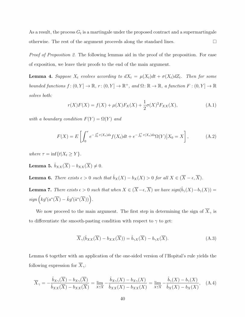
As a result, the process Gt is a martingale under the proposed contract and a supermartingale

otherwise. The rest of the argument proceeds along the standard lines.

Proof of Proposition 2. The following lemmas aid in the proof of the proposition. For ease

of exposition, we leave their proofs to the end of the main argument.

Lemma 4. Suppose Xt evolves according to dXt = µ(Xt)dt + σ(Xt)dZt. Then for some

bounded functions f : (0, Y ]→ R, r : (0, Y ]→ R+, and Ω: R→ R, a function F : (0, Y ]→ R

solves both:

r(X)F (X) = f(X) + µ(X)FX(X) +1

2σ(X)2FXX(X), (A.1)

with a boundary condition F (Y ) = Ω(Y ) and

F (X) = E

[∫ τ

0

e−∫ t0 r(Xs)dsf(Xt)dt+ e−

∫ τ0 r(Xs)dsΩ(Y )

∣∣X0 = X

], (A.2)

where τ = inft|Xt ≥ Y .

Lemma 5. bXX(X)− bXX(X) 6= 0.

Lemma 6. There exists ε > 0 such that bX(X)− bX(X) > 0 for all X ∈ (X − ε,X).

Lemma 7. There exists ε > 0 such that when X ∈ (X−ε,X) we have sign(bγ(X)−bγ(X)) =

sign(kg′(a∗(X)− kg′(a∗(X))

).

We now proceed to the main argument. The first step in determining the sign of Xγ is

to differentiate the smooth-pasting condition with respect to γ to get:

Xγ(bXX(X)− bXX(X)) = bγX(X)− bγX(X). (A.3)

Lemma 6 together with an application of the one-sided version of l’Hopital’s rule yields the

following expression for Xγ:

Xγ = − bXγ(X)− bXγ(X)

bXX(X)− bXX(X)= lim

X↑X− bXγ(X)− bXγ(X)

bXX(X)− bXX(X)= lim

X↑X− bγ(X)− bγ(X)

bX(X)− bX(X), (A.4)

40

so that determining the sign of Xγ is equivalent to determining the sign of the last limit

above.

If g′(a∗(X))

g′(a∗(X))< k

k, Lemmas 6 and 7 imply there exists ε > 0 such that:

− bγ(X)− bγ(X)

bX(X)− bX(X)< 0

for all X ∈ (X − ε,X), which in turn implies:

limX↑X− bγ(X)− bγ(X)

bX(X)− bX(X)≥ 0,

since bγ(X)− bγ(X) and bX(X)− bX(X) are nonzero and continuous. Thus, Xγ ≤ 0. If

g′(a∗(X))

g′(a∗(X))< k

k, a similar argument shows Xγ ≥ 0.

Proof of Lemma 4. The proof essentially follows the proof of DeMarzo and Sannikov (2006)

for Lemma 4. Suppose V solves Equation (A.1) and define the process Ht by:

Ht =

∫ t

0

e−∫ s0 r(Xu)duf(Xs)ds+ e−

∫ t0 r(Xs)dsV (Xs).

An application of Ito’s formula gives the dynamics for Ht:

e∫ t0 r(Xs)dsdHt = (f(Xt)+µ(Xt)VX(Xt)+

1

2σ(Xt)

2VXX(Xt)−r(Xt)V (Xt))dt+σ(Xt)V (Xt)dZt.

By Equation (A.1), the drift in the above dynamics is zero, so that Ht is a martingale. Since

V (X) is bounded on [0, X], Hτ is a martingale and:

V (X0) = H0 = E[Hτ |X0] = E

[∫ τ

0

e−∫ t0 r(Xs)dsf(Xt)dt+ e−

∫ τ0 r(Xs)dsV (Xτ )

∣∣X0

]= E

[∫ τ

0

e−∫ t0 r(Xs)dsf(Xt)dt+ e−

∫ τ0 r(Xs)dsW (Y )

∣∣X0

].

where the last equality follows from the definition of the stopping time τ and the boundary

41

condition V (Y ) = W (Y ).

Proof of Lemma 5. Assume that bXX(X) − bXX(X) = 0. We show that this leads to a

contradiction. First, differentiate the smooth-pasting condition (23) with respect to p to

obtain:

bXp(X) = −(bXX(X)− bXX(X))Xp.

bXX(X) − bXX(X) = 0 implies that bXp(X) = 0. Next, differentiate the ODE (21) with

respect to X and p to get an ODE for bXp:

(r − a∗(X)µ)bXp = (a∗(X)µ+ σ2)XbXXp +1

2σ2X2bXXXp.

Lemma 4 then implies:

bXp(X) = E[e−

∫ τ0 (r−a∗(Xs)µ)dsbXp(X)|X0 = X

]= 0,

where X is a process with the following dynamics:

dX = (a∗(X)µ+ σ2)Xdt+ σXdZ.

Since bXp(X) = 0, then bp(X) must be a constant inX. By differentiating the value-matching

condition (22) with respect to p, we get:

bp(X) = (bX(X)− bX(X))Xp − 1 = −1,

where the second equality follows from the smooth-pasting condition (23). Differentiating

the ODE (21) with respect to p to gives an ODE for bp:

rbp(X) = a(X)µXbXp(X) +1

2σ2X2bXXp(X).

42

Lemma 4 then implies:

bp(X) = E[e−rτbp(X)|X0 = X

].

In particular,

limX→0

bp(X) = limX→0

E[e−rτbp(X)|X0 = X

]= 0,

as X = 0 is an absorbing point for the process Xt. This means that bp(X) cannot be a

constant, which is a contradiction.

Proof of Lemma 6. Suppose there does not exist ε > 0 such that bX(X) < bX(X) for all

X ∈ (X − ε,X), then for all ε > 0 there exists X ∈ (X − ε,X) such that bX(X) ≥ bX(X).

Now since bX(X) = bX(X) and bX and bX are continuous, this implies that there exists ε > 0

such that bX(X) ≥ bX(X) for all X ∈ (X − ε,X). This implies that for X ∈ (X − ε,X), we

have:

b(X)− b(X) = b(X)− b(X)−∫ X

X

(bX(x)− bX(x))dx ≥ p,

which is a contradiction to the definition of X.

Proof of Lemma 7. First, we differentiate the HJB equations (17) and (21) with respect to

γ to get:

rbγ = hγ(X, a∗(X)) + a∗(X)µXbXγ +

1

2σ2X2bXXγ,

and:

rbγ = hγ(X, a∗(X)) + a∗(X)µXbXγ +

1

2σ2X2bXXγ,

subject to bγ(X) = bγ(X). For the remainder of the proof of this lemma, we will suppress

the dependence of hγ and hγ on a∗ and a∗ to ease notation. Note that hγ(X) ≥ hγ(X) is

equivalent to g′(a∗(X))

g′(a∗(X))< k

k.

43

Let X∗ and X∗ be given by the following dynamics:

dX∗ = a∗(X∗)µX∗dt+ σX∗dZ

dX∗ = a∗(X∗)µX∗dt+ σX∗dZ.

Applying Proposition 4 we have:

bγ(X) = E

[∫ τ

0

e−rthγ(X∗t )dt+ e−rτ bγ(X)

∣∣X∗0 = X

]

and

bγ(X) = E

[∫ τ

0

e−rthγ(X∗t )dt+ e−rτ bγ(X)

∣∣X∗0 = X

],

where τ = inft|X∗t ≥ X and τ = inft|X∗t ≥ X. Subtracting we get:

bγ(X)−bγ(X) = E

[∫ τ

0

e−rthγ(X∗t )dt−

∫ τ

0

e−rthγ(X∗t )dt+ (e−rτ − e−rτ )bγ(X)

∣∣X∗0 = X∗0 = X

].

Now by continuity and the fact that τ , τa.s.→ 0 as X∗0 , X

∗0 ,→ X, there exists ε > 0 such

that when X∗0 , X∗0 ∈ (X − ε,X) we have:

sign(bγ(X)− bγ(X)) = sign(hγ(X)− hγ(X)) (A.5)

= sign(kg′(a∗(X)− kg′(a∗(X))

), (A.6)

which is the desired result.

Proof of Proposition 4. To consider the effect of the size of investment opportunities on

incentives, we analyze the effect of increasing post-investment capital k.

44

First, consider the effect on pre-investment βt:

dβt

dk=

1

µkg′′(a∗(Xt))

da∗(Xt)

dk.

Consider next the effect of k on φt:

dφt

dk= − µ2

(µ2 + γrσ2Xtkg′′(a∗(Xt)))2γrσ2Xtkg

′′′(a∗(Xt))da∗(Xt)

dk.

So:

sign

(dφt

dk

)= sign

(−g′′′(a∗(Xt))

da∗(Xt)

dk

).

This shows that the sign of the effect of k on φt is the same as on βt if g′′′(a∗) < 0 and the

opposite (negative) if g′′′(a∗) > 0.

Proof of Proposition 5. The result for β follows directly by comparing pre- and post-investment

βt at the moment of investment. The relation for φ is found similarly using the smooth-

pasting condition (23).

45

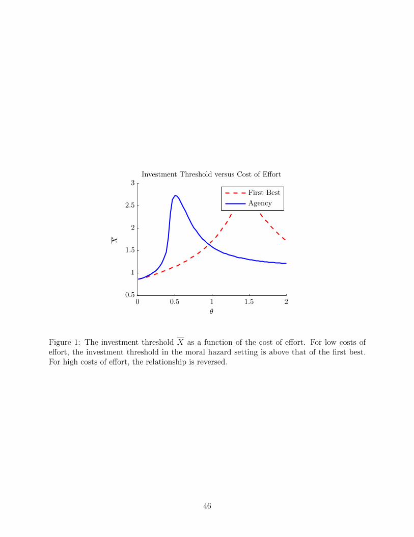
Agency

First Best

Investment Threshold versus Cost of Effort

X

θ

0 0.5 1 1.5 20.5

1

1.5

2

2.5

3

Figure 1: The investment threshold X as a function of the cost of effort. For low costs ofeffort, the investment threshold in the moral hazard setting is above that of the first best.For high costs of effort, the relationship is reversed.

46

Agency

First Best

Investment Threshold versus Risk Aversion

X

γ

0 1 2 31

1.5

2

2.5

3

Figure 2: The investment threshold X as a function of the risk aversion.

47

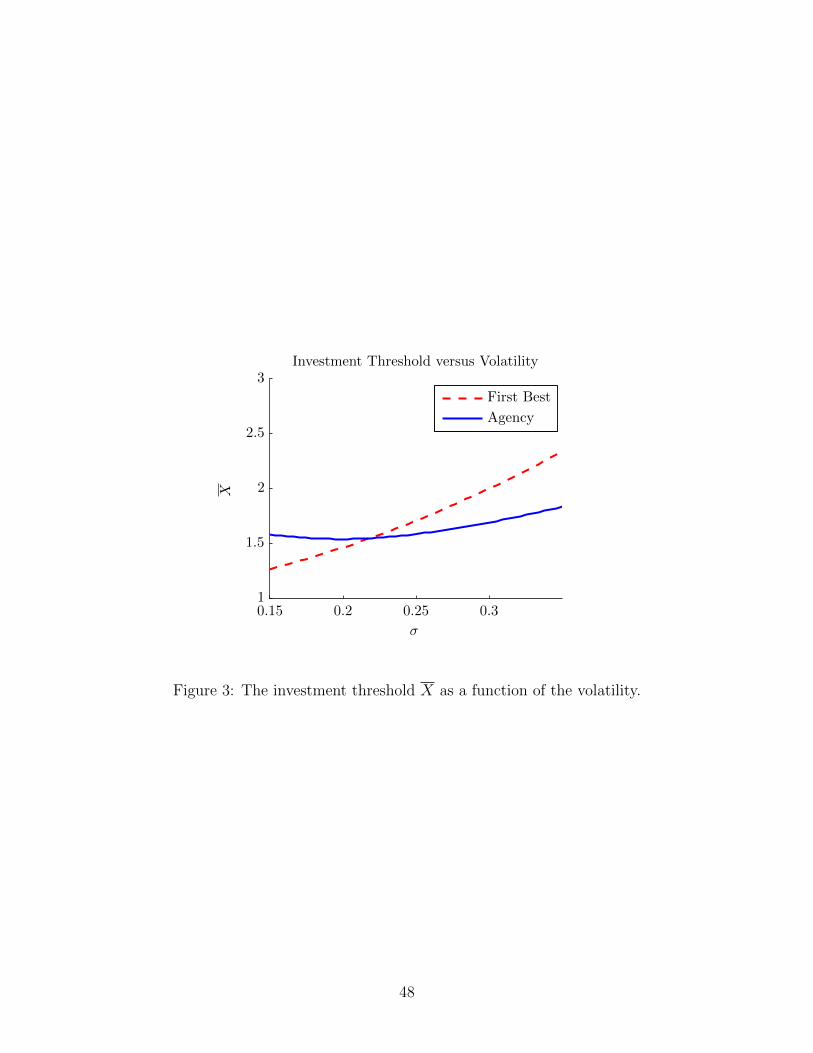
Agency

First Best

Investment Threshold versus Volatility

X

σ

0.15 0.2 0.25 0.31

1.5

2

2.5

3

Figure 3: The investment threshold X as a function of the volatility.

48

Agency Small No Growth

Agency Mature

Agency Young

θ = 2

a∗

X

θ = 0.5

a(X

)

X

Optimal Effort

0 0.5 1 1.50 1 2 30

0.1

0.2

0.3

0.4

0.5

0.6

0.7

0.4

0.5

0.6

0.7

0.8

0.9

1

Figure 4: The optimal effort at two levels of the cost of effort: θ = 1 (left) and θ = 2 (right).

49